development of protocols to inventory or monitor wildlife
TRANSCRIPT

Development of Protocols To Inventory or Monitor Wildlife, Fish, or Rare Plants
United States Department of Agriculture
Forest Service
Gen. Tech.Report WO-72
June 2006

Development of Protocols To Inventory or Monitor Wildlife, Fish, or Rare Plants
By
David VeselyBrenda C. McCombChristina D. VojtaLowell H. SuringJuraj HalajRichard S. HolthausenBenjamin ZuckerbergPatricia M. Manley
United States Department of Agriculture
Forest Service
Gen. Tech.Report WO-72
June 2006

The proper citation for this document is as follows:
Vesely, D.; McComb, B.C.; Vojta, C.D.; Suring, L.H.; Halaj, J.; Holthausen, R.S.;
Zuckerberg, B.; Manley, P.M. 2006. Development of Protocols To Inventory or Monitor
Wildlife, Fish, or Rare Plants. Gen. Tech. Rep. WO-72. Washington, DC: U.S. Department
of Agriculture, Forest Service. 100 p.
Cover photos. Monitoring wildlife, rare plants, and their habitats is conveyed through
three photos: (1) Peromyscus maniculatus, on Pesola scale (photo credit: Dean E.
Pearson); (2) western prairie fringed orchid (Platanthera praeclara) (photo credit:
Carolyn Hull Sieg); and (3) measuring a ponderosa pine (Pinus ponderosa) log in Idaho
(photo credit: Victoria A. Saab).
The U.S. Department of Agriculture (USDA) prohibits discrimination in all its programs and
activities on the basis of race, color, national origin, age, disability, and where applicable,
sex, marital status, familial status, parental status, religion, sexual orientation, genetic
information, political beliefs, reprisal, or because all or part of an individual’s income
is derived from any public assistance program. (Not all prohibited bases apply to all
programs.) Persons with disabilities who require alternative means for communication
of program information (Braille, large print, audiotape, etc.) should contact USDA’s
TARGET Center at (202) 720-2600 (voice and TDD). To file a complaint of
discrimination, write USDA, Director, Office of Civil Rights, 1400 Independence Avenue,
S.W., Washington, D.C. 20250-9410, or call (800) 795-3272 (voice) or (202) 720-6382
(TDD). USDA is an equal opportunity provider and employer.

Development of Protocols To Inventory or Monitor Wildlife, Fish, or Rare Plants iii
Acknowledgments
We sincerely thank Jeff Beck, Curt Flather, and Michael Schwartz for helping to write
portions of this technical guide and Rudy King for providing an extensive review of the
statistical principles addressed in the guide. We also thank the following colleagues for
reviewing earlier drafts of the technical guide: Jeff Beck, Brad Compton, Margaret Griep,
Tim Hardin, Greg Hayward, Kim Mellen, Sylvia Mori, Maile Neel, Rob Pabst, and Fred
Samson.

iv Development of Protocols To Inventory or Monitor Wildlife, Fish, or Rare Plants

Development of Protocols To Inventory or Monitor Wildlife, Fish, or Rare Plants v
Authors
David Vesely
Pacific Wildlife Research
P.O. Box 1061
Corvallis, OR 97330
Brenda C. McComb
Department of Natural Resources Conservation
216 Holdsworth Hall
University of Massachusetts
Amherst, MA 01003
Christina D. Vojta
USDA Forest Service
Terrestrial Wildlife Ecology Unit
Forestry Sciences Laboratory
2500 S. Pine Knoll
Flagstaff, AZ 86004
Lowell H. Suring
USDA Forest Service
Terrestrial Wildlife Ecology Unit
Aquatic Sciences Laboratory
322 East Front Street, Suite 401
Boise, ID 83702
Juraj Halaj
Cascadien, Inc.
1903 NW Lantana Drive
Corvallis, OR 97330–1016
Richard S. Holthausen
USDA Forest Service
Terrestrial Wildlife Ecology Unit
Forestry Sciences Laboratory
2500 S. Pine Knoll
Flagstaff, AZ 86004
Benjamin Zuckerberg
Department of Environmental and Forest Biology
College of Environmental Science and Forestry
State University of New York
244A Illick Hall
1 Forestry Drive
Syracuse, NY 13210
Patricia M. Manley
USDA Forest Service
Wildlife, Fish, and Watershed Research
Rosslyn Plaza, Building C
1601 N. Kent Street
Arlington, VA 22209

vi Development of Protocols To Inventory or Monitor Wildlife, Fish, or Rare Plants

Development of Protocols To Inventory or Monitor Wildlife, Fish, or Rare Plants vii
Contents
Acknowledgments ......................................................................................iii
Authors ...........................................................................................................v
Contents ...................................................................................................... vii
Chapter 1. Overview .................................................................................1-1
1.0 Overview and Purpose ....................................................................................... 1-1
1.1 Background and Business Needs....................................................................... 1-2
1.2 Key Concepts ..................................................................................................... 1-3
1.3 Roles and Responsibilities ................................................................................. 1-5
1.3.1 National Responsibilities ..................................................................... 1-5
1.3.2 Regional Responsibilities .................................................................... 1-5
1.3.3 Forest and Grassland Responsibilities ................................................. 1-6
1.4 Relationship to Other Federal Inventory and Monitoring Programs ................. 1-6
1.4.1 Forest Service Programs ...................................................................... 1-7
1.4.2 Programs in Other Federal Agencies ................................................... 1-7
1.5 Quality Control and Assurance .......................................................................... 1-7
1.6 Change Management .......................................................................................... 1-8
Chapter 2. Specific Inventory and Monitoring Strategies ..............2-1
2.0 Objective ............................................................................................................ 2-1
2.1 Planning and Design .......................................................................................... 2-2
2.1.1 Species’ Life History and Conceptual Model ...................................... 2-2
2.1.2 Selected Measures of Population and Habitat ..................................... 2-3
2.1.3 Sampling Design ................................................................................. 2-4
2.1.4 Pilot Studies ......................................................................................... 2-5
2.1.5 Prospective Power Analysis ................................................................. 2-6
2.2 Data Collection .................................................................................................. 2-6
2.2.1 Data Collection Methods ..................................................................... 2-6
2.2.2 Personnel Qualifications and Training ................................................. 2-8
2.2.3 Quality Control and Assurance ............................................................ 2-8
2.2.4 Data Forms .......................................................................................... 2-9
2.2.5 Logistics .............................................................................................. 2-9
2.3 Data Storage ..................................................................................................... 2-10
2.3.1 Data Cleaning Methods ..................................................................... 2-10
2.3.2 Database Structure ............................................................................. 2-11
2.3.3 Metadata Requirements ..................................................................... 2-11

viii Development of Protocols To Inventory or Monitor Wildlife, Fish, or Rare Plants
2.4 Data Analysis ................................................................................................... 2-11
2.4.1 Analysis, Synthesis, and Interpretation ............................................. 2-11
2.4.2 Analysis Tools ................................................................................... 2-12
2.5 Reporting .......................................................................................................... 2-12
2.5.1 Expected Reports ............................................................................... 2-12
2.5.2 Reporting Schedule ........................................................................... 2-13
2.6 List of Preparers ............................................................................................... 2-13
2.7 Literature Cited ................................................................................................ 2-13
2.8 Appendixes ....................................................................................................... 2-13
Chapter 3. Further Considerations in Developing Inventory and Monitoring Protocols ....................................................3-1
3.0 Stating the Objective .......................................................................................... 3-1
3.1 Considerations for Planning and Design ............................................................ 3-2
3.1.1 Conceptual Model ............................................................................... 3-2
3.1.2 Selected Measures of Population and Habitat ..................................... 3-3
3.1.3 Developing a Sampling Design ........................................................... 3-9
3.2 Data Collection: Biological Study Ethics ........................................................ 3-16
3.3 Data Storage: Metadata Purpose and Standards .............................................. 3-17
3.4 Analytical Methods .......................................................................................... 3-18
3.4.1 Data Visualization and Exploratory Data Analysis ........................... 3-19
3.4.2 Basic Assumptions of Parametric Models ......................................... 3-22
3.4.3 Possible Remedies if Parametric Assumptions Are Violated............. 3-24
3.4.4 Statistical Distributions of Plant and Animal Population Data ......... 3-27
3.4.5 Analysis Models and Methods .......................................................... 3-28
3.4.6 Interpreting the Analysis ................................................................... 3-43
3.4.7 Assessment of Meeting Management Goals ..................................... 3-43
3.5 Reporting .......................................................................................................... 3-44
Appendix A. Literature Cited .................................................................A-1
Appendix B. Glossary ..............................................................................B-1
Appendix C. References .........................................................................C-1
Aquatic Habitat Monitoring .....................................................................................C-1
Fish and Aquatic Amphibian Populations ................................................................C-2
Rare Plant Populations .............................................................................................C-2
Terrestrial Habitat Monitoring .................................................................................C-3
Wildlife Populations .................................................................................................C-4
Biological Research Ethics ......................................................................................C-6
Statistical Guidance and Software Tools ..................................................................C-7

Development of Protocols To Inventory or Monitor Wildlife, Fish, or Rare Plants 1-1
Chapter 1. Overview
Suggested Outline for WFRP I&M Protocols
Chapter 1. Overview
1.0 Overview and Purpose
1.1 Background and Business Needs
1.2 Key Concepts
1.3 Roles and Responsibilities
1.4 Relationships to Other Federal Inventory and Monitoring Programs
1.5 Quality Control and Assurance
1.6 Change Management
Chapter 2. Specific Inventory
and Monitoring Strategies
2.0 Objective
2.1 Planning and Design
2.2 Data Collection
2.3 Data Storage
2.4 Data Analysis
2.5 Reporting
2.6 List of Preparers
Appendixes
Literature Cited
Glossary
References
Chapters 1 and 2 use the Forest Service technical
guide format to describe the expected content of
WFRP inventory or monitoring technical guides (see
the box entitled Suggested Outline for WFRP I&M
Protocols). Chapter 3 provides additional supporting
material relevant to the design of I&M projects and
describes various data analysis approaches to give
protocol developers a starting point for their own
literature reviews for designing I&M protocols. The
information in chapter 3 is also intended to provide
a basis for early consultations with statisticians
familiar with the design of biological investigations
and subsequent analysis of data. We urge all
protocol developers to enlist the assistance of such
statisticians early in the process and to keep them
involved throughout the process. This publication is
not intended to be a comprehensive guide to these
topics. Numerous other resources exist to serve those
roles (e.g., Nielsen and Johnson 1983, Bibby et al.
1992, Heyer et al. 1994, Wilson et al. 1996, Elzinga
et al. 2001, Thompson et al. 1998).
1 Terms indicated in bold typeface are defined in the glossary in appendix B.
1.0 Overview and Purpose
The purpose of this technical guide (hereafter referred to as the Species Protocol
Technical Guide) is to provide guidelines for developing inventory1 and monitoring
(I&M) protocols for wildlife, fish, and rare plants (WFRP) using the U.S. Department of
Agriculture (USDA) Forest Service technical guide format. In particular, this publication
will accomplish the following:
• Facilitate the development of WFRP I&M protocols for species and groups of
species at national and regional levels.
• Provide expectations for presenting the protocols in Forest Service technical
guide format.
• Provide technical information on sampling
designs, measure selection, and analysis tools
that will aid in designing specific I&M protocols.

1-2 Development of Protocols To Inventory or Monitor Wildlife, Fish, or Rare Plants
The major headings of chapters 1 and 2 provide the format for subsequent WFRP
I&M technical guides and are mandatory for development of any Forest Service I&M
technical guide. Some major headings include recommended subheadings. As we present
each subheading, we describe why it is recommended and give suggestions for content.
For example, the Planning and Design section addresses the importance of clearly
articulating the inventory or monitoring questions and gives examples of the types of
questions likely to be addressed in subsequent protocols. It is intended that Forest Service
sponsored teams will use this guide for preparing inventory and/or monitoring plans at
national, regional, and local scales for species and their habitats.
1.1 Background and Business Needs
This section of each WFRP I&M technical guide will provide the ecological and/or
social history that created an interest or need to conduct an inventory or to develop
a monitoring program for the subject species or species group. This section should
begin with a description of the species or species group targeted by the technical guide,
including scientific names and, if appropriate, subspecies names. If the technical guide is
for a species group, this section will identify each of the species in the group and provide
a rationale for treating the group as an assemblage. It should include brief information
about the known or suspected impacts from management actions, the current legal or
conservation status (Federal, State, and Forest Service), and the history of petitions to
list the species under the Federal Endangered Species Act (ESA) or other actions. More
specifics about the effects of management actions should be included in section 2.2.1.,
Species Life History and Conceptual Model.
As an example of a background section, we present the background for the Species
Protocol Technical Guide as follows. The Forest Service, through the Ecosystem
Management Coordination staff, has undertaken a multiyear effort to improve the
consistency of inventory and monitoring throughout the agency. All resource areas have
participated in this effort. The tasks for improving I&M are outlined in the National
Inventory and Monitoring Action Plan (Inventory and Monitoring Issue Team 2000). Task
8 of the action plan is to “ensure [that] scientifically credible sampling, data collection,
and analysis protocols are used in all inventory and monitoring activities” (Inventory
and Monitoring Issue Team 2000). To achieve this task, various resource areas within the
Forest Service are establishing protocols for how data are to be collected, stored, analyzed,
and reported. Protocols with national or regional application will generally be written as
technical guides within the Forest Service directives system.
To inventory and monitor the diverse WFRP resources found in national forests and
grasslands, many protocols will need to be developed. As a result, several technical guides

Development of Protocols To Inventory or Monitor Wildlife, Fish, or Rare Plants 1-3
will be prepared. Each guide will be designed for a species or a group of similar species.
National protocols will be developed for species that occur across several administrative
regions. In most cases, however, protocols will be developed by or at the request of Forest
Service administrative regions to meet needs unique to each region. In some situations,
protocols may be developed for use in a single forest or adjacent forests.
“Business needs” are the motivating reasons for undertaking an activity. Many WFRP
I&M activities are prompted by existing laws and policies (table 1.1). For example, if the
I&M technical guide is for a federally listed species under the ESA, the Business Needs
section should provide the ecological and/or social reasons explaining why the species
is federally listed and should reference the recovery plan for that species. In addition
to addressing legal business requirements, the Business Needs section might address a
variety of other business needs that require inventory or monitoring information, such
as whether the distribution of the species is well established, a current petition to list the
species under the ESA exists or is expected, an interagency agreement to monitor the
species is in place, or the public has expressed high interest in the status of the species.
In the case of this Species Protocol Technical Guide, the Forest Service identified
a need for guidelines to help develop I&M technical guides similar in format, content,
and level of detail. Also, the Forest Service recognized the need for specific information
on setting objectives, choosing a sampling design, and conducting data analysis so I&M
protocol development teams would meet standards required under the Data Quality Act.
This Species Protocol Technical Guide was created to meet these needs.
1.2 Key Concepts
The introductory chapter of each I&M technical guide will include a section describing
the key concepts related to I&M of the targeted species or species group. For example, if
a species is migratory and if monitoring will occur only during the breeding season, a key
concept is the limited nature of the data, because it provides information on population
status only during the breeding season. Other key concepts might relate to specific aspects
of the species’ life history that affect the inventory or monitoring design, such as colonial
nesting, the use of leks, or territoriality.
A key concept of this Species Protocol Technical Guide is the term “protocol,” which
is often used to refer to standards for collecting field data. The Forest Service Inventory
and Monitoring Issue Team has recommended a broader interpretation of the term
protocol to include all aspects of an inventory or a monitoring plan: the sampling design,
data collection methods, data analysis methods, and reporting structure. We have followed
this recommendation and have included these topics in our descriptions of inventory and
monitoring protocols in the following chapters.

1-4 Development of Protocols To Inventory or Monitor Wildlife, Fish, or Rare Plants
Table 1.1. Forest Service inventory and monitoring business needs pertaining to wildlife, fish, and rare plants.
Business need Target group Type of information Analysis scale Type of report needed
To provide information on MIS for forest planning (NFMA 1982 reg. & Dept. reg. 9500-004)
To provide information for Forest Plan revision
To aid in the recovery of species listed under the ESA
To avoid Federal listing of plant and animal species (FSM 2670)
To aid in the conservation of birds protected by the MBTA
To provide information for the environmental analysis of proposed projects (NEPA)
To gather subsistence harvest data, in compliance with the Alaska National Interest Lands Conservation Act
To work cooperatively with States in the conservation of selected species
MIS (may be any taxa)
Any species, as needed
Federal threatened or endangered species
Plant and animal species designated as Sensitive by the Forest Service
All bird species protected by the MBTA
Primarily TES and MIS species, but may be species without formal status
Species harvested for subsistence uses
Any species identified for conservation through a MOU between a State and the Forest Service
Population trends in relation to habitat
Data and information needs to be identified through scoping
Population trends, habitat trends, trends in affecters/stressors
Distribution, status, and trend of species and their habitats
Not specified; infor-mation, as needed, to be shared with other agencies
Availability of suitable habitat and species’ presence in project area and larger landscape context
Population trends
Information specified in the MOU; States usually collect population data and the Forest Service usually collects habitat data
The planning area: usually national forest or multi-forest/grassland
The planning area
Species range or a significant portion of their range
Not specified
Not specified
Usually the project area and larger land-scape context
Subsistence harvest units in Alaska
A State or the range of a species within a State
Forest plan; annual monitoring and evaluation reports
Forest plan and associated EIS
Annual reports of recovery plans or in biological opinions
Conservation agreements and progress reports
MOUs with USF&WS and associated progress reports
Project EA and post-activity monitoring reports as specified in EA
Regulations for subsistence harvest
Progress reports as specified by the MOU
EA = environmental assessment.EIS = environmental impact statement.ESA = Endangered Species Act.FSM = Forest Service Manual.
GPRA = Government Performance Review Act.MBTA = Migratory Bird Treaty Act.MIS = management indicator species. MOU = memorandum of understanding.
NEPA = National Environmental Policy Act.NFMA = National Forest Management Act.TES = threatened, endangered, and sensitive species.USF&WS = U.S. Fish & Wildlife Service.

Development of Protocols To Inventory or Monitor Wildlife, Fish, or Rare Plants 1-5
1.3 Roles and Responsibilities
Each WFRP I&M technical guide will contain a section on each administrative level’s
roles and responsibilities in carrying out the specific inventory or monitoring plan. The
following lists of roles and responsibilities apply to all aspects of WFRP I&M protocol
development and implementation.
1.3.1 National Responsibilities
• Develop a Species Protocol Technical Guide and provide a review of the guide at
5-year intervals to ensure it contains timely and relevant information.
• Develop I&M protocols for species and species groups with inventory and/
or monitoring needs that are shared by two or more regions and that require
consistency in the regions’ inventory and/or monitoring approaches.
• Provide criteria for administrative regions to evaluate existing protocols’ compre-
hensiveness and capability of meeting Forest Service I&M protocol requirements.
• Facilitate information sharing and collaboration across administrative regions,
with other Federal and State agencies, and with Forest Service Research and
Development efforts to avoid development of duplicate protocols.
• Provide adequate funding for protocol development at regional levels and for
collaboration with other agencies.
• Obtain technical and administrative review of protocols developed at a national
level. Provide timely technical and administrative review of protocols developed
for multiregional use.
1.3.2 Regional Responsibilities
• Ensure the use of the Species Protocol Technical Guide during the development
of inventory and/or monitoring technical guides at regional and local scales.
• Develop technical guides for species and species groups with inventory and
monitoring needs shared by several forests and grasslands.
• Use nationally developed criteria to evaluate existing protocols’
comprehensiveness and capability of meeting Forest Service I&M protocol
requirements.
• Facilitate information sharing and collaboration within the region, with adjacent
regions, with other Federal and State agencies, and with Forest Service Research
and Development efforts to avoid the development of duplicate protocols for the
same species.
• Include protocol development in regional I&M program plans.
• Obtain technical and administrative review of protocols developed by the region.
• Provide timely technical and administrative review of protocols developed for use
within the region.

1-6 Development of Protocols To Inventory or Monitor Wildlife, Fish, or Rare Plants
1.3.3 Forest and Grassland Responsibilities
• Obtain a list of protocols applicable to species on the forest or grassland with
inventory and/or monitoring needs.
• Participate in regional or bioregional monitoring efforts as described in
applicable protocols.
• Ensure the use of established protocols for I&M of species occurring on the
forest or grassland.
• Develop protocols for species and species groups with I&M needs that are local
in nature and for which regional or national protocols are not available.
• Use nationally developed criteria to evaluate existing local protocols’
comprehensiveness and capability of meeting Forest Service I&M protocol
requirements.
• Use the Species Protocol Technical Guide during the development of I&M
protocols at the local scale.
• Facilitate sharing of information with adjacent forests/grasslands and regions to
avoid developing duplicate protocols.
• Obtain technical and administrative review of locally developed protocols.
1.4 Relationship to Other Federal Inventory and Monitoring Programs
Each WFRP I&M technical guide should explain how the technical guide fits in with
other Federal I&M programs developed by the Forest Service and other Federal agencies.
For example, an I&M technical guide for a bird species should describe how the
monitoring program complements existing Forest Service regional land bird monitoring
programs. Such a guide also should explain the monitoring protocol’s relationship to the
U.S. Geological Survey (USGS) Breeding Bird Survey program.
WFRP I&M technical guides should also describe the relationship between the
protocol and the Forest Service Natural Resource Information System (NRIS). The NRIS
is a set of corporate databases and computer applications designed to fulfill many of
field-level users’ information needs (NRIS 2005). NRIS databases contain basic natural
resource data in standard formats designed for application within the Forest Service
computing environment. This unified system is organized into seven NRIS modules; six
focus on different resource information areas and one develops applications and analysis
tools for the other six modules. It is anticipated that WFRP inventory or monitoring
efforts will be entered into the NRIS FAUNA Module as basic survey data and as basic
observation data.
The remainder of this section describes the relationship of this Species Protocol
Technical Guide to other Federal I&M programs.

Development of Protocols To Inventory or Monitor Wildlife, Fish, or Rare Plants 1-7
1.4.1 Forest Service Programs
The Forest Service has been developing several other I&M technical guides concurrently
with this technical guide: Terrestrial Ecological Unit Inventory (Winthers et al. 2005),
Aquatic Ecological Unit Inventory, Existing Vegetation Classification and Mapping
(Brohman and Bryant 2005), Multiple Species Inventory and Monitoring (Manley et
al., in press), Northern Goshawk Inventory and Monitoring (Woodbridge and Hargis,
in press), and Social and Economic Profiles. We anticipate that WFRP I&M technical
guides could use the Terrestrial Ecological Unit Inventory, the Aquatic Ecological Unit
Inventory, and the Existing Vegetation Classification and Mapping protocols to classify
and map habitat. We also anticipate a relationship between monitoring designs targeted for
individual species and the monitoring design described in the Multiple Species Inventory
and Monitoring Technical Guide.
1.4.2 Programs in Other Federal Agencies
The Species Protocol Technical Guide does not currently have an equivalent in other
Federal agencies. Several agencies, however, have developed I&M Web sites that contain
information about protocol development. Comprehensive Web sites are maintained by the
National Park Service (DOI NPS 2005) and the USGS Patuxent Wildlife Research Center
(USGS PWRC 2005). In Canada, the British Columbia Ministry of Sustainable Resource
Management has published a Species Inventory Fundamentals guide that contains
information that is similar to the content of this technical guide (Ministry of Environment,
Lands and Parks 1998). The Web sites that describe these efforts may be located through a
search engine.
1.5 Quality Control and Assurance
This section should briefly describe processes that have been used to ensure the technical
guide meets Data Quality Act standards. It does not need to describe quality control and
assurance for specific field protocols; this topic is addressed under each specific I&M
chapter. Instead, this section should describe the technical guide peer review process, list
the credentials of those who prepared the technical guide, and reference the use of peer-
reviewed protocols that served as the basis for the specific I&M protocols described in
subsequent chapters.
To ensure the quality of every WFRP I&M technical guide, all aspects of each
inventory or monitoring strategy (including setting the objective, selecting population and
habitat measures, selecting a sampling design, and selecting analytical tools) should be
done in consultation with a statistician as well as those experts who are knowledgeable
about the targeted species or species group. The draft strategy should then be reviewed by
statisticians and other experts on the organism’s biology. The design must be statistically

1-8 Development of Protocols To Inventory or Monitor Wildlife, Fish, or Rare Plants
sound and biologically meaningful. External review of the design can help identify
sampling design features that may limit usefulness of the data in the monitoring program’s
analytical phase. It is much better to be thorough when developing the design phase and
minimize the risk of making errors at that point than to find out after a year or more of
data collection that the results are biased, not independent, or are too variable to make
inferences.
Biologists, research scientists, and statisticians involved in developing a specific
inventory or monitoring strategy will be listed in section 2.6 of the chapter in which the
strategy is presented. If the list of preparers is the same for all chapters, the list will follow
the title page of the technical guide. Reviewers will be acknowledged on an introductory
page before the Contents page.
The quality control and assurance for the Species Protocol Technical Guide is as
follows. The concepts for this technical guide were developed by a Forest Service team
consisting of wildlife ecologists at the national and regional levels with assistance from
Forest Service research scientists. A Request for Proposal to develop this technical guide
was advertised in November 2002. After reviewing potential developers’ credentials, the
Forest Service selected Pacific Wildlife Research, Inc., a consulting firm with expertise
in ecological principles and biostatistics, to develop this technical guide in cooperation
with Forest Service personnel. Credentials of the Pacific Wildlife Research, Inc., staff and
associates are posted on the company’s Web site.
The content of this technical guide is based on more than 150 published references
from ecological, statistical, and biometric literature and on the authors’ expertise. The
draft technical guide was internally reviewed by the initial team of Forest Service wildlife
ecologists and research scientists who developed the concept and outline. Two Forest
Service research statisticians then reviewed the draft to ensure statistical concepts were
accurately portrayed.
1.6 Change Management
This section describes how the technical guide will be kept current and what
circumstances will trigger the decision to update the document. The potential for regional
supplementation of the technical guide, if appropriate, also would be addressed here.
Anticipated actions that may require changes in an I&M technical guide include
the publication of a new Federal regulation to guide planning on national forests and
grasslands; the regulation will likely change monitoring requirements in support of
forest planning. Roles and responsibilities for protocol development may also change
as WFRP I&M technical guides are completed and implemented. Aspects of data
collection, storage, analysis, and reporting may need to be updated to accommodate
changes in technology or new information. Each WFRP I&M protocol will describe

Development of Protocols To Inventory or Monitor Wildlife, Fish, or Rare Plants 1-9
anticipated changes in protocols and provide a timeframe for incorporating these changes.
At a minimum, each WFRP I&M technical guide should state that it is a draft until the
protocols have been field tested for at least one season. The Change Management section
should state approximately when field tests are planned and when final publication of
the technical guide is expected. The Change Management section might also describe
monitoring techniques, vegetation mapping, or analytical tools that are under development
and that could require subsequent changes to the protocol.
Change management for the Species Protocol Technical Guide is as follows:
Because this technical guide provides guidelines for developing subsequent WFRP I&M
technical guides, the general format is not expected to change for many years. New
developments in biostatistics and new tools for I&M, however, would trigger the need to
update the technical guide. For example, this technical guide mentions genetics as a tool
for determining species distribution and estimating minimum population size. Because
the use of genetics is advancing rapidly, future guide revisions would certainly include
recent applications of genetic data to I&M. This technical guide will be reviewed 5
years after publication by Forest Service wildlife ecologists and research scientists; their
recommendations for changes will be incorporated in an updated revision.

1-10 Development of Protocols To Inventory or Monitor Wildlife, Fish, or Rare Plants

Development of Protocols To Inventory or Monitor Wildlife, Fish, or Rare Plants 2-1
Each WFRP I&M technical guide will likely contain two or more chapters following
the introductory chapter. Each chapter will address a specific inventory or monitoring
objective for the species or species group. The title of each subsequent chapter will be the
title of the specific objective. Suggested chapters are:
• Chapter 2. Bioregional or Other Broad-Scale Monitoring Objective
• Chapter 3. Forest or Multiforest Monitoring Objective
• Chapter 4. Protocols for Project Surveys
The subheadings of each chapter will be Objective, Planning and Design, Data Col-
lection, Data Storage, Data Analysis, and Reporting. Using this format, we describe the
expected content of each section.
2.0 Objective
This section should contain a clear, concise statement of the current chapter’s specific
inventory or monitoring objective. Here are some examples of objectives:
• To conduct a single or multiple species inventory of a specific area.
• To estimate the distribution of a species in a specific area.
• To monitor the status and trend of a species in a specific area.
• To monitor the effects of management activities on a species in a specific area.
The objective section should also include the following:
• The desired levels of precision. What confidence level is desired or necessary to
provide managers with useful information?
• The desired (or anticipated) power to detect change (if the objective is monitor-
ing). How much sensitivity to change is necessary to determine whether a modifi-
cation of management practices is appropriate?
• The estimated level of change (trigger point) that would result in management
modifications.
• The scope of inference. The spatial and temporal scales over which the inventory
or monitoring results are to be applied should be identified. In most cases, the
spatial scope of inference is the area from which a random sample of the selected
population and habitat attributes was taken. The temporal scope of inference may
be affected by anticipated rates of change in human influences (e.g., urbanization),
habitat (e.g., succession), or climate (e.g., drought periodicity) and may affect the
period of time over which the monitoring or inventory occurs.
Chapter 2. Specific Inventory and Monitoring Strategies

2-2 Development of Protocols To Inventory or Monitor Wildlife, Fish, or Rare Plants
Detail and focus are crucial to a well-designed inventory or monitoring protocol. The
use of vague or unclear terms, broad questions, or unclear spatial and temporal extents
will increase the risk that the data collected will not adequately address the key questions
at meaningful scales. Furthermore, clearly articulated questions ensure that data collected
are adequate to address specific key knowledge gaps or assumptions. In addition, clearly
articulated questions provide the basis for identifying response thresholds, or trigger
points, that indicate management actions that need to be changed.
2.1 Planning and Design
2.1.1 Species’ Life History and Conceptual Model
This section should highlight aspects of life history that influence the choice of inventory
and monitoring approaches. The life history description should contain sufficient details
to support the conceptual model.
Relevant material might include the following items:
• Description. Diagnostic characteristics and behaviors of the species or species
group and variation in these characteristics among subpopulations.
• Distribution. The species’ geographic range and altitudinal limits; local
boundaries (if known) of population distribution within the I&M protocol’s
geographic scope.
• Habitat. Habitats and environmental conditions with which the species is most
closely associated, including fine-scale habitat elements (e.g., cobble-type
stream substrates, large-diameter conifer trees) required by the species for
reproduction or other life requisites.
• Reproduction and ontogeny. Mating strategy, growth patterns (in plants),
reproductive and rearing behavior (in animals), differences among life stages or
age classes, life span (in animals).
• Phenology (in plants) or activity patterns (in animals). Aspects of natural history
that influence the organism’s temporal and spatial patterns.
• Intra- or inter-specific relationships. Territoriality, colonial behavior, lek behavior,
avoidance of or co-occurrence with other species.
• Stressors. Known or suspected factors that affect population status, both those
external to Forest Service control and those believed to relate to Forest Service
management.
A conceptual model represents a hypothesis regarding the expected response of a
species or species group to changes in environmental conditions and/or management.
It can help I&M strategy developers identify the states and processes in which we have
the least confidence and that may be most directly affected by management activities. A

Development of Protocols To Inventory or Monitor Wildlife, Fish, or Rare Plants 2-3
conceptual model predicts how a species might respond to a specific activity. Thus, the
model suggests ecological elements to monitor.
Links between stressors and biotic responses may be indirect; the conceptual
model can be a valuable tool to show these pathways (Noon et al. 1999). For example, a
management activity could reduce the competitive advantage of a target species relative to
another species, which, in turn, could reduce the targeted species’ reproductive output. In
this case, the conceptual model would suggest monitoring the target species’ reproductive
output and the competitor’s presence or relative abundance.
A conceptual model is integral to a monitoring design. The model can also be useful
for developing an inventory strategy. Models of wildlife and plant habitat relationships
can help focus on the location where and the time period when a targeted species is likely
to occur, and can provide rationale for sampling areas where occupancy is likely but
currently unknown.
No inventory or monitoring program will have all the information needed to
completely develop a conceptual model for the system under consideration. Available
information will have to be extracted from literature, other systems, and expert opinion.
Nonetheless, the conceptual model needs to be developed to identify the key gaps in our
knowledge, enable clear articulation of the most pertinent questions, provide rationale for
selecting population and habitat measures, and establish the link from monitoring results
to management actions.
2.1.2 Selected Measures of Population and Habitat
To attain the inventory or monitoring objective in a quantifiable way, population and
habitat measures that represent the objective must be selected. If the objective is to
monitor a population’s status and trend, examples of relevant population measures may
include frequency of occurrence, relative abundance, density, or total population size
(a complete census). If the objective is to estimate changes in reproductive success,
examples of relevant measures may include the number of adults with offspring, the
number of young (or, for plants, seeds) per reproductive unit, or the number of offspring
successfully fledged.
Habitat measures should be drawn from the habitat relationships described in the
conceptual model. If a species is affected by landscape pattern, some possible measures
may include patch size, patch isolation, edge density, or the number of vegetation types
and structural stages per unit area. Measures of stand structure include vegetation height,
diameter, and species composition. Special habitat features (snags, logs) can be measured
by presence, density, size class, volume, or condition class.

2-4 Development of Protocols To Inventory or Monitor Wildlife, Fish, or Rare Plants
2.1.3 Sampling Design
The sampling design provides the approach for selecting individual sampling units from
a statistical population for measurement or observation. The primary functions of a
sampling design include the following:
• To ensure that the sample’s attributes (particularly the population or habitat
indices of interest) accurately represent the attributes of the larger population.
• To ensure that sampling is conducted as efficiently as possible. That is, the
sample will have the best statistical properties (usually the lowest variance) that
can be achieved within the project’s budget and time constraints.
A sampling design that best meets a monitoring plan’s objectives should be selected
for each monitoring plan. For an area inventory, the sampling design should provide
for good spatial dispersion of observations within the inventory area, across all of the
targeted species’ potential habitats. For cause-and-effect monitoring, the sampling design
should include replicates of the management action, if possible, and replicates of sites
without implementation of management practices (i.e., controls). This replication is
necessary to isolate, as much as possible, the management action as the only difference
among treatment and control sites. Also, while not absolutely essential, sampling
pretreatment conditions on all sites is important for analyzing cause and effect. Chapter
3 addresses several different sampling designs and their possible application to WFRP
monitoring.
The sampling design must also take into account specific aspects of a species’ life
history and habitats so data collection can be optimized and results can be properly
interpreted. Four aspects of life history that might affect sampling design are home range
size, territoriality (or conversely, social clumping), seasonal use patterns, and natural
population fluctuations. Home range size could influence plot size or the spacing between
plots within the sampling frame. Territoriality or social clumping could be deciding
factors in whether the sampling design is simple random sampling or stratified random
sampling. Seasonal use patterns could affect the optimal time of year for detecting a
species and for interpreting fluctuations within a season related to the appearance of
young of the year. For multiple species monitoring, the sampling design should include
sampling several times over the potential sampling season so data are not biased toward
early or late seasonal species. Natural population fluctuations affect the ability to detect
significant change in abundance, and must be considered when specifying a desired
effect size. For example, if a 20 percent change in abundance is within the range of
normal fluctuations, it may not be relevant to detect a 20 percent change in abundance
for management purposes. A larger effect size and, hence, smaller sample size might be
adequate.

Development of Protocols To Inventory or Monitor Wildlife, Fish, or Rare Plants 2-5
The size, shape, and spacing of sampling units can have major effects on population
or habitat index values. Chapter 3 of this technical guide addresses considerations for
determining the optimum configuration of sampling units for a particular project. I&M
protocol development teams, however, should also review more comprehensive texts on
the subject. Hayek and Buzas (1997), Thompson (1992), and Thompson et al. (1998) are
three examples among many excellent references on natural resource sampling designs.
Furthermore, I&M teams are strongly encouraged to consult with a statistician early in the
design process to help ensure the sampling design matches the scale and objectives of the
inventory or monitoring questions.
The Sampling Design section of each WFRP I&M technical guide should address the
following elements:
• Definition of the target population.
• The sampling frame (i.e., spatial and temporal bounds of sample selection) and
statistical scope of inference, and how these elements relate to the target popula-
tion.
• Sample selection and stratification methods (e.g., stratified random, systematic)
and the process for selecting sampling units (e.g., mechanism for random
selection of a unit).
• The size, shape, and spacing of sampling units.
• Methods to control or measure observer bias resulting from imperfect observa-
tion or species detectability.
• An estimation of sample size needed to meet the objectives.
• Temporal aspects of the sampling design, annually and over the course of a
multiyear measurement cycle, if applicable.
2.1.4 Pilot Studies
This section can be used to describe an intended pilot study of the monitoring strategy
or report a pilot study’s outcome. If the pilot study has not yet occurred, this section will
describe the study’s objective and state when, where, and how the pilot study will occur.
If the pilot study has already taken place, this section will describe how the data from
this effort applies to the inventory or monitoring design. Pilot study data may be valuable
in estimating optimal sample size, providing estimates of needed parameters (e.g.,
detection probability, sex ratio of detected individuals), or focusing attention on specific
habitats. Pilot study data also might be helpful in the selection of a more effective index of
population size (Gibbs et al. 1998). Because early knowledge about data characteristics,
logistical constraints, and potential sources of bias can pay huge dividends in the long run,
we recommend that all I&M designs begin with pilot studies.

2-6 Development of Protocols To Inventory or Monitor Wildlife, Fish, or Rare Plants
2.1.5 Prospective Power Analysis
The primary purpose of a prospective power analysis is to choose a sample size that will
meet the desired levels of precision and power for detecting a biologically significant
phenomenon. The ability to meet the inventory or monitoring objective largely depends
on the sampling intensity. An insufficient sample is nearly equivalent to not sampling
at all, because meaningful inferences are not possible. Statistical power is a function
of sample size, effect size, and significance level (α) and can be calculated using a
wide range of statistical software (see Thomas and Krebs 1997 for an excellent review
of suitable software). Pilot studies can provide the data to use in these calculations;
therefore, the prospective power analysis can be included in the Pilot Studies section
instead of appearing as a separate section.
2.2 Data Collection
2.2.1 Data Collection Methods
This section should adequately describe all the methods associated with randomly
selecting sampling units in the field, observing or trapping target organisms, recording
and managing data in the field, and handling voucher specimens. Protocol developers
should consider adapting tested and peer-reviewed methods before developing new
techniques. A bibliography of selected reference publications for sampling rare plants,
fish, and wildlife is provided in appendix C of this technical guide.
The Data Collection section might logically be divided into A. Population Data and
B. Habitat Data, since each type of data will require different data collection methods.
The subheadings used below may not be necessary if field method descriptions are short,
but all the topics listed under these subheadings should be addressed.
Locating Sampling Units
The technical guide should clearly identify field methods necessary for biologists to
translate the conceptual sampling design into field procedures for locating sampling
units, even under challenging conditions. Criteria or rules for establishing plot boundaries
should be described, if required by the design. Consideration should be given to mapping
sampling sites using a geographic information system (GIS) and then using global posi-
tioning sensors to field-locate them.
Layout and Marking
The dimensions of plots, transects, or other sampling units should be described. Efficient
techniques for positioning and measuring sampling units under field conditions should
be identified. Providing a diagram or map to indicate the spacing and configuration of
sampling units would also be useful. Recommendations for marking and establishing
monuments that are resistant to natural disturbances and vandalism should be provided

Development of Protocols To Inventory or Monitor Wildlife, Fish, or Rare Plants 2-7
for long-term monitoring projects. Elzinga et al. (2001) provide an excellent review of
such techniques.
Field Methods
A comprehensive description of field methods for sampling the target species or habitat
element should be provided. This description should include the following elements:
• Observational or capture techniques. This element should include a description
of the equipment used and the rationale for the equipment chosen. The rationale
should point out the chosen method’s advantages and disadvantages with regard
to the technique’s precision and repeatability. Subtle details of techniques such
as guidelines for trap placement, binoculars used, and weather conditions may be
very useful in reducing interannual variability in estimates.
• Temporal sampling period. Explain how the temporal framework for sampling
interfaces with periods of activity for the species of interest or how it is
associated with the function of the habitat element of interest. Point out the
advantages and disadvantages of the proposed timing with regards to the
precision and repeatability of estimating the index of interest.
• Duration of sampling. This element should ensure the sampling effort is adequate
for developing a precise estimate over a period of time that is meaningful to the
population of concern.
• Data recording. For each variable, document exactly how data are to be collected.
Include references to the significant digits used to record data. Clearly state the
taxonomic level expected, the measurement’s degree of precision, and the specific
techniques used to acquire the data.
• Plant or animal marking techniques. These elements must be considered carefully
because any marking technique that introduces bias relative to survival or
reproduction can lead to highly unreliable monitoring information. References
to standard guidelines for marking plants and animals should be provided. In the
case of radio transmitters, make it clear that transmitter mass should not exceed
specific guidelines provided in the literature. Bands, ear tags, passive integrated
transponder (i.e., PIT) tags, and other markers should not unduly modify the
organism’s mobility, survival, reproductive potential, or other functions that may
result in an unreliable indication of population function.
• Use of equipment and materials. This element should be precisely described. It is
better to provide too much detail than too little regarding how equipment should
be used, maintained, and stored.
Voucher Specimens
The methods used to handle, prepare, and store plant or animal specimens collected in the
field should be described. If laboratory analyses are required for the protocol, the facility

2-8 Development of Protocols To Inventory or Monitor Wildlife, Fish, or Rare Plants
where the analyses will be conducted should be identified along with appropriate shipping
methods. The museum or university collection that will ultimately house voucher
specimens also should be identified.
2.2.2 Personnel Qualifications and Training
One of the most important considerations in planning a biological monitoring program is
to ensure that trained technicians, working under the supervision of well-qualified biolo-
gists, perform data collection and analytical procedures. Advanced, electronic data loggers
and other technological improvements improve good surveyors’ efficiency, but cannot
make up for the shortcomings of inexperienced or poorly trained personnel. Moreover,
different levels of training and experience among survey personnel may be a significant
source of observer variability. To ensure reliable and efficient data collection, WFRP I&M
technical guides should specify the minimum qualifications and responsibilities for biolo-
gists, crew leaders, and crew members involved in conducting the inventory or monitoring
study. Establishing written qualifications for personnel is particularly important for multi-
year monitoring studies in which a significant amount of turnover among the monitoring
program participants is likely during the course of the study.
2.2.3 Quality Control and Assurance
The purposes of quality control and assurance include the following:
• To ensure consistent implementation of an inventory or monitoring design by
different Forest Service units or other agencies.
• To maintain the scientific credibility of the results by standardizing materials and
methods used during data collection and analysis, thus facilitating independent
review and replication of the monitoring design.
• To quantify measurement error associated with implementation of the sampling
design.
Forest Service personnel customarily perform remeasurements to verify stand exam
data during timber inventories contracted to private surveyors, yet, such data quality
assurance methods are infrequently used for WFRP inventories. WFRP I&M technical
guide developers should consider the data collection tasks most vulnerable to error and
should describe procedures to minimize the likelihood of such errors occurring. For ex-
ample, the Quality Control and Assurance section might recommend midseason calibration of
scales or other instruments, midseason calibration of ocular estimates, and weekly exami-
nation of forms for potential errors. Developers could also design data verification tests
and recommend their use when the protocol is implemented. They could also recommend
that an independent examiner conduct resurveys on a subset of sampling units to measure
error rates. This section should also establish criteria for acceptable levels of observer
error and describe remedial measures when measurement error is not acceptable.

Development of Protocols To Inventory or Monitor Wildlife, Fish, or Rare Plants 2-9
2.2.4 Data Forms
This section should briefly list all forms needed for data collection, indicate whether
each form is optional or required, and refer to an appendix containing templates for these
forms. The appendix should also provide a data format sheet that identifies the data type,
unit of measurement, and valid range of values for each field of the data collection form.
The data format sheet should identify all codes and abbreviations used in the form. We
encourage developing digital forms and providing ways to access digital forms (e.g., on a
personal digital recorder).
2.2.5 Logistics
This section covers the following logistical considerations for administering and
conducting field surveys:
• Types of permits needed and how to obtain them.
• Safety considerations.
• Sources of field equipment.
• Anticipated work schedules.
The Logistics section should also outline the expected content of an annual operation
plan that would be prepared by personnel implementing the specific inventory or monitoring
design. In general, an annual operation plan should address the following items:
• The current year’s status of memorandums of understanding (MOUs) and
agreements with monitoring collaborators.
• The current year’s status of any permits needed for access to private lands.
• The current year’s status of scientific collecting permits.
• Plans for housing field personnel.
• Arrangements for vehicles.
• Radio communications and frequencies.
• The coordination of flagging and marking schemes with other concurrent projects.
• A checklist of field equipment.
• Safety considerations.
Permits
Most States require surveyors to possess scientific collecting permits for studies involving
the removal of rare plants or capture of native wildlife. Species listed as endangered or
threatened under the ESA receive additional, stringent protection. I&M protocols that
target ESA-listed species may require Forest Service personnel to consult with the U.S.
Fish and Wildlife Service or National Oceanic and Atmospheric Administration Fisheries
Service before beginning work. The Logistics section should identify State and Federal
collecting permits that may be necessary for conducting fieldwork, as well as permits that

2-10 Development of Protocols To Inventory or Monitor Wildlife, Fish, or Rare Plants
must be obtained to use controlled substances or materials (e.g., immobilizing agents or
other drugs, syringes, dart guns).
Safety Considerations
The Forest Service requires a job hazard analysis for each task that is carried out by
Forest Service personnel or contractors. The Logistics section should list all potential
safety hazards associated with data collection to enable the personnel implementing
the specific inventory or monitoring design to develop appropriate job hazard analyses.
Examples of potential safety hazards include the following:
• Exposure to animal-borne diseases (e.g., rabies, hantavirus).
• Risk of injury from handling wild animals (e.g., capturing large carnivores).
• Risk of injury from using special equipment or materials (e.g., an electroshocker).
• Hazardous activities (e.g., tree climbing, spelunking).
• Risks associated with weather.
• Risks associated with driving.
• Risks associated with off-trail hiking.
The National Center for Infectious Diseases provides fact sheets for many diseases
that biological technicians may be at risk of contracting (NCID 2003). The Logistics
section should also describe training or qualifications necessary for performing hazardous
procedures.
2.3 Data Storage
Data from WFRP inventory or monitoring programs will be stored in the Forest Service’s
NRIS (NRIS 2005). Steps in preparing data for entry into NRIS need to be addressed in
the Data Storage section. Data storage details may not be known until the inventory or
monitoring design has been tested or even implemented, so the Data Storage section could
be rudimentary in the first draft of the technical guide. Also, it is expected that NRIS
will not have capabilities to store specialized data that might be produced by a specific
inventory or monitoring design. Those who develop and test the I&M designs will need to
work with NRIS developers to enhance the system to store specific data. They can use the
following subheadings to elaborate on various aspects of data storage.
2.3.1 Data Cleaning Methods
Data collected in the field must be reviewed for completeness and errors before entry
into NRIS. Concerns and techniques specific to the protocol being developed should be
addressed.

Development of Protocols To Inventory or Monitor Wildlife, Fish, or Rare Plants 2-11
2.3.2 Database Structure
This section would describe the entire database, both the variables collected in the field
and any derived variables, including how the derived variables are calculated. For each
variable, this section would provide the unit of measurement, and the valid range of
values.
2.3.3 Metadata Requirements
The term “metadata” refers to “data about data.” Metadata is information about the origins
of a database or a map provided by its developer, changes to the work made by secondary
users, and quality of the data. WFRP protocol development teams should become familiar
with the major elements of the Federal Geographic Data Committee (FGDC) Content
Standard for Digital Geospatial Metadata (CSDGM) Biological Metadata Profile (FGDC
and USGS 1999), and how these metadata standards are incorporated into NRIS. The
FGDC metadata standard includes seven major elements; some are mandatory for every
database and map, and some are applicable only to certain types of data. NRIS automates
all the mandatory elements of the standards. NRIS developers would work with WFRP
I&M technical guide authors to ensure that any other necessary metadata are incorporated
into the guide. These metadata could then be summarized in the Metadata Requirements
section of the technical guide, as in the following examples:
• Complete descriptions and bibliographic citations for taxonomic, population, or
ecological classification systems used in the guide, including identification of
keywords consistent with the Biological Metadata Profile, where appropriate.
• Sources of maps, geospatial data, and population information that are used to de-
lineate the monitoring program’s geographic boundaries or locate sampling units.
• Units of measurement.
• Names and qualifications of field personnel and of people who will be
responsible for maintaining and distributing data (i.e., data stewards).
• All data codes, variable names, acronyms, and abbreviations used in the protocol.
• An outline or template of the structure of tabular databases.
Additional information about metadata is provided in Section 3.3, Data Storage:
Metadata Purpose and Standards.
2.4 Data Analysis
2.4.1 Analysis, Synthesis, and Interpretation
This section will describe the general approach to data analysis, specific statistical tests
that will be used, and why they will be used. The rationale for selecting the statistical tests
will include the type of data (e.g., continuous, binary), the expected distribution of the
data, underlying assumptions, and any other relevant factors.
2-12 Development of Protocols To Inventory or Monitor Wildlife, Fish, or Rare Plants
In WFRP I&M technical guides, this section will be divided into subheadings (e.g.,
A, B, C) for each analysis objective. For example, a monitoring strategy designed to
detect changes in relative abundance in relation to changes in habitat might have three
objectives:
• A. Single-Year Estimate of Relative Abundance.
• B. Changes in Relative Abundance Between Two Time Periods.
• C. Correlations Between Relative Abundance and Habitat.
The analysis need not always be statistical. For example, a species list, diversity
index, distribution maps, or other graphical techniques may often be sufficient to
convey information at a level appropriate for a given objective. Alternative techniques to
traditional statistical frameworks such as Bayesian inference (Dennis 1996, Ellison 1996,
Taylor et al. 1996), or testing based on confidence intervals also may be recommended
(Steidl et al. 1997, Johnson 1999). Analytical Methods, Section 3.4, describes the logic
and utility behind selected generalized statistical models that are commonly used to
analyze data from inventory and monitoring designs.
2.4.2 Analysis Tools
Use this section to provide information about analytical software that is available for
the specific analyses. The vendor information necessary for ordering software could be
included to facilitate software acquisition. Countless software packages are available for
application of a wide range of statistical tests in ecological applications. Individual prod-
ucts vary in their sophistication, ease of use, computer requirements, and purchase price
(see appendix C for references on recommended software tools).
2.5 Reporting
2.5.1 Expected Reports
This section will describe the reports that will result from the inventory or monitoring
design and may suggest a format for specific reports. The Reporting section encourages
those who implement the design to report results from the standpoint of the inventory
or monitoring objective and to recommend how the results might be used to improve
and/or validate Forest Service resource management. The Reporting section, however,
should clearly differentiate between data results and management recommendations. The
discussion of management recommendations should give attention to the Forest Service
information needs identified in the Background and Business Needs section.

Development of Protocols To Inventory or Monitor Wildlife, Fish, or Rare Plants 2-13
2.5.2 Reporting Schedule
This section will list a timetable of expected reports, beginning with the pilot study, then
the first year of full implementation, followed by annual reports and landmarks at perhaps
5- and 10-year intervals.
2.6 List of Preparers
Each chapter of the technical guide should list the contributing authors, their titles or
positions, and their Forest Service units or the organizations where they work. If the list
of preparers is the same for all chapters, the list will follow the title page of the technical
guide.
2.7 Literature Cited
The Literature Cited section will appear as appendix A following the numbered chapters
of the technical guide and will list all publications referenced in the text. The format for
literature cited will comply with the standard established and used by the Forest Service.
2.8 Appendixes
The titles of all appendixes to the technical guide will be listed on the Contents page. The
following materials may appear in an appendix:
• Glossary.
• Examples of field data forms.
• Identification keys or guides.
• Database structure and data dictionary.
• Copies of contracts, MOUs, and other agreements.

2-14 Development of Protocols To Inventory or Monitor Wildlife, Fish, or Rare Plants

Development of Protocols To Inventory or Monitor Wildlife, Fish, or Rare Plants 3-1
The purpose of this chapter is to provide technical assistance for developing each section
of a WFRP I&M technical guide. The chapter is organized around the primary headings
and subheadings of chapter 2 so protocol developers can locate information relevant to
each section.
3.0 Stating the Objective
I&M objectives should be applicable throughout most of the range of the targeted
species or species group and should focus on broad information needs that are relevant
to management. In addition, those who implement the I&M protocols should be able
to narrow certain objectives to address local information needs. Examples of broad
objectives are as follows:
• Expand knowledge about the spatial distribution of the targeted species.
• Expand knowledge about habitat associations of the targeted species.
• Expand knowledge about co-occurrence of the targeted species with other species.
• Monitor broad-scale population trends in relation to habitat changes.
• Monitor changes in population in relation to specific management actions.
• Monitor changes in demographic factors in relation to specific management actions.
As part of the objective statement, protocol developers need to determine the level
of confidence desired or necessary to provide managers with useful information. For an
inventory design, the developers will need to decide whether it is important to know with
very high confidence that a species occurs in a specific habitat or specific area or if some
lesser level of confidence is acceptable. The level of confidence needed will dictate the
sampling design and the intensity with which the area is sampled.
The issue of statistical power is particularly pressing in conservation work and other
applications with direct bearing on critical management decisions. Committing a Type II
error (β; missed-effect) can have more adverse consequences under these circumstances
than declaring statistical significance for an effect lacking biological meaning (Taylor and
Gerrodette 1993, Hayes and Steidl 1997, Steidl et al. 1997, Johnson 1999, Roosenburg
2000). For example, if results of monitoring failed to statistically detect the presence
of a true adverse effect of forest thinning on a rare amphibian species, failure to take
appropriate actions could speed up the species’ demise in commercially managed forests.
The Data Analysis section addresses retrospective (post hoc) power analysis.
The objective statement also should include an estimated threshold or trigger point
that would result in changes in management. Frequently a 20 percent change in population
Chapter 3. Further Considerations in Developing Inventory and Monitoring Protocols

3-2 Development of Protocols To Inventory or Monitor Wildlife, Fish, or Rare Plants
level is adopted as a trigger point for change, but this number is often selected arbitrarily,
without ecological considerations. If the population of interest is very small, it may
be essential to alter management when only a 10 percent decline has occurred. If the
population of interest frequently fluctuates 10 to 20 percent, then a value larger than 20
percent should be selected for a trigger point.
The threshold should apply to a unidirectional change (i.e., declining or increasing,
but not both), because a smaller sample size is needed for a one-tailed versus a two-
tailed test. Thresholds are usually set for an undesired decline, but they may be set for an
increase (e.g., for recovering species at the point when intensive management would no
longer be necessary; or the point when an overabundant species might be detrimental to
habitat condition).
3.1 Considerations for Planning and Design
3.1.1 Conceptual Model
The development of a conceptual model is critical to the development of a successful
monitoring program that is scientifically based and founded in ecological theory.
Before developing and implementing a monitoring program, it is essential to clearly
understand why the proposed monitoring is important, determine which characteristics
of the environments are to be monitored, know what that information indicates about
environmental quality, and know how to use that information to better manage the
landscape (Noon et al. 1999). Conceptual models document the ecosystem components
and processes we believe are relevant to the species’ well-being, document our
assumptions about how those components and processes are related, and identify gaps in
what we know about contributing factors (Manley et al. 2000).
Through the development of a conceptual model, the factors that drive ecological
systems often become apparent, which enables us to determine which attributes may
be important to system function and suggests ecological elements to monitor. These
factors can also help us identify the components and processes about which we have
the least confidence in our understanding but which might be most directly affected
by management activities. This process leads to the identification of parameters that
will need to be measured by monitoring. For example, it might be determined through
the development of a conceptual model that a change in a species’ relative abundance,
reproductive output, or genetic makeup may result if proposed management actions are
implemented. The parameter that appears to be most sensitive to management actions and
to a species’ well-being may then be selected as the monitoring measure (fig. 3.1). The
overall purpose of the model is to provide a logical sequence to the selection and use of
monitoring measures.
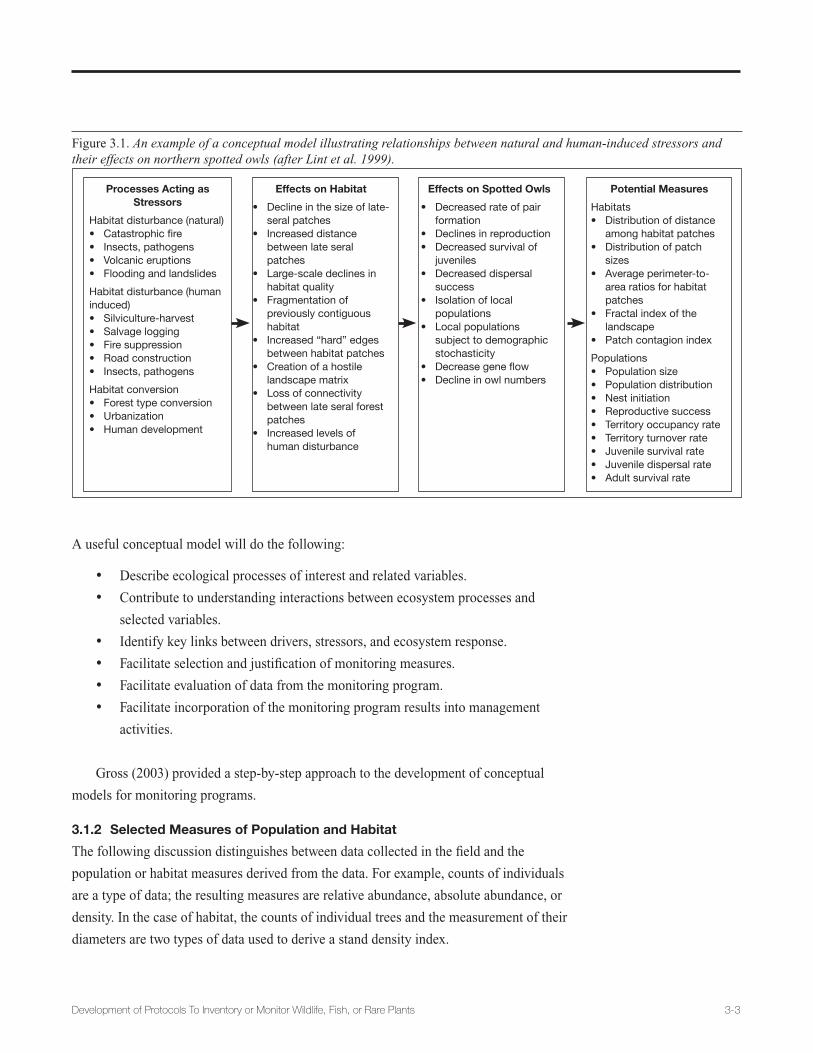
Development of Protocols To Inventory or Monitor Wildlife, Fish, or Rare Plants 3-3
A useful conceptual model will do the following:
• Describe ecological processes of interest and related variables.
• Contribute to understanding interactions between ecosystem processes and
selected variables.
• Identify key links between drivers, stressors, and ecosystem response.
• Facilitate selection and justification of monitoring measures.
• Facilitate evaluation of data from the monitoring program.
• Facilitate incorporation of the monitoring program results into management
activities.
Gross (2003) provided a step-by-step approach to the development of conceptual
models for monitoring programs.
3.1.2 Selected Measures of Population and Habitat
The following discussion distinguishes between data collected in the field and the
population or habitat measures derived from the data. For example, counts of individuals
are a type of data; the resulting measures are relative abundance, absolute abundance, or
density. In the case of habitat, the counts of individual trees and the measurement of their
diameters are two types of data used to derive a stand density index.
Figure 3.1. An example of a conceptual model illustrating relationships between natural and human-induced stressors and their effects on northern spotted owls (after Lint et al. 1999).
Processes Acting as Stressors
Habitat disturbance (natural)• Catastrophicfire• Insects, pathogens• Volcanic eruptions• Flooding and landslides
Habitat disturbance (human induced)• Silviculture-harvest• Salvage logging• Fire suppression• Road construction• Insects, pathogens
Habitat conversion• Forest type conversion• Urbanization• Human development
Effects on Habitat
• Decline in the size of late-seral patches
• Increased distance between late seral patches
• Large-scale declines in habitat quality
• Fragmentation of previously contiguous habitat
• Increased “hard” edges between habitat patches
• Creation of a hostile landscape matrix
• Loss of connectivity between late seral forest patches
• Increased levels of human disturbance
Effects on Spotted Owls
• Decreased rate of pair formation
• Declines in reproduction• Decreased survival of
juveniles• Decreased dispersal
success• Isolation of local
populations• Local populations
subject to demographic stochasticity
• Decreasegeneflow• Decline in owl numbers
Potential Measures
Habitats• Distribution of distance
among habitat patches• Distribution of patch
sizes• Average perimeter-to-
area ratios for habitat patches
• Fractal index of the landscape
• Patch contagion index
Populations• Population size• Population distribution• Nest initiation• Reproductive success• Territory occupancy rate• Territory turnover rate• Juvenile survival rate• Juvenile dispersal rate• Adult survival rate

3-4 Development of Protocols To Inventory or Monitor Wildlife, Fish, or Rare Plants
Population and Community Measures
To be meaningful, all population and community measures require an estimate of
detection probability, unless surveyors are confident that all individuals present at the
sampling unit will be detected each time a survey is conducted. Although detection
probabilities are not explicitly addressed here, the concept is integral to all the population
and community measures presented. Methods for estimating detection probabilities are
presented in Section 3.4, Analytical Methods.
ECOLOGY OF
PENSTEMON LEMHIENSIS
Conceptual Models1
When developing a conceptual model, consider the following points:
• It should represent your current understanding of the system you intend to monitor.• It should help you understand how the system works. What are the entities that define the
structure of the system? What are the key processes? This knowledge often yields a narrative model—a concise statement of how (you think) the system works.
• It should describe the state variables. What mechanisms and constraints will be included, and which will be excluded?
• What assumptions will be made about the system? At what spatial and temporal scales does the system operate? These considerations often result in the construction of a schematic model, perhaps a Forester diagram (a “box and arrow” model). It should provide a framework for generating hypotheses about how the system works. The key states or processes most likely to be affected by management actions should be identified for monitoring.
1 Figure excerpted from Elzinga et al. (2001: 262).

Development of Protocols To Inventory or Monitor Wildlife, Fish, or Rare Plants 3-5
Population measures are derived from the following types of data:
• Detection of unmarked individuals or associated signs (e.g., tracks, scat, hair).
• Detection and location of marked individuals.
• Counts of marked or unmarked individuals.
• Reproductive parameters.
• Genetic data.
Community measures are derived from detections or counts of individuals within
species or species groups. The following is a description of common population and
community measures and their usefulness in meeting different inventory and monitoring
objectives (adapted from Holthausen et al. 2005).
Population Measures
Presence/Absence. Presence/absence is derived from detection data by direct
observation or a reliable sign of the species’ presence (e.g., vocalization, genetic sample,
scat), and is adjusted for bias of imperfect detection. This measure is useful when the
objective is to expand knowledge about the habitat associations of a targeted species or to
expand knowledge about the co-occurrence of a species with other species. It is primarily
an inventory measure that results in species lists and habitat associations.
Frequency of Occurrence. This measure estimates, for a statistical population of
survey sites, the proportion of sites with the target species present, based on a random
sample of the statistical population. Frequency of occurrence is not spatially explicit, so it
cannot be used to map a species’ spatial distribution. It can be used, however, to estimate
whether the spatial distribution is changing over time; for instance, whether the number
of occurrences (as opposed to numbers of individuals) of a rare plant are increasing or
decreasing. Frequency of occurrence is a useful indicator of relative abundance if the
relationship between frequency of occurrence and population density has been established
or estimated (e.g., each survey site represents one breeding pair). If so, then change in
frequency of occurrence can be used to estimate change in relative abundance over time.
Abundance or Density. These measures are derived from counts of individuals or
from the presence and location of marked individuals. Abundance is either absolute (a
complete census or an estimate of total abundance), or relative (number-of-individuals-
per-unit effort). Relative abundance becomes relative density when the comparative unit
is area (number of individuals per unit of area). Relative density can be estimated from
counts of individuals and their detection probabilities. It can also be estimated from
habitat associations and average home range size derived from the presence and location
of marked individuals. Abundance or density provides more information than does
presence/absence about the relative importance of different habitats and about the strength
of association in co-occurrence of certain species. Also, it provides greater sensitivity to
detect change over time than frequency of occurrence does.

3-6 Development of Protocols To Inventory or Monitor Wildlife, Fish, or Rare Plants
Indices of Relative Abundance. This suite of measures is based on detections
or counts of objects, such as pellets, tracks, or vocalizations, which are surrogates for
individuals. Thompson et al. (1998) state that any unadjusted partial count of individuals
is an index; therefore, relative density without an adjustment for detectability is
technically an index of relative abundance. An index can be used for inventory purposes
such as mapping spatial distribution and co-occurrence with other species. Caughley
(1977) advocated the use of indices for monitoring change in abundance over time,
indicating that many studies that used estimates of absolute density could have used
density indices without losing information. He suggested that use of indices often results
in a more efficient use of time and resources and produces results with higher precision
than population estimates do (Caughley 1977, Caughley and Sinclair 1994).
Others have questioned the reliability of index values for monitoring change over
time, however, because the relationship between the index and true population abundance
usually is not quantified or known (Thompson et al. 1998; Anderson 2001, 2003), and
the opportunity for bias associated with indices of abundance is quite high. For instance,
track counts could be related to animal abundance, animal activity levels, or both.
Capture rates of animals over area and time may be related to animal abundance or to
the animals’ vulnerability to capture in areas of differing habitat quality. Consequently,
although indices of abundance are often used because of logistical constraints,
considerable caution must be exercised when interpreting these results. Nevertheless,
Engeman (2003) concluded that an index may be the most efficient means to address
population monitoring objectives and that the concerns associated with the use of
indices can be addressed with appropriate and thorough experimental design and data
analyses. Moreover, McKelvey and Pearson (2001) found that some indices exhibit lower
variance than do population estimators, particularly with small sample sizes or when the
estimators’ underlying population attributes are largely unknown. Therefore, the choice of
an index or an estimator will depend on data quality.
Vital Rates. Vital rates are age-specific birth and death rates or emigration/
immigration rates that are derived from evidence of reproduction, such as the number
of young per female or the number of seed pods per plant. Vital rates are a cornerstone
of population viability analysis. An understanding of vital rates provides insight into
population status. Depending on life history, monitoring of vital rates can provide a
better measure of population status than do measures of abundance. Furthermore,
understanding how vital rates change in response to management provides insight into
potential mediation or mitigation. Demographic sensitivity analysis can help identify the
appropriate vital rate to monitor.
Range Distribution Measures. Geographic range can be estimated from presence/
absence or counts of individuals, while further differentiation of breeding and non-
breeding range can be determined from evidence of reproduction. Boundaries of

Development of Protocols To Inventory or Monitor Wildlife, Fish, or Rare Plants 3-7
genetically distinct populations can be estimated from genetic data. Range distribution
measures are valuable when the monitoring goal is to estimate whether the range of a
species is expanding, contracting, or remaining relatively constant. This information is
needed for exotic species and endangered species management, where the goal may be to
compare the current geographic range to historic distributions. Current research indicates
a correlation between a species’ abundance and distribution, so range dynamics may
provide an effective indication of abundance (He and Gaston 2000).
Genetic Measures. DNA-based inventory and monitoring efforts will provide new
insights into fish, wildlife, and plant population health and trends. There are two distinct
ways in which DNA and population genetics can be used for inventory and monitoring.
First, genetics can be used to bolster other monitoring efforts described above. For
example, to delineate an animal’s range, traditional methods often call for the use of
historical records or the identification of snow tracks; both delineation techniques are
highly unreliable and prone to high error rates. Using DNA obtained from hair, urine,
or scat associated with snow tracks, however, can provide reliable, positive species
identification. In this sense, DNA can augment traditional methods and provide more
reliable estimates of abundance, presence/absence, and geographic range. Many examples
of such DNA usage exist for estimating abundance (Paetkau 2003, Schwartz et al. 2004),
presence/absence (Taberlet et al. 1997, Schwartz et al. 2004), and geographic range
(Taberlet et al. 1997, McKelvey et al., in press).
Secondly, data from DNA can be used to abet I&M in a population genetics
framework. That is, once samples are collected, the genetic data can be tapped for further
information about the population. In particular, the genetic data can be used for the
following purposes:
• To examine changes in genetic diversity in the population over time or compare
genetic diversity across space.
• To detect recent genetic population bottlenecks.
• To estimate effective population size or changes in effective population size over
time (detailed in following sections).
Some of these techniques are well established; others will require additional develop-
ment before implementation. Overall, the genetics field is rapidly advancing, with novel
and more precise techniques available each year. In the not-too-distant future, advances in
conservation genetics may provide us with unprecedented power to infer change in WFRP
populations.
Community Measures
Diversity Measures. Species richness, evenness, or diversity can be estimated from
counts of individuals. Research studies have used diversity measures to examine particular

3-8 Development of Protocols To Inventory or Monitor Wildlife, Fish, or Rare Plants
questions in community and ecosystem ecology, such as community relationships based
on trophic, functional, or taxonomic groupings. Diversity measures pose challenges,
however, because they are not easily interpreted. For example, an increase in species
diversity could represent restoration of a native community, but it could also indicate loss
of rare species and gains of invasive species. These challenges have limited the utility of
these measures in resource management monitoring.
Integrity Measures. Karr and Dudley (1981) define biological integrity as the
“capability of supporting and maintaining a balanced, integrated, adaptive community
of organisms having a species composition, diversity, and functional organization
comparable to that of the natural habitat of the region.” The concept of biological integrity
has evolved in response to perceived flaws in biological diversity measures. Biological
integrity is used to compare current conditions on the landscape with conditions present
at a specific instance in history or to a nearby “natural” baseline condition. Because this
measure relies on one of the diversity measures described above it is subject to all the
strengths and weaknesses associated with those measures.
Habitat Measures
The ability to correlate species and habitat data allows for better predictions of species
occurrence and distribution and the effects of management on populations. Two critical
elements are needed for an accurate, sound comparison of population and habitat data
(Jones 1986). First, both species and habitat data must be collected on the same site and
during the same time period. If habitat data are collected at a later date, correlations
between species’ presence and seasonal changes in the habitat might be missed. Second,
the habitat definition must be determined before data collection. If habitat is defined as
any set of ecological conditions in which the species is present, then presence/absence
data will suffice. If the objective is to identify breeding habitat or differentiate between
source and sink habitat, however, then data about the species’ ability to survive and
reproduce (e.g., mortality, survivorship, predation, parasitism) also must be collected
(Cody 1985).
Species respond to habitat availability and quality at multiple scales. Most habitat
assessment techniques are designed for assessing vegetation composition and structure
within a patch or stand, but many organisms also respond to habitat at landscape scales
(e.g., McGarigal and McComb 1995). Concepts such as metapopulation dynamics,
source-sink dynamics, dispersal capabilities, and landscape heterogeneity have become
an important basis for collecting data that characterize landscapes. Examples of such data
are mean patch size, patch isolation, and edge density. FRAGSTATS (McGarigal and
Marks 1995) provides descriptions and algorithms for a suite of landscape measures. It
also provides software for performing calculations on vector or rastor images.

Development of Protocols To Inventory or Monitor Wildlife, Fish, or Rare Plants 3-9
3.1.3 Developing a Sampling Design
Spatial Patterns of Organisms
The spatial distribution of organisms within a population is an important consideration
for sampling design selection. The three basic population spatial patterns are random,
aggregated, and uniform (fig. 3.2). Random dispersion, often approximated by a Poisson
distribution, is found in populations in which the spacing between individuals is irregular
and the presence of one individual does not directly affect the location of another
individual. Aggregated (also known as “clumped”) populations are characterized by
patches or clusters of individuals; the probability of finding one individual increases with
the presence of another individual. Count data from populations exhibiting aggregated
spatial patterns can frequently be modeled with the negative binomial distribution.
Uniform (also known as “regular”) distributed populations have individuals that are
distributed more or less evenly throughout an area; the presence of one individual decreases
the probability of finding another individual closer than the spacing pattern.
Resource distribution and habitat quality may affect the dispersion of individuals
and populations (McComb 2001). Random distribution is often found in species that
depend on ephemeral resources; species that depend on temporary or seasonal resources
may exhibit different types of distribution at different points in their life histories. Social
behavior and territoriality may affect vertebrates’ distribution. Highly territorial species
tend to follow a regular distribution, while more gregarious and colonial nesting species
tend to occur in clumps (Curtis and Barnes 1988, Newton 1998). Spatial patterns of
organisms, and, consequently, sample distributions resulting from their enumeration,
often change with the spatial scale of observations. Populations may appear uniformly
distributed at a fine scale, but may show a more random or aggregated distribution
throughout their range.
As observed organisms become more numerous and the mean number of individuals
per sample exceeds 10, the Poisson distribution begins to approach a normal distribution.
Similarly, if the total number of observed individuals (pooled across samples) exceeds
100, the normal distribution can be used to calculate confidence intervals for the
population mean (Krebs 1989). Zar (1999) suggested adjusting the sampling unit (e.g.,
Figure 3.2. Three basic spatial patterns of biological populations (Curtis and Barnes 1988, Krebs 1989).

3-10 Development of Protocols To Inventory or Monitor Wildlife, Fish, or Rare Plants
quadrat size, length of the sampling period) to increase the probability of detecting
more individuals in the habitat. If data counts follow the Poisson or negative binomial
distributions, and the primary objective of monitoring is to estimate only the parameter’s
population mean, the protocol may suggest that the appropriate sample size and
confidence intervals be determined using calculations developed specifically for both
types of distributions (see Krebs 1989 for examples).
Statistical Population
A statistical population is the entire set of potential sampling units from which a sample
is drawn and from which inferences can be made. For example, if bird-count stations are
randomly selected from a grid of potential x,y coordinates superimposed over a watershed,
the statistical population is the total number of x,y coordinates on the grid. The sample
might be 30 stations within a population of 3,000 coordinates. There is not necessarily a
correspondence between a statistical population and a biological population.
Standard Sampling Designs
As noted in section 2.1.3, sampling designs may have multiple objectives. First, the
design should ensure that the sample selected represents the population being monitored
or studied. This objective is usually accomplished by incorporating a random selection
procedure into the design process so all members of the population have an equal, or at
least known, probability of being selected. Randomization is essential for reducing bias
and estimating the parameters of a population. Second, the design may seek to maximize
the statistical efficiency of data collection by achieving the greatest possible precision
for the least cost. The greatest gains in statistical precision are usually attained with
increasing sample size, which can be financially impractical for most I&M programs.
Therefore, we recommend that the design process include criteria to allocate a sample
size sufficient to answer the primary questions of interest with a desired level of certainty.
The following are five sampling designs that have been found to be useful for natural
resource I&M projects. This introductory material is meant only to guide protocol
developers toward more comprehensive references on sampling design.
Simple Random Sampling. Simple random sampling occurs when a random
subset of units are selected as observations from a population in such a way that every
unit has an equal chance of being chosen (Krebs 1989). This randomly generated set
of observations may be collectively analyzed as representative of the population within
the study area. The strength of simple random sampling is that it makes no assumptions
about the distribution of features in the landscape being sampled. The weakness of simple
random sampling is that unless the sample size is large, it may not represent the range
of conditions that occur on the landscape. Consequently, simple random sampling is
generally not appropriate for large-scale monitoring because it is not cost-efficient.

Development of Protocols To Inventory or Monitor Wildlife, Fish, or Rare Plants 3-11
Stratified Random Sampling. Stratified random sampling is intended to reduce
variation in a sample by allocating observations to individual strata and then randomly
locating sample sites within each stratum. Stratification is based on any factor or set of
factors that could reduce variability within each stratum, such as habitat types, habitat
quality, or topography. Stratification can also be designed to increase the cost efficiency
of a sampling scheme (i.e., units of information collected per unit cost). Cost stratification
can be placed over any other stratification (Scheaffer et al. 1996). For example, sampling
costs might differ among sites depending on the distance of sample sites from roads. Near
and far distances from roads may then be used as two strata, with a greater proportion of
the total sample allocated to the near stratum to reduce costs. Control of costs via stratification,
however, will not necessarily achieve an overall estimate with the smallest variance.
The strength of stratified random sampling is that it can increase efficiency by
reducing the number of observations required to reach a desired precision level in an
estimate. It is most commonly and effectively used for monitoring species that occur in
low numbers, or when different habitats have different probabilities of the organism’s
presence. For example, the bioregional monitoring design for the northern goshawk
(Accipiter gentilis) (Hargis and Woodbridge 2006) uses a stratified random sampling
design because goshawks’ occupancy rates are expected to be higher in primary habitat
than in secondary habitat.
The weakness of stratified sampling is that it requires assumptions about the relative
spatial and temporal variability of strata and its design is inflexible. Strata should remain
fixed on the landscape over time and data should not be restratified based on some other
strata of interest that may arise in the future. Sampling designs based on strata that may
be ephemeral (e.g., early successional stages for vegetation) may not be useful over long
periods of time. Habitat boundaries may change over time or the same habitats may not be
present during all sampling periods.
Systematic Sampling. Systematic sampling consists of a fixed, regular pattern of
sampling units after random selection of a starting point for the systematic layout. The
strength of systematic sampling is that it confers an equal probability of selection for
all observations within the geographic area of inference, enabling observations to be
aggregated by various strata (e.g., national forests, vegetation types, species ranges,
with and without experimental treatments) without having to estimate the probability of
selection within strata. In addition, it can be readily augmented by increasing sample site
density in strategic locations to reach species-specific sampling objectives (e.g., increase
sample site density within specific habitats for species of interest at national forests or
larger scales to improve estimates).
A weakness of systematic sampling is that it may over sample some strata of interest
and under sample others; systematic sampling is thereby less efficient than a stratified
sampling approach for those particular strata (e.g., common, widespread vegetation

3-12 Development of Protocols To Inventory or Monitor Wildlife, Fish, or Rare Plants
types). Systematically sampled observations may also be correlated, which increases
analysis complexity. Systematic sampling is recommended for forest- and regional-
scale monitoring of multiple species because it does not make assumptions about the
distribution or abundance of various strata across the landscape and it is flexible in terms
of analyzing subsets of observations to address various management questions.
The Multiple Species Inventory and Monitoring (MSIM) protocol (Manley et al.
2004, Manley et al., in press) uses a systematic sampling design based on the sampling
grid of the Forest Service Forest Inventory and Analysis (FIA) program. The current FIA
sampling design consists of a systematic hexagonal grid across all ownerships in the
United States; each hexagon contains approximately 2,403 hectares. One FIA sampling
unit is randomly located within each hexagon. At each unit, vegetation structure and
composition are scheduled to be surveyed once every 10 to 15 years (Roesch and Reams
1999). The MSIM collects information on a variety of terrestrial and aquatic plant and
animal species at plots located 100 meters from the FIA sampling unit in a random
direction. In addition to the MSIM design, wildlife habitat information for a variety of
species has been gleaned from FIA vegetation data (e.g., Rudis 1991).
When establishing a systematic sample, care must be taken to ensure that the spatial
arrangement of observations is not correlated with any regular environmental parameter.
For example, in the Midwestern United States, placement of sampling points at 1.6-
kilometer (km) intervals may result in a biased sample because the arrangement of roads
and agricultural infrastructure in the region is based on a 1.6-km land survey scheme.
Adaptive Cluster Sampling. Many species have a tendency to occur in population
clusters because of dispersal mechanisms, behavior patterns (e.g., herding, colonialism),
or habitat associations. Under these conditions, it is predictable that monitoring programs
conducted according to conventional procedures will expend most of the sampling
effort at locations where the species is not observed. Adaptive cluster sampling refers to
procedures in which sample selection depends on the values of counts or other variables
observed during the course of sampling. Initially, a probability procedure is used to select
a set of sampling units in the study area. When any of the selected units satisfy some
predetermined criterion (e.g., detection of the target species), additional units are sampled
in the neighborhood of the qualifying unit. Sampling is extended until no further units
satisfy the criterion.
For rare or highly aggregated populations, adaptive cluster sampling may greatly
increase the precision of population size or density estimates when compared to a simple
or stratified random design of equal cost (Thompson 1992). Adaptive cluster sampling
can be used with quadrats, belt transects, variable circular plots, and other types of
sampling units. Pilot studies are strongly recommended to determine the sampling
design’s optimal scale. Adaptive cluster sampling is more complex to implement than
most other sampling designs. Therefore, most teams developing WFRP I&M protocols

Development of Protocols To Inventory or Monitor Wildlife, Fish, or Rare Plants 3-13
will need to arrange for a statistical consultant to develop analytical methods appropriate
for adaptive sampling. Teams conducting I&M projects will require similar assistance in
performing data analysis.
Before-After Control-Impact. The recommended design for monitoring the effects
of a management treatment is a before-after control-impact (BACI) design (Green 1979,
Stewart-Oaten et al. 1986), which enables comparison of before-and-after effects as well
as treatment-control effects. The ideal design consists of before-and-after data on repli-
cates of control and treatment sites, but it is usually not possible to replicate the treatment
due to the treatment’s large spatial extent or its unique nature (e.g., a single power plant,
ski area, or dam). The asymmetrical BACI design has a single treatment and one or more
controls, with before-and-after data collected from each (Stewart-Oaten and Bence 2001).
Other variants to the basic BACI design are possible, depending on the type of
treatment and the anticipated effects. The gradient design involves placing sites at varying
distances from the source of the treatment (Ellis and Schneider 1997). The factorial
design creates several paired sites within the treatment and the control that share similar
attributes; the distinguishing attributes become the factors (Evans and Coote 1993). For
example, the factors could be two vegetation cover types and dense versus open stands,
with paired sites in and out of the treatment that represent each cover type and stand
density combination. Several BACI design variants are presented in Smith (2002).
Size and Shape of Sampling Units
Count data obtained from plots are affected by the sampling unit’s size and shape. Square
plots and circular plots have smaller boundary/interior ratios than rectangular shapes of
equal area. Plots with exaggerated lengths are sometimes referred to as strip transects
or belt transects. Under some sampling conditions it might be difficult for the surveyor
to determine whether organisms occurring near a plot boundary are inside or outside
the plot, resulting in counting errors. In these circumstances, compact plot shapes are
preferred. Boundary/interior ratios also decrease as plot size increases. As a result larger
plots seemingly offer another approach for reducing counting errors. The tedious nature
of counting organisms on a large plot under difficult field conditions, however, may
cause surveyors to make mistakes. Counting error is not the only factor to consider when
determining plot size and shape. In heterogeneous habitats, data collected on long plots
often have been found to have lower statistical variance than data from compact plots of
the same total area (Krebs 1989).
The optimum size and shape of a plot will differ according to the species,
environmental conditions, and monitoring program objectives. Typically, the optimum
plot configuration will be one that provides the greatest statistical precision (i.e., lowest
standard error) for a given area sampled. Several investigators have developed approaches
for selecting the most appropriate plot size and shape for a particular population

3-14 Development of Protocols To Inventory or Monitor Wildlife, Fish, or Rare Plants
monitoring program (e.g., Hendricks 1956, Wiegert 1962). Krebs (1989) provides a useful
review of standardized plot configurations.
While the usual notion of a plot is that of an area delineated by a frame or flagging,
other techniques may be used to obtain a sample count of target organisms in a given area.
For example, cover board surveys have been widely adopted for estimating the relative
abundance of amphibian and reptile populations in different habitat types (Grant et al.
1992, Harpole and Haas 1999).
Line-transect and point-transect sampling are specialized plot methods in which
a search for the target organism is conducted along a narrow strip with a known area.
Rarely can it be assumed that all animals are detected along a transect. If the probability
of detection can be predicted from the distance between the animal and the centerline
of the transect, however, then a detection function can be used to estimate population
density. The approach can be adapted to monitoring programs conducted by foot,
snorkeling, and ground or air vehicles. Buckland et al. (2001) provides a complete,
although highly technical, introduction to line-transect and point-transect distance
sampling methods. The approach has been widely applied to monitoring of vertebrates,
including desert tortoises (Gopherus agassizii) (Anderson et al. 2001), marbled murrelets
(Brachyramphus marmoratus) (Madsen et al. 1999), songbirds in oak-pine woodlands
(Verner and Ritter 1985), and mule deer (Odocoileus hemionus) (White et al. 1989),
among many others.
Population abundance can be estimated by a variety of “plotless” monitoring methods
that use measurements to describe individuals’ spacing in an area. These techniques
are founded on the assumption that the number of individuals in a population may be
estimated by measuring the average distance among individuals in the population or
between individuals and randomly selected observations. One of the most widely used
techniques is the point-centered quarter method (Cottam and Curtis 1956). Distance
methods have been commonly used for vegetation surveys and are easily adapted to
inventories of rare plants or other sessile organisms. The approach may also be useful for
population studies of more mobile animal species by obtaining abundance estimates of
their nests, dens, roosting sites, or scat piles.
Plotless methods may have some practical advantages over plots or transects, such as
the following:
• Plotless methods are less susceptible to counting errors that often occur near plot
boundaries; thus, they may yield more accurate abundance estimates.
• The time and effort required to attain an adequate sample of plotless
measurements in an area often is less than that required to search for every target
organism on a plot; thus, the efficiency of the monitoring program increases.

Development of Protocols To Inventory or Monitor Wildlife, Fish, or Rare Plants 3-15
Field techniques vary depending on the plotless method selected for the monitoring
program. All plotless methods use random selection procedures to choose center points
and/or compass bearings. Equipment requirements are minimal; usually only a compass,
flagging, and measuring device appropriate to the scale of the population and monitoring
area are needed. However, data collection protocols may be relatively complicated and
sample size calculations may need to be performed in the field. Therefore, a rigorous
training program is recommended for personnel conducting the monitoring program. Two
useful references for designing inventories based on plotless methods are Seber (1982)
and Bonham (1989).
Temporal Aspects of the Sampling Design
The description of the sampling design should include temporal aspects within a sampling
period, such as the optimal time period (month or season) for conducting surveys, any
daily restrictions in sampling period (e.g., mornings only), and the temporal sequence
of within-year sampling (e.g., once a month, every 2 weeks). For monitoring strategies,
the design should also describe the resampling cycle. Any restrictions imposed by the
sampling design, however, may affect how well the sample represents the adopted target
population and/or sampling frame.
Monitoring strategies typically call for resampling the same set of units in each
sampling period, thus building a history of site conditions across a consistent set of sites.
This approach is effective if the sampling effort is sufficient to represent the range of
conditions across the area of inference. It is sometimes called a “single panel” design.
The term “panel” describes the set of units that are sampled every sampling period. From
the standpoint of statistical analysis of temporal change, data collected for the same units
every sampling period will have lower variance than data collected for different units
each year. As a result, the sample size needed to detect a change with the desired level
of precision and power will be smaller than if the sampling units changed each year.
A main attribute of the panel approach is the ability to make estimates for individual
years or other points in time. The ability to estimate change, however, is not necessarily
improved over a repeated sampling design (see Cochran [1977] for a summary of the
tradeoffs). One weakness of repeated measurements of the same sites over time is that
through chance (or selection of which sites are being monitored), sites with changes in the
monitoring measure may not be included in the sample (i.e., a change may occur during
the monitoring period, but the change is not detected because no or too few monitored
sites are affected). A new random sample drawn at each time point has a better chance
of picking up such a change, but the tradeoff is that the sample size needed each time is
larger than that needed for the repeated-measures design.
Over the past decade, the use of rotating panels has gained popularity as an approach
to gaining greater representation of ecological conditions across large landscapes (a rotat-
ing-panel design is different from drawing a new random sample each time). A resampling
3-16 Development of Protocols To Inventory or Monitor Wildlife, Fish, or Rare Plants
design, known as a serial alternating panel approach, involves cycling through a series of
panels, each of which contains a set of points that spatially represents the landscape and
which, in sum, is more likely to ecologically represent the area of inference. In a panel ap-
proach, a systematic subset of points (a panel) is identified for each sampling period. The
alternating-panel design generally consists of n sampling units partitioned into m panels.
Each panel contains np sampling units (np = n/m) and has the same temporal pattern of
remeasurement. The remeasurement schedule determines the number of panels; if all sites
are visited every 5 years, then there are five panels, one for every year. As an example, the
FIA sampling design is based on a serial alternating-panel approach (Lesser and Overton
1994, Thornton et al. 1994, Roesch and Reams 1999). Most FIA regions use 10 panels
consisting of 10 percent of the sample, resampled every 10 years.
For cases in which resource conditions vary substantially from year to year and
influence the abundance of organisms (e.g., the abundance of mice), it is wise to augment
the panel approach with an additional panel that is sampled every year to track annual
variation. This additional panel is the augmented serial alternating panel (ASAP) design.
When a series of panels is completed, the strength of an ASAP design is its ability to
rival or exceed the statistical power to detect a population trend obtained from the single-
panel design while achieving better ecological representation across the landscape. Also,
it creates larger data sets for exploring habitat relationships and potential causal factors
for observed changes. A weakness of the ASAP design is that the statistical model is not
well developed; thus, some uncertainties exist regarding the exact procedure to follow for
generating trends. Also, the ASAP design requires consistent funding each year to ensure
that each scheduled panel is fully surveyed. Incomplete or unsurveyed panels would
further complicate the statistical analysis or could reduce the design to one that simply
samples different sites every year. Because of the advantages, however, many broad-scale
monitoring programs are moving toward a panel approach (e.g., Reeves et al. 2003). To
determine which approach best meets the needs and capabilities of the national forests/
grasslands and regions, it is recommended that panel approaches be considered and
evaluated against single-panel designs for monitoring population trends.
3.2 Data Collection: Biological Study Ethics
Capture, marking, and observation techniques may cause subject animals to experience
pain, permanent injuries, and increased mortality rates. Indeed, some animal inventories
and monitoring studies depend on lethal traps for the collection of voucher specimens
or population data. The justification for such studies must balance the benefits of newly
acquired knowledge with the welfare of animals subjected to study methods. Most
wildlife, fisheries, and zoological professional societies have adopted guidelines to help
field biologists minimize adverse impacts on individual animals and populations (e.g.,
American Society of Mammalogists 1987; ASIH, AFS, and AIFRB 1988; Gaunt et al.

Development of Protocols To Inventory or Monitor Wildlife, Fish, or Rare Plants 3-17
1997). In some situations, university faculty collaborating with the Forest Service may
also be required to maintain the standards prescribed by their universities’ Institutional
Animal Care and Use Committees. We recommend that protocol developers become
familiar with the standards for animal usage in field studies and that the methods be
designed with consideration of these standards.
3.3 Data Storage: Metadata Purpose and Standards
I&M data can benefit scientific research and facilitate species conservation programs
for many decades. The usefulness of a database is determined not only by the rigor of
the methods used to conduct the monitoring program, but also by the ability of future
investigators to decipher the variable codes, measurement units, and other details
associated with the database. The term “metadata” refers to “data about data.” Metadata
is information about the origins of a database or a map provided by its developer, changes
to the work made by secondary users, and quality of the data. Metadata facilitates
information sharing among current users. It is crucial for maintaining the value of data
to future investigations. The standardized metadata that will accompany I&M databases
should be recognized as one of the principle means to improve the transferability
of biological monitoring information among different Forest Service programs and
management units.
Since 1995, all Federal agencies have adopted a content standard for geospatial data
sets. The standard, called Content Standard for Digital Geospatial Metadata (CSDGM),
was developed by the Federal Geographic Data Committee (FGDC); this group also is
responsible for reviewing and updating the standard as needed. The currently approved
FGDC standard is CSDGM Version 2 – FGDC-STD-001-1998. The FGDC metadata
standard includes seven major elements, some of which are mandatory for every database
and map; other elements are applicable only to particular types of work (fig. 3.3). Some
GIS packages include software tools that automate some metadata documentation tasks;
however, most fields must be manually completed by the originator of the database.
The process of describing data sources, precision tests, geoprocessing methods, and
organizational information can be tedious and add many hours to the preparation of a data
set. The initial cost of the labor, however, will ensure that the data can be used for many
years, possibly for research or conservation purposes not anticipated by the originator of
the data set.
The CSDGM was developed to be applicable to all geospatial databases. The CSDGM
framework identifies the originators of the database, describes data sources, and captures
spatial reference information. But the generic nature of the CSDGM does not provide
for standardization of many attributes commonly shared among biological databases. To
extend the effectiveness of the CSDGM framework, the FGDC’s Biological Data Working
Group has developed the Biological Metadata Profile (FGDC and USGS 1999) to

3-18 Development of Protocols To Inventory or Monitor Wildlife, Fish, or Rare Plants
standardize the use of terms and definitions in metadata prepared for biological databases.
The Biological Metadata Profile addresses topics such as taxonomic classification,
voucher specimens, environmental attributes, and similar issues not considered in the
CSDGM. The Biological Metadata Profile is also applicable to nongeospatial data sets.
Figure 3.3. Graphical representation of major metadata elements specified by the approved Federal standard for geospatial databases (CSDGM Version 2–FGDC-STD-001-1998). (This figure was copied from http://biology.usgs.gov/fgdc.metadata/version2.)
3.4 Analytical Methods
This section should help familiarize the reader with the basic characteristics and
assumptions of analysis models and the circumstances under which they can be employed
effectively. The purpose of this information is to help build a well-planned and effective
data analysis framework. Since this section deals with complex technical issues, only
key elements and concepts of effective data processing are addressed in this technical
guide. Protocol developers should consult statisticians and more comprehensive statistical
resources to establish a rigorous context for data analysis. General references such as Zar
(1999) provide useful guidance for many aspects of analysis.

Development of Protocols To Inventory or Monitor Wildlife, Fish, or Rare Plants 3-19
3.4.1 Data Visualization and Exploratory Data Analysis
The initial phase of every data analysis should include exploratory data evaluation.
Graphical display of information is an integral component of every research undertaking.
As a first step in evaluating the data’s nature, quality, and underlying assumptions, I&M
technical guides should encourage a visual exploratory data analysis (Tukey 1977) before
statistical testing. The protocol may direct users to excellent examples of graphical display
in Spear (1952), Tukey (1977), Tufte (1983), Elzinga et al. (2001), and Ellison (2001).
Tufte (1983, 1997, 1990) gives a thorough overview of how to design and use images in a
wide range of applications.
Anscombe (1973) advocates several iterations in the process of examining data to
reveal unique features. Hilborn and Mangel (1997) recommend plotting data in different
ways to uncover “plausible relationships.” Numerous types of graphical displays can
be used to examine data before analysis and to display summary statistics. The most
commonly used include normal probability plots, density plots (histograms, dit plots), box
plots, scatter plots, bar charts, and point-and-line charts (Elzinga et al. 2001). The reader
can find excellent examples of how to construct and use graphical displays in almost any
introductory text on statistical analysis.
According to Tufte (1983), effective graphical displays show the essence of the col-
lected data and should do the following:
• Show the data.
• Induce the viewer to think about the substance rather than methodology, graphic
design, the technology of graphic production, or something else.
• Avoid distorting what the data have to say.
• Present many numbers in a small space.
• Make large data sets coherent.
• Encourage the eye to compare different pieces of data.
• Reveal the data at several levels of detail, from a broad overview to the fine structure.
• Serve a reasonably clear purpose—description, exploration, tabulation, or decoration.
• Be closely integrated with the statistical verbal descriptions of a data set.
In some cases, the pattern of the data will actually guide the selection of the model
that can be used to describe the relationship in the data (Anscombe 1973, Hilborn and
Mangel 1997). For example, refer to the four graphs in figure 3.4. They all display
relationships that produce identical outputs if subjected to a simple linear regression
analysis (table 3.1).

3-20 Development of Protocols To Inventory or Monitor Wildlife, Fish, or Rare Plants
Figure 3.4. Relationships between the four sets of x,y pairs (after Anscombe 1973).
Table 3.1. Four hypothetical data sets of x,y variable pairs.
A B C D Analysis output
X Y X Y X Y X Y
10.0 8.04 10.0 9.14 10.0 7.46 8.0 6.58
8.0 6.95 8.0 8.14 8.0 6.77 8.0 5.76
13.0 7.58 13.0 8.74 13.0 12.74 8.0 7.71
9.0 8.81 9.0 8.77 9.0 7.11 8.0 8.84
11.0 8.33 11.0 9.26 11.0 7.81 8.0 8.47
14.0 9.96 14.0 8.10 14.0 8.84 8.0 7.04
6.0 7.24 6.0 6.13 6.0 6.08 8.0 5.25
4.0 4.26 4.0 3.10 4.0 5.39 19.0 12.50
12.0 10.84 12.0 9.13 12.0 8.15 8.0 5.56
7.0 4.82 7.0 7.26 7.0 6.42 8.0 7.91
5.0 5.68 5.0 4.74 5.0 5.73 8.0 6.89
N = 11
Mean of Xs = 9.0
Mean of Ys = 7.5
Regression line: Y = 3 + 0.5X
Regression SS = 27.50
r = 0.82
R2 = 0.67
Source: Modified from Anscombe (1973).

Development of Protocols To Inventory or Monitor Wildlife, Fish, or Rare Plants 3-21
Yet, whereas a simple linear regression model may describe the trend in Case A
reasonably well, its use in the remaining three cases may not be appropriate, at least
not without an adequate examination and transformation of the data. Case B could be
described best using a logarithmic rather than a linear model. The relationship in Case D
is spurious, resulting from connecting a single point to the rest of the data cluster. Case C
also reveals the presence of an apparent outlier (i.e., an extreme value that may have been
missed without a careful examination of the data). This simple example illustrates the
value of a visual scrutiny of data before data analysis.
Under some circumstances, visual displays alone can provide an adequate assessment
of the data. This approach may even be superior to formal data analyses in situations with
large quantities of data (e.g., detailed measurements of demographics or vegetation cover)
or if data sets are sparse as a result of inadequate sampling or pilot investigations. For ex-
ample, maps can be used effectively to present a great volume of information (if a spatial
context is relevant to the question of interest). Tufte (1983) argues that maps are the only
means for displaying large quantities of spatial data in a relatively small amount of space
while still allowing for a meaningful interpretation of the information. In addition, maps
allow for a visual analysis of data at different levels of temporal and spatial resolution.
They also allow for the assessment of relationships among variables and can help identify
causes of the detected pattern.
A simple assessment of the species richness of a community can be accomplished
by presenting the total number of species found. Additional information can be acquired
by plotting the cumulative number of species detected against sampling effort to assess
whether the survey includes all or most of the species in the community. A steep slope
of the resulting curve would suggest that additional sampling effort might yield more
species, whereas flattening of the curve would indicate that most of the species in the
community have been detected (Magurran 1988, Southwood 1992).
Construction of species abundance models such as log-normal distribution, log series,
McArthur’s broken stick, or geometric series may be used to visually acquire additional
information about a particular research area. Individual species abundance models
describe communities with unique characteristics. For example, mature undisturbed
systems characterized by greater species richness typically display a log-normal
relationship between the number of species and their respective abundances. On the
other hand, early successional sites or environmentally stressed communities (e.g., those
affected by pollution) are characterized by geometric or log series species distribution
models (Southwood 1992).
The use of confidence intervals presents another attractive approach to exploratory
data analysis. Some even argue that confidence intervals represent a more meaningful
and powerful alternative to statistical hypothesis testing since they give an estimate of the
magnitude of an effect under investigation (Steidl et al. 1997, Johnson 1999). Confidence

3-22 Development of Protocols To Inventory or Monitor Wildlife, Fish, or Rare Plants
intervals can be placed on estimates of population density, observed effects of population
change in observations taken over time, or treatment effects in perturbation experiments.
They are also commonly used in calculations of effect size in power or meta-analysis
(Hedges and Olkin 1985, Gurevitch et al. 1992).
3.4.2 Basic Assumptions of Parametric Models
Parametric statistical models are based on a set of assumptions that are necessary for
models to properly fit and describe the data. If assumptions are violated, statistical
analyses may produce erroneous results (Krebs 1989, Sabin and Stafford 1990, Sokal and
Rohlf 1995). Thus, developers of I&M protocols should consider whether data will likely
fit the assumptions of a selected model. Options for dealing with problems of assumption
violations should always be presented.
Independence of Observations
An essential condition of most statistical tests is the independence of observations in
space and time (usually obtained using random selection). Observations can be counts of
individuals or replicates of treatment units in manipulative studies. Krebs (1989) argues
that if the assumption of independence is violated, the chosen probability for Type I error
(α) cannot be achieved. Analysis of variance (ANOVA) and linear regression techniques
are sensitive to this violation (Sabin and Stafford 1990, Sokal and Rohlf 1995). Mixed-
model analysis procedures, which are now available in some statistical software packages,
allow for some relaxation of the assumption of independence.
Homogeneity of Variances
Parametric models frequently assume that sampled populations have similar variances
even if their means are different. This assumption becomes critical in studies comparing
different groups of organisms, treatments, or sampling intervals. If the sample sizes are
equal, then parametric tests are fairly robust to the departure from homoscedasticity (i.e.,
equal variance of errors across the data) (Day and Quinn 1989, Sokal and Rohlf 1995).
In fact, equal sample sizes across treatments should be obtained whenever possible since
most tests are overly sensitive to violations of assumptions in situations with unequal
sample sizes (Day and Quinn 1989). Plotting the residuals of the analysis against
predicted values can reveal the nature and severity of the potential problem. This type of
output is a standard feature in many statistical packages. Visual inspection of the data can
help determine if transformation of the data is needed and can also indicate the type of
distribution (fig. 3.5). Although several formal tests exist to determine the heterogeneity
of variances (e.g., Bartlett’s test, Levine’s test), these techniques assume normal data
distribution, which reduces their utility in most ecological studies (Sokal and Rohlf 1995).

Development of Protocols To Inventory or Monitor Wildlife, Fish, or Rare Plants 3-23
Figure 3.5. Three hypothetical residual scatters. In Case A, the variance is proportional to predicted values, which suggests a Poisson distribution. In Case B, the variance increases with the square of expected values and the data approximate a log-normal distribution. The severe funnel shape in Case C indicates that the variance is proportional to the fourth power of predicted values (from Sabin and Stafford 1990).
A B C
Normality
Unfortunately, ecological data rarely follow a normal distribution and nonnormality
appears to be the norm in biology (Potvin and Roff 1993, White and Bennetts 1996,
Hayek and Buzas 1997, Zar 1999). Moreover, the normal distribution primarily describes
continuous variables whereas count data, often the type of information gathered during
I&M studies, are discrete (Krebs 1989). Although parametric statistics are fairly robust
to violations of normality, highly skewed distributions can significantly affect the results.
Ideally, the sample size should be equal among groups and sufficiently large (e.g., n > 20).
The significance of nonnormality can be tested with several techniques, including the
W-test and the Kolmogorov-Smirnov D-test for larger sample sizes. Sabin and Stafford
(1990), however, argue that the applicability of both tests is limited because they exhibit
low power if the sample size is small, and excessive sensitivity when the sample size is
large. Graphical examinations of the data are actually more appropriate than formal tests
because they enable one to detect the extent as well as the type of the problem. I&M
protocols may suggest plotting and scrutinizing data in normal-probability plots (fig. 3.6),
stem-and-leaf diagrams, or histograms (Day and Quinn 1989, Sabin and Stafford 1990).
Data that are reasonably symmetric about the mean and that do not have a large number of
observations in the distribution tails are generally well enough approximated by a normal
distribution for most standard analyses for which this is an assumption.

3-24 Development of Protocols To Inventory or Monitor Wildlife, Fish, or Rare Plants
Figure 3.6. Plots of four hypothetical distributions (left column) with their respective normal probability plots (right column). Solid and broken lines show the observed and normal (expected) distributions, respectively (from Sabin and Stafford 1990).
3.4.3 Possible Remedies if Parametric Assumptions Are Violated
Data Transformation
If significant violations of parametric assumptions occur, protocol users should be
advised to implement an appropriate data transformation to try to resolve the violations.
During a transformation, data will be converted and analyzed at a different scale than the
original data. Transformations effectively reweight the data and can result in detecting
statistical differences when none could be detected otherwise, so it is important to
consider the effects of transforming dependent variables on the eventual output. Protocol
users must also be aware of the need to back-transform the results after analysis to present
parameter values on the original data scale. Table 3.2 gives examples of common types of

Development of Protocols To Inventory or Monitor Wildlife, Fish, or Rare Plants 3-25
Table 3.2. Some common data transformations in biological studies. Transformations in this table are for dependent (y) variables typically transformed to meet assumptions of statistical tests when testing means. Biologists should be aware of assumptions for each statistical procedure to assess the need to transform variables before transforming variables.
Transformation When appropriate to consider using Transformation
Back type transformation
Square root
Logarithmic
Inverse
Arcsine square root
Box-Cox objective approach
Use with count data following a Poisson distribution (figure 3.5A); more gener-ally, when variances are proportional to means. In some instances, addition of 3/8 will improve normality.
Use with count data when means are proportional to standard deviations (figure 3.5B). A rule of thumb suggests its use when the largest value of the dependent variable is at least 10 times the smallest value.
Use when data residuals exhibit a severe funnel shaped pattern (figure 3.5C), which is often the case in data sets with many near-zero values.
Appropriate for proportional or binomial data. This transformation is beneficial if it improves normality for nonbinomial proportions. Most efficient when most proportions occur at ends of the scale (0.0–0.25 and/or 0.75–1.0), and least ef-fective when proportions are distributed in the middle (0.25–0.75).
If it is difficult to decide on what trans-formation to use, this procedure finds an optimal model for the data. Box-Cox approaches may address skewed residual distributions and heterogeneous variance.
y′ = loge(y+c)where c = 0 if all y > 1and c = 1 otherwise
y′ = 1/y
Note: Inverse transformations will cause very large values to be very small and very small values to be very large. Thus, one must reverse the distribution before transforming by multiplying a variable by -1, and then adding a constant to the distribution to bring the minimum value above 1.0. Once the inverse transformation is complete, the ordering of values will be identical to the original data.
y′ = arcsin(square root[y]), where y is a proportion.
where,λ is an estimated parameter
y = y′2
y = exp(y′)-c
y = 1/y′
y = (sin y′)2
Source: Modified from Sabin and Stafford (1990).
3-26 Development of Protocols To Inventory or Monitor Wildlife, Fish, or Rare Plants
transformations that may be recommended for use. A wisely chosen transformation can
often improve homogeneity of variances as well as produce an approximation of a normal
distribution. Sabin and Stafford (1990) and Zar (1999) give good overviews of data
transformations in ANOVA and regression models.
A primary reason to avoid transformations is that interpreting transformed variables
is very difficult (e.g., what is the arcsine square root of a proportion?). As a result, it is
recommended that the data be back-transformed after analysis but back-transformations
are not always necessarily at the same scale as the original data. Therefore, practitioners
must be aware of the assumptions of the particular statistical model and how transforming
will affect their data set. Removing outliers or perhaps using a nonparametric technique
may be a better approach than trying to normalize the distribution of data and homogenize
variances to meet the assumptions of a parametric model.
Nonparametric Alternatives
If the data violate basic parametric assumptions and transformations fail to remedy the
problem, a nonparametric method might be appropriate (Sokal and Rohlf 1995, Conover
1999). Nonparametric techniques have less stringent assumptions about the data, are less
sensitive to the presence of outliers, and are often more intuitive and easier to compute
(Sokal and Rohlf 1995, Hollander and Wolfe 1999). Since nonparametric models are less
powerful than their parametric counterparts, protocols should not advocate the use of
nonparametric tests if data meet, or approximate, parametric assumptions (Day and Quinn
1989, Johnson 1995, Smith 1995).
Randomization Tests
These tests are not alternatives to parametric tests, but rather are a means of estimating
the statistical significance that relies only on the independence of observations. They
are extremely versatile and can be used to estimate significance of test statistics for
a wide range of models. Although randomization tests are computationally difficult
even with small sample sizes (Edgington 1995), the Forest Service (R. King, personal
communication) has developed a Microsoft® Excel macro for randomization tests that
is available to Forest Service employees at http://statistics.fs.fed.us. More information
on computation-intensive techniques can be found in Crowley (1992), Potvin and Roff
(1993), and Petraitis et al. (2001).
Other Approaches
Other parametric techniques such as generalized linear models employ a distribution
appropriate for the data instead of trying to normalize them (Ministry of Environment,
Lands and Parks 1998). For example, White and Bennetts (1996) give an example of
fitting the negative binomial distribution to point-count data for orange-crowned warblers
(Vermivora celata) to compare their relative abundance among forest sites. Zero-inflated
Poisson (ZIP) models and negative binomial regression models are recommended for

Development of Protocols To Inventory or Monitor Wildlife, Fish, or Rare Plants 3-27
analysis of count data with frequent 0 values (e.g., rare species studies) in which data
transformations are not feasible (e.g., Heilbron 1994, Welsh et al. 1996, Ridout et al.
1998, Agarwal et al. 2002, Hall and Berenhaut 2002).
3.4.4 Statistical Distributions of Plant and Animal Population Data
Poisson Distribution
The Poisson distribution approximates a random spatial distribution common among
species with low population density, where the probability of detecting an individual in
any sample is rather low (Southwood 1992). As the mean number of individuals in the
sample increases, the Poisson distribution begins to approach the normal distribution
(Krebs 1989, Zar 1999).
During sampling, the key assumption of the Poisson distribution is that the expected
number of organisms in a sample is the same and that it equals μ, the population
mean (Krebs 1989). One intriguing property of the Poisson distribution is that it can
be described by its mean and that the mean equals the variance (s2). The probability
(frequency) of detecting a given number of individuals (x) in a sample collected from a
population with mean = μ is:
Px = (e-μ μx)/x!
Whether or not the data follow a Poisson distribution can be tested with a simple Chi-
square goodness of fit test:
Chi-square =Σ (observed frequency-expected frequency)2/expected frequency,
or with an index of dispersion (I), which is expected to be 1.0 if the assumption of
randomness is satisfied:
I = s2 / x,
where x and s2 are the observed sample mean and variance, respectively.
Krebs (1989) and Zar (1999) provide excellent worked examples of tests for goodness
of fit for Poisson distributions. The presence of a Poisson distribution in data can also be
assessed visually by examining the scatter pattern of residuals during analysis (fig. 3.5;
Sabin and Stafford 1990). If we reject the null hypothesis that observations came from a
Poisson distribution, the sampled organisms are either distributed uniformly or regularly
(underdispersed) with s2 < x, and s2/ x < 1.0, or they are clumped (overdispersed).
Negative Binomial Distribution
One mathematical distribution that describes clumped or aggregated spatial patterns is
the negative binomial (Pascal) distribution (Anscombe 1950, Krebs 1989). White and
Bennetts (1996) suggested that this distribution is frequently a better approximation to
3-28 Development of Protocols To Inventory or Monitor Wildlife, Fish, or Rare Plants
count data than the Poisson or normal distributions. The negative binomial distribution
is described by the mean and the dispersion parameter k, which expresses the extent
of clumping. As a result of aggregation, it always follows that s2 > x and the index
of dispersion (I) > 1.0. The value of k decreases with an increase in the degree of
aggregation and vice versa. The value of k can be approximated with:
k = x2 / (s2 –x)
Several techniques exist to evaluate the goodness-of-fit of data to the negative binomial
distribution. Good descriptions and examples of their use can be found in Krebs (1989),
Southwood (1992), and Zar (1999). Since the variety of possible clumping patterns in
nature is practically infinite, neither the Poisson or negative binominal distributions may
always adequately fit the data at hand (Krebs 1989).
3.4.5 Analysis Models and Methods
Species’ Presence and Frequency of Occurrence
In some cases, simply determining whether a species is present in an area may be a suf-
ficient objective. For example, biologists attempting to conserve a threatened wetland
orchid may need to monitor the extent of the species’ range and degree of population
fragmentation on a national forest. One hypothetical approach is to map all wetlands in
which the orchid is known to be present as well as additional wetlands that may qualify as
potential habitat. To monitor changes in orchid distribution at a coarse scale, data col-
lection could consist of a semiannual monitoring program conducted along transects at
each mapped wetland to determine if at least one individual orchid (or some alternative
criterion to establish occupancy) is present. Using only a list that includes the wetland
label (i.e., the unique identifier), the monitoring year, and whether the species was present
or absent, biologists could prepare a time series of maps displaying all the wetlands on
the forest by monitoring year and distinguish the subset of wetlands that were found to be
occupied by the orchid (i.e., frequency of occurrence). Such an approach could support
a qualitative assessment of changes in the species distribution pattern and generate new
hypotheses regarding the cause of the observed changes.
An analysis of species’ presence usually requires estimation of the probability of
detection because it is rare that individuals of a species will always be detected during a
survey. Without estimation of a detection probability, it will not be known whether a lack
of detection truly represents a species’ absence, or if it represents some probability of the
species’ presence.
Detection probabilities are estimated from repeated surveys of the same samples,
either during a pilot study or during the actual survey (MacKenzie et al. 2002). For ex-
ample, if a site is sampled three times, with X representing presence and O representing
absence, the possible outcomes of three surveys are 3 X’s, 3 O’s, 1 X and 2 O’s or 2 X’s

Development of Protocols To Inventory or Monitor Wildlife, Fish, or Rare Plants 3-29
and 1 O, in various patterns of XOX, XXO, etc. An average detection probability for all
sites sampled can be calculated; the standard error of this average can be estimated using
a nonparametric bootstrap method.
MacKenzie et al. (2002) estimated the frequency of occurrence (proportion of sites
with species’ presence), using a maximum likelihood estimation technique in which the
detection probability and probability of occupancy are both estimated parameters. The
method is similar to a closed-population, mark-recapture model. In their example, the
statistical population was the total number of ponds in a prescribed area and the object
was to estimate the proportion of ponds with frogs present (MacKenzie et al. 2002). In
a grid-based sample, the total number of grid cells is the statistical population, and the
object is to estimate the proportion of grid cells that are likely to be occupied by the target
species, given the outcome from a sample of grid cells. This approach has been adopted
for estimating goshawk presence over large geographic areas (Hargis and Woodbridge
2006). Recently, new methods such as noninvasive genetic sampling have bolstered our
ability to detect presence in grid cells and thus have increased our detection probabilities
and precision in presence/absence measures (McKelvey et al. 1999, McDaniel et al. 2000).
Recent studies indicate a positive correlation between frequency of occurrence and
species’ abundance, because species that increase in abundance also show increases in the
number of sites they occupy (Gaston et al. 2000, He and Gaston 2000). As a consequence,
presence-absence information is useful for monitoring population trends, (He and Gaston
2000, MacKenzie et al. 2003, MacKenzie et al. 2005).
Assumptions, Data Interpretation, and Limitations. Presence-absence data are
binary because each survey site has one of two possible outcomes: presence or absence.
A major assumption of presence-absence data is that a species’ presence or absence at a
site does not change during the survey period because the detection probability is based
on a constant state of presence (or absence) during all the visits to the same site. An
additional assumption is imposed if the average detection probability for all observations
is calculated from pilot data: the detection probability for the actual sample period is
the same as that of the pilot study. The detection probability could change, however, if
the pilot study took place in a different year, took place at a different time of the same
year, used different observers, or was in slightly different habitats. Thus, we recommend
that detection probabilities be calculated for each survey period from the actual survey
data even though this approach will require multiple visits per site. Survey costs can be
reduced by obtaining the detection probability from a subsample of sites as long as the
subsample is fairly representative of other sites in terms of factors (such as vegetation
density) that could affect detection of the target species.
An analysis of presence or frequency of occurrence works best if the plot size is
designed to contain only one or two individuals of the target species because density
can affect the detection probability, with higher probability of detections associated with
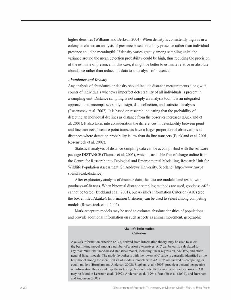
3-30 Development of Protocols To Inventory or Monitor Wildlife, Fish, or Rare Plants
higher densities (Williams and Berkson 2004). When density is consistently high as in a
colony or cluster, an analysis of presence based on colony presence rather than individual
presence could be meaningful. If density varies greatly among sampling units, the
variance around the mean detection probability could be high, thus reducing the precision
of the estimate of presence. In this case, it might be better to estimate relative or absolute
abundance rather than reduce the data to an analysis of presence.
Abundance and Density
Any analysis of abundance or density should include distance measurements along with
counts of individuals whenever imperfect detectability of all individuals is present in
a sampling unit. Distance sampling is not simply an analysis tool; it is an integrated
approach that encompasses study design, data collection, and statistical analyses
(Rosenstock et al. 2002). It is based on research indicating that the probability of
detecting an individual declines as distance from the observer increases (Buckland et
al. 2001). It also takes into consideration the differences in detectability between point
and line transects, because point transects have a larger proportion of observations at
distances where detection probability is low than do line transects (Buckland et al. 2001,
Rosenstock et al. 2002).
Statistical analyses of distance sampling data can be accomplished with the software
package DISTANCE (Thomas et al. 2005), which is available free of charge online from
the Centre for Research into Ecological and Environmental Modelling, Research Unit for
Wildlife Population Assessment, St. Andrews University, Scotland (http://www.ruwpa.
st-and.ac.uk/distance).
After exploratory analysis of distance data, the data are modeled and tested with
goodness-of-fit tests. When binomial distance sampling methods are used, goodness-of-fit
cannot be tested (Buckland et al. 2001), but Akaike’s Information Criterion (AIC) (see
the box entitled Akaike’s Information Criterion) can be used to select among competing
models (Rosenstock et al. 2002).
Mark-recapture models may be used to estimate absolute densities of populations
and provide additional information on such aspects as animal movement, geographic
Akaike’s Information Criterion
Akaike’s information criterion (AIC), derived from information theory, may be used to select the best fitting model among a number of a priori alternatives. AIC can be easily calculated for any maximum likelihood-based statistical model, including linear regression, ANOVA, and other general linear models. The model hypothesis with the lowest AIC value is generally identified as the best model among the identified set of models; models with ΔAIC <5 are viewed as competing, or equal, models (Burnham and Anderson 2002). Stephens et al. (2005) provide a general perspective on information theory and hypothesis testing. A more in-depth discussion of practical uses of AIC may be found in Lebreton et al. (1992), Anderson et al. (1994), Franklin et al. (2001), and Burnham and Anderson (2002).

Development of Protocols To Inventory or Monitor Wildlife, Fish, or Rare Plants 3-31
distribution, and survivorship (Krebs 1989). Open mark-recapture models (e.g., Jolly-
Seber) assume natural changes in the population size of the species of interest during
sampling. In contrast, closed models (e.g., Petersen, Schnabel) assume a constant
population size (Krebs 1989). Program MARK (White and Burnham 1999) performs
sophisticated maximum-likelihood-based mark-recapture analyses and can test and
account for many of the assumptions such as open populations and heterogeneity. The
selection of appropriate models to analyze mark-recapture data can be enhanced with the
use of AIC (Lebreton et al. 1992, Anderson et al. 1994, Burnham and Anderson 2002).
Excellent discussions of absolute abundance techniques can be found in Krebs (1989)
and Caughley (1977). Recently, due to the popularity of abundance estimates with genetic
data, new mark-recapture models have been created that consider unique properties of
genetic tagging (McKelvey and Schwartz 2004, Lukacs and Burnham, in press).
Occurrence data may be used to predict density if the relationship between species
occurrence and density is known and the model’s predictive power is reasonably high
(Hayek and Buzas 1997). For example, one can record plant abundance and species
richness in sampling quadrats. The species’ proportional abundance, or constancy of its
frequency of occurrence (Po), can then be calculated as:
Po = No. of species occurrences (+ or 0) / sample size (quadrats)
Consequently, the average species density is plotted against its proportional abundance
to derive a model to predict species abundance in other locations with only occurrence
data (fig. 3.7). Note, however, that the model may function reasonably well only in similar
Figure 3.7. A relationship between a species sample frequency (proportion of occurrences) and its mean density in habitat (from Hayek and Buzas 1997).

3-32 Development of Protocols To Inventory or Monitor Wildlife, Fish, or Rare Plants
and geographically related types of plant communities (Hayek and Buzas 1997). Other
examples of the use and analysis of relative density data can be found in James et al.
(1996), Rotella et al. (1996), Huff et al. (2000), and Knapp and Matthews (2000).
Assumptions, Data Interpretation, and Limitations. Analyses of relative
abundance data require attention to data distribution. Since the focus is on count data,
alternative statistical methods can be employed to fit the data distribution. Absolute
abundance techniques have stringent requirements (Krebs 1989). Given that statistical
power negatively correlates with the variability of the monitoring index, choosing an
appropriate measure of abundance and estimates of its confidence interval is crucial
(Harris 1986, Gerrodette 1987, Gibbs et al. 1999). An excellent overview of a variety of
groups of animals and plants for which the variability in estimating their population is
known is given in Gibbs et al. (1999).
Vital Rates
The effects of population and habitat management and other environmental factors often
directly influence vital rates of populations (DeSante and George 1994). Therefore,
an understanding of demographic parameters of populations such as productivity and
survivorship is an important element in efforts to monitor any population (Baillie 1990,
DeSante and Nott 2000). Information on population density alone may not provide a true
indication of population status due to source-sink dynamics (Van Horne 1983). Variation
in population size, reflected by density changes, which may potentially be associated
with management actions or environmental factors may be confounded by immigration
and/or emigration from the surrounding area (George et al. 1992). Monitoring a
variety of demographic factors such as age-specific mortality, reproductive rates, age
of first reproduction, or number of offspring per female can reveal specific aspects of
demography that correlate with observed population changes. These correlations can
then be used to investigate whether certain age groups or life events are particularly
sensitive to management actions. Furthermore, an understanding of vital rates can
provide information about when a population has been stressed in a yearly life cycle.
This information may be particularly important to determine if management actions on
migratory animals’ breeding or wintering areas are influencing the population (DeSante
and Nott 2000).
When vital rates are used to monitor population change, efforts must be made
to ensure that the vital rates represent the entire population and not a subset of the
population that has greater opportunities for survival and reproduction. For example,
when estimating reproductive rates or adult survival, the lower rates of senescing adults
could be an important consideration (Raphael et al. 1996). Reproductive rates should
also include an estimate of the proportion of nonbreeding females in the population.
All aspects of population demography must reflect rates associated with low-quality as

Development of Protocols To Inventory or Monitor Wildlife, Fish, or Rare Plants 3-33
well as high-quality habitat (Raphael et al. 1996). A good sampling design will reduce
potential bias associated with habitat quality.
The ability to use a finite rate of population change (λ) for monitoring purposes is
often challenged by a lack of data on juvenile emigration rates. This problem is not trivial,
as seen in the case of the northern spotted owl (Strix occidentalis), in which original
estimates of juvenile survival rates for three study areas were adjusted 42 to 137 percent
when researchers were able to incorporate radio telemetry data of juvenile emigration
(Franklin et al. 1999, cited in Franklin et al. 2004). In the absence of site-specific
emigration rates, Pradel (1996) developed analytical techniques that estimate λ directly
from capture-recapture data.
Monitoring efforts associated with land management practices that potentially
influence populations should be designed to address the demographic parameters
responsible for population change (DeSante 1995). This design may have a higher
likelihood of determining the effect of the management practice on the population
of interest than relying only on habitat correlations with presence-absence or relative
abundance data (DeSante and Rosenberg 1998, Villard et al. 1999).
Emphasis in monitoring populations of northern spotted owls shifted from estimating
numbers and densities to evaluating trends of vital rates (e.g., reproduction, survival)
(Gutiérrez et al. 1996) because the relationship between land management practices and
population trends was considered to be better estimated by vital rates (Franklin et al.
1996). However, a continuing need is recognized for independent estimates of population
trend to allow comparisons with, and evaluations of, demographic study results (Bart and
Robson 1995, Lint et al. 1999).
Measures of Geographic Range
The principal measures of a species’ geographic range are its size, shape, orientation, and
internal structure (Rapoport 1982, Maurer 1994, Brown et al. 1996). Estimates of range
size at two or more points in time enable analyses of range expansions (Andow et al.
1990, Hastings 1996) or contractions (e.g., Fisher and Shaffer 1996, Flather et al. 2004,
Laliberte and Ripple 2004). Range shape is a useful measure for evaluating the influences
of physical geography (Rapoport 1982, Brown and Maurer 1989), other environmental
limitations (Brown et al. 1996), and factors that result in contractions or expansions
(Laliberte and Ripple 2004). Range orientation is less useful for monitoring purposes, but
reveals basic relationships between orientation and range size (Brown and Maurer 1989).
The internal structure of a geographic range is a measure of discontinuities caused by the
number, size, and location of holes and fragments (Brown et al. 1996). Characterizations
of internal structure can reveal the processes by which range expansions or contractions
take place. Rapoport (1982) observed that home ranges tend to be less continuous toward
the periphery, but Channell and Lomolino (2000) found abundant examples of range
contractions that left holes within the range’s core.

3-34 Development of Protocols To Inventory or Monitor Wildlife, Fish, or Rare Plants
Before conducting an analysis of geographic range, investigators must first decide
whether their interest is in the full geographic range, including areas not used by the
species, or in only the specific areas where the species actually occurs. Gaston (1991)
coined the term “extent of occurrence” for the full range and “area of occupancy” for the
areas within the range that actually are occupied. Each of these definitions is associated
with different ecological questions. Range maps typically show the extent of occurrence
and much of the theory of range size, orientation, and boundary characteristics has
stemmed from studies of generalized range maps. In contrast, analyses based on area
of occupancy provide information about how the species is distributed within its range.
These patterns reveal changes in the internal structure of a geographic range that would
not be detectable with generalized range maps. This section highlights three approaches
for evaluating changes in a species’ geographic range: spatial analysis of occurrence
records, spatial analysis of abundance, and analysis of range maps. The first two
approaches are based primarily on area of occupancy, whereas the third approach is based
on extent of occurrence.
A spatial analysis of occurrence is actually a special case of an analysis of a species’
frequency of occurrence as described under the first subheading of this section. The
distinction is that the objective is to evaluate all known occurrences, display them
spatially, and use them to infer a geographic distribution. For monitoring purposes, a
comparison is made of historic and recent occurrences, with historic occurrences based
on museum specimens and accounts and recent occurrences based on databases such
as the Natural Heritage Programs or on recent field data collected specifically for the
purpose of the analysis. For statistical comparisons, occurrences are displayed on a grid
or by administrative units such as counties or States. Fisher and Shaffer (1996) mapped
historical and current occurrences of amphibians by county in the Central Valley of
California and documented statistically significant declines in the number of species
currently found in most counties. When mapped, the current distribution of occurrences
revealed substantial range contractions for three native species. Flather et al. (2004) used
State-level occurrence data to evaluate changes in species’ ranges for 1,642 terrestrial
animal species in the United States that are associated with forest habitats. Their two
sources of historic and current occurrences were NatureServe’s central databases and
the historic and current geographic range data for all species listed under the ESA. Their
analysis showed that the percentage of each taxonomic group now occupying less than 80
percent of historic range was 5.7 percent for mammals, 2.3 percent for amphibians, 1.4
percent for birds, and less than 1 percent for reptiles.
A spatial analysis of abundance takes advantage of abundance estimates obtained
from field data across large geographic extents. An estimate of range shape and its
internal structure is possible by constructing a probability ellipse based on the likelihood
of the species’ presence in areas surrounding sites with abundance estimates (Maurer

Development of Protocols To Inventory or Monitor Wildlife, Fish, or Rare Plants 3-35
1994). Rodríguez (2002) used Breeding Bird Survey data to map areas of high and low
abundance for 27 species of birds that had undergone significant declines since 1966. He
observed range contractions in 22 of the 27 declining species and was able to detect how
these contractions affected the internal structure of the geographic ranges.
An analysis of range maps compares changes in the mapped extent of a species’
distribution between two or more time periods. This approach is particularly challenging
because the mapped image of a species’ range lacks precision and accuracy and is subject
to considerable interpretation. Current and historic maps might exhibit differences in
geographic range that are not ecologically meaningful but instead reflect differences
in map resolution, mapping rules, and survey efforts between the two time periods. A
historic map might simply display the outline of a species’ range, whereas a current
map might show holes within a range boundary and islands around the perimeter where
isolated populations are found (Brown et al. 1996). In spite of these difficulties, a
comparison of historic and current range maps is highly valuable because it can reveal an
increased risk of extinction for some species and unwanted expansions for others.
Channell and Lomolino (2000) used published range maps as well as authorities’
opinions as the basis for comparing historic and current range maps for 309 species of
animals and plants. They developed an “index of centrality” to characterize whether the
current (remnant) range fell inside or outside the central portion of the historic range.
Laliberte and Ripple (2004) compared historic and current geographic ranges of 43
North American carnivores and ungulates using published range maps that they digitized
into a GIS. Like Channell and Lomolino (2000), they looked at whether the observed
contraction was toward the center or toward the periphery of the historic range. They
additionally evaluated whether the pattern of contraction was associated with one or more
variables of human influence.
Genetic Measures
Genetic measures are a potential useful monitoring tool because sometimes only relatively
small sample sizes are required to make inferences about the population under consideration.
(Note: the power to detect a phenomenon can be amplified by increasing the number of
genetic markers analyzed and the sample size.) In particular, the following three genetic
assays will provide data using only a single sampling occasion (in a single year):
• Changes in genetic diversity.
• Detection of genetic bottlenecks.
• Estimation of effective population size.
Examining differences in genetic diversity, or, more specifically, measures of allelic
diversity and heterozygosity, is a powerful approach. It is well documented that in
contracting populations, “rare alleles” (rare forms of genes) are rapidly lost; over time

3-36 Development of Protocols To Inventory or Monitor Wildlife, Fish, or Rare Plants
this loss is reflected in low levels of allelic diversity and heterozygosity. By comparing
allelic diversity or heterozygosity between populations we can assess which populations
may be at higher risk of population extinction (Saccheri et al. 1998). If no baseline exists,
comparisons can be made across populations.
Furthermore, even without a reference population at time zero for comparison,
patterns of allelic diversity (and patterns of allelic diversity combined with
heterozygosity) can be used to assess genetic bottlenecks. Luikart and Cornuet (1998)
clearly show the detection of previously unknown bottlenecks in natural populations of
mountain sheep, wolves, coyotes, brown bears, wombats, and various bird species using
single-year samples. Research is currently underway to determine if we can “screen a
landscape” to find “cryptic genetic bottlenecks.”
Effective population size can also be estimated with a single-year sample. Effective
population size is an estimate of population size discounted by demographic factors such
as unequal sex ratios in a population and variance in reproductive success. This measure
may be more pertinent to managers than abundance estimates because it is the measure
that natural selection and other evolutionary forces act upon. Good estimates of effective
population size can be obtained with small genetic samples from a population (Schwartz
et al. 1998). The measure is more precise, however, if multiple genetic samples can
be obtained spanning several generations. Recently, effective population size has been
estimated by collecting one sample in a single year and then comparing this sample to
DNA obtained from museum specimens (Miller and Waits 2003). One cautionary note
is that while DNA can lead to effective population size estimates, it can be difficult to
interpret the spatial and temporal scale encompassed by this estimate. The spatial problem
is no different than what is encountered when trying to traditionally estimate density.
The temporal problem can be used to the manager’s advantage as it is probably a more
pertinent piece of information than a single-point estimate.
The advantage of using genetic measures as described above or to help estimate
geographic distribution, presence-absence, or abundance (see the Population Measures
section) is that once the DNA is collected, ancillary information can readily be extracted.
For example, without collecting any additional information we can estimate substructure,
migration rates between populations, or relatedness between individuals within a
population (Manel et al. 2003, McKelvey and Schwartz 2004).
Species-Habitat Relationship Models
Presence-absence data, relative abundance, and estimates of absolute density can be used
to build models of species’ habitat relationships. The presence and location of marked
individuals are especially valuable because the data provide information about species’
home ranges and resource usage (Smith et al. 1982, Otis and White 1999, Compton
et al. 2002), although such information is usually obtained through specific research
studies instead of through monitoring. Regardless of the source, the data must enable

Development of Protocols To Inventory or Monitor Wildlife, Fish, or Rare Plants 3-37
a comparison between habitats that were used versus what was available, or between
habitats where species were present versus absent, in order to model habitat selection.
Chi-square goodness-of-fit analysis has been widely used to compare observed versus
expected use of potential habitat types (Neu et al. 1974, Alldredge and Ratti 1986, 1992).
The significance of different explanatory variables (habitat descriptors) in modeling the
species’ habitat use may be assessed with multivariate techniques (James and McCulloch
1990, Block et al. 1998), logistic regressions (North and Reynolds 1996, Block et al.
1998, Compton et al. 2002), multiple regressions (Orians and Wittenberger 1991, Block
et al. 1998), and classic ANOVAs (Orians and Wittenberger 1991) or their nonparametric
equivalents such as the Friedman’s test and Wilcoxon’s signed-ranks test (Alldredge and
Ratti 1986, 1992). Additional information on the analysis of habitat selection can be found
in Thomas and Taylor (1990), Arthur et al. (1996), Cherry (1996), Garshelis (2000), and
McDonald and Manly (2001).
Using a logistic regression, presence-absence data can be used to model the
relationship between species occurrence and habitat variables (Breslow and Day 1993,
Trexler and Travis 1993, Hosmer and Lemeshow 2000, Agresti 2002). For example, a set
of variables to predict the presence of a forest-dwelling salamander species can include
such attributes as the percentage of vegetation cover, amount of coarse woody debris, or
presence of snags. The resulting function provides an index of certainty regarding species’
presence. Cross-validation functions enable the user to identify the probability value that
best separates sites where a species was found from where it was not found based on the
existing data. Ideally, observations are withheld from formal analysis and used to test the
relationships after the predictive relationships are developed on most of the data. A similar
model, Poisson regression, is appropriate for data that include counts or the probability
of occurrence. This approach is similar to multiple regression except that it models count
data from a Poisson distribution (Zar 1999, Agresti 2002). In contrast to the logistic
regression, there is no limit on the number of values of the dependent variable in a Poisson
regression (i.e., 0 or 1 versus 0, 1, 2, 3…). Count data may also be modeled with negative
binominal regressions (White and Bennetts 1996)
Another model that has some utility in modeling presence or absence of a species is
discriminant function analysis (DFA), which is a multivariate technique used to determine
a set of variables that discriminate between two or more groups. An example is the set of
variables that discriminate between surveyed locations where a species is present from
locations where a species was absent, with presence and absence being the two groups of
interest. Whereas a primary goal of regression analyses is to predict the value of a variable
of interest based on a set of predictor variables, a primary application of discriminant
analysis is to classify group membership of an observation based on a set of predictor
variables (Johnson 1998). A fundamental similarity between DFA and logistic regression
is that dependent variables are categorical, while in linear regression they are continuous

3-38 Development of Protocols To Inventory or Monitor Wildlife, Fish, or Rare Plants
(James and McCulloch 1990). DFA assumes that predictor variables are distributed
multivariate normal and that across-group variance-covariance matrices for variables are
homogeneous (although this assumption may be relaxed), whereas logistic regression
does not. Overall, DFA is less efficient than logistic regression because the latter can
consider categorical and continuous predictor variables and has fewer assumptions (James
and McCulloch 1990, Johnson 1998).
DFA can also be used in an exploratory analysis context, much like principal
components analysis. When used in exploratory analysis, relationships are assessed by
creating discriminant functions among a group of habitat predictor variables. Scores
computed from discriminant functions can be plotted along discriminant axes or
incorporated into regression models to further understand their influence on presence
or absence of species. Because discriminant function axes are orthogonal to each
other, one can compute correlation coefficients between each habitat predictor variable
and discriminant axis to provide an interpretation of those variables most influencing
variation in a species’ presence or absence along a particular axis. Logistic regression is
more interpretable than DFA because it computes odds ratios for categorical predictor
variables, providing an interpretation of the likelihood of a species being present based
on one subgroup in a category in relation to the other subgroups in that category. Logistic
regression models, however, are typically limited to analysis of two groups (extension to
more than two groups is possible, although more complex).
Assumptions, Data Interpretation, and Limitations. Van Horne (1983) and Block
et al. (1998) questioned the general assumption that density estimates alone represent
a sufficient measure of habitat quality and, in describing habitat choice, suggested a
complementary use of demographic data such as individual survivorship rates and
expected future reproduction. For example, the need for this approach could arise in
situations in which the species’ density may reflect largely past habitat conditions rather
than current or long-term habitat quality (Van Horne 1983, Knick and Rotenberry 2000).
Additional issues to consider in analyzing habitat selection data include scale-dependency
(Orians and Wittenberger 1991, North and Reynolds 1996), subjective decisions about
what habitat components constitute potential habitats (Johnson 1980), and species
mobility (Rosenberg and McKelvey 1999, Hjermann 2000, Compton et al. 2002).
Species Diversity
The number of species per sample (e.g., 1-m2 plot) can give a simple assessment of local,
α diversity or these data may be used to compare species composition among several
locations (β diversity) using simple binary formulas such as Jaccard’s index or the
Sorensen coefficient (Magurran 1988, Krebs 1989). For example, the Sorensen qualitative
index may be calculated as:
CS = 2j / (a +b),
Development of Protocols To Inventory or Monitor Wildlife, Fish, or Rare Plants 3-39
where a and b are numbers of species in locations A and B, respectively, and j is the
number of species found at both locations. If species abundance is known (number
individuals/species), species diversity can be analyzed with a greater variety of descriptors
such as numerical species richness (e.g., number of species/number of individuals),
quantitative similarity indices (e.g., Sorensen quantitative index, Morisita-Horn index),
proportional abundance indices (e.g., Shannon index, Brillouin index), or species
abundance models (Magurran 1988, Krebs 1989, Hayek and Buzas 1997). Dyer (1978)
describes additional general modeling of species diversity.
Assumptions, Data Interpretation, and Limitations. Species diversity measures
can yield results that do not lend themselves to facile interpretations. For example,
replacement of a rare or keystone species by a common or exotic species would not affect
the community’s species richness and could actually improve diversity metrics. The infor-
mative value of qualitative indices is rather low because they disregard species abundance
and are sensitive to sample size differences (Magurran 1988, Krebs 1989). Rare and common
species are weighted equally in community comparisons. Often this assumption may be
erroneous since the effect of a species on the community is expected to be proportional to
its abundance; keystone species are rare exceptions (Power and Mills 1995).
Trend Data: Change in a Population Measure Over Time
Nearly all types of population measures (e.g., frequency of occurrence, relative density,
absolute abundance, vital rates, and a variety of genetic measures) can be used to examine
change in population status over time. In this section we highlight a few of the many
population measures that can be used to evaluate population trend, and then we provide a
brief overview of analytical models.
There is high interest in using frequency of occurrence (proportion of sites with
presence) data to evaluate population trends because the data are often easier to obtain
than relative abundance or any measure of vital rates. Statistical power simulations,
however, indicate that power to detect small changes in the frequency of occurrence is
generally low and that managers must be prepared to obtain sample sizes in the hundreds,
depending on detection rates, to detect moderate to large changes (Kendall et al. 1992,
Zielinski and Stauffer 1996, Strayer 1999). Moreover, possible differences in detection rates
from year to year require multiple visits per site to estimate each year’s detection probability
(MacKenzie et al. 2003). Nevertheless, for species that occur at low densities there is
value in pursuing the use of frequency of occurrence data to evaluate trends, at least in the
context of broad-scale monitoring designs where adequate sample size is possible.
Relative and absolute abundance and relative density tend to provide greater
sensitivity to change than does frequency of occurrence, thus requiring smaller sample
sizes to detect change than with frequency of occurrence data. This increased sensitivity
brings with it a greater expression of variance, however, creating a challenge to separate
a potentially meaningful change in population size from random noise and normal

3-40 Development of Protocols To Inventory or Monitor Wildlife, Fish, or Rare Plants
fluctuations in population. Thompson et al. (1998) address the following sources of
variation that must be considered when trying to detect trends:
• Sampling variation (uncertainty in each year’s population estimate).
• Spatial variation (differences in population size between sites).
• Temporal variation (population fluctuations within a “normal” range).
Generalized linear regression models, in which estimates of population size are
plotted against time, are commonly used to analyze trend data. A useful exercise is to
begin with a least-squares estimation model and examine whether the residuals exhibit
a normal distribution. If not, then a simple linear regression model cannot be used for
the analysis (Krebs 1989, Zar 1999). Since count data can be approximated by either a
Poisson or negative binomial distribution, other forms of generalized linear models, such
as a Poisson regression model, are likely to be more appropriate than a simple linear
regression model. Thomas (1996) thoroughly reviews four regression models used for
evaluating trends in bird populations and the assumptions associated with each approach.
He also addresses factors that complicate analysis of trend data, including observer bias
and missing data.
If individual measurements in trend data are autocorrelated, regression models
can give skewed estimates of standard errors and confidence intervals and inflate the
coefficient of determination (Edwards and Coull 1987, Gerrodette 1987). The Durbin-
Watson test (Draper and Smith 1981) can be used to test for autocorrelation among least-
squares residuals for an entire analysis. However, computation of a Durbin-Watson test
within a grouping factor (e.g., for observations within each plot) is not typically available
in commercial software. Several applications, however, can estimate models with plot-
level temporal correlation. The MIXED procedure in the SAS statistical analysis software
package is capable of specifying temporal (and many other) correlation structures within
plots, or more generally within a specified grouping structure, for estimation of models
assuming normally distributed residuals (SAS Institute Inc. 2004). The GLIMMIX
procedure in SAS extends this capability to generalized linear model formulations, such
as Poisson and logistic regression models. The GENMOD procedure in SAS supports a
more limited set of correlation structures for generalized linear models, but the estimation
procedure used is more robust to small sample sizes than the estimation procedure
used in GLIMMIX. S-PLUS and R analysis software packages also provide support for
specifying correlation structures among observations for linear and generalized linear
models (Insightful Corporation 2001, Venables and Smith 2005). Edwards and Coull
(1987) suggested that correct errors in linear regression analysis can be modeled using an
autoregressive integrated moving-average process model (ARIMA model). Mixed models
provide a general framework within which correlated data may be modeled (e.g., Littell et
al. 1996).

Development of Protocols To Inventory or Monitor Wildlife, Fish, or Rare Plants 3-41
Alternative analytical approaches may be necessary for some data where large sample
sizes are not possible or where variance structure cannot be estimated reliably. This need
is particularly true when the risk of concluding that a trend cannot be detected is caused
by large variance or small sample sizes, the species is rare, and the failure to detect a trend
could be catastrophic for the species. Wade (2000) provides an excellent overview of the
use of Bayesian analysis (see the box entitled Bayesian Inference) to address these types
of problems. Trend analyses provide information on how populations have changed in the
past but cannot be used for projecting change into the future because each trend analysis
is limited to the years the data were collected. It is sometimes possible to make short-
term projections, but reliability quickly diminishes as the projection is pushed further
out. Nevertheless, trend data can be used to estimate future changes in population in the
context of simulation models where habitat and other environmental factors are varied
to produce a suite of possible population outcomes. An example of predictive population
modeling is demonstrated by research done on the northern spotted owl on Washington
State’s Olympic Peninsula. Fecundity and adult survivorship were varied in relation to
the amount of nesting, roosting, and foraging habitat, producing four possible population
outcomes (Raphael and Holthausen 2002). In this manner, the uncertainty of future
projections can be clearly displayed.
Bayesian Inference
Bayesian inference represents an alternative to traditional statistical methodology. Bayesian methods test hypotheses not by rejecting or accepting them, but by calculating their probabilities of being true. Thus, P-values, significance levels, and confidence intervals are moot points here (Dennis 1996, Taylor et al. 1996). Basing their decisions on existing knowledge, investigators assign a priori probabilities to alternative hypotheses and then use data to calculate (“verify”) posterior probabilities of the hypotheses with a likelihood function (Bayes theorem). The highest probability identifies the hypothesis that is most likely to be true given the experimental data at hand (Dennis 1996, Ellison 1996). Bayesian inference—
• Takes advantage of pre-existing data.
• May be used with small sample sizes.
• Is relatively easy to calculate.
• Yields results that are intuitively easier to understand and are more relevant to management (Den-nis 1996, Ellison 1996).
For example, conclusions of an I&M analysis could be framed as: “There is a 65 percent chance that clearcutting will negatively affect this species,” or, “The probability that this population is declining at a rate of 3 percent per year is 85 percent.” Bayesian inference can be used in a variety of statistical tasks, including parameter estimation and hypothesis testing, post hoc multiple comparison tests, trend analysis, ANOVA, and sensitivity analysis (Ellison 1996). A more in-depth coverage of the use of Bayesian inference in ecology can be found in Dennis (1996), Ellison (1996), Dixon and Ellison (1996), Taylor et al. (1996), Wade (2000), Burnham and Anderson (2002), and O’Hara et al. (2002). Even though Bayesian inference is easy to grasp and perform, it is still relatively rare in natural resources applications, and sufficient support resources for these types of tests may not be readily available. It is recommended that it be implemented only with the assistance of a consulting statistician.

3-42 Development of Protocols To Inventory or Monitor Wildlife, Fish, or Rare Plants
Cause-and-Effect Data
The value of trend studies lies in their capacity to detect changes in populations. To
understand the reason for population fluctuations, however, the causal mechanism behind
the observed change needs to be determined. Cause-and-effect studies represent the only
appropriate approach to test cause-and-effect relationships and are often used to assess
effects of management decisions on populations. Estimation of cause-and-effect requires
control of presumed causative factors within a study in which manipulation of these fac-
tors is possible.
Many of the population measures addressed above can be used as response variables
in cause-and-effect studies, most notably relative abundance, absolute abundance,
and measures of vital rates. Additional response variables include characteristics of
individuals such as weight, physiology, onset of first breeding, home range size, activity
periods, diet, or social behavior.
Experimental design is the critical component in estimating cause-and-effect.
Once a design is in place, however, parametric and distribution-free (nonparametric)
models provide countless alternatives to interpreting cause-and-effect data (Sokal and
Rohlf 1995, Zar 1999). Excellent introductions to the design and analysis of ecological
experiments, specifically for ANOVA models, can be found in Underwood (1997)
and Scheiner and Gurevitch (2001). In situations in which repeated measurements are
taken from the same sampling units (e.g., quadrats, individuals), the assumption of
independence among observations is violated and a more appropriate design calls for
a special type of ANOVA, the repeated-measures model (Gurevitch and Chester 1986).
Hollander and Wolfe (1999) review application of nonparametric models.
Assumptions, Data Interpretations, and Limitations. When using ANOVA
models, one must pay attention to parametric assumptions. Alternative means of assessing
manipulative studies may also be employed. For example, biologically significant effect
size with confidence intervals may be used in lieu of classic statistical hypothesis testing.
An excellent overview of arguments in support of this approach with examples can be
found in Hayes and Steidl (1997), Steidl et al. (1997), Johnson (1999), and Steidl and
Thomas (2001).
Evaluating the Effects of Management Actions
Analysis of BACI design data depends on the specifics of the design and the properties
of the response variables. Generally speaking, the analysis will be a form of ANOVA.
If the treatment and control are replicated and have before-after measurement pairs, the
analysis will be a repeated measures design (Stewart-Oaten et al. 1986, Smith 2002). If
the response variable is species abundance, the data might be first log transformed and
the subsequent analysis is basically an analysis of ratios of abundance in the control
versus the treatment (Smith 2002). If multiple visits are made to each site (for example,
three bird point counts per year), the visits would be treated as subsamples and would

Development of Protocols To Inventory or Monitor Wildlife, Fish, or Rare Plants 3-43
contribute another error term to the ANOVA. If it is not possible to replicate the treatment,
the design might call for multiple sites within the treatment to be paired with sites
outside the treatment that resemble each other in some aspect, such as stand density or
vegetation type. In this case, the multiple sites would not be considered subsamples but
would be treated as a factorial design, with each density category or each vegetation
type representing a factor in the ANOVA (Smith 2002). It should be recognized that an
unreplicated comparison is essentially a case study in which data apply only to the sites
that are sampled, not to a larger population (i.e., the population of inference is defined
only by the sampled sites). There is a cost in treating subsamples as analysis units because
constraints need to be imposed on the inference from the analysis. Other variations and
extensions of the basic BACI model and analysis are presented by Evans et al. (1993).
3.4.6 Interpreting the Analysis
When using a statistical hypothesis test, the results should be carefully evaluated for valid-
ity. If a statistical test turns out to be non-significant and fails to reject the null hypothesis
(HO); does this outcome truly indicate that a biological change has not occurred? Or, was
an effect not detected due to low statistical power, thus committing a Type II (β; missed-
effect) error in the process? Confidence intervals can lend insight into test results. If
the set of values associated with non-significance range widely from the null value, the
rejected hypothesis may not actually represent a “near-null” state (Hoenig and Heisey
2001). Confidence intervals not only indicate whether the effect was different from 0; they
also provide an estimate of the likely magnitude of the true effect size and its biological
significance (Hayes and Steidl 1997, Steidl et al. 1997, Johnson 1999).
Some researchers advocate the use of retrospective power analysis to interpret test
results. Once a confidence interval is constructed, however, power calculations provide no
additional insights and can even be misleading (Hoenig and Heisey 2001). If used, retro-
spective power analysis should be performed only using an effect size other than the effect
size observed in the study (Hayes and Steidl 1997, Steidl et al. 1997). In other words, post
hoc power analyses can answer only whether the performed study, in its original design,
would have allowed for detection of the newly selected effect size.
3.4.7 Assessment of Meeting Management Goals
Two primary goals of monitoring projects are to evaluate whether management objectives
are being met and to provide early warnings of unfavorable conditions. The initial step in
this process involves comparing the estimates of population indices or parameters acquired
during an I&M program against a priori target (threshold) values (Elzinga et al. 2001).
The principle of management goal assessment is illustrated in figure 3.8. In this
scenario, a natural resource team wanted to know whether implemented eradication
measures (e.g., mechanical plant removal) reduced an exotic plant’s population size to
a specified level that made further actions (e.g., biocontrol options) feasible. If both the

3-44 Development of Protocols To Inventory or Monitor Wildlife, Fish, or Rare Plants
observed parameter (e.g., index of relative abundance) and its confidence interval (e.g.,
95 percent) were below or above the target threshold value the results would be easy
to interpret because the team could be 95 percent confident that the observed value did
not reach the target threshold value or it completely crossed the designated target point.
Consequently, the management team could proceed with follow up measures designated
for either scenario. On the other hand, if the confidence intervals included the threshold
value, the interpretation of the monitoring outcome would be less straightforward. One
approach is to decide before monitoring that, if any part of the confidence interval crosses
the threshold, action will be taken (Elzinga et al. 2001).
3.5 Reporting
The format and content of reports generated from I&M efforts will vary depending
on the purpose of the report and the time period of the inventory or monitoring effort
that the report represents. Types of reports include reports of pilot studies, interim
reports, monitoring and evaluation reports in support of forest plans, final reports at
the conclusion of the inventory or monitoring effort, and peer-reviewed publications.
Regardless of the reporting purpose, all reports should contain certain elements. The
Reporting section provides the opportunity to specify key elements that all reports need
to include to meet data quality standards and ensure that the reports are sufficiently
thorough.
The following key elements are recommended for inclusion in all reports:
• A statement of the local or regional management problem or policy that
prompted the inventory and/or monitoring effort.
• A statement of the inventory or monitoring objective (which could be taken
directly from the technical guide that the monitoring effort is based on).
Figure 3.8. A decisionmaking process in which an observed population parameter (± confidence interval) is compared against its a priori target (threshold) value (from S. Mori [unpublished data] cited in Elzinga et al. 2001: fig. 9.8).

Development of Protocols To Inventory or Monitor Wildlife, Fish, or Rare Plants 3-45
• A description of previous I&M efforts relevant to the targeted species or species
group in the management area.
• A description of the area where work was conducted, including a brief
characterization of physiography, ecosystems, hydrology, plant communities, and
current and past management practices.
• A brief description of the inventory or monitoring design, with reference to a
specific technical guide for further details.
• A brief description of how the design was implemented locally or regionally,
including the number of sampling units, time period, and any sampling design
modifications that were necessary due to local or regional conditions.
• A description of actions taken to ensure data quality (e.g., personnel training,
precision checks).
• A detailed description of I&M results in text format and in supporting tables,
figures, and/or maps.
• An interpretation of the results, given the limitations imposed by the time period
of the inventory or monitoring effort.
• Recommendations for further I&M efforts.
If the report is final or represents a major milestone (e.g., 5 years, 10 years), address
the relationship of the inventory or monitoring effort to any preselected threshold value
and provide recommendations for how the results may be applied to evaluate or improve
management strategies.

3-46 Development of Protocols To Inventory or Monitor Wildlife, Fish, or Rare Plants

Development of Protocols To Inventory or Monitor Wildlife, Fish, or Rare Plants A-1
Agarwal, D.; Gelfand, A.E.; Citron-Pousty, S. 2002. Zero-inflated models with application
to spatial count data. Environmental and Ecological Statistics. 9: 341-355.
Agresti, A. 2002. Categorical data analysis. 2nd ed. New York: John Wiley & Sons. 734 p.
Alldredge, J.R.; Ratti, J.T. 1986. Comparison of some statistical techniques for analysis of
resource selection. Journal of Wildlife Management. 50: 157-165.
Alldredge, J.R.; Ratti, J.T. 1992. Further comparison of some statistical techniques for
analysis of resource selection. Journal of Wildlife Management. 56: 1-9.
American Society of Ichthyologists and Herpetologists, American Fisheries Society, and
American Institute of Fisheries Research Biologists (ASIH, AFS, and AIFRB). 1988.
Guidelines for use of fishes in field research. Fisheries. 13: 16-23.
American Society of Mammalogists. 1987. Acceptable field methods in mammalogy:
preliminary guidelines approved by the American Society of Mammalogists. Journal of
Mammalogy. 68(Suppl.): 1-18.
Anderson, D.R. 2001. The need to get the basics right in wildlife field studies. Wildlife
Society Bulletin. 29: 1294-1297.
Anderson, D.R. 2003. Response to Engeman: index values rarely constitute reliable
information. Wildlife Society Bulletin. 31: 288-291.
Anderson, D.R.; Burnham, K.P.; White, G.C. 1994. AIC model selection in overdispersed
capture-recapture data. Ecology. 75: 1780-1793.
Anderson, D.R.; Link, W.A.; Johnson, D.H.; Burnham, K.P. 2001. Suggestions for
presenting the results of data analyses. Journal of Wildlife Management. 65: 373-378.
Andow, D.A.; Kareiva, P.M.; Levin, S.A.; Okuba, A. 1990. Spread of invading organisms.
Landscape Ecology. 4: 177-188.
Anscombe, F.J. 1950. Sampling theory of the negative binomial and logarithmic series
distribution. Biometrika. 37: 358-382.
Anscombe, F.J. 1973. Graphs in statistical analysis. American Statistician. 27: 17-21.
Arthur, S.M.; Manly, B.F.J.; McDonald, L.L.; Garner, G.W. 1996. Assessing habitat
selection when availability changes. Ecology. 77: 215-227.
Appendix A. Literature Cited

A-2 Development of Protocols To Inventory or Monitor Wildlife, Fish, or Rare Plants
Baillie, S.R. 1990. Integrated population monitoring of breeding birds in Britain and
Ireland. Ibis. 132: 151-166.
Barrett, G.W.; Van Dyne, G.M.; Odum, E.P. 1976. Stress ecology. BioScience. 26: 192-
194.
Bart, J.; Robson, D.S. 1995. Design of a monitoring program for northern spotted owls.
In: Ralph, C.J.; Sauer, J.R.; Droege, S., eds. Monitoring bird populations by point counts.
Gen. Tech. Rep. PSW-149. Albany, CA: U.S. Department of Agriculture, Forest Service,
Pacific Southwest Research Station: 75-81.
Bibby, C.J.; Burgess, N.D.; Hill, D.A. 1992. Bird census techniques. London: Academic
Press. 302 p.
Block, W.M.; Morrison, M.L.; Scott, P.E. 1998. Development and evaluation of habitat
models for herpetofauna and small mammals. Forest Science. 44: 430-437.
Bonham, C.D. 1989. Measurements for terrestrial vegetation. New York: Wiley
InterScience. 352 p.
Breslow, N.E.; Day, N.E. 1993. Statistical methods in cancer research. Volume 1: the
analysis of case-control studies. Lyon, France: International Agency for Research on
Cancer. 352 p.
Brohman, R.; Bryant, L., eds. 2005. Existing vegetation classification and mapping
technical guide. Gen. Tech. Rep. WO-67. Washington, DC: U.S. Department of
Agriculture, Forest Service, Washington Office. 305 p.
Brown, J.H.; Maurer, B.A. 1989. Macroecology: the division of food and space among
species on continents. Science. 243: 1145-1150.
Brown, J.H.; Stevens, G.C.; Kaufman, D.M. 1996. The geographic range: size, shape,
boundaries, and internal structure. Annual Review of Ecology and Systematics. 27: 597-
623.
Buckland, S.T.; Anderson, D.R.; Burnham, K.P.; Laake, J.L.; Borchers, D.L.; Thomas, L.
2001. Introduction to distance sampling: estimating abundance of biological populations.
Oxford, England: Oxford University Press. 448 p.
Burnham, K.P.; Anderson, D.R. 2002. Model selection and multimodel inference: a
practical information-theoretic approach. New York: Springer-Verlag. 488 p.

Development of Protocols To Inventory or Monitor Wildlife, Fish, or Rare Plants A-3
Caughley, G. 1977. Analysis of vertebrate populations. New York: John Wiley & Sons.
234 p.
Caughley, G.; Sinclair, A.R.E. 1994. Wildlife ecology and management. Boston, MA:
Blackwell Publishing. 334 p.
Channell, R.; Lomolino, M.V. 2000. Trajectories to extinction: spatial dynamics of the
contraction of geographical ranges. Journal of Biogeography. 27: 169-179.
Cherry, S.A. 1996. A comparison of confidence interval methods for habitat use-
availability studies. Journal of Wildlife Management. 60: 653-658.
Cochran, W.G. 1977. Sampling techniques. New York: John Wiley & Sons. 427 p.
Cody, M.L., ed. 1985. Habitat selection in birds. Orlando, FL: Academic Press. 558 p.
Compton, B.W.; Rhymer, J.M.; McCollough, M. 2002. Habitat selection by wood turtles
(Clemmys insculpta): an application of paired logistic regression. Ecology. 83: 833-843.
Conover, W.J. 1999. Practical nonparametric statistics. 3rd ed. Wiley Series in Probability
and Mathematical Statistics. New York: John Wiley & Sons. 592 p.
Cottam, G.; Curtis, J.T. 1956. The use of distance measures in phytosociological sampling.
Ecology. 37: 451-460.
Crowley, P.H. 1992. Resampling methods for computation-intensive data analysis in
ecology and evolution. Annual Review of Ecology and Systematics. 23: 405-447.
Curtis, H.; Barnes, N.S. 1988. Biology. 5th ed. New York: Worth Publishers. 1050 p.
Day, R.W.; Quinn, G.P. 1989. Comparisons of treatments after an analysis of variance in
ecology. Ecological Monographs. 59: 433-463.
Dennis, B. 1996. Discussion: Should ecologists become Bayesians? Ecological
Applications. 6: 1095-1103.
DeSante, D.F. 1995. Suggestions for future directions for studies of marked migratory
landbirds from the perspective of a practitioner in population management and
conservation. Journal of Applied Statistics. 22: 949-965.
DeSante, D.F.; George, T.L. 1994. Population trends in the landbirds of Western North
America. Studies in Avian Biology. 15: 173-190.
A-4 Development of Protocols To Inventory or Monitor Wildlife, Fish, or Rare Plants
DeSante, D.F.; Nott, M.P. 2000. An overview of the North American monitoring avian
productivity and survivorship (MAPS) program. Point Reyes Station, CA: Contribution
150, The Institute for Bird Populations, Point Reyes Station. 17 p.
DeSante, D.F.; Rosenberg, D.K. 1998. What do we need to monitor in order to manage
landbirds? In: Marzluff, J.; Sallabanks, R., eds. Avian conservation: research and
management. Washington, DC: Island Press: 93-106.
Dixon, P.; Ellison, A.M. 1996. Bayesian inference. Ecological Applications. 6: 1034-1035.
Draper, N.R.; Smith, H. 1981. Applied regression analysis. 2nd ed. New York: John Wiley
& Sons. 709 p.
Dyer, D.P. 1978. An analysis of species dissimilarity using multiple environmental
variables. Ecology. 59: 117-125.
Edgington, E.S. 1995. Randomization tests. 3rd ed. New York: Marcel Dekker. 409 p.
Edwards, D.; Coull, B.C. 1987. Autoregressive trend analysis: an example using long-term
ecological data. Oikos. 50: 95-102.
Ellis, J.I.; Schneider, D.C. 1997. Evaluation of a gradient sampling design for
environmental impact assessment. Environmental Monitoring and Assessment. 48: 157-
172.
Ellison, A.M. 1996. An introduction to Bayesian inference for ecological research and
environmental decision-making. Ecological Applications. 6: 1036-1046.
Ellison, A.M. 2001. Exploratory data analysis and graphic display. In: Scheiner, S.M.;
Gurevitch, J., eds. Design and analysis of ecological experiments. 2nd ed. Oxford,
England: Oxford University Press: 37-62.
Elzinga, C.L.; Salzer, D.W.; Willoughby, J.W.; Gibbs, J.P. 2001. Monitoring plant and
animal populations. Malden, MA: Blackwell Publishing. 368 p.
Engeman, R.M. 2003. More on the need to get basics right: population indices. Wildlife
Society Bulletin. 33: 286-287.
Evans, J.C.; Coote, B.G. 1993. Matching sampling designs and significance tests in
environmental studies. Environmetrics. 4: 413-437.
Evans, M.I.; Symens, P.; Pilcher, C.W.T. 1993. Short-term damage to coastal bird
populations in Saudi Arabia and Kuwait following the 1991 Gulf War marine pollution.
Marine Pollution Bulletin. 27: 157-161.
Development of Protocols To Inventory or Monitor Wildlife, Fish, or Rare Plants A-5
Federal Geographic Data Committee Biological Data Working Group and U.S. Geological
Survey Biological Resources Division (FGDC and USGS). 1999. Content standard
for digital geospatial metadata—biological data profile. FGDC-STD-001.1-1999.
Washington, DC: Federal Geographic Data Committee. 53 p.
Fisher, R.N.; Shaffer, H.B. 1996. The decline of amphibians in California’s Great Central
Valley. Conservation Biology. 10: 1387-1397.
Flather, C.H.; Sieg, C.H.; Knowles, M.S.; McNees, J. 2004. Criterion 1: conservation of
biological diversity. Indicator 8: the number of forest-dependent species that occupy a
small portion of their former range. In: Darr, D., comp. Technical document supporting
the 2003 national report on sustainable forests. Washington, DC: U.S. Department of
Agriculture, Forest Service: 1-19. http://www.fs.fed.us/research/sustain/documents/
Indicator%208/c1i8_new.pdf. [1 December 2005].
Franklin, A.B.; Anderson, D.R.; Forsman, E.D.; Burnham, K.P.; Wagner, F.W. 1996.
Methods for collecting and analyzing demographic data on the northern spotted owl.
Studies in Avian Biology. 17: 12-20.
Franklin, A.B.; Burnham, K.P.; White, G.C.; Anthony, R.G.; Forsman, E.D.; Schwarz,
C.J.; Nichols, J.D.; Hines, J.E. 1999. Range-wide status and trends in northern spotted
owl populations. Unpublished report. On file with: U.S. Fish & Wildlife Service, Portland,
OR. 71 p.
Franklin, A.B.; Gutiérrez, R.J.; Nichols, J.D.; Seamans, M.E.; White, G.C.; Zimmerman,
G.S.; Hines, J.E.; Munton, T.E.; LaHaye, W.S.; Blakesley, J.A.; Steger, G.N.; Noon, B.R.;
Shaw, D.W.H.; Keane, J.J.; McDonald, T.L.; Britting, S. 2004. Population dynamics of the
California spotted owl (Strix occidentalis): a meta-analysis. Ornithological Monographs.
54: 1-54.
Franklin, A.B.; Shenk, T.M.; Anderson, D.R.; Burnham, K.P. 2001. Statistical model
selection: an alternative to null hypothesis testing. In: Shenk, T.M.; Franklin, A.B., eds.
Modeling in natural resource management. Washington, DC: Island Press: 75-90.
Garshelis, D.L. 2000. Delusions in habitat evaluation: measuring use, selection, and
importance. In: Boitani, L.; Fuller, T.K., eds. Research techniques in animal ecology:
controversies and consequence. New York: Columbia University Press: 111-164.
Gaston, K.J. 1991. How large is a species’ geographic range? Oikos. 61: 434-438.
Gaston, K.J.; Blackburn, T.M.; Greenwood, J.D.; Gregory, R.D.; Quinn, R.M.; Lawton,
J.H. 2000. Abundance-occupancy relationships. Journal of Applied Ecology. 37: 39-59.

A-6 Development of Protocols To Inventory or Monitor Wildlife, Fish, or Rare Plants
Gaunt, A.S.; Oring, L.W.; Able, K.P.; Anderson, D.W.; Baptista, L.F.; Barlow, J.C.;
Wingfield, J.C. 1997. Guidelines to the use of wild birds in research. The Ornithological
Council Special Publication. 59 p.
George, T.L.; Fowler, A.C.; Knight, R.L.; McEwen, L.D. 1992. Impacts of a severe
drought on grassland birds in Western North America. Ecological Applications. 2: 275-
284.
Gerrodette, T.A. 1987. A power analysis for detecting trends. Ecology. 68: 1364-1372.
Gibbs, J.P.; Droege, S.; Eagle, P. 1998. Monitoring populations of plants and animals.
BioScience. 48: 935-940.
Gibbs, J.P.; Snell, H.L.; Causton, C.E. 1999. Effective monitoring for adaptive wildlife
management: lessons from the Galápagos Islands. Journal of Wildlife Management. 63:
1055-1065.
Grant, B.W.; Tucker, A.D.; Lovich, J.E.; Mills, A.M.; Dixon, P.M.; Gibbons, J.W. 1992.
The use of coverboards in estimating patterns of reptile and amphibian biodiversity. In:
McCullough, D.R.; Barrett, R.H., eds. Wildlife 2001: populations. New York: Elsevier
Applied Science: 379-403.
Green, R.H. 1979. Sampling design and statistical methods for environmental biologists.
New York: John Wiley & Sons. 272 p.
Gross, J.E. 2003. Developing conceptual models for monitoring programs. Fort Collins,
CO: U.S. Department of the Interior, National Park Service, Inventory and Monitoring
Program. 26 p. http://science.nature.nps.gov/im/monitor/docs/Conceptual_Modelling.pdf.
[1 December 2005].
Gurevitch, J.; Chester, S.T. 1986. Analysis of repeated measures experiments. Ecology. 67:
251-255.
Gurevitch, J.; Morrow, L.L.; Wallace, A.; Walsh, J.S. 1992. A meta-analysis of competition
in field experiments. American Naturalist. 140: 539-572.
Gutiérrez, R.J.; Forsman, E.D.; Franklin, A.B.; Meslow, E.C. 1996. History of
demographic studies in the management of the northern spotted owl. Studies in Avian
Biology. 17: 6-11.
Hall, D.B.; Berenhaut, K.S. 2002. Score tests for heterogeneity and overdispersion in
zero-inflated Poisson and binomial regression models. Canadian Journal of Statistics. 30:
415-430.

Development of Protocols To Inventory or Monitor Wildlife, Fish, or Rare Plants A-7
Hargis, C.D.; Woodbridge, B. 2006. A design for monitoring northern goshawks
(Accipiter genitilis) at the bioregional scale. Studies in Avian Biology. 31: 275-288.
Harpole, D.N.; Haas, C.A. 1999. Effects of seven silvicultural treatments on terrestrial
salamanders. Forest Ecology and Management. 114: 349-356.
Harris, R.B. 1986. Reliability of trend lines obtained from variable counts. Journal of
Wildlife Management. 50: 165-171.
Hastings, A. 1996. Models of spatial spread: Is the theory complete? Ecology. 77: 1675-
1679.
Hayek, L.C.; Buzas, M.A. 1997. Surveying natural populations. New York: Columbia
University Press. 563 p.
Hayes, J.P.; Steidl, R.J. 1997. Statistical power analysis and amphibian population trends.
Conservation Biology. 11: 273-275.
He, F.; Gaston, K.J. 2000. Estimating species abundance from occurrence. American
Naturalist. 156: 553-559.
Hedges, L.V.; Olkin, I. 1985. Statistical methods for meta-analysis. Orlando, FL:
Academic Press. 369 p.
Heilbron, D.C. 1994. Zero-altered and other regression models for count data with added
zeros. Biometrical Journal. 36: 531-547.
Hendricks, W.A. 1956. The mathematical theory of sampling. New Brunswick, NJ:
Scarecrow Press. 364 p.
Heyer, W.R.; Donnelly, M.A.; McDiarmid, R.W.; Hayer, L.C.; Foster, M.S., eds. 1994.
Measuring and monitoring biological diversity: standard methods for amphibians.
Washington, DC: Smithsonian Institution Press. 364 p.
Hilborn, R.; Mangel, M. 1997. The ecological detective: confronting models with data.
Princeton, NJ: Princeton University Press. 330 p.
Hjermann, D.Ø. 2000. Analyzing habitat selection in animals without well-defined home
ranges. Ecology. 81: 1462-1468.
Hoenig, J.M.; Heisey, D.M. 2001. The abuse of power: the pervasive fallacy of power
calculations for data analysis. The American Statistician. 55: 19-24.

A-8 Development of Protocols To Inventory or Monitor Wildlife, Fish, or Rare Plants
Hollander, M.; Wolfe, D.A. 1999. Nonparametric statistical methods. 2nd ed. New York:
John Wiley & Sons. 816 p.
Holthausen, R.; Czaplewski, R.L.; DeLorenzo, D.; Hayward, G.; Kessler, W.B.; Manley, P.;
McKelvey, K.S.; Powell, D.S.; Ruggiero, L.F.; Schwartz, M.K.; Van Horne, B.; Vojta, C.D.
2005. Strategies for monitoring terrestrial animals and habitats. Gen. Tech. Rep. RMRS-
GTR-161. Fort Collins, CO: U.S. Department of Agriculture, Forest Service, Rocky
Mountain Research Station. 34 p.
Hosmer, D.W.; Lemeshow, S. 2000. Applied logistic regression. 2nd ed. New York: John
Wiley & Sons. 672 p.
Huff, M.H.; Bettinger, K.A.; Ferguson, H.L.; Brown, M.J.; Altman, B. 2000. A habitat-
based point-count protocol for terrestrial birds, emphasizing Washington and Oregon.
Gen. Tech. Rep. PNW-GTR-501. Portland, OR: U.S. Department of Agriculture, Forest
Service, Pacific Northwest Research Station. 39 p.
Insightful Corporation. 2001. S-PLUS 6 for Windows user’s guide. Seattle, WA.
Inventory and Monitoring Issue Team. 2000. National inventory and monitoring action
plan. Washington, DC: U.S. Department of Agriculture, Forest Service, Ecosystem
Management Coordination. 18 p. http://www.fs.fed.us/emc/rig/iim/dec2002/I_M_action_
plan_tasks_Sept2001_update.doc. [1 December 2005].
James, F.C.; McCulloch, C.E. 1990. Multivariate analysis in ecology and systematics:
Panacea or Pandora’s box? Annual Review of Ecology and Systematics. 21: 129-166.
James, F.C.; McCulloch, C.E.; Wiedenfeld, D.A. 1996. New approaches to the analysis of
population trends in land birds. Ecology. 77: 13-27.
Johnson, D.E. 1998. Applied multivariate methods for data analysts. Pacific Grove, CA:
Duxbury Press, Brooks Cole Publishing. 425 p.
Johnson, D.H. 1980. The comparison of usage and availability measurements for
evaluating resource preference. Ecology. 61: 65-71.
Johnson, D.H. 1995. Statistical sirens: the allure of nonparametrics. Ecology. 76: 1998-
2000.
Johnson, D.H. 1999. The insignificance of statistical significance testing. Journal of
Wildlife Management. 63: 763-772.

Development of Protocols To Inventory or Monitor Wildlife, Fish, or Rare Plants A-9
Jones, K.B. 1986. Data types. In: Cooperrider, A.Y.; Boyd, R.J.; Stuart, H.R., eds.
Inventorying and monitoring wildlife habitat. Denver, CO: U.S. Department of the
Interior, Bureau of Land Management: 11-28.
Karr, J.R.; Dudley, D.R. 1981. Ecological perspective on water quality goals.
Environmental Management. 5: 55-68.
Kendall, K.C.; Metzgar, L.H.; Patterson, D.A.; Steele, B.M. 1992. Power of sign surveys
to monitor population trends. Ecological Applications. 2: 422-430.
King, R.M. 2005. Personal communication. Station statistician, U.S. Department of
Agriculture, Forest Service, Rocky Mountain Research Station, Fort Collins, CO.
Knapp, R.A.; Matthews, K.R. 2000. Non-native fish introductions and the decline of the
mountain yellow-legged frog from within protected areas. Conservation Biology. 14: 428-
438.
Knick, S.T.; Rotenberry, J.T. 2000. Ghosts of habitats past: contribution of landscape
change to current habitats used by shrubland birds. Ecology. 81: 220-227.
Krebs, C.J. 1989. Ecological methodology. New York: Harper Collins. 654 p.
Laliberte, A.S.; Ripple, W.J. 2004. Range contractions of North American carnivores and
ungulates. BioScience. 54: 123-138.
Lebreton, J.D.; Burnham, K.P.; Clobert, J.; Anderson, D.R. 1992. Modeling survival and
testing biological hypotheses using marked animals: a unified approach with case studies.
Ecological Monographs. 62: 67-118.
Lesser, V.M.; Overton, W.S. 1994. EMAP status estimation: statistical procedures and
algorithms. EPA/620/R-94/008. Corvallis, OR: U.S. Environmental Protection Agency.
112 p.
Lint, J.; Noon, B.R.; Anthony, R.; Forsman, E.D.; Raphael, M.G.; Collopy, M.; Starkey,
E.E. 1999. Northern spotted owl effectiveness monitoring plan for the Northwest Forest
Plan. Gen. Tech. Rep. PNW-GTR-440. Portland, OR: U.S. Department of Agriculture,
Forest Service, Pacific Northwest Research Station. 43 p.
Littell, R.C.; Milliken, G.A.; Stroup, W.W.; Wolfinger, R.D. 1996. SAS system for mixed
models. Cary, NC: SAS Publishing. 656 p.
Luikart, G.; Cornuet, J.M. 1998. Empirical evaluation of a test for detecting recent
historical population bottlenecks. Conservation Biology. 12: 228-237.

A-10 Development of Protocols To Inventory or Monitor Wildlife, Fish, or Rare Plants
Lukacs, P.M.; Burnham, K.P. [In press]. Estimating population size from DNA-based
capture-recapture data incorporating genotyping error. Journal of Wildlife Management.
MacKenzie, D.I.; Nichols, J.D.; Hines, J.E.; Knutson, M.G.; Franklin, A.B. 2003.
Estimating site occupancy, colonization, and local extinction when a species is detected
imperfectly. Ecology. 84: 2200-2207.
MacKenzie, D.I.; Nichols, J.D.; Lachman, G.B.; Droege, S.; Royle, J.A.; Langtimm, C.A.
2002. Estimating site occupancy rates when detection probabilities are less than one.
Ecology. 83: 2248-2255.
MacKenzie, D.I.; Royle, J.A.; Brown, J.A.; Nichols, J.D. 2005. Occupancy estimation
and modeling for rare and elusive populations. In: Thompson, W.L., ed. Sampling rare or
elusive species: concepts, designs, and techniques for estimating population parameters.
Washington, DC: Island Press: 149-172.
Madsen, S.; Evans, D.; Hamer, T.; Henson, P.; Miller, S.; Nelson, S.K.; Roby, D.;
Stapanian, M. 1999. Marbled murrelet effectiveness monitoring plan for the Northwest
Forest Plan. Gen. Tech. Rep. PNW-GTR-439. Portland, OR: U.S. Department of
Agriculture, Forest Service, Pacific Northwest Research Station. 51 p.
Magurran, A.E. 1988. Ecological diversity and its measurements. Princeton, NJ: Princeton
University Press. 179 p.
Manel, S.; Schwartz, M.K.; Luikart, G.; Taberlet, P. 2003. Landscape genetics: combining
landscape ecology and population genetics. Trends in Ecology and Evolution. 18: 189-
197.
Manley, P.N.; Van Horne, B.; Roth, J.K.; Zielinski, W.J.; McKenzie, M.M.; Weller, T.J.;
Weckerly, F.W.; Hargis, C.D. [In press]. Multiple species inventory and monitoring
technical guide. Gen. Tech. Rep. WO-73. Washington, DC: U.S. Department of
Agriculture, Forest Service, Washington Office.
Manley, P.N.; Zielinski, W.J.; Schlesinger, M.D.; Mori, S.R. 2004. Evaluation of a
multiple-species approach to monitoring species at the ecoregional scale. Ecological
Applications. 14: 296-310.
Manley, P.N.; Zielinski, W.J.; Stuart, C.M.; Keane, J.J.; Lind, A.J.; Brown, C.; Plymale,
B.L.; Napper, C.O. 2000. Monitoring ecosystems in the Sierra Nevada: the conceptual
model foundations. Environmental Monitoring and Assessment. 64: 139-152.
Maurer, B.A. 1994. Geographic population analysis: tools for the analysis of biodiversity.
Oxford, England: Blackwell Publishing. 144 p.

Development of Protocols To Inventory or Monitor Wildlife, Fish, or Rare Plants A-11
McComb, W.C. 2001. Management of within-stand features in forested habitats.
In: Johnson, D.H.; O’Neill, T.A., eds. Wildlife habitat relationships in Oregon and
Washington. Corvallis, OR: Oregon State University Press: 140-153.
McDaniel, G.W.; McKelvey, K.S.; Squires, J.R.; Ruggiero, L.F. 2000. Efficacy of lures
and hair snares to detect lynx. Wildlife Society Bulletin. 28: 119-123.
McDonald, L.L.; Manly, B.F.J. 2001. Modeling wildlife resource selection: Can we do
better? In: Shenk, T.M.; Franklin, A.B., eds. Modeling in natural resource management.
Washington, DC: Island Press: 137-145.
McGarigal, K.; Marks, B.J. 1995. FRAGSTATS: spatial analysis program for quantifying
landscape structure. Gen. Tech. Rep. PNW-GTR-351. Portland, OR: U.S. Department of
Agriculture, Forest Service, Pacific Northwest Research Station. 122 p.
McGarigal, K.; McComb, W.C. 1995. Relationships between landscape structure and
breeding birds in the Oregon Coast Range. Ecological Monographs. 65: 235-260.
McKelvey, K.S.; Claar, J.J.; McDaniel, G.W.; Hanvey, G. 1999. National lynx detection
protocol. Unpublished report. On file with: U.S. Department of Agriculture, Forest
Service, Rocky Mountain Research Station, Missoula, MT. 11 p.
McKelvey, K.S.; Pearson, D.E. 2001. Population estimation with sparse data: the role of
estimators versus indices revisited. Canadian Journal of Zoology. 79: 1754-1765.
McKelvey, K.S.; Schwartz, M.K. 2004. Providing reliable and accurate genetic capture-
mark-recapture estimates in a cost-effective way. Journal of Wildlife Management. 68:
453-456.
McKelvey, K.S.; von Kienast, J.; Aubry, K.B.; Koehler, G.M.; Maletzke, B.T.; Squires,
J.R.; Lindquist, E.; Loch, S.; Schwartz, M.K. [In press]. DNA analysis of hair and scat
collected along snow tracks to document the presence of Canada lynx (Lynx canadensis).
Wildlife Society Bulletin.
Miller, C.R.; Waits, L.P. 2003. The history of effective population size and genetic
diversity in the Yellowstone grizzly (Ursus arctos): implications for conservation.
Proceedings of the National Academy of Sciences USA. 100: 4334-4339.
Ministry of Environment, Lands and Parks. 1998. Species inventory fundamentals.
Version 2.0. Victoria, BC: Ministry of Environment, Lands and Parks, Resources
Inventory Committee. 119 p.
A-12 Development of Protocols To Inventory or Monitor Wildlife, Fish, or Rare Plants
National Center for Infectious Diseases (NCID). 2003. NCID publications available
online. U.S. Centers for Disease Control and Prevention, National Center for Infectious
Diseases publications. http://www.cdc.gov/ncidod/publicat.htm. [26 October 2005].
Natural Resource Information Center (NRIS). 2005. Natural resource information
system. Washington, DC: U.S. Department of Agriculture, Forest Service, Ecosystem
Management Coordination. http://www.fs.fed.us/emc/nris/. [26 October 2005].
Neu, C.W.; Byers, C.R.; Peek, J.M. 1974. A technique for analysis of utilization-
availability data. Journal of Wildlife Management. 38: 541-545.
Newton, I. 1998. Population limitations in birds. New York: Academic Press. 597 p.
Nielsen, L.A.; Johnson, D.L. 1983. Fisheries techniques. Bethesda, MD: American
Fisheries Society. 468 p.
Noon, B.R.; Spies, T.A.; Raphael, M.G. 1999. Conceptual basis for designing an
effectiveness monitoring program. In: Mulder, B.S.; Noon, B.R.; Spies, T.A.; Raphael,
M.G.; Palmer, C.J.; Olsen, A.R.; Reeves, G.H.; Welsh, H.H., tech. coords. The strategy
and design of the effectiveness monitoring program in the Northwest Forest Plan. Gen.
Tech. Rep. PNW-GTR-437. Portland, OR: U.S. Department of Agriculture, Forest Service,
Pacific Northwest Research Station: 21-48.
North, M.P.; Reynolds, J.H. 1996. Microhabitat analysis using radiotelemetry locations
and polytomous logistic regression. Journal of Wildlife Management. 60: 639-653.
O’Hara, R.B.; Arjas, E.; Toivonen, H.; Hanski, I. 2002. Bayesian analysis of
metapopulation data. Ecology. 83: 2408-2415.
Orians, G.H.; Wittenberger, J.F. 1991. Spatial and temporal scales in habitat selection.
American Naturalist. 137: S29-S49.
Otis, D.L.; White, G.C. 1999. Autocorrelation of location estimates and the analysis of
radiotracking data. Journal of Wildlife Management. 63: 1039-1044.
Paetkau, D. 2003. An empirical exploration of data quality in DNA-based population
inventories. Molecular Ecology. 12: 1375-1387.
Petraitis, P.S.; Beaupre, S.J.; Dunham, A.E. 2001. ANCOVA: nonparametric and
randomization approaches. In: Scheiner, S.M.; Gurevitch, J., eds. Design and analysis of
ecological experiments. 2nd ed. Oxford, England: Oxford University Press: 116-133.

Development of Protocols To Inventory or Monitor Wildlife, Fish, or Rare Plants A-13
Potvin, C.; Roff, D.A. 1993. Distribution-free and robust statistical methods: viable
alternatives to parametric statistics. Ecology. 74: 1617-1628.
Power, M.E.; Mills, L.S. 1995. The keystone cops meet in Hilo. Trends in Evolution and
Ecology. 10: 182-184.
Pradel, R. 1996. Utilization of capture-mark-recapture for the study of recruitment and
population growth rate. Biometrics. 52: 703-709.
Raphael, M.G.; Anthony, R.G.; DeStefano, S.; Forsman, E.D.; Franklin, A.B.; Holthausen,
R.; Meslow, E.C.; Noon, B.R. 1996. Use, interpretation, and implications of demographic
analyses of northern spotted owl populations. Studies in Avian Biology. 17: 102-112.
Raphael, M.G.; Holthausen, R.S. 2002. Using a spatially explicit model to analyze effects
of habitat management on northern spotted owls. In: Scott, J.M.; Heglund, P.J.; Morrison,
M.L.; Haufler, J.B.; Raphael, M.G.; Wall, W.W.; Samson, F.B., eds. Predicting species
occurrences: issues of accuracy and scale. Washington, DC: Island Press: 701-712.
Rapoport, E.H. 1982. Aerography: geographical strategies of species. Oxford, England:
Pergamon Press. 269 p.
Reeves, G.H.; Hohler, D.B.; Larsen, D.P.; Busch, D.E.; Kratz, K.; Reynolds, K.; Stein,
K.F.; Atzet, T.; Hays, P.; Tehan, M. 2003. Aquatic and riparian effectiveness monitoring
plan for the Northwest Forest Plan. Gen. Tech. Rep. PNW-GTR-577. Portland, OR: U.S.
Department of Agriculture, Forest Service, Pacific Northwest Research Station. 71 p.
Ridout, M.; Demétrio, C.G.B.; Hinde, J. 1998. Models for count data with many zeros.
Proceedings of the International Biometric Conference. 19: 1-13.
Rodríguez, J.P. 2002. Range contraction in declining North American bird populations.
Ecological Applications. 12: 238-248.
Roesch, F.A.; Reams, G.A. 1999. Analytical alternatives for an annual inventory system.
Journal of Forestry. 97: 33-37.
Roosenburg, W.M. 2000. Hypothesis testing, decision theory, and common sense in
resource management. Conservation Biology. 14: 1208-1210.
Rosenberg, D.K.; McKelvey, K.S. 1999. Estimation of habitat selection for central-place
foraging animals. Journal of Wildlife Management. 63: 1028-1038.
Rosenstock, S.S.; Anderson, D.R.; Giesen, K.M.; Leukering, T.; Carter, M.F. 2002.
Landbird counting techniques: current practices and an alternative. The Auk. 119: 46-53.

A-14 Development of Protocols To Inventory or Monitor Wildlife, Fish, or Rare Plants
Rotella, J.J.; Ratti, J.T.; Reese, K.P.; Taper, M.L.; Dennis, B. 1996. Long-term population
analysis of gray partridge in eastern Washington. Journal of Wildlife Management. 60:
817-825.
Rudis, V.A. 1991. Wildlife habitat, range, recreation, hydrology, and related research using
forest inventory and analysis surveys: a 12-year compendium. Gen. Tech. Rep. SO-GTR-84.
New Orleans, LA: U.S. Department of Agriculture, Forest Service, Southern Research
Station. 61 p.
Sabin, T.E.; Stafford, S.G. 1990. Assessing the need for transformation of response
variables. Corvallis, OR: Oregon State University Forest Research Laboratory Special
Publication 20. 31 p.
Saccheri, I.; Kuussaari, M.; Kankare, M.; Vikman, P.; Fortelius, W.; Hanski, I. 1998.
Inbreeding and extinction in a butterfly metapopulation. Nature. 392: 491-494.
SAS Institute Inc. 2004. SAS/STAT 9.1 user’s guide. 7 volumes. Cary, NC: SAS
Publishing. 5136 p.
Scheaffer, R.L.; Mendenhall, W.; Ott, R.L. 1996. Elementary survey sampling. 5th ed.
Belmont, CA: Duxbury Press. 501 p.
Scheiner, S.M.; Gurevitch, J. 2001. Design and analysis of ecological experiments. 2nd
ed. New York: Oxford University Press. 432 p.
Schwartz, M.K.; Pilgrim, K.L.; McKelvey, K.S.; Lindquist, E.L.; Claar, J.J.; Loch, S.;
Ruggiero, L.F. 2004. Hybridization between Canada lynx and bobcats: genetic results and
management implications. Conservation Genetics. 5: 349-355.
Schwartz, M.K.; Tallmon, D.; Luikart, G. 1998. Using non-invasive genetic sampling
methods and new analytical tools to detect population declines and minimize extinctions.
Animal Conservation. 1: 293-299.
Seber, G.A.F. 1982. The estimation of animal abundance and related parameters. 2nd ed.
London: Griffin. 654 p.
Smith, E.P. 2002. BACI design. Encyclopedia of Environmetrics. 1: 141-148.
Smith, L.M.; Hupp, J.W.; Ratti, J.T. 1982. Habitat use and home range of gray partridge in
eastern South Dakota. Journal of Wildlife Management. 46: 580-587.
Smith, S.M. 1995. Distribution-free and robust statistical methods: Viable alternatives to
parametric statistics? Ecology. 76: 1997-1998.

Development of Protocols To Inventory or Monitor Wildlife, Fish, or Rare Plants A-15
Sokal, R.R.; Rohlf, F.J. 1995. Biometry: the principles and practice of statistics in
biological research. 3rd ed. New York: W. H. Freeman. 887 p.
Southwood, T.R.E. 1992. Ecological methods: With particular reference to the study of
insect populations. 2nd ed. London: Chapman and Hall. 524 p.
Spear, M.E. 1952. Charting statistics. New York: McGraw-Hill. 253 p.
Steidl, R.J.; Hayes, J.P.; Schauber, E. 1997. Statistical power analysis in wildlife research.
Journal of Wildlife Management. 61: 270-279.
Steidl, R.J.; Thomas, L. 2001. Power analysis and experimental design. In: Scheiner,
S.M.; Gurevitch, J., eds. Design and analysis of ecological experiments. 2nd ed. New
York: Oxford University Press: 14-36.
Stephens, P.A.; Buskirk, S.W.; Hayward, G.D.; Del Rio, C.M. 2005. Information theory
and hypothesis testing: a call for pluralism. Journal of Applied Ecology. 42: 4-12.
Stewart-Oaten, A.; Bence, J.R. 2001. Temporal and spatial variation in environmental
impact assessment. Ecological Monographs. 71: 305-339.
Stewart-Oaten, A.; Murdoch, W.W.; Parker, K.R. 1986. Environmental impact assessment:
“Pseudoreplication” in time? Ecology. 67: 929-940.
Strayer, D.L. 1999. Statistical power of presence-absence data to detect population
declines. Conservation Biology. 13: 1034-1038.
Taberlet, P.; Camarra, J.J.; Griffin, S.; Uhrès, E.; Hanotte, O.; Waits, L.P.; Dubois-
Paganon, C.; Burke, T.; Bouvet, J. 1997. Noninvasive genetic tracking of the endangered
Pyrenean brown bear population. Molecular Ecology. 6: 869-876.
Taylor, B.L.; Gerrodette, T. 1993. The use of statistical power in conservation biology:
The vaquita and northern spotted owl. Conservation Biology. 7: 489-500.
Taylor, B.L.; Wade, P.R.; Stehn, R.A.; Cochrane, J.F. 1996. A Bayesian approach to
classification criteria for spectacled eiders. Ecological Applications. 6: 1077-1089.
Thomas, D.L.; Taylor, E.J. 1990. Study designs and tests for comparing resource use and
availability. Journal of Wildlife Management. 54: 322-330.
Thomas, L. 1996. Monitoring long-term population change: Why are there so many
analysis methods? Ecology. 77: 49-58.

A-16 Development of Protocols To Inventory or Monitor Wildlife, Fish, or Rare Plants
Thomas, L.; Krebs, C.J. 1997. A review of statistical power analysis software. Bulletin of
the Ecological Society of America. 78: 126-139.
Thomas, L.; Laake, J.L.; Strindberg, S.; Marques, F.F.C.; Buckland, S.T.; Borchers, D.L.;
Anderson, D.R.; Burnham, K.P.; Hedley, S.L.; Pollard, J.H.; Bishop, J.R.B.; Marques, T.A.
2005. Distance 5.0. Release 1. Research Unit for Wildlife Population Assessment, University
of St. Andrews, UK. http:www.ruwpa.st-and.ac.uk/distance/. [25 October 2005].
Thompson, S.K. 1992. Sampling. New York: Wiley InterScience. 343 p.
Thompson, W.L.; White, G.C.; Gowan, C. 1998. Monitoring vertebrate populations. San
Diego, CA: Academic Press. 365 p.
Thornton, K.W.; Saul, G.E.; Hyatt, D.E. 1994. Environmental monitoring and assessment
program and assessment framework. EPA/620/R-94/016. Research Triangle Park, NC:
U.S. Environmental Protection Agency.
Trexler, J.C.; Travis, J. 1993. Nontraditional regression analyses. Ecology. 74: 1629-1637.
Tufte, E.R. 1983. The visual display of quantitative information. Cheshire, CT: Graphics
Press. 197 p.
Tufte, E.R. 1990. Envisioning information. Cheshire, CT: Graphics Press. 156 p.
Tufte, E.R. 1997. Visual explanations: images and quantities, evidence and narrative.
Cheshire, CT: Graphics Press. 156 p.
Tukey, J.W. 1977. Exploratory data analysis. Reading, MA: Addison-Wesley. 499 p.
Underwood, A.J. 1997. Experiments in ecology: their logical design and interpretation
using analysis of variance. New York: Cambridge University Press. 522 p.
U.S. Department of the Interior (DOI), National Park Service (NPS). 2005. NPS
Inventory & Monitoring Program. Washington, DC: U.S. Department of the Interior,
National Park Service. http://science.nature.nps.gov/im/monitor/index/htm. [26
October 2005].
U.S. Geological Survey (USGS) Patuxent Wildlife Research Center (PWRC). 2005.
Monitoring. Patuxent, MD: U.S. Geological Survey Biological Resources Discipline.
http:/www.pwrc.usgs.gov/monitoring/. [26 October 2005].
Van Horne, B. 1983. Density as a misleading indicator of habitat quality. Journal of
Wildlife Management. 47: 893-901.

Development of Protocols To Inventory or Monitor Wildlife, Fish, or Rare Plants A-17
Venables, W.N.; Smith, D.M. 2005. An introduction to R. Version 2.1.1. Vienna, Austria:
The R Foundation for Statistical Computing. http:www.r-project.org/. [26 October 2005].
Verner, J.; Ritter, L.V. 1985. A comparison of transects and point counts in oak-pine
woodlands of California. Condor. 87: 47-68.
Villard, M.-A.; Trzcinski, M.K.; Merriam, G. 1999. Fragmentation effects on forest
birds: relative influence of woodland cover and configuration on landscape occupancy.
Conservation Biology. 13: 774-783.
Wade, P.R. 2000. Bayesian methods in conservation biology. Conservation Biology. 14:
1308-1316.
Welsh, A.H.; Cunningham, R.B.; Donnelly, C.F.; Lindenmayer, D.B. 1996. Modelling
the abundance of rare species: statistical models for counts with extra zeros. Ecological
Modelling. 88: 297-308.
White, G.C.; Bartmann, R.M.; Carpenter, L.H.; Garrott, R.A. 1989. Evaluation of aerial
line transects for estimating mule deer densities. Journal of Wildlife Management. 53:
625-635.
White, G.C.; Bennetts, R.E. 1996. Analysis of frequency count data using the negative
binomial distribution. Ecology. 77: 2549-2557.
White, G.C.; Burnham, K.P. 1999. Program MARK: Survival estimation from populations
of marked animals. Bird Study. 46: S120-S138.
Wiegert, R.G. 1962. The selection of optimum quadrat size for sampling the standing crop
of grasses and forbs. Ecology. 43: 125-129.
Williams, A.K.; Berkson, J. 2004. Reducing false absences in survey data: Detection
probabilities of red-backed salamanders. Journal of Wildlife Management. 68: 418-428.
Wilson, D.E.; Cole, F.R.; Nichols, J.D.; Rudran, R.; Foster, M.S. 1996. Measuring and
monitoring biological diversity: Standard methods for mammals. Washington, DC:
Smithsonian Institution Press. 409 p.
Winthers, E.; Fallon, D.; Haglund, J.; DeMeo, T.; Nowacki, G.; Tart, D.; Ferwerda, M.;
Robertson, G.; Gallegos, A.; Rorick, A.; Cleland, D.T.; Robbie, W. 2005. Terrestrial
ecological unit inventory technical guide. Gen. Tech. Rep. WO-68. Washington, DC: U.S.
Department of Agriculture, Forest Service, Washington Office. 245 p.
A-18 Development of Protocols To Inventory or Monitor Wildlife, Fish, or Rare Plants
Woodbridge, B.; Hargis, C.D. 2006. Northern goshawk inventory and monitoring
technical guide. Gen. Tech. Rep. WO-71. Washington, DC: U.S. Department of
Agriculture, Forest Service, Washington Office.
Zar, J.H. 1999. Biostatistical analysis. 4th ed. Upper Saddle River, NJ: Prentice Hall. 660 p.
Zielinski, W.J.; Stauffer, H.B. 1996. Monitoring Martes populations in California: survey
design and power analysis. Ecological Applications. 6: 1254-1267.

Development of Protocols To Inventory or Monitor Wildlife, Fish, or Rare Plants B-1
accuracy. (1) The closeness of computations or estimates to the exact or true value; (2)
the magnitude of systematic errors or degree of bias associated with an estimation proce-
dure that affects how well the estimated value represents the true value (not synonymous
with precision).
bias. The difference between the true value of a parameter and its expected value based on
sampling. Sources of bias include measurement error (e.g., poorly calibrated instruments)
or use of inappropriate estimators for a given sampling design (e.g., failing to correct for a
small sample size in estimating the variance of a sample, where n = 9).
biological population. A defined group of organisms of one species living in a particular
area at a particular time.
biological studies. A wide range of scientific investigations designed to test hypotheses or
elucidate ecological relationships. The following two general types of studies are particu-
larly relevant to WFRP I&M technical guides:
• Cause and effect studies—Experiments and rigorously controlled observational
studies designed to test whether a change in a specific environmental, ecological, or
human factor causes a measurable response in a population.
• Wildlife-habitat relationship studies—The coincidental measurement of a popula-
tion parameter (or an index) and ancillary measurements of the site or surrounding
environment. Qualitative or quantitative analyses are conducted to determine correla-
tive relationships between the population parameter and environmental variables for
the purpose of determining species-habitat associations.
case study. The collection and presentation of detailed data from an inventory or monitor-
ing effort that did not replicate treatments and/or did not collect observations in a random
fashion. Conclusions may be drawn only about the area in which data were collected
and only about the individuals from which observations were made. Case studies do not
focus on the determination of findings that are generally applicable, nor do they typically
provide cause-and-effect relationships; instead, emphasis is placed on exploration and
description.
census. A complete enumeration or count of individuals to determine population size.
Appendix B. Glossary

B-2 Development of Protocols To Inventory or Monitor Wildlife, Fish, or Rare Plants
detectability. The conditional probability that an individual from the target population
will be observed or captured on a sampling unit, given that the species is present. Only
in rare situations is it tenable to assume that every individual is detected in a sample or
that detectability is uniform across the sampling frame. Pilot studies, double sampling,
and capture-recapture methods may be employed to estimate detectability and improve
estimates of population size or density.
effect size. The magnitude of a biological effect, often expressed in the original units of
measurements as a difference between two means divided by their pooled standard devia-
tion. The power of a statistical test depends, in part, on the effect size identified by the
investigator based on biological (as opposed to statistical) significance.
effective population size. The number of breeding individuals in a population.
element. An individual, object, or item of interest that is directly measured, counted, or
recorded.
habitat element. Abiotic and biotic features such as rock, soil, elevation, vegetation
types, snags, ground cover, and litter that may be ecologically important to a species’
welfare.
inventory. (1) The process of collecting data to describe the size, status, or distribution of
a population; (2) A survey designed to develop a list of species in a particular area.
landscape. A spatially heterogeneous area, scaled relative to the organism or process of
interest.
management indicator species. Those species whose response to environmental condi-
tions is assumed to index like responses of a larger number of species and whose habitats
can therefore be managed to benefit a larger set of species; more broadly, species for
which a set of management guidelines has been written.
metapopulation. Distinct subpopulations linked by the migration of individuals, which
permits the recolonization of an area after the occurrence of a local extinction.
monitor. To watch, keep track of, or check, usually for a special purpose.
monitoring measure. Quantitative criteria for measuring or assessing the attainment of
project objectives and/or the effects of project activities. Monitoring measures should be
explicit, pertinent, and objectively verifiable.

Development of Protocols To Inventory or Monitor Wildlife, Fish, or Rare Plants B-3
parameter. A statistical metric that describes the central tendency (e.g., population
mean), dispersion (e.g., standard deviation), or other variable of interest for a popula-
tion. Parameter values are based on a complete set of observations for every member of
the population, a circumstance that is very rarely attained in natural resource inventories.
Typically, parameter values are approximated using measurements, called statistics, based
on data from an incomplete sample of the population.
population monitoring. The process by which a biological population is repeatedly
sampled over time for the purpose of detecting changes in abundance, distribution, or
demographic parameters.
precision. The closeness to each other of repeated measurements of the same quantity
(not synonymous with accuracy).
sampled population. All elements associated with sampling units listed or mapped within
the sampling frame.
sampling. The process of selecting and observing (or measuring) a portion of a popula-
tion for the purpose of estimating a population parameter.
sampling frame. The spatial and temporal limits of the sampled population. A list of all
possible sampling units eligible to be selected for sampling.
sampling unit. The basic component of sampling on which observations or measurements
are performed. Examples include plots, transects, or individual organisms.
scale, spatial. A measure that is characterized by extent and grain. Extent refers to the
area across which the population of interest is distributed. Grain refers to the size of the
sampling unit on which observations are made. From a cartographic perspective, the ex-
tent is the area of the landscape encompassed within the boundaries of a map, and grain is
determined by the size of the minimum mapping unit (e.g., a 25-m pixel).
scale, temporal. A measure of time, usually in years or groups of years.
scope of inference. The scale (of space or time) over which the results can be extrapo-
lated. The scope of inference will depend on the area from which sampling sites were
randomly chosen, which is the statistical population or sampling frame. If choice of sites
is not random, then the scope of inference is only to those sites and not to other areas (i.e.,
a case study).

B-4 Development of Protocols To Inventory or Monitor Wildlife, Fish, or Rare Plants
spatial extent. (1) The area over which observations are made (e.g., the boundaries of a
study area, a species range); (2) the geographic extent of a geographic data set specified
by the minimum bounding rectangle (i.e., xmin, ymin and xmax, ymax).
statistical population. The entire underlying set of individuals from which samples are
drawn. The population is defined implicitly by the sampling frame.
stressors. Physical, chemical, or biological perturbations to a system that are either (1)
foreign to that system or (2) natural to the system but applied at an excessive [or defi-
cient] level (Barrett et al. 1976: 192). Stressors cause significant changes in the ecological
components, patterns, and processes in natural systems. Examples include water with-
drawal, pesticide use, timber harvesting, traffic emissions, stream acidification, trampling,
poaching, land-use change, and air pollution.
survey. Within the Forest Service, the term commonly refers to inventories performed at a
small spatial scale, usually for an individual project. Surveys are distinguished from field
checks, site visits, and other casual inspections of an area or a condition because surveys
typically have written, systematic protocols for data collection.
target population. All elements representing the species of interest within some defined
area and time period.
trigger point. A value of the parameter being monitored. When this value is reached or
exceeded, specific, previously defined mitigation measures are implemented.

Development of Protocols To Inventory or Monitor Wildlife, Fish, or Rare Plants C-1
Appendix C. References
It is beyond the scope of this technical guide to list the thousands of sampling protocols
and data collection methods developed by botanists and vertebrate biologists to inventory
and monitor biological diversity. However, we offer a short list of references used
during the course of our own field work and recommended to us by other plant, wildlife,
and aquatic ecologists. We have selected these particular references because of their
applicability to a wide range of I&M applications. Authors of WFRP I&M protocols are
encouraged to conduct a comprehensive review of existing sampling methods relevant to
the particular species of interest before developing new protocols.
Aquatic Habitat Monitoring
Armour, C.L.; Burnham, K.P.; Platts, W.S. 1983. Field methods and statistical analyses for
monitoring small salmonid streams. FWS/OBS-83/33. Washington, DC: U.S. Department
of the Interior, U.S. Fish & Wildlife Service. 200 p.
Bain, M.B.; Stevenson, N.J., eds. 1999. Aquatic habitat assessment: common methods.
Bethesda, MD: American Fisheries Society. 224 p.
Barbour, M.T.; Gerritsen, J.; Snyder, B.D.; Stribling, J.B. 1999. Rapid bioassessment
protocols for use in streams and wadeable rivers: periphyton, benthic macroinvertebrates,
and fish. 2nd ed. EPA-841-B-99-002. Washington, DC: U.S. Environmental Protection
Agency. 339 p.
Dolloff, C.A.; Hankin, D.G.; Reeves, G.H. 1993. Basinwide estimation of habitat and fish
populations in streams. Gen. Tech. Rep. SE-GTR-83. Asheville, NC: U.S. Department of
Agriculture, Forest Service, Southeastern Forest Experiment Station. 25 p.
Flosi, G.; Downie, S.; Hopelain, J.; Bird, M.; Coey, R.; Collins, B. 1998. California
salmonid stream habitat restoration manual. 3rd ed. Rancho Cordova, CA: California
Department of Fish and Game, Inland Fisheries Division. 497 p.
Murphy, B.R.; Willis, D.W., eds. 1996. Fisheries techniques. 2nd ed. Bethesda, MD:
American Fisheries Society. 732 p.
Platts, W.S.; Megahan, W.F.; Minshall, W.G. 1983. Methods for evaluating stream,
riparian, and biotic conditions. Gen. Tech. Rep. INT-GTR-138. Ogden, UT: U.S.
Department of Agriculture, Forest Service, Intermountain Research Station. 70 p.
C-2 Development of Protocols To Inventory or Monitor Wildlife, Fish, or Rare Plants
Fish and Aquatic Amphibian Populations
Bury, R.B.; Corn, P.S. 1991. Sampling methods for amphibians in streams in the
Pacific Northwest. Gen. Tech. Rep. PNW-GTR-275. Portland, OR: U.S. Department of
Agriculture, Forest Service, Pacific Northwest Research Station. 29 p.
Dolloff, C.A.; Hankin, D.G.; Reeves, G.H. 1993. Basinwide estimation of habitat and fish
populations in streams. Gen. Tech. Rep. SE-GTR-83. Asheville, NC: U.S. Department of
Agriculture, Forest Service, Southeastern Forest Experiment Station. 25 p.
Murphy, B.R.; Willis, D.W., eds. 1996. Fisheries techniques. 2nd ed. Bethesda, MD:
American Fisheries Society. 732 p.
Thurow, R.F. 1994. Underwater methods for study of salmonids in the Intermountain
West. Gen. Tech. Rep. INT-GTR-307. Ogden, UT: U.S. Department of Agriculture, Forest
Service, Intermountain Research Station. 28 p.
Rare Plant Populations
Baskin, J.M.; Baskin, C.C. 1986. Some considerations in evaluating and monitoring
populations of rare plants in successional environments. Natural Areas Journal. 6: 26-30.
Borchert, M. 1989. Post-fire demography of Thermopsis macrophylla H.A. var. agina
J.T. Howell (Fabaceae), a rare perennial herb in Chaparral. American Midland Naturalist.
122: 120-132.
Bowles, M.L.; Apfelbaum, S.I. 1989. Effects of land use and stochastic events on the
heart-shaped plantain (Plantago cordata Lam.) in an Illinois stream system. Natural Areas
Journal. 9: 90-101.
Chambers, M.P.; Brown, R.W. 1988. A mapping table for obtaining plant population data.
Journal of Range Management. 41: 267-268.
Elzinga, C.L.; Salzer, D.W.; Willoughby, J.W.; Gibbs, J.P. 2001. Monitoring plant and
animal populations. Malden, MA: Blackwell Publishing, Inc. 360 p.
Kennedy, K.A.; Addison, P.A. 1987. Some considerations for the use of visual estimates
of plant cover in biomonitoring. Journal of Ecology. 75: 151-157.
Laferriere, J.E. 1987. A central location method for selecting random plots for vegetation
surveys. Vegetation. 71: 75-77.
Development of Protocols To Inventory or Monitor Wildlife, Fish, or Rare Plants C-3
Menges, E.S.; Gordon, D.R. 1996. Three levels of monitoring intensity for rare plant
species. Natural Areas Journal. 16: 227-237.
Miller, R.I.; Wiegert, R.G. 1989. Documenting completeness, species-area relations, and
the species-abundance distribution of a regional flora. Ecology. 70: 16-22.
Owens, M.K.; Gardiner, H.G.; Norton, B.E. 1985. A photographic technique for
repeated mapping of rangeland plant populations in permanent plots. Journal of Range
Management. 38: 231-232.
Pavlik, B.; Barbour, M.G. 1988. Demographic monitoring of endemic sand dune plants,
Eureka Valley, California. Biological Conservation. 46: 217-242.
Schwegman, J. 1986. Two types of plots for monitoring individual herbaceous plants over
time. Natural Areas Journal. 6: 64-66.
Sutter, R.D. 1986. Monitoring rare plant species and natural areas—ensuring the
protection of our investment. Natural Areas Journal. 6: 3-12.
Whysong, G.L.; Miller, W.H. 1987. An evaluation of random and systematic plot
placement for estimating frequency. Journal of Range Management. 40: 475-479.
Wiegert, R.G. 1962. The selection of optimum quadrat size for sampling the standing crop
of grasses and forbs. Ecology. 43: 125-129.
Windas, J.L. 1986. Photo-quadrat and compass-mapping tools. Natural Areas Journal. 6:
66-67.
Terrestrial Habitat Monitoring
Avery, T.E.; Burkhart, H.E. 2002. Forest measurements. 5th ed. New York: McGraw-Hill.
456 p.
Awbrey, R.T. 1977. Locating random points in the field. Journal of Range Management.
30: 157-158.
Bate, L.J.; Garton, E.O.; Wisdom, M.J. 1999. Estimating snag and large tree densities and
distributions on a landscape for wildlife management. Gen. Tech. Rep. PNW-GTR-425.
Portland, OR: U.S. Department of Agriculture, Forest Service, Pacific Northwest Research
Station. 76 p.
Bonham, C.D. 1989. Measurements for terrestrial vegetation. New York: John Wiley &
Sons. 338 p.

C-4 Development of Protocols To Inventory or Monitor Wildlife, Fish, or Rare Plants
Cooperrider, A.Y.; Boyd, R.J.; Stuart, H.R. 1986. Inventory and monitoring of wildlife
habitat. Denver, CO: U.S. Department of the Interior, Bureau of Land Management,
Service Center. 858 p.
Frances, J.C.; Shugart, H.H., Jr. 1970. A quantitative method of habitat description.
Audubon Field Notes. 24: 727-736.
Gove, J.H.; Ducey, M.J.; Stahl, G.; Ringvall, A. 2001. Point relascope sampling: a new
way to assess downed coarse woody debris. Journal of Forestry. 99: 4-11.
Harmon, M.E.; Sexton, J. 1996. Guidelines for measurements of woody detritus in forest
ecosystems. US LTER Publication 20. Seattle, WA: US LTER Network Office, University
of Washington, College of Forest Resources. 73 p.
Hart, R.H.; Laylock, W.A. 1996. Repeat photography of range and forest lands in the
Western United States. Journal of Range Management. 49: 60-67.
Scott, C.T. 1996. Sampling methods for estimating change in forest resources. Ecological
Applications. 8: 228-233.
Wildlife Populations
Bibby, C.J.; Burgess, N.D.; Hill, D.A.; Mustoe, S.H. 2000. Bird census techniques.
London: Academic Press. 302 p.
Braun, C., ed. 2005. Techniques for wildlife investigations and management. 6th ed.
Bethesda, MD: The Wildlife Society. 974 p.
Burnham, K.P.; Anderson, D.R.; Laake, J.L. 1980. Estimation of density from line transect
sampling of biological populations. Wildlife Monograph. 72: 1-202.
Corn, P.S.; Bury, B.R. 1990. Sampling methods for terrestrial amphibians and reptiles.
Gen. Tech. Rep. PNW-GTR-256. Portland, OR: U.S. Department of Agriculture, Forest
Service, Pacific Northwest Research Station. 34 p.
Franklin, A.B.; Anderson, D.R.; Forsman, E.D.; Burnham, K.P.; Wagner, F.W. 1996.
Methods for collecting and analyzing demographic data on the northern spotted owl.
Studies in Avian Biology. 17: 12-20.
Heyer, W.R.; Donnelly, M.A; McDiarmid, R.W.; Hayek, L.C.; Foster, M.S., eds. 1994.
Measuring and monitoring biodiversity: standard methods for amphibians. Washington,
DC: Smithsonian Institution Press. 364 p.

Development of Protocols To Inventory or Monitor Wildlife, Fish, or Rare Plants C-5
Huff, M.H.; Bettinger, K.A.; Ferguson, H.L.; Brown, M.J.; Altman, B. 2000. A habitat-
based point-count protocol for terrestrial birds, emphasizing Washington and Oregon.
Gen. Tech. Rep. PNW-GTR-501. Portland, OR: U.S. Department of Agriculture, Forest
Service, Pacific Northwest Research Station. 39 p.
Jenni, L.; Leuenberger, M. 1996. Capture efficiency of mist nets with comments on their
role in the assessment of passerine habitat use. Journal of Field Ornithology. 67: 263-274.
Kreeger, T.J. 1996. Handbook of wildlife chemical immobilization. Laramie, WY:
International Wildlife Veterinary Services Inc. 340 p.
Manuwal, D.A.; Carey, A.B. 1991. Methods for measuring populations of small,
diurnal forest birds. Gen. Tech. Rep. PNW-GTR-278. Portland, OR: U.S. Department of
Agriculture, Forest Service, Pacific Northwest Research Station. 23 p.
Mills, L.S.; Citta, J.J.; Lair, K.P.; Schwartz, M.K.; Tallmon, D.A. 2000. Estimating
animal abundance using noninvasive DNA sampling—promise and pitfalls. Ecological
Applications. 10: 283-294.
Moritz, C. 1994. Applications of mitochondrial DNA analysis in conservation: A critical
review. Molecular Ecology. 3: 401-411.
Neave, H.M.; Norton, T.W.; Nix, H.A. 1996. Biological inventory for conservation
evaluation I: Design of a field survey for diurnal, terrestrial birds in southern Australia.
Forest Ecology and Management. 85: 107-122.
Olson, D.H.; Leonard, W.P.; Bury, R.B. 1997. Sampling amphibians in lentic habitats:
Methods and approaches for the Pacific Northwest. Northwest Fauna. 4: 1-134.
Ralph, C.J.; Geupel, G.R.; Pyle, P.; Martin, T.E.; DeSante, D.F. 1993. Handbook of field
methods for monitoring landbirds. Gen. Tech. Rep. PSW-GTR-144. Albany, CA: U.S.
Department of Agriculture, Forest Service, Pacific Southwest Research Station. 41 p.
Ralph, C.J.; Sauer, J.R.; Droege, S. 1995. Monitoring bird populations by point counts.
Gen. Tech. Rep. PSW-GTR-149. Albany, CA: U.S. Department of Agriculture, Forest
Service, Pacific Southwest Research Station. 187 p.
Ralph, C.J.; Scott, J.M., eds. 1981. Estimating numbers of terrestrial birds. Studies in
Avian Biology. 6: 1-630.
Reynolds, R.T.; Scott, J.M.; Nussbaum, R.A. 1980. A variable circular-plot method for
estimating bird numbers. Condor. 82: 309-313.
C-6 Development of Protocols To Inventory or Monitor Wildlife, Fish, or Rare Plants
Sauer, J.R.; Droege, S., eds. 1990. Survey designs and statistical methods for the
estimation of avian population trends. Washington, DC: U.S. Department of the Interior,
Fish & Wildlife Service Biological Report. 90(1): 1-166.
Sauer, J.R.; Pendleton, G.W.; Peterjohn, B.G. 1996. Evaluating causes of population
change in North American insectivorous songbirds. Conservation Biology. 10: 465-478.
Scotts, D.J.; Craig, S.A. 1988. Improved hair-sampling tube for the detection of rare
mammals. Australian Wildlife Research. 15: 469-472.
Suckling, G.C. 1978. A hair sampling tube for the detection of small mammals in trees.
Australian Wildlife Research. 5: 249-252.
Sullivan, T.P. 1997. Sampling methodology for small mammals. Vancouver, BC:
University of British Columbia. 31 p.
Taberlet, P.; Waits, L.P. 1998. Non-invasive genetic sampling. Trends in Ecology and
Evolution. 13: 26-27.
Thomas, D.W.; La Val, R.K. 1988. Survey and census methods. In: Kunz, T.H., ed.
Ecological and behavioral methods for the study of bats. Washington, DC: Smithsonian
Institution Press: 77-89.
White, G.C.; Anderson, D.R.; Burnham, K.P.; Otis, D.L. 1982. Capture-recapture and
removal methods for sampling closed populations. Rep. LA-8787-NERP. Los Alamos,
NM: Los Alamos National Laboratory. 235 p.
Wilson, D.E.; Cole, F.R.; Nichols, J.D.; Rudran, R.; Foster, M.S., eds. 1996. Measuring
and monitoring biodiversity: standard methods for mammals. Washington, DC:
Smithsonian Institution Press. 409 p.
Zielinski, W.J.; Kucera, T.E., tech. eds. 1995. American marten, fisher, lynx, and wolverine:
survey methods for their detection. Gen. Tech. Rep. PSW-GTR-157. Albany, CA: U.S.
Department of Agriculture, Forest Service, Pacific Southwest Research Station. 163 p.
Biological Research Ethics
American Society of Ichthyologists and Herpetologists, American Fisheries Society, and
American Institute of Fisheries Research Biologists (ASIH, AFS, and AIFRB). 1988.
Guidelines for use of fishes in field research. Fisheries. 13: 16-23.

Development of Protocols To Inventory or Monitor Wildlife, Fish, or Rare Plants C-7
American Society of Mammalogists. 1987. Acceptable field methods in mammalogy:
preliminary guidelines approved by the American Society of Mammalogists. Journal of
Mammalogy. 68(Suppl.): 1-18.
Gaunt, A.S.; Oring, L.W.; Able, K.P.; Anderson, D.W.; Baptista, L.F.; Barlow, J.C.;
Wingfield, J.C. 1997. Guidelines to the use of wild birds in research. Washington, DC: The
Ornithological Council Special Publication 1997. 59 p.
Statistical Guidance and Software Tools
Ellison, A.M. 1992. Statistics for PCs. Bulletin of the Ecological Society of America. 73:
74-87.
Ellison, A.M. 1993. Statistical updates III. Bulletin of the Ecological Society of America.
74: 214-216.
Englund, G.; Sarnelle, O.; Cooper, S.D. 1999. The importance of data-selection criteria:
Meta-analysis of stream predation experiments. Ecology. 80: 1132-1141.
Fowler, N. 1990. The 10 most common statistical errors. Bulletin of the Ecological
Society of America. 71: 161-164.
Gurevitch, J.; Hedges, L.V. 2001. Meta-analysis: Combining the results of independent
experiments. In: Scheiner, S.M.; Gurevitch, J., eds. Design and analysis of ecological
experiments. 2nd ed. Oxford, England: Oxford University Press: 347-369.
Hedges, L.V.; Gurevitch, J.; Curtis, P.S. 1999. The meta-analysis of response ratios in
experimental ecology. Ecology. 80: 1150-1156.
Light, R.J.; Pillemer, D.B. 1984. Summing up: the science of reviewing research.
Cambridge, MA: Harvard University Press. 191 p.
Nur, N.; Jones, S.L.; Geupel, G.R. 1999. A statistical guide to data analysis of avian
monitoring programs. BTP-R6001-1999. Washington, DC: U.S. Department of the
Interior, U.S. Fish & Wildlife Service. 54 p.
Osenberg, C.W.; Sarnelle, O.; Cooper, S.D. 1997. Effect size in ecological experiments:
The application of biological models in meta-analysis. American Naturalist. 150: 798-812.
Osenberg, C.W.; Sarnelle, O.; Goldberg, D.E. 1999. Meta-analysis in ecology: Concepts,
statistics, and applications. Ecology. 80: 1103-1104.
C-8 Development of Protocols To Inventory or Monitor Wildlife, Fish, or Rare Plants
Palmer, A.R. 1999. Detecting publication bias in meta-analyses: A case study of
fluctuating asymmetry and sexual selection. American Naturalist. 154: 220-233.
Potvin, C.; Travis, J. 1993. Concluding remarks: A drop in the ocean.… Ecology. 74:
1674-1676.
Raphael, M.G.; Anthony, R.G.; DeStefano, S.; Forsman, E.D.; Franklin, A.B.; Holthausen,
R.; Meslow, E.C.; Noon, B.R. 1996. Use, interpretation, and implications of demographic
analyses of northern spotted owl populations. In: Forsman, E.D.; DeStefano, S.; Raphael,
M.G.; Gutiérrez, R.J., eds. Demography of the northern spotted owl. Studies in Avian
Biology. 17: 102-112.
Raphael, M.G.; Holthausen, R.S. 2002. Using a spatially explicit model to analyze effects
of habitat management on northern spotted owls. In: Scott, J.M.; Heglund, P.J.; Morrison,
M.L.; Haufler, J.B.; Raphael, M.G.; Wall, W.W.; Samson, F.B., eds. Predicting species
occurrences: issues of accuracy and scale. Washington, DC: Island Press: 701-712.
Rosenberg, M.S.; Adams, D.C.; Gurevitch, J. 2000. MetaWin: Statistical software for
meta-analysis with resampling tests. Version 2.0 [CD-ROM]. Sunderland, MA: Sinauer
Associates.
Scheiner, S.M.; Gurevitch, J., eds. 2001. Design and analysis of ecological experiments.
2nd ed. New York: Oxford University Press. 415 p.
Sokal, R.R.; Rohlf, F.J. 1995. Biometry: The principles and practice of statistics in
biological research. 3rd ed. New York: W. H. Freeman. 887 p.
Steel, R.G.D.; Torrie, J.H.; Dickey, D.A. 1997. Principles and procedures of statistics:
A biometrical approach. 3rd ed. New York: McGraw-Hill. 666 p.
Steidl, R.J.; Thomas, L. 2001. Power analysis and experimental design. In: Scheiner,
S.M.; Gurevitch, J., eds. Design and analysis of ecological experiments. 2nd ed. New
York: Oxford University Press: 14-36.
Underwood, A.J. 1997. Experiments in ecology: Their logical design and interpretation
using analysis of variance. New York: Cambridge University Press. 504 p.