DEVELOPMENT OF NONLINEAR MODEL FOR PLUG FLOW REACTORPROCESS

AHMAD AKMAL BIN WAHAMID

Thesis submitted to the Faculty of Chemical and Natural Resources Engineering in

Partial Fulfillment of the Requirement for the

Degree of Bachelor Engineering in Chemical Engineering

Faculty of Chemical Engineering & Natural ResourcesUniversiti Malaysia Pahang

DECEMBER 2010

v

ABSTRACT

Plug Flow Reactor are wildly use in chemical industries. The advantages of PFR

reactor is Plug flow reactors have a high volumetric unit conversion and run for long

periods of time without maintenance. The control of Plug Flow Reactor process a

problem frequently encountered in the chemical industries. Controlling Plug Flow

Reactor in chemical industries is very challenging because of the time varying and

nonlinear characteristics of the Plug Flow Reactor processes. Nonlinear model of Plug

flow reactor (PFR) process model is used to estimate the key unit operation variables

when using a continuous tubular reactor to reach a specified output. In this paper gives

an overview in selecting the best model in developing a nonlinear model for plug flow

reactor. The steps in developing nonlinear model for plug flow reactor are developing of

mathematical model in first principal including simulate under steady state and unsteady

state condition, validation the mathematical model through an experimental. This model

used reaction of ethyl acetate and sodium hydroxide to perform saponification for

simulating the behavior of a simple Plug Flow Reactor process in a time. The

mathematical model based on first principles is developed then, the model equation is

solving in MATLAB environment by doing algorithm for this process. The program for

Plug Flow Reactor system is created and this program known as nonlinear fundamental

model. Two models were developed in this step in for comparison. The result from the

MATLAB simulation program is compared with experimental results which have been

selected from two difference method to validate the fundamental model. The result

showed that the different between the model and experiment result is around 1-37%. As

conclusion, the suitable nonlinear model for PFR system has been developed and

analyses have been carried out to check the compatibility of the model.

vi

ABSTRAK

Reactor aliran plag digunakan secara meluas didalam industri kimia. Kelebihan didalam

penggunaan reactor ini ialah ia mempunyai penukaran kadar isipadu yang sangat tinggi

selain dapat beroperasi dilam jangka masa yang sangat panjang tanpa pengelolaan.

Pengawalan reactor aliran plug di dalam industri kimia sering kali mengundang masalah.

Pengawalan reactor ini adalah sangat mencabar disebabkan perubahan terhadap waktu

dan ciri- cirinya yang tidak linear. Model reactor aliran plag yang tidak linear model

digunakan bagi mennganggar pemboleh ubah operasi apabila reactor ini mencapai hasil

yang tertentu. Di dalam kajian ini ada memberitahu serba sedikit isu-isu utama dalam

memilih model terbaik dalam mengembangkan model tidak linear untuk reaktor aliran

plug. Langkah- langkah di dalam membina satu model reaktor aliran plug yang tidak

linear adalah seperti membina model matematik termasuk membuat simulasi di dalam

keadaan sekata dan tidak sekata, dan mengesahkan model itu melalui berbandingan

dengan experimen. Model ini menggunakan tindak balas diantara ethyl acetate dan

sodium hydroxide kepada proses saponification bagi mengsimulasi perilaku sebuah

reactor aliran plag terhadap masa. Model matematik berdasarkan prinsip pertama dibina.

Dua buah model dibina bagi tujuan perbandingan. Model itu kemudiannya di selesaikan

di dalam MATLAB dengan menjalankan algoritma untuk proses ini. Program untuk

reactor aliran plag terhasil dan ia dinamakan sebagai model aliran tidak sekata

fudamental. Keputusan daripada MATLAB kemudiannya di bandingkan dengan

keputusan experiment yang mana telah terpilih daripada dua experiment yang berbeza.

bagi tujuan pengesahan. Keputusan menunjukkan berbezaan diantara model funamental

dan experimen data adalah sebanyak 1 hingga 37 peratus kesalahan. Sebagai

kesimpulan, model yang sesuai untuk reactor aliran plag tidak linear telah pun terbina

dan analisis telah pun dijalankan bagi menguji kesesuaian model ini.

vii

TABLE OF CONTENTS

CHAPTER TITLE PAGE

TITLE PAGE

DECLARATION

DEDICATION

ACKNOWLEGMENT

ABSTRACT

ABSTRAK

TABLES OF CONTENTS

LIST OF TABLES

LIST OF FIFURE

LIST OF ABBREVIATIONS

LIST OF NOMENCLATURE

LIST OF APPENDICES

I

III

IV

V

VI

VII

VIII

X

XI

XII

XII

XIV

1 INTRODUCTION

1.1 BACKGROUND STUDY

1.2 PROBLEM STATEMENT

1.3 RESEARCH OBJECTIVE

1.4 SCOPE OF RESEARCH

1.5 SIGNIFICANCE OF THE STUDY

1 - 5

1

3

4

4

5

viii

2 LITERATURE REVIEW

2.1 PLUG FLOW REACTOR PROCESS

2.2 SAPONIFICATION PROCESS

2.3 MODELING THE PFR

2.4 EMPRICAL MODEL

2.4.1 Wiener Identification Method

2.4.2 Artificial Neural Networks

2.4.1 Hammerstein Models

2.4.2 Narmax Models

2.5 HYBRID MODELS

6 - 18

6

8

10

13

14

15

15

17

18

3 METHODOLOGY

3.1 DEVELOP MATHEMATICAL MODEL

3.1.1 Model I

3.1.2 Model II

3.2 SOLVING MODEL EQUATION IN MATLABENVIRONMENT

3.3 EXPERIMENTAL VALIDATION

19 - 29

19

20

23

26

27

ix

4 RESULTS AND DISCUSSION

4.1 COMPARISON BETWEEN CONDUCTIVITYAND TITRATION EXPERIMENT

4.2 COMPARISON BETWEEN NONLINEARMODEL 1 AND NONLINEAR MODEL 2

4.3 INPUT CHANGE TESTING

4.3.1 Temperature,T change

4.3.2 Volumetric flow rate, vo change

4.3.1 Mole flow rate, Fao change

30 - 44

31

33

38

38

40

42

5 COCNCLUSION AND RECOMMENDATION 44 - 45

REFERENCES 46 - 48

APPENDICES 49 - 54

x

LIST OF TABLES

TABLE NO TITLE PAGE

3.1 Initial value 26

4.1 Differential of Temperature 38

4.2 Differential of volumetric flow rate 41

4.3 Differential of mole flow rate 42

4.4 Model 1 and experiment titration in term of volume 49

4.5 Model 2 and experiment titration in term of volume 50

4.6 Model 1 and experiment titration in term of

concentration 51

4.7 Model 2 and experiment titration in term of

concentration52

xi

LIST OF FIGURE

FIGURE NO TITLE PAGE

2.1Effect of time to percentages of oil saponified

(T.W.G.L. Klaassen, 2000)9

3.1 Chemical reactor service unit 27

3.2 Plug flow reactor pilot plant 27

4.1 Conductivity method 31

4.2 Titration method 31

4.3Comparison between volume of NaoH model 1

and experiment data33

4.4 Volume of NaoH model 2 and experiment data 34

4.5Concentration of NaoH model 1 and experiment

data.35

4.6Concentration of NaoH model 2 and experiment

data.36

4.7 Effect of temperature to model concentration 38

4.8Effect of volumetric flow rate to model

concentration40

4.9 Effect of mole flow rate to model concentration 42

xii

LIST OF ABBREVIATIONS

PFR - Plug Flow Reactor

MPC - Model Predictive control

NMPC - Nonlinear model Predictive control

CTRs - Continuous tubular reactors

CSTR - Continuous stirred tank reactor

NaOH - Sodium Hydroxide

KOH - Potassium Hydroxide

HCl - Acid sulfuric

H20 - Water

PDEs - Partial differential equations

SQP - Sequential quadratic programming

xiii

NOMENCLATURE

Τ - Residence Time

u - Velocity

Ci - Molar concentration of species i

Fi - Molar flow rate of species i

Fao - Initial molar flow rate of species a

Fbo - Initial molar flow rate of species b

Cao - Initial molar concentration of species a

Cbo - Initial molar concentration of species b

X - Conversion

-ra - Reaction rate

- Theta

K - Kinetic constant

k0 - Kinetic constant at 250C

Cp - Heat Capacity

H - Enthalpy

T - Temperature, Kelvin

Q - Heat Transfer system

R - The ideal gas constant

E - Activation energyΩ - Ohm

- Estimation coefficient

- Overhead split fraction

-Difference operator

Vo -Volumetric flow rate

Q -Heat

-Density

xiv

V -VolumeoC -Degree Celsius

xv

LIST OF APPENDICES

APPENDIX TITLE PAGE

A Comparison table 49 - 52

B M-File programming cording 53 - 54

1

Chapter 1

INTRODUCTION

1.1 BACKGROUND STUDY

1.1.1 Plug Flow Reactor Process

Plug flow reactors play an important role in many production facilities involving the

chemical transformation of substances. Plug flow reactors usually operate in

adiabatic or nonisothermal conditions (Minsker and et.al, 1999). The plug flow

reactor (PFR) process is used to estimate the key unit operation variables when using

a continuous tubular reactor to reach a specified output. In a PFR, the fluid passes

through in a coherent manner, so that the residence time, τ, is the same for all fluid

elements ( H. Scott Fogler, 2006). Consequently, from the standpoint of the kinetic

parameters of a chemical reaction under isothermal conditions, plug-flow reactors are

more efficient than stirred tank reactors, especially when both volumes are equal

(Dipa Dey, Amanda Herzog, and Vidya Srinivasan, 2007) The advantages of PFR

reactor is Plug flow reactors have a high volumetric unit conversion and run for long

periods of time without maintenance (H. Scott Fogler, 2006). The mathematical

model works well for many fluids: liquids, gases, and slurries. In a tubular reactor,

the feed enters at one end of a cylindrical tube and the product stream leaves at the

other end. The long tube and the lack of provision for stirring prevent complete

mixing of the fluid in the tube. Hence the properties of the flowing stream will vary

from one point to another, namely in both radial and axial directions ( John Wiley &

2

Sons, 1999). In the ideal tubular reactor, which is called the “plug flow” reactor,

specific assumptions are made about the extent of mixing:

1. No mixing in the axial direction, i.e., the direction of flow

2. Complete mixing in the radial direction

3. A uniform velocity profile across the radius.

The absence of longitudinal mixing is the special characteristics of this type of

reactor. It is an assumption at the opposite extreme from the complete mixing

assumption of the ideal stirred tank reactor. The validity of the assumptions will

depend on the geometry of the reactor and the flow conditions. Deviations, which are

frequent but not always important, are of two kinds:

1. Mixing in longitudinal direction due to vortices and turbulence

2. Incomplete mixing in radial direction in laminar flow conditions.

Sometimes turbulent flow or axial diffusion is sufficient to promote mixing in the

axial direction, which undermines the assumption of zero axial mixing. However if

these effects can be ignored, the PFR provides an excellent mathematical model.

The control of Plug Flow Reactor process a problem frequently encountered

in the chemical industries. Controlling Plug Flow Reactor in chemical industries is

very challenging because of the time varying and nonlinear characteristics of the

Plug Flow Reactor processes. Nonlinear model of Plug flow reactor (PFR) process

model is used to estimate the key unit operation variables when using a continuous

tubular reactor to reach a specified output.

3

1.1.2 Type of Nonlinear process model

There are 3 type of nonlinear process model. There are:

Fundamental models

Empirical models

o Hammerstein

o Wiener

o NARMAX

o Artificial neural network

Hybrid models

1.2 PROBLEM STATEMENT

PFR control is well known as a difficult problem frequently encountered in

the chemical process and biotechnology industries It has be recognized as a

challenging problem due to the time- varying and nonlinear characteristics of the pH

process. The difficulty arises from the high nonlinearities of the process

Because of the PFR process nonlinear characteristic, the linear model cannot

predict the process behavior accurately in all operating region. The steady state gain

of PFR process shows significant variation with the change of in the operating point.

This makes it difficult to design a single linear controller to perform accurately in all

the regions. This is because linear model only acceptable when the process operates

at a single set point. The problem is many chemical processes including PFR process

do not operate at single set points. They are often required to operate at different set

points depending on the product needed.

4

1.3 OBJECTIVES

These are the main purposes of carrying out this study:

1.3.1 Development of mathematical model for PFR process based on first

principles.

1.3.2 Validation of mathematical model through experimentation.

1.3.3 Simulation studies under steady and unsteady state conditions

1.4 SCOPE OF RESEARCH

There are some important tasks to be carried out in order to achieve the objective of

this study. The important scopes have been identified for this research in achieving

the objective. In this study, developing nonlinear model for plug flow reactor process

is my selected study. These steps have been outlined as the scopes to be done in this

research:

Development of mathematical model based on first principle.

Simulation steady and unsteady state conditions.

Nonlinear model validation and analysis

5

1.5 SIGNIFICANCE OF STUDY

The rational and significance of this study are as development of suitable nonlinear

model is necessary to implement NMPC for PFR in industries. A NMPC in plug flow

reactor system are wildly benefited to a chemical plant. NMPC can decrease a cost of

production; decrease a power usage, saving a time and energy, and provide a low

maintenance in chemical plants. Furthermore, a NMPC are provided more safety in

plants.

6

Chapter 2

LITERATURE REVIEW

2.1 PLUG FLOW REACTOR PROCESS

The plug flow reactor (PFR) model is used to describe chemical reactions in

continuous, flowing systems. The PFR model is used to predict the behavior of

chemical reactors, so that key reactor variables, such as the dimensions of the

reactor, can be estimated. PFRs are also sometimes called Continuous Tubular

Reactors (CTRs).

Fluid going through a PFR may be modeled as flowing through the reactor as

a series of infinitely thin coherent "plugs", each with a uniform composition,

traveling in the axial direction of the reactor, with each plug having a different

composition from the ones before and after it. The key assumption is that as a plug

flows through a PFR, the fluid is perfectly mixed in the radial direction but not in the

axial direction (forwards or backwards). Each plug of differential volume is

considered as a separate entity, effectively an infinitesimally small batch reactor,

limiting to zero volume. As it flows down the tubular PFR, the residence time (τ) of

the plug is a function of its position in the reactor. In the ideal PFR, the residence

time distribution is therefore a Dirac delta function with a value equal to τ.

PFRs are frequently referred to as piston flow reactors, or sometimes as

continuous tubular reactors. They are governed by ordinary differential equations,

7

the solution for which can be calculated providing that appropriate boundary

conditions are known.

The PFR model works well for many fluids: liquids, gases, and slurries.

Although turbulent flow and axial diffusion cause a degree of mixing in the axial

direction in real reactors, the PFR model is appropriate when these effects are

sufficiently small that they can be ignored.

In the simplest case of a PFR model, several key assumptions must be made

in order to simplify the problem, some of which are outlined below. Note that not all

of these assumptions are necessary; however the removal of these assumptions does

increase the complexity of the problem. The PFR model can be used to model

multiple reactions as well as reactions involving changing temperatures, pressures

and densities of the flow. Although these complications are ignored in what follows,

they are often relevant to industrial processes.

A material balance on the differential volume of a fluid element, or plug, on

species i of axial length dx between x and x + dx gives

[Accumulation] = [in] - [out] + [generation] - [consumption]

1. Fi(x) − Fi(x + dx) + Atdxνir = 0.

When linear velocity, u, and molar flow rate relationships, Fi, u =

\frac{\dot{v}}{At} = \frac{4 \dot{v}}{\pi D^2} and Fi = At u Ci \, are applied to

Equation 1 the mass balance on i becomes

2. At u [Ci(x) - Ci(x + dx)] + At dx \nu i r = 0 \.

When like terms are canceled and the limit dx → 0 is applied to Equation 2

the mass balance on species i becomes

3. u \frac{dC_i}{dx} = \nu_i r

8

where Ci(x) is the molar concentration of species i at position x, At the cross-

sectional area of the tubular reactor, dx the differential thickness of fluid plug, and νi

stoichiometric coefficient. The reaction rate, r, can be figured by using the Arrhenius

temperature dependence. Generally, as the temperature increases so does the rate at

which the reaction occurs. Residence time, τ, is the average amount of time a discrete

quantity of reagent spends inside the tank.

PFRs are used to model the chemical transformation of compounds as they

are transported in systems resembling "pipes". The "pipe" can represent a variety of

engineered or natural conduits through which liquids or gases flow. (e.g. rivers,

pipelines, regions between two mountains, etc.)

An ideal plug flow reactor has a fixed residence time: Any fluid (plug) that

enters the reactor at time t will exit the reactor at time t + τ, where τ is the residence

time of the reactor. The residence time distribution function is therefore a dirac delta

function at τ. A real plug flow reactor has a residence time distribution that is a

narrow pulse around the mean residence time distribution.

A typical plug flow reactor could be a tube packed with some solid material

(frequently a catalyst). Typically these types of reactors are called packed bed

reactors or PBR's. Sometimes the tube will be a tube in a shell and tube heat

exchanger.

2.2 SAPONIFICATION PROCESS

T.W.G.L. Klaassen (2000) stat that a simple definition will be that it is a

substance that washes dirt away. Chemically, soap is a compound formed from fatty

acid and an alkali. The fatty acids are in turn derived from fatty oils. He also uses a

batch-process method for making soap, also known as the semi-boiled method. This

method represent soap-making in its simplest form. The fat is caused to react with a

quantity of strong alkali very nearly equal to that just required for complete

9

saponification (soap making), and the entire mass is solidified without separation of

the free glycerine and without separation of neat and niger phases. This process has

the advantage of requiring simple equipment.

Shivji & Sons (2000) uses Sodium Hydroxide (NaOH) for alkali. Also

Potassium Hydroxide (KOH) is used, but it makes the soap softer. For fatty oil,

mostly tallow or coconut oil is used. In the overall reaction, no H20 is consumed or

produced, but it is needed to catalyse the reaction. Off course, in theory the reaction

is more complicated, but it is of no importance for the final product. The

saponification process is carried out by boiling the fat and alkali together with open

steam in a kettle. In the beginning the reaction goes very slow, but then accelerates as

increased quantities of fat are produced, and then slows again toward the end as the

concentration of fat becomes low (Figure 2.2.1).

Figure 2.1: Effect of time to percentages of oil saponified (T.W.G.L. Klaassen,

2000)

10

2.3 MODELING THE PLUG FLOW REACTOR

Direct coupling of endothermic and exothermic reactions leads to improved

thermal efficiency and, for reversible reactions, to increased equilibrium conversion

and reaction rate due to equilibrium displacement (Towler & Lynn, 1994). As a

result, energy savings and reduced reactor size can be achieved. The idea is present

in several studies concerning processes of practical importance as, for example, in

situ hydrogen combustion in oxidative dehydrogenation (Grasselli, Stern, &

Tsikoyiannis, 1999a, 1999b; Henning & Schmidt, 2002); coupling thermal cracking

of propane to ethylene and propylene with combustion (Chaudhary, Rane, & Rajput,

2000); coupling methane steam reforming with catalytic oxidation (De Groote &

Froment, 1996; Hickman & Schmidt, 1993; Hohn & Schmidt, 2001); coupling

ethylbenzene dehydrogenation with water–gas shift reaction, CO2 methanation and

nitrobenzene hydrogenation (Qin, Liu, Sun, &Wang, 2003).

Pushpavanam and Kienle (2001) analyzed the dynamic behavior of a CSTR-

separation-recycle system where a first-order exothermic reaction takes place. They

presented 25 bifurcation diagrams exhibiting a maximum of two coexisting steady-

state solution regimes, two isolated steady-state solution branches and Hopf

bifurcations giving rise to periodic solution regimes. Kiss, Bildea, Dimian, and

Iedema (2002, 2003) showed that, as result of material recycle; nonlinear phenomena

can arise in CSTR-separation-recycle and PFR-separation-recycle systems where

complex reactions take place. The importance of these results for design and control

was thoroughly discussed by Bildea and Dimian (2003). They investigated the

nonlinear behavior of several systems involving first- and second-order exothermic

reactions, providing detailed explanations of some control difficulties addressed by

previous plant wide control studies (Luyben&Luyben, 1997).

To assess the feasibility of coupling endothermic and exothermic reactions,

operational and control difficulties arising from the more complex behavior should

be taken into account. However, despite the increasing interest towards the

development of this type of intensified process systems, the research in this field has

been mainly focused on the efficient design and analysis of stand-alone reactor units,

11

while no studies concerning the implementation of this operation mode in plant wide

systems have been reported.

The hierarchical character of plant wide control which always employs local

control to change the complex behaviour of open-loop units into an ideally linear

behavior of the closed loop units (Gilles, Lauschke, Kienle, & Storz, 1996).

The study of the dynamical properties of nonisothermal reactors with a view

to process control has been the object of active research over the last decades. If the

control-oriented contributions were mainly dedicated to lumped parameter

nonisothermal reactors (i.e. continuous stirred tank reactors (CSTRs)) a large

research activity has been dedicated to the analysis of the properties of partial

differential equations (PDEs) tubular reactor models for a survey, and more recently

to the control design based on distributed parameter models and to system theoretic

properties of such models. However, a number of important questions remained

unsolved so far, in particular connected to the existence of solutions and the

multiplicity of the equilibrium pro les in tubular reactors. The dynamics of tubular

reactors are typically described by nonlinear PDEs derived from mass and energy

balance principles. Here, we are interested in the study of the existence and

uniqueness of the trajectories for two classes of tubular reactors, namely plug flow

reactors and axial-dispersion reactors. Let us consider a nonisothermal reactor with

the following chemical reaction:

A - B:

If the kinetics of the above reaction is characterized by first-order kinetics

with respect to the reactant concentration

C and by an Arrhenius-type dependence with respect to the temperature T,

the dynamics of the process are described by the following two energy and mass

balance PDEs:

τ = 1 τ − exp − − ( − ) (1)

12

τ = 2 ζ2 − ζ exp − (2)

where the boundary conditions are

− 1 ζ (0, ) = ( − (0, ))− 2 ζ (0, ) = ( − (0, )) (3)

− 1 ζ ( , ) = 0− 2 ζ ( , ) = 0 (4)

The initial conditions are assumed to be given by(, , = 0) =(, , = 0) = , 0 < < .In the above equations, D1; D2; v; ΔH; p; Cp; k0; E; R; h; d; Tc; Tin and Cin

hold for the energy and mass dispersion coefficients, the superficial fluid velocity,

the heat of reaction, the density, the specific heat, the kinetic constant, the activation

energy, the ideal gas constant, the wall heat transfer coefficient, the reactor diameter,

the coolant temperature, the inlet temperature, and the inlet reactant concentration,

respectively. τ, ς and L denote the time- and space-independent variables, and the

length of the reactor, respectively.

Let us consider the following state transformation:

1 = , 2 = .

(5)

which transforms the two state variables T and C in dimensionless variables x1 and

x2, respectively. Let us consider dimensionless time t and space z variables:

= , = (6)

13

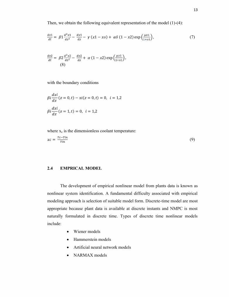
Then, we obtain the following equivalent representation of the model (1)-(4):

= 1 − − ( 1 − ) + (1 − 2) exp , (7)

= 2 − + (1 − 2) exp ,(8)

with the boundary conditions

( = 0, ) − ( = 0, ) = 0, = 1,2( = 1, ) = 0, = 1,2

where xc is the dimensionless coolant temperature:= (9)

2.4 EMPRICAL MODEL

The development of empirical nonlinear model from plants data is known as

nonlinear system identification. A fundamental difficulty associated with empirical

modeling approach is selection of suitable model form. Discrete-time model are most

appropriate because plant data is available at discrete instants and NMPC is most

naturally formulated in discrete time. Types of discrete time nonlinear models

include:

Wiener models

Hammerstein models

Artificial neural network models

NARMAX models