1

Development of geometallurgical characterization and comminution testing of the Kittilä gold deposit Maja Lange

School of Engineering Master’s thesis Espoo 22.11.2019 Supervisors

Prof. Jussi Leveinen Prof. Bernd Lottermoser

Dr Mike Buxton

Advisor M.Sc. Lasse Kangas

2

Copyright © 2019 Maja Lange

Aalto University, P.O. BOX 11000, 00076 AALTO

www.aalto.fi

5

Author Maja Lange Title of thesis Development of geometallurgical characterization and comminution testing of the Kittilä gold deposit Master programme European Mining, Minerals and Environmental Programme Major European Mining Course

Code of major ENG3077

Thesis supervisors Prof. Jussi Leveinen, Prof. Bernd Lottermoser, Dr Mike Buxton Thesis advisor(s) M.Sc. Lasse Kangas Date 22.11.2019 Number of pages 80+46 Language English

Abstract Efficient measurements of comminution are important for testing the variability of the ore within the geometallurgical context. An essential part of this work is the inves-tigation of the influence of texture, mineralogy, liberations of minerals and density on the grindability of the rock. Parameters such as the Bond Work Index and the Point Load Index are commonly used to optimize comminution processes. Comminution testing is key to the proper geometallurgical characterization of various deposits. The focus of this study has been to develop geometallurgical characterization and comminution testing, which allows efficient measurement of crushing or grinding indices and their connection with min-eralogical parameters. The results from comminution testing were collected and used to determine the crush-ability and grindability properties of the Kittilä gold deposit (Northern Finland). For this thesis, three tests were conducted – JK Drop Weight impact test, Bond Ball Mill and Point Load Strength test. Furthermore, mineral composition and density measurements have been determined for a detailed analysis of the samples. Statistical analysis was carried out by using IBM SPSS software. The conducted tests are designed to be implemented in early stages for identification of differences in comminution properties leading to detailed geometallurgical charac-terization of the ore. Later testing and sampling can be done on a bigger scale to obtain efficient and economical circuit design. From the results, it was concluded that there is a strong positive relationship between the grindability and crushability of the ore. It was also confirmed that the mineral com-position, hardness of the ore and rock texture influence rock breakage mechanisms. All of the comminution tests, were strongly and positively correlated to each other. The Point Load Test can be used to indicate the ore hardness rather than time-consum-ing and complicated Bond Ball Mill Test. Keywords Geometallurgy, Comminution, Crushing, Milling, Grindability, Kittilä

Aalto University, P.O. BOX 11000, 00076 AALTO

www.aalto.fi

5

Preface This thesis is the final step in my academic career and it was one of the most challeng-ing tasks during the last years. I wish to thank my supervisors Jussi Leveinen, Bernd Lottermoser, and Mike Buxton, as well as my advisor Lasse Kangas for their support during my Master’s thesis project and clear guidance in the last months. Additionally, I would like to thank Wout Lohle and Joseph Millington for the preparation of the samples for comminution tests and performing the Bond Ball Mill test and SEM analysis. Your help was essential in this project and once again – thank you for devoting your time and effort. I also would like to thank my entire research group for assistance in the experiments and for every help, which was needed. I am grateful to the Aalto laboratory technicians from the Civil Engineering Department, for assisting me in the laboratory and for providing crucial knowledge about equipment. Furthermore, I wish to thank Laboratory Manager Otto Hedström for his commitment to my project and patience when I was asking many questions. Besides, I am grateful to the Agnico Eagle for providing me with samples from the Kittilä gold deposit and enabling this Master’s thesis project to be realized and completed. At last, I would like to thank my family for the best support during my studies, which I can imagine. Otaniemi, 22.11.2019

Maja Lange

1

Table of contents Abstract Preface Table of contents ............................................................................................................... 1 Symbols and Abbreviations .............................................................................................. 3 List of figures .................................................................................................................... 5 List of tables ...................................................................................................................... 6

1 Introduction ............................................................................................................. 8 1.1 Hypothesis ............................................................................................................. 8

1.1.1 Research questions ...................................................................................... 9

1.1.2 Objectives of the thesis ............................................................................... 9 2 Literature review .................................................................................................. 10

2.1 Geometallurgy ..................................................................................................... 10 2.1.1 Geometallurgical characterization of gold ore .......................................... 11

2.2 Essential properties ............................................................................................. 13 2.2.1 Cleavage and breakage ............................................................................. 13 2.2.2 Hardness .................................................................................................... 14 2.2.3 Texture ...................................................................................................... 16

2.2.4 Liberation and free surface area ................................................................ 17 2.3 Comminution....................................................................................................... 18

2.3.1 Definition .................................................................................................. 19

2.3.2 Comminution devices ............................................................................... 21

2.3.3 Comminution by compression .................................................................. 22 2.3.4 Comminution by impact ........................................................................... 23 2.3.5 Grinding process ....................................................................................... 24

2.4 Geological background and mineral processing at Kittilä .................................. 25 3 Ore samples characterization .............................................................................. 28

3.1 Mineralogy and rock properties .......................................................................... 29 3.2 Scanning Electron Microscope ........................................................................... 31

3.2.1 Equipment description .............................................................................. 32

3.2.2 Sample preparation ................................................................................... 33 3.3 Thermo Scientific Portable XRF Analyzer ......................................................... 33

3.4 Density measurements ........................................................................................ 34

4 Comminution testing ............................................................................................ 36

4.1 Bond Ball Mill test .............................................................................................. 36 4.1.1 Test description ......................................................................................... 37 4.1.2 Test procedure ........................................................................................... 37

4.2 Drop Weight test ................................................................................................. 39 4.2.1 Test description ......................................................................................... 40

4.2.2 Test procedure ........................................................................................... 41 4.3 Point Load test..................................................................................................... 43

4.3.1 Test description ......................................................................................... 43 4.3.2 Test procedure ........................................................................................... 45

5 Results .................................................................................................................... 47

5.1 SEM results ......................................................................................................... 47

5.2 XRF results.......................................................................................................... 50 5.3 Bond Ball Mill test .............................................................................................. 52

2

5.4 Drop Weight test ................................................................................................. 56 5.5 Point Load test..................................................................................................... 63 5.6 Summary of results ............................................................................................. 66

6 Discussion .............................................................................................................. 67 6.1 Relations between comminution tests and mineralogical composition .............. 67 6.2 Relations between comminution tests and geometallurgical properties ............. 70 6.3 Relations between As-content in the Scanning Electron Microscope and XRF analyzer .......................................................................................................................... 71

6.4 Relations between comminution tests ................................................................. 72 7 Conclusions ............................................................................................................ 74 8 Recommendations ................................................................................................. 76 9 References .............................................................................................................. 77

10 Appendices ............................................................................................................. 81

3

Symbols and Abbreviations Symbols Axb - product of empirical drop-weight test parameters, A and b are related to the hard-ness of the ore

𝐶𝐼95% - confidence interval

d - average size of particles after the process

D - average size of particles before grinding

𝐷𝑒2 - equivalent core diameter, 4A/π for axial

E - Young modulus

ɛL, L - degree of liberation

Ecs - specific comminution energy

Ei - impact breakage energy

𝐹 - size correction factor

F80 - the sieve size at which 80% of the feed passes

G - net mass of undersize material per revolution

g - gravitational acceleration

hf - the final height of the drop head above the anvil

hi - the initial height of the drop head above the anvil

𝐼𝑠 - point load strength index

𝐼𝑠50 - point load index after correction

�̅� - mean mass of each set of particles

Mi - comminution index

n - the number of tests, which were done in this test

P - failure load

P1 - closing sieve size

P80 - the sieve size at which 80% of the product passes

𝑆𝐷 - standard deviation of the UCS results

ta - measure of abrasion resistance of the ore

t10 - breakage index number

W - plant data, mass specific energy divided by throughput

Wi - bond work index

x1, x2 - equivalent to F80 and P80

4

θ - the nip angle

µ - coefficient of friction between the particle and the crushing surface

γs - surface energy of the particle Abbreviations AG/SAG – Autogenous/Semi-autogenous

BIF – Banded Iron Formation

BMWi – Bond Mill Work index

EDX – Energy Dispersive X-Ray

GTK – Geological Survey of Finland

JKMRC – Julius Kruttschnitt Mineral Research Centre

PSD – Particle Size Distribution

SCSE – Standard Circuit Specific Energy

SEM – Scanning Electron Microscope

TEM – Transmission Electron Microscope

UCS – Uniaxial Compressive Strength

VMS – Volcanogenic Massive Sulfide

5

List of figures Figure 2.1 Essential disciplines in geometallurgy. ........................................................ 10

Figure 2.2 Flowsheet of typical geometallurgical approach. ......................................... 11

Figure 2.3 Gold ore types’ classification (based on M. Adams, 2016). Gold ore in Kittilä miner belongs to the eighth category. ............................................................................. 12

Figure 2.4 Different types of cleavage: a) basal cleavage in sheets minerals, b) cubic cleavage in halite (left) and rhombohedral cleavage in calcite (right) (Liber-Madziarz and Teisseyre 2002). .............................................................................................................. 14

Figure 2.5 Mohs scale (modified from Liber, 2002). .................................................... 15

Figure 2.6 Minerals hardness: a) hardness curves for halite, b) different hardness of kyanite (Liber-Madziarz and Teisseyre 2002). ............................................................... 16

Figure 2.7 Textural changes in rock due to deformation or oxidation (Butcher 2010)…17

Figure 2.8 Liberation and free surface area (All and Goodall 2005). ............................ 18

Figure 2.9 Comminution equipment according to the hardness of the ore (left) and the aim of comminution in microscopic view (right). .......................................................... 19

Figure 2.10 Comminution methods (Drzymala 2007). .................................................. 19

Figure 2.11 Comminution: a) smashing; b) impact, shearing; c) attrition, abrasion; d) cutting; e) splitting; e) breaking; f, g) fracture; h, i) shattering (Blaschke 1981). .......... 20

Figure 2.12 Comminution devices: a) roll crusher, b) tumbling mill, c) pendulum mill, d) hammer crusher, e) jaw crusher and f) cone crusher (Picture by Drzymala, 2007). ...... 22

Figure 2.13 Angle of nip (α) and nip region (B) in roller crusher (Wills 1985). ........... 23

Figure 2.14 Charge motion in a tumbling mill (based on A. Wills, 1985). ................... 24

Figure 2.15 The location of the study area – regional geology map of Kittilä mine ..... 25

Figure 2.16 Suurikuusikko – geological cross section of deposit (Agnico Eagle Mines 2019). .............................................................................................................................. 26

Figure 2.17 Kittilä mineral processing plant flowsheet – crushing and grinding processes (Agnico Eagle Mines 2019). ........................................................................................... 27

Figure 3.1 Kittilä ore - composite longitudinal section (Agnico Eagle Mines 2019). ... 28

Figure 3.2 Sample 1R390 (7) II – 2: a) ore sample after drilling, b) ready sample for microscopic tests, white circle represents the area of further stereoscopic microscope analysis, c) precise view of white circle area, d) microscopic view of the sample. ....... 30

Figure 3.3 Graphite occurrence. On the top-right picture is presented quartz inclusion. The image on the left-bottom represents fine-grained matrix. The last sample shows foliated, layered texture. ................................................................................................. 31

Figure 3.4 FE-SEM-EDS System. ................................................................................. 32

Figure 3.5 Sample preparation from bulk specimen and SEM sample example extracted from 1R390 (10). ............................................................................................................ 33

Figure 3.6 Thermo Scientific Niton handheld XRF analyzer. ....................................... 34

Figure 3.7 Density ranges for all sample sets. Horizontal line represents average density, while colorful boxes show the range. ............................................................................. 35

Figure 4.1 Locked-cycle grinding in the Bond Ball Mill Test. ...................................... 36

6

Figure 4.2 Bond Ball Mill setup (left) and steel ball charge (right). ............................. 37

Figure 4.3 Drop Weight Tester components. ................................................................. 40

Figure 4.4 Point Load testing device set up (E. Broch 1972). ....................................... 44

Figure 4.5 Testing of Kittilä sample with Point Load device. ....................................... 44

Figure 4.6 Size correction factor chart from ASTM (1995). ......................................... 45

Figure 5.1 Element analysis by FE-SEM-EDS. Sample 1X900 (2) II 3. ....................... 48

Figure 5.2 Element analysis by FE-SEM-EDS. Sample 2X900 (5) II 10. ..................... 49

Figure 5.3 Correlation between Arsenic SEM and Arsenic X-Ray content. ................. 52

Figure 5.4 F80 (3045 microns) and P80 (84 microns) distribution - sample 2S175. .... 54

Figure 5.5 Drop Weight Test parameters for all sample sets. ........................................ 58

Figure 5.6 t10% parameter vs Ecs for 4 size fractions – sample 1S175. ....................... 59

Figure 5.7 t10% parameter vs Ecs for 4 size fractions – sample 2S175. ....................... 60

Figure 5.8 Overall relationship between specific comminution energy vs cumulative t10% for sample sets S175, S325, R390 and X900. ....................................................... 61

Figure 5.9 SAG (kWh/t) vs Axb for operating AG/SAG (911Metallurgist 2017). ....... 62

Figure 5.10 Examples of cores diversity – specimens after Point Load Test. ............... 64

Figure 5.11 Range of Uniaxial Compressive Strengths for all sample sets. .................. 65

Figure 6.1 The Drop Weight Test and the mineral composition relations. .................... 68

Figure 6.2 The Point Load Test and the mineral composition relations. ....................... 69

Figure 6.3 The Bond Ball Mill Test and the mineral composition relations. ................ 70

Figure 6.4 Correlation between XRF analyzer and FE-SEM-EDS results. ................... 72

List of tables Table 2.1 Mineralogical issues affecting gold extraction (based on M. Adams, 2016)..12

Table 2.2 Hardness measurement methods (based on Malewski, 2015). ...................... 15

Table 2.3 Mode of size reduction (based on Drzymala, 2007). ..................................... 22

Table 3.1 Sample description – labeling and weight. .................................................... 29

Table 3.2 The effect of temperature on the water density. ............................................. 35

Table 3.3 Average solid density for all sample sets. ...................................................... 35

Table 4.1 Bond Ball Mill charge distribution. ............................................................... 37

Table 4.2 Drop Weight Test specifications for sample set 1S175. ................................ 41

Table 4.3 Sieve sets used for different sample fraction. ................................................ 42

Table 5.1 Average mineral content based on SEM results. ........................................... 47

Table 5.2 1R390 (10) I - 4. Scanning Electron Microscope results. .............................. 50

Table 5.3 X-Ray analyzer results for all sample sets. .................................................... 51

Table 5.4 Summary results of Arsenic measurements. .................................................. 52

Table 5.5 Calculation of the grindability parameters in Bond Ball Mill Test. Sample 2S175. ............................................................................................................................. 53

7

Table 5.6 Product and feed analysis for sample set 2S175. ........................................... 53

Table 5.7 Bond Ball Mill test results for all sample sets. .............................................. 54

Table 5.8 Relationship between ore hardness and Bond Work index (Tsakalakis 2015). ........................................................................................................................................ 55

Table 5.9 Ore hardness classification based on Bond Ball Mill Test. ........................... 55

Table 5.10 Drop Weight Test results for sample 1S175. ............................................... 56

Table 5.11 Non-linear regression analysis for sample set 1S175. ................................. 57

Table 5.12 Summary of the Axb parameter for sample set 1S175. ............................... 57

Table 5.13 Axb breakage parameters for all sample sets. .............................................. 58

Table 5.14 Hardness classification based on crushability in the Drop Weight Test. ..... 59

Table 5.15 Breakage function used by JKMRC for AG/SAG model (T.J. Napier-Munn, 1996). .............................................................................................................................. 62

Table 5.16 Basic parameters for JK Drop Weight Test (JK Tech 2018). ...................... 63

Table 5.17 Point Load Strength Index for sample group 1S175 (4) II. ......................... 63

Table 5.18 Overall results from Point Load Test. .......................................................... 64

Table 5.19 Summarized results from comminution tests. .............................................. 66

Table 6.1 The correlation between the Drop Weight Test (Axb parameters) and the mineral composition for all sample sets. ........................................................................ 67

Table 6.2 The correlation between the Pont Load strength index and the mineral composition for all sample sets. ...................................................................................... 68

Table 6.3 The correlation between the Bond Ball Mill test and the mineral composition for all sample sets. .......................................................................................................... 69

Table 6.4 Texture in comparison with comminution tests. ............................................ 71

Table 6.5 Relations between comminution tests. ........................................................... 72

8

1 Introduction This Master’s thesis was carried out as a part of the research project GAGS funded by the Academy of Finland with support from Agnico Eagle Company. The work involved com-minution testing of representative ore samples from Kittilä mine (Northern Finland) in the laboratory of Aalto University, Department of Civil Engineering and comparison of the geometallurgical properties, petrography and mineralogy.

In this study, emphasis was on different measurements of grindability and crushability. One of the aims was an investigation of geometallurgical properties of ore samples and determination of relations between tests, mineral composition and texture of the ore. Sec-ond objective of this study was to estimate the potential effects of the variable rock prop-erties on the crushing and grinding process, which are carried out in the Kittilä processing plant. In the beginning, basic research and investigation on petrographical, physical and mechanical properties of rocks was executed. In Appendix 13, the Master’s thesis work-flow is presented. The most important for crushing and milling processes are texture, hardness, cleavage and breakage, liberation, free surface area, and density measurements. These features influence flotation, gravity, and leaching and tails disposal.

Comminution testing involved samples (in example for drop weight test it was 96 sam-ples), which were obtained from about 100 kg of rocks from Kittilä mine. Rock samples were taken from the recently blasted part of the mine at the excavation tunnels (sublevel drifts perpendicular or parallel to the ore). Each sample set represents different parts of the deposit. Comminution tests are usually time-consuming operations and rely on var-ious laboratory tests that require larger samples than 100 kilograms. Due to these circum-stances, each test in this thesis can be described as a simplification of the proper and complicated ore comminution operations that are done at a mineral processing plant.

Comminution circuits usually define plant material throughput. Mineral processing properties of the ore body can vary and as a result, can give changes during production stages. The target for the comminution processes is to produce a specific size distribution and simultaneously maximize the profit. If the ore is very hard, it shows that the through-put should be decreased to achieve a certain particle size. Additionally, there exist adjust-able process variables, for example, a quantity of grinding media in the mill, cut size and rotational speed of the mill. Hence, the design of the comminution circuit in the right way is an essential part of the mine planning (Mwanga 2014).

1.1 Hypothesis

In this Master’s thesis, the geometallurgical properties of the Kittilä gold deposit are studied to distinguish significant rock properties for the comminution processes in the Kittilä mine. This work also provides background information for the GAGS-project where relations between laser-spectral characteristics and mineralogical characteristics are compared. This study is based on the following hypothesis:

1) Geometallurgical properties of the rock like texture, breakage, hardness, size of particles and mineral composition significantly influence milling and grinding processes.

2) Comminution tests results can be used to optimize mineral processing phases.

9

1.1.1 Research questions

Research questions were determined based on the research hypothesis and they were established as the main targets of this study:

1. How the ore texture influences crushing, milling and grinding in the mineral processing phase?

2. What properties of the ore are important in mineral processing? 3. How does shape of the mineral in particle affects the milling process? 4. How does the liberation of the mineral and free surface areas influence

the grindability of the ore? 5. How does the mineral composition of the ore correlate with the comminution

process? 6. How do the sample sets differ in terms of crushability and grindability?

1.1.2 Objectives of the thesis

The main objectives of the thesis were to: Measurements of grindability and crushability properties of the ore based on the

various tests: Drop Weight test, Point Load and Bond Ball Mill test. Investigation of the effect of geometallurgical properties based on additional

industrial studies and scientific papers. Ore’s density measurements and its influence on ore comminution and

relationship with mineral composition. Sample group classification and characterization with special regard to

comminution properties of the ore. Study of relations between geometallurgical properties, mineral composition, and

comminution factors. Recommendation of the path forward and implementation of optimizing of

the mineral processing.

1.1.3 Structure of the thesis Chapter 1. Introduction – describes the problem statement, hypothesis, research questions and objectives of this work.

Chapter 2. Literature review – contains essential information about geometallurgy, rock properties and comminution testing.

Chapter 3. Ore sample characterization – includes detailed description of the ore sample collection.

Chapter 4. Comminution testing – in this chapter are presented comminution methods, which were done during this thesis work.

Chapter 5. Results – contains results of experimental part of the work.

Chapter 6. Discussion – presents comments and analysis of the results and includes gen-eral conclusion about the research.

Chapter 7. Conclusions – this section is a summary of all the research work.

Chapter 8. Recommendations – focuses on the path forward and potential future re-searches, which can be done to develop this topic then.

10

2 Literature review In this chapter are presented basic concepts about comminution, essential rock properties and why crushability and grindability tests are important for achieving improvement in comminution efficiency. The key to designing the processing plant and its operation is to understand deeply the ore properties.

2.1 Geometallurgy

Geometallurgy is a multidisciplinary science dealing with an ore extraction. It is difficult to present one and a proper definition of this term. There are various descriptions of geometallurgy as follows (Adams 2016):

- An interdisciplinary science that links the geochemical, geological or mineralogical characteristics to the metallurgical performance of a deposit. It is a methodology and framework for mine planning, plant optimization, and mine planning.

- A discipline in which mining, processing, and geological data are analyzed to determine useful knowledge for resource profitability optimization.

- A multidiscipline approach to the modeling and collection of all geometallur-gical information.

- A scientific approach in which mineralogical and geological characteristics are linked to the metallurgical performance of the ore.

- Geometallurgical mapping quantifies the impact of geology and documents the variability of an orebody. It is an important tool to describe mineralogy and metal recovery processes.

Orebodies are a natural accumulation of valuable elements in the Earth’s crust. Even within a single deposit, rock types, chemistry, ore grade, alteration, mineralogy; orebody often changes laterally or vertically. These changes cause additional difficulties during mineral processing. Geometallurgy aims to understand and identify the deposit variability and define its metallurgical performance. This process should take into consideration factors such as specific gravity, comminution, leaching and flotation parameters, and later metal recoveries (Adams 2016). In Figure 2.1are presented an essential disciplines in geometallurgy.

Figure 2.1 Essential disciplines in geometallurgy.

11

Geometallurgy has been used at many stages of mining projects like scoping, pre-feasibility and feasibility studies. This discipline has a significant role in the following areas (Adams 2016):

- equipment selection, - flowsheet development, - plant optimization and design, - mine planning, - production prediction.

Figure 2.2 Flowsheet of typical geometallurgical approach.

Geometallurgy uses geological information and geostatistics as a foundation and as a tool to distinguish representative samples of mine-specific ore types and then conduct metallurgical and mineralogical tests on these samples to create a new database. Figure 2.2 shows a typical geometallurgical approach, where he data is analyzed, processed and imported into the geological model. The geological model is then used for flowsheet development, mine planning, process selection and plant optimization (Adams 2016).

2.1.1 Geometallurgical characterization of gold ore

In common classification, gold ores can be divided into two categories: refractory and free milling. Free-milling ores are described as those where more than 90% of gold particles can be recovered by cyanide leaching. Refractory ores can be determined as those that obtain low gold recoveries and require complex pretreatment phases. Based on the mineral processing techniques and the mineralogical characteristics, gold ores are classified into twelve types, presented in Figure 2.3. The first six types require a free-milling process, whereas the other six are more refractory. Arsenic sulfide ores, which were discovered in Kittilä mine, require some additional pretreatment in the mineral processing stage are in the eighth place in this classification (Eilu and Wyche 2015).

12

Figure 2.3 Gold ore types’ classification (based on Adams, 2016). Gold ore in Kittilä miner belongs to

the eighth category. According to mineralogical classification, gold can be divided into the surface, microscopic and submicroscopic forms. Microscopic gold or visible gold includes gold minerals such as gold sulfides, selenides, alloys, and tellurides. This type of gold is found in various gold ores and it is a major form in nonrefractory gold ores. Gold that is invisible even under SEM and optical microscopes is called a submicroscopic gold (Eilu and Wyche 2015). Submicroscopic form is common in orogenic gold deposits, such as Kittilä and in some epithermal gold deposits or volcanogenic massive sulfide deposits (VMS). Table 2.1 Mineralogical issues affecting gold extraction (based on Adams, 2016).

Mineralogical issue Affected process association flotation, gravity, leaching liberation flotation, gravity, leaching grain size flotation, gravity, leaching coating and rimming flotation, gravity, leaching surface chemistry flotation, gravity, leaching dissolution kinetics leaching pre-robbing (iron oxide) leaching cyanides and oxygen consumers leaching refractoriness (submicroscopic gold) leaching, gravity toxic elements (As, Hg, Se, Sb et cetera) flotation, solution purification, tails dis-

posal, leaching gangue (clay, acid-forming minerals) flotation, leaching, tails disposal

The extractive metallurgy of gold depends on various mineralogical factors because gold usually occurs in submicroscopic or surface-bound form. These factors contain particle size, presence of cyanides, association with other particles, coatings, and locking of submicroscopic gold in sulfarsenide and sulfide minerals (like arsenopyrite and pyrite).

The main mineralogical issues and their effect on mineral processing are presented in Table 2.1. The top three factors that have a significant influence on ore treatment are association, grain size, and liberation of the particle (Adams 2016).

13

2.2 Essential properties

The shape of mineral particles is one of the most important qualitative features in rock processing and ore beneficiation. It also influences the efficiency of mineral processing determination. The shape of comminuted particles depends on the natural properties of the rock and manner of rock crushing. Rock, which will be crushed, needs to be characterized by the structure of the mineral composition and specific physical properties. Dynamics and complexity of the comminution processes have a significant effect on the crushing and milling actions (J. Malewski 1984).

There is no one or clear measurement, which can properly show the best and most profitable way of crushing, grinding and milling optimization in mineral processing in the mining industry. Choice with best matching is a complex and long process. Nowadays there exist various grinding machines with different dynamics, the shape of crumble chamber and crushing elements (J. Malewski 2012).

Mining companies and mineral processing plants face constant challenges to become profitable and more efficient, but they are also faced with complex deposits. The complexity is described by many mineralization events and variations in ore bodies. These obstacles could be observed by a change in deposit texture. A proper understanding of the ore texture is an essential tool in developing mineral processing and optimizing existing procedures. The texture of the ore has also a significant influence on grade, plant efficiency, recovery, and operational economics. The main goal of mining companies is to reduce costs, produce a high-quality product and improve recovery systems (All and Goodall 2005).

2.2.1 Cleavage and breakage

Cleavage can be described as the minerals’ ability to shear along parallel surfaces due to the influence of impact or pressure. This feature is closely related to the internal structure of a specific crystal. Cleavage surfaces coincide with the strongest bond surfaces in the crystal structure; thereby cleavage is one of the most important physical features in mineral identification (Alvarez 1978). Following types of the cleavage can be distinguished during measurements:

- Basal – only one cleavage plane. Common features for graphite and micas (muscovite and biotite). Basal cleavage is characteristic of minerals with sheets structure, which split into very thin and large layers.

- Cubic – three cleavage planes intersecting at 90 degrees. Cubic cleavage is common for halite and galena; minerals with cubic cleavage split into parts with smooth and straight sides, which are connected with mineral natural shape.

- Octahedral – four cleavage planes in a crystal; could be found in fluorite and diamond.

- Rhombohedral – three cleavage planes intersecting at angles that are not 90 degrees. Rhombohedral cleavage is observed in calcites.

- Prismatic – two cleavage planes in a crystal. Spodumene represents prismatic cleavage.

- Dodecahedral cleavage – six cleavage planes in a crystal. In an example, this cleavage is common for sphalerite (Rocha 2018).

14

Figure 2.4 Different types of cleavage: a) basal cleavage in sheets minerals, b) cubic cleavage in halite

(left) and rhombohedral cleavage in calcite (right) (Liber-Madziarz and Teisseyre 2002). Under the microscopic view, the cleavage of minerals looks like parallel cracks or slits (Figure 2.4). These cracks are a trace of the cleavage surface. In the example, muscovite (with unidirectional cleavage) cleavage traces will be perpendicular to the cleavage surface of the mineral. When in the mineral can be observed more than one cleavage system, then in specific intersections can be found overpasses, various cleavages (Liber-Madziarz and Teisseyre 2002).

Due to impact forces, some of the minerals split into different and random directions. Fracture differs from cleavage in that the crystal structure involves clean splitting along the cleavage planes of the mineral’s crystal structure, as opposed to more general breakage. In nature, all minerals have a fracture, although when strong cleavage is observed, it could be difficult to see. This feature is common and easy to distinguish for crystals, which do not have a cleavage and they split among irregular and abnormal surfaces (Liber-Madziarz and Teisseyre 2002). The fracture surfaces are usually uneven and the most characteristic forms have their description (Liber-Madziarz and Teisseyre 2002):

- Conchoidal – concentric ripples of a mussel shell. Often occurs in amorphous of very fine-grained minerals like opal or obsidian (obsidian is not a mineral, but igneous rock, although it shows a conchoidal breakage very good).

- Earthy – looks like a freshly broken soil, seen in soft very fine-grained minerals like limonite, kaolinite or aluminite.

- Hackly – sharp, jagged. It occurs in chalcedony and native metals like copper or silver.

- Splintery – sharp elongated points, seen in fibrous minerals like chrysotile. - Uneven – rough and irregular surface, seen in pyrite and arsenopyrite.

2.2.2 Hardness

Hardness is the measure of resistance to localized plastic deformation induced by either mechanical indentation or abrasion. It is the resistance of mineral during scratching or grinding. The hardness of the rock is dependent on ductility, strain, strength, viscosity, and viscoelasticity (Craig 1994). In mineralogy, different methods are used for hardness determination (Table 2.2).

15

Table 2.2 Hardness measurement methods (based on Malewski, 2015).

Type of methods Mode of measurement Measurements static scraping

mashing

Mohs, Brinnell, Knoop, Rock-well and Vicker scale

Baron scale

dynamic drilling stamping digging

sclerometer

Poldi hardness test

static abrasion Rosiwal, Boehmy

The simplest and fastest way to determine this feature is by using the Mohs scale. This scale evaluates the relative hardness of minerals by comparison of the resistance of a specific mineral with the hardness of one of the mineral from the Mohs scale. Minerals in the Mohs scale are ordered according to increasing toughness:

Figure 2.5 Mohs scale (modified from Liber, 2002).

For example, when with specific mineral can be scratched by quartz, but it is making a crack in orthoclase, then the hardness of the mineral can be evaluated as 6.5 in the Mohs scale. Besides, hardness is a typical vector feature. Usually, in minerals, differences in measured hardness in different directions are not significant. Kyanite (disthene) is a mineral known for a visible difference in hardness in various directions (Figure 2.6) (Liber-Madziarz and Teisseyre 2002).

16

Figure 2.6 Minerals hardness: a) hardness curves for halite, b) different hardness of kyanite (Liber-

Madziarz and Teisseyre 2002). Hardness of the rock depends on its mineral composition and mineral cohesion; it is determined by different methods like abrasion tests such as Boehmy and Deval drum. Rocks can be divided into high (containing high quantity of soft minerals) and low (with hard minerals or hard matrix) grindability. Hardness of the rock is one of the most important features, which needs to be taken into consideration during comminution process planning. It has a significant influence on rock crushing and milling, and therefore affects the profitability of the whole process – hard rocks required much more energy in the comminution process. For this reason, proper evaluation of rock hardness is essential in the mining industry (Liber-Madziarz and Teisseyre 2002).

2.2.3 Texture

Texture in the context of geometallurgy refers to the relationship between the minerals in a rock. This concept includes the shape, size, association, and distribution of the mineral grains in the rock. As was mentioned before, the sizes of the mineral grains and the bonding between the particles are the main characteristics connected with mineral liberation and ore breakage. Why is texture so important? When considering only a grade of two ore types; the ores can have the same grade, although there is nothing to prompt these ores will have the same or similar processing characteristics. One of the samples may contain very finely target minerals, while the second may be easily liberated and coarse-grained. Furthermore, two ore types with various grades may have similar or the same mineral processing characteristic (All and Goodall 2005).

Rocks are heterogeneous and complex materials. The texture, fabric and weathering have an important influence on rocks’ mechanical properties. Texture of the rock gives an idea about the process and mechanism for the formation of rocks fabric. The texture of an ore affects the (All and Goodall 2005):

grindability of the ore, grain size and target grind size, degree of the liberation of target minerals, number of coarse composite grains, phase-specific area of the target minerals.

The ore texture can be changed by groundwater, oxidation, metamorphism and hydrothermal alteration as is shown in the Figure 2.7. Groundwater and oxidation can weather surfaces of the ore particles and can result in a reaction like alteration of surface on ore grains. The broadest textural categories are crystalline, fragmental, aphanitic and glassy. Crystalline texture occurs when the components are interlocking and intergrown crystals, while fragmental texture is observed in rocks with an accumulation of fragments

17

due to some process. Crystalline textures include phaneritic (large crystals, seen without a microscope), foliated (repetitive layering in metamorphic rocks) and porphyritic form (in rocks with different sizes of minerals, where one of them is much bigger than others). Big minerals in porphyritic texture are phenocrysts. When crystals are not visible to the naked eye, it is characteristic for aphanitic texture. In glassy texture, the particles are too small to be seen (Koch 2013).

Figure 2.7 Textural changes in the rock due to deformation and oxidation (Butcher 2010).

Texture has a major role in grade of the concentrate and in mineral recovery. In different sources, theoretical grade-recovery curves can be found and used to determine the potential maximum recovery for a given feed ore at a specific Particle Size Distribution (PSD). Any changes to plant conditions will improve this curve due to physical limitations connected with the texture. To improve the grade-recovery curve, changes can be implemented to the feed such as increasing liberation, reducing fines or larger free surface area (Koch 2013).

2.2.4 Liberation and free surface area

The degree of liberation is calculated from the set of particles containing the mineral. Liberation measurements are based on the area percentage of the mineral grain in the particle; it is different from an estimate of the phase-specific surface area, what is presented in the Figure 2.8. Measurement of this feature estimate the volumetric grade distribution of the mineral as a quality class in the processing stream (All and Goodall 2005).

18

Figure 2.8 Liberation and free surface area (All and Goodall 2005).

A grain usually contains a single mineral, while a particle contains one or more grains. In mineralogy, the liberation of a mineral is classified from examining 2D sections of a representative set of particles. Particles are ordered according to the particle grades of different incremental steps (liberation classes are presented in the Figure 2.8).

The free surface area is also calculated from examining 2D sections of a representative set of particles; however, it is an estimate of the percentage of the grains of interest, which has a free surface. The Figure 2.8 combines both concepts and highlight the influence of texture and particle for grade and recovery calculations. Both textural classifications are essential for mineral processing, where the ideal particle has 100% of liberation and 100% of free surface area. The influence of free surface area and liberation is crucial in leaching, flotation and gravity circuits. Understanding these terms should be a primary step for any operation including a flotation circuit (All and Goodall 2005).

2.3 Comminution

Grinding or crushing is a high energy-consuming process, which provides specific granulation of the ore. The crushing process is showed in the Figure 2.9. Crushing is realized on large particles when grinding on particles smaller than 50 mm. Comminution analysis depends on the natural properties of the rock, energy of the process and manner of rock size reduction (Mindat 2019). Main goals of comminution process are:

- to obtain a product following customer´s requirements (main process), - liberation of a mineral grain, differentiation of the ore from gangue

(preparation to enrichment process).

19

Figure 2.9 Comminution equipment according to the hardness of the ore (left) and the aim of comminu-

tion in microscopic view (right).

2.3.1 Definition

Comminution is a basic operation in mineral processing when a raw ore cannot be directly sent to farther processes like sizing and concentration. It can be realized chemically or mechanically. Crushing is usually carried out on “run-of-mine” when grinding may be conducted on slurred or dry material. Mechanical comminution is connected with external or special forces, while chemical processes are a result of leaching ore dissolution operation. Figure 2.10 lists the different types of comminution processes. Chemical size reduction is different from mechanical comminution; hence, it is a part of the extraction process in metallurgy rather than mineral processing (Drzymala 2007).

Figure 2.10 Comminution methods (Drzymala 2007).

20

Figure 2.11 Comminution: a) smashing; b) impact, shearing; c) attrition, abrasion; d) cutting; e) splitting;

e) breaking; f, g) fracture; h, i) shattering (Blaschke 1981). Abrasion is an operation where an ore chunk is torn off into small parts of a solid body with small energy forces. Breakage takes place when the force is strong enough to divide the chunk into smaller particles. Shattering provides a higher number of particles due to significant force. In Figure 2.11 are presented different ways of mechanical comminution of the ore, although there are other possible manners like twisting, compressing, stretching, torsion and so on (Drzymala 2007).

Grinding is performed on mills containing water, feed, and grinding media. Grinding media could be ceramic or metallic with different shapes and sizes like balls, bars, pebbles, cylpebs or lumps. This operation uses a significant amount of energy that is why the effectiveness of the process is important. Overgrinding should be avoided because of generating a high cost. Every method and phase of the comminution process requires an optimal particle size definition (Drzymala 2007).

Breaking of ore particles is a highly complicated process where particles are not perfect, ideal in structure and do not follow a specific pattern or way of disintegration. The same situation happens with monocrystals, glass or metals, because particles and grains have various defects, cracks, inclusions, and accumulated strain energy. Comminution energy can be used for increasing particle surfaces, to form cracks, stresses, and defects (Drzymala 2007).

Mechanical comminution can be conducted as a process to change particle size or separate of different particles from each other. Comminution conducting to liberation is a selective comminution. Non-selective comminution is connected with a size reduction. Crushing and grinding operations could be either non-selective or selective.

The main parameter in this process can be susceptibility to comminution. The definition of the susceptibility to comminution is based on the surface energy of the particle 𝛾𝑠 and Young modulus E. Unfortunately, the surface energy of solids is difficult to measure. Therefore, empirical constants n and K describe comminution and predict its results.

21

Constant K and n usually depend on the type of machine and procedure used in measurement. Moreover, grinding constants are constants of the ideal grinding process.

Size reduction does not lead to separate products although the same minerals and particles tend to accumulate in various sites of the machine. Rather, crushing and grinding processes lead to mixing the products (Drzymala 2007).

In grinding as the upgrading process, it is not important what major feature of the operation is, but crucial is the fact about the quantity and quality of the feed and product. In a situation when the process is non-selective, only tiny particles are produced and one product is obtained (is called modified feed). Moreover grinding can be described by the degree of size reduction as in Formula 2.1:

𝐼 =𝐷

𝑑=

𝑝𝑎𝑟𝑡𝑖𝑐𝑙𝑒 𝑠𝑖𝑧𝑒 𝑏𝑒𝑓𝑜𝑟𝑒 𝑔𝑟𝑖𝑛𝑑𝑖𝑛𝑔

𝑝𝑎𝑟𝑡𝑖𝑐𝑙𝑒 𝑠𝑖𝑧𝑒 𝑎𝑓𝑡𝑒𝑟 𝑔𝑟𝑖𝑛𝑑𝑖𝑛𝑔

Where: D – the average size of particles before grinding, d – the average size of particles after the process.

In the case of grinding and liberation of particles, the expression of the degree of liberation is defined in Formula 2.2:

𝐿 = 𝜀𝐿 =𝑚𝑎𝑠𝑠 𝑜𝑓 𝑓𝑟𝑒𝑒 𝑝𝑎𝑟𝑡𝑖𝑐𝑙𝑒𝑠 𝑖𝑛 𝑐𝑜𝑚𝑝𝑜𝑛𝑒𝑛𝑡

𝑚𝑎𝑠𝑠 𝑜𝑓 𝑐𝑜𝑚𝑝𝑜𝑛𝑒𝑛𝑡 𝑖𝑛 𝑡ℎ𝑒 𝑓𝑒𝑒𝑑 ∙ 100%

For determination of liberation, different methods can be used such as flotation, gravity and magnetic separation and microscopic analysis (Drzymala 2007).

2.3.2 Comminution devices

Comminution is conducted in mills and crushers. In the crushing process, the size of particles is reduced to 50-150 mm. Common types of devices and their size reduction mechanisms are presented in Figure 2.12 and Table 2.3.

For initial size reduction jaw, gyratory and cone crushers can be used. Medium size grains require cone, jaw, gyratory or roll crushers. Smaller grains are ground in rolls, hammer and cone crusher or rotary breakers. Grinding can be also realized by tumbling mills, rotary breakers, and pendulum mills. Milling is conducted in mills and is usually performed wet. In comparison with dry milling, a wet process needs lower energy input and consumption of energy could be controlled by the use of different chemical reagents (Drzymala 2007).

(2.1)

(2.2)

22

Figure 2.12 Comminution devices: a) roll crusher, b) tumbling mill, c) pendulum mill, d) hammer

crusher, e) jaw crusher and f) cone crusher (Picture by Drzymala, 2007). Table 2.3 Mode of size reduction (based on Drzymala, 2007).

2.3.3 Comminution by compression

The compression devices include gyratory, jaw and roll crushers and pan, roller and disc mills. In these machines, particles are broken by compression between surfaces and they can be subdivided into those in which a fixed force is used and the crushing surfaces are almost in the contact (roller mills) and in which there is a fixed gap (roll, jaw and gyratory crushers). In the fixed gap devices, particles will be crushed if they are bigger than the gap size (B) shown in Figure 2.13. All particles should also be smaller than limiting size determined by angle of nip. Limiting angle of nip is determined by the equation (2.3):

23

tan𝜃

2= µ

Where: 𝜃 – an angle of nips, µ - coefficient of friction between the particle and the crushing surface. Large particles will slip rather than be drawn into the device and broken. What is more, because of the fixed gap, all particles in the appropriate size should be broken (Committee C&E 1981).

Figure 2.13 Angle of nip (α) and nip region (B) in roller crusher (Wills 1985).

For other types of nipping devices, the upper size limit will be defined by the nip angle. In these systems, a fixed force is applied and there is not defined fixed gap size. In general, the effective gap size depends on the amount of material in the device and on material size distribution. The compression method is the most efficient from an aspect of energy requirement and is more efficient for coarse size fractions (Committee C&E 1981).

2.3.4 Comminution by impact

The impact devices, which include vibratory and hammer mills, work by subjecting material to sudden stress through impact. In hammer mills, particles are stressed by high impact with swinging hammer and then by collision with surfaces in the mill. Vibratory mills are characterized by high-speed compression of particles between two surfaces. Tumbling mills are the most important comminution devices, in terms of overall energy usage and installed capacity. In these machines, particles are crushed by impact with a tumbling mass of grinding media. The latter can have the shape of steel balls, rods or other large pieces. Tumbling mills consist of a rotating cylinder, which is filled with grinding media. Rod mills are usually used for coarse feed and ball mills for finer material. Another type of device – autogenous mills – can be used for mixed feed and they combine coarse crushing and grinding in one operation (Wills 1985).

(2.3)

24

Figure 2.14 Charge motion in a tumbling mill (based on A. Wills, 1985).

In general, the effectiveness of comminution in a tumbling machine is determined by the nature of the motion in a shear zone. At low rotation speed, the ore undergoes cascading, which is a kind of rolling movement involving collisions between the particles and balls. At high speed, particles are in free flight in the rotating drum. This kind of motion is known as cataracting and includes more collisions than cascading (Figure 2.14). During normal working conditions, the motion in a mentioned shear zone is a combination of cascading and cataracting (Wills 1985).

2.3.5 Grinding process

The crushing circuit is used to prepare ore for heap leaching or milling. Milling of the ore is the last stage of comminution; in this phase, the particle size is reduced either by abrasion and impact, dry or in water. This process is performed in a rotating drum and contains a charge of material and the grinding medium. In the grinding process, all particles are reduced in size to 10-300 µm (Wills 1985).

All materials have an economic mesh of grind, which depends on many factors. One of the aims of the grinding process is the close control of the product size because this is the key to further, proper mineral processing. Undergrinding of material results in a prod-uct, which is too large and coarse and with too low degree of liberation. Furthermore, when undergrinding happens poor enrichment ratio and recovery will be obtained in the concentrate. Instead, overgrinding reduces the particle sizes below the size required for separation. This process wastes energy and time in the processing plant. It is essential to realize that milling is the most energy consuming operation in mineral processing. For these reason, it is strongly recommended to avoid any potential under- and overgrinding in the process (Wills 1985). Milling can take place by different mechanisms:

- impact (forces applied normally to the particle surface), - compression (forces applied almost normally to the particle surface), - chipping (forces parallel to the particle surface), - abrasion (forces parallel to the particle surface).

25

These mechanisms, listed above, change the shape of the particles beyond specific limits determined by degree of elasticity. Grinding is often performed wet; however, in some applications, dry milling is used. The progress of the comminution of the particles is strictly connected with the speed of rotation of the device. A significant amount of the loads’ kinetic energy is lost as noise and heat, only a part of the energy is milling the particles (Wills 1985).

2.4 Geological background and mineral processing at Kittilä

The Kittilä mine is the largest gold producer in Europe and achieved commercial production in 2009. Open pit mining was completed in 2012 and after that, Kittilä has become an underground mine. This mine is located in Lapland in northern Finland, 150 km north of Arctic Circle. Figure 2.15 presents the location of the study area. Nowadays mine has probable and proven mineral reserves around 4.4 million ounces of gold. The mine area is located along the Suurikuusikko Trend, which is a major gold-bearing shear zone and it includes a group of six deposits. The largest deposits in Kittilä are Suuri, Roura and Rimpi zones that contain a significant part of the current reserves (Agnico Eagle Mines 2019).

Figure 2.15 The location of the study area – regional geology map of Kittilä mine

(Agnico Eagle Mines 2019).

26

Geology The Kittilä mine is a part of the Paleoproterozoic Central Lapland Greenstone Belt and is underlain by sedimentary and mafic volcanic rocks. The contact between sedimentary and iron-rich and magnesium-rich volcanic rocks varies between 50 to 200 meters in thickness. The transitional zone is strongly brecciated, sheared and contains gold mineralization and intense hydrothermal alteration. This area is a part of the Suurikuus-ikko Trend shear zone. The mineralization occurs in a transitional between two mafic lava sequences. In the main ore area, host rocks change from mafic transitional to mafic pillow and massive lavas to intermediate lavas within mineralized zones. Graphitic sediment containing the chart, BIF and argillitic material are located within mafic volcanic at the margin of mineralized zones presented in the Figure 2.16. Banded iron formation typically contains low or any gold grade, while ultramafic rocks are determined as unmineralized (Patison 2007).

Figure 2.16 Suurikuusikko – geological cross section of deposit (Agnico Eagle Mines 2019).

Alteration around and in the deposit appears typical for this type of deposit. Intense albite and carbonate alteration is strongly connected with gold-bearing pyrite and arsenopyrite. Albite may be found as a matrix overprint as brecciated micro veinlets, while carbonates include calcite, dolomite/ankerite veins, and hydrothermal breccia. The abundance of graphite in the Kittilä deposit is correlated with the intense shearing and suggests extremely reducing fluid conditions. Argillite-rich zones have high primary carbon content and may have been chemically important for gold-rich phase locations. Other alterations and mineral phases contain rutile, tetrahedrite, gersdorffite, chalcopyrite, sphalerite, chalcocite, chromite, bornite, Fe- hydroxides and galena (Patison 2007).

The host rocks include three major lithologies – mafic pillow lavas, mafic massive lavas, and mafic volcanogenic explosive rocks. As mentioned before, shearing is abundant in the deposit and is determined as a graphitic failure zone. These lithologies represent

27

various grades of brecciation and shearing. Mafic massive lavas and mafic pillow lavas occur mostly in the footwall with less reworking and brecciation. Graphitic failure zones also exist in the footwall, whereas some parts of mafic massive lavas may be located in the hanging wall. The mineralization zone typically occurs within mafic volcanogenic explosive rocks and mafic massive lavas (Patison 2007). Mineral processing at Kittilä The feed to the processing plant in Kittilä is approximately 5 000 tonnes per day. In the beginning, the ore is crushed and grinded for further processes – flotation, pressure oxidation, and carbon-in-leach. In Kittilä mine gold is refractory what means that it can be determined as those that obtain low gold recoveries and required complex pretreatment phases. That is why in mineral processing plant is only used pressure oxidation circuit (autoclave). During the leaching process, gold is recovered from the carbon (in a Zadra elution circuit) and recovered from solution by using electrowinning, and later smelted and poured into doré bars (Agnico Eagle Mines 2019). The whole process of gold recovery is presented in the Figure 2.17.

Figure 2.17 Kittilä mineral processing plant flowsheet – crushing and grinding processes (Agnico Eagle

Mines 2019). It is expected to obtain 86% of gold recovery over the life of the mine. A four-phase mill expansion may increase throughput from the level of 1.6 million tonnes per year to almost 2.0 million tonnes by the year 2021. The mill expansion is connected with the installation of a secondary crushing circuit, new reactor capacity and thickener, and some modifica-tions to the current autoclave and grinding circuit (Agnico Eagle Mines 2019).

28

3 Ore samples characterization In this thesis, the sample sets used in various comminution tests correspond to four locations from deposit in Kittilä mine. To avoid any potential test mistakes and to exam-ine the heterogeneity of the ore, for each location duplicate samples were tested. The orogenic gold deposit is located in Paleoproterozoic Central Lapland Greenstone Belt. In the main ore zone presented in the Figure 3.1, host rocks have been interpreted to changes from massive lavas and mafic pillow to mafic transitional to intermediate lavas and minor pyroclastic elements within the zone of mineralization. Graphitic sediments with chert, BIF and argillitic material are observed within mafic volcanic at the eastern part of mineralization. Most of the ore is hosted by mafic or felsic rocks. Metasedimentary parts including BIF usually have low or any gold content, where ultramafic rocks are typically unmineralized (Meier, Lahtinen and O'Brien 2015).

The sample sets tested in this study are mafic to intermediate volcanic rocks with intense albite and carbonate alteration with gold-bearing pyrite and arsenopyrite. The rock has green-brown to black color; the main mineral composition includes quartz, ankerite, al-bite, micas (muscovite and biotite), pyrite, graphite, and arsenopyrite (Patison 2007).

Each sample was labeled with a specific code, which begins with a letter S, R or X. The letter S stands for Suurikuusikko, R stands for Rouravaara and X stands for a newly discovered part of Rimpi deposit. The next part of the code – three numbers – refers to the depth at which these samples have been taken for the test. The following letter and numbers are connected with location coordinates of the stope of extraction. Sample coding was simplified and modified as shown in the Table 3.1.

Figure 3.1 Kittilä deposit – composite longitudinal section (Agnico Eagle Mines 2019).

29

Table 3.1 Sample description – labeling and weight.

Sample label Simplified sample label Weight (kg) S175L161-1 1S175 2.871 S175L161-1-2 2S175 2.036 S325L172-1 1S325 2.398 S325L172-1-2 2S325 1.838 R390L200-1 1R390 2.346 R390L200-1-2 2R390 2.154 X900P327 1X900 3.518 X900P327-2 2X900 3.229

The samples vary in texture, mineral composition, and hardness. The mineral composi-tion of each sample set was determined with a Scanning Electron Microscope. The other characteristics were delivered from organoleptic classification and further comminution testing.

3.1 Mineralogy and rock properties

The samples are mainly mafic volcanic host rock with sulfides mineralization of arseno-pyrite and pyrite. The abundance of graphite correlates with the intensive shearing and suggests extremely reducing fluid content conditions and possibly mineralization. Gold is refractory and can be found in arsenopyrite or pyrite. In some parts of rocks, brittle deformation has formed breccias with a carbonate-quartz hydrothermal matrix (Meier, Lahtinen and O'Brien 2015). This thesis mainly focuses on gold-bearing arsenopyrite and pyrite.

The mineral texture of the ore has a significant influence on various metallurgical aspects like comminution, liberation or recovery. It is important, because two ore types with various grades may have similar or the same mineral processing characteristics. Besides, two samples could have the same grade; however, one of the sample could have very fine target minerals, while the next one may be easily liberated. The textural classification of samples is usually based on subjective evaluation. The texture of the ore varies - for mafic rocks is granoblastic, massive with interstitial quartz and a fine-grained matrix. The massive texture is a result of metamorphism processes under high-pressure condi-tions (Meier, Lahtinen and O'Brien 2015).

30

Figure 3.2 Sample 1R390 (7) II – 2: a) ore sample after drilling, b) ready sample for microscopic tests, white circle represents the area of further stereoscopic microscope analysis, c) precise view of white cir-

cle area, d) microscopic view of the sample. In the precise view and microscopic view of the 1R390 sample can be seen arsenopyrite and pyrite particles. In Figure 3.2 - 1b) and 1c) are presented white quartz veins and dark minerals like biotite with silicates. Silicates and carbonates are the main part of a fine-grained matrix of the ore. It is difficult to distinguish specific minerals from the matrix, even under a microscopic view. The gold-bearing minerals occur in shear fabrics and microstructures, which is a result of greenschist-phase metamorphism. All samples sets in this study contain graphite in the form of flakes or alterations, what is shown in Figure 3.3. The comminution of the ore is strongly connected with a fine-grained and soft graph-ite and its failure zones.

31

Figure 3.3 Graphite occurrence. In the top-right picture is presented quartz inclusion. The image on the

left-bottom represents fine-grained matrix. The last sample shows foliated, layered texture.

3.2 Scanning Electron Microscope

In this thesis, the mineral composition of the ore samples from Kittilä mine was deter-mined by the FE-SEM-EDS – Field Emission - Scanning Electron Microscope – Energy Dispersive X-Ray Spectroscopy. The Scanning Electron Microscope is being successfully used to solve various production and exploration problems. Some of these issues include (Welton 2003):

- identification of animal microfossils and plants (environmental or age interpretations),

- reservoir quality evaluation, - production problems investigation, such as the effect of clay minerals, chemical

treatments on equipment, proper planning of crushing and milling et cetera.

During the last years, the use and implementation of SEM analysis has increased. With the introduction of the Scanning Electron Microscope, geologists and scientists are now able to do thin section measurements – identify the smallest possible minerals, look down into the pores of the rock and determine the distribution of minerals within the pores.

32

Also, shorter training is required to analyze and interpret SEM results. With SEM equip-ment, it was possible to establish the average mineral composition of eight sample sets, and later find the correlation to the breakage mechanisms and the influence of certain mineral on geometallurgical properties of the rock (Welton 2003).

3.2.1 Equipment description

The SEM consists of an electronics console and an electron optics column. The sample is placed in the special sample chamber (in the optics column) and evacuated to a high vacuum. The SEM image is created by an electron beam, which is formed by heating a tungsten filament in the electron gun. In the Figure 3.4 is presented whole FE-SEM-EDS system. The electron is accelerated and focused through electromagnetic lenses into a beam, which bombards the specific sample (Welton 2003).

Figure 3.4 FE-SEM-EDS System.

This optical test has been carried out at the Geological Survey of Finland (GTK) FE-SEM Laboratory. For mineral composition analysis Field Emission Scanning Electron Micro-scope, model JEOL JSM-7100F Schottky was used with following run conditions: 0.5 nA probe current and 20 kV acceleration voltages. The INCA Feature software was used to determine the mineralogical composition of all samples by scanning the sample area and detection of the grains using electron image by recording shape, size and grey level. The INCA analyses the sample by EDS System – Energy Dispersive X-Ray Spectroscopy (Welton 2003).

In this test, for each sample approximately 10 000 individual measurement points were detected and analyzed. Proper identification of phases is not always available from the EDS System. Elements with atomic number (Z) below 5 are determined as light ele-ments. Transmission of X-Rays for minerals that contains elements with Z below 5 is not possible. It is recommended to use different treatment for light elements, due to difficul-ties of detecting them with EDS system. Light elements generate weaker signals than other particles and most of the weak signals will be absorbed by the sample itself. A special case is carbon, which has a low (6) atomic number and high electroconductivity.

33

It is difficult to analyze, because of the evaluation that whether the graphite/carbon signal is from the contaminant or from the sample itself. Test samples were covered with a thin carbon layer. As a result, it is complicated to positively identify phases/minerals, which contain C, H2O- and OH- groups or lighter elements (Welton 2003).

3.2.2 Sample preparation

SEM analysis and measurement can be done on various types of materials, for example core, drill cuttings, sidewall samples, and thin sections. The main requirement in this test is that the specific sample is small enough to put into the sample chamber in a device. Sample specifications for SEM include the following dimensions - 25.44 mm diameter and 9.5 mm height. Example sample is shown in Figure 3.5. Core samples for the test were obtained from the bulk specimens from Kittilä. After extractions of the drill cores, samples were cut to the required size. In total 48 samples were tested, which gives six samples per eight sample sets. All sample surfaces were grinded on rotating steel plates with required roughness. After the grinding process, the specimens were polished in three stages - 3µm, 1µm, and 0.25µm.

Figure 3.5 Sample preparation from bulk specimen and SEM sample example extracted from 1R390 (10).

3.3 Thermo Scientific Portable XRF Analyzer

The X-ray fluorescence can be described as the emission of secondary X-rays from a material that has been measured by being bombarded with X-rays. This phenomenon is widely used for chemical or elemental analysis – especially in the investigation of pre-cious metals. Each of the elements located in a sample emits a set of specific fluorescent X-rays that is unique for the exact element (Thermo Fisher Scientific 2012).

The X-ray fluorescence process begins with the sample’s irradiation with high energy X-rays from an X-ray tube. Equipment used in this measurement is shown in Figure 3.6. When an atom in the sample is struck with sufficient energy, an electron located at one of the atom’s inner orbital shells is moved. The atom gets back stability by filling the

34

vacancy in the orbital shell with an electron from one of the atom’s higher energy orbital shells. Afterward, the electron drops to the lower energy state by releasing a fluorescent X-ray. The measurement of this energy is the goal of the XRF analysis (Thermo Fisher Scientific 2012).

Figure 3.6 Thermo Scientific Niton handheld XRF analyzer.

3.4 Density measurements

Various methods of rock density identification are connected with the type of volume to be determined. Bulk volume measurement is based on the solid volume with pore vol-ume made up of closed, open and inter-particles. Envelope volume is the volume of a particle or element around the envelope and it is taking into consideration any surface irregularities with all closed and open pores. Skeletal or apparent volume measures solid volume and closed pore volume. Absolute or true volume is a measure of the solid vol-ume, where all closed and open pores are excluded. In this thesis, density measurements were based on Archimedes’ principle, where the weight of the displaced fluid has an analogy to the volume of this fluid. Water is the most common liquid applied, though different liquid could be used depending on the test implementation. For example, for compost or soil with density smaller than that of water, hexane can be used as a displace-ment fluid (Crawford 2013). In hydrostatic immersion method, the weight of the water is equal to the buoyancy force (3.1):

𝑅𝑒𝑙𝑎𝑡𝑖𝑣𝑒 𝐷𝑒𝑛𝑠𝑖𝑡𝑦 = 𝑊𝑒𝑖𝑔ℎ𝑡 𝑜𝑓 𝑡ℎ𝑒 𝑠𝑎𝑚𝑝𝑙𝑒

𝐵𝑢𝑜𝑦𝑎𝑛𝑐𝑦 𝑓𝑜𝑟𝑐𝑒

The buoyancy force can be estimated as the difference in the weight of the sample in air and water. To achieve the relative density of the rock, the specimen should be weighted in air and after in water. In general, relative density is determined as (3.2):

𝑅𝑒𝑙𝑎𝑡𝑖𝑣𝑒 𝑑𝑒𝑛𝑠𝑖𝑡𝑦 = 𝑊𝑒𝑖𝑔ℎ𝑡 𝑠𝑎𝑚𝑝𝑙𝑒𝑎𝑖𝑟

𝑊𝑒𝑖𝑔ℎ𝑡 𝑠𝑎𝑚𝑝𝑙𝑒 𝑎𝑖𝑟 − 𝑊𝑒𝑖𝑔ℎ𝑡 𝑠𝑎𝑚𝑝𝑙𝑒 𝑤𝑎𝑡𝑒𝑟

The proper density of the rock is determined by multiplying the result of relative density by the density of the water at a specific temperature. The density of water varies in dif-ferent temperatures as shown in Table 3.2.

(3.1)

(3.2)

35

Table 3.2 The effect of temperature on the water density.

Temperature (ºC) Density (g/cm3) 14.3 0.99920 15.0 0.99910 19.3 0.99835 19.2 0.99836

In this measurement, 77 samples in eight sample sets were conducted. The average den-sity for each sample set is presented in the Table 3.7, whereas the detailed report is enclosed as Appendix 5. The first step in the density determination was dry weighting and then all samples were weighted in water. Figure 3.7 shows density ranges for all sample sets. Table 3.3 Average solid density for all sample sets.

Sample set code Average density (g/cm3) 1S175 2.87 2S175 2.87 1S325 2.88 2S325 2.90 1R390 2.87 2R390 2.94 1X900 2.87 2X900 2.86

Figure 3.7 Density ranges for all sample sets. Horizontal line represents average density, while colorful

boxes show the range.

36

4 Comminution testing In this study, the direct measurements involved the traditional comminution tests such as Bond Ball Mill, Drop Weight, and Point Load test. The goal of these methods was to provide information about the mechanical properties of the ore and to investigate the crushability and grindability.

4.1 Bond Ball Mill test

According to (Man 2002), the Bond Ball Mill Test is probably based on a grindability test developed by Cadena, Maxson, and Bond in 1934. The first laboratory grindability test was locked-cycle with top size of the feed equals to 3.35 mm and a 700 cc volume of the feed. Figure 4.1 represents the locked-cycle grinding in the Bond Ball Mill Test. The same specification is required in the Bond Ball Mill Test. Besides, both tests end when they have achieved equilibrium. Bond used the procedure of the previous test and defined the Bond Work Index. The Bond Work Index is an essential tool for laboratory test results to evaluate the performance of the mills or rock mechanical properties. It also presents an empirical relationship between laboratory index and the performance of various types of pulverizes. Furthermore, the index estimates the energy needed for grinding (Man 2002).

Figure 4.1 Locked-cycle grinding in the Bond Ball Mill Test.

There are three reasons, which had a significant influence on the test specifications. Firstly, this test requires only a small quantity of the sample (10 kilograms) in comparison with other comminution tests. Secondly, the test is quick and easy to carry out. Lastly, the test provides the results, which are suitable for industry ball mills and for comparing various materials’ resistance to milling (Man 2002).

37

4.1.1 Test description

The Bond Ball Mill Grindability Test is a locked-cycle test. This method was invented and developed to predict the required energy for milling a ton of the ore from a specific feed to a needed product size (Levin 1989). The test is carried out in the standardized ball mill with an ore charge and pre-defined media. The Bond Work Index retrieved from the testing can be used in the analysis and design of the ball mill circuits (Man 2002).

According to the Bond standard (Levin 1989), the following specific features were used in the test: the size of the ball mill was equal to ϕ=305 mm (internal diameter) x 305 mm (internal length), corresponding to 1

100 of the ball mill. The rotating speed can be regulated

by the control system and the number of revolutions is presented in the display screen. A magnetic sensor is installed on the drum to count the number of revolutions. The device is equipped with additional elements needed for loading or unloading the material and separating it (Man 2002). In Figure 4.2 a basic Bond Ball Mill setup used in this test is presented.

Figure 4.2 Bond Ball Mill setup (left) and steel ball charge (right).

4.1.2 Test procedure

First, the ball mill should be cleaned before any testing to avoid potential contamination with another material. The next step in the test is the counting and then weighing of the grinding media – steel balls. The charge contains 285 balls with different sizes and weigh-ing in a total of 20.18 kilograms. The steel balls half fill the drum and it is a quantity where energy consumption (per kilograms) of grinding media is maximum. With a heavy ball charge, the energy consumption increases very slow, while with a lighter ball charge it increases significantly (Man 2002). Steel balls specification was made according to the test and industry standards and is shown in Table 4.1. Table 4.1 Bond Ball Mill charge distribution.

Number of balls Ball diameter, inch Distribution, % 25 1 ½ 8.8 39 1 ¼ 13.7 60 1 21.0 68 7/8 23.9 93 ¾ 32.6

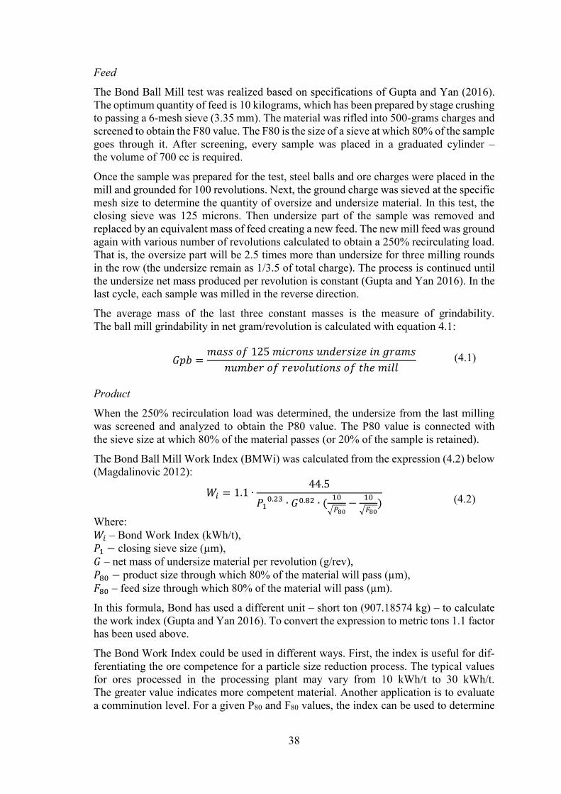
38

Feed

The Bond Ball Mill test was realized based on specifications of Gupta and Yan (2016). The optimum quantity of feed is 10 kilograms, which has been prepared by stage crushing to passing a 6-mesh sieve (3.35 mm). The material was rifled into 500-grams charges and screened to obtain the F80 value. The F80 is the size of a sieve at which 80% of the sample goes through it. After screening, every sample was placed in a graduated cylinder – the volume of 700 cc is required.

Once the sample was prepared for the test, steel balls and ore charges were placed in the mill and grounded for 100 revolutions. Next, the ground charge was sieved at the specific mesh size to determine the quantity of oversize and undersize material. In this test, the closing sieve was 125 microns. Then undersize part of the sample was removed and replaced by an equivalent mass of feed creating a new feed. The new mill feed was ground again with various number of revolutions calculated to obtain a 250% recirculating load. That is, the oversize part will be 2.5 times more than undersize for three milling rounds in the row (the undersize remain as 1/3.5 of total charge). The process is continued until the undersize net mass produced per revolution is constant (Gupta and Yan 2016). In the last cycle, each sample was milled in the reverse direction.

The average mass of the last three constant masses is the measure of grindability. The ball mill grindability in net gram/revolution is calculated with equation 4.1:

𝐺𝑝𝑏 =𝑚𝑎𝑠𝑠 𝑜𝑓 125 𝑚𝑖𝑐𝑟𝑜𝑛𝑠 𝑢𝑛𝑑𝑒𝑟𝑠𝑖𝑧𝑒 𝑖𝑛 𝑔𝑟𝑎𝑚𝑠

𝑛𝑢𝑚𝑏𝑒𝑟 𝑜𝑓 𝑟𝑒𝑣𝑜𝑙𝑢𝑡𝑖𝑜𝑛𝑠 𝑜𝑓 𝑡ℎ𝑒 𝑚𝑖𝑙𝑙

Product

When the 250% recirculation load was determined, the undersize from the last milling was screened and analyzed to obtain the P80 value. The P80 value is connected with the sieve size at which 80% of the material passes (or 20% of the sample is retained).

The Bond Ball Mill Work Index (BMWi) was calculated from the expression (4.2) below (Magdalinovic 2012):

𝑊𝑖 = 1.1 ∙44.5

𝑃10.23 ∙ 𝐺0.82 ∙ (

10

√𝑃80−

10

√𝐹80)

Where: 𝑊𝑖 – Bond Work Index (kWh/t), 𝑃1 − closing sieve size (µm), 𝐺 – net mass of undersize material per revolution (g/rev), 𝑃80 − product size through which 80% of the material will pass (µm), 𝐹80 – feed size through which 80% of the material will pass (µm).

In this formula, Bond has used a different unit – short ton (907.18574 kg) – to calculate the work index (Gupta and Yan 2016). To convert the expression to metric tons 1.1 factor has been used above.

The Bond Work Index could be used in different ways. First, the index is useful for dif-ferentiating the ore competence for a particle size reduction process. The typical values for ores processed in the processing plant may vary from 10 kWh/t to 30 kWh/t. The greater value indicates more competent material. Another application is to evaluate a comminution level. For a given P80 and F80 values, the index can be used to determine

(4.1)

(4.2)

39

the specific energy needed for size reduction. The widely used breakage characterization method in the mineral industries and mining is the Bond Work Index, based on the “Third theory of comminution” (Merkus and Meesters 2016). It may be written as an equation 4.3:

𝑊 = 𝑊𝑖 ∙ (10

√𝑃80

−10

√𝐹80

)

Where: 𝑊 – plant data; mass specific energy divided by throughput (kWh/t), 𝑊𝑖 – Bond Work Index (kWh/t), √𝑃80 − product size through which 80% of the material will pass (µm), √𝐹80 − feed size through which 80% of the material will pass (µm). Later, a ball mill is selected according to the calculations and equipment specifications, which can obtain the required power with given operating conditions (like speed or ball charge).

The implementation of the Bond equation and method has been criticized by different researchers. Morell suggested that the basic problem with this equation is connected with a size exponent and proposed a size-energy relationship (4.4):

𝑊 = 𝑀𝑖 ∙ 𝐾 ∙ (𝑥2

𝑓(𝑥2)− 𝑥1

𝑓(𝑥1)) Where: 𝑀𝑖 – the comminution index (kWh/t), 𝐾- constant value to balance the units of the formula (-), 𝑥1, 𝑥2 – equivalent to F80 and P80 (µm), 𝑓(𝑥𝑗) – has the following form (4.5):

𝑓(𝑥𝑗) = −(0.295 +𝑥𝑗

1,000,000)

Morell demonstrates that by taking values K and Mi can predict required total specific energy in the milling process with a 95% confidence (+/- 15%) (Merkus and Meesters 2016).

The other limitation of the Bond equation is that it ignores the fact that the associated specific comminution energy and the shape of the product size distribution are variable. They are changing in three cases- in the batch test, the standard Bond test, and steady-state continuous mill. What is more, this method tends to be a weak predictor of a real closed circuit when throughput increases, unless the performance of the classifier is adjusted to the new conditions. Application of this method to AG/SAG mills is limited and it cannot be used directly in circuit optimization. In this case, an essential step is to determine a work index from a pilot plant and operating data (Merkus and Meesters 2016).

4.2 Drop Weight test

In 1992, Julius Kruttschnitt Mineral Research Center (JKMRC) invented and developed the Drop Weight Test. JK Drop Weight Test measures an impact, the breakage factor and characteristics of ore in an AG/SAG mill. This test is commonly used in test laboratories. The ore parameters can be determined from low and high-energy impact devices.

(4.3)

(4.4)

(4.5)

40

The tumbling test provides the abrasion breakage factor, whereas JK Drop Weight Tester determines the impact breakage parameter. The JKMRC has been tested a wide range of ores, coal samples, and quarry particles. These data have been implemented in simulation and modeling research activities or in consulting work (Napier-Munn 1996).

Drop Weight Test may be required in different situations and cases, in example to deter-mine the parameters for an existing or new crusher. The test also could be used in green-field, to establish the breakage factors of ore under milling conditions (AG/SAG) so that the new circuit can be planned, designed or optimized. The ore characterization tests measure the size reduction and energy behavior. These values can be expressed as a breakage or appearance functions, or as a degree of breakage at different comminution energy levels (JK Tech 2018).

4.2.1 Test description

The Drop Weight Tester was designed at the JKMRC to replace an old apparatus (the twin pendulum) for determining impact breakage characteristics of different ore types. It consists of a drop head, which is lifted and dropped onto the rock particle (JK Tech 2018). In this thesis was used a non-standard device built by laboratory technicians from the rock engineering laboratory. The drop head weight is equal 13.671 kg and the weight is re-leased by an adjustable wrench and falls under gravity to crush a sample on a steel anvil.

Figure 4.3 Drop Weight Tester components.

Tester is built on a strong steel frame and base, and drop head is attached to a steel rod. Drop height can be controlled by a wrench – it is possible to lock or unlock the tool in the specific positions. All samples for this test were located under the drop head, on a steel anvil as presented in Figure 4.3. Additional support construction was installed to keep the device stable and safety.

41

4.2.2 Test procedure

Drop Weight Tester is designed for testing different rock types, including hard rock ores, whose specific gravity varies from 2.8 to 4 g/cm3. For coal or other softer materials, the breakage energy of interest is much lower, so it is recommended to re-design the tester to include a light drop head for example 2.0 kg.

For coarse particle measurement, standard practice is testing of 20-50 particles at each energy/size combination. This test was carried out for four particle sizes, with three dif-ferent energy levels per fraction. To drop test 8 different sample groups, with 12 drops per single set were prepared, which gives 96 drops in total. Sample specifications are presented in the Table 4.2. Table 4.2 Drop Weight Test specifications for sample set 1S175.

Fraction Nominal size Number of particles No. of particles in test Ecs mm mm - - kWh/t

-20.0+16.0 17.3 80 80 80

20 20 20

0.22 0.44 0.66

-11.2+8.0 10.2 100 100 100

25 25 25

0.50 1.00 1.50

-5.6+4.0 4.5 120 120 120

120 120 120

1.01 2.02 3.03

-4.0+2.0 2.4 200 200 200

200 200 200

2.40 4.81 7.21

The test procedure required a specific quantity of material (Table 4.2), to generate 20-25 particles in two size fractions, in the range from 8.0 to 20.0 mm. All of the particles were selected randomly from the representative coarse sample.

Following sample set preparation, the height from which drop head was released and the mean mass of each set of particles were determined. The test involves different energy levels, which were achieved by adjusting the drop head and drop heights. The impact energy level and specific comminution energy level were determined from equations 4.6 and 4.7, presented below and based on specifications by Napier-Munn (1996).

𝐸𝑖 = 𝑚𝑑 ∙ 𝑔 ∙ (ℎ𝑖 − ℎ𝑓) Where: 𝐸𝑖- the impact breakage energy (𝑚2 ∙ 𝑘𝑔/𝑠2), 𝑚𝑑- the mass of the drop weight head (kg), 𝑔 - gravitational acceleration (9.81 𝑚/𝑠2), ℎ𝑖- the initial height of the drop weight head (m), ℎ𝑓- the final height from the anvil (m).

𝐸𝑐𝑠 =𝐸𝑖

�̅�

(4.6)

(4.7)

42

Where: 𝐸𝑐𝑠- the specific comminution energy (kWh/t), 𝐸𝑖- the impact breakage energy (𝑚2 ∙ 𝑘𝑔/𝑠𝑒𝑐2), �̅�- mean mass of each set of particles (g).

Usually, 10 mm is added during the calculation of different drop heights for the test. This step ensures that the proper final specific comminution energy is determined, due to the presence of the crushed samples on the anvil. The specific input energy is equal to the specific comminution energy as far as the drop head does not rebound after impact (Napier-Munn 1996).

After impact tests, all samples were sieved to obtain t10 value. The value of t10 is tradi-tionally called a breakage index number or the fineness of the ore. In the JKTech conven-tion, this value is defined as the percentage passing 1/10th of the original particle size (geometric mean of the broken fraction). In this test, √2 sieve series were used, all essen-tial data is presented in Table 4.3. The behavior of the ore during impact breakage test can be compared and characterized through a single distribution at a specific comminu-tion energy level by using the t10 value. The relationship between the amount of breakage and the specific comminution energy is described by the following equation 4.8:

𝑡10 = 𝐴 × [1 − exp(−𝑏 × 𝐸𝑐𝑠)] Where: 𝑡10 – the amount of breakage (%), 𝐴, 𝑏 – the material impact parameters, related to hardness of the ore, 𝐸𝑐𝑠 – the specific comminution energy (kWh/t). Table 4.3 Sieve sets used for different sample fraction.

Fraction Sieves set 1/10th sieve size

16.0-20.0 mm 10.00 1.68 4.00 2.00 1.68

8.0-11.2 mm 4.00 1.00 2.00 1.68 1.00

4.0-5.6 mm 2.00 0.50 1.68 1.00 0.50

2.0-4.0 mm 1.68 0.18 1.00 0.50 0.18

(4.8)

43

For fraction 16-20 mm sieves of 10 mm, 4 mm, 2 mm, and 1.68 mm were used. All specifications were based on the t10 definition presented in equation 4.9 and 4.10:

𝑔𝑒𝑜𝑚𝑒𝑡𝑟𝑖𝑐 𝑚𝑒𝑎𝑛 = √16 ∙ 20 = 17.88 1

10 𝑣𝑎𝑙𝑢𝑒 = 0.1 ∙ 17.9 = 1.79

As can be seen, the 1/10th value for the 16.0-20.0 mm sample size is equal to 1.79 mm. Due to the sieves size limitation 1.68 mm sieve was accepted. Using a different en-ergy/size combination, A and b parameters were determined by non-linear regression with IBM SPSS statistical program. The resulting Axb parameter is connected with the re-sistance of the ore to the high impact breakage (Genç 2004).

4.3 Point Load test

In the United States, Reichmuth directed an experimental study of shape and size effects. Reichmuth’s work used the diametral test on the core sample as one of ten index tests. The aim of this measurement was an attempt to predict compressive strength. The highest correlation with uniaxial compressive strength was achieved with the Point load Test with a correlation coefficient was equal to 0.9479. Later, McWilliams used this test to study the relationship of microstructural defects in the rock material to weakness planes in the core. The sample core was sawn into disks, which were tested by loading in the axial direction to show the preferred failure direction (Bieniawski 1975).

4.3.1 Test description

The prototype built by Selmer-Olsen and Bergh-Christensen used a mechanical jack. The ram retraction of the machine was slow and has a consequent delay between tests. The final version of the device used a high-pressure hydraulic ram with a small hydraulic hand pump. They noticed that the design of the loading plates needed standardization and therefore conducted a test to evaluate ‘wedge’ and ‘cone’ platens for the same rock sam-ples. Finally, a conical design was selected. Wedge platens imposed a failure direction and these kind of platens could only be used for diametral tests on the core (E. Broch 1972).

This test can be performed in a laboratory or in the field. Usually, Point Load Test is used in the field due to easy testing possibility – the device is small, portable and requires only minimal sample preparation. The procedure includes compressing a sample between two conical (steel) platens until failure. Typically, failure occurs within 10-60 seconds after the starting of measurement and peak load indicator is essential to record the failure load. The test is rejected when the failure occurs only in loading point (E. Broch 1972).

(4.9)

(4.10)

44

Figure 4.4 Point Load testing device set up (E. Broch 1972).

The equipment set up consists of two-point load platens, a loading frame and a load cell, a pressure gauge and a load measuring system pictured in Figure 4.4. In this study, the Point Load device is connected to a hydraulic pump to adjust the pressure flow. With the hydraulic pump, it is possible to control the speed of the test (E. Broch 1972).

Figure 4.5 Testing of Kittilä sample with Point Load device.

A digital barometer measures the applied pressure to the system. When Is values are de-termined, they are multiplied with a specific correction factor of 0.85 to obtain the Is50 index (ASTM 1995). The sample holder was designed with OpenScad 3D-modelling soft-ware and printed with a 3D-printer. This holder is useful for applying the force in the center of the sample surface and it was created according to the sample specifications.

45

4.3.2 Test procedure

The rock samples were divided into eight groups and all specimens were prepared ac-cording to ASTM standards (ASTM 1995). In this test, a 25 mm reference sample diam-eter was used, which is the optimum size for testing brittle ores according to Rusnak (2000). Only axial test was conducted, because of limitations in the number of samples. The axial test was carried out on the core sample of a small length (approximately 1/3 of the diameter). All core specimens were completely dry and were prepared at the labora-tory in the Civil Engineering Department of Aalto University. The angle between the structural planes and the axis of the core should not exceed 30 degrees according to standard (Rusnak 2000).

On the beginning of calculations, the uncorrected Point Load Strength Index was deter-mined for all samples with the following equation 4.11:

𝐼𝑠 =𝑃

𝐷𝑒2

Where: 𝐼𝑠 – Point Load Strength Index (MPa), P – failure load (N), 𝐷𝑒

2 – equivalent core diameter (mm2), 4A/π for axial tests.

After Strength Index determination, the shape correction factor F was used to obtain a representative value, which may be implemented in rock strength classification. Then a new Is50 index was determined as a value of Is which would have been measured with diametric test where De=50 mm. The size correction factor is presented in the Figure 4.6.

Figure 4.6 Size correction factor chart from ASTM (1995).

(4.11)

46

After size correction, the new Point Load Index Is50 was calculated according to equation 4.12:

𝐼𝑠50 = 𝐹 ∙ 𝐼𝑠 Where: 𝐼𝑠50 – Point Load Index after correction (MPa), 𝐹 – size correction factor (-), 𝐼𝑠 – Point Load Strength Index (MPa).

The data from the Point Load Test can be easily applied to determine Uniaxial Compres-sive Strength. The UCS is the most commonly used factor during rock strength determi-nation (Bieniawski 1975). The relationship between Point Load Test and uniaxial Com-pressive Strength is presented below in equation 4.13:

𝑈𝐶𝑆 = 24 ∙ 𝐼𝑠50 Where: 𝑈𝐶𝑆 – Uniaxial Compressive Strength (MPa), 𝐼𝑠50 – Point Load Index after correction (MPa).

A confidence interval has been implemented to the relationship between UCS and Point Load Test. This calculation is based on the equation 4.14.

𝐶𝐼95% = 1.96 ∙𝑆𝐷

√𝑛

Where: 𝐶𝐼95% − 95 % confidence interval, 𝑆𝐷 – standard deviation of the UCS results (MPa), √𝑛 –the number of tests which were done in this test (-).

(4.12)

(4.13)

(4.14)

47

5 Results This chapter includes results from all comminution tests described in the previous section. The results from each test are discussed individually, whereas a summary of this work can be found at the end of this chapter.

5.1 SEM results The essential part of sample analysis was obtained by collecting the X-rays generated during sample scanning. Each element and particle in the sample emits X-rays with char-acteristic wavelengths and energies. This section is focused on the mineral composition of the ore samples and its relation to the comminution process. In the Table 3.2 are pre-sented major minerals identified in the SEM analysis for all sample sets (in total for 48 samples). Table 5.1 Average mineral content based on SEM results.

Mineralogical content (average)

Sample code Quartz Arsenopyrite Albite Muscovite Pyrite Ankerite - % % % % % %

1S175 10.93 0.54 32.34 8.63 2.22 26.29

2S175 14.53 0.55 25.60 10.29 1.81 27.18

1S325 13.03 0.11 14.69 12.08 0.88 33.43

2S325 11.56 0.17 21.91 11.36 1.07 31.36

1R390 14.98 0.35 4.84 18.80 2.33 39.94

2R390 29.09 0.12 16.86 10.44 1.11 28.41

1X900 13.61 0.00 24.36 3.60 0.23 26.54

2X900 15.69 0.00 19.77 2.97 0.32 25.32

As can be seen, all sample sets contain a significant quantity of quartz, albite, and anker-ite. Quartz is composed of oxygen and silicon atoms and is one of the most abundant minerals in the Earth’s crust, behind feldspar. This mineral has an ideal crystal shape and cannot be scratched by steel. Albite is a plagioclase feldspar mineral and it is common in felsic rocks. Ankerite is a mineral of the group of carbonates and it is closely related to dolomite. These minerals have a significant influence on the crushing and grinding of the ore, due to their hardness (Liber-Madziarz and Teisseyre 2002):

- quartz – 7.0 on Mohs scale (cannot be scratched by steel), - albite – 6.0-6.5 on Mohs scale (can be scratched by steel; however, it required

additional effort), - ankerite – 3.5-4.0 on Mohs scale (can be scratched by steel).

Thus, most of the sample sets are relatively hard rocks. Quartz and albite content evalua-tion is essential to explain the variation of the geometallurgical properties of the ore (Liber-Madziarz and Teisseyre 2002).

48

Another major mineral in these ore samples is muscovite. As opposed to quartz and albite, muscovite is a soft mineral also known as a common mica or isinglass. Muscovite was evaluated on the Mohs scale of 2.0-2.25 parallel to the face and 4.0 perpendicular. This mineral has perfect cleavage and forms of thin, elastic sheets. A high quantity of muscovite in the mineral composition of the sample can influence a grindability of the ore by making the rock softer and easier to break (Liber-Madziarz and Teisseyre 2002).

Pyrite and arsenopyrite are sulfide minerals, which are usually found associated with small to significant quantities of gold. The average amount of pyrite in the samples varies from 0.23 % until 2.33 % when arsenopyrite has a range of 0.00% to 0.55%. Pyrite is often associated with oxides or other sulfides in quartz veins, while arsenopyrite could be located in high-temperature hydrothermal veins, in areas of contact metasomatism and metamorphism or pegmatites. The full SEM analysis result for sample set 1R390 (10) is provided in Table 5.2. Classification is based on order respect to the total area of the particles.

After first SEM measurement additional scanning was performed. The reason of this test was to check an accuracy of scanning whole sample in comparison with scanning of spe-cific area (point) in the specimen. Each sample was tested with three sites of interest and after choosing of definite area, several points were measured. From an output of the test, different minerals were established. In the Figure 5.1 and Figure 5.2 are presented results for sample 1X900 (2) II 3 and 2X900 (5) II 10. In the table are listed all spectrum points with defined mineral, where in the picture below is shown electron image with spectrum points.

Figure 5.1 Element analysis by FE-SEM-EDS. Sample 1X900 (2) II 3.

Spectrum 1 cobaltite Spectrum 1 monazite Spectrum 1 cobaltite

2 cobaltite 2 monazite 2 cobaltite

3 unknown 3 monazite 3 albite

4 ilmenite 4 monazite 4 illite

5 ilmenite 5 albite 5 rutile

6 albite 6 rutile 6 clinochlore

7 ilmenite 7 clinochlore 7 unknown

8 K-feldspar

Site of interest 1 Site of interest 2 Site of interest 3

Sample 1X900 (2) II 3

49

Figure 5.2 Element analysis by FE-SEM-EDS. Sample 2X900 (5) II 10.

As can be seen from point measurement, there is a difference between previous scanning of whole sample and point testing. From spectrum points were determined minerals like clinochlore, rutile, monazite, cobaltite, gersdorffite or illite. Monazite, gersdorffite and clinochlore were not found in samples during whole scanning. It can be concluded that detailed measurement is highly recommended for proper mineral composition prepara-tion. However, major minerals found in first SEM test are also present in precise meas-urement. In sample 1X900 (2) II 3 was found albite and k-feldspar, while in sample 2X900 (5) II 10 was detected ankerite, albite, quartz and pyrrhotite. More results with mineral determination are enclosed in Appendix 9 and Appendix 10.

Spectrum 1 pyrrhotite Spectrum 1 pyrrhotite Spectrum 1 pyrrhotite

2 pyrrhotite 2 pyrrhotite 2 pyrrhotite

3 albite 3 albite 3 quartz

4 ankerite 4 ankerite 4 clinochlore

5 pyrrhotite 5 ilmenite 5 unknown

6 ilmenite 6 albite 6 albite

7 pyrrhotite

8 clinochlore

Sample 2X900 (5) II 10

Site of interest 1 Site of interest 2 Site of interest 3

50

Table 5.2 1R390 (10) I - 4. Scanning Electron Microscope results.

5.2 XRF results The same samples as in the previous SEM test were measured with XRF. Each sample was measured with an X-ray analyzer three times to minimize the potential errors and differences in arsenic content detection. All sample sets included six specimens, which gave over 140 measurements. In the Table 3.4 are presented all the results from this test.

1R390 (10) I-4 Classification Feature Feature %

Ankerite 3658 38.20

Muscovite 2010 20.99

Quartz 963 10.06

Albite 961 10.04 Pyrite 199 2.08

Mg-biotite 175 1.83

Feldspar, mixed 98 1.02

Wollastonite 96 1.00

K-fsp 82 0.86

Biotite 56 0.58 Plagioclase 50 0.52

Arsenopyrite 46 0.48

Rutile_Ti-Ox 35 0.37

Apatite 13 0.14

Chlorite 9 0.09

Gypsum 5 0.05 Sphene 4 0.04

Olivine 3 0.03

Aegerine 2 0.02

Ilmenite 2 0.02

Gersdorffite 1 0.01

Fe-ox, altered 1 0.01 Calcite 1 0.01

Almandine 1 0.01

Unclassified 1105 11.54

SUM 9576 100.00

51

Table 5.3 X-Ray analyzer results for all sample sets.

Sample code I try II try III try

As (%) As (%) As (%)

1S175 (8) V - 2 0.0220 0.0641 0.0250 1S175 (I) I - 2 0.1500 0.1200 0.0920 1S175 (II) II - 4 0.2200 0.1900 0.4700 1S175 (8) II -1 0.0613 0.1300 0.3000 1S175 (I) VI -7 0.0525 0.4400 0.1500 1S175 (II) I -6 0.3300 0.2900 0.2200

mean 0.14 0.21 0.21

2S175 (8) II -11 0.5600 0.6500 0.5600 2S175 (1) II- 5 0.0054 0.0039 0.0054 2S175 (1) II - 7 0.0074 0.0057 0.0065 2S175 (II) II - 10 0.2800 0.4300 0.1600 2S175 (II) III - 15 0.1400 0.1700 0.5800

mean 0.20 0.25 0.26

1X900 (2) IV - 9 0.0036 0.0105 0.0107 1X900 (6) II - 1 0.0087 0.0043 0.0026 1X900 (1) III - 1 0.0201 0.0067 0.0026 1X900 (6) V -2 0.0058 0.0059 0.0051 1X900 (1) II - 13 0.0028 0.0026 0.0030 1X900 (2) II - 3 0.0014 0.0012 0.0024

mean 0.007 0.005 0.004

2X900 (5) I - 4 0 0 0.0005 2X900 (5) II - 10 0.0139 0.0010 0.0095 2X900 (7) IV - 3 0.0045 0.0035 0.0065 2X900 (7) II - 2 0.0091 0.0026 0.0030 2X900 (4) II - 10 0 0 0 2X900 (4) IV - 17 0.0009 0.0023 0.0025

mean 0.005 0.002 0.004

1S325 (2) III -3 0.0552 0.0505 0.0549 1S325 (12) I - 3 0.6900 0.1100 0.4600 1S325 (8) III - 6 0.0095 0.0089 0.0094 1S325 (8) II -1 0.0117 0.0096 0.0060 1S325 (12) II -1 0.2100 0.1700 0.1700 1S325(2) I - 1 0.0440 0.0413 0.0416

mean 0.17 0.07 0.12

2S325 (I) III - 10 0.0631 0.1100 0.0562 2S325 (I) I -1 0.1100 0.0169 0.5900 2S325 (2) II - 1 0.0781 0.1200 0.1200 2S325 (2) III -4 0.0123 0.0128 0.0146 2S325 (8) III - 3 0.0597 0.0419 0.0901 2S325 (8) I - 3 0.0742 0.0965 0.0825

mean 0.07 0.07 0.16

1R390 (10) I - 4 0.1900 0.2100 0.1700 1R390 (1) III - 6 0.0013 0.0023 0.0011 1R390 (7) II - 2 0.0389 0.0360 0.0761 1R390 (I) II - 4 0.0082 0.0044 0.0114 1R390 (10) III - 1 0.1000 0.6500 0.3000 1R390 (7) III - 3 0.3800 1.4000 0.5600

mean 0.12 0.38 0.19

2R390 (I) I -8 0.0011 0 0 2R390 (3) II - 3 0.0307 0.0334 0.0427 2R390 (2) II - 1 0.0731 0.0835 0.4300 2R390 (3) IV - 6 0.2000 0.0867 0.4700 2R390 (2) IV - 4 0.0114 0.0179 0.0103 2R390 (1) III - 1 0.0005 0 0

mean 0.05 0.04 0.16

52

Arsenic content in sample sets varies significantly – samples 1S175 and 2S175 have the highest quantity of As from 0.19 % to 0.24 % when samples 1X900 and 2X900 do not contain this element at all. There is a strong relation between overall results from X-Ray analysis and SEM measurements, what is presented in Table 5.4. Most of the sample sets show a strong correlation between each other; only sample 1S175 and 2X900 repre-sent weak relation -0.392 and 0.570. Table 5.4 Summary results of Arsenic measurements.

Summary I try II try III try Mean SEM results Correlation

As % As % As % % As % XRay vs SEM

1S175 0.14 0.21 0.21 0.19 0.27 -0.392 2S175 0.20 0.25 0.26 0.24 0.27 0.999 1X900 0.01 0.01 0.00 0.01 0.00 0.707 2X900 0.01 0.00 0.00 0.00 0.00 0.570 1R390 0.12 0.38 0.19 0.23 0.17 0.848 2R390 0.05 0.04 0.16 0.08 0.08 0.973 1S325 0.17 0.07 0.12 0.12 0.09 0.850 2S325 0.07 0.07 0.16 0.10 0.12 0.977

The IBM SPSS Statistic 26 was used to test the statistical correlation between SEM and XRF measurements. (Thermo Fisher Scientific 2012). The overall correlation is signifi-cantly positive, which means that the results from X-Ray equipment confirm the amount of Arsenic from the Scanning Electron Microscope test. This linear correlation can be used for the estimation of element content from another. Figure 5.3 presents a table with calculated Pearson correlation between Arsenic content with SEM and XRF measure-ment.

Figure 5.3 Correlation between Arsenic SEM and Arsenic X-Ray content.

5.3 Bond Ball Mill test

The Bond Ball Mill Test was conducted in different grinding stages in range from 6 to 13 times, for eight sample sets. The variation between quantities of grinding rounds is con-nected with the equilibrium requirement in each sample set. The closing sieve in this test was 125 µm and it was used to determine the mass of retained or passing material. After first grinding, the drum was dumped, and the 700 cm3 of material was screened on sieves to distribute the under- and oversize particles. The undersize was weighted, and then fresh feed was added to the part above 125 µm to achieve the initial weight back. After that,

53

the feed was returned into the mill and ground again until equilibrium was found. Mill losses were taken into consideration in this method.

In Table 5.1 below are presented calculations for a one sample set 2S175. The same for-mulas and steps were applied in every sample set. More results can be found in Appendix 1, Appendix 2 and Appendix 3. Table 5.5 Calculation of the grindability parameters in Bond Ball Mill Test. Sample 2S175.

In Table 5.6 information about the feed and product of the Bond Ball Mill Test is pro-vided. The P80 and F80 values, which are bolded in the bottom of the table, represent the sieve size through which 80% of the material will pass. The closing sieve size is 125 µm. Table 5.6 Product and feed analysis for sample set 2S175.

Feed 1174.3 g Product 99.9 g

Sieve size Stayed Passed Cum Pass Sieve size Stayed Passed Cum Pass

microns g g % microns g g %

4000 0.0 1173.6 100.0 125 0.1 97.5 99.9

3350 153.6 1020.0 86.9 106 6.5 91.0 93.3

2800 146.4 873.6 74.4 88 9.6 81.4 83.5

2300 133.9 739.7 63.0 75 11.7 69.7 71.5

2000 105.0 634.7 54.1 63 12.7 56.9 58.4

1000 305.1 329.6 28.1 Y 56.9 59.3 60.8

500 161.1 168.5 14.4 loss 2.4

125 161.8 6.7 0.6

Y 6.7 7.4

loss 0.7

F80 3045 P80 84

The product distribution is presented in the Figure 5.4 and varies from 125 microns to 63 microns, whereas the feed distribution changes from 3350 microns to 125 microns.

2S175 A B C D E F G H I

Grind-ing

stage

Mill revs

Mass +125µm

Mass -125µm

Loss from mill-ing

Refill mass reqd

Total refill used

Mass -125µm in refill

Mass -125µm mill-ing

Mass -125µm per rev

1/3.5

Revs for

next run

revs gram gram gram gram gram gram gram gram gram revs Initial feed - - - - 1174.3 - - - - - -

1 100 1098.0 76.2 0.1 76.3 1174.3 6.7 69.5 0.70 335.5 482.75

2 482 750.5 416.4 7.4 423.8 76.3 0.3 416.1 0.86 335.5 388.65

3 388 801.6 382.9 -10.2 372.7 423.8 0.7 382.2 0.99 335.5 340.61

4 340 835.7 341.7 -3.1 338.6 372.7 2.1 339.6 1.00 335.5 335.94

5 336 829.6 341.1 3.6 344.7 338.6 1.9 339.2 1.01 335.5 332.38

6 332 843.7 331.0 -0.4 330.6 344.7 2.0 329.0 0.99 335.5 338.54

A+B C last run D*(Ei/Di) A-E F/revs Di/3.5 H/G

54

Figure 5.4 F80 (3045 microns) and P80 (84 microns) distribution - sample 2S175.

In this test, two parameters were evaluated during calculations – the Bond Work Index and the Plant Energy Consumption. The formulas used to obtain these values are pre-sented in the Section 4.1.2. Each value of different sample sets was determined with the same specific steps as before. Summary results from the Bond Ball Mill Test are en-closed in Table 5.7. Table 5.7 Bond Ball Mill test results for all sample sets.

Sample code

Feed mass 80% passing feed (F80)

80% passing prod-uct (P80)

Bond Work Index (Wi)

Plant data (W)

- g µm µm kWh/t kWh/t

1S175 1222.4 3223 86 18.62 16.79

2S175 1174.3 3045 84 17.75 16.13

1X900 1227.7 2961 98 20.40 16.45

2X900 1246.8 3189 97 18.31 15.35

1R390 1260.0 2823 85 15.81 14.22

2R390 1341.2 3069 90 16.56 14.42

1S325 1291.7 3079 86 19.38 17.44

2S325 1228.5 2985 94 18.85 15.95

0,00%

20,00%

40,00%

60,00%

80,00%

100,00%

1 10 100 1000 10000

Cu

mu

latv

ie %

of

pas

sin

g m

ater

ial

Sieve size (microns)

Feed and product for sample 2S175

2S175 Feed

Product

55

The Bond Work Index varies from 15.81 to 19.38 kWh/t. Energy consumption is strongly connected with the Bond Work Index values, hence the ore samples with the greater BMWi need more comminution energy to mill and reduce the particles to the required size. Table 5.8 Relationship between ore hardness and Bond Work index (Tsakalakis 2015).

BWI (kWh/t) <7.0 7.0-9.0 9.0-14.0 14.0-18.0 18.0-20.0

>20.0

Ore-hardness very soft

soft medium medium hard

hard very hard

In general, the texture and mineral content and hardness of the ore control the breakage mechanisms, which are strongly connected with grindability values from the Bond Ball Mill test. It is highly complicated to determine which factor is mainly controlling the grindability in this case, due to the heterogeneity of the ore (carbonate and albitic alteration). Table 5.9 Ore hardness classification based on Bond Ball Mill Test.

Sample code Bond Work Index Class range 1S175 hard (18.0-20.0) 2S175 moderate hard (14.0-18.0) 1X900 very hard >20.0 2X900 hard (18.0-20.0) 1R390 moderate hard (14.0-18.0) 2R390 moderate hard (14.0-18.0) 1S325 hard (18.0-20.0) 2S325 hard (18.0-20.0)

As can be seen, the sample sets 1R390 and 2R390 are the least resistant to grinding pro-cess, while sample set 1X900 was evaluated as very hard and the most resistant. Table 5.9 shows ore hardness classification. Material, which was obtained for comminu-tion testing, was not homogenous and therefore the Bond Work index is not a constant value. There are no big-scale grinding tests, which can be used to directly determine the Work Index to the feed to SAG mills. When the results from crushing and grinding tests are available, the Bond equation should be used in the power calculations. Usually, a rule of thumb is used – a primary SAG mill requires 25% more energy than rod mills and crush-ers doing the same work. When SAG mill operating data is accessible, using the feed, product size distribution data and power, the Work Index can be evaluated from the pilot-plant data. Then the Work Index can be used in the Bond equation to determine the grind-ing energy that is needed for a primary Semi-autogenous Grinding Mill (911Metallurgist 2017).

56

5.4 Drop Weight test

The value of t10 was calculated for every sample set. In Table 5.6, the test results are presented. This example of energy levels, fraction, starting weight and t10 value corre-sponds to the one sample set 1S175, whereas the full and detailed report for all sample sets can be found in Appendix 4. Table 5.10 Drop Weight Test results for sample 1S175.

Fraction Start weight Material passing 1/10

sieve t10 Ecs

mm g g % kWh/t

16.0-20.0

76.6 2.25 2.94 0.22

89.3 5.10 5.71 0.44

106.5 6.95 6.53 0.66

8.0-11.2

31.4 0.90 2.87 0.50

40.1 1.86 4.64 1.00

49.1 2.35 4.79 1.50

4.0-5.6

18.0 0.48 2.67 1.01

19.8 0.70 3.54 2.02

21.9 1.00 4.57 3.03

2.0-4.0

7.8 0.17 2.18 2.40

8.2 0.30 3.66 4.81

9.1 0.40 4.40 7.21

A and b parameters are the high impact breakage factors, where A is the maximum t10 value accomplished. This parameter is essential for higher energy impact, but it is not critical in the SAG mill. A value measures the breakage of the ore at higher energy levels than those one that are usually determined in the SAG mill. The A parameter characterizes the overall breakage curve. The b parameter is connected with the overall slope at a lower energy of the Ecs vs t10 curve (JK Tech 2018). A and b values are interrelated and are derived from the t10 equation (Chapter 4.2.2, equation 4.8). Non-linear regression results for sample set 1S175 are presented in the Table 5.11. The final value of the Axb breakage parameters is provided in Table 5.12.

57

Table 5.11 Non-linear regression analysis for sample set 1S175.

Iteration History 1S175

Iteration Number

Residual Sum of Squares

Parameter

A b

1.0 203.930 10.000 1.000 1.1 55.757 2.940 1.783 2.0 55.757 2.940 1.783 2.1 24.889 3.426 5.680 3.0 24.889 3.426 5.680 3.1 17.967 4.034 9.672 4.0 17.967 4.034 9.672 4.1 18.155 4.137 6.148 5.0 17.919 4.126 7.078 5.1 17.919 4.126 7.078 6.0 17.872 4.095 8.832 6.1 17.872 4.095 8.832 7.0 17.882 4.130 7.394 7.1 17.882 4.130 7.394 8.0 17.853 4.118 8.151 8.1 17.853 4.118 8.151 9.0 17.853 4.120 8.119 9.1

10.0 10.1 11.0 11.1 12.0 12.1 13.0 13.1 14.0 14.1

17.853 17.853 17.853 17.853 17.853 17.853 17.853 17.853 17.853 17.853 17.853

4.120 4.120 4.120 4.120 4.120 4.120 4.120 4.120 4.120 4.120 4.120

8.119 8.148 8.148 8.122 8.122 8.138 8.138 8.130 8.133 8.133 8.135

Table 5.12 Summary of the Axb parameter for sample set 1S175.

Parameter Estimates

Parame-ter

Estimate Std. Error 95% Confidence Interval

Lower bound Upper Bound

A 4.120 0.429 3.165 5.075

b 8.135 8.901 -11.697 27.966

Each Axb value was determined with the same, specific steps in the SPSS program (An-alyze -> Regression -> Nonlinear). Model expression formula was constant, while Ecs and t10 were changing with sample set modification. The Axb parameters are significant for the classification of the ore samples according to their crushability shown in Table 5.13.

58

Table 5.13 Axb breakage parameters for all sample sets.

Sample code b A Axb

1S175 8.135 4.120 33.52

2S175 8.581 3.550 30.46

1S325 9.554 4,133 39.49

2S325 9.764 3,893 38.01

1R390 9.741 3.135 30.54

2R390 6.008 5.113 30.72

1X900 12.126 3.788 45.93

2X900 8.964 3.727 33.41

The Axb parameters are the utile index of the ore hardness, which can be implemented to AG/SAG mill for process optimization. Higher parameters of Axb denote softer ore. The comparison of the Axb parameters for all sample sets is presented in Figure 5.5.

Figure 5.5 Drop Weight Test parameters for all sample sets.

The A and b indexes are interdependent and have no physical meaning. The product of Axb is universally used for the determination of an ore’s resistance to impact breakage. Although, there are a few disadvantages of using this Axb method. The A and b parame-ters are qualitative measure, the relationship between Axb and impact resistance is non-linear and it is inversely connected with impact resistance. The non-linear relationship is a highly important factor during the comparison of the Axb values of various samples. Differences in hardness between two samples, in example 24 and 30 (20 % difference) could be significantly different; while for samples 100 and 150 (50 % difference) may not be statistically different. To solve this trouble and avoid potential mistakes, it is rec-ommended to use simulations of Axb influence on the AG/SAG specific energy (911Metallurgist 2017).

33,5230,46

39,49 38,01

30,54 30,72

45,93

33,41

0,00

5,00

10,00

15,00

20,00

25,00

30,00

35,00

40,00

45,00

50,00

Axb

(-)

Axb for all samples

1S175 2S175 1S325 2S325 1R390 2R390 1X900 2X900

59

Hardness classification results for all sample sets are tabulated in Table 5.14. As can be seen, Axb indexes indicate, that samples from Kittilä mine are mostly hard rocks. Only two sample sets (1S325 and 1X900) were evaluated as moderate or medium-hard. Table 5.14 Hardness classification based on crushability in the Drop Weight Test.

Sample b A Axb Axb Range result (hardness of the ore)

1S175 8.135 4.120 33.52 (30-38) hard

2S175 8.581 3.550 30.46 (30-38) hard

1S325 9.554 4.133 39.49 (38-43) moderate hard

2S325 9.764 3.893 38.01 (30-38) hard

1R390 9.741 3.135 30.54 (30-38) hard

2R390 6.008 5.113 30.72 (30-38) hard

1X900 12.126 3.788 45.93 (43-56) medium

2X900 8.964 3.727 33.41 (30-38) hard

Figure 5.6 presents the results for breakage parameter t10 versus specific comminution energy for four different size fractions. Generally, it became more difficult to break sam-ples by impact when the fraction got finer. Coarse size fractions (for example 16.0-20.0 mm) were easy to break in Drop Weight Tester, but fine size fraction (2.0-4.0 mm) needed a higher level of specific comminution energy. For fraction, 16.0-20.0 mm energy levels increased from 0.22 kWh/t to 0.66 kWh/t and t10% value varied from 2.94% until 6.53%. In the case of 2.0-4.0 mm particle size, energy levels had ranged from 2.40 kWh/t to 7.21 kWh/t, while the breakage parameter had lower values from 2.18% to 4.40%.

Figure 5.6 t10% parameter vs Ecs for 4 size fractions – sample 1S175.

Almost the same tendency is showed in Figure 5.7. Coarse particles are easy to crush, while fine fraction needs higher energy levels. This condition showed, that for 2.0-4.0 mm particles additional energy is needed or modified comminution mechanism is re-quired for better and further impact breakage of the samples.

R² = 0,9096

R² = 0,8073

R² = 0,9976

R² = 0,964

1,80

2,30

2,80

3,30

3,80

4,30

4,80

5,30

0,00 1,00 2,00 3,00 4,00 5,00 6,00 7,00

t10

(%

)

Ecs (kWh/t)

Drop weight test - size reduction 1S175

16.0-20.0 mm

8.0-11.2 mm

4.0-5.6 mm

2.0-4.0 mm

Linear (16.0-20.0 mm)

Linear (8.0-11.2 mm)

Linear (4.0-5.6 mm)

Linear (2.0-4.0 mm)

Fraction:

60

Figure 5.7 t10% parameter vs Ecs for 4 size fractions – sample 2S175.

All of the Ecs-t10% models have the same tendency and are provided in Appendix 6. A linear relationship was established between breakage parameters and specific comminu-tion energies. Different R2 values are presented in each chart in the legend, while all frac-tion sizes are marked by the chosen color.

From these results, it may be observed that the relationship between t10 and Ecs changes even for the same fraction size in the same sample groups. For sample 1R390 and fraction 2.0-4.0 mm, the breakage parameter is equal 1.33, 2.73 and 3.33. However, in the sample set 2R390 and the same fraction, the t10% level varies from 3.37 to 5.62. Energy levels input for both sample sets are similar, but the amount of material passing 1/10th of the original particle size differs significantly. At this moment, it can be noticed that the sample set 1X900 was the easiest part to crush. Simultaneously, the sample sets R390 and S175 had the hardest particles to crush. These variations may be connected with the mi-crotextures and variable mineral composition of the rock. The overall relationship between specific comminution energy and t10% is presented in Figure 5.8. Values obtained from experiments were plotted and then, compared to the fitted model. Sufficient agreement between the model fitted and the experimental val-ues was noticed. A steeper gradient between the t10 and Ecs curve provides a softer ore.

R² = 0,8779

R² = 0,9813

R² = 0,9489

R² = 1

1,35

1,85

2,35

2,85

3,35

3,85

4,35

4,85

0,00 1,00 2,00 3,00 4,00 5,00 6,00 7,00 8,00 9,00

t10

(%

)

Ecs (kWh/t)

Drop weight test - size reduction 2S175

16.0-20.0 mm

8.0-11.2 mm

4.0-5.6 mm

2.0-4.0 mm

Linear (16.0-20.0 mm)

Linear (8.0-11.2 mm)

Linear (4.0-5.6 mm)

Linear (2.0-4.0 mm)

Fraction:

61

Figure 5.8 Overall relationship between specific comminution energy vs cumulative t10% for sample sets

S175, S325, R390 and X900.

0,00

10,00

20,00

30,00

40,00

50,00

60,00

0,00 1,00 2,00 3,00 4,00 5,00 6,00 7,00 8,00 9,00

Cu

mu

lati

ve t

10

(%

)

Ecs (kWh/t)

Overall relationship between specific comminution energy vs t10% for sample sets S175

1S175

2S175

Log. (1S175)

Log. (2S175)

0,00

10,00

20,00

30,00

40,00

50,00

60,00

70,00

0,00 1,00 2,00 3,00 4,00 5,00 6,00 7,00

Cu

mu

lati

ve t

10

(%

)

Ecs (kWh/t)

Overall relationship between specific comminution energy vs t10% for sample sets R390

1R390

2R390

Log. (1R390)

Log. (2R390)

0,00

10,00

20,00

30,00

40,00

50,00

60,00

0,00 5,00 10,00 15,00

Cu

mu

lati

ve t

10

(%

)

Ecs (kWh/t)

Overall relationship between specific comminution energy vs t10% for sample sets S325

1S3252S325Log. (1S325)Log. (2S325)

0,00

10,00

20,00

30,00

40,00

50,00

0,00 5,00 10,00

Cu

mu

lati

ve t

10

(%

)

Ecs (kWh/t)

Overall relationship between specific comminution energy vs t10% for sample sets X900

1X900

2X900

Log. (1X900)

Log. (2X900)

62

As is known, the mill models are determined on the specific assumption, that all of the contents inside the device are mixed. The AG/SAG function is based on three size fractions and defined by three abrasion and impact breakage parameters (A, b and ta). The appearance functions depend on size and energy values. During AG/SAG milling, particle size reduction occurs by crushing (high impact) and chipping or abrasion. In the original modeling, the mean specific comminution energy for an AG/SAG is de-scribed as a function of mill diameter. Further, some modifications were implemented to this approach to allow the mean Ecs to be determined separately for every fraction size. In Table 5.11 is presented the standard appearance function developed at Julius Kruttschnitt Mineral Research Center and widely used in the AG/SAG modeling (Napier-Munn 1996). Table 5.15 Breakage function used by JKMRC for AG/SAG model (T.J. Napier-Munn, 1996).

t10 (%) t75 t50 t25 t4 t2 10 2.33 3.06 4.98 23.33 50.53 30 6.89 9.41 15.62 61.58 92.49 50 10.32 14.71 25.88 82.86 96.47

Another important parameter, which made Drop Weight Test results more understanda-ble, is SAG Circuit Specific Energy (SCSE). The SCSE may be an effective tool in com-parison to the expected behavior of variable ores in the AG/SAG mills adequately, as the Bond Ball Mill index can be used in the comparison of the grindability of ores during ball milling. The main goal of this Drop Weight Test is the proper selection of AG/SAG devices following the ore hardness. In Figure 5.9, can be observed the example of variable types of the operating AG/SAG mills concerning Axb parameter values (911Metallurgist 2017).

Figure 5.9 SAG (kWh/t) vs Axb for operating AG/SAG mills (911Metallurgist 2017).

In the AG/SAG mills, the specific gravity of the different ore has a significant influence on the power draw and charge density. The second step of the JK Drop Weight Test is low energy breakage (abrasion) testing. It is characterized by using a tumbling test of different single particle sizes. In JK Drop Weight Tests basic parameters relevant to

63

AG/SAG mills are A, b and ta. As was mentioned before, A and b are used to determine the impact breakage, while ta is a measure of abrasion resistance of the ore. For both results, a dependency is the same – the lower the parameters value the greater the re-sistance of the sample. In Table 5.16, the classification of the sample based on Axb, ta and SCSE values is presented. Table 5.16 Basic parameters for JK Drop Weight Test (JK Tech 2018).

Property Very hard Hard Moderate

hard Medium Moderate medium Soft Very Soft

Axb <30 30-38 38-43 43-56 56-67 67-127 >127

ta <0.24 0.24-0.35 0.35-0.41 0.41-0.54 0.54-0.65 0.65-1.38 >1.38

SCSE >10.7 10.7-9.7 9.7-9.3 9.3-8.4 8.4-7.9 7.9-6.5 <6.5

5.5 Point Load test

The Point Load Test is an efficient method to determine rock strength properties. It has become a widely used test in geotechnical evaluations. In the Table 5.13 calculations to establish the Point Load Strength index, for sample 1S175 (4) II, are presented. The Point Load Test was carried out for over 400 specimens. In this test, the axial cores were crushed by applying a force to parallel to planes of the weakness of the sample. Table 5.17 Point Load Strength Index for sample group 1S175 (4) II.

Type Sample

code

W D De P Is Is(50) Is(50) median

mm mm mm2 bar MPa MPa MPa

a //

1S175 (4) II side

8,97 24,55 602,70 35,01 8,14 25,42

a // 9,07 24,55 602,70 24,27 5,64 17,62

a // 9,30 24,55 602,70 43,80 10,18 31,80

a // 8,86 24,55 602,70 35,75 8,31 25,96

a // 9,09 24,55 602,70 38,15 8,87 27,70 31,77

a // 9,07 24,55 602,70 44,45 10,34 32,27

a // 9,07 24,55 602,70 43,77 10,18 31,78

a // 8,95 24,55 602,70 44,09 10,25 32,01

a // 9,05 24,55 602,70 43,91 10,21 31,88

a // 9,13 24,55 602,70 33,11 7,70 24,04

a // 8,96 24,55 602,70 43,76 10,18 31,77

A detailed report for all measured samples is in Appendix 8 and the summary of the re-sults is provided in Appendix 7. In Appendix 7 information about I(50) median, I(50) stand-ard deviation, UCS median and UCS standard deviation can be found. The abridged ver-sion of the results is presented in Table 5.14.

64

Table 5.18 Overall results from Point Load Test.

Sample code UCS median (MPa) Classification

1X900 149,84 high strength 2X900 116,25 high strength 1R390 85,43 medium strength 2R390 112,83 high strength 1S325 114,76 high strength 2S325 123,24 high strength 1S175 119,01 high strength 2S175 113,33 high strength

As can be seen, most of the samples have similar values of UCS but a significant differ-ence was noticed for sample 1X900 and 1R390. Sample set 1R390 was the softest, which can be caused by the variation in mineral composition and microstructure of the ore. In all of the specimens (1R390) was observed high graphite occurrence and failure zones connected with this mineral. A fine-grained silicate matrix with an association of pyrite was found in sample set 1X900 (Figure 5.10).

Figure 5.10 Examples of cores diversity – specimens after Point Load Test.

The range of Uniaxial Compressive Strength is presented in Figure 5.11, where the hori-zontal line denotes the median UCS value. The reason for differences in the UCS values is strongly connected with the ore heterogeneity. What is more, minerals like quartz, al-bite, ankerite, graphite, and muscovite affect the geometallurgical properties like hardness and failure zones.

65

Figure 5.11 Range of Uniaxial Compressive Strengths for all sample sets.

In Appendix 9 can be found information about histograms of the standard deviation of UCS and Is(50) values for all sample sets. It can be seen, that the average standard devia-tion is located between 20-25 (for UCS SD) and it has characteristics similar to a plot of normal distribution. In this chart, one of the scores is stray from the rest of the values and it could be caused by a high diversity of the ore or error of measurement. The situation showed in the histogram of the standard deviation of Is(50) leads to the higher variability of the results. The spread between the maximum and minimum value is equal to 2.79 and the average value of the standard deviation was evaluated as 0.98. The Point Load Test provides for full data utilization which can be improved from explo-ration drilling. Intact rock strength can be implemented in geotechnical evaluation and design work by rock mass classification systems and numerical modeling. Moreover, the cost of this testing is minimal in comparison with overall exploration expenses (Rusnak 2000).

66

5.6 Summary of results

The results from the comminution tests are presented in Table 5.19. The Uniaxial Com-pressive Strength represents the average rate from point load tests, in order to achieve one value per sample set. In the case of Drop Weight Test, the classification of the rock was based on Axb parameters, while the hardness of the ore in the Bond Ball Mill Test was evaluated by using the Bond Mill Work Index. Table 5.19 Summarized results from comminution tests.

Sample code

Bond Ball Mill Test Drop Weight Test Point Load Test

BMWi (kWh/t) Axb (-) UCS (MPa)

1S175 18.62 hard 33.52 hard 119,01 high strength 2S175 17.75 mod. hard 30.46 hard 113,33 high strength 1S325 19.38 hard 39.49 mod. hard 114,76 high strength 2S325 18.85 hard 38.01 hard 123,24 high strength 1R390 15.81 mod. hard 30.54 hard 85,43 medium 2R390 16.56 mod. hard 30.72 hard 112,83 high strength 1X900 20.40 very hard 45.93 medium 149,84 high strength 2X900 18.31 hard 33.41 hard 116,25 high strength

67

6 Discussion The development of comminution testing methods aims to describe the essential commi-nution properties of the ore. It is complicated to achieve this goal since most of the pro-grams use variable tests for different sample sizes. Nowadays, it is common to perform separate characterization tests for SAG grinding, crushing and ball mill grinding. Bond Work Index generally has a positive correlation with SAG indexes like Axb parameters. Unfortunately, the difference is still significant that it is not popular to use only Bond Ball Mill test as a proper estimate for the full grindability characterization. The developed tests are designed to be implemented in early stages for identification of differences in com-minution properties leading to detailed geometallurgical characterization of the ore. Later testing and sampling can be done on a bigger scale to obtain efficient and econom-ical circuit design. This step ensures the quality of mineral processing and is the key foundation of geometallurgy (Mwanga 2014).

6.1 Relations between comminution tests and mineralogical composition

The relation between Drop Weight Test and mineral composition can be described as poor, with negative its value for muscovite and quartz content, what is shown in Table 6.1 and Figure 6.1. The reason for these results can be connected with SEM classification. Scanning Electron Microscope is a device, which shows the morphology of the sample and it focuses on the sample’s surface and its composition. The classification used for these samples had specific ranges, which determines the mineral or element. Kittilä gold ore represents high heterogeneity and fluctuation, which causes significant changes in the deposit, in drill cores and then in the samples in one set. Table 6.1 The correlation between the Drop Weight Test (Axb parameters) and the mineral composition for all sample sets.

Drop Weight TEST Quartz Albite Muscovite Ankerite

Pearson correlation -0.376 0.217 -0.459 0.026

Sig. (2 - tailed) 0.358 0.605 0.253 0.952

N 8 8 8 8

68

Figure 6.1 The Drop Weight Test and the mineral composition relations.

The Point Load Test (UCS) shows a good positive relationship with albite content, while it appears to have a strong, negative relation with muscovite. The relation between quartz, ankerite and Point Load index is poor and negative. These results present that albite-rich samples were more resistant to uniaxial compression, whereas the samples’ riches in soft minerals like muscovite were much softer. Another important mineral, which had a sig-nificant influence on the compression strength of the samples, was graphite. The sample sets, which contained a high quantity of graphite (like 1R390 and 2R390), showed spe-cific failure zones during the test and were the softest from all specimens. All relations from this test and SEM are presented in Table 6.2 and Figure 6.2. Table 6.2 The correlation between the Pont Load strength index and the mineral composition for all sample sets.

Point Load TEST Quartz Albite Muscovite Ankerite

Pearson Correlation -0.180 0.656 -0.788 -0.298

Sig. (2 - tailed) 0.670 0.077 0.020 0.474

N 8 8 8 8

69

Figure 6.2 The Point Load Test and the mineral composition relations.

The last comminution test, which was performed in this thesis, was the Bond Ball Mill test. The relation between the Bond Work index and albite is strongly positive. In contrast, the relation between the muscovite and Bond Work index is strongly negative; other re-lations can be described as poor and negative. It can be seen that both, Point Load test and Bond Ball Mill test represent similar results for albite and muscovite content. Then, the sample sets 1R390 and 2R390 were evaluated as the softest from all specimens, the same as after Point Load test. Table 6.3 The correlation between the Bond Ball Mill test and the mineral composition for all sample sets.

Bond Ball Mill TEST Quartz Albite Muscovite Ankerite

Pearson Correlation -0.537 0.568 -0.652 -0.480

Sig. (2 - tailed) 0.170 0.142 0.080 0.229

N 8 8 8 8

70

Figure 6.3 The Bond Ball Mill Test and the mineral composition relations.

Similar studies such as comminution testing by Bis (2018) have been carried out regard-ing the Bond Ball Mill, Point Load and Drop Weight test. From the results, it can be concluded that muscovite content positively relates to the values presented in the previous study. However, the rest of the values is different. Couple of reasons for this situation can be found – high heterogeneity of the ore, testing of different samples, changes in SEM classification, a greater quantity of samples or human error.

6.2 Relations between comminution tests and geometallurgical properties

In this thesis, variable geometallurgical properties of the ore were considered - hardness, texture, liberation, free surface area, cleavage, and breakage. The hardness of the ore can be described as the most important issue for crushing and grinding processes. The relationship between the albite content and ore hardness was presented in Figure 6.3 and it indicates that the samples with higher albite content are harder (higher Bond Work Index). It can suggest that the albite in the ore may be harder than the non-albite compo-nent. Adequate situation was observed with muscovite content – the samples with its higher content are softer. Then, for Point Load Test, it was noticed that there is a positive good relation between albite content and ore hardness; and a negative high correlation between UCS and muscovite quantity. Different studies by Jankovic (2010) and Mwanga (2014) - concluded that ore hardness is controlled by the hardness of the mineral compo-nents in the rock. However, it cannot be used to directly assess the relative grindability of the ore. This trend indicates a size reduction in the Bond Work index. In contrast, the Drop Weight test showed that albite does not have a big influence on the ore hardness. Therefore, to properly assess the grinding energy requirement, additional test work is required.

71

The relation between liberation and breakage mechanisms is important in mineral pro-cessing. Recent studies showed the importance of texture in liberation. Texture can be defined as the distribution of pores and minerals in a specific volume. The textural prop-erty which was considered with particular attention is related to grain size. Grain size is a complex textural property, which can be a bullet point of mineral processing for Kittilä ore. As was mentioned before, Kittilä ore has a submicroscopic gold, which can be invis-ible even under the Scanning Electron Microscope. The texture of all sample sets in com-parison with comminution tests is presented below (Table 6.4). Table 6.4 Texture in comparison with comminution tests.

Sam-ple

code

Bond Ball Mill Test Drop Weight Test Point Load Test Texture

BMWi (kWh/t) Axb (-) UCS (MPa) (subjective evaluation)

1S175 hard hard high strength massive, granoblastic

2S175 mod. hard hard high strength massive, granoblastic

1S325 hard mod. hard high strength granoblastic, banded

2S325 hard hard high strength granoblastic, banded

1R390 mod. hard hard medium banded foliated

2R390 mod. hard hard high strength banded foliated

1X900 very hard medium high strength fine-grained matrix, mas-sive

2X900 hard hard high strength banded, layered

The mineral textures of the samples were classified into three categories: massive-grano-blastic, granoblastic-banded and banded-foliated. Due to the heterogeneity of the ore, these textures can be identified in most of the sample sets. That is why it is complicated to find a direct connection of the texture properties with crushability and grindability of the ore. As can be seen in Table 6.4, the softest sample (1R390) was described as banded-foliated. Furthermore, during the Point Load Test many graphite layers were found. Hard samples (S175, X900) were characterized as massive-granoblastic, massive or banded. With these results, it can be concluded that it is easier to crush or grind samples with banded foliated texture. However, the samples with fine-grained and massive texture were harder than other sets.

The cleavage and breakage characterization depends on the physical properties of rock. During comminution tests, it was noticed that the breakage of the sample is strongly con-nected with graphite – graphite failure zones, as well as with micas content (Figure 5.10). Liberation and free surface area are essential issues for mineral recovery. The aim of mineral processing is to prepare a specific size of feed, from which it will be possible to obtain valuable mineral. To recover gold from Kittilä ore, feed needs to be crushed and grind very precisely. This requirement demands appropriate energy consumption and great processing planning to avoid time and money loss.

6.3 Relations between As-content in the Scanning Electron Mi-croscope and XRF analyzer

Each sample set was tested for As content by a Scanning Electron Microscope and XRF analyzer. As a result, the high positive relation between tests was observed (Figure 6.4). It can be concluded, that these methods can be used as an alternative to each other. The Thermo Scientific XRF Analyzer identifies only elementary composition, the same

72

as a FE-SEM-EDS. It is highly recommended to use the XRF analyzer at the beginning of the exploration of a deposit, at scoping studies. After preliminary analysis of the de-posit, SEM equipment can be implemented.

Figure 6.4 Correlation between XRF analyzer and FE-SEM-EDS results.

6.4 Relations between comminution tests

In order to find the easiest way to determine ore crushability and grindability, relation were carried out between the comminution tests. The results are provided in a matrix in Table 6.5. Table 6.5 Relations between comminution tests.

BMWi Drop Weight (Axb) Point Load (UCS)

BMWi

Pearson correlation 1 0.866** 0.868**

Sig. (2 - tailed) - 0.005 0.005

N 8 8 8

Drop Weight (Axb)

Pearson correlation 0.866** 1 0.815*

Sig. (2 - tailed) 0.005 - 0.014

N 8 8 8

Point Load (UCS)

Pearson correlation 0.868** 0.815* 1

Sig. (2 - tailed) 0.005 0.014 -

N 8 8 8

*. Correlation is significant at the 0.05 level (2-tailed). **. Correlation is significant at the 0.01 level (2-tailed).

73

From the relation matrix can be concluded that all comminution test are interrelated with each other on a similar stage (high and positive relationship that is equal to more than 0.8). The highest correlation can be observed for Point Load and Bond Ball Mill Test. This means that the samples, which were less resistant to uniaxial compression, were also easier to grind with Bond mill. In a similar study by Bis (2018), the correlation between the Bond Ball Mill and the Point Load Test was 0.985. In this connection, it is a great possibility to use the Point Load Test instead of Bond mill during grindability determina-tion. This step can simplify the process of comminution testing of the ore. Bond Ball Mill is a complicated and time-consuming grindability test, which requires high attention and effort - sample testing can take even one month. A detailed description of the test can be found in Chapter 4.1. On the other hand, Point Load test has a simple procedure and the average time dedicated to crushing a sample varies from 10-60 seconds. The difference between these tests is meaningful, where the results are highly correlated. In addition, to complete and check the values obtained from the Point Load Test, the Drop Weight test can be implemented. The drop weight test has also a simple procedure and takes as much time as the Point Load test. However, for Drop Weight test additional sieving is required. In Appendix 10 were enclosed simple scatters with fit line for all comminution tests.

74

7 Conclusions In this work, comminution tests have been carried out for eight locations from the Kittilä gold deposit for detailed determination of geometallurgical properties and their relations with crushability and grindability of the ore. Experimental results from this thesis showed an essential insight into the prediction of the grindability behavior of the specimens. The summary of the results and a conclusion of the work is presented in the following bullet points:

The Bond Work index varies from 15.81 to 20.40 kWh/t, and the sample sets were determined as hard or moderate hard to crush. This test showed that the ore re-quired a high amount of energy to grind it to the specific grain size. The Bond Ball Mill test has a complicated and time-consuming procedure in comparison with other tests carried out in this project.

Even though the Bond Ball Mill test and Drop Weight test are significantly dif-ferent, the Axb parameters confirmed results from the previous test. Values were changing from 30.52 to 45.93 and most of the samples were classified as hard to crush. The Drop Weight test is based on the impact breakage of the sample and the procedure is simpler than for the Bond mill.

The last comminution test provided in this thesis was the Point Load test.

The results represent a range between 85.43-149.84 MPa and ore was determined as medium or high strength. Especially this experiment showed high heterogene-ity of the ore, which was observed even during testing of the one sample set. The Point Load Test delivered information about the uniaxial compressive strength of the rock and it is the fastest test in comparison with Bond Ball Mill and Drop Weight tests.

All comminution tests are strongly related to each other, with the correlation

above 0.8. There is a positive correlation between the crushability and grindability of the ore. With this knowledge, it can be possible to determine one comminution index based on another. Due to the simplicity and a time saving, one of the oppor-tunities is to use the Point Load Test and Drop Weight Test instead of the Bond Ball Mill Test.

Mineral composition of the ore has a significant influence on ore crush- and

grindability. Graphite and muscovite effect on ore hardness, as well as albite, quartz, and ankerite. Graphite and micas decrease the resistance of the ore to crushing and grinding, while others (mentioned before) affect the breakage mechanisms in a way that the ore became harder to crush.

75

Average density, which was measured for the ore samples, is equal to 2.87 g/cm3. The highest difference in density was noticed for sample 2S325 (2.90 g/cm3) and 2R390 (2.94 g/cm3). The reason for this issue can be a high quantity of quartz, albite, and ankerite. It was concluded that the density of the ore is connected with mineral composition, and there is a possibility to predict what kind of mineral can be expected in the specific rock.

All of the geometallurgical properties are connected. The texture of the ore is im-

portant for comminution processes and it changes with grain size and mineral composition. The samples with a fine-grained matrix and massive texture were harder. On the other hand, the samples with banded-foliated texture are easier to crush and grind. However, in this work, the textural evaluation of the ore was determined subjectively and further, detailed measurements are required.

Liberability and free surface area depending on the grain size, texture, and the ore grade. There is a relation between breakage behavior of the ore and mineral com-position. High graphite content defined failure zone or surface in the sample dur-ing Point Load test.

Relation between the SEM classification and XRF analyzer can be described as

highly positive (0.920). XRF analyzer is faster and easier to use in the field, whereas Scanning Electron Microscope provides a more detailed view into the mineral composition of the ore sample.

The most important properties of the ore during mineral processing are hardness,

texture, liberation, free surface area, grain size, cleavage, and breakage. The grain size and shape of the mineral are essential for the crushing and grinding process. Kittilä ore has a submicroscopic gold, which can be invisible even under Scanning Electron Microscope. For that reason, the crushing and grinding process in Kittilä mine requires a high amount of energy for ore preparation for the next stages of gold recovery. With submicroscopic gold, treatment of the ore is focused on proper grinding and then on flotation. Flotation is a common process used in ore enrichment for very fine-grained minerals.

Implementation of the milling process based on geometallurgical properties

should include the following information about the ore. The most important fac-tor, which is directly connected with the process, is the hardness of the ore. The hardness dictates the energy consumption of the crushing and milling. The next factors taken into consideration are liberation and texture. Texture of the ore affects the grain size, degree of the liberation of target minerals and grinda-bility of the ore.

76

8 Recommendations The aim of this work was to develop the geometallurgical characterization and commi-nution testing of the Kittilä gold ore. For the next part of this research, it is recommended to expand knowledge in the following areas:

Point Load test can be implemented as a basic comminution test and used rather than the Bond Ball Mill test, because is less time-consuming and easier to do and interpret. This test can be used simultaneously with the Drop Weight test, which assures corresponding results about crushing and grinding of the ore.

The SEM classification should be updated and improved due to weak correlations for some of the minerals and comminution tests. An additional solution to this problem can be measurements with the Transmission Electron Microscope. With the TEM equipment, it is possible to achieve information about grain boundaries, dislocations and defect structures in solids. These features can be useful for further work on the influence of texture on crush- and grindability of the ore.

Detailed textural analysis will provide more information about the ore, which is

important for processing. For example, the optic method can be used in the next research.

With detailed information about drill holes and geometallurgical characteristics, it is possible to prepare geometallurgical mapping and block models of the de-posit. For future work, the creation of 3D models of the deposit can be a signifi-cant simplification for mine and mineral processing planning.

77

9 References 911Metallurgist. 2017. [Online] 911 Metallurgist Q and A forums. Accessed May 13,

2019. https://www.911metallurgist.com/grinding/how-we-can-chosse-the-best-comminution-circuit/.

Adams, M. D. 2016. Gold Ore Processing - Project Development and Operations.

Netherlands and United Kingdom: Elsevier. Agnico Eagle Mines. 2019. [Online] Kittila, northern Finland. Accessed July 4, 2019.

https://www.agnicoeagle.com/English/operations-and-development-projects/operations/kittila/default.aspx.

All Cropp and W Goodall. 2005. "The infulence of rock texture on mineral processing."

MinAssist 1-9. Alvarez, W. 1978. Classification of solution cleavage in pelagic limestones. Geology. Andrews, J.R.G. and Mika T.S. 1975. Comminution of a heterogeneous material:

Development of a model for liberation phenomena. International Mineral Processing Congress.

ASTM. 1995. Standard Test Method for Determination of the Point Load Strength Index

of Rock. Annual book, Barr Haror Dr: ASTM . Bieniawski, Z. 1975. The Point Load Test in Geotechnical Practice. Amsterdam:

Elsevier. Book. Bis, K. 2018. Geometallurgical characterization of the Kittilä gold ore deposit. Espoo.

Master's thesis. Aalto University. Blaschke, Z. 1981. Zarys tehnologii procesow przerobczych . script, Krakow: AGH . Broch, E. 1972. “The point-load strength test.” International Journal of Rock Mechanics

and Mining Science and Geomechanics Abstracts 669-697. Broch, E. 1983. Estimation of Strength Anisotropy Using the Point-Load Test . Great

Britain: Pergamen Press Ltd. Brook, N. 1980. Size correction for point load testing . J. Rock Mech. Min. Sci &

Geomech. Abstr. Butcher, A.R. 2010. "A practical guide to some aspects of mineralogy that affect

flotation." Flotation Plant Optimisation 83-93. Committee C&E, Comminution and Energy Consumption. 1981. Comminution and

Energy Consumption. U.S.A.: National Materials Advisory Board.

78

Craig, J. 1994. Ore microscopy & ore petrography. Canada: A Wiley-Interscience Publication.

Crawford, K. 2013. Determination of bulk density of rock core using standard industry

methods. Report, Michigan Technological University. Deutch, C.V. 2013. Geostatistical modeling of geometallurgical variables - problems and

solution . Austalasian Institute of Mining and Metallurgy . Doucet, D. 2010. Mineral Resource and Mineral Reserve Estimate and the Suuri

Extension Project, Kittilä mine . Finland Technical Report. Drzymala, J. 2007. Mineral Processing. Wroclaw: Wroclaw University of Technology. Eilu, P, and Wyche N.L. 2015. Minerals Deposits of Finland. Elsevier. Gay, S.L. 2004. Simple texture-based liberation modelling of ores. Minerals Engineering. Genç, Ö. 2004. "Single particle impact breakage characterization of materials by drop

weight testing." Physicochemical Problems of Mineral Processing 241-255. Gupta, A, and D Yan. 2016. Mineral Processing Design and Operations. Perth: Elsevier. Jankovic, A. and Dundar, H. and Mehta R. 2010. Relationships between comminution

energy and product size for a magnetite ore. Non-refereed paper, The Journal of The Southern African Insititute of Mining an Metallurgy.

JK Tech Pty Ltd. 2018. [Online] JK Tech SMI Technology Transfer. Accessed April 20,

2019. https://jktech.com.au/jk-drop-weight-tester. Koch, P-H. 2013. Textural variants of iron ore from Malmberget. Mater's thesis, Luleå:

Luleå University of Technology. Krekeler, M. 2004. "A microscope study of palygorskite-rich sediments from the

Hawthrone formation." Clays and Clay Minerals 263-274. Lamberg, P. and Rosenkranz, J. 2013. Building a Geometallurgical Model in iron ores

using a Mineralogical Approach with Liberation Data. Geomet. Levin, J. 1989. Observations on the Bond Standard Grindability Test, and a proposal for

a Standard Grindability Test for Fine Materials. South Africa: Journal of the South African Institue of Mining and Metallurgy .

Liber-Madziarz, E. and Teisseyre, B. 2002. Mineralogia i petrografia. Wroclaw: Oficyna

Wydawnicza Politechniki Wroclawskiej. Lund, C. 2013. Mineralogical, Chemical and Textural Characterization of the

Malmberget Iron Ore Deposit for a Geometallurgical Model. Luleå: Luleå University of Technology.

79

Magdalinovic, N. 2012. "Determination of the Bond Work index on samples of nonstandard size." International Journal of Mineral Processing (International Journal of Mineral Processing ) 114-117.

Malewski, J. 1984. A comparison of particle shape characteristics of crushed basalt and

granite rocks. Paris: Bulletin of the International Association of Engineering Geology.

Malewski, J. 2014. Ksztalt ziarn w produktach kruszenia. Wroclaw: Politechnika

Wroclawska. Malewski, J. 2012. Ksztalt ziarn w produktach kruszenia. Wroclaw: Politechnika

Wroclawska. Malewski, J. 2012. Urabianie skal w kopalniach odkrywkowych jako problem

optymalizacyjny. Wroclaw: Politechnika Wroclawska. Man, Y.T. 2002. Why is the Bond Ball Mill Grindability Test done the way it is done?

Queensland : EJMP&EP. Meier, W., Lahtinen, R., and O'Brien, H. 2015. Mineral Deposits of Finland. The

Netherlands, Finland: Elsevier. Merkus, H., and G Meesters. 2016. Production, Handling and Characterization of

Particulate Materials. Switzerland: Springer. Mindat glossary. 2019. [Online] Definition of grindability. Accessed April 14, 2019.

https://www.mindat.org/glossary/grindability. Mwanga, A. 2014. "Test Methods for Characterising Ore Comminution Behavior in

Geometallurgy." Sweden. Napier-Munn, T.J. 1996. Mineral Comminution Circuits . Indooroopilly, Australia: Julius

Kruttschnitt Minral Research Centre; University of Queensland. Patison, N. 2007. "The Suurikuusikko Gold Deposit and the Kolari IOCG Deposit." GTK

Guide 54 55-63. Petruk, W. 1990. Measurments of Mineral Liberation in Connection with Mineral

Beneficiation . Ontario : The Minerals, Metals and Materials Society . Rocha, G. 2018. [Online] Minerals - cleavage and fracture. Accessed May 25, 2019.

http://academic.brooklyn.cuny.edu/geology/grocha/mineral/cleavage.html. Rusnak, J. 2000. Using the Point Load Test to determine the Uniaxial Compressive

Strength of coal measure rock. Tavares, L.M. 2009. Modeling breakage rates of coarse particles in ball mills. Minerals

Engineering.

80

Thermo Fisher Scientific Inc. 2012. XR Analyzers. Boston, 11. Tsakalakis, K. 2015. Modelling the specific grinding energy and ball mill scale-up.

scientific paper, Athens: National Technical University of Athens. Welton, J. 2003. SEM Petrology Atlas. Tulsa, Oklahoma U.S.A.: Chevron. Wills, B.A. 1985. Mineral Processing Technology: an introduction to the Practical

Apsects of Ore Treatment nad Mineral Recovery . Oxford : Pergamon Press.

81

10 Appendices

Appendix 1. Bond Ball Mill Test report

1R390

A B C D E F G H I

Grinding

stage

Mill

revs

Mass

+125µm

Mass -

125µm

Loss

from

milling

Refill

mass

reqd

Total

refill

used

Mass -

125µm

in refill

Mass

-

125µm

from

milling

Mass -

125µm

per rev

1/3,5 Revs

for

next run

revs gram gram gram gram gram gram gram gram gram revs

Initial

feed

- - - - 1260.0

1 300 919.5 335.2 5.3 340.5 1260.0 3.8 331.4 1.10 360.0 325.89

2 326 907.5 352.1 0.4 352.5 340.5 1.0 351.1 1.08 360.0 334.29

3 334 855.9 400.6 3.5 404.1 352.5 1.1 399.6 1.20 360.0 300.92

4 301 893.8 367.1 -0.9 366.2 404.1 1.2 365.9 1.22 360.0 296.16

5 296 907.3 342.5 10.2 352.7 366.2 1.1 341.4 1.15 360.0 312.13

6 319 899.6 361.1 -0.7 360.4 352.7 1.1 360.0 1.13 360.0 318.97

A+B C last

round

D*(Ei/Di) A-E F/revs Di/3,5 H/G

2R390 A B C D E F G H I

Grinding

stage

Mill

revs

Mass

+125µm

Mass -

125µm

Loss

from

milling

Refill

mass

reqd

Total re-

fill

used

Mass -

125µm

in refill

Mass -

125µm

from

milling

Mass -

125µm

per rev

1/3,5 Revs for

next run

revs gram gram gram gram gram gram gram gram gram revs

Initial feed - - - - 1341.2

1 280 1047.3 291.1 2.8 293.9 1341.2 6.1 285.0 1.02 383.2 376.48

2 376 945.7 393.1 2. 4 395.5 293.9 1.3 391.8 1.04 383.2 367.78

3 368 923.7 415.0 2.5 417.5 395.5 1.8 413.2 1.12 383.2 341.28

4 341 970.3 369.0 1.9 370.9 417.5 1.9 367.1 1.08 383.2 355.95

5 356 931.3 408.0 1.9 409.9 370.9 1.7 406.3 1.14 383.2 335.75

6 336 942.8 396.6 1.8 398.4 409.9 1.9 394.7 1.17 383.2 326.18

7 326 964.5 374.1 2.6 376.7 398.4 1.8 372.3 1.14 383.2 335.56

8 336 963.7 376.4 1.1 377.5 376.7 1.7 374.7 1.12 383.2 343.63

9 343 935.6 395.0 10.6 405.6 377.5 1.7 393.3 1.15 383.2 334.21

10 343 923.2 417.0 1.0 418.0 405.6 1.8 415.2 1.21 383.2 316.60

11 317 971.3 369.1 0.8 369.9 418.0 1.9 367.2 1.16 383.2 330.81

12 331 959.5 380.0 1.7 381.7 369.9 1.7 378.3 1.14 383.2 335.27

13 335 955.5 382.8 2.9 385.7 381.7 1.7 381.1 1.14 383.2 336.88

A+B C last r D*(Ei/Di) A-E F/revs Di/3,5 H/G

82

1S175

A B C D E F G H I

Grind-

ing

stage

Mill

revs

Mass

+125µ

m

Mass -

125µm

Loss

from

milling

Refill

mass

reqd

Total re-

fill

used

Mass -

125µm

in refill

Mass -

125µm

from

milling

Mass -

125µm

per rev

1/3,5 Revs

for

next

run

revs gram gram gram gram gram gram gram gram gram revs

Initial

feed

- - - - 1222.4

1 280 991.8 222.1 8.5 230.6 1222.4 2.8 219.3 0.78 349.3 445.93

2 350 918.0 304.4 0.0 304.4 230.6 0.5 303.9 0.87 349.3 402.28

3 402 856.3 368.2 -2.1 366.1 304.4 0.7 367.5 0.91 349.3 382.04

4 382 858.9 358.8 4.7 363.5 366.1 0.8 358.0 0.94 349.3 372.71

5 373 866.0 355.7 0.7 356.4 363.5 0.8 354.9 0.95 349.3 367.10

6 367 864.1 355.6 2.7 358.3 356.4 0.8 354.8 0.97 349.3 361.28

A+B C last

round

D*(Ei/Di) A-E F/revs Di/3,5 H/G

1X900

A B C D E F G H I

Grinding

stage

Mill

revs

Mass

+125µm

Mass -

125µm

Loss

from

milling

Refill

mass

reqd

Total

refill

used

Mass -

125µm

in refill

Mass -

125µm

from

milling

Mass -

125µm

per rev

1/3,5 Revs

for

next

run

revs gram gram gram gram gram gram gram gram gram revs

Initial

feed

- - - - 1227.7

1 280 892.9 327.5 7.3 334.8 1227.7 7.8 319.7 1.14 350.7 307.21 2 307 915.9 311.4 0.4 311.8 334.8 2.1 309.3 1.01 350.7 348.19 3 348 839.0 385.8 2.9 388.7 311.8 2.0 383.8 1.10 350.7 318.04 4 317 902.0 324.8 0.9 325.7 388.7 2.5 322.3 1.02 350.7 344.97 5 343 892.3 332.3 3.1 335.4 325.7 2.1 330.2 0.96 350.7 364.34 6 363 863.4 358.4 5.9 364.3 335.4 2.1 356.3 0.98 350.7 357.40 7 356 872.0 355.6 0.1 355.7 364.3 2.3 353.3 0.99 350.7 353.47 8 353 882.5 338.7 6.5 345.2 355.7 2.3 336.5 0.95 350.7 368.02

A+B C last round

D*(Ei/Di) A-E F/revs Di/3,5 H/G

83

1S325

A B C D E F G H I Grinding

stage Mill revs

Mass +125µm

Mass -125µm

Loss from

milling

Refill mass reqd

Total refill used

Mass -125µm in refill

Mass -

125µm from

milling

Mass -125µm per rev

1/3,5 Revs for

next run

revs gram gram gram gram gram gram gram gram gram revs

Initial feed

- - - - 1291.7

1 280 1043.9 244.5 3.3 247.8 1291.7 7.2 237.3 0.85 369.1 435.45 2 435 919.3 370.3 2.1 372.4 247.8 1.4 368.9 0.85 369.1 435.16 3 435 899.9 388.8 3.0 391.8 372.4 2.1 386.7 0.89 369.1 415.13 4 415 885.9 402.0 3.8 405.8 391.8 2.2 399.8 0.96 369.1 383.07 5 426 896.8 383.6 11.3 394.9 405.8 2.3 381.3 0.90 369.1 412.28 6 412 914.8 373.6 3.3 376.9 394.9 2.2 371.4 0.90 369.1 409.40 7 409 908.9 379.2 3.6 382.8 376.9 2.1 377.1 0.92 369.1 400.25 8 400 800.0 363.1 128.6 491.7 382.8 2.1 361.0 0.90 369.1 408.97

A+B C last round

D*(Ei/Di) A-E F/revs Di/3,5 H/G

2X900

A B C D E F G H I

Grind-ing

stage

Mill

revs

Mass +125µ

m

Mass -

125µm

Loss from mill-ing

Refill mass reqd

Total refill used

Mass -125µm in refill

Mass -125µm from

milling

Mass -125µm per rev

1/3,5 Revs for next run

revs

gram gram gram gram gram gram gram gram gram revs

Initial feed

- - - - 1246.8

1 280 974.4 268.2 4.2 272.4 1246.8 4.7 263.5 0.94 356.2 378.54

2 378 876.5 366.6 3.7 370.3 272.4 1.0 365.6 0.97 356.2 368.34

3 368 864.4 383.1 -0.7 382.4 370.3 1.4 381.7 1.04 356.2 343.44

4 343 877.5 366.8 2.5 369.3 382.4 1.4 365.4 1.07 356.2 334.43

5 334 884.8 358.5 3.5 362.0 369.3 1.4 357.1 1.07 356.2 333.18

6 333 890.9 351.6 4.3 355.9 362.0 1.4 350.2 1.05 356.2 338.70

A+B C last D*(Ei/Di) A-E F/revs Di/3,5 H/G

84

2S325 A B C D E F G H I

Grinding stage

Mill revs

Mass +125µm

Mass -125µm

Loss from mill-ing

Refill mass reqd

Total refill used

Mass -125µm in refill

Mass -

125µm from

milling

Mass -125µm per rev

1/3,5 Revs for

next run

revs gram gram gram gram gram gram gram gram gram revs

Initial feed

- - - - 1228.5

1 280 969.1 252.8 6.6 259.4 1228.5 7.5 245.3 0.88 351.0 400.65

2 401 836.6 391.3 0.6 391.9 259.4 1.6 389.7 0.97 351.0 361.16

3 361 834.8 389.9 3.8 393.7 391.9 2.4 387.5 1.07 351.0 326.99

4 327 863.2 361.9 3.4 365.3 393.7 2.4 359.5 1.10 351.0 319.27

5 319 879.9 345.1 3.5 348.6 365.3 2.2 342.9 1.07 351.0 326.56

6 327 891.2 334.2 3.1 337.3 348.6 2.1 332.1 1.02 351.0 345.64

7 346 868.8 355.6 4.1 359.7 337.3 2.1 353.5 1.02 351.0 343.51

8 343 872.9 352.1 3.5 355.6 359.7 2.2 349.9 1.02 351.0 344.07

9 344 880.1 345.3 3.1 348.4 355.6 2.2 343.1 1.00 351.0 351.89

A+B C last round

D*(Ei/Di) A-E F/revs Di/3,5 H/G

85

Appendix 2. F80 and P80 results for all sample sets.

1R390

Feed 1260.0 g Product 101.7 g

Sieve size Stayed Passed Cum Pass Sieve size Stayed Passed Cum Pass

microns g g % microns g g %

4000 0.0 1256.2 100.0 125 0.3 99.3 99.7

3350 132.9 1123.3 89.4 106 7.3 92.0 92.7

2800 123.6 999.7 79.6 88 8.5 83.5 83.8

2300 116.6 883.1 70.3 75 14.3 69.2 69.5

2000 88.3 794.8 63.3 63 12.2 57.0 57.2

1000 328.4 466.4 37.1 Y 57.0 59.1 59.3

500 183.9 282.5 22.5 loss 2.1

125 275.5 7.0 0.6 P80 85

Y 7.0 10.8 0.9

loss 3.8

F80 2823

2R390

Feed 1341.2 g Product 108.4 g

Sieve size Stayed Passed Cum Pass Sieve size Stayed Passed Cum Pass

microns g g % microns g g %

4000 0.0 1340.4 100.0 125 0.8 104.6 99.2

3350 173.6 1166.8 87.0 106 12.7 91.9 87.2

2800 184.9 981.9 73.3 88 8.8 83.1 78.8

2300 157.4 824.5 61.5 75 23.7 59.4 56.4

2000 119.2 705.3 52.6 63 9.5 49.9 47.3

1000 302.6 402.7 30.0 Y 49.9 52.9

500 184.0 218.7 16.3 loss 3.0

125 212.6 6.1 0.5 P80 90

Y 6.1 6.9 0.5

loss 0.8 F80 3069

1S175

Feed 1222.4 g Product 102.5 g Sieve sizes Stayed Passed Cum Pass Sieve size Stayed Passed Cum Pass

microns g g % microns g g %

4000 0.0 1222.4 100.0 125 0.3 99.1 99.7 3350 201.6 1019.4 83.5 106 8.9 90.2 90.8

2800 185.0 834.4 68.3 88 8.8 81.4 82.0

2300 146.1 688.3 56.4 75 13.1 68.4 68.8 2000 108.4 579.9 47.5 63 10.8 57.5 57.9 1000 313.3 266.6 21.8 Y 57.5 60.7 500 141.3 125.3 10.3 loss 3.2 125 122.5 2.8 0.2 P80 86

Y 2.8 4.2 0.3 loss 1.4

F80 3223

86

1X900

Feed 1227.7 g Product 100.0 g Sieve sizes Stayed Passed Cum Pass Sieve size Stayed Passed Cum Pass

microns g g % microns g g %

4000 0.0 1227.1 100.0 125 0.8 94.5 99.2 3350 150.6 1076.5 87.7 106 13.2 81.3 85.3 2800 134.0 942.5 76.8 88 10.9 70.4 73.9 2300 124.3 818.2 66.7 75 18.9 51.5 54.0 2000 95.0 723.2 58.9 63 19.6 31.9 33.5 1000 308.8 414.4 33.8 Y 31.9 36.6 500 202.2 212.2 17.3 loss 4.7 125 204.4 7.8 0.6 P80 98

Y 7.8 8.4 0.7 loss 0.6

F80 2961

2X900

Feed 1246.8 g Product 100.0 g

Sieve sizes Stayed Passed Cum Pass Sieve size Stayed Passed Cum Pass

microns g g % microns g g %

4000 0.0 1245.4 100.0 125 1.4 96.6 98.6

3350 210.4 1035.0 83.1 106 13.6 83.0 84.7

2800 132.5 902.5 72.5 88 9.2 73.8 75.3

2300 112.2 790.3 63.5 75 36.3 37.5 38.3

2000 92.2 698.1 56.1 63 3.9 33.6 34.3

1000 324.1 374.0 30.0 Y 33.6 35.6 36.3

500 187.0 187.0 15.0 loss 2.0

125 182.3 4.7 0.4 P80 97 microns

Y 4.7 6.1 0.5

loss 1.4 F80 3189

1S325

Feed 1291.7 g Product 120.2 g

Sieve size Stayed Passed Cum Pass Sieve size Stayed Passed Cum Pass

microns g g % microns g g %

4000 0.0 1290.9 100.0 125 0.1 115.3 99.9 3350 196.0 1094.9 84.8 106 6.4 108.9 94.4

2800 126.2 968.7 75.0 88 12.7 96.2 83.4

2300 104.2 864.5 67.0 75 22.2 74.0 64.1 2000 82.8 781.7 60.6 63 12.2 61.8 53.6 1000 345.2 436.5 33.8 Y 61.8 66.6 57.7 500 207.8 228.7 17.7 loss 4.8

125 221.5 7.2 0.6 P80 86

Y 7.2 8.0 0.6

loss 0.8

F80 3079

87

2S325

Feed 1228.5 g Product 115.6 g

Sieve size Stayed Passed Cum Pass Sieve size Stayed Passed Cum Pass

microns g g % microns g g %

4000 0.0 1226.6 100.0 125 0.0 57.7 100.0

3350 178.1 1048.5 85.5 106 7.6 50.1 86.8

2800 101.3 947.2 77.2 88 6.1 44.0 76.3

2300 95.2 852.0 69.5 75 13.3 30.7 53.2

2000 83.0 769.0 62.7 63 2.2 28.5 49.4

1000 328.7 440.3 35.9 Y 28.5 86.4

500 207.9 232.4 18.9 loss 57.9

125 224.9 7.5 0.6 P80 94

Y 7.5 9.4 0.8

loss 1.9

F80 2985

88

Appendix 3. Graphical distribution of P80 and F80 values for all sample sets.

0,00%

20,00%

40,00%

60,00%

80,00%

100,00%

1 10 100 1000 10000

Cu

mu

lati

ve %

of

pas

sin

g m

ate

rial

Sieve size (microns)

Feed and product for sample 1R390

1R390 Feed

Product

0,00%

20,00%

40,00%

60,00%

80,00%

100,00%

1 10 100 1000 10000

Cu

mu

lati

ve %

of

pas

sin

g m

ate

rial

Sieve size (microns)

Feed and product for sample 1S175

1S175 Feed

Product

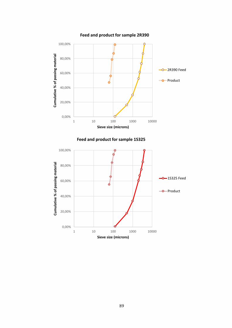
89

0,00%

20,00%

40,00%

60,00%

80,00%

100,00%

1 10 100 1000 10000

Cu

mu

lati

ve %

of

pas

sin

g m

ate

rial

Sieve size (microns)

Feed and product for sample 2R390

2R390 Feed

Product

0,00%

20,00%

40,00%

60,00%

80,00%

100,00%

1 10 100 1000 10000

Cu

mu

lati

ve %

of

pas

sin

g m

ate

rial

Sieve size (microns)

Feed and product for sample 1S325

1S325 Feed

Product

90

0,00%

20,00%

40,00%

60,00%

80,00%

100,00%

1 10 100 1000 10000

Cu

mu

lati

ve %

of

pas

sin

g m

ate

rial

Sieve size (microns)

Feed and product for sample 2S325

2S325 Feed

Product

0,00%

20,00%

40,00%

60,00%

80,00%

100,00%

1 10 100 1000 10000

Cu

mu

lati

ve %

of

pas

sin

g m

ate

rial

Sieve size (microns)

Feed and product for sample 1X900

1X900 Feed

Product

0,00%

20,00%

40,00%

60,00%

80,00%

100,00%

1 10 100 1000 10000

Cu

mu

lati

ve %

of

pas

sin

g m

ate

rial

Sieve size (microns)

Feed and product for sample 2X900

2X900 Feed

Product

91

Appendix 4. Drop Weight Test Report Sample 1S175

Fraction Start weight Material passing 1/10th sieve t10 Ecs

mm g g % kWh/t

16.0-20.0

76.6 2.25 2.94 0.22

89.3 5.10 5.71 0.44

106.5 6.95 6.53 0.66

8.0-11.2

31.4 0.90 2.87 0.50

40.1 1.86 4.64 1.00

49.1 2.35 4.79 1.50

4.0-5.6

18.0 0.48 2.67 1.01

19.8 0.70 3.54 2.02

21.9 1.00 4.57 3.03

2.0-4.0

7.8 0.17 2.18 2.40

8.2 0.30 3.66 4.81

9.1 0.40 4.40 7.21

Sample 2S175 Fraction Start weight Material passing 1/10th sieve t10 Ecs

mm g g % kWh/t

16.0-20.0

92.4 2.60 2.81 0.18

109.3 3.50 3.20 0.36

129.8 6.50 5.01 0.55

8.0-11.2

29.2 0.80 2.74 0.55

38.9 1.40 3.47 1.10

42.1 1.70 3.92 1.64

4.0-5.6

21.5 0.30 1.40 0.91

22.0 0.50 2.27 1.81

23.1 1.00 4.33 2.72

2.0-4.0

6.5 0.10 1.54 2.76

7.5 0.20 2.67 5.51

7.9 0.30 3.80 8.27

Sample 1S325 Fraction Start weight Material passing 1/10th sieve t10 Ecs

mm g g % kWh/t

16.0-20.0

81.0 2.80 3.46 0.21

89.8 4.10 4.57 0.41

120.5 8.00 6.64 0.62

8.0-11.2

28.5 0.70 2.46 0.54

40.6 1.50 3.69 1.09

41.9 2.10 5.01 1.63

4.0-5.6

20.7 0.50 2.42 0.92

22.3 0.80 3.59 1.84

22.7 1.10 4.85 2.76

2.0-4.0

6.6 0.20 3.03 2.77

7.1 0.30 4.23 5.54

8.1 0.40 4.94 8.31

92

Sample 2S325 Fraction Start weight Material passing 1/10th sieve t10 Ecs

mm g g % kWh/t

16.0-20.0

78.4 2.70 3.44 0.23

88.8 3.55 4.00 0.46

96.8 5.90 6.10 0.69

8.0-11.2

30.5 0.90 2.95 0.57

37.5 1.60 4.27 1.13

38.4 2.20 5.73 1.70

4.0-5.6

19.3 0.50 2.59 0.98

19.4 0.60 3.09 1.96

22.9 1.10 4.80 2.94

2.0-4.0

5.5 0.10 1.82 3.23

6.3 0.20 3.17 6.45

6.9 0.30 4.35 9.68

Sample 1R390 Fraction Start weight Material passing 1/10th sieve t10 Ecs

mm g g % kWh/t

16.0-20.0

83.8 2.00 2.39 0.20

100.8 4.30 4.27 0.40

120.3 5.10 4.24 0.59

8.0-11.2

29.4 0.60 2.04 0.53

41.8 1.60 3.83 1.06

42.7 2.10 4.80 1.59

4.0-5.6

19.3 0.40 2.28 0.93

21.9 0.70 3.20 1.86

23.8 0.90 3.66 2.79

2.0-4.0

7.5 0.10 1.33 1.98

11.0 0.30 2.73 3.96

12.0 0.40 3.33 5.94

Sample 2R390

Fraction Start weight Material passing 1/10th sieve t10 Ecs

mm g g % kWh/t

16.0-20.0

71.0 2.40 3.38 0.23

80.4 4.50 5.60 0.45

116.6 7.30 6.26 0.68

8.0-11.2

22.6 0.80 3.54 0.75

26.0 1.20 4.62 1.49

32.3 2.00 6.19 2.24

4.0-5.6

13.3 0.50 3.76 1.37

14.8 0.90 6.08 2.75

15.8 0.90 5.70 4.12

2.0-4.0

8.9 0.30 3.37 2.07

9.8 0.50 5.10 4.13

10.5 0.60 5.62 6.20

93

Sample 1X900 Fraction Start weight Material passing 1/10th sieve t10 Ecs

mm g g % kWh/t

16.0-20.0

56.0 2.00 3.54 0.25

67.0 2.90 4.33 0.50

117.2 6.10 5.20 0.75

8.0-11.2

28.0 0.80 2.86 0.57

32.2 1.20 3.73 1.15

45.0 2.00 4.44 1.72

4.0-5.6

20.3 0.50 2.46 0.93

20.8 0.60 2.88 1.87

23.6 1.10 4.66 2.80

2.0-4.0

7.5 0.10 1.33 2.30

7.8 0.20 2.56 4.61

10.9 0.50 4.59 6.91

Sample 2X900 Fraction Start weight Material passing 1/10th sieve t10 Ecs

mm g g % kWh/t

16.0-20.0 74.9 2.30 3.11 0.24 80.6 3.50 4.34 0.48 96.2 6.20 6.44 0.72

8.0-11.2 15.8 0.40 2.53 0.97 22.1 0.90 4.07 1.95 24.0 1.40 5.83 2.92

4.0-5.6 24.8 0.50 2.02 0.73 28.5 0.70 2.46 1.47 29.0 1.20 4.14 2.20

2.0-4.0 5.2 0.10 1.92 3.23 6.5 0.20 3.08 6.45 7.0 0.30 4.29 9.68

94

Appendix 5. Density measurement report

2X900 (average temperature 14.7 ⁰C)

Weight dry Weight

wet Density

Grams Grams g/cm3

1 4372.5 2852.6 2.874532535 2 2583.0 1684.8 2.873450902 3 3116.6 2030.0 2.865918204 4 5470.1 3565.8 2.869913832

5 4009.4 2620.2 2.883523999 6 147.9 96.3 2.863699419 7 4925.3 3214.5 2.876354472

2.872484766

1X900 (average temperature 19.3 ⁰C)

Weight dry Weight

wet Density

Grams Grams g/cm3

1 4933.2 3201.4 2.843896651

2 2584.2 1678.6 2.848869335

3 4015.3 2623.3 2.879795083

4 2095.1 1366.6 2.871164152

5 1914.0 1251.1 2.882549253

6 5188.8 3386.0 2.87344047

7 4026.6 2620.8 2.859550512

8 2514.2 1633.2 2.849093723

9 2498.5 1626.8 2.861509091

10 2515.8 1632.2 2.842518029 2.86123863

2S175 (average temperature 15.0 ⁰C)

Weight dry Weight

wet Density

Grams Grams g/cm3

1 2691.1 1748.7 2.853011471

2 2458.8 1601.2 2.864490532

3 1186.0 776.4 2.892901855

4 3662.0 2386.5 2.86844704

5 1162.0 752.2 2.83297755

6 1299.6 847.8 2.873905179

7 1553.8 1013.0 2.870565052

8 3818.1 2480.5 2.851871793

9 1538.5 1017.5 2.95031737

10 994.2 649.2 2.879145565 2.873763341

95

1S175 (average temperature 19.3 ⁰C)

Weight dry Weight

wet Density

Grams Grams g/cm3

1 4661.7 3045.2 2.879064766 2 4503.6 2922.3 2.843337166 3 3427.8 2278.5 2.97758995 4 2932.7 1921.9 2.896578003 5 3085.4 2010.6 2.865937002 6 2024.1 1301.5 2.796512919 7 1441.5 940.1 2.870206472 8 2918.6 1879.9 2.80522221 9 1727.1 1123.1 2.854719015

10 1982.9 1294.1 2.874024702 2.866319221

1R390 (average temperature 15.0 ⁰C)

Weight dry Weight

wet Density

Grams Grams g/cm3

1 2468.8 1650.2 3.013166479 2 1792.7 1186.1 2.952664969 3 2043.9 1364.8 3.007009999 4 698.0 458.6 2.912998329 5 2365.2 1540.3 2.864676106 6 565.4 310.8 2.218739749 7 2502.0 1652.6 2.942957617 8 4226.4 2792.6 2.945038527 9 1713.4 1122.1 2.895075156

10 5085.5 3359.7 2.944097259 2.869642419

2R390 (average temperature 19.2 ⁰C)

Weight dry Weight

wet Density

Grams Grams g/cm3

1 5092.9 3332.9 2.888947525 2 3078.1 2011.2 2.880356093 3 3353.9 2203.9 2.91165183 4 1359.8 899.5 2.949315507 5 815.1 530.9 2.863347065 6 679.3 448.3 2.935869905 7 824.3 547.9 2.977381143 8 4102.9 2764.1 3.059584138 9 657.6 427.6 2.854441461

10 1574.0 1066.1 3.093952825 2.941484749

96

1S325 (average temperature 15.0 ⁰C)

Weight dry Weight

wet Density

Grams Grams g/cm3

1 1122.5 760.0 3.093764828 2 2061.9 1342.9 2.865152003 3 3267.7 2092.0 2.776864055 4 2577.0 1685.5 2.888032193 5 1980.7 1287.3 2.853933329 6 1194.2 790.7 2.956939827 7 740.8 497.4 3.040810518 8 2438.3 1591.9 2.878196515 9 2302.8 1481.8 2.802347722

10 697.9 452.9 2.846007714 2.90020487

2S325 (average temperature 19.2 ⁰C)

Weight dry Weight

wet Density

Grams Grams g/cm3

1 5681.5 3699.7 2.862136613 2 3374.1 2188.7 2.841712904 3 3121.8 2064.8 2.948609506 4 1652.2 1067.6 2.821570975 5 1717.8 1113.5 2.837965924 6 1587.3 1040.1 2.896010285 7 1694.7 1118.4 2.935833233 8 1800.7 1165.0 2.827979947 9 1946.2 1299.6 3.004961695

10 1398.5 895.3 2.774655127 2.875143621

97

Appendix 6. Drop Weight Test – size reduction for all sample sets.

R² = 0,9703

R² = 0,9997

R² = 0,9996

R² = 0,9792

2,40

2,90

3,40

3,90

4,40

4,90

5,40

5,90

6,40

6,90

0,00 1,00 2,00 3,00 4,00 5,00 6,00 7,00 8,00

t10

(%

)

Ecs (kWh/t)

Drop weight test - size reduction 1S325

16.0-20.0 mm

8.0-11.2 mm

4.0-5.6 mm

2.0-4.0 mm

Linear (16.0-20.0 mm)

Linear (8.0-11.2 mm)

Linear (4.0-5.6 mm)

Linear (2.0-4.0 mm)

Fraction:

R² = 0,519

R² = 0,9991

R² = 0,9096

R² = 0,9983

1,80

2,30

2,80

3,30

3,80

4,30

4,80

5,30

5,80

0,00 1,00 2,00 3,00 4,00 5,00 6,00 7,00 8,00 9,00

t10

(%

)

Ecs (kWh/t)

Drop weight test - size reduction 2S325

16.0-20.0 mm

8.0-11.2 mm

4.0-5.6 mm

2.0-4.0 mm

Linear (16.0-20.0 mm)

Linear (8.0-11.2 mm)

Linear (4.0-5.6 mm)

Linear (2.0-4.0 mm)

Fraction:

R² = 0,7393

R² = 0,9025

R² = -0,251

R² = 0,9508

1,30

1,80

2,30

2,80

3,30

3,80

4,30

4,80

5,30

5,80

6,30

0,00 2,00 4,00 6,00

t10

(%

)

Ecs (kWh/t)

Drop weight test - size reduction 1R390

16.0-20.0 mm

8.0-11.2 mm

4.0-5.6 mm

2.0-4.0 mm

Linear (16.0-20.0 mm)

Linear (8.0-11.2 mm)

Linear (4.0-5.6 mm)

Linear (2.0-4.0 mm)

Fraction:

98

R² = 0,9117

R² = 0,9882

R² = 0,6057

R² = 0,9114

3,20

3,70

4,20

4,70

5,20

5,70

6,20

6,70

7,20

7,70

0,00 2,00 4,00 6,00

t10

(%

)

Ecs (kWh/t)

Drop weight test - size reduction 2R390

16.0-20.0 mm

8.0-11.2 mm

4.0-5.6 mm

2.0-4.0 mm

Linear (16.0-20.0 mm)

Linear (8.0-11.2 mm)

Linear (4.0-5.6 mm)

Linear (2.0-4.0 mm)

Fraction:

R² = -1,221

R² = -0,483

R² = 0,6835

R² = 0,9806

1,30

1,80

2,30

2,80

3,30

3,80

4,30

4,80

5,30

0,00 2,00 4,00 6,00

t10

(%)

Ecs (kWh/t)

Drop weight test - size reduction 1X900

16.0-20.0 mm

8.0-11.2 mm

4.0-5.6 mm

2.0-4.0 mm

Linear (16.0-20.0 mm)

Linear (8.0-11.2 mm)

Linear (4.0-5.6 mm)

Linear (2.0-4.0 mm)

Fraction:

R² = 0,9778

R² = 0,9985

R² = 0,8975

R² = 0,99981,90

2,40

2,90

3,40

3,90

4,40

4,90

5,40

5,90

6,40

0,00 1,00 2,00 3,00 4,00 5,00 6,00 7,00 8,00 9,00 10,00

t10

(%)

Ecs (kWh/t)

Drop weight test - size reduction 2X900

16.0-20.0 mm

8.0-11.2 mm

4.0-5.6 mm

2.0-4.0 mm

Linear (16.0-20.0 mm)

Linear (8.0-11.2 mm)

Linear (4.0-5.6 mm)

Linear (2.0-4.0 mm)

Fraction:

99

Appendix 7. Summary Point Load Test results. Sample code Is(50) median (MPa) Is(50) SD UCS median (MPa) UCS SD

1X900 (6) II 6,76 0,77 162,22 18,49

1X900 (1) II 5,65 0,76 135,70 18,32

1X900 (2) IV 5,51 0,86 132,24 20,56

1X900 (1) II 6,24 0,75 149,84 18,05

1X900 (6) II 6,76 0,77 162,22 18,49

1X900 (1) III 6,06 0,85 145,53 20,30

1X900 (2) II 7,07 0,77 169,62 18,49

1X900 (10) 10,27 - 246,44 -

1X900 (6) 4,32 0,51 103,69 12,33

2X900 (5) II 3,66 0,70 87,77 16,88

2X900 (4) IV 4,84 1,09 116,09 26,04

2X900 (4) II 5,62 0,87 134,89 20,96

2X900 (5) I 4,85 0,84 116,41 20,23

2X900 (7) IV 4,28 0,79 102,64 18,93

2X900 (7) II 6,98 0,49 167,49 11,66

1S325(6) II 5,64 0,39 135,46 9,38

1S325 (3) II 1,08 - 25,97 -

1S325(4) I 4,22 1,31 101,34 31,46

1S325 (4) II 3,33 1,12 79,90 26,88

1S325 (2) I 2,24 0,73 53,65 17,42

1S325 (8) III 5,47 0,69 131,16 16,47

1S325 (12) I 6,39 - 153,39 -

1S325 (12) II 4,07 0,91 97,69 21,73

1S325 (6) I 7,49 0,71 179,75 17,04

1S325 (3) III 5,34 1,96 128,18 47,12

2S325(2) III 5,04 1,78 121,03 42,79

2S325(1) III 3,51 1,40 84,24 33,58

2S325 (2) III 5,04 1,78 121,03 42,79

2S325 (2) II 5,23 1,02 125,45 24,40

2S325 (1) III 4,51 0,88 108,23 21,12

2S325 (12) II 4,48 0,40 107,62 9,72

2S325 (8) III 6,31 1,16 151,34 27,84

2S325(12) I 5,91 - 141,80 -

2S325 (1) I 5,24 0,85 125,67 20,36

1R390 (7) III 3,78 0,83 90,82 20,03

1R390 (10) III 2,78 0,86 66,72 20,65

1R390 (1) II 5,38 0,86 129,22 20,63

1R390 (7) II 4,33 0,55 104,01 13,09

1R390 (10) I 3,33 1,96 80,03 46,93

1R390 (1) III 3,17 1,27 75,97 30,38

2R390(1)III 3,97 1,44 95,20 34,46

2R390(3) II 3,39 0,55 81,44 13,20

100

2R390 (3) IV 4,95 0,70 118,88 16,81

2R390 (1) I 5,43 1,63 130,23 39,13

2R390 (2) IV 7,08 3,11 169,82 74,55

2R390 (2) II 4,47 - 107,22 -

2R390 (8) I 6,38 - 153,04 -

2R390(8) IV 3,87 0,69 92,89 16,66

1S175 (11) II 6,30 0,93 151,22 22,43

1S175 (9) II 6,56 0,78 157,34 18,64

1S175 (4) II 7,39 1,10 177,31 26,48

1S175 (8) II 4,27 0,44 102,41 10,57

1S175 (1) I 5,82 1,18 139,73 28,43

1S175 (9) I 4,96 0,47 119,01 11,22

1S175 (1) VI 4,30 0,79 103,08 18,90

1S175 (8) I 3,72 - 89,22 -

1S175 (2) I 4,10 1,39 98,30 33,30

2S175 (8) III 4,46 0,88 107,13 21,07

2S175 (2) III 4,58 0,32 109,91 7,72

2S175 (1) II 8,23 1,13 197,63 27,23

2S175 (8) II 6,79 1,48 162,91 35,63

2S175 (2) II 4,86 0,94 116,74 22,53

2S175 (1) III 4,05 0,65 97,09 15,55

101

Appendix 8. Point Load Test report

Type Sample code

W D De P Convert P P Is F Is(50)

mm mm mm2 bar

kN N MPa - MPa

a //

1X900 (6) II side

9.09 24.55 602.70 48.18 0.688 6.75 6752.08 11.20 0.726084 8.13

a // 9.01 24.55 602.70 38.69 0.553 5.42 5422.13 9.00

6.53

a // 8.99 24.55 602.70 41.38 0.591 5.80 5799.11 9.62

6.99

a // 8.91 24.55 602.70 38.33 0.548 5.37 5371.68 8.91 6.47

a //

1X900 (1) II side

8.85 24.55 602.70 41.54 0.593 5.82 5821.53 9.66 7.01

a // 9.14 24.55 602.70 36.15 0.516 5.07 5066.16 8.41

6.10

a // 9.16 24.55 602.70 35.68 0.510 5.00 5000.30 8.30

6.02

a // 9.17 24.55 602.70 31.17 0.445 4.37 4368.25 7.25

5.26

a // 8.67 24.55 602.70 29.22 0.417 4.09 4094.97 6.79

4.93

a // 9.12 24.55 602.70 31.30 0.447 4.39 4386.47 7.28 5.28

a //

2S325(2) III side

9.12 24.55 602.70 37.62 0.537 5.27 5272.17 8.75 6.35

a // 8.78 24.55 602.70 29.87 0.427 4.19 4186.07 6.95

5.04

a // 8.77 24.55 602.70 13.15 0.188 1.84 1842.88 3.06

2.22

a // 8.72 24.55 602.70 37.97 0.542 5.32 5321.22 8.83

6.41

a // 8.96 24.55 602.70 13.73 0.196 1.92 1924.16 3.19

2.32

a // 8.94 24.55 602.70 34.17 0.488 4.79 4788.68 7.95

5.77

a // 9.21 24.55 602.70 24.03 0.343 3.37 3367.63 5.59 4.06

a //

2S325(1) III side

8.91 24.55 602.70 40.24 0.575 5.64 5639.35 9.36 6.79

a // 8.99 24.55 602.70 16.31 0.233 2.29 2285.73 3.79

2.75

a // 8.98 24.55 602.70 21.78 0.311 3.05 3052.31 5.06

3.68

a // 9.11 24.55 602.70 20.79 0.297 2.91 2913.57 4.83

3.51

a // 8.97 24.55 602.70 19.64 0.281 2.75 2752.41 4.57

3.32

a // 8.91 24.55 602.70 15.16 0.217 2.12 2124.57 3.53

2.56

a // 9.09 24.55 602.70 18.83 0.269 2.64 2638.89 4.38

3.18

a // 9.17 24.55 602.70 25.69 0.367 3.60 3600.27 5.97

4.34

a // 8.93 24.55 602.70 30.64 0.438 4.29 4293.98 7.12

5.17

a // 8.63 24.55 602.70 9.82 0.140 1.38 1376.20 2.28

1.66

a // 8.88 24.55 602.70 26.71 0.382 3.74 3743.22 6.21 4.51

a //

2R390(8) IV side

8.86 24.55 602.70 22.80 0.326 3.20 3195.26 5.30 3.85

a // 9.05 24.55 602.70 23.57 0.337 3.30 3303.17 5.48

3.98

a // 9.19 24.55 602.70 30.09 0.430 4.22 4216.90 7.00

5.08

a // 8.99 24.55 602.70 30.01 0.429 4.21 4205.69 6.98

5.07

a // 9.04 24.55 602.70 22.72 0.325 3.18 3184.05 5.28

3.84

a // 8.79 24.55 602.70 30.67 0.438 4.30 4298.18 7.13

5.18

a // 9.02 24.55 602.70 23.05 0.329 3.23 3230.29 5.36

3.89

a // 9.05 24.55 602.70 25.09 0.358 3.52 3516.18 5.83

4.24

a // 8.82 24.55 602.70 18.32 0.262 2.57 2567.42 4.26

3.09

a // 8.95 24.55 602.70 21.87 0.312 3.06 3064.92 5.09

3.69

a // 9.16 24.55 602.70 19.13 0.273 2.68 2680.93 4.45

3.23

a // 8.89 24.55 602.70 24.52 0.350 3.44 3436.30 5.70

4.14

102

a // 9.06 24.55 602.70 24.99 0.357 3.50 3502.17 5.81

4.22

a // 9.14 24.55 602.70 18.50 0.264 2.59 2592.64 4.30

3.12

a // 8.95 24.55 602.70 17.88 0.255 2.51 2505.75 4.16

3.02

a // 9.08 24.55 602.70 21.45 0.306 3.01 3006.06 4.99 3.62

a //

1X900 (2) IV side

8.98 24.55 602.70 32.68 0.467 4.58 4579.87 7.60 5.52

a // 8.89 24.55 602.70 27.44 0.392 3.85 3845.52 6.38

4.63

a // 9.04 24.55 602.70 33.41 0.477 4.68 4682.17 7.77

5.64

a // 9.20 24.55 602.70 25.49 0.364 3.57 3572.24 5.93

4.30

a // 9.10 24.55 602.70 32.03 0.458 4.49 4488.78 7.45

5.41

a // 8.85 24.55 602.70 24.62 0.352 3.45 3450.32 5.72

4.16

a // 9.18 24.55 602.70 39.80 0.569 5.58 5577.69 9.25

6.72

a // 8.90 24.55 602.70 32.59 0.466 4.57 4567.26 7.58

5.50

a // 9.03 24.55 602.70 38.79 0.554 5.44 5436.14 9.02

6.55

a // 8.97 24.55 602.70 34.11 0.487 4.78 4780.27 7.93 5.76

a //

1X900 (1) II side

8.85 24.55 602.70 41.35 0.591 5.79 5794.91 9.61 6.98

a // 9.02 24.55 602.70 41.91 0.599 5.87 5873.39 9.75

7.08

a // 8.49 24.55 602.70 35.73 0.510 5.01 5007.30 8.31

6.03

a // 8.91 24.55 602.70 44.32 0.633 6.21 6211.13 10.31

7.48

a // 9.10 24.55 602.70 36.98 0.528 5.18 5182.48 8.60

6.24

a // 8.51 24.55 602.70 35.49 0.507 4.97 4973.67 8.25

5.99

a // 9.14 24.55 602.70 45.23 0.646 6.34 6338.66 10.52

7.64

a // 8.98 24.55 602.70 34.65 0.495 4.86 4855.95 8.06

5.85

a // 8.96 24.55 602.70 39.86 0.569 5.59 5586.09 9.27

6.73

a // 9.29 24.55 602.70 36.20 0.517 5.07 5073.17 8.42

6.11

a // 9.07 24.55 602.70 36.55 0.522 5.12 5122.22 8.50

6.17

a // 8.97 24.55 602.70 45.38 0.648 6.36 6359.68 10.55

7.66

a // 8.89 24.55 602.70 31.51 0.450 4.42 4415.90 7.33

5.32

a //

1S325(6) II side

8.95 24.55 602.70 29.60 0.423 4.15 4148.23 6.88 5.00

a // 8.97 24.55 602.70 33.77 0.482 4.73 4732.62 7.85

5.70

a // 9.01 24.55 602.70 33.43 0.478 4.68 4684.98 7.77 5.64

a // 1S325 (3) II 8.76 24.55 602.70 6.41 0.092 0.90 898.32 1.49 1.08

a //

1S325(4) I side

9.05 24.55 602.70 28.66 0.409 4.02 4016.49 6.66 4.84

a // 9.03 24.55 602.70 37.45 0.535 5.25 5248.35 8.71

6.32

a // 9.17 24.55 602.70 21.36 0.305 2.99 2993.45 4.97

3.61

a // 9.19 24.55 602.70 20.91 0.299 2.93 2930.39 4.86

3.53

a //

1S325 (4) II side

8.97 24.55 602.70 24.41 0.349 3.42 3420.89 5.68 4.12

a // 8.92 24.55 602.70 15.03 0.215 2.11 2106.35 3.49

2.54

a //

1X900 (6) II side

9.09 24.55 602.70 48.18 0.688 6.75 6752.08 11.20 8.13

a // 9.01 24.55 602.70 38.69 0.553 5.42 5422.13 9.00

6.53

a // 8.99 24.55 602.70 41.38 0.591 5.80 5799.11 9.62

6.99

a // 8.91 24.55 602.70 38.33 0.548 5.37 5371.68 8.91

6.47

a //

1X900 (1) III side

8.85 24.55 602.70 41.54 0.593 5.82 5821.53 9.66 7.01

a // 9.14 24.55 602.70 36.15 0.516 5.07 5066.16 8.41

6.10

a // 9.16 24.55 602.70 35.68 0.510 5.00 5000.30 8.30

6.02

103

a // 9.17 24.55 602.70 41.17 0.588 5.77 5769.68 9.57

6.95

a // 8.67 24.55 602.70 29.22 0.417 4.09 4094.97 6.79

4.93

a // 9.12 24.55 602.70 31.30 0.447 4.39 4386.47 7.28

5.28

a //

1S175 (11) II side

9.15 24.55 602.70 30.68 0.438 4.30 4299.58 7.13 5.18

a // 9.25 24.55 602.70 39.03 0.558 5.47 5469.78 9.08

6.59

a // 9.13 24.55 602.70 35.91 0.513 5.03 5032.53 8.35

6.06

a // 9.11 24.55 602.70 45.96 0.657 6.44 6440.97 10.69

7.76

a // 9.11 24.55 602.70 37.32 0.533 5.23 5230.13 8.68

6.30

a //

1S175 (9) II side

9.06 24.55 602.70 38.69 0.553 5.42 5422.13 9.00 6.53

a // 8.86 24.55 602.70 38.97 0.557 5.46 5461.37 9.06

6.58

a // 9.07 24.55 602.70 35.54 0.508 4.98 4980.68 8.26

6.00

a // 9.08 24.55 602.70 46.39 0.663 6.50 6501.23 10.79

7.83

a //

1S175 (4) II side

8.97 24.55 602.70 35.01 0.500 4.91 4906.40 8.14 5.91

a // 9.07 24.55 602.70 24.27 0.347 3.40 3401.27 5.64

4.10

a // 9.30 24.55 602.70 43.80 0.626 6.14 6138.26 10.18

7.39

a // 8.86 24.55 602.70 35.75 0.511 5.01 5010.11 8.31

6.04

a // 9.09 24.55 602.70 38.15 0.545 5.35 5346.45 8.87

6.44

a // 9.07 24.55 602.70 44.45 0.635 6.23 6229.35 10.34

7.50

a // 9.07 24.55 602.70 43.77 0.625 6.13 6134.05 10.18

7.39

a // 8.95 24.55 602.70 44.09 0.630 6.18 6178.90 10.25

7.44

a // 9.05 24.55 602.70 43.91 0.627 6.15 6153.67 10.21

7.41

a // 9.13 24.55 602.70 33.11 0.473 4.64 4640.13 7.70

5.59

a // 8.96 24.55 602.70 43.76 0.625 6.13 6132.65 10.18

7.39

a //

1S175 (8) II side

9.04 24.55 602.70 25.81 0.369 3.62 3617.09 6.00 4.36

a // 9.10 24.55 602.70 25.58 0.365 3.58 3584.85 5.95

4.32

a // 9.14 24.55 602.70 28.32 0.405 3.97 3968.85 6.59

4.78

a // 9.12 24.55 602.70 24.97 0.357 3.50 3499.37 5.81

4.22

a // 8.92 24.55 602.70 22.47 0.321 3.15 3149.01 5.22

3.79

a // 9.13 24.55 602.70 26.19 0.374 3.67 3670.34 6.09

4.42

a // 9.10 24.55 602.70 20.33 0.290 2.85 2849.10 4.73

3.43

a // 9.15 24.55 602.70 21.58 0.308 3.02 3024.28 5.02

3.64

a // 8.99 24.55 602.70 22.52 0.322 3.16 3156.02 5.24

3.80

a // 9.16 24.55 602.70 27.10 0.387 3.80 3797.87 6.30

4.58

a //

1S175 (1) I side

9.17 24.55 602.70 39.15 0.559 5.49 5486.59 9.10 6.61

a // 9.06 24.55 602.70 32.35 0.462 4.53 4533.62 7.52

5.46

a // 8.89 24.55 602.70 36.66 0.524 5.14 5137.64 8.52

6.19

a // 9.16 24.55 602.70 31.34 0.448 4.39 4392.08 7.29

5.29

a // 8.90 24.55 602.70 19.60 0.280 2.75 2746.80 4.56

3.31

a // 9.06 24.55 602.70 36.62 0.523 5.13 5132.03 8.52

6.18

a //

1S175 (9) I side

9.18 24.55 602.70 32.99 0.471 4.62 4623.31 7.67 5.57

a // 9.17 24.55 602.70 29.37 0.420 4.12 4116.00 6.83

4.96

a // 9.09 24.55 602.70 27.55 0.394 3.86 3860.94 6.41

4.65

a // 2S325 (2) III side

9.12 24.55 602.70 37.62 0.537 5.27 5272.17 8.75 6.35

a // 8.78 24.55 602.70 29.87 0.427 4.19 4186.07 6.95

5.04

104

a // 8.77 24.55 602.70 13.15 0.188 1.84 1842.88 3.06

2.22

a // 8.72 24.55 602.70 37.97 0.542 5.32 5321.22 8.83

6.41

a // 8.96 24.55 602.70 13.73 0.196 1.92 1924.16 3.19

2.32

a // 8.94 24.55 602.70 34.17 0.488 4.79 4788.68 7.95

5.77

a // 9.21 24.55 602.70 24.03 0.343 3.37 3367.63 5.59

4.06

a //

2S325 (2) II side

9.05 24.55 602.70 17.35 0.248 2.43 2431.48 4.03 2.93

a // 9.17 24.55 602.70 38.57 0.551 5.41 5405.31 8.97

6.51

a // 9.14 24.55 602.70 24.14 0.345 3.38 3383.05 5.61

4.08

a // 9.04 24.55 602.70 33.72 0.482 4.73 4725.62 7.84

5.69

a // 9.07 24.55 602.70 30.30 0.433 4.25 4246.33 7.05

5.12

a // 9.01 24.55 602.70 28.49 0.407 3.99 3992.67 6.62

4.81

a // 9.03 24.55 602.70 30.96 0.442 4.34 4338.82 7.20

5.23

a // 9.07 24.55 602.70 31.74 0.453 4.45 4448.13 7.38

5.36

a // 9.00 24.55 602.70 31.74 0.453 4.45 4448.13 7.38

5.36

a //

2S325 (1) III side

8.91 24.55 602.70 40.24 0.575 5.64 5639.35 9.36 6.79

a // 8.99 24.55 602.70 26.31 0.376 3.69 3687.16 6.12

4.44

a // 8.98 24.55 602.70 21.78 0.311 3.05 3052.31 5.06

3.68

a // 9.11 24.55 602.70 20.79 0.297 2.91 2913.57 4.83

3.51

a // 8.97 24.55 602.70 29.64 0.423 4.15 4153.83 6.89

5.00

a // 8.91 24.55 602.70 25.16 0.359 3.53 3525.99 5.85

4.25

a // 9.09 24.55 602.70 28.83 0.412 4.04 4040.32 6.70

4.87

a // 9.17 24.55 602.70 25.69 0.367 3.60 3600.27 5.97

4.34

a // 8.93 24.55 602.70 30.64 0.438 4.29 4293.98 7.12

5.17

a // 8.63 24.55 602.70 29.82 0.426 4.18 4179.06 6.93

5.03

a // 8.88 24.55 602.70 26.71 0.382 3.74 3743.22 6.21

4.51

a //

2S325 (12) II side

9.22 24.55 602.70 26.56 0.379 3.72 3722.19 6.18 4.48

a // 9.09 24.55 602.70 22.99 0.328 3.22 3221.88 5.35

3.88

a // 8.82 24.55 602.70 27.55 0.394 3.86 3860.94 6.41

4.65

a //

2S325 (8) III side

8.83 24.55 602.70 38.38 0.548 5.38 5378.68 8.92 6.48

a // 8.94 24.55 602.70 32.48 0.464 4.55 4551.84 7.55

5.48

a // 8.84 24.55 602.70 39.65 0.566 5.56 5556.66 9.22

6.69

a // 9.00 24.55 602.70 26.05 0.372 3.65 3650.72 6.06

4.40

a // 8.90 24.55 602.70 18.61 0.266 2.61 2608.06 4.33

3.14

a // 8.87 24.55 602.70 35.70 0.510 5.00 5003.10 8.30

6.03

a // 9.09 24.55 602.70 40.10 0.573 5.62 5619.73 9.32

6.77

a // 9.01 24.55 602.70 40.90 0.584 5.73 5731.84 9.51

6.91

a // 8.95 24.55 602.70 39.14 0.559 5.49 5485.19 9.10

6.61

a // 8.69 24.55 602.70 34.29 0.490 4.81 4805.50 7.97

5.79

a // 8.97 24.55 602.70 37.35 0.534 5.23 5234.34 8.68

6.31

a // 2S325(12) I side

9.18 24.55 602.70 32.39 0.463 4.54 4539.23 7.53 5.47

a // 9.10 24.55 602.70 37.60 0.537 5.27 5269.37 8.74

6.35

a //

2X900 (5) II side

8.89 24.55 602.70 22.94 0.328 3.21 3214.88 5.33 3.87

a // 9.06 24.55 602.70 21.66 0.309 3.04 3035.49 5.04

3.66

a // 9.01 24.55 602.70 29.62 0.423 4.15 4151.03 6.89

5.00

105

a // 9.06 24.55 602.70 20.83 0.298 2.92 2919.18 4.84

3.52

a // 8.98 24.55 602.70 20.82 0.297 2.92 2917.77 4.84

3.52

a // 9.09 24.55 602.70 24.36 0.348 3.41 3413.88 5.66

4.11

a // 9.04 24.55 602.70 15.48 0.221 2.17 2169.41 3.60

2.61

a // 8.96 24.55 602.70 16.57 0.237 2.32 2322.17 3.85

2.80

a // 9.07 24.55 602.70 22.66 0.324 3.18 3175.64 5.27

3.83

a //

2X900 (4) IV side

8.95 24.55 602.70 34.83 0.498 4.88 4881.18 8.10 5.88

a // 8.99 24.55 602.70 26.19 0.374 3.67 3670.34 6.09 4.42

a // 8.96 24.55 602.70 21.37 0.305 2.99 2994.85 4.97 3.61

a // 9.11 24.55 602.70 24.91 0.356 3.49 3490.96 5.79 4.21

a // 8.93 24.55 602.70 30.75 0.439 4.31 4309.39 7.15 5.19

a // 9.18 24.55 602.70 21.58 0.308 3.02 3024.28 5.02 3.64

a // 9.03 24.55 602.70 29.85 0.426 4.18 4183.26 6.94 5.04

a // 8.87 24.55 602.70 33.54 0.479 4.70 4700.39 7.80 5.66

a // 9.02 24.55 602.70 28.65 0.409 4.02 4015.09 6.66 4.84

a // 9.17 24.55 602.70 19.52 0.279 2.74 2735.59 4.54 3.30

a // 9.00 24.55 602.70 21.97 0.314 3.08 3078.94 5.11 3.71

a // 9.05 24.55 602.70 22.40 0.320 3.14 3139.20 5.21 3.78

a // 8.92 24.55 602.70 29.10 0.416 4.08 4078.16 6.77 4.91

a // 9.14 24.55 602.70 34.73 0.496 4.87 4867.16 8.08 5.86

a // 9.16 24.55 602.70 31.68 0.453 4.44 4439.73 7.37 5.35

a // 9.19 24.55 602.70 18.50 0.264 2.59 2592.64 4.30 3.12

a // 9.16 24.55 602.70 41.62 0.595 5.83 5832.75 9.68 7.03

a //

2X900 (4) II side

9.07 24.55 602.70 19.68 0.281 2.76 2758.01 4.58 3.32

a // 9.05 24.55 602.70 25.19 0.360 3.53 3530.20 5.86

4.25

a // 9.21 24.55 602.70 36.15 0.516 5.07 5066.16 8.41

6.10

a // 9.24 24.55 602.70 33.29 0.476 4.67 4665.36 7.74

5.62

a // 9.27 24.55 602.70 29.87 0.427 4.19 4186.07 6.95

5.04

a // 9.05 24.55 602.70 30.82 0.440 4.32 4319.20 7.17

5.20

a // 9.19 24.55 602.70 33.60 0.480 4.71 4708.80 7.81

5.67

a // 9.05 24.55 602.70 36.83 0.526 5.16 5161.46 8.56

6.22

a // 9.08 24.55 602.70 34.89 0.498 4.89 4889.58 8.11

5.89

a // 9.05 24.55 602.70 35.01 0.500 4.91 4906.40 8.14

5.91

a // 9.08 24.55 602.70 29.61 0.423 4.15 4149.63 6.89

5.00

a //

2X900 (5) I side

9.16 24.55 602.70 18.69 0.267 2.62 2619.27 4.35 3.16

a // 9.00 24.55 602.70 29.44 0.421 4.13 4125.81 6.85

4.97

a // 8.86 24.55 602.70 28.73 0.410 4.03 4026.30 6.68

4.85

a // 9.08 24.55 602.70 22.49 0.321 3.15 3151.81 5.23

3.80

a // 9.27 24.55 602.70 29.85 0.426 4.18 4183.26 6.94

5.04

a //

2X900 (7) IV side

9.02 24.55 602.70 35.37 0.505 4.96 4956.85 8.22 5.97

a // 8.97 24.55 602.70 25.50 0.364 3.57 3573.64 5.93

4.31

a // 8.77 24.55 602.70 32.19 0.460 4.51 4511.20 7.48

5.43

a // 9.16 24.55 602.70 25.16 0.359 3.53 3525.99 5.85

4.25

a // 8.98 24.55 602.70 24.16 0.345 3.39 3385.85 5.62

4.08

106

a // 9.16 24.55 602.70 25.14 0.359 3.52 3523.19 5.85

4.24

a //

2X900 (7) II side

8.86 24.55 602.70 37.74 0.539 5.29 5288.99 8.78 6.37

a // 9.29 24.55 602.70 44.47 0.635 6.23 6232.15 10.34

7.51

a // 9.07 24.55 602.70 39.45 0.564 5.53 5528.64 9.17

6.66

a // 9.10 24.55 602.70 39.90 0.570 5.59 5591.70 9.28

6.74

a // 8.83 24.55 602.70 42.77 0.611 5.99 5993.91 9.95

7.22

a // 9.12 24.55 602.70 44.67 0.638 6.26 6260.18 10.39

7.54

a //

1R390 (7) III side

8.71 24.55 602.70 28.33 0.405 3.97 3970.25 6.59 4.78

a // 8.96 24.55 602.70 24.81 0.354 3.48 3476.94 5.77

4.19

a // 8.76 24.55 602.70 23.32 0.333 3.27 3268.13 5.42

3.94

a // 8.82 24.55 602.70 17.93 0.256 2.51 2512.76 4.17

3.03

a // 8.91 24.55 602.70 14.75 0.211 2.07 2067.11 3.43

2.49

a // 8.86 24.55 602.70 23.52 0.336 3.30 3296.16 5.47

3.97

a // 8.84 24.55 602.70 14.49 0.207 2.03 2030.67 3.37

2.45

a // 9.03 24.55 602.70 21.51 0.307 3.01 3014.47 5.00

3.63

a //

1R390 (10) III side

9.07 24.55 602.70 5.33 0.076 0.75 746.96 1.24 0.90

a // 8.98 24.55 602.70 7.63 0.109 1.07 1069.29 1.77

1.29

a // 8.93 24.55 602.70 18.68 0.267 2.62 2617.87 4.34

3.15

a // 9.00 24.55 602.70 11.51 0.164 1.61 1613.04 2.68

1.94

a // 8.87 24.55 602.70 27.27 0.390 3.82 3821.70 6.34

4.60

a // 9.08 24.55 602.70 14.36 0.205 2.01 2012.45 3.34

2.42

a // 9.08 24.55 602.70 15.49 0.221 2.17 2170.81 3.60

2.62

a // 9.01 24.55 602.70 11.07 0.158 1.55 1551.38 2.57

1.87

a // 9.06 24.55 602.70 13.48 0.193 1.89 1889.13 3.13

2.28

a // 9.13 24.55 602.70 14.42 0.206 2.02 2020.86 3.35

2.43

a // 9.25 24.55 602.70 19.90 0.284 2.79 2788.84 4.63

3.36

a // 9.00 24.55 602.70 9.55 0.136 1.34 1338.36 2.22

1.61

a // 8.84 24.55 602.70 17.45 0.249 2.45 2445.49 4.06

2.95

a // 9.05 24.55 602.70 12.69 0.181 1.78 1778.41 2.95

2.14

a // 9.17 24.55 602.70 19.59 0.280 2.75 2745.40 4.56

3.31

a // 9.08 24.55 602.70 21.28 0.304 2.98 2982.24 4.95

3.59

a // 8.99 24.55 602.70 17.46 0.249 2.45 2446.89 4.06

2.95

a // 8.75 24.55 602.70 18.32 0.262 2.57 2567.42 4.26

3.09

a // 8.92 24.55 602.70 17.44 0.249 2.44 2444.09 4.06

2.94

a // 8.99 24.55 602.70 17.75 0.254 2.49 2487.54 4.13

3.00

a //

1R390 (1) II side

9.05 24.55 602.70 29.66 0.424 4.16 4156.64 6.90 5.01

a // 9.10 24.55 602.70 29.57 0.422 4.14 4144.02 6.88

4.99

a // 8.92 24.55 602.70 33.61 0.480 4.71 4710.20 7.82

5.67

a // 8.86 24.55 602.70 31.89 0.456 4.47 4469.16 7.42

5.38

a // 8.92 24.55 602.70 25.94 0.371 3.64 3635.31 6.03

4.38

a // 9.10 24.55 602.70 41.25 0.589 5.78 5780.89 9.59

6.96

a // 9.20 24.55 602.70 25.87 0.370 3.63 3625.50 6.02

4.37

a // 9.13 24.55 602.70 32.33 0.462 4.53 4530.82 7.52

5.46

a // 9.00 24.55 602.70 37.09 0.530 5.20 5197.90 8.62

6.26

107

a // 8.96 24.55 602.70 30.49 0.436 4.27 4272.96 7.09

5.15

a // 8.78 24.55 602.70 39.73 0.568 5.57 5567.88 9.24

6.71

a //

2R390(1)III side

9.14 24.55 602.70 30.93 0.442 4.33 4334.62 7.19 5.22

a // 9.20 24.55 602.70 18.03 0.258 2.53 2526.78 4.19

3.04

a // 9.04 24.55 602.70 26.77 0.382 3.75 3751.62 6.22

4.52

a // 8.88 24.55 602.70 6.58 0.094 0.92 922.14 1.53

1.11

a // 8.86 24.55 602.70 22.39 0.320 3.14 3137.80 5.21

3.78

a // 8.84 24.55 602.70 24.60 0.351 3.45 3447.51 5.72

4.15

a //

2R390(3) II side

9.06 24.55 602.70 15.23 0.218 2.13 2134.38 3.54 2.57

a // 9.05 24.55 602.70 20.90 0.299 2.93 2928.99 4.86

3.53

a // 9.10 24.55 602.70 20.91 0.299 2.93 2930.39 4.86

3.53

a // 8.91 24.55 602.70 20.10 0.287 2.82 2816.87 4.67

3.39

a // 9.14 24.55 602.70 14.28 0.204 2.00 2001.24 3.32

2.41

a //

2R390 (3) IV side

9.04 24.55 602.70 29.51 0.422 4.14 4135.62 6.86 4.98

a // 8.98 24.55 602.70 34.99 0.500 4.90 4903.60 8.14

5.91

a // 8.99 24.55 602.70 27.41 0.392 3.84 3841.32 6.37

4.63

a // 8.96 24.55 602.70 20.75 0.296 2.91 2907.96 4.82

3.50

a // 9.14 24.55 602.70 29.65 0.424 4.16 4155.24 6.89

5.01

a // 9.07 24.55 602.70 31.21 0.446 4.37 4373.86 7.26

5.27

a // 8.91 24.55 602.70 23.85 0.341 3.34 3342.41 5.55

4.03

a // 8.97 24.55 602.70 29.34 0.419 4.11 4111.79 6.82

4.95

a // 9.02 24.55 602.70 33.07 0.472 4.63 4634.52 7.69

5.58

a // 8.77 24.55 602.70 24.53 0.350 3.44 3437.70 5.70

4.14

a // 8.87 24.55 602.70 28.77 0.411 4.03 4031.91 6.69

4.86

a //

2R390 (1) I side

9.09 24.55 602.70 40.05 0.572 5.61 5612.72 9.31 6.76

a // 9.35 24.55 602.70 34.61 0.494 4.85 4850.34 8.05

5.84

a // 9.20 24.55 602.70 35.45 0.506 4.97 4968.06 8.24

5.99

a // 9.17 24.55 602.70 32.06 0.458 4.49 4492.98 7.45

5.41

a // 9.08 24.55 602.70 31.69 0.453 4.44 4441.13 7.37

5.35

a // 8.99 24.55 602.70 11.42 0.163 1.60 1600.43 2.66

1.93

a // 8.90 24.55 602.70 39.70 0.567 5.56 5563.67 9.23

6.70

a // 9.11 24.55 602.70 17.92 0.256 2.51 2511.36 4.17

3.03

a // 9.10 24.55 602.70 32.14 0.459 4.50 4504.19 7.47

5.43

a //

2R390 (2) IV side

8.91 24.55 602.70 41.91 0.599 5.87 5873.39 9.75 7.08

a // 8.94 24.55 602.70 12.38 0.177 1.73 1734.97 2.88

2.09

a // 8.69 24.55 602.70 46.16 0.659 6.47 6468.99 10.73 7.79

a // 2R390 (2) II 9.07 24.55 602.70 26.46 0.378 3.71 3708.18 6.15 4.47

a // 2R390 (8) I 8.62 24.55 602.70 37.77 0.540 5.29 5293.20 8.78 6.38

a //

1S325 (2) I side

8.31 24.55 602.70 13.24 0.189 1.86 1855.49 3.08 2.24

a // 8.42 24.55 602.70 10.79 0.154 1.51 1512.14 2.51

1.82

a // 8.52 24.55 602.70 16.45 0.235 2.31 2305.35 3.83

2.78

a // 8.46 24.55 602.70 17.43 0.249 2.44 2442.69 4.05

2.94

a // 8.66 24.55 602.70 6.88 0.098 0.96 964.18 1.60

1.16

a // 1S325 (8) III side 8.86 24.55 602.70 32.84 0.469 4.60 4602.29 7.64 5.54

108

a // 8.66 24.55 602.70 31.95 0.456 4.48 4477.56 7.43

5.39

a // 8.84 24.55 602.70 27.57 0.394 3.86 3863.74 6.41

4.65

a // 8.89 24.55 602.70 38.95 0.556 5.46 5458.56 9.06

6.58

a // 8.66 24.55 602.70 32.37 0.462 4.54 4536.42 7.53

5.47

a // 1S325 (12) I side

8.80 24.55 602.70 31.63 0.452 4.43 4432.72 7.35 5.34

a // 8.70 24.55 602.70 44.08 0.630 6.18 6177.50 10.25

7.44

a //

1S325 (12) II side

9.08 24.55 602.70 24.11 0.344 3.38 3378.84 5.61 4.07

a // 8.79 24.55 602.70 15.39 0.220 2.16 2156.80 3.58

2.60

a // 8.97 24.55 602.70 25.16 0.359 3.53 3525.99 5.85

4.25

a //

1S325 (6) I side

8.92 24.55 602.70 39.54 0.565 5.54 5541.25 9.19 6.68

a // 8.77 24.55 602.70 44.36 0.634 6.22 6216.74 10.31

7.49

a // 8.97 24.55 602.70 47.92 0.685 6.72 6715.65 11.14

8.09

a //

1S325 (3) III side

8.82 24.55 602.70 32.20 0.460 4.51 4512.60 7.49 5.44

a // 9.08 24.55 602.70 5.56 0.079 0.78 779.19 1.29

0.94

a // 9.02 24.55 602.70 49.77 0.711 6.97 6974.91 11.57

8.40

a // 9.01 24.55 602.70 23.30 0.333 3.27 3265.33 5.42

3.93

a // 9.01 24.55 602.70 32.28 0.461 4.52 4523.81 7.51

5.45

a // 8.91 24.55 602.70 31.07 0.444 4.35 4354.24 7.22

5.25

a // 8.97 24.55 602.70 37.31 0.533 5.23 5228.73 8.68

6.30

a // 8.46 24.55 602.70 24.13 0.345 3.38 3381.65 5.61

4.07

a // 9.04 24.55 602.70 26.31 0.376 3.69 3687.16 6.12

4.44

a // 8.94 24.55 602.70 38.44 0.549 5.39 5387.09 8.94

6.49

a //

1X900 (2) II side

8.98 24.55 602.70 40.21 0.574 5.64 5635.14 9.35 6.79

a // 8.84 24.55 602.70 39.27 0.561 5.50 5503.41 9.13

6.63

a // 8.79 24.55 602.70 42.22 0.603 5.92 5916.83 9.82

7.13

a // 8.70 24.55 602.70 42.81 0.612 6.00 5999.52 9.95

7.23

a // 8.98 24.55 602.70 51.92 0.742 7.28 7276.22 12.07

8.77

a // 8.76 24.55 602.70 41.50 0.593 5.82 5815.93 9.65 7.01

a // 1X900 (10) 9.01 24.55 602.70 60.82 0.869 8.52 8523.49 14.14 10.27

a //

1X900 (6) side

8.87 24.55 602.70 27.90 0.399 3.91 3909.99 6.49 4.71

a // 8.56 24.55 602.70 28.47 0.407 3.99 3989.87 6.62

4.81

a // 8.79 24.55 602.70 23.52 0.336 3.30 3296.16 5.47

3.97

a // 9.10 24.55 602.70 24.40 0.349 3.42 3419.49 5.67

4.12

a // 9.05 24.55 602.70 25.36 0.362 3.55 3554.02 5.90

4.28

a // 8.60 24.55 602.70 18.65 0.266 2.61 2613.66 4.34

3.15

a // 9.12 24.55 602.70 24.65 0.352 3.45 3454.52 5.73

4.16

a // 9.09 24.55 602.70 25.82 0.369 3.62 3618.49 6.00

4.36

a // 9.02 24.55 602.70 28.63 0.409 4.01 4012.29 6.66

4.83

a // 9.10 24.55 602.70 26.07 0.372 3.65 3653.52 6.06

4.40

a // 9.10 24.55 602.70 28.32 0.405 3.97 3968.85 6.59

4.78

a // 8.86 24.55 602.70 23.52 0.336 3.30 3296.16 5.47

3.97

a // 8.74 24.55 602.70 28.04 0.401 3.93 3929.61 6.52

4.73

a // 8.29 24.55 602.70 20.49 0.293 2.87 2871.53 4.76

3.46

a // 1S175 (1) VI side 9.11 24.55 602.70 29.39 0.420 4.12 4118.80 6.83 4.96

109

a // 9.06 24.55 602.70 16.97 0.242 2.38 2378.22 3.95

2.87

a // 8.92 24.55 602.70 27.53 0.393 3.86 3858.13 6.40

4.65

a // 8.90 24.55 602.70 29.93 0.428 4.19 4194.48 6.96

5.05

a // 8.87 24.55 602.70 23.02 0.329 3.23 3226.09 5.35

3.89

a // 9.07 24.55 602.70 27.19 0.388 3.81 3810.48 6.32

4.59

a // 9.17 24.55 602.70 25.44 0.363 3.57 3565.23 5.92

4.30

a // 9.11 24.55 602.70 23.99 0.343 3.36 3362.03 5.58

4.05

a // 9.09 24.55 602.70 17.85 0.255 2.50 2501.55 4.15

3.01

a // 1S175 (8) I side

8.94 24.55 602.70 19.41 0.277 2.72 2720.17 4.51 3.28

a // 9.14 24.55 602.70 24.63 0.352 3.45 3451.72 5.73

4.16

a //

1S175 (2) I side

9.07 24.55 602.70 21.91 0.313 3.07 3070.53 5.09 3.70

a // 9.12 24.55 602.70 36.18 0.517 5.07 5070.37 8.41

6.11

a // 9.08 24.55 602.70 23.58 0.337 3.30 3304.57 5.48

3.98

a // 9.17 24.55 602.70 12.53 0.179 1.76 1755.99 2.91

2.12

a // 9.18 24.55 602.70 24.94 0.356 3.50 3495.16 5.80

4.21

a // 9.01 24.55 602.70 31.76 0.454 4.45 4450.94 7.38

5.36

a //

2S325 (1) I side

9.12 24.55 602.70 29.73 0.425 4.17 4166.45 6.91 5.02

a // 8.81 24.55 602.70 30.59 0.437 4.29 4286.97 7.11

5.16

a // 8.92 24.55 602.70 40.01 0.572 5.61 5607.12 9.30

6.75

a // 9.15 24.55 602.70 31.44 0.449 4.41 4406.09 7.31

5.31

a // 8.98 24.55 602.70 34.32 0.490 4.81 4809.70 7.98

5.79

a // 9.08 24.55 602.70 24.97 0.357 3.50 3499.37 5.81

4.22

a //

2S175 (8) III side

9.16 24.55 602.70 30.15 0.431 4.23 4225.31 7.01 5.09

a // 9.07 24.55 602.70 24.84 0.355 3.48 3481.15 5.78

4.19

a // 9.18 24.55 602.70 29.29 0.418 4.10 4104.78 6.81

4.95

a // 9.24 24.55 602.70 26.44 0.378 3.71 3705.38 6.15

4.46

a // 9.19 24.55 602.70 37.69 0.538 5.28 5281.98 8.76

6.36

a // 8.95 24.55 602.70 36.74 0.525 5.15 5148.85 8.54

6.20

a // 9.23 24.55 602.70 20.96 0.299 2.94 2937.39 4.87

3.54

a // 9.22 24.55 602.70 25.37 0.362 3.56 3555.42 5.90

4.28

a // 9.16 24.55 602.70 23.88 0.341 3.35 3346.61 5.55

4.03

a // 9.20 24.55 602.70 29.99 0.428 4.20 4202.88 6.97

5.06

a // 9.08 24.55 602.70 25.80 0.369 3.62 3615.69 6.00

4.36

a //

2S175 (2) III side

9.18 24.55 602.70 29.32 0.419 4.11 4108.99 6.82 4.95

a // 9.19 24.55 602.70 26.06 0.372 3.65 3652.12 6.06

4.40

a // 9.00 24.55 602.70 25.15 0.359 3.52 3524.59 5.85

4.25

a // 9.02 24.55 602.70 29.55 0.422 4.14 4141.22 6.87

4.99

a // 9.16 24.55 602.70 27.04 0.386 3.79 3789.46 6.29

4.57

a // 9.15 24.55 602.70 29.06 0.415 4.07 4072.55 6.76

4.91

a // 9.01 24.55 602.70 29.27 0.418 4.10 4101.98 6.81

4.94

a // 9.09 24.55 602.70 24.36 0.348 3.41 3413.88 5.66

4.11

a // 9.13 24.55 602.70 26.87 0.384 3.77 3765.64 6.25

4.54

a // 9.15 24.55 602.70 28.00 0.400 3.92 3924.00 6.51

4.73

a // 9.02 24.55 602.70 29.43 0.420 4.12 4124.40 6.84

4.97

110

a // 9.11 24.55 602.70 24.71 0.353 3.46 3462.93 5.75

4.17

a // 9.13 24.55 602.70 27.21 0.389 3.81 3813.29 6.33

4.59

a // 9.21 24.55 602.70 25.22 0.360 3.53 3534.40 5.86

4.26

a //

2S175 (1) II side

9.02 24.55 602.70 48.81 0.697 6.84 6840.37 11.35 8.24

a // 9.21 24.55 602.70 52.64 0.752 7.38 7377.12 12.24

8.89

a // 9.23 24.55 602.70 33.66 0.481 4.72 4717.21 7.83

5.68

a // 9.09 24.55 602.70 48.74 0.696 6.83 6830.56 11.33

8.23

a // 9.10 24.55 602.70 50.03 0.715 7.01 7011.35 11.63

8.45

a // 9.02 24.55 602.70 45.78 0.654 6.42 6415.74 10.64

7.73

a //

1R390 (7) II side

9.01 24.55 602.70 19.18 0.274 2.69 2687.94 4.46 3.24

a // 9.05 24.55 602.70 25.57 0.365 3.58 3583.45 5.95

4.32

a // 8.99 24.55 602.70 21.56 0.308 3.02 3021.48 5.01

3.64

a //

2S175 (8) II side

9.13 24.55 602.70 39.89 0.570 5.59 5590.30 9.28 6.73

a // 9.18 24.55 602.70 34.55 0.494 4.84 4841.94 8.03

5.83

a // 9.23 24.55 602.70 45.14 0.645 6.33 6326.05 10.50

7.62

a // 9.15 24.55 602.70 42.97 0.614 6.02 6021.94 9.99

7.25

a // 9.17 24.55 602.70 40.52 0.579 5.68 5678.59 9.42

6.84

a // 9.12 24.55 602.70 36.77 0.525 5.15 5153.05 8.55

6.21

a // 9.20 24.55 602.70 36.19 0.517 5.07 5071.77 8.42

6.11

a // 9.15 24.55 602.70 45.37 0.648 6.36 6358.28 10.55

7.66

a // 9.27 24.55 602.70 14.98 0.214 2.10 2099.34 3.48

2.53

a // 9.13 24.55 602.70 41.15 0.588 5.77 5766.88 9.57

6.95

a //

2S175 (2) II side

9.18 24.55 602.70 32.83 0.469 4.60 4600.89 7.63 5.54

a // 9.24 24.55 602.70 30.31 0.433 4.25 4247.73 7.05

5.12

a // 9.22 24.55 602.70 22.71 0.324 3.18 3182.64 5.28

3.83

a // 9.25 24.55 602.70 14.50 0.207 2.03 2032.07 3.37

2.45

a // 9.15 24.55 602.70 32.06 0.458 4.49 4492.98 7.45

5.41

a // 9.15 24.55 602.70 29.54 0.422 4.14 4139.82 6.87

4.99

a // 9.22 24.55 602.70 32.82 0.469 4.60 4599.49 7.63

5.54

a // 9.27 24.55 602.70 25.67 0.367 3.60 3597.47 5.97

4.33

a // 9.19 24.55 602.70 23.89 0.341 3.35 3348.01 5.56

4.03

a // 9.22 24.55 602.70 28.08 0.401 3.94 3935.21 6.53

4.74

a // 9.26 24.55 602.70 32.26 0.461 4.52 4521.01 7.50

5.45

a // 9.22 24.55 602.70 23.08 0.330 3.23 3234.50 5.37

3.90

a //

1R390 (10) I side

9.03 24.55 602.70 17.65 0.252 2.47 2473.52 4.10 2.98

a // 8.94 24.55 602.70 16.48 0.235 2.31 2309.55 3.83

2.78

a // 9.03 24.55 602.70 41.36 0.591 5.80 5796.31 9.62

6.98

a // 8.89 24.55 602.70 21.85 0.312 3.06 3062.12 5.08

3.69

a //

1R390 (1) III side

9.08 24.55 602.70 6.38 0.091 0.89 894.11 1.48 1.08

a // 8.77 24.55 602.70 17.89 0.256 2.51 2507.16 4.16

3.02

a // 9.05 24.55 602.70 21.18 0.303 2.97 2968.23 4.92

3.58

a // 9.03 24.55 602.70 28.14 0.402 3.94 3943.62 6.54

4.75

a // 9.06 24.55 602.70 24.90 0.356 3.49 3489.56 5.79

4.20

a // 9.06 24.55 602.70 18.75 0.268 2.63 2627.68 4.36

3.17

111

a // 8.75 24.55 602.70 11.51 0.164 1.61 1613.04 2.68

1.94

a //

2S175 (1) III side

9.06 24.55 602.70 23.96 0.342 3.36 3357.82 5.57 4.05

a // 9.15 24.55 602.70 28.02 0.400 3.93 3926.80 6.52

4.73

a // 9.09 24.55 602.70 20.18 0.288 2.83 2828.08 4.69

3.41

a // 9.12 24.55 602.70 27.53 0.393 3.86 3858.13 6.40

4.65

a // 9.09 24.55 602.70 20.04 0.286 2.81 2808.46 4.66 3.38

112

Appendix 9. Histograms of standard deviation of UCS and Is(50).

0

2

4

6

8

10

12

14

16

5 10 15 20 25 30 35 40 45 50 55 60 65 70 75

Co

un

t

Standard deviation of UCS

Histogram of standard deviation - all samples, UCS

0

2

4

6

8

10

12

0,3 0,5 0,7 0,9 1,1 1,3 1,5 1,7 1,9 2,1 2,3 2,5 2,7 2,9 3,1

Co

un

t

Standard deviation of Is (50)

Histogram of standard deviation - all samples, Is(50)

113

Appendix 10. Relations between comminution tests (IBM SPSS Statistics 26 software).

114

115

Appendix 11. Elements analysis by FE-SEM-EDS.

Spectrum 1 pyrite Spectrum 1 pyrite Spectrum 1 pyrite

2 siderite 2 pyrite 2 pyrite

3 pyrite 3 ankerite 3 unknown

4 quartz 4 oligoclase 4 ankerite

5 albite 5 hematite

6 albite 6 albite

Sample 1S325 (8) II 1

Site of interest 1 Site of interest 2 Site of interest 3

Spectrum 1 pyrite rich in arsenic Spectrum 1 gersdorffite Spectrum 1 pyrite

2 pyrite 2 pyrite 2 gersdorffite

3 gersdorffite 3 unknown 3 quartz

4 pyrite 4 pyrite 4 illite

5 Illite 5 unknown 5 iron sulphate

6 quartz 6 unknown 6 illite

7 Illite 7 k-feldspar

8 Illite 8 k-feldspar

9 Illite 9 k-feldspar

10 unknown

11 unknown

12 rutile

13 unknown

Sample 2S325 (1) I 1

Site of interest 1 Site of interest 3 Site of interest 4

116

Spectrum 1 arsenopyrite Spectrum 1 arsenopyrite Spectrum 1 gersdorffite

2 arsenopyrite 2 arsenopyrite 2 gersdorffite

3 tetrahedrite 3 arsenopyrite 3 albite

4 pyrite 4 arsenopyrite 4 albite

5 albite 5 albite 5 ankerite

6 arsenopyrite 6 albite 6 ankerite

Sample 2S175 (8) II 11

Site of interest 2 Site of interest 3 Site of interest 4

Spectrum 1 pyrrhotite Spectrum 1 monazite Spectrum 1 monazite

2 albite 2 monazite 2 pyrite

3 ilmenite 3 albite 3 albite

4 ankerite 4 ilmenite 4 albite

5 clinochlore 5 pyrite 5 pyrite

6 clinochlore 6 clinochlore

Sample 2X900 (5) I 4

Site of interest 1 Site of interest 2 Site of interest 3

117

Appendix 12. Spectrum point SEM report.

118

119

120

121

122

123

124

125

1

Appendix 13. Master’s thesis project work.

126