development of fluidic oscillators as flow control actuators

DEVELOPMENT OF FLUIDIC OSCILLATORS

AS FLOW CONTROL ACTUATORS

A Thesis

Submitted to the Faculty

of

Purdue University

by

James Winborn Gregory

In Partial Fulfillment of the

Requirements for the Degree

of

Doctor of Philosophy

August 2005

ii

In pursuit of Truth Great are the works of the LORD; They are studied by all who delight in them. Splendid and majestic is His work, And His righteousness endures forever.

Psalm 111:2-3

iii

ACKNOWLEDGEMENTS

Knowledge cannot be effectively pursued or ascertained by individuals operating in a

relational vacuum. Rather, it is a communal process that is profoundly impacted by those

around us. Thus, this research has been molded and influenced by many individuals and

organizations. It is here that I attempt to recognize their contribution and express my

deepest gratitude.

The singular individual who has had the most profound impact on this work is my

advisor, Professor John Sullivan. He not only provided extensive insight and wisdom for

this project, but helped in many other ways. He extended freedom for me to pursue the

projects that most interested me. Prof. Sullivan sacrificed some of his funding to provide

equipment when I needed it most, and to attend many professional conferences. He has

invested substantial time – over 20% of his career – in mentoring me and helping me

grow as a researcher and academic. The most memorable times are the hundreds of miles

we have run together in New York, Chicago, Indianapolis, Louisville, and around the

cornfields of Tippecanoe County. I am deeply grateful for his influence on this work and

my life.

This work was funded by the NASA Graduate Student Researchers Program

Fellowship. I spent several summers at NASA Glenn Research Center through this

program and the NASA Lewis’ Educational and Research Collaborative Internship

Program. Through my collaborations with Tim Bencic, we conceived ideas together for

several tests related to pressure-sensitive paint.

In summer of 2004 I visited Prof. Keisuke Asai’s laboratory at the Tohoku University

Department of Aeronautics and Space Engineering in Sendai, Japan. This visit was

funded through the 21st Century COE of Flow Dynamics International Internship

Program. While in Japan I had the pleasure to work with Prof. Asai, Dr. Hiroki Nagai,

iv

Shunsuke Ohmi, and Toshiyuki Kojima. It was there that I learned more about

international collaborations. My Japanese colleagues were very gracious hosts.

Prof. Ganesh Raman of the Illinois Institute of Technology and Dr. Surya Raghu of

Advanced Fluidics Corporation were key collaborators throughout my work with the

fluidic oscillators. Many of the ideas presented in this dissertation were conceived in

conversations with them. Dr. Raghu is the inventor of the feedback-free fluidic

oscillator, which is one of the cornerstones of this work. He also helped conceive the

piezo-fluidic oscillator presented in chapter five, and invited me to help him develop the

dual-frequency actuator presented in chapter four. Prof. Ganesh Raman suggested the

micro fluidic oscillator tests presented in chapter three. He also graciously hosted me at

his laboratory for two days in June 2005 for cavity tone suppression tests. Praveen

Panickar, one of his Ph.D. students, selflessly provided his time to work with me on the

experimental setup and data acquisition. The fruits of this test are presented in chapter

six.

Prof. Narayanan Komerath was my advisor while I was an undergraduate at Georgia

Tech. He provided me the opportunity to work in his research group when I was a

freshman, and I credit this opportunity with opening my eyes to the world of research.

More recently, I worked with Prof. Komerath and Sam Wanis on a collaborative research

project on PSP development for acoustics. To me this work was the epitome of a

successful collaboration: we accomplished much more together than we would have been

able to achieve individually. It was an excellent fusion of my experience in pressure-

sensitive paint and their expertise in acoustics. The fruit of this collaboration is presented

in chapter eight.

I would like to thank my committee members for their insightful comments and

advice for this dissertation: Tim Bencic, Steven Collicott, Sanford Fleeter, Anastasios

Lyrintzis, John Sullivan, and Marc Williams. Prof. Gregory Blaisdell also provided

useful insight into the fluid dynamics of axis-switching, including a hands-on

demonstration in the Grissom faculty lounge.

The 14-bit CCD camera used for many of these tests was loaned by the Boeing

Company, thanks to Mike Benne. Jim Crafton of International Scientific Solutions, Inc.

v

loaned an LED array used for some of these tests. I appreciate their generosity in sharing

their research equipment.

The Aerospace Sciences Lab machine shop – comprised of Madeline Chadwell, Jerry

Hahn, Robin Snodgrass, and Jim Younts – fielded my many fabrication questions and

patiently helped me manufacture the fluidic oscillators. Joan Jackson of the AAE

business office would often save the day by placing orders for me on her own personal

time and phone bill.

Colleagues at ASL provided moral support, friendship, and stimulating technical

discussions. In particular, I would like to thank Matt Borg, Budi Chandra, Matt

Churchfield, Ebenezer Gnanamanickam, Chih-Yung Huang, Leon Walters, Tyler

Robarge, Shann Rufer, Craig Skoch, and Erick Swanson. Discussions with friends such

as Andrew Brightman, Corey Miller, and Kent Miller have had a profound impact on

how I approach aerospace engineering. They have encouraged me as I follow Christ in

learning how to integrate faith with my vocation. I have benefited greatly, and in ways

that I may never know, from the prayers of friends and family. In particular, I would like

to thank Hyukbong Kwon, Bob Manning, Howoong Namgoong, and the other friends

who prayed with us for each other and our department.

I would like to thank my parents, Winborn and Marilyn Gregory, for their continued

support throughout the years. They have encouraged me in all of my endeavors, which is

a tremendous blessing. I am thankful that they have been very free in allowing me to

pursue the unique calling of my life. My mother’s faith-filled prenatal prayers of 1

Samuel 1, and subsequent dedication of my life, are yielding fruit today.

Finally, I wish to thank the One for whom I work. Acknowledgements of Divine

assistance in a scholarly work may be viewed by some with cynicism. However, I find

that God’s grace is relevant, tangible, substantial, and freely available for all who desire

it. His grace is always humbling because it is never deserved. This work is what it is,

and I am who I am, because Jesus died to set me free.

vi

TABLE OF CONTENTS

Page

LIST OF TABLES.............................................................................................................. x

LIST OF FIGURES ........................................................................................................... xi

ABSTRACT..................................................................................................................... xix

INTRODUCTION .............................................................................................................. 1

PART ONE: FLUIDIC OSCILLATORS ........................................................................... 6

CHAPTER 1: FLUID DYNAMICS OF THE FEEDBACK-FREE FLUIDIC OSCILLATOR.................................................................................................................... 7

1.1 Fluidic Oscillator Geometry ..................................................................................... 7 1.2 Schlieren Flow Visualization.................................................................................... 9 1.3 PSP Experimental Setup ......................................................................................... 10 1.4 Pressure-Sensitive Paint Visualization ................................................................... 12

1.4.1 High Flow Rates .............................................................................................. 12 1.4.1.1 Equal Supply Pressures............................................................................. 12 1.4.1.2 Unequal Supply Pressures......................................................................... 15

1.4.2 Low Flow Rates ............................................................................................... 15 1.4.2.1 Internal Visualization................................................................................ 15 1.4.2.2 External Visualization............................................................................... 16

1.5 Water Visualization ................................................................................................ 18 1.5.1 High Flow Rates .............................................................................................. 18 1.5.2 Low Flow Rates ............................................................................................... 19

1.6 Summary ................................................................................................................. 20

CHAPTER 2: FREQUENCY STUDIES AND SCALING EFFECTS ............................ 21

2.1 Experimental Setup and Data Reduction ................................................................ 21 2.2 Fluidic Oscillator Operating Map ........................................................................... 22 2.3 Scaling Studies........................................................................................................ 25 2.4 Aspect Ratio Studies ............................................................................................... 30

vii

Page

2.5 Inlet Geometry Effects............................................................................................ 32 2.6 Supply Gas Effects.................................................................................................. 33 2.7 Unequal Inlet Flow Rates........................................................................................ 37 2.8 Summary ................................................................................................................. 38

CHAPTER 3: CHARACTERIZATION OF THE MICRO FLUIDIC OSCILLATOR ... 39

3.1 Introduction............................................................................................................. 39 3.2 Experimental Setup................................................................................................. 40

3.2.1 Device Fabrication ........................................................................................... 40 3.2.2 Instrumentation for Frequency Evaluation ...................................................... 40 3.2.3 Pressure-Sensitive Paint................................................................................... 40

3.3 Results and Discussion ........................................................................................... 42 3.3.1 Water Visualization ......................................................................................... 42 3.3.2 Frequency vs. Flow Rate Evaluation ............................................................... 43 3.3.3 Pressure-Sensitive Paint Results ...................................................................... 46

3.4 Summary ................................................................................................................. 55

CHAPTER 4: MODULATED JET BURSTS WITH A PULSED FLUIDIC OSCILLATOR.................................................................................................................. 56

4.1 Introduction............................................................................................................. 56 4.2 Experimental Setup................................................................................................. 57 4.3 Results..................................................................................................................... 58

4.3.1 Carrier Frequency Variation ............................................................................ 58 4.3.2 Pressure Variation............................................................................................ 60 4.3.3 Duty Cycle Variation ....................................................................................... 63

4.4 Summary ................................................................................................................. 65

CHAPTER 5: DEVELOPMENT OF THE PIEZO-FLUIDIC OSCILLATOR ............... 66

5.1 Introduction............................................................................................................. 66 5.2 Piezo-Fluidic Oscillator Design Concepts .............................................................. 69 5.3 Measurement Techniques ....................................................................................... 72 5.4 Results and Discussion ........................................................................................... 74

5.4.1 Flow Visualization ........................................................................................... 75 5.4.2 Hot Film Probe Data ........................................................................................ 76

5.4.2.1 Velocity Time Histories............................................................................ 76 5.4.2.2 Frequency Bandwidth ............................................................................... 80

5.5 Summary ................................................................................................................. 86

CHAPTER 6: CAVITY TONE SUPPRESSION WITH A FLUIDIC OSCILLATOR ... 87

6.1 Introduction............................................................................................................. 87 6.2 Experimental Setup................................................................................................. 90 6.3 Results..................................................................................................................... 91

viii

Page

6.4 Summary ................................................................................................................. 97

PART TWO: PRESSURE-SENSITIVE PAINT.............................................................. 98

CHAPTER 7: THE EFFECT OF QUENCHING KINETICS ON THE UNSTEADY RESPONSE OF PSP......................................................................................................... 99

7.1 Nomenclature........................................................................................................ 100 7.2 Introduction........................................................................................................... 101 7.3 Background........................................................................................................... 103 7.4 Stern-Volmer Quenching Model........................................................................... 105

7.4.1 Model Development....................................................................................... 105 7.4.2 Intensity Response ......................................................................................... 111 7.4.3 Pressure Response.......................................................................................... 112 7.4.4 Frequency Response ...................................................................................... 116 7.4.5 Adsorption Effects ......................................................................................... 121

7.5 Experimental Results ............................................................................................ 122 7.5.1 Fluidic Oscillator ........................................................................................... 123 7.5.2 Results............................................................................................................ 127

7.6 Summary ............................................................................................................... 133

CHAPTER 8: PRESSURE-SENSITIVE PAINT AS A DISTRIBUTED OPTICAL MICROPHONE ARRAY ............................................................................................... 134

8.1 Introduction........................................................................................................... 134 8.2 Paint Development................................................................................................ 138

8.2.1 Characteristics of Pressure-Sensitive Paint.................................................... 138 8.2.2 Morphology.................................................................................................... 141 8.2.3 Dynamic Response Characteristics................................................................ 143 8.2.4 Sensitivity ...................................................................................................... 145

8.3 Experimental Setup............................................................................................... 147 8.4 Data Reduction...................................................................................................... 149

8.4.1 Shot Noise...................................................................................................... 149 8.4.2 Temperature Effects....................................................................................... 149 8.4.3 Image Misalignment ...................................................................................... 150 8.4.4 Data Reduction Procedure ............................................................................. 151

8.5 Results................................................................................................................... 151 8.5.1 Linear Modal Theory ..................................................................................... 151 8.5.2 Pressure-Sensitive Paint Results .................................................................... 155 8.5.3 Discussion ...................................................................................................... 161

8.6 Summary ............................................................................................................... 164

CHAPTER 9: CHARACTERIZATION OF THE HARTMANN OSCILLATOR........ 166

9.1 Introduction........................................................................................................... 166

ix

Page

9.2 Experimental Setup............................................................................................... 170 9.2.1 Hartmann Tube .............................................................................................. 170 9.2.2 Pressure-Sensitive Paint................................................................................. 171 9.2.3 Schlieren Imaging .......................................................................................... 173

9.3 PSP Data Reduction.............................................................................................. 173 9.4 Results and Discussion ......................................................................................... 174

9.4.1 Flat-Face 3/16” Cavity................................................................................... 174 9.4.2 Flat-Face 1/4” Cavity..................................................................................... 176 9.4.3 Angled-Face 1/4” Cavity ............................................................................... 185

9.5 Summary ............................................................................................................... 192

CHAPTER 10: CONCLUSIONS AND RECOMMENDATIONS................................ 193

10.1 Conclusions......................................................................................................... 193 10.2 Recommendations............................................................................................... 196

LIST OF REFERENCES................................................................................................ 197

APPENDICES

Appendix A: Flow Visualization with Laser-Induced Thermal Tufts ........................ 213 Nomenclature.......................................................................................................... 213 Introduction and Background ................................................................................. 214 Experimental Setup................................................................................................. 216 Results and Discussion ........................................................................................... 218 Selection of Substrate Material............................................................................... 219 Thermal Tuft Response to Velocity Variation........................................................ 222 Thermal Tuft Response to Laser Power Variation ................................................. 223 Experimental Observations..................................................................................... 225 Natural Convection ................................................................................................. 225 Location of Reattachment ....................................................................................... 226 Computational Model ............................................................................................. 227 Physical Phenomena ............................................................................................... 227 Icepak / FLUENT .................................................................................................... 228 Temperature-Sensitive Paint Results ...................................................................... 229 A New Concept: Thermally Ablative Tufts............................................................ 231 Summary ................................................................................................................. 232

Appendix B: PSP Measurements with a High-Speed Camera.................................... 233

VITA............................................................................................................................... 237

x

LIST OF TABLES

Table Page

Table 2.1: Oscillator dimensions for scaling studies. ...................................................... 26

Table 2.2: Oscillator dimensions for aspect ratio studies. ............................................... 31

Table 3.1: Summary of linear dependence of oscillation frequency on flow rate. .......... 44

Table 5.1: Summary of step response times..................................................................... 79

Table 6.1: Suppression results for Actuator 1 at Mach 0.5.............................................. 92







Table 7.1: Frequency response characteristics............................................................... 118

Table 7.2: Summary of dynamic calibration methods. .................................................. 122

Table 8.1: Theoretical minimum-detectable-level of pressure-sensitive paint. ............. 147

Appendix Table

Table A.1: Liquid crystal sheet temperature range. .........................................................218

Table A.2: Summary of substrate material thermal properties. .......................................220

Table A.3: Thermal properties of backing materials. ......................................................228

xi

LIST OF FIGURES

Figure Page

Figure 1.1: Photograph of a typical fluidic oscillator........................................................8

Figure 1.2: X-ray images showing internal geometry of fluidic oscillator. ......................8

Figure 1.3: Scale drawing of a typical fluidic oscillator internal geometry. .....................9

Figure 1.4: Schlieren images of the fluidic oscillator flowfield at (a) 0° phase and (b) 180° phase. ..............................................................................................10

Figure 1.5: Experimental setup for the pressure-sensitive paint measurements. ............11

Figure 1.6: Visualization of jet mixing at several time steps within the 400-μs period. ...........................................................................................................13

Figure 1.7: Internal fluid dynamics of the fluidic oscillator............................................13

Figure 1.8: (a) Visualization of jet mixing with equal supply pressures. (b) Cross-sections of the data along a line one jet-diameter downstream of the exit. ..14

Figure 1.9: Visualization of jet mixing for unequal flow inputs at 5.25 kHz. Left inlet: nitrogen at 3.61 psig. Right inlet: oxygen at 3.81 psig. ......................15

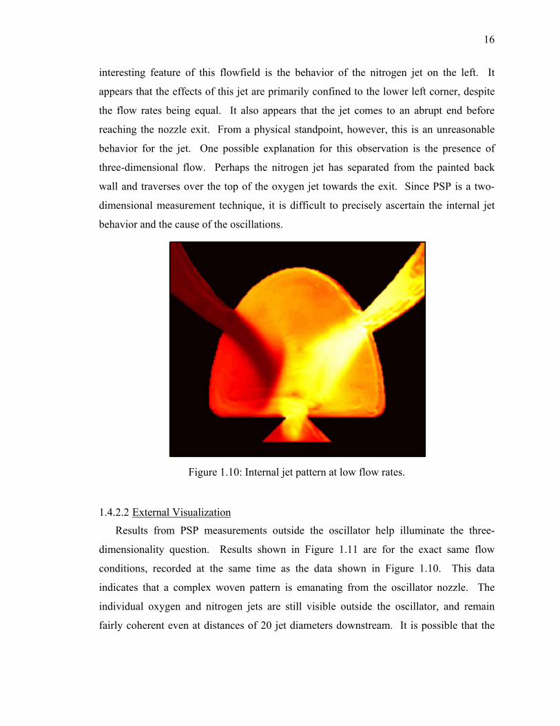
Figure 1.10: Internal jet pattern at low flow rates. ............................................................16

Figure 1.11: External flowfield at low flow rates..............................................................17

Figure 1.12: Water visualization of the fluidic oscillator at a supply pressure of 1.8 psi..................................................................................................................18

Figure 1.13: Water visualization of fluidic oscillator at low flow rates (Pwater = 0.8 psi).................................................................................................................20

Figure 2.1: Frequency spectra over a range of supply pressures.....................................22

Figure 2.2: Power spectra at three representative pressures. The three spectra correspond to vertical slices of Figure 2.1, marked by arrows. ....................23

Figure 2.3: High-frequency mode-hopping at very low supply pressures. .....................24

Figure 2.4: Oscillator geometry for scaling studies.........................................................26

Figure 2.5: Frequency map for the response of design three. .........................................27

Figure 2.6: Low flow rate frequency map for design three.............................................27

xii

Figure Page

Figure 2.7: Frequency response of the primary oscillation frequency for design three...............................................................................................................29

Figure 2.8: Frequency response of all five scaled designs. .............................................29

Figure 2.9: Reduced frequency response of all five scaled designs. ...............................30

Figure 2.10: Effect of aspect ratio on the oscillation frequency........................................31

Figure 2.11: Effect of aspect ratio on reduced frequency. ................................................32

Figure 2.12: Oscillator geometries for inlet variation study: (a) concave, (b) straight, (c) convex......................................................................................................34

Figure 2.13: Effect of inlet geometry on the frequency response of design three.............35

Figure 2.14: Effect of inlet geometry on the reduced frequency response of design three...............................................................................................................35

Figure 2.15: Frequency response of design three to air and argon gases. .........................36

Figure 2.16: Reduced frequency response of design three to air and argon gases. ...........36

Figure 2.17: Response of the fluidic oscillator to unequal flow rates on the inlets. .........37

Figure 3.1: Experimental setup for the pressure-sensitive paint measurements. ............41

Figure 3.2: Water visualization of micro fluidic oscillator flowfield, (a) instantaneous (1/60 s with flash), and (b) time-averaged (1/2 s, no flash). ..43

Figure 3.3: Frequency and flow rate evaluation, oscillator operating with air................44

Figure 3.4: Frequency response of the fluidic oscillator supplied with air. ....................46

Figure 3.5: Power spectrum of Kulite signal, 9.4 kHz oscillations. ................................48

Figure 3.6: Phase-averaged pressure-sensitive paint data for the micro fluidic oscillator with nitrogen gas at 9.4 kHz, flow rate of 554 mL/min (~0.67 g/min), supply pressure of 6.69 kPa, and 20-μs delay step. ........................49

Figure 3.7: Cross-sectional data taken from the PSP results at 9.4 kHz, at a location 500 μm downstream of the nozzle exit. ........................................................50

Figure 3.8: RMS Intensity plot from the phase-averaged time history at 9.4 kHz..........50

Figure 3.9: Power spectrum of Kulite signal, 21.0 kHz oscillations...............................52

Figure 3.10: Phase-averaged pressure-sensitive paint data for the micro fluidic oscillator with nitrogen gas at 21.0 kHz, flow rate of 1168 mL/min (~1.91 g/min), supply pressure of 44.47 kPa, and 18-μs delay step. ............53

Figure 3.11: Cross-sectional data taken from the PSP results at 21.0 kHz, at a location 500 μm downstream of the nozzle exit. ..........................................54

Figure 3.12: RMS Intensity plot from the phase-averaged time history at 21.0 kHz........54

xiii

Figure Page

Figure 4.1: Experimental setup for characterization of the pulsed-fluidic oscillator. .....57

Figure 4.2: Variation of carrier frequency from 10 Hz to 200 Hz, with a constant high-frequency of 3 kHz and a supply pressure of 6 kPa. ............................59

Figure 4.3: Zoomed-in portion of Figure 4.2. .................................................................59

Figure 4.4: Power spectra of the time histories shown in Figure 4.2. .............................60

Figure 4.5: Input pressure variation, measured by a Kulite pressure transducer between the solenoid valve and the fluidic oscillator, with a constant carrier frequency at 50 Hz.............................................................................61

Figure 4.6: Response of the dual-frequency actuator to changes in pressure, with a constant carrier frequency of 50 Hz..............................................................61

Figure 4.7: Zoomed-in portion of Figure 4.6. The high-frequency component increases in frequency and amplitude as the pressure is increased...............62

Figure 4.8: Power spectra of the time histories shown in Figure 4.6. .............................62

Figure 4.9: Input duty-cycle variation, measured by a Kulite pressure transducer between the solenoid valve and the fluidic oscillator. ..................................63

Figure 4.10: Response of the actuator to variation in duty cycle. Pressure remains constant and the carrier frequency remains constant at 25 Hz......................64

Figure 4.11: Zoomed-in portion of Figure 4.10. ...............................................................64

Figure 4.12: Power spectra of the time histories in Figure 4.10........................................65

Figure 5.1: The principle of wall attachment in a fluidic device, known as the Coanda Effect................................................................................................68

Figure 5.2: Scale diagram of the first design. The piezoelectric bender is positioned in the diffuser, pointing upstream into the flow............................................71

Figure 5.3: Photograph of the first design, with the piezo device removed for clarity. ..71

Figure 5.4: Scale diagram of the second design. The bender is oriented with the tip pointing downstream from the throat............................................................72

Figure 5.5: Photograph of the second design, with the piezo bender installed. ..............72

Figure 5.6: Experimental setup for the pressure-sensitive paint and hot film probe instrumentation. ............................................................................................74

Figure 5.7: Schlieren images of the bi-stable operation of the oscillator, with hydrogen gas used for visualization..............................................................75

Figure 5.8: Series of PSP images with successive delays of 1 ms at an oscillation frequency of 50 Hz. Flow is from left-to-right, and the piezo bender is on the right. ...................................................................................................77

xiv

Figure Page

Figure 5.9: Time history of the oscillator outputs simultaneously measured by hot film probes. (a) 10 Hz, (b) 200 Hz. Pressure ratio is 1.69. .........................78

Figure 5.10: Step response of the piezo-fluidic oscillator.................................................79

Figure 5.11: High frequency oscillations at 1.0 kHz and a pressure ratio of 1.14. ...........81

Figure 5.12: Response of the piezo-fluidic oscillator at sonic nozzle conditions. The pressure ratio is 2.15 and the oscillation frequency is 5 Hz..........................81

Figure 5.13: Frequency maps of the piezo-fluidic oscillator performance at a supply pressure ratio of 1.14.....................................................................................82

Figure 5.14: (a) Magnitude and (b) phase plots of the piezo-fluidic oscillator response with the bender facing upstream. ..................................................................84

Figure 5.15: (a) Magnitude and (b) phase plots of the piezo-fluidic oscillator response with the bender facing downstream (with the flow). ....................................85

Figure 6.1: Geometry of actuator 1, a wide-angle fluidic oscillator. ..............................89

Figure 6.2: Geometry of actuator 2, a narrow-angle fluidic oscillator. ...........................89

Figure 6.3: Geometry of actuator 3, a converging nozzle for steady blowing. ...............89

Figure 6.4: Jet-cavity facility at the Illinois Institute of Technology. .............................90

Figure 6.5: Suppression results for Actuator 1 (wide fan angle) at Mach 0.5.................94



Figure 6.8: Suppression results for Actuator 2 (narrow fan angle) at Mach 0.5. ............95

Figure 6.9: Suppression results for Actuator 2 (narrow fan angle) at Mach 0.7. ............96

Figure 6.10: Suppression results for Actuator 3 (steady blowing) at Mach 0.5. ...............96

Figure 6.11: Suppression results for Actuator 3 (steady blowing) at Mach 0.7. ...............97

Figure 7.1: Diagram of modeled PSP geometry............................................................106

Figure 7.2: Gas diffusion (a) into and (b) out of the paint layer. ..................................108

Figure 7.3: Typical calibration curves for various pressure-sensitive paint formulations. ...............................................................................................110

Figure 7.4: PSP calibration data plotted to show the nonlinear Stern-Volmer intensity response........................................................................................110

Figure 7.5: Integrated intensity response to step-changes in pressure, compared to oxygen concentration; A=0.9, B=0.1, γ=1.0. ..............................................112

Figure 7.6: PSP indicated pressure step-response, variation from atmosphere to vacuum; A=0.9, B=0.1, γ=1.0....................................................................114

xv

Figure Page

Figure 7.7: PSP indicated pressure step-response, variation with γ; A=0.9, B=0.1, γ=1.0 or 0.1. ................................................................................................114

Figure 7.8: PSP indicated pressure step-response, variation with pressure jump magnitude; A=0.9, B=0.1, γ=1.0, ΔP=6.9 kPa............................................115

Figure 7.9: PSP indicated pressure step-response, variation from 101 kPa to 202 kPa; A=0.9, B=0.1, γ=1.0. ..........................................................................116

Figure 7.10: Bode plots of (a) magnitude and (b) phase for the frequency response of Fast FIB PSP. ..............................................................................................119

Figure 7.11: Bode plots of (a) magnitude and (b) phase for the frequency response of Polymer/Ceramic PSP.................................................................................120

Figure 7.12: Hot-film probe characterization of fluidic oscillator flow with various gases............................................................................................................124

Figure 7.13: Experimental setup for fluidic oscillator dynamic calibrations. .................125

Figure 7.14: Polymer/ceramic PSP response to the argon jet at a) 0 μs and b) 314 μs (180° delay), at an oscillation frequency of 1.59 kHz. ...............................128

Figure 7.15: Polymer/ceramic PSP response to the oxygen jet at a) 0 μs and b) 314 μs (180° delay), at an oscillation frequency of 1.59 kHz. ...............................129

Figure 7.16: Polymer/ceramic PSP response to argon, nitrogen, and oxygen jets from the fluidic oscillator at 1.59 kHz.................................................................130

Figure 7.17: Fast FIB response to argon, nitrogen, and oxygen jets from the fluidic oscillator at 1.59 kHz. .................................................................................131

Figure 7.18: Comparison of diffusion model with experimental results for nitrogen and oxygen jets. ..........................................................................................132

Figure 8.1: Rotor-stator interaction in a turbofan engine. .............................................135

Figure 8.2: Morphology of the polymer/ceramic pressure-sensitive paint formulation..................................................................................................142

Figure 8.3: Dynamic calibration of polymer/ceramic pressure-sensitive paint with a fluidic oscillator. .........................................................................................144

Figure 8.4: Typical calibration of polymer/ceramic pressure-sensitive paint over a range from vacuum to two atmospheres. ....................................................145

Figure 8.5: Experimental setup for acoustic PSP measurements. .................................148

Figure 8.6: Analytical solution for the (1,1,0) mode shape in a rectangular cavity, ω = 1298 Hz. Pressure is expressed in (a) Pascals and (b) pressure ratio. 154

Figure 8.7: Pressure-sensitive paint data for the (1,1,0) mode shape at 145.4 dB and ω = 1286 Hz. Pressure is expressed in (a) Pascals and (b) pressure ratio. 156

xvi

Figure Page

Figure 8.8: Time-sequence of PSP data for the (1,1,0) mode shape in phase steps of 30° (64.8 μs) from (a) 0° to (f) 150°. ..........................................................157

Figure 8.9: A continuation of the time-sequence of PSP data for the (1,1,0) mode shape in phase steps of 30° (64.8 μs) from (a) 180° to (f) 330°. ................158

Figure 8.10: Pressure time-history comparison between pressure-sensitive paint, Kulite pressure transducer measurements, and linear theory......................159

Figure 8.11: Vertical cross-section of the pressure-sensitive paint data at x/Lx = 0 at twelve time steps equally spaced throughout the period. ...........................160

Figure 8.12: RMS pressure data (Pa) as measured by PSP for the (1,1,0) mode shape..160

Figure 8.13: Acoustic box image; no image averaging or spatial filtering. ....................162

Figure 8.14: Average of 100 speaker-on images divided by average of 100 speaker-off images, no filtering................................................................................163

Figure 8.15: 100-image average with spatial filtering using a 3-pixel radius moving window........................................................................................................164

Figure 9.1: Conceptual drawing showing the operating mechanism of the Hartmann tube (a) Filling of resonance cavity and (b) cavity discharge (after Brocher et al.151). ........................................................................................167

Figure 9.2: Schlieren image of underexpanded open jet, showing the shock-cell structure.......................................................................................................168

Figure 9.3: Photograph of two resonance cavities.........................................................170

Figure 9.4: Geometries for the (a) flat face and (b) 45° angled face resonance cavities. All dimensions are in inches, and the cavity shapes are made from 1” thick acrylic. ..................................................................................171

Figure 9.5: Diagram of experimental setup for PSP measurements..............................172

Figure 9.6: PSP image sequence depicting shock oscillation, with 10 μs time steps between each image. ...................................................................................175

Figure 9.7: PSP image sequence showing shock wave oscillation for the flat resonance cavity with 24 μs time steps.......................................................177

Figure 9.8: Schlieren image sequence showing shock wave oscillation for the flat resonance cavity with 16 μs time steps.......................................................178

Figure 9.9: PSP image sequence showing acoustic wave propagation for the flat resonance cavity with 16 μs time steps.......................................................180

Figure 9.10: Schlieren image sequence showing acoustic wave propagation for the flat resonance cavity with 16 μs time steps. ...............................................181

xvii

Figure Page

Figure 9.11: Reconstructed time history from phase-averaged PSP data for the flat resonance cavity..........................................................................................183

Figure 9.12: RMS pressure levels (psi) in the near field of the shock oscillation for the flat resonance cavity..............................................................................184

Figure 9.13: Sound pressure levels (dB, ref. 20 μPa) for the flat resonance cavity. .......184

Figure 9.14: PSP image sequence showing shock wave oscillation for the angled resonance cavity with 20 μs time steps.......................................................187

Figure 9.15: Schlieren image sequence showing shock wave oscillation for the angled resonance cavity with 16 μs time steps.......................................................188

Figure 9.16: PSP image sequence showing acoustic wave propagation for the angled resonance cavity with 12 μs time steps.......................................................189

Figure 9.17: Schlieren image sequence showing acoustic wave propagation for the angled resonance cavity with 16 μs time steps. ..........................................190

Figure 9.18: RMS pressure values (psi) in the near field of the shock oscillation for the angled resonance cavity. .......................................................................191

Figure 9.19: Sound-pressure levels (dB, ref. 20 μPa) for the angled resonance cavity. .192

Appendix Figure

Figure A.1: Typical example of a laser-induced thermal tuft, indicating flow from left to right. .................................................................................................214

Figure A.2: Diagram of the thermal tuft concept. ..........................................................215

Figure A.3: Diagram of the thermal tuft experimental setup. ........................................217

Figure A.4: Images of thermal tufts generated with various insulating substrate layers...........................................................................................................221

Figure A.5: Definition of length (l) and width (w) dimensions on a thermal tuft. .........222

Figure A.6: Response of tuft geometry to variation in Reynolds number. Velocity varies from 10 to 60 m/s and laser power is 277 mW. ...............................224

Figure A.7: Response of tuft geometry to variation in laser power. Velocity is held constant at 4.9 m/s. .....................................................................................225

Figure A.8: Thermal tuft at zero flow velocity, demonstrating the effect of natural convection...................................................................................................226

Figure A.9: Thermal tuft at a flow reattachment point, indicating flow in opposite directions.....................................................................................................227

Figure A.10: Numerical simulation of a thermal tuft with thermochromic liquid crystals and a balsa wood substrate with flow from left to right. ...............229

Figure A.11: Temperature-sensitive paint results. ...........................................................230

xviii

Appendix Figure Page

Figure A.12: Thermally ablative tufts with temperature-sensitive paint with impinging flow from left to right. ................................................................................232

Figure B.1: Unfiltered PSP data from the high-speed camera.......................................234

Figure B.2: Filtered PSP data from the high-speed camera, with a disk radius of 5 pixels...........................................................................................................235

Figure B.3: Variation in the camera gain.......................................................................235

Figure B.4: Time sequence of PSP data at 125 μs intervals. .........................................236

xix

ABSTRACT

Gregory, James Winborn. Ph.D., Purdue University, August, 2005. Development of Fluidic Oscillators as Flow Control Actuators. Major Professor: John P. Sullivan.

This work is comprised of two key accomplishments: the study and design of fluidic

oscillators for flow control applications, and the development and application of porous

pressure-sensitive paint (PSP) for unsteady flowfields. PSP development was a necessary

prerequisite for characterizing the unsteady fluid dynamics of the fluidic oscillators.

Development work on the fluidic oscillator commences with a study on the internal fluid

dynamics of the feedback-free class of oscillators. This study demonstrates that the

collision of two jets within a mixing chamber forms an oscillating shear layer driven by

counter-rotating vortices. A micro-scale version of this type of oscillator is also

characterized with PSP measurements and frequency surveys. Subsequently, this high-

frequency oscillator (~ 5 kHz) is coupled with a low-frequency solenoid valve to create

dual-frequency injection that is useful in flow control applications. A new hybrid

actuator is developed that merges piezoelectric and fluidic technology. This piezo-fluidic

oscillator successfully decouples the oscillation frequency from the supply pressure,

thereby enabling closed-loop flow control actuation. Fluidic oscillators are then applied

to a practical flow control application for cavity tone suppression. The fluidic oscillators

are able to suppress the tone by 17.0 dB, while steady blowing at the same mass flow rate

offers only 1.6-dB suppression. Work with pressure-sensitive paint involved

development of a model for the quenching kinetics of the paint. Two fast-responding

paint formulations, Polymer/ceramic and Fast FIB, are evaluated experimentally and

compared to the model predictions. Both the model and experiments demonstrate that a

paint layer will respond faster to a decrease in pressure than an increase of the same

magnitude, and that the polymer/ceramic paint has a flat frequency response of at least

xx

1.59 kHz. Furthermore, the excellent response characteristics of porous PSP are

highlighted by applying the paint to various flowfields. The polymer/ceramic

formulation is used to record the 12-kHz oscillating shock wave and propagating acoustic

waves generated by a Hartmann oscillator. Polymer/ceramic PSP is also used to measure

the acoustic mode shapes in a rectangular resonance cavity driven by a speaker at 145 dB.

These results compare favorably to the analytical solution for the same geometry.

1

INTRODUCTION

Flow control actuators are devices that are used to enact large-scale changes in a

flowfield with a relatively small control input. Often these changes are focused on

improving the performance of a flight vehicle – by delaying stall, reducing drag,

enhancing lift, abating noise, reducing emissions, etc. In many flow control situations,

unsteady actuation is required for optimal performance. Unsteady actuators are

particularly beneficial in closed-loop control applications when the unsteady actuation

can be controlled. If the unsteady actuation is synchronized with the characteristic time

scales of the flowfield, then the actuator power requirements can often be minimized.

Common flow control actuators include synthetic jets,1 piezoelectric benders,2,3 powered

resonance tubes (also known as Hartmann whistles),4-6 plasma actuators,7-11 pulsed jets,12-

14 and steady blowing15 or suction.16 These devices and concepts all have inherent

strengths and some limitations. Thus, the selection of a flow control actuator often is

driven by the requirements of the application. A new class of flow control actuators is

introduced in this work – the fluidic oscillator. This particular type of actuator has the

advantages of high frequency bandwidth, low mass flow requirements, and simplicity.

The fluidic oscillator is a fascinating device that produces an oscillating jet when

supplied with a pressurized fluid. The oscillations are typically on the order of several

kilohertz, and can range up to over 20 kHz for small devices. The internal geometry of

the device may be tailored to produce specific jet wave patterns, such as sinusoidal,

sawtooth, or even square waveforms.17 Fluidic oscillators were originally developed in

the 1960’s, evolving out of research in fluid amplifiers. The fluidic oscillator has its

roots based in the field of fluid logic, as detailed by Morris,18 and Kirshner and Katz.19 A

comprehensive overview of the fluid amplifier technology and an extensive bibliography

may be found in the NASA contractor reports edited by Raber and Shinn.20,21 The fluidic

2

principles were first applied by Spyropoulos22 to create a self-oscillating fluidic device,

and later refined by Viets.23 Perhaps the single-largest application of fluidic oscillator

technology is for windshield washer devices,24 with over 45 million produced annually.25

Since the operating frequency of the oscillator is directly related to the flow rate, fluidic

oscillators have also been used extensively as flow-rate metering devices.26-28 In recent

years, the fluidic oscillator has been applied to a range of aerodynamic flow control

applications.

The fluidic oscillator represents a useful device for flow control applications because

of its variable frequency, the unsteady nature of the oscillating jet, the wide range of

dynamic pressures possible, and the simplicity of its design. A very attractive feature of

fluidic oscillators is that they have no moving parts – the simple design of the fluidic

oscillator produces an oscillating jet based solely on fluid-dynamic interactions. Flow

control applications of the fluidic oscillator have included cavity resonance tone

suppression,17,29 enhancement of jet mixing,30-32 and jet thrust vectoring.33

Fluidic oscillators may be classified into two different groups – wall attachment

devices and jet interaction devices. The oscillators in the wall-attachment class are based

on the attachment of a fluid jet to an adjacent wall, a phenomenon known as the Coanda

effect.34,35 The second class of oscillators is fairly new, and based on the interaction of

two fluid jets inside a specially-designed chamber. This oscillator has been described as

a ‘feedback-free’ type, details of which are described in Raghu’s patent.36

There has been some level of prior work directed towards characterizing the flow of

fluidic oscillators, including miniature fluidic oscillators. Raman et al.37 and Raghu et

al.17 have characterized these devices to evaluate their utility for flow control

applications. Sakaue et al.38 and Gregory et al.39-41 have used pressure-sensitive paint to

characterize the flow of miniature fluidic oscillators.

The first part of this work involves the development and application of fluidic

oscillators for flow control problems. The feedback-free class of fluidic oscillators is still

relatively new and not completely understood. Thus, the first three chapters are devoted

to characterizing this style of oscillator and understanding the operating fluid dynamics.

Flow visualization techniques such as schlieren imaging, pressure-sensitive paint, and

3

water visualization are used to study the fluid dynamics of the device. Frequency studies

are presented in the next chapter, with the aim of understanding geometrical effects on

the fluidic response of the oscillator. In the third chapter, micro fluidic oscillators based

on the feedback-free design are evaluated for their potential as flow control actuators.

These devices have the advantages of low flow rate requirements, high frequency, and

small size.

Flow control applications often require dual time scales within the actuation signal.

Fluidic oscillators can provide the high-frequency content for mixing, while low-

frequency content can provide high-momentum pulsing. The combination of a fluidic

oscillator with a fast-acting solenoid valve is evaluated as an actuator for flow control

applications in chapter four. One significant limitation of conventional fluidic oscillators

is that the oscillation frequency is coupled to the supply pressure. In flow control

applications, the ideal actuator would have a frequency that could be specified

independently of pressure. Thus, a new fluidic oscillator design is presented, where the

oscillator output is modulated by piezoelectric devices. Chapter five details the

development of the piezo-fluidic actuator, and characterizes the frequency response

limitations of the device. The conclusion of the fluidic oscillator development involves

the demonstration of miniature fluidic oscillators for a practical flow control application.

Here, the fluidic oscillator is applied as a flow control actuator for cavity tone

suppression. The goal of this application is to demonstrate enhanced suppression with a

fluidic oscillator, relative to steady blowing at the same mass flow rate.

Throughout the work of this dissertation, pressure-sensitive paint (PSP) has been used

extensively as an advanced measurement technique. The PSP technique is an essential

technology for characterizing the unsteady fluid dynamics of the fluidic oscillator. State-

of-the-art PSP technology, however, has been limited to steady-state measurements.

Thus, the second part of this dissertation focuses on the development of pressure-

sensitive paint for unsteady applications such as the fluidic oscillator. PSP measures

surface pressure distributions through the processes of luminescence and oxygen

quenching. Typically, PSP is illuminated with an excitation light, which causes

luminophore molecules in the paint to luminesce. In the presence of oxygen in a test gas,

4

the luminescent intensity of the luminophore is reduced by oxygen molecules from the

gas through the process of oxygen quenching. Since the amount of oxygen in air is

proportional to pressure, one can obtain static pressure levels from the change in the

luminescent intensity of PSP, with intensity being inversely proportional to pressure.

Pressure-sensitive paint was initially proposed as a qualitative flow-visualization tool,42

and was subsequently developed as a quantitative technique.43 The accuracy and utility

of PSP has improved such that the technique provides results that rival data obtained

from conventional pressure instrumentation. Comprehensive reviews of the PSP

technique have been published by Bell et al,44 Liu et al,45 and Liu and Sullivan.46

PSP formulations traditionally used for conventional testing typically include a

polymer binder. Conventional polymer-based PSPs are limited in response time,

however. The slow response time characteristic of conventional PSP makes it a limited

tool in the measurement of unsteady flow fields. Therefore, a fast responding paint, such

as porous PSP, is needed for application to unsteady flow.

Porous PSP uses an open, porous matrix as a PSP binder, which improves the oxygen

diffusion process. For conventional PSP, oxygen molecules in a test gas need to

permeate into the binder layer for oxygen quenching. The process of oxygen permeation

in a polymer binder layer produces slow response times for conventional PSP. On the

other hand, the luminophore in porous PSP is opened to the test gas so that the oxygen

molecules are free to interact with the luminophore. The open binder creates a PSP that

responds much more quickly to changes in oxygen concentration, and thus pressure.

There are three main types of porous pressure-sensitive paints currently in use,

depending on the type of binder used. Anodized aluminum PSP (AA-PSP)47-52 uses

anodized aluminum as a porous PSP binder. Thin-layer chromatography PSP (TLC-PSP)

uses a commercial porous silica thin-layer chromatography (TLC) plate as the binder.53

Polymer/ceramic PSP (PC-PSP) uses a porous binder containing hard ceramic particles in

a small amount of polymer.41,54,55 For each of these porous surfaces, the luminophore is

applied directly by dipping or spraying.

Before using pressure-sensitive paint to characterize the unsteady flow field of the

fluidic oscillator, it is important to evaluate the unsteady response of the paint. Previous

5

work by Gregory et al.39-41 demonstrates that porous PSP has a flat frequency response in

excess of 40 kHz. Asai et al.56 have done tests with a shock tube and have shown

response times on the order of 500 kHz with porous PSP.

In chapter seven, the dynamic quenching kinetics of pressure-sensitive paint are

evaluated. Some researchers have observed differences in response characteristics,

depending on the magnitude and direction of the pressure change. This work investigates

this behavior through analytical modeling and experiments. In the subsequent chapter,

pressure-sensitive paint is presented as a tool for acoustic measurements. Here the PSP

was used to resolve acoustic-level pressure fluctuations in a resonance cavity. In the final

chapter, the unsteady flowfield of the Hartmann tube is characterized with pressure-

sensitive paint. Both oscillating shock waves and propagating acoustic waves are

resolved by the paint.

6

PART ONE: FLUIDIC OSCILLATORS

7

CHAPTER 1: FLUID DYNAMICS OF THE FEEDBACK-FREE FLUIDIC OSCILLATOR

The fluidic oscillator evaluated in the current study is comprised of two fluid jets that

interact in an internal mixing chamber, producing the oscillating jet at the exit. The goal

of the work presented in this chapter is to characterize the internal jet mixing

characteristics through flow visualization techniques. Schlieren imaging, porous

pressure-sensitive paint (PSP), and dye-colored water flow are used to visualize the

internal and external fluid dynamics of the oscillator. Porous PSP formulations have

recently been under development for unsteady measurements, as detailed in the second

part of this dissertation. Porous pressure-sensitive paints have been shown to have

frequency responses on the order of 100 kHz, which is more than adequate for visualizing

the fluidic oscillations. In order to provide high-contrast PSP data in these tests, one of

the internal jets of the fluidic oscillator is supplied with oxygen, and the other with

nitrogen. Results indicate that two counter-rotating vortices within the mixing chamber

drive the oscillations. It is also shown that the fluidic oscillator possesses excellent

mixing characteristics.

1.1 Fluidic Oscillator Geometry

Depending on the size of the device, a fluidic oscillator can be formed into a compact

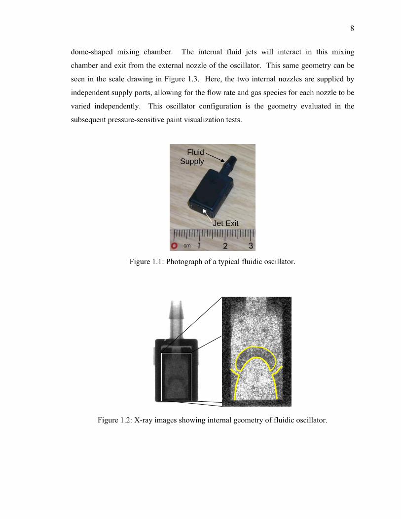
package. An external view of a typical fluidic oscillator is shown in Figure 1.1. This

oscillator is about 1-cm wide, 2-cm long, and a few millimeters thick. The pressurized

fluid supply is provided on the barbed fitting, while the oscillating jet exits from a small,

rectangular orifice measuring about 1-mm wide. The internal geometry of the device is

fairly simple, as shown in the x-ray images in Figure 1.2. These images are for the exact

same oscillator pictured in Figure 1.1. Visible inside the device are two internal orifices

which are fed by the common supply port. Fluid from the internal nozzles exits into a

8

dome-shaped mixing chamber. The internal fluid jets will interact in this mixing

chamber and exit from the external nozzle of the oscillator. This same geometry can be

seen in the scale drawing in Figure 1.3. Here, the two internal nozzles are supplied by

independent supply ports, allowing for the flow rate and gas species for each nozzle to be

varied independently. This oscillator configuration is the geometry evaluated in the

subsequent pressure-sensitive paint visualization tests.

Figure 1.1: Photograph of a typical fluidic oscillator.

Figure 1.2: X-ray images showing internal geometry of fluidic oscillator.

Fluid Supply

Jet Exit

9

Figure 1.3: Scale drawing of a typical fluidic oscillator internal geometry.

1.2 Schlieren Flow Visualization

A schlieren imaging setup was used to visualize the flowfield of the fluidic oscillator.

The experimental setup involved the use of a single-pass schlieren system. The

illumination source was a strobe light, a General Radio company model 1538-A

Strobotac. The flash rate of the strobe light was phase-locked to the fluidic oscillations

through a microphone measurement. A neutral density filter was placed in front of the

strobe light to control the light intensity passing through the flow and reaching the

camera. A 6-inch diameter front-surface concave mirror with a focal length of 5 feet was

used to pass the light through the flowfield. A knife-edge was placed at the focal point of

the mirror to improve the image contrast. The flowfield was then imaged with a digital

video camera. HFC-134a refrigerant gas was used as a supply fluid for these images,

since the high density gradient can be easily viewed with schlieren instrumentation. The

flow pattern of this particular fluidic oscillator (Figure 1.1) is shown in phase-averaged

the schlieren images in Figure 1.4. Notice that the jet varies roughly in a saw-tooth

fashion. The jet begins to thoroughly mix with the ambient fluid just a few jet diameters

downstream of the nozzle. Thus, the schlieren images reveal a flowfield rich in high-

frequency content that is beneficial for mixing.

10

(a) (b)

Figure 1.4: Schlieren images of the fluidic oscillator flowfield at (a) 0° phase and (b) 180° phase.

1.3 PSP Experimental Setup

A schematic of the instrumentation setup used for the PSP experiments is shown in

Figure 1.5. A rough outline of the geometry of the patented oscillator36 is shown in the

figure. The paint was applied to the inside back wall of the fluidic oscillator, and a clear

acrylic cover was mounted on the other side for optical access. The particular PSP

formulation used in these experiments was polymer/ceramic PSP (PC-PSP). The

polymer/ceramic paint is a hybrid development – it is highly porous because of the

ceramic particles, with only a small amount of polymer used to bind the paint together.

Details of the polymer/ceramic paint development are available from Scroggin, et al.54

and Gregory.41

11

Figure 1.5: Experimental setup for the pressure-sensitive paint measurements.

Nitrogen gas was supplied to the left input, and oxygen gas to the right. The flow

rates of each gas were measured with FT-133 calibrated flow rate tubes from Dwyer

Instruments, and the pressures were measured with a Heise DXD pressure transducer. A

Kulite pressure transducer (XCQ-062-15D) was mounted near the nozzle exit of the

fluidic oscillator to record the operating frequency. The frequency bandwidth of the

Kulite transducer and its signal conditioner is well over 100 kHz. The Kulite signal was

passed through analog high-pass and low-pass filters before being measured on a

Tektronix 466 analog oscilloscope and an Ono-Sokki CF-4220 personal FFT analyzer.

PSP measurements were made with a Photometrics 14-bit CCD camera and an ISSI LM2

pulsed LED array for illumination. A camera shutter speed of 0.7 s (typical) was

required to fill the pixel wells to near-capacity for best results. Since the flowfield is

unsteady, phase-locking techniques were required to record time-resolved PSP data. The

pulsing of the LED array was synchronized with the oscillations measured by the Kulite

pressure transducer through the gating function on a triggered oscilloscope. A variable

delay was added to the oscilloscope’s TTL pulse with a Berkeley Nucleonics BNC-555

12

pulse/delay generator. Phase-locked time histories were recorded by varying the delay

throughout the oscillation cycle. Thus, this system makes phase-averaged measurements

of the unsteady flowfield. The excitation pulse width was typically 2.5% of the

oscillation period, and each delay step was 5% of the period.

Once raw intensity images of the painted oscillator were acquired with the CCD

camera, the data was reduced to provide gas concentration results. An intensity ratio was

calculated by dividing the wind on image by a reference image, and then smoothed with a

3-pixel-square spatial filter. The intensity ratio was then converted to oxygen

concentration through a Stern-Volmer calibration. The calibration for these tests was

performed from pure oxygen at 1 atm, down to vacuum (simulating pure nitrogen at 1

atm). Once the oxygen concentration was obtained, the data was normalized between 0

(pure nitrogen) and 1 (pure oxygen). The PSP data presented in this chapter represents

gas concentration only, since current paint technology is unable to simultaneously

measure pressure and gas concentration. Any effects of pressure are neglected, since the

supply pressures are small and typically equal on both inlets.

1.4 Pressure-Sensitive Paint Visualization

1.4.1 High Flow Rates

1.4.1.1 Equal Supply Pressures

PSP visualization data in Figure 1.6 shows the internal fluid dynamics of the

oscillator at moderate flow rates and an oscillation frequency of 2.5 kHz. Each image

represents a successive phase delay of 90° within the oscillation cycle of 400 μs.

Nitrogen is the gas on the left, and oxygen is the gas on the right, with equal supply

pressures (0.34 psig). The color scale represents oxygen concentration: pure oxygen is 1,

pure nitrogen is 0, and 0.21 is atmosphere. The color scale for the flowfield data outside

the oscillator (the lower half of each image) has been adjusted to enhance contrast. The

contrast-adjusted color scale ranges from 0.2 to 0.5. An enlarged view of the internal jet

interaction is shown in Figure 1.7.

13

Notice that the jets collide near the center of the mixing chamber, but the interface

between the two jets is not stationary. The shear layer between the two jets oscillates at

the same frequency as the external jet produced by the device. In general, the amplitude

of this interface motion is larger for higher supply pressures. The shape of the shear layer

also changes as the jets oscillate. When the shear layer moves towards the left it exhibits

rightward-facing concave curvature. When the shear layer moves to the right, the

curvature is concave left. The shape of the internal mixing chamber controls the

formation and oscillatory growth of counter-rotating vortex pairs, which drive the shear-

layer oscillations.

Figure 1.6: Visualization of jet mixing at several time steps within the 400-μs period.

Figure 1.7: Internal fluid dynamics of the fluidic oscillator.

14

The jet issuing from the nozzle is fairly well mixed, because the jet interface is

directly in line with the exit. This characteristic highlights the utility of the fluidic

oscillator for fluid mixing applications. The mixing characteristics are clearly seen in

Figure 1.8. The lower portion of Figure 1.8 (a) shows the same external flowfield as

Figure 1.6, but not adjusted for contrast. In a short distance downstream of the nozzle

exit, the jet is very well mixed. The curves shown in Figure 1.8 (b) are cross-sections

taken one jet diameter downstream of the nozzle exit. Each curve represents a different

time step, as shown in the legend. The movement of the peak correlates with the external

jet oscillations shown in Figure 1.6. The evolution of the jet magnitude in time is not yet

symmetric because the output contains disproportionate levels of oxygen and nitrogen at

various points in the cycle. The excellent mixing characteristics of the oscillator are

evidenced by the 10% variation in oxygen concentration. Thus, the original nitrogen and

oxygen jets have achieved 90% mixing at a distance of one jet diameter downstream of

the nozzle. Note that the values at the edge of the jet cross-section in Figure 1.8 (a) are

0.21, corresponding to atmospheric conditions.

(a) (b)

Figure 1.8: (a) Visualization of jet mixing with equal supply pressures. (b) Cross-sections of the data along a line one jet-diameter downstream of the exit.

15

1.4.1.2 Unequal Supply Pressures

Data from a test with asymmetric flow rates is shown in Figure 1.9, with oscillations

at 5.25 kHz. In this case, the supply pressure for the oxygen (right side, 3.8 psig) was

slightly higher than the nitrogen supply pressure (left side, 3.6 psig). The asymmetry in

the flowfield is clearly evident. The oxygen jet is dominant throughout the oscillation

cycle, both inside and outside the mixing chamber, yet it is remarkable that the device is

still oscillating. The shear layer created by the confluence of the two jets is slanted

towards the incident angle of the oxygen jet. With the higher supply pressures, there is a

corresponding larger range of motion of the jets and shear layer within the mixing

chamber. There is also a wider oscillation spread of the external flowfield.

Figure 1.9: Visualization of jet mixing for unequal flow inputs at 5.25 kHz. Left inlet: nitrogen at 3.61 psig. Right inlet: oxygen at 3.81 psig.

1.4.2 Low Flow Rates

1.4.2.1 Internal Visualization

PSP measurements were made at very low flow rates as well, where markedly

different oscillatory behavior was observed. The flow rate on each inlet was 540 ± 5

mL/min, with a supply pressure of 0.103 ± 0.003 psig, yielding an oscillation frequency

of 7.8 kHz. One phase-locked PSP image is shown in Figure 1.10. At this flow rate there

were no discernable oscillations on the inside of the oscillator, despite the measurement

of oscillations in the external flowfield by the Kulite pressure transducer. One very

16

interesting feature of this flowfield is the behavior of the nitrogen jet on the left. It

appears that the effects of this jet are primarily confined to the lower left corner, despite

the flow rates being equal. It also appears that the jet comes to an abrupt end before

reaching the nozzle exit. From a physical standpoint, however, this is an unreasonable

behavior for the jet. One possible explanation for this observation is the presence of

three-dimensional flow. Perhaps the nitrogen jet has separated from the painted back

wall and traverses over the top of the oxygen jet towards the exit. Since PSP is a two-

dimensional measurement technique, it is difficult to precisely ascertain the internal jet

behavior and the cause of the oscillations.

Figure 1.10: Internal jet pattern at low flow rates.

1.4.2.2 External Visualization

Results from PSP measurements outside the oscillator help illuminate the three-

dimensionality question. Results shown in Figure 1.11 are for the exact same flow

conditions, recorded at the same time as the data shown in Figure 1.10. This data

indicates that a complex woven pattern is emanating from the oscillator nozzle. The

individual oxygen and nitrogen jets are still visible outside the oscillator, and remain

fairly coherent even at distances of 20 jet diameters downstream. It is possible that the

17

oscillator output is a highly three-dimensional weave of the two laminar jets, with very

little mixing. Data animations of the results in Figure 1.11 suggest that there are periodic

oscillations of this woven pattern. Despite being limited to a two-dimensional

representation, the PSP data implies that the woven structure has rotated 90° to the left,

around a vertical axis. Obviously, more detailed measurements with a three-dimensional

flow visualization technique are needed. Questions requiring conclusive answers are

whether the flow field is indeed three-dimensional, and if so, how this complex pattern is

generated.

(a)

(b)

Figure 1.11: External flowfield at low flow rates.

18

1.5 Water Visualization

1.5.1 High Flow Rates

The fluidic oscillator was also operated with water as the supply fluid for simple flow

visualization studies, and to validate the PSP measurements. Both clear water and dyed

water were used in these tests. Since the density of water is much higher than either

nitrogen or oxygen, the oscillation frequency is much lower for a given supply pressure.

Thus, it is possible to capture one instant in the oscillations with flash photography or

with a fast shutter speed on an SLR camera. Typical results with clear water (a) and

colored water (b) are shown in Figure 1.12. Both images clearly show the sinusoidal

waveform that is generated by the fluidic oscillator at a water supply pressure of 1.8 psig.

The colored water was supplied with pure red dye on the left input and pure blue dye on

the right input. Bubbles are visible in each of the lower corners of the oscillator mixing

chamber. These bubbles were observed to rotate in circles, coincident with the expected

vortical motion. Notice that the color of the fluid exiting from the oscillator just a few jet

diameters downstream from the nozzle is very homogeneous. This indicates that the red

and blue jets are mixed together thoroughly by the oscillator.

(a)

(b)

Figure 1.12: Water visualization of the fluidic oscillator at a supply pressure of 1.8 psi.

19

1.5.2 Low Flow Rates

Water flow visualization results were also obtained at low flow rates, as shown in

Figure 1.13. Clearly, the flow is not oscillating, but a long continuous stream of fluid

issues from the oscillator nozzle. Despite the lack of oscillations, the flowfield does

exhibit three-dimensional characteristics. Both images demonstrate a twisted pattern that

is somewhat similar to the woven structure seen in Figure 1.11. In particular, the colored

dye seen in Figure 1.13 (b) shows that the two jets are mixing very little. The red and

blue streams of fluid remain distinct and separate far downstream of the nozzle. The

twisting pattern is peculiar because the pair twists 90° to the left, and then 90° back to the

right, along a vertical axis. This behavior is in contrast to a continual twist about the

longitudinal axis. The direction of the 90° twist agrees with the behavior suggested by

the PSP results in Figure 1.13 (b). This twisting behavior may be thought of as axis-

switching of a rectangular jet. The major axis switches orientations with the minor axis

some distance downstream from the nozzle exit. The results shown in Figure 1.13 (b)

show the axis switching at least eight times. Axis switching of jets has been thoroughly

studied in previous work, and is summarized by Gutmark and Grinstein.57 In their review

paper, Gutmark and Grinstein even discuss jet bifurcation as a result of axis switching.

These concepts of axis switching and jet bifurcation are a plausible explanation for the

intriguing results observed at low flow rates. Further studies are needed to determine the

effects of the internal geometry on the axis switching behavior. Furthermore, three-

dimensional measurement techniques are needed to characterize the complex flow

structure at these low flow rates.

20

(a) (b)

Figure 1.13: Water visualization of fluidic oscillator at low flow rates (Pwater = 0.8 psi).

1.6 Summary

Schlieren imaging, pressure-sensitive paint, and dyed water have been used for flow

visualization studies with the fluidic oscillator. These techniques have been used to

visualize the internal fluid dynamics, as well as the external flow field of the oscillator.

This patented feedback-free device oscillates via the interaction of confluent jets in a

mixing chamber. Pairs of counter-rotating vortices within the mixing chamber drive the

oscillation of the shear layer, resulting in an external oscillatory flowfield. The fluidic

oscillator also exhibits excellent mixing characteristics. PSP data shows that the jets are

90% mixed at a distance only one jet-diameter downstream of the oscillator exit.

21

CHAPTER 2: FREQUENCY STUDIES AND SCALING EFFECTS

The oscillation frequency of the fluidic oscillator varies with the flow rate through the

device. The work presented in this chapter focuses on understanding the relationship

between the oscillation frequency and the flow rate. This information, coupled with the

flow visualization data in chapter one, will provide a detailed description of how the

oscillator functions. This work also provides a database of information available for

future design of the oscillators for specific applications. The frequency response

characteristics are recorded for the exact same oscillator used for the visualization

experiments presented in chapter one (Figure 1.3). The intriguing behavior at low flow

rates is investigated in more detail with frequency studies. Scaling effects of the fluidic

oscillator are studied next, with oscillators spanning a range in sizes of over one order of

magnitude. Aspect ratio effects are also evaluated to determine the optimum depth of the

oscillator. The effects of various inlet geometry shapes are evaluated, and their effects on

the oscillatory behavior are recorded. Variation in the test gas is studied by tests of the

oscillator supplied with air, argon, and hydrogen. Finally, the effect of unequal flow rates

on the oscillation frequency is evaluated as a companion study to the flow visualization

presented in Figure 1.9.

2.1 Experimental Setup and Data Reduction

In these tests the fluidic oscillator was instrumented with a Kulite pressure transducer

to record the oscillation frequency. Pressure transducers and rotameters were placed on

the supply line to measure the supply pressure and volume flow rate, allowing

determination of the mass flow rate. The experimental setup for these tests is virtually

the same as that shown in Figure 1.5, but without the paint sample present.

22

2.2 Fluidic Oscillator Operating Map

Power spectra of the signal from the Kulite pressure transducer provide detailed

information about the flow at each operating pressure. The operating map represented in

Figure 2.1 is a composite of power spectra across the range of operating pressures when

the oscillator (Figure 1.3) is supplied with oxygen gas. The power spectra are generated

from the Kulite signal, which was sampled at 100 kHz, with 50 kHz low-pass and 100 Hz

high-pass analog filtering. Each vertical slice of the figure represents an individual

power spectrum at a specific operating pressure. The three arrows at the top of Figure 2.1

indicate the locations of the three power spectra shown in Figure 2.2.

Figure 2.1: Frequency spectra over a range of supply pressures.

There are several interesting features about the operating map shown in Figure 2.1.

First, the primary operating frequency is clearly visible as the dark red streak, beginning

at 1.5 kHz at low pressures, and increasing to just under 5 kHz at high pressures. As the

frequency of this primary peak increases at higher pressures, the magnitude and width of

23

the peak increase as well. The second and third harmonics are also visible in the

operating map, and at higher pressures, a second trio of harmonics are visible between 30

and 40 kHz.

Figure 2.2: Power spectra at three representative pressures. The three spectra correspond to vertical slices of Figure 2.1, marked by arrows.

At very low supply pressures (up to 0.2 psig), there are some very intriguing results.

These are highlighted in the enlarged portion of the operating map shown in Figure 2.3.

This figure simply represents the lower-left region of Figure 2.1. Before the inception of

the 1.5 kHz oscillations at about 0.205 psig, there are oscillations at very low flow rates

and very high frequencies. Oscillations begin at 0.122 psig, with a frequency of

approximately 10 kHz. As the pressure increases, the frequency also increases rapidly,

while a secondary peak develops at 7.5 kHz. At a pressure of 0.136 psig, the 10 kHz

peak completely vanishes, and the 7.5 kHz peak is dominant. Subsequently, at 0.141 psig

a new peak appears at 9.7 kHz, and the 7.5 kHz rapidly evanesces. The frequency of the

new 10 kHz peak rapidly increases with supply pressure, until 0.159 psig. At this point,

the slope of the curve decreases slightly, and broadband noise is incipient. Shortly

thereafter, the 1.5 kHz primary peak develops and the 10 kHz peak eventually fades.

24

Figure 2.3: High-frequency mode-hopping at very low supply pressures.

There seems to be some type of mode hopping that occurs as the frequency jumps

from 10 kHz down to 7.5 kHz, back up to 10 kHz, and finally down to 1.5 kHz. This

entire process occurs within a pressure range of only 0.08 psig! This pressure range

corresponds to extremely low flow rates – from 1168 up to 1600 mL/min. The unusual

mode hopping behavior raises several interesting questions. First, is the mode-hopping

process repeatable? Multiple investigations were performed, and similar results were

obtained each time. Second, it is possible that this behavior is due to disturbances from

the pressure regulator. To investigate this possibility, two regulators were mounted in

line, rather than just one, and similar results were obtained each time. Third, the mode-

hopping behavior depended on the supply gas used. The results presented here were

obtained with oxygen. Nitrogen exhibited mode-hopping as well, although the

frequencies were slightly different. This suggests that the molecular weight of the gas

may have an influence on the mode-hopping behavior. Fourth, the measured frequencies

and mode-hopping are very sensitive to the input pressure. A change in pressure of only

0.004 psi can induce a change in frequency of over 100 Hz! These small pressure

25

changes are on the same order as the resolution of the instrumentation (0.001 psi) and are

smaller than the specified accuracy (±0.02% FS, corresponding to ±0.006 psi). Perhaps

the most significant question about the mode-hopping behavior relates to its fundamental

nature: Are the measured oscillations and the corresponding mode-hopping an acoustic

phenomenon, or hydrodynamic? It is important to note that the flow rates where the

mode-hopping occurs are in the same range as the flow visualization data presented in

Figure 1.10 and Figure 1.11. It is clear from these figures that the rotation of the

complex, woven structure of bifurcating jets is the source of the measured oscillations.

Perhaps the discrete mode-hops are due to sudden changes (bifurcations) in the jet

structure.

2.3 Scaling Studies

Scaling studies were performed on the basic feedback-free fluidic oscillator design

for two purposes. First, the studies establish a base of engineering data available for

design of fluidic oscillators for particular applications. Second, non-dimensionalization

of the scaling data will help provide further insight into the driving mechanism of the

oscillations. Five designs were fabricated, all with the same geometrical layout as the

oscillator shown in Figure 2.4. The dimensions for each of the five designs are

summarized in Table 2.1. Each design is geometrically similar, but varies in scale by a

factor of two. Design three is considered the baseline case, with the other designs being a

factor of 2 or 4 larger or smaller than the baseline.

First, frequency studies are performed to generate a frequency map similar to Figure

2.1. In this case the frequency is plotted versus Reynolds number, which is defined as

2Vw QRed

ρμ ν

= = , 2.1

where ρ is density, V is velocity, μ is dynamic viscosity, ν is kinematic viscosity, and Q

is volumetric flow rate. The frequency map for design three (baseline) operated with air

is shown in Figure 2.5. The basic characteristics of the spectra are the same as those in

Figure 2.1, which is expected because the oscillator geometries are similar. There is a

distinct increase in the broadband noise at a Reynolds number of about 2800. This value

26

is similar to the critical Reynolds number for transition from laminar to turbulent pipe

flow (Recrit ~ 2300).58 Thus, this increase in broadband noise is an indicator of transition

of the internal jets. At low flow rates the oscillation frequency commences at about 2

kHz, as shown in the enlarged region in Figure 2.6. Seven successive harmonics are also

visible at the low flow rates. Mode-hopping is also visible in Figure 2.6; however the

nature of the mode-hopping is different than the behavior shown in Figure 2.3. This

current mode-hopping is more clearly observed by examining a plot of only the primary

frequency in Figure 2.7. Three distinct mode hops are present in the frequency response,

yet the magnitude of the frequency jump is not as great as the data seen in Figure 2.3.

The geometry of the two devices is very similar: the only differences between the two

tests are the shape and length of the inlet channel, and the test gas used (oxygen vs. air).

These observations indicate that the mode-hopping behavior is very sensitive to inlet

geometry and test gas. These properties will be evaluated in subsequent sections.

Figure 2.4: Oscillator geometry for scaling studies.

Table 2.1: Oscillator dimensions for scaling studies.

Design 1 2 3 4 5 Internal Nozzle (w1) 0.0086” 0.0172” 0.0344” 0.0688” 0.1376”

Exit Nozzle (w2) 0.01” 0.02” 0.04” 0.08” 0.16” Depth (d) 0.0060” 0.0119” 0.0239” 0.0477” 0.0954”

Aspect Ratio (AR) 1.67 1.67 1.67 1.67 1.67 Nozzle Half Angle (φ) 48.7° 48.7° 48.7° 48.7° 48.7°

w2 w1

φ

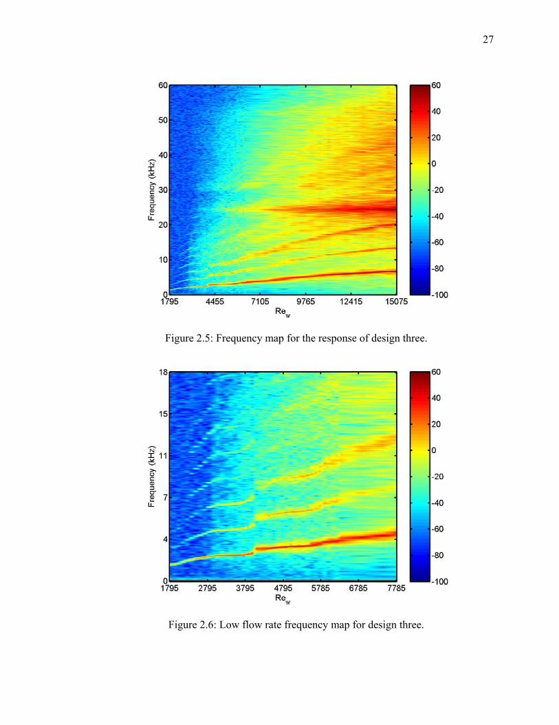
27

Figure 2.5: Frequency map for the response of design three.

Figure 2.6: Low flow rate frequency map for design three.

28

The frequency response of design three is compared with the other four designs in

Figure 2.8. The data is plotted on a log-log scale because of the wide range of flow rates

and frequencies involved. The range of flow rates spans two orders of magnitude, while

the frequency response spans over three orders of magnitude. Between the five

oscillators studied, nearly the entire range of frequencies and flow rates of Figure 2.8 can

be continuously covered. Thus, if a specific frequency or flow rate is required for a

particular application, the size of the required oscillator may be determined from the data

in Figure 2.8.

The data presented in Figure 2.8 may be non-dimensionalized in order to compare the

mode-hopping behavior of the oscillator at various scales. If the oscillation behavior is

self-similar, and the correct non-dimensionalization parameters are employed, then the

curves should collapse. Reynolds number (based on the nozzle exit dimension) is

maintained as the proper scaling parameter for the flow rate data. A reduced frequency is

defined as

2

2 2fw fdwF

V Q+ = = , 2.2

where f is the measured frequency in Hz. The scaled data for the various sizes of the

fluidic oscillator is shown in Figure 2.9. Despite the wide range of frequencies and flow

rates spanning several orders of magnitude, the curves coalesce into a group with about

±50% variation. Designs two, three, and four are the only ones that exhibit the mode-

hopping behavior at low flow rates. The mode-hopping behavior is distinctly different

between the scaled designs, however. Design two has several small jumps in frequency;

design three exhibits larger frequency jumps; while design four has only one, large mode

hop.

29

Figure 2.7: Frequency response of the primary oscillation frequency for design three.

Figure 2.8: Frequency response of all five scaled designs.

30

Figure 2.9: Reduced frequency response of all five scaled designs.

2.4 Aspect Ratio Studies

The effects of aspect ratio of the fluidic oscillators are also evaluated. Aspect ratio is

defined as the nozzle width divided by the depth of the device,

2wAR

d= . 2.3

Devices with a higher aspect ratio will have a smaller depth, and thus a smaller cross-

sectional area for a given oscillator geometry. Four designs were fabricated, all of which

had the same profile as design three (Figure 2.4). The only difference between these four

designs is in the depth of each device, which varies the aspect ratio. A summary of the

design dimensions is presented in Table 2.2.

Frequency response data for the four designs is presented in Figure 2.10. The design

with the smallest aspect ratio (largest depth) exhibits the lowest frequency response.

Devices with higher aspect ratio, and shorter depths, have a higher frequency response

for a given flow rate. This result indicates that the shear layer is more easily modulated

in the devices with a shorter depth. For the larger-depth devices, three-dimensional

31

effects become dominant, which reduces the efficacy of the internal pseudo-feedback

loop and decreases the oscillation frequency.

Table 2.2: Oscillator dimensions for aspect ratio studies.

Design AR1 AR2 AR3 AR4 Internal Nozzle (w1) 0.0344” 0.0344” 0.0344” 0.0344”

Exit Nozzle (w2) 0.04” 0.04” 0.04” 0.04” Depth (d) 0.01” 0.0239” 0.03” 0.04”

Aspect Ratio (AR) 4.00 1.67 1.33 1.00 Nozzle Half Angle (φ) 48.7° 48.7° 48.7° 48.7°

Non-dimensional data for the aspect ratio effect is presented in Figure 2.11. The

mode-hopping behavior is distinctly different for each of the four designs that were

evaluated. This indicates that the mode-hopping is a three-dimensional effect, or at least

is impacted by three-dimensional characteristics of the device. Also note that the two

short-depth designs and the two large-depth designs collapse onto separate curves. This

indicates that there is a fundamental change in the operating characteristics between the

two sets of designs.

Figure 2.10: Effect of aspect ratio on the oscillation frequency.

32

Figure 2.11: Effect of aspect ratio on reduced frequency.

2.5 Inlet Geometry Effects

To further study the causes of the mode-hopping behavior at low flow rates, the inlet

geometry of the fluidic oscillators was varied. Three oscillators were fabricated with the

same basic geometry as design three (Figure 2.4), but with different inlet channels. Scale

drawings of the designs fabricated for this work are shown in Figure 2.12. The design

with concave inlet passages (Figure 2.12a) is identical to design three. The other two

inlet channel orientations are straight and convex. These inlet orientations are chosen

because the wall pressure gradients and vorticity induced into the flow will vary

depending on the curvature of the inlet. The results of the frequency study for the three

designs are shown in Figure 2.13. The design with straight inlets produced higher

oscillation frequencies, while the convex-inlet design produced significantly lower

frequencies than the concave baseline. These differences in oscillation frequency may be

a result of the jet impingement location within the mixing chamber. The shape of the

inlet nozzle will affect the impingement location, which in turn dictates the length of the

33

feedback path and vortex size. These fluid structures are the primary mechanisms that

drive the oscillations.

Plots of reduced frequency are shown in Figure 2.14. The oscillatory behavior of the

straight-inlet design exhibited no mode-hopping behavior, and the convex-inlet design

apparently has one mode hop. This is in contrast to the presence of four mode hops in the

frequency response of the concave-inlet design. These differences in oscillatory behavior

can only be due to the variation in inlet geometry, since all other parameters were held

constant. The repeatability of the mode hopping behavior was also evaluated in this

study. The frequency response of the concave-inlet design was recorded as flow rate was

increased as well as decreased. There is no hysteresis in the value of flow rate where the

mode hop occurs. Furthermore, the curves in Figure 2.13 and Figure 2.14 show excellent

repeatability of the measurements.

2.6 Supply Gas Effects

The effects of the supply gas on the frequency response are also evaluated. Air,

argon, and hydrogen were tested in the third oscillator design (Figure 2.4). Since argon

(1.690 kg/m3) is a heavier gas than air (1.225 kg/m3), and hydrogen (0.085 kg/m3) is

much lighter, significant differences in the response of the fluidic oscillator are

expected.59 The frequency response of the oscillator to these two gases is presented in

Figure 2.15 and the reduced frequency is plotted in Figure 2.16. The oscillation

frequency is slightly lower for the response to argon gas, because the density of argon is

higher than air. Conversely, the lighter hydrogen gas produces much higher oscillation

frequencies. When presented in dimensionless form, however, the response of the

oscillator to the gases collapses to a single curve. The mode-hopping behavior is

significantly different, yet the slope of the reduced frequency curve is often similar

(between Reynolds numbers of 4000 and 6000, for example). Furthermore, the

oscillatory response at higher flow rates is very similar, with the slope of the response

being nearly identical.

34

(a)

(b)

(c)

Figure 2.12: Oscillator geometries for inlet variation study: (a) concave, (b) straight, (c) convex.

35

Figure 2.13: Effect of inlet geometry on the frequency response of design three.

Figure 2.14: Effect of inlet geometry on the reduced frequency response of design three.

36

Figure 2.15: Frequency response of design three to air and argon gases.

Figure 2.16: Reduced frequency response of design three to air and argon gases.

37

2.7 Unequal Inlet Flow Rates

Flow visualization data presented in chapter one indicated that the fluidic oscillator

has a fairly robust response to unequal flow rates on the symmetric inlets. The frequency

response due to unequal inlet flow rates is evaluated by keeping one inlet flow rate

constant, while varying the flow rate on the other inlet and measuring the frequency

response. In the data presented in Figure 2.17, the left flow input is a constant 7.4×10-5

m3/s, while the right input varies as a fraction of this from 50% to 150%. Remarkably,

the fluidic oscillator maintains oscillations throughout this range of asymmetric flow

rates, with a concomitant frequency variation from 5.5 kHz to 11 kHz. This indicates that

the fluid-dynamic mechanisms responsible for the oscillations are quite robust, and that

the oscillator can be used across a wide range of unequal flow rates. The external

flowfield of the oscillator, however, will be yawed in a preferential direction, depending

on which flow input is dominant. This yawing behavior is clearly seen in Figure 1.9,

where the right input dominates the left and the external flow is yawed to the left.

Figure 2.17: Response of the fluidic oscillator to unequal flow rates on the inlets.

38

2.8 Summary

Results presented in this chapter detail the frequency response of the fluidic oscillator

under various geometric, supply gas, and symmetry conditions. The aim of these

experiments was to provide an engineering database of information for future oscillator

designs, as well as a study of the basic fluid dynamics of the fluidic oscillators.

Frequency maps of the oscillator response indicate a flowfield that is rich in high-

frequency content, with up to the 7th harmonic visible in the spectra. Scaling studies were

performed in order to establish the operating range of the device. Oscillators were built

and tested over a range of two orders of magnitude in flow rate and three orders of

magnitude in frequency response. The observed mode hopping behavior was found to

vary with the size of the oscillator, the aspect ratio, the inlet geometry, and the test gas.

The mode hopping is due to three-dimensional effects that are highly sensitive to all of

the above conditions. The response of the oscillator to unequal supply flow rates was

also evaluated, and the fluidic oscillations are fairly robust to a wide range of input

asymmetry.

39

CHAPTER 3: CHARACTERIZATION OF THE MICRO FLUIDIC OSCILLATOR

The small-scale fluidic oscillators studied in chapter two are promising candidates for

flow control actuators. The micro-scale devices can produce a 325-μm wide oscillating

jet at high frequencies (over 22 kHz) and very low flow rates (~1 L/min or ~1 gram/min).

These properties are advantageous for flow control, because the small package can easily

be integrated into a flight vehicle, and the low flow rate requirement makes the device an

efficient actuator. In this work, the flowfield of a micro fluidic oscillator is investigated

in more detail with pressure transducers, water visualization, and pressure-sensitive paint

(PSP). The acoustic field and frequency spectrum are characterized for the oscillator at

several flow rates. Full-field PSP images were acquired of the micro fluidic oscillator

flow at oscillation frequencies up to 21 kHz. A macro imaging system was used to

provide a spatial resolution of approximately 3-μm per pixel. Thus, this work also

showcases recent advances in porous pressure-sensitive paint technology, which enable

measurements of micro-scale flows, as well as very high frequency unsteady flow.

3.1 Introduction

The micro fluidic oscillators characterized in these tests are unique in three aspects.

These actuators require very low flow rates, typically 450-1100 mL/min. In addition, the

size of the oscillating jet is on the micro scale, approximately 325 μm wide. The jet

produced by the micro fluidic oscillator has a much higher oscillation frequency than the

miniature fluidic oscillator. The typical range of oscillation frequency for the micro

fluidic oscillator is from 6 kHz up to over 22 kHz. The design of the micro fluidic

oscillator evaluated in these tests follows the principles detailed in Raghu’s patent.36 The

oscillator operates without feedback tubes: the unsteady interaction of two colliding fluid

jets inside a mixing chamber causes the oscillatory motion of the issuing jet.

40

3.2 Experimental Setup

3.2.1 Device Fabrication

The micro fluidic oscillator requires special care in the fabrication process. A small

3-axis CNC machine was used to fabricate the device out of acrylic material. The

smallest dimensions of the micro oscillator are on the order of 200 μm. Thus, the

diameter of the tooling must be less than this critical dimension. A 0.005” diameter (127

μm) end mill (Fullerton Tool, #3215SM) was used with an air turbine operating at 40,000

rpm to machine the fluidic oscillator resonance cavity.

3.2.2 Instrumentation for Frequency Evaluation

A miniature electret microphone was used to characterize the oscillation frequency of

the micro fluidic oscillator. The microphone was mounted in the near field of the

oscillator flow (within approx. 10 jet diameters). The signal was digitized with a

National Instruments BNC-2080 board and AI-16E-4 DAQ card, with a sampling rate of

250 kHz. The flow rate of the fluidic oscillator was measured with an Omega FL-3600

Rotameter, and the pressure was measured with a digital pressure transducer.

3.2.3 Pressure-Sensitive Paint

The experimental setup of the micro fluidic oscillator with PSP instrumentation is

shown in Figure 3.1. Anodized aluminum pressure-sensitive paint (AA-PSP) was used as

the PSP formulation for these tests. The anodized aluminum surface was prepared

according to Sakaue’s procedure,60 and Tris(Bathophenanthroline) Ruthenium

Dichloride, (C24H16N2)3RuCl2 from GFS Chemicals, served as the luminophore. The

paint sample was positioned parallel to the jet flow exiting the micro fluidic oscillator, as

shown in Figure 3.1.

41

Figure 3.1: Experimental setup for the pressure-sensitive paint measurements.

The imaging system consisted of a CCD camera, a bellows assembly, a reversed lens,

and a long-pass optical filter. A 12-bit Photometrics SenSys CCD camera with 512x768

pixel resolution was used for imaging. A Nikon PB-6 bellows was used to extend the

lens from the image plane, with the extension set at approximately 200 mm. A 50-mm

f/1.8 Nikon lens was reversed and mounted on the bellows with a Nikon BR-2A lens

reversing ring. A 590-nm long pass filter (Schott Glass OG590) was used for filtering

out the excitation light, and was attached to the lens bayonet mount with a Nikon BR-3

filter adapter ring.

A pulsed array of 48 blue LEDs (OptoTech, Shark Series) was used for excitation of

the PSP. This LED array removes the individual LED packaging and mounts the

individual dies in a TO-66 package, creating a compact unit. The excitation light was

filtered with an Oriel 58879 short-pass filter. For full-field imaging, the camera shutter

must be left open for an extended period (typically several seconds) to integrate enough

light for quality images. Therefore, the pulsing of the excitation light was phase-locked

with the oscillation of the micro fluidic oscillator in order to capture one point in the

42

oscillation cycle. The strobe rate was synchronized with the signal of a Kulite pressure

transducer (XCS-062) mounted in the near field of the oscillator flow. The Kulite signal

was passed to an oscilloscope with a gate function. The gate function produced a TTL

pulse with a width corresponding to the time the scope was triggered on. Thus, the

oscilloscope was used to generate a once-per-cycle TTL pulse. This TTL signal from the

oscilloscope was sent to the external trigger input of a pulse/delay generator (Berkeley

Nucleonics Corporation, BNC 555-2). The BNC pulse generator, with its variable delay,

then triggered an HP 8011A pulse generator with variable pulse width and voltage. The

output voltage of the HP pulse generator was set at 16V, and this signal directly strobed

the LED array at any arbitrary phase-locked point in the oscillation cycle. The pulse

width of the excitation light was set at 2.48 μs for the 9.4-kHz oscillations, and 1.0 μs for

the 21.0-kHz oscillations. These pulse width values are less than 2.5% and 5.0% of the

oscillation period, respectively. Images throughout the oscillation period were acquired,

with a constant delay between data points (5 μs delay for 9.4-kHz oscillations, and 2 μs

delay for 21.0-kHz oscillations). The camera exposure time for these experiments was on

the order of several seconds.

Wind-on and wind-off reference images are needed for the PSP data reduction

process. The wind-off reference image was divided by the particular wind-on image for

each phase delay. In some cases the ratio of the two images was then normalized to

match a known value in the image region.

3.3 Results and Discussion

3.3.1 Water Visualization

A simple test to verify the operation of the micro fluidic oscillator is to use water as

the working fluid. Since the density of water is much higher than air or other gases, the

operating frequency of the device is much lower. The low frequencies (on the order of

several hundred Hertz) facilitate visualization using simple techniques. The disadvantage

of using water as a working fluid is that surface tension effects may become important to

the resultant flowfield. For these tests, a digital SLR camera with macro lens and

43

external flash were used to visualize the flowfield. Typical results are shown in Figure

3.2(a), an image captured with a flash duration of 1/500 s. The flowfield issuing from the

nozzle is clearly an oscillatory waveform. The range of oscillation is several times the

diameter of the jet exit (325 μm), and the amplitude of the oscillations grows with

distance downstream of the nozzle. Figure 3.2(b) shows the oscillator at the same

operating conditions, but with a longer time exposure for a time-averaged image. It is

clear that the flow is largely bimodal, with the flow dwelling longer at the extremes.

(a) (b)

Figure 3.2: Water visualization of micro fluidic oscillator flowfield, (a) instantaneous (1/60 s with flash), and (b) time-averaged (1/2 s, no flash).

3.3.2 Frequency vs. Flow Rate Evaluation

The oscillation frequency of the micro fluidic oscillator was evaluated across a range

of flow rates. Figure 3.3 shows the variation of oscillation frequency with flow rate for

the micro fluidic oscillator. The oscillation frequency was measured by determining the

frequency of the primary peak on a power spectrum of the signal from a single electret

44

microphone. Oscillations begin at 6.0 kHz with a flow rate of 464 mL/min, and increase

in frequency up to 22.5 kHz at a flow rate of 1123 mL/min. Notice that there is a change

in slope of the curve at about 763 mL/min. During the testing, this point corresponded

with a distinct change in the tone produced by the oscillator. The variation of frequency

with flow rate is linear, but discontinuous at 763 mL/min. The values of slope for the

two linear regions are summarized in Table 3.1. It is possible that the nature of the

oscillations has changed at this inflection point. The fluid dynamics of the jet interaction

within the fluidic oscillator may be responsible for this change in behavior. This

supposition will be investigated further with the pressure-sensitive paint data.

Figure 3.3: Frequency and flow rate evaluation, oscillator operating with air.

Table 3.1: Summary of linear dependence of oscillation frequency on flow rate.

Flow Rate Range Slope Intercept 464-763 mL/min 31.8 Hz / (mL/min) –8439 Hz 763-1123 mL/min 19.2 Hz / (mL/min) 1003 Hz

45

The results in Figure 3.3 only show the variation of the primary oscillation frequency

with flow rate. The power spectrum for the oscillations is rich in higher-order frequency

content, which is not revealed in Figure 3.3. Thus, a frequency map was generated to

cover the range of supply pressures and across the entire frequency spectrum, as shown in

Figure 3.4. Each vertical slice of this frequency map is essentially an individual power

spectrum at one specific operating condition. The color scale in the figure represents the

relative magnitude within the power spectrum. Both supply pressure and volumetric flow

rate were measured simultaneously, such that mass flow rate may be determined if one

assumes an ideal gas and calculates density using ambient conditions (in this case, 296.6

K and 99.622 kPa). The corresponding mass flow rates for the abscissa of Figure 3.4

range from 0.52 g/min up to 2.7 g/min. Unfortunately, the original oscillator that was

characterized in Figure 3.3, and which was used for the PSP experiments, was

unavailable for this test. Instead, an oscillator of the same geometry was fabricated.

Manufacturing tolerances yielded slight changes in the geometry, resulting in a slightly

different oscillator flowfield. Thus, the results shown in Figure 3.4 should only be

considered representative of a typical micro oscillator, and should not be directly

compared with the results shown in Figure 3.3. The frequency map in Figure 3.4 clearly

shows the primary frequency peak, beginning at just under 10 kHz and increasing to

approximately 20 kHz. Higher harmonics are clearly visible all the way up to 100 kHz,

particularly at the low flow rates. This indicates that the oscillations are very rich in

high-frequency content. Another interesting feature visible in the frequency map is the

sudden incidence of broadband noise at a supply pressure of 6.76 kPa. This can be seen

on the frequency map as the sudden increase in the noise floor, indicated by a change in

color from dark blue to cyan (approx. 10 dB increase). The change in the noise level is

typically associated with a transition from laminar to turbulent flow inside the oscillator,

as discussed in chapter two. Also noteworthy is the evanescence of the primary

frequency peak at a supply pressure of about 17.7 kPa. At about the same pressure, a

new high-frequency peak emerges at approximately 70 kHz. This high frequency peak

then dominates the power spectrum for higher pressures.

46

Figure 3.4: Frequency response of the fluidic oscillator supplied with air.

3.3.3 Pressure-Sensitive Paint Results

Two points on the frequency curve of Figure 3.3 were chosen for further evaluation

with pressure-sensitive paint. One point was chosen in the first linear region of the curve,

at a low flow rate where oscillations just begin. The second point was selected in the

other linear region, at a high flow rate near the highest oscillation frequency.

The first point corresponds to an oscillation frequency of 9.4 kHz, near the low end of

the frequency range. This represents a very low flow rate (554 mL/min or ~0.67 g/min,

with a supply pressure of 6.69 kPa). A Kulite pressure transducer was positioned in the

near field of the jet oscillations, and the time history recorded. The power spectrum of

this signal is shown in Figure 3.5. Note that the spectrum is rich in higher-frequency

harmonics, in addition to the primary peak at 9.4 kHz. PSP data for this flow condition is

shown in Figure 3.6 (a) through (c). This PSP data was acquired with nitrogen gas for

47

high-contrast visualization. A photographic bellows was used with the CCD camera to

create an image 4x life size on the image plane. The dimensions on the axes of the

images were calibrated by imaging a scale with 100 lines per inch and determining the

imaging area of each pixel. Note that the entire image area covers a region measuring

approximately 2000-μm square, with each pixel representing an area measuring 3.2-μm

square. This represents one of the smallest flow fields visualized with PSP technology,

following the work of Huang, et al.61

The data shown in Figure 3.6 is phase-averaged through one period of the jet

oscillation, with each image representing successive time delays from a fixed trigger.

Each image is separated by 20 μs, or approximately 19% of the total cycle. Another

representation of this same data set is shown in Figure 3.7. This plot represents a cross-

section of the PSP data taken at a point 500-μm downstream of the nozzle exit. Each

curve in the figure represents a successive time step of 10 μs. Notice that the jet has a bi-

stable behavior: the jet snaps between the two end points. The transition time for the jet

between the two extremes is very fast (on the order of 20 μs), while it dwells longer at the

outer positions. The distance traversed by the jet between the two extremes is

approximately 300 μm. The oscillatory motion is similar to a square wave, or possibly

triangular. Another indicator of the oscillator characteristics is the RMS intensity plot

shown in Figure 3.8. For each pixel location, a phase-averaged time-history is generated

from the PSP intensity data. The root-mean-square value of the fluctuations is calculated

for each point in the flow. This figure indicates that there is a two-lobed region of high

fluctuations, with the area near the jet centerline being relatively constant. This supports

the bi-modal observation of the jet oscillations. The slight asymmetry visible between

the two lobes may be due to imperfect alignment of the PSP with respect to the nozzle.

48

Figure 3.5: Power spectrum of Kulite signal, 9.4 kHz oscillations.

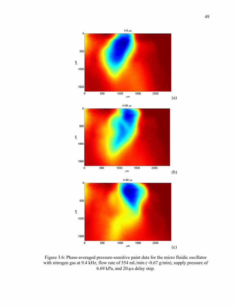
49

(a)

(b)

(c)

Figure 3.6: Phase-averaged pressure-sensitive paint data for the micro fluidic oscillator with nitrogen gas at 9.4 kHz, flow rate of 554 mL/min (~0.67 g/min), supply pressure of

6.69 kPa, and 20-μs delay step.

50

Figure 3.7: Cross-sectional data taken from the PSP results at 9.4 kHz, at a location 500 μm downstream of the nozzle exit.

Figure 3.8: RMS Intensity plot from the phase-averaged time history at 9.4 kHz.

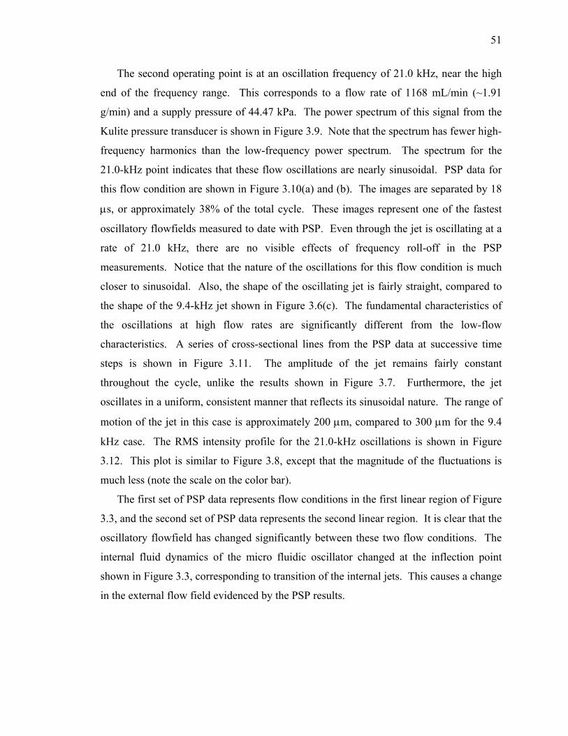
51

The second operating point is at an oscillation frequency of 21.0 kHz, near the high

end of the frequency range. This corresponds to a flow rate of 1168 mL/min (~1.91

g/min) and a supply pressure of 44.47 kPa. The power spectrum of this signal from the

Kulite pressure transducer is shown in Figure 3.9. Note that the spectrum has fewer high-

frequency harmonics than the low-frequency power spectrum. The spectrum for the

21.0-kHz point indicates that these flow oscillations are nearly sinusoidal. PSP data for

this flow condition are shown in Figure 3.10(a) and (b). The images are separated by 18

μs, or approximately 38% of the total cycle. These images represent one of the fastest

oscillatory flowfields measured to date with PSP. Even through the jet is oscillating at a

rate of 21.0 kHz, there are no visible effects of frequency roll-off in the PSP

measurements. Notice that the nature of the oscillations for this flow condition is much

closer to sinusoidal. Also, the shape of the oscillating jet is fairly straight, compared to

the shape of the 9.4-kHz jet shown in Figure 3.6(c). The fundamental characteristics of

the oscillations at high flow rates are significantly different from the low-flow

characteristics. A series of cross-sectional lines from the PSP data at successive time

steps is shown in Figure 3.11. The amplitude of the jet remains fairly constant

throughout the cycle, unlike the results shown in Figure 3.7. Furthermore, the jet

oscillates in a uniform, consistent manner that reflects its sinusoidal nature. The range of

motion of the jet in this case is approximately 200 μm, compared to 300 μm for the 9.4

kHz case. The RMS intensity profile for the 21.0-kHz oscillations is shown in Figure

3.12. This plot is similar to Figure 3.8, except that the magnitude of the fluctuations is

much less (note the scale on the color bar).

The first set of PSP data represents flow conditions in the first linear region of Figure

3.3, and the second set of PSP data represents the second linear region. It is clear that the

oscillatory flowfield has changed significantly between these two flow conditions. The

internal fluid dynamics of the micro fluidic oscillator changed at the inflection point

shown in Figure 3.3, corresponding to transition of the internal jets. This causes a change

in the external flow field evidenced by the PSP results.

52

Figure 3.9: Power spectrum of Kulite signal, 21.0 kHz oscillations.

53

(a)

(b)

Figure 3.10: Phase-averaged pressure-sensitive paint data for the micro fluidic oscillator with nitrogen gas at 21.0 kHz, flow rate of 1168 mL/min (~1.91 g/min), supply pressure

of 44.47 kPa, and 18-μs delay step.

54

Figure 3.11: Cross-sectional data taken from the PSP results at 21.0 kHz, at a location 500 μm downstream of the nozzle exit.

Figure 3.12: RMS Intensity plot from the phase-averaged time history at 21.0 kHz.

55

3.4 Summary

The micro fluidic oscillator is an excellent candidate for a flow control actuator. The

fluidic device produces an unsteady jet that oscillates at frequencies from 6 to 22 kHz.

These particular micro oscillators require only very small flow rates – on the order of 1

L/min (~1 g/min). One of the most significant advantages of the fluidic oscillator is its

simplicity. Fluidic oscillations are generated purely by fluid dynamic phenomena; thus,

the lack of moving parts makes the micro oscillator attractive as a practical excitation

device.

As such, the flow field of the micro fluidic oscillator needed to be characterized. This

work used porous pressure-sensitive paint to make time-resolved full-unsteady

measurements of the jet oscillations. In addition, microphones and Kulite pressure

transducers were used to characterize the power spectra at various operating conditions.

Water flow was also used to visualize the instantaneous and time-averaged behavior of

the micro oscillator.

The dependence of frequency on flow rate was evaluated and found to range from 6

kHz to over 22 kHz, corresponding to flow rates of about 400 to 1100 mL/min.

Interestingly, the variation of frequency with flow rate was found to be linear, except at

one distinct inflection point. The oscillations above and below this inflection point were

shown to exhibit different characteristics. Oscillations at points below the inflection

point were similar to a square wave or triangular wave, with rich high-frequency content.

Oscillations above the inflection point, however, were nearly sinusoidal as shown by PSP

data and power spectra.

56

CHAPTER 4: MODULATED JET BURSTS WITH A PULSED FLUIDIC OSCILLATOR

4.1 Introduction

In the field of active flow control, there is a need for actuators that can address

multiple time scales simultaneously. These situations arise when there is a low-

frequency component and a high-frequency component to the flowfield. In some

situations, the low-frequency component is related to instabilities such as vortex

shedding, while the high-frequency component is related to fine-scale turbulent mixing.

The ideal actuator would be able to address both of these time-scales simultaneously.

In this work, the high-frequency flowfield of a miniature fluidic oscillator is

modulated by a pulsed solenoid valve. The solenoid valve input to the oscillator

modulates the flow at a low frequency on the order of 200 Hz or less. The fluidic

oscillator, however, oscillates the supplied air at a frequency on the order of 3 kHz.

Thus, with a simple combination of two modulating sources, a dual time-scale actuator

can be developed.

The fluidic oscillator used in these tests is shown in Figure 1.1. This device measures

only about 1-cm wide, allowing it to be employed in many space-limited applications on

aircraft. The high-frequency flowfield of the oscillator is shown in the schlieren images

in Figure 1.4. This particular oscillator generates a sawtooth waveform when supplied

with a fluid at pressure. The oscillator operates with no moving parts, and its operation is

based purely on fluid dynamic interactions within the oscillator cavity.

57


This new actuator concept is comprised of a fluidic oscillator driven by a solenoid

valve. The fluidic oscillator produces the high-frequency content of the flowfield, while

the solenoid valve produces the low-frequency carrier signal. The solenoid valve is

driven by a square wave from a BNC-555 pulse generator (Berkeley Nucleonics

Corporation). The driving signal from the pulse generator was varied in frequency,

magnitude, and duty cycle to control the solenoid valve. The pressure supplied to the

solenoid valve was also controlled by a pressure regulator. The flowfield of the fluidic

oscillator was characterized by a hot film probe and a Kulite pressure transducer, as

shown in Figure 4.1. The pressure transducer was mounted between the solenoid valve

and the fluidic oscillator, to record the input pressure fluctuations to the oscillator. The

hot film probe was positioned in the oscillatory jet flow and recorded the velocity time-

history.

Figure 4.1: Experimental setup for characterization of the pulsed-fluidic oscillator.

58

4.3 Results

The actuator behavior was characterized at multiple frequencies and multiple

pressures. The driving frequency of the pulse generator determines the rate of the low-

frequency carrier signal. The pressure supplied to the fluidic oscillator determines not

only the velocity of the jet exiting from the actuator, but also the rate of the high-

frequency component of the flowfield. Furthermore, the response of the actuator to

variations in duty cycle was also evaluated. These tests are performed with the aim of

characterizing the operating range of this new actuator and understanding its limitations.

4.3.1 Carrier Frequency Variation

The solenoid valve was driven at rates ranging from 10 Hz to 200 Hz, with a constant

supply pressure of 6 kPa. These results are shown in Figure 4.2, with a zoomed-in

portion shown in Figure 4.3. The frequency response characteristics of the valve begin to

roll off at frequencies beyond 100 Hz. Clearly visible in the velocity time-histories is the

presence of both the low-frequency and high-frequency (3 kHz) components of the

actuation. Each waveform shows that the high-frequency component has a startup

transient that lasts on the order of 2 to 3 ms. When the carrier frequency approaches the

frequency response limit of the solenoid valve, the pressure does not have enough time to

build up and initiate high-frequency oscillations beyond the startup transient. On the

decay side of the waveform, the high-frequency component decreases in magnitude and

frequency until the solenoid valve shuts off. This high-frequency response is expected

because the fluidic oscillator has a direct correlation between oscillation frequency and

supply pressure. Power spectra of these velocity time-histories are shown in Figure 4.4.

Note that the 3-kHz high-frequency peak in the spectrum is invariant with a change in the

low frequency carrier signal. The high-frequency spectra remain relatively unchanged

until the carrier frequency reaches 100 Hz, where the magnitude of the high-frequency

peaks begins to diminish.

59

Figure 4.2: Variation of carrier frequency from 10 Hz to 200 Hz, with a constant high-frequency of 3 kHz and a supply pressure of 6 kPa.

Figure 4.3: Zoomed-in portion of Figure 4.2.

60

Figure 4.4: Power spectra of the time histories shown in Figure 4.2.

4.3.2 Pressure Variation

The response of the solenoid valve to pressure variation is shown in Figure 4.5. The

carrier frequency is held constant at 50 Hz, but the supply pressure is varied such that the

output of the valve ranges from 0.5 kPa to over 13.5 kPa. At the higher pressures the

valve has more difficulty in modulating the waveform as a square wave. This roll-off in

the response of the solenoid valve will have an effect on the fluidic oscillator response,

particularly at higher pressures. Velocity measurements of the fluidic oscillator response

at these supply pressures are shown in Figure 4.6 and Figure 4.7. The amplitude of the

dual-modulated jet increases with the supply pressure, as expected. Furthermore, the

high-frequency component of the signal increases with the supply pressure as well. Thus,

for a given carrier frequency (50 Hz in this case), the frequency and magnitude of the

high-frequency component can be controlled independently of the carrier frequency by

varying the supply pressure. This frequency shift is clearly visible in the power spectrum


61

Figure 4.5: Input pressure variation, measured by a Kulite pressure transducer between the solenoid valve and the fluidic oscillator, with a constant carrier frequency at 50 Hz.

Figure 4.6: Response of the dual-frequency actuator to changes in pressure, with a constant carrier frequency of 50 Hz.

62

Figure 4.7: Zoomed-in portion of Figure 4.6. The high-frequency component increases in frequency and amplitude as the pressure is increased.

Figure 4.8: Power spectra of the time histories shown in Figure 4.6.

63

4.3.3 Duty Cycle Variation

The duty cycle of the signal applied to the solenoid valve was varied from 12.5% up

to 87.5%, and the response of the solenoid valve was recorded by the pressure transducer.

This data is shown in Figure 4.9 for a supply pressure of approximately 14.5 kPa and a

carrier frequency of 25 Hz. The response of the solenoid-fluidic combined actuator is

shown in Figure 4.10 and Figure 4.11. Note that the startup transient and decay of the

high-frequency component of the waveform are the same for each duty cycle. The

primary effect of the duty cycle variation is to determine the length of time that high-

frequency actuation is on for a given period of the carrier signal. This allows for tailoring

the level of high-frequency mixing available for a given forcing frequency (the low-

frequency carrier). Figure 4.12 illustrates that the high-frequency peak is invariant with

changes in the duty cycle of the carrier signal.

Figure 4.9: Input duty-cycle variation, measured by a Kulite pressure transducer between the solenoid valve and the fluidic oscillator.

64

Figure 4.10: Response of the actuator to variation in duty cycle. Pressure remains constant and the carrier frequency remains constant at 25 Hz.

Figure 4.11: Zoomed-in portion of Figure 4.10.

65

Figure 4.12: Power spectra of the time histories in Figure 4.10.

4.4 Summary

This work has demonstrated the development of a combined fluidic oscillator /

solenoid valve device as a flow control actuator. This type of actuator is useful for

applications where dual time-scales of modulation are required. The solenoid valve

modulates the carrier jet at a frequency on the order of 100 Hz, while the fluidic oscillator

modulates the jet at a much higher frequency of 3 kHz. The response of this actuator to

variation in the low-frequency carrier signal, supply pressure, and duty cycle was studied.

These parameters establish the operating limits of the current configuration of this

actuator concept. This new actuator will be particularly beneficial for flow control

applications where disparate high- and low-frequency actuation is required for

simultaneous mixing and forcing.

66

CHAPTER 5: DEVELOPMENT OF THE PIEZO-FLUIDIC OSCILLATOR

This chapter describes a new actuator for flow control applications: the piezo-fluidic

oscillator. The actuator is a fluidic device based on wall-attachment of a fluid jet, and

modulated by piezoelectric devices. The piezo-fluidic oscillator successfully decouples

the operating frequency from the flow characteristics of the device. The frequency is

specified by an input electrical signal that is independent of pressure, making this

actuator ideal for closed-loop control applications. The oscillator exhibits high

bandwidth (up to 1.2 kHz), modulation rates up to 100%, and a velocity range reaching

sonic conditions. Furthermore, the bi-stable actuator may be operated in a steady state,

with momentum flux in one of two desired directions. The piezo-fluidic oscillator may

be used in flow control applications where synthetic jets cannot provide enough

momentum for control authority. The actuator can also be used as an alternative to

traditional aircraft control surfaces while operating in the steady bi-directional mode.

This chapter details the design and characterization of the piezo-fluidic oscillator. The

dynamic response characteristics are evaluated with flow visualization and hot film probe

measurements on the output.

5.1 Introduction

Flow control is a rapidly developing field in applied fluid dynamics, with much of the

work focused on actuator development, sensor systems, control logic, and applications.

Flow control actuators are devices that are used to enact large-scale changes in a

flowfield. Often these changes are focused on improving the performance of a flight

vehicle – by delaying stall, reducing drag, enhancing lift, abating noise, reducing

emissions, etc. In many flow control situations, unsteady actuation is required for

optimal performance. Unsteady actuators are particularly beneficial in closed-loop

67

control applications when the unsteady actuation can be controlled and synchronized with

characteristic time scales of the flowfield.

The ideal actuator will have a high frequency bandwidth and direct control by an

electrical signal for closed-loop applications. The device should be simple and robust for

reliable flight operations, for devices with few moving parts are desirable for mechanical

reliability. The ideal actuator should also be capable of a large range of flow rates, but

only enough for sufficient control authority. Some applications require large flow rates

that current actuators cannot deliver. Jet thrust vectoring on a flight vehicle is one such

example. D.Miller62,63 has specified that the ideal actuator for this application is a pulsed

jet that operates at 1 kHz with 100% modulation of the jet at sonic conditions. The focus

of this work is development of the piezo-fluidic oscillator towards these design goals.

The fluidic oscillator that forms the basis for this new invention is one that operates

on the wall-attachment principle, as shown in Figure 5.1. When a jet of fluid is adjacent

to a wall, entrainment of flow around the jet causes a low-pressure region between the

wall and the jet that draws the jet closer to the wall. Thus, the jet will deflect until it has

attached to the wall. This principle was observed by Henri Coanda in the 1930’s34 and

was later named the Coanda effect.35 The Coanda effect is most commonly encountered

in daily life by observing a stream of water from a faucet attach to one’s hand when the

two are brought close together. Coanda noticed this phenomenon and applied the

principle to steering streams of fluid.

If there are two adjacent walls, such as the symmetric configuration shown in Figure

5.1, the jet will randomly attach to one wall or the other, based on the randomness of

turbulence in the flow. Now, if a pressure pulse is introduced at the control port

perpendicular to the jet, the jet will detach from the wall and re-attach to the opposite

wall. This occurs through the creation of a separation bubble between the jet and the

wall. As more fluid is injected from the control port, the separation bubble enlarges and

extends downstream until the jet has entirely separated. The pressure differences and

momentum of this separation process then carry the jet over to the opposite wall where it

re-attaches.

68

Figure 5.1: The principle of wall attachment in a fluidic device, known as the Coanda Effect.

If the two control ports are set up with a feedback loop system, then the fluidic device

can create self-sustained oscillations. This is the typical arrangement of many traditional

fluidic oscillators. The disadvantage of this arrangement, however, is that the frequency

of oscillations is directly coupled to the flow rate of the device.

For practical flow control problems, it is highly desirable to decouple the operating

frequency from the flow rate of the actuator. This is the motivation for developing a

piezoelectric-driven fluidic oscillator. This concept has been used in the past to develop

a bi-stable pneumatic valve for fluid amplifier technology. The field of fluidics was a

significant focus of research efforts in the 1960’s and 70’s. Some of this work

concentrated on developing electro-fluidic converters. W.Miller64 originally proposed

using piezoelectric devices for fluidic control. He implemented a double-clamped

piezoelectric bender to produce acoustic signals for control. As such, the pressures

produced by the piezo bender were very low (~ 100 Pa) and even a high-gain fluidic

amplifier would have a marginal output. He did demonstrate operation of the device up

to 1 kHz. Tesar65 was also an early developer of the concept of external control of a

fluidic device. He demonstrated the use of a ferromagnetic filament to guide a jet of air

or water in various directions through the Coanda effect. The deflection of the filament

was controlled by an adjacent electromagnet. His demonstrations were confined to low

frequency deflections (68 Hz) at low pressures. Tesar also briefly suggested the use of

Receptivity Zone

69

filaments with an electrostatic charge, as well as piezoelectric benders for jet control.

Taft and Herrick66,67 used a piezoelectric bender to alternately block the input to either

one of the two control ports. They operated the device in an unsteady mode, and

recorded a flat frequency response up to about 40 Hz with a corresponding phase shift of

90°.66 In later work they demonstrated a flat frequency response of 1 kHz with this same

device.67 Chen68,69 developed a mono-stable fluidic injector with a piezo bender on the

unstable-side control port. His work focused on developing the device as a fuel injector

for natural gas engines. He achieved switch-on response times of 1.65 ms and switch-off

response times of 1.85 ms.

This work seeks to develop a piezo-driven fluidic oscillator for use as a flow control

actuator. A bi-stable, wall-attachment fluidic oscillator is used along with piezoelectric

transducers to achieve oscillatory or steady-state control flow. The piezo-fluidic

oscillator successfully decouples the operating frequency from the supply pressure to the

device. The actuator can deliver the high mass flow rates that are demanded in some

flow control applications. Furthermore, the device is shown to have a wide bandwidth,

with partial frequency coverage from 0 to 1.2 kHz.

5.2 Piezo-Fluidic Oscillator Design Concepts

The main concept of the piezo-fluidic oscillator is the modulation of a fluid jet by

piezoelectric transducers. There are many possible realizations of this concept, which are

described as follows. In all cases, the piezoelectric transducer creates a geometrical or

fluid dynamic asymmetry in a receptive location in the flowfield. The area of maximum

receptivity is just downstream of the power nozzle (as shown in Figure 5.1), where a

traditional fluidic oscillator’s control ports are typically located. The first concept

employs piezoelectric buzzers coupled to the control ports in a manner similar to

W.Miller’s design.64 The challenge with this design is that a high level of acoustic

energy is needed to reach the jet switching threshold of a practical device. This design

was attempted in the early stages of this work, but was later abandoned due to insufficient

control authority of the piezo buzzers. A similar iteration on this concept would employ

synthetic jets at the control ports.

70

Other concepts employ piezoelectric benders or extenders to change the geometry of

the device. A small asymmetry in the power nozzle region can readily cause the jet to

switch to the opposite sidewall. A single piezoelectric bender may be positioned on the

jet centerline, with the oscillating end pointing either upstream or downstream in the

flow. The oscillatory motion of the bender will cause deflection and switching of the jet

between the two sidewalls. Another concept is to use piezoelectric benders or extenders

in lieu of the control ports. When two extenders are driven 180° out of phase from one

another, a geometric asymmetry is created in the shear layer of the jet, causing the jet to

attach to the alternate sidewalls. A final concept involves a mono-stable oscillator with

only one attachment wall and a piezoelectric bender mounted flush on the attachment

wall with the free end pointing upstream into the jet. As the transducer is modulated, the

tip will be either flat against the wall, or facing into the flow such that the jet detaches

from the wall. In the mono-stable configuration, the unstable location is a free jet that is

not attached to an adjacent sidewall.

Two designs were characterized in the work presented here. Both designs rely on a

piezoelectric bender mounted on the centerline of the fluidic oscillator nozzle. The first

design has the bender tip pointing upstream into the nozzle, as shown in Figure 5.2 and

Figure 5.3. The power nozzle in this geometry is 0.5 mm wide and about 5.5 mm high,

with an adjacent wall angle of 30°. The primary disadvantage of this design is the

location of the piezoelectric transducer with respect to the flow exit of the device. The

protrusion of the bender on the exterior of the oscillator makes it somewhat infeasible for

practical applications. One possible solution is to employ a piezo bender with a much

shorter length, which would typically decrease the tip deflection range and increase the

resonance frequency. The second design, shown in Figure 5.4 and Figure 5.5, has a

similar nozzle geometry, but with the piezo bender mounted upstream of the nozzle with

the tip just downstream of the nozzle exit. The nozzle width of the second design is 3

mm wide and 5.5 mm high, with a diffuser half-angle of 15°. The nozzle width was

increased over the first design to allow room for the piezo bender to oscillate inside the

nozzle. The piezoelectric bender employed in both of these designs is a 4-layer

piezoceramic (T434-A4-302 from Piezo Systems, Inc.) that measures 72.4 mm long, 5.1

71

mm high, and 0.86 mm thick. The specified deflection of the device is ±1050 μm with a

resonant frequency of 121 Hz. The piezo bender was driven by a square wave signal

from a function generator and amplified by a Lasermetrics voltage amplifier. The

amplifier output was passed through an RC circuit to remove the DC bias on the supply.

The resulting signal supplied to the piezo bender was a 40 VRMS square wave.

Figure 5.2: Scale diagram of the first design. The piezoelectric bender is positioned in the diffuser, pointing upstream into the flow.

Figure 5.3: Photograph of the first design, with the piezo device removed for clarity.

72

Figure 5.4: Scale diagram of the second design. The bender is oriented with the tip pointing downstream from the throat.

Figure 5.5: Photograph of the second design, with the piezo bender installed.

5.3 Measurement Techniques

Instrumentation systems involved in characterizing the fluidic oscillator were

schlieren imaging, pressure-sensitive paint (PSP), and hot film probes with a computer

data acquisition system. The schlieren and PSP systems were used for flow visualization,

while the hot film probes were used for quantitative velocity and frequency

73

measurements. The experimental setup for the PSP and hot film probe techniques is


The schlieren imaging experimental setup involved the use of a single-pass schlieren

system. The illumination source was a strobe light, a General Radio company model

1538-A Strobotac. A neutral density filter was placed in front of the strobe light to

control the light intensity passing through the flow and reaching the camera. A 6-inch

diameter front-surface concave mirror with a focal length of 5 feet was used to pass the

light through the flowfield. A knife-edge was placed at the focal point of the mirror to

improve the image contrast. The flowfield was then imaged with a Nikon D100 digital

camera. Hydrogen gas was used with the oscillator to enhance the density contrast with

ambient air.

Pressure-sensitive paint was used to visualize the internal fluid dynamics of the

oscillator. Recent work with PSP has extended the frequency response well beyond 20

kHz, such that the current unsteady tests at 50 Hz are fairly straightforward. The PSP

imaging system consisted of a 14-bit CCD camera with a 55-mm f/2.8 Nikon macro lens.

A 590-nm long pass filter (Schott Glass OG590) filtered out the excitation light. The

paint sample was back-illuminated with an LED array emitting 473-nm light. The

illumination from the LED’s was phase-locked with the driving frequency of the

piezoelectric transducer. The pulse width was set to 2.5% of the period, and the delay

step was 5% of the period. One image was taken at each delay step, producing 20

equally-spaced images throughout the oscillation cycle. Nitrogen was used as the supply

gas for the PSP tests, to enable high-contrast visualization of the jet dynamics. Wind-on

and wind-off images were used to calculate the intensity ratio presented for visualization.

74

Figure 5.6: Experimental setup for the pressure-sensitive paint and hot film probe instrumentation.

Hot film probes were positioned at the ends of both attachment walls to measure the

velocity and frequency content of the exiting flow. The probes and controller have a

specified frequency response of 10 kHz. The data from the probes was recorded through

a computer data acquisition system with a sampling rate at least 500 times the driving

frequency. Data was simultaneously sampled to record the input signal to the

piezoelectric bender, as well as the velocity signals from both hot film probes.


Results presented in this section involve flow visualization with schlieren and PSP

techniques, and velocity measurements at the exit plane with hot film probes. The

velocity data is used to evaluate the response of the piezo-fluidic oscillator at various

operating conditions, and to generate frequency maps and bode plots. All of the

subsequent data is for the first design (piezo bender pointing upstream as shown in Figure

5.2), except where noted.

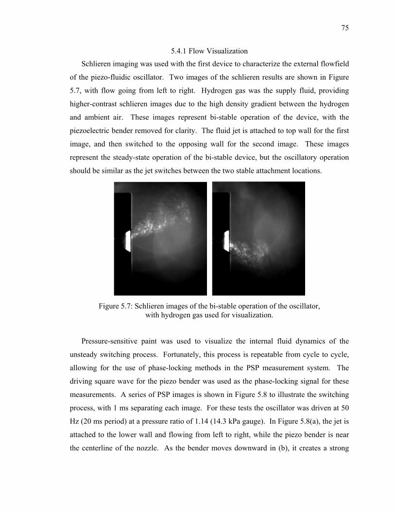
75

5.4.1 Flow Visualization

Schlieren imaging was used with the first device to characterize the external flowfield

of the piezo-fluidic oscillator. Two images of the schlieren results are shown in Figure

5.7, with flow going from left to right. Hydrogen gas was the supply fluid, providing

higher-contrast schlieren images due to the high density gradient between the hydrogen

and ambient air. These images represent bi-stable operation of the device, with the

piezoelectric bender removed for clarity. The fluid jet is attached to top wall for the first

image, and then switched to the opposing wall for the second image. These images

represent the steady-state operation of the bi-stable device, but the oscillatory operation

should be similar as the jet switches between the two stable attachment locations.

Figure 5.7: Schlieren images of the bi-stable operation of the oscillator, with hydrogen gas used for visualization.

Pressure-sensitive paint was used to visualize the internal fluid dynamics of the

unsteady switching process. Fortunately, this process is repeatable from cycle to cycle,

allowing for the use of phase-locking methods in the PSP measurement system. The

driving square wave for the piezo bender was used as the phase-locking signal for these

measurements. A series of PSP images is shown in Figure 5.8 to illustrate the switching

process, with 1 ms separating each image. For these tests the oscillator was driven at 50

Hz (20 ms period) at a pressure ratio of 1.14 (14.3 kPa gauge). In Figure 5.8(a), the jet is

attached to the lower wall and flowing from left to right, while the piezo bender is near

the centerline of the nozzle. As the bender moves downward in (b), it creates a strong

76

adverse pressure gradient in the jet and causes the jet to separate from the attachment

wall. Within 1 ms, the jet has reattached to the opposing (upper) wall since this location

is more stable than the lower wall in the presence of the piezo bender. In image (d) the

jet begins to convect downstream towards the exit of the oscillator (at the edge of the PSP

image), and the piezo bender returns to the center location. These images represent one

switching process, whereas two switches occur within each oscillation cycle.

5.4.2 Hot Film Probe Data

5.4.2.1 Velocity Time Histories

The exit flow of the piezo-fluidic oscillator was characterized by simultaneous

measurement of dual hot film probes on either side of the device. Anticipated results

should show that the two signals are 180° phase shifted from one another, and

comparable in velocity magnitude. Temporal velocity data is presented in Figure 5.9 at

(a) 10 Hz and (b) 200 Hz for a pressure ratio of 1.69 (68.9 kPa gauge). The velocity

signals for the low frequency case show very little phase delay from the control signal,

with very fast rise and decay times. The output of the oscillator at 200 Hz is phase

shifted approximately 180° from the low frequency case, but the modulation rate remains

fairly high. This operating frequency is near the maximum for this modulation mode and

the oscillator soon loses synchronization from the driving signal at higher frequencies.

As will be shown later, however, another modulation mode emerges at higher frequencies

to maintain operation to over 1 kHz.

The step response characteristics of the piezo-fluidic oscillator are shown in Figure

5.10. A step input signal was sent to the piezoelectric bender, and the velocity response

was recorded by a hot film probe at the end of the adjacent attachment wall. The test was

performed over a range of pressure ratios and the response time calculated. The step

response times are summarized in Table 5.1. As should be expected, the response time

decreases as the jet velocity increases. There is a finite amount of time required for the

jet to convect from where it is switched at the control nozzle, down to the exit of the

device. Since the convection time is related to the velocity of the jet, the higher velocities

77

will produce a faster step response. The convection time is also related to the length of

the attachment wall. As the wall length is decreased, the convection time will also

decrease. These relationships indicate that the fastest step response time can be achieved

with a high velocity jet and the shortest possible wall length. Also notice that the step

response times are reaching an asymptotic limit for this geometry as the jet velocity is

increased. This limit in the step response indicates that there are two time scales involved

in the response – one due to the fluid convection time, and the other due to delays in the

electrical and mechanical switching time of the piezoelectric bender. The first time scale

may be controlled by changing the jet velocity and wall length, while the second time

scale can only be controlled by changing the piezoelectric bender and driving circuitry.

(a) (b)

(c) (d)

Figure 5.8: Series of PSP images with successive delays of 1 ms at an oscillation frequency of 50 Hz. Flow is from left-to-right, and the piezo bender is on the right.

78

(a)

(b)

Figure 5.9: Time history of the oscillator outputs simultaneously measured by hot film probes. (a) 10 Hz, (b) 200 Hz. Pressure ratio is 1.69.

79

Figure 5.10: Step response of the piezo-fluidic oscillator.

Table 5.1: Summary of step response times.

Pressure Ratio Response Time (ms) 1.07 4.52 1.14 3.41 1.21 2.78 1.28 2.47 1.34 2.34 1.41 2.16 1.48 2.06 1.55 1.99

Although the square wave response characteristics of the oscillator begin to diminish

at 200 Hz, the device is able to oscillate at frequencies in the kilohertz range. Figure 5.11

shows the response of the piezo-fluidic oscillator at a 1.0 kHz driving frequency and a

pressure ratio of 1.14 (13.8 kPa gauge). The temporal velocity profile is no longer a

square wave, but the jet is clearly modulated at the driving frequency.

P/Patm=1.07

P/Patm=1.55

80

The piezo-fluidic oscillator also responds well at very high pressure ratios, as shown

in Figure 5.12. The pressure ratio for this case is 2.15 (115 kPa gauge), creating a sonic

jet at the power nozzle. Despite the very high dynamic pressure loads on the

piezoelectric bender, it is still able to modulate the jet at low frequencies (5 Hz).

Although the jet has not yet been modulated at both high frequency and high pressure,

design modifications are underway that should enable this performance level to be

attained.

5.4.2.2 Frequency Bandwidth

While the piezo-fluidic oscillator was operated at a pressure ratio of 1.14, the driving

frequency was swept across a range from 0 to 1200 Hz to evaluate the bandwidth

characteristics of the device. The low frequency characteristics (0 – 250 Hz) are shown

in Figure 5.13 (a) and the high-bandwidth characteristics are shown in Figure 5.13(b).

Each vertical cross section of the figures is a typical power spectrum generated from the

velocity measurements. Note that the primary frequency peak increases linearly with the

driving frequency in a 1-to-1 relationship in both figures. For the low frequency range,

the first six or seven harmonics are clearly visible and increase linearly with the input

frequency. The horizontal and vertical bands correspond to natural resonances of the

piezoelectric bender in this flowfield. Figure 5.13(b) shows that the oscillator has a wide

operating range from 0 to 1.2 kHz. There is a small region from 250 to 500 Hz where the

piezo bender is unable to modulate the jet at this pressure. Within this region, the energy

in the power spectrum shifts to the horizontal resonance line at 121 Hz. This indicates

that the beam is oscillating at its resonant frequency rather than the driving frequency in

this range. At approximately 500 Hz, however, the synchronous modulations resume and

increase linearly to the upper limit. The second and third harmonics are also visible at

the higher driving frequencies.

81

Figure 5.11: High frequency oscillations at 1.0 kHz and a pressure ratio of 1.14.

Figure 5.12: Response of the piezo-fluidic oscillator at sonic nozzle conditions. The pressure ratio is 2.15 and the oscillation frequency is 5 Hz.

82

(a)

(b)

Figure 5.13: Frequency maps of the piezo-fluidic oscillator performance at a supply pressure ratio of 1.14.

83

Magnitude and phase plots may be generated from the hot film probe velocity data.

The magnitude values are calculated from the modulation index (M) which is defined as

max min

max min

V VM

V V−

=+

5.1

where V is the measured velocity. A modulation index of 1 indicates that jet is

modulated from zero velocity up to its maximum value. The phase angle is defined as

the delay between the control signal and the measured velocity at the exit of the actuator.

This phase delay includes any electrical, mechanical, and fluid dynamic delays inherent

in the system. Figure 5.14 shows data for the (a) magnitude and (b) phase for the first

design actuator at three operating pressure ratios. First, it is important to point out that

the range of operating pressures has little effect on the response characteristics of the

piezo-fluidic oscillator across this frequency range. The modulation index remains quite

high (80 to 90%) across the entire range. The phase data shows little roll-off until the

resonance frequency of the bender is reached (121 Hz). The phase delay is less that 90°

until this point, but then quickly rolls off beyond 180°. For some applications this phase

delay is of no consequence, but for some closed-loop applications across a range of

frequencies, it can be an issue.

Data for the second oscillator design (with the piezo bender pointing downstream as

shown in Figure 5.4) is presented in Figure 5.15. The modulation index for all three

operating pressures is somewhat lower than the results for the first design, typically

ranging from 70 – 80%. Furthermore, the modulation of the low speed jet is significantly

diminished. This is most likely due to attachment of the jet to the piezo bender rather

than the adjacent attachment walls. Thus, the piezo bender serves to impart a small

deflection to the jet by directing it, rather than causing it to switch to an opposing wall.

There is also more variation in the phase data between the three pressure ratios. The

break point varies from 100 Hz for the lowest pressure up to 150 Hz for the highest. In

general, the second design (Figure 5.4) does not perform as well as the first design with

the piezo bender pointing upstream (Figure 5.2). The performance of the second design

may be improved by narrowing the width of the throat such that the jet attaches to the

walls rather than the bender.

84

(a)

(b)

Figure 5.14: (a) Magnitude and (b) phase plots of the piezo-fluidic oscillator response with the bender facing upstream.

85

(a)

(b)

Figure 5.15: (a) Magnitude and (b) phase plots of the piezo-fluidic oscillator response with the bender facing downstream (with the flow).

86

5.5 Summary

This work has presented the development of the piezo-fluidic oscillator as a new type

of flow control actuator. The oscillator can be driven directly by an electrical signal for

closed-loop control applications. The piezo-fluidic oscillator exhibits a fairly high

bandwidth with a maximum operating frequency of 1.2 kHz at certain pressures. Over a

range of 0 to 250 Hz the oscillation frequency was nearly independent of supply pressure,

and operation was maintained well beyond the piezo resonance frequency of 121 Hz.

The modulation level remained constant near 90% across this frequency range, and the

phase angle didn’t break beyond 90° until the piezo resonance frequency. For

oscillations at higher frequencies (500 to 1200 Hz), the jet is most likely modulated in

some other manner by the piezo bender, rather than by attachment to the adjacent walls.

The piezo-fluidic oscillator was also successfully operated at sonic nozzle conditions at a

frequency of 5 Hz. Two designs were evaluated in this work – one with the piezo bender

pointed upstream, and the other with the bender pointed downstream. The upstream-

pointing bender provided superior modulation characteristics, with a higher modulation

index and higher-frequency roll-off. The disadvantage of this configuration is that is less

compact and not as practical for use as an actuator in flow control applications.

Future work with the piezo-fluidic oscillator will focus on design iterations to

improve the operating characteristics. The frequency bandwidth of the oscillator may be

increased by selecting a piezo bender with a higher resonance frequency. Also, the

length of the attachment walls may be shortened in order to decrease the convection time

of the jet, thus increasing the maximum frequency. The ultimate design goal is to create

an actuator that will provide a sonic pulsed jet at 100% modulation at 1 kHz. Future

work will also involve application of this new actuator to practical flow control problems

where high bandwidth and closed-loop control is required.

87

CHAPTER 6: CAVITY TONE SUPPRESSION WITH A FLUIDIC OSCILLATOR

6.1 Introduction

This chapter details the use of fluidic oscillators for suppression of flow-induced

cavity tones. This work demonstrates the utility of the feedback-free fluidic oscillator for

a practical flow control application. High-intensity tones are produced when an open

cavity is exposed to high-subsonic, transonic, or supersonic flows. This can become a

significant issue in aircraft applications, such as weapons bays or landing-gear wheel

wells where the tones produce vibration-induced fatigue. Cavity tones are produced by

the interaction of a free shear layer with the downstream cavity wall. The shear layer is

formed when the flow separates from the leading edge cavity lip. At certain flight

speeds, the shear layer develops an instability which induces periodic shear layer growth

and oscillations. The unsteady shear layer interacts with the downstream edge of cavity.

The interaction effectively adds or removes flow from the cavity in a periodic fashion.

This process generates acoustic waves which propagate upstream and reinforce the shear

layer instability. In this manner, the cavity oscillations are self-induced and the acoustic

signal is a forced feedback mechanism. Rockwell and Naudascher70 have given a general

review of self-sustained oscillations of impinging shear layers, including discussion of

cavity resonance. Heller and Bliss71 have written a clear, concise explanation of the

cavity resonance mechanism, as well as a discussion of flow control techniques that could

be used for cavity tone suppression. Komerath, et al.72 wrote a review paper detailing

prior work to understand and predict cavity resonance phenomena.

Various flow control actuators, both passive and active, have been employed for

suppression of cavity resonance tones. Heller and Bliss used a slanted wall at the trailing

edge of the cavity to stabilize the impingement of the shear layer.71 Spoilers positioned

88

upstream of the cavity are commonly used in current aircraft applications, but do not

suppress cavity tones at supersonic Mach numbers.73 Cylinders have been placed

upstream of the cavity, where the shed vorticity from the rod-in-crossflow serves as high-

frequency excitation of the shear layer.74 Recent work with active control of cavity tones

has included steady suction and blowing75 and pulsed blowing with powered resonance

tubes (Hartmann tubes).4,76 Raman et al.29,77 used a square-wave fluidic oscillator for

suppression of the Mode II tone by 10 dB. These tests were accomplished in a jet-cavity

setup with a jet Mach number of 0.69 and 0.12% mass injection through the fluidic

oscillator. Raman’s earlier work demonstrated that the jet-cavity setup is a valid

approximation of the physics of cavity interaction with freestream flow.78

The purpose of this work is to further demonstrate the use of fluidic oscillators for

cavity tone suppression. The oscillators have the advantage of simplicity over many

other flow control actuators. They have no moving parts, but can generate an oscillating

jet of fluid at high frequency and a wide fan angle. Fluidic actuation is compared with

steady blowing to evaluate the effectiveness of each actuator. Three actuators are

evaluated in this work: actuator 1 is a typical fluidic oscillator (shown in Figure 6.1),

actuator 2 is a similar fluidic oscillator with a narrow exit angle (Figure 6.2), and actuator

3 is a steady jet with a throat width the same size as the fluidic oscillators (Figure 6.3).

The actuators are mounted just upstream of the front edge of the cavity, and oriented such

that the blowing is upwards into the shear layer. The aim of this actuation technique is to

reduce the cavity tones by modifying the shear layer. The actuation will alter the stability

characteristics of the shear layer, as well as potentially alter the impingement location of

the shear layer on the downstream cavity wall.

89

Figure 6.1: Geometry of actuator 1, a wide-angle fluidic oscillator.

Figure 6.2: Geometry of actuator 2, a narrow-angle fluidic oscillator.

Figure 6.3: Geometry of actuator 3, a converging nozzle for steady blowing.

90


The experimental facility used for these experiments is a blow-down jet with adjacent

cavity, located in Raman’s laboratory at the School of Mechanical, Materials, and

Aerospace Engineering at the Illinois Institute of Technology. The jet and cavity

arrangement are shown in Figure 6.4. The jet exit area is 1-in2, and arranged such that

the jet width more than covers the cavity width. The subject cavity is 0.5-in deep, 0.75-

in. wide, and 2-in. long; giving an L/D of 4 and an L/W of 2.67. Each actuator was

placed 0.05-in. upstream of the cavity, with the nozzle ejecting flow upwards into the

main jet flow and centered on the jet centerline. The nozzle width of each actuator was

0.04-in. and the depth of the two-dimensional actuators was 0.024-in.

Figure 6.4: Jet-cavity facility at the Illinois Institute of Technology.

A B&K microphone (Type 2670) was used to quantify the effectiveness of the three

actuators for cavity tone suppression. The microphone was mounted 6.5 inches above the

floor of the cavity, 2.8 inches downstream of the jet exit, and on the horizontal centerline

of the jet. The microphone was located outside the freestream of the jet, and faced

Cavity

Jet Actuator Location

91

downstream. The front face of the plenum was covered with sound-absorbing material in

order to reduce reflections of the acoustic waves. The microphone was powered by a

B&K Type 2804 power supply / signal conditioner. The signal was high-pass filtered at

1 Hz and low-pass filtered at 100 kHz with an Ithaco analog filter. The microphone data

was digitized with a National Instruments BNC-2110 data acquisition system. Data was

acquired in LabVIEW at a 50 kHz sampling rate. Plenum pressure was recorded with a

Setra model 204 pressure transducer. The volume flow rate through the actuator was

measured with a Dwyer FT-137 rotameter, and the supply pressure was measured with a

Setra 204 pressure transducer. Ambient temperature was assumed throughout the system

for mass flow calculations.

6.3 Results

The three actuators were tested at various Mach numbers to evaluate their

effectiveness for cavity tone suppression. The mass flow rate for each actuator was set

approximately equal, to facilitate comparison between the actuators. The test cases

included Mach 0.5 and 0.7 for the primary jet flowing over the cavity. The test results

are summarized in Table 6.1 through Table 6.7 and Figure 6.5 through Figure 6.11.

Uncertainty in the measurement of mass flow rate is approximately ±10% and uncertainty

in sound pressure level is approximately ±0.5%. Percent mass flow is defined as the

control flow divided by the mass flow of the main jet, expressed as a percentage. The

blowing coefficient is defined as

inj injc

cavity

QB

V Aρ

ρ∞ ∞

= , 6.1

where Acavity is the area of the cavity (length times width), ρ is density, V is velocity, and

Qinj is the volume flow rate through the actuator. This blowing coefficient parameter is

the standard measure of actuator mass flow rate for cavity studies in freestream flow.75

The broadband sound-pressure-level (SPL) measured by the microphone increases as

the Mach number of the jet increases. The SPL of the peak tone also increases with

Mach number. The frequency of the cavity tone is 4.7 kHz for the Mach 0.5 jet. When

the Mach number is increased to 0.7, a second tone appears. The two tones, at 3.2 and

92

5.6 kHz, correspond to two simultaneous modes. At a Mach number of 0.9 there is only

one resonance present at 3.6 kHz.

The result of the fluidic injection is that the tonal magnitude is significantly

suppressed, and the broadband noise is typically lowered as well. The most significant

tonal suppression that was observed was with the wide-angle fluidic oscillator injecting

0.9% mass flow into the Mach 0.5 jet for a reduction of 17.0 dB. Other fluidic actuation

cases produced similar results, with typical mass flow rates on the order of 0.5% of the

main jet. It is remarkable that such a reduction of the cavity tone is possible with so little

mass injection.

Also noteworthy is the comparison between fluidic injection and steady blowing. For

approximately the same actuation mass flow rates, the wide-angle and narrow-angle

fluidic oscillators suppressed the cavity tone by 17.0 dB and 16.5 dB, respectively.

Steady blowing at the same mass flow rate, however, suppressed the cavity tone by only

1.6 dB. This highlights the efficiency of the fluidic oscillators for flow control. There is

no penalty for using a fluidic oscillator instead of steady actuation because there are no

moving parts. The only requirement is a higher supply pressure since the pressure drop

across the fluidic oscillator is somewhat higher. The difference between the wide-angle

and the narrow-angle fluidic oscillators is indiscernible from the current results. In some

cases, the wide-angle oscillator provides superior suppression. In other cases, however,

the narrow-angle oscillator performs better.

Table 6.1: Suppression results for Actuator 1 at Mach 0.5.

Percent Mass Injection

Blowing Coefficient, Bc

Peak SPL (dB)

Suppression (dB)

Overall SPL (dB)

Suppression (dB)

Baseline Baseline 110.8 – 121.6 – 0.204 0.102 98.8 12.0 119.1 2.5 0.897 0.449 93.8 17.0 118.8 2.8




Peak SPL (dB)

Suppression (dB)

Overall SPL (dB)

Suppression (dB)

Baseline Baseline 124.4 – 134.2 – 0.141 0.070 123.8 0.6 134.6 -0.3 0.622 0.311 116.8 7.6 131.2 3.0

93




Peak SPL (dB)

Suppression (dB)

Overall SPL (dB)

Suppression (dB)

Baseline Baseline 135.8 – 139.7 – 0.509 0.254 132.0 3.8 137.3 2.4




Peak SPL (dB)

Suppression (dB)

Overall SPL (dB)

Suppression (dB)





Peak SPL (dB)

Suppression (dB)

Overall SPL (dB)

Suppression (dB)





Peak SPL (dB)

Suppression (dB)

Overall SPL (dB)

Suppression (dB)





Peak SPL (dB)

Suppression (dB)

Overall SPL (dB)

Suppression (dB)

Baseline Baseline 126.7 – 134.9 – 0.121 0.061 127.7 -1.0 135.2 -0.3 0.586 0.293 124.9 1.8 134.9 0.0

94

Figure 6.5: Suppression results for Actuator 1 (wide fan angle) at Mach 0.5.


17.0 dB

7.6 dB

95


Figure 6.8: Suppression results for Actuator 2 (narrow fan angle) at Mach 0.5.

3.8 dB

16.5 dB

96

Figure 6.9: Suppression results for Actuator 2 (narrow fan angle) at Mach 0.7.

Figure 6.10: Suppression results for Actuator 3 (steady blowing) at Mach 0.5.

8.2 dB

1.6 dB

97

Figure 6.11: Suppression results for Actuator 3 (steady blowing) at Mach 0.7.

6.4 Summary

Three different flow control actuators were evaluated in this work for their

effectiveness in cavity tone suppression. Two fluidic oscillators with wide and narrow

fan angles were tested, as well as a converging nozzle for steady blowing. The fluidic

oscillators provided far superior tone suppression when compared with steady blowing at

the same mass flow rate. Tone suppression of over 17.0 dB was achieved with

approximately 0.9% blowing mass flow at a main jet Mach number of 0.5. These results

demonstrate the utility and simplicity of fluidic oscillators for flow control applications.

1.8 dB

98

PART TWO: PRESSURE-SENSITIVE PAINT

99

CHAPTER 7: THE EFFECT OF QUENCHING KINETICS ON THE UNSTEADY RESPONSE OF PSP

Pressure-sensitive paints (PSP) have recently been extended to high-frequency

flowfields. Paint formulations have effectively been used to characterize pressure

fluctuations on the order of 100 kHz. As the limits of PSP are extended, various

experimental results indicate that the unsteady response characteristics are non-linear. A

thorough understanding of the photo-physical mechanisms in paint response is needed.

Gas transport properties, coupled with the non-linear nature of the Stern-Volmer

relationship have an effect on the paint response. This work discusses the full

implications of a diffusion-based model on the unsteady response of pressure-sensitive

paint. Based on this model, it is shown that the indicated pressure response of PSP is

faster for a decrease in pressure, and slower for a pressure increase. Effects of other

factors, such as pressure-jump magnitude, pressure-jump range, and Stern-Volmer non-

linearity, are evaluated. Furthermore, a fluidic oscillator is used to experimentally

demonstrate the quenching kinetics of two types of PSP – Polymer/Ceramic and Fast

FIB. Results from the oscillator operated with argon, nitrogen, and oxygen gases at 1.59

kHz demonstrate behavior that agrees with the diffusion model. The Polymer/Ceramic

PSP exhibited no delay between different test gases, indicating a flat frequency response

of at least 1.59 kHz. Fast FIB, on the other hand, demonstrated a significant delay in rise

time between the nitrogen and oxygen cases. Both the diffusion model and the

experimental results demonstrate that the different responses to nitrogen and oxygen only

become critical when the period of the flowfield oscillations is shorter than the response

time of the paint formulation.

100

7.1 Nomenclature

( )

0

2

Stern-Volmer calibration constant


gas concentration

reference gas concentration

diffusion coefficient, m / s

time-history of gas concentration at the paint

m

A

B

C

C

D

f t

μ

=

=

=

=

=

=

( )

( )

0

surface

normalized form of

first derivative of with respect to time

paint thickness, m

paint intensity

intensity per unit thickness

paint intensity in the absence of oxygen

paint

t

ref

g t f

g t g

h

I

I

I

I

μ

′ =

′ =

=

=

=

=

=

[ ]2

intensity at a reference condition


number of samples in a time-history

non-dimensional gas concentration

O oxygen concentration

pressure, Pa

non-dimensional pre

K

N

n

P

P

=

=

=

=

=

′ = ssure

reference pressure, Pa

heat of adsorption, J / mol

universal gas constant, 8.31447 J / mol-K

temperature, K

refP

Q

R

T

=

=

=

=

101

7.2 Introduction

Pressure-sensitive paint (PSP) has recently emerged as a powerful measurement tool

for global pressure distributions.42,43,79 PSP is an optical method for measuring surface

pressures based on the principle of oxygen quenching of a luminescent molecule.

Reviews by Bell et al.44 and Liu et al.45 have summarized the PSP technique and

common applications. Furthermore, Liu and Sullivan have written a recently-published

book which details the development and application of luminescent paints.46

Typical paints are composed of an oxygen-sensitive molecule known as the

luminophore, and a physical binder or matrix for the luminophore. Since luminophores

are available with very short lifetimes (~ 1 μs), the binder typically limits the frequency

response of the paint. Traditional polymer binders have response times as long as

seconds. The recent emergence of porous binders, however, has enabled measurements

( )

2

time, s

non-dimensional time,

substituted time variable

, solution of the diffusion equation

paint thickness coordinate measured from paint surface, m

non-dimensional thickness,

m

m

t

t tD h

u

W t z

z

z z h

μ

α

=

′ =

=

=

=

′ =

=

130

odal states

average phase delay

exponent for the Freundlich isotherm

eigenvalues

time constant, s

adsorption time, s

oscillation time of molecules in the adsorbed state, 1.6 10 s

frequenc

ads

φ

γ

λ

τ

τ

τ

ω

−

=

=

=

=

=

= ×

= y, Hz

102

of unsteady pressure fluctuations on the order of 100 kHz. Development of binders for

unsteady measurements has generally focused on improving the oxygen diffusivity within

the binder. Common binders in use today for unsteady measurements are thin-layer

chromatography plate53 (TLC-PSP), anodized aluminum48,50-52 (AA-PSP),

Polymer/Ceramic54,55 (PC-PSP), poly(TMSP)56,80,81 and Fast FIB.82 Thin-layer

chromatography plate is commonly used in chemistry laboratories and is composed of a

thin layer (~ 250 μm) of silica gel. The disadvantages of the thin-layer chromatography

plate are that it is fragile and limited to simple shapes. Anodized aluminum is created

through an electrochemical process by etching small pores (~ 10-nm diameter) on an

aluminum surface. The luminophore is deposited directly on the porous surface by

chemical and physical adsorption. Anodized aluminum is regarded as providing the

fastest PSP response times, but is limited by the choice of material and cannot be sprayed

onto a model. Polymer/ceramic PSP is a hybrid that uses a small amount of polymer with

a large amount of ceramic particles. The resulting aggregate is a highly porous surface

that allows for rapid diffusion. The primary advantage of Polymer/Ceramic PSP is that it

may be sprayed on a model, and offers reasonable response times. Poly(TMSP) is a

functional polymer with extremely high oxygen permeability. Its response is much faster

than most polymer binders, but still quite a bit slower than the new porous PSP

formulations. FIB (Fluoro / Isopropyl / Butyl) is a fluorinated co-polymer originally

developed at the University of Washington as an “ideal” paint. Fast FIB, essentially a

thin layer of FIB, has recently been developed by Innovative Scientific Solutions, Inc. for

unsteady measurements.

Dynamic calibrations with a shock tube51 and a fluidic oscillator38,40 have shown that

most porous PSP formulations have typical frequency responses in excess of 10 kHz.

Anodized aluminum PSP has been further developed and characterized by Kameda et

al.83 such that the reported response time is less than 10 μs. Unsteady pressure fields

such as the fluidic oscillator (22 kHz),40,41,84 a turbocharger compressor (10 kHz),41,85 or

the oscillating shock in a Hartmann tube (12 kHz)6 have been characterized. Some of

these experimental results41 apparently indicate that the dynamic response of PSP is non-

linear. These results have suggested that the response to an increase in oxygen

103

concentration may be slower than the response to a corresponding increase in nitrogen

concentration.

The purpose of this paper is to develop a model for the quenching dynamics of

pressure-sensitive paint. The implications of the model on the dynamic response of PSP

are discussed in detail. Furthermore, it will be shown that the diffusion-based model is

applicable to the recently-developed fast PSP formulations. Experimental results from

the fluidic oscillator will illustrate the effects of the quenching dynamics and will be

compared with the theoretical model.

7.3 Background

Polymer chemists have done a large amount of experimental and theoretical work on

the quenching kinetics of luminescent molecules immobilized in a polymer binder. It has

been known for quite some time that the luminescent response of a luminophore in a

polymer matrix is different for oxygen sorption or desorption experiments. Chemists

have used these observations along with simple diffusion models to determine the

diffusivity of a polymer film. The first known published work involving this method was

by MacCallum and Rudkin.86 These researchers applied a simplified form of this model

to the measurement of the oxygen diffusion coefficient in two polymer films. Cox and

Dunn87 also measured the oxygen diffusion coefficient via temporal fluorescence

quenching in a polymer. The films used by Cox and Dunn were 1-cm thick, resulting in

response times on the order of hours. They also demonstrated excellent agreement

between the diffusion model and experimental results. Carraway et al.88 discussed the

kinetics of quenching due to several possible models, including pure diffusion,

adsorption, and other combinations of models. Perhaps the clearest explanation of the

diffusion model and its interaction with the Stern-Volmer relation is given by Mills and

Chang.89 Subsequent researchers90-96 have used the diffusion modeling technique

extensively, and report a fast luminescent response to oxygen sorption, and a slower

response to oxygen desorption.

Within the field of PSP research, there has been some work done to model and

experimentally determine the dynamic response characteristics of pressure-sensitive

104

paints. Liu, et al.97 developed a phenomenological model describing the time constant

for paint response. They showed that the traditional square-law estimate for paint

response

2mh Dτ ∝ 7.1

is valid only for traditional polymer binders. Liu et al. derived a modified relation

2 frdmh Dτ −∝ 7.2

for highly porous surfaces, where dfr is the fractal dimension that represents the

complexity of the pore pathway. Furthermore, Liu et al. invoked the Fickian diffusion

model, lending credence to the current use of a diffusion model with porous paints.

Kameda et al.83 discuss gaseous transport in relation to the porous structure of anodized

aluminum PSP. They suggest that the diffusion model is valid for anodized aluminum

paints, but with a modified diffusion coefficient. Since the Knudsen number for

molecular motion within the porous structure is on the order of 1, Kameda et al. posited

that a modified diffusion coefficient is necessary because of Knudsen diffusion. This

effective diffusion coefficient varied with the pore diameter over a range from 10 to 100

nm, and with pressure. Schairer98 also employed a diffusion model in his analysis of

optimum thickness of a PSP layer, which he found to be a tradeoff between signal-to-

noise ratio and dynamic response. Carroll, et al.99 modeled the PSP step-response with a

diffusion-based model, and compared the response times of three different polymer-based

PSP formulations. Winslow, et al.100 developed both an empirical model as well as a

physics-based diffusion model, with the aim of developing a compensator. They applied

both a linear calibration and a Stern-Volmer calibration to the diffusion model and

showed that the Stern-Volmer calibration provides a better fit to the experimental data.

Winslow, et al. also briefly compared the predicted step response behavior of the Stern-

Volmer model to the linear model. Most recently, Drouillard and Linne101 applied the

diffusion-based model to luminescent lifetime measurements with pressure-sensitive

paint. They incorporated Beer’s law into their model to account for attenuation of light in

a paint layer that is not optically thin. When compared to experimental results, however,

optical thickness only appeared to be a relevant parameter at paint thicknesses greater

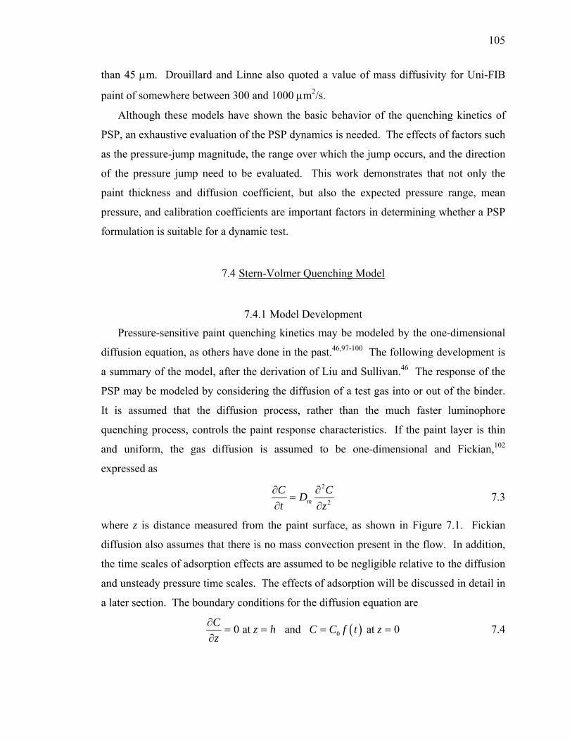
105

than 45 μm. Drouillard and Linne also quoted a value of mass diffusivity for Uni-FIB

paint of somewhere between 300 and 1000 μm2/s.

Although these models have shown the basic behavior of the quenching kinetics of

PSP, an exhaustive evaluation of the PSP dynamics is needed. The effects of factors such

as the pressure-jump magnitude, the range over which the jump occurs, and the direction

of the pressure jump need to be evaluated. This work demonstrates that not only the

paint thickness and diffusion coefficient, but also the expected pressure range, mean

pressure, and calibration coefficients are important factors in determining whether a PSP

formulation is suitable for a dynamic test.

7.4 Stern-Volmer Quenching Model

7.4.1 Model Development

Pressure-sensitive paint quenching kinetics may be modeled by the one-dimensional

diffusion equation, as others have done in the past.46,97-100 The following development is

a summary of the model, after the derivation of Liu and Sullivan.46 The response of the

PSP may be modeled by considering the diffusion of a test gas into or out of the binder.

It is assumed that the diffusion process, rather than the much faster luminophore

quenching process, controls the paint response characteristics. If the paint layer is thin

and uniform, the gas diffusion is assumed to be one-dimensional and Fickian,102

expressed as

2

2mC CDt z

∂ ∂=

∂ ∂ 7.3

where z is distance measured from the paint surface, as shown in Figure 7.1. Fickian

diffusion also assumes that there is no mass convection present in the flow. In addition,

the time scales of adsorption effects are assumed to be negligible relative to the diffusion

and unsteady pressure time scales. The effects of adsorption will be discussed in detail in

a later section. The boundary conditions for the diffusion equation are

( )00 at and at 0C z h C C f t zz

∂= = = =

∂ 7.4

106

where f(t) is a function that describes the time history of gas concentration at the paint

surface. The initial state of the paint layer is a uniform gas concentration throughout the

thickness. Thus the initial condition for the diffusion equation 7.3 is

( )0 0 at 0C C f t= = 7.5

z

z=hz=0

PS

P S

urfa

ce

Wal

l

z

z=hz=0

PS

P S

urfa

ce

Wal

l

Figure 7.1: Diagram of modeled PSP geometry.

In order to make the diffusion equation tractable for numerical solution, the following

non-dimensional variables are introduced

( ) ( )0

2

, 0

m

n t z C C fz z h

t tD h

′ ′ = −

′ =

′ =

7.6

The diffusion equation may then be rewritten as

2

2

n nt z∂ ∂

=′ ′∂ ∂

7.7

with boundary and initial conditions

( )0 at 1 and at 00 at 0

n z z n g t zn t

′ ′ ′ ′∂ ∂ = = = =

′= = 7.8

A function g(t') = f(t') – f(0) is used to satisfy the boundary condition at the paint surface.

This non-dimensional differential equation 7.7 is then solved with Laplace transforms.

When the boundary and initial conditions 7.8 are applied, a general convolution solution

is obtained for the non-dimensional gas concentration

( ) ( ) ( )0

, ,t

tn t z g t u W u z du′

′ ′ ′ ′= −∫ 7.9

107

The function ( )tg t is the derivative ( ) ttg ∂∂ , and ( ),W t z is defined as

( ) ( ) ( )0 0

1 2 1 2, 1 12 2

k k

k k

k z k zW t z erfc erfct t

∞ ∞

= =

⎛ ⎞ ⎛ ⎞+ − + += − + −⎜ ⎟ ⎜ ⎟

⎝ ⎠ ⎝ ⎠∑ ∑ 7.10

For a step increase in gas concentration at the paint surface, the function gt is defined

as the delta function, ( ) ( )tg t tδ= , which gives

( ) ( ), ,n t z W t z′ ′ ′ ′= 7.11

from the convolution integral 7.9. Analogously, a step decrease in gas concentration is

given by

( ) ( ), ,n t z W t z′ ′ ′ ′= − 7.12

From Equations 7.11 and 7.12, it can be seen that there is no difference in the time scale

of diffusion, whether a gas is diffusing into or out of the paint binder. Gas concentration

profiles for several time steps of diffusion into and out of the paint binder are shown in

Figure 7.2. Each step in dimensionless time is given as a successive power of ten

according to

410 where 20 2Nt N′ = − ≤ ≤ 7.13

This diffusion process is independent of the particular gas species of interest.

Pressure-sensitive paint, however, is sensitive only to oxygen concentration. Thus,

oxygen diffusion will be the focus of the remainder of this discussion. The sensitivity of

PSP to oxygen is dictated by Stern-Volmer quenching behavior, which is an inherently

nonlinear relationship.103 The key to the difference in time scales of the PSP response is

in the characteristic non-linearity of the Stern-Volmer calibration curve. The Stern-

Volmer relation may be expressed as103

[ ]0 2

11

II K O

=+

7.14

where K is a constant if temperature is invariant.

108

(a)

(b)

Figure 7.2: Gas diffusion (a) into and (b) out of the paint layer.

Increasing Time

Increasing Time

109

The form of the Stern-Volmer equation typically used for PSP calibrations, given as

ref

ref

I PA BI P

= + 7.15

is obtained by taking the ratio of Equation 7.14 at two conditions – a reference and a test

condition. When Equation 7.14 is compared with the Stern-Volmer form used for PSP

calibrations 7.15, the value of K can be derived as

ref

AKB P

=⋅

7.16

since the concentration of oxygen in air is proportional to the air pressure. A variation of

Equation 7.15 is the Stern-Volmer relation following the Freundlich Isotherm, namely

ref

ref

I PA BI P

γ⎛ ⎞

= +⎜ ⎟⎜ ⎟⎝ ⎠

7.17

This calibration behavior is characteristic of porous PSP formulations, particularly

anodized aluminum PSP. Typical PSP calibration curves for γ = 1.0 and γ = 0.1 are

shown in Figure 7.3, with A = 0.9 and B = 0.1. In addition to these typical calibration

curves, experimental calibrations for the Fast FIB and Polymer/Ceramic formulations are

shown in the same figure. PSP calibration data is most often presented as intensity ratio

vs. pressure ratio, as shown in Figure 7.3. This format, however, does not intuitively

indicate the nonlinear nature of the Stern-Volmer relationship of Eq. 7.14. Therefore, the

same calibration data is shown in Figure 7.4, but with normalized intensity shown ( 0I I )

rather than intensity ratio ( refI I ). The highly non-linear nature of the Stern-Volmer

relationship is more readily apparent in this representation. The coupling of the nonlinear

intensity response with the diffusion of gas within the paint thickness is the primary

mechanism for the difference in rise and fall times of the paint response.

110

Figure 7.3: Typical calibration curves for various pressure-sensitive paint formulations.

Figure 7.4: PSP calibration data plotted to show the nonlinear Stern-Volmer intensity response.

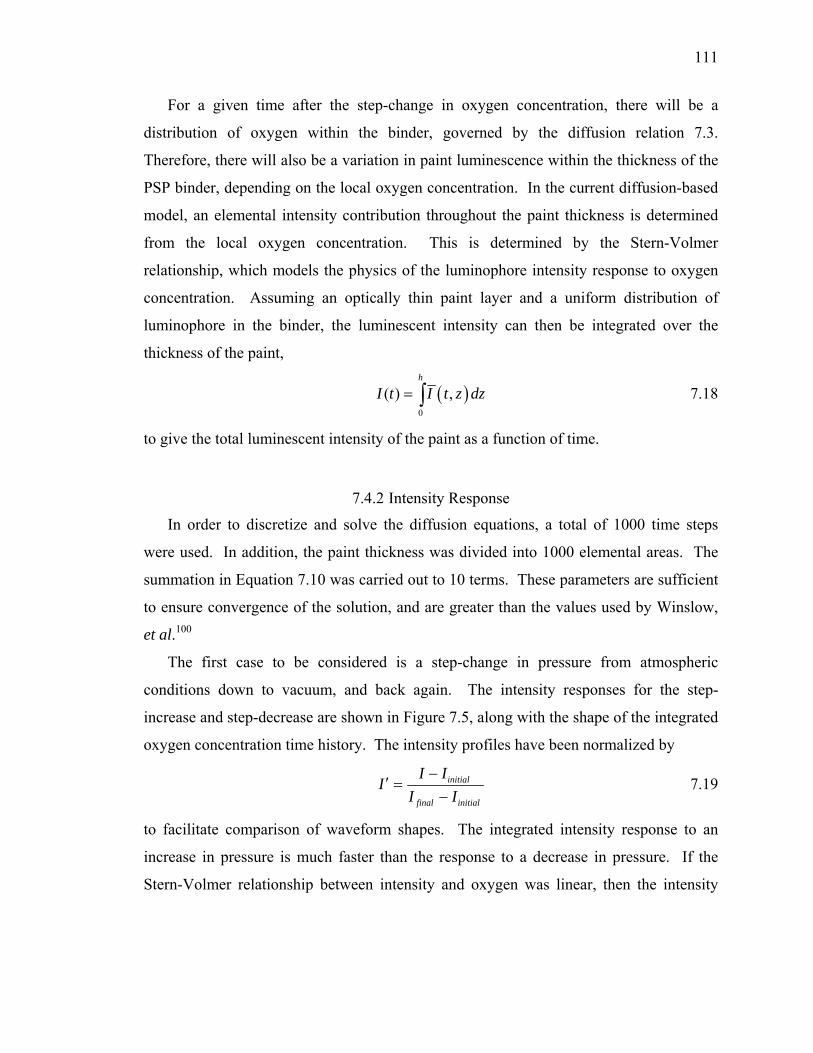
111

For a given time after the step-change in oxygen concentration, there will be a

distribution of oxygen within the binder, governed by the diffusion relation 7.3.

Therefore, there will also be a variation in paint luminescence within the thickness of the

PSP binder, depending on the local oxygen concentration. In the current diffusion-based

model, an elemental intensity contribution throughout the paint thickness is determined

from the local oxygen concentration. This is determined by the Stern-Volmer

relationship, which models the physics of the luminophore intensity response to oxygen

concentration. Assuming an optically thin paint layer and a uniform distribution of

luminophore in the binder, the luminescent intensity can then be integrated over the

thickness of the paint,

( )0

( ) ,h

I t I t z dz= ∫ 7.18

to give the total luminescent intensity of the paint as a function of time.

7.4.2 Intensity Response

In order to discretize and solve the diffusion equations, a total of 1000 time steps

were used. In addition, the paint thickness was divided into 1000 elemental areas. The

summation in Equation 7.10 was carried out to 10 terms. These parameters are sufficient

to ensure convergence of the solution, and are greater than the values used by Winslow,

et al.100

The first case to be considered is a step-change in pressure from atmospheric

conditions down to vacuum, and back again. The intensity responses for the step-

increase and step-decrease are shown in Figure 7.5, along with the shape of the integrated

oxygen concentration time history. The intensity profiles have been normalized by

initial

final initial

I II

I I−

′ =−

7.19

to facilitate comparison of waveform shapes. The integrated intensity response to an

increase in pressure is much faster than the response to a decrease in pressure. If the

Stern-Volmer relationship between intensity and oxygen was linear, then the intensity

112

response for the rise and fall would both collapse to the oxygen concentration curve.

Since the Stern-Volmer relation is not linear, the rise and fall responses differ.

Figure 7.5: Integrated intensity response to step-changes in pressure, compared to oxygen concentration; A=0.9, B=0.1, γ=1.0.

7.4.3 Pressure Response

The final step in the simulation is to convert integrated paint intensity back to an

indicated pressure. This replicates the experimental procedure of acquiring paint

intensity data and calibrating the intensity ratio to an indicated pressure ratio. To

summarize, the key steps in the modeling procedure are detailed as follows. First, a step-

change in pressure is modeled at the paint surface. Oxygen concentration throughout the

paint thickness is calculated by the diffusion equation for each time step. The resulting

temporal and spatial distribution of oxygen is converted to intensity by the Stern-Volmer

relationship. The local intensity across the entire paint thickness is then integrated to

simulate the experimentally-observed intensity for each time step. This integrated

intensity is finally converted back to an indicated gas concentration (pressure) by again

113

applying the Stern-Volmer relationship. The result of the model simulation is the paint’s

indicated response to an arbitrary step-change in pressure.

When the intensity time-histories shown in Figure 7.5 are converted to pressure, the

shapes of the curves change such that the indicated pressure-response to a decrease in

pressure leads that of an increase in pressure. This result is shown in Figure 7.6, for the

same parameters used in the solution represented in Figure 7.5. The pressure step-

response curves have been normalized by

initial

final initial

P PP

P P−

′ =−

7.20

in a manner similar to the intensity step-response curves. The change in behavior

(contrasted with the intensity profiles) is due to the inversion process within the Stern-

Volmer relation. This result also highlights the importance of calibrating experimental

intensity results before drawing conclusions about the temporal response characteristics

of PSP. For both modeling and experimental work (even flow visualization), the

observed time history may be altered significantly if the intensity is not calibrated to

pressure or gas concentration.

The pressure response curves in Figure 7.6 are plotted against non-dimensional time,

2mtDtt

hτ′ = = . 7.21

Notice the effects that the paint thickness (h) and diffusion coefficient (Dm) have on the

step-response of the paint. A thinner paint sample will have a much faster response time.

Likewise, a paint binder with a high diffusion coefficient will also exhibit a faster

response time. Thus, the relative impact of the response differences to a step-increase or

step-decrease will depend on the diffusion coefficient and thickness of the paint sample

being implemented.

The effect of γ in the Freundlich Isotherm calibration 7.17 on the PSP response is also

evaluated. Figure 7.7 shows the results with A=0.9, B=0.1, and γ=1.0 or 0.1. The

Freundlich Isotherm does have some effect on the shape of the indicated pressure-time

history, although the effect is minimal. The basic trend remains the same – there is a fast

response to a step-decrease, and a slower response to a step-increase in pressure.

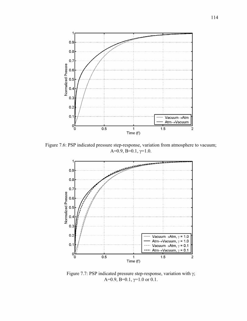
114

Figure 7.6: PSP indicated pressure step-response, variation from atmosphere to vacuum; A=0.9, B=0.1, γ=1.0.

Figure 7.7: PSP indicated pressure step-response, variation with γ; A=0.9, B=0.1, γ=1.0 or 0.1.

115

The effects of a small change in pressure are shown in Figure 7.8. For this case, a

change in pressure of 6.9 kPa above atmosphere was considered. As expected, a smaller

change in pressure produces a much smaller difference between the rise and fall in

indicated pressure. The reduced difference is due to a minimal nonlinearity in the smaller

portion of the Stern-Volmer curve that is traversed by the small pressure jump. The trend

remains the same, however – the response to a pressure decrease is faster than the

response to a pressure increase.

Figure 7.8: PSP indicated pressure step-response, variation with pressure jump magnitude; A=0.9, B=0.1, γ=1.0, ΔP=6.9 kPa.

The effect of the overall range of the pressure change is shown by comparing Figure

7.6 with Figure 7.9. Both cases have a pressure change of 101 kPa, but the first case is a

change to vacuum and back, while the second case is a change from 101 kPa to 202 kPa

and back. Note that the pressure change at lower pressures produces a greater difference

in the time scales of the indicated pressure than the case at higher pressures. The effect

of the mean pressure on the indicated pressure-jump response is due to the non-linear

116

nature of the Stern-Volmer curve. Figure 7.4 shows that the highly non-linear region of

the curve is focused at lower pressures, while the curve becomes more linear at high

pressures.

Figure 7.9: PSP indicated pressure step-response, variation from 101 kPa to 202 kPa; A=0.9, B=0.1, γ=1.0.

7.4.4 Frequency Response

The preceding step-response data was modeled for typical pressure-sensitive paint

calibrations. This data provides a foundational understanding of the diffusion and

quenching mechanisms responsible for the nonlinear response characteristics. The

following results extend the preceding data by incorporating experimental calibration

data for two PSP formulations, and generalizing the model to allow for an arbitrary input

for pressure time-history.

The present solution scheme remains the same as the previous derivation, except an

alternative method is employed for calculating the distribution of gas concentration

within the paint layer. The following results are based on the modal analysis technique

117

presented by Winslow et al.100 The system of equations to be solved for oxygen

concentration is given by

( ) ( ) ( ) ( )( )

2

0 00 0 0 2sin0 0

i i i i i

P tt t

P tα λ α λ λ⎛ ⎞ ⎡ ⎤ ⎛ ⎞ ⎡ ⎤

′ ′⎛ ⎞⎜ ⎟ ⎜ ⎟⎢ ⎥ ⎢ ⎥′ ′= − + − ⎜ ⎟⎜ ⎟ ⎜ ⎟⎢ ⎥ ⎢ ⎥ ′ ′⎝ ⎠⎜ ⎟ ⎜ ⎟⎢ ⎥ ⎢ ⎥⎝ ⎠ ⎣ ⎦ ⎝ ⎠ ⎣ ⎦

M O M M M

&&

M O M M M

7.22

( ) ( )( ) ( ) ( ) ( )( )

, cos 1 0i i

P tn x t x t

P tλ α

⎛ ⎞′ ′⎛ ⎞⎜ ⎟′ ′ ′ ′= + ⎜ ⎟⎜ ⎟ ′ ′⎝ ⎠⎜ ⎟

⎝ ⎠

M

L L &M

, 7.23

where P′ is the dimensionless input pressure waveform. Complete details of the

derivation of this system of equations are given by Winslow et al.100 Equations 7.22 and

7.23 were modeled with 200 steps through the paint thickness, 500 steps in time, and 100

wave numbers to provide the distribution of oxygen concentration throughout the paint

thickness for an arbitrary pressure time-history. The oxygen concentration is then

converted to intensity by a Stern-Volmer intensity calibration for the paint of interest.

The intensity is integrated over the paint thickness, and then converted back to an

indicated pressure by the same Stern-Volmer calibration for the subject paint.

In order to evaluate the response characteristics of actual paint formulations,

Equations 7.22 and 7.23 are solved for a sine wave over a range of frequencies and

experimental calibrations (Figure 7.3 and Figure 7.4) are used in the modeling process.

The responses of both Fast FIB and Polymer/Ceramic PSP are evaluated across a range of

frequencies, and compared with the response for a linear calibration. Two pressure

ranges were considered: from atmosphere to pure oxygen ([ ]2 1O = ), and from

atmosphere to pure nitrogen ([ ]2 0O = ), both varying in a sinusoidal fashion. Bode plots

for the Fast FIB results are shown in Figure 7.10. The asymptote for the linear

calibration response is -10 dB per decade, and the phase delay levels out at -45°. There is

a difference in the frequency roll-off characteristics between the nitrogen and oxygen

waveforms, however. Notice that the differences in response only become significant

when the flowfield frequency has exceeded the frequency response of the paint ( 1ωτ > ).

Table 7.1 summarizes the magnitude and phase delay characteristics shown in Figure

7.10. The magnitude attenuation is defined as

118

10

std( )Mag 20log

std( )output

input

PP

⎛ ⎞= ⎜ ⎟⎜ ⎟

⎝ ⎠ 7.24

and the average phase delay is defined as

( ) ( )1

1 arcsin arcsinN

i ioutput input

iP P

Nφ

=

⎡ ⎤= −⎣ ⎦∑ 7.25

since the output wave form is distorted through the nonlinear system.

The same flowfield inputs of nitrogen and oxygen sine waves were modeled for the

Polymer/Ceramic paint. Bode plots for these results are shown in Figure 7.11. The

nitrogen and oxygen responses are very similar, and relatively close to the linear

calibration roll-off of -10 dB per decade. The plateau in the phase delay also exhibits less

variation than the Fast FIB case. The reason for the diminished variation is because the

intensity response of the Polymer/Ceramic paint calibration is not as strongly non-linear

as the Fast FIB calibration, as shown in Figure 7.4.

Table 7.1: Frequency response characteristics.

Linear Calibration Fast FIB Polymer/Ceramic Magnitude

(dB/dec) Phase (deg.)

Magnitude(dB/dec)

Phase (deg.)

Magnitude (dB/dec)

Phase (deg.)

Nitrogen -10.0 -45 -9.37 -36 -9.90 -42 Oxygen -10.0 -45 -9.78 -41 -9.94 -44

119

(a)

(b)

Figure 7.10: Bode plots of (a) magnitude and (b) phase for the frequency response of Fast FIB PSP.

120

(a)

(b)

Figure 7.11: Bode plots of (a) magnitude and (b) phase for the frequency response of Polymer/Ceramic PSP.

121

7.4.5 Adsorption Effects

Some researchers have observed hysteresis effects in the paint response while

conducting PSP tests in a cryogenic wind tunnel.104 It has been suggested that this

observed hysteresis may be due to adsorption of gases on the porous PSP surface, and

could have implications on the unsteady response of porous pressure-sensitive paint. If a

significant quantity of nitrogen, oxygen, or some other gas adsorbs on the porous paint

surface, then the indicated intensity response of the paint may not be a true representation

of the local gas concentration. The luminophore molecules are typically adsorbed on the

paint surface (as in the case of anodized aluminum PSP105), and thus are primarily

responsive to any gas that may be adsorbed on the paint surface. If there are no gas

molecules adsorbed on the porous surface, then the luminophore responds primarily to

gas collisions. These two quenching mechanisms – adsorption-controlled and collision-

controlled – are discussed in more detail by Sakaue.106

Porous surfaces such as Zeolite X107 or anodized alumina surfaces108 are commonly

used in gas separation processes because the rates of adsorption differ between various

gas species. The affinity of a given gas species for adsorption on a particular surface is

given by the heat of sorption (Q). Published values for nitrogen, oxygen, and argon on

porous surfaces107 indicate that heats of sorption for nitrogen are typically 1.5 times the

values for oxygen or argon. The length of time that a gas molecule remains in contact

with a surface is called the adsorption time. deBoer109 gives a relation for the adsorption

time as

( )0 expads Q RTτ τ= 7.26

where 0τ is the oscillation time of molecules in the adsorbed state, a constant of about

131.6 10 sec−× . Thus, the adsorption time increases exponentially with the heat of

sorption. Since nitrogen typically has a higher heat of sorption for porous surfaces, the

adsorption time will be longer for nitrogen when compared to oxygen.

In relation to the present study, the primary question is whether this adsorption time is

large enough to affect the observed quenching behavior of the PSP. If one assumes

ambient conditions (298 K) and an aggressive value for the heat of sorption (28.8 kJ/mol

for Nitrogen on CaNaX-97107), the adsorption time is still only 18 ns. In order for the

122

adsorption time to be on the order of 1 ms at ambient conditions, the heat of sorption

must be approximately 56 kJ/mol. Now if a more conservative value for the heat of

sorption (15 kJ/mol) and cryogenic temperature (100 K) are assumed, then the adsorption

time is on the order of 10 μs. Thus, adsorption effects may become critical at cryogenic

temperatures with porous surfaces. For the present evaluation at ambient conditions,

however, adsorption effects are assumed negligible.

7.5 Experimental Results

The objective of the following work is to experimentally verify the results of the

diffusion model. It is difficult to experimentally demonstrate this non-linear quenching

behavior with fast paints because most dynamic calibration devices are limited by either

frequency response or pressure range. Calibration tools that have been commonly used

include shock tube facilities,51,56 solenoid valves,50,53,99,110,111 loudspeakers,112,113 siren

pressure generators,114 pulsating jets,115 and fluidic oscillators.40,84 The characteristics of

these calibration techniques are summarized in Table 7.2.

Table 7.2: Summary of dynamic calibration methods.

Method Δt Δp References Shock Tube 1 μs 101 kPa increase only Sakaue and Sullivan51,

Asai et al.56 Solenoid Valve

1 ms 101 kPa increase / decrease

Carroll et al.99, Baron et al.53, Asai et al.48,50,111, Fonov et al.110

Loudspeaker 10 μs 1.2 kPa sinusoidal Jordan et al.112 Boerrigter and Charbonnier113

Siren Pressure Generator

100 μs 60 kPa sinusoidal Davis and Zasimowich114

Pulsating Jet 667 μs 250 kPa increase / decrease

Sakamura et al.115

Fluidic Oscillator

50 μs 101 kPa increase / decrease

Gregory et al.40,84

These calibration methods have various limitations. Loudspeakers typically have a

frequency response on the order of a few hundred kilohertz, but it is difficult to generate

pressure waves with large enough amplitude for a useful calibration. Solenoid valves are

quite common and can generate a step change in pressure, but are plagued by ringing and

123

a response time that is not fast enough to characterize porous PSP formulations. Shock

tube facilities are most common for calibrating transducer response, but can only

generate a step increase in pressure. Modulated jets can provide a pressure increase and

decrease, but typically are not fast enough to calibrate fast paints.

The ideal calibration tool for demonstrating the quenching kinetics of PSP must have

a frequency that is much faster than the expected response of the paint. Ideally, this

frequency should be arbitrarily specified and independent of pressure. Furthermore, the

ideal calibrator should generate arbitrary pressure ranges, mean pressures, and pressure

jump direction. Such a device is not currently available, but the fluidic oscillator

approaches this ideal calibrator.

7.5.1 Fluidic Oscillator

In order to experimentally evaluate the quenching kinetics of porous PSP, a fluidic

oscillator is used. The unsteady flow of the oscillator is suitable for making dynamic

measurements. The fluidic oscillator used in these experiments is one that produces a

square-wave flow pattern. This is the same identical oscillator that has been

characterized by Gregory, et al.40 and Raman and Raghu77 in the past. The flow pattern

of the oscillator is bimodal, as shown in the previous work. This device is used for

characterizing the unsteady response of PSP because it has a very fast rise time, and the

entire oscillation cycle is on the order of 629 μs long.

The rise time of the PSP response to the issuing jet can be compared when the

oscillator is operated with different test gases. Argon, nitrogen, and oxygen are all used

in the current experiments. Argon and nitrogen will both purge the oxygen in the PSP,

simulating a pressure decrease to vacuum conditions. The oxygen will have the opposite

quenching behavior, with the luminophore being nearly quenched under the presence of

pure oxygen. The pure oxygen condition simulates a large pressure increase, up to 482

kPa. If the fluid dynamic behavior of the oscillator is independent of the test gas used,

then the PSP response to these three cases may be compared and the response behavior

evaluated. Commonality of fluid dynamics among the test gases cannot be immediately

assumed, however. Each gas has a different molecular weight, and a different speed of

124

sound.59 Because of this, the supply pressure required of each gas to generate a given

oscillation frequency varies somewhat. To evaluate the flow commonality, a hot-film

probe was placed in the fluidic oscillator flowfield, and subjected to flow from air, argon,

nitrogen, and oxygen. The pressure for each gas was adjusted such that the measured

frequency was 1.83 kHz. The normalized time history from each of these gases is shown

in Figure 7.12. Despite differences in supply pressure, the normalized waveforms have

collapsed into one shape. The absence of waveform distortion indicates that the oscillator

may be used with different test gases to evaluate the PSP response.

Figure 7.12: Hot-film probe characterization of fluidic oscillator flow with various gases.

The quenching kinetics of two paint formulations was evaluated – Fast FIB and

Polymer/Ceramic PSP. The response time of Fast FIB is about 1 ms – on the same order

of magnitude as the oscillation period of the fluidic oscillator. On the other hand, the

response time of the Polymer/Ceramic PSP is less than 25 μs, much faster than the

characteristic time scale of the fluidic oscillator flowfield. The Polymer/Ceramic PSP

sample was prepared with tris(bathophenanthroline) ruthenium dichloride (RuBpp) as the

125

luminophore, while the Fast FIB sample employed platinum

tetra(pentafluorophenyl)porphine (PtTFPP). Calibration data for the two paint

formulations are shown in Figure 7.3. The thicknesses of the paint samples were

measured with a profilometer – the Polymer/Ceramic was 73 μm thick, and the Fast FIB

was on the order of 1 μm thick (near the uncertainty limit of the profilometer).

Polymer/Ceramic paint samples are not usually as thick as the subject sample. A thick

sample was chosen because the diffusion coefficient of porous paints is known to be very

high. The aim of this selection is to offset the high diffusion coefficient with a large

thickness-squared term in Equation 7.1, such that the response time of the paint will

approach the time scale of the flowfield.

The experimental setup for the fluidic oscillator is shown in Figure 7.13. The paint

samples were mounted parallel to and at the edge of the jet exit. The supply gases were

argon, nitrogen, or oxygen – all three were set at a pressure such that the oscillation

frequency was maintained constant at 1.59 kHz. The corresponding gauge supply

pressures were 40.4 kPa for argon, 26.3 kPa for nitrogen, and 31.0 kPa for oxygen.

Figure 7.13: Experimental setup for fluidic oscillator dynamic calibrations.

126

A Kulite pressure transducer was positioned adjacent to the oscillator to provide a

reference signal for triggering and phase-locking. The Kulite signal was low-pass filtered

at 2 kHz and high-pass filtered at 1 kHz to eliminate all but the primary frequency

component. This filtered signal was sent to an oscilloscope with a gating function and

trigger output. The TTL output from the oscilloscope was used to phase lock the LED

illumination with the oscillation frequency. Successive delays within the oscillation

period were set with a pulse / delay generator. The pulse width was set to 15.723 μs

(2.5% of the oscillation period), and the successive delays were set at 31.446 μs intervals

for 20 equal steps throughout the cycle.

A 14-bit CCD camera was used with an f/2.8 macro lens for imaging. An ISSI blue

LED array (465 nm) was used for excitation of the Polymer/Ceramic PSP, and a violet

LED array (405 nm) was used for the Fast FIB PSP. A long-pass colored glass filter (590

nm) eliminated the excitation light from the image, leaving only the paint luminescence.

The camera shutter was set open for a long period to integrate enough light, while the

LED array was strobed to freeze and phase-average the oscillatory motion. The exposure

time for the Polymer/Ceramic paint was 60 ms because it is a very bright paint, while the

Fast FIB paint required an exposure time of 2.5 sec.

Acquired intensity images were converted to gas concentration levels through a priori

paint calibrations (Figure 7.3). Each paint sample was calibrated from vacuum up to

100% oxygen at atmospheric pressure. This calibration range corresponds to a variation

in pressure from vacuum to 482 kPa. In the data reduction process, an intensity ratio of a

wind-off and wind-on image was computed. In order to eliminate any bias error due to

temporal light variation, the intensity ratio was normalized by a point on the PSP known

to be at atmospheric conditions. Finally, the intensity ratio was spatially filtered with a 3-

pixel square window.

In the current PSP tests, any experimental errors are predominantly due to random

shot noise on the CCD array and bias errors in the a priori calibration. Errors due to the

temperature-sensitivity of PSP are considered negligible, and any cooling due to the jet

flow is the same for all three test gases. Random shot noise error is estimated to be

±0.2%, and all bias errors are estimated to be ±3%.

127

7.5.2 Results

Typical full-field PSP images of the fluidic oscillator, in response to argon gas, are

shown in Figure 7.14 for Polymer/Ceramic PSP. Corresponding results for the paint

response to oxygen gas are shown in Figure 7.15. Full-field results for the nitrogen gas

are fairly identical to the argon data, since both gases purge away oxygen and cause the

paint luminescence to increase. The nitrogen and argon jets thus simulate a decrease in

pressure down to a vacuum (a change in 101 kPa). The oxygen jet, on the other hand,

serves to quench the paint luminescence and simulates a change in pressure from

atmospheric conditions up to 482 kPa for 100% oxygen.

The data shown in Figure 7.14 and Figure 7.15 represents an oscillation frequency of

1.59 kHz (629 μs period) at a supply pressure of 40.4 kPa for argon and 31.0 kPa for

oxygen. Notice that the jet switches between left and right extrema in the oscillation

process. This particular oscillator generates a square waveform, with the jet pulsing

between the left and right outputs. These PSP measurements compare well with the

water visualization performed by Raman and Raghu77 on the exact same oscillator. The

distributions of gas concentration for the two cases are very similar. The primary

difference is the scaling of the data: the argon jet purges oxygen and sends the value

towards zero, but the oxygen jet increases the value towards unity.

A wealth of information is available from the PSP measurements since the data is

phase-locked with images taken throughout the oscillation period. Each pixel location in

the data set represents an individual phase-averaged time history of the paint response.

This array of time histories throughout the fluidic oscillator flowfield may be compared

between the three test gases. In order to verify the diffusion-based model for these fast

paints, the time history at the same point in the flowfield is examined for all three gases.

If there is no difference between the time histories for each gas, then either the paint is so

fast that quenching kinetics are negligible, or the diffusion model is insufficient. If, on

the other hand, there is a difference in response between the gases, then the effects of the

modeled response may be evaluated. Recall that the diffusion model predicts that the

response of PSP to a step-decrease in pressure will be faster than the step-increase

128

response. If the diffusion model is applicable to these tests, then the PSP response to

nitrogen or argon is expected to be faster than the oxygen response.

(a)

(b)

Figure 7.14: Polymer/ceramic PSP response to the argon jet at a) 0 μs and b) 314 μs (180° delay), at an oscillation frequency of 1.59 kHz.

129

(a)

(b)

Figure 7.15: Polymer/ceramic PSP response to the oxygen jet at a) 0 μs and b) 314 μs (180° delay), at an oscillation frequency of 1.59 kHz.

130

Comparisons of the Polymer/Ceramic PSP response to argon, nitrogen, and oxygen

are shown in Figure 7.16. These compiled time histories are phase-averaged and the gas-

concentration amplitude is normalized to a scale from 0 to 1. Unity represents complete

gas saturation, while zero represents atmospheric conditions. Within the experimental

uncertainty, Polymer/Ceramic exhibits no phase delay and no magnitude differences

between the responses to the argon, nitrogen, or oxygen jets. This indicates that the

Polymer/Ceramic formulation is able to respond to pressure fluctuations at 1.59 kHz and

a range of about 5 atmospheres with no frequency delay. This is noteworthy, considering

that the thickness of the paint sample is so high (73 μm). This data indicates that the

response time of the Polymer/Ceramic paint is faster than 629 μs, and that the diffusion

coefficient is greater than 8.4 × 106 μm2/s.

Figure 7.16: Polymer/ceramic PSP response to argon, nitrogen, and oxygen jets from the fluidic oscillator at 1.59 kHz.

Data for the response of Fast FIB paint to each of the gases is shown in Figure 7.17.

The measurement location is not in the same position in the flowfield as the

131

Polymer/Ceramic data in Figure 7.16, so the amplitudes of the two data sets do not

necessarily correlate. Note that the argon and nitrogen time histories in Figure 7.17

correlate well with one another, despite the difference in supply pressures. The response

to the oxygen jet, however, never reaches the full magnitude that the nitrogen or argon

jets achieve. Furthermore, the oxygen rise time is delayed relative to the argon and

nitrogen responses, but exhibits a faster decay time. These properties indicate that the

PSP response to the oxygen jet is quite slow relative to the argon or nitrogen jet

responses. This behavior agrees quite well with the predicted response from the diffusion

model. Even though the Fast FIB is an extremely thin layer, it is not suitable for tests at

this extreme frequency and pressure range. The Fast FIB formulation may be entirely

suitable for tests at slightly lower frequency and with smaller pressure changes. This

highlights the importance of evaluating not only the thickness and diffusivity

characteristics of the paint, but also the expected pressure ranges that will be measured

when estimating the suitability of a paint formulation for a particular test.

Figure 7.17: Fast FIB response to argon, nitrogen, and oxygen jets from the fluidic oscillator at 1.59 kHz.

132

A quantitative comparison between the model predictions and the Fast FIB

experimental results is shown in Figure 7.18. Here the input to the diffusion model is the

hot-film probe data shown in Figure 7.12, with the amplitude being arbitrarily scaled to

provide the best fit. The predicted response from the diffusion model compares quite

well with the measured experimental results for the nitrogen and oxygen jets. The value

of the diffusion coefficient was varied until the best fit was achieved between the model

and the experimental results, giving a value of 633 μm2/s. The RMS error for this fit is

1.6% gas concentration for the nitrogen jet, and 1.1% gas concentration for the nitrogen

get. The value of diffusion coefficient measured by these experiments compares well

with the quoted values of Winslow et al.100 (660 μm2/s) for a polymer-based binder with

ruthenium, and the estimated values of Drouillard and Linne101 (300 – 1000 μm2/s) for

Uni-FIB paint. Since the thickness of the subject Fast FIB paint sample is approximately

1 μm, Eq. 7.1 yields a time constant for the paint sample of 1.6 ms. This experimental

data falls at the point 0.410ωτ = on the Bode plot in Figure 7.10.

Figure 7.18: Comparison of diffusion model with experimental results for nitrogen and oxygen jets.

133

7.6 Summary

This work has shown through modeling and experiments that the unsteady response

of pressure-sensitive paint is affected by the non-linear nature of the Stern-Volmer

calibration. A calibration that is highly non-linear will cause the paint to respond quickly

to a decrease in oxygen concentration (pressure decrease), and relatively slowly to

oxygen sorption (pressure increase). In addition, it has been shown that this observed

affect is more pronounced for larger changes in pressure, particularly if the pressure

change covers the non-linear portion of the Stern-Volmer curve at low pressures. The

effect of the Freundlich isotherm on the Stern-Volmer relationship produced a minimal

variation from the quenching effects of the basic Stern-Volmer relation. Ultimately, it

was found that these nonlinear effects only become significant when the characteristic

time scale of the flowfield is faster than the response time of the paint.

The unsteady flowfield of a fluidic oscillator was used to verify the model predictions

and evaluate the response characteristics of two paint formulations. Experimental results

with Polymer/Ceramic PSP demonstrated no frequency roll-off at 1.59 kHz, indicating

that the diffusion coefficient is at least 8.4 × 106 μm2/s. Results with the Fast FIB paint

formulation did demonstrate the non-linear response characteristics predicted by the

diffusion model. The Fast FIB results indicated a much slower response to an increase in

oxygen when compared to argon or nitrogen at the same conditions. A quantitative

comparison between the Fast FIB results and the diffusion model showed good

agreement, and yielded a diffusion coefficient of 633 μm2/s and a time constant of 1.6 ms

for the 1-μm-thick Fast FIB paint.

134

CHAPTER 8: PRESSURE-SENSITIVE PAINT AS A DISTRIBUTED OPTICAL MICROPHONE ARRAY

Pressure-sensitive paint (PSP) is presented and evaluated in this chapter as a

quantitative technique for measurement of acoustic pressure fluctuations. This work is

the culmination of advances in paint technology which enable unsteady measurements of

fluctuations over 10 kHz at pressure levels as low as 125 dB. Pressure-sensitive paint

may be thought of as a nano-scale array of optical microphones with a spatial resolution

limited primarily by the resolution of the imaging device. Thus, pressure-sensitive paint

is a powerful tool for making high-amplitude sound pressure measurements. In this

work, the paint was used to record ensemble-averaged, time-resolved, quantitative

measurements of two-dimensional mode shapes in an acoustic resonance cavity. A wall-

mounted speaker generated nonlinear, standing acoustic waves in a rigid enclosure

measuring 216 mm wide, 169 mm high, and 102 mm deep. The paint recorded the

acoustic surface pressures of the (1,1,0) mode shape at ~1.3 kHz and a sound pressure

level of 145.4 dB. Results from the paint are compared with data from a Kulite pressure

transducer, and with linear acoustic theory. The paint may be used as a diagnostic

technique for ultrasonic tests where high spatial resolution is essential, or in nonlinear

acoustic applications such as shock tubes.

8.1 Introduction

Within the field of nonlinear acoustics and aeroacoustics there is a significant need

for a measurement tool such as pressure-sensitive paint. Major NASA initiatives, such as

the Quiet Aircraft Technology (QAT) program, will benefit from the development of PSP

for acoustics measurements. One of the major research goals of the Quiet Aircraft

Technology program is to reduce jet engine noise. Rotor-stator interactions are a

significant source of broadband and tonal noise within turbofan engines, as shown in

135

Figure 8.1. As part of the QAT program, it is important to characterize these interactions,

which create unsteady pressure fluctuations. With current measurement technology,

however, researchers cannot generate a complete map of the surface pressures.

Measurements are limited to transducers at discrete points which must be mounted

without any a priori knowledge of the pressure field. Thus, the transducer locations may

miss significant features in the pressure field. Pressure-sensitive paint is an ideal

candidate to fill in the gaps between the point transducers. This work has developed

pressure-sensitive paint to a mature technology that may be used to characterize rotor-

stator interactions. The key accomplishments are extending the frequency response to

cover the entire audible range (~ 20 kHz), and developing data acquisition and reduction

techniques to enhance the signal-to-noise ratio. PSP will enable measurements that are

impossible with traditional point-measurement transducers. Pressure-sensitive paints can

provide a global perspective of the complex aerodynamic and acoustic interactions

involved in rotor-stator interaction.

Figure 8.1: Rotor-stator interaction in a turbofan engine.

136

When applied to acoustics measurements, pressure-sensitive paint may be thought of

as a distributed nano-scale array of optical microphones. Optical microphones are

transducers that modulate light in response to acoustic signals. Most prior instances of

optical microphone designs involve the use of some mechanical membrane to modulate

the light. Bilaniuk116 has classified optical microphone transduction techniques into three

categories – intensity modulating,117,118 polarization modulating,119 and phase

modulating.116 Often these optical microphones are interrogated through fiber optics.

The primary advantage of this type of setup is that electrical connections are not required,

allowing optical microphones to be used in harsh experimental environments. There are

some drawbacks to this type of microphone, however. The typical sensitivity of these

optical transducers is not as good as traditional microphones. Furthermore, the fiber-

optic interrogation bundle must be positioned close to the sensing membrane element,

and these devices are limited to point measurements.

Pressure-sensitive paint (PSP) is detailed in this article as an alternative form of

optical microphone. The paint is similar to optical microphones in that it modulates light

intensity in response to an acoustic signal. It is fundamentally different, however, in that

the paint does not have any mechanical membranes or moving parts. Instead, pressure-

sensitive paint modulates the light intensity through a repeatable chemical interaction of

the sensing layer with atmospheric oxygen. A photodetector such as a CCD camera or

photomultiplier tube (PMT) is employed for interrogation of the paint. Since the paint is

composed of nano-scale chemical sensors, the microphone spatial density is quite high.

Thus, pressure-sensitive paint serves as a nano-distributed optical microphone array with

a spatial resolution limited only by the pixel resolution of the photodetector. The high

spatial resolution and fast response allows the paint to be used for high-frequency

applications where the characteristic wavelengths are small.

McGraw et al.120 recently demonstrated pressure-sensitive paint as a form of optical

microphone. They calibrated the paint for intensity and frequency response, and

measured acoustic pressure fluctuations in a standing-wave tube. McGraw’s paint

formulation involved a chemical sensor of platinum tetra(pentafluorophenyl)porphine

(PtTFPP) mixed with a polymer and applied to thin-layer chromatography (TLC) plate.

137

With this formulation they resolved pressure fluctuations as low as 6 Pa in a frequency

range of 150 to 1300 Hz. Their measurements, however, were limited to the end plate a

one-dimensional standing wave tube where light intensity was integrated over a large

area. By integrating light over a large area they were able to improve the signal-to-noise

ratio of their measurements, but sacrificed the ability to make two-dimensional

measurements. One of the characteristic advantages of pressure-sensitive paint is the

ability to make two-dimensional measurements with high spatial resolution. Sakaue has

also demonstrated acoustic measurements with pressure-sensitive paint.121 He developed

a paint formulation incorporating PtTFPP deposited on an anodized aluminum surface.

Sakaue’s measurements were also in a one-dimensional standing-wave tube, although the

PSP was positioned along the length of the tube. His data was recorded at very acoustic

high pressures, on the order of 172 dB.

When used as a distributed optical microphone array, pressure-sensitive paint can

provide quantitative mode-shape visualization data. Previous methods for determining

acoustic mode shapes have been either qualitative or quantitative methods. Galaitsis

developed a qualitative visualization method based on the refraction of light through

water.122 His experiments involved a rectangular cavity partially-filled with water. The

standing waves inside the cavity deformed the water such that a time-averaged image of

the mode shape could be recorded by the varying refraction of light passing through the

water. Chinnery et al. have recently employed schlieren imaging techniques for the

visualization of mode shapes in cylindrical cavities at ultrasonic frequencies.123

Quantitative methods for determining mode shapes have required microphone

measurements. Either a large array of microphones is required, or more commonly, a

small array that can be traversed throughout the region of interest. Smith suggested the

use of microphone measurements at multiple locations within an enclosure.124 He

computed the transfer function between signals from multiple microphones at different

locations in order to determine the mode shape. Nieter and Singh developed a concept

whereby the transfer function between a driving speaker and multiple microphone

measurements was used to calculate the mode shape.125 Their experiments used a

traversing microphone within a cylindrical resonance cavity, with the results showing

138

good agreement with linear acoustic theory. In subsequent work, Kung and Singh

determined mode shapes in three-dimensional cavities through microphone

measurements on the cavity boundary.126 Knittel and Oswald,127 as well as Whear and

Morrey,128 developed a technique using an array of two or three microphones to calculate

a time-resolved spatial derivative of pressure. They coupled this information with

accelerometer data for the loudspeaker cone to determine the mode shapes using

structural modal analysis software.

In the current work a rigid, rectangular cavity excited by a single-frequency sound

source was chosen as a benchmark application for evaluating the capabilities of PSP for

acoustics measurements. The advantage of the rectangular enclosure is that the pressure

field is well-known from linear acoustic theory.129 Furthermore, high-amplitude pressure

waves may be generated through resonant amplification, enabling the use of a relatively

low-power compression driver to generate measurable pressures. The cavity used in this

work was originally developed and used for acoustic shaping experiments in

microgravity, where acoustic radiation forces were used to collect particles into desired

surfaces.130 Theoretical131 and numerical132 solutions are available for high-amplitude,

non-linear wall pressures in resonant enclosures, but an experimental technique specific

to this cavity is needed. Thus, pressure-sensitive paint was used to verify the surface

pressure distribution in a rigid enclosure.

8.2 Paint Development

8.2.1 Characteristics of Pressure-Sensitive Paint

Pressure-sensitive paint is an oxygen-sensitive optical measurement technique,

traditionally developed for aerodynamics applications.44,46 The oxygen-sensing

molecule, known as the luminophore, interacts with oxygen atoms in the test gas in a

reversible process that alters the luminescent intensity of the paint. Since oxygen

concentration is proportional to air pressure, the oxygen sensor forms the basis for a

pressure-sensitive paint.

139

In a typical pressure-sensitive paint test, the luminophore molecules are excited to a

heightened energy state by illuminating the paint with light of a specific wavelength.

This light is best tuned to the absorption spectrum of the paint, and is typically in the

ultraviolet to blue range of the spectrum. Before excitation, electrons of the luminophore

molecule are in the ground state. When the paint is illuminated, photons are absorbed by

the luminophore molecules and the luminophore electrons are elevated to a heightened

vibrational state. These electrons in the higher state can release their energy through

several mechanisms which return the energy of the molecule back to its ground state. For

pressure-sensitive paint applications, the relevant and dominant energy transfer

mechanisms are oxygen quenching, phosphorescence, and radiationless decay. For

quasi-steady quenching, these mechanisms are denoted by the rate constants kQ, kP, and

kNR, respectively. Oxygen quenching occurs when oxygen molecules in the test gas

collide with the activated luminophore molecules. An energy transfer occurs from the

luminophore to the oxygen, as the oxygen is easily elevated to a heightened energy state.

The oxygen molecules subsequently release this energy through long-wavelength infrared

radiation or vibrational relaxation. Phosphorescence of the luminophore (also referred to

as luminescence) is the radiative release of energy at a longer wavelength than the

excitation light. Nonradiative transfer of energy involves an inter-system transfer from

the triplet state to the singlet state, and subsequent vibrational relaxation. Thus, the

primary physical mechanisms of energy transfer of interest in pressure-sensitive paint

applications are phosphorescence and oxygen quenching. Oxygen quenching is related to

the local acoustic pressure, while phosphorescence is measured by photodetectors.

The luminescent intensity of a pressure-sensitive paint (I) may be expressed as a first-

order differential equation,44

( )PdI I k a tdt τ

+ = Φ , 8.1

where Φ is the phosphorescence quantum yield (the fraction of absorbed photons that

produces phosphorescence), and a(t) is the rate of absorption of photons by the

luminophore. The luminescent lifetime τ is given by

140

1

NR P Qk k kτ =

+ +, 8.2

and the quenching constant is related to the local oxygen concentration [O2] by

[ ]2Q Qk Oκ= , 8.3

where Qκ is the quenching rate constant. Thus, the quasi-steady form of Eq. 8.1 is given

by

[ ]2

PP

NR P Q

k aI k a

k k Oτ

κΦ

= Φ =+ +

. 8.4

An intensity ratio may be obtained when Eq. 8.4 is expressed as a ratio between the test

condition and vacuum conditions (the complete absence of oxygen):

[ ] [ ]20

21NR P QSV

NR P

k k OIK O

I k kκ+ +

= = ++

. 8.5

Here the subscript 0 indicates vacuum conditions, and KSV is the Stern-Volmer

constant.103 Equation 8.5 expresses the essence of the pressure-sensitive paint technique:

measured light intensity from the paint is inversely proportional to the oxygen

concentration.

In practical applications it is often infeasible to use vacuum as a reference condition

(I0). Thus, an arbitrary reference condition (Iref) is often used by taking the ratio of Eq.

8.5 at the test condition and a practical reference point such as atmospheric conditions.

This yields the Stern-Volmer relation,

ref

ref

I PA BI P

= + , 8.6

which is common in aerodynamic applications of pressure-sensitive paint. Here the

oxygen concentration [O2] has been replaced by pressure P since the concentration of

oxygen in atmosphere is constant at 21%. A and B are the Stern-Volmer calibration

coefficients, which are typically sensitive to temperature.

141

8.2.2 Morphology

Conventional pressure-sensitive paint formulations are composed of oxygen-sensitive

luminophore molecules embedded in a polymer matrix. The polymer serves as a

mechanical binder to hold the luminophore to the model of interest. The properties of

most polymers inhibit the diffusion of oxygen within the binder and delay quenching of

the luminophore. Sakaue et al. have shown that the response time of conventional paint

formulations can be as long as a few seconds.38 These slow response characteristics

preclude the use of traditional paint formulations for acoustic measurements. Therefore,

a new morphology has been developed to enable rapid response times.

The time response of paint formulations may be modeled by one-dimensional

diffusion of a gas through the polymer binder. The relevant parameters controlling the

response time τresp are given by51,133

2

resphD

τ ∝ , 8.7

where h is the paint thickness and D is the gas diffusion constant for the binder.

According to Eq. 8.7, the time response of pressure-sensitive paints may be improved by

reducing the paint thickness or by increasing the diffusivity of the binder matrix. As the

paint thickness is decreased, the amount of light emitted by the paint also decreases with

a concomitant decrease in signal-to-noise ratio. Also, the gas diffusion constant of many

polymers is so low that even very thin paint films will still exhibit unacceptably slow

response times. Thus, a decrease in paint thickness is not an ideal solution for optimizing

the paint response. A better solution is to significantly increase the gas diffusion constant

of the matrix binder. This concept has led to a new class of pressure-sensitive paints

based on porous binders.

Porous pressure-sensitive paints are based upon a matrix structure that is porous and

relatively open to the test gas. The open structure allows for oxygen molecules to freely

move in and out of the binder by gas diffusion processes. Three types of porous binders

have recently been developed for aerodynamic testing: thin-layer chromatography plate,53

anodized aluminum,48,50,51 and polymer/ceramic.54,55 Thin-layer chromatography plate is

commonly used in chemistry laboratories and is composed of a thin layer (~ 250 μm) of

142

silica gel. The disadvantages of the thin-layer chromatography plate are that it is fragile

and limited to simple shapes. Anodized aluminum is created through an electrochemical

process by etching small pores (~ 10-nm diameter) on an aluminum surface. The

luminophore is deposited directly on the porous surface by chemical and physical

adsorption. Anodized aluminum provides the fastest paint response times, but is limited

by the choice of material and cannot be sprayed onto a model. Polymer/ceramic PSP is a

hybrid that uses a small amount of polymer with a large amount of ceramic particles, as

shown in Figure 8.2. The resulting aggregate is a highly porous surface that allows for

rapid diffusion of the test gas. The primary advantage of polymer/ceramic paint is that it

may be sprayed on a model, and offers reasonable response times.

Figure 8.2: Morphology of the polymer/ceramic pressure-sensitive paint formulation.

Polymer/ceramic was selected for the current investigation because of its robust

mechanical properties. The particular formulation created for acoustic testing is a water-

based paint that was sprayed on one wall of the cavity. A slurry mixture was prepared by

mixing 1.8 g of 0.4 μm rutile titanium dioxide (DuPont R-900) for every gram of distilled

water. In order to separate any TiO2 agglomerates, 12 mg of dispersant (Rohm & Haas

D-3021) was added for every gram of water. The resulting slurry mixture was ball-

milled for one hour to mechanically break up TiO2 agglomerates. The polymer (Rohm &

Haas B-1035) was then stirred into the slurry mixture at a 3.5% weight ratio. The

resulting polymer/ceramic formulation was then sprayed directly onto the test article.

The chemical sensor, known as the luminophore, is the active ingredient of the paint

formulation that is sensitive to local oxygen concentration. The luminophore selected for

143

these tests was Tris(Bathophenanthroline) Ruthenium Dichloride (GFS Chemicals, CAS

# 36309-88-3). This luminescent molecule was chosen because of its characteristically

fast lifetime – approximately 5 μs at atmospheric conditions.45 The luminophore was

dissolved in methanol, sprayed over the binder, and allowed to leach into the

polymer/ceramic structure.

8.2.3 Dynamic Response Characteristics

The polymer/ceramic paint morphology has been tailored to optimize the frequency

response characteristics of the paint. Before being applied to acoustic testing, however,

the response characteristics must be evaluated in some manner. The fluid-dynamic

flowfield of a fluidic oscillator was used to demonstrate the fast response characteristics

of these paints. The waveform of the oscillating jet approximates a square wave. As

such, the flowfield is rich in high-frequency content, and is ideal for calibrating the

frequency response of the paint sensor. The pressure field of the impinging fluidic jet is a

hydrodynamic pressure fluctuation, rather than an acoustic pressure fluctuation. The

pressure levels induced by the fluidic jet are much greater than typical sound pressures.

There is no expected difference in the frequency response characteristics of the paint due

to the excitation mechanism (i.e. hydrodynamic vs. acoustic) because the quenching

mechanism remains the same. Gregory and Sullivan133 have shown that large-amplitude

pressure fluctuations near the frequency response limit of the paint may induce a

nonlinear response. Low-level pressure fluctuations such as acoustic pressures typically

are not affected by the nonlinear response characteristics. Thus, it is presumed that the

response for acoustic pressures will be at least as fast as the hydrodynamic response.

In the dynamic calibration experiments, the paint was excited with a 404-nm diode

laser and the intensity response was recorded with a photomultiplier tube (PMT). The

paint response was compared with measurements from a collocated Kulite pressure

transducer. Power spectra of the two signals are shown in Figure 8.3. The 5.3-kHz

fundamental frequency from the fluidic oscillator is clearly shown as the dominant peak

in both the Kulite and pressure-sensitive paint power spectra. Higher-order harmonics

are visible up through the fourth harmonic for the Kulite and the third harmonic for the

144

PSP. Spurious harmonics at 2.7 kHz and 8.0 kHz are also present in the Kulite data, but

not in the pressure-sensitive paint data. This is an artifact of the large scale of the Kulite

(~2.5 mm) relative to the hydrodynamic jet diameter (~1.5 mm), while the diameter of

the laser spot for PSP is much smaller (~0.5 mm). Thus, the absence of these spurious

harmonics in the paint signal’s power spectrum is not due to a deficiency in the paint

response. The peak magnitudes in the paint spectrum correlate well to the Kulite peak

magnitudes, with the largest difference occurring at 10.5 kHz where the paint signal is

only 2 dB down from the Kulite response. The signal-to-noise ratio of the

instrumentation employed in these experiments was low, rendering the higher-frequency

content of the flowfield undetectable. The noise floor at -15 dB was higher than any

frequency component above 20 kHz. Thus, the paint’s frequency response is flat to at

least 15 kHz, and beyond this point the data is inconclusive because of the high noise

level in the paint measurements. These response characteristics are sufficient for the

current study, where the frequency of interest is on the order of 1.3 kHz.

Figure 8.3: Dynamic calibration of polymer/ceramic pressure-sensitive paint with a fluidic oscillator.

145

8.2.4 Sensitivity

The luminophore molecules employed in porous paint formulations exhibit a

nonlinear intensity response when subjected to a wide range of pressures, as shown in

Figure 8.4. The sensitivity is relatively high at very low ambient pressures, but the

response is less sensitive near atmospheric conditions. When the paint is subjected to

small pressure changes at atmospheric conditions, however, the response may be

considered linear and Eq. 8.6 serves as a good description of the intensity response. The

linear calibration coefficients at atmospheric conditions for the polymer/ceramic paint are

A = 0.791 and B = 0.209. The slope of the calibration curve (B) is somewhat lower than

the B = 0.66 sensitivity of the paint developed by McGraw et al.120 Note that this

diminished sensitivity is a consequence of the porous structure of the paint formulation

that enables fast response times. Despite having a lower sensitivity, the frequency

response of the polymer/ceramic paint formulation (≥ 15 kHz) is significantly greater

than the response of McGraw’s formulation (3.55 kHz).

Figure 8.4: Typical calibration of polymer/ceramic pressure-sensitive paint over a range from vacuum to two atmospheres.

146

The sensitivity of the paint formulation establishes a limit on the minimum detectable

pressure change that can be resolved by the system. This minimum level also depends on

the quality of the photodetector and digitizing equipment used for the measurements.

Pressure-sensitive paint measurements are inherently absolute, rather than AC-coupled.

The chemistry and optics of the system are unable to separate the pressure fluctuations

from the mean pressure. Thus, there is no way to offset the signals to remove the paint

response to the mean pressure before the signals are recorded. For example, a strong

acoustic signal with a pressure amplitude of 283 Pa (140 dB sound pressure level) and a

mean atmospheric pressure of 101.3 kPa produces a maximum pressure ratio of ±0.28%.

The intensity response of the polymer/ceramic paint to this pressure fluctuation is

±0.058%. If a 14-bit photodetection system is used to record this signal, the maximum

bit change that will be recorded is ±10 counts (out of a possible 16384!). The theoretical

minimum-detectable-limit can be estimated by assuming that a pressure change will

induce a single bit-flip on the photodetector system. A summary of these minimum

levels is presented in Table 8.1 for detectors with various resolutions. With a 16-bit

photodetector, the minimum detectable sound pressure level with the polymer/ceramic

paint is 108 dB. Further enhancements in the paint sensitivity can yield better results: if

the paint sensitivity is at the theoretical maximum of B = 1, and a 16-bit photodetector is

used, the minimum resolvable sound pressure level will be 95 dB.

The main challenge in using pressure-sensitive paint for acoustic measurements is

thus to resolve small intensity changes. Conversely, one advantage is that the paints do

not have a rated maximum pressure that can be resolved. Microphones and piezoresistive

pressure transducers have an upper pressure limit based on the mechanical properties of

the diaphragm. The burst pressure can limit the usefulness of these conventional

transducers for some nonlinear measurements.

147

Table 8.1: Theoretical minimum-detectable-level of pressure-sensitive paint.

Scroggin’s polymer/ceramic formulation54,55

(≥ 15 kHz response)

McGraw’s paint formulation120 (3.55 kHz response)

Photodetector Resolution

Minimum Pressure

Amplitude (Pa)

Minimum SPL (dB, ref 20 μPa)

Minimum Pressure

Amplitude (Pa)

Minimum SPL (dB, ref 20 μPa)

10 bit 473.8 144.5 150.0 134.5 12 bit 118.4 132.4 37.5 122.4 14 bit 29.6 120.4 9.4 110.4 16 bit 7.4 108.3 2.3 98.4


The experimental setup for the cavity pressure measurements is shown in Figure 8.5.

The cavity is made of 12.7 mm thick acrylic, with overall dimensions of 216 mm length

(Lx), 169 mm height (Ly) and 102 mm depth (Lz). The sound source used to drive the

oscillations was a 100-Watt compression driver typically used on emergency vehicles

(Southern Vehicle Products, D-60). The driver was mounted in the upper right-hand

corner of the cavity (x/Lx ≈ 0.9, y/Ly = 1, z/Lz ≈ 0.5), flush with the inner cavity wall and

facing downwards. The corner is the most efficient location for exciting a rectangular

cavity because it is always a pressure anti-node for any mode. A Kulite pressure

transducer (XCQ-062-15D) was mounted in the forward upper-left corner, as shown in

Fig. 4. The transducer signal was high-pass filtered at 500 Hz and low-pass filtered at 50

kHz. The Kulite measured the pressure fluctuations at the antinode, and provided a

reference signal for phase-locking the pressure-sensitive paint data to the resonant

oscillations.

The cavity was mounted with the x-dimension horizontal and the y-dimension

vertical, with the speaker on the upper surface as shown in Fig. 4. The back surface of

the cavity was a removable lid painted with polymer/ceramic PSP and bathophen

ruthenium luminophore. Pressure-sensitive paint measurements were made with a

Photometrics 14-bit CCD camera and an ISSI LM2 pulsed LED array (λ ≈ 470 nm) for

illumination. A 590-nm long-pass colored-glass filter was mounted on the camera to

separate the excitation light from the paint luminescence. A camera shutter speed of 185

148

ms was selected in order to acquire sufficient luminescence from the paint. Since the

acoustic pressure field is unsteady, phase-locking techniques were required to record

time-resolved pressure-sensitive paint data. The pulsing of the LED array was

synchronized with the pressure fluctuations measured by the Kulite pressure transducer

through the gating function on a triggered oscilloscope. A variable delay was added to

the oscilloscope’s TTL pulse with a Berkeley Nucleonics BNC-555 pulse/delay

generator. Phase-locked time histories were recorded by varying the delay throughout

the oscillation cycle. Thus, this system makes phase-averaged measurements of the

unsteady pressure field. The excitation pulse width was typically 1.0% of the oscillation

period, and each delay step was 8.3% of the period. Thus, there were 12 time steps

evenly spaced throughout the complete oscillation cycle.

Figure 8.5: Experimental setup for acoustic PSP measurements.

149

8.4 Data Reduction

Data reduction techniques were developed in order to successfully resolve acoustic-

level pressures. The fidelity of pressure-sensitive paint measurements is primarily

limited by shot noise in the CCD camera. Furthermore, the temperature sensitivity of

PSP is a source of significant bias errors in most paint measurements. These two factors

combined account for most of the errors in paint measurements.134 Another potential

source of error in pressure-sensitive paint measurements is any misalignment of the test

object between the reference and test condition images. Particularly when low-level

pressures are being measured, image misalignment errors can be substantial. These

sources of error were reduced through use of the data acquisition and reduction

techniques discussed as follows.

8.4.1 Shot Noise

Random errors in the paint’s intensity signal are primarily attributable to shot noise in

the CCD sensor. Shot noise is related to the electrical noise generated when the sensor

converts the photons to an electrical signal, and in the digitization of that signal. Since

shot noise is a random error, it may be reduced through averaging.135 The error decreases

with the square root of the number of samples acquired. Image averaging is a

straightforward technique for reducing shot noise, but offers diminishing returns as the

number of samples increases. In the current tests, 100 images were averaged to compile

a wind-on image. The reference image was also an average of 100 images. Thus, the

random shot noise for both the wind-on and reference images was reduced by an order of

magnitude by averaging.

8.4.2 Temperature Effects

In aerodynamic testing in wind tunnels, temperature variations can be a significant

source of error for pressure-sensitive paint measurements. If there is an unknown

temperature change between the reference and test condition images, the temperature

effect will produce a bias of unknown magnitude in the pressure data. Researchers have

compensated for the temperature effect by using a temperature-sensitive paint to correct

150

the luminescent data.136 An alternative technique is to use a bi-luminophore paint, which

allows acquisition of the pressure and temperature data simultaneously without having to

repaint the model.137,138

The maximum temperature fluctuation induced by sound pressure fluctuation is given

by129

00

1 PT TP

γγ

′−′ = . 8.8

Thus, for a ±500-Pa pressure fluctuation at atmospheric pressure (101.3 kPa) and

temperature (298 K), the maximum temperature fluctuation will be ±0.42 K. The

temperature sensitivity of polymer/ceramic pressure-sensitive paint is given as 1.24%

change in intensity per degree Kelvin.41 Despite these factors, temperature-induced

errors are negligible in the current set of experiments. The painted acrylic surface has a

fairly large heat capacity, making the temperature oscillations in the paint layer several

orders of magnitude less than the maximum fluctuation in the test gas. McGraw et al.120

made a similar argument for their paint tests, and showed experimentally that temperature

gradients induced by high-amplitude acoustic fields could be safely neglected.

Furthermore, Sakaue121 showed a temperature gradient of less than 0.01 K across the

entire painted surface of the cavity, even when driving at high sound pressure levels (172

dB). This represents an error in sound pressure of about 7 Pa. Thus, temperature

gradients and fluctuations are considered negligible, and explicit temperature-correction

schemes are unnecessary for the subject work.

8.4.3 Image Misalignment

Any slight displacement of the cavity between the speaker-on and reference images

can cause substantial errors, particularly if there are significant spatial inhomogenaities in

the paint layer. Image registration techniques are one attempt at mitigating this issue.139

A more effective and straightforward correction, however, is to limit or eliminate the

model motion. In these tests, the cavity was securely fixed to the table with rubber

mounts and clamps. The rubber provided a certain amount of damping and traction to

prevent motion of the box induced by speaker vibrations. Furthermore, it was important

151

to minimize the vibrations in the lab. Data quality was significantly enhanced when

images were acquired in a quiet, vibration-free environment.

8.4.4 Data Reduction Procedure

A total of 200 images were acquired for each phase-locked position within the

oscillation cycle. The images were acquired in 20 sets of 10 images, each set consisting

of 5 speaker-on and 5 speaker-off conditions. Each image was normalized by the average

intensity value of the painted surface. The 100 speaker-on images were averaged

together, as were the 100 speaker-off images. An intensity ratio was calculated by

dividing the speaker-off averaged image by the speaker-on averaged image. This scheme

was repeated for all 12 phase delays to compile a time history throughout the oscillation

cycle. The intensity images were then converted to pressure through an in situ calibration

from the Kulite pressure transducer. The pressure data was then spatially filtered with a

two-dimensional low-pass spatial filter with a frequency cutoff of 3 wavelengths per

dimension. This filter is useful in this application because sinusoidal fluctuations are

anticipated in the resonance cavity, and any higher spatial frequencies will be due only to

non-linear effects and should not exceed the third harmonic. After spatial filtering, a

temporal low-pass filter was applied to the pressure time-history at each pixel location.

The filter was a 3rd order Chebyshev-II filter with the stop-band 20-dB down and a cutoff

frequency of 5 kHz.

8.5 Results

The (1,1,0) mode within the cavity was excited by a corner-mounted loudspeaker and

the paint response was recorded. The pressure-sensitive paint results are then compared

with linear acoustic theory as well as measured data from a conventional piezoresistive

pressure transducer.

8.5.1 Linear Modal Theory

Despite the fact that the acoustic pressures in the resonance cavity are so high that

nonlinear effects are anticipated, linear modal theory can serve as a useful comparison to

152

the experimental data. The following development of the modal theory is after the

derivation of Pierce.129 Linear modal theory for an enclosed cavity assumes that the

walls are rigid, with infinite impedance (perfect reflectivity). The pressure time-history

within the resonance cavity may be expressed as

( ) ( ) ( ), , i n tp t n e ω−=x xΨ 8.9

where ( )nω is the oscillation frequency and ( ), nxΨ is an eigenfunction that satisfies

the Helmholtz equation

( ) ( )2 2 , 0k n n⎡ ⎤+ =⎣ ⎦ x∇ Ψ 8.10

within the volume of the cavity. The boundary condition

( ) out, 0n • =n∇Ψ x 8.11

is satisfied at the walls of the resonance cavity. The dimensions of the box on each

coordinate axis are given by Lx, Ly, and Lz. Thus, the spatial variation of pressure is given

by the eigenvalue problem, with the eigenvalues given by

( ) ( )2 2 2k n n cω= 8.12

where c RTγ= is the speed of sound. A solution for the Helmholtz equation may be

found by breaking the eigenfunction up by separation of variables:

( ) ( ) ( ) ( ), t X x Y y Z z=xΨ 8.13

When equation 8.13 is inserted into the Helmholtz equation we obtain

( ) ( ) ( ) 2 0

X x Y y Z zk

X Y Z′′ ′′ ′′

+ + + = 8.14

which may be broken up into three ordinary differential equations

( ) ( )( ) ( )( ) ( )

2

2

2

0

0

0

x

y

z

X x k X x

Y y k Y y

Z z k Z z

′′ + =

′′ + =

′′ + =

8.15

with the three separation constants kx, ky, and kz being related to the eigenvalues by

2 2 2 2x y zk k k k= + + 8.16

153

The boundary condition at 0x = dictates that the solution for equation 8.15a be of the

form cos xk x . The second boundary condition at xx L= requires that sin 0x xk L = ,

which gives x x xk n Lπ= . Therefore, the solution of the x-component differential

equation (8.15a) is given by

( ) ( )cos x xX x A n x Lπ= 8.17

where A is an arbitrary constant. The solutions to the y- and z-component differential

equations follow the same reasoning. Thus, a solution for the eigenfunction is

( ), , , cos cos cosyx zx y z

x y z

n yn x n zn n n A

L L Lππ π⎛ ⎞⎛ ⎞ ⎛ ⎞

= ⎜ ⎟⎜ ⎟ ⎜ ⎟⎜ ⎟ ⎝ ⎠⎝ ⎠ ⎝ ⎠xΨ 8.18

The corresponding eigenvalues for this eigenfunction are

( )22 2

2 2, , yx zx y z

x y z

nn nk n n n

L L Lπ

⎡ ⎤⎛ ⎞⎛ ⎞ ⎛ ⎞⎢ ⎥= + +⎜ ⎟⎜ ⎟ ⎜ ⎟⎜ ⎟⎢ ⎥⎝ ⎠⎝ ⎠ ⎝ ⎠⎣ ⎦ 8.19

Thus, the complete pressure-time history inside the resonance cavity is given by

( ) ( ), , , cos cos cosy i n tx z

x y z

n yn x n zp x y z t A e

L L Lωππ π −⎛ ⎞⎛ ⎞ ⎛ ⎞

= ⎜ ⎟⎜ ⎟ ⎜ ⎟⎜ ⎟ ⎝ ⎠⎝ ⎠ ⎝ ⎠ 8.20

with the frequency being specified by the speed of sound, the box dimensions, and the

mode numbers nx, ny, and nz as

( )22 2

yx z

x y z

nn nn c

L L Lω π

⎛ ⎞⎛ ⎞ ⎛ ⎞= + +⎜ ⎟⎜ ⎟ ⎜ ⎟⎜ ⎟ ⎝ ⎠⎝ ⎠ ⎝ ⎠

8.21

The dimensions of the subject cavity were Lx = 0.216 m, Ly = 0.169 m, and

Lz = 0.102 m and the experiments were performed at room temperature (24.1°C). With

these parameters, Eq. 8.21 indicates that the resonant frequency should be 1298 Hz for

the (1,1,0) mode. Equation 8.20 yields the pressure distribution inside the cavity volume.

The calculated surface-pressure field on the cavity wall is shown in Figure 8.6, with the

amplitude scaled to match the experimental data. The nodal lines in the pressure field are

along the central axes of the x- and y- coordinates (x is horizontal and y is vertical in the

figure).

154

(a)

(b)

Figure 8.6: Analytical solution for the (1,1,0) mode shape in a rectangular cavity, ω = 1298 Hz. Pressure is expressed in (a) Pascals and (b) pressure ratio.

155

8.5.2 Pressure-Sensitive Paint Results

The frequency of the driving signal was adjusted such that a maximum pressure

amplitude was obtained near the resonant frequency for the (1,1,0) mode. The tuned

driving frequency was 1286 Hz, which is within 1% of the predicted resonance

frequency. Figure 8.7 shows pressure-sensitive paint data for the (1,1,0) mode shape at

an SPL of 145.4 dB. This pressure map represents one phase-averaged point within the

oscillation period, at the condition when the anti-node pressure is nearly maximum. The

pressure distribution compares favorably with the general distribution from linear theory

shown in Figure 8.6. There are some minor differences between the paint data and the

theoretical solution: the nodal lines are slightly curved, and the pressure in the center of

the resonance cavity is slightly lower than ambient pressure. Furthermore, the maximum

amplitudes in the left corners are slightly greater than the pressure amplitudes in the right

corners. These differences may be attributed to nonlinear effects at the high sound

pressure levels of these tests (145.4 dB).

Figure 8.8 and Figure 8.9 show the spatial pressure distribution at all twelve time

steps, with each step separated by 30° phase within the oscillation cycle. Figure 8.8 (a)

and Figure 8.9 (a) show the antinode pressures at their maxima and minima. Figure 8.8

(d) and Figure 8.9 (d), however, show a nearly uniform pressure across the cavity, as

expected. The uniform pressure distribution at these time steps confirms the isothermal

assumption.

One sample time-history from the paint data at a single point is shown in Figure 8.10.

The signal from the Kulite pressure transducer is compared with the analytical solution

and the pressure-sensitive paint data points. The paint data results from averaging the

signal in a 10-pixel square window in the bottom, left corner of the cavity (x/Lx ≈ 0,

y/Ly ≈ 0). The error bars on the PSP data are estimated from the standard deviation of

the 100-sample average, yielding a mean error of ± 12.5 Pa. The paint data is in good

agreement with both the Kulite data and the analytical solution. The pressure time-

history within the cavity is slightly nonlinear, as evidenced by the slight differences

between the Kulite transducer measurement and the linear theory. These slight

156

nonlinearities are to be expected at the moderately high pressure levels at which the

cavity was driven.

(a)

(b)

Figure 8.7: Pressure-sensitive paint data for the (1,1,0) mode shape at 145.4 dB and ω = 1286 Hz. Pressure is expressed in (a) Pascals and (b) pressure ratio.

157

(a) 0°

(b) 30°

(c) 60°

(d) 90°

(e) 120°

(f) 150°

Figure 8.8: Time-sequence of PSP data for the (1,1,0) mode shape in phase steps of 30° (64.8 μs) from (a) 0° to (f) 150°.

158

(a) 180°

(b) 210°

(c) 240°

(d) 270°

(e) 300°

(f) 330°

Figure 8.9: A continuation of the time-sequence of PSP data for the (1,1,0) mode shape in phase steps of 30° (64.8 μs) from (a) 180° to (f) 330°.

159

Figure 8.10: Pressure time-history comparison between pressure-sensitive paint, Kulite pressure transducer measurements, and linear theory.

A cross-section of the paint data along the left vertical edge (x/Lx = 0) of the cavity is

shown in Figure 8.11. Each curve represents a separate time step, spaced equally

throughout the period of 777 μs. The node is clearly visible at the midpoint of the wall

(y/Ly = 0.5), where the pressure fluctuations are nearly zero. There is some distortion

visible in the spatial waveform, but the data largely resembles the linear numerical results

of Vanhille and Campos-Pozuelo.132 A pressure plot of the phase-averaged RMS

pressure fluctuations is shown in Figure 8.12. This plot also indicates the node locations

across the end wall of the resonance cavity, taking into account the entire cycle of the

pressure fluctuation. This plot is a concise representation of the large volume of data

generated by the pressure-sensitive paint measurements.

160

Figure 8.11: Vertical cross-section of the pressure-sensitive paint data at x/Lx = 0 at twelve time steps equally spaced throughout the period.

Figure 8.12: RMS pressure data (Pa) as measured by PSP for the (1,1,0) mode shape.

161

8.5.3 Discussion

The level of the pressure amplitudes measured in these experiments is on the order of

500 Pa. It is estimated that this pressure-sensitive paint system and data reduction

methodology are capable of reliably resolving pressure amplitudes as low as 50 Pa (125

dB). This SPL is about 4.6 dB higher than the theoretical minimum detectable level

presented in Table 8.1 for a 14-bit camera with the polymer/ceramic paint. A unique

characteristic of porous paint formulations can be employed to improve the pressure

sensitivity. Figure 8.4 shows that the slope of the calibration curve near vacuum

conditions is approximately 3.7 times higher than the slope at atmospheric conditions. If

the mean pressure can be reduced, then the higher sensitivity of the paint formulation at

these pressures can be advantageously exploited. A second alternative is to alter the test

gas within the resonance cavity. If an inert gas such as nitrogen or argon at atmospheric

pressure is injected with trace amounts of oxygen, then the resulting gas mixture

approximates air at low mean pressures as sensed by the paint.

One significant advantage of the current test is that the pressure field is repeatable.

This allows for phase-averaging techniques to be employed. If a transient pressure field

must be measured, then other techniques and instrumentation can be utilized. A high-

speed CCD camera may be used, although the lower signal-to-noise ratio of these

cameras will establish a higher minimum-detectable-level. Alternatively, a point

measurement could be acquired with a laser-scanning system for illumination and a

photomultiplier tube for detection. This type of system offers much higher light

intensity, which improves the signal-to-noise ratio for real-time measurements.

A hallmark of the polymer/ceramic paint utilized in these tests is that it is a very

bright paint formulation. The titanium dioxide particles present in the paint not only

enhance the response time, but also serve as reflective particles that make the paint much

brighter than most other formulations. This allows for a very short shutter exposure time

(185 ms), which decreases thermal noise in the image. The total amount of light

integrated by the camera was 185 ms: 100 images were acquired at 185-ms each, but the

excitation light was pulsed such that the paint was illuminated for 1% of the exposure

time. This contrasts with the 4-seconds of light required for Brown’s tests of a NACA

162

0012 airfoil in a low-speed wind tunnel.135 He found that RMS error was adequately

reduced by averaging 8 wind-on images, with a 500 ms exposure for each image. The

total pressure gradient over the airfoil surface was about 4 kPa. The significant limiting

error source in his tests was a temperature change as the wind tunnel cooled down after

the run. In the current acoustic PSP tests, which are not hindered by temperature

problems, the resolved pressure is on the order of 1 kPa and the total integrated light is

185 ms.

The power of the image averaging methodology is shown by comparing Figure 8.13

with Figure 8.14. The first figure is an intensity ratio with no image averaging applied –

it is the ratio of a single speaker-off image to a single speaker-on image. Figure 8.14

represents a ratio of the 100-average speaker-off image to the 100-average speaker-on

image. The same intensity scale has been applied to both figures. Notice that the un-

averaged image has absolutely no useful data. The 100-image averaged data, however,

shows the general expected pressure field of the (1,1,0) mode shape. The unfiltered data

in Figure 8.14 compares favorably with the analytical solution shown in Figure 8.6.

Figure 8.13: Acoustic box image; no image averaging or spatial filtering.

163

Figure 8.14: Average of 100 speaker-on images divided by average of 100 speaker-off images, no filtering.

The two different spatial filtering techniques are compared in Figure 8.15 and Figure

8.7. The PSP data shown in Figure 8.15 is filtered with the 3-pixel radius moving

window. This filtering technique significantly reduces the spatial noise present in Figure

8.14. Even with the spatial averaging, there is still a substantial amount of noise. This is

typical of low-level pressure measurements, since the magnitude of the pressure

fluctuations is so small and the signal-to-noise ratio is low. When filtered with the 2D

FIR spatial filter, the pressure field improves significantly, as shown in Figure 8.7.

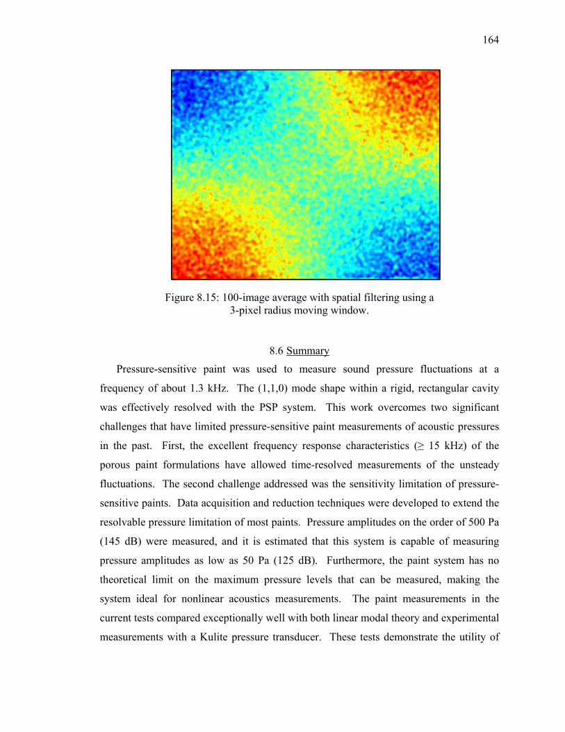
164

Figure 8.15: 100-image average with spatial filtering using a 3-pixel radius moving window.

8.6 Summary

Pressure-sensitive paint was used to measure sound pressure fluctuations at a

frequency of about 1.3 kHz. The (1,1,0) mode shape within a rigid, rectangular cavity

was effectively resolved with the PSP system. This work overcomes two significant

challenges that have limited pressure-sensitive paint measurements of acoustic pressures

in the past. First, the excellent frequency response characteristics (≥ 15 kHz) of the

porous paint formulations have allowed time-resolved measurements of the unsteady

fluctuations. The second challenge addressed was the sensitivity limitation of pressure-

sensitive paints. Data acquisition and reduction techniques were developed to extend the

resolvable pressure limitation of most paints. Pressure amplitudes on the order of 500 Pa

(145 dB) were measured, and it is estimated that this system is capable of measuring

pressure amplitudes as low as 50 Pa (125 dB). Furthermore, the paint system has no

theoretical limit on the maximum pressure levels that can be measured, making the

system ideal for nonlinear acoustics measurements. The paint measurements in the

current tests compared exceptionally well with both linear modal theory and experimental

measurements with a Kulite pressure transducer. These tests demonstrate the utility of

165

pressure-sensitive paint for making acoustics measurements. The pressure-sensitive paint

data provides a complete time-history of the pressure at over 137,000 pixel locations

across the 365-cm2 area of the cavity. As such, the paint system is a distributed array of

nano-scale optical microphones. The pressure-sensitive paint system described in this

work may be applied to tests where high spatial resolution is required, such as nonlinear

acoustics, ultrasonic measurements, and acoustics in MEMS devices.

166

CHAPTER 9: CHARACTERIZATION OF THE HARTMANN OSCILLATOR

The Hartmann tube is a device that generates high-intensity sound through the

oscillation of a shock wave. Shock oscillations are created by the flow of an

underexpanded jet interacting with a resonance cavity. Recent interest in the Hartmann

tube has focused on using the high-intensity sound for flow-control applications. In this

work, pressure-sensitive paint (PSP) was used to characterize the unsteady flowfield of

the Hartmann tube. PSP effectively resolved the shock oscillations at 12 kHz.

Furthermore, PSP was used to measure propagating acoustic waves emanating from the

Hartmann tube. This work provides new insight into the relationship between the

unsteady fluid dynamics and acoustics of the Hartmann tube – including the nature of the

shock oscillations, unsteady flow interaction with the resonance cavity, and directionality

of the radiated sound.

9.1 Introduction

The Hartmann tube is a device that generates large-amplitude sound waves through

the oscillation of a shock wave. Julius Hartmann discovered this phenomenon as he

moved a pitot probe throughout an underexpanded jet, and first reported his results in

1919.140 Hartmann observed that the pressure measured by the pitot probe fluctuated

cyclically at certain locations in the jet of air, which he referred to as “intervals of

instability”. Hartmann’s later experiments with schlieren imaging141-147 revealed that the

sound generation is due to oscillation of the shock wave. The operating principle of the

Hartmann tube is depicted in Figure 9.1, with flow coming from a jet nozzle on the left

and flowing into a typical resonance cavity on the right. The oscillation cycle is

characterized by two primary phases indicated in the diagram, (a) filling of the resonance

cavity, and (b) discharge of flow from the cavity. When the exhausting flow from the

167

cavity meets the oncoming flow from the jet, the two jets disperse radially, as shown in

Figure 9.1(b). The motion of the external shock wave is driven by the periodic nature of

the flow entering and exiting the resonance cavity. The shock position and range of

motion are dependent upon the axial location of the resonance cavity with respect to the

shock-cell structure of the impinging jet, shown for a typical underexpanded jet in Figure

9.2. According to Powell and Smith,148 the maximum range of shock motion is limited to

within one cell of the shock structure. Thus, both the frequency and amplitude of the

shock oscillations are dependent upon the location of the resonance cavity along the axis

of the underexpanded jet. In addition, Thompson has shown that the oscillation

frequency depends on wave propagation within the resonance cavity.149 Thus, the length

of the resonance cavity also has an influence on the oscillation frequency. Finally, the

diameter of the resonance cavity has been shown to have an influence on the intensity of

the radiated sound from the Hartmann tube. Brun and Boucher found that a resonance

cavity diameter from 1.33 to 2.5 times the nozzle diameter produced the highest intensity

sound.150 This is due to the characteristic broadening of an underexpanded jet, and the

need to accommodate the maximum width of the jet within the resonance cavity, without

frictional losses associated with the cavity walls. These three factors – length, depth, and

location of the resonance cavity – can be tailored to maximize the power output and tune

the frequency of the Hartmann tube to arbitrary values over a wide range.

(a)

(b)

Figure 9.1: Conceptual drawing showing the operating mechanism of the Hartmann tube (a) Filling of resonance cavity and (b) cavity discharge (after Brocher et al.151).

168

Figure 9.2: Schlieren image of underexpanded open jet, showing the shock-cell structure.

Several researchers have made modifications to improve the performance of

Hartmann’s original design. Savory experimented with various pads and rings

surrounding the jet to enhance the acoustic power output.152 He also suggested the use of

a stem along the axis of the jet to stabilize the flow. This modification, which Hartmann

and Trudsø also implemented,153 allowed the tube to oscillate even when the jet was

operating in the high-subsonic region. Brun and Boucher,150 and Kurkin154 implemented

a horn-shaped cavity around the Hartmann tube to amplify and direct the propagating

acoustic waves. The size and shape of these cavities were tailored such that acoustic

waves were reflected in phase with the generating waves to amplify the power output. As

such, the horn shapes are wavelength-dependent and must be tailored for one specific

operating frequency of the Hartmann tube. Sprenger,155 Brocher and Aridssone,156 and

Kawahashi et al.,157 introduced a variation on the Hartmann tube by creating stepped or

conical shaped resonance cavities. The change in area inside the resonance cavity serves

to strengthen the propagating shock wave within the cavity. The main intent of changing

the cavity area in these investigations was to increase the heating characteristics of the

tube so that it could be used as an igniter.

Despite being an invention from the early 20th century, the Hartmann tube is

experiencing a resurgent interest in development for flow control applications. The high-

amplitude acoustic fluctuations generated by the Hartmann tube and the high-bandwidth

tunable frequency characteristics have made the Hartmann tube an ideal candidate for an

effective flow control device. Both Raman et al.4 and Kastner and Samimy5,158 have

169

developed the Hartmann tube for flow control applications. Their work has involved

making variable-frequency actuators, characterizing the frequency response and acoustic

output of these devices, and modifying the geometry to improve sound intensity. In

particular, researchers have seen a directivity pattern of the flow field4 that can be

exploited for flow control applications. Some computational work has been done to

explore the fluid mechanics of the directivity pattern.4 There is a need for experimental

data to validate the computational work and provide further insight into the Hartmann

tube flow field.

There is a significant volume of literature regarding the theoretical151,159-161 and

experimental characterization of the Hartmann tube flow field. These measurements,

however, have been limited to qualitative schlieren imaging, or point-wise pressure

measurements. A quantitative and full-field measurement technique is needed to

characterize the flow field to provide information for design of Hartmann tubes as flow

control devices. Porous pressure-sensitive paint, recently developed for unsteady global

pressure measurements, is an ideal tool for characterizing the Hartmann tube flow.

The purposes of this work were three-fold. First, the dynamic response

characteristics of porous pressure-sensitive paint will be demonstrated. Porous paints are

known to have exceptionally fast response characteristics, and the Hartmann tube is a

good high-frequency flowfield to demonstrate the capabilities of porous PSP. Second,

the sensitivity of PSP will be extended such that large-amplitude, propagating acoustic

waves can be measured. Third, both PSP and schlieren imaging techniques will be used

to characterize the unsteady fluid dynamics and acoustics of the Hartmann tube. For flow

control applications, it is important to be able to tailor and direct the injected flow. The

impact of resonance cavity geometry on the fluid dynamics and radiated sound field will

be evaluated.

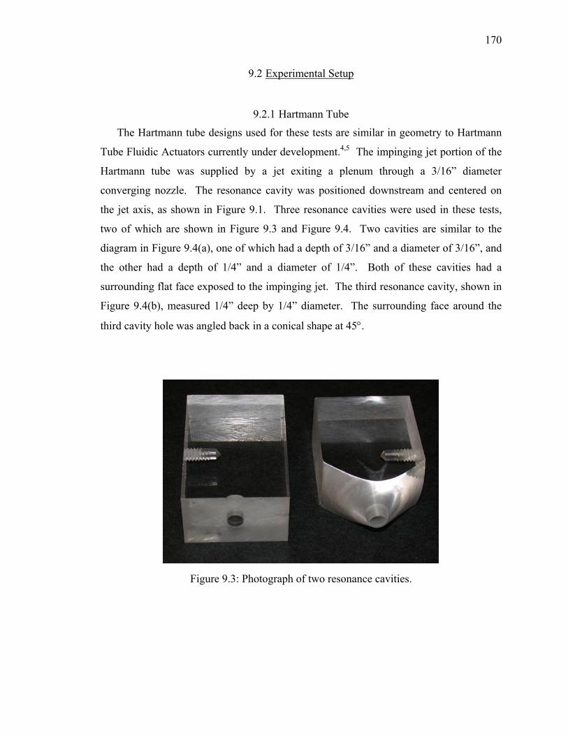
170


9.2.1 Hartmann Tube

The Hartmann tube designs used for these tests are similar in geometry to Hartmann

Tube Fluidic Actuators currently under development.4,5 The impinging jet portion of the

Hartmann tube was supplied by a jet exiting a plenum through a 3/16” diameter

converging nozzle. The resonance cavity was positioned downstream and centered on

the jet axis, as shown in Figure 9.1. Three resonance cavities were used in these tests,

two of which are shown in Figure 9.3 and Figure 9.4. Two cavities are similar to the

diagram in Figure 9.4(a), one of which had a depth of 3/16” and a diameter of 3/16”, and

the other had a depth of 1/4” and a diameter of 1/4”. Both of these cavities had a

surrounding flat face exposed to the impinging jet. The third resonance cavity, shown in

Figure 9.4(b), measured 1/4” deep by 1/4” diameter. The surrounding face around the

third cavity hole was angled back in a conical shape at 45°.

Figure 9.3: Photograph of two resonance cavities.

171

(a)

(b)

Figure 9.4: Geometries for the (a) flat face and (b) 45° angled face resonance cavities. All dimensions are in inches, and the cavity shapes are made from 1” thick acrylic.

9.2.2 Pressure-Sensitive Paint

The experimental setup of the Hartmann tube with PSP instrumentation is shown in

Figure 9.5. Polymer/ceramic was used as the porous binder for the PSP in these tests.

The paint binder was prepared in a manner similar to Scroggin’s procedure,54,55 and

Tris(Bathophenanthroline) Ruthenium Dichloride, (C24H16N2)3RuCl2 from GFS

Chemicals, served as the luminophore. The paint was applied to a 0.020” thick

aluminum sheet by air brush. For measurement of the Hartmann tube flow, the paint

sample was positioned on the edge of the jet, as shown in Figure 9.5. The paint sample

was originally positioned on the centerline of the jet; however the presence of the paint

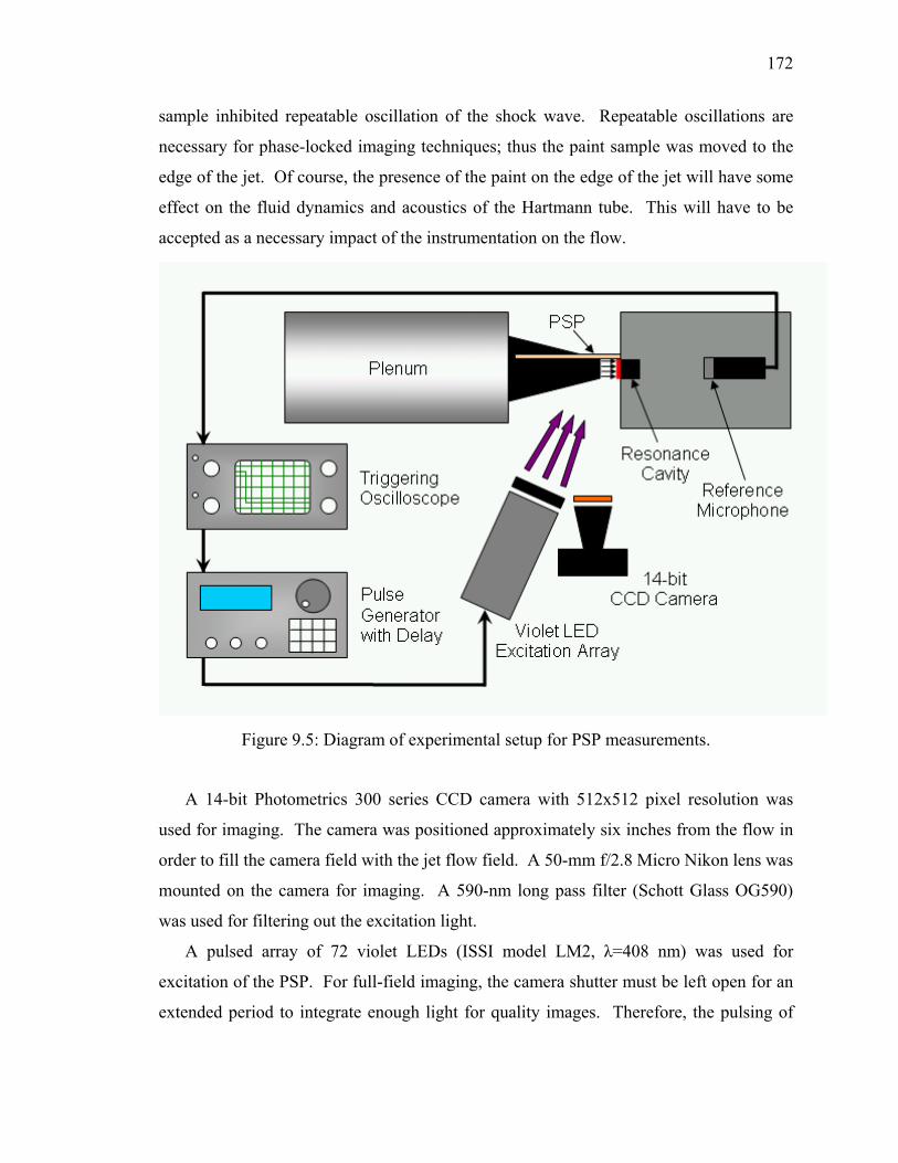
172

sample inhibited repeatable oscillation of the shock wave. Repeatable oscillations are

necessary for phase-locked imaging techniques; thus the paint sample was moved to the

edge of the jet. Of course, the presence of the paint on the edge of the jet will have some

effect on the fluid dynamics and acoustics of the Hartmann tube. This will have to be

accepted as a necessary impact of the instrumentation on the flow.

Figure 9.5: Diagram of experimental setup for PSP measurements.

A 14-bit Photometrics 300 series CCD camera with 512x512 pixel resolution was

used for imaging. The camera was positioned approximately six inches from the flow in

order to fill the camera field with the jet flow field. A 50-mm f/2.8 Micro Nikon lens was

mounted on the camera for imaging. A 590-nm long pass filter (Schott Glass OG590)

was used for filtering out the excitation light.

A pulsed array of 72 violet LEDs (ISSI model LM2, λ=408 nm) was used for

excitation of the PSP. For full-field imaging, the camera shutter must be left open for an

extended period to integrate enough light for quality images. Therefore, the pulsing of

173

the excitation light was phase-locked with the oscillation of the shock wave in order to

capture one point in the oscillation cycle. The strobe rate was synchronized with the

signal of a miniature electret microphone. The microphone signal was passed to an

oscilloscope with a gate function. The gate function produced a TTL pulse with a width

corresponding to the time the scope was triggered on. Thus, the oscilloscope was used to

generate a once-per-cycle TTL pulse. This TTL signal from the oscilloscope was sent to

the external trigger input of a pulse/delay generator (BNC 555-2). The pulse generator,

with variable pulse width and delay, directly strobed the LED array at any arbitrary

phase-locked point in the oscillation cycle. The pulse width of the excitation light was

set at 1 μs, which was less than 1.2% of the oscillation period. Images throughout the

oscillation period were acquired, with a delay of 4 μs between data points. The camera

exposure time for these experiments was on the order of 400 ms.

9.2.3 Schlieren Imaging

A schlieren imaging setup was used to visualize the flowfield of the Hartmann tube.

The experimental setup involved the use of a single-pass schlieren system. The

illumination source was a strobe light, a General Radio company model 1538-A

Strobotac. The flash rate of the strobe light was phase-locked to the Hartmann tube

oscillations in the same manner as used for PSP. A neutral density filter was placed in

front of the strobe light to control the light intensity passing through the flow and

reaching the camera. A 6-inch diameter front-surface concave mirror with a focal length

of 5 feet was used to pass the light through the flowfield. A knife-edge was placed at the

focal point of the mirror to improve the image contrast. The flowfield was then imaged

with a digital video camera.

9.3 PSP Data Reduction

Initially, a dark image was subtracted from all of the data images to remove the dark

current on the CCD and any effects of stray light. The wind-off reference image was

subsequently divided by the particular wind-on image for each phase delay. The intensity

ratio was then converted to pressure through an a priori Stern-Volmer calibration, and in

174

some cases the calibration curve was shifted to match the indicated pressure in the data

set to a known value. Application of spatial filtering, using a 3 pixel by 3 pixel window

size, reduced the spatial noise in the data.


9.4.1 Flat-Face 3/16” Cavity

Initial tests were conducted with the 3/16” resonance cavity with flat face. It was

found that the smaller diameter resonance cavity (3/16”, equal to the jet nozzle diameter)

produced higher-frequency oscillations than the larger cavity (1/4”, 1.3 times the jet

nozzle diameter). The larger cavity, however, produced higher-intensity sound, agreeing

with the results of Brun and Boucher.150 Therefore, the 3/16” resonance cavity, which

produced oscillations at 12 kHz, was used to demonstrate the fast response characteristics

of porous PSP.

The results of the pressure-sensitive paint tests from the Hartmann tube with 3/16”

cavity are shown in Figure 9.6. The nozzle is shown in black on the left side of the

image, with the flow moving from left to right. The resonance cavity is shown in blue on

the right side of the image. The PSP data is shown in the gap between the nozzle and the

cavity. The series of eight images represent eight equally spaced time steps of 10 μs

within the oscillation period of the Hartmann tube. The nozzle pressure ratio (P0/Patm)

was 2.73, which generated flow oscillations at a frequency of 12.0 kHz.

The PSP clearly resolves the pressure field of the oscillating shock wave at each point

within the cycle. Notice the pressure wave near the wall around the resonance cavity.

This pressure wave also oscillates in phase with the shock oscillation, and appears to

interact with the adjacent wall. This fluid-structure interaction will be investigated

further with the 1/4” resonance cavities.

175

Figure 9.6: PSP image sequence depicting shock oscillation, with 10 μs time steps between each image.

psia

176

9.4.2 Flat-Face 1/4” Cavity

PSP and schlieren results from tests with the flat-faced cavity are shown in Figure 9.7

and Figure 9.8, respectively, with the jet flowing from left to right. The nozzle pressure

ratio was 2.47, producing an oscillation frequency of 9.1 kHz. Upon initial inspection, it

is clear that PSP resolves the position of the shock wave at various points in the cycle.

The series of six images in Figure 9.7 are equally spaced with 24 μs time steps, and

represent the entire oscillation period. Likewise, the images in Figure 9.8 are equally

spaced with 16 μs time steps, and also cover the entire period of cavity filling and

exhaust. Exhaust of flow from the resonance cavity is shown in Figure 9.7 (a) through

(c) and Figure 9.8 (a) through (d). Filling of the cavity is shown in Figure 9.7 (d) through

(f) and Figure 9.8 (e) through (h). Several key features of the flow may be noticed. First,

the beginning of the exhaust phase produces quite a sudden movement in shock location,

as seen in the difference between Figure 9.8 (a) and (b). This impulsive shock movement

initiates a strong outward-moving pressure pulse, as seen in the near-field images of

Figure 9.7 (b) through (d). Another interesting feature is that the exhausting flow from

the resonance cavity appears to have an effect on the pressure distribution around the

shock, even altering the shape of the shock itself. There is a certain backwards curvature

to the edges of the shock during the exhaust phase, as can be seen in Figure 9.7 (a). This

curvature is most likely due to the radial interaction of the escaping flow with the

oncoming jet. Furthermore, the interaction of the exhausting flow from the cavity with

the oncoming jet creates regions of high vorticity. In particular, a region of high vorticity

may be seen in the upper portion of Figure 9.8 (c). These vortical structures are then

convected radially away from the resonance cavity, as shown in Figure 9.8 (c) through

(h). These regions or vorticity are similar to the observations of Kastner and Samimy5

with their Hartmann Tube Fluidic Actuator. It should be noted that the propagation speed

of the pressure-pulse is much faster than the speed at which the vortical structures are

convected outward.

177

(a)

(b)

(c)

(d)

(e)

(f)

psia

Figure 9.7: PSP image sequence showing shock wave oscillation for the flat resonance cavity with 24 μs time steps.

178

(a) (b) (c) (d)

(e) (f) (g) (h)

Figure 9.8: Schlieren image sequence showing shock wave oscillation for the flat resonance cavity with 16 μs time steps.

179

Further results from the same flow conditions can be seen in the PSP images of

Figure 9.9 and the schlieren images of Figure 9.10. Both sets of images have equal time

delays of 16 μs. One significant feature shown in Figure 9.9 is the outward propagation

of the acoustic wave. The black arrows in each figure mark the approximate leading edge

of the propagating acoustic wave. The pressure fluctuation associated with this wave is

about 0.8 psi from peak-to-peak. This highlights the capability of porous PSP to make

acoustics measurements. The PSP data also indicates that the pressure wave is initiated

by the impulsive outward movement of the shock wave, which may be considered similar

to a vibrating piston. The fluid dynamics in the near-field of the shock oscillation may

also have an impact on the radiation pattern of the emitted sound waves. The schlieren

images of Figure 9.10 agree well with the PSP results, and with the historical results of

Hartmann and Trolle.142,145 Both image sequences begin at approximately the same

phase in the oscillation cycle, at the initiation of the acoustic pressure pulse. The

schlieren images also demonstrate how the acoustic wave rapidly propagates away to the

far-field, compared with the relatively slow convection of the vortical regions away from

the resonance cavity. Approximately three vortical regions, generated by three

successive cycles, can be seen moving up and down the front face of the resonance cavity

in Figure 9.10 (c).

180

(a) (b)

(c)

(d) (e)

(f)

psia

Figure 9.9: PSP image sequence showing acoustic wave propagation for the flat resonance cavity with 16 μs time steps.

181

(a) (b) (c)

(d) (e) (f)

Figure 9.10: Schlieren image sequence showing acoustic wave propagation for the flat resonance cavity with 16 μs time steps.

182

When the Hartmann tube was driven at 9.1 kHz, and phase-locked PSP images were

taken at 4-μs intervals, a total of approximately 28 images were compiled to represent the

entire oscillation cycle. These twenty-eight phase-averaged samples can be reconstructed

to generate an average time history at any point in the measurement area. A typical

pressure time-history of one point is shown in Figure 9.11. Note that the four waveforms

visible are simply a concatenation of the one phase-averaged time-history. This was done

for visualization purposes, and the exact repeatability is only due to the concatenation

process. Notice the steep, rapid rise and decay times of the pressure pulse. This data

sample represents a rich source of information – essentially, a phase-averaged time-

history is available at every spatial point in the image. If the entire 512x512 CCD image

plane is utilized, over 260,000 reconstructed time-histories are available. The volume of

this information is limited primarily by the spatial resolution of the imaging system. This

large volume of data can be reduced to a manageable level by determining the root-mean-

square (RMS) pressure fluctuations for each point in the image plane. Pressure-sensitive

paint inherently measures absolute pressures (rather than dynamic pressures normally

used for determining RMS pressures). Therefore, a mean value of pressure over the

entire time history for each point was subtracted from each location. Once the dynamic

pressure was determined, the RMS pressure fluctuations were calculated by

( ) ( )2

1

1, ,N

rms ii

P x y P x yN =

= ∑ , 9.1

where Pi(x,y) the pressure at a spatial location (x,y), i is the sample within the time

history, and N is the total number of samples in the time history. The RMS pressure

levels throughout the near-field of the flat-face resonance cavity are shown in Figure

9.12. The high pressure-fluctuation levels between the nozzle and resonance cavity are

due to the shock oscillations. Also significant is the circular region of higher RMS

pressures above the shock oscillation region. These pressure fluctuations are most likely

due to the vortical regions created by interaction of exhausting flow with the incoming

jet. From the RMS pressure values, the sound pressure level (SPL) at each point was

calculated by

( ) ( ){ }10, 20log ,rms refSPL x y P x y P= , 9.2

183

where Pref is a reference pressure of 20 μPa. Sound pressure levels throughout the

measurement region are shown in Figure 9.13. The logarithmic scale of SPL data

provides a more useful representation of the pressure fluctuation directivity, since the

fluctuations range over several orders of magnitude. Clearly visible in Figure 9.13 is the

directivity of the near-field flow back towards the jet nozzle. The pressure fluctuations

across the measurement region range from over 170 dB near the oscillating shock wave,

to about 155 dB in peripheral regions. The sound pressure level for the point indicated in

Figure 9.11 is 162 dB. These sound pressure levels are similar to the results obtained by

Raman, et al.4 Pressure fluctuations on this scale are quite suitable for flow control

applications.

Figure 9.11: Reconstructed time history from phase-averaged PSP data for the flat resonance cavity.

Measurement Location

184

Figure 9.12: RMS pressure levels (psi) in the near field of the shock oscillation for the flat resonance cavity.

Figure 9.13: Sound pressure levels (dB, ref. 20 μPa) for the flat resonance cavity.

185

9.4.3 Angled-Face 1/4” Cavity

In order to investigate the effect of the resonance cavity geometry on the near-field

fluid dynamics and far-field acoustics, a 45° angled cavity was made to compare with the

flat-faced cavity. The flow conditions for the angled cavity were tailored such that the

oscillation frequency was matched to that of the flat-faced cavity. Thus, the nozzle

pressure ratio was adjusted slightly to 2.66, producing an oscillation frequency of 9.1

kHz. The small change in pressure required to match the frequency may be due to the

manufacturing tolerances involved in making two resonance cavities of the same

dimensions. The oscillation frequency is quite sensitive to the cavity dimensions,

particularly the depth and distance from the nozzle. The PSP sample used with the

angled cavity is a different shape than the flat-faced cavity, but made from the same batch

of paint.

PSP and schlieren results showing the shock oscillation for the angled cavity are

represented in Figure 9.14 and Figure 9.15, respectively, with the jet flowing from left to

right. As in the flat cavity results, the cavity exhaust phase is shown in Figure 9.14 (a)

through (c) and Figure 9.15 (a) through (d). The cavity filling portion of the cycle is

shown in Figure 9.14 (d) through (f) and Figure 9.15 (e) through (h). As in the flat cavity

results, the shock position is resolved by PSP at various phase-averaged points within the

cycle. Similar regions of vorticity are also visible in the schlieren images of Figure 9.15.

Closer examination of these results, however, reveals key differences. In Figure 9.14 (a),

near the beginning of the exhaust phase, the behavior of the collision of the two jets may

be observed. (Recall the characteristic behavior of the colliding jets shown in Figure 9.1

and described by Brocher et al.151). At this point in the oscillation cycle, the main jet

from the nozzle appears to be deflected normal to the axis of the jet. The jet exhausting

from the cavity, however, appears to be inclined back towards the cavity. At later points

in the cycle (Figure 9.14 (c), for example), the exhausting jet also turns in a direction

normal to the jet axis. Then, again, as the exhaust phase nears completion, the flow

exiting the cavity is redirected back towards the angled cavity. Time-sequence

animations of the data reveal that the position of the exhausting jet is bi-stable, and the

movement between the two states is quite rapid. The results of this exhausting jet

186

oscillation can be seen in the bi-stable flow pattern moving away from the cavity in the

lower portion of Figure 9.15 (b) and (c). This behavior may be explained by reasoning

that the main jet overpowers the exhausting jet at the beginning and end of the exhaust

phase, causing the exhaust flow to be directed back and away from the cavity. During

certain periods within the oscillation cycle, the exhausting jet may actually be attached to

the cavity face. The phenomenon of wall-attachment, called the Coanda effect,34,35 is the

tendency of a free jet to be drawn towards an adjacent wall. If this is the case, then wall

attachment may be capitalized upon to direct flow from the resonance cavity in a

particular direction. It is clear from this data that the geometry of the angled cavity has a

significant impact on the near-field fluid dynamics, when compared to the flow around

the flat-faced cavity.

Measurements of the propagating acoustic waves are shown in Figure 9.16 and Figure

9.17 for PSP and schlieren imaging, respectively. Arrows on the PSP images indicate the

approximate edge of the acoustic wave front. The initiation of the acoustic wave is not

clearly visible in the PSP results, because the near-field fluid dynamics dominates the

pressure field. As the acoustic wave moves out into the far field, however, it is clearly

discernable. The magnitude of the acoustic wave tends to be higher on the nozzle side,

compared to the resonance cavity side. The schlieren images in Figure 9.17 also clearly

show the propagating acoustic wave. Another interesting feature, shown in Figure 9.17

(e) and (f), is the presence of a weaker secondary wave propagating behind the initial

wave front. It is not known whether this wave is a reflection, or if it is generated by the

fluid dynamics of the Hartmann tube.

187

(a)

(b)

(c)

(d)

(e)

(f)

psia

Figure 9.14: PSP image sequence showing shock wave oscillation for the angled resonance cavity with 20 μs time steps.

188

(a) (b) (c) (d)

(e) (f) (g) (h)

Figure 9.15: Schlieren image sequence showing shock wave oscillation for the angled resonance cavity with 16 μs time steps.

189

(a) (b) (c)

(d) (e) (f)

psia

Figure 9.16: PSP image sequence showing acoustic wave propagation for the angled resonance cavity with 12 μs time steps.

190

(a)

(b)

(c)

(d)

(e)

(f)

Figure 9.17: Schlieren image sequence showing acoustic wave propagation for the angled resonance cavity with 16 μs time steps.

191

Root-mean-square pressure values were calculated from Eq. 9.1, and are shown in

Figure 9.18. The RMS pressures clearly indicate the region of shock oscillation, as well

as the directions of the deflected jet and exhausting flow. It is interesting to note that the

bi-stable characteristics of the exhausting jet are shown by the two-lobed directional

pattern of the flow. Sound pressure levels, as calculated by Eq. 9.2, are shown in Figure

9.19. Despite the presence of noise in this data set, there are several interesting features

that may be observed. The direction of the fluid dynamic near-field is clearly inclined

back towards the resonance cavity. This is in agreement with the bi-stable directional

tendency of the exhaust flow. The acoustic directionality in the far field, however, is

stronger on the nozzle side. This indicates that the geometry and near-field fluid

dynamics influence the propagation characteristics of acoustic waves in the far field.

Thus, the propagating acoustic waves have directivity in a different direction than the

near-field fluid dynamics. This behavior is important to consider when designing a

Hartmann tube for flow control purposes.

Figure 9.18: RMS pressure values (psi) in the near field of the shock oscillation for the angled resonance cavity.

192

Figure 9.19: Sound-pressure levels (dB, ref. 20 μPa) for the angled resonance cavity.

9.5 Summary

This work has demonstrated the utility of pressure-sensitive paint for resolving the

pressure field of the Hartmann tube. PSP was able to measure the location and strength

of a shock wave oscillating at a rate of 12 kHz, as well as the propagating acoustic waves

emanating from the Hartmann tube. The global pressure data obtained with PSP has

provided unique insight into the fluid dynamics and acoustics of the Hartmann tube. It

has been found that the exterior shape of the resonance cavity has a significant impact on

the directivity of the propagating acoustic waves, as well as on the near-field fluid

dynamics. It has been shown that the propagation characteristics of the acoustic wave are

different than the near-field fluid dynamics. In flow control applications, either the

acoustics or the fluid-dynamics may be employed for control authority, and care should

be taken to differentiate between the two phenomena.

193

CHAPTER 10: CONCLUSIONS AND RECOMMENDATIONS

10.1 Conclusions

The work has presented two key accomplishments: the study and design of fluidic

oscillators for flow control applications, and the development and application of porous

pressure-sensitive paint for unsteady flowfields. Development work on the fluidic

oscillator began with an investigation of the internal fluid dynamics of the feedback-free

class of oscillators. This study demonstrated that two jets within a mixing chamber

collide to form an oscillating shear layer driven by pairs of counter-rotating vortices.

This oscillatory vortical growth drives the external oscillations of the fluidic device. It

was shown that the fluidic oscillator can operate over a wide range of unequal flow rates

through the internal nozzles. Flow visualization studies at low flow rates revealed a

complex, woven structure of bifurcating jets that rotates in an ensemble motion.

Frequency studies revealed a peculiar mode-hopping behavior at these low flow rates,

where the operating frequency would make a series of jumps. The cause of this mode

hopping is not yet fully understood, but three-dimensional effects are an important factor.

The observed mode-hopping phenomenon is sensitive to the scale of the device, aspect

ratio, inlet geometry, and gas species. Scaling studies revealed that the oscillation rate

could be varied over a wide range of over two orders of magnitude by properly scaling

the device. These studies also determined that the contour of the inlet geometry is critical

for proper operation of the oscillator.

Beyond the basic studies of the oscillator’s fluid dynamics, the devices were

developed for practical flow control applications. A micro-scale version with a jet exit of

350 μm was characterized with PSP measurements and frequency surveys. This micro

fluidic oscillator possessed two different operating regimes that exhibited different

194

external flowfield characteristics. Internal jet transition from laminar to turbulent flow is

the likely mechanism for this observed change. Furthermore, the micro device issued a

very high frequency jet (> 20 kHz) at very low flow rates (~ 1 L/min).

In subsequent work, a miniature fluidic oscillator with a 3 kHz oscillation rate was

coupled with a low-frequency (200 Hz) solenoid valve to create dual-frequency injection.

This new actuator concept can simultaneously provide high-frequency content for mixing

enhancement, and powerful low-frequency content for forcing at the characteristic

frequency of a flowfield. The dual-frequency oscillator can be modulated across a wide

range of supply pressures, carrier frequencies, and duty cycles. In general, the low-

frequency carrier signal could be modified independently of the high-frequency

component of the flowfield.

A second novel actuator concept was developed to address the coupling of frequency

to flow rate in traditional fluidic oscillators. A hybrid oscillator was developed, where

the jet flow was modulated by a piezoelectric bender. This new oscillator successfully

decouples the oscillation frequency from the supply pressure, thereby enhancing the

utility of this device as a closed-loop flow control actuator. The piezo bender serves as a

destabilizing device, causing a wall-attached jet to separate and switch to an opposing

wall in a cyclical fashion. Current design iterations of the piezo-fluidic oscillator have

continuous frequency coverage up to 250 Hz, and discontinuous coverage to over 1.2

kHz. Furthermore, a sonic jet can be modulated by the piezo-fluidic device at low

frequencies at a modulation index of nearly 100%.

Miniature fluidic oscillators of the type investigated in the first few chapters were

applied to a practical flow control application. The oscillators were used to suppress

cavity resonance tones induced by jet-cavity interaction in transonic flow. Blowing from

the fluidic oscillator successfully suppressed the cavity tone by 17.0 dB, while steady

blowing at the same mass flow rate suppressed the tone by only 1.6 dB.

The work in the second part of this dissertation focused on the continued

development of pressure-sensitive paint. This work was an essential prerequisite for the

fluid-dynamic studies of the fluidic oscillator, since the PSP was used extensively as a

diagnostic tool. This work focused on understanding the frequency response limits of

195

various paint formulations. It also provides demonstrations of the paint applied to

unsteady flowfields with high frequency content.

A model was developed for the quenching kinetics of pressure-sensitive paint, and the

full implications on the unsteady response were presented. Two fast-responding paint

formulations – Polymer/ceramic and Fast FIB – were evaluated experimentally and

compared to the model predictions. Both the model and experiments demonstrated that a

pressure-sensitive paint layer responds faster to a decrease in pressure than an increase of

the same magnitude. The model shows excellent agreement with experimental results

obtained with a fluidic oscillator. Ultimately, it was found that these nonlinear effects

only become significant when the characteristic time scale of the flowfield is faster than

the response time of the paint. The polymer/ceramic PSP exhibited no roll-off in

frequency response at 1.59 kHz, indicating that the time constant is less than 630 μs.

Experimental results from Fast FIB, on the other hand, indicated a time constant of

approximately 1.6 ms.

The excellent response characteristics of the polymer/ceramic PSP were highlighted

by the demonstration of the paint for various applications. Polymer/ceramic PSP

resolved the (1,1,0) acoustic mode shape in a rectangular resonance cavity driven by a

speaker at 145 dB. Data acquisition and reduction techniques were developed to enable

measurement of the low-level unsteady pressures. The pressure-sensitive paint results

compared favorably to the analytical solution for the same geometry. A theoretical

minimum-detectable level was also established for the paint system, and a practical

minimum-detectable level was estimated to be 125 dB.

The polymer/ceramic formulation also recorded the 12-kHz oscillating shock wave

generated by a Hartmann oscillator, as well as the propagating acoustic waves. The

Hartmann tube application demonstrated the usefulness of PSP for complex flowfields by

revealing differences in the flow structures between the various cases studied. These

tests showed that there are significant differences between the acoustic near field and the

fluid dynamics generated by the Hartmann tube, which has a bearing on the use of

Hartmann tubes for flow control applications.

196

10.2 Recommendations

In addition to solving several basic and applied problems, this work has also revealed

new questions and opportunities for investigation. The mode-hopping behavior of the

fluidic oscillators at low flow rates is an intriguing effect that demands further study.

Three-dimensional flow visualization techniques are required for an extensive assessment

of the source of the mode-hopping behavior.

Other experimental methods such as particle image velocimetry (PIV) should be used

to investigate the internal fluid dynamics of the oscillator. PIV would reveal greater

insight into the dynamic vortical growth and decay that drives the oscillations. This data

would also serve as a good complement to the pressure-sensitive paint data acquired in

this work.

Further development work must be done with the new piezo-fluidic oscillator in order

to achieve the design goals of 100% modulation of a sonic jet at 1 kHz. These design

improvements will involve the creation of a more compact geometry and the selection of

piezo benders with a higher natural resonance frequency. Another design is also being

constructed that incorporates dual piezoelectric transducers positioned along the

converging region of the power nozzle. Both the piezo-fluidic and dual-frequency fluidic

oscillators will be applied to practical flow control problems such as jet thrust vectoring

and enhancement of mixing.

Further work with pressure-sensitive paints should focus on developing new sensing

techniques that will enhance the sensitivity for PSP in acoustic tests. The porous

pressure-sensitive paint formulations may also be applied to other nonlinear acoustic

problems such as shock waves used in thermoacoustic refrigeration. The effects of

temperature remain a significant issue when applying PSP to various tests, and new paint

formulations should be developed to further reduce or offset the temperature sensitivity.

LIST OF REFERENCES

197

LIST OF REFERENCES

1. Glezer, A. and Amitay, M., "Synthetic jets," Annual Review of Fluid Mechanics, Vol. 34, 2002, pp. 503-529.

2. Wiltse, J. M. and Glezer, A., "Direct excitation of small-scale motions in free shear flows," Physics of Fluids, Vol. 10, No. 8, 1998, pp. 2026-2036.

3. Wiltse, J. M. and Glezer, A., "Manipulation of free shear flows using piezoelectric actuators," Journal of Fluid Mechanics, Vol. 249, 1993, pp. 261-285.

4. Raman, G., Khanafseh, S., Cain, A. B., and Kerschen, E., "Development of high bandwidth powered resonance tube actuators with feedback control," Journal of Sound and Vibration, Vol. 269, No. 3-5, 2004, pp. 1031-1062.

5. Kastner, J. and Samimy, M., "Development and characterization of Hartmann tube fluidic actuators for high-speed flow control," AIAA Journal, Vol. 40, No. 10, 2002, pp. 1926-1934.

6. Gregory, J. W. and Sullivan, J. P., "Characterization of Hartmann Tube Flow with Porous Pressure-Sensitive Paint," AIAA 2003-3713, 33rd Fluid Dynamics Conference, American Institute of Aeronautics and Astronautics, Orlando, FL, 2003.

7. Roth, J. R., Sherman, D. M., and Wilkinson, S. P., "Electrohydrodynamic flow control with a glow-discharge surface plasma," AIAA Journal, Vol. 38, No. 7, 2000, pp. 1166-1172.

8. Stepaniuk, V., Sheverev, V., Otugen, V., Tarau, C., Raman, G., and Soukhomlinov, V., "Sound Attenuation by Glow Discharge Plasma," AIAA Journal, Vol. 42, No. 3, 2004, pp. 545-550.

9. Artana, G., D'Adamo, J., Leger, L., Moreau, E., and Touchard, G., "Flow control with electrohydrodynamic actuators," AIAA Journal, Vol. 40, No. 9, 2002, pp. 1773-1779.

10. Enloe, C. L., McLaughlin, T. E., VanDyken, R. D., Kachner, K. D., Jumper, E. J., and Corke, T. C., "Mechanisms and Responses of a Single Dielectric Barrier Plasma Actuator: Plasma Morphology," AIAA Journal, Vol. 42, No. 3, 2004, pp. 589-594.

198

11. Enloe, C. L., McLaughlin, T. E., VanDyken, R. D., Kachner, K. D., Jumper, E. J., Corke, T. C., Post, M., and Haddad, O., "Mechanisms and Responses of a Single Dielectric Barrier Plasma Actuator: Geometric Effects," AIAA Journal, Vol. 42, No. 3, 2004, pp. 595-604.

12. Magill, J. C. and McManus, K. R., "Exploring the feasibility of pulsed jet separation control for aircraft configurations," Journal of Aircraft, Vol. 38, No. 1, 2001, pp. 48-56.

13. M'Closkey, R. T., King, J. M., Cortelezzi, L., and Karagozian, A. R., "The actively controlled jet in crossflow," Journal of Fluid Mechanics, No. 452, 2002, pp. 325-335.

14. Chiekh, M. B., Bera, J. C., Michard, M., Comte-Bellot, G., and Sunyach, M., "Control of a plane jet by fluidic wall pulsing," AIAA Journal, Vol. 41, No. 5, 2003, pp. 972-975.

15. Rao, N. M., Feng, J., Burdisso, R. A., and Ng, W. F., "Experimental demonstration of active flow control to reduce unsteady stator-rotor interaction," AIAA Journal, Vol. 39, No. 3, 2001, pp. 458-464.

16. Saric, W. S. and Reed, H. L., "Effect of Suction and Weak Mass Injection on Boundary-Layer Transition," AIAA Journal, Vol. 24, No. 3, 1986, pp. 383-389.

17. Raghu, S. and Raman, G., "Miniature Fluidic Devices for Flow Control," FEDSM 99-7526, Proceedings of the ASME Fluids Engineering Division Summer Meeting, 1999.

18. Morris, N. M., An Introduction to Fluid Logic, McGraw-Hill, London, 1973, pp. 58-66.

19. Kirshner, J. M. and Katz, S., Design Theory of Fluidic Components, Academic Press, New York, 1975.

20. Raber, R. A. and Shinn, J. N., "Fluid Amplifier State of the Art, Vol. I: Research and Development - Fluid Amplifiers and Logic," NASA, Contractor Report CR-101, Oct. 1964.

21. Raber, R. A. and Shinn, J. N., "Fluid Amplifier State of the Art, Vol. II: Bibliography," NASA, Contractor Report CR-102, Oct. 1964.

22. Spyropoulos, C. E., "A Sonic Oscillator," Proceedings of the Fluid Amplification Symposium, Vol. III, Harry Diamond Laboratories, Washington, D.C., 1964, pp. 27-51.

23. Viets, H., "Flip-flop jet nozzle," AIAA Journal, Vol. 13, No. 10, 1975, pp. 1375-1379.

199

24. Stouffer, R. D., "Liquid Oscillator Device", U.S. Patent 4,508,267, Issued April 2, 1985.

25. Bowles Fluidics Corporation, http://www.bowlesfluidics.com/about/index.html, 2003, Accessed 5-29-2004.

26. Beale, R. B. and Lawler, M. T., "Development of a wall-attachment fluidic oscillator applied to volume flow metering," Flow: Its measurement and control in science and industry., Vol. 1, ISA, Pittsburgh, PA, USA, 1974, pp. 989-996.

27. Beale, Robert Bonine, "The Design of a Liquid Fluidic Reaction Jet System," M.S. Thesis, Department of Mechanical Engineering, Massachusetts Institute of Technology, Cambridge, MA, 1969.

28. Wang, H., Beck, S. B. M., Priestman, G. H., and Boucher, R. F., "Fluidic pressure pulse transmitting flowmeter," Chemical Engineering Research & Design, Transactions of the Institute of Chemical Engineers, Part A, Vol. 75, No. A4, 1997, pp. 381-391.

29. Raman, G., Raghu, S., and Bencic, T. J., "Cavity Resonance Suppression Using Miniature Fluidic Oscillators," AIAA 99-1900 (Also NASA/TM-1999-209074), 5th Aeroacoustics Conference, American Institute of Aeronautics and Astronautics, Seattle, WA, 1999.

30. Raman, G., Hailye, M., and Rice, E. J., "Flip-flop jet nozzle extended to supersonic flows," AIAA Journal, Vol. 31, No. 6, 1993, pp. 1028-1035.

31. Raman, G., "Using controlled unsteady fluid mass addition to enhance jet mixing," AIAA Journal, Vol. 35, No. 4, 1997, pp. 647-656.

32. Raman, G. and Cornelius, D., "Jet mixing control using excitation from miniature oscillating jets," AIAA Journal, Vol. 33, No. 2, 1995, pp. 365-368.

33. Raman, G., Packiarajan, S., Papadopoulos, G., Weissman, C., and Raghu, S., "Jet thrust vectoring using a miniature fluidic oscillator," FEDSM 2001-18057, Proceedings of the ASME Fluids Engineering Division Summer Meeting, Vol. 1, American Society of Mechanical Engineers, New Orleans, LA, 2001, pp. 903-913.

34. Coanda, Henri, "Device for Deflecting a Stream of Elastic Fluid Projected into an Elastic Fluid", United States Patent 2,052,869, Issued September 1, 1936.

35. Metral, A., "Sur un Phenomene de Deviation des Vienes Fluides et Ses Applications (Effet Coanda)," Proceedings of the 5th International Congress for Applied Mechanics, Cambridge, MA, 1939.

36. Raghu, Surya, "Feedback-Free Fluidic Oscillator and Method", U.S. Patent 6,253,782, Issued July 3, 2001.

http://www.bowlesfluidics.com/about/index.html,

200

37. Raman, G., Rice, E. J., and Cornelius, D. M., "Evaluation of flip-flop jet nozzles for use as practical excitation devices," Journal of Fluids Engineering, Transactions of the ASME, Vol. 116, No. 3, 1994, pp. 508-515.

38. Sakaue, H., Gregory, J. W., Sullivan, J. P., and Raghu, S., "Porous Pressure-Sensitive Paint for Characterizing Unsteady Flowfields," AIAA Journal, Vol. 40, No. 6, 2002, pp. 1094-1098.

39. Gregory, J. W., Sakaue, H., Sullivan, J. P., and Raghu, S., "Characterization of Miniature Fluidic Oscillator Flowfields Using Porous Pressure Sensitive Paint," FEDSM 2001-18058, post-deadline paper, Proceedings of the ASME Fluids Engineering Division Summer Meeting, New Orleans, LA, 2001.

40. Gregory, J. W., Sakaue, H., and Sullivan, J. P., "Fluidic Oscillator as a Dynamic Calibration Tool," AIAA 2002-2701, 22nd Aerodynamic Measurement Technology and Ground Testing Conference, American Institute of Aeronautics and Astronautics, St. Louis, MO, 2002.

41. Gregory, James W., "Unsteady Pressure Measurements in a Turbocharger Compressor Using Porous Pressure-Sensitive Paint," M.S. Thesis, School of Aeronautics and Astronautics, Purdue University, West Lafayette, IN, 2002.

42. Peterson, J. I. and Fitzgerald, R. V., "New Technique of Surface Flow Visualization Based on Oxygen Quenching of Fluorescence," Review of Scientific Instruments, Vol. 51, No. 5, 1980, pp. 670-671.

43. Kavandi, J., Callis, J., Gouterman, M., Khalil, G., Wright, D., Green, E., Burns, D., and McLachlan, B., "Luminescent barometry in wind tunnels," Review of Scientific Instruments, Vol. 61, No. 11, 1990, pp. 3340-3347.

44. Bell, J. H., Schairer, E. T., Hand, L. A., and Mehta, R. D., "Surface pressure measurements using luminescent coatings," Annual Review of Fluid Mechanics, Vol. 33, 2001, pp. 155-206.

45. Liu, T., Campbell, B. T., Burns, S. P., and Sullivan, J. P., "Temperature- and pressure-sensitive luminescent paints in aerodynamics," Applied Mechanics Reviews, Vol. 50, No. 4, 1997, pp. 227-246.

46. Liu, T. and Sullivan, J. P., Pressure and Temperature Sensitive Paints, Springer, New York, 2004.

47. Sakaue, Hirotaka, "Anodized Aluminum Pressure Sensitive Paint for Usteady Aerodynamic Applications," Ph.D. Dissertation, School of Aeronautics and Astronautics, Purdue University, West Lafayette, IN, 2003.

201

48. Asai, K., Iijima, Y., Kanda, H., and Kunimasu, T., "Novel Pressure-Sensitive Coating Based on Anodic Porous Alumina," 30th Fluid Dynamics Conference, Okayama, Japan (in Japanese), 1998.

49. Asai, K., Amao, Y., Iijima, Y., Okura, I., and Nishide, H., "Novel Pressure-Sensitive Paint for Cryogenic and Unsteady Wind Tunnel Testing," AIAA 2000-2527, 21st Aerodynamic Measurement Technology and Ground Testing Conference, American Institute of Aeronautics and Astronautics, Denver, CO, 2000.

50. Teduka, N., Kameda, M., Amao, Y., and Asai, K., "Experimental Investigation on the Time Response of Pressure-Sensitive Paint," Proceedings of the 31st JSASS Annual Meeting, 2000, pp. 218-221 (in Japanese).

51. Sakaue, H. and Sullivan, J. P., "Time response of anodized aluminum pressure-sensitive paint," AIAA Journal, Vol. 39, No. 10, 2001, pp. 1944-1949.

52. Sakaue, H., Sullivan, J. P., Asai, K., Iijima, Y., and Kunimasu, T., "Anodized aluminum pressure sensitive paint in a cryogenic wind tunnel," Proceedings of the 45th International Instrumentation Symposium, May 2-6 1999, Instrumentation in the Aerospace Industry : Proceedings of the International Symposium, Instrument Society of America, Albuquerque, NM, United States, 1999, pp. 337-346.

53. Baron, A. E., Danielson, J. D. S., Gouterman, M., Wan, J. R., Callis, J. B., and McLachlan, B., "Submillisecond response times of oxygen-quenched luminescent coatings," Review of Scientific Instruments, Vol. 64, No. 12, 1993, pp. 3394-3402.

54. Scroggin, A. M., Slamovich, E. B., Crafton, J. W., Lachendro, N., and Sullivan, J. P., "Porous polymer/ceramic composites for luminescence-based temperature and pressure measurement," Materials Research Society Symposium - Proceedings, Vol. 560, 1999, pp. 347-352.

55. Scroggin, Aaron M., "Processing and Optimization of Doped Polymer/Ceramic Composite Films for Luminescence-Based Pressure and Temperature Measurement in Aerodynamic Applications," M.S. Thesis, School of Materials Engineering, Purdue University, West Lafayette, IN, 1999.

56. Asai, K., Nakakita, K., Kameda, M., and Teduka, K., "Recent topics in fast-responding pressure-sensitive paint technology at National Aerospace Laboratory," ICIASF 2001 Record, 19th International Congress on Instrumentation in Aerospace Simulation Facilities, IEEE, Cleveland, OH, USA, 2001, pp. 25-36.

57. Gutmark, E. J. and Grinstein, F. F., "Flow control with noncircular jets," Annual Review of Fluid Mechanics, Vol. 31, 1999, pp. 239-272.

58. White, F. M., Fluid Mechanics, 5th ed., McGraw-Hill, Boston, 2003.

202

59. John, J. E. A., Gas Dynamics, 2nd ed., Prentice-Hall, Englewood Cliffs, NJ, 1984, pp. 416.

60. Sakaue, Hirotaka, "Anodized Aluminum Pressure Sensitive Paint for Usteady Aerodynamic Applications," Ph.D. Dissertation, School of Aeronautics and Astronautics, Purdue University, West Lafayette, IN, 2003.

61. Huang, C. Y., Sakaue, H., Gregory, J. W., and Sullivan, J. P., "Molecular Sensors for MEMS," AIAA 2002-0256, 40th Aerospace Sciences Meeting, American Institute of Aeronautics and Astronautics, Reno, NV, 2002.

62. Miller, D. N., Yagle, P. J., Bender, E. E., Smith, B. R., and Vermeulen, P. J., "A Computational Investigation of Pulsed Injection into a Confined, Expanding Crossflow," AIAA 2001-3026, 31st Fluid Dynamics Conference and Exhibit, American Institute of Aeronautics and Astronautics, Anaheim, CA, 2001.

63. Yagle, P. J., Miller, D. N., Bender, E. E., Smith, B. R., and Vermeulen, P. J., "A Computational Investigation of Pulsed Ejection," AIAA 2002-3278, 1st Flow Control Conference, American Institute of Aeronautics and Astronautics, St. Louis, MO, 2002.

64. Miller, W. V., "Experimental Feasibility Study of an Analog Electrical-to-Fluidic Transducer," IEEE Transactions on Industrial Electronics and Control Instrumentation, Vol. IECI-16, No. 1, 1969, pp. 50-58.

65. Tesar, V., "The Guided Jet Principle," Fluidics Quarterly, Vol. 3, No. 4, 1971, pp. 77-99.

66. Taft, C. K. and Herrick, B. M., "A Proportional Electro-Fluidic Pneumatic Valve Design," 20th Anniversary of Fluidics Symposium, American Society of Mechanical Engineers, New York, 1980, pp. 1-7.

67. Taft, C. K. and Herrick, B. M., "A Proportional Piezoelectric Electro-Fluidic Pneumatic Valve Design," Journal of Dynamic Systems, Measurement, and Control, Vol. 103, No. 4, 1981, pp. 361-365.

68. Chen, R. and Lucas, G. G., "Investigation into the use of piezo-fluidic combined units as fuel injectors for natural gas engines," Proceedings of the 1996 International Fall Fuels & Lubricants Meeting & Exposition, Oct 14-17 1996, SAE Special Publications, Vol. 1208, SAE, Warrendale, PA, USA, San Antonio, TX, USA, 1996, pp. 123-134.

69. Chen, R., "Piezo-fluidic gaseous fuel MPI system for natural gas fuelled IC engines," JSME International Journal, Series B: Fluids and Thermal Engineering, Vol. 44, No. 1, 2001, pp. 158-165.

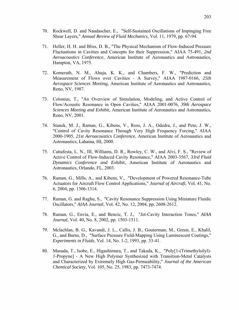
203

70. Rockwell, D. and Naudascher, E., "Self-Sustained Oscillations of Impinging Free Shear Layers," Annual Review of Fluid Mechanics, Vol. 11, 1979, pp. 67-94.

71. Heller, H. H. and Bliss, D. B., "The Physical Mechanism of Flow-Induced Pressure Fluctuations in Cavities and Concepts for their Suppression," AIAA 75-491, 2nd Aeroacoustics Conference, American Institute of Aeronautics and Astronautics, Hampton, VA, 1975.

72. Komerath, N. M., Ahuja, K. K., and Chambers, F. W., "Prediction and Measurement of Flows over Cavities - A Survey," AIAA 1987-0166, 25th Aerospace Sciences Meeting, American Institute of Aeronautics and Astronautics, Reno, NV, 1987.

73. Colonius, T., "An Overview of Simulation, Modeling, and Active Control of Flow/Acoustic Resonance in Open Cavities," AIAA 2001-0076, 39th Aerospace Sciences Meeting and Exhibit, American Institute of Aeronautics and Astronautics, Reno, NV, 2001.

74. Stanek, M. J., Raman, G., Kibens, V., Ross, J. A., Odedra, J., and Peto, J. W., "Control of Cavity Resonance Through Very High Frequency Forcing," AIAA 2000-1905, 21st Aeroacoustics Conference, American Institute of Aeronautics and Astronautics, Lahaina, HI, 2000.

75. Cattafesta, L. N., III, Williams, D. R., Rowley, C. W., and Alvi, F. S., "Review of Active Control of Flow-Induced Cavity Resonance," AIAA 2003-3567, 33rd Fluid Dynamics Conference and Exhibit, American Institute of Aeronautics and Astronautics, Orlando, FL, 2003.

76. Raman, G., Mills, A., and Kibens, V., "Development of Powered Resonance-Tube Actuators for Aircraft Flow Control Applications," Journal of Aircraft, Vol. 41, No. 6, 2004, pp. 1306-1314.

77. Raman, G. and Raghu, S., "Cavity Resonance Suppression Using Miniature Fluidic Oscillators," AIAA Journal, Vol. 42, No. 12, 2004, pp. 2608-2612.

78. Raman, G., Envia, E., and Bencic, T. J., "Jet-Cavity Interaction Tones," AIAA Journal, Vol. 40, No. 8, 2002, pp. 1503-1511.

79. Mclachlan, B. G., Kavandi, J. L., Callis, J. B., Gouterman, M., Green, E., Khalil, G., and Burns, D., "Surface Pressure Field-Mapping Using Luminescent Coatings," Experiments in Fluids, Vol. 14, No. 1-2, 1993, pp. 33-41.

80. Masuda, T., Isobe, E., Higashimura, T., and Takada, K., "Poly[1-(Trimethylsilyl)-1-Propyne] - A New High Polymer Synthesized with Transition-Metal Catalysts and Characterized by Extremely High Gas-Permeability," Journal of the American Chemical Society, Vol. 105, No. 25, 1983, pp. 7473-7474.

204

81. Asai, K., Amao, Y., Iijima, Y., Okura, I., and Nishide, H., "Novel pressure-sensitive paint for cryogenic and unsteady wind-tunnel testing," Journal of Thermophysics and Heat Transfer, Vol. 16, No. 1, 2002, pp. 109-115.

82. Puklin, E., Carlson, B., Gouin, S., Costin, C., Green, E., Ponomarev, S., Tanji, H., and Gouterman, M., "Ideality of pressure-sensitive paint. I. Platinum tetra(pentafluorophenyl)porphine in fluoroacrylic polymer," Journal of Applied Polymer Science, Vol. 77, No. 13, 2000, pp. 2795-2804.

83. Kameda, M., Tezuka, N., Hangai, T., Asai, K., Nakakita, K., and Amao, Y., "Adsorptive pressure-sensitive coatings on porous anodized aluminium," Measurement Science & Technology, Vol. 15, No. 3, 2004, pp. 489-500.

84. Gregory, J. W., Sullivan, J. P., Raman, G., and Raghu, S., "Characterization of a Micro Fluidic Oscillator for Flow Control," AIAA 2004-2692, 2nd Flow Control Conference, American Institute of Aeronautics and Astronautics, Portland, OR, 2004.

85. Gregory, J. W., "Porous Pressure-Sensitive Paint for Measurement of Unsteady Pressures in Turbomachinery," AIAA 2004-0294, 42nd Aerospace Sciences Meeting, American Institute of Aeronautics and Astronautics, Reno, NV, 2004.

86. Maccallum, J. R. and Rudkin, A. L., "Novel Technique for Measuring the Diffusion Constant of Oxygen in Polymer-Films," European Polymer Journal, Vol. 14, No. 9, 1978, pp. 655-656.

87. Cox, M. E. and Dunn, B., "Oxygen Diffusion in Poly(Dimethyl Siloxane) Using Fluorescence Quenching .1. Measurement Technique and Analysis," Journal of Polymer Science Part A-Polymer Chemistry, Vol. 24, No. 4, 1986, pp. 621-636.

88. Carraway, E. R., Demas, J. N., and DeGraff, B. A., "Photophysics and Oxygen Quenching of Transition-Metal Complexes on Fumed Silica," Langmuir, Vol. 7, No. 12, 1991, pp. 2991-2998.

89. Mills, A. and Chang, Q., "Modeled Diffusion-Controlled Response and Recovery Behavior of A Naked Optical Film Sensor with A Hyperbolic-Type Response to Analyte Concentration," Analyst, Vol. 117, No. 9, 1992, pp. 1461-1466.

90. Yekta, A., Masoumi, Z., and Winnik, M. A., "Luminescence measurements of oxygen permeation and oxygen diffusion in thin polymer films," Canadian Journal of Chemistry-Revue Canadienne de Chimie, Vol. 73, No. 11, 1995, pp. 2021-2029.

91. Masoumi, Z., Stoeva, V., Yekta, A., Pang, Z., Manners, I., and Winnik, M. A., "Luminescence quenching method for probing the diffusivity of molecular oxygen in highly permeable media," Chemical Physics Letters, Vol. 261, No. 4-5, 1996, pp. 551-557.

205

92. Vasil'ev, V. V. and Borisov, S. M., "Optical oxygen sensors based on phosphorescent water-soluble platinum metals porphyrins immobilized in perfluorinated ion-exchange membrane," Sensors and Actuators B-Chemical, Vol. 82, No. 2-3, 2002, pp. 272-276.

93. Ruffolo, R., Evans, C. E. B., Liu, X. H., Ni, Y. Z., Pang, Z., Park, P., McWilliams, A. R., Gu, X. J., Lu, X., Yekta, A., Winnik, M. A., and Manners, I., "Phosphorescent oxygen sensors utilizing sulfur-nitrogen-phosphorus polymer matrixes: Synthesis, characterization, and evaluation of poly(thionylphosphazene)-b-poly(tetrahydrofuran) block copolymers," Analytical Chemistry, Vol. 72, No. 8, 2000, pp. 1894-1904.

94. Lu, X. and Winnik, M. A., "Luminescence quenching in polymer/filler nanocomposite films used in oxygen sensors," Chemistry of Materials, Vol. 13, No. 10, 2001, pp. 3449-3463.

95. Jayarajah, C. N., Yekta, A., Manners, I., and Winnik, M. A., "Oxygen diffusion and permeability in alkylaminothionylphosphazene films intended for phosphorescence barometry applications," Macromolecules, Vol. 33, No. 15, 2000, pp. 5693-5701.

96. Kneas, K. A., Demas, J. N., Nguyen, B., Lockhart, A., Xu, W. Y., and DeGraff, B. A., "Method for measuring oxygen diffusion coefficients of polymer films by luminescence quenching," Analytical Chemistry, Vol. 74, No. 5, 2002, pp. 1111-1118.

97. Liu, T., Teduka, N., Kameda, M., and Asai, K., "Diffusion timescale of porous pressure-sensitive paint," AIAA Journal, Vol. 39, No. 12, 2001, pp. 2400-2402.

98. Schairer, E. T., "Optimum thickness of pressure-sensitive paint for unsteady measurements," AIAA Journal, Vol. 40, No. 11, 2002, pp. 2312-2318.

99. Carroll, B. F., Abbitt, J. D., Lukas, E. W., and Morris, M. J., "Step response of pressure-sensitive paints," AIAA Journal, Vol. 34, No. 3, 1996, pp. 521-526.

100. Winslow, N. A., Carroll, B. F., and Kurdila, A. J., "Model development and analysis of the dynamics of pressure-sensitive paints," AIAA Journal, Vol. 39, No. 4, 2001, pp. 660-666.

101. Drouillard II, T. F. and Linne, M. A., "Luminescence Lifetime Response of Pressure-Sensitive Paint to a Pressure Transient," AIAA Journal, Vol. 43, No. 5, 2005, pp. 1100-1108.

102. Bird, R. B., Stewart, W. E., and Lightfoot, E. N., Transport Phenomena, Wiley, New York, 1960, pp. Chapter 16: Diffusivity and the Mechanisms of Mass Transport.

206

103. Stern, O. and Volmer, M., "Uber die Abklingungszeit der Fluoreszenz," Physikalische Zeitschrift, Vol. 20, No. 8, 1919, pp. 183-188.

104. Egami, Y., Iijima, Y., and Asai, K., "Hysteresis of Pressure-Sensitive Paint in Cryogenic Wind Tunnels," Proceedings of the 34th Fluid Dynamics Conference, Kochi University, Kochi, Japan (in Japanese), 2002.

105. Teduka, N., Kameda, M., Asai, K., Amao, Y., and Nakakita, K., "Adsorptive Pressure-Sensitive Coatings for Unsteady Flow Measurements," Transactions of the Japan Society of Mechanical Engineers.Series B., Vol. 68, No. 669, 2002, pp. 1391-1399.

106. Sakaue, Hirotaka, "Porous pressure sensitive paints for aerodynamic applications," M.S. Thesis, School of Aeronautics and Astronautics, Purdue University, West Lafayette, IN, 1999.

107. Jasra, R. V., Choudary, N. V., and Bhat, S. G. T., "Correlation of sorption behavior of nitrogen, oxygen, and argon with cation locations in zeolite X," Industrial & Engineering Chemistry Research, Vol. 35, No. 11, 1996, pp. 4221-4229.

108. Crawford, G. P., Steele, L. M., Ondris-Crawford, R., Iannacchione, G. S., Yeager, C. J., Doane, J. W., and Finotello, D., "Characterization of the cylindrical cavities of Anapore and Nuclepore membranes," Journal of Chemical Physics, Vol. 96, No. 10, 1992, pp. 7788-7796.

109. deBoer, J. H., The Dynamical Character of Adsorption, 2nd ed., Clarendon Press, Oxford, 1968, pp. 30-32.

110. Fonov, S. D., Engler, R. H., Klein, C., Mihailov, S. V., Mosharov, V. E., Kulesh, V. P., Radchenko, V. N., and Schairer, E., "Pressure sensitive paint for oscillating pressure fields measurements," ICIASF '99 Record: 18th International Conference on Instrumentation in Aerospace Simulation Facilities, Institute of Electrical and Electronics Engineers Inc., Piscataway, NJ, USA, Toulouse Cedex, France, 1999, pp. 24-1.

111. Asai, K., "Status of Pressure Sensitive Paint Technology at National Aerospace Laboratory," ICIASF 1999 Record, 18th International Congress on Instrumentation in Aerospace Simulation Facilities, IEEE, Toulouse, France, 1999.

112. Jordan, J. D., Weaver, W. L., Trump, D. D., Sarka, B., Goss, L. P., Navarra, K. R., and Neal Watkins, A., "Extending PSP technology for the investigation of HCF-related phenomena," Proceedings of the 45th International Instrumentation Symposium, May 2-6 1999, Instrumentation in the Aerospace Industry : Proceedings of the International Symposium, Instrument Society of America, Albuquerque, NM, United States, 1999, pp. 327-336.

207

113. Boerrigter, H. L. and Charbonnier, J. M., "Design and calibration of an unsteady pressure measurement system," ICIASF'97 Record. International Congress on Instrumentation in Aerospace Simulation Facilities, IEEE, Pacific Grove, CA, USA, 1997, pp. 185-194.

114. Davis, P. A. and Zasimowich, R. F., "High Frequency Dynamic Pressure Calibration Technique," Instrumentation in the Aerospace Industry: Proceedings of the 31st International Instrumentation Symposium, Vol. 31, ISA, Research Triangle Park, NC, USA, San Diego, CA, USA, 1985, pp. 59-91.

115. Sakamura, Y., Suzuki, T., Matsumoto, M., Masuya, G., and Ikeda, Y., "Optical measurements of high-frequency pressure fluctuations using a pressure-sensitive paint and Cassegrain optics," Measurement Science & Technology, Vol. 13, No. 10, 2002, pp. 1591-1598.

116. Bilaniuk, N., "Optical Microphone Transduction Techniques," Applied Acoustics, Vol. 50, No. 1, 1997, pp. 35-63.

117. Garthe, D., "Fiber- and integrated-optical microphones based on intensity modulation by beam deflection at a moving membrane," Sensors and Actuators A - Physical, Vol. A37 - A38, 1993, pp. 484-488.

118. Hu, A. and Cuomo, F. W., "Theoretical and experimental study of a fiber optic microphone," Journal of the Acoustical Society of America, Vol. 91, No. 5, 1992, pp. 3049-3056.

119. Vinogradova, E. L., Kapustina, O. A., Reshetov, V. N., Svet, V. D., and Yakovenko, G. N., "Characteristics of an optical microphone using a nematic liquid crystal," Soviet Physics - Acoustics, Vol. 31, No. 1, 1985, pp. 10-12.

120. McGraw, C. M., Shroff, H., Khalil, G., and Callis, J. B., "The phosphorescence microphone: A device for testing oxygen sensors and films," Review of Scientific Instruments, Vol. 74, No. 12, 2003, pp. 5260-5266.

121. Sakaue, Hirotaka, "Anodized Aluminum Pressure Sensitive Paint for Unsteady Aerodynamic Applications," Ph.D. Dissertation, School of Aeronautics and Astronautics, Purdue University, West Lafayette, IN, 2003.

122. Galaitsis, A. G., "Visualization of the Time-Average Pressure Distribution in a Rectangular Resonant Cavity," Journal of the Acoustical Society of America, Vol. 52, No. 5, part 2, 1972, pp. 1569-1571.

123. Chinnery, P. A., Humphrey, V. F., and Beckett, C., "The schlieren image of two-dimensional ultrasonic fields and cavity resonances," Journal of the Acoustical Society of America, Vol. 101, No. 1, 1997, pp. 250-256.

208

124. Smith, D. L., "Experimental Techniques for Acoustic Modal Analysis of Cavities," Inter-noise, 1976, pp. 129-132.

125. Nieter, J. J. and Singh, R., "Acoustic modal analysis experiment," Journal of the Acoustical Society of America, Vol. 72, No. 2, 1982, pp. 319-326.

126. Kung, C.-H. and Singh, R., "Experimental modal analysis technique for three-dimensional acoustic cavities," Journal of the Acoustical Society of America, Vol. 77, No. 2, 1985, pp. 731-738.

127. Knittel, J. D. and Oswald, L. J., "An Experimental Technique for Acoustic Modal Analysis in Three-Dimensional Cavities," SAE paper 870974, Society of Automotive Engineers, 1987, pp. 205-217.

128. Whear, F. R. and Morrey, D., "A technique for experimental acoustic modal analysis," Proceedings of the Institution of Mechanical Engineers.Part C, Journal of Mechanical Engineering Science, Vol. 210, No. c2, 1996, pp. 143-151.

129. Pierce, A. D., Acoustics - An Introduction to Its Physical Principles and Applications, Acoustical Society of America, Woodbury, NY, 1989, pp. 284-287.

130. Wanis, S., Sercovich, A., and Komerath, N. M., "Acoustic Shaping in Microgravity: Higher Order Surface Shapes," AIAA 99-0954, 37th Aerospace Sciences Meeting and Exhibit, American Institute of Aeronautics and Astronautics, Reno, NV, 1999.

131. Coppens, A. B. and Sanders, J. V., "Finite-amplitude standing waves within real cavities," Journal of the Acoustical Society of America, Vol. 58, No. 6, 1975, pp. 1133-1140.

132. Vanhille, C. and Campos-Pozuelo, C., "Numerical simulation of two-dimensional nonlinear standing acoustic waves," Journal of the Acoustical Society of America, Vol. 116, No. 1, 2004, pp. 194-200.

133. Gregory, J. W. and Sullivan, J. P., "The Effect of Quenching Kinetics on the Unsteady Response of Pressure-Sensitive Paint," AIAA Journal, 2005.

134. Liu, T., Guille, M., and Sullivan, J., "Accuracy of Pressure-Sensitive Paint," AIAA Journal, Vol. 39, No. 1, 2001, pp. 103-112.

135. Brown, Owen Clayton, "Low-Speed Pressure Measurements using a Luminescent Coating System," Ph.D. Dissertation, Department of Aeronautics and Astronautics, Stanford University, Stanford, CA, 2000.

136. Woodmansee, M. A. and Dutton, J. C., "Treating temperature-sensitivity effects of pressure-sensitive paint measurements," Experiments in Fluids, Vol. 24, 1998, pp. 163-174.

209

137. Klein, C., Engler, R. H., Fonov, S. D., and Trinks, O., "Pressure sensitive paint measurements on a wing model in a low-speed wind tunnel," ICIASF '99: 18th International Conference on Instrumentation in Aerospace Simulation Facilities, Jun 14-Jun 17 1999, ICIASF Record, International Congress on Instrumentation in Aerospace Simulation Facilities, Institute of Electrical and Electronics Engineers Inc., Piscataway, NJ, USA, Toulouse Cedex, France, 1999, pp. 22-1.

138. Subramanian, C. S., Amer, T. R., Oglesby, D. M., and Burkett, J., "New self-referencing pressure-sensitive-paint measurement," AIAA Journal, Vol. 40, No. 3, 2002, pp. 582-584.

139. Bell, J. H. and Mclachlan, B. G., "Image Registration for Pressure-Sensitive Paint Applications," Experiments in Fluids, Vol. 22, 1996, pp. 78-86.

140. Hartmann, J., "Om en ny Metode til Frembringelse af Lydsvingninger," Kongelige Danske Videnskabernes Selskab Matematisk-Fysiske Meddelelser, Vol. 1, No. 13, 1919.

141. Hartmann, J., "On a New Method for the Generation of Sound Waves," Physical Review, Vol. 20, 1922, pp. 719-727.

142. Hartmann, J. and Trolle, B., "New Investigation on the Air Jet Generator for Acoustic Waves," Kongelige Danske Videnskabernes Selskab Matematisk-Fysiske Meddelelser, Vol. 7, No. 6, 1926.

143. Hartmann, J. and Trolle, B., "A New Acoustic Generator. The Air-Jet-Generator," Journal of Scientific Instruments, Vol. 4, No. 4, 1927, pp. 101-111.

144. Hartmann, J. and Trolle, B., "Modus Operandi of the Air-Jet Pulsator," Kongelige Danske Videnskabernes Selskab Matematisk-Fysiske Meddelelser, Vol. 10, No. 4, 1930.

145. Hartmann, J., "On the Production of Acoustic Waves by means of an Air-jet of a Velocity exceeding that of Sound," The London, Edinburgh and Dublin Philosophical Magazine and Journal of Science, ser.7, Vol. 11, 1931, pp. 926-948, plates VII-XI.

146. Hartmann, J., "Construction, Performance, and Design of the Acoustic Air-Jet Generator," Journal of Scientific Instruments, Vol. 16, 1939, pp. 140-149.

147. Hartmann, J. and Lazarus, F., "The Radiation of the Acoustic Air-Jet Generator derived from direct Observation of the Amplitude of the Aerial Vibrations in the Oscillator," The London, Edinburgh and Dublin Philosophical Magazine and Journal of Science, ser.7, Vol. 29, 1940, pp. 140-147, plates VI-VIII.

210

148. Powell, A. and Smith, T. J. B., "Experiments Concerning the Hartmann Whistle," University of California, Los Angeles, UCLA Report 64-42, Los Angeles, CA, 1964.

149. Thompson, P. A., "Jet driven resonance tube," AIAA Journal, Vol. 2, No. 7, 1964, pp. 1230-1233.

150. Brun, E. and Boucher, R. M. G., "Research on acoustic air-jet generator: new development," Journal of the Acoustical Society of America, Vol. 29, No. 5, 1957, pp. 573-583.

151. Brocher, E., Maresca, C., and Bournay, M. H., "Fluid dynamics of the resonance tube," Journal of Fluid Mechanics, Vol. 43, No. pt.2, 1970, pp. 369-384.

152. Savory, L. E., "Experiments with Hartmann acoustic generator," Engineering, Vol. 170, No. 4411, 1950, pp. 136-138.

153. Hartmann, J. and Trudso, E., "Synchronization of Air-Jet Generators with an Appendix on the Stem Generator," Kongelige Danske Videnskabernes Selskab Matematisk-Fysiske Meddelelser, Vol. 26, No. 10, 1951.

154. Kurkin, V. P., "Sound Generated by a Gas Jet Siren," Soviet Physics - Acoustics, Vol. 7, No. 4, 1962, pp. 357-359.

155. Sprenger, H., "Ueber thermische Effeckte in Resonanzrohen," Mitteilungen aus dem Institut fuer Aerodynamik, Federal Institute of Technology, Zurich, Vol. 21, 1954, pp. 18-35.

156. Brocher, E. and Aridssone, J.-P., "Heating Characteristics of a New Type of Hartmann-Sprenger Tube," International Journal of Heat and Fluid Flow, Vol. 4, No. 2, 1983, pp. 97-102.

157. Kawahashi, M., Bobone, R., and Brocher, E., "Oscillation modes in single-step Hartmann-Sprenger tubes," Journal of the Acoustical Society of America, Vol. 75, No. 3, 1984, pp. 780-784.

158. Samimy, M., Kastner, J., and Debiasi, M., "Control of a High-Speed Impinging Jet using a Hartmann-Tube based Fluidic Actuator," AIAA 2002-2822, 1st AIAA Flow Control Conference, American Institute of Aeronautics and Astronautics, St. Louis, MO, 2002.

159. Gravitt, J. C., "Frequency response of acoustic air-jet generator," Journal of the Acoustical Society of America, Vol. 31, No. 11, 1959, pp. 1516-1518.

160. Morch, K. A., "Theory for mode of operation of Hartmann air jet generator," Journal of Fluid Mechanics, Vol. 20, No. Part 1, 1964, pp. 141-159.

211

161. Kawahashi, M. and Suzuki, M., "Generative mechanism of air column oscillations in a Hartmann-Sprenger tube excited by an air jet issuing from a convergent nozzle," Zeitschrift fur Angewandte Mathematik und Physik, Vol. 30, No. 5, 1979, pp. 797-810.

162. Smith, C. R., Sabatino, D. R., and Praisner, T. J., "Temperature sensing with thermochromic liquid crystals," Experiments in Fluids, Vol. 30, No. 2, 2001, pp. 190-201.

163. Jones, T. V., "The Use of Liquid Crystals in Aerodynamic and Heat Transfer Testing," Proceedings of the Fourth International Symposium on Transport Phenomena in Heat and Mass Transfer, 1992, pp. 1199-1230.

164. Hollingsworth, D. K., Boehman, A. L., Smith, E. G., and Moffat, R. J., "Measurement of temperature and heat transfer coefficient distributions in a complex flow using liquid crystal thermography and true-color image processing," Collected Papers in Heat Transfer 1989: Presented at the Winter Meeting of the ASME, Dec 10-15 1989, American Society of Mechanical Engineers, Heat Transfer Division, (Publication) HTD, Vol. 123, Publ by ASME, New York, NY, USA, San Francisco, CA, USA, 1989, pp. 35-42.

165. Campbell, B. T., Liu, T., and Sullivan, J. P., "Temperature Sensitive Fluorescent Paint Systems," AIAA 94-2483, 18th AIAA Aerospace Ground Testing Conference, American Institute of Aeronautics and Astronautics, Colorado Springs, CO, 1994.

166. Allison, S. W. and Gillies, G. T., "Remote thermometry with thermographic phosphors: instrumentation and applications," Review of Scientific Instruments, Vol. 68, No. 7, 1997, pp. 2615-2650.

167. Baughn, J. W., Byerley, A. R., Butler, R. J., and Rivir, R. B., "Experimental investigation of heat transfer, transition and separation on turbine blades at low Reynolds number and high turbulence intensity," Proceedings of the 1995 ASME International Mechanical Engineering Congress & Exposition, Nov 12-17 1995, American Society of Mechanical Engineers (Paper), ASME, New York, NY, USA, San Francisco, CA, USA, 1995, pp. 14.

168. Batchelder, K. A. and Moffat, R. J., "Surface flow visualization using the thermal wakes of small heated spots," Experiments in Fluids, Vol. 25, No. 2, 1998, pp. 104-107.

169. Rivir, R. B., Baughn, J. W., Townsend, J. L., Butler, R. J., and Byerley, A. R., "Thermal Tuft Fluid Flow Investigation Apparatus with a Color Alterable Thermally Responsive Liquid Crystal Layer", U.S. Patent 5,963,292, Issued October 5, 1999.

212

170. Byerley, A. R., Stormer, O., Baughn, J. W., Simon, T. W., and Van Treuren, K., "A 'cool' thermal tuft for detecting surface flow direction," Transactions of the ASME.Journal of Heat Transfer, Vol. 124, No. 4, 2002, pp. 594.

171. Butler, R. J., Byerley, A. R., Van Treuven, K., and Baughn, J. W., "The effect of turbulence intensity and length scale on low-pressure turbine blade aerodynamics," International Journal of Heat and Fluid Flow, Vol. 22, No. 2, 2001, pp. 123-133.

172. Byerley, A. R., Stormer, O., Baughn, J. W., Simon, T. W., Van Treuren, K. W., and List, J., "Using Gurney flaps to control laminar separation on linear cascade blades," Transactions of the ASME.The Journal of Turbomachinery, Vol. 125, No. 1, 2003, pp. 114-120.

173. Campbell, B. T., Crafton, J. W., Witte, G. R., and Sullivan, J. P., "Laser Spot Heating / Temperature-Sensitive Paint Heat Transfer Measurements," AIAA 98-2501, 20th AIAA Advanced Measurement Technology and Ground Testing Conference, American Institute of Aeronautics and Astronautics, Albuquerque, NM, 1998.

174. Campbell, B. T., "Aerodynamic Losses and Surface Heat Transfer in a Strut / Endwall Intersection Flow," Ph.D. Thesis, School of Aeronautics and Astronautics, Purdue University, West Lafayette, IN, 1999.

175. Johnson, S. M., TPSX Material Properties Database, Web Edition Version 4.1, http://tpsx.arc.nasa.gov, 2003, NASA Ames Research Center, Moffett Field, CA, Accessed 4-23-2004.

176. Maya Simulation, The Thermal Wizard, http://www.mayahtt.com/tmwiz/, 1999, Maya Heat Transfer Technologies, Ltd., Montreal, Quebec, Accessed 4-23-2004.

177. Incropera, F. P. and DeWitt, D. P., Fundamentals of Heat and Mass Transfer, 4th ed., John Wiley & Sons, New York, 1996.

178. Fox, R. W. and McDonald, A. T., Introduction to Fluid Mechanics, 5th ed., John Wiley & Sons, New York, 1999.

http://tpsx.arc.nasa.gov,/

http://www.mayahtt.com/tmwiz/,

APPENDICES

213

Appendix A: Flow Visualization with Laser-Induced Thermal Tufts

The laser-induced thermal tuft is a new flow visualization technique for simulating

traditional tufts with a thermal plume. A laser is used to heat a point of interest on a

wind-tunnel model, causing downstream convection of thermal energy from the heated

spot. A temperature-sensitive coating is used to visualize the thermal plume. This

technique can be used to indicate flow direction, locate regions of separated flow, and

detect laminar/turbulent transition. One primary advantage of thermal tufts is that the

measurement technique is less intrusive than traditional tufts. In addition, thermal tufts

may be generated at any optically-accessible point during a test, whereas string tufts must

be applied to specified locations before a test. This enables greater experimental

efficiency, which is particularly important in large-scale ground-testing facilities. This

work extends and develops the thermal tuft concept by employing temperature-sensitive

paint, as well as the previously used thermochromic liquid crystals. The effect of various

substrate materials on tuft quality is evaluated. Calibrations of tuft length dependency on

Reynolds number and laser power are made. Furthermore, a computational model is

developed to simulate the tuft shape and structure. Finally, a new variation of the

technique is presented, based on thermal ablation of the substrate material.

Nomenclature AR = tuft aspect ratio

Cp = specific heat (J/kg/K)

k = thermal conductivity (W/m/K)

l = tuft length (mm)

Rex = Reynolds number, based on distance from nozzle

T = temperature (K)

V = velocity (m/s)

w = tuft width (mm)

x = distance from nozzle to tuft (m)

μ = dynamic viscosity (kg/m/s)

ρ = density (kg/m3)

214

Introduction and Background

Thermal tufts are a relatively new flow-visualization technique, based on the

downstream convection of heat from a locally-heated spot. A traversable laser is used to

heat any optically-accessible point on the model. Temperature-sensitive coatings are

used to detect the thermal plume, while the orientation and shape of the plumes indicate

flow direction and speed. A typical example of a laser-induced thermal tuft is shown in

Figure A.1. Scientific-grade CCD cameras, or even consumer-grade digital cameras may

be used to visualize the flowfield. The technique is unique in that the tufts can be

positioned at any point on a model during a wind-tunnel run, without having to stop the

tunnel for model modification. This allows the experimentalist to maximize productivity

and enables detailed study of regions of interest in the flow. A second significant

advantage of thermal tufts over traditional tufts is the lack of flow interference. The

thermal tuft technique is relatively non-intrusive because the only model modification

required is the application of a thin layer of a temperature-sensitive coating. A diagram

representing the thermal tuft technique is shown in Figure A.2.

Figure A.1: Typical example of a laser-induced thermal tuft, indicating flow from left to right.

The key element of the thermal tuft technique is the sensing layer that coats the

model. The sensing layer can be comprised of thermochromic liquid crystals (TLC),

temperature-sensitive paint (TSP), or thermographic phosphors. Thermochromic liquid

crystals are a temperature-sensitive coating that changes color over a specific temperature

range. The typical progression in colors is from red to green to blue as temperature

increases. The color change may be recorded with any color camera, including

consumer-grade digital cameras. TLCs have commonly been used in aerodynamic

215

applications for measurement of surface temperature and heat transfer properties.162-164

Temperature-sensitive paint is another optical method for measuring surface temperature,

but this technique is based on a change in intensity of the emitted light from the

paint.45,165 An illumination source is required to excite the paint, and a scientific-grade

CCD camera is required to record the change in light level. The intensity of the TSP is

inversely proportional to the surface temperature. A third measurement technique is

thermographic phosphors.166 The experimental methods of the phosphor technique are

similar to temperature-sensitive paint techniques, involving a change of intensity. The

chemical sensor in phosphors produces phosphorescent emission, rather than the

luminescent emission of organic compounds used with TSP.

Figure A.2: Diagram of the thermal tuft concept.

The thermal tuft flow visualization technique was originally proposed in a paper by

Baughn et al. in 1995.167 In this work, they briefly described the laser-induced thermal

tuft method, and used the technique to detect boundary layer separation on a turbine

blade. Several years later, Batchelder and Moffat168 employed the thermal tuft technique

for visualization of flow direction about a cylinder. In this work, however, a laser was

not used to induce the thermal tufts. Instead, an array of heated pins contacted the

surface to generate the tufts on thermochromic liquid crystals. A complete description of

216

the laser-induced thermal tuft technique is in the U.S. Patent awarded to Rivir et al. in

1999.169 Byerley et al.170 created a new variation on the technique by generating cooled

thermal tufts, rather than heated spots. To accomplish this, they affixed reflective spots

on a model and heated the entire model with infrared heaters. Each reflective spot was

cool relative to the rest of the model, and a plume of cooler air created a tuft with a

temperature gradient opposite of the heated-spot technique. In addition to the

aforementioned applications, Butler et al.171 and Byerley et al.172 used the technique to

detect the location and size of a separation bubble on a turbine blade. In Byerley’s

work,172 they defined an eccentricity parameter to quantify the size and shape of the

thermal tuft.

At the time the work presented in this appendix was completed (2000), the authors

were unaware of the existence or prior development of the thermal tuft flow visualization

technique. The authors independently developed this method, based on their expertise in

thermal coatings. The idea in this case came from experiments using a laser spot with

temperature-sensitive paint for heat transfer measurements.173,174 This work builds upon

prior development in the following ways. Various substrate materials are evaluated for

their effect on the size and shape of the thermal tuft. Both flow velocity and incident

laser power affect the characteristics of the thermal tuft, and these effects are

characterized. For a constant laser power, this effectively allows velocity measurement

based on tuft length. A computational model was developed and is presented as a tool for

characterizing the effect of various parameters on tuft geometry. Furthermore,

temperature-sensitive paint is demonstrated as an alternative to thermochromic liquid

crystals as the sensing layer. The final contribution of this work is the demonstration of a

new variation of the thermal tuft technique based on ablation and downstream transport

of molten substrate.

Experimental Setup

A compressible nozzle facility was used to demonstrate the thermal tuft technique, as

shown in the experimental setup diagram in Figure A.3. A solid-state IR laser was used

to heat a spot in the flowfield. The IR laser has a wavelength of 1064 nm and a

217

maximum power output of approximately 277 mW. A variable neutral-density filter

wheel positioned at the laser output controlled the laser power. A Newport laser power

meter (818-SL) was used to measure the output power of the IR laser when attenuated

with the neutral density filter. The compressible nozzle was comprised of a 1.9 cm (3/4”)

jet nozzle, supplied with air from a plenum chamber. The plenum was supplied with

shop air and instrumented with a pressure transducer and thermocouple. The test sample

was placed at a 5° angle with respect to the axis of the nozzle exit. The shallow angle to

the freestream was used, rather than an angle of 0°, to generate longer tufts. Furthermore,

a jet impinging on a plate at a slight angle creates a spread of angular flow across the

surface, providing a more interesting flowfield for flow visualization.

Figure A.3: Diagram of the thermal tuft experimental setup.

The test specimen was a small sample of a temperature-sensing layer – either

temperature-sensitive paint (TSP) or thermochromic liquid crystals (TLC). The

temperature-sensitive paint formulation was composed of the Europium (III)

Thenoyltrifluoro-acetonate, 3-Hydrate (EuTTA) compound. The EuTTA compound was

chosen because it makes for a very bright paint. The EuTTA was mixed in equal parts of

paint thinner and a binder of model airplane dope. The paint was then applied to the

218

substrate by either spraying or brushing. If the TSP was brushed directly on the substrate,

a binder was unnecessary. The temperature-sensitive paint was applied to a heat-

absorbing layer, either black or gray tape in this case. For TSP measurements, an

ultraviolet light source excited the paint, and the tufts were imaged with a 12-bit

scientific-grade CCD camera. A set of optical filters were mounted on the camera lens to

remove the ultraviolet and IR light from the image. The filter set was comprised of a

590-nm long-pass filter for elimination of UV and a 1000-nm short-pass filter for IR.

The thermochromic liquid crystals used in these experiments were in sheet form,

Hallcrest model BM/R29C4W/C11/FA. Table A.1 indicates the color ranges of the

liquid crystals, corresponding to a 4°C bandwidth. This particular liquid crystal sheet

was composed of a black painted background, a layer of liquid crystals, and a 0.125 mm

thick Mylar sheet on top. The sheet has an adhesive backing, which was used to affix the

liquid crystals to an insulating substrate layer. A consumer-grade color digital camera

was used for imaging the thermal tufts, and ambient lighting was used for illumination.

Table A.1: Liquid crystal sheet temperature range.

Color Change Temperature (K) Black to Red 302 Red to Green 303 Green to Blue 306 Blue to Black 323

Results and Discussion

The quality of the thermal tufts is dependent on many parameters. When considering

the concept of the technique (shown pictorially in Figure A.2), the three most dominant

parameters are laser power, flow velocity, and substrate material. The substrate material

affects how much thermal energy is absorbed from the incident IR laser energy. The

radiative heat transfer will depend on the absorptivity of the substrate. The thermal

conductivity of the substrate also dictates the extent of radial conduction of thermal

energy away from the heated spot. An ideal substrate will absorb a large amount of

thermal energy, but conduct little radial heat away from the spot. This will produce a

heated spot with the highest temperature possible, while minimizing the radius of the

219

heated area on the surface. A small heated area will yield a tuft with a smaller radius and

larger aspect ratio (length / width). Similarly, the temperature of the heated spot should

increase with the incident laser power. The velocity of the freestream will have an effect

on the thermal boundary layer, transporting the heat downstream. The boundary layer

characteristics, whether laminar or turbulent, will also have an effect on the downstream

transport and dissipation of heat energy.

The following sections summarize the results from the development of the thermal

tuft technique. Several different substrate materials are evaluated, and qualitative

assessments are made on tuft quality. The responses of the tuft length and width to the

velocity and laser power parameters are characterized. A few experimental observations

are presented, demonstrating the utility of the thermal tuft technique. Furthermore, a

computational model is presented, that allows for evaluation of parameters such as laser

power, flow velocity and direction, etc. In the penultimate section, the thermal tuft

technique is extended to temperature-sensitive paint measurements. Finally, ablative

tufts are demonstrated as a new variation on the thermal tuft technique. The ultimate goal

of these experiments is to understand the mechanisms behind the generation of thermal

tufts, and to evaluate the relevant parameters to optimize the tuft shape.

Selection of Substrate Material

The choice of the substrate material has a significant affect on the quality and size of

the tuft that is generated by the infrared laser. Therefore, a comparison of the tufts

generated with various insulating layers gives an indication of the best material to select

for future experiments. The materials selected for this study are balsa wood on aluminum

sheet backing (oriented with-grain and cross-grain), corrugated cardboard, heavy paper (a

manila file folder), acrylic, plywood (oriented with-grain and cross-grain), a thin

aluminum sheet, and a thick aluminum plate. These materials were chosen due to their

availability, thermal conductivity characteristics, and their potential for use in a wind

tunnel environment. The thermal properties of each of these materials are listed in Table

A.2.175-177 The flow velocity for the substrate material comparisons was 4.9 m/s, and the

laser power was 277 mW.

220

Table A.2: Summary of substrate material thermal properties.

k (W/m/K) ρ (kg/m3) Cp (J/kg/K) Balsa Wood (across grain)175 0.0502 130 2300

Cardboard176 0.064 - - Plywood177 0.12 545 1215

Acrylic175 0.15 1200 1300 Manila Folder (paper)177 0.18 930 1340

Thin Aluminum Sheet (2024-T4)175 118 2780 837 Thick Aluminum Plate (2024-T6)175 177 2770 875

A qualitative comparison between the tufts on each substrate material can be made by

evaluating the images in Figure A.4. The best substrate material appears to be cardboard,

as shown in Figure A.4(b). Other noteworthy substrate materials are balsa wood (a) and

plywood (e and f). Not surprisingly, the substrate materials that provide the highest-

quality tufts are also materials that are inherently good insulators. The low thermal

conductivity of these materials mitigates the radial conduction of thermal energy away

from the laser-heated spot. Notice that both the aluminum sheet and the aluminum plate

produce poor results. This is unfortunate, since many models used in ground testing are

manufactured from metal such as aluminum or stainless steel. One potential solution is

to apply a supplementary insulating layer between the model and the thermochromic

liquid crystals. From a practical standpoint, balsa wood is one of the easiest insulating

materials to apply to a wind tunnel model. For this reason, balsa was used for subsequent

experiments studying the variation of laser power and flow velocity. One important

caveat regarding these results is worth mentioning. Due to limitations in the

experimental facility, it was difficult to position the substrate material in the exact same

position relative to the jet nozzle for each experiment. Thus, there may be a variation in

boundary layer characteristics between the various tests depicted in Figure A.4. The

general trends should be considered reliable, however.

221

Flow Direction

(a) Balsa, with-grain

(b) Corrugated cardboard

(c) Manila folder

(d) Acrylic

(e) Plywood, cross-grain

(f) Plywood, with-grain

(g) Thick aluminum plate

(h) Thin aluminum sheet

Figure A.4: Images of thermal tufts generated with various insulating substrate layers.

One interesting phenomenon is seen in the results for the plywood insulating material

(and also the balsa wood, to a lesser extent). The orientation of the wood grain clearly

affects the shape of the tuft. When Figure A.4(e) is compared with Figure A.4(f) for

plywood, it can be seen that the cross-grain orientation makes the tuft somewhat thicker

in the direction normal to the freestream. This increase in thickness is most likely due to

the anisotropic properties of wood. Thermal conductivity is greater in the grain direction

than the cross-grain direction. Thus, the cross-grain orientation of the wood enlarges the

width of the tuft. Since wider tufts are generally undesirable, the wood grain should be

oriented in a direction parallel to the freestream. A better solution is to use an insulating

material with isotropic thermal properties.

222

Thermal Tuft Response to Velocity Variation

The length of the thermal tufts will vary with respect to the freestream velocity, or

more appropriately, Reynolds number. The tuft geometry can be characterized by

measuring the length and width of the tuft, as shown in Figure A.5. The length (l) is

defined as the distance from the laser spot to the furthest location in the tail of the thermal

tuft. Width (w) is defined as the radius of the tuft, from the laser spot at the center to the

edge. The aspect ratio of the tuft is defined as

lARw

= , A.1

which is similar to the definition proposed by Byerley et al.172 The Reynolds number

associated with a particular flow velocity is calculated by

xVxRe ρμ

= , A.2

where μ is 1.846x10-5 kg/m/s, ρ is 1.152 kg/m3, and x (distance from the nozzle) is

8.34x10-3 m. The velocity for these experiments ranged from 10 up to 60 m/s. The laser

power was a constant 277 mW, with an ambient temperature of 300 K.

Figure A.5: Definition of length (l) and width (w) dimensions on a thermal tuft.

In this analysis, the tuft direction and length were subjectively determined using an

image-processing program. The accuracy of this method is relatively low, but it is

sufficient as an initial proof of concept. One possible improvement to the process would

be to develop an algorithm that determines the laser spot location, and automatically

dimensions the tuft.

223

The uncertainty in velocity measurements ranged from 0.015 to 5.6%, calculated

using the traditional uncertainty formulation found in Appendix F of Fox and

McDonald.178 The uncertainty in the tuft length is less rigorously quantified however.

Each image was analyzed twice to determine repeatability. Analysis shows that an error

of plus or minus 5 pixels in length is typical, corresponding to a measurement error of

plus or minus 0.4 mm. For long tufts at low speed, the edge of the tuft is fairly blurred,

making it difficult to accurately determine the edge. For short tufts (corresponding to

sharp temperature gradients), the edge of the tuft is more well-defined. Analysis of the

images produces data relating the effect of velocity on tuft length and width. This data is

plotted in Figure A.6, along with error bars for velocity and tuft length. This graph

shows that the tuft length decreases as the velocity increases and begins to flatten out at

velocities above about 40 m/s (Reynolds numbers of 20,000). A second order

polynomial curve fit appears to accurately represent the data (although an exponential fit

may fall within the error bars as well). There is not necessarily any physical significance

to the second order fit; rather the polynomial seems to follow the data trend well. The

tuft width is approximately linear and varies much less with velocity than the length,

indicating that this flow visualization technique is much more useful for low-speed flows.

The tuft length curve and tuft width curve should asymptotically approach one another as

speed increases. As the flow rate increases, the air convected from the heated laser spot

has less contact time with the liquid crystals downstream. Therefore, the effect of the

heated spot is not felt as far downstream at high speeds. In the limiting case, the velocity

is too high to cause the crystals to react at all, and the spot size becomes a function of

conduction only. In this case, the tuft length and width would be approximately equal

(AR = 1).

Thermal Tuft Response to Laser Power Variation

Similar experiments for evaluating the effect of incident laser power on the tuft length

reveal an increase in tuft length with laser power. A neutral-density filter wheel was used

at the laser output to attenuate the incident laser energy reaching the surface. The

incident energy was measured at each setting with a laser power meter. The flow

224

velocity was 4.9 m/s, and the ambient temperature was 299 K. The tuft length was

measured in the manner defined by Figure A.5.

Figure A.6: Response of tuft geometry to variation in Reynolds number. Velocity varies from 10 to 60 m/s and laser power is 277 mW.

Results from the laser power variation tests are shown in Figure A.7. Estimated error

in length measurements is the same as the previous case (plus or minus 0.4 mm), and the

accuracy of the power measurements is specified by the manufacturer as ± 3%. One

interesting feature of these results is that the highest laser power produces the longest

tufts with the highest aspect ratio. This is an intuitive result, since the high laser power

will create a large temperature difference between the model surface and the freestream.

Once can expect this temperature gradient to be advected further downstream.

A logarithmic fit is applied to both curves, but in two separate regions. There is a

discontinuity in the slope of the log fit at approximately 100 mW laser power. This

discontinuity is most likely due to melting of the Mylar layer that encapsulates the liquid

crystals, which was observed to occur at 100 mW power. When the Mylar layer melts,

the absorptivity characteristics of the layer must change, affecting the amount of thermal

225

energy imparted to the liquid crystals by the laser. Also, the melted Mylar layer may

introduce small disturbances in the boundary layer, which could affect the length of the

thermal tuft. The quality of the logarithmic fit is a striking feature of the relationship

between tuft length and incident laser power.

Figure A.7: Response of tuft geometry to variation in laser power. Velocity is held constant at 4.9 m/s.

Experimental Observations

Natural Convection The effects of natural convection are a potential source of error that must be

considered when making measurements with thermal tufts. This becomes an issue when

the model or surface being tested is mounted vertically, such that buoyancy forces are no

longer negligible. In the experiments presented in this work, the temperature-sensing

specimen was always mounted in the vertical orientation. An example of a thermal tuft

due to natural convection is shown in Figure A.8. This image represents a case with

quiescent flow conditions. The thermal boundary layer develops because of the

226

buoyancy of the less dense air in the heated region. Byerley, et al.170 have pointed out

that thermal tufts are particularly useful in vertical applications because the

experimentalist does not have to worry about dripping oil from other flow visualization

techniques. While this is true, the experimentalist must be aware of the effects of natural

convection. It was found that natural convection became negligible when the flow

velocity exceeded ~1 m/s. Even in higher-speed flows, however, regions of separated

flow may have very low local flow velocity and natural convection may dominate the

shape of a tuft.

Figure A.8: Thermal tuft at zero flow velocity, demonstrating the effect of natural convection.

Location of Reattachment

It is possible to use the thermal tuft technique to determine the location of separation

and reattachment regions in a flow. In one test, the heated laser spot was placed in a flow

reattachment region. This produced a tuft that actually propagates in two separate flow

directions, as shown in Figure A.9. By traversing the laser and observing the tuft(s), it is

possible to locate the reattachment point accurately. Separation and reattachment in fluid

dynamics are often unsteady phenomena. The thermal tuft technique, however, is

inherently a steady-state flow visualization method. The liquid crystals do not respond

quickly enough to indicate unsteady fluctuations in the flow. This is one limitation of the

thermal tuft method, as compared to traditional string tufts. This should be considered

when making measurements in separated flows or other unsteady flowfields.

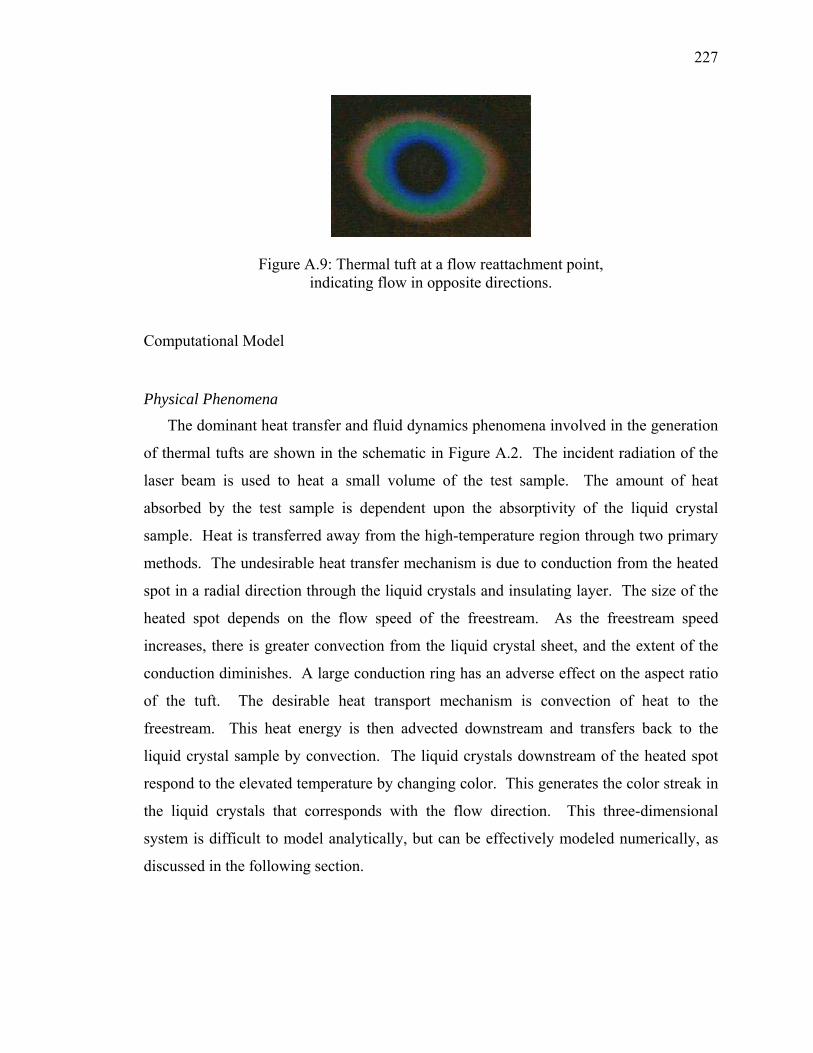
227

Figure A.9: Thermal tuft at a flow reattachment point, indicating flow in opposite directions.

Computational Model

Physical Phenomena

The dominant heat transfer and fluid dynamics phenomena involved in the generation

of thermal tufts are shown in the schematic in Figure A.2. The incident radiation of the

laser beam is used to heat a small volume of the test sample. The amount of heat

absorbed by the test sample is dependent upon the absorptivity of the liquid crystal

sample. Heat is transferred away from the high-temperature region through two primary

methods. The undesirable heat transfer mechanism is due to conduction from the heated

spot in a radial direction through the liquid crystals and insulating layer. The size of the

heated spot depends on the flow speed of the freestream. As the freestream speed

increases, there is greater convection from the liquid crystal sheet, and the extent of the

conduction diminishes. A large conduction ring has an adverse effect on the aspect ratio

of the tuft. The desirable heat transport mechanism is convection of heat to the

freestream. This heat energy is then advected downstream and transfers back to the

liquid crystal sample by convection. The liquid crystals downstream of the heated spot

respond to the elevated temperature by changing color. This generates the color streak in

the liquid crystals that corresponds with the flow direction. This three-dimensional

system is difficult to model analytically, but can be effectively modeled numerically, as

discussed in the following section.

228

Icepak / FLUENT

To complement the experimental results and verify the analysis, a numerical model is

implemented using the Icepak computer program. Icepak is a FLUENT module

specifically designed for electronic component modeling. The goal of the numerical

simulation is to model the experimental setup to a reasonable degree of accuracy, and to

extract useful heat transfer information from the results. At this stage, the goal is not to

produce an accurate tuft length to compare with experimental tufts.

The computational domain (defined as a cabinet in Icepak) measures 25 cm by 16 cm

by 25 cm and is open on every face to ambient conditions (T=299 K). A circular fan with

diameter of 1.9 cm is used to model the nozzle. The fan induces no swirl, and produces a

constant volumetric flow rate of 0.09025 m3/s. This corresponds to a freestream velocity

of 10 m/s. Three plates model the composite test surface, each plate being 24 cm by 14

cm. The composite consists of a 0.125 mm thick Mylar surface coat attached to a 1.040

mm thick slab of balsa wood. A 0.533 mm thick 2024-T6 aluminum backing plate is the

third material. The composite surface is placed at the centerline of the fan to accurately

model the experimental conditions. The thermal properties of the materials are presented

in Table A.3.175,176 The conductivity of balsa wood is for a cross grain orientation. The

material is modeled as an isotropic substance, though it is truly anisotropic.

Table A.3: Thermal properties of backing materials.

k (W/m/K) ρ (kg/m3) Cp (J/kg/K) Balsa Wood (across grain)175 0.0502 130 2300

Mylar176 0.19 1100 2010 Thick Aluminum Plate (2024-T6)175 177 2770 875

The laser spot is modeled by a source on the Mylar surface, 12.7 mm downstream and

at the centerline of the fan. The source is 0.5 mm in diameter and produces 277 mW of

power. This power corresponds to the experimentally measured laser output. In the

experiment, not all of the power emitted by the laser is absorbed by test surface. In this

model however, it is assumed that all of the laser power is absorbed and converted to

thermal energy. This will affect the tuft length, but the general heat transfer

characteristics remain the same. The computational mesh has 150038 elements and

229

155984 nodes. The solution converged in about 200 iterations. The default convergence

criterion was used and an under relaxed solution technique was employed.

The numerically generated thermal tuft is shown in Figure A.10(a). The temperature

range in Figure A.10 corresponds to the temperature range of the thermochromic liquid

crystals. The computational tuft is very similar in form to the tufts produced

experimentally. There is a ring around the laser spot where conduction dominates and a

downstream streak produced by convection. The convection mechanism is described in

detail in the physical phenomena section. The tuft length is not relevant since the laser

power used to produce it is not replicated in experiment. The amount of laser power

absorbed by the liquid crystal layer in the experiments must be determined before the

numerical data can be directly compared to the experimental data.

Figure A.10(b) shows the effect of the heated spot on the air temperature, with the

view being a cross-section of the plate. The composite structure of the model can be seen

in the cross-section. It is clear that the air temperature above the laser spot is heated

locally above 50ºC. This hot air is then advected downstream, producing the streak in the

liquid crystals. The resolution in the wall-normal direction above the spot is low because

the grid in this region is coarse. A course grid in this region was chosen to reduce the

computational time required for convergence.

(a) Top view (b) Side view

Figure A.10: Numerical simulation of a thermal tuft with thermochromic liquid crystals and a balsa wood substrate with flow from left to right.

Temperature-Sensitive Paint Results

Temperature-sensitive paint (TSP) was evaluated as an alternative to thermochromic

liquid crystals (TLC). The primary advantage of TSP over TLC is expanded bandwidth.

The temperature range of liquid crystals is typically limited to about 5°C. Temperature-

230

sensitive paint, however, has a much higher bandwidth – often spanning over several

hundred degrees. The enhanced bandwidth characteristics allow the experimentalist to

record both the very high-temperature region at the laser spot, as well as the temperature

at the end of the tuft which is just above ambient. Another advantage of TSP is the fact

that an arbitrary temperature range is available. Thermochromic liquid crystals must be

tailor-made for a specific temperature range, but TSP allows for a flexible temperature

range when used with thermal tufts. The disadvantages of the TSP technique are that a

scientific-grade CCD camera is required, an ultraviolet light source is required for paint

excitation, and both wind-on and wind-off images must be acquired in order to compute

an intensity ratio of the image pair.

The temperature-sensitive paint experiments largely parallel the development with the

thermochromic liquid crystals. Thus, only example results will be shown to demonstrate

the concept. Typical TSP results of a thermal tuft are shown in Figure A.11. For this

test, the TSP was applied directly to a section of gray tape. The tape served as a layer

designed to absorb thermal energy from the incident laser light. The gray tape was

mounted over an air gap, an alternative to the insulating layers evaluated earlier. The air

gap was used because its thermal conductivity is very low (0.02624 W/m/K).176

Although an air gap produces excellent tufts, the use of this as an insulator on a typical

model in a wind tunnel facility is impractical. Notice that the aspect ratio of the tuft is

excellent – due in part to the use of an air gap insulator, and the high bandwidth of TSP.

Tufts with high aspect ratio were obtained with other insulating layers, even aluminum

sheeting. This indicates that the large bandwidth of temperature-sensitive paint is highly

advantageous.

Figure A.11: Temperature-sensitive paint results.

231

A New Concept: Thermally Ablative Tufts

As testing progressed with temperature-sensitive paint on gray tape, one interesting

variation was discovered. When high power from the incident laser was used, the tape

often melted in the region of the laser spot. This was also observed with the

thermochromic liquid crystals, when laser energy over 100 mW melted the Mylar layer.

The interesting feature with the TSP and gray tape, however, is that the molten tape

would often be transported downstream of the laser spot. As the molten tape moved

downstream, it would permanently change the intensity characteristics of the

temperature-sensitive paint by removing or covering the TSP dye. This effectively

created a permanent tuft that indicates flow direction. The downstream transport of

molten tape would often take several minutes to complete. Thus, this is a steady flow

visualization technique.

The most valuable aspect of this thermal ablation is the high aspect ratio of the tufts

that it generates. The width of the tuft is on the order of the laser spot diameter (less than

1 mm), but the transport length is approximately 10 to 20 diameters long, depending on

flow velocity. One striking example of the ablative tuft technique is shown in Figure

A.12. The laser spot was traversed to eight independent, equally-spaced locations along

the TSP surface. The line of laser spots was perpendicular to the axis of the impinging

jet. The spread of the jet impinging on the plate is clearly visible. Also striking is the

varying length of the ablative tufts, representing regions of varying velocity. Since

thermal ablation is involved, and the intensity characteristics of the paint are changed, the

ablative tufts produce a permanent change in the paint layer. The thermally ablative tuft

may have application to wind tunnel tests where a permanent record of flow velocity and

direction is desired, which can be examined and recorded closely after a run has been

completed.

232

Figure A.12: Thermally ablative tufts with temperature-sensitive paint with impinging flow from left to right.

Summary

This work has demonstrated the utility of thermal tufts as a flow visualization

technique. Various substrate materials were qualitatively evaluated for suitability;

cardboard, balsa, and plywood provided the best results since they are materials with low

thermal conductivity. The variation of tuft length with laser power and flow velocity was

characterized, with the tufts demonstrating a logarithmic relationship between laser

power and tuft length. The thermal tuft technique was applied to the visualization of

natural convection and flow separation / reattachment phenomena. Furthermore, a

computational model was developed that may be used to evaluate the tuft response to

parameters such as laser power, substrate material, substrate thickness, flow velocity, or

angle of attack. The thermal tuft technique was also extended to temperature-sensitive

paints, which provided better visualization results due to the high bandwidth of TSP.

Finally, a new variation of the thermal tuft technique was developed, based on the

ablation and downstream transport of molten substrate material. Thus, the laser-induced

thermal tuft technique is an excellent alternative to traditional flow visualization

techniques in ground-testing environments.

233

Appendix B: PSP Measurements with a High-Speed Camera

Most measurements with pressure-sensitive paint for unsteady flowfields involve

phase-locking techniques. This requires that the flowfield be repeatable and eliminates

the possibility of measuring one-time pressure transients. The alternative is to use a high-

speed camera with a frame rate fast enough to capture the unsteady phenomenon.

Modern high-speed cameras, however, typically do not have the bit-depth resolution

necessary for quality pressure-sensitive paint measurements. Colleagues in Japan at the

Tohoku University Department of Aeronautics and Space Engineering have a newly

developed 10-bit CCD camera with a 1-MHz frame rate, specially manufactured by

Shimadzu. This camera was used to record the real-time fluctuations of the fluidic

oscillator flowfield with pressure-sensitive paint. These tests serve as a proof-of-concept

that high-speed imaging can be effectively used for unsteady PSP measurements, as well

as a validation of the phase-locking technique for repeatable unsteady flowfields.

The test case involved a square-wave fluidic oscillator, the same device that is

characterized in Figure 7.14 and Figure 7.15. The fluidic oscillator was supplied with

nitrogen gas, producing an oscillation frequency of 1.04 kHz. Polymer/ceramic PSP was

used as the paint specimen, which was illuminated by two, large Hamamatsu LED arrays.

The imaging device was the Shimadzu high-speed camera, with a Hamamatsu A4539

image intensifier installed. The frame rate on the camera was 16 kHz, the camera gain

was set at 10x, and the image intensifier gain was set at 4.0. Each video frame had an

exposure time of half the sampling period. A Nikon 105-mm f/2.8 macro lens with a

Kenko 1.5x teleconverter was used for imaging. A Melles Griot long-pass filter with a

590-nm cutoff was used to filter out the excitation light. Signal-to-noise ratio is the

significant limiting factor on the data quality of these tests. Thus, these parameters and

equipment installation were established such that the light captured by the camera could

be maximized.

The resulting data from the high-speed camera tests is very noisy, despite the efforts

to maximize the signal-to-noise ratio. One example image from the fluidic oscillator

measurements is shown in Figure B.1. The structure of the jet is discernable, but the

random noise is significant. Spatial filtering can be employed to reduce the visible

234

structure of the noise in the same manner as used in the acoustic tests. Figure B.2 shows

the same data as Figure B.1, but with a circular disk filter with a radius of five pixels.

This filtering significantly reduces the noise level, but the edges of the jet remain fairly

jagged with many lingering artifacts of the high noise level.

The camera used in these tests offered very high-speed frame rates, but also had a

primary shortcoming. The gain of the camera was not constant in time. This variation in

gain is shown in Figure B.3. There are two sources of fluctuations in the camera gain.

The first is a ±3% variation due to power line source noise (50 Hz in Japan). The other,

more significant noise source is a 10% drop in gain on every 13th frame. Unfortunately,

these are inherent characteristics of the camera, and compensation methods must be

developed.

A series of PSP images recorded by the high-speed camera is shown in Figure B.4.

Here, the delay between images is 125 μs, and a spatial disk filter with 10-pixel radius

was used. A very fast switching time between the two extremes is observed in the bi-

modal jet distribution at ~ 1 kHz. These results compare favorably with the phase-

averaged PSP data presented in Figure 7.14 and Figure 7.15, yielding credibility to the

phase-averaging technique.

Figure B.1: Unfiltered PSP data from the high-speed camera.

235

Figure B.2: Filtered PSP data from the high-speed camera, with a disk radius of 5 pixels.

Figure B.3: Variation in the camera gain.

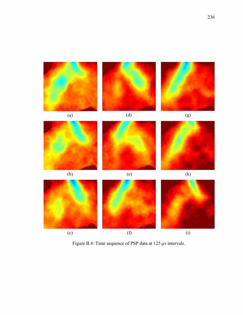
236

(a)

(d)

(g)

(b)

(e)

(h)

(c)

(f)

(i)

Figure B.4: Time sequence of PSP data at 125 μs intervals.

237

VITA

Jim Gregory received his Bachelor of Aerospace Engineering with highest honors in

1999 from the Georgia Institute of Technology. He received his M.S. in Aeronautics and

Astronautics in 2002 from Purdue University with a thesis entitled Unsteady Pressure

Measurements in a Turbocharger Compressor Using Porous Pressure-Sensitive Paint.

He won first place in the 2004 AIAA National Student Paper Competition with a paper

based on his Master’s thesis. He was also a recipient of the AIAA Orville and Wilbur

Wright Graduate Award in 2004. In August of 2005, he completed his Ph.D. work at

Purdue University under the direction of Prof. John Sullivan. His doctoral work was

funded by a NASA Graduate Student Researchers Program Fellowship through NASA

Glenn Research Center.

Dr. Gregory’s research interests include unsteady measurements with pressure-

sensitive paint, and development of flow control actuators such as the fluidic oscillator.

His short-term career goal is to pursue this research in a faculty position in aerospace

engineering at a prominent research university. In autumn of 2005 he will be a policy

fellow at the National Academies in Washington, DC through the Christine Mirzayan

Science & Technology Policy Graduate Fellowship Program. Dr. Gregory’s lifetime

forwarding e-mail address is [email protected].

development of fluidic oscillators as flow control actuators

Documents