modular fluidic propulsion robots
TRANSCRIPT
This is a repository copy of Modular fluidic propulsion robots.
White Rose Research Online URL for this paper:https://eprints.whiterose.ac.uk/166757/
Version: Published Version
Article:
Doyle, M., Marques, J., Vandermeulen, I. et al. (5 more authors) (2021) Modular fluidic propulsion robots. IEEE Transactions on Robotics, 37 (2). pp. 532-549. ISSN 1552-3098
https://doi.org/10.1109/TRO.2020.3031880
[email protected]://eprints.whiterose.ac.uk/
Reuse
This article is distributed under the terms of the Creative Commons Attribution (CC BY) licence. This licence allows you to distribute, remix, tweak, and build upon the work, even commercially, as long as you credit the authors for the original work. More information and the full terms of the licence here: https://creativecommons.org/licenses/
Takedown
If you consider content in White Rose Research Online to be in breach of UK law, please notify us by emailing [email protected] including the URL of the record and the reason for the withdrawal request.
This article has been accepted for inclusion in a future issue of this journal. Content is final as presented, with the exception of pagination.
IEEE TRANSACTIONS ON ROBOTICS 1
Modular Fluidic Propulsion RobotsMatthew J. Doyle , Student Member, IEEE, João V. Amorim Marques , Student Member, IEEE,
Isaac Vandermeulen, Student Member, IEEE, Christopher Parrott, Yue Gu , Student Member, IEEE, Xinyu Xu ,
Andreas Kolling , Senior Member, IEEE, and Roderich Groß , Senior Member, IEEE
Abstract—We propose a novel concept for modular robots,termed modular fluidic propulsion (MFP), which promises to com-bine effective propulsion, a large reconfiguration space, and ascalable design. MFP robots are modular fluid networks. To propel,they route fluid through themselves. In this article, both hydraulicand pneumatic implementations are considered. The robots movetowards a goal by way of a decentralized controller that runs inde-pendently on each module face, uses two bits of sensory informationand requires neither run-time memory, nor communication. Weprove that 2-D MFP robots reach the goal when of orthogonally con-vex shape, or reach a morphology-dependent distance from it whenof arbitrary shape. We present a 2-D hydraulic MFP prototype andshow, experimentally, that it succeeds in reaching the goal in at least90% of trials, and that 71% less energy is expended when modulescan communicate. Moreover, in simulations with 3-D hydraulicMFP robots, the decentralized controller performs almost as wellas a state-of-the-art and centralized controller. Given the simplicityof the hardware requirements, the MFP concept could pave theway for modular robots to be used at sub-centimeter-scale, whereeffective modular propulsion systems have not been demonstrated.
Index Terms—Distributed control, hydraulic propulsion,modular reconfigurable robots, pneumatic propulsion.
I. INTRODUCTION
ONE OF THE principal aims of robotics is to develop
machines that can carry out tasks that are difficult for
Manuscript received December 17, 2019; revised June 20, 2020; acceptedSeptember 17, 2020. This work was supported by the Engineering and PhysicalSciences Research Council under Grant EP/J013714/1. The work of MatthewJ. Doyle was supported by the Engineering and Physical Sciences ResearchCouncil through a Doctoral Training Grant. This article was recommended forpublication by Associate Editor N. Agmon and Editor P. Dupont upon evaluationof the reviewers’ comments. (Matthew J. Doyle and João V. Amorim Marques
contributed equally to this work.) (Corresponding author: Roderich Groß).Matthew J. Doyle, João V. Amorim Marques, Christopher Parrott, Yue Gu,
Xinyu Xu, and Roderich Groß are with Sheffield Robotics, The Universityof Sheffield, S1 3JD Sheffield, U.K. (e-mail: [email protected];[email protected]; [email protected]; [email protected]; [email protected]; [email protected]).
Isaac Vandermeulen is with iRobot, Pasadena, CA 91101 USA (e-mail:[email protected]).
Andreas Kolling is with Amazon Robotics, North Reading, MA 01864 USA(e-mail: [email protected]).
This article has supplementary downloadable material available at http://ieeexplore.ieee.org. The material consists of video clips of MHP robots usingthe occlusion-based controller, both experimentally and in simulation. Theexperiment clips show 2 × 2 robots using both the default controller and avariant with communication enabled. The simulation clips show a 125 modulecubic robot using a controller variant with obstacle avoidance, and a 125 modulerobot of random morphology using the default controller.
Color versions of one or more of the figures in this article are available onlineat https://ieeexplore.ieee.org.
Digital Object Identifier 10.1109/TRO.2020.3031880
humans. This includes working in inhospitable or inaccessi-
ble environments, such as deep water, space, storage tanks,
pipe networks, or even the human vascular network. Modular
self-reconfigurable robots [1], [2] are well suited for these
environments as they can adapt their morphology and func-
tionality to cope with complex tasks and unexpected situations.
Examples include shifting between configurations with longer
reach or greater strength to repair equipment in space [3], using
reconfiguration to deploy and retrieve the modular nodes of
an underwater sensing network [4], or moving through small
apertures and shoring up a damaged structure in a search and
rescue scenario [5]. Additionally, a given system could be used
in a wide range of scenarios, reducing production costs due to
mass manufacture and lowered training time for operators.
Modular reconfigurable robotic systems are yet to realize their
full potential in the real world. We hypothesize that to improve
the general utility, a system should combine all of the following
properties:1
1) effective propulsion: fast and precise movement as a con-
nected robot, independent of modular configuration;
2) large reconfiguration space: a rapid increase of the number
of possible configurations with the number of modules;
3) scalable design: a performance that scales favorably as the
number of modules increases or their size decreases.
Most current systems excel at one or two of the aforemen-
tioned properties, though at the expense of the remaining ones:
Some systems prioritize effective propulsion. The AMOUR
robot [6], distributed flight array (DFA) [7], and ModQuad [8],
[9] are among the most efficacious mobile connected systems,
capable of up to six degrees-of-freedom (DoF) movement. How-
ever, this comes at a cost to reconfiguration: The AMOUR robot
can reconfigure only in 1-D, whereas the DFA and ModQuad
robots can reconfigure only in 2-D. Moreover, current imple-
mentations do not demonstrate a high degree of scalability: The
AMOUR robot relies on a centralized motion controller, the DFA
relies on external sensing, and ModQuad relies on a centralized
path planner. For some other systems, the modules can move
effectively on their own, yet connected robots have only limited
propulsion effectiveness [10]–[13].
Some systems prioritize a large reconfiguration space, but lack
effective movement capabilities as a connected robot [14]–[16].
The M-Blocks [15], for example, can self-assemble into 3-D
structures that produce net movement primarily via progressive
1In addition, the utility of modular systems improves if they are capable ofself-reconfiguration.
1552-3098 © 2020 IEEE. Personal use is permitted, but republication/redistribution requires IEEE permission.See https://www.ieee.org/publications/rights/index.html for more information.
This article has been accepted for inclusion in a future issue of this journal. Content is final as presented, with the exception of pagination.
2 IEEE TRANSACTIONS ON ROBOTICS
repositioning of the modules. As a result, the robot’s propulsion
speed is limited by its reconfiguration speed. M-TRAN [17] can
move effectively in some, but not all configurations.
Some systems prioritize scalability [18]–[20]. Scaling
systems up in number of modules and down in size allows
modular robots to take a given form with a higher resolution.
Such systems should be able to adapt with greater precision to
the task at hand. In addition, decreasing the size of the modules
allows the robots to fit into smaller environments. Current
systems that prioritize scalability exhibit limited propulsion
efficacy. For example, the Pebbles robot [20], while having
an impressive module side-length of only 12 mm, features no
explicit propulsion mechanism. Similarly, claytronics robots can
only ambulate slowly via progressive repositioning of individual
modules [18], [21].
In this article, we introduce the modular fluidic propulsion
(MFP) concept. The concept combines a large reconfiguration
space and scalable design with the ability to move effectively in
any configuration. An MFP robot is a modular fluid network. By
rearranging the constituent modules, robots (i.e., fluid networks)
of different shapes can be built. MFP robots self-propel by
routing fluid through themselves. We consider a directed motion
task, where an MFP robot has to move toward a goal. We present
a fully decentralized motion controller, which is inspired by an
occlusion-based object transportation controller developed for
swarms of mobile robots [22]. The controller runs independently
on each module face, uses 2 bits of sensory information and re-
quires neither run-time memory, nor communication. It could be
realized on hardware that does not offer arithmetic computation,
thereby engendering the future miniaturization of the system.
This article extends preliminary work on a related, hydraulic
propulsion concept [23]. In particular,
1) It proposes the MFP concept, and discusses a pneumatic
implementation in addition to the hydraulic implementa-
tion proposed in [23].
2) It derives the number of unique forces and torques that
2-D orthogonally convex MFP robots can produce.
3) It proposes two novel variants of the decentralized motion
controller presented in [23]: one using communication to
reduce energy consumption; the other using range sensors
to avoid obstacles. By simulation, it evaluates the perfor-
mance of the new variants, and compares them to both the
original controller and/or the state-of-the-art (centralized)
controller in [24].
4) It proves for the first time that 2-D MFP robots reach the
goal or a morphology-dependent distance from it, if of
orthogonally convex or arbitrary shape, respectively.
5) It presents a new, smaller 2-D hydraulic prototype, which
additionally features communication and range sensing.
6) By systematic experiment, it shows that the new prototype
successfully completes the directed motion task when
using the original controller in [23], and that 71% less en-
ergy is expended when using the communication-enabled
variant of this controller.
The rest of this article is organized as follows. Section II
provides further related work. Section III outlines the MFP
concept, along with hydraulic and pneumatic examples of
TABLE IOVERVIEW OF RELATED RECONFIGURABLE MODULAR FLUIDIC SYSTEMS
Number of modules are those within a same experiment (in parenthesis if only simulated).
Data for our system (MFP) are shown in boldface.
implementations. Section IV analyzes the static forces and
torques that an orthogonally convex 2-D MFP robot can gener-
ate. Section V describes the directed motion task and controllers.
Section VI provides a formal analysis of the controllers. Sec-
tion VII presents simulations of a 3-D hydraulic MFP system.
Sections VIII and IX describe a 2-D hydraulic MFP hardware
prototype and the experiments, respectively. Finally, Section X
concludes this article.
II. FURTHER RELATED WORK
We discuss further related work on reconfigurable modular
fluidic systems. In particular, the propulsion capabilities of these
systems are analyzed to serve as points of comparison to the
MFP system (see Table I). We classify the work into two groups,
systems with self-propelling modules, and those which rely on
an external source of propulsion.
A. Self-Propelled Modular Systems
In early work [25], controllers and morphologies for the
Neubot underwater modular robots are evolved. Each module
has six connectors, giving the system a 3-D lattice structure.
Rotational joints between connected modules allow robots to
self-propel in 3-D through coordinated movement.
Hydron modules [26] move underwater in 3-D. An impeller
and collar mechanism controls horizontal movement, whereas a
syringe controls buoyancy, allowing the modules to move verti-
cally. Simulated modules can self-assemble into 3-D structures,
although a connection mechanism is not proposed.
The AMOUR robot can perform 6-DoF motion underwater.
It is conceptualized to self-reconfigure in 1-D, and has manu-
ally reconfigurable thruster pose [6]. The controller can handle
arbitrary thruster configurations. An inertial measurement unit
This article has been accepted for inclusion in a future issue of this journal. Content is final as presented, with the exception of pagination.
DOYLE et al.: MODULAR FLUIDIC PROPULSION ROBOTS 3
provides input to the controller. In [38], the AMOUR robot can
learn its own thruster configuration.
ANGELS [27] is an underwater modular system that can form
chain configurations. Individually, each module can translate
and rotate using propellers. Connected modules can collectively
produce an undulatory swimming motion. Buoyancy can be
controlled using a swim bladder.
The REMORA project [39] examines the use of aquatic
modular robots for the inspection and maintenance of off-shore
structures, such as oil platforms. The robots can move under-
water in 3-D. Furno et al. [28] present a hardware prototype
of the system and perform experiments in which three robots
reconfigure from an “I” shape to an “L” shape.
The tactically expendable marine platform (TEMP) [29] is
envisaged for use as a rapidly deployable structure for hu-
manitarian missions. The modules can self-assemble into 2-D
structures on the surface of water. Both individual modules and
connected structures can self-propel in 2-D.
Naldi et al. [30] study the dynamics and control of a modular
aerial robot. Each module consists of a ducted fan and a set of
vanes that allow the robot to move in 3-D. The design allows
modules to be attached both horizontally and vertically, and still
fly. However, only configurations with horizontal connections
are tested.
Wang et al. [40] introduce the Roboat, a modular robotic
boat with a force-efficient thruster configuration. The modules
can move and reconfigure in 2-D, thereby dynamically forming
floating structures. Docking experiments, in the presence of
turbulent currents, are reported in [41]. The Roboats are further
used for shapeshifting experiments [31].
B. Externally Propelled Modular Systems
Inou et al. [32] develop a set of mechanical modules which
reconfigure by pumping air through a set of bellows but are
not capable of translational motion. The air is provided by an
external pump to each module individually, although the authors
propose a future system for routing air internally from one
module to another. The robots can form a 2-D lattice, although
experiments are restricted to two modules.
White et al. [33] present two systems in which individual
modules move in 3-D inside an oil-filled tank. The oil is agi-
tated externally to provide stochastic motion. The modules can
connect to a base plate to construct immobile 3-D structures. The
modules of one of the systems have a similar internal structure to
the MFP system, allowing fluid to pass through them. However,
they are passive, with no propulsion method or internal energy
source of their own. Tolley et al. [42] and Tolley and Lipson [43]
investigate different self-assembly strategies for similar systems.
The Tribolon system [35] uses vibrating pager motors as a
source of propulsion. This achieves a similar effect to externally
induced stochastic motion. Power is provided externally via a
pantograph. The modules can reconfigure in 2-D.
The Lily robots float on the surface of water, which is agitated
by external submerged pumps [44]. The robots both move and
reconfigure in 2-D. The system is used for the study of stochastic
self-assembly [45], for which the authors develop a simple
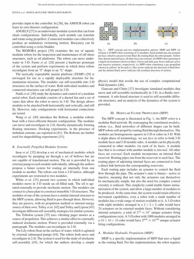
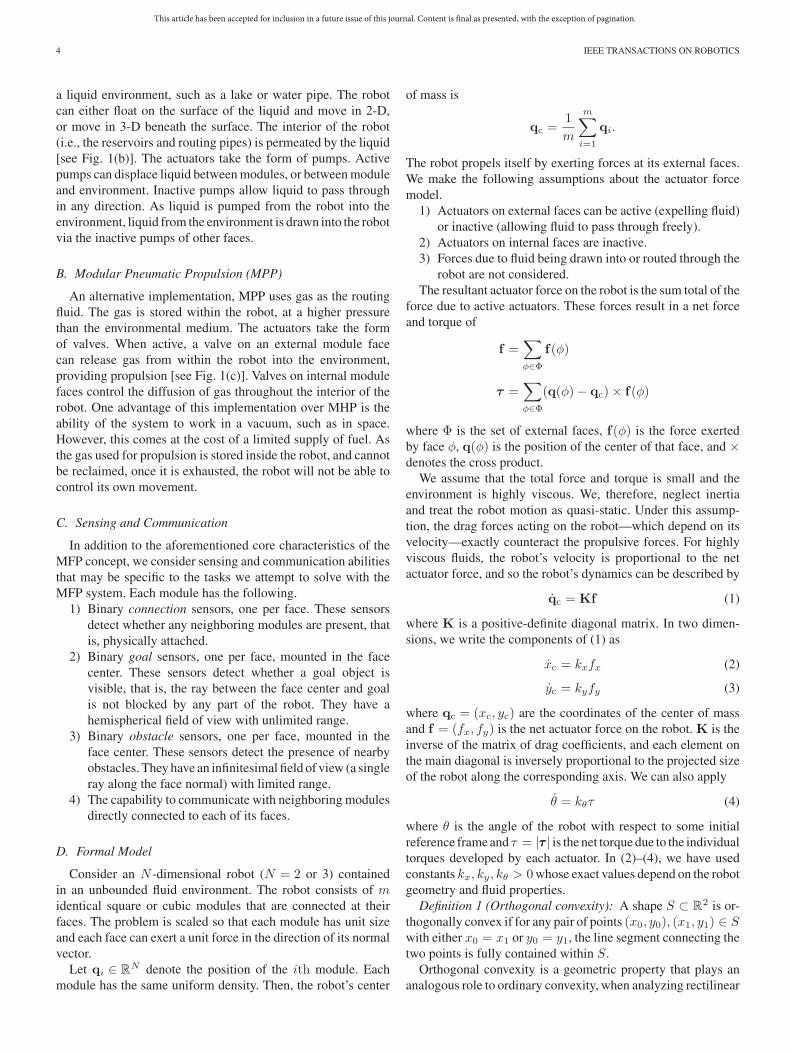
Fig. 1. MFP concept and two implementation options: MHP and MPP. (a)Generic 2-D MFP robot consisting of 12 modules. Each module has one actuatorper face, which it can use to route fluid. By routing fluid, the robot propels. Yellowlines denote internal faces, all other faces are external. (b) MHP robot operating ina liquid environment (shown in blue). Green and dark gray boxes indicate activeand inactive actuators, respectively. (c) MPP robot containing a gas propellant(shown in yellow). In (b) and (c), blue arrows indicate the direction of fluid flow,and the dashed black arrow indicates the resultant direction of motion.
physics model that avoids the use of complex computational
fluid dynamics [46].
Ganesan and Chitre [37] investigate simulated modules that
move and self-assemble stochastically in 3-D, in a fluidic envi-
ronment. A rule-based structure is used to self-assemble differ-
ent structures, and an analysis of the dynamics of the system is
provided.
III. MODULAR FLUIDIC PROPULSION (MFP)
The MFP concept is illustrated in Fig. 1. An MFP robot is a
modular fluid network. By rearranging the constituent modules,
robots (i.e., fluid networks) of different shapes can be built.
MFP robots self-propel by routing fluid through themselves. The
modules are homogeneous squares in 2-D or cubes in 3-D. With
a slight abuse of terminology, we use face to refer to both 3-D
module faces and 2-D module sides. A module can be physically
connected to other modules via each of its faces. A module
face that is in contact with another module is internal. All other
faces are external. Each module incorporates an internal fluid
reservoir. Routing pipes run from the reservoir to each face. The
routing pipes of adjoining internal faces are connected to form
a direct link between the corresponding reservoirs.
Each routing pipe includes an actuator to control the fluid
flow through the pipe. The actuator’s state is binary—active or
inactive, meaning that not only the actuators can themselves
be mechanically simple, but also the need for complex control
circuitry is reduced. This simplicity could enable future minia-
turization of the system, and allow a large number of modules to
be produced. At the same time, the system would retain effective
movement capabilities; even a robot with a small number of
modules has a wide range of motion available to it. A 3-D robot
with eight modules arranged in a 2× 2× 2 cube would have
24 actuators on its external module faces. Without considering
internal actuators, a total of 224 ≈ 107 unique actuator firing
configurations exist. A 3-D robot with 1000 modules arranged in
a 10× 10× 10 cube would have 2600 ≈ 10180 unique actuator
firing configurations.
A. Modular Hydraulic Propulsion (MHP)
MHP is a specific implementation of MFP that uses a liquid
as the routing fluid. For this implementation, the robot requires
This article has been accepted for inclusion in a future issue of this journal. Content is final as presented, with the exception of pagination.
4 IEEE TRANSACTIONS ON ROBOTICS
a liquid environment, such as a lake or water pipe. The robot
can either float on the surface of the liquid and move in 2-D,
or move in 3-D beneath the surface. The interior of the robot
(i.e., the reservoirs and routing pipes) is permeated by the liquid
[see Fig. 1(b)]. The actuators take the form of pumps. Active
pumps can displace liquid between modules, or between module
and environment. Inactive pumps allow liquid to pass through
in any direction. As liquid is pumped from the robot into the
environment, liquid from the environment is drawn into the robot
via the inactive pumps of other faces.
B. Modular Pneumatic Propulsion (MPP)
An alternative implementation, MPP uses gas as the routing
fluid. The gas is stored within the robot, at a higher pressure
than the environmental medium. The actuators take the form
of valves. When active, a valve on an external module face
can release gas from within the robot into the environment,
providing propulsion [see Fig. 1(c)]. Valves on internal module
faces control the diffusion of gas throughout the interior of the
robot. One advantage of this implementation over MHP is the
ability of the system to work in a vacuum, such as in space.
However, this comes at the cost of a limited supply of fuel. As
the gas used for propulsion is stored inside the robot, and cannot
be reclaimed, once it is exhausted, the robot will not be able to
control its own movement.
C. Sensing and Communication
In addition to the aforementioned core characteristics of the
MFP concept, we consider sensing and communication abilities
that may be specific to the tasks we attempt to solve with the
MFP system. Each module has the following.
1) Binary connection sensors, one per face. These sensors
detect whether any neighboring modules are present, that
is, physically attached.
2) Binary goal sensors, one per face, mounted in the face
center. These sensors detect whether a goal object is
visible, that is, the ray between the face center and goal
is not blocked by any part of the robot. They have a
hemispherical field of view with unlimited range.
3) Binary obstacle sensors, one per face, mounted in the
face center. These sensors detect the presence of nearby
obstacles. They have an infinitesimal field of view (a single
ray along the face normal) with limited range.
4) The capability to communicate with neighboring modules
directly connected to each of its faces.
D. Formal Model
Consider an N -dimensional robot (N = 2 or 3) contained
in an unbounded fluid environment. The robot consists of midentical square or cubic modules that are connected at their
faces. The problem is scaled so that each module has unit size
and each face can exert a unit force in the direction of its normal
vector.
Let qi ∈ RN denote the position of the ith module. Each
module has the same uniform density. Then, the robot’s center
of mass is
qc =1
m
m∑
i=1
qi.
The robot propels itself by exerting forces at its external faces.
We make the following assumptions about the actuator force
model.
1) Actuators on external faces can be active (expelling fluid)
or inactive (allowing fluid to pass through freely).
2) Actuators on internal faces are inactive.
3) Forces due to fluid being drawn into or routed through the
robot are not considered.
The resultant actuator force on the robot is the sum total of the
force due to active actuators. These forces result in a net force
and torque of
f =∑
φ∈Φ
f(φ)
τ =∑
φ∈Φ
(q(φ)− qc)× f(φ)
where Φ is the set of external faces, f(φ) is the force exerted
by face φ, q(φ) is the position of the center of that face, and ×denotes the cross product.
We assume that the total force and torque is small and the
environment is highly viscous. We, therefore, neglect inertia
and treat the robot motion as quasi-static. Under this assump-
tion, the drag forces acting on the robot—which depend on its
velocity—exactly counteract the propulsive forces. For highly
viscous fluids, the robot’s velocity is proportional to the net
actuator force, and so the robot’s dynamics can be described by
qc = Kf (1)
where K is a positive-definite diagonal matrix. In two dimen-
sions, we write the components of (1) as
xc = kxfx (2)
yc = kyfy (3)
where qc = (xc, yc) are the coordinates of the center of mass
and f = (fx, fy) is the net actuator force on the robot. K is the
inverse of the matrix of drag coefficients, and each element on
the main diagonal is inversely proportional to the projected size
of the robot along the corresponding axis. We can also apply
θ = kθτ (4)
where θ is the angle of the robot with respect to some initial
reference frame and τ = |τττ | is the net torque due to the individual
torques developed by each actuator. In (2)–(4), we have used
constants kx, ky, kθ > 0whose exact values depend on the robot
geometry and fluid properties.
Definition 1 (Orthogonal convexity): A shape S ⊂ R2 is or-
thogonally convex if for any pair of points (x0, y0), (x1, y1) ∈ Swith either x0 = x1 or y0 = y1, the line segment connecting the
two points is fully contained within S.
Orthogonal convexity is a geometric property that plays an
analogous role to ordinary convexity, when analyzing rectilinear
This article has been accepted for inclusion in a future issue of this journal. Content is final as presented, with the exception of pagination.
DOYLE et al.: MODULAR FLUIDIC PROPULSION ROBOTS 5
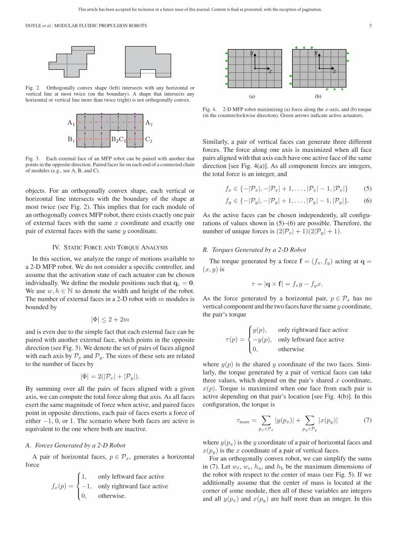
Fig. 2. Orthogonally convex shape (left) intersects with any horizontal orvertical line at most twice (on the boundary). A shape that intersects anyhorizontal or vertical line more than twice (right) is not orthogonally convex.
Fig. 3. Each external face of an MFP robot can be paired with another thatpoints in the opposite direction. Paired faces lie on each end of a connected chainof modules (e.g., see A, B, and C).
objects. For an orthogonally convex shape, each vertical or
horizontal line intersects with the boundary of the shape at
most twice (see Fig. 2). This implies that for each module of
an orthogonally convex MFP robot, there exists exactly one pair
of external faces with the same x coordinate and exactly one
pair of external faces with the same y coordinate.
IV. STATIC FORCE AND TORQUE ANALYSIS
In this section, we analyze the range of motions available to
a 2-D MFP robot. We do not consider a specific controller, and
assume that the activation state of each actuator can be chosen
individually. We define the module positions such that qc = 0.
We use w, h ∈ N to denote the width and height of the robot.
The number of external faces in a 2-D robot with m modules is
bounded by
|Φ| ≤ 2 + 2m
and is even due to the simple fact that each external face can be
paired with another external face, which points in the opposite
direction (see Fig. 3). We denote the set of pairs of faces aligned
with each axis by Px and Py . The sizes of these sets are related
to the number of faces by
|Φ| = 2(|Px|+ |Py|).
By summing over all the pairs of faces aligned with a given
axis, we can compute the total force along that axis. As all faces
exert the same magnitude of force when active, and paired faces
point in opposite directions, each pair of faces exerts a force of
either −1, 0, or 1. The scenario where both faces are active is
equivalent to the one where both are inactive.
A. Forces Generated by a 2-D Robot
A pair of horizontal faces, p ∈ Px, generates a horizontal
force
fx(p) =
⎧
⎪
⎨
⎪
⎩
1, only leftward face active
−1, only rightward face active
0, otherwise.
Fig. 4. 2-D MFP robot maximizing (a) force along the x-axis, and (b) torque(in the counterclockwise direction). Green arrows indicate active actuators.
Similarly, a pair of vertical faces can generate three different
forces. The force along one axis is maximized when all face
pairs aligned with that axis each have one active face of the same
direction [see Fig. 4(a)]. As all component forces are integers,
the total force is an integer, and
fx ∈ {−|Px|,−|Px|+ 1, . . . , |Px| − 1, |Px|} (5)
fy ∈ {−|Py|,−|Py|+ 1, . . . , |Py| − 1, |Py|}. (6)
As the active faces can be chosen independently, all configu-
rations of values shown in (5)–(6) are possible. Therefore, the
number of unique forces is (2|Px|+ 1)(2|Py|+ 1).
B. Torques Generated by a 2-D Robot
The torque generated by a force f = (fx, fy) acting at q =(x, y) is
τ = |q× f | = fxy − fyx.
As the force generated by a horizontal pair, p ∈ Px has no
vertical component and the two faces have the same y coordinate,
the pair’s torque
τ(p) =
⎧
⎪
⎨
⎪
⎩
y(p), only rightward face active
−y(p), only leftward face active
0, otherwise
where y(p) is the shared y coordinate of the two faces. Simi-
larly, the torque generated by a pair of vertical faces can take
three values, which depend on the pair’s shared x coordinate,
x(p). Torque is maximized when one face from each pair is
active depending on that pair’s location [see Fig. 4(b)]. In this
configuration, the torque is
τmax =∑
px∈Px
|y(px)|+∑
py∈Py
|x(py)| (7)
where y(px) is the y coordinate of a pair of horizontal faces and
x(py) is the x coordinate of a pair of vertical faces.
For an orthogonally convex robot, we can simplify the sums
in (7). Let wℓ, wr, ha, and hb be the maximum dimensions of
the robot with respect to the center of mass (see Fig. 5). If we
additionally assume that the center of mass is located at the
corner of some module, then all of these variables are integers
and all y(px) and x(py) are half more than an integer. In this
This article has been accepted for inclusion in a future issue of this journal. Content is final as presented, with the exception of pagination.
6 IEEE TRANSACTIONS ON ROBOTICS
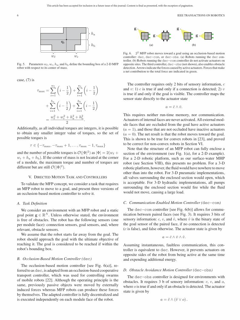
Fig. 5. Parameters wℓ, wr, ha, and hb define the bounding box of a 2-D MFProbot with respect to its center of mass.
case, (7) is
τmax =
wℓ∑
i=1
(
i−1
2
)
+
wr∑
i=1
(
i−1
2
)
+
ha∑
i=1
(
i−1
2
)
+
hb∑
i=1
(
i−1
2
)
=w2
ℓ + w2r + h2
a + h2b
2.
Additionally, as all individual torques are integers, it is possible
to obtain any smaller integer value of torques, so the set of
possible torques is
τ ∈ {−τmax,−τmax + 1, . . . , τmax − 1, τmax}
and the number of possible torques is O(|Φ|2) as |Φ| = 2(wℓ +wr + ha + hb). If the center of mass is not located at the corner
of a module, the maximum torque and number of torques are
different but are still O(|Φ|2).
V. DIRECTED MOTION TASK AND CONTROLLERS
To validate the MFP concept, we consider a task that requires
an MFP robot to move to a goal, and present three versions of
an occlusion-based motion controller to solve it.
A. Task Definition
We consider an environment with an MFP robot and a static
goal point g ∈ RN . Unless otherwise stated, the environment
is free of obstacles. The robot has the following sensors (one
per module face): connection sensors, goal sensors, and, where
relevant, obstacle sensors.
We assume that the robot starts far away from the goal. The
robot should approach the goal with the ultimate objective of
reaching it. The goal is considered to be reached if within the
robot’s bounding box.
B. Occlusion-Based Motion Controller (dec)
The occlusion-based motion controller [see Fig. 6(a)], re-
ferred to asdec, is adapted from an occlusion-based cooperative
transport controller, which was used for controlling swarms
of mobile robots [22]. Although the operating principle is the
same, previously passive objects were moved by externally
induced forces whereas MFP robots can produce these forces
by themselves. The adapted controller is fully decentralized and
is executed independently on each module face of the robot.
Fig. 6. 22 MFP robot moves toward a goal using an occlusion-based motioncontroller: dec, dec-com, or dec-obs. (a) Robots running the dec con-troller. (b) Robots running the dec-com controller do not activate actuators onopposite sites. The third controller,dec-obs (not shown), also enables obstacledetection. Arrows indicate the forces caused by active actuators. Forces that makea net contribution to the total force are indicated in green.
The controller requires only 2 bits of sensory information, cand v: 1) c is true if and only if a connection is detected; 2) vis true if and only if the goal is visible. The controller maps the
sensor state directly to the actuator state
a = c ∧ v.
This requires neither run-time memory, nor communication.
Actuators of internal faces are never activated. All external mod-
ule faces that are occluded from the goal have active actuators
(a = 1), and those that are not occluded have inactive actuators
(a = 0). The net result is that the robot moves toward the goal.
This is shown to be true for convex robots in [23], and proved
to be correct for non-convex robots in Section VI.
Note that the structure of an MFP robot can fully enclose a
section of the environment (see Fig. 1(a), for a 2-D example).
For a 2-D robotic platform, such as our surface-water MHP
robot (see Section VIII), this presents no problem. For a 3-D
robotic platform, however, the fluid would have nowhere to move
other than into the robot. For 3-D pneumatic implementations,
all valves surrounding the enclosed section would open, which
is acceptable. For 3-D hydraulic implementations, all pumps
surrounding the enclosed section would fire while the fluid
would not move, causing a large load.
C. Communication-Enabled Motion Controller (dec-com)
The dec-com controller [see Fig. 6(b)] allows for commu-
nication between paired faces (see Fig. 3). It requires 3 bits of
sensory information: c, v, and v, where v is the binary state of
the goal sensor of the paired face, if no connection is detected
(c is false), and false otherwise. The actuator state is given by
a = c ∧ v ∧ v.
Assuming instantaneous, faultless communication, this con-
troller is equivalent to dec. However, it prevents actuators on
opposite sides of the robot from being active at the same time
and expending additional energy.
D. Obstacle Avoidance Motion Controller (dec-obs)
The dec-obs controller is designed for environments with
obstacles. It requires 3 b of sensory information: c, v, and o,
where o is true if and only if an obstacle is detected. The actuator
state is given by
a = c ∧ (v ∨ o) .
This article has been accepted for inclusion in a future issue of this journal. Content is final as presented, with the exception of pagination.
DOYLE et al.: MODULAR FLUIDIC PROPULSION ROBOTS 7
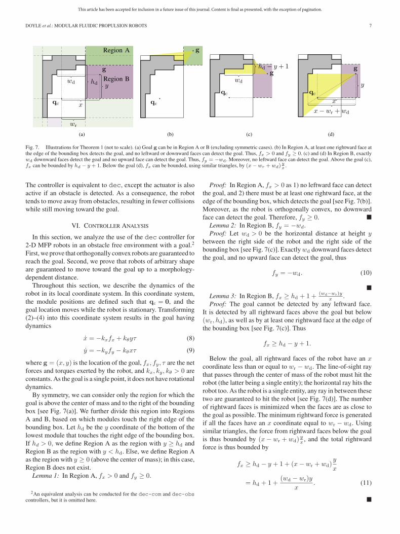
Fig. 7. Illustrations for Theorem 1 (not to scale). (a) Goal g can be in Region A or B (excluding symmetric cases). (b) In Region A, at least one rightward face atthe edge of the bounding box detects the goal, and no leftward or downward faces can detect the goal. Thus, fx > 0 and fy ≥ 0. (c) and (d) In Region B, exactlywd downward faces detect the goal and no upward face can detect the goal. Thus, fy = −wd. Moreover, no leftward face can detect the goal. Above the goal (c),fx can be bounded by hd − y + 1. Below the goal (d), fx can be bounded, using similar triangles, by (x−wr +wd)
yx
.
The controller is equivalent to dec, except the actuator is also
active if an obstacle is detected. As a consequence, the robot
tends to move away from obstacles, resulting in fewer collisions
while still moving toward the goal.
VI. CONTROLLER ANALYSIS
In this section, we analyze the use of the dec controller for
2-D MFP robots in an obstacle free environment with a goal.2
First, we prove that orthogonally convex robots are guaranteed to
reach the goal. Second, we prove that robots of arbitrary shape
are guaranteed to move toward the goal up to a morphology-
dependent distance.
Throughout this section, we describe the dynamics of the
robot in its local coordinate system. In this coordinate system,
the module positions are defined such that qc = 0, and the
goal location moves while the robot is stationary. Transforming
(2)–(4) into this coordinate system results in the goal having
dynamics
x = −kxfx + kθyτ (8)
y = −kyfy − kθxτ (9)
where g = (x, y) is the location of the goal, fx, fy, τ are the net
forces and torques exerted by the robot, and kx, ky, kθ > 0 are
constants. As the goal is a single point, it does not have rotational
dynamics.
By symmetry, we can consider only the region for which the
goal is above the center of mass and to the right of the bounding
box [see Fig. 7(a)]. We further divide this region into Regions
A and B, based on which modules touch the right edge of the
bounding box. Let hd be the y coordinate of the bottom of the
lowest module that touches the right edge of the bounding box.
If hd > 0, we define Region A as the region with y ≥ hd and
Region B as the region with y < hd. Else, we define Region A
as the region with y ≥ 0 (above the center of mass); in this case,
Region B does not exist.
Lemma 1: In Region A, fx > 0 and fy ≥ 0.
2An equivalent analysis can be conducted for the dec-com and dec-obscontrollers, but it is omitted here.
Proof: In Region A, fx > 0 as 1) no leftward face can detect
the goal, and 2) there must be at least one rightward face, at the
edge of the bounding box, which detects the goal [see Fig. 7(b)].
Moreover, as the robot is orthogonally convex, no downward
face can detect the goal. Therefore, fy ≥ 0. �
Lemma 2: In Region B, fy = −wd.
Proof: Let wd > 0 be the horizontal distance at height ybetween the right side of the robot and the right side of the
bounding box [see Fig. 7(c)]. Exactlywd downward faces detect
the goal, and no upward face can detect the goal, thus
fy = −wd. (10)
�
Lemma 3: In Region B, fx ≥ hd + 1 + (wd−wr)yx
.
Proof: The goal cannot be detected by any leftward face.
It is detected by all rightward faces above the goal but below
(wr, hd), as well as by at least one rightward face at the edge of
the bounding box [see Fig. 7(c)]. Thus
fx ≥ hd − y + 1.
Below the goal, all rightward faces of the robot have an xcoordinate less than or equal to wr − wd. The line-of-sight ray
that passes through the center of mass of the robot must hit the
robot (the latter being a single entity); the horizontal ray hits the
robot too. As the robot is a single entity, any ray in between these
two are guaranteed to hit the robot [see Fig. 7(d)]. The number
of rightward faces is minimized when the faces are as close to
the goal as possible. The minimum rightward force is generated
if all the faces have an x coordinate equal to wr − wd. Using
similar triangles, the force from rightward faces below the goal
is thus bounded by (x− wr + wd)yx
, and the total rightward
force is thus bounded by
fx ≥ hd − y + 1 + (x− wr + wd)y
x
= hd + 1 +(wd − wr)y
x. (11)
�
This article has been accepted for inclusion in a future issue of this journal. Content is final as presented, with the exception of pagination.
8 IEEE TRANSACTIONS ON ROBOTICS
Theorem 1: If kx = ky and the robot is orthogonally convex,
then any initial robot configuration will eventually result in the
goal being contained in the bounding box.
Proof: We use the Lyapunov function,
V =1
2(g − qc)
⊤ (g − qc) . (12)
This function is positive semidefinite with V = 0 if and only if
g = qc. To prove the theorem, it is sufficient to show that V < 0whenever the goal is not contained in the bounding box of the
robot, which means the goal is getting closer to the robot’s center
of mass.
By differentiating (12) using the dynamics of the goal loca-
tion, (8)–(9), the Lyapunov derivative is
V = xx+ yy
= −xkxfx − ykyfy. (13)
Without loss of generality, we assume that the problem is
scaled such that kx = ky = 1. Then the goal has dynamics
V = −xfx − yfy. (14)
In Region A, from Lemma 1, fx > 0 and fy ≥ 0. As in this
region x ≥ wr > 0 and y ≥ 0, V is negative. Thus, the goal
approaches the robot’s center of mass.
In Region B, using the bounds (10)–(11) in the Lyapunov
derivative (14), we obtain
V ≤ −x
(
hd + 1 +(wd − wr)y
x
)
+ ywd
= −x (hd + 1)− y (wd − wr) + ywd
= −x (hd + 1) + ywr.
Region B was defined by x > wr and y < hd, and so
V < −wr (hd + 1) + hdwr
= −wr < 0.
Therefore, whenever the goal is in Region B, it approaches the
robot’s center of mass. We can conclude that whenever the goal
is not in the bounding box, it approaches the robot’s center of
mass, and will eventually enter the bounding box. �
In Theorem 1, we exploited the fact that for orthogonally
convex robots, no more than two directions of faces can detect
the goal at any given time. For a general MFP robot, it is possible
for three different directions of faces to detect the goal at the same
time. As a consequence, the goal could recede from the center of
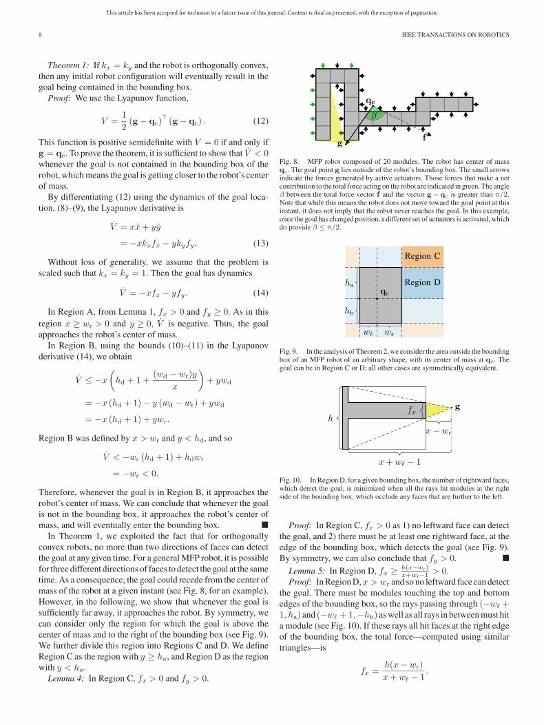
mass of the robot at a given instant (see Fig. 8, for an example).
However, in the following, we show that whenever the goal is
sufficiently far away, it approaches the robot. By symmetry, we
can consider only the region for which the goal is above the
center of mass and to the right of the bounding box (see Fig. 9).
We further divide this region into Regions C and D. We define
Region C as the region with y ≥ ha, and Region D as the region
with y < ha.
Lemma 4: In Region C, fx > 0 and fy > 0.
Fig. 8. MFP robot composed of 20 modules. The robot has center of massqc. The goal point g lies outside of the robot’s bounding box. The small arrowsindicate the forces generated by active actuators. Those forces that make a netcontribution to the total force acting on the robot are indicated in green. The angleβ between the total force vector f and the vector g − qc is greater than π/2.Note that while this means the robot does not move toward the goal point at thisinstant, it does not imply that the robot never reaches the goal. In this example,once the goal has changed position, a different set of actuators is activated, whichdo provide β ≤ π/2.
Fig. 9. In the analysis of Theorem 2, we consider the area outside the boundingbox of an MFP robot of an arbitrary shape, with its center of mass at qc. Thegoal can be in Region C or D; all other cases are symmetrically equivalent.
Fig. 10. In Region D, for a given bounding box, the number of rightward faces,which detect the goal, is minimized when all the rays hit modules at the rightside of the bounding box, which occlude any faces that are further to the left.
Proof: In Region C, fx > 0 as 1) no leftward face can detect
the goal, and 2) there must be at least one rightward face, at the
edge of the bounding box, which detects the goal (see Fig. 9).
By symmetry, we can also conclude that fy > 0. �
Lemma 5: In Region D, fx ≥ h(x−wr)x+wℓ−1 > 0.
Proof: In Region D,x > wr and so no leftward face can detect
the goal. There must be modules touching the top and bottom
edges of the bounding box, so the rays passing through (−wℓ +1, ha) and (−wℓ + 1,−hb) as well as all rays in between must hit
a module (see Fig. 10). If these rays all hit faces at the right edge
of the bounding box, the total force—computed using similar
triangles—is
fx =h(x− wr)
x+ wℓ − 1.
This article has been accepted for inclusion in a future issue of this journal. Content is final as presented, with the exception of pagination.
DOYLE et al.: MODULAR FLUIDIC PROPULSION ROBOTS 9
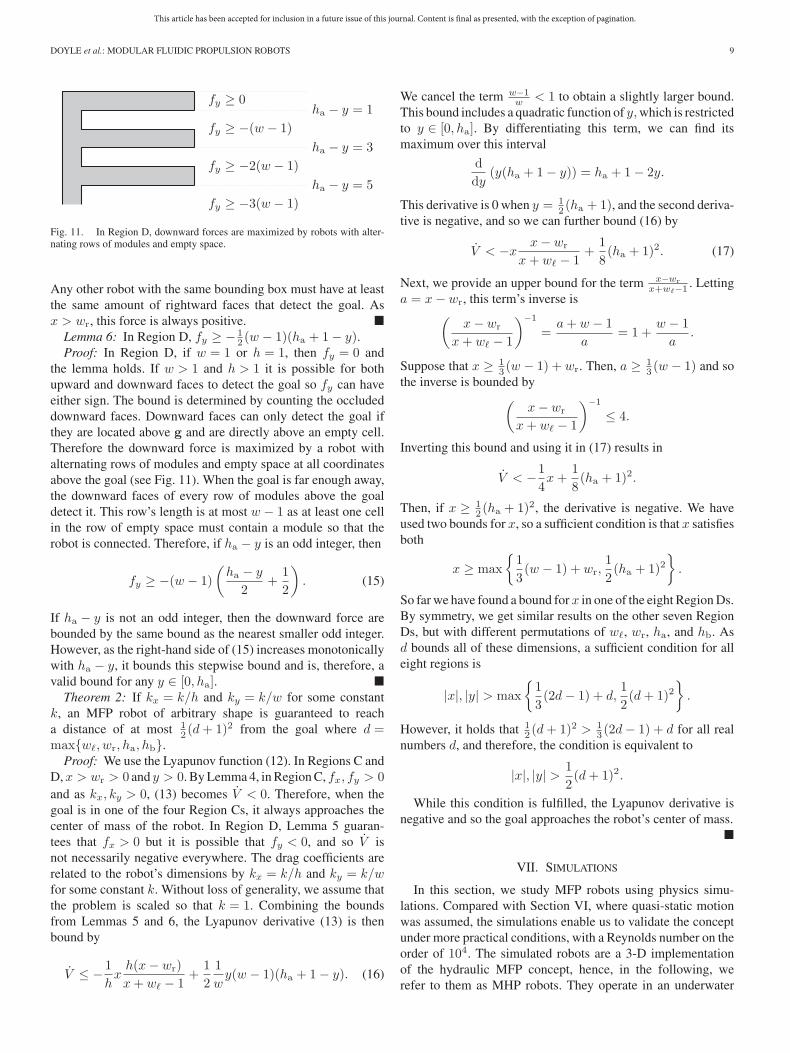
Fig. 11. In Region D, downward forces are maximized by robots with alter-nating rows of modules and empty space.
Any other robot with the same bounding box must have at least
the same amount of rightward faces that detect the goal. As
x > wr, this force is always positive. �
Lemma 6: In Region D, fy ≥ − 12 (w − 1)(ha + 1− y).
Proof: In Region D, if w = 1 or h = 1, then fy = 0 and
the lemma holds. If w > 1 and h > 1 it is possible for both
upward and downward faces to detect the goal so fy can have
either sign. The bound is determined by counting the occluded
downward faces. Downward faces can only detect the goal if
they are located above g and are directly above an empty cell.
Therefore the downward force is maximized by a robot with
alternating rows of modules and empty space at all coordinates
above the goal (see Fig. 11). When the goal is far enough away,
the downward faces of every row of modules above the goal
detect it. This row’s length is at most w − 1 as at least one cell
in the row of empty space must contain a module so that the
robot is connected. Therefore, if ha − y is an odd integer, then
fy ≥ −(w − 1)
(
ha − y
2+
1
2
)
. (15)
If ha − y is not an odd integer, then the downward force are
bounded by the same bound as the nearest smaller odd integer.
However, as the right-hand side of (15) increases monotonically
with ha − y, it bounds this stepwise bound and is, therefore, a
valid bound for any y ∈ [0, ha]. �
Theorem 2: If kx = k/h and ky = k/w for some constant
k, an MFP robot of arbitrary shape is guaranteed to reach
a distance of at most 12 (d+ 1)2 from the goal where d =
max{wℓ, wr, ha, hb}.
Proof: We use the Lyapunov function (12). In Regions C and
D,x > wr > 0 and y > 0. By Lemma 4, in Region C, fx, fy > 0
and as kx, ky > 0, (13) becomes V < 0. Therefore, when the
goal is in one of the four Region Cs, it always approaches the
center of mass of the robot. In Region D, Lemma 5 guaran-
tees that fx > 0 but it is possible that fy < 0, and so V is
not necessarily negative everywhere. The drag coefficients are
related to the robot’s dimensions by kx = k/h and ky = k/wfor some constant k. Without loss of generality, we assume that
the problem is scaled so that k = 1. Combining the bounds
from Lemmas 5 and 6, the Lyapunov derivative (13) is then
bound by
V ≤ −1
hxh(x− wr)
x+ wℓ − 1+
1
2
1
wy(w − 1)(ha + 1− y). (16)
We cancel the term w−1w
< 1 to obtain a slightly larger bound.
This bound includes a quadratic function of y,which is restricted
to y ∈ [0, ha]. By differentiating this term, we can find its
maximum over this interval
d
dy(y(ha + 1− y)) = ha + 1− 2y.
This derivative is 0 when y = 12 (ha + 1), and the second deriva-
tive is negative, and so we can further bound (16) by
V < −xx− wr
x+ wℓ − 1+
1
8(ha + 1)2. (17)
Next, we provide an upper bound for the term x−wr
x+wℓ−1 . Letting
a = x− wr, this term’s inverse is(
x− wr
x+ wℓ − 1
)−1
=a+ w − 1
a= 1 +
w − 1
a.
Suppose that x ≥ 13 (w − 1) + wr. Then, a ≥ 1
3 (w − 1) and so
the inverse is bounded by
(
x− wr
x+ wℓ − 1
)−1
≤ 4.
Inverting this bound and using it in (17) results in
V < −1
4x+
1
8(ha + 1)2.
Then, if x ≥ 12 (ha + 1)2, the derivative is negative. We have
used two bounds for x, so a sufficient condition is that x satisfies
both
x ≥ max
{
1
3(w − 1) + wr,
1
2(ha + 1)2
}
.
So far we have found a bound forx in one of the eight Region Ds.
By symmetry, we get similar results on the other seven Region
Ds, but with different permutations of wℓ, wr, ha, and hb. As
d bounds all of these dimensions, a sufficient condition for all
eight regions is
|x|, |y| > max
{
1
3(2d− 1) + d,
1
2(d+ 1)2
}
.
However, it holds that 12 (d+ 1)2 > 1
3 (2d− 1) + d for all real
numbers d, and therefore, the condition is equivalent to
|x|, |y| >1
2(d+ 1)2.
While this condition is fulfilled, the Lyapunov derivative is
negative and so the goal approaches the robot’s center of mass.
�
VII. SIMULATIONS
In this section, we study MFP robots using physics simu-
lations. Compared with Section VI, where quasi-static motion
was assumed, the simulations enable us to validate the concept
under more practical conditions, with a Reynolds number on the
order of 104. The simulated robots are a 3-D implementation
of the hydraulic MFP concept, hence, in the following, we
refer to them as MHP robots. They operate in an underwater
This article has been accepted for inclusion in a future issue of this journal. Content is final as presented, with the exception of pagination.
10 IEEE TRANSACTIONS ON ROBOTICS
environment. We analyze their speed and energy consumption
as they move toward a goal, as well as their ability to avoid
obstacles. We compare the decentralized controller variants from
Section V against the state-of-the-art (centralized) controller
from the literature.
A. General Setup
The simulator is based on the Open Dynamics Engine (ODE)
[47], an open source 3-D physics library. Modules are modeled
as solid cubes of neutral buoyancy with an edge length of
8 cm. A simplified model of fluid drag is used to avoid a full,
computationally expensive, fluid dynamics treatment. The drag
force on each external module face is calculated individually
without reference to the overall shape of the robot. It is assumed
to follow the quadratic drag equation for turbulent flow. This
means the drag force on each external module face is
fd =
{
− 12ρCDs2q · uq, q · u > 0
0, otherwise
where ρ = 1 g·cm−3 is the density of the surrounding fluid
(water), CD = 0.8 is the drag coefficient, s is the module side
length, u is the face normal vector, and q is the velocity of the
face center.
Three types of robot configuration are used, cubic, orthogo-
nally convex, and unconstrained. Robots of cubic shape com-
prise 125 modules, arranged in a 53 cubic (and thus convex)
configuration. Robots of unconstrained shape comprise 125
modules, arranged as follows: The configuration is initialized
with a single module. Additional modules are added one at a
time. A new module is added to a face that is chosen randomly
from all available external module faces on the robot. This
repeats until the robot consists of the desired number of modules.
Robots of orthogonally convex shape comprise 125 modules,
and are arranged in a similar manner to unconstrained robots.
However, additional modules may only be added in such a
manner that the robot remains orthogonally convex.
Each module has six pumps, one per face. Firing (active)
pumps apply a force of 640 dyn to the center of the module
face, along the inward face normal. The net resultant force and
torque acting on a robot are integrated by ODE. As none of the
controllers fire pumps of internal module faces, only the pumps
of external module faces are considered. The routing of fluid
throughout the robot is not simulated.
Each module has one connection sensor, one goal sensor, and
one obstacle sensor, on each of its six faces. Goal sensors use the
ray casting functionality of ODE to check line of sight between
the module face center and the goal. Line of sight can be occluded
by the body of the robot itself. Obstacle sensors use a ray of
length 40 cm, cast from the center of the face, parallel to the
face normal. The sensor returns true if and only if it intersects
with an obstacle, which could be another module of the same
robot. The specific ray length was chosen following preliminary
trials.
When using controller dec-com, a module’s face may com-
municate with a paired face (see Fig. 3). Each face simply knows
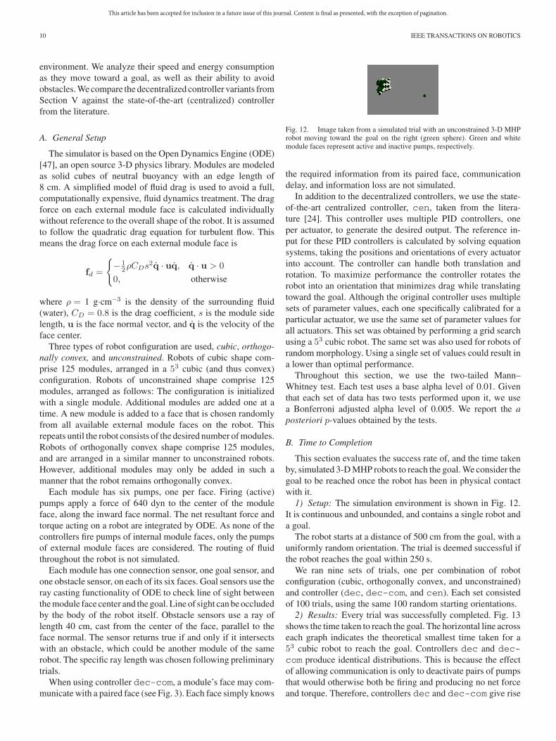
Fig. 12. Image taken from a simulated trial with an unconstrained 3-D MHProbot moving toward the goal on the right (green sphere). Green and whitemodule faces represent active and inactive pumps, respectively.
the required information from its paired face, communication
delay, and information loss are not simulated.
In addition to the decentralized controllers, we use the state-
of-the-art centralized controller, cen, taken from the litera-
ture [24]. This controller uses multiple PID controllers, one
per actuator, to generate the desired output. The reference in-
put for these PID controllers is calculated by solving equation
systems, taking the positions and orientations of every actuator
into account. The controller can handle both translation and
rotation. To maximize performance the controller rotates the
robot into an orientation that minimizes drag while translating
toward the goal. Although the original controller uses multiple
sets of parameter values, each one specifically calibrated for a
particular actuator, we use the same set of parameter values for
all actuators. This set was obtained by performing a grid search
using a 53 cubic robot. The same set was also used for robots of
random morphology. Using a single set of values could result in
a lower than optimal performance.
Throughout this section, we use the two-tailed Mann–
Whitney test. Each test uses a base alpha level of 0.01. Given
that each set of data has two tests performed upon it, we use
a Bonferroni adjusted alpha level of 0.005. We report the a
posteriori p-values obtained by the tests.
B. Time to Completion
This section evaluates the success rate of, and the time taken
by, simulated 3-D MHP robots to reach the goal. We consider the
goal to be reached once the robot has been in physical contact
with it.
1) Setup: The simulation environment is shown in Fig. 12.
It is continuous and unbounded, and contains a single robot and
a goal.
The robot starts at a distance of 500 cm from the goal, with a
uniformly random orientation. The trial is deemed successful if
the robot reaches the goal within 250 s.
We ran nine sets of trials, one per combination of robot
configuration (cubic, orthogonally convex, and unconstrained)
and controller (dec, dec-com, and cen). Each set consisted
of 100 trials, using the same 100 random starting orientations.
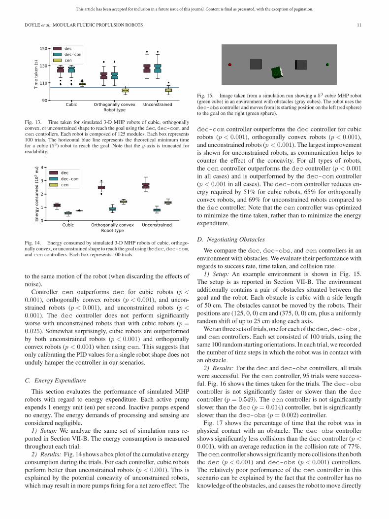
2) Results: Every trial was successfully completed. Fig. 13
shows the time taken to reach the goal. The horizontal line across
each graph indicates the theoretical smallest time taken for a
53 cubic robot to reach the goal. Controllers dec and dec-
com produce identical distributions. This is because the effect
of allowing communication is only to deactivate pairs of pumps
that would otherwise both be firing and producing no net force
and torque. Therefore, controllers dec and dec-com give rise
This article has been accepted for inclusion in a future issue of this journal. Content is final as presented, with the exception of pagination.
DOYLE et al.: MODULAR FLUIDIC PROPULSION ROBOTS 11
Fig. 13. Time taken for simulated 3-D MHP robots of cubic, orthogonallyconvex, or unconstrained shape to reach the goal using the dec, dec-com, andcen controllers. Each robot is composed of 125 modules. Each box represents100 trials. The horizontal blue line represents the theoretical minimum timefor a cubic (53) robot to reach the goal. Note that the y-axis is truncated forreadability.
Fig. 14. Energy consumed by simulated 3-D MHP robots of cubic, orthogo-nally convex, or unconstrained shape to reach the goal using thedec,dec-com,and cen controllers. Each box represents 100 trials.
to the same motion of the robot (when discarding the effects of
noise).
Controller cen outperforms dec for cubic robots (p <0.001), orthogonally convex robots (p < 0.001), and uncon-
strained robots (p < 0.001), and unconstrained robots (p <0.001). The dec controller does not perform significantly
worse with unconstrained robots than with cubic robots (p =0.025). Somewhat surprisingly, cubic robots are outperformed
by both unconstrained robots (p < 0.001) and orthogonally
convex robots (p < 0.001) when using cen. This suggests that
only calibrating the PID values for a single robot shape does not
unduly hamper the controller in our scenarios.
C. Energy Expenditure
This section evaluates the performance of simulated MHP
robots with regard to energy expenditure. Each active pump
expends 1 energy unit (eu) per second. Inactive pumps expend
no energy. The energy demands of processing and sensing are
considered negligible.
1) Setup: We analyze the same set of simulation runs re-
ported in Section VII-B. The energy consumption is measured
throughout each trial.
2) Results: Fig. 14 shows a box plot of the cumulative energy
consumption during the trials. For each controller, cubic robots
perform better than unconstrained robots (p < 0.001). This is
explained by the potential concavity of unconstrained robots,
which may result in more pumps firing for a net zero effect. The
Fig. 15. Image taken from a simulation run showing a 53 cubic MHP robot(green cube) in an environment with obstacles (gray cubes). The robot uses thedec-obs controller and moves from its starting position on the left (red sphere)to the goal on the right (green sphere).
dec-com controller outperforms the dec controller for cubic
robots (p < 0.001), orthogonally convex robots (p < 0.001),
and unconstrained robots (p < 0.001). The largest improvement
is shown for unconstrained robots, as communication helps to
counter the effect of the concavity. For all types of robots,
the cen controller outperforms the dec controller (p < 0.001in all cases) and is outperformed by the dec-com controller
(p < 0.001 in all cases). The dec-com controller reduces en-
ergy required by 51% for cubic robots, 65% for orthogonally
convex robots, and 69% for unconstrained robots compared to
the dec controller. Note that the cen controller was optimized
to minimize the time taken, rather than to minimize the energy
expenditure.
D. Negotiating Obstacles
We compare the dec, dec-obs, and cen controllers in an
environment with obstacles. We evaluate their performance with
regards to success rate, time taken, and collision rate.
1) Setup: An example environment is shown in Fig. 15.
The setup is as reported in Section VII-B. The environment
additionally contains a pair of obstacles situated between the
goal and the robot. Each obstacle is cubic with a side length
of 50 cm. The obstacles cannot be moved by the robots. Their
positions are (125, 0, 0) cm and (375, 0, 0) cm, plus a uniformly
random shift of up to 25 cm along each axis.
We ran three sets of trials, one for each of thedec,dec-obs,
and cen controllers. Each set consisted of 100 trials, using the
same 100 random starting orientations. In each trial, we recorded
the number of time steps in which the robot was in contact with
an obstacle.
2) Results: For the dec and dec-obs controllers, all trials
were successful. For the cen controller, 95 trials were success-
ful. Fig. 16 shows the times taken for the trials. The dec-obs
controller is not significantly faster or slower than the dec
controller (p = 0.549). The cen controller is not significantly
slower than the dec (p = 0.014) controller, but is significantly
slower than the dec-obs (p = 0.002) controller.
Fig. 17 shows the percentage of time that the robot was in
physical contact with an obstacle. The dec-obs controller
shows significantly less collisions than the dec controller (p <0.001), with an average reduction in the collision rate of 77%.
Thecen controller shows significantly more collisions then both
the dec (p < 0.001) and dec-obs (p < 0.001) controllers.
The relatively poor performance of the cen controller in this
scenario can be explained by the fact that the controller has no
knowledge of the obstacles, and causes the robot to move directly
This article has been accepted for inclusion in a future issue of this journal. Content is final as presented, with the exception of pagination.
12 IEEE TRANSACTIONS ON ROBOTICS
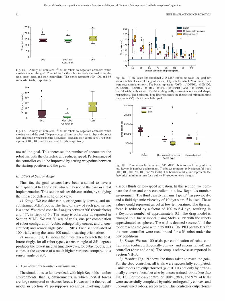
Fig. 16. Ability of simulated 53 MHP robots to negotiate obstacles whilemoving toward the goal. Time taken for the robot to reach the goal using thedec, dec-obs, and cen controllers. The boxes represent 100, 100, and 95successful trials, respectively.
Fig. 17. Ability of simulated 53 MHP robots to negotiate obstacles whilemoving toward the goal. The percentage of time the robot was in physical contactwith an obstacle when using thedec,dec-obs, andcen controllers. The boxesrepresent 100, 100, and 95 successful trials, respectively.
toward the goal. This increases the number of encounters the
robot has with the obstacles, and reduces speed. Performance of
the controller could be improved by setting waypoints between
the starting position and the goal.
E. Effect of Sensor Angle
Thus far, the goal sensors have been assumed to have a
hemispherical field of view, which may not be the case in a real
implementation. This section relaxes this constraint, by studying
the impact of different fields of view.
1) Setup: We consider cubic, orthogonally convex, and un-
constrained MHP robots. The field of view of each goal sensor
is a cone. We tested cone half-angles between 90◦ (hemisphere)
and 45◦, in steps of 5◦. The setup is otherwise as reported in
Section VII-B. We ran 30 sets of trials, one per combination
of robot configuration (cubic, orthogonally convex and uncon-
strained) and sensor angle (45◦, ..., 90◦). Each set consisted of
100 trials, using the same 100 random starting orientations.
2) Results: Fig. 18 shows the times taken to reach the goal.
Interestingly, for all robot types, a sensor angle of 85◦ degrees
produces the lowest median time; however, for cubic robots, this
comes at the expense of a much higher variance compared to a
sensor angle of 90◦.
F. Low Reynolds Number Environments
The simulations so far have dealt with high Reynolds number
environments, that is, environments in which inertial forces
are large compared to viscous forces. However, the theoretical
model in Section VI presupposes scenarios involving highly
Fig. 18. Time taken for simulated 3-D MFP robots to reach the goal forvarious fields of view of the goal sensor. Only sets for which 20 or more trialswere successful are shown. The boxes represent –/96/94, –/100/100, –/100/100,85/100/100, 100/100/100, 100/100/100, 100/100/100, and 100/100/100 suc-cessful trials with robots of cubic/orthogonally convex/unconstrained shape,respectively. The horizontal blue line represents the theoretical minimum timefor a cubic (53) robot to reach the goal.
Fig. 19. Time taken for simulated 3-D MFP robots to reach the goal in alow Reynolds number environment. The boxes represent only successful trials(100, 100, 100, 98, 100, and 97 trials). The horizontal blue line represents thetheoretical minimum time for a cubic (53) robot to reach the goal.
viscous fluids or low-speed actuation. In this section, we com-
pare the dec and cen controllers in a low Reynolds number
environment. The fluid density remains 1 g·cm−3 as previously,
and a fluid dynamic viscosity of 10 dyn·s·cm−2 is used. These
values could represent an oil at low temperature. The thruster
force is reduced by a factor of 100 to 6.4 dyn, resulting in
a Reynolds number of approximately 0.1. The drag model is
changed to a linear model, using Stoke’s law with the robots
approximated as spheres. The trial is deemed successful if the
robot reaches the goal within 25 000 s. The PID parameters for
the cen controller were recalibrated for a 53 robot under the
new conditions.
1) Setup: We ran 100 trials per combination of robot con-
figuration (cubic, orthogonally convex, and unconstrained) and
controller (dec and cen). The setup is otherwise as reported in
Section VII-B.
2) Results: Fig. 19 shows the times taken to reach the goal.
For the dec controller, all trials were successfully completed.
Cubic robots are outperformed (p < 0.001) not only by orthog-
onally convex robots, but also by unconstrained robots (see also
Fig. 13). For the cen controller, 100%, 98%, and 97% of trials
were successfully completed by cubic, orthogonally convex, and
unconstrained robots, respectively. This controller outperforms
This article has been accepted for inclusion in a future issue of this journal. Content is final as presented, with the exception of pagination.
DOYLE et al.: MODULAR FLUIDIC PROPULSION ROBOTS 13
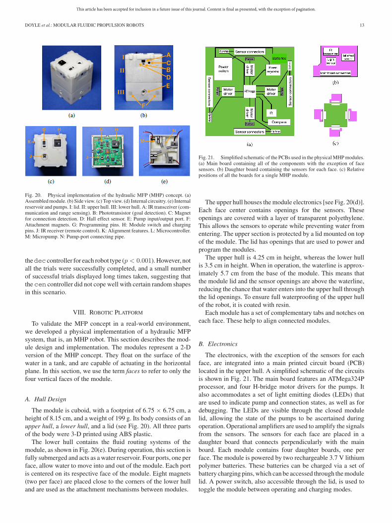
Fig. 20. Physical implementation of the hydraulic MFP (MHP) concept. (a)Assembled module. (b) Side view. (c) Top view. (d) Internal circuitry. (e) Internalreservoir and pumps. I: lid. II: upper hull. III: lower hull. A: IR transceiver (com-munication and range sensing). B: Phototransistor (goal detection). C: Magnetfor connection detection. D: Hall effect sensor. E: Pump input/output port. F:Attachment magnets. G: Programming pins. H: Module switch and chargingpins. J: IR receiver (remote control). K: Alignment features. L: Microcontroller.M: Micropump. N: Pump-port connecting pipe.
thedec controller for each robot type (p < 0.001). However, not
all the trials were successfully completed, and a small number
of successful trials displayed long times taken, suggesting that
the cen controller did not cope well with certain random shapes
in this scenario.
VIII. ROBOTIC PLATFORM
To validate the MFP concept in a real-world environment,
we developed a physical implementation of a hydraulic MFP
system, that is, an MHP robot. This section describes the mod-
ule design and implementation. The modules represent a 2-D
version of the MHP concept. They float on the surface of the
water in a tank, and are capable of actuating in the horizontal
plane. In this section, we use the term faces to refer to only the
four vertical faces of the module.
A. Hull Design
The module is cuboid, with a footprint of 6.75 × 6.75 cm, a
height of 8.15 cm, and a weight of 199 g. Its body consists of an
upper hull, a lower hull, and a lid (see Fig. 20). All three parts
of the body were 3-D printed using ABS plastic.
The lower hull contains the fluid routing systems of the
module, as shown in Fig. 20(e). During operation, this section is
fully submerged and acts as a water reservoir. Four ports, one per
face, allow water to move into and out of the module. Each port
is centered on its respective face of the module. Eight magnets
(two per face) are placed close to the corners of the lower hull
and are used as the attachment mechanisms between modules.
Fig. 21. Simplified schematic of the PCBs used in the physical MHP modules.(a) Main board containing all of the components with the exception of facesensors. (b) Daughter board containing the sensors for each face. (c) Relativepositions of all the boards for a single MHP module.
The upper hull houses the module electronics [see Fig. 20(d)].
Each face center contains openings for the sensors. These
openings are covered with a layer of transparent polyethylene.
This allows the sensors to operate while preventing water from
entering. The upper section is protected by a lid mounted on top
of the module. The lid has openings that are used to power and
program the modules.
The upper hull is 4.25 cm in height, whereas the lower hull
is 3.5 cm in height. When in operation, the waterline is approx-
imately 5.7 cm from the base of the module. This means that
the module lid and the sensor openings are above the waterline,
reducing the chance that water enters into the upper hull through
the lid openings. To ensure full waterproofing of the upper hull
of the robot, it is coated with resin.
Each module has a set of complementary tabs and notches on
each face. These help to align connected modules.
B. Electronics
The electronics, with the exception of the sensors for each
face, are integrated into a main printed circuit board (PCB)
located in the upper hull. A simplified schematic of the circuits
is shown in Fig. 21. The main board features an ATMega324P
processor, and four H-bridge motor drivers for the pumps. It
also accommodates a set of light emitting diodes (LEDs) that
are used to indicate pump and connection states, as well as for
debugging. The LEDs are visible through the closed module
lid, allowing the state of the pumps to be ascertained during
operation. Operational amplifiers are used to amplify the signals
from the sensors. The sensors for each face are placed in a
daughter board that connects perpendicularly with the main
board. Each module contains four daughter boards, one per
face. The module is powered by two rechargeable 3.7 V lithium
polymer batteries. These batteries can be charged via a set of
battery charging pins, which can be accessed through the module
lid. A power switch, also accessible through the lid, is used to
toggle the module between operating and charging modes.
This article has been accepted for inclusion in a future issue of this journal. Content is final as presented, with the exception of pagination.
14 IEEE TRANSACTIONS ON ROBOTICS
C. Actuation
The module is actuated by four submersible centrifugal mi-
cropumps (M200S-SUB from TCS micropumps). Each pump
has dimensions of 2.9 × 1.6 × 1.6 cm, and is capable of a max-
imum flow rate of 11 mL · s−1. Each pump outlet is connected
via a pipe to one of four ports on the lower hull. When active,
a pump extracts water from the reservoir and discharges it into
the environment (or a neighboring module). Correspondingly,
fluid is drawn into the reservoir from the environment (or a
neighboring module) via inactive pumps. This routing process
provides the motive force for the module.
D. Sensing
Each module face has a magnet–hall sensor pair, a photo-
transistor, and an infrared (IR) transceiver. The magnet–hall
sensor pair provides the ability to detect connections between
modules. The phototransistor allows the module to sense visible
light. It is used to determine whether the goal is visible to the
face. If the face is connected, the IR transceiver can be used
for communication. If not, the IR transceiver can be used as an
obstacle sensor.
An IR receiver mounted on the main board allows the module
to receive information from an overhead controller or a con-
ventional television remote control. The combination of the
IR receiver and the power switch allows for three operating
modes: the off/charging mode, the standby mode, and
the activemode. In the off/chargingmode, the batteries
are disconnected from the rest of the circuit. In the standby
mode, the batteries are connected to the circuit allowing the
sensors and LEDs to be active, but the pumps do not respond.
In the activemode, the pumps respond to the sensor readings
in accordance with the controller implemented. An electronic
compass in each module can provide orientation sensing. It
returns the angular offset of the module, relative to an initial
orientation.
IX. EXPERIMENTS
This section details the physical experiments undertaken with
the prototype MHP system. As we could not realize reliable real-
time communication of the robot’s pose with respect to the goal
via the IR receivers, the centralized controller was not tested.
In the following, we compare the performance of the dec and
dec-com controller variants from Section V.
A. General Setup
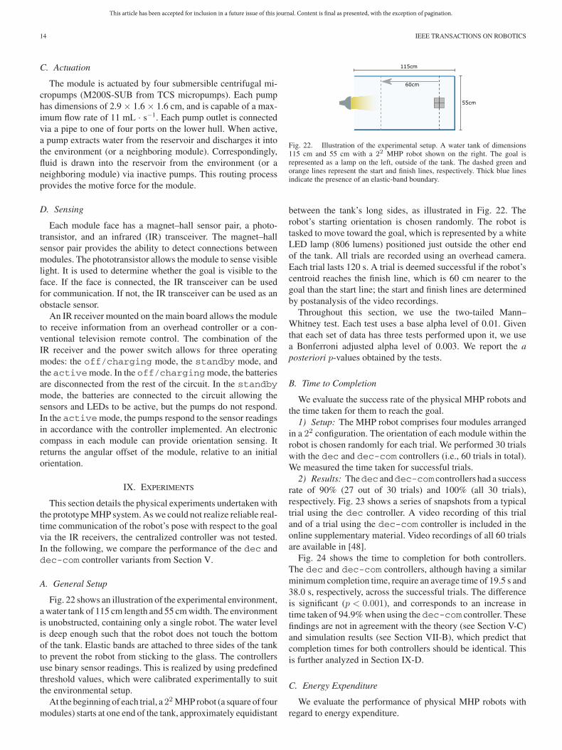
Fig. 22 shows an illustration of the experimental environment,
a water tank of 115 cm length and 55 cm width. The environment
is unobstructed, containing only a single robot. The water level
is deep enough such that the robot does not touch the bottom
of the tank. Elastic bands are attached to three sides of the tank
to prevent the robot from sticking to the glass. The controllers
use binary sensor readings. This is realized by using predefined
threshold values, which were calibrated experimentally to suit
the environmental setup.
At the beginning of each trial, a22 MHP robot (a square of four
modules) starts at one end of the tank, approximately equidistant
Fig. 22. Illustration of the experimental setup. A water tank of dimensions115 cm and 55 cm with a 22 MHP robot shown on the right. The goal isrepresented as a lamp on the left, outside of the tank. The dashed green andorange lines represent the start and finish lines, respectively. Thick blue linesindicate the presence of an elastic-band boundary.
between the tank’s long sides, as illustrated in Fig. 22. The
robot’s starting orientation is chosen randomly. The robot is
tasked to move toward the goal, which is represented by a white
LED lamp (806 lumens) positioned just outside the other end
of the tank. All trials are recorded using an overhead camera.
Each trial lasts 120 s. A trial is deemed successful if the robot’s
centroid reaches the finish line, which is 60 cm nearer to the
goal than the start line; the start and finish lines are determined
by postanalysis of the video recordings.
Throughout this section, we use the two-tailed Mann–
Whitney test. Each test uses a base alpha level of 0.01. Given
that each set of data has three tests performed upon it, we use
a Bonferroni adjusted alpha level of 0.003. We report the a
posteriori p-values obtained by the tests.
B. Time to Completion
We evaluate the success rate of the physical MHP robots and
the time taken for them to reach the goal.
1) Setup: The MHP robot comprises four modules arranged
in a 22 configuration. The orientation of each module within the
robot is chosen randomly for each trial. We performed 30 trials
with the dec and dec-com controllers (i.e., 60 trials in total).
We measured the time taken for successful trials.
2) Results: Thedec anddec-com controllers had a success
rate of 90% (27 out of 30 trials) and 100% (all 30 trials),
respectively. Fig. 23 shows a series of snapshots from a typical
trial using the dec controller. A video recording of this trial
and of a trial using the dec-com controller is included in the
online supplementary material. Video recordings of all 60 trials
are available in [48].
Fig. 24 shows the time to completion for both controllers.
The dec and dec-com controllers, although having a similar
minimum completion time, require an average time of 19.5 s and
38.0 s, respectively, across the successful trials. The difference
is significant (p < 0.001), and corresponds to an increase in
time taken of 94.9% when using the dec-com controller. These
findings are not in agreement with the theory (see Section V-C)
and simulation results (see Section VII-B), which predict that
completion times for both controllers should be identical. This
is further analyzed in Section IX-D.
C. Energy Expenditure
We evaluate the performance of physical MHP robots with
regard to energy expenditure.
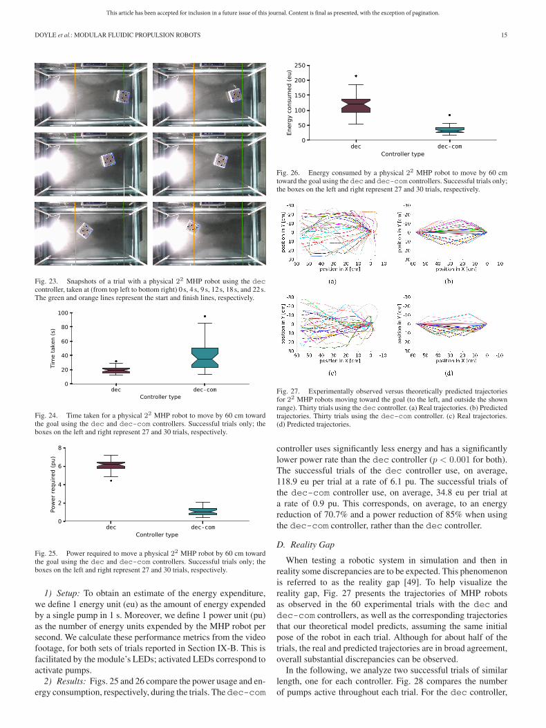
This article has been accepted for inclusion in a future issue of this journal. Content is final as presented, with the exception of pagination.
DOYLE et al.: MODULAR FLUIDIC PROPULSION ROBOTS 15
Fig. 23. Snapshots of a trial with a physical 22 MHP robot using the deccontroller, taken at (from top left to bottom right) 0 s, 4 s, 9 s, 12 s, 18 s, and 22 s.The green and orange lines represent the start and finish lines, respectively.
Fig. 24. Time taken for a physical 22 MHP robot to move by 60 cm towardthe goal using the dec and dec-com controllers. Successful trials only; theboxes on the left and right represent 27 and 30 trials, respectively.
Fig. 25. Power required to move a physical 22 MHP robot by 60 cm towardthe goal using the dec and dec-com controllers. Successful trials only; theboxes on the left and right represent 27 and 30 trials, respectively.
1) Setup: To obtain an estimate of the energy expenditure,
we define 1 energy unit (eu) as the amount of energy expended
by a single pump in 1 s. Moreover, we define 1 power unit (pu)
as the number of energy units expended by the MHP robot per
second. We calculate these performance metrics from the video
footage, for both sets of trials reported in Section IX-B. This is
facilitated by the module’s LEDs; activated LEDs correspond to
activate pumps.
2) Results: Figs. 25 and 26 compare the power usage and en-
ergy consumption, respectively, during the trials. Thedec-com
Fig. 26. Energy consumed by a physical 22 MHP robot to move by 60 cmtoward the goal using the dec and dec-com controllers. Successful trials only;the boxes on the left and right represent 27 and 30 trials, respectively.
Fig. 27. Experimentally observed versus theoretically predicted trajectoriesfor 22 MHP robots moving toward the goal (to the left, and outside the shownrange). Thirty trials using the dec controller. (a) Real trajectories. (b) Predictedtrajectories. Thirty trials using the dec-com controller. (c) Real trajectories.(d) Predicted trajectories.
controller uses significantly less energy and has a significantly
lower power rate than the dec controller (p < 0.001 for both).
The successful trials of the dec controller use, on average,
118.9 eu per trial at a rate of 6.1 pu. The successful trials of
the dec-com controller use, on average, 34.8 eu per trial at
a rate of 0.9 pu. This corresponds, on average, to an energy
reduction of 70.7% and a power reduction of 85% when using
the dec-com controller, rather than the dec controller.
D. Reality Gap
When testing a robotic system in simulation and then in
reality some discrepancies are to be expected. This phenomenon
is referred to as the reality gap [49]. To help visualize the
reality gap, Fig. 27 presents the trajectories of MHP robots
as observed in the 60 experimental trials with the dec and
dec-com controllers, as well as the corresponding trajectories
that our theoretical model predicts, assuming the same initial
pose of the robot in each trial. Although for about half of the
trials, the real and predicted trajectories are in broad agreement,
overall substantial discrepancies can be observed.
In the following, we analyze two successful trials of similar
length, one for each controller. Fig. 28 compares the number
of pumps active throughout each trial. For the dec controller,
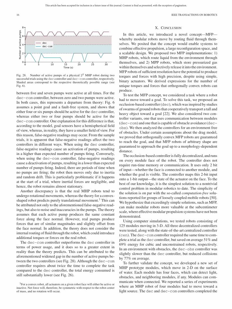
This article has been accepted for inclusion in a future issue of this journal. Content is final as presented, with the exception of pagination.
16 IEEE TRANSACTIONS ON ROBOTICS
Fig. 28. Number of active pumps of a physical 22 MHP robot during twosuccessful trials using thedec controller anddec-com controller, respectively.Shaded areas correspond to the respective theoretically possible range (seeFig. 6).
between five and seven pumps were active at all times. For the
dec-com controller, between zero and two pumps were active.
In both cases, this represents a departure from theory: Fig. 6
assumes a point goal and a fault-free system, and shows that
either four or six pumps should be active for the dec controller,
whereas either two or four pumps should be active for the
dec-com controller. One explanation for this difference is that,
according to the model, goal sensors have a hemispherical field
of view, whereas, in reality, they have a smaller field of view. For
this reason, false-negative readings may occur. From the sample
trials, it is apparent that false-negative readings affect the two
controllers in different ways. When using the dec controller,
false-negative readings cause an activation of pumps, resulting
in a higher than expected number of pumps firing. Conversely,
when using the dec-com controller, false-negative readings
cause a deactivation of pumps, resulting in a lower than expected
number of pumps firing. Indeed, there are periods of time when
no pumps are firing; the robot then moves only due to inertia
and random drift. This is particularly problematic if it happens
at the start of a trial, where inertial forces are negligible, and
hence, the robot remains almost stationary.
Another discrepancy is that the real MHP robots tend to
undergo rotational movements, whereas the theory for a convex-
shaped robot predicts purely translational movement.3 This can
be attributed not only to the aforementioned false-negative read-
ings, but also to noise and inaccuracies in the pumps. The theory
assumes that each active pump produces the same constant
force along the face normal. However, real pumps produce
forces that are of similar magnitudes and slightly offset from
the face normal. In addition, the theory does not consider the
internal routing of fluid through the robot, which could introduce
additional torques or forces on the real robot.
The dec-com controller outperforms the dec controller in
terms of power usage, and it does so to a greater extent in
reality than the theory predicts. This can be attributed to the
aforementioned widened gap in the number of active pumps be-
tween the two controllers (see Fig. 28). Although the dec-com
controller requires about twice the time to complete the task
compared to the dec controller, the total energy consumed is
still substantially lower (see Fig. 26).
3For a convex robot, all actuators on a given robot face will either be active orinactive. Net force will, therefore, be symmetric with respect to the robot centerof mass, and no rotation will occur.
X. CONCLUSION
In this article, we introduced a novel concept—MFP—
whereby modular robots move by routing fluid through them-
selves. We posited that the concept would enable systems to
combine effective propulsion, a large reconfiguration space, and
a scalable design. We proposed two MFP implementations: 1)
MHP robots, which route liquid from the environment through
themselves, and 2) MPP robots, which store pressurized gas
within themselves and selectively release it into the environment.
MFP robots of sufficient resolution have the potential to produce
torques and forces with high precision, despite using simple,
binary actuators. We derived expressions for the number of
unique torques and forces that orthogonally convex robots can
produce.
To test the MFP concept, we considered a task where a robot
had to move toward a goal. To solve this task, we proposed an
occlusion-based controller (dec), which was inspired by studies
of swarms of ground robots that cooperatively transport a tall and
heavy object toward a goal [22]. We also considered two con-
troller variants, one that uses communication between modules
(dec-com) and one that is capable of obstacle avoidance (dec-
obs). We then analyzed the controllers for an environment free
of obstacles. Under certain assumptions about the drag model,
we proved that orthogonally convex MFP robots are guaranteed
to reach the goal, and that MFP robots of arbitrary shape are
guaranteed to approach the goal up to a morphology-dependent
distance.
The occlusion-based controller is fully decentralized, and runs
on every module face of the robot. The controller does not
require run-time memory or communication. It uses only 2 bit
of input—whether the face is connected to another module, and
whether the goal is visible. The controller maps this 2-bit input
onto a 1-bit output—the state of the actuator on the face. To the
best of our knowledge, it is the simplest solution to a nontrivial
control problem in modular robotics to date. The simplicity of
the solution is on par with the so-called computation-free solu-
tions reported for groups of loosely coupled mobile robots [50].
We hypothesize that exceedingly simple solutions, such as MFP,
can make modular robots more valuable at the subcentimeter
scale, where effective modular propulsion systems have not been
demonstrated.
Using computer simulations, we tested robots consisting of
125 modules moving in 3-D. All three decentralized controllers
were tested, along with the state-of-the-art centralized controller
(cen). The dec-com controller required the same time to com-
plete a trial as the dec controller, but saved on average 51% and
69% energy for cubic and unconstrained robots, respectively.
In an environment with obstacles, the dec-obs controller was
slightly slower than the dec controller, but reduced collisions
by 77% on average.
To further validate the concept, we developed a new set of
MHP prototype modules, which move in 2-D on the surface
of water. Each module has four faces, which can detect light,
obstacles, and neighboring modules, if any. Modules can com-
municate when connected. We reported a series of experiments
where an MHP robot of four modules had to move toward a
light source. The dec and dec-com controllers completed the
This article has been accepted for inclusion in a future issue of this journal. Content is final as presented, with the exception of pagination.
DOYLE et al.: MODULAR FLUIDIC PROPULSION ROBOTS 17
task in 90% and 100% of the experimental trials, respectively.
The dec-com controller saved 71% energy on average, at the
expense of increasing the time taken to reach the goal by 95%
on average.
Future work could include a physical implementation with
modules of subcentimeter size, targeted at operations in highly
confined spaces, such as pipe networks, and possibly in 3-D.
In addition to effective watertightness, a 3-D MHP system
would have to consider the effects of submersion on sensors
and communication (e.g., attenuation). Buoyancy control could
be provided via existing actuators, or the use of swim blad-
ders. Pneumatic prototypes of MFP could be considered, for
applications in space. Incorporating self-reconfiguration into
the design, potentially by repurposing the propulsion actuators,
would further increase the utility of the system.
ACKNOWLEDGMENT
The authors would like to thank P. Eastwood and M. Port
for technical support, F. Perez-Diaz for fruitful discussions on
the original MHP concept, and M. Watson for advice on circuit
design.
REFERENCES
[1] M. Yim et al., “Modular self-reconfigurable robot systems,” IEEE Robot.
Autom. Mag., vol. 14, no. 1, pp. 43–52, Mar. 2007.[2] K. Stoy, D. Brandt, and D. J. Christensen, Self-Reconfigurable Robots: An
Introduction. Cambridge, MA, USA: MIT Press, 2010.[3] M. Yim, K. Roufas, D. Duff, Y. Zhang, C. Eldershaw, and S. Homans,
“Modular reconfigurable robots in space applications,” Auton. Robot.,vol. 14, no. 2/3, pp. 225–237, 2003.
[4] I. Vasilescu, P. Varshavskaya, K. Kotay, and D. Rus, “Autonomous modularoptical underwater robot (AMOUR) design, prototype and feasibilitystudy,” in Proc. IEEE Int. Conf. Robot. Autom., 2005, pp. 1603–1609.
[5] M. Yim, D. G. Duff, and K. Roufas, “Modular reconfigurable robots, anapproach to urban search and rescue,” in Proc. 1st Int. Workshop Human-
Friendly Welfare Robot. Syst., 2000, pp. 69–76.[6] I. Vasilescu et al., “AMOUR V: A hovering energy efficient underwater
robot capable of dynamic payloads,” Int. J. Robot. Res., vol. 29, no. 5,pp. 547–570, 2010.
[7] R. Oung and R. D’Andrea, “The distributed flight array: Design, imple-mentation, and analysis of a modular vertical take-off and landing vehicle,”Int. J. Robot. Res., vol. 33, no. 3, pp. 375–400, 2014.
[8] D. Saldana, B. Gabrich, G. Li, M. Yim, and V. Kumar, “ModQuad: Theflying modular structure that self-assembles in midair,” in Proc. IEEE Int.
Conf. Robot. Autom., 2018, pp. 691–698.[9] G. Li, B. Gabrich, D. Saldaña, J. Das, V. Kumar, and M. Yim, “ModQuad-
Vi: A vision-based self-assembling modular quadrotor,” in Proc. Int. Conf.
Robot. Autom., 2019, pp. 346–352.[10] R. Groß, M. Bonani, F. Mondada, and M. Dorigo, “Autonomous
self-assembly in swarm-bots,” IEEE Trans. Robot., vol. 22, no. 6,pp. 1115–1130, Dec. 2006.
[11] M. Bonani et al., “The marXbot, a miniature mobile robot opening newperspectives for the collective-robotic research,” in Proc. IEEE/RSJ Int.
Conf. Intell. Robots Syst., 2010, pp. 4187–4193.[12] J. Davey, N. Kwok, and M. Yim, “Emulating self-reconfigurable robots-
design of the SMORES system,” in Proc. IEEE/RSJ Int. Conf. Intell.
Robots Syst., 2012, pp. 4464–4469.[13] C. Parrott, T. J. Dodd, and R. Groß, “HyMod: A 3-DOF hybrid mobile and
self-reconfigurable modular robot and its extensions,” in Proc. Distrib.
Auton. Robot. Syst., 2018, vol. 6, pp. 401–414.[14] V. Zykov, P. Williams, N. Lassabe, and H. Lipson, “Molecubes extended:
Diversifying capabilities of open-source modular robotics,” in Proc. IROS-
2008 Self-Reconfigurable Robot. Workshop, 2008, pp. 22–26.[15] J. W. Romanishin, K. Gilpin, and D. Rus, “M-Blocks: Momentum-driven,
magnetic modular robots,” in Proc. IEEE/RSJ Int. Conf. Intell. Robot. Syst.,2013, pp. 4288–4295.
[16] M. W. Jorgensen, E. H. Ostergaard, and H. H. Lund, “Modular ATRON:Modules for a self-reconfigurable robot,” in Proc. IEEE/RSJ Int. Conf.
Intell. Robot. Syst., 2004, vol. 2, pp. 2068–2073.[17] S. Murata, E. Yoshida, A. Kamimura, H. Kurokawa, K. Tomita, and
S. Kokaji, “M-TRAN: Self-reconfigurable modular robotic system,”IEEE/ASME Trans. Mechatron., vol. 7, no. 4, pp. 431–441, Dec. 2002.
[18] S. C. Goldstein and T. C. Mowry, “Claytronics: A scalable basis for futurerobots,” in Proc. 2nd Workshop Self-Sustain. Robot. Syst. (RoboSphere
2004), NASA Ames Res. Center, USA, Nov. 2004.[19] S. C. Goldstein, J. D. Campbell, and T. C. Mowry, “Programmable matter,”
Computer, vol. 38, no. 6, pp. 99–101, 2005.[20] K. Gilpin, A. Knaian, and D. Rus, “Robot pebbles: One centimeter modules
for programmable matter through self-disassembly,” in Proc. IEEE Int.
Conf. Robot. Autom., 2010, pp. 2485–2492.[21] B. Piranda and J. Bourgeois, “Designing a quasi-spherical module for
a huge modular robot to create programmable matter,” Auton. Robot.,vol. 42, no. 8, pp. 1619–1633, 2018.
[22] J. Chen, M. Gauci, W. Li, A. Kolling, and R. Groß, “Occlusion-basedcooperative transport with a swarm of miniature mobile robots,” IEEE
Trans. Robot., vol. 31, no. 2, pp. 307–321, Apr. 2015.[23] M. J. Doyle, X. Xu, Y. Gu, F. Perez-Diaz, C. Parrott, and R. Groß, “Modular
hydraulic propulsion: A robot that moves by routing fluid through itself,”in Proc. IEEE Int. Conf. Robot. Autom., 2016, pp. 5189–5196.
[24] M. Doniec, I. Vasilescu, C. Detweiler, and D. Rus, “Complete SE3 under-water robot control with arbitrary thruster configurations,” in Proc. IEEE
Int. Conf. Robot. Autom., 2010, pp. 5295–5301.[25] B. von Haller, A. Ijspeert, and D. Floreano, “Co-evolution of structures
and controllers for neubot underwater modular robots,” in Proc. 8th Eur.
Conf. Artif. Life, 2005, pp. 189–199.[26] G. Konidaris, T. Taylor, and J. Hallam, “Hydrogen: Automatically gener-
ating self-assembly code for hydron units,” in Proc. Distrib. Auton. Robot.
Syst., 2007, pp. 33–42.[27] S. Mintchev et al., “An underwater reconfigurable robot with bioin-
spired electric sense,” in Proc. IEEE Int. Conf. Robot. Autom., 2012,pp. 1149–1154.
[28] L. Furno, M. Blanke, R. Galeazzi, and D. J. Christensen, “Self-reconfiguration of modular underwater robots using an energy heuristic,”in Proc. IEEE/RSJ Int. Conf. Intell. Robots Syst., 2017, pp. 6277–6284.
[29] J. Paulos et al., “Automated self-assembly of large maritime structures bya team of robotic boats,” IEEE Trans. Autom. Sci. Eng., vol. 12, no. 3,pp. 958–968, Jul. 2015.
[30] R. Naldi, F. Forte, A. Serrani, and L. Marconi, “Modeling and controlof a class of modular aerial robots combining under actuated and fullyactuated behavior,” IEEE Trans. Control Syst. Technol., vol. 23, no. 5,pp. 1869–1885, Sep. 2015.
[31] B. Gheneti et al., “Trajectory planning for the shapeshifting of autonomoussurface vessels,” in Proc. IEEE Int. Symp. Multi-Robot Multi-Agent Syst.,
2019, pp. 76–82.[32] N. Inou, H. Kobayashi, and M. Koseki, “Development of pneumatic
cellular robots forming a mechanical structure,” in Proc. 7th Int. Conf.
Control, Autom., Robot. Vision, 2002, pp. 63–68.[33] P. White, V. Zykov, J. Bongard, and H. Lipson, “Three dimensional
stochastic reconfiguration of modular robots,” in Proc. Robot. Sci. Syst.
Conf., 2005, pp. 161–168.[34] M. T. Tolley and H. Lipson, “Fluidic manipulation for scalable stochastic
3D assembly of modular robots,” in Proc. IEEE Int. Conf. Robot. Autom.,
2010, pp. 2473–2478.[35] S. Miyashita, M. Lungarella, and R. Pfeifer, “Tribolon: Water-based self-
assembly robots,” in Artif. Life Models Hardware. London, U.K.: Springer,2009, pp. 161–184.
[36] B. Haghighat and A. Martinoli, “Characterization and validation of anovel robotic system for fluid-mediated programmable stochastic self-assembly,” in Proc. IEEE/RSJ Int. Conf. Intell. Robot. Syst., 2016,pp. 2778–2783.
[37] V. Ganesan and M. Chitre, “On stochastic self-assembly of under-water robots,” IEEE Robot. Autom. Lett., vol. 1, no. 1, pp. 251–258,Jan. 2016.
[38] M. Doniec, C. Detweiler, and D. Rus, “Estimation of thruster configura-tions for reconfigurable modular underwater robots,” in Proc. Exp. Robot.,2014, vol. 79, pp. 655–666.
[39] D. J. Christensen et al., “Collective modular underwater robotic systemfor long-term autonomous operation,” in Proc. ICRA Workshop Persis-
tent Autonomy Aquatic Robot.: Role Control Learn. Single Multi-Robot
Syst., 2015. [Online]. Available: https://orbit.dtu.dk/files/112200773/ChristensenPAAR2015.pdf
This article has been accepted for inclusion in a future issue of this journal. Content is final as presented, with the exception of pagination.
18 IEEE TRANSACTIONS ON ROBOTICS
[40] W. Wang et al., “Design, modeling, and nonlinear model predictive track-ing control of a novel autonomous surface vehicle,” in Proc. IEEE/RSJ Int.
Conf. Intell. Robots Syst., 2018, pp. 1–5.[41] L. A. Mateos, W. Wang, B. Gheneti, F. Duarte, C. Ratti, and D. Rus,
“Autonomous latching system for robotic boats,” in Proc. IEEE Int. Conf.
Robot. Autom., 2019, pp. 7933–7939.[42] M. T. Tolley, M. Kalontarov, J. Neubert, D. Erickson, and H. Lipson,
“Stochastic modular robotic systems: A study of fluidic assembly strate-gies,” IEEE Trans. Robot., vol. 26, no. 3, pp. 518–530, Jun. 2010.
[43] M. T. Tolley and H. Lipson, “On-line assembly planning for stochasticallyreconfigurable systems,” Int. J. Robot. Res., vol. 30, no. 13, pp. 1566–1584,2011.
[44] B. Haghighat, E. Droz, and A. Martinoli, “Lily: A miniature floatingrobotic platform for programmable stochastic self-assembly,” in Proc.
IEEE Int. Conf. Robot. Autom., 2015, pp. 1941–1948.[45] B. Haghighat, M. Mastrangeli, G. Mermoud, F. Schill, and A. Marti-
noli, “Fluid-mediated stochastic self-assembly at centimetric and sub-millimetric scales: Design, modeling, and control,” Micromachines, vol. 7,no. 8, 2016, Art. no. 138.
[46] B. Haghighat, H. Khodr, and A. Martinoli, “Design and calibration ofa lightweight physics-based model for fluid-mediated self-assembly ofrobotic modules,” in Proc. Distrib. Auton. Robot. Syst., 2019, pp. 197–210.
[47] R. Smith et al., “Open dynamics engine,” 2005. [Online]. Available:http://www.ode.org
[48] M. J. Doyle et al., “Online supplementary material: Modular fluidicpropulsion robots,” figshare, 2020. [Online]. Available: http://dx.doi.org/10.6084/m9.figshare.13089911
[49] N. Jakobi, P. Husbands, and I. Harvey, “Noise and the reality gap: Theuse of simulation in evolutionary robotics,” in Proc. Adv. Artif. Life, 1995,pp. 704–720.
[50] M. Gauci, J. Chen, W. Li, T. J. Dodd, and R. Groß, “Self-organizedaggregation without computation,” Int. J. Robot. Res., vol. 33, no. 8,pp. 1145–1161, 2014.
Matthew J. Doyle (Student Member, IEEE) receivedthe M.Phys. degree in physics from Oxford Univer-sity, Oxford, U.K., in 2014, and the Ph.D. degree inautomatic control and systems engineering from TheUniversity of Sheffield, Sheffield, U.K., in 2020.
His research interests include modular robotics andartificial life.
João V. Amorim Marques (Student Member, IEEE)received the B.Eng. degree in biomedical engineeringfrom the Catholic University of Portugal, Lisbon,Portugal, in 2012, the M.Eng. degree in biomedicalengineering from Instituto Superior Técnico, Univer-sity of Lisbon, Lisbon, in 2015, and the Ph.D. degreein automatic control and systems engineering fromThe University of Sheffield, Sheffield, U.K., in 2020.
His research interests include multirobot system,modular robotics, and autonomous systems.
Isaac Vandermeulen (Student Member, IEEE) re-ceived the B.Sc.E. degree in engineering chemistry,the B.A. degree in mathematics, the M.A.Sc. degreein chemical engineering from Queen’s University,Kingston, ON, Canada, in 2014 and 2016, respec-tively, and the Ph.D. degree in automatic controland systems engineering from The University ofSheffield, Sheffield, U.K., in 2020.
He is currently with iRobot, Pasadena, CA, USA.His research interests include multirobot systems,planning, navigation, and computational geometry.
Christopher Parrott received the B.Sc. degree in ar-tificial intelligence and robotics from The Universityof Wales, Aberystwyth, U.K., in 2009, and the Ph.D.degree in modular robotics from The University ofSheffield, Sheffield, U.K., in 2017.
Since then, he has been a Research Associate withthe Department of Mechanical Engineering, The Uni-versity of Sheffield, working on the robotics theme ofthe TWENTY65 project. His research interests in-clude modular robotics, legged robotics, mechanicaldesign, embedded systems, and autonomous systems.
Yue Gu (Student Member, IEEE) received the B.Eng.degree in automation from Northwestern Polytech-nical University, Xi’an, China, in 2014, and theM.Sc.Eng. degree in advanced control and systemsengineering in 2015 from The University of Sheffield,Sheffield, U.K., where he is currently working towardthe Ph.D. degree in automatic control and systemsengineering
His research interests include swarm robotics andmachine learning.
Xinyu Xu received the M.Sc. degree in control sys-tem engineering from The University of Sheffield,Sheffield, U.K., in 2015.
He is currently a Robotics and Motion SystemR&D Engineer with SimWorx RoboCoaster, Ltd.,Kingswinford, U.K., mainly working on develop-ment of passenger carrying mobile platform andAGV systems. His research interests include self-reconfigurable robotics, autonomous mobile robotics,and advanced driving assistant systems.
Andreas Kolling (Senior Member, IEEE) receivedthe B.S. degree in mathematics and the M.S. degreein computer science from Jacobs University, Bremen,Germany, in 2006 and 2004, respectively, and thePh.D. degree in electrical engineering and computerscience from the University of California, Merced,CA, USA, in 2009.
He is currently a Principal Applied Scientist withAmazon Robotics, North Reading, MA, USA, work-ing on autonomous mobility. Previously, he was withiRobot, where he contributed core technologies for
the Roomba i7+, which received numerous awards as the most advanced con-sumer robot. He was an Assistant Professor with The University of Sheffield,Sheffield, U.K., and a Postdoctoral Research Fellow with Carnegie MellonUniversity, Pittsburgh, PA, USA. He has authored/coauthored more than 60 peer-reviewed articles. His research interests include planning, mapping, machinelearning, multirobot systems, human–robot interaction, and robot software.
Dr. Kolling was a General Co-Chair for DARS 2016, and has been anAssociate Editor for International Conference on Robotics and Automation andInternational Conference on Intelligent Robots and Systems since 2014.
Roderich Groß (Senior Member, IEEE) received thePh.D. degree in engineering sciences from Universitélibre de Bruxelles, Brussels, Belgium, in 2007.
Since 2010, he has been with The University ofSheffield, Sheffield, U.K., where he is currently aSenior Lecturer. Previously, he was a JSPS Fellowwith the Tokyo Institute of Technology, Tokyo, Japan,a Marie Curie Fellow with Unilever, London, U.K.,and EPFL, Lausanne, Switzerland, and a VisitingScientist with MIT, Cambridge, MA, USA. His re-search interests include robot swarms and modular
reconfigurable robots.Dr. Groß was the General Chair of DARS in 2016 and the Editor of IROS
from 2015 to 2019, and has been an Associate Editor for Swarm Intelligence,IEEE ROBOTICS AND AUTOMATION LETTERS, and International Conference onRobotics and Automation.