VTT P

UB

LICA

TION

S 683 D

evelopment of fire sim

ulation models for radiative heat transfer and...

Hostikka

ESPOO 2008ESPOO 2008ESPOO 2008ESPOO 2008ESPOO 2008 VTT PUBLICATIONS 683

Simo Hostikka

Development of fire simulationmodels for radiative heat transferand probabilistic risk assessment

An essential part of fire risk assessment is the analysis of fire hazards andfire propagation. In this work, models and tools for two different aspectsof numerical fire simulation have been developed. In the first part of thework, an engineering tool for probabilistic fire risk assessment has beendeveloped. The tool can be used to perform Monte Carlo simulations offires and is called Probabilistic Fire Simulator (PFS). By the use of theTwo-Model Monte Carlo (TMMC) technique, developed in this work, thecomputational cost of the simulation can be reduced significantly bycombining the results of two different models.

In the second part of the work, a numerical solver for thermalradiation has been developed for the Fire Dynamics Simulator code. Thesolver can be used to compute the transfer of thermal radiation in amixture of combustion gases, soot and liquid droplets. A new model hasbeen developed for the absorption and scattering by liquid droplets. Theradiation solver has been verified by comparing the results againstanalytical solutions and validated by comparisons against experimentaldata from pool fires and experiments of radiation attenuation by watersprays at two different length scales.

12345678901234567890123456789012123456789012345678901234567890123456789012345678901234567890121234567890123456789012345678901234567890123456789012345678901212345678901234567890123456789012345678901234567890123456789012123456789012345678901234567890123456789012345678901234567890121234567890123456789012345678901234567890123456789012345678901212345678901234567890123456789012345678901234567890123456789012123456789012345678901234567890123456789012345678901234567890121234567890123456789012345678901234567890123456789012345678901212345678901234567890123456789012345678901234567890123456789012123456789012345678901234567890123456789012345678901234567890121234567890123456789012345678901234567890123456789012345678901212345678901234567890123456789012345678901234567890123456789012123456789012345678901234567890123456789012345678901234567890121234567890123456789012345678901234567890123456789012345678901212345678901234567890123456789012345678901234567890123456789012123456789012345678901234567890123456789012345678901234567890121234567890123456789012345678901234567890123456789012345678901212345678901234567890123456789012345678901234567890123456789012123456789012345678901234567890123456789012345678901234567890121234567890123456789012345678901234567890123456789012345678901212345678901234567890123456789012345678901234567890123456789012123456789012345678901234567890123456789012345678901234567890121234567890123456789012345678901234567890123456789012345678901212345678901234567890123456789012345678901234567890123456789012123456789012345678901234567890123456789012345678901234567890121234567890123456789012345678901234567890123456789012345678901212345678901234567890123456789012345678901234567890123456789012123456789012345678901234567890123456789012345678901234567890121234567890123456789012345678901234567890123456789012345678901212345678901234567890123456789012345678901234567890123456789012123456789012345678901234567890123456789012345678901234567890121234567890123456789012345678901234567890123456789012345678901212345678901234567890123456789012345678901234567890123456789012123456789012345678901234567890123456789012345678901234567890121234567890123456789012345678901234567890123456789012345678901212345678901234567890123456789012345678901234567890123456789012123456789012345678901234567890123456789012345678901234567890121234567890123456789012345678901234567890123456789012345678901212345678901234567890123456789012345678901234567890123456789012123456789012345678901234567890123456789012345678901234567890121234567890123456789012345678901234567890123456789012345678901212345678901234567890123456789012345678901234567890123456789012123456789012345678901234567890123456789012345678901234567890121234567890123456789012345678901234567890123456789012345678901212345678901234567890123456789012345678901234567890123456789012123456789012345678901234567890123456789012345678901234567890121234567890123456789012345678901234567890123456789012345678901212345678901234567890123456789012345678901234567890123456789012123456789012345678901234567890123456789012345678901234567890121234567890123456789012345678901234567890123456789012345678901212345678901234567890123456789012345678901234567890123456789012123456789012345678901234567890123456789012345678901234567890121234567890123456789012345678901234567890123456789012345678901212345678901234567890123456789012345678901234567890123456789012123456789012345678901234567890123456789012345678901234567890121234567890123456789012345678901234567890123456789012345678901212345678901234567890123456789012345678901234567890123456789012123456789012345678901234567890123456789012345678901234567890121234567890123456789012345678901234567890123456789012345678901212345678901234567890123456789012345678901234567890123456789012123456789012345678901234567890123456789012345678901234567890121234567890123456789012345678901234567890123456789012345678901212345678901234567890123456789012345678901234567890123456789012123456789012345678901234567890123456789012345678901234567890121234567890123456789012345678901234567890123456789012345678901212345678901234567890123456789012345678901234567890123456789012123456789012345678901234567890123456789012345678901234567890121234567890123456789012345678901234567890123456789012345678901212345678901234567890123456789012345678901234567890123456789012123456789012345678901234567890

ISBN 978-951-38-7099-7 (soft back ed.) ISBN 978-951-38-7100-0 (URL: http://www.vtt.fi/publications/index.jsp)ISSN 1235-0621 (soft back ed.) ISSN 1455-0849 (URL: http://www.vtt.fi/publications/index.jsp)

Julkaisu on saatavana Publikationen distribueras av This publication is available from

VTT VTT VTTPL 1000 PB 1000 P.O. Box 1000

02044 VTT 02044 VTT FI-02044 VTT, FinlandPuh. 020 722 4520 Tel. 020 722 4520 Phone internat. + 358 20 722 4520

http://www.vtt.fi http://www.vtt.fi http://www.vtt.fi

VTT PUBLICATIONS 683

Development of fire simulation models for radiative heat transfer and

probabilistic risk assessment

Simo Hostikka

Thesis for the degree of Doctor of Technology to be presented with due permission for public examination and criticism in Lecture Room E at Helsinki

University of Technology on the 6th of June, 2008, at 12 oclock noon.

ISBN 978-951-38-7099-7 (soft back ed.) ISSN 1235-0621 (soft back ed.)

ISBN 978-951-38-7100-0 (URL: http://www.vtt.fi/publications/index.jsp) ISSN 1455-0849 (URL: http://www.vtt.fi/publications/index.jsp)

Copyright © VTT Technical Research Centre of Finland 2008

JULKAISIJA UTGIVARE PUBLISHER

VTT, Vuorimiehentie 3, PL 1000, 02044 VTT puh. vaihde 020 722 111, faksi 020 722 4374

VTT, Bergsmansvägen 3, PB 1000, 02044 VTT tel. växel 020 722 111, fax 020 722 4374

VTT Technical Research Centre of Finland, Vuorimiehentie 3, P.O. Box 1000, FI-02044 VTT, Finland phone internat. +358 20 722 111, fax + 358 20 722 4374

VTT, Kivimiehentie 4, PL 1000, 02044 VTT puh. vaihde 020 722 111, faksi 020 722 4815

VTT, Stenkarlsvägen 4, PB 1000, 02044 VTT tel. växel 020 722 111, fax 020 722 4815

VTT Technical Research Centre of Finland, Kivimiehentie 4, P.O. Box 1000, FI-02044 VTT, Finland phone internat. +358 20 722 111, fax +358 20 722 4815

Edita Prima Oy, Helsinki 2008

3

Hostikka, Simo. Development of fire simulation models for radiative heat transfer and probabilistic risk assessment [Tulipalon simuloinnissa käytettävän säteilylämmönsiirtomallin ja riskianalyysi-menetelmän kehittäminen]. Espoo 2008. VTT Publications 683. 103 p. + app. 82 p.

Keywords fire simulation, Monte Carlo simulation, probabilistic risk assessment, thermalradiation, verification, validation

Abstract

An essential part of fire risk assessment is the analysis of fire hazards and fire propagation. In this work, models and tools for two different aspects of numerical fire simulation have been developed. The primary objectives have been firstly to investigate the possibility of exploiting state-of-the-art fire models within probabilistic fire risk assessments and secondly to develop a computationally efficient solver of thermal radiation for the Fire Dynamics Simulator (FDS) code.

In the first part of the work, an engineering tool for probabilistic fire risk assessment has been developed. The tool can be used to perform Monte Carlo simulations of fires and is called the Probabilistic Fire Simulator (PFS). In Monte Carlo simulation, the simulations are repeated multiple times, covering the whole range of variability of the input parameters and thus resulting in a distribution of results covering what can be expected in reality. In practical applications, advanced simulation techniques based on computational fluid dynamics (CFD) are needed because the simulations cover large and complicated geometries and must address the question of fire spreading. Due to the high computational cost associated with CFD-based fire simulation, specialized algorithms are needed to allow the use of CFD in Monte Carlo simulation. By the use of the Two-Model Monte Carlo (TMMC) technique, developed in this work, the computational cost can be reduced significantly by combining the results of two different models. In TMMC, the results of fast but approximate models are improved by using the results of more accurate, but computationally more demanding, models. The developed technique has been verified and validated by using different combinations of fire models, ranging from analytical formulas to CFD.

4

In the second part of the work, a numerical solver for thermal radiation has been developed for the Fire Dynamics Simulator code. The solver can be used to compute the transfer of thermal radiation in a mixture of combustion gases, soot particles and liquid droplets. The radiative properties of the gas-soot mixture are computed using a RadCal narrow-band model and spectrally averaged. The three-dimensional field of radiation intensity is solved using a finite volume method for radiation. By the use of an explicit marching scheme, efficient use of look-up tables and relaxation of the temporal accuracy, the computational cost of the radiation solution is reduced below 30% of the total CPU time in engineering applications. If necessary, the accuracy of the solution can be improved by dividing the infrared spectrum into discrete bands corresponding to the emission bands of water and carbon dioxide, and by increasing the number of angular divisions and the temporal frequency. A new model has been developed for the absorption and scattering by liquid droplets. The radiative properties of droplets are computed using a Mie-theory and averaged locally over the spectrum and presumed droplet size distribution. To simplify the scattering computations, the single-droplet phase function is approximated as a sum of forward and isotropic components. The radiation solver has been verified by comparing the results against analytical solutions and validated by comparisons against experimental data from pool fires and experiments of radiation attenuation by water sprays at two different length scales.

5

Hostikka, Simo. Development of fire simulation models for radiative heat transfer and probabilisticrisk assessment [Tulipalon simuloinnissa käytettävän säteilylämmönsiirtomallin ja riskianalyysi-menetelmän kehittäminen]. Espoo 2008. VTT Publications 683. 103 s. + liitt. 82. s.

Keywords fire simulation, Monte Carlo simulation, probabilistic risk assessment, thermal radiation, verification, validation

Tiivistelmä Paloriskien arvioinnissa on olennaista palon seurausten ja leviämismahdollisuuksien analysointi. Tässä työssä on kehitetty tulipalojen numeerisen simuloinnin malleja ja työkaluja. Työn päätavoitteita ovat olleet palosimuloinnin parhaimpien laskenta-mallien hyödyntäminen todennäköisyyspohjaisessa paloriskien arvioinnissa sekä laskennallisesti tehokkaan säteilylämmönsiirron ratkaisijan kehittäminen Fire Dynamics Simulator -ohjelmaan.

Työn ensimmäisessä osassa on kehitetty insinöörikäyttöön soveltuva, Probabilistic Fire Simulator (PFS) -niminen työkalu paloriskien arviointiin. PFS-työkalulla tulipaloa voidaan tutkia Monte Carlo -menetelmällä, jossa simulointeja toistetaan useita kertoja satunnaisilla syöteparametrien arvoilla, jolloin yksittäisen numero-arvon sijaan tuloksena saadaan tulosten jakauma. Käytännön sovelluksissa tarvitaan numeeriseen virtauslaskentaan perustuvia simulointimenetelmiä, koska simuloitavat tilavuudet ovat suuria ja monimutkaisia ja koska niissä pitää pystyä simuloimaan palon leviämistä. Monte Carlo -menetelmän toteutuksessa on tällöin käytettävä tehtävään sopivia erikoismenetelmiä, koska virtauslaskenta on laskennallisesti raskasta ja aikaa vievää. Tässä työssä kehitetyn Kahden mallin Monte Carlo -menetelmän avulla laskentaa voidaan nopeuttaa yhdistämällä kahden eritasoisen mallin tulokset. Nopeasti ratkaistavan mutta epätarkan mallin tuottamia tuloksia parannetaan hitaammin ratkaistavan mutta tarkemman mallin avulla. Menetelmää on testattu erilaisilla palomallien yhdistelmillä aina analyyttisistä kaavoista virtauslaskentaan asti.

6

Työn toisessa osassa on kehitetty säteilylämmönsiirron numeerinen ratkaisija Fire Dynamics Simulator -ohjelmaan. Ratkaisija laskee säteilyn etenemistä palo-kaasuja, nokea ja nestepisaroita sisältävässä väliaineessa. Palokaasujen ja noen muodostaman seoksen säteilyominaisuudet lasketaan keskiarvoistamalla RadCal-kapeakaistamallin tulokset aallonpituuden yli. Lämpösäteilyn eteneminen ratkaistaan säteilylämmönsiirron kontrollitilavuusmenetelmällä. Säteilyratkaisijan vaatima laskenta-aika saadaan alle 30 %:iin kokonaislaskenta-ajasta käyttämällä eksplisiittistä ratkaisumenetelmää ja tehokkaita taulukkohakuja sekä luopumalla ratkaisun aikatarkkuudesta. Tarkkuutta voidaan tarvittaessa parantaa jakamalla tarkasteltava aallonpituusalue veden ja hiilidioksidin tärkeimpiä absorptiokaistoja vastaaviin osiin sekä tihentämällä diskretointia avaruuskulman ja ajan suhteen. Työssä on kehitetty uusi laskentamalli nestepisaroiden ja säteilyn vuoro-vaikutukselle. Pisaroiden säteilyominaisuudet lasketaan Mie-teorian avulla ja keskiarvoistetaan sekä spektrin että pisarakokojakauman yli. Yksittäisen neste-pisaran sirottaman energian vaihefunktiota approksimoidaan eteenpäin siroavien ja isotrooppisten komponenttien summana. Säteilyratkaisijaa on testattu vertaamalla laskettuja tuloksia analyyttisiin ja kokeellisiin tuloksiin.

7

Preface

This work has been carried out during 19972007 under the auspices of the VTT Technical Research Centre of Finland, and the Building and Fire Research Laboratory of National Institute of Standards and Technology (NIST), USA, where I worked as a guest researcher.

I am grateful to my supervisor, Dr. Olavi Keski-Rahkonen, who originally introduced me to the scientific approach to fire and fire technology. At the age of 12, I had joined Vehkalahti volunteer fire brigade, to which I wish to express my gratitude, but during my studies at Helsinki University of Technology, I already thought that fire, as interesting as it had been, was in my past. With his enthusiasm to for fire dynamics, Dr. Keski-Rahkonen showed that fire might become my profession and the source of challenges for research. Dr. Keski-Rahkonen is my co-author in two of the papers of this thesis.

The favourable and encouraging attitude of Prof. Rolf Stenberg from the Institute of Mathematics at Helsinki University of Technology is greatly acknowledged. I thank Prof. Frederick W. Mowrer and Dr. Stewart Miles for reading the manuscript and suggesting numerous improvements.

I have had the privilege to have a group of wonderful colleagues at two research organizations, VTT and NIST. To these people and especially to the co-authors of the papers, I wish to express my gratitude. The most important of my colleagues and co-authors has been Dr. Kevin McGrattan of NIST. His commitment and self-sacrifice have been essential for our successful co-operation. From the very first moment when I visited NIST and later when my wife, Salla, and I lived in Maryland, I have constantly been overtaken by the hospitality and friendship of the entire McGrattan family.

I wish to thank my wife Salla − the most important person in my life − for the love and encouragement, and our children Helka, Kerkko, Iisak and Atro for sharing my attention during the preparation of this thesis. I also wish to thank my parents Raita and Veikko Hostikka for their endless support and trust.

Finally, I thank my Heavenly Father for everything He has done, and all the victories I have already won.

8

List of publications

The dissertation is based on the following publications, which are referred to in the text by Roman numerals IV:

I Hostikka, S. & Keski-Rahkonen, O. Probabilistic simulation of fire scenarios. Nuclear engineering and design, 2003. Vol. 224, No. 3, pp. 301311.

II Hostikka, S., Korhonen, T. & Keski-Rahkonen, O. Two-model Monte Carlo simulation of fire scenarios. In: Gottuk, D. & Lattimer, B. (Eds.). Proceedings of the Eighth International Symposium on Fire Safety Science. Beijing, China, 1823 Sept. 2005. International Association for Fire Safety Science, 2005. Pp. 12411252.

III Floyd, J.E., McGrattan, K.B., Hostikka, S. & Baum, H.R. CFD fire simulation using mixture fraction combustion and finite volume radiative heat transfer. Journal of Fire Protection Engineering, 2003. Vol. 13, No. 1, pp. 1136.

IV Hostikka, S., McGrattan, K.B. & Hamins, A. Numerical modeling of pool fires using LES and finite volume method for radiation. In: Evans, D.D. (Ed.). Proceedings of the Seventh International Symposium on Fire Safety Science. Worcester, MA, 1621 June 2003. International Association for Fire Safety Science, 2003. Pp. 383394.

V Hostikka, S. & McGrattan, K. Numerical modeling of radiative heat transfer in water sprays. Fire Safety Journal, 2006. Vol. 41, No. 1, pp. 7686.

9

Authors contribution

Paper I deals with the development of a probabilistic approach and tool for fire simulations. The author implemented the first version of Probabilistic Fire Simulator software, performed the application simulations and did most of the writing. Paper II is an extension of the probabilistic tool to more complicated scenarios. The software was implemented jointly with the co-author, Dr. Timo Korhonen but the model formulation, actual application simulations and most of the writing were made by the author. In papers III, the formulation of the general approach and analysis of the results were made jointly by Dr. Olavi Keski-Rahkonen, who supervised the work.

Papers IIIV deal with the development of Fire Dynamics Simulator (FDS) computer code. Paper III is a general description of the major development steps that were taken during 20002001 when the author worked as a guest researcher at NIST, developing and implementing a new computational model for thermal radiation. In Paper III, the author contributed to the description of Finite Volume Radiation Model. In Paper IV, the author is responsible for the computations, analysis of the results and most of the writing.

Paper V deals with the extension of the radiation model described in Papers IIIIV to account for the interaction of thermal radiation and liquid droplets. Water sprays were used as an application. The author is solely responsible for the model development, computations and writing the paper. All the model implementations to FDS code were made in close co-operation with Dr. Kevin McGrattan of NIST.

10

Contents

Abstract ................................................................................................................. 3

Tiivistelmä ............................................................................................................ 5

Preface .................................................................................................................. 7

List of publications ............................................................................................... 8

Authors contribution............................................................................................ 9

List of symbols and abbreviations ...................................................................... 12

Part I Probabilistic simulation of fires ................................................................ 15

1. Introduction................................................................................................... 17

2. Development of Probabilistic Fire Simulator ............................................... 21 2.1 Monte Carlo simulation of fires........................................................... 21 2.2 Two-Model Monte Carlo simulations ................................................. 23 2.3 Probabilistic Fire Simulator................................................................. 26

3. Results and discussion .................................................................................. 27 3.1 Scope ................................................................................................... 27 3.2 Verification of TMMC ........................................................................ 27 3.3 Validation of TMMC........................................................................... 28

Part II Radiative heat transfer solver for FDS fire model ................................... 35

4. Introduction................................................................................................... 37

5. Fire modelling using Computational Fluid Dynamics.................................. 38 5.1 Scope of the review ............................................................................. 38 5.2 Physical models ................................................................................... 39

5.2.1 Fluid dynamics ........................................................................ 39 5.2.2 Combustion ............................................................................. 42 5.2.3 Radiation ................................................................................. 44 5.2.4 Solid phase heat transfer ......................................................... 48 5.2.5 Flame spread ........................................................................... 49

11

5.2.6 Multiple phases ....................................................................... 50 5.3 Numerical implementations................................................................. 50 5.4 User interfaces ..................................................................................... 51

6. Development of the radiation solver............................................................. 53 6.1 Radiative transport equation................................................................ 53 6.2 Model formulation............................................................................... 54

6.2.1 Spectrally averaged RTE......................................................... 54 6.2.2 Discretized RTE...................................................................... 58 6.2.3 Spatial and angular discretization ........................................... 60 6.2.4 Computation of cell face intensities ........................................ 62 6.2.5 Interaction between liquid sprays and radiation...................... 64

7. Results........................................................................................................... 70 7.1 Verification of the radiation solver...................................................... 70 7.2 Radiative fluxes from diffusion flames ............................................... 72 7.3 Attenuation of radiation in water sprays.............................................. 74

8. Discussion..................................................................................................... 81

9. Concluding remarks...................................................................................... 83 9.1 Summary ............................................................................................. 83 9.2 Development of probabilistic fire simulation...................................... 83 9.3 Weaknesses of TMMC technique and suggestions for future work.... 84 9.4 Development of radiation solver for Fire Dynamics Simulator .......... 84 9.5 Weaknesses of the radiation solver and suggestions for future work.....86

References........................................................................................................... 88

List of related publications................................................................................ 103

12

List of symbols and abbreviations A cell face area B radiative emission term C cross sectional area (absorption or scattering) c speed of light d droplet diameter eλb Plancks spectral distribution of emissive power E3 exponential integral function (order 3) f probability density function F probability distribution function g limit state function I intensity ijk cell indices P probability q ′′& heat flux vector m cell index N number of random samples, spectral bands or solid angles, droplet

number density n cell face normal vector n number of random variables, spectral band r droplet radius s unit direction vector T temperature t time tg growth time of the heat release rate U total combined intensity Vijk cell volume x random vector, position vector xs scaling point x random variable Greek

χf forward scattering fraction χr local radiative fraction ∂Ωl discretized solid angle ε surface mean hemispherical emissivity Φ scaling function, scattering phase function φ joint density function, azimuthal angle

13

κ absorption coefficient λ wavelength Ω random space, solid angle θ polar angle ρ density σ scattering coefficient, Stefan-Boltzmann constant Subscripts

d droplet m mean droplet property λ spectral value n average over spectral band r radiant x,y,z co-ordinate directions w water

Abbreviations

CFD Computational Fluid Dynamics CFL Courant-Friedrichs-Lewy DNS Direct Numerical Simulation FDS Fire Dynamics Simulator EBU Eddy Break-Up DOM Discrete Ordinates Methods DT Discrete Transfer FVM Finite Volume Method LES Large Eddy Simulation LHS Latin Hypercube Sampling MC Monte Carlo NPP Nuclear Power Plant PFS Probabilistic Fire Simulator PRA Probabilistic Risk Assessment PSA Probabilistic Safety Assessment RANS Reynolds-Averaged Navier-Stokes RTE Radiation Transport Equation SRS Simple Random Sampling TMMC Two-Model Monte Carlo

14

15

Part I Probabilistic simulation of fires

16

17

1. Introduction

The primary purpose of fire safety engineering is to ensure that the risk of fire induced losses for humans, property, environment and the surrounding society associated with the target of the analysis is acceptable by the common standards of the society. Additional objectives may be imposed, for example by economical goals and needs to protect cultural heritage. Fire safety engineering is typically used to design the fire safety measures of new buildings or transportation vehicles. Traditionally, the design is based on a set of requirements for the physical characteristics, such as the dimensions of the fire compartments, classification of structures and width and length of evacuation routes. These requirements are described in the national building codes and are based mainly on experimental findings and lessons learned from past fires. An alternative way, currently applicable in most countries in some form, is the use of the performance-based design, or alternative design as it is called in the ship industry. In a performance-based design method, the effectiveness of the fire safety measures is studied considering the performance of an entire system, not as fulfilment of individual requirements given by the building code. As a result, the apparent safety level of individual components of the system may be higher or lower, but the total risk level should be at least as good as using the traditional way. Definition of the acceptable risk level is still very much an open question in the context of building design. However, an essential part of the design process is the analysis of the risks associated with fires and the assessment of the efficiency of proposed fire safety measures.

The roots of modern risk analysis are in the 19th century, when both probability theory and scientific methods to assess the health effects of hazardous activities were developed [1]. For example, the probability of dying was calculated for insurance purposes. Conceptual development of risk analysis in industrially developed countries started from two directions: (1) with the development of nuclear power plants and concerns about their safety, and (2) with the establishment of governmental institutions for the protection of the environment, health and safety as a response to a rapid environmental degradation [1]. The development of fire risk analysis has been considerably slower than on the other fields because fire as a physical phenomenon is extremely difficult to model on a real scale. The complexity of fire modelling results from the multitude of

18

physical problems and chemical reactions to be solved simultaneously and the wide range of associated time and length scales. A lack of resources for fire research and education may also be a partial explanation for the relatively slow development. Sufficiently accurate computational models for fires have been introduced during the last two or three decades, and the development of computational resources has allowed their use in probabilistic fire risk analysis during just the last few years. The computational models are discussed in detail in the second part of the thesis.

An important field of fire risk analysis is the probabilistic risk assessment (PRA) of nuclear power plants (NPP). The first systematic application of PRA1 to study the probabilities and consequences of severe reactor accidents in commercial NPPs was made in WASH-1400 [2] (Rassmussen report). WASH-1400 was later updated in NUREG-1150 [3]. In PRA, the fire risk analysis is performed in pieces, typically for one room or class of rooms at the time. Individual damage probabilities are not used directly to make judgements on the plant safety, but weighted by the ignition frequencies and used as node probabilities in the event or fault trees, thus contributing to the probability of severe accidents and overall assessment of the safety [4]. Most early attempts of fire PRA were qualitative, since the fire consequences were usually assumed, rather than predicted using some physically realistic models. A PRA guide [5] introduced three methods for fire propagation analysis, with zone model simulations being the most advanced one, and was based on the use of a few selected scenarios, which was a big step compared to the first generation conservative assumptions. A four-phase procedure proposed in [5] is still valid: (Task 1) fire hazard analysis to identify the critical plant areas and fire frequencies, (Task 2) fire propagation analysis, (Task 3) plant and system analysis to estimate the likelihood of fires leading to damage states, and (Task 4) release frequency analysis. However, the procedure still lacked the possibility to be truly quantitative because the choice of fire scenarios was based on expert opinion. In this work, computational tools are developed for the assessment of conditional fire damage probabilities in a way that has a potential to become truly quantitative by covering the distributions of input parameters and using sufficiently detailed fire models. Expert opinions are still needed in the selection of the rooms and targets to be modelled. The

1 An alternative term is Probabilistic Safety Assessment (PSA).

19

development work has been part of the Finnish nuclear power plant safety research programmes [6, 7] with a central goal of improving the deterministic and stochastic tools for fire-PRA. During the work, both small additions and total re-interpretations have been made for Tasks 13 of the four phase procedure mentioned above [8, 9].

In the analysis of large and complicated targets, both the existing ones and the ones to be designed, the various techniques of fire risk analysis are usually combined. Qualitative and semi-quantitative methods, such as the fire risk index [10], are fast and simple to use and may be sufficient in some cases. Quantitative techniques such as event and fault trees can be used to manage the complex chains of safety measures, and are the fundamental parts of probabilistic fire risk analysis. One problem of using event trees is the static nature of the tree. Early attempts to bring in the time component to event tree analysis were made in the context of fire spreading [11, 12] and recently in the context of structural safety [13]. Expert judgement is always needed to focus the analysis to the most relevant regions and Bayesian techniques can be used to reduce the uncertainty in the probability estimates by utilizing the observed evidence [14]. The risk analysis techniques may be used to compute probabilities of individual pre-defined events or a general relation between the probability and the hazard severity, in which case the results can be conveniently presented as FN-curves [15, 16, 17]. In FN-curves, the probability of an event is plotted against the severity measure of the event, such as number of fatalities. The role of the fire statistics as a source of information for risk analysis has been studied at VTT by Tillander and Keski-Rahkonen [18,19]. The importance of the fire statistics was recently discussed by Sekizawa [20].

The practical technique for the combination of deterministic fire models to the probabilistic treatment of model variables has been the use of Monte Carlo simulation (MC). In MC, the uncertainty or statistical nature of the initial and boundary conditions can be taken into account rigorously by sampling the model variables randomly from their given distributions and computing a large number of model realizations leading to a distribution of all the potential outcomes that could occur under these uncertainties [21]. The term Monte Carlo refers to the application of probabilistic thinking in the computation of the probability of a successful outcome of a game of solitaire [22]. A guide for using MC in the quantitative risk analysis has been written by Vose [23]. Examples of the use of

20

MC simulations in the PSA work are found in the articles of Hofer and his co-authors [24, 25]. In Paper I of this thesis, a similar approach was chosen to compute the component failure probabilities in NPP cable tunnels and electronics rooms. Within the NPP fire safety projects at VTT, the computational tools were implemented in Probabilistic Fire Simulator (PFS) software [26]. For efficiency reasons, MC is often performed using Latin Hypercube Sampling [27, 28] rather than simple random sampling.

In fire safety engineering, MC simulations can be used for at least two purposes: integration over the statistical distributions to deduce the probability, and for propagation of uncertainty [29]. However, Hofer et al. [30, 31] have shown that the separation of these two purposes is not necessary since both sources of randomness can be taken into account within the same single-stage MC. The fast increase of computational resources during the last 10 years has made it possible to use numerical fire models within the MC simulation. In the context of fire safety engineering, Monte Carlo simulations have been used for instance to model the risks to human life due to PCB-contaminated oil fires [32] and building fires [33], to model fires at dwellings [34], assembly halls [35] and office buildings [36] and the probability of fire deaths due to toxic gas inhalations [37]. Computer tools such as CRISP [38, 34, 36] and CESARE-RISK [37, 39] that include the possibility for MC simulations were developed in the 1990s. Notarianni used Monte Carlo simulation and a two-zone fire model to study the role of uncertainty in fire regulations [40]. Some recent applications of Monte Carlo simulations include the following: the computation of the probability of reaching critical temperatures in steel members [41], the introduction of a probabilistic aspect to fire resistance specification for regulatory purposes [42], the identification of the most critical factors in determining the cost-benefit ratio for sprinkler installation in parking buildings [43], as well as the computation of the failure probabilities of fire detection system designs [44] and structural reliability [39]. In the studies mentioned above, fires were typically modelled using simple hand calculation formulas of zone models because the use of more advanced models has been computationally too expensive. In Paper II of this thesis, the Monte Carlo technique has been extended to allow the use of state-of-the art fire models like CFD as a computational tool. Additional examples of the use of the new technique can be found in reference [9].

21

2. Development of Probabilistic Fire Simulator

2.1 Monte Carlo simulation of fires

Monte Carlo (MC) simulation is a method of performing numerical experiments using random numbers and computers. An introduction to the mathematical aspects of MC simulations can be found in [45]. Several textbook level references can be found on the use of MC simulation in physics, for example see [46], and in risk analysis [21, 23]. Only a short description of the technique is given here, with an emphasis on the specific application to fire safety.

The question set by the PRA process is usually the following: What is the probability of event A in case of fire? Examples of target events are the failure of a certain component or system, activation of a heat detector, smoke filling, flashover, extinction of the fire and fire death. The probability of event A is a function of all possible factors that may affect the development of the fire and the systems reaction to it. The affecting variables, denoted by a vector

( )TnXXX ...21=X , are considered random variables, since the exact values of these variables are not known. Instead, they are associated with probability distributions with density functions by fi and distribution functions by Fi. The occurrence of the target event A is indicated by a limit state function g(t,x), which depends on time t and vector x containing the values of the random variables. As an example of the target event, we consider the loss of some component. The limit state condition is now defined using function g(t,x):

ttgttg

at timelost not iscomponent theif ,0),( at timelost iscomponent theif ,0),(

>≤

xx

(1)

The development of fire and the response of the components under consideration are assumed to be fully deterministic processes where the same initial and boundary conditions always lead to the same final state. With this assumption, the probability of event A can now be calculated by the integral

22

∫∫ ∫

≤

=0),(

)()(xx

xtg

ixA dxtP φL (2)

where φX is the joint density function of variables X. The assumption of deterministic processes is valid if the epistemic uncertainty of the applied deterministic models is small as compared with the uncertainties caused by the input distributions. In practice, this means that all the relevant processes can be explicitly depicted as mathematical models that are numerically stable and sufficiently accurate. In highly non-linear problems, such as fire spread, these requirements may sometimes be difficult to meet.

In this work, the probability PA is calculated using Monte Carlo simulations where input variables are sampled randomly from the distributions Fi. The usability of the Monte Carlo simulation often depends on the number of random samples N required for a sufficient degree of accuracy. If N is large and g(t,x) is expensive to evaluate, the computational cost of the MC simulation may become very high. For large N, the error of the simple random sampling (SRS) decreases as N/1 according to the central limit theorem [47]. The convergence rate of the simulation can be improved by using sampling schemes that have smaller variance than SRS. Examples of more advanced sampling schemes are the use of quasi-random numbers, importance sampling and stratified sampling [45].

The simulations are made using a stratified sampling scheme called Latin Hypercube Sampling (LHS) [27]. In stratified sampling, the random space is divided into a discrete number of intervals in the direction of each random variable. As the number of samples from each interval is the same, the samples are given weights based on the total probability of the intervals. The advantage of the stratification is that the random samples are generated from all the ranges of possible values, thus giving insight into the tails of the probability distributions. In LHS, the n-dimensional parameter space is divided into Nn cells. Each random variable is sampled in a fully stratified way and then these samples are attached randomly to produce N samples from n dimensional space. LHS will decrease the variance of the integral in equation (2) relative to the simple random sampling whenever the sample size N is larger than the number of variables n [48]. However, the amount of reduction increases with the degree of additivity in the random quantities on which the function being simulated depends. In fire simulations, the simulation result may often be a strongly

23

nonlinear function of the input variables. For this reason, we cannot expect that LHS would drastically decrease the variances of the probability integrals. Problems related to LHS with small sample sizes are discussed by Hofer [49] as well as by Pebesma & Heuvelink [50].

2.2 Two-Model Monte Carlo simulations

The numerical simulation of the complicated physical processes is always trading between the desired accuracy of the results and the computational time required. Quite often, the same problem can be tackled by many different models with different physical and numerical simplifications. A good example of this is the fire simulation in which zone models provide a fast way to simulate the essential processes of the fire, being inevitably coarse in the physical resolution. As an alternative, computational fluid dynamics (CFD) models have potentially higher physical resolution and can describe more complicated physical phenomena. The time needed for the CFD computation may be several orders of magnitude longer than the time needed for the zone models. A technique is therefore needed which can combine the results of the different models in a computationally efficient way. In this work, we have developed a technique that allows the use of two different models in one Monte Carlo simulation, and is therefore called Two-Model Monte Carlo (TMMC). TMMC is based on the assumption that the ratio of the results given by two models has smooth variations when moving from point to point of the random space. Therefore, if one of the models is presumably more accurate than the other, the ratio calculated at some point of the random space can be used to scale the result of the less accurate model within the neighbourhood of the point. By using a relatively small number of scaling points, the scaling function or surface can be created. The technique can be compared to the use of response surfaces to model the Monte Carlo data [39]. Instead of using the data from the scaling points directly, they are used to improve the accuracy of the actual Monte Carlo. The TMMC model was originally presented in Paper II of the thesis.

We assume that we have two numerical models, A and B, which can calculate the physical quantity a(x,t) depending on a parameter x and the time t. In our analysis, x is considered to be a random variable from a random space Ω. Model B is more accurate than model A, but the execution time of model B is (much)

24

longer than model A. The models are used to get two estimates of the time series: ),(~ ta s

A x and ),(~ ta sB x . In TMMC, we assume that at any point x of the

random space, the accuracy of the model A results can be improved by multiplying them with a scaling function, which is the ratio of model B time series to model A time series at some point xs in the vicinity of the current point x. The points xs are called scaling points.

In the beginning of the simulation, the random space is divided into distinct regions. A scaling function is then calculated for each region

),(~),(~

),(tatat

sB

sA

s xxx =Φ (3)

where xs is the mid-point of the scaling region Ωs. This process is illustrated in the upper part of Figure 1 showing the two time series corresponding to models A and B, and the scaling function Φ(xs,t). During the Monte Carlo, the result of the model A is multiplied by the scaling function corresponding to the closest scaling point, to get the corrected times series ),(~ ta AB x

ssA

ssAB tatta Ω∈⋅Φ= xxxx ),,(~),(),(~ (4)

The correction is illustrated in the lower part of Figure 1 showing again the time series A and B, and the corrected time series AB, which would be the result used within the TMMC. TMMC can provide significant time savings with respect to a full MC using model B because model B is used only in scaling points. The actual MC is still performed using model A. The magnitude of the time saving depends on the number of scaling points to the number of random points ratio.

Quite often, the result of the MC simulation is not the time series itself, but some scalar property derived from the time series. A typical result is the time to reach some critical value. A simplified version of the TMMC technique can be obtained if the scaling is done for scalar numbers directly. Although the scaling would be easier to implement for the scalars than for the whole time series, the simplification has some unwanted properties, which are demonstrated in Paper II of the thesis.

25

Figure 1. An example of TMMC scaling. Time series ),(~ ta A x and ),(~ ta B x and scaling function ),( tsxΦ at scaling point (upper figure) and random point (lower figure). The lower figure also shows the estimate ),(~ ta AB x .

For a general function a(x,t), it is not possible to tell how fast the function ),(~ ta AB x converges towards ),(~ ta B x , when the number of scaling points is

increased. However, it is clear that

26

),(~),(~lim tata sB

sAB

Ns

xx =∞→

(5)

where Ns is the number of scaling points.

2.3 Probabilistic Fire Simulator

The techniques described above have been implemented in a Probabilistic Fire Simulator tool (PFS). PFS has been developed at VTT in the projects concerning the fire safety of nuclear power plants [26], but applications are already much wider, covering the performance-based design of large buildings and ships. In addition to the actual Monte Carlo simulations, PFS can be used as an interface for several fire models: Fire Dynamics Simulator, CFAST [51], Ozone [52,53] and OptiMist [54].

PFS tool is implemented as a Microsoft Excel workbook including internal (Visual Basic) and external (Fortran DLL) subroutines for statistics and interfacing with the fire models. The first version of PFS [26] used commercial @Risk package for performing the Monte Carlo simulation and statistical operations, but in later versions, the necessary FORTRAN subroutines have been written for PFS.

27

3. Results and discussion

3.1 Scope

The results presented in this section fall into two categories: verification and validation. Verification is performed to ensure that the software has been implemented as planned and works as could be expected based on the provided documentation. Validation in turn deals with the actual accuracy of the software in the intended application. The verification problem is simple and fictitious but the validation problems are designed to be relevant for the software user. Some results from real applications can be found in [9].

3.2 Verification of TMMC

To verify the TMMCs capability to capture the cumulative distributions of scalar quantities, the technique is applied to the approximation of analytical function

( )[ ] [ ]1,0 ,18.0,1min),( ∈−⋅−= teetxa xxt (6)

The min-function is used to simulate a plateau of the time series reaching a steady state. In model A, the analytical function is approximated by a two term Taylor series expansion. Model B output is the function itself ),(),(~ txatxa B = . The random variable x is distributed uniformly between 1 and 2. The actual outcome of the simulation, denoted by c(x), is the time when a(x,t) reaches a value am = 2 for the first time. Figure 2 shows the cumulative distributions of c(x). The curve AB, corresponding to TMMC, is very close to the distribution of values derived from the exact function. As shown in Paper II, the scalar scaling would not produce good results in this particular case.

28

Figure 2. Cumulative distributions of scalar quantities in the verification example. Curve B corresponds to the exact solution, curve A to its Taylor series approximation and curve AB to the TMMC estimate of the exact solution.

3.3 Validation of TMMC

The possibilities to validate the probabilistic techniques are much more limited than the possibilities to validate the deterministic models, for which experimental data with well-defined boundary conditions can be found. Since the experimental data from a series of hundreds of fire tests is not available, the performance of the probabilistic fire simulation techniques is studied by performing numerical experiments. In the two validation tests, presented originally in Paper II, the reference result is obtained by performing a full MC analysis using the same model that is used as a basis for the scaling functions, i.e. Model B.

In the first validation test, Alperts ceiling jet model [55] (Model A) and CFAST two-zone model (Model B) were used to predict the ceiling jet temperature under the ceiling of a 10 m × 10 m × 5 m (height) room with a fire in the middle of the floor. The room had one, 2.0 m × 2.0 m door to ambient. We simply assumed that in the current application, CFAST is more accurate than Alperts model, whether this is true or not in reality. The validity of the applied tools is not relevant for the purpose of TMMC validation because we only want to validate the capability of TMMC to generate a useful correction for one models

29

output using the output from another model. The actual model uncertainties become relevant in applications and should be evaluated in relation to the input uncertainties, as discussed in Section 2.1.

The fire heat release rate was of t2-type with a random, uniformly distributed growth time tg. Two scalar results were studied. The scalar result b(tg) was the ceiling jet temperature at time = 30 s. The scalar result c(tg) was the time to reach a critical temperature of 100 °C in the ceiling jet. The random space was divided into three sub domains. 1000 samples were calculated using both models. The predicted cumulative distributions of b(tg) are shown in the left part of Figure 3. At all values of tg, CFAST predicted higher temperatures than Alperts model. TMMC distribution was very close to the CFAST result, but had small discontinuities at the boundaries of the divisions. The right hand side of Figure 3 shows the cumulative distributions of c(tg). As can be seen, TMMC scaling very accurately captured the shape of the CFAST distribution.

Figure 3. Distributions of temperature at time = 30 s (left) and time to reach 100 °C (right) in the first validation test.

The second validation test was the prediction of gas and heat detector temperatures in a room with concrete surfaces and predefined fire. In the test, CFAST two-zone model was used as Model A and FDS as Model B. The fire source was a rectangular burner at the floor level with maximum HRR per unit area of 700 kW/m2. The co-ordinates and surface area of the fire source were random variables. In the beginning, the heat release rate increased proportional to t2 reaching the final value at time tg, which was a uniformly distributed

30

random variable. A list of the random variables is given in Table 1. The time to reach 200 °C at a certain location under the ceiling and the heat detector activation time were monitored.

Table 1. Random variables in the second validation test.

Variable Units Distribution Min Max Mean Std.dev

BeamHeight zB m Uniform 0.0 0.6

GrowthTime tg s Uniform 60.0 180.0

Area m2 Normal 0.2 1.5 0.80 0.60

FireX m Uniform 0.0 4.0

FireY m Uniform 0 3.0

The predicted probability distributions for the time to reach a 200°C gas temperature are shown in Figure 4. As can be seen, the predictions using CFAST and FDS are considerably different: CFAST predicts that the 200°C temperature is reached in only 60% of the fires, but according to FDS the condition is met in 90% of fires. This makes the test very relevant and challenging.

The rank order correlations between the random variables and the time to reach the 200 °C gas temperature are shown in Figure 5. It demonstrates that in the cases where CFAST and FDS lead to different correlations, TMMC can make the necessary correction to the CFAST results.

The effect of the number of TMMC scaling points was studied by using different ways to divide the random space. The number of scaling points was varied from 1 to 32 and the basis for the division was taken from the CFAST simulations, which predicted that the fire surface area, the HRR growth time, and FireX-position were the most important random variables, as shown in Figure 5. The number of scaling points is denoted in the parentheses in Figure 4. For the case with 32 scaling points, a version with two scaling points per random variable (TMMC(32B)) was also tested (25 = 32).

31

0 %

10 %

20 %

30 %

40 %

50 %

60 %

70 %

80 %

90 %

100 %

0 50 100 150 200Time to reach 200 C

Pro

babi

lity

FDSCFASTTMMC(1)TMMC(3)TMMC(6)TMMC(27)TMMC(32)TMMC(32B)

Figure 4. Predicted probability distributions of time to reach 200 °C at gas in the second validation test.

Beam Height

Fire Area Growth time

Fire X

Fire Y

-1 -0.5 0 0.5 1RCC

FDSCFASTTMMC(27)

Figure 5. Rank order correlation coefficients for the time to reach 200°C gas temperature.

The division of the random space has a clear effect on the accuracy of the TMMC distribution. If the division is made based on the relative importance of the random variables, the higher number of scaling points generally improves the accuracy. If the scaling points are chosen without any prior information of the importance, the results do not improve as much, as is demonstrated in the case TMMC(32B). In addition, smoothing the transient data was shown to improve the results.

32

The prediction of the heat detector activation time distribution was not as successful as the time to reach a certain gas temperature. The reason turned out to be the fact that in FDS, the heat detector temperature was not updated after the activation. An artificial limiter was thus applied to the model prediction, while the other model did not have such a limiter. In later versions of FDS, this feature has been changed accordingly, but the actual lesson learned from this exercise is that variables being scaled should rigorously represent the same physical quantity without any artificial limiters. If there is no correlation between the outputs of the two models, it does not make sense to scale one with another. Unfortunately, there is no simple way to identify the cases where this is not the case. The basic requirement for the TMMC applicability is that the relevant phenomena are included in both models at sufficient accuracy. In the validation tests above, both models had the necessary physics to describe the studied variables. Even though the zone and CFD models are mathematically very different, they both are theoretically capable of modelling the gas and heat detector temperatures within the fire room. However, trying to predict the vent mass flow using both ceiling jet correlation and zone model, for instance, would have been unsuccessful. In principle, the correlation between the two models can be ensured by computing a large number of model realizations with both models but in case of computationally expensive models like CFD, this is hardly practical. A good understanding of the behaviour of the physical models is therefore required for the judgement of the applicability of TMMC technique to the problem under consideration. Additionally, special attention should be paid to the choice of model B, since there is an inherent assumption that it is always more accurate than model A.

In the light of the above discussion, an important alternative for the use of totally different models than models A and B is the use of same model but with different numerical discretizations. The dependency of computational cost and accuracy of the CFD codes on the spatial resolution makes them suitable for the TMMC. The use of an FDS model in both phases of TMMC was demonstrated in [56]. Models A and B were FDS models with relatively coarse and fine computational meshes, respectively. When 1000 simulations were performed using model A and 24 simulations using model B, the savings in computation time was roughly a factor of five.

33

The results presented are special cases and do not prove that TMMC technique always works. However, the experiences so far have been positive, considering the improvement of both probabilities and correlations. This demonstrates the potential value of TMMC for large-scale quantitative fire risk studies in the future.

34

35

Part II Radiative heat transfer solver for

FDS fire model

36

37

4. Introduction

The quantitative risk analysis and performance-based design relies greatly on the use of numerical modelling and simulation of both the fire and evacuation processes. The increased size and complexity of the buildings make new demands for the techniques used for simulations. During the last few years, CFD has become the most widely used technique for the simulation of smoke transport and fire spread. The more simple techniques, such as the hand-calculation formulas and two-zone models, still have an important role in engineering because they are faster and simpler to use, but the majority of challenging fire simulations are performed using CFD. A literature review on CFD fire modelling is given in the next section.

Thermal radiation plays a very important role in the development of fires by allowing the gaseous combustion products to cool due to the emitted radiation and by preheating combustible materials ahead of the flame front. This preheating increases the rate of flame spread, often causing ignition of surfaces without direct flame impingement. Solution of the radiation transport equation requires determining radiative properties of the medium over a wide range of infrared frequencies. It is possible to create a radiation transport model that tracks the emission, transport, and absorption at many frequencies of infrared light. However, such an approach is very time consuming and memory intensive. One typical simplification is to assume a grey gas and solve for only one integrated intensity. The presence of condensed phase particles or droplets can block thermal radiation and thus reduce the rate of fire spread. To incorporate the effect of radiation-spray interaction to the model, the radiative properties of the spray must be calculated with the same level of detail as the gas phase, and the scattering effects must be considered.

The Fire Dynamics Simulator (FDS), developed at the National Institute of Standards and Technology (NIST), originally used a simple Monte Carlo ray tracing method for solving the transport of heat by radiation from the combustion region to the surroundings. This model was easy to implement and worked well for small fires. However, the model did not function well for large fires or fires approaching flashover, and a new radiation heat transfer solver was based on the finite volume method for radiation [57], as described in the papers IIIV of the thesis.

38

5. Fire modelling using Computational Fluid Dynamics

5.1 Scope of the review

The purpose of this section is to review the aspects of the physical and numerical modelling in the present CFD fire models. The emphasis is put on the physical issues such as fluid dynamics, combustion, radiation, solid phase heat transfer, flame spread and two-phase flows. The features of LES and RANS models and the challenges of radiation modelling are discussed in detail. The issues of numerical implementations and user interfaces are shortly discussed. The models designed for some special types of applications, such as explosions or Direct Numerical Simulation of combustion processes are not discussed.

In 2002 SFPE Handbook chapter concerning the CFD Fire Modelling, Cox and Kumar [58] presented the principles, practices and instruction for proper use of CFD in fire applications, from the perspective of Reynolds-averaged Navier-Stokes (RANS) technique. When the chapter was written, it was widely accepted that the proper method for low speed turbulent flow was RANS using an eddy viscosity turbulence model such as the k-ε model, SIMPLE pressure correction algorithm [59] or some of its variants, and the various sub-models like Eddy Break-Up [60] for combustion. However, in a few years, due to faster computers and specialized algorithms, Large Eddy Simulation (LES) is now considered by many to be the preferable technique to study fire-driven flows. LES technique is used in Fire Dynamics Simulator (FDS) [61, 62], which was made publicly available in the year 2000. For FDS users, the article of Cox and Kumar provides very little guidance, although there is no fundamental difference between RANS and LES, other than the treatment of time dependence of the Navier-Stokes equations. This example illustrates how rapidly a computational field of engineering may evolve.

The CFD fire models can be classified based on many different criteria, with RANS vs. LES being probably the most widely used. Other possibilities would be the type of radiation model, availability, price, user interface and hardware requirement. All these aspects have been discussed in the review article of Olenick and Carpenter [63].

39

5.2 Physical models

5.2.1 Fluid dynamics

The core of any CFD model is its Navier-Stokes solver. The numerical solution of these equations is considered by many to be a "mature" field because it has been practised for over 30 years, but the nature of turbulence is still one of the unsolved problems of physics. All the current solvers are based on the approximations that have effects on the applicability of the solver and the accuracy of the results also in the fire simulations.

Current, practical CFD fire models fall into one of two major categories: Reynolds-averaged Navier-Stokes (RANS) or Large Eddy Simulation (LES). The difference of these two categories is the nature of the starting equations: In RANS, the Navier-Stokes equations are time or ensemble averaged before the derivation of the discrete form suitable for programming as a solver algorithm. The solver then finds a steady state or quasi steady state solution for the equations. Time dependent flows can be solved as long as the time scale of the mean flow is large compared to the time scale of the turbulent fluctuations [64]. In LES, the time averaging is not performed, and the solutions can be considered accurate in time, meaning that the variations in the solution correspond to the motions resolvable by the numerical grid. The marching in time takes place using a short time step ∆t, which is usually defined by the following stability criteria

( )ijkijkijkuxt /min ∆<∆ (7)

where ∆x and u are the grid cell size and velocity, respectively, and the minimum is found over the whole domain. Equation (7) is called Courant-Friedrichs-Lewy (CFL) condition [65, 66] according to the German mathematicians who invented it in 1928 well before modern computers. In LES, the filtering is performed in space, although the actual filtering is usually limited to the length scales below the grid cell size.

The difference of the RANS and LES results is depicted in Figure 6 showing the temperature fields of a pool fire flame. While the RANS result shows smooth

40

variations and looks like a laminar flame, the LES result clearly illustrates the large scale eddies. Both results are correct solutions of the corresponding equations. However, the time accuracy of LES is also essential for the quantitative accuracy of the buoyancy driven flows. As the NIST researches Rehm and Baum have shown [67], the dynamic motions or eddies are responsible for most of the air entrainment into the fire plumes. Since these motions can not be captured by RANS, LES is usually better suited for fire-driven flow. LES typically requires a better spatial resolution than RANS. Examples of RANS-based fire CFD codes are JASMINE, KAMELEON [68], SMARTFIRE [69], SOFIE [70], ISIS [71] and ISIS-3D [72]. Examples of LES codes are the FDS [61, 62]; SMAFS, developed at Lund University [73]; and the LES fire code developed at the City University of Hong Kong [74].

Figure 6. A comparison of temperature fields in a pool fire flame simulations using RANS and LES.

There are certain applications, where RANS has a clear advantage over LES. RANS models can take advantage of any a priori knowledge of the mean flow direction by accepting high aspect ratio grid cells. An example of such an application is a flow in a tunnel, where the grid cells can be made long and thin, giving good accuracy in the direction normal to the tunnel walls but saving cells in the direction of the tunnel, where variations are slow. In LES, all the velocity components are present with likelihood of same order, and the cell aspect ratios

41

must be close to unity. For this reason, the tunnel simulations using LES are computationally expensive. The second type of application where the use of RANS is advantageous is the simulation of long, close to steady state or steady state fires. In such cases, RANS allows fast marching in time using long time steps, while LES is bound by the CFL condition.

Turbulence modelling and time accuracy are closely related. In RANS solvers, the turbulence models are used to describe all the turbulent properties of the flow. A range of different models have been developed. The differences in the models have been mainly related to the assumption of homogenous (k-ε, k-ω) or inhomogeneous (Reynolds stress models) turbulence and the treatment of boundary layers (Wall functions vs. Small Reynolds Number models). The problems of these models to accurately predict the entrainment of buoyant plumes has been known for long, and is more fundamental than just turbulence closure problem. A review of the turbulence modelling in RANS is given by Kumar [75], and the effect of turbulence models on the CFD simulation of buoyant diffusion flames has been studied by, for example, Liu and Wen [76].

In LES, the role of turbulence models is only to describe the sub-grid scale phenomena that cannot be solved with the computational grid used. In regions of high shear, the sub-grid scale models have a stronger effect on the solution and a lot of research is still needed to find good solutions for handling these flows. Examples of high shear flows in fire simulations are the solid wall boundaries and the interface of the hot and cold flows in doors and windows.

Despite the relatively short history of LES fire modelling, the accuracy of LES technique in fire simulation has been studied extensively. Early validation of FDS predecessor was performed by comparing simulations against salt water experiments [77, 78, 79], fire plumes [80, 81] and room fires [82]. More recently, FDS code has been validated for fire plumes [83] and fires in enclosures in the context of the World Trade Center investigation [84, 85] and the fire model validation project sponsored by the U.S. Nuclear Regulatory Commission [86].

Virtually all CFD fire models assume incompressible flow, which is adequate in typical fire application, but should be kept in mind when dealing with high velocity cases and explosions. Inclusion of the compressibility effects in fire simulations would increase the computational cost considerably. One of the few

42

compressible fire codes is the Uintah Computational Framework developed at C-SAFE project of the University of Utah [87].

In RANS simulations, the boundary layers have traditionally been handled using the wall functions which assume the logarithmic velocity profile on the wall. In simple applications of the process industry, these functions work well, having the most serious problems in situations involving separation and reattachment. Similar sub-grid scale wall functions can be derived for LES, or the effect of the wall can be taken into account in the sub-grid scale model of viscosity [88]. Currently, FDS does not include any wall functions. Only an adjustment of the slip-velocity and simple heat transfer coefficient correlations are used. In their comparison of measured and predicted turbulence statistics, Zhang et al. [89] showed that even with these simple boundary treatments, FDS was able to produce good flows in a room scale. Naturally, new techniques must be studied to improve the accuracy of solid phase heat transfer and flame spread predictions.

5.2.2 Combustion

The most important difference between the majority of the CFD applications and the fire CFD is what drives the flow. In typical non-fire CFD, the boundary conditions such as inflow velocity drive the flow. Fire problems, in turn, are always driven by the combustion source terms. The accuracy of the combustion model is therefore essential for the quality of the whole simulation.

Fire science has always been a small field compared to combustion science, which is clearly the closest relative. Through the history of fire CFD, the combustion models have been developed for other combustion problems and directly applied to fire problems. For almost 20 years, the eddy break-up (EBU) or eddy dissipation models were the standard. With the EBU, in its simplest form, the local rate of fuel consumption is calculated as [60]

⎥⎦⎤

⎢⎣⎡ ′

=smCmC

kR oxR

fuRFU ,minερ (8)

where ε and k are the turbulent diffusivity and energy, respectively; mfu and mox are the time averaged mass fractions of fuel and oxidant, respectively; s denotes

43

the stoichiometric oxygen to fuel mass ratio and CR and C"R are empirical constants. The form of EBU expression is based mainly on dimensional arguments. Ratio k/ε is the turbulent time scale. If the turbulence intensity is high, so is the fuel consumption. For the prediction of secondary species, like CO and HCl, and soot, more advanced models based on the laminar flamelets have been used [90].

In LES, it is obvious that the EBU type of model cannot be used because the turbulence quantities are not calculated. The models developed by the combustion scientists for LES are usually based on the use of flamelets and rely on good spatial accuracy where both temperature and concentration fields are well captured in the vicinity of the reaction zone. From this starting point, the range of possible physical models is only limited by the imagination of the engineers or mathematicians and the requirement of computational efficiency. In a typical fire simulation, neither the temperature nor the species concentrations are accurately captured. The robustness can thus only be achieved by simplicity.

In FDS, a relatively simple flame sheet model, presented in Paper III of the thesis, has been used. The local heat release rate is based on the mass loss rate of oxygen that is computed from the mixture fraction diffusion across the flame surface using the following formula:

fZZO

O nZDdZ

dYm

=⋅∇−=′′ r

& ρ2

2

(9)

where YO2 is the oxygen mass fraction, D is the diffusion coefficient and nr is the flame surface normal. The derivative of the oxygen mass fraction, dYO2/dZ, depends only on the assumed chemical reaction. The model has performed very well for most fire scenarios but has had problems capturing some of the more complicated phenomena, such as under-ventilated fires and local ignition and extinction. An extension of the single-scalar mixture fraction model to a two- or three-scalar version has been made in the latest version of FDS [61] in order to capture these effects. The use of laminar flamelet combustion models within FDS have been studied by Yang et al. [91] and Kang & Wen [92]. Unfortunately, the performance or advantage over the simple flame-sheet model in large-scale fire simulation was not demonstrated in these studies. In large-scale calculations, the mixture fraction and temperature fields close to the flame sheet have

44

overshoots, caused by the second-order transport scheme. It is still unclear how the laminar flamelet models that require both second and first moments of the local mixture fraction field could work in this situation.

5.2.3 Radiation

In enclosure fires, radiation may be the dominating mode of heat transfer. For flames burning in an open atmosphere, the radiative fraction of overall heat transfer ranges from less than 0.1 up to 0.4, depending both on the fuel type and the fire diameter [93]. Due to the important role that the radiation plays in fires, all the fire CFD models have a radiation model that solves the radiation transport equation (RTE) [94, 95]

[ ]

44444 344444 21

44344214444 34444 2143421

scattering-in

4

sourceesmission nattenuatio of ratechange of rate

')',()',(4

)(

),()(),()()(),(

ΩΦ+

++−=∇⋅

∫ dI

III b

sxssx

xxsxxxsxs

λπ

λ

λλλλλ

πσ

λκσκ

(10)

where s is the unit direction vector; Iλ is the intensity at wavelength λ; κλ(x) and σλ(x) are the local absorption and scattering coefficients at λ, respectively; Ib is the emissive power of the medium; Φ(s,s) is the scattering phase function giving the scattered intensity from direction s to s. The terms of the RTE have the following interpretations: The left hand side is the rate of change of the intensity in direction s; the first right hand side term describes the attenuation by absorption and scattering to other directions; the second right hand side term is the emission source term; the last right hand side term is the in-scattering integral, describing how much intensity is gained by scattering from all the other directions to the present direction. The intensity depends on place, direction and wavelength. Typically, the wavelength dependence is removed by first integrating the RTE over the spectrum, and solving RTE for the integrated field.

Like combustion modelling, the development of radiation modelling in fire CFD has consisted mostly of the copying of techniques developed for combustion simulations. However, in fires the radiation modelling may be even more challenging and its role more pronounced than in the pure combustion problems.

45

A wide range of different radiation models have been used for fire CFD over the years. The models mainly differ from each other in the way how they solve the spatial and angular field of intensity. The simple models like P-1 and six flux models [94] were popular in the early years. In P-1, the diffusion approximation of RTE is adopted, and spherical harmonics are used to describe the intensity. It is best suited for optically thick cases where intensity fields are fairly smooth. The six-flux model in turn is related to the use of Cartesian grid system; the intensity is solved in the six co-ordinate directions. The ray tracing models such as Discrete Transfer (DT) [96] are theoretically good for fires but may become computationally expensive. In DT, RTE is integrated along the imaginary lines of sight, or rays, starting from the boundaries of the domain. The flux models like Discrete Ordinates Methods (DOM) [95] and Finite Volume Method (FVM) [57] are currently the most popular in new codes. In these models, the solid angle is first divided to small control angles or directions, and the flux of intensity for each direction is solved separately in space. DOM and FVM are very similar techniques. In DOM, the angular distributions are defined by generalized SN and TN quadratures. In FVM, the polar/azimuthal discretization is code specific but the angular integration is performed exactly. The most general technique is the use of Monte Carlo where the radiative emission and absorption processes are modelled by sending photons with random energy and direction. It is currently beyond the computational resources in most practical simulations, but an important validation tool for the other models. However, MC can be used if the spatial resolution of the simulation is very coarse, in which case the total number of photons does not increase too much. Various modelling approaches for radiative heat transfer in pool fires are compared in [97].

Another feature of RTE that needs modelling is the calculation of the absorption coefficient κ(x,λ), which depends on the local gas and soot concentrations. In a typical fire CFD, a grey gas is assumed, which means that a single value is used for the whole spectrum. Some aspects of the spectral resolution can be captured by dividing the spectrum to a relatively small number of bands, and solving a separate RTE for each band. In the combustion literature, a large number of wide-band models have been developed to account for the band-structure of the emission spectra of the most important combustion gases. The most accurate results could be obtained by using a narrow-band model, where separate RTEs are solved for hundreds of wavelengths. This is still too expensive for practical

46

fire CFD. The use of correlated-k [98] and spectral narrow-band and global gas radiation models [99, 100] have been studied at Kingston University.

Next, some of the challenges of radiation modelling are discussed:

i. Inhomogeneity: The strong inhomogeneity of the optical properties and temperature field makes the simplest and fastest models like P-1 and six flux models very inaccurate. The presence of large optically thin areas aggravates the ray effect for all the models dealing with discrete directions, especially the ray tracing methods.

ii. Emission source term: For spectrally integrated RTE, the emission source term is

4TIb κκ =

(11)

where T is the local temperature. Due to the T4-dependence, it is extremely sensitive to errors in temperature. For example, a 15% underestimation of temperature would lead to a source term that is 48% too small. In large-scale simulation, this kind of error in the flame region can rarely be avoided. The problem is typically solved by modelling the emission term either as a linear function of heat release rate (used in FDS) or using precomputed flamelet libraries (e.g. SOFIE).

iii. Spectral dependence: Ways to handle the spectral dependence of the radiation are currently being studied to find computationally efficient ways to include both the smooth emission spectrum from soot and solid surfaces, and the sharp peaks of gaseous combustion products.

iv. Time dependence: The inherent time dependence of the fires sets strong requirements for the computational efficiency. In RANS codes, the radiation field must be updated within the internal iterations of the time step, but the computational cost can be relaxed by solving RTE only every Nth iteration. In SOFIE, for example, it is typical to use N=10. In FDS, the time accuracy of the radiation field has been relaxed by solving the FVM equations typically every third time step and only part of the directions at the time.

47

v. Scattering: When the beam of radiation meets soot or water droplets, it is scattered to all directions. The scattering has a tremendous effect on the radiation blocking ability of the fine water sprays and smoke. Due to the computational complexity, scattering has often been neglected in fire CFD codes. To accurately simulate the water mist and sprinkler systems, this effect should be taken into account. There are actually two challenges related to the scattering: The first challenge is the computation of the radiative properties, i.e. absorption and scattering coefficients and the scattering phase function. For water droplets, Mie-theory can be used for the calculation of single droplet radiative properties. Free subroutines performing these Mie-calculations are available for use in the radiation solvers [101, 102]. The integration over the spectrum and droplet size distribution must be performed in the model. The second challenge is the computation of the scattering integral. The first approximation is to use isotropic scattering, which considerably simplifies the computation. Full integrations using DOM and FVM have been performed in simplified scenarios [103, 104, 105], but not yet in practical fire CFD. In FDS, the scattering integral is approximated by a combination of functions describing isotropic and forward scattering, as explained in Paper V of this thesis and summarized in Section 6.2.5.

vi. Soot: In fires, soot is usually the most important source and absorber of radiation. The modelling of soot formation and oxidation processes is therefore important for the accurate prediction of radiation emissions. Detailed models that solve the fields of soot number density and mass fraction have been developed over the years, and implemented also in fire CFD codes such as SOFIE, and more recently in [106] and [107]. In post-flame conditions, the problem is mostly following of the soot produced in the flame zone. Currently, FDS can only follow this inactive soot, but an attempt to include more advanced soot modelling was presented by Lautenberger et al. [108]. Unfortunately, the soot formation and oxidation processes are sensitive to the temperature and the same problems appear as in the detailed modelling of combustion.

48

5.2.4 Solid phase heat transfer

The solution of solid phase heat transfer is needed in the analysis of structures response to fires and the simulation of flame spread on solid surfaces. The solution of this conjugate heat transfer problem is typical for fires but rarely found from commercial CFD packages. Over the years, different techniques have been developed to tackle this problem. Since the solid phase heat transfer is a completely separate problem from the fluid dynamics problem, the following techniques are code specific, having no relation to the use of RANS or LES.

i. The simplest technique is to use separate numerical solvers for the fluid and solid phases and to exchange information through the boundary conditions. The use of separate solver allows a flexible gridding inside the solid phase, which is required due to the three orders of magnitude in thermal conductivities. It is also easy to include various physical phenomena like charring and moisture transfer. Quite often, one-dimensional solution of the heat conduction equation on each wall cell is accurate enough. This technique is implemented as an internal subroutine for FDS.

ii. Separate solvers of three-dimensional heat conduction can be linked to the CFD solver, either as an external code (e.g. KAMELEON) or internal subroutine (SOFIE). Specialized algorithms may be needed to model the connection between the gas and solid phases due to the disparity in length and time scales [109]. In the recent ECSC project concerning the CFD modelling of natural fires (The development and validation of a CFD-based engineering methodology for evaluating thermal action on steel and composite structures, co-ordinated by BRE, UK), a three-dimensional heat conduction model was developed for SOFIE code. The model allows the simulation of temperature profiles in structural metal elements such as beams and columns. The information between the fluid and solid phases is passed through the boundary conditions, and fine structural gridding can be used. The solver requires a special user interface developed by BRE (UK) and is limited to I-shape structures.

iii. A full coupling of the solid and fluid phases can be achieved by solving only one enthalpy equation, common for both phases. Such an approach was used in SOFIE code [70], but the use of a structured grid system

49

usually prevented the necessary refinement inside the solids. A fully coupled system is being developed in the C-SAFE project at University of Utah [87]. However, the practical applications of this code have not been demonstrated, probably due to the extremely high computational cost of the solver.

5.2.5 Flame spread

The simulation of flame spread is one of the most challenging and most important physical modelling problems in fire CFD. The importance is caused by the need to simulate fire development instead of fire consequences. The challenge comes from the fact that in order to simulate the flame spread process, one must be able to simulate all three sub-processes:

i. The development of far field temperature and radiation. In large fires, the far field radiation dominates the heat transfer.

ii. The flame structure and heat transfer in the region close to the wall. In small fires, the near field flames are responsible for most of the heat transfer to the wall. In a typical fire simulation, this region is totally covered by one or two grid cells, making it impossible to capture the flame structure and temperature distribution. Some kind of sub-grid scale model of this region is needed in fire CFD codes to accurately model the flame spread. The sub-grid scale model might use the ideas of wall functions and boundary layer flame structures [110].

iii. The heat transfer and pyrolysis inside the solid material.

In the context of fire CFD, the flame spread simulation usually means the ability to predict the fire growth starting from a small initial fire or ignition point, where all three sub-processes are important but the second sub-process dominates the heat transfer. The fire spread, in turn, means the ignition of solid surfaces in the presence of a relatively large initial fire dominating the heat transfer by radiation. In practice, the small and large initial fires should be defined relative to the CFD mesh: A large initial fire spans from 10 to 20 grid cells, for example. Currently, none of fire CFD codes can reliably predict the flame spread, with the exception of some relatively simple cases. The reason is

50

the inability to capture the near wall phenomena, as explained above. Despite this fact, fire spread simulations are routinely performed.

5.2.6 Multiple phases

The transport of water droplets can be simulated with practically all the fire CFD codes. The level of detail may vary, but the basics of the mass and heat transfer can be handled. Monodisperse droplets have traditionally been assumed by the two-phase solvers, but in fires, it is important to include the whole size distribution of droplets, because the different droplet sizes have very different effects in the fire: large droplets transport most of the water mass and have a sufficient momentum to penetrate the buoyant flow. Small droplets in turn block radiation more efficiently than large droplets. The evaporation of droplets is important to include for the simulation of the gas phase suppression effects. Far more difficult than the actual modelling is to find good boundary conditions for water nozzles. Surprisingly little data has been published on the droplet size and velocity distributions of common sprinkler or water mist nozzles. To some extent, the uncertainty of droplet size distributions can be reduced by modelling the secondary droplet breakup mechanism [110], i.e. by trying to predict the stable droplet size of the water jet. Various models for droplet breakup and coalescence were summarized by Madsen [112].

5.3 Numerical implementations

The efficiency and robustness of the numerical implementation is often equally or even more important than the sophistication of the physical models. For academic purposes, the implementation of the most elaborate physical models may be justified, but quite often the resulting code is of little use for fire engineering. The requirement of computational efficiency is even more pronounced when CFD is used as a tool of probabilistic analysis, as discussed in Part I of the thesis.

Most fire CFD codes use structured meshes; some of them curvilinear and some Cartesian. The advantage of the Cartesian mesh is the simplicity of the solver, which often leads to fast computing and reduced risk of coding errors. The

51

obvious weakness is the difficulty of describing complex geometries. To overcome this, methods such as cut-cell method have been developed [113] Naturally, there are cases where the geometry could be much more efficiently described by curved structured or unstructured mesh. Therefore, the comparison of various codes based on some individual property is not justified. The most important question is: Which code gives the required answer with lowest cost and sufficient reliability? The cost naturally includes both the price of the software and the required hardware, but also the required working time and learning.

A common way to add some flexibility to the structured and Cartesian solvers is the so-called multi-block technique, where the solution domain is divided to individual blocks having a their own computational grids. The availability of low-cost personal computers and the possibility to build small computer clusters has increased the interest in the parallel processing which is often based on the domain decomposition where each block is associated with its own processor. This parallelisation technique has the following advantages: (1) It is relatively easy to implement, although the efficient communications need careful organisation of the data structures. (2) It can be very efficient when the individual blocks share only a small amount of common information. The natural boundaries of the fire scenario, such as walls and floors, should be used as block boundaries whenever possible. The disadvantages of this technique include: (1) The possibility of instability, especially in LES, if the block boundaries are out of phase. (2) The difficulty of load balancing.

5.4 User interfaces

The quality of the user interface has been claimed to be crucial for the reliability and usability of fire CFD codes. From this perspective, it has been quite surprising to see the success of FDS, having originally no user interface at all for input. Lately, such an user interface has become available as a commercial software [114]. Naturally, the availability of a good post processing tool has been crucial for the FDS success. One reason for the emphasis on (graphical) user interfaces may have been the large number of controlling parameters in the RANS codes. These parameters have a strong effect on the convergence of the solver, but are difficult to understand by ordinary users. In engineering applications with complicated geometries and high requirements for efficiency, a

52

well-designed graphical user interface may help to avoid user errors by giving instant visual feedback. At best, the interface guides the user through the modelling process thus reducing the need to remember the meanings of the input parameters and syntaxes and therefore improving the modelling reliability.

Several challenges are associated with the development of the graphical user interfaces: (1) They must be maintained parallel with the actual solver, and this may be more laborious than the solver development. (2) It may be difficult to select which features of the CFD code should be available in the user interface and which should not. (3) So far, the tools of 3D geometry definition are neither versatile nor easy to use. In most cases, it is faster to write the definition in a simple text file than create the three-dimensional drawing. Tools that use CAD and other building design information may change the situation in the future. Automatic generation of FDS models from a building product model has been studied in [115] and [116].

53

6. Development of the radiation solver

6.1 Radiative transport equation

The radiative transport equation (RTE) for spectral intensity Iλ passing through a participating medium is [94, 95]

[ ]

'),',()',(4

)(

),(),,()()(),,(),,(1

4

ΩΦ+

++−=∇⋅+∂

∂

∫ dtI

tBtItIt

tIc

sxssx

xsxxxsxssx

λπ

λ

λλλλλλ

πσ

σκ

(12)

For most engineering applications, the time derivative can be neglected because of the large magnitude of c. If we assume that a local thermodynamic equilibrium is established and that the Kirchoffs law is valid, the emission term Bλ(x,t) is related to the Planck function

πκκ λλλλλ

)()()()(),( TeTItB bb xxx == (13)

The RTE for absorbing-emitting and scattering medium can now be written as

[ ]

44444 344444 21

434214444 34444 2143421

scattering-in

4

sourceesmission nattenuatio of ratechange of rate

')',()',(4

)(

)()(),()()(),(

ΩΦ+

++−=∇⋅

∫ dI

III b

sxssx

xxsxxxsxs

λπ

λ

λλλλλλ

πσ

κσκ

(14)

where the temperature dependence of the Planck function is implicit through the position vector x. In a non-scattering case, the RTE simplifies to

[ ]),()()(),( sxxxsxs λλλλ κ III b −=∇⋅ (15)

54

6.2 Model formulation

This section describes the approximations and assumptions that are made during the development of the numerical radiation transport solver in FDS. The general description and applications of the Finite Volume radiation solver were provided in papers III and IV of the thesis. Paper V described the model for radiation-water spray interaction. Section 7 summarizes the results of two verification tests, also available in the FDS (version 5) Users guide [62] and the validation tests originally presented in papers IV and V.

6.2.1 Spectrally averaged RTE

In practical fire simulations, the spectral (λ) dependence of thermal radiation cannot be solved accurately. Instead, the radiation spectrum can be divided into a relatively small number of wavelength bands and a separate RTE is derived for each band. For a non-scattering gas, the band specific RTE is

[ ] NnIII nnbnn ...1,),()()(),( =−=∇⋅ sxxxsxs κ (16)

where In is the intensity integrated over the band n, and κn is the appropriate mean absorption coefficient within the band. The source term can be written as a fraction of the blackbody radiation

πσ 4TFI nnb =

(17)

where σ is the Stefan-Boltzmann constant. Fn is defined as

⎥⎥⎦

⎤

⎢⎢⎣

⎡−=

−=−==

∫∫

−−−−−T

bT

b

TTn

TdT

TeTdT

Te

FFFFFFminmax

minmaxminmaxmaxmin

05

05

0000

)(),()(),(1 λλ

λλ

λλλλλλ

λλλλσ

(18)

where λmin and λmax are the lower and upper bounds of the wavelength band, respectively [94]. F0-λT can be written as an infinite series [117]

55

∑∞

=

−

− ⎟⎟⎠

⎞⎜⎜⎝

⎛+++=

132

23

4066315

j

jz

T jjz

jzz

jeF

πλ (19)

where z = C2/λT and C2 is the Plancks second radiation constant. In FDS, 50 terms are used in the series to compute F0−λT. The values of F0−λT are tabulated in the range 0 < λT < 105 µmK with 25 µmK intervals. During the simulation, the values of Fn are found by table-lookup using the band limits and local temperature.

When the intensities corresponding to the bands are known, the total intensity is calculated by summing over all the bands

∑=

=N

nnII

1

),(),( sxsx (20)

Even with a reasonably small number of bands, solving multiple RTEs is very time consuming. Fortunately, in most large-scale fire scenarios, soot is the most important combustion product controlling the thermal radiation from the fire and hot smoke. As the radiation spectrum of soot is continuous, it is possible to assume that the gas behaves as a grey medium. The spectral dependence is then lumped into one absorption coefficient (N = 1) and the source term is given by the blackbody radiation intensity

πσ 4TIb =

(21)

This is the default mode of FDS and appropriate for most problems of fire engineering. In optically thin flames, where the amount of soot is small compared to the amount of CO2 and water, the grey gas assumption may produce significant overpredictions of the emitted radiation. From a series of numerical experiments it has been found that six bands (N = 6) are usually enough to improve the accuracy in these cases. The limits of the bands are selected to give an accurate representation of the most important radiation bands of CO2 and water. If the absorption of the fuel is known to be important, separate bands can be reserved for fuel, and the total number of bands is increased to nine (N = 9).

56

For simplicity, the fuel is assumed to be CH4. The limits of the bands are shown in Table 2.2

Table 2. Limits of the wavelength bands in both wave numbers (ν) and wave lengths (λ).

9 Band Model 1 2 3 4 5 6 7 8 9 Major Species Soot CO2

H2O, Soot CH4 Soot

Soot CO2 Soot

H2O H2O CH4, Soot

Soot Soot

ν (1/cm) 10000 3800 3400 2800 2400 2174 1429 1160 1000 50

λ (µm) 1.00 2.63 2.94 3.57 4.17 4.70 7.00 8.62 10.0 200

6 Band model 1 2 3 4 5 6 Major Species Soot CO2

H2O, Soot CH4 Soot

CO2 Soot H2O, CH4, Soot Soot

For the calculation of the grey or band-mean absorption coefficients, κn, a narrow-band model, RadCal [118], has been implemented in FDS. At the start of a simulation, the absorption coefficients are tabulated as a function of mixture fraction and temperature. During the simulation, the local absorption coefficient is found by table-lookup.

In calculations of limited spatial resolution, the source term, Ib, in the RTE requires special treatment. In the neighbourhood of the flame sheet, both temperatures and absorption coefficient are smeared out over a grid cell and are thus considerably lower than one would expect in a diffusion flame. Because of its fourth-power dependence on the temperature, the source term must be modelled in those grid cells cut by the flame sheet. Elsewhere, there is greater confidence in the computed temperature, and the source term can be computed directly

2 The presented band structure corresponds to version 5 of FDS [61]. Slightly different band limits were used in the pool fire simulations in Paper II.

57

( )⎪⎩

⎪⎨⎧

′′′=

zone flame Inside/,4/max

zone flame Outside/4

4

πκσπχ

πκσκ

TqF

TFI

rn

nnb

& (22)

Here, q ′′′& is the chemical heat release rate per unit volume and χr is an empirical estimate of the local fraction of that energy emitted as thermal radiation. For a small fire (D < 1 m), the local χr is approximately equal to its global counterpart. However, as the fire increases in size, the global value will typically decrease due to the net absorption of the thermal radiation by the increasing smoke mantle.

The boundary condition for the radiation intensity leaving a diffuse wall is given as

∫<⋅′

⋅′−

+=0

4

')'(1)(ns

snsss dITFI nww

nnw πε

πεσ

(23)

where Iw(s) is the intensity at the wall, ε is the mean hemispherical emissivity, and Tw is the wall surface temperature. The walls are assumed to behave as diffuse reflectors when ε < 1.

The radiant heat flux vector is defined as

∫=′′π4

')',(')( ssxsxq dI& (24)

and the total combined intensity as

∑ ∫=

=N

nn dIU

1 4

')',()( π

ssxx (25)

The radiative loss term in the gas phase energy equation is

[ ])(4)()()gas)(( xxxxq br IU πκ −=′′⋅∇− & (26)

In words, the net radiant energy gained by a control volume is the difference between that which is absorbed and that which is emitted.

58

6.2.2 Discretized RTE

The radiative transport equation (16) is solved using techniques similar to those for convective transport in finite volume methods for fluid flow [57], thus the name given to it is the Finite Volume Method (FVM). Note that the procedure outlined below is appropriate for each band of a wide band model, thus the subscript n has been removed for clarity.

To obtain the discretized form of the RTE, the unit sphere is divided into a finite number of solid angles. In each grid cell, a discretized equation is derived by integrating equation over the volume of cell ijk and the control angle ∂Ωl, to obtain

[ ]∫ ∫∫ ∫Ω∂Ω∂

−=∇⋅l

ijkijk Vb

V

ddIIddI '')','()'()'('')','( sxsxxxsxsxs κ (27)

The volume integral on the left-hand side is replaced by a surface integral over the cell faces using the divergence theorem. Assuming that the radiation intensity I(x,s) is constant on each of the cell faces, the surface integral can be approximated by a sum over the cell faces. Assuming further that I(x,s) and κ(x) are constants within the volume Vijk and over the angle ∂Ωl we obtain

( ) [ ] lijk

lijkijkbijkm

m

lmijkm VIIdIA

l

Ω∂−=⋅∫∑Ω∂=

,

6

1, '' κsns (28)

where

lijkI is the radiant intensity in direction sl in cell ijk l

mijkI , is the radiant intensity in direction sl at face m of cell ijk ijkbI , is the radiant source term in the cell ijk

lΩ∂ is the solid angle centred around the direction vector sl Vijk is the volume of cell ijk Am is the area of cell face m of cell ijk nm is the unit normal vector of the cell face m of cell ijk.

Note that while the intensity is assumed constant within the angle lΩ∂ , its direction covers the angle ∂Ωl exactly.

59

In Cartesian coordinates, the normal vectors nm are the base vectors of the coordinate system. As a result, the integrals over the solid angle do not depend on the physical coordinate, but the direction only, and can be calculated analytically. Equation (28) can be simplified to

lijk

lzu

lz

lyu

ly

lxu

lx

lijk

lijk bIaIaIaIa +++= (29)

where

lijkijk

lzz

lyy

lxx

lijk VDADADAa Ω+++= δκ (30)

lzz

lz

lyy

ly

lxx

lx

DAa

DAa

DAa

=

=

=

(31)

lijkijkbijk

lijk VIb Ω= δ,κ

(32)

∫ ∫∫ =Ω=ΩΩ φ

φδ δθ

θθsinδ dddl

l

(33)

( )( )

( ) ( )[ ]−−++−+

Ω

−−∆−=

=

⋅=

Ω⋅=

∫ ∫

∫ ∫∫

θsinθcosθsinθcosθsinsin21

θθsinθsincos

θθsin

δ δθ

δ δθ

φφ

φφ

φ

φ

φ

dd

dd

dD

l

lx

l

is

is

(34)

60

( )

( ) ( )[ ]−−+++−

Ω

−−∆−=

=

Ω⋅=

∫ ∫

∫

θsinθcosθsinθcosθcoscos21

θθsinθsinsinδ δθ

φφ

φφφ

dd

dDl

ly js

(35)

( )

( )−+

Ω

−∆=

=

Ω⋅=

∫ ∫

∫

θsinθsin21

θθsincosθ

22

δ δθ

φ

φφ

dd

dDl

lz ks

Here i, j and k are the base vectors of the Cartesian coordinate system. θ+, θ-, φ+ and φ- are the upper and lower boundaries of the control angle in the polar and azimuthal directions, respectively, and ∆θ = θ+ - θ- and ∆φ = φ+ - φ-. The solution method of equation (29) is based on an explicit marching sequence [119]. The marching direction depends on the propagation direction of the radiation intensity. As the marching is done in the downwind direction, the upwind intensities in all three spatial directions are known, and the intensity l

ijkI can be solved directly from an algebraic equation. This makes the numerical solution of the FVM very fast. Iterations are needed only to account for the reflective boundaries, optically very thick scenarios and scattering. In practice, no iterations are made in FDS because the frequency of radiation solutions is quite high due to the small time step of the LES flow solver, and the time accuracy of the radiative heat fluxes is sufficient for engineering purposes. Some degree of delay between the flow and radiation solutions is accepted.

6.2.3 Spatial and angular discretization

The grid used for the RTE solver is the same as for the fluid solver. The rectangular domain is divided into rectangular grid cells. Each cell is assigned indices i, j and k, representing the position of the cell in x, y and z directions, respectively.

61

The coordinate system used to discretize the solid angle is shown in Figure 7. The discretization of the solid angle is done by dividing first the polar angle, θ, into Nθ bands, where Nθ is an even integer. Each θ-band is then divided into Nφ(θ) parts in the azimuthal (φ) direction. Nφ(θ) must be divisible by 4. The numbers Nθ and Nφ(θ) are chosen to give the total number of angles NΩ as close to the value defined by the user as possible. NΩ is calculated as

∑=

Ω =θ

θφ

N

iiNN

1

)( (36)

The distribution of the angles is based on empirical rules that try to produce equal solid angles δΩl = 4π/NΩ. The number of θ-bands is

26.2/117.1 Ω= NNθ

(37)

rounded to the nearest even integer. The number of φ-angles on each band is

[ ]⎭⎬⎫

⎩⎨⎧ −= +−Ω )cos()cos(

2,4max)( iii

NN θθθφ

(38)

rounded to the nearest integer that is divisible by 4. θ− and θ+ are the lower and upper bounds of the θ-band, respectively. The discretization is symmetric with respect to the planes x = 0, y = 0, and z = 0. This symmetry has three important benefits: First, it avoids the problems caused by the fact that the first-order upwind scheme, used to calculate intensities on the cell boundaries, is more diffusive in non-axial directions than axial. Second, the treatment of the mirror boundaries becomes very simple. Third, it avoids the so-called overhang situations, where s·i, s·j or s·k would change sign inside the control angle. These overhangs would make the resulting system of linear equations more complicated. In the axially symmetric case, these overhangs can not be avoided, and a special treatment, developed by Murthy and Mathur [120], is applied. In these cases, Nφ(θ) is kept constant, and the total number of angles is NΩ = Nθ × Nφ. In addition, the angle of the vertical slice of the cylinder is chosen to be the same as ∆φ.

62

Figure 7. The discretization of the angular direction in FVM for radiation.

6.2.4 Computation of cell face intensities

To close the system described by equation (29), the cell face intensities lmijkI ,

must be computed. Several alternatives have been proposed, but the FVM does not constrain this choice provided that conservation is rigorously maintained [121]. To illustrate some typical schemes to compute the cell face intensities, let us consider the situation shown in Figure 8. The task is to solve the intensity Il to the direction sl at cell ijk when the value of l

jkiI )1( − in the cell (i-1)jk is known. The intensity at the cell face between (i-1)jk and ijk is l

uI .

If the intensity ljkiI )1( − is written as a weighted sum of cell face intensities

ijk(i-1)jkuu u

lijkIl

jkiI )1( −

Figure 8. The notation of cell face intensities.

63

luu

lu

ljki IffII )1()1( −+=− (39)

we can solve

[ ] fIfII luu

ljki

lu /)1()1( −−= − (40)

The simplest possible approximation is f = 1. In the numerical heat transfer literature, the resulting scheme is called the step scheme:

ljki

lu II )1( −= (41)

The step scheme is first order accurate in space, and is sometimes referred to as the upwind scheme. It is very fast to compute, since the cell face intensities are directly taken from the upstream solutions. A scheme of second-order accuracy is obtained by setting f = 0.5. The resulting scheme is called diamond scheme

luu

ljki

lu III −= − )1(2 (42)

The diamond scheme is supposed to be more accurate than the step scheme, but like the higher-order schemes in fluid dynamics, it may become unstable in some situations. As a result, the intensities may have positive and negative spikes or unphysical values like l

uI < 0. The diamond scheme requires more memory than the step scheme because the intensities l

uuI must also be stored.

Even higher accuracy can be achieved by the use of exponential schemes where the development of intensity inside the grid cells is computed using the Beer-Lambert law. The modified exponential scheme of Chai et al. [122] is formulated as

( )xijkb

xljki

lu eIeII ∆−∆−

− −+= κκ 1,)1( (43)

where ∆x is the distance that the intensity has travelled within cell (i-1)jk. The schemes based on the use of exponential functions may have much higher computing times than the schemes based on simple algebraic operations.

64

In FDS code, the cell face intensities are computed using the first-order step scheme. The advantage of the lower order accuracy is that the ray effect is actually reduced due to the numerical diffusion. This phenomenon is illustrated in Figure 9 showing the total combined intensity around a methane flame. The step scheme was used in the figure on the left and diamond scheme in the figure on the right. The intensity field of the step scheme is more uniform than the intensity of the diamond scheme, which clearly shows the directions of angular discretization.

Figure 9. Effect of intensity interpolation schemes on ray effect. The step scheme is on the left and the diamond scheme is on the right.

6.2.5 Interaction between liquid sprays and radiation

The attenuation of thermal radiation by liquid droplets is an important consideration, especially for water mist systems [123]. Liquid droplets attenuate thermal radiation through a combination of scattering and absorption. The radiation-droplet interaction must therefore be solved for both the accurate prediction of the radiation field and for the droplet energy balance.

The situation of radiation-spray interaction is illustrated in Figure 10. Intensity Iλ(s) is entering to a grid cell containing liquid droplets with size distribution

65

f(r,x). The mass of liquid within the cell is ρd(x) Vijk. Some part of the energy is scattered to an angle θd from the original direction. The scattering is assumed to be axially symmetric around the initial direction.

Iλ θd

s

Figure 10. The radiation-droplet interaction.

If the gas phase absorption and emission are temporarily neglected for simplicity, the radiative transport equation (14) becomes

[ ]')',()',(

4)(

)()(),()()(),(

4

,

,,,,

ΩΦ+

++−=∇⋅

∫ dI

III

d

dbddd

sxssx

xxsxxxsxs

λπ

λ

λλλλλλ

πσ

κσκ (44)

where κλ,d and σλ,d are the droplet absorption and scattering coefficients at wavelength λ, respectively, and Iλb,d is the emission term of the droplets. Φ(s,s) is a scattering phase function that gives the scattered intensity from direction s to s. The local absorption and scattering coefficients are calculated from the local droplet number density N(x) and mean diameter dm(x) as

∫

∫∞

=

∞

=

=

=

0,

0,

),())(,()()(

),())(,()()(

rsmd

ramd

drrCdrfN

drrCdrfN

λσ

λκ

λ

λ

xxx

xxx

(45)

66

where r is the droplet radius and Ca and Cs are absorption and scattering cross sections, respectively. The droplet number density function f (r,dm) is assumed to have the same form as the initial droplet size distribution, but a mean diameter depending on the location x. For the numerical implementation, the above equations are written in the form

[ ]

[ ]∫

∫∞

=

∞

=

=

=

02,

02,

2/)(),())(,()()(

2/)(),())(,()()(

r m

dmdd

r m

amdd

drd

rCdrfA

drd

rCdrfA

xxxx

xxxx

πλσ

πλκ

λ

λ

(46)

where Ad is the total cross sectional area per unit volume of the droplets. Ad is approximated as

3/)(2)()(x

xxmw

dd d

Aρρ

≈ (47)

where ρw is the density of liquid water. An accurate computation of the in-scattering integral on the right hand side of equation (44) would be extremely time consuming. It is here approximated by dividing the total 4π solid angle to a forward angle δΩl and ambient angle δΩ* = 4π−δΩl . For compatibility with the FVM solver, δΩl is set equal to the control angle given by the angular discretization. However, it is assumed to be symmetric around the centre of the control angle. Within δΩl the intensity is ),( sxlI and elsewhere it is approximated as

**

δ)(δ)()(

ΩΩ−

=xxx λλ

λIUU

l

(48)

where Uλ(x) is the combined intensity at wavelength λ. The in-scattering integral can now be written as

[ ])()1(),()(')',()',(4

)( *,

4

, xsxxsxssx

UIdI ffdd χχσπ

σλλλ

π

λ −+=ΩΦ∫ (49)

67

where ),( λχχ rff ≡ is a fraction of the total intensity originally within the solid angle δΩl that is scattered into the same angle δΩl. A derivation of the formula for χf in case of two-flux approximation has been presented in Ref. [124]. For an arbitrary solid angle it becomes

( )( ) ( )[ ] '''11

)(δ

1),(0 0

2/1222

0,

0,

µµµµµµµµ

µλχµ µ µ

µ

π

dddPrl l

d

d

d

d

dlf ∫ ∫ ∫

−−−−Ω= (50)

where µd = cosθd and P0(µd) is a single droplet scattering phase function

( )),(2

)()()(

22

21

2

0 λµµλ

µrC

SSP

s

ddd

+= (51)

S1(µd) and S2(µd) are the two polarized scattering amplitudes, given by Mie-theory. The integration limit µl is a cosine of the polar angle defining the boundary of the symmetric control angle δΩl

Ω

−==N

ll 21)cos(θµ (52)

The limits of the innermost integral are

22,

220,

'11

'11

µµµµµ

µµµµµ

π −−−=

−−+=

ld

ld (53)

When χf is integrated over the droplet size distribution to get an averaged value, it is multiplied by Cs(r,λ). It is therefore |S1|2 + |S2|2, not P0(µd), that is integrated. Physically, this means that intensities are added, not probabilities [125].

An effective scattering coefficient can now be defined

∫∞

−Ω−

=0

, ),()1(δ4

)(4)( drrCNsfld λχ

ππσλ

xx (54)

68

and the spray RTE becomes

[ ])(

4)(

)()(),()()(),(

,

,,,,

xx

xxsxxxsxs

λλ

λλλλλλ

πσ

κσκ

U

III

d

dbddd

+

++−=∇⋅ (55)

This equation can be integrated over the spectrum to get the band specific RTEs. The procedure is exactly the same as that used for the gas phase RTE. After the band integrations, the spray RTE for band n becomes

[ ])(

4)(

)()(),()()(),(

,

,,,,

xx

xxsxxxsxs

ndn

dbndnndndnn

U

III

πσ

κσκ

+

++−=∇⋅ (56)

where the source function is based on the average droplet temperature within a cell. The droplet contribution to the radiative loss is

[ ])()()()droplets)(( ,r xxxxq dbd IU −=′′⋅∇− κ& (57)

For each individual droplet, the radiative heating/cooling power is computed as

[ ])()()()( ,r xxx

x dbdd

d IUmq −= κρ

& (58)

where md is the mass of the droplet and ρd(x) is the total density of droplets in the cell.

The absorption and scattering cross sections and the scattering phase functions are calculated using the MieV code developed by Wiscombe [125]. Currently, the spectral data on is only included for water. The values of the imaginary part of the complex refractive index (absorption coefficient) are taken from Ref. [126], and value 1.33 is used for the real part (index of refraction).

Before the actual simulation, both κd and σd are averaged over the possible droplet radii and wavelength. A constant radiation temperature, Trad, is used in the wavelength averaging. Trad should be selected to represent a typical radiating

69

flame temperature. By default, Trad = 1173 K. After the averaging processes, the spray radiative properties are functions of the mean droplet diameter only. The properties are computed for a range of different mean diameters and stored in one-dimensional arrays. During the simulation, the local properties are found by table look-up using the local mean droplet diameter.

70

7. Results

7.1 Verification of the radiation solver

The purpose of the computer program verification is to ensure that the program works as intended by the developers and indicated by the program documentation. The verification cases are typically simpler than the actual applications of the program. The verification may have some features of validation, if the verification includes assessment of the accuracy of the results.

The first verification test is the computation of the configuration factors within a rectangular enclosure with one hot wall and other walls maintained at 0 K, shown in Figure 11. The enclosure dimensions are chosen to be that of a cube. The exact values of the configuration factor from plane element dA to parallel rectangle H are calculated using the analytical solution [94]. Different variations of the case are generated by varying the mesh resolution (203 and 1003 cells) and the number of radiation angles (50, 100, 300, 1000, 2000). A comparison of the exact solutions and FDS predictions at different positions at the diagonal are shown in Figure 12. As can be seen, the FDS predictions converge towards the exact solution when both spatial and angular resolutions are improved.

(y,z)dAH2

cH3

H4

H1

c

ab

Figure 11. Radiation verification test for configuration factor computation.

71

Spatial resolution 20x20x20

0

0.1

0.2

0.3

0 0.2 0.4 0.6 0.8 1Position z

ΦH

dA

Exact2000100030010050

Spatial resolution 100x100x100

0

0.1

0.2

0.3

0 0.2 0.4 0.6 0.8 1Position z

ΦH

dA

Exact2000100030010050

Figure 12. Comparison of exact configuration factors to FDS predictions with different angular resolutions and two different spatial resolutions. Top: 20 × 20 × 20, bottom: 100 × 100 × 100.

The second verification test is a three-dimensional computation of the radiative heat flux from a 1.0 m thick homogenous layer of grey and stagnant gas between black infinitely wide walls. The range of optical thicknesses is studied by varying the absorption coefficient κ. The gas temperatures Tg = 1273.15 K and wall temperatures Tw1 = Tw2 = 0 K. In a special case with non-absorbing gas (κ = 0), the temperature of the opposite wall is Tw1 = 1273.15 K. The exact solution [127] for the heat flux to wall 2 is given by

[ ]⎪⎩

⎪⎨⎧

=

>−=

0

0)(21)(

41

34

κ

κκσκ

w

g

T

LETS (59)

72

where L = 1.0 m. The FDS results are computed at two mesh resolutions (I = 20 and I = 150 cells) in the direction over the layer. For the smaller resolution, both one-band and six-band results are included to test the integration of heat fluxes over multiple bands. Two-dimensional versions are also computed (J = 1). The number of radiation angles was 104. The exact values and the FDS predictions are shown in Table 3.

Table 3. The solutions for the radiative flux from a plane layer.

κ (m-1) S (κ) FDS 3D (I = 20) FDS 2D (I = 20) FDS 3D (I = 150) 1-band 6-band 1-band 6-band

0 149 149 148 148 147 149 0.01 2.90 2.92 2.91 2.84 2.83 2.93 0.1 24.9 25.6 25.5 25.1 25.0 25.7 0.5 82.9 83.1 82.8 84.4 84.1 84.0 1.0 116 115 115 118 117 117

10.0 149 149 148 149 148 149

7.2 Radiative fluxes from diffusion flames

The accuracy of the predicted radiative heat fluxes from methane pool flames was studied in Paper IV. Methane and natural gas fires were established in a quiescent environment using circular burners with diameters 0.10 m, 0.38 m and 1.0 m. Radiometers were used to measure the radial and vertical profiles of radiative heat flux outside the flame. A schematic diagram of the set-up is shown in Figure 13 and the experimental approach is reported in Ref. [128]. The radiative flux typically drops off very quickly in the radial direction, whereas in the vertical direction, the flux peaks at a vertical location equal to approximately 50% of the characteristic flame height and then drops to small values above the visible flame tip. The uncertainty (with a coverage factor of two) in the radiative flux measurement is estimated as 10%.

73

Flame

Pool Burner

Vertical Radiometers

Z0

R0

Rb

r

z

Radial Radiometers

Gaseous FuelRotometerWater cooling

Typical Vertical Flux

Typical Radial Flux

Figure 13. Experimental set-up for measurement of radiative flux.

The parameters of the simulated cases are summarized in Table 4, where D is the burner diameter, R0 is the radial position of the vertical row of radiometers, Fm ′′& is the mass burning rate per burner area and "Q& is the rate of heat release per burner area. The size of the simulation domain and the size of the computational grid cell just above the burner surface, δx, are also shown. The last two columns show the dimensionless heat release rates QD*= Q& /(ρ∞T∞cpD2 gD ) [55] and Qδx*= "Q& /(ρ∞T∞cpD2 xgδ ) where ρ∞, T∞ and cp are the properties of the ambient air. QD* is the standard dimensionless number, which characterizes the strength of the fire and Qδx* represents the resolution of the current grid, in proportion to the burning rate. A very low value of Qδx* indicates that the position of the flame near the burner surface cannot be resolved. 304 radiation angles were used. A soot conversion factor of 1.0% was assumed for all calculations.

The predictions for the radiative fractions of the heat release rate were systematically higher than the measurements, probably due to the overestimation of the flame temperatures. The measured and predicted radial distributions of

74

radiative flux are compared in Figure 14. The agreement is very good in general, but the heat flux is highly over estimated in cases B and E. Similar trends can be found in Figure 15, showing the vertical profiles. A few remarks should be made when interpreting the results. First, high radiative fluxes were predicted better than low fluxes, which is good for the applicability in safety relevant scenarios. Second, the 100% errors in radiative heat flux may be caused by as low as 20% error in absolute temperature. The reason for the large error in case B, where the flame should be relatively well resolved, is currently not known.

Table 4. Summary of the simulated methane / natural gas experiments.

Test configuration Simulated domain Simulation parameters Case D

(m)

R0

(m) Fm ′′&

(g/m2/s)

"Q&

(kW/m2)

x × y × z

(m3)

δx

(cm)

QD* Qδx*

A 0.10 0.82 1.08 53.8 0.315 × 0.21 × 0.45 0.525 0.12 0.67

B 0.10 0.82 4.80 240 0.315 × 0.21 × 0.45 0.525 0.53 3.0

C 0.38 0.732 5.90 295 1.26 × 0.84 × 1.80 2.1 0.34 1.8

D 0.38 0.732 31.0 1550 1.26 × 0.84 × 2.20 2.1 1.8 9.6

E 1.0 1.00 1.25 62.4 2.50 × 2.00 × 3.50 5.0 0.044 0.31

F 1.0 0.80 4.12 206 2.50 × 2.00 × 4.50 5.0 0.14 1.05

7.3 Attenuation of radiation in water sprays

Two validation tests were presented in Paper V. The first validation test is the simulation of an experiment conducted by Murrel et al. [129]. They measured the attenuation of thermal radiation passing through a water spray using a heat flux gauge. The schematics of the system are shown in Figure 16. The radiation was produced by a 1 m × 1 m heat panel at 900°C. Three different nozzles were simulated. Each nozzle was a full-cone type industrial nozzle. The simulations were performed at eight different flow rates for each nozzle.

The initial droplet size distribution was assumed to have the following cumulative distribution for droplet diameter d

75

5 10 15 200

0.02

0.04

0.06

0.08

Radial position (cm)

Rad

iativ

e flu

x (k

W/m

2 )

5 10 15 20

0

0.5

1

1.5

Radial position (cm)

Rad

iativ

e flu

x (k

W/m

2 )

20 40 60 800

1

2

3

Radial position (cm)

Rad

iativ

e flu

x (k

W/m

2 )

20 40 60 800

2

4

6

8

Radial position (cm)

Rad

iativ

e flu

x (k

W/m

2 )

50 100 1500

0.05

0.1

0.15

0.2

Radial position (cm)

Rad

iativ

e flu

x (k

W/m

2 )

50 100 1500

0.5

1

1.5

2

2.5

Radial position (cm)

Rad

iativ

e flu

x (k

W/m

2 )

Figure 14. Comparison of the measured (squares) and predicted (lines) radial heat flux distributions.

( )[ ]

⎪⎪⎪

⎩

⎪⎪⎪

⎨

⎧

>⎥⎥⎦

⎤

⎢⎢⎣

⎡⎟⎟⎠

⎞⎜⎜⎝

⎛−−

≤⎪⎭

⎪⎬⎫

⎪⎩

⎪⎨⎧−

=

∫

)(693.0exp1

)(2

/lnexp1

21

)(0

2

2

mm

m

dm

dddd

dddd

dF γ

τστ

στπ (60)

A C E

B D F

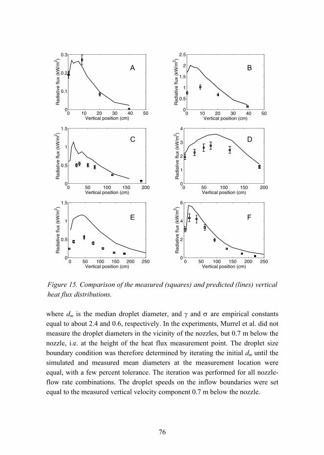
76

0 10 20 30 40 500

0.1

0.2

0.3

Vertical position (cm)

Rad

iativ

e flu

x (k

W/m

2 )

0 10 20 30 40 50

0

0.5

1

1.5

2

2.5

Vertical position (cm)

Rad

iativ

e flu

x (k

W/m

2 )

0 50 100 150 2000

0.5

1

1.5

Vertical position (cm)

Rad

iativ

e flu

x (k

W/m

2 )

0 50 100 150 200

0

1

2

3

4

Vertical position (cm)

Rad

iativ

e flu

x (k

W/m

2 )

0 50 100 150 200 2500

0.5

1

1.5

Vertical position (cm)

Rad

iativ

e flu

x (k

W/m

2 )

0 50 100 150 200 250

0

2

4

6

Vertical position (cm)

Rad

iativ

e flu

x (k

W/m

2 )

Figure 15. Comparison of the measured (squares) and predicted (lines) vertical heat flux distributions.

where dm is the median droplet diameter, and γ and σ are empirical constants equal to about 2.4 and 0.6, respectively. In the experiments, Murrel et al. did not measure the droplet diameters in the vicinity of the nozzles, but 0.7 m below the nozzle, i.e. at the height of the heat flux measurement point. The droplet size boundary condition was therefore determined by iterating the initial dm until the simulated and measured mean diameters at the measurement location were equal, with a few percent tolerance. The iteration was performed for all nozzle-flow rate combinations. The droplet speeds on the inflow boundaries were set equal to the measured vertical velocity component 0.7 m below the nozzle.

A C E

B D F

77

Figure 16. Schematics of the large-scale attenuation test.

In the computations, 10 cm grid cells, 1000 control angles, only one spectral band (grey assumption) and no gas phase absorption were used. The measured and predicted attenuation results are compared in Figure 17. Since a good general agreement was found for all three nozzles, and the results of the individual nozzles are well distinct in the flow-rate vs. attenuation space, we can assume that the model can properly take into account both the effect of the water load and the effect of the droplet size distribution. Only the mid-range flow rates of nozzle B and the highest flow rates of nozzle D show sizable discrepancies. These discrepancies are probably caused by a combination of measurement errors and model inaccuracy. The droplet size measurements, in particular, are difficult to conduct in large-scale sprays. The various challenges of spray measurements have been presented by Husted [130]. Some uncertainty is also related to the inverse determination of droplet size boundary conditions for the simulations.

The second validation test for spray-radiation interaction is the experiments of Dembele et al. [131]. They measured the attenuation of a collimated radiation beam passing through a water spray using a Fourier infrared spectrometer. The radiation source was a tungsten filament inside a silica tube. Its emission spectrum was close to that of a blackbody at 1300°C. The spray was produced with one, two or three hydraulic nozzles arranged in a row, and the measurements were made 20 cm below the nozzles at different flow rates. The schematics of the scenario are shown in Figure 18.

78

Figure 17. Results of the large scale attenuation.

Figure 18. Schematics of the small-scale attenuation test.

The simulations were performed at four different flow rates. The droplet size boundary conditions were determined using a procedure similar to the large-scale scenario. The velocity of the droplets at the inflow boundary was found from a simple geometrically based relationship between the flow velocity and distance. Modelling a collimated radiation beam is difficult with FVM due to the symmetric discretization of the unit sphere into solid angles. To alleviate the problem, the radiation source in this exercise was modelled simply as a 4 cm by 4 cm diffuse surface. Despite the strong approximation of the radiation source, the comparison with the measurements is valid on the opposite side of the spray

79

because the air surrounding the water spray was transparent and non-scattering, but not in the other directions. 2.0 cm grid cells, 1000 radiation angles and six radiation bands were used, but the gas phase absorption was neglected. In this scenario, the independence of the spatial and angular resolutions was very difficult to achieve. For a single-nozzle flow at 0.14 L/min, reducing the cell size from 2.0 cm to 1.0 cm increased the attenuation from 8.3% to 11.4%, with 10.0% being the experimental value. The convergence in angular resolution was difficult to achieve because the radiation source was very small compared to the domain size, and because the ray effect is difficult to avoid in direction of grid axis.

Figure 19. Comparison of measured (squares) and predicted (lines) attenuation in small-scale tests.

The measured and simulated attenuation results are compared in Figure 19. In the case of only one nozzle, the agreement is very good, taking into account the unavoidable dependence on the grid and angular resolutions. The root mean-square error between the predicted and measured attenuations is only 1.3%.

80

When more nozzles are put between the source and the measurement point, the attenuation is clearly over-predicted. The rms errors for two and three nozzles are 6.4 and 8.8%, respectively. One possible reason for the over prediction is the droplet coalescence, which is not taken into account by the model. Coalescence happens as a result of the hydrodynamic interaction between adjacent sprays [131]. This explanation is supported by the finding that while the predicted attenuations with two and three nozzles increase roughly by factors two and three from the values corresponding to the one nozzle, the experimental results increase only by factors of 1.3 and 1.8.

In Paper V, the computed droplet size distributions in different parts of the spray were compared, demonstrating that both the mean diameters and the shapes of the droplet size distributions may vary significantly in different parts of the spray. The same phenomena for hollow cone water mist sprays has been observed experimentally by Husted [130]. During the computation of the mean radiative properties for the spray in this work, the shape of the distribution is fixed to the presumed size probability density function, and only the droplet mean is allowed to vary according to the statistics predicted by the Lagrangian transport model. The importance of this approximation to the radiation solutions is not known, and should be studied in the future.

81

8. Discussion

The applicability of a numerical solver for the intended use depends on the accuracy, computational efficiency and reliability. In this context, the computational efficiency must be measured as a balance between accuracy and computational cost in relation to the rest of the computational framework. Since the intended use of FDS is mainly fire engineering and fire risk analysis, the radiation solver must be efficient and in concordance with the rest of the code to allow sufficiently accurate predictions with limited resources. According to Howard Baum, NIST Research Fellow, the CPU consumption of a given numerical routine ought to be commensurate with the particular phenomenon addressed [132]. In a simulation of a typical enclosure fire, where the fraction of heat transfer by radiation is around 30%, the FVM radiation solver consumes less than 30% of the total CPU time. At the same time, the accuracy of the radiation solution is expected to be of the same order with the other phenomena. More accuracy can be achieved by the increased angular, spatial, spectral and temporal resolutions, but at the expense of the increased CPU time. Other requirements, caused by the wide range of uses, are versatility, ease of use and ease of extension.

The presented verification cases demonstrated that in the case of three-dimensional radiation fields, FDS predictions converged towards the exact solutions when both spatial and angular resolutions were sufficient. In practical simulations, the spatial resolution is usually determined by the flow solution, and the default angular resolution of 104 directions seems to be an appropriate choice. It is important though that the code users are aware of the ray effect and the resulting errors when dealing with heat transfer dominated by far field radiation. The ray effect probably has more importance in code validation, where local radiative fluxes are compared against experiments, than in practical applications.

The validation of the flame radiation computation was performed using diffusion flames ranging from 10 to 100 cm. With few exceptions, the predictions were within 25 % of the measured radiative heat fluxes. Further developments in combustion and radiation source modelling are needed to improve the flame heat fluxes. This is especially true for small heat release rates because the problems appear when the combustion region close to the burning surface is not adequately resolved.

82

The accuracy of predicting the radiation attenuation by water spray was even better than in the case of flame heat fluxes, demonstrating that the physics of radiation-spray interaction are included with sufficient detail. Aspects of droplet breakup and coalescence should be considered to account for more complicated and dense sprays. Ultimately, the inclusion of secondary droplet breakup could reduce the sensitivity to the droplet size boundary conditions by allowing automatic adjustment of the droplet size according to the flow conditions. However, as pointed out by Madsen [112], the exact mechanisms behind the droplet breakup are still not completely understood. Prediction of the initial atomization processes from the first principles would require very detailed models of the nozzles and relatively complicated models of the two-phase flows, and seems to be beyond the current capabilities of fire simulation.

Due to the challenges of describing the experimental conditions, the angular resolutions and computational costs of the validation simulations were higher than the normal practice in applications. To evaluate the accuracy and cost in situations corresponding to the typical use of the code, a validation study involving real flames and water sprays from sprinklers or water mist nozzles would be needed.

83

9. Concluding remarks

9.1 Summary

The objective of this thesis has been to summarize the work of the author in the development of the computational tools for fire risk analysis and fire safety engineering. The work reported in this thesis focused on two particular topics: The first topic was the application of Monte Carlo simulation in the field of fire risk analysis and the development of the necessary tools for performing these simulations using a range of different fire models. The second topic was the development of a numerical solver for the transport of thermal radiation within Fire Dynamics Simulator code. The two topics are linked by the numerous applications of FDS as a deterministic model in fire risk analysis. The efficient and robust radiation solver, developed in the second part of the thesis, will thus benefit the application of the technique developed in the first part.

9.2 Development of probabilistic fire simulation

In fire risk analysis, the probabilities of fire consequences are computed using deterministic models for fire phenomena, taking into account the statistical variation or uncertainty of the initial and boundary conditions. The development of the computational resources has allowed the use of Monte Carlo simulation, the most general approach where the space of possible answers is covered in a statistically satisfactory manner. However, the convergence of the Monte Carlo simulation must be accelerated when computationally expensive tools such as CFD are used. The TMMC technique, developed in this work, allows the use of relatively simple and fast models in the collection of the main body of the statistical data, while retaining the physical accuracy by running a small set of simulations with more accurate but slower model and introducing a multi-dimensional scaling function to provide a correction to the main data. The performance of TMMC was validated using simple room fire scenarios, and the use of the FDS code as a deterministic tool of the Monte Carlo simulation was demonstrated.

84

9.3 Weaknesses of TMMC technique and suggestions for future work

The principal weakness of TMMC is a limited knowledge of its theoretical basis. Although it has been seen heuristically to yield good results, and the mechanism is understood, the evidence is not yet sufficient. In the examples presented, the method works well, but there is no general guarantee that the process converges towards the true solution if the fast and slow models differ considerably.

For economy, the accuracy and efficiency of the TMMC technique could be improved by a better numerical treatment of the scaling process. Possible reduction of the number of scaling points should be studied in the future because in some applications, the derivation of the scaling function may form the majority of the computational cost. As demonstrated in the second validation test, all the available a priori information on the relative importance of the random variables should be used to concentrate more scaling points to the most important variables. The application of adaptive sampling techniques to the scaling point placement should be studied in order to reduce the cost in the situations where a priori information is not valid. An example of such a situation is when the inaccuracy of the simple model (Model A) would lead to wrong conclusions on the relative importance of the random variables. Further improvement of the accuracy could be achieved by interpolating the scaling functions between the scaling points to ensure a smoother transition from one scaling region to another.

9.4 Development of radiation solver for Fire Dynamics Simulator

During the last few years, CFD fire simulation has become a routine part of fire engineering. This is especially true in the field of design work, where the introduction of a performance-based design concept has created a market for simulation tools that are reliable and accurate enough for the given purpose, and that are fast and relatively easy to use. After its release in 2000, FDS has become the most widely used fire simulation tool in the world. From the code reliability viewpoint, the high number of active users is an advantage, since the wide range of different applications inevitably reveals the errors in the code. The width of

85

the range also means that some of the applications push the limits of the code in terms of both applicability and validity. On the other hand, the widespread use of CFD may have lured the audience into a sense of complacency with its visually appealing presentation. As a result, CFD may be used or requested when more simple techniques would suffice.

In this work, an FVM-based radiation solver was implemented in FDS. The solver can be used to compute the transport of thermal radiation in a participating medium consisting of combustion gases, soot and water droplets. The goal of the solver implementation was to find a balance between accuracy and computational cost in engineering applications. In the presented verification and validation examples, the accuracy of the predictions was found sufficient for engineering purposes. The highest errors were found in predictions of heat fluxes from weak flames. Computational efficiency was achieved by making three major approximations. First, the use of rectilinear grids in spatial discretization, which is consistent with the rest of the code, increases the computational efficiency by allowing the use of an explicit marching scheme as a method for transport solution and reduces the memory requirement because the geometrical coefficients of the discretized RTE are constants over the whole domain. As a second approximation, the time accuracy of the radiation solution was relaxed by assuming that the numerical time step of the hydrodynamic solver, given by the CFL-condition, is much smaller than the time scale of the global heat transfer processes. The third approximation was the spectral averaging over wide wavelength regions. Additional efficiency was achieved by the extensive use of lookup tables and application of first order accurate scheme for intensities. The high numerical diffusion caused by the first order accuracy was not found to adversely affect the model accuracy.

An important enhancement of the basic radiation solver was the introduction of radiation-spray interactions. Despite the complexity of the physical phenomena, the computational cost of the radiation solution remained in balance with the physical importance. The major approximations were the assumed global similarity of the droplet size distributions and the approximation of scattering phase functions by a sum of isotropic and forward components. Speed of the solution was again achieved by computing the spray radiative properties in advance and storing in lookup tables.

86

9.5 Weaknesses of the radiation solver and suggestions for future work

Some of the model approximations are deeply embedded and improvements in the corresponding code capabilities would be difficult to carry out. The influences of other approximations, however, are more easily controlled by adjusting the model parameters. For example, the extension of the FDS capability with respect to the rectilinearity of the grid would require a complete revision of the radiation solver, whereas an accurate simulation of turbulence-radiation interactions could be implemented simply by adjusting the time interval of the radiation updates. Naturally, higher computational costs should then be expected.

Topics of future work include the generalization of the spectral band structure to allow the use of arbitrary species in the computation of absorption coefficients, generalization of the dispersed phase radiative properties beyond those of water, and allowing the suspensions of other types of particles than liquid droplets. For example, soot is known to both absorb and scatter radiation, but currently only the absorption is taken into account via RadCal. The water spray validation examples demonstrated that the shapes of the droplet size distributions may vary significantly in different parts of the spray. The effect of the global size distribution similarity approximation is currently not known and should be studied in the future by comparing against simulations where the local droplet size distributions are rigorously taken into account in the computation of spray radiative properties. Inclusion of secondary droplet breakup and coalescence processes may be necessary in order to reduce the sensitivity to the droplet size boundary conditions. In addition, a validation of the model using realistic sources of radiation and relevant water spray types should be performed.

In large scale fire simulations, the increase in spatial resolution that would be necessary for a detailed solution of the flame temperature distribution will not be possible for a long time. The modelling of the radiative source term is therefore needed in order to reduce the sensitivity on the unavoidable temperature errors. The current model is based on the assumption of local radiative fraction of heat release, and may be insufficient in fires where the flame optical properties change considerably. An example of such a situation is the transition from a well-ventilated to an under-ventilated enclosure fire. Possible means of

87

modelling could use the ideas of flamelets, adapted to the practical restrictions of large-scale simulations. A special problem is flame spread on a material, where the process essentially becomes two-dimensional. Application of submodels, similar to the boundary layer theory of Prandtl, might be feasible [133]. Interfacing them to LES codes and addressing the whole problem of wall functions is an issue still to be studied. One practical tool for studying the existence and shape of the flame spread wall functions could be the direct numerical simulation (DNS) of the near wall phenomena. In DNS, all the turbulent length scales are resolved by using very fine spatial resolution and sufficiently accurate numerical schemes. A two-dimensional approximation of DNS may already be possible using the existing tools. DNS can also serve as a detailed tool for experimental design.

88

References

1. Molak, V. (ed.) Fundamentals of Risk Analysis and Risk Management. Boca Raton: Lewis Publishers, 1997. 472 p.

2. The Reactor Safety Study An Assessment of Accident Risks in U.S. Commercial Nuclear Power Plants. Washington, D.C.: U.S. Nuclear Regulatory Commission (USNRC), 1975. WASH-1400 (NUREG-75/014).

3. Severe Accident Risks: An Assessment for Five U.S. Nuclear Power Plants. Washington, D.C.: U.S. Nuclear Regulatory Commission (USNRC), 1991. NUREG-1150.

4. Kaiser, G.D. Overall assessment. In: Green, A.E. (ed.). High Risk Safety Technology. Chichester: Wiley, 1982. Pp. 101110.

5. PRA Procedures Guide A Guide to the Performance of Probabilistic Risk Assessment for Nuclear Power Plants. Washington, D.C.: U.S. Nuclear Regulatory Commission (USNRC), 1983. NUREG/CR2300.

6. Keski-Rahkonen, O. Fire safety research (FISRE): FISRE summary report. In: Kyrki-Rajamäki, R. & Puska, E.-K. (eds.). FINNUS The Finnish Research Programme on Nuclear Power Plant Safety 19992002. Final Report. Espoo: VTT Processes, 2002. VTT Research Notes 2164. Pp. 197204.

7. Keski-Rahkonen, O., Mangs, J., Hostikka, S. & Korhonen, T. POTFIS summary report. In: Räty, H. & Puska, E.K. (ed.). SAFIR. The Finnish Research Programme on Nuclear Power Plant Safety 20032006. Final Report. Espoo: VTT, 2006. VTT Research Notes 2363. Pp. 335342.

8. Keski-Rahkonen, O., Mangs, J., Hostikka, S. & Korhonen, T. Quantitative assessment of potential fire spread in nuclear power plant scenarios. In: Post-Conference Seminar III of the 18th International Conference on Structural Mechanics in Reactor Technology (SMIRT 18). 2005. 9th International Seminar on Fire Safety in Nuclear Power Plants and Installations. August 2224, 2005, Vienna, Austria. CD-ROM.

89

9. Keski-Rahkonen, O., Mangs, J., Hostikka, S. & Korhonen, T. Quantitative application of Monte Carlo simulation in Fire-PSA. Kerntechnik, 2007. Vol. 72, No. 3, pp. 149155.

10. Karlsson, B. & Tomasson, B. Repeatability Tests of a Fire Risk Index Method for Multi-Storey Apartment Buildings. In: Gottuk, D.T. & Lattimer, B.Y. (eds.). Proceedings of Eighth International Symposium on Fire Safety Science. Beijing, China, September 1823, 2005. International Association for Fire Safety Science, 2005. Pp. 901912.

11. Williamson, R.B. Coupling Deterministic and Stochastic Modeling to Unwanted Fire. Fire Safety Journal, 1981.Vol. 3, pp. 243259.

12. Ling, W. C. T. & Williamson, R. B. Use of Probabilistic Networks for Analysis of Smoke Spread and the Egress of People in Buildings. In: Grant, C.E. & Pagni, P.J. (Eds.). Proceedings of 1st International Symposium. Fire Safety Science. October 711, 1985, Gaithersburg, MD. International Association for Fire Safety Science. Hemisphere Publishing Corp., NY, 1986. Pp. 953962.

13. Korhonen, T. Hietaniemi, J., Baroudi, D. & Kokkala, M. Time-dependent event-tree method for fire risk analysis: tentative results. In: Evans, D.D. (ed.). Proceedings of the Seventh International Symposium on Fire Safety Science. Worcester, MA, 1621 June 2003. International Association for Fire Safety Science, 2003. Pp. 321332.

14. Fontana, M. & Maag, T. Fire Risk Assessment Based on Bayesian Networks. In: Almand, K., Attlan, J.M., DHoop, J.M. & Gordon, J. (eds.) Proceedings of 5th International Conference on Performance-Based Codes and Fire Safety Design Methods. October 68, 2004, Luxembourg. 2004. Pp. 238249.

15. Frantzich, H. Risk Analysis and Fire Safety Engineering. Fire Safety Journal, 1998. Vol. 31, No. 4, pp. 313329.

16. Korhonen, T., Hostikka, S. & Keski-Rahkonen, O. A proposal for the goals and new techniques of modelling pedestrian evacuation in fires. In: Gottuk, D. & Lattimer, B. (eds.). Proceedings of the Eight International Symposium on Fire Safety Science. Beijing, China, 1823 Sept. 2005. International Association for Fire Safety Science, 2005. Pp. 557569.

90

17. Helton, J. C. Treatment of Uncertainty in Performance Assessments for Complex Systems. Risk Analysis, 1994. Vol. 14, No. 4, pp. 483511.

18. Tillander, K. & Keski-Rahkonen, O. The Ignition Frequency of Structural Fires in Finland 199699. In: Evans, D.D. (ed.). Proceedings of the Seventh International Symposium on Fire Safety Science. Worcester, MA, 1621 June 2003. International Association for Fire Safety Science, 2003. Pp. 10511062.

19. Tillander, K. Utilisation of statistics to assess fire risks in buildings. Espoo: VTT Building and Transport, 2004. VTT Publications 537. 224 p. + app. 37 p.

20. Sekizawa, A. Fire Risk Analysis: Its Validity and Potential for Application in Fire Safety. In: Gottuk, D.T. & Lattimer, B.Y. (eds.). Proceedings of Eighth International Symposium on Fire Safety Science. Beijing, China, September 1823, 2005. International Association for Fire Safety Science, 2005. Pp. 82100.

21. Vose, D. Monte Carlo Risk Analysis Modeling. In: Molak, V. (ed.). Fundamentals of Risk Analysis and Risk Management. Boca Raton: Lewis Publishers, 1997. 472 p.

22. Metropolis, N. & Ulam, S. The Monte Carlo Method. Journal of the American Statistical Association, 1949. Vol. 44, No. 247, pp. 335341.

23. Vose, D. Quantitative risk analysis: a guide to Monte Carlo simulation modelling. Chichester, England: Wiley, 1996. 328 p.

24. Hofer, E., Jahn, H. & Krzykacz, B. Uncertainty and sensitivity analysis of an oil and cable fire simulation with the code CRDLOC. In: Apostolakis, G. (ed.) Probabilistic Safety Assessment and Management, Elsevier Science Publishing Co., 1991.

25. Krzykacz, B., Hofer, E. & Kloos, M. A software system for probabilistic uncertainty and sensitivity analysis of results from computer models. In: Proceedings of PSAM II. San Diego, CA, USA, 2025 March 1994.

91

26. Hostikka, S., Keski-Rahkonen, O. & Korhonen, T. Probabilistic Fire Simulator. Theory and Users Manual for Version 1.2, Espoo: VTT Building and Transport, 2003. VTT Publications 503, 72 p. + App. 1 p.

27. McKay, M.D., Beckman, R.J. & Conover, W.J. A comparison of three methods for selecting values of input variables in the analysis of output from a computer code. Technometrics, 1979. Vol. 21, No. 2, pp. 239245.

28. Iman, R.L. & Helton, J.C. Investigation of Uncertainty and Sensitivity Analysis Techniques for Computer Models. Risk Analysis, 1988. Vol. 8, No. 1, pp. 7190.

29. Magnussion, S.E. Risk Assessment. International Association for Fire Safety Science. In: Hasemi, Y. (ed.) Proceedings of Fifth (5th) International Symposium on Fire Safety Science. March 37, 1997, Melbourne, Australia. Boston, MA: International Association for Fire Safety Science, 1997. Pp. 4158.

30. Hofer, E., Kloos, M., Krzykacz, B., Peschke, J. & Sonnenkalb, M. Methodenentwicklung zur simulativen Behandlung der Stochastik in probabilistischen Sicherheitsanalysen der Stufe 2. Garching: GRSA-2997, Gesellschaft für Anlagen- und Reaktorsicherheit, 2001.

31. Hofer, E, Kloos, M., Krzykacz-Hausmann, B. Peschke, J. & Woltereck, M. An approximate epistemic uncertainty analysis approach in the presence of epistemic and aleatory uncertainties, Reliability Engineering and System Safety, 2002. Vol. 77, pp. 229238.

32. Eschenroeder, A.Q. & Faeder, E.J. Monte Carlo Analysis of Health Risks From PCB-Contaminated Mineral Oil Transformer Fires. Risk Analysis, 1988. Vol. 8, No. 2, pp. 291298.

33. Zhao, L. Methodology of Calculating the Risk to People in Building Fires. In: Shields, J. (ed.). Proceedings of 1st International Symposium on Human Behavior in Fire. August 31 September 2, 1998, Belfast, Northern Ireland. Northern Ireland: University of Ulster, 1998. Pp. 401410.

34. Fraser-Mitchell, J. Risk Assessment of Factors Related to Fire Protection in Dwellings. In: Hasemi, Y. (ed.) Proceedings of Fifth (5th) International Symposium on Fire Safety Science. March 37, 1997, Melbourne,

92

Australia. Boston, MA: International Association for Fire Safety Science, 1997. Pp. 631642.

35. Magnusson, S.E., Frantzich, H. & Harada, K. Fire Safety Design Based on Calculations: Uncertainty Analysis and Safety Verification. Fire Safety Journal, 1996. Vol. 27, pp. 305334.

36. Fraser-Mitchell, J.N. Modelling Human Behavior Within the Fire Risk Assessment Tool "CRISP". In: Shields, J. (ed.). Proceedings of 1st International Symposium on Human Behavior in Fire. August 31 September 2, 1998, Belfast, Northern Ireland. Northern Ireland: University of Ulster, 1998. Pp. 447457.

37. Zhao, L. & Beck, V. Definition of Scenarios for the CESARE-RISK Model. In: Hasemi, Y. (ed.) Proceedings of Fifth (5th) International Symposium on Fire Safety Science. March 37, 1997, Melbourne, Australia. Boston, MA: International Association for Fire Safety Science, 1997. Pp. 655666.

38. Phillips, W.G.B. Simulation Models for Fire Risk Assessment. Fire Safety Journal, 1994. Vol. 23, No. 2, pp. 159169.

39. Hasofer, A.M. & Qu, J. Response Surface Modelling of Monte Carlo Fire Data. Fire Safety Journal, 2002. Vol. 37, No. 8, pp. 772784.

40. Notarianni, K.A. Role of Uncertainty in Improving Fire Protection Regulation. Pittsburgh, PA: Carnegie-Mellon Univ. 2000. Thesis, 269 p.

41. Hamilton, S.R. & Deierlein, G.G. Probabilistic Methodology for Performance-Based Fire Engineering. In: Almand, K., Attlan, J.M., DHoop, J.M. & Gordon, J. (eds.) Proceedings of 5th International Conference on Performance-Based Codes and Fire Safety Design Methods. October 68, 2004, Luxembourg. 2004. Pp. 327341.

42. Kirby, B.R., Newman, G.M., Butterworth, N., Pagan, J. & English, C. Development of a Performance Based Approach to Specifying Fire Resistance for Regulatory Purposes. In: Almand, K., Attlan, J.M., DHoop, J.M. & Gordon, J. (eds.) Proceedings of 5th International Conference on Performance-Based Codes and Fire Safety Design Methods. October 68, 2004, Luxembourg. 2004. Pp. 183194.

93

43. Li, Y. & Spearpoint, M. Cost-Benefit Analysis of Sprinklers for Property Protection in New Zealand Parking Buildings. Journal of Applied Fire Science, 20032004. Vol. 12, No. 3, pp. 223243.

44. Yuen, W.W. & Chow, W.K. Monte Carlo Approach for the Layout Design of Thermal Fire Detection System. Fire Technology, 2005. Vol. 41, No. 2, pp. 93104.

45. Madras, N. Lectures on Monte Carlo methods. Providence, RI: American Mathematical Society, 2002. 103 p.

46. Landau, D.P. & Binder, K.A guide to Monte Carlo simulations in statistical physics. Cambridge University Press, 2005. 2nd ed. 432 p.

47. Milton, J.S. & Arnold, J.C. Introduction to probability and statistics: principles and applications for engineering and the computing sciences. New York, NY: McGraw-Hill, 1990. 2nd ed. 700 p.

48. Stein, M.L. Large sample properties of simulations using latin hypercube sampling. Technometrics, 1987. Vol. 29, No. 2, pp. 143151.

49. Hofer, E. Sensitivity analysis in the context of uncertainty analysis for computationally intensive models. Computer Physics Communications, 1999. Vol. 117, pp. 2134.

50. Pebesma, E.J. & Heuvelink, G.B.M. Latin hypercube sampling of multigaussian random fields. Technometrics, 1999. Vol. 41, No. 4, pp. 303312.

51. Jones, W.W., Forney, G.P., Peacock, R.D. & Reneke, P.A. Technical Reference for CFAST: An Engineering Tool for Estimating Fire and Smoke Transport. Gaithersburg, MD: National Institute of Standards and Technology, 2000. NIST TN 1431. 190 p.

52. Cadorin, J.-F. & Franssen, J.-M. A tool to design steel elements submitted to compartment Þres-OZone V2. Part 1: Pre-and post-ßashover compartment Þre model. Fire Safety Science, 2003. Vol. 38, No. 5, pp. 395427.

53. Cadorin, J.-F., Pintea, D., Dotreppe, J.-C. & Franssen, J.-M. A tool to design steel elements submitted to compartment Þres-OZone V2. Part 2: Methodology and application. Fire Safety Science, 2003. Vol. 38, No. 5, pp. 429451.

94

54. Vaari, J. A transient one-zone computer model for total flooding water mist fire suppression in ventilated enclosures. Fire Safety Journal, 2002. Vol. 37, No. 3, pp. 229257.

55. Drysdale, D. An Introduction to Fire Dynamics. Chichester: Wiley-Interscience, 1999. Second Edition, 140 p.

56. Hostikka, S. & Keski-Rahkonen, O. Advanced probabilistic simulation of NPP fires. Proceedings of the 18th International Conference on Structural Mechanics in Reactor Technology. SMIRT 18. Beijing, China, August 712, 2005. Beijing: Atomic Energy Press, 2005. Pp. 39843996.

57. Raithby, G.D. & Chui, E.H. A Finite-Volume Method for Predicting Radiant Heat Transfer in Enclosures with Participating Media. Journal of Heat Transfer, 1990. Vol. 112, No. 2, pp. 415423.

58. Cox, G. & Kumar, S. Modelling Enclosure Fires Using CFD. In: SFPE Handbook of Fire Protection Engineering. Quincy, MA: Society of Fire Protection Engineers, 2002. 3rd Edition. Pp. 3-1943-218.

59. Patankar, S.V. & Spalding, D.B.A Calculation Procedure for Heat, Mass and Momentum Transfer in Three-dimensional Parabolic Flows. International Journal for Heat and Mass Transfer, 1972. Vol. 15, pp. 17871806.

60. Magnussen B. & Hjertager G.H. On mathematical modelling of turbulent combustion with special emphasis on soot formation and combustion. In: Proceedings of 16th International Symposium on Combustion. The Combustion Institute, 1976. Pp. 719729.

61. McGrattan, K.B., Hostikka, S., Floyd, J.E., Baum, H. & Rehm, R. Fire Dynamics Simulator (Version 5): Technical Reference Guide. Gaithersburg, MD: National Institute of Standards and Technology, October 2007. NIST Special Publication 1018-5.

62. McGrattan, K.B., Klein, B., Hostikka, S. & Floyd, J.E. Fire Dynamics Simulator (Version 5): Users Guide. Gaithersburg, MD: National Institute of Standards and Technology, October 2007. NIST Special Publication 1019-5.

95

63. Olenick, S. & Carpenter, D. An Updated International Survey of Computer Models for Fire and Smoke. Journal of Fire Protection Engineering, 2003. Vol. 13, pp. 87110.

64. Ferziger, J.H. & Perić, M. Computational Methods for Fluid Dynamics. Heidelberg: Springer, 1997. Corrected 2nd printing. 364 p.

65. Courant, R. Friedrichs, K.O. & Lewy, H. Über die partiellen Differential-gleichungen der mathematischen Physik. Mathematische Annalen 100, 1928. Pp. 3274.

66. Courant, R., Friedrichs, K. & Lewy, H. On the partial difference equations of mathematical physics. IBM Journal, 1967, pp. 215234. English translation of the 1928 German original paper.

67. Baum, H.R. & Rehm, R.G. Calculations of Three Dimensional Buoyant Plumes in Enclosures. Combustion Science and Technology, 1984. Vol. 40, pp. 5577.

68. Holen, J., Brostrom, M. & Magnussen, B.F. Finite Difference Calculation of Pool Fires. In: Proceedings of the 23rd Symposium (International) on Combustion, Combustion Institute, 1990. Pp. 16771683.

69. Taylor, S., Petridis, M., Knight, B., Ewer, J., Galea, E.R & Patel, M. SMARTFIRE: an integrated computational fluid dynamics code and expert system for fire field modelling. In: Hasemi, Y. (ed.) Proceedings of Fifth (5th) International Symposium on Fire Safety Science. March 37, 1997, Melbourne, Australia. Boston, MA: International Association for Fire Safety Science, 1997. Pp. 12851296.

70. Welch, S. & Rubini, P. Three-Dimensional Simulation of a Fire-Resistance Furnace. In: Hasemi, Y. (ed.) Proceedings of Fifth (5th) International Symposium on Fire Safety Science. March 37, 1997, Melbourne, Australia. Boston, MA: International Association for Fire Safety Science, 1997. Pp. 10091020.

71. Suard, S., Audouin, L., Babik, F., Rigollet, L. & Latche, J.C. Verification and Validation of the ISIS CFD Code for Fire Simulation. Workshop on Assessment of Calculation Methods in Fire Safety Engineering, San antonio, TX, USA, 10 April 2006. ISO/TC 92/SC4. 28 p.

96

72. Greiner, M. & Suo-Anttila, A. Radiation Heat Transfer and Reaction Chemistry Models for Risk Assessment Compatible Fire Simulations. Journal of Fire Protection Engineering, 2006. Vol. 16, No. 2, pp. 79104.

73. Yan, Z. Large Eddy Simulation of Soot Formation in a Turbulent Diffusion Flame. In: Gottuk, D.T. & Lattimer, B.Y. (eds.). Proceedings of Eighth International Symposium on Fire Safety Science. Beijing, China, September 1823, 2005. International Association for Fire Safety Science, 2005. Poster abstract.

74. Cheung, A.L.K., Cheung, S.C.P., Yeoh, G.H. & Yuen, R.K.K. Investigation of Pulsating Behaviour of Buoyant Fires by Using Large Eddy Simulation (LES) Approach with Soot and Radiation. In: Gottuk, D.T. & Lattimer, B.Y. (eds.). Proceedings of Eighth International Symposium on Fire Safety Science. Beijing, China, September 1823, 2005. International Association for Fire Safety Science, 2005. Poster abstract.

75. Kumar, S. Mathematical modelling of Natural Convection in Fire A State of the Art Review of the Field Modelling of Variable Density Turbulent Flow. Fire and Materials, 1983. Vol. 7, pp. 124.

76. Liu, F. & Wen, J.X. The effect of different turbulence models on the CFD simulation of buoyant diffusion flames. Fire Safety Journal, 2002. Vol. 37, No. 2, pp. 125151.

77. McGrattan, K.B., Rehm, R.G. & Baum, H.R. Fire-Driven Flows in Enclosures. Journal of Computational Physics, 1994. Vol. 110, No. 2, pp. 285291.

78. Rehm, R.G., McGrattan, K.B., Baum, H.R. & Cassel, K.W. Transport by Gravity Currents in Building Fires. In: Fire Safety Science Proceedings of the Fifth International Symposium. International Association for Fire Safety Science, 1997. Pp. 391402.

79. Clement, J.M. & Fleischmann, C.M. Experimental Verification of the Fire Dynamics Simulator Hydrodynamic Model. In: Fire Safety Science Proceedings of the Seventh International Symposium. International Association for Fire Safety Science, 2002. Pp. 839862

97

80. Baum, H.R., McGrattan, K.B. & Rehm, R.G. Three Dimensional Simulations of Fire Plume Dynamics. In: Hasemi, Y. (ed.) Proceedings of Fifth (5th) International Symposium on Fire Safety Science. March 37, 1997, Melbourne, Australia. Boston, MA: International Association for Fire Safety Science, 1997. Pp. 511522.

81. Baum, H.R. & McCaffrey, B.J. Fire Induced Flow Field Theory and Experiment. In: Proceedings of the Second International Symposium on Fire Safety Science. International Association for Fire Safety Science, 1989. Pp. 129148.

82. McGrattan, K.B., Baum, H.R. & Rehm, R.G. Large Eddy Simulations of Smoke Movement. Fire Safety Journal, 1998. Vol. 30, pp. 161178.

83. Ma, T.G. & Quintiere, J.G. Numerical simulation of axi-symmetric fire plumes: accuracy and limitations. Fire Safety Journal, 2003. Vol. 38, No. 5, pp. 467492.

84. Hamins, A., Maranghides, A., McGrattan, K.B., Johnsson, E., Ohlemiller, T., Donnelly, M., Yang, J., Mulholland, G., Prasad, K., Kukuck, S., Anleitner, R. & McAllister, T. Report on Experiments to Validate Fire Dynamic and Thermal-Structural Models for Use in the World Trade Center Investigation. Gaithersburg, MD: National Institute of Standards and Technology, 2004. NIST Special Publication 1000-B.

85. Hamins, A., Maranghides, A., McGrattan, K.B., Ohlemiller, T. & Anletiner, R. Experiments to Validate Models of Fire Growth and Spread for use in the World Trade Center Investigation. Gaithersburg, MD: National Institute of Standards and Technology, 2004. NIST Special Publication 1000-10E.

86. McGrattan, K.B. Verification and Validation of Selected Fire Models for Nuclear Power Plant Applications. Volume 7. Fire Dynamics Simulator (FDS). Gaithersburg, MD: National Institute of Standards and Technology. Washington, DC: Nuclear Regulatory Commission. Palo Alto, CA: Electric Power Research Institute, 2007. NUREG-1824, EPRI 1011999. Volume 7. 205 p.

98

87. de St. Germain, J.D., McCorquodale, J., Parker, S.G. & Johnson, C.R. Uintah: A Massively Parallel Problem Solving Environment, Ninth IEEE International Symposium on High Performance and Distributed Computing. IEEE, 2000. Pp. 3341.

88. Pope, S.B. Ten questions concerning the large-eddy simulation of turbulent flows. New Journal of Physics, 2004. Vol. 6, pp. 124.

89. Zhang, W., Hamer, A., Klassen, M., Carpenter, D. & Roby, R. Turbulence statistics in a fire room model by large eddy simulation. Fire Safety Journal, 2002. Vol. 37, No. 8, pp. 721752.

90. Tuovinen, H., Blomqvist, P. & Saric, F. Modelling of hydrogen cyanide formation in room fires. Fire Safety Journal, 2004. Vol. 39, No. 8, pp. 737755.

91. Yang, R., Weng, W.G., Fan, W.C. & Wang, Y.S. Subgrid scale laminar flamelet model for partially premixed combustion and its application to backdraft simulation. Fire Safety Journal, 2005. Vol. 40, No. 2, pp. 8198.

92. Kang, Y. & Wen, J. X. Large Eddy Simulation of a Small Pool Fire. Combustion Science and Technology, 2004. Vol. 176, No. 12, pp. 21932223.

93. Beyler, C.L. Fire Hazard Calculations for Large, Open Hydrocarbon Fires. In: SFPE Handbook of Fire Protection Engineering. Quincy, MA: Society of Fire Protection Engineers, 2002. 3rd Edition. Pp. 3-2683-314.

94. Siegel, R. & Howell, J.R. Thermal Radiation Heat Transfer. New York, NY: Hemisphere Publishing Corporation, 1981. 2nd ed. 862 p.

95. Özisik, M.N. Radiative transfer and interactions with conduction and convection. New York, NY: John Wiley & Sons Inc., 1973. 575 p.

96. Lockwood, F.C. & Shah, N.G. A new radiation solution method for incorporation in general combustion prediction procedures. In: Proceedings of the 18th Symposium (International) on Combustion. Pittsburgh, PA: The Combustion Institute, 1981. pp. 14051416.

97. Jensen, K.A., Ripoll, J.-F., Wray, A.A., Joseph, D. & El Hafi, M. On various modeling approaches to radiative heat transfer in pool fires. Combustion and Flame, 2007. Vol. 148, No. 4, pp. 263279.

99

98. Dembele, S. & Wen, J.X. Evaluation of a fast correlated-k approach for radiation calculations in combustion systems. Numerical Heat Transfer Part B, 2003. Vol. 44, No. 4, pp. 365385.

99. Dembele, S., Zhang, J. & Wen, J.X. Assessments of Spectral Narrow Band and Weighted-Sum-of-Gray-Gases Models for Computational Fluid Dynamics Simulations of Pool Fires. Numerical Heat Transfer Part B, 2005. Vol. 48, No. 3, pp. 257276.

100. Zhang, J., Dembele, S., Karwatzki, J. & Wen, J. X. Effect of Radiation Models on CFD Simulations of Upward Flame Spread. In: Gottuk, D.T. & Lattimer, B.Y. (eds.). Proceedings of Eighth International Symposium on Fire Safety Science. Beijing, China, September 1823, 2005. International Association for Fire Safety Science, 2005. Pp. 421432.

101. Wiscombe, W. Mie scattering calculations: Advances in technique and fast, vector-speed computer codes. National Center For Atmospheric Research, 1979 (revised 1996). NCAR Technical Note NCAR/TN-140+STR.

102. Bohren, C.F. & Huffman, D.R. Absorption and scattering of light by small particles. New York, NY: John Wiley & Sons, 1983. 530 p.

103. Berour, N., Lacroix, D., Boulet, P. & Jeandel, G. Radiative and conductive heat transfer in a nongrey semitransparent medium. Application to fire protection curtains. Journal of Quantitative Spectroscopy & Radiative Transfer, 2004. Vol. 86, pp. 930.

104. Trivic, D.N., OBrien, T.J. & Amon, C.H. Modeling the radiation of anisotropically scattering media by coupling Mie theory with Finite volume method. International Journal of Heat and Mass Transfer, 2004. Vol. 47, pp. 57655780.

105. Collin, A., Boulet, P., Lacroix, D. & Jeandel, G. On radiative transfer in water spray curtains using the discrete ordinates method. Journal of Quantitative Spectroscopy & Radiative Transfer, 2005. Vol. 92, pp. 85110.

106. Yeoh, G.H., Yuen, R.K.K., Chueng, S.C.P. & Kwok, W.K. On modelling combustion, radiation and soot processes in compartment fires. Building and Environment, 2003. Vol. 38, No. 6, pp. 771785.

100

107. Wen, J.X., Huang, L.Y. & Roberts, J. The effect of microscopic and global radiative heat exchange on the field predictions of compartment fires. Fire Safety Journal, 2001. Vol. 36, No. 3, pp. 205223.

108. Lautenberger, C.W., de Ris, J.L., Dembsey, N.A., Barnett, J.R. & Baum, H.R. A simplified model for soot formation and oxidation in CFD simulation of non premixed hydrocarbon flames. Fire Safety Journal, 2005. Vol. 40, No. 2, pp. 141176.

109. Prasad, K.R. & Baum, H.R. Coupled Fire Dynamics and Thermal Response of Complex Building Structures. In: Chen, J.H., Colket, M.D., Barlow, R.S. & Yetter, R.A. (eds.). Proceedings of the 30th Symposium (International) on Combustion. July 2530, 2004, Chicago, IL. Pittsburgh, PA: Combustion Institute, 2005. Vol. 30. Part 2. Pp. 22552262.

110. Atreya, A. & Baum, H.R. Model of Opposed-Flow Flame Spread Over Charring Materials. In: Chen, J.H. & Colket, M. D. (eds.). Proceedings of the 29th Symposium (International) on Combustion. July 2125, 2002, Sapporo, Japan. Pittsburgh, PA: Combustion Institute, 2002. Vol. 29. Part 1. Pp. 227236.

111. Kim, S.C. & Ryou, H.S. An experimental and numerical study on fire suppression using a water mist in an enclosure. Building and Environment, 2003. Vol. 38, No. 11, pp. 13091316.

112. Madsen, J. Computational and Experimental Study of Sprays from the Breakup of Water Sheets. Denmark: Aalborg University Esbjerg, 2006. PhD Thesis. 260 p.

113. Ingram, D.M., Causon, D.M. & Mingham, C.G. Developments in Cartesian cut cell methods. Mathematics and Computers in Simulation, 2003. Vol. 61, pp. 561572.

114. Gemeny, D.F., Alex, P.E., Kline, A.J. & Hardeman, B. PyroSim: A Dynamic Graphical User Interface for the Fire Dynamics Simulator and Pathfinder: A Companion Egress Model. INTERFLAM 2007. Proceedings of the 11th International Conference. September 35, 2007, London, England. Vol. 2, pp. 14171422.

101

115. Heinisuo, M. & Laasonen, M. Product modeling, part of the fire safety concept in the future for metal structures? In: Advanced research workshop on Fire Computer Modeling. Santander, Spain: University of Cantabria. 2007.

116. Dimyadi, J.A.W., Spearpoint, M. & Amor, R. Generating fire dynamics simulator geometrical input using an IFC-based building information model. Electronic Journal of Information Technology in Construction, 2007. Vol. 12, p. 443.

117. Chang, S.L. & Rhee, K.T. Blackbody radiation functions. International Communications in Heat and Mass Transfer, 1984. Vol. 11, pp. 451455.

118. Grosshandler, W. RadCal: A Narrow Band Model for Radiation Calculations in a Combustion Environment. Gaithersburg, MD: National Institute of Standards and Technology, 1993. NIST Technical Note TN 1402.

119. Kim, S.H. & Huh, K.Y. Assessment of The Finite-Volume Method and The Discrete Ordinate Method for Radiative Heat Transfer In a Three-Dimensional Rectangular Enclosure. Numerical Heat Transfer, Part B, 1999. Vol. 35, pp. 85112.

120. Murthy, J.Y. & Mathur, S.R. Radiative Heat Transfer in Axisymmetric Geometries Using an Unstructured Finite-Volume Method. Numerical Heat Transfer, Part B, 1998. Vol. 33, pp. 397416.

121. Raithby, G.D. Discussion of the Finite-Volume Method for Radiation, and its Application Using 3D Unstructured Meshes. Numerical Heat Transfer, Part B, 1999. Vol. 35, pp. 389405.

122. Chai, J.C., Lee, H.S. & Patankar, S.V. Finite Volume Method for Radiation Heat Transfer. Journal of Thermophysics and Heat Transfer, 1994. Vol. 8, No. 3, pp. 419425.

123. Ravigururajan, T. & Beltran, M. A Model for Attenuation of Fire Radiation Through Water Droplets. Fire Safety Journal, 1989. Vol. 15, pp. 171181.

124. Yang, W., Parker, T., Ladouceur, H.D. & Kee, R.J. The Interaction of Thermal Radiation and Water Mist in Fire Suppression. Fire Safety Journal, 2004. Vol. 39, pp. 4166.

102

125. Wiscombe, W.J. Improved Mie Scattering Algorithms. Applied Optics, 1980. Vol. 19, No. 9, pp. 15051509.

126. Hale, G.M. & Querry, M.R. Optical constants of water in the 200 nm to 200 mum wavelength region. Applied Optics, 1973. Vol. 12, No. 3, pp. 555563.

127. Zeldovich, Y.B. & Raizer, Y.P. Physics of shock waves and high-temperature hydrodynamic phenomena. New York, NY: Dover Publications, 2002. Translated from the Russian and then edited by W.D. Hayes and R.F. Probstein.

128. Hamins, A., Klassen, M., Gore, J. & Kashiwagi, T. Estimate of Flame Radiance via a Single Location Measurement in Liquid Pool Fires. Combustion and Flame, 1991. Vol. 86, pp. 223228.

129. Murrel, J.V., Crowhurst, D. & Rock, P. Experimental study of the thermal radiation attenuation of sprays from selected hydraulic nozzles. In: Proceedings of Halon options technical working conference. The University of New Mexico, Albuquerque, 1995. pp. 369378.

130. Husted, B.P. Experimental measurements of water mist systems and implications for modelling in CFD. Lund, Sweden: Lund University, 2007. Doctoral Thesis. 124 p. + app.

131. Dembele, S., Wen, J.X. & Sacadura, J.-F. Experimental study of water sprays for the attenuation of fire thermal radiation. Journal of Heat Transfer, 2001. Vol. 123, pp. 534543.

132. McGrattan, K. B. Fire Modeling: Where Are We? Where Are We Going? In: Gottuk, D.T. & Lattimer, B.Y. (eds.). Proceedings of Eighth International Symposium on Fire Safety Science. Beijing, China, September 1823, 2005. International Association for Fire Safety Science, 2005. Pp. 5368.

133. Schlichting, H. Boundary Layer Theory, New York, NY: McGraw-Hill, 1987. 7th reissued ed. 817 p.

103

List of related publications

1. Hostikka, S., Baum, H. & McGrattan, K. Large eddy simulation of the cone calorimeter. Proceedings of the 2nd Joint Meeting of the US Sections of the Combustion Institute. Oakland, CA, 2528 March 2001. Western States Section of the Combustion Institute, 2001.

2. Hostikka, S. & McGrattan, K. Large eddy simulation of wood combustion. INTERFLAM 2001. Proceedings of the 9th International Conference. Edinburgh, GB, 1719 Sept. 2001. Vol. 1, pp. 755765.

3. McGrattan, K.B., Floyd, J.E., Forney, G.P., Baum, H.R. & Hostikka, S. Improved radiation and combustion routines for a large eddy simulation fire model. Fire Safety Science. Proceedings of the seventh international symposium. Worcester, MA, 1621 June 2003. Evans, D.D. (ed.). International Association for Fire Safety Science, 2003, pp. 827838.

4. Hostikka, S., Keski-Rahkonen, O. & Korhonen, T. Probabilistic Fire Simulator. Theory and Users Manual for Version 1.2, VTT Building and Transport. VTT Publications 503, 2003. 72 p. + app. 1 p.

5. Hietaniemi, J., Hostikka, S. & Korhonen, T. Probabilistic Fire Simulation, Proc. of the 5th Intl Conference on Performance-Based Codes and Fire Safety Design Methods, Society of Fire Protection Engineers, 2004, pp. 280291.

6. Hostikka, S. & Keski-Rahkonen, O. Advanced probabilistic simulation of NPP fires. Proceedings of the 18th International Conference on Structural Mechanics in Reactor Technology. SMIRT 18. Beijing, China, August 712, 2005. Atomic Energy Press. Beijing (2005), 39843996.

7. Keski-Rahkonen, O., Mangs, J., Hostikka, S. & Korhonen, T. Quantitative application of Monte Carlo simulation in Fire-PSA. Kerntechnik, Vol. 72, 3, 2007, pp. 149155.

8. Heikkinen, J., Hostikka, S., Shemeikka, J. & Kauppinen, T. Prediction of Draught and Surface Temperatures in a Living Room Using CFD. Roomvent 2007, 10th International Conference on Air Distribution in Rooms, Helsinki, Finland, 1315 June 2007. Finvac ry, 2007.

PAPER I

Probabilistic simulation of fire scenarios

In: Nuclear Engineering and Design 2003. Vol. 224, No. 3, pp. 301–311.

Copyright Elsevier 2003. Reprinted with permission from the publisher.

Nuclear Engineering and Design 224 (2003) 301–311

Probabilistic simulation of fire scenarios

Simo Hostikka∗, Olavi Keski-RahkonenVTT Building and Transport, PO Box 1803, FIN-02044 VTT, Finland

Received 15 November 2002; received in revised form 26 March 2003; accepted 29 March 2003

Abstract

A risk analysis tool is developed for computation of the distributions of fire model output variables. The tool, called ProbabilisticFire Simulator (PFS), combines Monte Carlo simulation and CFAST, a two-zone fire model. In this work, the tool is used toestimate the failure probability of redundant cables in a cable tunnel fire, and the failure and smoke filling probabilities in anelectronics room during an electronics cabinet fire. Sensitivity of the output variables to the input variables is calculated in terms ofthe rank order correlations. The use of the rank order correlations allows the user to identify both modelling parameters and actualfacility properties that have the most influence on the results. Various steps of the simulation process, i.e. data collection, generationof the input distributions, modelling assumptions, definition of the output variables and the actual simulation, are described.© 2003 Elsevier Science B.V. All rights reserved.

1. Introduction

1.1. Setting the problem

Traditionally, the deterministic fire models havebeen used to estimate the consequences of the firewith some given set of input variables. Presuming themodel is principally valid for the given problem, theuncertainty of the prediction depends on, how the un-certainties in input values are transferred through thesystem described by the model. As the systems areusually non-linear and rather complicated, the clas-sical analytic methods of estimation of random errorpropagation are of little use. The possible uncertaintyor distribution of the input variables can be taken intoaccount by manually varying the inputs within allow-able and rather narrow limits. This is mathematically afairly well-posed problem, and a rough range of error

∗ Corresponding author. Tel.:+358-9-456-4839;fax: +358-9-456-4815.

E-mail address:simo.bostikka@vtt.fi (S. Hostikka).

can be established for the target function by carryingout a fairly small number of such calculations.

If more complete information of the error distri-bution is needed, Monte Carlo techniques should beused. In Monte Carlo, a large number of samples israndomly chosen from the input space and mappedthrough the system into the target distribution. Indemanding error analyses this has been a standardtechnique for some time.

The problem is somewhat different when fire mod-els are used for estimation of target fire safety. Toenlighten the difference, we consider two examples.In Example 1, the scenario is taken as the author’soffice. While writing this paper, the computer mightcatch fire. The target question is: what is the proba-bility that the fire spreads outside the room of origin,i.e. outside the author’s office?

While this target question might be interesting in-dividually, a more relevant question for the fire safetyof our office building would be (Example 2): givena fire breaks out in an office, what is the probabilityit spreads outside the room of origin? Since various

0029-5493/$ – see front matter © 2003 Elsevier Science B.V. All rights reserved.doi:10.1016/S0029-5493(03)00106-7

I/1

302 S. Hostikka, O. Keski-Rahkonen / Nuclear Engineering and Design 224 (2003) 301–311

Nomenclature

Afuel area of the fuel surface inside theelectronics cabinet

Ae area of the cabinet exhaust openingAi area of the cabinet inflow openingFi probability distribution function

of variableifi probability density function of

variableig limit state functionHv height between the cabinet openingsn number of random variablesPA probability of event APign probability of ignitionQ rate of heat release (RHR)Q′′

fuel rate of heat release per fuel areaX vector of random variablesx random variablet timetg RHR growth timetd starting time of the RHR decay phasez heightztarget height of the target componentzsource height of the fire source

Greek lettersχ combustion efficiencyφx joint probability density functionτ RHR decay time

rooms do not differ considerably from each other, adeterministic room fire model could be used as wellfor the both cases. Since in Example 2, the room ofignition could be any of the rooms in the building,an averaging over the rooms is needed to answer thefinal question. For Example 1, we assess only oneroom, for Example 2, some 100 rooms need to beassessed. To find an answer to Example 2, we have totake averages over the whole set of these 100 roomsforming our office building.

1.2. Goal of the paper

The goal of this study is to develop a calculationtool for Example 2 in the form of a probabilisticfire simulation. A specific task is the prediction ofthe failure probabilities of specified items in fires. If

the size of the set to be assessed grows, individualassessment of each scenario becomes uneconomic.Describing variables of the set to be assessed as dis-tributions a risk analysis model can be developedusing the Monte Carlo simulation. Formally, deter-ministic calculations are the same for Examples 1 and2. Backed by some experience we believe, that inputdistributions are generally much narrower for Ex-ample 1 than for Example 2. Typically, for Example1, an input variable is normally distributed, whereasfor Example 2, the same variable has lognormal orother skewed distribution. While using this approach,we presume further, that the epistemic uncertainty ofthe applied deterministic model is small as comparedwith the uncertainties caused by input distributions.When this is not the case, Monte Carlo is not the wayto handle the problem. Instead, the modelling mustbe improved. We have already built this possibility inour tool: starting economically from correlations forsimple cases, we can change to a zone model, andultimately go to computational fluid dynamics.

Commercial Monte Carlo simulation software@RISK1 is used for the random sampling and postprocessing. A two-zone model CFAST (Peacock et al.,1993) is used to model smoke spreading and gas tem-perature during the fire. The risk analysis softwareand CFAST are combined in a spreadsheet computingenvironment. The tool, called Probabilistic Fire Sim-ulator (PFS), is intended to be fully general and ap-plicable to any fire scenario amenable to deterministicnumerical simulation. The main outcome of the newtool is the automatic generation of the distributions ofthe selected result variables, for example, componentfailure time. The sensitivity of the output variablesto the input variables can be calculated in terms ofthe rank order correlations. The use of the rank ordercorrelations allows the user to simultaneously identifyboth the modelling parameters and the actual facilityproperties that have the most influence on the re-sults. Typically, the simulation process consists of thedata collection, generation of the input distributions,modelling and assumptions, definition of the outputvariables and the actual Monte Carlo simulation.

The validity of the models used is not discussedhere. We do not compare our results with experiments

1 @RISK is a product of Palisade Corporation, Newfield, NY.

I/2

S. Hostikka, O. Keski-Rahkonen / Nuclear Engineering and Design 224 (2003) 301–311 303

either, because the results from some 1000 randomexperiments are not available for any real fire sce-nario. There is only one potential source on such data:fire statistics. Even the best statistical data would notcontain information detailed enough for comparisonwith deterministic calculations. In the future, we aregoing to enlarge the input database, and improvethe fire models for the calculation of true scenariosallowing comparison with fire statistics directly. Sofar it is too early to say whether this goal is realis-tic. Meanwhile, we concentrate on the collection ofgood statistical data for input distributions, and usedeterministic fire models, which are well evaluated.

Two example scenarios are studied here: a fire ina nuclear power plant cable tunnel and a fire in anelectronics room. The cable tunnel fire was studiedexperimentally byMangs and Keski-Rahkonen (1997)and theoretically byKeski-Rahkonen and Hostikka(1999). These studies showed that the CFASTtwo-zone model can be used to predict the thermalenvironment of a cable tunnel fire, at least in its earlystages. Here, the effects of the input variables, liketunnel geometry and fire source properties, are studiedby choosing them randomly. The input distributionsare based on the statistics collected from the powerplant.

The electronics room fire was previously studied byEerikäinen and Huhtanen (1991). They used compu-tational fluid dynamics to predict the thermal environ-ment inside the room, when one electronics cabinet isburning. The same scenario is studied here using thetwo-zone model. The fire source is selected randomlybased on the collected distribution of different cabinettypes.

2. Monte Carlo simulation

The question set by the probabilistic safety assess-ment process is usually: “What is the probability thata certain component or system is lost during a fire?”This probability is a function of all possible factorsthat may affect on the development of the fire and thesystems reaction to it. This question has not been dealtwith exactly for fire in this form, but similar systemsin other fields have been studied extensively (Spiegel,1980; Vose, 1996). Here we adapt this general theoryfor our specific fire problem.

Let us denote the group of affecting variables by avectorX = (X1, X2, . . . , Xn)

T and the correspond-ing density functions byfi and distribution functionsby Fi. The occurrence of the target event A is indi-cated by a limit state functiong(t, x), which dependson time t and vectorx containing the values of therandom variables. As an example of the target event,we consider the loss of some component. The limitstate condition is now defined using functiong(t, x):

g(t, x) ≤ 0, if the component is lost at timet

g(t, x) > 0, if the component is not lost at timet(1)

Other possible target events are, for example, heat de-tector activation and smoke filling. The developmentof fire and the response of the components underconsideration are assumed to be fully deterministicprocesses where the same initial and boundary con-ditions always lead to the same final state. With thisassumption, the probability of event A can now becalculated by the integral

PA(t) =∫∫

x|g(t,x)≤0· · ·

∫φx(x) dxi (2)

whereφx is the joint density function of variablesX.Generally, variablesX are dependent, andφx(x) =∏n

i=1fi(xi).In this work, the probabilityPA is calculated using

Monte Carlo simulations where input variables aresampled randomly from the distributionsFi. If g(t, x)

is expensive to evaluate, a stratified sampling tech-nique should be used. In Latin Hypercube sampling(LHS) the n-dimensional parameter space is dividedinto Nn cells (McKay et al., 1979). Each random vari-able is sampled in fully stratified way and then thesesamples are attached randomly to produceN sam-ples fromn dimensional space. The advantage of thisapproach is that the random samples are generatedfrom all the ranges of possible values, thus givinginsight into the tails of the probability distributions.A procedure for obtaining a Latin Hypercube samplefor multiple, spatially correlated variables is given byStein (1987). He showed that LHS will decrease thevariance of the resulting integral relative to the simplerandom sampling whenever the sample sizeN is largerthan the number of variablesn. However, the amountof reduction increases with the degree of additivityin the random quantities on which the function beingsimulated depends. In fire simulations, the simulation

I/3

304 S. Hostikka, O. Keski-Rahkonen / Nuclear Engineering and Design 224 (2003) 301–311

result may often be a strongly non-linear function ofthe input variables. For this reason, we cannot expectthat LHS would drastically decrease the variancesof the probability integrals. Problems related to LHSwith small sample sizes are discussed byHofer (1999)as well as byPebesma and Heuvelink (1999).

The sensitivity of the outputy to the different inputvariablesx is studied by calculating the Spearman’srank-order correlation coefficients (RCC). A value’s“rank” is determined by its position within themin–max range of possible values for the variable.RCC is then calculated as

RCC= 1 − 6∑

d2

m(m2 − 1)(3)

whered is the difference between ranks of correspond-ing x andy, andm is the number of data pairs. RCCis independent of the distribution of the initial vari-able. The significance of the RCC values should bestudied with the methods of statistical testing. In caseof small datasets, the actual values of RCC should beinterpreted with caution due to the possible spuriouscorrelations inside the input data (Hofer, 1999).

3. Fire modelling

The transport of heat and smoke is simulated usinga multi-room two-zone model CFAST (Peacock et al.,1993). It assumes two uniform layers, hot and cold,in each room of the building and solves the heat andmass balance equations for each room. A PFS work-sheet is used to generate the input data for CFAST.The user may combine any experimental informationor functions to the fire model input. The most impor-tant source term in the simulation is the rate of heatrelease (RHR). The RHR can be defined using analyt-ical curves, liket2-curve (Heskestad and Delichatsios,1977; NFPA, 1985), or specific experimental curves.

Typical results of the fire simulation are gas temper-atures, smoke layer position and temperature of somesolid object like cable. Usually, the actual target func-tion is the time when some event takes place. Someexamples of the target functions are smoke filling time,flash over time and component failure time. In thiswork, the most important target function is the cablefailure time. An analytical, time dependent solution ofthe axially symmetric heat transfer equation is used

to calculate the cable core and surface temperatures.The boundary condition is the gas temperature, givenby CFAST. The analytical solution is relatively easyto implement, but the actual calculation may be timeconsuming, because the solution involves the roots of anon-linear equation and long convolution sums. Theseoperations are made faster by pre-computing and tab-ulating the roots in advance, and by re-arranging theconvolution sums to a form, where only current, andprevious time step values are needed. The accuracyof the model has been validated by comparing against1-D finite element solutions of the same problem. Thefailure of the cable is assumed, when it reaches somepredefined failure temperature, which may be chosenrandomly to consider the uncertainty of the method.

4. Results and discussion

4.1. Cable tunnel fire scenario

A fire in the cable tunnel of a nuclear power plantis simulated to find out the failure probability of ca-bles located in the same tunnel with the fire. The fireignites in a cable tray and the fire gases heat up aredundant cable, located on the opposite side of thesame tunnel. The effect of a screen that divides thetunnel between the source and target is also studied.The distribution of the heat detector activation times isalso calculated. A plan view of the physical geometryand the corresponding CFAST model are outlined inFig. 1. A vertical cut of the tunnel is shown inFig. 2.The tunnel is divided into five virtual rooms to al-low horizontal variations in layer properties. The firesource is located in ROOM 1 and the target cable inROOM 3, just on the opposite side of the screen. Thelength of the screen does not cover the whole tunnel,and therefore it is possible that smoke flows aroundthe screen to the target. It is also possible, that smokeflows below the screen. In the end of the tunnel is adoor to the ambient. The RHR from the fire source ismodelled using an analyticalt2-type curve

Q(t) (kW) = min

Qmax, 1000

(t

tg

)2

(4)

wheret is time, tg is the RHR growth time andQmaxis the maximum RHR, that depends on the tunnel size.

I/4

S. Hostikka, O. Keski-Rahkonen / Nuclear Engineering and Design 224 (2003) 301–311 305

Fig. 1. A plan view of the cable tunnel model.

tg is treated as a normally distributed random variablewith mean of 1000 s and standard deviation of 300 s.

Two different versions of the screen are studied.First, the screen is assumed to exist, with the loweredge below the 50% of the tunnel height. In the sec-ond scenario, the screen is removed by setting thelower edge very close to the ceiling, retaining the vir-tual room structure of the model. The dimensions ofthe tunnel and the cable tray locations are taken fromthe measured distributions of the power plant. About50 tunnel cross sections have been studied to generatethe distributions. The distribution of the cable diame-ter is based on the measurements in seven tunnel crosssections, containing 815 cables. A complete list of therandom variables is given inTable 1. Fictitious, buttypical values are assumed for the heat detector proper-ties. Detector Response Time Index (RTI) determinesthe thermal inertia of the detector. While most of thevariables are true physical properties and dimensions,the lengths of the virtual rooms are purely associated to

Fig. 2. A vertical cut A–A′ of the cable tunnel model. D1 and D2denote heat detectors 1 and 2, respectively.

the numerical model. It is desirable that these variablesare less important than the true physical variables.

Three output variables are considered:

1. Failure time of the target cable.2. Activation time of the first heat detector (D1),

located in the room of fire origin.3. Activation time of the second heat detector (D2),

located in the room of target cable.

The Monte Carlo simulations were performed forboth scenarios to generate the distributions of theoutput variables, and to find out the importance ofeach input variable. The convergence of the simula-tions was ensured by monitoring the values of the10, 20,. . . , 90% fractiles, mean values and standarddeviations of the output variable distributions. Theconvergence was assumed, when the values changedless than 1.5% in 50 iterations. About 1000 iterationswere needed to reach the convergence. The simula-tions took typically about 1 day on a 1.7 GHz PentiumXeon processor.

The distributions of the target failure times areshown in Fig. 3. The overall failure probabilitiescannot be derived from the simulations because thedistributions do not reach their final values during thetotal simulation time of 2400 s. However, the exis-tence of the screen is found to dramatically decreasethe failure probability of the redundant cable.

The distributions of the activation times of firedetectors D1 and D2 are shown inFigs. 4 and 5,respectively. The activation time distributions of de-tector D1 are very narrow. For D2, the distributionsare wider than for D1, and the existence of the screendecreases the activation probability from 1.0 to 0.8.

I/5

306 S. Hostikka, O. Keski-Rahkonen / Nuclear Engineering and Design 224 (2003) 301–311

Table 1A list of random variables used in the cable tunnel fire scenario

Variable Distribution Mean S.D. Min Max Units

RHR growth timetg Normal 1000 300 0 3000 sSource heightzsource/H Uniform 0 0.7Ambient temperature Normal 20 3.0 CTunnel heightH Measured 1 8 mTunnel widthWtunnel Measured 1.5 6.5 mROOM 1 length Uniform 2 5 mROOM 2 length Uniform 5 10 mTunnel lengthL Uniform 30 100 mDoor heightzdoor/H Uniform 0.1 1.0Door width Wdoor/Wtunnel Uniform 0.01 1.0Screen edge heightzscreen/H Uniform 0/0.95 0.5/1.0Dimensionless cable heightztarget/H Measured 0.34 1Cable radius Measured 9 81 mmCritical cable temperature Normal 200 20 CCable conductivity Normal 0.16 0.05 0.1 0.5 W/kmCable density Normal 1400 200 1000 2000 kg/m3

Detector activation temperature Normal 57 3 CDetector RTI Normal 50 10 40 60 (m/s)1/2

Ventilation time constant Uniform 0.5 10 hConcrete density Uniform 1500 3000 kg/m3

The probability that the fire is detected before thetarget failure is studied inFig. 6 by plotting the fail-ure times of both scenarios against the correspondingdetection times. In all cases, the detection takes placebefore the failure. However, this does not tell aboutthe probability of the fire extinction because thesprinkler reliability and suppression processes are notconsidered.

The sensitivity of the target failure time for thevarious input variables is studied by calculating the

Fig. 3. The distributions of the target cable failure time.

rank order correlations. A graphical presentation ofthe rank order correlation coefficients is shown inFig. 7. For clarity, only the values corresponding tothe situation without a screen are shown. The threemost important variables are the RHR growth time,assumed cable failure temperature and the cable ra-dius. As the distributions of the first two variables donot have a solid physical background, this result canbe used to direct the future research. In addition, thelength of the virtual fire room has a strong correlation

Fig. 4. The distributions of the heat detector D1 activation times.D1 is located inside the fire room (ROOM 1).

I/6

S. Hostikka, O. Keski-Rahkonen / Nuclear Engineering and Design 224 (2003) 301–311 307

Fig. 5. The distributions of the heat detector D2 activation times.D2 is located inside the target room (ROOM 3).

with the failure time. In the scenario where screen ispresent, the height of the lower edge of the screen hasstrong negative correlation with the failure time. It istherefore recommended, that the screen, when present,should reach as low as possible to prevent smokefrom flowing under the screen. The correlations withabsolute value less than about 0.2 are not significant.

4.2. Electronics room fire scenario

As a second example, a fire of an electronics cabinetinside the electronics room is studied. In their previ-ous study of the similar fire,Eerikäinen and Huhtanen(1991) found that a fire of a single cabinet does notcause direct threat to the other cabinets, in terms of the

Fig. 6. Comparison of D1 activation times vs. target failure times(N = 954).

Fig. 7. The sensitivity of the target failure time to the inputvariables in the cable tunnel scenario.

gas temperature. However, the spreading of the fire,conductive heating of the components in the neigh-bour cabinets and the effect of smoke on the electroniccomponents may cause failures in the other cabinets ofthe fire room. Therefore, the probability that the roomis filled with smoke during a fire must be consideredin addition to the temperature increase.

The fire room is 18.5 m long, 12.1 m wide and3.0 m high electronics room, containing about 100electronics cabinets in 12 rows. The geometry is out-lined in Fig. 8. The room has mechanical ventilationwith a nominal flow rate (1.11 m3/s) and some addi-tional leakages to the ambient. Both the ventilationflow rate and the leakage area are taken to be randomvariables. Separate cooling devices and smoke cir-culation through the ventilation system are not takeninto account, nor is the heat transfer to the roomboundaries. The omission of the cooling devices isknown to change the predicted gas temperature sig-

I/7

308 S. Hostikka, O. Keski-Rahkonen / Nuclear Engineering and Design 224 (2003) 301–311

Fig. 8. An outline of the electronics room fire scenario.

nificantly. The results should therefore be consideredas indicative only.

The starting point of the simulation is the collectionof the physical data on the electronic cabinets. Thegeometrical properties and fuel content of 98 cabinetswere measured. Based on the collected information,the cabinets were grouped into seven groups, shownin Table 2. The second column shows the number ofcabinets in each group.Pign is the probability, that theignition takes place in the particular group, calculatedbased on the amount of electronic devices (circuitboards and relays) inside the cabinets. Most differ-ences are found in the fuel surface areaAfuel and fireload. As these properties have an effect on the heatrelease rate curve, they are chosen to be distinctiveproperties like the vent properties.

The RHR is calculated using a cabinet model ofKeski-Rahkonen and Mangs (2003), that assumes thatthe heat release rate during the fully developed cabinetfire is determined by the ventilation openings in theupper and lower parts of the cabinet. The maximumRHR is given by

Qmax,vent(kW) = 7400χ

√Hv

(2.3/A2e) + (1/A2

i )(5)

Table 2Grouping of the electronic cabinets

Cabinet group Number ofcabinets

Pign Hcabinet (m) Hv (m) Ae (m2) Ai (m2) Qmax,vent (kW) Afuel (m2) Fire load (MJ)

HA 42 0.53 2.33 1.96 0.126 0.121 425.8 5.35 15202HA 9 0.18 2.36 1.97 0.129 0.110 419.5 8.54 27002HD 1 0.02 2.36 1.97 0.129 0.110 419.5 7.76 2000JB 14 0.08 2.36 1.97 0.129 0.110 419.5 2.49 800JK2 3 0.05 2.20 2.05 0.015 0.068 63.8 7.37 1200JM 17 0.13 2.36 1.97 0.129 0.110 419.5 3.22 800P 5 0.01 2.19 1.89 0.215 0.126 574.4 0.64 100

The symbols are explained in the text.

where χ is combustion efficiency factor,Hv is theheight between the openings andAe andAi are the ar-eas of the exhaust and inflow openings, respectively.During the fire, the cabinet doors may open due to thethermal effects. In this case, the heat release rate isnot ventilation but fuel controlled, and the maximumRHR becomes

Qmax,fuel = Q′′fuel × Afuel (6)

whereQ′′fuel is the nominal heat release rate per unit

surface of fuel, a random variable in the simulation,andAfuel is the free fuel area. A door opening indicatoris used to select which equation is used to calculate themaximum RHR. The probability of the door-openingevent during the fire is assumed to be 0.50. At2-typeRHR curve with an exponential decay rate is used.

Q(t) (kW) = min

1000

(t

tg

)2

, Qmax,

Qmaxexp

(− t − td

τ

) (7)

whereQmax is eitherQmax,vent or Qmax,fuel, depend-ing on the value of the door opening indicator. The

I/8

S. Hostikka, O. Keski-Rahkonen / Nuclear Engineering and Design 224 (2003) 301–311 309

Table 3A list of random variables used in the electronics room fire scenario

Distribution type Mean S.D. Min Max Units

RHR growth timetg Uniform 750 2000 sDoor opening indicator Discrete 0 1RHR decay timeτ Uniform 800 1400 800 1400 sCabinet type Measured 1 7RHR per unit areaQ′′

fuel Normal 150 40 50 300 kW/m2

Detector RTI Normal 80 10 50 100 (m/s)1/2

Detector activation temperature Normal 57 5 40 100 CCritical target temperature Normal 80 10 50 200 CTarget radius Uniform 1 5 mmLeakage area Uniform 0 3 m2

Virtual source heightzf /Hcabinet Uniform 0 0.5Ventilation flow rate Normal 1.11 0.2 0.5 2 m3/s

growth and decay time constants,tg andτ, are randomvariables in the simulation. The parameters of theirdistributions are taken from the experimental works ofMangs and Keski-Rahkonen (1994, 1996). The decayphase starts (t= td) when 70% of the fire load is used.

It is very difficult to apply the zone-type fire modelto the cabinet fire, because the actual source term forthe room is the smoke plume flowing out of the cab-inet. A reasonable representation of the smoke flowcan be found if the base of the “virtual” fire source isplaced close to one-half of the cabinet height. Thenthe mass flow of free smoke plume at the height ofthe cabinet ceiling is roughly equal to the vent flow.Now, the height of the virtual fire source is consideredas a random variable. A list of the random variablesis given inTable 3.

Four output variables are considered

1. Failure time of the target cable. The cable is located0.5 m below the height of the cabinet, thereforesimulating a device inside a similar cabinet.

2. Smoke filling time: time when the smoke layerreaches the height 2.0 m.

3. Smoke filling time: time when the smoke layerreaches the height 1.5 m.

4. Smoke filling time: time when the smoke layerreaches the height 1.0 m.

The effect of the observation height is studied byobserving the smoke filling at three different heights.The convergence was ensured in the same manner,as in the previous example. Seven hundred iterationswere needed for convergence this time. The simula-tion took about 4 h on a 2.0 GHz Xeon processor.

Fig. 9. The distribution of the target failure time.

The distribution of the target failure times is shownin Fig. 9. Target failures start after 500 s, after whichthe failure probability increases to 0.8. Higher failureprobability would be found inside the neighbouringcabinets with a direct contact to the burning cabinet,and in the ceiling jet of the fire gases. These results areinconsistent with the previous findings ofEerikäinenand Huhtanen (1991), who concluded, based on theCFD simulations, that the mean gas temperatures inthe room do not become high enough for componentfailures. The most obvious reason for the inconsis-tency is the difference in the simulation times. Theoverall simulated period employed here was 7200 s,while Eerikäinen and Huhtanen stopped their simula-tion after 600 s. At this point, our failure probabilityis still very small. Other possible reasons for the in-consistency are the omission of the cooling devices

I/9

310 S. Hostikka, O. Keski-Rahkonen / Nuclear Engineering and Design 224 (2003) 301–311

Fig. 10. The distributions of the smoke filling time.

and the variation of the RHR curve, which may causevery severe conditions in some simulations.

The distributions of the smoke filling times areshown inFig. 10. The smoke layer reaches the heightof the electronic cabinets from 500 to 1800 s afterthe ignition. The overall probability of getting insidethe smoke layer drops from 0.8 to 0.2, when theobservation height is reduced from 2.0 to 1.0 m.

The sensitivity of the failure time to the input vari-ables is shown inFig. 11. The height of the virtualfire source has the strongest effect on the failure time.This is very unfortunate, because in this particular

Fig. 11. The sensitivity of the target failure time to the inputvariables in the electronics room scenario.

application it is a numerical parameter. Other impor-tant variables are the door opening indicator, RHRgrowth time and the ventilation flow rate. The reliablelocking of the cabinet doors is the most importantphysical variable that can be directly affected byengineering decisions.

5. Summary

Probabilistic Fire Simulator is a tool for MonteCarlo simulations of fire scenarios. The tool is imple-mented as a worksheet computing tool, using commer-cial @RISK package for Monte Carlo part. The fire ismodelled using two-zone model CFAST. The MonteCarlo simulations can provide the distributions of theoutput variables and their sensitivities to the input vari-ables. Typical outputs are for example the times ofcomponent failure, fire detection and flashover. Thetool can also be used as a worksheet interface toCFAST. Extension to the other fire models is possible.

The presented example cases demonstrate the useof the tool. Best available information on the inputdistributions was used in the cable tunnel scenario,which can therefore be considered as a realistic rep-resentation of the problem. The results of the tunnelscenario show that the heat detector gives an alarmbefore the loss of the redundant cables, with a veryhigh probability. However, the detector reliability wasnot considered. According to the sensitivity measures,the most important parameters for the safety of theredundant cables are (i) the growth rate of the fire, (ii)the screen providing a physical separation of the burn-ing and target cable trays, (iii) the critical temperatureof the cable material and (iv) the radius (mass) of thecable. Unfortunately, the failure time is also sensitiveto the length of the virtual room of fire origin, whichis a purely numerical parameter. This phenomenonshould be studied more carefully in the future.

The second example considered an electronic cab-inet fire inside an electronics room. The procedure ofdata collection, model development and actual sim-ulation were described to demonstrate the use of themodel in practical applications. The data collectionand analysis was found to be the most time consumingpart of the process. The various ways to enhance thiskind of analysis are therefore needed. The simulationresults showed that during a fire of a single cabinet,

I/10

S. Hostikka, O. Keski-Rahkonen / Nuclear Engineering and Design 224 (2003) 301–311 311

the thermal environment inside the room might causea failure of an electronic component, with a probabil-ity of 0.8. The inconsistency with the earlier studiescan be explained with the longer simulation time andthe variation of the RHR curve. Due to the strongeffect of opening the cabinet door on the RHR curve,a reliable locking of the cabinet doors is the most im-portant physical variable that can be directly affectedby engineering decisions.

Acknowledgements

The contribution of Dr. Timo Korhonen from VTTduring the data collection is greatly appreciated. Thisstudy has been financed by the Finnish Centre for Ra-diation and Nuclear Safety, the Ministry of Trade andIndustry, IVO Power Engineering Ltd. (now Fortum)and TeollisuudenVoima Oy.

References

Eerikäinen, L., Huhtanen, R., 1991. Ydinvoimalaitoksen huone-tilapalo, Loviisa 1:n valvomorakennuksen huonetilan palonnumeerinen tarkastelu (Room fire in a Nuclear Power Plant,Numerical Study of the Room Fire in a Control Buildingof Loviisa 1 Power Plant). Finnish Centre for Radiationand Nuclear Safety, Helsinki. Report STUK-YTO-TR 30, 59pp. + App. 26 pp.

Hofer, E., 1999. Sensitivity analysis in the context of uncertaintyanalysis for computationally intensive models. Comp. Phys.Commun. 117, 21–34.

Heskestad, G., Delichatsios, M.A., 1977. Environments of FireDetectors. Phase 1. Effect of Fire Size, Ceiling Height andMaterials. Vol. 2. Analysis. NBS GCR 77-95, National Bureauof Standards. Gaithersburg, MD, 129 pp.

Keski-Rahkonen, O., Hostikka, S., 1999. Theory versusexperiment—did you forget design of experiment and datareduction? Structural Mechanics in Reactor Technology 15, PostConference Seminar No. 6, Fire Safety in Nuclear Power Plantsand Installations. Munich-Garching, Germany, September 6–7,21 pp.

Keski-Rahkonen, O., Mangs, J., 2003. Quantitative determinationof source terms from fires in electronic cabinets: maximumrate of heat release, minimum rate of heat release needed forflashover, and effluent yields from incomplete combustion. FireSafety J., submitted for publication

Mangs, J., Keski-Rahkonen, O., 1994. Full scale fire experimentson electronic cabinets. Espoo, Technical Research Centre ofFinland. VTT Publications 186, 50 pp.+ App. 37 pp.

Mangs, J., Keski-Rahkonen, O., 1996. Full scale fire experimentson electronic cabinets II. Espoo, Technical Research Centre ofFinland. VTT Publications 269, 48 pp.+ App. 6 pp.

Mangs, J., Keski-Rahkonen, O., 1997. Full-scale fire experimentson vertical and horizontal cable trays. Technical ResearchCentre of Finland, Espoo. VTT Publications 324, 58pp. + App. 44 pp.

McKay, M.D., Beckman, R.J., Conover, W.J., 1979. A comparisonof three methods for selecting values of input variables in theanalysis of output from a computer code. Technometrics 21 (2),239–245.

NFPA, 1985. NFPA 204M, Guide for Smoke and Heat Venting,National Fire Protection Association, Quincy, MA.

Peacock, R.D., Forney, G.P., Reneke, P., Portier, R., Jones,W.W., 1993. CFAST, the Consolidated Model of Fire Growthand Smoke Transport. Gaithersburg, National Institute ofStandards and Technology, NIST Technical Note 1299. 118pp. + App. 116 pp.

Pebesma, E.J., Heuvelink, G.B.M., 1999. Latin hypercube samplingof multigaussian random fields. Technometrics 41 (4), 303–312.

Spiegel, M.R., 1980. Theory and Problems of Probability andStatistics, SI ed. McGraw-Hill, New York, 372 pp.

Stein, M.L., 1987. Large sample properties of simulations usinglatin hypercube sampling. Technometrics 29 (2), 143–151.

Vose, D., 1996. Quantitative risk analysis: a guide to MonteCarlo simulation modelling. Wiley, Chichester, England,328 pp.

I/11

PAPER II

Two-model Monte Carlo simulation of fire scenarios

In: Gottuk, D. & Lattimer, B. (Eds.). Proceedings of the Eighth International Symposium on Fire Safety

Science. Beijing, China, 18–23 Sept. 2005. International Association for Fire Safety Science, 2005.

Pp. 1241–1253. Reprinted with permission from the publisher.

Two-model Monte Carlo Simulation of Fire Scenarios

SIMO HOSTIKKA, TIMO KORHONEN, and OLAVI KESKI-RAHKONEN VTT Technical Research Centre of Finland P.O. Box 1803 FI-02044 VTT, Finland

ABSTRACT

A risk analysis tool called Probabilistic Fire Simulator (PFS) is developed for the computation of the distributions of fire model output variables and the sensitivities of the output variables to the inputs. PFS performs a Monte Carlo simulation using different fire models, including CFAST two-zone model and FDS fluid dynamics model. In this work, a new technique is developed for the use of two different fire models in the same Monte Carlo simulation. The two-model Monte Carlo technique provides a computationally effective means to improve the accuracy of the fast but inaccurate models, using the results of the more accurate but computationally more demanding models. The technique is tested in three scenarios: approximation of an analytical function, calculation of a ceiling jet temperature and a simulation of a simple room fire.

KEYWORDS: fire modelling, Monte Carlo simulation, risk assessment

INTRODUCTION

The numerical simulation of fires is widely used in the fire safety design and the risk analysis of large targets like shopping centres and industrial facilities. The uncertainty or the distribution of the predictions is of major interest in both applications. Presuming the model is principally valid for the given problem; the uncertainty of the prediction depends on, how the uncertainties of the input values are transferred through the system described by the model. In practically all applications, some uncertainty is related to the input values of the simulation. This uncertainty may be caused by the lack on information on the actual conditions, or by the fact that the simulation should actually represent a variety of different scenarios. Traditionally, the uncertainty has been taken into account by manually varying the input values. If more complete information of the output distribution is needed, Monte Carlo techniques should be used. This applies specially to fire problems, where many of the input distributions are skewed, of the class of lognormal distributions. In Monte Carlo, a large number of samples is randomly chosen from the input space and mapped through the system into the target distribution. Although Monte Carlo as a technique is almost sixty years old [1], its use in fire simulations has been prohibitively expensive. With modern computers, the situation has changed, and the tools described here have already been applied to engineering problems.

The numerical simulation of the complicated physical processes is always trading between the desired accuracy of the results and the computational time required. Quite often, the same problem can be tackled by many different models with different physical and numerical simplifications. A good example of this is the fire simulation, where zone models provide a fast way to simulate the essential processes of the fire, being inevitably coarse in the physical resolution. As an alternative, computational fluid dynamics (CFD) models have higher physical resolution and can describe more complicated physical

1241COPYRIGHT © 2005 INTERNATIONAL ASSOCIATION FOR FIRE SAFETY SCIENCE

FIRE SAFETY SCIENCE–PROCEEDINGS OF THE EIGHTH INTERNATIONAL SYMPOSIUM, pp. 1241-1252

II/1

processes. On the other hand, the time needed for the computation may be longer with several orders of magnitude. A technique is therefore needed, which can combine the results of the different models in a computationally effective way. A new technique, based on an intuitive approach, is proposed here. The technique allows the use of two different models in one Monte Carlo simulation, and is therefore called two-model Monte Carlo (TMMC). The technique is based on the assumption that the ratio of the results given by two models has smooth variations when moving from point to point of the random space. Therefore, if one of the models is presumably more accurate than the other, the ratio calculated at some point of the random space can be used to scale the result of the less accurate model within the neighbourhood of the point. The method is first presented in one dimensional problem, and extended later to general case.

In the previous research projects concerning the fire safety of Finnish nuclear power plants, a Monte Carlo tool called Probabilistic Fire Simulator (PFS) was developed [2]. The tool has been applied to fires in a cable tunnel and an electronics room. The tool allows the simulation of fire scenarios using various fire models, including two-zone model CFAST [3] and Fire Dynamics Simulator (FDS) [4]. The main outcomes of the tool are the distributions of the selected result variables, for example component failure time, and the sensitivities of the output variables to the input variables, in terms of the rank order correlations. The use of the rank order correlations allows the user to simultaneously identify both the modelling parameters and the actual physical properties that have the most influence on the results. The PFS tool has been implemented as a Microsoft Excel workbook with additional function libraries for the generation of random numbers and input and output of the external fire models. In the current work, the TMMC method is tested in three scenarios: approximation of an analytical test function, prediction of the ceiling jet temperature and a simple one room environment, where the CFAST results are scaled with the FDS results, and then compared against benchmark result, obtained by performing a full Monte Carlo with FDS. The validity of the used models is not discussed here. We do not compare our results with experiments either, because the results from some 1000 random experiments are not available for any real fire scenario.

MONTE CARLO SIMULATION

General

During the probabilistic safety assessment, one typically needs to estimate the probability that a certain component or system is damaged during a fire. This probability is a function of all possible factors affecting the development of the fire and the systems reaction to it. The occurrence of the target event is indicated by a limit state function, g(t,x), which depends on time t and a vector of random variables x. As an example of the target event, we consider the damage of a component. The limit state condition is now defined using the function g(t,x):

ttgttg

at time damagednot iscomponent theif ,0),( at time damaged iscomponent theif ,0),(

>≤

xx

(1)

1242

II/2

Other possible target events are, for example, heat detector activation and smoke filling. The development of a fire and the response of the components under consideration are assumed to be fully deterministic processes where the same initial and boundary conditions always lead to the same final state. With this assumption, the probability of an event at time t can now be calculated by the integral

∫∫ ∫

≤

=0),(

)()(xx

xtg

ix dxtP φ (2)

where φx is the joint density function of the random variables. In this work, the probability P(t) is calculated using Monte Carlo simulation where input variables are sampled randomly from the given distributions. Latin Hypercube sampling [5] is used to generate samples from all ranges of the possible values, thus giving insight into the tails of the probability distributions.

The sensitivity of the output y to the different input variables x is studied by calculating the Spearman’s rank order correlation coefficients (RCC). A value’s “rank” is determined by its position within the min-max range of possible values for the variable. RCC is then calculated as

)1(

61RCC 2

2

−−= ∑

mm

d (3)

where d is the difference between ranks of the corresponding x and y, and m is the number of data pairs. RCC is independent of the distribution of the initial variable. The significance of the RCC values is studied with the methods of statistical testing. In small data sets, the actual values of RCC should be interpreted with caution due to the possible spurious correlations inside the input data [6].

Two-model Monte Carlo (TMMC)

We assume that we have two numerical models A and B, which can calculate physical quantity a(x,t) depending on a parameter x and the time t. In our analysis, x is considered to be a random variable from a random space Ω. The model B is more accurate than the model A, but the execution time of model B is longer than model A. The models are used to get two estimates of the time series: ),(~ txa A and ),(~ txa B . The developed two-model Monte Carlo (TMMC) technique is based on the assumption that the results of the model A, at any point x of the random space, can be corrected by multiplying them with scaling function, which is the ratio of model B time series to model A time series at some point xs in the vicinity of the current point x. The points xs are called scaling points.

In the beginning of the simulation, the random space is divided into distinct regions. Scaling function is then calculated for each region

),(~),(~

),(tata

ts

As

B

s xx

x =Φ (4)

1243

II/3

where xs is the mid-point of the scaling region Ωs. During the Monte Carlo, the result of the model A is multiplied by the scaling function corresponding to the closest scaling point, to get the corrected times series ),(~ ta AB x

sA

sAB tatta Ω∈⋅Φ= xxxx , ),(~),(),(~ (5)

For a general function a(x,t), it is not possible to tell how fast the function ),(~ ta AB x converges towards ),(~ ta B x , when the number of scaling points is increased. However, it is clear that ),(~ ta AB x = ),(~ ta B x , when the number of scaling points goes to infinity. In this work, the performance of TMMC is studied in terms of practical examples.

The result of the Monte Carlo simulation is usually not the time series itself, but some scalar property derived from the time series. A typical result is the time to reach some critical value. A simplified version of the TMMC technique can be obtained, if the scaling is done for scalar numbers directly. Although the scaling would be easier to implement for the scalars than for the whole time series, the simplification has some bad properties, which are demonstrated below.

RESULTS AND DISCUSSION

Approximation of Analytical Function

The two models approximate function

( )[ ] [ ]1,0 ,18.0,1min),( ∈−⋅−= teetxa xxt (6)

The min-function was used to simulate a plateau of the time series reaching a steady state. In the model A, the analytical function was approximated by a two term Taylor series expansion. Model B output was ),(),(~ txatxa B = . The random variable x was distributed uniformly between 1 and 2. The actual outcome of the simulation, denoted by c(x), was the time when a(x,t) = am = 2 for the first time.

Figure 1 shows 100 realisations of the scalar result c(x) as a function of random variable x. The time series scaling was used in the left side and scalar scaling on the right. At all values of x, model A gave higher values of c(x) than model B. However, the monitoring value am was not reached at all values of x, corresponding to a situation where the overall probability of the event is smaller than one. As a result, the scalar scaling could not be performed adequately, since there was no data to scale in the region 1.25 < x < 1.45. The cumulative distributions of the 1000 realisations of c(x) are shown in Fig. 2. In the regions, where the model A results do exist (x > 1.45), the scalar scaling worked very well, but the tail of the distribution was not corrected at all. As the number of scaling points was increased, the errors of the time series scaling converged towards zero but for the scalar scaling, the errors did not converge at all. The result shows that the time series scaling should be used if there is a possibility that the event under consideration does not take place during the simulation period.

1244

II/4

Fig. 1. Realisations of function c(x) in the first example. Time series scaling on the left

and scalar scaling on the right. AB is the TMMC result.

Fig. 2. Model predictions for the cumulative distribution of c(x) in the first example.

Time series scaling on the left and scalar scaling on the right. AB is the TMMC result.

Ceiling Jet Temperature

Two models were used to predict the ceiling jet temperature under the ceiling of a 10 m × 10 m × 5 m (height) room with a fire in the middle of the floor. The room had one, 2.0 m × 2.0 m door to ambient. The fire heat release rate was of t2-type with a random, uniformly distributed growth time tg. Two scalar results were studied. The scalar result b(tg) was the ceiling jet temperature at time = 30 s. The scalar result c(tg) was the time to reach a critical temperature of 100 °C in the ceiling jet.

Alpert's ceiling jet model [7] was used as Model A and two-zone model CFAST as Model B. We simply assumed that CFAST is more accurate than Alpert's model, whether this is true or not in reality. The random space was divided into three subdomains. 1000 samples were calculated using both models. The predicted cumulative distributions of b(tg) are shown in the left part of Fig. 3. At all values of tg, CFAST predicted higher temperatures than Alpert's model. TMMC distribution was very close to the CFAST result, but had small discontinuities at the boundaries of the divisions. The right hand side of Fig. 3 shows the cumulative distributions of c(tg). As can be seen, TMMC scaling very accurately captured the shape of the CFAST distribution.

1245

II/5

Fig. 3. Distributions of temperature at time = 30 s (left) and time to reach 100 °C (right).

In this example, TMMC was able to accurately reproduce the results as a full CFAST Monte Carlo, within a fraction of time required for the full CFAST Monte Carlo. Assuming that the execution times for of Alpert's model and CFAST are one and 10 CPU seconds, respectively, and that the scaling overhead time is very small, the TMMC simulation time would be 1030 seconds in total. For comparison, the full CFAST Monte Carlo would take 10,000 seconds (2.8 hours).

Simple Room Fire

The purpose of this example was to provide a more realistic test for the TMMC technique. CFAST and FDS models were used for the fire modelling. For the evaluation of the TMMC results, a full Monte Carlo using FDS model was needed. Therefore, the size of the room was chosen very small in order to keep the simulation times short. The room was 4.0 m deep, 3.0 m wide and 3.0 m high, having a 1.0 m wide and 2.1 m high door to ambient. All the room boundaries were concrete and there was a concrete beam under the ceiling, 1.5 m from the back wall. The height of the beam was a random variable, ranging from zero to 0.6 m. A schematic picture of the room is shown in Fig. 4.

The fire source was a rectangular burner at the floor level. The co-ordinates and surface area of the fire source were random variables. The maximum value of the HRR per unit area was fixed to 700 kW/m2. In the beginning, the heat release rate increased proportional to t2 reaching the final value at time tg, which was a uniformly distributed random variable. A list of the random variables is given in Table 1. The target functions were the gas temperature and heat detector activation time under the ceiling, left from the concrete beam. For gas temperature, the time to reach 200 °C was monitored.

1246

II/6

3.0

m

4.0 m

1.5 m

GT

FireX

FireY

Bea

m

Burner

Fig. 4. The geometry of the room fire scenario. GT shows the location of the heat

detector and the gas temperature measurement point 5 cm under the ceiling.

CFAST was used as the model A and FDS as the model B. The absolute accuracy of these codes is not discussed here. It was simply assumed, that the FDS results were more accurate than the CFAST results. In CFAST, two virtual rooms were used by splitting the room at the beam location. In FDS, a constant grid cell size of 0.10 m was used. Before the actual TMMC application, simulations using only CFAST and only FDS were carried out. With 1000 realisations with both models, the final distributions were well converged. The maximum difference between the cumulative distributions after 500 iterations and 1000 iterations was 0.015 (1.5 %). The difference was smallest in the tails of the distributions, being order of 0.001 (0.1 %).

Table 1. A list of random variables in the room fire example.

Variable Units Distribution Min Max Mean Std.dev

BeamHeight zB m Uniform 0.0 0.6

GrowthTime tg s Uniform 60.0 180.0 Area m2 Normal 0.2 1.5 0.80 0.60

FireX m Uniform 0.0 4.0

FireY m Uniform 0.0 3.0

The effect of the number of TMMC scaling points was studied by using different ways to divide the random space. The number of scaling points varied from one to 32. A summary of the different versions is given in Table 2. The basis for the division was taken from the CFAST simulations, which predicted that the fire surface area, the HRR growth time, and FireX-position were the most important random variables. Due to the division to the virtual rooms, FireX variable was especially interesting as the results had a clear discontinuity at FireX = 1.5 m. Therefore, more divisions were used for FireX than for other variables in some of the cases.

1247

II/7

Table 2. A summary of scaling divisions in different TMMC versions.

Name Ntot N(zB) N(tg) N(Area) N(FireX) N(FireY) TMMC(1) 1 1 1 1 1 1 TMMC(3) 3 1 1 1 3 1 TMMC(6) 6 1 2 1 3 1 TMMC(27) 27 1 3 3 3 1 TMMC(32) 32 1 4 4 2 1 TMMC(32B) 32 2 2 2 2 2

0 %

10 %

20 %

30 %

40 %

50 %

60 %

70 %

80 %

90 %

100 %

0 50 100 150 200Time to reach 200 C

Pro

babi

lity

FDSCFASTTMMC(1)TMMC(3)TMMC(6)TMMC(27)TMMC(32)TMMC(32B)

Fig. 5. Predicted probability distributions of time to reach 200 °C.

A comparison of predicted probability distributions for the time when the gas temperature reached 200 °C is shown in Fig. 5. The large difference in the distributions of CFAST and FDS codes made this a challenging problem for the TMMC scaling. The overall probability was 63.5 % according to CFAST, while the FDS results lead to a final probability of 90.7 %. Unfortunately, the simulation time was slightly too short for FDS distribution to reach a fully converged value. Therefore, an uncertainty of 1 % percentage unit is associated with the final probability given by FDS.

The division of the random space had a clear effect on the accuracy of the TMMC distribution. If the division was made based on the information of the relative importance of the random variables, the higher number of scaling points generally improved the accuracy. However, if the scaling points were chosen without any prior information of the importance, the results did not improve as much as one might have expected, as was shown in the case TMMC(32B). In addition, the smoothness of the transient data affected the quality of the results. This is demonstrated in Fig. 6 showing the errors in the final probability in two cases. In the upper curve, the FDS data was not smoothed before the calculation of the scaling function ),( tsxΦ and in the lower curve a 5-point running average was taken. The original FDS data was saved with 2.0 second intervals. In the case of 32 scaling points, the filtered FDS data, which mostly works better, gave higher error than the unfiltered. The reason for this is currently not known.

1248

II/8

0.001

0.01

0.1

1

0 10 20 30 40Scaling points

Abs

olut

e er

ror o

f pro

babi

lity

NO SMOOTHING

SMOOTHING IN FDS TIME SERIES

Fig. 6. The error of final probability as a function of number of scaling points.

The dependence of the TMMC accuracy on the final probability was studied by varying the critical gas temperature from 150 °C to 500 °C. Fig. 7 shows the predicted final probabilities as a function of the probability given by FDS. The lowest probabilities correspond to the highest values of the critical gas temperature. The correct result is at the diagonal. The TMMC probabilities corresponding to 6, 27 and 32 scaling points are very close to the diagonal but the uniform distribution of scaling points (case 32B) results in clearly lower probabilities. An important observation of the figure is that, while CFAST did not observe the highest temperatures at all, after the scaling these highest temperatures are found, leading to non-zero probabilities in the low left corner of the figure. The accuracy of the smallest probabilities is sensitive to the smoothing of the FDS data. Here, the FDS results were obtained from the "raw" data without any smoothing, but five point smoothing was used before the computation of the scaling functions.

0

0.2

0.4

0.6

0.8

1

0 0.2 0.4 0.6 0.8 1FDS Probability

Pre

dict

ed P

roba

bilit

y

CFASTTMMC(1)TMMC(6)TMMC(27)TMMC(32)TMMC(32B)

Fig. 7. The effect of the final probability on the TMMC accuracy.

TMMC scaling also improves the predicted sensitivity measures. Fig. 8 shows the predicted rank order correlation coefficients between the time to reach 200 °C temperature and the random variables. For most variables, all the three methods, CFAST, FDS and TMMC, gave very similar coefficients. However, for the HRR growth time,

1249

II/9

CFAST gave much lower RCC than FDS, but the TMMC result was very close to FDS result. The case with 27 scaling points was used.

Beam Height

Fire Area Growth time

Fire X

Fire Y

-1 -0.5 0 0.5 1RCC

FDSCFASTTMMC(27)

Fig. 8. Rank order correlation coefficients for the gas temperature reaching time.

For the prediction of the heat detector activation time, the TMMC method was not as successful as for the time to reach a certain gas temperature. The predicted probability distributions are shown in Fig. 9. As before, the increased number of scaling points improved the results, but all the TMMC curves fall on the original CFAST curve at high values of activation time. The reason for this turned out to be the fact that, in FDS the detector temperature was not updated after the detector activation. To be compatible with FDS, the CFAST results were also limited to the detection temperature after the detection, although CFAST actually did update the detector temperature. This limiting process forced all the scaling functions to unity in the end of the time period, which is clearly seen in Fig. 9. The conclusion is that for the TMMC method to work, the time series should not have unphysical limitations, which prevent the calculation of realistic scaling functions.

This example demonstrates that the models A and B must always represent the same physical problem, at least quantitatively. If there is no correlation between the outputs of the two models, it does not make sense to scale one with another. Unfortunately, there is no simple way to identify the cases, where this is not the case, without plotting a large number of results to the same figure, like in Fig. 1. This, in turn, would require a large number of simulation runs. A good understanding of the behaviour of the physical models is therefore required for the judgement of the applicability of TMMC technique to the problem under consideration. Additionally, a special attention should be paid to the choice of the model B, since there is an inherent assumption that it is always more accurate than model A.

1250

II/10

0 %

10 %

20 %

30 %

40 %

50 %

60 %

70 %

80 %

90 %

100 %

0 50 100 150 200Activation time

Pro

babi

lity

FDSCFASTTMMC(1)TMMC(3)TMMC(6)TMMC(27)TMMC(32)

Fig. 9. Predicted probability distributions of the heat detector activation time.

CONCLUSIONS

Probabilistic Fire Simulator is a tool for Monte Carlo simulations of fire scenarios. The tool is implemented as a worksheet computing tool, and can be used as user interface for various fire models. The Monte Carlo simulations can provide the distributions of the output variables and their sensitivities to the input variables. Typical outputs are for example the times of component failure, fire detection, and flashover.

A new technique was developed that can be used to improve the accuracy of the Monte Carlo simulation. Two-model Monte Carlo is a computationally affordable technique to utilize advanced simulation techniques like CFD in the probabilistic safety assessment of large systems. In practical applications, the results of the simple but defective simulation models can be corrected by scaling them with the results achieved from an order of few tens of simulations with the more advanced model. A good accuracy can be achieved if the existing information on the relative importance of the random variables is used to efficiently place the scaling points. If such information is not available, or is not reliable, the random space must be divided uniformly in all dimensions, and the number of required scaling points may become very high. A special care must be taken to ensure that the physical time series, that are used to calculate the scaling functions, have no artificial and unphysical limitations. Such limitations may prevent the convergence of the TMMC distributions towards the correct results.

The new model has already found applications in the computation of the fire induced damage probabilities in large and complicated compartments like the switchgear rooms of the nuclear power plants. In these applications, we have demonstrated that an alternative for the use of two different computer codes is the modelling of the same scenario with one code but two different discretizations. The role of the TMMC scaling can then be seen as an utilisation of the posteriori error information. In the projects currently going on, the TMMC simulations are performed using FDS at two different grids.

As the experimental results from some 1000 experiments are not available for any real fire scenario, the only possible means to validate the probabilistic simulation technique is

1251

II/11

the use of the fire statistics or long series of small or medium scale laboratory experiments. The future work will include the collection of quantitative fire loss statistics and an attempt to reproduce the statistics using Monte Carlo simulation.

ACKNOWLEDGEMENTS

This study has been financed by the Finnish Centre for Radiation and Nuclear Safety, the Ministry of Trade and Industry, Fortum Engineering Ltd. and TeollisuudenVoima Oy.

REFERENCES

[1] Metropolis, N. and Ulam, S., “The Monte Carlo Method,” Journal of the American Statistical Association, 44 (1949) 247, pp.335-341.

[2] Hostikka, S. and Keski-Rahkonen, O., “Probabilistic Simulation of Fire Scenarios,” Nuclear engineering and design, 224 (2003) 3, pp. 301-311.

[3] Jones, W.W., Forney, G.P., Peacock, R.D., and Reneke, P.A. “Technical Reference for CFAST: An Engineering Tool for Estimating Fire and Smoke Transport,” National Institute of Standards and Technology NIST TN 1431, Gaithersburg, MD, 2000, 190 p.

[4] McGrattan, K.B., Baum, H.R., Rehm, R.G., Hamins, A., Forney, G.P, Floyd, J.E, Hostikka, S., and Prasad, K., “Fire Dynamics Simulator (Version 3) – Technical Reference Guide,” National Institute of Standards and Technology, Gaithersburg, MD, 2002, 46 p. NISTIR 6783, 2002 Ed.

[5] McKay, M.D., Beckman, R.J., and Conover, W.J., “A Comparison of Three Methods for Selecting Values of Input Variables in the Analysis of Output from a Computer Code,” Technometrics, 21(2) (1979), pp. 239-245.

[6] Hofer, E., “Sensitivity Analysis in the Context of Uncertainty Analysis for Computationally Intensive Models,” Computer Physics Communications 117 (1999), pp. 1-34.

[7] Drysdale, D. An Introduction to Fire Dynamics. Wiley-Interscience, Chichester, 1999. Second Edition, p. 140.

1252

II/12

PAPER III

CFD fire simulation using mixture fraction combustion and finite volume radiative heat transfer

In: Journal of Fire Protection Engineering 2003. Vol. 13, No. 1, pp. 11–36.

Reprinted with permission from the publisher.

CFD Fire Simulation Using MixtureFraction Combustion and Finite Volume

Radiative Heat Transfer

J. E. FLOYD1,*, K. B. MCGRATTAN

2, S. HOSTIKKA3

AND H. R. BAUM2

1Hughes Associates, Inc., 3610 Commerce Dr.,Suite 817, Baltimore, MD 21227-1652, USA

2Building and Fire Research Laboratory,National Institute of Standards and Technology,

100 Bureau Drive Stop 8640,Gaithersburg, MD 20899-8640, USA

3VTT Building and Transport, Espoo, Finland

ABSTRACT: A computational fluid dynamics (CFD) model of fire and smoketransport is described. Combustion is represented by means of a single conservedscalar known as the mixture fraction. Radiation transport is approximated in thegray gas limit. The algorithms have been incorporated in the Fire DynamicsSimulator (FDS), a computer program maintained by the National Institute ofStandards and Technology. Sample calculations are presented demonstrating theperformance of the new algorithms, especially as compared to earlier versions of themodel.

KEY WORDS: mixture fraction, computational fluid dynamics, fire simulation,radiation heat transfer.

INTRODUCTION

THE SIMULATION OF fires using computational fluid dynamics (CFD) ischallenging due to the need to resolve length scales ranging from those

characteristic of the combustion processes to those characteristic of the massand energy transport throughout an entire building. The width of adiffusion flame is on the order of a millimeter; the eddies associated with the

*Author to whom correspondence should be addressed. E-mail: jfloyd@haifire.com

Journal of FIRE PROTECTION ENGINEERING, Vol. 13—February 2003 11

1042-3915/03/01 0011–26 $10.00/0 DOI: 10.1177/104239103031494 2003 Society of Fire Protection Engineers

III/1

entrainment of air into a fire are of the order of centimeters; and the flowfields generated by a fire span an entire building. While it is possible tocreate a combustion model that tracks the significant species required tocalculate the heat release rate, it is too expensive to construct a grid fineenough to resolve individual flame sheets except in cases where the domainis very small. For example, consider a small compartment 1m on a side. Ifthe combustion length scale is assumed to be 1mm and the hydrodynamicscale 1 cm, this compartment would require one billion computational cellsat the combustion length scale and one million cells at the hydrodynamicscale. Few computers exist that can do a calculation with a billion cells.Even if current desktop computers could handle the calculation, it wouldtake 10,000 times as long to perform a billion node transient calculation ascompared to a million node calculation. A method, therefore, is needed tomodel the combustion chemistry in a manner that can be used at the lengthscales of the resolvable flow field.

The Fire Dynamics Simulator (FDS) [1,2], developed at the NationalInstitute of Standards and Technology (NIST), originally used Lagrangianparticles to represent burning fuel gases, hereafter referred to as the‘‘particle method’’. Each particle was assigned a user-prescribed energycontent and release rate. While this method was computationally simple andinexpensive, it lacked the necessary physics to describe underventilated firescenarios. The severest restriction of the model was that each particlerequired a user-prescribed fuel burn-out time, which has been characterizedfor well-ventilated fires but not for under-ventilated fires. A secondrestriction was that the fuel transport was purely convective, neglectingthe small-scale diffusive processes near the flame. A third restriction wasthat the model did not account for the effect of oxygen depletion on theburning rate, a very important consideration for underventilated firescenarios.

To better model realistic fire scenarios, a better combustion model wasneeded; but one that was consistent with the relatively large length and timescales afforded by typical computing platforms. The fast chemistryassumption inherent in the particle method could be maintained, butbetter transport phenomena were needed. A natural candidate for the jobwas the mixture fraction approach. The transport equations for the majorgas species can be combined into a single equation for a conserved scalarknown as the mixture fraction [3]. This quantity is defined as the fraction ofthe fluid mass that originates as fuel and, from it, mass fractions for all otherspecies can be derived based on semiempirical state relationships. Typically,a mixture fraction-based combustion model assumes that the reaction istaking place on an infinitely thin flame sheet where both the fuel and oxygenconcentrations go to zero. However, since we wish to avoid the expense of

12 J.E. FLOYD ET AL.

III/2

resolving the flow field at length scales fine enough to capture the actualflame sheet location, the traditional mixture fraction-based model is modifiedto allow for a reaction zone of finite thickness. These modifications preservethe original chemical equation for the combustion process as well as providea framework for the inclusion of minor combustion species.

In addition to an improved treatment of the combustion processes, itwas necessary to improve the radiation transport algorithm to handlephenomena such as flashover. Solution of the radiation transport equationrequires determining emission, transport, and absorption properties over awide range of infrared frequencies. Plus, the instantaneous nature ofradiation transport requires that every computational cell have knowledgeof the conditions in every other cell. As with the combustion model, it ispossible to create a radiation transport model that tracks the emission,transport, and absorption of many frequencies of infrared light. However,such an approach is very time consuming and memory intensive. Onetypical simplification is to assume a gray gas and solve for only onefrequency. This method still requires some form of coupling of every gridcell to every other grid cell to properly solve for attenuation. In the originalversion of FDS, a simple Monte-Carlo ray tracing method was used. Thismodel was easy to implement and worked well for small fires. However, aswith the particle method, this radiation model did not function well forunderventilated scenarios. Thus, a finite volume radiation model [4] wasadded to FDS.

In the present paper, the mixture fraction-based combustion model andthe finite volume radiation heat transfer model are described. Comparisonsbetween the new and old algorithms will be performed for a variety of testcases, demonstrating the improvements added by the new routines. Thesetest cases include a simple fire plume, a small compartment fire, and a full-scale multi-compartment fire.

IMPROVEMENTS TO FDS

Mixture Fraction Combustion Model

The Fire Dynamics Simulator solves the ‘‘low Mach number’’ form of theNavier–Stokes equations [5] for a multiple species fluid. These equations areobtained by filtering out pressure waves from the Navier–Stokes equations,resulting in a set of conservation equations valid for low-speed, buoyancydriven flow. These equations allow for large variations in density but notpressure. These equations are discretized in space using second order centraldifferences and in time using an explicit, second order, predictor–correctorscheme.

Computational Fluid Dynamics 13

III/3

For very small-scale fires, such as a small diffusion flame burner, it isfeasible to create a simulation capable of being run on a modestly poweredcomputing platform that is detailed enough in both length scales and timescales to directly capture the combustion processes. However, for the large-scale problems of interest to the fire safety community, this is not feasible.A typical compartment fire involves length scales of meters and time scalesof minutes. To create a simulation of a typical compartment fire at theresolution of a Bunsen burner could be done with an extremely powerfulsupercomputer; however, this would be of little practical use. Instead wemust approximate the combustion process in both space and time.

One simple method of coupling the combustion process with the flow fieldis to track three species: fuel, oxygen, and nitrogen. Since the time scales ofthe convective processes are much longer than the time scales of thecombustion processes, infinite reaction rate chemistry can be assumed.Note, however, that this method requires solving for three species and thatmore species would be required to handle combustion products.

The observation can be made, however, that to track both fuel andoxygen when assuming an infinite reaction rate is redundant if the localtemperature is not considered. Since neither fuel nor oxygen can coexistunder those assumptions, if fuel is present there can be no oxygen and vice-versa. Thus, the above method could be simplified further by replacing allthe species with a single conserved scalar that represents the amount of fuelor oxygen present in any given location.

One scalar parameter that can be used to represent the local concentrationof fuel or oxygen is the mixture fraction. If Y1

O2is defined as the ambient

oxygen mass fraction and YIF the fuel mass fraction in the fuel stream, then

the mixture fraction, Z, is defined as [6]:

Z ¼sYF ðYO2

Y1O2Þ

sYIF þ Y1

O2

; s ¼O2

wO2

FwFð1Þ

What the mixture fraction represents in Equation (1) can be seen inEquations (2) and (3). Equation (2) below gives the chemical reaction for thecombustion of a generic hydrocarbon fuel.

CxHy þ x þy

4

ðO2 þ 3:76N2Þ ! xCO2 þ

y

2H2O þ x þ

y

4

3:76N2 ð2Þ

In a simulation of the combustion of such a fuel, at any point in thecomputational domain, the ideal stoichiometric conditions shown inEquation (2) will not be present as either fuel or oxygen will be in excess.The reaction for this is shown in Equation (3) below where is a multiplier

14 J.E. FLOYD ET AL.

III/4

of the oxygen term to account for the relative amounts of fuel and oxygenand it varies from 0 to 1.

CxHy þ x þy

4

ðO2 þ 3:76N2Þ ! Max½0, 1 CxHy þ Min½1, xCO2

þ Min½1, y

2H2O þ Max½0, 1 x þ

y

4

O2 þ x þ

y

4

3:76N2 ð3Þ

The two terms on the left hand side will yield the mixture fraction if thedefinition in Equation (1) is applied. However, since the mixture fractionassumes infinitely fast chemistry, what is present in the computationaldomain is the right hand side of Equation (3). Thus the mixture fraction atall points in the computational domain, in essence represents a ‘post-combustion’ value, i.e., only products are present at any location in thecomputational domain.

Using Equation (1), the mass fractions of the products in Equation (3) canbe plotted as a function of Z. As varies from 1 to 0, Z will vary from 0 to1, and a series of state relationships for the species can be expressed in termsof the mixture fraction. In this manner, the mixture fraction can be used torepresent many species in the simulation. It is important to note that minorspecies such as carbon monoxide or soot (smoke) can be included in themixture fraction state relationships if their production can be defined interms of the mixture fraction. For example, if the molar production of soot,which can be assumed to be carbon, and CO is assumed to be proportionalto the molar production of CO2 where S and CO are the respective molarproduction ratios, then Equation (4) results; this is the manner in whichFDS v2 accounts for CO and soot formation. If the fuel is assumed to bepropane and S and CO are defined respectively as 0.15 and 0.1, chosenpurely for purposes of illustration, the corresponding state relations areshown in Figure 1. However, FDS is not truly predicting CO or sootformation as in fact CO and soot production is a much more complexphenomena that can be modeled by the mixture fraction as implemented.

CxHyþxð1þ1

2COÞ

1þSþCOþ

y

4

ðO2þ3:76N2Þ!Max½0,1CxHy

þMin½1,x

1þSþCO

CO2þMin½1,

y

2H2OþMin½1,

xCO

1þSþCO

CO

þMin½1,xS

1þSþCO

CþMax½0,1 xþ

y

4

O2þ xþ

y

4

3:76N2 ð4Þ

Computational Fluid Dynamics 15

III/5

With this representation, the flame sheet is defined to exist at the pointwhere both fuel and oxygen disappear as products. The mixture fractioncorresponding to this point is designated ZF and this point is equivalent tothe reaction shown in Equation (2). This region is a two-dimensional surfaceand, for larger-scale simulations, is difficult to resolve. To implement themixture fraction, an expression for the local heat release rate as a function ofthe mixture fraction must be developed.

This is done rather simply. Combustion of fuel consumes oxygen. Sincethe mixture fraction yields information about the local oxygen concentra-tion, we need only determine an expression for the oxygen consumption ratebased on the mixture fraction. Then, using the heat of combustion yields thelocal heat release rate. Consider the following two transport equations forthe conserved scalar Z and for oxygen:

DZ

Dt¼ r DrZ ð5Þ

DO2

Dt¼ r DrYO2

þ _mm000O2

ð6Þ

The derivatives for oxygen in Equation (6) are expressed in terms ofmixture fraction using the chain rule, diffusion is assumed constant with

Figure 1. Mixture fraction state relationships for propane assuming constant production ofsoot and CO at 0.15 mol Soot/mol CO2 and 0.10 mol CO/mol CO2.

16 J.E. FLOYD ET AL.

III/6

respect to species, and Equation (5) is multiplied by dYO2=dZ.

dYO2

dZ

DZ

Dt¼

dYO2

dZr DrZ ð7Þ

dYO2

dZ

DZ

Dt¼ r D

dYO2

dZrZ þ _mm000

O2ð8Þ

Equation (7) is subtracted from Equation (8).

_mm000O2

¼ r DdYO2

dZrZ

dYO2

dZr DrZ ð9Þ

At first glance, Equation (9) appears to be rather complex. However, itsmeaning can be understood simply. It can be seen in Figure 1 that dYO2/dZat any point in the computational domain is either zero or a constantdepending on which side of ZF one is located. If the computational domainis divided into the two regions of Z ZF and Z > ZF, then Equation (9) canbe integrated over these two regions while applying the divergence theorem.Since the dYO2/dZ term will be zero in the region Z > ZF, this region can beignored. The end result is the mass loss rate of oxygen as a function of themixture fraction diffusion across the flame surface as shown below:

_mm00O2

¼ dYO2

dZDrZ njZ¼ZF

ð10Þ

Since oxygen is a function of only the mixture fraction, this is equivalentto saying that the global heat release rate is a function of the oxygengradient across the flame sheet. In fact, due to the diffusion constant in theexpression and the assumption of infinite reaction rates, Equation (10) statesthat the heat release rate is due solely to the diffusion of oxygen across theflame, which is given by the hydrodynamic solver. Since we do not know apriori the location and orientation of the flame sheet, only Equation (9) isuseful for a numerical scheme. However, to save computational time,Equation (9) needs only be evaluated at the cell interfaces where one cell isgreater than ZF and one cell is less than ZF.

Finite Volume Radiation Model

FDS v1 computes radiative fluxes with a Monte-Carlo style ray-tracingfrom the burning particles to the walls. The model neglects gas-to-gasinteractions and wall-to-wall interactions, and, thus, performs poorly forcompartment scenarios with very hot gas layers or surfaces as would occur

Computational Fluid Dynamics 17

III/7

in a compartment approaching flashover. The original ray-tracing radiationmodel was changed to a Finite Volume Method [4]. This method is derivedfrom the radiative transport equation (RTE) for a nonscattering gray gas[7].

ss rIðx, ssÞ ¼ ðxÞ½Ibðx, ssÞ Iðx, ssÞ ð11Þ

I(x,ss) is the radiation intensity, Ib(x,ss) is the blackbody radiation intensity,(x) is the absorption coefficient, and ss is the unit normal direction vector.Implementing this equation in a large eddy simulation requires determininghow to specify the absorption coefficient, , and how to create the sourceterm, Ib(x,ss). For the length scales of interest to the fire research community,the specification of both terms in a computationally simple manner isnontrivial.

The source term is typically given by the Stefan–Boltzman law [7]:

Ib x, ssð Þ ¼T xð Þ

4

ð12Þ

Where T(x) is the local temperature and is the Stefan–Boltzman constant.Since the cell temperature represents the average temperature over the entirevolume of the cell, in the case of a computational cell without combustion,the cell temperature is a reliable indicator of the radiative emission.However, in the case of a cell with combustion occurring, where the averagetemperature is not necessarily the flame temperature, this may not hold true.For most computations, the volume of a grid cell is much larger than thevolume within the cell where combustion would actually be taking place.With the fourth power dependence on temperature, this will result in greatlyunder predicting the source term in cells with combustion. Thus, the sourceterm will need to be corrected in these cells. One manner of correcting thesource term is to simply add a fraction of the cell’s heat release, for examplea typical value of 35% [8] for a coarse grid, to the source term. FDS v2 usesa simple rule to adjust the source term. If the calculated emission from acombusting cell is less than a user specified fraction of the local heat releaserate, with a default of 35%, that calculated term is replaced with the userspecified fraction.

(x) is a function of the local concentrations of absorbing species (CO2,CO, H2O, Soot, and fuel), the local temperature, and a pathlength overwhich the radiation travels [9]. The species concentrations can be obtainedfrom the mixture fraction and the temperature can be obtained fromthe hydrodynamics solver. There is no simple way, however, to evaluate thepathlength. In reality, this would involve determining, for each grid cell, the

18 J.E. FLOYD ET AL.

III/8

potential travel distance through the computational domain for all possibledirections of travel, a computationally expensive process. Instead apathlength is assumed at the onset of a simulation based on the overallsize of the computational domain. Then an array of values of is created asa function of temperature and mixture fraction by using RADCAL with theassumed pathlength [10]. (x) is then found by table lookup.

To solve the RTE, the finite volume method first divides all possibledirection vectors, ss, into a number of spherical angles, typically around 100,which results in one RTE for each angle grouping. The RTE is thenintegrated over each cell, with cell indices of i, j, and k, resulting in thefollowing equation:

X6

m¼1

AmILm

ZL

ss nnm d ¼ ijk

Ib, ijk IL

ijk

Vijk dL ð13Þ

This RTE is solved for each grid cell and for each angle. For each angle,L, the upwind direction is determined and the appropriate boundarycondition used to determine the upwind flux. For example, if the currentangle were a vector pointing downward to the right and to the back of thedomain, the upwind direction would be the upper, front, left corner. Theflux into the domain from the three cells bounding that corner would beused for the boundary condition. The downwind fluxes are then determinedby marching through the domain in the downwind direction. The netradiant intensity is found by summing over all angle groupings. To savecomputational time, only a subset of the angle groupings is updated at eachtime step, typically about every fifth angle.

COMPARISONS OF FDS V1 TO FDS V2

The new version of FDS with the mixture fraction combustion and finitevolume radiation model has been tested with a variety of fire scenarios. Afew are shown here and compared with version 1 with its Lagrangianparticle model and ray-tracing model.

Pool Fire

Simulations of a 0.2 m diameter pool fire were performed for threedifferent fire sizes: 15, 30, and 60 kW. The cell size over the burner was0.024 m, the burner was defined in FDS as a square, and the default FDSfuel chemistry for propane was used. This grid size was chosen to meet therequirements of the flow solver, which requires that the grid be of the order

Computational Fluid Dynamics 19

III/9

of 10% of the plume length scale [5]. The 60 kW plume was also simulatedusing a denser grid with a grid size of 0.013 m. Once a steady-state wasreached, time averages were taken of the centerline temperatures andvertical velocities. These were compared with temperatures and velocitiescalculated using McCaffrey’s correlation [8].

Figure 2 illustrates the major advantage that arises from the use of themixture fraction as opposed to the Lagrangian particle model. Since theLagrangian particles are transported solely by the velocity field, and sincethe normal velocity at a surface is essentially zero, it takes the particles timeto move away from the burner. As a result, a large fraction of the particle’sheat is emitted incorrectly near the burner surface. The requirement thatcombustion occurs on the ZF surface results in the heat being releasedtowards the edge of the plume where the oxygen is located. In contrast, theLagrangian particles, which move towards the center of the plume due to theradial entrainment velocity, release their heat towards the plume center.

Figures 3 and 4 display respectively the centerline temperature andvelocity predictions of the 30 kW simulation versus McCaffrey’s correlation.FDS results are shown time-averaged over a period of approximately 30 s.The results of the other simulations were similar and are omitted for brevity.Far-field temperature predictions for both methods are the same and agree

Figure 2. Comparison of heat release rate contours for FDS v1 (Left) and FDS v2 (Right) for a0.2 m square burner, 60 kW pool fire.

20 J.E. FLOYD ET AL.

III/10

Figure 3. Centerline temperature profile for a 30 kW pool fire: FDS v1, FDS v2, andMcCaffrey’s correlations.

Figure 4. Centerline velocity profile for a 30 kW pool fire: FDS v1, FDS v2, and McCaffrey’scorrelations.

Computational Fluid Dynamics 21

III/11

with McCaffrey’s correlation. This is to be expected since buoyancy forcesdrive the far field calculation, which depends more upon the total heatrelease rate rather than its spatial distribution. Temperatures for the mixturefraction method are significantly better in the near field. The temperatureplots clearly show the improvement in the geometric distribution of theheat release. Velocity predictions show a small improvement relativeto McCaffrey’s correlation for the mixture fraction model. The mixturefraction method better captures the near-field velocity profile as the heatrelease is occurring in a more realistic distribution. Thus, the near-fieldbuoyancy forces are being better simulated with the mixture fraction modelthan with the Lagrangian particle method. The far field velocities areslightly worse with the mixture fraction, the reason for which is not clear.However, since the particle method does not show a smoothly decreasingcenterline velocity, the mixture fraction version while not matching the endmagnitude as close as the particle method, is matching the trend correctly.

NIST-BFRL 40% Reduced Scale Enclosure (RSE)

A recent investigation at NIST attempted to determine the measurementuncertainties in the use of bare-bead and aspirated thermocouples forcompartment fires [12]. As part of this investigation, natural gas and hexanefires were set inside of a 40% scale compartment based on a standardcompartment in ISO-9705. A 400 kW natural gas fire was selected from thisinvestigation for simulation with FDS. The compartment and themeasurement locations chosen for simulation are shown in Figure 5. Thegas burner was located in the center of the compartment with its top 0.15 mabove the floor. For the simulations, the grid size was 0.04 m and thecomputational domain was extended beyond the doorway by one third ofthe compartment’s length. The simulation results are compared with datacollected during the 400 kW test.

Figures 6 and 7 show predicted versus measured temperatures for the twoaspirated thermocouples (TC) located at 0.24 m and 0.80 m inside the frontof the compartment. These were the only aspirated TCs located inside thecompartment. A few observations are made from these figures:

1. At the start of the fire, both models show much faster temperatureincreases than measured during the test. This is probably due in part tonumerical diffusion of heat, since a relatively coarse grid was used.

2. For the upper TC, the particle method over predicts the temperatureincrease by 60% at this location whereas the new model over predicts themeasured value by 20%. The over prediction by the particle method isprimarily a result of the radiation model, which does not calculate

22 J.E. FLOYD ET AL.

III/12

Figure 5. NIST 40% reduced scale enclosure showing dimensions and locations ofinstrumentation.

Figure 6. FDS v1 and FDS v2 predictions for NIST 40% RSE lower layer temperature (frontcorner at 0.24 m above the floor) for a 400 kW fire. Plotted as temperature change fromambient.

Computational Fluid Dynamics 23

III/13

radiative transfer from the ceiling layer to the floor. The over predictionof the new model has two possible contributions. One, is that too muchheat is being released inside the compartment. This could result from anunderprediction of the flame lengths due to the grid resolution enhancingmixing, and it also results from the assumption of complete combustionwhich is not the case for a 400 kW fire in a compartment of that size.During the actual test, a significant portion of the heat release wasoutside the compartment, whereas FDS did not predict as large a flamesurface. Two, the new models may be under predicting the wall andradiative losses from the hot gas.

3. For the lower TC, after 40 s, the particle method predictions lie wellbelow the measured data whereas FDS v2 predictions agree well with themeasurements over this time period. These results are primarily due tothe different radiation models.

Figures 8 and 9 plot the predicted and measured velocities in the doorway.The measurements were made by bi-directional probes. In the lower layer,the particle method under predicts the velocity by 15% whereas the mixturefraction model over predicts the measured data by 40%. In the upper layer,it is observed that both FDS versions under predict the velocity at this

Figure 7. FDS v1 and FDS v2 predictions for NIST 40% RSE upper layer temperature (frontcorner at 0.80 m above the floor) for a 400 kW fire. Plotted as temperature change fromambient.

24 J.E. FLOYD ET AL.

III/14

Figure 8. FDS v1 and FDS v2 predictions for NIST 40% RSE lower layer doorway centerlinevelocity (0.1 m above the floor) for a 400 kW fire.

Figure 9. FDS v1 and FDS v2 predictions for NIST 40% RSE upper layer doorway centerlinevelocity (0.07 m below the top of the doorway) for a 400 kW fire.

Computational Fluid Dynamics 25

III/15

location by 31% for the particle method and by 35% for the mixturefraction. Again, it is observed that both versions of FDS show a faster initialtransient. This discrepancy has two possible contributions. The first may bethat the nodding results in smearing the doorway massflow profile resultingin lower velocities at the measurement location. The second is that FDS maybe predicting a slightly different shape for the velocity profile which wouldresult in a difference between the experiment and the simulation. Withoutfurther resolution in the data, the exact cause of the discrepancy cannot beidentified.

The final graphical comparisons for this scenario are Figures 10 and 11,which depict the temperature and velocity profiles in the doorway at 120 s.The temperature profile results clearly show that the mixture fractionpredictions are closer to the observed temperature profile than the particlemethod. Both versions predict a somewhat larger upper layer than indicatedby the data which could be due to the grid resolution. The velocity profilesshow both versions predicting similar profiles, though the mixture fractionmethod predicts a slightly smaller lower layer. The pointwise predictionerrors look more reasonable when the entire profile is considered.

Lastly, species predictions made by the mixture fraction method arecompared to values measured in the top center of the door in the vicinity ofthe uppermost thermocouple. CO2 and O2 concentrations measured during

Figure 10. FDS v1 and FDS v2 predictions for NIST 40% RSE doorway centerlinetemperature profile for a 400 kW fire at 120 s. Plotted as temperature change from ambient.

26 J.E. FLOYD ET AL.

III/16

the test were 8.7 and 0.2%, respectively. FDS predicted respectively 9.0 and0.0%. These values indicate that FDS with mixture fraction is capable ofmaking good predictions of major species concentrations. However, theyalso indicate a weakness of the current mixture fraction implementation.There were flames out the doorway during this test, indicating the presenceof yet unreacted fuel and oxygen. The mixture fraction model as imple-mented assumes infinitely fast chemistry and precludes the simultaneouspresence of fuel and oxygen. Thus, combustion inefficiencies that occurduring underventilated fires are not completely captured. See commentdiscussion of Figures 6 and 7.

HDR Propane Fire Test

The HDR test facility was the containment building from a decommis-sioned nuclear reactor in Germany. The facility was a cylinder 20 m indiameter and 50 m in height and was topped by a 10 m radius hemisphericaldome. The facility had eight levels and over 60 compartments. Multiplevertical flowpaths were present in the form of two axially located sets ofequipment hatches, two staircases, and an elevator shaft. The total free airvolume in the facility was 11,000 m3 of which the dome contained 4800 m3

[13]. The facility was used for a number of studies of different types of

Figure 11. FDS v1 and FDS v2 predictions for NIST 40% RSE doorway centerline velocityprofile for a 400 kW fire at 120 s.

Computational Fluid Dynamics 27

III/17

containment building threats including earthquakes, blowdowns, planecrashes, and fires. The fire study consisted of seven test groups usingdifferent fuels in different locations [14].

The test simulated in this paper is test T51.23, a 1MW propane fire testperformed in 1986 on the 4th level of the facility in a series of speciallyconstructed compartments [14,15], see Figure 12, which were lined with firebrick to prevent damage to the facility. Hatches on the 4th level were opento the levels above to provide an exhaust path to the dome for combustionproducts. For this test, five propane gas burners located near the outer wallof the facility were fed propane premixed with 10% excess air. The facilitywas instrumented with numerous velocity sensors (Pitot tubes) andthermocouples. The thermocouples were not aspirated, thus, significanterrors can be expected in the temperature measurements made in the lowerportion of the fire room.

The FDS simulation of this fire included the fire room and the curvedhallway leading to the open hatch to the 5th level. The resulting geometryyielded a computational domain 11.2 m x 9.6 m 4.6 m in dimension. Thisregion was mapped to a finite differenced volume of 108 cells 96 cells 54cells for a total of 560,000 nodes. The resulting geometry is shown inFigure 13. Since the mixture fraction model precludes a true premixed fuel–air mixture, two sets of five burners were defined for the simulation. One setof burners, located at the actual burner locations for the test, fed fuel, andthe other set, located just above the actual burners, fed air. The FDS

Figure 12. HDR propane fire test layout.

28 J.E. FLOYD ET AL.

III/18

simulations were run for 10 min of real time. An extensive description of theinput model for this simulation can be found in Reference [15].

The first two comparisons of FDS results to HDR data, Figures 14 and15, show the temperature rise in the fire room near the doorway atelevations 0.15 m above the floor and 0.2 m below the ceiling. Combined,these figures show the tremendous improvement in predictive capabilitiesfor large compartment fires. The particle method, with its simple radiationmodel, precludes the hot upper layer from radiating heat to the floor. Thisresults in over predicting the upper layer temperature by a factor of two andnot predicting any noticeable change in the lower layer temperature. Themixture fraction version of FDS, with its improved radiation model, doesmuch better at predicting the upper layer to lower layer heat transfer. It nowunder predicts the upper layer temperatures by less than 5% and predicts atemperature rise in the lower layer indicating that the floor is heating up andconvecting heat to the incoming gas in the lower layer. As thethermocouples in the fire room have a direct line of site to the gas burners,they indicate a measured temperature higher than the actual gastemperature. For the upper layer, this is not likely to be a large errorpercentage, but it will be for the lower layer. Thus, with the mixture fractionand finite volume radiation, FDS is likely performing better than indicatedby these plots. Both versions of FDS show a much faster initial transient,

Figure 13. FDS grid for the HDR propane fire test.

Computational Fluid Dynamics 29

III/19

Figure 14. FDS v1 and FDS v2 predictions for HDR fire room temperature rise 0.15 m abovethe floor near the doorway. Plotted as temperature change from ambient.

Figure 15. FDS v1 and FDS v2 predictions for HDR fire room temperature rise 0.2 m belowthe ceiling near the doorway. Plotted as temperature change from ambient.

30 J.E. FLOYD ET AL.

III/20

however, the particle method quickly reaches steady state, whereas after200 s, the mixture fraction method matches the rate of temperature rise seenin the data.

The next figure, Figure 16, depicts the wall temperature change oppositeBurner #3 at 0.6 m below the ceiling in the upper layer of the fire room. Thisfigure illustrates well the improvements made in modeling wall heat transfer.As in the previous two figures, the particle method shows a much fasterinitial transient than seen in the data. However, even though the gastemperatures are over predicted by a factor of two, the wall temperatures areunder predicted by a factor of two. Again, this is primarily a result of theradiation model. The mixture fraction version on the other hand shows aninitial transient that is closer, though still too fast, to that seen in the data,and at 600 s is predicting a surface temperature that is only 3% less than themeasured data. This improvement in surface temperature prediction greatlyimproves the ability of FDS to predict thermal damage potential and thepossible ignition of objects distant from the fire, which is critical inpredicting the onset of flashover.

The last figure, Figure 17, shows the upper layer temperature change inthe hallway 0.23 m below the ceiling approximately halfway between the fireroom doorway and the region beneath the maintenance hatch to thefacility’s 5th level. Again it is observed that both versions show too fast ofan initial transient. However, the particle method reaches a steady state

Figure 16. FDS v1 and FDS v2 predictions for HDR fire room wall temperature rise 0.6 mbelow the ceiling opposite burner #3 near the midpoint elevation of the fire room.

Computational Fluid Dynamics 31

III/21

temperature change approximately 15% lower than the mixture fractionversion. This is surprising since the initial temperature change of the upperlayer in the fire room was a factor of two higher. This would suggest thatthe heat transfer to the hallway ceiling is being greatly over predicted by theparticle method. The mixture fraction version, which over predictsthe hallway temperature rise by 12%, is slightly under predicting the heattransfer to the ceiling, a result which is similar to that seen in the fire roomwall temperature. Since radiation heat transfer plays a much smaller role inthe hallway due to the lower temperatures, the improvements seen in thislocation are likely the result of modifications to the convective heat transfermodel in FDS [1].

The final HDR comparisons are for a set of gas sensors located in thecenterline of the doorway, 0.16 m below the doorway soffit. Four sensorswere placed here, CO2, CO, unburned hydrocarbons, and O2. Only the CO2

and O2 sensors generated useable data for this test. At 10min, the sensorsindicated respective concentrations of 8.0 and 11.5% whereas mixturefraction predictions were 7.2 and 7.7%. For this simulation, the mixturefraction is still predicting well the CO2 concentration at this point, but isover predicting the oxygen consumption at this point. It is not clear why thisis the case, though it may result from the actual test using premixed air andfuel which cannot be directly simulated with the mixture fraction concept asimplemented.

Figure 17. FDS v1 and FDS v2 predictions for HDR hallway upper layer temperature rise0.23 m below the ceiling midway between fire room and hatch to 5th level.

32 J.E. FLOYD ET AL.

III/22

CONCLUSIONS

A new combustion model and a new radiation model have been added toFDS v1 as part of a series of enhancements to create a new version of FDS,which has been released as v2. The new combustion model is a mixturefraction model modified to work on the coarse grids usually used insimulating compartment fires. This model adds the ability to track majorcombustion species with only a small added computational cost. Themixture fraction model may also be extended to include minor species onceappropriate data concerning state relationships for compartment fires canbe developed. The new radiation model allows FDS to model gas–gas andgas–surface radiation heat transfer, which was not possible in the originalmodel.

To test the new version of FDS and to compare it with the previousrelease, two sets of simulations were done. The first set was a simulation ofthree different pool fires. Since this set involved nonventilation controlledfires that do not form hot gas layers, the results are a good comparison ofpredictive changes caused solely by the combustion model. The second setinvolved two compartment fires including a 400 kW fire in the NIST 40%Reduced Scale Enclosure, which was ventilation controlled and a 1MW firein the HDR test facility, which was not ventilation controlled.

The plume tests clearly indicate two things. First, since both versionspredict nearly the same results in the far-field, it is clear that the changesmade to add the mixture fraction and finite volume radiation models, did notadversely affect the hydrodynamics solution. Second, the results illustratewell a major advantage of the mixture fraction model. Since the mixturefraction model preserves the single step chemical reaction and has the fuel asa gas rather than solid particles, the volume where combustion takes place ismore realistic. With the Lagrangian particle method, combustion occurs tooclose to burner surface and the burner’s centerline. This is not realistic,as that region in reality will contain little oxygen to support combustion.The mixture fraction model, however, has the combustion occurring near theedge of the burner. It still has numerical artifacts, which can be seen inthe region of intense combustion at the burner’s edge where the coarseness ofthe grid results in overly high mixture fraction gradients at that location.

The compartment fire simulations also show that the new version of FDSis an improvement over the particle method. Temperature predictions,especially the lower layer temperatures, are greatly improved with the newversion. This is mostly a result of the new radiation model. However, thereare also some minor benefits from the mixture fraction model which doesaccount for the small changes in total moles of gas that result fromcombusting a hydrocarbon, which has a slight impact on the mass flow

Computational Fluid Dynamics 33

III/23

predictions, which in turn impacts the temperature predictions. The mixturefraction also managed to reasonably predict major species concentrationsexiting the compartment. This represents a major improvement over FDSv1, which did not have this capability.

The compartment simulations indicate that further improvements couldbe made to the mixture fraction model. The comparison of gas concentra-tions in the doorway, notably the complete lack of oxygen, and thecomparison of the FDS results with visual observations indicate that thecombusting surface in the mixture fraction model is too small. That is, toomuch combustion is taking place inside the compartment. An extension ofthe mixture fraction model to account for combustion inefficiencies duringunderventilated fires might improve the prediction of the flame surface,which in turn should lead to lower upper layer temperatures. The inclusionof a reaction progress parameter would also allow for a better simulation ofpremixed fuels.

In conclusion, the mixture fraction combustion model and finite volumemethod radiation solver were successfully implemented in FDS. Theseimprovements result in markedly improved predictive capabilities for thecases tested. However, these are not the only benefits. The mixture fraction,as a single species, through its state relationships, see Figure 1, containsinformation about combustion products. It is hoped that the currentidealized combustion can be expanded to more realistically include minorspecies such as soot and CO, e.g., by creating a two-parameter mixturefraction that includes a reaction progress variable as opposed to merelyspecifying a fixed CO/CO2 production ratio. The new radiation model,which includes gas-to-surface and surface-to-surface radiation heat transferenables FDS to begin making plausible predictions of object ignition timesfor flashover prediction. While further development could improve bothmodels, the mixture fraction combustion model and the finite volumeradiation transport model are a significant improvement over theLagrangian particle model and the ray-tracing model.

NOMENCLATURE

D=Dt substantial or material derivative of ijk cell indicesI radiation intensity (W/m2)Ib radiation source term (W/m2)_mm000

i production rate of change of species i per unit volume (kg/s m3)_mm00

i production rate of change of species i per unit area (kg/s m2)n normal vector

34 J.E. FLOYD ET AL.

III/24

s oxygen mass to fuel mass ratio for stoichiometry (kg O2/kg fuel)ss path vectort time (s)T temperature (K)x position vector (m)V volume (m3)Z mixture fractionZF stoichiometric value of the mixture fractionYi mass fraction (kg species i/kg gas)wi molecular weight of species i (g/mol)i yield of species i (moles species i/moles fuel burned) absorptivity (1/m)i stoichiometric coefficient of species i (moles) density (kg/m3) Stefan–Boltzman constant (W/m2 K4) ratio of supplied air to stoichiometrically required air (moles air

supplied/moles required)

REFERENCES

1. McGrattan, K. et al., Fire Dynamics Simulator (Version 2) – Technical Reference Guide,NISTIR 6783, National Institute of Standards and Technology, Gaithersburg, MD, 2001.

2. McGrattan, K. and Forney, G., Fire Dynamics Simulator (Version 2) – User’s Manual,NISTIR 6784, National Institute of Standards and Technology, Gaithersburg, MD, 2001.

3. Kuo, K., Principles of Combustion, New York, NY, John Wiley and Sons, 1986.

4. Raithby, G. and Chui, E., ‘‘A Finite-Volume Method for Predicting Radiant Heat Transferin Enclosures with Participating Media’’, Journal of Heat Transfer, Vol. 112, 1990, pp. 415–423.

5. Rehm, R. and Baum, H., ‘‘The Equations of Motion for Thermally Driven, BuoyantFlows’’, Journal of Research of the NBS, Vol. 83, 1978, pp. 297–308.

6. Mahalingam, S. et al., ‘‘Analysis and Numerical Simulation of a Nonpremixed Flame in aCorner’’, Combustion and Flame, Vol. 118, 1999, pp. 221–232.

7. Siegel, R. and Howell, J.R. Thermal Radiation Heat Transfer, 3rd Edn., Philadelphia, PA,Hemisphere Publishing Corp., 1992.

8. Karlsson, B. and Quintiere, J., Enclosure Fire Dynamics, Boca Raton, FL, CRC Press, 2000.

9. Mulholland, G. and Choi, M. Measurement of the Mass Specific Extinction Coefficient forAcetylene and Ethene Smoke Using the Large Agglomerate Optics Facility, 27thSymposium on Combustion, The Combustion Institute, 1998, pp. 1515–1522.

10. Grosshandler, W., RADCAL: A Narrow-Band Mode for Radiation Calculations in aCombustion Environment, NIST Technical Note 1402, National Institute of Standards andTechnology, Gaithersburg, MD, 1993.

11. Baum, H. et al., ‘‘Three Dimensional Simulations of Fire Plume Dynamics’’, In: Pro-ceedings of the 5th International IAFSS Symposium, Fire Safety Science, 1997, pp. 511–522.

12. Blevins, L., ‘‘Behavior of Bare and Aspirated Thermocouples in Compartment Fires,HTD99–280’’, In: Proceedings of the ASME National Heat Transfer Conference,Albuquerque, NM, 1999.

Computational Fluid Dynamics 35

III/25

13. Schall, M. and Valencia, L., Data Compilation of the HDR Containment for Input DataProcessing for Pre-Test Calculations, PHDR Working Report 3.143/79, Project HDRNuclear Center, Karlsruhe, Germany, 1982.

14. Floyd, J., Evaluation of the Predictive Capabilities of Current Computational Methods forFire Simulation in Enclosures Using the HDR T51 and T52 Tests with a Focus onPerformance-Based Fire Codes, Ph.D. Dissertation, University of Maryland, College Park,MD, 2000.

15. Floyd, J., Comparison of CFAST and FDS for Fire Simulation with the HDR T51 and T52Tests, NISTIR-6866, National Institute of Standards and Technology, Gaithersburg, MD,2002.

36 J.E. FLOYD ET AL.

III/26

PAPER IV

Numerical modeling of pool fires using LES and finite volume

method for radiation

In: Evans, D.D. (Ed.). Proceedings of the Seventh International Symposium on Fire Safety Science.

Worcester, MA, 16–21 June 2003. International Association for Fire Safety Science, 2003.

Pp. 383–394. Reprinted with permission from the publisher.

FIRE SAFETY SCIENCE--PROCEEDINGS OF THE SEVENTH INTERNATIONAL SYMPOSIUM, pp. 383-394 383

Numerical Modeling of Pool Fires Using LES andFinite Volume Method for Radiation

SIMO HOSTIKKAVTT Building and Transport, Espoo, Finlandsimo.hostikka@vtt.fi

KEVIN B. McGRATTAN and ANTHONY HAMINSBuilding and Fire Research LaboratoryNational Institute of Standards and TechnologyGaithersburg, Maryland, USA

ABSTRACT

The thermal environment in small and moderate-scale pool flames is studied by LargeEddy Simulation and the Finite Volume Method for radiative transport. The spectraldependence of the local absorption coefficient is represented using a simple wide bandmodel. The predicted radiative heat fluxes from methane/natural gas flames as well asmethanol pool burning rates and flame temperatures are compared with measurements.The model can qualitatively predict the pool size dependence of the burning rate, but theaccuracy of the radiation predictions is strongly affected by even small errors inprediction of the gas phase temperature.

KEYWORDS: Large Eddy Simulation, radiation modeling, pool flames, radiativefraction, burning rate

INTRODUCTION

Use of computational fluid dynamics (CFD) for fire modeling has increased dramaticallyduring the last few years, mainly due to the increased computational power and thedevelopment of fire specific computer codes. Most models have used Reynolds-averagedNavier-Stokes solvers combined with turbulence models and relatively simplecombustion models. On the other hand, highly complex combustion models with detailedsolution of gas phase flows have been presented by the combustion research communityfor many years. The exchange of information and experiences between the fire andcombustion communities has been rare, mainly due to the very different physical lengthscales over which the models are applied.

The objective of the paper is to explore the application of a Large Eddy Simulation (LES)technique to pool flames, which are typical source terms in the fire safety engineering.LES technique is used to model pool flames characterized by a physical scale that liesbetween combustion research and compartment fire research. Combustion is modeledusing a mixture fraction approach, which assumes that the reaction takes place in a flamesheet that moves with the three dimensional turbulent flow. The focus of the paper is inthe modeling of the transport of thermal radiation using a Finite Volume Methodcombined with a simple wide band model for the spectral dependence of the local

IV/1

384

absorption coefficient. The model is used to predict the radiation from methane/naturalgas flames for burner diameters between 10 cm and 100 cm. Another application testedby the models is the prediction of the burning rate of circular methanol pools, rangingfrom 1 cm to 100 cm diameter. The time averaged flame temperatures are compared withmeasurements in the case of the 30 cm methanol pool. Measurements of distribution ofradiative heat flux, the fuel mass burning rate, and the gas-phase temperature aredescribed here in detail.

MODEL DESCRIPTION

Hydrodynamic model

The fluid flow is modeled by solving the conservation equations for mass, mixturefraction, momentum and energy in a low Mach number form. The details of the modelhave been described previously [1,2] and will not be repeated here. A full description canbe found in Ref. [3]. The effect of the flow field turbulence is modeled using LES, inwhich the large scale eddies are computed directly and the sub-grid scale dissipativeprocesses are modeled. An explicit, second-order accurate scheme is used for the timeintegration.

Combustion model

The combustion model is based on the assumption that the combustion is mixing-controlled. This implies that all species of interest can be described in terms of themixture fraction Z, a conserved scalar variable. Heat from the reaction of fuel and oxygenis released along an infinitely thin sheet where Z takes on its stoichiometric value asdetermined by the solution of the transport equation for Z. The heat release rate per unitarea of flame surface is

( ) n⋅∇∆=′′<

ZDdZ

dYHqfzz

OOC ρ (1)

where ∆HO is the energy released per unit mass of oxygen consumed, being almostconstant for a wide range of fuels [4], and n is the unit normal facing outward from thefuel [5]. Note that both dYO/dZ and n⋅∇Z are negative. Expressing the heat release ratein terms of the oxygen consumption is very useful because the chemical composition ofthe fuel is not well characterized in compartment fires.

Thermal radiation model

The Radiative Transport Equation (RTE) for a non-scattering gas is

[ ]),()()(),( sxxxsxs λλλ κ III b −=∇⋅ (2)

where Iλ(x,s) is the radiation intensity at wavelength λ, Ib(x) is the source term given bythe Planck function, s is the unit normal direction vector and κλ(x) is the spectralabsorption coefficient. In practical simulations, the spectral dependence cannot be solvedaccurately. Instead, a simple wide band model is developed by dividing the radiationspectrum into a relatively small number of bands. The band specific RTE’s are

IV/2

385

[ ] NnIII nnbnn ...1 ,),()()(),( , =−=∇⋅ sxxxsxs κ (3)

where In is the intensity integrated over the band n and κn is the appropriate meanabsorption coefficient. The source term can be written as a fraction of the blackbodyradiation

4maxmin, )(),()( xx TFI nnb σλλ= (4)

where λmin and λmax are the limits of the band and σ is the Stefan-Boltzmann constant.The calculation of factors Fn is explained, for example, in Ref. [6]. A narrow-band modelRADCAL [7] is combined with the radiation solver for the calculation of the band meanabsorption coefficients κn. When the intensities corresponding to the bands are known,the total intensity is calculated by summation I(x,s) = ΣIn.

Even with a reasonably small number of bands, the solution of the RTE’s is very timeconsuming. Fortunately, in most large-scale fire scenarios soot is the most importantcombustion product affecting thermal radiation. As the radiation spectrum of soot iscontinuous, it is possible to assume that the gas behaves as a gray medium. The spectraldependence is then lumped into one effective absorption coefficient (N=1) and the sourceterm is given by the blackbody radiation intensity. For the computation of the effectiveabsorption coefficients with RADCAL, a path length must be defined. Here, it iscalculated as 0.1×3.6×LxLxLx/(LxLy+LxLz+LyLz) which is one tenth of the mean beamlength of the computational domain, with dimensions Lx, Ly and Lz. In case of the wideband model, the Planck mean absorption coefficients are used as band mean coefficients.The limits of the bands are selected to give an accurate representation of the mostimportant radiation bands of CO2 and water. The absorption coefficients are tabulated asa function of mixture fraction and temperature. During the simulation, the localabsorption coefficient is found by a look-up table.

To retain computational simplicity and applicability to the different length scales, thesoot formation and oxidation processes are not modeled. Instead, the soot concentration isobtained by assuming a certain conversion factor (yield) of soot. The local sootconcentration is based on the value of mixture fraction alone. This is not a very goodapproximation in general, as the soot chemistry depends on the scale of the problem.However, it is consistent with the relatively simple combustion model adopted. A staterelation between soot and mixture fraction is created, and the effect of soot is taken intoaccount during the tabulation of absorption coefficients.

Numerical experiments found that six bands are usually enough (N=6) for fireapplications. If the absorption of the fuel is known to be important, separate bands shouldbe reserved for the fuel, and the total number of bands is ten (N=10). For simplicity, thefuel is assumed to be CH4. The limits of the bands are shown in Table 1 below. Hightemperature spectral information is not currently available for methanol, but thedifference between its values and those of methane are expected to be relativelyinsignificant for the purpose of this investigation.

Equation (3) is solved using techniques similar to those for convective transport in finitevolume methods for fluid flow [8], thus its name is the Finite Volume Method (FVM). To

IV/3

386

obtain the discretized form of the RTE, the unit sphere is divided into a finite number ofsolid angles. The distribution of angles is based on empirical rules that try to produceequal solid angles δΩ l =4π/NΩ, where NΩ is the total number of control angles. In eachgrid cell a discretized equation is derived by integrating Eq. (3) over the cell volume Vijkand the control angle δΩ l, to obtain

[ ] Ω∂Ω∂

Ω−=Ω∇⋅ijk

lijk

l V

lnnbn

V

ln dVdIIdVdI ),()()( , sxxxs κ (5)

The volume integral on the left hand side is replaced by a surface integral over the cellfaces using the divergence theorem. Assuming that the radiation intensity is constant oneach of the cell faces, the surface integral can be approximated by a sum over the cellfaces. The cell face intensity is calculated from the neighboring cells using the so called"step scheme" which is equivalent to a first order upwind scheme. The numericaldiffusion caused by the low order scheme is actually used to smooth out the intensityfield. Therefore, FVM suffers from the ray effects to a smaller extent than the morecommonly used ray tracing approaches. The solution method of the resulting system isbased on an explicit marching sequence [9], in which the marching direction depends onthe propagation direction of the radiation intensity, and no iterations are needed.

Table 1. - Limits of the spectral bands. ν and λ are the wave number and wavelength.

Model version Bands

6 band model 1 2 3 4 5 6major species

limits

soot CO2 H2O soot CO2 soot soot

ν (1/cm) 10000 3800 3450 3200 2800 2400 2080 1400 1200 1000 50λ (µm) 1.00 2.63 2.90 3.13 3.57 4.17 4.81 7.14 8.33 10.0 200.0

10 band model 1 2 3 4 5 6 7 8 9 10major species soot CO2 H2O soot CH4 soot CO2 soot CH4 soot soot

Pyrolysis model for liquid fuels

The rate at which liquid fuel evaporates when burning is a function of the liquidtemperature and the concentration of fuel vapor above the pool surface. Equilibrium isreached when the partial pressure of the fuel vapor above the surface obtains equilibriumas determined by the Clausius-Clapeyron expression

−

∆=

bs

fvcc TTR

MHpp 11exp0 (6)

where vH∆ is the heat of vaporization, Mf is the molecular weight, R is the universal gasconstant, Ts is the surface temperature, and Tb is the boiling temperature of the fuel. Forsimplicity, the liquid fuel itself is treated like a thermally-thick solid for computing heatconduction into the pool. There is no consideration of convection within the liquid pool.

IV/4

387

EXPERIMENTAL METHOD

Methane, natural gas, and methanol fires were established in a quiescent environment usingsix different circular burners. A water-cooled, porous sintered-bronze 0.38 m burner and1.0 m and 0.10 m water-cooled sand burners were used for the gaseous fuels. The liquid fuelburners were 0.10 m, 0.30 m, and 1.0 m diameter. The sand burners had a 3 mm (outerdiameter) copper water-cooling tube positioned 1 cm below the sand in the form of a looselywound spiral. In addition, a copper water cooling tube was wrapped around the outside of theburner. The rate of gaseous fuel delivery was controlled using calibrated rotometers. Themass flow of the gaseous fuels was determined using a dry test meter and a stopwatch tomeasure the volume per unit time of fuel delivered to the burner and a thermocouplemeasurement of the ambient temperature. For the liquid fuel fires, the fuel was stored in areservoir and gravity-fed to the burner at a controlled rate such that the fuel was maintained½ cm below the rim of the burner. The mass delivery of liquid fuel was measured using acalibrated load-cell positioned under the fuel reservoir. Steady state burning conditions wereestablished before measurements were initiated. A warm-up period of approximately 10 minwas required for the experiments involving methanol and approximately 3 min for thegaseous fuels. The combined expanded measurement uncertainty for the burning rate wasestimated as 4 % for the gaseous fuels and 10 % for methanol (as determined from the loadcell measurements). All uncertainties are reported with a coverage factor of two, which isequal to two times the value of the standard deviation [10]. The experimental apparatusand method are described in more detail in Refs. [11] and [12], respectively.

Calibrated radiometers were used to measure the radiative flux along a cylindrical controlsurface surrounding the fire. Approximately 12 water-cooled (2.5 cm diameter) wide-angle (150o view) radiometers were positioned in two rows. The first row was positionedon a vertical axis several burner diameters away from the fire. These radiometers were alloriented radially facing the fire. The second row was oriented facing up and positionedalong a radius on the plane aligned with the burner surface. A schematic diagram of theset-up is shown in Fig. 1 and the experimental approach is reported in Ref. [12]. Thegauges were calibrated using a secondary standard in the BFRL/NIST RadiometerCalibration Facility [13]. The measured signal was averaged for a 90 s period. Theradiated power emitted by the fire was determined by integrating the measured spatialdistributions of radiant flux. The radiative flux typically drops off very quickly in theradial direction, whereas in the vertical direction, the flux peaks at a vertical locationequal to approximately 50% of the characteristic flame height and then drops to smallvalues above the visible flame tip. The uncertainty (with a coverage factor of two) in theradiative flux measurement is estimated as 10 %. The radiative heat loss fraction (χR) wasdetermined by dividing the measured radiant power by the idealized measured fire heatrelease rate. The uncertainty in the value of χR (with a coverage factor of two) isestimated as 11 % for the gaseous fuels and 14 % for methanol. Temperaturemeasurements were conducted using fine (75 µm) platinum/rhodium thermocouples andthe results were corrected for radiative losses. The absolute magnitude of the uncertaintyin the temperature is a function of the flame position; it typically was 5 % to 10 % (with acoverage factor of two).

IV/5

388

Flame

Pool Burner

Vertical Radiometers

Z0

R0

Rb

r

z

Radial Radiometers

Gaseous FuelRotometerWater cooling

Typical VerticalFlux

Typical Radial Flux

Fig. 1. - A schematic diagram of the set-up used to measure the radiative fraction.

RESULTS AND DISCUSSION

The model was used to predict the radiative heat flux from the methane / natural gas poolflames above the circular burners. The selected cases are summarized in Table 2, whereD is the burner diameter, R0 is the radial position of the vertical row of radiometers, Fm ′′is the mass burning rate per burner area and "Q is the rate of heat release per burner area.The size of the simulation domain and the size of the computational grid cell just abovethe burner surface, δx, are also shown. The last two columns show the dimensionless heatrelease rates QD*= Q /(ρ∞T∞cpD2 gD ) and Qδx*=( Q /A)/(ρ∞T∞cpD2 xgδ ) where Q isthe heat release rate, A is the burner area and ρ∞, T∞ and cp are the properties of theambient air. QD* is the standard dimensionless number, which characterizes the strengthof the fire and Qδx* represents the resolution of the current grid, in proportion to theburning rate. A very low value of Qδx* indicates that the position of the flame near theburner surface cannot be resolved.

Table 2. - Summary of the simulated methane burner experiments.

Test configuration Simulated domain Simulation parametersCase D

(m)R0

(m)Fm ′′

(g/m2/s)"Q

(kW/m2)x × y × z

(m3)δx

(cm)QD* Qδx*

A 0.10 0.82 1.08 53.8 0.315 × 0.21 × 0.45 0.525 0.12 0.67B 0.10 0.82 4.80 240 0.315 × 0.21 × 0.45 0.525 0.53 3.0C 0.38 0.732 5.90 295 1.26 × 0.84 × 1.80 2.1 0.34 1.8D 0.38 0.732 31.0 1550 1.26 × 0.84 × 2.20 2.1 1.8 9.6E 1.0 1.00 1.25 62.4 2.50 × 2.00 × 3.50 5.0 0.044 0.31F 1.0 0.80 4.12 206 2.50 × 2.00 × 4.50 5.0 0.14 1.05

IV/6

389

For simplicity, both methane and natural gas flames were modeled as methane flames.The gas burners were modeled as a fuel inflow boundary, with surface temperaturecorresponding to the measured values. The vertical and top boundaries of the domainwere open. The heat flux gauges were modeled as solid obstacles with a constant surfacetemperature of +20 °C. The size of the domain was selected such that the distancebetween the vertical boundaries and burner edge was at least one burner radius in thehorizontal direction and eight burner radii in the vertical direction. The results were foundinsensitive to the distance of the vertical boundaries. The length of the domain was largerin x-direction than in y-direction, to allow the definition of the heat flux gauges.Cartesian, non-uniform grid was stretched in the vertical direction to have the smallestcell size just above the burner. The simulation of the steady state burning was run untilthe time averages for the predicted heat fluxes converged. The grid dependence of thepredicted heat fluxes was studied by varying the grid size. Decreasing the cell size about20 % changed the results less than 20 % and further reduction of the cell size to 50 % ofthe original caused only minor changes. A large number (304) of control angles wereused for the radiation solver to ensure accuracy of the solution. The results were foundinsensitive to the temporal accuracy of the radiation solver.

A soot conversion factor of 1.0 % was assumed for all calculations. The resulting volumefractions inside the flame ranged from 0.05 to 0.12 ppm. The sensitivity of the predictedheat fluxes to the assumed conversion factor was studied for case D. Changing theconversion factor to 2.0 % increased the heat fluxes 10 % to 15 %, and correspondingly,setting it to zero decreased them by 15 % to 20 %.

For each case described in Table 2, the radiative fraction of the heat release wascalculated based on the predicted radiometer readings, using the same method, as in theinterpretation of the experimental results. The measured and predicted radiative fractionsare compared in Table 3. The predictions are systematically higher than themeasurements. The accuracy of the spectral dependence (6 band, 10 band or gray gas)does not have a strong effect on the results. The most probable reason for the highradiative fractions is the overestimation of the flame temperatures. Predicted peaktemperatures in the fluctuating flames were over 2100 °C, which is close to the adiabaticflame temperature. The observed peak mean temperatures were 1300 °C (A), 1700 °C(B), 1600°C (C), 1100 °C (D), 800 °C (D) and 1400 °C (E). As can be seen, thetemperatures are not systematically low or high, but in all cases the highest temperatureswere found in the first computational cell above the burner.

Table 3. - Comparison of the measured and predicted radiative fractions for themethane/natural gas pool flames.

Case D "Q χR Experiment χR Model(m) (kW/m2) 6 band 6 band, fine grid 10 band gray gas

A 0.10 53.8 0.10 0.11 0.13 0.13 0.12B 0.10 240 0.16 0.22 0.21 0.20 0.22C 0.38 295 0.15 0.19 0.24 0.19 0.20D 0.38 1550 0.19 0.21 0.23 0.21 0.24E 1.0 62.4 0.08 0.21 0.21 0.21 0.20F 1.0 206 0.16 0.19 0.20 0.18 0.20

IV/7

390

The measured and predicted radial distributions of radiative flux are compared in Fig. 2.The agreement is very good in general, but the heat flux is highly over estimated in twoof the cases: the higher burning rate of the 10 cm burner (case B) and the lower burningrate of the 100 cm burner (case E). Similar trends can be found in Fig. 3, showing thevertical profiles. As the main application of the model is the simulation of compartmentfires, it is encouraging to see that the high radiative fluxes have been predicted better thanlow fluxes. A few remarks should be made, when interpreting the results: First, the 100 %errors in radiative heat flux may be caused by as low as 20 % error in absolutetemperature. Second, the lowest radiative fluxes here are of the same order of magnitudeas the background radiation, and therefore very sensitive to the small errors in theboundary conditions and gas temperatures. Also, some errors are possible in the modelingof the heat flux gauges. For example, the view angle of the simulated gauges is always180 °, while the experimental gauges had a view angle of 150°.

5 10 15 200

0.02

0.04

0.06

0.08

Radial position (cm)

Rad

iativ

e flu

x (k

W/m

2 )

5 10 15 200

0.5

1

1.5

Radial position (cm)

Rad

iativ

e flu

x (k

W/m

2 )

20 40 60 800

1

2

3

Radial position (cm)

Rad

iativ

e flu

x (k

W/m

2 )

20 40 60 800

2

4

6

8

Radial position (cm)

Rad

iativ

e flu

x (k

W/m

2 )

50 100 1500

0.05

0.1

0.15

0.2

Radial position (cm)

Rad

iativ

e flu

x (k

W/m

2 )

50 100 1500

0.5

1

1.5

2

2.5

Radial position (cm)

Rad

iativ

e flu

x (k

W/m

2 )

Fig. 2. - Comparison of the measured (squares) and predicted (lines) radial heat fluxdistributions outside the methane flames.

A

C

E

B

D

F

IV/8

391

0 10 20 30 40 500

0.1

0.2

0.3

Vertical position (cm)

Rad

iativ

e flu

x (k

W/m

2 )

0 10 20 30 40 500

0.5

1

1.5

2

2.5

Vertical position (cm)

Rad

iativ

e flu

x (k

W/m

2 )

0 50 100 150 2000

0.5

1

1.5

Vertical position (cm)

Rad

iativ

e flu

x (k

W/m

2 )

0 50 100 150 2000

1

2

3

4

Vertical position (cm)

Rad

iativ

e flu

x (k

W/m

2 )

0 50 100 150 200 2500

0.5

1

1.5

Vertical position (cm)

Rad

iativ

e flu

x (k

W/m

2 )

0 50 100 150 200 2500

2

4

6

Vertical position (cm)

Rad

iativ

e flu

x (k

W/m

2 )

Fig. 3. - Comparison of the measured (squares) and predicted (lines) vertical heat fluxdistributions outside the methane flames.

Simulations of the methanol pool fires were carried out for four pool diameters: 1.0 cm,10 cm, 30 cm and 100 cm. The computational grid was 50 × 50 × 100 in all cases. 100control angles and 6 bands were used for the radiation. A zero soot conversion factor wasassumed. The burning rate of the pool was predicted using the pyrolysis model. Fig. 4shows the instantaneous simulated flame shapes for the four cases. The amount ofturbulence increases with diameter. The 1.0 cm flame is laminar and symmetric, but the10 cm flame already contains asymmetric shapes due to the weak turbulence. The 30 cmand 100 cm flames have a substantial amount of fine structure. The measured burningrates and the corresponding predicted burning rates are given in Table 4. Table 4 alsoshow the average values of the predicted radiative and convective heat fluxes on the poolsurface. The convective heat transfer dominates at small diameters and radiation becomesmore important at large diameters. The predicted burning rate of the smallest pool islower than the experimental value and the other three predictions are 37 % to 100 %higher than measured. These errors are larger than the experimental uncertainty and,therefore, significant. The same conclusion can be done, if we compare with theregression rate data presented, for example in [14]. However, it should be recalled that

A

C

E

B

D

F

IV/9

392

no account of convection in the liquid pool has been taken, plus the convective heattransfer from the gas to the pool surface is not well resolved.

Fig. 5 shows a comparison of the measured (circles) and predicted (solid line) radialprofiles of the mean temperatures above the 30 cm methanol pool. The effect of theburning rate on the temperatures was studied by repeating the simulation at a fixedburning rate, 14 g/m2/s. The corresponding calculated temperature profiles are shownwith dashed lines. The comparisons are shown at three heights above the pool: 3.0 cm, 30cm and 60 cm. Close to the pool surface, at a height of 3.0 cm, the location of thepredicted flame structure is too close to the pool edge. At the predicted burning rate, thetemperatures near the center of the pool are much lower than the measured and fixedburning rate predictions. Higher above the pool surface, the calculated high burning rateis linked to the calculated temperatures, which are too high. It seems that the hightemperatures in and above the flame zone are not the reason for the high burning rates,but a consequence. Possible sources of error are the lack of the liquid phase convectionand the fact, that simple empirical correlations of convective heat transfer are being usedto calculate the heat fluxes due to the flames touching down into the first grid cell abovethe liquid surface. Very high, moving spots of convective heat transfer were found totraverse the pool surface. This is also observed experimentally and remains a significantmodeling challenge.

Table 4. - Summary of the methanol pool fire burning rates and predicted average heatfluxes to the pool surface.

Pool diameter Measured burning rate Predicted burning rate Predicted heat fluxes (kW/m2)(cm) (g/m2/s) (g/m2/s) radiative convective1.0 59 (Corlett and Fu [15]) 32 5.7 175.510 16 22 18.7 27.330 13 28 35.4 25.9

100 15 33 56.1 25.7

The prediction of the liquid pool burning rate, starting from first principles, is anextremely challenging task. Individual numerical and physical errors are difficult toseparate due to the strong coupling between the pool burning rate, gas phase heat release,gas temperatures and gas to solid heat transfer. Further validation should be carried outby trying to separate the different sources of errors. In addition, the entrainment rate offresh air has a strong effect on the flame shape and temperatures. Comparison withexperimentally measured velocities is therefore needed.

CONCLUSIONS

Large eddy simulations of turbulent diffusion flames have been carried out with severalfire sizes and boundary conditions. Transport of thermal radiation was solved using theFinite Volume Method for radiation, combined with a simple wide band model for thespectral dependence of the absorption coefficient. The applications included theprediction of the radiative heat flux distributions outside the methane/natural gas flames,and the prediction of the methanol pool burning rates and flame temperatures. The modelis capable of capturing the dynamical differences of flames ranging from the small burnerto the scale close to the compartment fires.

IV/10

393

Fig. 4. - Instantaneous flame shapes of the simulated methanol pool fires.The diameters of the pools are a) 1.0 cm, b) 10 cm, c) 30 cm and d) 100 cm.

Fig. 5. - Comparison of the measured (circles) and predicted temperatures in the 30 cmmethanol pool flame. The simulated temperatures are shown for both the predicted (solidlines) and the prescribed (dashed lines) burning rates.

Based on the shown applications we can conclude, that the current model is able toprovide correct qualitative dependence between the pool size and burning rate, but morework is needed to improve the quantitative accuracy. The predicted radiative fractions ofthe methane/natural gas flames were shown to be systematically on the high side,probably due to the high temperatures close to the burner surface. However, the mostaccurate predictions of the heat flux distributions were found, where the heat fluxes werehighest. This makes the model relevant for the fire safety engineering purposes.However, the physical resolution in the current applications was much better than whatone can afford in the typical compartment fire simulations. The robustness of the currentmodels must therefore be studied to ensure the predictive capability of the model in thecompartment fires.

More detailed comparisons with measurements are needed to separate the individualsources of errors. The methods of calculating the band mean absorption coefficientsshould be studied more carefully. Also, the performance of the current combustion modelis a subject of critical examination.

b) c) d)a)

IV/11

394

ACKNOWLEDGEMENTS

The authors would like to thank Dr. Howard Baum of NIST for his guidance and Dr.Jason Floyd of NIST for his contribution to the model development.

REFERENCES

1. McGrattan, K.B., Baum, H.R., and Rehm, R.G. "Large Eddy Simulations of SmokeMovement," Fire Safety Journal, 30:161–178, 1998.

2. Rehm, R.G. and Baum, H.R. "The Equations of Motion for Thermally Driven,Buoyant Flows," Journal of Research of the NBS, 83:297–308, 1978.

3. McGrattan, K.B., Baum, H.R., Rehm, R.G., Hamins, A., Forney, G.P., Floyd, J.E.and Hostikka, S.. "Fire Dynamics Simulator (Version 2) – Technical ReferenceGuide," National Institute of Standards and Technology Report NISTIR 6783, 2001.

4. Huggett, C. "Estimation of the Rate of Heat Release by Means of OxygenConsumption Measurements," Fire and Materials, 4:61–65, 1980.

5. Floyd, J.E., Baum, H.R., and McGrattan, K.B. "A Mixture Fraction CombustionModel for Fire Simulation Using CFD," Proceedings of the International Conferenceon Engineered Fire Protection Design, Society of Fire Protection Engineers, 2001,279-290.

6. Siegel, R. and Howell, J.R. Thermal Radiation Heat Transfer, HemispherePublishing Corp., Philadelphia, 3rd edition, 1992.

7. Grosshandler, W.L. "RADCAL: A Narrow-Band Model for Radiation Calculationsin a Combustion Environment," National Institute of Standards and Technology.NIST Technical Note 1402, 1993.

8. Raithby, G.D. and Chui, E.H. "A Finite-Volume Method for Predicting Radiant HeatTransfer in Enclosures with Participating Media," Journal of Heat Transfer,112(2):415–423, 1990.

9. Kim, S.H. and Huh, K.Y. "Assessment of The Finite-Volume Method and TheDiscrete Ordinate Method for Radiative Heat Transfer In a Three-DimensionalRectangular Enclosure," Numerical Heat Transfer, Part B, 35:85–112, 1999.

10. International Organization of Standardization, Guide to the Expression ofUncertainty in Measurement, Geneve, Switzerland, 1993.

11. Hamins, A., Konishi, K., Borthwick, P. and Kashiwagi, T. "Global Properties ofGaseous Pool Fires", Proceedings of the Twenty-Sixth Sym. on Combust., 1996,1429-1436.

12. Hamins, A., Klassen, M., Gore, J., and Kashiwagi, T. "Estimate of Flame Radiancevia a Single Location Measurement in Liquid Pool Fires," Combustion and Flame,86:223-228, 1991.

13. Pitts, W.M., Lawson, J.R., and Shields, J.R.. Report of Test FR 4014, “NIST/BFRLCalibration System for Heat-Flux Gages”, August 6, 2001.

14. Drysdale, D., An Introduction to Fire Dynamics (2nd ed), John Wiley and Sons,Chichester, 1999, p. 163.

15. Corlett, R.C. and Fu, T.M., "Some Recent Experiments with Pool Fires,"Pyrodynamics, 4:253-269, 1966.

IV/12

PAPER V

Numerical modeling of radiative heat transfer in water sprays

In: Fire Safety Journal 2006. Vol. 41, No. 1, pp. 76–86. Copyright Elsevier 2006.

Reprinted with permission from the publisher.

ARTICLE IN PRESS

0379-7112/$ -

doi:10.1016/j.

Correspon

Fire Safety Journal 41 (2006) 76–86

www.elsevier.com/locate/firesaf

Numerical modeling of radiative heat transfer in water sprays

Simo Hostikkaa,, Kevin McGrattanb

aVTT Building and Transport, Technical Research Centre of Finland, FI-02044 VTT, FinlandbBuilding and Fire Research Laboratory, National Institute of Standards and Technology, Gaithersburg, MD 20899, USA

Received 28 February 2005; received in revised form 10 August 2005; accepted 1 September 2005

Available online 21 November 2005

f

Abstract

A numerical method is developed for the transport of polychromatic radiation in polydisperse sprays. The method is implemented

within a wide-band radiation solver using the Finite Volume Method. Mie theory is used to compute the absorption and scattering

characteristics of the water droplets. The solver is designed to be computationally effective because the simulations of fire scenarios are

inherently time-dependent and the radiative transport equation must be solved many times. The model is compared with two sets o

experimental data, and a discussion of the results is presented.

r 2005 Elsevier Ltd. All rights reserved.

Keywords: Water sprays; Radiation model; Scattering calculation; Lagrangian droplets

t

l

,

ft

.

l

,-

.

f

t

1. Introduction

Thermal radiation plays a very important role in thedevelopment of fires by preheating combustible materialsahead of the flame front. This preheating increases the rateof flame spread, often causing ignition of surfaces withoudirect flame impingement. Water-based fire suppressionsystems, like sprinklers and water mist, can reduce the rateof fire spread by blocking thermal radiation. Also, firefighters use water spray to protect themselves from thermaradiation during assaults on burning buildings.

Water droplets attenuate radiation by absorption andscattering. The relative importance of these mechanismsdepends on the droplet size and the wavelength of theradiation. For the fire protection performance of the spraythe geometrical dimensions and water density of the sprayare also important. To simulate the radiation transfer inwater sprays, one needs to calculate both the transport oenergy and the optical properties of the spray. The simplestechnique to calculate the transport of energy is to useLambert–Beer law which assumes that the droplets aretotally absorbing or the scattering can be excludedRavigururajan and Beltran [1] used Lambert–Beer lawfor the transport and simple correlations for the optica

f.

see front matter r 2005 Elsevier Ltd. All rights reserved.

firesaf.2005.09.003

ding author. Tel.: +358 20 722 4839; fax: +358 20 722 4815.

V/

properties of the droplets to find the optimum droplet sizefor the attenuation of fire radiation. Since the assumptionof pure absorption is not valid in most practical problemsmore advanced schemes such as two-flux model [3–6], sixflux model [7] and discrete ordinates method (DOM) orfinite volume method (FVM) [8–13] have been developedMie theory is typically used for the calculation of theoptical properties [2]. It is generally valid for spherical andisolated droplets. An early investigation of the efficiency olarge water droplets in the protection from heat radiationwas given by Thomas [3]. He derived the expressions forthe radiation transmissivity through the droplet cloudusing a two-flux model and the geometric optics. Coppalleet al. [4] used a two-flux model and simple approximationsof the droplet optical properties allowing for a fascomputation of the radiation flux through a layer of watermist. Log [5] used the method of Coppalle et al. to calculatethe attenuation of radiation in polydisperse water sprays byassuming that the attenuation effects of the droplet sizegroups are additive by nature. Yang et al. [6] used Mietheory for the calculation of the absorption and scatteringcoefficients and scattering phase functions of the waterdroplets. The spectrally resolved optical properties of waterdroplets were incorporated into the two-flux model. Themodel was used to predict the radiation penetration oa monodisperse water mist at different wavelengths

1

KadtdaiatcoiflrbsflettC4dwm[fossai

aaftTfi

rtMnacrSelrt

iMttdtpota

2

2

sd(dTmewFt

ARTICLE IN PRESS

Nomenclature

d droplet diameter, mf normalized droplet number density functionI total intensity, Wm2 sr1

Il monocromatic intensity, Wm3 sr1

r droplet radius, ms direction vectorx position vectorU combined total intensity, Wm2

Greek symbols

O solid angle, srF scattering phase function

wf fraction of forward scatteringf azimuthal anglel wavelength, mk absorption coefficient, m1

s scattering coefficient, m1

y polar angle

Subscripts

b blackbodym meann band-specific

S. Hostikka, K. McGrattan / Fire Safety Journal 41 (2006) 76–86 77

eramida et al. [7] used a six-flux model to predict thettenuation in polydisperse water mist. Contributions ofifferent droplet sizes were taken into account by summinghe coefficients of a monodisperse spray over the localroplet size distribution. Berour et al. [8] used Mie theorynd DOM to investigate the performance of water curtainsn fire protection. By stationary simulations of both mono-nd polydisperse water sprays in two-dimensional geome-ry, they studied the effects of droplet size and waterurtain thickness on the transmittance and energy balancef the water curtain. Jinbo et al. [9] studied the effect ofsotropic scattering approximation on the radiative heatuxes and temperatures in stationary two-dimensionalectangular media. By comparing the FVM results againstenchmark solutions, they concluded that the anisotropiccattering has stronger effect on the relative error of heatux than the temperature profiles inside the media. Trivict al. [10] coupled the Mie theory with FVM and studiedhe radiative transport in monodisperse particle clouds inwo dimensions. Similar coupling was made for DOM byolling et al. [11]. They divided the radiation spectrum to3–367 bands and solved the RTE for each band in a two-imensional domain to investigate the performance ofater curtains. The use of gray assumption for radiation inonodisperse particle clouds was studied by Consalvi et al.

12]. They also coupled the Mie theory with FVM, andound that the gray model provided correct results for anptical thickness less than 2. The reduction of falsecattering was studied in one-dimensional, anisotropicallycattering media by Liu et al. [13]. The false scatteringppears in the numerical approximation of the in-scatter-ng integral in DOM and FVM methods.All of the above models have features that limit their

pplicability on practical fire simulations. Although the onend two-dimensional geometries provide good environmentor generation of general rules, like those for water curtains,he practical fire scenarios are always three-dimensional.he same applies for stationary models; the simulations ofre scenarios are inherently time-dependent, and the

V/2

adiation transport equation must be solved thousands ofimes for a given scenario. In addition, the coupling of theie theory and radiation transport scheme should simulta-eously consider the whole spectrum of thermal radiationnd distribution of different droplet sizes. The realhallenge of the fire model development is to consider theseequirements while retaining the computational efficiency.ince radiation typically accounts for about one-third of thenergy transport in fires, convection making up the rest, it isogical to require that the computational cost of theadiation solution should not exceed roughly one-third ofhe overall cost of the calculation.In this work, a wide-band radiation solver using FVM is

mplemented within a large eddy simulation fire model.ie theory is used to compute the radiative properties of

he water droplets. The radiative properties of the spray arehen computed by averaging the properties of individualroplets over the spectrum and the droplet size distribu-ion. For the fast computation, the spray radiativeroperties are pre-computed and tabulated as functionsf the mean droplet diameter. A simple approximation ofhe scattering integral is developed to account for thenisotropic scattering.

. Model description

.1. Large eddy simulation fire model

The radiation solver and the droplet algorithms de-cribed in this paper have been incorporated into fireynamics simulator (FDS), a computational fluid dynamicsCFD) model of fire-driven fluid flow. The software iseveloped at the National Institute of Standards andechnology in co-operation with VTT (Finland). Theodel solves numerically a form of the Navier–Stokesquations appropriate for low-speed, thermally-driven flowith an emphasis on smoke and heat transport from fires.DS uses a large eddy simulation (LES) model forurbulence. Unlike most Reynolds-averaged Navier stokes

.

-

l

-

)

.f

f

-

t

Þ

-

.

t

Þ

.

)

f

l

)

)

f

l

Þ

ARTICLE IN PRESSS. Hostikka, K. McGrattan / Fire Safety Journal 41 (2006) 76–8678

(RANS) solvers, the LES model solves the time scales of theturbulent eddies and therefore requires the small time stepsbound by the CFL (Courant, Freidrichs, Lewy) conditionA full description of the model is given in Ref. [14].

2.2. Water droplets

The water spray is modelled as a Eulerian–Lagrangiansystem, where the gas phase is solved using a Eulerianmethod and the liquid phase is tracked as numerousLagrangian particles with mass, momentum and temperature. The Eulerian–Lagrangian approach is currently used inmost multidimensional spray simulations because it is simpleto implement and computationally efficient [15]. Eachdroplet, or ‘‘parcel’’, represents a large number of actuadroplets. For the statistical representation of the spray, theproperties of the parcels are randomly chosen from the givendroplet size and velocity distributions. The initial droplet sizedistribution is expressed in terms of its cumulative volumefraction (CVF), a function that relates the fraction of thewater volume (mass) transported by droplets less than agiven diameter. The CVF is here represented by a combination of log-normal and Rosin–Rammler distributions [16]

F ðdÞ ¼

1ffiffiffiffiffiffi2pp

Z d

0

1

s d 0e½lnðd0=dm Þ

2

2s2 dd 0 ðdpdmÞ;

1 e0:693d

dmð Þg

ðdmodÞ;

8><>: (1

where dm is the median droplet diameter, and g and s areempirical constants equal to about 2.4 and 0.6, respectivelyA stratified sampling technique is used for the sampling othe droplets to avoid tracking too many of the numerous tinydroplets and too few of the less numerous larger droplets. Inthis technique, the range of droplet diameters is divided intoa discrete number of intervals. The number of samples fromeach interval is the same, but the droplets are given weightsbased on the total volume of the interval. In this work, fiveintervals are used.

2.3. Wide band model for radiation

The attenuation of radiation is a well-known feature owater (and other) sprays. The attenuation is caused byabsorption by the droplets and scattering. The radiationdroplet interaction must therefore be solved for both theaccurate prediction of the radiation field and the dropleenergy balance. The radiative transport equation (RTE) forspectral intensity Il passing through an absorbing/emittingand scattering medium is

s rIlðx; sÞ ¼ klðxÞ þ slðxÞ½ Ilðx; sÞ þ klðxÞIbðx; lÞ

þslðxÞ4p

Z4pFðs; s0ÞIlðx; s0ÞdO0, ð2

where Ib is the blackbody source function and Fðs; s0Þ is thescattering phase function giving the scattered intensityfrom direction s0 to s. Although the emission of waterdroplets is usually much smaller than the absorption, it is

V/

included in the model for consistency and energy conservation. The gas phase absorption and emission are hereneglected for simplicity but included in the computationsThe computation of the gas phase radiative properties isexplained in Ref. [17].In practical simulations the spectral dependence canno

be solved accurately. Instead, the radiation spectrum isdivided into a relatively small number of bands, and aseparate RTE is derived for each band by integratingEq. (2) over the band. The band specific RTEs are

s rInðx; sÞ ¼ knðxÞ þ snðxÞ½ Inðx; sÞ þ knðxÞIb;nðxÞ

þsnðxÞ

4p

Z4pFðs; s0ÞInðx; s

0ÞdO0, ð3

where kn is the mean absorption coefficient inside the bandThe source term can be written as a fraction of theblackbody radiation

Ib;n ¼ F nðlmin; lmaxÞsT4i =p, (4

where s is the Stefan–Boltzmann constant and lmin andlmax are the limits of the n’th band. The calculation ofactors Fn is explained in Ref. [2]. When the integratedintensities corresponding to the bands are known, the totaintensity and combined total intensity are calculated bysumming over all the bands

Iðx; sÞ ¼XNb

n¼1

Inðx; sÞ, (5

UðxÞ ¼XNb

n¼1

UnðxÞ ¼XNb

n¼1

Z4p

Inðx; sÞdO. (6

To include the most important absorption bands owater and CO2, the most important gaseous species in firesimulations, six radiation bands are used. The limits of thebands are shown in Table 1. Even with a reasonably smalnumber of bands, the solution of Nb RTEs is very timeconsuming. Fortunately, in most large-scale fire scenariossoot is the most important combustion product controllingthe thermal radiation from the fire and hot smoke. As theradiation spectrum of soot is continuous, a gray gasbehaviour can be assumed (Nb ¼ 1).

2.4. Averaging over the droplet size distribution

The local absorption and scattering coefficients arefunctions of the local droplet size distribution:

klðxÞ ¼Z 10

Nðr;xÞCaðr; lÞdr,

slðxÞ ¼Z 10

Nðr;xÞCsðr; lÞdr, ð7

where Nðr;xÞ is the number of droplets having radiusbetween r and rþ dr at position x. The absorption andscattering cross sections, Ca and Cs, are calculated usingMie theory. In practical simulations, it is impossible toperform these integrations at each position at every time

3

sdpp

N

add

k

s

Fa

k

s

wuwpaa

sapioaradia

d

2

tc

siwcHaWW

U

wlm

wosd

s

BR

s

wt

iPcTr

e

w

ARTICLE IN PRESS

Table 1

Limits of the spectral bands for a 6-band model.

Band 1 2 3 4 5 6

Soot CO2 Soot CO2 H2O, Soot

Major Species H2O, Soot Soot Soot

n (1/cm) 10000 3800 3400 2400 2174 1000 50

l (mm) 1.00 2.63 2.94 4.17 4.70 10.0 200

S. Hostikka, K. McGrattan / Fire Safety Journal 41 (2006) 76–86 79

tep. Instead, we assume that the local droplet numberensity function has the same functional form regardless ofosition, with only the mean diameter varying from point tooint. The local size distribution can now be expressed by

ðr;xÞ ¼ N 0ðxÞf ðr; dmðxÞÞ (8)

nd the local absorption and scattering coefficients can beetermined by averaging over the initial droplet sizeistribution function

lðxÞ ¼ N 0ðxÞ

Z 10

f ðr; dmðxÞÞCaðr; lÞdr,

lðxÞ ¼ N 0ðxÞ

Z 10

f ðr; dmðxÞÞCsðr; lÞdr. ð9Þ

or the numerical implementation, it is useful to write thebove equation in the form

lðxÞ ¼ AdðxÞ

Z 10

f ðr; dmðxÞÞCaðr; lÞ

pðdmðxÞ=2Þ2

dr,

lðxÞ ¼ AdðxÞ

Z 10

f ðr; dmðxÞÞCsðr; lÞ

pðdmðxÞ=2Þ2

dr, ð10Þ

here Ad is the total cross sectional area of the droplets pernit volume. We approximate AdðxÞ rdðxÞ= 2rwdmðxÞ=3

,

here rw is the density of water and rdðxÞ is the water masser unit volume, which is provided by the droplet trackinglgorithm. The integrals of Eq. (10) can be calculated indvance and stored in tables for different values of dm.The absorption and scattering cross sections and the

cattering phase function are calculated using the ‘‘MieV’’lgorithm developed by Wiscombe [18]. The opticalroperties of water are taken from Ref. [19]. Mie theorys generally valid for homogenous isotropic sphericalbjects embedded in a homogenous, isotropic, dielectricnd infinite medium. As the current work considerselatively low speed droplets in air, most of the abovessumptions are valid. The interference between theroplets can be neglected when the center to center spacings more than about 3 diameters. In terms of mean diameternd average spacing the interference condition is

mðxÞffiffiffiffiffiffiffiffiffiffiffiffiN 0ðxÞ3

po

1

3. (11)

.5. Approximation of the scattering integral

An accurate computation of the in-scattering integral onhe right-hand side of Eq. (2) would be extremely timeonsuming. It is here approximated by dividing the total 4p

V/4

olid angle into a ‘‘forward angle’’ dOl and the correspond-ng ‘‘ambient angle’’ dO ¼ 4p dOl . For compatibilityith the FVM solver, the forward angle is set equal to theontrol angle resulting from the angular discretization.owever, the forward angle is assumed to be symmetricbout the center of the corresponding control angle.ithin the forward angle dOl , the intensity is Ilðx; sÞ.ithin the ambient angle, it is approximated as

lðxÞ ¼

UlðxÞ dOl Ilðx; sÞ

dO(12)

here UlðxÞ is the combined spectral intensity at wave-ength l. The in-scattering integral can now be approxi-ated as

slðxÞ4p

Z4pFðs; s0ÞIlðx; s0ÞdO0

¼ slðxÞ½wfIlðx; sÞ þ ð1 wf ÞUlðxÞ, ð13Þ

here wf ¼ wf ðr; lÞ is a fraction of incoming intensityriginally within solid angle dOl that is scattered into theame angle dOl . An effective scattering coefficient is nowefined as

¯ lðxÞ ¼4pAdðxÞ

4p dOl

Z 10

f ðr; dmðxÞÞ 1 wf ðr; lÞ Csðr; lÞ

pdmðxÞ2=4

dr.

(14)

y using the above definition of slðxÞ and integrating theTE over the spectrum we get a band-specific RTE

rInðx; sÞ ¼ knðxÞ þ snðxÞ½ Inðx; sÞ þ knðxÞIb;nðxÞ

þsnðxÞ

4pUnðxÞ, ð15Þ

here the source function is based on the average dropletemperature within a cell.During the simulation, the local values of kn and sn are

nterpolated from one-dimensional tables using dmðxÞ. Alanck spectrum, used in the wavelength averaging, isalculated using some appropriate value for temperature.his ‘‘radiation temperature’’ T rad should be selected toepresent the temperature of a radiating flame.A formula for wf was previously derived by Yang

t al. [6].

f ðr; lÞ ¼1

dOl

Z mx

0

Z mx

0

Z md;p

md;0

P0ðydÞ

1 m2Þð1 m02Þ ðmd mm0Þ2 dmddmdm0, ð16Þ

)

ttt

)

Þ

.t

f

.f

l

.

)

f

)

.

)

ftf

ARTICLE IN PRESSS. Hostikka, K. McGrattan / Fire Safety Journal 41 (2006) 76–8680

where md is a cosine of the scattering angle yd and P0ðydÞ isa single droplet scattering phase function

P0ðydÞ ¼l2 jS1ðydÞj2 þ jS2ðydÞj2

2Csðr; lÞ(17

and S1ðydÞ and S2ðydÞ are the scattering amplitudes, givenby Mie theory. When wf is integrated over the droplet sizedistribution in Eq. (14), it is multiplied by Csðr; lÞ. It istherefore jS1j

2 þ jS2j2, not P0ðydÞ, that is integrated. Some

examples of phase function P0ðydÞ are shown in Fig. 1, adifferent values of droplet size parameter X 2pr=l. Asmall values of X the phase function is almost constanover the scattering angle, and at high values the (largedroplets, small wavelength) the energy is scattered close tothe forward direction.

The integration limit mx is the cosine of the polar angledefining the boundary of the symmetric control angle dOl

mx ¼ cosðylÞ ¼ 1

2

NO, (18

where NO is the total number of control angles. The limitsof the innermost integral are

md;0 ¼ mm0 þffiffiffiffiffiffiffiffiffiffiffiffiffi1 m2

p ffiffiffiffiffiffiffiffiffiffiffiffiffiffi1 m02

q,

md;p ¼ mm0 ffiffiffiffiffiffiffiffiffiffiffiffiffi1 m2

p ffiffiffiffiffiffiffiffiffiffiffiffiffiffi1 m02

q. ð19

One weakness of the modeling approach is that a higherNO does not always imply better accuracy, because less andless radiation is scattered into the forward control angleThat is, the direction information of the scattered energy aangles y4yl is lost, and the energy is divided evenly overthe ambient angle dO.

2.6. Numerical solution of RTE

The radiative transport (3) is solved using the finitevolume method (FVM) for radiation [20]. The intensitieson the cell boundaries are calculated using a first order

t

t

f

t

.

,

t

10-2 10-1 10010-2

100

102

104

θd

P (

θ d)

0.83

2.8

6

15

82

2π r/λ

Fig. 1. Normalized unpolarized phase function of a single droplet.

V/

upwind scheme. The solution method of the discretizedRTE is based on an explicit marching sequence [21], wherethe physical space is swept in the propagation direction othe intensity and the intensities can be solved explicitlyfrom an algebraic equation. Iterations are needed only toaccount for the reflective boundaries and scatteringHowever, this is seldom necessary in practice, because othe small time step needed by the fluid flow solver.The spatial discretization for the RTE solver is the same

as for the fluid solver. The distribution of the angles isbased on empirical rules that attempt to produce equacontrol angles dOl ¼ 4p=NO, where NO is the number givenby the user. The polar angle, y, is first divided into Ny

bands, where Ny is an even integer. Each y-band is thendivided into NfðyÞ parts in the azimuthal (f) directionNfðyÞ must be divisible by 4. The number of y-bands is

Ny ¼ 1:17 N1=2:26O (20

rounded to the nearest even integer. The number of-angles on each band is

NfðyÞ ¼ maxf4; 0:5NO ½cosðyÞ cosðyþÞg (21

rounded to the nearest integer divisible by 4. y and yþ arethe lower and upper bounds of the y-band, respectivelyFinally, the exact NO is calculated as

NO ¼XNy

i¼1

NfðyiÞ. (22

The angular discretization is symmetric with respect tothe planes x ¼ 0, y ¼ 0, and z ¼ 0. This symmetry hasthree important benefits: first, it avoids the problemscaused by the fact that a first order upwind scheme is morediffusive in non-axial directions. Second, the treatment osymmetric boundaries becomes very simple. Third, iavoids so-called ‘‘overhang’’ situations, where the sign othe intensity direction vector components is changed insidethe control angle. These ‘‘overhangs’’ can make the systemof linear equations more complicated.Computational cost is always an issue in time-dependen

simulations, especially in simulations that are bound by theCFL condition. To reduce the cost of the radiationsolution, the radiation solver is typically not called aevery time step of the hydrodynamic solver. For time stepswhere the radiation is not being updated, only the radiativeloss term must be updated to maintain the time accuracy othe energy equation. More savings can be achieved byupdating only a fraction of the control angles for a givencall to the radiation solver. The effect of this kind of cosreduction is demonstrated in Fig. 2. The upper figure showsthe time development of the combined total intensity U

inside a hydrocarbon pool flame in some arbitrary unitsFig. 2(b) shows similar results inside a water spray withexternal radiation source. Local gas temperature anddroplet diameter are shown for reference. As can be seenthe cost reduction has a slight time-averaging effect. Thesecost–saving measures should not be applied when the exac

5

tnpsa

3

3

casapfta

goð

mdir

3tphnt

m0md

umtramidb5ud

ifpdNrdtt

ARTICLE IN PRESS

0 0.5 1 1.5 20

0.2

0.4

0.6

0.8

1

Time (s)

U, T

∆Nt, ∆NΩ

Gas temperature

1, 1

1, 5

3, 5

0 0.5 1 1.5 2-0.2

0

0.2

0.4

0.6

0.8

1

1.2

Time (s)

U, d

m

∆Nt, ∆NΩ

Mean droplet diameter

1, 1

1, 5

3, 5

(a)

(b)

Fig. 2. The effect of the temporal and angular increments on the

combined intensity in (a) pool flame and (b) water spray. The units are

arbitrary. The radiation solver is called every DNt time steps of the

hydrodynamic solver and every DNO control angles are updated per call.

HOTPLATE

0.7 m

NOZZLE

HEAT FLUXGAUGE

DROPLET SIZE MEAS.

2.2

m

1.5

m

4.0 m

1.0

m

Fig. 3. Schematics of the experiment of Murrel et al. [22].

S. Hostikka, K. McGrattan / Fire Safety Journal 41 (2006) 76–86 81

ime dependence of the turbulence-radiation interaction iseeded. Numerical experiments have shown that forractical fire simulations, calling the radiation every 3 timeteps and updating 1 out of 5 control angles per call givescceptable results.

. Results and discussion

.1. Large-scale experiment

The first validation test is the simulation of experimentonducted by Murrel et al. [22]. They measured thettenuation of thermal radiation passing through a waterpray using a heat flux gauge. The schematics of the systemre shown in Fig. 3. The radiation was produced by a heatanel, one meter square, at 900 C. The horizontal distancerom the radiation panel to the spray nozzle was 2m and tohe measurement point 4m. The nozzles were positioned atheight 0.24m above the panel upper edge. The heat flux

V/6

auge was positioned at the line passing through the centerf the panel. The attenuation of radiation was defined asq0 qsÞ=q0, where q0 is the initial radiative heat flux,easured without a spray, and qs is the heat flux measureduring the spray operation. The purpose of the simulations to compare the measured and simulated attenuation ofadiation at different flow conditions.The computational domain was 4m wide, 2m deep andm high. The vertical and top boundaries were open, andhe bottom of the domain was a solid floor. The nozzle wasositioned horizontally in the center of the domain ateight 2.24m. Three different nozzles were simulated. Eachozzle was a full-cone type industrial nozzle. The simula-ions were performed at eight different flow rates.In the experiments, Murrel et al. [22] did not measure theean droplet diameters in the vicinity of the nozzles, but.7m below the nozzle, i.e. at the height of the heat fluxeasurement point. The droplet size boundary condition

m (BC) was therefore determined by iterating dm (BC)ntil the simulated and measured mean diameters at theeasurement location were equal, with a few percentolerance. The iteration was performed for all nozzle-flowate combinations. The initial droplet size distribution wasssumed to have the functional form of Eq. (1). Theeasured and corresponding BC mean diameters are listed

n Table 2. For nozzle D, the measured mean dropletiameter increased with increasing pipe pressure Dp

etween 1 and 3 bar, and then dropped sharply betweenand 6 bar. The experimental results defy a commonlysed scaling relation for water droplets, which states that

m / Dp1=3 [23,24]. The measured mean diameters (shownn parentheses) were therefore replaced by values thatollow the trend found for nozzles A and B. For thearameters g and s controlling the width of the droplet sizeistribution, the default values 2.43 and 0.6 were used.umerical experiments showed that attenuation results areelatively insensitive to the small variations of g and s. Theroplet velocities on the inflow boundaries were set equalo the measured vertical velocity component 0.7m belowhe nozzle. At the chosen flow rates, the interference

.

f

t

-

)l

l

l

,

.t

ft

ARTICLE IN PRESS

Table 2

Boundary conditions of the A, B and D nozzles

Nozzle A Nozzle B Nozzle D

Dp Flow dm (exp.) dm (BC) Flow dm (exp.) dm (BC) Flow dm (exp.) dm (BC)

(bar) (L/min) (mm) (mm) (L/min) (mm) (mm) (L/min) (mm) (mm)

1 0.350 268 353 1.40 392 552 2.60 691 768

2 0.550 175 190 1.83 266 398 3.75 327 (753) 420

3 0.625 110 110 2.00 167 212 4.50 276 (794) 377

4 0.700 104 104 2.25 162 209 5.00 235 (638) 295

5 0.750 102 102 2.50 115 120 5.75 200 (550) 236

6 0.875 102 102 2.75 126 140 6.00 182 225

7 0.950 93 93 3.00 156 212 6.75 178 219

8 1.00 126 126 3.25 148 186 7.50 160 185

Four of the nozzle D measurements (shown in parentheses) were assumed erroneous and replaced by values having the same trend as nozzles A and B.

-2 -1 0 1 2-2.5

-2

-1.5

-1

-0.5

0

0.5

x (m)

U(x

)-U

0(x)

(kW

/m2 )

NΩ

304

1000

3016

2 3 4 5 6 7 80

5

10

15

20

25

30

35

Flow rate (l/min)

Atte

nuat

ion

(%)

∆x=0.10 m, Nb=1, κg=0

∆x=0.05 m, Nb=1, κg=0

∆x=0.10 m, Nb=6

(a)

(b)

Fig. 4. (a) The effect of the angular discretization on change of combined

intensity. (b) The effect of grid cell size, NO and gas phase absorption on

the attenuation at the measurement point.

S. Hostikka, K. McGrattan / Fire Safety Journal 41 (2006) 76–8682

condition (Eq. (11)) was satisfied in all parts of thecomputational domain.

The sensitivity to the numerical and other parameterswas first studied. For angular discretization NO ¼ 1000was found to be high enough, as can be seen in Fig. 4(a)The figure shows the change of combined total intensity U

from its initial value U0 on the line passing through thespray from the heat panel ðx ¼ 2mÞ to the heat fluxmeasurement point ðx ¼ 2mÞ. The spray nozzle D andpressure of 4 bar were used for the tests. On the left-handside of the spray U first increases due to the scattering fromthe spray. Strong attenuation is then seen at a distance o0.4m inside the spray. The results are independent of thesize of the grid cells, as shown in Fig. 4(b), where theattenuation at the different flow rates of nozzle D is plottedfor 10 and 5 cm grid cells. The same figure also shows thathe use of multiple radiation bands and gas phaseabsorption do not change the attenuation results considerably. For the calculation of the final results, the followingnumerical parameters were used: 10 cm grid cells, 1000control angles, only one spectral band (gray assumptionand no gas phase absorption. For each case, 15 s of reatime was simulated and the attenuation results were timeaveraged over the last 10 s. The simulation of 15 s requiredabout 160 s on a single 3.0GHz processor of a personacomputer. Without the cost-saving measures of theradiation solver, i.e. if all the radiation directionswere solved at every time step, the required CPU timewas about 1380 s.

The measured and predicted attenuation results for althree nozzles and flow rates are compared in Fig. 5. Since agood general agreement was found for all three nozzlesand the results of the individual nozzles are well distinct inthe flow-rate vs. attenuation space, we can assume that themodel can properly take into account both the effect of thewater load and the effect of the droplet size distributionOnly the mid-range flow rates of nozzle B and the highesflow rates of nozzle D show sizable discrepancies. Thesediscrepancies are probably caused by a combination omeasurement errors and model inaccuracy. The drople

V/

size measurements, in particular, are difficult to conduct inlarge scale sprays. Some uncertainty is also related to thesimulation boundary conditions of the droplet size.

7

3

Datmab3mrAsu

ropantbnwtps3w

tdawr

wacTod

2bsdvcgdgaf

rdcsedhsmr

svTaswdtaf

ARTICLE IN PRESS

0 2 4 6 80

10

20

30

40

Flow rate (l/min)

Atte

nuat

ion

(%)

A

B

D

Fig. 5. Comparison of measured and predicted attenuation of thermal

radiation at spray nozzles A, B and D, and different flow rates. Lines

represent simulation results.

SOURCE

0.2 m

SPRAY

SPECTROMETER

Fig. 6. Schematics of the experiment of Dembele et al. [25].

S. Hostikka, K. McGrattan / Fire Safety Journal 41 (2006) 76–86 83

.2. Small-scale experiment

In the second validation exercise, the experiments ofembele et al. [25] were simulated. They measured thettenuation of a collimated radiation beam passinghrough a water spray using a Fourier infrared spectro-eter. The radiation source was a tungsten filament insidesilica tube. Its emission spectrum was close to that of alackbody at 1300 C. The spray was produced with 1, 2 orhydraulic nozzles arranged in a row, and the measure-ents were made 20 cm below the nozzles at different flowates. The schematics of the scenario are shown in Fig. 6.gain, only total intensity data are compared and thepectral information available in the experiment is notsed.The simulations were performed at four different flow

ates. The computational domain was a 40 cm cube withpen, constant-pressure boundaries. The nozzles werelaced 5 cm below the top of the computational domain,nd the radiation source was located 20 cm below theozzles. A numerical grid of 20 20 20 cells was used forhe flow solver and 1000 angles for FVM. Six radiationands were used, but the gas phase absorption waseglected. At each flow rate, at least 15 s of constant flowas simulated to get a converged time-averaged value forhe attenuation. The uncertainty of the time-averagingrocess is less than 10% for the attenuation results. Aimulation of 15 s with 6 bands took about 320 s on a single.0GHz CPU. With only one band, the computation timeould drop down to 90 s.Modeling a collimated radiation beam is difficult with

he current implementation of FVM due to the symmetriciscretization of the unit sphere into solid angles. Tolleviate the problem, the radiation source in this exerciseas modeled simply as a 4 cm by 4 cm rectangular surface,adiating in all directions. Because the air surrounding the

V/8

ater spray was cool, practically transparent to radiation,nd did not contain any scattering particles, it did notontribute to the predicted intensity field behind the spray.herefore, the comparison with the measurements is validn the opposite side of the spray, but not in the otherirections.Dembele et al. measured the droplet size distribution0 cm below the nozzle for each flow rate. The droplet sizeoundary conditions were determined using a procedureimilar to the large scale scenario. Again, the droplet sizeistribution function Eq. (1) was assumed, with defaultalues for the width parameters g and s. The measured andorresponding mean diameter boundary conditions areiven in Table 3. For this exercise, the velocity of theroplets at the inflow boundary was found from a simpleeometrically-based relationship between the flow velocitynd distance. The cone angle of the nozzle was measuredrom the illustrations of Ref. [25], and set to 130.An example of the time-averaged spray pattern at a flow

ate of 0.22 L/min is shown in Fig. 7. The contours of theroplet mean diameter dm are shown in the vertical planeutting through the nozzle. The initial conical shape of thepray is very soon squeezed to a vertical column by thentraining air. The core of the spray contains smallerroplets than the edge because the larger droplets haveigher momentum and are not as easily entrained as themaller droplets. This suggests that the droplet sizeeasurement just below the nozzle does not necessarilyepresent the size distribution of the whole spray.In the radiation model, we approximate the local droplet

ize distributions by the initial functional form. Thealidity of this approximation is demonstrated in Fig. 8.he droplet diameters were sampled from two locations ofsimulated water spray. The number densities of the

ampled distributions are shown as vertical bars. The mass-eighted mean diameters were calculated from the sampledistributions, and corresponding theoretical density func-ions (Eq. (1)) were drawn on the figure. As can be seen, thepproximation holds well within the core of the spray, butails near the edge of the spray. Fortunately, the core area

.

f

.

.

lt

l.

ARTICLE IN PRESS

Table 3

Boundary conditions of the TG03 spray droplets

Flow rate dm (exp.) dm (BC) Velocity (BC)

(L/min/nozzle) (mm) (mm) (m/s)

0.14 187 264 0.33

0.22 135 187 0.51

0.28 115 155 0.65

0.33 104 140 0.75

-0.2 -0.1 0 0.1 0.20

0.05

0.1

0.15

0.2

0.25

0.3

0.35

0.4

x (m)

z (m

) 125

150

175

200

125

200 125

NOZZLE

dm (µ m)

Fig. 7. Contours of the time averaged droplet mean diameter field at

0.22L/min flow rate. The co-ordinates correspond to the computational

domain used.

0 100 200 300 400 5000

0.004

0.008

0.012

Diameter (µm)

Num

ber

dens

ity

SPRAY CORE dm = 163 µm

SPRAY EDGE dm = 261 µm

Fig. 8. Theoretical and sampled size distributions in the core and close to

the edge of the spray. Lines are the assumed probability density functions

and bars are the sample histograms from the simulation.

S. Hostikka, K. McGrattan / Fire Safety Journal 41 (2006) 76–8684

V/

is much more important for the radiation attenuationbecause the number density is higher there than at the edgeThe approximation may also fail if the spray penetrates ahot environment, because the evaporation rate depends onthe droplet radius, and probably affects the shape of thesize distribution.In this scenario, the independence of the spatial and

angular resolutions is very difficult to achieve. The effect othe spatial resolution was studied by reducing the cell sizefrom 2.0 cm to 1.0 cm. As a result, the attenuation in thecase of one nozzle at 0.14 L/min flow rate changed from8.3% to 11.4%, with 10.0% being the experimental valueUnfortunately, the 1 cm grid cells could not be used for theall cases due to the strong increase of computational costThe effect of angular resolution is studied in Fig. 9 byplotting the combined total intensity UðxÞ at the horizontaline passing through the center of the radiation source adifferent values of NO. Fig. 9(a) shows that UðxÞ

450 kW=m2 close to the source and UðxÞ 10 kW=m2 inthe spray region. For NOX1000, the absolute value seemswell converged but the change of the field from the initiastate in Fig. 9(b) shows no convergence even at NO ¼ 3000

-0.2 -0.1 0 0.1 0.2100

101

102

103

x (m)

U(x

) (k

W/m

2 )

NΩ

1003001000300010000

-0.2 -0.1 0 0.1 0.2-1

-0.8

-0.6

-0.4

-0.2

0

0.2

0.4

x (m)

U(x

)-U

0(x)

(kW

/m2 )

(a)

(b)

Fig. 9. The effect of the angular accuracy on (a) combined total intensity

U and (b) the change of U .

9

TacccasfiuiarsrdocciaN

titaspm

aadmapas8pio[ti

ci

4

wmaai

eptcdsuIilt

trtscc

A

VN

R

ARTICLE IN PRESS

Table 4

Results of the TG03 spray simulation

Flow rate Attenuation (%)

(L/min/nozzle) 1 nozzle 2 nozzles 3 nozzles

Measured Predicted Measured Predicted Measured Predicted

0.14 10.0 8.3 12.3 16.5 17.3 23.5

0.22 18.6 18.0 25.2 32.4 34.0 43.0

0.28 26.4 26.3 35.9 43.3 46.8 58.1

0.33 33.8 32.1 44.9 51.0 57.3 65.4

S. Hostikka, K. McGrattan / Fire Safety Journal 41 (2006) 76–86 85

here are two reasons why the results are sensitive to thengular resolution. First, the radiation source is very smallompared to the overall size of the domain. When 2 cm gridells are used, the radiation source is spanned by only fourells. The second reason is that the radiation is monitoredt the line perpendicular to the source plane. Despite themoothing effect of the numerical diffusion typical of arst-order solution scheme, the ray effect is practicallynavoidable for this direction because the solid angles usedn the FVM solver do not overlap with the domain axis. Asresult, a large number of solid angles may be needed toeach converged results at the axis perpendicular to themall source. Neither of the above reasons is directlyelated to the scattering solver, but to the applied angulariscretization and FVM schemes. However, at this pointne should remember that the numerical method toalculate the forward scattering fraction wf is not fullyonsistent with the angular discretization, i.e. the accuracys not consistently improved when the number of controlngles is increased. Therefore, the final results are given for

O ¼ 1000. In addition to the above, the spectral resolu-ion (use of multiband model) was also found to bemportant, especially in the case of low flow rate (opticallyhin case). Since the difficulties associated with the grid andngular dependence are much related to the small radiationource, rarely found in fire simulations, the results shouldrovide valuable information on the capability of theodel to capture the underlying physical processes.Finally, the measured and simulated attenuation results

re compared in Table 4. In the case of only one nozzle, thegreement is very good, taking into account the unavoidedependence on the grid and angular resolutions. The root-ean-square error between the predicted and measuredttenuations is only 1.3%-units. When more nozzles areut between the source and the measurement point, thettenuation is clearly over-predicted. The root-mean-quare errors for two and three nozzles are 6.4 and.8%-units, respectively. One possible reason for the over-rediction is the droplet coalescence, which is not takennto account by the model. Coalescence happens as a resultf the hydrodynamic interaction between adjacent sprays25]. This explanation is supported by the finding that whilehe predicted attenuations with two and three nozzlesncrease roughly by factors two and three from the values

V/10

orresponding to the one nozzle, the experimental resultsncrease only by factors 1.3 and 1.8.

. Conclusions

A numerical model of radiation transport in polydisperseater spray has been described. The turbulent fluid flow isodeled using a low Mach number large eddy simulationnd liquid droplets are tracked using a Lagrangianpproach. A finite volume method for radiation transports extended for the droplet absorption and scattering.In transient engineering applications, the computational

fficiency is of equal importance to the accuracy of thehysical models. Because of the limitations in computa-ional speed, only a small sample of the droplet populationan be explicitly tracked, leading to inaccuracies in theroplet size statistics needed for the absorption andcattering routines. Stratified sampling techniques can besed to improve the accuracy of the sampled distributions.n the radiation solver, the approximation of the incomingntensity by combined intensity U and the efficient use ofook-up tables allow the reasonably accurate solution ofhe droplet scattering with only a small additional cost.The simulations of two validation scenarios showed that

he current model can predict the attenuation of thermaladiation in water sprays when the hydrodynamic interac-ion between the droplets is weak. Modeling of interactingprays would require an implementation of the dropletoalescence model, increasing the cost of the entire flowalculation.

cknowledgements

The authors wish to acknowledge Dr. Jukka Vaari fromTT, and Dr. Howard Baum and Dr. John Widmann fromIST for the fruitful discussions and advice.

eferences

[1] Ravigururajan TS, Beltran MR. A model for attenuation of fire

radiation through water droplets. Fire Safety J 1989;15:171–81.

[2] Siegel R, Howell JR. Thermal radiation heat transfer, third ed.

Philadelphia: Hemisphere Publishing Corp; 1992.

[3] Thomas PH. Absorption and scattering of radiation by water sprays

of large drops. Brit J Appl Phys 1952;3:385–93.

.

,

f

.

.

e

:

.

f

e

t

t

r

t

l

.

,

t

-

l

-

/

t

e

-

l

:

e

e

l

r

r

r

ARTICLE IN PRESSS. Hostikka, K. McGrattan / Fire Safety Journal 41 (2006) 76–8686

[4] Coppalle A, Nedelka D, Bauer B. Fire protection: water curtains

Fire Safety J 1993;20:241–55.

[5] Log T. Radiant heat attenuation in fine water sprays. In: Interflam

96, Seventh international fire science and engineering conference

Interscience Communications; 1996, p. 425–34.

[6] Yang W, Parker T, Ladouceur HD, Kee RJ. The interaction o

thermal radiation and water mist in fire suppression. Fire Safety

J 2004;39:41–66.

[7] Keramida EP, Karayannis AN, Boudouvis AG, Markatos NC

Numerical modeling of radiant heat attenuation through water mist

Combust Sci Technol 2000;159:351–71.

[8] Berour N, Lacroix D, Boulet P, Jeandel G. Radiative and conductiv

heat transfer in a nongrey semitransparent medium. Application to

fire protection curtains. J Quant Spectrosc Radiat Transfer 2004;86

9–30.

[9] Jinbo H, Liming R, Heping T. Effect of anisontropic scattering on

radiative heat transfer in two-dimensional rectangular media

J Quantit Spectrosc Radiat Transfer 2003;78:151–61.

[10] Trivic DN, O’Brien TJ, Amon CH. Modeling the radiation o

anisotropically scattering media by coupling Mie theory with finit

volume method. Int J Heat Mass Transfer 2004;47:5765–80.

[11] Collin A, Boulet P, Lacroix D, Jeandel G. On radiative transfer in

water spray curtains using the discrete ordinates method. J Quanti

Spectrosc Radiat Transfer 2005;92:85–110.

[12] Consalvi JL, Porterie B, Loraud JC. On the use of gray assumption

for modeling thermal radiation through water sprays. Numer Hea

Transfer, Part A 2003;44:505–19.

[13] Liu LH, Ruan LM, Tan HP. On the discrete ordinates method fo

radiative heat transfer in anisotropically scattering media. Int J Hea

Mass Transfer 2002;45:3259–62.

[14] McGrattan KB, Baum HR, Rehm RG, Forney GP, Floyd JE, Prasad

K, Hostikka S. Fire dynamics simulator (Version 3), Technica

Reference Guide, Technical Report NISTIR 6783, 2002 edition

National Institute of Standards and Technology, Gaithersburg

Maryland, November 2002.

V/

[15] Are S, Hou S, Schmidt DP. Second-order spatial accuracy in

Lagrangian–Eulerian Spray Calculations. Numer Heat Transfer, Par

B 2005;48:25–44.

[16] Chan TS. Measurements of water density and droplet size distribu

tions of selected ESFR sprinklers. J Fire Prot Eng 1994;6(2):79–87.

[17] Hostikka S, McGrattan KB, Hamins A. Numerical modeling of poo

fires using LES and finite volume method for radiation, In: Fire safety

science—proceedings of the seventh international symposium. Inter

national Association for Fire Safety Science; 2003, p. 383–94.

[18] Wiscombe W. Mie scattering calculations: advances in technique and

fast, vector-speed computer codes, NCAR Technical Note NCAR

TN-140+STR, National Center For Atmospheric Research, 1979

(revised 1996).

[19] Hale GM, Querry MR. Optical constants of water in the 200 nm to

200mm wavelength region. Appl Opt 1973;12:555–63.

[20] Raithby GD, Chui EH. A finite-volume method for predicting

radiant heat transfer in enclosures with participating media. J Hea

Transfer 1990;112(2):415–23.

[21] Kim SH, Huh KY. Assessment of the finite-volume method and th

discrete ordinate method for radiative heat transfer in a three

dimensional rectangular enclosure. Numer Heat Transfer, Part B

1999;35:85–112.

[22] Murrel JV, Crowhurst D, Rock P. Experimental study of the therma

radiation attenuation of sprays from selected hydraulic nozzles. In

Proceedings of Halon options technical working conference. Th

University of New Mexico: Albuquerque; 1995. p. 369–78.

[23] You H. Investigation of spray patterns of selected sprinklers with th

FMRC drop size measuring system. In: Fire safety science—

proceedings of the first international symposium. Internationa

Association for Fire Safety Science; 1986. p. 1165–76.

[24] Widmann JF. Phase Doppler interferometry measurements in wate

sprays produced by residential fire sprinklers. Fire Safety

J 2001;36(6):545–67.

[25] Dembele S, Wen JX, Sacadura J-F. Experimental study of wate

sprays for the attenuation of fire thermal radiation. J Heat Transfe

2001;123:534–43.

11

Series title, number and report code of publication

VTT Publications 683 VTT-PUBS-683

Author(s) Hostikka, Simo Title

Development of fire simulation models for radiative heat transfer and probabilistic risk assessment Abstract In the first part of the work, an engineering tool for probabilistic fire risk assessment has been developed. The tool can be used to perform Monte Carlo simulations of fires and is called Probabilistic Fire Simulator (PFS). In practical applications, advanced simulation techniques based on computational fluid dynamics (CFD) are needed. Due to the high computational cost associated with CFD-based fire simulation, specialized algorithms are needed to allow the use of CFD in Monte Carlo simulation. By the use of the Two-Model Monte Carlo (TMMC) technique, developed in this work, the computational cost can be reduced significantly by combining the results of two different models. The developed technique has been verified and validated by using different combinations of fire models, ranging from analytical formulas to CFD.

In the second part of the work, a numerical solver for thermal radiation has been developed for the Fire Dynamics Simulator code. The solver can be used to compute the transfer of thermal radiation in a mixture of combustion gases, soot and liquid droplets. A new model has been developed for the absorption and scattering by liquid droplets. The radiative properties of droplets are computed using a Mie-theory and averaged locally over the spectrum and presumed droplet size distribution. To simplify the scattering computations, the single-droplet phase function is approximated as a sum of forward and isotropic components. The radiation solver has been verified by comparing the results against analytical solutions and validated by comparisons against experimental data from pool fires and experiments of radiation attenuation by water sprays at two different length scales.

ISBN 978-951-38-7099-7 (soft back ed.) 978-951-38-7100-0 (URL: http://www.vtt.fi/publications/index.jsp)

Series title and ISSN Project number

VTT Publications 1235-0621 (soft back ed.) 1455-0849 (URL: http://www.vtt.fi/publications/index.jsp)

Date Language Pages May 2008 English, Finnish abstr. 103 p. + app. 82 p.

Keywords Publisher fire simulation, Monte Carlo simulation, probabilistic risk assessment, thermal radiation, verification, validation

VTT Technical Research Centre of Finland P.O. Box 1000, FI-02044 VTT, Finland Phone internat. +358 20 722 4520 Fax +358 20 722 4374

Julkaisun sarja, numero ja raporttikoodi

VTT Publications 683 VTT-PUBS-683

Tekijä(t) Hostikka, Simo

Nimeke

Tulipalon simuloinnissa käytettävän säteilylämmönsiirto-mallin ja riskianalyysimenetelmän kehittäminen

Tiivistelmä Paloriskien arvioinnissa on olennaista palon seurausten ja leviämismahdollisuuksien analysointi. Tässä työssä on kehitetty tulipalojen numeerisen simuloinnin malleja ja työkaluja. Työn päätavoitteita ovat olleet palosimuloinnin parhaimpien laskentamallien hyödyntäminen todennäköisyyspohjaisessa paloriskien arvioinnissa sekä laskennallisesti tehokkaan säteilylämmönsiirron ratkaisijan kehittäminen Fire Dynamics Simulator -ohjelmaan.

Työn ensimmäisessä osassa on kehitetty insinöörikäyttöön soveltuva, Probabilistic Fire Simulator (PFS) -niminen työkalu paloriskien arviointiin. PFS-työkalulla tulipaloa voidaan tutkia Monte Carlo -menetelmällä, jossa simulointeja toistetaan useita kertoja satunnaisilla syöteparametrien arvoilla, jolloin yksittäisen numeroarvon sijaan tuloksena saadaan tulosten jakauma. Käytännön sovelluksissa tarvitaan numeeriseen virtauslaskentaan perustuvia simulointimenetelmiä, koska simuloitavat tilavuudet ovat suuria ja monimutkaisia ja koska niissä pitää pystyä simuloimaan palon leviämistä. Monte Carlo -menetelmän toteutuksessa on tällöin käytettävä tehtävään sopivia erikoismenetelmiä, koska virtauslaskenta on laskennallisesti raskasta ja aikaa vievää. Tässä työssä kehitetyn Kahden mallin Monte Carlo -menetelmän avulla laskentaa voidaan nopeuttaa yhdistämällä kahden eritasoisen mallin tulokset. Nopeasti ratkaistavan mutta epätarkan mallin tuottamia tuloksia parannetaan hitaammin ratkaistavan mutta tarkemman mallin avulla. Menetelmää on testattu erilaisilla palomallien yhdistelmillä aina analyyttisistä kaavoista virtauslaskentaan asti.

Työn toisessa osassa on kehitetty säteilylämmönsiirron numeerinen ratkaisija Fire Dynamics Simulator -ohjelmaan. Ratkaisija laskee säteilyn etenemistä palokaasuja, nokea ja nestepisaroita sisältävässä väliaineessa. Palokaasujen ja noen muodostaman seoksen säteilyominaisuudet lasketaan keskiarvoistamalla RadCal-kapeakaistamallin tulokset aallonpituuden yli. Lämpösäteilyn eteneminen ratkaistaan säteilylämmönsiirron kontrollitilavuusmenetelmällä. Säteilyratkaisijan vaatima laskenta-aika saadaan alle 30 %:iin kokonaislaskenta-ajasta käyttämällä eksplisiittistä ratkaisumenetelmää ja tehokkaita taulukkohakuja sekä luopumalla ratkaisun aikatarkkuudesta. Tarkkuutta voidaan tarvittaessa parantaa jakamalla tarkasteltava aallonpituusalue veden ja hiilidioksidin tärkeimpiä absorptiokaistoja vastaaviin osiin sekä tihentämällä diskretointia avaruuskulman ja ajan suhteen. Työssä on kehitetty uusi laskenta-malli nestepisaroiden ja säteilyn vuorovaikutukselle. Pisaroiden säteilyominaisuudet lasketaan Mie-teorian avulla ja keskiarvoistetaan sekä spektrin että pisarakokojakauman yli. Yksittäisen nestepisaran sirottaman energian vaihe-funktiota approksimoidaan eteenpäin siroavien ja isotrooppisten komponenttien summana. Säteilyratkaisijaa on testattu vertaamalla laskettuja tuloksia analyyttisiin ja kokeellisiin tuloksiin.

ISBN 978-951-38-7099-7 (nid.) 978-951-38-7100-0 (URL: http://www.vtt.fi/publications/index.jsp)

Avainnimeke ja ISSN Projektinumero VTT Publications 1235-0621 (nid.) 1455-0849 (URL: http://www.vtt.fi/publications/index.jsp)

Julkaisuaika Kieli Sivuja Toukokuu 2008 Englanti, suom. tiiv. 103 s. + liitt. 82 s.

Avainsanat Julkaisija

fire simulation, Monte Carlo simulation, probabilistic risk assessment, thermal radiation, verification, validation

VTT PL 1000, 02044 VTT Puh. 020 722 4520 Faksi 020 722 4374

VTT P

UB

LICA

TION

S 683 D

evelopment of fire sim

ulation models for radiative heat transfer and...

Hostikka

ESPOO 2008ESPOO 2008ESPOO 2008ESPOO 2008ESPOO 2008 VTT PUBLICATIONS 683

Simo Hostikka

Development of fire simulationmodels for radiative heat transferand probabilistic risk assessment

An essential part of fire risk assessment is the analysis of fire hazards andfire propagation. In this work, models and tools for two different aspectsof numerical fire simulation have been developed. In the first part of thework, an engineering tool for probabilistic fire risk assessment has beendeveloped. The tool can be used to perform Monte Carlo simulations offires and is called Probabilistic Fire Simulator (PFS). By the use of theTwo-Model Monte Carlo (TMMC) technique, developed in this work, thecomputational cost of the simulation can be reduced significantly bycombining the results of two different models.

In the second part of the work, a numerical solver for thermalradiation has been developed for the Fire Dynamics Simulator code. Thesolver can be used to compute the transfer of thermal radiation in amixture of combustion gases, soot and liquid droplets. A new model hasbeen developed for the absorption and scattering by liquid droplets. Theradiation solver has been verified by comparing the results againstanalytical solutions and validated by comparisons against experimentaldata from pool fires and experiments of radiation attenuation by watersprays at two different length scales.

12345678901234567890123456789012123456789012345678901234567890123456789012345678901234567890121234567890123456789012345678901234567890123456789012345678901212345678901234567890123456789012345678901234567890123456789012123456789012345678901234567890123456789012345678901234567890121234567890123456789012345678901234567890123456789012345678901212345678901234567890123456789012345678901234567890123456789012123456789012345678901234567890123456789012345678901234567890121234567890123456789012345678901234567890123456789012345678901212345678901234567890123456789012345678901234567890123456789012123456789012345678901234567890123456789012345678901234567890121234567890123456789012345678901234567890123456789012345678901212345678901234567890123456789012345678901234567890123456789012123456789012345678901234567890123456789012345678901234567890121234567890123456789012345678901234567890123456789012345678901212345678901234567890123456789012345678901234567890123456789012123456789012345678901234567890123456789012345678901234567890121234567890123456789012345678901234567890123456789012345678901212345678901234567890123456789012345678901234567890123456789012123456789012345678901234567890123456789012345678901234567890121234567890123456789012345678901234567890123456789012345678901212345678901234567890123456789012345678901234567890123456789012123456789012345678901234567890123456789012345678901234567890121234567890123456789012345678901234567890123456789012345678901212345678901234567890123456789012345678901234567890123456789012123456789012345678901234567890123456789012345678901234567890121234567890123456789012345678901234567890123456789012345678901212345678901234567890123456789012345678901234567890123456789012123456789012345678901234567890123456789012345678901234567890121234567890123456789012345678901234567890123456789012345678901212345678901234567890123456789012345678901234567890123456789012123456789012345678901234567890123456789012345678901234567890121234567890123456789012345678901234567890123456789012345678901212345678901234567890123456789012345678901234567890123456789012123456789012345678901234567890123456789012345678901234567890121234567890123456789012345678901234567890123456789012345678901212345678901234567890123456789012345678901234567890123456789012123456789012345678901234567890123456789012345678901234567890121234567890123456789012345678901234567890123456789012345678901212345678901234567890123456789012345678901234567890123456789012123456789012345678901234567890123456789012345678901234567890121234567890123456789012345678901234567890123456789012345678901212345678901234567890123456789012345678901234567890123456789012123456789012345678901234567890123456789012345678901234567890121234567890123456789012345678901234567890123456789012345678901212345678901234567890123456789012345678901234567890123456789012123456789012345678901234567890123456789012345678901234567890121234567890123456789012345678901234567890123456789012345678901212345678901234567890123456789012345678901234567890123456789012123456789012345678901234567890123456789012345678901234567890121234567890123456789012345678901234567890123456789012345678901212345678901234567890123456789012345678901234567890123456789012123456789012345678901234567890123456789012345678901234567890121234567890123456789012345678901234567890123456789012345678901212345678901234567890123456789012345678901234567890123456789012123456789012345678901234567890123456789012345678901234567890121234567890123456789012345678901234567890123456789012345678901212345678901234567890123456789012345678901234567890123456789012123456789012345678901234567890123456789012345678901234567890121234567890123456789012345678901234567890123456789012345678901212345678901234567890123456789012345678901234567890123456789012123456789012345678901234567890123456789012345678901234567890121234567890123456789012345678901234567890123456789012345678901212345678901234567890123456789012345678901234567890123456789012123456789012345678901234567890123456789012345678901234567890121234567890123456789012345678901234567890123456789012345678901212345678901234567890123456789012345678901234567890123456789012123456789012345678901234567890123456789012345678901234567890121234567890123456789012345678901234567890123456789012345678901212345678901234567890123456789012345678901234567890123456789012123456789012345678901234567890

ISBN 978-951-38-7099-7 (soft back ed.) ISBN 978-951-38-7100-0 (URL: http://www.vtt.fi/publications/index.jsp)ISSN 1235-0621 (soft back ed.) ISSN 1455-0849 (URL: http://www.vtt.fi/publications/index.jsp)

Julkaisu on saatavana Publikationen distribueras av This publication is available from

VTT VTT VTTPL 1000 PB 1000 P.O. Box 1000

02044 VTT 02044 VTT FI-02044 VTT, FinlandPuh. 020 722 4520 Tel. 020 722 4520 Phone internat. + 358 20 722 4520

http://www.vtt.fi http://www.vtt.fi http://www.vtt.fi