Brigham Young UniversityBYU ScholarsArchive

All Theses and Dissertations

2017-06-01

Development of a Performance-Based Procedureto Predict Liquefaction-Induced Free-FieldSettlements for the Cone Penetration TestMikayla Son HatchBrigham Young University

Follow this and additional works at: https://scholarsarchive.byu.edu/etd

Part of the Civil and Environmental Engineering Commons

This Thesis is brought to you for free and open access by BYU ScholarsArchive. It has been accepted for inclusion in All Theses and Dissertations by anauthorized administrator of BYU ScholarsArchive. For more information, please contact scholarsarchive@byu.edu, ellen_amatangelo@byu.edu.

BYU ScholarsArchive CitationHatch, Mikayla Son, "Development of a Performance-Based Procedure to Predict Liquefaction-Induced Free-Field Settlements for theCone Penetration Test" (2017). All Theses and Dissertations. 6455.https://scholarsarchive.byu.edu/etd/6455

Development of a Performance-Based Procedure to Predict

Liquefaction-Induced Free-Field Settlements for the

Cone Penetration Test

Mikayla Son Hatch

A thesis submitted to the faculty of Brigham Young University

in partial fulfillment of the requirements for the degree of

Master of Science

Kevin W. Franke, Chair Kyle M. Rollins

Paul W. Richards

Department of Civil and Environmental Engineering

Brigham Young University

Copyright © 2017 Mikayla Son Hatch

All Rights Reserved

ABSTRACT

Development of a Performance-Based Procedure to Predict Liquefaction-Induced Settlements for the

Cone Penetration Test

Mikayla Son Hatch Department of Civil Engineering, BYU

Master of Science

Liquefaction-induced settlements can cause a large economic toll on a region, from severe infrastructural damage, after an earthquake occurs. The ability to predict, and design for, these settlements is crucial to prevent extensive damage. However, the inherent uncertainty involved in predicting seismic events and hazards makes calculating accurate settlement estimations difficult. Currently there are several seismic hazard analysis methods, however, the performance-based earthquake engineering (PBEE) method is becoming the most promising. The PBEE framework was presented by the Pacific Earthquake Engineering Research (PEER) Center. The PEER PBEE framework is a more comprehensive seismic analysis than any past seismic hazard analysis methods because it thoroughly incorporates probability theory into all aspects of post-liquefaction settlement estimation. One settlement estimation method, used with two liquefaction triggering methods, is incorporated into the PEER framework to create a new PBEE (i.e., fully-probabilistic) post-liquefaction estimation procedure for the cone penetration test (CPT). A seismic hazard analysis tool, called CPTLiquefY, was created for this study to perform the probabilistic calculations mentioned above.

Liquefaction-induced settlement predictions are computed for current design methods and the created fully-probabilistic procedure for 20 CPT files at 10 cities of varying levels of seismicity. A comparison of these results indicate that conventional design methods are adequate for areas of low seismicity and low seismic events, but may significantly under-predict seismic hazard for areas and earthquake events of mid to high seismicity.

Keywords: cone penetration test (CPT), CPTLiquefY, liquefaction, performance-based earthquake engineering, seismic hazard, settlement

ACKNOWLEDGEMENTS

I want to thank my advisor chair, Dr. Kevin Franke, for all of his help, encouragement,

and patience. He recognized potential in me that I struggled to originally see in myself. I want to

thank him for the countless hours of tutoring and support he provided, without which I would not

have been able to complete this intensive research. Not only did he help me find my passion for

geotechnical engineering, he has inspired me to be the best person, and engineer, I can be. I

would not be where, or who, I am today without his support.

I also want to thank members of my graduate committee, Dr. Kyle M. Rollins and Dr.

Paul Richards. They have each had a significant influence in shaping me into the engineer I am

today. I thank my fellow team members, Tyler Coutu and Alex Arndt, both of whom I would not

have completed this project without. I am grateful for your support, help, and friendship.

I would like to thank my dad, Stacey Son, for not only all of the help and C++ tutoring he

provided, but for years of love, support and encouragement. I don’t think I would have had the

confidence to try, and discover my deep passion for, engineering without your encouragement. I

thank my mom, Pamela Paxman, for never letting me limit myself and teaching me how to set

and achieve goals. I thank my older sister, Melyssa Fowler, for being my biggest role model, for

all the phone calls of encouragement, help with C++, and for always being there for me.

Finally, and most of all, I thank my husband, Jarom Hatch. You are my biggest supporter

and have never questioned my ability to fulfill my dream of becoming an engineer. I’m so

grateful for all that you have done for me to help me through grad school, I love you.

iv

TABLE OF CONTENTS

TITLE PAGE…................................................................................................................................i

ABSTRACT .................................................................................................................................... ii

ACKNOWLEDGEMENTS……………………………………………………………………....iii

TABLE OF CONTENTS ............................................................................................................... iv

LIST OF TABLES ....................................................................................................................... viii

LIST OF FIGURES ....................................................................................................................... xi

1 Introduction ............................................................................................................................. 1

2 Sesimic Loading Characterization ........................................................................................... 4

2.1 Earthquakes ...................................................................................................................... 4

2.2 Ground Motion Parameters .............................................................................................. 6

2.2.1 Amplitude Parameters ............................................................................................... 7

2.2.2 Frequency Content Parameters ................................................................................. 8

2.2.3 Duration Parameters ................................................................................................ 10

2.2.4 Ground Motion Parameters that describe Amplitude, Frequency Content, and/or

Duration. ................................................................................................................. 10

2.3 Ground Motion Prediction Equations ............................................................................ 11

2.4 Local Site Effects ........................................................................................................... 12

2.5 Chapter Summary ........................................................................................................... 15

3 Review of Soil Liquefaction .................................................................................................. 16

3.1 Liquefaction ................................................................................................................... 16

3.2 Liquefaction Susceptibility ............................................................................................ 17

3.2.1 Historical Criteria .................................................................................................... 18

v

3.2.2 Geologic Criteria ..................................................................................................... 18

3.2.3 Compositional Criteria ............................................................................................ 18

3.2.4 State Criteria ........................................................................................................... 20

3.3 Liquefaction Initiation .................................................................................................... 24

3.3.1 Flow Liquefaction Surface ...................................................................................... 25

3.3.2 Flow Liquefaction ................................................................................................... 28

3.3.3 Cyclic Mobility ....................................................................................................... 29

3.4 Methods to Predict Liquefaction Triggering .................................................................. 31

3.4.1 Empirical Liquefaction Triggering Models ............................................................ 32

3.4.2 Robertson and Wride (1998, 2009) Procedure ....................................................... 33

3.4.3 Ku et al. (2012) Procedure [Probabilistic Version of Robertson and Wride

(2009) Method]. ...................................................................................................... 38

3.4.4 Boulanger and Idriss (2014) Procedure .................................................................. 39

3.4.5 Probabilistic Boulanger and Idriss (2014) Procedure ............................................. 44

3.5 Liquefaction Effects ....................................................................................................... 45

3.5.1 Settlement ............................................................................................................... 45

3.5.2 Lateral Spread ......................................................................................................... 46

3.5.3 Loss of Bearing Capacity ........................................................................................ 47

3.5.4 Alteration of Ground Motions ................................................................................ 47

3.5.5 Increased Lateral Pressure on Walls ....................................................................... 48

3.5.6 Flow Failure ............................................................................................................ 48

vi

3.6 Chapter Summary ........................................................................................................... 48

4 Liquefaction-Induced Settlement .......................................................................................... 50

4.1 Understanding Settlement .............................................................................................. 50

4.2 Calculating Settlement ................................................................................................... 53

4.2.1 Ishihara and Yoshimine (1992) Method ................................................................. 53

4.2.2 Juang et al. (2013) Procedure .................................................................................. 56

4.3 Settlement Calculation Corrections ................................................................................ 59

4.3.1 Huang (2008) Correction for Unrealistic Vertical Strains ...................................... 59

4.3.2 Depth Weighting Factor Correction ........................................................................ 62

4.3.3 Transition Zone Correction ..................................................................................... 62

4.3.4 Thin Layer Correction ............................................................................................. 64

4.4 Chapter Summary ........................................................................................................... 65

5 Ground Motion Selection for Liquefaction Analysis ............................................................ 66

5.1 Seismic Hazard Analysis ................................................................................................ 67

5.1.1 Deterministic Seismic Hazard Analysis .................................................................. 67

5.1.2 Probabilistic Seismic Hazard Analysis ................................................................... 68

5.1.2.1 Seismic Hazard Curves ....................................................................................... 70

5.2 Incorporation of Ground Motions in the Prediction of Post-Liquefaction Settlement ... 72

5.2.1 Deterministic Approach .......................................................................................... 74

5.2.2 Pseudo-Probabilistic Approach ............................................................................... 74

5.2.3 Performance-Based Approach ................................................................................ 76

5.2.4 Semi-Probabilistic Approach .................................................................................. 90

5.3 CPTLiquefY ................................................................................................................... 90

vii

5.4 Chapter Summary ........................................................................................................... 91

6 Comparison of Performance-Based, Pseudo-Probabilistic, and Semi-Probabilistic

Approaches to Settlement Analysis ....................................................................................... 93

6.1 Methodology .................................................................................................................. 93

6.1.1 Soil Profiles ............................................................................................................. 94

6.1.2 Site Locations.......................................................................................................... 96

6.1.3 Return Periods ......................................................................................................... 98

6.2 Results and Discussion ................................................................................................... 98

6.2.1 Robertson and Wride (2009) Results ...................................................................... 99

6.2.2 Boulanger and Idriss (2014) Results ..................................................................... 104

6.2.3 Comparison Analysis of Pseudo-Probabilistic, Semi-Probabilistic, and

Performance-Based Methods .......................................................................................... 110

6.2.4 Correction Factor Sensitivity Analysis ................................................................. 128

6.3 Chapter Summary ......................................................................................................... 131

7 Summary and Conclusions .................................................................................................. 133

References ................................................................................................................................... 136

Appendix A: CPTLiquefY Tutorial ............................................................................................ 144

Appendix B: Return Period Box Plot Data ................................................................................. 152

viii

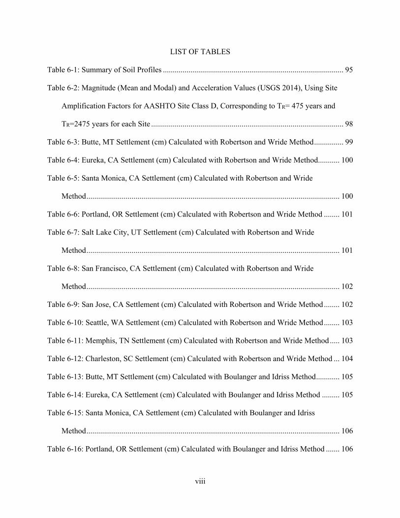
LIST OF TABLES

Table 6-1: Summary of Soil Profiles ............................................................................................ 95 

Table 6-2: Magnitude (Mean and Modal) and Acceleration Values (USGS 2014), Using Site

Amplification Factors for AASHTO Site Class D, Corresponding to TR= 475 years and

TR=2475 years for each Site .................................................................................................. 98 

Table 6-3: Butte, MT Settlement (cm) Calculated with Robertson and Wride Method ............... 99 

Table 6-4: Eureka, CA Settlement (cm) Calculated with Robertson and Wride Method ........... 100 

Table 6-5: Santa Monica, CA Settlement (cm) Calculated with Robertson and Wride

Method ................................................................................................................................. 100 

Table 6-6: Portland, OR Settlement (cm) Calculated with Robertson and Wride Method ........ 101 

Table 6-7: Salt Lake City, UT Settlement (cm) Calculated with Robertson and Wride

Method ................................................................................................................................. 101 

Table 6-8: San Francisco, CA Settlement (cm) Calculated with Robertson and Wride

Method ................................................................................................................................. 102 

Table 6-9: San Jose, CA Settlement (cm) Calculated with Robertson and Wride Method ........ 102 

Table 6-10: Seattle, WA Settlement (cm) Calculated with Robertson and Wride Method ........ 103 

Table 6-11: Memphis, TN Settlement (cm) Calculated with Robertson and Wride Method ..... 103 

Table 6-12: Charleston, SC Settlement (cm) Calculated with Robertson and Wride Method ... 104 

Table 6-13: Butte, MT Settlement (cm) Calculated with Boulanger and Idriss Method ............ 105 

Table 6-14: Eureka, CA Settlement (cm) Calculated with Boulanger and Idriss Method ......... 105 

Table 6-15: Santa Monica, CA Settlement (cm) Calculated with Boulanger and Idriss

Method ................................................................................................................................. 106 

Table 6-16: Portland, OR Settlement (cm) Calculated with Boulanger and Idriss Method ....... 106 

ix

Table 6-17: San Francisco, CA Settlement (cm) Calculated with Boulanger and Idriss

Method ................................................................................................................................. 107 

Table 6-18: Salt Lake City, UT Settlement (cm) Calculated with Boulanger and Idriss

Method ................................................................................................................................. 107

Table 6-19: San Jose, CA Settlement (cm) Calculated with Boulanger and Idriss Method……108

Table 6-20: Seattle, WA Settlement (cm) Calculated with Boulanger and Idriss Method……..108

Table 6-21: Memphis, TN Settlement (cm) Calculated with Boulanger and Idriss Method…...109

Table 6-22: Charleston, SC Settlement (cm) Calculated with Boulanger and Idriss Method….109

Table B-1: Actual Return Periods of Settlement Estimated for Butte, MT (1039) .................... 153

Table B-2: Actual Return Periods of Settlement Estimated for Butte, MT (2475) .................... 153

Table B-3: Actual Return Periods of Settlement Estimated for Eureka, CA (1039) .................. 154

Table B-4: Actual Return Periods of Settlement Estimated for Eureka, CA (2475) .................. 154

Table B-5: Actual Return Periods of Settlement Estimated for Santa Monica, CA (1039) ....... 155

Table B-6: Actual Return Periods of Settlement Estimated for Santa Monica, CA (2475) ....... 155

Table B-7: Actual Return Periods of Settlement Estimated for Salt Lake City, UT (1039) ....... 156

Table B-8: Actual Return Periods of Settlement Estimated for Salt Lake City, UT (2475) ....... 156

Table B-9: Actual Return Periods of Settlement Estimated for San Jose, CA (1039) ................ 157

Table B-10: Actual Return Periods of Settlement Estimated for San Jose, CA (2475) .............. 157

Table B-11: Actual Return Periods of Settlement Estimated for San Fran, CA (1039) ............. 158

Table B-12: Actual Return Periods of Settlement Estimated for San Jose, CA (2475) .............. 158

Table B-13: Actual Return Periods of Settlement Estimated for Seattle, WA (1039) ............... 159

Table B-14: Actual Return Periods of Settlement Estimated for San Fran, CA (2475) ............. 159

Table B-15: Actual Return Periods of Settlement Estimated for Charleston, S.C. (1039) ......... 160

Table B-16: Actual Return Periods of Settlement Estimated for Charleston, S.C. (2475) ......... 160

x

Table B-17: Actual Return Periods of Settlement Estimated for Portland, OR (1039) .............. 161

Table B-18: Actual Return Periods of Settlement Estimated for Portland, OR (2475) .............. 161

Table B-19: Actual Return Periods of Settlement Estimated for Memphis, TN (1039) ............. 162

Table B-20: Actual Return Periods of Settlement Estimated for Memphis, TN (2475)………..162

xi

LIST OF FIGURES

Figure 2-1: A typical recorded time history (Kramer, 1996). ......................................................... 6

Figure 2-2: Two hypothetical time histories with similar PGA values (Kramer, 1996). ................ 7

Figure 2-3: Fourier amplitude spectra for the E-W components of the Gilroy No. 1 (rock) and

Gilroy No.2 (soil) strong motion records (Kramer, 1996). ..................................................... 9

Figure 2-4: Bracketed duration measurement (Kramer, 1996). .................................................... 10

Figure 2-5: Amplification functions for two different sites (Kramer 1996). ................................ 13

Figure 2-6: Schematic illustration of directivity effect of motions at sites toward and away

from direction of fault rupture (Kramer, 1996). .................................................................... 14

Figure 2-7: Normalized peak accelerations (means and error bars) recorded on mountain

ridge at Matsuzaki, Japan (Jibson, 1987). ............................................................................. 14

Figure 3-1:(a) Stress-strain and (b) stress-void ratio curves for loose and dense sands at the

same confining pressure (Kramer, 1996). ............................................................................. 20

Figure 3-2: Behavior of initially loose and dense specimens under drained and undrained

conditions (Kramer, 1996). .................................................................................................... 21

Figure 3-3: Three-dimensional steady-state line showing projections on the e-τ plane, e-σ'

plane, and τ -σ' plane (Kramer, 1996). .................................................................................. 22

Figure 3-4: State criteria for flow liquefaction susceptibility based on the SSL for confining

pressure (left) or stead-state strength (right), plotted logarithmically (Kramer, 1996). ........ 23

Figure 3-5: State Parameter (Kramer, 1996). ................................................................................ 24

Figure 3-6: Response of isotropically consolidated specimen of loose, saturated sand: (a)

stress-strain curve; (b) effective stress path; (c) excess pore pressure; (d) effective

confining pressure (Kramer, 1996). ....................................................................................... 25

xii

Figure 3-7: Response of five specimens isotopically consolidated to the same initial void ratio

at different initial effective confining pressures (Kramer, 1996). ......................................... 26

Figure 3-8: Orientation of the flow liquefaction surface in stress path space (Kramer, 1996). .... 27

Figure 3-9: Initiation of flow liquefaction by cyclic and monotonic loading (Kramer, 1996). .... 28

Figure 3-10: Zone of susceptibility to flow liquefaction (Kramer, 1996). ................................... 29

Figure 3-11: Zone of susceptibility to cyclic mobility (Kramer, 1996). ....................................... 29

Figure 3-12: Three cases of cyclic mobility: (a) no stress reversal and no exceedance of the

steady-state strength; (b) no stress reversal with momentary periods of steady-state

strength exceedance; (c) stress reversal with no exceedance of steady-state strength

(Kramer, 1996). ..................................................................................................................... 31

Figure 3-13: Robertson and Wride (2009) liquefaction triggering curve with case history data

points. .................................................................................................................................... 33

Figure 3-14: Normalized CPT soil behavior type chart (after Robertson, 1990). Soil types: 1,

sensitive, fine grained; 2, peats; 3, silty clay to clay; 4, clayey silt to silty clay; 5, silty

sand to sandy silt; 6, clean sand to silty sand; 7, gravelly sand to dense sand; 8, very stiff

sand to clayey sand; 9, very stiff, fine grained. ..................................................................... 34

Figure 3-15: Summary of the Robertson and Wride (2009) CRR procedure. .............................. 36

Figure 3-16: CRR liquefaction triggering curves based on PL. .................................................... 39

Figure 3-17: Recommended correlation between Ic and FC with plus or minus one standard

deviation against the dataset by Suzuki et al. (1998) (after Idriss and Boulanger, 2014). .... 41

Figure 3-18: CRR curves and liquefaction curves for the deterministic case history database

(after Idriss and Boulanger, 2014). ........................................................................................ 43

xiii

Figure 3-19: Liquefaction triggering PL curves compared to case history data (after Idriss

and Boulanger, 2014) ............................................................................................................ 45

Figure 3-20: Lateral spreading from the 1989 Loma Prieta earthquake. ...................................... 46

Figure 3-21: Apartment buildings after the 1964 Niigata, Japan earthquake. .............................. 47

Figure 4-1: Volumetric change from settlement (after Nadgouda, 2007). ................................... 51

Figure 4-2: Buildings tipped over from differential settlement from the 2015 Kathmandu,

Nepal earthquake (after Williams and Lopez, 2015). ............................................................ 52

Figure 4-3: Differential settlement splitting an apartment building (after Friedman, 2007). ....... 52

Figure 4-4: The relationship between FSL, γmax, and DR (after Ishihara& Yoshimine, 1992). ..... 54

Figure 4-5: Maximum vertical strain levels inferred by deterministic vertical strain models

and weighted average used to define mean value (after Huang, 2008). ................................ 60

Figure 4-6: Penetration analysis for medium dense sand overlaying soft clay (after Ahmadi

and Robertson 2005) .............................................................................................................. 63

Figure 4-7: Tip resistance analysis for thin sand layer (deposit A) interbedded within soft clay

layer (deposit B). (Ahmadi & Robertson, 2005). .................................................................. 64

Figure 5-1: Four steps of a DSHA (Kramer, 1996). ..................................................................... 68

Figure 5-2: Four steps of a PSHA (Kramer, 1996). ...................................................................... 69

Figure 5-3: CPT profile used for example calculations. ............................................................... 73

Figure 5-4: Visualization of performance-based earthquake engineering (after Moehle and

Deierlein, 2004). .................................................................................................................... 77

Figure 5-5: Design objectives for variable levels of risk and performance (after Porter, 2003). . 78

Figure 5-6: Variable components of the performance-based earthquake engineering

framework equation (after Deierlein et al., 2003). ................................................................ 79

xiv

Figure 5-7: Example hazard curve for a given DV. ...................................................................... 81

Figure 5-8: Example FSL curve from one soil layer at a depth of 6m of a CPT profile shown in

Figure 5-3 calculated at Eureka, CA. .................................................................................... 84

Figure 5-9: Example of one strain hazard curve from one specific soil layer at a depth of 6m

of the CPT profile shown in Figure 5-3 calculated at Eureka, CA. ....................................... 85

Figure 5-10: Example of a total ground settlement hazard curve using the CPT profile shown

in Figure 5-3 calculated at Eureka, CA. ................................................................................ 86

Figure 5-11: Fully-probabilistic FSL values plotted across depth for the 2475 year return

period at the Salt Lake City, UT site. .................................................................................... 87

Figure 5-12: Strain hazard curves at the Salt Lake City Site at a range of depths. ....................... 88

Figure 5-13: Strain across depth for the 475, 1189, and 2475 year return periods at the Salt

Lake City Site. ....................................................................................................................... 89

Figure 5-14: Salt Lake City, UT example calculated fully-probabilistic settlement estimation

hazard curve. .......................................................................................................................... 89

Figure 6-1: Stiffness of CPT profiles plotted at depth. ................................................................. 94

Figure 6-2: Map of all ten cities in this study. .............................................................................. 97

Figure 6-3: Idriss and Boulanger (2014) mean pseudo-probabilistic method compared to the

PBEE procedure for the 475 year return period. ................................................................. 111

Figure 6-4: Idriss and Boulanger (2014) mean pseudo-probabilistic method compared to the

PBEE procedure for the 1039 year return period. ............................................................... 112

Figure 6-5: Idriss and Boulanger (2014) mean pseudo-probabilistic method compared to the

PBEE procedure for the 2475 year return period. ............................................................... 112

xv

Figure 6-6: Idriss and Boulanger (2014) modal pseudo-probabilistic method compared to the

PBEE procedure for the 475 year return period. ................................................................. 113

Figure 6-7: Idriss and Boulanger (2014) modal pseudo-probabilistic method compared to the

PBEE procedure for the 1039 year return period. ............................................................... 113

Figure 6-8: Idriss and Boulanger (2014) modal pseudo-probabilistic method compared to the

PBEE procedure for the 2475 year return period. ............................................................... 114

Figure 6-9: Idriss and Boulanger (2014) semi-probabilistic method compared to the PBEE

procedure for the 475 year return period. ............................................................................ 114

Figure 6-10: Idriss and Boulanger (2014) semi-probabilistic method compared to the PBEE

procedure for the 1039 year return period ........................................................................... 115

Figure 6-11: Idriss and Boulanger (2014) semi-probabilistic method compared to the PBEE

procedure for the 2475 year return period ........................................................................... 115

Figure 6-12: Robertson and Wride (2009) mean pseudo-probabilistic method compared to

the PBEE procedure for the 475 year return period. ........................................................... 116

Figure 6-13: Robertson and Wride (2009) mean pseudo-probabilistic method compared to

the PBEE procedure for the 1039 year return period. ......................................................... 116

Figure 6-14: Robertson and Wride (2009) mean pseudo-probabilistic method compared to

the PBEE procedure for the 2475 year return period. ......................................................... 117

Figure 6-15: Robertson and Wride (2009) modal pseudo-probabilistic method compared to

the PBEE procedure for the 475 year return period. ........................................................... 117

Figure 6-16: Robertson and Wride (2009) modal pseudo-probabilistic method compared to

the PBEE procedure for the 1039 year return period. ......................................................... 118

xvi

Figure 6-17: Robertson and Wride (2009) modal pseudo-probabilistic method compared to

the PBEE procedure for the 2475 year return period. ......................................................... 118

Figure 6-18: Robertson and Wride (2009) semi-probabilistic method compared to the PBEE

procedure for the 475 year return period. ............................................................................ 119

Figure 6-19: Robertson and Wride (2009) semi-probabilistic method compared to the PBEE

procedure for the 1039 year return period. .......................................................................... 119

Figure 6-20: Robertson and Wride (2009) semi-probabilistic method compared to the PBEE

procedure for the 2475 year return period. .......................................................................... 120

Figure 6-21: Box and whisker plots of actual return periods versus assumed 1039 year return

period for the Idriss and Boulanger (2014) Triggering Method. ......................................... 121

Figure 6-22: Box and whisker plots of actual return periods versus assumed 2475 year return

period for the Idriss and Boulanger (2014) Triggering Method. ......................................... 122

Figure 6-23: Box and whisker plots of actual return periods versus assumed 1039 year return

period for the Robertson and Wride (2009) Triggering Method. ........................................ 122

Figure 6-24: Box and whisker plots of actual return periods versus assumed 2475 year return

period for the Robertson and Wride (2009) Triggering Method. ........................................ 123

Figure 6-25: A heat map representing the number of CPT soundings, out of 20 soundings, in

which the pseudo-probabilistic method under predicted settlement compared to the

PBEE procedure. ................................................................................................................. 125

Figure 6-26: Box and whisker plots for R at a return period of 475 years. ................................ 129

Figure 6-27: Box and whisker plots for R at a return period of 1039 years. .............................. 130

Figure 6-28: Box and Whisker plots for R at a return period of 2475 years. ............................. 130

Figure A-1: Opening title page of CPTLiquefY. ........................................................................ 144

xvii

Figure A-2: Screen shot of “Soil Info” tab. ................................................................................ 145

Figure A-3: Screenshot of “Pseudo-probabilistic” tab................................................................ 146

Figure A-4: Screenshot of “Full-Probabilistic User Inputs” tab. ................................................ 147

Figure A-5: Screenshot of “Settlement Results” tab................................................................... 148

Figure A-6: Screenshot of “Strain Hazard Curves by Layer” sub-tab. ....................................... 149

Figure A-7: Screenshot of “Export” tab. ..................................................................................... 150

Figure A-8: Screenshot of “Batch Run” tab. .............................................................................. 151

1

1 INTRODUCTION

During an earthquake event, soil has the potential to liquefy and subsequently cause ground

surface settlements. Liquefaction-induced settlements are not directly life-threatening, but the

resulting effects can be dangerous and take a large economic toll. When settlements occur

unevenly, called differential settlement, they can cause the severing of lifelines, utility lines, and

severe structural and roadway damage. Structural damage caused by differential settlement can

range from cracking to dangerous structural collapse. The severing of lifelines or utilities can be

dangerous because it could spark a fire, spread disease when people are unable to receive clean

water, and even prevent firefighters from being able to put out earthquake-caused fires by

preventing access to water. In addition, the widespread damage caused by differential settlement

can cause a huge economic toll on a city. Also severe damage of roadways and highways can

prevent shipment of goods in or out of the city, adding to the financial distress.

To be able to prevent these scenarios, engineers need to be able to predict seismic effects,

and the damage they cause, accurately. Liquefaction was not critically studied until the 1964

Niigata and Alaska earthquakes, which caused extensive liquefaction damage. Therefore

liquefaction is a relatively new research area, so prediction methods are continually being

improved and developed. Originally, engineers used a deterministic (or scenario-based) analysis

method to predict liquefaction effects. In the past 20 years, however, engineers have relied more

2

on a pseudo-probabilistic approach to predict liquefaction effects. This approach uses a ground

motion from a probabilistic seismic hazard analysis (PSHA) to represent the design earthquake,

but computes the liquefaction and its effects using deterministic analysis procedures.

Recent research has found that a performance-based earthquake engineering (PBEE)

approach produces more accurate and consistent hazard estimates than the current pseudo-

probabilistic approach (Kramer & Mayfield, 2007; Franke et al. 2014). PBEE applies a fully-

probabilistic analysis into the prediction of earthquake effects and presents these predictions in

terms of levels of hazard. PBEE is extremely advantageous for not only predicting hazard for

liquefaction triggering and its effects, but also presenting this hazard in a way for all stakeholders

to make more informed decisions. Unfortunately, due to the complex nature of probability theory

and the numerous calculations required, PBEE is not used widely yet in practice.

Most geotechnical PBEE analysis methods have been developed for the standard penetration

test (SPT) rather than for the cone penetration test (CPT). This discrepancy is due to the relative

novelty of the CPT. The CPT is a method used to determine soil properties by pushing an

instrumented cone into the ground at a controlled rate. The cone reads the resistance it receives

from each soil layer as it is advanced through the soil. These resistances can then be correlated to

the soil’s relative density or consistency, which correlates to its ability to resist liquefaction. The

use of the CPT has grown rapidly due to the speed of the test and the continuous nature of its

results. Deterministic and pseudo-probabilistic post-liquefaction settlement analysis methods

have been developed for the CPT, but no performance-based method has been developed and

tested yet. As such, there are three purposes to this study: first, to create a new performance-

based procedure for the estimation of free-field post-liquefaction settlements for the CPT;

second, to develop an analysis tool to perform and simplify the necessary probabilistic

3

calculations; and third, to assess and quantify the differences between the performance-based

(i.e., fully-probabilistic) and pseudo-probabilistic post-liquefaction settlement analyses.

4

2 SESIMIC LOADING CHARACTERIZATION

When engineers can accurately quantify earthquake ground motion parameters, they are able

to accurately design for seismic events. Earthquake engineering is still a relatively new field but

is improving with improved instrumentation, an increase of instrumentation stations, and more

understanding of the physics and mechanics behind earthquake ground motions.

2.1 Earthquakes

Earthquakes continue to be one of the most devastating natural disasters civilizations must

face. Earthquakes and their effects can be extremely fatal and economically cripple a region.

Engineers attempt to reduce the negative causes of an earthquake by preparing their designs for a

certain level of earthquake. To accomplish this, it is important to have a metric to be able to

quantify an earthquake.

The first step in characterizing an earthquake is to quantify the “size” on an earthquake.

The size of an earthquake has historically been recorded and described in different ways. Prior to

modern technology, an earthquake was quantified based on crude and qualitative descriptions

(Kramer, 1996). With technological advancements, modern seismographs have been developed

to record earthquake sizes in a more quantitative fashion.

5

Before the development of seismographs, an earthquake’s size was recorded by recording

the intensity. The intensity is a qualitative measure recording of observed damage and people’s

reactions compared to their location. After a seismic event, intensities were recorded through

interviews and recorded observations. The measure of intensity is extremely subjective and

consistency is questionable because two different people could perceive the intensity differently

from each other.

With technological advancements and a need for a less subjective measure of earthquake

size, strong motion recording instruments, such as accelerometers and seismometers, were

developed and provided a quantitative measure of earthquake sizes. Instruments allow engineers

to record earthquake ground motions in the form of acceleration, velocity, and displacement.

These recordings became known as earthquake time histories. Time histories have led to an

objective and quantitative measurement of earthquake size called earthquake magnitude.

Many magnitude scales have been developed over the years. A commonly known

magnitude scale is the Richter local magnitude scale. In 1935, Charles Richter used a Wood-

Anderson seismometer to define a magnitude scale for shallow, local earthquakes in southern

California (Richter, 1935). The Richter scale is the most widely known magnitude scale but is

only applicable to shallow and local earthquakes. For this reason, it is not usually used in design.

Magnitude scales were then developed based on surface and body waves (Kanamori, 1983).

Surface and body wave magnitude scales are used more widely than the Richter scale but are less

reliable when distinguishing between large earthquakes. This is because large earthquakes tend

to produce saturation in their recordings. Saturation occurs when ground motion recordings

produce constant readings after a certain level of earthquake. As the total energy released during

an earthquake increases, the ground motion parameters do not increase at the same rate, causing

6

saturation in the readings. The most commonly used magnitude scale is the moment magnitude

scale, which is not directly measured from any ground motion and therefore is not subject to

saturation (Hanks & Kanamori, 1979; Kanamori, 1977). Ground motion recordings are used to

back calculate the seismic moment, which is a measure of the energy released by the earthquake.

This study uses moment magnitude in all references to an earthquake’s magnitude.

2.2 Ground Motion Parameters

To accurately characterize an earthquake’s strong ground motions quantitatively, ground

motion parameters are essential. The most commonly used ground motion parameters to

characterize a seismic event are amplitude, frequency content, and duration parameters. It is

impossible to accurately describe all important ground motion characteristics using a single

parameter (Jennings, 1985; Joyner & Boore, 1988). Ground motion parameters are usually

obtained from an acceleration, velocity, and/or displacement time histories. A typical recorded

time history is shown in Figure 2-1. Typically, an acceleration time history is recorded then used

to calculate a velocity and/or displacement time history through integration and filtering.

Figure 2-1: A typical recorded time history (Kramer, 1996).

7

2.2.1 Amplitude Parameters

Amplitude parameters are used to describe the maximum value of a specific ground

motion. Amplitude can be expressed as maximum acceleration, velocity, and/or displacement.

The most widely-used amplitude parameter is the peak ground acceleration (PGA) or peak

ground surface acceleration (amax). The PGA can be broken up into peak horizontal acceleration

(PHA) and peak vertical acceleration (PVA) to distinguish between horizontal and vertical

accelerations.

The PGA is a useful ground motion parameter, but it cannot be used on its own to

accurately characterize a seismic event. Figure 2-2 depicts two hypothetical acceleration time

histories with similar PGA values. To only characterize the earthquakes using the PGA ground

motion parameter would yield inaccurate results. It is apparent time history (b) developed more

energy than time history (a) because of the frequency content time history (b) developed. This

example shows how important it is to not characterize an earthquake using a single ground

motion parameter.

Figure 2-2: Two hypothetical time histories with similar PGA values (Kramer, 1996).

8

2.2.2 Frequency Content Parameters

Every structure is affected by the frequency content of an earthquake event uniquely.

Frequency content describes how quickly the amplitude of a ground motion is repeated over a

given duration of time. Every structure has a frequency at which it oscillates inherently, called its

natural frequency. When earthquake loading corresponds to a frequency that matches a

structure’s natural frequency, the structure will experience resonance. Resonance causes the

amplitudes of both the structure’s oscillation and oscillation from the earthquake to compound.

Resonance is the reason some structures hardly deform by a particular earthquake loading, but a

building next door may experience a drastic increase of deformation damage because of its

natural frequency.

The frequency content of a ground motion can be described as a mathematical function

known as the Fourier spectrum. A Fourier spectrum is an analysis of a series of simple harmonic

terms of varying frequency, amplitude and phase (Steven L Kramer, 1996). In respect to

earthquake engineering, a Fourier series shows the distribution of the amplitude of a specific

time history with respect to frequency.

The Fourier amplitude spectrum, a plot of Fourier amplitude versus frequency, is often

used to express frequency content. When plotted for a strong ground motion, the Fourier

amplitude spectrum shows how amplitude is distributed with respect to frequency. Figure 2-3

depicts two Fourier spectrums of the east-west loading from the 1989 Loma Prieta earthquake.

As shown, the shapes of the Fourier spectra are quite different. The Gilroy No.1 (rock) spectrum

is the strongest at low period, or high frequencies, while the Gilroy No.2 (soil) is the strongest at

high periods, or low frequencies.

9

Fourier spectra are very useful in predicting earthquake ground motion hazards.

Engineers can use Fourier spectra to predict the hazard level of specific ground motions for a

structure based on its natural frequency. If a structure has a natural frequency similar to the

critical frequency described by the Fourier spectrum, it will experience resonance. An engineer

could then know to design the structure to resist extreme lateral loads. Also, the engineer could

design the height and mass distribution of the structure to create a natural frequency different

from the critical frequency, based on the Fourier spectrum.

Figure 2-3: Fourier amplitude spectra for the E-W components of the Gilroy No. 1 (rock) and Gilroy No.2 (soil) strong motion records (Kramer, 1996).

10

2.2.3 Duration Parameters

Duration of strong ground motions can also affect the amount of earthquake damage.

Duration can cause degradation of stiffness and strength of structures, buildup of pore water

pressures in soils, and weakening of soil layers. A short duration of a large earthquake may not

occur long enough for intensive damage to occur. However, a weaker earthquake with a longer

duration may occur long enough for intensive damage to occur.

Different approaches exist to quantify duration. Most commonly used is the bracketed

duration (Bolt, 1969), which is the time between the first and last exceedance of a defined

threshold (usually 0.05g) on an accelerogram (Figure 2-4). An accelerogram generally records all

ground motions from an initial loading till the ground motions return to a standard level.

2.2.4 Ground Motion Parameters that describe Amplitude, Frequency Content, and/or Duration

Amplitude, frequency content, and duration are all influential parameters; consequently,

some parameters have been created that can describe more than one parameter at once. Each of

the discussed parameters are important but are limited to describing only one aspect of an

Figure 2-4: Bracketed duration measurement (Kramer, 1996).

11

earthquake, making these combined ground motion parameters very useful. The rms acceleration

parameter was created to describe the effects of both amplitude and frequency (Kramer, 1996).

Arias Intensity (Ia) also describes amplitude and frequency by integrating across the acceleration

time history, resulting in the amount of energy from a strong ground motion (Arias, 1970). A few

other common parameters include the cumulative absolute velocity (CAV) (Benjamin &

Associates, 1988), response spectrum intensity (SI) (Housner, 1959), acceleration spectrum

intensity (Von Thun, 1988), and effective peak acceleration (EPA) (Applied Technology

Council, 1978).

2.3 Ground Motion Prediction Equations

Engineers are able to predict ground motions for future events by using relationships

developed from previously recorded time histories, called ground motion prediction equations

(GMPEs). Attenuation relationships have been developed for numerous input variables including

magnitude, distance, and site specific effects that are described in detail in section 3.4.

Since peak acceleration is the most commonly used ground motion parameter, extensive

effort has been exerted in the development of attenuation relationships for peak acceleration. In

1981, Cambell used previously recorded data from across the world to develop an attenuation

relationship for the mean peak acceleration for sites within 50 km of the fault rupture and with

earthquake magnitudes 5.0 to 7.7. Cambell and Bozorgnia (1994) used earthquake data from

earthquakes of magnitudes 4.7 to 8.1 to predict peak acceleration at distances within 60 km from

the fault rupture. Boore et al. (1993) expanded this relationship to predict peak accelerations

within 100 km of fault rupture for earthquake magnitudes 5.0 to 7.7. Toro et al. (1995) developed

12

attenuation relationships for the mid-continental eastern United States. Finally, Youngs et al.

(1988) developed acceleration attenuation relationships for specifically subduction zones.

With an increase in new earthquake data, a more unified and updated relationship was

needed. Five research teams were given the same set of ground motion data and were asked to

each develop new relationships called the Next Generation Attenuation (NGA) Relationships

(Abrahamson & Silva, 2008; Boore & Atkinson, 2008; Cambell & Bozorgnia, 2008; Chiou &

Youngs, 2008; Idriss, 2008). The NGA equations were updated in 2013 to the NGA West 2

relationships (Ancheta et al., 2014). These attenuation relationships were developed specifically

for the western US and other areas of high seismicity. Care should be taken when using these

relationships to avoid using them incorrectly or extrapolating their use to invalid seismic

predictions.

2.4 Local Site Effects

Attenuation relationships depend heavily on magnitude and distance; however, local site

effects can profoundly influence ground motion parameters. The extent of their effects depends

on the soil properties, characteristics of earthquake loading, topography, and geometry of the

site. Local site effects can be very difficult to predict, but they are very important for designing

for an earthquake’s effects.

Soil properties of local soil deposits can alter a ground motion’s frequency and

amplification. Figure 2-5 demonstrates this phenomenon. Site A and site B have identical

geometries, but site B is considerably stiffer than site A. The softer site (site A) will amplify low-

frequency, or high-period, ground motions more than the stiffer site (site B). The opposite

amplification will occur with high-frequency, or low-period, ground motions (Steven L Kramer,

13

1996). The September 19, 1985 Mexico City earthquake is a good example of this soil

amplification phenomenon. The earthquake (Ms = 8.1) caused only moderate damage in the area

surrounding its epicenter near the Pacific coast of Mexico, but it severely damaged Mexico City

located 350 km away. The soft clay lake deposits amplified the ground motions increasingly

until it reached Mexico City (Dobry & Vucetic, 1987).

Near-source and directivity are also very influential local site effects. They tend to be

lumped together as one, although they are independent phenomena. Both phenomena have been

known to significantly alter ground motions within about 10 km of a rupturing fault. Small

earthquakes are usually modeled as point processes because their rupture lengths only span a few

kilometers. However, large earthquakes can have rupture lengths of hundreds of kilometers. The

earthquake will rupture with different strengths in different directions creating directivity effects

(Ben-Menachem, 1961; Benioff, 1955). Directivity is caused by constructive interference of

waves produced by successive dislocations that produce strong pulses of large displacements

(Benioff, 1955; Singh, 1985) (Figure 2-6).

Figure 2-5: Amplification functions for two different sites (Kramer 1996).

14

Site topography can also influence the magnitude of ground motion parameters. For

example, crests and ridges have been known to amplify ground motion parameters as they move

up the peak. Amplification of ground motions near the crest of a ridge was measured in five

different earthquakes in Matsuzaki, Japan (Jibson, 1987). Figure 2-7 depicts the normalized peak

accelerations from this study. The average peak acceleration was about 2.5 times the average

base acceleration. These effects are not usually accounted for due to complexity and the fact not

many structures are built on the crest of mountains. However, a finite element analysis can be

used for critical structures.

Figure 2-6: Schematic illustration of directivity effect of motions at sites toward and away from direction of fault rupture (Kramer, 1996).

Figure 2-7: Normalized peak accelerations (means and error bars) recorded on mountain ridge at Matsuzaki, Japan (Jibson, 1987).

15

Basin effects are very important because many cities are built near or on alluvial valleys.

The curvature of basin edges with soft alluvial soils can trap body waves causing propagation of

increased surface waves and longer shaking durations (Vidale & Helmberger, 1988). Currently,

shallow basin effects are relatively easy to predict, but predictions become complicated on the

edges of basins and within deep basins.

2.5 Chapter Summary

Understanding seismic loading and the capability to predict it is crucial to predict

earthquake hazards, including soil liquefaction. Seismic loading can be quantified into ground

motion parameters. The most commonly used ground motion parameters include amplitude,

frequency, and duration. Ground motion parameters can be significantly affected by local site

effects.

16

3 REVIEW OF SOIL LIQUEFACTION

Liquefaction-induced settlements can have extreme economic effects. Liquefaction can

cause differential settlement, which can be severely problematic for structures with shallow

foundations, roadways, utility lines, and life lines. The resulting fire from the 1906 San Francisco

earthquake showed how differential settlement can result in life-threatening tertiary hazards

when life and utility lines are severed. After the earthquake, San Francisco firefighters had no

access to water because the water mains had been severed in the earthquake. To provide the

necessary background to understand liquefaction-induced settlements, soil liquefaction is

reviewed in this chapter.

3.1 Liquefaction

Liquefaction is a complex phenomenon that has been closely studied for the past 50 years.

It was not until the 1964 Alaska earthquake (Mw=9.2) and Niigata, Japan earthquake (Ms=7.5)

occurred within three months of each other that liquefaction caught the attention of geotechnical

engineers. Both earthquakes had intensive liquefaction-induced damage causing slope failures,

bridge and building foundation failures, sinkholes, and flotation of buried structures (Steven L

Kramer, 1996). In the past 30 years in particular, liquefaction has been studied intensively,

resulting in many new prediction procedures, exploration technologies, and design methods.

17

Liquefaction, a term coined by Mogami and Kubo (1953), has been known to collectively

reference soil phenomena related to deformations caused by disturbances of undrained

cohesionless soils (Steven L Kramer, 1996). It is well known that dry cohesionless soils tend to

densify under static or cyclic loading. If the cohesionless soil is saturated, this densification

causes the pore water to be rapidly forced from the pore spaces causing a corresponding buildup

of excess pore water pressure and a decrease in effective stress. The decrease in effective stress

causes the soil to experience a temporary weakened state. If the effective stress reaches a null

value, then liquefaction has initiated. Liquefaction will manifest itself as either flow liquefaction

or cyclic mobility. Cyclic mobility is the most common and can occur a wide variety of site and

soil conditions. Flow liquefaction has the most damaging effects but occurs less frequently

because it requires specific site and soil characteristics. Both phenomena are discussed in more

detail in sections 3.4.2 and 3.4.3.

A comprehensive liquefaction analysis should consider liquefaction susceptibility,

initiation, and its corresponding effects. The remaining sections of this chapter will address each

of these aspects of liquefaction individually.

3.2 Liquefaction Susceptibility

The first step in a liquefaction hazard analysis is to determine if a soil is even susceptible

to liquefaction. If a soil is not susceptible to liquefaction, a hazard analysis is not needed.

However, if a soil is susceptible, an initiation analysis should be performed. Susceptibility is

judged by site historical information, geology, composition, and state. Each of these

susceptibility criteria are addressed in detail in the following sections.

18

3.2.1 Historical Criteria

The liquefaction history of a particular site can predict a site’s liquefaction susceptibility.

When the groundwater and soil conditions remain the same, liquefaction will often occur at the

same location it did in the past (T. L. Youd, 1984). Therefore, liquefaction case histories can be

used to predict whether or not a site is susceptible to liquefaction. Youd (1991) describes

multiple instances where this process has been used successfully.

3.2.2 Geologic Criteria

The hydrological environment, depositional environment, and age of a soil deposit all

contribute to liquefaction susceptibility (T. L. Youd & Hoose, 1977). Because liquefaction

occurs from pore water pressure build-up, liquefaction will only occur in saturated soils.

Therefore, soils must be below the water table to be susceptible to liquefaction. Saturated

uniform cohesionless soil particles placed in a loose state are most susceptible to soil

liquefaction. Therefore, saturated alluvial, fluvial, colluvial, and aeolian deposits tend to be

highly susceptible. Soil age also affects liquefaction susceptibility. The susceptibility of newer

deposits are generally more susceptible than older deposits.

Man-made deposits can also be susceptible to liquefaction. If a fill is placed without

compaction, it will be susceptible because of the loose state of the non-compacted soil particles.

Well-compacted fills will present a lower seismic liquefaction hazard.

3.2.3 Compositional Criteria

Liquefaction susceptibility is affected by compositional characteristics that influence

volume change behavior, including particle shape, size, and gradation (Steven L Kramer, 1996).

Liquefaction is known to occur when soils begin to densify and water is essentially pushed out of

19

the pore spaces. If pore water cannot escape quickly enough, the pore water will begin to push

back, generating excess pore water pressure.

Particle shape, size, and gradation affect a soil’s densification ability and consequently its

liquefaction susceptibility. Excess pore water pressures can only develop in soils that can densify

easily. If a soil cannot densify easily, or has high permeability that cannot sustain pore water

pressures, it is unlikely to liquefy. Smooth, rounded particles densify more easily than coarse and

jagged particles, indicating a higher susceptibility to liquefaction. Coarse and jagged particles

will interlock with each other resisting densification. Gradation also affects liquefaction

susceptibility. Poorly graded soils are more likely to liquefy than well graded soils. The voids in

well graded soils are filled with fines, resulting in less volume change under drained conditions

and consequently less pore water pressure under undrained conditions.

Fine-grained soils have generally been considered not susceptible to liquefaction due to

cohesion, but recent studies have found these soils could potentially still liquefy. Cohesion is a

chemical and electrical attraction between fine-grained soil particles that hold the particles

together. This cohesion is generally sufficient to prevent liquefaction initiation. However

liquefaction has been observed to occur in coarse fines with low to no plasticity and low

cohesion (K. Ishihara, 1984, 1985). Boulanger and Idriss (2005) reviewed case histories and

laboratory tests of cyclically loaded fine-grained soils. Boulanger and Idriss identified two types

of soil behavior of fines, “sand-like” and “clay-like”, based on stress-strain behavior and stress-

normalization. If a fine-grained soil exhibited “sand-like” behavior it was susceptible to

liquefaction. Boulanger and Idriss found that the lower the plasticity of a soil, the more “sand-

like” behavior it exhibited and is susceptible to liquefaction.

20

3.2.4 State Criteria

The initial state of a soil, or its stress and density characteristics, can have a significant

impact on liquefaction susceptibility. Even if a soil is considered liquefiable by all of the

previous criteria, its initial state could still prevent liquefaction from occuring. A soil loosely

placed is more likely to be contractive and therefore liquefiable, while a soil densely compacted

is more likely to be dilative and therefore not liquefiable.

Casagrande (1936) pioneered the understanding of soil behavior under various confining

pressures across various densities. His research showed all specimens, under the same confining

pressure, converged to the same density when sheared. Loose specimens contracted, or densified,

initially, while dense specimens initially contracted. However, both specimens converge to the

same void ratio (or relative density) at large strains, representing a steady or critical state. This

phenomenon is illustrated in Figure 3-1.

Figure 3-1:(a) Stress-strain and (b) stress-void ratio curves for loose and dense sands at the same confining pressure (Kramer, 1996).

21

The critical void ratio (ec) is the void ratio corresponding to the density at the steady or

critical state. This discovery led to Casagrande’s idea of the critical void ratio (CVR) line, which

is the critical void ratios plotted for a range of effective confining pressures. The CVR is a

boundary line between loose (contractive) and dense (dilative) soils, or susceptible and

nonsusceptible soils respectively, as shown in Figure 3-2.

In 1938 the failure of the Fort Peck Dam in Montana proved the CVR line to be an

insufficient method for predicting liquefaction susceptibility (Middlebrooks, 1942). The dam had

a flow liquefaction failure even though the initial state of the soils before liquefaction plotted

below the CVR line (i.e., in the nonsusceptible region). Casagrande concluded the failure was

due to the inability of a strain-controlled drained test to emulate all the phenomena that

influences soil behavior under the stress-controlled undrained conditions of an actual flow

liquefaction failure.

It was not until 1969 that Castro, one of Casagrande’s students, was able to effectively

replicate soil flow liquefaction. At this time, technology gained the ability to perform stress-

Figure 3-2: Behavior of initially loose and dense specimens under drained and undrained conditions (Kramer, 1996).

22

controlled undrained tests. Castro performed various static and cyclic triaxial tests, which helped

him discover the steady state of deformation (Castro & Poulos, 1977; Poulos, 1981). The steady

state of deformation describes the soil state in which it flows continuously under constant shear

stress and constant effective confining pressure at constant volume and velocity.

The steady-state line (SSL) can be plotted and viewed as a three-dimensional curve in the

e- σ’- τ space (Figure 3-3), to predict flow liquefaction susceptibility. The SSL can also be

projected onto a plane of the steady-state strength (Ssu) or confining pressure versus void ratio, as

shown in Figure 3-3.

When plotted logarithmically, the strength-based SSL is parallel to the effective confining

pressure-based SSL. This relationship is because the shearing resistance of a soil is proportional

to the effective confining stress. Soils that plot below the SSL are not susceptible to flow

liquefaction. A soil will be susceptible to flow liquefaction if it plots above the SSL and only if

the stress exceeds its steady state strength. It is important to note the SSL is only effective in

predicting flow liquefaction and cannot predict cyclic mobility (Steven L Kramer, 1996).

Figure 3-3: Three-dimensional steady-state line showing projections on the e-τ plane, e-σ' plane, and τ -σ' plane (Kramer, 1996).

23

The SSL is limited however, because it applies the absolute measure of density for

characterization of flow liquefaction susceptibility. As shown in Figure 3-4, a soil at one

particular density could be considered liquefiable at a very high confining pressure but not

susceptible to flow liquefaction at a low confining pressure.

To address this limitation of the SSL, Roscoe and Pooroshasb believed the behavior of

cohesionless soils should be related to the proximity of the soil’s initial state to the SSL. In other

words, soils with similar proximities to the SSL should behave similarly. Using this idea, Been

and Jefferies (1985) developed a state parameter (ψ). The state parameter can be defined as the

initial state void ratio subtracted by the void ratio on the SSL at the confining pressure of interest

(Figure 3-5). If the state parameter is positive, the soil is contractive and therefore may be

susceptible to flow liquefaction. If the state parameter is negative, the soil is dilative and not

Figure 3-4: State criteria for flow liquefaction susceptibility based on the SSL for confining pressure (left) or stead-state strength (right), plotted logarithmically (Kramer, 1996).

24

susceptible to flow liquefaction. It is important to note, however, that the accuracy of the state

parameter is dependent on the accuracy of the position of the SSL.

3.3 Liquefaction Initiation

Even if a soil meets all of the susceptibility criteria stated above, it is still possible for

liquefaction not to occur in a specific earthquake. The earthquake must create large enough

disturbances to initiate liquefaction. Both flow liquefaction and cyclic mobility are very different

phenomena that, in discussing liquefaction initiation, need to be discussed separately. Both,

however, can be described easily in stress path space (Hanzawa, 1979) using the three-

dimensional surface called the slow liquefaction surface (FLS). Understanding of the FLS, flow

liquefaction, and cyclic mobility are discussed in detail below.

Figure 3-5: State Parameter (Kramer, 1996).

25

3.3.1 Flow Liquefaction Surface

The conditions of flow liquefaction can be understood most easily when evaluating the

response of an isotopically consolidated specimen of loose saturated sand in an undrained triaxial

test under monotonic loading. Figure 3-6 demonstrates the stress path of such a specimen under

monotonic loading. The initial state, prior to loading, of the specimen is plotted well above the

SSL (point A). This indicates the soil will exhibit contractive behavior and is therefore

susceptible to flow liquefaction. Prior to loading, the soil has no excess pore water pressure or

any strain. Once loading begins, the sample will have an increase of shear strength until it

reaches a maximum shear strength (point B). If loading persists past the peak strength, the

sample will exhibit a drastic decrease in strength, becoming unstable and will collapse. This

drastic decrease in strength will result in a rapid increase of excess pore water pressure and

excess strains until the soil reaches a steady-state residual strength (point C). The soil has just

experienced flow liquefaction. Flow liquefaction occurred at point B, when the soil became

irreversibly unstable (Steven L Kramer, 1996).

Figure 3-6: Response of isotropically consolidated specimen of loose, saturated sand: (a) stress-strain curve; (b) effective stress path; (c) excess pore pressure; (d) effective confining pressure (Kramer, 1996).

26

Now consider the same test applied to multiple samples at the same void ratio, but at

varying effective confining pressures. Since all of the specimens have the same void ratio, they

will all reach the same effective stress conditions at the steady-state, but they will all follow

different paths to get there (Steven L Kramer, 1996). Figure 3-7 illustrates this response from

five different specimens. Sample A and B have initial states below the SSL and therefore exhibit

dilative behavior. Neither sample A or B reached flow liquefaction because of their initial

effective confining pressure, but they did dilate and settle at the steady-state point. However,

samples C, D, and E did achieve flow liquefaction because their initial state plotted above the

SSL. Each specimen reached a peak undrained shear strength (marked with an x), followed by a

rapid decrease in strength and settled at the steady state point.

Figure 3-7: Response of five specimens isotopically consolidated to the same initial void ratio at different initial effective confining pressures (Kramer, 1996).

27

Hanzawa et al. (1979) and Vaid and Chern (1983) found each initiation point can be

connected by a projected straight line that projects through the origin of the stress path. This

projected line creates the FLS and flow liquefaction occurs below this line. Figure 3-8 shows the

orientation of the flow liquefaction surface in the stress path space.

The FLS applies to not only monotonic loading but also cyclic loading (Vaid & Chern,

1983). Two identical specimens will both liquefy when their stress paths reach the FLS,

independent from how they are loaded. Figure 3-9 demonstrates this phenomenon. Two identical

loose saturated sand specimens were tested, one under monotonic loading and one under cyclic

loading. The monotonically loaded specimen is represented by path ABC and behaved according

to the phenomenon discussed above. The effective stress path of the cyclically loaded specimen

is represented by path ADC. As the specimen is loaded, it builds up pore water pressure with

each cycle until it reaches the FLS. At that point, flow liquefaction is initiated.

Figure 3-8: Orientation of the flow liquefaction surface in stress path space (Kramer, 1996).

28

Even though the effective stress conditions at the liquefaction initiation points (points B

and D) were different, they both experience flow liquefaction at the FLS. This indicates the FLS

marks the boundary between stable and unstable soil conditions. Lade (1992) developed a more

detailed description of this instability using continuum mechanics.

3.3.2 Flow Liquefaction

Flow liquefaction will only have the potential to occur when the shear stress required for

static equilibrium is greater than the steady-state strength. The shear stresses in the field are

caused by gravity and will therefore remain constant until large deformations develop. If a soil’s

initial state plots within the shaded region in Figure 3-10, it will be susceptible to flow

liquefaction. For flow liquefaction to occur, there must be a large enough undrained disturbance

to move the effective stress path to the FLS.

Figure 3-9: Initiation of flow liquefaction by cyclic and monotonic loading (Kramer, 1996).

29

3.3.3 Cyclic Mobility

Unlike flow liquefaction, cyclic mobility can occur when the initial effective stress point is

below the steady-state strength line. Therefore, initial states that plot below the steady-state point

are susceptible to cyclic mobility (Figure 3-11). The shaded region extends from very high to

very low effective confining stress. This indicates both loose and dense soils are susceptible to

cyclic mobility because soils across this region would plot both above and below the SSL.

Figure 3-10: Zone of susceptibility to flow liquefaction (Kramer, 1996).

Figure 3-11: Zone of susceptibility to cyclic mobility (Kramer, 1996).

30

There are three combinations of initial conditions and cyclic loading conditions that lead to

cyclic mobility (Figure 3-12). The first condition (Figure 3-12(a)) will occur when the static shear

stress is greater that the cyclic shear stress; in other words, no shear stress reversal occurs. There

is also no exceedance of steady-state strength as the effective stress path moves to the left until it

reaches the drained failure envelope and continues to move up and down the failure envelope

with additional loading cycles. This results in a stabilization of the effective stress conditions, but

the effective confining pressure has decreased significantly, resulting in large permanent strains

occurring within each load cycle.

The second case will occur when there is no shear stress reversal, but the steady-state

strength is momentarily exceeded (Figure 3-12(b)). With each load cycle, the effective stress path

will move to the left until it reaches the FLS. Momentary periods of instability occur, resulting in

significant permanent strains.

The third possible condition occurs when stress reversal occurs, but the steady-state

strength is not exceeded (Figure 3-12(c)). The shear stress changes direction in this case, causing

both compressional and extensional loading. Increasing rate of pore pressure generation

correlates with an increase degree of stress reversal (Mohamad & Dobry, 1986), resulting in the

effective stress path moving relatively quickly to the left. Once the effective stress path reaches

the FLS, it oscillates along the compressional and extensional portions of the drained failure

envelope. Every time it passes through the origin, it reaches a state of zero effective stress

causing large permanent strains.

31

Flow liquefaction occurs at a specific point, but there is no clear point at which cyclic

mobility occurs. Large deformations and strains from cyclic mobility occur incrementally. The

magnitude of strain deformations depends on duration and magnitude of soil loading. Cyclic

mobility will cause the most damage to sloping sites subjected to a long duration of ground

motions. However, for level sites subjected to short duration ground motions, the expected

resulting strains will be small.

3.4 Methods to Predict Liquefaction Triggering

Liquefaction initiation can be quantified and predicted by calculating liquefaction

triggering. Liquefaction triggering can be expressed as a factor of safety against liquefaction

(FSL) or a probability of liquefaction triggering (PL). This factor of safety represents the ratio of a

soil’s ability to resist liquefaction to the loading demand from an earthquake. Many liquefaction

triggering models have been developed, but the most prominent models, and the models used for

this study, are presented in this section.

Figure 3-12: Three cases of cyclic mobility: (a) no stress reversal and no exceedance of the steady-state strength; (b) no stress reversal with momentary periods of steady-state strength exceedance; (c) stress reversal with no exceedance of steady-state strength (Kramer, 1996).

32

3.4.1 Empirical Liquefaction Triggering Models

When calculating FSL, engineers rely predominately upon a simplified empirical

procedure by calculating the ratio of resistance to liquefaction to the seismic demand on the soil

(Seed, 1979; Seed & Idris, 1982). According to this procedure, liquefaction triggering is

evaluated by:

𝐹𝐹𝐹𝐹𝐿𝐿 =𝑐𝑐𝑐𝑐𝑐𝑐𝑐𝑐𝑐𝑐𝑐𝑐𝑐𝑐𝑐𝑐𝑑𝑑𝑑𝑑𝑑𝑑𝑐𝑐𝑑𝑑𝑑𝑑

=𝐶𝐶𝐶𝐶𝐶𝐶𝐶𝐶𝐹𝐹𝐶𝐶

(3-1)

where CRR represents the cyclic resistance ratio and the CSR represents the cyclic stress ratio.

The CSR represents the characterization of the earthquake loading and can be computed by:

𝐶𝐶𝐹𝐹𝐶𝐶 = 0.65𝑐𝑐𝑚𝑚𝑚𝑚𝑚𝑚

𝑔𝑔𝜎𝜎𝑣𝑣𝜎𝜎′𝑣𝑣

(𝑟𝑟𝑑𝑑) ∗1𝑘𝑘𝜎𝜎

∗1

𝑀𝑀𝐹𝐹𝐹𝐹 (3-2)

where 𝑐𝑐𝑚𝑚𝑚𝑚𝑚𝑚is the peak ground surface acceleration as a fraction of gravity, 𝜎𝜎𝑣𝑣 is the total vertical

stress, 𝜎𝜎′𝑣𝑣 is the vertical effective stress, 𝑟𝑟𝑑𝑑 is the stress reduction factor, 𝑘𝑘𝜎𝜎 is the overburden

correction factor, and MSF is the magnitude scaling factor. Various methods calculate these

variables for the CSR differently and will be discussed in the next sections.

The CRR represents a soil’s ability to resist liquefaction and is a function of the corrected

normalized equivalent clean sand CPT penetration resistance [(qc1N)cs]. Stiffer soil will result in a

higher CRR value, which will result in a higher FSL, meaning less of a chance to liquefy. Various

correlations have been produced to calculate (qc1N)cs differently and therefore produced differing

CRR values. Arguably, two of the most widely used CPT correlation methods are the Boulanger

and Idriss (2014) and Robertson and Wride (2009) methods. Each of these procedures are

explained in detail in the next sections.

33

3.4.2 Robertson and Wride (1998, 2009) Procedure

Until recent years, most liquefaction assessments for the CPT were calculated based on

CPT to SPT correlations, but the increased usage of the CPT initiated an increase of CPT

assessment methods. One of the most widely used CPT liquefaction triggering procedures is the

Robertson and Wride (1998), which was updated to the Robertson and Wride (2009) procedure.

This procedure uses all of the available CPT data variables [cone tip resistance (qc), sleeve

friction (fs), pore pressure (u), and depth] to calculate a corrected normalized equivalent clean

sand CPT penetration resistance, Qtncs [e.g. (qc1N)cs] based on correlations from case history data.

Robertson and Wride used these Qtncs values to develop a deterministic CRR curve, which

represents a boundary between cases that are expected to liquefy and those which are not

expected to liquefy (Figure 3-13).

Once the CRR is defined it is then possible to make a prediction of liquefaction triggering

by plotting the CPT resistance and the CSR calculated at a depth of interest for a certain

earthquake event. If the point plots above the CRR curve it is expected that the factor of safety

0

0.1

0.2

0.3

0.4

0.5

0.6

0 50 100 150 200

CSR

7.5

Corrected cone tip resistence, QtNcs

No Liquefaction

Figure 3-13: Robertson and Wride (2009) liquefaction triggering curve with case history data points.

34

against liquefaction (FSL) will be greater than 1 and thus not expected to liquefy. Conversely, if

the point plots below the curve, FSL will be less than 1 and liquefaction will be predicted.

To obtain a CRR, Qtncs must be calculated. To calculate the Qtncs, the Robertson and

Wride method is an iterative process (Figure 3-15). To start an initial stress exponent, n, is

calculated using:

𝑑𝑑 = 0.381(𝐼𝐼𝑐𝑐) + 0.05�𝜎𝜎′𝑣𝑣𝑣𝑣𝑃𝑃𝑣𝑣

� − 0.15 (3-3)

where Ic is the soil behavior index. The soil behavior index is an indicator of how much a soil

will behave like a fine-grained soil compared to a coarse grained material. Robertson (1990)

found a correlation for the Ic from the qc and fs. This relationship can be summarized with

the soil behavior chart (Jefferies & Davies, 1993; Robertson, 1990) shown in Figure 3-14.

Figure 3-14: Normalized CPT soil behavior type chart (after Robertson, 1990). Soil types: 1, sensitive, fine grained; 2, peats; 3, silty clay to clay; 4, clayey silt to silty clay; 5, silty sand to sandy silt; 6, clean sand to silty sand; 7, gravelly sand to dense sand; 8, very stiff sand to clayey sand; 9, very stiff, fine grained.

35

Ic cannot be calculated directly, so an initial seed Ic value is used to start the iterative

process. Using this seed value, n is calculated from Equation (3-3) and then used to calculate the

overburden stress correction factor, CN as:

𝐶𝐶𝑁𝑁 = �𝑃𝑃𝑚𝑚𝜎𝜎𝑣𝑣𝑣𝑣

�𝑛𝑛

< 2.0 (3-4)

The Ic value is then calculated as:

𝐼𝐼𝑐𝑐 = [(3.47 − log(𝑄𝑄))2 + (log(𝐹𝐹) + 1.22)2]0.5 (3-5)

where

𝑄𝑄 = � 𝑞𝑞𝑡𝑡 − 𝜎𝜎𝑣𝑣𝑣𝑣

𝑃𝑃𝑚𝑚� ∗ 𝐶𝐶𝑁𝑁 (3-6)

and

𝐹𝐹𝑟𝑟 =𝑓𝑓𝑠𝑠

(𝑞𝑞𝑡𝑡 − 𝜎𝜎𝑣𝑣𝑣𝑣) ∗ 100 (3-7)

Using the newly calculated Ic, from Equation (3-5), n is recalculated using Equation (3-3). This

process is repeated until the change in n (Δn) is less than 0.01. Once Δn < 0.01, all current

calculated values of Q, Fr, and Ic are used to calculate Qtn,cs, which is calculated using:

𝑄𝑄𝑡𝑡𝑛𝑛,𝑐𝑐𝑠𝑠 = 𝐾𝐾𝑐𝑐 ∗ 𝑄𝑄𝑡𝑡𝑛𝑛 (3-8)

where Kc is calculated using:

𝐾𝐾𝑐𝑐 = �𝐾𝐾𝑐𝑐 = 1.0 𝑐𝑐𝑓𝑓 𝐼𝐼𝑐𝑐 ≤ 1.64

𝐾𝐾𝑐𝑐 = 5.58𝐼𝐼𝑐𝑐3 − 0.403𝐼𝐼𝑐𝑐4 − 21.63𝐼𝐼𝑐𝑐2 + 33.75𝐼𝐼𝑐𝑐 − 17.88 𝑐𝑐𝑓𝑓 1.64 < 𝐼𝐼𝑐𝑐 < 2.60𝐾𝐾𝑐𝑐 = 6 ∗ 10−7(𝐼𝐼𝑐𝑐)16.76 𝑐𝑐𝑓𝑓 2.50 < 𝐼𝐼𝑐𝑐 < 2.70

(3-9)

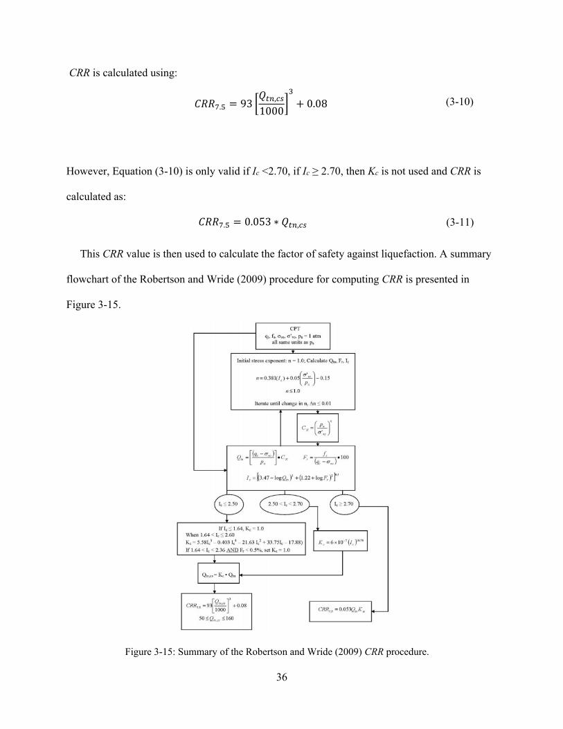
36

CRR is calculated using:

However, Equation (3-10) is only valid if Ic <2.70, if Ic ≥ 2.70, then Kc is not used and CRR is

calculated as:

This CRR value is then used to calculate the factor of safety against liquefaction. A summary

flowchart of the Robertson and Wride (2009) procedure for computing CRR is presented in

Figure 3-15.

𝐶𝐶𝐶𝐶𝐶𝐶7.5 = 93 �𝑄𝑄𝑡𝑡𝑛𝑛,𝑐𝑐𝑠𝑠

1000�3

+ 0.08 (3-10)

𝐶𝐶𝐶𝐶𝐶𝐶7.5 = 0.053 ∗ 𝑄𝑄𝑡𝑡𝑛𝑛,𝑐𝑐𝑠𝑠 (3-11)

Figure 3-15: Summary of the Robertson and Wride (2009) CRR procedure.

37

Robertson and Wride (2009) presents a procedure to calculate the CSR. Robertson and

Wride (2009) utilize Equation (3-2) to calculate the CSR, but calculates the MSF, rd, and Kσ

factors uniquely. Many values for MSF have been suggested by various researchers (Seed and

Idriss, 1982; Ambraseys, 1988), however, the Robertson and Wride method uses the lower-

bound equation values suggested by Youd et al. (2001):

where 𝑀𝑀𝑤𝑤 is the moment magnitude of the earthquake loading. The value rd is a depth

dependent shear stress reduction factor. The Robertson and Wride procedure calculates the rd,

based on the work of Liao and Whitman (1986), Robertson and wride (1998), and Seed and

Idriss (1971), as:

where z is the depth of interest in meters. Finally, to calculate the Kσ, Robertson and Wride

utilizes the procedure from Idriss et al. (2001):

where 𝜎𝜎𝑣𝑣𝑣𝑣′ is the effective overburden pressure, 𝑃𝑃𝑚𝑚 is atmospheric pressure in the same units and

𝑓𝑓 is an exponent that is a function of site conditions. After CRR and CSR are calculated FSL can

be computed using Equation (3-1).

𝑀𝑀𝐹𝐹𝐹𝐹 =102.24

𝑀𝑀𝑤𝑤2.56 (3-12)

𝑟𝑟𝑑𝑑 = �

1.0 − 0.00765𝑧𝑧 𝑓𝑓𝑓𝑓𝑟𝑟 𝑧𝑧 ≤ 9.15𝑑𝑑1.174 − 0.0267𝑧𝑧 𝑓𝑓𝑓𝑓𝑟𝑟 9.15𝑑𝑑 < 𝑧𝑧 ≤ 23𝑑𝑑0.744 − 0.008𝑧𝑧 𝑓𝑓𝑓𝑓𝑟𝑟 23𝑑𝑑 < 𝑧𝑧 ≤ 30𝑑𝑑

0.5 𝑓𝑓𝑓𝑓𝑟𝑟 𝑧𝑧 > 30𝑑𝑑

(3-13)

𝐾𝐾𝜎𝜎 = (𝜎𝜎𝑣𝑣𝑣𝑣′

𝑃𝑃𝑚𝑚) (𝑓𝑓−1) (3-14)

38

3.4.3 Ku et al. (2012) Procedure [Probabilistic Version of Robertson and Wride (2009)

Method]

Because of the increased usage and popularity of the Robertson and Wride (2009)

liquefaction triggering procedure, the need for a probabilistic version of this method was needed.

Ku et al. (2012) developed a probabilistic model of the Robertson and Wride (2009) method

through statistical analysis of the Robertson and Wride (2009) liquefaction triggering case

histories. The goal of this new model was to create a probabilistic method that could be easily

integrated into current reliability or performance-based design practices.

Ku et al. developed a function to relate FSL (from the Robertson and Wride method) to a

probability of liquefaction PL. This function was intended to provide a smooth transition of

integrating a probabilistic method into current design methods. By using the Bayesian statistical

analysis of a case history database and the principle of maximum likelihood, Ku et al. developed

the following relationship:

where 𝛷𝛷 is the standard normal cumulative distribution function, and 𝜎𝜎𝑚𝑚 is the model based

uncertainty and is equal to 0.276. This relationship between FSL and PL can be viewed visually in

Figure 3-16. The curve indicated by the “RW” represents the Robertson and Wride (2009)

deterministic triggering curve.

𝑃𝑃𝐿𝐿 = 1 − 𝛷𝛷 �0.102 + ln(𝐹𝐹𝐹𝐹𝐿𝐿)

𝜎𝜎𝑚𝑚 � (3-15)

39

3.4.4 Boulanger and Idriss (2014) Procedure

The Boulanger and Idriss (2014) procedure calculates the qc1Ncs differently than the

Robertson and Wride (2009) procedure, which results in a different calculated CRR value.

Boulanger and Idriss gathered together a database of old and recent (up through 2011)

earthquake data. Using this database, Boulanger and Idriss created a new correlation between

CPT data and the CRR for an earthquake.

Just like the Robertson and Wride method, the Boulanger and Idriss method requires an

iterative calculation for qc1Ncs. The method starts by correcting for overburden pressure as:

𝑞𝑞𝑐𝑐1𝑁𝑁 = 𝐶𝐶𝑁𝑁𝑞𝑞𝑐𝑐𝑃𝑃𝑚𝑚

(3-16)

Figure 3-16: CRR liquefaction triggering curves based on PL.

40

where 𝑞𝑞𝑐𝑐 is CPT cone tip resistance, 𝑃𝑃𝑚𝑚is atmospheric pressure, and 𝐶𝐶𝑁𝑁is the overburden

correction factor calculated as:

where 𝜎𝜎′𝑣𝑣is the vertical effective stress and 𝑑𝑑 is calculated as:

and where 𝑞𝑞𝑐𝑐1𝑁𝑁𝑐𝑐𝑠𝑠 is limited to values between 21 and 254. To start the iteration, an initial seed

value of 𝑞𝑞𝑐𝑐1𝑁𝑁𝑐𝑐𝑠𝑠 is specified, and Equations (3-16) through (3-18) are iteratively repeated until

the change in 𝑞𝑞𝑐𝑐1𝑁𝑁𝑐𝑐𝑠𝑠 is less than 0.5. Throughout the iterative process, the normalized clean-sand

cone tip resistance (𝑞𝑞𝑐𝑐1𝑁𝑁𝑐𝑐𝑠𝑠) value is calculated as:

where ∆𝑞𝑞𝑐𝑐1𝑁𝑁 is the fines content adjustment factor, ∆𝑞𝑞𝑐𝑐1𝑁𝑁 is calculated as:

where FC is the percentage of fines within the soil. To obtain FC from the CPT, Idriss and

Boulanger suggest using the FC and Ic correlation from the Robertson and Wride (1998)

procedure. However, Idriss and Boulanger suggest approaching this relationship with caution

due to the data scatter. Idriss and Boulanger suggest calculating FC as:

𝐶𝐶𝑁𝑁 = �𝑃𝑃𝑚𝑚𝜎𝜎′𝑣𝑣

�𝑚𝑚

≤ 1.7 (3-17)

𝑑𝑑 = 1.338 − 0.249(𝑞𝑞𝑐𝑐1𝑁𝑁𝑐𝑐𝑠𝑠)0.264 (3-18)

𝑞𝑞𝑐𝑐1𝑁𝑁𝑐𝑐𝑠𝑠 = 𝑞𝑞𝑐𝑐1𝑁𝑁 + ∆𝑞𝑞𝑐𝑐1𝑁𝑁 (3-19)

∆𝑞𝑞𝑐𝑐1𝑁𝑁 = �11.9 +𝑞𝑞𝑐𝑐1𝑁𝑁14.6

� exp�1.63 −9.7

𝐹𝐹𝐶𝐶 + 2− �

15.7𝐹𝐹𝐶𝐶 + 0.01�

2

� (3-20)

𝐹𝐹𝐶𝐶 = 80(𝐼𝐼𝑐𝑐 + 𝐶𝐶𝐹𝐹𝐹𝐹) − 137

0% ≤ 𝐹𝐹𝐶𝐶 ≤ 100% (3-21)

41

where 𝐼𝐼𝑐𝑐 is the soil behavior type index calculated from the Robertson and Wride procedure, and

𝐶𝐶𝐹𝐹𝐹𝐹 is a regression fitting parameter that can be used to minimize uncertainty when site-specific

fines content data is available. Figure 3-17 is a plot of the relationship between FC and Ic along

with the associated data scatter.

After the iteration has been completed to the desired level of accuracy, the CRR is then

calculated. For the Boulanger and Idriss method, the CRR is calculated as:

𝐶𝐶𝐶𝐶𝐶𝐶𝑀𝑀=7.5,𝜎𝜎′𝑣𝑣𝑣𝑣=1𝑚𝑚𝑡𝑡𝑚𝑚

= exp �𝑞𝑞𝑐𝑐1𝑁𝑁𝑐𝑐𝑠𝑠

113+ �

𝑞𝑞𝑐𝑐1𝑁𝑁𝑐𝑐𝑠𝑠1000

�2− �

𝑞𝑞𝑐𝑐1𝑁𝑁𝑐𝑐𝑠𝑠140

�3

+ �𝑞𝑞𝑐𝑐1𝑁𝑁𝑐𝑐𝑠𝑠

137�4− 2.8�

(3-22)

Figure 3-17: Recommended correlation between Ic and FC with plus or minus one standard deviation against the dataset by Suzuki et al. (1998) (after Idriss and Boulanger, 2014).

42

Idriss and Boulanger presents a procedure to calculate the CSR. Idriss and Boulanger

utilize Equation (3-2), just as the Robertson and Wride (2009) procedure, but implements

different methods to calculate the MSF, rd, and Kσ. Idriss and Boulanger (2014) developed a

relationship to calculate the MSF by combining past MSF relationships (Idriss, 1999; Boulanger

and Idriss, 2008). This new MSF relationship is calculated as:

where M is the moment magnitude of the scenario earthquake and 𝑞𝑞𝑐𝑐1𝑁𝑁𝑐𝑐𝑠𝑠 is the corrected cone

tip resistance for the Idriss and Boulanger (2014) method. This new relationship allows for soil

characteristics to be represented by CPT cone tip resistance and was found to improve the degree

of fit between CPT-based liquefaction triggering correlation and their respective history

databases (Idriss and Boulanger, 2014).

The Idriss and Boulanger procedure calculates rd by using the equations of Golesorkhi

(1989):

where z is the depth below the ground surface in meters, M is the moment magnitude of the

scenario earthquake, and the arguments within the trigonometric functions are in radians.

𝑀𝑀𝐹𝐹𝐹𝐹 = 1 + (𝑀𝑀𝐹𝐹𝐹𝐹𝑚𝑚𝑚𝑚𝑚𝑚 − 1) �8.64 exp �−𝑀𝑀

4 � − 1.325� (3-23)

𝑀𝑀𝐹𝐹𝐹𝐹𝑚𝑚𝑚𝑚𝑚𝑚 = 1.09 + �𝑞𝑞𝑐𝑐1𝑁𝑁𝑐𝑐𝑠𝑠

180�3≤ 2.2 (3-24)

𝑟𝑟𝑑𝑑 = exp [𝛼𝛼(𝑧𝑧) + 𝛽𝛽(𝑧𝑧) ∗ 𝑀𝑀] (3-25)

𝛼𝛼(𝑧𝑧) = −1.012 − 1.126 sin �𝑧𝑧

11.73+ 5.133� (3-26)

𝛽𝛽(𝑧𝑧) = 0.106 + 0.118 sin �𝑧𝑧

11.28+ 5.142� (3-27)

43

The Kσ factor in the Boulanger and Idriss method is calculated using the procedure

developed by Boulanger (2003):

Where 𝜎𝜎′𝑣𝑣is the vertical overburden pressure, 𝑃𝑃𝑚𝑚is a reference pressure equal to 1 atm, and

𝑞𝑞𝑐𝑐1𝑁𝑁𝑐𝑐𝑠𝑠 is the corrected cone tip resistance for the Idriss and Boulanger method.

Finally, with the calculated CSR and CRR values the liquefaction triggering model is

applicable to wide ranges of CPT resistance values. The liquefaction triggering curve, for the

Idriss and Boulanger deterministic model, is presented in Figure 3-18. The CRR line for both

Idriss and Boulanger studies (2008 and 2014) are shown.

𝑘𝑘𝜎𝜎 = 1 − 𝐶𝐶𝜎𝜎 ln�𝜎𝜎′𝑣𝑣𝑃𝑃𝑚𝑚� ≤ 1.1 (3-28)

𝐶𝐶𝜎𝜎 =1

37.3 − 8.27(𝑞𝑞𝑐𝑐1𝑁𝑁𝑐𝑐𝑠𝑠)0.264 ≤ 0.3 (3-29)

Figure 3-18: CRR curves and liquefaction curves for the deterministic case history database (after Idriss and Boulanger, 2014).

44

3.4.5 Probabilistic Boulanger and Idriss (2014) Procedure

Boulanger and Idriss (2014) also developed a probabilistic version of their liquefaction

triggering procedure. Using their CPT case history database (Idriss and Boulanger 2008),

Boulanger and Idriss developed an equation to calculate PL. Rather than being a function of FSL,

like the Ku et al. PL equation, this equation is a function of the seismic loading and soil stiffness

and can be expressed as:

where, 𝛷𝛷 is the standard normal cumulative distribution function, 𝑞𝑞𝑐𝑐1𝑁𝑁𝑐𝑐𝑠𝑠 is the clean sand

corrected CPT resistance, 𝐶𝐶𝐹𝐹𝐶𝐶𝑀𝑀=7.5,𝜎𝜎′𝑣𝑣=1𝑚𝑚𝑡𝑡𝑚𝑚 is the corrected CSR value for a standardized

magnitude and overburden pressure, and 𝜎𝜎ln(𝑅𝑅) is the computed model uncertainty in the

relationship. For their model, Idriss and Boulanger determined 𝜎𝜎ln(𝑅𝑅) to be 0.2. It is important to

note that the parameter uncertainties (uncertainty in 𝐶𝐶𝐹𝐹𝐶𝐶𝑀𝑀=7.5,𝜎𝜎′𝑣𝑣=1𝑚𝑚𝑡𝑡𝑚𝑚 and 𝑞𝑞𝑐𝑐1𝑁𝑁𝑐𝑐𝑠𝑠) are often

larger than the model uncertainty, and therefore treatment of these uncertainties need to be

addressed (Idriss and Boulanger, 2014).

Equation (3-17) can be used to develop liquefaction triggering curves, by calculating the

PL for a range of 𝑞𝑞𝑐𝑐1𝑁𝑁𝑐𝑐𝑠𝑠 and 𝐶𝐶𝐹𝐹𝐶𝐶𝑀𝑀=7.5,𝜎𝜎′𝑣𝑣=1𝑚𝑚𝑡𝑡𝑚𝑚 values (Figure 3-19). Idriss and Boulanger

compared these curves with their deterministic triggering curve and found the deterministic

triggering curve corresponds to PL of 16% if 𝜎𝜎ln(𝑅𝑅) = 0.2.

𝑃𝑃𝐿𝐿

= 𝛷𝛷 �−�𝑞𝑞𝑐𝑐1𝑁𝑁𝑐𝑐𝑠𝑠113 � + �𝑞𝑞𝑐𝑐1𝑁𝑁𝑐𝑐𝑠𝑠1000 �

2− �𝑞𝑞𝑐𝑐1𝑁𝑁𝑐𝑐𝑠𝑠140 �

3+ �𝑞𝑞𝑐𝑐1𝑁𝑁𝑐𝑐𝑠𝑠137 �

4− 2.60 − ln�𝐶𝐶𝐹𝐹𝐶𝐶𝑀𝑀=7.5,𝜎𝜎′𝑣𝑣=1𝑚𝑚𝑡𝑡𝑚𝑚�

𝜎𝜎ln(𝑅𝑅)�

(3-30)

45

3.5 Liquefaction Effects

Liquefaction can affect almost all types of infrastructure including buildings, bridges,

utilities, pipelines, roadways, and other constructed facilities through its effects. The effects of

liquefaction cause extreme physical and financial damage after an earthquake. The purpose of

this study is to improve prediction methods of liquefaction-induced effects. The most common

and damaging effects are described in detail below.

3.5.1 Settlement

When liquefaction occurs in loose sands, the soil tends to densify, manifesting itself as

settlement at the ground surface. When this settlement occurs unevenly, called differential

settlement, more severe damage occurs. Differential settlement can sever pipelines, sever

utilities, and cause damage to shallow foundation buildings. The target of this research is to

Figure 3-19: Liquefaction triggering PL curves compared to case history data (after Idriss and Boulanger, 2014)

46

predict liquefaction-induced settlements; therefore, settlement is discussed in more detail in

chapter 4.

3.5.2 Lateral Spread

Lateral spread is a liquefaction effect in which significant horizontal and vertical

deformations accumulate during an earthquake. Lateral spread occurs when blocks of the soil are

broken apart and essentially “float” on the liquefied soil down a slope (Figure 3-20). The

movement of these blocks can move from a few centimeters to several meters. Like settlement,

lateral spread can sever pipelines and utilities and cause severe damage to foundations.

Figure 3-20: Lateral spreading from the 1989 Loma Prieta earthquake.

47

3.5.3 Loss of Bearing Capacity

Liquefaction causes a significant loss of bearing capacity because of a loss in shear

strength during liquefaction. A loss in bearing capacity will cause severe damage to shallow

footings and embankments, which will experience bearing capacity failure. Apartment buildings

experienced this in the Niigata, Japan 1964 earthquake when they tipped over (Figure 3-21).

3.5.4 Alteration of Ground Motions

As a soil is seismically loaded, and liquefaction occurs, the stiffness of the soil decreases

significantly. This decrease in stiffness can significantly alter ground motions, such as amplitude

and frequency content. The high frequency ground motions are filtered out, resulting in only

lower frequency ground motions reaching the surface. This phenomenon can result in large

rolling displacements, which can cause extensive damage to buildings, especially those with low

natural frequencies.

Figure 3-21: Apartment buildings after the 1964 Niigata, Japan earthquake.

48

3.5.5 Increased Lateral Pressure on Walls

Liquefaction causes an increase of pore water pressure, which often pushes ground water

towards the surface. Retaining walls with liquefied soils as their backfills will experience a large

increase in static lateral pressures due to the hydrostatic force. Earthquake loading coupled with

this increased lateral pressures is often enough to cause large deformations, or even failure.

3.5.6 Flow Failure

As discussed in section 3.4.2, flow liquefaction is one of the most serious and dangerous

effects of liquefaction. Flow failures generally offer no warning because the loss of soil strength

is sudden as the effective stress path reaches the FLS. For flow failures to occur, static shear

stresses must already be present. Therefore, flow failures almost exclusively occur on sloping

ground. At the initiation of flow failure, large soil masses flow as a fluid in the downslope

direction. These flows can reach a velocity of several meters per second. All structures in the

path of such flows can be completely destroyed, due to the sheer size and speed of these failures.

3.6 Chapter Summary

Liquefaction is a complex phenomenon that causes loose, saturated sands to lose all

strength, and even flow as a fluid, under cyclic loading such as an earthquake. Liquefaction

susceptibility depends on historical, geologic, compositional, and initial effective stress state

criteria. Liquefaction will either occur as cyclic mobility or flow liquefaction, depending on the

soil’s initial effective stress state. This chapter presents the methods used to calculate the factor

of safety against liquefaction (FSL). Settlement, lateral spread, loss of bearing capacity, alteration

of ground motions, increased pressures on walls, and flow failures are all common liquefaction-

49

induced effects. Each effect can cause severe damage to buildings, utility lines, and other

important structures.

50

4 LIQUEFACTION-INDUCED SETTLEMENT

Settlement is one of the most damaging effects from an earthquake event. Settlement can

occur uniformly or differentially, meaning unevenly across a site. Differential settlement is much

more common and, unfortunately, is much more damaging. Differential settlement can cause

buildings to tip over, severance of life or utility lines, and severe structural damage. Settlement

can be life threatening, but generally in an indirect way (e.g. a building falling over, water supply

cut off). However, even though settlement is not directly life-threatening, the financial toll of

extreme liquefaction-induced settlements can be devastating to a city’s economy. To prevent

such extreme damage and design resilient structures, engineers need to fully understand how to

accurately predict liquefaction-induced settlement to design adequate structures, foundations,

and landlines.

4.1 Understanding Settlement

Whether or not a soil will settle is dependent on the soil’s depositional environment. Very

loose environments, such as Alluvial, Aeolian, and Colluvial deposits, are particularily

susceptible to settlement. Very loose deposits have very large void spaces between each particle,

which gives these deposits room to compact. Seismic loading can act as a compaction

51

mechanism by shaking the particles into a denser state creating large volumetric strains (Figure

4-1).

Differential settlement occurs because of varying thickness of liquefiable layers or

liquefaction occurring unevenly across a site. Settlement is a function of the volumetric strain

induced by a seismic event and the thickness of the liquefiable layer. When there are liquefiable

soil layers, with varying thicknesses, across a site, each portion of the layer will result in varying

amounts of surface settlement causing differential settlement.

When differential settlement is extreme, it can cause significant damage to surrounding

infrastructure. Differential settlement can cause buildings to tip over or severely crack as half of

the soil beneath a building’s foundation settles, but the other half remains stable. Differential

settlement is the main cause of the extreme damage and economic toll discussed previously.

Figures 4-2 and 4-3 show examples of damage caused by differential settlement.

Figure 4-1: Volumetric change from settlement (after Nadgouda, 2007).

52

Figure 4-2: Buildings tipped over from differential settlement from the 2015 Kathmandu, Nepal earthquake (after Williams and Lopez, 2015).

Figure 4-3: Differential settlement splitting an apartment building (after Friedman, 2007).

53

It is important to understand that other mechanisms, such as soil-foundation-structure

interaction (SFSI) and loss of soil due to piping, can affect the amount of soil deformations a site

will experience (Bray & Dashti, 2014). A structure’s weight and size can affect the amount

settlement to occur at a specific site (Dashti & Bray, 2010). All post-liquefaction calculations

and discussions for this study, therefore, only focus on free-field liquefaction-induced settlement.

This study does not take into consideration SFSI or any piping effects from transient hydraulic

gradients.

4.2 Calculating Settlement

There have been many settlement calculation methods created over the years, but three of

the most recent and commonly used include Cetin et al. (2009), Ishihara and Yoshimine (1992),

and Juang et al. (2013), which is a probabilistic extension of the Ishihara and Yoshimine method.

The Cetin et al. method is a semiempirical method that is calibrated against 49 case histories of

free-field liquefaction settlement and that uses the standard penetration test (SPT). Because this

method is based on SPT data, it was not used for this study. This study focuses on the Ishihara

and Yoshimine model, which is also a semiempirical method, but can be applied to CPT data.

4.2.1 Ishihara and Yoshimine (1992) Method

Ishihara and Yoshimine (1992) found that shear strain is a key parameter affecting post-

liquefaction volumetric strain. This relationship was discovered by extensive testing of

volumetric change characteristics of sand under undrained cyclic loading (Lee and Albaisa,

1974; Tatsuko et al., 1984; Nagase and Ishihara, 1988). Ishihara and Yoshimine (1992) produced

a deterministic procedure to calculate post-liquefaction ground settlements based on volumetric

strains in liquefiable soils, which is a function of FSL. The database, used to create the basis for

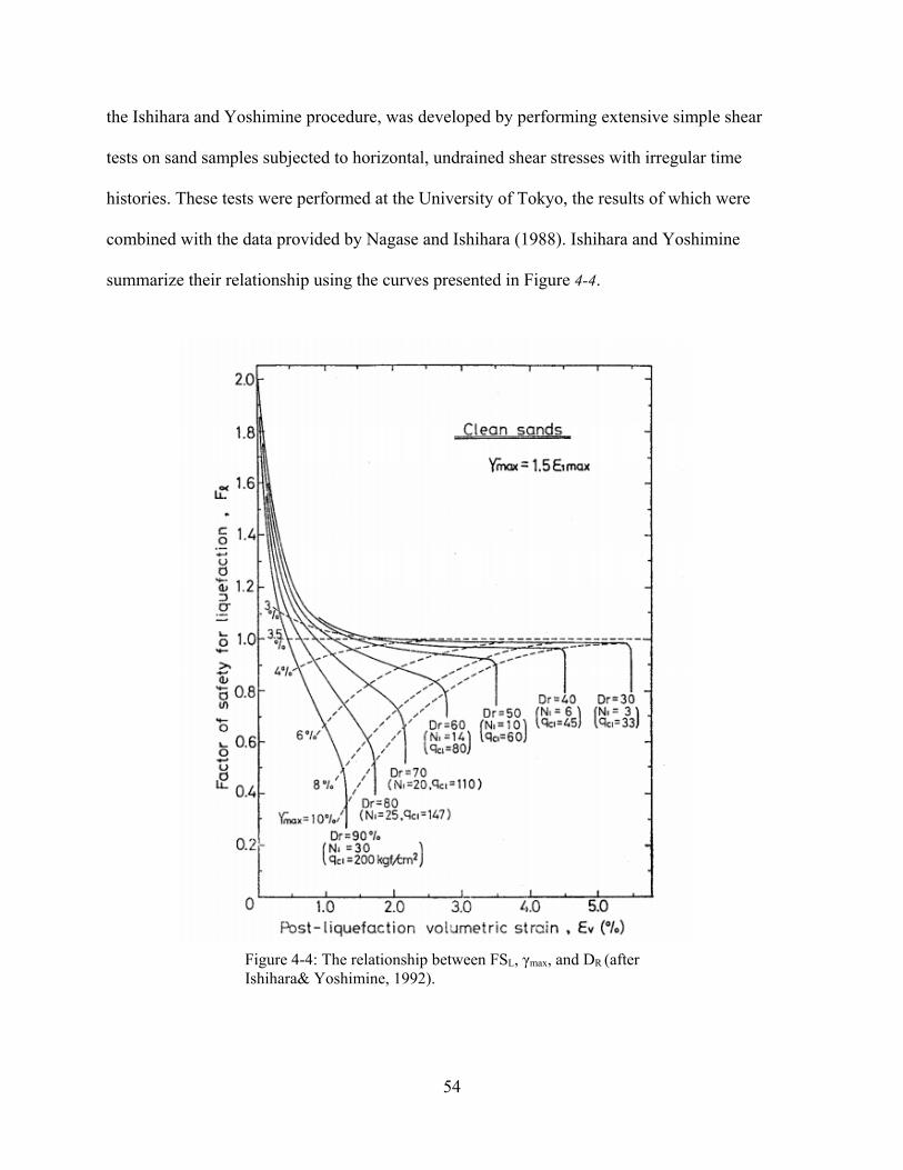
54

the Ishihara and Yoshimine procedure, was developed by performing extensive simple shear

tests on sand samples subjected to horizontal, undrained shear stresses with irregular time

histories. These tests were performed at the University of Tokyo, the results of which were

combined with the data provided by Nagase and Ishihara (1988). Ishihara and Yoshimine

summarize their relationship using the curves presented in Figure 4-4.

Figure 4-4: The relationship between FSL, γmax, and DR (after Ishihara& Yoshimine, 1992).

55

Ishihara and Yoshimine (1992) used their method to estimate the liquefaction-induced

settlements from the 1964 Niigata earthquake. The calculated values from their method

compared well to actual settlements from the Niigata earthquake. It was shown that the proposed

methodology may be used for predicting post-liquefaction settlements with a level of accuracy

suitable for many engineering purposes.

The procedure for applying the Ishihara and Yoshimine (1992) method is given as

follows: first, a factor of safety against liquefaction (FSL) is obtained for each layer using a

liquefaction triggering procedure (e.g., Robertson and Wride, 2009; Boulanger and Idris, 2014).

A relative density is also calculated for each layer, using Tatsuka et al. (1990):

where qc is the cone tip resistance and σ’v is the vertical effective stress. Using FSL and calculated

DR for each layer, volumetric strain can be obtained from the Ishihara and Yoshimine strain

curves (Figure 4-4). Each layer’s volumetric strain is multiplied by the layer’s thickness,

resulting in the vertical liquefaction-induced settlement (Sp) of each layer. Finally, each layer’s

settlement is summed together to calculate the predicted total ground surface settlement, using

the following equation:

where εv is volumetric strain for the ith layer, N is number of layers, and ΔZi is the ith layer’s

thickness.

𝐷𝐷𝑅𝑅 = −85 + 76𝑙𝑙𝑓𝑓𝑔𝑔𝑞𝑞𝑐𝑐�𝜎𝜎′𝑣𝑣

(4-1)

𝐹𝐹𝑝𝑝 = �𝜀𝜀𝑣𝑣∆𝑍𝑍𝑖𝑖

𝑁𝑁

𝑖𝑖=1

(4-2)

56

4.2.2 Juang et al. (2013) Procedure

The Juang et al. (2013) procedure calculates liquefaction-induced settlements by applying

a probabilistic approach to the deterministic Ishihara and Yoshimine (1992) method, for the cone

penetration test (CPT). Prior to the Juang et al. procedure, existing CPT-based models often

overestimated liquefaction-induced settlements. Juang et al. managed to compile a database of

free-field settlement case histories from recent earthquakes and used it to calibrate the Ishihara

and Yoshimine (1992) model for bias using the CPT. Using this bias-corrected model, a

simplified procedure was developed that allowed for the estimation of the probability of

exceeding a specified settlement at a given site.

The Juang et al. (2013) procedure also uses Equation (4-2) to calculate predicted vertical

settlements but adds probabilistic parameters by using the following equation:

where εv is volumetric strain for the ith layer, N is the number of layers, M represents a modal

bias correction factor equal to 1.0451, INDi represents the probability of liquefaction occurring,

and ΔZi is layer thickness for the ith layer. εv is calculated by using a curve-fitted equation, by

Juang et al., based on the Ishihara and Yoshimine (1992) curves (Figure 4-4), given as:

𝐹𝐹𝑝𝑝 = 𝑀𝑀�𝜀𝜀𝑣𝑣∆𝑍𝑍𝑖𝑖𝐼𝐼𝐼𝐼𝐷𝐷𝑖𝑖

𝑁𝑁

𝑖𝑖=1

(4-3)

𝜀𝜀𝑣𝑣 (%)

=

⎩⎪⎪⎨

⎪⎪⎧

0 𝑐𝑐𝑓𝑓 𝐹𝐹𝐹𝐹 ≥ 2

min�𝑐𝑐𝑣𝑣 + 𝑐𝑐1ln (𝑞𝑞)

1(2 − 𝐹𝐹𝐹𝐹)� − [𝑐𝑐2 + 𝑐𝑐3ln (𝑞𝑞)]

, 𝑏𝑏0 + 𝑏𝑏1 ln(𝑞𝑞) + 𝑏𝑏2ln (𝑞𝑞)2� 𝑐𝑐𝑓𝑓 2 − 1

𝑐𝑐2 + 𝑐𝑐3 ln(𝑞𝑞) < 𝐹𝐹𝐹𝐹 < 2

𝑏𝑏0 + 𝑏𝑏1 ln(𝑞𝑞) + 𝑏𝑏2ln (𝑞𝑞)2 𝑐𝑐𝑓𝑓 𝐹𝐹𝐹𝐹 ≤ 2 − 1

𝑐𝑐2 + 𝑐𝑐3 ln(𝑞𝑞)

Where: ao = 0.3773, a1 = -0.0337, a2 = 1.5672, a3 = -0.1833, bo = 28.45, b1 = -9.3372, b2 = 0.7975, q = qt1Ncs

(4-4)

57

The model bias correction factor, M, was calculated by Juang et al. (2013) calibrating

their model back to the case histories’ data through Bayesian maximum likelihood methods.

Juang et al. presents the INDi variable as probability of liquefaction (PL), which they calculate as:

where 𝜎𝜎ln (𝑠𝑠) represents the model uncertainty and is equal to 0.276.

One significant disadvantage associated with the Juang et al. (2013) probabilistic model

for CPT-based settlement prediction is that the model was based on the binomial assumption that

liquefaction settlements can be caused by both liquefied and non-liquefied soils. Engineers

commonly consider a soil layer susceptible to post-liquefaction settlement if the soil layer has a

sufficiently low factor of safety against liquefaction (usually less than 1.2 to 2.0). Engineers

rarely (if ever) consider non-liquefied soils to contribute to liquefaction settlements. However,

the Juang et al. (2013) model includes the probability that non-liquefied soil layers contribute to

the settlement, which may make sense mathematically, but not physically. While the possibility

of non-liquefied soil layers contributing to post-liquefaction settlements is likely greater than

zero, it is also likely sufficiently low that most engineers choose to neglect it. Furthermore, the

consideration of this possibility greatly increases the mathematical difficulty of the Juang et al.

model. Therefore, this study re-solved the maximum likelihood equation developed by Juang et

al. (2013), but neglected the possibility that non-liquefied layers contribute to liquefaction so as

to neglect the possible settlements. The resulting values of M and 𝜎𝜎ln (𝑠𝑠) are 1.014 and 0.3313,

respectively. Any potential error introduced by this simplification is accounted for in the larger

value of 𝜎𝜎ln (𝑠𝑠). Therefore, these re-regressed values of M and 𝜎𝜎ln (𝑠𝑠) are used in this study.

𝐼𝐼𝐼𝐼𝐷𝐷𝑖𝑖 = 𝑃𝑃𝐿𝐿 = 1 − 𝜙𝜙 �0.102 + ln (𝐹𝐹𝐹𝐹𝐿𝐿)

𝜎𝜎ln (𝑠𝑠)� (4-5)

58

These re-regressed values were calculated by altering the Juang et al. (2013) maximum

likelihood equation. The original Juang et al. (2013) maximum likelihood equation for the

database with m + n case histories, where m is the number of cases with a fixed settlement

observation and n is the number of case histories in which settlement is reported as a range, is

given as:

where Sa is the actual settlement observed, k represents the kth case history from the database

with m case histories, and l is the lth case history from the database with n case histories. For the

re-derivation, only the case histories containing actual recorded settlements were used. The case

histories with ranges of settlement (n case histories) were removed. In Equation (4-6), the λ and ξ

variables were represented as:

and

ln�𝐿𝐿�𝜃𝜃�𝐹𝐹𝑚𝑚(1), 𝐹𝐹𝑚𝑚(2), … , 𝐹𝐹𝑚𝑚(𝑑𝑑), 𝐹𝐹𝑚𝑚,𝑙𝑙𝑣𝑣𝑤𝑤(1), 𝐹𝐹𝑚𝑚,𝑢𝑢𝑝𝑝(1), … , 𝐹𝐹𝑚𝑚,𝑙𝑙𝑣𝑣𝑤𝑤(𝑑𝑑), 𝐹𝐹𝑚𝑚,𝑢𝑢𝑝𝑝(𝑑𝑑)��

= ��− ln�√2𝜋𝜋𝜉𝜉(𝑘𝑘)𝐹𝐹𝑚𝑚(𝑘𝑘)� −12�

ln[𝐹𝐹𝑚𝑚(𝑘𝑘)] − 𝜆𝜆(𝑘𝑘)𝜉𝜉(𝑘𝑘) �

2

�𝑚𝑚

𝑘𝑘=1

+ � ln �𝛷𝛷 �𝑙𝑙𝑑𝑑�𝐹𝐹𝑚𝑚,𝑢𝑢𝑝𝑝(𝑙𝑙)� − 𝜆𝜆(𝑙𝑙)

𝜉𝜉(𝑙𝑙)�

𝑛𝑛

𝑙𝑙=1

− 𝛷𝛷 �𝑙𝑙𝑑𝑑�𝐹𝐹𝑚𝑚,𝑙𝑙𝑣𝑣𝑤𝑤(𝑙𝑙)� − 𝜆𝜆(𝑙𝑙)

𝜉𝜉(𝑙𝑙)��

(4-6)

𝜆𝜆(𝑘𝑘) = ln �𝜇𝜇𝑚𝑚(𝑘𝑘)

�1 + 𝛿𝛿𝑚𝑚2(𝑘𝑘)�

0.5� (4-7)

𝜉𝜉(𝑘𝑘) = ln ��1 + 𝛿𝛿𝑚𝑚2(𝑘𝑘)�

0.5� (4-8)

59

where 𝜇𝜇𝑚𝑚(𝑘𝑘) represents the mean of actual observed settlement for the kth case history and 𝛿𝛿𝑚𝑚

represents the coefficient of variation (COV) of Sa. This 𝛿𝛿𝑚𝑚 is given as:

where 𝜇𝜇𝑀𝑀 is the mean of M, 𝜎𝜎𝑀𝑀 is the standard deviation of M, 𝜇𝜇𝑝𝑝 is the mean of the predicted

settlement, and 𝜎𝜎𝑝𝑝 is the standard deviation of the predicted settlement. For the re-regression, all

of the variables with a “p” term were removed to remove the assumption of non-liquefied layers

adding to settlement hazard. The 𝛿𝛿𝑚𝑚 term was simplified to:

This simplified 𝛿𝛿𝑚𝑚 replaced equation (4-9). The new M and 𝜎𝜎ln (𝑠𝑠) values were calculated by

using Juang et al. (2013) maximum likelihood equation (Equation 4-6), but by replacing

Equation (4-9) with Equation (4-10) and only using the m case histories.

4.3 Settlement Calculation Corrections

When dealing with all levels of probability, some unrealistic, incorrect, or impossible

strain values can be computed. Various correction methods have been developed to address and

correct unrealistic strain values that can be computed using simplified, semi-empirical strain

models. The corrections used in this study are described below.

4.3.1 Huang (2008) Correction for Unrealistic Vertical Strains

Huang (2008) developed a method to limit unrealistically high vertical strain values

computed in probabilistic calculations. Kramer et al. (2008) explained that direct computation of

probabilistic vertical strains has been found to produce significant unrealistically high

𝛿𝛿𝑚𝑚 =(𝜇𝜇𝑀𝑀

2𝜎𝜎𝑝𝑝2 + 𝜇𝜇𝑝𝑝2𝜎𝜎𝑀𝑀2 + 𝜎𝜎𝑀𝑀2𝜎𝜎𝑝𝑝2)0.5

𝜇𝜇𝑀𝑀2𝜇𝜇𝑝𝑝2= (𝛿𝛿𝑝𝑝

2 + 𝛿𝛿𝑀𝑀2 + 𝛿𝛿𝑝𝑝

2𝛿𝛿𝑀𝑀2)0.5 (4-9)

𝛿𝛿𝑚𝑚 =𝜎𝜎𝑀𝑀𝜇𝜇𝑀𝑀

= 𝛿𝛿𝑀𝑀 (4-10)

60

probabilities of very large strain values. Kramer et al. (2008) explains these unrealistically high

strain estimations are due to the assumption of lognormal probability distributions typically

associated with the calculation of vertical strains. For low soil stiffness values, the slope of the

lognormal probability density function increases infinitely, appropriately allowing large

probabilities to be associated with large strains. Denser soils, however, can still predict large

probabilities of vertical strain, even though both laboratory and field observations have shown

that large vertical strains with such soils are very unlikely.

Huang (2008) performed a study to find the maximum limited strain for different types of

soil. Huang evaluated theoretical, historical (i.e., field), and laboratory evidence of a maximum

vertical strain experienced by a given soil layer. He relied heavily on the apparent limiting strain

observed by four previous studies: Tokimatsu and Seed (1987), Ishihara and Yoshimine (1992),

Shamoto et al.(1998), and Wu and Seed (2004), to develop estimates of the maximum or limiting

Figure 4-5: Maximum vertical strain levels inferred by deterministic vertical strain models and weighted average used to define mean value (after Huang, 2008).

61

vertical strain as a function of SPT blow counts. The Huang (2008) and Kramer et al. (2008)

maximum vertical strain curves are shown in Figure 4-5.

Kramer et al. (2014) approximated the weighted average relationship of the Huang

(2008) and Kramer et al. (2008) maximum vertical strain curves as:

where (𝐼𝐼1)60,𝑐𝑐𝑠𝑠 is the normalized, clean sand-equivalent SPT resistance. Because there is scatter

in the maximum vertical strain curves based on the different studies that were evaluated, Huang

(2008) suggests using an εv,max range of 0.5*εv,max to 1.5*εv,max to account for uncertainty in the

true value of εv,max. To make Equation (4-6) compatible with CPT data for this study, Jefferies

and Davies (1993) is used to convert between CPT tip resistance and SPT resistance. This

relationship is presented as:

where Pa is atmospheric pressure, Ic is the Soil Behavior Type Index, and qt is the normalized tip

resistance. Using Equation (4-12), Equation (4-11) can be used for the CPT and rewritten as:

𝜀𝜀𝑣𝑣,𝑚𝑚𝑚𝑚𝑚𝑚(%) = 9.765 − 2.427𝑙𝑙𝑑𝑑[ (𝐼𝐼1)60,𝑐𝑐𝑠𝑠] (4-11)

(𝑞𝑞𝑡𝑡/𝑐𝑐𝑚𝑚) (𝐼𝐼1)60,𝑐𝑐𝑠𝑠

= 8.5(1 −𝐼𝐼𝑐𝑐

4.6) (4-12)

𝜀𝜀𝑣𝑣,𝑚𝑚𝑚𝑚𝑚𝑚(%) = 9.765 − 2.427𝑙𝑙𝑑𝑑 � �𝑞𝑞𝑡𝑡𝑐𝑐𝑚𝑚

�

8.5 �1 − 𝐼𝐼𝑐𝑐4.6�

� (4-13)

62

4.3.2 Depth Weighting Factor Correction

Calculated deformations at great depth have little influence on ground surface

displacements (Iwasaki et al., 1982). A depth weighting factor (DF) recommended by Cetin et al.

(2009) and Dr. Peter Robertson (personal communications) is incorporated to account and

correct for this phenomenon to reduce the influence of calculated strains at depth. This depth

factor aids in producing a better fit between models and case studies and is based on the

following: (1) the triggering of void ratio redistribution, and resulting in unfavorably higher void

ratios for shallower layers from upward seepage; (2) reduced induced shear stresses and number

of shear stress cycles transmitted to deeper soil layers due to initial liquefaction of surficial

layers; and (3) possible bridging effects due to nonliquefied soil layers (Cetin et al., 2009). This

depth weighting correction factor developed by Cetin et al. (2009) is given as:

where 𝑑𝑑𝑖𝑖 is the depth of the specific soil layer. At depths greater than 18m, the depth factor is

zero which indicates liquefaction past these depths will not contribute to ground surface

settlement. This depth factor is applied by multiplying the calculated strain for each layer by this

factor.

4.3.3 Transition Zone Correction

The CPT is known for its ability to provide a continuous soil profile. However, the

measured qc value does not sharply change as the cone reaches the inter-layer boundary between

one soil layer to another. Experimental studies have shown that the measured cone tip resistance

is affected by the material properties of soil layers both ahead and behind the penetrating cone

𝐷𝐷𝐹𝐹𝑖𝑖 = 1 −𝑑𝑑𝑖𝑖

18𝑑𝑑 (4-14)

63

(Treadwell, 1976). Thus, the cone will start to detect the soil layers below the cone tip before it

reaches them and will continue to sense overlaying material after it has penetrated the new

material. For example, the tip resistance, in a stiff layer, may start to decrease rapidly as it

approaches a softer layer below (Figure 4-6). Therefore, the CPT tip resistance may not always

measure the correct tip resistance in the transition zone between soil layers of significantly

different penetration resistances. A transition zone is identified if there is a steep change in the

soil behavior index (Ic), usually a change of 0.01 or greater, for multiple soil sublayer increments

(Robertson, 2011). To account for this Robertson (2011) suggests removing these sublayers from

the analysis. However, these sublayers could still potentially add to the liquefaction hazard.

Therefore, for this study, transition zones are addressed by correcting the tip resistance values

using the same process as thin layer correction, which is discussed in the next section.

Figure 4-6: Penetration analysis for medium dense sand overlaying soft clay (after Ahmadi and Robertson 2005)

64

4.3.4 Thin Layer Correction

When a thin sand layer is embedded within a soft clay, the cone from the CPT will read

the sand layer’s cone tip resistance as much lower than the actual stiffness of the thin layer

because it has started to detect the soft clay layer’s resistance early (Ahmadi & Robertson, 2005).

This discrepancy results in an over-prediction of post-liquefaction settlements because the cone

is interpreting the sandy soil as looser than it really is. Youd et al. (2001) presents a correction

factor to correct the cone tip resistance in these thin sand layers. As shown in figure 4-7, as the

cone enters deposit A (thin sand layer), the soil resistance is significantly reduced before the

cone reaches deposit B (soft clay layer). This phenomenon occurs because the cone is detecting

the softness of deposit B before it reaches deposit B. The higher the stiffness and thinner the

layer of sand interbedded within soft clay, the larger the thin layer correction factor should be.

Figure 4-7: Tip resistance analysis for thin sand layer (deposit A) interbedded within soft clay layer (deposit B). (Ahmadi & Robertson, 2005).

65

Once a layer has been identified as needing the thin layer correction, the tip resistance

can be adjusted with a correction factor. A layer is identified as a thin layer if there is a steep

negative change (e.g., going from a sand layer to a clay layer) in the soil behavior index (Ic),

usually a change of 0.01 or greater, for four consecutive soil sublayer increments (Robertson,

2011). Once identified, these layer’s tip resistances can be corrected as:

where 𝑞𝑞𝑐𝑐∗ is the corrected cone tip resistance and 𝐾𝐾𝐻𝐻 is the correction factor (Youd et al., 2001).

This factor is calculated as:

where 𝑑𝑑𝑐𝑐 is the diameter of the cone, and 𝐻𝐻 is the layer thickness.

4.4 Chapter Summary

Liquefaction-induced settlements pose a serious threat to infrastructure and to the people

who rely on it. While liquefaction-induced settlements are not directly life-threatening,

differential settlement can cause severe damage to structures, utility lines, and life lines, resulting

in a large economic toll on a community. The ability for engineers to predict liquefaction-

induced settlements is crucial to mitigate and prevent severe damage in the event of an

earthquake. This chapter presented a deterministic and probabilistic method to predict

liquefaction-induced settlements. Finally, this chapter addressed settlement correction factors to

account for unrealistic settlement estimations.

𝑞𝑞𝑐𝑐∗ = 𝐾𝐾𝐻𝐻𝑞𝑞𝑐𝑐 (4-15)

𝐾𝐾𝐻𝐻 = 0.25 ��𝐻𝐻𝑑𝑑𝑐𝑐

�

17− 1.77�

2

+ 1.0 (4-16)

66

5 GROUND MOTION SELECTION FOR LIQUEFACTION ANALYSIS

In seismic regions around the world, earthquakes pose enough of a hazard to promote careful

analysis and design of structures and facilities. Earthquake design involves designing a structure

to withstand a certain level of earthquake shaking or hazard. Specifying the design level of an

earthquake to resist is a difficult part of geotechnical earthquake engineering. Choosing a design

earthquake is difficult because there are high levels of uncertainty to deal with in determining the

location, magnitude, and ground motions of an earthquake.

To account for this difficulty, many engineers will design for what they perceive to be the

“worst case” scenario earthquake in their region. This approach, referred to as a deterministic

seismic hazard analysis (DSHA), does not take into account the likelihood of the controlling

event occurring and neglects the seismic hazard contribution of all other seismic sources near the

fault. To try to improve on the accuracy of the DSHA, more seismic hazard analysis (SHA)

methods have been created and applied to predicting post-liquefaction settlements. Each of these

SHA approaches differ in how ground motions are selected and applied. This chapter discusses

each of these approaches and presents the newly developed performance-based procedure to

predict post-liquefaction settlements for the CPT. It is not generally fully understood how

differing seismic hazard analyses add bias into the seismic hazard predictions. To address this

67

misunderstanding, this study was designed to compare conventional design methods to the new,

fully-probabilistic, design procedures. This comparative study and presented in Chapter 6.

5.1 Seismic Hazard Analysis

SHA involves the process of predicting strong ground motions for a given site, in a

quantitative fashion. There are two basic types of SHA, namely a DSHA and a probabilistic

seismic hazard analysis (PSHA). DSHA conservatively assumes an earthquake scenario, usually

ground motions from the most impactful fault near the site, and performs design calculations

based on the ground motion parameters from that single earthquake scenario. PSHA explicitly

takes into account the uncertainties in earthquake size, location, and time of occurrence to select

design ground motion parameters. Both methods are discussed in more detail below.

5.1.1 Deterministic Seismic Hazard Analysis

In the early years of geotechnical earthquake engineering, engineers generally used the

DSHA for earthquake design. DSHA involves selecting a particular seismic scenario to design

from (Steven L Kramer, 1996). Design ground motion parameters are selected based off of this

particular scenario. DSHA considers the fault capable of producing the largest ground motion at

the site. This assumption can result in inconsistent results.

Reiter (1990) organizes the DSHA into four general steps (Figure 5-1). The first step is to

identify and characterize all possible seismic sources capable of producing significant ground

motions at the site of interest. Characterizing the sources includes determining each source’s

geometry and level of seismicity. The second step is to determine the closest site-to-source

distances for each source. These distances could be epicentral or hypocentral distances.

Determining the controlling earthquake is the third step, which involves determining which

68

earthquake source will create the largest ground motions by comparing the levels of shaking

found in step one at distances found in step two. The final, and fourth, step formally defines the

seismic hazard at the site based on the controlling earthquake. Hazards are often defined in

multiple parameters, such as the ones discussed in chapter two.

5.1.2 Probabilistic Seismic Hazard Analysis

As geotechnical earthquake engineering has progressed, engineers have developed the

probabilistic seismic hazard analysis (PSHA) method. PSHA takes into account all of the

uncertainties relating to the size, location, and rate of occurrence of a seismic event. The PSHA

framework in which each uncertainty can be identified, quantified, and combined to provide a

clear level of site seismicity (Algermissen, 1982; Cornell, 1968).

Figure 5-1: Four steps of a DSHA (Kramer, 1996).

69

Just as the DSHA, the PSHA can be broken into four distinct steps (Steven L Kramer,

1996; Reiter, 1990). The first step (Figure 5-2) of the PSHA is to identify and characterize all

potential earthquake sources. This step is the same for the DSHA, except the PSHA also

identifies the distribution of the probability of rupture along the source. However, in most cases a

uniform probability distribution is used to indicate that all points along the fault are equally

likely to rupture. The second step takes into account the probability of the recurrence of a

specific level of earthquake. This utilizes recurrence relationships, which indicate average rates

of exceedance of a specific level of earthquake. Engineers will decide which return period, or

exceedance rate, is appropriate for the design of their structure. The next step is to determine the

ground motions, using attenuation relationships, at the site created by earthquakes of a given size

at a given location. The fourth, and final, step combines all of the inherent uncertainties, of

potential earthquake sizes, locations, and ground motions, to calculate the probability the ground

motion parameter will be exceeded during a seismic event.

Figure 5-2: Four steps of a PSHA (Kramer, 1996).

70

The result of a DSHA is usually a singular value, such as a factor of safety, but because a

PSHA takes into account all possible seismic events it produces a range of results, each value

associated with a different likelihood. PSHA results are generally expressed in terms of the

annual rate of exceedance (λ), which is the probability a specific event will be exceeded in any

given year. All of the annual rate of exceedances are generally combined and displayed as a

seismic hazard curve. Hazard curves are discussed in detail in the next section.

5.1.2.1 Seismic Hazard Curves

Seismic hazard curves represent the probability of exceeding a particular ground motion

at a site. These curves can be obtained for individual seismic sources or combined to represent

the comprehensive hazard of all surrounding sources (Kramer, 1996). Hazard curves are created

by calculating the probability of exceeding a particular value (y*) of a particular ground motion

(Y) for one possible earthquake at one possible location. This probability is then multiplied by

the probability that that particular earthquake will occur at a particular location. This calculation

is repeated for all possible magnitudes and locations. These probabilities are summed together to

calculate the total probability of exceeding (λ) the given ground motion parameter, y*. This

process is then repeated for a whole range of the ground motion parameter until it creates a

complete hazard curve. The inverse of the probability of exceedance is the return period (TR),

which describes the average number of years between exceedance occurrences.

The probability that a specified ground motion will be exceeded may be calculated using

the magnitude and source-to-site distance of all possible earthquakes that could affect the site.

The probability of exceedance can be computed as:

71

𝑃𝑃[ 𝑌𝑌 > 𝑐𝑐∗] = �𝑃𝑃[𝑌𝑌 > 𝑐𝑐∗|𝑑𝑑, 𝑟𝑟] 𝑓𝑓𝑀𝑀(𝑑𝑑)𝑓𝑓𝑅𝑅(𝑟𝑟) 𝑑𝑑𝑑𝑑 𝑑𝑑𝑟𝑟 (5-1)

where 𝑃𝑃[ 𝑌𝑌 > 𝑐𝑐∗] is calculated from the selected attenuation relationship(s) and 𝑓𝑓𝑀𝑀(𝑑𝑑) and

𝑓𝑓𝑅𝑅(𝑟𝑟) are probability density functions for magnitude and source-to-site distance, respectively

(Kramer, 1996). If the site is in a region of multiple seismic sources, the annual rate of

exceedance can be calculated as:

𝜆𝜆𝑦𝑦∗ = �𝑣𝑣𝑖𝑖

𝑁𝑁𝑠𝑠

𝑖𝑖=1

�𝑃𝑃[𝑌𝑌 > 𝑐𝑐∗|𝑑𝑑, 𝑟𝑟] 𝑓𝑓𝑀𝑀(𝑑𝑑)𝑓𝑓𝑅𝑅(𝑟𝑟) 𝑑𝑑𝑑𝑑 𝑑𝑑𝑟𝑟 (5-2)

where Ns represents all of the various seismic sources and 𝑣𝑣𝑖𝑖 represents average rate of threshold

magnitude exceedance, which can be computed as:

where α = 2.303a and β = 2.303b, and a and b are Gutenberg-Richter recurrence law

coefficients. The threshold magnitude is the magnitude that must be exceeded for significant

damage to be caused. The average rate of threshold magnitude exceedance limits the sources to a

specific range of magnitude. This limit is used because earthquakes below a magnitude of 4.0 or

5.0 will cause very little severe damage. These smaller earthquakes are generally ignored in a

hazard analysis.

Equation (5-2) is too complicated for the integrals to be evaluated with closed-form

solutions, so numerical integration is required to be used. Numerical integration can be

performed in a variety of ways; one approach is to divide all the possible ranges of magnitude

and distance into equal segments of NM and NR, respectively. An estimation of the average rate of

exceedance may be calculated by:

𝑣𝑣𝑖𝑖 = 𝑑𝑑𝛼𝛼𝑖𝑖−𝛽𝛽𝑖𝑖𝑚𝑚0 (5-3)

72

𝜆𝜆𝑦𝑦∗ = ���𝑣𝑣𝑖𝑖

𝑁𝑁𝑅𝑅

𝑘𝑘=1

𝑁𝑁𝑀𝑀

𝑗𝑗=1

𝑁𝑁𝑆𝑆

𝑖𝑖=1

𝑃𝑃�𝑌𝑌 > 𝑐𝑐∗�𝑑𝑑𝑗𝑗 , 𝑟𝑟𝑘𝑘� 𝑓𝑓𝑀𝑀𝑖𝑖(𝑑𝑑𝑖𝑖)𝑓𝑓𝑅𝑅𝑖𝑖(𝑟𝑟𝑘𝑘) 𝛥𝛥𝑑𝑑 𝛥𝛥𝑟𝑟 (5-4)

where 𝑑𝑑𝑖𝑖 = 𝑑𝑑𝑣𝑣 + (𝑗𝑗 − 0.5)(𝑑𝑑𝑚𝑚𝑚𝑚𝑚𝑚 − 𝑑𝑑𝑣𝑣)/𝐼𝐼𝑀𝑀 , 𝑟𝑟𝑘𝑘 = 𝑑𝑑𝑚𝑚𝑖𝑖𝑛𝑛 + (𝑘𝑘 − 0.5)(𝑟𝑟𝑚𝑚𝑚𝑚𝑚𝑚 − 𝑟𝑟𝑣𝑣)/𝐼𝐼𝑅𝑅, 𝛥𝛥𝑑𝑑 =

(𝑑𝑑𝑚𝑚𝑚𝑚𝑚𝑚 − 𝑑𝑑𝑣𝑣)/𝐼𝐼𝑀𝑀, and 𝛥𝛥𝑟𝑟 = (𝑟𝑟𝑚𝑚𝑚𝑚𝑚𝑚 − 𝑟𝑟𝑣𝑣)/𝐼𝐼𝑅𝑅. Equation (5-4) assumes that each source is only

capable of generating only NM different earthquakes at only NR different source-to-site distances

(Kramer, 1996). By using this assumption, an estimation of Equation (5-4) can be written as:

𝜆𝜆𝑦𝑦∗ ≈���𝑣𝑣𝑖𝑖

𝑁𝑁𝑅𝑅

𝑘𝑘=1

𝑁𝑁𝑀𝑀

𝑗𝑗=1

𝑁𝑁𝑆𝑆

𝑖𝑖=1

𝑃𝑃�𝑌𝑌 > 𝑐𝑐∗�𝑑𝑑𝑗𝑗 , 𝑟𝑟𝑘𝑘� 𝑃𝑃[𝑀𝑀 = 𝑑𝑑𝑗𝑗]𝑃𝑃[𝐶𝐶 = 𝑟𝑟𝑘𝑘] (5-5)

The accuracy of this numerical integration approach increases as the number of intervals of NM

and NR increase. It should be mentioned that using a more refined method of numerical

integration would produce more accurate results. Equation (5-5) produces only one point on a

hazard curve. To generate the whole curve the process is repeated for a whole range of ground

motion parameters (y*).

5.2 Incorporation of Ground Motions in the Prediction of Post-Liquefaction Settlement

Accurate selection of design ground motions is crucial to accurate liquefaction hazard

estimations. A structure will only be able to withstand earthquake shaking, and its effects, up to

the ground motions it was designed for. Therefore, to be able to accurately design for

liquefaction-induced settlements the correct level of ground motions need to be accounted for in

the hazard analysis. However, selecting correct ground motions can be difficult due to the

inherent uncertainty within predicting earthquake events. The most common approaches, for

incorporating ground motions into post-liquefaction settlement estimations, are addressed in this

study and discussed in this section.

73

The selection of ground motions is not directly incorporated into post-liquefaction

settlement estimations, but rather into the liquefaction triggering analysis. Therefore, this section

will also address how liquefaction triggering is computed for each approach and how it is

incorporated into post-liquefaction settlement estimations.

To present each of these approaches more clearly, an example calculation is performed for

each approach. This example calculation is performed for CPT profile at a site located in Salt

Lake City, Utah at a Latitude and longitude of 40.76, -111.89 degrees, respectively. The CPT

profile of interest is chosen due to its highly-liquefiable nature. The Qtn,cs across depth, for this

profile, is plotted in Figure 5-3. To simplify the example, settlement values are computed and

compared for the 2475 return period and only the Robertson and Wride (2009) triggering

procedure.

Figure 5-3: CPT profile used for example calculations.

74

5.2.1 Deterministic Approach

As discussed in section 5.1.1, a deterministic seismic hazard analysis involves designing

for the largest and most significant ground motions at the site. The ground motions (i.e., amax)

and corresponding moment magnitude, Mw, from this design earthquake are used to calculate a

FSL and Qtn,cs using the liquefaction triggering procedures discussed in sections 3.5.2 and 3.5.4,

specifically Equations (3-1) through (3-29). This FSL is calculated for each soil sublayer in the

CPT profile. This calculated FSL, and the corresponding Qtn,cs, is used with the Ishihara and

Yoshimine (1992) deterministic strain relationship given in Equations (4-1) through (4-4). Strain

values are calculated for each soil layer, multiplied by the layer thickness, and finally summed

together to calculate the total ground settlement.

For the Salt Lake City, UT example, the controlling fault is the Wasatch fault because it

is the closest and would have the greatest impact to Salt Lake City. The Wasatch fault has the

potential to produce a 7.0 magnitude earthquake. The NGA west-2 database (Ancheta et al.,

2014) is used to calculate amax (0.456g) at this location for the controlling fault. These values are

used to calculate Qtn,cs and FSL using the Robertson and Wride (2009) triggering procedure for

each layer [Equations (3-1) through (3-14)]. These values are then used to calculate settlement

using the Ishihara and Yoshimine (1992) procedure. The deterministic calculated settlement, for

this example, is 34.4cm.

5.2.2 Pseudo-Probabilistic Approach

The pseudo-probabilistic approach involves selecting design ground motions through

probabilistic methods and applying them to a deterministic calculation of earthquake effects.

This procedure involves using a deterministic triggering procedure (sections 3.5.2 and 3.5.4) to

75

calculate FSL, but by using a PSHA to select input ground motions. This PSHA selection of

ground motions is usually performed by using the USGS deaggregation tool

(https://earthquake.usgs.gov/hazards/interactive/). This magnitude can be either the mean (i.e.,

average) or modal (i.e., occurring the most often) magnitude for the specific location. The FSL

and Qtn,cs, from the triggering procedures, values are then applied to the deterministic Ishihara

and Yoshimine (1992) procedure to calculate post-liquefaction settlements. Even though the

pseudo-probabilistic approach accounts for some uncertainty in ground motions, inherent

uncertainty within the triggering of liquefaction and the calculation of its effects are generally

ignored. Furthermore, the approach assumes that all liquefaction hazard is caused by a single

return period of ground motions. Therefore, a common misperception of the pseudo-probabilistic

approach is that the return period of the computed post-liquefaction settlements is the same as

the return period of the input ground motions. This perception would only be true if there was no

uncertainty associated with the computation of settlements.

A pseudo-probabilistic settlement analysis is performed for the Salt Lake City, UT

example. From the USGS deaggregation tool as a return period of 2,475 years, the mean

magnitude and PGA are 7.53 and 1.325g, respectively. The modal magnitude is 7.10. For

simplicity in this example, amax is assumed to equal PGA. These deaggreagation values were

used with the Robertson and Wride (2009) triggering procedure, by using Equations (3-1)

through (3-14). The calculated settlements using mean and modal magnitudes are 34.9cm and

34.8cm, respectively. Because the mean and modal magnitudes are so similar, they produce

similar settlement estimations, in this case, but often produce very different settlements.

76

5.2.3 Performance-Based Approach

In an effort to promote advancement in the current building codes and to provide a fully-

probabilistic seismic analysis, a new seismic hazard design approach has been developed, known

as performance-based earthquake engineering (PBEE). This approach was developed by the

Pacific Earthquake Engineering Research (PEER) Center (C. A. Cornell & Krawinkler, 2000;

Deierlein, Krawinkler, & Cornell, 2003). The PEER framework was designed to address all

earthquake risks.

The PEER framework seeks to improve seismic risk decision-making through assessment

and design methods that are more transparent, scientific, and informative to stakeholders than

current prescriptive approaches (Deierlein et al., 2003). Conventional design methods usually

only present the earthquake risk in terms of a factor of safety, which can be hard for various

stakeholders to truly understand. This misunderstanding is because each stakeholder thinks about

risk differently. For example, structural engineers think of structural collapse or deformation,

owners think about cost or downtime, and government agencies think about fatalities. When

engineers, owners, and governing agencies are only presented with a factor of safety, it can be

difficult for them to make a truly informed decision. PBEE improves this decision-making by

presenting earthquake risks in metrics that matter to each stakeholder. Figure 5-4 illustrates the

various levels of performance across multiple metrics, important to different stakeholders.

77

The objective of PBEE is to quantify all of the inherent uncertainty in predicting seismic

hazards and using this calculated uncertainty to predict structural performance. This predicted

structural response can help stakeholders define a desirable level of structural performance.

Figure 5-5 provides a visual representation of the varying levels of seismic performance

objectives. For example, critical structures (e.g. hospitals, nuclear waste facilities, power plants,

emergency response facilities, etc.) must be designed to remain fully operational even after a rare

seismic event, while less critical structures (e.g. shopping centers, office buildings, etc.) have a

higher risk tolerance. PBEE helps stakeholders make informed decisions based on their level of

tolerable risk.

Figure 5-4: Visualization of performance-based earthquake engineering (after Moehle and Deierlein, 2004).

78

The PEER framework developed an equation to represent PBEE (5-7). The PEER framework

equation can be broken down into four main variables (Figure 5-6). These variables include the

following components (Deierlein et al., 2003):

• Intensity Measure (IM): a quantity that capture attributes of the ground motion hazard at

a site. IMs are usually calculated by seismologists. IMs are scaler values that involve the

consideration of nearby earthquake faults and the geologic characteristics of the

surrounding region and nearby site. Examples of IMs include PGA, PGV, Arias Intensity

(IA), and other ground motion parameters.

• Engineering Demand Parameter (EDP): describes the structural response to the IM in

terms of deformations, accelerations, or other structural response variables. The EDP can

Figure 5-5: Design objectives for variable levels of risk and performance (after Porter, 2003).

79

relate to the structural system (e.g. story drift, strength deterioration, etc.) or the

subsurface soil system below the structure (e.g. lateral spreading, settlement, FSL, etc.).

This study focuses on the EDP of settlement.

• Damage Measure (DM): describes the resulting physical condition of the structure and its

components as a function of the imposed EDPs. DMs could include pile deflection,

cracking, and collapse potential.

• Decision Variable (DV): quantifies DM into levels of risk. DVs translate damage

measures into quantities that relate risk management decisions concerning economic and

safety loss. Examples of DVs could include repair cost, lives lost, and down time.

The PBEE framework equation is structured similarily to PSHA, in that it also calculates the

mean annual rate of exceedance (λ) of a specific outcome for a range of possible seismic

Figure 5-6: Variable components of the performance-based earthquake engineering framework equation (after Deierlein et al., 2003).

80

scenarios. The outcome and possible siesmic scenarios are a specific EDP and ranges of a certain

IM, respectively. The equation to calculate λEDP is given as:

λ𝐸𝐸𝐸𝐸𝐸𝐸 = �𝑃𝑃[ 𝐸𝐸𝐷𝐷𝑃𝑃 > 𝑑𝑑𝑑𝑑𝑐𝑐|𝐼𝐼𝑀𝑀 = 𝑐𝑐𝑑𝑑𝑗𝑗]∆λ𝐼𝐼𝑀𝑀 (5-6)

where 𝑃𝑃[ 𝐸𝐸𝐷𝐷𝑃𝑃 > 𝑑𝑑𝑑𝑑𝑐𝑐|𝐼𝐼𝑀𝑀 = 𝑐𝑐𝑑𝑑𝑗𝑗] represents the probability that a specific EDP will exceed a

certain level of 𝑑𝑑𝑑𝑑𝑐𝑐, given a particular IM, and ∆λ𝐼𝐼𝑀𝑀 represents the incremental rate of

exceedance of the IM. This process is then repeated for a specific range of levels of EDPs to

calculate the total mean annual rate of eceedance of a DV (λDV). The complete PBEE framework

equation can be represented by:

λ𝐸𝐸𝐷𝐷 = ���𝑃𝑃[𝐷𝐷𝐷𝐷|𝐷𝐷𝑀𝑀]𝑑𝑑𝑃𝑃[𝐷𝐷𝑀𝑀|𝐸𝐸𝐷𝐷𝑃𝑃]𝑑𝑑𝑃𝑃[𝐸𝐸𝐷𝐷𝑃𝑃|𝐼𝐼𝑀𝑀]𝑑𝑑λ𝐼𝐼𝑀𝑀 (5-7)

which can be estimated numerically by:

λ𝐸𝐸𝐷𝐷 = � � �𝑃𝑃[𝐷𝐷𝐷𝐷 > 𝑑𝑑𝑣𝑣|𝐷𝐷𝑀𝑀 = 𝑑𝑑𝑑𝑑𝑘𝑘] × 𝑃𝑃�𝐷𝐷𝑀𝑀 = 𝑑𝑑𝑑𝑑𝑘𝑘�𝐸𝐸𝐷𝐷𝑃𝑃 = 𝑑𝑑𝑑𝑑𝑐𝑐𝑗𝑗�𝑁𝑁𝐼𝐼𝑀𝑀

𝑖𝑖=1

𝑁𝑁𝐸𝐸𝐸𝐸𝐸𝐸

𝑗𝑗=1

𝑁𝑁𝐸𝐸𝑀𝑀

𝑘𝑘=1

× 𝑃𝑃�𝐸𝐸𝐷𝐷𝑃𝑃 = 𝑑𝑑𝑑𝑑𝑐𝑐𝑗𝑗�𝐼𝐼𝑀𝑀 = 𝑐𝑐𝑑𝑑𝑖𝑖� ∆λ𝐼𝐼𝑀𝑀

(5-8)

where 𝐼𝐼𝐸𝐸𝑀𝑀, 𝐼𝐼𝐸𝐸𝐸𝐸𝐸𝐸, and 𝐼𝐼𝐼𝐼𝑀𝑀are the number of increments of DM, EDP, and IM, respectively. By

iterating through a range of DVs, using equation (5-8), a hazard curve will be developed (Figure

5-7). A hazard curve clearly indicates the probability of exceeding a range of specific DVs.

Stakeholders can choose what level of risk, or DV, is needed for their project. Then, by using the

hazard curve, engineers can obtain the λDV for the given risk level. The λDV will provide enigneers

with a clear understanding of what seismic hazard risk level they need to design for.

81

To apply the PEER framework to the estimation of post-liquefaction settlements, the PEER

framework is also applied to liquefaction triggering. To apply a performance-based procedure to

the liquefaction triggering calculations, FSL hazard curves are developed using the Kramer and

Mayfield (2007) PBEE approach. This approach utilizes the PEER PBEE framework by

assigning the joint occurrence of Mw and amax as an intensity measure and the FSL as the

engineering demand parameter. Engineers are more interested in when FSL is expected to not

exceed a certain value because FSL, unlike other EDPs, is more favorable the larger it is.

Therefore, Equation 5-6 is altered to predict the probability of non-exceedance, rather than the

probability of exceedance. This new equation of non-exceedance is presented as:

where 𝛬𝛬𝐹𝐹𝐹𝐹∗𝐿𝐿 is the mean annual rate of not exceeding some given value of factor of safety

(𝐹𝐹𝐹𝐹∗𝐿𝐿), 𝐼𝐼𝑀𝑀 and 𝐼𝐼𝑚𝑚𝑚𝑚𝑚𝑚𝑚𝑚are the number of magnitude and amax increments into which the hazard

space is subdivided, and ∆𝜆𝜆𝑚𝑚𝑚𝑚𝑚𝑚𝑚𝑚,𝑖𝑖,𝑚𝑚𝑗𝑗 is the incremental mean annual rate of exceedance for

intensity measures 𝑐𝑐𝑚𝑚𝑚𝑚𝑚𝑚,𝑖𝑖 and 𝑑𝑑𝑗𝑗.

𝛬𝛬𝐹𝐹𝐹𝐹∗𝐿𝐿 = � � 𝑃𝑃[𝐹𝐹𝐹𝐹𝐿𝐿 < 𝐹𝐹𝐹𝐹∗𝐿𝐿|𝑐𝑐𝑚𝑚𝑚𝑚𝑚𝑚,𝑖𝑖 ,𝑑𝑑𝑗𝑗]∆𝜆𝜆𝑚𝑚𝑚𝑚𝑚𝑚𝑚𝑚,𝑖𝑖,𝑚𝑚𝑗𝑗

𝑁𝑁𝑚𝑚𝑚𝑚𝑚𝑚𝑚𝑚

𝑖𝑖=1

𝑁𝑁𝑀𝑀

𝑗𝑗=1

(5-9)

Figure 5-7: Example hazard curve for a given DV.

82

Kramer and Mayfield also related performance based methodology with in-situ soil

resistance by using the term Nreq, which represents the SPT resistance required to prevent

liquefaction. In other words, Nreq is the number of blow counts required to prevent liquefaction

or the condition of FSL= 1. To apply this to the CPT qreq (i.e., the required tip resistance) can be

used. Following the work of Kramer and Mayfield an expression for the mean annual rate of

exceedance of the value q*req at a depth of interest can be defined as:

where

Each of the two triggering procedures calculate Equation (5-11) differently. The

Robertson and Wride (2009) PL can be calculated as:

where 𝜎𝜎𝑡𝑡𝑣𝑣𝑡𝑡𝑚𝑚𝑙𝑙 is the parameter and model uncertainty and is equal to 0.3537. The 𝐶𝐶𝐶𝐶𝐶𝐶 and 𝐶𝐶𝐹𝐹𝐶𝐶

are calculated according to Equations (3-3) through (3-14), but the input Qtn,cs is replaced with

q*req. For the Boulanger and Idriss (2014) procedure, the PL is calculated as:

𝜆𝜆𝑞𝑞∗𝑟𝑟𝑟𝑟𝑟𝑟 = � � 𝑃𝑃[𝑞𝑞𝑟𝑟𝑟𝑟𝑞𝑞 > 𝑞𝑞∗𝑟𝑟𝑟𝑟𝑞𝑞|𝑐𝑐𝑚𝑚𝑚𝑚𝑚𝑚,𝑖𝑖 ,𝑑𝑑𝑗𝑗]∆𝜆𝜆𝑚𝑚𝑚𝑚𝑚𝑚𝑚𝑚,𝑖𝑖,𝑚𝑚𝑗𝑗

𝑁𝑁𝑚𝑚𝑚𝑚𝑚𝑚𝑚𝑚

𝑖𝑖=1

𝑁𝑁𝑀𝑀

𝑗𝑗=1

(5-10)

𝑃𝑃 �𝑞𝑞𝑟𝑟𝑟𝑟𝑞𝑞 > 𝑞𝑞∗𝑟𝑟𝑟𝑟𝑞𝑞�𝑐𝑐𝑚𝑚𝑚𝑚𝑚𝑚,𝑖𝑖 ,𝑑𝑑𝑗𝑗� = 𝑃𝑃𝐿𝐿(𝑞𝑞∗𝑟𝑟𝑟𝑟𝑞𝑞) (5-11)

𝑃𝑃𝐿𝐿 = 1 − 𝛷𝛷 �0.102 + ln �𝐶𝐶𝐶𝐶𝐶𝐶𝐶𝐶𝐹𝐹𝐶𝐶�

𝜎𝜎𝑡𝑡𝑣𝑣𝑡𝑡𝑚𝑚𝑙𝑙� (5-12)

𝑃𝑃𝐿𝐿 = 𝛷𝛷

⎣⎢⎢⎢⎡−�𝑞𝑞∗𝑐𝑐1𝑁𝑁𝑐𝑐𝑠𝑠

113 � + �𝑞𝑞∗𝑐𝑐1𝑁𝑁𝑐𝑐𝑠𝑠1000 �

2

− �𝑞𝑞∗𝑐𝑐1𝑁𝑁𝑐𝑐𝑠𝑠

140 �3

+ �𝑞𝑞∗𝑐𝑐1𝑁𝑁𝑐𝑐𝑠𝑠

137 �4

− 2.60 − ln�𝐶𝐶𝐹𝐹𝐶𝐶𝑀𝑀=7.5,𝜎𝜎′𝑣𝑣=1𝑚𝑚𝑡𝑡𝑚𝑚�

𝜎𝜎total⎦⎥⎥⎥⎤ (5-13)

83

where 𝜎𝜎total is the parameter and model uncertainty and is equal to 0.506, 𝑞𝑞∗𝑐𝑐1𝑁𝑁𝑐𝑐𝑠𝑠 is equal to

𝑞𝑞∗𝑟𝑟𝑟𝑟𝑞𝑞, and the 𝐶𝐶𝐹𝐹𝐶𝐶𝑀𝑀=7.5,𝜎𝜎′𝑣𝑣=1𝑚𝑚𝑡𝑡𝑚𝑚 is calculated using Equations (3-25) through (3-29).

Equation (5-10) is repeated for a range of q*req (1 to 250) for each triggering method and

for every soil layer. These calculations result in a range of probabilities of exceedance (λ)

corresponding to qreq values. This process develops a qreq hazard curve. Because FSL and ΔNL

essentially provide the same information, Kramer and Mayfield (2007) provides a useful

conversion between the two:

This conversion may be applied to CPT data by using:

where 𝑞𝑞𝑠𝑠𝑖𝑖𝑡𝑡𝑟𝑟 is the measured corrected clean-sand equivalent CPT cone-tip resistance, and 𝑞𝑞𝑟𝑟𝑟𝑟𝑞𝑞𝑠𝑠𝑖𝑖𝑡𝑡𝑟𝑟 is

the computed corrected clean-sand equivalent CPT cone-tip resistance required to resist

liquefaction at the site of interest. By using Equations (5-14) and (5-15), the qreq hazard curves

are converted to FSL hazard curves. When qreq is converted to FSL the value 𝜆𝜆𝑞𝑞∗𝑟𝑟𝑟𝑟𝑟𝑟 is

automatically converted to an annual rate of non-exceedance of FSL (𝛬𝛬𝐹𝐹𝐹𝐹∗𝐿𝐿).

These calculations complete the process of creating a FSL hazard curve for one soil layer.

This process is repeated for each soil layer so that a FSL hazard curve exists for each soil layer

and for each triggering method. An example FSL hazard curve for one soil layer is presented in

(Figure 5-8). Each of these FSL hazard curves are used to calculate the PBEE predicted

settlements.

𝐹𝐹𝐹𝐹𝐿𝐿𝑠𝑠𝑖𝑖𝑡𝑡𝑟𝑟 =𝐶𝐶𝐶𝐶𝐶𝐶𝐶𝐶𝐹𝐹𝐶𝐶

=𝐶𝐶𝐶𝐶𝐶𝐶 (𝐼𝐼𝑠𝑠𝑖𝑖𝑡𝑡𝑟𝑟)𝐶𝐶𝐶𝐶𝐶𝐶 (𝐼𝐼𝑟𝑟𝑟𝑟𝑞𝑞𝑠𝑠𝑖𝑖𝑡𝑡𝑟𝑟)

(5-14)

𝐹𝐹𝐹𝐹𝐿𝐿𝑠𝑠𝑖𝑖𝑡𝑡𝑟𝑟 =𝐶𝐶𝐶𝐶𝐶𝐶𝐶𝐶𝐹𝐹𝐶𝐶

=𝐶𝐶𝐶𝐶𝐶𝐶 (𝑞𝑞𝑠𝑠𝑖𝑖𝑡𝑡𝑟𝑟)𝐶𝐶𝐶𝐶𝐶𝐶 (𝑞𝑞𝑟𝑟𝑟𝑟𝑞𝑞𝑠𝑠𝑖𝑖𝑡𝑡𝑟𝑟)

(5-15)

84

After the PBEE liquefaction triggering assessment is completed, a PBEE post-liquefaction

analysis can be performed. Equation (5-6) can be modified to calculate liquefaction-induced

settlements by using the developed FSL hazard curves, described above. The intensity measure is

FSL, which is used to calculate mean annual rate of exceedance of volumetric strain, the

engineering demand parameter. The modified equation is given as:

where 𝜆𝜆𝜀𝜀𝑣𝑣∗ is the mean annual rate of exceeding a specified level of strain (𝜀𝜀𝑣𝑣∗), 𝐼𝐼𝐹𝐹𝐹𝐹𝐿𝐿is the

number of FSL increments within the current soil layer’s FSL hazard space, 𝑞𝑞𝑐𝑐1𝑁𝑁𝑐𝑐𝑠𝑠 is the current

layer’s corrected cone tip resistance, ∆𝜆𝜆𝐹𝐹𝐹𝐹𝐿𝐿𝑗𝑗is the incremental mean annual rate of exceedance

for intensity measure FSL, and 𝑃𝑃�𝜀𝜀𝑣𝑣 > 𝜀𝜀𝑣𝑣∗�𝑞𝑞𝑐𝑐1𝑁𝑁𝑐𝑐𝑠𝑠𝑖𝑖,𝐹𝐹𝐹𝐹𝐿𝐿𝑗𝑗� represents the probability the

𝜆𝜆𝜀𝜀𝑣𝑣∗ = � 𝑃𝑃�𝜀𝜀𝑣𝑣� > 𝜀𝜀𝑣𝑣∗�𝑞𝑞𝑐𝑐1𝑁𝑁𝑐𝑐𝑠𝑠𝑖𝑖,𝐹𝐹𝐹𝐹𝐿𝐿𝑗𝑗�∆𝜆𝜆𝐹𝐹𝐹𝐹𝐿𝐿𝑗𝑗

𝑁𝑁𝐹𝐹𝑆𝑆𝐿𝐿

𝑗𝑗=1

(5-16)

Figure 5-8: Example FSL curve from one soil layer at a depth of 6m of a CPT profile shown in Figure 5-3 calculated at Eureka, CA.

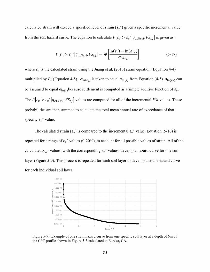
85

calculated strain will exceed a specified level of strain (𝜀𝜀𝑣𝑣∗) given a specific incremental value

from the FSL hazard curve. The equation to calculate 𝑃𝑃�𝜀𝜀𝑣𝑣� > 𝜀𝜀𝑣𝑣∗�𝑞𝑞𝑐𝑐1𝑁𝑁𝑐𝑐𝑠𝑠𝑖𝑖,𝐹𝐹𝐹𝐹𝐿𝐿𝑗𝑗� is given as:

where 𝜀𝜀�̅�𝑣 is the calculated strain using the Juang et al. (2013) strain equation (Equation 4-4)

multiplied by PL (Equation 4-5), 𝜎𝜎ln (𝜀𝜀𝑣𝑣) is taken to equal 𝜎𝜎ln (𝑠𝑠) from Equation (4-5). 𝜎𝜎ln (𝜀𝜀𝑣𝑣) can

be assumed to equal 𝜎𝜎ln (𝑠𝑠)because settlement is computed as a simple additive function of 𝜀𝜀𝑣𝑣.

The 𝑃𝑃�𝜀𝜀𝑣𝑣 > 𝜀𝜀𝑣𝑣∗�𝑞𝑞𝑐𝑐1𝑁𝑁𝑐𝑐𝑠𝑠𝑖𝑖 ,𝐹𝐹𝐹𝐹𝐿𝐿𝑗𝑗� values are computed for all of the incremental FSL values. These

probabilities are then summed to calculate the total mean annual rate of exceedance of that

specific 𝜀𝜀𝑣𝑣∗ value.

The calculated strain (𝜀𝜀�̅�𝑣) is compared to the incremental 𝜀𝜀𝑣𝑣∗ value. Equation (5-16) is

repeated for a range of 𝜀𝜀𝑣𝑣∗ values (0-20%), to account for all possible values of strain. All of the

calculated 𝜆𝜆𝜀𝜀𝑣𝑣∗ values, with the corresponding 𝜀𝜀𝑣𝑣∗ values, develop a hazard curve for one soil

layer (Figure 5-9). This process is repeated for each soil layer to develop a strain hazard curve

for each individual soil layer.

𝑃𝑃�𝜀𝜀𝑣𝑣� > 𝜀𝜀𝑣𝑣∗�𝑞𝑞𝑐𝑐1𝑁𝑁𝑐𝑐𝑠𝑠𝑖𝑖,𝐹𝐹𝐹𝐹𝐿𝐿𝑗𝑗� = 𝛷𝛷 �ln(𝜀𝜀�̅�𝑣) − ln(𝜀𝜀∗𝑣𝑣)

𝜎𝜎ln (𝜀𝜀𝑣𝑣)� (5-17)

Figure 5-9: Example of one strain hazard curve from one specific soil layer at a depth of 6m of the CPT profile shown in Figure 5-3 calculated at Eureka, CA.

86

After strain hazard curves are developed for each soil layer, settlement is calculated. A

hazard curve of total ground surface settlement is developed, by using each strain hazard curve

from each layer. This calculation is done by using equation (4-3), from the Juang et al. (2013)

procedure:

where εv is a strain value is obtained from each strain hazard curve at the return period of interest

from every soil layer. The strains from each soil layer are summed together and multiplied by the

layer thickness to calculate ground surface settlement. This process is repeated for a range of

mean annual rate of exceedances, corresponding to return periods from 475 years to 10,000

years, to develop a total settlement hazard curve (Figure 5-10).

𝐹𝐹𝑝𝑝 = 𝑀𝑀�𝜀𝜀𝑣𝑣∆𝑍𝑍𝑖𝑖

𝑁𝑁

𝑖𝑖=1

(5-18)

Figure 5-10: Example of a total ground settlement hazard curve using the CPT profile shown in Figure 5-3 calculated at Eureka, CA.

87

The PBEE settlement calculation has a higher level of accuracy and consistency than

conventional methods due to its fully-probabilistic nature, and is presented in a more robust

format than traditional methods. The PBEE calculation methods take into account all possible

earthquake scenarios and all uncertainty attributed to predicting liquefaction triggering and

uncertainty in predicting volumetric strain. In addition, by presenting settlement as a hazard

curve rather than a single value, engineers confidently design for a level of post-liquefaction that

is consistent with a targeted settlement to expect for a specific return period or level of hazard.

Settlement hazard curves are very useful for an engineer to decide how much settlement a

structure should be designed for, depending on structural importance. PBEE settlement results

from this study are presented in chapter 6.

A PBEE settlement analysis is performed for the Salt Lake City, UT site. The analysis is

performed using CPTLiquefy (see Section 5.3), an analysis tool. The analysis computed FSL and

strain hazard curves for each soil layer, just as the hazard curves presented in Figures 5-8 and 5-

9. The FSL, corresponding to the 2475 year return period, can be obtained from each layer’s

hazard curve and plotted with depth. This process is done for this example and is plotted in

Figure 5-11.

Figure 5-11: Fully-probabilistic FSL values plotted across depth for the 2475 year return period at the Salt Lake City, UT site.

88

A strain hazard curve is computed for each individual soil layer using the procedure

discussed in this section above. For this specific profile (Figure 5-3) a CPT reading was taken

every 0.1m and, therefore, a strain hazard curve is computed every 0.1m from 0m to 12m,

creating a total of 120 strain hazard curves. (Figure 5-12) depicts a few of these hazard curves at

a range of depths. The performance-based procedure also allows strain to be plotted by depth for

varying return periods (Figure 5-13).

Figure 5-12: Strain hazard curves at the Salt Lake City Site at a range of depths.

89

These strain hazard curves are used to calculate a ground surface settlement hazard curve.

The calculated ground surface settlement hazard curve, calculated using the process described

above, for this example is plotted in Figure 5-14. The dotted grey line corresponds to a return

period of 2475 years, at which the calculated settlement is about 42.5cm.

Figure 5-14: Salt Lake City, UT example calculated fully-probabilistic settlement estimation hazard curve.

Figure 5-13: Strain across depth for the 475, 1189, and 2475 year return periods at the Salt Lake City Site.

90

5.2.4 Semi-Probabilistic Approach

Semi-probabilistic methods calculate FSL using the fully probabilistic methods, described

in section 5.2.3, and applies this FSL to deterministic settlement calculations. This method

accounts for the inherent uncertainty in predicting liquefaction triggering and correctly computes

the return period of soil liquefaction. However, this method fails to account for the uncertainty in

calculating post-liquefaction settlement.

For the Salt Lake City example, the calculated FSL values (Figure 5-11) for the 2475 year

return period, are applied to the deterministic Ishihara and Yoshimine (1992) settlement

estimation procedure. These FSL values are obtained by selecting each FSL value that

corresponds to a 2475 return period from each FSL hazard curve. The calculated strain values,

calculated using the probabilistic FSL values, are multiplied by their respective layer thicknesses

and summed together to calculate ground surface settlement. The calculated semi-probabilistic

post-liquefaction settlement, for the 2475 year return period, is about 34cm.

5.3 CPTLiquefY

To simplify PBEE (i.e., fully-probabilistic) procedures, the creation of tools to run such

analyses is a very important step. Many practicing engineers simply do not have the

understanding of, or the time to delve into, probability theory. The creation of tools can simplify

the probabilistic design process by offering engineers a tool to run such calculations.

CPTLiquefY is an analysis tool which was created for the purpose of the analyses in this

study and future research projects. CPTLiquefY was created by Mikayla Hatch, Tyler Coutu, and

Alex Arndt under the direction of Dr. Kevin Franke at Brigham Young University. This program

was created within Microsoft Visual Studio using C++. CPTLiquefY has the capability to load a

91

CPT profile and run deterministic, pseudo-probabilistic, semi-probabilistic, and full-probabilistic

PBEE calculations for liquefaction triggering, post-liquefaction settlements, and lateral

spreading. A tutorial on how to run these analyses, with CPTLiquefY, can be found in Appendix

A.

As previously mentioned, this research is the first step to facilitate the creation of

simplified probabilistic design tools, which engineers can instantly implement. Future research

research will create settlement hazard maps, as done in previous PBEE studies for the SPT

(Franke et al. 2014). Hazard maps will be developed by using the newly developed procedure for

the CPT and CPTLiquefY. Hazard maps will depict contours of expected liquefaction-induced

settlements, for specific locations, with a reference soil profile. See Ulmer (2015) and Ekstrom

(2015) for more explanation on the development of liquefaction hazard maps and the benefit they

provide to probabilistic design.

5.4 Chapter Summary

Earthquake engineers strive to design a structure at or above an estimated seismic event.

There is a high level of uncertainty in determining the most likely earthquake event to occur at a

site, making earthquake engineering design very difficult. Historically engineers used a DSHA,

where design utilized the ground motions from the closest and most significant fault to the

specified site. However, DSHA neglects the seismic hazard contribution of all other seismic

sources near the fault and neglects the likelihood of the occurrence of the governing scenario

earthquake. To address these issues, the PSHA was developed. PSHA takes into account all of

the uncertainties relating to the size, location, and rate of occurrence of a seismic event by

quantifying the likelihoods of each event actually occurring.

92

The PBEE method was advanced and refined by the PEER. The PEER PBEE framework

seeks to improve risk decision-making through assessment and design methods that are more

transparent, scientific, and informative to stakeholders than current prescriptive methods

(Deierlein et al., 2003). The PEER framework facilitates crucial communication between

stakeholders by presenting the risk and performance in a format each stakeholder can relate to.

This chapter presented a new PBEE (i.e., fully-probabilistic) post-liquefaction settlement

estimation procedure for the CPT. An analysis tool called CPTLiquefY was developed to perform

these calculations.

It is not generally fully understood how the different ways of characterizing probabilistic

ground motions in a post-liquefaction settlement analysis (i.e., pseudo-probabilistic, semi-

probabilistic, and PBEE) effect the prediction of settlement. To address this lack of

understanding, this research will now perform a comparative study between these different

approaches. This comparative study will be presented and discussed in Chapter 6.

93

6 COMPARISON OF PERFORMANCE-BASED, PSEUDO-PROBABILISTIC, AND

SEMI-PROBABILISTIC APPROACHES TO SETTLEMENT ANALYSIS

This study focuses on the quantified comparison of the difference in settlement calculations

of the pseudo-probabilistic, semi-probabilistic, and PBEE (i.e., fully-probabilistic) methods.

Post-liquefaction settlement estimations are calculated for each of the approaches, for multiple

CPT profiles at multiple sites, and compared. The insufficiencies of conventional methods have

been highlighted in this study, by comparing conventional methods to the PBEE approach. These

results prove the need for a transition to fully-probabilistic design practices.

6.1 Methodology

To perform a thorough comparison of design methods, a comprehensive range of various

soil conditions and site seismicity level needs to be considered. The methods to create a thorough

comparative study are discussed below.

94

6.1.1 Soil Profiles

20 actual CPT soundings are selected, containing a comprehensive range of soil stiffness

and type. These CPT soundings are collected from the United States Geologic Survey (USGS)

database of CPT data (https://earthquake.usgs.gov/research/cpt/data/table/). The CPT profiles are

selected with the intention to have a thorough range of soil type and relative density/stiffness.

This range in relative density/stiffness is evident by investigating the plot of corrected cone tip

resistance (Qtncs) shown in Figure 6-1. Note the lack of “holes” (i.e., white space) in Figure 6-1.

Figure 6-1: Stiffness of CPT profiles plotted at depth.

95

Figure 6-1 shows how the chosen profiles adequately cover all potentially impactful Qtncs,

or stiffness, values across the depth. Only a few profiles are found with a Qtncs value less than

50kPa, because there are very few soils that exist naturally that are soft enough to have such a

low value of Qtncs. Also, any soil with a Qtncs value greater than 250kPa is automatically

considered too dense to liquefy per the liquefaction triggering databases of Boulanger and Idriss

(2014) and Robertson and Wride (1998). Therefore, it is not imperative to collect comprehensive

Qtncs data greater than 250kPa. All collect profiles are summarized in Table 6-1.

To accurately demonstrate the differences between design methods, independent

variables such as total depth and water table depth are standardized. Each sounding had a

different bottom depth. For this study, all profiles are truncated to 12m. This depth is chosen

because the vast majority of liquefaction triggering case histories correspond to depths less than

12 meters (Boulanger et al., 2012). The depth of the water table can have a considerable impact

on the about of liquefiable soil layers. For liquefaction to occur soils have to be saturated,

Table 6-1: Summary of Soil Profiles

96

therefore any soils above the water table cannot liquefy. For this study, the water table is

assumed to be at the ground surface. Finally, none of the CPT profiles from the USGS database

contained a cone pore water pressure reading. For this study, the cone pore water pressure is

assumed to be zero for each soil layer. Although altering the water table depth and assuming zero

for the cone pore water pressure reading will alter the Qtn,cs values from what they actually are in

the field, the purpose of this study is to compare the calculations from different design methods.

These changes would be problematic if the purpose was to accurately predict liquefaction effects

at a specific site. Because the purpose of this study is to simply compare calculation approaches,

the specific CPT used in the study are irrelevant as long as they are consistent for the various

approaches being tested. Therefore, these assumptions do not affect the accuracy or validity of

this comparative study’s results.

6.1.2 Site Locations

To address the potential variable levels of seismicity a site could have, ten different cities

are examined in this study. Each city is chosen to represent a different level of seismicity and in

part because they have been used in other PBEE studies (Kramer and Mayfield 2007, Franke et

al. 2014). The chosen cities are distributed as such: 4 on the west coast near the San Andreas

Fault, 2 in the pacific north-west near the Cascadia Subduction zone and associated faults, 2 near

the Wasatch fault and rocky mountain region, 1 near the New Madrid fault system, and 1 near

the Charleston liquefaction features. A map of the cities are shown in Figure 6-2.

97

Recently, USGS has released a new version of its seismic source model. This release

provides several updates to probabilistic earthquake hazard calculation for the conterminous

United States (Peterson et. al. 2015). The 2014 model has now replaced the 2008 USGS seismic

source model as the most current version of the USGS National Seismic Hazard Mapping Project

(NSHMP). This study utilizes the 2014 USGS model. This model is used to obtain the

earthquake magnitude (mean and modal) and maximum acceleration (amax) at each location.

These values are presented in Table 6-2 for two return periods (475 year and 2475 year). The

amax values presented are calculated from the PGA using site amplification factors for AASHTO

site class D. The values of amax seen below were applied to the conventional pseudo-probabilistic

analysis to represent the relative ground acceleration expected to possibly occur at each location.

Figure 6-2: Map of all ten cities in this study.

98

6.1.3 Return Periods

Every structure is designed for a different level of earthquake depending on either the

importance of that structure (e.g., hospitals, fire stations, etc.) or the level of negative impact

resulting from structural failure (e.g., nuclear facilities, football stadiums, etc.). Less critical

structures are designed for seismic events with shorter return periods, in other words smaller

seismic events. While more critical structures are designed for higher return periods. This study

focuses on return periods 475 years, 1039 years, and 2475 years, which correspond to

probabilities of exceedance of 10% in 50 years, 7% in 75 years, and 2% in 50 years, respectively.

These return periods represent relatively low, medium, and high levels of seismic loading,

respectively.

6.2 Results and Discussion

This section presents the complete results from this study. As previously explained, all

calculations are performed by applying a PBEE procedure to the Ishihara and Yoshimine (1992)

Table 6-2: Magnitude (Mean and Modal) and Acceleration Values (USGS 2014), Using Site Amplification Factors for AASHTO Site Class D, Corresponding to TR= 475

years and TR=2475 years for each Site

99

strain method, by using the Robertson and Wride (2009) and Boulanger and Idriss (2014)

methods for the required FSL inputs. The results are organized by city for each of the separate

methods used. A discussion of the trends, patterns, and findings from these results is presented

after the results sections. The results of the comparative analysis of the different hazard analyses

and the sensitivity analysis of settlement correction factors, are also presented and discussed

below.

6.2.1 Robertson and Wride (2009) Results

Tables 6-3 through 6-12 display all calculated results for the Robertson and Wride (2009)

triggering procedure. These tables contain results for the fully-probabilistic, pseudo-probabilistic

(both mean and modal magnitude), and semi-probabilistic methods for the 475 year, 1039 year,

and 2475 year return periods. All settlement values are presented in centimeters.

Table 6-3: Butte, MT Settlement (cm) Calculated with Robertson and Wride Method

100

Table 6-4: Eureka, CA Settlement (cm) Calculated with Robertson and Wride Method

Table 6-5: Santa Monica, CA Settlement (cm) Calculated with Robertson and Wride Method

101

Table 6-6: Portland, OR Settlement (cm) Calculated with Robertson and Wride Method

Table 6-7: Salt Lake City, UT Settlement (cm) Calculated with Robertson and Wride Method

102

Table 6-8: San Francisco, CA Settlement (cm) Calculated with Robertson and Wride Method

Table 6-9: San Jose, CA Settlement (cm) Calculated with Robertson and Wride Method

103

Table 6-10: Seattle, WA Settlement (cm) Calculated with Robertson and Wride Method

Table 6-11: Memphis, TN Settlement (cm) Calculated with Robertson and Wride Method

104

6.2.2 Boulanger and Idriss (2014) Results

Tables 6-13 through 6-22 display all calculated results for the Boulanger and Idriss

(2014) triggering procedure. These tables contain results for the full-probabilistic, pseudo-

probabilistic (both mean and modal magnitude), and semi-probabilistic methods for the 475 year,

1039 year, and 2475 year return periods. All settlement values are presented in centimeters.

Table 6-12: Charleston, SC Settlement (cm) Calculated with Robertson and Wride Method

105

Table 6-13: Butte, MT Settlement (cm) Calculated with Boulanger and Idriss Method

Table 6-14: Eureka, CA Settlement (cm) Calculated with Boulanger and Idriss Method

106

Table 6-15: Santa Monica, CA Settlement (cm) Calculated with Boulanger and Idriss Method

Table 6-16: Portland, OR Settlement (cm) Calculated with Boulanger and Idriss Method

107

Table 6-18: Salt Lake City, UT Settlement (cm) Calculated with Boulanger and Idriss Method

Table 6-17: San Francisco, CA Settlement (cm) Calculated with Boulanger and Idriss Method

108

Table 6-19: San Jose, CA Settlement (cm) Calculated with Boulanger and Idriss Method

Table 6-20: Seattle, WA Settlement (cm) Calculated with Boulanger and Idriss Method

109

Table 6-21: Memphis, TN Settlement (cm) Calculated with Boulanger and Idriss Method

Table 6-22: Charleston, SC Settlement (cm) Calculated with Boulanger and Idriss Method

110

6.2.3 Comparison Analysis of Pseudo-Probabilistic, Semi-Probabilistic, and Performance-

Based Methods

From the data above, and by comparing the pseudo-probabilistic and PBEE (i.e., fully-

probabilistic) methods, several trends are identified from the data. First, in areas of low

seismicity the pseudo-probabilistic methods calculated about 10-50% higher settlement values

than the PBEE method. This relationship is logical because the pseudo-probabilistic method does

not take into account the low probability of large earthquakes occurring. However, with higher

return periods, the PBEE method predicted about 5-50% more settlement than pseudo-

probabilistic procedures. Second, in areas of medium to high seismicity the pseudo-probabilistic

method predicts similar settlement values to the full-probabilistic method for lower return

periods, but about 30-100% less settlement values at higher return periods. The higher the return

period and the seismicity of a city, the more the pseudo-probabilistic method under-predicts

settlements. Observations support those found in a similar PBEE liquefaction-induced settlement

study for the SPT (B. D. Peterson, 2016). Finally, by comparing the liquefaction triggering

methods, both methods generally calculate similar settlement values, but the Boulanger and

Idriss method proves to be more conservative than the Robertson and Wride method.

A comparative study is also performed for the semi-probabilistic settlement approach and

the PBEE settlement approach. Similar trends observed from the pseudo-probabilistic

comparative study are observed from the semi-probabilistic approach. However, at the higher

return periods, the semi-probabilistic approach tends to under-predict settlements marginally

more than the pseudo-probabilistic approach. Also, across all return periods, the data scatter for

the semi-probabilistic approach is tighter than the pseudo-probabilistic results. This trend

111

indicates a slightly higher level of consistency and efficiency as compared to the pseudo-

probabilistic approach.

To see these trends visually, comparison plots are created to compare the pseudo-

probabilistic and semi-probabilistic results to the full-probabilistic results. These plots are

presented in Figures 6-3 through 6-20. The solid black line represents the one-to-one line (i.e., a

perfect match between the two approaches), and the data from each liquefaction triggering

method is plotted on separate plots. Best-fit linear regression lines are plotted on each plot. If the

pseudo-probabilistic or semi-probabilistic methods correlated perfectly with the PBEE methods

the data would fall directly on the 1 to 1 line. However, a data trend line that falls above the 1 to

1 line indicates an over-prediction of settlement by the pseudo-probabilistic and semi-

probabilistic methods and, conversely, when the data trend line plots below the 1 to 1 line

pseudo-probabilistic and semi-probabilistic methods are under predicting settlement.

Figure 6-3: Idriss and Boulanger (2014) mean pseudo-probabilistic method compared to the PBEE procedure for the 475 year return period.

112

Figure 6-4: Idriss and Boulanger (2014) mean pseudo-probabilistic method compared to the PBEE procedure for the 1039 year return period.

Figure 6-5: Idriss and Boulanger (2014) mean pseudo-probabilistic method compared to the PBEE procedure for the 2475 year return period.

113

Figure 6-7: Idriss and Boulanger (2014) modal pseudo-probabilistic method compared to the PBEE procedure for the 1039 year return period.

Figure 6-6: Idriss and Boulanger (2014) modal pseudo-probabilistic method compared to the PBEE procedure for the 475 year return period.

114

Figure 6-8: Idriss and Boulanger (2014) modal pseudo-probabilistic method compared to the PBEE procedure for the 2475 year return period.

Figure 6-9: Idriss and Boulanger (2014) semi-probabilistic method compared to the PBEE procedure for the 475 year return period.

115

Figure 6-11: Idriss and Boulanger (2014) semi-probabilistic method compared to the PBEE procedure for the 2475 year return period

Figure 6-10: Idriss and Boulanger (2014) semi-probabilistic method compared to the PBEE procedure for the 1039 year return period

116

Figure 6-12: Robertson and Wride (2009) mean pseudo-probabilistic method compared to the PBEE procedure for the 475 year return period.

Figure 6-13: Robertson and Wride (2009) mean pseudo-probabilistic method compared to the PBEE procedure for the 1039 year return period.

117

Figure 6-14: Robertson and Wride (2009) mean pseudo-probabilistic method compared to the PBEE procedure for the 2475 year return period.

Figure 6-15: Robertson and Wride (2009) modal pseudo-probabilistic method compared to the PBEE procedure for the 475 year return period.

118

Figure 6-16: Robertson and Wride (2009) modal pseudo-probabilistic method compared to the PBEE procedure for the 1039 year return period.

Figure 6-17: Robertson and Wride (2009) modal pseudo-probabilistic method compared to the PBEE procedure for the 2475 year return period.

119

Figure 6-18: Robertson and Wride (2009) semi-probabilistic method compared to the PBEE procedure for the 475 year return period.

Figure 6-19: Robertson and Wride (2009) semi-probabilistic method compared to the PBEE procedure for the 1039 year return period.

120

The data trend lines tend to correlate with the one-to-one line fairly well up to a certain

level of settlement for each return period when comparing the PBEE approach to the pseudo-

probabilistic (mean magnitude) approach. The Robertson and Wride (2009) data, from the two

settlement approaches, tend to match up well until about 20cm, 15cm, and 10cm of settlement

for the 475 year, 1039 year, and 2475 year return periods, respectively. While the Boulanger and

Idriss (2014) data, from the two settlement approaches, tend to line up fairly well until about

10cm, 5cm, and 3cm for the 475 year, 1039 year, and 2475 year return periods, respectively. The

modal magnitude pseudo-probabilistic approach follows similar trends, but digress from the one-

to-one line at lower values. The Robertson and Wride (2009) modal magnitude pseudo-

probabilistic data lines up with the PBEE data fairly well until about 13cm, 10cm, and 6cm for

the 475 year, 1039 year, and 2475 year return periods, respectively. While the Boulanger and

Figure 6-20: Robertson and Wride (2009) semi-probabilistic method compared to the PBEE procedure for the 2475 year return period.

121

Idriss (2014) data averages line up fairly well until about 8cm, 6cm, and 5cm for the 475 year,

1039 year, and 2475 year return periods, respectively.

To further examine the source of the trends mentioned above, the settlement values

computed from pseudo and semi-probabilistic methods, for the 1039 year and 2475 year return

periods, were entered into the probabilistic hazard curve to back-calculate the actual return

period associated with that settlement value. The results of this process are presented in

Appendix B (Figures B-1 through B-20), but summarized as box and whisker plots in Figures 6-

21 through 6-24.

Figure 6-21: Box and whisker plots of actual return periods versus assumed 1039 year return period for the Idriss and Boulanger (2014) Triggering Method.

122

Figure 6-22: Box and whisker plots of actual return periods versus assumed 2475 year return period for the Idriss and Boulanger (2014) Triggering Method.

Figure 6-23: Box and whisker plots of actual return periods versus assumed 1039 year return period for the Robertson and Wride (2009) Triggering Method.

123

The box and whisker plots shown in Figures 6-21 through 6-24 illustrate the median, first

and third quartiles, maximum and minimum values, and the average (marked by an “x”) values

of the return periods presented in the tables in Appendix B. As noted previously, these values

represent actual return periods because they are generated from the fully-probabilistic settlement

hazard curve. The assumed return period is presented as a red dashed line for reference.

The results for the 1039 return period (Figures 6-21 and 6-23) box plots seem to match

the results from Figures 6-3 through 6-20 fairly well. The one-to-one plots and the box and

whisker plots both indicated a fairly good match between approaches for the 1039 return period.

The Idriss and Boulanger (2014) results for the 2475 return period (Figure 6-22) also line up with

the results from the one-to-one plots, by indicating an under-prediction of post-liquefaction

Figure 6-24: Box and whisker plots of actual return periods versus assumed 2475 year return period for the Robertson and Wride (2009) Triggering Method.

124

settlements from conventional standards. The data suggests that 100% of the Idriss and

Boulanger (2014) settlement calculations (using conventional methods) under predicted

settlement compared to the PBEE settlement values.

The Robertson and Wride (2009) method also follows similar trends by under-predicting

settlement more as the return period is increased. However, this method did not under predict

settlements as much because it generated nearly vertical hazard curves for the stiffer soil profiles.

For example, one of the hazard curves had 0.3cm of settlement at the 475 return period and only

increased to 0.99cm of settlement by the 10,000 year return period. The steep slope of the hazard

curve caused a back calculation of extremely high return periods. For example, if the pseudo-

probabilistic methods produced 0.9cm of settlement, it would correlate to a return period of

9,500 years. The Robertson and Wride (2009) triggering method tended to produce these nearly

vertical hazard curves for the stiffer soil profiles. However, for the more-liquefiable profiles, the

Robertson and Wride (2009) method under-predicted settlement up to 84%. It was the steep

hazard curves that caused the spikes in actual return periods calculated in the Robertson and

Wride (2009) box and whisker plots (Figures 6-23 and 6-24). The Idriss and Boulanger (2014)

procedure did not result in any of these steep hazard curves. This discrepancy is likely due to the

different methods used to calculate the CRR. The data is suggesting that the Idriss and

Boulanger (2014) procedure is conservatively indicating these stiffer soil profiles are more

liquefiable than the Robertson and Wride (2009) indicates they are.

To examine the comparison, between conventional methods and the PBEE method, even

further a heat map was generated (Figure 6-25). Each number in the map represents the number

of CPT soundings, out of the total 20, in which the pseudo-probabilistic approach predicted less

settlement than the PBEE approach. These values are presented for both triggering procedures,

125

each return period, and both magnitudes (mean and modal) at each city. The cities are ordered

from the lowest amax values to the highest from top down.

The heat map reinforces the trends observed above. The heat map illustrates that the

Idriss and Boulanger (2014) triggering procedure is under predicting settlement at a higher

percentage than the Robertson and Wride (2009) method. This trend can also demonstrate how

the Idriss and Boulanger (2014) method produces larger PBEE settlement values than the

Robertson and Wride (2009) method. The heat map reinforces the trend indicating that the under

prediction of settlement increases with an increasing level of site seismicity and return period.

The Robertson and Wride (2009) has on about 50% of the soundings under predicting settlement

at the 2475 year return period. While the Idriss and Boulanger (2014) procedure under predicted

settlements for almost 90% of the CPT soundings at the 2475 return period.

The heat map points out 3 outliers at Butte, MT for the modal magnitude pseudo-

probabilistic values where all 20 profiles under predicted settlement for all three return periods.

Figure 6-25: A heat map representing the number of CPT soundings, out of 20 soundings, in which the pseudo-probabilistic method under predicted settlement compared to the PBEE procedure.

126

This discrepancy is likely due to a large difference in the MSF due to a significant difference in

the mean and modal magnitudes at Butte, MT (Table 6-2). This discrepancy does not manifest in

the Idriss and Boulanger (2014) procedure because of the differing MSF calculation methods

(Equations 3-12 and 3-23). The Boulanger and Idriss (2014) procedure does depend solely on the

magnitude to calculate the MSF like the Robertson and Wride (2009) method.

The results for the 475 return period at lower seismic areas are not surprising. At the 475

year return period pseudo-probabilistic method generally over-predicted or the methods

predicted similar settlement values. This trend is logical because the pseudo-probabilistic

procedure uses a deterministic method of predicting settlements. Deterministic methods are

considered to be a conservative approach because it generally designs for the controlling

scenario earthquake.

However, this idea is concerning after reviewing the results from the higher return

periods. The data suggests, as the return period increased, the pseudo-probabilistic analyses

under-predicted the level of liquefaction-induced settlement hazard by up to 90%. This trend is

likely caused by the fact that the pseudo-probabilistic and semi-probabilistic methods compute

post-liquefaction volumetric strains deterministically. Deterministic strain calculations ignore the

inherent uncertainty associated with calculating strain values. The PBEE procedure, however,

accounts for this uncertainty, resulting in higher settlement estimations.

Results from the semi-probabilistic approach had less scatter but underestimated

settlements at about the same percentage as the pseudo-probabilistic approach. The trends

depicted in the semi-probabilistic results are very similar to the trends from the pseudo-

probabilistic results. These similarities in the two method’s results suggests the uncertainty in the

liquefaction triggering is less significant than the uncertainty in the strain calculations. These

127

results also prove the semi-probabilistic method is not an improvement to the current pseudo-

probabilistic methods. Significant calculations are required to perform the calculations necessary

for the semi-probabilistic approach and, therefore, may not be worth it for engineers to use this

approach as a replacement to the pseudo-probabilistic approach. Engineers should either stick

with the easier and equally accurate pseudo-probabilistic approach, or go all the way to the

PBEE approach for more accuracy.

By comparing the results a comparison can be made between the Robertson and Wride

(2009) and Boulanger and Idriss (2014) triggering methods. The two methods consistently

predicted similar PBEE settlements for the varying CPT soundings and cities. However, the

Boulanger and Idriss procedure consistently produced larger settlement values. This trend

indicates the Boulanger and Idriss method is a more conservative option than the Robertson and

Wride method.

6.2.4 Discussion

Pseudo-probabilistic methods are widely accepted in industry because they are

considered to be a simple way to incorporate probabilistic ground motions into the liquefaction

analysis and are often considered as a conservative design practice. If, in fact, these methods are

under-predicting liquefaction-induced settlements, then relying on pseudo-probabilistic methods

for design presents a dangerous risk. Engineers could be severely under predicting post-

liquefaction settlements while believing their designs are conservatively over predicting

settlement. This data suggests that pseudo-probabilistic design methods are a good option for

areas of lower seismicity and lower return periods. However, according to this data, fully-

128

probabilistic methods should be used for regions of higher seismicity and when designing for

medium to large seismic events.

It is these larger seismic events that are the most concerning to the financial and physical

well-being of a region, because these events are capable of causing the most damaging and

hazardous events. If engineered structures, for these high return period events, are designed for

pseudo-probabilistic settlements it is likely they will be under-designed. These structures will be

especially under designed if located in high seismic regions. This level of under prediction of

settlement will likely lead to a large economic toll, should a seismic event occur.

It is important to note the scope limitations for this study. This study only focused on

settlement and only one settlement estimation method (Ishihara and Yoshimine, 1992). Only two

triggering methods (Robertson and Wride, 2009; Boulanger and Idriss, 2014) were applied to

this settlement method. To confirm the results of this study, research should be performed to

examine other seismic effects (e.g., lateral spread, bearing capacity, slope stability, etc.).

6.2.5 Correction Factor Sensitivity Analysis

In addition to the comparative study, a sensitivity analysis is performed. Four separate

PBEE settlement calculations are performed for each city and CPT sounding to test the

sensitivity of the PBEE procedure to the CPT correction factors presented in sections 4.3.2

through 4.3.4. These four calculations included a series termed the baseline (i.e., no corrections

applied), a series with the depth weighting factor (Section 4.3.2), a series with the combined

transition zone and thin layer correction (Sections 4.3.3 & 4.3.4), and a series with the transition

zone, thin layer, and depth weighting factor corrections applied. All 20 soil profiles are analyzed

for all cities and all three return periods for each of these series.

129

The resulting data is combined and is presented in box and whisker plots below (Figures

6-26 through 6-28). To create these box and whisker plots, a ratio (R) is created, which is

presented as:

where 𝐹𝐹𝑑𝑑𝑐𝑐𝑐𝑐𝑙𝑙𝑑𝑑𝑑𝑑𝑑𝑑𝑑𝑑𝑐𝑐𝐹𝐹𝑟𝑟𝑟𝑟𝑖𝑖𝑟𝑟𝑠𝑠 represents the calculated PBEE settlement from one of the correction

factor series described above and 𝐹𝐹𝑑𝑑𝑐𝑐𝑐𝑐𝑙𝑙𝑑𝑑𝑑𝑑𝑑𝑑𝑑𝑑𝑐𝑐𝐵𝐵𝑚𝑚𝑠𝑠𝑟𝑟𝑙𝑙𝑖𝑖𝑛𝑛𝑟𝑟 represents the calculated PBEE settlement

from the baseline series. This means that if R is equal to 1, the specific correction factor had no

impact on the settlement calculation. Therefore, the further away R is from 1, the more sensitive

the probabilistic procedure is to that particular option.

𝐶𝐶 =𝐹𝐹𝑑𝑑𝑐𝑐𝑐𝑐𝑙𝑙𝑑𝑑𝑑𝑑𝑑𝑑𝑑𝑑𝑐𝑐𝐹𝐹𝑟𝑟𝑟𝑟𝑖𝑖𝑟𝑟𝑠𝑠𝐹𝐹𝑑𝑑𝑐𝑐𝑐𝑐𝑙𝑙𝑑𝑑𝑑𝑑𝑑𝑑𝑑𝑑𝑐𝑐𝐵𝐵𝑚𝑚𝑠𝑠𝑟𝑟𝑙𝑙𝑖𝑖𝑛𝑛𝑟𝑟

(6-1)

Figure 6-26: Box and whisker plots for R at a return period of 475 years.

130

The box and whisker plots show the impact each correction factor has on the full-

probabilistic procedure. The box and whisker plots prove the importance and impact of

correction factors. Based on the plots it’s apparent the PBEE procedure is more sensitive to the

depth weighting factor than the thin layer and transition zone correction factor. However, the

Figure 6-27: Box and whisker plots for R at a return period of 1039 years.

Figure 6-28: Box and Whisker plots for R at a return period of 2475 years.

131

depth factor correction experienced a larger spread than the thin layer correction. It is logical that

the thin layer and transition zone correction had a smaller impact on the calculated settlement

values. For the thin layer correction to even be applied the soil profile needed to contain thin

sand layers interbedded within soft clay layers. A few of the 20 profiles did not have this criteria

and therefore did not experience any thin layer correction. However, because the depth

weighting factor is independent of soil type, the depth weighting factor was always applied.

The data suggests that return period does not affect the sensitivity significantly. Across all

three return periods, the median value and general trends are about the same. This is logical

because the degree of sensitivity is dependent on soil type for thin layer correction and the depth

factor correction will be constant because it is only dependent on depth. All of which are

constant for each settlement calculation. It appears that R seemed to range between 0.45 and 0.6

for 68% of the data (+/- 1σ) regardless of the triggering model or the return period.

6.3 Chapter Summary

The PBEE (i.e., fully-probabilistic) liquefaction-induced settlement estimation procedure,

presented in chapter 5, was tested using 20 different real CPT soundings, at 10 different seismic-

level cities, and for three return periods (e.g., 475 year, 1039 year, and 2475 year). These results

were compared to pseudo-probabilistic and semi-probabilistic values, calculated from the same

CPT profiles and locations. For low return periods, the pseudo-probabilistic settlement values

correlated fairly well with full-probabilistic settlement values. However, at higher return periods,

this correlation deteriorated and showed pseudo-probabilistic methods under-predicting

settlements significantly. The semi-probabilistic method followed similar trends to the pseudo-

probabilistic method. Engineers should either stick with the easier and equally accurate pseudo-

132

probabilistic approach, or go all the way to the PBEE approach for more accuracy. The PBEE

procedure was tested for its sensitivity to settlement correction factors. The PBEE procedure is

more sensitive to the weighted depth factor correction than to the thin layer correction. This

sensitivity remains pretty constant regardless of the triggering model or the return period.

133

7 SUMMARY AND CONCLUSIONS

Liquefaction is a phenomenon that occurs from cyclic loading from an earthquake.

Liquefaction occurs when a saturated soil is loaded cyclically, which cause it to densify.

Saturated soil densification causes the pore water to be squeezed out of the pore spaces,

generating excess pore water pressure. This excess pore water pressure causes the soil particles

to hydroplane on themselves resulting in zero effective stress, which is when liquefaction occurs.

Liquefaction can cause a many adverse effects, one of which is settlement. After a soil

has liquefied, and the excess pore water starts to dissipate, soil particles tend to settle into a

denser state, resulting in volumetric strains. These volumetric strains manifest themselves as

ground surface settlements. Liquefaction-induced settlements are not directly life threatening,

however they can cause extreme economic distress to an area because of the significant

infrastructural damage they cause.

To design seismic resilient structures and infrastructure, engineers need to be able to predict

seismic events, and their effects, accurately. Originally, engineers used a deterministic seismic

hazard analysis (DHSA) to predict seismic hazards, by designing for the controlling earthquake.

In the past 20 years engineers have relied on a pseudo-probabilistic seismic hazard analysis. This

method uses a probabilistic seismic hazard analysis (PSHA) to choose a design earthquake, but

134

computes the likelihood of liquefaction triggering, and its effects, using deterministic calculation

procedures.

Current research has found performance-based earthquake engineering (PBEE) procedures

produce more accurate and consistent hazard estimates than the current pseudo-probabilistic

methods (Kramer & Mayfield, 2007; Franke et al. 2014). The PBEE framework was proposed

by the Pacific Earthquake Engineering Research (PEER) Center. PBEE applies a fully-

probabilistic analysis into the prediction of seismic effects and presents these predictions in

terms of levels of hazard. PBEE is extremely advantageous for not only predicting liquefaction

and its effects, but also presenting these hazards in a way for all stakeholders to make more

informed decisions. This study proposes a PBEE, fully-probabilistic, procedure to estimate post-

liquefaction settlements for the CPT. This procedure incorporates the Ishihara and Yoshimine

(1992) settlement method, by inputting the liquefaction triggering Robertson and Wride (1998,

2009) and Boulanger and Idriss (2014) methods, into the PEER framework.

A seismic hazard analysis tool, called CPTLiquefY, was developed to perform the full-

probabilistic calculations. CPTLiquefY was developed within Microsoft Visual Studio, using

Visual C++. The tool was developed by Mikayla Hatch, Tyler Coutu, and Alex Arndt, under the

direction of Dr. Kevin Franke at Brigham Young University.

The calculated settlement values for the developed full-probabilistic procedure were

compared to conventional analyses for 20 CPT profiles and 10 cities of varying levels of

seismicity. It was observed that for a low return period, the pseudo-probabilistic settlement

values correlated fairly well with full-probabilistic settlement values. At these low return periods

and at cities of low seismicity the pseudo-probabilistic method over predicted settlements from

about 5-50%. However, at higher return periods and cities with medium to high seismicity this

135

correlation deteriorated and showed pseudo-probabilistic methods under-predicting settlements

significantly. In areas of high seismicity the pseudo-probabilistic procedure under predicted

settlements up to 100%. The semi-probabilistic method followed similar trends to the pseudo-

probabilistic method. These results suggest current design practices unintentionally ignore

considerable amounts of risk when estimating liquefaction-induced settlements for earthquakes

with higher return periods.

In addition to the comparative study, a sensitivity analysis was performed to test the effect of

settlement correction factors on the PBEE estimation procedure. This analysis was performed for

the thin layer correction and depth weighting factor correction. The results proved the fully-

probabilistic procedure was more sensitive to the depth weighting factor than the thin layer

correction. The study also proved the significance and importance of settlement calculation

correction factors.

136

REFERENCES

Abrahamson, N., & Silva, W. (2008). Summary of the Abrahamson & Silva NGA Ground-Motion Relations. Earthquake Spectra: February 2008, 24(1), 67-97.

Ahmadi, M. M., & Robertson, P. K. (2005). Thin-layer effects on the CPT qc measurement.

Canadian Geotechnical Journal, 42(5), 1302-1317. Algermissen, S. T., Perkins, D. M., Thenhaus, P. C., Hanson, S. L., & Bender, B. L. (1982).

Probabilistic estimates of maximum acceleration and velocity in rock in the contiguous United States. In U. S. G. Survey (Ed.), Open-File Report 82-1033 (pp. 99). Washington, D.C.

Ambraseys, N. N. (1988). Engineering Seismology (Vol. 17). Ancheta, T. D., Darragh, R. B., Stewart, J. P., Seyhan, E., Silva, W. J., Chiou, B. S.-J., . . .

Donahue, J. L. (2014). NGA-West2 Database. Earthquake Spectra:, 30(3), 989-1005. Arias, A. (1970). A measure of earthquake intensity. Seismic Design for Nuclear Power Plants,

438-483. Ben-Menachem, A. (1961). Radiation Patterns of seismic surface waves from finite moving

sources. Bulletin of the Seismological Society of America, 51, 401-435. Benioff, H. (1955). Mechanism and strain characteristics of the White Wolf fault as indicated by

the aftershock sequence: California Division of Mines, Bulletin 171. Benjamin, J. R., & Associates. (1988). A criterion for determining exceedance of the Operating

Basis Earthquake. In E. P. R. Institute (Ed.), EPRI Report NP-5930. Palo Alto, California.

Bolt, B. A. (1969). Duration of strong motion. Paper presented at the 4th World Conference on

Earthquake Engineering, Santiago, Chile.

137

Boore, D. M., & Atkinson, G. M. (2008). Ground-Motion Prediction Equations for the Average Horizontal Component of PGA, PGV, and 5%-Damped PSA at Special Periods between 0.01 s and 10.0 s. Earthquake Spectra: February 2008, 24(1), 99-138.

Boore, D. M., Joyner, W. B., & Fumal, T. E. (1993). Estimation of response spectra and peak

accelerations from western North America earthquakes: An interim report. In U. S. G. Survey (Ed.), Open-File-Report 93-509.

Boulanger, R., & Idriss, I. (2014). CPT and SPT based liquefaction triggering procedures. Center

for Geotechnical Modeling, Department of Civil and Environmental Engineering, University of California, Davis, CA. Report No. UCD/CGM-14/01.

Boulanger, R. W., & Idriss, I. M. (2005). New criteria for distinguishing between silts and clays

that are susceptible to liquefaction versus cyclic failure. Paper presented at the Technologies to Enhance Dam Safety and the Environment, 25th Annual United States Society on Dams, USSD, Denver.

Bray, J. D., & Dashti, S. (2014) Liquefaction -induced building movements. Vol. 3. Bulletin of

Earthquake Engineering (pp. 1129-1156). Cambell, K. W. (1981). Near source of peak horizontal acceleration. Bulletin of the

Seismological Society of America, 71, 2039-2070. Cambell, K. W., & Bozorgnia, Y. (1994). Near-source attenuation of peak acceleration from

worldwide accelerograms recorded from 1957 to 1993. Paper presented at the 5th U.S. National Conference on Earthquake Engineering, Earthquake Engineering Research Institute, Berkeley, California.

Cambell, K. W., & Bozorgnia, Y. (2008). NGA Ground Motion Model for the Geometric Mean

Horizontal Component of PGA, PGV, PGD, and 5% Damped Linear Elastic Response Spectra for Periods Ranging from 0.01 to 10 s. Earthquake Spectra: February 2008, 24(1), 139-171.

Casagrande, A. (1936). Characteristics of cohesionless soils affecting the stability of slopes and

earth fills. Journal of the Boston Society of Civil Engineers. Castro, G. (1969). Liquefaction of sands. Harvard Soil Mechanics Series 87. Cetin, K., Bilge, H., Wu, J., Kammerer, A., & Seed, R. (2009). Probabilistic Model for the

Assessment of Cyclically Induced Reconsolidation (Volumetric) Settlements. Journal of Geotechnical and Geoenvironmental Engineering, 3(135), 387-393.

Chiou, B. S.-J., & Youngs, R. R. (2008). A NGA Model for the Average Horizontal Component

of Peak Ground Motion and Response Spectra. Earthquake Spectra: February 2008, 24(1), 173-215.

138

Cornell. (1968). Engineering seismic risk analysis. Bulletin of the Seismological Society of America, 58, 1583-1606.

Cornell, C. A., & Krawinkler, H. (2000). Progress and challenges in seismic performance

assessment. PEER Center News, 3(2), 1-3. Dashti, S., Bray, J. D., Pestana, J. M., Riemer, M., & Wilson, D. (2010). Mechanisms of

Seismically Induced Settlement of Buildings with Shallow Foundations on Liquefiable Soil. Journal of Geotechnical and Geoenvironmental Engineering, 135(1).

Deierlein, G., Krawinkler, H., & Cornell, C. (2003). A framework for performance-based

earthquake engineering. Paper presented at the Pacific conference on earthquake engineering.

Dobry, R., & Vucetic, M. (1987). Dynamic properties and seismic response of soft clay deposits.

Paper presented at the International Symposium on Geotechnical Engineering of Soft Soils, Mexico City.

Elkstrom, L. T. (2015). A Simplified Performance-Based Procedure for the Prediction of Lateral

Spread Displacements. Franke, K. W., Wright, A. D., & Hatch, C. K. (2014). PBLiquefY: A New Analysis tool for the

performance-based evaluation of liquefaction triggering. Paper presented at the 10th National Conference on Earthquake Engineering.

Friedman, D. (2007). How to Detect, Diagnose, & Evaluate Earthquake Damage. from inspect-

ny.com G. Castro, S. J. P. (1977). Factors affecting liquefaction and cyclic loading. Journal of the

Geotechnical Engineering Division, 106(GT6), 501-506. Golesorkhi, R. (1989). Factors Influencing the Computational Determination of Earthquake-

Induced Shear Stress in Sandy Soils. (Ph.D.), University of California at Berkeley. Hanks, T. C., & Kanamori, H. (1979). A moment magnitude scale. Journal of Geophysical

Research, 84, 2348-2350. Hanzawa, H., Itoh, Y., & Suzuki, K. (1979). Shear characteristics of a quick sand in the Arabian

Gulf. SOILS AND FOUNDATIONS, 19(4), 1-15. Housner, G. W. (1959). Behavior of structures during earthquakes. Journal of the Engineering

Mechanics Division, 85(EM14), 109-129. Huang, Y. M. (2008). Performance-based design and evaluation for liquefaction-related seismic

hazards. (Ph.D. Dissertation), University of Washington, Seattle, WA.

139

Idriss, I. M. (2008). An NGA Empirical Model for Estimating the Horizontal Spectral Values Generated By Shallow Crustal Earthquakes. Earthquake Spectra: February 2008, 24(1), 217-242.

Idriss, I. M., & Boulanger, R. W. (2008). Soil Liquefaction During Earthquakes. Ishihara, K. (1984). Post-Earthquake Failure of Tailings Dam due to Liquefaction of the Pond

Deposit. Paper presented at the Int. Conference on Case Histories in Geotechnical Engineering, St. Louis, Missouri.

Ishihara, K. (1985). Stability of natural deposits during earthquakes. Paper presented at the 11th

International Conference on Soil Mechanics and Foundation Engineering. Ishihara, K., & Yoshimine, M. (1992). Evaluation of settlements in sand deposits following

liquefaction during earthquakes. SOILS AND FOUNDATIONS, 32(1), 173-188. doi: 10.3208/sandf1972.32.173

Iwasaki, T., Tokida, K., Tatsuka, F., Wantabe, S., Yasuda, S., & Sato, H. (1982). Miccrozonation

for soil liquefaction potential using the simplified methods. Paper presented at the 3rd International Conference on Microzonation, Seattle.

Jefferies, M. G., & Davies, M. P. (1993). Use of CPTU to estimate equivalent SPT N60.

Geotechnical Testing Journal, 16(4). Jennings, P. C. (1985). Ground motion parameters that influence structural damage. Berkeley,

California: Earthquake Engineering Institute. Jibson, R. (1987). Summary of research on the effects of topographic amplification of earthquake

shaking on slope stability Open-File Report 87-268. Melano Park, California: U.S. Geologic Survey.

Joyner, W. B., & Boore, D. M. (1988). Measurement, characterization, and prediction of strong

ground motion. Earthquake Engineering and Soil Dynamics II - Recent Advances in Ground-Motion Evaluation, 43-102.

Juang, C. H., Ching, J., Wang, L., Khoshnevisan, S., & Ku, C.-S. (2013). Simplified procedure

for estimation of liquefaction-induced settlement and site-specific probabilistic settlement exceedance curve using cone penetration test (CPT). Canadian Geotechnical Journal, 50(10), 1055-1066.

K. Been, M. G. J. (1985). A state parameter for sands. Geotechnique, 35(2), 99-112. Kanamori, H. (1977). The Energy Release in Great Earthquakes. Journal of Geophysical

Research, 82, 2981-2987.

140

Kanamori, H. (1983). Magnitude scale and quantification of earthquakes. Tectonophysics, 93, 185-199.

Kramer, S. L. (1996). Geotechnical Earthquake Engineering. Upper Saddle River, NJ: Prentice

Hall, Inc. Kramer, S. L. (2008). Evaluation of liquefaction hazards in Washington State WSDOT Report

WA-RD (Vol. 668.1, pp. 152). Kramer, S. L., & Mayfield, R. T. (2007). Return period of soil liquefaction. Journal of

Geotechnical and Geoenvironmental Engineering, 133(7), 802-813. Lade, P. V. (1992). Static instability and liquefaction of loose fine sandy slopes. Journal of

Geotechnical Engineering, 118(1), 51-71. Lee, K., & Albaisa, A. (1974). Earthquake induced settlements in saturated sands. Journal of

ASCE, 103(GT6), 565-588. Liao, S. S. C., & Whitman, R. V. (1986). Overburden Correction Factors for SPT in Sand.

Journal of Geotechnical Engineering, ASCE, 112(3). Middlebrooks, T. A. (1942). For Peck Slide. ASCE, 107, 723-764. Moehle, J., & Deierlein, G. G. (2004). A framework methodology for performance-based

earthquake engineering. Paper presented at the 13th World Conference on Earthquake Engineering, Vancouver B.C., Canada.

Mogami, T., & Kubo, K. (1953). The behaviour of soil during vibration. Proceedings, 3rd

International Conference on Soil Mechanics and Foundation Engineering, Zurich, 1. Mohamad, R., & Dobry, R. (1986). Undrained monotonic and cyclic triaxial strength of sand.

Journal of Geotechnical Engineering, 112(10), 941-958. Nadgouda, K. (2007). Earthquake in Japan. Geotechnical Engineering 101 and more. 2017, from

https://kshitija.wordpress.com/category/information/ Nagase, H., & Ishihara, K. (1988). Liquefaction-induced compaction and settlement of sand

during earthquakes. SOILS AND FOUNDATIONS, 28(1), 66-76. Peterson, B. D. (2016). Development of a Performance-Based Procedure for Assessment of

Liquefaction-Induced Free-Field Settlements. (Master of Science), Brigham Young University, Provo, UT.

Peterson, M. D., Moschetti, M. P., Powers, P. M., Mueller, C. S., Haller, C. M., Frankel, A. D.,

& Field, N. (2015). The 2014 United States national seismic hazard model. Earthquake Spectra, 31(S1).

141

Porter, K. A. (2003). An Overview of PEER's Performance-Based Earthquake Engineering

Methodology. Paper presented at the Ninth International Conference on Applications of Statistics and Probability in Civil Engineering.

Poulos, S. J. (1981). The steady state of deformation. Journal of Geotechnical Engineering

Division, 107(GT5), 553-562. Reiter, L. (1990). Earthquake Hazard Analysis - Issues and Insights. New York: Columbia

University Press. Richter, C. F. (1935). An instrumental earthquake scale. Bulletin of the Seismological Society of

America, 25, 1-32. Robertson, P. (2009). Performance based earthquake design using the CPT. Paper presented at

the Proceedings of IS-Tokyo 2009: international conference on performance-based design in earthquake geotechnical engineering—from case history to practice, Tokyo, Japan.

Robertson, P. (2011). Computing in Geotechnical Engineering-Automatic Software Detection of

CPT Transition Zones. Geotechnical News, 29(2), 33. Robertson, P., & Wride, C. (1998). Evaluating cyclic liquefaction potential using the cone

penetration test. Canadian Geotechnical Journal, 35(3), 442-459. Robertson, P. K. (1990). Soil classification using the cone penetration test. Canadian

Geotechnical Journal, 27. Roscoe, K. H., & Pooroshab, H. B. (1963). A fundamental principle of similarity in model tests

for earth pressure problems. Paper presented at the 2nd Asian Regional Conference on Soil Mechanics, Tokyo.

Seed, H. B., & Idriss, I. M. (1971). Simplified procedure for evaluating soil liquefaction

potential. Journal of Soil Mechanics & Foundations Div. Seed, H. B., & Idriss, I. M. (1982). Ground Motions and Soil Liquefaction During Earthquakes.

EERI, 134. Shamoto, Y., Zhang, J. M., & Tokimatsu, K. (1998). Methods for evaluating residual post-

liquefaction ground settlement and horizontal displacement. SOILS AND FOUNDATIONS, 2(2), 69-83.

Singh, J. P. (1985). Earthquake ground motions: Implications for designing structures and

reconciling structural damage. Earthquake Spectra, 1(2), 239-270.

142

Tatsuoka, F., Sasaki, T., & Yamada, S. (1984). Settlement in Saturated sand induced by cyclic undrained simple shear. Paper presented at the Eighth World Conference on Earthquake Engineering, San Francisco.

Tatsuoka, F., Zhou, S., Sato, T., & Shibuya, S. (1990). Evaluation method of liquefaction

potential and its application. Report on seismic hazards on the ground in urban areas. Ministry of Education of Japan, Tokyo, 75-109.

Tentative provisions for the development of seismic regulations for buildings. (1978). Applied

Technology Council. Thun, J. L. V., Rochim, L. H., Scott, G. A., & Wilson, J. A. (1988). Earthquake ground motions

for design and analysis of dams. Earthquake Engineering and Soil Dynamics II - Recent Advance in Ground-Motion Evaluation, 463-481.

Tokimatsu, K., & Seed, H. (1987). Evaluation of Settlements in Sands Due to Earthquake

Shaking. Journal of Geotechnical Engineering, 113(8), 861-878. Toro, G. R., Abrahamson, N. A., & Schneider, J. F. (1995). Engineering model of strong ground

motions from earthquakes in the central and eastern United States. Earthquake Spectra. Treadwell, D. D. (1976). The influence of gravity, prestress, compressibility, and layering on soil

resistance to static penetration. (PhD), Cambridge University. U.S.G.S. Earthquake Hazards Program. Table of CPT Data, All Regions. Retrieved March,

2017, from https://earthquake.usgs.gov/research/cpt/data/table/ Ulmer, K. J. (2015). Development of a Simplified Performance-Based Procedure for Assessment

of Liquefaction Triggering Using Liquefaction Loading Maps. Vaid, Y. P., & Chern, J. C. (1983). Effect of static shear on resistance of liquefaction. SOILS

AND FOUNDATIONS, 23(1), 47-60. Vidale, J. E., & Helmberger, D. V. (1988). Elastic finite difference of the 1971 San Fernando

earthquake. Bulletin of the Seismological Society of America, 78(1), 122-141. Williams, L., & Lopez, G. (2015). At Least 4,400 dead after devastating 7.8-Magnitude

earthquake strikes Nepal. Vox. Retrieved 2017, from https://www.vox.com/2015/4/25/8495927/nepal-earthquake-magnitude-devastation

Wu, J., & Seed, R. B. (2004). Estimation of liquefaction-induced ground settlement (case

studies). Paper presented at the 5th International Conference on Case Histories in Geotechnical Engineering, New York.

143

Youd, L. (2001). Liquefaction Resistance of Soils: Summary Report from the 1996 NCEER and 1998/NSF Workshops on Evaluation of Liquefaction Resistance of Soils. Journal of Geotechnical and Geoenvironmental Engineering, 127(4).

Youd, T. L. (1984). Recurrence of liquefaction at the same site. Paper presented at the 8th World

Conference on Earthquake Engineering. Youd, T. L. (1991). Mapping of earthquake-induced liquefaction for seismic zonation. Paper

presented at the 4th International Conference on Seismic Zonation, Stanford University. Youd, T. L., & Hoose, S. N. (1977). Liquefaction susceptibility and geologic setting. Paper

presented at the 6th World Conference on Earthquake Engineering, Englewood Cliffs, N.J.

Youngs, R. R., Day, S. M., & Stevens, J. L. (1988). Near field ground motions on rock for large

subduction earthquakes. Paper presented at the Earthquake Engineering and Soil Dynamics II: Recent Advances in Ground Motion Evaluation, New York.

144

APPENDIX A: CPTLIQUEFY TUTORIAL

CPTLiquefY is designed to be user friendly, but to ensure anyone can use the program a tutorial

is provided. When the program is started a title page will appear. To start, the user can navigate

to the “Soil Info” tab.

Figure A-1: Opening title page of CPTLiquefY.

145

Soil Info Tab:

Figure A-2: Screen shot of “Soil Info” tab.

1. Click on “Soil Info” tab (Figure A-2).

2. To upload a CPT profile, click “Browse for CPT File”, The CPT profile must be in an

excel “.csv” format. The recorded CPT depth, tip resistance, sleeve friction, and pore

water pressure need to be in the first, second, third, and fourth columns, respectively.

3. The user must next select what input units the data is currently in.

4. Next, fill out the water table information.

5. The user may adjust some advanced options by clicking the “Advanced Options” button.

Adjustable options include, but are not limited to: Net Area Ratio, Reference Pressure,

apply Kα, apply Kσ, apply depth correction factor, apply thin layer correction factor, etc.

146

6. To run preliminary calculations select the “Calculate” button. This button will run

calculations all the way through the calculation of the CRR.

Pseudo-Probabilistic Tab:

1. Navigate to the “Pseudo Probabilistic” tab (Figure A-3).

2. Select all desired deaggregation options: Mean or Modal magnitude, Return period,

USGS tool year, Latitude and Longitude, and if the location is within the western or

central/eastern United States.

3. Select which models to run.

4. Enter in Lateral Spread geometry.

5. Select which amplification factor to use.

Figure A-3: Screenshot of “Pseudo-probabilistic” tab.

147

6. To run a pseudo-probabilistic analysis, select “Run Analysis”. The results will be

displayed in the data grid view on that tab.

Full-Probabilistic User Inputs Tab:

1. Navigate to the “Full-Probabilistic User Inputs” tab (Figure A-4).

2. On this tab, options for the full-probabilistic liquefaction triggering and post-liquefaction

settlements and lateral spreading are available to be adjusted.

3. To collect all seismic data for the full-probabilistic analysis and to generate amax hazard

curves to run the liquefaction triggering analysis click “Load Seismic Data”. This runs a

deaggregations for return periods: 10, 22, 50, 108, 224, 475, 1039, 2475, 4975, 9950, and

Figure A-4: Screenshot of “Full-Probabilistic User Inputs” tab.

148

19990. CPTLiquefY collects the distance, magnitude, and contribution from each return

period. At this point everything is ready to run the full-probabilistic analysis.

4. To run the full probabilistic liquefaction triggering, post-liquefaction settlements, and

lateral spreading analyses click “Run Analysis”.

5. After the analysis is complete, results can be viewed in their respective tabs. To view

liquefaction triggering results navigate to the “Liquefaction Triggering Results” tab. To

view post-liquefaction settlement results, navigate to the “Settlement Results” tab. To

view post-liquefaction lateral spreading results, navigate to the “Lateral Spread Results”

tab.

Settlement Results Tab:

Figure A-5: Screenshot of “Settlement Results” tab.

149

1. Navigate to the “Settlement Results” tab (Figure A-5).

2. The total ground settlement for the full-probabilistic and semi-probabilistic methods are

displayed for return periods ranging from 475 to 10,000 years.

3. This data can be easily copy-pasted into excel for plotting.

4. To view the strain hazard curves for each soil layer click the sub tab “Strain Hazard

Curves by Layer” and enter the soil layer of interest (Figure A-6).

Figure A-6: Screenshot of “Strain Hazard Curves by Layer” sub-tab.

150

Export Tab:

1. All calculated data can be exported to an excel sheet by navigating to the “Export” tab

(Figure A-7).

2. Select which data to export.

3. Select “Save Location” to choose the file name and where to save the file.

4. Click “Export to Excel” to export the file.

Figure A-7: Screenshot of “Export” tab.

151

Batch Run Tab:

1. To run batch runs, navigate to the “Batch Run” tab (Figure A-8).

2. Here batches can be run for multiple soil profile files at one location, for multiple

locations for one soil profile file, or for multiple files and locations.

3. After all options, for all the tabs, are selected on this page select “Run Batch”. This

button will run the Soil Info, Pseudo-Probabilistic, and Full-Probabilistic tabs

automatically for all profiles and locations selected. The results are automatically

exported into an excel sheet and saved in the same location as the soil profiles that are

being ran.

Figure A-8: Screenshot of “Batch Run” tab.

152

APPENDIX B: RETURN PERIOD BOX PLOT DATA

Chapter 6 presented box and whisker plots depicting the actual return period compared to

the assumed return according to the calculated settlement for the pseudo-probabilistic and semi-

probabilistic approaches. The tables are presented in Figures B-1 through B-20, for each city and

return period.

153

Table B-1: Actual Return Periods of Settlement Estimated for Butte, MT (1039)

Table B-2: Actual Return Periods of Settlement Estimated for Butte, MT (2475)

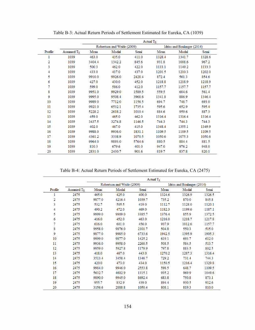
154

Table B-3: Actual Return Periods of Settlement Estimated for Eureka, CA (1039)

Table B-4: Actual Return Periods of Settlement Estimated for Eureka, CA (2475)

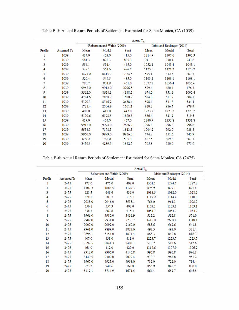
155

Table B-5: Actual Return Periods of Settlement Estimated for Santa Monica, CA (1039)

Table B-6: Actual Return Periods of Settlement Estimated for Santa Monica, CA (2475)

156

Table B-7: Actual Return Periods of Settlement Estimated for Salt Lake City, UT (1039)

Table B-8: Actual Return Periods of Settlement Estimated for Salt Lake City, UT (2475)

157

Table B-9: Actual Return Periods of Settlement Estimated for San Jose, CA (1039)

Table B-10: Actual Return Periods of Settlement Estimated for San Jose, CA (2475)

158

Table B-11: Actual Return Periods of Settlement Estimated for San Fran, CA (1039)

Table B-12: Actual Return Periods of Settlement Estimated for San Jose, CA (2475)

159

Table B-13: Actual Return Periods of Settlement Estimated for Seattle, WA (1039)

Table B-14: Actual Return Periods of Settlement Estimated for San Fran, CA (2475)

160

Table B-15: Actual Return Periods of Settlement Estimated for Charleston, S.C. (1039)

Table B-16: Actual Return Periods of Settlement Estimated for Charleston, S.C. (2475)

161

Table B-17: Actual Return Periods of Settlement Estimated for Portland, OR (1039)

Table B-18: Actual Return Periods of Settlement Estimated for Portland, OR (2475)

162

Table B-19: Actual Return Periods of Settlement Estimated for Memphis, TN (1039)

Table B-20: Actual Return Periods of Settlement Estimated for Memphis, TN (2475)