1

DDeevveellooppmmeenntt ooff aa PPeerrffoorrmmaannccee--bbaasseedd IInndduussttrriiaall EEnneerrggyy EEffffiicciieennccyy IInnddiiccaattoorr ffoorr

PPhhaarrmmaacceeuuttiiccaall MMaannuuffaaccttuurriinngg PPllaannttss

GGaallee AA.. BBooyydd

DDuukkee UUnniivveerrssiittyy

JJuunnee 22001111

SSppoonnssoorreedd bbyy tthhee UU..SS.. EEnnvviirroonnmmeennttaall PPrrootteeccttiioonn AAggeennccyy aass ppaarrtt ooff tthhee EENNEERRGGYY SSTTAARR pprrooggrraamm..

ACKNOWLEDGMENTS

The work described in this report was sponsored by the U.S. Environmental Protection Agency, Office of Atmospheric Programs, Climate Protection Partnership Division as part of the ENERGY STAR Focus on Energy Efficiency in Pharmaceutical Manufacturing. The research discussed in this report has benefited from the active review of pharmaceutical companies participating in the ENERGY STAR Focus.

Development of a Performance-based Industrial Energy Efficiency Indicator for

Pharmaceutical Manufacturing Plants

Gale A. Boyd

Abstract

Organizations that implement strategic energy management programs undertake a set of activities that, if carried out properly, have the potential to deliver sustained energy savings. One key management opportunity is determining an appropriate level of energy performance for a plant through comparison with similar plants in its industry. Performance-based indicators are one way to enable companies to set energy efficiency targets for manufacturing facilities. The U.S. Environmental Protection Agency (EPA), through its ENERGY STAR program, is developing plant energy performance indicators (EPIs) to encourage a variety of U.S. industries to use energy more efficiently. This report describes work with the pharmaceutical manufacturing industry to provide a plant-level indicator of energy efficiency for facilities 1 that develop and manufacture pharmaceutical products in the United States. How indicators are employed in EPA’s efforts to encourage industries to voluntarily improve their use of energy is discussed as well. The report describes the data and statistical methods used to construct the EPI for pharmaceutical manufacturing plants. The individual equations are presented, as well as instructions for using those equations as implemented in an associated Excel workbook.

1 Pharmaceutical manufacturing may occur in dedicated purpose buildings or in multi-use, campus-like settings with both research labs and manufacturing activities. We use the term “facilities” to encompass both types of locations.

1 Introduction

ENERGY STAR was introduced by EPA in 1992 as a voluntary, market-based partnership to reduce air pollution through increased energy efficiency. This government program enables industrial and commercial businesses as well as consumers to make informed decisions that save energy, reduce costs, and protect the environment. A key step in improving corporate energy efficiency is to institutionalize a strategic energy management framework and corporate energy program. The US EPA has observed that companies with established energy management programs based on a framework of continuous improvement achieve greater results. Based on the best practices of leading ENERGY STAR partners and informed by management standards for quality and environmental management (ISO 9000 & 14001), the US EPA developed the ENERGY STAR Guidelines for Energy Management that identify the components of successful energy management (EPA 2003). These include:

• Commitment from a senior corporate executive to manage energy across all businesses and facilities operated by the company;

• Appointment of a corporate energy director to coordinate and direct the energy program and multi-disciplinary energy team;

• Establishment and promotion of an energy policy; • Development of a system for assessing performance of the energy

management efforts, including tracking energy use as well as benchmarking energy in facilities, operations, and subunits therein;

• Setting of goals at the corporate, facility, and subunit levels; • Establishment of an action plan across all operations and facilities, as

well as monitoring successful implementation and promoting the value to all employees;

• Active communication across, and creation of rewards for the success of the program; and,

• Regular reevaluation of energy goals and action plans.

Of the major steps in energy management program development, benchmarking energy use by comparing current energy performance to that of a similar entity is critical. In manufacturing, it may take the form of detailed comparisons of specific production lines or pieces of equipment, or it may be performed at a higher organizational level by gauging the performance of a single manufacturing plant to its industry. Regardless of the application, benchmarking enables companies to determine whether better energy performance could be expected. It empowers them to set goals and evaluate their reasonableness.

2 Benchmarking the Energy Efficiency of Industrial Plants Among U.S. manufacturers, few industries participate in industry-wide plant benchmarking. The petroleum and petrochemical industries each support plant-wide surveys conducted by a private company, and are provided with benchmarks that address energy use and other operational parameters related to their facilities. Otherwise, most industries have not benchmarked energy use across their plants. As a result, some energy managers find it difficult to determine how well their plants might perform. The US EPA’s ENERGY STAR program released its first energy performance benchmarking tool in 1999 for commercial buildings. This whole-building energy performance benchmarking and rating tool was the first to enable comparisons between a single facility and the energy performance of the entire sector (EPA 2007). Since then, EPA has expanded its benchmarking and rating systems to other commercial and industrial subsectors. In 2000, EPA began developing a method for developing benchmarks of energy performance for plant-level energy use within various manufacturing industries. Discussions yielded a plan to use a source of data that would nationally represent manufacturing plants within a particular industry, create a statistical model of energy performance for the industry’s plants based on these data along with other available sources for the industry, and establish the benchmark on the comparison of those best practices, or best-performing plants, to the industry. The primary data sources would be the Census of Manufacturers, Annual Survey of Manufacturing, and Manufacturing Energy Consumption Survey collected by the Census Bureau, or data provided by trade associations and individual companies, when warranted by the specific industry circumstance and participation. At the outset, the term “plant benchmark” was discussed. Industry engineers routinely develop benchmarks at many levels of plant operation, but they expressed concern that using the word “benchmark” would be confusing and could imply a particular process or tool. For this reason, it was decided that a simple descriptive name would be clearer; thus, ENERGY STAR plant energy performance indicator (EPI) was adopted. In 2005, EPA released the first energy performance indicator for automobile assembly plants. Boyd, Dutrow, and Tunnessen (2008) describes early experiences in developing a statistically based plant energy performance indicator for the purpose of benchmarking manufacturing energy use. Additional details about the auto and corn refining industries are described in Boyd (2005, 2008), respectively. This report describes the basic concept of benchmarking and the statistical approach employed in developing performance-based energy indicators for pharmaceuticals, the evolution of the analysis done for this industry, the final results of this analysis, and ongoing efforts by EPA to improve the energy efficiency of this industry and others.

2.1 Scope of an Indicator — Experience with the Pharmaceutical Manufacturers EPA initiated discussions about developing a plant-level benchmark with the pharmaceutical manufacturers in 2004. Companies with facilities located within the United States were invited to participate in discussions. Initial reaction from most companies was supportive yet skeptical about whether a useful benchmark could be developed. The scope for ENERGY STAR EPIs is usually set at the plant-level, and is not process-specific. The EPI relates plant inputs in terms of all types of energy use to plant outputs as expressed in a unit of production. Discussion with industry representatives helped to define the energy focus of the model and the appropriate metrics. It was decided that value of product shipments would not provide a uniform measure of activity. Industry pricing and markups vary widely depending on the product, making the total value of product shipments an unreliable measure of production. While the level of production is clearly a component of the energy use, much of the energy in this industry is devoted to environmental controls. Pharmaceutical manufacturing encompasses a range of activities. Three primary types of activities were identified: Bulk Chemical, Fill/Finish, and Research & Development (defined in table 1 below). The first two categories describe the two basic stages of the manufacturing process. This industry differs from other industries due to the large component that the third type of activity, Research & Development (R&D), plays in this industry. While R&D may be conducted at a separate facility, it is also common for R&D to be co-located with manufacturing. Thus, it was decided that the pharmaceutical manufacturing EPI would have to consider the role that co-located R&D has on energy use at pharmaceutical manufacturing plants. The model is designed to account for major, measurable impacts that affect a plant’s energy use. Further discussion with the industry led to a focus on a limited set of measures to account for the differences between plants. These measures included facility size (in square feet), the fraction of these four space types representing the amount of facility space allocated to these activities, and the total operation hours for a plant to capture level of utilization. Finally, the heating and cooling loads of the plants would differ depending on their local climate/weather, so heating and cooling degree day (HDD and CDD, respectively) data were used in the model as well.

2.2 Data Sources

Since the categories of functional space types are not collected in the Census of Manufacturers, data was provided by eight companies that volunteered to participate in the study. These companies included Allergan, E.I. Lilly, GlaxoSmithKline, Johnson &

Johnson, Merck, Pfizer, Roche, and Schering-Plough.2 Companies provided the plant size (floor space), functional space types (listed above), and annual hours of operation for each space type. Energy data for fossil fuel and electricity use on a data template prepared by one of the companies was provided by companies for each plant. Climate data in the form of HDD and CDD were linked to the plant locations based on the first three digits of the plant ZIP code for each year of the data. The HDD/CDD data are the same as those used by ENERGY STAR for the National Energy Performance Rating System for buildings.

Table 1 Definition of Pharmaceutical Facility Space Types

Bulk Chemical Areas where both active and inactive ingredients are prepared in bulk form, including mixing, milling and drying of powders, and the mixing of liquids, gels and creams. All office space that shares HVAC with Bulk Chemical space will be considered as Bulk Chemical space. Fill/Finish All indoor areas used for Fill or Finish processes OR other manufacturing, production, or warehousing with climate-controlled environments due to product requirements. Fill or Finish includes tabulating, encapsulation of powders or liquids, the final bottling/packaging of this product, and the filling of liquids, gels or creams in their consumer packages. All office space that shares HVAC with Fill/Finish space will be considered Fill/Finish space. Research & Development Lab buildings including animal laboratories, storage space, laboratories, pilot plants and offices located in R&D facilities. This space includes in-process labs and QA labs. All office space that shares HVAC with R & D / Laboratory space will be considered R & D / Laboratory space. Other All other space that does not share HVAC with Bulk Chemical, Fill/Finish, Sterile Fill/Finish, Warehousing, or Laboratory spaces.

Three years of data (2004-2006) were provided for 61 locations. However, some

of these locations were R&D facilities with no manufacturing activities. The model excluded sites with more than 60% office/other or less than 10% manufacturing. The final dataset includes 95 observations. While the data was voluntarily provided by the companies identified above, these companies represent a large share of this industry. Comparing the voluntary data to Census data, the energy use in the sample comprised over 50% of the published total for NAICS 32541 Pharmaceutical and Medicine Manufacturing. Comparing the total value of shipments in the first version of the model (using Census data) for the companies that provided floor space data to the published total, the sample comprised over half of the total published value of shipments for this NAICS code.

2 The data used to develop the EPI are proprietary business information and was voluntarily provided to

Duke University under a nondisclosure agreement with the respective companies.

Table 2 provides the sample mean and standard deviation for the raw variables in the dataset. Total source energy (TSE) is the variable used to aggregate energy; that is, kilowatt-hours (kWh) are converted to British thermal units (Btu) using 10,236 Btu/kWh. The study focuses on the energy use per square foot, so these data are of particular interest. A histogram of the TSE used per sq. ft. is shown in Figure 1.

Table 2 Summary Statistics from the Plant Data Included in the Study Variable Mean St. Dev. HDD (thousand) 2.443 2.045 CDD (thousand) 1.882 1.624 Square Ft (thousand) 724 1210 Bulk Chemical Share 27% 0.239 Fill/Finish Share 20% 0.209 R&D Share 10% 0.130 Total Source Energy (MMBtu) per thousand sq.ft. 1194 834 Utilization (percent) 62% 0.252

Figure 1 Distribution of Energy Intensity

0%

10%

20%

30%

40%

50%

60%

70%

80%

90%

100%

0

5

10

15

20

25

30

35

500 1000 1500 2000 2500 3000 3500 More

Freq

uenc

y

MMBTU per Thousand Square Foot

Frequency

Cumulative %

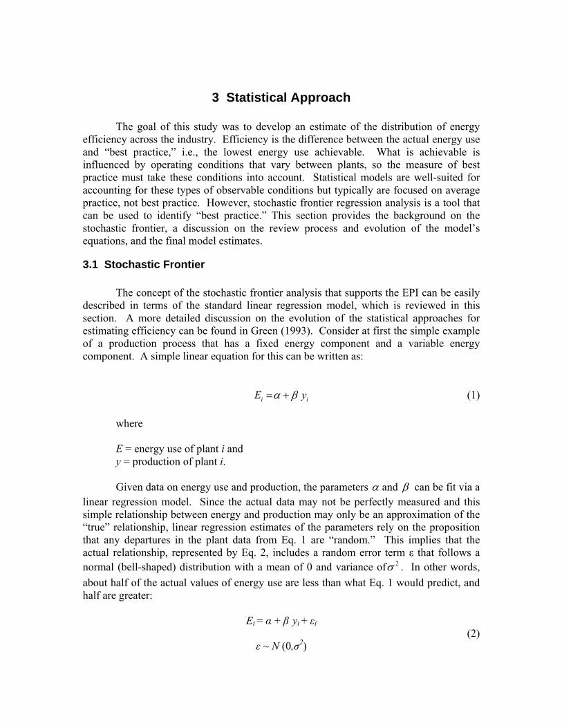
3 Statistical Approach The goal of this study was to develop an estimate of the distribution of energy

efficiency across the industry. Efficiency is the difference between the actual energy use and “best practice,” i.e., the lowest energy use achievable. What is achievable is influenced by operating conditions that vary between plants, so the measure of best practice must take these conditions into account. Statistical models are well-suited for accounting for these types of observable conditions but typically are focused on average practice, not best practice. However, stochastic frontier regression analysis is a tool that can be used to identify “best practice.” This section provides the background on the stochastic frontier, a discussion on the review process and evolution of the model’s equations, and the final model estimates.

3.1 Stochastic Frontier The concept of the stochastic frontier analysis that supports the EPI can be easily

described in terms of the standard linear regression model, which is reviewed in this section. A more detailed discussion on the evolution of the statistical approaches for estimating efficiency can be found in Green (1993). Consider at first the simple example of a production process that has a fixed energy component and a variable energy component. A simple linear equation for this can be written as:

i iE yα β= + (1)

where E = energy use of plant i and y = production of plant i.

Given data on energy use and production, the parameters α and β can be fit via a linear regression model. Since the actual data may not be perfectly measured and this simple relationship between energy and production may only be an approximation of the “true” relationship, linear regression estimates of the parameters rely on the proposition that any departures in the plant data from Eq. 1 are “random.” This implies that the actual relationship, represented by Eq. 2, includes a random error term ε that follows a normal (bell-shaped) distribution with a mean of 0 and variance of 2σ . In other words, about half of the actual values of energy use are less than what Eq. 1 would predict, and half are greater:

Εi = α + β yi + εi (2)

ε ~ Ν (0,σ2)

The linear regression gives the average relationship between production and energy use. If the departures from the average, particularly those that are above the average, are due to energy inefficiency, we would be interested in a version of Eq. 1 that gives the “best” (lowest) observed energy use. For example, consider that capacity utilization can influence the energy use per unit of production, due to the fixed and variable components of plant energy use (see Figure 2). A regression model can find the line that best explains the average response of energy use per unit of production to a change in utilization rates. The relationship between the lowest energy consumption per unit of production relative to changes in utilization can be obtained by shifting the line downward so that all the actual data points are on or above the line. This “corrected” ordinary least squares (COLS) regression is one way to represent the frontier.

While the COLS method has its appeal in terms of simplicity, a more realistic view is that not all the differences between the actual data and the frontier are due to efficiency. Since we recognize that there may still be errors in data collection/reporting, effects that are unaccounted for in the analysis, and that a linear equation is an approximation of the complex factors that determine manufacturing energy use, we still wish to include the statistical noise, or “random error,” term vi in the analysis but also add a second random component ui to reflect energy inefficiency.3 Unlike the statistical noise term, which may be positive or negative, this second error term will follow a one-sided distribution. If we expand the simple example of energy use and production to include a range of potential effects, we can write a version of the stochastic frontier model as energy use per unit of production as a general function of systematic economic decision variables and external factors,

( , , ; )i i i i iE h Y X Z β ε= + (3)

i ii u vε = − v ~ Ν [0,σv2] ,

where E = TSE, Total Source Energy (or other measure of total fuel and electricity); Y = production, measured by dollar shipments or physical production; X = systematic economic decision variables (i.e., labor-hours worked, materials processed, plant capacity, or utilization rates); Z = systematic external factors (e.g., heating and cooling loads); and, β = all the parameters to be estimated.

We assume that energy (in)efficiency u is distributed according to one of several possible one-sided statistical distributions, for example exponential, half normal, or truncated normal. We also assume that the two types of errors are uncorrelated, i.e. σu,v = 0 . It is then possible to estimate the parameters of Eq. 3, along with the distribution parameters of u.

3 By random we mean that this effect is not directly measurable by the analyst, but that it can be

represented by a probability distribution.

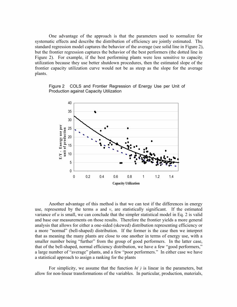
One advantage of the approach is that the parameters used to normalize for systematic effects and describe the distribution of efficiency are jointly estimated. The standard regression model captures the behavior of the average (see solid line in Figure 2), but the frontier regression captures the behavior of the best performers (the dotted line in Figure 2). For example, if the best performing plants were less sensitive to capacity utilization because they use better shutdown procedures, then the estimated slope of the frontier capacity utilization curve would not be as steep as the slope for the average plants.

Figure 2 COLS and Frontier Regression of Energy Use per Unit of Production against Capacity Utilization

0

5

10

15

20

25

30

35

40

0 0.2 0.4 0.6 0.8 1 1.2 1.4

Capacity Utilization

E/Y

- E

nerg

y us

e pe

r un

it of

pro

duct

ion

Another advantage of this method is that we can test if the differences in energy

use, represented by the terms u and v, are statistically significant. If the estimated variance of u is small, we can conclude that the simpler statistical model in Eq. 2 is valid and base our measurements on those results. Therefore the frontier yields a more general analysis that allows for either a one-sided (skewed) distribution representing efficiency or a more “normal” (bell-shaped) distribution. If the former is the case then we interpret that as meaning the many plants are close to one another in terms of energy use, with a smaller number being “further” from the group of good performers. In the latter case, that of the bell-shaped, normal efficiency distribution, we have a few “good performers,” a large number of “average” plants, and a few “poor performers.” In either case we have a statistical approach to assign a ranking for the plants

For simplicity, we assume that the function h( ) is linear in the parameters, but allow for non-linear transformations of the variables. In particular, production, materials,

and labor enter the equation in log form, as does the energy variable. This means that the terms u and v can easily be interpreted as percentage deviations in energy, rather than absolute. This has implications for the model results since we now think of the distributional assumptions in terms of percent, rather than absolute level. When there is wide variation in plant scale, this seems appropriate and may avoid possible heteroscedasticity in either or both error terms.

Given data for any plant, we can use Eq. 3 to compute the difference between the actual energy use and the predicted frontier energy use:

[ ] i i( , , ; )i i i iE h Y X Z u vβ− = − (4)

In the case where the frontier model is appropriate, we have estimated the probability distribution of u. Eq. 5 represents the probability that the plant inefficiency is greater than this computed difference:

( )Probability ( , , ; )

1 ( ( , , ; ))i i i i

i i i i

energy inefficiency E h Y X Z

F E h Y X Z

β

β

⎡ ⎤≥ − =⎣ ⎦− −

(5)

F( ) is the cumulative probability density function of the appropriate one-sided density function, i.e., gamma, exponential, truncated normal, etc. The value 1 - F( ) in Eq. 5 defines the EPI rating and may be interpreted as a percentile ranking of the energy efficiency of the plant. In practice, we only can measure i i( , , ; )i i i iE h Y X Z u vβ− = − , so this implies that the EPI rating, ( ) ( )i i1 ( , , ; ) 1i i i iF E h Y X Z F u vβ− − = − − , is affected by the random component of vi; that is, the rating will reflect the random influences that are not accounted for by the function h(*).

In the case where the frontier model is not appropriate there is no u term and corresponding estimate, only v. [ ] i( , , ; )i i i iE h Y X Z vβ− = (6) We can drop the minus sign for v since the normal distribution is two sided. The estimate of the variance v ~ Ν [0,σv

2] can be used in Eq. 5 where F( ) is now the cumulative probability density function of a standard normal distribution.

Since this ranking is based on the distribution of inefficiency for the entire industry, but normalized to the specific systematic factors of the given plant, this statistical model allows the user to answer the hypothetical but very practical question, “How does my plant compare to everyone else’s in my industry, if all other plants were similar to mine?”

3.2 Evolution of the Model The statistical model used in the EPI evolved over a period of time, based on comments from industry reviewers and subsequent analyses. Industry participants tested each version of the model. Companies were asked to input actual data for all of their plants and then to determine whether the results were consistent with any energy efficiency assessments that may have been made for these plants. The resulting comments improved the EPI.

The primary areas for comment and development included the best way to incorporate plant utilization, treatment of office and “other” space types, and the role of climate. These issues included whether to use annual labor (person hours) or hours of operation to measure utilization, whether to separately estimate the energy implications of office and “other,” and whether climate has different impact for different space types.

In the early stages, the use of labor hours (i.e. average annual employment times

the average number of hours worked per person) was proposed to represent the utilization of a facility. It was argued that energy is used to provide services and comfort for the people working to make products and services. Measuring labor (work hours) can present problems because hourly production workers may have careful accounting of work time, but salaried employees may not. Differences in labor productivity may also mask the amount of time a facility is operating and using energy. It was proposed to use the hours of operation in each space type as a more direct measure.

During the analysis it was observed that some plants with a high share of “other”

space types had very high energy use, but others had very low. The differences were dramatic. A similar disparity, but smaller in range, was observed for office space. In the absence of more detail about the nature of the “other” space types it was impossible to assign a meaningful estimate. One argument was that both of these space types were support functions for the primary activities of manufacturing and R&D. In fact, office space was often integrated in those other functional space types. “Other” space might even be large energy support facilities required for manufacturing, e.g. a boiler house. It was proposed to treat these as support functions so that the space in office and other was allocated back to the three functional space types: Bulk Chemical, Fill/Finish, and R&D.

Different space types may have different requirements for climate control. These

differences would be reflected in the energy use that is driven by heating and cooling loads. Energy is used for environmental, safety, and comfort control in this industry, but bulk chemical synthesis requires process energy as well. From that perspective it is important to allow the model to be flexible in the representation of HDD and CDD for different space types.

Throughout the process the estimation approach provided statistical tests to

determine the confidence level of the adjustment factors that would or would not be included. Use of labor vs. operation hours could not be tested statistically since only operation hours were provided by the companies. This choice is instead driven by data

availability. Treating office and other space types as support functions is consistent with the results presented below. In particular, treating “other” as a separate category resulted in a very high, but statistically insignificant, parameter for energy use. Allocating office and other resulted in lower standard errors for the other space types in the model. A flexible approach to measuring impacts of HDD and CDD was taken in the model development. Bulk chemical space types had lower response to climate (both HDD and CDD) that was statistically significant. The two remaining space types did not show statistically different responses from each other. The model was also estimated with non-linear (quadratic) terms of climate and utilization (to capture possible diminishing returns). These terms were not statistically significant.

3.3 Model Estimates

For simplicity, we assume that the function h( ) is log linear in energy and facility size, and linear in all other variables, but allow for non-linear transformations of the variables. In particular, we tested non-linear (quadratic) and second order interaction terms in some of the variables where appropriate. The model was estimated with non-linear (quadratic) terms of climate and utilization (to capture possible diminishing returns). These terms were not statistically significant. Several alternatives for the distribution of the inefficiency term u were tried.

The final version of the model is:

1 2 3 4 5 62

11 12 1

ln( ) % & %

% % ln( )

E a a HDD a CDD a Bulk a F F a Util

b HDD Bulk b CDD Bulk c ft u v

= + + + + + +

+ + + − (7)

where E = Total Source Energy use in MMBtu; ft2 = total floor space (thousands of square feet); UTIL = plant utilization rate, defined as annual hours of operation / 8760; HDD = heating degree days for the plant location and year (thousands); CDD = cooling degree days for the plant location (thousands); Bulk% = ratio of bulk chemical manufacturing space to the total; F & F% = ratio of fill/finish manufacturing space to the total;

The error term v is distributed as N(0, σv

2) and error term u is distributed as truncated normal with variance σu

2. The estimated parameters of the model are shown in Table 3. All parameters with

an asterisk are statistically significant at the 10% level or greater in a two-tailed test. All other estimates shown are significant at the 99% level in a two-tailed test. The large size of λ suggests that the model has very little error attributable to random noise and that most departures are attributable to inefficiency. The coefficients for bulk chemical and fill/finish are interpreted as relative to R&D space. The stylized facts are that bulk

chemical is the most intensive, i.e. the coefficient is positive and larger than for fill/finish. It also has almost no sensitivity to climate, since the interaction coefficients, b11 and b12, for HDD and CDD are of opposite sign and nearly identical magnitude to a1 and a2, respectively. Fill/finish space is also more intensive than R&D. The coefficient on the log of sq. ft. does not suggest any economies of scale in energy use for this industry.

Table 3 TSE Model Estimates

Variable Estimate Standard Error t-ratio Constant 3.026 0.572 5.29 BULK % 2.952 0.876 3.37 FF % 0.836 0.279 2.99 LSQFT 0.977 0.053 18.47 UTILIZATION 1.858 0.301 6.17 HDD * BULK % -0.275* 0.166 -1.66 HDD 0.298 0.095 3.15 CDD * BULK % -0.503 0.186 -2.71 CDD 0.417 0.106 3.93 Error Distribution Parameters

λ 1.56E+07 7.06E+12 0σu 0.527282 0.052639 10.017

4 Judging Pharmaceutical Manufacturing Plant Energy Efficiency

4.1 How the EPI Works

The pharmaceutical manufacturing EPI rates the energy efficiency of a pharmaceutical manufacturing plant based in the United States. To use the tool, the following information must be available for a plant:

• Annual energy use for the current year and a reference year as defined

by the user; • Total facility floor space; • Allocation of space for each space type; • Hours of operation for each space type; • Five-digit ZIP code for the location of the plant if the default 30-year

average HDD and CDD data are used; otherwise, the user provides actual annual HDD and CDD for that year.

Based on these data inputs, the pharmaceutical manufacturing EPI will calculate an energy performance rating for the plant in the current time period that reflects the relative

energy efficiency of the plant compared to that of the industry. The performance rating is a percentile rating on a scale of 0–100. Plants that rate 75 or better are classified as efficient (ENERGY STAR defines the 75th percentile as “efficient”). A rating of 75 means a particular plant is performing better than 75% of the plants in the industry. Plants that rate a 75 or higher on the EPI are then eligible for ENERGY STAR recognition and certification. For ENERGY STAR recognition of pharmaceutical plants, more than 50% of the plant floor space must be considered manufacturing (bulk chemical and fill/finish). The model also reports on energy use for the average plant in the industry (defined as the 50th percentile) and the efficient plant. This is also reported as an energy output ratio (million Btu/ sq. ft.). While the underlying model was developed from data for individual facilities, it does not contain or reveal any confidential information.

4.2 Spreadsheet Tool

To facilitate the review of, and use by, industry energy managers, a spreadsheet was constructed to display the results of the EPI for any actual or hypothetical plant-level inputs. The spreadsheet accepts the raw plant-level inputs described above, computes the values for h( ), and then displays the results from the truncated normal distribution functions for the model presented in Eq. 7. The results are based on user-input values of the basic model input described above. This aids in comparing the magnitude of the systematic effects attributable to changes in those inputs on the efficiency distribution by graphically displaying the results. The energy managers were encouraged to input data for their own plants and then provide comments on the observed results. A version of this spreadsheet which corresponds to the results described in this report (release 2 (2/22/2010), is available from the EPA ENERGY STAR web site.4 An example of the input section of the spreadsheet is shown in Figure 3. The results section for TSE use is shown in Figure 4.

4.3 Summary Results Although the pharmaceutical manufacturing EPI is intended to produce plant-

specific analysis of energy efficiency, some broad inferences about efficiency in pharmaceutical manufacturing can be made based on the models and the underlying data. The average energy consumed per sq. ft. of manufacturing space was 1,210 million Btu. If we compute the EPI model’s “best practice” estimates (i.e., the predicted values for the function h ( ) for every plant in the dataset), we obtain the results shown in Table 5. The average “best practice” consumption per sq. ft. would be 806 million Btu, or about a one-third reduction in energy use below the average. The variety of plants still implies a range of performance. The distribution of actual and best practice based on our sample is shown in Figure 5.

4 http://www.energystar.gov/EPIS

17

Figure 3 Input Section of the EPI Spreadsheet Tool

Figure 4 Results Section of the EPI Spreadsheet Tool

18

Figure 5 Comparison of the Distribution of Actual and Best Practice Energy Intensity (MMBtu/thousand sq. ft.)

0

5

10

15

20

25

30

35

40

500 1000 1500 2000 2500 3000 3500 More

Freq

uenc

y

MMBTU per Thousand Square Foot

Raw Data

Best Practice

Table 5 Summary Statistics for the Predicted “Best Practice” Values of Fossil Fuel, Electric, and TSE Aggregate Energy Use per Vehicle

TSE 106 Btu/103 square feet Actual Performance Best Practice Mean 1,210 806 Median 1,391 890

4.4 Caveats This model was estimated using a set of plant data for specific years and locations.

The spreadsheet is intended to apply to other pharmaceutical manufacturing plants, not just those in the original dataset; in this sense, the model is being used to measure efficiency behavior beyond the original sample dataset. The use of plant-level information that is dramatically different from that used to develop the model may produce unreliable results. Users of the model equations presented above and implemented in the spreadsheet should consider if the plant-level data inputs are within a similar range as those use to estimate the model parameters (see below).

19

As is described above, the analysis that supports the model excluded sites with more than 60% office/other space or less than 10% manufacturing. For example, this means that the model may not produce reliable results for a facility that is exclusively R&D. By the same token, if the energy use for different space types is sub-metered or can be reasonably estimated via an allocation, the model could be used to benchmark sub-sets of the plant that more closely conform to the limits of the data that underlie the model. Different types of manufacturing operations, e.g. medical devices, may seem similar to pharmaceutical manufacturing; using this tool to benchmark energy use for these types of operations should only be approached with judgment and care in interpreting the results since these types of facilities were not included in the primary data set. This does not mean that this tool cannot be used to inform management about energy use in more diverse applications, but that it is not the primary focus.

For purposes of recognition by EPA under the ENERGY STAR program, additional limits are placed on the types of plants that can use the EPI tool. Plants must have more than 50% of the plant floor space in manufacturing: either bulk chemical, fill/finish, or some combination of the two. This minimum requirement for ENERGY STAR recognition must either be met for the entire facility or via sub-metered energy use for the space types that are included in the EPI and ENERGY STAR application. This can be met by sub-metering the manufacturing space itself, or by sub-metering R&D / Other space and subtracting it from the plant size and energy inputs.

4.5 Use of the ENERGY STAR Pharmaceutical Manufacturing EPI After several years of work with the pharmaceutical manufacturers, the ENERGY STAR pharmaceutical manufacturing EPI is now complete as a spreadsheet tool for calculating EPI ratings. EPA intends to use the EPI to motivate improvement in energy performance in pharmaceutical manufacturing. EPA works closely with the manufacturers, through an ENERGY STAR Industrial Focus on energy efficiency in pharmaceutical manufacturing, to promote strategic energy management among the companies in this industry. The pharmaceutical manufacturing EPI is an important tool that enables companies to determine how efficiently each of the plants in the industry is using energy and whether better energy performance could be expected. EPA recommends that companies use the pharmaceutical manufacturing EPI on a regular basis. At a minimum, it is suggested that corporate energy managers benchmark each pharmaceutical manufacturing plant on an annual basis. A more proactive plan would provide for quarterly use for every plant in a company. EPA suggests that the EPI rating be used to set energy efficiency improvement goals at both the plant and corporate levels. The model described in this report is based on the performance of the industry for a specific period of time. One may expect that energy efficiency overall will change as technology and business practices change, so the model will need to be updated. EPA

20

plans to update this model every few years, contingent on newer data being available for this industry.

4.6 Steps to Compute a Rating All of the technical information described herein is built into a spreadsheet available from EPA (http://www.energystar.gov/epis). Anyone can download, open the EPI spreadsheet and enter, update, and manage data as they choose. The following details each step involved in computing an EPI rating for a plant. 1. User enters plant data into the EPI spreadsheet

• Complete energy information includes all energy purchases (or transfers) at the plants for a 12-month period. The data do not need to correspond to a calendar year.

• The user must enter specific operational characteristic data. These characteristics are those included as independent variables in the analysis described above.

2. EPI computes the Total Source Energy Use • TSE is computed from the metered energy data. • The total consumption for each energy type entered by the user is converted into

source energy using the source-to-site conversion factors. • TSE is the sum of source energy across all energy types in the plant. • TSE per square foot is also computed.

3. EPI computes the Predicted “Best Practice” TSE • Predicted “Best Practice” TSE is computed using the methods above for the

specific plant. • The terms in the regression equation are summed to yield a predicted TSE. • The prediction reflects the expected minimum energy use for the building, given

its specific operational constraints. 4. EPI compares Actual TSE to Predicted “Best Practice” TSE

• A lookup table maps all possible values of TSE that are lower than the Predicted “Best Practice” TSE to a cumulative percent in the population.

• The table identifies how far the energy use for a plant is from best practice. • The lookup table returns a rating on a scale of 1-to-100. • The Predicted TSE for a median and 75th percentile plant is computed based on

the plant specific characteristics. • A rating of 75 indicates that the building performs equal to or better than 75% of

its peers. • Plants that earn a 75 or higher may be eligible to earn the ENERGY STAR.

21

5 References Gale A. Boyd, "Estimating Plant Level Manufacturing Energy Efficiency with Stochastic Frontier Regression", The Energy Journal, Vol 29, No. 2, pp 23-44, (2008) Boyd, G., E. Dutrow and W. Tunnessen, “The Evolution of the Energy Star Industrial Energy Performance Indicator for Benchmarking Plant Level Manufacturing Energy Use.” Journal of Cleaner Production, Invited paper for the special issue Pollution Prevention and Cleaner Production in the United States of America, Volume 16, Issue 6, pp 709-715, April 2008 Boyd, G.A., “A Statistical Model for Measuring the Efficiency Gap between Average and Best Practice Energy Use: The ENERGY STAR™ Industrial Energy Performance Indicator,” Journal of Industrial Ecology, Vol. 9 (3): pp 51-56, (2005) EPA, 2003, Guidelines for Energy Management, U.S. Environmental Protection Agency, Washington, DC; available online at http://www.energystar.gov/index.cfm?c=guidelines. guidelines_index. Greene, W.H., 1993, “The Econometric Approach to Efficiency Analysis,” pp. 68–119 in The Measurement of Productive Efficiency: Techniques and Applications, H. Fried, et al., (editors), Oxford University Press, NY.