i

DEVELOPMENT OF A CONTROLLER FOR FUEL CELL

USING FPGA

A thesis submitted in partial fulfilment of the requirements for the degree

of

Master of Technology in

VLSI Design & Embedded System

by

Sadhana Kumari

Roll No. 209ec2129

Under the guidance of

Prof. Kamalakanta Mahapatra

Department of Electronics & Communication Engineering

National Institute of Technology, Rourkela, Odisha

2011

ii

National Institute of Technology Rourkela

CERTIFICATE

This is to certify that the thesis entitled, “DEVELOPMENT OF A CONTROLLER FOR

FUEL CELL USING FPGA” submitted by SADHANA KUMARI (Roll No.-209ec2129) in

partial fulfilment of the requirements for the degree of Master of Technology in VLSI Design &

Embedded system, Session 2009-2011, in the Department of Electronics and Communication

Engineering, National Institute of Technology, Rourkela is an authentic work carried out by her

under my supervision and guidance.

To the best of my knowledge, the matter embodied in the thesis has not been submitted to any

other University / Institute for the award of any Degree.

Date: Prof. K.K.Mahapatra

SUPERVISOR

Dept. of Electronics & Communication Engineering

National Institute of Technology Rourkela –769008

iii

National Institute Of Technology

Rourkela

DECLARATION

I hereby declare that this thesis entitled “DEVELOPMENT OF A CONTROLLER FOR

FUEL CELL USING FPGA” submitted to National Institute of Technology, Rourkela for the

award of the degree of Master of Technology is a record of original work done by me under the

guidance Prof. Kamalakanta Mahapatra and that it has not been used, they have been

acknowledged.

Place: ROURKELA

Date: Signature

iv

ACKNOWLEDGEMENTS

I am heartily thankful to my supervisor, Prof. Kamalakanta Mahapatra, whose

encouragement, guidance and support from the initial to the final level enabled me to develop

an understanding of the concept, which was very necessary for me. He had been very kind and

patient while suggesting me the topics and correcting my doubts.

I am equally grateful to Mr.P.Karupanan (Ph.D Scholar), and Mr. Ayashkant Swain, Lab

Engineer for their positive support, despite of their busy schedule, they gave me different ideas

in making this project unique.

Last but certainly not the least; I would like to show my gratitude to my parents and my friends

that had a positive influence in my life.

Lastly, I offer my regards and best wishes to all of those who supported me in any respect during

the completion of this project.

Thanking you all.

SADHANA KUMARI

v

Contents Page no.

Chapter1.Introduction 1

1.1.Advantage of modeling of fuel cell 1

1.2 .Advantages of FPGA based design 2

1.3 .PWM Technique 2

1.4 .Fuel Cell system Implementation in system level language 2

Chapter 2.An Introduction to the Fuel cell and its Modeling 4

2.1.Introduction 4

2.2.PEMFC Functionality 5

2.2.1.Static Model 6

2.2.2.Dynamic Model 6

2.3.MATLAB Simulation Results of all type losses and thermodynamic potential 10

Summary: 13

Chapter 3.Buck And Boost Converter Circuit Topologies 14

3.1.Introduction 14

3.2 .Buck Converter working principle 14

3.3.Boost Converter working principle: 17

3.4.Simulink model of Buck Converter: 20

3.5 .Simulink model of Boost Converter: 23

Summary: 26

Chapter 4.Fuel Cell System 27

4.1.Introduction 27

4.2 .Modeling of Fuel Cell System Using Matlab/Simulink 27

4.3 .Simulation of fuel cell model under time varying load 28

4.3.1.Simulation Results of the fuel cell system model with varying flow rate : 31

4.3.2.Result Demonstration 35

4.4.Simulation of fuel cell system model under time varying load 36

4.4.1.Simulation Results 37

4.4.2.Result Demonstration: 39

Summary: 40

vi

Chapter 5.Implementation of Fuel Cell System Using VHDL and hardware Prototyping of

(PI+PWM) 41

5.1.Introduction 41

5.2.Implementation of Dynamic model of Fuel cell 41

5.3 .Converter part implementation 42

5.4 .PWM implementation 42

5.4.1.High frequency counter based PWM Generator 42

5.4.2.Counter based PWM Generator 43

5.4.3.Cascaded Counter based PWM generator 44

5.4.4.Proposed method 45

5.5.PI implementation 46

5.6.State Diagram of Fuel Cell System for VHDL Implementation 48

5.7.Result and Discussion 49

5.8.Real Time Debugging of the Fuel Cell System 49

Chapter 6.Conclusion and Future Work 51

6.1 .Conclusion 51

6.2.Future Work 51

References: 52

List of figures

Fig.2.1.Schematic of Fuel Cell 4

Fig.2.2.Fuel Cell Model 6

Fig.2.3.Equivalent electrical circuit of PEM fuel cell. 9

Fig.3.1.Schematic of Buck Converter 15

Fig.3.2.waveform of an ideal buck convert current and voltage in continuous mode 16

Fig.3.3.Voltage and current of an ideal buck converter operating in Discontinuous mode. 17

Fig.3.4.Boost Converter (step up chopper) 18

Fig.3.5.Voltage and Current of a Boost Converter operating in continuous mode. 19

Fig.3.6.Voltage and current of a Boost Converter operating in discontinuous mode. 20

Fig.3.7.Simulink model of Buck converter 20

Fig.3.8.Voltage and current of the buck converter 21

Fig.3.9.Buck converter voltage at steady state 22

Fig.3.10.Open loop Boost Converter 23

Fig.3.11.Output current of the Boost converter 24

Fig.3.12. Output voltage of the Boost converter 24

Fig.3.13. Simulink model of Closed Loop Boost Converter 25

vii

Fig.3.14. Output current of closed loop Boost Converter 26

Fig.3.15. Output current of the closed loop Boost Converter 26

Fig.4.1.Block Diagram of closed loop fuel cell system 27

Fig.4.2.Dynamic model of fuel cell 28

Fig.4.3.Simulink model of fuel cell system with varying flow rate 28

Fig.4.4.Model of flow rate selector 29

Fig.4.5.Model of boost Converter 29

Fig.4.6.Simulink model of fuel cell system under switched load 36

Fig.5.1.Architecture of PWM Generator proposed by E. Koutroulis 43

Fig.5.2.Architecture of Counter based PWM Generator proposed by A.P Dancy. 44

Fig.5.3.Cascade counter based PWM generator 44

Fig.5.4.RTL Schematic of high frequency based PWM generator 45

Fig.5.5.RTL Schematic of counter based PWM generator 45

Fig.5.6.RTL schematic of cascaded counter based PWM generator 45

Fig.5.7.RTL schematic of method discussed in 5.4.4 46

Fig.5.8.Test Bench waveform of PWM generator 46

Fig.5.9.RTL Schematic of PI Controller 47

Fig.5.10. Test Bench waveform of PI controller 47

Fig.5.11. Test Bench Waveform OF The Fuel Cell System Using XILINX ISE Simulator 49

Fig.5.12. Experimental setup 50

Fig.5.13. Resulted PWM with Duty cycle D =.5 50

List of tables

Table 2.1 11

Table 3.1 21

Table 3.2 23

Table 3.3 25

Table 4.1 30

List of graphs

Graph 2.1.Ohmic Loss versus Current Density 10

Graph 2.2. Activation Loss versus current Density 10

Graph 2.3 .Activation Loss versus fuel cell current 11

Graph 2.4.Entropy of H2,O2 and H2o versus temperature 12

Graph 2.5.Concentration Loss versus cell current density 12

viii

Graph 4.1.Flow rate versus time 31

Graph 4.2.Utilization of fuel and oxidant (air) 31

Graph 4.3.Consumption of fuel and oxidant(air) versus time 32

Graph 4.4.Stack efficiency versus time 32

Graph 4.5.Fuel cell voltage versus time 33

Graph 4.6.Fuel cell current versus time 33

Graph 4.7.Boost output voltage versus time 34

Graph 4.8.Boost output current versus time 34

Graph 4.9.Nernst voltage versus time 35

Graph 4.10.Output power versus time 35

Graph 4.11.Load switching pulse 37

Graph 4.12.Fuel cell voltage versus time 37

Graph 4.13.Boost output voltage versus time 38

Graph 4.14.Boost output current versus time 38

Graph 4.15.Output power of fuel cell versus time 39

Graph 4.16. Nernst voltage versus time 39

ix

Abstract

This thesis is a sample of what we can do to reduce the complexity of a fuel cell controller

and research carried out in the modeling of a renewable energy sources like fuel cell. This thesis

mainly deals the control of the fuel cell under variation of different parameters, and

implementation of the system in VHDL. As we know that not any voltage source, weather it is

traditional energy source or fuel cell system behaves as an ideal source. The output of these cells

depends upon some parameter of the cell. To control the output voltage of a fuel cell we need

some controller, it may be digital or analog.

At the present time, PWM has become an integral part of all the electronic system. This

technique has some salient feature, due to which it has replaced the traditional use of digitally

just on off signal to control the switching action of the converter. There are two basic techniques

of PWM generation, analog and digital. The disadvantages of the analog methods are that they

are prone to noise, and they change with voltage and temperature change, they suffer changes

due to component variation. To overcome the problem, associated with the analog technique,

various types of digital technique are available. Implementation of these techniques in VHDL

has done.

First we have synthesized the whole system, using Matlab/Simulink then VHDL code for

various topology of digital technique of PWM generation. After behavioral Simulation and

verification of the results this VHDL code has downloaded to SPARTAN3E FPGA. After

downloading the code in FPGA real time debugging has done for the architecture. The overall

work done in this thesis aims to promote professional activity in the area of fuel cell controller

and low power electronics used in the modern age, with an important focus on the design,

development, simulation, and verification, and to examine the possibility of using Field

Programmable Gate Arrays (FPGA) for the rapid prototyping of a PI+PWM digital electronic

controller used in a power system consisting of a 2.4 kW 96 v fuel cell system, which is made up

of two main component, fuel cell stack and boost converter.

Key terms: PWM, Boost Converter, FPGA, PEM fuel cell.

Chapter 1

Introduction

1

Chapter1

Introduction Now this is the age of VLSI and this technology has become advanced and more

prominent, due to development of EDA tools. To design a Novel system often means that the

design should reach certain goal under certain constraint applied to it, and to perform better in

the operating limit for which the system has to be design. Holistic modelling of any complex

system plays the vital role in the design of the system. The goal of this thesis is to examine

the possibility of FPGA based hardware prototyping for a complex fuel cell system, so that

we can use this system controller efficiently for controlling the voltage. Traditional methods

are not able to cope with increased complexity and demand of very higher level of system

integration and relatively short time to market. Nowadays functional description and

hardware implementation has brought to be closer with the help of recent advancement in

CAD methodologies/language. The chief contribution of this work is to demonstrate control

techniques based on system level digital language, which can show the possibility of using an

FPGA based digital controller to reduce the system complexity, and also increase its

reusability.

1.1 Advantage of modeling of fuel cell

Successful innovation often means a design that achieves a desirable cluster of

performance characteristics, subject to certain constrains and holistic modelling of complex

technical systems can constitute the first step towards novel designs of high performance [1].

FCS (fuel cell system) is a good energy sources to provide reliable power at steady state;

however, due to their slow internal electrochemical and thermodynamic characteristics, they

cannot respond to electrical load transients as quickly as desired. They are connected to the

power grid through power electronic interfacing devices, and it is possible to control their

performance by controlling the interfacing devices. Modeling of FCS can therefore be helpful

in evaluating their performance and for designing controllers [2]. Modelling of any complex

system gives a mathematical description and provides a way to implement the whole system

on a single platform. Holistic modelling of complex technical systems can constitute the first

step towards the creation of novel circuit designs of high performance [3]. A holistic, system

level, approach to the design and development of an electronic system enables a top-down

2

design methodology, which begins with modelling an idea at an abstract level, and proceeds

through the iterative steps necessary to further refine this into a detailed system [3].

1.2 Advantages of FPGA based design

Field programmable gate array are a special class of ASIC‟S. Advantages offered by FPGA

are [4].

Cost .reduction

Confidentiality.

Embedded system.

Improvement of control performance.

Fuel cell output voltage depends upon various design parameters, and it is a unique function

of these parameters. To design a controller for this energy source is a complex problem. This

problem can be short out with the help of prototyping and behavioural synthesis of the

controller on the FPGA.

1.3 PWM Technique

A modulation technique that generates variable width pulses to represent the amplitude of

an analog input signal. Pulse Width Modulation (PWM) has now become an integral part of

almost all embedded systems. It has been widely accepted as control technique in most of the

electronic appliances. Pulse width modulation (PWM) is a powerful technique for controlling

analog circuits with a processor's digital outputs. PWM is employed in a wide variety of

applications, ranging from measurement and communications to power control and

conversion. There are various methods depending upon architecture and requirement of the

system. Their design implementation depends upon application type, power consumption,

semiconductor devices, performance and cost criteria, these all determine the PWM method

[5]. Digital methods are the most suited form for designing PWM generators, because they

are very flexible and less sensitive to environmental noise [5].

1.4 Fuel Cell system Implementation in system level language

This thesis describes holistic modelling of the fuel cell different techniques of the voltage

converter, and different techniques of digital controller design, and hardware prototyping of a

2.4 kW fuel cell energy system for supplying a 96v dc voltage load. There are certain

advantages of this thesis, such as: the modelling of fuel cell, parameter evaluation of fuel cell

hardware prototyping of the digital controller (PI+PWM).

3

The experimental validation has done, by taking Simulink of fuel cell system as reference. A

fuel cell system has developed in VHDL which allows FPGA based prototyping for

controller part, after that, experimental validation has done through comparison between the

reference (MATLAB/Simulink) and VHDL implemented system.

Chapter 2

An Introduction to the Fuel

Cell and its Modeling

4

Chapter 2

An Introduction to the Fuel cell and its Modeling

2.1 Introduction

A fuel cell is a device that converts the chemical energy of a fuel and an oxidant directly

into electricity. Operating principal of fuel cell is almost similar to that of the battery, but

unlike a battery a fuel cell is a renewable source of energy, which runs continuously, if we

supply fuel and an oxidant to it.

In a fuel cell, the same basic chemical reactions, as occur in traditional method of generation

of heat, but generate electricity directly as an electrochemical device. This direct conversion

of chemical energy to electrical energy is more efficient and generates much less pollutants

than traditional methods that based on combustion of reactants.

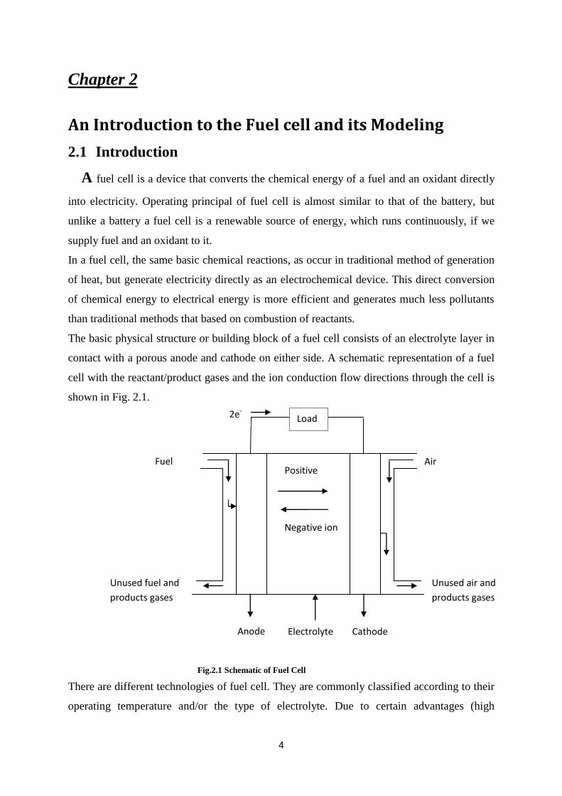
The basic physical structure or building block of a fuel cell consists of an electrolyte layer in

contact with a porous anode and cathode on either side. A schematic representation of a fuel

cell with the reactant/product gases and the ion conduction flow directions through the cell is

shown in Fig. 2.1.

Fig.2.1 Schematic of Fuel Cell

There are different technologies of fuel cell. They are commonly classified according to their

operating temperature and/or the type of electrolyte. Due to certain advantages (high

Positive

ion

Negative ion

Fuel

(H2)

Air

Electrolyte

Unused air and

products gases

out

Load

Unused fuel and

products gases

out

2e-

Cathode Anode

5

efficiency, low operating temperature) of PEM (polymer electrolyte membrane) fuel cell,

over other fuel cell, nowadays people prefer PEMFC to other conventional type fuel cell.

Polymer electrolyte membrane (PEM) fuel cells are the most popular type of fuel cell, and

traditionally use hydrogen as the fuel. PEM fuel cells also have many other fuel options,

which range from hydrogen to ethanol to biomass-derived materials. These fuels can either be

directly fed into the fuel cell, or sent to a reformer to extract pure hydrogen, which is then

directly fed to the fuel cell [5].

2.2 PEMFC Functionality

Fuel cells generate electricity from a simple electrochemical reaction in which an

oxidizer, typically oxygen from air, and a fuel, typically hydrogen, combine to form a

product, which is water for the typical fuel cell. Oxygen (air) continuously passes over the

cathode, and hydrogen passes over the anode to generate electricity, by-product heat and

water. As the name suggests, in between the anode and cathode terminals, there is a

membrane (electrolyte) can conduct only positive charge ion. Sulphonated polymer

(NAFLON) can be used as a membrane of the PEMFC.

The reactions are shown below.

Reaction at Anode:

eHH 442 2 (1)

Reaction at Cathode:

OHeHO 22 244

(2)

The electron freed at anode travels through another wire and react with the oxygen as well as

proton thus water is produced. When the electron travels through external circuit, electricity

is also produced.

Cathode and anode both have channel etched into it, which disperse the H2 gas equally over

the surface of the catalyst. Individual fuel cells can then be combined into a fuel cell stack to

take a desired power from the fuel cell. The number of fuel cells in the stack determines the

total voltage taken from the stack of fuel cell, and the surface area of each cell determines the

total current.

Modeling of PEMFC:

To achieve desirable performance characteristics, under certain constraints, Holistic

modeling of complex technical systems can constitute the first step. The model of fuel cell

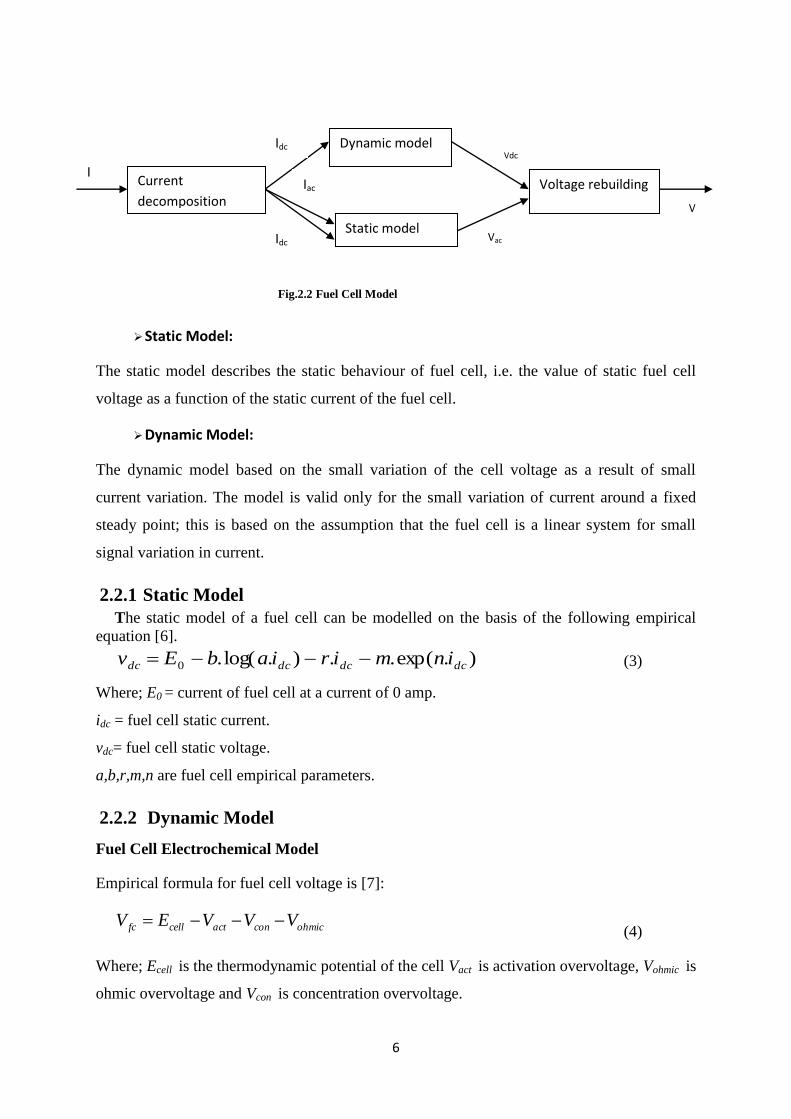
separated in two parts as denoted in Fig.2.2 [6]:

6

Fig.2.2 Fuel Cell Model

Static Model:

The static model describes the static behaviour of fuel cell, i.e. the value of static fuel cell

voltage as a function of the static current of the fuel cell.

Dynamic Model:

The dynamic model based on the small variation of the cell voltage as a result of small

current variation. The model is valid only for the small variation of current around a fixed

steady point; this is based on the assumption that the fuel cell is a linear system for small

signal variation in current.

2.2.1 Static Model

The static model of a fuel cell can be modelled on the basis of the following empirical

equation [6].

).exp(..).log(.0 dcdcdcdc inmiriabEv (3)

Where; E0 = current of fuel cell at a current of 0 amp.

idc = fuel cell static current.

vdc= fuel cell static voltage.

a,b,r,m,n are fuel cell empirical parameters.

2.2.2 Dynamic Model

Fuel Cell Electrochemical Model

Empirical formula for fuel cell voltage is [7]:

ohmicconactcellfc VVVEV (4)

Where; Ecell is the thermodynamic potential of the cell Vact is activation overvoltage, Vohmic is

ohmic overvoltage and Vcon is concentration overvoltage.

Static model

Dynamic model

model

Voltage rebuilding Current

decomposition

Idc

Idc

Iac

I

V

Vdc

Vac

7

I. Nernst voltage (ECell):

The overall reaction in a PEM fuel cell can be simply written as

OHOH 222 22 (5)

The Nernst equation for the hydrogen/oxygen fuel cell for the above reaction is [8]:

22,0 ln

2

1ln.

2

.oHcellcell PP

F

TREE

(6)

Where; T is the cell temperature (K), PH2 is the partial pressure of hydrogen at the anode

catalyst/gas interface (atm), and PO2 is the partial pressure of oxygen at the cathode

catalyst/gas interface (atm).E0,cell is a function of temperature and can be expressed as [9] :

)228(,00

,0 TkEE Ecellcell (7)

II. Activation loss (Vact):

The activation overvoltage is the voltage drop due to the activation of the anode and the

cathode. Tafel equation, given below, is used to calculate activation overvoltage in a fuel cell

[9]:

Fcact iTcoTTV ln)ln( 42321 (8)

Where; iFc is cell operating current and ξ1, ξ2, ξ3 ,ξ4 are parametric coefficient of fuel cell

,Co2 is the concentration of dissolved oxygen at liquid gas interface. The value of Co2 can be

estimated by using [10]:

T

o

o

e

PC

498

6

2

2

10.08.5

(9)

III. Ohmic loss (Vohmic)

Ohmic loss of fuel cell using ohm‟s law is:

prelFcohmic RRiV .

(10)

Where; Rel is the resistance produced by membrane to electron flow, and RPr is the

resistance to proton flow.

RPr is usually considered to be constant quantity whereas Rel is given by the following

equation [11]

8

A

lR mel

(11)

Where; l is membrane thickness (cm), A is the cell active area (cm2), and ρm is specific

resistivity of membrane for the electron flow (Ώ.cm), which for the Naflon type membrane

can be given by [12]:

T

T

A

i

A

iT

A

i

Fc

FcFc

m303

18.4exp.3634.0

303062.0.03.016.181

5.22

(12)

IV. Concentration Voltage Drop:

During the reaction process, concentration gradients can be formed due to mass diffusions

from the flow channels to the reaction sites (catalyst surfaces). At high current densities, slow

transportation of reactants (products) to (from) the reaction sites is the main reason for the

concentration voltage drop [13]. This voltage is given by [1].

max

1ln.j

jBVCon

(13)

Where: B represents a parametric coefficient (v), and j represents the actual current density of

the cell (A/cm2) and jmax is the limiting current density.

Applying assumption that parameters for individual cells can be lumped together to represent

a fuel-cell stack, the output voltage of the fuel-cell stack can be written as [14]:

)(. conohmicactcellcellcellcellout vvvENvNv (14)

Where; Ncell = Number of fuel cell in stack.

Vcell = fuel cell voltage.

Ecell = Thermodynamic potential of the fuel cell.

vact,vcon,vohmic are losses, introduced into the fuel cell.

v. Double layer charging effect:

In a PEM fuel cell, the two electrodes are separated by a solid membrane (Fig. 2.1) which

only allows the H+ ions to pass, but prevents the motion of electrons [7],[13]. The electrons at

the anode will flow through the external load and comes to the surface of the cathode, to

which the protons of hydrogen will be attracted at the same time. Thus, two charged layers of

9

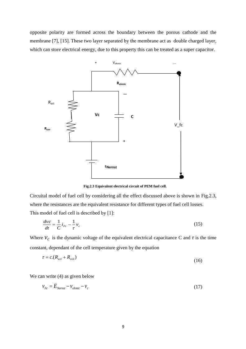
opposite polarity are formed across the boundary between the porous cathode and the

membrane [7], [15]. These two layer separated by the membrane act as double charged layer,

which can store electrical energy, due to this property this can be treated as a super capacitor.

Fig.2.3 Equivalent electrical circuit of PEM fuel cell.

Circuital model of fuel cell by considering all the effect discussed above is shown in Fig.2.3,

where the resistances are the equivalent resistance for different types of fuel cell losses.

This model of fuel cell is described by [1]:

cFc vi

Cdt

dvc

11

(15)

Where vc is the dynamic voltage of the equivalent electrical capacitance C and τ is the time

constant, dependant of the cell temperature given by the equation

).( conact RRc (16)

We can write (4) as given below

cohmicNernstFc vvEv (17)

+ Vohmic -―

Ract

Rcon

C

+

―

Vc

ENernst

V_fc

Rohmic

10

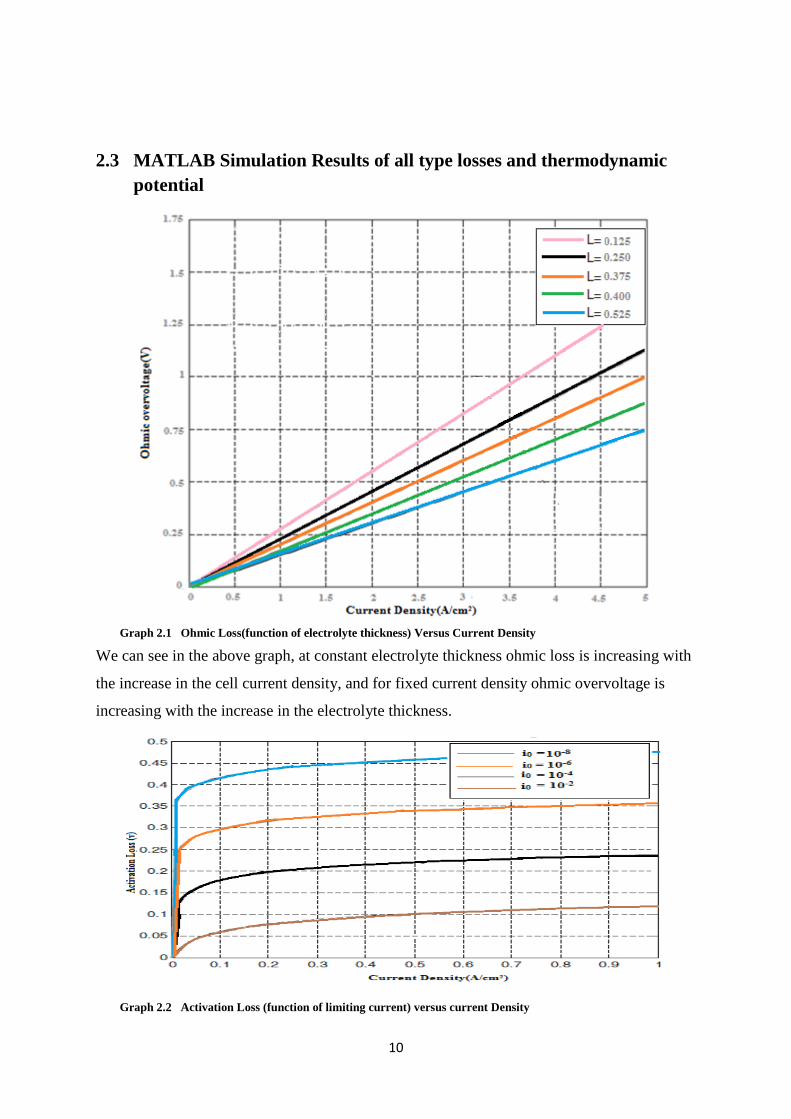
2.3 MATLAB Simulation Results of all type losses and thermodynamic

potential

Graph 2.1 Ohmic Loss(function of electrolyte thickness) Versus Current Density

We can see in the above graph, at constant electrolyte thickness ohmic loss is increasing with

the increase in the cell current density, and for fixed current density ohmic overvoltage is

increasing with the increase in the electrolyte thickness.

Graph 2.2 Activation Loss (function of limiting current) versus current Density

11

In the above graph we can see that at a fixed value of limiting current activation loss is

increasing with the increase in Cell current density, and at a fixed value of the current density

activation loss increasing with increase in limiting current.

If the exchange current is very large, the system will supply large currents with very small

activation overvoltage. If a system has an extremely small exchange current density, no

significant current will flow unless large activation overpotential is applied.

Graph 2.3 Activation Loss(function of transfer coefficient) versus fuel cell current density

Activation loss shown in the above graph (Graph 2.3) is increasing with the increase in the

cell current density, however it is decreasing with the increase in the transfer coefficient

(denoted as alpha in the graph). In order to simulate the entropy of fuel, water and oxidant,

we have taken the value of different parameter, as given in table 2.1.

Table 2.1

Name of parameters Value

Temperature 353(K)

Reference Temperature 298(K)

Moles of Hydrogen 2.016

Moles of oxygen 31.999

Enthalpy of O2 at standard

state

0

Enthalpy of H2 at standard

state

0

Moles of H2O 18

Enthalpy at standard state of

water in liquid phase(J/mol)

-285 826

Enthalpy at standard state of

water in gas phase(J/mol)

-241 826

12

Graph 2.4 Entropy of H2,O2 and H2o versus temperature

Entropy of H2, H2o and O2, in the above graph has obtained with the help of the parameter

given in the table 2.1.

Graph 2.5 Concentration Loss versus cell current density

Concentration overvoltage of fuel cell in the above graph is decreasing with the increase in

cell current density.

13

Summary: Fuel cell is a renewable source of energy. Due to double charge layer effect, fuel cell can act

like an ultra capacitor. There are different types of losses associated with fuel cell, which

causes reduction in the cell voltage. In this chapter the modeling of different type of losses

and thermodynamic potential has discussed. Dynamic model of fuel cell converted into the

electric circuital model, consists of resistance (equivalent to losses), electrical capacitance

and a voltage source (ENernst).

13

Chapter3

Buck and Boost Converter

Circuit Topologies

14

Chapter 3

Buck and Boost Converter Circuit Topologies

3.1 Introduction

Buck and boost Converter used in Switched Mode Power Supply abbreviated as SMPS is

nothing but a dc-to-dc switching converter for the conversion of unregulated dc input voltage

to regulated dc output voltage. The switch employed in SMPS is turned „ON‟ and „OFF‟

(referred as switching) at a high frequency, with the help of an external switching circuit.

During „ON‟ state of the switch, the transistor acting as a switch will be in saturation mode

with negligible voltage drop across the collector and emitter terminals of the switch, whereas

in „OFF‟ state the transistor acting as a switch will be in cut-off mode with negligible current

through the collector and emitter terminals. Unlike in the voltage-regulating switch, a linear

regulator circuit always remains in the active region, which results in low efficiency, only

applicable to low power application. SMPS is well suited for high power applications.

3.2 Buck Converter working principle

The operation of the buck converter is very simple, with an inductor and two switches (a

transistor and a diode) that control the inductor. Two switches come into action and alternate

between connecting the inductor to voltage source to store energy in the inductor and

discharging it into the connecting load. The inductor L and capacitor C in Fig.3.1 contributes

into the filtering to avoid from the current, and voltage ripple respectively. Diode in the

figure is a freewheeling diode, to ensure a continuous flow of the current into the circuit. The

output voltage of the circuit can be controlled by the duty cycle D given byT

tD on . Output

voltage vo is always lower than input voltage vi hence, we can also call this converter a “Buck

Converter”.

15

Fig.3.1 Schematic of Buck Converter

There are two basic modes in which Buck Converter operates:

(a) Continuous mode:

A buck converter operates in continuous mode if current through inductor never falls to

zero, during the commutation cycle. Its operating principle is described by the Fig.3.2. When

the switch shown above is closed, the voltage across the inductor is vl = vi-vo. The current

through inductor rises linearly. As the diode is reverse biased by the voltage source, no

current flows through it.

When the switch is opened the diode D becomes forward biased.

Current iL decreases.

The rate of change of current iL can be calculated from:

dt

diLv L

L (3.1)

Increase in current during on state can be calculated from [16]:

on

oi

T

LonL T

L

vvdt

L

vi

on

.0

,

(3.2)

The decrease in inductor current is given by [16]:

off

T

LoffL T

L

vodt

L

vi

off

.0

,

(3.3)

R C D

E S L

+

-

V0

16

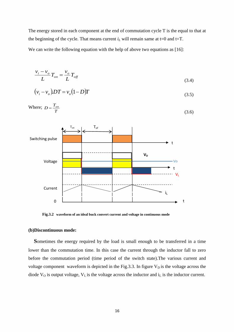
The energy stored in each component at the end of commutation cycle T is the equal to that at

the beginning of the cycle. That means current iL will remain same at t=0 and t=T.

We can write the following equation with the help of above two equations as [16]:

off

oon

oi TL

vT

L

vv

(3.4)

TDvDTvv ooi 1.

(3.5)

Where; T

TD on

(3.6)

Fig.3.2 waveform of an ideal buck convert current and voltage in continuous mode

(b)Discontinuous mode:

Sometimes the energy required by the load is small enough to be transferred in a time

lower than the commutation time. In this case the current through the inductor fall to zero

before the commutation period (time period of the switch state).The various current and

voltage component waveform is depicted in the Fig.3.3. In figure VD is the voltage across the

diode VO is output voltage, VL is the voltage across the inductor and iL is the inductor current.

VL

t

t

t

Vo

VD

iL Current

Voltage

Switching pulse

Ton Tof

f

0

17

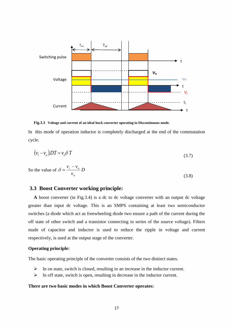
Fig.3.3 Voltage and current of an ideal buck converter operating in Discontinuous mode.

In this mode of operation inductor is completely discharged at the end of the commutation

cycle.

TvDTvv ooi .

(3.7)

So the value of Dv

vv

o

oi

(3.8)

3.3 Boost Converter working principle:

A boost converter (in Fig.3.4) is a dc to dc voltage converter with an output dc voltage

greater than input dc voltage. This is an SMPS containing at least two semiconductor

switches (a diode which act as freewheeling diode two ensure a path of the current during the

off state of other switch and a transistor connecting in series of the source voltage). Filters

made of capacitor and inductor is used to reduce the ripple in voltage and current

respectively, is used at the output stage of the converter.

Operating principle:

The basic operating principle of the converter consists of the two distinct states.

In on state, switch is closed, resulting in an increase in the inductor current.

In off state, switch is open, resulting in decrease in the inductor current.

There are two basic modes in which Boost Converter operates:

t

t

t

Vo

VD

iL Current

Voltage

Switching pulse

Ton Tof

f

VL

18

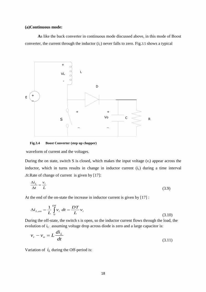
(a)Continuous mode:

As like the buck converter in continuous mode discussed above, in this mode of Boost

converter, the current through the inductor (iL) never falls to zero. Fig.3.5 shows a typical

Fig.3.4 Boost Converter (step up chopper)

waveform of current and the voltages.

During the on state, switch S is closed, which makes the input voltage (vi) appear across the

inductor, which in turns results in change in inductor current (iL) during a time interval

Δt.Rate of change of current is given by [17]:

L

v

t

i iL

(3.9)

At the end of the on-state the increase in inductor current is given by [17] :

i

DT

ionL vL

DTdtv

Li

0

,

1

(3.10)

During the off-state, the switch s is open, so the inductor current flows through the load, the

evolution of iL’, assuming voltage drop across diode is zero and a large capacitor is:

dt

diLvv L

oi (3.11)

Variation of iL during the Off-period is:

C S

E

L

-

+

VL

D

+

_

+

_

Vo R

19

TD

L

vvdt

L

vvi oi

DT

T

oioffL

1,

(3.12)

The energy stored in each component at the end of commutation cycle T is the equal to that at

the beginning of the cycle. That means overall change in current is zero [17]:

0 LoffLon ii

(3.13)

Substituting Loni and Loffi by their expression in above equation we get [17]

01

TD

L

voviDT

L

viii LoffLon

(3.14)

This can be written as [17]:

Dv

v

i

o

1

1

(3.15)

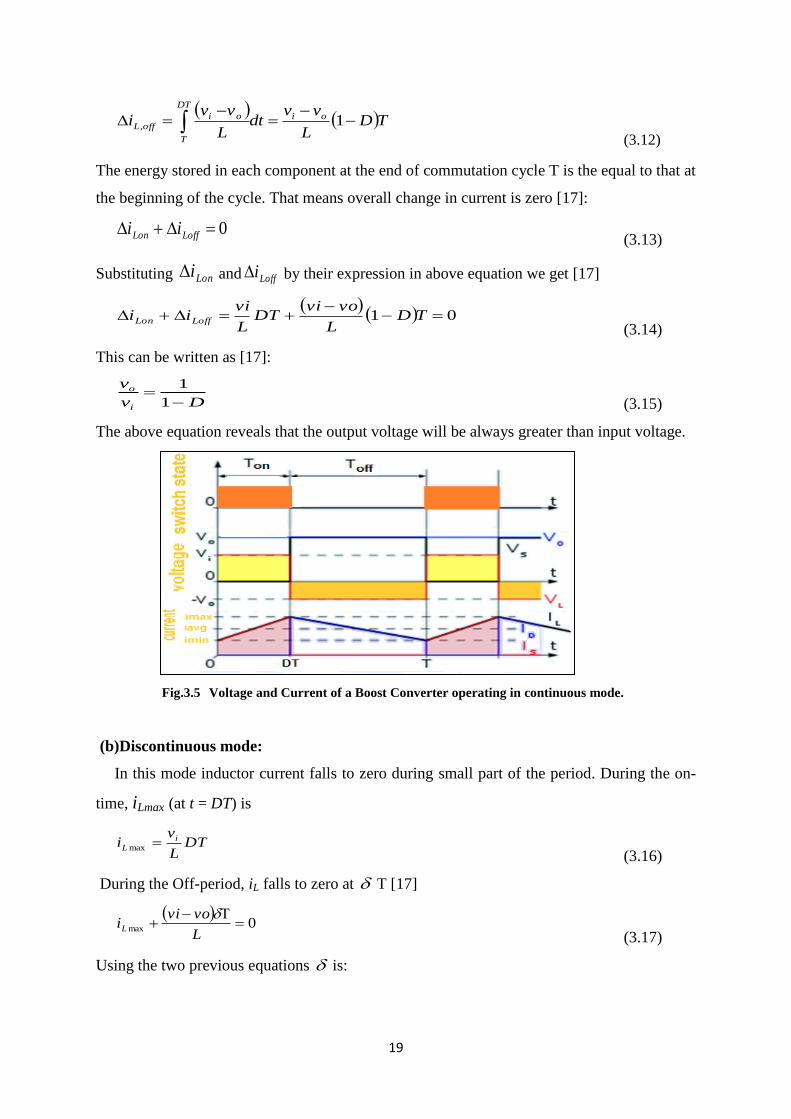
The above equation reveals that the output voltage will be always greater than input voltage.

Fig.3.5 Voltage and Current of a Boost Converter operating in continuous mode.

(b)Discontinuous mode:

In this mode inductor current falls to zero during small part of the period. During the on-

time, iLmax (at t = DT) is

DT

L

vi i

L max

(3.16)

During the Off-period, iL falls to zero at T [17]

0max

L

voviiL

(3.17)

Using the two previous equations is:

20

vivo

Dvi

(3.18)

Load current is given by the average diode current [17]

2

max

max

L

DL

iii

(3.19)

Replacing iLmax and by their respective expressions the following relation yields [17]:

io

iii

ovvL

TDv

vivo

Dv

L

DTvi

2.

2

22

(3.20)

Output and input voltage ratio can be expressed as [17]:

o

i

i

o

Li

TDv

v

v

21

2

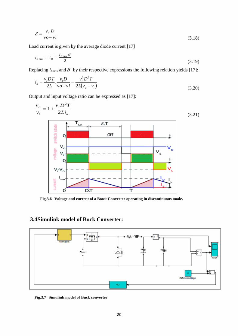
(3.21)

Fig.3.6 Voltage and current of a Boost Converter operating in discontinuous mode.

3.4 Simulink model of Buck Converter:

Fig.3.7 Simulink model of Buck converter

21

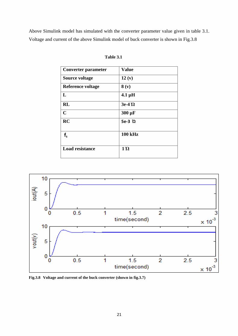
Above Simulink model has simulated with the converter parameter value given in table 3.1.

Voltage and current of the above Simulink model of buck converter is shown in Fig.3.8

Table 3.1

Fig.3.8 Voltage and current of the buck converter (shown in fig.3.7)

Converter parameter Value

Source voltage 12 (v)

Reference voltage 8 (v)

L 4.1 µH

RL 3e-4 Ώ

C 300 µF

RC 5e-3 Ώ

fs 100 kHz

Load resistance 1 Ώ

22

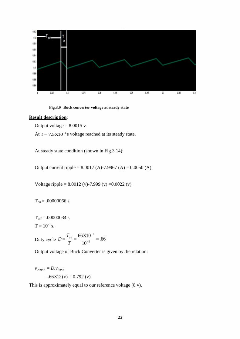
Fig.3.9 Buck converter voltage at steady state

Result description:

Output voltage = 8.0015 v.

At 4105.7 t s voltage reached at its steady state.

At steady state condition (shown in Fig.3.14):

Output current ripple = 8.0017 (A)-7.9967 (A) = 0.0050 (A)

Voltage ripple = 8.0012 (v)-7.999 (v) =0.0022 (v)

Ton = .00000066 s

Toff =.00000034 s

T = 10-5

s.

Duty cycle 66.10

10665

7

T

TD on

Output voltage of Buck Converter is given by the relation:

voutput = D.vinput

= 1266. (v) = 0.792 (v).

This is approximately equal to our reference voltage (8 v).

23

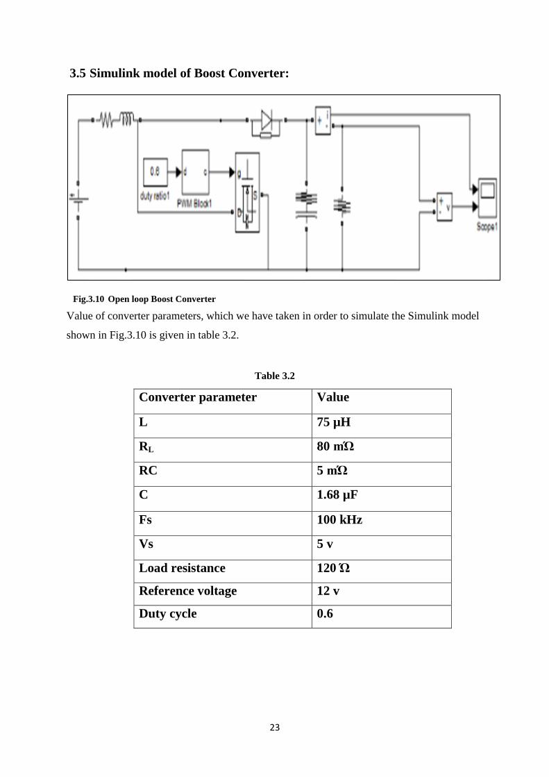
3.5 Simulink model of Boost Converter:

Fig.3.10 Open loop Boost Converter

Value of converter parameters, which we have taken in order to simulate the Simulink model

shown in Fig.3.10 is given in table 3.2.

Table 3.2

Converter parameter Value

L 75 µH

RL 80 mΏ

RC 5 mΏ

C 1.68 µF

Fs 100 kHz

Vs 5 v

Load resistance 120 Ώ

Reference voltage 12 v

Duty cycle 0.6

t

24

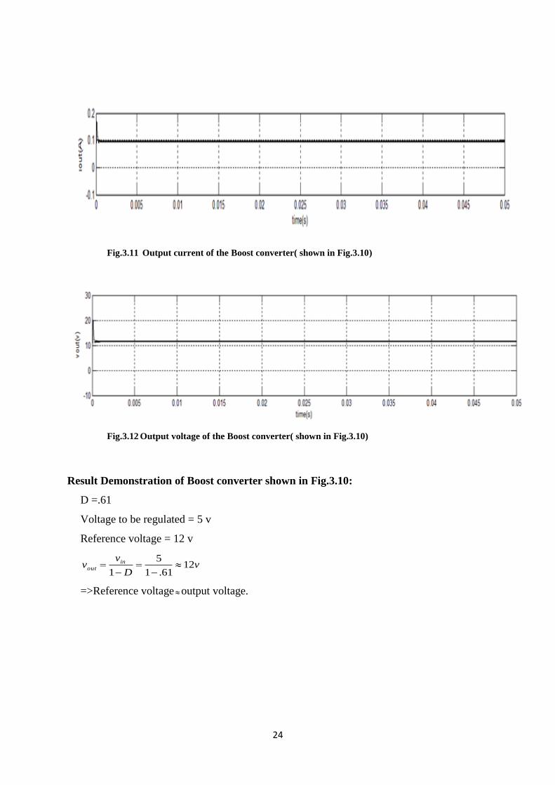
Fig.3.11 Output current of the Boost converter( shown in Fig.3.10)

Fig.3.12 Output voltage of the Boost converter( shown in Fig.3.10)

Result Demonstration of Boost converter shown in Fig.3.10:

D =.61

Voltage to be regulated = 5 v

Reference voltage = 12 v

vD

vv in

out 1261.1

5

1

=>Reference voltage output voltage.

25

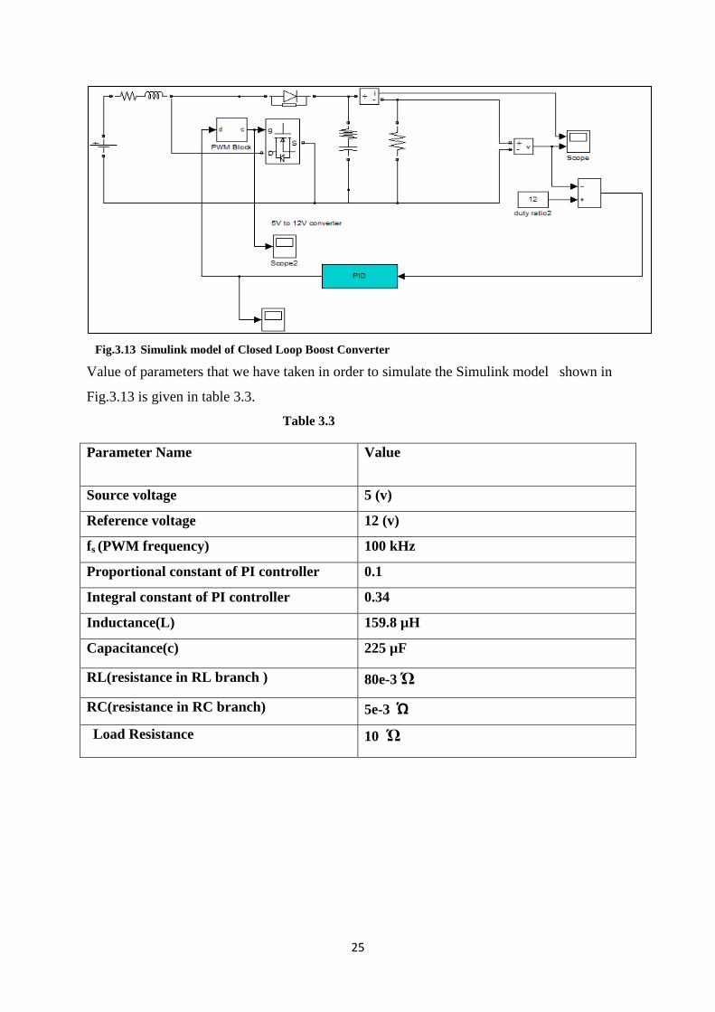
Fig.3.13 Simulink model of Closed Loop Boost Converter

Value of parameters that we have taken in order to simulate the Simulink model shown in

Fig.3.13 is given in table 3.3.

Table 3.3

Parameter Name Value

Source voltage 5 (v)

Reference voltage 12 (v)

fs (PWM frequency) 100 kHz

Proportional constant of PI controller 0.1

Integral constant of PI controller 0.34

Inductance(L) 159.8 µH

Capacitance(c) 225 µF

RL(resistance in RL branch ) 80e-3 Ώ

RC(resistance in RC branch) 5e-3 Ώ

Load Resistance 10 Ώ

26

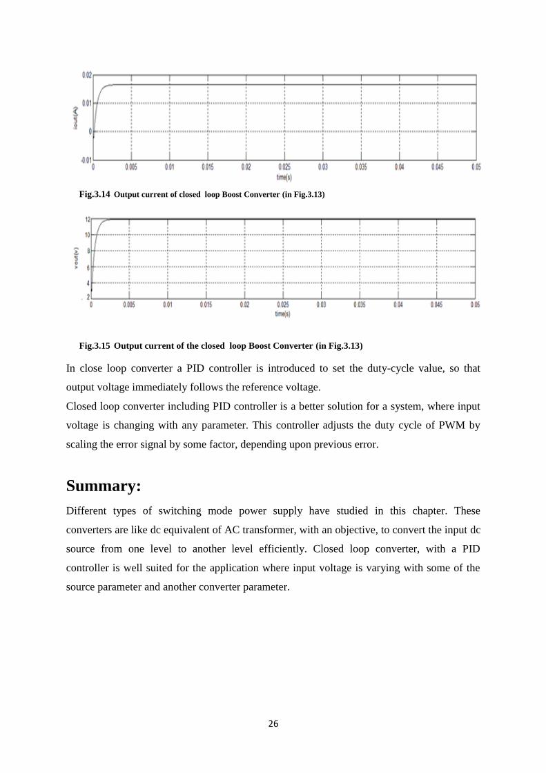
Fig.3.14 Output current of closed loop Boost Converter (in Fig.3.13)

Fig.3.15 Output current of the closed loop Boost Converter (in Fig.3.13)

In close loop converter a PID controller is introduced to set the duty-cycle value, so that

output voltage immediately follows the reference voltage.

Closed loop converter including PID controller is a better solution for a system, where input

voltage is changing with any parameter. This controller adjusts the duty cycle of PWM by

scaling the error signal by some factor, depending upon previous error.

Summary:

Different types of switching mode power supply have studied in this chapter. These

converters are like dc equivalent of AC transformer, with an objective, to convert the input dc

source from one level to another level efficiently. Closed loop converter, with a PID

controller is well suited for the application where input voltage is varying with some of the

source parameter and another converter parameter.

27

Chapter 4

Fuel Cell System

27

Chapter 4

Fuel Cell System

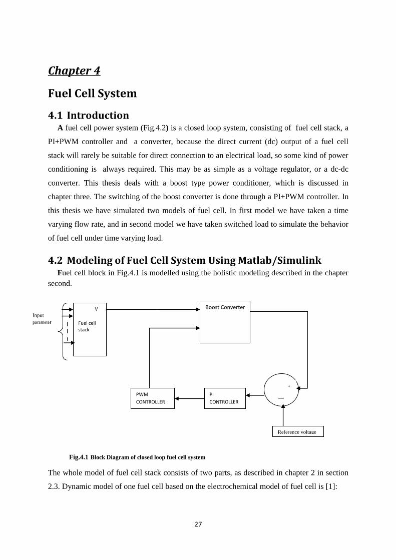
4.1 Introduction A fuel cell power system (Fig.4.2) is a closed loop system, consisting of fuel cell stack, a

PI+PWM controller and a converter, because the direct current (dc) output of a fuel cell

stack will rarely be suitable for direct connection to an electrical load, so some kind of power

conditioning is always required. This may be as simple as a voltage regulator, or a dc-dc

converter. This thesis deals with a boost type power conditioner, which is discussed in

chapter three. The switching of the boost converter is done through a PI+PWM controller. In

this thesis we have simulated two models of fuel cell. In first model we have taken a time

varying flow rate, and in second model we have taken switched load to simulate the behavior

of fuel cell under time varying load.

4.2 Modeling of Fuel Cell System Using Matlab/Simulink Fuel cell block in Fig.4.1 is modelled using the holistic modeling described in the chapter

second.

Fig.4.1 Block Diagram of closed loop fuel cell system

The whole model of fuel cell stack consists of two parts, as described in chapter 2 in section

2.3. Dynamic model of one fuel cell based on the electrochemical model of fuel cell is [1]:

PI

CONTROLLER

V

Fuel cell stack

Boost Converter

Input

parameter

Reference voltage

PWM

CONTROLLER

+

―

28

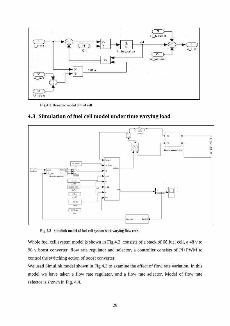
Fig.4.2 Dynamic model of fuel cell

4.3 Simulation of fuel cell model under time varying load

Fig.4.3 Simulink model of fuel cell system with varying flow rate

Whole fuel cell system model is shown in Fig.4.3, consists of a stack of 68 fuel cell, a 48 v to

96 v boost converter, flow rate regulator and selector, a controller consists of PI+PWM to

control the switching action of boost converter.

We used Simulink model shown in Fig.4.3 to examine the effect of flow rate variation. In this

model we have taken a flow rate regulator, and a flow rate selector. Model of flow rate

selector is shown in Fig. 4.4.

29

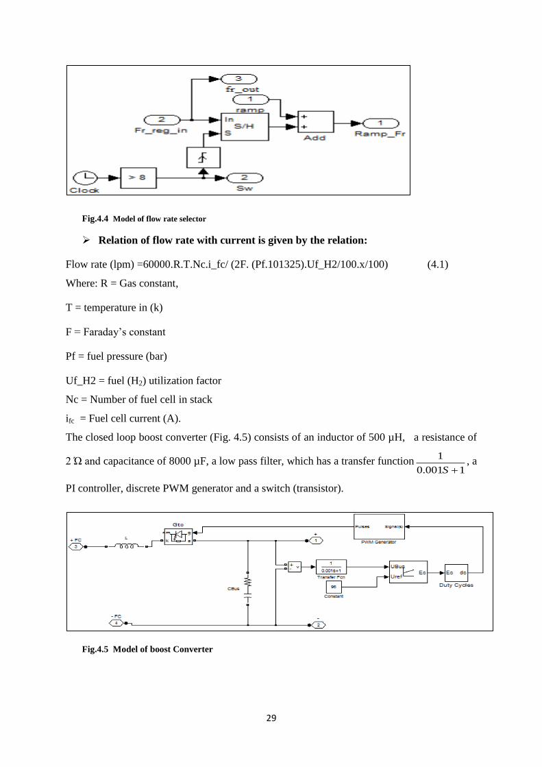
Fig.4.4 Model of flow rate selector

Relation of flow rate with current is given by the relation:

Flow rate (lpm) =60000.R.T.Nc.i_fc/ (2F. (Pf.101325).Uf_H2/100.x/100) (4.1)

Where: R = Gas constant,

T = temperature in (k)

F = Faraday‟s constant

Pf = fuel pressure (bar)

Uf_H2 = fuel (H2) utilization factor

Nc = Number of fuel cell in stack

ifc = Fuel cell current (A).

The closed loop boost converter (Fig. 4.5) consists of an inductor of 500 µH, a resistance of

2 Ώ and capacitance of 8000 µF, a low pass filter, which has a transfer function1001.0

1

S, a

PI controller, discrete PWM generator and a switch (transistor).

Fig.4.5 Model of boost Converter

30

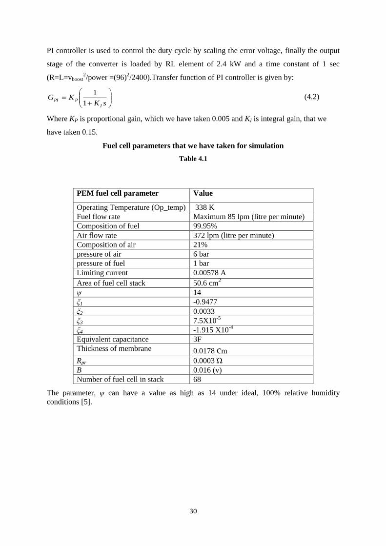
PI controller is used to control the duty cycle by scaling the error voltage, finally the output

stage of the converter is loaded by RL element of 2.4 kW and a time constant of 1 sec

(R=L=vboost2/power =(96)

2/2400).Transfer function of PI controller is given by:

sKKG

I

PPI1

1 (4.2)

Where KP is proportional gain, which we have taken 0.005 and KI is integral gain, that we

have taken 0.15.

Fuel cell parameters that we have taken for simulation

Table 4.1

The parameter, ψ can have a value as high as 14 under ideal, 100% relative humidity

conditions [5].

PEM fuel cell parameter Value

Operating Temperature (Op_temp) 338 K

Fuel flow rate Maximum 85 lpm (litre per minute)

Composition of fuel 99.95%

Air flow rate 372 lpm (litre per minute)

Composition of air 21%

pressure of air 6 bar

pressure of fuel 1 bar

Limiting current 0.00578 A

Area of fuel cell stack 50.6 cm2

ψ 14

ξ1 -0.9477

ξ2 0.0033

ξ3 7.5X10-5

ξ4 -1.915 X10-4

Equivalent capacitance 3F

Thickness of membrane 0.0178 cm

Rpr 0.0003 Ώ

B 0.016 (v)

Number of fuel cell in stack 68

31

4.3.1 Simulation Results of the fuel cell system model with

varying flow rate :

Graph 4.1 Flow rate versus time

In the above graph flow rate has changed at 8 s, from 16 lpm to 85 lpm, during the time

interval 3.5 s.

Graph 4.2 Utilization of fuel and oxidant (air)

32

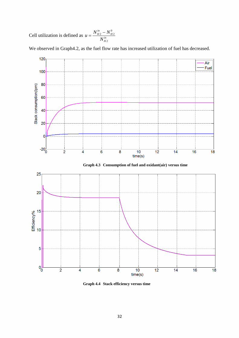
Cell utilization is defined as in

H

H

in

H

N

NNu

2

0

22

We observed in Graph4.2, as the fuel flow rate has increased utilization of fuel has decreased.

Graph 4.3 Consumption of fuel and oxidant(air) versus time

Graph 4.4 Stack efficiency versus time

33

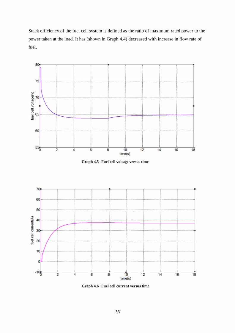
Stack efficiency of the fuel cell system is defined as the ratio of maximum rated power to the

power taken at the load. It has (shown in Graph 4.4) decreased with increase in flow rate of

fuel.

Graph 4.5 Fuel cell voltage versus time

Graph 4.6 Fuel cell current versus time

34

Graph 4.7 Boost output voltage versus time

Graph 4.8 Boost output current versus time

35

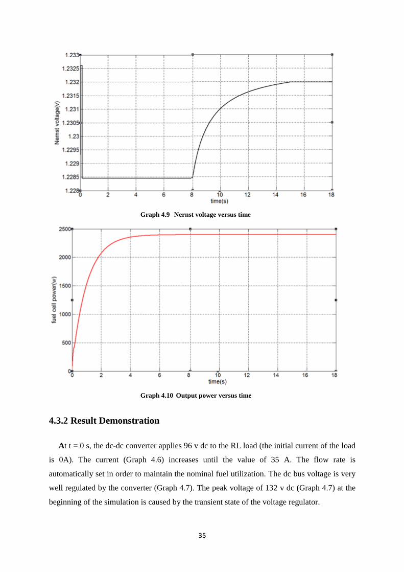
Graph 4.9 Nernst voltage versus time

Graph 4.10 Output power versus time

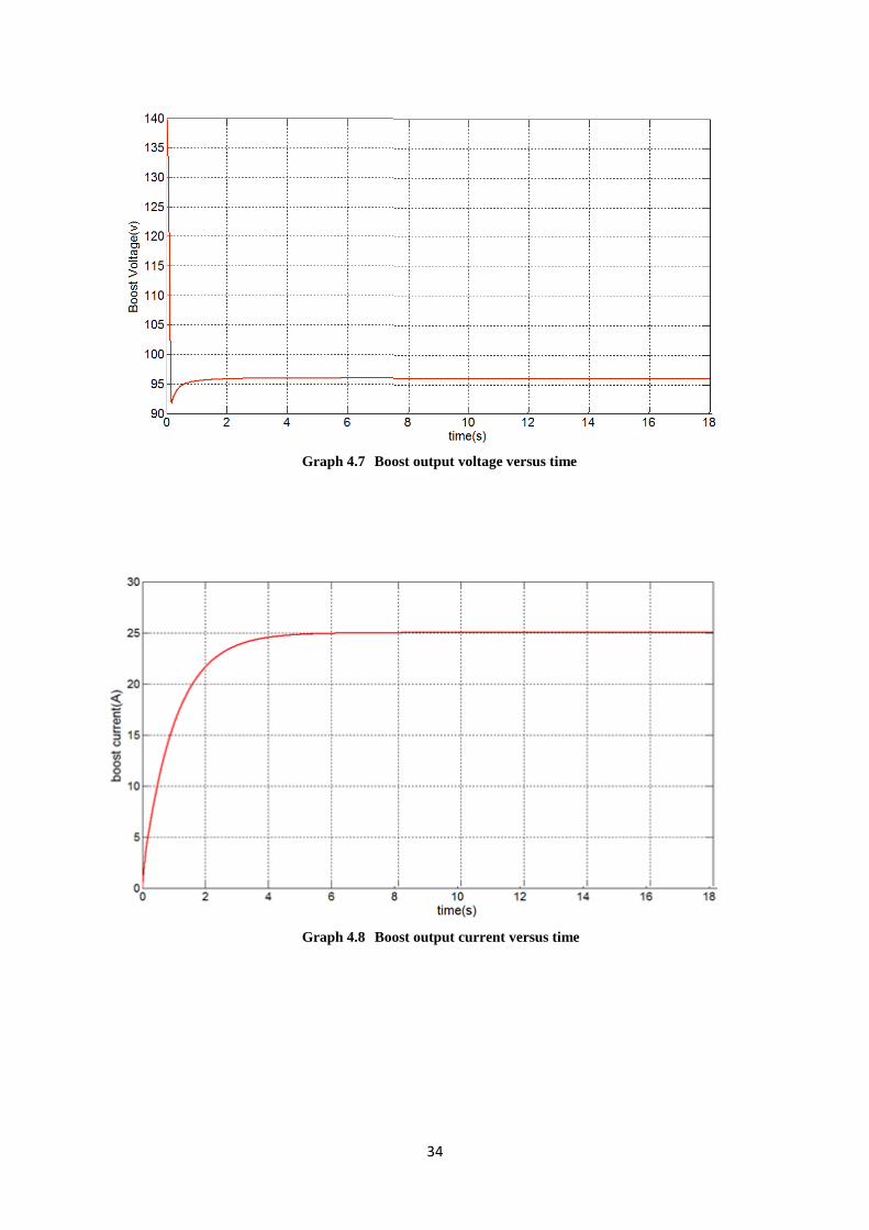
4.3.2 Result Demonstration

At t = 0 s, the dc-dc converter applies 96 v dc to the RL load (the initial current of the load

is 0A). The current (Graph 4.6) increases until the value of 35 A. The flow rate is

automatically set in order to maintain the nominal fuel utilization. The dc bus voltage is very

well regulated by the converter (Graph 4.7). The peak voltage of 132 v dc (Graph 4.7) at the

beginning of the simulation is caused by the transient state of the voltage regulator.

36

At t = 8 s, the fuel flow rate is increased from 18 litres per minute (lpm) to 85 lpm during 3.5

s (Graph4.1), reducing by doing so the hydrogen utilization (Graph 4.2). This causes an

increasing of the Nernst voltage (thermodynamic potential) (Graph 4.9), so the fuel cell

current will decrease (Graph 4.6). Therefore the stack consumption (Graph 4.3) and the

efficiency (Graph4.4) will decrease.

4.4 Simulation of fuel cell system model under time varying load In order to simulate the fuel cell system under the variation of load, we have taken

another Simulink model (Fig. 4.6) to examine the regulation of the output voltage with the

variation of the load with time.

Figure 4.6 Fuel cell system with switched load model

Fig.4.6 Simulink model of fuel cell system under switched load

In this Simulink model we have used the entire component same as first Simulink model,

except for the time varying load. The variation of the load is done through two parallel load

connecting at the terminal of the RL load, whose connectivity is changed at a regular interval

of 5 s with the help of a switch, to see the changes in the output voltage, current and the rated

power.

37

4.4.1 Simulation Results

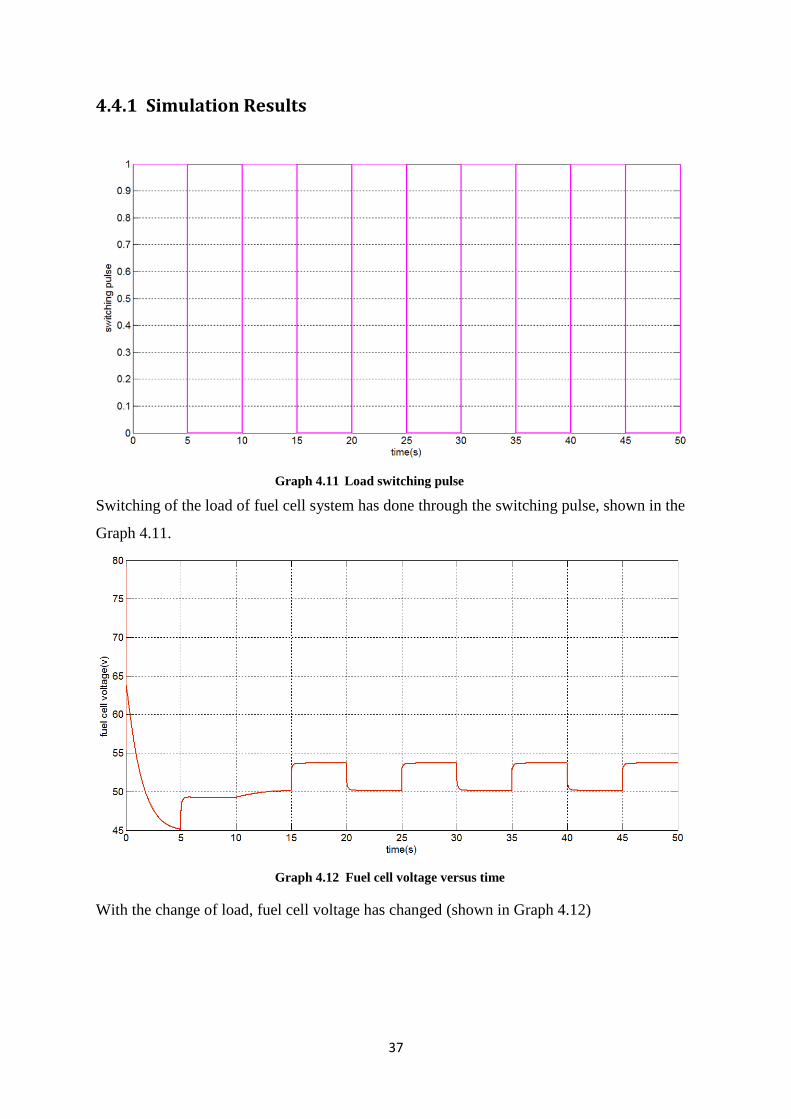
Graph 4.11 Load switching pulse

Switching of the load of fuel cell system has done through the switching pulse, shown in the

Graph 4.11.

Graph 4.12 Fuel cell voltage versus time

With the change of load, fuel cell voltage has changed (shown in Graph 4.12)

38

Graph 4.13 Boost output voltage versus time

At the switching instant of the load boost voltage has change for a very short time interval

(shown in Graph 4.13), this is what we were looking for.

\

Graph 4.14 Boost output current versus time

39

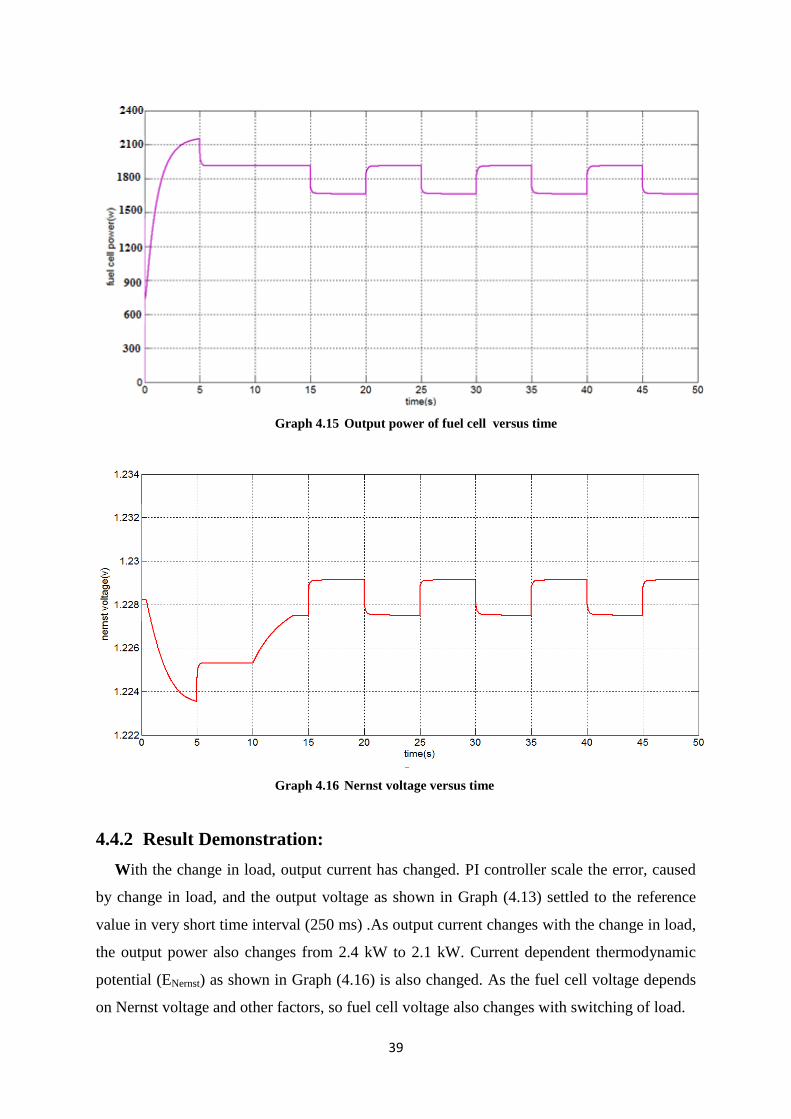
Graph 4.15 Output power of fuel cell versus time

Graph 4.16 Nernst voltage versus time

4.4.2 Result Demonstration:

With the change in load, output current has changed. PI controller scale the error, caused

by change in load, and the output voltage as shown in Graph (4.13) settled to the reference

value in very short time interval (250 ms) .As output current changes with the change in load,

the output power also changes from 2.4 kW to 2.1 kW. Current dependent thermodynamic

potential (ENernst) as shown in Graph (4.16) is also changed. As the fuel cell voltage depends

on Nernst voltage and other factors, so fuel cell voltage also changes with switching of load.

40

Summary:

Fuel cell system is an energy system, whose output voltage (v_fc) depends on so many

parameters, which makes it complex system. Output voltage of this energy system will

change with any of the parameter variation. Voltage of this system under the flow rate

variation and load variation is very well regulated by the converter with a PI controller.

Chapter 5

Implementation of Fuel Cell System

Using VHDL and Hardware

Prototyping of (PI+PWM)

41

Chapter 5

Implementation of Fuel Cell System Using VHDL and

hardware Prototyping of (PI+PWM)

5.1 Introduction: The recent advancement of VLSI technology, strongly enabled by Electronic Design

Automation (EDA) tools has created the opportunity for the development of complex and

compact high performance controllers for power electronic systems [1]. This approach

extends the use of high level digital language to make a high efficient controller for a

complex electrical circuit. This has made possible due to the synthesis of the whole system in

a single environment.

To achieve a high precision, floating type package of 32 bit (fphdl32_pkg) has added to the

VHDL library.

Complex equations like logarithmic and exponential function has approximated by using its

expansion series (Taylor series). We had applied differentiation and integration by numerical

method (Euler Forward method) e.g. differentiation of y with respect to x is given by

nn

nn

xx

yy

dx

dy

1

1 .

Boost current has been discretized using the equation [18].

)1.5()()1(

)1(

R

Ve

R

Vni

L

DTVni

fcL

TDRfcfc

5.2 Implementation of Dynamic model of Fuel cell

We have seen in chapter 2, only three parameters, activation overvoltage, ohmic voltage

and concentration overvoltage of dynamic model (electrochemical model) depends on the

fuel cell current. In order to reasonably simplify the solution of dynamic model, we have

taken two look up table, one for ohmic overvoltage, and other for activation overvoltage, as

expression for concentration overvoltage is simple we have directly applied this by Taylor

series expansion method. We have taken, such values in look-up tables, which can give better

approximation after implying it through convolution linear curve fitting equation. In order to

42

simplifying the dynamic model, the partial pressure of hydrogen PH2 of the fuel cell system is

normally kept constant, and the temperature is also kept constant. With these assumptions,

the dynamic model of the fuel cell can be implemented in a simple way.

5.3 Converter part implementation

The boost converter, fuel cell and load are simulated with a sample time Ts = 100 μs. The

controller is simulated with a higher sample time Ts = 10 ms, since the FCS‟s dominant time

constant is much higher [1]. The main reason to take short sample time is to reduce errors

confine distortion and strengthen the stability. We have taken resolution (maximum number

of pulses that we can pack into a PWM period) of the PWM 100 and frequency of the PWM

is set equal to controller sampling frequency. Generation of PWM has done with the counter

based topology.

5.4 PWM implementation PWM is a modulation technique that generates variable width pulses to represent the

amplitude of an analog input signal.

Pulse width modulation (PWM) is a powerful technique for controlling analog circuits with a

processor's digital outputs. PWM is employed in a wide variety of applications, ranging from

measurement and communications to power control and conversion. Through the use of high

resolution counter, the duty cycle is modulated to encode a particular analog signal.

PWM signals are typically created by using a clock at some multiple of the switching

frequency with a counter [19].

In order to get less quantization error of the duty cycle we have taken resolution of the PWM

100. As more bits of resolution are added to the error sample, the digital system starts to

approach a linear analog controller.

It is impossible to choose frequency small enough to give fast transient performance without

destabilizing the feedback loop, so we have limit the frequency of the PWM equal to

controller sampling frequency.

There are various methods to generate PWM; few of them are described here.

5.4.1 High frequency counter based PWM Generator

This architecture in Fig. 5.1 was proposed by E.Koutroulis , A.Dollas and K.Kalaitzakis in

[19].

43

In this architecture there is a high speed N-bit free running counter, N-bit register and N-bit

comparator. Output, coming from counter is used to be compared with register output, which

stores desired input duty cycle (N-bit value), with the help of comparator. The comparator output

is set equal to “1” when both counter and register output values are equal. This comparator output

is used to set RS latch. The overflow signal gets high when counter reach to its maximum value.

This overflow signal is used to reset RS latch, and to load new input data in register. The output

of RS latch gives the PWM output. It can be used to generate High-frequency PWM output which

is not possible in normal counter based approach.

Fig.5.1 Architecture of PWM Generator proposed by E. Koutroulis

5.4.2 Counter based PWM Generator

In digital systems, PWM signals are typically created by using a clock at some multiple of

the switching frequency with a counter. The PWM signal is set high at the beginning of a

switching period and then reset after the counter detects that some number of cycles of the

faster clock have passed [20].

Counter clock frequency in this architecture is chosen to be 2N

times of the switching

frequency of the converter, where N is the number of bits. This architecture is well suited for

ultrafast clocked-counters. Architecture of this type of digital PWM generator is depicted as

below in the Fig.5.2. This is acceptable for dc–dc converters that deliver power in the watt

range, but not for systems in the milli watt range.

off

Nbit counter

out

Register

N bit input

R

S

G

N bit comparator

H equal

out

Q

Pwm out

Clock

44

Fig.5.2 Architecture of Counter based PWM Generator proposed by A.P Dancy.

5.4.3 Cascaded Counter based PWM generator

Fig.5.3 Cascade counter based PWM generator

In this architecture shown in Fig.5.3, two N/2 bit counters are cascaded together. In order to

compare the output data of both counters is given to the N-bit input of comparator, where

these data get compare with duty cycle. The output of comparator is “1” when both value

matches together. This comparator output is used to reset the RS latch. MSB counter

overflow signal is used to set RS latch, whenever it becomes activated by overflow of the

LSB counter value. The PWM output is given by RS latch.

D Q

S

R

N bit down counter Zero detector

PWM out N bit duty cycle

RS latch

D flip flop

Load

clock

PWM

out

Out

Nit

dat

a

equal

out

off

N/2 bit

Counter

Clock

out

en

N/2 bit

counter

Clock

N bit Input

N-bit counter

N-Bit duty

cycle

R

S

Clock

45

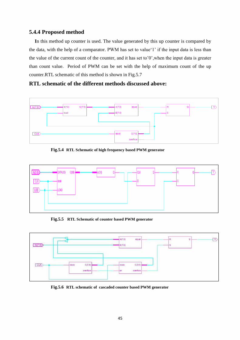
5.4.4 Proposed method

In this method up counter is used. The value generated by this up counter is compared by

the data, with the help of a comparator. PWM has set to value„1‟ if the input data is less than

the value of the current count of the counter, and it has set to‟0‟,when the input data is greater

than count value. Period of PWM can be set with the help of maximum count of the up

counter.RTL schematic of this method is shown in Fig.5.7

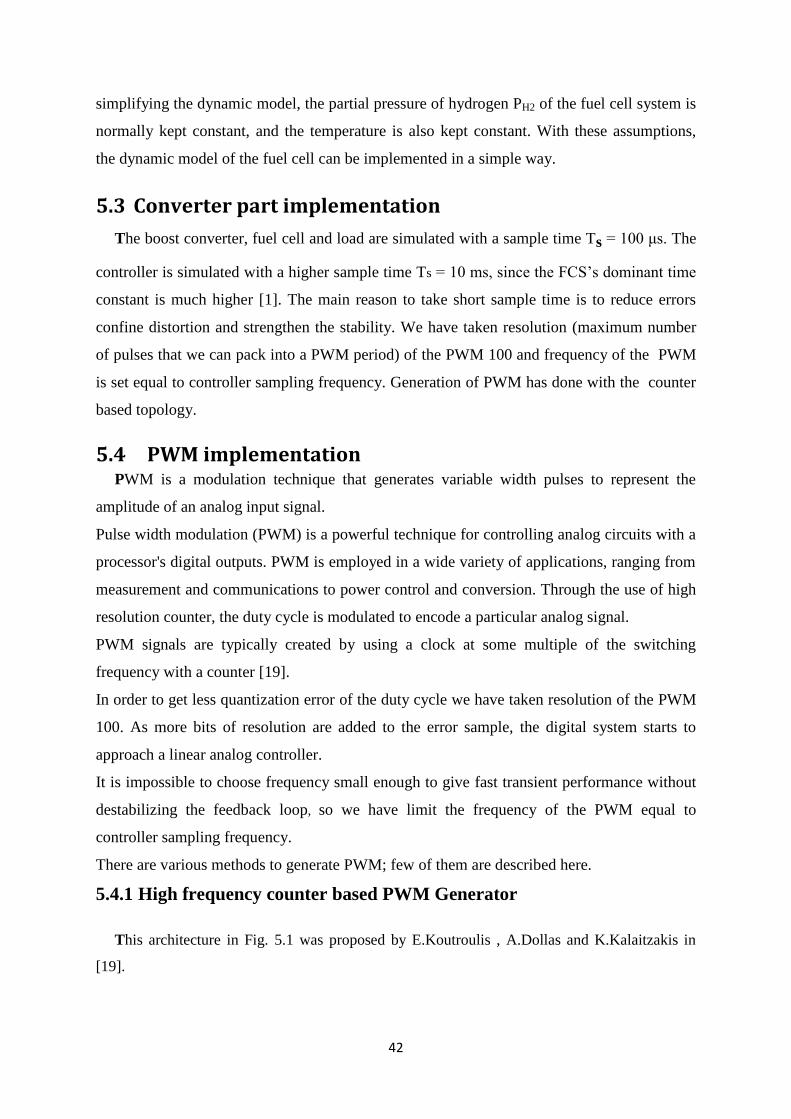
RTL schematic of the different methods discussed above:

Fig.5.4 RTL Schematic of high frequency based PWM generator

Fig.5.5 RTL Schematic of counter based PWM generator

Fig.5.6 RTL schematic of cascaded counter based PWM generator

46

Fig.5.7 RTL schematic of method discussed in 5.4.4

Theoretical value of duty cycle is given by the relation:

)2.5(2N

dataBitNofvalueIntegerD

Fig.5.8 Test Bench waveform of PWM generator

K = “1100”

Duty cycle =12/16=0.75 (from equation 5.2)

From Test Bench waveform D= 670-100/760 =.75

We have got the same value of D as theoretical value of it.

5.5 PI implementation

PI controller is used to control the duty cycle of varying error signal due to variation in

load, which in turns set the output voltage to reference voltage in very short time.

Discretization of this PI controller has done through the discrete equation:

u(n+1) = k1 u(n) + k2e(n-1).

47

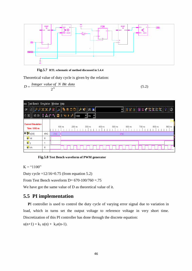
Fig.5.9 RTL Schematic of PI Controller

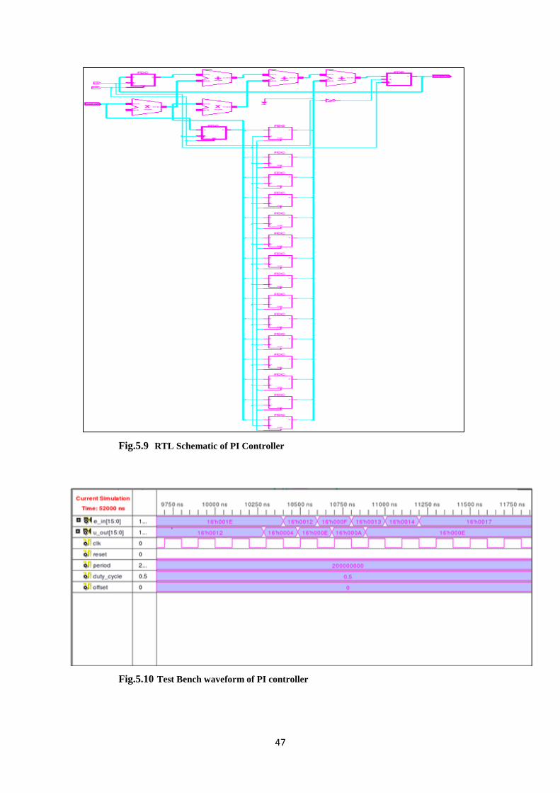
Fig.5.10 Test Bench waveform of PI controller

48

We can see in the above Test Bench waveform, that error signal at time 10500 ns, e_in has a

value of 12 H and its corresponding output has a value of 4 H, which is less compare to e_in.

On the basis of above study of Test Bench waveform we can say that the error signal has got

scaled by the PI controller. We can use this PI controller to scale the duty cycle of the PWM,

so that the PWM waveform cannot change for a little variation of error signal, and thus we

can get constant output voltage with a little change in load value.

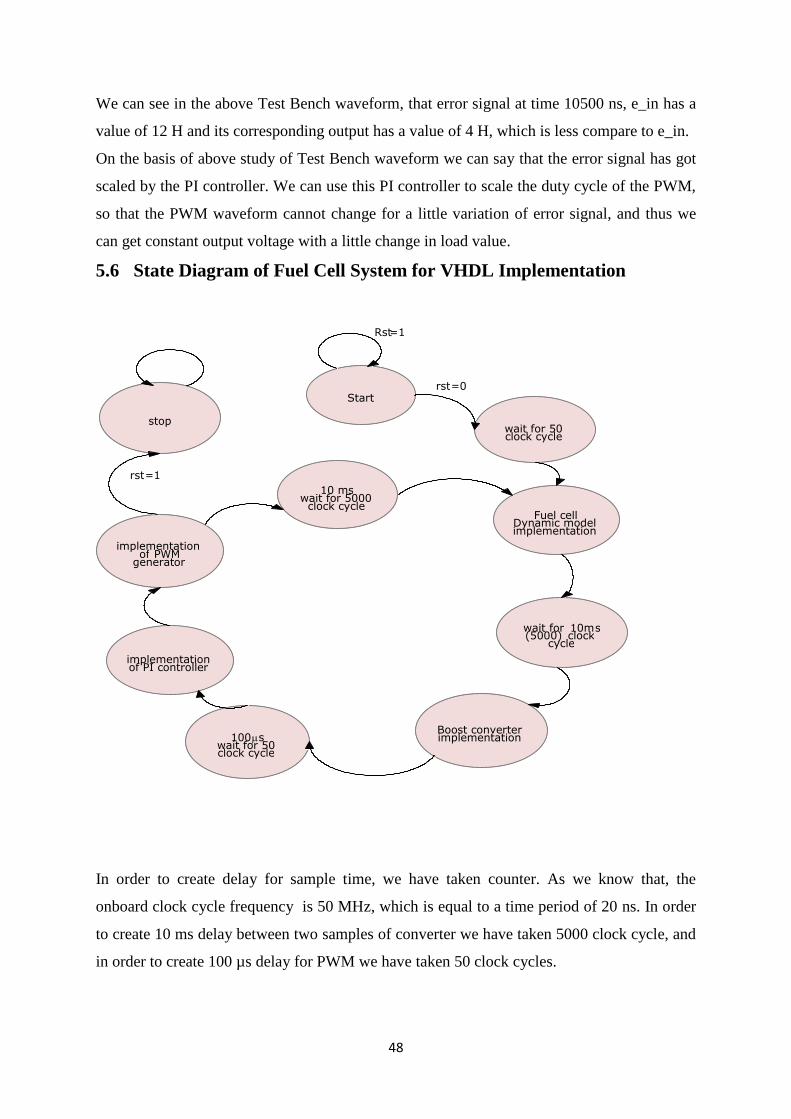
5.6 State Diagram of Fuel Cell System for VHDL Implementation

In order to create delay for sample time, we have taken counter. As we know that, the

onboard clock cycle frequency is 50 MHz, which is equal to a time period of 20 ns. In order

to create 10 ms delay between two samples of converter we have taken 5000 clock cycle, and

in order to create 100 µs delay for PWM we have taken 50 clock cycles.

Start

wait for 50 clock cycle

Fuel cell Dynamic model implementation

wait for 10m s (5000) clock

cycle

Boost converter implementation 100 s

wait for 50 clock cycle

implementation of PI controller

implementation of PWM

generator

10 ms wait for 5000

clock cycle

stop

rst =0

Rst =1

rst =1

49

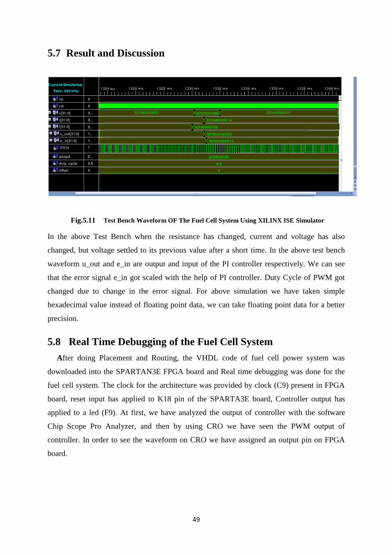
5.7 Result and Discussion

Fig.5.11 Test Bench Waveform OF The Fuel Cell System Using XILINX ISE Simulator

In the above Test Bench when the resistance has changed, current and voltage has also

changed, but voltage settled to its previous value after a short time. In the above test bench

waveform u_out and e_in are output and input of the PI controller respectively. We can see

that the error signal e_in got scaled with the help of PI controller. Duty Cycle of PWM got

changed due to change in the error signal. For above simulation we have taken simple

hexadecimal value instead of floating point data, we can take floating point data for a better

precision.

5.8 Real Time Debugging of the Fuel Cell System

After doing Placement and Routing, the VHDL code of fuel cell power system was

downloaded into the SPARTAN3E FPGA board and Real time debugging was done for the

fuel cell system. The clock for the architecture was provided by clock (C9) present in FPGA

board, reset input has applied to K18 pin of the SPARTA3E board, Controller output has

applied to a led (F9). At first, we have analyzed the output of controller with the software

Chip Scope Pro Analyzer, and then by using CRO we have seen the PWM output of

controller. In order to see the waveform on CRO we have assigned an output pin on FPGA

board.

50

Fig.5.12 Experimental setup

Fig.5.13 Resulted PWM with Duty cycle D =.5 at the output pin of the SPARTAN3E with

oscilloscope

Waveform of PWM, which is shown above is having a duty cycle of 0.5 and frequency of

100 kHz, that is what we require to convert a 48 v dc to 96 v dc, with the help of a Boost-

Converter.

Chapter 6

Conclusions and future work

51

Chapter 6

Conclusion and Future Work

6.1 Conclusion:

In order to examine the possibility to implement digital controller based on FPGA

prototyping, a new method is proposed and analyzed. The proposed digital controller is able

to control the output of any renewable energy sources. A method to synthesized whole fuel

cell power system is developed using VHDL. This approach using VHDL is applied to a fuel

cell power system of 2.4 kW and 96 v is. The proposed method is simulated, and the results

demonstrate appropriate performance of the system and controllers. This thesis presents a

very simple and reasonable approach to model a particular PEM (Polymer electrolyte

membrane) fuel cell, and its real time debugging using SPARTAN3E board. Initially the

system were simulated in Matlab/Simulink, to make a reference for VHDL implementation,

after the Matlab/Simulink modeling, fuel cell system model has developed in VHDL by using

some approximation and assumption. The work carried out in this thesis has allowed to

prototype hardware of fuel cell controller.

6.2 Future Work:

This prototyped board controller can be used with a real fuel cell. The novel approach

proposed in this thesis can be also used with another type of renewable sources.

.

52

References:

[1] K. Petrinec, M. Cirstea, , K. Seare, C. Marinescu “A Novel FPGA Fuel Cell System Controller Design”.11th

International conference on Optimization of Electrical and Electronic Equipmen,2008, pp. 401-406.

[2] Nehrir.H, Caisheng Wang, Shaw, S.R, 2006. “Fuel cells: promising devices for distributed generation”,

IEEE Power and Energy Magazine, vol. 4, issue 1, pp. 47-53.

.

[3] K. Petrinec, M. Cirstea, "Holistic modelling of a fuel cell power system and FPGA controller using

Handel-C", IEEE IECON'06, Paris, France, November 7-10, 2006.

[4] http://vega.unitbv.ro/~ieee

[5] Rahim N.A. and Islam Z., “Field Programmable Gate Array-Based Pulse-Width Modulation for Single

Phase Active Power Filter”; American Journal of Applied Sciences, Vol.6 (2009): pp. 1742-1747.

[6] ElieLafy,Marie-Cecile pera and Daniel hissel femto “PEM fuel cell modeling with static dynamic

decomposition and voltage rebuilding” IEEE Transaction on Power Electronics, vol.19, issue 5,Sept

2004, pp-1234 – 1241.

[7] J. Larminie and A. Dicks: Fuel Cell Systems Explained. 2nd ed, J. Wiley & Sons, England, 2003.

[8] G. Kortum, Treatise on Electrochemistry (2nd Edition). New York: Elsevier, 1965

[9] J. C. Amphlett, R. M. Baumert, R. F. Mann, B. A. Peppley, and P. R. Roberge, “Performance modeling of

the Ballard Mark IV solid polymer”

[10] M.T. Iqbal, “Modeling and control of a wind fuel cell hybrid energy system”, Renewable Energy, vol. 28,

issue 2, Feb. 2003, pp. 223 – 237. electrolyte fuel cell, I. Mechanistic model development,” J.

Electrochem. Soc., vol. 142, no. 1, Jan. 1995, pp. 1–8.

[11] J.M. Correa, F.A. Farret, L.N. Canha, M.G. Simoes, “An electrochemical-based fuel-cell model suitable

for electrical engineering automation approach,” IEEE Trans. Ind. Electronics, vol. 51, issue 5, Oct.

2004, pp.1103 – 1112.

[12] R.F. Mann, J.C. Amphlett, M.A.I. Hooper, H.M. Jensen, B.A. Peppley, P.R. Roberge, “Development

and application of a generalised steady-state electrochemical model for a PEM fuel cell,” Journal of

Power Sources, vol. 86, issues 1-2, Mar. 2000, pp. 173 – 180.

[13] Fuel Cell Handbook (Fifth Edition), EG&G Services, Parsons Inc., DEO of Fossil Energy, National

Energy Technology Lab, Oct. 2000. IEEE Transactions on energy conversion, vol. 20, no. 2, June 2005.

[14] CaishengWang, ,M. Hashem Nehrir, and Steven R. Shaw, “Dynamic Models and Model Validation for

PEM Fuel Cells Using Electrical Circuits” IEEE Transaction on Energy conservation,vol.20, issue 2,

June 2005, pp.442-451.

[15] A. Schneuwly,M. Bärtschi, V. Hermann, G. Sartorelli, R. Gallay, and R. Koetz, “BOOST CAP double-

layer capacitors for peak power automotive applications,” in Proc. 2nd Int. Advanced Automotive

Battery Conf., Las Vegas, NV, Feb. 2002.

[16] http://en.wikipedia.org/wiki/Buck_converter

[17] http://en.wikipedia.org/wiki/Boost_converter

53

[18] Ataollah Abbasi Mehrdad rostami Jafar abdollahi and Hamid abbasi hasan.n “An analytical discrete

model for evaluation the chaotic behavior of Boost converter under current control mode” Symposium

on Industrial Electronics and Applications (ISIEA 2009), October 4-6, 2009, pp.-403-407.

[19] Koutroulis E., Dollas A. and Kalaitzakis K., “High-frequency pulse width modulation implementation

using FPGA and CPLD ICs”, Journal of Systems Architecture , Vol.52 (2006): pp. 332–344 .

[20] Dancy A.P., Amirtharajah R. and Chandrakasan A.P., “High-Efficiency Multiple-Output DC–DC

Conversion for Low-Voltage Systems”, IEEE Trans. on Very Large Scale Integration (VLSI) Systems,

Vol. 8, No. 3, June 2000: pp.252-263.