development at the urban fringe and beyond: impacts...

Development at the Urban Fringe and Beyond: Impacts on Agriculture and RuralLand. By Ralph E. Heimlich and William D. Anderson. Economic Research Service,U.S. Department of Agriculture. Agricultural Economic Report No. 803.

AbstractLand development in the United States is following two routes: expansion of urbanareas and large-lot development (greater than 1 acre per house) in rural areas. Urbanexpansion claimed more than 1 million acres per year between 1960 and 1990, yet is notseen as a threat to most farming, although it may reduce production of some high-valueor specialty crops. The consequences of continued large–lot development may be lesssanguine, since it consumes much more land per unit of housing than the typical suburb.Controlling growth and planning for it are the domains of State and local governments.The Federal Government may be able to help them in such areas as building capacity toplan and control growth, providing financial incentives for channeling growth in desir-able directions, or coordinating local, regional, and State efforts.

Keywords: land development, sprawl, large-lot housing, land zoning, populationgrowth, housing, specialty agriculture, high-value agriculture, rural amenities, smartgrowth

Contributors Charles Barnard—Wrote sections on costs of use value assessment and purchase ofdevelopment rights, the effect of technology on employment location, and metropolitanagriculture.

John Cromartie—Wrote sections on population and household trends, and technologyand employment.

Richard Reeder—Wrote the sections on local responses to growth, impacts on commu-nity and quality of life, and planning capacity.

Peter Feather—Wrote the section on nonmarket benefits from preserving farmland,including water quality impacts from reducing erosion from construction sites.

Cindy Nickerson—Wrote the section on State responses to growth and “smart growth.”

Robert Hoppe and Penni Korb—Wrote the section on metropolitan agriculture and tran-sitions between metro farm types.

Marlow Vesterby and William Quinby—Wrote sections on trends in land use and hous-ing development as a driving force.

Daniel Mullarkey—Wrote the section on rural amenities and the WTO agreements.

1800 M Street, NW.Washington, DC 20036-5831 June 2001

DedicationThis report is dedicated to the memory of Robert Otte, who died November 6, 2000. AsChief of the Land Resources Branch of the Economic Research Service’s NaturalResource Economics Division in the late 1960’s, Dr. Otte pioneered early research onthe urbanization of agricultural land. He authored Farming in the City’s Shadow in1974, and was co-author of ERS’s first study of land use change in urbanizing areas,Dynamics of Land Use in Fast Growth Areas in 1976. Dr. Otte was a gentleman, a gen-erous colleague, and a mentor to many land economics researchers, in ERS and otherinstitutions, who followed in his footsteps.

William D. Anderson

AcknowledgmentsThe authors want to thank editor Thomas McDonald and designer Susan DeGeorge fortheir tireless efforts in improving and presenting this report. The report benefited greatlyfrom peer reviews by Nelson Bills, Cornell University, David Holder, USDA-CREES,Douglas Lawrence, USDA-NRCS, Lawrence Libby, Ohio State University, and AnnSorensen, American Farmland Trust, Center for Agriculture and the Environment. Anyremaining errors in fact and judgment are the authors’.

��

Contents

Summary . . . . . . . . . . . . . . . . . . . . . . . . . . . . . . . . . . . . . . . . . . . . . . . . . . . . . . . . . . . . . . .iv

I. Overview . . . . . . . . . . . . . . . . . . . . . . . . . . . . . . . . . . . . . . . . . . . . . . . . . . . . . . . . . . . .1

II. Trends in Land Use: Two Kinds of Growth . . . . . . . . . . . . . . . . . . . . . . . . . . . . . . . .9What is Sprawl? . . . . . . . . . . . . . . . . . . . . . . . . . . . . . . . . . . . . . . . . . . . . . . . . . . . . . . . . . .9

Two Kinds of Growth . . . . . . . . . . . . . . . . . . . . . . . . . . . . . . . . . . . . . . . . . . . . . . . . . . . . .12

III. Driving Forces . . . . . . . . . . . . . . . . . . . . . . . . . . . . . . . . . . . . . . . . . . . . . . . . . . . . . .15

U.S. Population Growth and Household Formation . . . . . . . . . . . . . . . . . . . . . . . . . . . . . . .15

Household Land Consumption . . . . . . . . . . . . . . . . . . . . . . . . . . . . . . . . . . . . . . . . . . . . . .16

Demand for Low-Density Development . . . . . . . . . . . . . . . . . . . . . . . . . . . . . . . . . . . . . . . .17

Metropolitan Expansion . . . . . . . . . . . . . . . . . . . . . . . . . . . . . . . . . . . . . . . . . . . . . . . . . . .18

Infrastructure . . . . . . . . . . . . . . . . . . . . . . . . . . . . . . . . . . . . . . . . . . . . . . . . . . . . . . . . . . . .20

Employment, Economic Development and Technology . . . . . . . . . . . . . . . . . . . . . . . . . . . .23

IV. The Costs of Growth . . . . . . . . . . . . . . . . . . . . . . . . . . . . . . . . . . . . . . . . . . . . . . . . .26

Costs Imposed by Growth . . . . . . . . . . . . . . . . . . . . . . . . . . . . . . . . . . . . . . . . . . . . . . . . . .26

Infrastructure Costs . . . . . . . . . . . . . . . . . . . . . . . . . . . . . . . . . . . . . . . . . . . . . . . . . . . . . . .27

Transportation . . . . . . . . . . . . . . . . . . . . . . . . . . . . . . . . . . . . . . . . . . . . . . . . . . . . . . . . . . .28

Impacts on Taxpayers . . . . . . . . . . . . . . . . . . . . . . . . . . . . . . . . . . . . . . . . . . . . . . . . . . . . .28

Impacts on Landscape, Open Space, and Sense of Community . . . . . . . . . . . . . . . . . . . . . .31

Environmental Changes . . . . . . . . . . . . . . . . . . . . . . . . . . . . . . . . . . . . . . . . . . . . . . . . . . . .31

Other Quality of Life Issues . . . . . . . . . . . . . . . . . . . . . . . . . . . . . . . . . . . . . . . . . . . . . . . .35

An Economic Interpretation of the Demand for Low-Density Development . . . . . . . . . . . . .36

V. Consequences for Farming . . . . . . . . . . . . . . . . . . . . . . . . . . . . . . . . . . . . . . . . . . . .38

Agriculture: Farming in the City’s Shadow . . . . . . . . . . . . . . . . . . . . . . . . . . . . . . . . . . . . .38

Working Landscapes and Rural Amenities . . . . . . . . . . . . . . . . . . . . . . . . . . . . . . . . . . . . . .43

Benefits of Famland and Open Space . . . . . . . . . . . . . . . . . . . . . . . . . . . . . . . . . . . . . . . . .44

VI. Local Responses to Growth . . . . . . . . . . . . . . . . . . . . . . . . . . . . . . . . . . . . . . . . . . . .50

Playing Catch Up . . . . . . . . . . . . . . . . . . . . . . . . . . . . . . . . . . . . . . . . . . . . . . . . . . . . . . . .50

How Local Governments Address Growth Problems . . . . . . . . . . . . . . . . . . . . . . . . . . . . . .50

Planning Efforts to Control Growth . . . . . . . . . . . . . . . . . . . . . . . . . . . . . . . . . . . . . . . . . . .51

Capacity for Response in Relation to Urbanization Pressure . . . . . . . . . . . . . . . . . . . . . . . .52

Federal Assistance for Planning . . . . . . . . . . . . . . . . . . . . . . . . . . . . . . . . . . . . . . . . . . . . . .54

Slow Growth, No Growth, and Smart Growth . . . . . . . . . . . . . . . . . . . . . . . . . . . . . . . . . . .55

Monetary Incentives for Conserving Farm and Forest Land . . . . . . . . . . . . . . . . . . . . . . . . .57

��

VII. Potential Federal Roles . . . . . . . . . . . . . . . . . . . . . . . . . . . . . . . . . . . . . . . . . . . . . . .65

Helping Increase State and Local Planning Capacity . . . . . . . . . . . . . . . . . . . . . . . . . . . . . .65

Coordinating Local, Regional, and State Efforts . . . . . . . . . . . . . . . . . . . . . . . . . . . . . . . . .66

Coordinating Federal Development Activities and Growth Management Goals . . . . . . . . . .67

Funding Monetary Conservation Incentives . . . . . . . . . . . . . . . . . . . . . . . . . . . . . . . . . . . . .68

Conserving Rural Amenities As Part of Greater Agricultural and Trade Policy Goals . . . . . .69

References . . . . . . . . . . . . . . . . . . . . . . . . . . . . . . . . . . . . . . . . . . . . . . . . . . . . . . . . . . . . . .71

List of Figures

Figure 1—Schematic diagram of urban geography . . . . . . . . . . . . . . . . . . . . . . . . . . . . . . .11

Figure 2—Trends in developed land use, 1960-2000 . . . . . . . . . . . . . . . . . . . . . . . . . . . . . .13

Figure 3—Land base of the United States, 1992 . . . . . . . . . . . . . . . . . . . . . . . . . . . . . . . . .13

Figure 4—Annual additions to housing area, by lot size, 1900-97 . . . . . . . . . . . . . . . . . . . .14

Figure 5—Additions to U.S. population 1972-2007 . . . . . . . . . . . . . . . . . . . . . . . . . . . . . . .15

Figure 6—U.S. population and household change 1982-97 . . . . . . . . . . . . . . . . . . . . . . . . .16

Figure 7—Household formation and housing completions, 1960-97 . . . . . . . . . . . . . . . . . .16

Figure 8—County typology, 1990 . . . . . . . . . . . . . . . . . . . . . . . . . . . . . . . . . . . . . . . . . . . .19

Figure 9—U.S. population change 1982-97 . . . . . . . . . . . . . . . . . . . . . . . . . . . . . . . . . . . . .20

Figure 10—Sewage disposal by lot size, 1994-97 . . . . . . . . . . . . . . . . . . . . . . . . . . . . . . . .21

Figure 11—Water supply by lot size, 1994-1997 . . . . . . . . . . . . . . . . . . . . . . . . . . . . . . . . .22

Figure 12—High-tech jobs grow more slowly in cities than in suburbs 1992-97 . . . . . . . . .24

Figure 13—Private and public capital costs by community type . . . . . . . . . . . . . . . . . . . . .27

Figure 14—Relative capital costs of public infrastructure . . . . . . . . . . . . . . . . . . . . . . . . . .28

Figure 15—Ratio of community service costs to tax revenues (n=85) . . . . . . . . . . . . . . . . .29

Figure 16—Savings of agricultural and environmentally sensitive lands, compact growth versus “sprawl” . . . . . . . . . . . . . . . . . . . . . . . . . . . . . . . . . . . . . . . . . . . . . . . . . . . .33

Figure 17—Water quality impacts by community type . . . . . . . . . . . . . . . . . . . . . . . . . . . .35

Figure 18--Distribution of farmers’ markets . . . . . . . . . . . . . . . . . . . . . . . . . . . . . . . . . . . . .40

Figure 19--Conceptual model of agricultural adaptation to urbanization . . . . . . . . . . . . . . .42

Figure 20--Farms in 1978 out of business by 1997, by farm category . . . . . . . . . . . . . . . . .44

Figure 21--Transitions between farm types, metro farms, 1978-97 . . . . . . . . . . . . . . . . . . . .45

Figure 22—Composition of land use change in urbanizing areas, 1970’s and 1980’s . . . . . .45

Figure 23—Degree of urban influence, 1990 . . . . . . . . . . . . . . . . . . . . . . . . . . . . . . . . . . . .47

Figure 24—Comparison of estimated urban growth boundaries and percent of area changing to developed uses, 1982-92 . . . . . . . . . . . . . . . . . . . . . . . . . . . . . . . . . . . .48

Figure 25--Actual and estimated easement value for cropland, by urban influence . . . . . . . .61

Figure 26—Costs of purchase of development rights and use-value assessment relative to benefits for preserving cropland, by urban influence . . . . . . . . . . . . . . . . . . . . . . . . . . . .63

��

List of Tables

Table 1—Trends in U.S. urban development, 1960-2000 . . . . . . . . . . . . . . . . . . . . . . . . . . .12

Table 2—Growth-related issues, impacts, and possible solutions . . . . . . . . . . . . . . . . . . . . .32

Table 3—Metro and nonmetro farm characteristics, United States, 1991 and 1997 . . . . . . .38

Table 4—Estimates of the average amenity value of farmland . . . . . . . . . . . . . . . . . . . . . . .46

Table 5—Estimated nonmarket value of land under urban influence estimated to be developed in succeeding decades . . . . . . . . . . . . . . . . . . . . . . . . . . . . . . . . . . . . . . . . . . . . .49

Table 6—Annual recreational water quality damages due to urbanization of farmland . . . . .49

Table 7—State implementation of smart growth strategies . . . . . . . . . . . . . . . . . . . . . . . . . .58

Table 8—Comparison of costs and benefits for protecting cropland, by degree of urban influence, 1995 . . . . . . . . . . . . . . . . . . . . . . . . . . . . . . . . . . . . . . . . . . . . . .64

Appendix table 1—Implicit tax subsidy attributable to tax expenditures in use-value assessment programs, by State, 1995 . . . . . . . . . . . . . . . . . . . . . . . . . . . . . . . . . . . . . . . . . .79

Appendix table 2—Estimated purchase of development rights expenditures for urban-influenced cropland, compared with actual expenditures, acreage, and use-value assessment tax expenditures, 1995 . . . . . . . . . . . . . . . . . . . . . . . . . . . . . . . . . . . . . . . . . . . . . . . . . . . . .80

��

In the early 1970's, bipartisan legislation was intro-duced in Congress to establish a national land-use pol-icy, but failed after extensive debate. In the decades thatfollowed, the urbanized area in the United States hasmore than doubled. Public concerns about ill-controlledgrowth once again have raised the issue of the Federalrole in land-use policy. While anecdotes are legion,there are surprisingly few places to find a comprehen-sive picture of land-use changes in urbanizing areas,relative to the rural landscape. This report describes theforces driving development, its character and impactson agriculture and rural communities, the means avail-able to channel and control growth, and the pros andcons of potential Federal roles. The report also providesdetailed, documented, objective evidence culled fromthe literature and from original analyses.

What Is Sprawl?

This report is about urban development at the edges ofcities and in rural areas, sometimes called “urbansprawl.” Because “sprawl” is not easily defined, thisreport is couched in the more neutral terms “develop-ment” or “growth,” without making implicit judgmentsabout the quality or outcomes of that development orgrowth. Concerns about development around urbanareas are not new, but have arisen periodically duringmost of the last century, and certainly since automobileownership became widespread after World War II.What lessons have been learned about urban develop-ment and the Federal role in managing it?

The processes of land-use change are well under-stood and flow predictably from population growth,household formation, and economic development—Changes in land use are the end result of many forcesthat drive millions of separate choices made by home-owners, farmers, businesses, and government. The ulti-mate drivers are population growth and household for-mation. Economic growth increases income and wealth,and preferences for housing and lifestyles, enabled bynew transportation and communications technologies,spur new housing development and new land-use pat-terns. Metropolitan areas grow organically, followingwell-known stages of growth.

There are two kinds of growth, but both affect theamount and productivity of agricultural land andcreate other problems—Our existing urban areas con-tinue to grow into the countryside, and more isolated

large-lot housing development is occurring, generallybeyond the urban fringe.

Development imposes direct costs on the communi-ties experiencing it, as well as indirect costs in termsof the rural lands sacrificed to it—A number of stud-ies show that less dense, unplanned developmentrequires higher private and public capital and operatingcosts than more compact, denser planned development.Residential development requires $1.24 in expendituresfor public services for every dollar it generates in taxrevenues, on average. By contrast, farmland or openspace generates only 38 cents in costs for each dollar intaxes paid.

Continued demand for low-density developmentdespite negative consequences for residents can beunderstood as a market failure—Consumers, busi-nesses, and communities fail to anticipate the results ofdevelopment because they often lack information onpotential or approved development proposals for sur-rounding land. Often, communities fail to plan andzone to provide an institutional framework withinwhich development can proceed. Real estate marketsare based on many small decisions which, when takenwithout an overall context, produce results that can nei-ther be envisioned by nor anticipated by consumers anddevelopers. Inaccurate judgments about future land-scapes are locked in because development is irre-versible.

Urban growth and development is not a threat tonational food and fiber production, but may reduceproduction of some high-value or specialty crops—Despite doubling since 1960, urban area still made upless than 3 percent of U.S. land area in 1990 (excludingAlaska). Developed area, including rural roads andtransportation, made up less than 5 percent in 1992.The increase in urban area in the United States poses nothreat to overall U.S. food and fiber production, butsome crops in some areas are particularly vulnerable todevelopment.

Agriculture can adapt to development, but does soby changing the products and services offered—Low-density, fragmented settlement patterns leaveroom for agriculture to continue. Farms in metropolitanareas are an increasingly important segment of U.S.agriculture, making up 33 percent of all farms, 16 per-cent of cropland, and producing a third of the value of

��

Summary

U.S. agricultural output. However, to adapt to risingland values and increasing contact with new residents,farmers may have to change their operations to empha-size higher-value products, more intensive production,enterprises that fit better in an urbanizing environment,and a more urban marketing orientation.

Benefits of conserving rural land are difficult to esti-mate and vary widely depending on the circum-stances—Based on information and assumptions aboutthe number of acres likely subject to development inthe future, and limited studies of residents’ willingnessto pay to conserve farmland and open space, we esti-mate that households would be willing to pay $1.4-$26.6 billion per year to conserve rural lands. Thisequals $13.5 to $255.8 billion in present value. Con-serving land for agriculture helps preserve farming inthe rural economy, and is often seen as a bulwarkagainst the worst effects of development.

Local governments generally do not develop ade-quate capacity to plan for and manage growth untilit is too late to effectively channel development—Because urban growth processes are well understood,strategically directing development to the most favor-able areas well in advance of urban pressures offers thegreatest hope for controlling growth. Local govern-ments often fail to appreciate impending growth facingthem, and generally lack capacity to develop adequateresponses before growth overwhelms them.

State governments can do more to deal with growthstrategically—Increasingly, States are realizing thatlocal governments cannot adequately address growthpressures that transcend local boundaries. Some of themore progressive States have adopted “smart growth”strategies that actively direct transportation, infrastruc-ture, and other resources to channel growth into appro-priate areas.

The cost of effective land conservation incentiveswould be large, but if resources were redirected,almost one-third of the cropland with the greatestdevelopment potential could be protected—Purchas-ing the development rights to rural land effectively pro-tects it from being developed, while continuing farmuse. We estimate the cost to purchase developmentrights on cropland most likely subject to urban pressureover the next 30 to 50 years at $87-$130 billion. If taxexpenditures currently devoted to use-value assessmentwere redirected to purchase of development rights,almost one-third of the cropland with greatest potentialfor development could be protected.

There are neither clear requirements for nor restric-tions on Federal roles in managing growth—Histori-cally, authority over land-use decisions has beenreserved to the States, which have delegated these pow-ers to local governments. However, the evolution ofenvironmental policy shows an expanding Federalinvolvement in site-specific, local circumstances thatrecur across the Nation. The Federal Government hasno constitutional mandate to take action on urbangrowth and development issues, but it can define anappropriate role for itself.

Potential Federal roles include:

• Helping Increase State and Local Planning Capacity

• Coordinating Local, Regional, and State Efforts

• Coordinating Federal Development Activities andGrowth Management Goals

• Funding Monetary Conservation Incentives

• Conserving Rural Amenities as Part of Greater Agri-cultural and Trade Policy Goals.

��

��

In the early 1970's, bipartisan legislation was intro-duced in Congress to establish a national land-use pol-icy, but failed after extensive debate. In the decades thatfollowed, urban area in the United States has more thandoubled. Public concerns about ill-controlled growthonce again have raised the issue of the Federal role inland-use policy.

Purpose of This Report

Although land-use issues have traditionally been theprerogative of State and local government, policymak-ers at the Federal level are increasingly urged torespond to concerns about development and growth,particularly with regard to their impacts on agricultureand rural land uses. While anecdotes are legion, andmuch has been written by commentators, advocates,and experts, there are surprisingly few places to find acomprehensive picture of land-use changes in urbaniz-ing areas, relative to the rural landscape. This reportresponds to that need in two ways.

This overview provides a summary of our findingsabout the forces driving development, its character andimpacts on agriculture and rural communities, themeans available to channel and control growth, and thepros and cons of potential Federal roles.

The following chapters provide the details, presented ina documented, objective way that make the case for thearguments presented here. A consensus culled from theliterature supports some of the points, while originalanalyses presented in this report have not been pub-lished elsewhere.

What is Sprawl?

This report is about urban development at the edges ofcities and in rural areas, sometimes called “urbansprawl.” With no widely accepted definition of sprawl(U.S. GAO, 1999; Staley, 1999), attempts to define itrange from the expansive to the prescriptive.

Most definitions have some common elements, includ-ing:

• Low-density development that is dispersed and uses alot of land;

• Geographic separation of essential places such aswork, homes, schools, and shopping; and

• Almost complete dependence on automobiles fortravel.

Without an agreed definition, any growth in suburbanareas may be accused of “sprawling.”

Short of a return to a form of urban living not seensince before World War II, it is not clear how growthcan be accommodated at suburban densities withoutincurring the worst features of “sprawl.” Because“sprawl” is not easily defined, this report is couched inthe more neutral terms “development” or “growth,”without making implicit judgments about the quality oroutcomes of that development or growth. See Trends InLand Use: Two Kinds of Growth p. 9.

How To Think About Development

Concerns about development around urban areas arenot new, but have arisen periodically during most of thelast century, and certainly since automobile ownership

��

Development at the Urban Fringe and Beyond

Impacts on Agriculture and Rural Land

Ralph E. Heimlich and William D. Anderson

I. Overview

became widespread after World War II. Amid the envi-ronmental concerns during the 1970’s, bipartisan legis-lation was introduced in Congress to establish anational land-use policy. Recognizing the primacy ofState authority over land use, the legislation sought toprovide Federal grants to States to strengthen their abil-ity to plan for development and channel growth. After 5years of debate, the legislation was passed in the Sen-ate, but narrowly defeated in the House on June 11,1974. What lessons have been learned about urbandevelopment and the Federal role in managing it in the26 years since then?

There are two kinds of growth, but both affect theamount and productivity of agricultural land andcreate other problems—Our existing urban areas con-tinue to grow into the countryside, and more isolatedlarge-lot housing development is occurring, generallybeyond the urban fringe.

At the urban fringe—The urban “fringe” is that part ofmetropolitan counties that is not settled densely enoughto be called “urban.” Low-density development (2 orfewer houses per acre) of new houses, roads, and com-mercial buildings causes urban areas to grow fartherout into the countryside, and increases the density ofsettlement in formerly rural areas. The extent of urban-ized areas and urban places, as defined by the Bureauof Census, more than doubled over the last 40 yearsfrom 25.5 million acres in 1960 to 55.9 million acres in1990, and most likely reached about 65 million acresby 2000.

Beyond the urban fringe—Another kind of develop-ment often occurs farther out in the rural countryside,beyond the edge of existing urban areas and often inadjacent nonmetropolitan counties. Development ofscattered single-family houses removes land from agri-cultural production and changes the nature of openspace, but is not “urban.” Large lots dominate thisprocess, and growth in large-lot development has accel-erated with business cycles since 1970. Nearly 80 per-cent of the acreage used for new housing constructionin 1994-97—about 2 million acres—is outside urbanareas. Almost all of this land (94 percent) is in lots of 1acre or larger, with 57 percent on lots 10 acres orlarger. About 16 percent was located in existing urbanareas and 5 percent was on farms. See Two Kinds ofGrowth, p. 12.

Growth in developed areas is increasing, but at ratesonly slightly higher than in the past—Urbanizedareas and urban places increased at about the same 1

million acres per year between 1960 and 1990. Devel-oped land, including residential and other developmentthat is not dense enough to meet urban definitions,increased from 78.4 million acres in 1982 to 92.4 mil-lion acres in 1992, and was estimated to be about 107million acres in 2000. The rate of increase in developedland grew from 1.4 million acres per year to about 1.8million acres. See Two Kinds of Growth, p. 12.

The processes of land-use change are well under-stood and flow predictably from population growth,household formation, and economic development—Changes in land use are the end result of many forcesthat drive millions of separate choices made by home-owners, farmers, businesses, and government. The ulti-mate drivers are population growth and household for-mation. Economic growth increases income and wealth,and preferences for housing and lifestyles, enabled bynew transportation and communications technologies,spur new housing development and new land-use pat-terns. Metropolitan areas grow organically, followingwell-known stages of growth.

Almost alone among developed nations, the UnitedStates continues to add population from high fertilityrates, high immigration, and longer life expectancy,increasing 1 percent per year, or another 150 millionpeople by 2050. Average household size has dropped to2.6 persons, creating about 1 million new households,the unit of demand for new housing, each year in the1990’s.

Increased income and wealth increased the number ofnew houses constructed each year by 1.5 million units,faster than the rate of household formation. Two-thirdsof these houses are single-family dwellings. Whileaverage lot sizes have been dropping near cities asowners turn to townhouses and condominiums, a paral-lel growth in large-lot (greater than 1 acre) housing hasoccurred beyond the urban fringe.

Metropolitan expansion since 1950 has occurredbecause rural people moved off the farms, and residentsof the densely populated central cities dispersed to sur-rounding suburbs. Urbanized areas (excluding towns of2,500 or more) increased from 106 to 369 andexpanded to five times their size. Population density inurbanized areas dropped by more than 50 percent, from8.4 to 4 people per acre, over the last 50 years. Growthis spilling out of metropolitan areas, as population dis-perses to rural parts of metropolitan counties and previ-ously rural nonmetropolitan counties.

� ��

Enabling this dispersion are investments in new infra-structure such as roads, sewers, and water supplies.New information and communication technologies,such as the Internet and cellular telephone networks,facilitate population in rural areas, and free employ-ment to follow. New retail, office, warehouse, and othercommercial development follows in the wake of newhousing development, to serve the new population andto employ the relocated labor force. See DrivingForces, p. 15.

There are benefits of low-density development thatattract people—Living beyond the edge of the city is alifestyle much sought after by the American people.While 55 percent of Americans living in medium tolarge cities preferred that location, 45 percent wanted tolive in a rural or small town setting 30 or more milesfrom the city (Brown et al., 1997). Of those living inrural or small towns more than 30 miles from largecities, 35 percent wanted to live closer to the city. Theurban fringe is thus under development pressure fromboth directions. The most obvious benefit is that growthin rural areas has allowed many people, including thosewho cannot afford city real estate, to buy single-familyhomes because land costs are cheaper on the fringethan in the core.

The automobile imposes private and social costs inexchange for the comfort, flexibility, low door-to-doortravel time, freight-carrying capacity (for shoppingtrips), cheap long-distance travel, and aesthetic benefitsof extensive, automobile-dependent development. Airquality improvements may also result from decentraliz-ing population and employment, because emissions aredispersed over larger rural airsheds and are reduced byhigher speeds. Automobile pollution is more stronglyrelated to the number of trips than to the length of eachtrip, with a major part of auto pollution deriving fromcold starts.

Not everyone wants to live the rural lifestyle. The “newurbanism” school of urban design is redesigning con-ventional suburban developments as small towns andfinding a market (Chen, 2000; Duany et al., 2000). In1992, 55 percent of those surveyed living in large cities(over 50,000) preferred that type of community (Brownet al., 1997). See Demand for Low-Density Develop-ment, p. 17.

Development imposes direct costs on the communi-ties experiencing it, as well as indirect costs in termsof the rural lands sacrificed to it—A number of stud-ies show that less dense, unplanned development

requires higher private and public capital and operatingcosts than more compact, denser planned development.Eighty-five studies gauging the cost of communityservices around the country have shown that residentialdevelopment requires $1.24 in expenditures for publicservices for every dollar it generates in tax revenues, onaverage. By contrast, farmland or open space generatesonly 38 cents in costs for each dollar in taxes paid. SeeImpacts on Taxpayers, p. 28.

Finally, development can disrupt existing social, com-munity, environmental and ecological patterns, impos-ing a variety of costs on people, wildlife, water, air, andsoil quality. Agricultural production has its own nega-tive environmental impacts, but these are generally lesssevere than those from urban development. See Impactson Landscape, Open Space, and Sense of Community,p. 31.

However, does moving out into the “country” ulti-mately destroy all the good things that prompt thatmove? In the words of the National Governor’s Associ-ation, “In the context of traditional growth patterns, thedesire to live the ‘American Dream’ and purchase a sin-gle-family home on a large lot in a formerly open spacecan produce a negative outcome for society as a whole”(Hirschorn, p. 55).

Continued demand for low-density developmentdespite negative consequences for residents can beunderstood as a market failure—Consumers, busi-nesses, and communities fail to anticipate the results ofdevelopment because they often lack information onpotential or approved development proposals for sur-rounding land. When communities fail to plan andzone, there is no institutional framework within whichdevelopment can proceed, and little information to helphousing buyers anticipate their future landscape setting.

Spillovers from development include the loss of ruralamenities, open space, and environmental goods whenpreviously existing farms and rural land uses are devel-oped. Negative spillovers from increased housing con-sumption in developing areas can include traffic con-gestion, crowding, and destruction of visual amenities.If the landscape features that contribute to ruralamenity were marketed in developments, housingprices would be higher.

Real estate markets are based on many small decisionswhich, when taken without an overall context, produceresults that can neither be envisioned by nor anticipatedby consumers and developers. Cumulative impacts

��

from this myriad of decisions can be large, but are notreflected in market prices until disamenities becomelarge. Inaccurate judgments about future landscapes arelocked in because development is irreversible. See AnEconomic Interpretation of the Demand for Low-Den-sity Development, p. 36.

Urban growth and development is not a threat tonational food and fiber production, but may reduceproduction of some high-value or specialty crops—Despite doubling since 1960, urban area still made upless than 3 percent of U.S. land area in 1990 (excludingAlaska). Developed area, including rural roads andtransportation, made up less than 5 percent in 1992.Development affects local agricultural economies andcan cause other environmental and resource problemsin local areas, but the increase in urban area in theUnited States poses no threat to U.S. food and fiberproduction. Some crops in some areas are particularlyvulnerable to development. For example, 61 percent ofU.S. vegetable production is located in metropolitanareas, but vegetable production takes up less than 1 per-cent of U.S. cropland. See Consequences for Farming,p. 38.

Agriculture can adapt to development, but does soby changing the products and services offered—Low-density, fragmented settlement patterns leaveroom for agriculture to continue. Farms in metropolitanareas are an increasingly important segment of U.S.agriculture. They make up 33 percent of all farms, 16percent of cropland, and produce a third of the value ofU.S. agricultural output. However, to adapt to risingland values and increasing contact with new residents,farmers may have to change their operations to empha-size higher value products, more intensive production,enterprises that fit better in an urbanizing environment,and a more urban marketing orientation.

Development can be profitable for farmers who can seeand take advantage of opportunities in the new situa-tion. Forces of urbanization allow a variety of farmtypes to coexist. Farms in metropolitan areas are gener-ally smaller, but produce more per acre, have morediverse enterprises, and are more focused on high-valueproduction than nonmetropolitan farms. Metropolitanagriculture is characterized by recreational farmers whofollow both farm and non-farm pursuits; a smallergroup of adaptive farmers who have accommodatedtheir farm operation to the urban environment; and aresidual group of traditional farms that are trying tosurvive in the face of urbanization. Both of the latter

types are generally working farms. See Consequencesfor Farming, p. 38.

Benefits of conserving rural land are difficult to esti-mate, and vary widely depending on the circum-stances—Because there are no markets for some char-acteristics of land, such as scenic amenity, there are noobservable prices apart from the land’s value for devel-opment. Lacking prices, it is difficult to develop eco-nomic benefit measures for policymaking.

Rural lands in a working landscape provide economicbenefits as resources for agricultural production, assources of employment, and through property andincome taxes. Working landscapes are defined as farm,ranch, and forest lands actively used in agricultural orforestry production. While agricultural production cancreate environmental problems of its own, properlymanaged farmlands provide nonmarket benefits fromimproving water and air quality, protecting natural bio-diversity, and preserving wetlands relative to develop-ment. They create aesthetically pleasing landscapes andcan provide social and recreational opportunities. Therural landscape reflects and conserves rural culture andtraditions, and maintains traditions of civic leadershipand responsibility in voluntary rural institutions, suchas fire companies and village boards. See Impacts onLandscape, Open Space, and Sense of Community, p.31.

Based on information and assumptions about the num-ber of acres likely subject to development in the future,and on limited studies of residents’ willingness to payto conserve farmland and open space, we estimate thathouseholds would be willing to pay $1.4-$26.6 billionper year to conserve rural lands. In addition, another$0.7-$1.1 billion in sediment and water quality dam-ages would be avoided if the land were prevented frombeing developed. Conserving land for agriculture helpspreserve farming as a part of the rural economy, and isoften seen as a bulwark against the worst effects ofdevelopment. See Benefits of Farmland and OpenSpace, p. 44.

Local governments generally do not develop ade-quate capacity to plan for and manage growth untilit is too late to effectively channel development—Because urban growth processes are well understood,strategically directing development to the most favor-able areas well in advance of urban pressures offers thegreatest hope for controlling growth. Planning and zon-ing have generally been upheld by the courts as validregulation so long as a reasonable basis for them is laid

� ��

out. If planning is not in place as development beginsto occur, property owners’ expectations about higherland values can exacerbate property rights conflicts andcomplicate subsequent growth-control efforts. Localgovernments often fail to appreciate impending growthfacing them, and generally lack capacity to developadequate responses before growth overwhelms them.

Better planning and zoning is central to the ability torespond to growth. A U.S. General Accounting Officesurvey found that 75 percent of the communities thatwere concerned with “sprawl” were highly involved inplanning for and managing growth (U.S. GAO, 2000, p.99).

However many cities and counties may be falling shortof what is needed to control and manage growth effec-tively. A recent survey of Alabama’s mayors and countycommissioners found that only a minority of theresponding officials (18 percent of the mayors and 19percent of the commissioners) believed they currentlyhad the necessary staff and resources to plan and man-age growth effectively. High-growth communities wereonly somewhat more likely to have the capacity tomanage growth than were other communities.

Most of the smaller rural towns do not have a full-timeplanner. To meet their planning needs, these communi-ties may be served by a circuit riding planner, or sev-eral towns and a county may combine their efforts toset up one planning office to serve their joint needs.Even at the county level, rural planners often mustspend part of their time doing other duties. See LocalResponses to Growth, p. 50.

State governments can do more to deal with growthstrategically—Our Constitution reserves control ofland use to the States, which usually have delegated theresponsibility to local governments. Increasingly, Statesare realizing that local governments cannot adequatelyaddress growth pressures that transcend local bound-aries. Some States have adopted “smart growth” strate-gies that actively direct transportation, infrastructure,and other resources to channel growth into appropriateareas.

The term “smart growth” is a catch-all phrase used todescribe a group of land-use planning techniques thatinfluence the pattern and density of new development.In general, smart growth strategies represent a move-ment away from State-imposed requirements for localcompliance with State planning goals. Because smartgrowth strategies tend to use financial incentives to

encourage voluntary adoption, they are generally sup-ported by a broad spectrum of interest groups. Thesestrategies also garner support because they direct,rather than inhibit, growth and development. There’s no‘one size fits all’: the specific smart-growth strategiesthat have been adopted vary by location but often sharecommon elements. Smart-growth principles favorinvesting resources in center cities and older suburbs,supporting mass transit and pedestrian-friendly devel-opment, and encouraging mixed-use development whileconserving open space, rural amenities, and environ-mentally sensitive resources (Hirschhorn 2000). Thesestrategies also typically remove financial incentivesprovided by State funding to develop outside desig-nated growth areas. In essence, smart growth encour-ages development in designated areas without prohibit-ing development outside them. See Slow Growth, NoGrowth, and Smart Growth, p. 55.

Existing monetary incentives for conserving ruralland are not as effective as they could be—Use-valueassessment, enacted in every State, is one of the mostwidespread public policies aimed at conserving ruralland. Under use-value assessment, the owner is taxedbased on what the land could earn in agriculture, ratherthan the higher developed value. We estimated the costof tax reductions under use-value assessment nationallyat $1.1 billion per year.

However, most students of use-value assessmentacknowledge that it is not effective at preventing devel-opment. use-value assessment spreads resources overall qualifying rural land, providing a small incentive toconserve land to all landowners. The size of the taxreduction is insufficient to keep land with the highestdevelopment potential from conversion, while taxexpenditures to less developable land produce littleresult. Redirecting tax expenditures on use-valueassessment could increase the resources available forincentives to conserve the most developable land, butcould make some land currently getting the tax subsidymore vulnerable to urbanization and would face stiffopposition from property owners currently enjoying thetax reduction. See Monetary Incentives for ConservingFarm and Forest Land, p. 57.

The cost of effective incentives would be large, but ifresources were redirected, almost one-third of thecropland with the greatest development potentialcould be protected—Purchasing the developmentrights to rural land effectively protects it from beingdeveloped. The landowner retains ownership and cancontinue to farm the land, but the deed restriction con-

��

tinues indefinitely. The implicit economic value of theeasement is the difference between the unrestricted ormarket value of the parcel and its restricted or agricul-tural value.

Nineteen States have State-level PDR (purchase ofdevelopment rights) programs using public funds tocompensate landowners for the easements on otherwiseprivate farm or forest land. In addition, at least 34county programs in 11 States operate separate pro-grams. The American Farmland Trust estimates that,nationwide, PDR programs have cumulatively protected819,490 acres of farmland with an expenditure of $1.2billion.

We estimate the cost to purchase development rights oncropland most likely subject to urban pressure over thenext 30 to 50 years at $88-$130 billion. If tax expendi-tures currently devoted to use-value assessment wereredirected to purchase of development rights, almostone-third of the cropland with greatest potential fordevelopment could be protected.

Targeting funds to land under less development pres-sure could protect the same amount of land at lowercost. For example, development rights on the 25 mil-lion acres under medium urban pressure are estimatedto cost $25 billion, less than one-third the cost of the33 million acres under heaviest development pressure.Selecting land with lowest current development pres-sure would reduce costs to $18 billion.

Even if funds were available to purchase developmentrights, it may not be desirable to do so. The develop-ment pressure exerted on this land will not disappear ifthis cropland is protected. While some growth might beaccommodated in existing urban areas, demand forother rural land would intensify, and growth could frag-ment even more as development moves out farther intothe rural countryside. Purchasing development rights isalso no guarantee that the land will be used for workingagricultural enterprises. The perpetual deed restrictionscould prevent future desirable adjustments in land-usepatterns. See Monetary Incentives for Conserving Farmand Forest Land, p. 57.

There are neither clear requirements for nor restric-tions on Federal roles in managing growth—Histori-cally, authority over land-use decisions has beenreserved to the States, who have delegated these powersto local governments. However, the evolution of envi-ronmental policy shows an expanding Federal involve-ment in site-specific, local circumstances that recur

across the Nation. The Federal Government has no con-stitutional mandate to take action on urban growth anddevelopment issues, but it can define an appropriaterole for itself. See Potential Federal Roles, p. 65.

Federal activity in the potential roles identified below isdescribed and pros and cons of expanding each role areenumerated.

Potential Federal Roles

Helping Increase State and Local Planning Capac-ity—The Federal Government has had a long history ofprograms to improve the planning capabilities of Stateand local governments. Perhaps the most notable ofthese efforts was the HUD 701 planning grant program,established in 1954 (40 USC 461). As late as 1975, theHUD 701 program spent $100 million per year payingas much as two-thirds of the costs of an “ongoing com-prehensive planning process” required of all grantrecipients. However, the budget was cut to $75 millionin 1976 and was gradually phased down until elimi-nated in the early 1980’s.

Within the U.S. Department of Agriculture, the RuralDevelopment Act of 1972 established the Section A-111 Rural Development Planning Grants, also fundedinto the 1980’s. In 1996, the farm bill established newauthority for the Rural Business Opportunity Grant pro-gram (RBOG), which received $3.5 million in FY2000appropriations. RBOG provides money to nonprofits,public bodies, Indian tribes, and cooperatives for plan-ning and technical assistance to assist economic devel-opment in rural areas. FY 2001 appropriations legisla-tion increased the funding for RBOG to $8 million.Several other smaller USDA grant programs couldpotentially assist local communities with planning, butthey are not specifically directed at planning to guidegrowth and development and are not integrated into acoordinated program.

Pros—Funding requirements for such programs wouldbe relatively small, and could potentially leverage sig-nificant impacts. Impacts from limited funding for suchprograms could be increased by targeting them to theareas most likely affected by growth in the mediumterm. Limiting program activities to those most directlyrelevant to guiding new growth and development wouldalso increase the impact of the program.

Cons—Failures in past programs were attributed towide use of consultants who provided little service forthe money spent, and who did little to add permanently

� ��

to local government planning capacity. Emphasis on“paper plans” did little to actually direct growth. Tar-geting funds to areas immediately affected by develop-ment wasted resources on efforts that were already toolate, while spreading funding widely included areaswith little development pressure in reasonable time-frames.

Coordinating Local, Regional, and State Efforts—Urban growth processes often create multi-jurisdic-tional impacts. Federal coordination and integrationhave been exercised in other areas of environmentalconcern, such as water quality, water quantity, and airquality. In addition, the U.S. Office of Management andBudget Circular A-95 review process formerly guidedFederal agencies for cooperation with State and localgovernments in the evaluation, review, and coordinationof Federal assistance programs and projects. A-95review is no longer mandated by the Federal Govern-ment, although the process is still voluntarily practicedby some States. USDA has had a long history of area-wide coordination, dating back to efforts like the GreatPlains Agricultural Council, the Resource Conservationand Development Council (RC&D), the Small Water-shed Program (PL-566), and various river basin plan-ning processes. While these have generally beenfocused on agricultural, resource, or rural developmentconcerns, their extension to urban development andgrowth control issues would be reasonable.

Pros—Past Federal funding for transportation, water,and sewer construction and other major infrastructureprojects has been identified as a major driver in growthand development. Explicitly monitoring and reviewingpotential impacts on urbanization from such invest-ments could, at a minimum, defuse these accusations.Federal funding could serve as a rationale for efforts tocoordinate State and local growth control activities,especially where these cross jurisdictional boundaries.Such efforts would cost very little, but would leverageexisting expenditures.

Cons—Without convincing resolution to reduce ordeny funding to State and local governments that donot cooperate, attempts at coordination could provefutile and frustrating. Congressional attempts to obtainadditional funding for local constituents can be at oddswith Executive branch notions of coordination and inte-gration.

Coordinating Federal Development Activities andGrowth Management Goals—Lines between areasneeding development assistance and those suffering

from problems of growth and development are geo-graphic ones, and are often exceedingly fine, and shiftover time. The Federal Government has had a long his-tory of programs to foster development, and less expe-rience at helping control it. The superficial dichotomydisappears when considered in the context of directinggrowth and development to appropriate places andunder an appropriate timetable, which serves both setsof interests.

Pros—A wide array of rural development and eco-nomic development activities in the Departments ofAgriculture and Commerce, abetted by less direct activ-ities in the Departments of Housing and Urban Devel-opment, Transportation, and Defense, date at least tothe War on Poverty and related efforts of the 1960’s.The existing institutional structure of these programscould be redirected to growth control and management,but would require new visions by leadership. Someexisting resources could be leveraged.

Cons—These programs have become entrenched andrather balkanized and may be difficult to integrate intoan effort of sufficient weight to effectively deal withthe problem. While pro- and anti-growth interestswould hopefully recognize common ground in well-planned and appropriate development, extremes onboth sides may be difficult to persuade, and both sidesmay be suspicious of Federal help.

Funding Monetary Conservation Incentives—TheFederal Government has often been enlisted as an allywith deep pockets, and analogous programs for soil andwater conservation, wildlife habitat acquisition, andother land resource issues have existed since the1930’s. USDA’s Farmland Protection Program wasauthorized in the 1996 Farm Act for up to $35 millionin matching funds for State programs over 6 years. Theinitial funding was $33.5 million and it was spent toprotect 127,000 acres in over 19 States. The goal of theprogram is to protect between 170,000 and 340,000acres of farmland. An additional $10 million wasappropriated in FY2000. Direct Federal acquisition ofeasements is included in USDA’s Conservation ReserveProgram and Wetland Reserve Program, as well as inseveral of the U.S. Fish and Wildlife Service’s habitatprograms.

Pros—Limited Federal funding for farmland protectioneasements could act as seed money for programs inStates with no current program, or as a bonus for Statesdoing a particularly effective job. Utilizing existingState programs may be cost-effective because it both

��

avoids creating a new bureaucracy within the FederalGovernment and provides an incentive to States thathave not yet developed a program to do so. By care-fully specifying rules for matching State funding, sucha program could avoid discouraging State effort, andcould maximize the incentive for new programs.

Cons—As outlined above, the amount of land andresources subject to development is large and State pro-grams are relatively small, posing questions about theeffectiveness of a small Federal program and largerquestions about the ultimate size needed to make animpact. While the marginal benefits of a small programat this point are likely to be greater than the costs, thewisdom of a larger program becomes problematic.Questions about the displacement of growth and thelongrun fate of protected land become more significantas the amount of land protected increases.

Conserving Rural Amenities as Part of GreaterAgricultural and Trade Policy Goals—Conservingthe amenities provided by rural land is no longer a mat-ter of merely domestic concern. Proposals to directagri-environmental assistance are widespread in theEuropean Union and other Organization for EconomicCooperation and Development (OECD) countries. Suchefforts meet the “green box” requirements for accept-able agricultural policies under agricultural tradereforms in the Uruguay Round of the General Agree-ment on Tariffs and Trade (GATT). Some proponents ofgreater Federal involvement in rural land conservationbelieve that a larger share of Federal funding for agri-culture could be directed toward land conservationthrough agri-environmental payments designed to pre-serve more of the multiple functions of agriculture inan urbanizing context. While not required by tradeagreements to date, such proposals are allowed by themand may garner support from constituents in urbanizingareas, the urban fringe, and among agricultural commu-nities.

Pros—Frameworks for agri-environmental paymentshave already been proposed in the form of the Conser-vation Security Act of 2000 (S.3260/H.R. 5511), intro-duced by Senator Harkin and Congressman Minge, andin the Clinton Administration’s proposal for a Conser-

vation Security Program in October 2000. While notexplicitly addressing farmland protection, eligible landin urbanizing areas could be included. This kind of pro-gram helps align U.S. agricultural support programswith legitimate purposes recognized in trade liberaliza-tion agreements.

Cons—The farmland conservation issues in Europeand the United States are fundamentally different.While European efforts are largely aimed at keepingeconomically marginal farmland from abandonment,U.S. concerns are with preventing otherwise viablefarms from being developed. The latter is a far moreexpensive proposition. Channeling large amounts ofassistance to farms in urbanizing areas risks losses ifincentives are not sufficiently large to prevent develop-ment, and may be pyhrric if protected farms cannotviably continue in operation, despite protection. Onbalance, preventing the environmental problems fromlosing farms in urbanizing areas may not yield benefitsas large as correcting environmental problems fromfarming in more rural areas.

Organization of the Remainder of the Report

The remainder of the report provides a more in-depth,documented discussion of this overview. The next twochapters describe trends in land use and the two kindsof growth that are occurring around cities, then enu-merate the driving forces behind these trends. Thefourth chapter describes the costs of growth in ruralareas, including public and taxpayer costs, and theenvironmental and other benefits of conserving farm-land. The fifth chapter outlines consequences for agri-culture and looks at the problems and opportunitiespresented by urbanization. A partial estimate of thenonmarket benefits of farmland conservation is derivedfrom the literature on willingness-to-pay for farmlandpreservation. The sixth chapter looks at State and localresponses to urban development, provides informationon local capacity to deal with growth, and summarizesthe new State initiatives characterized as “smartgrowth.” The final chapter ends the report with anassessment of potential Federal roles.

� ��

In the early 1970’s, bipartisan legislation was intro-duced in Congress to establish a national land-use pol-icy. The proposals, recognizing the primacy of Stateauthority over land use, would have provided Federalgrants to States to better manage growth and develop-ment. The bills were debated for 5 years and passed bythe Senate, but died on a narrow vote in the House onJune 11, 1974.

In the decades that followed, urban area in the UnitedStates has more than doubled. Some of this growth hasbeen at low densities, with little planning, and has frag-mented the rural landscape, prompting communities,States, and the Federal Government to examine moreclosely unplanned development and its consequences,including the loss of productive farmland. Public con-cerns about the consequences of ill-controlled growthonce again have raised the issue of the Federal role inland-use policy.

Anecdotes of uncontrolled growth across the Nationabound:

• From 1950 to 1990, St. Louis experienced a 355-per-cent growth in developed land even though populationincreased by just 35 percent (Missouri Coalition forthe Environment).

• Between 1970 and 1990, Kansas City’s populationgrew by 29 percent while developed land increasedby 110 percent (Missouri Coalition for the Environ-ment).

• Between 1990 and 1996, the Denver metropolitanregion increased by 66 percent. If each county in theDenver metro area grew based on its current compre-hensive plan, Denver’s urbanized area would swell to1,150 square miles, an area larger than California’smajor cities combined (Sierra Club, 1998).

• The Chicago metropolitan area now covers over 3,800square miles. Over the last decade, the population ofthe area grew by only 4 percent, but land occupied byhousing increased by 46 percent and commercial landuses by 74 percent (U.S. OTA, 1995).

• From 1950 to 1980, population in the ChesapeakeBay watershed increased by 50 percent, while landused for commercial and residential activity climbed180 percent (EPA, 1993).

• Philadelphia’s population increased 2.8 percentbetween 1970 and 1990, but its developed areaincreased by 32 percent (U.S. OTA, 1995).

While anecdotes are legion, and much has been writtenby commentators, advocates, and experts, there are sur-prisingly few places to find a comprehensive picture ofland-use changes in urbanizing areas, relative to therural landscape. This report responds to that need.

What Is Sprawl?

This report is about urban development at the edges ofcities and in rural areas, often referred to as “urbansprawl.” There is no widely accepted definition ofsprawl (U.S. GAO, 1999; Staley, 1999). Definitionsrange from the expansive…

“When you cannot tell where the country endsand a community begins, that is sprawl. Smalltowns sprawl, suburbs sprawl, big cities sprawl,and metropolitan areas stretch into giant mega-lopolises—formless webs of urban developmentlike Swiss cheeses with more holes than cheese.”

U.S. House, 1980.

“Cities have become impossible to describe. Theircenters are not as central as they used to be, theiredges ambiguous, they have no beginnings andapparently no end. Neither words, numbers, norpictures can adequately comprehend their com-plex forms and social structures. …It’s almost asif Frank Lloyd Wright’s 1932 tract against themetropolis, The Disappearing City, has been vin-dicated, and the diffusionary proposal of Broad-acre City has become the de facto ideology ofurbanism.”

Ingersoll, 1992.

to the prescriptive…

“…a spreading, low-density, automobile depend-ent development pattern of housing, shoppingcenters, and business parks that wastes land need-lessly.”

Pennsylvania 21st Century Environment Commission cited in Staley, 1999.

Burchell et al. (1998) devote the first chapter of theirreport, “The Costs of Sprawl – Revisited,” to definingthe elusive term. Commonly cited are several features

��

II. Trends in Land Use: Two Kinds of Growth

that are captured in urban economist John F. McDon-ald’s characterization:

• Low-density development that is dispersed and uses alot of land;

• Geographic separation of essential places such aswork, homes, schools, and shopping; and

• Almost complete dependence on automobiles fortravel.

Myers and Kitsuse (1997) point out that “the very lackof agreed definition about what constitutes density,sprawl or compactness prevents any authoritative meas-urement.” Any growth in suburban areas may beaccused of “sprawling.” Planned developments at rela-tively high densities can be accused of acceleratingsprawl. As Ewing (1997) points out,

. . sprawl is a matter of degree. The line betweenscattered development, a type of sprawl, and mul-

ticentered development, a type of compact devel-opment by most people’s reckoning, is a fine one.. . Equally elusive is the line between leapfrogdevelopment and economically efficient ‘discon-tinuous development’, or between commercialstrips and ‘activity corridors’.

Ewing also suggests that his notion of compact devel-opment—which is multicentered, has moderate averagedensities, and is continuous except for permanent openspaces or vacant lands to be developed in the nearfuture—is not all that different from Gordon andRichardson’s (1997) definition of sprawl.

Short of a return to a form of urban living not seensince before World War II, it is not clear how growthcan be accommodated at suburban densities withoutbeing accused of being “sprawl.”

Some people oppose any change in established landuses and react just as negatively to well-planned, rea-

��

�� !��"��#�� !�!��$ ��%�� &�� '�'�(#��#��%� �)�#�*��'�'�)�#+�,�!��$ ��%��-��#�".+�� /��"��#��0��&�*/�0.+�� 1�#��!��#��&�*�1�.'�

��

�� 2��!��"��!�$�$#"��#�"#+��!� ��3�� 4��2�#�� ! ��!��%��"��!��3�� '�-��%��%��#��*5�$��/3��!"��+�3 ��3��#�.'�-��$�"��5��%�"��#+��!2��!�%��+�%��+��%��+��# #� ��"��2��$+��"#�� #� ��'�0��+�� 3��$�"��+��!��'��""��$�2$"�*��$��%�� "��'�'�$�$#"��.��!��$��%��'�'�"��'�

��)�#��%��#� ��$��!��""��2��&+�$�$#"��+�� #��!�#��"��#� ��6��*��.+��%��%��#��+��$"��%��+�� #��%��'�0��+��""��$�$"�*��$��%�� ".�"��+��$"��%��+��!��'��$��%��'�'�"��'�

�� *��.��#�#"&� #�"�2#$��3�� $�$#"��%��+��+��$��%��

��$"��7��"�$"��*.7�� 4��"&��"��#��#��!��!��%�� $"��2��&��%��$"��'�

��!��"� �#$� ��%�� &��$��$"��)�#2��!��$"��*)�8.�3�� "��+�� 2��'�

�$��!��"� ��&�� "��%��#� ��"�2�%��#��"'�9��+��#��"�$"��&��$�2��$"��)�8 3�� %3�� +�� "��#��%��'�� $"�� "&�#� ��"&��#��"'�

�� %��#��"��$�"��#�2��'�: �$��%�� #� ��%��!��5��!��#� ��$"��"�;"&��!��3�� %��#�""& �� 3 ��#� ��"�"'�

��)�#��%��$"��%�$�$#2"��+�3�� "��"��!��+�� $��%��&�� $"��'�� $"�� "!�""&��$��#�� "�3��%��$��"�<#��"�� )�#�(#��#��)�#2��!��$"��*)�8.'�/��&��$"��=��+��$$��5�2��"&��""��$�$"�*��$��.�� "��#��%��&�$"��+�� ""��"��+�� $��#��&��+�� "&��"��%��!��%"��!�� 3�� #�"�2#$+� #��%�� "��$"��'�-��)�#�$"��*��+��#��%��"��%��+��.��$��'

Metropolitan, Urban, and Rural Geography

��

��

�� /��"��#��0��&��2��%�#� �� #�"�2#$��"��#��"��$��'�

�� %��"+��#��"+��"+��#��"�"��=��#��$# "��=��"��&��+��+��$��+!�"%��#�+��&�"��%�""+�3�!�$"��+�3��"��#��#�+��""�$��;+��$��%��"��3�� #� ��'�

'��$��$��$�� "#��"�$��%��'�

(��$��$�� "#��"�$��%��'��+�3 �� %��%�#� ��+� #��$"�"&�#��#�� &�#� �� #�"�2#$�"��'�

�� "#�� ! 3�&+��+��"2��! �2�%23�&��#��%�#� �� #�"�2#$��'

��

: ��1�#��!��#��&+��#��&��&�� &� �(#��#��%�� )�#��$��""� �#��!�#��%�� /��+��"#��!� �#��!�"��%��'�: �1�� #��'

�� "��"� �#��!�"��+ �� #� ��#��"+� ��$��> ��%�"��

�6�%�� #'��$"2 ��$��5$��"'�

��

�#��%%��""�� <#��%��2��+�� /�0��%�?"��!�#� �� #�"�2#$��@��##�""&� �! �� )�#�?#� ��@��%��"&��""��'�: �)�#�#� ��#�%��+�3 �"�� /�0��$��!��'�8�� /�0+�)�#�#� ��3�� "&��"�� "��"��#��%�#� ��"� "'�

: ��1�#��!��#��&��"�� #��%��"��#��%�� #��!�#��'�A �"�� "��"� "� &��+�� ""�3��$�"��%��3��$��'�9��+��2��%�� "��$��%�#� ��"�� 3� �3�#� �"��#��%�� #��!��#� ��#�"��#��%��""�� #� ��$#�$�+�#� ��"��#��"��+��#��"�#+�#� ��$��;+��""�� 2 �#��!�#� ��#'��$��+��%�"��#��%��#��"��'��"&�� $$�� !��3��!��3��!��%��"��!�� #��!�"��#��%�#� ��'�: ��1��"��"#��2��"�� 3�� )�#��/�0+� #��"#��"��!��%��#��"��"�"��%�#�� )�#�� /�0'

Metropolitan, Urban, and Rural Geography (continued)

Schematic diagram of urban geography

Urbanized area> 50 ,000 population

with a central city

Urban place> 2,500 population





Metropolitan Area

Metro county 1 Metro county 2

Nonmetropolitan Area

Adjacent nonmetro county 1





Metropolitan rural area

Nonmetro rural area

Nonmetrorural area

Nonmetrorural area

Figure 1

sonably dense and compact development as others doto “sprawl.” Because “sprawl” is so hard to define, weuse it only when citing others and set it off in quotationmarks. We couch our discussion in the more neutralterms “development” or “growth,” without makingimplicit judgments about the quality or outcomes ofthat development or growth.

Two Kinds of Growth

Government officials, housing consumers, farmers, andother interest groups appear to be concerned about twokinds of growth. First is the continuing accretion ofurban development at the fringes of existing urbanareas in rural parts of metropolitan counties. A secondkind of growth is the proliferation of more isolatedlarge-lot housing development (1 acre or more) wellbeyond the urban fringe and into adjacent nonmetropol-itan counties. Growth at the edge of existing developedareas gradually shades out into more and more frag-mented developments, farther out in the countryside, sothere is no clear geographic dividing line between thetwo kinds of growth. While related, these two forms ofgrowth have qualitatively different causes and have dif-ferent consequences, especially for agriculture and theenvironment.

Trends at the Urban FringeEven low-density development (2 or fewer houses peracre) of new houses, roads, and commercial buildingsat the fringe of existing urban areas can cause greatertraffic congestion, loss of open space, loss of agricul-tural land, and impacts on the natural environment.

The amount of land in urban and developed land uses ismeasured in different ways, all of which have specificdenotations (see box “Metropolitan, Urban, and RuralGeography” and figure 1). The concept of “urbanizedarea,” defined by the Bureau of Census, includes thedensely settled areas within and adjacent to cities with50,000 people or more, while “urbanized places”include populations of 2,500 people or more that areoutside of urbanized areas. Urbanized areas aloneincreased from 15.9 million acres in 1960 to 39 millionacres in 1990, increasing 2.5 times. Total Census urbanarea (urbanized areas and urban places) more than dou-bled over the last 40 years from 25.5 million acres in1960 to 55.9 million acres in 1990. These two cate-gories of urbanization likely reached about 65 millionacres by 2000 (table 1; figure 2; Daugherty, 1992).

“Urban and built-up areas” counted in USDA’sNational Resources Inventory (NRI) include those

measured by the Census Bureau, as well as developedareas as small as 10 acres outside urban areas, encom-passing some large-lot development. NRI urban andbuilt-up area increased from 51.9 million acres in 1982to 76.5 million acres in 1997, and likely rose to about79 million acres by 2000 (table 1 and figure 2). “Devel-oped land” defined by NRI adds the area in rural roadsand other transportation developments. By this defini-tion, developed area increased from 73.2 million acresin 1982 to 98.3 million acres in 1997, and likelyreached 107 million acres by 2000.

Census-defined urban area has grown by about a mil-lion acres per year since 1960, an increase of about 4percent per year. The rate of increase dropped from 3.5percent per year in the 1960’s and 1970’s to 1.8 percentper year in the 1980’s. NRI urban and built-up areaincreased faster than Census urban area in the 1980’s,rising 2.9 percent. Much of the increase in NRI urbanand built-up area is in less dense, extensive large-lotdevelopment beyond the urban fringe and in nonmetro-politan counties. This kind of development will notmeet the population density criteria for Census-definedurban area for many years.

Despite doubling since 1960, urban areas still made upless than 3 percent of U.S. land area (excluding Alaska)in 1990 (figure 3). Developed areas, including ruralroads and transportation, made up less than 5 percent in1992. Both kinds of growth (on the metro fringe andlarge-lot development) take land irreversibly out ofcommercial agricultural production that might other-wise be available for use. Growth causes social andenvironmental problems in local areas, but the increasein urban area in the United States poses no threat toU.S. food and fiber production capacity (Vesterby etal., 1994; USDA, 2000).

��

Table 1—Trends in U.S. urban development, 1960-2000

Year Census NRI urban NRIurban and built-up developed

Million acres

1960 251970 341980 471982 52 731987 58 801990 561992 57 65 871997 1 62 76 982000 1 65 79 107Sources and definitions: See box “ Metropolitan, Urban, and RuralGeography.”1Census urban for 1997 estimated; all data for 2000 estimated

Trends Beyond the Urban FringeAnother kind of development occurs beyond the exist-ing urban fringe, often far out in the rural countrysideof metropolitan counties or adjacent nonmetropolitancounties. Development of new housing on large parcelsof land is growth with a different character than thatoccurring at the city’s edge. Instead of relatively dense

development of 4-6 houses per acre, exurban develop-ment consists of scattered single houses on largeparcels (often 10 acres or more). Rural large-lot devel-opment is not a new phenomenon, although it may begetting more attention than in the past. Growth in thearea used for housing rose steadily throughout the lastcentury (figure 4, Peterson and Branagan, 2000).

��

Trends in developed land use, 1960-2000Figure 2

Million acres

Census urban

NRI developed

NRI urban and built up

0

20,000

40,000

60,000

80,000

100,000

120,000

1955 1960 1965 1970 1975 1980 1985 1990 1995 2000 2005

Dotted lines = estimates

Figure 3Land base of the United States, 1992

0

5

455

145

74

372

249

91

397

260

78

78 59

Federal

State/Indian

Private

Ownership

Million acres

Cropland Pasture and range Forest Other Urban

Source: Daugherty, 1995.

Total U.S. land area =2.2 billion acres

0 500 1000 1500

Large-lot categories dominate this process, and growthin large-lot development has accelerated with periodsof prosperity and recession since 1970. The largest lotsize category (10-22 acres) accounted for 55 percent ofthe growth in housing area since 1994, and lots greaterthan 1 acre accounted for over 90 percent of land fornew housing. About 5 percent of the acreage used byhouses built between 1994 and 1997 is for existingfarms, and 16 percent is in existing urban areas withinMetropolitan Statistical Areas (MSAs) defined by theBureau of the Census. Thus, nearly 80 percent of theacreage used for recently constructed housing—about 2million acres—is land outside urban areas or in non-

metropolitan areas. Almost all of this land (94 percent)is in lots of 1 acre or larger, with 57 percent on lots of10 acres or larger.

The people who move into these new houses may bepioneers moving from cities that once seemed distant.They may be pioneers in another sense: Areas experi-encing this kind of development may be just starting ona gradual process of infill and expansion that will grad-ually transform the once-rural countryside into subur-ban and urban settlements resembling the existingurban fringe.

��

Annual additions to housing area, by lot size, 1900-97Figure 4

Acres per year

1900-19 annual

1920-29 annual

1930-39 annual

1940-49 annual

1950-59 annual

1960-69 annual

1970-74 annual

1975-79 annual

1980-84 annual

1985-89 annual

1990-94 annual

1994-97 annual

Source: ERS analysis of American Housing Survey, 1997 data.

1,800,000

1,600,000

1,400,000

1,200,000

1,000,000

800,000

600,000

400,000

200,000

0

0 to 1/8 acre

1/8 to 1/4 acre

1/4 to 1/2 acre

1/2 to 1 acre

1 to 5 acres

5 to 10 acres

10 to 22 acres

Changes in land use are the end result of a variety offorces that drive the millions of separate choices madeby individuals and governments. In this chapter, thedriving forces behind the trends in land use are care-fully laid out in a way that shows the links betweenthem at each step in the development process.

The forces that drive urban growth are well known andfairly well understood. The ultimate driver is popula-tion growth and household formation, which, whencombined with growth in income and wealth, spursnew housing development and consumption of land forhousing. Population growth in outlying areas is mostoften the result of redistribution of the metropolitanpopulation, but may result from new influxes of popu-lation from outside the area. Metropolitan areas groworganically, like a living thing, with stages of growththat are palpable and predictable. After the new housingdevelopments are built and occupied, the new residentsrealize they need new schools and improvements in theroads, sewers, and water supplies servicing the newhousing; the expanded infrastructure then attracts morehousing at higher densities. When a critical mass isreached, shopping centers and businesses follow thepopulation, to serve them and to be closer to the laborforce.

U.S. Population Growth andHousehold Formation

Almost alone among developed nations, the UnitedStates continues to experience a high rate of populationgrowth, adding 1 percent per year to a large base popu-lation (Riche, 2000, p. 5). Population grew from 150 to250 million people between 1950 and 1990 and isexpected to add another 150 million by 2050 (U.S.Census Bureau, 2000). The number of people added tothe U.S. population during 1987-92 and 1992-97 (eachover 12 million) was the highest of any recent 5-yearperiod, and the rate is expected to stay high (figure 5).Increasing immigration and higher life expectancy havehelped maintain high growth levels. Immigration levelstoday are similar to those in 1900. Then, as now, abouta third of new population was due to movement fromabroad. Fertility levels have declined since the 1950’sbut remain higher than those in other developed coun-tries: on average, U.S. women are currently bearingclose to 2.1 children, the number necessary for a popu-lation to replace itself, compared with 1.6 children perwoman in Europe.

Household formation (marriages, divorces, moving out)and the demand for new land for housing is affected bypopulation growth, but is also strongly influenced by

��

III. Driving Forces

1972-77

Million persons

1977-82 1982-87 1987-92 1992-97 1997-2002 2002-07 2007-12

Figure 5Additions to U.S. population, 1972-2007

0

2

4

6

8

10

12

14

Middle series projectionsIntercensal estimates

Source: U.S. Census Bureau.

social and cultural trends and economic conditions.Employment opportunities and increases in wealthaffect how and when new families and individualsmove into separate housing and when established fami-lies upgrade to larger houses. Thus, the rate of house-hold formation, and consequently the demand for landfor new housing, fluctuates with cyclical economicconditions as well as long-term social and demographictrends.

Changing household size can have a bigger impact onthe housing market and the demand for land than over-all population growth. The rate of household formationhas been outpacing population growth as averagehousehold size dropped from 3.7 in 1950 to 2.6 today;the same number of people now require up to 30 per-cent more housing (figure 6).

Growth in household formation increased in the early1960’s to a peak of 1.7 million per year in the late1970’s. Factors contributing to this peak included adownward shift in average household size in the 1970’swhen the baby boom generation entered the housingmarket, and a rapid increase in the elderly population.In the 1980’s, housing demand began to shrink with thematuring of the baby bust generation (born during thelow-birth years of the 1960’s and 1970’s); but during1982-87, household numbers grew by 7 percent, whilepopulation grew by only 4.5 percent. With fewer young

adults and retirees creating a smaller pool of housingconsumers (reducing especially the number of new, sin-gle-person households), household growth dropped to5.5 percent during 1992-97 as average household sizestabilized. Household formation in the 1990’s averagedless than 1 million per year, rising late in the decade.

Household Land Consumption

The total number of housing units completed mirroredhousehold formation, with peaks in the mid-1970’s, late1970’s, and mid-1980’s (U.S. Census Bureau, 2000c;figure 7). These data are from developers and largelyreflect tract housing, primarily built at the urban fringe.However, household formation in the 1990’s averaged

��

Percent change

1982-87 1987-92 1992-97

Figure 6U.S. population and household change, 1982-97

0

2

4

6

8

HouseholdsPopulation


Household formation and housing completions, 1960-97Figure 7

Number, thousand

Source: ERS analysis of U.S. Census of Population, Construction Series C-22, and American Housing Survey data.

1,800

1,600

1,400

1,200

1,000

800

600

400

200

0

Households added(4-year average)

AHS total new construction

AHS single-familynew construction

Single-familyhousing completions

1955 1960 1965 1970 1975 1980 1985 1990 1995 2000 2005

826,000 per year, but total new construction averagedabout 1.5 million units per year, with single-family newconstruction at more than 1 million per year.

Household formation and housing construction areoften out of sync when poor economic conditions pre-vent new households from purchasing new housing(such as 1968-1971,1974-78, and 1980-83 in figure 7),followed by better times when pent-up demand is met(1976-79, 1983-87, and since 1992). Data from theAmerican Housing Survey also show that total newconstruction (including apartments, condominiums, andmobile homes) followed the pattern of householdchange, and mirrored housing completions recorded inCensus housing construction statistics (USDC, 1999).However, single-family housing reported in the Ameri-can Housing Survey (AHS) rose from the mid-1980’sthrough the 1990’s. Thus, new housing outstrippedbasic household formation, particularly in the kind ofhousing likely to be built in exurban locations. Favor-able economic conditions drove homeownership to arecord high of 66.8 percent in 1999, with over 8.7 mil-lion new home-owning households since 1992 (U.S.HUD, 2000, p. 58). While central city homeownershipalso increased to 50.4 percent, many of the new homesare in outlying areas.

Average lot size for new single-family houses hasdecreased for much of the new housing built in urbanareas and the urban fringe, as new owners turn to con-dominiums, townhouses, and larger houses on smallerlots. The average lot size of tract housing dropped from0.4 acre in the mid-1970’s to 0.3 acre in the 1990’s.

Median lot size in the American Housing Survey hasbeen about 0.5 acre, dropping slightly from the late-1980’s. However, the average lot size has increased toalmost 2 acres because of growth in large-lot housingof 5 and 10 acres or more. Much of this large-lot con-struction has occurred beyond the urban fringe and far-ther out in nonmetropolitan counties. Large-lot hous-ing, as a proportion of new construction in rural areas,rose from 40 percent in 1980-93 to 45 percent in 1994-97. Median lot size of new construction in central citieswas 0.23 acre, but averaged 0.78 acre, while median lotsize outside Metropolitan Statistical Areas (MSAs) was1.6 acres, and averaged almost 3 acres. While averageland consumption per new housing unit decreased formost new housing added at the urban fringe, theamount of land consumed in relatively small numbersof new large-lot housing units located beyond thefringe grew. Most of the land developed for housing is

not urban, as defined by Census, but occurs beyond theurban fringe in largely rural areas.

Large-lot zoning is not entirely a matter of preferenceor markets. Zoning laws are part of the land-use guid-ance institutionalized by government and put con-straints, either in terms of minimum or maximum lotsizes, on developers and consumers (Haar, 1976).Large-lot zoning, requiring a minimum lot size of 3 to20 or more acres, was an early attempt to limit devel-opment (Coughlin and Keene, 1981, p. 21). Large-lotzoning is now recognized as being ineffective in reduc-ing development, and actually contributes to significantloss of farmland. However, setting minimum acreagesapplying to subdivision control regulations that moreactively guide development has inadvertently resultedin de facto large-lot zoning since developers can choosea lot size just above the minimum and avoid the morestringent controls. Subdivision control regulations arelimited to parcels of 5 acres or less in Ohio, 10 acres orless in Michigan, and 25 acres or less in Colorado(Libby, 2000).

Demand for Low-DensityDevelopment

There is an undeniable appeal of extensive single-fam-ily housing development for the American people. Sur-veys ratify the prevailing U.S. consumer preference forsingle-family detached housing surrounded on all sideswith yards (Fannie Mae, 1996). A 1988 survey showedthat 70 percent of Americans preferred a rural or smalltown setting within 30 miles or more of a city over50,000 in population (Fuguitt and Brown, 1990). And,35 percent of those living in a rural or small town morethan 30 miles away from a city stated a preference forthe same type of setting within 30 miles. So pressureon fringe development in the form of stated locationalpreferences comes from both ends of the rural-urbanspectrum. The survey was repeated in 1992-93 andconfirmed the initial findings. While most people preferthe residence situation they are living in, those whowould rather live elsewhere are more likely (by a 2 to 1margin) to prefer a less densely populated setting(Brown et al., 1997).

Surveys undertaken by the Federal National MortgageAgency (Fannie Mae Survey of Residential Satisfac-tion of Housing Occupants) during the mid-1990’sreveal that personal open space is highly desired bymost Americans. In terms of buying preference, single-family detached housing was more popular during themid-1990’s than it was a decade earlier. In the Novem-

��

ber 2000 election, anti-sprawl measures in Arizona andColorado were opposed by 70 percent of voters (Wash-ington Post, November 10, 2000).

As metropolitan areas grow in population, there areonly two basic choices for urban form: grow outward atsimilar or lower densities, or grow upward at higherdensities. Beyond a certain size, an urban form withmultiple centers is more efficient than a compact,highly centralized monocentric form, because it allowsthe clustering of land uses to reduce trip lengths andcongestion (Haines, 1986; Steiner, 1994). What hasbeen called the “New Urbanism” is a school of urbandesign that counters conventional suburban develop-ment in favor of design elements that mimic features ofsmall towns (Chen, 2000; Duany et al., 2000). Thesedevelopments emphasize a more traditional grid layout,walkability, and more compact design. Some newdevelopments designed using these principles inFlorida, Virginia, and Kentucky have been commer-cially successful.

Potential benefits from lower density development atthe city’s fringe include access to employment, accessto open space amenities, lower crime rates, lower hous-ing costs, better air quality, more flexible transportationby auto, and preferred separation of residences fromcommercial and industrial activities (Gordon andRichardson, 1997; Peiser,1989).

The most obvious benefit is that low-density develop-ment in rural areas has allowed many people, includingthose who cannot afford city real estate, to buy single-family homes because land costs are cheaper on thefringe than in the core. Many people are willing to payboth the private and social costs of such auto-dependentdevelopment in exchange for the automobile’s comfort,flexibility of use, low door to-door travel time, freight-carrying capacity (for shopping trips), and cheap long-distance travel, as well as the aesthetic benefits of sepa-rated land uses associated with such development (U.S.OTA, 1994). Benefits to society include increased loca-tion options for businesses, greater consumer access toshopping centers and superstores with greatereconomies of scale and lower prices, and commuterfreedom from dependence on the timetables of publictransit systems, allowing more flexible work schedules.Decentralizing both homes and work may decreasesome commutes, saving both time and energy (Gordonand Wong, 1995). So far there is no evidence this hashappened, mostly because of increased cross-commut-ing between one suburb and another (Downs, 1994).

Low density and fragmentation, it is argued, are notproblems because leaving parcels of land undevelopedin the urban area in the short run will increase landdensities over the long term, as these parcels increasein value and, eventually, become developed for moreintensive use. Peiser (1989) examined this hypothesisin Fairfax County, Virginia; Dallas, Texas; and Mont-gomery County, Maryland. Montgomery County didnot show evidence of infill development because itsland-use regulations do not allow higher densities onthe leapfrogged parcels. The infill parcels in Fairfax didgenerally conform to the hypothesis with higher densi-ties, and the results from Dallas were mixed.

Residents may also enjoy air quality improvementsfrom decentralizing population and employment. Baeand Richardson (1994) note that greater automobile usedoes not necessarily lead to worsening air quality.Lower per capita emissions at high densities have moreenvironmental impact than higher per capita emissionsin a low-density environment because of the ability oflocal airsheds to absorb pollutants, and the fact thatpollution levels increase exponentially, not linearly, asthe percent of capacity absorbed rises. Automobile pol-lution is more strongly related to the number of tripsand to the hours of driving, rather than to the length ofeach trip in miles. A major part of auto pollutionderives from cold starts. A recent study in San Diegofound that by balancing jobs and housing, a 5- to 9-per-cent reduction in miles traveled would reduce trafficcongestion by 31-41 percent, but vehicle emissionswould be cut by only 2 percent (San Diego Assn. ofGovts., 1991). The New Jersey State Planning Agencyfound that a more compact urban development scenariodid not significantly improve air quality over that inlow-density development (Burchell, 1992). New Jerseyofficials found that improvements in air quality fromcleaner fuels, more efficient engines, more stringentemission inspection, and more cars with anti-pollutiondevices dwarfed any improvements derived from landuse.

Metropolitan Expansion

The concentration of population into ever-expandingurban centers was the most important development inpopulation distribution in the first half of the 20th cen-tury. While rural people moved into metropolitan areas,the dense populations of central cities emptied out intothe surrounding countryside. The automobile helpedtrigger both a rural-to-urban migration, and a city-to-suburb relocation, resulting in settlement patterns todaythat conform more to commuting, recreation, and

��

retirement than to farming, mining, or logging. Manyareas once entirely rural have been absorbed into thriv-ing metropolitan regions. Retail centers and officeparks have followed housing out to the urban fringe,greatly expanding commuting patterns. Urbanizedareas, including the central cities and adjacent, denselysettled territory at the core of metropolitan areas, havegrown in number from 106 to 369, since 1950, nearlyquintupling in area to 39 million acres (1.7 percent oftotal land area). The same number of people nowrequire more land: Population density in urbanizedareas has dropped by more than 50 percent, from 8.4 to4 people per acre over the last 50 years (U.S. HUD,2000; U.S. Bureau of the Census).

Changes in the U.S. settlement pattern have combinedpopulation concentration into metropolitan areas andpopulation deconcentration toward the metropolitanfringe and nearby nonmetropolitan territory (U.S.HUD, 2000). Metropolitan population grew at morethan twice the rate of nonmetropolitan areas in the1950’s and 1960’s and again in the 1980’s. The expan-

sion of the interstate highway system, the extension ofpublic utilities, advances in telecommunications tech-nology, the availability of standardized consumergoods, and life-style changes oriented toward lowerdensity settings laid the groundwork for expanded non-metropolitan growth in the 1970’s. These advantagesgave way temporarily under economic recessions, afarm debt crisis, movement of manufacturing jobs over-seas, and other “period” effects in the 1980’s. The1990’s witnessed a rebound in growth outside metro-politan areas, and rural experts once again are predict-ing a permanent, gradual dispersion of the population,brought about by improved transportation, telecommu-nications, and other technological innovations (John-son, 1999c).

The highest rates of population growth are occurring atthe edges of metropolitan areas, in the predominantlyrural counties that have already been absorbed into themetropolitan area through increased commuting (figure8). Population growth at the metropolitan fringeincreased from 7.1 percent during 1982-87 to over 10

��

Figure 8County typology, 1990

County type

Source: USDA, ERS analysis of data from the U.S. Census Bureau.ECONOMIC RESEARCH SERVICEROOTS IN AGRICULTURE, FUTURE IN THE WORLD

ERS

Metro, coreMetro, edgeNonmetro, adjacentNonmetro, nonadjacent

percent during 1992-97, while growth in the metropoli-tan core dropped (figure 9). Adjacent nonmetropolitancounties now have a higher rate of growth than metrocore areas as people move even farther out in search ofless expensive land for housing. Areas far removedfrom metropolitan influence lost population during the1980’s, but in the 1990’s entered a period of generalpopulation gain.

Dynamics of land-use ChangeUrbanization of rural land is a dynamic process that,despite its chaotic appearance at any particularmoment, occurs in regular spatial and temporal patternsthat are clearly distinguishable to anyone who haswatched a city grow over time. Starting at the historicalorigin of any metropolitan area (New York’s battery,Chicago’s lakefront, or Denver’s original pueblo),growth expands outward at the urban periphery. Thedense, inner city neighborhoods of today were the mar-ket gardens and farms of the former city, and the innersuburbs of any metropolitan city were rural landsdeveloped in the decades after the city’s initial growthbegan.

The German land economist Von Thunen recognizedthat rural areas surrounding cities arranged themselvesin concentric rings of decreasing development intensitybecause of declining bid rent surfaces reflecting the

value to agriculture of proximity to urban markets (Sin-clair, 1967; Brooks, 1987). Transportation and commu-nication improvements in the 20th century transferredthis same sorting to developed uses. The value of landdeclined with distance from the city center as peoplesought their own place on the continuum between ruralamenity and urban access that plays out on every radiusleading from downtown (Sinclair, 1967; Alonso, 1968;Brooks, 1987). The natural distortions of mountains,bays, and rivers, and those imposed by transportationarteries, result in the zones of decreasing developmentsurrounding every metropolitan center (Fales andMoses, 1972).

What may be less obvious in any snapshot of the city isthe dynamic element implied by this spatial pattern. Asa city grows in population and spreads out seeking lessdense and more amenable living arrangements, thesezones also shift outward, creating Hart’s “perimetropol-itan bow wave” (Hart, 1976, 1991). Hart’s case study ofthe New York metropolitan area (1991) showed thatthese outward shifts of population and development rollthrough the agricultural economy, affecting land rents,the amount of land in agricultural production, and thecharacter of agricultural production. In the words of theU.S. Office of Technology Assessment (OTA, p. 99),“the historic dominance of the central city is givingway to a much more dispersed pattern of growth as

��

Figure 9U.S. population change, 1982-97

Percent change for the period

-5

0

5

10

15

1982-1987 1987-1992 1992-1997

Metropolitan core Metropolitan edge Nonmetropolitanadjacent

Nonmetropolitannonadjacent


economic activity spreads unevenly throughout themetropolitan areas in other nodes and centers.”

Economic theory suggests a partial explanation for theincreasingly diffuse settlement pattern that developsfrom technological innovation. New technology lowersthe cost of communication and transportation, drivinghigher land prices farther out into rural areas, andincreasing the size of the urbanizing area. Advancedtelecommunications capabilities, such as the Internetand cable, are already available in many areas of thecountry, but there are currently significant gaps in itsavailability in some States and rural areas. However,these gaps are expected to diminish over time. Eventu-ally, when access to the urban center through communi-cation and transportation technology is nearly effort-less, the development value of land completely over-shadows the value for agricultural purposes. Peoplewill then choose where to live based entirely on theamenities offered by the various locales. This is notespecially unrealistic: consider airline pilots (who flyfree on employing airlines) who may live in Seattle, but“commute” weekly to Dallas or other distant cities.Writers and others whose production process does not

require urban contact for long periods of time are freeto seek living space rich in amenities. Knowledge-based companies in the new economy bring this free-dom to more and more employees.

Infrastructure

Investments in infrastructure, such as roads, sewers,and water supplies, can be one of the most importantdrivers of urbanization, since infrastructure providesthe essential framework for development. There is,however, a dynamic to infrastructure investment thataffects land-use change. At the very edges of urbandevelopment in metropolitan areas, construction of newhomes depends on private wells and septic systems.Under these conditions, house lots may be required tobe sufficiently large to ensure that wells are not con-taminated and that adequate area is allowed for septicdrainage fields, thus consuming larger-than-averageamounts of land per household. New single-familyhouse data from 1997 show that half the lots betweenhalf an acre and 1 acre were not sewered, and nearly alllots greater than 1 acre were not sewered (figure 10).The percentage of lots on public water supplies

��

Figure 10Sewage disposal by lot size, 1994-97

0

10

20

30

40

50

60

70

80

90

Public sewer Septic tank Other or nonresponse

Source: American Housing Survey data in Peterson and Branagan, 2000.

Percent of lots

0 to 1/8 1/8 to 1/4 1/4 to 1/2 1/2 to 1 1 to 5 5 to 10 10 to 22+

Lot size, acres

dropped below half for lots greater than 1 acre (figure11).

As sufficient development occurs, one of the firstdemands of new rural citizens is for road improve-ments, which often fuel even more development. Atanother critical mass of development, public healthpressures motivate replacement of private wells withpublic water supplies. Sewer service, and especiallytrunk sewer lines, are the last infrastructure investmentsto occur. These facilitate full-blown developments,often at density levels comparable to inner suburbs asinfill development occurs.

A study in Maryland showed that highway constructionwas a key factor in growth, with new roads precedingmigration outward from the cities (Heavner, 2000).Extension and upgrading of automobile transportationnetworks is both demanded as the negative impacts ofgrowth become manifest in congested highways, andcontributes to the further growth that will spawn the

next generation of complaints. Road building is, at theinterstate and primary highway levels, a joint effort oflocal, State, and Federal transportation authorities.Interstate highways, in and of themselves, offer littleincentive for development. However, where there arenumerous interchanges and a widening network offeeder and tributary road construction, and growth isnot controlled, development is inevitable.

Once again, there is a dynamic to this infrastructureinvestment. In the most remote corners of the metropol-itan area, existing, narrow, two-lane roads are the firstchannels for new development at low densities. Atsome point, a critical mass of citizenry is in place todemand upgraded and improved road systems, whichsoon generate additional development pressure. Thepressure for new and improved interstate and primaryhighways can often propagate in reverse as focal pointsof development generate sufficient traffic to justifychanges to these top-level systems.

��

Figure 11Water supply by lot size, 1994-97

Lot size, acres

Public water Private water Individual well Bottled water Other or nonresponse

Source: American Housing Survey data in Peterson and Branagan, 2000.

Percent of lots

0 to 1/8 1/8 to 1/4 1/4 to 1/2 1/2 to 1 1 to 5 5 to 10 10 to 22+0

10

20

30

40

50

60

70

80

90

100

Thus, while provision of infrastructure investment isalmost always a clear inducement to urban develop-ment, its absence is usually not enough to curtail devel-opment. “Adequate facilities laws,” which explicitlystage infrastructure investments and simultaneouslyrestrict unserviced development, may be the best wayto use the leverage of infrastructure to control growth.

Employment, EconomicDevelopment, and Technology

Face-to-face contact has been the main factor behindthe attraction of the city center for employment (Sin-clair, 1967; Alonso, 1968). Developments in informa-tion and communication technology have been a majordriver in the recent U.S. economic expansion. TheUnited States, like other industrial economies, is in themidst of a technological revolution. In recent years,society has embraced cellular (wireless) phones, videophones, pagers, e-mail, call-forwarding systems, voicemessaging, facsimile machines, the Internet, local andwide-area networks, optical scanners, barcode readers,fiber optics, data transfer protocols, digital switching,satellites, and portable computers. Based on advancesin microelectronics, these innovations are directly alter-ing telecommunications, information, and transporta-tion technologies, and indirectly reshaping America’scities. An array of even more sophisticated microelec-tronic technologies, including high-definition images,high-speed, high-capacity Internet connections, andwireless computing and data transfer, already on theconsumer horizon, conceptually have the potential tofurther reduce the importance of center cities.

Clearly, the Internet has not been widely available longenough to change development patterns to any notice-able degree . . . yet. Internet access and cable are notcurrently uniformly available. This may change if wire-less Internet access is widely deployed, because high-speed fiber optic wiring is currently a limiting factor inmany areas. Rapid adoption of these innovations can becompared with earlier innovations including electricpower, automobiles, and television (Levitt, 2000). Thenew technologies may not only increase productivity,but may transform how firms do business, the way theycompete, and the nature of work (Economic Report ofthe President; Horan et al., 1996). New technologieshave changed the economics of locational decisions,both for consumers and businesses, and are facilitatingthe existing trend toward a more dispersed economy.Because these technologies reduce the frictions ofspace and time, businesses and people are freer to

choose where they locate, no longer as tightly tethered,economically and functionally, to the major metropoli-tan core. Just how “footloose” these businesses andemployees become depends on how many and whichbusiness functions are transformed into electronicflows, how much activity still requires face-to-faceinteraction among suppliers, customers, and competi-tors, and the path of future technological change.

Although the new technologies will technically enablefirms and residents to disperse to rural areas, they aremore likely to relocate both to lower cost metropolitanareas and to suburban and exurban locations withinmetros. The Office of Technology Assessment (OTA),in its comprehensive review of the impact of communi-cation and information technologies on human settle-ment patterns, concludes that “a limited number ofhigh-amenity rural areas and rural areas at the periph-ery of metropolitan areas may experience significantgrowth...”, but “at least in the foreseeable future, mostof the economy will be locating in metropolitan areas,perhaps not the largest, highest-cost metros, but thenext tier of mid-sized metros” (U.S. OTA, p. 6).

The concept of telework has obvious appeal, suggestingthat large numbers of workers may be able to avoid thenegative aspects of urban congestion, while at the sametime enjoying lower real estate costs, lower propertytaxes, and more rural residential settings. Widespreadadoption of telework would accelerate the trend towarddispersed land-use patterns (U.S. OTA, 1995, p. 171;Kunar, 1990; Horan et al, 1996). But OTA concludesthat “those who think of telecomuters living in idyllic,remote locations are generally thinking of fulltimetelecommuters. Most experts expect that fulltime tele-work is unlikely to result in a widespread shift ofhouseholds to rural locations” (U.S. OTA, 1995, p.172).

The trend in job growth on the urban fringe for muchof the last 50 years was strengthened by the preponder-ance of high-tech job growth in the suburbs engenderedby the so-called “New Economy,” or high-technology,companies (figure 12). A recent HUD report finds thatlarger metro areas in all parts of the country lead theNation in high-tech jobs. High-tech jobs, including theoccupational classifications of telecommunications, sci-ence, and research and technology, accounted for 9.3percent of job growth in the suburbs, and increased attwice the rate of 1992-97 overall job growth in the sub-urbs. In 1997, 57 percent of metropolitan area jobswere located in the suburbs, a 17.8-percent increasesince 1992 (HUD, 2000). With access to more skilled,

��

college-educated residents, especially women ready toreturn to work, suburban firms can fill positions fasterat lower wages. As technology plays an increasinglylarger role, labor quality becomes more important forfirms, and firms are more likely to meet their skillneeds in the suburbs. New technology enables greatereconomies of scale by reducing the constraints of dis-tance on business operations, letting them serve morecustomers and a wider area from fewer locations. Busi-ness service facilities have consolidated into fewer,larger service centers. Taken together, the decreasingneed for physical proximity and the consolidation ofactivity into larger operations both favor suburban loca-tions on the edge of fast-growing metro areas.

Confirming evidence of suburban job growth comesfrom the U.S. Conference of Mayors 2000 surveyshowing high-tech jobs growing 20 percent faster inNorthwest suburbs than in cities, 60 percent faster insuburbs in the Midwest than cities, and 25 percentfaster in suburbs in the South than in the cities. Accord-ing to Hirshhorn (2000, p. 7), suburbs are now home to60 percent of office space nationwide. That is anincrease of 25 percent since 1970. The rise of high-techcorridors outside cities, such as Silicon Valley, Route128 in Boston, and the Dulles Corridor near Washing-ton, DC, illustrates the phenomenon of new high-tech

growth (Conference of Mayors, 2000). These high-techcorridors have begun to spawn outlying employmentgrowth centers even farther out in the rural hinterland,such as Loudoun County, Virginia, California’s CentralValley, and southeastern New Hampshire.

In addition, many of the New Economy companies, nolonger economically and functionally tethered to majormetropolitan areas, are locating in suburban areas ofsmall cities in less populated States. Long-distance and800-number services are examples, like Citigroup’sback office credit card functions in Sioux Falls, SD.

The search for quality-of-life characteristics is of par-ticular significance to the location decisions of knowl-edge-based, New Economy companies. The relativelysmall pool of highly skilled New Economy employeescan perform their jobs nearly anywhere, providingunprecedented choice about where to live and work.More traditional criteria, such as salary and cost ofhousing now appear to be less important than quality ofthe environment (Hirshhorn, 2000, p. 23). To attractthese highly skilled employees, companies must locatewhere many intangible amenities contribute to qualityof life. Fortunately, the knowledge-based nature of theirproducts also allows New Economy companies tolocate nearly anywhere they wish. These companies are

��

Percent change

Figure 12High-tech jobs grow more slowly in cities than in suburbs, 1992-1997

Source: U.S. Department of Housing and Urban Development, State of the Cities, 2000.

0

5

10

15

20

25

30

35

40

45

50

All areas Northeast Midwest South West

Cities

Suburbs

among the most footloose, and are increasingly locat-ing in rural suburban or exurban locations.

Suburban job growth, while slower than suburban pop-ulation growth, is compounding the pressure on landfar out in the countryside. The number of suburban jobshas grown to satisfy employers’ needs to, first, exploitthe labor force that now lives in suburban locations,and, second, to provide services to the new suburbanpopulations. The old central city/suburb commutingpatterns have been replaced with a web of commutingbetween satellite city employment nodes and residentialsuburbs, and between outlying areas and these nodes.

Residential development reaches out earlier and fartherthan office and commercial development. In a 10-yearstudy of development in Columbus, Ohio, and sur-rounding Delaware County, Hite et al. showed that resi-dential development was largely completed beforecommercial and industrial development commenced.Almost all parcels that eventually were converted tocommercial and industrial uses “survived” in rural usesfor nearly the entire period before being developed,while more than 70 percent of the parcels converted toresidential use were converted before nonresidentialdevelopment began.

��

Local, State, and Federal governments and the publicthey represent incur costs from development, some ofwhich are borne directly by the land uses replaced.However, many of the costs of growth are apparentonly after the development is in place. The conse-quences of growth for the communities and the benefitsof retaining rural lands also need to be accounted for injudging the need for measures to control growth.

Poorly planned, extensive low-density, fragmented pat-terns of settlement impose a variety of direct and indi-rect costs on individuals and society. These costs canbe approached in two ways. First, it is important toenumerate the costs imposed by new development inpreviously rural areas—real impacts and their monetaryand nonmarket costs that accompany the replacementof rural landscapes with more developed ones. Second,urbanization has hidden costs because it causes us toforgo the benefits previously enjoyed from rural land-scapes. Because low-density development is so com-mon, we also examine possible benefits of low-densitysettlement patterns that may act as incentives ormotives for that kind of growth.

Costs Imposed by Growth

There is a general consensus in the planning literaturethat low-density development costs more than compactdevelopment. For example, compared with more com-pact forms of development, low-density “sprawl” canresult in (Burchell et al., 1998):

• Greater capital costs associated with building newinfrastructure;

• Greater vehicle miles traveled and, consequently,higher levels of automobile emissions;

• More adverse fiscal impacts when annual tax rev-enues from residential uses are inadequate to coverthe annual costs of providing public services;

• Higher rates of conversion of prime agricultural landsand lands with fragile environments.

The following reviews key findings synthesized byAxelrad (1998) from three major research investiga-tions on this topic completed by Frank (1989); Duncan(Florida Community Case Studies, 1989); and Burchell(NJ, Michigan, City of Lexington, Delaware Estuary,South Carolina Studies 1992-1997). For counter-argu-

ments, however, see Gordon and Richardson (Winter1997, Spring 1997) and Peiser (1989).

Infrastructure Costs

The capital cost per dwelling unit of providing publicservices and infrastructure for new residential develop-ment varies by density, lot size, type of dwelling unit(single-family versus multifamily, detached versusattached), proximity to service areas, population char-acteristics, and utility capacity utilization. In a land-mark study based on the characteristics observed innumerous developments using different patterns, RealEstate Research Corporation constructed hypotheticalcommunities of 10,000 housing units in patterns rang-ing from low-density “sprawl” to high-density planneddevelopments (RERC, 1974). They found that “sprawl”created 74 percent greater capital costs than high-den-sity planned development, primarily due to higher land,residential construction, road, and utility costs. Publiccapital costs for streets and utilities were 120 percentgreater for “sprawl” than for high-density planneddevelopment. Operating and maintenance costs were 13percent higher with “sprawl.”

Windsor (1979) recalculated these impacts for stan-dardized 1,200-square-foot units in different housingtypes (figure 13). The RERC study has been criticizedin part because assumptions relating to population andthe sizes of dwelling units across community typesinfluenced the results. In a comprehensive review ofmajor studies conducted to determine the costs imposedby “sprawl” in various parts of the country, Burchell etal. (1998) found that infrastructure costs for “sprawl”development were 5 to about 25 percent higher than forcompact development. (An exception is a study byPeiser (1984), which found that road infrastructurecosts were lower with unplanned versus planned devel-opment.) Burchell et al. also found that school andmunicipal operating costs may be 2-5 percent lessannually under compact development.

These calculations capture the inevitable economies ofscale lost with low-density development: a fire hydrantserving a block with 20 families is more cost efficientthan one serving a block with 5 families (U.S. House,1980, p. 6). A more subtle cost not included above isthe opportunity cost of leaving existing urban capitalunderutilized and losing support for maintaining exist-

��

IV. The Costs of Growth

ing urban institutions like schools, public facilities, andchurches.

In five studies of managed growth in New Jersey,Michigan, South Carolina, Lexington, KY, and theDelaware Estuary Region, low-density developmentgenerally resulted in greater public capital and operat-ing costs for infrastructure (Axelrad, 1998; figure 14).Costs of providing local roads were about 25 percenthigher, new schools were about 5 percent higher, andutilities were about 20 percent higher than for planneddevelopment. Overall, capital and operating costs forpublic infrastructure are from 5 to 63 percent lowerwith planned development than with “sprawl” (figure14). The annual costs required to provide services andinfrastructure to a new dwelling unit are 20-30 percentof total annual costs (annual capital plus annual operat-ing and maintenance costs).

Low-density development incurs private capital costs,both because it increases the cost of building housing,and because demand for higher-density housing isreduced. Burchell found that private housing savingswith more compact development ranged from 2.5 to 8.4percent of costs under “sprawl” development.

That low-density development results in higher capitalcosts is not necessarily a public policy concern, unlessthese costs are borne by all the citizenry, instead of justthe new residents of these developments. In a study ofthe incidence of costs from a 200-acre developmentnear Lexington, KY, less than 1 percent of more than$100,000 in increased costs was paid by the new resi-dents (Archer, 1973). Local governments are increas-ingly using development exactions to force developers,and their eventual customers, to internalize infrastruc-ture costs of roads, sewers, water supply, and otherinvestments, rather than pass them on to existing resi-dents (Fischel, 2000, p. 412; Altshuler et al., 1993;Babcock, 1987). However, such exactions have beenimposed only on relatively large developments that aresubject to considerable planning and site review.

Transportation

Quantitative data show a strong relationship betweenlow-density development and increased transportationand travel costs. Less compact development generatesmore vehicle miles traveled (VMT) than more compactforms of development. HUD reports VMT nationwideincreased sixfold between 1950 and 1998 and by 25

��

Figure 13Private and public capital costs by community type

Planned mix "Sprawl" mix Low-density planned Low-density "sprawl" High-density planned

Costs, thousands of 1996 constant dollars1,200,000

1,000,000

800,000

600,000

400,000

200,000

0Land cost Residential costs Infrastructure Total

Source: Windsor, 1979.

percent in the last 10 years (HUD, 2000). Daily tripsper household were up 35.2 percent between 1977 and1995 and vehicle miles were up by 38.1 percent. Low-density development creates longer distances traveledand increases dependence on the automobile—two ofthe three primary factors behind the trend to increasedVMT nationally (the third is changing demographics).The expansion of commuter distances and traffic vol-umes further taxes rural roads and leads to highwayexpansion. Some argue that new roads lead to “inducedtravel demand” and that a better solution to congestionsis to shift travel behavior, travel mode, route, and timeof day (U.S. HUD, 2000). In addition, low-densitydevelopment leads to a less cost-efficient and effectivepublic transit. These findings are repeated across thecountry:

• Household transportation expenditures ranged from17 to 22 percent of household spending in the 10most “sprawling” cities, according to a study by theSurface Transportation Policy Project. Households in7 of the 28 cities studied that had the greatest“sprawl” spent at least 20 percent more on transporta-tion than households in the 7 cities with the least“sprawl” (Surface Transportation Policy Project/Cen-ter for Neighborhood Technology, 2000).

• Based on a 1994 study of 28 California communities(controlling for levels of transit service and vehicleownership), a doubling of residential density was

associated with a 16-percent decline in vehicle milesof travel (Holtzclaw, 1994).

• A simulation comparing future growth patterns inPortland, Oregon, found that a “growing out” pattern(with new development continuing at current typesand densities) resulted in an estimated 15 percenthigher average daily VMT than in a “growing up”pattern that kept all growth within the existing urbangrowth boundary by reducing lot sizes and introduc-ing more multi-family housing (Portland Metro,1994).

• Between 1970 and 1994, under the prevailing low-density trends in development, the Chesapeake Bayarea population grew by 26 percent while VMTincreased by 105 percent (Chesapeake Bay Commis-sion, 1996, cited in Axelrad, 1998).

• An econometric study using 1995 data from theNationwide Personal Transportation Survey showed astatistically significant 24- to 60-percent increase inhousehold vehicle mileage in metropolitan areas com-pared with the central city (Kahn, 2000).

Impacts on Taxpayers

Concern about development includes its relationship totaxes and the costs of providing services. New develop-ment is a “shock,” whose effects ripple through theeconomic, fiscal, environmental, and social fabric of acommunity, influencing employment, income, govern-

��

Figure 14Relative capital costs of public infrastructure

0

20

40

60

80

100

120

Percent relative to sprawl

"Sprawl" Planned (Burchell, 1997) Planned (Duncan) Planned (Frank) Planned (Burchell, 1992)

Local roads Schools Utilities (sewer and water) Police/fire stations

ment tax revenues, quantity and quality of public serv-ices, and nonmarketed “public” goods related to thequality of life and the environment. Increasinglysophisticated and expensive methods can be used toestimate more or less of the fiscal and economic effectsof urban development. These methods include Cost ofCommunity Service studies (COCS), fiscal impactanalysis, and cost/benefit analysis (see box, “Methodsfor Estimating Growth’s Economic Impact”).

Costs of Community ServicesIn recent years, COCS has been widely applied, in partbecause of its relatively low-cost, straightforwardmethodology, and the intuitive appeal and ease inunderstanding the results. The American FarmlandTrust developed this approach in the early 1980’s andconducted a large number of studies (AFT, 1986 a andb, 1991, 1992, 2000; Hartman and Meyer, 1997).

The more than 80 cost-of-community-services (COCS)studies conducted across the country found that resi-dential development provides less tax revenue than itconsumes in public service expenditures. According tothese studies, farm and open space lands contributemore to tax revenues than they use in public serviceexpenditures, but contribute much smaller proportionsof total community tax revenues than does residentialdevelopment (6.4 percent vs. 66 percent).

The ratio of service expenditures per dollar of revenuegenerated by residential land is greater than 1 (figure15). The studies conclude that farmland and open spacelands consistently make a positive net contribution tocommunity budgets, even though agricultural landsgenerate relatively little tax revenue. A large proportionof the disparity in service costs between residential andfarmland uses is attributable to the costs of educatingchildren. Public schools account for 60-70 percent ofspending in typical communities, constituting the singlelargest expenditure category (Prindle and Blaine, 1998).

COCS studies do not provide a full picture of the costsand benefits of urban growth, and consequently aresubject to criticism (see box, “Methods for EstimatingGrowth’s Economic Impact”). New residents do notjust pay taxes and demand services; they contribute tothe economic base of the community. Populationchanges affect the local labor force, which in turnchanges employment, income, income taxes, businessactivity, and property and sales taxes. This economicmultiplier effect, not captured in COCS studies, cangenerate significant revenues in the form of additionalsales and services.

Further, COCS studies take a “cost theory” of taxation,which does not consider how growth increases individ-ual wealth through increases in property values. Giventhat the supply of land is fixed, increased demand forland due to growth increases land values, and thus thetotal property tax revenue. If growth brings increasedpublic expenditures that increase services and the qual-ity of life, then the benefits of this higher quality of lifewill also be capitalized in land values. Of course, nega-tive effects of growth (e.g., loss of landscape amenitiesand sense of community, increased congestion, andreduced air and water quality) also change land values.

Fiscal ImpactsFiscal impact analysis focuses on the net cash flow tothe public sector from new development, includingthose indirect or secondary effects discussed above(see box, “Methods for Estimating Growth’s EconomicImpact”). Fiscal impact analysis requires projections ofchanges in the local economy, tax revenues, and thecost of public services, which COCS studies do notmake.

Studies find that for relatively low annual growth rates,local per capita government spending does not increaserapidly (Kelsey, 1993; Kelsey, 2000, Lincoln Institute,1993; Esseks et al., 1998). For higher growth rates,however, per capita spending begins to increase dramat-ically. Whether increases in per capita spending reflect

��

Figure 15Ratio of community service costs to tax revenues (n=85)

1.24

0.19 0.170.35 0.38

Residential

Commercial

Industrial

Commercial/

industrial

Farmland and

open space

Ratio of expense to revenue

Source: American Farmland Trust, 2000.

3.50

3.00

2.50

2.00

1.50

1.00

.50

0

Maximum

Minimum

Mean

Mean

��

Cost of Community Services—COCS studies allocatea community's current budget to the category of land usethat generated the tax revenues and consumed the publicservices. Revenues include taxes and nontax fees; costsinclude the local share of expenditures for education,social programs, public health and safety, highwaymaintenance, other public works such as sewer andwater, and local government. The local government'sincome and expenses are allocated to various land usecategories, usually residential, commercial/industrial,and farmland and open space, for a recent year. To tracethe flow of tax revenues and public service expendituresto their associated land uses, the analyst must reorganizelocal financial (budget) records at a point in time. Con-clusions drawn from COCS studies implicitly assumecurrent infrastructure and services, thus the results arecommunity-wide averages. Deller maintains that thoughthe results are consistent, the implications drawn fromthe results may be wrong. Results can be affected byallocation of costs between States (or other regionalauthorities or the Federal Government) and the localjurisdiction being studied. The size of the governmentbeing studied and whether it includes commercial andindustrial enterprises that support the residential devel-opment also affect the results. Timing of major capitalpurchases is also important. Further, the ratios reflectaverage community revenues and expenditures at a pointin time, not marginal costs and revenues, which are par-ticularly affected by capacity and congestion considera-tions. Deller cites the following methodological and the-oretical flaws associated with COCS studies:

� Aggregation across land use types—The residentialgroup makes no distinction between important residen-tial categories including mobile homes, single-familydwellings, apartments, or retirement homes.

� Intensity of manufacturing—There is no distinctionbetween low-intensity manufacturing and large-scaleindustrial uses.

� Basis measure bias—COCS uses a gross dollar basisto make comparisons, and thus predetermines the out-come of the study. If the basis of ratio comparison was“per acre” rather than “per dollar,” commercial andindustrial uses would advance in importance.

� Capacity to add development is ignored—Whetherexisting public utilities have excess capacity is crucial todetermining the impact of any development.

� Economies of scale ignored—The high fixed cost ofmany public services means that spreading that cost overmore residents will lower the per resident costs.

� Nature of public goods ignored—COCS treats publicgoods (those with nonrival, nonexcludable characteris-tics) as if they were private goods.

Fiscal Impact Analysis—Fiscal impact studies take theperspective that residential developments create eco-nomic changes that are not reflected in existing commu-nity budgets. New residents contribute to a community'seconomic base in ways that are not captured by COCSstudies. In essence, fiscal impact studies attempt toincorporate the multiplier effect that is associated withany new economic activity generated by the new resi-dential development. In general, fiscal impact studies areof two forms: one that is project specific, such as a newhousing development or new industry, and one that takesan area-wide perspective. In either case, fiscal impactstudies project public costs and revenues under alterna-tive land development scenarios, but remain focused onthe local government budget, not the full social cost ofthe new economic activity.

Costs and Benefits—Fiscal impact analysis does notaccount for an array of nonmarket costs and benefits thatchange when farmland is converted to urban develop-ment. These nonmarket effects are not reflected inchanges in government expenditures and revenues, norin land values or other market price signals. Many of thecosts are related to externalities including environmentaldegradation, traffic congestion, and loss of open space.Other intangible costs include noise, crime, and changesin community character. If additional developmentchanges the quantity or quality of these nonmarket char-acteristics of the rural environment, then consumers’willingness to pay to preserve positive characteristicsand avoid negative ones should be accounted for in acomplete analysis. Such complete cost/benefit analysesdepend on estimating nonmarket impacts so the cost ofsuch studies is often prohibitive. Studies of this kindmust rely upon expensive nonmarket valuation tech-niques, such as hedonic price analysis, travel cost mod-els, or stated preference surveys. Sometimes results froma limited study are “transferred” to other or broaderapplications using what are called “benefits transfer”procedures.

Methods for Estimating Growth's Economic Impact

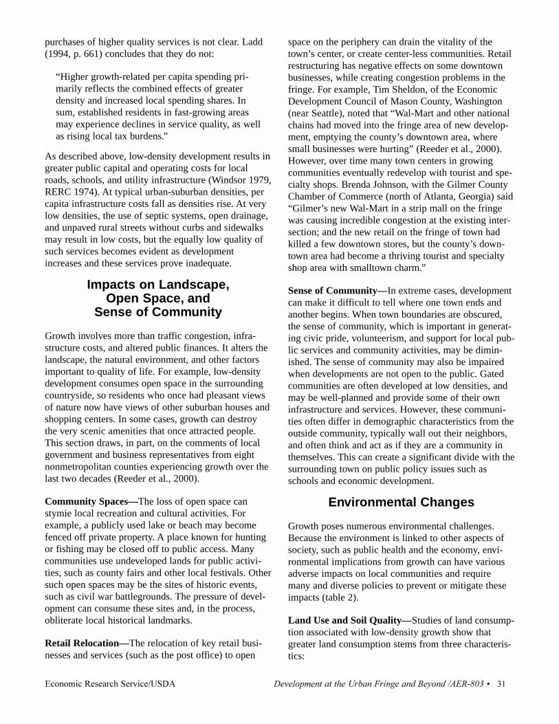
purchases of higher quality services is not clear. Ladd(1994, p. 661) concludes that they do not:

“Higher growth-related per capita spending pri-marily reflects the combined effects of greaterdensity and increased local spending shares. Insum, established residents in fast-growing areasmay experience declines in service quality, as wellas rising local tax burdens.”

As described above, low-density development results ingreater public capital and operating costs for localroads, schools, and utility infrastructure (Windsor 1979,RERC 1974). At typical urban-suburban densities, percapita infrastructure costs fall as densities rise. At verylow densities, the use of septic systems, open drainage,and unpaved rural streets without curbs and sidewalksmay result in low costs, but the equally low quality ofsuch services becomes evident as developmentincreases and these services prove inadequate.

Impacts on Landscape,Open Space, and

Sense of Community

Growth involves more than traffic congestion, infra-structure costs, and altered public finances. It alters thelandscape, the natural environment, and other factorsimportant to quality of life. For example, low-densitydevelopment consumes open space in the surroundingcountryside, so residents who once had pleasant viewsof nature now have views of other suburban houses andshopping centers. In some cases, growth can destroythe very scenic amenities that once attracted people.This section draws, in part, on the comments of localgovernment and business representatives from eightnonmetropolitan counties experiencing growth over thelast two decades (Reeder et al., 2000).

Community Spaces—The loss of open space canstymie local recreation and cultural activities. Forexample, a publicly used lake or beach may becomefenced off private property. A place known for huntingor fishing may be closed off to public access. Manycommunities use undeveloped lands for public activi-ties, such as county fairs and other local festivals. Othersuch open spaces may be the sites of historic events,such as civil war battlegrounds. The pressure of devel-opment can consume these sites and, in the process,obliterate local historical landmarks.

Retail Relocation—The relocation of key retail busi-nesses and services (such as the post office) to open

space on the periphery can drain the vitality of thetown’s center, or create center-less communities. Retailrestructuring has negative effects on some downtownbusinesses, while creating congestion problems in thefringe. For example, Tim Sheldon, of the EconomicDevelopment Council of Mason County, Washington(near Seattle), noted that “Wal-Mart and other nationalchains had moved into the fringe area of new develop-ment, emptying the county’s downtown area, wheresmall businesses were hurting” (Reeder et al., 2000).However, over time many town centers in growingcommunities eventually redevelop with tourist and spe-cialty shops. Brenda Johnson, with the Gilmer CountyChamber of Commerce (north of Atlanta, Georgia) said“Gilmer’s new Wal-Mart in a strip mall on the fringewas causing incredible congestion at the existing inter-section; and the new retail on the fringe of town hadkilled a few downtown stores, but the county’s down-town area had become a thriving tourist and specialtyshop area with smalltown charm.”

Sense of Community—In extreme cases, developmentcan make it difficult to tell where one town ends andanother begins. When town boundaries are obscured,the sense of community, which is important in generat-ing civic pride, volunteerism, and support for local pub-lic services and community activities, may be dimin-ished. The sense of community may also be impairedwhen developments are not open to the public. Gatedcommunities are often developed at low densities, andmay be well-planned and provide some of their owninfrastructure and services. However, these communi-ties often differ in demographic characteristics from theoutside community, typically wall out their neighbors,and often think and act as if they are a community inthemselves. This can create a significant divide with thesurrounding town on public policy issues such asschools and economic development.

Environmental Changes

Growth poses numerous environmental challenges.Because the environment is linked to other aspects ofsociety, such as public health and the economy, envi-ronmental implications from growth can have variousadverse impacts on local communities and requiremany and diverse policies to prevent or mitigate theseimpacts (table 2).

Land Use and Soil Quality—Studies of land consump-tion associated with low-density growth show thatgreater land consumption stems from three characteris-tics:

��

��

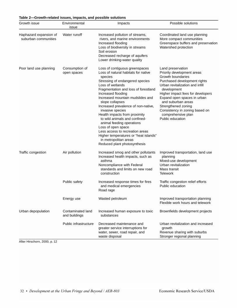
Table 2—Growth-related issues, impacts, and possible solutions

Growth issue Environmental Impacts Possible solutionsissue

Haphazard expansion of Water runoff Increased pollution of streams, Coordinated land use planningsuburban communities rivers, and marine environments More compact communities

Increased flooding Greenspace buffers and preservationLoss of biodiversity in streams Watershed protectionSoil erosionDecreased recharge of aquifersLower drinking-water quality

Poor land use planning Consumption of Loss of contiguous greenspaces Land preservationopen spaces Loss of natural habitats for native Priority development areas

species Growth boundariesStressing of endangered species Purchased development rightsLoss of wetlands Urban revitalization and infillFragmentation and loss of forestland developmentIncreased flooding Higher impact fees for developersIncreased mountain mudslides and Expand open spaces in urban

slope collapses and suburban areasIncreased prevalence of non-native, Strengthened zoning

invasive species Consistency in zoning based onHealth impacts from proximity comprehensive plan

to wild animals and confined- Public educationanimal feeding operations

Loss of open spaceLess access to recreation areasHigher temperatures or “heat islands”

in metropolitan areasReduced plant photosynthesis

Traffic congestion Air pollution Increased smog and other pollutants Improved transportation, land use Increased health impacts, such as planning

asthma Mixed-use developmentNoncompliance with Federal Urban revitalization

standards and limits on new road Mass transitconstruction Telework

Public safety Increased response times for fires Traffic congestion relief effortsand medical emergencies Public education

Road rage

Energy use Wasted petroleum Improved transportation planningFlexible work hours and telework

Urban depopulation Contaminated land Increased human exposure to toxic Brownfields development projectsand buildings substances

Public infrastructure Decreased maintenance and Urban revitalization and increasedgreater service interruptions for growthwater, sewer, road repair, and Revenue sharing with suburbswaste disposal Stronger regional planning

After Hirschorn, 2000, p. 12

• low density of settlement;

• unlimited outward extension of growth;

• “leapfrog” or fragmented development pattern (Axel-rad, 1998).

Low-density development results in a greater loss ofagricultural lands than more compact development.However, studies have shown that, nationwide, theamount of prime and class I-IV cropland lost in urban-izing areas was proportional to the amount of thosesoils found in the area (Heimlich and Bills, 1997;Heimlich and Krupa, 1994; Vesterby and Krupa, 1993;Vesterby et al., 1994). Low-density patterns of develop-ment result in a greater loss of sensitive environmentallands, including wetlands, flood plains, critical habitat,aquifer recharge areas, stream corridors, and steepslopes.

Better planned, more compact settlement patterns canoften avoid converting such lands, incorporating theminto open space and environmental protection zones.Studies by Burchell (1992-97) and Landis (1995), sum-marized in Axelrad (1998), estimated such land con-sumption savings (figure 16).

Wildlife Habitat—Development disturbs, pollutes, anddestroys the natural habitats for various native specieswhen it consumes wetlands, forests, alpine, and desertterrain. Insecticides and fertilizers used on lawns can

have significant negative effects on wildlife. In somecases, Federal or State governments will cause commu-nities to restrict development and related activities toprotect wildlife. For example, Bob Fink, of MasonCounty’s planning office, noted that “because of a newseries of endangered species announcements coveringseveral species of fish, his county may change itsdevelopment regulations.” However, not all wildlifeeffects are bad. For example, some types of develop-ments provide protected green space or parkland thatcreates mini-ecosystems where habitat-generalistspecies and those that can fly between fragments canflourish (Lovejoy et al., 1984, Whitcomb et al., 1981).

Growth seriously fragments wildlife habitats. Habitatfragmentation is often singled out as a principal threatto the preservation of biodiversity (Harris and Gal-lagher 1989; Wilcox and Murphy 1985; Noss andCooperrider 1994). The negative effects of fragmenta-tion on biodiversity are numerous, and can be groupedinto four major categories:

• Reduction in total habitat area. Habitat remnants sup-port fewer species and smaller populations of thesame species than larger swaths;

• Loss of wide-ranging, low-density, and habitat-spe-cialist species. Mountain lions, which have rangesthat can exceed 1,000 square kilometers (Hemker etal. 1984) are now extinct in a recently isolated habitat

��

Figure 16Savings of agricultural and environmentally sensitive lands, compact growth versus "sprawl"

0

10

20

30

40

50

60Percent reduction relative to sprawl

New Jersey Lexington, KY MichiganSouth Carolina Delaware Bay San Francisco Bay

Sources: Studies reported in Axelrad, 1998.

Agricultural land Environmentallysensitive land

fragment in Orange County, California. Habitat inte-rior dwellers, such as some forest birds, may belocally extinct from fragments of 1 square kilometeras studies in eastern North American deciduousforests have shown (Whitcomb, 1977; Wilcove et al.,1986);

• Increased “edge effects,” or the microclimaticchanges that occur along power line corridors, roadsand urban development which favor exotic speciesoften at the expense of native and interior species(Newmark, 1987); and

• Increased extinction risk from demographic, environ-mental, and genetic variances (Menges, 1992).

Urban development is one of the principal causes ofwetland loss. In 1985, 85 percent of Maine’s wetlandswere visible from a road or within 2,000 feet of a road,and thus of limited habitat value. Of Maine’s 2,700lakes, 200 have been harmed by development, and 300are at risk (Maine State Planning Office, 1997).Between 1982 and 1992, the National Resources Inven-tory showed that 89,000 acres of wetlands were lost tourban uses per year, 57 percent of total gross wetlandloss (Heimlich et al., 1998).

Development of roads in formerly rural areas createsincreased opportunities for collisions between wildlifeand new urban residents. The Humane Society and theUrban Wildlife Research Center estimate that morethan 1 million large animals are killed annually on U.S.highways. Roadkills usually increase with trafficspeeds and volumes. Studies in the state of Floridaindicate that road kills are the primary cause of deathfor most large mammals, including several threatenedspecies. Some animals have an aversion to roads, whichmay affect their behavior and movement patterns. Forexample, black bears cannot cross highways withguardrails. Other species become accustomed to roads,and are therefore more vulnerable to harmful interac-tions with humans. By forming a barrier to speciesmovement, roads and development fragment and isolatewildlife populations, preventing interaction and crossbreeding between population groups of the samespecies. This reduces population health and genetic via-bility. Development and road construction and useintroduce a variety of noise, air, and water pollutants.Loss of habitat, invasion of exotic species, alteration ofwatershed hydrology through changes in water qualityand water quantity, stream channels, and groundwaterall accompany development, as does increased access

by hunters, poachers, and irresponsible visitors (Lit-man, 1999).

Water—Many of development’s health-related issuesinvolve water. For example, much of the developmentin the countryside involves homes with on-site septicsystems, which often cause greater water pollutionproblems than municipal sewage systems. While manyof the bigger developments are hooked up to municipalor county water and sewer systems, these systems cansometimes overflow, particularly during heavy storms,causing significant pollution problems. Some develop-ers build their own wastewater treatment plants, andthese systems sometimes prove to be inadequate.“These private developer-built systems sometimesprove to be unacceptable in quality. This happenedrecently in Lyon County (Nevada), and the countyended up having to pay for upgrades and repairs tothese systems to meet public standards,” according toMark Clarkson, manager of Lyon County’s UtilitiesDivision.

The type of land use, and particularly its density andthe amount of impervious surface, affects the amountof pollutants in storm water runoff. More intense usesengender more pollutants, and large impervious sur-faces lead to greater volumes of runoff and more pollu-tion. The original “Costs of Sprawl” report (RERC,1974) estimated that low-density “sprawl” generatedthe most sediment, biological and chemical oxygendemand, nitrogen and phosphorus runoff, and sus-pended solids and fecal coliform bacteria of any devel-opment pattern.

A New Jersey study of different urban developmentpatterns found that compact development would gener-ate significantly less pollution than low-density devel-opment for all categories of pollutants (Burchell, 1992).The reduction ranged from over 40 percent for phos-phorus and nitrogen to 10 percent for lead (figure 17).The study noted that, in some places where develop-ment is particularly dense, water quality will deterio-rate, but in general water quality will be better withplanned growth than with unplanned development.

Another problem, particularly in the West, involveslimited or declining water supplies. Many new homesin the countryside use on-site wells for water, and insome cases underground water supplies are declining.This problem is exacerbated by less natural replenish-ing of underground water due to increased water runoffcaused by increased area of impervious surfaces, such

��

as roofs, roads and parking lots, and the building ofsewers.

Floods and fires can become more significant concernsas more people move to the countryside (Esseks et al.,1998). For example, Rob Nesbitt, of the LamoilleCounty Planning Commission (near Burlington, Ver-mont) reported that “Lamoille County has had a historyof floods. None of our water bodies have flood controldams on them.” Development not only raises the stakesof life and property loss, it may also help cause oraggravate floods and fires. For example, constructionoften causes erosion which fills ups streams and in-creases the likelihood of floods, and the increased areaof impervious surface increases flood peaks. Develop-ment may add to heat retention, eliminate wetlands,and result in reduced forestland management, resultingin increased fuel and adding to the threat of fires.

Air Quality—Air pollution is sometimes an importantenvironmental issue in areas with high rates of com-muting, where ground level ozone (smog) emitted fromautos creates significant health concerns. When thelevel of air pollution exceeds EPA standards, Federallaw requires that planning be aimed at reducing air pol-lution levels, or the State may be penalized by reduc-tions in Federal highway aid.

Other Quality of Life Issues

Aside from traffic congestion, other quality of lifeissues affected by growth are the quality of educationand the affordability of housing.

Education—Many are drawn to these rapidly growingareas by the perception that schools are of better qual-ity than those in the central cities. However, newcomers

��

Figure 17Water quality impacts by community type

0

20

40

60

80

100

120

140

160

Sediment Volume Biological oxygen demand

Chemical oxygen demand

Nitrogen Phosphorus Suspended solids

Fecal coliform bacteria

Percent of pollutant runoff relative to "sprawl" level

"Sprawl" mix Planned mix Combination mix Low-density planned

Low-density "sprawl" High-density planned New Jersey OPS Trend New Jersey OPS Plan

Sources: RERC, 1974; Burchell, 1992 New Jersey Office of State Planning Trend was for existing mix of development; Plan was for greater density.

often demand improvements after they arrive. In addi-tion, the influx of new students is so rapid andunplanned that schools can quickly become over-crowded. Even in places that plan well ahead for theincoming school populations, some problems remainfor schools in growing areas. For example, according toPete Kelly, school superintendent for Citrus County,Florida, “Many schools are already built in the develop-ing areas, however there are too many developing areasto build high schools in every one. With the populationspread far and wide, long bus trips are required totransport students to the high schools.”

While demands for schools and other services areincreasing, many growing communities experienceslower growth in tax base and expendable revenue, dueto the tendency of commercial and industrial develop-ment to lag behind residential growth. Without concur-rent growth in the commercial and industrial tax base,schools often must make cuts in current spending perpupil. In addition, because most of these places findthat their new student population is above the povertylevel, State and Federal aid does not grow proportion-ally with student populations. As a result, many schoolsystems in growing communities are constantly playingcatch-up in school construction, and are hard pressed tocome up with sufficient tax revenues to maintain edu-cation quality.

Affordable Housing—Affordable housing is anotherissue of concern. Though single-family housing may becheaper on the fringe than in central cities or the innersuburbs, not much housing is available at prices thatlow-income individuals or families can afford. In somecases, local zoning provisions exacerbate this situationby requiring more expensive large-lot development. Forexample, Comissioner John Metli of Elbert County,Colorado (near Denver), said “Elbert County’s averagehome costs $225,000—up from $150,000 just 5 yearsago, and this lack of affordable housing is self-inflicted, because regulations are more stringent on the5-acre lots, making it more economical to buy andbuild on a 60-acre lot than on a 5-acre lot in a high-priced development.”

Although the lack of affordable housing may not beperceived as a problem by most local residents, itbecomes a problem for low-wage industries, includingretail and services. It is also a problem for the childrenof long-term residents who may lack the incomes to be able to afford new housing in the area. Conse-quently, local governments often must require thatdevelopers build some affordable housing.

Despite these negative aspects, it would be wrong toconclude that the quality of life declines in all respectsfor places experiencing low-density development. Forexample, the retail and commercial growth that followsresidential growth provides local residents with agreater diversity of goods and services to purchase, aswell as a growing supply of jobs. While it is true thatmany of these jobs are low paying compared with sometraditional rural jobs (such as mining and manufactur-ing), many provide part-time or seasonal employmentthat is critical for supplementing family income. Forexample, farmers have come to rely on this form of off-farm employment to maintain their standard of living inthe face of weak agricultural markets.

An Economic Interpretation of the Demand for

Low-Density Development

The worst consequences of unplanned, low-densitydevelopment are not the result of some vast conspiracyby ruthless capitalists known as “developers.” WaltKelly’s famous cartoon character Pogo correctlyobserved that, “We have met the enemy, and he is US”(Walt Kelly). Millions of individual choices by con-sumers and businesses which are aimed at creating abetter way of life designed to garner the benefits oflow-density development outlined above instead resultin patterns of development that often have negativeconsequences for new and old residents alike in loss ofrural amenity, traffic congestion, and environmentaldegradation. How can consumers, businesses, and com-munities so consistently fail to anticipate the results oftheir actions with regard to development?

Economists usually attribute such unanticipated resultsto market failure. While the markets for housing andcommercial real estate work efficiently, the market for“lifestyles,” including landscape or rural amenitieseither fails to exist or fails to deliver the anticipatedbenefits. This market failure can be understood as aris-ing from interactions among the following factors:

• Markets for positive externalities from agriculturalproduction, such as open space and rural amenities,do not exist. Therefore, these attributes in the land-scape are neither permanent nor even necessarilylong-lived when development begins to occur. Hous-ing construction does not impose negative spillovereffects (externalities) in this regard, it removes posi-tive spillovers that were in place from the previouseconomic activity, farming.

��

• Negative spillovers from housing consumption, suchas traffic congestion, destruction of visual amenities,and crowding, are not priced in the cost of the hous-ing or other development. If the cost of the landscapeamenities were accurately included, “housing” costswould be much higher and demand lower. For exam-ple, fully planned communities with carefully con-trolled land uses and landscape amenities such asopen space, lakes, and recreational facilities includedare more expensive than nearby developments withoutthese amenities.

• Imperfect information creates a market failurebecause consumers do not anticipate future develop-ment patterns and do not weigh them perfectly in cur-rent housing purchase decisions.

• Absence or failure of planning and zoning in localcommunities contributes to this failure because thereis no information about the institutional frameworkwithin which future development can take place.When future development is dealt with on a piece-meal or ad hoc basis, neither consumers nor develop-ers can adequately anticipate what development willoccur on surrounding parcels.

• Developers, who generally have a good grasp of future development potential, have no incentive toinform housing consumers who value open space and other rural amenities that they are likely to bedeveloped.

Other sources of failure in the “lifestyle” market derivefrom the nature of development and land-use change.Development results from the cumulative impacts ofmany small decisions, with the rare exception of alarge, planned, “new town,” such as Columbia, Mary-land, Reston, Virginia, or Irvine Ranch, California.Markets proceed on the basis of many small decisions,which when taken without an overall context, produceresults that can be neither envisioned by nor anticipatedby consumers and developers (Kahn, 1966). There is noproblem when consumers of corn or soap fail to antici-pate the resultant changes in supply and demand thatresult from their atomistic consumption decisionsbecause corn and soap producers respond quickly and

seamlessly to small variations in supply and demand invery short order. However, the cumulative effects ofsimilar decisions in land use can result in significantdisamenity over time (CEQ, 1997; Spaling and Smit,1993). Specifically:

• Individual developers’ decisions, which produce nega-tive spillovers for existing land users, are generallysmall in scale relative to the entire landscape, occur-ring subdivision by subdivision, or even house byhouse (Fischel, 1999, p. 411).

• Consumers’ decisions on housing consumption, whichproduce negative spillovers for each other from con-sumption, are made one house at a time.

• Both developers’ and consumers’ decisions are irre-versible over time scales of a lifetime, providing littlescope for adjustment except to move to a “clean can-vas” in another rural setting (Tiebout, 1956; Hamil-ton, 1975).

• Efficiency in the real estate market increases propertyvalues as development proceeds in desirable newneighborhoods, creating greater incentives to develop(Lafferty and Frech, 1978; Burnell, 1985; Speyer,1989).

• Negative spillovers from development do not create adrag on property values in the real estate market untildisamenities are quite high.

In summary, there are substantial costs imposed byallowing low-density development, both at the fringe ofexisting urban area and farther out in the rural country-side. People recognize substantial benefits from main-taining and conserving rural land uses in farming, graz-ing, and forestry. While some communities activelyaddress growth control issues, private market forcesoften operate with minimal intervention from fragmentedland-use control authorities at the State and local levelsand cannot recognize and avoid these costs, nor capital-ize on the benefits. land-use issues are primarily localin nature, and, under our constitutional system, author-ity over them rests with State and local government.But the consequences of development are being felt allacross the Nation, in almost a third of the country.

��

Through the entire process of development, farmingcoexists with development and adapts, howeveruneasily, in the shadow of the city. Settlement patternsthat create low-density development and fragmentationacross rural landscapes have both negative and positiveconsequences for agriculture. Increasing population andemployment provide some opportunities for farms, butalso create problems.

Agriculture: Farming in the City’s Shadow

Large and growing areas of U.S. agriculture are influ-enced by proximity to urbanization and concentrationsof population brought about by growth. MetropolitanStatistical Areas (MSAs), defined by the Bureau of theCensus, contain 20 percent of U.S. land area and 80percent of the U.S. population (Bureau of the Census,

GARMS, 2000). Nationally, farms in metropolitanareas are an increasingly important component of U.S.agriculture. In 1997, they made up a third of all farmsand controlled 39 percent of farm assets (table 3). Eigh-teen percent of farmland operated was located in metroareas in 1997, roughly proportional to the total land inmetro areas (Barnard and Heimlich, 1993; Heimlichand Barnard, 1992, 1997; Hoppe and Korb, 2000). Thecount of farms excludes service firms, such as horseboarders and landscape services that are not directlyinvolved in agricultural production, but that contributeto open space and economic activity.

As urbanization proceeds, landowners may seek enter-prises and markets that offer returns to land more com-mensurate with those from development, in part to off-set the higher property taxes that are incurred as landprices rise to reflect the potential for future nonagricul-

��

V. Consequences for Farming

Table 3—Metro and nonmetro farm characteristics, United States, 1991 and 1997

MetroCharacteristic Recreational Adaptive Traditional Subtotal Nonmetro Total

Number

Number of farms, 1991 372,689 97,024 226,704 696,416 1,390,607 2,087,023Number of farms, 1997 283,776 74,522 199,569 557,867 1,181,349 1,739,216

Thousand acres

Acres owned, 1991 23,107 12,613 55,996 91,927 417,182 509,109Acres operated, 1991 33,542 24,741 142,370 200,568 1,090,236 1,290,804Acres operated, 1997 22,675 13,894 123,323 159,892 733,031 892,923

Million dollars

Sales of agr. products, 1991 910 18,877 17,647 36,900 69,975 106,875Net cash farm income, 1991 -1,813 4,190 2,752 4,993 13,866 18,858Total off-farm income, 1991 16,708 4,564 2,102 27,883 38,301 66,185Assets, 1991 92,026 90,537 129,420 311,982 489,434 801,416Net worth, 1991 85,251 79,328 116,207 280,786 424,312 705,098Sales of agr. products, 1997 996 27,652 38,055 66,703 130,162 196,865Sales per acre operated, 1991 27 763 124 184 64 83Sales per acre operated, 1997 44 1,990 309 417 178 220

Percent of all farms

Number of farms, 1991 18 5 11 33 67 100Number of farms, 1997 16 4 11 32 68 100Acres owned, 1991 5 2 11 18 82 100Acres operated, 1991 3 2 11 16 84 100Acres operated, 1997 3 2 14 18 82 100Sales of agr. products, 1991 1 18 17 35 65 100Sales of agr. products, 1997 1 14 19 34 66 100Net cash farm income, 1991 -10 22 15 26 74 100Total off-farm income, 1991 25 7 3 42 58 100Assets, 1991 11 11 16 39 61 100Net worth, 1991 12 11 16 40 60 100Sources: 1991 data from Heimlich and Barnard, 1996; 1997 data from Hoppe and Korb, 2000

tural development. Initially, this may involve innovativemarketing techniques, such as U-pick, community agri-culture, contracts with restaurants, or farmers’ markets.At some point, successfully adapting farmers maybecome more general rural entrepreneurs, not limitingthemselves to farm activities at all. Landowners mayalso sell off less productive woodlots and pastureland,concentrating on more intensive production on remain-ing cropland. Other farmers attempt to maintain tradi-tional crops and practices, some merely waiting for theperceived inevitable sale for development. Some farmssimply go out of business and the land remains idle, orthe land is divided and sold to hobby farmers, recre-ational farmers, or part-time farmers whose primary useof the land is as a residence.

Many of the economic changes faced by farmers on theurban fringe have a dual-edged impact on agriculture,bringing pressures to adapt, while simultaneously offer-ing opportunities and rewards for doing so. On thedown side, proximity to urban areas can present obsta-cles to profitable farming operations.

Positive Impacts on Farming from Urbanization• Proximity to urban centers may provide a larger pool

of seasonal or part-time labor that is especially impor-tant to harvest high-value crops. One reason metrofarms can adopt high-value crops is because localsources of labor are available at peak periods (Jordon,1989).

• Greater off-farm employment opportunities for thefarmer or his/her family may help support the farmingoperation (Stallman and Alwang, 1991). Off-farmemployment can also provide a transition to part-timefarming, particularly if enterprise changes are under-taken that reduce full-time labor needs on the farm.Opportunities from urban employment run in bothdirections. People in urbanizing areas may work part-time on the farm or start recreational farms that even-tually develop into full-time, part-time, or retirementbusinesses.

• Nationally, 90 percent of average farm householdincome was from off-farm sources in 1999, includingpart-time employment, spousal income, and otherbusiness income. The percentage in recent years hasvaried from 83 to 90 percent. Government paymentsare part of gross cash income, and cannot be com-pared to net farm income or household income. Only36 percent of farms receive government payments,

and the percentage is lower in metro areas (Sommeret al., 1998, table 31).

• Expanding populations provide opportunities forfarmers to grow new crops and to market them in newways, such as through farmers’ markets (figure 18;Price and Harris, 2000). High-value crops, such asfresh fruits and vegetables, can be sold throughrestaurants and gourmet grocery outlets or directly toconsumers in roadside stands or U-pick operations(see box, “Urbanization and Vegetable Production”).U-pick farms may combine produce sales with value-added products like dried herbs or flowers, jams andjellies, homemade breads or pastries, or other farm-related products. Recreational aspects of U-pick oper-ations, such as hayrides, picnics, farm-pond fishing,and special holiday features, such as old-fashionedHalloween or Christmas activities, may also add valueto urban customers’ purchases. Horse boarding,breeding, and training facilities, cattle-breeding oper-ations or other specialty livestock operations mayreplace more extensive dairy farms and cow-calfoperations.

Negative Impacts on Farmingfrom Urbanization• Suburban neighbors’ complaints about farm odors and

chemical spraying may force farmers to turn to enter-prises that produce fewer negative side effects. Someof the alternatives will be more profitable and somewill be less (Reynnells, 1987; Van Driesche et al.,1987).

• Conflicts can arise between growers and new subur-ban neighbors over early morning noise, andincreased traffic can hinder farmers’ ability to movetheir equipment along overcrowded rural roads beingused as commuter routes.

• Markets for traditional dairy products or field cropsmay be reduced, as milk-collection routes are cur-tailed and grain elevators go out of business. In someareas, farm input suppliers, machinery dealers, andother forms of agricultural support may decline.

• Real estate taxes may rise as land prices rise to reflectthe potential for nonfarm development.

• Growers may face increased pressure from water- andland-use restrictions.

• Farms may face deteriorating crop yields from urbansmog, theft, and vandalism.

��

The dynamic forces of urbanization create an urbanfringe in which a variety of farm types coexist, reflect-ing different paths that farms have taken in adapting tourban influence (figure 19; see box “CategorizingMetro Farms” for methods). These changes occur pri-marily through changes in the product and input mar-kets in which farmers buy and sell, and through theactions of local government institutions, which by lawand tradition exercise control over property taxes andland use (Heimlich and Brooks, 1989). Farms in metroareas are generally smaller, produce more per acre,have more diverse enterprises, and are more focused onhigh-value production than nonmetro farms (Barnardand Heimlich, 1993; Heimlich and Brooks, 1989;Heimlich 1988; Heimlich and Barnard, 1992, 1997;Hoppe and Korb, 2000). Metro agriculture is character-ized by a relatively large group of recreational farmerswho are availing themselves of opportunities in bothfarm and nonfarm pursuits, a smaller group of moreadaptive farmers who have accommodated their farm-ing operation to an urban environment, and a residualgroup of more traditional farmers who are trying to sur-

vive in the face of urbanization (see box, “CategorizingMetro Farms”).

Recreational farms in metro areas accounted for 16-18percent of U.S. farms, but contributed only 1 percent toaggregate U.S. sales of agricultural products. Withinmetro areas, recreational farms accounted for 51-54percent of farms and controlled 29-30 percent of farmsector assets and equity and 14-17 percent of the landoperated. These recreational farms have little viabilityas economic enterprises and are essentially a consump-tion activity that will become increasingly expensivefor their owners as urban development continues. Tra-ditional farms made up a third of metro farms, operated71-77 percent of metro farm acreage, and controlledmore than 40 percent of assets, sales, and net cash farmincome. When a farm hobby is no longer fun, or thefarming tradition finally yields too little profit to con-tinue, development may soon follow.

Adaptive farms accounted for 13-14 percent of metrofarms and 9-12 percent of metro farm acreage operated,

��

#

#

#

#

#

#

#

#

#

#

#

#

#

#

#

#

#

#

#

##

#

#

#

##

#

#

##

#

#

###

##

#

###

#

#

#

#

#

#

##

##

#

#

#

#

#

#

#

#

##

##

#

#

#

#

#

#

#

##

#

##

#

#

#

#

#

#

#

#

#

#

###

#

#

#

#

#

#

#

#

##

#

#

#

##

#

## #

#

#

#

#

##

#

#

#

#

#

#

#

##

#

#

#

#

#

#

#

#

#

#

##

#

#

#

#

#

#

#

#

#

##

#

#

##

#

#

#

#

#######

#

#

#

#

#

#

###

####

##

##

#

#

##

###

#

#

##

#####

##

#

#

# #

#

##

##

#

#

#

#

#

#

#

#

#

#

#

#

##

#

#

#

###

##

#

#

#

# ####

#

#

#

#

##

#

#

#

##

#

#

#

#

##

# #

#

#

#

#

#

#

##

#

#

#

#

#

#

#

#

##

#

#

#

##

#

#

#

##

# ###

### #

#

###

#

##

#

#

##

#

#

#

##

#

##

#

#

###

####

#

#

#

#

#

#

#

#

#

#

#

#

#

#

#

#

#

#

#

#

#

###

#

#

#

#

#

#

#

#

#

#

#

#

#

##

#

#

#

#

#

#

#

#

#

#

#

#

###########

#

#

####

#

##

#

#

#

#

#

#

#

#

#

#

#

#

#

#

##

#

#

#

#

#

##

#

#

#

#

#

#

#

#

#

#

#

#

#

#

#

#

#

#

#

#

#

#

#

#

#

#

#

#

#

#

##

#

#

#

#

##

#

#

#

# ##

#

#

##

#

#

#

#

#

#

#

#

#

#

#

#

#

##

###

#

#

#

#

#

#

#

#

#

#

#

#

#

#

#

#

#

#

#

#

#

# ##

#

#

# #

##

#

##

#

#

#

#

#

#

#

#

#

#

#

#

#

#

#

#

#

#

#

#

#

###

#

##

#

#

#

#

#

#

#

#

#

#

##

#

#

#

#

#

#

#

#

#

#

#

##

##

#

#

#

# #

#

#

#

#

#

##

#

##

#

##

#

#

#

#

##

# #

#

#

#

#

#

#

#

#

#

##

#

#

#

##

#

#

#

#

#

#

#

#

#

#

#

#

#

#

#

##

#

#

#

#

#

#

#

#

#

#

#

##

##

#

#

#

#

#

#

#

##

#

#

###

#

#

#

#

#

# #

#

#

#

#

#

#

#

##

#

#

##

##

#

##

##

#

##

#

#

##

#

#

#

## #

##

#

#

#####

#

####

#

#

## ###

###

####

##

####

#

#

#

#

#

#

#

#

##

##

#

#

##

#

#

#

#

#

#

#

##

#

#

#####

#

## ##

##

#

##

#

#

#

#

#

#

#

##

#

#

#

##

# #

#

#

#

####

#

##

#

#

#

# #

##

##

#

##

#

#

#

#

###

#

###

##

#

#

#

#

#

#

#

#

##

##

# #

#

#

##

#

##

#

#

##

#

#

#

#

#

#

#

#

#

#

#

#

#

#

#

#

#

#

#

###

#

## #

#

#

#

#

#

#

#

#

#

#

#

#

#

##

#

#

#

#

#

##

#

#

#

#

#

#

#

#

##

##

#

#

#

#

#

#

#

#

#

#

#

#

#

#

#

#

#

#

#

#

#

#

##

#

#

#

##

####

#

#

#

####

#

#

#

#

#

##

#

#

#

#

#

#

#

#

#

#

#

##

#

##

##

#

#

###

#

#

#

##

# #

#

#

#

#

##

#

#

#

#

#

#

#

#

#

#

#

#

#

#

#

#

#

#

#

#

##

#

#

#

#

#

#

#

#

#

##

##

#

#

#

#

#

##

#

#

##

#

#####

# #

##

# #

#

#

#

#

#

##

#

# #

#

#

#

#

##

##

#

#

#

#

#

#

#

#

#

#

#####

##

#

#

#

#

#

#

#

#

#

#

#

#

#

#

##

#

#

#

##

#

#

#

#

#

#

#

##

#

#

#

#

##

#

#

#

#

#

#

## #

##

#

# #

#

#

#

#

#

##

#

##

#

#

#

#

##

##

#

#

#

#

#

#

#

#

#

#

##

#

#

##

#

#

###

#

#

#

##

#

#

# #

###

#

#

#

#

##

#

# #

#

#

####

# #

#

#

#

#

# #

#

#

##

#

#

#

#

##

#

#

#

#

##

#

#

##

#

#

#

#

#

##

##

#

#

#

#

#

#

#

##

##

#

#

#

#

#

#

#

#

#

###

#

##

#

#

#

#

#

#

#

#

#

#

#

#

#

#

#

#

#

#

#

#

#

#

#

#

#

#

#

#

#

#

##

#

#

#

#

##

#

##

#

##

#

#

#

##

#

#

#

#

#

#

#

#

#

#

#

#

#

#

#

###

#

##

#

#

#

#

#

#

#

#

#

#

#

##

#####

#

#

#

##

#

#

##

#

#

#

#

#

#

#

#

#

#

#

#

#

#

#

#

#

##

#

#

#

#

#

#

#

#

#

##

#

#

#

##

##

#

#

#

#

#####

####

#

##

#

#

#

##

##

#

# ##

##

#

#

#

##

#

#

#

#

#

##

#

#

#

#

#

#

##

#

# #

#

##

#

#

#

#

#

#

##

#

##

#

#

#

##

#

#

#

#

#

#

#

#

#

#

##

#

#

#

#

#

#

#

#

##

#

#

#

#

#

#

#

###

#

#

#

#

#

#

#

#

#

#

#

#

#

#

#

#

#

#

###

#

#

#

#

#

##

#

#

#

#

#

#

#

####

#

#

#

#

#

#

#

#

#

#

# ##

#

#

###

## #

##

#

#

#

##

##

##

#

#

#

#

#

#

#

#

#

#

##

#

#

###

#

#

#

#

#

#

#

##

#

#

#

#

#

#

#

##

#

#

#

#

#

#

#

#

#

#

#

#

#

##

#

#

#

#

#

#

#

##

#

#

#

###

##

#

#

#

#

##

#

##

#

#

#

#

#

#

##

#

#

#

###

#

##

#

#

#

#

# ## ##

#

##

#

#

##

##

#

#

#

#

#

#

#

#

#

#

#

##

## ##

#

# #

#

##

#

#

#

#

###

#

#

##

#

# #

#####

#

#

#

#

#

#

###

#######

#

#

#

#

#

#

#

# #

#

#

#

#

##### #

#

#

#

#

#

##

##

#

# #

#

###

#

#

#

#

##

##

#

#

#

#

#

#

#

#

#

##

##

#

#

#

#

#

#

#

#

###

#

#

#

#

#

#

#

#

#

#

#

#

#

#

#

###

#

#

#

#

#

#

#

#

#

##

#

#

#

#

#

#

#

#

#

#

#

##

#

#

#

#

#

##

#

#

#

#

#

#

#

#

#

#

#

#

#

#

#

#

#

#

#

##

##

#

#

#

#

#

#

#

#

#

#

#

#

#

##

#

#

#

#

#

##

##

#

##

#

# #

#

#

#

##

#

#

##

##

##

#

#

#

# #

#

#

###

#

#

#

#

#

#

#

##

##

##

#

#

#

#

#

#

#

#

#

#

#

#

##

#

#

#

#

#

#

#

#

# #

#

##

##

##

#

###

#

## #

#

#

#

#

##

#

#

#

##

#

##

#

#

#

#

#

#####

#

#

#

####

#

#

#

#

#

#

##

#

#

# ###

##

## #

###

#

#

#

#

#

#

##

#

#

#

#

# #

##

#

#

#

#

#

###

#

#

#

#

#

#

#

# #

#

#

##

#####

#

#

#

#

#

#

#

#

##

#

#

#

#

##

#

#

#

#

#

#

#

#

#

#

#

#

#

#

#

#

#

## #

#

#

#

#

#

#

#

#

#

#

#

#

#

#

#

#

#

#

#

#

##

##

#

##

#

#

#

#

#

##

#

#

#

#

#

#

# #

##

#

#

#

#

#

#

#

#

#

#

#

#

#

#

#

#

#

#

#

#

#

#

#

#

#

#

#

##

#

##

#

####

# ###

##

#

#

##

##

##

#

#

### ##

##

#

#

#

#

#

##

###

#

#

#

##

#

####

#

#

#

#

#

#

###

#

#

#

#

#

#

#

##

#

#

#

#

#

#

#

#

#

##

#

#

#

#

#

#

#

#

#

#

#

#

#

#

##

#

#

#

#

#

# ##

#

#

#

#

#

##

##

#

#

##

#

###

#

#

#

##

#

#

#

#

#

#

#

#

#

#

##

#

#

#

#

#

#

#

##

#

##

#

#

#

###

#

#

#

#

#

#

#

#

#

#

#

#

#

#

#

#

#

#

#

#

## #

#

#

#

#

#

#

#

#

#

#

#

#

#

#

#

#

#

#

#

#

#

#

##

##

#

#

#

#

#

#

#

#

##

#

#

#

# #

#

#

#

#

#

#

##

#

#

#

#

###

#

## #

#

##

#

# #

#

# #

#

#

#

####

# #

####

#

###

#

###

####

#

#

#

#

#

#

#

#

#

#

#

#

#

#

# ##

# #

#

#

#

#

#

#

#

#

#

#

#

#

#

#

##

#####

#

#

#

##

#

#

#

#

#

#

#

#

#

#

#

##

#

#

#

#

#

#

#

#

#

##

#

#

#

##

#

#

#

#

##

#

#

#

#

#

#

## ##

# #

#

#

#

#

#

#

#

#

###

#

##

##

#

#

#

#

##

#

#

#

##

#

#

#

###

#

#

#

#

#

#

#

#

##

###

#

#

##

#

#

#

#

#

#

#

#

#

#

#

#

##

#

#

#

#

#

#

##

#

#

##

#

#

#

#

#

#

#

#

#

#

#

#

#

#

#

#

#

#

#

#

#

#

####

#

#

##

##

###

#

###

#

###

#

#

####

##

#

#

#

#

#

#

#

#

#

#

#

#

# #

###

#

#

#

##

#

#

#

##

#

#

#

#

#

#

#

#

#

#

##

#

##

#

#

#

#

#

#

#

#

#

#

#

#

#

##

##

#

#

##

# #

#

##

#

#

#

##

#

#

#

#

#

#

#

#

####

#

#

#

#

#

#

##

##

#

##

#

##

##

#

#

#

##

#

#

#

#

#

##

#

#

#

#

#

#

#

#

#

##

#

#

#

#

#

#

Distribution of farmers' marketsFigure 18

1 dot = 1 zip code centroid with a farmers' market

Source: Price and Harris, 2000.

but they controlled more than proportional shares ofmetro farm sales, assets, and net cash farm income.These are the farms that have a better chance of contin-uing in an urbanizing setting.

Survival of Farm Types in Metropolitan AreasLongitudinal data from the 1997 Census of Agriculturewere used to follow farms existing in 1978 throughtime (Hoppe and Korb, 2000; see box “The 1997 Cen-sus of Agriculture Longitudinal File”). A farm was

defined to be “out of business” in a given year if it hadno sales that year, either because it had ceased opera-tion or had been sold to another farm. As shown in fig-ures 20 and 21, the share of farms that went out ofbusiness be-tween 1978 and 1997 varied widely amongthe farm categories.

Virtually all the farms classified as recreational in 1978were out of business by 1997, regardless of geographiclocation. Data from the 1995 Farm Costs and ReturnsSurvey (FCRS) indicate that small farm operators who

��

�� #��#� ��6+��%"�� 3��!��#"�#��"��!��#"�#��"�#��%�"��3�""��%&'�: �� !��$��#"��"&��$��%�� !�� "��#��&'�: ��!�� %�"�� ;&�%��!�� "�$��#��*3��$��#�+$��""&�� 3��=��<#��#$$"&��%�3��=��"�"+�3""2��".��"�� ! "&��"#��%��#� ��"�$��'�-��&��%�� 4��"�$��#��%��!�� "��"��"��# 4��$�#��%��#� ��"�$��'�� !��%��$��!��%��'�'��!�� "��!�*��$��.��"��$�"��'�

B!�� "��"��$��#�� !�!��$ ��""&��)�"�%��+�9"��+�:5�+��6��': ��!��"�6��%�$��#��#��#�2��!�� 3�� +�3�� $��#��"��!"&��%��"��"&�%3��#��3�� %�#��'�(#�+�� "��;� �! ��$�$#"��$��4��$�$#"��!��3� '�: �(#��#��%�� )�#$��4��2��2$��$�$#"�� 3��'��%�� $��!2�� "2$��#��!��#��)�"�%��'�)�"�%��C-��&�)�#��&�� /��C��$��!�� "��+�3�� $��%�� '�: �%��"��"��B�""&+3 �� ""�� 3��"�>��"�� 3"� ��#��%� ��$��#��%�!��!�� "+��"��-��&�)�#��&'��$��!�$�$#"��!��3� $��;��!�� "��"��$��#��D

: ��%�� 3��!�� "�$��#��"�$2��#� ��%��!��#��#$��$��%�� #��%�%��"�� !��$��$��!�� "��!'�� #�!�� ! ��#��$�� !��#"�#��"�#+�3�� <#�� #� ��#��#� ��!��#"�#��"�#��%��"��"&��"�$��#'�(#�+��#� ��6��$��+�� !�� "��"��%��!��#"�#��#��"��!�� #�� "��&��%�#� ��2��%"#��%��"��%��!�� "�$��2�#��'�9��+�$�$#"��!��3� �� &�#� ��2��%��"��""&�!��3��%� ��!�� "'

: ��%%��$"�� !�%��$��#��"��"��%��#��'��+��"�� !��#"�#��"�$��#��+��&��!2�� "�$��#�� ! ��#��$��+��!��$��2�� ! %�� !�� " $��#�� #� ��6��! ��'�# ��#��%��!�� "�$��#��%�� "��$��&��#��!�� "�$��#��+��"��$��"&+��&�#� ��6��!��'�: ��#��2�#��#"�� #� ��6��$��+��!�� "�$��#��&��#�""&��'�: ��%��!��3�� $��"3 ��*�(��E#��=�E�$6+��"�4�+��3+��=�1��"�� (��=�1��=�B�� &��F�#$�+��.'�

�� 6��%�� !��$��#$��!��#"�#��"$��#��+��"#��!��!�� "�$��#��'�0��#� ��!��2�#"�#��"�%��!+��%"�� 3��!��3��3�# #�2 ��! ��#��3�� $��#�#� ��%��+��"&��!��+�$��$$"��+�� 2��%�%��C�� "��&��%��<#�$��"��!��3��#��"�� !�#��#��#�',��3��"��%��$�#��%��3��2��"��2#��'��%�� #� ��%��!�%��$2&�"��%��#� ��!+�� %�+��"��'

E��#��%�� $��3��%�� %��!��2 "��"��7�""��!�� "�$��#�� #��"�� $��%��"��$"��'�0��+�� '��""��%��!2�� "7� �#��'��$��%��"��$"��'�: ��3��!�!��$ ��$��%�� $��!�� "��#��+��2��!�� &��%�� $��#��!�� "��"��"7�"� �#! ��"&��"��%3��&��#��'�: ��$��!�� "��#��+3 �� $��+��#��%��"&��$��%��!�� "��'�0��+��+�� #�� $2��"��'�: ��#��"��!�$�#��%�#� ��6�� !2�� "�$��#�� "��!�+�� ! ��"#�� 3 ��#� ��$�#��$��"+��!�� "�$��#�� &�� #� ��%��!+��3��%�� 5�� #��%��"�$��+��%��'

Urbanization and Vegetable Production

do not report farming as their occupation gave “a rurallifestyle” as their highest-ranking goal from farming(Hoppe, 2000). In contrast, farmers depending on farm-ing for substantial portions of their income reportedsurvival of the farm as their most important goal. How-ever, more than three-fourths of the 1978 traditionalfarms had also left business by 1997. Again, there waslittle variation by geographic location.

Adaptive farms were much more likely than eitherrecreational or traditional farms to survive the full twodecades. In the case of adaptive farms, the percentageleaving business varied substantially by geographicarea, with the percentage declining with distance fromthe metro core. Adaptive farms may have a survivaladvantage over recreational or traditional farms inurban or metro areas, but they survive better wherethere is less development.

��

Figure 19Conceptual model of agricultural adaptation to urbanization

Population growth

Markets--Land--Labor--Commodities

Local institutions

--Other

--Growth control

Existing farms

Pressures

--Higher land prices--Nuisance problems--Reduced farm labor supply

Opportunities

--Higher farm equity--Off-farm employment--Niche markets--Political support

Adaptations--Enterprises--Markets--Occupation--Assets

Metropolitan farm types

Adaptive Traditional

--Farmland retention

Farm sizeIntensity Land Labor Capital Inputs

EnterprisesOccupation

Large

Recreational

SmallVery small

LowHigh

HighLowHighHigh

HighHigh

Very low

HighVery low

ConventionalHigh-valueEither

Very high

Either FarmerNonfarmer

Source: Heimlich and Brooks, 1989.

Although the 20-year survival rates were fairly low forall farm categories in the metro counties, survival ratesfor farms were similar to those for businesses in gen-eral (Hoppe and Korb). Furthermore, the fact that indi-vidual farms may go out of business does not mean thatfarms and their land disappear into subdivisions. Metroareas experience substantial entry of new farm busi-nesses (figure 21).

The different types of farms and the turnover in farmshave implications for metro areas’ attempts to preserveopen space held by farms. Adaptive farms are the mostlikely to survive as farms. Programs to preserve farm-land through commercial farming may have minimalimpact on traditional and recreational farms, becausethese farms have difficulties generating enough rev-enues to resist development. The turnover in farms ofall types suggests that land-use planners concernedwith maintaining viable farm businesses will need tomonitor sales of land among farmers as well as salesbetween farmers and developers.

Working Landscapes and Rural Amenities

At the extreme, urbanization brings about the localextinction of farming as an economic activity and as aworking landscape. However, the transition from ruralto urban is not entirely negative, since some farmingactivities benefit from greater proximity to urban popu-lation. Growth makes this transition more difficult than

it might otherwise be because the future pattern is morehaphazard and less certain than development guidedthrough planned growth.

Farming activities adapted to urbanizing areas can pro-vide rural amenities that are profitable for the landown-ers and operators, and desirable for the surroundingpopulation. Inevitably, these activities differ from thosethat went before, and they may not be embraced by thefarm’s prior owners or operators. Different kinds of

��

: ��%��#�"�%��%�� +��+��+��+��)�#��%�!��#"�#�'��%�� #�3��!��%��#�"�%��'�: #+��#�"�%�� %�"2"�3��%��2&��$��'�B�� "��#��""��%��""��'�B�"#�%��"��&��4#��3�� $"��,�8 �%"��'

� %��%�� ?�#��%� #��@��!��&��%�� "�� &��'�9��%��%� ��$��+�� $��"��%�"��'�)��%��3 ��""� ��%��3��$��4#�� !��!��%��'�: �%�"� �3��%��!��!��#��%� #��*� �%��$�� &�� 5��!�%��.��%�� !��!� #��*� �%��%�� 3��$��.'�0%�� 5��!�%��"�� %�� "� ��%��+�� %�"�3�#"�� 3��%��!��!��#��%� #��%��#��!�� #��'

The 1997 Census of Agriculture Longitudinal File

�� %��3��!��#$��%�� !�� #�&��+�#��!�� "+��$��+��2��"�!��#$�%��1��"�� (��*��.'�: ��%�2��"�$�� "��#�&��#"�� 5��"&�#$"�� #�� "��!��#��"�)�#��#�� #� �"��"�� #��"��'�: �%��!��G��

�� 0��"#��&�%��3�� "�"�� H��+��+��%��""��'�9��3�� "� ��"�3��&��""�� "��"�� "��&��!��%�� %��%��"&'�0��%��%%2%��#��%��&+� #��;�#$��"��!�$��2��%��"��%�� %�� # �"�'��""��"2#�%��"��&��4#��3�� $"��,�8�%"��'�

�!� �� 0��"#��%�� $��#��"��"&� �! 2��"#�$��#��+�3�� "��%�H��+�� !

�"��%�� H��$��%�"��'��$��"�6��!�� ! 2��"#�$��#��""�3�� %��4#��2��!�"��$��+�$�$#"��&+��#��!��2��%�"��"��!��#"�#��"�"��%��#'

��"�� %��$��"�6�� ! 2��"#��+�3�� #��!�%�� $��%�� %��>��"'�

"��!� �� ""�� %��%�""�� "�!��#$'1�3��+�%��3�� "�!�� H��$��3��"��%��"��%�� &�� ! 2��"#�$2��"�6��'�:��"�%��"�;"&��#��+�3 �� "��$��%��"��"� ��%3��%%2%��4� ��$$��#��'�

I� ��"��%��%�%�� *�%��5��$"+�1�$$��"'+��.'�1�3��+�� "��%��$�� %��# �� %��> �� "�$��'

Categorizing Metro Farms

products and services are produced, in different ways,for different markets that are better suited to an urban-izing environment. How permanent these adaptationscan be in the face of development, and how much andin what ways public support for these amenities shouldbe provided are questions that cannot yet be answered.

Farmland encompasses cropland, pasture, range, andfarm woodlots, all of which serve some function in aworking farm and also provide rural amenities. Even ifactive farming as an economic activity is no longerprofitable, conserving rural land uses may continue toprovide rural amenities that justify protection programs.Other rural landscapes that may never have been infarms (forestland, wetlands, barrens, etc.) or to whichabandoned farmland may revert may also provide ruralamenities worth preserving.

Benefits of Farmland and Open Space

A question for thoughtful consumers and public policyofficials is: Do those who move to new suburban orexurban developments actually get what they paid for?

That is, does moving into the “country” ultimatelydestroy the good things that prompt that move? In thewords of the National Governor’s Association, “In thecontext of traditional growth patterns, the desire to livethe ‘American Dream’ and purchase a single-familyhome on a large lot in a formerly open space can pro-duce a negative outcome for society as a whole.”(Hirschhorn, 2000, p. 55). Can the potential benefits oflower density development, which accrue from a betterrelationship between home place and work place, actu-ally come about without planning communities? Whatbenefits of rural landscapes do we destroy by growingout into previously undeveloped rural areas?

It is important to consider what is sacrificed for devel-opment. Rural land is more than “vacant” building lotswaiting for development. It is a working landscape offunctioning farms and forests that serve both economicand environmental purposes. In a study of rapidlygrowing counties during the 1970’s, cropland and pas-ture provided about a third of the area for urban expan-sion, and rangeland and forestland each provided abouta fourth (Vesterby, Heimlich and Krupa, 1994; figure22). About a sixth of urbanized land came from other

��

Figure 20Farms in 1978 out of business by 1997, by farm category

0

20

40

60

80

100

120

Metro core Metro edge Nonmetro adjacent Nonmetro nonadjacent

Percent out of business by 1997

Recreational Adaptive Traditional

64

78 76 78 80

46

97 98 98 98

4034

Source: Hoppe and Korb, 2000 from USDA, ERS and NASS, 1997 Census of Agriculture Longitudinal File.

Category in 1978

��

Figure 21Transitions between farm types, metro farms, 1978-97

Out of business

Entered business

(4,430 remained)

217,060 in 1978

198,605in 1997

317,053in 1978

119,386 in 1997

(36,433 remained)

526,320

251,165

59,189

113,751in 1978

54,718 in 1997

(9,891 remained)

1,679

23,057

149,362

42,614

707

33,30111,512

534

211,389

245,640

69,291

Sizes of circles, boxes, and arrows proportional to farm numbers.Source: ERS analysis of 1978 to 1997 Census of Agriculture microdata, Hoppe and Korb, 2000.

Recreational

Traditional

Adaptive

Figure 22Composition of land use change in urbanizing areas, 1970's and 1980's

Crop/pasture46%

Forestland38%

Rangeland14%

Other2%

Crop/pasture37%

Forestland24% Rangeland

23%

Other16%

1970-80 Fast-growth counties 1982-92 NRI

Sources: Vesterby et al.,1994; National Resources Inventory.

land uses, including vacant land whose previous usecould not be determined. Based on the NRI data forurban and built-up land for the 1980’s, 46 percent ofland converted to urban uses came from cropland andpasture, 38 percent from forestland, and 14 percentfrom range land.

Aside from the direct economic use of these lands infarming and timber production, they provide amenitiesthat cannot be measured in the marketplace. Individualsmay derive pleasure from the use of these lands forrecreational purposes, they may enjoy viewing theselands from a distance, or they may derive pleasure fromknowing that these lands are being protected fromdevelopment. Rural land provides nearby residents anabsence of congestion and scenic views for which theyare willing to pay. In other words, rural land may bevalued most for what it is not, namely, developed land.For example, focus groups conducted by the AmericanFarmland Trust of residents in Kane, McHenry, andDeKalb Counties in Illinois found that the most impor-tant aspect of open space for these residents is its rolein slowing growth and reducing development (Krieger,1999). This result is borne out by contingent valuationstudies used to estimate the amount people would bewilling to pay to preserve land in agriculture. Halstead(1984) and Beasley, Workman, and Williams (1986)found that households were willing to pay about $150each to preserve an acre of average-quality farmlandwhen the replacement for agriculture was hypothesizedto be high-density development, but only about $50 ifthe alternative was low-density development.

Nonmarket Values Associated With PreservingOpen SpacePreviously published estimates give benchmarks forestimating the total economic value of preserving openspace. All of the six studies listed in table 4 directly

asked individuals to state their willingness to pay for achange in farmland or asked them to vote yes or no to aset amount of money to preserve various amounts offarmland. For purposes of comparison, the averagevalue of preserving 1,000 acres of farmland (convertedto year 2000 constant dollars) appears in the last col-umn of table 4.

The values reported in the six studies vary and arelikely affected by study location. Beasely et al. (1986)and Halstead (1984) studied areas with scarce farm-land, which is reflected by relatively high value esti-mates. Ready et al. (1997) focused on preserving horsefarms, which tend to be a more specialized type of landthan generalized agricultural land, and may thus have ahigher value than other farmland. The Bergstrom et al.(1985), Bowker and Didychuk (1994), and Krieger(1999) studies were conducted in predominantly agri-cultural areas, which is reflected in their lower esti-mates of willingness to pay.

We used the Bergstrom et al. (1985) and Krieger(1999) studies to estimate benefits as an illustration ofthe potential nonmarket value for undeveloped farm-land and open space in the United States, based on con-servative estimates that reflect the preferences of U.S.residents. To estimate an aggregate value for land sub-ject to development, we first estimated how many acreswere threatened by development. Using the 1992 NRIand a variable measuring urban influence, acres by useclass were identified in low, medium, and high urbaninfluence categories. Of 3,077 U.S. counties, 1,062have some land in at least one of these urban influencecategories (figure 23). Comparing the areas of urbaninfluence with areas that changed to developed landuses between 1982 and 1992 shows that the urbaninfluence boundaries capture most of the area experi-encing development (figure 24).

��

Table 4—Estimates of the average amenity value of farmland1

Annual value per 1,000 acres per household

Study Geographic area Good valued (2000 constant dollars)Bergstrom et al., 1985 South Carolina Prevent development of agricultural land $0.21-$0.54

Beasley et al., 1986 Alaska Prevent development of agricultural land $17.56

Krieger, 1999 Illinois Prevent development of agricultural land $2.93

Halstead, 1984 Massachusetts Prevent development of agricultural land $17.82-$49.80

Ready et al., 1997 Kentucky Prevent development of horse farm $4.34-$4.94

Bowker and Didychuk, 1994 New Brunswick, Canada Prevent development of agricultural land $1.08-$2.451All estimates are determined using the contingent valuation method with exception of the lower Ready et al. value, which used the hedonicproperty value approach. Values are average per household values inflated to year 2000 dollars using the April 2000 CPI.

We examined two potential development scenarios. Inthe “low-density” scenario, we assumed that 10 per-cent of the acres will be developed in the lowest urbaninfluence class over the next few decades, 20 percent inthe medium class, and 60 percent in the highest class,an estimate of the potential development in these areasis 50 million acres (table 5). In the “high-density” sce-nario, we assumed that development is more weightedto the high urban influence areas, with 90 percent ofland there developed, 10 percent of the acres are devel-oped in the medium urban influence area, and only 5percent in the low urban influence area.

Most of the studies, including the two selected, askedrespondents to place a value on preventing developmentnear their residence. To generalize the results of thetwo selected studies to the Nation, we assumed that thepublic is willing to pay to preserve threatened openspace only in their county of residence. We used thelowest of Bergstrom’s willingness-to-pay estimates($0.21 per 1,000 acres) because Bergstrom concen-

trated on farmland only. Accounting for all types ofland, residents of counties expected to face develop-ment over the next few decades across the Nation wereestimated to be willing to pay from $1.4 to $26.6 bil-lion per year, depending on which willingness-to-payestimate and development scenario was considered.

These estimates are subject to a great deal of qualifica-tion. Because the amount and location of open spacevaries so much from site to site, better estimates wouldhave to focus on the actual and potential settlement pat-terns in particular areas to account for local supply anddemand conditions, particularly the availability of alter-natives to existing farmland. Most valuation studies ofthis type are valid for only marginal changes. Becausewe are estimating many years of development, the val-ues now held by residents would likely change asdevelopment proceeds. The likely direction of thesequalifications is not easy to determine. Thus, the esti-mates presented here serve more to illustrate the poten-tially large value the public may place on preserving

��

Urban influenceRuralLowMediumHigh or developed

Source: USDA, ERS analysis of 1990 Census population data, by block group.

Figure 23Degree of Urban Influence, 1990

ECONOMIC RESEARCH SERVICEROOTS IN AGRICULTURE, FUTURE IN THE WORLD

ERS

��

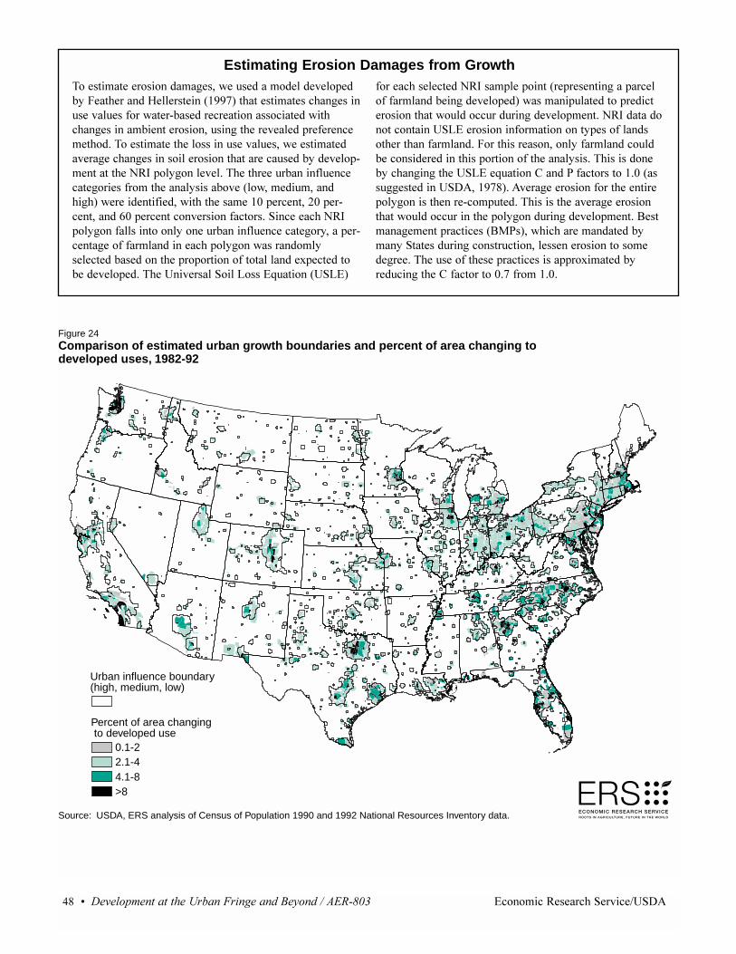
0.1-22.1-44.1-8>8

Figure 24Comparison of estimated urban growth boundaries and percent of area changing to developed uses, 1982-92

Source: USDA, ERS analysis of Census of Population 1990 and 1992 National Resources Inventory data. ECONOMIC RESEARCH SERVICEROOTS IN AGRICULTURE, FUTURE IN THE WORLD

ERS

Percent of area changing to developed use

Urban influence boundary(high, medium, low)

:��!+�3�#��"��"�$� &�9�� 1""��*��.�� !��#��"#�%��3��2 ��3�� !�� +�#��!�� "��$�%�� '�:�� "��#��"#+�3��!�� !��"�� #�� &��"�$2�� /�0�$�"&!��"�"'�: �� #� ��%"#��!��%�� "&�� *"�3+��#�+�� ! .�3��%��+�3�� $��+��$�2��+��$��%��'�� /�0$�"&!��%�""��"&��#� ��%"#��!��&+��$�2��!��%�%��"�� $�"&!��3��"&"�� $��$��%��"�"��5$�� "�$�'�: ��"��"�E��<#��*��E�.

%�� "��/�0��$"�$��*�$��!��$��"�%�%��"�� !��"�$�.�3��$#"��$�� 3�#"��#��#��!��"�$��'�/�0��E��%��&$��%�"�� %��"��'�9�� +��"&�%��"��#"� �� $��%�� "&�'�: �� &�� !��!�� E��<#��)��8 %��'��*�#!!��+��.'��!��%�� $�"&!�� 2��$#��'�: �� !�� 3�#"��#�� $�"&!��#��!��"�$��'�(��!��$��*(-8.+�3 �� &��&��#��!��#��+�"��!�'�: �#��%�� $��$$��5�� &��#��!�� )�%��'��%��'�'

Estimating Erosion Damages from Growth

open space under three hypothetical developmentschedules than any prediction of development or howresidents value conservation.

The total benefit estimated also depends on the patternand level of development expected to occur, which can-not be predicted with very much accuracy. In the “low-density” scenario in table 5, arbitrary percentages ofthe land in each urban influence zone are assumed tobe developed, totaling 50 million acres, resulting inannual losses of nonmarket value of between $1.4 and$19.3 billion. However, if more development occurredand if it were more focused on the area of most heavyurban influence, as in the “high-density” scenario, 58.1million acres would be developed with annual benefitlosses ranging from $1.9 to $26.6 billion. This resultspartly because of the increase in development level, andpartly because there are more households in the highurban influence zone than in the other two, resulting inhigher values.

These willingness-to-pay estimates do not include off-site damages that result from construction, such as thereduction in surface water quality caused by erosionfrom construction sites. Clearing land for construction

causes significant erosion, beyond that experienced inagricultural production. This increased runoff dimin-ishes the quality of nearby lakes and streams that areused for recreation. Although these damages occur in ashort period (1-2 years), they are potentially significantand were estimated (see box “Estimating Erosion Dam-ages from Growth”). The estimated annual losses dueto erosion are $0.93-$1.06 billion without constructionbest management practices (BMPs) and $0.67-$0.79billion with construction BMPs, depending on settle-ment patterns (table 6).

��

Table 6—Annual recreational water quality damages dueto urbanization of farmland1

Scenario Erosion damages(percent of high, medium, and low urban influence No BMP With BMP

assumed developed)

Billion 2000 constant dollarsLow density (60, 20,10) 0.93 0.67High density (90, 10, 5) 1.06 0.791Annual losses due to changes in erosion resulting from conversionof farmland to urban uses. Losses are reductions in the enjoyment(use value) of water-based recreation resulting from diminished waterquality. Estimates are inflated to year 2000 dollars using the April2000 CPI.

Table 5—Estimated nonmarket value of land under urban influence estimated to be developed in succeeding decades

Degree of urban influence1

Low Medium High TotalDevelopable land Thousand acres

Cropland 30,179 30,690 33,840 94,709Pasture/range land 28,424 25,077 21,299 74,800Total developable land 58,603 55,767 55,139 169,509

Land assumed developedLow-density scenario3 5,860 11,153 33,083 50,096High-density scenario4 2,930 5,577 49,625 58,132

Estimated annual value of conserving rural land2

Billion dollars

Low-density scenario3

Proportion assumed developed 10% 20% 60%Low-benefit estimate 0.1 0.1 1.2 1.4High-benefit estimate .8 1.6 16.9 19.3

High-density scenario4

Proportion assumed developed 5% 10% 90%Low-benefit estimate >0.1 0.1 1.8 1.9High-benefit estimate 0.4 .8 25.4 26.6

1See box “Methods for Estimating Cropland and Farmland Purchase of Development Rights Cost” (p. 62) for a description of how urban influ-ence is determined.2Total willingness to pay (in year 2000 dollars) for preserving all land indicated in the row weighting scheme based on $0.21 per 1,000 acres forthe low-benefit estimate, $2.93 per 1,000 acres for the high-benefit estimate.3Assuming development is distributed more broadly, 50.1 million acres are developed.4Assuming development is more concentrated in the areas of highest urban influence, 58.1 million acres are developed.

Source: ERS analysis of 1992 National Resources Inventory and NASS June Ag Survey land value data.

In all States, local governments have been delegatedauthority for control of land use and growth. Sinceearly in the last century, planning and zoning have beenthe principal tools for controlling growth and directingland-use change in local communities. Increasingly,State governments are taking a more active role inattempting to strategically change incentives and disin-centives for development, without exerting direct con-trol over growth, a process known as “smart growth.”Because of strong interest in maintaining individuallandowners’ property rights, direct financial incentivesto keep rural land in agricultural uses have becomeimportant tools. These include preferential or use-valueproperty taxation and direct purchase of developmentrights.

Most rural communities experiencing growth have theirhands full simply trying to catch up with the growth indemand for public services, such as education, waterand sewer, and police and fire. Some respond withactions aimed at limiting growth and mitigating its con-sequences. There is a fine line between rural counties atthe metropolitan fringe that are still trying to attractdevelopment, and those that have been all too success-ful at attracting growth and are now trying to controldevelopment.

Playing Catch-Up

The need to play catch-up seems to be the most com-mon response of local governments. A recent GeneralAccounting Office (GAO) survey of almost 2,000 gov-ernments in cities over 25,000 population (949responded) and all metropolitan counties (609responded) found that 53 percent of the counties and 35percent of the cities claimed “sprawl” was a high orvery high concern. GAO identified these respondents as“communities concerned about sprawl” (44 percent ofrural counties were concerned about “sprawl,” com-pared with 56 percent of nonrural counties). As awhole, GAO found that the priorities of the sprawl-con-cerned communities were fairly similar to the prioritiesof all communities. The most frequently cited prioritiesin planning for the future involved increasing the localtax base to support better schools and roads, attractingbusinesses, and enhancing transportation systems (U.S.GAO, 2000). But more sprawl-concerned communities(66 percent) were experiencing fast growth than non-sprawl communities (46 percent), which may explainwhy sprawl-concerned communities were more likely

than other communities to place a high priority onenhancing their transportation systems.

Planning priorities differed between more urban andmore rural places. Metropolitan counties that identifiedthemselves as “rural” (27 percent of the metro countiesresponding to the survey) placed a much higher prioritythan “nonrural” counties on increasing job opportuni-ties and attracting new development to areas with infra-structure; “nonrural counties” were relatively moreinterested in enhancing their transportation systems todeal with growth. Cities put a greater priority on revi-talizing downtowns, which are also affected by growth,than did counties.

How Local Governments AddressGrowth Problems

This section provides examples of some of the wayslocal communities deal with problems caused bygrowth. The examples are based on information andstatements from local officials when ERS conducted itsstudy of eight counties experiencing growth in the1980’s and 1990’s (Reeder et al., 2000). Growth-relatedproblems are often hard to address because they com-pound each other. For example, growth control advo-cates favor concentrating development in town centers.However, towns such as Shelton in Mason County,Washington, cannot grow due to limits on infrastruc-ture, which is constrained by an inadequate tax base.Growth and development could increase the tax base,but is constrained by lack of infrastructure in the town,and so on.

Some places have gotten around this conundrum byraising special sales taxes, imposing impact fees ondevelopers, or creating special districts where taxes areraised to pay for infrastructure and public servicesneeded for development. However, these efforts are notalways successful since local voter approval may berequired. In some cases, State regulations constrainlocal efforts to raise more revenues, such as in MonroeCounty, in the Pocono Mountains of Pennsylvania,where State rules make it difficult to use impact fees.

Aggressive business recruiting is another approach toadd more to the tax base than to public spending oninfrastructure and services. Monroe County, Pennsylva-nia, is using tax incentives together with industrial andbusiness parks, to entice new businesses into the area.

��

VI. Local Responses to Growth

However, such an approach is not without risk. Accord-ing to John Woodling, of the Monroe County PlanningCommission, “Some of the local schools had a concernthat the tax incentive program might give away toomuch tax revenue for the number of jobs it created.More important was the concern that new firms wouldhire too many nonresidents who subsequently wouldmove into the county, bringing their children withthem, and that this could ultimately burden the schoolsystem. However, Monroe County statistics suggestthese concerns are not justified, because most of thenew employees of these firms are county residents atthe time they are hired” (Reeder et al., 2000).

Many localities take advantage of Federal programs toaddress their growth-related infrastructure, business-attraction, and affordable-housing needs. For example,some communities attempt to combat growth-inducedtransportation problems through public transportation, afederally subsidized activity. Public transportation hasthe added advantage of strengthening central locationsthat are more readily served by public transit systems.But funding is limited for these activities. The elderlyand homebound in Wise County, Texas, use a State-funded Para-Transit system. But according to CountyCommissioner James Hubbard, “expansion and mainte-nance needs far exceed current funding levels.”

This is not an unusual problem for growing communi-ties. A GAO survey of local growth challenges foundthat 40 percent of responding local governments sup-ported more Federal assistance with “smart growth”programs (U.S. GAO, 2000). The U.S. Department ofTransportation’s Transportation and Community andSystem Preservation Pilot program is so popular thatthe demand for funding exceeded the program’s appro-priations in fiscal year 2000. DOT funded 84 projectsfrom 292 applications received. The program fundsprojects that integrate transportation initiatives with thegoals of community development, environmental pro-tection, access to jobs and markets, and efficient landdevelopment patterns. GAO’s survey showed that“sprawl” communities were more likely than “non-sprawl” communities to complain about inadequateFederal funding for public transportation.

Planning Efforts To Control Growth

Rather than simply reacting to growth by addressingthe problems it creates, communities are increasinglyusing planning to help prevent or reduce growth’s con-sequences. GAO found that 34 percent of the countiesexpected to increase their involvement in planning and

growth management activities over the next 5 years(GAO, 2000). A common first step is to establish orupdate the county’s comprehensive plan. Such plansmay envision ways to prevent or limit ill effects fromgrowth by employing land-use and zoning techniquesthat result in more concentrated development, such asencouraging mixed-use development within a desig-nated centrally located area, or encouraging cluster orlarge-lot development on the fringe, or increased use ofconservation easements to preserve open space. Infra-structure and public services, such as public transporta-tion, may be planned and implemented to discourage“sprawl.” Plans may also provide for ways to addressgrowth-related problems, such as through encouragingthe construction of local industrial or commercial parkswith incentives to attract businesses that can augmentthe tax base and reduce commuter-related transporta-tion problems, or by identifying areas and incentivesfor developing affordable housing.

In some cases, States require or encourage their locali-ties to pursue comprehensive planning and growthmanagement. For example, Florida’s growth manage-ment legislation in the early 1980’s required localitiesto prepare comprehensive plans that assured that ade-quate infrastructure, and a funding plan to finance it,was present. Gary Kuhl, former Administrator of CitrusCounty, Florida (now the Water Resource Team Admin-istrator for Hillsborough County), said “Citrus Countyexperienced a lot of sprawl issues during the rapidgrowth of the 1980’s, but with help from the compre-hensive plan, growth was well-managed in the 1990’s.Citrus uses a variety of zoning and land-use provisionsthat have the effect of limiting sprawl by targetingdevelopment in a central portion of the county that iswell-drained and served by the county water and sewersystem and by discouraging development in more sen-sitive wetland and coastal areas. Citrus also has beenhelped by Federal and State agencies, the water man-agement district, and by private trusts, which haveacquired and protected some environmentally valuableland in the county” (Reeder et al., 2000).

Although all States require at least some local plan-ning, many communities are not required to conform totheir plans, and even when conformance is required, itis often not enforced. A common problem is thatcounty plans capable of restricting growth are disre-garded by municipalities, which actually control mostof the development. Due to this fragmentation of gov-ernment responsibility, efforts to control growth areoften ineffective or, at best, piecemeal.

��

Michele Boomhower, Director of the Lamoille CountyPlanning Commission, explained that “The State ofVermont did not require growth management. A signifi-cant portion of zoning controls are at the municipallevel, and every town is upgrading growth managementin some way.” But according to State Senator SusanBartlett, “Sprawl is overrunning the county as looselocal zoning laws allow strip-style development todominate the local landscape. Uneven development isthe rule, as all of the desirable development is going totowns with good local planning, while unwanted devel-opment goes to poorly regulated towns” (Reeder et al.,2000).

Despite its fragmentation problems, Lamoille hasaccomplished a great deal in farm and forestland pro-tection. According to Boomhower, “Farm and forest-land are most threatened by sprawl, so protection ofthese lands is of great importance.” Using zoning toprotect some working lands, limited use of large-lot-size requirements, conservation easements, and pur-chase of development rights (PDR’s), Lamoille Countynow has the largest percentage of publicly and privatelyprotected land in the State.

In other places, land conservation efforts are just begin-ning. According to John Woodling of the MonroeCounty Planning Commission, “Pennsylvania’s Agri-cultural Preservation Program encourages the purchaseof farmland conservation easements. And in MonroeCounty, a bond issue was passed recently which willprovide money for the acquisition of open space andrecreation areas. In addition, the county’s new compre-hensive plan encourages the transfer of developmentrights (TDR). Recently, the Commonwealth allowedthe transfer of development rights from one municipal-ity to another, which should enhance the use of TDR’s”(Reeder et al., 2000). Mason County, Washington, alsoauthorizes the use of these conservation devices, andthe State provides some money for purchase of devel-opment rights (PDR’s), but as yet it is unclear whetherthe voters will support local PDR bonds.

Efforts to control growth sometimes run into significantconstitutional and political obstacles. For example,many rural areas have been traditionally opposed tozoning, and such traditions can be hard to overcome.The big problem in Wise County, Texas, according tocity administrator Brett Shanon, is that the county con-stitution prohibits zoning in unincorporated areas,resulting in uncontrolled growth outside town limits.Wise County commissioner James Hubbard adds that“Some progress was made in the State Assembly in

enhancing county legal authority during the last ses-sion, and the Assembly may add additional countyauthority this year.” Local political barriers can be justas formidable as legal or constitutional ones. A goodexample comes from Georgia. According to BrendaJohnson at the Chamber of Commerce in GilmerCounty, Georgia, “The last county commissioner whotried to establish zoning in the rural portion of thecounty was recalled from office” (Reeder et al., 2000).

Growth control efforts can also run into problems in thecourts. Mason County established a new comprehen-sive county plan in 1996 in conformance with the newState growth management requirements for rapidlygrowing rural areas. According to Bob Fink of theCounty Planning Office, “This included many ‘goodplanning’ requirements, including protecting environ-mentally critical areas, preserving the rural character ofthe land, and encouraging urban and cluster develop-ment. This would have made for a great change frombefore, when growth was uncontrolled. But the planhas been challenged in court, nearly stopping all non-residential development in the rural portion of thecounty, including some desirable forms of developmentsuch as agricultural buildings and fire stations, until thelegal issue is decided” (Reeder et al., 2000). Similarlegal challenges have resulted in a significant weaken-ing of Florida’s growth management law in recentyears. In many newly developing areas, local capacityto develop and implement such growth-directing plansin the face of sophisticated challenges to their validityis limited. Either assistance from State and Federalgovernments to develop the capacity to effectively planfor growth is not authorized or funding has been inade-quate.

Some municipalities attempt to control development ontheir fringe by annexing land adjacent to city limits.Such annexation can be used as a way to control orlimit growth. However, annexation can also be used toencourage even more growth on a city’s edge. Annexa-tion is limited by State law, which varies from State toState. This often requires the approval of the jurisdic-tion that would lose the land. Nevertheless, the affectedrural residents outside city limits often feel powerlessto oppose these annexation efforts.

Capacity for Response in Relation to Urbanization Pressure

A local government’s capacity to respond to growthpressures generally increases with the degree of urban-ization. Urbanization usually results in higher income,

��

wealth, and tax base, which translates into more publicand private financial resources that can be devoted tohiring more planners, offering incentives for mixed-usedevelopment, paying for public transportation services,or purchasing open space. Strong rural traditions ofproperty rights cause people to oppose planning andzoning in some regions. Economies of scale in the pro-vision of many types of government services, includingplanning functions, means that planning is more eco-nomical and efficient in larger, more urbanized commu-nities that require more such work. Consequently, mostrural areas begin with relatively little capacity torespond to urbanization pressures, and it may takeyears of development before the community is able todevelop capacity to control growth.

Communities Affected by Growth Are AlreadyPlanning, but Capacity is Limited Better planning and zoning are central to the ability torespond to growth. GAO found that 75 percent of thecommunities that were concerned with “sprawl” werehighly involved in planning for and managing growth,which indicates a relatively high level of planningactivity, compared with 72 percent for cities and 59percent for metropolitan counties in general (U.S.GAO, 2000, p. 99). Moreover, about a third of thesecounties expected to increase their planning involve-ment over the next 5 years.

GAO also found that the majority of “sprawl-con-cerned” counties were already using several keygrowth-management tools, including land-use planning,zoning, mixed-use zoning, working with adjacent com-munities, and targeting State infrastructure funding toareas where development is desirable (U.S. GAO, 2000,figure 19, p. 101). In addition, 78 percent of thesesprawl-affected communities use regional planningapproaches—some focusing on specific functions, suchas affordable housing in Seattle and traffic congestionand pollution in Atlanta.

Many cities and counties, however, are falling short ofwhat is needed to control and manage growth effec-tively. A recent Alabama survey of mayors in 458municipalities and 358 county commissioners in 67counties found a general consensus in support ofgrowth management or smart growth approaches(Seroka and Veal, 2000). Despite their overall goodintentions, only a minority of the responding officials(18 percent of the mayors and 19 percent of the com-missioners) believed they currently had the necessarystaff and resources to plan and manage growth effec-tively. Another 24 percent of the mayors and 17 percent

of the commissioners thought they could do the jobeffectively with modest increases in funding and staffresources. High-growth communities were only some-what more likely to have the capacity to managegrowth than were other communities.

Seroka and Veal found that more than 80 percent of theAlabama officials surveyed said that their local govern-ment needed more powers to manage growth. They alsofound that counties were more likely than cities to facesignificant opposition to growth management fromrural residents, other constitutional officers, the elderly,and long-term residents of the county. Most local offi-cials looked to the State to provide leadership in thisarea. Although these findings pertain only to Alabama,they point to some of the potential obstacles that ruralgrowth management efforts face in other States as well.

Rural areas often have very limited planning capacity.Most of the smaller rural towns cannot afford a full-time planner. To meet their planning needs, these com-munities may be served by a circuit riding planner;another alternative is that several towns and a countymay combine their efforts to set up one planning officeto serve their joint needs (Lapping, Daniels, and Keller,1989, p. 56). Shared service arrangements can sufferfrom conflicts between communities. Even at thecounty level, rural planners often must spend part oftheir time doing other duties. In addition, rural plannersmay lack important technical tools (such as GIS, com-puter, and legal services) needed to do their job.

One result of this limited capacity for planning is thatrural counties tend to rely more on nongovernmentalinstitutions—such as regional development organiza-tions—for planning. Planning for key functions drivingdevelopment, such as transportation investment, is car-ried out by separate special-purpose planning offices,such as the highway department, that may ignorebroader concerns affecting growth management.

Planning for major roads and institutions in the morerural, nonmetropolitan counties is often done at theState rather than the local level, bypassing local gov-ernment. Rural places often are forced to compete withneighboring communities to obtain Federal and Statetransportation funding, leading to conflicts betweenjurisdictions. In urban areas, transportation planning isdone by multicounty Metropolitan Planning Organiza-tions (MPO’s) which are capable of superior planningand coordination through regional collaboration, butmay be too narrowly focused on transportation issues.However, the more fragmented rural planning process

��

adds to the difficulty of doing good comprehensiveplanning needed to control growth.

Federal Assistance for Planning

The Federal Government has supported programs toimprove the planning capabilities of State and localgovernments in the past, but support was cut for bothideological and practical reasons. The most well knownof these efforts was the HUD 701 planning grant pro-gram, established as part of the Housing and Commu-nity Development Act of 1954 (40 USC 461). As lateas 1975, the HUD 701 program spent $100 million peryear, paying as much as two-thirds of the costs of an“ongoing comprehensive planning process” required ofall grant recipients. However, the budget was cut to $75million in 1976 and was proposed for elimination in1977 (NRDC, 1977, p. 334). Comprehensive planning,as defined in the 1954 law, included:

• Preparation of guides for governmental policies andactions on the pattern and intensity of land use, theprovision of public facilities, including transportation,and development of human and natural resources;

• Identification and evaluation of area housing, employ-ment, education, and health needs, and plans to meetthose needs;

• Historical and architectural structure surveys;

• Long-range physical and fiscal plans;

• Programming of capital improvements and infrastruc-ture needs;

• Coordination of all related plans and activities of theState and local governments concerned; and

• Preparation of regulatory and administrative measuresneeded to support the above plans.

Stringent review of Section 701 followed amendmentsin the Housing and Community Development Act of1974. HUD also required that each comprehensive planhave housing and land-use elements, and that NationalEnvironmental Policy Act (NEPA) environmentalassessments, public participation, and nondiscrimina-tion guidelines be followed in all plans prepared withthis funding.

One early estimate of the impact of the Section 701program suggested that the business of planning con-sultation had multiplied tenfold (ASPO, 1968). Criti-cisms were that administrative requirements unneces-

sarily raised planning costs, and that plans were stereo-typical, filled with boilerplate text, and overly elegantfor the situation (National Academy of Public Adminis-tration, 1998). Questions were raised as to how muchthe plans were in fact used and what effect they werehaving on land-use regulation. Reform, rather thanelimination, was suggested as a cure.

The HUD Section 701 program and OMB Circular A-95 provided impetus for regional or areawide planningand coordination, among other things. By 1976, therewere 669 regional councils. In the 1980’s, the FederalGovernment largely abandoned these efforts, and simi-lar regional planning efforts with regard to waterresources and transportation, with the exception of met-ropolitan planning organizations linking transportationwith air quality (National Academy of Public Adminis-tration, 1998).

Within USDA, the Rural Development Act of 1972authorized Section A-111 Rural Development PlanningGrants (U.S. Senate, 1973). Grants under the programcould not exceed $10 million annually. Outlays for A-111 in FY1980 were $6 million. However, the incom-ing Reagan Administration budget for FY1981 severelyreduced, then eliminated Section A-111 assistance(Stansberry, 2000). In 1981, the National AgriculturalLands Study, begun in the Carter Administration, rec-ommended that USDA “…assess the feasibility of pro-viding small matching grants for ‘capacity building’ tostate departments of agriculture (or other appropriatestate agencies) that seek to manage agricultural landissues” (NALS, 1981). No legislation was ever pro-posed or enacted.

Authority for Section A-111 continued, without fund-ing, until the 1990 farm bill, which replaced it withauthority for some technical assistance and planninggrants. These were also not funded, and regulationswere not even prepared to implement the grants. The1996 FAIR Act replaced this program with new author-ity for the Rural Business Opportunity Grant program(RBOG), first funded in 1999 with $3.5 million inFY2000 appropriations. RBOG provides money to non-profits, public bodies, Indian tribes, and cooperativesfor planning and technical assistance to assist economicdevelopment in rural areas, so it could potentially cre-ate more growth than it combats (see Web site athttp://www.rurdev.usda.gov/rbs/busp/rbog.htm fordetails). USDA’s FY2001 appropriations increasedRBOG funding to $8 million.

��

Other Federal agencies and programs provide somesupport for planning in rural areas, particularly regionalplanning through the Department of Commerce Eco-nomic Development Administration’s support for localplanning organizations. The Appalachian RegionalCommission, Tennessee Valley Authority, USDA’sRural Conservation and Development (RC&D) pro-gram, and HUD’s Rural Housing and Economic Devel-opment and Community Builder programs all providelimited, fragmentary planning or planning assistance.However, this piecemeal approach tends to focus onmore narrow, limited objectives particular to the pro-gram. They do not provide much increase in capacityfor general-purpose land-use planning efforts needed tounderstand and control growth.

One can imagine how difficult it is for local govern-ments to become aware of this fragmented basket ofprograms, muster the effort needed to make applicationto them, and overcome the variety of rules for differentprograms to effectively use the funds to develop plansfor growth control. The ambiguity between rural devel-opment objectives, which seek to foster growth anddevelopment, and planning for growth control in ruralareas, may also pose problems for both the local com-munities and the agencies seeking to provide assis-tance. In many situations, it is a fine line between needsfor economic development and needs for growth con-trol.

Slow Growth, No Growth,and Smart Growth

Land-use planning and zoning authority has been dele-gated to local governments by all 50 States (Meck,1999). Historically, local governments have relied uponzoning regulations and subdivision requirements basedon the landmark Euclid case to manage the characterand density of new development (Village of Euclid v.Ambler Realty Co., 272 U.S. 365, 47 S. CT. 114, 71 L.ED. 303 (1926) in Haar, 1976, p. 194.). By the 1970’s,local and State governments in rapidly urbanizing areaswere learning that these techniques were inadequate toinfluence the character of growth (Platt, 1996). Acrossthe country, concerns about the impact of growth arefueling a growing recognition that local land-use plan-ning efforts are in desperate need of updating. In somelocalities, land-use plans have not been updated sincethey were developed based on statutes enacted in the1920’s; in others, such plans are nonexistent (Salkin,1999a). As HUD recognized in its scrutiny of Section701 planning assistance, simply having a land-use plan

and a zoning map to guide parcel-by-parcel decisions isinsufficient to control the cumulative impacts ofgrowth, and applying inappropriate development stan-dards across the landscape may actually exacerbate“sprawl” (Chen, 2000). The American Planning Associ-ation recognizes six States as having substantially mod-ernized planning legislation to address growth manage-ment issues (Maryland, New Jersey, Oregon, RhodeIsland, Tennessee, Washington), as well as 10 Statesthat have not updated their land-use statutes or pro-posed significant legislation or studies to addressreforms (Alaska, Louisiana, Michigan, Nebraska, NorthDakota, Ohio, Oklahoma, South Dakota, West Virginia,Wyoming).

Obtaining political support for updating land-use poli-cies to address growth issues can be difficult, particu-larly in light of U.S. constitutional protections for prop-erty rights and the freedom to move. When the Califor-nia town of Petaluma responded to a surge of new con-struction in the early 1970’s by imposing a moratoriumon extensions of public sewer and water services, andthus constraining the number of building permits issuedannually, the plan was challenged in court by a buildingtrade association (Platt, 1996). The city of Livermore,California, was similarly challenged when it imposed amoratorium on residential development until publicservices (water and sewer provision, and schools) wereupdated (Platt, 1996). Although eventually upheld,these policies are not permanent solutions, but ratheract to delay rapid growth and the problems it causes.

In efforts to tame growth, local governments subse-quently turned to policies such as “adequate publicfacilities” ordinances, impact fees, zoning changes toallow mixed-use developments, and working withneighboring communities to develop compatible growthmanagement plans. However, obtaining political sup-port for even these milder policies can be challenging.In Virginia, bills that would allow local governments toenact adequate public facilities ordinances died inHouse and Senate committees as a result of claims bybuilding industry lobbyists, and real estate and businessrepresentatives that the bills would diminish propertyrights (Smart Growth Network, 2000). Some of thesepolicies, in fact, may have done little to control growthand may even have exacerbated growth’s consequences.For example, if public water and sewer services were atcapacity, the bills proposed that developers could meethousing demands by building even more low-densitydevelopment with septic systems in surrounding ruralareas.

��

Georgia’s Growth Strategies Reassessment Task Forcerecently concluded that comprehensive planning bynearly all of its 700 local governments has done little todirect development, and cited a need for a broader“vision” to guide local planning efforts (Hirschhorn,2000). While local governments are increasingly chal-lenged to consider the impacts of their local land-usepolicies beyond their own borders, they individuallylack the authority to enact changes outside their juris-dictions. This is not a new phenomenon: Regional plan-ning has attempted to provide coordination within areasof a State and across several States since at least the1950’s, and 29 States had passed regional planning-enabling acts by 1957 (Bossleman and Callies, 1971;Linowes and Allensworth, 1975; Healy, 1976; Pooley,1961). To deal with these problems today, severalStates have adopted a substate regional or metropolitanapproach to address problems where the geographicextent of growth-induced impacts spreads over multiplejurisdictions. For example, Georgia’s Regional Trans-portation Authority covers the 13 counties in theAtlanta metropolitan area. Regional planning commis-sions also exist in Florida, Vermont, and Maine. Vir-ginia’s Regional Competitiveness Act, passed in 1996,provides for incentive payments to encourage regionalplanning and cooperation. Regional commissions workto identify resources of regional importance, developregional plans, review local plans for consistency, andprovide technical assistance to local governments.However, these commissions typically act as planningcoordinators and do not have statutory authority(DeGrove and Metzger 1993). Implementation remainsthe responsibility of local governments (U.S. GAO,2000; National Academy of Public Administration,1998).

State Responses to GrowthThe last two decades have witnessed a growing butgradual shift from reliance on local and regional plan-ning to statewide strategies to counter the negativeimpacts of growth. In the 1980’s, States began using acoordinated planning approach to manage growth andits associated costs. Typically, States do not enactsweeping changes all at once. In a recent comprehen-sive study of planning statutes and legislative activity,the American Planning Association found that Stateshave tended first to enact legislation that authorizeschanges in land-use planning, then progress to legisla-tion that requires it (Meck, 1999).

The term “smart growth” is a catch-all phrase used todescribe a number of policies that influence the patternand density of new development (Chen, 2000). In gen-

eral, smart growth strategies represent a movementaway from State-imposed requirements for local com-pliance with State planning goals. Because smartgrowth strategies tend to use financial incentives toencourage voluntary adoption, they are generally sup-ported by a broad spectrum of interest groups. Thesestrategies also garner support because they direct,rather than inhibit, growth and development. There isno “one size fits all”: the specific smart growth strate-gies that have been adopted vary by location but oftenshare common elements. Smart growth principles favorinvesting resources in center cities and older suburbs,supporting mass transit and pedestrian-friendly devel-opment, and encouraging mixed-use development whileconserving open space, rural amenities, and environ-mentally sensitive resources (Hirschhorn, 2000). Thesestrategies also typically remove financial incentivesprovided by State funding to develop outside desig-nated growth areas. In essence, smart growth encour-ages development in designated areas, without prohibit-ing development outside them, while not threateningindividual property rights.

The following land-use planning techniques imple-mented by various States highlight the objectives ofsmart growth:

• Urban growth boundaries—Oregon pioneered thisstrategy in the 1970’s to discourage urban sprawl.Oregon’s statewide plan mandated the designation ofurban growth boundaries, within which urban devel-opment would take place. Although this policy hasnot entirely curtailed development outside the bound-aries, Oregon is recognized as being the most suc-cessful State in separating rural and urban uses(DeGrove and Metzger, 1993). In 1998, Tennesseeadopted legislation that requires counties to establishurban growth boundaries for municipalities andplanned-growth areas.

• Designation of priority funding areas—With thisstrategy, local governments take the lead in designat-ing growth areas to concentrate development anddirect State funding. In Washington, cities and coun-ties exceeding a certain size or experiencing rapidpopulation increases are required to designate urbangrowth areas (Johnson, 1999b). This can apply to pri-vate financing, such as the Location Efficient Mort-gage (LEM) pioneered by banks in Seattle, Chicago,and California and underwritten by Fannie Mae(Chen, 2000). LEM’s let homebuyers increase themortgages for which they can qualify by the amount

��

of savings expected in compact versus low-densityneighborhoods.

• Farmland/environmental resource preservation—The goal of these strategies is to proactively preservefarmland and other environmental resources of localimportance, rather than trust their preservation todevelopment controls. Maryland is one of severalStates with a well-established State-level farmlandpreservation program. In addition to its existing farm-land preservation program (administered by theMaryland Agricultural Land Preservation Founda-tion), the smart growth initiatives implemented in1997 included the Rural Legacy Program. In this pro-gram, the State partners with local governments, landtrusts, and citizens, aiming to protect an additional200,000 acres of farms and forestland by 2011 (Officeof the Governor, 1998). Washington’s Growth Man-agement Act requires localities to adopt land-use poli-cies that protect commercially significant agriculturallands (WSCTED, 1997).

• Brownfields redevelopment—Brownfields (urbanredevelopment sites in older developed areas) pro-grams limit the liability of redevelopers of old indus-trial sites. In 1998, New Jersey enacted the Brown-field and Contaminated Site Remediation Act, which,in addition to limiting liability for redevelopers, pro-vides financial incentives for remediation and redevel-opment of brownfields. It also includes brownfieldsre-use as part of its urban redevelopment programs(Finucan, 1999a). Another example at the local levelis the “Homerama” demonstration project, whichbuilds affordable new homes on redevelopment sitesin distressed neighborhoods of Detroit, begun by adozen local developers in 1987 (Chen, 2000).

• Neighborhood business development—Throughthese programs, small businesses can obtain financialassistance in designated revitalization areas. Since1993, the Illinois Main Street Program has providedState support in the form of technical assistance tocommunities that are defining and implementingplans to improve development and redevelopment.The goals are to foster public and private support forthe initiatives, enhance downtown areas through his-toric preservation, develop strategies to encouragedowntown activity, and maintain the vitality of down-town areas. More than 50 communities are participat-ing in the program (Hirshhorn, 2000). Consistent withState planning goals, a task force in South Providence,Rhode Island, adopted a program that provides State-funded assistance to new small businesses locating in

one of its 10 State-designated enterprise zones (Davis,1999, in Finucan, 1999b).

•Multi-jurisdictional planning—This strategyinvolves State incentives for coordination of localplanning efforts. Wisconsin gives State funding prior-ity to its local governments that address the needs ofadjacent communities in their own developmentplans, rather than follow a “beggar-thy-neighbor”strategy (Smart Growth Network, 2000).

• Coordinating transportation systems and develop-ment—This strategy seeks to increase transportationefficiency by linking development and transportationinvestments by locating transportation infrastructurewithin designated urban growth areas. In 1998, Ten-nessee passed a law directing that funding under theFederal Transportation Equity Act for the 21st Cen-tury (TEA-21) be reserved exclusively for localitiesthat have growth plans with identified urban growthboundaries for cities, planned growth areas, and ruralareas (Finucan, 1999c).

• Public/private partnerships—This strategy involvesrepresentatives from multiple levels of government,non-governmental organizations, special interestgroups, and other stakeholders in the planningprocess. Utah’s Envision Utah partnership is workingto create a growth strategy based on informing citi-zens about the causes of and implications ofunplanned growth, rather than government-imposedrequirements. The goal is to achieve reform and toshape future development based on citizens’ demandsfor such changes. The partnership includes State andlocal government officials, business people, develop-ers, environmentalists, and citizens (Hirschhorn, 2000).

Table 7 identifies some of the State actions implement-ing smart growth strategies. Many other States havelegislation that allows, but does not require, adoption ofsmart growth strategies. Smart growth strategies take asynoptic view of growth and attempt to marshall theresources of the State to address growth. A larger viewof the monetary resources deployed to control growthand estimates of the magnitude of the problem aremade in the next section.

Monetary Incentives for ConservingFarm and Forest Land

Despite the benefits farmland provides to residentsbeyond the urban fringe, and to society in general, anddespite adaptations farm operators can make to accom-modate an urbanizing environment, few landowners can

��

��

Table 7—State implementation of smart growth strategies

State Commission/task force to study smart growth in 1999 Enacted State-level smart growth legislation

Arizona Growing Smarter Commission (1998-99) Growing Smarter Act (1998) in part requires that municipalities’and counties’ plans identify growth areas. The Growing Smarter Plus bill (Senate Bill 1001, 2000) authorizes municipalities to designate boundaries beyond which public water, sewer and street service will not be provided.

Colorado Interim Legislative Committee on Development Governor’s Smart Growth Award Program awards matching and Growth (1998) grants for measures that balance growth with community needs.

Delaware Shaping Delaware’s Future Act (1995).

Florida House Bill 17 (1999) offers financial incentives to local governments to adopt plans for and to develop in urban infill and redevelopment areas, by granting authority to issue bonds or to engage in tax increment financing and by providing grants for local public projects in these areas.

Iowa Commission on Urban Planning, Growth Management of Cities, and Protection of Farmland (1998-99)

Kentucky Legislative Subcommittee on Planning andLand Use (1999)

Maine Passed legislation (2000) to direct State capital investment projects to designated growth areas and areas served by public sewer systems. State grants for capital investments are awarded first to municipalities that have comprehensive plans consistent with State smart growth objectives. Requires adoption of rules that encourage siting of State office buildings and schools in growth areas.

Maryland Smart Growth and Neighborhood Conservation The Neighborhood Conservation and Smart Growth initiatives Sub-Cabinet to coordinate State agency actions (1998) (1997) rely on incentives to encourage local governments

to voluntarily adopt smart growth strategies. They direct State funding for capital investments to designated “priority funding areas,” preserve farmland and natural resources through the Rural Legacy Program, encourage redevelopment of old industrial sites, and provide financial incentives for businesses to locate in priority funding areas. Also provides homebuyers with financial assistance with purchasing a home in an older neighborhood near their jobs.

Massachusetts Sustainable Development Act (proposed in 1999). Executive Order 385 “Planning for Growth” (1996) in part requires coordination of State agencies, and provides incentives for local governments to engage in planning.

New Hampshire Land Use Management and Farmland Preservation House Bill 1259 (2000) requires State agencies to make Study (1998); Cost of Sprawl Study (1999) decisions consistent with smart growth principles when funding

and siting infrastructure and public facilities.

New Jersey State Planning Commission (1985) The Commission adopted (1999) a revised State development and redevelopment plan that includes financial incentives for communities to engage in multijurisdictional planning through a Smart Growth grant program.

New Mexico Legislative subcommittee on enabling statutes (1999-2000)

Continued—

��

Table 7—State implementation of smart growth strategies (continued)

State Commission/task force to study smart growth in 1999 Enacted State-level smart growth legislation

New York Smart Growth Economic Competitiveness Task The Smart Growth Economic Competitiveness Act and severalForce (1999); Quality Communities Task Force (2000) other bills were introduced in 1999. The proposed Smart

Growth for the New Century Act would favor local governments with smart growth plans when allocating State funding; State financial assistance for public projects is limited to locally designated “smart growth” or redevelopment areas. The proposed New York State Smart Growth Compact Act would authorize creation of smart growth compact areas and governing councils, and gives funding priority for drinking water and wastewater infrastructure projects to localities with certified smart growth plans. AB 9080 and SB 5893 (1999, in committee) would create the Smart Growth Planning Council,which would provide incentive grants to local governments that meet smart growth goals.

North Carolina Smart Growth Study Commission (1999)

Oregon The land-use plan enacted in 1973 (and subsequent amendments) contains mandatory provisions for cities to designate urban growth boundaries, for local plans to be consistent with State planning goals, local governments to coordinate planning efforts, and that counties use protective zoning to help preserve farms and forestland. In the recent “Smart Development” initiative, local governments are encouraged to locate development near existing urban services. S.B. 1128 (1999) promotes “sustainable development”and helps economically distressed communities by providing State assistance.

Pennsylvania 21st Century Environment Commission (1997)

Rhode Island The Comprehensive Planning and Land Use Regulation Act (1988) requires cities and towns to adopt comprehensive plans that comply with State plans, and that these local plans address natural resources, farmland, open space, and economic devel-opment. The Act contains incentives for “smart development.”

Tennessee Pub. Chap. 1101 (1998) requires counties to adopt and adhere to growth plans that include urban growth boundaries for each municipality, planned growth areas, and rural areas. Funding provided by the State for economic development and infrastructure projects is to be limited to counties with approved growth plans after July 1, 2001.

Utah Quality Growth Commission (1999) formed to Quality Growth Act (1999) established the Quality Growth identify growth areas and administer conservation Commission.fund to purchase easements on agricultural and open space land.

Virginia Joint Legislative Smart Growth Subcommittee (1998)to identify smart growth areas where State infrastructurefunds are to be directed.

Washington The Growth Management Act (1990) in part requires cities and counties (a) exceeding a certain population or population increase to designate urban growth areas and to adoptconsistent comprehensive plans, (b) to protect environmentally sensitive resources, and (c) to identify and design policies to protect commercially important farmland.

Wisconsin The Smart Growth Law (1999) gives funding priority to local governments that address the needs of adjacent communitiesand identify planned growth areas for development or redevel-opment. The Smart Growth Dividend Aid Program was established to award funds to local governments that have increased the amount of compact development and moderately priced housing.

Sources: Finucan (1999a-c); Johnson (1999a,b); Hirschhorn (2000); NCSL (2000); Salkin (1999a,b) and references therein.

continue to farm in the face of high competing returnsfrom development. Real resources are needed to pro-vide incentives for landowners to conserve land in agri-culture. The most widely enacted provision to provideincentives for farmland preservation, use-value or pref-erential assessment, has been scrutinized very little,while the most effective, purchase of developmentrights, is under-funded relative to the amount of landthat could be enrolled.

Cost of Preferential AssessmentPreferential or differential property tax assessment isthe most popular farmland preservation technique andis authorized in all States (Aiken, 1989; AFT, 1997).Preferential assessment removes a disincentive for con-serving farmland in the face of development pressureby assessing the property at its value in agriculturaluse, rather than the higher developed land values foundnear cities, often in exchange for an agreement not todevelop for some period. Penalties (called rollback pro-visions) can be imposed if the land is developed withinthe agreed term. While not widely recognized by thepublic, tax reductions like this are a form of expendi-ture in disguise, called “tax expenditures.” We esti-mated the implicit subsidy that farm operations receivethrough tax expenditures in preferential assessmentprograms by applying each State’s tax rate per $100 offull market value against the difference between currentland values and land values in rural areas withoutdevelopment pressure (appendix table 1). Nationally,the estimated tax subsidy is $1.1 billion annually. Thisannual flow of tax expenditures has a present value(from discounting the stream of annual tax expendi-tures at 4 percent) totaling nearly $27 billion.

Evaluations of preferential assessment generally recog-nize that, while it is a popular subsidy for farmlandowners, it has not provided a strong incentive for con-serving farmland (Tremblay et al., 1987; MacKenzie,1989; Lincoln Institute, 1993). With relatively minoragricultural activity, developers as well as otherlandowners can reap reductions in property taxes thatreduce the cost of holding land prior to development.The rollback penalties are generally too small, relativeto the potential rewards from development, to deterlandowners from selling out for development if theopportunity arises. At best, preferential assessment mayslow the transition from rural to developed uses, but itis not a permanent solution. Other tools, such as pur-chase or transfer of development rights, are more effec-tive in permanently preventing development.

Buying Development RightsAll States now have laws enabling conservation ease-ments on agricultural land through voluntary donationsfrom landowners, and about 19 States have programsfor purchase of development rights (PDR), purchase ofagricultural conservation easements (PACE), or transferof development rights (TDR) (Buist et al., 1995; Wiebeet al., 1996). With PDR’s and related programs, publicfunds purchase permanent or specified-term restrictionson the deeds of individual parcels, effectively prohibit-ing future development or use of the parcel for nonfarmuses. These programs are intended to retain parcelswith high potential for continued, active agriculturaluse, and usually focus on cropland. The distinctionbetween “cropland” and “farmland” is important: crop-land is a higher quality subset of all land operated infarms, which can contain pasture, range, woodland, andother kinds of land.

The restricted deed to the parcel, and all remainingproperty rights associated with ownership, are retainedby the landowner, who can continue farming. Deedrestrictions are binding not just on the current owner,but on all future owners. The implicit economic valueof the easement is the difference between the unre-stricted (market) value of the parcel and its restricted(agricultural) value, as determined by modern appraisalmethods or by easement valuation “point” systems.

Nineteen States have State-level PDR programs, and atleast 34 counties operate separate programs in 11 States(AFT, 1997; 2000). The growing popularity of theseprograms nationwide is due to:

• The nearly unique ability of this public policy tool topermanently preserve farmland;

• The voluntary nature of the programs, which avoidsthe takings issues that cloud the outcome of regula-tory techniques such as zoning; and

• The ability of these programs to target funds towardparcels with the most important characteristics, anability that is lacking in most other economic incen-tive-based farmland preservation techniques such aspreferential assessment.

PDR’s and related programs are a relatively new farm-land preservation technique, although land trusts andother private conservation organizations have a longhistory of obtaining conservation easements on valu-able or unique wetlands, wildlife or biotic habitat,riparian areas, and scenic landscapes (Wiebe et al.,

��

1996). Until fairly recently, these easements were mostoften obtained from landowners as a donation to acharitable organization compensated by a Federalincome tax deduction under Section 170 (h) of theInternal Revenue Code (Ward et al., 1989). Conserva-tion easements for agricultural land were first obtainedin Suffolk County, New York, in the mid-1970’s (AFT,1998a, 1998b). Since that time, 21 States have basedconservation easement-enabling legislation on theNational Conference of Commissioners on UniformState Laws Uniform Conservation Easement Act(1981). Another 23 States have enacted their own ver-sions of enabling legislation.

AFT estimates that, nationwide, PDR programs havecumulatively protected 819,490 acres of farmland withan expenditure of $1.2 billion, slightly more in totalthan the annual tax expenditure on use-value assess-ment. The average easement cost $1,519 per acre. Pub-lic expenditures for PDR programs are reported from20 States, with the most active programs existing in theNortheast (AFT, 2000). Maryland, Massachusetts, NewJersey, and Pennsylvania account for 68 percent ofPDR expenditures to date (appendix table 2). Programsare usually funded through bond issues approved inpublic referenda. The Conservation Fund compiledresults of 35 referenda on funding for easement pro-grams in States, counties, and townships around thecountry in November 2000 (Conservation Foundation,2000). Seven proposals for $403 million were rejectedby voters. Another 28 for $1 billion were approved.

An important advantage of PDR’s and related programsas farmland protection tools is their ability to targetfunds to the highest quality land parcels or to parcelswith the highest degree of development pressure. Pro-grams choose the parcels on which to spend their lim-ited funds from those offered by eligible landowners onthe basis of legislatively or administratively determinedcriteria, or on the basis of scoring systems that rankparcel and landowner characteristics. Some programscombine the two procedures, awarding ranking “points”only to parcels that meet a set of minimum criteria(e.g., outside water and sewer service boundaries, or inareas zoned for agricultural or rural uses). Most pro-grams award progressively higher ranking points forparcels with higher quality soils, proximity to existingpreserved parcels, or proximity to existing develop-ment, with the progression heavily weighted towardparcels consisting of “prime” cropland under imminentthreat of development.

Both of these features increase the cost of PDR’s andrelated programs. An increased likelihood of develop-ment, for example, from proximity to roads or existingdevelopment, increases the cost of the easement to theprogram by further increasing the difference betweenthe parcel’s market value and its agricultural value.Facing limited funds, programs must choose betweenpreserving more farmland acres of poorer quality underless development pressure, and preserving fewer acresof higher quality under greater development pressure.

Potential Cost of Development RightsState PDR’s and related programs focus on protectingcropland as the highest quality farmland that holds themost potential for long-term viability in agriculturaluse. We estimated the cost for voluntary easements onall urban-influenced U.S. cropland (94.7 million acres)at $130 billion (figure 25; appendix table 2; see box,“Methods for Estimating Cropland and Farmland Pur-chase of Development Rights Cost”). The easementcost of 36 percent of the acres subject to the highestlevel of urban influence is $88 billion. Thus, expendi-tures nationwide for PDR’s and related programsthrough February 2000 constitute just 1 percent of theestimated total easement cost to preserve all urban-influenced cropland. Cropland acres protected to datethrough PDR’s constitute less than 1 percent of urban-influenced cropland acres nationwide.

Nationally, figure 25 indicates that it would cost $88billion to purchase easements on the 34 million crop-

��

Figure 25Actual and estimated easement value for cropland, by urban influence

Actual,February

2000

Low Medium High Total

Urban influence

Estimated cropland (Thousand acres)

Total cropland estimated easement value (Million dollars)

Source: ERS analysis of National Resources Inventory land use and NASS land values data.

0

30,000

60,000

90,000

120,000

150,000

land acres most influenced by urbanization, at an aver-age cost of $2,595 per acre. However, purchasing ease-ments only on the 31 million acres of cropland subjectto the medium level of urban influence preservesroughly the same number of acres for $25 billion, $806per acre, or less than one-third the cost. Selecting crop-land parcels only in the low urban influence category,for which urban conversion might not be expected formany years, would reduce current easement costs by anadditional third, to $592 per acre, or $18 billion.

The chief obstacle to conserving more farm and forest-land through PDR programs is the high cost of pur-chasing easements. However, States already incur a taxexpenditure in use-value assessment programs for allfarmland of $1.1 billion annually, which equals a pres-ent value of $27 billion when amortized at 4 percent(figure 26; appendix table 1). The tax subsidy on use-value assessment dwarfs the $1.2 billion in cumulativepublic expenditures on PDR programs since the mid-1970’s. Since use-value assessment is generallyacknowledged to provide far less certainty that farm-land will actually be preserved from development thanPDR’s and related programs, more effective farmland

conservation could perhaps be obtained by reallocatingthese expenditures.

We estimated that by applying the annual expenditureon use-value assessment to PDR’s, State programscould cover 30 percent of the $88 billion easement costneeded to conserve cropland in the high-urban-influ-ence category, or 63 percent of the cost of easements inthe middle- and low-urban-influence categories. Be-cause use-value assessment is generally provided to allqualifying farmland, redirecting expenditures on it toconserving cropland alone could cover a substantialportion of the total cost of cropland easements, particu-larly in States with less urban pressure, or with a lowerratio of cropland to all farmland (appendix table 2). Inother words, converting use-value assessment tax subsi-dies to PDR expenditures could fund permanent ease-ments on much of the cropland really at risk of devel-opment.

These estimates do not include costs associated withpurchasing easements, which can be substantial. Directcosts—such as those incurred from settlement fees, titlework and insurance, and conducting appraisals—

��

��C�/��"��!��#"�#��"��#�""&��""��%��%��"��"#�� "J#��!��#"�#��"��#��&�*J��.'�9��"��"#�%�� J��+�$��"��%��2��+��%�� +�� !�2�%�� $$��5��$��""��*"��#��"��!��#�.'�� $��"�3��"��2%��#� ��2��%"#�� 5��%�$��52��&��#� ��%��)�#��$�$#"��#��!�,0�2 ��"�� !�� <#'�0�!�!��$ �> ��"�!&+�� 5��%��?!��&@��"��%�#� ��"�$��+�3 �� $��#��%�� "��&��$�$#"��'�: ��5��#��%�� $�$#"��6��"��%�� $��"��"�� $�$#"��*��3�� 2��"��#.'�: ��5��$�$#"��%�� $��"��$�$#"��+� ��+� �?!��&@��"�!&'�)�#��3��!��?��""&��#��"@��!��&� ��#��!��)�#�(#��#�!�!��$ ��%��'�?:��""&��#��"@�� &�$��%��3��%�+�� $��&��#��!�$��2��3��3�� '�J��$��"�3��"��2%��#� ��2��%"#��%�� $�$#"�� "��&��5�5�� $��"��%�� 5>�� #2

��%�� %��""&��#��"�� !��*E��.��!�� $��"'�A�� E��+�� #� ��2��%"#2��J��$"�$��3�� &�� $�$#"�� "��&��5��#� �� #��$"�� !��+�� !�<#�"��#� ��%�J��$"�$��'

: ��"��!��$��$��%�� J�� #�� #� ��%�� !��2;��"#�$�� ""&��#��"��!��&�� %�� #� ��2��%"#��!��%�� E��'(��#�� !��;��"#�� ""&��#��"��2!��&��#��$$��5�� !��#"�#��"��"#�� %�� #� ��2��%"#��!��+�� "#�$�� %%�� 3��!��;��"#�� ""&��#��"��!��&�� %�� #� ��2��%"#��!��'�A��#�� "��3��3�#"�� 3�""��!��""��"#��&�� $��'�-#"��$"�� &�� $��$��%��2"�� !��&�� %�$#�2� ��!��""�� $��%��"��"�$��! �� #� ��2��%"#��!��&'��#"��3��#��6�� '�'�"�"'�

Methods for Estimating Cropland and Farmland Purchase of Development Rights Cost

amount to several thousand dollars for each easementpurchased. Appraisals, which may be needed to estab-lish the market value of the property and hence theeasement value, can cost $1,500 to $2,500 per property(MALPF, 2000; Daniels, 2000). In the LancasterCounty, Pennsylvania, program in 1993, administrativecosts averaged $83 per acre (4 percent) on easementsaveraging over $2,000 per acre (Wiebe, 1996, p. 13).Administering agencies also incur indirect costs in theform of salaries, administrative expenses, and legalfees. On the other hand, the cost of administering use-value assessment programs is also not included in theestimates of tax expenditures for use-value assessment.Assuming a cost of $2,000 per acre, and a $2,500administrative cost, a 100-acre parcel would have addi-tional costs of 1.27 percent, while a 10-acre parcelwould have costs of 14.3 percent. A generous estimateof additional administrative costs for easements wouldbe 5 percent of the easement cost, averaged across alltransactions of different parcel sizes.

Redirecting use-value assessment tax expenditures toPDR’s is not without risks. Essentially, this replaces asmall monetary incentive applied to many farmland

acres (the tax reduction) with a larger monetary incen-tive on fewer cropland acres (the easement purchase).Owners who no longer receive the tax reduction will bemore inclined to sell land for development due tohigher taxes. However, tax revenues from the land onwhich development rights are purchased will likely riseabove agricultural use values, but will probably not riseto full market value levels. This is because a market forland with severed development rights has developed inStates with extensive PDR programs (Nickerson andLynch, 1999; Blakely, 1991). There are potential buyersof these parcels who are not primarily interested inagricultural production. Politically, many property own-ers will object to losing a property tax reduction, andfewer of them will benefit from PDR purchase. Theremay also be difficulty in getting voter agreement toconvert the annual and largely disguised tax expendi-ture into a bond or other financing instrument for capi-tal purchases of development rights.

Targeting cropland with the highest urban influence forprotection may be a shifting target. Unless consumerpreferences for single-family homes and low-densitydevelopment patterns are altered, or growth control

��

Figure 26Costs of purchase of development rights and use-value assessment relative to benefits forpreserving cropland, by urban influence

Total Low Medium High

Urban influence

Million dollars

Estimated use-value assessment value (present value)Estimated purchase of development rights costEstimated benefit (low value/low density)

Estimated benefit (low value/high density)Estimated benefit (high value/low density)Estimated benefit (high value/high density)

See text for explanation of value/density scenarios. Source: ERS analysis of National Resources Inventory land use and NASS land values data.

0

50,000

100,000

150,000

200,000

300,000

250,000

policies pursued more vigorously, purchasing develop-ment rights on land currently under the most intensedevelopment pressure would likely shift developers’attention to other land. The $27 billion that could bederived from current use-value assessment tax expendi-tures is more than the estimated $18 billion cost ofeasements for cropland with middle and low urbaninfluence farther out from the urbanized areas, andwould put “greenbelts” totaling more than 30 millionacres around existing urban areas and surroundingareas of high urban influence.

Comparing Benefits and CostsThe costs of purchasing development rights easementson cropland estimated above can be compared with thebenefits of conserving cropland (table 8). Because PDReasements are essentially an up-front capital invest-ment, the annual stream of benefits estimated above intable 5 must first be converted to a present value (usinga 4 percent discount rate consistent with that used toanalyze use-value assessment above). An estimate ofthe benefits of conserving cropland, distinct from allfarmland, is made by assuming that the benefits areproportional to the amount of cropland in the land base.After these adjustments, the costs and benefits can becompared (table 8). The benefits from not incurringadditional soil erosion during construction in table 6are not included in these estimates.

The most important conclusion from this exercise isthat the relationship between costs and benefitsdepends heavily on the initial value per acre per house-

hold ($0.21 versus $2.93) assumed from the literature,and on the development scenario assumed. If the lowervalue estimate and a relatively low-density develop-ment scenario are correct, the benefits from croplandconservation probably will not justify the costs of acomprehensive PDR program. Not surprisingly, 87 per-cent of the benefits occur in the high-urban-influencearea because more households are located there. Evenin that area, however, estimated benefits are only about13 percent of easement costs.

However, if the true per acre value is higher and devel-opment follows the high-density pattern with the landtargeted for conservation in the more populated highurban influence area, then estimated benefits are muchgreater than expected costs. Estimated benefits exceedcosts in total and for the high-urban-influence areawhenever the high value per household per acre isassumed.

Estimated costs are relatively certain, and likely have afairly narrow band of confidence, simply because wehave market data on which to base these estimates. Theresults must be tempered by the fact that the benefitestimates cover only part of the benefits from farmlandconservation that can be estimated quantitatively. Theliterature provides a wide range of values from whichto choose, and the site-specific characteristics andpreferences of areas across the country need to be fac-tored in. However, the exercise is a useful one to judgethe potential magnitudes and to provoke discussion andfurther analysis.

��

Table 8—Comparison of costs and benefits for protecting cropland, by degree of urban influence, 1995

Degree of urban influence1

High Medium Low Total

Million dollarsCost of PDR easements2

Cropland 87,803 24,741 17,894 130,438

Estimated benefits of conserving farmland3

High-density scenarioPercent developed 90% 10% 5%Low value/acre/household 17,500 500 250 18,250High value/acre/household 243,500 8,500 3,750 255,750

Low-density scenario Percent developed 60% 20% 10%Low value/acre/household 11,750 1,250 500 13,500 High value/acre/household 162,250 17,250 7,500 187,250

1 See box “Methods for Estimating Cropland and Farmland Purchase of Development Rights Cost” for an explanation of urban influence.2See appendix table 2 for details and box “Methods for Estimating Cropland and Farmland Purchase of Development Rights Cost.”3Present value of estimated annual benefits capitalized at 4 percent. See table 5 for details of estimated annual benefits.Sources: ERS analysis of NASS June Agricultural Survey and USDA National Resources Inventory data.

The primary direct authority over land-use mattersunder our constitutional system rests with the States.However, there have been issues raised throughout U.S.history about what role in land use, if any, the FederalGovernment should play. In the early 1970’s, alongwith a tide of other environmental legislation, billswere introduced in the Congress by both political par-ties to establish a national land-use policy (Anderson etal., 1975). The proposals universally recognized theprimacy of State authority but approached policy as amatter of “process reform,” which would help theStates meet the challenges of urbanization more effec-tively. In a foreshadowing of smart growth strategies,the proposals provided Federal grants to States toenable them to take back certain land-use controlauthorities historically delegated by them to local gov-ernments. Several States were already moving in thisdirection, having adopted more comprehensive Stateand regional planning processes in several areas,including Vermont, California, Hawaii, Florida, andMassachusetts (Bosselman and Callies, 1971; Healy,1976; U.S. Senate, 1974). The national land-use policybills were characterized as Federal enabling legislationto encourage States to exercise States’ rights (U.S. Sen-ate, 1973). Congress held hearings and debated propos-als for 5 years. The Senate passed land-use policy billsin the 92nd and 93rd Congresses, but the issue died ona very narrow vote in the House on June 11, 1974(Whittaker, 1976).

Against the backdrop of limited Federal land-useauthorities has been the recognition that Federal Gov-ernment programs can be powerful, and have pervasiveinfluences on land-use decisions made by private andpublic actors (U.S. Senate, 1972). Federal income taxlaw, highway programs, sewer and water programs, andenvironmental programs have exercised great influenceon land-use decisions. Most often, this pervasive Fed-eral influence has been examined to see whether Fed-eral policies aimed at other objectives are having unin-tended consequences for land use. Only occasionallyhave positive impacts from Federal leveraging beenexplicitly considered, and explicit leveraging of Federalspending to get land-use controls adopted at the State

or local level has only rarely been attempted. Recentexamples include the Coastal Zone Management ActReauthorization Amendments of 1990 and the CleanWater Act (U.S. EPA, 1996, 1993).

With the costs and benefits of controlling growth beinglargely local, States and the Federal Government maybe seen to have little rationale for involvement. Theexpansiveness of modern metropolitan growth patterns,however, makes it clear that problems of growth are notconfined to local government boundaries. Increasingly,States find it easy to rationalize a major role, on eco-nomic and political grounds, to say nothing of constitu-tional authority. The case for Federal involvement isless clear. Growth control issues recur in nearly everymetropolitan area across the Nation. In this sense, it isidentical to other “local” problems ranging from waterquality to education that have been redefined as“national” issues. There are no clear tests that divideFederal and local issues: If a majority in Congressdecides that a Federal role is appropriate, the FederalGovernment will act. The current outpouring of con-cerns over land-use and growth control issues posesquestions that have been raised before:

• What, if anything, should the Federal Government doabout growth?

• What role does farmland preservation play in control-ling growth?

• What is the unique contribution of the U.S. Depart-ment of Agriculture?

In this chapter, we examine the evidence for unintendedimpacts on growth from Federal actions and the argu-ments for Federal assistance to local governments toindirectly and directly affect urban growth.

Helping Increase State and LocalPlanning Capacity

Because of the way that metropolitan areas grow,expectations of development often long antedate thedevelopment itself. Planning for development and the

��

VII. Potential Federal Roles

The right to control land uses exists and lies in the sovereignpower of the state and may be exercised through the police power, eminent domain, and taxation....

(Ely and Wehrwein, 1964)

design of growth controls need to be in place to containsuch expectations, to avoid potential conflicts withproperty rights (National Commission on Urban Prob-lems, 1969; ASPO, 1968). However, the ability to payfor all kinds of government services, including plan-ning, is limited in rural areas with limited tax base.There is a disconnect between the time property trans-fers, leading to development, and the time tax revenuesare available to pay for the planning capacity needed tocontrol growth. There may also be a disconnectbetween jurisdictions approving development and thosebearing the consequences. For example, by locating ashopping center on its border, a county can shunt trafficproblems onto an adjacent county.

The conundrum regarding planning capacity and publicresponsibility for it in rural areas is longstanding. Ruralresidents have been antagonistic toward planning, andpoliticians are understandably wary about taking astand on growth control, particularly well before itoccurs.

In 1981, the National Agricultural Lands Study recom-mended that USDA “…assess the feasibility of provid-ing small matching grants for ‘capacity building’ tostate departments of agriculture (or other appropriatestate agencies) that seek to manage agricultural landissues.”

Before massive amounts of funding are made availableexclusively for monetary incentives to preserve farm-land, the case for a properly structured planning grantprogram needs to be revisited as a potentially morecost-effective use of Federal funds.

Coordinating Local, Regional,and State Efforts

Another potential role for the Federal Government incontrolling growth is coordinating efforts across Fed-eral agencies and across State and local governmentboundaries. U.S. GAO (1999) notes that there isincreasing coordination among Federal agencies ongrowth-related issues, including the President’s Councilon Sustainable Development, and the EPA Smart GrowthNetwork. GAO suggests that these efforts are too new,and the research is too limited, to provide guidance onhow the Federal Government can better assist State andlocal governments in managing growth. There is a longhistory of Federal coordination through the Office ofManagement and Budget A-95 review process, whichwas designed to get feedback from surrounding com-

munities and State agencies on Federal Governmentfunding proposals for local communities. During the1980’s, the A-95 review and comment process wastransferred to the States. A recent report suggests thatthe process has deteriorated because most States havenot been committed to continuing the process (NationalAcademy of Public Administration, 1998).

While 36-42 percent of local governments respondedthat coordination with Federal agencies was good orexcellent (GAO, 2000, p. 27), over 40 percent ofrespondents to GAO’s survey wanted increased Federalincentives to pursue regional growth managementstrategies, such as smart growth. Increased technicalassistance from the Federal Government was favoredby 29-37 percent of local governments. GAO alsopoints to Federal regulatory review authorities in theNational Environmental Policy Act (NEPA) and theFarmland Protection Policy Act (FPPA) as opportuni-ties to consider the potential influence of their actionson patterns of growth. Both NEPA and FPPA processesfocus on assessing the impacts of proposed developmentthat are influenced by qualifying Federal actions. ForFPPA in particular, the decision regarding what lands toprotect is in the hands of State or local governments,and their planning processes presumably would deter-mine how growth control is addressed in the decision.

The National Environmental Policy Act (NEPA),passed in 1969, was the first step in a new suite ofnational environmental protection laws (Stokes andWatson, 1989). NEPA’s key provision is a requirementfor environmental impact statements (EIS’s) for pro-posed actions that might affect the environment. Land-use changes are properly considered as impacts becausethe guiding language of the act discusses irreversibleand irretrievable commitments of resources, relation-ships between short-term uses and maintenance andenhancement of long-term productivity, and alternativesto actions that can be avoided, all of which characterizeland-use change. Private projects with major Federalfunding are also covered by NEPA, in addition toagency actions.

The Farmland Protection Policy Act (7 USC 4201)directs USDA to work with other Federal agencies todevelop criteria for identifying the effects of Federalprograms on the conversion of farmland to nonagricul-tural uses. Federal agencies are to:

• use the criteria to identify and take into account theadverse effects of their programs on the preservationof farmland;

��

• consider alternative actions, as appropriate, that couldlessen adverse effects; and

• ensure that their programs, to the extent practicable,are compatible with State and local government andprivate programs to protect farmland (7 USC 4202).

One of the beneficial features of the FPPA is that it is apotential source of information about conversionsresulting from Federal actions.

The White House Task Force on Livable Communitiesrequired the establishment of a USDA task force toidentify actions for maintaining agriculture and forestryin rapidly growing regions (White House, 2000).Among the charges to the task force was the admoni-tion to “…consider the extent to which actions by Fed-eral agencies, such as construction, development grantsand loans and federal land management decisions, con-tribute to the loss of farm and forest lands and whetheradditional measures or policy changes can be taken tolessen their impact.”

In response, a USDA Task Force categorized animpressive array of programs that “protect or convertfarm or forest land,” but concluded that the lack ofcompliance with the Farmland Protection Policy Act byother Federal agencies had resulted in a lack of infor-mation about the impacts of Federal programs.

Coordinating Federal DevelopmentActivities and Growth Management Goals

The Federal Government has had long experience instimulating economic growth and development in ruraland urban areas alike, but less experience in controllinggrowth. If both roles are undertaken, potential conflictsbetween the roles, and between different Federalagency goals could easily develop. In documenting theland development process, we noted the critical role ofinfrastructure investments in the growth process. Focus-ing NEPA and FPPA review on Federal programsinvolved in supporting infrastructure development, likesewer and water programs, would permit tradeoffs to bemade between development and other quality-of-lifefactors better served by conserving rural land. Forexample, Section 201 Municipal Facilities Constructiongrants for wastewater treatment facilities and the RuralHousing Service’s waste disposal and water supply sys-tem grants and loans help State and local governmentsfinance sewer and water investments. These programsprovide incentives and financing for construction and

upgrading of systems designed to address point sourcewater pollution concerns and concerns over safe drink-ing water supplies (figure 11). There are potential con-flicts between social objectives of clean water, safedrinking water, and rural development and the desire tocontrol urbanization and reduce problems from growth.Facilities greatly oversized for the current population orinappropriately located relative to existing developmentcenters contribute unduly to growth.

An oft-cited argument for a Federal role is the con-tention that powerful and pervasive influences on land-use decisions are inadvertently exercised by Federalprograms aimed at other objectives (U.S. House, 1980;U.S. HUD, 2000). Most often identified as influentialhave been the interstate highway construction program,tax deductions for interest on home mortgages, and var-ious programs for infrastructure investments in sewers,water supply, and schools. The U.S. General Account-ing Office completed the most recent review of thisargument, focusing on Federal programs and policies“reflecting decisions on spending, taxation, and thelocation of Federal facilities.” GAO concluded that somany factors contributed to “sprawl,” and that the rela-tionships among factors were so complex, thatresearchers have great difficulty isolating the impact ofindividual factors (U.S. GAO, 1999). Anecdotal evi-dence supports the belief that the Federal Governmentinfluences growth, but quantitative results showing themagnitude or extent of influence is lacking. Programagencies have responded to such criticisms over theyears as well, building review and mitigation featuresinto their programs that reduce unintended negativeimpacts. GAO points out that the lack of evidence tomeasure the influence does not mean that Federal poli-cies and programs have no effect.

A second GAO report surveyed local communitiesregarding the impacts of Federal programs (U.S. GAO,2000). About half of the communities surveyed saidthat the Federal impact was low, very low, or nonexist-ent, compared with only 17 percent that rated Federalinfluence as high or very high. Many of the latter com-munities had large Federal facilities located in them ornearby (GAO, 2000, p. 18). Local officials cited threeareas in which Federal programs affect their growthmanagement activities: programs to construct infra-structure or other physical improvements; programs forinfill development or urban redevelopment; and pro-grams to preserve or protect farmland or open space(GAO, 2000, p. 17). Local complaints about Federalprograms are generally not that the programs exist, butthat there is insufficient flexibility to tailor the pro-

��

grams to local needs. In the case of farmland preserva-tion, local officials sought more assistance (GAO,2000, p. 26).

Past Federal programs may have inadvertently con-tributed to problems with urban growth. However, it isunlikely that new programs will be developed of a scalesimilar to the interstate highway construction programor the EPA Section 201 sewage treatment program.While tax deductions, like that for mortgage interest,are used in areas with new residential construction,short of abandoning a competing goal of increasedhomeownership, it is unlikely that these provisions willbe repealed. Tax breaks for home mortgages couldwork just as effectively to subsidize new residentialconstruction in compact suburbs or as infill develop-ment in cities.

Funding Monetary Conservation Incentives

The Federal Farmland Protection Program (FPP) wasestablished in the 1996 Farm Act to provide funding toState, local, or tribal entities with existing farmlandprotection programs for purchase of conservation ease-ments or other interests. The goal of the program, runby USDA’s Natural Resources Conservation Service, isto protect between 170,000 and 340,000 acres of farm-land. Priority is given to applications for perpetualeasements, although a minimum of 30 years isrequired. FPP was funded at $35 million (NRCS,2000), and it was spent to protect 127,000 acres in over19 States. FPP funding to date represents just 2.5 per-cent of total State funding on PDR, and less than 1 per-cent of potential PDR expenditures in highly urbaninfluenced areas. Given these small percentages of pastand potential PDR effort, the ultimate goal of Federalassistance to PDR programs is unclear.

The Farmland Protection Program is the only Federalprogram that provides direct financial incentives toaddress the farmland conversion issue through conser-vation easements. The Federal Government also sup-ports farmland protection indirectly through Section170 (h) charitable deductions under the Internal Rev-enue Code.

Several observations emerge from our analysis:

• Collectively, the amount spent by the public to pre-serve farmland through State and local purchase ofdevelopment programs and Federal contributions tothese programs amounts to more than $2 billion, in

total. Annual tax expenditures for State use-valueassessment programs are an additional $1.1 billionper year.

• However, current efforts are only a small fraction ofthe $130 billion cost of easements to protect allurban-influenced cropland.

• There are substantial tradeoffs between relativelyweak instruments like preferential assessment versuspurchasing development rights through a conservationeasement. The annual expenditure on use-valueassessment would cover a significant part of the costof purchasing easements on cropland most heavilyinfluenced by urban pressure. Purchase of develop-ment rights is the preferred tool in terms of effective-ness, but such programs have a higher up-front cost.

• To be used effectively, public funds for purchase ofdevelopment rights should be used strategically. Thereare substantial tradeoffs between saving more acresunder less development pressure, versus using avail-able funds to purchase development rights on thosefewer acres that are under more immediate pressurefor development.

Federal direct support for farmland protection isarguably modest, amounting to less than 3 percent ofState and local expenditures to date (American Farm-land Trust, 1998). However, a clear rationale for a moreexpansive program is similarly lacking. The totalamount of expenditures needed to acquire developmentrights on all cropland or farmland that could beexpected to be developed over the next several decadesranges from $87 to $130 billion. Purchase of develop-ment rights should likely be done strategically, in con-junction with other growth management tools, ratherthan rely solely on monetary incentives. Absent someclear, mutually exclusive, Federal interest, the role theFederal Government can play in providing monetaryincentives to preserve farmland is uncertain. The casefor Federal involvement may simply rest on the argu-ment that seed money is needed to persuade States toact. If that is the rationale, funds should be targeted toStates with a demonstrable urbanization problem that isnot being addressed by State programs. Another ration-ale could be that some Federal cost share is appropriateto support successful State initiatives. In this case,funding should go to States that can demonstrate adegree of effort in addressing farmland conservation,perhaps leavened by objective evidence on the scope ofthe problem occurring in each State.

��

Conserving Rural Amenities Part of Greater Agricultural

and Trade Policy Goals

Policies that support agriculture could be tools for con-trolling growth. Agricultural land provides various pub-lic benefits, such as open space and scenic amenities.Many countries are actively trying to increase the sup-ply of these benefits, and to reduce the negative by-products of agriculture, such as soil erosion. However,a word of caution is required when considering agricul-tural policy in what is increasingly a global trade con-text. As part of the 1994 Uruguay Round Agreement onAgriculture (URAA), member countries of the WorldTrade Organization (WTO) agreed to limit policies thatcause trade distortions in international agricultural mar-kets. These limits are not focused on policy objectives.Rather, countries have agreed to restrictions on the pol-icy instruments used to achieve domestic objectives.

Policies that cause minimal or no trade distortions areconsidered to be part of what is called the “green box”(Vasavada and Warmerdam, 1998). The URAA placesno restrictions on how much green box support can begiven to farmers. Policies that do create trade distor-tions are placed in the “amber box.” WTO membershave agreed to limit the amount of support provided byamber box policies, and to work to reduce amber boxsupport levels in subsequent rounds of trade negotia-tions. Policies that directly target agricultural produc-tion may cause trade distortions by affecting relativeinternational prices. Thus, agricultural price supportsand production subsidies are likely to be subject to theamber box restrictions.

In general, policies that are not linked to production arelikely to be considered part of the green box. Fortu-nately, it is also the case that many policy objectivescan be more efficiently met by directly targeting thedesired amenities than by targeting agricultural produc-tion (Bohman et al., 2000). In fact, for many desirableagricultural byproducts, there is no consistent relation-ship with increased agricultural production. For exam-ple, a scenic landscape may be no more lovely with 40cows than it is with 30 (Mullarkey, Cooper, and Skully,2000).

There is a desire, both in the United States and Europe,to keep farmland in farming, as evidenced by the“Working Lands” concept in the United States. Somedegree of agricultural production is critical to achievingthis policy objective. These objectives do not requiretrade-distorting subsidies, however, because there is arange of policy alternatives available that do not fallinto the amber box. In the United States, purchase ofdevelopment rights programs and the Federal FarmlandProtection Program to assist State programs are exam-ples. Other options include cost-share payments foradopting best-management practices, and support formetropolitan agriculture through research, training, andextension.

The European Community is discussing many policiesthat can help provide open space and other amenities(see Potter, 1991). Hodge (2000) discusses a range ofpolicy options that are not linked to agricultural pro-duction. For example, European Conservation, Amenityand Recreation Trusts (CARTs), and U.S. conservationgroups like Ducks Unlimited and The Nature Conser-vancy, purchase and manage lands in order to provideand protect various public benefits. These types of landpurchases and management are facilitated by Federaland State laws granting tax-exempt status to nonprofitorganizations (Wiebe et al., 1996). Other green boxpolicies include agricultural zoning, urban growthboundaries, agricultural use taxation, and programs likethe Conservation Reserve Program and WetlandsReserve Program.

While there are some parallels between rural amenitygoals in Europe and the United States, there are impor-tant differences. Farmlands provide a much larger per-centage of the total landscape in Europe than in theUnited States, and thus are a much more importantcomponent of wildlife habitats and ecosystems. Devel-opment restrictions in Europe are generally more severethan in the United States, and property rights prohibi-tions against regulation less stringent. Agriculturallandscapes in Europe are generally threatened more byabandonment to less intensive uses, compared withpressures for urbanization in the United States.

��

Aiken, J.D. State Farmland Preferential AssessmentStatutes. Institute of Agriculture & Natural Resources,University of Nebraska-Lincoln. RB310, September1989.

Alonso, W. “A Theory of the Urban Land Market,”Papers and Proceedings of the Regional Science Asso-ciation, 1968, pp. 149-157.

American Farmland Trust. Density-Related PublicCosts in Loudoun County, VA. Northampton, MA,1986a.

American Farmland Trust. Fiscal Impacts of MajorLand Uses in the Town of Hebron, Connecticut.Northampton, MA, 1986b.

American Farmland Trust. The Cost of Community Ser-vices in Deerfield, Massachusetts. Northampton, MA,1991.

American Farmland Trust. Does Farmland ProtectionPay? The Cost of Community Services in Three Massa-chusetts Towns. Northampton, MA, 1992.

American Farmland Trust. Saving American Farmland:What Works? Northampton, MA, 1997.

American Farmland Trust. Farmland Protection Pro-gram, Fact Sheet rev. September 1998a, athttp://www.farmlandinfo.org/fic/tas/tafs-fpp.html

American Farmland Trust. Purchase of AgriculturalConservation Easements, Fact Sheet rev. September1998a, at http://www.farmlandinfo.org/fic/tas/tafs-pace.html

American Farmland Trust. Agricultural ConservationEasements, Fact Sheet rev. September 1998b, athttp://www.farmlandinfo.org/fic/tas/tafs-ace.html

American Farmland Trust. Cost of Community ServicesStudies, Fact Sheet rev. January 2000, athttp://www.farmlandinfo.org/fic/tas/tafs-cocs.html

American Farmland Trust. Status of Selected LocalPACE Programs, Fact Sheet rev. March 2000, athttp://www.farmlandinfo.org/fic/tas/tafs-pacestate.pdf

American Society of Planning Officials. Problems ofZoning and Land Use Regulation. Research Report No.

2, National Commission on Urban Problems, Washing-ton, DC, 1968.

Anderson, William D., Gregory C. Gustafson, andRobert F. Boxley. “Perspectives on Agricultural LandPolicy,” Journal of Soil and Water Conservation.30(1):36-43 January-February 1975.

Archer, R.W. “Land Speculation and Scattered Devel-opment: Failures in the Urban-Fringe Market,” UrbanStudies 10, 1973, pp. 367-372.

Audirac, I. “Rural Sustainable Development: A Post-modern Alternative,” in Rural Sustainable Developmentin America, I. Audirac, ed. John Wiley and Sons, Inc.,New York, 1997.

Axelrad, Tina, Clarion Associates. 1998. “The Costs ofSprawl: Summary of National Literature Review.”Report prepared by Clarion Associates for The Penn-sylvania Costs of Sprawl Study, July 1998, athttp://www.wulaw.wustl.edu/~mandelke/Land_Use/axelrad.html

Bae, C.C., and H.W. Richardson. Automobiles, theEnvironment and Metropolitan Spatial Structure. Lin-coln Institute of Land Policy, Cambridge, MA, 1994.

Barnard, C.H., and R.E. Heimlich. “Agricultural Adap-tation to Urban Influence in U.S. Metro Counties.”Agricultural Income & Finance Situation and OutlookReport, U.S. Dept. Agr., Econ. Res. Serv. AIS-51, ,Dec. 1993, pp. 18-25.

Barnard, C.H., and G. Lucier. “Urban Influence and theU.S. Vegetable Industry.” In Vegetables and Specialties:Situation and Outlook Report. U.S. Dept. Agr., Econ.Res. Serv. VGS-276, November 1998.

Beasley, S., W. Workman, and N. Williams. “AmenityValues of Urban Fringe Farmland: A Contingent Valua-tion Approach.” Growth and Change, 17(4), 1986, pp.70-78.

Bergstrom, J., B. Dillman, and J. Stoll. “Public Envi-ronmental Amenity Benefits of Private Land: The Caseof Prime Agricultural Land.” Southern Journal of Agri-cultural Economics, 17(1), 1985, pp. 139-149.

Blakely, M. “An Economic Analysis of the Effects ofDevelopment Rights Purchases on Land Values in King

��

References

County, Washington.” Ph.D. thesis. Washington StateUniversity, 1991.

Bohman, M., J. Cooper, D. Mullarkey, M.A. Normile,D. Skully, S. Vogel, and C.E. Young. The Use andAbuse of Multifunctionality. U.S. Dept. Agr., Econ.Res. Serv., 2000, at http://www.ERS.USDA.gov/what-snew/issues/multifunction/index.htm

Bosselman, F. and D. Callies. The Quiet Revolution inLand Use Control. Council on Environmental Quality,U.S. Government Printing Office, Washington, DC,1971.

Bowker, J.M., and D. D. Didychuk. “Estimation ofNonmarket Benefits of Agricultural Land Retention inEastern Canada.” Agricultural and Resource EconomicsReview, October 1994, pp. 218-225.

Brooks, D.H. Land Use in Economic Theory: Princi-ples and Prospects. Staff Report No. AGES870806.U.S. Dept. Agr., Econ. Res. Serv., September 1987, 16pp.

Brown, David L., Glenn V. Fuguitt, Tim B. Heaton, andSaba Waseem. “Continuities in Size of Place Prefer-ences in the United States, 1972-1992.” Rural Sociol-ogy 62 (4) 1997, pp. 408-428.

Buist, H., C. Fisher, J. Michos, and A. Tegene. Pur-chase of Development Rights and the Economics ofEasements. AER-718, U.S. Dept. Agr., Econ. Res.Serv., 1995.

Burchell, Robert W. Impact Assessment of the New Jer-sey Interim State Development and RedevelopmentPlan, Report II: Research Findings. New Jersey Officeof State Planning, Trenton, NJ, February 1992.

Burchell, Robert W., and Harvey S. Moskowitz. ImpactAssessment of DELEP CCMP versus STATUS QUO onTwelve Municipalities in the DELEP Region. Reportprepared for the Local Governments Committee of theDelaware Estuary Program, Philadelphia, PA, August1995.

Burchell, Robert W. “Economic and Fiscal Costs (andBenefits) of Sprawl.” Urban Lawyer 29(2), Spring1997, pp.159.

Burchell, Robert W., and David Listokin. The Eco-nomic Impacts of Trend Versus Vision Growth in the

Lexington Metropolitan Area. Report prepared for BlueGrass Tomorrow, Lexington, KY, January 1995.

Burchell, Robert W. South Carolina InfrastructureStudy: Projection of Statewide Infrastructure Costs1995-2015. Center for Urban Policy Research, RutgersUniversity, New Brunswick, NJ, 1997.

Burchell, Robert W., Naveed A. Shad, David Listokin,Hilary Phillips, Anthony Downs, Samuel Seskin, JudyS. Davis, Terry Moore, David Helton, Michelle Gall.The Costs of Sprawl – Revisited. Report 39, Transporta-tion Research Board, National Academy Press, Wash-ington, DC, 1998.

Chen, Donald D.T. “The Science of Smart Growth.”Scientific American, December 2000, pp. 84-91(www.sciam.com).

Conservation Foundation. “Open Space Wins AcrossCountry” Common Ground, 12(1):1-7.

Cornell Cooperative Extension of Dutchess County,and American Farmland Trust. Cost of Community Ser-vices Study: Towns of Beekman and Northeast DutchessCounty, New York, 1989.

Coughlin, Robert E., and John C. Keene. The Protec-tion of Farmland: A Reference Guidebook for State andLocal Governments. National Agricultural LandsStudy, U.S. Government Printing Office, 1981, 284 pp.

Daniels, Tom, former Director of the Lancaster CountyFarmland Preservation Program and current Professorof Geography, State University of New York at Albany.Personal communication, December 4, 2000.

Daugherty, A.B. Major Uses of Land in the UnitedStates, 1992. AER-723. U.S. Dept. Agr., Econ. Res.Serv., September 1995.

Davis, Karen A. “Center to Offer Urban Business aHelping Hand.” The Providence Journal, February 15,1999.

DeGrove, John M., and Patricia M. Metzger. “GrowthManagement and the Integrated Roles of State,Regional, and Local Governments,” in Growth Man-agement: the Planning Challenge of the 1990’s, Jay M.Stein, ed. Sage Publications, Inc., Newbury Park, CA,1993.

��

Downs, A. New Visions for Metropolitan America. TheBrookings Institution, Washington, DC, 1994.

Duany, Andrés, Elizabeth Plater-Zyberk, and JeffSpeck. Suburban Nation: The Rise of Sprawl and theDecline of the American Dream. North Point Press,New York, 2000.

Duncan Associates, Van Horn-Gray Associates, IveyBennett Harris and Walls, and Wade Trim. The Searchfor Efficient Urban Growth Patterns. Florida Depart-ment of Community Affairs, Tallahassee, FL, July1989.

Economic Report of the President, 2000 athttp://w3.access.gpo.gov/eop/index.html

Ely, R.T., and G.S. Wehrwein. Land Economics. Uni-versity of Wisconsin Press, Madison, WI, 1964.

Esseks, J. Dixon, Harvey E. Schmidt, and Kimberly L.Sullivan. Fiscal Costs and Public Safety Risks of Low-Density Residential Development on Farmland: Find-ings from Three Diverse Locations on the Urban Fringeof the Chicago Metropolitan Area. CAE/WP98-1,American Farmland Trust Center for Agriculture in theEnvironment, DeKalb, IL, 1998, 69 pp.(http://www.farmlandinfo.org/cae/wp/98-1/wp98-1.html)

Ewing, Reid. “Is Los Angeles-Style Sprawl Desirable?”Journal of the American Planning Association, 63(1),Winter 1997, pp. 107-126.

Fales, Raymond L., and Leon N. Moses. “Land-UseTheory and the Spatial Structure of the Nineteenth-Century City,” Papers of the Regional Science Associa-tion 28, 1972, pp.49-80.

Feather, P., and D. Hellerstein. “Calibrating BenefitFunction Transfer to Assess the Conservation ReserveProgram.” American Journal of Agricultural Economics79(1), February 1997, pp.151-162.

Federal National Mortgage Association (FNMA). Sur-vey of Residential Satisfaction of Housing Occupants,Washington, DC, 1996.

Finucan, Karen. “New Jersey,” in Planning Communi-ties for the 21st Century. American Planning Associa-tion, Washington, DC, 1999a, pp. 37-46.

Finucan, Karen. “Rhode Island,” in Planning Commu-nities for the 21st Century. American Planning Associa-tion, Washington, DC, 1999b, pp. 59-68.

Finucan, Karen. “Tennessee,” in Planning Communitiesfor the 21st Century. American Planning Association,Washington, DC, 1999c, pp. 69-76.

Frank , James E. The Costs of Alternative DevelopmentPatterns: A Review of the Literature. Urban Land Insti-tute, Washington, DC, 1989.

Fuguitt, Glenn V., and David L. Brown. “ResidentialPreferences and Population Redistribution, 1972-1988,”Demography 27, 4, 1990, pp. 589-600.

Gordon, R., and H.L. Wong. “The Costs of UrbanSprawl: Some New Evidence,” Environment and Plan-ning 17, 1995, pp.661-666.

Gordon, Peter, and Harry W. Richardson. “Are Com-pact Cities a Desirable Planning Goal?” Journal of theAmerican Planning Association, 63(1), Winter 1997,pp. 95-105.

Gordon, Peter, and Harry W. Richardson. Spring 1997.“Where’s the Sprawl?” Letter to the Editor, Journal ofthe American Planning Association 63(2), Spring 1997.

Haar, Charles M. Land Use Planning: A Casebook onthe Use, Misuse, and Re-use of Urban Land. Little,Brown and Co., Boston. 1976.

Haines, E. “Energy and Urban Form: A Human Eco-logical Critique,” Urban Affairs Quarterly 21(3), 1986,pp. 337- 353.

Halstead, J. “Measuring the Nonmarket Value of Mass-achusetts Agricultural Land: A Case Study.” Journal ofNortheastern Agricultural Economics Council 13(3),April 1984, pp. 226-247.

Harris, L.D., and P.B. Gallagher. “New Initiatives forWildlife Conservation: The Need for Movement Corri-dors.” In G. Mackintosh, ed. Preserving Communitiesand Corridors. Defenders of Wildlife, Washington DC,1989.

Hart, John F. “Urban Encroachment on Rural Areas.”The Geographical Review 66(1), January 1976, pp.1-17.

��

Hart, J.F. “The Perimetropolitan Bow Wave.” Geo-graphical Review 81, 1991, pp.37-51.

Hartman, Martha, and Neil Meyer. Financing Servicesfor Residential, Commercial, and Agricultural Parcels:The Cases of Canyon and Cassia Counties. A.E. Exten-sion series No. 96-13, University of Idaho College ofAgriculture, January 1997,http://www.farmlandinfo.org/fic/tas/tafs-cocs.pdf

Healy, Robert G. Land Use and the States. Resourcesfor the Future and Johns Hopkins University Press,Baltimore, MD, 1976.

Heimlich, R.E., and N.L. Bills. “Soil and LandscapeLimitations on the Supply of Land in UrbanizingAreas,” American Agricultural Economics AssociationMeeting, Toronto, Ontario, Jul. 27-30, 1997.

Heimlich, R.E. “Metropolitan Growth and High-ValueCrop Production.” In Vegetables and Specialties Situa-tion and Outlook Report. TVS-244, U.S. Dept. Agr.,Econ. Res. Serv., February 1988, pp. 17-26.

Heimlich, R.E., and C.H. Barnard. “Agricultural Adap-tation to Urbanization: Farm Types in Northeast Metro-politan Areas.” Northeastern Journal of Agriculturaland Resource Economics 21(1), April 1992, pp. 50-60.

Heimlich, R.E., and C.H. Barnard. “Agricultural Adap-tation to Urbanization: Farm Types and AgriculturalSustainability in U.S. Metropolitan Areas.” In RuralSustainable Development in America, I. Audirac (ed.).John Wiley and Sons, Inc., 1997, pp. 283-303.

Heimlich, R.E., and D.H. Brooks. Metropolitan Growthand Agriculture: Farming in the City’s Shadow. AER-619. U.S. Dept. of Agr., Econ. Res. Serv., 1989.

Heimlich, R.E., and K. Krupa. “Changes in Land Qual-ity Accompanying Urbanization in U.S. Fast-GrowthCounties” Journal of Soil and Water Conservation. Vol.49, No. 4, May 1994, pp. 367-374.

Heimlich, R.E., K.D. Wiebe, R. Claassen, D. Gadsby,and R.M. House. Wetlands and Agriculture: PrivateInterests and Public Benefits. AER-765, U.S. Dept.Agr., Econ. Res. Serv., 1998.

Hemker, T.P., F.G. Lindzey, and B.A. Ackerman. “Pop-ulation Characteristics and Movement Patterns ofCougars in Southern Utah,” Journal of Wildlife Man-agement 48(4):1275-1284 (1984).

Hirschhorn, Joel S. Growing Pains: Quality of Life inthe New Economy. National Governors’ Association,Washington, DC, 2000, 68 pp.

Hite, D., B. Sohngen, J. Simpson, and J. Templeton.“Competing Risks in the Suburbanization of Agricul-tural Land.” Selected paper, American AgriculturalEconomics Association meetings, Tampa, FL July 31-August 2, 2000. 23 pp.

Hodge, I. “Current Policy Instruments: Rationale,Strengths and Weaknesses.” Paper presented at theOECD workshop Towards Policies for Rural Amenities:Valuing Public Goods and Externalities, Organizationfor Economic Cooperation and Development, June2000.

Holtzclaw, John. Using Residential Patterns and Tran-sit to Decrease Automobile Dependence and Costs.Natural Resources Defense Council, San Francisco,CA, June 1994 at http://www.nrdc.org/publications/default.asp#water

Hoppe, Robert A. “The ERS Farm Typology and TheDiversity of Small Farms.” Paper presented to theFood and Agriculture Leadership Institute, Cornell Uni-versity. Washington, DC, Oct. 18, 2000.

Hoppe, Robert A. and Penni Korb. “The Fate of FarmOperations Facing Development.” Draft manuscript,U.S. Dept. Agr., Econ. Res. Serv. 2000.

Horan, Thomas A., Benjamin Chinitz, and DareenHackler. 1996. Stalking the Invisible Revolution: TheImpact of Information Technology on Human Settle-ment Patterns. Claremont Graduate University, athttp://www.cgs.edu/inst/cgsri/stalking.html

Ingersoll, Richard. “The Disappearing Suburb.” DesignBook Review, Fall 1992.

Irwin, Elena, and David Kraybill. “Costs and Benefitsof New Residential Development.” Paper presented atthe “Better Ways to Develop Ohio” conference, OhioState University, August 1999, at http://www-agecon.ag.ohio-state.edu/comregecon/costsdev.htm

Johnson, Denny. “Oregon,” In Planning Communitiesfor the 21st Century. American Planning Association,Washington, DC, 1999a, pp. 47-58.

��

Johnson, Denny. “Washington,” In Planning Communi-ties for the 21st Century. American Planning Associa-tion, Washington, DC, 1999b, pp.77-84.

Johnson, Kenneth M. “The Rural Rebound.” Reports onAmerica, 1 (3): 1-19 1999c.

Jordon, C. “The Pendletons of Kansas: Doing Betterwith Asparagus and Tomatoes,” In Farm Management:How to Achieve Your Farm Business Goals. 1989 Year-book of Agriculture. U.S. Dept. of Agriculture.

Kahn, M.E. “The Environmental Impact of Suburban-ization,” Journal of Policy Analysis and Management,19(4), 2000, pp. 569-587.

Kelsey, Tim. “Fiscal Impacts of Different Land Uses:The Pennsylvania Experience.” Pennsylvania State Uni-versity, University Park, PA, 2000 athttp://cax.aers.psu.edu/landuse/cocs.htm

Kelsey, Timothy W. “Local Taxbases and Change: TheFiscal Impacts of Alternative Land Uses.” PennsylvaniaState University Cooperative Extension, UniversityPark, PA. 1993.

Krieger, Douglas. “Saving Open Spaces: Public Sup-port for Farmland Protection.” Working Paper Serieswp99-1, Center for Agriculture in the Environment,April 1999.

Kunar, Ajay. “Impact of Technological Development onUrban Form and Travel Behavior,” Regional Studies24(2), 1990, pp.137-148.

Ladd, H.F. “Fiscal Impacts of Local PopulationGrowth: A Conceptual and Empirical Analysis,”Regional Science and Urban Economics 24, 1994, pp.661-686.

Landis, John D. “Imagining Land Use Futures. Apply-ing the California Urban Futures Model,” Journal ofthe American Planning Association 61(4), 1995, pp.438-457.

Lapping, Mark B., Thomas L. Daniels, and John W.Keller. Rural Planning and Development in the UnitedStates. Guilford Press, New York, 1989.

Levitt, James N. The Interconnected Futures of theInternet and Conservation, White Paper Internet andConservation Project, Taubman Center for State andLocal Government, John F. Kennedy School of Govern-

ment, Harvard University, 2000 at http://www.ksg.har-vard.edu/taubmancenter/icp_white_paper.htm

Libby, Lawrence. Personal communication. 2000.

Lincoln Institute of Land Policy. Does Land Conserva-tion Pay? Determining the Fiscal Implications of Pre-serving Open Land. The Lincoln Institute of Land Pol-icy, Cambridge, MA, 1993.

Linowes, R. Robert, and Don T. Allensworth. TheStates and Land-Use Control. Praeger Publishing Co.,NY, 1975, 243 pp.

Litman, Todd. Land Use Impact Costs of Transporta-tion. Victoria Transport Policy Institute, Canada,November 1999, at http://www.vtpi.org/landuse.htm

Lopez, R.A., A.O. Adelaja, and M.S. Andrews. “TheEffects of Suburbanization on Agriculture,” AmericanJournal of Agricultural Economics 70(2), May 1988,pp. 346-58.

Lovejoy, T.E., J.M. Rankin, R.O Bierregaard, Jr., K.S.Brown, Jr., L.H. Emmons, and M.E. Van der Voort.“Ecosystem Decay of Amazon Forest Remnants,” inExtinctions, M.H. Nitecki, ed. The University ofChicago Press, Chicago, IL, 1984.

MacKenzie, John. “Use Value Assessment,” Land UseTransition in Urbanizing Areas: Research and Informa-tion Needs, R.E. Heimlich, ed. Proceedings of a work-shop sponsored by the U.S. Dept. Agr., Econ. Res.Serv., and The Farm Foundation, June 6-7, 1988. Wash-ington, DC, 1989, pp. 173-181.

Maine State Planning Office. The Cost of Sprawl. May1997.

Maryland Agricultural Land Preservation Foundation.Budget Estimates FY 2002, May 2000.

Meck, Stuart. “Introduction,” In Planning Communitiesfor the 21st Century. American Planning Association,Washington, DC, 1999.

Menges, E.S. “Stochastic Modeling of Extinction inPlant Populations,” in Conservation Biology: The The-ory and Practice of Nature Conservation, Preservationand Management, P.L. Fiedler and S.K. Jain, eds.Chapman and Hall, New York, 1992.

��

Myers, Dowell, and Alicia Kitsuse. “The Debate OverFuture Density of Development: An InterpretiveReview.” Lincoln Institute of Land Policy WorkingPaper WP99DM1, 1997, 33 pp.

Missouri Coalition for the Environment. “UrbanGrowth,” in 1998-99 Environmental Briefing Book athttp://www.moenviron.org/bb/urbgrow.htm

Mullarkey, D., J. Cooper, and D. Skully. “Multifunc-tionality of Agriculture: A Look Behind the Buzz-word.” Forthcoming in Choices, 2001.

National Agricultural Lands Study. Final Report, AnInteragency Study Jointly sponsored by the President’sCouncil on Environmental Quality and USDA with 12participating Federal Agencies. Washington, DC, 1981.

National Academy of Public Adminsitration. BuildingStronger Communities and Regions: Can the FederalGovernment Help? National Academy of PublicAdministration. Washington, DC, 1998.

National Conference of State Legislatures (NCSL).State Incentive-Based Growth Management Laws, 2000at www.ncsl.org/programs/ESNR/growthdata.cfm.

Natural Resources Defense Council. Land Use Controlsin the United States, Elaine Moss (ed.), DialPress/James Wade, New York, 1977.

Newmark, W.D. “A Land-bridge Island Perspective onMammalian Extinctions in Western North AmericanParks.” Nature 325, 1987, pp. 430-432.

Nickerson, Cynthia J., and Lori Lynch. “The Effect ofFarmland Preservation Programs on Farmland Prices,”WP-99-08, Department of Agricultural and ResourceEconomics, University of Maryland, College Park,1999.

Noss, R.F., and A.Y. Cooperrider. Saving Nature’sLegacy. Island Press, Washington DC, 1994.

Office of Technology Assessment. The Reshaping ofMetropolitan America. Washington, DC, September1995.

Office of the Governor. “Governor Announces State’sFirst Rural Legacy Areas.” News release. Annapolis,MD: Office of the Governor, June 9, 1998.

Otte, Robert. Farming in the City’s Shadow: Urbaniza-tion of Land and Changes in Farm Output in StandardMetropolitan Statistical Areas, 1960-70. AER-250, U.S.Dept. of Agr., Econ. Res. Serv., 1974.

Peiser, Richard B. “Does it Pay to Plan SuburbanGrowth?” Journal of the American Planning Associa-tion 50(4), 1984, pp. 419-33.

Peiser, Richard B. “Density and Urban Sprawl,” LandEconomics 65(3), 1989, pp. 193-204.

Pennsylvania 21st Century Environment Commission.Cited in The Sprawling of America: In Defense of theDynamic City. Policy Study No. 251 February 1999Executive Summary athttp://www.rppi.org/ps251.html#_Toc 440269869

Peterson, Thomas, and Michael Branagan. “Large LotsConsume America’s Landscape,” Environmental Pro-tection Agency Study, May 2000. (Power Point presen-tation).

Platt, Rutherford H. Land Use and Society: Geography,Law and Public Policy. Island Press, Washington, DC,1996.

Pooley, B.J. Planning and Zoning in the United States.Michigan Legal Publications, Ann Arbor, MI, 1961.

Portland Metro. Region 2040: Recommended Alterna-tive Decision Kit. Portland, OR, 1994.

Potter, C. “Land Diversion Programmes as Generatorsof Public Goods,” Chapter 13 in Farming and theCountryside: An Economic Analysis of External Costsand Benefits, ed. Nick Hanley, CAB International 1991.

Price, Charlene C., and J. Michael Harris. IncreasingFood Recovery from Farmers’ Markets: A PreliminaryAnalysis. FANRR-4. U.S. Dept. Agr., Econ. Res. Serv.,2000.

Prindle, Allen M., and Thomas W. Blaine. “Costs ofCommunity Services.” Fact Sheet CDFS-1260-98, OhioState University, Columbus, OH, 1998, http://ohio-line.ag.ohio-state.edu/cd-fact/1260.html

Ready, Richard, Mark Berger, and Glenn Blomquist.“Measuring Amenity Benefits From Farmland: HedonicPricing vs. Contingent Valuation.” Growth and Change,28 (4), 1997, pp. 438-458.

��

Real Estate Research Corporation (RERC). The Costsof Sprawl: Environmental and Economic Costs of Alter-native Development Patterns at the Urban Fringe. U.S.Government Printing Office, Washington, DC, 1974.

Reeder, R., Brown, D., and McReynolds, K. “RuralSprawl: Problems and Policies in Eight Rural Coun-ties,” in Proceedings, Small Cities and Regional Com-munities Conference, Madison, WI, September 28-29,2000.

Reynnells, M.L.R. “Urban Sprawl as it Affects theSouthern California Poultry Industry,” in

Sustaining Agriculture Near Cities, edited by W.H.Lockeretz, 63-76. Soil and Water Conservation Society,Ankeny, IA, 1987.

Riche, Martha F. 2000. “America’s Diversity andGrowth: Signposts for the 21st Century.” PopulationBulletin, Vol. 55, No. 2, pp. 1-43.

Salkin, Patricia E. “Smart Growth at Century’s End:The State of the States.” The Urban Lawyer 31(3),1999a, pp. 601-648.

Salkin, Patricia E. “Reform Proposals by the Thou-sand,” in Planning Communities for the 21st Century.American Planning Association, Washington, DC,1999b.

Seroka, Jim, and Don-Terry Veal. “Smart Growth andLocal Elected Officials in Alabama,” a paper presentedat the 14th conference on the Small City and RegionalCommunity, Madison, Wisconsin, September 30, 2000.

Sierra Club. The Dark Side of the American Dream:The Costs and Consequences of Suburban Sprawl.1998 at http://www.sierraclub.org/sprawl/report98/

Sinclair, R. “Von Thunen and Urban Sprawl,” Annals,Association of American Geographers 57, 1967, pp.72-87.

Smart Growth Network. “Smart Growth State byState,” updated February 20, 2000 at www.smart-growth.org/information/news/news_trends2-00.html.

Sommer, J.E., R. Hoppe, R. Green, and P. Korb. Struc-tural and Financial Characteristics of U.S. Farms,1995. 20th Annual Family Farm Report, AIB-746, U.S.Dept. Agr., Econ. Res. Serv., 1998.

Stallman, J.I., and J. Alwang. “Local Labor Marketsand Part-time Farming in Virginia,” pp. 357-65 in RuralPlanning and Development: Visions of the 21st Cen-tury, I. Audirac and E.M. Starnes, eds. Gainesville, FL:University of Florida, 1991.

Staley, Samuel R. The Sprawling of America: InDefense of the Dynamic City. Policy Study No.251Reason Public Policy Institute, February 199 ExecutiveSummary at http://www.rppi.org/ps251.html#_Toc440269869

Stansberry, Wayne. Rural Business Cooperatives Ser-vices, USDA. Personal communication. October, 2000.

Steiner, F. “Sprawl Can Be Good,” Planning 60, July1994, pp. 14-17.

Stokes, Samuel N., and A. Elizabeth Watson. SavingAmerica’s Countryside: A Guide to Rural Conserva-tion. Johns Hopkins University Press, Baltimore, 1989.

Surface Transportation Policy Project/Center for Neigh-borhood Technology. “Driven to Spend: The Impact ofSprawl on Household Transportation Expenses.” Athttp://www.epa.gov/owow/cwa/history.htm

Tremblay, R.H., J.H. Foster, J. MacKenzie, D.A. Derr,B.V. Lessley, G.L. Cole, and N.L. Bills. Use ValueAssessment of Agricultural Land in the Northeast.Northeast Regional Research Publication, VermontAgricultural Experiment Station Bulletin No. 694. Uni-versity of Vermont, Burlington, 1987.

U.S. Conference of Mayors and the National Associa-tion of Counties. U.S. Metro Economies: The Enginesof America’s Growth. May 2000 at http://www.usmay-ors.org/citiesdrivetheeconomy/report2000.pdf

U.S. Congress, Office of Technology Assessment (U.S.OTA). Saving Energy in U.S. Transportation, OTA-ETI-589. Washington, DC, July 1994.

U.S. Congress, Office of Technology Assessment (U.S.OTA). The Technological Reshaping of MetropolitanAmerica. Washington, DC, September 1995.

U.S. Department of Agriculture, Agricultural ResearchService. Predicting Rainfall Erosion Losses: A Guide toConservation Planning. AH-537, December 1978.

U.S. Department of Agriculture, National AgriculturalStatistics Service Agricultural Land Values; Final Esti-

��

mates 1994-98. SB-957, Agricultural Statistics Board,March 1999 at http://usda.mannlib.cornell.edu/reports/general/sb/b9570399.pdf

U.S. Department of Agriculture, National AgriculturalStatistics Service. Agricultural Land Values; March2000. Agricultural Statistics Board, March 2000 athttp://usda.mannlib.cornell.edu/reports/nassr/other/plr-bb/land0300.pdf

U.S. Department of Agriculture. Natural ResourcesConservation Service. “USDA 1996 Farm Bill Conser-vation Provision.” http://www.nhq.nrcs.usda.gov/OPA/FB96OPA/FPPfact.html

U.S. Department of Agriculture, Policy Advisory Com-mittee on Farmland Protection and Land Use. Main-taining Farm and Forest Lands in Rapidly GrowingAreas. Report to the Secretary of Agriculture, Septem-ber 2000.

U.S. Department of Commerce, Bureau of the Censusand U.S. Department of Housing and Urban Develop-ment, Office of Policy Development and Research(USDC). American Housing Survey for the UnitedStates, 1997 Current Housing Reports. H150/97. Sept.1999.

U.S. Dept. of Commerce, Bureau of the Census, Geo-graphic Areas Reference Manual, Chapter 12. 2000a athttp://www.census.gov/geo/www/garm.html

U.S. Dept. of Commerce, Bureau of the Census.Annual Projections of the Total Resident Population asof July 1: Middle, Lowest, Highest, and Zero Interna-tional Migration Series, 1999-2000. 2000b.http://www.census.gov/population/projections/nation/summary/np-t1.pdf.

U.S. Dept. of Commerce, Bureau of the Census. Hous-ing Completion Statistics, Series C-22, 2000c athttp://www.census.gov/ftp/pub/const/www/c22index.html

U.S. Dept. of Commerce, Bureau of the Census. Geo-graphic Areas Reference Manual. 2000 athttp://www.census.gov/geo/ www/garm.html

U.S. Department of Housing and Urban Development.The State of the Cities 2000: Megaforces Shaping theFuture of the Nation’s Cities, June 2000 athttp://www.huduser.org/publications/polleg/soc2000_rpt.html

U.S. Environmental Protection Agency. ProtectingCoastal Waters from Nonpoint Source Pollution. PointerNo. 5. EPA-841-F-96-004E. Office of Water. 1996.

U.S. Environmental Protection Agency. Guide to Fed-eral Water Quality Programs and Information. Officeof Policy, Planning and Evaluation. EPA-230-B-93-001.February 1993.

U.S. Environmental Protection Agency. Cost of Provid-ing Government Services to Alternative Residential Pat-terns. Report prepared for the Chesapeake Bay Pro-grams’ Subcommittee on Population Growth andDevelopment, May 1993.

U.S. General Accounting Office. Community Develop-ment: Local Growth Issues—Federal Opportunities andChallenges. GAO/RCED-00-178, GAO, September2000.

U.S. General Accounting Office. Community Develop-ment: Extent of Federal Influence on “Urban Sprawl”is Unclear. GAO/RCED-99-87, GAO, April 1999.

U.S. House Committee on Banking, Finance and UrbanAffairs: Subcommittee on the City. Compact Cities:Energy Saving Strategies for the Eighties. July 1980.86 pp.

U.S. National Commission on Urban Problems. Build-ing the American City. Report of the National Commis-sion on Urban Problems to the Congress and to thePresident of the United States. House Document 91-34,91st Congress, 1st Session. 1969.

U.S. Senate Committee on Agriculture and Forestry.Progress and Plans for Implementation of the RuralDevelopment Act of 1972. Report of the Subcommitteeon Rural Development. Committee Print, 93rd Con-gress, 1st Session. 1973.

U.S. Senate Committee on Agriculture and Forestry.Agriculture, Rural Development, and the Use of Land.A series of papers compiled by the Subcommittee onRural Development, Committee print, 93rd Congress,2nd Session. 1974.

U.S. Senate Committee on Interior and Insular Affairs(U.S. Senate). Land Use Policy: Background Papers onPast and Pending Legislation and the Roles of theExecutive Branch, Congress, and the States in LandUse Policy and Planning. (Committee print) 92rd Con-gress, 2nd Session. 1972.

��

U.S. Senate Committee on Interior and Insular Affairs(U.S. Senate). Land Use Policy and Planning Assis-tance Act. S. Rept. No. 93-197. 93rd Congress, 1st Ses-sion. 1973.

U.S. Senate Committee on Interior and Insular Affairs(U.S. Senate). State Land Use Programs. 1974.

Van Driesche, R.G., J. Carlson, D.N. Ferro, and J.M.Clark. “Pesticides and Suburban Agriculture,” in Sus-taining Agriculture Near Cities, edited by W.H. Lock-eretz, 47-62, Soil and Water Conservation Society,Ankeny, IA, 1987.

Vasavada, Utpal, and Steve Warmerdam. “Environmen-tal Policy and the WTO: Unresolved Questions.” Agri-cultural Outlook, AGO-256 (1998), pp. 12-14.

Vesterby, M., R.E. Heimlich, and K.S. Krupa. Urban-ization of Rural Land in the United States. AER-673.U.S. Dept. Agr., Econ. Res. Serv., 1994.

Vesterby, M., and K. S. Krupa. “Effects of Urban LandConversion on Agriculture,” Urbanization and Devel-opment Effects on the Use of Natural Resources,E. Thumberg and J. Reynolds, eds. SRDC-169 South-ern Rural Development Center and the Farm Founda-tion, Mississippi State University, 1993.

Ward, J.R., F. K. Benfield, and A. E. Kinsinger. Reap-ing the Revenue Code: Why We Need Sensible TaxReform for Sustainable Agriculture. Natural ResourcesDefense Council, New York, 1989.

Washington Post, “Sprawl on the Ballot.” Editorial,November 10, 2000, p. A44.

Washington State Community, Trade and EconomicDevelopment and the League of Women Voters ofWashington (WSCTED). Growth Management: It’sBeginning to Take Shape, Seattle, WA. 1997.

Wiebe, K.D., A. Tegene, and B. Kuhn. Partial Interestsin Land: Policy Tools for Resource Use and Conserva-tion. AER-744. U.S. Dept. Agr., Econ. Res. Serv., 1996.

Whitcomb, R.F., C.S. Robbins, J.F. Lynch, B.L. Whit-comb, M.K. Klimdiewicz, and D. Bystrak. “Effects ofForest Fragmentation on Avifauna of the EasternDeciduous Forest.” in R.L. Burgess and D.M. Sharpe(eds.) Forest Island Dynamics in Man-DominatedLandscapes. New York: Springer-Verlag (1981).

Whitcomb, R.F. “Island Biogeography and ‘HabitatIslands’ of Eastern Forests.” American Birds 31(1):3-5(1977).

White House Task Force on Livable Communities.Building Livable Communities. June 2000.

Whittaker, John C. Striking a Balance: Environmentand Natural Resource Policy in the Nixon-Ford Years,American Enterprise Institute, Hoover Policy Studies,Washington, DC, and Stanford, CA, 1976.

Wilcove, D.S., C.H. McLellan, and A.P. Dobson.“Habitat Fragmentation in the Temperate Zone,” inM.E. Soulé, ed. Conservation Biology: The Science andScarcity of Diversity. Sunderland, MA: Sinauer Associ-ates, Inc. (1986).

Wilcox, B.A., and D.D. Murphy. “Conservation Strat-egy: The Effects of Fragmentation on Extinction.”American Naturalist 125:879-887 (1985).

Windsor, D. “A Critique of The Costs of Sprawl.” Jour-nal of the American Planning Association 45(2), 1979,pp.279-292.

Zeimetz, K.S., E. Dillon, E.E. Hardy, and R.C. Otte.Dynamics of Land Use in Fast Growth Areas. AER-325. U.S. Dept. of Agr., Econ. Res. Serv., 1976.

��

��

Appendix table 1—Implicit tax subsidy attributable to tax expenditures on use-value assessment, by State, 1995

State 1995 tax rate Total Amortization ofper $100 of full tax tax subsidy at market value subsidy 4 percent

Dollars per $100 Dollars Dollars

California 0.85 218,227,211 5,455,680,283Illinois 0.99 122,342,509 3,058,562,728Arizona 2.03 90,664,131 2,266,603,272Pennsylvania 0.99 72,228,470 1,805,711,746Ohio 0.81 59,040,192 1,476,004,790New Jersey 0.99 45,305,354 1,132,633,850Massachusetts 0.68 38,472,196 961,804,901Wisconsin 1.86 37,244,494 931,112,347Texas 0.61 36,385,104 909,627,596Nebraska 1.59 30,957,149 773,928,732Michigan 1.32 29,795,084 744,877,098Iowa 0.94 28,800,328 720,008,205New York 1.60 26,911,431 672,785,784Florida 0.80 26,696,426 667,410,662Indiana 0.56 23,745,892 593,647,303Connecticut 0.64 18,791,742 469,793,544North Carolina 0.50 16,839,904 420,997,609Oregon 0.51 15,235,621 380,890,519Minnesota 0.88 13,781,163 344,529,075Colorado 0.67 13,250,874 331,271,862Tennessee 0.43 12,201,871 305,046,787Maryland 0.41 10,003,056 250,076,402Utah 0.36 8,566,680 214,167,008Virginia 0.56 7,921,353 198,033,835Missouri 0.37 7,547,210 188,680,256Washington 0.74 7,411,916 185,297,907Idaho 0.40 7,283,765 182,094,128Montana 0.50 6,102,508 152,562,690Kentucky 0.28 5,462,798 136,569,958Georgia 0.52 4,182,142 104,553,558North Dakota 0.62 4,029,474 100,736,841Louisiana 0.26 3,888,120 97,202,988Kansas 0.45 3,868,966 96,724,139South Carolina 0.46 2,569,992 64,249,802Maine 1.08 2,292,155 57,303,864Alabama 0.14 1,744,730 43,618,262Rhode Island 1.11 1,365,195 34,129,864New Hampshire 1.04 1,130,948 28,273,688South Dakota 0.74 1,097,834 27,445,847New Mexico 0.17 1,081,109 27,027,732Mississippi 0.27 1,048,629 26,215,718Vermont 1.27 995,566 24,889,155Nevada 0.36 940,808 23,520,188West Virginia 0.21 930,258 23,256,450Oklahoma 0.37 878,075 21,951,885Arkansas 0.40 589,568 14,739,205Delaware 0.09 253,888 6,347,189Wyoming 0.47 25,467 636,675U.S. total na 1,070,129,357 26,753,233,926Source: ERS analysis of farm real estate tax and NASS June Agricultural Survey land value data.

��

Appendix table 2—Estimated purchase of development rights expenditures for urban-influenced cropland, comparedwith actual expenditures, acreage, and use value assessment tax expenditures, 1995

State Urban sprawl potential Actual PDR Total PDR funds Actual PDR Low Medium High Total expenditure, spent as a acres protected

February 2000 percentage of February 2000total farmland

easement value

Million dollars Percent Thousand acres

Maryland 764 668 1,008 2,440 303 12.4 207 Pennsylvania 1,311 1,558 4,427 7,296 269 3.7 166 Colorado 359 330 1,289 1,978 24 1.2 84 Vermont 1,054 26 335 1,415 42 3.0 83 New Jersey 152 144 341 636 169 26.6 59 California 3,623 2,595 19,456 25,674 54 0.2 55 Massachusetts 203 9 0 212 109 51.4 44 Delaware 11 230 41 282 40 14.2 37 Connecticut 0 893 2,043 2,936 76 2.6 26 Washington 19 504 479 1,002 61 6.1 16 New York 358 31 261 650 48 7.4 11 New Hampshire 0 722 3,854 4,576 11 0.2 9 Michigan 85 645 1,528 2,257 15 0.7 6 Virginia 45 34 0 78 2 2.6 4 North Carolina 506 404 1,037 1,947 3 0.2 3 Rhode Island 0 68 55 123 15 12.2 3 Maine 598 593 4,467 5,658 2 0.0 2 Kentucky 568 225 1,157 1,951 1 0.1 1 Wisconsin 411 0 32 443 1 0.2 1 Alabama 64 329 854 1,246 0 0.0 0 Arkansas 0 1,197 3,269 4,466 0 0.0 0 Arizona 29 25 93 147 0 0.0 0 Florida 954 1,352 1,031 3,337 0 0.0 0 Georgia 169 363 273 804 0 0.0 0 Iowa 182 40 1,599 1,821 0 0.0 0 Idaho 1,068 1,948 9,342 12,358 0 0.0 0 Illinois 620 1,589 2,031 4,240 0 0.0 0 Indiana 125 537 2,402 3,064 0 0.0 0 Kansas 116 317 427 860 0 0.0 0 Louisiana 62 212 1,220 1,495 0 0.0 0 Minnesota 449 497 620 1,566 0 0.0 0 Missouri 37 0 351 388 0 0.0 0 Mississippi 141 251 1,648 2,040 0 0.0 0 Montana 547 497 176 1,221 0 0.0 0 North Dakota 216 0 45 261 0 0.0 0 Nebraska 3 94 13 109 0 0.0 0 New Mexico 459 421 803 1,682 0 0.0 0 Nevada 322 888 2,158 3,368 0 0.0 0 Ohio 242 379 6,667 7,289 0 0.0 0Oklahoma 40 110 88 237 0 0.0 0 Oregon 214 1,254 1,520 2,987 0 0.0 0 South Carolina 13 139 408 559 0 0.0 0 South Dakota 62 53 33 148 0 0.0 0 Tennessee 717 754 1,366 2,838 0 0.0 0 Texas 440 973 4,553 5,965 0 0.0 0 Utah 344 369 1,666 2,380 0 0.0 0 West Virginia 195 472 1,336 2,002 0 0.0 0 Wyoming 0 5 0 5 0 0.0 0 Total 17,894 24,741 87,803 130,438 1,245 1.0 819 Sources: ERS, USDA; American Farmland Trust, 2000

development at the urban fringe and beyond: impacts...

Documents