development and testing of the icacc intersection ... · 3.3.1 calculate the conflict zone...

DEVELOPMENT AND TESTING OF THE ICACC INTERSECTION CONTROLLER FOR AUTOMATED VEHICLES

Ismail Hisham Zohdy

Dissertation submitted to the faculty of the

Virginia Polytechnic Institute and State University

in partial fulfillment of the requirements for the degree of

Doctor of Philosophy

in Civil Engineering

Committee members

Hesham A. Rakha, Chair

Kathleen L. Hancock

Zachary R. Doerzaph

Bryan J. Katz

Ihab E. El-Shawarby

September 26th, 2013 Blacksburg, VA

Copyright © 2013, Ismail Zohdy

DEVELOPMENT AND TESTING OF THE ICACC INTERSECTION CONTROLLER FOR AUTOMATED VEHICLES

Ismail Hisham Zohdy

ABSTRACT

Assuming that vehicle connectivity technology matures and connected vehicles hit the market,

many of the running vehicles will be equipped with highly sophisticated sensors and

communication hardware. Along with the goal of eliminating human distracted driving and

increasing vehicle automation, it is necessary to develop novel intersection control strategies.

Accordingly, the research presented in this dissertation develops an innovative system that

controls the movement of vehicles using cooperative cruise control system (CACC) capabilities

entitled: iCACC (intersection management using CACC).

In the iCACC system, the main assumption is that the intersection controller receives vehicle

requests from vehicles and advises each vehicle on the optimum course of action by ensuring no

crashes occur while at the same time minimizing the intersection delay. In addition, an

innovative framework has been developed (APP framework) using the iCACC platform to

prioritize the movements of vehicles based on the number of passengers in the vehicle. Using

CACC and vehicle-to-infrastructure connectivity, the system was also applied to a single-lane

roundabout. In general terms, this application is considered quite similar to the concept of

metering single-lane entrance ramps.

The proposed iCACC system was tested and compared to three other intersection control

strategies, namely: traffic signal control, an all-way stop control (AWSC), and a roundabout,

considering different traffic demand levels ranging from low to high levels of congestion

(volume-to-capacity ration from 0.2 to 0.9). The simulated results showed savings in delay and

fuel consumption in the order of 90 to 45 %, respectively compared to AWSC and traffic signal

control. Delays for the roundabout and the iCACC controller were comparable. The simulation

results showed that fuel consumption for the iCACC controller was, on average, 33%, 45% and

11% lower than the fuel consumption for the traffic signal, AWSC and roundabout control

strategies, respectively.

iii

In summary, the developed iCACC system is an innovative system because of its ability to

optimize/model different levels of vehicle automation market penetrations, weather conditions,

vehicle classes/models, shared movements, roundabouts, and passenger priority. In addition, the

iCACC is capable of capturing the heterogeneity of roadway users (cyclists, pedestrians, etc.)

using a video detection technique developed in this dissertation effort. It is anticipated that the

research findings will contribute to the application of automated systems, connected vehicle

technology, and the future of driverless vehicle management.

Finally, the public acceptability of the new advanced in-vehicle technologies is a challenging

task and this research will provide valuable feedback for researchers, automobile manufacturers,

and decision makers in making the case to introduce such systems.

iv

ACKNOWLEDGEMENTS

First, I would like to extend my deepest thanks and gratitude to my advisor, Dr. Hesham Rakha

for his academic leadership and professional advice. Right from the beginning of my research

and dissertation, his guidance and complete support made my working and learning experience

very special and enjoyable. Dr. Rakha provided extensive guidance toward all the chapters of

this dissertation. I also want to extend my thanks to Dr. Kathleen Hancock, Dr. Zac Doerzaph,

Dr. Ihab El-Shawarby and Dr. Bryan Katz for their support and enthusiasm as members of my

advisory committee.

I would like to dedicate my PhD dissertation to my lovely daughter Malika and I am waiting for

the day that she could read it to know how much I love her. Special thanks go to my wife, Dalia

for her understanding and her encouragement all the time during my studies and research at

Virginia Tech. She is always surrounding me with love and kindness and I could never

accomplish my PhD degree without her. I would like also to thank my brother, mother and father

for making me believe in myself and encourage me to pursue my PhD’s degree. Their blessings,

guidance and love have brought me a long way in my life although they are thousand miles away

from me. Last, but not the least, I would like to express my heartfelt gratitude to all my friends

and colleagues at Virginia Tech. Throughout my life as a graduate student, their regular support,

advice and friendship has been a very vital factor in seeing this day.

v

TABLE OF CONTENTS

Table of Contents ........................................................................................................................v

List of Figures ........................................................................................................................... ix

List of Tables ............................................................................................................................ xi

Chapter 1 Introduction ................................................................................................................1

1.1 Introduction ......................................................................................................................1

1.2 Problem Statement ............................................................................................................2

1.3 Research Objective ...........................................................................................................4

1.4 Research Methodology ......................................................................................................4

1.5 Research Contribution .......................................................................................................7

1.6 Dissertation Layout ...........................................................................................................8

Chapter 2 Research Background ................................................................................................ 10

2.1 Introduction .................................................................................................................... 10

2.2 Agent-based Modeling Overview .................................................................................... 10

2.2.1 Agent Definition and Structure.................................................................................. 11

2.2.2 Agent Classifications ................................................................................................ 13

2.2.3 Agent-Based Modeling Applications ......................................................................... 14

2.2.4 Agent-based Modeling Conclusions .......................................................................... 16

2.3 Advanced Cruise Control Systems Overview .................................................................. 17

2.3.1 Advanced Cruise Control Systems on Highways ....................................................... 18

2.3.2 Advanced Cruise Control Systems at Intersections .................................................... 21

2.3.3 Advanced Cruise Control Conclusions ...................................................................... 23

2.4 Chapter Conclusions ....................................................................................................... 24

vi

Chapter 3 Game Theory Algorithm Approach ........................................................................... 26

3.1 Introduction .................................................................................................................... 26

3.2 Proposed Multi-agent Modeling Layout .......................................................................... 27

3.3 Proposed Real-Time Simulation for CACC-Equipped Vehicles ...................................... 29

3.3.1 Calculate the Conflict Zone Occupancy Time in Conflict Areas ................................ 30

3.3.2 Game Theory Optimization Process .......................................................................... 32

3.4 Elements of the Game (Describing a Game) .................................................................... 32

3.5 System Testing................................................................................................................ 36

3.6 Summary and Conclusions .............................................................................................. 38

Chapter 4 Driver Gap Acceptance Behavior For Non-automated Vehicles................................. 39

4.1 Introduction .................................................................................................................... 39

4.2 Literature Review............................................................................................................ 40

4.3 Study Objectives ............................................................................................................. 41

4.4 Study Site Description and Data Acquisition Equipment ................................................. 42

4.5 Data Analysis Process and Data Reduction Results ......................................................... 44

4.6 Logistic Regression Models ............................................................................................ 48

Model 1, (M1) ................................................................................................................... 48

Model 2, (M2) ................................................................................................................... 49

Model 3, (M3) ................................................................................................................... 49

4.6.1 Model Comparison.................................................................................................... 52

4.7 Critical Gap Estimation Based on Logistic Regression .................................................... 54


Chapter 5 Introduction to The “icacc” Tool ............................................................................... 57

vii

5.1 Introduction .................................................................................................................... 57

5.2 iCACC System Overview ............................................................................................... 58

5.3 iCACC Input Module ...................................................................................................... 60

5.3.1 Van Aerde Steady-state Car-following Model ........................................................... 62

5.3.2 Modeling Vehicle Dynamics ..................................................................................... 63

5.3.3 Gap Acceptance Model ............................................................................................. 63

5.3.4 Fuel Consumption Model (VT-CPFM) ...................................................................... 64

5.4 iCACC Simulation/Optimization Module ........................................................................ 65

5.5 iCACC Output Module ................................................................................................... 71


Chapter 6 Simulation Testing and Sensitivity Analysis .............................................................. 73

6.1 Introduction .................................................................................................................... 73

6.2 Simulation Results .......................................................................................................... 74

6.3 Sensitivity Analysis......................................................................................................... 79


Chapter 7 Intersection Management using Agent-based Passenger Priority (APP) ..................... 86

7.1 Introduction .................................................................................................................... 86

7.2 Agent-based Modeling Layout ........................................................................................ 87

7.3 The Optimization Process in the APP Framework ........................................................... 90

7.4 Simulation Testing .......................................................................................................... 91


Chapter 8 Roundabout Application............................................................................................ 98

8.1 Introduction .................................................................................................................... 98

viii

8.2 The System Overview ................................................................................................... 100

8.3 Numerical Example and Sensitivity Analysis ................................................................ 106

8.4 Summary and Conclusions ............................................................................................ 110

Chapter 9 Vehicle Detection System for Mixed Users ............................................................. 111

9.1 Introduction .................................................................................................................. 111

9.2 Research Objectives ...................................................................................................... 112

9.3 The General Concept of The Proposed System .............................................................. 112

9.4 The Computer Vision Framework ................................................................................. 114

9.5 Case Study Application ................................................................................................. 116

9.6 Summary and Conclusions ............................................................................................ 120

Chapter 10 Conclusions and Recommendations ...................................................................... 121

10.1 Research Conclusions ............................................................................................. 121

10.1.1 Game Theory Algorithm .................................................................................. 122

10.1.2 Driver Behavior for Non-automated Vehicles at Intersections .......................... 122

10.1.3 The iCACC Basic Framework .......................................................................... 123

10.1.4 The Agent-based Passenger Priority Framework using the iCACC Platform .... 124

10.1.5 The iCACC Application at Roundabouts .......................................................... 124

10.2 Research Assumptions and Limitations ................................................................... 125

10.3 Recommendations for Future Research ................................................................... 126

Chapter 11 References ............................................................................................................ 129

ix

LIST OF FIGURES

Figure 1: The research methodology............................................................................................7

Figure 2: The structure of a typical agent-based model (source [6]) ........................................... 12

Figure 3: An example for changing intersection control scenario using multi-agent collaboration

(source [20]) .............................................................................................................. 15

Figure 4: The layout of the proposed MAS for equipped vehicles at uncontrolled intersections . 28

Figure 5: Conflict Zone Occupancy Time (CZOT) output example ........................................... 31

Figure 6: The extensive form (game tree & normal-form) for the CACC-CG proposed game .... 36

Figure 7: Total delay comparison between Stop Sign control and proposed optimization control

using game theory ...................................................................................................... 37

Figure 8: (a) Layout of study intersection; (b) Video surveillance system; and (c) Weather

monitoring system ...................................................................................................... 43

Figure 9: Screen shots from the recording videos of the intersection showing the four types of

weather surface coverage ........................................................................................... 45

Figure 10: Dataset distributions for different weather conditions ............................................... 47

Figure 11: The proposed model (M2) probability distribution of gap acceptance per each lane for

each weather category ................................................................................................ 54

Figure 12: A screen shot from the iCACC used for simulating automated vehicles .................... 59

Figure 13: The different modules of iCACC .............................................................................. 60

Figure 14: The input page of the iCACC tool ............................................................................ 61

Figure 15: (a) The different zones of the optimization process in the iCACC (b) Vehicle

trajectories inside the intersection zone ...................................................................... 67

Figure 16: A screen shot for an output example for the iCACC tool .......................................... 71

Figure 17: Different intersection scenarios (a) Signal (b) AWSC (c) Roundabout (d) iCACC .... 75

x

Figure 18: Comparison between different scenarios (a) Average delay comparison per vehicle

(seconds) (b) Average fuel consumption per vehicle (milliliters) ................................ 78

Figure 19: The impact of level of penetration, v/c and weather condition on (a) average delay per

vehicle (seconds) and (b) average fuel consumption (milliliters) per vehicle ............... 83

Figure 20: The layout of the proposed Multi Agents System (MAS) .......................................... 88

Figure 21: An example of the APP framework .......................................................................... 90

Figure 22: An example for APP optimization output by changing the vehicles’ trajectory

between the West Bound Through and South Bound Left Turn Movements. .............. 94

Figure 23: Comparison between the total (a) delay and (b) fuel consumption per passenger for

each volume scenario ................................................................................................. 96


trajectories inside the roundabout ............................................................................. 102

Figure 25: Comparison between different scenarios (a) Average delay comparison per vehicle (s)

(b) Average fuel consumption per vehicle (mL) ....................................................... 109

Figure 26: The framework of the RTR-CV system in connection with the intersection

management tool iCACC ......................................................................................... 113

Figure 27: Video analysis block diagram ................................................................................. 116

Figure 28: The studied roundabout for testing the object detection/tracking concept ................ 117

Figure 29: A screenshot for the recorded videos at the tested roundabout ................................ 117

Figure 30: The output of the video analysis using the proposed algorithm ............................... 119

Figure 31: The experiment structure: Input, Processing, Tuning and Validation ...................... 127

xi

LIST OF TABLES

Table 1: The different proposed properties for agent classifications (source [8]) ........................ 13

Table 2: The elements of the proposed game CACC-CG ........................................................... 33

Table 3: Different weather condition categories......................................................................... 45

Table 4: Travel time values for different weather categories ...................................................... 48

Table 5: The estimated parameters for the three proposed models and the statistics tests ........... 51

Table 6: The different critical gap values per conflict point for different weather categories ...... 56

Table 7: The simulation inputs .................................................................................................. 76

Table 8: Simulation results for average delay and fuel consumed for all scenarios ..................... 77

Table 9: The optimization simulation inputs .............................................................................. 81

Table 10: Average delay and fuel consumed for all scenarios .................................................... 82

Table 11: The physical characteristics and the calibrated values of the input vehicles ................ 92

Table 12: The simulation results for all scenarios: delay (seconds) and fuel consumption

(milliliter) .................................................................................................................. 95

Table 13: The Lane-conflict relationship (lmn) ......................................................................... 105

Table 14: The simulation/optimization inputs .......................................................................... 107

Table 15: Simulation results for average delay and fuel consumed for all scenarios ................ 108

1

CHAPTER 1 INTRODUCTION

1.1 INTRODUCTION

Every year in the United States, approximately six million traffic accidents occur on US roads

[1]. While different factors contribute to vehicle crashes, such as vehicle mechanical problems

and bad weather, driver behavior is considered to be the leading cause of more than 90 percent of

all accidents. These accidents are attributed to human distraction and/or misjudgment [1].

Consequently, the idea of an automated driving environment has been studied for decades in an

attempt to reduce the number of crashes and enhance system mobility. The introduction of

cooperative systems will lead to an automation of the driving task and will help to prevent

human oversight while enhancing traffic performance.

As one of the early trials for automation, the United States Department of Transportation

(USDOT) established the Automated Highway System (AHS) program for the purpose of

increasing the efficiency (e.g., reducing delay and enhancing safety) of the traffic network by

using automated vehicle control. The main concept of the AHS was to use vehicle and highway

control technologies that shift driving functions from the driver to the vehicle. While the AHS

program did not continue, it is considered to be the basis of many current driver assistance

systems; for example, cruise control, forward collision avoidance, and lane departure keeping

systems. Thereafter, many initiatives have been presented by the USDOT, including VII

(Vehicle Infrastructure Initiative), IntelliDrive, and CV (Connected Vehicles), for enhancing

safety and mobility[2]. The basic assumption of these initiatives (especially CV) is that vehicles

are able to communicate with each other (V2V) or with infrastructure (V2I) to provide custom

messages to the driver for crash prevention and decision-making. These messages could be

transferred using many forms of communication; however, the most efficient and applicable

form would be Dedicated Short Range Communication (DSRC) protocols. The word ‘dedicated’

in DSRC refers to the fact that the US Federal Communications Commission has allocated 75

MHz of licensed spectrum in the 5.9 GHz band for DSRC [2]. While the communication

between DSRC devices must follow carefully designed interoperability standards, automobile

manufacturers determine the internal threat computation and warning system employed by a

2

vehicle. In general, the message/feedback to the driver can be conveyed audibly, visually (e.g.,

heads-up-display, dashboard screen, mirror signal), and haptically (e.g., shaking seat or steering

wheel), varying in automation control.

With in-vehicle automation and vehicle connectivity gaining momentum, Cooperative Adaptive

Cruise Control (CACC) systems are expected to enter the market as an application for in-vehicle

speed adaptation. The CACC is considered to be the latest generation of the traditional cruise

control systems and the following generation for the adaptive cruise control (ACC). In such a

system, vehicles can communicate with other vehicles (V2V) and with infrastructure (V2I)

within a communication range using CV technologies. After coordinating all information,

“vehicles” make decisions regarding acceleration, deceleration, or maintaining the current speed.

This system allows the driver to take an action (i.e., accelerate/decelerate) in case of an

emergency or a desire to change speed. However, for most of the cases, the CACC governs the

speed of the vehicle as long as the system is activated based on the information exchanged with

the surrounding environment (vehicles and infrastructure). The CACC system was mainly

introduced for use on highways to reduce the gaps between vehicles, and the majority of studies

used simulation to validate the system.

Assuming that the technology matures and the CVs hit the market, many of the vehicles will be

equipped with highly sophisticated sensors and communication hardware and there will certainly

be a need for innovative algorithms for controlling these vehicles. Very few research efforts have

studied the impact of advanced cruise control and automated vehicle systems on intersection

performance, as compared to the many highway studies that have been conducted. As a result,

the main goal of the research effort presented in this dissertation is to develop a system for

intersection control that communicates with equipped vehicles to adjust their trajectories within

what is termed the intersection zone (IZ).

1.2 PROBLEM STATEMENT

Many of the technical challenges to highway automation have been addressed in a significant

number of research efforts. Generally, the literature available on automated vehicles and

advanced cruise control systems (ACC or CACC) is limited to studies on the development and

3

feasibility of this technology, and mostly for highway environments. However, none of these

approaches considered an explicit optimization objective of reducing delay or minimizing travel

time at intersections. The goal of reducing delay, in all of these cases, is transformed to simpler

functions of acceleration/deceleration rates, or the duration of these events, or even the time of

arrival at the intersection. Previous research has made simplifying assumptions and has failed to

capture the impact of various aspects of advanced cruise controls systems and vehicle

automation at intersections, as evidenced by the following:

1. All previous simulation tools manage the movement of automated vehicles without

optimizing the global benefit (i.e., total intersection delay). Some algorithms only

optimize conflicting vehicle trajectories, not the entire intersection operation, and

others simply apply the FIFO (First In First Out) rule for managing the intersection;

2. All current algorithms do not account for weather condition impacts on roadway

friction and how this impacts the system performance;

3. Most of the simulators/algorithms do not use vehicle physical characteristics (e.g.

vehicle power, mass and engine capacity) in the simulation of vehicle acceleration

and deceleration behavior; instead, these are assumed to be constant;

4. None of the previous research efforts studied the impact of different vehicle

classes/types on the intersection operation;

5. All previous studies ignored the level of penetration (mixed automation

environment), uncertainty, and the percentage of error in developing their proposed

algorithms. The algorithms have no moving horizon optimization;

6. In a number of studies, the functionality, architecture, or design of the CACC systems

were not described;

7. Most of the literature studied the impact of CACC using a case study consisting of a

single lane approach, which is quite similar to the FIFO concept given that overtaking

is not possible. Very few references considered multi-lane approaches with different

vehicle movements.

8. Finally, it could be stated that none of the previous research efforts used an explicit

optimization algorithm to reduce the total delay at roundabouts via connected vehicle

applications.

4

1.3 RESEARCH OBJECTIVE

As stated in the discussion above, the research effort presented in this dissertation attempts to

develop an optimization framework for controlling the movement of automated vehicles

(equipped with CACC systems) at intersections. The research assumes that some vehicles have

some form of communication with the intersection controller that replaces traditional traffic

control systems at intersections (e.g., traffic signals, stop signs, yield signs, etc.). For non-

equipped vehicles, it is assumed that they would come to a stop/yield before proceeding through

the intersection and they are detected/tracked using computer vision tools. No explicit modeling

of the communication system is considered in this effort; instead the focus is on designing a

controller that can compute local optimum solutions for the minimization of the intersection

delay.

1.4 RESEARCH METHODOLOGY

In order to fulfill this objective, the research was conducted in multiple stages, as summarized in

Figure 1. First, the research began with a literature review in order to identify the current state-

of-the-art in modeling advanced/automated vehicles at intersections and identifying the needs for

further research. At the second stage, the study started with a heuristic optimization algorithm for

controlling vehicle movements of vehicles equipped with CACC systems at uncontrolled

intersections using "Game Theory Decision" field theory. The vehicles are modeled as agents

interacting with the intersection controller (manager agent) and obeying the optimum decision

made by the intersection controller. In other words, the vehicles collaborate in a form of a

"Cooperative Game" with the controller installed at the intersection. The main principle of this

research is to employ communication technologies with advanced vehicle capabilities to replace

the usual state-of-the-practice control systems at intersections (e.g., stop signs, yield signs, etc.).

However, this part of the research only considered through movements at intersections; thus, to

overcome this limitation, a third stage was needed.

In the third stage, extensive research was conducted to study driver behavior at intersections for

non-automated vehicles. This research quantified the impact of a number of variables on left-turn

gap acceptance behavior of drivers at signalized intersections. The variables included the gap

5

duration accepted/rejected by drivers, the travel time needed to cross the intersection, and the

impact of the corresponding weather conditions on driver behavior. For this research, a data set

was gathered over 6 months at a signalized intersection in Christiansburg, VA. The data was

divided into six weather categories for different combinations of precipitation and roadway

surface conditions. Subsequently, logistic regression models were calibrated to the data and

compared to identify the best model for capturing driver behavior at intersections. Hence, at this

stage, a simulation/optimization tool for mixed-automation level could be built and that led to the

fourth stage.

In this fourth stage, a new user-friendly tool entitled “iCACC” (intersection management for

CACC-equipped vehicles) was presented in order to develop an optimal control strategy. Each

vehicle is modeled as a unique entity with its own goals and behavioral characteristics. The tool

uses a moving horizon optimization framework to compute the optimal control strategy that

ensures no collisions occur while at the same time minimizing the total intersection delay. The

iCACC tool has the capability to let the user enter the traffic volumes, intersection

characteristics, weather conditions, and the percentage of automation in the system.

Consequently, the iCACC is able to model the change of automation level at the intersection

based on the level of penetration of the system of the vehicles crossing the intersections.

Subsequently, the proposed tool was compared to different intersection controls (all-way stop

control [AWSC], signal and roundabout) at the following stage.

In the fifth stage, four intersection control scenarios were analyzed, namely: a traffic signal, an

AWSC, a roundabout, and the iCACC controller, considering different traffic demand levels

ranging from a volume-to-capacity ratio of 0.27 to 0.91. Two measures of effectiveness (MOEs)

were considered: average vehicle delay and fuel consumption level. The simulated results

showed savings in delay and fuel consumption of the order of 90 and 45 percent, respectively,

compared to AWSC and traffic signal control. Delays for the roundabout and the iCACC

controller were comparable. The simulation results showed that fuel consumption for the iCACC

controller was, on average, 33%, 45%, and 11% lower than the fuel consumption for the traffic

signal control, AWSC, and roundabout scenarios, respectively. In addition, a sensitivity analysis

was conducted to quantify the impact of weather condition and different levels of market

6

penetration/automation on the iCACC tool’s performance. During the comparison of the

proposed tool to the roundabout control, it was found that the simulation results were analogous

to the extent that further investigation is needed as a separate stage of research. Also, it could be

stated that none of the previous research considered the CV application at the roundabout.

Within the same stage, an innovative framework entitled APP (Agent-based Passenger Priority)

was developed as an attempt to provide priority to specific vehicles/movements based on the

number of passengers.

In the sixth stage, this research effort investigated the potential benefits of optimizing vehicle

trajectories approaching a single-lane roundabout using CACC systems and V2I connectivity.

The optimization ensures that vehicles can enter the roundabout when gaps in the circulating

roadway are available. In general terms, the proposed idea is quite similar to the concept of

metering single-lane entrance ramps. The system was simulated on a single-lane roundabout for

different traffic demand and CACC market penetration levels. The study demonstrated that

CACC systems could produce savings of up to 80 and 40 percent in total delay and fuel

consumption levels, respectively, relative to traditional roundabout control. Further benefits are

also achievable if one considers the potential for reducing the time headway between CACC-

equipped vehicles, thus increasing the lane capacity. By reaching this stage of research, a field

testing of the proposed tool is needed to address some of the unanswered questions raised by

many researchers as they solicit driver acceptance of automation systems at intersections.

Consequently, two further stages are proposed to accomplish the research objectives.

In the seventh stage, the issues associated with having mixed automation levels and the

heterogeneity of users at urban roundabouts are covered using a real-time video

detection/tracking system. The determination of the trajectory of vehicles for road intersections

has been always a vital theme for traffic management. Therefore, a proposed detection/tracking

system is introduced for roundabouts; that can also be used for the control of any type of

intersection. Vehicles are detected and tracked within a range of the detection zone, and then

speeds are calculated using vehicle spatial and temporal signatures. The same concept is used for

pedestrians and bicycles in the vicinity of roundaboust. The main purpose of this stage is to

detect/track the different roadway users for use in the optimization process for the iCACC

7

system. It should be noted that this detection/tracking system is by no means complete but does

highlight some of the issues associated with the tracking of non-automated vehicles.

Figure 1: The research methodology

1.5 RESEARCH CONTRIBUTION

By accomplishing the research objectives, this research will provide many benefits. This research

will be unique given that none of the previous research efforts developed an optimization tool

that is calibrated using field results in a CV environment, especially at roundabouts. Also, it

could be stated that the proposed tool is the first of its kind regarding simulating/optimizing the

advanced vehicles’ speed profile, and taking into consideration weather conditions, vehicle

8

dynamics, and shared-lanes movements. In addition, the iCACC has the ability to prioritize

movements at intersections based on the number of passengers per vehicle. In other words, the

tool would not only reduce fuel consumption, but also reduce the delay in a passenger basis.

In general, the public acceptability of the new advanced in-vehicle technologies is a challenging

task and these experiments will provide valuable feedback for researchers, automobile

manufacturers, and decision makers. It is anticipated that the research findings will contribute to

the future of automation systems and connected vehicles technology.

1.6 DISSERTATION LAYOUT

This dissertation is organized into ten chapters and the description of each chapter is given

below:

Chapter 1: The first chapter describes the problem statement, research objectives, research

methodology, and research contributions.

Chapter 2: The second chapter presents the necessary definitions and summarizes the basic

findings of the current state-of-the-art procedures in agent-based modeling and vehicle

automation on highways and intersections.

Chapter 3: The third chapter presents a heuristic optimization algorithm for controlling vehicle

movements of vehicles equipped with CACC systems at uncontrolled intersections using "Game

Theory Decision" field theory. The vehicles collaborate in a form of a "Cooperative Game" with

the controller installed at the intersection.

Chapter 4: The fourth chapter studies the driver behavior at intersections for non-automated

vehicles. This research quantified the impact of a number of variables on left-turn gap

acceptance behavior of drivers at signalized intersections.

Chapter 5: The fifth chapter presents the detailed description of the proposed “iCACC” tool. It

shows the different capabilities of the tool and how it is able to accommodate different traffic

volumes, intersection characteristics, weather conditions, and the percentage of automation in the

system.

9

Chapter 6: The sixth chapter compares the iCACC tool to different intersection controls

(AWSC, signal, and roundabout) using two MOEs: average delay and fuel consumption. Also, it

shows the sensitivity of the tool to different weather conditions and levels of penetration.

Chapter 7: The seventh chapter shows the APP framework algorithm using the iCACC platform

and its capability of reducing the passenger delay vs. vehicle delay.

Chapter 8: The eighth chapter studies the application of the iCACC concept on roundabouts. It

demonstrates how savings of up to 80 and 40 percent could be reached in delay and fuel

consumption, respectively, by applying CV algorithms.

Chapter 9: The ninth chapter addresses the issues of having mixed-automation levels at

intersections by applying computer vision techniques. It proposes the Foreground/Background

detection method using a mixture of Gaussians, which is the method accommodated by the

MATLAB tool box for computer vision.

Chapter 10: The tenth chapter presents the research conclusion, anticipated future work, and the

timeline for the dissertation research.

Chapter 11: The eleventh chapter shows the references of the research.

Noteworthy is the fact that the research effort of this dissertation has resulted in the submission

and publication of a number of journal and refereed conference publications.

10

CHAPTER 2 RESEARCH BACKGROUND

As mentioned in Chapter 1, this dissertation attempts to optimize the movement of vehicles

equipped by advanced cruise control systems (CACC) at intersections using a centralized

approach. Each vehicle is modeled as a unique entity (agent) with its own goals and behavioral

characteristics. Accordingly, this chapter sheds light on the relevant literature concerned with

agent-based modeling and advanced cruise control systems in general. The connectivity between

vehicles could include precise speed information, acceleration, fault warnings, warnings of

forward hazards, and braking capability. With information of this type, the CACC controller can

better anticipate problems, enabling the vehicle to be safer, smoother, and faster in response. The

idea of an automated driving environment has been studied for decades as an attempt to enhance

mobility and safety (e.g., Stanley [3] and the Google car [4]). The literature shows that there has

been research related to algorithms for CACC applications at intersections. However, none of

these approaches used an explicit optimization objective of reducing delay or minimizing travel

time. It could be stated that previous research has made simplifying assumptions and failed to

capture the impact of various aspects in studying the CACC at intersections; e.g., impact of

weather, different classes of vehicles, etc.

2.1 INTRODUCTION

First, this chapter starts with the different agent definitions and structures. It then moves to the

different classifications and the transportation-related applications. Thereafter, the second half of

this chapter shows the literature review of the advanced cruise control systems on highways and

intersections.

2.2 AGENT-BASED MODELING OVERVIEW

The use of “agents” in a variety of fields of artificial intelligence is increasing rapidly due to

their flexibility in application. Agent-based modeling (or multi-agent modeling) has emerged as

an algorithm for modeling complex systems composed of interacting and autonomous units (i.e.

agents). Agents have behaviors—often described by simple rules—to interact with other agents

and the surrounding environment. A multi-agent system is considered as an intelligent system in

11

which every agent always has a certain level of intelligence. The level of an agent’s intelligence

could vary from having pre-determined roles and responsibilities to a learning entity.

Each agent has its own plan and goal and it can use its sensed attributes in achieving them. In the

same context, a vehicle with its driver can also be treated as an agent because it is a part of an

environment (i.e., surrounding traffic), and it can sense the environment by communicating to

other vehicles on the road. Consequently, intelligent agents can be used to simulate the driving

behavior of individual drivers where each vehicle agent’s general goal is to reach its destination

safely in the fastest possible way. Each agent can be equipped with specific settings to simulate

personalized driving behavior in order to simulate vehicles in a real manner.

The goal of agent-based modeling is to identify the consequences, the dynamics of each agent

behavior, and the interactions between agents at a microscopic level. In other words, the agent-

based modeling is considered as a synonym for microscopic modeling (in opposition to

macroscopic modeling).

2.2.1 Agent Definition and Structure

In the literature related to agent modeling, the definition of "an agent" varies among the research.

Hence, it could be stated that there is no universal agreement in the literature on the precise

definition of an agent beyond the essential characteristic of "autonomy" (to act on its own

without external directions in response to situations it encounters) [5, 6].

As an example, Selker [7] views agents as “computer programs that simulate a human

relationship by doing something that another person could do for you.” Luck and D’Inverno [5]

simply defined an agent as an object with goals. For the autonomous agent, Luck and D’Inverno

defined it as self-motivated agents in the sense that they pursue their own “agendas” as opposed

to functioning under the control of another agent. In transportation applications, each entity is

defined as an agent; these include: vehicles, signal controllers, advisory signs, and sometimes the

traffic management systems. However, some of the literature just simply avoided the issue

completely and left the interpretation of their agents to the reader [8].

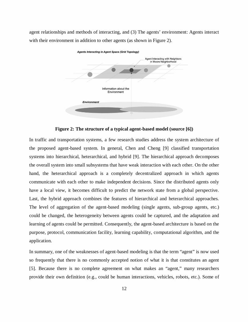
Macal and North [6] presented the structure of a typical agent-based model and limited the

elements of a typical model into: (1) A set of agents, their attributes and behaviors, (2) A set of

12

agent relationships and methods of interacting, and (3) The agents’ environment: Agents interact

with their environment in addition to other agents (as shown in Figure 2).

Figure 2: The structure of a typical agent-based model (source [6])

In traffic and transportation systems, a few research studies address the system architecture of

the proposed agent-based system. In general, Chen and Cheng [9] classified transportation

systems into hierarchical, heterarchical, and hybrid [9]. The hierarchical approach decomposes

the overall system into small subsystems that have weak interaction with each other. On the other

hand, the heterarchical approach is a completely decentralized approach in which agents

communicate with each other to make independent decisions. Since the distributed agents only

have a local view, it becomes difficult to predict the network state from a global perspective.

Last, the hybrid approach combines the features of hierarchical and heterarchical approaches.

The level of aggregation of the agent-based modeling (single agents, sub-group agents, etc.)

could be changed, the heterogeneity between agents could be captured, and the adaptation and

learning of agents could be permitted. Consequently, the agent-based architecture is based on the

purpose, protocol, communication facility, learning capability, computational algorithm, and the

application.

In summary, one of the weaknesses of agent-based modeling is that the term “agent” is now used

so frequently that there is no commonly accepted notion of what it is that constitutes an agent

[5]. Because there is no complete agreement on what makes an “agent,” many researchers

provide their own definition (e.g., could be human interactions, vehicles, robots, etc.). Some of

13

the literature used the definition of an agent based on the proposed list of agents’ characteristics

as will be described in the following section.

2.2.2 Agent Classifications

Franklin and Graesser [8] proposed to use the following characteristics to classify the agents

used in the modeling process: reactive, autonomous, goal-oriented, communicative, learning,

mobile, and flexible (as described in Table 1); e.g., an agent could be a mobile agent or a non-

mobile (stationary) agent.

Table 1: The different proposed properties for agent classifications (source [8])

Property Other Names Meaning

reactive (sensing and acting) responds in a timely fashion to changes in the

environment

autonomous exercises control over its own actions

goal-oriented pro-active purposeful does not simply act in response to the environment

temporally continuous is a continuously running process

communicative socially able communicates with other agents, perhaps including

people

learning adaptive changes its behavior based on its previous experience

mobile able to transport itself from one machine to another

flexible actions are not scripted

character believable "personality" and emotional state

Some literature classified the agents from a planning standpoint, such as Brustoloni [10], who

classified the agents into three types. (1) Regulation agents: agents do not do planning (such as a

thermostat for temperature regulation); (2) Planning agents: they can do the job of regulation

agent plus planning; and (3) Adaptive agents: react to the updated environment situation.

Ultimately, the agents’ classifications, used during the process of agent-based (or multi-agent)

modeling, mainly depend upon the purpose or the assigned tasks for agents during simulation.

The agent-based modeling architecture differs from one research to another based on the agents’

characteristics and the proposed protocols.

14

2.2.3 Agent-Based Modeling Applications

Transportation systems are considered to be the interaction of many complex entities which are

communicating with each other, such as drivers/vehicles, signal lights, and advisory signs. Multi-

agent systems have been used in many transportation applications: network management [11],

traffic control systems interaction [12], modeling driver route-choice decisions [13], and real-

time traffic management [14]. For the case of managing vehicles (especially autonomous

vehicles) at intersections, agent-based modeling is one of the methods used to present the

interaction of autonomous entities, as was suggested in much of the literature (e.g., [15-21]).

Dresner and Stone [19] proposed the reservation-based system in the multi-agent approach at

intersections for autonomous agents (vehicles). In this study, it is assumed that vehicles must

traverse intersections according to a set of parameters agreed upon by the vehicle and the

intersection manager similar to the concept of obeying the signal lights (red and green).

However, agents are free to decide for themselves how to drive without the centralized decision

maker surrendering any control. The proposed system consists of two types of agents: (1)

Intersection managers: responsible for directing the vehicles through the intersection, and (2)

Driver agents: responsible for controlling the vehicles to which they are assigned. Each agent

sends a "request" to the manager for reserving a certain spot at a certain time in the intersection

area, and the manager should reply back with a "confirmation" or a "rejection."

Zou and Levinson [20] presented a framework for the impact of microscopic adaptive control on

traffic delay and collisions at intersections using multi-agent systems and ad-hoc network

communications. Respective agents represented both the vehicles and the management. Figure 3

shows an example of how changing the scenario of intersection control impacts the delay value

(presented by the authors [20]).

15

Figure 3: An example for changing intersection control scenario using multi-agent

collaboration (source [20])

Bazzan [12] proposed a multi-agent system for interacting with the signal controllers in the

arterial networks using a game theory algorithm. The system is a two-player game, each agent

plays the game against each member of its neighborhood of the agents (signal controllers) in the

Network. The decision of the signal agents concerns whether to change phases or not for the

synchronization of the traffic signals along an arterial for the green light wave.

For different roadway users’ environments, Kukla et al. [22] described the development of a

microscopic simulation tool for modeling pedestrian flow using autonomous agents to optimize

the design of public areas with regard to their efficiency and attractiveness. Each pedestrian,

represented by an autonomous agent, can occupy a space in an orthogonal grid. The agent would

react to other agents and features of the environment such as curbs, edges, and obstructions.

A number of studies proposing the implementation of different agent-based architectures for

modeling driver route-choice decisions are also present in the literature. Dia and Purchase [13]

and Dia [23] proposed the use of a cognitive agent architecture composed of beliefs, capabilities,

commitments, and behavioral rules to model individual drivers based on behavioral surveys.

Rossetti et al. [24] proposed the implementation of similar techniques within the DRACULA

traffic simulation model. Wahle et al. [25] proposed a two-layer agent architecture for modeling

individual driver behavior. The first layer (tactical) describes the perception and reaction of the

16

driver-vehicle entity on a short time scale. The second strategic layer, however, extends the basic

layer and is responsible for information assimilation and the decision-making process.

For providing traffic information systems to drivers, Hernandez et al. [14] described the

development of a knowledge-based agent architecture for real-time traffic management at a

strategic level in urban, interurban, or mixed areas. The traffic network is divided into several

sections called problem areas. Moreover, Dia [16] demonstrated the feasibility of using

autonomous agents for modeling dynamic driver behavior and analyzing the effect of ATIS

“Advance Traveler Information Systems” on the performance of a congested commuting

corridor in Australia. This research was based on a behavioral survey of congestion in a real-

world traffic-commuting corridor. In another application, Jin et al. [26] proposed an agent-based

hybrid model for traffic information intelligent control simulation that performs the basic

interface, planning, and support services for managing different types of DRT (Demand

Response Transport) services.

Ehlert et al. [21] described a model of a reactive agent that is used to control a simulated vehicle.

The agent was designed to perform tactical-level driving and to decide in real time what

maneuvers to perform in every situation at intersections. Tactical-level driving consisted of all

driving maneuvers that were selected to achieve short-term objectives. Based on the current

situation and certain pre-determined goals, the agent continuously makes control decisions in

order to keep its vehicle on the road and reach its desired destination safely. The results showed

that the proposed agent-based system is capable of modeling different driving styles

(aggressiveness) using a series of stored realistic behaviors such as collision detection and

emergency braking, and obeying traffic lights and any general traffic rules.

2.2.4 Agent-based Modeling Conclusions

In summary, the agents’ definition and classification, used during the process of agent-based (or

multi-agent) modeling, mainly depend on the purpose or the assigned tasks for agents during

simulation. The agents are autonomous if they are not dependent on the goals of others and

possess goals that are generated within rather than adopted from other agents. Also, the level of

aggregation of the agent-based modeling could be changed, the intra- and inter-variability

between agents could be captured, and learning of agents could be permitted. In general, any

17

computational algorithm could be used for modeling agents: case-based reasoning, cellular

automata, multi-nominal logit, rule-based engine, etc. Subsequently, the agent-based model

could be applied in all transportation aspects: intersection management, traffic control, route

choice, traffic information systems, etc.

Most reported agent-based applications in traffic and transportation systems focus on developing

multi-agent systems that consist of multiple distributed stationary agents [27]. After reviewing

the literature for multi-agent intersection management, it could be concluded that the effects of

many essential factors for modeling agents (vehicles) are either completely neglected or only

qualitatively described. For example, the simulators used for modeling agents at intersections do

not take into consideration the impact on the total delay value. Also, the FCFS (First Come, First

Served) concept—presented in many research papers—gives the advantage to vehicles with

shorter times to intersection regardless of the types of vehicles, transit priority, and total delay

for the network. The physical characteristics’ variability for each vehicle (i.e., agent) is not

captured in many of the previous models in the literature, nor is the impact of weather conditions

on roadway surfaces on agents’ movements. Last, many of challenges in managing vehicles

(agents) at intersections need more investigation, especially the type of communication protocol

that could allow efficient, safe, and optimum systems. At the end, the agent-based modeling

concept has been well used in many different transportation applications; however, its use for

advanced cruise control system applications is very limited.

2.3 ADVANCED CRUISE CONTROL SYSTEMS OVERVIEW

Many of the technical barriers to highway automation have been addressed successfully in many

research studies. However, the transition from today’s manually controlled vehicle system to the

future system, in which traffic could be fully automated, still needs more investigation.

For the next generation of cruise control systems; the ACC is already available in some of the

new car models; however, the CACC—using the connectivity between vehicles and

infrastructure—is still under research and is not yet available on the road. Cooperative adaptive

cruise control (CACC) is an extension of ACC where it can measure the distance to the vehicle

18

ahead and can also exchange information with the surrounding vehicles by wireless

communication.

Most of the past work has been based on analytical models and simulations since there were no

sufficient (C)ACC control systems (i.e., ACC and CACC) in use on the roadway for evaluations

at that time. The literature is well supplied with papers attempting to predict the effects of the

introduction of (C)ACC vehicles into the traffic stream and its impact (on congestion, safety,

emissions, fuel consumption, etc.). However, a few papers do address the consequence of

introducing the (C)ACC system controls in the operation of intersections. The following section

presents an overview for the past studies related to the (C)ACC control systems and it is divided

into two main parts: Advanced Cruise Control Systems on Highways and Advanced Cruise

Control Systems at Intersections.

2.3.1 Advanced Cruise Control Systems on Highways

The automation concept was first introduced on highways under different project titles (e.g.,

AHS) and the (C)ACC is considered one of the main applications of vehicle-highway

automation. Much literature covered the impact of (C)ACC on highways with regard to different

aspects (traffic flow, safety, driver comfort, etc.). In 1998, Zwaneveld and van Arem [28]

presented an intensive literature review for the ACC systems and their impacts on the traffic

flow. The authors summarized a variety of papers to synthesize existing predictions of the effects

of ACC on traffic and showed its potential for the reduction of congestion and the enhancement

of traffic flow stability.

The first report on capacity implications on mixing supported and manually driven vehicles is

found in Zhang [29] (1991) and Benz [30] (1992). The traffic simulator AS (Autobahn

Simulator) was used to investigate the effect of ACC on traffic. The ACC function investigated,

with the use of simulation, was capable of informing/warning the driver instead of controlling

the vehicle. In addition, Rothengatter & Heino (1994) conducted a driving simulator experiment

with 80 test drivers on a four-lane highway [31]. The systems tested were a Collision Warning

System (CWS) —where the gas pedal will be pushed back if a time-to-collision falls below a

certain threshold—and an ACC system. The results showed that the time-headway increased in

19

the case using the CWS system and the time-headway decreased while using the ACC system

(with autonomous brake).

To study the presence of ACC lane on the network, Smith & Noel (1995) investigated four

situations: an abstract freeway interchange using the simulation system FRESIM and three

existing freeway configurations: the Capital Beltway (I-495), the Boston I-93, and the New York

Thruway [32]. The existing freeway configurations were investigated with the use of the

INTEGRATION microscopic traffic simulation model. Investigated traffic demands were such

that no conclusions with respect to capacity gains were stated. Mauro (1993) addressed the basic

principles of assessing the efficiency of true autonomous ACC with some first results [33].

Mauro identifies the improved reliability of the traffic flow as the major positive effect.

Reliability is defined as the probability of traffic breaking down.

Regarding CACC studies, Arem et al. (2006) had focused on the impact of CACC on traffic-flow

characteristics using the traffic-flow simulation model MIXIC that was specially designed to

study the impact of intelligent vehicles on traffic flow [34]. The authors studied the impacts of

CACC for a highway-merging scenario from four to three lanes. The results showed an

improvement of traffic-flow stability and a slight increase in traffic-flow efficiency compared to

the scenario without equipped vehicles. In addition, it was proved to be correct that the

expectation of a low penetration rate of CACC (< 40%) does not have an effect on traffic flow

throughput. However, those results [34] were not consistent with the study of VanderWerf et al.

[35] in 2001. VanderWerf et al. investigated the impacts of autonomous ACC (AACC) and

cooperative ACC (CACC) on traffic based on their microscopic simulation [35]. They found that

AACC has a very small impact on highway capacity. The capacity gain from 0% to 20% AAC

penetration is greater than that from 20% to 40% and there is no capacity increase with more

AACC penetration [35]. Cooperative ACC, on the other hand, can potentially increase capacity

quadratically along with CACC penetration [35].

Another study was made by Bruin et al. (2004) where they proposed a design for the CACC

system [36] that uses inter-vehicle communications. The authors showed how the CACC could

reduce shock waves, which in turn has a positive effect on traffic flow [36] and this is consistent

with Arem et al.’s [34] findings. A reduction in the number of shockwaves could be seen as a

20

safety improvement; however, that conclusion was not made because lateral vehicle control is

also required for safe lane merging, which was not addressed by this study.

The PATH program of the University of California addressed the CACC system in several

reports where the impact of the system on traffic flow and drivers' perceptions were investigated

[37-39]. In 2001, the PATH report [37] studied the paths that could be taken from today’s

driving environment to vehicle-highway automation. The CACC model evaluated in this study is

intended to increase highway capacity by minimizing time gaps between vehicles, while

maintaining the typical ACC goals of increasing driving comfort and convenience and preserving

driving safety. This report showed how the CACC systems have the potential to produce

significant highway capacity increases. The research conducted in the PATH study was part of

the investigation of VanderWerf et al. research paper [35]. Results have been shown for the

validation cases used to test the models individually, for the capacity estimates for the 100%

market penetration cases for each of the three modes of operation: manually driven vehicles,

AACC, and CACC, and for the capacity impacts of different combinations of market

penetrations for AACC and CACC mixed with manually driven vehicles. For the three 100%

market penetration cases, nominal capacity estimates for the manual driving, AACC, and CACC

cases were, respectively: 2,050, 2,200, and 4,550 vehicles per hour.

In 2009 and 2010 reports of the PATH [38, 39], the authors described the design and

implementation of the CACC system on two Infiniti FX-45 test vehicles, as well as the data

acquisition system that has been installed to measure how drivers use the system. The results of

quantitative performance testing of the CACC on a test track were presented, followed by the

experimental protocol used for on-road testing with human subjects.

In the same context, starting from January 2009, the Connect & Drive (C&D) research project

was established as an advanced driver assistance system (ADA) [40]. The project is funded by

the High Tech Automotive System (HTAS) in the Netherlands and is still under development.

This project aims to design and develop new-generation vehicles equipped with ADA systems in

order to improve the current traffic congestion, the road capacity, and safety in the Netherlands.

The C&D project is expected to develop a complete CACC (or, as it is called in the project:

21

"Connected Cruise Control" CCC) controller with communications system, and even human-

machine interface.

Laumonier et al. (2006) presented a preliminary CACC approach for the design of a multiple-

level architecture using reinforcement learning techniques and game theory for multi-agent

coordination [41]. Their approach is based on building a world model from the positioning and

communication systems followed by building the action choice module to give commands to the

vehicle. This article showed promising results for the vehicle-following controller stability;

especially for the coordination controller that could allow an efficient lane allocation for

vehicles.

2.3.2 Advanced Cruise Control Systems at Intersections

Very few research studies have studied the impact of advanced cruise control systems or, in

general terms, autonomous vehicles’ algorithms at intersections compared to highway

investigations and reports. For example, Reece and Shafer (1991) [42] developed a driving

program called Ulysses. The Ulysses goal is to prevent the simulated robot from having or

causing accidents, and from unnecessarily constraining itself to stop.

Moreover, Dresner and Stone [17, 19, 43] proposed an intersection control protocol called

Autonomous Intersection Management (AIM) and built their custom simulator using the multi-

agent approach. Dresner and Stone showed that with autonomous vehicles it is possible to

develop intersection control that is much more efficient than the traditional control mechanisms,

such as traffic signals and stop signs. The AIM custom simulator is based on the reservation

paradigm, in which vehicles “call ahead” to reserve space-time in the intersection under the

FCFS (First Come, First Served) policy [43]. The main concept is that each autonomous vehicle

sends a request to the intersection manager and asks permission to pass through the intersection.

Thereafter, the intersection manager decides whether to grant or reject requested reservations

according to an intersection control policy and FCFS.

Most of the studies directly related to CACC at intersections had focused on fuel consumption

and emissions impacts. There has been little research on developing dynamic optimal speed

advising algorithms on the vehicle side, based on traffic signal timing information. Rather than

modifying the design of the signal timing controller at the traffic signals [44, 45], optimal speed

22

advice algorithms can be developed. The main purpose of the speed advice algorithm is to assure

the arrival of the vehicle at the green light with optimizing certain constraints (the fuel

consumption, emissions, delay, etc.). For example, based on the traffic signal information,

Mandava et al. (2009) developed arterial velocity planning algorithms that give dynamic speed

advice to the driver [46]. The algorithms seek the maximization of having a higher probability of

green light when approaching signalized intersections. Using a stochastic simulation technique,

the algorithms are used to generate sample vehicle velocity profiles along a 10-intersection

signalized corridor. The resulting vehicle fuel consumption and emissions from these velocity

profiles were calculated using a modal emissions model, and then compared to those from a

typical velocity profile of vehicles without velocity planning. The energy/emission savings for

vehicles with velocity planning were found to be 12-14%.

Another example by Rakha and Kamalanathsharma (2011) presented a framework to enhance

fuel consumption efficiency "eco-driving" while approaching a signalized intersection. The

framework attempts to use the signal phase and timing information that may be available through

V2I communication for the optimization process [47]. The results showed how the speed

adjustment strategies are vehicle-dependent and how explicitly the fuel consumption models

could be introduced in an optimization function.

Regarding research directly related to CACC applications, Malakorn and Park (2010) explored

the difference between intelligent traffic signals that cooperated with CACC system and

traditional intersection controls [48]. The ultimate goal of this system is to reduce the

environmental impacts of driving by minimizing vehicle acceleration depending on the VT

micro-model [49]. The traditional scenario was represented by a pre-timed, signalized

intersection. The cooperative scenario was represented by an intersection equipped with

intelligent traffic signal control and vehicles equipped with CACC for advanced control over

acceleration and velocity. The results showed how the system is beneficial to the drivers and the

environment (e.g., the amount of CO2 and fuel consumption).

Under the connected vehicles (CV) environment, Lee and Park [50] created a Cooperative

Vehicle Intersection Control (CVIC) system that enables cooperation between vehicles and

infrastructure for effective intersection operations and management. The CVIC algorithm was

23

designed to manipulate individual vehicles’ maneuvers so that vehicles can safely cross the

intersection without colliding with other vehicles. The proposed algorithm seeks the

minimization of the overlapping distance for any two conflicting trajectories. This paper

assumed that there is an Intersection Control Agent (ICA) especially designed to gather

individual vehicular information and to provide the best maneuvers to the vehicles crossing an

intersection. The ICA performs a sequence of optimization processes to obtain acceptable

acceleration/deceleration rates. The authors addressed one intersection with four legs (one lane

per leg) as an application study. Although this paper did not perform proper case studies for both

multi-lane and coordinated intersections, the results showed promising results for air quality and

energy savings assuming 100% level of penetration for the system.

In 2011, by expanding the concept presented in [50], Park et al. examined an IntelliDrive-based

cooperative vehicle-infrastructure control system as an alternative to current transportation

infrastructure. The authors evaluated the system from an environmental perspective using Life

Cycle Assessment [51]. However, the studied intersection remained as four legs with one lane

per approach; in other words, only through movements were considered in the study. The results

showed that the CVIC-based control algorithm under the IntelliDrive environment could

improve both the mobility and the environmental performances of the urban corridor.

2.3.3 Advanced Cruise Control Conclusions

From the literature review many conclusions can be drawn. The CACC effect studies that have

been performed emphasize that CACC is able to increase the capacity of a highway significantly.

Such a Cooperative ACC (CACC) system can be designed to follow the preceding vehicle with

significantly higher accuracy and faster response to changes.

Although there is much literature on ACC, the literature related to CACC is limited; especially

the studies of CACC capabilities at intersections. The connectivity between vehicles could

include precise speed information, acceleration, fault warnings, warnings of forward hazards,

and braking capability. With information of this type, the CACC controller can better anticipate

problems, enabling the vehicle to be safer, smoother, and faster in response. In general, the

CACC has the potential to increase capacity by minimizing time gaps between consecutive

vehicles and traffic flow stability. Safety is very challenging to assess using simulation for

24

typical conditions, and this technology is not widely available for testing on-road; consequently

very few studies encountered it. Most of the literature had focused on the traffic flow impact

after introducing the (C)ACC systems and ignored some other important aspects. In a number of

studies, the functionality, architecture, or design of CACC systems have been described.

However, extensive exploration of the CACC’s impact on delay and its possible use as a tool for

optimizing the movements of vehicles at intersections has been done by only a few researchers.

The aforementioned literature shows that there has been research in algorithms for CACC

applications at intersections. However, none of these approaches used an explicit optimization

objective of reducing delay or minimizing travel time. The goal of reducing delay, in all these

cases, is transformed to simpler functions of acceleration/deceleration rates, or duration of these

events. It could be stated that previous research has made simplifying assumptions and failed to

capture the impact of various aspects when studying the CACC at intersections; e.g., impact of

weather, different classes of vehicles, etc.

2.4 CHAPTER CONCLUSIONS

Automated vehicles are considered a major part of future intelligent transportation systems.

Semi-automated systems in which the speeds are governed by sensors using ACC systems are

already available in the market. This chapter presented a review of the literature relevant to the

agent-based modeling and advanced cruise control /automation topics. The reviewed literature

showed that there are diverse research efforts that address modeling/simulating vehicles

equipped by (C)ACC systems. A few attempts have been made in the literature for the use of

CACC technology at intersections. Nevertheless, there are still some gaps that have not been

thoroughly investigated. Examples of the areas that have these gaps are the inclement weather

impact, different vehicles’ class management, and level of penetration of the system effect on the

intersection operation. In addition, past research did not explicitly optimize the total delay at the

intersection as it focused more on optimizing acceleration/deceleration levels for crash avoidance

and/or emissions.

Accordingly, this dissertation attempts to fill some of these gaps for the sake of bettering

automated vehicle control at intersections. This research presents an innovative approach for

25

optimizing the movements of vehicles equipped by Cooperative Adaptive Cruise Control

systems at "smart" intersections. This research mainly focused on developing a strategy which

yields the most optimal speed profile for a vehicle approaching intersections using V2V and V2I

communications for total delay minimization and crash prevention simultaneously. To

accomplish all the research objectives mentioned above, an optimization/simulation tool, which

can support simulations in microscopic detail is accommodated as will be presented in the

following chapters.

26

CHAPTER 3 GAME THEORY ALGORITHM APPROACH

In this chapter, a heuristic optimization algorithm is developed for automated vehicles (equipped

with CACC systems) at uncontrolled intersections using a game theory framework. The

proposed system models the automated vehicles as reactive agents interacting and collaborating

with the intersection controller (manager agent) to minimize the total delay. However, the system

proposed in this chapter is only limited to 100% level of penetration of the CACC system. The

system is evaluated using a case study considering two different intersection control scenarios: a

four-way stop control and the proposed intersection controller framework. In both scenarios, four

automated vehicles (a single vehicle per approach) were simulated using a Monte Carlo

simulation that was repeated 1000 times. The results show that the proposed system reduces the

total delay relative to a traditional stop control by 35 seconds, on average, which corresponds to

an approximately 70-percent reduction in the total delay.

3.1 INTRODUCTION

The idea of an automated driving environment has been studied for decades to reduce the

number of crashes and enhance mobility the transportation system mobility. After the

development and deployment of the USDOT Connected Vehicle initiative [2], the enhancement

of the current driver assistance systems has become an expected step towards achieving better

mobility and safety. Consequently, the concept of Cooperative Adaptive Cruise Control (CACC)

systems has been introduced as an advanced generation for the traditional cruise control. In such

a system, vehicles can not only sense the information from the preceding vehicle, but also

communicate with other vehicles through vehicle-to-vehicle (V2V) and vehicle-to-infrastructure

(V2I) communication. After fusing all data sources, vehicles make decisions with regards to

acceleration, deceleration, or maintaining their current speed. The basic idea of the system is to

assist the driver by controlling the speed of the vehicle; however it leaves the maneuver

responsibility to the driver.

In general, as mentioned previously, the literature related to CACC is limited; especially the

studies of CACC capabilities at intersections. The CACC controller can better foresee problems,

enabling the vehicle to be safer and faster in response to various stimuli. However, extensively

27

exploring the CACC impact on delay and how it could be used as a tool for optimizing the

movements of vehicles at intersections is limited to only a few researchers.

Subsequently, this chapter develops a heuristic optimization algorithm for automated vehicles

(equipped with cooperative adaptive cruise control CACC systems) at uncontrolled intersections

using a game theory framework. The proposed system models the automated vehicles as reactive

agents interacting and collaborating with the intersection controller (manager agent) to minimize

the total delay. The vehicles are modeled as agents interacting with the intersection controller

(manager agent) and obeying the optimum decision made by the intersection controller. In other

words, the vehicles collaborate in a form of a "Cooperative Game" with the controller installed at

the intersection. The main principle of this research is to employ the communication

technologies with advanced vehicle capabilities to replace the usual state-of-the-practice control

systems at intersections (e.g. stop sign, yield signs, etc.).

In terms of the chapter layout, initially a description of the proposed multi-agent system is

presented. Subsequently, the built-in simulation process using game theory is presented and the

testing of the optimization algorithm is then discussed. Finally, the conclusions of the chapter are

discussed.

3.2 PROPOSED MULTI-AGENT MODELING LAYOUT

The adaptability and flexibility of an intelligent agent makes it possible to control various types

of vehicles with different driving behavior. For the case of automated vehicles, agent-based

modeling is most appropriate as was suggested in several literature sources [16, 18]. Here we

propose the use of agent-based modeling of CACC-equipped vehicles because the agents have

two main features: (1) they are at least to some extent capable of autonomous actions or

decisions and (2) they are capable of interacting with other agents through cooperation,

coordination and negotiation [9].

The proposed multi-agent system (MAS) consists of two types of agents: reactive agents

(vehicles equipped by CACC) and a manager agent (intersection controller). The main idea of

the proposed system is that the manager agent communicates with the reactive agents in the

intersection study zone (IZ) and determines the optimum movements for each reactive agent

28

based on a "Game Theory Decision Framework". The IZ is the zone area around the intersection

where the reactive agents begin to exchange information with the manager agent. The IZ in this

research 200 m upstream of the intersection to ensure that vehicles have sufficient time to

receive and respond to the information received.

The proposed layout for the MAS assumes that all agents in the IZ are interacting,

communicating and exchanging information for the common benefit using some form of

communication (e.g. Dedicated Short Range Communication (DSRC)). The global benefit is

defined as reducing the total delay while ensuring no vehicle collisions occur. The reason for

modeling the collaboration between agents is to overcome any selfish behavior by any vehicle or

in other words to seek the global benefit for all vehicles in the IZ. Therefore, the main task for

the manager agent is to determine the optimum speed for each reactive agent at each time step by

processing the input data through a real-time simulation. The MAS layout consists of three main

components for controlling the movements of reactive agents in the IZ: Input, Data processing

and Output. Figure 4 illustrates the layout of the proposed CACC multi-agent system.

Figure 4: The layout of the proposed MAS for equipped vehicles at uncontrolled

intersections

The input data for the manager agent consists of: intersection characteristics, weather station

input and reactive agent input. The intersection characteristics contain the speed limit of the

intersection and number of lanes of each approach. The weather station provides the

instantaneous weather condition to take into account the roadway surface condition (dry or wet)

in simulating the reactive agent movements. At each time step, all reactive agents in the IZ report

29

their physical characteristics, current speed, location and acceleration to the manager agent. All

input information is received by the manager agent then processed and optimized using a game

theory decision process. For the purpose of this research, a simulation tool was developed using

Matlab.

3.3 PROPOSED REAL-TIME SIMULATION FOR CACC-EQUIPPED VEHICLES

This section describes the state-of-art simulation test bed that was developed to model the

intersection controller. The research presented here is considered a first step in developing a fully

automated intersection vehicle controller. In general, the simulation algorithm computes the

optimum location, speed and acceleration of vehicles to ensure that no conflicts occur while at

the same time minimizing the total intersection delay each time step (e.g. 0.5 sec). The total

delay is defined by the summation of the delay experienced by each vehicle at each time step.

The proposed software is considered as a novel tool for optimizing the movement of automated

vehicles at intersections; however, it has some limitations and assumptions. First, we assume a

market penetration of 100% of CACC-equipped vehicles. Second, all drivers/vehicles in the IZ

are assumed to follow the recommendations made by the intersection controller to achieve the

global profit. Last, only one speed profile, i.e. one vehicle (the most critical one), is adjusted

(optimized) each time step.

It should be mentioned that the vehicle dynamics (acceleration and deceleration) models are part

of the simulation software. The dynamics models take into account the tractive and resistance

forces (referred to the literature [52]) acting on vehicles at each time step. Consequently, the

simulation process reflects the physical characteristics (power of engine, mass, etc.) and the

weather condition (wet or dry) affecting the movements of vehicles.

At each time step of simulation, the existing vehicles in the IZ are determined and thereafter the

built-in simulation uses a heuristic optimization process divided into two main stages. The stages

are: 1) calculate the Conflict Zone Occupancy Time (CZOT) for each conflict area, 2) conduct a

Game Theory Optimization, as will be explained in more detail in the following sub-sections.

30

3.3.1 Calculate the Conflict Zone Occupancy Time in Conflict Areas

A conflict point in the intersection is a point that can be occupied by two different crossing

vehicles during the same time interval. It is introduced the term Conflict Zone Occupancy Time

(CZOT) in the optimization process. The CZOT is the time interval where the two intersecting

vehicles will be occupying the same conflict area. The simulation software uses the input

information to simulate the trajectory of the vehicles; therefore estimates the time needed to enter

and leave the conflict zone. The simulation software assumes that all vehicles will accelerate to

the maximum speed (if their speed is less than the maximum) as an “initial decision” to reduce

the total travel time for each vehicle. If the estimated CZOT value is positive (>0), it is an

indication that by accepting the initial decision for both intersecting vehicles, a collision would

occur. Alternatively, if CZOT is equal to zero (or less) that means the intersecting vehicles will

not be conflicting with each other and it is safe to accept the initial decision.

For illustrating purposes, for a four-legged intersection there would be four conflict zones

(assuming on through traffic on each approach), as shown in Figure 5 (a). Consequently, the

CZOT value for each conflict area, CZOT1, CZOT2, CZOT3 and CZOT4 can be computed.

Thereafter, the CZOT plot is drawn as shown in Figure 5 (b) where each rectangle illustrates the

conflict occupancy time for each vehicle. In the example, it is observed that CZOT1, CZOT2 and

CZOT4 have positive values (i.e. there is a common time interval between the two intersecting

vehicles). Consequently, it is needed adjusting the vehicle trajectories in order to avoid a

collision with the intersecting vehicles. On the other hand, the CZOT3 value is equal to zero as

the two intersecting vehicles occupy the conflict zone at different time intervals.

As mentioned before, the built-in simulation selects only one vehicle to modify its trajectory

each time step (i.e. 0.5 second). Therefore the next step is to select the appropriate vehicle to

adjust its trajectory.

31

(a)

(b)

Figure 5: Conflict Zone Occupancy Time (CZOT) output example

12 12.2 12.4 12.6 12.8 13 13.2 13.4 13.6 13.8

veh1

veh4

veh1

veh2

veh2

veh3

veh3

veh4

CZOT1

CZOT2

CZOT3

CZOT4

Time (s)

32

3.3.2 Game Theory Optimization Process

Various models that incorporate concepts from Game Theory are described in many

transportation related literature [41, 53-55]. Interaction and collaboration are essential aspects in

the dynamic multi-agent systems (MASs); consequently, game theory provides powerful tools

for analyzing those types of transport systems. Multi-agent systems (MASs) are systems

composed of multiple agents, which cooperate with each other to reach desired objectives. In

general, formulating a problem as a game is meaningful if the solution, such as Nash

equilibrium, results in a relatively fair situation for all players.

A game of strategy is defined as the game of two or more players where each player is trying to

choose the best strategy to maximize the total benefit (or pay-off) [56]. In cooperative games

(one of the types of the strategy games), the pay-off (benefit) for each potential group can be

obtained by the coalitional of its members (or players). The challenge of the cooperative game is

to allocate the pay-off (benefit) among the players in some fairway. Consequently, collaborating

with all CACC-equipped vehicles together with the intersection controller, using communication

technology, could be formulated in a cooperative game framework. Defining a game requires

identification of the players, their alternative strategies and their objectives as will be described

in the following section.

3.4 ELEMENTS OF THE GAME (DESCRIBING A GAME)

Game theory provides a framework for modeling interactions between groups of decision-

makers when individual actions jointly determine the outcome [56]. The proposed cooperative

game framework in this research is entitled: CACC-CG (Cooperative Adaptive Cruise Control -

Cooperative Game). The CACC-CG represents the decision process of the built-in simulation

software to optimize the movement of automated vehicles at intersections. The proposed CACC-

CG is considered a decision process that is repeated at each time step of the simulation. The

CACC-CG cooperative game consists of the following elements: players (s), actions (A),

information (I), strategies (S), pay-offs (U), outcomes (O) and equilibrium (π) as summarized in

Table 2.

33

Table 2: The elements of the proposed game CACC-CG

Elements Description

Players (s) The manager agent (intersection Controller) and the reactive agents (vehicles) existed in the IZ

Actions (A) The intersection controller: select one vehicle among the conflicting vehicles to change its speed profile Vehicles: accelerate, decelerate or maintain the same speed

Information (I) The information is symmetric and certain for all players Strategy (S) The decision taken is the one corresponding to the maximum benefit for all players (i.e. Pay-off (U) The summation of the total CZOT (conflict occupancy time) values and the total delay Outcome (O) An optimum speed profile for each reactive agent (vehicle) Equilibrium (π) The action combination which no player would be willing to change it

Players are the individuals who make decisions. Each player’s goal is to maximize his utility by

choice of actions. The players in the CACC-CG are the manager agent and all existing reactive

agents at each time step. Actions are the choices of each player can make and it could be one or a

set of actions for a player to choose between them. For the manager agent, the action could be

taken is to select one reactive agent for optimizing its movement per each time step and all other

vehicles will keep their initial state. Reactive agents have three possible actions: decelerate,

accelerate or maintain the current speed. It is assumed the information set is available for all

players during the game decision process. In other words, the information is symmetric and

certain for all players using communication technology (DSRC).

The player’s strategy is a rule that tells him/her which action to choose at each instant of the

game given his/her information set. It is simply the set of actions that could provide the

maximum profit for all agents at the intersections, in other word, the actions corresponding to

minimum total delay.

Furthermore, Pay-off is the expected benefit or utility that the player will receive after all players

have picked their strategies and the game has been played. In the CACC-CG, the pay-off is

determined based on the actions of the players and it is proposed to be formulated as a Utility

function. It is assumed in this framework that the optimum decision taken by the players would

be the action set that lead to the minimum utility function (conflict zone and delay

minimization). Consequently, the players follow the maximin principle (the player chooses the

strategy with the least possible utility value). The value of utility function depends on the

34

distance remaining to the intersection relatively to the needed stopping sight distance for each

vehicle. Generally, the utility value is considered as the summation of the total CZOT values and

the total delay due to the actions of manager agent (i) and any selected reactive agent (j).

However, if the distance remaining for a vehicle to the intersection is less than minimum

stopping sight distance, its utility value is set to be an infinity value. In other words, if a vehicle

does not have the option other than decelerating to complete stop, this vehicle will not be a part

of the optimization process as presented in Equation (1).

, ,1 1

,

; if

; if

P N

i j i j j jp i

i j

j j

CZOT D X SSDU

X SSD

(1)

Where, i is the action taken by the manager agent; j is the action taken by the reactive agent; Ui,j

is the utility value corresponding to the action set (i, j), P is the total number of conflict points;

CZOTi,j is the conflict zone occupancy time value (explained previously) corresponding to the

action set (i, j); Xj is the current distance to the intersection for vehicle j; SSDj is the minimum

stopping sight distance to the intersection for vehicle j; N is the total number of reactive agents

(vehicles) existed in the current time step; and Di,j is the delay value for each reactive agent also

corresponding to the action set (i, j).

The “Outcome” is a set of elements that the modeler picks from the values of actions, pay-offs

and other variables after the game is played out. Consequently, the outcome of the proposed

game is simply: A speed change (acceleration, deceleration or constant) for a chosen vehicle that

would give the least total delay value and eliminate the conflicting maneuvers (CZOT=0).

For the equilibrium, once the players have settled on strategies that neither player has incentive

to deviate, this condition is called the Nash equilibrium (named after John Forbes Nash) [56].

Some of the literature simply define the equilibrium as the best decision by the player given that

the other player already chose his decision. Consequently, every dominant strategy is Nash

equilibrium, but not every Nash equilibrium is a dominant strategy[56]. The Nash equilibrium

condition would be the case expressed shown in Equation (2)

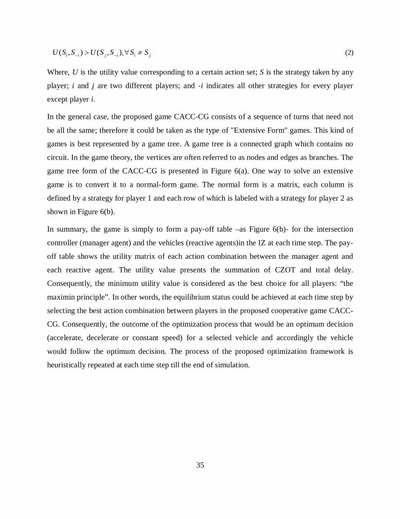
35

( , ) ( , ),i i j i i jU S S U S S S S (2)

Where, U is the utility value corresponding to a certain action set; S is the strategy taken by any

player; i and j are two different players; and -i indicates all other strategies for every player

except player i.

In the general case, the proposed game CACC-CG consists of a sequence of turns that need not

be all the same; therefore it could be taken as the type of "Extensive Form" games. This kind of

games is best represented by a game tree. A game tree is a connected graph which contains no

circuit. In the game theory, the vertices are often referred to as nodes and edges as branches. The

game tree form of the CACC-CG is presented in Figure 6(a). One way to solve an extensive

game is to convert it to a normal-form game. The normal form is a matrix, each column is

defined by a strategy for player 1 and each row of which is labeled with a strategy for player 2 as

shown in Figure 6(b).

In summary, the game is simply to form a pay-off table –as Figure 6(b)- for the intersection

controller (manager agent) and the vehicles (reactive agents)in the IZ at each time step. The pay-

off table shows the utility matrix of each action combination between the manager agent and

each reactive agent. The utility value presents the summation of CZOT and total delay.

Consequently, the minimum utility value is considered as the best choice for all players: “the

maximin principle”. In other words, the equilibrium status could be achieved at each time step by

selecting the best action combination between players in the proposed cooperative game CACC-

CG. Consequently, the outcome of the optimization process that would be an optimum decision

(accelerate, decelerate or constant speed) for a selected vehicle and accordingly the vehicle

would follow the optimum decision. The process of the proposed optimization framework is

heuristically repeated at each time step till the end of simulation.

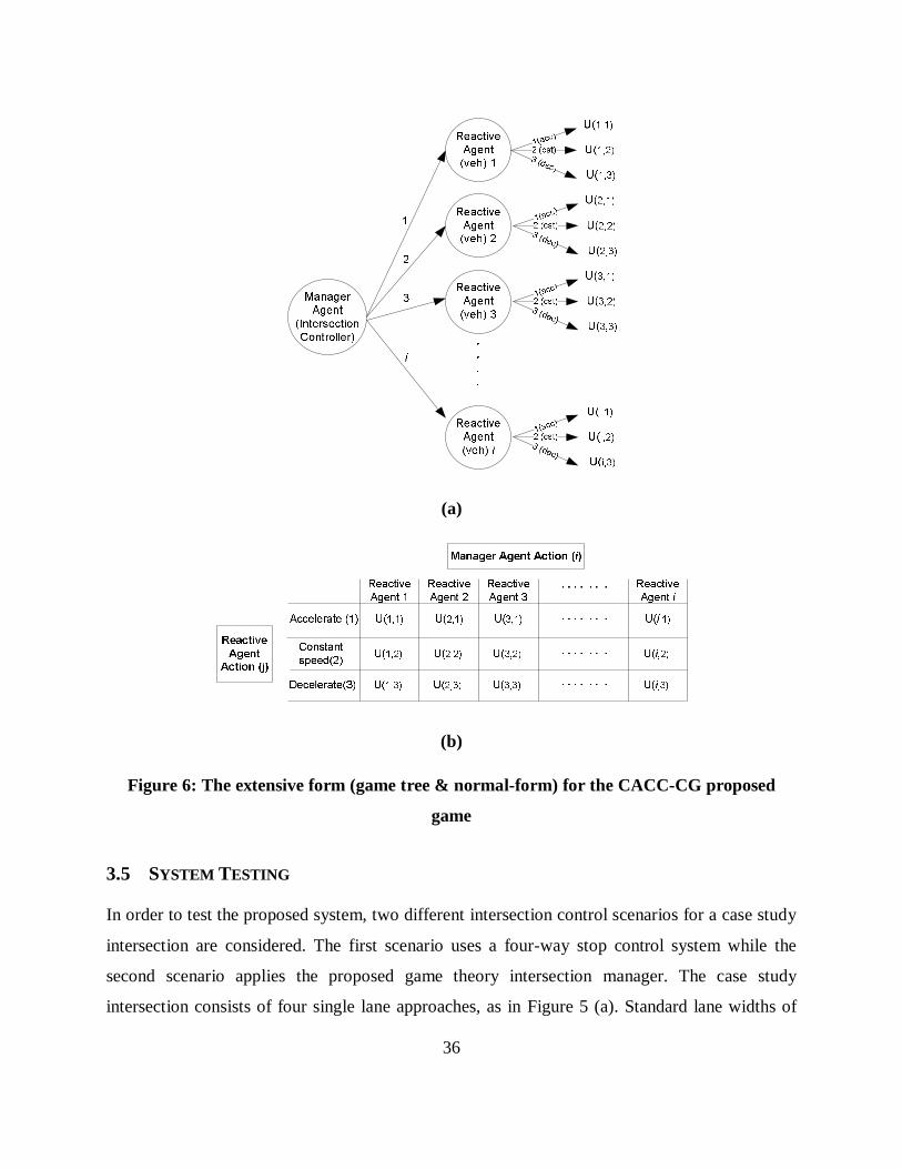
36

(a)

(b)

Figure 6: The extensive form (game tree & normal-form) for the CACC-CG proposed

game

3.5 SYSTEM TESTING

In order to test the proposed system, two different intersection control scenarios for a case study

intersection are considered. The first scenario uses a four-way stop control system while the

second scenario applies the proposed game theory intersection manager. The case study

intersection consists of four single lane approaches, as in Figure 5 (a). Standard lane widths of

37

3.5 meters are considered with approach speed limits of 35 mph (approximately 16 m/s). For

illustration purposes, a Toyota Prius 2010 was modeled with an engine power of 134 Horse

Power (Hp). This vehicle is similar to the tested vehicle in the Google Driverless experiment [4].

The study considered a single vehicle arrival on each approach considering the proposed

intersection manager and an all-way stop controlled intersection. For both scenarios, the entrance

time, speed, and acceleration of each vehicle were randomly generated. The system was then

modeled considering a time step (∆t) of 0.5 s. The total delay was computed for each run

considering the two intersection control scenarios. The total delay was computed for all four

automated vehicles. This procedure was repeated 1000 times using a Monte Carlo simulation and

the total delay time was recorded for each simulation. Figure 7 shows the total delay variation for

the 1000 simulations for both intersection control strategies.

Figure 7: Total delay comparison between Stop Sign control and proposed optimization

control using game theory

The results demonstrate that the proposed framework is giving less total delay time comparing to

the stop sign control scenario. The average total delay time for the proposed scenario is

approximately 19 seconds and for the stop sign control is 54 seconds. Thus, for the case of only

four crossing vehicles, the proposed system reduces the total delay more than the traditional stop

0 100 200 300 400 500 600 700 800 900 10000

10

20

30

40

50

60

70

80

Simulation #

Tota

l Del

ay ti

me

(s)

Stop Sign ControlThe Proposed Optimum Control

38

control by 35 seconds on average and obviously the total delay reduction would enlarge by

having more vehicles crossing the intersection.

3.6 SUMMARY AND CONCLUSIONS

The approach presented in this chapter developed an innovative heuristic algorithm for

optimizing the movement of vehicles at intersections within a CACC framework. The proposed

framework uses game theory to ensure that no crashes occur while minimizing the intersection

delay. The proposed framework assumes communication between vehicles and the intersection

infrastructure to control the movements of the reactive agents approaching the intersection study

zone (IZ). A real-time simulation tool is developed that would be loaded onto an intersection

controller to govern the vehicle movements. The simulation determines the vehicles currently in

the IZ and then estimates their trajectories based on their current state. Thereafter, the

optimization process begins by forming a pay-off table for what would be the output in case of

any action taken by the controller or the vehicles. Consequently, the intersection controller

would advise the vehicle (using communication) to the best action. This process is repeated

heuristically at each time step for the duration of the simulation (i.e. all vehicles traverse the

intersection).

Thereafter, the system is evaluated using a case study considering two different intersection

control scenarios: a four-way stop control and the proposed intersection controller framework. In

both scenarios, four automated vehicles (a single vehicle per approach) were simulated using a

Monte Carlo simulation that was repeated 1000 times. The results show that the proposed system

reduces the total delay relative to a traditional stop control by 35 seconds on average, which

corresponds to an approximately 70 percent reduction in the total delay. The proposed work

serves as an initial step towards the development of agent-based CACC intersection control

systems. The research results demonstrate the promising potential benefits of such a system over

conventional state-of-the-practice intersection control systems. However, this part of research

only considered through movements at intersection and level of penetration 100%, so to

overcome these limitations, further research were done as illustrated in the following chapters.

39

CHAPTER 4 DRIVER GAP ACCEPTANCE BEHAVIOR FOR NON-

AUTOMATED VEHICLES

This chapter presents an extensive research study for studying driver gap acceptance for non-

automated vehicles at intersections. An empirical study was conducted to quantify the impact of

a number of variables on driver left-turn gap acceptance behavior at signalized intersections. The

main purpose of this study is to model non-automated vehicles’ behavior under inclement

weather conditions as an essential input in managing mixed automation environment. The

variables that are considered include the gap duration, the travel time needed to cross the

intersection, and the corresponding weather conditions. The collected data set was divided into

six weather categories for different combinations of precipitation and roadway surface

conditions. Logistic regression models were calibrated to the data and compared to identify the

best model for capturing driver gap acceptance behavior. The models reveal that drivers are more

conservative during snow precipitation compared to rain precipitation. In the case of the roadway

surface condition, drivers require larger gaps for wet surface conditions compared to snowy and

icy surface conditions and, as would be expected, require the smallest gaps for dry roadway

conditions. In addition, the models show that the drivers require larger gaps as the distance

required to traverse the offered gap increases. It is anticipated that these findings will be used for

the future of driver intelligent assistance systems and incorporated in the optimization process

for automated vehicles at intersections.

4.1 INTRODUCTION

Congestion mitigation in urban areas is an important issue that needs addressing in our modern

society. One of the major factors that affect the capacity and saturation flow rate at signalized

and non-signalized intersections is gap acceptance behavior. Gap acceptance is defined as the

process that occurs when a traffic stream (known as the opposed flow) has to either, cross or

merge with another traffic stream (known as the opposing flow). This chapter focuses on

crossing gap acceptance behavior for permissive left turns.

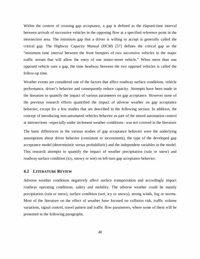
40

Within the context of crossing gap acceptance, a gap is defined as the elapsed-time interval

between arrivals of successive vehicles in the opposing flow at a specified reference point in the

intersection area. The minimum gap that a driver is willing to accept is generally called the

critical gap. The Highway Capacity Manual (HCM) [57] defines the critical gap as the

“minimum time interval between the front bumpers of two successive vehicles in the major

traffic stream that will allow the entry of one minor-street vehicle.” When more than one

opposed vehicle uses a gap, the time headway between the two opposed vehicles is called the

follow-up time.

Weather events are considered one of the factors that affect roadway surface conditions, vehicle

performance, driver’s behavior and consequently reduce capacity. Attempts have been made in

the literature to quantify the impact of various parameters on gap acceptance. However none of

the previous research efforts quantified the impact of adverse weather on gap acceptance

behavior; except for a few studies that are described in the following section. In addition, the

concept of introducing non-automated vehicles behavior as part of the mixed automation control

at intersections –especially under inclement weather conditions– was not covered in the literature

The basic differences in the various studies of gap acceptance behavior were the underlying

assumptions about driver behavior (consistent or inconsistent), the type of the developed gap

acceptance model (deterministic versus probabilistic) and the independent variables in the model.

This research attempts to quantify the impact of weather precipitation (rain or snow) and

roadway surface condition (icy, snowy or wet) on left-turn gap acceptance behavior.

4.2 LITERATURE REVIEW

Adverse weather conditions negatively affect surface transportation and accordingly impact

roadway operating conditions, safety and mobility. The adverse weather could be mainly

precipitation (rain or snow), surface condition (wet, icy or snowy), strong winds, fog or storms.

Most of the literature on the effect of weather have focused on collision risk, traffic volume

variations, signal control, travel pattern and traffic flow parameters, where some of them will be

presented in the following paragraphs.

41

Datla and Sharma (2008) [58] characterized highway traffic volume variations with severity of

cold, amount of snowfall and various combinations of cold and snowfall intensities. Cools

(2008) [59] quantified the impact of weather conditions on traffic intensity and volume

variations. The study considered: the daily precipitation, hail, snow and thunderstorm,

cloudiness, temperature, wind speed, sunshine and duration of diminished visibility due to fog as

potential explanatory variables.

There have been limited studies that directly address how adverse weather affects traffic flow

variables, including speed, flow, density, headway and capacity. Brilon and Ponzlet (1996) [60]

investigated the impact of various weather conditions on capacity and on other traffic flow

parameters on an Autobahn in Germany. Rakha et al. (2008) [61] quantified the impact of

inclement weather (precipitation and visibility) on traffic stream behavior and key traffic stream

parameters including free-flow speed, speed-at-capacity, capacity, and jam density. Daniel et al.

(2009) [62] collected speed, flow and density data under no adverse weather, as well as under

rain, snow, darkness and sun glare conditions.

Several studies in the literature have investigated the impact of different factors on driver gap

acceptance behavior. These factors include day and nighttime effects [63], the speed of the

opposing vehicle [64, 65], the type of intersection control (yield versus stop sign) [66], the driver

sight distance [67], the geometry of the intersection, the trip purpose, the expected waiting time

[68] and gap acceptance crash patterns at intersections [69]. Zohdy et al. [70] and Rakha et al.

(2010) [71] quantified the impact of rain intensity, waiting time and travel time on driver left

turn gap acceptance behavior using empirical and stochastic modeling approaches. However,

these studies were limited to rain precipitation only.

4.3 STUDY OBJECTIVES

The main objectives of the study are to investigate the influence of weather precipitation and

roadway surface condition on left-turn gap-acceptance behavior for non-automated vehicles. The

weather condition in the study is divided into six categories for different combinations of

weather precipitation “rain and snow” and roadway surface conditions “wet, icy and snowy”.

42

Logit models are fit to the data to model driver gap acceptance behavior and compute driver-

specific critical gap sizes.

In terms of this chapter layout, initially the study site and data acquisition procedures are

presented followed by a description of the data analysis procedures and a summary of the

preliminary results. A description of the different proposed models is followed along with model

calibration results. Subsequently, the predicted critical gap is presented and the impact of various

factors on opposed saturation flow rates is analyzed. Finally, the study conclusions are presented.

4.4 STUDY SITE DESCRIPTION AND DATA ACQUISITION EQUIPMENT

The study site that was considered in this study was the signalized intersection of Depot Street

and North Franklin Street (Business Route 460) in Christiansburg, Virginia. A schematic of the

intersection is shown in Figure 8a. It consists of four approaches at approximately 90° angles.

The posted speed limit for the eastbound and northbound approaches was 35 mph and for the

westbound and southbound approaches was 25 mph at the time of the study.

The signal phasing of the intersection included three phases, two phases for the Depot street

North and South (one phase for each approach) and one phase for the Route 460 (two approaches

discharging during the same phase) with a permissive left turn movement. Figure 8a illustrates

the movement of vehicles during the green phase of Route 460 and the dashed lines show the left

turn vehicle trajectory where drivers are facing a gap acceptance/rejection situation. The dashed

line is opposed by the through movements at three conflict points P1, P2 and P3 respectively.

Each conflict point presents the location of possible collision with the through opposing

movement. The data acquisition hardware of the study site consisted of two components as

follows:

(a) Video cameras to collect the visual scene (Figure 8 b). There were four cameras

installed at the intersection (one camera for each approach) to provide a video feed of the

entire intersection environment at 10 frames per second.

(b) Weather station (Figure 8 c). The weather station provided weather information every

minute. The collected weather data included precipitation, wind direction, wind speed,

temperature, barometric pressure, and humidity level.

43

(a)

(b) (c)

Figure 8: (a) Layout of study intersection; (b) Video surveillance system; and (c) Weather

monitoring system

44

4.5 DATA ANALYSIS PROCESS AND DATA REDUCTION RESULTS

The data were collected over a six-month period (the first half of 2010 year). The data output per

day consisted of 15 hourly video files and the corresponding weather measurements. The video

data were reduced manually by recording the time instant at which a subject vehicle initiated its

search to make a left turn maneuver, the time stamp at which the vehicle made its first move to

execute its left turn maneuver, and the time the left turning vehicle reached each of the conflict

points..

Each rejected or accepted gap was recorded as an observation in the reduced dataset and the

corresponding variables for each observation were also recorded. More than 5,000 observations

were excluded because they ended with a red light indication (i.e., the gap occurred between a

vehicle and no second opposing vehicle due to ending of the green phase). The final dataset that

was analyzed consisted of a total of 11,114 gap observations of which 1,176 were accepted and

9,938 were rejected. The reduced variables for each observation were as follows:

Gap size(s)

Weather condition

Weather station measurements (precipitation, pressure, and temperature)

Day or night

Lane number of the offered gap

Travel time to reach the conflict point

Decision of the driver regarding the offered gap (accept or reject)

The gap size “g” is a continuous variable measured in seconds and defined as the time

headway difference between the passage of the front bumper of a lead vehicle and the following

vehicle at a reference point (P1, P2 or P3) in the opposing direction as presented in Figure 8a.

The analysis assumed that left turning vehicles heading for South Depot Street were similar in

gap acceptance behavior to left turning vehicles heading for North Depot Street. Only the first

vehicle in the queue was considered in studying the gap acceptance/rejection behavior. The

dataset was classified into six categories for weather conditions depending on the precipitation

type and roadway surface condition as illustrated in Table 3.

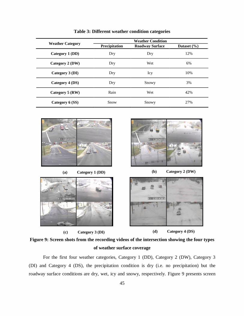
45

Table 3: Different weather condition categories

Weather Category Weather Condition Precipitation Roadway Surface Dataset (%)

Category 1 (DD) Dry Dry 12%

Category 2 (DW) Dry Wet 6%

Category 3 (DI) Dry Icy 10%

Category 4 (DS) Dry Snowy 3%

Category 5 (RW) Rain Wet 42%

Category 6 (SS) Snow Snowy 27%

(a) Category 1 (DD) (b) Category 2 (DW)

(c) Category 3 (DI) (d) Category 4 (DS)

Figure 9: Screen shots from the recording videos of the intersection showing the four types

of weather surface coverage

For the first four weather categories, Category 1 (DD), Category 2 (DW), Category 3

(DI) and Category 4 (DS), the precipitation condition is dry (i.e. no precipitation) but the

roadway surface conditions are dry, wet, icy and snowy, respectively. Figure 9 presents screen

46

shots from the recorded videos at the studied intersection showing the first four categories. For

the last two weather categories, Category 5 (RW) presents the case of rain precipitation and wet

surface condition, and the last category (SS) is for the snow precipitation and snowy surface

condition.

In summary, the weather condition for the collected dataset could be one of the

following: DD, DW, DI, DS, RW or SS. The distribution of accepted gap size for the different

weather conditions is shown in Figure 10a and Figure 10b.

The weather station measurements were extracted each minute and synchronized with the

gap acceptance/rejection behavior. In the reduced dataset, the rain precipitations ranged from

0.025 cm/hr to 1 cm/hr and the snow precipitations ranged from 0.025 cm/hr to 0.25 cm/hr as

presented in Figure 10c and Figure 10d. The average recorded measurements for wind speed,

barometric pressure and temperature were 3.45 km/hr, 106 millibar and 3 Celsius respectively.

The day or nighttime conditions corresponding to each gap acceptance/rejection were also

considered. The day/night is considered as a binary variable (1 for day and 0 for night).

47

(a) (b)

(c) (d)

Figure 10: Dataset distributions for different weather conditions

The lane number variable indicates the location of the offered gap with respect to the left turn

vehicle. The lane number variable is flagged as 1, 2 or 3 corresponding to the conflict point P1,

P2 or P3, respectively. The travel time “τi” is a continuous variable measured in seconds and

defined as the time required by the left turning vehicle to reach conflict point Pi. The mean and

median (50th percentile) values for travel time to reach each conflict point (P1, P2 and P3),

respectively are presented in Table 4 for different weather categories.

The Gap decision was recorded as a binary variable (0=rejection and 1=acceptance) and

was modeled as the response variable considering different explanatory variables. Logistic

models were fit to the data to estimate the probability (p) of accepting a gap as will be described

in the following section.

48

Table 4: Travel time values for different weather categories

Weather Category Travel Time (s) P 1 P 2 P 3

Category 1 (DD) Mean 0.89 1.93 3.21 Median 0.90 2.00 3.30

Category 2 (DW) Mean 1.56 2.72 4.12 Median 1.10 2.30 3.60

Category 3 (DI) Mean 1.56 2.74 4.12 Median 1.50 2.50 3.90

Category 4 (DS) Mean 1.48 2.53 3.95 Median 1.60 2.50 4.00

Category 5 (RW) Mean 2.16 3.08 4.40 Median 1.60 2.50 3.90

Category 6 (SS) Mean 1.51 2.55 4.05 Median 1.60 2.50 4.00

4.6 LOGISTIC REGRESSION MODELS

Different model formulations were considered in modeling gap acceptance behavior. Given that

the response variable is discrete (0 or 1) while the explanatory variables are continuous, a logistic

model was fit to the data to estimate the probability (p) of accepting a gap as shown in Equation

(1) and (2):

( )

( )1

U x

U x

epe

(3)

0 1 1 2 2( ) logit ln ...1 n n

pU x p x x xp

(4)

Where; p is the probability of accepting a gap; x1, x2,…, xn are the explanatory variables; and β0,

β1, β2, …, βn are the estimated regression coefficients.

By applying different statistical approaches for variable elimination, and treating the accepted

and rejected decision as a binary choice (0 or 1), and assuming a logit link function for the

generalized linear model (GLM), three different models were developed as follows:

Model 1, (M1)

1 2 3 4 5 6 7 8 9logit ( ) ( )op g DW DI DS RW SS L RW SS (5)

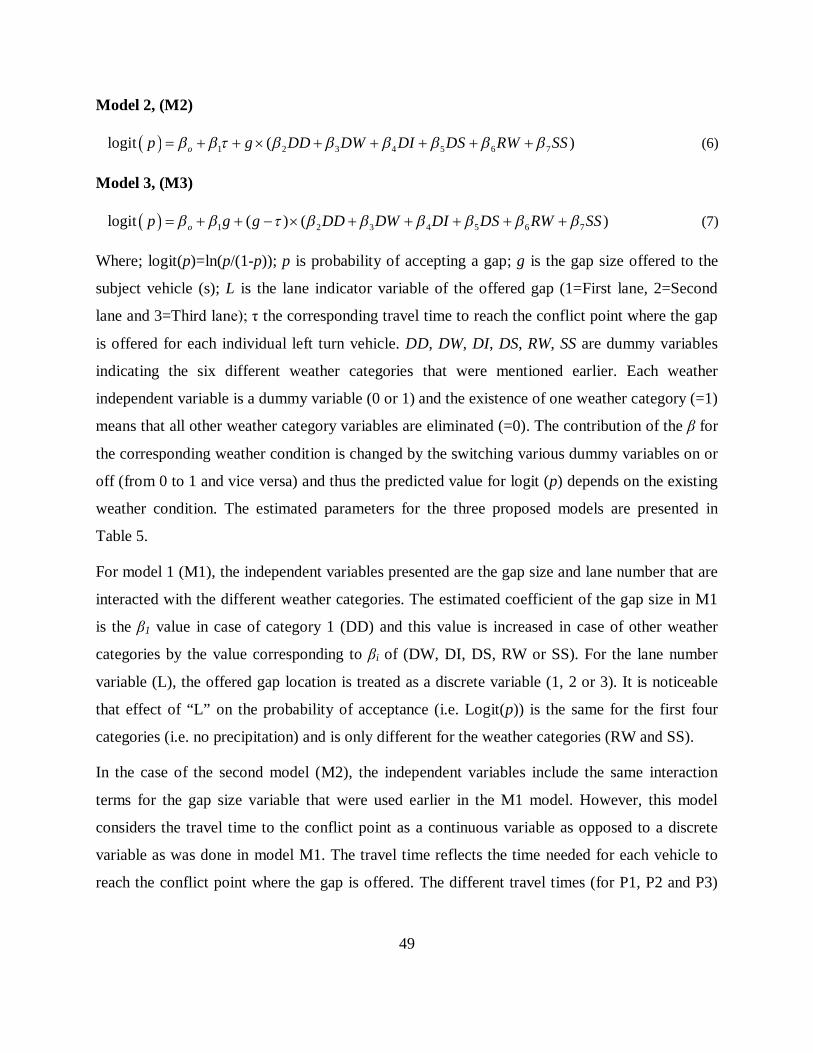
49

Model 2, (M2)

1 2 3 4 5 6 7logit ( )op g DD DW DI DS RW SS (6)

Model 3, (M3)

1 2 3 4 5 6 7logit ( ) ( )op g g DD DW DI DS RW SS (7)

Where; logit(p)=ln(p/(1-p)); p is probability of accepting a gap; g is the gap size offered to the

subject vehicle (s); L is the lane indicator variable of the offered gap (1=First lane, 2=Second

lane and 3=Third lane); τ the corresponding travel time to reach the conflict point where the gap

is offered for each individual left turn vehicle. DD, DW, DI, DS, RW, SS are dummy variables

indicating the six different weather categories that were mentioned earlier. Each weather

independent variable is a dummy variable (0 or 1) and the existence of one weather category (=1)

means that all other weather category variables are eliminated (=0). The contribution of the β for

the corresponding weather condition is changed by the switching various dummy variables on or

off (from 0 to 1 and vice versa) and thus the predicted value for logit (p) depends on the existing

weather condition. The estimated parameters for the three proposed models are presented in

Table 5.

For model 1 (M1), the independent variables presented are the gap size and lane number that are

interacted with the different weather categories. The estimated coefficient of the gap size in M1

is the β1 value in case of category 1 (DD) and this value is increased in case of other weather

categories by the value corresponding to βi of (DW, DI, DS, RW or SS). For the lane number

variable (L), the offered gap location is treated as a discrete variable (1, 2 or 3). It is noticeable

that effect of “L” on the probability of acceptance (i.e. Logit(p)) is the same for the first four

categories (i.e. no precipitation) and is only different for the weather categories (RW and SS).

In the case of the second model (M2), the independent variables include the same interaction

terms for the gap size variable that were used earlier in the M1 model. However, this model

considers the travel time to the conflict point as a continuous variable as opposed to a discrete

variable as was done in model M1. The travel time reflects the time needed for each vehicle to

reach the conflict point where the gap is offered. The different travel times (for P1, P2 and P3)

50

are observed during the maneuver of each vehicle in case of accepting a gap and these values are

applied to rejected gaps depending on the location of each offered gap.

For the third model (M3), the independent variables include the gap size and the difference

between the gap size and the travel time to the conflict point interacted with different weather

categories. The difference between the gap size and the travel time is considered as the buffer of

safety in order to avoid a conflict.

It is obvious that some variables were eliminated from the different model formulations and

these eliminations were based on the Chi-Square significance test. Specifically, the weather

measurements of precipitation, wind speed, barometric pressure, and temperature were not found

to be statistically significant. A possible explanation for the insignificance of the precipitation

variable can be attributed to the fact that most observations occurred at low precipitation levels.

Similarly, the other weather measurements were almost constant with very limited variations

during the data collection timeframe. In addition, the day and night variable was found to be

insignificant, which is consistent with other findings reported in the literature [63].

51

Table 5: The estimated parameters for the three proposed models and the statistics tests

Term βi Estimated

mean values

Std Error

L-R ChiSquare

Prob>ChiSq (p values)

Lower CL

Upper CL

Model 1 (M1)

Intercept o -4.744 0.161 1293.569 <.0001 -5.060 -4.428

g 1 1.021 0.052 784.843 <.0001 0.931 1.122

g*DW 2 -0.188 0.051 13.351 0.0003 -0.288 -0.087

g*DI 3 -0.126 0.040 9.649 0.0019 -0.206 -0.046

g*DS 4 -0.137 0.055 6.062 0.0138 -0.245 -0.028

g*RW 5 -0.237 0.0571 17.275 <.0001 -0.349 -0.125

g* SS 6 -0.270 0.060 20.421 <.0001 -0.387 -0.153

L 7 -0.898 0.126 50.412 <.0001 -1.167 -0.650

L*RW 8 0.357 0.142 6.313 0.0120 0.078 0.635

L* SS 9 0.348 0.153 5.126 0.0236 0.047 0.649

Model tests: LogLikelihood= -1531.998, ChiSquare= 4441.727, Prob>ChiSq (p-value) <0.0001

Model 2 (M2)

Intercept o -4.956 0.127 2478.181 <.0001 -5.206 -4.706

1 -0.297 0.038 82.976 <.0001 -0.373 -0.220

g*DD 2 0.844 0.034 866.951 <.0001 0.776 0.911

g*DW 3 0.729 0.042 376.209 <.0001 0.646 0.811

g*DI 4 0.780 0.029 1252.677 <.0001 0.723 0.836

g*DS 5 0.765 0.046 327.776 <.0001 0.674 0.855

g*RW 6 0.789 0.021 2969.196 <.0001 0.746 0.831

g* SS 7 0.733 0.022 1964.470 <.0001 0.689 0.776

Model tests: LogLikelihood= -1501.048, ChiSquare= 4448.177, Prob>ChiSq (p-value) <0.0001

Model 3 (M3)

Intercept o -5.027 0.128 2541.336 <.0001 -5.277 -4.775

g 1 0.500 0.038 169.706 <.0001 0.425 0.575

(g- )*DD 2 0.449 0.054 67.738 <.0001 0.342 0.556

(g- )*DW 3 0.186 0.065 8.018 0.0046 0.057 0.314

(g- )*DI 4 0.311 0.049 39.307 <.0001 0.213 0.407

(g- )*DS 5 0.264 0.071 13.732 0.0002 0.124 0.403

(g- )*RW 6 0.295 0.042 47.552 <.0001 0.220 0.378

(g- )* SS 7 0.236 0.041 31.849 <.0001 0.153 0.317 Model tests: LogLikelihood= -1498.677, ChiSquare= 4456.928, Prob>ChiSq (p-value) <0.0001

52

4.6.1 Model Comparison

In comparing the different models (M1, M2 & M3), two criteria were considered, namely: (a) the

Success Rate (SR) and (b) the corrected Akaike's Information Criterion (AICc). These criteria are

briefly described.

a) The SR is defined as the percentage of observations with acceptance/rejection

outcomes from the each model (rounded to 0 or 1) that are identical to field

responses. Consequently, the model that has a higher SR, is a better model.

b) The negative log likelihood (or, equivalently, the deviance) can be used as a measure

of how well a model fits a data set, with smaller values being indicative of a better fit.

However, due to the difference in number of parameters from one model to the other,

this criterion will be biased in favor of less parsimonious models. Therefore, the

corrected Akaike's Information Criterion (AIC) is used for comparison as was

suggested in the literature [72]. AIC is a measure of the goodness of fit of an

estimated statistical model and is a tool for model selection that could be employed

regardless of sample size. Given a data set, several competing models may be ranked

according to their AIC, with the one having the lowest AIC being the best as:

2 ( 1)2 21

N NAIC LL NN p

(8)

Where; LL is the posterior expected log likelihood, p is the number of parameters

used in the model, and N is the number of datum points (number of observations).

By applying the two criteria on the three proposed models (M1, M2, and M3), the SR values

were found to be 95.11%, 95.12% and 95.07%, respectively. The AIC measure was 3084, 3074

and 3065 for the M1, M2 and M3 models, respectively.

In the case of the SR criteria, the M1 and M2 offer the highest success rates. Alternatively, in the

case of the AIC criterion, the M2 and M3 models are superior to the M1 model. In summary,

given the small differences for the three models with respect to the two evaluation criteria,

identification of the optimum model is not simple. Each of the three models provides similar

inferences concerning the relation between gap acceptance and lane number (or travel time) for

different weather categories. Specifically, the models demonstrate that the probability a driver

53

accepts a gap decreases as the travel time needed to reach the gap increases (i.e. ,the further the

gap is the longer the required gap). The main difference between the proposed models is the

definition of the offered gap location. The M1 model can be applied in a simulation environment

where the lane width information may not be available. Alternatively the M2 model is more

general given that the time to reach the conflict point is a continuous variable. The drawback of

the M3 is that the estimated buffer of safety (i.e., the difference between the gap size offered and

the required time to reach the offered gap) could be a very large number in the case of large gap

sizes but the driver in reality could accept smaller buffers of safety.

In conclusion, the M2 model is considered more general because it explicitly considers the

location of the conflict point. The proposed model explicitly captures the vehicle constraints on

driving behavior (presented in the travel time value) and the driver’s deliberation in accepting or

rejecting a gap in different weather conditions. The model can be generalized to capture different

vehicles, roadway, movement, intersection characteristics, and weather effects on driver gap

acceptance behavior. Consequently, the remainder of the chapter considers the analysis of the second

model “M2”. Figure 11 presents the probability distribution of gap acceptance per lane separately for

different weather and roadway surface conditions.

The model demonstrates a larger gap is required for a wet surface (DW) compared to a snowy (DS)

and icy surface (DI) followed by a dry surface (DD). The higher gap required for a wet surface

could be caused by the fact that drivers are more worried about vehicles skidding when the

roadway surface is wet and that the opposing traffic is traveling at a higher speed compared to

the snowy and icy roadway conditions. Comparing the accepted gap size value for the same

probability between the different precipitation weather categories (Category 5 and 6), snow

precipitation (SS) has a higher value than the rain precipitation (RW) followed by dry conditions

(DD). These results are consistent with intuition.

54

Figure 11: The proposed model (M2) probability distribution of gap acceptance per each

lane for each weather category

4.7 CRITICAL GAP ESTIMATION BASED ON LOGISTIC REGRESSION

As mentioned before, the critical gap is considered the minimum gap size that a driver is willing

to accept in order to make a gap acceptance maneuver. The critical gap value is considered as the

gap size used to determine the saturation flow rate and is typically computed as the 50th

percentile gap size (probability of acceptance equal to zero). The fundamental assumption is that

drivers accept all gaps that are larger than their critical gap and reject all smaller gaps. The

critical gap is defined as the gap size that is equally likely to be accepted and rejected; and thus

corresponds to the median of the probability of accepted gaps.

For permissive left-turn traffic, HCM [57] estimates the opposed saturation flow rate based on

the critical gap and follow-up time. The HCM considers the critical gap accepted by left-turn

drivers as a deterministic value equal to 4.5 s at signalized intersections with a permitted left-turn

55

phase and this value is independent of the number of opposing-through lanes to be crossed and

the weather condition.

The American Association of State Highway and Transportation Officials (AASHTO, 2001)

[73], classifies the left turning movements from the major road across opposing traffic as Case F.

AASHTO recommends that for case F opposed movements, the critical gap for left-turning

passenger cars be set equal to 5.5 s (for passenger cars). For left-turning vehicles that cross more

than one opposing lane, add an additional 0.5 s for each additional lane of travel.

The critical gap can be computed for the proposed model (M2) by setting the probability of

accepting a gap equal to 0.5 which entails setting the Logit function to zero. Consequently the

critical gap (tc) for the proposed model (M2) can be computed using Equations (7).

1

2 3 4 5 6 7

oct DD DW DI DS RW SS

(9)

The critical gap values derived from the proposed models are summarized in Table 6 using the

median travel times corresponding to each weather category (see Table 4) Apart from Category

2 all results seem reasonable with an increase in the critical gap size as the roadway surface and

weather condition deteriorates. The results of Category 2, however, indicate that a wet roadway

surface has in the largest critical gap values compared to other roadway surface conditions.

These findings may be attributed to the small number of observations for this category (6% of

the total observations) or alternatively could be attributed to the high speeds of the opposing

vehicles (given that the visibility is not reduced) which makes drivers more cautious in accepting

gaps. Further investigation into these results is required using additional data from other sites in

order to validate and identify the cause of this behavior.

The critical gap values that are presented in Table 6 are significantly larger than the HCM [57]

recommended value of 4.5 s and slightly larger than the AASHTO recommended value of 5.5 s.

One possible explanation for the higher critical gaps is the geometry of the intersection.

Specifically, the intersection approaches were slightly curved and thus drivers might have had a

difficult time establishing which lane the opposing vehicles were in and which movement they

were executing (left, through, or right). An earlier study [67] showed that the opposing vehicles

turning left may block a driver’s view of oncoming traffic, which results in larger accepted gap

56

sizes. Specifically, the study indicates that in case of no opposing left turn vehicles (no sight

blockage) the critical gap is 5.6 s and increases by 2.1 s in the case of sight blockage.

Consequently, the results of this study are consistent with what is reported in the literature.

The difference between the critical gap values for different opposing lanes is approximately 0.5 s

for all weather and roadway conditions and thus is consistent with the recommended value in the

AASHTO 2001 design procedures [73].

Table 6: The different critical gap values per conflict point for different weather categories

Weather Category Percent of Total Observations

(tc ) Critical Gap (s)

P 1 P 2 P 3

Category 1 (DD) 12% 6.19 6.58 7.03

Category 2 (DW) 6% 7.25 7.74 8.27

Category 3 (DI) 10% 6.93 7.31 7.84

Category 4 (DS) 3% 7.09 7.45 8.03

Category 5 (RW) 42% 6.88 7.22 7.75

Category 6 (SS) 27% 7.41 7.77 8.38


The study gathered field data at a signalized intersection (a total of 11,114 observations of which

1,176 were accepted and 9,938 were rejected gaps) over a six-month period in an attempt to

characterize driver left-turn gap acceptance behavior under various weather and roadway surface

conditions. Logistic regression models were calibrated to the data and compared in order to

identify the best model for capturing driver gap acceptance behavior. The models reveal that

drivers are more conservative during snow precipitation compared to rain precipitation. In the

case of the roadway surface condition, drivers require larger gaps for wet surface conditions

compared to snowy and icy surface conditions, and, as would be expected, require smallest gaps

for dry roadway conditions. In addition, the models show that the drivers require larger gaps as

the distance required to clear the conflict point increases. Using the study findings, the proposed

tool for optimizing the movements of vehicles (presented in the following chapter) at

intersections could encounter the drivers’ behavior for non-automated vehicles (left-turn) under

different weather conditions.

57

CHAPTER 5 INTRODUCTION TO THE “ICACC” TOOL

This chapter presents the state-of-the-art of a proposed optimization/simulation tool for CACC-

equipped vehicles in the vicinity of intersections, entitled: iCACC (Intersection Management

using Cooperative Adaptive Cruise Control). The iCACC system optimizes vehicle trajectories

to ensure that no collisions occur while at the same time minimizing the intersection delays in

real time. Optimizing vehicle trajectories may have an inherent advantage of reducing fuel

consumption. It is proposed that the intersection be equipped with a controller that receives

requests from vehicles approaching the Intersection Zone (IZ), optimizes the vehicle movements,

and sends the optimum movement strategies to the vehicles. In case of non-automated vehicles, it

is assumed that the intersection is equipped with roadside sensors or video detection technology

to track the movement of these vehicles. These vehicles serve as constraints in the optimization

logic. The system is thus able to deal with different levels of automation; i.e., from legacy

vehicles (e.g., classic cars with no automation) to fully automated vehicles at intersections, as

will be explained in this chapter.

5.1 INTRODUCTION

Since the initialization of research based on VII and the Connected Vehicles Research,

communication systems promising Vehicle-Infrastructure and Vehicle-Vehicle information

transfer are being developed using DSRC communication and other wireless technologies [5].

These advancements lay foundation for this research in which vehicles that assume automated

driving (or enforced driving agents) use Cooperative Adaptive Cruise Control (CACC) to pass

through an intersection devoid of signal controllers or stop/yield signs.

Consequently, this chapter presents the state-of-art of a proposed optimization/simulation tool for

CACC-equipped vehicles in the vicinity of intersections, entitled: iCACC (Intersection

Management using Cooperative Adaptive Cruise Control). The iCACC system optimizes vehicle

trajectories to ensure that no collisions occur while at the same time minimizing the intersection

delays in real-time. It is proposed that the intersection be equipped with a controller that receives

requests from vehicles approaching the Intersection Zone (IZ), optimizes the vehicle movements,

and sends the optimum movement strategies to the vehicles. In case of non-automated vehicles, it

58

is assumed that the intersection is equipped with road-side sensors or video detection technology

to track the movement of these vehicles. These vehicles serve as constraints in the optimization

logic. The logic uses the lane striping to identify potential vehicle trajectory conflicts.

Subsequently, the iCACC system simulates and optimizes the automated vehicle trajectories to

ensure that no conflicts result. The system is thus able to deal with different levels of automation,

i.e. from legacy vehicles (e.g. classic cars with no automation) to fully automated vehicles at

intersections.

As far as the chapter layout is considered, an overview of the tool is firstly described. This is

followed by the different modules (input, optimization and output modules) that constitute the

proposed tool. At the end, a section on findings and conclusions is presented as well as the future

direction of this research.

5.2 ICACC SYSTEM OVERVIEW

This research effort is a modest attempt at not only addressing some of the issues neglected in

state-of-the-art research efforts described earlier, but more importantly to develop a real-time

simulation/optimization intersection management tool that can operate in a mixed vehicle

automation environment. In general, the tool computes and simulates the optimum trajectory of

vehicles to ensure no conflicts occur while also minimizing the total intersection delay in real-

time. Figure 12 shows a screen shot of the visualization interface for the iCACC

simulation/optimization tool.

The tool enhances the intersection mobility by optimizing the arrival time of vehicles at the

intersection box. The assumptions used in developing the tool are:

1- All equipped vehicles in the IZ are assumed to follow the iCACC instructions;

2- Wireless communication is secure and supports high speed and low latency

communication;

3- The intersection is fully equipped with road-side sensors to track non-automated

vehicles; and

4- All equipped vehicles report their destination, location, speed and acceleration to the

controller each time step.

59

Figure 12: A screen shot from the iCACC used for simulating automated vehicles

The intersection controller is assumed to have full control of the automated vehicles entering the

intersection zone (IZ), which is determined by the communication range. A DSRC (Dedicated

Short Range Communication) is assumed for V2I/I2V communication as recommended by many

literature sources [2, 74, 75]. For high efficiency, the suggested communication range in this

research is assumed to be 200 meter in each direction from the center of the intersection;

consequently this is considered the IZ for the controller.

To realize the optimum trajectory for vehicles, the tool consists of three main modules: an Input

Module, an Optimization/Simulation Module and an Output Module, as will be explained in the

following sub-sections. Figure 13 summarizes the different iCACC modules.

60

Figure 13: The different modules of iCACC

5.3 ICACC INPUT MODULE

The iCACC input module consists of five main entry categories: weather, intersection, vehicle,

simulation/optimization input, and the built-in state-of-art models. Figure 14 shows the GUI

(Graphical User Interface) used to input data to the iCACC tool.

0 if Dry (no Rain)>0 Otherwise

1 if equipped vehicle0 Otherwise

minip jpt t t

N

ii

Min D

Rain, Snow or Dry

61

Figure 14: The input page of the iCACC tool

The tool capture inclement weather impacts on both driver behavior and vehicle dynamics. The

weather input for the current version of iCACC is divided into four weather categories from 1 to

4 for dry, rain, snow and ice, respectively. With regards to the intersection input, the tool

requires the intersection geometry, the number of lanes per approach and the speed limit. To

account for vehicle differences, the physical characteristics of each vehicle entering the IZ

should also be provided. It should be mentioned that this option is first of its kind compared to

any similar automated vehicle traffic simulation tools. The fourth entry is limited to the

simulation period, number of optimization iterations and the time increment update for the

optimization process (Δt).

Last, the iCACC uses few state-of-the-art models for its optimization and comparison purposes

as will be described in the following sub-sections. The model uses the Rakha-Pasumarthy-

Adjerid (RPA) car-following model that integrates vehicle dynamics and collision avoidance

constraints with the Van Aerde steady-state car-following model [76]. In addition, the tool

utilizes the Virginia Tech Comprehensive Power-based Fuel consumption Model (VT-CPFM) to

estimate fuel consumption and CO2 emission levels. In addition, as part of modeling various

62

levels of automation, the gap acceptance modeling is a vital part for the optimization process;

especially for non-automated vehicles.

5.3.1 Van Aerde Steady-state Car-following Model

The car following model integrated in iCACC uses the Van Aerde steady-state car-following

model [77] with vehicle dynamics and collision avoidance models. The RPA car-following

model computes the vehicle speed as the minimum of: the maximum allowed speed based on

vehicle dynamics, the steady-state car-following desired speed, and collision avoidance speed as:

1 3

3

21 max

( ) min

( ) ( )( ) 3.6 ,

( )

2

1( ) 25920 ( ( ) )

n

n nn

f n

n nj

u t t

F t R tu t t

mc c u s t t A

c

u t t d s t tk

(10)

21 2 32 2 2

12 ; ;f f f

c f f ccj c j c j c

u u uc u u c u u c

qk u k u k u

(11)

2

1 3 3 1 2( ) 4 ( )

f n n f fA c c u s t t c s t t u c u c (12)

21 1

( ) ( ) ( ) ( ) 0.5 ( )n n n n n

s t t s t u t u t t a t t

(13)

where un(t) is the speed of vehicle n at time t (km/h).; c1, c2, and c3 are steady-state car-following

model parameters; uf is the free-flow speed (km/h); uc is the speed-at-capacity (km/h); sn(t) is the

spacing at time (t); Fn(t) and Rn(t) are the resultant forces acting on vehicle n at time t; kj is the

jam density (veh/km/lane); qc is the capacity (veh/h/lane); sn(t) is vehicle spacing between the

following vehicle n and the lead vehicle n-1 (km) at time t; sn(t+Δt) is the predicted spacing at

time t+Δt considering that vehicle n continues at its current speed (km); an(t) is the acceleration

of vehicle n at time t; dmax is the maximum acceptable deceleration level the driver is willing to

exert (m/s2).

As can be seen in the Equations (10) through (13), the car-following model is calibrated by by

setting four traffic stream model parameters, the maximum acceptable deceleration level, and

vehicle characteristics that govern vehicle acceleration capabilities as will be described shortly.

63

Changes in roadway surface conditions are reflected in the calibration of the various parameters,

as will be described later in the chapter.

5.3.2 Modeling Vehicle Dynamics

The vehicle dynamics model is used to model capture vehicle acceleration constraints. In doing

so, the vehicle speed is computed from the resultant forces acting on the vehicle. These forces

include the tractive forces given by Equation (14) and the resistive forces given in Equation (15).

min 3600 ,d ta

PF m g

v

. (14)

2 01 225.92 1000

rd h f r r

cR C C A v mg c v c mgG

. (15)

where ηd is the driveline efficiency (unitless); P is the vehicle power (kW); mta is the mass of the

vehicle on the tractive axle (kg); v is the vehicle speed (km/h); g is the gravitational acceleration

(9.8067 m/s2); µ is the coefficient of road adhesion (a function of the roadway surface condition)

or the coefficient of friction (unitless); ρ is the air density at sea level and a temperature of 15C

(1.2256 kg/m3); Cd is the vehicle drag coefficient (unitless), typically 0.30; Ch is the altitude

correction factor (unitless); Af is the vehicle frontal area (m2); cr0 is rolling resistance constant

(unitless); cr1 is the rolling resistance constant (h/km); cr2 is the rolling resistance constant

(unitless); m is the total vehicle mass (kg); and G is the roadway grade at instant t (unitless).

The vehicle acceleration is calculated as the ratio of the difference in tractive and the resistive

forces and the vehicle mass (i.e., a = (F-R)/m). The vehicle speed at (t + t) is then computed by

solving the differential equation using a first-order Euler approximation as

( ) ( )( ) ( ) 3.6

F t R tv t t v t t

m

. (16)

5.3.3 Gap Acceptance Model

As explained in the previous chapter, the minimum gap that a driver is willing to accept is

generally called the critical gap. The Highway Capacity Manual [78] defines the critical gap as

the “minimum time interval between the front bumpers of two successive vehicles in the major

64

traffic stream that will allow the entry of one minor-street vehicle.” The iCACC tool models the

minimum acceptable gap for each driver as a stochastic value based on the vehicle capability, the

crossing distance and the weather condition (rain intensity). A gap is defined as the elapsed-time

interval between arrivals of successive vehicles in the opposing flow at a specified reference

point in the intersection area. The minimum gap that a driver is willing to accept is generally

called the critical gap. The iCACC system models the minimum acceptable gap for each driver

as a stochastic value based on the vehicle capability, the crossing distance and the weather

condition. In the previous chapter, it was demonstrated that the critical gap values corresponding

to different weather conditions can be computed using the following equation:

1

2 3 4 5 6 7

oct DD DW DI DS RW SS

(17)

where; tc is the critical gap; the average travel time to a conflict point; DD, DW, DI, DS, RW,

SS are dummy variables indicating the six different weather categories. Each weather

independent variable is a dummy variable (0 or 1) and the existence of one weather category (=1)

means that all other weather category variables are eliminated (=0). and β0, β1, β2, β3, β4 , β5 , β6 ,

β7 were estimated to be equal to -4.95, -0.29, 0.84, 0.72, 0.78, 0.76, 0.78 and 0.73 , respectively.

5.3.4 Fuel Consumption Model (VT-CPFM)

The iCACC tool uses the Virginia Tech Comprehensive Power-based Fuel Model (VT-CPFM-1)

due to its simplicity, accuracy, and ease of calibration. The fuel consumption model utilizes

instantaneous power as an input variable and can be calibrated using publicly available fuel

economy data (i.e., EPA published city and highway mileage). Thus, the calibration of model

parameters does not require gathering any vehicle-specific data. This study uses a microscopic

model since optimizing speed trajectories requires estimating vehicle fuel consumption based on

instantaneous vehicle operational data.

The fuel consumption model is formulated as Equation (18), where α0 is the fuel consumption

rate (g/s or l/s) for idling conditions and P(t) is the instantaneous total power in kilowatts (kW).

The idling fuel consumption rate is estimated using Equation (10), where Pmfo is idling fuel mean

pressure (400,000 Pa), ωidle is idling engine speed (rpm), d is engine displacement (liters), Q is

fuel lower heating value (43,000,000 J/kg for gasoline fuel), and N is the number of engine

65

cylinders. Estimation of the model coefficients (α1, α2) uses the fuel consumption rates of the

standard fuel economy cycles (e.g., EPA-published city and highway mileage).

Here Fcity and Fhwy are the total fuel consumed for the EPA city and highway driving cycles,

respectively. The value of Fcity is adjusted to represent the engine transient operation since the

EPA city cycle includes the cold start operation in the Bag 1 of Federal Test Procedure (FTP).

Tcity and Thwy are the durations of the city and highway cycles (1875s and 766s). In addition, Pcity

and Pcity2 represent the total power used and total sum of the squared power during the city

driving cycle, expressed as 0( )cityT

tP t

and 20

( )cityT

tP t

respectively. Similarly, Phwy and Phwy2 are

estimated for the highway cycle. Specific model relations can be found in [79].

20 1 2

0

( ) 0( ) ( )( )

( ) 0

P tP t P tFC t

P t

(18)

2 2

0 max ,22164

city citycity hwy city hwy

mfo idle city hwy

citycity hwy

city

P PF F P P

P d P P

QN PT T

P

(19)

20 2

1hwy hwy hwy

hwy

F T P

P

(20)

0

22 2

1E-06

city citycity hwy city hwy

hwy hwy

citycity hwy

hwy

P PF F T T

P P

PP P

P

(21)

5.4 ICACC SIMULATION/OPTIMIZATION MODULE

In this module, three zones are considered in the optimization logic. These zones include Zone I,

Zone II and the Intersection Box (IB), as shown in Figure 15(a). The ideal profile entails

traveling the entire IZ at the speed limit. Zone I is used so that each vehicle can accelerate to the

speed limit and maintain that speed for the remainder of the zone (assumed to be 50 meters long

in this research). As a result, the end-point of Zone I is considered as the first fixed speed point

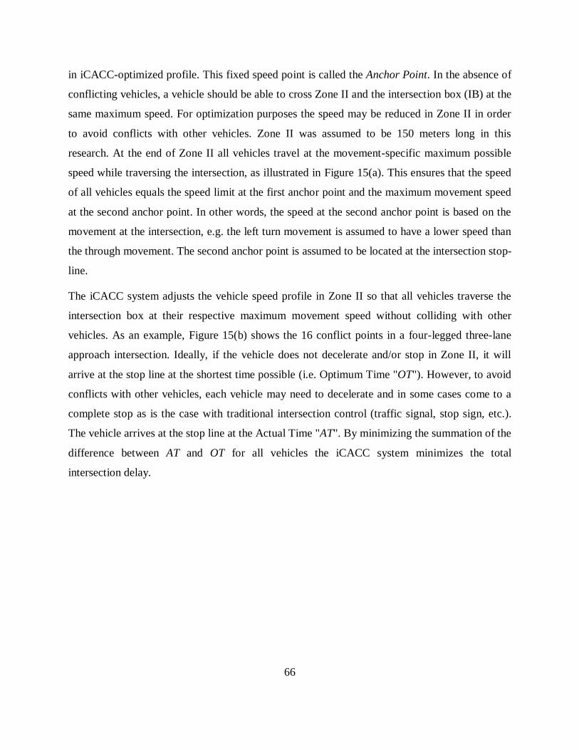
66

in iCACC-optimized profile. This fixed speed point is called the Anchor Point. In the absence of

conflicting vehicles, a vehicle should be able to cross Zone II and the intersection box (IB) at the

same maximum speed. For optimization purposes the speed may be reduced in Zone II in order

to avoid conflicts with other vehicles. Zone II was assumed to be 150 meters long in this

research. At the end of Zone II all vehicles travel at the movement-specific maximum possible

speed while traversing the intersection, as illustrated in Figure 15(a). This ensures that the speed

of all vehicles equals the speed limit at the first anchor point and the maximum movement speed

at the second anchor point. In other words, the speed at the second anchor point is based on the

movement at the intersection, e.g. the left turn movement is assumed to have a lower speed than

the through movement. The second anchor point is assumed to be located at the intersection stop-

line.

The iCACC system adjusts the vehicle speed profile in Zone II so that all vehicles traverse the

intersection box at their respective maximum movement speed without colliding with other

vehicles. As an example, Figure 15(b) shows the 16 conflict points in a four-legged three-lane

approach intersection. Ideally, if the vehicle does not decelerate and/or stop in Zone II, it will

arrive at the stop line at the shortest time possible (i.e. Optimum Time "OT"). However, to avoid

conflicts with other vehicles, each vehicle may need to decelerate and in some cases come to a

complete stop as is the case with traditional intersection control (traffic signal, stop sign, etc.).

The vehicle arrives at the stop line at the Actual Time "AT". By minimizing the summation of the

difference between AT and OT for all vehicles the iCACC system minimizes the total

intersection delay.

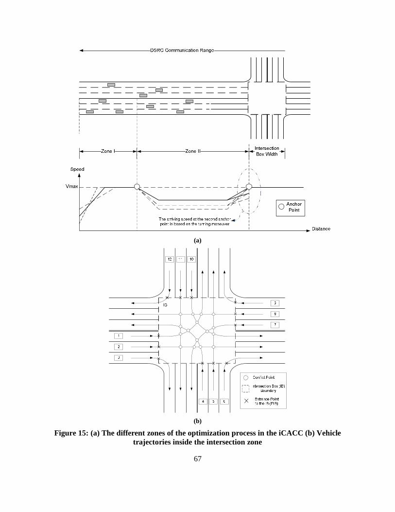
67

(a)

(b)

Figure 15: (a) The different zones of the optimization process in the iCACC (b) Vehicle trajectories inside the intersection zone

68

Consequently, the decision of arrival time for each vehicle is made using an optimization

module. In optimizing the vehicle trajectories, the optimization module optimizes the time of

arrival of each vehicle at the intersection stop-line at each time step (i.e. optimization loop). The

main objective of the optimization problem is to minimize the delay (D) that is added to the OT,

needed to avoid conflicts with crossing vehicles. This optimization problem is formulated as:

1

1

: ii

Min D

(22)

Subject to:

min( ) ( ) ( ); , , ,i i j j im jmOT D OT D H l l i j i j m (23)

1( ) ( ) ( ); , , , ,i i mn k k nm im kn mnOT D OT D l l c i k i k m n (24)

1 0( ) max ( ), ( ) ; , , , ,i i mn f f mn p p nmOT D OT D OT D i f p m n (25)

0; iD i (26)

Where (as illustrated in Figure 15),

i,j,f,p: Vehicle identification number;

Di: The time difference between the optimum time (OT) and the actual time (AT) for vehicle

i; for the ideal case Di is zero (no deceleration occurs in Zone II);

OTi: The optimum arrival time of vehicle i at the PIB (Entrance Point to the IB). OTi is

estimated assuming that each vehicle accelerates to the maximum speed in Zone I and

continues to travel at that maximum speed until PIB.;

Ω0: The set of vehicles that entered the IZ the last time step and are still in the IZ in the

current time step;

Ω1: The set of vehicles that enter the IZ in the current time step;

Ω: The set of vehicles in IZ in the current time step (Ω= Ω0+ Ω1);

m,n: Lane identification number;

69

Ψ: The set of lanes at the intersection;

lim:= 1 if vehicle i enters the IB from lane m; and 0 otherwise, with m

iml =1.

cmn:= 1 if vehicle i from lane m has a conflict point with vehicles traveling on lane n; and 0

otherwise, with nm

mnc,

=1.

τmn : Travel time from the point PIB of lane m entering into IB to the conflict point of lane n.

Distance to each conflict point is based on the intersection geometry. It is assumed that

all vehicles will be running at maximum speed in the IB, thus, τmn is fixed for all vehicles

from the same lane m to the same conflict point mn (to facilitate the optimization

process). It should be noted that the maximum speed may be different for different

movements.

Δτ: The duration of time that a vehicle occupies the conflict point, in other words, the safety

interval between two consecutive vehicles occupying the same conflict point. The

duration depends on the vehicle physical characteristics (size, engine power, etc.)

Hmin: The minimum headway between vehicles in the same lane.

The objective function (Equation (22)) is to minimize the total delay (Di) across all vehicles

traversing the intersection. In order to achieve the proposed objective, four constraints are listed.

Equation (23) ensures that the first in first out (FIFO) rule is maintained for all vehicles in the

same lane. In other words, the arrival of each following vehicle should be after the arrival of the

leading vehicle in the same lane by the minimum headway (minimum headway Hmin). Equation

(24) ensures that a vehicle does not conflict with another vehicle in the IB, by ensuring that the

arrival times of two intersecting vehicles at the same conflict point is separated by a minimum

safety interval (Δτ). For non-automated vehicles, the minimum safety interval is considered the

minimum acceptable gap (critical gap) value plus the minimum time needed to clear the conflict

point.

At each time step (optimization loop), vehicles in the system are divided into two groups,

namely: vehicles that entered in previous time steps and are still in the IZ (Ω0 group) and

vehicles that enter in the current step (Ω1 group). For the set of vehicles Ω0, the vehicle entry

70

times to the IZ were optimized in previous time steps. Re-optimization of entry times can

decrease the algorithm’s computational efficiency and increase vehicle fuel consumption by

changing vehicle decisions. Hence, only the set of vehicles Ω1 are optimized each time step. At

each time step, the occupied time for each conflict point is stored as a new constraint for the

following time step (optimization loop), as demonstrated in Equation (25). The last constraint is

the non-negativity constraint for the additional time (Di), in other words, the additional time

should be zero (no delay) or greater.

In summary, the iCACC tool uses an algorithm consisting of four main steps to solve the

optimization problem. First, based on the entry speed and acceleration of each vehicle to the IZ,

the arrival time of each vehicle to the IB is estimated. Second, assuming all vehicles will be

running at maximum speed, the occupancy time for each conflict point is calculated. Third, the

tool begins to search for unsafe conflict points; in other words, the points where the time

difference between two crossing vehicles is less than the minimum safety interval (Δτ). Last, the

tool modifies the arrival time of each vehicle (triggered as unsafe arrival time) to the IB and

determines the optimum additional time needed (D) using Equations (22) to (26). It could be

stated that the idea of controlling the arrival time of each vehicle at the IB is quite similar to the

concept of metered single-lane entrance ramps. In other words, the iCACC controls the flow of

vehicles to the entry of the intersection to ensure that they can cross the intersection safely and

smoothly with minimum delays.

This problem is a constrained nonlinear optimization program. Consequently, the optimization

module attempts to find the constrained minimum delay of a scalar function (Equation (22))

given an initial estimate of designated variables and subject to constraints (23) through (26). At

the start of the optimization process, as an initial estimation, all vehicles are assumed to arrive at

the IB at the optimum time (OT), implying delay (Di) of zero. In solving the problem, the

adopted algorithm for optimization is an “interior-point” algorithm. This algorithm – also

referred to as a barrier algorithm – attempts to solve the problem as a sequence of approximate

minimization problems where the bounds (constraints) are satisfied at all iterations.

Consequently, the algorithm can handle large, sparse problems, as well as small dense problems.

The main idea behind the interior point method is fundamentally different from the simplex

71

linear programming (LP) algorithm. Here, the optimal vertex is approached by moving through

the interior of the feasible region whereas the simplex moves along the vertices of the feasible

solution. This is done by creating a family of parameterized approximate solutions that

asymptotically converge to the exact solution [80].

5.5 ICACC OUTPUT MODULE

After the different input data are provided to the iCACC tool, the optimization process is run and

displayed to the output module, as illustrated in Figure 16. The output includes:

The time space profile for every vehicle at Δτ increments (e.g. deci-second);

The average delay for every simulated vehicle (s);

The average fuel consumption for every simulated vehicle (mL)

Figure 16: A screen shot for an output example for the iCACC tool

The tool was built in the MATLAB environment; however, the tool can be compiled as a DLL

(Dynamic Link Library) and integrated with any traffic micro-simulation software (e.g. VISSIM,

Paramics, or TransModeler).

72


This chapter gave an overview on the iCACC optimization/simulation tool and presented the

state-of-the art models implemented in the tool. The iCACC tool seeks the minimization of the

total delay for the intersection and preventing crashes simultaneously. The objective function of

the tool is to minimize the total adding time to the optimum travel time for each crossing

vehicles. For the constraints, the tool assures there is no conflict between vehicles at expected

conflict points and the minimum headway between vehicles is applied at the same time.

The iCACC contains built-in Van Aerde car following models, vehicle dynamics models and

VTCFM fuel consumption models. The presented tool in this chapter is considered as the first

version for this optimization/simulation effort. In this version, the required inputs for the tool are:

1) the physical characteristics of all vehicles, 2) entry speed and acceleration of all vehicles, 3)

the weather condition and 4) the intersection characteristics 5) the level of

penetration/automation for the system. The first version of the tool has some limitations and

assumptions: all exchanged information are certain and symmetric, and only one vehicle class

type crossing the intersection.

In the following chapters, it is anticipated to overcome some of the limitations of the first version

of the iCACC tool. It is planned to model different classes of vehicles, modeling pedestrians’

interaction and uncertainty in exchanged information between V2V and V2I. In addition, it is

attempted to have priority index for simulated vehicles based on number of passengers per car. In

other words, it is planned to give priority for transit vehicles over passenger vehicles. It is

anticipated that this research will contribute in the future of intelligent transportation system

(ITS), connected vehicle technology systems, and driverless vehicles applications.

73

CHAPTER 6 SIMULATION TESTING AND SENSITIVITY ANALYSIS

This chapter attempts to validate the proposed simulation/optimization “iCACC” tool.

Consequently, four intersection control scenarios were analyzed, namely: a traffic signal, an all-

way stop control (AWSC), a roundabout, and the iCACC controller, considering different traffic

demand levels ranging from a volume-to-capacity ratio of 0.27 to 0.91. The simulated results

showed savings in delay and fuel consumption on the order of 90 and 45 percent, respectively,

compared to AWSC and traffic signal control. On the other hand, the delays for the roundabout

and the iCACC controller were found to be comparable. The simulation results showed that fuel

consumption for the iCACC controller was, on average, 33%, 45% and 11% lower than the fuel

consumption for the traffic signal control, AWSC, and roundabout scenarios, respectively. In

addition, this research effort investigates the impact of inclement weather on the performance of

the futuristic automated vehicle intersection management system iCACC. The system was

simulated and evaluated on an intersection for a range of traffic demand levels (volume-to-

capacity ratios ranging from 0.2 to 0.8) and system market penetration levels (from 20% to

100%) under different weather conditions (dry, rain and snow). The study demonstrated that the

iCACC system can produce savings of up to 55 and 10 percent in total delay and fuel

consumption levels, respectively, for a high level of market penetration compared to a low level

of market penetration for the different weather conditions.

6.1 INTRODUCTION

In this chapter, the iCACC (intersection management using CACC) is used to manage the

vehicles approaching an intersection to control automated vehicles' speed profile to avoid

collisions and minimize delay. Different simulations tests were done to compare conventional

traffic control system (signal control round-abouts) with iCACC for two measures of

effectiveness - delay and fuel consumption. Savings were found when iCACC was used over

conventional intersection control as will be shown in this chapter. As far as the chapter layout is

considered, a section on the preliminary simulation analysis and results are presented. This is

followed by sensitivity analysis for the weather conditions and level of penetration as well as

findings and conclusions of this research.

74

6.2 SIMULATION RESULTS

For validating the proposed iCACC algorithm, four different scenarios for intersection control

were tested: traffic signal control, AWSC, roundabout and iCACC control (as shown in Figure

17). The case study intersection consists of 4 approaches and each approach has two lanes with

shared movements. Each lane is 3.5m wide with a speed limit of 35 mph (approximately 16 m/s).

The maximum desired travel speed and the speed at the anchor points are assumed to be the

speed limit. In calibrating the vehicle dynamics and fuel consumption model parameters, the

physical and mechanical characteristics of a 2010 Honda Accord was used. The vehicle has an

engine power of 177 Horse Power (Hp). The analysis assumes that the vehicle travels on a good

flat asphalt surface (grade 0%) and the current weather condition is dry.

The four intersection control scenarios were tested using different random number seeds for 16

different volume combinations resulting in intersection volume-capacity ratios ranging from 0.27

to 0.91. The major street volume ranged between 500 to 2000 veh/h/approach and the minor

street volume ranged between 250 to 1000 veh/h/approach. The direction-split for each approach

was 0.2:0.6:0.2 for left, through and right turn movements. The micro-simulation software

INTEGRATION was used for simulating the three conventional intersection control scenarios,

namely, signal control, AWSC and roundabout. The signal timing cycle length and phase splits

were optimized using the Synchro 6 software and then modeled in the INTEGRATION software.

The iCACC- intersection control was simulated using the INTEGRATION state-of-the-art car-

following and vehicle dynamics models. The entrance time of each vehicle to the Intersection

Zone (IZ), their initial speed and acceleration were picked using a random number generator.

75

(a) (b)

(c) (d)

Figure 17: Different intersection scenarios (a) Signal (b) AWSC (c) Roundabout (d) iCACC

The iCACC scenario was simulated in MATLAB using the "moving horizon optimization"

concept at each time step (i.e. 30 seconds) to speed-up the optimization process. In other words,

at each time step, the new entering vehicles to the IZ are optimized with the expected entering

vehicles in the following time step. Consequently, by using the moving horizon concept, the

optimization process takes shorter time as the preliminary optimization results are used in the

following time step as the initial input to the optimization process. Table 7 summarizes the

specifications and the parameters used for testing the proposed connected vehicle application.

iCACC

76

Table 7: The simulation inputs

Parameter Value

Exchanged Information Rate 0.1 second

Optimization Inputs Number of Optimization Iterations 30 Iterations

Optimization Horizon 20 seconds

The Physical Parameters of the tested vehicle (2010

Honda Accord)

Power of engine (P) 177 Hp

Transmission Efficiency (η) 0.92

Total Weight (W) 1453 Kg

Mass on Tractive Axle (mta) 785 Kg

Air Drag Coefficient (Cd) & Altitude Factor (Ch) 0.3 & 1

Frontal Area (A) 2.32 m2

Rolling Coefficient Cr0= 1.75

Cr1= 0.0328& Cr2= 4.575

EPA Estimates City/Combined/Highway

21/25/31 MPG

Two measures of effectiveness (MOEs) were computed, namely: the average vehicle delay and

the average vehicle fuel consumption level. Table 8 tabulates the different volume cases and the

corresponding values of both MOEs for comparison purposes. Delay incurred to a vehicle was

computed as the deviation in time to cover the distance under consideration including the IZ at

the speed-limit versus its actual travel time. This value was averaged across all vehicles for the

four scenarios for the 16 traffic demand cases, as illustrated in Figure 18(a). Fuel consumption

estimates were made using the VT-CPFM model calibrated for the test-vehicle. Input for the

model were instantaneous speed vectors for vehicles derived from the MATLAB simulation and

trajectories extracted from the INTEGRATION software. The average fuel consumed for the

vehicles were also computed the same way for all sixteen scenarios as shown in Figure 18(b).

77

Table 8: Simulation results for average delay and fuel consumed for all scenarios

Case #

Major Volum

e (vph)

Minor Volum

e (vph)

Traffic Signal AWSC Intersection Roundabout iCACC

Average

Vehicle Delay

(s)

Average Fuel

Use (mL)

Average Vehicle Delay

(s)

Average Fuel

Use (mL)

Average

Vehicle Delay

(s)

Average Fuel

Use (mL)

Average

Vehicle Delay

(s)

Average Fuel

Use (mL)

1 500 250 10.4 25.7 12.8 26.6 1.8 23.9 1.0 20.8 2 600 300 14.4 28.3 13.2 26.7 2.1 24.0 1.9 21.2 3 700 350 15.4 28.6 14.2 27.1 2.3 24.0 2.1 21.2 4 800 400 16.6 28.1 15.4 27.6 2.6 24.1 2.8 21.6 5 900 450 15.7 29.0 19.4 29.5 2.8 24.3 3.3 21.7 6 1000 500 15.2 28.3 21.1 30.3 3.0 24.4 4.5 22.3 7 1100 550 16.7 30.8 22.2 30.8 3.2 24.5 4.0 22.0 8 1200 600 22.0 29.9 40.3 39.3 3.6 24.7 5.8 22.7 9 1300 650 19.9 31.0 52.5 45.1 4.1 25.0 5.8 22.8 8 1400 700 18.4 30.3 55.2 46.3 3.9 24.8 4.8 22.3 11 1500 750 18.8 35.4 60.0 48.4 4.5 25.2 6.1 22.9 12 1600 800 19.7 36.9 68.1 52.2 4.8 25.3 5.7 22.8 13 1700 850 23.3 36.3 75.6 55.7 5.5 25.7 5.9 22.9 14 1800 900 31.7 39.7 72.3 54.1 6.0 25.9 5.6 22.7 15 1900 950 34.2 44.5 76.6 56.1 6.8 26.2 6.5 23.2 16 2000 1000 39.5 49.3 76.8 56.1 8.3 27.0 6.3 23.1

Highlighted cells indicate the lowest value for the specific case.

78

(a)

(b)

Figure 18: Comparison between different scenarios (a) Average delay comparison per vehicle (seconds) (b) Average fuel consumption per vehicle (milliliters)

0.0

10.0

20.0

30.0

40.0

50.0

60.0

70.0

80.0

0 1 2 3 4 5 6 7 8 9 10 11 12 13 14 15 16

Aver

age D

elay

(s)

Case Number

iCACCSignalRoundaboutAWSC

10.0

15.0

20.0

25.0

30.0

35.0

40.0

45.0

50.0

55.0

60.0

0 1 2 3 4 5 6 7 8 9 10 11 12 13 14 15 16

Aver

age F

uel C

onsu

mpt

ion

(mL

)

Case Number

iCACCSignalRoundaboutAWSC

79

Figure 18 (a) and (b) compare the benefits of iCACC intersection control over conventional

signalized intersection control in terms of delay and fuel consumed on a per-vehicle basis for the

different traffic demand scenarios. The intersection and vehicles simulated in all cases were

similar in all geometric and physical aspects. The AWSC produced the highest average delay per

vehicle followed by the signal control scenario. The roundabout and iCACC scenarios showed

the least average delay per vehicle. The average delay value for the roundabout scenario was

almost consistent with the iCACC scenario for each of the traffic demand scenarios.

Consequently, it appears that by reducing the number of conflict points (i.e. roundabout), the

impact on the average delay is nearly the same as managing/optimizing the movement of

crossing vehicles considering a larger number of conflict points (i.e. iCACC). In the case of fuel

consumption, the iCACC scenario showed higher savings over the conventional scenarios. The

simulation results shows that fuel consumption for the iCACC scenario was, on average, 33%,

45% and 11% lower than the fuel consumption for the traffic signal control, AWSC and

roundabout scenarios, respectively.

In general, on a vehicle-by-vehicle basis, the iCACC algorithm reduces vehicle delay

significantly when compared to conventional intersection control scenarios. In case of high-

volume intersections, the iCACC optimization algorithm would compromise the no-stop

constraints and thus revert to approach-by-approach control. In other words, by increasing the

volume of vehicles at intersections, the iCACC system reverts to a regular signal control because

the accumulation of vehicles in the waiting queue entails managing queues. This study

demonstrates the promising potential of iCACC intersection control when automated vehicles

enter the market because it not only seeks crash avoidance but also reduces the total intersection

delay and fuel consumption.

6.3 SENSITIVITY ANALYSIS

Adverse weather conditions negatively affect surface transportation and accordingly impact

roadway operating conditions, safety and mobility. Most of the literature on the effect of weather

have focused on collision risk, traffic volume variations , signal control, travel pattern and traffic

flow parameters [81, 82]. In addition, there have been limited studies that directly address how

80

adverse weather affects traffic flow variables, including speed, flow, density, capacity and gap

acceptance [60, 61, 83]. However, it is hard to find studies that characterize individual driver

behavior for non-equipped vehicles under adverse weather conditions in conjunction with

automated vehicles.

The system capture inclement weather impacts on both driver behavior and vehicle dynamics.

The iCACC system has the ability to model the driver behavior in non-automated vehicles by

adjusting the minimum acceptable gap based on the weather condition and the travel time needed

to cross (using the vehicle dynamics model).

The objective of the work documented in this section is to extend the previous analysis and

investigate the impact of inclement weather on the intersection performance under different

levels of market penetration and congestion. Specifically, this study investigates general

approaches to construct simulation models accounting for the impact of rain and snow

precipitation by means of calibrating car-following and gap-acceptance models. The adjustment

factors corresponding to each weather condition is summarized in Rakha el al. report [84].

The evaluation of the iCACC system is made considering three different volume scenarios for a

maximum volume-to-capacity (v/c) ratio of 0.20, 0.5 and 0.80. The simulated level of

penetration ranged between 20% to 100%. All input information for the optimization process is

summarized in Table 9.

81

Table 9: The optimization simulation inputs

Parameter Value

Car-

following

and Gap

Acceptance

Parameters

Weather Dry, Rain and Snow

Approach Free-flow Speed uf 38 mph (60 km/h)

Approach Speed-at-capacity uc 25 mph (38 km/h)

Approach Jam Density kj 143 veh/km

Approach Capacity qc 1700 veh/h

Minimum acceptable

gap(critical gap ) for non-

automated vehicles (for dry

conditions)

4 seconds

Minimum acceptable gap for

automated vehicles

The estimated travel time

needed to reach and clear the

conflict point

Roadway Adhesion (µ) Dry = 1, Wet= 0.8 &

Snow=0.6

A Monte Carlo Simulation was adopted using random seeds to evaluate the different

combinations of weather conditions, v/c ratios and levels of market penetration. Two MOEs

were calculated to evaluate the optimization/simulation performance: average vehicle delay and

the average fuel consumed. These were computed using a deci-second interval for the vehicle

trajectories derived from the MATLAB simulation. Table 10 summarizes the average vehicle

delay and fuel consumed for different scenarios.

Given that it is not anticipated that the level of market penetration would be high in the near

future, the research evaluates the performance of the intersection for various levels of market

penetration. Obviously, by increasing the level of penetration (automation), the iCACC is able to

reduce the delay and fuel consumption level by controlling the movements of the accessible

automated vehicles. Consequently, at 100% LMP, the potential benefits are provided if full

deployment of CACC is achieved.

82

Table 10: Average delay and fuel consumed for all scenarios

LMP MOE V/C=0.2 V/C=0.5 V/C=0.8

Dry Rain Snow Dry Rain Snow Dry Rain Snow

20% Delay (s) 2.54 2.42 7.75 7.70 10.72 17.78 8.55 12.13 19.65

Fuel (mL) 22.32 22.14 24.16 24.25 25.46 27.91 24.56 26.05 27.98

40% Delay (s) 2.70 2.53 6.61 6.56 12.90 17.15 14.06 13.97 15.19

Fuel (mL) 22.30 22.05 23.97 23.80 26.54 27.81 27.09 26.94 26.09

60% Delay (s) 2.14 2.27 5.92 5.08 10.92 21.52 15.46 13.70 18.77

Fuel (mL) 21.90 21.97 23.59 23.16 25.66 29.76 27.70 26.98 28.16

80% Delay (s) 1.88 1.29 2.42 4.81 4.81 10.72 13.19 18.11 12.12

Fuel (mL) 21.77 21.40 22.13 24.50 22.94 25.45 26.67 28.97 26.05

100% Delay (s) 1.29 2.47 4.40 4.06 8.61 15.43 18.11 13.84 16.05

Fuel (mL) 21.40 21.78 23.10 22.60 24.57 27.15 28.97 26.90 27.10

It is observed that in case of low volumes (v/c=0.2), the impact of introducing the iCACC

intersection controller is relatively small compared to more congested conditions. For the high

volume case (v/c=0.8), the iCACC is able to reduce the delay and fuel consumption. On the other

hand, for dry condition scenarios, the delay and fuel consumption were the least compared to

rain and snow conditions. Both plots in Figure 19 illustrate the variation in the average delay and

fuel consumption values with the increase in the LMP corresponding to different weather

conditions.

The impact of weather condition was captured in various models: vehicle dynamics (coefficient

of friction and rolling resistance coefficients), car-following (free-flow speed, speed-at-capacity,

and capacity) and the gap acceptance models (critical gap and follow-up time). In other words,

the weather condition directly affected the vehicle acceleration capability and the decision of

non-autnomous vehicles (gap acceptance/rejection) at the intersection zone (IZ).

83

(a)

(b)

Figure 19: The impact of level of penetration, v/c and weather condition on (a) average

delay per vehicle (seconds) and (b) average fuel consumption (milliliters) per vehicle

2040

6080

100 0.20.4

0.60.8

0

5

10

15

20

25

30

Volume to Capacity RatioLevel of Penetration (%)

Average Delay (s)

SnowRain

Dry

2040

6080

100 00.2

0.40.6

0.8

20

25

30

35

Volume to Capacity RatioLevel of Penetration (%)

Fuel Consumption (mL)

Dry

RainSnow

84

In general, the weather causes a variety of impacts on traffic management during and after

weather events. However, the linkages between inclement weather conditions and advanced

automated systems remain tenuous. The proposed system demonstrated the ability to deal with

different levels of automation, i.e. from legacy vehicles (e.g. classic cars with no automation) to

fully automated vehicles at intersections. The primary concern of the analyst is to understand

how drivers make their decisions at intersections for various levels of market penetration of the

system under different weather conditions. Additionally, this chapter demonstrated how the

impact of inclement weather and LMP of automated vehicles could impact the results.


Automated vehicles are considered a major part of the future intelligent transportation system.

This research presents an innovative approach for optimizing the movements of vehicles

equipped with CACC systems at "smart" intersections. The research relies on advanced

computing at vehicles can communicate with the intersection controller to receive and send

messages to CACC-equipped vehicles. The proposed tool (iCACC) was built to overcome some

of the drawbacks in simulating automated vehicles, namely capturing the physical capabilities of

vehicles in accelerating and decelerating, the different weather conditions (roadway surface) on

vehicle behavior, and different shared movements at intersections.

In order to validate the proposed algorithm, four different intersection control scenarios were

applied on a typical intersection, including: traffic signal control, AWSC, a roundabout and the

proposed iCACC controller. The results demonstrate that the iCACC controller can reduce the

average vehicle delay significantly when compared to traditional traffic signal and the AWSC for

different volume cases. However, the iCACC controller results in intersection delays similar in

magnitude to a roundabout intersection control. Specifically, the simulation results showed that

the fuel consumption using the iCACC controller was, on average, 33%, 45% and 11% lower

than the fuel consumption for the traffic signal control, AWSC and roundabout control scenarios,

respectively. These fuel consumption savings were achieved by successfully reducing the stop-

go actions of vehicles while traversing the intersection.

85

One of the concerns of the analyst was to understand how drivers make their decisions at

intersections for various levels of market penetration of the system under different weather

conditions. Subsequently, this chapter investigated the impact of inclement weather and LMP of

automated vehicles on the optimization results. The impact of weather condition was captured in

various models: vehicle dynamics (coefficient of friction and rolling resistance coefficients), car-

following (free-flow speed, speed-at-capacity, and capacity) and the gap acceptance models

(critical gap and follow-up time). In other words, the weather condition directly affected the

vehicle acceleration capability and the decision of non-automated vehicles (gap

acceptance/rejection) at the intersection zone (IZ).

At the end, the results from this research warrant studies with regard to incorporating non-CACC

vehicles into the system and studies pertaining to tackling unexpected system changes,

pedestrian movements etc.

86

CHAPTER 7 INTERSECTION MANAGEMENT USING AGENT-BASED

PASSENGER PRIORITY (APP)

This chapter illustrates the potential benefits of optimizing vehicle trajectories approaching an

intersection to minimize the total passenger delay using an agent-based framework entitled:

Agent-based Passenger Priority (APP). The proposed framework attempts to manage the

movement of automated vehicles equipped with CACC in order to prevent crashes and reduce

the total passenger delay, simultaneously. This concept is similar to Transit Signal Priority

(TSP); however, the APP concept can accommodate more complex situations, different vehicle

maneuvers, various weather conditions, and levels of market penetration of vehicle automation

using the iCACC platform. The proposed algorithm was tested on a sample intersection. The test

results demonstrate that the basic idea of APP can reduce traveler delay by granting priority to

vehicles with higher passenger occupancy (e.g., transit vehicles) in the optimization/simulation

process. Furthermore, it is expected that this approach can produce further intersection delay and

fuel consumption savings by encouraging carpooling and the use of public transit.

7.1 INTRODUCTION

The concept of vehicle priority has been widely addressed in the literature from a Transit Signal

Priority (TSP) standpoint [85-88]. This application provides a mechanism by which transit

vehicles equipped with on-board equipment can communicate information such as passenger

count data and passenger stop requests to roadside equipment. The basic idea of TSP is to

establish priority requirements among transit vehicles based on passenger loads and intersection

arrival time via V2I and V2V communications. Although the idea of passenger priority has been

widely tested in transit systems, there is still a lack of research for its use in optimizing/managing

the movements of automated vehicles at intersections.

The purpose of this study is to develop an agent-based modeling framework for optimizing the

movement of automated vehicles at intersections. The proposed framework takes into account

the number of passengers for each vehicle, the physical characteristics of each vehicle (size,

engine power, etc.) and the level of penetration of the system. It is introduced an innovative

87

concept for optimizing the movements of vehicles at intersection by exchanging the number of

passengers of each vehicle using V2I/I2V communication. This idea attempts to reduce the delay

per person instead of delay per vehicle; consequently a transit vehicle will have a priority in the

optimization/simulation process. It is expected this kind of approaches will reduce the fuel

consumption and delay by encouraging carpooling and the use of public transit. The proposed

framework is considered a new level of complexity in the optimization process of the iCACC

tool and the new framework is entitled: “Agent-based Passenger Priority (APP)” framework. The

description and the validation of the proposed framework are illustrated in the following

sections.

In terms of the chapter layout initially an overview of the proposed multi-agent modeling layout

is illustrated followed by the optimization process explanation and numerical analysis. Finally,

the conclusions of the paper are discussed.

7.2 AGENT-BASED MODELING LAYOUT

Agents are considered interactive units that have their own plans and goals using their sensed

attributes in achieving them. A vehicle with its driver can also be viewed as an agent; it can

sense the environment by communicating with other vehicles on the road. The adaptability and

flexibility of an intelligent agent makes it possible to control various types/classes of vehicles[16,

18]. This section illustrates the proposed multi-agent system “Agent-based Passenger Priority

(APP)” concept as integrated part of the iCACC tool. The APP is an innovative framework that

consists of two types of agents: “driving-reactive” agents (automated vehicles) and “manager”

agent (intersection controller). The proposed reactive-driving agent is considered as a mix

between traditional (driving) and reactive methods for decision making.

The main idea of the proposed system is that the manager agent communicates with the driving-

reactive agents in the intersection study zone (IZ) and determines the optimum movements for

each agent based on an Agent-based Passenger Priority (APP) concept. This concept attempts to

manage the movements of vehicles approaching the IZ with the goal of reducing the total delay

of intersection weighted by the number of passengers of each vehicle. As previously explained,

the IZ is the zone area around the intersection where the reactive agents begin to exchange

88

information with the manager agent. The IZ in this research 200 m (650 ft) upstream of the

intersection to ensure that vehicles have sufficient time to receive and respond to the information

received.

The proposed layout for the APP (Figure 20) assumes that all agents in the IZ are interacting,

communicating and exchanging information for the common benefit using some form of

communication (e.g. DSRC). Using certain input information, the main task for the manager

agent is to determine the optimum speed for each driving-reactive agent at each time step using

the APP concept. The input data for the manager agent consists of: intersection characteristics,

weather station input and driving-reactive agent input. The intersection characteristics contain

the speed limit of the intersection and number of lanes of each approach. The weather station

provides the instantaneous weather condition to take into account the roadway surface condition

in simulating the agent movements.

Figure 20: The layout of the proposed Multi Agents System (MAS)

Vehicle Characteristics

(power of engine, weight,..

Intersection characteristics

(number of lanes, speed,…)

Number of passengers

Weather station measurements and Surface condition

sensing (dry or wet)

Optimum Trajectory of each vehicle for each

time increment

Sensors Input Vehicle Input

Output

Entry speed & acceleration to the Intersection Zone

Level of Penetration (Autonomous or not)

Driving-reactive Agents Manager Agent

Intersection Controller

Optimization/ Simulation Process

89

At each time step, every driving-reactive agent in the IZ reports its physical characteristics, the

number of passengers in the vehicle, its current speed, location and acceleration to the manager

agent. All input information is received by the manager agent then processed and optimized

using the APP framework. The main idea of the APP framework is to optimize the trajectory of

each vehicle at the intersection zone in order to prevent crashes and minimize the total delay per

passenger per vehicle. Figure 21 shows an example for how the APP framework works. In the

example, two approaching vehicles (Vehicle 1 and Vehicle 2) are conflicting with each other if

they keep the same entering speed to the intersection zone. Each vehicle sends its information

(vehicle characteristics, speed, number of passengers, etc.) to the intersection controller using

V2I/I2V communication. Thereafter, the controller/manager assigns a priority level for each

vehicle based on the number of passengers and sends the optimum trajectory (speed profile) to

each vehicle (driver-reactive agent) to prevent crashes and minimize total delay per passenger.

90

Figure 21: An example of the APP framework

7.3 THE OPTIMIZATION PROCESS IN THE APP FRAMEWORK

The general assumption of the proposed framework remains the same of iCACC that if all

vehicles entering the IZ accelerate to the free-flow speed and maintain it while crossing the

intersection box; this would be the "optimum (ideal) case". After entering the IZ, vehicles

proceed through three main zones: Zone I, Zone II and the intersection box, as summarized in

Figure 15(a). In Zone I, vehicles are assumed to accelerate to the free-flow speed and maintain

that speed until the end of Zone I, which is assumed to be 50 m (160 ft) in length in this research

effort. As a result, the end of Zone I is considered as the first fixed speed point in the speed

Conflict Zone

Intersection Zone

Vehicle ID: 2Number of Passengers: 4

Intersection Controller

Intersection Zone

Priority 1

Priority 2

Time

Vehicle 2Vehicle 1

Conflict Zone

Time

Vehicle 2Vehicle 1

Conflict Zone

Priority 1Priority 2

Passengers

Priority

Delay per passenger

Vehicle ID 1Number of Passengers: 1

91

profile of any vehicle in the IZ where all vehicles are running at the free-flow speed. This fixed

speed point is called the "Anchor Point".

As mentioned previously, it is assumed that all vehicles will be crossing the intersection box at

the maximum turning speed; as a result, the tool would only optimize the arrival time at the

entrance point of intersection box (PIB). The main objective of the optimization problem is to

minimize the delay (D) of each vehicle weighted by the number of passengers, needed to avoid

conflicts with crossing vehicles. This optimization problem is formulated as:

1

1: ( )i i

iMin D P

(27)

Where,

i: Vehicle identification number;

Di: The time difference between the optimum time (OT) and the actual time (AT) for vehicle i;

for the ideal case Di is zero (no deceleration occurs in Zone II);

Pi: The number of passengers in vehicle i;

The objective function (Equation 27) is to minimize the total delay (Di) across all vehicles

traversing the intersection by taking into consideration the number of passengers in each vehicle

(Pi).

7.4 SIMULATION TESTING

The proposed framework was tested by simulating a single four-legged intersection with three-

lane approaches (similar to Figure 15). Each lane represents one movement, i.e. shared lanes are

not considered in this example. The lanes are assumed to be 3.5 m wide with a speed limit of 35

mph on a flat terrain. The intersection is studied for clear weather conditions (rain intensity = 0

cm/h). For calibration purposes it is assumed that each vehicle (driver-reactive agent) is

randomly selected from six types of vehicles representing the different vehicles classes (as

summarized in Table 11).The level of market penetration (LMP) of automated vehicles is

assumed to be 100% in order to test the system at full functionality. Although the system would

92

be introduced gradually the evaluation presented here provides an estimate of the potential

system benefits if the system were to be fully deployed.

Table 11: The physical characteristics and the calibrated values of the input vehicles

Vehicle Class

Class 1: Compact Cars

Class 2: Mid-size cars

Class 3: Full-size cars

Class 4: Light Duty Trucks

Class 5: Sport Utility

Class 6: Mini-vans

Honda Civic Nissan Altima Chevrolet Impala Dodge Ram Ford

Explorer Nissan Quest

Length (m) 4.5 4.7 5.1 5.5 5.2 5.2

Frontal Area (m2) 2.01212 2.1164 2.20863 3.00797 2.86686 2.86368

Rolling Coefficient 1.75 1.75 1.75 1.75 1.75 1.75

Rolling Resistance Factor 2

0.0328 0.0328 0.0328 0.0328 0.0328 0.0328

Rolling Resistance Factor 3

4.55 4.55 4.55 4.55 4.55 4.55

Drag Coefficient 0.27 0.31 0.33 0.38 0.35 0.32

Engine Efficiency 0.92 0.92 0.92 0.92 0.92 0.92

Percentage Mass on Tractive Axle 0.54 0.54 0.54 0.54 0.54 0.54

Mass (kg) 1212 1442 1613 2050 2210 1967

Power (kW) 104.4 130.5 223.7 160.3 216.2 184.9

VTCPFM Alpha 0 0.00034133 0.00043211 0.00079341 8.76E-04 6.86E-04 6.88E-04

VTCPFM Alpha 1 0.000058303 0.000056867 0.00002242 -2.34E-19 3.05E-05 8.66E-19

VTCPFM Alpha 2 0.000001 0.000001 0.000001 3.04E-06 1.00E-06 2.50E-06

The evaluation of the APP framework is made considering fourteen different volume

combinations resulting in intersection volume-capacity ratios ranging from 0.2 to 0.9. The major

street volume ranged between 500 to 1800 veh/h/approach (100 veh/h increment) and the minor

street volume ranged between 250 to 900 veh/h/approach (50 veh/h increment). The direction-

split for the main approach was 0.2:0.6:0.2 for left, through and right turn movements and for the

minor approach, it was 0.4:0.2:0.4 for left, through and right turn movements . The entrance time

93

of each vehicle to the Intersection Zone (IZ), their initial speed and acceleration were picked

using a random number generator. For all volume combinations, the total delay for all

approaching vehicle is computed and the corresponding total delay for passengers. For

comparison purpose, it is assumed 100% level of penetration (all vehicles are automated) and the

weather condition is dry. In this simulation testing, two scenarios are compared: 1) Managing the

intersection using the traditional iCACC algorithm (optimizing the total vehicle delay) “base

case” and 2) Managing the intersection using the APP Framework (optimizing the total vehicle

delay) embedded in the iCACC Algorithm.

In order to test the APP framework, a number between 1 and 5, is randomly generated to

represent the number of passengers in each vehicle. An example for the APP framework output

is illustrated in Figure 22. This example shows the difference between the trajectories of vehicles

in two scenarios: Considering the number of passengers and Neglecting the number of

passengers per each vehicle. Figure 22 shows an example how the trajectory of vehicles are

changed based on the priority (number of passengers) level to prevent crashes at the conflict

point and reduce the total passenger delay, simultaneously. In this example, a vehicle with 3

passengers is reducing its speed to give the priority to another vehicle with 5 passengers (i.e. the

5 passengers vehicle passes first).

At the end of the analysis, two measures of effectiveness (MOEs) were computed: average

vehicle/passenger delay and the average fuel consumed for each volume scenario. Table 8 shows

the summary of the MOEs output for the different number of passengers; in other words, the

delay and fuel consumption that will encounter each passenger if s/he was in 1, 2, 3, 4 or 5

passengers vehicle. In this table, it is presented a comparison between two algorithms: 1)Total

vehicle delay optimization; regardless the number of passengers in each vehicle (traditional

iCACC algorithm) and 2)Total passenger delay optimization (APP algorithm). The simulation

results demonstrated that APP framework could reduce the total passenger delay and fuel

consumption by giving the priority to vehicles with higher number of passengers. Figure 23

shows how the APP framework (total minimization of passenger delay) could considerably

reduce the total delay and fuel consumption by 60% and 10% on average, respectively for the

different volume scenarios.

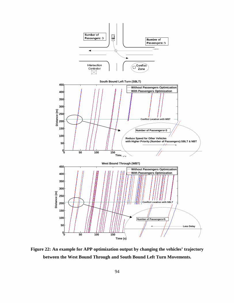
94

Figure 22: An example for APP optimization output by changing the vehicles’ trajectory

between the West Bound Through and South Bound Left Turn Movements.

0 50 100 150 200 250 300 3500

50

100

150

200

250

300

350

400

450

Time (s)

Dis

tanc

e (m

)

South Bound Left Turn (SBLT)

Without Passengers OptimizationWith Passengers Optimization

Conflict Location with WBT

0 50 100 150 200 250 300 3500

50

100

150

200

250

300

350

400

450

Time (s)

Dis

tanc

e (m

)

West Bound Through (WBT)

Without Passengers OptimizationWith Passengers Optimization

Conflict Location with SBLT

Number of Passengers=3

Reduce Speed for Other Vehicles with Higher Priority (Number of Passengers):SBLT & NBT

Less Delay

Number of Passengers=5

95

Table 12: The simulation results for all scenarios: delay (seconds) and fuel consumption

(milliliter)

Case #

V major

V minor

Optimization for Total Vehicle Delay (neglecting number of passengers) “base case”

Optimization for Total Passenger Delay “APP Framework”

Average MOE based on the number of passengers in the vehicle Total

MOE for all

passengers

Average MOE based on the number of passengers in the vehicle

Total MOE for

all passenger

s 1

Pass 2

Pass 3

Pass 4

Pass 5

Pass 1

Pass 2

Pass 3

Pass 4

Pass 5

Pass

Delay (seconds)

1 500 250 1.2 0.4 0.3 0.2 0.2 42.8 0.7 0.4 0.3 0.2 0.3 35.1

2 600 300 2.0 0.9 0.8 0.7 0.4 140.5 0.9 0.5 0.5 0.2 0.2 68.9

3 700 350 4.6 1.9 1.4 1.0 1.0 318.1 1.0 0.6 0.4 0.4 0.2 98.5

4 800 400 3.1 2.0 1.3 0.9 0.4 314.7 1.1 0.6 0.5 0.4 0.2 108.8

5 900 450 4.1 2.3 1.6 1.0 0.9 421.7 1.2 1.0 0.6 0.4 0.4 171.3

6 1000 500 3.6 1.7 1.5 0.9 0.6 387.4 1.1 0.6 0.5 0.3 0.2 129.8

7 1100 550 5.1 2.3 1.6 1.3 1.0 481.1 1.5 0.7 0.4 0.5 0.3 134.2

8 1200 600 8.7 3.4 2.1 2.1 1.1 474.3 1.7 0.7 0.4 0.3 0.2 136.6

9 1300 650 8.9 4.6 3.1 2.0 1.7 1200.3 2.0 0.8 0.5 0.4 0.3 167.2

10 1400 700 8.5 4.4 3.0 2.3 2.2 1208.3 2.4 1.1 0.7 0.6 0.5 298.3

11 1500 750 9.4 3.9 2.8 2.0 1.5 1386.9 2.6 1.3 0.6 0.5 0.5 288.4

12 1600 800 9.7 6.6 3.1 2.6 1.8 1593.0 2.8 1.2 0.7 0.6 0.4 389.8

13 1700 850 10.2 4.9 3.3 2.7 1.9 1408.2 2.9 1.5 0.8 0.7 0.5 457.1

14 1800 900 9.6 5.0 3.5 2.7 1.7 1330.9 2.0 1.0 0.7 0.5 0.5 433.3

Average (s) 6.3 3.2 2.1 1.6 1.2 1.7 0.8 0.5 0.4 0.3

Fuel Consumption (milliliter)

1 500 250 23.7 11.3 8.1 5.6 4.6 1289.9 23.6 11.3 8.1 5.7 4.6 1286.0

2 600 300 24.8 12.0 8.2 6.0 4.4 1663.9 11.7 11.7 8.0 5.7 4.3 1620.2

3 700 350 25.5 12.2 9.1 6.0 5.2 1878.2 25.3 11.5 8.4 5.7 4.6 1749.9

4 800 400 25.0 12.0 8.7 6.3 4.7 2165.7 11.2 11.2 8.2 5.9 4.6 2046.4

5 900 450 23.2 12.8 8.2 6.5 5.3 2355.1 12.1 12.1 7.7 6.1 5.0 2222.8

6 1000 500 25.3 12.1 8.5 6.1 4.9 2634.7 11.4 11.4 7.9 5.8 4.8 2483.8

7 1100 550 28.7 13.2 8.9 6.4 5.3 2793.1 25.8 11.9 8.1 5.9 4.8 2602.8

8 1200 600 29.3 13.8 8.7 6.9 4.9 3066.8 24.5 12.1 7.7 5.9 4.4 2880.9

9 1300 650 29.3 13.9 9.6 6.7 5.7 3939.4 24.7 11.9 8.2 5.8 4.9 3336.9

10 1400 700 25.3 12.5 8.4 6.5 5.2 3701.0 23.8 11.6 7.8 6.0 4.8 3179.8

11 1500 750 28.7 13.4 9.1 6.9 5.5 4592.9 25.3 11.8 8.0 6.0 4.9 3934.9

12 1600 800 29.1 14.9 9.4 7.3 5.5 4486.6 24.5 11.9 8.1 6.2 4.5 3747.7

13 1700 850 29.4 14.5 8.9 7.5 5.7 4954.3 24.7 14.5 8.9 7.5 5.7 4343.2

14 1800 900 29.4 14.1 9.6 7.5 5.5 5047.2 24.6 11.6 8.0 6.1 4.7 4507.2

Average (s) 26.9 13.1 8.8 6.6 5.2 20.9 11.9 8.1 6.0 4.8

96

(a)

(b) Figure 23: Comparison between the total (a) delay and (b) fuel consumption per passenger

for each volume scenario

1 2 3 4 5 6 7 8 9 10 11 12 13 14140

500

1000

1500

Volume Scenarios

Tota

l Del

ay/p

asse

nger

(sec

onds

)

Total Delay/passenger using APP FrameworkTotal Delay/passenger (base case)

1 2 3 4 5 6 7 8 9 10 11 12 13 141000

1500

2000

2500

3000

3500

4000

4500

5000

5500

Volume Scenarios

Tota

l Fue

l Con

sum

ptio

n/pa

ssen

ger (

mL)

Total Fuel Consumption/passenger using APP FrameworkTotal Fuel Consumption/passenger (base case)

97


The basic idea of transit signal priority is to establish right of way requirements among transit

vehicles based on passenger loads and intersection arrival times via V2I and V2V

communications. Although the idea of passenger priority has been previously tested in transit

systems, none of the previous research efforts introduced this concept for automated vehicle

management. Consequently, this research presented an innovative agent-based framework for

optimizing the movements of automated vehicles at intersections considering the number of

passengers per vehicle: Agent-based Passenger Priority (APP). The new concept (APP) mainly

depends on vehicle-to-vehicle and vehicle-to-infrastructure communication technology to

provide of passenger and vehicle information. The APP framework is an extension of the

previously developed tool by the authors “iCACC”. In general, iCACC captures the physical

characteristics of vehicle acceleration/deceleration behaviour, the different weather conditions

(roadway surface conditions) and different levels-of-market penetration of CACC-equipped

vehicles. The proposed concept was tested on a single four-legged intersection with three-lane

approaches and the results demonstrated how the APP framework can significantly reduce the

total passenger delay and fuel consumption level.

As is the case with any research effort, further improvements can be made. First, the possibility

of implementing the APP framework on multi-lane intersections could be addressed in the future.

In addition, simulations for different weather conditions require further testing. The results from

this research also warrant studies with regard to incorporating different intersection users

(cyclists, pedestrians, etc.) into the system. It is clear that the high occupancy vehicles experience

less delay and fuel consumption in most of the cases compared to vehicles with low occupancy.

At the end, the public acceptability of the increase of vehicle automation is a challenging task

and this research will provide valuable feedback for researchers, automobile manufacturers and

decision makers.

98

CHAPTER 8 ROUNDABOUT APPLICATION

Given that the number of roundabouts in the US has increased significantly, this chapter

investigates the potential benefits of optimizing vehicle trajectories approaching a single-lane

roundabout using CACC systems and V2I/I2V connectivity. The optimization ensures that

vehicles can enter the roundabout when gaps in the circulating roadway are available. In general

terms, the proposed idea is quite similar to the concept of metering single-lane entrance ramps.

The system is simulated on a single-lane roundabout for different traffic demand and CACC

market penetration levels. The study demonstrates that CACC systems could produce savings of

up to 80 and 40 percent in total delay and fuel consumption levels, respectively, compared to

traditional roundabout control.

8.1 INTRODUCTION

Modern roundabouts have been used successfully in many cities throughout the world. In the US,

the number of roundabouts has increased significantly in the last decade. Specifically, the

number of roundabouts was 2,300 in 2009 compared to only 310 roundabouts in 2003 [89].

Modern roundabouts are simply designed to control traffic flow at intersections without the use

of stop signs or traffic signals. Generally, there are two features that characterize most of the

modern roundabouts: (1) entering traffic should yield to circulating traffic (i.e. offside-priority

rule) and (2) the geometric design limits the speed of the entering/circulating vehicles.

Several studies have shown that modern roundabouts (or simply referred to as roundabouts) can

be safe and effective, and they could reduce delays by approximately 70% on average compared

to alternative traffic signal controlled intersections [90]. In addition, roundabouts could reduce

overall crash rates and particularly injury crash rates compared to all forms of traffic control

(except for all-way stop control) [90]. In general, most of the literature divided the roundabouts

into three basic categories according to size (the circle diameter) and number of lanes: mini-

roundabouts, single-lane roundabouts and multilane roundabouts. Though, this research focuses

on studying the single-lane type. Single-lane roundabouts designed for low speed operations are

one of the safest treatments available for at-grade intersections [91].

99

Consequently, this chapter presents a proposed simulation/optimization tool for CACC-equipped

vehicles at intersections entitled iCACC. Optimizing vehicle trajectories at intersections may

have an inherent advantage of reducing the fuel consumption [6]. It is proposed that the

intersection (roundabout) will be equipped by a controller that optimizes the trajectories of

vehicles arriving at an intersection (within the intersection zone (IZ)) using the iCACC tool. In

the case of non-automated vehicles, it is assumed that the intersection will be equipped with

road-side sensors that could detect the precise location and speed of the vehicles. Subsequently,

the iCACC has the ability to simulate/optimize all levels of automation, i.e. from legacy vehicles

(e.g. standard vehicles with no automation) to fully automated vehicles.

The roundabout is considered one of the a significant intersection type in both urban and rural

environments nowadays [92]. This is due to the potential benefits deriving from the reduction in

both speed and the number of conflict points compared to traditional crossroad intersections. In

the literature, there are several methodologies proposed to evaluate roundabout performance:

analytical models (e.g. the Highway Capacity Manual (HCM)), statistical models (e.g. TRRL),

etc. [93]. However, the performance of some roundabouts cannot be considered satisfactory, and

many of them could be improved [92]. Consequently, many technical reports have been released

to enhance “roundabout” design in roadway networks in the United States (e.g. [91, 94]). As an

example, the National Cooperative Highway Research Program (NCHRP) [91] have provided

planning guidelines and evaluation procedures for designing safe and practical roundabouts.

Initially, modern roundabouts were presented as alternatives to signalized intersections, which

tend to control the traffic flow more optimally and in a safer manner. Though, some researchers

addressed the combination of signal design control with roundabouts. This type of intersection

was named by Webb[95] “SIG-NABOUT” that combines the features of a signalized intersection

and a roundabout. The traffic signals are usually installed on the approaches to the roundabout;

however, Yang et al. [96] explored the concept of introducing a second stop line to control the

left turn traffic. In the same context, Fahmy[97] presented an adaptive traffic signaling method

based on fuzzy logic for roundabout signalized control.

Previous models of roundabout operations mostly focused on entry capacity models [98-100]

and/or safety performance measurements [101]. Nevertheless, a limited number of publications

100

addressed the concept of advanced technologies in roundabout operations. For example,

Mussone et al. [92] developed a vehicle tracking tool to obtain paths, kinematic variables of

vehicles inside the roundabout and the entry/exit demand using video recording. In addition,

Chen et al. [102] proposed an optimum control for vehicles movements using the VISSIM test-

bed. The general idea of the optimization was to fix the headway between the vehicles and

consequently, the authors claimed that their approach would increase the traffic capacity by four

folds.

In addition, it could be stated that none of the previous research efforts used an explicit

optimization algorithm to reduce the total delay at roundabouts via connected vehicle

applications. As far as the chapter layout is considered, a detailed description of the optimization

algorithm and assumptions made are given, followed by a brief section on the preliminary

simulation analysis and results drawn using different level of penetration. This is followed by a

section on findings and conclusions that can be derived as well as the future direction of this

research.

8.2 THE SYSTEM OVERVIEW

As mentioned previously, the iCACC tool optimizes the movements of CACC-equipped vehicles

traversing a roundabout by avoiding conflicts and minimizing the total intersection delay. The

total delay is defined as the summation of all delay times for all vehicles crossing the subject

roundabout relative to traveling at free-flow speed.

The general assumption is that if all vehicles entering the IZ accelerate to the free-flow speed and

maintain it while crossing the roundabout; this would be the "optimum (ideal) case". After

entering the IZ, vehicles proceed through three main zones: Zone I, Zone II and the circulatory

roadway of the roundabout, as summarized in Figure 24(a). In Zone I, vehicles are assumed to

accelerate to the free-flow speed and maintain that speed until the end of Zone I, which is

assumed to be 50 m (160 ft) in length in this research effort. As a result, the end of Zone I is

considered as the first fixed speed point in the speed profile of any vehicle in the IZ where all

vehicles are running at the free-flow speed. This fixed speed point is called the "Anchor Point".

101

To facilitate the optimization process speed variations (decelerations and accelerations) occur in

Zone II, which is assumed to be 150 m (490 ft) in length. At the end of Zone II, all vehicles are

running at the maximum circulating speed (the second anchor point), as demonstrated in Figure

24(b). The second anchor point is considered the entrance point to the roundabout where all

vehicles begin to cross the intersection.

As mentioned previously, it is assumed that all vehicles will be crossing the intersection box at

the maximum circulating speed; as a result, the tool would only optimize the arrival time at the

roundabout entrance point (RE). In other words, the tool adjusts the speed profile of each vehicle

in Zone II to ensure that by the arrival at the RE, all vehicles can enter the roundabout and run at

the maximum circulating speed without stopping and certainly without conflicting with other

vehicles.

Figure 24(b) shows an example for a single-lane roundabout and demonstrates the different

conflict points and entrance points to the roundabout. Ideally, if the vehicle does not decelerate

and/or stop in Zone II, it will arrive at the RE at the shortest time possible (i.e. optimum time)

"OT". However, to avoid conflicts with other intersecting vehicles, vehicles may decelerate or

come to a complete stop to arrive at the RE at the Actual Time "AT". Therefore, by minimizing

the time difference between AT and OT for all vehicles the total delay can be minimized.

102

(a)

(b)


trajectories inside the roundabout

Zone I Zone II

Vmax

Speed

Distance

Anchor Point

DSRC Communication Range

103

In managing the vehicle movements, at each time step (i.e. optimization loop), an optimization of

vehicle to arrivals at RE is implemented. The main idea of the optimization module is to

minimize the additional time (D) to the OT, needed to avoid conflicts with other circulating

vehicles in the roundabout. To formulate the simulation/optimization process for the roundabout

type of control, the following equations are developed:

1

1

: ii

Min D

(28)

Subject to:

min( ) ( ) ; , ,i i j jOT D OT D H i j i j (29)

1( ) ( ) ( ); , , , , ,i i mn k k pn mn pnOT D OT D l l i k i k m p n CP (30)

1 0( ) ( ); , , ,i i mn f f mnOT D OT D i f m n CP (31)

0; iD i (32)

Where (as illustrated in Figure 24),

i,j,f,p: Vehicle identification number;

Di: The time difference between the optimum time (OT) and the actual time (AT) for vehicle i

and ideally it will be equal to zero if there is no deceleration happened in Zone II;

OTi: The optimum arrival time for vehicle i at the RE. OTi is estimated assuming that each

vehicle will accelerate to maximum speed in Zone I and ideally will continue with the same

speed till RE. The arrival time is calculated based on the dynamic Equations and car following

models;

Ω0: the set of vehicles that entered into IZ last time step but still in IZ at current time step;

Ω1: The set of vehicles that enter into IZ at current step;

Ω: The set of vehicles in IZ at current time step (Ω= Ω0+ Ω1);

Hmin: The minimum headway between vehicles at the same lane.

104

m, p: Lane identification number;

n: Conflict Point identification number;

Ψ: the set of lanes at the intersection;

CP: the set of conflict points;

lmn:=1 if the coming vehicle from lane m passes by conflict point n; and 0 otherwise;

lpn:=1 if the coming vehicle from lane p passes by conflict point n; and 0 otherwise,

τmn : travel time from the RE of lane m to the conflict point n; given the distance to each conflict

point based on the intersection geometry. It is assumed that all vehicles will be running at the

maximum circulating speed; hence, τmn is fixed for all vehicles from the same lane m to same

conflict point n (to facilitate the optimization process).

Δτ: Minimum time buffer between vehicles occupying the same conflict point. The Δτ value is

function of minimum acceptable gap for each vehicle. Obviously, the value of Δτ changes if the

vehicle is equipped with a CACC system (i.e. advanced vehicle) or not (i.e. traditional vehicle)

to accommodate the different levels of marked penetration.

The objective function (Equation 28) minimizes the total delay (Di) across all vehicles traversing

the intersection. In order to achieve the proposed objective, four constraints are listed. Equation

29 ensures that the first in first out (FIFO) rule is maintained for all vehicles in the same lane. In

other words, the arrival of each following vehicle should be after the leading vehicle by a

specified interval (minimum headway Hmin). Equation 30 ensures that a vehicle cannot conflict

with another vehicle in the circulating roadway of the roundabout, by ensuring that the arrival of

two intersecting vehicles at the same conflict point is separated by a minimum safety buffer (Δτ).

Table 13 shows the different values of lmn which presents the relationship between the

intersection lanes and the different conflict points, as illustrated in Figure 24(b). If the value of

lmn is equal to 1, it implies that the vehicle going from lane m to p will pass by conflict point n, in

other words, it depends on the destination of the vehicle. It should be stated that in case of non-

automated vehicles, the iCACC will not be able to identify the destination of the vehicle so in

this case all conflict points are considered in the optimization process.

105

Table 13: The Lane-conflict relationship (lmn)

Lanes

From (m) 1 2 3 4

To (p) 2 3 4 3 4 5 4 1 2 1 2 3

CP (n)

A 1 1 1 0 0 0 0 0 1 0 1 1

B 1 1 1 0 0 0 0 0 1 0 1 1

C 0 1 1 1 1 1 0 0 0 0 0 1

D 0 1 1 1 1 1 0 0 0 0 0 1

E 0 0 1 0 1 1 1 1 1 0 0 0

F 0 0 1 0 1 1 1 1 1 0 0 0

G 0 0 0 0 0 1 0 1 1 1 1 1

H 0 0 0 0 0 1 0 1 1 1 1 1

At each time step (optimization loop), vehicles in the system are divided into two groups,

namely: vehicles that entered in the previous time step and still in the IZ (Ω0 group) and vehicles

that enter in the current step (Ω1 group). For the set of vehicles Ω0, the vehicle entry times at the

IZ were optimized in the previous step, and each vehicle profile was determined/ optimized. Re-

optimization of entry times can decrease the algorithm computational efficiency and increase

vehicle fuel consumption by changing vehicle movements. Hence, only the set of vehicles Ω1 are

optimized each time step. At each time step, the occupied time for each conflict point is stored as

a new constraint for the following time step (optimization loop), as demonstrated in Equation 31.

The last constraint is the non-negativity condition for the additional time (Di), in other words, the

additional time should be zero (no delay) or greater.

In summary, the iCACC tool uses an algorithm composed of four main steps to solve the

optimization problem using Equations 28 through 32. First, based on the entry speed and

acceleration for each vehicle in the IZ, the arrival time for each vehicle at the RE is estimated.

Second, assuming all vehicles run at the maximum circulating speed, the occupancy time for

each conflict point is calculated using the tabular information from Table 13. Third, the tool

begins to search for the unsafe conflict points; in other words, the points where the time

106

difference between two crossing vehicles is less than the minimum time difference Δτ (i.e. the

minimum acceptable gap). Last, the tool modifies the arrival times of vehicles and determines

the optimum additional time needed (D).

8.3 NUMERICAL EXAMPLE AND SENSITIVITY ANALYSIS

In validating the proposed iCACC algorithm, a single-lane roundabout (similar to Figure 24(b))

was simulated using different traffic demand combinations. The maximum entry design speed

for the tested roundabout was 35 km/h (20 mph) and the central island diameter was 40 m (130

ft) following the recommendations of the Federal Highway Administration (FHWA) (e.g. [90]).

In calibrating the vehicle dynamics and fuel consumption model parameters, the physical and

mechanical characteristics of a 2010 Honda Accord was used. The vehicle has an engine power

of 177 Horse Power (Hp). The analysis assumes that the vehicle travels on a good flat asphalt

surface (grade 0%) and the current weather condition is dry. Table 14 summarizes the

specifications and the parameters used for testing the proposed connected vehicle application.

The single-lane roundabout was tested using different random number seeds for 5 different

volume combinations resulting in volume-to-capacity ratios ranging between 0.2 and 1.0. The

entrance time of each vehicle to the IZ, their initial speed and acceleration were picked using a

random number generator. The volume-to-capacity ratios were estimated based on the entry and

the circulating volumes at the roundabout using the HCM 2000 guidelines [103]. The major

street volume ranged between 200 to 1000 veh/h/approach and the minor street volume ranged

between 100 to 500 veh/h/approach. The direction-split for the major approach was assumed

0.2:0.6:0.2 and for the minor approach, was 0.4:0.2:0.4 for left, through and right turn

movements, respectively.

The iCACC scenario was simulated in MATLAB using the "moving horizon optimization"

concept at each time step (i.e. 20 seconds). In other words, at each time step, the new entering

vehicles to the IZ were optimized and simultaneously the expected entering vehicles in the

following time step were optimized in advance. Consequently, by using the moving horizon

concept, the optimization process takes shorter time in the preliminary optimization of entering

vehicles. The solution for these vehicles is then used in the following time step as the initial input

107

to the optimization algorithm. In order to evaluate the proposed iCACC system, different level-

of-market penetrations were modeled.

Table 14: The simulation/optimization inputs

Parameter Value Exchanged Information Rate 0.1 second

Optimization Inputs Number of Optimization Iterations 30 Iterations Optimization Horizon 20 seconds

Geometric Design of Roundabout

Number of lanes per approach 1 lane Speed Limit for each approach 35 mph (55 km/h)

Entry Design Speed to Roundabout 20 mph (35 km/h) Central Island Diameter 130 ft (40 m)

Car Following and Gap Acceptance Parameters

Approach Free flow speed uf 38 mph (60 km/h) Approach Speed at capacity uc 25 mph (38 km/h)

Approach Jam Density kj 143 veh/km Approach Capacity qc 1700 veh/hr

Minimum acceptable gap(critical gap ) for non-automated vehicles (i.e. Δτ) 4 seconds (source [94])

Minimum acceptable gap for automated vehicles (i.e. Δτ)

The estimated travel time needed to reach and clear the

conflict point

The Physical Parameters of the tested vehicle (2010

Honda Accord)

Power of engine (P) 177 Hp Transmission Efficiency (η) 0.92

Total Weight (W) 1453 Kg Mass on Tractive Axle (mta) 785 Kg

Roadway Adhesion (µ) Dry = 1 & Wet= 0.8 Air Density (ρ) 1.2256 Kg/m3

Air Drag Coefficient (Cd) 0.3 Altitude Factor (Ch) 1

Frontal Area (A) 2.32 m2

Rolling Coefficient Cr0= 1.75 Cr1= 0.0328& Cr2= 4.575

EPA Estimates City/Combined/Highway 21/25/31 MPG

Two measures of effectiveness (MOEs) were computed, namely: the average vehicle delay

(seconds) and the average vehicle fuel consumption (milliliters). Table 8 tabulates the different

volume cases and the corresponding values of both MOEs for different levels-of-market

penetration levels of CACC systems. The delay values were averaged across all vehicles for the

different traffic demand cases, as illustrated in Figure 7(a). The average fuel consumed for the

vehicles to pass through the intersection were also computed the same way for all scenarios as

shown in Figure 7(b).

108

Table 15: Simulation results for average delay and fuel consumed for all scenarios

Major flow (vph)

Minor flow (vph)

Max

v/c ratio

Average Delay (s) Fuel (mL)

LMP (%) LMP (%)

0% 20% 40% 60% 80% 100% 0% 20% 40% 60% 80% 100%

200 100 0.2 5.0 4.9 4.5 2.4 1.6 1.0 22.2 22.1 21.9 21.0 20.6 20.5

400 200 0.4 20.1 9.0 8.9 7.5 3.5 3.8 29.3 23.9 23.8 23.2 21.5 21.6

600 300 0.6 24.1 14.7 10.9 8.6 5.5 5.4 31.1 26.6 24.9 23.7 22.4 22.3

800 400 0.8 29.5 27.6 16.6 9.9 7.0 5.8 33.7 32.7 27.6 24.3 23.0 22.5

1000 500 1.0 39.8 39.2 25.3 19.2 12.9 7.8 38.6 38.3 31.7 28.8 25.8 23.4

Figure 7(a) and (b) show the benefits of iCACC intersection control in terms of delay and fuel

consumed on a per-vehicle basis for the different traffic demand scenarios. The traditional

single-lane roundabout (base case) is represented by the zero percent level of penetration, i.e.,

before introducing our proposed system (iCACC) control. Obviously, by increasing the level of

penetration (automation) at the roundabout, the iCACC is able to reduce the delay and fuel

consumption level by controlling the movements of the accessible automated vehicles.

Consequently, at 100% LMP, the potential benefits are provided if full deployment of CACC is

achieved.

It is noticeable in case of low volume (v/c=0.2), the impact of introducing the iCACC

intersection control is relatively small compared to more congested conditions. For the high

volume case (v/c=1.0), the iCACC is able to dramatically reduce the delay and fuel consumption

by 80% and 40%, respectively compared to traditional single-lane roundabout control (0%

LMP).

109

(a)

(b)

Figure 25: Comparison between different scenarios (a) Average delay comparison per

vehicle (s) (b) Average fuel consumption per vehicle (mL)

0 10 20 30 40 50 60 70 80 90 1000

5

10

15

20

25

30

35

40

45

Level of Penetration (%)

Ave

rage

Del

ay p

er V

ehic

le (s

ec)

v/c=0.2v/c=0.4v/c=0.6v/c=0.8v/c=1.0

0 10 20 30 40 50 60 70 80 90 10020

22

24

26

28

30

32

34

36

38

40

Level of Penetration (%)

Ave

rage

Fue

l Con

sum

ptio

n pe

r Veh

icle

(mL)

v/c=0.2v/c=0.4v/c=0.6v/c=0.8v/c=1.0

110

In general, on a vehicle-by-vehicle basis, the iCACC algorithm reduces vehicle delay

significantly when compared to conventional roundabout control. It could be stated that the idea

of controlling the arrival time of each vehicle at the RE is quite similar to the concept of metered

single-lane entrance ramps. In other words, the iCACC controls the flow of vehicles to the

circulatory roadway of the roundabout to ensure that they can enter the roundabout smoothly

with minimum delays.


This research presented a new application for the simulation/optimization tool (iCACC) to

optimize the movements of vehicles approaching the roundabout using V2I/I2V communication

technology. The proposed concept was tested on a single-lane roundabout considering traffic

demand and level-of-market penetration scenarios. The study shows that the introduction of

CACC is positive with savings up to 80% and 40% in total delay and fuel consumption levels,

respectively. In general, this study demonstrates the promising potential of CACC systems in

optimizing the trajectories of vehicles so that they can enter the roundabout efficiently. It should

be noted that the study did not consider additional benefits that could arise by having CACC

vehicles travel at shorter time headways.

In future research, the possibility of implementing the iCACC concept on multi-lane roundabouts

could be addressed. In addition, simulations with dissimilar types of vehicles and different

weather conditions require further testing. The results from this research also warrant studies

with regard to incorporating different intersection users (cyclists, pedestrians, etc.) into the

system and this will lead to the following chapter of introducing the computer vision into

analysis.

111

CHAPTER 9 VEHICLE DETECTION SYSTEM FOR MIXED USERS

This chapter is a first attempt to address some of the issues associated with having mixed

automation levels and the heterogeneity of users at urban roundabouts by using a real-time video

detection/tracking system. The determination of the trajectory of vehicles for road

intersections—especially in the urban areas—has always been a vital theme for traffic

management. In general, visual data provided by cameras can efficiently provide traffic

information with non-intrusiveness, lower cost, and high efficiency. The proposed

detection/tracking system is introduced for roundabouts; however, it may be used for any other

type of intersection. It is entitled: RTR-CV (Real-time Tracking at Roundabouts via Connected

Vehicles environment). Vehicles are detected and tracked within a range of the detection zone,

and then speeds are calculated using vehicle spatial and temporal signatures. The same concept is

used for pedestrians and bicycles in the vicinity of the roundabout. The main purpose of the

proposed RTR-CV system is to detect/track the different roadway users for use in the

optimization process for the iCACC system.

9.1 INTRODUCTION

Modern roundabouts have been used successfully in many cities throughout the US in the last

decade. Consequently, introducing the Connected Vehicle (CV) concept at roundabout controlled

intersections is expected to be one of the main applications in the future. This is given that

automated control can be easily reverted to manual control in the event that communication is

lost or the system experiences a malfunction.

Already, today’s literature suggests that cooperative driving is more efficient, provides more

safety and improvements of traffic efficiency. In addition, cooperative behavior could provide a

possible solution to achieve applications such as collision avoidance or automatic merging of

vehicles on highway. In terms of CACC applications at intersections, most of the previous

literature focused on studying the impact of introducing the system under the assumption of

100% level of market penetration. In addition, none of the previous research investigated the

impact of introducing Connected Vehicle Applications (e.g. CACC) at roundabout controlled

intersections. Consequently, this chapter focuses on the concept of “vehicle surrounding

112

situation awareness” at intersections (roundabouts) and makes it more effective by introducing

the computer vision applications to overcome the diversity of roadway users and level of

penetration.

9.2 RESEARCH OBJECTIVES

This research effort is a first attempt to address some of the issues not covered in previous

research efforts to develop a real-time simulation/optimization tool for mixed automation control

at roundabouts. This research effort focuses on single-lane roundabouts as it is considered a very

suitable platform for applying the CACC concept and the roadway speeds are low enough to

allow mixed automation. However, it could be stated the proposed concept could be applied at

any type of intersections. In order to fulfill the research objective, a research stages is proposed,

namely: Video Detection/Tracking System at the Roundabout (RTR-CV).

In this stage, the issues associated with having mixed automation levels and the heterogeneity of

users at urban roundabouts are covered by using a real-time video detection/tracking system as

will be explained in the following section.

9.3 THE GENERAL CONCEPT OF THE PROPOSED SYSTEM

The determination of the trajectory of vehicles for road intersections- in the urban zones in

general- has been always an vital theme for traffic management[104]. Various kinds of sensors

(optical, magnetic, etc.) are used since several decades to detect vehicles. In the last years several

applications have been proposed, using the techniques of digital photogrammetry, computer

vision and image understanding, for the detection and tracking of roadway users. [105]. Proper

classification is therefore necessary to learn traffic scenarios and understand behavior patterns

within each road-user class[105]. It could be stated that previous research has failed to study the

heterogeneity of intersection users (vehicles, pedestrians and bicycles) in studying Connected

Vehicle applications at intersections. As a result, this section presents the framework for

detecting different roadway users using vehicle detection techniques and this will be integrated

to the tool iCACC.

113

In general, visual data provided by cameras can efficiently provide traffic information with non-

intrusiveness, lower cost and high efficiency. For the sake of this research, the proposed

detection/tracking system is introduced for roundabouts; however it may be used for any other

type of intersections. The proposed system is entitled: RTR-CV (Real-time Tracking at

Roundabouts via Connected Vehicles environment). Vehicles are detected and tracked within a

range of the detection zone, and then speeds are calculated using vehicle spatial and temporal

signatures. The same concept is used for pedestrians and bicycles in the vicinity of the

roundabout. The main purpose of the proposed RTR-CV system is to detect/track the different

roadway users for use in the optimization process for the iCACC system, as shown in Figure 26.

Figure 26: The framework of the RTR-CV system in connection with the intersection

management tool iCACC

Vehicle Detection/Tracking using RTR-CV

Real timeIn-site

Processing (iCACC tool)

Desired Cruise Control

Tuning

Vehicles equipped by advanced cruise control

system (CACC)

DSRC

System Update after

Δt

The exact location and trajectory of each vehicle, pedestrian and bicycle at the roundabout area

114

This challenge must be made in the context of real-time application which runs on common PC

and so two constraints are introduced: less computation time (CT) and less memory requirement

(MR) as possible. The proposed video analysis system (RTR-CV) integrated with advanced

intersection management system (using iCACC tool) has mainly four processing steps at each

time instant (t). First, the system would identify the current intersection users (vehicles,

pedestrians and bicycles) in the vicinity of the roundabout, track their movements and derive

their trajectories using the RTR-CV framework. Secondly, the system would provide/feed the

in-site processor equipped by iCACC tool with the location/speed of each element in the vicinity

of the roundabout. Third, the system would estimate and send the best/optimum speed for each

vehicle equipped with CACC using wireless communication. Thereafter, all previous steps are

repeated after Δt to update the system with the information of all types of vehicles (equipped and

non-equipped), pedestrians and bicycles located at the roundabout area. It is anticipated the

results of this research will be a valuable addition to the proposed simulation/optimization tool.

The research findings would capture the heterogeneity of roundabout users to create an

innovative/optimum intersection management control. However, this research effort only

presents the study for the stage of identifying users (vehicles, pedestrians and bicycles) in the

vicinity of the roundabout using computer vision analysis.

9.4 THE COMPUTER VISION FRAMEWORK

Computer vision analysis based classification has applications in traffic monitoring and the

activity recognition. Many algorithms have been used for moving object detection; however,

foreground/background method is often used in different applications to detect the moving

objects in the scene like in video surveillance, optical motion capture and multimedia [106]. The

basic idea of this method is to compare a color or grayscale video frame to a background model

to determine whether individual pixels are part of the background or the foreground. In other

words, the concept of detecting moving objects is simply detecting the parts of the video frame

that will not show up if the scene (intersection) is clear/empty.

The simplest way to model the background is to acquire a background image/frame which

doesn't include any moving object. In some environments, the background isn’t available and can

115

always be changed under critical situations like illumination changes, objects being introduced or

removed from the scene. To take into account these problems of robustness and adaptation, many

background modeling methods have been developed. In any background subtraction context, the

following steps are taken: background modeling, background initialization, background

maintenance, foreground detection, choice of the feature size (pixel, a block or a cluster), choice

of the feature type (color features, edge features, stereo features, motion features and texture

features)[106].

In the context of a traffic surveillance system, Friedman and Russell[106, 107] proposed to

model each background pixel using a mixture of three Gaussians corresponding to road, vehicle

and shadows. Then, the Gaussians are manually labeled in a heuristic manner as follows: the

darkest component is labeled as shadow; in the remaining two components, the one with the

largest variance is labeled as vehicle and the other one as road[108]. For the foreground

detection, each pixel is compared with each Gaussian and is classified according to it

corresponding Gaussian[106]. Many improvements can be found in the literature for this

algorithm and they are classified as intrinsic and extrinsic model improvements. For the purpose

of this study, it is used the Foreground/Background detection method using mixture of Gaussians

which is the method accommodated by the MATLAB tool box for computer vision.

The proposed Foreground/Background algorithm is summarized in Figure 27. The algorithm first

starts with converting each frame from RGB format to intensity format, then a system object for

detecting foreground using Gaussian mixture models. Thereafter, a blob analysis system is

applied to segment each moving object (vehicle, pedestrian or cyclist) in the video frame/scene.

Subsequently for tracking the moving objects, the entering vehicles/pedestrians/cyclists and

those already present in the previous frames, should be recognized to determine their trajectories.

At the end, the algorithm draws a bounding box around each detected object and records the

number of tracking objects.

116

Figure 27: Video analysis block diagram

9.5 CASE STUDY APPLICATION

In order to test the proposed system, a single-lane roundabout positioned in Virginia Tech

campus area has been considered as a case study. The suggested roundabout is located at the

intersection of Washington Street and West Campus Drive in Blacksburg, Virginia as shown in

Figure 28. One of the main reasons for selecting the single-lane type is the roadway speeds and

widths are low enough to allow mixed automation (penetration levels). In addition, a roundabout

allows the system to revert to typical control in the event of lost communication between

vehicles.

Video Frames/images decomposition

Video Input

Each frame/image is converted from RGB to

intensity format

A blob analysis system is applied to segment each moving object

A bounding box around each bounding

box

The number of detected/tracked

objects is recorded

117

Figure 28: The studied roundabout for testing the object detection/tracking concept

For the purpose of this study, a video camera was mounted at the top of the building (Litton

Reaves Hall) facing the roundabout in a position to capture the northern and eastern approaches

of the roundabout. Figure 29 shows a screen shot for the recording video with a frequency of 30

frames/second.

Figure 29: A screenshot for the recorded videos at the tested roundabout

118

A video camera was used to record the activities that occurred over a time period of two days.

The length of each recording was 7 hours per day, beginning at 10:00 AM and ending at

4:00PM. By reducing the collected video dataset, it was found that the site has many challenges

for applying video detection techniques and some of them could be listed as follows:

1. The roundabout is in front of the Student Recreational Center and this leads to

intensive volume for pedestrians and cyclists aside with the vehicles.

2. All vehicle types are passing by this roundabout, e.g. buses (four routes of buses

pass by this roundabout), light and heavy trucks (a construction site is just across

the roundabout) and passenger cars. Hence, from computer vision standpoint, it is

very complicated to train the system for detecting/tracking objects with numerous

size and movement characteristics.

3. Due to the small trees in the middle of the roundabout and the vision angle of the

camera, the vehicles are partially occluded during their turns at the middle of

roundabout. Hence, tracking the vehicles in this part was very challenging task.

The video has been analyzed using Foreground/Background algorithm combined with Gaussian

Mixture Models (illustrated in the previous section) and a screen shot for the results is shown in

Figure 30. It is noticeable how the proposed algorithm could successfully detect moving objects

including vehicles and pedestrians and the output has been recorded and uploaded as presented in

the following link: http://www.youtube.com/watch?v=mm-ds2c7u48

It is noteworthy to mention that due the shaking of camera there might be some miss-detected

objects; however, these might be easily overcame by setting the detection zone limited to certain

regions (the pavement surface, cross walk, etc.).

http://www.youtube.com/watch?v=mm-ds2c7u48

119

(a) The Foreground/background stage

(b) The results of detecting/tracking featured objects (vehicles and pedestrians)

Figure 30: The output of the video analysis using the proposed algorithm

120


This chapter attempts to overcome one of the most challenging issues in automation/cooperative

environment: the heterogeneity of roadway users and the different level of penetrations. The

proposed algorithm is considered a vital step in a huge research area about controlling/adjusting

the speed of crossing vehicles at intersections to prevent crashes and reduce delay using V2V

and V2I communications

There are several areas of potential improvements of the proposed approach. One advantage of

the proposed method is its seamless extension to accommodate other feature selection like spatial

locations and speed. Currently, the implementation does not take into account the spatial

information of the RUs or information about their size. In addition, this research did not

encounter the prediction level of computer vision for better intersection management

performance.

A foreground/background methodology has been described, for the vehicles detection in a

roundabout and for the determination of their locations/trajectories. The results of a test lead on a

real case have been described and showed the capability of the proposed algorithm. Next studies

will be addressed to the resolution of the problems to face, with particular regard to the

radiometric variations of the background image, to elimination of the shadows from the regions

associated to the vehicles. It is anticipated that this research effort will be introduced as an

effective solution for having many roadway users and different level of penetration for any

cooperative system.

121

CHAPTER 10 CONCLUSIONS AND RECOMMENDATIONS

This chapter summarizes the main findings of the research presented in the dissertation. In

addition, the chapter illustrates the different limitations of the iCACC (Cooperative Adaptive

Cruise Control at intersections) system. Finally, recommendations for future work are discussed.

10.1 RESEARCH CONCLUSIONS

The goal of this research initiative is to develop an optimization framework for controlling the

movement of vehicles equipped with CACC systems at intersections. Hence, the previous

chapters covered six main tasks: (1) Optimize automated vehicle movements using a game

theory algorithm, (2) Model driver behavior for non-automated vehicles under different weather

conditions; (3) Develop the modeling and GUI for the proposed iCACC tool; (4) Develop the

passenger priority concept for automated vehicle control “APP”; (5) Evaluate the tool using a

simulation test-bed; and (6) Propose a computer vision algorithm for detecting vehicles,

pedestrians, and cyclists at the intersection vicinity.

A review of the literature reveals that the effects of many essential factors for modeling agents

(vehicles) are either completely neglected or only qualitatively described. For example, the

simulators used for modeling agents at intersections do not take into consideration the impact on

the total intersection delay. Furthermore, the FCFS (First Come, First Served) concept—

presented in many research papers—gives priority to vehicles with shorter times-to-intersection

regardless of the vehicle type, the number of passengers in the vehicle, and/or the total

intersection delay. The variability in vehicle physical characteristics (i.e., agent) is not captured

in many of the previous models in the literature, nor is the impact of weather conditions on

roadway surface conditions and the effect on vehicle performance. Accordingly, the research

presented in this dissertation develops an innovative approach for optimizing the movement of

vehicles equipped with advanced cruise control systems at "smart" intersections. In addition, this

research has successfully addressed some of the gaps identified in the literature on vehicle

automation, as will be discussed in the following sections.

122

10.1.1 Game Theory Algorithm

Various models that incorporate the concepts of Game Theory are described in much of

the transportation-related literature; however, none of these sources attempted to optimize

the movement of vehicles through intersections.

The proposed cooperative game framework in this research: CACC-CG (Cooperative

Adaptive Cruise Control-Cooperative Game); successfully demonstrated the promising

potential benefits of such a system over conventional state-of-the-practice intersection

control systems.

By comparing the proposed system to a four-way stop control, the results showed that the

proposed system reduced the total delay by approximately 70 percent.

10.1.2 Driver Behavior for Non-automated Vehicles at Intersections

Driver behavior modeling at intersections for non-automated vehicles is a vital stage in

modeling the mixed automation environment; i.e., various levels of penetration of the

CACC system, especially under inclement weather.

A logit regression model was proposed to quantify the impact of inclement weather

conditions on driver behavior using a collected data set for six weather categories.

The recommended model explicitly captures the vehicle constraints on driving behavior

(presented in the travel time value) and the driver’s deliberation in accepting or rejecting a

gap in different weather conditions.

The model demonstrated that the probability that a driver accepts a gap decreases as the

travel time needed to reach the gap increases (i.e., the further the gap is, the longer the

required gap).

The model proved that a larger gap is required for a wet surface compared to a snowy and

icy surface followed by a dry surface. The higher gap required for a wet surface could be

caused by the fact that drivers are more worried about vehicles skidding when the

roadway surface is wet and that the opposing traffic is traveling at a higher speed

compared to the snowy and icy roadway conditions.

The model revealed that drivers are more conservative during snow precipitation as

compared to rain precipitation.

123

In the case of the roadway surface condition, drivers require larger gaps for wet surface

conditions compared to snowy and icy surface conditions and, as would be expected,

require the smallest gaps for dry roadway conditions.

Using this study’s findings, the proposed tool (iCACC) for optimizing the movements of

vehicles at intersections could model the drivers’ behavior for non-automated vehicles

(left-turn) under different weather conditions.

10.1.3 The iCACC Basic Framework

The iCACC tool is considered the first of its kind in optimizing and simulating automated

vehicles’ movements at intersections.

The tool has the ability to model different weather impacts, vehicle physical

characteristics, shared movement lanes, uncertainty of exchanged information in V2I/I2V,

mixed automation environment (different levels of penetration), and roundabout control.

The tool contains built-in car-following (Van Aerde) models, vehicle dynamics models,

and fuel consumption (VTCFM) models.

The impact of weather conditions was captured in the iCACC tool using various models:

vehicle dynamics (coefficient of friction and rolling resistance coefficients), car-following

(free-flow speed, speed-at-capacity, and capacity), and the gap acceptance models (critical

gap and follow-up time). In other words, the weather conditions directly affected the

vehicle acceleration capability and the decision of non-automated vehicles (gap

acceptance/rejection) at the intersection zone (IZ).

Four intersection control scenarios were tested (traffic signal control, AWSC, roundabout,

and iCACC control) for intersection volume-capacity ratios ranging from 0.27 to 0.91.

The results demonstrated that the iCACC controller could reduce the average vehicle

delay by more than 60% when compared to traditional traffic signal and the AWSC for

different volume cases.

On the other hand, the iCACC controller results in intersection delays similar in

magnitude to a roundabout intersection control. In other words, for low v/c ratios, the

system performance of roundabouts is quite similar to the iCACC controller for four-

legged intersections.

124

Regarding fuel consumption, the simulation results showed that the iCACC controller

scenario was, on average, 33%, 45%, and 11% lower than the fuel consumption for the

traffic signal control, AWSC, and roundabout control scenarios, respectively. These fuel

consumption savings were achieved by successfully reducing the stop-go actions of

vehicles while traversing the intersection.

10.1.4 The Agent-based Passenger Priority Framework using the iCACC Platform

The concept of vehicle priority has been widely addressed in the literature from a Transit

Signal Priority (TSP) standpoint; however, none of the previous research addressed this

concept in vehicle automation management.

Consequently, an innovative framework was proposed “Agent-based Passenger Priority

(APP)” using the iCACC platform to overcome some of the limitations of past research.

The proposed framework takes into account the number of passengers for each vehicle, the

physical characteristics of each vehicle (size, engine power, etc.), and the level of

penetration of the system.

The main concept of APP is to optimize the movements of vehicles at intersections by

exchanging the number of passengers of each vehicle using V2I/I2V communication as an

attempt to reduce the delay per person instead of delay per vehicle.

The proposed concept was tested on a single four-legged intersection with three-lane

approaches. The results demonstrated how, on average, the APP framework could

significantly reduce the total passenger delay and fuel consumption level by 60% and

10%, respectively, comparing to the basic iCACC tool.

Using the APP framework, the high occupancy vehicles experienced less delay and fuel

consumption similarly to the TSP concept.

10.1.5 The iCACC Application at Roundabouts

In the US, the number of roundabouts has increased significantly in the last decade;

however, none of the previous research related to roundabouts addressed the vehicle

connectivity application in the literature.

125

Consequently, the research presented a new application for the simulation/optimization

tool (iCACC) by optimizing the movements of vehicles approaching the roundabout using

V2I/I2V communication technology as a first-of-its-kind.

The proposed concept was tested on a single-lane roundabout considering traffic demand

and level-of-market penetration scenarios. The study showed that the introduction of

CACC is a positive step, with savings up to 80% and 40% in total delay and fuel

consumption levels, respectively.

In general, this study demonstrated the promising potential of CACC systems in

optimizing the trajectories of vehicles so that they can enter the roundabout efficiently.

A new system has been developed in this dissertation for Video Detection/Tracking at the

Roundabout (RTR-CV). The RTR-CV system proved its ability to overcome the previous

research limitations, the issues associated with having mixed automation levels, and the

heterogeneity of users at urban roundabouts.

10.2 RESEARCH ASSUMPTIONS AND LIMITATIONS

The proposed tool has been successfully tested in a simulation test-bed; however, it should be

noted that the study did not consider additional benefits that could arise by having CACC

vehicles travel at shorter time headways. In addition, all information is symmetric and exchanged

perfectly between vehicles, and the wireless communication is secure and supports high speed

and low latency communication. Also, one of the main assumptions of the system is that all

equipped vehicles are following the iCACC instructions and report their destination, location,

speed, and acceleration to the controller each time step.

However, the implementation of the iCACC tool in a field test will address many assumptions.

The field testing of the proposed tool will be able to address some of the unanswered questions

raised by many researchers and the current limitations of the iCACC tool, some of which are

listed as follows:

1. Solicit driver acceptance of automation systems;

2. Solicit driver interaction to displayed speed advisory and/or self-controlled

vehicles;

126

3. Identify possible demographic characteristic effects (age, gender, etc.) on driver

acceptance of in-vehicle technologies;

4. Quantify the error in the information (location, speed, etc.) exchanged between

V2V and V2I;

5. The latency and inaccuracy in communications between the intersection controller

and different vehicles.

10.3 RECOMMENDATIONS FOR FUTURE RESEARCH

As is the case with any research effort, further improvements can be made and the following

areas of research should be pursued to expand the current research work. First, the possibility of

implementing the iCACC tool on an arterial corridor needs more investigation. Also, as

mentioned previously, none of the past research efforts considered advanced cruise control

systems; in other words, speed adaptation concepts at roundabouts. Therefore, it would be a

unique addition if the equipped vehicles with advanced technologies could be tested on a

roundabout.

Three field testing scenarios are anticipated to extend the iCACC research effort. For each

scenario, the driver behavior, fuel consumption, and delay will be recorded for comparison

purposes. In scenario 1, there will be no information provided for the driver in the subject vehicle

and this will be the base scenario. In scenario 2, the driver would be advised with a certain speed.

This scenario aims to study the driver perception/reaction time for this kind of message and how

accurate the driver could follow a recommended speed.

In scenario 3, the vehicle will be fully controlled by the RSU using an optimum speed profile.

This scenario is expected to consist of four main steps: Input, Processing, Output (tuning), and

Validation, as summarized in Figure 31. The input is the entry speed of the vehicle, exact

location (using GPS/Radar), and the acceleration. Those inputs will be delivered to an on-site

processor using SAE J2735 DSRC. Thereafter, the processor will optimize the vehicle trajectory

and send back the optimum desired cruise control to reduce delay and prevent crashes.

Subsequently, the subject vehicle would regulate its speed to follow the desired cruise control

speed. At the end, the actual speed profile would be stored and compared to the desired profile in

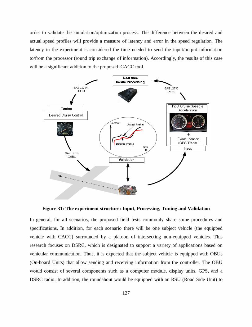
127

order to validate the simulation/optimization process. The difference between the desired and

actual speed profiles will provide a measure of latency and error in the speed regulation. The

latency in the experiment is considered the time needed to send the input/output information

to/from the processor (round trip exchange of information). Accordingly, the results of this case

will be a significant addition to the proposed iCACC tool.

Figure 31: The experiment structure: Input, Processing, Tuning and Validation

In general, for all scenarios, the proposed field tests commonly share some procedures and

specifications. In addition, for each scenario there will be one subject vehicle (the equipped

vehicle with CACC) surrounded by a platoon of intersecting non-equipped vehicles. This

research focuses on DSRC, which is designated to support a variety of applications based on

vehicular communication. Thus, it is expected that the subject vehicle is equipped with OBUs

(On-board Units) that allow sending and receiving information from the controller. The OBU

would consist of several components such as a computer module, display units, GPS, and a

DSRC radio. In addition, the roundabout would be equipped with an RSU (Road Side Unit) to

128

enable an exchange of information. Last, for all cases, it is anticipated that the exchanged

messages will be mainly based on three main message formats of SAE J2735: (a) BSM (Basic

Safety Message); (b) MAP (Map Data); and (c) ICA (Intersection Collision Avoidance).

It is anticipated that the results of this research will be a valuable addition to the proposed

simulation/optimization tool. This research will be unique, given that none of the previous

research efforts developed an optimization tool that is calibrated using field results in a CV

environment. In addition, the research findings would allow for the characterization of

parameters for use in the simulation of potential benefits of such a system.

At the end, the field testing of the proposed tool will be able to address the driver acceptance of

automation systems and to quantify the error in the information (location, speed, etc.) exchanged

between V2V and V2I. In general, the public acceptability of the new advanced in-vehicle

technologies is a challenging task and these experiments will provide valuable feedback for

researchers, automobile manufacturers, and decision makers. It is anticipated that the research

findings will contribute to the future of automation systems, unmanned applications, and

connected vehicles technology.

129

CHAPTER 11 REFERENCES

1. NCSA, National Center for Statistics and Analysis, Traffic Safety Facts 2003, D.H. 767, Editor. 2004: U.S. DOT, Washington, DC.

2. RITA, Connected Vehicle Research program (IntelliDrive), http://www.its.dot.gov/connected_vehicle/connected_vehicle.htm. 2012.

3. Thrun, S., et al., Stanley: The Robot that Won the DARPA Grand Challenge. Journal of Field Robotics, 2006. 23(9): p. 661–692.

4. Markoff, J., The New York Times http://www.nytimes.com/2010/10/10/science/10google.html. 2011.

5. Luck, M. and M. D'Inverno, A conceptual framework for agent definition and development. The Computer Journal 2001(44 (1)): p. 1-20.

6. Macal, C. and M. North, Tutorial on agent-based modelling and simulation. Journal of Simulation, 2010. 4: p. 151-162.

7. Selker, T., A teaching agent that learns. Communications of the ACM, 37(7), 1994: p. 92-99.

8. Franklin, S. and A. Graesser. Is it an agent, or just a program?: a taxonomy for autonomous agents. in Proceedings of the Third International Workshop on Agent Theories, Architectures, and Languages. 1996. Springer, Berlin.

9. Chen, B. and H.H. Cheng, A Review of the Applications of Agent Technology in Traffic and Transportation Systems. IEEE Transactions on Intelligent Transportation Systems, 2010. 11: p. 485-497.

10. Brustoloni, J.C., Autonomous Agents: Characterization and Requirements, in CMU-CS-91-204, C.M.T. Report, Editor. 1991, Carnegie Mellon University: Pittsburgh.

11. Ossowski, S., J. Cuena, and A. Garcia-Serrano, in Social Structure as a Computational Co-ordination Mechanism in Societies of Autonomous Problem-solving Agents. Intelligent Agents 1999: V. Springer-Verlag. p. 133-148.

12. Bazzan, A.L.C., A Distributed Approach for Coordination of Traffic Signal Agents, in Autonomous Agents and Multi-Agent Systems, S.S.B. Media, Editor. 2005. p. 131–164.

13. Dia, H. and H. Purchase, Modelling the impacts of advanced traveller information systems using intelligent agents, in Road and Transport Research 8 (3), ARRB Transport Research Ltd. 1999: Vermont South, Victoria, Australia.

14. Hernandez, J., J. Cuena, and M. Molina, Real-time traffic management through knowledge-based models: the TRYS approach. Tutorial on Intelligent Traffic Management Models, in Proceedings of the 11th Mini-Euro Conference on Artificial Intelligence in Transportation Systems and Science. 1999: Helsinki University of Technology, Espoo, Finland.

15. Chantaraskul, S. and L. Cuthbert, Using Case-Based Reasoning in Traffic Pattern Recognition for Best Resource Management in 3G Networks, in Proceedings from 7th ACM

http://www.its.dot.gov/connected_vehicle/connected_vehicle.htm.

http://www.nytimes.com/2010/10/10/science/10google.html

130

international symposium on Modeling, analysis and simulation of wireless and mobile systems. 2004. p. 252-259.

16. Dia, H., An agent-based approach to modelling driver route choice behaviour under the influence of real-time information. Transportation Research Part C 2002: p. 331-349.

17. Dresner, K. and P. Stone, Multiagent traffic management: A reservation-based intersection control mechanism, in The Third International Joint Conference on Autonomous Agents and Multiagent Systems. 2004: New York, New York, USA. p. 530-537.

18. Dresner, K. and P. Stone, Multiagent Traffic Management: Opportunities for Multiagent Learning, in K. Tuyls, et al, editors, LAMAS, Lecture Notes In Artificial Intelligence. 2005: Springer Verlag, Berlin.

19. Dresner, K. and P. Stone, Multiagent Traffic Management: An Improved Intersection Control Mechanism, in The Fourth International Joint Conference on Autonomous Agents and Multiagent Systems. 2005: Utrecht, The Netherlands. p. 471-477.

20. Zou, X. and D. Levin, Vehicle-based intersection management With intelligent agents, in ITS America Annual Meeting Proceedings. 2003.

21. A.M.Ehlert, P. and L. J.M.Rothkrantz, Microscopic traffic simulation with reactive driving agents, in IEEE Intelligent Transportation Systems Conference Proceedings. 2001: Oakland (CA) USA.

22. Kukla, R., et al., PEDFLOW: Development of an autonomous agent model of pedestrian flow. Transportation Research Record No. 1774, Transportation Research Board, 2001: p. 11-17.

23. Dia, H., A conceptual framework for modelling dynamic driver behaviour using intelligent agents, in the 6th International Conference on Applications of Advanced Technologies in Transportation Engineering. 2000: Singapore. p. 28-30.

24. R.Rossetti, et al., An agent-based framework for the assessment of drivers decision-making, in Proceedings of the 2000 IEEE Intelligent Transportation Systems: Dearborn, MI, USA. p. 387-392.

25. Wahle, J., et al., Anticipatory traffic forecast using multi-agent techniques. In: Helbing, D., Hermann, H., Schreckenberg, M., Wolf, D. (Eds.), 1999. Traffic and Granular Flow, Springer, Heidelberg.

26. Jin, X., M. Itmi, and H. Abdulrab, A cooperative multi-agent system simulation model for urban traffic intelligent control, in Proceedings of the 2007 Summer Computer Simulation Conference, Society for Computer Simulation International, . 2007: San Diego, CA. p. 953-958.

27. Chen, B., H.H. Cheng, and J. Palen, Integrating mobile agent technology with multi-agent systems for distributed traffic detection and management systems. Transportation Research Part C, 2009: p. 1-10.

28. Zwaneveld, P. and B.v. Arem, Traffic Effects of Automated Vehicle Guidance Systems, in Fifth World Congress on Intelligent Transport Systems. 1998: Seoul, Korea.

131

29. Zhang, X., Intelligent Driving - Promotheus Approaches to Longitudinal Traffic Flow Control. VNIS ’91, 1991: p. 999-1010.

30. Benz, T. The Microscopic Traffic Simulator AS (Autobahn Simulator). in PROMOTHEUS Workshop on Traffic Related Simulation. 1991. Stuttgart.

31. Rothengatter, J.A. and A. Heino. Safety evaluation of Collision Avoidance Systems. in The first World Congress on Applications of Transport Telematics and Intelligent Vehicle-Highway Systems. 1994. Paris.

32. Smith, E.R. and E.C. Noel, Assessment of the Impact of an Automated Lane in Freeway Operations, in Institute of Transportation Engineers 65th Annual Meeting. 1995. p. 41-48.

33. Mauro, V., Effectiveness of AICC: outline of an assessment. AICC Workshop-Dudenhofen, 1993.

34. Arem, B.v., C.J.G.v. Driel, and R. Visser, The Impact of Cooperative Adaptive Cruise Control on Traffic-Flow Characteristics. IEEE Transactions On Intelligent Transportation Systems, 2006. 7(4).

35. VanderWerf, J., et al., Evaluation of the Effects of Adaptive Cruise Control Systems on Highway Traffic Flow Capacity and Implications for Deployment of Future Automated Systems, in Transportation Research Board 81st Annual Meeting. 2001.

36. Bruin, D.d., et al., Design and Test of a Cooperative Adaptive Cruise Control System. IEEE Intelligent Vehicles Symposium, 2004.

37. Shladover, S., et al., Development and Performance Evaluation of AVCSS Deployment Sequences to Advance from Today's Driving Environment to Full Automation, California PATH Research Report # UCB-ITS-PRR-2001-18. 2001.

38. Shladover, S.E., et al., Effects of Cooperative Adaptive Cruise Control on Traffic Flow: Testing Drivers' Choices of Following Distances, California PATH Research Report # UCB-ITS-PRR-2009-23. 2009.

39. Nowakowski, C., et al., Cooperative Adaptive Cruise Control: Testing Drivers’ Choices of Following Distances, California PATH Research Report # UCB-ITS-PRR-2010-39. 2010.

40. Connect & Drive (C&D) Official Website http://www.vvr.ctw.utwente.nl, Retrived on December 21st 2011.

41. Laumonier, J., C. Desjardins, and B. Chaibdraa, Cooperative Adaptive Cruise Control: a Reinforcement Learning Approach, in Autonomous Agents and Multiagent Systems (AAMAS). 2006.

42. Reece, D.A. and S. Shafer, A computational model of driving for autonomous vehicles, C.M.U. Technical Report CMU-CS-91-122, Editor. 1991: Pittsburgh, Pennsylvania, USA.

43. Dresner, K. and P. Stone, Multiagent traffic management: A protocol for defining intersection control policies, in Technical Report UT-AI-TR-04-315. 2004, The University of Texas at Austin, Department of Computer Sciences, AI Laboratory.

http://www.vvr.ctw.utwente.nl,

132

44. Stevanovic, A., et al., Optimizing traffic control to reduce fuel consumption and vehicular emissions: an integrated approach of VISSIM, CMEM, and VISGAOST, in The 88th Annual Meeting of the Transportation Research Board. 2009.

45. Nishuichi, H. and T. Yoshii, A study of the signal control for the minimization of CO2 emission, in Proceedings of the 12th World Congress on Intelligent Transport Systems. 2005: San Francisco, CA.

46. Mandava, S., K. Boriboonsomsin, and M. Barth, Arterial Velocity Planning based on Traffic Signal Information under Light Traffic Conditions. The 12th International IEEE Conference on Intelligent Transportation Systems, 2009.

47. Rakha, H. and R. Kamalanathsharma, Eco-driving at Signalized Intersections using V2I Communication. 14th International IEEE Annual Conference on Intelligent Transportation Systems, 2011.

48. Malakorn, K.J. and B.B. Park, Assessment of Mobility, Energy, and Environment Impacts of IntelliDrive-based Cooperative Adaptive Cruise Control and Intelligent Traffic Signal Control. IEEE International Symposium on Sustainable Systems and Technology, 2010.

49. Rakha, H. and K. Ahn, Integration Modeling Framework for Estimating Mobile Source Emissions. Transportation Engineering ASCE, 2004: p. 183-193.

50. Lee, J. and B.B. Park, Development and Evaluation of a Cooperative Vehicle Intersection Control Algorithm under the Connected Vehicles Environment. IEEE Transactions on Intelligent Transportation Systems, 2011.

51. Park, B.B., K. Malakorn, and J. Lee, Quantifying Benefits of Cooperative Adaptive Cruise Control Toward Sustainable Transportation System, Final Report# UVACTS-14-5-161. 2011.

52. Rakha, H. and I. Lucic, Variable power vehicle dynamics model for estimating maximum truck acceleration levels. Journal of Transportation Engineering, 2002. 128(5): p. 412-419.

53. Xinhai, X. and X. Lunhui, Traffic Signal Control Agent Interaction Model based on Game Theory and Reinforcement Learning, in International Forum on Computer Science-Technology and Applications. 2009.

54. Martın, J.C. and C. Roman, Hub location in the South-Atlantic airline market A spatial competition game. Transportation Research Part A, 2003: p. 865–888.

55. Shyr, O. and M.-F. Hung, Intermodal Competition with High Speed Rail- a Game Theory Approach. Journal of Marine Science and Technology, 2010. 18(1): p. 32-40.

56. Rasmusen, E., Games and Information: An Introduction to Game Theory. 1990: Basil Blackwell, Inc.

57. TRB, HCM :Highway Capacity Manual 2000, in Transportation Research Board. 2000. 58. Datla, S. and S. Sharma, Association of Highway Traffic Volumes with Cold, Snow and Their

Interactions, in Transportation Research Board TRB 2010.

133

59. Cools, M., E. Moons, and G. Wets, Assessing the Impact of Weather on Traffic Intensity, in Transportation Research Board TRB 2008.

60. Brilon, W. and M. Ponzlet, Variability of Speed-Flow Relationships on German Autobahns. Transportation Research Record 1555: Transportation Research Board, National Research Council, Washington, D.C., 1996: p. 91-98.

61. Rakha, H., et al., Inclement Weather Impacts on Freeway Traffic Stream Behavior, in Transportation Research Record: Journal of the Transportation Research Board, ISSN: 0361-1981. 2008.

62. Daniel, J., J. Byun, and S. Chien, Impact of Adverse Weather on Freeway Speeds and Flows, in Transportation Research Board TRB 2009, Paper #09-2837. 2009.

63. Tsongos, N.G., Comparison of Day and Night Gap-Acceptance Probabilities. Public Road, 35(7), 1969: p. 157-165.

64. Sinha, K.C., and Tomiak, W.W., Gap Acceptance Phenomenon at Stop Controlled Intersections. Traffic Engineering and Control, 41(7), 1971: p. 28-33.

65. Brilon, W., Recent Developments in Calculation Methods for Unsignalized Intersections in West Germany, Intersections Without Traffic Signals. Proceedings of the International Workshop on Intersections without Traffic Signals, Bochum, Federal Republic of Germany, 1988: p. 111-153.

66. Polus, A.W., Gap Acceptance Characteristics at Unsignalized Urban Intersections. Traffic Engineering and control, 24(5), 1983: p. 255-258.

67. Yan, X., and Radwan,E., Influence of Restricted Sight Distances on Permitted Left-Turn Operation at Signalized Intersections. Journal of Transportation Engineering ASCE, February 2008. 134.

68. Hamed, M.M. and S. Easa, Disaggregate Gap-Acceptance Model for Unsignalized T-Intersections. Journal of Transportation Engineering, 1997. 123(1).

69. Caird, J.K. and P.A. Hancock, Left-Turn and Gap Acceptance Crashes, in Human factors in traffic safety, R. E.Dewar and P. Olson, Editors. 2002, Lawyers & Judges Publishing: Tucson, AZ. p. 613-652.

70. Zohdy, I., S. Sadek, and H. Rakha, Empirical Analysis of Wait time and Rain Intensity Effects on Driver Left-Turn Gap Acceptance Behavior, in Transportation Research Record: Journal of the Transportation Research Board, ISSN: 0361-1981. 2010.

71. Rakha, H., S. Sadek, and I. Zohdy, Modeling Stochastic Left-Turn Gap Acceptance Behavior in Transportation Research Board TRB 2010, Paper #10-0208. 2010.

72. Burnham, K. and D. Anderson, Multimodel inference:Understanding AIC and BIC in model selection. Amsterdam Workshop on Model Selection, 2004.

73. AASHTO, A policy on geometric design of highways and streets. 2001: Washington, D.C.

134

74. Neale, V.L., et al., Intersection decision support: evaluation of a violation Warning system to mitigate straight crossing path collisions. Virginia Tech Transportation Institute, Final Contract Report # VTRC 06-CR10, 2006.

75. Chen, C.Y., California Intersection Decision Support: A Systems Approach to Achieve Nationally Interoperable Solutions. California PATH Research Report UCB-ITS-PRR-2005-11, 2005.

76. Rakha, H., P. Pasumarthy, and S. Adjerid, A simplified behavioral vehicle longitudinal motion model. Transportation Letters: The International Journal of Transportation Research, 2009. 1(2): p. 95-110.

77. Rakha, H. and B. Crowther, Comparison of Greenshields, Pipes, and Van Aerde Car-Following and Traffic Stream Models. Transportation Research Record: Transportation Research Board, National Research Council, Washington, D.C., 2002.

78. HCM, Highway Capacity Manual 2000. Transportation Research Board. , 2000. 79. Rakha, H.A., et al., Virginia Tech Comprehensive Power-Based Fuel Consumption Model:

Model development and testing. Transportation Research Part D-Transport and Environment, 2011. 16(7): p. 492-503.

80. Karmarkar, N., A new polynomial-time algorithm for linear programming. STOC '84 Proceedings of the sixteenth annual ACM symposium on Theory of computing, 1984.

81. Datla, S. and S. Sharma, Association of Highway Traffic Volumes with Cold, Snow and Their Interactions, in Transportation Research Board TRB 2008, Paper #08-0843. 2008.

82. Cools, M., E. Moons, and G. Wets, Assessing the Impact of Weather on Traffic Intensity, in Transportation Research Board TRB 2008, Paper #08-1903. 2008.

83. Zohdy, I., et al., Inclement Weather Impact on Left-Turn Gap Acceptance Behavior of Drivers. Transportation Research Record: Journal of the Transportation Research Board, 2011(2257): p. 51-61.

84. Rakha, H., et al., Microscopic Analysis of Traffic Flow in Inclement Weather, Part 2, Report No. FHWA-JPO-11-020. 2011: Washington D.C.

85. Smith, H.R., B. Hemily, and M. Ivanovic, Transit Signal Priority (TSP): A Planning and Implementation Handbook. 2005.

86. Dion, F., et al. Transit signal priority impacts along a fixed-time signalized arterial. in Intelligent Vehicles Symposium, 2003. Proceedings. IEEE. 2003: IEEE.

87. Dion, F., H. Rakha, and Y. Zhang, Evaluation of potential transit signal priority benefits along a fixed-time signalized arterial. Journal of Transportation Engineering, 2004. 130(3): p. 294-303.

88. Rakha, H., et al., Transit signal priority project, phase II : field and simulation evaluation results. VTRC. 2006, Charlottesville, Va.: Virginia Transportation Research Council. iii, 31 p.

135

89. History of the Modern Roundabout, http://www.roundaboutsusa.com/history.html, Retrieved 2012.

90. Robinson, B., et al., Roundabouts: An Informational Guide. US Department of Transportation. 2000.

91. NCHRP, Roundabouts in the United States, Report 672. Transportation Research Board (TRB) 2010.

92. Mussone, L., et al., An Innovative Method for the Analysis of Vehicle Movements in Roundabouts Based on Image Processing. Journal of Advanced Transportation, 2011.

93. Gallelli, V. and R. Vaiana, Roundabout Intersections: Evaluation of Geometric and Behavioural Featutes with VISSIM. TRB National Roundabout Conference, 2008.

94. NCHRP, Roundabouts in the United States, Report 572. Transportation Research Board (TRB) 2007.

95. Webb, P.J., “SIG-NABOUT”-the development and trial of a novel junction design. Transportation Research Laboratory, 1994.

96. Yang, X., X. Li, and K. Xue, A New Traffic-Signal Control for Modern Roundabouts: Method and Application. IEEE Intelligent Transportation Systems, 2004. 5.

97. Fahmy, M., An Adaptive Traffic Signaling for Roundabout with Four Approach Intersections Based on Fuzzy Logic. Journal of Computing and Information Technology, 2007.

98. Wang, R. and H. Ruskin, Modeling traffic flow at multi-lane urban roundabouts. International Journal of Modern Physics C, 2006. 17: p. 693-710.

99. Wang, R. and H. Ruskin, Modeling traffic flow at a single-lane urban roundabout. Proceedings of the Europhysics Conference on Computational Physics Computational Modeling and Simulation of Complex Systems, 2002: p. 570–576.

100. Fouladvand, M.E., Z. Sadjadi, and M.R. Shaebani, Characteristics of Vehicular Traffic Flow at a Roundabout. The American Physical Society, 2004.

101. Campari, E., G. Levi, and V. Maniezzo, Cellular Automata and Roundabout Traffic Simulation. Lecture Notes in Computer Science, Vol. 3305, p. 202-210, 2004.

102. Chen, J., Q. Yang, and X. Qiu, Urban Road Roundabout Method of Contrast Optimization and Research. Applied Mechanics and Materials, 2012: p. 178-181.

103. HCM, Highway Capacity Manual, in Transportation Research Board. 2000. 104. Artese, G., Detecting And Tracking Vehicles In A Roundabout, in International Society

for Photogrammetry and Remote Sensing. 2012. 105. Zaki, M. and T. Sayed, Automatic Classification of Road-User Travel Modes in a Mixed

Traffic Roundabout, in Transportation Research Board (TRB) Annual Meeting, Jan 2013. 2013: Washington, D.C.

http://www.roundaboutsusa.com/history.html,

136

106. T.Bouwmans, F.E. Baf, and B.Vachon, Background Modeling using Mixture of Gaussians for Foreground Detection - A Survey. Recent Patents on Computer Science, 2008: p. 219-237.

107. Friedman, N. and S. Russell, Image Segmentation in Video Sequences: A Probabilistic Approach, in Proceedings Thirteenth Conference on Uncertainty in Artificial Intelligence (UAI 1997). 1997.

108. Dempster, A., N. Laird, and D. Rubin, Maximum likelihood from incomplete data via the EM algorithm. J Royal Statistical Society, Series B (Methodological) 1977: p. 1-38.

development and testing of the icacc intersection ... · 3.3.1 calculate the conflict zone...

Documents