development and commissioning of a dp system for rov sf 30k
TRANSCRIPT

Development and Commissioning of a DP system for ROV SF 30k
Viktor Berg
Marine Technology
Supervisor: Asgeir Johan Sørensen, IMT
Department of Marine Technology
Submission date: June 2012
Norwegian University of Science and Technology


Master Thesis
Spring 2012
Development and Commissioningof a DP system for ROV SF 30k
Keywords:Vessel modelling,
Author:Viktor Berg
Co-advisors:Fredrik Dukan
Martin LudvigsenSupervisor:
Prof. Asgeir Sørensen
June 8, 2012


NTNU Trondheim
Norwegian University of Science and Technology
Department of Marine Technology
MASTER THESIS IN MARINE CYBERNETICS
SPRING 2012
STUD. TECHN. VIKTOR BERG
Development and Commissioning of a DP system for ROV SF 30k
Work description:
At NTNU AUR-Lab, a dynamic positioning (DP) system is developed for the ROV Minerva.
AUR-Lab does also operate a second ROV, SF 30k. In this MSc thesis the development and
commissioning of DP system for the ROV SF 30k will be addressed.
This includes adaptation of software architecture and code, the modification and brief tuning
of control parameters, including the Kalman observer, the DP controller(s), the thrust
allocation system and the vehicle interface system (input/output) to sensors and thrusters.
The scope of the thesis requires extensive modification of large parts of the system in the
existing DP system done together with researchers and other MSc students. A sea trial is
planned to document the work done.
Scope of work:
1. Review of documentation of DP system for ROV Minerva, and specifications of ROV
SF 30k.
2. Modelling and determination of the parameters and coefficients for ROV SF 30k by
hydrodynamic SW code, and experience from ROV Minerva.
3. Modification of the LabView structure of the DP system.
4. Brief tuning and adjustments of the system based on sea trials.
5. Carrying out sea trials and documenting the results.
The report shall be written in English and edited as a research report including literature
survey, description of mathematical models, description of control algorithms, simulation
results, model test results, discussion and a conclusion including a proposal for further work.
Source code should be provided on a CD with code listing enclosed in appendix. It is
supposed that Department of Marine Technology, NTNU, can use the results freely in its
research work, unless otherwise agreed upon, by referring to the student’s work. The thesis
should be submitted in three copies within June 10th.
Advisors: Dr. Martin Ludvigsen and PhD candidate Fredrik Dukan
Professor Asgeir J. Sørensen
Supervisor


Preface
The work within this thesis was done within the time span of the Spring 2012semester, as a part of the Applied Underwater Robotics Laboratory at the Norwe-gian University of Science and Technology (NTNU). The main motivation of thethesis was the delivery of a working control system for the ROV SF 30k.
This thesis was a part of a larger project of designing and developing a new DPsystem for NTNU-owned ROVs during Spring 2012. A part of this work was thuswritten in collaboration with Espen Tolpinrud. This includes Chapter 4 (Section4.1) and Chapter 5.
i

ii

Abstract
This Master thesis details the development of a mathematical model of ROV SF30k, and its implementation into a DP control system developed by Espen Tolpin-rud. The project was performed as a part of the Applied Underwater Robotics atNTNU.
A 6DOF model of the ROV was developed. The parameters of the model werefound using both the 3D model of the ROV provided by Sperre AS, and based onthe parameters found previously for ROV Minerva. Both ROVs were developedby Sperre AS and share many similarities. Thrust configuration was developed forthe ROV based on the geometric positions and orientations of its thrusters, whilethrust coefficients were found using propeller data provided by Sperre AS. The DPcontrol system was configured to operate SF 30k by using a configuration file basedon the found parameters.
A number of modules were ported from the old DP system, which was tailor-made for ROV Minerva, to the new one. This includes the Kalman Filter, con-trollers and thrust allocation. An adaptive passive nonlinear observer was devel-oped and implemented.
The existing simulator model for ROV Minerva was modified to be able tosimulate ROV SF 30k. This was done by changing the parameters of the processplant model and thrust dynamics.
The parameters in the configuration file for the new control system were verifiedduring sea trials onboard R/V Gunnerus on May 29-30th 2012. The thrust alloca-tion parameters were found to be satisfactory during ROV operation, however, themathematical model of the ROV could not be verified due to the small window ofoperation during the sea trials.
iii

iv

Acknowledgments
This project is a result of collaboration between several students within the AUR-Lab, both Master and PhD. I have worked alongside brilliant minds, and this thesiswould not have been possible without their assistance and help.
First and foremost, I would like to thank my supervisor, Professor AsgeirSørensen. During the course of writing this thesis, he provided me with a greatamount of help and feedback on my progress, providing me with ideas for improve-ment and additions. At the same time, he did not restrict me in any way, andallowed me to approach the problems that I faced at my own pace.
I would also like to thank my co-advisors, PhD candidate Fredrik Dukan and Dr.Martin Ludvigsen. Fredrik helped me immensely when approaching the problems ofworking with the DP control system, as well as when developing the model for ROVSF 30k. Preparing the ROV for sea trials took a large amount of effort, and muchof it was exerted by Fredrik. He also set up most of the telecommunication buffersystem, which my work was based on. Martin Ludvigsen was an invaluable help inproducing information on the SF 30k. Most of the information in the appendicesof this thesis was provided by him, including the 3D model and specifications ofthe ROV.
Much of the work in this thesis was done in collaboration with Master candidateEspen Tolpinrud. The sheer amount of work he put into developing a flexible andpowerful DP control system eased my work greatly. Due to the fact that we satin the same office, we could maintain contact throughout the day, which bothmotivated me and brightened my day, even in the dark winter months. In thatcontext, I would also like to thank Mats Nåvik Hval who, along with Espen, keptme company in the long days of working on the thesis. He was also an immensehelp with many technical questions regarding the thesis.
Finally, in regards to the sea trials, I have to offer my sincere gratitude to thecrew of R/V Gunnerus who made it possible. Their hospitality made the days ofstaying onboard the ship enjoyable and peaceful.
v

vi

Nomenclature
η Position vector
ν Velocity vector
τ Control force vector
τ cable Umbilical force vector
ηd Desired position
ηref Position reference
η Estimated position
Ib Inertia matrix
In×n Identity matrix of size n× n
K Thrust coefficient matrix
T (α) Thrust configuration matrix
χ Number of flop per cycle on a given processor
∇ Volume displacement
ω Frequency
ρ Water density
σflop Number of flop per iteration
$ data size in byte
C Coriolis and centripetal matrix
CD Drag coefficient
DL Linear damping matrix
DNL Nonlinear damping matrix
vii

fcore Clock Frequency for a given processor
flop FLoating-point OPeration
flops Floating-point Operations Per Second
g Gravitational constant
J Transformation matrix
M Mass matrix
MA Added mass matrix
MRB Rigid body mass matrix
N Number of elements to be stored
ncore Number of cores
niter Number of iterations
AHRS Attitude and Heading Reference System
AUR-Lab Applied Underwater Robotics Laboratory
AUV Autonomous Underwater Vehicle
BODY Body-fixed
CB Center of Buoyancy
CG Center of Gravity
CO Center of Origin
DOF Degree Of Freedom
DP Dynamic Positioning
HIL Hardware In the Loop
HPR Hydroacoustic Position Reference
LQR Linear-Quadratic Regulator
MRU Motion Reference Unit
N Newton
NED North East Down
NED North-East-Down
NTNU Norwegian University of Science and Technology
viii

PID Proportional-Integral-Derivative
R/V Research Vessel
ROV Remotely Operated Vehicle
RPM Rotations Per Minute
SIL Software In the Loop
Telebuf Telecommunication buffer
UUV Unmanned Underwater Vehicle
WF Wave frequency
ix

x
Contents
1 Introduction 31.1 Underwater Vehicles . . . . . . . . . . . . . . . . . . . . . . . . . . . 31.2 Unmanned Underwater Vehicles . . . . . . . . . . . . . . . . . . . . . 3
1.2.1 Autonomous Underwater Vehicles . . . . . . . . . . . . . . . 41.2.2 Remotely Operated Vehicles . . . . . . . . . . . . . . . . . . . 4
1.3 Applied Underwater Robotics Lab . . . . . . . . . . . . . . . . . . . 51.4 ROV Minerva . . . . . . . . . . . . . . . . . . . . . . . . . . . . . . . 51.5 ROV SF 30k . . . . . . . . . . . . . . . . . . . . . . . . . . . . . . . 51.6 Control systems for marine vessels . . . . . . . . . . . . . . . . . . . 71.7 Vessel modelling . . . . . . . . . . . . . . . . . . . . . . . . . . . . . 81.8 Contributions . . . . . . . . . . . . . . . . . . . . . . . . . . . . . . . 91.9 Outline of thesis . . . . . . . . . . . . . . . . . . . . . . . . . . . . . 9
2 Vessel modelling 112.1 Kinematics . . . . . . . . . . . . . . . . . . . . . . . . . . . . . . . . 112.2 Kinetics . . . . . . . . . . . . . . . . . . . . . . . . . . . . . . . . . . 13
2.2.1 Rigid body kinetics . . . . . . . . . . . . . . . . . . . . . . . . 132.2.2 Hydrostatics . . . . . . . . . . . . . . . . . . . . . . . . . . . 142.2.3 Hydrodynamics . . . . . . . . . . . . . . . . . . . . . . . . . . 142.2.4 Damping . . . . . . . . . . . . . . . . . . . . . . . . . . . . . 15
2.3 Umbilical forces . . . . . . . . . . . . . . . . . . . . . . . . . . . . . . 172.4 Control forces . . . . . . . . . . . . . . . . . . . . . . . . . . . . . . . 18
3 Modelling of ROV SF 30k 213.1 Vessel model . . . . . . . . . . . . . . . . . . . . . . . . . . . . . . . 21
3.1.1 Mass and added mass calculations . . . . . . . . . . . . . . . 223.1.2 Damping . . . . . . . . . . . . . . . . . . . . . . . . . . . . . 283.1.3 Restoring forces and moments . . . . . . . . . . . . . . . . . . 313.1.4 Umbilical forces . . . . . . . . . . . . . . . . . . . . . . . . . . 31
3.2 Thrust allocation . . . . . . . . . . . . . . . . . . . . . . . . . . . . . 323.2.1 Thrust configuration matrix . . . . . . . . . . . . . . . . . . . 323.2.2 Thrust coefficient matrix . . . . . . . . . . . . . . . . . . . . 373.2.3 Thrust loss . . . . . . . . . . . . . . . . . . . . . . . . . . . . 39
xi

4 Control system 414.1 6DOF adaptation . . . . . . . . . . . . . . . . . . . . . . . . . . . . . 41
4.1.1 Observers . . . . . . . . . . . . . . . . . . . . . . . . . . . . . 414.1.2 Guidance systems . . . . . . . . . . . . . . . . . . . . . . . . 454.1.3 Controllers . . . . . . . . . . . . . . . . . . . . . . . . . . . . 474.1.4 Thrust allocation . . . . . . . . . . . . . . . . . . . . . . . . . 48
4.2 SF 30k telecommunication implementation . . . . . . . . . . . . . . . 484.3 SIL and HIL simulator models . . . . . . . . . . . . . . . . . . . . . 49
5 Commissioning and sea trials 51
6 Conclusions and further work 576.1 Conclusions . . . . . . . . . . . . . . . . . . . . . . . . . . . . . . . . 576.2 Recommendations for further work . . . . . . . . . . . . . . . . . . . 58
A ROV 30k specifications I
B Model files VIIB.A Original model . . . . . . . . . . . . . . . . . . . . . . . . . . . . . . VIIB.B Simplified model . . . . . . . . . . . . . . . . . . . . . . . . . . . . . VIIB.C Converted model . . . . . . . . . . . . . . . . . . . . . . . . . . . . . VIIB.D WAMIT model . . . . . . . . . . . . . . . . . . . . . . . . . . . . . . VIIB.E Model used to calcualte projected area . . . . . . . . . . . . . . . . . VII
C RPM-to-thrust data IX
D Information on the telecommunication buffer for ROV SF 30k XIII
xii

List of Figures
1.1 ROV Minerva (from [9]). . . . . . . . . . . . . . . . . . . . . . . . . . 61.2 ROV SF 30k mid-emergence while being lifted by R/V Gunnerus. . 71.3 The real-time control structure, taken from [12]. . . . . . . . . . . . 8
2.1 The setup of the umbilical cable, with the vertical tangent pointshown. . . . . . . . . . . . . . . . . . . . . . . . . . . . . . . . . . . . 18
3.1 Original AutoCAD model with added weight emulating sensory sys-tems. . . . . . . . . . . . . . . . . . . . . . . . . . . . . . . . . . . . . 23
3.2 Simplified model intended for WAMIT analysis. . . . . . . . . . . . . 243.3 ROV thruster positions, top view. . . . . . . . . . . . . . . . . . . . 333.4 ROV thruster positions, side view. . . . . . . . . . . . . . . . . . . . 343.5 ROV thruster positions, front view. . . . . . . . . . . . . . . . . . . . 343.6 ROV thruster IDs. . . . . . . . . . . . . . . . . . . . . . . . . . . . . 353.7 The regressed thrust-RPM curve and the fitted coefficient. . . . . . . 38
4.1 Complete model of the adaptive nonlinear passive observer. . . . . . 454.2 Wave filter subsystem including adaptive law. . . . . . . . . . . . . . 464.3 Modified bias estimator. . . . . . . . . . . . . . . . . . . . . . . . . . 464.4 Modified wave estimator. . . . . . . . . . . . . . . . . . . . . . . . . 474.5 The basic concept of hardware-in-the-loop simulation (from [33]). . . 50
5.1 Plots of Translational motion during DP test. . . . . . . . . . . . . . 525.2 Plots of Rotational motion during DP test. . . . . . . . . . . . . . . 535.3 Plots of Translational motion during Direct Thrust Allocation Mode
with Joystick. . . . . . . . . . . . . . . . . . . . . . . . . . . . . . . . 545.4 Plots of Rotational motion during Direct Thrust Allocation Mode
with Joystick. . . . . . . . . . . . . . . . . . . . . . . . . . . . . . . . 55
1

2

Chapter 1
Introduction
The aim of this thesis is to commission the Dynamic Positioning system (DP sys-tem) outlined in Master’s thesis by Espen Tolpinrud [1] for ROV SF 30k. Thisproject is a part of the Applied Underwater Robotics Laboratory (AUR-Lab), whichis a collaboration between the different faculties within the Norwegian Universityof Science and Technology (NTNU). An effort is being made into procurring addi-tional assets for the operations, which includes putting ROV SF 30k into operation.The goal of this thesis is to provide the ability to use the DP system on SF 30k,thus including it as an active asset for AUR-Lab.
1.1 Underwater VehiclesAccording to [2], an underwater vehicle is defined as: “a small vehicle that is capableof propelling itself beneath the water surface as well as on the water surface. Thisincludes unmanned underwater vehicles (UUV), remotely operated vehicles (ROV),autonomous underwater vehicles (AUV) and underwater robotic vehicles (URV)”.Underwater vehicles are a relatively new addition to the list of man-made seafaringvehicles. The first such vehicles were submarines, the first of which was built in1620 by Cornelious Jacobszoon Drebbel using design standards outlined by WilliamBourne [3]. Their significance within the military field was quickly recognized, andin 1775, the first military submarine, “Turtle”, was built by David Bushnell [4].
1.2 Unmanned Underwater VehiclesUnmanned underwater vehicles describe all vehicles that can operate underwaterwithout a human operator in them. They are typically divided into two categories:AUVs and ROVs. The earliest application of UUVs, also sometimes called un-derwater drones, were torpedoes. Later on, UUVs were taken into use in a widevariety of non-military fields, most particularly the oil & gas industry, since theuse of UUVs significantly simplifies deep sea operations [5].
3

4 CHAPTER 1. INTRODUCTION
1.2.1 Autonomous Underwater VehiclesThe Autonomous Underwater Vehicle is a device that can operate underwater with-out any connection to the surface, with all the systems installed onboard, includinga power supply [6]. Such a configuration greatly improves the flexibility of such avehicle, since it is not bound by constraints to a point in the sea, and can operateover longer distances, and in more complex environments. However, developmentand usage of AUVs provides additional challenges. An AUV must be able to hosta power source with sufficiently high capacity to perform long duration opera-tions. Additionally, the operating system of an AUV must be sophisticated enoughto ensure completely autonomous operation. AUVs are most often shaped to haveminimal damping and to maximize battery life, and are often underactuated, whichis to say, it is not possible to control every DOF (degree of freedom) individually.
1.2.2 Remotely Operated VehiclesIn contrast to AUVs, Remotely Operated Vehicles are underwater vehicles that areconnected to the operator on the surface by a umbilical cable. There is also lessconcern as to the shape of the ROV, since the power to the vehicle is providedthrough the umbilical cable, and thus the only concern is maximum movementspeed. Since the ROV is controlled by a human operator, it is often equipped witha wide assortment of tools, cameras and lights, which makes it possible to performa wide variety of tasks. ROVs are also fully actuated, and are thus better suitedthan AUVs to performing tasks that require high precision.
ROVs are typically classified into different categories [7]. An example of classi-fication is shown in the table below.
• Micro - very small ROVs. Typical weight is within 2-10kg. Mainly used as ameans to access places that a human diver cannot enter. Can only performsurveillance tasks.
• Mini - somewhat larger than the Micro category, typical weight is around15kg. Serves a similar role to the Micro. It is also mainly used for surveillance,which is why this class (as well as the Micro class) are sometimes called the“eyeball” classes.
• General - the smallest class of ROVs that can perform intervention tasks.They have typically less than 5 horsepower (HP) (3750 Watts) propulsion,and have an operating depth of less than 1000m on average. Manipulatorsare sometimes installed on general class ROVs.
• Light Workclass - less than 50HP (37.5kW) propulsion. Usually fitted withone or several manipulators. Working depth of less than 2000m.
• Heavy Workclass - less than 220HP (165kW) propulsion. Carry at least 2manipulators. Working depths of up to 3500m.
• Trenching/Burial - between 200-500HP (150-375kW) propulsion. Equippedwith a cable laying sled, and able to operate at depths of up to 6000m.

1.3. APPLIED UNDERWATER ROBOTICS LAB 5
1.3 Applied Underwater Robotics LabThe Applied Underwater Robotics Laboratory (AUR-Lab) was established byNTNU in late 2009. Its purpose is to provide an ability to join the efforts ofexperts from cybernetics, control engineering, marine biology, marine archaeology,electrical engineering and communications. The result is a joint effort in researchand development in the field of underwater robotics [8]. As of June 2012, theAUR Lab has two ROVs: ROV Minerva and ROV SF 30k, with the latter beinga recent addition. The ROV operations are performed onboard R/V Gunnerusapproximately once a month. There are also plans of acquiring an AUV.
1.4 ROV MinervaROV Minerva was designed and produced by Sperre AS for NTNU in 2003. Thebase model for Minerva is called the SUB-Fighter 7500. It is used for biologicalresearch and sampling, as well as development of new control technology, archaeo-logical and geological surveys etc. Minerva has the dimensions of 1.44m long, 0.82mwide and 0.8m high, and weighs 450kg [16]. It is equipped with 5 2HP thrusters(1.5kW), each providing between 300-340N thrust force. Two of the thrusters arevertical, two thrusters provide forward and backward thrust, and the last one is atunnel thruster providing lateral thrust. The two vertical thrusters are positionedon the left and the right sides of the ROV, but are combined to have the same shaftspeed in the control system. This makes the ROV underactuated in roll. However,due to the position of the thrusters, it would be impossible to control pitch inde-pendently even if it was possible to control the thrusters individually. The ROVcarries a manipulator without position feedback, a sonar, 4 lights, 4 cameras anda range of sensors measuring depth and heading. The umbilical connecting theROV to the winch is 600m long. According to the classification outlined in Section1.2.2 ROV Minerva can be classified as a general class ROV. Figure 1.1 shows ROVMinerva [9].
1.5 ROV SF 30kROV SUB-Figher 30000 (also called SF 30k), just like ROV Minerva, was producedby Sperre AS. A working name “Neptune” was proposed by Fredrik Dukan, but wasnot finalized at the time of writing this thesis. The ROV was used by TrondheimBiological Station until December 2010. It has a length of 2.5m, a width of 1.5m,a height of 1.6m and has a weight of 1850kg (Appendix A). There are 6 thrusterswith 3kW installed on the ROV, with a similar thruster configuration to that ofROV Minerva, with the addition of a third vertical thruster. This ROV is alsounderactuated in pitch and roll, since the 3 vertical thrusters are given the sameRPM by the control box and are impossible to control independently of one another.A “Raptor” model manipulator was installed onto the ROV [10]. Other equipmentincludes 4 cameras, 4 lights, as well as a wide range of sensors including:

6 CHAPTER 1. INTRODUCTION
Figure 1.1: ROV Minerva (from [9]).
• Sonar
• Multibeam
• Cable tracker
• Side scan
• Altimeter
• Doppler log
• Motion reference unit (MRU)
• Lasers
• Hyrdoacoustic position reference system (HPR)
The SF 30k is connected to the winch with a 1100m long umbilical cable,almost double that of Minerva’s cable length. The maximum listed working depthfor ROV SF 30k is 3000m, which is constrained by the umbilical. Due to thesespecifications, SF 30k can be placed between general class and light worker classROVs in the classification table. Figure 1.2 shows the ROV being lifted from waterby R/V Gunnerus during sea trials on May 30th.

1.6. CONTROL SYSTEMS FOR MARINE VESSELS 7
Figure 1.2: ROV SF 30k mid-emergence while being lifted by R/V Gunnerus.
1.6 Control systems for marine vesselsThe development of automated control systems for ships started as early as late19th century [11]. They started off as simple PI controllers operating as binaryswitches, turning the actuators on or off based on the error. However, in 1939, acontroller with continuously variable control action was introduced. This allowedsmooth control without the inevitable chattering produced by the binary natureof early controllers. One of the first marine vessels to make use of automatedcontrol was the U.S. battleship “New Mexico”. During the period of the early 20thcentury, great strides were made in the control theory, as military vessels requiredmovement compensating systems in order to increase the precision of artillery fire.
The real-time control system structure (taken from [12]) is outlined in Figure1.3. Every layer from the bottom up increases the level of control in the real-timesystem.
• Actuator control - performs local control on the actuators present on the ves-sel: propellers, rudders, azimuth thrusters, etc. The control may be exertedupon the speed, torque or thrust of the actuators, or else a combination ofthem.
• Plant control - this layer calculates the controlling forces based on input sig-nals, including wind, wave and current loads, as well as position and velocitymeasurements. This layer typically houses observers (which estimate systemstates to account for events like dead reckoning and non-measured data, as

8 CHAPTER 1. INTRODUCTION
well as with the purpose of wave filtering), controllers (which employ a con-trol algorithm to calculate the control forces based on position and velocityinput) and thrust allocation (which distributes thrust setpoints to the ac-tuators based on the control vector and the actuator configuration on thevessel).
• Local optimization - provides an optimized set of instructions to the plantcontrol based on the current task at hand. This layer houses systems thatare responsible for generating movement trajectories and position setpoints.This includes tracking and guidance systems, as well as DP mode controls.
The focus of this thesis lies mainly within the plant control layer of the controlstructure.
Figure 1.3: The real-time control structure, taken from [12].
1.7 Vessel modellingSeveral stages of development of an efficient control system require a reasonablyaccurate model of the controlled vessel. This includes observers, certain controlalgorithms and thrust allocation. Additionally, in order to develop a simulator ofthe system, the model parameters have to be calculated or estimated as accuratelyas possible, often more accurately than the model developed for a control system.
Vessel modelling is peformed using various techniques, both analytical, numericand empirical. In many cases, an analytic solution is not possible, or is too com-putationally heavy, in which case an approximate solution might be found using

1.8. CONTRIBUTIONS 9
either computer-based numeric methods, or tests performed either on a scaled downmodel, or in full scale if possible.
1.8 ContributionsThe contributions of the author of this thesis are outlined in this section. Theseinclude:
• A mathematical model describing ROV SF 30k has been developed in Chap-ter 3. The parameters for inertial, damping and restoring forces have beencalculated either analytically, numerically or estimated based on ROV Min-erva.
• The model was implemented into the DP control system developed by EspenTolpinrud [1], into the configuration file describing the ROV. This includes thedata for establishing the observers, the controllers and the thrust allocationsystem.
• A number of modules were adapted from the old DP system, which wasdeveloped exclusively for ROV SF 30k, into the new DP system. Thesemodules were reworked to be more generalized, and thus work on any ROVprovided the correct configuration file is provided. These modules include theKalman Filter, the four controllers (linear and nonlinear PID, LQR, slidingmode). This process is outlined in Chapter 4.
• An adaptive nonlinear passive observer has been developed and implementedinto the control system (also shown in Chapter 4).
• The original HIL/SIL simulators used for testing ROV Minerva have beenpartially reworked to be able to simulate ROV SF 30k. This includes theadjusted vessel model, thrust dynamics and telecommunication buffer imple-mentation. In addition, the simulators were modified to be more flexible andaccept additional ROVs.
1.9 Outline of thesisChapter 2 presents theory on modelling of vessel parameters, mostly based on
[2]. The result is a vessel process plant model in 6DOF.
Chapter 3 presents the process and results of estimating model parameter values.The methods used vary from analytical to numerical to empirical (based onROV Minerva). The numerical methods include using SolidWorks,Rhinoceros and WAMITv6. In addition a thrust allocation system is set upfor the ROV.
Chapter 4 outlines the work done on the ROV DP control system in collabora-tion with Espen Tolpinrud. In particular the development of the adaptive

10 CHAPTER 1. INTRODUCTION
nonlinear passive observer is presented, as well as the modification of the SILand HIL simulators.
Chapter 5 shows the results of ROV behavior when controlled by the DP controlsystem using the model parameters found in Chapter 3. The validity of thethrust allocation algorithm is tested, and preliminary tuning of the observeris performed.
Appendix A contains the specifications of ROV SF 30k.
Appendix B contains all the 3D models that were used during the calculation orestimation of parameters in Chapter 3.
Appendix C contains graphs that detail thruster characteristics for ROV SF 30k.
Appendix D contains information about the telecommunication buffer for theROV. This document was written by Fredrik Dukan.

Chapter 2
Vessel modelling
The goal of this chapter is to establish a mathematical model of an ROV. Sincethe control system which will use this model will operate in real time, a relativelysimple control plant model has to be used. Still, the information on various valueshas to be as accurate as possible. However, due to the unavailability of some ofthe required information, assumptions have to be made on a number of occasions.
The ROV is to be used mostly outside of the wave-zone, and as such, the controlplant is not required to simulate wave forces and motions. As well, due to the lowvelocity of the ROV, a high amount of coupling is expected in most terms, includingthe inertial forces, Coriolis-centripetal forces and damping forces.
The ROV will be modelled using the general equations of motion for a marinecraft, which can be expressed in vectorial form according to [13]:
η = JΘ(η)ν (2.1)Mν +C(ν)ν +D(ν)ν + g(η) = τ + τ cable (2.2)
The vectors η and ν are the vessel’s position and velocity vectors respectively.τ is the control force vector, and τ cable is the vector describing the umbilical forcesfrom the cable attached to the ROV.
2.1 KinematicsThe ROV SF 30k is stable in roll and pitch, which means that typically, a 4DOFmodel would suffice. However, since the secondary objective of this project is tomake the DP system more flexible for use on any arbitrary ROV, the system willbe modified for 6DOF.
• The Earth-fixed frame (NED) is a reference frame that is usually defined asthe tangent plane on the surface of the Earth moving with the craft. For thisreference frame, the x−axis points towards North, the y−axis points towardsEast, and the z−axis points Down. Considering that the motions of the ROVare rather small in scale, the NED frame can be considered inertial.
11

12 CHAPTER 2. VESSEL MODELLING
• The body-fixed frame (BODY) is a moving reference frame that is fixedto the craft. Its axes coincide with the principal axes of inertia, where thex−axis is longitudinal (directed from aft to fore), the y−axis is transversal(directed to starboard), and z−axis is normal (directed from top to bottom).
Typically, a vessel’s position and orientation are expressed in NED, while itslinear and angular velocities are expressed in BODY. These values are expressedusing the SNAME notation [14], which is given in Table 2.1.
Table 2.1: SNAME notation.DOF Description Forces Velocities Positions1 Surge X u x2 Sway Y v y3 Heave Z w z4 Roll K p φ5 Pitch L q θ6 Yaw M r ψ
According to [2], motions of a vessel can be described as following vectors:
η =[pnb/nΘnb
],ν =
[vbb/nwbb/n
], τ =
[f bbmbb
](2.3)
Where:
• pnb/n =[x y z
]> ∈ R3 is NED position,
• Θnb =[φ θ ψ
]> ∈ S3 is attitude in Euler angles,
• vbb/n =[u v w
]> ∈ R3 is BODY linear velocity,
• wbb/n =
[p q r
]> ∈ R3 is BODY angular velocity,
• f bb =[X Y Z
]> ∈ R3 are body-fixed forces,
• mbb =
[K M N
]> ∈ R3 are body-fixed moments.
The transformation between BODY and NED is performed using the followingformula:
η = JΘ(η)ν, (2.4)
where JΘ(η) is the BODY-to-NED transformation matrix given by:
JΘ(η) =[Rnb (Θnb) 03×303×3 TΘ(Θnb)
], (2.5)

2.2. KINETICS 13
Rnb (Θnb) and TΘ(Θnb) are given by:
Rnb (Θnb) =
cψcθ −sψcφ+ cψsθsφ sψsφ+ cψcφsθsψcθ cψcφ+ sφsθsψ −cψsφ+ sθsψcφ−sθ cθsφ cθcφ
(2.6)
Tnb (Θnb) =
1 sφtθ cφtθ0 cφ −sφ0 sφ
cθcφcθ
, cθ 6= 0→ θ 6= 90degrees, (2.7)
where c(·) = cos(·), s(·) = sin(·) and t(·) = tan(·).
2.2 KineticsThe motion of a marine craft can be divided into rigid body motions, hydrostaticsand hydrodynamics.
2.2.1 Rigid body kineticsAccording to [13], rigid body kinetics can be expressed as:
MRBν + CRB(ν)ν = τRB (2.8)Here, MRB is the rigid body mass matrix, CRB is the rigid body Coriolis
and centripetal matrix due to the rotation of BODY about NED, and τRB is thegeneralized vector of external forces and moments expressed in BODY.
MRB is a matrix unique to the geometry of the body. It is symmetric, positivedefinite and constant, which means that it satisfies the following criteria:
MRB = M>RB > 0, MRB = 06×6 (2.9)
According to [2], MRB is defined as:
MRB =[mI3×3 −mS(rbg)mS(rbg) Ib
]
=
m 0 0 0 mzg −myg0 m 0 −mzg 0 mxg0 0 m myg −mxg 00 −mzg myg Ix −Ixy −Ixz
mzg 0 −mxg −Iyx Iy −Iyz−myg mxg 0 −Izx −Izy Iz
(2.10)
Here, m is the mass of the vehicle, I3×3 is the identity matrix, Ib is the inertiamatrix, and S(rbg) is the skew-symmetric matrix, where rbg is location of center ofgravity (CG) with respect to center of origin (CO). S(rbg) is defined as:
S(rbg) =
0 −zg ygzg 0 −xg−yg xg 0
, (2.11)

14 CHAPTER 2. VESSEL MODELLING
where rbg =[xg yg zg
]>.The Coriolis and centripetal matrix CRB(ν) can be defined in several ways.
For the purposes of this paper, the Lagrangian parameterization is used, accordingto [15]:
CRB(ν)
=[
03×3 −mS(ν1)−mS(ν2)S(rbg)−mS(ν1) +mS(rbg)S(ν2) −S(Ibν2)
](2.12)
Here, ν1 = vbb/n, ν2 = wbb/n.
2.2.2 HydrostaticsThe hydrostatic vector g(η) will create restoring forces and moments and can,according to [2], be expressed as:
g(η) =
(W −B)s(θ)
−(W −B)c(θ)s(φ)−(W −B)c(θ)c(φ)
−(ygW − ybB)c(θ)c(φ) + (zgW − zbB)c(θ)s(φ)(zgW − zbB)s(θ) + (xgW − xbB)c(θ)c(φ)−(xgW − xbB)c(θ)s(φ)− (ygW − ybB)s(θ)
(2.13)
Here, W = mg is the weight of the vehicle, B = ρwg∇ is the buoyant force,where g is the gravitational constant, ρw is the density of water, and ∇ is thevolume displacement of the ROV. rbg =
[xg yg zg
]> is the position of the its CGand rbb =
[xb yb zb
]> is the position of its center of buoyancy (CB).
2.2.3 HydrodynamicsAccording to [16], the hydrodynamic forces and moments on a body in 6DOF canbe expressed as such:
τhyd = −MAνr −CA(νr)νr −D(νr)νr, (2.14)
where MA = M>A > 0 ∈ R6×6 is the added mass system inertia matrix, CA =
−C>A ∈ R6×6 is the hydrodynamic Coriolis-centripetal matrix and D(ν) ∈ R6×6
represents damping. νr is the relative velocity of the body due to currents, ex-pressed as: νr = ν − νc where νc =
[uc vc wc 0 0 0
]>. The current isassumed to be varying, thus νr = ν − νc, where νc =
[uc vc wc 0 0 0
]>.Due to the ROV operating outside of the wave zone, the added mass matrix
can be assumed approximately constant. It is defined according to [2] as following:
MA =[A11 A12A21 A22
]=
Xu Xv Xw Xp Xq Xr
Yu Yv Yw Yp Yq YrZu Zv Zw Zp Zq ZrKu Kv Kw Kp Kq Kr
Mu Mv Mw Mp Mq Mr
Nu Xv Nw Np Nq Nr
(2.15)

2.2. KINETICS 15
Here, the SNAME notation [14] is used to determine the coefficients in thematrix. For instance Xw denotes the added mass force X along the x-axis due tofluid acceleration w in the z-direction.
The hydrodynamic Coriolis and centripetal matrix can be defined as:
CA =[
03×3 −S(A11ν1 + A12ν2)−S(A11ν1 + A12ν2) −S(A21ν1 + A22ν2)
](2.16)
2.2.4 DampingHydrodynamic damping for marine craft has several different causes [2], such as:
1. Potential damping: caused by oscillation of a body with the wave excita-tion frequency in the absence of incident waves. It is worth noting that sinceROV SF 30k operates outside of the wave-zone, this term will be omittedfrom the vessel model.
2. Skin friction: appears due to the friction between the surface of a movingbody and the boundary layer of the fluid it moves in.
3. Wave drift damping: added resistance for surface bodies advancing inwaves.
4. Damping due to vortex shedding: appears due to the shedding of vor-texes at sharp edges.
All of these damping terms can be rather difficult to separate from one another.In addition, for bodies that move in 6DOF, damping is highly nonlinear and cou-pled. However, it is common to divide damping into linear and nonlinear terms, asshown below:
D(νr) = DL + DNL(νr) (2.17)
DL are the linear, velocity-independent damping terms, whileDNL(νr) are the nonlinear terms that can change with the velocity of the body.
Nonlinear viscous damping
According to Fsn:11, the nonlinear damping matrix includes quadratic and higherorder terms. It is typical to model this damping term using Morrison’s equationas seen in [17]:
FD = 12ρCDAp|v|v, (2.18)
where ρ is the density of the fluid, CD is the drag coefficient, Ap is the projectedarea and v is the velocity of the body.
The drag coefficients can either be found empirically, or approximated basedon previous tests performed on bodies of similar shape. In case of ROV SF 30k,it would be possible to approximate its drag coefficients to those of ROV Minerva,for which model-scale tests have been performed.

16 CHAPTER 2. VESSEL MODELLING
The full nonlinear uncoupled damping matrix becomes:
DNL(ν) = 12ρdiagAp (2.19)
diagCD,x|ur|, CD,y|vr|, CD,z|wr|, CD,φ|pr|, CD,θ|qr|, CD,ψ|rr|, (2.20)
where bsAp is the vector containing projected areas in all degrees of freedom.
Linear viscous damping
According to [2] the linear viscous damping matrix in CO with decoupled surgedynamics can be written as:
DL = DP + DV = −
Xu 0 0 0 0 00 Yv 0 Yp 0 Yr0 0 Zw 0 Zq 00 Kv 0 Kp 0 Kr
0 0 Mw 0 Mq 00 Nv 0 Np 0 Nr
(2.21)
The diagonal terms can be expressed using seakeeping theory:
−Xu = B11v (2.22)−Yv = B22v (2.23)−Zw = B33v +B33(ωheave) (2.24)−Kp = B44v +B44(ωroll) (2.25)−Mq = B55v +B55(ωpitch) (2.26)−Nr = B66v (2.27)
Here, the B-terms can be calculated based on the system time constants Tsurge,Tsway and Tyaw using the following formulas:
B11v = m+Xu(0)Tsurge
(2.28)
B22v = m+ Yv(0)Tsway
(2.29)
B33v = 2∆ζheaveωheave[m+ Zw(ωheave)] (2.30)B44v = 2∆ζrollωroll[Ix +Kp(ωroll)] (2.31)B55v = 2∆ζpitchωpitch[Iy +Mq(ωpitch)] (2.32)
B66v = Iz +Nr(0)Tyaw
, (2.33)
where ∆ζheave, ∆ζroll and ∆ζpitch represent additional damping in heave, roll andpitch, and ωheave, ωroll and ωpitch are the system’s eigenfrequencies in these direc-tions.
The off-diagonal terms cannot be determined analytically with a reasonabledegree of accuracy in this case, and are thus omitted.

2.3. UMBILICAL FORCES 17
2.3 Umbilical forcesAccording to [16], the umbilical cable that connects the ROV to the vessel canbe affected by many parameters, including the motions of either the ROV or thevessel, the current along the cable and the total length of the cable itself. Themotions of the cable produce forces upon the ROV, which have to be includedinto the motion equations for it. Thus, the dynamics of the umbilical have to bestudied.
The simplest way to model the cable dynamics without losing a large amount ofprecision is by balancing the forces imposed upon the umbilical upon the currentsand motions and the forces the umbilical transfers to the ROV and the operatorvessel.
It is assumed that the vertical forces from the current are negligible, which leavesonly the horizontal component. Thus, it is possible to use Morison’s equation tocalculate forces upon the cable [2]:
f(ur) = 12ρdCd|ur|ur (2.34)
Here, d is the diameter of the cable, Cd is the drag coefficient, ρ is the densityof water and ur is the horizontal current velocity relative to the velocity of thecable. Integrating Equation 2.34 over the length of the cable provides the totalforce acting upon it. Due to ignoring vertical forces and currents, it is possible toapproximate the length of the cable to the height h between the operator vesseland the ROV. Thus:
Fd =∫ h
0f(ur) dz (2.35)
Under the influence of the side current, and provided there is slack in thecable, the umbilical will form a curve. Along the curve, there is a point called thevertical tangent point [18]. It denotes the location where no horizontal forces aretransferred. This means that above this point, all the horizontal forces must betaken up by the operator ship and below, by the ROV. Thus, the location of thevertical tangent point is decisive in the distribution of the total horizontal forcesbetween the ship and the ROV. See Figure 2.1.
It is assumed that the velocity profile of the current is uniform, which meansthat the vertical tangent point is located approximately halfway down the cable.Thus, the distribution of horizontal forces between the ROV and the operator vesselis equal. The horizontal force upon the ROV thus becomes τ1 = τ2 = − 1
2Fd.For the vertical component, it is required to consider the total weight of the
cable submerged in water (wcableh). Using [16], the cable length is assumed to be20% longer than the height h. Thus, the total heave force is τ3 = 1.2wcableh.
Finally, in order to find the pitch and roll moments induced upon the ROV, thearm between the CG and the attachment point for the umbilical has to be found(rx and ry). There will be almost no moment in yaw, due to the small arm.
Assembling all the force components into a force vector:

18 CHAPTER 2. VESSEL MODELLING
Figure 2.1: The setup of the umbilical cable, with the vertical tangent point shown.
τ cable =
− 1
4ρdCd∫ h
0 |ur|ur dz− 1
4ρdCd∫ h
0 |vr|vr dz1.2wcablehrzτcable(1)rzτcable(2)
0
(2.36)
2.4 Control forcesThe control forces and moments are the components of the motion equations thatexecute control over the vessel [2]. In order to find the control force vector, it isnecessary to transform the actuator force vector using Equation 2.37.
τ = T (α)Ku (2.37)
Here, T (α) ∈ Rn×r is the thrust configuration matrix, K is the thrust coef-ficient matrix, τ ∈ Rn is the control force vector in nDOF, and u ∈ Rr is theactuator input vector consisting of r actuator inputs ([2]). The relation between rand n determines whether the control problem is over-, under- or fully actuated.In the case that r > n, the control problem is overactuated, in which case an opti-mization algorithm is needed in the control allocation system, in order to find theoptimal control force vector. If r < n, the problem is underactuated, which leads tothe inability to independently control certain DOFs, limiting the control system.Finally, if r = n, the control problem is fully actuated.
2.4. CONTROL FORCES 19
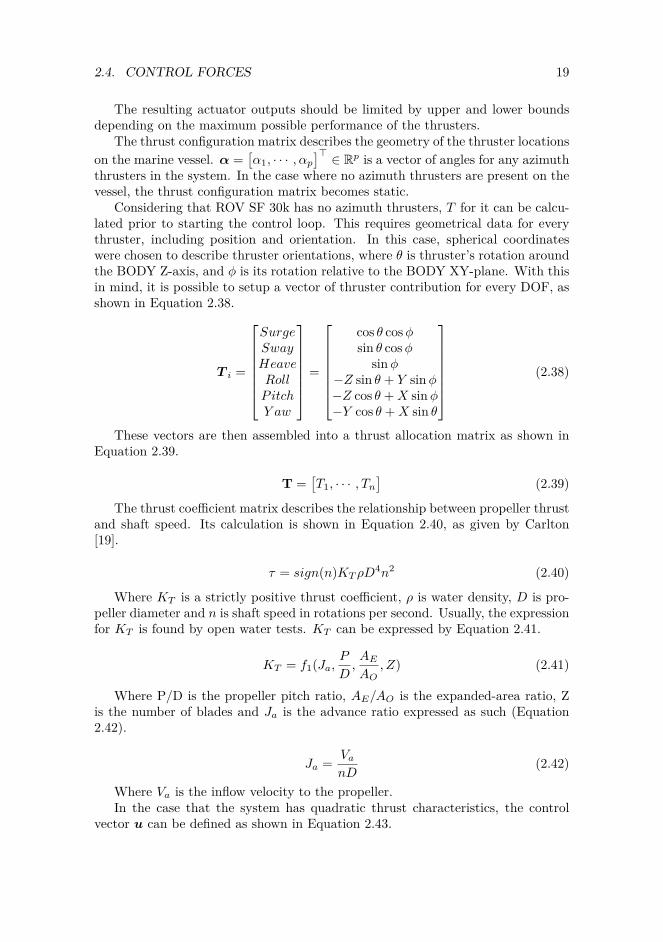
The resulting actuator outputs should be limited by upper and lower boundsdepending on the maximum possible performance of the thrusters.
The thrust configuration matrix describes the geometry of the thruster locationson the marine vessel. α =
[α1, · · · , αp
]> ∈ Rp is a vector of angles for any azimuththrusters in the system. In the case where no azimuth thrusters are present on thevessel, the thrust configuration matrix becomes static.
Considering that ROV SF 30k has no azimuth thrusters, T for it can be calcu-lated prior to starting the control loop. This requires geometrical data for everythruster, including position and orientation. In this case, spherical coordinateswere chosen to describe thruster orientations, where θ is thruster’s rotation aroundthe BODY Z-axis, and φ is its rotation relative to the BODY XY-plane. With thisin mind, it is possible to setup a vector of thruster contribution for every DOF, asshown in Equation 2.38.
T i =
SurgeSwayHeaveRollP itchY aw
=
cos θ cosφsin θ cosφ
sinφ−Z sin θ + Y sinφ−Z cos θ +X sinφ−Y cos θ +X sin θ
(2.38)
These vectors are then assembled into a thrust allocation matrix as shown inEquation 2.39.
T =[T1, · · · , Tn
](2.39)
The thrust coefficient matrix describes the relationship between propeller thrustand shaft speed. Its calculation is shown in Equation 2.40, as given by Carlton[19].
τ = sign(n)KT ρD4n2 (2.40)
Where KT is a strictly positive thrust coefficient, ρ is water density, D is pro-peller diameter and n is shaft speed in rotations per second. Usually, the expressionfor KT is found by open water tests. KT can be expressed by Equation 2.41.
KT = f1(Ja,P
D,AEAO
, Z) (2.41)
Where P/D is the propeller pitch ratio, AE/AO is the expanded-area ratio, Zis the number of blades and Ja is the advance ratio expressed as such (Equation2.42).
Ja = VanD
(2.42)
Where Va is the inflow velocity to the propeller.In the case that the system has quadratic thrust characteristics, the control
vector u can be defined as shown in Equation 2.43.

20 CHAPTER 2. VESSEL MODELLING
ui = |ni|ni (2.43)
where ui and ni are respectively the control component and the shaft speed forthruster i. Conversely, it is easy to find the shaft speed based on known controlinput:
ni = sign(ui)√ui (2.44)
This relation is useful when designing the thrust allocation system, as the ulti-mate goal of thrust allocation is providing shaft speeds for the actuators based onthe force control vector provided by the control algorithm. In this case, Equation2.37 has to be inverted. The resulting equation is as shown:
u = T †K−1τ (2.45)
Here, K−1 = 1/K and T † is the generalized inverse of the matrix T . Sincethe thrust allocation matrix is not necessarily square (in the cases where n 6= r),it is not always possible to take a direct inverse of it. The generalized inverse, alsocalled the pseudoinverse [20]. The generalized inverse is calculated as shown inEquation 2.46:
T †w = W−1T>(TW−1T>)−1 (2.46)
where W is a diagonal weight matrix. In the case where W = I, the equationis reduced (Equation 2.47):
T †w = T>(TT>)−1 (2.47)
and is called the Moore-Penrose pseudoinverse.

Chapter 3
Modelling of ROV SF 30k
3.1 Vessel modelIn this section, the process to evaluate or estimate the parameters of ROV Neptuneis shown. Certain parameters can be calculated analytically based on existingdocumentation, while other parameters cannot be computed directly, and have tobe estimated based on either empirical data, or reasonable approximations. A3-dimensional model of the ROV was provided by Sperre AS. It was designed inAutoCAD. This model was used as a base for calculating several parameters of themodel. The programs that were used are SolidWorks, Rhinoceros and WAMIT:
• SolidWorks (version: 2011 x64 bit) - a CAD (computer-aided design) pro-gram. In the scope of this thesis, it is used to redesign and simplify themodel of ROV SF 30k for use in other programs. It can also be used to setmaterial properties of different elements in the model, which can be used toevaluate weight, mass center, or moment inertia of the model.
• Rhinoceros 3D (version: 4.0) - a NURBS (Non-uniform rational basis spline)based 3D modelling program. In the context of this thesis, it is used as a toolto transform the NURBS-based 3D model of the ROV into a polygon meshthat can be analyzed in programs based on numeric algorithms, like WAMIT.
• WAMIT (version: v6) - a program for calculating motions and loads uponoffshore structures in waves. Despite it being primarily used for surface struc-tures in the wave zone, it can still be used to calculate certain parametersof underwater vessels that operate outside of the wave zone. These param-eters include, amongst others, added mass coefficients, buoyancy and centerof buoyancy.
• MATLAB (version: R2011b) - this program is mainly used as an assistancefor calculations. Several helping routines have been written in MATLABscript, particularly for dealing with the added mass coefficient matrix.
21

22 CHAPTER 3. MODELLING OF ROV SF 30K
3.1.1 Mass and added mass calculationsAll of the parameters in this section were evaluated using the aforementioned pro-grams. A detailed description of the usage of each program is outlined below.
SolidWorks
The program SolidWorks was used for several purposes, mainly for finding the rigidbody matrix and center of gravity, as well as for simplifying the model to a degreethat could be analyzed by WAMIT. The version of the program that was used wasSolidWorks 2011 x64 edition.
The first step was importing the AutoCAD drawing into the program. It had tobe converted to a SolidWorks compatible format. This generated an assembly withseveral parts, where every thruster is considered a separate part. In addition, thetwo electrical cylinders in the middle of the ROV are separate parts as well. Thelast part is the remaining structure of the ROV, including the floating element, theframe and the small components attached to it.
The unedited model was then used to calculate the rigid body matrix of theROV. An assumption was made that most of the features in the 3D model consistof steel. The amount of rubber or plastic components is insignificant in this case,and the assumption is then considered sufficiently accurate. Thus, every singlecomponent was converted to the material “Plain Carbon Steel”. After that, themass properties of the ROV were evaluated. This provided several key parameters,namely the mass, volume, center of gravity and moments of inertia at the originand at the center of gravity. Finally, the ROV was moved such that its centerof gravity coincided with the origin of the coordinate system. This significantlysimplified several future calculations, as well as the WAMIT simulations. Theunedited but converted model can be found in Appendix B.A.
The next step was simplifying the model in order to make it feasible for hy-drodynamic calculations in WAMIT. SolidWorks has a feature recognition systemcalled FeatureWorks. Its purpose is analysis of an imported structure, and itsbreakdown into elementary components that can be modified within the program(features, sketches, reference geometry). However, due to the complexity of theROV, as well as overlapping of components in several places, FeatureWorks wasnot able to analyze the structure properly. Thus, most of the editing had to bedone manually. This was performed in several steps:
1. Removal of unnecessary components - features such as small flat beams, orstructures embedded into the floating element from below. Such componentshave no significant effect on the hydrodynamic properties, and can thus beremoved without severely altering the results of the WAMIT simulations.
2. Breakdown and simplification of all the thrusters and electrical cylinders.Unlike the main ROV frame, the parts featuring the thrusters of the ROVwere simple enough to be analyzed using FeatureWorks. The thrusters werestripped of most of their elements, including the entirety of the electricalengines (since those are embedded into the floating element, and can be

3.1. VESSEL MODEL 23
assumed to have little influence on hydrodynamic properties of the ROV).Furthermore, at a later stage, it was found out that the fine cylindrical shapesof the thrusters did not mesh very well, and created various problems inWAMIT analysis (more on that later), which is why they were reduced tohollow octagonal cylinders.
3. Simplification of the floating element - due to the way it was designed, thefloating element was imported as a single continuous surface into SolidWorks.Thus, it had to be rebuilt from ground up. In the process, any irregularitieson its bottom (where it connects to the rest of the ROV structure) had beensmoothed out, as a compensation for the removal of embedded components,and to further reduce the polygon count of the model. The thruster housingtunnels were remodeled to be octagonal as well.
4. Simplification of the ROV frame - most of the beams used in the constructionof the ROV had the U-profile. These were replaced with solid beams withthe same outward dimensions. The small cylinder in the front of the ROVwas also reduced to an octagonal profile.
Figures 3.1 and 3.2 show the result of the simplification process performed onthe model:
Figure 3.1: Original AutoCAD model with added weight emulating sensory sys-tems.
It should be noted that the boxes on the bottom of the model are not the samesize. This is due to the fact that the models are used for different purpose. Thesmall box in the original model (top) serves as a way to estimate the approximateweight and moments of inertia of installed sensory equipment on SF 30k, with-out regards to its volume. The large box on the simplified model represents anapproximate volumetric equivalent of the equipment, and is used for volume (andthus buoyancy) and added mass calculations in WAMIT. The simplified model islocated in Appendix B.B.

24 CHAPTER 3. MODELLING OF ROV SF 30K
Figure 3.2: Simplified model intended for WAMIT analysis.
Conversion to WAMIT through Rhinoceros
Analyzing a model in WAMIT requires the input model to be converted to a meshand saved in a compatible file format. SolidWorks can perform neither of thoseactions, which is why a secondary program is used. In this case, Rhinoceros 4.0(henceforth named Rhino) was used. First, the simplified model was saved inSolidWorks as a .STEP file. This file was then opened in Rhino, and the model wasthen meshed using the meshing tool. The .STEP file (along with the Rhinoceros.3DM file as a backup) is located in Appendix B.C.
SolidWorks does not operate with polygon meshes, but rather with NURBS ob-jects (Non-uniform rational basis spline), which use curves and continuous curvedsurfaces to generate objects in 3D. When meshing curved objects, a very high reso-lution of a mesh is required to avoid geometrical artifacts. This leads to unnecessaryamounts of polygons, increasing WAMIT simulation times dramatically. This is theprimary reason for reducing all cylinders in the ROV model to octagons. Doingthat made it possible to mesh the ROV with the lowest possible resolution withoutsacrificing geometry detail, but reducing simulation time to just a few minutes.
The resulting polygon mesh was saved as a .GDF file, compatible with WAMIT.The heading of the file indicates that the mesh consists of 1484 polygons. It is alsoworth noting that during the conversion of the model in Rhino, the unit systemwas changed from millimeters to meters. The converted .GDF file can be foundalongside other WAMIT files in Appendix B.D
WAMIT simulation
WAMIT is a specialized program designed for calculating hydrodynamic wave loadsand motions on offshore structures. Despite being primarily used for wave calcu-lations, it can also be used to find added mass coefficients for underwater vesselsoutside of the wave zone provided a proper set of rules to use. The program must

3.1. VESSEL MODEL 25
be run through either a command prompt, or through a BATCH file, and the set-tings and parameters of the simulation are stored in several files. Below is a list ofthose files, as well as the settings used for calculation of added mass and buoyancyof ROV SF 30k. The documentation on setting up those files was found in [21]
• SF 30k.GDF - the Geometric Data File. This file describes the polygon meshthat the simulated object is described by. For SF 30k, the file was generatedby Rhino using the roughest polygon mesh settings possible.
• SF 30k.FRC - the Force Control File. This file stores the parameters for theFORCE subprogram of WAMIT. This file has 2 different forms (alternative1 and alternative 2). This is determined in the configuration file (.CFG), andthe form decides which parameters the file includes. In this case, alternativeform 2 was used.The first 9 integers indicate the hydrodynamic parameters that can be calcu-lated using this subprogram. For SF 30k, only the parameter 1 was chosen tobe calculated. The rest of the parameters are irrelevant outside of the wavezone. The first parameter describes added mass and damping coefficients. Itshould be noted that the damping coefficient only describes potential damp-ing resulting from wave forces, and is not calculated if the wave period is 0or infinite.Aside from the hydrodynamic parameters, the file stores information on thephysical parameters of the simulated body. The 3 numbers below the waterdensity (RHO) denote the center of gravity of the object relative to the centerof origin for the simulation (to be determined in the potential control file,.POT). Due to the fact that the ROV is centered at its geometric center ofmass in the 3D modelling programs, the CG vector is [0 0 0] in this case.The next block of data stores the 6x6 rigid body mass matrix of the body.In this case, the results of Mass Property evaluation of the original, uneditedmodel in SolidWorks were used. It is remarkable that the resulting rigid bodymass matrix is very similar to the one calculated on the rough model in theFall 2011 project. The last four numbers determine, respectively:
– IDAMP - the inclusion of the internal damping matrix, in this case 0.– ISTIFF - the inclusion of the internal stiffness matrix, also 0.
item NBETAH - the amount of Haskind wave headings to be simulated.Since wave forces are not relevant for this simulation, the number is setto 0 as well.
– NFIELD - the amount of points at the surface of the fluid domain to beevaluated. Also 0 due to irrelevance.
• SF 30k.POT - the Potential Control File. This file determines the parametersinput into the POTEN subprogram of WAMIT. Just like the Force ControlFile, it has 2 alternative forms. Alternative form 2 was used for this file.

26 CHAPTER 3. MODELLING OF ROV SF 30K
The parameters input into this file control the potential flow in the simulation,including wave behavior, body positions, water depth as well as specificationon whether the radiation and diffraction problems are to be solved.The first number (HBOT ) specifies dimensional water depth. This parameteris relevant when waves are included into calculations. In the case of SF 30k,since at this stage it operates outside of the wave zone, this parameter canbe chosen arbitrarily, in this case it’s 50m.The second line with two numbers (IRAD, IDIFF) controls whether radiationand diffraction problems are going to be solved during simulation. Bothoptions have 3 settings: -1 (do not solve the problem), 0 (solve the problemonly for specified degrees of freedom) and 1 (solve the problem for all degreesof freedom). At least one of the problems must be solved for the simulationto give any results. In this case, both options have been set to 1.The next four numbers determine the wave periods and headings in the sim-ulation:
– NPER - the amount of different wave periods, in this case 1.– PER - array of wave periods. Setting it to 0 will assume a wave period
of 0, and -1 assumes a wave period of infinity.– NBETA - the amount of incident wave headings, again, 1.– BETA - array of wave headings. The only heading specified is 0 degrees.
The last part of the .POT file determines the properties of the simulatedbody or bodies. NBODY specifies how many separate bodies are involved inthe simulation, each requiring its own .GDF file. The name of the .GDF fileis on the next line, in this case it’s SF 30k.gdf.The line of four numbers below the .GDF name (XBODY 1 ) specifies theX, Y, Z coordinates of the first body, as well as its heading relative to thecoordinate system used in WAMIT. It should be noted that WAMIT usesthe right-hand rule, but unlike most hydrodynamic calculations involving theearth-reference frame, Z is positive upwards and not downwards. Thus, theZ coordinate of -5 used for the SF 30k denotes that it is located 5m belowsurface of the water. The depth of the ROV is not relevant in this case, solong as it is completely submerged, since there are no wave forces acting uponit.MODES BODY 1 determines which degrees of freedom the diffraction and/orradiation problems should be calculated for. In this case, all the DOFs arechosen to be evaluated.Finally, the NEWMDS line is defined as “the number of generalized modesfor Kth body” (reference: WAMITv6.4 manual). In most cases, this optionis set to 0, but must be included in the .POT file regardless of the setting,just like NBODY.

3.1. VESSEL MODEL 27
• SF 30k.CFG - the Configuration File. This is the master configuration file,which controls most of the top-level parameters of the simulation, as well asdetermines which forms of .POT and .FRC are to be used in the simulation.Below is the list of options in the file:
– IPLTDAT determines whether a file containing panel and patch data isgenerated. Due to its irrelevance to this simulation, it is set to 0.
– MAXSCR specifies the allotted RAM for scratch storage for POTEN.– IFORCE and IPOTEN determine whether the FORCE and POTEN
subprograms should run. Both are set to 1.– IALTFRC and IALTPOT determine which forms of .FRC and .POT
files are used. Both are 2 in this case, as specified in the individual fileanalyses earlier.
– MAXITT determines the maximum amount of iterations POTENshould run. This is generally determined by the complexity of the model.The number 100 is probably unnecessary large for the relative simplicityof the ROV calculations, but it’s preferable to have a number too large,rather than too small.
– ISOLVE determines which solver should be used. ISOLVE=0 uses theiterative solver. The next several parameters (ISCATT, IQUAD, ILOG,IDIAG, IRR) calibrate the operation of the solver in POTEN. The valueschosen in the case of SF 30k are determined not to affect the results ofthe simulation with any significance.
– MONITR and NUMHDR operate with data output, and are not neces-sary to be changed, due to all the required data being output to separatefiles.
– USERIDPATH is standard installation procedure, and should be mod-ified according to the installation path for WAMITv6.
• fnames.WAM - File Name Manager File. This file determines which files areinvolved in the simulation. All of the above files are included in it.
• Simulation output - WAMIT outputs its data into several files, including an.OUT file, a .HST file, a .PNL file (determined by IPLTDAT ) and .* files,where * corresponds to the number of the option chosen in the .FRC file. Inthe case of the simulation of SF 30k, the following files were output:
– SF 30k.out– SF 30k.hst– SF 30k.1
All the required parameters can be extracted from the .OUT file, namely thecenter of buoyancy (Xb, Yb, Zb), which is determined to be:

28 CHAPTER 3. MODELLING OF ROV SF 30K
rb =[0.0822 −0.00773 0.3872
](3.1)
However, the main purpose of the simulation is the added mass coefficientmatrix. WAMIT outputs the matrix on a per-element basis, which mustfurther be edited into a single matrix. Using a simple MATLAB script (alsoincluded in Appendix B.D), the added mass matrix is properly formatted.It is worth noting a peculiar tendency of WAMIT to output an asymmetricaladded mass matrix. The values on the opposite sides of the main diagonalare not equal, even though they should be. This problem persisted withevery single simulation performed in WAMIT, even ones performed on asimple cube. Thus, the MATLAB script performs an additional function ofaveraging out the off-diagonal values. The resulting added mass matrix issymmetric, but must be multiplied by water density before being able to beused in simulators or observers.
The results of the simulations led to the following rigid body and added massmatrices:
MRB =
1862.87 0 0 0 0 0
0 1862.87 0 0 0 00 0 1862.87 0 0 00 0 0 525.39 1.44 33.410 0 0 1.44 794.20 2.600 0 0 33.41 2.60 691.23
(3.2)
MA =
779.79 −1.3053 −94.244 14.652 −165.06 −6.7288−12.449 1222 124.5 436.34 −20.566 59.971−112.4 −21.919 3659.9 −33.129 −382.17 −12.5712.433 382.55 45.351 534.9 −13.53 7.9038−166.02 8.868 −390.67 −6.5248 842.69 0.16383−8.8778 65.481 34.121 34.133 −2.4007 224.32
(3.3)
Using the MATLAB script, the matrix was symmetrized to the following:
MA =
779.79 −6.8773 −103.32 8.5426 −165.54 −7.8033−68.773 1222 51.29 409.44 −5.8488 62.726−103.32 51.29 3659.9 6.1112 −386.42 10.7748.5426 409.44 6.1112 534.9 −10.027 21.019−165.54 −5.8488 −386.42 −10.027 842.69 −1.1162−7.8033 62.726 10.775 21.019 −1.1162 224.32
(3.4)
3.1.2 DampingNonlinear damping
Unlike added mass, it is much harder to determine the damping coefficients for avessel without performing towing tests and determining the damping experimen-

3.1. VESSEL MODEL 29
tally. However, model-scale tests were performed on ROV Minerva. Minerva andSF 30k share many similarities, including the relative dimensions and approximateshape. Thus, it is possible to estimate the nonlinear damping coefficients for SF30k based on those of Minerva with a decent degree of accuracy. According to [16],the nonlinear damping coefficients for Minerva are as follows:
Cd,NL(Minerva) =
0.870.991.051.001.001.00
(3.5)
In order to convert them into a nonlinear damping matrix, these coefficientshave to be multiplied by projected area of the ROV in surge, sway, heave and alongthe axes of rotation of the ROV. The projected area was calculated in SolidWorks(The relevant files are located in Appendix B.E). A rough sketch of an area wasdrawn in every DOF. The sketch was then converted into a feature (extruded bossin this case), and its projected area was measured using the “Measure” tool. Theresulting projected areas are as follows:
Aproj =
1.67811.95623.38404.31073.84492.6410
[m2] (3.6)
These values make it possible to calculate nonlinear damping in translationalDOFs using Morrison’s equation:
DNL = 12ρCdAproj |vr| (3.7)
Thus, the nonlinear translational damping coefficients were found to be:
DNL,trans = diag748.22|ur|, 992.53|vr|, 1821.01|wr| (3.8)
However, this method is not applicable to rotational DOFs. It was thus decidedto scale up the nonlinear damping values from ROV Minerva. According to [16],the nonlinear damping values for ROV Minerva are:
DNL = diag292|ur|, 584|vr|, 635|wr|, 84|p|, 148|q|, 100|r| (3.9)
The last three values are scaled up using the scaling factors found by comparingthe dimensions of the two ROVs. According to [22] and Appendix A, the two ROVshave the dimensions outlined in Table 3.1.
Scaling was performed based on geometric similarity [23], using the largestapplicable scale factor. The formula used is as follows:

30 CHAPTER 3. MODELLING OF ROV SF 30K
Fs = ρsρm
λ3Fm (3.10)
where ρs and ρm are water density for full-scale ship and the model respectively,and λ is the scaling factor. This equation is used to scale up forces from modeltests to ship dimensions, but here, it can be used to scale dimensions from Minervaup to SF 30k. In this case, Fs denotes the nonlinear damping forces for SF 30k,while Fm denotes the same forces for Minerva.
Using 3.1.2, 3.9 and 3.10, the following rotational nonlinear damping coefficientswere found:
DNL,rot = diag672|p|, 774.44|q|, 523.27|r| (3.11)
Combining 3.8 and 3.11, the following nonlinear damping matrix is achieved:
DNL =
748.22|ur| 0 0 0 0 0
0 992.53|vr| 0 0 0 00 0 1821.01|wr| 0 0 00 0 0 672|p| 0 00 0 0 0 774.44|q| 00 0 0 0 0 523.27|r|
(3.12)
Linear damping
Linear viscous damping is harder to estimate than its nonlinear counterpart, andoften requires model scale or full scale tests. For Minerva, the damping forces werefound by bollard pull tests of the ROV, where the pulling force loss is compared toquadratic damping calculated previously. The force loss was larger than estimatedby the nonlinear damping equations, and the remainder was thus attributed to lin-ear damping forces. The linear damping matrix was then estimated based on this.The linear damping coefficients were estimated as a percentage of the nonlinearones, as follows [16]:
Table 3.1: Dimension and scale comparison of ROV Minerva and ROV SF 30k.Dimensions[m] Scale
Minerva SF 30k λ1.44 2.50 1.73610.82 1.50 1.82930.80 1.60 2.0000

3.1. VESSEL MODEL 31
DL = diag
10%7%40%40%40%20%
DNL (3.13)
Due to the lack of test data for ROV SF 30k, the most accurate method ofcalculating linear viscous damping would be to use the linear damping correlationsfrom ROV Minerva. These values can be calibrated once sea trials begin. Thus,the linear damping coefficient matrix for SF 30k is calculated to be:
DL =
74.82 0 0 0 0 0
0 69.48 0 0 0 00 0 728.40 0 0 00 0 0 268.80 0 00 0 0 0 309.77 00 0 0 0 0 105.00
(3.14)
3.1.3 Restoring forces and momentsOne of the parameters output in the WAMIT .OUT file is the volume of the vessel.The data, just like buoyancy data, can be found in the header of the file. Any ofthe three calculated volumes can be used. Thus, the volume displacement of theROV is found to be V OLX = ∇ = 1.83826m3. Multiplying it by the density of seawater and then by the gravitational constant, it is possible to obtain the buoyancyforce upon the ROV when fully submerged: B = ρ∇g = 1025 · 1.83826 · 9.81 =18484.168N . The weight of the ROV is W = mg = 1862.87 · 9.81 = 18274.75NThus, the net difference is B−W = 18484.16−18274.75 = 209.4N . This differenceis a bit too large, and is most likely caused by rounding errors due to the fact thatthe volume of the ROV was calculated using a simplified model.
The restoring forces are calculated based on the relative positions of the centerof gravity and the center of buoyancy. Since the ROV is positioned such that itscenter of gravity is at the center of origin, the following applies:
rCG =
000
[m], rCB =
0.0822−0.00770.3872
[m] (3.15)
3.1.4 Umbilical forcesAccording to Appendix A, the diameter of the umbilical is 27mm, that is, d =0.027m. The drag coefficient is assumed to be Cd = 1.2. The cable weight is notgiven, however, the cable can be assumed to be approximately neutrally buoyant,due to being designed for use underwater.

32 CHAPTER 3. MODELLING OF ROV SF 30K
The attachment point of the cable is assumed to be at the top of the ROV,approximately directly above the CG. Thus, rx = ry ' 0. Using the 3D model ofthe ROV, the vertical arm was found to be rz = 0.9317m.
Assuming uniform current speed ur, it is possible to set up the following um-bilical force vector:
τ cable =
−8.3025h|ur|ur−8.3025h|vr|vr
07.7354h|ur|ur7.7354h|vr|vr
0
(3.16)
3.2 Thrust allocationModelling thrust allocation for an ROV involves calculating three main parameters:the thrust allocation matrix T, which specifies the configuration of the thrusters onthe vessel; the thrust coefficient matrix, which establishes dependencies betweenapplied thruster RPM and the resulting thrust; and finally, the thrust loss coeffi-cients, which compensate for any thrust losses affecting the propulsion system ofthe vessel. Unfortunately, it is impossible to find thrust losses without any kind ofempirical data, and thus they will have to be estimated.
3.2.1 Thrust configuration matrixFor ROV SF 30k, it is possible to calculate the thrust configuration matrix basedon the model provided by Sperre, since this matrix is based purely on geometricdata. Unfortunately, the thrust allocation subroutine in the control system requiresthe thruster data to be input in a specific order, which is impossible without actualtrial and error. Thus, for the purposes of this document, the thrusters were giventheir IDs arbitrarily, with the possibility of switching out their IDs later.
SF 30k has 6 thrusters, which means that it is fully actuated. Figures 3.3, 3.4and 3.5 show the positions and orientations for all the thrusters.

3.2. THRUST ALLOCATION 33
Figure 3.3: ROV thruster positions, top view.

34 CHAPTER 3. MODELLING OF ROV SF 30K
Figure 3.4: ROV thruster positions, side view.
Figure 3.5: ROV thruster positions, front view.

3.2. THRUST ALLOCATION 35
The preliminary IDs have been given to the thrusters based on the top view,shown in figure 3.6.
Figure 3.6: ROV thruster IDs.

36 CHAPTER 3. MODELLING OF ROV SF 30K
The positions and orientations of all the thrusters were found by measuringthem in SolidWorks using the “Measure” tool, relative to the center of gravity(which coincides with the center of origin of the model). Thruster orientation datawas output in spherical coordinates relative to body center of origin, as this signifi-cantly simplified the setup of thrust allocation. A table reflecting the measurementsis shown in Table 3.2.
Table 3.2: Thruster positions and orientations for ROV SF 30k.
Thruster ID Thruster position Thruster orientationX[m] Y[m] Z[m] θ[deg] φ[deg]
1 0.4878 0 -0.2373 -90 902 -0.8217 0 -0.5890 0 153 0.8654 -0.5322 -0.5332 90 22.54 0.8654 0.5322 -0.5332 -90 22.55 -0.7076 -0.5129 -0.2404 -25 906 -0.7076 0.5129 -0.2404 25 90
The coordinates are given in the BODY coordinate system, with the X axispointing forward, the Y axis pointing to the starboard (right) side and the Z axispointing downward. The angle θ is measured as a rotation about the Z axis, positivewhen clockwise if looking from above. The angle φ is measured as a rotation awayfrom the Z axis, with 0 being pointing straight down, 90 being horizontal and180 straight up.
It is worth noting that all the thrusters have a negative Z coordinate, that is,they are located above the center of gravity of the ROV. This will create a netpitch or roll moment when moving in horizontal degrees of freedom. However, theROV’s high restoring moment will prevent it from pitching or rolling to a significantdegree.
Another noteworthy mention is that the control box installed on SF 30k doesnot allow control of individual vertical thrusters. Instead, they are combined intoa single “vertical thruster”. Thus, the thrust allocation system must reflect thislimitation. Thrusters 2, 3 and 4 are combined into a single thruster. The positionof their combined thrust force vectors is calculated as an average of thrust con-tributions of every thruster. Since thrusters 3 and 4 face in opposite horizontaldirections (positive and negative in sway), they offset each other’s contribution insway, and their orientations θ and φ can be assumed to be 0 and 90 respectively.The average of the positions and orientations for the combined thruster can nowbe calculated using equations outlined in 3.17.

3.2. THRUST ALLOCATION 37
Table 3.3: Thruster positions and orientations with combined vertical thrusters.
Thruster ID Thruster position Thruster orientationX[m] Y[m] Z[m] θ[deg] φ[deg]
1 0.4878 0 0.2373 90 902 0.2862 0 0.5518 0 53 -0.7076 -0.5129 0.2404 -25 904 -0.7076 0.5129 0.2404 25 90
Xvert =∑4
i=2Xi
i
Yvert =∑4
i=2Yi
i
Zvert =∑4
i=2Zi
i
θvert =∑4
i=2θi
i
φvert =∑4
i=2φi
i (3.17)
Here, Xi, Yi, Zi, θi and φi are the position and orientation data for thrusterID i.
The rest of the thrusters that come after the combined vertical thruster havehad their thruster IDs shifted so as to match the reduced thruster count. Thus,the modified thrust ID Table 3.3 is set up.
The geometrical data is input into the control system, which calculates thethrust allocation matrix according to Equation 2.38. This is repeated for everythruster in sequence. The vectors are then inserted into the matrix. The result isas shown in Equation 3.18.
T =
0 0.0872 0.9063 0.90631 0 −0.4226 0.42260 0.9962 0 0
−0.2373 0 −0.4113 0.41130 −0.2815 0.2179 0.2179
0.4878 0 0.7639 −0.7639
(3.18)
3.2.2 Thrust coefficient matrixThe thrust coefficient matrix for SF 30k is derived from the thrust-RPM curvesprovided by Sperre AS (Appendix C). According to Sperre AS, the thruster modelused in SF 30k is Sleipner SP 125 T. The thrust-RPM curve in Appendix C islabeled as SE 120, which is what is going to be used in the calculation of thrustcoefficient data. No data for maximum RPM was given for the thrusters, and it is

38 CHAPTER 3. MODELLING OF ROV SF 30K
thus assumed that it is similar to the RPM boundaries for ROV Minerva [24], andis set to be 1500.
The curve is quadratic, and thus the coefficient matrix is not constant. However,it is possible to derive a simple equation for the curve based on the provided data.This is performed by regressing the graph in MATLAB, and then using the foundcoefficients in a second-degree equation shown in 3.19.
τ = A ·RPM2 (3.19)
where A is the quadratic coefficient to be found through regression.Quadratic regression requires at least 3 uniquely defined entries in the data set
that is to be regressed. For the sake of simplicity, the graph endpoint (2300, 1540)was used as one of the entries. This point was then mirrored across the Y-axis, toget the point (-2300, 1540). Including the point of origin (0, 0) and regressing theresulting data set will result in a parabolic curve, where the section of it to theright of the Y-axis (positive X-values) is the regressed thrust-RPM curve. It shouldbe noted that the section of the curve to the left of the X-axis does not reflect thephysical behavior of the thruster, but is merely included to provide a 3rd uniquepoint for curve regression.
The data set was defined as two vectors in MATLAB, and can be seen inEquation 3.20.
RPM =
−23000
2300
, τ =
15400
1540
(3.20)
These vectors were plotted using the “plot” command and then fitted with aquadratic function to find the coefficients. Figure 3.7 shows the regression processof the thrust-RPM curve.
Figure 3.7: The regressed thrust-RPM curve and the fitted coefficient.

3.2. THRUST ALLOCATION 39
As can be seen from the figure, the coefficient was found to be A = 0.00029112.Thus, the final RPM-to-thrust equation is shown in Equation 3.21.
τ = 0.00029112 ·RPM2 (3.21)
3.2.3 Thrust lossUnfortunately, no towing tests were performed on ROV SF 30k, and as such, thereis no thrust loss data accumulated for this ROV. Therefore, a preliminary set ofconservative thrust loss coefficients was used in the scope of the project. Everythrust loss factor was set to 40%, as shown in Equation 3.22.
Cl =
0.40.40.40.40.40.4
(3.22)

40 CHAPTER 3. MODELLING OF ROV SF 30K

Chapter 4
Control system
The control system for ROV Neptune was developed in LabVIEW, which is agraphical programming language not too dissimilar to MATLAB Simulink. Thedevelopment of the program is outlined in Master’s Thesis by Espen Tolpinrud [1].This chapter outlines the development and modification of individual sections ofthe control system on the plant control layer (see Figure 1.3).
4.1 6DOF adaptationThe original system, which was tailor-made for ROV Minerva, was limited by thefact that it operated in 4 DOFs. One of the goals of this thesis was to delivera more generalized system, one which is able to provide fully actuated control inall 6 DOFs. Most of the main elements of the system had to be modified to beable to provide additional control in pitch and yaw, including the observer, thecontroller(s), the tracking/guidance subsystems and the thrust allocation system.
4.1.1 ObserversSector Kalman Filter
The Kalman Filter observer from the old system has been translated to the newstructure. The output is transformed to work with a 6DOF system. However, theobserver is not actually 6DOF.
The linearization has only been done with respect to 36 different yaw angles. Ifthis were to be done for both roll and pitch as well, the initialization would needto iterate and store values from 363 iterations for a sampling interval of 10 degreesin each rotation direction. The performance requirement needed can be calculatedby the following formulas:
N ×$ = Memory requirement (4.1)
41

42 CHAPTER 4. CONTROL SYSTEM
N is the number of elements to be stored and $ is the data size. The pro-cessor usage can be found by identifying FLoating-point OPerations (flop) in theroutine and how many FLoating-point Operations Per Second (flops) the processoris capable to perform.
σflop × niter = flop (4.2)χ×core ×ncore = flops (4.3)
flop
flops= t (4.4)
σ is the number of flop per iteration, n is the number of iterations. In Equation4.3 χ is number of flop the processor is able to perform on each cycle. On modernprocessors this is usually 4. f is the clock frequency or cycle frequency of theprocessor, and m is the number of cores available on the processor.
(2× (18× 363 × 18) + 18× 363 × 6)× 8B = 282175488B ∼= 282MB (4.5)
The expression in Equation 4.5 applies for the linearization matrices Φ, Γ and∆ in the Kalman Filter. 282 MB free memory is needed for each Kalman Filterobject initialized in the system in order to store these matrices.
6943 flop
iteration× 363 iterations = 323932608 flop (4.6)
4 flopcycle
× 1.6e9 cyclessecond
× 4 cores = 25.6e10 flops (4.7)
323932608 flop25.6e9flops
∼= 0.01seconds (4.8)
The values in Equation 4.3 is based on the authors PC which has a Intel i7-720QM [25], hence the numeric result in Equation 4.4 is only valid for this processor.It should however be noted that the difference in run-time performance for thedifferent processors is of O(10−2), hence the calculation time for the matrices canbe neglected.
With the results given in Equations 4.5 and 4.8 there should in theory be noproblem running a 6DOF linearized Kalman Filter on a modern PC. However, thesystem performance may be reduced due to large memory operations, especially ifglobal variables are used [26], [27].
Passive non-linear observer
A Passive Non-Linear observer was implemented in order to have access to a 6DOFobserver for the system. The algorithms outlined for this observer described in [2]and [12] applied to a 3DOF surface vessel in DP, hence the equations had to beslightly modified in order to be suitable for an ROV. The notation used in Equation4.9 is explained in Table 2.1.

4.1. 6DOF ADAPTATION 43
˙ξ = Aw +K1(ω0)y (4.9)˙η = J(η)ν +K2y (4.10)˙b = −T−1b+K3y (4.11)
M ˙ν = −DLν −DNL|ν|ν + J−1b+ τ + J−1K4y − Cν (4.12)y = η + Cw ξ (4.13)
In the implementation y = η was chosen in order to have full 6DOF system. Itis also possible to expand the the observer to include velocity measurements.
The observer gains must be tuned to retain its passivity, and to relate the gainsto the dominating wave response frequencies. [12] proposes the following rules forpassive observer tuning.
The four gain matrices K1,K2,K3,K4 are all diagonal:
K1 =[diagk1, · · · , k6diagk7, · · · , k12
](4.14)
K2 = diagk13, · · · , k18 (4.15)K3 = diagk19, · · · , k24 (4.16)K4 = diagk25, · · · , k30 (4.17)
where the values k1, · · · , k30 have the following proposed values:
ki =
−2(ζni − ζi)ωci
ωiif i = 1, · · · , 6
2ωi(ζni − ζi)ωci
ωiif i = 7, · · · , 12
2ωci if i = 13, · · · , 18(4.18)
where ωci > ωi is the filter cut-off frequency. ζci > ζi is a tuning parameter(between 0.5 and 1.0). ki, i = 19, · · · , 24 should be large enough to ensure properbias estimation. The values ki, i = 25, · · · , 30 have to be tuned according to thefinal performance of the observer.
ωi = 2πTpi
is the peak response frequency. In most cases, this frequency can beapproximated to the peak wave frequency. This is especially true for ROVs, whichare much more sensitive to the different wave frequencies than, for example, a ship.
Adaptive observer
In addition to the 4DOF Kalman Filter and the 6DOF Nonlinear Passive Observer,an adaptive observer was implemented into the system. This observer is designedfor situations where the parameters of Aw are not known [28]. This particularfeature makes the observer able to adjust wave filter gains to the current sea statethrough an iterative process, thus making it viable to use in the wave zone forprolonged periods of time. It is uncommon to conduct important missions with an

44 CHAPTER 4. CONTROL SYSTEM
ROV in the wave zone. However, with the addition of the adaptive observer, it ispossible to extend the range of ROV operations closer to the surface.
Adaptive observer design is based on augmented observer equations (equations4.19 through 4.23) [2].
˙ξ =Awξ +K1hyf (4.19)˙η =J(η)ν +K2y +K2lxf +K2hyf (4.20)˙b =− T−1
b b+K3y +K3lxf (4.21)M ˙ν =−Dν − J>(η)Gη + J−1(η)b+ τ
+ J−1(η)(K4y +K4lxf +K4hyf ) (4.22)
y =η +Cwξ (4.23)
where K1h ∈ R12×6 and K2l,K2h,K3l,K4l,K4h ∈ R6×6 are additional gainmatrices to be determined. A new state has been introduced: xf , which is thelow-pass filtered innovation. It is defined as shown in Equation 4.24 [28].
xf = −T−1f xf + y = −T−1
f xf + η +Cwxi (4.24)
where xf ∈ R6, and T f = diagTf1, · · · , Tf6 contains filter constants. Thehigh-pass filtered innovation yf can be derived from 4.24 in the form of Equation4.25
yf = xf (4.25)
The adaptive observer operates with the estimation problem where the param-eters of Aw are unknown [28]. The elements in the matrix vary depending on thecurrent sea-state. Assuming decoupled motions, the composition of the matrix Aw
is shown in Equation 4.26.
Aw(θ) =[06×6 I6×6−Ω2 −∆Ω
],
[06×6 I6×6
−diag(θ1) −diag(θ2)
](4.26)
where θ =[θ>1 ,θ
>2]>. The vectors θ1,θ2 ∈ R6 contain the unknown values
that are to be estimated. In order for the adaptive law to operate, it is assumedthat these values are constant or at least slowly-varying compared to the systemstates.
Thus, the new WF model is modified as shown:
˙ξ = Aw(θ)ξ +K1hyf (4.27)
The parameter update law for θ is as follows:
˙θ = −ΓwΦ(ξ)Chxa = −ΓwΦ(ξ)yf ,Γ > 0 (4.28)
The regressor matrix Φ(ξ) is defined as:

4.1. 6DOF ADAPTATION 45
Φ>(ξ) ,[diag(ξ1) diag(ξ2)
](4.29)
The tuning matrices K1h,K2l,K2h,K3l,K4l and K4h should be tuned ina similar manner to the original matrices K1,K2,K3 and K4, as described inSection 4.1.1.
The complete structure of the adaptive observer is displayed in Figure 4.1. Thestructures for the bias and wave estimators, as well as the wave filter, are shownin Figures 4.2, 4.3 and 4.4.
Figure 4.1: Complete model of the adaptive nonlinear passive observer.
4.1.2 Guidance systemsThere are two main guidance systems implemented in the system as of June 2012.These are Dynamic Positioning and Joystick mode. The DP guidance system isbased on the work done in [29]. Some small modifications in vector and matrixdimension have been done, as well as a new architecture of the method. However,the logic is the same.

46 CHAPTER 4. CONTROL SYSTEM
Figure 4.2: Wave filter subsystem including adaptive law.
Figure 4.3: Modified bias estimator.
The Joystick mode is based on the work done by Fredrik Dukan in [30]. Somesmall modifications have been done in the implementation here as well as the

4.1. 6DOF ADAPTATION 47
Figure 4.4: Modified wave estimator.
joystick input have been mapped to a number ∈ [−100, 100] rather than using a bitvalue ∈
[−215, 215]. This mode has three main modes, direct Thrust Allocation,
Position Reference, and Velocity Reference. The joystick frame can also be modifiedbetween body and NED.
Implementation of a third guidance strategy was attempted. This was a track-ing model with a synthetic reference model[31]. However, the complex nature ofthe guidance strategy created problems during implementation and due to short-age of time, it was abandoned. All guidance systems implemented are set up for6DOF reference generation. However, only 4 DOFs (Surge/North, Sway/East,Heave/Depth and Yaw/Heading) are given reference values from the user.
4.1.3 ControllersA selection of controller algorithms was developed for ROV Minerva. When thesystem was rewritten to accommodate 6 DOFs, the controllers had to be redesignedto be able to control pitch and roll as well as the other 4 DOFs. There are 4 differentcontrollers implemented in the system:
• Linear PID Controller - a very basic control algorithm.
• Non-linear PID Controller - an expansion of the linear PID Controller, in-cluding a feedforward term. In the old control system for ROV Minerva, thiscontroller was preferred for full scale tests [16].
• LQR Controller - built on the framework of the non-linear PID controller,but calculates the proportional and derivative controller gain matrices (re-spectively Kp and Kd) by solving the Riccati equation.
• Sliding Mode Controller - controls the system by forcing it to converge to astable set of state variables, the so-called sliding surface.
The nonlinear PID, LQR, and the Sliding Mode controller are based on theones described in [16].

48 CHAPTER 4. CONTROL SYSTEM
Every controller requires adjustments in 2 main areas: integrators and tun-ing matrices. Due to the way the integrators are implemented, they have to beexpanded from 4DOF to 6DOF, most notably the integrator initializing vectorsand integrator limits. The tuning matrices also have to be adjusted, in order toaccommodate the additional 2 DOFs.
The 6DOF implementation is backwards-flexible. The controllers can now beused for controlling 6DOF systems, while retaining the possibility of controllingsystems with a reduced number of DOFs. This is achieved by simply setting thecontroller gains for the irrelevant DOFs to 0.
4.1.4 Thrust allocationDuring the implementation of the thrust allocation algorithm, several alterationsto the system were made in order to increase its adaptability in case of thrusterfailure. The thrust allocation matrix is calculated in real-time during the operationof the system. This allows to make it possible to dynamically alter the matrix in thecase of thruster failure. Any thrusters set to be disabled will be excluded duringcomputation of the matrix. In the future, an algorithm to detect any disabledthrusters can be created, which would allow for the operation of the ROV to beautomatically adjusted in case of partial failure.
During the calculation of the thrust allocation matrix, a check is performedon the contributions of the thrusters for different DOFs. Since the algorithm isnumeric, small rounding errors are present when calculating contributions that areclose to 0. In order to avoid unnecessary strain on the ROV motors, errors below10−6 are rounded down to 0.
The control vector u that comes out of the thrust allocation algorithm is con-verted to n[RPM ] via Equation 2.45, and is then limited using a saturation func-tion. This function prevents the values in the RPM vector from increasing past themaximum allowed rotational velocity.
4.2 SF 30k telecommunication implementationThe telecommunication buffer, also called telebuf, is the means by which the ROVcommunicates with the control system. It is set up in such a way as to be ableto be interpreted by the local system installed onboard the ROV. This systemis what dictates which format the telebuf should operate in. In this case, thetelecommunication format was developed by Sperre AS, who developed both ROVMinerva and ROV SF 30k. As a result, the telebufs for the two ROVs are verysimilar. This significantly simplifies the implementation of the buffer for SF 30k.
In addition, as per request, Sperre AS sent a document with brief descriptionsof the telebuf entries. Some of the entries, however, were not properly explained,and thus required further investigation by direct testing. Fredrik Dukan performedthis job, and set up a working telebuf for SF 30k, which was then used in the controlsystem.

4.3. SIL AND HIL SIMULATOR MODELS 49
The telebuf consists of 23 bytes of data, used for transmission of control signalsto the thrusters and equipment (cameras and lights). Appendix D shows a detailedbreakdown of the telecommunication signals, along with the content of the originalemail. Since each byte of data can hold any value from 0 to 255, certain bytes areable to control more than one device or setting.
The biggest limitation of using this telebuf system comes when controllingthrusters. Due to the fact that one can only transmit 256 different values meansthat each thruster can only have 256 speed setpoints. When considering that ev-ery thruster is bidirectional, this amount is further reduced to 127 setpoints perdirection (as well as one for no thrust, and one leftover). Divided by maximumthruster speed, this would mean that the thrusters can only be controlled in stepsof 1500/127 = 11.8RPM. However, experiments have shown that the actual resolu-tion is even less, and every thruster only has 64 setpoints in either direction, whichresults in steps of 1500/64 = 23.4RPM.
4.3 SIL and HIL simulator modelsIn order to be able to test Njord without introducing the risk of equipment damageduring sea trials, a simulation environment is required. Two simulation systems aredeveloped for ROV Minerva: a SIL (Software In the Loop) and a HIL (HardwareIn the Loop) simulator.
Hardware In the Loop testing technology utilizes the idea of creating a virtualsimulation environment that emulates large parts of the system [32]. The mainadvantage using a HIL simulator lies in the ability to test the functionality ofthe control system in any kind of failure state, saving large amounts of time andexpenses. A HIL simulator is able to detect the following:
• Erroneous configuration parameters
• Design flaws in the software
• Sleeping and hidden software errors
• Missing functionality
• Errors in documentation
In the case of Njord, this simulator can be used to detect any flaws in thedesign of the system, as well as eliminate most of the implementation errors. Itruns on a separate closed-loop system, typically communicating with the systemthrough an interface similar to the interface on the actual ROV. The SIL simulatoroffers a similar functionality, however it has distinct advantages and disadvantagescompared to the HIL version, such as being able to simulate the system at a muchfaster pace, resulting in shorter simulation time, at the cost of being unable toperform online tuning and adjustments [1].
The basic premise of a HIL simulator is presented in Figure 4.5 (from [33]) .The simulator replaces the actual controllable environment with a virtual system
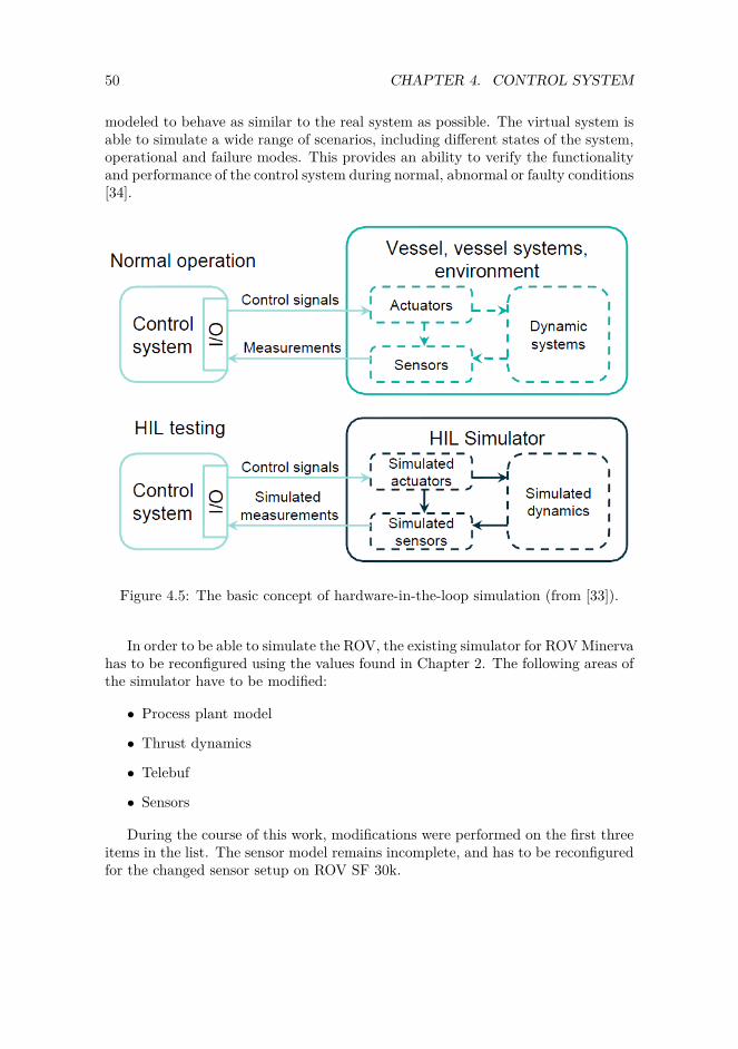
50 CHAPTER 4. CONTROL SYSTEM
modeled to behave as similar to the real system as possible. The virtual system isable to simulate a wide range of scenarios, including different states of the system,operational and failure modes. This provides an ability to verify the functionalityand performance of the control system during normal, abnormal or faulty conditions[34].
Figure 4.5: The basic concept of hardware-in-the-loop simulation (from [33]).
In order to be able to simulate the ROV, the existing simulator for ROVMinervahas to be reconfigured using the values found in Chapter 2. The following areas ofthe simulator have to be modified:
• Process plant model
• Thrust dynamics
• Telebuf
• Sensors
During the course of this work, modifications were performed on the first threeitems in the list. The sensor model remains incomplete, and has to be reconfiguredfor the changed sensor setup on ROV SF 30k.

Chapter 5
Commissioning and sea trials
A couple of days before the sea trial for the ROV 30k, a series of wet tests wereconducted. These were aimed at checking the functionality of original system andensuring that it worked properly. The vessel’s behavior had to be modified suchthat it had a good balance both in weight-buoyancy ratio and weight distribution.After some weight had been added to the ROV, it seemed more relaxed and easyto control.
The night before the sea trial, the ROV was finally ready to be connected tothe new control system. However, during the sea trials, time had to be used onestablish full communication between the control system and the ROV. As this wasthe first time the control system were connected to 30k, there were problems in thesensor setup which had to be fixed before the ROV could be launched in the sea.After the communications were established, the manual thrust control mode wasused to check maneuverability given the thruster allocation developed in Section3.2. The new control system is superior to the original system in this area as thedesired thrust is run through thruster allocation. Unwanted movement is then tosome degree accounted for, i.e. compensation in pitch angle when going forward.
Due to limited window of operation, tuning of the Kalman Filter was prioritizedinstead of the Nonlinear PID controller, as it was a necessity in order to be able totry the DP system. After reducing the response of the estimated surge and swayvelocities, u and v, the observer behaved in accordance with the measured values.The bias component had to be tuned as well, as there were stationary deviationsin the North and East position estimates.
Figure 5.1 shows the position data for 30k during DP operation. From 10to about 90 seconds the ROV performed station keeping at its position at theactivation time for DP Mode, ηref = [0, 0, 33.5, 2.2, 1.8,−50]>. Even though theNonlinear PID controller was not tuned, it managed to keep the ROV on position.The lack of controller tuning can especially be seen in the transit between twoset points. After about 90 seconds a new position was given to the ROV, ηref =[2, 0, 33.5, 0, 0, 0]>. The first graph in Figure 5.1 indicates that the proportionalgain is too low. This is in accordance with the fact that the tuning values used areexactly the same as for Minerva, which is a much smaller and more agile ROV. The
51

52 CHAPTER 5. COMMISSIONING AND SEA TRIALS
0 100 200 300 400 500 600 700−4
−2
0
2
4
Time [s]
No
rth
[m
]North
Measured
Estimated
Desired
0 100 200 300 400 500 600 700−4
−2
0
2
4
Time [s]
Ea
st
[m]
East
Measured
Estimated
Desired
0 100 200 300 400 500 600 70031
32
33
34
35
Time [s]
De
pth
[m
]
Depth
Measured
Estimated
Desired
Figure 5.1: Plots of Translational motion during DP test.
reference model parameters in the guidance system were also suited for Minervarather than 30k, which can be seen by the rapid increase in desired position.
The orientation of the ROV during DP operation is shown in Figure 5.2. Graphnumber three is of most interest as it illustrates the heading angle of . It can be seenthat the controller makes the ROV follow the reference. However, the same problemas described above yield in yaw as the controller is too weak to reduce the error in atimely manner. The orientations of the ROV is measured with a Xsense MTi [35],which is a gyro-enhanced Attitude and Heading Reference System (AHRS). Thissensor has its own observer and is more accurate than the compass measurementsfrom the DVL. The estimated attitude values are sent to the Kalman Filter in orderto estimate the yaw rate, r, as well as being used in the estimated position vector,η. Because of this the plot of the measured heading values is hidden behind theestimated values.
In Figure 5.2, the first station keeping period (10-90 seconds) has desired valuesin accordance to the logic mentioned above, i.e. station keeping of position atactivation time for DP Mode. When a new reference position is given, a faultoccurs in the desired roll value. This should have been set to zero. However,as both roll and pitch are not independently controlled due to the ROV thruster

53
configuration, the fault never propagates and becomes a failure.
0 100 200 300 400 500 600 700−2
0
2
4
6
Time [s]
Ro
ll [d
eg
]
Roll
Measured
Estimated
Desired
0 100 200 300 400 500 600 700−2
0
2
4
6
Time [s]
Pitch
[d
eg
]
Pitch
Measured
Estimated
Desired
0 100 200 300 400 500 600 700−100
0
100
200
Time [s]
Ya
w [
de
g]
Yaw
Measured
Estimated
Desired
Figure 5.2: Plots of Rotational motion during DP test.
After about 680 seconds in Figure 5.1 and 5.2, or 50 seconds in Figure 5.3 and5.4 manual thrust control with joystick was activated. These plots indicate thatthe observer manages to follow the measurements in a satisfactory manner, hencethe Kalman Filter is working properly.
In Joystick Mode with Force control frame, the desired position values are setto the estimated values, ηd = η. This results in a plot with only one graph for yawangles as measured, estimated and desired values are the same.

54 CHAPTER 5. COMMISSIONING AND SEA TRIALS
0 100 200 300 400 500 600 700 800 900 1000−20
−10
0
10
Time [s]
Nort
h [m
]
North
Measured
Estimated
Desired
0 100 200 300 400 500 600 700 800 900 1000−10
0
10
20
Time [s]
East [m
]
East
Measured
Estimated
Desired
0 100 200 300 400 500 600 700 800 900 10000
10
20
30
40
Time [s]
Depth
[m
]
Depth
Measured
Estimated
Desired
Figure 5.3: Plots of Translational motion during Direct Thrust Allocation Modewith Joystick.

55
0 100 200 300 400 500 600 700 800 900 1000−5
0
5
10
Time [s]
Ro
ll [d
eg
]
Roll
Measured
Estimated
Desired
0 100 200 300 400 500 600 700 800 900 1000−5
0
5
10
Time [s]
Pitch
[d
eg
]
Pitch
Measured
Estimated
Desired
0 100 200 300 400 500 600 700 800 900 1000−200
−100
0
100
200
Time [s]
Ya
w [
de
g]
Yaw
Measured
Estimated
Desired
Figure 5.4: Plots of Rotational motion during Direct Thrust Allocation Mode withJoystick.

56 CHAPTER 5. COMMISSIONING AND SEA TRIALS

Chapter 6
Conclusions and furtherwork
6.1 ConclusionsThe prime goal of this thesis was the commissioning of a DP control system forROV SF 30k. A large amount of work has been done within this thesis in order toachieve that.
The primary focus was the establishment and estimation of the mathematicalmodel of the ROV. The parameters of the model were not always possible to findanalytically or empirically, and thus a number of assumptions were made. A 3Dmodel of the vessel was provided by Sperre AS. It was simplified using a variety of3D modeling programs and then was used as a basis for calculation of rigid bodyand added mass kinetics of the ROV. No data representing the damping parametersof the ROV is present, which made it necessary to estimate the values based onother methods. Since ROV Minerva and ROV SF 30k have rather similar shapesand proportions, the damping coefficients for SF 30k were guesstimated based onthose found for Minerva.
In order to set up a thrust allocation system, thrust dynamics were determinedbased on the 3D model, as well as thruster properties, which were also provided bySperre AS. The thrust allocation was implemented into the DP system, and latertested in the sea trials. During manual operation of the ROV, the thrust allocationsystem was used to provide direct thrust control, which has shown that the thrustconfiguration matrix was set up properly. The system was able to allocate thrustcommanded by the joystick to the actuators on the ROV, ensuring that any coupledmotions (such as the fact that the tunnel thruster produces a yaw moment) wereaccounted for.
The thrust coefficient matrix was found based on curve regression from Ap-pendix C. During this thesis, the curve for thrusters SE120/150 was regressed.However, during sea trials, the second curve (for thrusters SE80/100) was regressedand tested as well. However, it proved to not provide sufficient thrust, and thus
57

58 CHAPTER 6. CONCLUSIONS AND FURTHER WORK
the system was reverted back to using the coefficients from the SE120/150 curve.The model was implemented into the DP system developed by Espen Tolpinrud
[1]. Additionally, the author of this thesis contributed to porting several modulesfrom the old DP system, which was tailor-made for ROV Minerva, into the moregeneralized new one. This includes the porting and modification for 6DOF of allcontrollers (linear and nonlinear PID, LQR, Sliding Mode), the Kalman Filter andthe thrust allocation module. An effort was made to make these modules as generalas possible, with the fuure purpose of being able to use them on any arbitrarilydefined ROV.
As an addition to the passive nonlinear 6DOF observer developed by EspenTolpinud, an adaptive observer was designed and partially implemented into thesystem. Due to the fact that the ROV was not required to operate in the wave-zone, it was not completed. It can, however, be developed to be used in the futurefor operating the ROV close to the surface, which is beneficial for shallow water oroffshore operations.
The sea trials for ROV SF 30k had a small window of operation. The reason forthis is the fact that the DP control system did not have the necessary functionalityto be used on an ROV. When the system gained enough functionality, a largeamount of work was required to prepare the ROV for sea trials. Because of this,the DP system was not completely adjusted to work with the ROV before the startof the cruise that was scheduled for testing it.
When testing the ROV in DP mode, the Kalman Filter was used, as it wasextensively tested previous to being ported to the new DP system, and was thusfaster to adapt for SF 30k. Tests have shown that the observer was abnormally fastwhen compared to the real system. Two possible solutions were available: tuningdown the thrust coefficients, or increasing the mass of the vessel in the observer.Since modifying thrust allocation affected the behavior of the ROV adversely, itwas decided to scale up the mass of the vessel. Due to time constraints, the sourceof the error was not determined, however, it might be attributed to an error inmodelling.
6.2 Recommendations for further workPreliminary testing of the control system at the sea trials showed that the modelderived within this thesis is reasonably accurate. However, certain parameters haveto be analyzed more accurately in order to improve the efficiency of the observersand controllers.
Damping coefficients are the primary area for further improvement, as most ofthe values were roughly guesstimated. Ideally, a series of towing tests could beperformed on a scaled model of SF 30k. These tests were not within the scope ofthis thesis, and thus the values were roughly approximated based on ROV Minerva.While such an approach might provide a sufficient accuracy for the control system,which can compensate for eventual modelling errors by control dynamics, a moreprecise model is necessary in order to complete the SIL and HIL simulators.
In regards to the simulators, the signal modeling part needs to be fitted for SF

6.2. RECOMMENDATIONS FOR FURTHER WORK 59
30k, most notably the sensor offsets, which are different between ROV Minerva(which the simulators use) and ROV SF 30k.
As of June 2012, the control system can not operate within the wave zone.This is attributed to two shortcomings: an incomplete wave estimator within theobservers, and lack of hydrodynamic data for the ROV. It is recommended toperform a series of WAMIT simulations in different depths and sea states in orderto determine the added mass coefficients within different conditions. Furthermore,the wave estimator has to be completed. The main focus of improvement within itis design of a proper significant wave frequency predictor. The adaptive observeralso has to be tuned appropriately. It has the basic functionality, but does notproduce proper estimated values.

60 CHAPTER 6. CONCLUSIONS AND FURTHER WORK

Bibliography
[1] E. Tolpinrud. Implementation of computer-based control systems for rovs.Master’s thesis, Norwegian University of Science and Technology, 2012.
[2] T.I. Fossen. Handbook of Marine Craft Hydrodynamics and Motion Control.Wiley, 2011.
[3] G. Tierie. Cornelis Drebbel. Amsterdam: HJ Paris, 1932.
[4] F. Wagner. Submarine fighter of the American Revolution: the story of DavidBushnell. Dodd, Mead, 1963.
[5] D.R. Blidberg. The development of autonomous underwater vehicles (auvs);a brief summary. In IEEE ICRA, volume 6500, 2001.
[6] C. von Alt. Autonomous underwater vehicles. In Autonomous UnderwaterLagrangian Platforms and Sensors Workshop, 2003.
[7] Wikipedia. Remotely operated underwater vehicle. http://en.wikipedia.org/wiki/Remotely_operated_underwater_vehicle, 2012. [vis-ited 04.06.2012].
[8] NTNU. Aur lab. http://www.ntnu.edu/news/aur-lab, 2011. [visited02.06.2012].
[9] Svenn Ole Linde. Pictures of minerva. http://www.ntnu.edu/marine/minerva/pictures, 2012. [visited 06.06.2012].
[10] Kraft Telerobotics. Raptor remotely operated force feedback manipulator armsystem. http://krafttelerobotics.com/products/raptor.htm, 2012. [vis-ited 03.06.2012].
[11] N. Minorsky. Steering of ships. 1984.
[12] A.J. Sørensen. Marine Control Systems. Propulsion and motion control ofships and ocean structures. Norwegian University of Science and Technology,2011.
[13] T.I. Fossen. Nonlinear modelling and control of underwater vehicles. PhDthesis, Norwegian University of Science and Technology, 1991.
61

62 BIBLIOGRAPHY
[14] Nomenclature for treating the motion of a submerged body through a fluid:report of the American Towing Tank Conference. Technical and research bul-letin. Society of Naval Architects and Marine Engineers, 1950.
[15] T.I. Fossen and O.E. Fjellstad. Nonlinear modelling of marine vehicles in 6degrees of freedom. Mathematical Modelling of Systems, 1(1):17–27, 1995.
[16] M. Kirkeby. Comparison of controllers for dynamic positioning and tracking ofrov minerva. Master’s thesis, Norwegian University of Science and Technology,2010.
[17] O.M. Faltinsen. Sea loads on ships and offshore structures. Cambridge Uni-versity Press, 1990.
[18] B. Sortland and K. Vartdal. Optimization of rov pipeline inspection speed.In On the shores of tomorrow: Intervention’90 Conference and Exposition,June 25-27, 1990, Vancouver Trade & Convention Centre, Vancouver, BritishColumbia, Canada, page 118. Marine Technology Society, 1990.
[19] J. Carlton. Marine Propellers and Propulsion. Elsveier Ltd., 2007.
[20] S.L. Campbell and C.D. Meyer. Generalized Inverses of Linear Transforma-tions. Classics in Applied Mathematics. Society for Industrial and AppliedMathematics, 2009.
[21] INC. WAMIT. Wamit user manual. http://www.wamit.com/manual.pdf,2011.
[22] Norwegian University of Science and Technology. Ntnu, minerva specifications.http://www.ntnu.edu/marine/minerva/spesifications, 2003.
[23] S. Steen. Motstand og propulsjon - propell- og foilteori. Norwegian Universityof Science and Technology, 2007.
[24] E. Svendby. Robust control of rov/auvs. Master’s thesis, Norwegian Universityof Science and Technology, 2007.
[25] Intel Corporation. Intel processor specifications. http://www.intel.com/content/www/us/en/processor-comparison/processor-specifications.html?proc=43122, 2009. [visited 18.05.2012].
[26] National Instruments. Using local and global variables carefully.http://zone.ni.com/reference/en-XX/help/371361E-01/lvconcepts/using_local_and_global/, 2008. [visited 18.05.2012].
[27] National Instruments. Are labview global variables good or bad, and whenis it ok to use them? http://zone.ni.com/devzone/cda/tut/p/id/5317,2011. [visited 13.12.2011].

BIBLIOGRAPHY 63
[28] Jann Strand and Thor Fossen. Nonlinear passive observer design for shipswith adaptive wave filtering. In H. Nijmeijer and T.I. Fossen, editors, New Di-rections in nonlinear observer design, volume 244 of Lecture Notes in Controland Information Sciences, pages 113–134. Springer Berlin / Heidelberg, 1999.10.1007/BFb0109924.
[29] S.Ø. Kørte. Guidance & control strategies for uuvs. Master’s thesis, NorwegianUniversity of Science and Technology, 2011.
[30] F. Dukan and A. J. S?rensen. Joystick in closed-loop control of rovs with exper-imental results. Technical report, Norwegian University of Science and Tech-nology, Department of Marine Technology and Centre for Ships and OceanStructures, 2012.
[31] D. A Fernandes, F. Dukan, and A. S?rensen. Reference model for higher per-formance and lower energy consumption in motions of marine crafts: Theoryand experiments. IEEE Journal of Oceanic Engineering, 2011.
[32] T.A. Johansen and A.J. Sørensen. Experiences with hil simulator testing ofpower management systems. Marine Technology Society, Houston, US, 2009.
[33] Ø. Smogeli. Third party hil testing of control system software. Marine Cyber-netics, 2011.
[34] Ø. Smogeli. Experiences from five years of dp software testing. Marine Cy-bernetics, 2010.
[35] Xsense. Mti. http://www.xsens.com/en/general/mti, 2012. [visited01.06.2012].

Appendix A
ROV 30k specifications
I

SPERRE A.S
Notodden Næringspark
Postboks 44
N-3671 Notodden
Norway
Telephone: +4735025000
E-mail: [email protected]
http://www.sperre-as.com
Telefax
Mobile
+4735025120
+4793425700
Visitor address Bygg 90
Hjartdal Sparebank 2699.05.11119
VAT 968 411 438 MVA
SUB-fighter 30K
Heavy duty electric work-class ROV
Dynamic Positioning, DP available
Industry and science applications
Interface for standard tools
Additional tools on skid Control container
Reliable and well proven design
STANDARD SPECIFICATION
SUB-fighter 30K
Standard delivery:
Vehicle LWH 250 x 150 x 160 cm.
Frame: Aluminum, black anodized
Housings: 2 electronic pressure bottles
Weight in air: Approximately 1350 kg
LARS: 1,5 ton latch with auto
release
Payload : 60 kg.
Max. depth: 700 m.
Power input: 230 VAC, 3 phase, 30 kW.
Thrusters: 6 thrusters with 3kW,
pressure compensated,
Speed app.: Horizontal 2.1 knot
Vertical 1.8 knot
Lateral 0,9 knot
Turn 90 deg/sec.
Manipulator: Hydraulic or electric available
Lights: 4 x 250W halogen lights
4 channel light dimmer
Camera: 7 camera interfaces
PAL color CCDs
Color camera 0.1 lux
Zoom camera, Sony
Sit camera
HD-SDI camera
Telemetry: Fiber optic CWDM system
Focal mux, model 907
4 video, synchronous
16 RS 232 channels
5 RS 485 channels
3 port 20 base Ethernet
Sensors: Depth sensor, accurate 0.15%
Fluxgate compass,
Leakage detector
Auto func.: DP, Dynamic positioning
AD, Auto depth
AH, Auto heading

SPERRE A.S
Notodden Næringspark
Postboks 44
N-3671 Notodden
Norway
Telephone: +4735025000
E-mail: [email protected]
http://www.sperre-as.com
Telefax
Mobile
+4735025120
+4793425700
Visitor address Bygg 90
Hjartdal Sparebank 2699.05.11119
VAT 968 411 438 MVA
OPTIONS ROV
Depth
700 - 3000 meter depth rating
LARS and TMS
Different models
Manipulators and HPU
Different hydraulic manipulators
7-5-4-3 function
Standard electric grabber manipulator
Hydraulic cable cutter
HPU 5,5 kw. 18 l/min. 140 bar
Video and Still cameras
Mini color camera
LL CCD monochrome camera
Zoom camera
3 CCD zoom camera HD-
SDI camera Stillcamera, 8
mPix. Online Photo mosaic
camera
Light
Halogen lights, 250 W
HMI gas lights, 200 and 400 W
Auto functions
DP, Dynamic Positioning system
AA, Auto altitude
ATC, Auto track control – closed loop control
(if integrated LBL system and doppler/MRU)
Position and survey system
SSBL HPR system
LBL, integrated into ROV
EIVA survey mapping and monitoring
system
Other sensors and equipment
Scanning sonars
Multibeam
Cable tracker
Side scan
Altimeter
Doppler log
MRU Lasers
HPR LBL integrated
Transponders
1 kw. Vacuum pump
2,2 kw. Water pump

SPERRE A.S
Notodden Næringspark
Postboks 44
N-3671 Notodden
Norway
Telephone: +4735025000
E-mail: [email protected]
http://www.sperre-as.com
Telefax
Mobile
+4735025120
+4793425700
Visitor address Bygg 90
Hjartdal Sparebank 2699.05.11119
VAT 968 411 438 MVA
Control container
Size: Std ISO, 20’ container. AC
system
Weight: 2800 kg
Power input: 230 VAC , 3 phase, 30 kW.
Pilot chairs: 2 leather chairs
Rack: ROV system PC,
Video switch and quad
Focal multiplexer
ROV Control: ROV control, integrated in
chair. Mobile ROV control for
outside use
Wiewing: 42” Plasma videomonitor,
5 LCD screens for data
Overlay: Vig Option
overlay, screenwriter and
video grabber
Video storing: DVD standard, HDD (option)

SPERRE A.S
Notodden Næringspark
Postboks 44
N-3671 Notodden
Norway
Telephone: +4735025000
E-mail: [email protected]
http://www.sperre-as.com
Telefax
Mobile
+4735025120
+4793425700
Visitor address Bygg 90
Hjartdal Sparebank 2699.05.11119
VAT 968 411 438 MVA
Umbilical storage winch
Winch with 2000 m cable
Storage winch for ROV tether
Overall dimensions
Width 2500 mm.
Height 1550 mm.
Depth 1450 mm.
Drum dimension
Core length 1500 mm.
Core diameter 610 mm.
Flange diameter 1050 mm.
Cable capacity
1100 meter of 27 mm. cable diameter
Weight
Approx 1350 kg. with cable
Cable pull, theoretic
Layer 1 3942 N
Layer 9 2464 N
Cable speed
Layer 1 : 0 – 20.4 m/min.
Layer 9 : 0- 34.5 m/min.
Electric input
Single phase 230 V AC 50 Hz. 16 A
Controls
Manual control with 10 meters cable.
Emergency stop, up, down and speed control.
Slip ring
Focal electro/optical model 176/190
Brake
Automatic self blocking gearbox

VI APPENDIX A. ROV 30K SPECIFICATIONS

Appendix B
Model files
B.A Original modelLocated in folder “Appendices/Appendix B/Appendix B-A”.
B.B Simplified modelLocated in folder “Appendices/Appendix B/Appendix B-B”.
B.C Converted modelLocated in folder “Appendices/Appendix B/Appendix B-C”.
B.D WAMIT modelLocated in folder “Appendices/Appendix B/Appendix B-D”.
B.E Model used to calcualte projected areaLocated in folder “Appendices/Appendix B/Appendix B-E”.
VII

VIII APPENDIX B. MODEL FILES

Appendix C
RPM-to-thrust data
IX


XII APPENDIX C. RPM-TO-THRUST DATA

Appendix D
Information on thetelecommunication buffer forROV SF 30k
XIII

Telebuf protocol for Sperre 30k ROV /* Dataformat: * RS232 * 9600,n,8,1 */ /* * the receive-data-from-surface process * * data are received on the B-port of QUART * * telegram format (26 bytes) : * 7 bits for data, bit 8 (0x80(hex80)) is startbit. * 00: start (0x9C) (startbit + telegram length) * 01: forward (forward thrust) * 02: turn (jalla thruster allocation) * 03: z1 (chair right joystick turn, not in use in org. setup) * 04: vertical (all vertical thrusters) * 05: side (side thrusters) * 06: z2 (chair left joystick turn, not in use in org. setup) * 07: MSB thruster (Most significant bit of thrusters) * 08: thrust (knob for vertical thrust) * 09: dimmer 1 (dimmer for lights 1) * 10: dimmer 2 (dimmer for lights 2) * 11: dimmer 3+4 (dimmer for lights 3+4) * 12: spare 1 (spare knob on control panel) * 13: spare 2 (vacuum pump knob) * 14: extra thruster (excavation unit knob) * 15: digital 1 (switch remote/chair joystick, trim, power excavation unit) * 16: digital 2 (lights 1-4, tilt/pan) * 17: digital 3 (Kraft power, HMI 1-2, HPR) * 18: digital 4 (Sonar 1-2, Doppler, laser, pan/tilt, transponder, still cam) * 19: digital 5 (vacuum pump, wet mate) * 20: digital 6 (zoom 1-2,camera selector 1-4) * 21: digital 7 (pressure -/+, vacuum -/+, collect unit out/in, ccw) * 22: digital 8 (lock, test, to/from) * 23: MSB digital (Most significant byte: HD cam, cam 2, sss, collect unit cw, tilt up) * 24: AF digital (Auto depth/heading) * 25: checksum 1 * 26: checksum 2

Bit no. 1 2 3 4 5 6 7 8 Value. 1 2 4 8 16 32 64 128
start 0 1 0 1 1 0 0 1
forward 0
turn 0
Z1 0
Vertical 0
Side 0
Z2 0
MSB thr 0 Z2 side vertical Z1 turn Forward 0
Thrust 0
Dim 1 0
Dim 2 0
Dim 3+4 0
Spare 1 0
Spare 2 0
Extra 0
Dig 1 0 spare Exc. unit 0 remote trim 0 0
Dig 2 Light 1 Light 2 Light 3 Light 4 Pan Pan Tiltdown 0
Dig 3 Kraft HPR HMI 1 HMI 2 0 0 0 0
Dig 4 Sonar 1 Sonar 2 Doppler Laser Pan-tilt Transp. Still cam 0
Dig 5 0 0 0 Wetmate 0 0 Vacuum 0
Dig 6 Zoom 2 Zoom 2 Cam 3 0 Zoom 1 Zoom 1 Cam 4 0
Dig 7 +pressure -press. +vacuum -vacuum out in CCW 0
Dig 8 to from lock 0 test 0 0 0
MSB dig CW Cam 2 0 HD cam 0 Tilt up sss-stick 0
AF dig Auto h Auto d 0 0 0 0 0 0
Checksum1 0
Checksum2 0

Figure 1: 30k Control panel
Figure 2: 30k portable command console
Figure 3: Joystick on chair

Figure 4: Maximum byte value of joysticks in chair; max byte value (MSB thruster)
Figure 5:Maximum byte value of joysticks on portable command console; max byte value (MSB thruster)