developing environmental and ecological …€¦ · (in memoriam); irm~as, ana paula e elaine; e do...
TRANSCRIPT

UNIVERSIDADE DE SAO PAULO
FACULDADE DE ECONOMIA, ADMINISTRACAO E CONTABILIDADE
DEPARTAMENTO DE ECONOMIA
PROGRAMA DE POS-GRADUACAO EM ECONOMIA
Guilherme de Oliveira
DEVELOPING ENVIRONMENTAL AND
ECOLOGICAL MACROMODELS
DESENVOLVENDO MACROMODELOS ECOLOGICOS E
AMBIENTAIS
Sao Paulo
2016

Prof. Dr. Marco Antônio Zago
Reitor da Universidade de São Paulo
Prof. Dr. Adalberto Américo Fischmann
Diretor da Faculdade de Economia, Administração e Contabilidade
Prof. Dr. Hélio Nogueira da Cruz
Chefe do Departamento de Economia
Prof. Dr. Márcio Issao Nakane
Coordenador do Programa de Pós-Graduação em Economia

Guilherme de Oliveira
DEVELOPING ENVIRONMENTAL AND
ECOLOGICAL MACROMODELS
DESENVOLVENDO MACROMODELOS ECOLOGICOS E
AMBIENTAIS
Tese apresentada ao Programa de Pos–Graduacao
em Economia da Faculdade de Economia, Ad-
ministracao e Contabilidade da Universidade
de Sao Paulo como requisito parcial para a
obtencao do tıtulo de Doutor em Ciencias.
Area de Concentracao: Economia do Desen-
volvimento
Orientador: Prof. Dr. Gilberto Tadeu Lima
Versao Corrigida
Sao Paulo
2016

FICHA CATALOGRÁFICA
Elaborada pela Seção de Processamento Técnico do SBD/FEA/USP
Oliveira, Guilherme de Developing environmental and ecological macromodels / Guilherme de Oliveira. -- São Paulo, 2016. 114 p.
Tese (Doutorado) – Universidade de São Paulo, 2016. Orientador: Gilberto Tadeu Lima.
1. Desenvolvimento econômico 2. Economia - Desenvolvimento 3. Sus-
tentabilidade ambiental I. Universidade de São Paulo. Faculdade de Econo- mia, Administração e Contabilidade II. Título.
CDD – 338.9

Para Maria Ines Quariniri e Joel de Oliveira (in memoriam) com amor.

Acknowledgements
I have incurred in many debts along the way to writing this Dissertation, which is the
last act of my first long drama. My advisor, Gilberto Tadeu Lima has shaped most of what
I have written in this work. While I owe him an incalculable debt, I am especially grateful
for his detailed and patient comments to all versions. All that I can say is that Poucas
vezes eu vi alguem tao grande se fazer de tao pequeno na esperanca de que os pequenos
sejam grandes algum dia.
I wrote part of this Dissertation at the University of Massachusetts - Amherst, and
I would like to thank my sponsor at UMass, Peter Skott, for his detailed and fruitful
comments on earlier drafts of each chapter. At UMass I would like to thank Arslan Razmi,
Michael Ash, Raphael Gouvea, Klara Zwickl, Leopoldo Gomez-Ramirez, Joao P. Souza
and Emiliano Libman for all the hospitality. I had a great time in Amherst, so I should
thank my family there: Jim Luippold, Raphael Gouvea, Mariana, Xiaoyu, Lin, Lucy and
Henry.
I spent countless fruitful hours discussing many of the issues dealt with in this Dis-
sertation with Julia M. Costa and Thales Z. Pereira, and without such conversations this
work would never have taken its present shape. Many thanks my dear friends.
I would like to thank USP and FEA for their fundamental role in my intellectual, acade-
mic and personal growth. My dear professors, colleagues and friends: Hugo Chu, Richard
Simpson, Pedro G. Duarte, Renato Colistete, Fernando Rugitsky, Fernando Postali, Jose
R. Chiappin, Vera Fava, Raul Cristovao, Laura Carvalho, Eleuterio Prado, Kechi Hirama,
Rodrigo Filev, Andre Roncaglia, Andre Mountian, Carlandia, Vivian, Rodger, Carlos,
Elaine, Mariana, Neto and Gustavo Serra. I am extremely fortunate in the administrative
assistance I have received along the way from Pinho, Leka and Cida. I should thank the
financial support, at several stages and for different purposes, granted by FIPE, CAPES
and CNPQ.
I have an incalculable intellectual debt with Adalmir Marquetti, Andre Pereira, J.
Roberto Iglesias e Izete P. Bagolin. Many thanks for all the support and inspiration along
these years. An especial thank also go to Henrique Blois, Denize Grzybovski, Marco A.
Montoya, Thelmo Vergara, Paulo Jacinto, Jaylson Silveira, Carlos I. Drumond, Cleiton
Silva, Viviane Santos, Giana Mores, Ricardo Lopes, Marılia, Christiano Avanegra, Deise
Bourscheidt, Lucas, Cassiano, Diegao, Jean, Jose Martins, Isabel, Cassia Ternus, Letıcia
Pedrini and my dear friend Fabio J. Piccinini. Thank you all.
I should thank my family in Sao Paulo: Thalez Z. Pereira, Andre Marques, Hugo
Chu, Marcos Blumer, Mari and Gabi. Gostaria de agradecer o imenso apoio e carinho
recebido da minha famılia em Passo Fundo: minha mae, Maria Ines; pai, Joel de Oliveira
(in memoriam); irmas, Ana Paula e Elaine; e do restante da famılia, em especial: Mateus
F. Antunes, Paulo, Maria, Marcos, Tulio, Lucas, Artur, Vo Cinira e Familia Baldi. Eu
agradeco Marilice Baldi por seu constante suporte e doses subsequentes de interrupcao e
ajuda neste trabalho. I love you all.
Agradeco a compilacao do codigo fonte em Latex disponibilizado pelo IAG USP.

“Por amor as causas perdidas [...]”
Humberto Gessinger


Resumo
OLIVEIRA, G. Developing Ecological and Enviromental Macromodels. 2016. 114
p. Tese (Doutorado em Economia do Desenvolvimento). Faculdade de Economia, Admi-
nitracao e Contabilidade, Universidade de Sao Paulo, Brasil.
O objetivo desta Dissertacao e desenvolver modelos macro que exploram implicacoes
economicas de algumas questoes ecologicas e ambientais. O primeiro ensaio desenvolve
uma extensao ambiental de um modelo Lewisiano de economia dual para explorar efeitos
de longo prazo de uma regra de abatimento da poluicao em paıses em desenvolvimento.
Mostra-se que tal regra pode gerar uma armadilha de desenvolvimento ecologica. Con-
tudo, esta economia pode ser libertada da armadilha nao apenas por meio de um Big
Push padrao, mas tambem por meio do que o ensaio chama de um Big Push Ambiental.
O segundo ensaio apresenta uma extensao de um modelo Harrodiano que explora uma
relacao causal bidirecional entre meio ambiente e demanda efetiva em economias duais de
baixa renda com nıveis baixos de qualidade ambiental. Mostra-se que cırculos viciosos
perpetuos podem caracterizar o padrao de flutuacoes cıclicas da atividade economica. O
terceiro ensaio apresenta um modelo classico-Marxiano que explora uma possıvel dinamica
de transicao para a tecnologia limpa baseada em jogos evolucionarios. Mostra-se que a he-
terogeneidade na distribuicao de frequencia das estrategias de adocao de tecnologia limpa
e suja pode ser persistente. Um resultado em que todas, ou uma grande proporcao de
firmas adota a tecnologia limpa, e teoricamente possıvel, mas so sera atingido com um
choque inicial redutor de lucros sobre a distribuicao funcional da renda e uma queda no
crescimento economico.
Palavras-chave: Desenvolvimento economico; crescimento economico; sustentabilidade.


Abstract
OLIVEIRA, G. Developing Ecological and Enviromental Macromodels. 2016. 114
p. Dissertation (Doutorado em Economia do Desenvolvimento). Faculdade de Economia,
Adminitracao e Contabilidade, Universidade de Sao Paulo, Brazil.
The objective of this Dissertation is to develop alternative macromodels that explore ma-
croeconomic implications of some environmental and ecological economics concerns. The
first essay develops an environmental extension of a Lewis dual economy model to explore
long-run effects of a pollution abatement rule in developing economies. It is shown that
this pollution abatement requirement makes for the possible emergence of an ecological
development trap. Meanwhile, this economy can be released from such a trap not only
through a standard Big Push, but also by means of what the essay calls an Environmental
Big Push. The second essay presents an extension of a Harrodian model of cyclical growth,
which explores a bidirectional causal relationship between the environment and effective
demand in dual low-income economies with relatively low levels of environmental quality.
The model shows that perpetual vicious circles may characterize the pattern of fluctuati-
ons in economic activity. Finally, the third essay presents a classical–Marxian model that
describes a possible transitional dynamics to clean technology based on evolutionary game
theory. The results show that heterogeneity in the frequency distribution of strategies of
the adoption of clean and dirty techniques may be a persistent outcome. An outcome in
which all, or at least a great proportion of firms, adopt the clean technique is theoretically
possible, but inevitably, such a result is only achieved with an initial profit-reducing shock
on functional income distribution and thus a fall in economic growth.
Keywords: Development economics; Economic growth; Sustainability.

List of Figures
2.1 Saddle-point instability in the surplus labor phase. . . . . . . . . . . . . . . 39
2.2 Stable equilibrium in the mature phase. . . . . . . . . . . . . . . . . . . . . 41
2.3 Comparative dynamics in each development phase. . . . . . . . . . . . . . 42
2.4 A possible configuration of multiple equilibria along the development path. 44
3.1 Environmental quality, effective demand, and economic growth. . . . . . . 62
3.2 A possible limit cycle in the surplus labor economy. . . . . . . . . . . . . . 64
3.3 A locally asymptotically stable equilibrium point in the surplus labor economy. 66
4.1 The average growth and distribution schedule. . . . . . . . . . . . . . . . . 78
4.2 Transitional dynamics in the non-regulated regime. . . . . . . . . . . . . . 87
4.3 Growth and distributional effects in the non-regulated regime. . . . . . . . 88
4.4 Transitional dynamics in the regulated regime. . . . . . . . . . . . . . . . . 90
4.5 Growth and distributional effects in the regulated regime. . . . . . . . . . . 92

Contents
1. Introduction . . . . . . . . . . . . . . . . . . . . . . . . . . . . . . . . . . . . . . 17
2. A Green Lewis Development Model . . . . . . . . . . . . . . . . . . . . . . . . . 25
2.1 Introduction . . . . . . . . . . . . . . . . . . . . . . . . . . . . . . . . . . . 25
2.2 General framework . . . . . . . . . . . . . . . . . . . . . . . . . . . . . . . 27
2.3 The model . . . . . . . . . . . . . . . . . . . . . . . . . . . . . . . . . . . . 31
2.3.1 The environmental and macroeconomic dynamics . . . . . . . . . . 34
2.3.1.1 Balanced growth and (in)stability . . . . . . . . . . . . . . 36
2.3.1.2 Multiple equilibria analysis . . . . . . . . . . . . . . . . . 43
2.4 Conclusions . . . . . . . . . . . . . . . . . . . . . . . . . . . . . . . . . . . 46
3. Environment, Effective Demand, and Cyclical Growth in Surplus Labor Economies 49
3.1 Introduction . . . . . . . . . . . . . . . . . . . . . . . . . . . . . . . . . . . 49
3.2 The model . . . . . . . . . . . . . . . . . . . . . . . . . . . . . . . . . . . . 53
3.2.1 The output expansion function and the environment dynamics . . . 55
3.3 Demand-driven economic growth and (in)stability . . . . . . . . . . . . . . 60
3.3.1 An economic interpretation of the cycles . . . . . . . . . . . . . . . 67
3.4 Conclusions . . . . . . . . . . . . . . . . . . . . . . . . . . . . . . . . . . . 70
4. Growth, Distribution, and a Transitional Dynamics to Clean Technology . . . . 73
4.1 Introduction . . . . . . . . . . . . . . . . . . . . . . . . . . . . . . . . . . . 73
4.2 The model . . . . . . . . . . . . . . . . . . . . . . . . . . . . . . . . . . . . 75
4.2.1 The behavioral foundation . . . . . . . . . . . . . . . . . . . . . . . 78
4.3 The classical–Marxian closure . . . . . . . . . . . . . . . . . . . . . . . . . 84

4.3.1 The non-regulated regime . . . . . . . . . . . . . . . . . . . . . . . 84
4.3.2 The regulated regime . . . . . . . . . . . . . . . . . . . . . . . . . . 88
4.4 Conclusions . . . . . . . . . . . . . . . . . . . . . . . . . . . . . . . . . . . 93
5. Final Remarks . . . . . . . . . . . . . . . . . . . . . . . . . . . . . . . . . . . . 97
References . . . . . . . . . . . . . . . . . . . . . . . . . . . . . . . . . . . . . . . . . 105
Chapter 1
Introduction
Clearly, the world of the twenty-first century is much more populated and has much
higher living standards than any previous period in history. Undoubtedly, a great part
of this progress is due to the process of economic growth. The same growth, however,
has been exerting an unprecedented negative influence on the environment so that the
environmental degradation and anthropogenic climate change, more broadly, are now issues
of public concern and central importance. Given their roots, they are important economic
issues.
Most of the modern economic treatment of environmental issues is implicit or explicit
based on an anthropogenic vision of sustainable development (SD). In a nutshell, a de-
velopment is sustainable if it does not decrease the capacity to provide non-declining per
capita utility for infinity (Neumayer, 2010). This utility can be formed by a set of different
types of capital stock: physical, human, social and natural. The different existing visions
on the subject can be roughly synthesized with regards to their assumptions about the
aggregate capital stock: the “weak” and “strong” sustainability assumptions.1
The concept of weak sustainability (WS) derives from the work of Dasgupta and Heal
(1974), Dasgupta and Heal (1980), Stiglitz (1974) and especially Solow (1974), Solow
(1986), Solow (1991), Hartwick (1977), and Hartwick (1990) (the Hartwick/Solow rule).
WS requires maintaining the total net investment, defined as involving all relevant forms
of capital, above or equal to zero, or in other words, keeping the total value of physical
and natural capital constant. To achieve SD, the Hartwick/Solow rule consists of the
following assumptions: Resources are abundant; there is infinite substitution among all
1 This anthropogenic and materialistic perspective is not unique. For a different perspective see, for
example, Abramovay (2015).

18 Chapter 1. Introduction
forms of capital; and technological progress can overcome any resource (environmental)
constraint. Another important implicit assumption is that all negative environmental
impact is reversible, given the technological opportunities available in a capitalist economy.
In this Dissertation, strong sustainability, SS, is understood as a non-substitutability
paradigm according to which physical capital is not a perfect substitute for natural capital.
In addition, natural capital must remain at least constant for infinity. Following Turner
and Pearce (1993), the main factors contributing to the non-substitutability assumption
are that we are largely uncertain about the consequences of the overexploitation of natural
capital; the negative environmental impact on natural capital is irreversible; and basic
natural capital is the support for many life functions on Earth.
The first formal distinction between WS and SS is credited to Pearce et al. (1989).
David Pearce has also provided arguments for SS in Pearce et al. (1990) and Turner and
Pearce (1993). The list of those who helped to define SS is large, and I mention only
some important figures: Jacobs (1991), Spash (1993), Daly (1991) and Costanza and Daly
(1992). Understandably, a significant characteristic of SS is interdisciplinarity, which
makes it difficult to agree on a general definition. For most ecological economists, WS
and SS may also be associated with different fields in applied and theoretical economics:
environmental and ecological economics, respectively.
These assumptions underlie the answers to one of the most important questions in
economic theory: Are there limits to growth? In the past, answers were articulated in the
context of natural resource exploitation. In environmental economics, and therefore under
the WS assumption, most positions defend that there are no limits to growth, and indeed,
sustainability “has nothing necessarily to do with growth” (Solow, 1991, p. 179).2 In this
context, some may agree with Solow (1991) that the preferences of the future generation
are unknown and that we should focus in WS. However, it has become clear that limits
to growth may not arise from natural resource exploitation, but rather from the limited
capacity of nature to act as sink for capitalist wastes so that it is reasonable to believe
that people in the future would prefer to breathe clean air and to drink fresh water.
These new contours for the relation between economic growth and the environment
raises new versions of old challenges. Does capitalism have a strong tendency toward
a steady state of full employment with decreasing negative externalities on the environ-
2 For contributions in this unending controversy see, for example, Meadows et al. (1972), Solow (1974).
Chapter 1. Introduction 19
ment? Are developing countries capable to adopting clean technology to achieve the same
living standards of rich countries without destroying the planet? Both are macroeconomic
questions.
Environmental economics has addressed related issues, and important contributions,
such as the Green Solow model (Brock and Taylor, 2010), have attracted great attention.3
Recently, however, Rezai et al. (2013) and Rezai and Stagl (2016) raised an important
point. In comparison with environmental economics, ecological economics has not been
paying enough attention to the macroeconomic level both in terms of theory and mode-
ling. In fact, key topics debated in the field, such as sustainable consumption, a reduction
in working time, the Degrowth debate, and so forth, require a macroeconomic perspec-
tive. They call for a conciliation between ecological economics and post-Keynesian theory.
As important as this conciliation may be, I am not sufficiently convinced that the state-
ment should not be the opposite as well: Heterodox macroeconomics has largely neglected
ecological (and, indeed, environmental) issues.4
In fact, a close look at the history of economic ideas reveals that, ironically, alternative
macromodels have by a large neglected sustainability issues. This is ironic because a set
of theories concerned with the demonstration that what neoclassical theory calls “market
failures” are, in fact, the normal state of affairs, left the perhaps most important coordi-
nation failure in a second plan. While great names of the economics profession, such as
Solow (1974) and Stiglitz (1974), for instance, tried to demonstrate that economic growth
is compatible with the optimal inter-temporal rate of exploitation of natural resources,
most heterodox economists were out of the debate.5
The point would be simply that answers to the new challenges mentioned above are
sensitive not only to the sustainability assumptions but also to the internal consistence
of macroeconomic theories. Therefore, it does not logically follow that one should focus
on conciliating ecological economics with heterodox macroeconomics in order to describe
sustainability issues. In fact, as heterodox theory, it is more promising to address the
environmental challenges from both sustainability perspectives. As a matter of logic, it is
much more strong, for example, to demonstrate that there is no stable and well-behaved
3 See also Stokey (1998), Copeland and Taylor (1994).4 As a matter of logic, the causality is relevant, of course.5 It is beyond the scope of this Dissertation to discuss the reasons for this silence. Of course, the
qualification is important since some exceptions always exist.
20 Chapter 1. Introduction
tendency toward a steady state with full employment and decreasing pressures on the
environment under WS than SS assumptions.
Obviously, this does not exclude the important conciliation between post-Keynesian
with ecological macroeconomics. It just amplifies the alternative modeling set.6 One
may argue, for example, that the Georgescu-Roegen (1971) thermodynamics equilibrium
contribution, followed by many ecological economists, can be more compatible with a
classical description of the economic system than an aggregate structuralist approach.7
In turn, post-Keynesian economics may describe very well how fluctuations in economic
activity are affected by environmental policies, such as the cap and trade system (an
instrument proposed by environmental economics), or the reduction in working time and
so forth.
I shall argue in each chapter of the present Dissertation that it is possible to accommo-
date explicitly or implicitly both sustainability assumptions in heterodox macroeconomic
frameworks of cyclical fluctuations, economic growth and development economics. Of
course, simplifying assumptions that sometimes differ from the original contributions, es-
pecially in ecological economics, is necessary: Otherwise, steady-state macromodels may
become analytically intractable.
These theoretical aspects and the search for answers for some environmental issues
fundamental to economic and political decision-making motivated this analysis, whose ge-
neral purpose is to develop alternative macromodels that explore, in some of
their many relevant aspects, macroeconomic implications of some environmen-
tal and ecological economics concerns. The present Dissertation pursues this general
goal throughout three independent and self-contained theoretical essays, which explore the
following concerns: economic effects of a stylized environmental policy in developing coun-
tries; the emergence of endogenous cyclical fluctuations; and the role of clean technical
change.
There is some general consensus in the environmental and ecological literature that
the relationship between macroeconomy and the environment remains relatively unclear.8
6 Foley (2003) and Michl and Foley (2007), for example, present interesting classical-Marxian models
addressing environment-saving technological change.7 Foley (2004) interprets the classical view as a thermodynamics equilibrium and also as a complex
system.8 See, for example, Brock and Taylor (2004).

Chapter 1. Introduction 21
The economics profession has only a limited understanding of the basic behavior of the
environment and very limited high-quality data. Because of these shortcomings, it is
particularly relevant to develop a set of relatively simple theoretical macroeconomic models
that generate logical and robust predictions.
The present Dissertation is addressed not only to the audience of heterodox macroe-
conomists, but also to scholars of ecological and environmental economics, as well as to
a more neoclassical tradition. My general contribution aligns with this recent movement
to model sustainability issues in heterodox macromodels.9 Along the way, I hope to show
that alternatives and internally plural perspectives can give precise and new contributions.
Finally, one may wonder, of course, why the concern with developing environmental
and ecological heterodox macromodels. The answer is simply that it seems illusory to
believe that one universally applicable framework, the neoclassical one, is suitable and has
answers for all environmental problems.10 Pluralism is beneficial for any environmental
question at hand, and as in other contexts, a set of models must be adapted to any of
them so that the dominance of a particular framework should not to be desired by its own
sake.
The structure of this dissertation is as follows. Chapter 2 presents the first essay, which
extends a Lewis dual economy development approach to explore the very timely issue of
the interaction between environmental quality and economic growth. The development
framework is set under WS assumptions. The chapter was influenced by the recent and
relevant contribution of the so-called “green Solow model,” set forth in Brock and Taylor
(2010). The green Solow model shows the existence of a steady state of full labor employ-
ment with diminishing negative externalities on the environment. The result is achieved
throughout an abatement mechanism that consumes a fraction of aggregate production,
which, even though it lowers savings, does not prevent any particular country from achie-
9 See the especial issue of Ecological economics in Rezai and Stagl (2016). See also Foley (2003), Michl
and Foley (2007), Fontana and Sawyer (2013) and Dafermos et al. (2014).10 A word about labels: It is always difficult and noisy to confine a set of relevant models in just one
subset, but I will shall refer to “neoclassical” as the subset of models or frameworks that follow the Wal-
rasian general equilibrium paradigm. Consequently, alternative (or heterodox) models are the remaining
subset, especially: Classical–Marxian, post-Keynesian, Ricardian (Sraffian), Kaldorian, Harrodian and
other macromodels that formalize the pioneers of economic development. This definition is close to the
one adopted by Setterfield (2010).

22 Chapter 1. Introduction
ving such a sustainable steady-state level.
The essay asks whether developing countries are not structurally any different in the
sense that such an abatement mechanism can prevent them from achieving economic ma-
turity and thus such a sustainable level. Although subject to the limitations of an analysis
based on a stylized economy, the main qualitative results contribute to shed light on on-
going heated political discussions about whether developing countries can simultaneously
stimulate economic growth and reduce negative externalities on the environment. In fact,
a similar question underlies one of the most recent international round of negotiations on
climate change, just held at the 2015 Paris Climate Conference. More than 190 developed
and developing countries agreed that they need to collectively chip in by curbing gree-
nhouse gas emissions responsible for global warming. To the best of my knowledge, our
green Lewis development approach proposed in the first essay is the first theoretical model
that formalizes such an issue.
Chapter 3 presents a Harrodian model that incorporates an ecological dimension. It
examines implications for a low-income developing country with relatively low levels of
environmental quality of the flexibility of a questionable assumption of the environmental
Kuznets curve, EKC, which predicts an unidirectional causal correlation from economic
growth to environment. In line with a relevant literature, the chapter suggests that the
behavior from the environment should also be considered to affect economic growth.11
In such developing countries, this causality channel may assume the form of environ-
mental adjustment costs. However, instead of assuming solely a long-run relationship, the
essay argues that these adjustment costs are also binding in the medium run so that we
should also pay attention to endogenous cyclical fluctuations that arise from these ecolo-
gical constraints. In this context, under reasonable parameters, we show that perpetual
cyclical growth may characterize these economies. From a theoretical macroeconomic pers-
pective, it is demonstrated the existence of a steady state in which capital accumulation
is compatible with a “natural growth rate,” the environment intrinsic growth rate. The
instability of capital accumulation raised by effective demand is now accommodated by
variations in the level of environmental quality.
Chapter 4 explores the adoption clean technical change, which was absent in the pre-
vious chapters for analytical and theoretical purposes. The literature context of the essay
11 See, for example, Stern (2007) and Dasgupta et al. (2002).

Chapter 1. Introduction 23
is the economic models of climate change, such as that of Nordhaus (2008). As pointed
out by Acemoglu et al. (2012), Aghion et al. (2016) and Acemoglu et al. (2016), it has
been largely unsatisfactory to treat the adoption of clean technology as exogenously gi-
ven in these models. The essay proposes a novel behavioral foundation for the process of
the adoption of clean technology, in which agents are heterogeneous and make strategic
decisions based on historical learning.
This behavioral foundation co-evolves with a classical-Marxian description of the ma-
croeconomy. The contribution of the model lies in the description of what accounts for
the diffusion and maybe the non-use of available clean techniques in a competitive envi-
ronment. For reasonable parameters values, the model shows that heterogeneity in the
frequency distribution of the adoption strategies of clean and dirty techniques may be a
persistent outcome, either in response to pecuniary externality effects or public policy. The
model also explores several economic impacts in terms of income distribution and economic
growth along these transitional dynamics to clean technology.
Chapter 5, finally, summarizes the main contributions and limitations of this Disserta-
tion, as well as related questions and issues left for future research.

24 Chapter 1. Introduction

Chapter 2
A Green Lewis Development Model
2.1 Introduction
In recent years there has emerged considerable, if not conclusive, scientific evidence that
anthropogenic greenhouse gas (GHG) emissions accelerate the natural process of climate
change on Earth (IPCC, 2014). Environmental economics has incorporated such evidence,
and its consequences, in macroeconomic models of optimal exploitation of natural resour-
ces, for instance, Solow (1974). However, the literature has not paid sufficient attention
to the limited ability of the planet to act as a sink for capitalist waste, and the challenge
that it poses to economic growth and development theory.
A notable exception and important contribution is “The Green Solow Model” set forth
in Brock and Taylor (2010).1 This work is an elegant combination of Solow (1956) model
and the Environmental Kuznets Curve (EKC). The authors start with a technology that
combines capital and labor to produce a single good through constant returns to scale,
which in turn generates emissions that must be mitigated through an abatement mecha-
nism. As the production function is concave, given the assumption of diminishing marginal
returns to capital, externalities also exhibit a non-linear pattern in the inverted U-shaped
format - the EKC. This formalization contributes to improve the estimation quality of
convergence in per capita CO2 emissions, one of the main motivations of the paper.
The Green Solow model has an optimistic message to developing countries. It suggests
that it may be enough to allocate a fraction of economic activity to abatement while, at
same time, the economy accumulates capital to improve the level of environmental quality
and per capita income. There is no any endogenous force in such environmental policy that
1 See Copeland and Taylor (1994), and Stokey (1998) for other examples.
26 Chapter 2. A Green Lewis Development Model
can qualitatively compromise the transition of a particular country to the steady state.2
This message confronts a political argument of many developing countries that see res-
trictive instruments for environmental control, such as emission targets, as an obstacle to
economic development, which can prevent them from achieving the economic level of deve-
loped, rich countries (Green et al., 2014). Based on these interregional justice arguments,
the political view that is gaining prominence is that without international environmen-
tal compensations policies, developing economies will be unable to have higher growth
rates while at the same time reducing their emissions.3 By contrast, the Green Solow
model seems to imply that designing compensation policies for developing countries is not
necessary.
Recent econometric evidence suggests that pollution costs are already high in many
economies, as it has been found, for instance, that exposure to a poor environment can de-
crease labor productivity (Graff Zivin and Neidell, 2012), and has long-term consequences
on health and human capital (Currie et al., 2009). Thus, for some developing countries, a
direct implementation of the abatement mechanism embodied in the Green Solow model
would imply in a steady decrease of environmental quality over the subsequent decades,
which might compromise capital accumulation and economic development. Along with
pollution costs imposed by abatement targets, such mechanism may result in a fall of sa-
vings, which in turn, may create economic conditions for the formation of a new source of
development trap in developing economies.
This particular feature is not captured by models a la Solow (1956), since such mo-
dels, given several of their assumptions, is best seen as describing the pattern of economic
growth in mature economies, unlike the models in the tradition of the pioneers of econo-
mic development, such as Nurkse (1952), Rosenstein-Rodan (1943), and, especially, Lewis
(1954). In their view, in developing economies, among other structural features, the labor
force is usually not a binding constraint, capital accumulation is not necessarily subject to
diminishing returns, and natural resources play an important role. These structural charac-
teristics are still found, mutatis mutandi, in many developing countries, and can crucially
2 Brock and Taylor (2010, p. 136) are careful enough to mention that such conclusions are valid in a con-
text in which the intensity of abatement is fixed, and “there are no political economy or intergenerational
conflict to resolve”.3 See Nagashima et al. (2009) and Verbruggen (2009) for some discussions on and simulations of inter-
national environment agreements.

Section 2.2. General framework 27
affect the pattern of convergence to the steady state with achievement of maturity through
the emergence of development traps.
Thus, the economic implications that arise from the standard prediction of the Green
Solow model pose a natural question: are not developing countries structurally any dif-
ferent? In other words, is the dynamic of long-run convergence to the steady state with
achievement of maturity any different for a developing economy, in the sense that a simple
environmental policy can prevent them from achieving the mature phase? In this con-
text, the main goal and contribution of this paper is to develop a “green” extension of
a Lewis dual economy model, in which the macroeconomy and the environment interact,
thus illustrating some of the structural characteristics and mechanisms mentioned above.
These issues are explored using a similar framework to the Green Solow model, but in
a developing macroeconomics context, inspired in Ros (2013). It is shown that abatement
policies without international compensation mechanisms may result in an ecological deve-
lopment trap, from which a developing economy, if left to the free play of its structural
forces, may never escape, a prediction in the spirit of the pioneers of development econo-
mics. Despite this potentially pessimistic message, it is also shown that in some particular
cases, exogenous compensation strategies can help developing countries to get (back) on
track to maturity, even if a long track, through either a standard Big Push, or what we
call an environmental Big Push.
The remainder of the paper is organized as follows: Section 2.2 describes the gene-
ral framework, and Section 2.3 presents the building blocks of the model. Section 2.3.1
analyzes the behavior of the model in the long run. The balanced growth and (in)stability
conditions are qualitatively analyzed in subsection 2.3.1.1, in which a possible configu-
ration of multiple equilibria and development trap is explored. The paper closes with a
summary of the main conclusions derived along the way, and some final comments.
2.2 General framework
The model presented in the subsequent section is a Lewis dual economy model in which
the environment plays an important role. To understand the general framework, consider
an economy that is closed and has no explicit fiscal activities. In addition, suppose that this
economy follows a pollution abatement rule, which is defined by the government according
28 Chapter 2. A Green Lewis Development Model
to some level of negative externalities on the environment that must be mitigated.
The dualism is represented by two sectors that produce a single good used for both
consumption and investment: the Traditional T and the Modern M . Moreover, there are
two possible phases of development: the surplus labor (or underdevelopment) phase and the
mature (or developed) phase. The underdevelopment is characterized by the coexistence
of the two sectors and, therefore, as the T sector is a reserve of abundant labor, also by an
unlimited supply of labor to the M sector. Meanwhile, the developed phase, or maturity,
begins when the T sector ceases to exist and, therefore, the supply of labor to the M sector
becomes inelastic as in the Solow (1956) model.
The M sector combines physical capital with labor in a Cobb-Douglas production func-
tion with constant returns to scale, jointly producing the M-good and a flow of pollution.
A governmental authority requires the M sector to dedicate a fraction of its production to
abatement. This fraction is calibrated according to a rule that is endogenous to the level
of environmental quality.
When the economy is in the underdevelopment phase, it is supposed that the amount
of negative externalities comes from the production process of a local urban M sector.
In addition, such economy is exogenously affected by the level of negative externalities
generated by developed countries, through a mechanism of pollution transfer. In such case,
the sensitivity of a developing country to this international problem is inversely related
to its level of economic development: the less developed is the economy, the greater is its
sensitivity to this pollution transfer. Once maturity is achieved, it is supposed that this
negative effect ceases. For simplicity, this pollution transfer is treated as exogenous, and
free of any monetary compensation mechanism.4
Some real–world features on the interaction between the environment and development
seems to justify such simple theoretical assumption. Jacob and Marschinski (2013), for
example, argue that most industrialized countries are net importers of carbon emissions,
that is, they release fewer emissions for the production of their total exported goods and
4 An important aspect of environmental externalities takes place in a global scale, in which the weak
capacity of developing countries to adapt to climate change may play an important role. However, as this
model is a one-country model, we abstract from more complex pollution interactions between countries.
See Razmi (2015) for a model that explores similar environmental dynamics in a North-South economic
context.

Section 2.2. General framework 29
services than the amount generated by their developing countries trading partners for pro-
ducing their total imported goods and services. In this sense, the negative environmental
impact embodied in trade can be seen as a mechanism of pollution transfer. Another well-
documented pollution transfer mechanism is the international trade in waste products,
which has been negatively affecting especially developing countries in Africa. Exploring
such an evidence, Copeland (1991), for instance, developed a model to analyze the welfare
effects of international trade in waste products in the presence of illegal disposal. The
author argues that taxation to control externalities associated with waste disposal in this
economies can be welfare improving.
To complement this dualism, it is supposed that the T sector houses a surplus labor
that is large enough to ensure an infinitely elastic supply of labor in both sectors at the
subsistence wage, which in turn, is equal to the average product of effective labor in the
T sector (Lewis, 1954). For simplicity, it is supposed that the pollution in the T sector
is negligible. Wages in the M sector are determined by the wages in the T sector, plus
a wage premium that must be paid to attract workers from the Traditional sector. This
wage premium compensates for any economic and psychological costs of migrating. The
Lewisian dualism persists until the T sector disappears when all workers are attracted to
the M sector, and the supply of labor becomes inelastic to wages.
The environmental dimension is represented by an index of environmental quality, ε.
Therefore, the pollution generated by the M sector reduces the level of environmental
quality in the economy. It is supposed that if this negative impact is persistent, the
exposure to a poor environment can lower labor productivity, through health and cognitive
channels. To model this effect, we specify a process of labor–augmenting technical change
that is endogenous to the level of environmental quality.5
This latter assumption is based on recent robust empirical evidence, such as that provi-
ded by Graff Zivin and Neidell (2012), who found a causal relation between the variations
in the atmosphere ozone concentration and the labor productivity of American farmers.
They find that a 10 ppb (parts per billion) decrease in ozone concentration increases labor
productivity by 5.5 percent. Chang et al. (2014) find similar results for industrial workers:
5 The negative externalities on the environment should not be thought of exclusively as carbon dioxide
CO2 emissions, but as a set of pollutants, or environmental degradation in general, that may lower labor
productivity.

30 Chapter 2. A Green Lewis Development Model
the reduction of an outdoor pollutant increases the labor productivity, measured as the
average time of tasks. In both cases, the authors argue that pollution control policies can
be seen as an investment in human capital.
In global terms, Kjellstrom et al. (2009) have forecasted that the climate change effects,
measured in terms of increase in average temperature, may negatively affect labor produc-
tivity, an effect that may be heterogeneously distributed across regions. They argue that
the lost labor productivity will be greater in Southeast Asia, Central America, and the
Caribbean, given the more intense heat in those locales. From the industrial side, Berman
and Bui (2001) use an estimation of the total factor productivity and find positive effects
of environmental regulation on productivity at a set of refineries in Los Angeles (USA)
from 1972-1992, despite the high cost of abatement technologies.
The causality channel through which the environment affects labor productivity occurs
through observable and unobservable effects, such as effort, health, and cognitive abilities
(Graff Zivin and Neidell, 2013). The most direct observable impact may be the improve-
ment in occupational health in terms of internal firm effects, which includes reorganization
of the production process (Delmas and Pekovic, 2013), and also external effects, such as
reducing air pollution (Chang et al., 2014).
These effects are also latent in the long run; for instance, Currie et al. (2009) examine
the effects of pollutants on school attendance and find that the increase in carbon monoxide
(CO) emissions, even when below federal air quality standards, significantly raises absences.
Their results suggest that the substantial decline in CO levels over the past two decades has
yielded economically significant health benefits, which also have consequences for future
generations.
It is important to keep in mind that the environmental dimension is included in this
dual economy model via the interaction between negative externalities from the M sec-
tor, and the positive effects of environmental quality on labor productivity and savings.
However, Lewis (1954, 1955 and 1958) was not explicitly concerned with the impact of
economic growth on natural resources but rather the opposite. In addressing the issue of
the scarcity of natural resources, Lewis (1955) referred to Malthus and Ricardo, his classi-
cal inspirations, which had a pessimistic view. In this sense, this green extension enriches
the 60-year-old Lewis model with a modern notion about environmental economics.
It is now possible to build on this intuitive discussion to flesh out the model in stages,

Section 2.3. The model 31
starting with the baseline structure.
2.3 The model
The model starts by considering that the M sector jointly produces two outputs: the M
good and a flow of pollution, z. Hence, the production of every unit of M generates some
level of externalities, but following Copland and Taylor (2005), the amount of pollution
released in the environment will differ from the amount generated if there is abatement.
In the present instance, however, the fraction of M output dedicated to abatement, φ,
is determined by an environmental authority, and it is not a choice variable of the firm.
Increases in φ reduce the net flow of pollution, but at the cost of, say, primary inputs from
M production. Equivalently, it is possible to interpret the M sector as producing a given
level of gross output, and using a fraction φ to abatement. This leaves the M sector with
a net output to be sold in the goods market which is given by:
M = (1− φ)Kα(ξLM)1−α, (2.1)
in which M , LM , and K are output, employment, and capital stock in the M sector,
with 0 < α < 1, while ξ is a labor productivity measure.6 The level of this productivity
measure is given by Aε, where A represents the level of technology and ε denotes the level
of environmental quality. Therefore, the growth rate of this productivity measure is given
by the growth rate of the environmental quality, ε, plus an exogenous growth component,
σ:
ξ = (σ + ε). (2.2)
In the Solow exogenous growth model a similar effect represents the state of technology
only, which grows exogenously, and in the present instance, such exogenous growth is cap-
tured by σ. We are augmenting this interpretation to feature changes in labor productivity
being also affected by changes in the environmental quality. In line with the empirical evi-
dence, which finds a negative association of pollution and labor productivity, we suppose
6 Note that in such circumstances, the abatement technology uses the same factor intensity as the
Modern sector. Copland and Taylor (2005) show that this is an easy way to capture the notion that
abatement is costly, but avoids the complexity of modeling another sector, and/or another technology.

32 Chapter 2. A Green Lewis Development Model
that the accumulation of environmental quality creates conditions for an expansion of this
productivity measure, ξ (a property of the labor force). We are augmenting the standard
prediction of EKC to capture the possibility of reverse causality between environmental
quality and economic growth, which is one of the sources of pollution costs in the mo-
del. Thus, it is supposed that the levels of technology and environmental quality jointly
determine labor productivity.
Another source of cost is measured by φ, the fraction of the M product that must be
dedicated to pollution abatement, which is made endogenous to the level of environmental
quality, and is defined according to the following rule:
φ = (1− ε/E), (2.3)
where E is a maximum attainable level of environmental quality, which is used by the
government authority as a benchmark in the abatement rule.7 The level of E is given
exogenously by intrinsic characteristics of the environment. It is supposed that the envi-
ronmental authority is risk averse, and committed to the biophysical limits of the planet,
taking into account the maximum attainable level of environmental quality. When the
current level of environmental quality falls below E, the government requires that the M
sector uses a fraction of the M output in the abatement activity. Given the specification
in (2.3), the current level of environmental quality, ε, cannot be higher than its maximum
attainable level, while the abatement activity only ceases with ε = E.
In the surplus labor phase, the actual amount of pollution released in the environment
is given by the net flow of domestic negative externalities plus the pollution coming from
developed countries, which ceases at the mature phase. The corresponding functions (in
intensive units, k ≡ K/ξL) in each development phase are defined as follows:
zU = (γ1 − γ2φ)kµ − γ0, (2.4)
zM = (γ1 − γ2φ)kµ, (2.5)
in which γ0 is an exogenous pollution parameter, γ1 is a catch coefficient, which measures
the negative impact of k on the environment, and γ2 is a productivity parameter that
7 Therefore, limφε/E→0 = 1, and limφε/E→1 = 0.

Section 2.3. The model 33
measures the M sector’s efforts at abatement, all these parameters being strictly positive.
As the negative externalities are a joint production mechanism, µ is a scale effect, which
is equal to 1 along the surplus labor phase, and to α in the mature one, in line with the
effect of capital intensity in efficiency units in a general Lewis model (Ros, 2013). Hence,
we follow a similar optimistic scenario for the EKC as modeled in Brock and Taylor (2010).
When the M and T sectors coexist they produce the same good. This single good,
which is sold in a competitive goods market, and whose price is normalized to unity, is
produced in the T sector under constant returns to scale:
T = ξLT , (2.6)
where T and LT are the output and employment in the T sector. It is supposed that the
productivity of the labor force employed in the T sector is also affected by the level of
environmental quality. However, as it is solely the (capital-using) production in the M
sector which generates a flow of pollution, the pollution abatement rule in (2.3) does not
apply to the T sector. For the sake of simplicity and tractability, we further assume that
the productivity measure represented by ξ refers to the entire labor force, regardless of the
sector where it is employed. Therefore, the specification in (2.2) applies to the effective
labor in the T sector as well, which means that we are implicitly assuming that the T
sector is also subject to the exogenous growth of labor productivity given by σ. Finally,
we assume that there is no open unemployment, L = LT +LM , with the labor force growing
at the exogenous rate n > 0, in both development phases.
In the surplus labor phase, the marginal product of effective labor in the T sector is
constant, and thus the average product of effective labor, T/ξLT , remains constant as well.
The M sector hires labor from the T sector by paying a constant wage premium, f − 1,
over the average product of effective labor in the T sector, so that w = fwT . Since f is
constant, the wage premium can be normalized to zero (so that f = 1) without it making
any significant qualitative difference to the analysis that follows. Therefore, it follows that
w = 1, and the labor force does not constrain capital accumulation for as long as the two
sectors coexist.
When maturity is reached, labor supply becomes inelastic, and the present Lewis model
behaves like the Solow (1956) model. In this phase, workers receive a wage equal to their
marginal productivity. Thus, from the competitive labor and capital market equilibrium
34 Chapter 2. A Green Lewis Development Model
conditions, and profit-maximizing behavior on the part of the firms in the M sector, it
follows from (2.1) that:
r = α(1− φ)1/α[1− αw
]
1−αα
, (2.7)
w = (1− α)(1− φ)[K
ξLM]α
. (2.8)
Note that the profit rate in (2.7), r, depends on the real wage in both phases of
development. From (2.7) first with w = 1 and LT > 0, and then with w being determined
by (2.8), and LT = 0, respectively, the profit rate in each developing phase is given by:
r = α(1− φ)1/α(1− α)1−αα , (2.9)
r = α(1− φ)kα−1. (2.10)
The existence of surplus labor counterbalances the operation of the decreasing marginal
returns to capital, but the net result depends on (2.3). In the mature phase, the profit
rate depends negatively on k. Capital accumulation in the M sector raises labor demand,
but the supply of labor is now inelastic, and the available labor force becomes a binding
constraint.
From these structural equations, a comment as regards the notion of Sustainable Deve-
lopment (SD) discussed in the environmental literature (e.g. Neumayer 2010) is in order.
In the present instance, SD is the capacity to provide non-decreasing utility for future
generations. The arguments of such implicit utility function include physical capital, and
some level of environmental quality. It is supposed that natural and physical capital are
substitutes and that all negative environmental impact may be reversible in the very long
run. Therefore, this economy is modeled under the weak sustainability (WS) assumption.
In what follows, we describe the long run dynamics, when it is assumed that the
economy is moving over time, with the state variables being the capital-labor ratio in
efficiency units, k, and the level of environmental quality, ε.
2.3.1 The environmental and macroeconomic dynamics
In the present instance, the environmental quality is modeled in a broad sense, abstrac-
ting its capacity of reproduction or intrinsic growth, and in this sense, we follow a similar
approach as the one followed in the Green Solow model. First, it seems implausible not to
take into account the environmental capacity of regeneration, but when we consider that

Section 2.3. The model 35
natural environmental changes occur over a very long time horizon, generally 200 − 400
years, it seems more plausible not to include these natural changes in a dynamic system
that includes capital accumulation functions with shorter time horizons.8
Therefore, the level of environmental quality changes according to the negative influence
of the flow of pollution in each development phase. Using (2.3), (2.4) and (2.5), such
dynamics are given by:
dε
dt= [(γ2(1− ε/E)− γ1)k − γ0]ε, (2.11)
dε
dt= [(γ2(1− ε/E)− γ1)kα]ε. (2.12)
Recall that in the surplus labor (maturity) phase we have µ = 1 (µ = α). As regards
γ0, in the mature phase the economy stops receiving transfer of foreign pollution, and thus
γ0 = 0. Note also that we make the change in environmental quality to depend on the
level of capital-labor ratio in efficiency units, and not solely on capital accumulation. In
fact, empirical evidence presented in Marquetti and Pichardo (2013) suggest that labor
intensive economies, and thus economies with lower capital-labor ratios, emit less CO2.
Hence, it seems that it is not the amount of production, but the way that a particular
economy produces, with more or less dirty capital stock per worker, that matters the most
when it comes to model pollution dynamics.
The dynamics of the capital-labor ratio in efficiency units is given by:
dk
dt= srk − (n+ ξ)k, (2.13)
in which firm-owner capitalists save a given fraction, s, of their profits in efficiency units
of labor, given by rk. In addition, we assume, just for simplicity, that capital does not
depreciate over time, whereas n is the population growth rate, taken as exogenous. By
definition, the proportionate rate of change of labor-augmenting technical change, ξ, ne-
gatively affects k.
8 In general, when this intrinsic growth is take into account it is used a logistic function to model
environmental dynamics. Theoretical and practical modeling discussions can be found in Arrow et al.
(1995) and Brander and Taylor (1998), respectively. This analytical strategy is avoided here to maintain
the model analytically tractable.

36 Chapter 2. A Green Lewis Development Model
As with the level of environmental quality, the dynamics of the capital-labor ratio in
efficiency units will vary according to each development phase. Therefore, first substituting
(2.3), (2.4), and (2.9) into (2.13) under TS > 0, and then substituting (2.3), (2.4) and (2.10)
into (2.13) under LT = 0, we have:
dk
dt= Ωk(ε/E)1/α − (n+ σ + ε)k, (2.14)
dk
dt= sαkαε/E − (n+ σ + ε)k, (2.15)
where Ω = sα(1 − α)(1−α)/α. Note that the level of environmental quality affects the
capital-labor ratio in efficiency units both positively, by decreasing the fraction of M out-
put allocated to pollution abatement, and negatively through labor-augmenting technical
change. The latter also defines the scale effect over the surplus labor phase, as discussed
later on.
2.3.1.1 Balanced growth and (in)stability
The existence of these two development phases raises the possibility of multiple equili-
bria along the development path. Assuming that ε < E, we can compute these equilibria
given by k = (dk/dt) = ε = (dε/dt) = 0. First, with the labor force being infinitely elastic
at the subsistence wage in the underdevelopment phase, we have the following unique pair
of economically relevant (that is, strictly positive) equilibrium values:
kU∗ =
Ωαγ0
(γ2 − γ1)Ωα − γ2(n+ σ)α, (2.16)
εU∗ = [
n+ σ
Ω]αE. (2.17)
Even under weak sustainability assumptions the conditions for the existence of a po-
sitive real solution are very specific.9 As all parameters values in (2.16) and (2.17) are
strictly positive, a strictly positive value for kU requires (γ2 − γ1)Ω > γ2(n + σ), which
implies that abatement productivity must be higher than the catch coefficient. Note that
the necessary condition given by (γ2 > γ1) is similar to the assumption of sustainable
growth which appears in Brock and Taylor (2010), but in that case, it is the technological
9 In general, models with strong sustainability assumptions are not fully compatible with equilibrium
models, since the biophysical limits of the planet are modeled according to the laws of thermodynamics.
Section 2.3. The model 37
progress in abatement that must exceed growth in aggregate output in order for the flow
of pollution to fall and the level of environmental quality to improve.
Regarding kU∗, the higher the parameters associated with negative externality effects,
γ0 and γ1, the higher the ratio of capital to effective labor in equilibrium. The same is true
for n and σ. Meanwhile, the greater is the abatement effort, the lower is the equilibrium
value for k. As we have defined the change of ε as governed by anthrogenic reasons, the
opposite is true for εU∗. Note also that the greater is the maximum attainable level for the
environment, the greater is the steady-state value of environmental quality in the surplus
labor phase, as further discussed later on.
The system of differential equation in (2.11) and (2.14) can be analyzed through a
Taylor’s expansion of the form xi − xi∗ = JU(xi − xi), in which JU is the corresponding
Jacobian matrix, and x ≡ ∂x/∂t. The properties of the system can be qualitatively
analyzed using local stability criteria. The Jacobian matrix, JU , is given by:
JU =
−[γ2k∗
E]ε∗ [γ2(1− ε∗/E)− γ1]ε∗
[1/αΩε∗(1−α)/α
E1/α + γ2k∗
E]k∗ −[γ2(1− ε∗/E)− γ1]k∗
.Thus, using the corresponding equilibrium values it follows that:
JU11 ≡∂ε
∂ε= − γ2γ0(n+ σ)α
(γ2 − γ1)Ωα − γ2(n+ σ)α< 0,
JU12 ≡∂ε
∂k=
(γ2 − γ1)Ωα − γ2(n+ σ)α
Ωα[n+ σ
Ω]αE > 0,
JU21 ≡∂k
∂ε=
Ωα(n+ σ)1−αγ0
αE[(γ2 − γ1)Ωα − γ2(n+ σ)α]+γ2
E[
Ωαγ0
(γ2 − γ1)Ωα − γ2(n+ σ)α]2 > 0,
JU22 ≡∂k
∂k= −γ0 < 0.
Note that JU11 is negative, reflecting the fact that when the level of environmental qua-
lity increases the fraction of M output used for abatement decreases, marginally decreasing
as well the rate of change of ε. Expectedly, this pattern also appears in the mature phase.
Therefore, it is important to stress that this negative and self-correcting behavior arises
in a context in which the environment is defined according to anthropogenic influences.
Thus, each increase in the level of ε will marginally decrease its rate of change. If we
had supposed that the intrinsic logistic growth rate of the environment also matters for

38 Chapter 2. A Green Lewis Development Model
the whole dynamics of the environment, this negative effect would be compatible with a
situation in which the system is to the right of the maximum sustainable yield.10
The conditions for the existence and uniqueness of k∗U ensure that JU12 > 0, so that
a rise in the capital-labor ratio in efficiency units raises the rate of change of ε. The
positive environmental effect on k, given by JU21 , occurs through several channels. An
increase in the level of environmental quality decreases the fraction of M output dedicated
to abatement, thus increasing profits and, therefore, savings. Note also that a rise in ε will
speed up the rate of change of the capital-labor ratio in efficiency units, ceteris paribus, via
indirect effects of the corresponding decrease in ε. Finally, as the effect of k on ε is positive,
the corresponding increase in the level of environmental quality lowers the capital-labor
ratio in efficiency units required to yield k = 0.
The determinant of the Jacobian matrix in the underdevelopment phase, |JU |, is given
by:
|JU | = −α−1(n+ σ)Ωαγ0 < 0, (2.18)
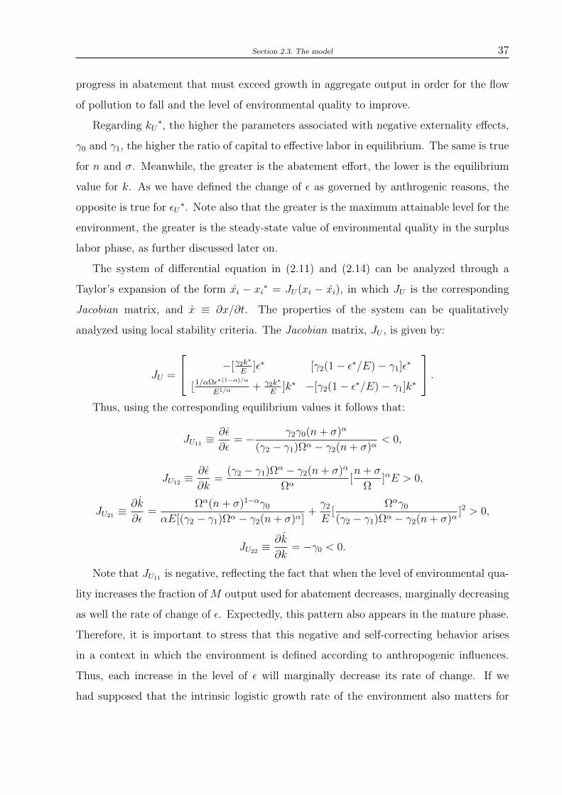
which is unambiguously negative. Therefore, the equilibrium in the surplus labor phase is
a saddle-point, which is represented in Figure 2.1. The phase portrait is presented in panel
(a), while a vector field simulation is presented in panel (b). The simulation parameters
are plausible, but arbitrary, and the conditions for existence of a real positive solution for
k and ε are satisfied.
The axis are the respective levels for ε and k, with the two demarcation curves intersec-
ting at the equilibrium point U∗ and dividing the system into four distinct regions. Recall
that J11 < 0, and thus, when the level of environmental quality is continuously increasing
(ε-axis), the rate of change of ε undergoes a steady decrease, so that ε is positive (negative)
below (above) the ε = 0 isocline. Meanwhile, when the capital-labor ratio in efficiency units
is increasing (k-axis), its rate of change is decreasing, with k being positive (negative) to
the left (right) of k = 0. Both curves are positively related in the neighborhood of U∗,
and thus, note that even facing an infinitely elastic labor supply, capital accumulation is
environment-constrained in the underdevelopment phase.11
10 The maximum sustainable yield is the largest average catch that can be captured from a stock of
environmental quality under existing environment conditions.11 These are plausible slopes of the curves; only the positive slope of both curves in the neighborhood
of the unique equilibrium is important to the argument. It can be checked that, in the neighborhood of
Section 2.3. The model 39
Figure 2.1: Saddle-point instability in the surplus labor phase.
Note also that the stable arm of the saddle-point, the separatrix SS, has a negative
slope. All the area to the left of such stable arm constitutes what it is called here an
ecological development trap, in which either one or both state variables experience a steady
downward pressure. If the system starts to the left of SS there are no endogenous forces
capable of reverting such downward pressure. This trap is called ecological because it arises
from a pollution abatement rule enforced by an environmental authority concerned with
the biophysical limits of the Planet. The economic consequences of this trap are explored
in the next section.
Note that a necessary condition for the existence and uniqueness of the ecological
development trap is the presence of a pollution abatement mechanism that operates when
the current level of environmental quality is below its maximum attainable level. As we
are interested in exploring the macrodynamic effects of such an environmental policy, we
can focus our attention on the case that ε < E, though. In fact, recall that according to
(2.3), when ε is equal to E, the fraction of the M output allocated to abatement is null.
As a result, it can be checked that the profit rate in the surplus labor phase (given in 2.9)
becomes solely determined by the parameters of the production function. Meanwhile, it
follows from (2.11) and (2.14) that there is no pair of economically relevant equilibrium
U∗, the ε = 0 isocline, whose slope is given by −J11/J12, is steeper than the k = 0 isocline, whose slope is
given by −J21/J22.

40 Chapter 2. A Green Lewis Development Model
values in the surplus labor phase when ε = E, given that ε is unambiguously negative.
And, according to (2.12) and (2.15), the same applies to ε = E in the mature phase.
Assuming that the economy overcomes the underdevelopment stage, let us analyze the
behavior of the laws of motion of the state variables in the mature phase, when the labor
supply becomes inelastic. First, computing k = ε = 0, the unique economically relevant
pair of equilibrium values is given by:
kD∗ = [
sα(γ2 − γ1)
γ2(n+ σ)]
11−α , (2.19)
εD∗ = [
γ2 − γ1
γ2
]E. (2.20)
Intuitively, the steady-state value of the level of environmental quality varies positively
with the abatement effort and the maximum attainable level of environmental quality
that is used as a benchmark by the government, but negatively with the catch coefficient,
an immediate implication of (2.12). The same is true for the steady-state value of the
capital-labor ratio in efficiency units. As in the underdevelopment equilibrium, the system
is qualitatively analyzed using the criteria for local stability from the Jacobian matrix.
Thus,
JD =
−[γ2k∗α
E]ε∗ [α(γ2(1− ε∗/E)− γ1)k∗α−1]ε∗
[ sαk∗α−1
E+ γ2k∗α
E]k∗ [ (α−1)sαk∗α−2ε∗
E− α(γ2(1− ε∗/E)− γ1)k∗α−1]k∗
.Substituting the corresponding equilibrium values it follows that:
JD11 ≡∂ε
∂ε= −[
sα(γ2 − γ1)
γ2(n+ σ)]α
1−α (γ2−γ1) < 0,
JD12 ≡∂ε
∂k= 0,
JD21 ≡∂k
∂ε= [(
sα(γ2 − γ1)
γ2(n+ σ))
α1−α +
γ2
E(sα(γ2 − γ1)
γ2(n+ σ))α+11−α ] > 0,
JD22 ≡∂k
∂k= (α− 1)(n+ σ) < 0.
The effect of ε in ε, JD11 , remains negative, but now the effect of the capital-labor
ratio in efficiency units on the rate of change of the level of environmental quality in
the neighborhood of the equilibrium, is null. This feature is similar to a result of the

Section 2.3. The model 41
Green Solow model, according to which the environmental rate of change is independent
of the level of k. However, here the existence of decreasing marginal returns to capital
is not a sufficient condition for a lowering of the amount of negative externalities on the
environment. Despite JD21 is capturing the effect of decreasing marginal returns to capital,
its sign remains the same, but with a smaller marginal effect than in the underdevelopment
phase. The same is true for JD22 , which cannot be determined directly by JD12 . Note that
the effect of k on its rate of change is now solely captured by the effect of k on the
investment function.
As it turns out, the determinant of such Jacobian is unambigously positive:
|JD| = (γ2 − γ1)[sα(γ2 − γ1)
γ2(n+ σ)]α
1−α (1− α)(n+ σ) > 0. (2.21)
Figure 2.2: Stable equilibrium in the mature phase.
As the corresponding Trace, Tr(JD), is negative, the equilibrium in the mature phase
is locally stable. Figure 2.2 presents the phase portrait (panel (a)) and a vector field
simulation (panel (b)) of the system in the neighborhood of the equilibrium. As JD11 < 0,
when the level of environmental quality is increasing (ε-axis) its rate of change undergoes
a steady decrease, so that ε is positive (negative) below (above) the ε = 0 isocline. The
same remains true for k. When the capital-labor ratio in efficiency units is increasing, its
rate of change experience a steady decrease, so that k is positive (negative) to left (right)
of the k = 0 isocline.
42 Chapter 2. A Green Lewis Development Model
While the k = 0 isocline remains positively sloped in the neighborhood of the equili-
brium, the ε = 0 isocline is now horizontal, given that JD12 = 0. Regarding the transition to
such steady state, the mathematical properties of the system and the vector field simulation
reveal that the convergence is in the form of a stable improper node. Hence, convergence
to equilibrium occurs with monotonically increasing or decreasing levels of environmental
quality and capital-labor ratio in efficiency units, a result qualitatively analyzed in the
next section.
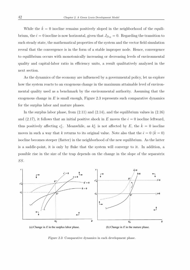
As the dynamics of the economy are influenced by a governmental policy, let us explore
how the system reacts to an exogenous change in the maximum attainable level of environ-
mental quality used as a benchmark by the environmental authority. Assuming that the
exogenous change in E is small enough, Figure 2.3 represents such comparative dynamics
for the surplus labor and mature phases.
In the surplus labor phase, from (2.11) and (2.14), and the equilibrium values in (2.16)
and (2.17), it follows that an initial positive shock in E moves the ε = 0 isocline leftward,
thus positively affecting ε∗U . Meanwhile, as k∗U is not affected by E, the k = 0 isocline
moves in such a way that k returns to its original value. Note also that the ε = 0 (k = 0)
isocline becomes steeper (flatter) in the neighborhood of the new equilibrium. As the latter
is a saddle-point, it is only by fluke that the system will converge to it. In addition, a
possible rise in the size of the trap depends on the change in the slope of the separatrix
SS.
Figure 2.3: Comparative dynamics in each development phase.

Section 2.3. The model 43
In the mature phase, from (2.12) and (2.15), and the equilibrium values in (2.19) and
(2.20), it follows that an exogenous increase in E also moves the economy to a higher level
of environmental quality, initially positively affecting k as well. However, given (2.19), the
equilibrium level of the capital-labor ratio in efficiency units is unaffected by E, so that the
k = 0 isocline moves in such a way to restore k∗D. In the process of adjustment, a higher
environmental quality increases labor productivity, which in turn, lowers the required level
of capital per effective worker in the economy. Note also that the k = 0 isocline becomes
less steep in the neighborhood of D′∗. In both phases, the net effect of a higher value of
E is to increase the steady-state level of per capita income of the economy, as it increases
the level of environmental quality and, therefore, labor productivity in the modern sector.
2.3.1.2 Multiple equilibria analysis
This section provides a further qualitative and illustrative representation of the dy-
namic system by combining the unique economically relevant equilibrium in each phase
of development. Indeed, there is a set of parameters for which a joint representation of
Figures 2.1 and 2.2 exists. A necessary condition for this is related to the slope of each
isocline in the surplus labor phase, as pointed out earlier. Note also that with LT = 0, the
ε = 0 is horizontal, so that a possible multiple equilibria configuration can be illustratively
represented as in Figure 2.4.
Consider, for example, that the system starts at point A, where the level of ε is rela-
tively low, and the Modern sector must dedicate a relatively high fraction of its output
to abatement. Since the level of environmental quality is relatively far from its maximum
attainable level and the activity of cleaning up the environment is assumed to be effective,
such positive effect overcomes the negative marginal impact of ε on ε, so that the level of
environmental quality increases. Meanwhile, the capital-labor ratio in efficiency units is
affected in two ways. First, as the fraction of output dedicated to abatement is relatively
high at low levels of ε, the net M output (and, therefore profits and savings) is relatively
lower. Second, at relatively low levels of ε, the magnitude of the impact of the rise in
the level of environmental quality on labor productivity is greater than the accompanying
effect on savings, so that the capital-labor ratio in efficiency units falls along the trajectory
started at A.
Conversely, if the economy starts at point B the level of environmental quality is

44 Chapter 2. A Green Lewis Development Model
Figure 2.4: A possible configuration of multiple equilibria along the development path.
relatively high, and therefore, the fraction of the M output dedicated to abatement is
relatively low. Since the level of environmental quality is relatively high, the marginal
effect of ε on ε is greater than the positive effect of k on ε, so that the level of ε experiences
a steady decrease. Meanwhile, the capital-labor ratio in efficiency units is affected in
two ways. First, at point B the level of pollution abatement does not compromise much
the levels of profit and saving, so that capital accumulation is able to raise k. Second,
the corresponding fall in ε requires a higher capital-labor ratio in efficiency units to yield
k = 0. Note that at both points, A and B, the development problem is the absence of a
minimum level of environmental quality and/or capital stock per effective worker, which
prevents the economy from being located somewhere to the right of the separatrix SS.
Consequently, the trajectories started at points A and B will eventually take the eco-
nomy to a subset of the ecological development trap, the H region. Once in this region the
economy experiences a cumulative decline in environmental quality and capital intensity
in efficiency units, which interact in a way of a vicious circle. As a result, the H region
illustrates the occurrence of a perverse Kaldor-Myrdal circular and cumulative causation
mechanism of interaction between capital accumulation and environmental quality.
Note that even an economy with relatively high levels of environmental quality which
Section 2.3. The model 45
adopts a pollution abatement rule may eventually fall in the Kaldor-Myrdal region of
cumulative decline. This is in contrast with existing environmental macromodels, such
as Brock and Taylor (2010) and Chimeli and Branden (2009). In these macromodels
an economy which adopts an abatement policy will never experience a steady decline in
the level of environmental quality. The result is a consequence of their sustainable growth
assumptions and stability properties. In the present model, given the cumulative causation
between capital accumulation and environmental quality, unfortunately this possibility
arises quite naturally in the ecological development trap.
The size of the trap varies according to changes in EU and, as a consequence, in
the separatrix SS. Therefore, the main effect of the pollution abatement rule assumed
here is that a developing economy, if left to the free play of its structural forces, can
be trapped in the underdevelopment phase. This theoretical result illustrates the claim of
many developing countries regarding the possibility of a delay in the economic development
process, given the backward effects caused by the unequal distribution of costs and benefits
of pollution abatement and, more broadly, climate change. But if the economy starts to
the right of the separatrix SS, for instance at points C or F , it will converge towards
maturity, even if it possibly slowly.
Once in the ecological development trap, the economy can be exogenously pushed
from there to the right side of the separatrix SS by means of a standard Big Push, in the
sense of Rosenstein-Rodan (1943), whose real counterpart is an international compensation
mechanism. This can be accomplished through an international mechanism of transfer of
financial resources that exogenously increases the level of capital intensity in efficiency
units, for the same level of environmental quality.
In the present model, the theoretical possibility of a Big Push is extended to an en-
vironmental dimension. If the economy is located to the left of the separatrix SS, the
ecological development trap can also be overcome by means of what we call here an En-
vironmental Big Push, EBC. While the case for a standard Big Push is well established
in the economic development literature (see, e.g., Murphy et al. 1989, and Skott and Ros
1997), this paper contributes to the environmental macroeconomics literature by providing
a theoretical rationale for an Environmental Big Push. For instance, if the economy is in
the H region, an EBC can push the economy from there to a point to the right of the
separatrix SS, from which the convergence towards the mature equilibrium takes place,
46 Chapter 2. A Green Lewis Development Model
even if possibly slowly. The same possibility applies, of course, to points located out of the
H region, but still in the ecological development trap, such as points A and B. Intuitively,
as the level of environmental quality at point A is lower than at point B, the capital-labor
ratio in efficiency units is higher in the former.
Concretely, the Environmental Big Push can be interpreted, for instance, as an exo-
genous transfer of green technology developed in advanced economies to the abatement
activity in developing economies, which will result in exogenous improvements in the level
of environmental quality in the latter. In turn, the exogenous environmental recovery will
lower the fraction of the M output dedicated to abatement, which will raise the amount
of savings available to finance investment. Moreover, the corresponding increase in the
labor-augmenting technical change will require a lower capital-labor ratio in efficiency
units to achieve similar productivity levels. Therefore, both effects are positive along the
development path.
In the mature phase, unlike in Brock and Taylor (2010), our Green Lewis development
model may not reproduce an EKC pattern for the environmental dynamics. For instance,
if the economy starts, by a fluke, in the mature phase, say at point I, with a relatively high
level of environmental quality, the system experiences a monotonic fall in ε towards the
steady state. Consider instead that the system starts at pointG, where k is relatively higher
than ε. The level of environmental quality experiences a monotonic increase towards D∗,
while k first fall and after some threshold it increases. This occurs because at G the level of
environmental quality is relatively far from its maximum attainable level, and the amount
of M output dedicated to abatement compromises the expansion of k. After the threshold
the system enters a region of positive cumulative causation between environmental quality
and capital-labor ratio in efficiency units that takes the economy to the steady state.12
2.4 Conclusions
This paper extends a Lewis dual economy development model to explore the interaction
between environmental quality and economic growth, according to a modern notion of sus-
12 When the steady state at maturity, D∗, is reached, it follows from (1) with LM = L that the level
of per capita income is given by M/L = α(1 − φ)kαAε. Therefore, as both k and ε are stationary in
equilibrium, the steady-state growth rate of per capita income, as expected from the Solow (1956) nature
of the mature development phase, occurs at the exogenous rate A = σ.

Section 2.4. Conclusions 47
tainability. Although subject to the limitations of a stylized model, the main qualitative
results derived in the paper contribute to shed light on ongoing heated political discus-
sions about whether developing countries can simultaneously stimulate economic growth
and reduce negative externalities on the environment. In fact, the most recent round of
these discussions was just held at the 2015 Paris Climate Conference, where over 190 de-
veloped and developing countries agreed that they need to collectively chip in by curbing
greenhouse gas emissions responsible for global warming, and doing so with specific targets
and performance monitoring.
When compared to the Green Solow model set forth in Brock and Taylor (2010), our
Green Lewis development model yields a less auspicious prediction about the interaction
between economic growth and environmental quality in developing economies. This predic-
tion is that a developing dual economy that faces an environmental constraint to economic
growth-enhancing capital accumulation by dedicating a fraction of its output to pollution
abatement may not achieve the mature, developed stage. The intuition for this prediction
is that such pollution abatement requirement affects capital accumulation-enhancing profi-
tability both negatively (by reducing marketable net output) and positively (by increasing
labor productivity-enhancing environmental quality). As the relative strength of these two
effects depend on the prevailing levels of environmental quality and capital intensity, there
emerges an ecological development trap from which a developing dual economy, if left to
the free play of its structural forces, never escapes. In fact, once in such ecological deve-
lopment trap, a developing dual economy is either already experiencing or will eventually
come to experience a Kaldor-Myrdal circular and cumulative causation process of decline
in capital intensity and environmental quality.
Fortunately, however, a developing dual economy can be released from such ecological
development trap and eventually, even if slowly, overcome underdevelopment not only
through a standard, capital-based Big Push, in the spirit of Rosenstein-Rodan (1943), but
also by means of what we call an Environmental Big Push. The latter could be based,
for instance, on the adoption of international redress and compensation mechanisms in
favor of developing economies. While the case for a standard Big Push is quite well
established in the economic development literature, this paper is intended to contribute
to the environmental macroeconomics literature by providing a sound theoretical rationale
for an Environmental Big Push.
48 Chapter 2. A Green Lewis Development Model
Finally, it should be emphasized that the emergence of an ecological development trap
occurs in this paper in the context of a model developing economy which does not accumu-
late cleaner, less polluting capital. Therefore, a natural extension of this model (for which
we invite the reader to stay tuned) is to incorporate the possibility of adoption of cleaner
technologies. Admittedly, however, both the production and adoption of cleaner techno-
logies are likely to be influenced, inter alia, by profitability considerations. More broadly,
the Green Lewis development model set forth in this paper is expected to stimulate further
research on other issues in ecological and environmental dynamics in developing economies.
Given that global warming takes place in a global scale, it is especially appropriate to tac-
kle these issues as they materialize in open developing economies, which may also require
the use of stronger notions of sustainability.

Chapter 3
Environment, Effective Demand, and Cyclical Growth
in Surplus Labor Economies
3.1 Introduction
Theoretical and empirical advances in environmental and ecological economics pose new
challenges to economic growth and development theory, suggesting that limits to growth
may not arise from the limited capacity of nature to provide resources, but instead from
the limited ability of the planet to act as a sink for capitalist waste.1
Neoclassical answers to these challenges are typically optimistic, relying on the assump-
tion that the capitalist system may still endogenously achieve a stable sustainable growth
path. Hence, under certain conditions, the environmental constraints do not prevent the
economy from achieving a full employment growth trajectory with diminishing negative
impacts on the environment. In general, the argument is justified by using the controver-
sial empirical evidence on the environmental Kuznets curve (EKC), which first appeared
in Grossman and Krueger (1995).2
Concretely, the EKC hypothesis proposes that there is an inverted U-shaped relation
between the flow of negative externalities on the environment and the levels of per capita
income. In the first stage of development the environmental degradation grows quickly
because financial resources to invest in pollution abatement are relatively low and capi-
tal accumulation is at the forefront.. With this ongoing development process, there is an
1 See, for example, Brock and Taylor (2004) and Foley (2012) for some reflections on these new challenges
(or dilemmas).2 Stokey (1998) and Brock and Taylor (2010), for instance, formulated models in which the EKC stan-
dard prediction plays an important role in generating such a sustainable growth path in mature economies.

50 Chapter 3. Environment, Effective Demand, and Cyclical Growth in Surplus Labor Economies
income threshold above which the economy starts to invest in pollution abatement and
mitigation so that eventually, growth reduces the negative environmental impact of eco-
nomic activity. In the words of Stokey (1998, p.1): “while the early stages of economic
growth cause the problem, later ones bring the remedy.”
Several objections can be raised against the theoretical foundations of the EKC. Mostly,
its concept is dependent on a model of the economy in which there is no feedback from the
environmental quality to economic growth, meaning that in the absence of an environmen-
tal regulation, growth can expand at no environmental cost. One might wonder whether
the assumption of zero environmental cost is so general as supposed. The answer is no. It
is difficult to imagine, for instance, that such assumption remains true when we consider
that the environmental degradation problem takes place on a global scale in which trade
has, by no means, a neutral effect (Stern, 2004). Some may choose, of course, to transfer
this global cost to future generations, but in the face of the climate change problem, this
line of argument has not been helpful.3
The heart of the critique is simply that the neoclassical optimism is implicitly based
on the assumption that countries in the early stages of development have relatively high
levels of environmental quality and may sacrifice of these levels in order to grow quickly.
However, in some low-income developing economies (including much of Asia and Africa),
such a growth strategy can actually result in an unsustainable increase in environmental
degradation before the maximum range of pollution illustrated by the EKC is reached
(Dasgupta et al., 2002). This is so precisely because they have relatively low levels of
environmental quality.
The main feature of these developing economies is the occurrence of environment adjust-
ment costs that are already binding in the short run. Any expansion of economic activity
comes with even more negative impacts on the environment which, if strong enough, may
compromise output expansion in the capitalist sector. It is the corresponding lowering
in economic growth toward the medium run that reduces the negative pressures on the
environment so that, for environmentalists, the existence of developing countries with re-
3 The feedback effect from environmental quality to economic growth also has serious implications for
the assumption of of strict exogeneity in econometrics models seeking to empirically test the EKC. This
paper, however, scrutinizes the voluminous literature on the EKC. See Carson (2010) and Stern (2015)
empirical analyses of the EKC.

Section 3.1. Introduction 51
latively low levels of environmental quality offers empirical evidence against the arguments
based on the EKC and the prediction of a well-behaved growth trajectory.4
International development agencies have highlighted empirical evidence that illustrates
such a claim for developing countries such as Rwanda, were the cost of land degradation
has been negatively affecting gross domestic product (GDP).5 Particularly, Rwanda is un-
der perverse Malthusian dynamics: an increase in economic growth stimulates agricultural
consumption, which given the rudimentary techniques adopted by low-skilled workers, ac-
celerates soil degradation and reduces productivity, in turn lowering GDP. Furthermore,
in several low-income regions of China, industrial production has led to atmospheric pol-
lution, increasing the rate of health and occupational problems with direct consequences
on labor productivity. In turn, less productive workers exert downward pressure on indus-
trial production and growth. Moreover, both cases illustrates the occurrence of different
types of environmental adjustment costs; this operates as a feedback mechanism from
environmental quality to output expansion.
Relatively much less attention has been given to the theoretical macroeconomic aspects
of the problem. Bulte and van Soest (2001), as a notable exception, formalize a model in
which production and consumption patterns of rural households in developing countries
are the main source of environmental degradation. Depending on the indicator that is
used to represent the environmental externality, for reasonable parameters, the model
demonstrates that a reverse causal behavior may arise as a particular case of the EKC
dynamics. Its focus is on the generation of an extended EKC and not on the macroeconomic
consequences for such an extension for developing countries; thus, many issues remain.
A major question in this context is how these developing countries, or some of them,
are likely to behave in a trajectory of this type as far as their macroeconomy is concerned.
A first step in addressing such concern is to set forth a formal model that explores the
macroeconomic implications, in one of its several relevant aspects, of such a conflictive
relation between environmental quality and economic growth in these surplus labor low-
income economies. The main purpose of this paper is to develop such a model.
Far from full employment, these economies are characterized by hidden unemployment
4 In the long run effect, of course, this will depend on how absolute poverty responds to slower economic
growth.5 See, for example, Downing et al. (2009) and part of the environment–poverty literature: Bojo et al.
(2001), Dasgupta et al. (2005).

52 Chapter 3. Environment, Effective Demand, and Cyclical Growth in Surplus Labor Economies
and the existence of a relatively large capitalist sector coexisting with a larger subsistence
sector. In this context, effective demand plays an important role in generating a long
run path, which according to Harrod (1939) is likely to be unstable. In the medium
run, in addition to driving the output expansion, effective demand generates negative
externalities on the environment that reduce the level of environmental quality. In turn,
such an effect raises the environmental adjustment costs of firms, thus exerting a downward
pressure on economic growth. Hence, instead of suggesting a stable sustainable growth
path, as proposed by most neoclassical constructions, this aspect of the relation between
environmental quality and economic growth may result in a medium run vicious circle, in
which the level of environmental quality operates as a potential taming mechanism for the
Harrodian instability in such developing economies.
Such theoretical description requires that we shift the focus from a well-behaved tra-
jectory of long run stable growth to the description of endogenous cyclical fluctuations.
A theoretical framework that quite naturally accommodates this possibility is the Har-
rodian one, in which effective demand plays a pivotal role. However, cycles arises in a
standard version of this model only for mature economies, in which capital accumulation
endogenously affects the structure of the labor market. In the present surplus labor case,
however, the theoretical explanatory power of the Harrodian framework is extendend to
include environmental considerations, with which another source of cyclical growth arises
as a new accommodation mechanism of instability.
Ironically, the post-Keynesian literature is not immune to the criticism that it has
largely ignored sustainable development issues. However, the tide is changing, and the
present paper is related to a few attempts to model environmental and ecological issues in
a post-Keynesian framework, such as Fontana and Sawyer (2016) and Taylor et al. (2016).
The main distinguishing feature and contribution of the present simple model is that it
provides a plausible explanation for a possible new source of cyclical growth in such surplus
labor economies. At the very least, the model set forth herein provides insights that should
be considered in an evaluation of the conflictive relation between environmental quality
and economic growth in low-income developing economies with relatively low levels of
environmental quality.
The remainder of this paper is organized as follows: Section 3.2 extends a standard
Harrodian model to include an environmental dimension, thus exploring the relationship

Section 3.2. The model 53
between effective demand and the environmental adjustment costs. The balanced growth
and the (in)stability properties of the model are analyzed in Section 3.3, in which an
economic interpretation of the main results is presented. Finally, the main conclusions
derived along the way are summarized in Section 3.4.
3.2 The model
Consider a surplus labor developing economy with relatively low levels of environmental
quality that is closed and has no fiscal activities. Such a relatively low level of environmen-
tal quality is caused by a local effect (to be described latter). The dualism is represented by
the coexistence of capitalist and backward sectors, the latter being a repository of hidden
unemployment. The capitalist sector produces according to a production function with
fixed coefficients that combines capital, K, and labor, L, in which it is supposed that there
is no labor hoarding and the excess of capital capacity is the normal state of affairs. These
assumptions imply that the output, X, is given by the following:
X = xL ≤ ρmaxK, (3.1)
where x is labor productivity and ρmax is capital productivity at the full capacity level.
Since capital stock is subject to lag adjustments, firms may want to maintain excess of
capacity to deter new entry and to respond to fluctuations in demand (Steindl, 1952).
One of the crucial aspects of the Harrodian benchmark is related to the investment
sensitivity to capital capacity utilization in the short and long run, the equality of desired
(ρ∗), and actual output–capital ratio (ρ) in the steady state. Hence, a standard Harrodian
investment function relates the rate of change in the rate of accumulation, dK/dt, to the
difference between the actual output–capital ratio and the desired ratio (Skott, 2010).6
Hence,
d
dtK = λ(ρ− ρ∗), λ > 0. (3.2)
Following the classical economists and the Cambridge (UK) tradition, it is supposed
that workers as a class spend all of their income, whereas capitalists save a constant
6 This function is a continuous approximation for a discrete investment function that only considers the
output–capital ratio as affecting investment for the purpose of simplicity. See Skott (2010).

54 Chapter 3. Environment, Effective Demand, and Cyclical Growth in Surplus Labor Economies
fraction, s, of gross profits, Π (Kaldor, 1966):
S = sΠ. (3.3)
Regarding gross investment, a standard specification is given by the following:
I =dK
dt+ δK, (3.4)
in which δ is an exogenous depreciation rate. The capital stock, the rate of capital accu-
mulation, and the output are predetermined in the ultra-short run. These past production
decisions are governed by demand expectations that sometimes are not fulfilled. Unlike
most Keynesian and Kaleckian approaches, it is supposed that output cannot adjust ins-
tantaneously to a demand shock. The Keynesian equilibrium condition, S = I, is thus
brought about by changes in prices (in both directions). Therefore, it is supposed that
firms may respond to unexpected shocks in aggregate demand by adjusting prices, and
as profit share, π, is determined by a mark-up pricing equation, profits increase. This
approach also finds support on the Treatise on Money of Keynes (1976).7
The causality channel is as follows: the level of output is predetermined in the ultra
short run, and a rise in demand leads to an increase in the price of output. Money wages are
fixed since there is no perfect foresight and instantaneous feedback from prices to money–
wages rates. Thus, real wages and the profit share respond to unanticipated movements
in prices, and a positive demand shock increases the profit share. The investment and
savings equilibrium condition for a given profit share generates the following solution for
the output–capital ratio, ρ, in the ultra short run:
ρ =K + δ
sπ. (3.5)
Therefore, the Keynesian equilibrium condition, S = I, defines a sort of Marshallian
ultra-short run equilibrium: a market clearing price vector is defined, but it may give firms
an incentive to change their production directly after this.
When the system moves over time using (3.5) in (3.2) the rate of change of capital
accumulation becomes the following:
7 As argued by Skott (2015), perfect flexible prices are not so problematic an assumption as imagined,
since in his approach, cyclical growth can arise with or without flexible prices.

Section 3.2. The model 55
d
dtK = λ(
K + δ
sπ− ρ∗), (3.6)
which in equilibrium, defines the warranted growth rate, gw:
K∗ = sπρ∗ − δ = gw. (3.7)
This solution for the rate of accumulation at the stationary level is warranted because
on average, firms achieve precisely the desired rate of utilization in the long run, ρ∗, a
rational expectation equilibrium (Nakatani and Skott, 2007), as can be seen by using (3.7)
in (3.5). However, it gives rise to the well know instability mechanism described in Harrod
(1939) as well as the likely inequality between gw and the natural growth rate, which
Harrod sees as an intrinsic characteristic of capitalist societies.
Skott (1989a) reconciles the warranted and natural growth rate without leaving aside
the endogenous fluctuations of capitalist economies. This mechanism operates through
the interaction between effective demand and the employment rate, which evolves in time
according to predator–prey dynamics. However, in a surplus labor economy, the employ-
ment rate carries little information to the capitalist sector. As a result, the labor market
may not change endogenously in response to variations in capital accumulation. In this
case, the cyclical pattern of Harrodian models may not arise unless another containment
mechanism is in operation. As described in what follows, the environmental quality can
serve as a channel for such a mechanism.
3.2.1 The output expansion function and the environment dynamics
The Harrodian framework supposes that firms respond to shocks in aggregate demand
in the ultra short run via price adjustments because production is subject to adjustment
costs and takes place after some time. To accommodate such an assumption, it is supposed
that profit-maximizing firms choose the rate of expansion of production instead of the level
of output, which balance the costs and economic benefits of moving toward a desired level
of utilization. This rate of expansion is selected subject to effective demand, technical,
and cost constraints.
In the present surplus labor case, the demand signs comes from the profit share and the
cost signs from the level of environmental quality, ε. To model the feedback effect from the
56 Chapter 3. Environment, Effective Demand, and Cyclical Growth in Surplus Labor Economies
level of environmental quality to economic growth, it is supposed that a relatively lower
level of environmental quality is associated with a relatively higher amount of environmen-
tal adjustment costs of production. The effect will be modeled through its negative effects
on the productivity of the labor force. Hence, the Harrodian rate of growth of production
is algebraically defined as follows:
X = h(π, ε), hπ, hε > 0, (3.8)
which supposes that the environmental adjustment costs, whose effect is captured by the
level of environmental quality, are convex; thus X can be modeled in continuous time. The
model, therefore, leaves aside the possibility that relatively strong changes in the environ-
ment can cause discrete changes in the environmental adjustment costs (non-convexities).
However, in a scenario of climate change, this discrete effects may be important for the
cost structure of firms, a possibility from which we abstract.
In a Harrodian framework a certain degree of capitalists’ inability to respond to demand
shock is supposed, but in the present case, this inability also assumes an environmental
dimension. The inability of instantly adjusting to a change in the environmental quality
arises because the economic representative agent does not perfectly observe his or her
negative externalities on the environment (Kelly et al., 2005). An agent in a developing
country with a relatively low level of environmental quality only slowly realizes that the
environment has changed.
However, if a negative change in environmental quality is persistent, firms know that it
lowers labor productivity, given the negative effects of pollution on the health and cognitive
abilities of factory workers. To counterbalance the reduction in the level of environmental
quality, firms increase investments in occupational health and training of the labor force
in the exact amount to maintain labor productivity unchanged, which I shall refer to as
environmental adjustment costs. It is supposed that firms always achieve such a goal at
any level of ε. Note that there is an inverse relationship between the level of environmental
quality and the environmental adjustment costs; thus we can model the output expansion
dynamics as described in (3.8).
The recognition that the level of environmental quality can affect human health is not
new, but the economic research only recently expanded the focus of analysis beyond direct
health outcomes. Many health effects can affect human capital and labor productivity both
Section 3.2. The model 57
in the short run (Currie and Stabile, 2006) and the long run (Cunha and Heckman, 2007). A
recent and growing body of literature has begun to make this link more explicit, providing
empirical evidence that justifies this functional relation between environmental quality (or
pollution, as the inverse) and labor productivity as well as the cognitive outcomes.8
Analyzing the effects of negative changes in ozone concentration, Graff Zivin and Neidell
(2012) found robust evidence that ozone levels well below the federal air quality standards
have a significant negative impact on labor productivity. The magnitude of the impact is
large, since they found that a 10 ppb (parts per billion) decrease in ozone concentration
increases labor productivity by 5.5 percent. The authors argued that investment in envi-
ronmental protection could be seen as an investment in human capital as well. Similarly,
Chang et al. (2014) estimated the effect of outdoor air pollution on the labor productivity
of indoor workers in a pear-packing factory. They also found that an increase in particulate
matter less than 2.5 micrometers in diameter (PM2.5) of a harmful pollutant outdoors,
which easily penetrates indoor settings, lead to a statistically and economically significant
decrease in packing speeds inside the factory.
The level of environmental quality modeled as environmental adjustment costs is also
compatible with short-run adjustments in the Harrodian perspective. Graff Zivin et al.
(2015) provided the first estimates of the potential impact of climate change on human
capital, focusing on the impacts from both short-run weather and long-run climate. Exploi-
ting a longitudinal structure of the NLSY 79 and random fluctuations in weather across
interviews, they identified the effect of temperature in models with child-specific fixed
effects, finding that short-run changes in temperature lead to statistically significant de-
creases in cognitive performance in mathematics.9 In contrast, a long-run analysis revealed
no statistically significant relationship between climate and human capital. According to
the authors, this finding is consistent with the notion that adaptation, particularly com-
pensatory behavior, plays a significant role in limiting the long run impacts from short
run weather shocks. In the present approach, it may be consistent that in the long run,
firms move to a desired level of utilization via adaptation, even when facing environmental
constraints on the labor force.
8 See Graff Zivin and Neidell (2013) for a summary of this literature.9 The NLSY79 cohort is a longitudinal project that follows the lives of a sample of American youth
born between 1957 and 1964.

58 Chapter 3. Environment, Effective Demand, and Cyclical Growth in Surplus Labor Economies
One may ask, however, if these environmental adjustment costs are economically re-
levant. In the climate change literature, this is a controversial point. In fact, most old
quantitative estimates of the cost of environmental damages in mature economies are mo-
dest. This is a different cost perspective taked by the empirical evidence reviewed by
Graff Zivin and Neidell (2013), which argue that most recent estimates inf the literature
have found economically relevant parameters related to environmental damages. Intui-
tively, for low-income developing economies with relatively low levels of environmental
quality, however, a conclusion that such a cost is relatively small seems misguided. In the
real world, of course, the way in which the signals of environmental quality are captured
by the capitalist sector are diverse and difficult to generalize; thus, I focus on the effects on
labor productivity following the recent and robust empirical evidence that is economically
relevant (Graff Zivin and Neidell, 2013).
In contrast, the level of environmental quality changes endogenously according to the
pollution that the capitalist sector releases into the environment. This is captured by a
local scale effect.10 Hence, the flow of pollution is defined according to the following::
Ω = ϑ(X), ϑ > 0, (3.9)
where the higher the scale of the economy, the lower the level of environmental quality.
The level of environmental quality is given in the short run, but it has an exogenously
given natural capacity of regeneration over time, β.
The level of environmental quality grows according to a logistic function, which is
perhaps the simplest plausible functional form for biological growth in a constrained envi-
ronment, G(ε), defined as follows:
G(ε) = β(E − ε)ε, (3.10)
where E, the maximum carrying capacity point, is the maximum possible level of environ-
mental quality, so that when ε = E, further growth cannot occur, G(ε) = 0. It is supposed
that the proportional rate of change of environmental quality is negatively affected by the
10 From an empirical perspective, there are three ways through which an economy generates pollution:
scale, composition, and technical effects. The present model concentrates only on scale effects since it is
a one sector model that abstracts from the occurrence of technical change.
Section 3.2. The model 59
growth rate of the flow of pollution, thus having an inverse relationship with the output
expansion function:
ε = β(E − ε)− ω[h(π, ε)], (3.11)
where ω measures the intensity of the negative impact of the output expansion on the envi-
ronment. A stationary solution for ε, thus, requires the balance between effective demand
and its polluting dynamics with the natural capacity of regeneration of the environment.
For the present purposes, it is not convenient to link this description of the environmen-
tal quality to climate change. In all of the analyses that follow, the negative externalities
from the capitalist sector are local, as in many models in the related literature.11 Thus, it is
more convenient to think of the environmental quality as the ecological complex consisting
of the forest, soil, water, and air quality so that “the environment” assumes this particular
meaning. A substantive assumption, however, is necessary. The level of environmental
quality must respond in a sufficiently positive amount to the negative oscillation in the
production in order to capture the diminishing pressures on the environmental adjustment
costs. Therefore, all of the environmental externalities are suitable to this medium run
perspective of the model since some negative impacts on the environment are permanent
or take a very long time for significant regeneration, thus exerting a continuous negative
effect on the labor force.12
Before analyzing the mathematical properties of the model, it may be useful to com-
pare it with other attempts to model similar environmental and ecological dynamics in
macromodels, especially the attempt to model how environmental quality affects labor
productivity and economic growth, growth, with which the present model shares a lot of
inspiration.
Oliveira and Lima (2015), using a Lewis dual economy framework, specify a labor-
augmenting process of technical change that is influenced by the level of environmental
quality in a Cobb–Douglas technology. They show that even in a very optimistic EKC
context, pollution abatement policies without exogenous compensation mechanisms may
11 For the present purposes, an open macroeconomic model of climate change will just increase the
negative environmental effect. See, for example, Copland and Taylor (2005) for some open macromodels
along neoclassical lines. A recent and elegant structuralist formalization of open ecological macroeconomic
issues can be found in Razmi (2015).12 Industrial toxic pollution is typically procyclical.
60 Chapter 3. Environment, Effective Demand, and Cyclical Growth in Surplus Labor Economies
result in an ecological development trap, from which a developing economy, if left to the
free play of its structural forces, may never escape. However, such a result is indepen-
dent of the labor-augmenting effect. The main source of environmental cost comes from
a profitability reducing pollution abatement rule, which is endogenous to the level of en-
vironmental quality. Meanwhile, the authors ignore effective demand issues as affecting
economic growth. Here, I consider that even without environmental regulation, a simi-
lar conflictive behavior may arise in a context in which the role of effective demand in
generating an unstable warranted growth path is explicitly taken into account.
In Taylor et al. (2016), a large set of variables affect labor productivity. In particular,
they claim that greenhouse gas emissions may decrease labor productivity since they also
cuts “profitability and destroys the stock of capital”. However, this channel from which
environmental quality (or pollution) affects labor productivity is not explained in detail.
They also establish an interesting link between energy and productivity through which
important growth and distribution outcomes are analyzed. In contrast, the present model
adopts a more parsimonious specification, examining the role of environmental adjustment
costs, which arise from the action of firms to prevent the loss in labor productivity through
health shocks, in generating cyclical growth.
3.3 Demand-driven economic growth and (in)stability
At any moment in time, the rate of output, X, the capital stock, K, the level of
environmental quality, ε, and the output–capital ratio, ρ, are given. The equilibrium
in the goods market determines income distribution, π. As a consequence, the output
expansion and the investment function determine the growth rate of output and capital
accumulation, which in turn will determine the level of environmental quality.
In a simple Harrodian benchmark, the output–capital ratio is constant and equal to
ρ∗ along a steady-state path. As argued before, a key element is the distinction between
a weak short-run and strong long-run sensitivity of investment to variations in aggregate
demand. With capacity utilization being a state variable, this distinction is captured by a
static relation between the accumulation rate and capacity utilization (Skott, 2010):
K = ϕ(ρ), (3.12)

Section 3.3. Demand-driven economic growth and (in)stability 61
in which ϕ measures the relationship between accumulation and the output–capital ratio.
As the profit share is determined by the equilibrium condition for the goods market, we
can use (3.12) in (3.5) to determine the long run relation given by the following equation:
π =ϕ(ρ) + δ
sρ= µ(ρ), (3.13)
in which the strong long run sensitivity of the rate accumulation to changes in output–
capital ratio implies that µ′ > 0.
Using (3.8), (3.11), and (3.12) the two-dimensional system can be algebraically written
as follows:
ρ = X − K = h(µ(ρ), ε)− ϕ(ρ), (3.14)
ε = β(E − ε)− ω[h(µ(ρ), ε)]. (3.15)
The system given by (3.14) and (3.15) will have a steady state solution if ε ≡ dε/dt
and ρ ≡ dρ/dt are simultaneously equal to zero so that reconciliation between the war-
ranted and natural growth rate is environment-constrained in this surplus labor eco-
nomy. This simple model exhibits four steady states: three corner solutions of (ε∗, ρ∗) =
(0, 0), (E, 0), (0, ρ∗′) and one interior solution, which is the unique pair of equilibrium that
is economically relevant and will be explored in the (in)stability analysis that follows.
Figure 3.1 illustrates a possible steady-state configuration using the output expansion
(3.8) and the logistic growth function of environmental quality (3.10) in Panel (a). The
equilibrium level of environmental quality, ε∗, implies that X = h(π, ε∗)X just matches
the growth of environmental quality, G(ε), at ε = ε∗. Hence, ε∗ is an equilibrium point if
we explicitly treat ρ as fixed. However, ρ varies over time, which is pictured in Panel (b)
in Figure 3.1. The illustrative discussion of Figure 3.1 implicitly assumes so far that the
effects of ε on the output expansion function is nonlinear but focusing only on the relevant,
positive domain.
The nonlinearity of the output expansion illustrates that for a relatively high level
of environmental quality, the growth rate of output is relatively insensitive. The same
remains true for the growth rate of the output–capital ratio.

62 Chapter 3. Environment, Effective Demand, and Cyclical Growth in Surplus Labor Economies
Figure 3.1: Environmental quality, effective demand, and economic growth.
In order to compute the interior solution of the dynamical system given by (3.14) and
(3.15), I set ε = 0 to obtain the following:
β(E − ε)ω
= h(µ(ρ), ε) (3.16)
and substituting (3.16) in (3.14) with ρ = 0, the following is true:
ϕ(ρ) =β(E − ε)
ω. (3.17)
Isolating ρ under the equilibrium for the profit share in the long run, (3.13), we can use
the corresponding result in (3.16) to obtain the equilibrium level of environmental quality,
ε∗. Intuitively, such a level will be in the relevant positive domain if and only if the impact
of economic activity on the environment is not too high. Such a corresponding solution
for (3.16) can be substituted in (3.17) to obtain the unique relevant positive equilibrium
value for the output–capital ratio.
The system (3.14)–(3.15) is qualitatively analyzed around the interior steady-state so-
lution, in which the local stability properties are determined by the corresponding Jacobian
matrix:
J =
(hπµ′ − ϕ′)ρ hερ
−ωhπµ′ε −(β + ω)hεε
.
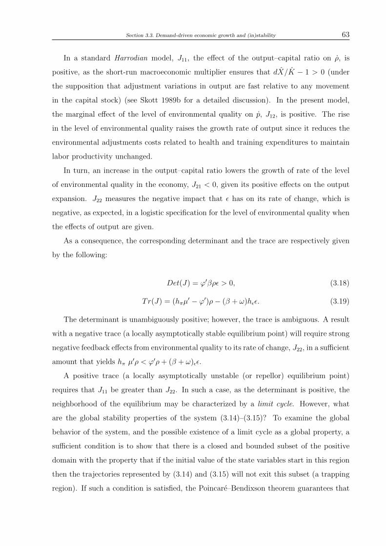
Section 3.3. Demand-driven economic growth and (in)stability 63
In a standard Harrodian model, J11, the effect of the output–capital ratio on ρ, is
positive, as the short-run macroeconomic multiplier ensures that dX/K − 1 > 0 (under
the supposition that adjustment variations in output are fast relative to any movement
in the capital stock) (see Skott 1989b for a detailed discussion). In the present model,
the marginal effect of the level of environmental quality on p, J12, is positive. The rise
in the level of environmental quality raises the growth rate of output since it reduces the
environmental adjustments costs related to health and training expenditures to maintain
labor productivity unchanged.
In turn, an increase in the output–capital ratio lowers the growth of rate of the level
of environmental quality in the economy, J21 < 0, given its positive effects on the output
expansion. J22 measures the negative impact that ε has on its rate of change, which is
negative, as expected, in a logistic specification for the level of environmental quality when
the effects of output are given.
As a consequence, the corresponding determinant and the trace are respectively given
by the following:
Det(J) = ϕ′βρε > 0, (3.18)
Tr(J) = (hπµ′ − ϕ′)ρ− (β + ω)hεε. (3.19)
The determinant is unambiguously positive; however, the trace is ambiguous. A result
with a negative trace (a locally asymptotically stable equilibrium point) will require strong
negative feedback effects from environmental quality to its rate of change, J22, in a sufficient
amount that yields hπ µ′ρ < ϕ′ρ+ (β + ω)εε.
A positive trace (a locally asymptotically unstable (or repellor) equilibrium point)
requires that J11 be greater than J22. In such a case, as the determinant is positive, the
neighborhood of the equilibrium may be characterized by a limit cycle. However, what
are the global stability properties of the system (3.14)–(3.15)? To examine the global
behavior of the system, and the possible existence of a limit cycle as a global property, a
sufficient condition is to show that there is a closed and bounded subset of the positive
domain with the property that if the initial value of the state variables start in this region
then the trajectories represented by (3.14) and (3.15) will not exit this subset (a trapping
region). If such a condition is satisfied, the Poincare–Bendixson theorem guarantees that
64 Chapter 3. Environment, Effective Demand, and Cyclical Growth in Surplus Labor Economies
all trajectories in the subset will converge to a closed orbit, thus exhibiting perceptual
cyclical behavior (Lima, 2004).
First, note that by the Bendixon criteria we cannot rule out that Div ~F ≡ dρdt
+ dεdt
= 0;
thus we cannot rule out the non-existence of a closed orbit within the economically relevant
domain and thus the non-existence of a limit cycle. Figure 3.2 shows a qualitative illustra-
tion of a possible trapping region in the state space of the dynamical system represented
by (3.14) and (3.15) with a positive trace.
Figure 3.2: A possible limit cycle in the surplus labor economy.
The rationale for the construction of this trapping region is as follow. Both isoclines,
ε = 0, and ρ = 0, are negatively sloped in the neighborhood of the unique equilibrium
point, U∗. The ε = 0 isocline is negatively sloped in the positive domain. Around U∗, as
J22 < 0, when the level of environmental quality is increasing, its rate of change is steadily
decreasing so that the signals of ε are positive (negative) below (above) the ε = 0 isocline.
In turn, in the neighborhood of U∗, a rise in the output–capital ratio raises its rate of
change so that ρ is increasing (decreasing) above (below) ρ = 0. The full configuration
of ρ = 0 is depicted under the following assumptions: (i) there is a minimum level of
output–capital ratio in the economy, ρmin, at which I suppose that Y > K; (ii) for high

Section 3.3. Demand-driven economic growth and (in)stability 65
values of ρ, Y < K; and (iii) for high levels of environmental quality, the locus, ρ = 0, is
flatter.
The first assumption is important to generate a floor for the cyclical fluctuations, which
are now bounded from below, and to guarantee that for relatively low levels of output–
capital ratio, ρ is increasing. This is consistent with the notion that firms target a minimum
margin of profits to produce so that below this point, the output–capital ratio is increasing
to maintain at least the minimum profit share. The second assumption is important to
ensure that the fixed–coefficient assumption, ρ < ρmax, holds for relatively high values
of ρ (that is, far from the neighborhood of U∗). The third assumption is related to the
lower sensitivity of output–capital ration for relatively high levels of environmental quality
since at such a level the influence of the environmental adjustments costs on the output
expansion is lower.
To check the consistency of the bounded subset, note that if these assumptions are
satisfied, at very large values of output–capital ratio, ρ is decreasing. Note also that the
system is naturally bounded from above by the maximum carrying capacity, E, so that
at very large values of ε, the rate of change of the level of environmental quality is also
decreasing. Both are represented by the silver area. In addition, for very large values of
ρ and ε (the northeast region in Figure 3.2), the sensitivity of the output expansion to
a change in the output-capital ratio (capacity utilization) and the level of environmental
quality is zero; thus ρ = −ϕ(ρ) and ε = −∞ – so that dρ/dε ≈ 0. Such conditions form
a possible trapping region that do not contain an equilibrium point (except in the closed
orbit), so that the Poincare–Bendixon theorem guarantees the existence of a limit cycle
within such a region.
As the stability of the unique economically relevant equilibrium solution cannot be
ruled out, Figure 3.3 depicts this possibility. The main difference between this and the
previous analysis is that instead of exhibiting perpetual oscillatory behavior, the economy
moves cyclically to the stable focus, U∗′, which is likely much different from U∗ in Figure
3.2. Whether this equilibrium is higher or lower that the one represented in Figure 3.1,
this is of course something which depends on the parameter values.
One may wonder in what situations the response of the rate of change of the level
of environmental quality to changes in ε is strong enough to produce such a result. It
depends on the type of negative externality in each low-income developing economy. It

66 Chapter 3. Environment, Effective Demand, and Cyclical Growth in Surplus Labor Economies
Figure 3.3: A locally asymptotically stable equilibrium point in the surplus labor economy.
is plausible to think, for instance, that the natural rate of environmental regeneration
is relatively low in response to externalities related to land degradation, poisoned water,
and atmospheric pollution concentration than for indoor pollution (burning of biomass);
thus, stability might be a regular feature of the latter. However, in the most common
environmental problems, a lower β should be expected.
The sensitivity of the level of environmental quality to output expansion is also im-
portant. It can be argued, however, that in the absence of discrete effects, ω, is relatively
small. It is only under anthropogenic environmental disasters that a relatively high ω
should be expected.13
At the same time, it is difficult to assume that the environmental adjustment costs
related to different externalities are relatively homogenous. Intuitively, what matters the
most for the argument is how rapid the output expansion responds to a change in the level
of environmental quality and thus in the environmental adjustment costs, hε. To treat
the possibility of stability as a special case in the interaction between economic growth
13 As an example of the destructive potential of capitalist activities, it is worth noting the recent collapse
of a mining dam that occurred in the Brazilian state of Minas Gerais in 2015. It was one of the biggest
environmental disasters in Brazilian, and maybe in Latin American, history. See Massarani (2016).

Section 3.3. Demand-driven economic growth and (in)stability 67
and environmental quality, I suppose that this sensitivity is relatively low compared to the
adjustment process in the capital–output ratio over the cycle.
3.3.1 An economic interpretation of the cycles
This section provides an economic interpretation of the vicious circle. A limit cycle
need not to be unique, as it is sensitive to the initial conditions of the economy. Figure
3.2 presents one of the possible branches covered in the system. Note that the set of
trajectories must exhibit the same oscillatory behavior; thus, the economy is represented
without the loss of generality.14
Consider that the economy is at point A in a situation with a relatively high level of
output–capital ratio and share of profits in income but a relatively low level of environ-
mental quality. The adjustment costs corresponding to environmental quality signals are
relatively high, given the negative pressure that economic activity exerts on the environ-
ment. This negative effect helps to compress the rate of output expansion below the rate
of capital accumulation. The output–capital ratio is therefore falling at A. As ρ is falling,
the level of investment and effective demand is also falling; thus equilibrium in the goods
market is maintained by a reduction in the profit share. In contrast, the environmental
quality is increasing, given the diminishing negative scale effects on the environment, and
the economy is moving toward region II.
At B, the output-capital ratio and profit share are relatively low, but with relatively
average levels of ε. The smaller ρ compresses capital accumulation, which then drops below
the rate of output expansion, thus increasing ρ. Investment is increasing, and the effective
demand changes raises π, which restores the equilibrium in the goods market. As the
profit share is increasing, and adjustment costs that come from the level of environmental
quality are decreasing (for this level of ε), the output is growing at a rate that does not
compromise the expansion in the level of environmental quality, with the economy moving
toward region III. However, when the system enters region IV , output expansion starts
to compromise environmental quality since the negative effects of the scale of the economy
14 For illustrative purposes, the reader may think of the negative environmental externality as the local
emission of a toxic industrial pollutant, which in such a case is clearly pro-cyclical. As the health effects
are sensitive to the atmospheric flow of this pollutant, the growth rate of environmental quality is also
compatible with the business cycle.

68 Chapter 3. Environment, Effective Demand, and Cyclical Growth in Surplus Labor Economies
are greater than the natural growth rate (the environmental capacity of regeneration, thus
decreasing labor productivity). Such an effect is represented by point C.
After a while, the corresponding decrease in the level of environmental quality, given
the environmental deterioration, begins to exert a stronger pressure on the adjustment
costs, which in turn, starts to compress the output expansion, with the economy moving
toward region I. Furthermore, at point D, the output–capital ratio and profit share are
relatively high, and the capital accumulation rate is above the growth rate of output. The
corresponding negative changes in effective demand are accommodated by reductions in
the profit share, thus exerting further downward pressure on X. Even with such a decrease,
the level of environmental quality is relatively low in such a way that ε and ρ are both
declining.
Therefore, without exogenous intervention, such a cyclical counter-clockwise behavior
will go on perceptually in this dual economy. Note that this oscillatory behavior is possible
under the assumption of free utilization of environmental quality in the sense that there is
no vector of prices clearing the “environmental market.” What prevents the economy from
achieving complete environmental decline is the rise in adjustment costs when the level of
environmental quality is relatively low. Regarding the possibility of stability presented in
Figure 3.3, the properties of the oscillatory behavior are similar, but the economy converges
to the stable focus, U∗. In such a case, if the sensitivity of the environmental quality to
output expansion is relatively high and the natural rate of regeneration of the environment
is relatively low, the economy may eventually experience a decline.
The present model is also related to (and somehow inspired by) an interesting environ-
mental macromodel of economic growth: the Brander and Taylor (1998) Ricardo-Malthus
general equilibrium model of renewable resource use. They model population dynamics
related to the Lotka–Volterra predator–prey model, with the humans as the predator and
the resources base as the prey, offering a possible explanation for the rise and fall of past
civilizations such as Easter Island. In the model, it is the population growth that degrades
the resource base. In turn, the reduction of the resource stocks exerts a downward effect
on the fertility rate of population. Such dynamics also result in an oscillatory behavior
of the system. Locally stable cycles arise because the resource base has a slow rate of
regeneration, but it focus is on the long run.
The present results have some similarities with the work of Brander and Taylor (1998)

Section 3.3. Demand-driven economic growth and (in)stability 69
in the sense that a low natural growth rate (a low rate of regeneration of the environmental
quality) may eventually compromise economic activity. This can happen only in the set-
ting illustrated in Figure 3.3, in which a strong negative labor productivity effect generates
stability. However, I extended the results in several directions. I combine environmental
and effective demand issues via the relationship between capital–output ratio and environ-
mental quality in a medium run vicious circle. More importantly, capital accumulation is
included in the model, in with which the role of the capitalist sector is explicitly analyzed.
It is this conflictive relation that creates the conditions for perpetual oscillation in the
medium run, instead of asymptotically stable behavior in the long run.
In concluding, a brief political economy discussion is in order. One may wonder whether
the behavior of the system described in this paper underestimates the power of institutio-
nal change since we should expect the possible creation of efficiency resource arrangements
through market solutions or institutional evolution, even in low-income developing eco-
nomies. Note that a market solution (a price vector for the negative externalities) only
magnifies the sensitivity of the output expansion to changes in the level of environmental
quality through the occurrence of more direct environmental adjustment costs. It is only
if these costs create incentives for the adoption of clean technologies, for instance, that
an eventual market solution helps the economy to solve or at least reduce the operation
of the vicious circle. However, it seems unlikely that a low-income developing economy,
if left to the free play of its structural forces, and facing poverty, education, and health
development problems, is capable of generating, or even adopting, clean technologies to
reduce its negative externalities on the environment.
Meanwhile, even without market or governmental (taxation) solutions, in some way,
it is also possible that the population of agents endogenously learns to solve its common
pool problem through institutional co-evolution (Bowles, 2004). This argument brings
me to the seminal work of Elinor Ostrom (see Ostrom (1990) and Ostrom et al. (1994)),
which shows that primitive and advanced societies can eventually resolve the common pool
problem through cooperative arrangements; however, this does not mean that all of them
will do so. As described in Ostrom (1990), in the end, this is an empirical question, and
she collected evidence to determine which factors favor the survival of efficient institutions.
Brander and Taylor (1998) point out that the most important favorable factor is an
agreed-upon and correct understanding of the problem. They use a modern example, ex-

70 Chapter 3. Environment, Effective Demand, and Cyclical Growth in Surplus Labor Economies
plaining that it was not possible to settle upon an effective response to ozone deterioration
until there was substantial agreement that the problem existed and that the mechanism
causing the problem was anthropogenic. Ostrom (1990) also points out other several im-
portant factors: the size of the resource stock, such as the size and homogeneity of the
group, the existence of a leadership, and the likelihood of punishment in case of deviation
from the cooperative equilibrium.
Therefore, it is not clear that all low-income developing countries are capable of promo-
ting this cooperative outcome, thus reducing the negative externalities on the environment
and decreasing the sensitivity of the output expansion to the corresponding environmental
adjustment costs. From an empirical perspective, however, certain development agencies
are carrying out initiatives in an attempt to promote these changes in developing coun-
tries such as Rwanda. As mentioned in the introduction, Rwanda has serious problems
with land degradation that compromises GDP. The Poverty-Environment Initiative of the
United Nations Development Programme (UNDP) and the United Nations Environment
Programme (UNEP) in this country, for instance, focuses on enhancing the contribution
of sound environmental management to poverty reduction, sustainable economic growth,
and the achievement of the Millennium Development Goals. In parallel to the present
results, it is an important political attempt to reduce the occurrence of vicious circles in
low-income developing economies.
3.4 Conclusions
This paper argues that when environmental adjustment costs are binding already in the
medium run in low-income developing economies with relatively low levels of environmental
quality, we should consider turning the focus from a long run well-behaved trajectory of
economic growth to a possible new channel of endogenous cyclical fluctuations. One of
the contributions of this paper is to model such a possibility through a simple Harrodian
macrodynamic model of economic growth that explores, in one of its relevant aspects, this
conflictive interaction between environmental quality and economic growth.
From a methodological perspective, the current results extend the theoretical expla-
natory power of the Harrodian models, showing that the environmental dynamics may
operate as another taming mechanism for instability raised by effective demand issues.
Section 3.4. Conclusions 71
Essentially, this occurs through the interaction between environmental adjustment costs
in the production process and its negative scale effects that endogenously change the level
of environmental quality in the whole economy, thus affecting the health of the labor force
and the productivity of factory workers.
The same mechanism that “stabilizes” the Harrodian instability may create a region
of perpetual vicious cycles, from which this dual economy may never leave without firs-
tly resolving its exploitative relationship with the environment. A dirty growth strategy
is environmentally unsustainable in the medium run because the effective demand that
expands investment also exerts a downward pressure on the environmental quality. In
turn, a fall in the level of environmental quality raises the environmental adjustment costs
of production. In this sense, the conflictive relation between effective demand (economic
growth) and the environment (environmental quality) illustrates a Keynesian perspective
for the environmental problem of some low-income developing economies.
Possible theoretical extensions of the present model could incorporate the role of aba-
tement efforts from a Keynesian perspective, which should include an explicit abatement
function affecting investment decisions. In addition, the adoption of clean technology could
exert a powerful role in avoiding the emergence of such endogenous cyclical fluctuations.

72 Chapter 3. Environment, Effective Demand, and Cyclical Growth in Surplus Labor Economies
Chapter 4
Growth, Distribution, and a Transitional Dynamics to
Clean Technology
4.1 Introduction
The world of the twenty-first century has much higher average living standards than
any previous period in history. Undoubtedly, a great part of this progress is due to the
process of economic growth. The same growth, however, creates perhaps the greatest
challenge in our society: anthropogenic climate change. Normally, economists tend to be
relatively optimistic about the economic consequences of climate change on the basis that
innovation may switch from dirty to clean technologies in response to changes in relative
prices in a process of induced technical change.1
Standard approaches to this issue are based on the assumption that there is always a
backstop technology available that can potentially resolve all environmental problems cre-
ated by economic activity. Despite that most backstop technologies are not yet profitable,
the concept predicts that they will become affordable as a result of the natural resources
depletion or sink. The idea goes back to Nordhaus (1973) and is influential in most eco-
nomic models and discussions of climate change (see, e.g., Nordhaus 1994; Nordhaus and
Boyer 2000; Nordhaus 2008).2 Along with other factors, the concept suggests that we can
1 Some ecological economists, on the other hand, advocate that only a de-growth strategy, or at least
a steady-state economy, can resolve this and other challenges, see, for example, Daly (1991) and Kallis
et al. (2012). For a model of induced environment-saving technical change along classical lines, see Foley
(2003).2 Michl and Foley (2007), for instance, developed a classical–Marxian model that analyzes the growth
and distribution effects of the so-called Hubbert’s peak (the end of a petroleum-based technology). In the
model, portfolio effects on oil property express themselves in changes in income distribution and capital

74 Chapter 4. Growth, Distribution, and a Transitional Dynamics to Clean Technology
(and, indeed, we should) face the problem of climate change with moderate policies, only
slowly reducing the pace of greenhouse gas (GHG) emission in the present.3
When the choice of technique is not modeled, this exogenous treatment for technical
change has an unsatisfactory answer for the climate change challenge. Even from a theo-
retical perspective, it seems illusory to believe that changes in the relative prices of dirty
and backstop technology can account for the whole history. In fact, recently, the issue
has received a more complete treatment from part of the endogenous growth literature
(Acemoglu et al. 2012, Aghion et al. 2016 and Acemoglu et al. 2016). This literature has
important insights about the process of inventing new techniques. However, some ques-
tions concerning the process of technology adoption, mostly in line with robust empirical
evidence, remain open.4
First, standard models routinely treat the innovation process by assuming atomistic
agents, in which the answer of why an individual firm does or does not adopt clean tech-
nology is obtained from the solution of an inter–temporal maximization problem, which
ignores strategic decision aspects. Important as the maximum orientation of the firm may
be, my argument here is relatively different: the existence of strategic interaction and co-
ordination failures may prevent firms from switching from dirty to clean technology, even
under the occurrence of increasing returns to the adoption of the latter. In this context,
these failures assume a particular form: the cost of adoption is decreasing in the number of
firms taking the same action, but potential positive outcomes are not taken into account in
the individual decision process. As a consequence, an environmentally inferior equilibrium
in which no firm uses clean technology may emerge. To paraphrase Myrdal (1957), the
technology adoption dynamics can also be understood as a process of cumulative causation.
A second issue is whether the design of correct incentives (a carbon tax, for instance,
even in a context of a tough policy action) can account for a “sufficient” rate of adoption
necessary to “resolve” the climate change problem. This brings us back to a problem that
classical economists have refer to as “getting the rules right”.5 The criticism would be
accumulation, thus affecting and being affected by the transition from dirty to clean technology.3 This is sometimes called the climate–policy ramp. Stern (2007), meanwhile, calls for a quick rise in
political action.4 In the heterodox tradition, the process of clean technical change has receiving little attention. See
Foley (2003) for a notable exception.5 See Bowles (2004).

Section 4.2. The model 75
simply that it is not obvious that such a design produces an aggregate outcome in which
all, or at least a great fraction, of firms will adopt the environment-saving technique in
the long run. A strictly empirical feature of the innovation process is the coexistence of
different production techniques in a competitive environment (Arthur, 2011). Whether
this feature also holds true for the clean technology, and how the persistence of these
heterogeneous strategies may determine (and be determined by) growth, distribution, and
climate change outcomes, are still, in my view, relevant open questions.
A first step in addressing these issues is to elaborate a model in which the heteroge-
neity and adaptive strategic behavior of firms is explicitly accounted for in the process of
technical choice. The main purpose of this paper is to develop such a model, in which
I ask the following questions: In large populations of firms, what accounts for the diffu-
sion and maybe the non-use of the available clean techniques? What are the growth and
distributional effects along the corresponding transitional dynamics?
The model proposes a novel behavioral foundation for the process of technical choice in
which heterogeneous firms interact through the so-called replicator dynamics. The focus
on the microeconomic dimensions is primarily to understand macrodynamics so that the
behavior of individual firms co-evolves with a classical-Marxian description of the macro-
economy. The political economy of classical economists has important insights for unders-
tanding technical choice. Marx himself was quite concerned with the role of innovations in
the determination of profits, as well as with the possibility of coexistence among different
modes of production, affecting the accumulation dynamics in the capitalist sector. In this
context, this paper treats clean technology partially along the lines of Michl and Foley
(2007); however, its novel behavioral foundation brings new contributions to the field.
The remainder of this paper is organized as follows: Section 4.2 presents the structure
of the model, followed by the description of its behavioral foundation in Section 4.3. In
Section 4.4, the macrodynamics effects are analyzed in detail. The paper closes with some
final remarks.
4.2 The model
Consider an economy with two classes: workers and capitalists. Only one good, X, is
produced, and it can be either consumed or invested. The production process is carried

76 Chapter 4. Growth, Distribution, and a Transitional Dynamics to Clean Technology
out by a fixed (and large) number of firms that are homogeneous except regarding their
production techniques, which results in different cost structures. At any moment in time,
X can be produced by a fraction, p ∈ [0, 1], of firms applying capital and labor alone in
fixed proportions using a “clean” technique that does not pollute. Alternately, it can be
obtained by the remaining fraction of firms, 1 − p, using a “dirty” technique responsible
for all negative externalities on the environment.6
Firms produce using homogeneous capital stock, K (for simplicity, assumed to be
non-depreciating), and homogeneous labor, L. As the capital stock is homogeneous, it is
supposed, without any loss of generality, the clean the clean technique is a more sustainable
technique of production. This simply means that the clean firm, c, uses the existing capital
stock in a less polluting way than the dirty firm, d. To focus on the adoption of clean
technology, I abstract from other sources of technical change, in particular, labor–saving
technical change.
The dirty technique dominates the clean technique, meaning that its labor productivity,
xd, and output–capital ratio, ρd, are greater than that of the clean technology, xc and ρc.
With capital stock homogeneity, it is supposed that the capital–labor ratio is identical
across both techniques; thus kd = kc. As in Michl and Foley (2007), this brings the
convenience of imposing a Hicks-neutral pattern of the technical progress driving growth
and distribution.
The clean firm pays workers a wage, wc, a cost to adopt and use the clean technology,
τc, and it retain the residual as profits. Such a cost of adoption and use is over the capital
stock of c-firms, for simplicity. The total profits per unit of capital measure the profit rate,
rc. The dirty firm pays workers a wage wd the cost for the use of dirty technology, τd,
which can be either its intrinsic (fixed) value or a carbon tax, the latter defined over the
flow of GHG emissions. All residual is retained as cash flow, which defines the profit rate
of d-firm, rd. At any moment in time, both costs are given; in the next section, I describe
its behavior in detail. Therefore, it is possible to write the wageaprofit for the c-firm and
d-firm, respectively, as follows:
6 As I suppose that there is one backstop and one dirty technique available to all firms, I can use the
terms clean and dirty technology, respectively. From this point on, I refer to clean firms and dirty firms
as c-firm and d-firm, respectively.
Section 4.2. The model 77
wc = xc[1−(rc + τc)
ρc], (4.1)
wd = xd[1−(rd + τd)
ρd]. (4.2)
The wage–profit relation for both firms says that there is a tradeoff between wages,
profits, and the cost of each technique given the value of output. The conventional wage is
fixed and equal in both firms so that it is the difference regarding the cost structure that
will affect the distribution of profits in each type of firm (as detailed in the Section 4.2.1).
Regarding the uses of output, X, it is supposed that workers as a class spend all of
their wages, whereas capitalists save a common fraction, s, of their aggregate profits and
use them for investment purposes. Therefore, ωc and ωd can be defined as the consumption
per worker (including the capitalist’s consumption), and gkc , gkd the growth rate of capital
stock of both clean and dirty firms, respectively. Thus, the counterpart of the wage–profit
relation is the following consumption–growth relation:
ωc = xc(1−gkcρc
), (4.3)
ωd = xd(1−gkdρd
). (4.4)
Note that the consumption–growth schedule in both firms is instantaneously unaffec-
ted by changes in the distribution of income; therefore, it is identical to the wage–profit
schedule only when the cost of clean and dirty technology are both equal to zero.
The aggregate behavior of the economy depends on the fraction of firms using clean
and dirty technologies, p and 1 − p. Hence, we can re-write (4.1) and (4.2) as (4.3) and
(4.4) to express this aggregate behavior as follows:
w = pxc[1−(rc + τc)
ρc] + (1− p)xd[1−
(rd + τd)
ρc], (4.5)
ω = pxc(1−gkcρc
) + (1− p)xd(1−gkdρd
), (4.6)
which represents the average growth and distribution schedule in Figure 4.1.
The average consumption–growth relation shows the pair of gk and ω that describes the
composition of output between investment and consumption. The heterogeneity changes
the interpretation of the average aggregate results. Now, the average growth changes with

78 Chapter 4. Growth, Distribution, and a Transitional Dynamics to Clean Technology
Figure 4.1: The average growth and distribution schedule.
the productivity differential of x and ρ and with the proportion of firms adopting clean or
dirty technology, p and 1− p, respectively.
When the proportion of firms using clean technology rises, with capital and labor
productivity remaining constant, the consumption–growth relation lowers, ∂ω/∂p < 0, in
a Hicks-neutral sense that lowers economic growth. This is only true if the profitability of
the clean innovation is less than the profitability of the dirty innovation (whose adjustment
is via cost, as detailed below). Regarding distributional effects, note that they depend on
the cost structure of both techniques. Suppose that, just as a first approximation, that
these costs are fixed and equal. Thus, a rise in the fraction of firms using clean technology
will have a negative effect on the average wage–profit schedule, with this frontier decreasing
because the dirty technique dominates the clean technique, ∂w/∂p < 0.
4.2.1 The behavioral foundation
This paper covers some of the same ground as Foley and Michl (1999), but it differs
regarding the behavioral foundation of capitalists. First, it avoids complications of optimal
control to describe the savings behavior of capitalists; thus, it is more closely related to
the formulation of Marglin (1984) and Dutt (1990) for the classical–Marxian model, just

Section 4.2. The model 79
supposing that capitalists save a constant fraction of their profits. In the present instance,
forward-looking behavior of capitalists is not the whole picture. Capitalists are inserted in
a competitive environment in which the decision process is taken on the basis of a historical
learning, which is locally acquired.
At any moment in time, a proportion, α ∈ [0, 1], of both c- and d-firms in this market
consider the possibility of switching their production technique. The remaining firms do not
contemplate such a possibility irrespective of their past experience. This feature captures
the fact that not all firms are open to change at each moment in time. They typically
keep choices either in clean or dirty technology over a period of time. α can be subject to
historical learning, but I simplify matters by assuming that it is exogenously given. The
size of this parameter will account for the speed of adjustment of the transitional dynamics.
Firms are randomly matched. This can be seen as an exchange in the market, but it
is not necessarily a geographical matching. Thus, at any period, the expected number of
c-firms seeking to switch to dirty technology who are matched with d-firms is αp(1 − p).
Each potential adopter firm meets just one firm per period, either changing its technique
or not. The probability of a technique switch depends on the evaluation of the difference
between the profit rate of both techniques, whose expressions are obtained from (4.1) and
(4.2) as follows:
rc =xc − wc
k− τc, (4.7)
rd =xd − wd
k− τd. (4.8)
Firms use a learning-based rule: if a d-firm considering adopting the clean technique
meets a c-firm, the switch occurs if the profit rate of the dirty-based technology is smaller
than the profit rate of the clean-based technology. A small difference in profit rates need
not induce the change; thus, with probability, β(rc−rd), the d-firm will innovate if rc > rd.
If rc ≤ rd, the firm will not adopt the clean technique. β is a positive parameter reflecting
the effect on switching of relatively large profit rates differences, but it is exogenously given
and sufficiently small to ensure that such probability varies over the unity interval.
Taking the expected values of a large population of firms, it is possible to write the
expected population frequency adopting the clean technique in time t+ 1, pt+1, as:
80 Chapter 4. Growth, Distribution, and a Transitional Dynamics to Clean Technology
pt+1 = p− αp(1− p)λcβ(rd − rc) + αp(1− p)(1− λd)β(rc − rd), (4.9)
where λc = 1 if rc > rd and zero otherwise, and λd = 1 if rd > rc, and zero otherwise.
Therefore, the expected number of clean firms in the next period is the proportion of c-
firms in this period, minus any c-firm that switches from clean to dirty technology, plus
any dirty firm that switches to the clean technique. Under λc + λd = 1, we can rearrange
this equation taking its time derivative in the following manner:
dp
dt= αp(1− p)β(rc − rd), (4.10)
which is the so-called replicator dynamic equation, from which it can be seen that the
direction and pace of the adoption of clean technology depend on the value of p, the profit
rate differential, and the number of potential adopter firms.7
Note that the variance of profit rate, p(1 − p), measures the number of c-firms that
will be paired with a d-firm. The extreme values of p make this matching very unlikely.
Supposing that costs are exogenously given in (4.7) and (4.8), it is readily seen that the
two unique values of p that stabilize (4.9) are 0 and 1. Thus, if rd > rc, the equilibrium
p = 0 is an attractor, and no firm will eventually adopt clean technology. However, if
rc > rd, p = 0 is a reppeler and all firms will eventually adopt clean technology. Of course,
such a simplified analysis is very unsatisfactory, and we need the support of a theory or
some empirical evidence to describe the cost structure of each technique.
It is reasonable to suppose that, on average, a clean technique is more costly than its
average dirty substitute. In fact, there are many policy debates on how to invert, or at least
reduce, this inequality (see Acemoglu et al. 2016).8 Most propositions focus on the design
of a carbon tax over dirty techniques or on the design of a cap and trade system. The
idea is to create a mechanism to raise the dirty technique share in the total cost in order
do induce the adoption (and even the invention) of clean techniques. Both mechanisms
have been attracting the attention of a substantial number of researchers, and the body of
literature on the topic is growing.
7 See for example, Gintis (2009) for details about the mathematical derivation and properties of the
replicator dynamic equation.8 A recent international round of negotiation was the Sustainable Innovation Forum (SFI15) held in
Paris 2015, where 90 have discussed a climate agreement with ambitious emission abatement targets.

Section 4.2. The model 81
Aghion et al. (2016), using patents data on dirty and clean technologies in the American
automobile industry from 1978 to 2007, find a sizable impact of carbon taxes on the
direction of innovation. They also show that the share of clean over dirty patents has
experienced a steady increase since 1990. In 2007, for instance, around 4 clean patents
were filed for every 10 dirty patent. They also provide evidence that clean innovation has a
self-perpetuating nature feeding on its past success. Concretely, firms with past experience
in dirty patenting are more likely to pursue dirty innovation activities in the future. The
reverse is true for firms that have been more active in clean patenting. This result is
striking since it suggests that heterogeneity may be persistent, a result that can emerge in
the model set forth in this essay.
The authors do not present statistics of emissions in the sector. Even so, it is not clear
how much of the reduction on the pace of emission in this sector is due to innovation or
command and control policies. This question was investigated in India by Harrison et al.
(2015), whose paper compares the impacts of environmental regulations with changes in
coal prices on establishment-level pollution abatement, coal consumption, and productivity.
They find that higher coal prices reduce coal use within establishments and are associated
with lower pollution emissions at the district level.
In turn, Bruvoll and Larsen (2004) investigate the effectiveness of carbon taxes in
reducing GHG emissions in Norway. For this particular case, despite considerable tax
increases for some fuel types, the effect has been modest. They show that while the partial
effect from lower energy intensity and energy mix changes was a reduction in CO2 emissions
of 14 percent, the carbon taxes contributed to only a 2 percent reduction. Therefore, the
evidence on the effectiveness of carbon taxes is mixed and expectedly heterogeneous among
countries. Even if one believes that the effect is positive, concretely, not much is known
about the size of the impact in the long run.
Inspired by this evidence, the present paper explores two distinct settings. First, it
models the feature that a clean technology has a cost threshold, from which the adoption
becomes profitable for firms. The cost threshold is determined by the point at which the
profit rates of clean and dirty firms are equalized. In turn, the cost of adopting clean
technology is decreasing within the firms adopting it. This effect is represented by a linear
function that is defined as being equal to the following:9
9 There is no substantial gain in using a nonlinear specification.
82 Chapter 4. Growth, Distribution, and a Transitional Dynamics to Clean Technology
τc = γo − γ1p, (4.11)
in which γ0 represents the intrinsic cost of the clean technique in the absence of strategic
complementarity among firms and γ1 is the cost sensitivity to changes in the proportion
of firms producing with the clean technique, representing a pecuniary externality effect
or the internal economies of scale. The cost of the dirty technique remains exogenously
determined and constant over time, thus reflecting a scenario in which the cost of a dirty-
based technology takes some time to respond to changes in the stock reserves, for instance.
I will call this setting of the non-regulated regime. In this game, we can use (4.11) in (4.7),
and treat τd as parametric in (4.8).
The pecuniary externality effect arises when the interdependence of firms takes place
through the market mechanism (Scitovsky, 1954). In the present instance, the production
of the clean technique is exogenously given, but the cost of production is supposed to
be a decreasing function of the extension of the market for clean technology. Therefore,
when a firm chooses to produce with the clean technique, it enlarges the market for clean
technology, thus positively affecting profits of other firms in the market that can benefit
from a lower cost of adoption. This strategic complementarity illustrates the occurrence
of increasing returns to scale or cumulative causation effects in the adoption process.
However, an environmental policy may exert an important role in the process of tech-
nical choice. In exploring this possibility of intervention in the non-interventionist game,
a second setting supposes that an environmental authority designs carbon taxes that are
applied to GHG emissions, the regulated regime. To model this, suppose that the flow of
emissions, G, is determined by a composition output effect under the assumption that only
d-firms generate negative externalities on the environment in a non-negligible amount: so
that:
G = (1− p)X, (4.12)
in which the flow of GHG emissions is related with the flow–stock production equation.
The tax rate, µ, is applied to G so that τd = µG is the tax revenue, representing for
firms the new aggregate cost of adopting the dirty technique. It is further supposed that
all of the corresponding tax revenue is used in the recovery of the environmental quality, ε,

Section 4.2. The model 83
whose efficiency in the recovery of the environmental damage is measured by the exogenous
parameter, 0 < φ < 1. The higher the φ, the higher the efficiency of the abatement activity.
The environmental quality grows according to a logistic function, L = χ(E − ε)ε, the
perhaps easiest way to model the environmental dynamics. χ is the intrinsic growth rate
of environmental quality and E is the maximum carrying capacity point, from which, in
the absence of anthropogenic influences, further growth cannot occur, L = 0.
In addition, the flow of GHG emission negatively affects the level of environmental
quality, whose marginal impact is normalized to one for the sake of simplicity. Therefore,
the rate of change of the environmental quality is equal to ε = L − (1 − φµ)Gε. The
proportional rate of change of environmental quality, thus, is defined as follows:
ε = χ(E − ε)− (1− φµ)(1− p)X, (4.13)
where ε denotes ε ≡ dε/dt/ε.
In the regulated regime, we can use (4.11) in (4.7), but now, (4.8) is replaced by the
following equation:
rd =xd − wd − τd
k. (4.14)
The reason is that now, the cost of the dirty technique is measured as a flow, which
depends on the GHG emissions in a similar way as labor in the d-firms’ technology.
Inserting both cost descriptions, τc and τd, in the profit rate function of each type of
firm, (4.7), (4.8), and (4.14), we can compute the new stability properties of the replicator
dynamics as well as its effects on income distribution and capital accumulation in the long
run. The next section explores these transitional dynamics in the context of a Classical–
Marxian model of economic growth.
A comment as regards this novel behavioral foundation, however, is in order. Microe-
conomic models using evolutionary game theory have been successfully adopted by Bowles
(2004) in a series of works. Silveira and Lima (2016), in turn, have extended this applica-
tion to understand the co-evolution between microeconomic motives and macroeconomic
outcomes. The authors measure the impacts of effort elicitation over income distribution
and economic growth in a post-Keynesian growth model.10 The present paper draws a
10 This research program, however, is not new. See, for example, Silveira and Lima (2008) for an early
macrodynamic model with evolutionary dynamics.
84 Chapter 4. Growth, Distribution, and a Transitional Dynamics to Clean Technology
great deal of inspiration from these previous theoretical initiatives.
4.3 The classical–Marxian closure
At any moment in time, the profit rate, the real wage, the cost of adopting clean
technology, the flow of emissions, and the carbon tax are all given. The economy moves over
time due to changes in the proportion of firms using clean technology, capital accumulation,
and the level of environmental quality.
The conventional wage is exogenously determined by the material goods required to
sustain workers and their families in both kinds of firms. Along with the proportion
of firms using clean technology, obtained from the equilibrium solution of the replicator
dynamic equation, (4.10), with wages as exogenous, the profit rate is determined. As
mentioned before, both types of capitalists save a fraction, s, of their profits, and as there
are no effective demand complications, savings (S ≡ I) determines the pace of capital
accumulation according to the following function:
g = sr = s[prc + (1− p)rd], (4.15)
in which there is no depreciation rate and r is the average profit rate. Note that the
intensity of capital accumulation changes with the proportion of firms using dirty or clean
technology. In turn, the capital stock of d-firms will solve for GHG emission in (4.12),
which jointly with p determines the level of environmental quality in the economy.
Therefore, the causality channel in this Classical–Marxian model remains loyal to its
steady-state representation, as in Marglin (1984), but it is made dependent on the historical
learning of firms. The important aspect is that in equilibrium, the model is able to generate
the classical profit rates equalization through evolutionary dynamics. Given its novel
behavioral foundation, I refer to the model as evolutionary.11
4.3.1 The non-regulated regime
In the non-regulated regime, we use (4.11) and (4.7) into (4.10) to determine the new
replicator dynamic equation:
11 See Dumenil and Levy (1995) for a classical–Marxian evolutionary model of endogenous technical
change.

Section 4.3. The classical–Marxian closure 85
dp
dt= αp(1− p)β[rc(p)− rd], (4.16)
in which rc is a function of p.
Initially, we see that this equation has two corner solutions: p∗ = 0 and p∗ = 1.
Computing the partial derivative, ∂p/∂p, (where p indicates the time derivative) at the
equilibrium values, respectively we have the following:
∂p
∂p
∣∣∣∣(p∗=0)
= αβ(ρc − ρd + τd − γ0), (4.17)
∂p
∂p
∣∣∣∣(p∗=1)
= (αβ − 2αβ)[γ1 + (ρc − ρd + τd − γ0)]. (4.18)
Recall that dirty technology dominates clean technology, ρd > ρc, but suppose that this
capital productivity differential is not too high. In this case, the stability condition for the
equilibrium in which all firms are using dirty technologies, p∗ = 0, requires that the cost of
the clean technology in the absence of pecuniary externality or strategic complementarity
effect, γ1, be relatively high so that ‖γ0‖ > τd. In practice, as discussed earlier, the intrinsic
initial cost of an average clean technology is likely be to relatively higher than the cost
of its dirty substitute. Therefore, in the non-regulated regime, this condition is usually
satisfied.
As the stability of p∗ = 0 is supposed to usually hold, the equilibrium in which all firms
switch to clean technology, p = 1, is locally asymptotically stable only when the magnitude
of the pecuniary externality effect over the new technique, γ1, is relatively strong enough
(4.18). Meanwhile, if the magnitude of the pecuniary externality is relatively weak, the
equilibrium with p∗ = 1 is locally unstable.
If stability is the normal state of affairs, then, there is an interior solution for p∗, which
satisfies rc(p)− rd = 0, it is equal to the following:
p∗ =ρd − ρc + γ0 − τD
γ1
, (4.19)
which is always in the interval [0, 1] when the pure strategy equilibrium, p∗ = 1, is locally
stable; thus γ1 > (ρd − ρc + γ0 − τD).
Figure 4.2 plots the transitional dynamics in the non-regulated regime. Panel (b) shows
the result for the solution with only a corner equilibrium, in which the profit rate of the

86 Chapter 4. Growth, Distribution, and a Transitional Dynamics to Clean Technology
dirty technique is always above the profit rate of its clean substitute given a relatively
weak pecuniary externality effect, γ1. The economy is experiencing the positive feedback
in the adoption of dirty technology. In this case, p∗ = 1 is locally unstable and p∗ = 0 is
locally stable, and it is only by a fluke that firms will promote the environmental benefits
of a complete transition to clean technology.
Panel (a) shows the setting with an interior solution. The straight line is the profit rate
of d-firms that is independent of p. In turn, rc is positively sloped, as in panel (b), but now,
the pecuniary externality effect is relatively strong enough to produce an interior solution
for p. To the left of p∗, firms are under the influence of the positive feedback in the adoption
of dirty technology. However, to the right of the mixed-strategy equilibrium, the positive
feedback is now influencing the clean technology. It can also be stressed that despite the
existence of this unstable equilibrium, it is very unlikely (mathematically impossible) that
it it can be achieved. It is only through an exogenous exact shock, or if the economy begins
exactly at that equilibrium, that p∗ is achieved.
However, we can compute the impact of a change in the exogenous parameters on the
mixed-strategy equilibrium value of the distribution of adoption strategies. From (4.19),
note that p is increasing in the magnitude of the capital productivity differential, ρd > ρc,
as well as in a relatively high intrinsic cost of adoption of the clean technique, γ0. Of
course, as the equilibrium is asymptotically unstable, these results disfavor the adoption
of the clean technique, increasing the region of negative cumulative causation to the left
of p∗, in which coordination failure prevails. The coordination failure assumes the form of
a non-cooperative behavior since, because of the relatively high instability, potential firms
cannot plan a collective action.
In turn, the partial derivative, ∂p/∂γ1 < 0, implies that the mixed-strategy equilibrium
of the distribution of techniques, which also represents the cost threshold (the point where
rc = rd), is decreasing in the extension of the pecuniary externality effect over the clean
technique, γ1. The same result is true for the cost of the dirty technique since an increase
in τd reduces the profit rate of d-firms.
The non-regulated regime has implications for income distribution and economic growth.
From the definition of average profit rate, r = prc+(1−p)rd, we have the following solution
for the profit rate in the corner equilibrium values:

Section 4.3. The classical–Marxian closure 87
Figure 4.2: Transitional dynamics in the non-regulated regime.
r(p∗) ≡ r(0) =
(xd − wd
k− τd
), (4.20)
r(p∗) ≡ r(1) =
(xc − wc
k− γ0 + γ1
). (4.21)
As in the absence of any depreciation rate, the capital accumulation function is simply
g = sr; it is straightforward to obtain the capital accumulation values in each equilibrium
point from (4.20) and (4.21). Figure 4.3 plots the profit rate and the capital accumulation
function for both relatively weak (panel a) and strong (panel b) pecuniary externality
effects. Of course, in both cases, the capital accumulation is a mirror of the profit rate
and the levels difference are given by the saving rate, s. The slope’s differential tend to
reduce as both curves approach the mixed-strategy equilibrium (the point of equalization
of profit rates).
Note in panel (a) of Figure 4.3 that all along the p-axis, the dirty technology is in a
region of positive cumulative causation. As in this case, rd > rc, the profit rate and capital
accumulation are monotonically increasing toward p∗ = 0 in an environmentally inferior
equilibrium. Meanwhile, if by a fluke, the economy is in the equilibrium point, p∗ = 1, both
growth and distribution are lower than in the complementary subset of the economically
relevant domain.
In panel (b), the dynamics of growth and distribution are nonlinear. If the economy is
at the interior equilibrium point, p∗, the average profit rate is at its lowest possible value.
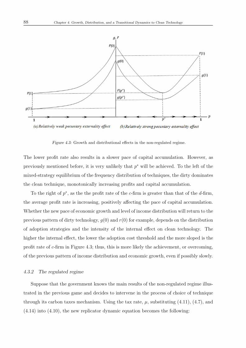
88 Chapter 4. Growth, Distribution, and a Transitional Dynamics to Clean Technology
Figure 4.3: Growth and distributional effects in the non-regulated regime.
The lower profit rate also results in a slower pace of capital accumulation. However, as
previously mentioned before, it is very unlikely that p∗ will be achieved. To the left of the
mixed-strategy equilibrium of the frequency distribution of techniques, the dirty dominates
the clean technique, monotonically increasing profits and capital accumulation.
To the right of p∗, as the the profit rate of the c-firm is greater than that of the d-firm,
the average profit rate is increasing, positively affecting the pace of capital accumulation.
Whether the new pace of economic growth and level of income distribution will return to the
previous pattern of dirty technology, g(0) and r(0) for example, depends on the distribution
of adoption strategies and the intensity of the internal effect on clean technology. The
higher the internal effect, the lower the adoption cost threshold and the more sloped is the
profit rate of c-firm in Figure 4.3; thus, this is more likely the achievement, or overcoming,
of the previous pattern of income distribution and economic growth, even if possibly slowly.
4.3.2 The regulated regime
Suppose that the government knows the main results of the non-regulated regime illus-
trated in the previous game and decides to intervene in the process of choice of technique
through its carbon taxes mechanism. Using the tax rate, µ, substituting (4.11), (4.7), and
(4.14) into (4.10), the new replicator dynamic equation becomes the following:
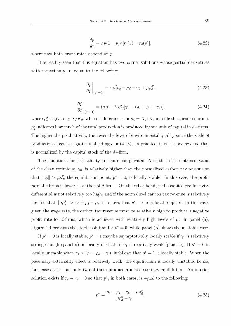
Section 4.3. The classical–Marxian closure 89
dp
dt= αp(1− p)β[rc(p)− rd(p)], (4.22)
where now both profit rates depend on p.
It is readily seen that this equation has two corner solutions whose partial derivatives
with respect to p are equal to the following:
∂p
∂p
∣∣∣∣(p∗=0)
= αβ[ρc − ρd − γ0 + µρgd], (4.23)
∂p
∂p
∣∣∣∣(p∗=1)
= (αβ − 2αβ)[γ1 + (ρc − ρd − γ0)], (4.24)
where ρgd is given by X/Kd, which is different from ρd = Xd/Kd outside the corner solution.
ρgd indicates how much of the total production is produced by one unit of capital in d−firms.
The higher the productivity, the lower the level of environmental quality since the scale of
production effect is negatively affecting ε in (4.13). In practice, it is the tax revenue that
is normalized by the capital stock of the d−firm.
The conditions for (in)stability are more complicated. Note that if the intrinsic value
of the clean technique, γ0, is relatively higher than the normalized carbon tax revenue so
that ‖γ0‖ > µρgd, the equilibrium point, p∗ = 0, is locally stable. In this case, the profit
rate of c-firms is lower than that of d-firms. On the other hand, if the capital productivity
differential is not relatively too high, and if the normalized carbon tax revenue is relatively
high so that ‖µρgd‖ > γ0 + ρd − ρc, it follows that p∗ = 0 is a local reppeler. In this case,
given the wage rate, the carbon tax revenue must be relatively high to produce a negative
profit rate for d-firms, which is achieved with relatively high levels of µ. In panel (a),
Figure 4.4 presents the stable solution for p∗ = 0, while panel (b) shows the unstable case.
If p∗ = 0 is locally stable, p∗ = 1 may be asymptotically locally stable if γ1 is relatively
strong enough (panel a) or locally unstable if γ1 is relatively weak (panel b). If p∗ = 0 is
locally unstable when γ1 > (ρc−ρd−γ0), it follows that p∗ = 1 is locally stable. When the
pecuniary externality effect is relatively weak, the equilibrium is locally unstable; hence,
four cases arise, but only two of them produce a mixed-strategy equilibrium. An interior
solution exists if rc − rd = 0 so that p∗, in both cases, is equal to the following:
p∗ =ρc − ρd − γ0 + µρgd
µρgd − γ1
, (4.25)

90 Chapter 4. Growth, Distribution, and a Transitional Dynamics to Clean Technology
which is always in the interval [0, 1] if the (in)stability conditions are satisfied.
Panel (a) in Figure 4.4 presents a result similar to the one depicted in Figure 4.2,
panel (a): the stability case. Note, however, that for similar reasonable parameters, the
illustration in Figure 4.4 generates a mixed-strategy equilibrium for the distribution of
techniques that is relatively higher than in the previous case. The reason for this is
that the relatively weak carbon tax counterbalances the pecuniary externality effect in the
denominator of (4.25). The growth and distributional effects will present a similar pattern,
illustrated in Figure 4.3, panel (b), but in this case, carbon taxes will reduce the level of
profits of d-firms, thus lowering the pace of capital accumulation relatively faster.
Figure 4.4: Transitional dynamics in the regulated regime.
Meanwhile, if the gains from the pecuniary externality effect on clean technology are
relatively weak, the distribution of adoption strategies will be asymptotically locally stable,
with heterogeneity emerging as a persistent feature of the economy. If all firms are using
dirty technology, the only mechanism that the government has to confront the effects
of positive feedback is to select a carbon tax that, along with the real wage, produces
a negative profit rate for d-firms. If a new entrant chooses to produce using the clean
technique, it will have a positive profit rate. Now, if a d-firm is randomly paired with the
new c-firm, it switches from dirty to clean technology. Thus, all the relevant p domain
to the left of the mixed-strategy equilibrium is a region of positive cumulative causation
toward the adoption of clean technology.
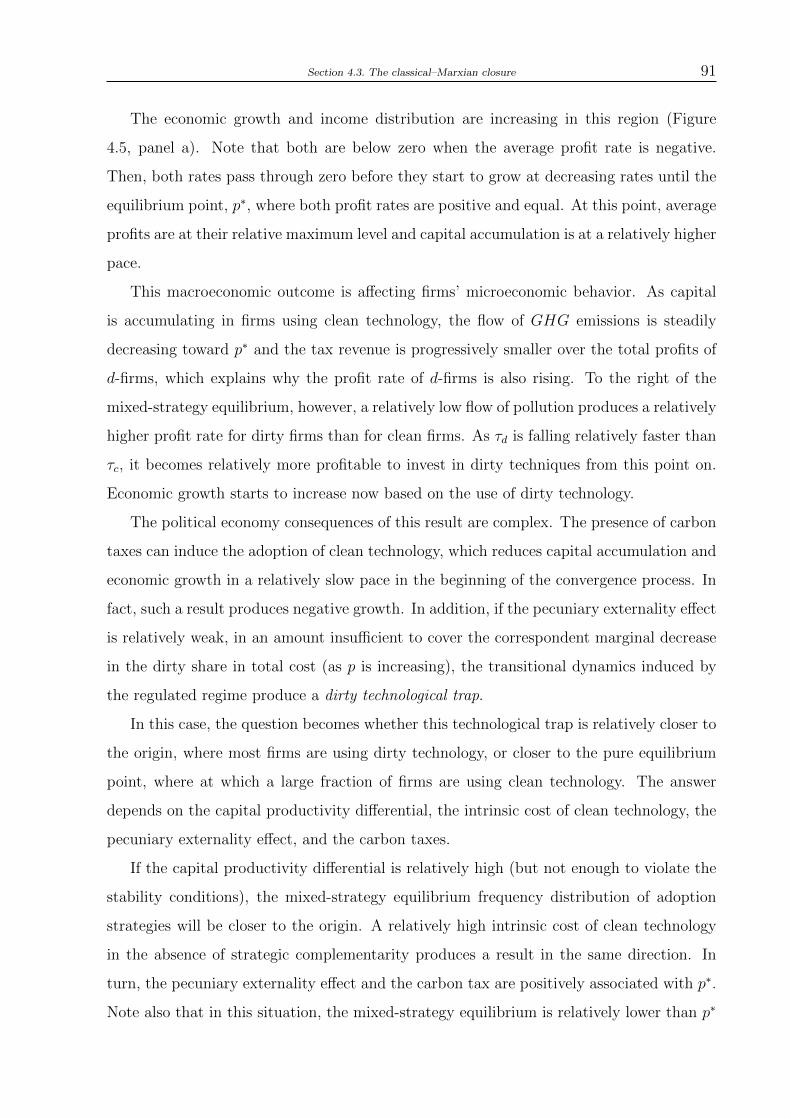
Section 4.3. The classical–Marxian closure 91
The economic growth and income distribution are increasing in this region (Figure
4.5, panel a). Note that both are below zero when the average profit rate is negative.
Then, both rates pass through zero before they start to grow at decreasing rates until the
equilibrium point, p∗, where both profit rates are positive and equal. At this point, average
profits are at their relative maximum level and capital accumulation is at a relatively higher
pace.
This macroeconomic outcome is affecting firms’ microeconomic behavior. As capital
is accumulating in firms using clean technology, the flow of GHG emissions is steadily
decreasing toward p∗ and the tax revenue is progressively smaller over the total profits of
d-firms, which explains why the profit rate of d-firms is also rising. To the right of the
mixed-strategy equilibrium, however, a relatively low flow of pollution produces a relatively
higher profit rate for dirty firms than for clean firms. As τd is falling relatively faster than
τc, it becomes relatively more profitable to invest in dirty techniques from this point on.
Economic growth starts to increase now based on the use of dirty technology.
The political economy consequences of this result are complex. The presence of carbon
taxes can induce the adoption of clean technology, which reduces capital accumulation and
economic growth in a relatively slow pace in the beginning of the convergence process. In
fact, such a result produces negative growth. In addition, if the pecuniary externality effect
is relatively weak, in an amount insufficient to cover the correspondent marginal decrease
in the dirty share in total cost (as p is increasing), the transitional dynamics induced by
the regulated regime produce a dirty technological trap.
In this case, the question becomes whether this technological trap is relatively closer to
the origin, where most firms are using dirty technology, or closer to the pure equilibrium
point, where at which a large fraction of firms are using clean technology. The answer
depends on the capital productivity differential, the intrinsic cost of clean technology, the
pecuniary externality effect, and the carbon taxes.
If the capital productivity differential is relatively high (but not enough to violate the
stability conditions), the mixed-strategy equilibrium frequency distribution of adoption
strategies will be closer to the origin. A relatively high intrinsic cost of clean technology
in the absence of strategic complementarity produces a result in the same direction. In
turn, the pecuniary externality effect and the carbon tax are positively associated with p∗.
Note also that in this situation, the mixed-strategy equilibrium is relatively lower than p∗
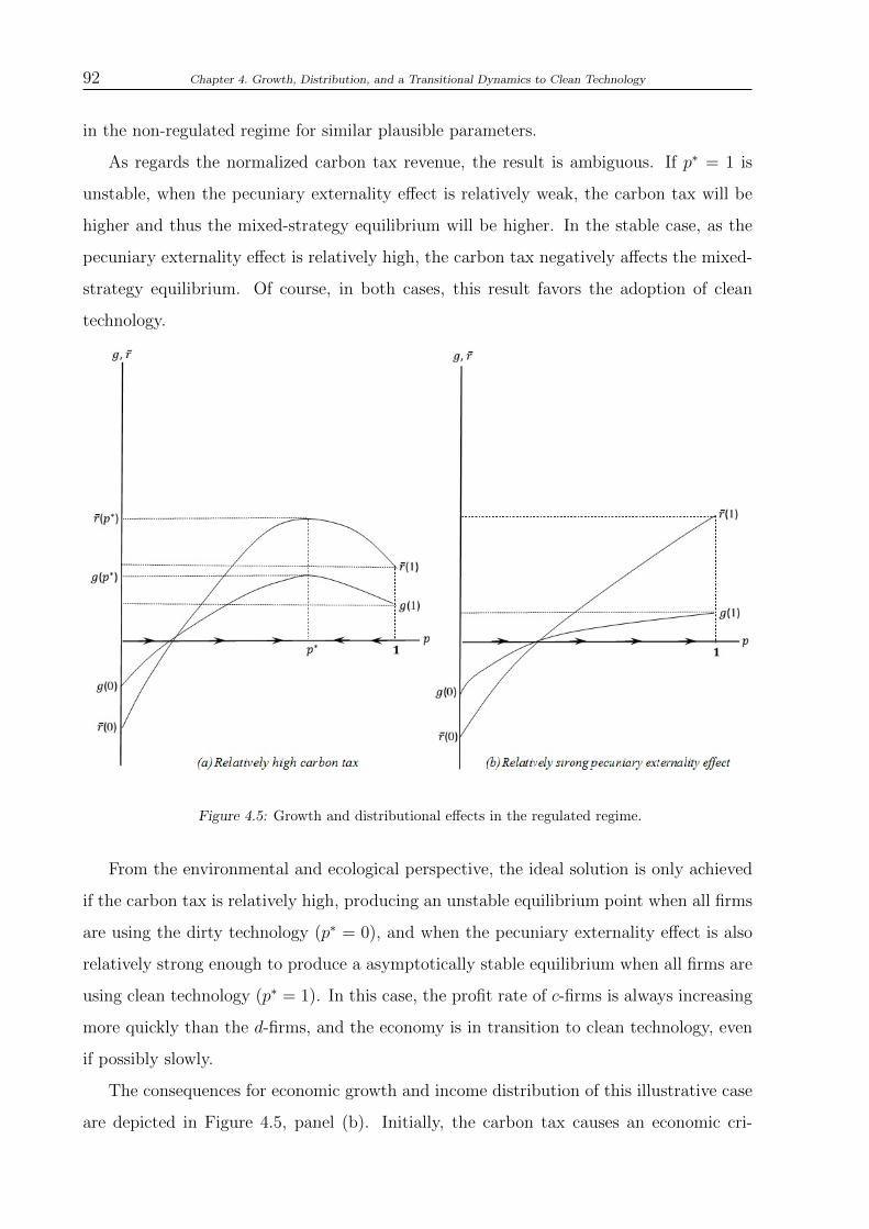
92 Chapter 4. Growth, Distribution, and a Transitional Dynamics to Clean Technology
in the non-regulated regime for similar plausible parameters.
As regards the normalized carbon tax revenue, the result is ambiguous. If p∗ = 1 is
unstable, when the pecuniary externality effect is relatively weak, the carbon tax will be
higher and thus the mixed-strategy equilibrium will be higher. In the stable case, as the
pecuniary externality effect is relatively high, the carbon tax negatively affects the mixed-
strategy equilibrium. Of course, in both cases, this result favors the adoption of clean
technology.
Figure 4.5: Growth and distributional effects in the regulated regime.
From the environmental and ecological perspective, the ideal solution is only achieved
if the carbon tax is relatively high, producing an unstable equilibrium point when all firms
are using the dirty technology (p∗ = 0), and when the pecuniary externality effect is also
relatively strong enough to produce a asymptotically stable equilibrium when all firms are
using clean technology (p∗ = 1). In this case, the profit rate of c-firms is always increasing
more quickly than the d-firms, and the economy is in transition to clean technology, even
if possibly slowly.
The consequences for economic growth and income distribution of this illustrative case
are depicted in Figure 4.5, panel (b). Initially, the carbon tax causes an economic cri-
Section 4.4. Conclusions 93
sis defined as the propagation of profitability loss and negative growth in the economy.
Progressively, as firms adopt clean technology, the total profits begin to increase and the
growth becomes positive, both at decreasing rates. The flow of emission will decline to
zero and the environmental quality converges to its maximum carrying capacity level.
In the present instance, as mentioned before, the government invests all of the corres-
ponding tax revenue into the recovery of the environmental damage. The government has
a restriction to increase the tax rate. This restriction emerges from the negative impact
of the environmental policy on economic growth. The higher the tax rate, the lower the
pace of capital accumulation in the beginning of convergence. Another possibility arises
when the government applies all of the tax revenue to the production of clean technology
in the form of a subsidy. In this case, the speed with which the price of clean technology
is falling is relatively faster than the case illustrated in (4.8). In addition, the likelihood is
that p∗ stabilizes closer to the full specialization in clean technology than in the previous
case. As the main qualitative result will be the same, I abstract from formally addressing
such a possibility.
4.4 Conclusions
This paper presents a model that provides a novel behavioral foundation for the tran-
sition to clean technology in capitalist economies. The model has many limitations and
clearly provides (at best) some elements to understand the adoption of clean technology
in a context in which the price of backstop technology is not exogenously given.
The adaptive behavior of firms based on historical learning is central to the story,
demonstrating that the persistence of a heterogeneous frequency distribution of adoption
strategies may be, in various settings previously explored, the normal state of affairs. All
these settings are sensitive to reasonable configurations of the parameters, especially the
intrinsic value of clean technology, the intensity with which the cost of clean technology
decreases with the proportion of firms adopting it, as well the magnitude of carbon taxes.
In a non-regulated regime, in which the cost of adoption of clean technologies is decre-
asing in the proportion of firms taking the same action, the model shows that instability
characterizes the transitional dynamics in the long run. It is only if the clean technology
surpasses some cost threshold that its adoption can benefit from the occurrence of positive
94 Chapter 4. Growth, Distribution, and a Transitional Dynamics to Clean Technology
feedback. In this context, the pecuniary externality effect, in other words, the strategic
complementarity behavior of firms, plays a central role. On the other hand, the economy
is constantly pushed toward the the full specialization in dirty technology (the non-use of
the clean technique) and a possible environmental collapse in the long run. In this case, an
exogenous discontinuous shock on fraction of firms using the clean technique is required.
Such an exogenous intervention also can be implemented as a governmental policy.
In a regime with relatively high policy activity, the regulated regime, the possibility
of a full and continuous transition to clean technology arises. This outcome is achieved
through a relatively high carbon tax and a relatively rapid decrease of the cost of adopting
on clean technology due to the operation of pecuniary externality effects, which are both
central to the argument. At the same time, however, for reasonable parameters, the model
also shows that instead of producing full specialization in clean technology, the carbon
taxes may push the economy to a dirty technological trap, which is characterized by a
stable mixed-strategy equilibrium point from which the economy, if left to the free play of
its structural forces, may never escape. This occurs if the strategic complementarity effect
on the cost of clean technology is relatively weak.
The contribution of this paper relates to a large and growing literature on the re-
lationship between economic growth, technical change and the environment. Based on
economic models of climate change, this literature has suggested either relatively strong
and immediate governmental action at a relatively high cost in the present (Stern, 2007),
a more gradualist approach, the climate-policy ramp (Nordhaus, 2008) or only a tempo-
rary intervention (Acemoglu et al., 2012). The present contribution, thus, indicates that
a relatively high governmental interventions is required either in the form of an exogenous
shock on clean technology, or relatively high carbon tax.
In addition, the paper shows that the political issue involves more than just the choice
of the “correct” intensity of policy actions. Important as this discussion may be, firms’
strategic complementarity behavior is crucial in this setting, because it is through it that
the positive cumulative causation effects on clean technology operate. Therefore, we can-
not give to the complex mechanisms of technological adoption a simplified treatment in
the story. Eventually, the design of mechanisms to promote the technological interaction
among firms may be a viable environmental policy in the real world.
In terms of growth and distributional effects, if the behavioral foundation of firms and

Section 4.4. Conclusions 95
its interaction with macroeconomic outcomes is taken into account, the unique (continuous)
scenario that may promote the full transition to clean technology, or at least for a relatively
high proportion of firms, is achieved through initial negative adverse effects on income
distribution, and thus, economic growth. Note, however, that it effect is not the same as
the one proposed by a degrowth strategy. The degrowth strategy focus has been less on
a positive approach of the sustainability problem and more on the social transformation
necessary to achieve sustainable development. The particular emphasis has been on power,
income distribution, and conflict. The present result, in turn, implies that initially, growth
must be reduced in order for firms to consider the possibility of switching to a clean
production technique. Over time, therefore, the profits will begin to increase again toward
the capitalists who are using clean technology.

96 Chapter 4. Growth, Distribution, and a Transitional Dynamics to Clean Technology

Chapter 5
Final Remarks
All capitalist economies have a predatory relation with the environment, even if these
may be at different levels. There is significant, if not conclusive, evidence relating such a
predatory relation to environmental degradation and anthropogenic climate change, more
broadly, so that they are now issues of public concern and central importance. This begs
the following question: What do macroeconomists know about it?
Unfortunately, the relationship between macroeconomics and the environment is not
well understood. On the one hand, our knowledge about the science involved in such issues
and its relation with economics is limited. On the other hand, the quality of environmental
data is relatively poor, and we cannot estimate robust empirical evidence relating the
negative environmental externalities to economic aggregates. So, what can we do? There
is a relative consensus between environmental macroeconomists that we should focus on
formulating simple theoretical models that can clarify our understanding about the relation
between macroeconomics and the environment either in its medium- or long-run dimension.
In this context, is there any particular reason to focus on a single approach such as
the orthodox or post-Keynesian answer to the problem? The answer, in my view, is no.
The reason is that answers to environmental challenges such as degradation and climate
change are sensitive to the internal consistency of macroeconomic models and their implicit
or explicit assumption concerning sustainable development. I would argue, therefore, that
pluralism is beneficial for these questions at hand; hand; thus, focusing on a particular
framework is not desirable by its one sake.
The present Dissertation incorporates much of this spirit of pluralism. I have developed
three theoretical models that incorporate different environmental problems and implicit
or explicit weak and strong sustainability assumptions. I have focused on alternative
98 Chapter 5. Final Remarks
macromodels because the heterodox tradition has largely ignored sustainable development
issues. It is ironic that a set of theories and models concerned with what neoclassical
economists call market failures are, in fact, structural deficiencies, have ignored the perhaps
most important of them: the negative externalities on the environment.
Therefore, the first contribution of the present Dissertation is to model environmental
sustainability issues in alternative macroeconomic models. Here I have explored environ-
mental issues involving the medium (fluctuations) and long run (economic growth and
economic development) perspective of the macroeconomy. The medium-run dimension,
despite being surrounded by a great deal of controversy, is modeled in a particularly novel
way. The other two essays address a long run perspective.
In the first essay (Chapter 2), I present “a green Lewis development model”. The first
contribution of this essay is to extend a Lewis development model to an environmental
dimension. To the best of my knowledge, this is the first attempt to do so. I justify this
extension using recent and robust econometric evidence on the relation between pollution
and labor productivity. Motivated by the recent contribution of the so-called “green Solow
model” (Brock and Taylor, 2010), I was interested in investigating whether developing
countries are not structurally any different in the sense that a simple environmental policy
can prevent them from achieving economic maturity (in a Kaldorian sense). The reader
should recall that “the green Solow model” has an optimist view about sustainable deve-
lopment in developing countries: there is no endogenous force that is capable of preventing
them achieving economic maturity, even in the face of abatement policies that compromise
a fraction of their gross savings. In fact, this result is in contrast with many of the claims
that developing countries make during international environmental negotiations.
Interestingly, the essay finds that a developing dual economy that has to comply with
a pollution abatement requirement may fall in what I dub an ecological development trap
and therefore may fail to reach mature development. Moreover, once in such trap, a deve-
loping dual economy is either already experiencing or will eventually come to experience
a Kaldor–Myrdal circular and cumulative causation process of decline in capital intensity
and environmental quality. Fortunately, however, a developing dual economy that hap-
pens to fall in such trap can be released from it not only through a standard Big Push, in
the spirit of Rosenstein–Rodan, but also by means of what I dub an Environmental Big
Push. The latter could be based, for instance, on the adoption of international redress and
Chapter 5. Final Remarks 99
compensation mechanisms in favor of developing economies. While the case for a standard
Big Push is quite well established in the economic development literature, this essay con-
tributes to the environmental macroeconomics literature by providing a sound theoretical
rationale for an Environmental Big Push.
The essay, thus, can be read as being more closely related to the weak sustainability
assumption. The reason for this is that I have assumed that all environmental impact is
potentially reversible in the long run, and that there is some degree of substitution among
physical capital stock and the level of environmental quality. To what extent does my
main result, the ecological development trap, depend on this sustainability assumption?
Certainly, it depends a great deal on it; however, the weak sustainability assumption
makes the result stronger. If, on the other hand, I had supposed the strong sustainability
assumption, the ecological development trap would become more pervasive since there
would be no reversibility in the environmental impact in the long run.
In the second essay (Chapter 3), I explore the issue of reverse causality in the environ-
mental Kuznets curve. International development agencies have discussed and addressed
the situation of some developing countries that have relatively low levels of environmen-
tal quality, such as Rwanda, for example. In such countries, much of the macroeconomic
instability involving economic growth is caused by their environment fragility in response
to soil erosion, poisoned water resources, or toxic pollution in the local atmosphere. An
economic development strategy based on the environment Kuznets curve may eventually
result in an unsustainable vicious circle in these regions, possibly even in the medium run.
What is important to the argument and hence the contribution of this second essay
is that it is necessary to understand that in such dual low-income developing economies,
the relatively low levels of environmental quality result in a cost that is binding in the
short run, and not only in the long run, as we are accustomed to thinking. This cost
arises from the negative effects of pollution (not all sources of pollution, of course) on the
labor force. Based on robust and recent empirical evidence, I refer to those these costs as
environmental adjustment costs. The model incorporates such environmental adjustment
costs in a a post-Keynesian framework: the Harrodian benchmark. The reason for this
is that the Harrodian model supposes that the output is not fully flexible in the short
run; instead, it only slowly responds to unexpected shocks in aggregate demand. This
slow adjustment is justified by the existence of adjustment costs. In this second essay, I

100 Chapter 5. Final Remarks
examined how a developing economy is likely to behave in a context like that.
The well trained long run mind would choose to relate variations in the level of envi-
ronmental quality to capital accumulation, thus exploring an eventual occurrence of long
term vicious circles (which is natural and easy in a Harrodian model). However, I have
deliberately choosen to use the capacity utilization as an accommodating variable. The
reason for this is that I believe that much of the macroeconomic medium run instability
in these countries is due to the relatively low level of environmental quality. My main
contribution is to show that the environmental adjustment costs may also contribute to
the emergence of perpetual vicious circles in dual low-income economies with relatively
low levels of environmental quality.
Interestingly, the model thus creates an innovative link between effective demand and
environmental quality. A rise in effective demand is associated with a fall in the level
of environmental quality. In addition, to explicitly mention the Harrodian instability
“problem”, effective demand is endogenously linked to the natural growth rate of the
environment. Such an apparently naive result has an important implication for ecological
and environmental macroeconomics: if the environmental adjustment costs are taken into
account, the model shows that there is a long run trajectory linking economic growth
(the warranted growth rate) to the behavior of the environment (the natural growth rate).
What the model emphasizes, in line with its Harrodian specification, is that this trajectory
is cyclically unstable and not well behaved, as is argued by most neoclassical models based
on the unidirectional (and endogenous) prediction of the environmental Kuznets curve.
The model can be read as implicitly in line with the strong sustainability assump-
tion. This is because the environment does not play a passive role in the model. The
non-substitutability assumption, by means of a fixed–proportions production function, is
also important. The main contribution, thus, relates to the recent movement to model
sustainable development issues in the post-Keynesian tradition, as suggested by Taylor et
al. (2015).
The first two essays have a characteristic in common: there is no room for the adoption
of clean technology. This should not be understood as a limitation. On the contrary, the
previous contributions show that in the absence of clean technical change, the relation
between the macroeconomy and the environment is subjected to multiple equilibria and
cyclical instability. However, at some moment, the possibility of adopting clean technology

Chapter 5. Final Remarks 101
has to be faced; this is so precisely the main objective of the third (and last) essay (Chapter
4).
In the third essay, I explored what accounts for the diffusion and maybe the non-
use of clean technology in a competitive environment. This is a very timely issue. The
old growth models and most of the recent economic models of climate change assume
exogenous technical change. Recently, however, Acemoglu et al. (2016) have questioned
this view. They formulated an endogenous growth model with direct technical change that
accounts for most of the dynamics involved in the invention and the adoption of new clean
techniques. However, several questions regarding the empirical evidence remain open.
Thus, the third essay addresses two of several important issues: the existence of stra-
tegic complementarity behavior among firms and the role of carbon taxes in the process
of technical choice. I have modeled these issues an using an evolutionary game-theoretic
approach. Evolutionary game theory offers a novel behavioral foundation for the microeco-
nomics of clean technical change. The focus on microeconomics was primarily to unders-
tand macrodynamics so that I have incorporated this foundation in a classical-Marxian
description of the macroeconomy. The classical–Marxian model is helpful in exploring the
problem of technical choice, especially because the classical economists and Marx were
quite concerned with the role of technology in the capitalist society.
The main preliminary contributions of the essay are the following. First, it shows that
a mixed-strategy equilibrium in which firms produce using clean and dirty technology is a
possible evolutionary outcome. The result illustrates an empirical evidence that different
techniques of production may survive in a competitive environment. Furthermore, in some
cases, the carbon taxes set by the government can create a dirty technological trap. The
political question then becomes if such a trap (the mixed-strategy equilibrium) will be clo-
ser to the full specialization in dirty or clean technology. In the model, the main economic
mechanism that can prevent firms from being trapped close to the pure specialization in
dirty technology is the pecuniary externality effect on the adoption of clean technology.
The second contribution is to show that potentially beneficial environmental outcomes
require exogenous interventions, which in the paper assumes the format of government
policies. These policies may promote discontinuous shocks (investments) in the adoption of
clean technology as well the “correct” calibration of carbon taxes. Inevitably, however, the
ideal environmental scenario in which all firms use clean technology and the environmental

102 Chapter 5. Final Remarks
quality converges to it maximum carrying capacity point, is only achieved through an initial
adverse macroeconomic impact. Such an impact is a profit-reducing shock on functional
income distribution, and thus, a fall in economic growth. Meanwhile, such a result is not
similar to a degrowth strategy, which requires some level of social transformation. The
present result implies that the degrowth is temporary, so that that at some time, profits
will increase based on clean technology.
The third essay is suitable to both sustainability assumptions because both ecological
and environmental economics assume that clean technological change is important in order
to achieve sustainable development. My contribution, however, reveals that the transitional
dynamics to clean technology are not easy and calm; instead, they are a conflictual process
that may eventually reduce capital accumulation for a considerable amount of time. The
result thus adds to the claim against the so-called climate policy ramp.
Motivated by all these specific contributions to economics, I conclude that the pre-
sent Dissertation has achieved its main objective of developing alternative macromodels
that explore, in some of their many relevant aspects, the macroeconomic implications of
some environmental and ecological economics concerns. The central message is that our
intuition and understanding about the relationship between the macroeconomy and the en-
vironment can be broadened rather than shaped by a particular macroeconomic framework
or assumption concerning sustainable development. The progress of the field requires that
we are able to develop and study all approaches, so that economists should have the op-
portunity to have their intuition about the economics of the environment shaped by all of
them.
One of the main limitations of the present Dissertation is that I treat the negative
environmental externalities as a local effect. Most externalities are, in fact local; howe-
ver, greenhouse gas emissions, one of the most important externalities, and one that has
attracted a great deal of attention, is global. There is no logical shortcoming in approa-
ching only the local aspect of the negative externalities. As a matter of logic, I tend to
believe that an open setting would make the ecological development trap and the vicious
circles, for instance, even more pervasive. Meanwhile, the global treatment of the negative
environmental externalities should be pursued as future research. It would be particularly
interesting to examine environmental issues in open macroeconomic models.
In the first essay, for instance, the main result indicates that if left to free play of
Chapter 5. Final Remarks 103
its structural forces, developing countries cannot converge to the mature phase. Thus, a
natural step is to stress the role of developed countries in this international political sce-
nario. Can developed countries help developing countries to converge without destroying
the planet? In addition, as much of the technological knowledge is developed in the rich
countries, developed countries may exert an important influence on the adoption of clean
technology in developing countries. Thus, an extension of the the third essay is in or-
der. However, will this process generate divergence or convergence in terms of per capita
income? North–South models can illuminate this relevant question.
These are very timely issues since the relationship between the environment, open ma-
croeconomics, and income distribution has not received sufficient attention. The analysis
of the relation between global warming and structural change and its consequences for
developing countries may finally be a necessary step before addressing the effectiveness
of sustainable development policies. These latter questions arguably present the greatest
challenge to environmental and ecological macroeconomics.

104 Chapter 5. Final Remarks
References
Abramovay R., Beyond the Green Economy. Taylor & Francis, 2015
Acemoglu D., Aghion P., Bursztyn L., Hemous D., The Environment and Directed Tech-
nical Change, American Economic Review, 2012, vol. 102, p. 131
Acemoglu D., Akcigit U., Hanley D., Kerr W., Transition to Clean Technology, Journal of
Political Economy, 2016, vol. 124, p. 52
Aghion P., Dechezlepretre A., Hemous D., Martin R., Reenen J. V., Carbon Taxes, Path
Dependency, and Directed Technical Change: Evidence from the auto industry, Journal
of Political Economy, 2016, vol. 124, p. 1
Arrow K. J., Bolin B., Costanza R., Dasgupta P., Folke C., Holling C. S., Jansson B.-O.,
Levin S., Meler K.-G., Perrings C., Pimentel D., Economic Growth, Carrying Capacity,
and the Environment, Science, 1995, vol. 268, p. 520
Arthur W. B., The Nature of Technology: What it is and how it evolves. Free Press, 2011
Berman E., Bui L. T., Environmental Regulation and Productivity: evidence from oil
refineries, The Review of Economics and Statistics, 2001, vol. 83, p. 498
Bojo J., Bucknall J., Hamilton K., Kishor N., Kraus C., Pillai P., , 2001 Techini-
cal Report 1 Environment Chapter, Poverty Reduction Strategy PapersSource Book
http://web.worldbank.org/WBSITE/EXTERNAL/TOPICS/EXTPOVERTY/. World Bank
Bowles S., Microeconomics: Behavior, institutions and evolution. Princeton University
Press, 2004

106 References
Brander J. A., Taylor M. S., The Simple Economics of Easter Island: A Ricardo-Malthus
model of renewable resource use, The American Economic Review, 1998, vol. 88, p. 119
Brock W. A., Taylor M. S., , 2004 Working Paper 10854 Economic Growth and the En-
vironment: A Review of Theory and Empirics http://www.nber.org/papers/w10854.
National Bureau of Economic Research
Brock W. A., Taylor M. S., The Green Solow Model, Journal of Economic Growth, 2010,
vol. 15, p. 127
Bruvoll A., Larsen B. M., Greenhouse Gas Emissions in Norway: Do carbon taxes work?,
Energy Policy, 2004, vol. 32, p. 493
Bulte E. H., van Soest D. P., Environmental Degradation in Developing Countries: Hou-
seholds and the (reverse) Environmental Kuznets Curve, Journal of Development Eco-
nomics, 2001, vol. 65, p. 225
Carson R. T., The Environmental Kuznets Curve: Seeking Empirical Regularity and The-
oretical Structure, Review of Environmental Economics and Policy, 2010, vol. 4, p. 3
Chang T., Zivin J. S. G., Gross T., Neidell M. J., , 2014 Working Paper 19944 Particulate
Pollution and the Productivity of Pear Packers http://www.nber.org/papers/w19944.
National Bureau of Economic Research
Chimeli A. B., Branden J. B., A Capital Scarcity Theory of the Environmental Kuznets
Curve, Environment and Development Economics, 2009, vol. 14, p. 541
Copeland B. R., International Trade in Waste Products in the Presence of Illegal Disposal,
Journal of Environmental Economics and Management, 1991, vol. 20, p. 143
Copeland B. R., Taylor M. S., North-South Trade and the Environment, The Quarterly
Journal of Economics, 1994, vol. 109, p. 755
Copland Brian R., Taylor M. S., Trade and the Environment: Theory and evidence. Prin-
ceton University Press, 2005
Costanza R., Daly H. E., Natural Capital and Sustainable Development, Conservation
biology, 1992, vol. 6, p. 37
References 107
Cunha F., Heckman J., The Technology of Skill Formation, American Economic Review,
2007, vol. 97, p. 31
Currie J., Hanushek E. A., Kahn E. M., Neidell M., Rivkin S. G., Does Pollution Increase
School Absences?, The Review of Economics and Statistics, 2009, vol. 91, p. 682
Currie J., Stabile M., Child Mental Health and Human Capital Accumulation: The case
of ADHD, Journal of Health Economics, 2006, vol. 25, p. 1094
Dafermos Y., Galanis G., Nikolaidi M., An Ecological Stock-Flow-Fund Modelling Fra-
mework, Draft: http://www. boeckler. de/pdf/v 2014 10 30 dafermos galanis nikolaidi.
pdf, 2014
Daly H. E., Steady-state Economics. Island Press, 1991
Dasgupta P., Heal G., The Optimal Depletion of Exhaustible Resources, The Review of
Economic Studies, 1974, vol. 41, p. 3
Dasgupta P. S., Heal G. M., Economic Theory and Exhaustible Resources. Cambridge
University Press, 1980
Dasgupta S., Deichmann U., Meisner C., Wheele D., Where is the Poverty-Environment
Nexus? Evidence from Cambodia, Lao PDR, and Vietnam, World Development, 2005,
vol. 33, p. 617
Dasgupta S., Laplante B., Wang H., Wheeler D., Confronting the Environmental Kuznets
Curve, Journal of Economic Perspectives, 2002, vol. 16, p. 147
Delmas M. A., Pekovic S., Environmental Standards and Labor Productivity: Understan-
ding the mechanisms that sustain sustainability, Journal of Organizational Behavior,
2013, vol. 34, p. 230
Downing T., Watkiss P., Dyszynski J., et al., 2009 Techi-
nical Report 1 Economics of Climate Change in Rwanda
http://www.sei-international.org/publications?pid=1579. Stocholm Envi-
ronment Institute
Dumenil G., Levy D., A Stochastic ModelL of Technical Change: An application to US
Economy (1869a1989), Metroeconomica, 1995, vol. 46, p. 213
108 References
Dutt A. K., Growth, Distribution and Uneven Development. Cambridge University Press,
1990
Foley D. K., Endogenous Technical Change with Externalities in a Classical Growth Model,
Journal of Economic Behavior Organization, 2003, vol. 52, p. 167
Foley D. K., Unholy Trinity: Labor, capital and land in the new economy. The Graz
Schumpeter Lectures, Taylor & Francis, 2004
Foley D. K., Dilemmas of Economic Growth, Eastern Economic Journal, 2012, vol. 38, p.
283
Foley D. K., Michl T., Growth and Distribution. Harward University Press, 1999
Fontana G., Sawyer M., Post-Keynesian and Kaleckian Thoughts on Ecological Macroeco-
nomics, European Journal of Economics and Economic Policies, 2013
Fontana G., Sawyer M., Towards Post-Keynesian Ecological Macroeconomics, Ecological
Economics, 2016, vol. 121, p. 186
Georgescu-Roegen N., The Entropy Law and the Economic Process. A Harvard paperback:
Economics, Harvard University Press, 1971
Gintis H., Game Theory Evolving: A problem-centered introduction to modeling strategic
interaction (Second Edition). Game Theory Evolving: A Problem-centered Introduction
to Modeling Strategic Behavior, Princeton University Press, 2009
Graff Zivin J., Hsiang S. M., Neidell M. J., , 2015 Working Paper 21157 Temperature and
Human Capital in the Short- and Long-Run http://www.nber.org/papers/w21157.
National Bureau of Economic Research
Graff Zivin J., Neidell M., The Impact of Pollution on Worker Productivity, American
Economic Review, 2012, vol. 102, p. 3652
Graff Zivin J., Neidell M., Environment, Health, and Human Capital, Journal of Economic
Literature, 2013, vol. 51, p. 689
Green J. F., Sterner T., Wagner G., A Balance of Bottom-up and Top-down in Linking
Climate Policies, Nature Climate Change, 2014, vol. 4, p. 1064
References 109
Grossman G. M., Krueger A. B., Economic Growth and the Environment, The Quarterly
Journal of Economics, 1995, vol. 110, p. 353
Harrison A., Hyman B., Martin L., Nataraj S., , 2015 Working Paper 21763 When do
Firms Go Green? Comparing price incentives with command and control regulations in
India http://www.nber.org/papers/w21763. National Bureau of Economic Research
Harrod R. F., An Essay in Dynamic Theory, The Economic Journal, 1939, vol. 49, p. 14
Hartwick J. M., Intergenerational Equity and the Investing of Rents from Exhaustible
Resources, The American Economic Review, 1977, vol. 67, p. 972
Hartwick J. M., Natural Resources, National Accounting and Economic Depreciation, Jour-
nal of Public Economics, 1990, vol. 43, p. 291
IPCC, 2014 Climate Change 2014: Synthesis Report. IPCC Geneva, Switzerland pp 1–141
Jacob M., Marschinski R., A Balance of Bottom-up and Top-down in linInterpreting Trade-
related CO2Emission Transfersking climate Policies, Nature Climate Change, 2013,
vol. 3, p. 19
Jacobs M., The Green Economy: Environment, sustainable development, and the politics
of the future. Pluto Press, 1991
Kaldor N., Marginal Productivity and the Macro-Economic Theories of Distribution: Com-
ment on Samuelson and Modigliani, The Review of Economic Studies, 1966, vol. 33, p.
309
Kallis G., Kerschner C., Martinez-Alier J., The Economics of Degrowth, Ecological Eco-
nomics, 2012, vol. 84, p. 172
Kelly D. L., Kolstad C. D., Mitchell G. T., Adjustment Costs From Environmental Change,
Journal of Environmental Economics and Management, 2005, vol. 50, p. 468
Keynes J., A Treatise on Money. No. v. 1 in A Treatise on Money, AMS Press, 1976
Kjellstrom T., R. Kovats S., Lloyd S. J., Holt T., Tol R. S. J., The Direct Impact of Climate
Change on Regional Labor Productivity, Archives of Environmental & Occupational
Health, 2009, vol. 64, p. 217

110 References
Lewis W. A., Economic Development with Unlimited Supplies of Labour, The Manchester
School, 1954, vol. 22, p. 139
Lewis W. A., The Theory of Economic Growth. Manchester: George Allen Unwin Ltd,
1955
Lewis W. A., Unlimited Labour: Further notes, The Manchester School, 1958, vol. 26, p.
1
Lima G. T., Endogenous Techonological Innovation, Capital Accumulation and Distribu-
tion Dynamics, Metroeconomica, 2004, vol. 55, p. 386
Marglin S. A., Growth, Distribution and Prices. Harward University Press, 1984
Marquetti A. A., Pichardo G. M., Patrones de crecimiento y cambio tecnico en la pro-
duccion de un producto bueno y otro malo, Investigacion Economica, 2013, vol. 72, p.
57
Massarani L., Brazil Mine Disaster Floods Area With Toxic Substances, Scientific America,
2016
Meadows D., of Rome C., Associates P., The Limits to Growth: A report for the Club of
Rome’s project on the predicament of mankind. No. pt. 1 in Potomac Associates book,
Universe Books, 1972
Michl T. R., Foley D. K., Crossing Hubbertas Peak: Portfolio effects in a growth model
with exhaustible resources, Structural Change and Economic Dynamics, 2007, vol. 18,
p. 212
Murphy K. M., Shleifer A., Vishny R. W., Industrialization and the Big Push, Journal of
Political Economy, 1989, vol. 97, p. 1003
Myrdal G., Economic Theory and Under-Developed Regions. Gerald Duckworth Co, 1957
Nagashima M., Dellink R., van Ierland E., Weikard”H.-P., Stability of International Cli-
mate Coalitions: A comparison of transfer schemes, Ecological Economics, 2009, vol. 68,
p. 1476

References 111
Nakatani T., Skott P., Japanese Growth and Stagnation: A Keynesian perspective, Struc-
tural Change and Economic Dynamics, 2007, vol. 18, p. 306
Neumayer E., Weak versus Strong Sustainability: Exploring the limits of two opposing
paradigms. Edward Elgar, 2010
Nordhaus W. D., The Allocation of Energy Resources, Broken Paper Series, 1973, vol. 1,
p. 529
Nordhaus W. D., Managing the Global Commons: The economics of climate change. MIT
Press: Cambridge, MA, 1994
Nordhaus W. D., A Question of Balance: Weighing the options on global warming policies.
Yale University Press: New Haven, CT, 2008
Nordhaus W. D., Boyer J., Warming the World: Economic modeling of global warming.
MIT Press: Cambridge, MA, 2000
Nurkse R., Some International Aspects of the Problem of Economic Development, The
American Economic Review, 1952, vol. 42, p. 571
Oliveira G., Lima G. T., , 2015 Working Paper 201549 A Green Lewis Development Model.
Departament of Economics, University of Sao Paulo
Ostrom E., Governing the Commons: the evolution of institutions for collective action.
Cambridge University Press, 1990
Ostrom E., Gardner R., Walker J., Rules, Games and Common Pool Resources. University
of Michigan Press, 1994
Pearce D., Barbier E., Markandya A., Sustainable Development: Economics and environ-
ment in the Third World. An Earthscan paperback, Earthscan, 1990
Pearce D., Markandya A., Barbier E., of the Environment G. B. D., Blueprint for a Green
Economy. AnEarthscan original, Earthscan, 1989
Razmi A., North-South Interactions in the Presence of Trade in Environmental Permits:
A structuralist investigation, Cambridge Journal of Economics, 2015, vol. 39, p. 1

112 References
Rezai A., Stagl S., Ecological Macroeconomics: Introduction and review, Ecological Eco-
nomics, 2016, vol. 121, p. 181
Rezai A., Taylor L., Mechler R., Ecological Macroeconomics: An application to climate
change, Ecological Economics, 2013, vol. 85, p. 69
Ros J., Rethinking Economic Development, Growth, and Institutions. Oxford University
Press, 2013
Rosenstein-Rodan P. N., Problems of Industrialisation of Eastern and South-Eastern Eu-
rope, The Economic Journal, 1943, vol. 53, p. 202
Scitovsky T., Two Concepts of External Economies, Journal of Political Economy, 1954,
vol. 62, p. 143
Setterfield M., Handbook of Alternative Theories of Economic Growth. Edward Elgar Pu-
blishing, Inc. Cheltenham, UK, 2010
Silveira J. J., Lima G. T., Conhecimento Imperfeito, Custos de Otimizacao e Racionalidade
Limitada: Uma dinamica evolucionaria de de ajustamento nominal incompleto, Revista
Brasileira de Economia, 2008, vol. 62, p. 57
Silveira J. J., Lima G. T., Effort Elicitation, Wage Differentials and Income Distribution
in A Wage-Led Growth Regime, Metroeconomica, 2016, vol. 67, p. 44
Skott P., Effective Demand, Class Struggle and Cyclical Growth, International Economic
Review, 1989a, vol. 30, p. 231
Skott P., Conflict and Effective Demand in Economic Growth. Cambridge University Press,
1989b
Skott P., , 2010 in Setterfield M., ed., Edward Elgar Publishing, Inc., Handbook of Alter-
native Theories of Economic Growth. Edward Elgar Publishing, Inc.
Skott P., Growth Cycles With or Without Price Flexibility, Review of Keynesian Econo-
mics, 2015, vol. 3, p. 374
Skott P., Ros J., The “Big Push” in an Open Economy with Nontradable Inputs, Journal
of Post Keynesian Economics, 1997, vol. 20, p. 149

References 113
Solow R., Sustainability: an economists perspective. J. Seward Johnson lecture in marine
policy, Marine Policy Center, 1991
Solow R. M., A Contribution to the Theory of Economic Growth, The Quarterly Journal
of Economics, 1956, vol. 70, p. 65
Solow R. M., Intergenerational Equity and Exhaustible Resources, The Review of Economic
Studies, 1974, vol. 41, p. 29
Solow R. M., On the Intergenerational Allocation of Natural Resources, The Scandinavian
Journal of Economics, 1986, vol. 88, p. 141
Spash C. L., Economics, Ethics, and Long-term Environmental Damages, Environmental
Ethics, 1993, vol. 15, p. 117
Steindl J., Maturity and Stagnation in American Capitalism. London: Monthly Review
Press, 1952
Stern D., , 2015 Ccep working papers The Environmental Kuznets Curve after 25 years
http://EconPapers.repec.org/RePEc:een:ccepwp:1514. Centre for Climate Econo-
mics Policy, Crawford School of Public Policy, The Australian National University
Stern D. I., The Rise and Fall of the Environmental Kuznets Curve, World Development,
2004, vol. 32, p. 1419
Stern N., The Economics of Climate Change: The Stern review. Cambridge University
Press, 2007
Stiglitz J., Growth with Exhaustible Natural Resources: Efficient and optimal growth
paths, The Review of Economic Studies, 1974, vol. 41, p. 123
Stokey N. L., Are There Limits to Growth?, International Economic Review, 1998, vol. 39,
p. 1
Taylor L., Rezai A., Foley D. K., An Integrated Approach to Climate Change, Income
Distribution, Employment, and Economic Growth, Ecological Economics, 2016, vol. 121,
p. 196

114 References
Turner R. K., Pearce D. W., , 1993 Economics and Ecology: New frontiers and sustainable
development. Springer Netherlands Dordrecht pp 177–194
Verbruggen A., Beyond Kyoto, plan B: A climate policy master plan based on transparent
metrics, Ecological Economics, 2009, vol. 68, p. 2930