Deuchar, Christopher Norton (2003) The detection and measurement of hydrogen sulphide. PhD thesis, University of Nottingham.

Access from the University of Nottingham repository: http://eprints.nottingham.ac.uk/10223/1/ThesisDeuchar2003.pdf

Copyright and reuse:

The Nottingham ePrints service makes this work by researchers of the University of Nottingham available open access under the following conditions.

This article is made available under the University of Nottingham End User licence and may be reused according to the conditions of the licence. For more details see: http://eprints.nottingham.ac.uk/end_user_agreement.pdf

For more information, please contact eprints@nottingham.ac.uk

THE DETECTION AND MEASUREMENT

OF HYDROGEN SULPHIDE

by Christopher Norton Deuchar B.Ed, HNC

A thesis submitted to the University of Nottingham

for the degree of Doctor of Philosophy

in the School of Life and Environmental Sciences

December 2002

ii

CONTENTS

ACKNOWLEDGEMENTS

ABSTRACT

A NOTE ON UNITS AND CONVENTIONS

Chapter 1: INTRODUCTION

1.1 BACKGROUND 1.1

1.1.1 Air pollution and vehicles 1.1

1.1.2 Hydrogen sulphide emissions from vehicles 1.4

1.1.3 Road users’ perceptions 1.7

1.2 H2S PROPERTIES 1.10

1.2.1 Chemistry 1.10

1.2.2 Reactivity 1.11

1.2.3 Toxicology 1.13

1.3 SUMMARY AND OBJECTIVES 1.16

Chapter 2: LITERATURE & TECHNOLOGY REVIEW

2.1 ANALYTICAL METHODS 2.1

2.1.1 ‘Wet’ active methods 2.1

2.1.2 ‘Dry’ active methods 2.4

2.1.3 ‘Wet’ passive methods 2.9

2.1.4 ‘Dry’ passive methods 2.9

2.2 COMMERCIAL INSTRUMENTATION 2.13

2.2.1 Electrochemical sensor based equipment 2.14

2.2.2 Volatile Organic Compound (VOC) & related detectors2.15

2.2.3 Gas Chromatographs (GCs) and other gas analysers 2.16

2.2.4 Other equipment 2.16

2.3 DEVELOPING TECHNIQUES 2.20

2.3.1 The electronic nose 2.20

2.3.2 Surface Acoustic Wave (SAW) devices 2.21

iii

2.3.3 ‘Thin Film’ sensors 2.23

2.3.4 Langmuir-Blodgett (LB) films 2.23

2.3.5 Electro-active polymers 2.24

2.3.6 Biosensors 2.24

2.3.7 Fourier Transform Infra Red (FTIR) spectroscopy 2.25

2.4 SUMMARY 2.28

Chapter 3: DEVELOPMENT OF THE ‘DIFFUSION RESERVOIR’

3.1 INTRODUCTION 3.1

3.2 METHODS 3.2

3.2.1 Chemistry of sulphide capture and methylene-blue assay 3.4

3.2.2 Analysis of sulphide captured in solution 3.5

3.2.3 Comparison of results using different colorimeter filters 3.9

3.2.4 Stability of the collection solution 3.9

3.2.5 The Diffusion Reservoir 3.11

3.3 SUMMARY 3.16

Chapter 4: DEVELOPMENT OF THE ‘H.S.P.G.’

4.1 INTRODUCTION 4.1

4.2 HSPG DESIGN 4.3

4.2.1 Summary 4.3

4.2.2 Sensor and headstage amplifier 4.5

4.2.3 The Differentiator 4.9

4.2.3.1 Differentiator circuit description 4.10

4.2.3.2 Differentiator circuit action 4.12

4.2.4 Signal processing and control 4.14

4.2.4.1 The bargraph display 4.14

4.2.4.2 The inverter/buffer and DC level restorer 4.15

4.2.4.3 The peak hold circuit 4.15

4.2.4.4 The timer and solenoid control circuitry 4.17

4.2.5 Arrangement of pipework 4.18

4.2.6 Signal monitoring and logging 4.19

4.3 RESULTS AND DISCUSSION 4.20

iv

4.3.1 Laboratory trials with the HSPG resistive sensor 4.20

4.3.2 Field trial with the HSPG headstage 4.22

4.3.3 Calibration and instrument responses 4.23

4.3.3.1 Response to H2S-free air 4.24

4.3.3.2 Response to step changes in input 4.25

4.3.3.3 Ageing of gel and carbon filters 4.30

4.3.3.4 Repeatability of response to different input

concentrations 4.30

4.3.3.5 Linearity of HSPG response 4.31

4.3.4 HSPG limitations 4.32

4.4 SUMMARY 4.32

Chapter 5: FIELD EXPERIMENTS

5.1 LONG TERM MEASUREMENTS 5.1

5.1.1 Experiment 1; ACUs at Molehill Farm 5.1

5.1.2 Experiment 2; ACUs at Molehill Farm 5.4

5.1.3 Experiment 3; ACUs at Molehill Farm 5.5

5.1.4 Experiment 4; ACUs at Molehill Farm 5.6

5.1.5 Experiment 5; DR exposure at five sites 5.7

5.1.6 Experiment 6; DR exposure at two sites 5.9

5.1.7 Experiment 7; DR exposure at a single site 5.10

5.1.8 Experiment 8; DR exposure at three sites 5.11

5.1.9 Experiment 9; DR exposure at three sites 5.12

5.1.10 Experiment 10; DR exposure at five sites 5.13

5.1.11 Experiment 11; DR exposure at six sites 5.14

5.1.12 Experiment 12; DR exposure on part of a land fill site 5.15

5.1.13 Experiment 13; DR area survey on a landfill site 5.17

5.1.14 Experiment 14; DR whole site survey of a landfill site 5.18

5.1.15 Experiment 15; DRs on a detail survey of a landfill site5.19

5.2 MEASUREMENTS OF PEAKS 5.23

5.2.1 Experiment A; Static HSPG measurements at Molehill Farm

5.23

5.2.2 Experiment B; Static HSPG measurements at Molehill Farm

v

5.24

5.2.3 Experiment C; Mobile HSPG measurements on a road trip

5.24

5.2.4 Experiment D; HSPG survey of a landfill site 5.26

5.2.5 Experiment E; HSPG detail survey of a landfill site 5.27

Chapter 6: DISCUSSION AND CONCLUSIONS

6.1 LONG TERM MEASUREMENTS 6.1

6.1.1 Experiments using aspiration 6.1

6.1.2 Experiments using DRs 6.4

6.2 MEASUREMENTS OF PEAKS 6.8

6.3 CONCLUSIONS 6.11

APPENDICES

A. MEASUREMENTS FROM COMMERCIAL INSTRUMENTS 7.1

B. HSPG DIFFERENTIATOR ANALOGY 8.1

REFERENCES I

ACKNOWLEDGMENTS

Firstly, I would like to acknowledge my considerable debt to Dr Jeremy J Colls for

his guidance and supervision throughout the many years since I initially

approached him with my suggestion for this project. I don’t think either of us

anticipated that this work would expand in the way it has.

Additionally, I would like to thank Dr Jerry A Clark, for his encouragement and

supervision during the first part of this work, and Dr Scott D Young for his

supervision and assistance during the latter part. I am particularly grateful to all

three of my supervisors for coping with my eccentricities and idiosyncrasies in such

a constructive manner.

I would also like to thank all those who have given any technical, administrative

or educational help during the course of my research. There are just too many to

name individually, but I would like to express my thanks to everyone who as

helped in any way. This includes the assistance of numerous commercial bodies,

and their representatives, who have loaned equipment and given freely of their

time and expertise.

Finally, I gratefully record the parts played by my wife, Jan, and our sons Jacob and

Joseph, without whose help, support and encouragement I might never have begun

this.

ABSTRACT

Gas measurement techniques for hydrogen sulphide (H2S) have been investigated,

with particular reference to the monitoring of average ambient concentrations and

also the rapidly changing concentrations which may be associated with vehicle

pollution. Two new techniques have been identified, and new equipment built and

tested, for H2S determination. The first of these is designed to measure long term

average concentrations of H2S and the second to evaluate rapidly changing peak

concentrations over very short periods of time.

The implementation of catalytic converters in modern petrol driven motor vehicles

has resulted in undesirable emissions of hydrogen sulphide gas. The reasons for

these emissions are discussed. Ambient concentrations of H2S have been measured

at the roadside and the average contribution originating from vehicular emissions

on major roads determined. Results are presented which confirm the elevation of

hydrogen sulphide concentrations at the road side of an average of single figure

parts per billion. Peak H2S concentrations of up to 100 ppb were also measured

at the roadside and within motor vehicles. The peaks were of very short duration

and therefore of only minimal contribution to average ambient concentrations.

Measurements of H2S concentrations at a variety of locations have also been made,

and results are presented, of comparisons between areas with no source of H2S

nearby, roadside sites and other possible H2S sources such as sewage treatment

works and landfill sites.

Known H2S concentrations, in excess of 500 ppm from a point source on a landfill

site, were found to diminish rapidly toward zero, within 150 m of the source. This

demonstrated the high reactivity of H2S and therefore the importance of measuring

H2S concentration as closely as possible to the emission source. Consequently, this

high reactivity is particularly important in the consideration of roadside and ‘on-

road’ monitoring of H2S.

A NOTE ON UNITS AND CONVENTIONS

For consistency, units quoted throughout use the Système Internationale d’Unités

(SI). In many instances, quantities shown have been converted from other units to

a close approximation.

Symbols in circuit diagrams follow conventional publishing practice - which differs

in some respects from the appropriate British Standards.

Component values in circuit diagrams are shown using ‘unit point’ practice which

avoids possible ambiguities in the meaning of the decimal point. For example

1M2 = 1.2 MΩ, 220k = 220 kΩ, 100R = 100 Ω and 0F1 = 0.1 FF.

“Until recently it was commonly assumed that the air, water and

earth had miraculous powers of regeneration and recuperation. Each

community was an open system through which flowed streams of

clean air and water, sweeping away pollutants that were

subsequently rendered harmless by natural processes. We have come

to see the inadequacies of this view...” (Fay, 1971)

1.1

Chapter 1: INTRODUCTION

1.1 BACKGROUND

1.1.1 Air pollution and vehicles

The subject of air pollution became of increasing concern in the second half of the

twentieth century. Motor vehicle pollution was one aspect which received

particular attention, because despite the increasing use of motor vehicles,

opportunities were seen for a reduction in the pollution produced. These included

changing the constituents of the fuel used, improving the efficiency of its

combustion, the introduction of catalytic converters and changing vehicle designs

and components to produce lighter vehicles which use less fuel, and therefore

produce less pollution, per mile travelled. For example, recent advances in the

development of ultra-light steel for vehicle suspension systems have resulted in

weight savings of up to 34% compared with conventional steel (Anon., 2001).

Motor vehicles have become an indispensable part of modern society but the

pollution they produce is exhausted into the same micro environment as that in

which most people lead their everyday lives. Those most at risk from any adverse

effects are the road users themselves - both those in vehicles (Clifford et al., 1997)

and those exercising or walking by the roadside (Natusch and Slatt, 1978; Quality

of Urban Air Review Group (QUARG), 1993). Therefore motor vehicle pollution

contrasts with the majority of industrial pollution which can travel large distances -

allowing mixing, dilution and other mechanisms to reduce the eventual effects on

the environment.

The main chemical constituents of motor vehicle pollution are well documented.

Carbon monoxide (CO), nitrogen oxides (NOx) and hydrocarbons (HC) are

regulated in some regions by law (Federal Register, 1986; cited in Westerholm et

al., 1996), and are the constituents which three-way catalytic converters were

1

These figures were originally quoted in Imperial tons and have been nominally converted toSystème Internationale (SI) units. All subsequent data has been similarly treated.

1.2

Gas Man Made(Tg yr-1)

Natural(Tg yr-1)

Sulphur dioxide 148 6-12

Hydrogen sulphide 3 30-102

Table 1.1. Emissions of SO2 and H2S for anthropogenic and natural sources.

designed to reduce, but there are also a large number of unregulated constituents

which contribute to air pollution in varying amounts, depending on the fuel used

as well as the type of engine and how well it is maintained.

Hydrogen sulphide is one such constituent and, in their ‘Recommendations for

Further Research’, the Department of Health Advisory Group on the Medical

Aspects of Air Pollution Episodes (1992), advocated much more research into the

effects of airborne pollutants in general terms, and sulphur compounds in

particular.

However, hydrogen sulphide in the atmosphere has many origins other than motor

vehicles. Worldwide, the greatest proportion is from natural sources - such as

volcanic activity and the anaerobic decomposition of organic matter - but

humankind also contributes with emissions from industrial processes, sewers and

animal wastes. Strauss and Mainwaring (1984) quoted the following figures1

(Table 1.1) for the quantities of sulphur dioxide and hydrogen sulphide emitted

from natural and man made sources.

Shooter (1999) suggested that H2S played a decreasing role in the sulphur budget

but Watts (2000) maintained that there was much greater uncertainty.

1.3

Figure 1.1 Mean annual concentrations of black smoke and SO2 in the UK ( U K N a t i o n a l A i r Q u a l i t y I n f o r m a t i o n A r c h i v e a thttp://www.aeat.co.uk/netcen/airqual/home.html)

Although SO2 emissions have declined during the 1980s and 90s, as seen in

Figure 1.1, the majority of sulphur-based compounds emitted to the atmosphere

(ie. all forms included), are still anthropogenic (~160 TgS yr-1) rather than natural

(~50 TgS yr-1) and do not appear to be decreasing (Bates et al., 1992). The

dominant anthropogenic source is still SO2 from fossil fuel burning and the

dominant natural sources are carbonyl sulphide (OCS) and dimethyl sulphide

(DMS).

On a world scale, therefore, hydrogen sulphide from vehicle pollution might seem

to be a minor problem, but the present concern is that such emissions might have

a detrimental effect on crops, people and animals close to the point of emission,

particularly drivers of other vehicles, pedestrians and cyclists (Deuchar et al.,

1999).

1.4

1.1.2 Hydrogen sulphide (H2S) emissions from vehicles

The first observation of H2S in vehicle exhaust gases is believed to have been made

in 1974 by Chrysler technicians testing early catalytic converters

(U.S.Environmental Protection Agency, 1974). The effect was generally considered

a minor byproduct of catalytic action, due to the chemical reduction of sulphur

dioxide, and not investigated further. However, the first report of the Quality of

Urban Air Review Group (1993), remarked that “Catalytic converters can be

associated with emissions of hydrogen sulphide, which may constitute a local

nuisance rather than a health issue”. In the context of the compulsory introduction

of catalytic converters in the United Kingdom (effective for new vehicles from

1st January 1993) this was a reasonable view. Other contemporary studies

(Wehinger and MeyerPittroff, 1994; eg. Westerholm et al., 1996) were also

unconcerned about H2S emissions.

The potential for H2S emissions from vehicles exists simply because sulphur exists

in petroleum. From the combustion chamber, sulphur, in elemental or compound

form, will pass to the catalytic converter. Here, carbon monoxide and

hydrocarbons will be oxidised to carbon dioxide and water whilst, at the same

time, nitrogen oxides will be reduced to nitrogen and oxygen. Superficially, these

contradictory requirements appear possible through the transfer of oxygen from

one compound to another, but in practice a fine balance of temperature and

mixture control is required (U.S.Environmental Protection Agency, 1974; Simpson,

1975; Watkins, 1991). The situation is further complicated by differing driving

conditions and differing mixture requirements depending on whether the vehicle

is accelerating, running at constant speed or decelerating (Seinfeld, 1986). Engine

loadings, whether due to varying payload or gradients, will obviously have similar

effects.

In the converter numerous different reactions take place - many of which are non-

preferred - as compromises are made in catalytic converter construction with the

1.5

Figure 1.2 Cross section through three way catalytic converter (courtesy AudiMotors)

aim of producing an acceptable exhaust composition. The interior of a typical

catalytic converter is seen in Figure 1.2.

For example, nickel is sometimes a constituent of engine system components and

has been used in catalytic converters. It has an affinity for sulphur, which it will

remove (Thomas, 1970). Thereby it will protect other sulphur sensitive catalysts

and the nickel catalyst is discarded after becoming sulphided. Although employed

in the United Sates, the European Community views this discarding of nickel as

undesirable and forbids its use. A further reason for not using nickel is that it acts

as a catalyst in an undesirable reaction which leads to the production of methane

(Gates, 1996) - a gas known to increase global warming. Figure 1.3 shows sulphur

deposits around the tail pipes of early catalytic vehicles.

1.6

Figure 1.3 Visible sulphur deposits around the tail pipes of vehicles fitted withcatalytic converters.

In addition to the catalytic converter’s components and exhaust gas constituents,

there are potential contaminants from other sources such as phosphorous, lead,

zinc, calcium, magnesium and barium from engine oils or fuels, and iron, copper,

nickel and chrome from engine system components (McArthur, 1975). These

make the possibilities for unpredictable reactions almost limitless. Twenty three

“important” sulphur reactions in three-way catalysts are listed by Seinfeld (1986).

Around thirteen base and noble metals have been used in catalytic converters. All

of these are each capable of being sulphided at one particular temperature and can

theoretically release sulphur, in the form of hydrogen sulphide, at a second, higher

temperature. Both ranges of temperatures are within the normal working range of

the converter (Simpson, 1975). The same study showed that for a (then typical,

see section 1.1.3) sulphur content of 300 ppm in the fuel, the theoretical

concentration of H2S in the exhaust gas could be as much as 20 ppm by volume.

Engine maintenance is a factor in the effectiveness of any catalytic converter. It has

been shown (Seinfeld, 1986; Watkins, 1991) that deviation from the stoichiometric

air:fuel ratio of 14.7 by as little as one per cent, toward a leaner mixture, can

reduce the NOx conversion efficiency by up to 10 %. Although lean mixtures have

only minor effects on HC and CO, similar one per cent changes toward a richer

1.7

mixture can reduce the efficiency of catalysis by some 20 % and 40 % respectively.

Cadle and Mulawa (1978) and Fried, Henry, Ragazzi, et al., (1992) investigated

a number of vehicles and concluded that rich mixtures, in conjunction with high

catalytic converter temperatures, can lead to reducing conditions in which H2S can

also be produced. More recently, Watts (1999) concluded that roadside H2S

concentrations were elevated as a result of the introduction of catalytic converters.

It is generally acknowledged that toward the end of the lifespan of any vehicle, as

its value declines, that there is a tendency for later owners to resort to

inappropriate maintenance. This was confirmed in the US (Calvert et al., 1993)

where, after several years of catalytic converter use, higher emission rates than

expected occurred in 20 % of cars investigated. The prime reason was the use of

more acceleration than expected, but the second and third reasons, were tampering

and mis-fuelling respectively - where one tank of leaded fuel can cause major

poisoning of the catalyst. Such factors need to be taken into account in estimates

of future global pollution.

1.1.3 Road users perceptions

Hydrogen sulphide has been a difficult gas to quantify and, as will be discussed

later, only recent advances in instrumentation have made accurate measurement at

low concentrations possible with portable instruments. Although the ‘rotten eggs’

smell of H2S is easily recognised, and universally disliked (Moncrieff, 1966), the

threshold of detection by the human nose is inconsistent. The fact that hydrogen

sulphide in vehicle emissions was originally detected by smell, suggests that the

nose is a suitable guide to its concentration. Unfortunately, the situation is not so

straightforward, as perceptions of H2S odour vary enormously from one individual

to another.

1.8

Five ppm is often quoted as the lower limit of detection by the human nose (eg

Lenga, 1988) but this figure varies from one person to another. Warner (1976)

quoted a number of studies conducted between 1939 and 1968 which showed that

the odour threshold for hydrogen sulphide varied from 0.0065 - 0.7 ppm. It was

Warner's belief that the actual odour threshold is 0.00047 ppm, but that water

vapour and impurities raise this level and so 0.0047 ppm is a more realistic figure,

still three orders of magnitude below 5 ppm. A more recent worker (Smith, 1983)

also asserted that the actual odour threshold is 0.0005 ppm thereby supporting

Warner’s figure.

Hence, there is a problem in subjective measurement of hydrogen sulphide

concentrations, probably due to rapid olfactory fatigue as the concentration

increases. Warner suggested that hydrogen sulphide odour is “distinct” at

0.35 ppm, “offensive and moderately intense” at 2.8 - 5.6 ppm and “strong but not

intolerable” at 21 - 35 ppm, but not as intense at 226 ppm due to paralysis of the

olfactory nerves. He went on to advise that the maximum urban concentration of

hydrogen sulphide should lie between 0.001 to 0.009 ppm and thereby implied

that as little as 1 ppb is potentially harmful. Therefore, to encompass Warner’s

recommendation and Lenga’s viewpoint, the range initially considered in the

current work was between 1 ppb and 5 ppm hydrogen sulphide by volume.

It seems likely, as with other odours, that even at very low levels that there is some

olfactory desensitisation within a few seconds of the first exposure. However

hydrogen sulphide is unusual in that this is a physiological response rather than

solely psychological filtering (Beauchamp, Jr. et al., 1984; World Health

Organization, 1996). This effect could account for the wide range of threshold

measurements reported. As will be discussed later in the section on reactivity

(1.2.3), the lifespan of H2S in ambient air is short. When combined with the

relatively brief emissions of H2S from vehicles fitted with catalytic converters

reported by Cadle and Mulawa (1978), these factors confirm anecdotal evidence

from road users that H2S emissions are fleeting, but pungent, and so make it harder

1.9

to evaluate subjective measurements.

In Australia, the first catalyst-equipped cars appeared in 1985 and numerous

complaints of unpleasant odours soon followed. After a literature review and a

preliminary study of the chemistry occurring in the catalyst, a further study

(Williams et al., 1987) was published under restriction. This important work

included extensive on-line testing of a variety of vehicles under varying conditions

and with varying sulphur content in the fuel. Williams et al. decided that three

factors were involved in odour emission - the presence of a catalyst, the sulphur

content of the petrol and reducing conditions in the exhaust. They concluded that

reduction of the sulphur content of fuel was the only feasible method of control.

In 1993 it was estimated that it would take 15 years, from commencement in 1990,

for existing vehicle fleets to be replaced by catalyst-equipped vehicles throughout

Europe (Arco Chemical Europe Inc, 1993). Also, in the absence of fuel

reformulation, it would be some 10 years before the older, more polluting, cars

were responsible for less than 50 % of total exhaust emissions. An increasing

proportion of diesel-engined vehicles would tend to reduce this percentage,

although such growth might be tempered by the assertion that diesel pollution

could have health costs up to two and a half times higher than those of petrol

engined vehicles (Eyre et al., 1995).

In fact, there have been considerable developments in fuel technology in the 1990s

with far reaching implications for the subject matter of this project. Watkins

(1991) noted that there were no emission standards, for vehicles, for any sulphur

products, but there were air quality standards for sulphur dioxide within the

European Community. Both leaded and unleaded petrol could then contain 0.2%

(by weight) of sulphur and diesel fuel could contain a similar proportion (Watkins,

1991) At that time European petrol contained a maximum of 240 ppm (by weight)

of sulphur compared to 340 ppm in US ‘gasoline’.

1.10

LRP SU ULSU SD ULSD

Texaco 2000 124 124 45 400 40

BP 2000 120 120 50 280 43

Mandatory 2001 150 150 150 350 350

Mandatory 2005 N/A N/A 50 N/A 50

All figures in ppm (w/w), LRP= lead replacement petrol, SU=standard/premium/super unleaded, ULSU= ultra low sulphur unleaded, SD=standard/regular diesel, ULSD= ultra low sulphur diesel.

Table 1.2. Sulphur content of fuels

In 2000, UK petrol companies were already reducing the sulphur content of fuels

in anticipation of forthcoming mandatory reductions. Figures for January 2001 of

the sulphur content of fuels for Texaco UK and BP Oil UK are given in Table 1.2

below, along with the mandatory levels then current in the European Community

(EN590), and anticipated (Branif, S, 2001, personal communication and Newey, J,

2001, personal communication).

These are very considerable reductions and should do much to reduce all forms of

sulphur based pollution originating from vehicles - especially if considered in

tandem with continually improving vehicle fuel economy.

1.2 HYDROGEN SULPHIDE (H2S) PROPERTIES

1.2.1 Chemical and physical properties

Hydrogen sulphide is a colourless gas with an offensive odour and is highly

flammable, in both liquid and gaseous forms. It may produce explosive mixtures

with air (Lenga, 1988) and may ignite on contact with a wide range of metal oxides

(Royal Society of Chemistry, 1981).

1.11

1mg.m-3 0.670 ppm H2S in air

Melting point -85.5 EC

Boiling point -60.7 EC

Density 1.54 g/L @ 0 EC

Water solubility 4370 mL/L @ 0 EC, 1860 mL/L@40 EC

Vapour pressure 1875 kPa @ 20 EC(World Health Organization, 1996)

Table 1.3. Physical properties of H2S

The structure of hydrogen sulphide is analogous to that of water. H2S is also

highly soluble in water (2.6 L of gas dissolve in 1 L of water at 20 EC), forming a

slightly acidic solution which may be oxidised by atmospheric oxygen to give a

milky sulphur precipitate. (Pauling and Pauling, 1975).

Reactions between H2S and oxygen are particularly important in this study and are

discussed in more detail in section 1.2.2. H2S gas will readily attack copper and

blacken silver but aluminium and carbon steel are fairly resistant. On the other

hand, H2S dissolved in water can corrode steel at a rate of up to 2.5 mm per year

(Beauchamp, Jr. et al., 1984).

The physical properties of hydrogen sulphide are shown in Table 1.3.

1.2.2 Reactivity

Within two to forty eight hours of emission, hydrogen sulphide reacts with

atmospheric ozone to produce sulphur dioxide, and is therefore an indirect source

of SO2 (Strauss and Mainwaring, 1984). Other reactions also contribute to the

oxidation of H2S to SO2, but Strauss and Mainwaring (1984) confirmed that all

hydrogen sulphide is ultimately converted to sulphur dioxide in the atmosphere.

Taking into account the different molecular masses, they argue that the total

1.12

sulphur dioxide and hydrogen sulphide emissions from natural sources are similar

to those from pollutant sources. This finding was supported by Bates et al. (1992).

Hydrogen sulphide can be dissociated by photolysis by ultra-violet light in the

wavelength range 180 - 270 nm (Andersson et al., 1974; Wilson et al., 1996).

This is rare in the troposphere but diurnal fluctuations have been observed near

H2S sources and photolysis may be a factor (Tarver and Dasgupta, 1997). The

reaction is of the form:

H2S + h ÷ H + SH

Under differing oxidising conditions H2S may react to produce either SO2 or S,

along with water. If there is sufficient oxygen, S is fully oxidised to SO2

(Beauchamp, Jr. et al., 1984):

2H2S + 3O2 = 2H2O + 2SO2

However, if oxygen is limited, the H2S is converted to elemental sulphur:

2H2S + O2 = 2H2O + 2S

Tropospheric ozone is also an effective oxidant:

H2S + O3 6 H2O + SO2

The time for this oxidation to take place is discussed by Andersson et al. (1974).

Cadle and Ledford (1966) suggest the lifespan of hydrogen sulphide in atmospheric

ozone concentrations of 50 Fg m-3 is 1.7 days. By contrast Robinson and Robbins

(1970) suggested a lifetime of two hours for H2S in an urban atmosphere but

regarded two days as appropriate for unpolluted air. An ozone concentration of

50 Fg m-3 approximates to 23 ppb, which is near the lower end of the 20-80 ppb

1.13

concentration range of ozone quoted for the clean troposphere (Seinfeld, 1986).

Hence, hydrogen sulphide from motor vehicle emissions is likely to remain present

for periods of between two and forty eight hours - long enough to contribute to the

exposure of people, and other life forms, to this form of air pollution.

1.2.3 Toxicology

Hydrogen sulphide is very toxic by inhalation, but is also of widespread occurrence

(Health & Safety Executive and Factory Inspectorate, 1976). Like carbon

monoxide and the cyanides it is also classed as an asphyxiant (U.S.Department of

Health, 1994). H2S is a respiratory inhibitor, that is it affects the part of the brain

which controls the lungs, and is similar in action, and toxicity, to hydrogen

cyanide. Riffat (1999) drew attention to the need for appropriate monitoring to

warn workers of the presence of H2S because of the olfactory paralysis that occurs.

Deaths due to H2S poisoning are often attributed to workers not being aware of the

danger to which they were exposed (Fuller and Suruda, 2000).

Typical physiological responses to low concentrations of hydrogen sulphide (say,

1-20 ppm) are a sore throat, cough, shortness of breath, headaches, dizziness and

conjunctivitis (Royal Society of Chemistry, 1981; Croner, 1990). Chronic H2S

poisoning has also been linked to spontaneous abortions in women at

concentrations as low as 4 Fg m-3 (3 ppb) (Hemminki and Niemi, 1982; Xu et al.,

1998; Fielder et al., 2000). Plants have also been shown to be highly sensitive to

hydrogen sulphide emissions (Maas, 1987).

However, H2S is highly reactive and combines rapidly with other elements to form

less toxic compounds such as sulphur dioxide. The close relationships between

H2S, O2 and SO2 are important in this study and therefore neither of these sulphur

species can be considered in isolation in terms of their effects. Sulphur dioxide is

1.14

a respiratory sensitiser which can aggravate other conditions as well as causing

medical problems in its own right. Concentrations of SO2 are currently decreasing

in the atmosphere, accounting for less than 1 % of the total UK emissions

(Williams, 1986; cited in Watkins, 1991). Nevertheless, in 1987, 50 % of roadside

sulphur dioxide concentrations were derived from vehicular emissions (Bennet,

1987; cited in Watkins, 1991).

Hydrogen sulphide’s characteristically unpleasant odour, of rotten eggs, serves both

as a warning of its poisonous nature and as a repellant to those at risk.

Unfortunately at high, and potentially lethal, concentrations this warning is lost

due to olfactory paralysis (Warner, 1976; Beauchamp, Jr. et al., 1984; Lenga,

1988). Consequently, health and safety concerns have led to increased monitoring

for H2S in the work place, where dangerous concentrations may be found (Anon.,

1994). Commercial detection instruments, for safety monitoring, typically operate

in the range 0-50 ppm but, below 5 ppm, manufacturers’ data suggests the results

are not very accurate (Section 2.2 gives details of proprietary instrumentation

which has been assessed as part of this study). The figure of 5 ppm falls below

recommended occupational exposure limits (OELs) (NIOSH, 1980; Royal Society

of Chemistry, 1981; eg. Lenga, 1988) so accuracy below this concentration is not

considered important in this kind of device. As discussed in section 1.1.3, the

figure of 5 ppm is often quoted as the lower limit of detection by the human nose

(eg. Lenga, 1988), but huge variations are observed between individuals.

In an extensive study of the toxicity of hydrogen sulphide (Beauchamp, Jr. et al.,

1984), it was noted that there was some disagreement over the manifestation of

chronic intoxication due to the difficulties in objectively recording “the

psychosomatic subjective nature of the signs and symptoms”. The authors

recommended a study to determine the effects on the respiratory, cardiovascular

and central nervous systems and the eye. The same study also reported that carbon

monoxide (CO) enhanced the toxic effects of H2S. This has an obvious relevance

in the context of vehicle emissions. Notwithstanding its highly toxic nature, no

1.15

evidence of teratogenicity, carcinogenicity or direct mutagenicity has been reported

(Beauchamp, Jr. et al., 1984; World Health Organization, 1996).

In Finland, ‘The South Karelia Air Pollution Study’ (Jaakkola et al., 1990), looking

at an anthropogenic source of H2S emanating from the paper pulping industry,

concluded that adverse human health effects occurred at long term concentrations

as low as 10 ppb. Similar conclusions have been reached elsewhere (Bassmadzieva

et al., 1987). Although Warner (1976) suggested that concentrations should be

kept below this value, he did not present evidence to support this assertion. Little

is known about the chronic effects of low level H2S exposure on humans, animals

or plants. Most studies have been the result of localised industrial accidents

(Arnold et al., 1985; eg. Tvedt et al., 1991; Kilburn, 1995; Hirsch and Zavala,

1999) but downward extrapolation from such data is not necessarily valid.

There appears to have been no specific research into the effects of slightly elevated

concentrations of H2S, with sporadic brief peaks of greater concentrations, as may

occur with vehicle emissions. The nearest equivalent study compared an

occupational, cross-sectional group of non-smoking sewerage workers with a

similar group of water treatment workers (Richardson, 1995). This study

concluded that the influence of hydrogen sulphide reduced lung ‘forced expiratory

volume’ (FEV) by as much as 10 %.

The adverse health effects, reported in the Finnish study at concentrations of less

than 10 ppb, seem to appear at very low concentrations when compared with

typical international exposure limits of 10 - 20 ppm. This suggests that a re-think

of occupational exposure levels is required. The relevance of exposure levels to the

present work is that it seems likely that vehicle drivers will be subjected to much

higher concentrations of H2S than have so far been measured at the roadside and

it needs to be ensured that at least the average concentrations fall below any revised

OEL. Higher concentrations, and higher doses, of other pollutants (eg CO, ozone

(O3) and nitric oxide (NO2)) have already been measured inside vehicles compared

1.16

to the kerbside (Clifford et al., 1997). By the time the pollutant has reached the

kerb, it may have been substantially diluted - due to a combination of turbulent

mixing and reaction. Thus, although any concentration of H2S, moving from the

point of emission, could be reduced over a few seconds before it is measured at the

roadside, it could still be subjecting following drivers to a more polluted slipstream

within a shorter time scale.

Close to major roads, the average concentration of hydrogen sulphide is therefore

probably low, but significant peaks might still have a detrimental effect on crops,

people and animals close to the point of emission, particularly drivers of other

vehicles, pedestrians and cyclists. Ironically, as well as those with respiratory

problems, physically active persons, such as agricultural and other outdoor workers

would appear to be at greatest risk (Natusch and Slatt, 1978). In addition, the

toxic effects of H2S may increase following exposure to and/or consumption of

alcohol (Lenga, 1988) or in the presence of other gases such as carbon di-sulphide

(CS2), carbon monoxide (CO), carbon dioxide (CO2) and ammonia (NH3) (Natusch

and Slatt, 1978). Such gases are potentially present in motor vehicle, or agricul-

tural, environments.

1.3 SUMMARY AND OBJECTIVES

Whilst a reasonable amount appears to be known, largely from industrial accidents,

about acute hydrogen sulphide poisoning, little appears to be known about the

effects of low level chronic exposure. However, there is an increasing body of

opinion that H2S could have a more deleterious effect upon the human body than

has previously been acknowledged. Commercial instrumentation has tended

toward providing personal monitors, with alarms, to warn workers of exposure to

dangerous concentrations of H2S of typically 20 ppm and above. However, low

concentrations of H2S, up to 100 ppb are receiving increasing attention by

researchers, as will be discussed in Chapter 2. This study is therefore intended to

1.17

contribute to this knowledge by identifying possible sources of H2S at these lower

concentrations and by suggesting new techniques for their determination.

To monitor H2S in the environment, and thereby identify possible causes of health

effects, a two-way approach is required. Firstly, it is necessary to be able to

measure low concentrations of H2S over prolonged periods, to determine

background concentrations and to measure any average elevation locally above that

background. Secondly, it is necessary to confirm the nature of any short term

variations, in particular any peaks of higher concentration, which might be being

integrated to provide that local average elevation in concentration.

Hence the following objectives were set:-

• to determine whether Hydrogen Sulphide (H2S) emissions from motor

vehicles contribute significantly to air pollution compared to H2S emissions

from agricultural and other sources,

• to measure H2S levels in the atmosphere, with particular reference to

roadside sites,

• to investigate the relationship between peak, and long term average, H2S

concentrations,

• to investigate new technology suitable for the measurement of rapidly

changing ambient concentrations of H2S.

2.1

Chapter 2: LITERATURE & TECHNOLOGY REVIEW

DETERMINATION OF GASEOUS H2S CONCENTRATIONS

2.1 ANALYTICAL METHODS

Methods for the detection and measurement of hydrogen sulphide date back at

least 50 years. For the purposes of health and safety, the detection of dangerous

concentrations of H2S in the workplace is often sufficient, without necessarily

knowing the concentration. All detection methods may be divided into two

categories: those requiring mechanical aspiration and those which rely upon passive

collection. Both categories may be sub-divided into those in which the adsorbent,

or reactant, is either ‘wet’ or ‘dry’. A summary of the principal methodologies is

given in Table 2.1 at the end of section 2.1.

2.1.1 ‘Wet Active’ collection methods

Methods in this group typically employ an electrical or mechanical pump which is

used to draw gas through a solution which acts as a zero sink for H2S. The solution

may then be assayed using colorimetry, fluorimetry, spectroscopy or titration.

Calibration is usually achieved using standard solutions of sodium sulphide

(Na2S.9H2O) in a sodium hydroxide (NaOH) matrix.

For example, the ‘methylene blue’ method for the colorimetric determination of

H2S has been widely used (Jacobs et al., 1957). The term ‘methylene blue’ has

become a generic name for a number of similar methods where sulphide is captured

in an alkaline solution and developed to form a blue colour which is measured

colorimetrically. Typically this method captures H2S in a suspension of alkaline

cadmium hydroxide (Jacobs, 1965; Harrison and Perry, 1986). The resulting

precipitated sulphide is converted to the methylene blue complex using N,N-

2.2

dimethyl-p-phenylendiamene (DPPDA) and ferric chloride (Fe2Cl3). (This method

will be described in more detail in Chapter 3.)

However, collection methods using a solution of sodium hydroxide, including the

methylene blue method above, were shown to be unreliable due to the oxidation,

or photo-decomposition, of the sulphide in solution (Bamesburger and Adams,

1969; NIOSH, 1977; NIOSH, 1994). Nevertheless, this method is attractive due

to its simplicity, its use of chemicals of lower toxicity than some of the alternatives

which are described below and the relative cheapness of colorimeters compared

with other instrumentation. A number of experimenters have therefore attempted

to improve the stability and accuracy of the methylene blue technique by modifying

the absorbing solution. The American Public Health Association Intersociety

Committee for Manual Methods of Air Sampling and Analysis (1977) added

arabinogalactan (commercially known also as STRactan 10) to their solution to

minimise photo-decomposition. They were able to measure between 1 and

100 ppb using the revised method, for a 2 hour sampling period.

Purdham and Yongyi (1990) demonstrated that the stability of the solution, and

therefore sampling times and sensitivity, could be greatly increased by adding

triethanolamine (TEA) and ethylenediaminetetraacetic acid (EDTA) to the

collection solution (0.1 M NaOH). Solutions containing both reagents were found

to lose less than 5 % sulphide over 10 days, compared with previous sampling

techniques where as much as 10 % loss was experienced in only a few hours. Their

solution was also seen to be stable under normal lighting conditions.

A similar study (Balasubramanian and Kumar, 1990) used EDTA in solution with

NaOH and zinc acetate. In this case the solution was found to be stable for

approximately 70 hours before rapidly degrading by 70 % over a further 70 hour

period. It was claimed that the presence of the EDTA in the alkaline solution

stabilised the sulphide by masking trace contaminants (eg FeIII, MnIV) that could

catalyse oxidation.

2.3

Shanthi and Balasubramanian (1996) also employed a modified zinc acetate

trapping solution for H2S which was then analysed colorimetrically after

stabilisation with gelatin and thiocyanate. A comparison was made with the

methylene blue method and the results were found to agree very closely.

Koh et al. (1990) attempted to eliminate errors due to oxidation and photo-

decomposition by converting the captured sulphide to thiocyanate in reactions with

iodine and cyanide. Their method was successfully applied to the determination

of sulphide in natural water samples but may be adaptable for the determination

of hydrogen sulphide in air. A significant disadvantage of this method, however,

is the use of cyanide.

Diarova et al. (1983) compared a photo-colorimetric methods using DPPDA (ie a

‘methylene blue’ technique) or silver nitrate (AgNO3), with a colorimetric method

involving two different gas analysers. For the comparison, a standard gas calibrator

was used to produce H2S concentrations similar to those found in the field. The

results obtained showed considerable differences between the three approaches.

The DPPDA method however, provided the closest agreement to known

concentrations.

A fluorescence method for the determination of H2S in air was developed by

Axelrod et al. (1969). Following active collection in an alkaline solution, samples

were subsequently treated with a solution of very dilute fluorescein mercuric

acetate (FMA). The quenching action of sulphide in the sampled solution

produced an inverse linear relation with fluorescence. The method has the

advantage of simplicity and can be used to measure background concentrations as

low as 0.2 ppb H2S. Unfortunately, as with the methylene blue methods, the

sulphide suffers from instability within the NaOH. Therefore sampling and

analysis must both be carried out within a few hours.

Active collection methods using solutions in bubblers have inherent problems.

2.4

They are cumbersome, they need lengthy, preparatory and post-collection,

analytical procedures. They also require power and regular servicing. A

sophisticated mobile atmospheric research laboratory (“MARL”), capable of

continuous monitoring of atmospheric H2S and mercaptans was developed by

Tarver and Dasgupta (1995). This was built to monitor these gases in US oilfields

and employed a porous membrane diffusion scrubber for the capture of H2S in

NaOH. The H2S was then desorbed by acidification and measured with an on-

board gas chromatograph. The MARL therefore was able to minimise degradation

of the H2S in NaOH and reduce all analysis times.

2.1.2 ‘Dry Active’ collection methods

In ‘dry active’ collection methods, the gas to be sampled is drawn across a solid

surface, treated to adsorb H2S. As with the ‘wet active’ methods, the collection

medium may then be assayed using colorimetry, fluorimetry, spectroscopy or

titration. Calibration is achieved by a variety of methods depending upon the

collection technique - including the use of standard solutions of Na2S.9H2O as

described in section 2.1.1. The methods may also be divided into those which

measure the average concentration over the sampling period, and those which can

simply detect that a given average concentration has been exceeded.

Paper tape methods, where the sample gas is passed through an impregnated tape

made of an appropriate filter material, are still employed in commercial

instrumentation (see section 2.2). The paper tape is moved periodically so that a

new section receives the sample gas stream. The paper tape is then either

‘developed’ chemically to produce coloured spots, or these may appear

spontaneously during exposure. In either case the measure of discolouration is

linearly proportional to the target gas concentration. Paré (1966) investigated the

lead acetate impregnated tapes then in common use, and concluded that they were

not suitable for long period sampling - such as occurs in air pollution work. He

2.5

developed a new mercuric chloride (HgCl2) tape which he found more stable and

suitable for the H2S concentrations (1-10 ppb) he considered would be found in a

city atmosphere. Paré also added urea to the HgCl2 to improve the homogeneity

of the spots produced. A drawback of this method is the highly toxic nature of

mercuric compounds.

A different approach was taken by Buck and Gies (1966) who used glass beads in

a glass tube through which the sample gas was passed. The glass beads were first

coated with an equi-mixture of saturated silver sulphate solution (Ag2SO4) and 5%

potassium sulphate (KHSO4) and then dried in a stream of nitrogen. Hydrogen

sulphide concentration was determined after a 30 minute sampling period. The

H2S was evolved in acid, collected in acidified ammonium molybdate and assayed

colorimetrically as the molybdenum-blue complex. A modified version of this

technique (Vadic et al., 1980) used HgCl2 on filter paper to collect the H2S. This

was found to be much simpler, and more stable - even after four weeks of sample

storage - than the Buck and Gies (1966) method.

A similar technique, employing filter papers impregnated with silver nitrate

(AgNO3), was claimed to be capable of measurement of concentrations of H2S as

small as 5 parts per trillion (ppt) (Natusch et al., 1972). The method of H2S assay

employed was sulphide fluorescence quenching of a very dilute solution of FMA,

which had several similarities with that of Axelrod et al. (1969), previously

described. The earlier method, however, suffered from the instability of the

captured sulphide in the alkaline capturing solution, and this was avoided here.

Unfortunately, in this method the resulting silver sulphide (AgS) has to be dissolved

using sodium cyanide (NaCN) - a highly toxic compound - as part of the analysis,

prior to fluorimetric determination as before.

A review of impregnated paper methods was conducted by Natusch et al. (1974).

They considered a number of methodologies including tapes impregnated with

silver nitrate, di-cyanoargentate, mercuric chloride and lead acetate. Each method

2.6

was investigated considering possible modifying parameters such as humidity, light,

flow rate, H2S concentration, paper type, impregnation time and interfering gases.

They concluded that Whatman No 4 tapes impregnated with silver nitrate were

suitable for the collection of H2S in concentrations from 1 ppb to 50 ppm.

As implied previously, there is an important difference between those collection

techniques which can be used for continuous H2S monitoring, those which can be

used to determine mean concentrations over the length of a sampling period and

those intended for health and safety monitoring where an immediate visible, or

audible, indication of exceeding a preset limit is required. Prior to advancements

in semiconductor and other electronically dependant technologies, visible methods

based on colour changes were employed in each of the latter two categories.

British patent 1-084-469 (1967) describes a commercial instrument which

simultaneously detected H2S and SO2. This is based on a technique (Summer,

1971) in which the air to be sampled is drawn through two glass tubes. One

contains silver cyanide, using an inorganic solid such as aluminium trioxide as a

carrier, to detect H2S. The other uses a silica gel carrier for either phenol red or

bromothyl blue, to detect SO2. Exposure to the target gases causes a colour change

which progresses along the tube as exposure continues. The length of colour

change is therefore proportional to the total dosage.

Similar techniques are employed by other manufacturers for gas detection. Possibly

the most common are disposable ‘Draeger tubes’ which are generally used, with a

hand operated pump, to make a single measurement.

The Health and Safety Executive/ HM Factory Inspectorate (1976) published a

method using Whatman No 3MM filter papers impregnated with lead acetate

trihydrate. A 125 mL aliquot of the gas to be sampled is passed through the paper

and the gas concentration determined by comparison of the stain produced with

a standard colour chart. This technique gives an immediate indication of

2.7

concentration and is suitable for concentrations of H2S from 5 ppm to over

40 ppm. Another similar technique (Graedel and Franey, 1979) uses the

discolouration of lead-stabilised PVC. This method is capable of detecting the

range of concentrations referred to in the HSE/HMFI document above, however

the detection limit is determined by the exposure time. For example mean

concentrations as low as 10 ppb may be measured if exposed for 15 hours.

Although the higher concentrations referred to may be estimated by eye, the lowest

concentrations require laboratory determination using a spectrophotometer.

Another self indication technique was suggested by Tarasanka et al. (1986). This

appears to be considerably more accurate than those previously described in that

it is claimed to measure concentrations of H2S between 0.3 and 30 ppb. The

method uses a glass tube containing silica gel impregnated with silver-gelatin

complex. There is a colour change to steel-grey in the presence of H2S which

advances along the tube with increasing dose. The sensitivity of the method is

partly dependant upon the geometry of the tube and the flow rate, 100 mL min-1

as published. It was found that the colour change was linear in the concentration

range of 0-10 ppb H2S. The only significant drawback appears to be the sensitivity

of the impregnated silica gel to light, but this may be overcome by covering the

tube with dense black paper during exposure.

The American National Institute for Occupational Safety and Health (NIOSH) has

been active in promoting, and updating, methodologies for monitoring

concentrations of pollutants. NIOSH method 296 (2nd Ed. 1980) for the

collection and determination of hydrogen sulphide, uses molecular sieve, preceded

by a dessicant tube containing sodium sulphate to remove water vapour, to collect

any H2S. A 5 L sample is taken and analysis is by means of a flame photometer.

However, this method is only suitable for measuring concentrations of H2S at their

stated occupational exposure level (OEL) of 10 ppm and above.

Because of the low concentrations of H2S normally found in ambient air, attempts

2.8

have been made to pre-concentrate the captured gas to make analysis easier and

bring measurement within the range of pre-existing instruments. Fatkullina et al.

(1979) used Polysorb 1 as a sorbent for H2S and then subsequently analysed their

samples using a gas-chromatograph in conjunction with a flame photometric

detector (FPD).

A combination of molecular sieves Porapak Q (150-190 Fm) and molecular sieve

type 5A (180-250 Fm) were used in series to collect gas samples in order to

determine the composition of odorous sulphur based compounds suspected around

a water reclamation works (WRW) (Roe, 1982). The results were again analysed

using a gas-chromatograph in conjunction with an FPD. This technique was used

to discriminate between H2S and other sulphide compounds such as di-methyl

sulphide.

Although semiconductors, and other contemporary electronic technology used for

gas monitoring, will be primarily left for discussion in section 2.3 (Developing

Techniques), certain ‘dry active’ detectors for H2S have a sufficiently established

history to warrant brief mention here. Commercially, there are a considerable

number of aspirated H2S monitors available which are aimed primarily at the safety

and occupational health market. (Some examples will be discussed in section 2.2,

Commercial instrumentation.) These are generally based on gold or metal oxide

semiconductor (MOS) sensors. Smith and Shulman (1988) of NIOSH evaluated

a number of MOS sensors for use in the concentration range of 0-110 ppm and

found that, while they were suitable for safety purposes, there were a number of

concerns which would limit their use scientifically for accurate monitoring of H2S.

2.9

2.1.3 ‘Wet Passive’ collection methods

Personal exposure monitoring for health and safety requirements relating to

hydrogen sulphide has led to increasing interest in the use of passive instruments.

Such devices need to be lightweight, unobtrusive and not require servicing during

deployment. The modification of previously used active techniques is a logical step

forward and a methylene blue-based method was proposed by Hardy et al. (1981).

This method utilised a short section of tube, held vertically, with a membrane fitted

at the lower end. The absorbing solution was retained by the membrane, and a

stopper was fitted at the upper end. Hydrogen sulphide gas molecules permeating

the membrane were captured in a sodium hydroxide based solution. The technique

was found to be suitable over an eight hour exposure for a time-weighted-average

working range of 0.1-20 ppm.

A personal monitoring ‘badge’ marketed by Du Pont uses zinc hydroxide solution

to trap the H2S and after an eight hour exposure period is analysed

spectrophotometrically using a molybdenum blue method (Kring et al., 1984).

This ‘Pro-tek’ badge consists of a substrate 76 mm by 71 mm, with the solution

contained in two ‘blisters’ on the outer surface. Exposure commences when the

badge is removed from its sealed pouch, but only one of the blisters is exposed to

the ambient air using an incorporated patented ‘multicavity diffuser’. The other

is used as a blank for comparison in the subsequent analysis and therefore

experiences similar temperature conditions.

2.1.4 ‘Dry Passive’ collection methods

A diffusion tube method for H2S has been identified (Shooter et al., 1995), suitable

for measuring extremely low concentrations. Like the ‘wet passive’ collection

methods above (section 2.1.3), this was based on previously described active

techniques (Axelrod et al., 1969; Natusch et al., 1972; Shooter, 1993). The

2.10

researchers claim a detection limit of 50 ppt for a one week exposure. The method

uses standard diffusion tubes containing either stainless steel meshes or circles of

Whatman No 4 filter paper, impregnated with a mixture of silver nitrate, ethanol

and glycerol.

Analysis after exposure uses the fluorescence quenching of FMA, as described

before, to indicate sulphide concentration. An early suggestion of using the

fluorescence quenching of FMA to measure sulphide was reported by Karush et al.

(1964). However, it was not until much later (Shipchandler and Fino, 1986) that

the correct molecular structure for FMA was determined. This might account for

some stability problems experienced by the earlier authors.

This would seem to be a cheap and highly convenient method, but suffers from the

necessity of using sodium cyanide to dissociate the sulphide from the silver, and the

tendency of FMA solutions to hold dissolved oxygen. This can greatly modify the

response and requires scrupulous care, including the purging of all laboratory ware

with an inert gas such as nitrogen, during analysis.

2.11

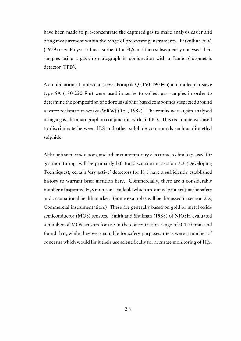
Table 2.1 Summary of principal published techniques for the determination of hydrogen sulphide

Technique Range Resolution Reference

Cadmium sulphide/

Sodium hydroxide

bubbler + pump 1 ppb -

>200 ppb

1 ppb (Jacobs et al., 1957; American

Public Health Association

Intersociety Committee, 1977;

NIOSH, 1977; Hardy et al.,

1981)

passive (membrane) (Deuchar et al., 2002)

Lead acetate Okita et al 2 ppb - 200 ppb (Okita et al., 1971)

HSE 0-50 ppm but could be extended

to ppb region with colorimetric

analysis

~5ppm with eye or 1 ppm with

colorimeter

(Health & Safety Executive and

Factory Inspectorate, 1976)

Pare (Pare, 1966)

Silver nitrate fluorimetric ~5 ppt 1 ppt (Borovskaya, 1988)

colorimetric 0.1-15 mg m-3 0.1 mg m-3 (Diarova et al., 1983)

Micro-coulimetric titration by bromine 5-30 ppb 1 ppb (Adams et al., 1968)

Molecular sieve depends on time & rate 14Fg/sample (NIOSH, 1980)

Silica gel/silver gelatin complex 0-10 ppb (Summer, 1971)

Technique Range Resolution Reference

2.12

Silver cyanide (in tubes) Depends on vol/time

~0-100 ppm

British Patent

1-084-469, 1967

Silver sulphate 9 Fg m-3 (Buck and Gies, 1966)

Potassium sulphate 1-30 mg m-3 1.4 Fg (Vadic et al., 1980)

Passive, silver nitrate etc in diffusion tubes down to 50 ppt in 1 week ±0.1 ppb (Shooter et al., 1995)

Thiocyanate 3.2 - 192 Fg (Koh et al., 1990)

Zinc acetate 0-2 mg (Balasubramanian and Kumar,

1990; SHANTHI and

Balasubramanian, 1996)

2.13

2.2 COMMERCIAL INSTRUMENTATION

The list of commercial instruments, reviewed in this section, is not exhaustive. The

products were selected to be suitable for the range of concentrations anticipated

during the course of this project. They were assessed for their capability to

measure, either mean concentrations of H2S over several hours, or rapid

fluctuations in concentration over a few seconds.

Ideally, the measurement of peak concentrations requires a rapidly responding

instrument which is specific to H2S and which is also portable, so that it may be

carried within a motor vehicle for on-road measurements. On the other hand, for

long term averages over a day or a week, roadside measurements can be taken with

more cumbersome, and possibly mains powered, equipment.

Unfortunately, although cheaper than their bench counterparts, commercial

portable instruments are typically aimed at the 0-50 ppm H2S concentration range.

These are intended for use as personal monitors and alarms in situations where a

worker might be exposed to high concentrations. Great accuracy is not required

under such conditions, nor is it necessary to discriminate completely between

detected gases. More accurate and specific instruments - suitable for monitoring

long-term mean concentrations - also tend to be more costly, have slower response

times and be intended for bench operation.

In this study, the reduced sensitivity of the more portable instruments was offset

by their more rapid response. The portable instruments also tend to be less specific

to H2S. For example, there are often cross sensitivities to carbon monoxide and

benzene - both likely to be present in emissions from motor vehicles. These cross

sensitivities can sometimes be compensated for by an appropriate combination of

sensors, but this inevitably makes the instrument more costly. Instruments for the

measurement of long term average concentrations, whilst needing to be much more

sensitive to measure background levels accurately, can at least be placed in fixed

2.14

locations where it is easier to service power and other requirements. A summary

of the instruments considered is given in Table 2.2 at the end of section 2.2.

The information in Table 2.2 has been taken from manufacturers’ data sheets and

personal communications. Certain items of equipment have either been

demonstrated or borrowed for field trials. The results obtained are reviewed in the

subsequent discussion on equipment and analysis techniques. (See Appendix A)

2.2.1 Electrochemical sensor based equipment

Electrochemical sensors for gas detection and measurement represent a fast

developing section of the equipment market. This is due to the parallel demands

for increased safety for personnel and for increasingly accurate measurement

equipment for environmental monitoring. Although broadly categorised in similar

terms in the preceding table, there are variations between sensors from different

manufacturers, in regard to cross sensitivities in particular, and also in other factors

such as temperature stability and inherent accuracy. There has been a marked

increase in claimed sensor quality in the last few years.

Oldham Gas Toximeter for H2S

The Oldham Gas Toximeter is based on City Technology sensors. The commercial

instrument has a range of 0-50 ppm, with a resolution of 1 ppm. Casella London

Ltd loaned a specially calibrated instrument with 0.1 ppm resolution. After switch

on, a fifteen minute settling time was allowed and the instrument taken on

numerous car journeys, of variable length and with differing weather conditions,

during which many H2S incidents were noted, by smell, by the vehicle driver and

passengers. At these times the Oldham Gas Toximeter indicated changes in

concentration of a maximum of 0.3 ppm, but due to significant cross sensitivity to

2.15

other exhaust gases, it is arguable how much of this was due to H2S. Rarer negative

excursions of down to -0.2 ppm were also recorded which may have been due to

the NO2 cross sensitivity indicated in the instrument’s specification table.

2.2.2 Volatile Organic Compound (VOC) and related detectors

Equipment of this type is generally based on flame ionisation (FID) or photo-

ionisation (PID) detectors. The former type uses a burning flame - typically

hydrogen fuelled - to ionise the incoming, pumped, gas stream. The latter type

uses a UV lamp instead of the flame and both types use either a silicon detector or

a photo-multiplier (PM) tube. These methods are not gas specific and will detect

any gas falling into the measured ionisation range. Depending on the target gas and

the relevant environment this may not be a problem. However, vehicular hydrogen

sulphide emissions are likely to coexist with benzene and many other compounds.

Many manufacturers offer ‘add-on’ portable gas chromatographs, but these tend

either to be not sufficiently accurate, or add greatly to price.

UVIC Gas and Vapour Monitor (Enviro Systems)

An example of the UVIC PID-based instrument was loaned by Enviro Systems. It

was taken on numerous car journeys along with a standard Oldham meter as

described above. Although supposedly sensitive down to 10 ppb, no H2S incidents

were recorded. Many other peaks were observed on the inbuilt graphical LCD

screen, but none corresponded with perceived odours. The Oldham Toximeter

only had a 0.1 ppm H2S resolution so comparisons of peaks could not be made.

2.16

2.2.3 Gas chromatographs (GCs) and other gas analysers

Apart from standard bench machines, there is now an increasing number of

portable and semi-portable GCs available. The most portable, unfortunately, are

also the least sensitive. GCs designed for fully portable operation typically have a

sensitivity of only 100 ppb, which is no better than instruments based on

electrochemical sensors, which are a fraction of the price. The only advantage of

a portable GC, but a significant one, is therefore the gas specificity.

There is a small number of semi-portable GCs and other equipment types, which

are essentially small laboratory machines. All are expensive but give 1 ppb

resolution or better. Sampling times depend on resolution but vary from 1 -

2 minutes.

An alternative approach to a dedicated H2S analyser, is to use an SO2 analyser

preceded by an H2S to SO2 converter such as the converter marketed by Dasibi.

This technique can produce accurate measurements of low concentrations of H2S.

For researchers who already have an SO2 analyser, the purchase of a relatively

cheap converter is a cost-effective alternative to purchasing another specialised

analyser if portability is not an issue.

2.2.4 Other equipment

The range of monitoring equipment supplied by MDA Scientific uses a gas-specific,

impregnated, paper tape through which the sample gas is passed continually. The

discolouration of the tape, after a predetermined interval, determines the gas

concentration. This is then displayed and can be relayed, via an industry-standard

4-20 mA interface, to separate recording equipment. The electronics then re-zero,

and the same area on the tape is used repeatedly until discolouration becomes

excessive and the tape moves to a new section. This procedure minimises tape

2.17

usage - especially at low concentrations. For hydrogen sulphide, two ranges are

available, 0-100 ppb and 0-25 ppm, with sampling times of approximately

10 minutes and 10 seconds, respectively. The gap between these two measuring

ranges typifies the technology gap, referred to earlier, between safety monitoring

and environmental monitoring equipment.

The Jerome 631-X (Arizona Instrument Corp., ) is a portable H2S monitor based

on a gold film sensor. Readings can be taken individually on demand or at a set

frequency. At the lowest end of the scale, the frequency is dependent upon the

concentrations themselves - typically once every 15 seconds for concentrations of

1 ppb H2S.

The reading is indicated on an in-built display and may also be sent via an RS-232

port to an independent data-logger or laptop computer. The instrument is

intended for rapid, and convenient, monitoring around landfill sites or water

reclamation works but is also suitable for roadside measurements.

2.18

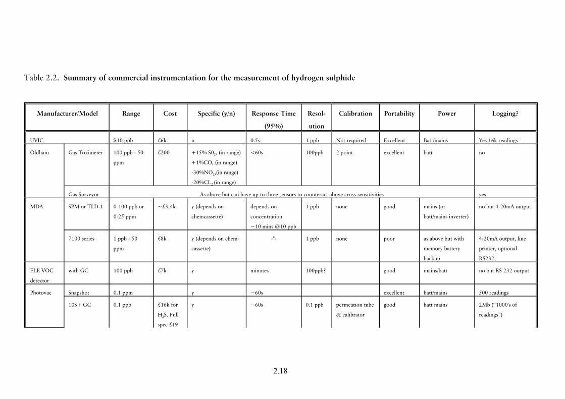
Table 2.2. Summary of commercial instrumentation for the measurement of hydrogen sulphide

Manufacturer/Model Range Cost Specific (y/n) Response Time

(95%)

Resol-

ution

Calibration Portability Power Logging?

UVIC $10 ppb £6k n 0.5s 1 ppb Not required Excellent Batt/mains Yes 16k readings

Oldham Gas Toximeter 100 ppb - 50

ppm

£200 +15% S02, (in range)

+1%CO, (in range)

-30%NO2,(in range)

-20%CL2 (in range)

<60s 100ppb 2 point excellent batt no

Gas Surveyor As above but can have up to three sensors to counteract above cross-sensitivities yes

MDA SPM or TLD-1 0-100 ppb or

0-25 ppm

~£3-4k y (depends on

chemcassette)

depends on

concentration

~10 mins @10 ppb

1 ppb none good mains (or

batt/mains inverter)

no but 4-20mA output

7100 series 1 ppb - 50

ppm

£8k y (depends on chem-

cassette)

-"- 1 ppb none poor as above but with

memory battery

backup

4-20mA output, line

printer, optional

RS232,

ELE VOC

detector

with GC 100 ppb £7k y minutes 100ppb? good mains/batt no but RS 232 output

Photovac Snapshot 0.1 ppm y ~60s excellent batt/mains 500 readings

10S+ GC 0.1 ppb £16k for

H2S, Full

spec £19

y ~60s 0.1 ppb permeation tube

& calibrator

good batt mains 2Mb (“1000's of

readings”)

Manufacturer/Model Range Cost Specific (y/n) Response Time

(95%)

Resol-

ution

Calibration Portability Power Logging?

2.19

AF21M (for

SO2) with H2S

converter

1 ppb £9k5 for

analyser

£2k5

converter

y

Misc.

(Electro-

chemical

Sensors)

Envin Commercially

used above

100 ppb

~£40 ea No but susceptiblities

known and subtrac-

tion may be used

between different

sensors

excellent batt possible

City

Technology

Similar to Oldham Gas Toximeters and Surveyors above

Capteur

Sensors

Similar to Envin above

Quantitech Dasibi 1408

analyser with

H2S converter

0-2000 ppb £9k for

analyser

£3k for

converter

y 8 sec lag time

95 sec rise time

1 ppb poor mains (2-300 W)

STX70

personal moni-

tor

0-50 ppm £350 As Oldham Gas Toximeters and Surveyors above - but waterproof

Arizona

Instruments

Inc

Jerome 631-X 1 ppb - 50

ppm

£10k y 20 sec for 1-100

ppb

1 ppb ‘self calibrating’ excellent batt/mains yes, via RS 232 output

2.20

2.3 DEVELOPING TECHNIQUES

Sensor technology is a constantly advancing aspect of science. Increasing health

and safety demands imposed on industry by both the legislature and the threat of

litigation, mean that new sensor development is a high priority in many fields.

This section describes some of the latest techniques to be applied to H2S detection,

and those which show promise for the future. A summary of this equipment is

shown in Table 2.3 at the end of section 2.3.

2.3.1 The electronic nose

The idea of an ‘electronic nose’ (Corcoran, 1993) has been of particularly interest

to the food industries as a means of quantifying the concepts of personal taste and

smell. A group of different sensors - each of which need not necessarily be gas-

specific - is mounted together in the same sample chamber. The gas mixture under

scrutiny is introduced, and the readings from all sensors simultaneously monitored.

Detection is achieved by means of ‘training’ the array, using neural network

software in an attached computer. The corollary of this is that the individual

sensors do not need to be sophisticated or expensive types (Corcoran et al., 1993).

To train the array, single gases, or mixtures of gases in accurately known

proportions, are monitored in the sample chamber and the outputs of each sensor

recorded. The gas concentration, or mixture proportions, are then changed and a

new set of readings obtained. This procedure is repeated numerous times, but in

each case the data obtained is fed back into the computer concurrently with each

new data set and compared with the known proportions existing in each case.

Progressively therefore, the computer ‘learns’ by iteration which results will

correspond to a given gas combination. The greater the number of data-sets, the

more accurate these results will be.

It is advisable to condition the signal from each sensor separately (Corcoran, 1994)

2.21

to remove unwanted electrical ‘noise’ and to bring signal levels to within the range

of the computer’s voltage input. This then ensures that the individual sensors are

broadly matched against one another, despite differing sensitivities and response

curves.

Although the greatest current interest in the electronic nose is in the food industry,

smell and flavour are inextricably linked with gas composition. However, there is

also interest in the use of the electronic nose for the detection of single gases. This

is because most sensors have cross sensitivities to other gases which can interfere

with the accurate reporting of results. The electronic nose, and its neural network,

turns these cross sensitivities to its advantage because each sensor that has even the

slightest cross sensitivity to the target gas is able to contribute to the resulting

measurement. The electronic nose is therefore able to measure concentrations of

gases for which no specific sensor has been designed.

The sensors used in the array can be of a variety of types (Corcoran and Shurmer,

1994), including standard, ‘off the shelf’ products, but the new concept of the

electronic nose has run in parallel with the development of new sensor types which

have also been incorporated in monitoring equipment designs. The remainder of

this chapter will describe these newer types where there is some relevance to the

detection and measurement of H2S.

2.3.2 Surface Acoustic Wave (SAW) devices

Piezoelectricity is the phenomenon whereby an electrical potential is created as a

result of distorting a quartz crystal. The most common, simple application of this

is probably the domestic gas lighter. Conversely, the application of a voltage to the

ends of such a crystal causes a distortion of the crystal and an appropriate regular

voltage variation can cause the crystal to oscillate. If the excitation electrodes are

placed either side of the crystal, this oscillation occurs throughout the crystal and

2.22

is therefore three-dimensional in nature. This is known as a bulk acoustic wave

(BAW) (Nieuwenhuizen and Nederlof, 1992). A surface acoustic wave (SAW), as

the name suggests, occurs only on the surface of the material and is therefore

essentially two-dimensional. This form of oscillation has several advantages of

which probably the most advantageous is that the frequency of oscillation can be

increased without having to make the crystal substrate ever thinner, and therefore

more brittle.

Surface acoustic wave oscillations are stimulated by means of an inter-digital

transducer (IDT) (Nieuwenhuizen and Nederlof, 1992). This consists of

interleaved metal electrodes at each end of the SAW substrate. The surface waves

are induced by passing an oscillating current between the interleaved electrodes and

the waves continue along the surface of the device from the ends. The oscillation

frequency is not only dependant on the applied voltage waveform and the resonant

frequency of the substrate, but also to any surface coating. Therefore, to turn this

device into a sensor, a chemical or biochemical coating can be applied to the

surface which is selectively sensitive to the fluid under investigation. Chemical or

biological interactions change the frequency of oscillation, by changing the mass

of the coating, and it is this change that is representative of the fluid under

investigation.

In practice, an exposed IDT is placed alongside an unexposed IDT. Ideally these

are formed on the same substrate so that any changes due to factors such as

temperature variations may be minimised. The same substrate may also be used for

more than one set of sensors to present a highly refined form of the electronic

nose. Either a trained neural network or pattern recognition techniques - known

as chemometrics - (Cranny and Atkinson, 1992) may then be used to determine the

concentrations of the compounds of interest.

SAW devices have been used to measure concentrations of a variety of gases, such

as hydrogen (D'Amico et al., 1982), ammonia (D'Amico et al., 1987) and nitric

2.23

oxide (Barendsz et al., 1985; Hoummady et al., 1991), as well as H2S (Vetelino

et al., 1986; De Andrade et al., 1989; Falconer, 1995; Galipeau et al., 1995).

SAW devices have also been investigated for a variety of other purposes - including

their use as liquid, pressure and biosensors - the latter being described later in this

section 2.3 (Bryant et al., 1981; White, 1985; Hoummady and Hauden, 1992;

Yakovkin et al., 1994).

2.3.3 ‘Thin Film’ sensors

Surface acoustic wave devices are generally constructed by applying electrodes to

a chemically inert substrate. The sensitive layer is then applied to the whole

surface. On the other hand, ‘thin film’ sensors have the sensitive layer applied

directly to the substrate and the electrodes added on top.

This method of construction is particularly well suited to tin oxide sensors which

are commonly used in gas detection. A drawback is that they have to work at an

elevated temperature but a heater element can easily be integrated into another

layer of the thin film sensor during construction (Bartlett and Gardner, 1992).

2.3.4 Langmuir-Blodgett (LB) films

Strictly speaking, Langmuir-Blodgett (LB) films are ultra-thin organic films

deposited on a substrate by means of a particular process, but the term is now

commonly applied to any film consisting of either a single molecular layer, or a

number of superimposed, discreet molecular layers, however they are applied

(Ulman, 1991a; Ulman, 1991b).

The films are created by manipulating the film material on the surface of a liquid

in a specialised trough - in a similar way to that in which oil can be moved on the

2.24

surface of water using a paddle blade. When the film is of the desired shape and

thickness, it is floated onto a substrate - typically by withdrawing the substrate

upwards through the film.

These ultra-thin films are potentially useful as highly sensitive gas sensors.

Currently however, they suffer from their great susceptibility to physical damage.

2.3.5 Electro-active polymers

Electro-active polymers (EP) are created by ‘doping’ the polymer material during

production. Polymers manufactured in this way can be used in a variety of sensors

including the SAW types mentioned above as well as optical, potentiometric and

bio-sensors (Josowicz and Janata, 1993). They are especially well suited for use in

resistive sensors.

The initial doping of the material of the polymer can comprise a number of

different doping compounds for different purposes. The primary purpose is to

make the sensor under construction sensitive and selective to the target compound.

The target may be gas or liquid and, as polymers are chemically and physically

robust, sensors based on EPs are inherently tougher than those made of LB films.

The secondary doping may then be used, for example, to enable improved

conductivity.

2.3.6 Biosensors

Biosensors combine a biological component, typically an enzyme, with a transducer

- which is generally a pair of electrodes (Chemnitius and Cammann, 1996). The

fluid under analysis - which is generally a liquid rather than a gas - is immobilised

2.25

on the sensor at the molecular level, by a variety of methods which include

covalent binding, adsorption, cross-linking and entrapment. Electrodes on the

sensor are then used to convert these molecular changes to an electrical signal -

typically by monitoring changes in conductivity.

The sensor itself may be as simple, and therefore cheap, as a suitably impregnated

strip of filter paper, or may be more sophisticated using the thin-film techniques

described previously or glass frits. Because of the way in which the bio-reactions

occur, biosensors should be thought of as ‘single-use’ devices which are disposed

of after analysis. A significant advantage of the biosensor used in this way, is that

the sensor may be exposed to the target fluid before connection to the electrodes,

and ancillary analysis equipment, which may be some distance away. The ‘single-

use’ approach also avoids many of the usual problems associated with electrical

sensors, in that long term stability, deterioration of the device and repeated

calibration can be avoided by suitable batch production and quality control

techniques.

The biosensor is currently being appraised primarily in the medical, and associated

healthcare fields - but there is obviously considerable scope for future deployment

as a passive gas sensor.

2.3.7 Fourier Transform Infra-Red spectroscopy(FTIR)

FTIRs are a highly sophisticated means of measurement. The equipment comprises

two parts, a transmitter and a receiver, which may be mounted close together or

long distances apart, and are a variant of a standard infrared spectrometer which

yields an output signal as a function of 'spectral colour'. The FTIR may therefore

be used to monitor multiple gas concentrations in a small cell in a laboratory,

across a road or along the perimeter of a site by comparing the sample spectrum

2.26

with a database of spectral ‘fingerprints’. This is a highly sensitive, but expensive,

technique.

2.27

Table 2.3 Summary of developing techniques for the measurement of hydrogen sulphide

Technique Range Cost Specific Time Resolution Calibration Portability Power Logging?

Electronic Nose. To detect an

“array” of smells & gas com-

binations.

~100 ppb

upwards

sensors cheap but

associated

instruments currently

expensive

no - but use of neural

networks can make

so

<1 min ? ? via neural

network “learn-

ing”

not at present mains yes

Langmuir Blodgett Films (under

development)

~100 ppb

upwards

high initial but low

per unit

poor currently for

H2S but will probably

improve

<1 min ? ? gas calibrator probably good

soon

possibly

battery

eventually

probably

Biosensors

Reactive

films

Piezoelectric (bulk

wave)

down to

ppb, up to

many ppm

low, 10's of £ y seconds +/- 5% full

scale

gas calibrator excellent batt/mains possible

Surface Acoustic

Wave (SAW)

Resistive

Thin Film

FTIRs down to

ppb

expensive y seconds poor mains yes

2.28

2.4 SUMMARY

The methylene blue assay method has been refined over several decades to

determine ever smaller concentrations of H2S in air. It was decided to attempt

further refinements of this methodology as this seemed to offer the greatest number

of opportunities over a considerable H2S concentration range. These refinements

were to include the development of an improved trapping solution and the

investigation of possible passive techniques, and their application to measure ppb

concentrations over periods of several days.

Techniques and instrumentation to track and record rapidly changing

concentrations of H2S were found to be in short supply both in the literature and

from commercial sources. Although sensor development, and electronic

conditioning for specific gases, appears to be going through a period of rapid

development, no portable instruments at all were found to satisfy the requirements

of this project. Therefore it was decided to develop a new instrument for this

purpose.

3.1

Chapter 3: DEVELOPMENT OF THE DIFFUSION RESERVOIR

3.1 INTRODUCTION

The initial objectives of the project (section 1.3) were to measure H2S

concentrations as long-term averages and also as rapidly changing values. The

literature and technology review (Chapter 2) suggested that there were no

proprietary methods, nor commercial instruments, which were able to achieve both

of these measurements using portable equipment. Therefore, it was decided to use

a different technique for each type of measurement.

This chapter is concerned with the development of a method for measuring long-

term average H2S concentrations over periods of several days. The following

chapter (Chapter 4) describes a new instrument, developed for measuring rapid

changes in H2S concentration during periods of a few seconds.

The literature review (section 2.1.1) included a number of studies (Jacobs et al.,

1957; Jacobs, 1965; American Public Health Association Intersociety Committee,

1977; Harrison and Perry, 1986; Balasubramanian and Kumar, 1990; Purdham

and Yongyi, 1990) in which the measurement of long term average concentrations

of H2S was achieved by capturing sulphide in solution and then using a variant of

the methylene-blue method for sulphide assay. The measurement range quoted for

these studies ranged from 1 ppb up to several ppm - depending upon the sampling

period used and the type of exposure site.

A common feature of these techniques, is the drawing of ambient air through a

solution by means of a pump. Hydrogen sulphide in the atmosphere is captured

in the solution. At the end of the sampling period, the concentration of sulphide

is determined using a colorimetric assay and the average gaseous concentration of

H2S then calculated from the volume of air sampled. The combination of capture,

followed by methylene-blue assay, is simple, and relatively inexpensive, to perform.

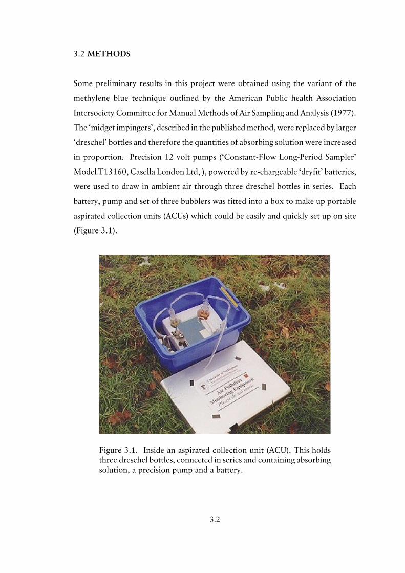
3.2

Figure 3.1. Inside an aspirated collection unit (ACU). This holdsthree dreschel bottles, connected in series and containing absorbingsolution, a precision pump and a battery.

3.2 METHODS

Some preliminary results in this project were obtained using the variant of the

methylene blue technique outlined by the American Public health Association

Intersociety Committee for Manual Methods of Air Sampling and Analysis (1977).

The ‘midget impingers’, described in the published method, were replaced by larger

‘dreschel’ bottles and therefore the quantities of absorbing solution were increased

in proportion. Precision 12 volt pumps (‘Constant-Flow Long-Period Sampler’

Model T13160, Casella London Ltd, ), powered by re-chargeable ‘dryfit’ batteries,

were used to draw in ambient air through three dreschel bottles in series. Each

battery, pump and set of three bubblers was fitted into a box to make up portable

aspirated collection units (ACUs) which could be easily and quickly set up on site

(Figure 3.1).

3.3

Initially, it was not known how efficient the capture of H2S would be and

measuring the sulphide content, of the sulphide captured in each dreschel bottle,

enabled the collection efficiency to be estimated.

The first experiment used dreschel bottles with plain tube outlets. These produced

large bubbles and the presence of sulphide in the third (last) bottle indicated poor

collection efficiency. Unfortunately, the pumps were inadequate to draw air

through each series of three bottles when fitted with fritted pipes. Therefore,

plastic caps with nine x 1 mm holes were used to reduce the size of the bubbles

from the inlet tubes. Subsequent experiments showed that no sulphide reached the

third bottle.

The ACUs were successfully used in several experiments to determine gaseous H2S

concentration alongside major roads. However, aspirated collection methods have

several inherent problems. The apparatus is cumbersome, analysis requires time -

consuming chemical procedures, before and after collection, and the equipment

requires both power and regular (daily) servicing. Other collection methods were

therefore sought as alternatives. In particular, it was thought that a passive, self-

indicating technique would save time, and enable greater replication at more

remote sites.

Calibration of the sulphide captured in solution used in a colorimetric method is

easily achieved using sodium sulphide solution standards. Whilst this calibration

method may be used to provide a reliable indication of the amount of sulphide

captured, it does not take into account the collection efficiency of the bubbler

method. The collection efficiency must therefore be determined separately, or a

calibration made which includes capture and assay.

3.4

3.2.1 The chemistry of sulphide capture and methylene-blue assay

Jacobs’ (1957) reviewed early attempts at using the methylene-blue colorimetric

method for hydrogen sulphide assay and concluded that these methods suffered

from oxidation of the captured sulphide. He described a comparison between two

versions of the method. One version used a collecting solution containing zinc

acetate, the other contained cadmium hydroxide. He concluded that whilst the

latter solution captured in excess of 90 % hydrogen sulphide, the former captured

less than 10 % and that the difference arose from different rates of oxidation of the

sulphide in solution. The cadmium hydroxide version was later published as a

‘Standard Method’ (Jacobs, 1965).

Subsequently, Bamesburger and Adams (1969) used a cadmium hydroxide solution

similar to that described above, with the addition of arabinogalactan (‘STRactan

10') to the absorbing solution, to reduce photo-decomposition. The addition of

arabinogalactan reduced that part of the sulphide loss attributed to photo-

decomposition, from 95 % to 15-30 % over a 24 hour period. It is not clear how

much of the sulphide loss was attributable to other factors, nor what they might be.

The methylene-blue method used in this project was based on that of the American

Public Health Association Intersociety Committee (ISC) for Manual Methods of Air

Sampling and Analysis (1977). This variant appeared in a review of H2S sampling

methods by Harrison and Perry (1986), and is similar to the method of

Bamesburger and Adams (1969). Harrison and Perry (1986) noted that the ISC

version of the methylene-blue method was only suitable for sampling periods of

several hours, and also indicated that sampling and analysis should be carried out

within 24 hours, to minimise photo-decomposition of the sulphide.

Other authors (Hardy et al., 1981; Balasubramanian and Kumar, 1990; Purdham

and Yongyi, 1990) also attributed sulphide losses primarily to oxidation of

captured sulphide, and described the addition of ethylene-diamine tetra-acetic acid

3.5

(EDTA) and tri-ethanolamine as alternative ameliorating measures. These

additions, in varying proportions, reduced sulphide losses by between 40 - 85 %

over a 24 hour period.

Adaptation of the ISC method, to produce more stable collection solutions and

combine the benefits of arabinogalactan, EDTA and tri-ethanolomine, had

unforeseen problems. These required further modifications to be made before a

reliable technique was established. The order of mixing constituents proved crucial

to avoid a precipitate and the addition of ethylene-diamine tetra-acetic acid

(EDTA) to the absorbing solution caused it to become acidified. However, this was

rectified, using additional NaOH, to produce a collection solution with pH 11.9.

3.2.2 Analysis of sulphide captured in solution

A cadmium hydroxide based solution was used to capture sulphide and this was

then assayed using the methylene-blue colorimetric method described below. This

is summarised in Figure 3.2.

3.6

Figure 3.2. Summary of the Methylene Blue method used. Adapted from Harrison& Perry (1986), Balasubramanian & Kumar (1990) and Purdham & Yongyi (1990)

A capture solution was prepared by dissolving 4.3 g cadmium sulphate (CdSO4)

and 10 g arabinogalactan in separate 100 mL aliquots of de-ionised water and

mixing these in a 1 L volumetric flask. Ten grammes of tri-ethanolamine (TEA)

and 1 g of EDTA were then added with further mixing. Finally, 4 g of sodium

hydroxide (NaOH), dissolved in a separate 100 mL aliquot of de-ionised water,

was also added to the flask and the flask contents made up to volume with de-

ionised water. It was found to be important that the constituents were mixed in

this order to produce a clear solution, free from any precipitate.

An amine stock solution was prepared by adding 50 mL concentrated H2SO4 to

30 mL of de-ionised water. After cooling, 12 g of N,N-dimethyl-p-phenylene

diamine dihydrochloride was added and the mixture stirred. A working solution

3.7

was prepared using 25 mL stock solution diluted to 1 L with 50 % H2SO4.

A ferric chloride solution was prepared by dissolving 100 g ferric chloride hexa-

hydrate (FeCl3.6 H2O) in de-ionised water and making up to 100 mL

An ammonium phosphate solution was prepared by dissolving 400 g di-ammonium

phosphate in de-ionised water and making up to 1 L.

A sodium sulphide stock solution was prepared from approximately 4 g of sodium

sulphide (Na2S.9H2O) which was first washed in 100 mL ethanol and dried on

filter paper to minimise the risk of contamination. A quantity of the dried salt

(3.746 g) was dissolved in de-ionised water and the solution made up to 1 L. A

working solution of 5.00 Fg mL-1 was prepared by diluting 10 mL stock solution

to 1 L.

It was found that the sodium sulphide solutions had to be made up on the day

required as the sulphide content degraded rapidly. The other reagents could be

stored in a refrigerator for at least a month.

After exposure of the capture solution to atmospheric H2S (in 7 mL aliquots),

1.5 mL of amine stock solution was added to each container, thoroughly mixed,

and the contents washed through a funnel into a 25 mL volumetric flask, using de-

ionised water. One or two drops of ferric chloride solution were added to the

flask, which was then agitated, and two drops of ammonium phosphate solution

added. The flask contents were then made up to volume, shaken and left for one

hour in the shade for the colour to develop.

To calibrate the colorimeter, 0.5 mL, 1 mL and 2 mL of the sodium sulphide

working solution were added to 7 mL aliquots of unexposed absorbing solution in

25 mL volumetric flasks and the colour developed in the same way as the samples

from the exposed DRs. As previously discussed (Section 3.2.1), the sulphide

3.8

Figure 3.3. A colorimeter calibration showing a typical relationship betweenabsorbance and sulphide concentration in solution.

calibration standards were found to oxidize rapidly over time periods as short as

24 hours. Therefore a calibration graph was prepared for each day of assay. A

typical calibration curve for the colorimeter is shown in Figure 3.3. On all

occasions, the data points showed minimal scatter and followed very closely the

straight line of the graph through the origin. This graph also indicates the overall

linearity of the methylene blue method in its response to concentrations of H2S.

A colorimeter (Jenway 6061, fitted with a 671 nm interference filter and a flow-

through cell of 10 mm path length) was used to determine the absorbance of the

contents of each flask. The absorbance of unexposed blanks was measured first

and the colorimeter zero adjusted to the average absorbance of these. The relative

absorbance of the solution from each of the other flasks was then determined,

before re-testing the initial blanks to ensure that no instrument drift had occurred.

3.9

Figure 3.4 Comparison of absorbances using 671 nm filter (9) and710 nm filter (Ê) on the same samples.

3.2.3 Comparison of results using different colorimeter filters

The ISC methylene-blue method (American Public Health Association Intersociety

Committee, 1977) specifies that a 670 nm filter should be used for the colorimeter

measurement. A 671 nm filter was borrowed to compare the response with the

710 nm filter initially available. The response was compared at the lower end of

the working range where it was expected the greatest discrepancies might occur.

It can be seen from Figure 3.4 that the 671 nm filter gave the larger response, by

approximately 30 %, and therefore this filter was used in all subsequent

experiments.

3.2.4 Stability of the collection solution

In order to determine the stability of the new solution described in section 3.2.2,

before and after exposure to H2S, an experiment was carried out to compare the

absorbances of exposed and unexposed solution over time. The experiment was

designed to indicate the changes, or degradation, of the collected sulphide from

3.10

day to day and also to indicate whether the age of the absorbing solution was a

significant factor in any degradation.

Eighteen aliquots of fresh absorbing solution were prepared in 25 mL volumetric

flasks. Six flasks were dosed with 0.5 mL of the NaS working calibration solution

(as described in section 3.2.2). These were denoted ‘high standard’. Another six

flasks were dosed with 0.05 mL NaS (denoted ‘low standard’) and six with no

sulphide added at all. A further group of six flasks contained similar aliquots of

absorbing solution which had been made up one month previously. These also had

0.5 mL of the working calibration solution added to them on the same day as the

others and were denoted ‘old standard’. All 24 flasks were then flushed with

nitrogen gas and stoppered prior to storage in a refrigerator.

The 24 flasks were divided into six sets of four flasks in order to determine changes

in the four sulphide standards through time. Each set included one flask containing

0.5 mL of the NaS working calibration solution in fresh absorbing solution and one

containing 0.5 mL of the NaS in one month old solution. The third flask contained

0.05 mL NaS in fresh solution and the last flask contained fresh solution but no

added sulphide.

One set was assayed for sulphide on the first day. The other sets were then assayed

at the same time on the five following days. The results from this stability test are

shown in Figure 3.5.

3.11

Figure 3.5. Degradation of different sulphide concentrations in absorbingsolutions of different ages. 9=high standard, ¶=low standard, u=oldstandard.

Fitting regression lines to Figure 3.5 showed that there was no evidence (p>0.1)

of a trend with time in any of the sample groups. There was also no evidence

(p>0.1) of difference between the means in the results from the fresh and one

month old solutions. It can also be seen that degradation of the collected sulphide

does not appear to depend upon the concentration of the sulphide captured.

3.2.5 The Diffusion Reservoir (DR)

A passive approach to gas monitoring has been suggested previously for sulphur

dioxide (Reiszner and West, 1973) and subsequently adapted for hydrogen

sulphide (Hardy et al., 1981). This method has considerable appeal because of its

simplicity and it was decided to attempt the same technique for H2S, but to use the

collection solution described in sections 3.2.1 to 3.2.4. Other changes to the

method included the use of a more modern gas-permeable membrane. An

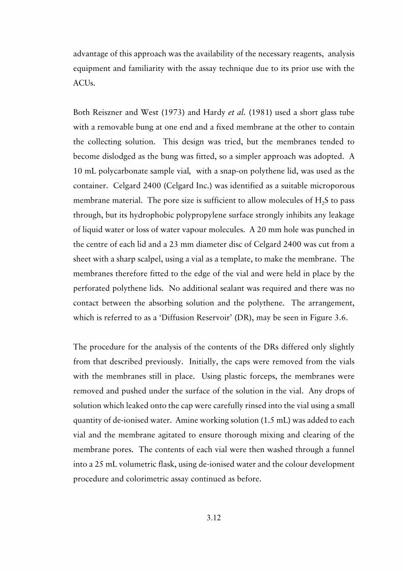
3.12

advantage of this approach was the availability of the necessary reagents, analysis

equipment and familiarity with the assay technique due to its prior use with the

ACUs.

Both Reiszner and West (1973) and Hardy et al. (1981) used a short glass tube

with a removable bung at one end and a fixed membrane at the other to contain

the collecting solution. This design was tried, but the membranes tended to

become dislodged as the bung was fitted, so a simpler approach was adopted. A

10 mL polycarbonate sample vial, with a snap-on polythene lid, was used as the

container. Celgard 2400 (Celgard Inc.) was identified as a suitable microporous

membrane material. The pore size is sufficient to allow molecules of H2S to pass

through, but its hydrophobic polypropylene surface strongly inhibits any leakage

of liquid water or loss of water vapour molecules. A 20 mm hole was punched in

the centre of each lid and a 23 mm diameter disc of Celgard 2400 was cut from a

sheet with a sharp scalpel, using a vial as a template, to make the membrane. The

membranes therefore fitted to the edge of the vial and were held in place by the

perforated polythene lids. No additional sealant was required and there was no

contact between the absorbing solution and the polythene. The arrangement,

which is referred to as a ‘Diffusion Reservoir’ (DR), may be seen in Figure 3.6.

The procedure for the analysis of the contents of the DRs differed only slightly

from that described previously. Initially, the caps were removed from the vials

with the membranes still in place. Using plastic forceps, the membranes were

removed and pushed under the surface of the solution in the vial. Any drops of

solution which leaked onto the cap were carefully rinsed into the vial using a small

quantity of de-ionised water. Amine working solution (1.5 mL) was added to each

vial and the membrane agitated to ensure thorough mixing and clearing of the

membrane pores. The contents of each vial were then washed through a funnel

into a 25 mL volumetric flask, using de-ionised water and the colour development

procedure and colorimetric assay continued as before.

3.13

Figure 3.6. Construction of a Diffusion Reservoir (DR).

A gas calibrator (Monitor Labs Inc, model 8550), containing an H2S permeation

tube, was used in conjunction with an H2S converter (Dasibi Inc, model 4109) and

an SO2 bench analyser (Analysis Automation Limited, model 477), to perform a

calibration of the DRs for different exposure time periods and for a variety of

gaseous H2S concentrations.

At standard temperature and pressure, the H2S concentration at the output of the

calibrator is given by:-

H2S concentration (ppb) = permeation rate (ng min-1)

flow rate (L min-1) x density (kg m-3)

The DRs were exposed using the arrangement shown in Figure 3.7. The exposure

box (Figure 3.8) had a quick release lid and the DRs were temporarily fixed to the

base using Blu-tac. The lid was then replaced and the box carefully inverted so that

the absorbing solution came into contact with the membrane surface. The gas flow

rate through the SO2 analyser was monitored throughout the exposure time.

3.14

Figure 3.7. Dose response calibration layout

Figure 3.8. Layout of DR exposure box for dose responseexperiments

When no DRs were placed in the sealed box, the H2S concentration reading on the

gas analyser agreed with the theoretical H2S output concentration of the calibrator.

When DRs were fixed in the box as described, the reduction in the output reading

of the SO2 analyser was noted. In all cases, the analyser reading was reduced with

the DRs in place in the exposure box, compared with no DRs, and a capture

efficiency for the DRs was indicated of approximately 9 %. This was confirmed

by measuring the total sulphide captured, and comparing it with the available

sulphide in the gas volume passed through the exposure box during the exposure

3.15

Figure 3.9. DR dose response curve

time.

Each time the calibrator output was changed, the system was allowed to re-

equilibrate for at least ten minutes before new samples were fitted in the exposure

box.

For each data point, the dose (in ppb hours) was calculated by multiplying the

exposure time by the gaseous concentration of H2S present. The results of the

calibration dose response experiments are shown in Figure 3.9 and are an amalgam

of the data from a group of experiments in which the gas calibrator was used to

provide different doses of H2S to calibrate the DRs. This included different

concentrations for a similar period of time and also the same concentration for

different periods of time.

3.16

3.3 SUMMARY

The modifications made to the methylene blue method have resulted in a more

stable solution, both before and after exposure, than that previously reported. The

use of diffusion reservoirs (DRs) has also enabled this assay technique to be used

in a cheap, passive manner for area and point monitoring in a variety of locations

and over a large range of H2S concentrations.

4.1

Chapter 4: DEVELOPMENT OF THE HYDROGEN SULPHIDEPEAK GAUGE (HSPG)

4.1 INTRODUCTION

Most modern monitoring equipment is based around a sensor producing an

analogue voltage, or current, which is converted to a digital signal, at the earliest

stage possible, for further processing. The advantage of this method is that, after

the initial conversion, the resulting digital signal is substantially impervious to

electrical noise, drift, minor changes in component values, temperature and supply

voltage. In many cases, the final data output is easily passed to a computer for

analysis by appropriate application software. Contemporary instrumentation

therefore endorses the view that, in most cases, it is easier to develop digital

technology to monitor and control processes, than it is to overcome the problems

inherent in the manufacture of analogue components.

However, digital sampling of the analogue sensor output is discontinuous. In many

situations this is not important but, if the sensor signal changes rapidly, data will

be lost. If the digitisation occurs at a sufficiently rapid rate, then the large amounts

of data recorded will oblige the digital designer to periodically, or continuously,

average groups of measured data points. A specific example of this problem relates

to very narrow spikes, or transients, incorporating changes of relatively large

magnitude. Unless the digital sampling occurs exactly at the peak then only the

rising or falling edge will be sampled, or the incident missed entirely. Automated

digital averaging is likely to miss such spikes altogether.

If problems of drift and stability can be adequately controlled, or separated from

the desired signal, then the output from an analogue circuit should follow the

source with greater accuracy than the digital equivalent. Accordingly, the HSPG

was designed with the intention of taking continuous measurements for several

minutes at a time. With this system, some data loss will still occur at the end of

4.2

each measurement period, during reset of the instrument zero. However, the

remaining data should provide a more accurate record of variation in concentration

than a digitised signal.

In the early design stages, little was known of the variation and magnitude of the

concentrations of H2S to be monitored. The ability of a monitoring instrument to

correctly track variations in actual concentration depends on the frequency

response of the instrument being similar to that of the signal under investigation.

Accordingly, as the characteristics of the variation in H2S concentration are an

important aspect of this study, it was decided that an error in absolute measurement

in concentrations of ±10 % was acceptable. This was considered an adequate

compromise in finding a balance between extremely rapid response with poor

accuracy, and a highly accurate measurement but with a very slow response. For

example, the commercially available Jerome 631X is capable of ±1 ppb resolution

with an accuracy of ±3 ppb at 50 ppb concentration, but can only take one

measurement every 15 seconds at such low concentrations.

Concentrating on the variations in H2S concentrations, rather than accuracy alone,

would also enable greater attention to be paid to discriminating against electrical

and electrochemical noise. The intention was to monitor the sensor out put for as

long a period as possible and then to re-check the zero of the instrument at

intervals, using a source of H2S-free air, to monitor any drift in sensor output. Ten

minutes of monitoring, followed by one minute for a zero check, were initially

considered sufficient for periods of data acquisition and to re-establish a zero point.

Electronic constraints resulted in these figures being modified to 8.5 minutes and

40 seconds respectively.

From a review of literature, discussed in Chapter 2, it was decided to develop a

resistive sensor using an H2S-sensitive coating. The coating had to react rapidly,

and reversibly, with variations in H2S concentration and exhibit concurrent changes

in conductivity. Two coatings discussed in the literature appeared to exhibit these

4.3

Figure 4.1 The completed Hydrogen Sulphide peak Gauge

characteristics; both have been used extensively in the development of surface

acoustic wave (SAW) devices as previously described (See section 2.3.2).

The first coating considered was tungsten trioxide (WO3), but the technology in its

production is highly specialised and beyond the capability of the workshop facilities

‘in-house’. The second coating was a gel, consisting of a mixture of cadmium

iodide, urea and glycerol (De Andrade et al., 1989). This was readily applied in

solution to the sensor surface using a glass rod. This approach has the advantage

of simplicity, and replaceability, and was therefore adopted for the sensor to be

described in the following section.

4.2 HSPG DESIGN

4.2.1 Summary

4.4

The completed Hydrogen Sulphide Peak Gauge (HSPG, Figure 4.1) is a fully

portable, and self contained, instrument designed specifically to measure rapidly

changing hydrogen sulphide (H2S) concentrations up to 200 parts per billion to

within an accuracy of ±10%. It uses an analogue resistive sensor coated with a

chemical gel which is replenished every few days. The novel electronic design of

the HSPG, circumvents problems of drift and electrical noise using a combination

of unorthodox differentiating and convergent-zero techniques.

Calibration is achieved using a permeation tube in a gas calibrator or could be

accomplished using a specialised gas source and a diluter. Controls are provided

to enable display features, and facilitate setting up and zeroing. In normal use the

HSPG will perform an automatic zero cycle approximately every 10 minutes, but

this may be overridden manually if desired. The HSPG output is displayed in

millivolts on a liquid crystal display (LCD) and also on its own mini, 8-bit data

logger, based on a second LCD. Data may be downloaded to a computer from the

internal logger via a serial port, but a further voltage output is provided to enable

recording using a chart recorder, a more accurate external data logger, or an

analogue to digital converter and laptop computer combination.

4.5

Figure 4.2 Block diagram of the HSPG connections. (Gas flows in yellow, controlcircuitry in green and signal routes in red)

A block diagram of the main modules of the HSPG are shown in Figure 4.2. These

are discussed in detail in the following sections.

4.2.2 Sensor and headstage amplifier

The resistive sensor consists essentially of two electrodes, with a medium spanning

them whose conductivity is responsive to the target. The conductivity is directly

proportional to the cross sectional area of the electrodes, whilst being inversely

proportional to their separation.

In the case of a gas sensor, the medium must respond rapidly to changes which will

predominantly take place at or near the surface. To maximise the surface area

available for reaction, and therefore the response, the electrodes comprise

interlocking ‘fingers’ with the sensitive medium largely held between them

(Figure 4.3).

4.6

Figure 4.3 Gas sensor electrode layout.(Approx 1.5x Actual Size)

Figure 4.4 Enlarged cross section through gel coated sensor

The conductivity is therefore proportional to the total length of the edge of the

electrodes, rather than their surface area, but inversely proportional to their

separation, as before. Figure 4.4 shows a cross section through part of the sensor

with the vertical scale exaggerated. Although the gel coating partially covers the

copper strips, these areas are effectively shorted out by the copper and so do not

contribute to the sensor resistance. It is only the resistance of the gel between the

copper strips which is affected.

To minimise the effect on the gel-coated sensor of errors due to factors such as

varying temperature and humidity, a reference sensor was also used. The latter was

placed in the airstream following the measuring sensor, but separated from it by a

filter containing activated charcoal. The purpose of the filter was to absorb

4.7

Figure 4.5 Prototype gas sensor for hydrogen sulphide, incorporatingmeasuring and reference cells (Approx. Actual size).

hydrogen sulphide but to leave the airstream otherwise unchanged (Masuda et al.,

1999). The voltage output of the reference cell is subtracted electronically from

that of the measuring cell so that the net output depends only on the incoming H2S

concentration. The general physical arrangement is shown in Figure 4.5. Because

one electrode of each cell is connected in common with one electrode of the other,

only three connections are necessary in all.

The outputs from the prototype gas sensor in Figure 4.5 were amplified using a

TLC271P operational amplifier (op-amp). Op-amps have two complementary

inputs, one inverting (denoted ‘-’) and one non-inverting (‘+’). Feeding identical

voltages into each input will therefore, theoretically, give a null output. The circuit

employed with the prototype sensor is given in Figure 4.6. This is a standard 4-

arm bridge. The purpose of the 100 kΩ resistor is to limit the current through, and

thereby the voltage across, the two sets of sensor electrodes. The 20 kΩ trimmer

sets the zero by balancing the bridge for a null output with both halves of the

sensor exposed to zero concentration of H2S gas. The 270 kΩ feedback resistor

4.8

Figure 4.6 Circuit used with prototype gas sensor.

sets the gain of the circuit.

Although this circuit appeared to respond to H2S when coated with the gel

previously described, experience elsewhere (Pritchard, 1985) suggested that it is

necessary to use an alternating current to supply the sensor cells, to avoid

polarising effects within the gel. Therefore, the following additions to the basic

circuit were devised which alternate the polarity of both halves of the sensor

simultaneously, at a frequency of 50 Hz. The outputs of each cell need to be

reversed at the same time, if the polarity of the output is also not to be reversed.

This was accomplished using a 50 Hz oscillator to drive a series of three, single-

pole, double-throw, CMOS switches. A large capacitor (470 µF) was used to

smooth the output of the stage and remove any switching spikes. Additionally, a

2.1 V precision voltage reference was employed to standardise the voltage across

the sensor and replaced the 100 kΩ resistor in the previous circuit, as this resistor

would make the sensor inherently non-linear. The final version of the headstage

amplifier is depicted in Figure 4.7.

4.9

Figure 4.7 Headstage amplifier used with H2S sensor.

4.2.3 The Differentiator

The differentiator is the key to stabilising the drift inherent in the use of a wet

sensor in an input stage. As discussed previously (section 4.1), some baseline drift

is acceptable in the context of a regular (10 minute) zero check and so a

differentiator, in conjunction with a timer, is used to turn any drift into a flat

baseline.

4.10

Figure 4.8 Differentiator circuit incorporating offset bias, single rail powersupply and low leakage properties.

4.2.3.1 Differentiator circuit description

The novel circuit in Figure 4.8 is an adaptation of the conventional differentiator

circuit (eg. Pippenger and Tobaben, 1985). Using the component values shown,

this circuit permits any input variations, other than those deemed to be due to

baseline drift, to pass through to the final output.

The 220 µF capacitor provides DC isolation, but allows voltages on the right hand

side to respond immediately, in both direction and amplitude, to changes on the

left. The following 1 MΩ resistor, however, limits the rate at which capacitor

recharging can occur, but does not affect the output at the signal levels under

investigation. Both this resistor, and those on the op-amp non-inverting input, and

the OA47 germanium diode, are additions to the standard circuit. In the

conventional circuit, the 1 MΩ op-amp feedback resistor is the sole factor limiting

the current, which allows the right hand side of the input capacitor to recharge to

the virtual-earth potential of the inverting (‘-’) input of the op-amp. In Figure 4.8

the extra 1 MΩ resistor between the capacitor and the inverting input of the op-

amp, prevents the inverting input from immediately detecting the changed voltage

on the capacitor as this potential difference will at first appear across the resistor.

Instantaneously, the circuit will behave in the same manner as a unity-gain

4.11

inverting amplifier. The extra 1 MΩ resistors on the non-inverting inputs act

conventionally to minimise the common mode rejection ratio (CMRR). Since the

op-amp inputs each have an input impedance of greater than 1012 Ω, and are

therefore effectively infinite, as the right hand side of the capacitor discharges (or

charges) through the input resistor, an identical current will flow through the

feedback resistor creating a voltage on the output equal and opposite to that on the

capacitor. The capacitor discharge is therefore not controlled by the feedback

resistor, as in the conventional differentiator circuit, but by the input resistor.

The addition of an LM78L05 voltage regulator to provide a bias point for the non-

inverting input is necessary since the differentiated output is an inverted image of

the input. In a standard differentiator, a dual rail power supply is employed,

allowing the output to become negative with respect to the supply ground. In the

present design it was desired to operate from a single supply and so this biasing

technique was employed. The inversion and DC bias is corrected in the

Inverter/Buffer and DC Level Restorer stage which follows.

When the HSPG is calibrated and set up, there should be no negative voltage

excursions from the output of the sensor stage. However, due to voltage droop,

such excursions may still occur on the right hand side of the input capacitor of the

differentiator. Any negative potentials here however, are limited to the 0.3 V

forward voltage of the OA47 germanium diode. The germanium type was chosen

in preference to the usual silicon, which has a greater forward conduction voltage

of 0.6 V.

The output stage of the differentiator comprises the 10 nF capacitor and a 270 Ω

resistor across the output. These are to suppress electrical noise and to provide an

output load for the op-amp, respectively. The TLC2274 quad operational

amplifier was chosen for its stability, low quiescent current, extremely high input

impedance and ability to operate to 0 V with a single rail, low voltage supply.

4.12

4.2.3.2 Differentiator circuit action

It must be remembered that the prime purpose of the HSPG is not necessarily to

measure steady state concentrations, but those which are subject to rapid change

such as spikes.

Once switched on and allowed to stabilise as explained in section 4.2.1, a steady

null voltage from the sensor will have no effect on the right hand side of the

differentiator input capacitor whose output will also remain at ‘zero’. To be

strictly accurate, this will in fact be the 5 volt bias voltage, which hereafter is

designated 0 V5.

From a steady zero state, if the input voltage rises instantaneously by an amount

VL - as it will if the sensor experiences an instantaneous increase in H2S

concentration - then the voltage on the right hand side of the input capacitor, VR,

will rise by the same amount. If VL remains constant, however, the magnitude of

VR will gradually diminish at a rate determined by the value of the capacitor, the

value of VR (always measured relative to 0 V5), the differentiator input resistor and

leakages due to the capacitor’s own internal resistance and op-amp input

impedance.

If the initial positive change in VL is followed immediately by a negative change of

identical magnitude, returning VL to 0 V, then VR will also return to 0 V5.

However, if there is a delay before VL returns to zero then the magnitude of VR will

have diminished slightly. Nevertheless VR will still fall by the same amount and the

value of VR will become negative relative to 0 V5. Once again, the magnitude of

VR will tend to diminish due to all the previously indicated factors, but in addition,

the increasing forward conduction of the germanium diode will become of

overriding importance as VR approaches -0.3 V relative to 0 V5. This diode

therefore minimises unnecessary negative excursions of VR and also has an

important role in ensuring that subsequent positive excursions can be more

4.13

correctly recorded. Its effect will counteract the continually drooping waveform

for a series of spikes on the input, by returning the ensuing voltage waveform

closer to its absolute value, each time the differentiator output attempts to fall

below zero.

It can be seen that if any change in the input state is followed by a period without

change, then VR will tend to 0 V5. Paradoxically, this tendency towards a nominal

zero is the crucial factor in not only ensuring a base line almost impervious from

drift, but also in minimising voltage droop when the input contains narrow voltage

spikes - due to the action of the germanium diode as previously described.

Provided the rate of baseline drift is less than, or equal to, the rate of droop of VR,

then no change on the output will be observed. The time constant of the

differentiator capacitor, and associated components, is critical in the operation of

this circuit and the optimum values have been determined empirically.

In practice, the upper limit of voltage measurement, imposed by the voltages and

amplifier gains of the circuitry, is for a +5 V step input relative to 0 V5. This

corresponds to approximately 200-500 ppb H2S as will be discussed later, in

section 4.3.

Ideally, a succession of spikes and varied high and low concentrations of H2S

should always cause proportional changes in VR. However, due to the capacitor

voltage droop, and the action of the germanium diode, the value of VR could

approach either -0.3 V or +5 V relative to 0 V5 if the instrument were left

indefinitely. Therefore, at the end of each zero-check period, the electronics

should also be returned to zero state, by operating the output and peak monitoring

reset switches as required.

A mechanical analogy of the operation of the differentiator is given in Appendix B.

4.14

Figure 4.9 Circuit diagram of bargraph display for 0 - 5 V input

4.2.4 Signal Processing and control

4.2.4.1 The Bargraph Display

The main function of the bargraph display is to assist in setting up the HSPG after

it is first switched on. During monitoring, the display should also be checked

periodically to ensure that the indicating LED appears in the lower half of the

display during zero-air cycles. Adjustment should be made using the front panel

zero, multi-turn potentiometer which should then be locked in position to prevent

accidental movement. This procedure ensures that the differentiator, and hence

the HSPG, can be used for the widest range of inputs by keeping the signal voltage

central between the supply rails. The overall accuracy and calibration are

unaffected because this control has no effect on output amplitude and because a

manual zero is always made at the start of measurements.

The circuit for the bargraph display is shown in Figure 4.9. The 3914 IC contains

a potential divider chain, fed by an external reference voltage, and ten comparators

- each of which drives a single LED in the bargraph itself. As depicted, only a

single LED will be driven at any one time to conserve battery voltage.

4.15

Figure 4.10 Inverter/buffer and DC level restoring circuit to correctinversion & level shift of preceding differentiator.

4.2.4.2 The inverter/buffer and DC level restoring circuit

A standard unity gain inverting op-amp circuit was used, but configured as a

differential amplifier (Figure 4.10). The non-inverting input was biased to the

same point as that of the preceding differentiator circuit and this ensured that the

output was free of any DC offset. The purpose of this circuit was to re-invert the

waveform previously inverted by the differentiator and replace its reference, 0 VZ,

with the conventional 0 V line. This is extremely accurate, as any variations in

tolerance of 0 VZ are equally, but oppositely, reflected in the two stages and

therefore effectively cancel out.

4.2.4.3 The peak hold circuit

A peak hold circuit is intended to measure the peak voltage of a varying input

waveform - in this case equivalent to the peak H2S concentration detected. The

voltage is stored on a capacitor, but in a standard active circuit this suffers from

‘voltage droop’ due to the capacitor’s own internal leakage.

The following circuit (Figure 4.11) is designed to minimise this effect and uses,

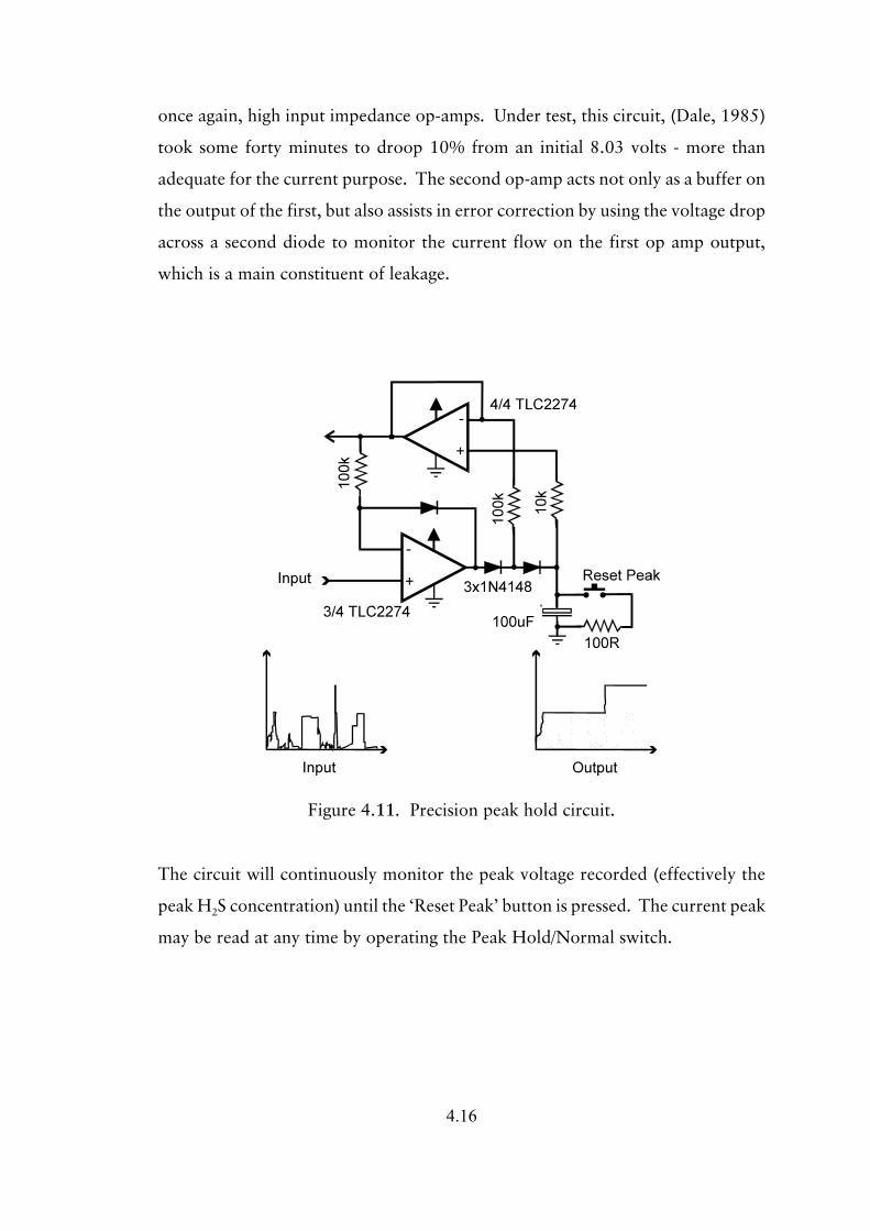
4.16

Figure 4.11. Precision peak hold circuit.

once again, high input impedance op-amps. Under test, this circuit, (Dale, 1985)

took some forty minutes to droop 10% from an initial 8.03 volts - more than

adequate for the current purpose. The second op-amp acts not only as a buffer on

the output of the first, but also assists in error correction by using the voltage drop

across a second diode to monitor the current flow on the first op amp output,

which is a main constituent of leakage.

The circuit will continuously monitor the peak voltage recorded (effectively the

peak H2S concentration) until the ‘Reset Peak’ button is pressed. The current peak

may be read at any time by operating the Peak Hold/Normal switch.

4.17

Figure 4.12. Auto-zero timer and solenoid driving and indicator circuit.

4.2.4.4 The timer and solenoid control circuitry

The integrated circuit which activates the three-way solenoid valve, controls the

admission to the sensor of either ambient air, or zero-air. The circuit in

Figure 4.12 is adapted from that used previously in a more complex sampling

system (Micallef et al., 1998) and conserves power by energising the solenoid

valve momentarily.

As well as controlling the solenoid valve, the timer also activates red and green

indicator LEDs to show the valve status; green for sampling, red for auto zero.

Either of these states may be overridden manually for setup, calibration or other

testing.

4.18

Figure 4.13 Schematic of HSPG Plumbing

4.2.5 Arrangement of pipework

Figure 4.13 shows the internal pipework connections of the HSPG for gas flow.

The pump is adjacent to the exhaust so that it cannot affect the gas to be sampled.

The three-way solenoid valve is on the input. Its orientation with respect to the

different flow circuits is important. Solenoid valves only operate reliably at low

pressures, if the gas flows across their ports are in specific directions. In this case,

the valve also had different sized ports, which affected flow rates, and so the valve

was configured so that the most restricted route directed the flow through the

sensor. The route having the lower pressure drop was connected to the zero-air

filter. This arrangement resulted in flow rates, whether through the sensor alone,

or through the sensor and filter, of approximately 0.7 L m-1.

A miniature 12 V diaphragm pump (model PM 11-2, Charles Austen Pumps Ltd,

Byfleet, England) was used. Stainless steel tubing, 4 mm ID, was used within the

HSPG case, and flexible PTFE tubing externally. All fittings, including the solenoid

valve body, were of brass. The sensor and filter housings were built from a

combination of acrylic sheet and polycarbonate, embedded in an inert epoxy

4.19

compound. The sensor box was sealed using closed-cell, inert EPDM foam rubber

strip.

4.2.6 Signal monitoring and logging

The HSPG has a number of data outputs. First, there is the liquid crystal display

(LCD). This gives a direct read out, in millivolts, of the output of the differentiator

circuitry. No attempt was made to convert these values to H2S gas concentrations

as part of the design, because of the unknown variation in calibration to be

expected at the time.

Second, there are two 4 mm sockets on the casing which may be connected to an

external datalogger, chart recorder or computer. The sockets receive the same

voltage as that for the LCD. The use of these connections can give improved

resolution of the HSPG output compared with the built in display.

Finally, the HSPG has a built-in mini-datalogger. This is only an 8-bit logger,

however, and its use is therefore mostly limited to instances where H2S

concentrations are in at least tens of ppb because of the poor resolution achieved.

In practice each data bit corresponds to approximately 5 ppb. Use of the logger in

conjunction with the peak hold circuitry does however enable peak values to be

stored within the instrument itself. This is an extremely useful feature as it saves

the operator from having to make separate notes of each event.

The peak hold switch permits the viewing of the peak values obtained during a

period of field monitoring. If the operator regularly switches between peak and

normal display modes, then each peak value can be recorded, either visually from

the LCD or by the datalogger, and the peak hold circuit zeroed in readiness for the

next peak. Alternatively, the peak hold circuit can be used to record the single

highest peak achieved during a measurement period.

4.20

4.3 RESULTS AND DISCUSSION

4.3.1 Laboratory trials with the HSPG resistive sensor

The sensor described in section 4.2.1 and shown in Figure 4.1, was used in

conjunction with the headstage amplifier described in section 4.2.1. The headstage

amplifier output was monitored directly using a chart recorder rather than the

complete HSPG circuitry. Using the gas calibration arrangement discussed

previously in Chapter 3, the input to the HSPG sensor was switched alternately

between the H2S supply and ambient air.

To avoid risk of overloading the sensor with H2S, the input was first switched to

ambient air. After approximately 5 minutes, the input was switched to the H2S

supply and left until the reading peaked and started to fall. At this point the input

was switched back to ambient. This cycle was then repeated at 2-3 minute intervals

and with differing values of H2S. The results of this trial are shown in Figure 4.14.

4.21

Figure 4.14. HSPG headstage response to H2S test peaksshowing the peak amplitudes on a slowly changing baseline

Although this was a fairly crude technique, the chart recorder output shows peaks

whose amplitudes above the baseline are approximately in proportion with the H2S

gas concentration in each case. As can be clearly seen, the baseline decreased

rapidly during the experimental period. However, the 200 ppb peaks were almost

exactly the same height as each other (40 mm) when the height was measured

relative to the average of the ‘before’ and ‘after’ baseline heights. The 350 ppb

peaks were also of similar height (48 mm) to each other.

The experiment therefore showed that, provided such a mobile baseline could be

accommodated, the sensor could be used as a suitable transducer for the

monitoring of H2S.

4.22

4.3.2 Field trial with the HSPG headstage

The output of the HSPG headstage was used in a comparison trial with the output

of a Jerome 631X portable H2S analyser (Arizona Instrument Corporation). A

laptop computer was used to record the instrument outputs. Both instruments

were taken on a short car journey and readings were taken continuously, although

not simultaneously. The inputs to both instruments were both taken from the

vehicle’s cold air ventilation duct - directly from the front grill - to avoid any

contamination from gases associated with the vehicle itself.

The readings from the HSPG headstage are shown in Figure 4.15. These show a

falling baseline, similar to that in Figure 4.14, on which are superimposed at least

three major peaks indicating H2S incidents. The results from the Jerome 631X are

presented in Appendix A (Measurements From Commercial Instruments).

Although a direct comparison of readings from the two instruments was not

possible, the results obtained in each case show a similar style of a ‘background’

output, varying within a narrow band, interspersed with much higher, but brief,

peaks.

4.23

Figure 4.15. Raw data from HSPG sensor.

4.3.3 Calibration and instrument responses

Consistent responses to the following conditions were considered necessary to

demonstrate an adequate calibration of the HSPG.

1. An H2S-free input (ie. a stable baseline for ‘zero-air’).

2. A step input

(ie. an abrupt increase from zero to a known hydrogen sulphide

concentration - taking into account the response time and the

response to a continued step value).

3. The descent from a step

(as above; including the response time and the time to stabilise at

zero).

4. A step input followed, within less than 1 second, by an equal descent (a

‘spike’).

5. Repeatability of response to different input concentrations.

6. Linearity

4.24

7. Auto-zero mode.

In addition, an understanding was required of any change in response due to:

1. Replacement of sensor gel.

2. Ageing of the sensor gel.

3. Ageing of the activated charcoal in the sensor.

4. Ageing of the activated charcoal in the auto-zero path.

Finally, it was necessary to confirm that the instrument responses were due to

genuine voltage changes from the sensor headstage output. Therefore,

comparisons were to be made between each of the responses listed above, using the

actual sensor, and those from similar signals created artificially, using a millivolt

calibrator (Type 1045, Time Electronics Ltd.) instead of the sensor.

A permeation tube calibrator (Model 8550, Monitor Labs Inc. San Diego, U.S.A.)

was used in conjunction with one of a series of low output H2S permeation tubes

from Kin-Tek, supplied in the UK by ECO Scientific. Different tubes, employed

at different times during the project, ranged in output from 465 to 805 ng min-1,

when installed in the calibrator oven at either 40 EC or 50 EC. The HSPG was

supplied with either a fraction of the diluted H2S airstream, or H2S-free air from

the same source as that supplying the calibrator, via manually operated needle

valves. A constant flow rate of 0.7 L m-1 was maintained to the HSPG.

4.3.3.1 Response to H2S-free air

The HSPG was designed to respond only to rapid changes in ambient H2S

concentration. It was an inherent aspect of the design, as discussed in section

4.2.3.2, that all slow changes in ambient H2S concentration would result in an

electrical signal which would tend toward zero to provide a stable base line.

4.25

Figure 4.16 HSPG response to step change input of ~80 ppb H2S and subsequentzero air. (Chart speed 20 mm min-1, 2 V fsd.)

Therefore, provided that all changes are within those parameters, the baseline will

remain absolutely flat. It is only immediately after occurrences of manual or auto

zero that the output will indicate the true ambient H2S concentration. All other

things remaining constant, the indication of this ambient value will then also tend

to zero.

4.3.3.2 Response to step changes in input

Figure 4.16 shows a typical response to an abrupt increase in H2S concentration

from zero. It can be seen that the immediate response is extremely rapid (50 %

within 15 seconds), but this slows as the maximum height of the ‘step’ is

approached. After reaching a peak, the output decreases slightly as the

differentiator input capacitor begins discharging in the manner described in

section 4.2. Note, as indicated on the graph, that there is a slight time delay

4.26

following the change to and from the H2S diluted supply. This corresponds to the

time required for the gas to travel through the pipework to the HSPG from the

needle valves.

After a return to zero-air, the output voltage initially changes rapidly and then the

slows. This time however, the output voltage passes through zero and becomes

slightly negative before gradually returning to zero as also described in section 4.2.

The equivalent response in the voltage simulation shown in Figure 4.17 is far

sharper. There are a number of possible reasons for this discrepancy. Firstly, in

the gas calibration, the changeover to H2S from zero-air is not instantaneous - due

to a combination of initial mixing and the operating time for the needle valves.

Secondly, the reaction of the new gas with the sensor gel coating must take a finite

time, and will only reach equilibrium when the rates of H2S adsorption and

desorption are equal - due to the nature of the reversible reaction taking place in

the gel. The simulated response suffers from none of these delays.

Note: To emphasise the characteristics of the curves in the simulated responses, it

was necessary to alter the value of the differentiator capacitor, and therefore the

time scale of the chart recording.

4.27

Figure 4.17. HSPG response to voltage input simulatingstep input of H2S and return to zero. (Chart speed 200mm min-1, 200 mV fsd.)

After reaching a maximum, the voltage falls steadily due to capacitor discharge -

as occurs with the sensor. When the input voltage returns to zero, the output

would attempt to fall by an identical amount to the initial rise, but negative voltage

excursions are largely prevented by the action of the germanium diode previously

described, and the output gradually returns to zero volts as before.

The foregoing describes the HSPG responses to single steps, such as those used for

calibration purposes, but it is also necessary to consider the responses if the initial

step is followed by one or more subsequent steps, or spikes - for example those

which might be encountered in a roadside environment.

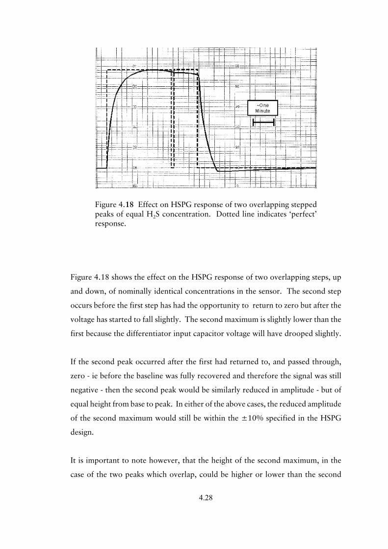
4.28

Figure 4.18 Effect on HSPG response of two overlapping steppedpeaks of equal H2S concentration. Dotted line indicates ‘perfect’response.

Figure 4.18 shows the effect on the HSPG response of two overlapping steps, up

and down, of nominally identical concentrations in the sensor. The second step

occurs before the first step has had the opportunity to return to zero but after the

voltage has started to fall slightly. The second maximum is slightly lower than the

first because the differentiator input capacitor voltage will have drooped slightly.

If the second peak occurred after the first had returned to, and passed through,

zero - ie before the baseline was fully recovered and therefore the signal was still

negative - then the second peak would be similarly reduced in amplitude - but of

equal height from base to peak. In either of the above cases, the reduced amplitude

of the second maximum would still be within the ±10% specified in the HSPG

design.

It is important to note however, that the height of the second maximum, in the

case of the two peaks which overlap, could be higher or lower than the second

4.29

Figure 4.19 Simulation of HSPG response to two closely following peaksof H2S gas concentration. Dotted line indicates ‘perfect’ response.

peak in the case where the second peak falls in the area of the first peaks ‘zero

depression’. As discussed previously, the reduction of peak height in the latter is

limited by the forward voltage of the germanium diode, whereas in the former, it

is only affected by the extent of capacitor voltage droop.

Because of the almost instantaneous response of the HSPG, to a voltage simulating

the sensor, it is not possible to adequately demonstrate the effect of two

overlapping ‘concentrations’. These are always revealed as two distinct steps - as

seen in Figure 4.19. The same figure does however show the effect of the zero

depression following a broad step and confirms that the second step height, if not

its amplitude, relative to the 5 V bias voltage, is identical to the other.

The auto-zero mode causes the HSPG to behave in a similar manner to that where

a downward step change in H2S concentration occurs. At the end of the auto-zero

period, the HSPG responds as it would when being presented with the ambient

4.30

concentration as another upward step change.

4.3.3.3 Ageing of gel and carbon filters

It was found that the sensor gel, after the initial evaporation of the carrying

solvents, gave consistent results for up to ten days. During the first 24 hours, the

electrical output appeared somewhat noisy (±20 %), presumably due to residual

solvents or other chemical instability after mixing, and so the HSPG was not used

during this period. Daily calibrations were then performed, but it was found that

these did not vary significantly until approximately the tenth day, after which the

sensitivity fell at approximately 10 % per day. It was suspected that this was due

to drying of the gel coating.

The lifespan of the carbon granules, in both the reference chamber and in the

zeroing chamber, is dependant upon the total H2S dose to which they are each

subjected. Because the HSPG was used in various ways, and calibrated under

differing regimes, at different times, it proved difficult to estimate how soon the

carbon would become unusable. The prime symptoms of carbon exhaustion were

loss of sensitivity and inability to zero the HSPG. The maximum period of use,

achieved without changing the carbon in either chamber, was approximately one

month. However, it was decided that, as carbon replacement and gel refreshment

each entailed undoing the measurement cell, both activities should be done every

ten days.

4.3.3.4 Repeatability of response to different input concentrations

The calibration curve for the HSPG is shown in Figure 4.20. The formula for the

curve was calculated using the Excel ‘solver’ function. This curve is a composite

produced from a number of different experiments using varied H2S gas

4.31

Figure 4.20 HSPG calibration curve. Curve formula is C=2.3E0.5508 (where C= H2S concentration in ppb and E=HSPG reading in millivolts)

concentrations on different days and with sensor gels of different ages. Viewed

separately, each day’s calibration produced a curve of similar shape to Figure 4.20.

All the points on the curves obtained however, fell within ±10 % of the values

indicated in the composite curve. This close repeatability was very useful in

quickly estimating H2S concentrations during experiments.

4.3.3.5 Linearity of HSPG response

Figure 4.20 shows that the HSPG does not have a linear response. This was also

suggested earlier by Figure 4.14, in that the 100 ppb peak was noticeably less in

magnitude than half that of the 200 ppb peaks.

Therefore, it now seems likely that the complete response curve for the sensor is

4.32

sigmoidal in character. This would be in agreement with the responses of other

gels to chemical and biological agents.

4.3.4 HSPG limitations

The HSPG is not suitable for the continuous monitoring of 100 ppb H2S or greater,

as the activated charcoal employed will rapidly become exhausted. However, this

was not the intention of this design, for which a proprietary digitally based

instrument (such as the Jerome 631X previously described) would be more

appropriate.

A slow change in concentration of H2S, such as small changes in ambient

concentration, would not be detected if this was similar in magnitude to the rate

of charging or discharging of the differentiator capacitor. However, these would

become measurable after each zero setting procedure.

The need to regenerate the sensor gel coating approximately every ten days is an

inconvenience and could interrupt a series of experiments. There is also the need

to wait another day after regeneration, until the sensor coating has stabilised,

before use.

4.4 SUMMARY

The hydrogen sulphide peak gauge (HSPG), has been shown to respond extremely

rapidly to changes in H2S concentration and to reveal the nature of variations in

concentration more accurately than any other known portable instrument. To

some extent because of this, the calibration of the HSPG proved difficult. It is

evident from field experiments that the HSPG is capable of much more rapid

response than the changes the gas calibrator was able to provide, because plumbing

4.33

volume, flow rate and switching valve constraints meant that step changes in

calibrator output were inherently impossible.

It is acknowledged that for a commercial instrument, a sensor that does not require

weekly replacement or daily calibration is an essential pre-requisite. Therefore,

metallic oxide sensors should be considered where the technology is available for

their production.

5.1

Chapter 5: FIELD EXPERIMENTS

This chapter is divided into two sections. The first section (5.1) outlines those

experiments which relate to the development of the DRs, described in Chapter 3,

and their use for the measurement of long term measurements. The second section

(5.2) outlines experiments conducted using the HSPG, described in Chapter 4, for

the measurements of peaks.

Each site used, and the criteria for its selection, is described in the appropriate

experimental section the first time the site is referred to.

5.1 LONG TERM MEASUREMENTS

5.1.1 Experiment 1: ACUs at Molehill Farm

The objective of this experiment was to determine whether the aspirated collection

units (ACUs) described in section 3.2, were a viable method of monitoring ambient

H2S.

A site was chosen close to junction 24 of the M1 motorway, for the following

reasons:-

• It is close to the laboratory used for sample preparation and analysis.

• Two heavily used major roads, totalling 12 lanes, run alongside each other

in this vicinity. Likely concentrations of H2S were not known at this stage

therefore the large amount of traffic would maximise the chances of H2S

detection.

• The motorway is in a cutting in this locality. When the wind is in the

prevailing (south westerly) direction, the overbridge tends to direct traffic

fumes from both roads towards the eastern sampling point. This was

expected to maximise any differential in H2S concentrations between the

two sites.

5.2

Figure 5.1. Site plan of Molehill Farm showing direction of prevailingwind and cross section between west and east sites.

• The farmer at Molehill Farm was agreeable to the use of his land for this

work.

Two ACUs were deployed adjacent to Molehill Farm in the locations indicated by

X and Y in the site layout (Figure 5.1).

The view westwards from the farm entrance is shown in Figure 5.2. The western

ACU was situated at the foot of the distant hedge on the extreme right of the

photograph. Therefore, with the wind from the direction shown, only the eastern

ACU was in the path of vehicular pollution.

5.3

Figure 5.2. View from Molehill Farm, westwards over M1 to A453.

The absorbing solution used was as described in the ISC method (American Public

Health Association Intersociety Committee, 1977) and not the formulation

described in section 3.2.3 which had not yet been developed. The ACUs were

exposed for 3 hours 30 minutes. The weather was warm but damp throughout the

exposure period. The temperature varied between approximately 26 OC and 21 OC

whilst the humidity varied between 48 % and 66 %.

The results of this experiment are shown in Figure 5.3. Each absorbance was

measured against a de-ionised water blank. All subsequent experiments used blanks

which were unexposed solution which was otherwise subjected to the same

environment as the measurement samples. The stacked bar charts indicate the

amounts of sulphide captured in each of the series bottles. At this stage the

absolute values of sulphide could not be calculated, nor converted into average

concentrations over the exposure period. This was because the presence of

sulphide in the third bottle, from each ACU, indicated that not all available

sulphide might have been captured and therefore that calculated concentrations

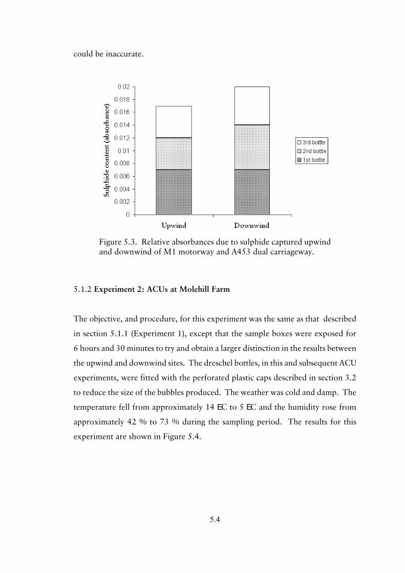
5.4

Figure 5.3. Relative absorbances due to sulphide captured upwindand downwind of M1 motorway and A453 dual carriageway.

could be inaccurate.

5.1.2 Experiment 2: ACUs at Molehill Farm

The objective, and procedure, for this experiment was the same as that described

in section 5.1.1 (Experiment 1), except that the sample boxes were exposed for

6 hours and 30 minutes to try and obtain a larger distinction in the results between

the upwind and downwind sites. The dreschel bottles, in this and subsequent ACU

experiments, were fitted with the perforated plastic caps described in section 3.2

to reduce the size of the bubbles produced. The weather was cold and damp. The

temperature fell from approximately 14 EC to 5 EC and the humidity rose from

approximately 42 % to 73 % during the sampling period. The results for this

experiment are shown in Figure 5.4.

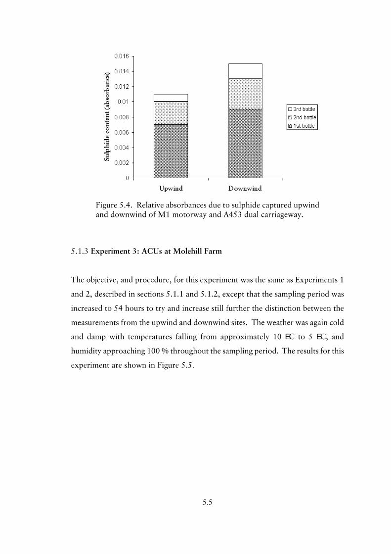
5.5

Figure 5.4. Relative absorbances due to sulphide captured upwindand downwind of M1 motorway and A453 dual carriageway.

5.1.3 Experiment 3: ACUs at Molehill Farm

The objective, and procedure, for this experiment was the same as Experiments 1

and 2, described in sections 5.1.1 and 5.1.2, except that the sampling period was

increased to 54 hours to try and increase still further the distinction between the

measurements from the upwind and downwind sites. The weather was again cold

and damp with temperatures falling from approximately 10 EC to 5 EC, and

humidity approaching 100 % throughout the sampling period. The results for this

experiment are shown in Figure 5.5.

5.6

Figure 5.5. Relative absorbances due to sulphide captured upwindand downwind of M1 motorway and A453 dual carriageway.

5.1.4 Experiment 4: ACUs at Molehill Farm

This experiment was similar to that described in section 5.1.3 above except the

sampling period was for 26 hours and the collection solution used in the dreschel

bottles was the new formulation described in section 3.2.3 (Deuchar et al., 2002).

The objective of the experiment was to test whether the new solution gave

improved results over its predecessor. The new formulation for the collecting

solution is referred to hereafter as ‘DR solution’. The weather was again cold and

damp with temperatures of only a few degrees Celsius. The results of this

experiment are shown in Figure 5.6. The total of the absorbances obtained, upwind

and downwind of the motorway, were later translated into atmospheric

concentrations of H2S of approximately 2 ppb and 4 ppb, respectively.

5.7

Figure 5.6. Relative absorbances due to sulphide captured upwindand downwind of M1 motorway and A453 dual carriageway.

5.1.5 Experiment 5: DR exposure at five sites

The object of this experiment was to test the newly developed passive technique,

described in Chapter 3, section 3.2.5. Single diffusion reservoirs containing 7 mL

of DR solution were fixed to fences at five local sites approximately 0.8 m above

the ground surface. The sites were adjacent to one of the University fields at

Sutton Bonington (denoted F12), alongside, and east of, the M1 motorway at Long

Whatton (LWE), either side the M1 motorway near Molehill Farm (J24W &

J24E), and adjacent to Kegworth water treatment works (KWT).

The sites used in addition to the previously described Molehill Farm locations were

chosen for the following reasons. The F12 site was chosen because of its

completely rural location and proximity to the laboratory. The LWE site was used

because it, like J24E, was downwind of the motorway but in an otherwise rural

location with no other major road nearby and the KWT was chosen because it was

expected that the treatment works would be a considerable source of H2S.

5.8

Figure 5.7 Fence holder for up to three DRs

Extra DRs were fitted with blank caps, for use as assay blanks. The DRs were

transported to the measurement site in sealed plastic boxes with the caps and

membranes upwards. The DRs were then fitted into purpose made holders, to the

specification in Figure 5.7. The holders were clipped on a convenient fence rail,

with the membranes in the downward position to be in contact with the DR

solution. The DRs were exposed for 24 hours and were deployed and collected in

the same order. Therefore, although the period of measurement was the same for

each DR, the individual sampling periods were staggered by up to 15 minutes.

After retrieval, the DRs were transported back to the laboratory, membranes

upward but covered by a thin plastic sheet, in the same sealed, plastic boxes and

refrigerated until analysis the following day. The wind direction was from the

south-west throughout the experimental period.

5.9

Figure 5.8. H2S concentrations at various roadside and rural locations

The results of this experiment are shown in Figure 5.8. The calibration was carried

out as described in section 3.2.

5.1.6 Experiment 6: DR exposure at two sites

This experiment was carried out in a similar manner to that described in

Experiment 5, section 5.1.5 but the DRs were set out with three replicates at each

of two different sites for a period of 11 hours. One site was at Trent Lock, Sawley,

South Derbyshire (TL), at a rural, traffic free, riverside location and the other was

adjacent to, and downwind of, the M1 motorway at Watford Gap (WG),

Northamptonshire, in an otherwise rural location. A further three DRs were kept

unexposed in the laboratory for use as blanks. The objective was to assess the

variability between replicates at each site.

The results of this experiment are shown in figure 5.9.

5.10

Figure 5.9. H2S concentrations adjacent to a motorway (WG) andat a rural location (TL)

5.1.7 Experiment 7: DR exposure at a single site

This experiment was carried out in a similar manner to that described in

Experiment 6, section 5.1.6 but the DRs were set out with three replicates each at

Normanton on Soar, Nottinghamshire (NoS) for ten days - a rural, riverside site.

A further three DRs were kept unexposed in the laboratory as controls. The

objective was to further investigate typical rural H2S concentrations at a different

site and assess the variability of replicates.

The results of this experiment are shown in Figure 5.10.

5.11

Figure 5.10. H2S concentrations at a single rural location

5.1.8 Experiment 8: DR exposure at three sites

This experiment was carried out in a similar manner to that described in

Experiment 7, section 5.1.7 but the DRs were set out with three replicates at each

of three different sites for 3 days. The sites were F12, Long Whatton west of the

M1 motorway (LWW) and Long Whatton east of the M1 motorway (LWE). A

further three DRs were kept unexposed in the laboratory for use as controls. The

objectives were to make further comparisons between the ambient H2S recorded

at each site over the same time period and also to compare ambient H2S on both

upwind and downwind sides of a major road. The wind direction was from the

east throughout the experimental period.

The results of this experiment are shown in Figure 5.11.

5.12

Figure 5.11. H2S concentrations at various locations including east(upwind) and west (downwind) of a major road

5.1.9 Experiment 9: DR exposure at three sites

This experiment was carried out in a similar manner to that described in

Experiment 8, section 5.1.8. The DRs were set out with three replicates at the

same three sites for a period of seven days. A further three DRs were kept

unexposed in the laboratory for use as controls. The object was to repeat the

previous experiment but over a different sequence of days and to compare the two

sets of results and see whether responses were consistent. The wind direction was

from the south-west throughout the experimental period.

The results of this experiment are shown in Figure 5.12.

5.13

Figure 5.12 H2S concentrations at various locations including westand east of a major road

5.1.10 Experiment 10: DR exposure at five sites

This experiment was carried out in a similar manner to that described in

Experiment 9, section 5.1.9. The DRs were set out with three replicates at each

of five different sites (including the three from the previous experiment) for a

period of 24 hours. The additional sites were Molehill Farm, between the A453

dual carriageway and the M1 motorway (MHM), and KWT. A further three DRs

were kept unexposed in the laboratory for use as colorimeter blanks. The objective

was to further investigate the variability of ambient H2S simultaneously at different

sites. The wind direction was from the south-west throughout the experimental

period. This meant that the location LWE was downwind of the motorway,

MHFM was downwind of the A453 dual carriageway and KWT was downwind of

Kegworth water treatment works.

The results of this experiment are shown in Figure 5.13.

5.14

Figure 5.13 H2S concentrations at various locations including west andeast of major roads

5.1.11 Experiment 11: DR exposure at six sites

This experiment was carried out in a similar manner to that described in

Experiment 10, section 5.1.10. The DRs were set out with three replicates at each

of six different sites (including the five from the previous experiment) for a period

of five days. The additional site used was MHW. A further three DRs were kept

unexposed in the laboratory for use as colorimeter blanks. The objective was to

repeat the previous experiment for a longer time period to assess long term

variability of H2S concentrations in the atmosphere. The wind direction was from

the east throughout the experimental period. This meant that the location LWW

was downwind of the motorway. MHFM was upwind of the A453 dual

carriageway, but downwind of the M1 motorway. MHFW was downwind of both

the motorway and the dual carriageway and KWT was upwind of the water

treatment works.

The results of this experiment are shown in Figure 5.14.

5.15

Figure 5.14. H2S concentrations at various locations including west and eastof major roads

5.1.12 Experiment 12: DR exposure on part of a land fill site

This was a preliminary experiment with the objective of assessing the suitability of

DRs for the monitoring of H2S around a landfill site. For the monitoring of

landfill H2S, the survey method employed may vary according to requirements.

For example, a grid formation over the entire site may be used to determine spatial

variation or a perimeter survey employed to assess the significance of gas migration

from the site.

The particular site surveyed had a history of nuisance odours which were attributed

to H2S by the site owners. The study site was first used for landfill over 20 years

ago and was progressively covered with a mixture of soil and quarry waste until

completion some 10 years ago. H2S originates from plasterboard, or other gypsum

waste, buried with organic material, because of reaction with acidified leachate. A

variety of trees was planted on completion of the covering. The site was

approximately 300 m square. The whole site was traversed first on foot and areas

identified where the smell of H2S seemed particularly strong.

5.16

Figure 5.15. H2S concentrations on a landfill site. 2 Hr and 4 Hr are timedcover box measurements. ‘Adj’, ‘Vent’ and ‘Mid’ are 4 hour DRmeasurements made adjacent to the cover box, the eastern vent and midwaybetween these points, respectively. Non-cover box measurements weremade on posts 0.8 m above ground.

A cover-box technique, employing four DRs, was used on one portion of bare earth

where the smell of H2S was evident in the south-west corner of the site. Two other

DRs were taped to a post, approximately 0.8 m above ground, adjacent to the

cover box. Two more DRs were taped to another post near a leaking gas valve in

the south-eastern corner of the site, approximately 140 m from the cover boxes,

and a further two to a third post midway between the two locations. The DRs

were fixed in the inverted position so that the membranes faced downward and

were in contact with the absorbing solution. Additional DRs were kept unexposed

for use as controls. Heavy duty, silver, self-adhesive tape was used to protect the

DRs from direct sunlight and minimise solar heating. The DR blanks were

similarly taped to an additional post. All samples were exposed for four hours

except for two of the four associated with the cover box, which were only exposed

for the first two hours.

The results of this experiment appear in Figure 5.15.

5.17

5.1.13 Experiment 13: DR area survey on a landfill site

The object of this experiment was to map typical H2S concentrations around one

of the H2S ‘hot-spots’ identified on the landfill site described in section 5.1.12.

Posts (W1-W4, X1-X4, Y1-Y4 and Z1-Z4) were driven into the ground around the

leaking valve on a 4x4 matrix with an interval of 7 m between posts as indicated

in Figure 5.16. The posts were set out so that the gas valve coincided with post

B2. Two additional posts were driven into the ground adjacent to the valve so that

sampling of the immediate environment at the valve could be made in 120E sectors.

The asymmetrical nature of the grid layout assumed a longer ‘plume’ of H2S would

be evident to the north east due to the prevailing south westerly wind.

Single DRs were taped to each post 0.8 m above the surface of the ground. The

results of this experiment appear in Figure 5.16. The DR measurements were

mapped using Golden Software’s ‘Surfer’ package, version 7, and interpolation

performed by kriging.

5.18

W1

W2

W3

W4

X1

X2

X3

X4

Y1

Y2

Y3

Y4

Z1

Z2

Z3

Z4

0 2 4 6 8 10 12 14 16 18 200

2

4

6

8

10

12

14

16

18

20

Figure 5.16. H2S concentrations around a leaking landfill gas valve (X2).Distances in metres, contours show ppb H2S.

5.1.14 Experiment 14: DR whole site survey of a landfill site

A whole-site survey was conducted of the landfill site described previously in

section 5.1.12, with the objective of refining the location of hot-spots. The site

was set out with posts at each intersection of a 50 m grid. A single DR was fixed

to each post. The post layout and results are shown in Figure 5.17.

5.19

CLG1

CLG2

CLG2A

CLG3

CLG4

CLG5CLG6

CLG7

CLG8

CLG9CLG10CLG11

CLG12CLG12B

CLG13

CLG14 CLG15

CLG16

Leachate

CH2S1

CH2S2

CH2S3

CH2S4

A2

A3

A4

A5

A6

A7

B2

B3

B4

B5

B6

B7

C1

C2

C3

C4

C5

C6

C7

D1

D2

D3

D4

D5

D6

D7

E1

E2

E3

E4

E5

E6

E7

F1

F2

F3

F4

F5

F6

F7

G1

G2

G5

G6

H2S1H2S1H2S2H2S2

479650 479700 479750 479800 479850 479900347950

348000

348050

348100

348150

348200

348250

Figure 5.17. Landfill site survey using DRs. Eastings and northings inmetres, contours show ppb H2S.

5.1.15 Experiment 15: DRs on a detail survey of a landfill site

Experiment 14 (section 5.1.14) revealed that nearly all H2S emissions originated

from one part of the site. Therefore, this experiment related only to the south

eastern quarter of the site, some 150 m square, which was identified as the

predominant area for H2S emissions. The topography of the selected area is shown

in Figure 18, along with the positions of the relevant sampling posts (A1...A4,

B1...B4, C1...C4, D1...D3 and CH2S1) and gas valves. The valve CH2S1 is the

prime source for H2S emissions, whereas the valves CLG2 and CLG3, and the

leachate well, are secondary sources.

5.20

Sufficient vials were prepared to allow three DR replicates at each of the 16

monitoring locations, plus three additional DRs for use as unexposed assay blanks.

Aliquots of 7 mL of the absorbing solution were placed in each vial. Three vials

were fitted with plain caps to be used as the blanks and the remainder fitted with

a perforated cap and membrane.

The DRs were taped to the posts, with the membranes exposed downwards, 0.8

m above the ground surface. The time was noted at which the first and last DRs

were set out.

Meteorological data was not recorded on site, but temperatures, wind speed and

wind direction were monitored hourly throughout the exposure period at a site a

few miles away. These data were supported by qualitative observations on site.

Previous experience had shown that the only notable meteorological differences

between the two sites were in the timing of events. No rainfall was recorded

during the sample period.

After 50 hours, at the end of the exposure period, the DRs were recovered in the

same order as that in which they had been set out, and the start and finish times

were again noted.

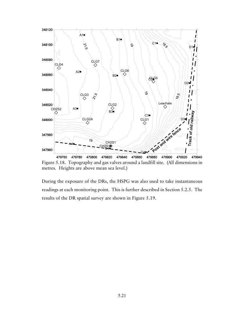
5.21

CLG1

CLG2

CLG2A

CLG3

CLG4

CLG5

CLG6

CLG7

Leachate

CH2S1

CH2S2

479760 479780 479800 479820 479840 479860 479880 479900 479920 479940

347960

347980

348000

348020

348040

348060

348080

348100

348120

A4

A3

A2

A1B1

B2

B3

B4

C1

C2

C3

C4

D3

D2

D1

CH2S1

479760 479780 479800 479820 479840 479860 479880 479900 479920 479940

347960

347980

348000

348020

348040

348060

348080

348100

348120

Post and wire

fence

Trac

k of

old

railw

ay

Figure 5.18. Topography and gas valves around a landfill site. (All dimensions inmetres. Heights are above mean sea level.)

During the exposure of the DRs, the HSPG was also used to take instantaneous

readings at each monitoring point. This is further described in Section 5.2.5. The

results of the DR spatial survey are shown in Figure 5.19.

5.22

479760 479780 479800 479820 479840 479860 479880 479900 479920 479940

347960

347980

348000

348020

348040

348060

348080

348100

348120

CLG1

CLG2

CLG2A

CLG3

CLG4

CLG5

CLG6

CLG7

Leachate

CH2S1

CH2S2

479760 479780 479800 479820 479840 479860 479880 479900 479920 479940

347960

347980

348000

348020

348040

348060

348080

348100

348120

A4

A3

A2

A1B1

B2

B3

B4

C1

C2

C3

C4

D3

D2

D1

CH2S1

479760 479780 479800 479820 479840 479860 479880 479900 479920 479940

347960

347980

348000

348020

348040

348060

348080

348100

348120

Post and wire

fence

Trac

k of

old

railw

ay

Figure 5.19. H2S concentrations around vents on a landfill site. (Eastings andnorthings in metres. Concentrations in ppb H2S.)

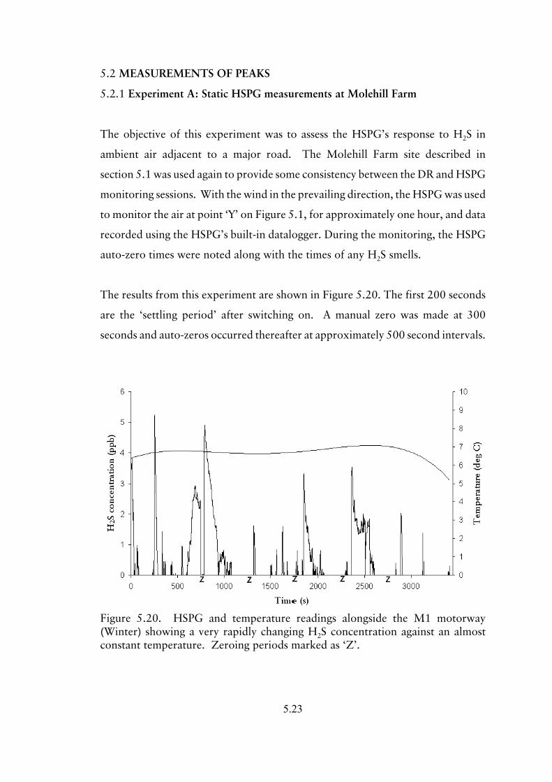
5.23

Figure 5.20. HSPG and temperature readings alongside the M1 motorway(Winter) showing a very rapidly changing H2S concentration against an almostconstant temperature. Zeroing periods marked as ‘Z’.

5.2 MEASUREMENTS OF PEAKS

5.2.1 Experiment A: Static HSPG measurements at Molehill Farm

The objective of this experiment was to assess the HSPG’s response to H2S in

ambient air adjacent to a major road. The Molehill Farm site described in

section 5.1 was used again to provide some consistency between the DR and HSPG

monitoring sessions. With the wind in the prevailing direction, the HSPG was used

to monitor the air at point ‘Y’ on Figure 5.1, for approximately one hour, and data

recorded using the HSPG’s built-in datalogger. During the monitoring, the HSPG

auto-zero times were noted along with the times of any H2S smells.

The results from this experiment are shown in Figure 5.20. The first 200 seconds

are the ‘settling period’ after switching on. A manual zero was made at 300

seconds and auto-zeros occurred thereafter at approximately 500 second intervals.

5.24

Figure 5.21. HSPG and temperature readings taken alongside M1 motorway(Early summer) showing a very rapidly changing H2S concentration against analmost constant temperature. Zeroing periods marked as ‘Z’.

5.2.2 Experiment B: Static HSPG measurements at Molehill Farm

This experiment was a repetition of that described in section 5.2.3 but at a

different time of year. A separate temperature logger was used to monitor the

ambient air temperature at the input to the HSPG. The results are shown in

Figure 5.21. A manual zero was forced 420 seconds after switching on, and

thereafter auto-zeros occurred approximately every 420 seconds.

5.2.3 Experiment C: Mobile HSPG measurements on a 40 mile road trip

Whereas the measurements described in sections 5.2.3 and 5.2.4 were static, this

experiment was conducted using the HSPG on a motorway journey across the UK

Midlands in the manner described in section 5.2.1. The results are shown in

Figure 5.22. Events, and information about the environment through which the

vehicle was passing, are detailed in table 5.1. The objective of the experiment was

to compare the values of roadside H2S concentration, obtained in the previous two

experiments, with those concentrations which might be experienced by a driver on

5.25

a similar road.

Table 5.1.

Time Event

0 Commencement of journey. Residential area.

330 Joined A5 dual carriageway

400 Auto-zero

630 Joined M42. Entered rural area.

860 Auto-zero

1430 Auto-zero

1500 Outskirts of Ashby-de-la-Zouch

1600 Manual zero

1630 Adjacent to Lount landfill site

1920 Auto-zero

2000 In cutting. Passed sewage works.

2290 Joined M1. H2S smelt by vehicle occupants.

2380 Left motorway at Junction 24

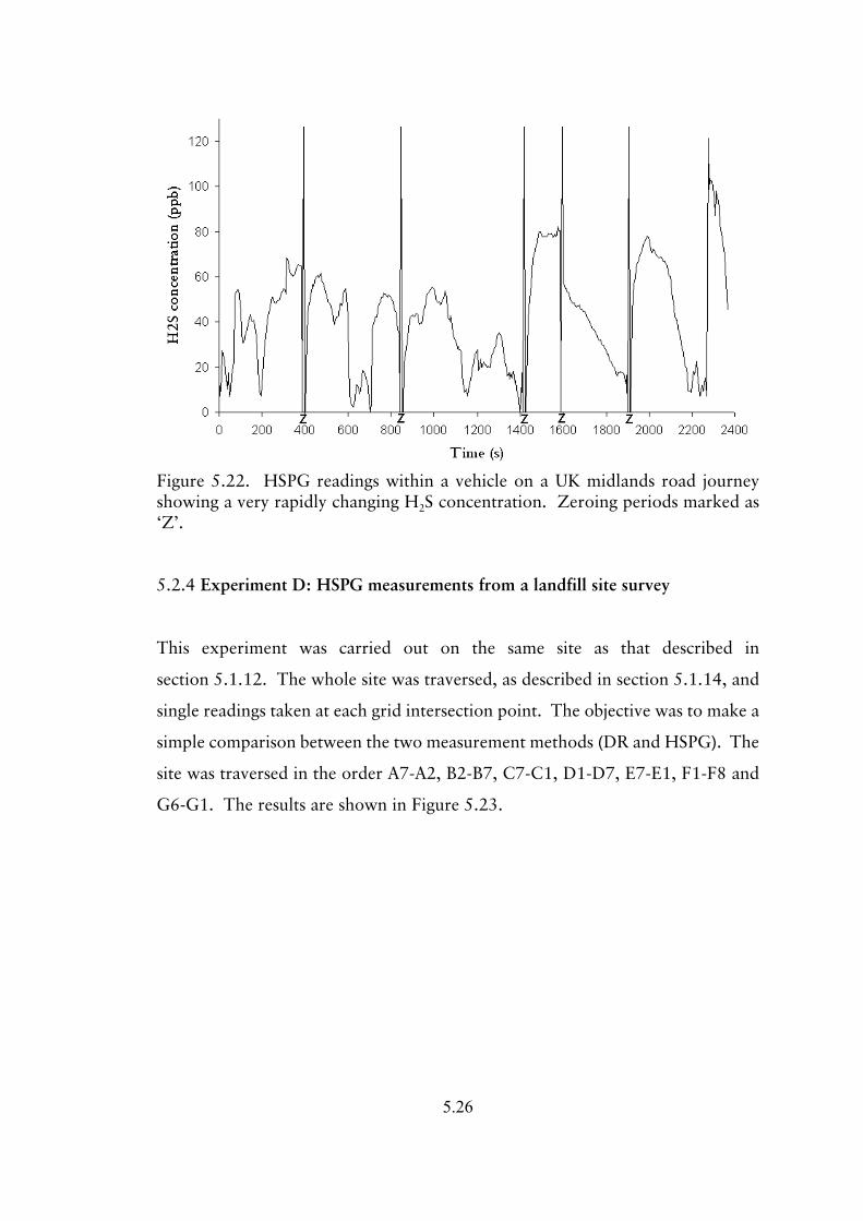
5.26

Figure 5.22. HSPG readings within a vehicle on a UK midlands road journeyshowing a very rapidly changing H2S concentration. Zeroing periods marked as‘Z’.

5.2.4 Experiment D: HSPG measurements from a landfill site survey

This experiment was carried out on the same site as that described in

section 5.1.12. The whole site was traversed, as described in section 5.1.14, and

single readings taken at each grid intersection point. The objective was to make a

simple comparison between the two measurement methods (DR and HSPG). The

site was traversed in the order A7-A2, B2-B7, C7-C1, D1-D7, E7-E1, F1-F8 and

G6-G1. The results are shown in Figure 5.23.

5.27

479650 479700 479750 479800 479850 479900347950

348000

348050

348100

348150

348200

348250

A2

A3

A4

A5

A6

A7

B2

B3

B4

B5

B6

B7

C1

C2

C3

C4

C5

C6

C7

D1

D2

D3

D4

D5

D6

D7

E1

E2

E3

E4

E5

E6

E7

F1

F2

F3

F4

F5

F6

F7

G1

G2

G5

G6

H2S1H2S1H2S2H2S2

Figure 5.23. HSPG survey of whole landfill site. Contours show ppb H2S. Eastingsand northings in metres.

5.2.5 Experiment E: A detail survey of a landfill site using the HSPG

This experiment was also carried out on the south eastern quarter of the landfill

site, and during the same period, as Experiment 15 described in section 5.1.15. The

same portion of the site was traversed, in the same order, several times during the

daytime on each monitoring day. These additional readings were used in this

experiment in addition to the DRs to verify the two different approaches and

obtain a simple comparison between the results during the same monitoring period.

5.28

Figure 5.24. HSPG landfill survey. Day 1, traverse 1.

Figure 5.25. HSPG landfill survey. Day 1, Traverse 2.

Figure 5.26 HSPG landfill survey. Day 1, traverse 3.

Figure 5.27. HSPG landfill survey. Day 2, traverse 1.

The results for each traverse of the site are shown in Figures 5.24 to 5.33. A

composite of the results obtained using the HSPG at each of the 16 locations is

plotted in Figure 5.34. Contours show ppb H2S. Eastings and northings in metres.

5.29

Figure 5.30. HSPG landfill survey. Day 2, traverse 4.

Figure 5.31. HSPG landfill survey. Day 3, traverse 1.

Figure 5.32. HSPG landfill survey. Day 3, traverse 2.

Figure 5.33. HSPG landfill survey. Day 3, traverse 3.

Figure 5.28. HSPG landfill survey. Day 2, traverse 2.

Figure 5.29. HSPG landfill survey. Day 2, traverse 3.

5.30

Figure 5.34. HSPG landfill survey. Composite of traverse results. Contours showppb H2S. Eastings and northings in metres.

6.1

Chapter 6: DISCUSSION AND CONCLUSIONS

6.1 LONG TERM MEASUREMENTS

6.1.1 Experiments using aspiration

These experiments (Experiments 1 - 4, section 5.1) used bubblers upwind and

downwind of the M1 motorway at Molehill Farm to detect any elevation in H2S

concentration due to the road. The results of Experiments 1, 2 and 3 showed that

the total amount of sulphide measured in the downwind dreschel bottles was

higher than that in the upwind bottles. However, because sulphide was detected in

the third of the three of the bottles at the downwind site, it was not appropriate to

estimate an average H2S concentration over the sampling period. This is because

it was possible that not all the sulphide inspired had been captured by the solution

in the bottles, and that some was exhausted back to the atmosphere. The

differences in absorbance between the upwind and downwind sites, obtained in the

three experiments, was not large (ie within ±10-15 %) and therefore it was

possible that these differences might have been within experimental error, which

was initially estimated as ±10 %.

Experiment 1 used bubblers with plain tube outlets whereas subsequent ACU

experiments used bubblers fitted with perforated caps, as described in section 3.2,

which improved H2S capture. In Experiment 1 the absorbances obtained for the

three bottles, in each ACU, were similar - within 20 % of each other. This result

suggests that the total mass of sulphide entering the ACUs exceeded the capture

capabilities of all three bottles at each location and therefore could account for the

similarity in the two totals. Experimental errors were considered to see whether

this experiment had any statistical significance in spite of this. Two possible

sources of error were identified between the samples. The first possibility was in

incorrectly making up the solutions to volume during analysis. This would be only

a fraction of a per cent and was discounted. The second possible source of error

6.2

was in the readings obtained from the colorimeter, which was working at the lower

limit of its range. If the readings recorded were analysed, with an error range of

1 digit, then a marginal significance (p<0.05) was obtained for the differences in

absorbance between the samples from the two locations.

In Experiment 2, each successive bottle in each ACU group captured slightly less

sulphide than its predecessor. However the presence of sulphide in the third bottle

of each ACU still indicated inadequate capture overall. A similar statistical

approach to experimental errors, as that described in relation to Experiment 1,

showed the results also had significance (p<0.05).

Experiment 3 showed, for the first time, no sulphide capture in the third upwind

bottle and very little in the second bottle. Although the exposure period was more

than eight times longer than that of Experiment 2, the ambient H2S concentration

at the upwind site was lower than that previously measured. This concentration

was therefore within the collection capability of the upwind ACU. However the

presence of sulphide in the third downwind bottle again meant that any absolute

comparison was of little value. The difference in the totals measured indicated a

higher statistical significance (p=0.015) than that of Experiments 1 and 2.

The other point of note in the results from the first three experiments, was that the

sampling duration did not appear to be closely related to the absorbances obtained.

This might, of course, have been a genuine variation in atmospheric H2S

concentration between the different sampling dates. However, it might also have

been due to increased oxidation of the absorbed sulphide in solution, because of

the longer sampling period, as discussed previously in Chapter 3. In particular, the

absorbances obtained in Experiment 3 (section 5.1.3) were much lower than those

obtained for Experiments 1 and 2 (sections 5.1.2 and 5.1.3) than would be

expected for the longer sampling duration. This might have been because of

changes in humidity (see Chapter 1)(Cadle and Allen, 1971), however, the general

weather conditions on all these days were cool and damp and therefore

6.3

absorbances roughly correlated with exposure time might be expected.

Because of these apparent discrepancies, the objectives of these three experiments

were not considered fully met but they did demonstrate the basic viability of the

ACUs, the ability to capture sulphide in low ambient H2S concentrations and that

there was a statistical significance in the difference between the H2S concentrations

upwind and downwind of the motorway.

The ACU measurements made alongside the M1 motorway between junctions 23A

and 24 in Experiment 4, which used the new absorbing solution described in

section 3.2, showed that sulphide was not detected in either of the third bottles,

from the upwind and downwind sites. From this it could be inferred that all the

sulphide, in the volumes of ambient air sampled at each location, was captured by

the solution in the first and second bottles. The work on the ageing of sulphide in

solution, described in section 3.2.4, demonstrated that the sulphide captured did

not oxidise appreciably during the sampling duration of 26 hours, and therefore

that the mass of captured sulphide was indicative of H2S concentration at each

ACU location.

The results from Experiment 4, indicated a H2S concentration of approximately

4 ppb (vol/vol) of hydrogen sulphide downwind, and 2 ppb upwind, of the

motorway. A number of experiments were conducted with the wind in opposite

directions at different times and in each case the upwind H2S concentration was

similar, and the downwind concentration was 1 - 2 ppb higher. This consistency

implied that the extra contribution was not merely due to an unknown local source

but was probably due to vehicles on the road. The ACU method was therefore

considered validated for use in this context. The new absorbing solution was also

shown to have an improved sulphide capture ability, over that previously used.

The upwind H2S concentration of approximately 2 ppb is consistent with that

suggested by other workers for a rural environment (eg. Andersson et al., 1974).

6.4

6.1.2 Experiments using DRs

Experiment 5 was the first occasion in which DRs were used in the field. Five sites

were used as described in section 5.1.5. Although varying amounts of sulphide

were captured at each site over the 24 hour duration, these variations were within

±20% of the mean value obtained. Therefore the variations might have been due

to experimental error between the non-replicated DRs, and further investigation

was deemed necessary to estimate the likely actual errors. However, the results

obtained did suggest that there was an elevation in sulphide concentration

downwind of the motorway at both LWE and J24E compared with the upwind and

rural sites J24E and F12. These results therefore supported the findings previously

obtained with the ACUs. There did not appear to be any more H2S captured at the

treatment works (KWT) than the upwind and rural locations. Some elevation of

H2S concentration was expected but it might be that the sulphide emissions were

in other forms such as SO2 or di-methyl sulphide (DMS).

For Experiment 6, only two sites were used with DRs, but three replicates were set

out at each. One site was adjacent to a motorway (WG) and the other was a rural

location (TL). The results showed that there was approximately 50 % more

sulphide captured, and therefore a 50 % higher H2S concentration, at the side of

the motorway compared with the non-motorway location.

The variations between replicates in Experiment 6 were, however, greater than

expected (coefficient of variance . 100 %). The highest sulphide concentration at

the rural TL location exceeded the two lower values of the three replicates at the

motorway adjacent WG location although the total sulphide captured was much

higher at WG than TL . This finding brought the whole procedure into question

and prompted a full review of the laboratory procedures before and after capture.

Experiment 7 used the DR method for a 10 day period at a single site and showed

that at a rural, riverside location, the amount of hydrogen sulphide in the air was

6.5

low (between 1-2 ppb), which was in accordance with results from similar locations

elsewhere. However, there was still a large variation between replicates apparent

(coefficient of variance = 60 %). In this case it was considered that the manner in

which the membranes on the DRs were initially treated on their return to the

laboratory was crucial to the results obtained. The procedure which was finally

adopted was fully described in section3.2.5 and ensured that the membrane pores

were fully cleared at the start of the analysis. All subsequent experiments showed

much smaller standard errors (SE # 0.14).

Experiment 8, using DRs to make upwind and downwind comparisons of H2S

concentration alongside a major road and at a rural location, used three of the

locations used in the first DR experiment (Experiment 5) but for three times the

duration of the previous exposure. The locations were adjacent to a field on the

University campus at Sutton Bonington (F12) and upwind and downwind of the

M1 motorway at Long Whatton (LWW and LWE respectively). The results were

compatible with those previously made, and the absorbances obtained for the

replicates were very similar at F12 and identical at the other two locations. This

was taken as confirmation of the importance of the procedure for membrane

treatment during analysis.

Experiment 9 was a repeat of Experiment 8, but with a measurement period of one

week, to see if the H2S concentrations measured varied appreciably from the time

of one experiment to another. The longer sampling duration of Experiment 9 was

incidental, but a major change in the conditions between the two trials was that the

wind direction changed approximately 180 E. The results were compatible with

those previously obtained and again the replicates showed similar concentrations

(SE # 0.14). The rural F12, and motorway downwind and upwind, H2S

concentrations were also similar in both experiments.

Experiment 10 was to obtain simultaneous collection of data from five sites using

DRs, so that direct comparisons in the H2S concentrations at these locations could

6.6

be made over the same time period. There was reasonable agreement (SE # 0.14)

between the replicates at each site. The rural F12 site and the upwind motorway

site (LWW) showed similar concentrations of H2S. Downwind of the motorway

at LWE there was an elevation of H2S concentration and a still higher elevation

between the two major roads at MHFM. A similar elevation of H2S concentration

to that found at the MHFM site was found downwind of Kegworth water

treatment works (KWT).

Experiment 11 provided similar results to Experiment 10 and the inclusion of

MHFW gave an upwind and downwind comparison of H2S concentrations on the

A453 dual carriageway. The highest H2S concentrations however were found

upwind of the water treatment works KWT. This was surprising, but could be

related to emissions from an animal house which lay upwind of KWT, or to

emissions from the KWT outfall, which runs in a narrow open ditch to the north-

east.

Experiments 12 to 15 showed that the DRs could be used for mapping H2S

contours around a known source. The data obtained also enabled the location of

a previously unknown H2S emission areas on this site for possible future remedial

work by the site owners.

In Experiment 12 a cover box technique was tested as a means of measuring

ground emissions of H2S. It was later realised that the smell of H2S at this point

could be attributed to the plume of landfill gas being borne along the narrow valley

from the valve CH2S1 to the cover box location. The H2S concentrations obtained

at the Adj, Mid and Vent DR posts (Figure 5.15) show how rapidly these

concentrations diminished along a transect from a point source. These results were

substantiated by those obtained in Experiments 13 to 15. The inference which may

be drawn from these results is that H2S in the atmosphere reacted with other

chemicals to, or was diluted in the atmosphere by, approximately 90 % of the

concentration at the emission source, in travelling a distance 140 m.

6.7

The use of un-replicated DRs in Experiments 13 and 14 was considered sufficient

to reveal hot-spots of H2S emission from the landfill site surface and from around

valves in a reconnaissance survey. Preliminary mapping was then used to

determine which area of the site was most appropriate for further detailed

monitoring with replicated DRs. The results obtained confirmed the extremely

rapid reduction in H2S concentration with distance, from the known source

discovered in Experiment 12, and described above. Experiments 13 and 14

showed that this rapid reduction occurred in all directions.

In the detail survey (Experiment 15), a very high concentration of H2S was found

around one particular vent but this concentration diminished to virtually zero,

approximately 100 m away from the source. The H2S concentration contours were

very tightly packed between the vent CH2S1 and the post B4 (Figure 5.19). This

irregularity was probably accentuated by the steep gradient, and consequent

difference in elevation of about 3 m, between these two points. This is evident

from the topographical map (Figure 5.18). Another contributing factor to the

concentration gradient might have been that the gas emissions were at an elevated

temperature, and also tend to jet vertically upwards from the leaking valve.

6.8

6.2 MEASUREMENTS OF PEAKS

The results of Experiment A (section 5.2.1) show the response of the HSPG in

ambient air downwind of a major road and therefore indicate how the H2S

concentration fluctuates rapidly, and considerably, over time. The response is very

similar in character to that found by Cadle and Mulawa (1978) in laboratory

experiments into the production of H2S resulting from vehicular catalytic

converters. Characteristically there are small variations in low concentrations of

H2S which are interspersed with relatively large but brief transitions to

concentrations several times larger in magnitude.

It should be noted that although some temperature variation was evident during

the monitoring period, this bears no relationship to the HSPG readings. This

confirms the assertion in Chapter 4, that the HSPG response is not temperature

sensitive, but might also suggest the oxidation of ambient H2S is not particularly

sensitive to changes in temperature either. (This was also indicated by the

experiments undertaken with the ACUs and DRs discussed in section 6.1.)

However, the peaks of H2S found were much smaller in amplitude than those

resulting from Experiment B (section 5.2.2) which was conducted at a different,

and warmer, time of year.

It is apparent that the character of the graphical data from experiment A is

different to that from Experiment B. Experiment A shows a near zero baseline

which is occasionally broken by the rapid fluctuations already described.

Experiment B appears to show an elevated base line with more frequent excursions

which are rather smaller than those of Experiment A. There is no reason to suspect

instrumental changes, because the HSPG performed similarly in all laboratory

calibrations, therefore an alternative explanation is needed for the differing

behaviour.

It must be assumed that vehicles passing on the nearby roads were statistically

6.9

similar when considered as a group, both in vehicles passing per hour and in

proportions of each vehicle type. It is also reasonable to assume that an equivalent

number had catalytic converters which were operating under similar conditions.

Higher humidity levels will cause a more rapid oxidation of H2S to SO2 because

H2S is highly soluble in water (see Chapter 1). Therefore, in minimal wind

conditions, this reaction will occur more quickly before reaching the monitoring

point. Higher wind speeds would reduce the transit time from source to the

monitoring point, but would also result in greater mixing, and therefore dilution,

of the H2S. The most likely explanation however, is that, regardless of the precise

mechanism, the results from Experiment B are actually showing a large number of

peaks of H2S concentrations, which are following each other in rapid succession,

rather than an elevated base line with smaller peaks superimposed. The latter view

would be in conflict with our original assumptions concerning vehicle numbers and

type.

The results of Experiment C, conducted from within a moving vehicle, show H2S

concentrations two orders of magnitude higher than Experiments A and B. This

is consistent with the work of Clifford et al. (1997) who also found that

concentrations of certain vehicular pollutants (which did not include H2S) were

several times higher within vehicles travelling along a road than those measured at

the roadside. Both studies therefore indicate that the results from contemporary

roadside pollution monitoring sites, put in place by governmental and other bodies,

must be considered in context. Results from roadside sites might be safely used in

a consideration of the effects of vehicle pollution on people and property adjacent

to the road, but would seem to be appreciable underestimates of the effects on road

users.

The HSPG was designed to monitor intermittent peaks of H2S against a low

background value, but in Experiment D the instrument was used to measure

relatively constant concentrations at a series of fixed locations on a landfill site.

Although this was not a direct comparison with any of the measurements taken

6.10

using DRs, the HSPG results show a similar pattern of concentration to that

revealed by the DR method on other occasions. This suggested that either

monitoring technique could be used for a similar purpose of site mapping, within

certain constraints.

Experiment E was designed to obtain a qualitative comparison of results from the

HSPG and DR methods. Both methods show the same hot-spots in similar

concentrations. Direct comparison of the results obtained using the DRs and the

HSPG is not strictly valid because both sets of instrumentation were not deployed

continuously throughout the monitoring period. It would not be sensible to

compare a single HSPG traverse of the whole site with the results from the DRs

which were exposed for the whole 50 hour period. However, the results obtained

using the two methods are qualitatively in agreement when the DR results are

compared with the average of the HSPG results.

6.11

6.3 CONCLUSIONS

The catalytic converter is a reaction chamber for numerous catalytic and

conventional reactions between compounds which may contain impurities. It is

therefore not surprising that the production of hydrogen sulphide was discovered

accidentally rather than predicted theoretically.

Roadside and ambient measurements of hydrogen sulphide have been made. The

results show a small but repeatable elevation of mean H2S concentrations

downwind from a main road. The ambient rural H2S concentration was

consistently measured as 1-2 ppb. Busy main roads appear to add approximately

1-2 ppb H2S to the mean ambient value when measured at the roadside.

Therefore, in relation to the first objective stated in section 1.3, it is now clear that

this additional pollution load is probably not significant in either local or global

terms. The second objective, to measure atmospheric concentrations of H2S, is also

met, and the H2S concentrations measured agree with those of other workers.

For drivers and passengers in vehicles on busy roads however, the situation is

rather different. Drivers, and passengers, on such roads are subjected to a series

of relatively high peaks of concentration of H2S gas, whose amplitude may be

measured in 100's of ppb. The third objective, stated in section 1.3, was to

investigate the relationship between peak and long term concentrations of H2S and

this work suggests that, in a road side or on-road environment, it would appear

that it is the integration of these brief peaks that is the cause of the elevation of

mean ambient H2S downwind of the carriageway. This is a new area of research

and the field measurements obtained as part of this study confirm the theoretical

expectations and also measurements made previously in the laboratory by others.

Whilst, as discussed in Chapter 2, a considerable amount of work has been done

worldwide on the human health effects of H2S at low ambient concentrations, as

a result of industrial pollution, and at very high, life threatening, concentrations,

6.12

as a result of industrial accidents, there appears to have been no research directed

at assessing any effects on human physiology which might be due to vehicular

pollution in the manner found in this study.

Alternative measurement methods have been identified, both for passive

background measurement and also for short term, rapid response measurements.

The latter included the development of a new resistance sensor and its

incorporation in a new piece of equipment for use in the measurement of low

concentrations of H2S gas. This required the specialist development of

conventional analogue electronic techniques.

The Diffusion Reservoirs provide a reliable, low cost, method of measuring average

H2S concentrations. The method produces results which are in agreement with

those obtained by other means. The results indicated the additional ambient H2S

pollution, due to catalytic converters fitted to road vehicles, and also clearly

revealed the ‘hotspots’ of H2S concentration on a landfill site. The hotspots were

associated with failed valves in the gas extraction system and with sub-surface

fissures in the land fill cover. The results also indicate that the concentrations of

H2S at the perimeter of the site are of relatively minor significance.

The HSPG enabled the detection of transient peaks of H2S for the first time in a

portable instrument and completed the fourth objective stated in section 1.3.

There is, however, considerable scope for further improvements to this prototype.

Fine tuning of the electronics, such as determining the optimum component values

for the differentiator for a particular input range, would be a relatively minor issue,

but it is believed that considerable improvement could be made to the instrument

by making a number of modifications to the sensor cell. These might include:-

C improved cell geometry to minimise ‘dead’ space above the sensor surface.

The present 9 mm above the sensor surface could be reduced to 1 or 2 mm

which should reduce the response time approximately in proportion.

6.13

C changes in the size of the sensor and/or alter the spacing of the electrode

‘fingers’ and their fineness. With combination of these approaches, it

should be possible to increase the effective ‘length’ of the electrodes within

a smaller area and thereby increase not only the sensitivity of the device but

also further reduce the response time. Gold plating of the copper electrodes

should also minimise corrosion and increase the re-usability of the sensor.

C improved containment of both sets of carbon granules and refinement in the

size of granules. Finer granules mean that airspaces between them are

minimised and also increases the unit area for adsorption of H2S onto a

given volume of carbon due to the ‘scale effect’. Shortening of the gas flow

path, whilst ensuring the absorption of the maximum H2S, is particularly

desirable. This will minimise the opportunity for mixing, dilution and

reaction of the H2S and yield potentially more accurate results with a more

rapid response time.

C the use of a non-gel surface coating - such as tungsten trioxide - to improve

stability and also to reduce the re-coating frequency. Gold electrodes could

be sputtered directly onto the sensor surface or applied using a chemical

deposition technique.

C The variation in sensitivity over time with the gel sensor only occurs within

a narrow band and so the millivolt display could be conditioned to read

±10 % ppb directly for field use. This would be particularly appropriate

if the gel coated sensor is replaced by a metallic oxide sensor as described

above.

C The possible sigmoidal response of the gel sensor warrants further

investigation if the gel coating is developed further. This would require a

calibrator of suitable output range to locate the possible upper end of the

6.14

curve where increasing H2S concentration resulted in proportional less

voltage change.

Some of the results obtained led to suggestions that ambient H2S concentrations

may be affected by meteorological conditions. It is suspected that ambient

concentrations monitored will be subject to seasonal variations, which are due to

changes in the reactivity of H2S and other chemical compounds. This would

require further investigation, but temperature and humidity are indicated as a

factors. It is also suspected that atmospheric pressure will affect the emission rate

for gases originating from landfill sites.

7.1

Appendix A:

MEASUREMENTS FROM COMMERCIAL INSTRUMENTS

7100 H2S Analyser

A borrowed model 7100 H2S bench analyser (MDA Scientific) was used on a

number of occasions to measure H2S alongside major roads. This mains operated

piece of equipment was used outside in conjunction with a portable generator

placed downwind. The analyser was operated in its ‘continuous’ mode which

prompted it to measure ambient H2S concentration as frequently as possible. On

average this resulted in a reading being taken at least every 30 seconds.

The readings obtained using this equipment suggested that peak roadside H2S

concentrations, due to vehicle emissions, reached 100 ppb.

Single Point Monitor (SPM)

A borrowed SPM instrument (MDA Scientific), fitted with an H2S Chemcassette

was also used on a number of occasions to measure H2S alongside major roads.

Like the model 7100 analyser, this gave readings approaching 100 ppb. However,

it was noted that approximately 15 minutes after switching on the instrument, that

the readings always diminished in magnitude.

Discussions with the manufacturer came to the conclusion that the impregnated

paper tape used in this instrument was becoming bleached during measurement by

SO2 and readings were discontinued. The results obtained did, however, confirm

the magnitude of those readings of H2S concentration obtained with the 7100 toxic

gas analyser.

7.2

Figure A1 Output from Jerome 631X taken during a trip on a major road

Jerome 631X portable H2S monitor

A Jerome 631X H2S monitor (Arizona Instrument Corporation) was borrowed

from Able Instruments and Controls Ltd and used, in conjunction with an early

incarnation of the HSPG (see section 4.3.2), to monitor H2S concentrations from

within a vehicle whilst travelling on a major road.

The results from the Jerome 631X are shown in Figure A1. The readings from this

instrument show peaks of H2S concentration much lower than those obtained using

the MDA Scientific instrumentation. This is believed to be because of differences

in the way the sample is analysed within the instruments, as discussed in

section 4.1, and that the Jerome 631X missed the actual concentration peaks.

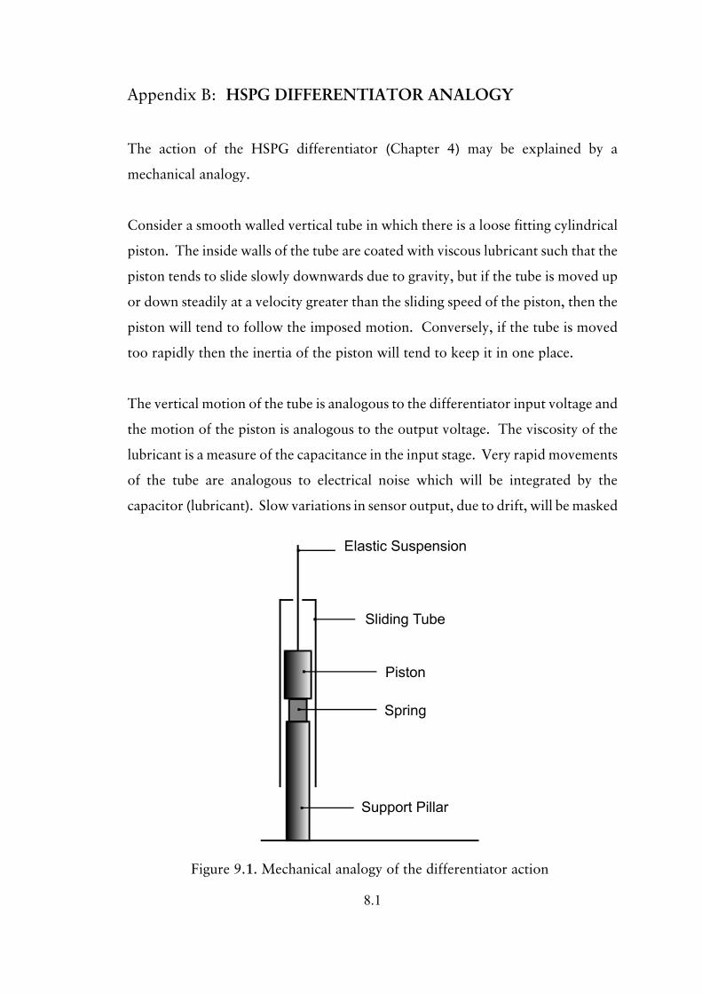
8.1

Figure 9.1. Mechanical analogy of the differentiator action

Appendix B: HSPG DIFFERENTIATOR ANALOGY

The action of the HSPG differentiator (Chapter 4) may be explained by a

mechanical analogy.

Consider a smooth walled vertical tube in which there is a loose fitting cylindrical

piston. The inside walls of the tube are coated with viscous lubricant such that the

piston tends to slide slowly downwards due to gravity, but if the tube is moved up

or down steadily at a velocity greater than the sliding speed of the piston, then the

piston will tend to follow the imposed motion. Conversely, if the tube is moved

too rapidly then the inertia of the piston will tend to keep it in one place.

The vertical motion of the tube is analogous to the differentiator input voltage and

the motion of the piston is analogous to the output voltage. The viscosity of the

lubricant is a measure of the capacitance in the input stage. Very rapid movements

of the tube are analogous to electrical noise which will be integrated by the

capacitor (lubricant). Slow variations in sensor output, due to drift, will be masked

8.2

by the tendency of the piston to reach equilibrium (ie the limit of downward

movement). Between these two extremes, moderately fast movements of the tube

will be followed accurately by the piston - over short time scales. The dynamics of

system depend solely on the lubricant’s viscosity.

To continue the analogy, the piston is freely suspended by a long elastic cord

through a cap at the top of the tube and, with no movement of the tube (ie. zero

change in input), will reach equilibrium at a point where the piston is barely

touching the upper end of a fully expanded compression spring. The latter is, in

turn, supported on a vertical pillar which fits easily within the tube (Figure 9.1).

Now, an upward movement of the tube will tend to carry the piston upward as

before, but the higher they are raised (ie. the larger the input and output voltages),

the greater will be the tendency for the piston to return to its equilibrium position.

Not only will it still be under the influence of gravity, but it will also lose some

support from the elastic (ie. capacitor leakage). Alternatively, downward

movements from equilibrium will be assisted by gravity but opposed by the elastic

and the spring (ie. diode forward current). The upper limit, on piston movement,

is imposed by the tube cap (ie. the operating voltage of the circuitry, approximately

+5 volts relative to the differentiator 5 V bias voltage, 0 V5), and the downward

limit by the post supporting the spring (ie. combined in the form of the OA47

diode in the circuit diagram, approximately -0.3 volts relative to the 5 V bias

voltage, 0 V5).

If the ‘input’ tube is raised and held at a new value (ie. a step change), the piston

will initially rise by an equivalent amount. If there is no further movement of the

tube then the piston will gradually slide down to its equilibrium position. This will

be a decelerating, exponential fall however, as the piston will gradually experience

the increasing tension in the elastic. This is analogous to the decaying voltage on

the differentiator capacitor. Instead of a rise, if the input tube were to descend

from the equilibrium position, then again the piston would fall, but would

8.3

experience not only increasing tension in the elastic, but also the upward force of

the spring, and ultimately the support pillar. The exponential decay voltage on the

capacitor is analogous to the elastic tension as before, and that of the spring is

similar to the change in forward conduction current, with increasing voltage, of the

germanium diode up to its nominal maximum forward voltage of 0.3 volts - which

is represented by the downward limit to movement imposed by the support pillar.

Thus, if an initial upward step change is followed a short time later by a downward

one of identical magnitude then the input tube will return to its start position. The

output piston however will not because, during the interval between rise and fall,

it will have slid a short distance downwards. Initially therefore the piston will

descend to a point slightly below its starting position before returning to

equilibrium in the manner described above. There is, however, no such thing as

a ‘negative’ concentration of H2S. So, provided that drift and noise are within the

designed limits of the differentiator, then negative excursions of the piston (ie

output voltage) will normally be due to this slippage. This corresponds to

capacitor leakage, and results in what is commonly known as voltage ‘droop’ on

the output of the differentiator.

Nevertheless, in spite of the in-built tendency toward equilibrium, it can be seen

that over time, with successive and irregular changes in position of the tube, that

the piston might gradually approach either the upper limit of the cap or the lower

limit of the pillar - even if the sum total of all the input movements is zero. This

would be due to the accumulated errors engendered by piston slippages - the

analogy for capacitor leakages and diode conduction. Therefore, in ‘auto’ mode,

every ten minutes the actual HSPG is switched to H2S free air, the voltage at the

differentiator input may be adjusted as previously described and the circuitry

output can be manually zeroed. In the analogy, this is returning the tube to its

‘start’ position, and the piston to its equilibrium position, respectively.

REFERENCES

Anonymous (1994) Green concerns and legislation to aid pollution monitoringequipment sales. International Environmental Technology 9/10 4.Environmental Technology (Publications), London.

Anonymous (2001) The Way Forward For Safer, Lighter Vehicles? OEMDesign (1):15. Wilmington Publishing, London.

ADAMS, D.F., BAMESBURGER, W.L. and ROBERTSON, T.J. (1968) Analysisof sulfurcontaining gases in the ambient air using selective prefilters anda microcoulometric detector. Journal of air pollution control association 18, 145-148.

AMERICAN PUBLIC HEALTH ASSOCIATION INTERSOCIETYCOMMITTEE (1977) Tentative method of analysis for hydrogen sulfidecontent of the atmosphere. In: Katz,M., (Ed.) Methods of Air Samplingand Analysis, 2nd Edn. pp. 676-681. American Public HealthAssociation, Washington DC.

ANDERSSON, G., BROSSET, C. and GRENNFELT, P. (1974) The stability ofemitted odorous compounds in the atmosphere. In: Turk,A., JohnstenJr.,JW. and Moultan,DG., (Eds.) Human responses to environmentalodours, pp. 335-343. Academic Press Inc,

ARCO CHEMICAL EUROPE INC (1993) Predicted penetration of catalystcars in europe. In: European Clean Gasoline, Arco Chemical EuropeInc, Maidenhead, England.

ARNOLD, I.M.F., DUFRESNE, R.M., ALLEYNE, B.C. and STUART, P.J.W.(1985) Health implication of occupational exposures to hydrogensulfide. Journal of Occupational Medicine 27, 373-376.

AXELROD, H.D., CARY, J.H., BONELLI, J.E. and LODGE JR, J.P. (1969) Fluorescence determination of sub-parts per billion hydrogen sulfide inthe atmosphere. Analytical Chemistry 41, 13, 1856-1858.

BALASUBRAMANIAN, N. and KUMAR, B.S.M. (1990) Extraction -Spectrophotometric determination of hydrogen sulphide. Analyst 115,859-863.

BAMESBURGER, W.L. and ADAMS, D.F. (1969) Improvements in the

collection of hydrogen sulfides in cadmium hydroxide suspension. Environ.Sci.Technol. 3, 258-261.

BARENDSZ, AW., VIS, JC., NIEUWENHUIZEN, MS., NIEUWKOOP, E.,VELLEKOOP, MJ., GHIJSEN, WJ. and VENEMA, A. A SAW-chemosensor for NO2 gas concentration measurement. 1985 UltrasonicsSymposium , 586-590. 1985. IEEE, San Francisco, CA.

BARTLETT, P.N. and GARDNER, J.W. (1992) Odour sensors for anelectronic nose. In: Gardner,J.W. and Bartlett,P.N., (Eds.) Sensors andsensory systems for an electronic nose: Proceedings of NATO advancedworkshop., pp. 38-51. NATO, Reykjavik.

BASSMADZIEVA, K., NIKIFOROV, B., TABAKOVA, S., BALABAEVA, L.,DAVIDKOVA, E., ANTOVA, T., BENCEV, I. and KALPAZANOV, J.(1987) Health effects of ambient air pollution in a district with paper-cellulose industry and fodder yeast production. Problemi na Higienata 12, 17-26.

BATES, T.S., LAMB, B.K., GUENTHER, A., DIGNON, J. and STOIBER, R.E.(1992) Sulfur emissions to the atmosphere from natural sources. Journal of Atmospheric Chemistry 14, 315-337.

BEAUCHAMP, R.O., Jr., BUS, J.S., POPP, J.A., BOREIKO, C.J. andANDJELKOVICH, D.A. (1984) A critical review of the literature onhydrogen sulfide toxicity. Critical Reviews in Toxicology 13, 25-97.

BOROVSKAYA, V.D. (1988) Outcome of pregnancy and labor followinghydrogen sulphide balneotherapy at early dates of pregnancy. VoprosyOkhrany Materinstva i Detstva 33, 68-70.

BRYANT, A., LEE, D.L. and VETELINO, J.F. A surface acoustic wave gasdetector. 1981 Ultrasonics Symposium , 171-174. 1981. IEEE, NewYork.

BUCK, M. and GIES, H. (1966) The Measurement of hydrogen sulfide in theatmosphere. Staub, Reinhaltung der Luft 26 (9), 379-384.

CADLE, R.D. and ALLEN, E.R. (1971) Atmospheric Chemistry. In:Berkowitz,D.A. and Squires,A.M., (Eds.) Power Generation andEnvironment Change, 1st Edn. pp. 263-288. MIT Press, Cambridge,Massachusetts.

CADLE, R.D. and LEDFORD, M. (1966) The reaction of ozone with hydrogensulfide. International Journal of Air & Water Pollution 10, 25-30.

CADLE, S.H. and MULAWA, P.A. (1978) Sulfide emissions from catalyst-equipped cars. In: Congress and exposition of the Society of AutomobileEngineers, pp. 1-9. Society of Automobile Engineers, Detroit, Michigan.

CALVERT, J.G., HEYWOOD, J.B., SAWYER, R.F. and SEINFELD, J.H.(1993) Achieving Acceptable Air Quality. Science 261,

CHEMNITIUS, G.C. and CAMMANN, K. (1996) Sense and Sensor-ability. Analysis Europa 3, 30-33.

CLIFFORD, M.J., CLARKE, R. and RIFFAT, S.B. (1997) Driver's exposure tocarbon monoxide in Nottingham UK. Atmospheric Environment 31, 7,1003-1009.

CORCORAN, P. (1993) Electronic odour sensing systems. Electronics &communication engineering journal 5, 5, 303-308.

CORCORAN, P. (1994) The effects of signal conditioning and quantizationupon gas and odour sensing system performance. Sensors and actuatorsB 18-19, 649-653.

CORCORAN, P. and SHURMER, HV. (1994) An intelligent gas sensor. Sensors and actuators A 41-42, 192-197.

CORCORAN, P., SHURMER, HV. and GARDNER, JW. (1993) Integrated tinoxide sensors of low power consumption for use in gas and odoursensing. Sensors and actuators B 15-16, 32-37.

CRANNY, A.W. and ATKINSON, J.K. (1992) The use of pattern recognitiontechniques applied to signals generated by a multi element gas sensorarray as a means of compensating for poor individual sensor response.In: Gardner,J.W. and Bartlett,P.N., (Eds.) Sensors and sensory systemsfor an electronic nose: Proceedings of NATO advanced workshop., pp.200-209. NATO, Reykjavik.

CRONER (1990) Croner's Substances Hazardous to Health, 3rd Edn. CronerPublications,

D'AMICO, A., PALMA, A. and VERONA, E. Hydrogen sensor using apalladium coated surface acoustic wave delay-line. 1982 UltrasonicsSymposium , 308-311. 1982. IEEE, San Diego, CA.

D'AMICO, A., PETRI, A., VERARDI, P. and VERONA, E. NH3 surfaceacoustic wave gas detector. 1987 Ultrasonics Symposium , 633-636.1987. IEEE, Denver, CO.

DALE, D.P.E. (1985) The LinCMOS Design Manual, 1st European Edn. TexasInstruments, Kettering.

DE ANDRADE, J., SULEIMAN, A.A. and GUILBAULT, G.G. (1989) A CoatedPiezoelectric Crystal Detector for the Determination of HydrogenSulfide. Analytica Chimica Acta 217 , 187-192.

DEPT OF HEALTH ADVISORY GROUP ON THE MEDICAL ASPECTS OFAIR POLLUTION EPISODES (1992) Sulphur dioxide, acid aerosols andparticulates, HMSO, London.

DEUCHAR, C.N., COLLS, J.J. and YOUNG, S.D. (1999) Hydrogen sulphidefrom vehicle exhaust: exposure dynamics. Atmospheric Environment 33,3077-3079.

DEUCHAR, C.N., COLLS, J.J. and YOUNG, S.D. (2002) A technique for thepassive monitoring of hydrogen sulphide on landfill sites. In: Lencioni,E.and Dhanda,R., (Eds.) Integrated Waste Management and PollutionControl: Research, Policy and Practice, pp. 473-483. Waste2002,Warwick.

DIAROVA, N.A., POTAPOVA, M.V. and RUVINSKII, L.Y. (1983) Comparison of methods for monitoring hydrogen sulfide concentrationin atmospheric air. Chemistry & Technology of Fuels & Oils 19, 210-211.

EYRE,N., PEARCE,D. and TURNER,K. (1995) Diesel most costly fuel forpollution. International Environmental Technology 5, (3) 4.Environmental Technology (Publications), London.

FALCONER, R.S. (1995) A versatile saw-based sensor system for investigatinggas-sensitive coatings. Sensors and Actuators, B: Chemical 24, 54-57.

FATKULLINA, A.F., ZAKHAROVA, N.V., AKHMETZYANOVA, G.S. andBONDARENKO, L.L. (1979) Selective determination of hydrogensulfide in atmosphere by chromatographic method. Chemistry &Technology of Fuels & Oils 15, 249-251.

FAY, J.A. (1971) Environmental Science and Public Policy. In: Berkowitz,D.A.and Squires,A.M., (Eds.) Power Generation and Environment Change, 1st Edn. pp. 3-6. MIT Press, Cambridge, Massachusetts.

FIELDER, H.M., POON-KING, C.M., PALMER, S.R., MOSS, N. andCOLEMAN, G. (2000) Assessment of impact on health of residentsliving near the Nant-y-Gwyddon landfill site: retrospective analysis. British Medical Journal 320, 19-22.

FRIED, A., HENRY, B., RAGAZZI, R.A., MERRICK, M., STOKES, J.,PYZDROWSKI, T. and SAMS, R. (1992) Measurements of carbonylsulfide in automotive emissions and an assessment of its importance tothe global sulfur cycle. Journal of Geophysical Research 97, D13,14621-14634.

FULLER, D.C. and SURUDA, A.J. (2000) Occupationally Related HydrogenSulfide Deaths in the United States From 1984 to 1994. Journal OfOccupational And Environmental Medicine 42/9, 939

GALIPEAU, J.D., VETELINO, J.F., CARON, J.J., WITTMAN, E.L.,SCHWEYER, M.G. and ANDLE, J.C. (1995) Theory, design andoperation of a surface-acoustic-wave hydrogen-sulfide microsensor. SENSORS AND ACTUATORS B-CHEMICAL 24, 49-53.

GATES, B.C. (1996) Catalytic Chemistry, John Wiley, New York.

GRAEDEL, T.E. and FRANEY, J.P. (1979) Gaseous hydrogen sulfidedetermination by discoloration of lead- stabilized PVC. AmericanIndustrial Hygiene Association Journal 40, 947-954.

HARDY, J.K., STRECKER, D.T., SAVARIAR, C.P. and WEST, P.W. (1981) Amethod for the personal monitoring of hydrogen sulfide utilizingpermeation sampling. American Industrial Hygiene Association Journal 42, 283-286.

HARRISON, R.M. and PERRY, R. (1986) Handbook of Air Pollution Analysis, 2nd Edn. Chapman & Hall, London & New York.

HEALTH & SAFETY EXECUTIVE and FACTORY INSPECTORATE (1976) Methods for the detection of toxic substances in air: Booklet No1:Hydrogen Sulphide, 3rd Edn. HMSO, London.

HEMMINKI, K. and NIEMI, M.L. (1982) Community study of spontaneousabortions: Relation to occupation and air pollution by sulfur dioxide,hydrogen sulfide, and carbon disulfide. International Archives ofOccupational and Environmental Health 51, 55-63.

HIRSCH, A.R. and ZAVALA, G. (1999) Long term effects on the olfactorysystem of exposure to hydrogen sulphide. Occupational andEnvironmental Medicine 56, 284-287.

HOUMMADY, M. and HAUDEN, D. (1992) Elastic plate mode sensitivities tomass loading applications to gas sensors. Proceedings of the 6thEuropean frequency and time forum 203-207.

HOUMMADY, M., REBIERE, D., HAUDEN, D., PISTRE, J., CUNIN, P. andPLANADE, R. (1991) NO2 surface acoustic wave gas sensor. 5thEuropean frequency and time forum Besancon 6A, 57, 309-313.

JAAKKOLA, J.J.K., VILKKA, V., MARTTILA, O., JAPPINEN, P. andHAAHTELA, T. (1990) The South Karelia air pollution study. Theeffects of malodorous sulfur compounds from pulp mills on respiratoryand other symptoms. American Review of Respiratory Diseases 142,1344-1350.

JACOBS, M.B. (1965) Recommended standard method for continuing airmonitoring for hydrogen sulfide. Ultramicro-determination of sulfides inthe air. Journal of the Air Pollution Control Association 15, 314-315.

JACOBS, M.B., BRAVERMAN, M.M. and HOCHHEISER, S. (1957) Ultramicro-determination of sulfides in air. Analytical Chemistry 29,1349-1351.

JOSOWICZ, M. and JANATA, J. (1993) Electroactive polymers in chemicalsensors. In: Scrosati,B., (Ed.) Applications of Electroactive polymers, 1st

Edn. pp. 311-343. Chapman & Hall, London.

KARUSH, F., KLINMAN, N.R. and MARKS, R. (1964) An assay method fordisulphide groups by fluorescence quenching. Analytical Biochemistry 9,100-114.

KILBURN, K.H. (1995) Hydrogen-sulfide and reduced-sulfur gases adverselyaffect neurophysiological functions. Toxicology and Industrial Health 11, 185-197.

KOH, T., MIURA, Y., YAMAMURO, N. and TAKAKI, T. (1990) Spectrophotometric determination of trace amounts of sulphide andhydrogen sulphide by formation of thiocyanate. Analyst 115, 1133-1137.

KRING, E.V., DAMRELL, D.J., HENRY, T.J. and ET AL (1984) Laboratoryvalidation and field verification of a new passive colorimetric airmonitoring badge for sampling hydrogen sulfide in air. AmericanIndustrial Hygiene Association Journal 45, 1-9.

LENGA, R.E. (1988) Sigma Aldrich Library of Chemical Safety Data, 2nd Edn. Sigma Aldrich Corporation, N.Y.

MAAS, F. (1987) Responses of Plants to Sulfur containing air pollutants, Maas,Netherlands.

MASUDA, J., FUKUYAMA, J. and FUJII, S. (1999) Influence of concurrentsubstances on removal of hydrogen sulfide by activated carbon. Chemosphere 39, 1611-1616.

MCARTHUR, D.P. (1975) Deposition and distribution of lead, phosphorous,calcium, zinc, and sulfur poisons on automobile exhaust NOx catalysts.In: U.S.Congresses., (Ed.) Catalysts for the control of automotivepollutants., pp. 85-89. U.S. Congresses, New York.

MICALLEF, A., DEUCHAR, C.N. and COLLS, J.J. (1998) A System forMeasuring Vertical Concentration Profiles of Gaseous Pollutants, UsingCarbon Dioxide as a Case Study. International Journal of OccupationalSafety and Ergonomics 4, 3, 333-346.

MONCRIEFF, R.W. (1966) Odour Preferences , Leonard Hill, London.

NATUSCH, D.F.S. and SLATT, B.J. (1978) Hydrogen sulfide as an airpollutant. In: Strauss,W., (Ed.) Air Pollution Control Part III, pp. 459-518. John Wiley & Sons Inc., New York.

NATUSCH, D.F.S., KLONIS, H.B., AXELROD, H.D., TECK, R.J. and LODGE

JR, J.P. (1972) Sensitive method for measurement of atmospherichydrogen sulfide. Analytical Chemistry 44, 12, 2067-2070.

NATUSCH, D.F.S., SEWELL, J.R. and TANNER, R.L. (1974) Determinationof hydrogen sulfide in air - an assessment of impregnated paper tapemethods. Analytical Chemistry 46, 3, 410-415.

NIEUWENHUIZEN, M.S. and NEDERLOF, A.J. (1992) Silicon Based SurfaceAcoustic Waves. In: Gardner,J.W. and Bartlett,P.N., (Eds.) Sensors andsensory systems for an electronic nose: Proceedings of NATO advancedworkshop., pp. 131-145. NATO, Reykjavik.

NIOSH (1977) Criteria for a Recommended Standard - Occupational Exposureto Hydrogen Sulfide, 1st Edn. NIOSH (National Institute forOccupational Safety & Health), Washington.

NIOSH (1980) Hydrogen sulphide, method 296. In: Woebkenberg,ML., (Ed.) NIOSH manual of analytical methods, 2nd Edn. pp. 296-1-296-8. NIOSH (National Institute for Occupational Safety & Health),Washington.

NIOSH (1994) Hydrogen Sulphide, method 6013. In: Cassinelli,M.E., (Ed.) NIOSH manual of analytical methods, 4th Edn. pp. 6013-1-6013-4. NIOSH (National Institute for Occupational Safety & Health),Washington.

OKITA, T., LODGE, J.P. and AXELROD, H.D. (1971) Filter method for themeasurement of atmospheric hydrogen sulfide. Environ.Sci.Technol. 6,532-534.

PAL, T., GANGULY, A. and MAITY, D.S. (1986) Use of a silver - gelatincomplex for the microdetermination of hydrogen sulphide in theatmosphere. Analyst 111, 691-693.

PARE, J.P. (1966) A new tape reagent for the determination of hydrogensulfide in air. Journal of air pollution control association 16, 6, 325-327.

PAULING, L. and PAULING, P. (1975) Chemistry, W H Freeman & Co, SanFrancisco.

PIPPENGER, D.E. and TOBABEN, E.J. (1985) Linear and Interface Circuit

Applications, 1st European Edn. Texas Instruments,

PRITCHARD, P.R. (1985) Environmental factors affecting brown rust ofbarley. [Thesis]. Nottingham University. PhD.

PURDHAM, J.T. and YONGYI, L. (1990) Sodium hydroxide containingtriethanolamine and EDTA as a collection medium for hydrogen sulfide. American Industrial Hygiene Association Journal 51, 269-272.

QUALITY OF URBAN AIR REVIEW GROUP (QUARG) (1993) Urban AirQuality in the UK, HMSO, London.

REISZNER, K.D. and WEST, P.W. (1973) Collection and determination ofsulphur dioxide incorporating permeation and West-Gaeke procedure. Environmental Science and Technology 7, 526-532.

RICHARDSON, D.B. (1995) Respiratory effects of chronic hydrogen sulfideexposure. American Journal of Industrial Medicine 28, 99-108.

RIFFAT, R., WEEKS, J.L. and BRADY, P. (1999) Safety Alert. IndustrialWastewater 7, 31-34.

ROBINSON, E. and ROBBINS, R.C. (1970) Gaseous sulfur pollutants fromurban and natural sources. Journal of air pollution control association 20 (4), 233-235.

ROE, A.B. (1982) Sampling and determination of volatile organo-sulphurcompounds in a sewage works environment. Journal of the Institute ofWater Engineers & Scientists 36, 118-128.

ROYAL SOCIETY OF CHEMISTRY (1981) Hazards in the chemicallaboratory, 3rd Edn. Royal Society of Chemistry, London.

SEINFELD, J.H. (1986) Atmospheric Chemistry and the Physics of AirPollution, John Wiley & Sons Inc, New York.

SHANTHI, K. and BALASUBRAMANIAN, N. (1996) A simplespectrophotometric method for the determination of hydrogen sulfidebased on Schiff's reaction. Microchemical Journal 53, 168-174.

SHIPCHANDLER, M.T. and FINO, J.R. (1986) A revised structure offluorescein mercuric acetate. Analytical Biochemistry 154, 476-477.

SHOOTER, D. (1993) Nitrogen dioxide and its determination in theatmosphere. Journal of Chemical Education 70, A133-A140

SHOOTER, D. (1999) Sources and sinks of oceanic hydrogen sulfide - anoverview. Atmospheric Environment 33, 3467-3472.

SHOOTER, D., WATTS, S.F. and HAYES, A.J. (1995) A passive sampler forhydrogen sulfide. Environmental Monitoring and Assessment 38, 11-23.

SIMPSON, H.D. (1975) Thermodynamic interactions between transitionalmetals and simulated auto-exhausts. In: U.S.Congresses., (Ed.) Catalystsfor the control of automotive pollutants., pp. 46-51. U.S. Congresses,New York.

SMITH, J.P. and SHULMAN, S.A. (1988) An evaluation of H2S continuousmonitors using metal oxide semiconductor sensors. Applied IndustrialHygiene 3, 214-221.

SMITH, R.P. (1983) Hydrogen sulphide and health. In: Hydrogen Sulphideand Health, pp. 1-29. Amoco Canada Petroleum Company Ltd, Calgary,Alberta.

STRAUSS, W. and MAINWARING, SJ. (1984) Air pollution, Edward Arnold,London.

SUMMER, W. (1971) Odour pollution of air , 1st Edn. Leonard Hill, London.

TARVER, G.A. and DASGUPTA, P.K. (1995) Design and development of asystem to measure ambient levels of hydrogen-sulfide and lowermercaptans from a mobile platform. Atmospheric Environment 29,1291-1298.

TARVER, G.A. and DASGUPTA, P.K. (1997) Oil field hydrogen sulfide inTexas: emission estimates and fate. Environ.Sci.Technol. 31, 3669-3676.

THOMAS, CL. (1970) Catalytic processes and catalysts, 1st Edn. AcademicPress Inc, New York.

TVEDT, B., SKYBERG, K., AASERUD, O., HOBBESLAND, A. andMATHIESEN, T. (1991) Brain damage caused by hydrogen sulfide: Afollow-up study of six patients. American Journal of Industrial Medicine 20, 91-101.

U.S.DEPARTMENT OF HEALTH (1994) Hydrogen sulfide. Environment,safety & health. Health hazards alert. Health Hazards Alert - frominternet EH-0395, issue 94-1,

U.S.ENVIRONMENTAL PROTECTION AGENCY (1974) Evaluation ofCatalytic Converters, U.S. Environmental Protection Agency, New York.

ULMAN, A. (1991b) Langmuir-Blodgett Films. In: An introduction to ultrathinOrganic Films: from Langmuir-Blodgett to self-assembly, 1st Edn. pp.361-412. Academic Press Inc, London.

ULMAN, A. (1991a) Langmuir-Blodgett Films. In: An introduction to ultrathinOrganic Films: from Langmuir-Blodgett to self-assembly, 1st Edn. pp.101-133. Academic Press Inc, London.

VADIC, V., GENTILIZZA, M., HRSAK, J. and FUGAS, M. (1980) Determination of hydrogen sulphide in the air. Staub, Reinhaltung derLuft 40, 73-75.

VETELINO, JF., LADE, R. and FALCONER, RS. Hydrogen sulfide surfaceacoustic wave gas detector. 1986 Ultrasonics Symposium , 549-554.1986. IEEE, Piscataway, NJ.

WARNER, PO. (1976) Analysis of Air Pollutants, 1st Edn. John Wiley & Sons,New York & London.

WATKINS, L.H. (1991) Air Pollution From Road Vehicles, HMSO, London.

WATTS, S.F. and ROBERTS, C.N. (1999) Hydrogen sulfide from car catalyticconverters. Atmospheric Environment 33, 169-170.

WATTS, S.F. (2000) Mass budgets of carbonyl sulfide, dimethyl sulfide, carbondisulfide and hydrogen sulfide. Atmospheric Environment 34, 761-779.

WEHINGER, C. and MEYERPITTROFF, R. (1994) Exhaust emissions fromOtto-engines with three-way catalysts. Measurement regarding the

secondary emission of nitrous oxide. Staub, Reinhaltung der Luft 54, 9-15.

WESTERHOLM, R., CHRISTENSEN, A. and ROSEN, A. (1996) Regulatedand unregulated exhaust emissions from two three-way catalyst equippedgasoline fuelled vehicles. Atmospheric Environment 30, 20, 3529-3536.

WHITE, RM. Surface acoustic wave sensors. 1985 Ultrasonics Symposium ,490-494. 1985. IEEE, San Francisco, CA.

WILLIAMS, D.J., QUIGLEY, S.M. and HALEY, J. (1987) Sulphide Emissionsfrom Catalyst-Equipped Cars in Australia, 1st Edn. CSIRO Institute ofEnergy and Earth Resources, North Ryde.

WILSON, S.H.S., HOWE, J.D. and ASHFOLD, M.N.R. (1996) On the nearultraviolet photo-dissociation of hydrogen sulphide. Molecular Physics 88, 841-858.

WORLD HEALTH ORGANIZATION (1996) Hydrogen sulfide. In: Guidelines for Drinking Water Quality, 2 nd Edn. pp. 242-248. WorldHealth Organization, Geneva.

XU, X., CHO, S.I., SAMMEL, M., YOU, L., CUI, S., HUANG, Y., MA, G.,PADUNGTOD, C., POTHIER, L., NIU, T., CHRISTIANI, D., SMITH,T., RYAN, L. and WANG, L. (1998) Association of petrochemicalexposure with spontaneous abortion. Occupational and EnvironmentalMedicine 55, 31-36.

YAKOVKIN, LB., VLASSOV, Y., KOZLOV, AS. and REPINSKY, SM. (1994) Highly sensitive SAW sensors. 1994 IEEE International frequencycontrol symposium 395-400.