deterministic algorithm for 1-median 1-center two ...mdmonfared/uploads/technical...

Deterministic Algorithm for 1-Median 1-CenterTwo-Objective Optimization Problem

Vahid Roostapour, Iman Kiarazm, and Mansoor Davoodi

Institute for Advanced Studies in Basic Sciences (IASBS), Zanjan, Iranv.roostapour,i.kiarazm,[email protected]

Abstract. k-median and k-center are two well-known problems in fa-cility location which play an important role in operation research, man-agement science, clustering and computational geometry. To the bestof our knowledge, although these problems have lots of applications,they have never been studied together simultaneously as a multi objec-tive optimization problem. Multi-objective optimization has been appliedin many fields of science where optimal decisions need to be taken inthe presence of trade-offs between two or more conflicting objectives. Inthis paper we consider 1-median and 1-center two-objective optimizationproblem. We prove that Ω(n logn) is a lower bound for proposed prob-lem in one and two dimensions in Manhattan metric. Also, by using theproperties of farthest point Voronoi diagram, we present a deterministicalgorithm which output the Pareto Front and Pareto Optimal Solutionsin O(n logn) time.

Keywords: computational geometry, Pareto optimal solutions, 1-center,1-median, multi-objective optimization

1 Introduction

When evaluating different solutions from a design space, it is often the case thatmore than one criterion comes into play. For example, when choosing a routeto drive from one point to another, we may care about the time it takes, thedistance traveled and the complexity of the route (e.g. number of turns). Whendesigning a (wired or wireless) network, we may consider its cost, capacity andcoverage. Such problems are known as Multi-Objective Optimization Problems(MOOP). Multi-objective optimization can be described in mathematical termsas follows:

S = x ∈ Rd : h(x) = 0, g(x) ≥ 0min [f1(x), f2(x), . . . , fN (x)]

x ∈ S,

where N > 1, fi is a scalar function for 1 ≤ i ≤ N and S is the set of constraints.The space in which the objective vector belongs is called objective space. The

scalar concept of optimality does not apply directly in the multi-objective setting.

2 Vahid Roostapour et. al

Here the notion of Pareto optimality and dominance has to be introduced. In amulti-objective minimization problem, a solution s1 ∈ S dominates a solutions2 ∈ S, denoted by s1 ≺ s2, if fi(s1) ≤ fi(s2) for all i ∈ 1, . . . , N, withat least one strict inequality. A point s∗ is said to be a Pareto optimum or aPareto optimal solution for the multi-objective problem if and only if there is nos ∈ S such that s ≺ s∗. The image of such an efficient set, ie., the image of allthe efficient solutions in the objective space are called Pareto optimal front orPareto curve.

One of the common approaches for such problems is evolutionary algorithms[7]. These algorithms are iterative and converge to Pareto front. However theyneed more time as the complexity of the Pareto front increases. Moreover, all ofthese approaches have major problems with local optimums. On the other handthere are some classical approaches like weighted sum and ϵ-constraint whichcan apply on MOOPs. Although these approaches guarantee finding solutionson the entire Pareto optimal set for problems having a convex Pareto front,they are largely depend on chosen weight and ϵ vectors respectively. Moreover,these approaches require some information from user about the solution space.Furthermore, in most nonlinear MOOPs, a uniformly distributed set of weightvectors wont necessarily find a uniformly distributed set of Pareto optimal so-lutions. Also there may exist multiple minimum solutions for a specific weightvector [8]. However we find the Pareto front of a MOOP with deterministic al-gorithm. Here we consider two famous propounded facility location problems[17].

k-median: In this problem the goal is to minimize summation of distances be-tween each demand point and its nearest center. Charikar et. al proposed the firstconstant time approximation algorithm which its outputs is 62

3 times the optimal[5]. This improved upon the best previously known result of O(log p log log p),which was obtained by refining and derandomizing a randomizedO(log n log log n)-approximation algorithm of Bartal [4]. The currently best known approximationratio is 3+ϵ achieved by a local search heuristic of Arya et. al [1]. Moreover, Jainet. al proved that the k-median problem cannot be approximated within a fac-tor strictly less than 1 + 2/e, unless NP ⊆ DTIME[nO(log logn)] [12]. This was animprovement over a lower bound of 1+1/e [16]. Using sampling technique Meyer-

son, et. al presented an algorithm with running time O(p(p2

ϵ log p)2 log(pϵ log p)).This was the first k-median algorithm with fully polynomial running time thatwas independent of n, the size of the data set. It presented a solution that is,with high probability, an O(1)-approximation, if each cluster in some optimalsolution has Ω(n·ϵp ) points [14]. Har-Peled and Kushal presented a (p, ϵ)-coreset

of size O(p2/ϵd) for k-median clustering of n points in Rd, which its size was in-dependent of n [9]. Also, Har-Peled and Mazumdar showed that there exist smallcoresets of size O(pϵ−d log n) for the problems of computing k-median cluster-ing for points in low dimension with (1+ ϵ)-approximation. Their algorithm haslinear running time for a fixed p and ϵ [10]. Moreover, using random samplingfor k-median problem Badoiu et. al proposed a (1+ ϵ)-approximation algorithm

with 2(p/ϵ)O(1)

dO(1)n logO(p) n expected time [3].

Deterministic Algorithm for MOOP 3

k-center: In this problem the goal is to minimize the maximum distance be-tween each demand point from its nearest center. Megiddo and Supowit provedthat k-center and k-median are NP-hard even to approximate the k-center prob-lems sufficiently closely [13]. Hochbaum and Shmoys proposed the first constantfactor approximation algorithm which its output is 2 times the optimal. It is thebest possible algorithm unless P = NP [11]. It is shown that there is an algorithmwith O(dO(d)n) time for 1-center problem [6]. In the high dimension, Badoiu andClarkson presented a (1 + ϵ)-approximation algorithm which find a solution in⌈2/ϵ⌉ passes using O(nd/ϵ + (1/ϵ)5) total time and O(d/ϵ) space [2]. Also, forproblem of 1-center with outliers, Zarrabi-Zadeh and Mukhopadhyay proposeda 2-approximation one pass streaming algorithm in high dimension which for z,as the number of outliers, needs O(zd2) space [19]. Moreover, Zarrabi-Zadeh andChan presented an streaming one pass 3/2-approximation algorithm for 1-center[18]. Badoiu et. al for 1-center problem, extracted a coreset of size O(1/ϵ2) whichits solution is (1+ϵ)-approximation set of points in Rd [3]. Also, for k-center they

presented a 2O((p log p)/ϵ2).dn time algorithm with (1+ ϵ)-approximation solutionusing previous result.

1-median and 1-center are practical problems which have not been consideredas a two-objective optimization problem yet. Imagine mayor of a small city wantsto build a fire station in a way that minimizes the distance between farthestbuilding to the station, also since the number of fire engines is limited and eachfire engine must return to the station after a service, it has to minimizes the totaldistance of station from all other buildings. As an another example, considerpower distribution network. Due to the dependency of energy leakage to wirelength, minimizing of the longest wire in the network would be regarded as anessential factor. Also, any decrement in total wire length of network consideredas a second objective. The first objective is 1-median, M(u), the summation ofdistances of demand points from center u and the second objective is 1-center,C(u), the farthest input point from center p. It can be described in mathematicalterms as follow:

Definition 1. 1-median 1-center two-objective optimization problem:Let P = p1, . . . pn be a set of demand points in Rd. Consider functions M(u) =∑n

i=1 D(u, pi) and C(u) = max1≤i≤n D(u, pi) are the values of point u ∈ Rd asa center for 1-median and 1-center objectives respectively for a certain distancefunction D. The goal is finding u∗ to minimize the objectives.

We study this problem in one and two dimensions in Manhattan metric. Weassume no input points have the same x or y coordinate.

This is a convex combinatorial multi-objective optimization problem whichhas been studied with a different approach called ϵ-Pareto. In [15] it is shownthat this approximate Pareto curve can be constructed in time polynomial inthe size of the instance and 1/ϵ, but here we propose a deterministic algorithmfor computing the exact Pareto curve because of specifying the problem.

This paper starts with considering 1-median and 1-center as two-objective ofMOOP in one dimension. We will find the optimal of objectives and in terms ofplacement of optimums we will also find the Pareto set in time O(n) (Lemma 1).


(a) n is odd. (b) n is even.

Fig. 1: 1-Median optimal.

We continue with a proof for convexity of Pareto set. At the end of second sectionwe give an algorithm to compute Pareto optimal front of 1-median 1-centertwo-objective optimization problem and prove the optimality of the algorithm.In section three the same problem considered in two dimensional space. Firstwe find optimums of 1-median objective. After that by using the properties offarthest point Voronoi diagram we determine the optimum of 1-center. Finallyafter limiting the solution space to regions which Pareto set lies on, we specificallypresent Pareto solutions. Convexity of Pareto front is proven in Theorem 2.

2 One dimensional

Let P = x1, x2, . . . xn be a set of input points in one dimension, the goal isto minimize M(x) =

∑ni=1 |x− xi| and C(x) = max1≤i≤n |x− xi|. According

to the properties of the absolute value function and some simple calculations,it is easy to see that M(x) is a continuous piecewise linear function which itsminimum depends on n. The minimum can either be one point or an intervalwhich we denote by Mopt in the rest of the paper. Also without loss of generalitywe assume that input points are sorted increasingly. In one dimensional space,Mopt = [mi,mj ] ⊂ R for 1 ≤ i, j ≤ n such that mi = xi, mj = xj . For oddn we have j = i and for even n, j = i + 1. Moreover, the function is strictlydecreasing before its minimum and is strictly increasing after it (Figure 1). ForC(x) suppose copt ∈ R denote the point which C(copt) is minimum. Obviouslycopt = (x1+xn)/2. Similarly to M(x), C(x) is strictly decreasing before optimalpoint and strictly increasing after that.

Lemma 1. Pareto optimal set in one dimensional 1-median 1-center two-objectiveoptimization problem is the smallest interval consisting of a solution with 1-center optimal and a solution with 1-median optimal.

Proof. Suppose that n is even (the proof is similar for odd n). As shown inFigure 2, there are three different cases:


(a) copt and Mopt have intersection. (b) copt is on the right side of Mopt.

(c) copt is on the left side of Mopt.

Fig. 2: Pareto set computation in one dimension.

First consider the case that copt and Mopt have an intersection (Figure 2a). Inthis case the intersection point is the only member of Pareto optimal solutions.Because not only it is optimal in both objectives, but also it is the only pointwhere C(x) is optimal. So it dominates all the other solutions and no solutiondominates it.

As shown in Figure 2b there are three regions in the second case. In regionC both functions are strictly increasing. Therefore, copt has the best value inboth objectives. It dominates all solutions of this region. In A, C(x) is strictlydecreasing, thus C(mj) is strictly smaller than 1-center objective of all the othersolutions. Moreover, M(mj) is smaller than or equal with 1-median objectiveof the other solutions. Hence mj dominates all solutions of A. Finally we claimthat B is Pareto set. By contradiction, suppose it is not true, then there must bea point p which dominates q ∈ B. It has to be on the left side or right side of q.Let p be on the right side, we know that M(x) is strictly increasing in this side.hence M(q) < M(p) and it contradicts with dominance of p. Similarly there is acontradiction if p lies on the left side of q, because C(x) is strictly decreasing inthis side, ie. C(q) < C(p). This implies that all the solutions that lie on B arePareto set.

The proof is similar for the third case which copt is on the left side of Mopt

(Figure 2c). ⊓⊔

Lemma 2. Pareto optimal front of one dimensional 1-median 1-center two-objective optimization problem forms a continuous, convex and piecewise linearfunction.

Proof. If there is an intersection between copt and Mopt the lemma is held. Nowsuppose there is no such intersection and consider copt is on the right side of Mopt

(resp. on the left side of Mopt). From lemma 1 for Pareto solutions we have Ps =[mj , copt] (resp. Ps = [copt,mi]). Since C(x) derivation is constant and M(x) ispiecewise linear in Ps, the diagram of M(x)-C(x) is piecewise linear and breakpoints are

(C(xi),M(xi)

)such that mj ≤ xi ≤ copt (resp. copt ≤ xi ≤ mi). The

absolute value of slope of M(x) increases on each linear piece in Ps. Thus Pareto


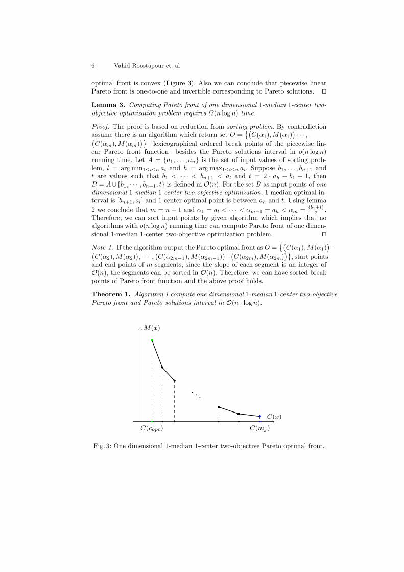
optimal front is convex (Figure 3). Also we can conclude that piecewise linearPareto front is one-to-one and invertible corresponding to Pareto solutions. ⊓⊔

Lemma 3. Computing Pareto front of one dimensional 1-median 1-center two-objective optimization problem requires Ω(n logn) time.

Proof. The proof is based on reduction from sorting problem. By contradictionassume there is an algorithm which return set O =

(C(α1),M(α1)

)· · · ,(

C(αm),M(αm))

–lexicographical ordered break points of the piecewise lin-ear Pareto front function– besides the Pareto solutions interval in o(n log n)running time. Let A = a1, . . . , an is the set of input values of sorting prob-lem, l = argmin1≤i≤n ai and h = argmax1≤i≤n ai. Suppose b1, . . . , bn+1 andt are values such that b1 < · · · < bn+1 < al and t = 2 · ah − b1 + 1, thenB = A∪b1, · · · , bn+1, t is defined in O(n). For the set B as input points of onedimensional 1-median 1-center two-objective optimization, 1-median optimal in-terval is [bn+1, al] and 1-center optimal point is between ah and t. Using lemma

2 we conclude that m = n + 1 and α1 = al < · · · < αm−1 = ah < αm = (b1+t)2 .

Therefore, we can sort input points by given algorithm which implies that noalgorithms with o(n log n) running time can compute Pareto front of one dimen-sional 1-median 1-center two-objective optimization problem. ⊓⊔

Note 1. If the algorithm output the Pareto optimal front asO =(

C(α1),M(α1))−(

C(α2),M(α2)), · · · ,

(C(α2m−1),M(α2m−1)

)−(C(α2m),M(α2m)

), start points

and end points of m segments, since the slope of each segment is an integer ofO(n), the segments can be sorted in O(n). Therefore, we can have sorted breakpoints of Pareto front function and the above proof holds.

Theorem 1. Algorithm 1 compute one dimensional 1-median 1-center two-objectivePareto front and Pareto solutions interval in O(n · log n).

. . .

C(mj)C(copt)

C(x)

M(x)

Fig. 3: One dimensional 1-median 1-center two-objective Pareto optimal front.


Proof. C(x) can be computed easily in constant time andM(x) can be computedin O(log n) using binary search, we obtain that line 13 is O(log n) running time.Therefore, we can conclude that Algorithm 1 is O(n · log n). ⊓⊔

Corollary 1. Pareto front of one dimensional 1-median 1-center two-objectiveoptimization problem can be computed in θ(n log n).

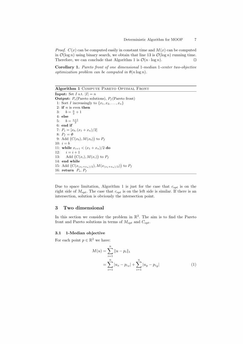
Algorithm 1 Compute Pareto Optimal Front

Input: Set I s.t. |I| = nOutput: Ps(Pareto solutions), Pf (Pareto front)1: Sort I increasingly to x1, x2, . . . , xn2: if n is even then3: b = n

2+ 1

4: else5: b = n+1

2

6: end if7: Ps = [xb, (x1 + xn)/2]8: Pf = Φ9: Add

(C(xb),M(xb)

)to Pf

10: i = b11: while xi+1 < (x1 + xn)/2 do12: i = i+ 113: Add

(C(xi),M(xi)

)to Pf

14: end while15: Add

(C(x(x1+xn)/2),M(x(x1+xn)/2)

)to Pf

16: return Ps, Pf

Due to space limitation, Algorithm 1 is just for the case that copt is on theright side of Mopt. The case that copt is on the left side is similar. If there is anintersection, solution is obviously the intersection point.

3 Two dimensional

In this section we consider the problem in R2. The aim is to find the Paretofront and Pareto solutions in terms of Mopt and Copt.

3.1 1-Median objective

For each point p ∈ R2 we have:

M(u) =n∑

i=1

∥u− pi∥1

=

n∑i=1

|ux − pix|+n∑

i=1

|uy − piy| (1)


−2x + 2y + cn2

, n2

+2 2y + cn2

+1, n2

+2 2x + 2y + cn2

+2, n2

+2

−2x + cn2

, n2

+1cn

2+1, n

2+1 2x + cn

2+2, n

2+1

−2x − 2y + cn2

, n2

−2y + cn2

+1, n2

2x − 2y + cn2

+2, n2

(a) Number of equations is even, 1-median optimal is a rectangular (blue) region.

−x − y + cn+12

,n+12

x − y + cn+32

,n+12

−x + y + cn+12

,n+32

x + y + cn+12

+1,n+32

(b) Number of equations is odd, 1-median is a (blue) point.

Fig. 4: 1-median optimal and equation of M(p) in middle cells.

We can observe that we need O(n) time to deterministically minimize equation1. Moreover, because of the assumption that no points have same coordinate theoptimal of Mopt may be just a point or area of a rectangle.

In the rest of this paper we assume that n is even (all proofs and discussionsare similar when n is odd.). Consider lines y = pix and x = piy such that1 ≤ i ≤ n which partition the xy-plane into (n + 1)2 cells where boundarycells are unbounded. The equation of M(p) for points in each cell is the samebecause of the absolute value function. Furthermore, for points in a column(resp. row) equation of

∑ni=1 |x− pix | (resp.

∑ni=1 |y − piy |) do not change but

for transformation to upper (resp. right) cell coefficient of y (resp. x) increasesby 2 (Figure 4).

3.2 1-Center objective

Let FVD be the farthest point Voronoi diagram of input points in Manhattanmetric, also let RFVD(p) denote the region of FVD which consist of p and


A

B

C

D

(a) Farthest point Voronoi diagram re-gions in Manhattan metric.

a

b

A

B

C

D

E

(b) Possible region for site of C is A\E .

Fig. 5: Farthest point Voronoi diagram properties.

SFVD(R) denote the site of region R. According to the definition of 1-centerobjective, C(p) is ∥p−SFVD(RFVD(p))∥1. Besides the FVD partition the planeinto at least two and at most four regions (Figure 5a).

According to the structure of FVD, it is impossible for regions A and C tohave a common site. However, either B (resp. D) can merge with A (resp. C)or B (resp. D) can merge with C (resp. A), ie. B and D cannot merge with acommon region simultaneously.

Proposition 1. Site of region C is in A\E. Otherwise distances between pointson segment ab and SFVD(C) are not equal and ab is not an edge of FVD. (Figure5b)

From proposition 1 it can be concluded that C(p) for p ∈ C is equal to distanceof p from segment ab add up to distance between segment ab and SFVD(C).Proposition 2. As shown in Figure 6a distances of m1,m2 ∈ A from line ℓ1is equal to their distances from segment ab. For point m1 both distances areobviously the same and are equal to ∥m1 −m′

1∥1. For point m2 we have ∆pqm′2

and ∆qm′2a as equal isosceles triangles. Therefore, segments qm′

2 and qa areequal. Hence ∥m2 −m′

2∥1 = ∥m2 − a∥1.The following two propositions determine the equation of C(p) in the plane andproof that it depends on which region of FVD includes p.

Proposition 3. For point p ∈ C (resp. p ∈ A), C(p) = kopt + c− px − py (resp.C(p) = kopt − c+ px + py) where c is y-intercept of ℓ1 (Figure 6b).

Proof. Suppose equation of line ℓ1 is y = −x + c and distance between siteof C and segment ab is kopt, then projection of point p = (x, y) on ℓ1 is p′ =( c−y+x

2 , c+y−x2 ). Using proposition 1 and proposition 2 can obtain that:

C(p) = kopt + ∥p− p′∥1 = kopt + c− px − py


⊓⊔

Proposition 4. In figure 7a since site of D is in hatched region or on its border,for point q ∈ D we have C(q) as the distance of point a from SFVD(D) add upto distance between point a and point q. Also since point a is an FVD vertex,we know that distance of point a from SFVD(D) is equal to its distance fromSFVD(C) and as equal to kopt, hence:

C(q) = kopt + ∥a− q∥1 = kopt + c− qx + qy

Similarly it can be proven that for q ∈ B:

C(q) = kopt + ∥b− q∥1 = kopt + c+ qx − qy

Corollary 2. According to propositions 3 and 4 we can conclude that points inA and C which are on segments parallel to segment ab have the same 1-centerobjective value. Also for B and D these points are on segments perpendicular toab. Moreover, points on ab are optimal of 1-center objective (Figure 7b).

3.3 Pareto Optimal Solutions

Suppose Mopt and Copt are calculated. Obviously if they have intersection, it isthe set of Pareto solutions. Hence in the rest of this section we assume that Mopt

and Copt have no intersection.

Possible Region for Pareto Optimal Set Here the goal is to find the regionP such that its boundary points dominate all points of the plane, ie. Pareto setis definitely in P.

a

b

m′2

m′1

q

p

X

Y

m1

m2

`1

(a) Property of 1-center optimal seg-ment in Manhattan metric.

p

p′

a

b

A

B

C

D

`1

(b) Projection of points to line ℓ1.

Fig. 6: Compute C(p) using FVD


a

b

AD

B

C

(a) Possible region for site of D.

a

b

A

B

C

D

(b) Points with the same 1-centervalue.

Fig. 7: Computing 1-center optimal using FVD.

According to the optimal of M(p) and C(p), three cases are possible. In thefirst case Mopt is in regions A or C, in the second case Mopt is in regions B orD and in the third case Mopt intersects with the axis aligned the edges of FVD.For the first case (Figure 8a) let e be the lower left point of Mopt and let efand ed be the vertical and horizontal segments hitting the edges of FVD. Forall points u on line of ed and w on half-line segment ℓ1 perpendicular to ℓed,C(u) < C(w) and M(u) ≤ M(w). Thus u dominates all points on ℓ1. Similarlyfor point q on ℓef and w on half-line segment ℓ2, q ≺ w. There are similar resultsfor other edges of adefb which make us able to conclude that polygon adefb isP.

Second and third cases are similar and we consider them simultaneously(Figure 8b and Figure 8c). Let bcde be in region B. Obviously above discussionholds for points p, q, r, s and half-line segments ℓ1, ℓ2, ℓ3 and ℓ4 respectively.Moreover, a dominates all points of D, any point t on ab dominates all points onhorizontal (resp. vertical) half-line segment which starts from t and pass throughC (resp. A) and b dominates all points on ab. Therefore, we can conclude thatpoints on the border of bcde dominate all points outside of it and bcde is P. Itis the same when bcde is in D.

Pareto Optimal Solutions We have shown that M(p) partitions the planeto cells in which equation of M(p) is known. According to this partitioning andCopt, seven cases are possible. First three cases happen when Mopt is in A or Cof FVD. Next three cases occur when Mopt is in B or D. Last case occurs whenMopt and axis aligned edges of FVD have intersection.

The claim is that cells in P whose equations are M(p) = αpx + βpy + c suchthat α = β, are part of Pareto set.


a

b

e

f

d u

`1

t`6

s

`4

`5 s

`3

q `2

P

B

C

D

Mopt

A

(a) Mopt is in A.

b

d

c

eq

`2

r`3

s

`4

p `1

A

BC

P

Mopt

(b) Mopt is in B.

b c

q

de

`2

r`3s

`4

p `1

A

BC

PMopt

(c) Mopt is on the axis aligned edge ofFVD.

Fig. 8: Different cases for possible region of Pareto solutions.

Proposition 5. Let P be in A. For each cell with M(p) = αpx + βpy + c whereα/β > 1, points on the right and bottom edges dominate other points of the cell.

Proof. For each point p in the cell, points with the same 1-median values areon a line which is parallel to y = −α/β. This line will hit the border of the cellin points p′ and p′′ such that p′x > p′′x, ie. p

′ is on bottom or right edge. Sinceα/β > 1 we have C(p′) < C(p) < C(p′′) and p′ dominates p and p′′. ⊓⊔

Proposition 6. Suppose P is in A (resp. C). In P let q be a point in a cell withequation M(q) = αqx + αqy + c such that α < 0 (resp. α > 0). Suppose ℓ be theline passing through q with equation y = −x + c′. By extending proposition 5,


for all p on ℓ or bellow (resp. on ℓ or above) we have M(q) ≤ M(p). The sameresult holds for B and D when ℓ is y = x+ c′.

The following lemma introduces special cells in P which are part of Pareto set.In the rest of this paper we refer to them as Pareto cells.

Lemma 4. Suppose P is in A (resp. C). All points like p of cells with M(p) =αpx+βpy + c such that α = β and α < 0 (resp. α > 0), are all or part of Paretoset.

Proof. Here we assume P ⊂ A but the proof is similar when P ⊂ C. Considerp ∈ P such that M(p) = αpx + αpy + c and α < 0. Suppose q dominates p andℓ be a line passing through p with y = −x + c′ equation. if q is above ℓ thenC(q) is greater than C(p). Therefore, q is on or bellow ℓ. By proposition 6, if q isbellow ℓ it means M(p) < M(q) otherwise q is on ℓ; but if both are in the samecell it concludes that C(p) = C(q) and M(p) = M(q), otherwise M(p) < M(q).We can obtain from these contradictions that no point dominates p. ⊓⊔

Similar to lemma 4, cells with M(p) = αpx + βpy + c such that β = −α andα > 0 (resp. α < 0) are Pareto cells in region B (resp. D).

For intersection of a Pareto cell with edges of FVD several cases are possible.If the Pareto cell intersects with a horizontal (resp. vertical) edge, segment fromb (resp. a) to border of the Pareto cell will be the rest of Pareto solutions, werefer to this segment as Pareto segment. Suppose point q dominates p ∈ Paretosegment and let ℓ be the line passing through p and parallel to y = −x, then qmust be on or below this line, otherwise C(q) > C(p). But if q is on or below ℓ,since p is in a cell that α/β > 1, M(p) < M(q). If Pareto cell intersects with ab,the part of cell which is in P is also Pareto cell (Figure 9).

B

C

DA

B

C

DMopt

Mopt

Mopt

Fig. 9: Intersection of Pareto cells with edges of FVD


Lemma 5. Points of a Pareto cell in solution space are a segment in objectivespace.

Proof. In a Pareto cell M(p) = αpx + αpy + c (α < 0) and C(p) = px + py + c′.Therefore, M(p)−αC(p) = c′′. This implies that Pareto cell in solution space isa segment with Y − αX = c′′ equation in objective space. It is easy to see thatthis holds for Pareto segments. ⊓⊔

Theorem 2. Pareto Front of two dimensional 1-median 1-center two-objectiveoptimization problem is continuous, convex and piecewise linear function.

Proof. By lemma 5 we can conclude that Pareto optimal front is piecewise linear.Since in the sequence of Pareto cells from Mopt to Copt each cell have a commonpoint with the next cell, the sequence of segments of Pareto front is continuous.Moreover, since in each cell the coordinate of x and y in M(p) is smaller thanthe previous ones, slope of segment of that cell in objective space will be biggerthan segments of previous cells which guarantees convexity of Pareto front. ⊓⊔

Corollary 3. Finding Pareto front and Pareto Solution set of two dimensional1-median 1-center two-objective optimization problem is θ(n log n).

4 Conclusion and Future Work

In this paper we introduced an important and useful multi-objective optimizationproblem with 1-median and 1-center in Manhattan metric as its objectives. Weconsidered the problem in one and two dimensional space. We also determinedthe Pareto optimal front and Pareto set simultaneously. Furthermore we provedfinding Pareto front and Pareto solution set of proposed problem is θ(n log n).

In higher dimensions, considering Manhattan metric, similar to two dimen-sional space we can show that optimal of 1-median, ie. M(x), will be a d dimen-sional hypercube. Also, it can be computed in O(dn). For optimal of 1-center,ie. C(x), the propositions are not straight forward. However finding the small-est circumferential hypercube drives us to the hyperplane which is the locusof cube’s center (optimal of 1-center). Moreover, it seems that farthest pointVoronoi diagram has the most 2d regions. Thus we guess the Pareto optimal setis very similar to two dimensional space; ie. smallest interval of hypercubes fromM(x) to C(x) which are connected by their corners in direction perpendicularto locus of optimal of C(x).

In Euclidean metric, we think this problem will be much harder and thePareto solutions cannot be computed exactly. In this case we have to approximatePareto solutions and Pareto front. Moreover, this approximation can be followedfor harder objectives such as 2-median and 2-center.

References

1. V. Arya, N. Garg, R. Khandekar, A. Meyerson, K. Munagala, and V. Pandit. Localsearch heuristics for k-median and facility location problems. SIAM Journal onComputing, 33(3):544–562, 2004.


2. M. Badoiu and K. L. Clarkson. Smaller core-sets for balls. In Proceedings of thefourteenth annual ACM-SIAM symposium on Discrete algorithms, pages 801–802.Society for Industrial and Applied Mathematics, 2003.

3. M. Badoiu, S. Har-Peled, and P. Indyk. Approximate clustering via core-sets. InProceedings of the thiry-fourth annual ACM symposium on Theory of computing,pages 250–257. ACM, 2002.

4. Y. Bartal. Probabilistic approximation of metric spaces and its algorithmic ap-plications. In Foundations of Computer Science, 1996. Proceedings., 37th AnnualSymposium on, pages 184–193. IEEE, 1996.

5. M. Charikar, S. Guha, E. Tardos, and D. B. Shmoys. A constant-factor approxima-tion algorithm for the k-median problem. In Proceedings of the thirty-first annualACM symposium on Theory of computing, pages 1–10. ACM, 1999.

6. B. Chazelle and J. Matousek. On linear-time deterministic algorithms for optimiza-tion problems in fixed dimension. Journal of Algorithms, 21(3):579–597, 1996.

7. C. A. C. Coello, D. A. Van Veldhuizen, and G. B. Lamont. Evolutionary algorithmsfor solving multi-objective problems, volume 242. Springer, 2002.

8. K. Deb. Multi-objective optimization using evolutionary algorithms, volume 16.John Wiley & Sons, 2001.

9. S. Har-Peled and A. Kushal. Smaller coresets for k-median and k-means clustering.In Proceedings of the twenty-first annual symposium on Computational geometry,pages 126–134. ACM, 2005.

10. S. Har-Peled and S. Mazumdar. Coresets for k-means and k-median clustering andtheir applications. pages 291–300, 2004.

11. D. Hochbaum and D. Shmoys. A best possible approximation algorithm for thek-center problem. Math. Oper. 10. 1985, 180-18.

12. K. Jain, M. Mahdian, and A. Saberi. A new greedy approach for facility locationproblems. In Proceedings of the thiry-fourth annual ACM symposium on Theoryof computing, pages 731–740. ACM, 2002.

13. N. Megiddo and K. J. Supowit. On the complexity of some common geometriclocation problems. SIAM journal on computing, 13(1):182–196, 1984.

14. A. Meyerson, L. O’Callaghan, and S. Plotkin. A k-median algorithm with runningtime independent of data size. Machine Learning, 56(1-3):61–87, 2004.

15. C. H. Papadimitriou and M. Yannakakis. On the approximability of trade-offsand optimal access of web sources. In Foundations of Computer Science, 2000.Proceedings. 41st Annual Symposium on, pages 86–92. IEEE, 2000.

16. D. B. Shmoys. Approximation algorithms for facility location problems. In Ap-proximation Algorithms for Combinatorial Optimization, pages 27–32. Springer,2000.

17. B. C. Tansel, R. L. Francis, and T. J. Lowe. State of the artlocation on net-works: a survey. part i: the p-center and p-median problems. Management Science,29(4):482–497, 1983.

18. H. Zarrabi-Zadeh and T. M. Chan. A simple streaming algorithm for minimumenclosing balls. In CCCG. Citeseer, 2006.

19. H. Zarrabi-Zadeh and A. Mukhopadhyay. Streaming 1-center with outliers in highdimensions. In CCCG, pages 83–86, 2009.

deterministic algorithm for 1-median 1-center two ...mdmonfared/uploads/technical...

Documents