a simple and deterministic competitive algorithm for

A Simple and Deterministic Competitive Algorithmfor Online Facility Location

Aris Anagnostopoulos, Russell Bent, Eli Upfal, and Pascal Van Hentenryck

Department of Computer ScienceBrown University

Box 1910Providence, RI 02912

Abstract

This paper presents a deterministic and efficient algorithm for online facility location. Thealgorithm is based on a simple hierarchical partitioning and is extremely simple to implement.It also applies to a variety of models, i.e., models where the facilities can be placed anywherein the region, or only at customer sites, or only at fixed locations. The paper shows that thealgorithm is O(log n)-competitive under these various models, where n is the total number ofcustomers. It also shows that the algorithm is O(1)-competitive with high probability and forany arrival order when customers are uniformly distributed or when they follow a distributionsatisfying a smoothness property. Experimental results for a variety of scenarios indicate thatthe algorithm behaves extremely well in practice.

1 Introduction

Online facility location problems arise in a variety of telecommunication, networking, and mobilecomputing applications. They consist of choosing when and where to open facilities in order to min-imize the associated cost of opening a facility and the (transportation) cost of servicing customers.The offline version of the problem is a well-known and well-studied combinatorial optimization prob-lem for which effective mathematical programming, local search, and approximation algorithms areknown. The online version, however, has received much less attention. Meyerson [16] presented thefirst randomized online algorithm for facility location and proves that it was O(log n)-competitivein the worst-case and O(1)-competitive when customers arrive in random order.1 An algorithm isconsidered α−competitive if for all instances the cost incurred by the algorithm is at most α timesthe cost incurred by an optimal offline algorithm [23]. For the purposes of this problem, n reflectsthe total number of customers. Very recently, Fotakis [7] presented the first deterministic onlinealgorithm which achieves the optimal competitive ratio of O( log n

log log n). Unfortunately, the resultingalgorithm is hard to implement and very demanding computationally.

This paper presents a simple and deterministic competitive algorithm for online facility location.The algorithm, whose key idea is a hierarchical partition of the region of interest, is O(log n)-competitive and runs in O(n log n) time in the worst case. The algorithm, developed independentlyof [7], is very simple to implement, and applies to a variety of models. Despite its simplicity, thealgorithm behaves very well in practice under a variety of models and distributions. More precisely,the main contributions of this paper are as follows:

1We use log n to denote the base-2 logarithm of n in this paper.

1

• The paper presents a simple and deterministic O(log n)-competitive algorithm for online fa-cility location. The algorithm applies to a variety of models (the region model, Meyerson’smodel, and the fixed location model). It is extremely simple to implement and is muchmore efficient, in terms of time complexity, than the other deterministic algorithm developedindependently in [7]. It is also the first competitive algorithm for the fixed location model.

• The paper presents the first probabilistic analysis of an online facility location algorithm. Theanalysis shows that our algorithm is O(1)-competitive for any arrival order when customersare uniformly distributed. It also shows that our algorithm remains O(1)-competitive for anyarrival order as long as the distribution satisfies a smoothness property.

• The paper presents the first experimental results comparing the various algorithms under avariety of hypotheses. They show that our algorithm compares well, and almost always out-performs, other competitive algorithms. It can also bring some significant benefits comparedto Meyerson’s randomized algorithm.

The rest of this paper is organized as follows. Section 2 specifies the problem and describes relatedwork. Section 3 presents the novel competitive algorithm for the region model and proves theO(log n)-competitive ratio. Sections 4 and 5 generalize the result to Meyerson’s model and tothe fixed location model. Section 6 shows that the quality of the online algorithm is independent(asymptotically) of the arrival order of the customer. Section 7 describes the probabilistic analysisof the algorithm. Section 8 reports the experimental results and Section 9 concludes the paper anddescribes future work.

2 Problem Description and Prior Work

This section describes the online facility problems and gives an overview of prior work.

Problem Description This paper considers a class of online facility location problems, whosecorresponding offline problem is essentially uncapacitated facility location. More precisely, givena set of facility and customer locations, the objective is to minimize the fixed costs of openingfacilities and travel costs to serve customers by choosing which facility to open. The fixed cost ofopening a facility is f , while the travel cost from a facility � to customer c is given by the metricdistance between � and c and denoted by t�,c. Hence the objective function can be specified as

f |Open| +∑

c∈Customers

min�∈Open

t�,c

where Open is the set of open facilities, Customers is the set of customers, and n = |Customers|.In the online problem, the customer locations are not known a priori but are revealed over

time. The goal is thus to decide dynamically when and where to open facilities. Once a facility isopened, it cannot be closed. Several online models are studied in this paper. In the region model,the facilities can be placed anywhere in a region. In Meyerson’s model, the facilities can only beplaced at existing customer locations. In the fixed location model, the facility locations are given

2

a priori and the objective is to decide whether, when, and where to open a given facility. For thepurposes of the competitive analysis evaluation, customers are assumed to arrive one at a time andhave a unique identifier.

Related Work Most of the work on facility location is concerned with the offline case, wherethe locations of all the customers are known in advance. See, for instance, [4, 9, 10, 14, 21, 22]for a variety of approximation algorithms. See also references [5, 6, 8, 13, 18] for some interestingmathematical programming and local search algorithms.

The online uncapacitated facility location problem was first studied by Meyerson in [16]. Mey-erson presents a randomized algorithm with an O(log n) expected competitive ratio for the modelwhere the facilities are placed at customer sites. The algorithm is simple and elegant; when a newcustomer arrives, a facility is opened at the new customer site with probability proportional to thedistance between the location of the new customer and the closest opened facility. In addition,Meyerson shows that, whenever the location of the incoming points is adversarial but the arrivalorder is random, the expected competitive ratio of the algorithm is constant. Fotakis [7] continuedthe study of the problem and showed that no randomized algorithm can achieve a competitiveratio better than Ω

(log n

log log n

)against an oblivious adversary, even if the metric space is a line

segment. Indeed, the Meyerson algorithm was shown to be Θ(

log nlog log n

)competitive [7]. He also

presented a deterministic algorithm for any metric space that achieves the optimal competitiveratio of O

(log n

log log n

). At the conceptual level, the algorithm can be thought of as a derandomized

version of Meyerson’s algorithm. Fotakis’ results, which are very elegant technically, represent afundamental theoretical advance. However, from a practical standpoint, his algorithm appears verydifficult to implement efficiently and to apply in practice. For each arriving customer, the algorithmfirst finds the nearest facility, say at a distance d, in a manner similar to the Meyerson algorithm.It then defines a cluster of “unsatisfied” customers that are within a radius d/x (for some x ≥ 10)of the new customer. The “potential” of the cluster is defined by the travel cost of the customersto their nearest facility. If the potential is greater than the cost of opening a facility, then a newfacility is opened within this cluster and the cluster is removed from the set of possible unsatisfiedcustomers. The location of the new facility is chosen very carefully. If the distance d is greaterthan the cost f of opening a facility, the facility is created at the location of the new customer.Otherwise, the algorithm opens a new facility in the smallest-radius subcluster that includes morethan half of the potential accumulated by the entire cluster.

The time complexity for Meyerson’s algorithm is at least Ω(log n) when the n-th customerarrives, even for a Euclidean space, since the algorithm must find the location of the nearestfacility. The time complexity of Fotakis’ algorithm is not addressed in [7]; however, a crude analysisindicates that it may take up to O(n2 + log d) time to process the n-th customer, where d is themaximum distance. It may be possible to improve this bound by using advanced data structuresto perform some of the queries. For the Euclidean space, see, for instance, [1] and, for a generalmetric space, refer to the survey in [3]. (A nice discussion also appears in [12]). Nevertheless, allthese data structures—especially their dynamic versions—are quite sophisticated and complicated,and it seems unlikely that his algorithm could approach the simplicity, practical efficiency, and

3

1 2

3 4

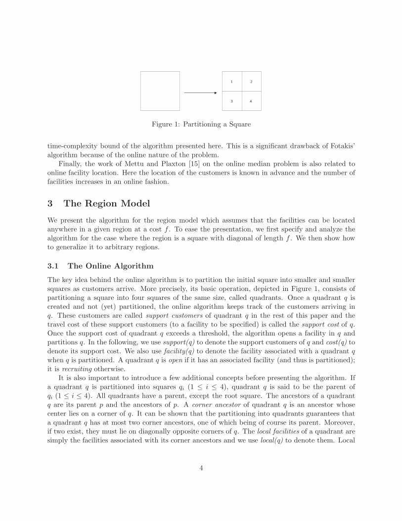
Figure 1: Partitioning a Square

time-complexity bound of the algorithm presented here. This is a significant drawback of Fotakis’algorithm because of the online nature of the problem.

Finally, the work of Mettu and Plaxton [15] on the online median problem is also related toonline facility location. Here the location of the customers is known in advance and the number offacilities increases in an online fashion.

3 The Region Model

We present the algorithm for the region model which assumes that the facilities can be locatedanywhere in a given region at a cost f . To ease the presentation, we first specify and analyze thealgorithm for the case where the region is a square with diagonal of length f . We then show howto generalize it to arbitrary regions.

3.1 The Online Algorithm

The key idea behind the online algorithm is to partition the initial square into smaller and smallersquares as customers arrive. More precisely, its basic operation, depicted in Figure 1, consists ofpartitioning a square into four squares of the same size, called quadrants. Once a quadrant q iscreated and not (yet) partitioned, the online algorithm keeps track of the customers arriving inq. These customers are called support customers of quadrant q in the rest of this paper and thetravel cost of these support customers (to a facility to be specified) is called the support cost of q.Once the support cost of quadrant q exceeds a threshold, the algorithm opens a facility in q andpartitions q. In the following, we use support(q) to denote the support customers of q and cost(q) todenote its support cost. We also use facility(q) to denote the facility associated with a quadrant qwhen q is partitioned. A quadrant q is open if it has an associated facility (and thus is partitioned);it is recruiting otherwise.

It is also important to introduce a few additional concepts before presenting the algorithm. Ifa quadrant q is partitioned into squares qi (1 ≤ i ≤ 4), quadrant q is said to be the parent ofqi (1 ≤ i ≤ 4). All quadrants have a parent, except the root square. The ancestors of a quadrantq are its parent p and the ancestors of p. A corner ancestor of quadrant q is an ancestor whosecenter lies on a corner of q. It can be shown that the partitioning into quadrants guarantees thata quadrant q has at most two corner ancestors, one of which being of course its parent. Moreover,if two exist, they must lie on diagonally opposite corners of q. The local facilities of a quadrant aresimply the facilities associated with its corner ancestors and we use local(q) to denote them. Local

4

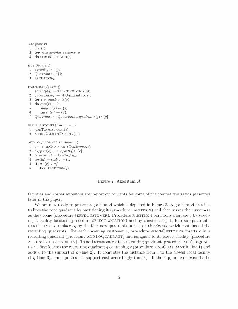
A(Square r)1 init(r);2 for each arriving customer c3 do serveCustomer(c);

init(Square q)1 parent(q) ← {};2 Quadrants ← {};3 partition(q);

partition(Square q)1 facility(q) ← selectLocation(q);2 quadrants(q) ← 4 Quadrants of q ;3 for r ∈ quadrants(q)4 do cost(r) ← 0;5 support(r) ← {};6 parent(r) ← {q};7 Quadrants ← Quadrants∪ quadrants(q) \ {q};

serveCustomer(Customer c)1 addToQuadrant(c);2 assignClosestFacility(c);

addToQuadrant(Customer c)1 q ← findQuadrant(Quadrants, c);2 support(q) ← support(q)∪ {c};3 tc ← min(� in local(q)) t�,c;4 cost(q) ← cost(q) + tc;5 if cost(q) > af6 then partition(q);

Figure 2: Algorithm A

facilities and corner ancestors are important concepts for some of the competitive ratios presentedlater in the paper.

We are now ready to present algorithm A which is depicted in Figure 2. Algorithm A first ini-tializes the root quadrant by partitioning it (procedure partition) and then serves the customersas they come (procedure serveCustomer). Procedure partition partitions a square q by select-ing a facility location (procedure selectLocation) and by constructing its four subquadrants.partition also replaces q by the four new quadrants in the set Quadrants, which contains all therecruiting quadrants. For each incoming customer c, procedure serveCustomer inserts c in arecruiting quadrant (procedure addToQuadrant) and assigns c to its closest facility (procedureassignClosestFacility). To add a customer c to a recruiting quadrant, procedure addToQuad-

rant first locates the recruiting quadrant q containing c (procedure findQuadrant in line 1) andadds c to the support of q (line 2). It computes the distance from c to the closest local facilityof q (line 3), and updates the support cost accordingly (line 4). If the support cost exceeds the

5

threshold af (line 5), where a is a parameter of the implementation2, the quadrant q is partitionedand becomes open (line 5). In the region model, procedure selectLocation simply chooses thecenter of the quadrant to locate the facility. (This implementation is reconsidered in other models).

Observe that the cost of a quadrant q is the cost of its associated facility (if any) and the supportcost of its support customers cost(q), i.e. ≤ (a + 2)f . Since all the facilities and all the customersare associated with quadrants, the cost of the solution is the sum of the costs of all quadrants.

It is important to emphasize that the support cost of a customer, i.e., the travel cost to itsclosest local facility, is greater or equal to the actual travel cost to its closest location. The use ofthe support cost in thresholding simplifies the analysis and makes it possible to prove robustnessresults with respect to the customer ordering. Note also that most (but not all) results in thispaper hold when line 3 in procedure addToQuadrant is replaced by tc ← tparent(q),c.

3.2 Worst-Case Competitive Analysis

This section analyzes the worst case performance of the algorithm assuming that the maximumlength (i.e., the diagonal) of the square is f , where f is the cost of opening a facility. This assumptionis relaxed in Section 3.3. The first lemma bounds the maximum depth of a partition produced byAlgorithm A. It does not depend on the location of the facilities inside the quadrants.

Lemma 1. The maximum partition depth produced by Algorithm A when serving n customersis O(log n).

Proof. Observe that there must be at least a2i customers in the support of a quadrant at depth iin order to partition it, since the maximum distance in a quadrant at depth i is not greater thanf2i . Hence, the maximum depth for n customers is log n − log a, which is O(log n).

The second lemma is central to the rest of the paper and will be adapted to other models subse-quently. Informally speaking, it specifies that every quadrant created by algorithm A is close to afacility in an optimal solution, the distance depending on the size of the quadrant.

Lemma 2. Let q be an open quadrant with sides of length μ produced by algorithm A. In an optimalsolution, there must exist at least one facility within distance αμ of q, where α =

√2(a+2)2a .

Proof. The proof is by contradiction. Assume that there exists no facility within distance αμ of anopen quadrant q in an optimal solution O. Let s = |support(q)|. Clearly

af <∑

c ∈ support(q)

travel-cost(c) ≤∑

c ∈ support(q)

√2μ = s

√2μ

where travel-cost(c) is the travel cost incurred by c, and√

2μ is the maximum value for travel-cost(c)because of the existence of the parent facility (see Figure 3). It follows that f <

√2

a sμ. If a new

2Parameterizing a is useful for improving the quality of empirical results on various types of problems. For thepurposes of the competitive analysis results, a is an arbitrary constant

6

��

��

��

��

��

��

��

��

��

��

��

another local facility

parent facility

new facility

{ {

��

�

Figure 3: Visualization of Optimal Facility Placement

��

��

��

��

��

��

��

��

��

��

��

��

parent facility

another local facility

new facility

{ {��

�

Figure 4: Illustrating Corollary 1. There must exist an optimal facility in the square whose sideshave length (2�α� + 1)μ.

facility is placed in the center of q and the support customers of q are re-routed to the new facility,the total cost is at most

f +√

22

sμ <

(√2

a+

√2

2

)sμ =

√2(a + 2)

2a= αsμ

If there is no facility within α of q, then the total travel cost of customers in support(q) is > αsμ,yielding the contradiction that there exists no facilities within α of q in the optimal solution.

The first corollary, which is illustrated graphically in Figure 4, is a direct consequence of Lemma2. The second corollary is used in Section 7.

Corollary 1. Let q be an open quadrant with sides of length μ produced by algorithm A. An optimalsolution must have at least one facility in a square of size (2�α�+ 1)μ by (2�α�+ 1)μ whose centeris q, where α =

√2(a+2)2a .

7

��

��

All customers

...

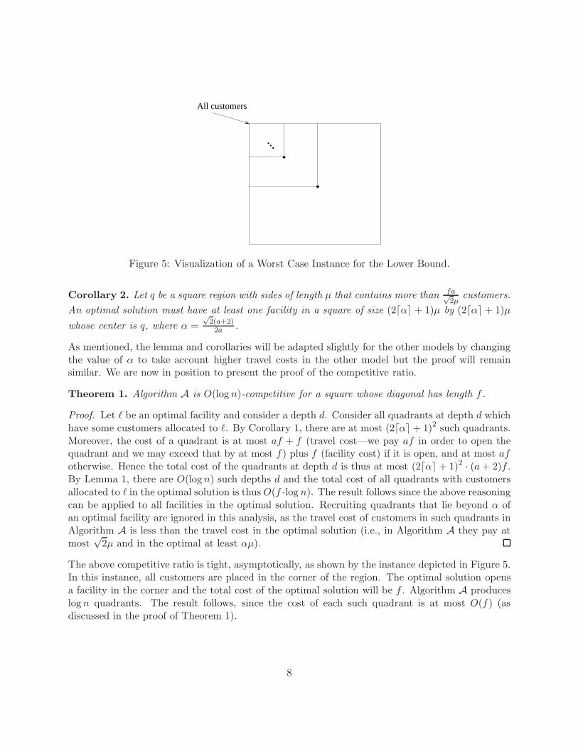
Figure 5: Visualization of a Worst Case Instance for the Lower Bound.

Corollary 2. Let q be a square region with sides of length μ that contains more than fa√2μ

customers.An optimal solution must have at least one facility in a square of size (2�α� + 1)μ by (2�α� + 1)μwhose center is q, where α =

√2(a+2)2a .

As mentioned, the lemma and corollaries will be adapted slightly for the other models by changingthe value of α to take account higher travel costs in the other model but the proof will remainsimilar. We are now in position to present the proof of the competitive ratio.

Theorem 1. Algorithm A is O(log n)-competitive for a square whose diagonal has length f .

Proof. Let � be an optimal facility and consider a depth d. Consider all quadrants at depth d whichhave some customers allocated to �. By Corollary 1, there are at most (2�α� + 1)2 such quadrants.Moreover, the cost of a quadrant is at most af + f (travel cost—we pay af in order to open thequadrant and we may exceed that by at most f) plus f (facility cost) if it is open, and at most afotherwise. Hence the total cost of the quadrants at depth d is thus at most (2�α� + 1)2 · (a + 2)f .By Lemma 1, there are O(log n) such depths d and the total cost of all quadrants with customersallocated to � in the optimal solution is thus O(f ·log n). The result follows since the above reasoningcan be applied to all facilities in the optimal solution. Recruiting quadrants that lie beyond α ofan optimal facility are ignored in this analysis, as the travel cost of customers in such quadrants inAlgorithm A is less than the travel cost in the optimal solution (i.e., in Algorithm A they pay atmost

√2μ and in the optimal at least αμ).

The above competitive ratio is tight, asymptotically, as shown by the instance depicted in Figure 5.In this instance, all customers are placed in the corner of the region. The optimal solution opensa facility in the corner and the total cost of the optimal solution will be f . Algorithm A produceslog n quadrants. The result follows, since the cost of each such quadrant is at most O(f) (asdiscussed in the proof of Theorem 1).

8

��

��

��

��

��

��

��

��

��

��

{

parent facility

new facility

P

2√

2µ

√2µ

µ

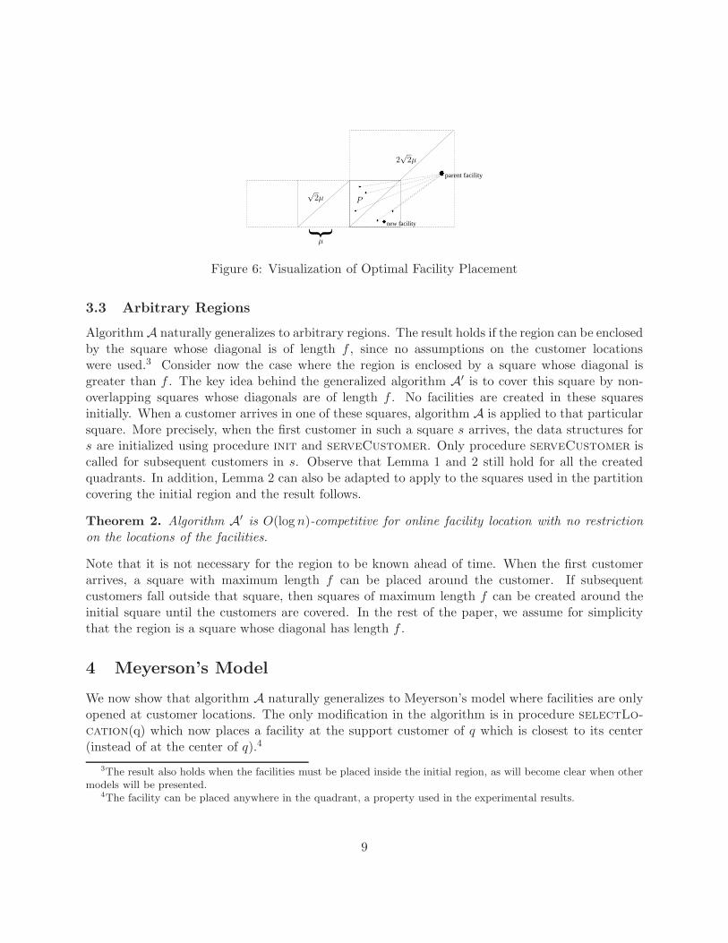
Figure 6: Visualization of Optimal Facility Placement

3.3 Arbitrary Regions

Algorithm A naturally generalizes to arbitrary regions. The result holds if the region can be enclosedby the square whose diagonal is of length f , since no assumptions on the customer locationswere used.3 Consider now the case where the region is enclosed by a square whose diagonal isgreater than f . The key idea behind the generalized algorithm A′ is to cover this square by non-overlapping squares whose diagonals are of length f . No facilities are created in these squaresinitially. When a customer arrives in one of these squares, algorithm A is applied to that particularsquare. More precisely, when the first customer in such a square s arrives, the data structures fors are initialized using procedure init and serveCustomer. Only procedure serveCustomer iscalled for subsequent customers in s. Observe that Lemma 1 and 2 still hold for all the createdquadrants. In addition, Lemma 2 can also be adapted to apply to the squares used in the partitioncovering the initial region and the result follows.

Theorem 2. Algorithm A′ is O(log n)-competitive for online facility location with no restrictionon the locations of the facilities.

Note that it is not necessary for the region to be known ahead of time. When the first customerarrives, a square with maximum length f can be placed around the customer. If subsequentcustomers fall outside that square, then squares of maximum length f can be created around theinitial square until the customers are covered. In the rest of the paper, we assume for simplicitythat the region is a square whose diagonal has length f .

4 Meyerson’s Model

We now show that algorithm A naturally generalizes to Meyerson’s model where facilities are onlyopened at customer locations. The only modification in the algorithm is in procedure selectLo-

cation(q) which now places a facility at the support customer of q which is closest to its center(instead of at the center of q).4

3The result also holds when the facilities must be placed inside the initial region, as will become clear when othermodels will be presented.

4The facility can be placed anywhere in the quadrant, a property used in the experimental results.

9

{

{

Facility

�

��

� �

��

�

��

��

Figure 7: Opening Facilities in the Fixed Location Model.

Under this model, Lemma 1 still holds, since its proof only relies on the sizes of the quadrant.Lemma 2 also holds under the new model by making α =

√2(a+2)

a , since the maximum distanceof a support customer to the facility of q increases to

√2μ (as opposed to

√2μ/2 that we had in

Lemma 2), since the facility of q can be anywhere in the quadrant (See Figure 6). As a consequence,algorithm A is also O(log n)-competitive under this model.

Theorem 3. Algorithm A is O(log n)-competitive for online facility location when facilities mustbe located at customer sites.

5 The Fixed Facility Location Model

We now consider the fixed facility location model, where facilities can only be located at a fixedset of locations. Once again, we assume that the region is a square whose diagonal is of size f forsimplicity. Clearly, the Ω(log n) lower bound still applies, since the fixed locations can be preciselylocated at the center of the quadrant as in Figure 5. We now prove that algorithm A can benaturally adapted to remain O(log n)-competitive under this model.

The main change in the algorithm is to restrict further when a facility can be opened for aquadrant. More precisely, a facility can be opened for a quadrant q with sides of length μ whenthe cost of its support customers exceeds af and when there exists a facility (inside or outside thequadrant) within distance 2

√2μ of q. Note that this facility may be opened already, implying that

the same facility may be associated with several quadrants. This amounts to replacing line 5 ofprocedure addToQuadrant by

if cost(q) > af ∧ existsFacility(q)

where existsFacility(q) returns true if there exists a facility location within distance 2√

2μ of q.

10

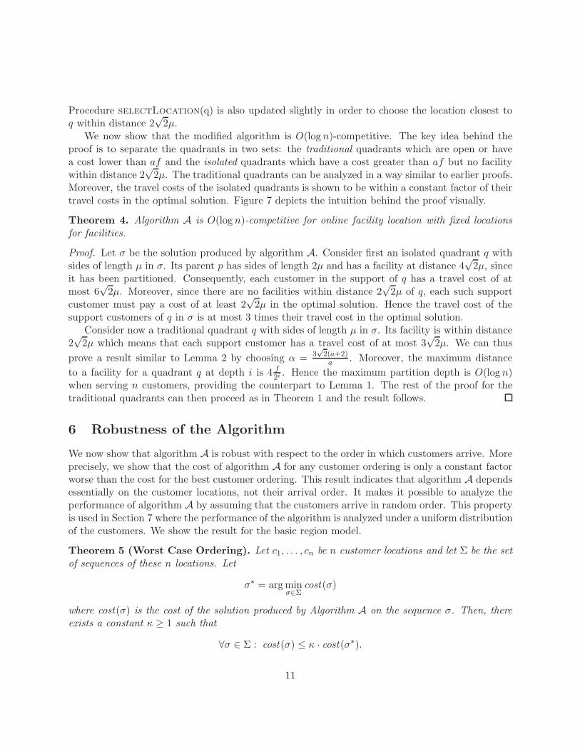
Procedure selectLocation(q) is also updated slightly in order to choose the location closest toq within distance 2

√2μ.

We now show that the modified algorithm is O(log n)-competitive. The key idea behind theproof is to separate the quadrants in two sets: the traditional quadrants which are open or havea cost lower than af and the isolated quadrants which have a cost greater than af but no facilitywithin distance 2

√2μ. The traditional quadrants can be analyzed in a way similar to earlier proofs.

Moreover, the travel costs of the isolated quadrants is shown to be within a constant factor of theirtravel costs in the optimal solution. Figure 7 depicts the intuition behind the proof visually.

Theorem 4. Algorithm A is O(log n)-competitive for online facility location with fixed locationsfor facilities.

Proof. Let σ be the solution produced by algorithm A. Consider first an isolated quadrant q withsides of length μ in σ. Its parent p has sides of length 2μ and has a facility at distance 4

√2μ, since

it has been partitioned. Consequently, each customer in the support of q has a travel cost of atmost 6

√2μ. Moreover, since there are no facilities within distance 2

√2μ of q, each such support

customer must pay a cost of at least 2√

2μ in the optimal solution. Hence the travel cost of thesupport customers of q in σ is at most 3 times their travel cost in the optimal solution.

Consider now a traditional quadrant q with sides of length μ in σ. Its facility is within distance2√

2μ which means that each support customer has a travel cost of at most 3√

2μ. We can thusprove a result similar to Lemma 2 by choosing α = 3

√2(a+2)a . Moreover, the maximum distance

to a facility for a quadrant q at depth i is 4 f2i . Hence the maximum partition depth is O(log n)

when serving n customers, providing the counterpart to Lemma 1. The rest of the proof for thetraditional quadrants can then proceed as in Theorem 1 and the result follows.

6 Robustness of the Algorithm

We now show that algorithm A is robust with respect to the order in which customers arrive. Moreprecisely, we show that the cost of algorithm A for any customer ordering is only a constant factorworse than the cost for the best customer ordering. This result indicates that algorithm A dependsessentially on the customer locations, not their arrival order. It makes it possible to analyze theperformance of algorithm A by assuming that the customers arrive in random order. This propertyis used in Section 7 where the performance of the algorithm is analyzed under a uniform distributionof the customers. We show the result for the basic region model.

Theorem 5 (Worst Case Ordering). Let c1, . . . , cn be n customer locations and let Σ be the setof sequences of these n locations. Let

σ∗ = arg minσ∈Σ

cost(σ)

where cost(σ) is the cost of the solution produced by Algorithm A on the sequence σ. Then, thereexists a constant κ ≥ 1 such that

∀σ ∈ Σ : cost(σ) ≤ κ · cost(σ∗).

11

Proof. Let q be a quadrant which is not partitioned in the best-case sequence σ∗ and which ispartitioned in the worst-case sequence σ. Since the same customers belong to q in both sequences,this happens when some of the customers are in the support of the ancestors of q in σ∗, but not inσ. Observe that the travel cost of any such unaccounted customer in sequence σ is not greater thanits travel cost in sequence σ∗, since its local facilities include its closest ancestor. Clearly, the setof unaccounted customers is not greater than the set of all customers whose travel cost is boundedby 2afw, where w is the number of facilities for sequence σ∗. As a consequence, since sequence σrequires at least af in travel cost to open a facility, the unaccounted customers can only open 2wfacilities.

We finally have to consider all the recruiting quadrants that did not open in the solution ofσ. For each such quadrant, we can associate its cost with its parent. For every quadrant (ofthe total of 2w that we have), the total additional travel cost cannot be more than 4af (af persubquadrant). Hence the cost of the solution of σ remains proportional to w, thus establishing theconstant ratio.

A simple bound on κ is calculated as follows. In σ∗ the open quadrants have cost at least (a + 1)f ,thus the total cost of the solution is (a + 1)fw. In σ, there are at most 2w open quadrants each ofwhich induces cost at most (a + 2)f , while the possible unopened recruiting quadrants induce anadditional cost of 8afw. Therefore we get a bound of κ ≤ 10a+4

a+1 .Note that this result can be generalized to the fixed location model provided that the choice

of the facility location for a quadrant be deterministic (e.g., ties are broken deterministically inprocedure selectLocation). Such a choice guarantees that the travel cost of the unaccountedcustomers is not greater in the worst-case sequence than in the best sequence. The result does notgeneralize to Meyerson’s model where facility location choices critically depend on the customerorder.

7 Probabilistic Analysis

The previous sections showed that the competitive ratio of the algorithm A is Θ(log n) but, inpractice, algorithm A should behave much better. It is thus interesting to analyze algorithm A,not under an adversarial model, but under various distributions of the customers. This sectionfollows this approach and analyzes algorithm A for a uniform distribution of the customers, aswell as for distributions which have smooth neighborhoods. In both cases, we show that algorithmA produces a solution whose cost is within a constant of the optimal offline solution with highprobability (whp).5 We start by proving the result for the uniform distribution. The result is thengeneralized to distributions with smooth neighborhoods.

7.1 Uniform Distribution of Customers

The intuition behind the proof for the uniform distribution is the following. First recall that thepartitioning threshold guarantees that the travel cost is proportional to the cost of the facilities, so

5Recall that an event E holds whp. if there is a constant c > 0 such that Pr(E) > 1 − 1nc .

12

that the proof can focus on the number of open facilities or, equivalently, on the number of openquadrants. We define depth d = (log n)/3, and by using the analysis of Section 3.2 we computea high-probability lower bound for the optimal algorithm; that follows from the fact that in anysquare of dimensions 2d × 2d there is a big number of customers to necessitate the opening of afacility in the area nearby the square. Finally, we show that whp. algorithm A does not openany quadrant at depth d + 1, and so we get a constant approximation ratio. A main result thatwe use in the proof is Theorem 5, which makes it possible to assume that the customers arrive inrandom order. In other words, the proof assumes that the location of a new customer is uniformlydistributed in the whole region and independent of all previous and subsequent customer locations.

For the sake of completeness we present a version of the Chernoff bound [20], that we usethroughout the proof and the next section.

Theorem 6 (Chernoff Bound). Assume that the Xi are mutually independent 0 − 1 randomvariables such that Pr(Xi = 1) = p, and let Y =

∑ni=1 Xi and μ = E[Y ] = np. Then, for any

ε > 0,Pr(Y ≥ (1 + ε)μ) ≤ e−

13με2 ,

and for any ε ∈ (0, 1),Pr(Y ≤ (1 − ε)μ) ≤ e−

12με2 .

We are now ready to prove the result.

Theorem 7. Consider a square region and assume that the customers are uniformly distributed inthe region and mutually independent. Then the cost of the solution produced by algorithm A is onlya constant times higher than that of the optimal offline algorithm, with probability at least 1− 1/n.

Proof. For simplicity, we assume that the region is a square with sides of length 1 (f =√

2) andthat the parameter a = 1/

√2 so that the threshold is 1. Define d = (log n)/3. We first show that

whp. the optimal solution opens at least 19n2/3 facilities.

Consider a quadrant in depth d, which has dimensions 2−d × 2−d = n−1/3 × n−1/3. Theprobability that a given customer falls in the quadrant equals n−2/3, so, in expectation, the quadrantreceives n · n−2/3 = n1/3 customers. By the Chernoff bound, we get that the probability that itaccepts fewer than 2

3n1/3 customers is bounded by

e−12( 1

3)2n

13

< n−3,

for sufficiently large n. Since the total number of quadrants at depth d is 4d < n, we conclude thatwith probability at least 1 − n−2 every quadrant accepts at least 2

3n1/3 customers.By applying Corollary 2 we get that in any square of dimensions 3 · 2−d × 3 · 2−d there exists an

open facility in the optimal solution. There exist 19n2/3 disjoint squares of dimensions 3·2−d×3·2−d,

hence, the optimal solution opens at least 19n2/3 facilities with probability at least 1 − n−2.

The second step is to show that algorithm A does not open too many quadrants. We now showthat, at level d + 1, no quadrants are partitioned whp. Consider a quadrant q at level d + 1. Themaximum distance (the diagonal) within q is 2

12−d−1 = n−1/2/

√2 and, hence, at least

√2 · n1/3

13

customers are needed to open q. Therefore, the probability to open quadrant q is bounded bythe probability that at least

√2 · n1/3 customers fall in q. Recall also that the probability that

a customer falls in the quadrant equals its area which is 2−2(d+1) = n−2/3/4. So the expectednumber of customers that fall in the quadrant is n · n−2/3/4 = n1/3/4. (Not all of those customerscontribute into partitioning q, since some of them have already been accounted for the partitioningof the quadrants down to q. Therefore we get an upper bound for the probability that we areinterested in.) By applying the Chernoff bound with ε = 4

√2 − 1, we get that the probability

that q becomes partitioned is bounded by

Pr(≥

√2 · n 1

3 customers fall in q)≤ Pr

(n1/3

4(1 + ε) customers fall in q

)

≤ e−13

n1/3

4ε2

≤ 1n3

for sufficiently large n. At level d + 1 there are 4d+1 < n quadrants, therefore the probabilitythat some quadrant becomes partitioned is bounded by n−2. In other words, there is no quadrantpartitioned at level d + 1, with probability at least 1 − n−2.

We have therefore proven that with probability at least 1 − 2n−2 > 1 − 1/n, in the optimalsolution there are at least 1

9n2/3 open facilities, while algorithm A opens at most∑d

i=0 4i = 43n2/3

facilities. This completes the proof.

7.2 Smooth Neighborhoods

We consider now a large class of distributions for which Algorithm A is O(1)-competitive whp.These distributions satisfy the smooth neighborhood property which we now define.

Definition 1 (Distribution with Smooth Neighborhoods). Let I = [0, 1]2 be the unit squareand ν be a probability distribution on I. Then, ν has a smooth neighborhood if there exists aconstant K such that

ν(Q1) ≤ K · ν(Q2).

for any neighboring quadrant Q1 and Q2, i.e., any quadrant Q1 and Q2 in I satisfying |Q1| = |Q2|and d(Q1, Q2) = 0 where

d(Q1, Q2) = min{|x1 − x2| : x1 ∈ Q1, x2 ∈ Q2}.

Distributions with smooth neighborhoods have the following useful property.

Lemma 3. Consider a quadrant q with four subquadrants qi, i = 1, 2, 3, 4. For any distribution νwith smooth neighborhoods, we have

ν(qi) ≥ p · ν(q),

where p = (3K + 1)−1.

14

Proof. Since d(q1, qi) = 0 (i = 2, 3, 4), it follows that

ν(q1) ≤ K · ν(qi).

Hence

ν(q1)ν(q)

=ν(q1)

ν(q1) + ν(q2) + ν(q3) + ν(q4)

≥ ν(q1)ν(q1) + K · ν(q1) + K · ν(q1) + K · ν(q1)

=1

3K + 1= p

.

The proof is similar for the other three subquadrants.

The following definitions are used in the probabilistic analysis. A bush is a quadrant that has morethan M descendants, where

M =√

2(

2p

+24

p2+

27

p3+

210

p4

),

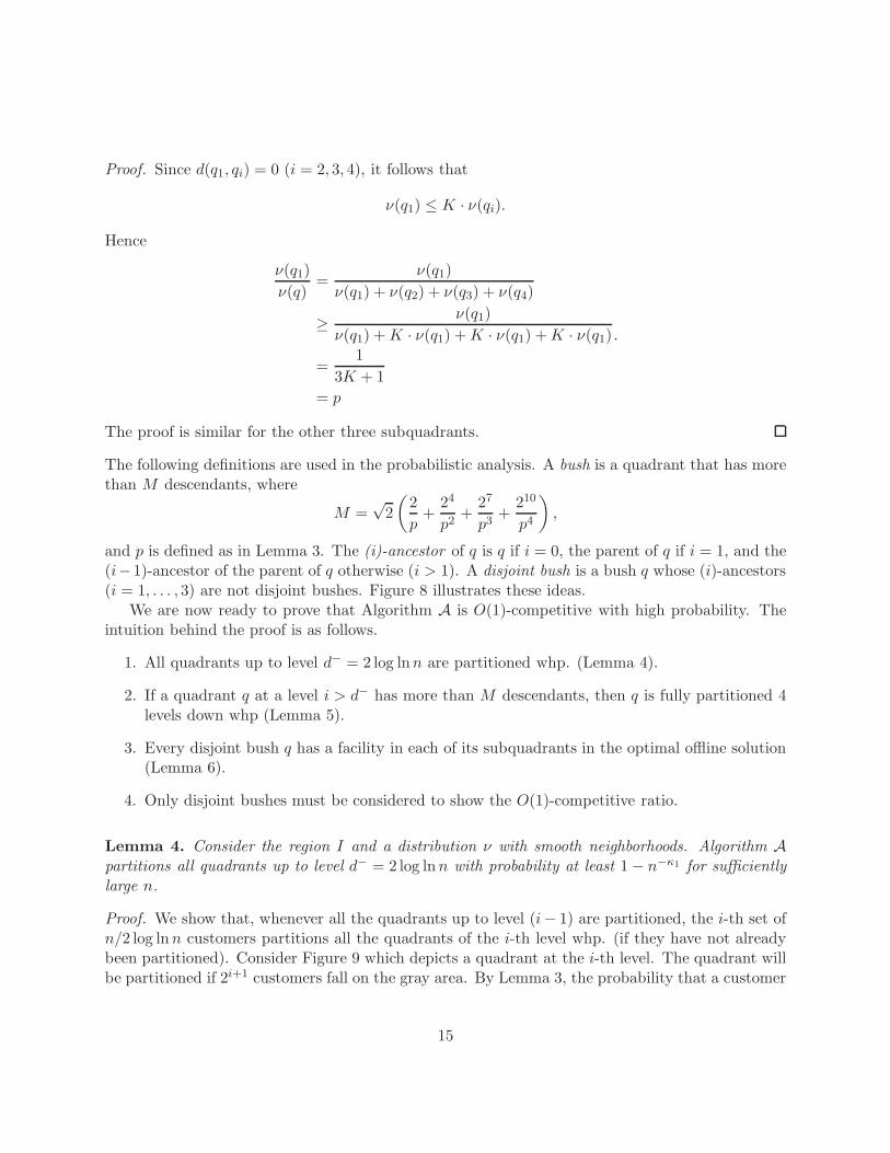
and p is defined as in Lemma 3. The (i)-ancestor of q is q if i = 0, the parent of q if i = 1, and the(i−1)-ancestor of the parent of q otherwise (i > 1). A disjoint bush is a bush q whose (i)-ancestors(i = 1, . . . , 3) are not disjoint bushes. Figure 8 illustrates these ideas.

We are now ready to prove that Algorithm A is O(1)-competitive with high probability. Theintuition behind the proof is as follows.

1. All quadrants up to level d− = 2 log lnn are partitioned whp. (Lemma 4).

2. If a quadrant q at a level i > d− has more than M descendants, then q is fully partitioned 4levels down whp (Lemma 5).

3. Every disjoint bush q has a facility in each of its subquadrants in the optimal offline solution(Lemma 6).

4. Only disjoint bushes must be considered to show the O(1)-competitive ratio.

Lemma 4. Consider the region I and a distribution ν with smooth neighborhoods. Algorithm Apartitions all quadrants up to level d− = 2 log ln n with probability at least 1 − n−κ1 for sufficientlylarge n.

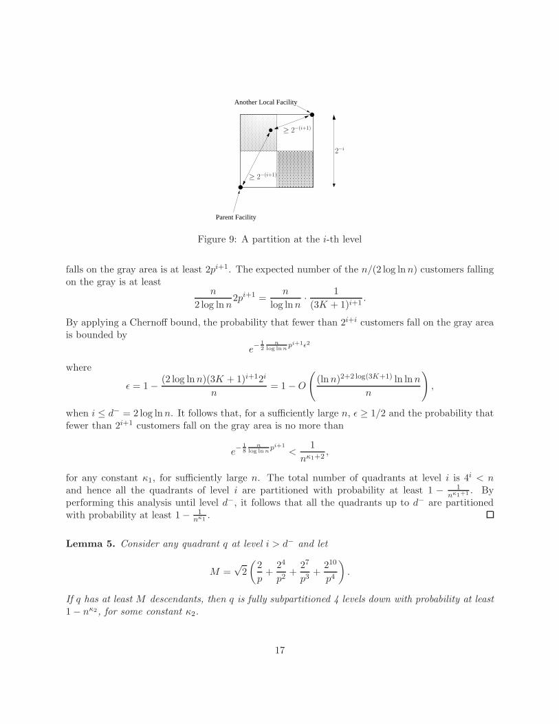
Proof. We show that, whenever all the quadrants up to level (i− 1) are partitioned, the i-th set ofn/2 log ln n customers partitions all the quadrants of the i-th level whp. (if they have not alreadybeen partitioned). Consider Figure 9 which depicts a quadrant at the i-th level. The quadrant willbe partitioned if 2i+1 customers fall on the gray area. By Lemma 3, the probability that a customer

15

Disjoint Bush

Bush

Figure 8: An example of the definitions of a bush and a disjoint bush. A node corresponds to aquadrant and its children to its subquadrants. For clarity every node has up to 2 children (insteadof 4) and we have M = 30.

16

��

��

��

��

Parent Facility

Another Local Facility

2−i

≥ 2−(i+1)

≥ 2−(i+1)

Figure 9: A partition at the i-th level

falls on the gray area is at least 2pi+1. The expected number of the n/(2 log ln n) customers fallingon the gray is at least

n

2 log ln n2pi+1 =

n

log ln n· 1(3K + 1)i+1

.

By applying a Chernoff bound, the probability that fewer than 2i+i customers fall on the gray areais bounded by

e− 1

2n

log ln npi+1ε2

where

ε = 1 − (2 log ln n)(3K + 1)i+12i

n= 1 − O

((ln n)2+2 log(3K+1) ln ln n

n

),

when i ≤ d− = 2 log ln n. It follows that, for a sufficiently large n, ε ≥ 1/2 and the probability thatfewer than 2i+1 customers fall on the gray area is no more than

e−18

nlog ln n

pi+1

<1

nκ1+2,

for any constant κ1, for sufficiently large n. The total number of quadrants at level i is 4i < nand hence all the quadrants of level i are partitioned with probability at least 1 − 1

nκ1+1 . Byperforming this analysis until level d−, it follows that all the quadrants up to d− are partitionedwith probability at least 1 − 1

nκ1 .

Lemma 5. Consider any quadrant q at level i > d− and let

M =√

2(

2p

+24

p2+

27

p3+

210

p4

).

If q has at least M descendants, then q is fully subpartitioned 4 levels down with probability at least1 − nκ2, for some constant κ2.

17

��

��

��

��

Parent Facility

Another Local Facility

≥ 2−(i+2)

≥ 2−(i+2)

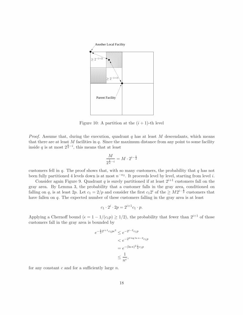
Figure 10: A partition at the (i + 1)-th level

Proof. Assume that, during the execution, quadrant q has at least M descendants, which meansthat there are at least M facilities in q. Since the maximum distance from any point to some facilityinside q is at most 2

12−i, this means that at least

M

212−i

= M · 2i− 12

customers fell in q. The proof shows that, with so many customers, the probability that q has notbeen fully partitioned 4 levels down is at most n−κ2. It proceeds level by level, starting from level i.

Consider again Figure 9. Quadrant q is surely partitioned if at least 2i+1 customers fall on thegray area. By Lemma 3, the probability that a customer falls in the gray area, conditioned onfalling on q, is at least 2p. Let c1 = 2/p and consider the first c12i of the ≥ M2i− 1

2 customers thathave fallen on q. The expected number of these customers falling in the gray area is at least

c1 · 2i · 2p = 2i+1c1 · p.

Applying a Chernoff bound (ε = 1 − 1/(c1p) ≥ 1/2), the probability that fewer than 2i+1 of thosecustomers fall in the gray area is bounded by

e−122i+1c1pε2 ≤ e−2i−2c1p

< e−22 log ln n−2c1p

= e−(ln n)2 14c1p

≤ 1nc

,

for any constant c and for a sufficiently large n.

18

We now condition on quadrant q having been partitioned and we consider level i+1. Quadrant qhas 4 subquadrants and we first focus attention on one of them. This quadrant is partitioned if thepertinent gray area receives at least 2i+2 customers (Figure 10). By applying Lemma 3 twice, theprobability that a customer falls on the gray area, conditioning that it fell on q, is at least 2p2. Letc2 = 4/p2 and consider the next c22i of the ≥ M2i− 1

2 customers which fell in q (after the c12i thatwe just accounted for). The expected number of those customers falling in the gray area is at least

c2 · 2i · 2p2 = 2i+1c2 · p2.

By applying a Chernoff bound (ε = 1 − 2/(c2p2) ≥ 1/2), the probability that fewer than 2i+2 of

those customers fall in the gray area is bounded by

e−122i+1c2p2ε2 ≤ e−2i−2c2p2

< e−22 log ln n−2c2p2

= e−(ln n)2 14c2p2

≤ 1nc

,

again for any constant c. Since q has 4 subquadrants, it follows that all the 4 subquadrants arepartitioned with probability at least 1 − 4n−c with the first 4c22i of the ≥ M2i− 1

2 customers thatfell in q.

A similar result holds for the next 16 subsubquadrants with c3 = 8/p3 and for the subsequent64 subquadrants with c4 = 16/p4. Since

M · 2i− 12 = 2i(c1 + 4c2 + 16c3 + 64c4),

it follows that, if at least M2i− 12 customers fall in q, then, for a sufficiently large n, all the 4 levels

from i downwards are fully partitioned with probability at least 1 − n−κ2 for any constant κ2.

Lemma 6. Every disjoint bush has a facility in each of its quadrants in the optimal, offline solution.

Proof. Consider Figure 11. Since the black quadrant is open, by Lemma 2 (a = 1/√

2 so α < 3),the optimal solution must have a facility in the gray box.

We are now ready to prove the main result on distributions with smooth neighborhoods.

Theorem 8. Consider the region I and assume that the customers are mutually independent andobey a distribution ν with smooth neighborhoods. Then, for sufficiently large n, the cost of thesolution produced by algorithm A is only a constant times higher than that of the optimal offlinealgorithm with probability at least 1 − 1/n.

Proof. Consider the solution of algorithm A and the induced partition. As shown earlier, it sufficesto bound the number of facilities and we may assume that the customers arrive in random order.By Lemma 4, all quadrants up to level d− = 2 log ln n are partitioned whp. By Lemma 5, if aquadrant q at a level i > d− has more than M descendants, then q is fully partitioned 4 levels downwhp. By Lemma 6, every disjoint bush q has a facility in each of its subquadrants in the optimaloffline solution. It remains to show that

19

��

��

Figure 11: A quadrant of a disjoint bush

1. the cost of the solution is only a constant higher than the cost of the disjoint bushes.

2. the number of disjoint bushes is proportional to the number of facilities in the optimal offlinesolution.

Since every bush has at least M descendants, every quadrant that is not a bush has at mostM − 1 descendants (none of which are bushes). Hence the number of nonbushes is at most 4Mtimes higher than the number of bushes. Therefore the cost of the solution is proportional to thenumber of bushes. Notice though that the number of disjoint bushes is at most

∑3i=0 4i = 85 times

higher than the number of bushes (a descendent of a disjoint bush that is 4 levels lower, has to bea disjoint bush). This proves point (1) above.

Consider now the tree where every node is a disjoint bush and the parent of a disjoint bush qis the closest (i)-ancestor of q which is a disjoint bush. The total number of nodes in the disjoint-bush tree is proportional to the number of leaves and nodes with a single child. By Lemma 6, theoptimal solution has at least 4 facilities for every leaf. Similarly, for every node with a single child,it also follows from Lemma 6 that there are at least three facilities in the optimal solution not inthe subquadrant of the child, proving point (2) above and concluding the proof.

The final result of this section identifies a large class of distributions with smooth neighborhoods.

Lemma 7. Consider a distribution ν on I = [0, 1]2 with probability density function ϕ. If ϕ iscontinuous on I and uniformly bounded from 0, then ν has smooth neighborhoods.

Proof. Since ϕ is uniformly bounded from 0, there exists some ε > 0 such that ∀x ∈ I : ϕ(x) > ε.Also, since ϕ is continuous on the set I and I is compact, we have that ϕ is bounded on I, i.e.,there exists a constant M such that ϕ(x) < M for all x ∈ I.

20

We now prove that ν satisfies the smooth neighborhoods property for K = M/ε. More precisely,we show that

ν(Q1) ≤ M

ε· ν(Q2)

for two neighboring squares Q1 and Q2 (of equal area). Rewrite this relation in terms of theprobability density function ∫

Q1

ϕ(x)dx ≤ M

ε·∫

Q2

ϕ(x)dx.

By applying the mean-value theorem (for integrals on R2), there exist x1 ∈ Q1 and x2 ∈ Q2 such

that|Q1| · ϕ(x1) =

∫Q1

ϕ(x)dx

and|Q2| · ϕ(x2) =

∫Q2

ϕ(x)dx,

Since |Q1| = |Q2|, the smooth neighborhood property becomes

ϕ(x1) ≤ M

ε· ϕ(x2)

and it holds since ϕ(x1) < M and ϕ(x2) > ε.

8 Empirical Results

This section describes empirical results on a variety of online facility location problems. To the bestof the authors’ knowledge, this is the first empirical evaluation of algorithms for this problem. InTables 1, 2, 3, 4, 5, and 6, the acronym M refers to Meyerson’s algorithm of [16] and F to Fotakis’algorithm [7]. The remaining acronyms refer to various ways of choosing facility locations for thepartitioning algorithm: C refers to choosing the center point, LC the last customer, and P theaverage position of customers in the quadrant. All the tables are divided in two parts. The toppart of the tables shows results for the region model, while the bottom part depicts the results forMeyerson’s model.

For each distribution, we give the results when the points come uniformly at random, as wellas when the points come in sorted order by their x coordinates. Each column section labels thenumber of customers generated and summarizes the reported results as an average of 10 problems.The C columns are the total cost and W refers to number of open facilities. Boldface indicates thebest results in Meyerson’s model. The best result in the region model is boldfaced when it is betterthan the best result in Meyerson’s model. All algorithms were tested on a variety of parametersand the best parameter over all customer sizes for each problem was chosen. It is important to notethat it is possible to do substantially better in some cases using different thresholds on a specificcustomer size. For the partitioning algorithms, the subscript is the thresholding parameter. InF the superscript refers to the x value. For values of x ≥ 10, F has a qualitative performanceguarantee but performs quite inefficiently. In particular, Fotakis’ algorithm is about 500 times

21

Random

1000 5000 10000 100000C W C W C W C W

C3.2 73.9 277.0 199.0 511.5 312.7 559.7 1465.5 1846.7P2.7 46.6 258.0 191.2 1022.2 266.1 1130.9 1258.9 4626.1

M1.9 52.9 243.5 173.1 692.2 282.1 1105.5 1393.8 5075.3F10

0.2 66.3 613.7 165.8 1214.4 242.6 1476.9 1195.9 4633.0C1 69.6 642.8 172.4 1192.9 287.4 1800.0 315.5 6137.6

P1.6 69.6 642.7 158.7 1037.5 254.6 1381.4 1384.5 5728.1LC1.1 69.6 642.8 167.0 1146.4 274.8 1728.4 1301.9 6176.6

Sorted

1000 5000 10000 100000C W C W C W C W

C3.6 62.2 135.4 183.2 379.8 278.8 407.1 1297.8 1607.2P3.3 51.0 254.1 200.5 980.7 296.5 1148.4 1457.1 4939.8

M2 54.0 228.5 171.5 631.5 279.8 1022.2 1354.6 4714.0F10

0.2 68.0 632.0 183.4 1377.7 273.4 1724.9 1263.2 5184.6C1.7 70.2 646.2 173.5 1049.7 296.8 1491.0 400.1 5043.8P1.7 70.2 646.2 173.5 1049.7 298.9 1491.4 1510.2 5310.6LC1.8 52.0 294.8 166.8 683.5 272.2 1109.2 1298.0 4925.3

Table 1: Uniform Distribution, Facility Cost = .1

slower than the partitioning algorithm to execute all the benchmarks used in this section. Thealgorithm by Meyerson does not involve any parameters, however, it is easy to add a parameterthat is similar to the ones described here In the original algorithm, as presented in [16], a newfacility is opened at a customer with probability d/f where d is the distance to the nearest facility.It is easy to see that this can be modified to d/af . If a is constant, then the same competitiveratio results hold, albeit with a different constant for the O(1) result that concerns random orderof the points (similarly, the subscript of F also refers to a thresholding parameter for indicatinghow much potential is needed to open a new facility). All the problem instances described belowexist in the two dimensional unit square.

Uniform Distributions Tables 1 and 2 assess how well the algorithms perform when the cus-tomers are distributed in the space uniformly for facility costs of .1 and 1. It is interesting tosee here that Meyerson’s models perform better than the regions models until high numbers ofcustomers are reached. This may be due, in part, to savings (travel cost of 0) gained by placing afacility with the most recent arriving customer. Overall, F and LC perform the best here, with Fhaving a slight edge as the number of customers increases. However, F is considerably slower.

Gaussian Distribution Tables 3 and 4 show the results of the algorithms when the points aredrawn from a Gaussian distribution located at the center of the unit square with a parameter of.25 for both the x and y directions with facility costs of .1 and 1. What is clear from these resultsis that the F method performs the best on the random ordered points and sorted points when

22

Random

1000 5000 10000 100000C W C W C W C W

C2.4 135.3 24.0 410.4 88.0 628.2 88.5 2968.5 373.6P2.1 141.9 69.9 495.9 280.8 626.1 279.6 2806.6 1140.7

M1.9 143.4 52.1 425.8 154.1 675.8 243.9 3141.3 1090.7F10

0.2 122.9 50.3 363.1 106.7 585.8 155.0 2905.3 566.8C2.8 132.8 24.3 413.3 87.9 635.0 88.7 3000.8 355.8P2.8 134.0 24.3 413.0 88.0 638.0 89.4 3019.0 367.0

LC1.0 146.6 82.0 443.6 226.0 677.8 330.1 3065.0 1370.5

Sorted

1000 5000 10000 100000C W C W C W C W

C2.5 127.0 24.0 381.1 88.0 573.6 91.0 2673.7 429.3P2.6 154.3 69.7 514.4 268.1 708.2 295.1 3225.8 1195.5

M1.9 141.3 52.3 412.0 143.5 650.5 234.1 3033.7 1054.7F10

0.2 130.4 56.2 380.1 121.9 604.7 177.4 2897.1 631.7C1.7 149.8 52.7 425.0 123.5 685.1 238.0 3115.1 1093.7P1.6 157.4 57.5 469.4 154.4 729.0 253.5 3388.6 1203.5

LC1.6 139.4 58.0 418.1 150.0 41.2 262.6 2916.0 1165.0

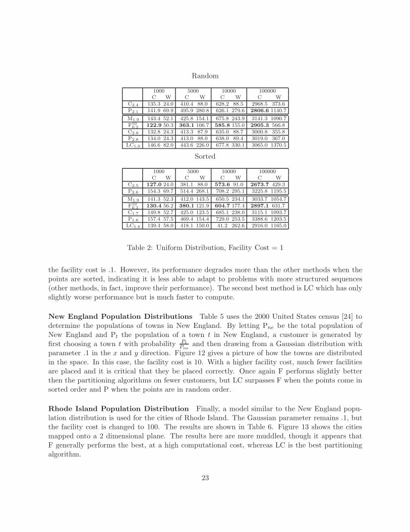
Table 2: Uniform Distribution, Facility Cost = 1

the facility cost is .1. However, its performance degrades more than the other methods when thepoints are sorted, indicating it is less able to adapt to problems with more structured sequences(other methods, in fact, improve their performance). The second best method is LC which has onlyslightly worse performance but is much faster to compute.

New England Population Distributions Table 5 uses the 2000 United States census [24] todetermine the populations of towns in New England. By letting Pne be the total population ofNew England and Pt the population of a town t in New England, a customer is generated byfirst choosing a town t with probability Pt

Pneand then drawing from a Gaussian distribution with

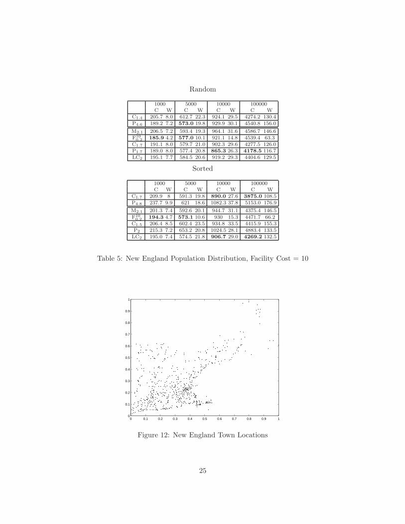
parameter .1 in the x and y direction. Figure 12 gives a picture of how the towns are distributedin the space. In this case, the facility cost is 10. With a higher facility cost, much fewer facilitiesare placed and it is critical that they be placed correctly. Once again F performs slightly betterthen the partitioning algorithms on fewer customers, but LC surpasses F when the points come insorted order and P when the points are in random order.

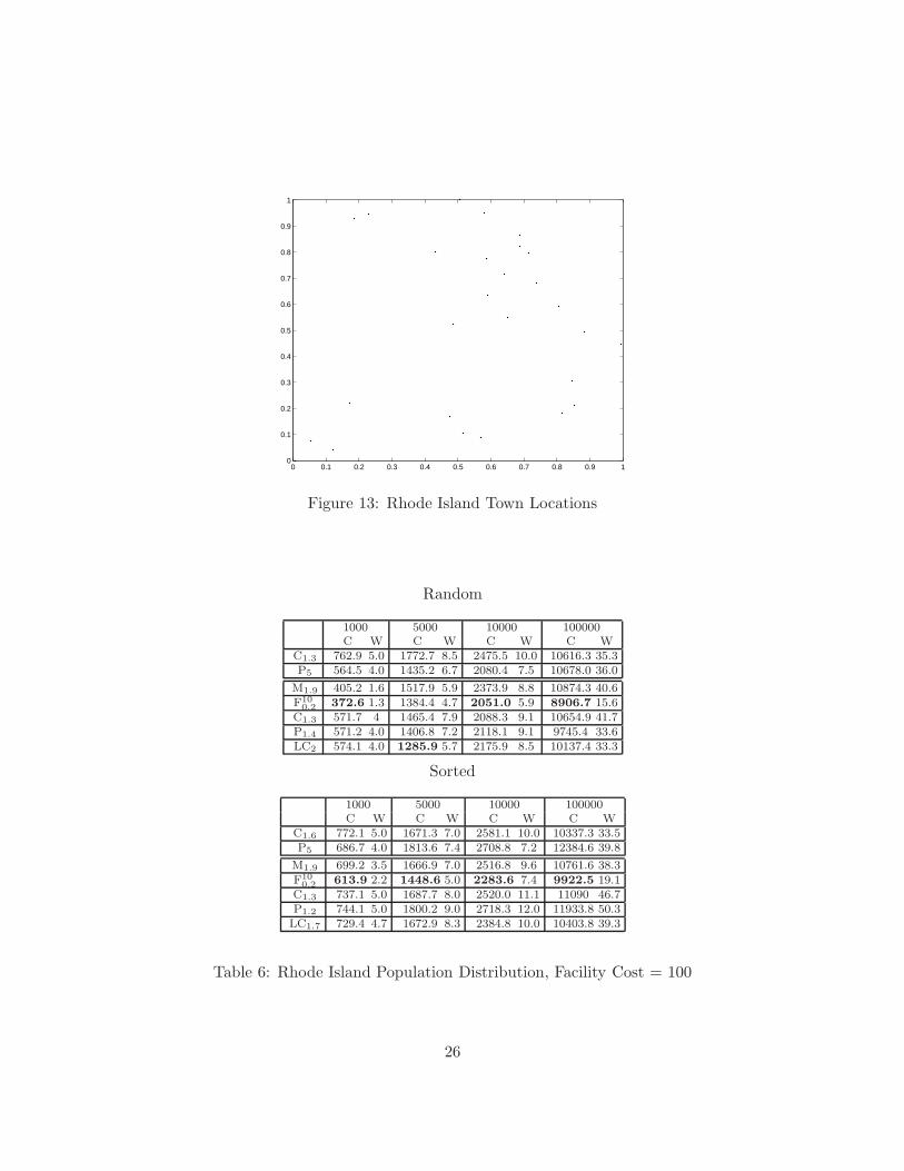
Rhode Island Population Distribution Finally, a model similar to the New England popu-lation distribution is used for the cities of Rhode Island. The Gaussian parameter remains .1, butthe facility cost is changed to 100. The results are shown in Table 6. Figure 13 shows the citiesmapped onto a 2 dimensional plane. The results here are more muddled, though it appears thatF generally performs the best, at a high computational cost, whereas LC is the best partitioningalgorithm.

23

Random

1000 5000 10000 100000C W C W C W C W

C1.8 56.0 257.3 158.3 571.1 246.6 807.2 1114.5 3007.0P3.5 40.6 228.0 136.9 604.2 225.5 933.1 1132.4 4407.3

M1.9 42.2 185.0 138.7 558.8 228.2 879.2 1120.4 4070.6F10

0.2 47.3 405.6 133.7 920.0 206.3 1234.0 961.6 3565.3C1.7 48.4 406.1 138.7 894.1 216.6 1191.7 1044.2 3750.1P1.7 48.4 405.6 138.6 894.1 217.0 1194.5 1047.4 3780.0LC1.7 48.4 406.8 137.8 902.8 216.5 1232.7 1050.0 4181.6

Sorted

1000 5000 10000 100000C W C W C W C W

C1.8 54.7 262.1 148.1 574.6 226.7 805.2 1001.9 2989.5P3.5 44.9 238.3 151.6 648.0 252.7 1045.0 1268.7 5089.5

M2 42.7 176.3 138.0 517.6 223.7 819.0 1090.4 3802.4F10

0.2 49.7 427.8 144.7 1004.7 225.3 1374.2 1020.0 4003.0C1.5 50.7 414.6 151.7 947.2 240.5 1304.7 1140.5 4453.0P1.7 50.7 412.3 154.3 930.5 248.9 1280.0 1232.7 4380.6LC1.8 42.1 240.9 134.1 583.7 218.6 888.3 1073.2 3865.5

Table 3: Gaussian Distribution, Facility Cost = .1

Random

1000 5000 10000 100000C W C W C W C W

C2.4 113.9 27.8 326.2 66.2 531.8 109.4 2511.5 520.1P4.6 104.4 34.2 335.6 114.7 527.5 164.5 2515.3 794.7

M1.9 110.9 41.7 334.6 118.7 535.5 190.0 2533.3 878.5F10

0.2 97.1 37.1 295.2 84.0 475.4 120.4 2353.5 448.3C1.4 103.9 46.7 314.5 117.7 505.4 181.6 2382.1 783.2P1.7 110.3 39.5 322.9 100.2 515.0 156.5 2404.9 682.1LC2.1 104.5 49.2 321.9 133.8 513.2 205.02 455.6 916.0

Sorted

1000 5000 10000 100000C W C W C W C W

C1.5 101.0 34.1 291.3 92.7 467.7 153.3 2144.7 687.2P3.6 121.3 46.8 373.6 146.6 602.3 242.3 2834.3 1110.7

M2.1 109.5 36.3 327.5 107.2 521.4 167.5 2428.0 795.6F10

0.2 102.9 41.0 304.0 95.0 487.1 137.5 2342.1 500.3C1.5 113.4 41.3 333.3 121.7 533.8 191.4 2485.5 867.2P1.4 120.2 49.3 366.2 139.3 582.2 216.4 2732.1 966.7

LC1.8 106.4 37.7 318.1 114.2 508.7 175.6 2388.6 809.7

Table 4: Gaussian Distribution, Facility Cost = 1

24

Random

1000 5000 10000 100000C W C W C W C W

C1.4 205.7 8.0 612.7 22.3 924.1 29.5 4274.2 130.4P4.6 189.2 7.2 573.0 19.8 929.9 30.1 4540.8 156.0

M2.1 206.5 7.2 593.4 19.3 964.1 31.6 4586.7 146.6F10

0.2 185.9 4.2 577.0 10.1 921.1 14.8 4539.4 63.3C1.7 191.1 8.0 579.7 21.0 902.3 29.6 4277.5 126.0P1.7 189.0 8.0 577.4 20.8 865.3 26.3 4178.5 116.7LC2 195.1 7.7 584.5 20.6 919.2 29.3 4404.6 129.5

Sorted

1000 5000 10000 100000C W C W C W C W

C1.7 209.9 8 591.3 19.8 890.0 27.6 3875.0 108.5P4.8 237.7 9.9 621 18.6 1082.3 37.8 5153.0 176.9

M2.1 201.3 7.4 592.6 20.1 944.7 31.1 4375.4 146.5F10

0.2 194.3 4.7 573.1 10.6 930 15.3 4471.7 66.2C1.5 206.4 8.5 602.4 23.5 934.8 33.5 4415.9 155.3P2 215.3 7.2 653.2 20.8 1024.5 28.1 4883.4 133.5

LC2 195.0 7.4 574.5 21.8 906.7 29.0 4269.2 132.5

Table 5: New England Population Distribution, Facility Cost = 10

0 0.1 0.2 0.3 0.4 0.5 0.6 0.7 0.8 0.9 10

0.1

0.2

0.3

0.4

0.5

0.6

0.7

0.8

0.9

1

Figure 12: New England Town Locations

25

0 0.1 0.2 0.3 0.4 0.5 0.6 0.7 0.8 0.9 10

0.1

0.2

0.3

0.4

0.5

0.6

0.7

0.8

0.9

1

Figure 13: Rhode Island Town Locations

Random

1000 5000 10000 100000C W C W C W C W

C1.3 762.9 5.0 1772.7 8.5 2475.5 10.0 10616.3 35.3P5 564.5 4.0 1435.2 6.7 2080.4 7.5 10678.0 36.0

M1.9 405.2 1.6 1517.9 5.9 2373.9 8.8 10874.3 40.6F10

0.2 372.6 1.3 1384.4 4.7 2051.0 5.9 8906.7 15.6C1.3 571.7 4 1465.4 7.9 2088.3 9.1 10654.9 41.7P1.4 571.2 4.0 1406.8 7.2 2118.1 9.1 9745.4 33.6LC2 574.1 4.0 1285.9 5.7 2175.9 8.5 10137.4 33.3

Sorted

1000 5000 10000 100000C W C W C W C W

C1.6 772.1 5.0 1671.3 7.0 2581.1 10.0 10337.3 33.5P5 686.7 4.0 1813.6 7.4 2708.8 7.2 12384.6 39.8

M1.9 699.2 3.5 1666.9 7.0 2516.8 9.6 10761.6 38.3F10

0.2 613.9 2.2 1448.6 5.0 2283.6 7.4 9922.5 19.1C1.3 737.1 5.0 1687.7 8.0 2520.0 11.1 11090 46.7P1.2 744.1 5.0 1800.2 9.0 2718.3 12.0 11933.8 50.3

LC1.7 729.4 4.7 1672.9 8.3 2384.8 10.0 10403.8 39.3

Table 6: Rhode Island Population Distribution, Facility Cost = 100

26

Summary Overall the experimental results are very favorable to the partitioning algorithm.The partitioning algorithm LC is generally the best partitioning version (although C is also veryrobust) and it is only slightly outperformed as far as quality is concerned by F. Algorithm Fhowever is much more demanding computationally and much more complicated to implement. Thedeterministic partitioning algorithm almost always outperforms Meyerson’s randomized algorithmand the benefits can be quite significant sometimes.

9 Conclusion and Future Work

This paper reconsidered online facility location and presented a simple and deterministic competi-tive algorithm for this problem. The algorithm, whose key idea is a hierarchical partitioning basedon thresholding, is very simple to implement and runs in O(n log n), where n is the number ofcustomers. The paper showed that the algorithm is O(log n)-competitive for a variety of models,including the region model, Meyerson’s model where facilities must co-exist with existing customers,and the fixed location model. The paper also presented the first probabilistic analysis of onlinefacility location, showing that the partitioning algorithm is O(1)-competitive for any arrival orderwhenever the customers are uniformly distributed in the region. Experimental results have shownthat the algorithm behaves very well in practice under a variety of hypotheses. It is only slightlyoutperformed by Fotakis’ algorithm that is much more demanding computationally. The experi-mental results also show that our algorithm can bring significant benefits compared to Meyerson’salgorithm.

There are still various open issues for future research. First, it is important to extend thepartitioning idea to other, and perhaps all, metric spaces. It would also be interesting to generalizethe online facility location algorithm presented here to account for non-uniform facility costs. Thiswould probably requiring changing the sizes of the partitioning dynamically. It is also important todevelop a model for online facility location that allows for capacitated facilities and the closing andre-opening of facilities as featured in a variety of networking and mobile computing applications.The partitioning scheme described here would naturally extend to such models. On the practicalside, it may be interesting to evaluate empirically adaptive versions of the algorithms where thresh-olds are refined on the fly. Indeed, early experimental results indicate it is better to have higherthresholds for smaller numbers of customers. On the theoretical side, there are many issues leftopen with the probabilistic analysis. These include identifying which distributions have smoothneighborhoods, and generalizing the proof to weaker properties, since we believe that the algorithmwould behave well in many other contexts.

Acknowledgments

This research, which is partially supported by NSF ITR Award DMI-0121495 and by an NDSEGfellowship from ASEE, has interesting connections to Paris Kanellakis. The research itself originatedfrom our interests in local search for facility location [18], which emerged from our research onconstraint programming languages for local search [17]. See [19] for a detailed account of Paris’influence on that line of research. This paper can also be seen as connecting two, less well-known,

27

research areas of Paris, i.e., online algorithms [2] and probabilistic analysis [11], and it is alwaysamazing to realize how broad Paris was. Last, but not least, Aris Anagnostopoulos has beensupported by Kanellakis’ fellowships for three semesters, bringing to this group the Mediterraneancharm he shares with Paris.

The authors would also like to thank the three anonymous referees for their comments on thispaper. They greatly assisted in simplifying the proofs and polishing the final presentation.

References

[1] J. L. Bentley. Multidimensional binary search trees used for associative searching. Communi-cations of the ACM, 18(9):509–517, Sept. 1975.

[2] A. Buchsbaum, P. Kanellakis, and J. Vitter. A Data Structure for Arc Insertion and RegularPath Finding. Annals of Mathematics and Artificial Intelligence, 3(2-4):187–211, 1991.

[3] E. Chavez, G. Navarro, R. Baeza-Yates, and J. L. Marroquın. Searching in metric spaces.ACM Computing Surveys, 33(3):273–321, Sept. 2001.

[4] F. A. Chudak and D. B. Shmoys. Improved approximation algorithms for a capacitated facilitylocation problem. In Proceedings of the Tenth Annual ACM-SIAM Symposium on DiscreteAlgorithms (SODA ’99), pages 875–876, N.Y., Jan. 17–19 1999. ACM-SIAM.

[5] G. Cornuejols, G. Nemhauser, and L. Wolsey. Discrete Location Theory, chapter The Unca-pacitated Facility Location Problem, pages 119–171. Lecture Note in Artificial Intelligence(LNAI 1865). Wiley, 1990.

[6] D. Erlenkotter. A Dual-Based Procedure for Uncapacitated Facility Location: General SolutionProcedures and Computational Experience. Operations Research, 26:992–1009, 1978.

[7] D. Fotakis. On the competitive ratio for online facility location. In Proceedings of the 13thInternational Colloquium on Automata, Languages and Programming (ICALP ’03), pages 637–652, 30 June–4 July 2003.

[8] L. Gao and E. Robinson. Uncapacitated Facility Location: General Solution Procedures andComputational Experience. European Journal of Operations Research, 76:410–427, 1994.

[9] S. Guha and S. Khuller. Greedy strikes back: Improved facility location algorithms. InProceedings of the Ninth Annual ACM-SIAM Symposium on Discrete Algorithms (SODA ’98),pages 649–657, San Francisco, California, 25–27 Jan. 1998.

[10] K. Jain and V. V. Vazirani. Approximation algorithms for metric facility location and k-medianproblems using the primal-dual schema and lagrangian relaxation. J. ACM, 48(2):274–296,2001.

28

[11] I. Karatzas, E. Protonotarios, and P. Kanellakis. Easy-to-Test Criteria for Weak StochasticStability of Dynamical Systems. In John Hopkins Conference on Information Sciences andSystems, page 535, Baltimore, MD, 1978.

[12] D. Karger and M. Ruhl. Finding nearest neighbors in growth-restricted metrics. In Proceedingsof the 34th Annual ACM Symposium on Theory of Computing (STOC ’02), pages 741–750,New York, May 19–21 2002. ACM Press.

[13] J. Kratica, D. Tosic, V. Filipovic, and I. Ljubic. Solving the Simple Plant LOcation ProblemsbyGenetic Algorithm. RAIRO Operations Research, 35:127–142, 2001.

[14] M. Mahdian, Y. Ye, and J. Zhang. Improved approximation algorithms for metric facility loca-tion problems. In Proceedings of Fifth International Workshop on Approximation Algorithmsfor Combinatorial Optimization (APPROX ’02), volume 2462 of Lecture Notes in ComputerScience, pages 229–242, 2002.

[15] R. R. Mettu and C. G. Plaxton. The online median problem. In IEEE, editor, Proceedings ofthe 41st Annual Symposium on Foundations of Computer Science (FOCS ’00), pages 339–348,1109 Spring Street, Suite 300, Silver Spring, MD 20910, USA, 2000. IEEE Computer SocietyPress.

[16] A. Meyerson. Online facility location. In IEEE, editor, 42nd IEEE Symposium on Foundationsof Computer Science: proceedings: October 14–17, 2001, Las Vegas, Nevada, USA, pages 426–431, 1109 Spring Street, Suite 300, Silver Spring, MD 20910, USA, 2001. IEEE ComputerSociety Press.

[17] L. Michel and P. Van Hentenryck. A Constraint-Based Architecture for Local Search. InOOPLSA’02, Seattle, WA, Nov. 2002.

[18] L. Michel and P. Van Hentenryck. A Simple Tabu-Search Algorithm for Warehouse Location.European Journal of Operations Research, 2003. to appear.

[19] L. Michel and P. Van Hentenryck. Comet in Context. In Principles of Computing and Knowl-edge (PCK’50), San Diego, CA, June 2003.

[20] R. Motwani and P. Raghavan. Randomized Algorithms. Cambridge University Press, Cam-bridge, England, June 1995.

[21] D. Shmoys. Approximation algorithms for facility location problems. In Proceedings of ThirdInternational Workshop on Approximation Algorithms for Combinatorial Optimization (AP-PROX ’00), volume 1913 of Lecture Notes in Computer Science, pages 27–33, 2000.

[22] D. B. Shmoys, E. Tardos, and K. Aardal. Approximation algorithms for facility locationproblems. In Proceedings of the 29th Annual ACM Symposium on the Theory of Computing(STOC ’97), pages 265–274, New York, May 1997. Association for Computing Machinery.

29

[23] D. Sleator and R. Tarjan. Amortized Efficiency of List Update and Paging Rules. Comm.ACM, 28:202–208, 1985.

[24] United States Census Bureau. Year 2000 Population Estimates. http://www.census.gov/, 2000.

30

a simple and deterministic competitive algorithm for

Documents