Determining the Cheapest-to-Deliver Bondsfor Bond Futures

Marlouke van Straaten

March 2009Master’s ThesisUtrecht UniversityStochastics and Financial Mathematics

March 2009Master’s ThesisUtrecht UniversityStochastics and Financial Mathematics

SupervisorsMichel Vellekoop Saen OptionsFrancois Myburg Saen OptionsSandjai Bhulai VU University AmsterdamKarma Dajani Utrecht University

Abstract

In this research futures on bonds are studied and since this future has several bonds as its un-derlyings, the party with the short position may decide which bond it delivers at maturity of thefuture. It obviously wants to give the bond that is the Cheapest-To-Deliver (CTD). The purposeof this project is to develop a method to determine, which bond is the CTD at expiration ofthe future. To be able to compare the underlying bonds, with different maturities and couponrates, conversion factors are used.

We would like to model the effects that changes in the term structure have on which bond ischeapest-to-deliver, because when interest rates change, another bond could become the CTD.We assume that the term structure of the interest rates is stochastic and look at the Ho-Leemodel, that uses binomial lattices for the short rates. The volatility of the model is supposedto be constant between today and delivery, and between delivery and maturity of the bonds.

The following questions will be analysed:

• Is the Ho-Lee model a good model to price bonds and futures, i.e. how well does the modelfit their prices?

• How many steps are needed in the binomial tree to get good results?

• At what difference in the term structure is there a change in which bond is the cheapest?

• Is it possible to predict beforehand which bond will be the CTD?

• How sensitive is the futures price for changes in the zero curve?

• How stable are the volatilities of the model and how sensitive is the futures price forchanges in these parameters?

To answer these questions, the German Euro-Bunds are studied, which are the underlying bondsof the Euro-Bund Future.

Acknowledgements

This thesis finishes my masters degree in ‘Stochastics and Financial Mathematics’ at the UtrechtUniversity. It was a very interesting experience to do this research at Saen Options and I hopethat the supervisors of the company, as well as my supervisor and second reader at the univer-sity, are satisfied with the result.

There are a few persons who were very important during this project, that I would like toexpress my appreciation to. First I would like to thank my manager Francois Myburg, who isa specialist in both the theoretical and the practical part of the financial mathematics. Unlikemany other scientists, he has the ability to explain the most complex and detailed things withinone graph and makes it understandable for everyone. It was very pleasant to work with him,because of his involvement with the project.Also, I would like to express my gratitude to Michel Vellekoop, who has taken care of thecooperation between Saen Options and the university. He proposed an intermediate presentationand report, so that the supervisors of the university were given a good idea of the project. Hewas very helpful in explaining the mathematical difficulties in detail and in writing this thesis.He always had interesting feedback, which is the reason that this thesis has improved so muchsince the first draft. Although the meetings with Francois and Michel were sometimes difficultto follow, especially in the beginning when I had very little background of the subject, it alwaysended up with some jokes and above all, many new ideas to work with.In addition, I would like to thank Sandjai Bhulai, who was my supervisor at the university.Although from the VU University Amsterdam and the subject of this thesis is not his expertise,he was excited about the subject from the start of the project and he has put a lot of effort intoit. It was very pleasant to work with such a friendly professor.I also want to thank Karma Dajani, who was the second reader, and who was so enthusiasticthat she wanted to read and comment all the versions I handed in.Finally I would like to thank my family and especially Joost, who was very patient with me andalways supported me during the stressful moments.

Contents

1 Introduction 121.1 Saen Options . . . . . . . . . . . . . . . . . . . . . . . . . . . . . . . . . . . . . . 121.2 Financial introduction . . . . . . . . . . . . . . . . . . . . . . . . . . . . . . . . . 121.3 Mathematical introduction . . . . . . . . . . . . . . . . . . . . . . . . . . . . . . . 181.4 Outline of Thesis . . . . . . . . . . . . . . . . . . . . . . . . . . . . . . . . . . . . 20

2 Short rate models 222.1 Introduction . . . . . . . . . . . . . . . . . . . . . . . . . . . . . . . . . . . . . . . 222.2 Solving the short-rate models . . . . . . . . . . . . . . . . . . . . . . . . . . . . . 27

2.2.1 Continuous time Ho-Lee model . . . . . . . . . . . . . . . . . . . . . . . . 272.2.2 Discrete time Ho-Lee model . . . . . . . . . . . . . . . . . . . . . . . . . . 282.2.3 Comparing the continuous and discrete time Ho-Lee models . . . . . . . . 312.2.4 Numerical test of the approximations . . . . . . . . . . . . . . . . . . . . 32

2.3 Bootstrap and interpolation of the zero rates . . . . . . . . . . . . . . . . . . . . 332.4 Conclusion . . . . . . . . . . . . . . . . . . . . . . . . . . . . . . . . . . . . . . . 37

3 Future and bond pricing 393.1 Introduction . . . . . . . . . . . . . . . . . . . . . . . . . . . . . . . . . . . . . . . 393.2 Cheapest-to-Deliver bond . . . . . . . . . . . . . . . . . . . . . . . . . . . . . . . 403.3 Finding all the elements to compute the bond prices at delivery . . . . . . . . . . 44

3.3.1 Zero Curve . . . . . . . . . . . . . . . . . . . . . . . . . . . . . . . . . . . 453.3.2 Short Rate Tree . . . . . . . . . . . . . . . . . . . . . . . . . . . . . . . . 453.3.3 Volatility σ1 . . . . . . . . . . . . . . . . . . . . . . . . . . . . . . . . . . . 463.3.4 Volatility σ2 . . . . . . . . . . . . . . . . . . . . . . . . . . . . . . . . . . . 47

4 Fitting with real market data 504.1 Increasing the number of steps in the tree . . . . . . . . . . . . . . . . . . . . . . 504.2 Fitting the volatities σ1 and σ2 . . . . . . . . . . . . . . . . . . . . . . . . . . . . 524.3 Which bond is the cheapest to deliver . . . . . . . . . . . . . . . . . . . . . . . . 544.4 Sensitivity of the futures price . . . . . . . . . . . . . . . . . . . . . . . . . . . . . 55

4.4.1 Influence of the bond prices on the futures price . . . . . . . . . . . . . . 554.4.2 Influence of the volatilities on the futures price . . . . . . . . . . . . . . . 57

5 Conclusion 59

6 Appendix 636.1 Derivation of the Vasicek model . . . . . . . . . . . . . . . . . . . . . . . . . . . . 636.2 Matlab codes . . . . . . . . . . . . . . . . . . . . . . . . . . . . . . . . . . . . . . 63

List of symbols

ak drift at time k in the discrete Ho-Lee modelAT value of an asset at time Tα constant used in the bond pricing formula of the Ho-Lee modelbk volatility at time k in the discrete Ho-Lee modelβ constant used in the bond pricing formula of the Ho-Lee modelct coupon payment at time tC0 cash price of a bond at time 0Caplet((k, s), t) value of the caplet with maturity t at node (k, s)dk,s one-period discount rate at node (k, s) in the discrete Ho-Lee model∆t length of time intervalE expectationEQ expectation under the probability measure QF σ-algebraFt natural filtration containing all the information up to tF (0, T ) price of a futures contract with maturity T , but fixed at time 0F ((M, s), td) price of a futures contract at node (M, s) with maturity tdf(t, T ) instantaneous forward rate at time t for the maturity Tf(t, T1, T2) continuously compounded forward rate at time t for maturity T2 as seen from expiry T1

f((M, s), tn+1) continuously compounded forward rate at node (M, s) for maturity tn+1

H((M, s), t) discount factor or bond price at node (M, s) with maturity tI0 value of coupon payments of a bond at time 0J(~c, ~tc, t) price at time t of a bond with coupons ~c at times ~tck time variable

K(~cj ,~tjc, (M, s)) price at node (M, s) of a bond j with coupons ~cj at times ~

tjcM number of time steps in a treeµ driftN (µ, σ2) normal distribution with mean µ and variance σ2

O(m, s, to) value of an option with maturity to, at node (m, s) of the treeΩ set of all possible outcomes(Ω,F , P) probability spaceP physical measure or real-world measureP (t, T ) discount factor or bond price at time t with maturity TP0(k, s) elementary price or bond price at time 0 paying 1 at time k in state sPf (t, T1, T2) forward zero-coupon bond price at time t for maturity T2 as seen from expiry T1

Q martingale measure or risk-neutral measurer(t) short rate or instantaneous spot rate at time tr(t) discrete short rate at time t

R discrete time short rate process on the trees state variableS strike level of an optionSk cap rate or strike at time kσ volatilityσ1 volatility from t = 0 until delivery of the future, t = tdσ2 volatility from t = td until maturity of the bondsσm market cap volatilityt timetn reset date of caplet ntn+1 payoff date of caplet n

tjN maturity of bond j, where j = 1, 2 or 3T maturityWt Brownian motion processX random variabley yieldz(t) continuously compounded zero or spot rate, at time zero for the maturity Tz(t, T ) continuously compounded zero or spot rate, at time t for the maturity Tz(t, T ) annually compounded zero or spot rate, at time t for the maturity T

1 Introduction

1.1 Saen Options

Since the change from the floor-based open out cry trading to screen trading in 2000, a lot haschanged for market makers, such as Saen Options. Technology has become one of the mostimportant facets of the trading. The software used by Saen Options, has to be faster than thesoftware of its competitors, so when previously a second would count to do a trade, nowadays,every nanosecond counts.

To be able to be the fastest on every market, software is needed, that incorporates the latestchanges in the field. Only half of the people that work at Saen Options are traders, and a bignumber of people works at either the IT, Development or Research department. At Researchnew products are investigated, problems that traders encounter in the markets are solved, andinvestigations are conducted to find the optimal trading. At the Development department newsoftware and programs are designed, according to what is needed in the market.

It is a great opportunity to be able to write my thesis at Saen Options and to know thatmy research is useful for them. As described above, the whole business is driven by being thefastest, the smartest and the best on the trading markets, and it is a great experience to be partof such a challenging business.

1.2 Financial introduction

In this section the most important financial terms are explained.

A futures contract is a contract between two parties to buy or sell a commodity, at acertain future time at a delivery price, that is determined beforehand. The delivery date, orfinal settlement date, is also fixed in the agreement. Futures are standardized contracts thatare traded on an exchange and can refer to many different types of commodities, like gold, silver,aluminium, wool, sugar or wheat, but also financial instruments, like stock indices, currenciesor bonds, can be the underlying of the contract. The quoted price of a certain contract is theprice at which traders can buy or sell the commodity and it is determined by the laws of supplyand demand. The settlement price is the official price of the contract at the end of a tradingday.

Forward contracts are similar contracts, but unlike the futures contracts, they are tradedover-the counter instead of on an exchange, i.e., they are traded between two financial institu-tions. This makes it a much less secure contract, because if one of the companies does not obeythe rules, e.g., if the buyer goes bankrupt and wants to back out of the deal, the other companyhas a problem.

To make sure that this does not happen when trading the futures contract on the exchange, abroker intervenes. This is a party that mediates between the buyer and the seller. An investorthat wants to buy a futures contract, tells his broker to buy the contract on the exchange, whichis the seller of the future, and the broker requires the investor to deposit funds in a marginaccount. The money that must be paid at the entering of the contract is the initial margin.When, at a later time point, the investor’s losses are more than what the maintenance marginallows, the investor receives a margin call from the broker, that he should top up the marginaccount to the initial margin level before the next day. The broker checks if all of this happensand makes sure that in case the investor does not answer his margin calls, that he can end the

12

contract on time and is able to pay for the debts.

The party with the short position in the futures contract agrees to sell the underlyingcommodity for the price and date fixed in the contract. The party with the long positionagrees to buy the commodity for that price on that date.

A bond is an interest rate derivative, which certifies a contract between the borrower (bondissuer) and the lender (bond holder). The issuer, usually a government, credit institution orcompany, is obliged to pay the bond’s principal, also known as notional, to the bond holder ona fixed date, the maturity date. Such debt securities are very important, because in almostevery financial transaction, one is exposed to interest rate risk and it is possible to control thisrisk using bonds. A discount bond or zero-coupon bond only provides the notional at ma-turity, while a coupon bond also pays a monthly, semiannually or annually coupon.

The spot rate, zero-coupon interest rate or simply zero rate z(t, T ), is defined as theinterest rate at time t, that would be earned on a bond with maturity T , that provides nocoupons. A term structure model describes the relationship between these interest rates andtheir maturities. It is usually illustrated in a zero-coupon curve or zero curve at some timepoint t, which is a plot of the function T → z(t, T ), for T > t.

The discount rate is the rate with which you discount the future value of the bond. Sincewe assume that the bond is worth 1 at maturity T , the discount rate is actually the value ofthe zero-coupon bond at time t for the maturity T , P (t, T ). By denoting the annuallycompounded zero rate from time t until time T by z(t, T ), the discount rate is

P (t, T ) =1

(1 + z(t, T ))(T−t),

but we will use continuously compounded zero rates z(t, T ) instead to compute the discountrate:

P (t, T ) = e−(T−t)z(t,T ). (1)

The zero rate z(t, T ) applies to the period [t, T ]. In most of the thesis, the zero rate z(T ),which is an abbreviation for z(0, T ), is used.

We first take a look at the discrete time and next we look at the continuous time.The forward rate is the interest rate for money to be borrowed between two dates in the future(T1, T2), where T1 < T2, but under terms agreed upon at an earlier time point t. It is denotedby f(t, T1, T2) at time t for the dates T1, T2, and defined as

Pf (t, T1, T2) = e−(T2−T1)f(t,T1,T2), (2)

where Pf (t, T1, T2) is defined as the forward zero-coupon bond price at time t for maturity T2

as seen from expiry T1 and it equals

Pf (t, T1, T2) =P (t, T2)P (t, T1)

. (3)

Borrowing an amount of money at time t until time T1 at the known interest rate z(t, T1), andcombining it from time T1 to T2 at the rate f(t, T1, T2), known at time t, should give the samediscount rates as when borrowing the amount of money at time t until T2 against the interestrate z(t, T2):

P (t, T1) · Pf (t, T1, T2) = P (t, T2) (4)

13

ore−(T1−t)z(t,T1) · e−(T2−T1)f(t,T1,T2) = e−(T2−t)z(t,T2). (5)

From Equation (5) one finds that:

f(t, T1, T2) =(T2 − t)z(t, T2)− (T1 − t)z(t, T1)

T2 − T1. (6)

When looking at discrete time models, the discrete short rate is defined to be the one-period interest rate r(t) for the next period [t, t + 1]. It is actually the forward rate spanning asingle time period,

r(t) = f(0, t, t + 1).

We now take a look at the continuous time.The instantaneous forward rate is the forward interest rate for an infinitesimally short periodof time, and is defined as

f(t, T ) := limε↓0

f(t, T, T + ε), for all t < T,

which equals

f(t, T )(2)= − lim

ε↓0

lnPf (t, T, T + ε)ε

= − limε↓0

lnPf (t, T, T + ε)− lnPf (t, T, T )ε

= − ∂

∂T2lnPf (t, T, T2)|T2=T

(3)= − ∂

∂T2lnP (t, T2)|T2=T = − ∂

∂TlnP (t, T ), (7)

which follows from the equations that are mentioned on top of the equal signs.

The instanteneous short rate r(t) is defined as the interest rate, for an infinitesimallyshort period of time after time t:

r(t) := limε↓0

z(t, t + ε).

In Chapter 2 both the continuous time and the discrete time short rate models are studied.When the term ‘short rate’ is mentioned, the instanteneous short rate is meant, unless statedotherwise.

To indicate the difference between a zero-coupon bond and a coupon-bearing bond, wedefine J(~c, ~tc, t) as the price of a bond at time t with coupons ~c = [ct1 , ct2 , . . . , ctN

], at thecoupon dates ~tc = [t1, t2, . . . , tN ] for t ≤ t1 < t2 < . . . < tN , where the last coupon date is thematurity of the bond.When the zero rates at time t until time ti are z(t, ti), for i = 1, . . . , N , then at time t, the priceof a coupon-bearing bond with the above coupons at the above dates, is:

J(~c, ~tc, t) =N∑

i=1

ctiP (t, ti) + P (t, tN ). (8)

P (t, ti) is the price of a bond at time t that pays one at time ti, so when a coupon of ctiis

paid at time ti, we have to discount with P (t, ti) to find the value of the coupon at time t. Thetotal price of the coupon-bearing bond is the sum of the discounted coupon payments plus thediscounted notional. We can rewrite this as:

J(~c, ~tc, t) =N∑

i=1

ctie−(ti−t)z(t,ti) + e−(tN−t)z(t,tN ). (9)

14

A bond’s yield y is defined as the interest rate at which the present value of the stream ofcash flows, consisting of the coupon payments and the notional of one, is exactly equal to thecurrent price of the bond, i.e.,

J(~c, ~tc, t) =N∑

i=1

ctie−(ti−t)y + e−(tN−t)y, (10)

As one can see, every cash flow is discounted by the same yield.

A future on a bond is a contract that obliges the holder to buy or sell a bond at maturity.Often, this future consists of a basket of bonds. In this thesis, the Euro-Bund future orFGBL contract, will be studied. The market data for this future and its underlying bondscan be extracted from Bloomberg, which is a computer system that financial professionals useto view financial market data movements. It provides news, price quotes, and other informationof the financial products.

Since the party with the short position may decide which bond to deliver, he chooses theCheapest-to-Deliver bond (CTD). The basket of bonds to choose from, consists of severalbonds with different maturities and coupon payments. To be able to compare them, conversionfactors are used. They represent the set of prices that would prevail in the cash market if all thebonds were trading at a yield equivalent to the contract’s notional coupon. They are calculatedby the exchanges according to their specific rules. The FGBL contract, that we look at, has anotional coupon of six percent, see Chapter 3. It is assumed that:

• the cash flows from the bonds are discounted at six percent,

• the notional of the bond to be delivered equals 1.

In Equation (10) the bond price for a given yield y can be seen. Since the contract’s notionalis six percent, the conversion factor of this contract can be found by filling in y = 0.06 inEquation (10):

Conversion factor =N∑

i=1

ctie−(ti−t)0.06 + e−(tN−t)0.06.

When bonds have a yield of six percent, the conversion factors are equal to one. If the bondshave a yield larger than six percent, then the conversion factors are larger than one, but theshorter the maturity, the closer the factor comes to one. Similarly, when the yields are smallerthan six percent, the conversion factors are smaller than one, but the longer the maturity, thecloser the conversion factor comes to one, see [9].

When pricing a bond, it is necessary to look at what moments the coupons are paid. Thebond is worth less on the days that the coupons are provided, because there will be one lessfuture cash flow at that point. For the same reason, when approaching the next coupon paymentdate, the bond will be worth more. To give the bond holder a share of the next coupon paymentthat he has the right to, accrued interest should be added to the price of the bond. This newprice is called the cash price or dirty price. The quoted price without the accrued interestis referred to as the clean price. The accrued interest can be calculated by multiplying theinterest earned in the reference period by

the number of days between today and the last coupon datethe number of days in the reference period

.

The reference period is the time period over which you receive the coupon. There are differentways to count the number of days of such a period, the most common are:

15

• actual/actual day count takes the exact number of days between the two dates and assumesthe reference period is the exact number of days of the year (either 365 or 366 days in ayear),

• 30/360 day count assumes there are 30 days in a month and 360 days in a year,

• actual/360 day count takes the exact number of days in a year, but assumes the referenceperiod has 360 days.

We use the actual/actual day count, because this is the type of day-count used for the Euro-Bund future.

To determine which bond is the CTD, one needs to look at what cash flows there are. Byselling the futures contract, the party with the short position receives:

(Settlement price× Conversion factor) + Accrued interest.

By buying the bond, that he should deliver to the party with the long position, he pays:

Quoted bond price + Accrued interest.

The CTD is therefore the bond with the least value of

Quoted bond price− (Settlement price× Conversion factor).

The corresponding price of the future fixed at time 0 with maturity T is:

F (0, T ) = (C0 − I0)ez(T )T , (11)

where C0 is the cash price of the bond at time 0, I0 is the present value of the coupon paymentsduring the life of the futures contract, T is the time until the maturity of the futures contract,and z(T ) is the risk-free zero rate from today to time T . Before showing why Equation (11)must hold, we introduce a new term: arbitrage. This is the possibility for investors to makemoney without taking a risk. Such an investor is called an arbitrageur. We want the economyto be arbitrage-free, because we do not want these self-financing strategies to lead to sure profit.If F (0, T ) > (C0 − I0)ez(T )T , an arbitrageur can make a profit by

• buying the bond; it costs him C0 today, but he will receive coupon payments worth I0

today. At maturity T his costs for buying the bond have become (C0 − I0)ez(T )T .

• shorting a future contract on the bond, for which he receives F (0, T ) at maturity, whichis more than what he paid for the bond.

If F (0, T ) < (C0 − I0)ez(T )T , an arbitrageur would be able to take advantage of the situation,by

• shorting the bond, for which he receives C0, but he has to pay the coupon payments, whichare worth I0 today. His gains from this are (C0 − I0)ez(T )T at maturity T .

• taking a long position in a future contract on the bond, for which he only pays F (0, T ),which is less than the profit that he has made from shorting the bond.

In both ways, the arbitrageur has made a riskless profit. Since we want the price of a future tobe arbitrage-free, it cannot be larger than (C0 − I0)ez(T )T , neither can it be smaller than this,so the futures price should be exactly as in Equation (11).

16

A call option is an agreement between two parties, which gives the holder the right, butnot the obligation, to buy the underlying asset for a certain price at a certain time. This priceis called the strike and the future time point is called the maturity. Regular types of assetsare stocks, bonds or futures (on bonds). In Figure 1a one can see that a call only has a strictlypositive payoff when the price of the underlying, AT , rises above the strike level S, at maturityT :

Payoff of a call option = max(AT − S, 0).

Figure 1:a. The payoff of a call option with strike K = 100,b. The payoff of a put option with strike K = 100

A put option is an agreement between two parties, which gives the holder the right, butnot the obligation, to sell the underlying asset for a certain price at a certain time. In Figure 1bone can see that it provides a strictly positive payoff only if the underlying, AT , is worth lessthan the strike price S, at maturity T :

Payoff of a put option = max(S −AT , 0).

A swap is an agreement between two companies to exchange one cash flow stream for an-other in the future. One interest rate is received, while at the same time the other one is paid.The swaps are netted, which means that only the difference in payments is made by the companythat owes this difference. A notional principal is fixed at the entering of the contract. It is usedto set the payments, but it will never be paid out.The most common type of swap is a plain vanilla interest rate swap, for which a fixed ratecash flow is exchanged for a variable rate cash flow or vice versa. The fixed rate is chosen insuch a way that the payoff of the swap would be zero. Because of this, and since the principalis never paid out, swaps have a very low credit risk. Potential losses from defaults on a swapare much less than the potential losses from defaults on a loan with the same principal, becausefor a loan, the lender has the risk that the borrower cannot pay the whole notional back, whilefor a swap it is only the difference in rates, taken over this principal, that one of the parties ofthe swap cannot gather.

An interest rate cap is an option that gives a payoff at the end of each period, when theinterest rate is above a certain level, which we call the cap rate or strike Sn at time n. Theinterest rate is a floating rate that is reset periodically and it is taken over a principal amount.The caps that we will look at, have the Euribor rate as the floating rate. Euribor is short forEuro Interbank Offered Rate and the rates they offer are the average interest rates at whichmore than fifty European banks borrow funds from one another. The time between resets is

17

called the tenor and is usually three or six months.Interest rate caps are invented to provide insurance against the floating rate. If the tenor isthree months and today’s Euribor rate is higher than today’s cap rate, then in three months thecap will provide a payoff of the difference in rates times the notional amount. Vice versa, whentoday’s Euribor rate is lower than today’s cap rate, the payoff in three months will be zero.A cap can be analyzed as a series of European call options or so-called caplets, which each havea payoff at time tn+1:

max(f(t, tn, tn+1)− Sn, 0),

where tn is the reset date, tn+1 is the payoff date, f(t, tn, tn+1) is the forward rate, at time t,between times tn and tn+1, and Sn is the strike at time n. The total payoff of a cap with Ncaplets, at time t is:

N∑n=1

(tn+1 − tn)P (t, tn+1) max(f(t, tn, tn+1)− Sn, 0), (12)

where tn+1 − tn is the tenor and P (t, tn+1) is the discount factor from t to tn+1.

1.3 Mathematical introduction

Although most of the mathematical background that will be used, is explained in this section,the reader is assumed to have some knowledge in probability theory. More information on thesubjects can be found in [10, 11, 13, 14].

Let (Ω,F , P) be a probability space, (E, E) be a measurable space and [0, T ] be a set. Astochastic process is defined as a collection X = (Xt)t∈[0,T ] of measurable maps Xt from theprobability space (Ω,F , P) to (E, E). The probability space (Ω,F , P) needs to satisfy a fewproperties. The collection of subsets F , of the set Ω, should be a σ-algebra:

• ∅ ∈ F ,

• if A ∈ F , then Ac ∈ F , and

• for any countable collection of Ai ∈ F , we have⋃

i Ai ∈ F .

This means that ∅,Ω ∈ F , and F is closed under complements and countable unions. Itshould also hold that P, the probability measure, is a function from F to [0, 1], such that

• P(Ω) = 1, and

• for any disjoint countable collection Ai of elements of F , one has P(⋃

i Ai) =∑

i P(Ai).

If the previous holds, then (Ω,F , P) is indeed a probability space.

We say that a random variable X (from Ω to R) is measurable with respect to F if for allx ∈ R, ω : X(ω) ≤ x ∈ F .For a random variable X ∈ L1(Ω,F , P), we define the expectation E(X) of X by

E(X) :=∫

Ω

XdP =∫

Ω

X(ω)P(dω).

Let (Ω,F , P) be a probability space and X a random variable with E(|X|) < ∞. Let G bea sub-σ-algebra of F . Then there exists a random variable Y such that Y is G-measurable,E(|Y |) < ∞ and for every set G ∈ G, we have∫

G

Y dP =∫

G

XdP.

18

Y is called a version of the conditional expectation E(X|G) of X given G, and we writeY = E(X|G), a.s.

If a collection (Ft)0≤t<∞ of sub-σ-algebras has the property that s ≤ t implies Fs ⊂ Ft,then the collection is called a filtration. Ft is the natural filtration (Ft)t≥0 and it containsall the information up to time t.

A real-valued stochastic process X, indexed by t ∈ [0, T ], is called a martingale w.r.t. thefiltration Ft, if the following conditions hold:

(i) Xt is adapted for all t ∈ [0, T ], i.e., Xt is Ft-measurable for all t ∈ [0, T ],

(ii) Xt is integrable, E|Xt| < ∞ for all t ∈ [0, T ],

(iii) for discrete time: E(Xs+1|Fs) = Xs a.s. for all s ∈ [0, T ],for continuous time: E(Xt|Fs) = Xs a.s. for all s ≤ t and s, t ∈ [0, T ].

By the third property we know that, given all information up to time s, the conditional ex-pectation of observation Xs+1 (resp. Xt), is equal to the observation at the earlier time s. Inparticular, EXt = EX0 for all t ∈ [0, T ].

A Brownian motion or Wiener process W = (Wt)t≥0 is a continuous-time stochasticprocess that satisfies:

• Wt is adapted to Ft,

• W0 = 0 a.s.,

• W has independent increments, i.e., Wt − Ws is independent of (Wu : u ≤ s) for alls ≤ t,

• W has stationary increments, i.e., Wt −Ws has a N (0, t− s)-distribution for all s ≤ t,

• the sample paths of W are almost surely continuous.

An Ito process is defined to be an adapted stochastic process which can be expressed as

X(t) = X(0) +∫ t

0

µ(s,X(s))ds +∫ t

0

σ(s,X(s))dWs. (13)

It is usually written in differential form as

dX(t) = µ(t,X(t))dt + σ(t, X(t))dWt. (14)

X(t) consists of a drift term µ(t,X(t))dt and a noise term σ(t, X(t))dWt.

If γ ∈ C1,2(R+ × R) and X(t) is a process that satisfies Equation (13), then the processY (t) = γ(t, X(t)) can be written as:

Y (t) = Y (0) +∫ t

0

∂γ

∂x(s,X(s))dX(s) +

∫ t

0

∂γ

∂t(s,X(s))ds +

12

∫ t

0

∂2γ

∂x2(s,X(s))σ2(s,X(s))ds,

(15)where ∂

∂x is the partial derivative with respect to the second variable Ws. This is called Ito’sformula and it equals:

dY (t) =∂γ

∂t(t, X(t))dt +

∂γ

∂x(t, X(t))dX(t) +

12

∂2γ

∂x2(t, X(t))σ2(t,X(t))dt. (16)

19

The class H2 = H2[0, T ] consists of all measurable adapted functions φ that satisfy theintegrability constraint:

E(∫ t

0

φ2(ω, s)ds

)< ∞,

which is a closed linear subspace of L(dP × dt) (see [10]). If φ ∈ H2, then for all t ∈ [0, T ]:

E(∫ t

0

φ(ω, s)dWs

)2

= E(∫ t

0

φ2(ω, s)ds

), (17)

which is called the Ito isometry.

The risk neutral measure or martingale measure, denoted by Q, is a probability measurethat results, when all tradeables have the same expected rate of return, regardless of the ‘risk-iness’, i.e., the variability in the price, of the tradeable. This expected rate of return is calledthe risk-free rate, so under Q, µ(s,X(s)) ≡ r(s) for all tradeables’ price processes X.

In the physical or real-world measure P this is the opposite case, more risky assets or as-sets with a higher price volatility, have a greater expected rate of return, than less risky assets.In [1] it can be seen how one can switch from the real-world measure to the risk-neutral measureby applying Girsanov’s theorem. The measure that will be used from now on is the risk-neutralmeasure.The fundamental theorem of arbitrage-free pricing roughly states that there is no arbi-trage if and only if there exists a unique risk neutral measure Q, that is equivalent to the originalprobability measure P.

For fixed T , the process t → P (t, T )0≤t≤T is a nonnegative, cadlag (continue a droite, limite agauche) semimartingale defined on the probability space (Ω,F , Ft0≤t≤T , P), with P (T, T ) = 1,because the bond is worth 1 at maturity. At time t > T , the bond is worthless, therefore P (t, T )is only defined when t ∈ [0, T ]. The adaptedness property must hold, because at time t the priceof the bond must be known.

When the instanteneous short rate rt is a stochastic process, the expectation under the risk-neutral measure Q of the value of a bond equals the current arbitrage-free price once discountedby the short rate. The discounted value of a bond at time t, paying 1 at maturity T , is:e−

∫ Tt

r(s)ds. The short rate being random, applying the conditional expectation operator underthe risk-neutral measure Q gives:

P (t, T ) = EQ

(e−

∫ Tt

r(s)ds|Ft

), (18)

for all t < T . The term e−∫ T

tr(s)ds can be interpreted as a random discount factor applied to

the notional of 1. Equation (18) is called the bond pricing equation. If the short rate isdeterministic, then for all t < T :

P (t, T ) = e−∫ T

tr(s)ds.

1.4 Outline of Thesis

In the introduction of Chapter 2 we give an overview of the short rate models that are mostcommon and in Section 2.2 it is explained how the Ho-Lee model can be used to find the shortrate in continuous and discrete time. The two methods are compared in Section 2.2.3 and in

20

the succeeding section a numerical test of the approximations of this comparison is made. InSection 2.3 it can be seen how spot rates can be computed from a series of coupon-bearingbonds, and how they can be interpolated. A number of interpolation methods is listed withtheir properties and it is explained why raw interpolation is used in this project. To concludethis chapter, an example is given of how to bootstrap and interpolate with real maket data.

Chapter 3 starts with an introduction about the Euro-Bunds and the Euro-Bund futures. Inthe next section it is looked at how to determine the Cheapest-to-Deliver bond and the futuresand bonds are priced. An example is given of how to calculate today’s bond and futures pricesand how to find the CTD, when the zero curve, the volatility and the bond prices at deliveryare given. In Section 3.3 it is explained how to find all the variables necessary to calculate theseprices.

In Chapter 4 real market data is used to fit the model. In Section 4.1 it is investigated howmany steps are needed to get a good fit and what happens to the futures and bond prices whenthere is only one volatility used in the model. In Section 4.2 we take a look at what valuesthe volatilities should have to get a nice fit and it can be seen which futures and bond pricesare obtained with these optimized volatilities. In Section 4.3 it can be found which bond is theCheapest-to-Deliver and what change in the short rate makes the CTD change from a certainbond to another. The influence of the bonds and the volatilities on the futures price is studiedin Section 4.4 and in the last section of this chapter we look at the possibility to get a niceprediction of the futures price, when fixing the volatilities on a certain date.

The conclusion can be found in Chapter 5 and in the appendix, starting on page 63, allMatlab commands, used in the project, are listed.

21

2 Short rate models

Over the last decades people have invented and improved many short rate models. In thissection the most popular models are discussed and it is explained how one of these models, theHo-Lee model can be solved in continuous and discrete time.All models that are studied are one-factor models, depending on a single Wiener process.

2.1 Introduction

Since bond prices can be characterized by Equation (18), we know that whenever we can char-acterize the distribution of e−

∫ Tt

r(s)ds in terms of a chosen model for r, conditional on theinformation available at time t, we are able to compute the bond prices. From the bond pricesthe zero rates are computable, so by knowing the characterization of the short rate, the wholezero curve can be constructed.

The short rate process r is assumed to satisfy the stochastic differential equation (14) underthe risk-neutral measure Q. By defining the short rate as an Ito stochastic differential equation,we are able to use continuous time instead of discrete time. The short rate that we look at inthis section is the instantaneous short rate, because the rate applies to an infinitisimally shortperiod of time. For more information on the short rate models, see [1].

When choosing a model, it is important to consider the following questions:

• What distribution does the future short rate have?

• Does the model imply positive rates, i.e., is r(t) > 0 a.s. for all t?

• Are the bond prices, and therefore the zero rates and forward rates, explicitly computablefrom the model?

• Is the model suited for building recombining trees? These are binomial trees for whichthe branches come back together, as can be seen in Figure 2a. The opposite of recombiningtrees are bushy trees, of which an example is given in Figure 2b, but we will not use thistype of tree, because the computation is be too cumbersome.

• Does the model imply mean reversion? This is a phenomenon, where the expectedvalues of interest rates are pulled back to some long-run average level over time. Thismeans that when the interest rate is low, mean reversion tends to give a positive drift andwhen the interest rate is high, mean reversion tends to give a negative drift.

Figure 2: a. Recombining tree, b. Bushy tree

In this section these questions will be answered for each considered short rate model and inTable 1 on page 27 the most important properties are summarized.

22

The first short-rate models that were proposed were time-homogeneous, which means thatthe functions µ and σ in the stochastic differential equation for the short rates r do not dependon time:

dr(t) = µ(r(t))dt + σ(r(t))dWt.

The advantage of such models is that bond prices can be calculated analytically, but the termstructure is endogenous, which means that the term structure of interest rates is an outputrather than an input of the model, so the rates do not necessarily match the market data.

One of the first to model the short rate, was Vasicek [12] in 1977, who proposed that theshort rate can be modeled as

dr(t) = a(θ − r(t))dt + σdWt,

where θ, a and σ are positive constants. The short rate r(u) conditional on Ft is normallydistributed with mean respectively variance:

E(r(u)|Ft) = r(t)e−a(u−t) + θ(1− e−a(u−t)),

Var(r(u)|Ft) =σ2

2a(1− e−2a(u−t)).

The derivation can be found in the appendix, on page 63. For more information about thecharacteristics of this short-rate model, see [1]. A disadvantage is that for each time u, the shortrate r(u) can be negative with positive probability. The model has the following advantages:the distribution of the short rates is Gaussian, and the bond prices can be solved explicitly bycomputing the expectation (18). It does incorporate mean reversion, because the short ratetends to be pulled to level θ at rate a.

In 1978, Dothan [3] introduced the following short rate model:

dr(t) = ar(t)dt + σr(t)dWt,

where a is a real constant and σ is a positive constant. By integrating, one finds for t ≤ u:

r(u) = r(t)e(a− 12 σ2)(u−t)+σ(Wu−Wt).

Therefore r(u), conditional on Ft is lognormally distributed with mean respectively variance:

E(r(u)|Ft) = r(t)ea(u−t),

Var(r(u)|Ft) = r2(t)e2a(u−t)(eσ2(u−t) − 1).

The short rate r(u) is always positive for each u, because of its lognormal distribution. The bondprices can be computed analytically, but the formulae are quite complex. For more informa-tion about the characteristics of this short-rate model and for the details of the derivation, see [1].

The Cox-Ingersoll-Ross model [2], developed in 1985, looks as follows:

dr(t) = a(θ − r(t))dt + σ√

r(t)dWt,

and takes into account mean reversion. It also adds another quality, namely multiplying thestochastic term by

√r, implying that the variance of the process increases as the rate r itself

increases. For the positive parameters θ, a, and σ ranging in a reasonable region (2aθ > σ2),

23

the model implies positive interest rates and the instanteneous rate is charactererized by anoncentral chi-squared distribution, with mean respectively variance:

E(r(u)|Ft) = r(t)e−a(u−t) + θ(1− e−a(u−t)),

Var(r(u)|Ft) = r(t)σ2

a

(e−a(u−t) − e−2a(u−t)

)+ θ

σ2

2a

(1− e−a(u−t)

)2

.

For more information of the characteristics of this short-rate model and for the details of thederivation, see [1]. The model has been used often, because of its analytical tractability and thefact that the short rate is positive.

As already mentioned briefly, the time-homogeneous models have an important disadvan-tage, which is that today’s term structure is not automatically fitted. It is possible to choosethe parameters of the model in such a way that the model gives an approximation of the termstructure, but it will not be a perfect fit. Therefore Ho and Lee [5] came up with an exogenousterm structure model in 1986. The term structure is an input of the model, hence it perfectlyfits the term structure. For these models, the drift does depend on t.

The Ho-Lee model is defined as

dr(t) = θ(t)dt + σdWt, (19)

where θ(t) should be chosen such that the resulting forward rate curve matches the current termstructure. It is the average direction that the short rate moves at time t. We will now determinehow θ(t) should be chosen.By integrating (19) we obtain:∫ u

t

dr(s) =∫ u

t

θ(s)ds + σ

∫ u

t

dWs

r(u) = r(t) +∫ u

t

θ(s)ds + σ(Wu −Wt).

The short rate r(u), conditional on Ft, is normally distributed with mean respectively variance:

E(r(u)|Ft) = r(t) +∫ u

t

θ(s)ds,

Var(r(u)|Ft) = E(σ2(Wu −Wt)2|Ft)

= σ2(u− t).

The bond price at time t with maturity T equals:

P (t, T ) = EQ

(e−

∫ Tt

r(u)du|Ft

)= EQ

(e−

∫ Tt

[r(t)+∫ u

tθ(s)ds+σ(Wu−Wt)]du|Ft

).

24

The integral Z = −σ∫ T

t(Wu −Wt)du is normally distributed with mean zero and variance:

Var

(−σ

∫ T

t

(Wu −Wt)du|Ft

)= σ2 Var

(∫ T−t

0

Wudu

)

= σ2 Var

((T − t)WT−t −

∫ T−t

0

u dWu

)

= σ2 E

(∫ T−t

0

(T − t− u)dWu

)2

(17)= σ2

∫ T−t

0

(T − t− u)2du

=13σ2(T − t)3.

The second equality follows from Ito’s formula (16):

d(uWu) = udWu + Wudu ⇒∫

Wudu = uWu −∫

udWu.

We have proved that the Ft-conditional variance of the variable Z, which has a normal distri-bution on Ft, equals 1

3σ2(T − t)3, therefore EQ(eZ |Ft) = e16 σ2(T−t)3 , hence

P (t, T ) = e−(T−t)r(t)−∫ T

t

∫ ut

θ(s)dsdu+ 16 σ2(T−t)3 . (20)

We want the bond prices to satisfy (7):

f(0, T ) = − ∂

∂TlnP (0, T ),

for a given function f(0, T ), therefore

f(0, T ) = − ∂

∂T

(−Tr(0)−

∫ T

0

∫ u

0

θ(s)dsdu + 16σ2T 3

)

= r(0) +∫ T

0

θ(s)ds− 12σ2T 2,

from which we conclude thatθ(t) =

∂

∂tf(0, t) + σ2t.

The model has many advantages, namely the bond prices are explicitly computable fromthe model, it is very well suited for building recombining lattices (see Section 2.2.2) and it isan exogenous model. A disadvantage of the model is that r(t) becomes negative with positiveprobability and that it does not incorporate mean reversion.

The well-known Hull-White model [7] is very similar to the Ho-Lee model except that amean reversion term is added:

dr(t) = (θ(t)− ar(t))dt + σdWt, (21)

where a and σ are positive constants. It is often called the extended Vasicek model, because θis no longer a constant, but a function of time, which is chosen to ensure that the model fits the

25

term structure. By integrating (21) we obtain:∫ u

t

dr(s) =∫ u

t

(θ(s)− ar(s)) ds + σ

∫ u

t

dWs

r(u) = r(t)e−a(u−t) +∫ u

t

e−a(u−s)θ(s)ds + σ

∫ u

t

e−a(u−s)dWs,

which is done in a similar way as for the Vasicek model, see appendix. The short rate r(u),conditional on Ft, is normally distributed with mean respectively variance:

E(r(u)|Ft) = r(t)e−a(u−t) +∫ u

t

e−a(u−s)θ(s)ds,

Var(r(u)|Ft) =σ2

2a

(1− e−2a(u−t)

).

The bond price at time t with maturity T equals:

P (t, T ) = EQ

(e−

∫ Tt

r(u)du|Ft

)= EQ

(e−

∫ Tt

[r(t)e−a(u−t)+∫ u

te−a(u−s)θ(s)ds+

∫ ut

σe−a(u−s)dWs]du|Ft

)= e−

∫ Tt

r(t)e−a(u−t)du−∫ T

t

∫ ut

e−a(u−s)θ(s)dsdu+∫ T

tσ22a (1−e−2au)du.

We want the bond prices to satisfy (7):

f(0, T ) = − ∂

∂TlnP (0, T ),

therefore

f(0, T ) = − ∂

∂T

(−∫ T

0

r(0)e−audu−∫ T

0

∫ u

0

e−a(u−s)θ(s)dsdu +∫ T

0

σ2

2a(1− e−2au)du

)

= r(0)e−aT + e−aT

∫ T

0

easθ(s)ds− σ2

2a(1− e−2aT ),

from which we conclude that∫ T

0

easθ(s)ds = eaT f(0, T ) + eaT · σ2

2a(1− e−2aT )− r(0),

hence

eaT θ(T ) =∂

∂T

(eaT f(0, T ) +

σ2

2a(eaT − e−aT )− r(0)

)= eaT · ∂

∂Tf(0, T ) + aeaT f(0, T ) +

σ2

2a(eaT − e−aT ),

thus

θ(t) =∂

∂tf(0, t) + af(0, t) +

σ2

2a(1− e−2at).

In Table 1 the properties of the short rate models are summarized. (log)N stands for (log)normallydistributed, NCχ2 for noncentral χ2 distributed and AB for analytical bond price.

It is made clear of all the models what their advantages and disadvantages are. In thisresearch we will work with the Ho-Lee model, because it is an exogenous term structure model,that can compute the bond prices, zero rates, and forward rates analytically and it is verysuitable for building recombining trees, which can be seen in Section 2.2.2.

26

Table 1: Properties of the short-rate models

Model Dynamics r > 0 r ∼ AB

Vasicek dr(t) = a(θ − r(t))dt + σdWt NO N YES

Dothan dr(t) = ar(t)dt + σr(t)dWt YES logN YES

Cox-Ingersoll-Ross dr(t) = a(θ − r(t))dt + σ√

r(t)dWt YES NCχ2 YES

Ho-Lee dr(t) = θ(t)dt + σdWt NO N YES

Hull-White dr(t) = (θ(t)− ar(t))dt + σdWt NO N YES

2.2 Solving the short-rate models

In this section we show how the Ho-Lee model can be solved for continuous and discrete time,the two methods are compared, and an approximation of the comparison is given.

2.2.1 Continuous time Ho-Lee model

We have already seen in Equation (20) that the bond price at time t for maturity T is:

P (t, T ) = e−(T−t)r(t)−∫ T

t

∫ ut

θ(s)dsdu+ 16 σ2(T−t)3 .

If the interest rates are constant, then θ(t) = 0 and σ = 0, hence

P (t, T ) = e−(T−t)r(t). (22)

When θ(t) equals some constant α, we find

P (t, T ) = e−(T−t)r(t)−∫ T

t

∫ ut

αdsdu+ 16 σ2(T−t)3

= e−(T−t)r(t)− 12 α(T−t)2+ 1

6 σ2(T−t)3 . (23)

If θ(t) is a polynomial function βtn for some constant β, we find

P (t, T ) = e−(T−t)r(t)−∫ T

t

∫ ut

βsndsdu+ 16 σ2(T−t)3

= e−(T−t)r(t)− βn+1

∫ Tt

un+1−tn+1)du+ 16 σ2(T−t)3

= e−(T−t)r(t)− βn+1 [ un+2

n+2 −tn+1u]Tt + 16 σ2(T−t)3

= e−(T−t)r(t)− βn+1 ( T n+2

n+2 −tn+1T+ n+1n+2 tn+2)+ 1

6 σ2(T−t)3 . (24)

It can be seen that θ(t) is not necessary to calculate the bond price. By filling inθ(s) = ∂

∂sf(0, s) + σ2s in the integral∫ T

t

∫ u

tθ(s)dsdu, one finds:∫ T

t

∫ u

t

θ(s)dsdu =∫ T

t

∫ u

t

(∂

∂sf(0, s) + σ2s

)dsdu

=∫ T

t

(f(0, u)− f(0, t) + 1

2σ2(u2 − t2))du

= −(T − t)f(0, t)− 12σ2(T − t)t2 +

∫ T

t

(− ∂

∂u(lnP (0, u)) + 1

2σ2u2

)du

= −(T − t)f(0, t)− 12σ2(T − t)t2 − lnP (0, T ) + lnP (0, t) + 1

6σ2(T 3 − t3).

27

The bond pricing formula (20) becomes:

P (t, T ) = e−(T−t)r(t)−∫ T

t

∫ ut

θ(s)dsdu+ 16 σ2(T−t)3

= e−(T−t)r(t)+(T−t)f(0,t)+ 12 σ2(T−t)t2+ln P (0,T )−ln P (0,t)− 1

6 σ2(T 3−t3)+ 16 σ2(T−t)3

=P (0, T )P (0, t)

e−(T−t)(r(t)−f(0,t))− 12 σ2t(T−t)2 , (25)

because

12σ2(T − t)t2 − 1

6σ2(T 3 − t3) + 16σ2(T − t)3 = 1

2σ2(T − t)t2 − 16σ2(T 3 − t3)

+ 16σ2(T 3 − 3tT 2 + 3t2T − t3)

= − 12σ2

(tT 2 − 2t2T + t3

)= − 1

2σ2t(T − t)2.

2.2.2 Discrete time Ho-Lee model

In this section we show how the continuous-time Ho-Lee model can be discretized, see [8]. Thiswill be done by using a binomial lattice. We show that the discrete time version converges tothe continuous time case for very small time intervals, in Section 2.2.3. In this section, the term‘short rate’ is used to indicate the discrete short rate.

We set up a lattice with a time span between the nodes equal to the time period we want touse to represent the term structure. At each node, we assign a short rate, which is the one-periodinterest rate for the next period. We then assign probabilities to the various node transitionsto create a fully probabilistic process for the short rate, where the probabilities are risk-neutralnode transition probabilities of 1

2 .

The nodes in the lattice are indexed by (k, s), where k is the time variable, k = 0, . . . , T , formaturity T , and s represents the state, s = 0, . . . , k, at time k, as can be seen in Figure 3. Weassume that there are M steps in the tree, which means the time intervals have length ∆t = T

M .The short rate at node (k, s) is given by r(k, s) ≥ 0.

Figure 3: The nodes are indexed as (k, s), where k refers to the time and s refers to the state

28

From the short rates, one can calculate the one-period discount rates at the nodes by:

d(k, s) = e−∆t r(k,s).

We use a different notation for these discount rates than for the original discount rates, to dis-tinguish between the one-period case and the usual case.

This lattice forms the basis for pricing bonds by using risk-neutral pricing. In [8] it is showedthat it is much more computationally extensive to determine the term structure by working back-words through the lattice, than by applying a forward recursion, as we will do in this section.This is based on calculating at each node the elementary price P0(k, s), which is the price attime zero of a contract paying one unit at time k and state s only.

If we look at the node (k + 1, s), for s 6= 0 and s 6= k + 1, we see that at the previous timek, there are two nodes leading to this state, namely nodes (k, s − 1) and (k, s), as can be seenin Figure 4.

Figure 4: From nodes (k, s) and (k, s− 1) to (k + 1, s)

When a bond pays 1 unit at node (k+1, s) and nothing elsewhere, then by going backwards,one finds that the bond would have value 1

2d(k, s − 1) at node (k, s − 1) and value 12d(k, s) at

node (k, s).By definition of the elementary prices, at time zero, these represent values

12d(k, s− 1)P0(k, s− 1)

at time zero and12d(k, s)P0(k, s)

at time zero. Since P0(k + 1, s) is the expectation of the contract at time zero under therisk-neutral measure, we find

P0(k + 1, s) = 12d(k, s− 1)P0(k, s− 1) + 1

2d(k, s)P0(k, s). (26)

These are the elementary prices in the middle of the lattice (0 < s < k +1). In this way, we cancompute the elementary prices at every node, but at the top or bottom of the lattice the nodeonly has one predecessor and therefore only depends on that node.For the nodes at the bottom (s = 0) the elementary prices are:

P0(k + 1, 0) = 12d(k, 0)P0(k, 0),

for the nodes at the top of the lattice (s = k + 1):

P0(k + 1, k + 1) = 12d(k, k)P0(k, k).

29

By definition of the elementary prices, we know that the price of a bond that pays one unitat time k = 0 and state s = 0 is one, so the first elementary price P0(0, 0) equals one. It ispossible to determine all the prices at later time points by the forward recursion. These pricesare strictly positive, because by moving step-by-step through the lattice, they are multiplied by12 and by the strictly positive discount factors and they are summed up eventually.

If the elementary prices would not be strictly positive, it would mean that at some node(k, s) the payout would be one unit, by definition of the elementary prices, although the price ofthis contract would be zero or negative, which is an arbitrage opportunity. Since this is not thecase, we know that there is no arbitrage, hence the probabilities of 1

2 are indeed risk-neutral.We could also have chosen to use for example probabilities 3

4 and 14 , which would lead to no-

arbitrage as well, but we decided to use the probabilities of 12 , because we want the short rate

to have the same probability to go up as to go down.

Summing all the elementary prices at time k, which are the elements in column k of thelattice, gives the price of a zero-coupon bond with maturity k,

P (0, k) =k∑

s=0

P0(k, s). (27)

From these bond prices, the zero rates can easily be computed.

In the Ho-Lee model, the short rate at node (k, s) is represented as:

r(k, s) = a(k) + b(k) · s, (28)

where a(k) is a measure of aggregate drift from 0 to k and b(k) is the volatility parameter. InFigure 5 it can be seen how the short rate tree is set up.

Figure 5: Ho-Lee short rate tree

From node (k, s) at time k, the short rate goes to node (k + 1, s) with the risk-neutralprobability 1

2 and to node (k + 1, s + 1) with probability 12 , as can be seen in Figure 6, with

corresponding valuesr(k + 1, s) = a(k + 1) + b(k + 1) · s,

respectivelyr(k + 1, s + 1) = a(k + 1) + b(k + 1) · (s + 1).

30

Figure 6: Short rate tree from node (k, s) to nodes (k + 1, s) and (k + 1, s + 1)

By matching the zero rates implied by the tree method, with the known zero rates fromthe market data, one can adjust the parameters a(k) is such a way that the term structure isperfectly fit. To ensure that this is a good approximation to the continuous case, we comparethe parameters a(k), b(k) with the parameters θ(t), σ in the continuous case in the followingsection.

2.2.3 Comparing the continuous and discrete time Ho-Lee models

Obviously we want the discrete time model for very small ∆t to give results close to the contin-uous time model. To check this, the expectations and variances are compared in this section.

If we define by R the discrete time short rate process on the tree, then, given the short rater(k, s) as in Equation (28), this satisfies:

R(k + 1)− R(k) = a(k + 1)− a(k) + (b(k + 1)− b(k))s,

with probability 12 , and

R(k + 1)− R(k) = a(k + 1)− a(k) + (b(k + 1)− b(k))s + b(k + 1),

with probability 12 . The conditional expectation and variation equal:

E(R(k + 1)− R(k) | R(k) = r(k, s)

)= a(k + 1)− a(k) + (b(k + 1)− b(k))s +

b(k + 1)2

, (29)

Var(R(k + 1)− R(k) | R(k) = r(k, s)

)=

b(k + 1)2

4. (30)

In the continuous time Ho-Lee model, one easily finds the conditional expectation and variance:

E(r(t + ∆t)− r(t)|Ft) = θ(t)∆t + o(∆t), (31)

Var(r(t + ∆t)− r(t)|Ft) = σ2∆t + o(∆t). (32)

The time steps of the tree in the discrete time Ho-Lee model, are chosen to represent the termstructure, which means that ∆t is the same time interval as the difference between times k andk + 1. This makes the conditional expectations and variances of the discrete and continuoustime versions comparable. When the first and second moment of the discrete time versionequal the first and second moment of the continuous time version, we know that the discretemodel converges to the continuous model. This holds true when the conditional expectations ofEquations (29) and (31) are equal:

a(k + 1)− a(k) + (b(k + 1)− b(k))s +b(k + 1)

2= θ(t)∆t, (33)

31

and the standard deviations, the square roots of Equations (30) and (32), are equal:

b(k + 1)2

= σ√

∆t. (34)

Since the Ho-Lee model assumes that the volatility per unit of time σ is constant, b(k+1)2 is

independent of k and equal to σ√

∆t. Therefore b(k + 1) − b(k) = 0, hence Equation (33)becomes

a(k + 1)− a(k) = θ(t)∆t− σ√

∆t. (35)

In case the tree satisfies Equation (35) for ∆t → 0, we know that the discrete-time versionconverges to the continuous-time Ho-Lee model. For this to happen, the parameters a(k) shouldincrease every time step by θ(t)∆t−σ

√∆t. A numerical test of this approximation can be found

in the next section.

2.2.4 Numerical test of the approximations

For constant interest rates, θ(t) and σ equal zero, and the increase of a is zero, hence all a’sare equal.

When θ(t) equals some constant α, then a(k + 1)− a(k) = α∆t− σ√

∆t, so the a’s growwith a constant value, because ∆t and σ are constant. This means that a is a linear function.This is confirmed in Figure 7a, where the time t is on the horizontal axis and a is on the verticalaxis.

For θ(t) linear, θ(t) = αt and a(k+1)−a(k) = αt∆t−σ√

∆t, where ∆t and σ are constant.Since a increases with αt per time step, we know a should be a quadratic function, as can beseen in Figure 7b, where the time t is on the horizontal axis and a on the vertical axis.

In all cases, when equating the bond prices from the discrete model (27) with the bond pricesfrom the continuous model, either (22), (23), or (24), we indeed find that Equation (35) holdsfor ∆t very small (in Figure 7a and b, ∆t = T

M = 1100 ). Therefore we can say that this discrete

time model gives a good approximation of the continuous time Ho-Lee model.

Figure 7:a. Graph of a, with r = 0.05, σ = 0.0001, T = 1, M = 100, and θ(t) = 0.5b. Graph of a, with r = 0.05, σ = 0.0001, T = 1, M = 100, and θ(t) = 0.5t

32

2.3 Bootstrap and interpolation of the zero rates

Bootstrapping is a method to calculate the zero curve from a series of coupon-bearing bonds.We have seen in Equation (9), that when the zero rates at time t for the maturities ti are z(t, ti),for i = 1, . . . , N , then at time t, the price of a coupon-bearing bond with coupons ~c at times ~tc,is:

J(~c, ~tc, t) =N∑

i=1

ctie−(ti−t)z(t,ti) + e−(tN−t)z(t,tN ). (36)

The total price of the coupon-bearing bond is the sum of the discounted coupon payments plusthe discounted notional. To give a reliable rate, the bonds, that are used to bootstrap, must beliquid, which means that they are traded often. If not, it is better to exclude them from thebootstraping.

Rewriting Equation (36) gives:

z(t, tN ) =−1

tN − tln

(J(~c, ~tc, t)−

∑N−1i=1 ctie

−(ti−t)z(t,ti)

1 + ctN

). (37)

By knowing a bond price J(~c, ~tc, t) and the zero-rates z(t, ti), for i = 1, . . . , N − 1, it is possibleto find the next zero-rate z(t, tN ). For example, if the zero-rates up to time tN−1 are knownand the zero-rate from time t until time tN is required, this is easily done, by discounting allearlier cash flows with z(t, t1), z(t, t2), . . . , z(t, tN−1), then the only unknown in Equation (36)is z(t, tN ). This can be done for every maturity tN .

In general, the earlier rates are not known exactly, because it is unlikely that there are al-ways bonds available that expire exactly at the times ti, for i = 1, . . . , N − 1, as can be seen inExample 1. The information that is lacking can be completed by using a method called inter-polation, see [4]. This is a technique that calculates the intermediate zero rates when the zerorates are only known for a few time points. Since the zero curve cannot be determined uniquelyby the bootstrap, an interpolation scheme is necessary. Therefore the interpolation method isclosely related to the bootstrap.

It could be the case that the rates are not even known after interpolation; for the smallestti, the rates might be available (eventually after interpolation), but the later ones might not beavailable. However, since Equation (37) is an iterative solution algorithm, it is possible to guessz(t, TN ).To see why this holds true, we give an example. Assume we have determined the zero curve attime t, up to ten years. If there is only a 15-years bond available for the succeeding years, wecan do the following:In Equation (37) it can be seen that, to calculate z(t, 15), we also need the zero rates for 11, 12,13 and 14 years. But bonds with these maturities are not available. Therefore we guess z(t, 15),interpolate between ten and fifteen years to find z(t, 11), z(t, 12), z(t, 13) and z(t, 14) and checkif the bond price, that follows from implementing these rates in Equation (36), is right. If not,then we try a bigger (or smaller) zero rate z(t, 15), interpolate and check, if the bond price isfitted well. We do this iteratively, until the bond is fitted perfectly and reach the zero curve inthis manner.

There are different ways to interpolate, but when choosing an interpolation method we shouldpay attention to the following:

• Are the forward rates positive? This is necessary to avoid arbitrage.

33

• Are the forward rates continuous? This is required, because pricing of interest sensitiveinstruments is sensitive to the stability of forward rates.

• How local is the interpolation method? When a change is made in the input, does it onlyhave an effect locally or also for the rest of the rates?

• Are the forwards stable, i.e., if an input is changed with one basis point up or down, whatis the change in the forward rate?

In Table 2, these questions are answered for a few interpolations methods. More on this canbe found in [4].

Table 2: Properties of the interpolation methods

Interpolation type Forwards Forward Method Forwards

positive? smoothness local? stable?

Linear on zero rates no not continuous excellent excellent

Linear on the log of zero rates no not continuous excellent excellent

Linear on discount factors no not continuous excellent excellent

Linear on the log of discount rates yes not continuous excellent excellent

Piecewise linear forward no continuous poor very poor

Quadratic no continuous poor very poor

Natural cubic no smooth poor good

Quartic no smooth poor very poor

Monotone convex yes continuous good good

As already stated before, the forward rates have to be positive to avoid arbitrage. The mostideal situation would be that forwards are also continuous, but these two properties are onlyfulfilled by the monotone convex interpolation, which is a method that is quite complex in use.Therefore we will use raw interpolation or linear interpolation on the log of discountfactors, because despite the fact that the forward rates are not continuous, it is really easy towork with and it gives positive forward rates. The method corresponds to piecewise constantforward rates, which can be seen as follows.For ti ≤ t ≤ ti+1, the continuously compounded risk-free rate for maturity t is:

z(t) =t− ti

ti+1 − ti

ti+1

tz(ti+1) +

ti+1 − t

ti+1 − ti

titz(ti). (38)

Taking the exponential gives

ez(t) = et−ti

ti+1−ti

ti+1t z(ti+1) · e

ti+1−t

ti+1−ti

tit z(ti).

34

By taking the t-th power one finds:(e−z(t)

)t

=(

e− t−ti

ti+1−ti

ti+1t z(ti+1)

)t

·(

e− ti+1−t

ti+1−ti

tit z(ti)

)t

⇔ e−tz(t) = e− t−ti

ti+1−titi+1z(ti+1) · e−

ti+1−t

ti+1−titiz(ti)

=(e−ti+1z(ti+1)

) t−titi+1−ti ·

(e−tiz(ti)

) ti+1−t

ti+1−ti.

Since the zero rates are continuously compounded, we can substitute P (0, t) = e−tz(t) andperceive:

P (0, t) = P (0, ti+1)t−ti

ti+1−ti P (0, ti)ti+1−t

ti+1−ti , (39)

which is equivalent to linear interpolation of the logarithm of the discount factors. Henceby linearly interpolating log(P ), and then reverting it to P by taking the exponential, wecan find all the intermediate discount factors. We then find the corresponding spot rates byz(t) = − 1

t lnP (0, t). Since the instantaneous forward rates equal f(0, t) = − ∂∂t lnP (0, t) and we

are interpolating linearly on the log of the discount rates, we find that the forward curves arepiecewise constant, because the derivative is constant.

We give a general explanation of how to interpolate. Suppose that from the bond prices thatare known, we have computed the zero rates (either at the given maturities or at other timepoints). The spot rates are given by

z(1), z(2), . . . , z(T ),

where T is the maturity.We want the new tree to have M steps, so the time steps in the interpolated tree are ∆t = T

M .The new interpolated spot rates are

z(∆t), z(2∆t), . . . , z((M − 1)∆t), z(M∆t).

By choice of ∆t, the latter equals z(T ). For the case that MT is not an integer, we introduce

the ceiling function, which also works if it is indeed an integer. For t = dMT e∆t until t = T

we will interpolate using raw interpolation (39), as it is explained above. For t = ∆t untilt = (dM

T e − 1)∆t we will extrapolate using

P (0, t) = P (0, 1)t∆t. (40)

In this case we find that P (0,∆t), P (∆t, 2∆t), . . . are equal. This is exactly what we want. Byextrapolating like this, we find that the spot rates between 0 and t = (dM

T e − 1)∆t are equal tothe original z(1).

In Bloomberg, one can find the prices of coupon-bearing bonds, that can be used to boot-strap and interpolate. In Example 1, the zero curve is computed from three months, six months,one, two, and three year bonds.

Example 1: Finding the zero curve using bootstrapping and interpolationInstead of the bonds with maturities equal to exactly 3 months, 6 months, 1 year, 2 years, and3 years, we have the bonds that are listed in Table 3. Bund 1 and 2 only provide the notionalat maturity and do not provide any coupons. We assume that the day count is act/365. Fillingin Equation (36), we find that

P (0, 77 days) = e−77365 z(77 days) = 0.9940,

35

hencez(77 days) = −365

77ln(0.9940) = 0.0285.

In the same way:P (0, 170 days) = e−

170365 z(170 days) = 0.9875,

hencez(170 days) = −365

170ln(0.9875) = 0.0270.

For Bund 3 we have

P (0, 362 days) = (1 + 0.04)e−362365 z(362 days) = 1.0135,

hence

z(362 days) = −365362

ln(

1.01351 + 0.04

)= 0.0260.

For Bund 4 we have

P (0, 758 days) = 0.035e−393365 z(393 days) + (1 + 0.035)e−

758365 z(758 days) (41)

= 1.0075,

hence

z(758 days) = −365758

ln

(1.0075− 0.035e−

393365 z(393 days)

1 + 0.035

).

To calculate z(758 days), we need to know z(393 days). However, until now, we have onlyobtained the zero rates for today until 77, 170, and 362 days, so z(393 days) cannot be foundby interpolating. There are two ways to solve this:

• extrapolate, or

• try a value for z(758 days), interpolate to find z(393 days) and check if this satisfiesEquation (41). If not, try a bigger (or smaller) value for z(758 days), until the bond priceis fit to the equation.

The first method is not a nice way to solve this, because it usually does not get close to theactual rates. The second method is the most precise, but for larger maturities with unknownzero rates, it could take some time to solve. In this case, we only have to interpolate one zerorate, which we do by applying Equation (38) for t =393 days, ti=362 days and ti+1=758 days:

z(393 days) =393− 362758− 362

758393

z(758 days) +758− 393758− 362

362393

z(362 days).

Table 3: Data of the bonds in the example

Bond Price Time to maturity Time to first coupon Coupon RateBund 1 0.9940 77 days = 0.2110 years - 0Bund 2 0.9875 170 days = 0.4658 years - 0Bund 3 1.0135 362 days = 0.9918 years 362 days = 0.9918 years 4Bund 4 1.0075 758 days = 2.0767 years 393 days = 1.0767 years 3.5Bund 5 1.0178 1080 days = 2.9589 years 350 days = 0.9589 years 3.75

36

If we substitute this is Equation (41), then the only unknown is z(758 days). Matlab can solvethis equation easily and finds that z(758 days) = 0.0295.

The price of Bund 5 is:

P (0, 1080 days) = 0.0375e−350365 z(350 days) + 0.0375e−

715365 z(715days)

+ (1 + 0.0375)e−1080365 z(1080 days). (42)

= 1.0178.

We need z(350 days) and z(715 days) to compute z(1080 days). We will find these rates easilyby interpolating.By applying Equation (38) for t =350 days, ti=170 days, and ti+1=362 days, we obtain:

z(350 days) =350− 170362− 170

362350

z(362 days) +362− 350362− 170

170350

z(170 days)

= 0.0261.

By applying Equation (38) for t =715 days, ti=362 days, and ti+1=758 days, we obtain:

z(715 days) =715− 362758− 362

758715

z(758 days) +758− 715758− 362

362715

z(362 days)

= 0.0293.

With these zero rates, it is possible to compute z(1080 days), which equals 0.0313. In Figure 8we can see what the zero curve looks like.

Figure 8: Zero curve

2.4 Conclusion

In this chapter a number of short rate models have been discussed, and their advantages anddisadvantages were pointed out. We have chosen to work with the Ho-Lee model, becausethe bond prices are explicitly computable, which we showed in Equation (20), it is very well

37

suited for building a recombining lattice, which we saw in Section 2.2.2 and it is an exogenousmodel. The continuous and discrete time Ho-Lee models were compared in Section 2.2.3 with anumerical approximation in Section 2.2.4. How to interpolate and bootstrap was explained inSection 2.3 and an example is given to show why and how we need to interpolate.

38

3 Future and bond pricing

In this chapter an introduction about the Euro-Bunds and the Euro-Bund futures is given. It islooked at how to price the bonds and futures and how to determine which bond is the cheapestat delivery of the future. An example is given to clarify how this can be done. Later on in thechapter we take a look at the variables necessary to calculate the bond and futures prices.

3.1 Introduction

The bonds that we look at, are the underlyings of the FGBL contract or Euro-Bund fu-tures contract. This contract is traded on the Eurex, one of the world’s largest derivativesexchanges and the leading clearing house in Europe (www.eurexchange.com). It is jointly oper-ated by Deutsche Borse AG and SIX Swiss Exchange. Since it has market participants connectedfrom 700 locations worldwide, the trading volume at Eurex exceeds 1,5 billion contracts a year.

The contract is unique in the sense that it only trades bonds with a maturity of 8.5 to 10.5years. To get an idea of what other contracts are traded on the Eurex, in Table 4 the notionalshort-, medium- or long-term debt instruments, issued by the Federal Republic of Germany, aresummarized. The currency is in euros.

Table 4: Data of the futures traded on the Eurex

Contract Product ID Remaining Term Years Coupon rateEuro-Schatz Futures FGBS 1.75 to 2.25 6Euro-Bobl Futures FGBM 4.5 to 5.5 6Euro-Bund Futures FGBL 8.5 to 10.5 6Euro-Buxl Futures FGBX 24.0 to 35.0 4

The value of the FGBL contract or par value is 100.000 euro and the price quotation is inpercent of the par value. The minimum price change should be one basis point (0.01 percent)or 10 euro. The delivery day is the tenth calendar day of the maturity month, if this day isan exchange day; otherwise, it is the exchange day immediately succeeding that day. For theDecember 2008 FGBL contract that we study this means that delivery takes place on Decem-ber 10, 2008. The last trading day is two exchange days prior to the delivery day. On thisday, the members with open short positions should notify Eurex which of the bonds they willdeliver. This is on December 8, 2008, and this is the day on which the short position determineswhich bond is the Cheapest-to-Deliver.

The final settlement price is established by Eurex on the last trading day at 12:30 and itis based on the volume-weighted average price of all trades during the final minute of trading,provided that more than ten trades occurred during this minute. Otherwise the volume-weightedaverage price of the last ten trades of the day is taken as the final settlement price, providedthat these are not older than thirty minutes. If such a price cannot be determined, or doesnot reasonably reflect the prevailing market conditions, Eurex will establish the final settlementprice.

The December 2008 FGBL contract has three bonds as its underlyings, i.e., the bonds withISIN codes DE0001135333, DE0001135341, and DE0001135358. They will be abbreviated byBund 1, 2, resp. 3. Bund 1 has the shortest maturity and Bund 3 the longest, as can be seen

39

in Table 5, where also their coupon rates and conversion factors can be found. Note that theday-count convention is actual/actual, the coupon rates are annual and the settlement date isthe day on which the bond is issued.

Table 5: Data of the bonds in the December 2008 FGBL contract

Bond Settle First Coupon Maturity Coupon Rate Conversion factorBund 1 25-5-2007 4-7-2008 4-7-2017 4.25 0.885104Bund 2 16-11-2007 4-1-2009 4-1-2018 4.00 0.863086Bund 3 30-5-2008 4-7-2009 4-7-2018 4.25 0.874950

The option on the FGBL contract is called the OGBL, or option on the Euro-Bund futures.It expires six exchange days prior to the first calendar day of the futures expiration month.For the December 2008 FGBL contract the option expires on November 21, 2008. Unlike otheroptions, the price of the OGBL option is settled daily, just like the future, with a margin account.

3.2 Cheapest-to-Deliver bond

The main goal of this thesis is to find out which of the three bonds, is the Cheapest-to-Deliveron the last trading day December 8, 2008. This is the day that the party with the short positionon the future, has to notify which bond it will deliver. From Bloomberg, we have collectedinformation of the dates from October 27, 2008 until December 8, 2008, and we would like topredict which bond will be the cheapest on the last trading day. We call the day that we lookat, ‘today’, or t = 0, and the last trading day, December 8, 2008, is called ‘delivery’, or t = td,although it is actually delivered on December 10, 2008.

The bond that is cheapest-to-deliver on t = td, is the bond with the least value of

Quoted bond price− (Settlement price× Conversion factor). (43)

The quoted bond price is the clean bond price and the settlement price is the price of the future.The conversion factors of the bonds can be seen in Table 5.

On the website of the Eurexchange can be found that for FGBL contracts with deliveryMarch, June, and September 2008 the short parties always delivered the cheapest bond. Forthe FGBL of December 2008, it states that in 98 % of the cases, the short position delivered thecheapest bond on the delivery day, which was Bund 1. The final settlement price of the futurewas 122.47 and the price of Bund 1 was 108.40 at that time point. The cost to deliver this bondwould therefore be:

108.40− 122.47× 0.885104 = 0.

This means that it would cost nothing to deliver Bund 1, and to deliver any of the other bondswould cost more. We can conclude that at delivery the futures price only depends on the bondfor which Equation (43) is zero, so at delivery the price of the future is the minimum of

Futures price = mini=1,2,3

(Clean price of bond i

Conversion factor of bond i

).

We want to calculate the prices of the bonds at delivery of the future. One way to do this,is by making a Ho-Lee short rate lattice from ‘today’ until maturity of the bonds, calculate all

40

the bond and future prices at the nodes by going backwards through the lattice, and find outwhich one is the cheapest to deliver. It is an extensive work to go through all the steps of thisenormous Ho-Lee tree, but luckily there is another less extensive way to do this.

Since we are only interested in the bond prices between today and delivery, we could alsoprice the bonds more efficiently, by making a short rate tree from ‘today’ until delivery of thefuture, and calculate the bond prices at delivery analytically, by applying Equations (8) and (25).When a bond j, for j = 1, 2, 3, has a series of coupons cj

tithat are paid at times tji , i = 1, . . . , N ,

where tjN is the maturity of the bond, then the price of this bond at time td is:

J(~cj ,~tjc, td) =

N∑i=1

cjti

P (td, tji ) + P (td, t

jN ). (44)

P (td, tji ) is the price of a bond at time td that pays one at time tji , so when a coupon of cti is

paid at time tji , we have to discount with P (td, tji ) to find the value of the coupon at time td.

The total price of the coupon-bearing bond is the sum of the discounted coupon payments plusthe discounted notional.

We want to price the bonds at delivery t = td, at the end nodes of a binomial tree withM steps, hence we want to know the prices of the three bonds at the nodes (M, s), wheres = 1, . . . ,M . We introduce two new notations, the first is the definition of H((M, s), t) as thediscount factor at node (M, s) with maturity t, hence it is the price at node (M, s) of a bond

that pays one unit at time t. Next, we define K(~cj ,~tjc, (M, s)) as the price at node (M, s) of a

bond j with coupons ~cj at times ~tjc, and it can be calculated by using the above formula:

K(~cj ,~tjc, (M, s)) =

N∑i=1

cjti

H((M, s), tji ) + H((M, s), tjN ). (45)

The coupon payments cjti

are known for every payment date of every bond j = 1, 2, 3 and so arethe dates on which the coupons are paid tji . How this equation can be solved, will be shown inSection 3.3.

When all the bond prices K(~cj ,~tjc, (M, s)) are known at delivery, for the nodes (M, s), s =

1, . . . ,M , we can calculate the bond prices at the nodes prior to delivery, by doing the following.At some node (M−1, s), then one time step later, we are either at node (M, s), with probability12 , or at node (M, s+1), with probability 1

2 . The price of Bund j, at node (M−1, s) is therefore:

K(~cj ,~tjc, (M − 1, s)) = 1

2dM−1,s

[K(~cj ,

~tjc, (M, s)) + K(~cj ,

~tjc, (M, s + 1))

], (46)

where dM−1,s is the discount factor at state s for the period M − 1 to M . Note that if a bondwould have a coupon payment between today and delivery of the future, then this cash flowshould be added to the bond price at that time point, hence it should be added to the bondprices in the nodes (k, s) for k closest to the coupon date. The three bonds that we study, donot have any coupons in this time interval.

We have seen that the futures price at delivery can be found by taking the minimum of thebond prices divided by their conversion factors:

F ((M, s), td) = minj=1,2,3

K(~cj ,~tjc, (M, s))CFj

. (47)

41

This is what we do at the final nodes of the tree (M, s), for s = 1, . . . ,M to find the price ofthe FGBL contract at delivery. One time step before, at t = M − 1, the future price equals

F ((M − 1, s), td) = 12 [F ((M, s), td) + F ((M, s + 1), td)] , (48)

because from node (M − 1, s), it goes to node (M, s) with probability 12 and to node (M, s + 1)

with probability 12 . Since the future is settled daily, we do not have to encounter a discount fac-

tor. In other words, the futures price is the average of the two next prices using the risk-neutralprobabilities without discounting. By going backwards through the lattice and computing theaverages like this, we can find today’s price of the future with delivery td at the initial node (0, 0).

Example 2: Finding the cheapest-to-deliver and the futures priceIn this example we will show how to use the above theory in practice. Assume that in exactlythree months the futures contract will expire. The zero curve for today until one, two and threemonths is given by:

Z(t) = (0.0260, 0.0269, 0.0275),

for t = ( 112 , 2

12 , 312 ). Assume the volatility σ1 equals 0.01. Since the zero rates and the volatil-

ity are known, we can build a short rate tree and its corresponding discount factor tree, seeFigures 9a and b. The difference of 0.0058 in the short rates between the states follows fromEquation (34):

for all k :b(k + 1)

2= σ

√∆t ⇒ b(1) = b(2) = 2 · 0.01

√112

= 0.0058.

Figure 9:a. Short rate tree, b. Discount factor tree

At delivery, at the last nodes, the Bund prices are as follows:

Table 6: Bond prices at the nodes of the tree

Bund 1 Bund 2 Bund 3Node (3,1) 108.88 107.53 109.34Node (3,2) 105.39 103.75 105.26Node (3,3) 100.18 98.66 98.79

The conversion factors are as given in Table 5: 0.885104, 0.863086, and 0.874950 for Bund1, 2, resp. 3. To find out which bond is the cheapest-to-deliver at the nodes (3, 1), (3, 2), and

42

(3, 3), we can compare the values of

K(~cj ,~tjc, (M, s))CFj

,

for the bonds j = 1, 2, and 3, as can be seen in Table 7.

Table 7: Calculation of the cheapest bond and the corresponding futures price

K(~c1,~t1c,(M,s))CF1

K(~c2,~t2c,(M,s))CF2

K(~c3,~t3c,(M,s))CF3

CTD F ((M, s), 312 )

Node (3,1) 123.01 124.59 124.79 1 123.01

Node (3,2) 119.07 120.21 120.30 1 119.07

Node (3,3) 113.18 114.31 112.91 3 112.91

The futures price is the minimum of these values. To calculate the futures price at the earliernodes, we use Equation (48). The futures price at nodes (2, 1), resp. (2, 2) equal:

F ((2, 1), 312 ) = 1

2

(F ((3, 1), 3

12 ) + F ((3, 2), 312 ))

= 12 (123.01 + 119.07) = 121.04,

resp.

F ((2, 2), 312 ) = 1

2

(F ((3, 2), 3

12 ) + F ((3, 3), 312 ))

= 12 (119.07 + 112.91) = 115.99.

Today’s price of the future can be found in the initial node (1, 1) of the tree:

F ((1, 1), 312 ) = 1

2

(F ((2, 1), 3

12 ) + F ((2, 2), 312 ))

= 12 (121.04 + 115.99) = 118.52.

In Figure 10 the probabilities that either Bund 1, 2, or 3 will be the cheapest, are summarized.

Figure 10: Tree with the probabilities that Bund 1, 2, or 3 will be the cheapest on delivery

We can also calculate the bond prices at the earlier nodes by applying Equation (46), as canbe seen in Table 8. We can conclude that Bund 1 is the cheapest-to-deliver in the nodes (3, 1)and (3, 2) and Bund 3 is cheapest-to-deliver in node (3, 3). Today’s price of the future is 118.52and today’s bond prices are 104.72, 103.18, and 104.42 for Bund 1, 2, resp. 3.

43

Table 8: Bond prices at the nodes of the tree

Bund 1 Bund 2 Bund 3Node (2,1) 106.91 105.42 107.08Node (2,2) 102.52 100.95 101.76Node (1,1) 104.72 103.18 104.42

3.3 Finding all the elements to compute the bond prices at delivery

In the previous section we have seen that the bond prices at delivery can be priced by Equa-tion (45). To calculate the discount factors H((M, s), tji ) of this equation, with which the cashflows have to be discounted, we can make use of Equation (25):

P (td, tji ) =

P (0, tji )P (0, td)

e−(tji−td)(r(td)−f(0,td))− 1

2 σ22td(tj

i−td)2 , (49)

hence at node (M, s) the discount factor H((M, s), tji ) equals:

H((M, s), tji ) =P (0, tji )P (0, td)

e−(tji−td)(r(M,s)−f(0,td))− 1

2 σ22td(tj

i−td)2 . (50)

At every state s of the tree, there is a different short rate and therefore a different bond price.

We will explain how the parameters that we need for Equation (50) can be found.

• the discount factors P (0, tji ) and P (0, td) are obtained by linearly interpolating the loga-rithm of the discount factors, which follow from the zero curve, see Section 3.3.1

• the short rates r(M, s) follow from the binomial tree from t = 0 until t = td, that weconstruct according to the Ho-Lee method, as can be seen in Section 2.2.2. We need thezero curve and the volatility for the period [0, td], which we denote by σ1, to build thistree, see Sections 3.3.1, 3.3.2 and 3.3.3

• the forward rate of the equation is found by Equation (7):

f(0, td) = − ∂

∂tlnP (0, t)|t=td

.

Since we interpolate linearly over the logarithm of the discount factors, we know that itsderivative must be constant on the time intervals.

• σ2 is the volatility for t = td until t = tjN , which we assume to be constant for all bonds j,see Section 3.3.4. The volatility σ2 that we use in Equation (50) is another volatility thanthe volatility σ1, that we use in the tree.

The reason why we have chosen to use two different volatilities in the model is the following. Wecan fit the volatility σ1 by pricing the call options on the FGBL contract, which is explained indetail in Section 3.3.3. This way to fit the volatility is very appropriate, because the options arebased on government interest rates, just like the future and the bonds. Unfortunately we canonly find the volatility for a very short time period, because the options expire on November21, 2008.Instead of applying the short term volatility for the larger time interval, we expect the model to

44

fit the bond and futures prices better, when using another volatility until maturity of the bonds.Since the call options are not available for this time interval, we make use of caps to fit thesevolatilities, see Section 3.3.4. This method is less appropriate, because it uses interbank interestrates instead of government interest rates. However, we suppose that this method still fits thebond and futures prices better, than applying the same short term volatility in the whole model.

3.3.1 Zero Curve

We start by creating a zero curve, from which the discount factors follow immediately. FromBloomberg we find the prices of a series of Euro Bunds with maturities of two until ten yearsthat are listed in Table 9. These bonds are coupon-bearing bonds, not zero-coupon bonds, whichmeans we first have to eliminate the coupons from the bond prices, by applying the bootstrap-ping method, as was showed in Section 2.3.

Since the first bond, that we use for bootstrapping, is a two years bond, we do not haveinformation about the zero curve within these two years. We can instead find this informationfrom the Eonia swap, or Euro Over-Night Index Average swap, which is a type of plain vanillainterest rate swap. It gives the zero rate from today until one week, two weeks, three weeks,one month, . . . , twelve months. Now that we have found the zero curve, which can be seen inFigure 11, we can calculate the discount factors by applying Equation (1).

Note that in Bloomberg, there is also information available about a three and six monthsbond and a one year bond, but since they are not liquid, which means that they are not tradedmuch, it results in a zero curve with extreme fluctuations. The Eonia swap rates, on the con-trary, are very liquid and therefore give a more reliable rate.

We are able to use the Eonia rates together with the zero curve from the government bonds,because in both cases, the credit risk is very low. For swaps this was already described in theintroduction, and for government bonds it holds that they are supposed to be very safe andtherefore they also have a low credit risk.

We want the zero curve to be as precise as possible, to price bonds 1, 2, and 3, so all threebonds have been used for bootstrapping, as can be seen in the table, Bund 1 is the 8.5 yearsbond, Bund 2 is the 9 years bond, and Bund 3 is the 10 years bond. In this way, we are surethat the bonds are priced well.

3.3.2 Short Rate Tree

We want to build a short rate tree with M steps, from ‘today’, t = 0, until December 8, 2008,t = td. To do so, according to the Ho-Lee model, we need to know the zero curve and thevolatility σ1 on [0, td].The zero curve has been determined by bootstrapping and the Eonia swap rates. To find thevolatility of the tree, is much more complicated, because the Ho-Lee volatility cannot be observedin the market. The method that we use to find volatility σ1 is first introduced shortly here andin the next section it is explained in detail.Assume the volatility on the interval [0, td] equals σ1, which is an estimator of the volatilityσ1. We can build a short rate tree and if all the other elements of Equations (45) and (50) are

known, we can find the bond prices K(~cj ,~tjc, (M, s)) at the nodes (M, s) of the tree and calculate

the futures price F ((M, s), td) in the nodes. Subsequently, we can calculate the theoretical priceof the OGBL option and compare it with the market option price. When the theoretical priceis larger than the market option price, we try a smaller σ1 and vice versa, when it is smaller, we

45

Table 9: Data of the bonds used for bootstrapping the zero curve

Bond Settle Next Coupon Maturity Coupon RateBund 2 year 9/10/2008 9/10/2009 9/10/2010 4Bund 3 year 9/29/2006 10/14/2009 10/14/2011 3.5Bund 4 year 9/28/2007 10/12/2009 10/12/2012 4.25Bund 5 year 9/26/2008 10/11/2009 10/11/2013 4Bund 6 year 11/26/2004 1/4/2009 1/4/2015 3.75Bund 7 year 11/25/2005 1/4/2009 1/4/2016 3.5Bund 8 year 11/17/2006 1/4/2009 1/4/2017 3.75Bund 8.5 year 5/25/2007 7/4/2009 7/4/2017 4.25Bund 9 year 11/16/2007 1/4/2009 1/4/2018 4Bund 10 year 5/30/2008 7/4/2009 7/4/2018 4.25Bund 15 year 1/4/1994 1/4/2009 1/4/2024 4.25

Figure 11: Zero curve on November 4, 2008

try a larger σ1. We do this iteratively until we find the volatility σ1 that fits the prices perfectly.Then we know that σ1 = σ1.

3.3.3 Volatility σ1

The price of an option depends on its underlying, in case of the OGBL the underlying is theFGBL contract. To compute today’s value of the option, we use part of the short rate latticethat we constructed earlier with the estimator of σ1. The lattice starts today at t = 0 and endsat expiration of the option t = to. We assume that there are m time steps in this lattice, so atexpiration of the option, we are at time m.

We calculate the futures prices at the nodes with Equation (47). At maturity of the calloption, t = to, the payoff of the option is

O((m, s), to) = max(0, F ((m, s), td)− S),

46

where S is the strike of the option.

The price of the option at one time step before expiration, at t = m− 1, and at state s, canbe calculated as follows:

O((m− 1, s), to) = 12 (O((m, s), to) + O((m, s + 1), to)) ,

where O((m, s), to) and O((m, s+1), to) are the prices of the option at nodes (m, s) resp. (m, s+1). Since the option is settled daily, just like the futures price, we do not encounter a discountfactor. Therefore, the price at delivery of the option, does not have to be discounted with adiscount factor to find the price of the option today.

By going backwards through the lattice from t = m− 1 to t = 0, one can find today’s valueof the option at node (0, 0) and compare this theoretical price with the price of the OGBL thatwe have found in Bloomberg and adjust σ1 in case they are not equal. We change the volatilityuntil the theoretical and market option price are equal, and then we have found the volatilityσ1 that fits the option price.

Note that the volatility that we look at in this section is actually the volatility on the timeinterval [0, to], but since we assume the volatility to be constant between t = 0 and t = td, weuse this volatility on the whole interval [0, td].

There are also other possibilities to find the volatility σ1, that we have not used:

• calculating the theoretical option price according to Black’s model, see [6], and comparingit with the market OGBL price. This is not possible, because the underlying of the optionneeds to be lognormally distributed. This is not the case, because the underlying futurehas three bonds as its underlyings and the minimum of the prices of three bonds, that arelognormally distributed, is not lognormal.

• using Black’s model for bond options instead of bond futures options, because the bondsare lognormally distributed, but these options are not available, so this is not possibleeither.

3.3.4 Volatility σ2

The objective is to find the volatility from t = td until the maturity of the bonds. We want touse one volatility in the model, that is used for all three bonds and we have chosen to work withthe volatility that corresponds to the longest maturity, that of Bund 3, of 9.5 years. The reasonfor this is that the differences between the 8, 9, and 10-years volatilities are very small, so wedo not expect it to have a big influence which one of them we take for the three bonds.Actually we should calculate the ‘forward volatility’, because the volatility that we obtain fromthe 10-years cap is from today until 10 years from today, but we want to find the volatility fromdelivery of the future until maturity of the bonds. Since we expect this difference to be verysmall, we decided to take today’s 10-years cap.

Although the cap volatilities are not equal to the Ho-Lee volatilities, we are indeed able tofind the Ho-Lee volatilities from the data that we have of the cap. In the introduction it wasexplained that a cap is a series of caplets or call options on interest rates. We can price theseoptions on our short rate tree, as it is explained in detail at the end of this section. By fittingour theoretical Ho-Lee price of the cap, which is the sum of the caplets, to the price of the capin the market, we can find the volatility of our model. We will first show how the market cap

47

pricecan be calculated from the cap strike and volatility and later on in this section it will beshowed how the theoretical price of the cap is computed.

In Bloomberg we have found that the 10-years cap has the six months Euribor rate as itsfloating rate. This means that the tenor is six months, so every half a year the cap rate orstrike is compared to the Euribor rate and when the Euribor rate is more than the strike, thedifference will be paid out six months later. The 10-years cap has 19 reset dates: 0.5, 1, 1.5,. . . , 9, 9.5 years and 19 payoff dates: 1, 1.5, 2, . . . , 9.5, 10 years.

In the market, the price of a cap is calculated according to Black’s model. It assumes thatthe underlyings of the option, the forward rates, are lognormal. When the cap strikes andvolatilities are known, the cap can be priced easily.The Ho-Lee model does not assume that the forward rates (and short rates) are lognormallydistributed, so when calculating the theoretical cap price later on in the section, Black’s modelwill not be used.

Black’s model states that at time t, the payoff of a caplet, with cap rate Sn and reset datetn and payoff date tn+1, is:

(tn+1 − tn)P (t, tn+1) [f(t, tn, tn+1)N (d1(n))− SnN (d2(n))] ,

where

d1(n) =ln( f(t,tn,tn+1)

Sn) + σ2

mtn

2

σm

√tn

,

d2(n) =ln( f(t,tn,tn+1)

Sn)− σ2

mtn

2

σm

√tn

= d1(n)− σm

√tn,

where P (t, tn+1) is the discount factor for the period from t to tn+1, f(t, tn, tn+1) is the forwardrate at time t for the period between tn and tn+1, and N is the normal distribution. The tenoris 6 months, hence tn+1 − tn = 1

2 . The cap volatility σm and the cap rates Sn can be foundin Bloomberg and the discount factors follow from the zero curve. The forward rates satisfyEquation (2), hence we can rewrite this as:

f(t, tn, tn+1) = − log Pf (t, tn, tn+1)tn+1 − tn

= −log(

P (t,tn+1)P (t,tn)

)tn+1 − tn

= − log P (t, tn+1)− log P (t, tn)tn+1 − tn

= 2(log P (t, tn)− log P (t, tn+1)). (51)

The 10-years cap consists of 19 caplets, so we can sum up the caplet payoffs to find the valueof the cap at time t:

12

19∑n=1

P (t, tn+1) [f(t, tn, tn+1)N (d1(n))− SnN (d2(n))] . (52)

Note that for all caplets, we have taken the same volatility σm. These volatilities are referredto as flat volatilities and all have the same maturity, namely the maturity of the cap. Wecould also have taken a different volatility for every caplet, which are called spot volatilities,that have the maturities of the caplets. Since the volatilities of the market caps, that we haveobtained from Bloomberg, are flat volatilities, we also use flat volatilities for the pricing of thecaps with the Ho-Lee model. The strikes or cap rates of the caps are at the money, which means

48

they equal the value of the underlying forward rate.

We will now take a look at how to price the caps on our Ho-Lee tree.The 10-years cap is a series of 19 call options with 19 different maturities (the payoff dates)with the forward rates as its underlying. For every option, we can build a short-rate tree withsome estimator of σ2, M steps, from t = 0 until the reset date of the caplet t = tn. At time tnwe are in any of the nodes (M, s), for s = 1, . . . ,M , and we want to know the half-year forwardrates at these nodes, that depend on the corresponding short rates.To achieve this, we start by calculating the discount factor for the interval tn to tn+1, at node(M, s), that we already defined as H((M, s), tn+1). From the Ho-Lee bond pricing formula (25)follows:

H((M, s), tn+1) =P (0, tn+1)P (0, tn)

e−12 (r(M,s)−f(0,tn))− 1

2 tnσ22(tn+1−tn)2

=P (0, tn+1)P (0, tn)

e−12 (r(M,s)−f(0,tn))− 1

8 tnσ22 ,

where f(0, tn) is the instantaneous forward rate. Since we linearly interpolate over the logarithmof the discount factors, the forward rate is constant on the interval [tn, tn + ε] according toEquation (7). Therefore:

f(0, tn) = − ∂

∂tlog P (0, t)|t=tn

=log P (0, tn)− log P (0, tn + ε)

ε.

We are now able to compute the discount factor H((M, s), tn+1), from which we can calculatethe forward rate f((M, s), tn+1), which is defined as the forward rate at node (M, s) for maturitytn+1. Just like in Equation (51), we find:

f((M, s), tn+1) = − log H((M, s), tn+1)tn+1 − tn

= −2 log H((M, s), tn+1).

Since the payoff of the caplet is given at time tn+1, but we want to know the payoff at theend nodes of the tree, at time tn, we have to discount it with H((M, s), tn+1) to find the payoffat node (M, s):

Caplet((M, s), tn+1) = max(f((M, s), tn+1)− Sn, 0) ·H((M, s), tn+1).

By going backwards through the lattice, one can find that at node (M − 1, s), the option isworth:

Caplet((M − 1, s), tn+1) = 12d(M − 1, s) (Caplet((M, s), tn+1) + Caplet((M, s + 1), tn+1)) ,

which follows from the risk-neutral pricing and by stepwise discounting instead of discountingfrom t to tn−1 in one time, like in Equation (52). Continuing like this, one finds today’s priceof the option at the node (0, 0).The payoff at time zero of a cap with cap rates Sn, reset dates tn, payoff dates tn+1, forn = 1, . . . , 19, is:

12

19∑n=1

Caplet((0, 0), tn+1). (53)

If the theoretical value of the cap in Equation (53) is lower than the market value in Equa-tion (52), then we need to try a bigger estimator for σ2. If it is higher than the market price,we need to try a smaller estimator for σ2. We adjust the estimator of σ2 in this manner, untilthe theoretical and the market price of the cap are equal. Then we have found the volatility σ2

that fits the cap price.

49

4 Fitting with real market data

In this chapter we take a look at the results of the model using real market data. At timet = td of the short rate tree, we calculate the bond prices and the futures prices, accordingto Equations (44), (50) and (47), and we fit the volatilities σ1 and σ2 as we described inSections 3.3.3, resp. 3.3.4.We take the data on a daily basis at 9.30 h, and in the first section it is studied how many stepsare needed in the tree to give reliable results. There is also showed how well the futures andbond prices would be fitted when assuming that the volatilities are equal, σ1 = σ2. In the nextsection the volatilities are fitted at every time point and it is looked at how well the futures andbond prices are fitted. In Section 4.3 we take a look at which bond is the cheapest to deliverand at what change in the short rates the bond changes from being the cheapest to deliver.In Section 4.4 it is analyzed how sensitive the futures price is to changes in the bond prices orvolatilities and in the last section we look at how well the futures price is fitted in future timepoints, when taking fixed volatilities of an earlier time point.

4.1 Increasing the number of steps in the tree

In this section we want to find out how many steps are needed to obtain reliables values for thebond and futures prices and the volatilities. We expect that the futures and bond prices con-verge to some value, because the more steps we take, the more the discrete time model converges.

When increasing the number of steps in the Ho-Lee tree, today’s bond prices converge tosome values between 0.027 and 0.033, which is 0.026 and 0.032 percent of the market price,see Figure 12a. Since the bond prices are used as an input of the model, they should be fitted‘perfectly’. The reason why they do not converge to zero is that we have taken two differentvolatilities in the tree, although the Ho-Lee model assumes that there is only one constantvolatility.

Figure 12:a. The difference between the Ho-Lee prices and the market prices of Bund 1, 2, and 3, whenincreasing the number of steps in the tree, on October 27, 2008b. The difference between the Ho-Lee futures price and the market futures price, when increasingthe number of steps in the tree, on October 27, 2008

We take a closer look at Equation (50) to see how this error is caused. When the zero curveis fixed, the only elements that can influence the equation, are the volatility σ2 and the shortrate tree, constructed according to the fixed zero curve and the volatility σ1. Equation (50) ismade according to the Ho-Lee model, that assumes that the volatility is constant. However, we

50

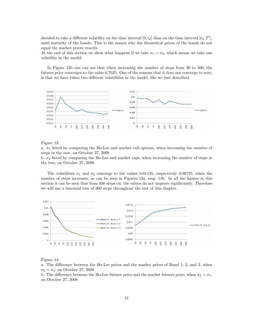
decided to take a different volatility on the time interval [0, td] than on the time interval [td, T i],until maturity of the bonds. This is the reason why the theoretical prices of the bonds do notequal the market prices exactly.At the end of this section we show what happens if we take σ1 = σ2, which means we take onevolatility in the model.

In Figure 12b one can see that when increasing the number of steps from 30 to 400, thefutures price converges to the value 0.7025. One of the reasons that it does not converge to zero,is that we have taken two different volatilities in the model, like we just described.

Figure 13:a. σ1 fitted by comparing the Ho-Lee and market call options, when increasing the number ofsteps in the tree, on October 27, 2008b. σ2 fitted by comparing the Ho-Lee and market caps, when increasing the number of steps inthe tree, on October 27, 2008

The volatilities σ1 and σ2 converge to the values 0.01135, respectively 0.00725, when thenumber of steps increases, as can be seen in Figures 13a, resp. 13b. In all the figures in thissection it can be seen that from 300 steps on, the values do not improve significantly. Thereforewe will use a binomial tree of 300 steps throughout the rest of this chapter.

Figure 14:a. The difference between the Ho-Lee prices and the market prices of Bund 1, 2, and 3, whenσ2 = σ1, on October 27, 2008b. The difference between the Ho-Lee futures price and the market futures price, when σ2 = σ1,on October 27, 2008

51

When taking volatility σ2 equal to σ1, it means that we do not calculate σ2 by fitting themarket and theoretical cap prices, but we assume that the volatility from delivery of the futureuntil maturity of the bonds equals the volatility from today until delivery of the future. Thisvolatility σ1 is found by fitting the OGBL market and theoretical price. In Figure 14a one can seethat the differences between the Ho-Lee and market Bund prices get smaller when the numberof steps increases. The error is much smaller than the error that we found, when assumingthat there are two different volatilities σ1 and σ2, and it is caused by the discretization of thecontinuous Ho-Lee model. When taking more steps, the discrete time model converges to thecontinuous time model and the errors becomes smaller.

4.2 Fitting the volatities σ1 and σ2

In this section we take a look at the results found by fitting the parameters σ1 and σ2. First wediscuss the volatilities, then the futures prices and at the end we look at the bond prices.

In Figure 15 one can see that the prices of the call option with strike 118 have extremefluctuations, so when fitting the volatility σ1 with these prices, we find unreliable values. Sincethe option with strike 119 has a much smoother graph, we decided to fit the volatility σ1 withthis option. The values that we have found for σ1 can be seen in Figure 16a.

Figure 15: Values of the call options with strikes S = 118, 119, and 120

The figure gives the volatility at the dates up to and including November 18, 2008. Thevolatility σ1 has a very nice value, because the difference between the smallest and largest valueis only 4.1 percent. On November 20, 2008, one day before expiration of the option, we cannotfit the volatility. The reason for this is that the closer we get to maturity, the closer the payoffof the option comes to

max(Futures price− Strike, 0),so the price of the option is not so sensitive to the volatility anymore. On November 20, 2008,the theoretical price of the call option can be calculated as:

Price of call option = max(Futures price− Strike, 0) = max(120.2− 119.0) = 1.20,

52

Figure 16:a. σ1 fitted by comparing the Ho-Lee and market call option with strike 119 b. σ2 fitted bycomparing the Ho-Lee and market caps

which is very close to the market call price of 1.21. This confirms what we just explained,the price of the call option does not depend on the volatility, but it converges to the value atdelivery. Therefore we were not able to fit the volatility on November 20, 2008.

In Figure 16b it can be seen that the volatility σ2 grows as the time evolves. The differencebetween the highest and lowest volatility is 4.3 percent.

We would like to check how well the model fits the theoretical futures price to the marketfutures price, when fitting the volatilities as described in Sections 3.3.3 and 3.3.4. In Figure 17awe can see the difference between these futures prices on the days between October 27, 2008 andNovember 18, 2008. We cannot look at the days after November 21, 2008, because the OGBLexpires on this day, so we cannot calculate σ1 on the succeeding days, because there is no marketprice of the call option available. We have just seen that one day before the expiration of theoption, the OGBL is not sensitive to volatility and therefore the value that we found for σ1 wasnot representative either. We exclude these dates in the rest of the analysis of this section andonly look at the futures price until November 18, 2008.

Figure 17:a. The difference between the Ho-Lee futures price and the market futures priceb. The difference between the Ho-Lee prices and the market prices of Bund 1, 2, and 3

From Figure 17a we can deduce that the closer we get to delivery of the future, the better

53

the model fits the futures price. This holds, because when we approach delivery, it becomesclearer, which bond will be the cheapest at delivery and the futures price depends on this bond.Also, as the time to delivery of the future decreases, it becomes more unlikely that there will beenormous changes in the zero curve. The largest difference between the market and theoreticalfutures price is on October 27, 2008 and is 6.0 percent, but the differences of the other datesare much smaller.

We will now take a look at the differences between today’s theoretical prices and today’smarket prices of Bund 1, 2, and 3, which can be seen in Figure 17b. Just like the futures pricedifferences, it also holds for the bond price differences that they become smaller when the timeevolves. The errors are very small, but still larger than zero.

4.3 Which bond is the cheapest to deliver

By calculating the bond and futures prices at the delivery nodes, we can find out at every node,which bond is the cheapest to deliver. In Table 10 it can be seen per day, what the lowest andthe highest short rate is in the tree, and at which value of the short rate Bund 1 and 3 switchfrom being the cheapest to deliver. Bund 1 is the CTD between the lowest short rate and thevalue in the second column of the table and Bund 3 is CTD between the value in column 3 andthe highest short rate. The short rates can be negative, as was already mentioned in Section 2,which can be seen very clearly in Figure 18a. The part between the blue line and the green lineis where Bund 1 is CTD, and the part between the red line and the purple line is where Bund3 is CTD.

Table 10: Overview of the short rate levels (in percent) at which the CTD changes from Bund1 to 3

Date Lowest short rate Bund 1 Bund 3 Highest short rateOctober 27, 2008 −3.60 5.10 5.14 9.67October 28, 2008 −3.77 4.92 4.96 9.76October 29, 2008 −4.20 4.79 4.84 10.18October 30, 2008 −4.55 4.61 4.66 10.42October 31, 2008 −3.85 4.65 4.70 9.60November 3, 2008 −4.03 4.55 4.59 9.83November 4, 2008 −3.47 4.71 4.75 9.21November 5, 2008 −3.43 4.75 4.80 9.12November 6, 2008 −3.14 4.73 4.77 8.62November 11, 2008 −1.84 4.72 4.75 7.54November 12, 2008 −2.04 4.57 4.60 7.59November 13, 2008 −1.59 4.52 4.54 6.94November 14, 2008 −1.52 4.37 4.40 6.83November 17, 2008 −1.45 4.82 4.85 7.56November 18, 2008 −1.17 4.71 4.74 6.97

We have seen which bond is the cheapest at the delivery of the future. In the nodes prior tothe delivery nodes, we can calculate the probabilities that Bund 1, Bund 2, or Bund 3 will bethe cheapest-to-deliver at delivery, just like we have done in Example 2. We look at the data ofOctober 27, 2008 and the graph demonstrates the probabilities between this date and delivery,that the bonds become the CTD. Bund 2 is in neither of the end nodes of the tree the cheapest,so the probability that Bund 2 becomes cheapest is zero in the whole tree. In Figure 18b the

54

Figure 18:a. The short rate levels, between the green and blue line Bund 1 is cheapest and between thered and purple line Bund 3 is cheapestb. The probability tree, in the blue area Bund 1 is cheapest, in the red area Bund 3 is cheapestand in the mixed colors they both have a probability of becoming the cheapest at delivery

blue area is the part where Bund 1 is the cheapest, the red area is where Bund 3 is the cheapestand the colors in between state that there is a probability that Bund 1 will become the cheapestat delivery aswell as there is a probability that Bund 3 will become the cheapest at delivery.

4.4 Sensitivity of the futures price

In this section we take a look at how sensitive the futures price is towards the bond prices andthe volatilities.

4.4.1 Influence of the bond prices on the futures price

First we show what happens to the theoretical futures price when one of the three bond pricesincreases or decreases by one. We assume that the bond prices are not correlated. We look atthe ratio:

original futures price− futures price after changing the bond priceoriginal bond price− bond price after changing

=∆Fj

∆bond j,

where j = 1, 2, or 3. In Section 4.2 we have fitted the volatilities σ1 and σ2, such that thetheoretical and market call, resp. cap prices were equal. We fix these volatilities and change oneof the three bond prices by one, which is approximately a one percent change. When the bondprice is changed, this means that the zero curve, the short rate tree and therefore the futuresprice is different. How much influence it has on the futures price can be seen in Figures 19a, band c.

In Section 3.2 we have seen that at delivery of the future, its price equals the minimum ofthe three bonds divided by their conversion factors. In case we change one of the bond pricesit is possible that another bond becomes the cheapest to deliver. In Figure 19c it can be seenthat even if Bund 3 would decrease with one, then its influence on the futures price is still verysmall.

If Bund 1 decreases with one, then the futures price decreases with approximately 1.13 atevery time point, see Figure 19a. This follows from the fact that Bund 1 is always cheaper than

55

Figure 19:a. The influence of Bund 1 on the futures priceb. The influence of Bund 2 on the futures pricec. The influence of Bund 3 on the futures price

the other bonds, so the futures price depends uniquely on this bond. This change in futuresprice is explainable, because when dividing the change in bond price by the conversion factor,we find:

1CF1

=1

0.885104≈ 1.13.

If Bund 1 increases by one, we see that its influence of the futures price is smaller. Thisfollows because Bund 1 is no longer the cheapest at all time points. For example, on November3, 2008,

price of Bund 1 + 1CF1

=104.02

0.885104≈ 117.53,

andprice of Bund 2

CF2=

101.090.863086

≈ 117.13,

so Bund 2 becomes the cheapest when Bund 1 increases by one.

The same holds when we decrease the price of Bund 2 by one, while keeping the other pricesfixed, then Bund 2 also becomes cheaper than Bund 1 at some time points. Figure 20 is a scatterdiagram with on the horizontal axis

price of Bund 1CF1

− price of Bund 2 − 1CF2

, (54)

Figure 20: On the horizontal axis: difference as described in Equation (54) and on the verticalaxis the difference in futures price when decreasing Bund 2 by one

56

and on the vertical axis the difference in futures price when decreasing Bund 2 by one. It canbe seen on the left side of the graph that when the term in Equation (54) is negative, Bund 1 isthe cheapest and Bund 2 barely effects the futures price. Otherwise, when it is positive, Bund2 is the cheapest and has a big effect on the futures price.

4.4.2 Influence of the volatilities on the futures price

In a similar way, we look at the difference in futures price when one of the volatilities is changed.We want to know vega, which is the ratio:

νi =original futures price− futures price after changing the volatility

original volatility− volatility after changing=

∆Fi

∆volatility i,

for i = 1 or 2. The value of νi that we obtain in this manner, is not very representative. It showsthe difference in futures price, when the volatility is changed by one, but since the volatilitiesare around 0.01 or even smaller, the ratio νi does not make sense. Therefore we look at the onepercent futures price change, so we divide look at vega divided by hundred.

We fix the bond prices and the volatility σ2, and change σ1 with approximately one percent,or 0.0001. We construct a new short rate tree and find different futures prices. The influenceof σ1 on the futures price, can be found in Figure 21a. From November 20, 2008, on, it isnot possible to determine the volatility σ1, so we use the volatility of November 18, 2008 forthese days. We can deduce from the results that when everything is kept fixed, except for thevolatility σ1, that has been increased, then the bond prices increase, and hence the futures priceincreases.

Figure 21:a. The influence of σ1 on the futures priceb. The influence of σ2 on the futures price

We change volatility σ2 with approximately one percent, or 0.00007, while fixing the bondprices and volatility σ1. We calculate the new bond and futures prices. The influence of σ2 onthe futures price, can be found in Figure 21b. In Equation (50), we can see that when everythingis kept fixed, except for the volatility σ2, that has been increased, the bond prices decrease, andhence the futures prices decrease. Vice versa, when σ2 decreases, the bond and futures pricesincrease.

One can see in the graphs of both volatilities that the lines of an up- or downwards change inthe volatilities are very close to each other, which means that for small changes, the difference

57

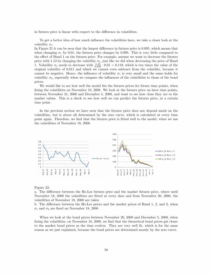
in futures price is linear with respect to the difference in volatilities.

To get a better idea of how much influence the volatilities have, we take a closer look at thevolatility σ1.In Figure 21 it can be seen that the largest difference in futures price is 0.095, which means thatwhen changing σ1 by 0.01, the futures price changes by 0.095. This is very little compared tothe effect of Bund 1 on the futures price. For example, assume we want to decrease the futuresprice with 1.13 by changing the volatility σ1, just like we did when decreasing the price of Bund1. Volatility σ1 needs to decrease with 1.13

0.095 · 0.01 = 0.119, which is ten times the value of theoriginal volatility of 0.011 and which we cannot even subtract from the volatility, because itcannot be negative. Hence, the influence of volatility σ1 is very small and the same holds forvolatility σ2, especially when we compare the influences of the volatilities to those of the bondprices.

We would like to see how well the model fits the futures prices for future time points, whenfixing the volatilities on November 18, 2008. We look at the futures price on later time points,between November 21, 2008 and December 5, 2008, and want to see how close they are to themarket values. This is a check to see how well we can predict the futures price, at a certaintime point.

In the previous section we have seen that the futures price does not depend much on thevolatilities, but is above all determined by the zero curve, which is calculated at every timepoint again. Therefore, we find that the futures price is fitted well to the model, when we usethe volatilities of November 18, 2008.

Figure 22:a. The difference between the Ho-Lee futures price and the market futures price, where untilNovember 18, 2008 the volatilities are fitted at every date and from November 20, 2008, thevolatilities of November 18, 2008 are takenb. The difference between the Ho-Lee prices and the market prices of Bund 1, 2, and 3, whenσ1 and σ2 are fixed on November 18, 2008

When we look at the bond prices between November 20, 2008 and December 5, 2008, whenfixing the volatilities, on November 18, 2008, we find that the theoretical bond prices get closerto the market bond prices as the time evolves. They are very well fit, which is for the samereason as we just explained, because the bond prices are determined mostly by the zero curve.

58

5 Conclusion

In this thesis we have studied the questions that were stated in the abstract. To answer thesequestions, we first examined a range of different short rate models in Chapter 2 and decidedthat the Ho-Lee model was the most appropriate model for our analysis. The reasons for thischoice are that the Ho-Lee model is an exogenous term structure model, that can compute thebond prices analytically, which is done in Section 2.2, and that it is very suitable for buildingrecombining trees, which we explained in detail in Section 2.2.2. The discrete and continuoustime models were compared in the succeeding section and a numerical approximation of thiscomparison was given. In the same chapter a series of interpolation methods was listed withtheir properties and it was pointed out why we decided to use the raw interpolation method inour model. The chapter was concluded with an example of how to bootstrap and interpolatewith real maket data to show that the bootstrapping and interpolation method go hand in hand.

In Chapter 3 we took a closer look at the Euro-Bunds and their futures. It was describedhow the bond and futures prices are calculated and how we can determine the cheapest bondat delivery from the bond prices and their conversion factors. We gave an overview of all theelements that were necessary to calculate the bond prices at delivery and made a Ho-Lee shortrate tree from ‘today’ until delivery of the future, on which we could price the bonds, futures,options and caps that we needed to find the volatilities and the bond and futures prices. Wetook two different volatilities in the model, one for ‘today’ until delivery of the future, and onefrom delivery until maturity of the bonds. We expected it to give a better fit than when usingone single volatility σ1 in the model, because this volatility could only be calculated for a veryshort time period.

In Chapter 4 real market data was used to fit the model and we were able to find the answersto the questions of the abstract.

How many steps are needed in the binomial tree to get good results?We investigated how many steps were needed to get nicely converged bond and futures pricesand discovered that from 300 steps on, the bond and futures prices and the volatilities σ1 andσ2 did not improve significantly anymore, hence we used a 300 steps-binomial tree in the restof our calculations.

Is it possible to predict beforehand which bond will be the CTD?Since the term structure is stochastic, we cannot give an exact prediction of which bond willbe the CTD on December 8, 2008, but what we can do, is make a tree of the probabilities thatBund 1, 2 or 3 will become the CTD. In Figure 18b these probabilities were demonstrated ofOctober 27, 2008. It gave an impression of the probabilities that Bund 1, resp. Bund 3 wouldbe the Cheapest-to-Deliver on December 8, 2008. The probability that Bund 2 would becomecheapest was zero. In the tree one can see that it is very likely that Bund 1 would becomethe cheapest at delivery, because only when the short rate would increase enormously, the CTDwould change from Bund 1 to Bund 3.

At what difference in the term structure is there a change in which bond is the cheapest?In Figures 18a and b it could be seen very clearly that in most cases Bund 1 was the cheapest.Together with Table 10 we can conclude that Bund 3 only becomes the cheapest, when the shortrate is very high, between 4.37 and 5.14. For more on this topic, see the next question.

How sensitive is the futures price for changes in the zero curve?The futures price is very sensitive to changes in the term structure. When Bund 1, that appeared

59

to be the cheapest at delivery, is decreased by one, the futures price decreases by approximately1.13 at all time points. When Bund 1 is increased by one, the change in futures price wasbetween 0.8 and 1.13, because at most dates, Bund 1 remained the CTD. Bund 2 also effectsthe futures price, but much less than Bund 1. If it decreases by one, the change in futures priceis at most 0.43. Bund 3 barely effects the futures price, because the change in futures price isat most 0.058.Note that the bond prices are usually highly correlated, so when looking at a change of onein the price of a bond, it is very unlikely that the other bonds stay fixed. Since Bund 1 hasthe most influence on the futures price, even with it is increased by one, we can conclude thatthere is only a very small probability that any of the other bonds would become the CTD. Forexample, when we mentioned that Bund 2 could become cheaper to deliver than Bund 1, if itsprice would decrease by one, this was based on the fact that the other bond prices were keptfixed. However, Bund 1 and Bund 3 will also decrease if Bund 2 decreases, so there is only avery small probability that Bund 2 would indeed become the cheapest.

How stable are the volatilities of the model and how sensitive is the futures price for changesin these parameters?The volatilities that we fitted, appeared to be quite stable, because the difference between theirsmallest and biggest values was only about four percent of the total value. They did not influ-ence the futures price much, because when changing σ1 by 0.01, the change in futures price wasbetween 0.01 and 0.095. Since volatilities cannot be negative and the value of the volatility σ1

itself is only around 0.011, this range actually gives the maximal decrease that is possible in thefutures price. Of course increasing the volatility can be done endlessly to increase the futuresprice, but to perceive a significant effect, the volatility should attain unreasonable high values.Changing σ2 with 0.01, leaded to a futures price change between −0.0575 and −0.0073, whichis even less than for volatility σ1. Indeed, the maximal futures change that can be reachedwhen decreasing this volatility does not attain these values, because the value of the volatilityis around 0.007, so it cannot decrease by 0.01. We can conclude that the volatilities both havea very small effect on the futures price.Because of this, we have taken a look at how far in the future we can still use the volatilities ofa certain date. We have looked at the bond and futures prices between November 20, 2008 andDecember 5, 2008, when we use the volatilities that were fitted on November 18, 2008. Sincethe futures price is mainly determined by the bond prices and much less by the volatilities, wealready expected the futures price to be priced well. In Section 4.4 this was confirmed. Sincethe model uses the bond prices as an input of the model, the bond prices were also fitted wellat the future time points, when using these fixed volatilities.

Is the Ho-Lee model a good model to price bonds and futures, i.e. how well does the model fittheir prices?After the analysis in Chapter 4 we are able to state that the Ho-Lee model is a very satisfactorymodel to price bonds and futures. We fitted the volatilities, and found a futures price that wasvery close to the market price. In the worst case, which was on October 27, 2008, there was adifference of 0.7 between the market and the theoretical price, which was only 0.6 percent of themarket price. At the later time points this difference was a lot smaller.A reason for the (small) difference between the theoretical and the market futures prices, couldbe that the market uses a slightly different term structure of interest rates than we have used toprice the future. For the first two years, we applied the Eonia swap rates, which are interbankinterest rates, and since they have a very low credit risk, just like the government bonds, wedecided that they would be a good replacement for the short term government rates. It couldbe that the gap between the market and theoretical futures price is caused by this differencebetween the two rates.

60

We checked what the differences between the market and theoretical bond and futures priceswere, when using one volatility for the whole model, σ1 = σ2. We calculated this volatility byfitting the market and theoretical OGBL prices, just like we did for σ1 and found a better fitfor the futures and bond prices. As the steps in the tree increased, the bond price differencesbecame much smaller than in the case we used two different volatilities. This means that wewere wrong in our assumption that it would be better to use a different volatility for the longterm instead of using the same volatility in the whole model. The short term volatility canindeed be used for the long term.

To conclude this thesis, here are some ideas for future investigation:

• taking one volatility for the whole model, as we just mentioned. This gave an improvedfit for the futures and bond prices.

• looking at a time-varying volatility, that is fitted at many time points. We have looked ata volatility with two different values, but maybe when increasing this number, it gives abetter fit.

• finding a better way to fit the long term volatility, until maturity of the bonds. This couldimprove the futures and bond prices. We have used the caps to do so, but as we mentionedearlier, they depend on interbank interest rates and the bonds and its future depend ongovernment interest rates.

• taking the forward volatility from td to the maturity of the bonds, when optimizing volatil-ity σ2. We have looked at the volatility from ‘today’ until the largest maturity of the threebonds, but it is more precise to take the volatility from time td on, and take some ‘averageforward volatility’ for the three maturities, eventually by calculating the spot and forwardvolatilities between the maturities and computing the intermediate volatility.

• using an alternative source for short term rates for the first two years, such as repo rates.These are rates at which one prime bank offers funds in euro to another prime bank if inexchange the former receives from the latter Eurepo as collateral, see www.eurepo.org.

61

References

[1] Damiano Brigo and Fabio Mercurio. Interest rate models, theory and practice. SpringerFinance, 2001.

[2] J.C. Cox, J.E. Ingersoll, and S.A. Ross. A theory of the term structure of interest rates.Econometrica, 53:385–407, 1985.

[3] M. Dothan. On the term structure of interest rates. Journal of Financial Economics,6:59–69, 1978.

[4] Patrick S. Hagan and Graeme West. Methods for constructing a yield curve. 2007.

[5] T.S.Y. Ho and S.-B. Lee. Term structure movements and the pricing of interest ratecontingent claims. The journal of finance, 41:1011–1029, 1986.

[6] John C. Hull. Options, Futures and Other Derivatives. Pearson Printice Hall, sixth edition,2006.

[7] John C. Hull and A. White. Pricing interest rate derivative securities. Review of financialstudies, 3:573–592, 1990.

[8] David G. Luenberger. Investment Science. Oxford University Press, 1998.

[9] Christopher Plona. The European Bond Basis. Irwin Professional Publishing, 1997.

[10] J. M. Steele. Stochastic Calculus and Financial Applications. Springer.

[11] A. W. v.d. Vaart. Financial stochastics. 2005.

[12] O. Vacıcek. An equilibrium characterization of the term structure. Journal of FinancialEconomics, 5:177–188, 1977.

[13] D. Williams. Probability with martingales. Cambridge University Press, 1991.

[14] Harry v. Zanten. An introduction to stochastic processes in continuous time. 2007.

62

6 Appendix

6.1 Derivation of the Vasicek model

dr(t) = a(θ − r(t))dt + σdWt,

where θ, a and σ are positive constants. Applying Ito’s formula with Y (u) = γ(u, r(u)) = r(u)eau

gives:

dY (u) = ar(u)eaudu + eaudr(u)= ar(u)eaudu + eau ((θ − ar(u))du + σdWu)= aθeaudu + σeaudWu

Integrating this equation for t ≤ u, leads to:

r(u)eau = r(t)eat +∫ u

t

aθeasds +∫ u

t

σeasdWs

= r(t)eat + θ(eau − eat) + σ

∫ u

t

easdWs

r(u) = r(t)e−a(u−t) + θ(1− e−a(u−t)) + σ

∫ u

t

e−a(u−s)dWs,

so r(u) conditional on Ft is normally distributed with mean respectively variance:

E(r(u)|Ft) = r(t)e−a(u−t) + θ(1− e−a(u−t)),

Var(r(u)|Ft) = E(

σ

∫ u

t

e−a(u−s)dWs|Ft

)2

(17)= σ2E

(∫ u

t

e−2a(u−s)ds|Ft

)=

σ2

2a(1− e−2a(u−t)).

6.2 Matlab codes

In this section, the following Matlab codes can be found:

1. bootstrapping per time, this file is the main file, which bootstraps the zero curve, addsthe Eonia rates to the zero curve, builds the Ho-Lee short rate lattice and calculates thefutures prices, bond prices, σ1 and σ2, by making use of the following other files, seepage 64.

2. vol1c calculates the σ1 by comparing the market option price by the option price thatfollows from the Ho-Lee tree, see page 66.

3. vol2a and vol2b calculate the σ2 by comparing the market cap price by the Ho-Lee capprice, see page 68.

4. InterpolatedSpot1 and InterpolatedSpot2 calculate the zero rates in the intermediate timesteps, see page 70.

5. fita1a, fita1b, fita2a, fita2b calculate the Ho-Lee short rate trees, see page 71.

63

function [sigma1,fval1,sigma2,fval2] = bootstrapping_per_time(k)

M = 300;[num1,txt1] = xlsread(’BondData_Compact.xls’,’BondInformation’);[num2,txt2] = xlsread(’BondData_Compact.xls’,’Aligned_HistoricalPrices’);[num3,txt3] = xlsread(’BondData_Compact.xls’,’Aligned Eonia Swap’);[num4,txt4] = xlsread(’BondData_Compact.xls’,’FGBL’);

Start = datenum(txt4(k+1,1));StartNum = floor(Start);StartDate = datestr(StartNum);BundDate = datenum(txt2(2:size(txt2,1),1));for i=1:length(BundDate)if Start < BundDate(i) && Start > BundDate(i+1)

Bund_m = num2(i+1,8:10)end

endFut_m = num4(k,1)

EoniaNum = datenum(txt3(3:size(txt3,1),1));for i = 1:length(EoniaNum)if EoniaNum(i) == StartNum

ZR_Eonia = num3(i+1,:)/100;end

endt_Eonia = num3(1,:)/365;ZR_Eonia;

BootDate = datenum(txt2(2:size(txt2,1),1));for i = 1:length(BootDate)

if Start < BootDate(i) && Start > BootDate(i+1)BPclean = num2(i+1,:);

elseif k==1BPclean = num2(1,:);

endend

MaturityDates(1:(size(txt1,1)-1)) = txt1(2:size(txt1,1),11);for i = 1:length(MaturityDates)

Maturity(i) = (datenum(cell2mat(MaturityDates(i)))-datenum(StartDate))/365;endFirstCouponDate = txt1(2:size(txt1,1),10);for j = 1:length(FirstCouponDate)

FirstCoupon(j) = (datenum(cell2mat(FirstCouponDate(j)))-datenum(StartDate))/365;end

c = num1(:,1);freq = [2,3,4,5,7,8,9,9,10,10,16];C = zeros(length(freq),freq(end));for i = 1:length(freq)

64

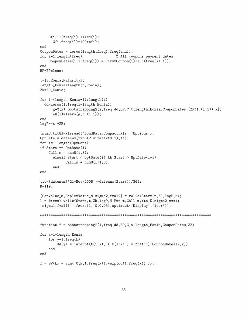
C(i,1:(freq(i)-1))=c(i);C(i,freq(i))=100+c(i);

endCouponDates = zeros(length(freq),freq(end));for i=1:length(freq) % All coupons payment dates

CouponDates(i,1:freq(i)) = FirstCoupon(i)+(0:(freq(i)-1));endBP=BPclean;

t=[t_Eonia,Maturity];length_Eonia=length(t_Eonia);ZR=ZR_Eonia;

for i=(length_Eonia+1):length(t)dd=zeros(1,freq(i-length_Eonia));

g=@(x) bootstrapping2(i,freq,dd,BP,C,t,length_Eonia,CouponDates,[ZR(1:(i-1)) x]);ZR(i)=fzero(g,ZR(i-1));

endlogP=-t.*ZR;

[num8,txt8]=xlsread(’BondData_Compact.xls’,’Options’);OptDate = datenum(txt8(2:size(txt8,1),1));for i=1:length(OptDate)if Start == OptDate(i)

Call_m = num8(i,3);elseif Start < OptDate(i) && Start > OptDate(i+1)

Call_m = num8(i+1,3);end

end

tto=(datenum(’21-Nov-2008’)-datenum(Start))/365;K=119;

[CapValue_m,CapletValue_m,sigma2,fval2] = vol2a(Start,t,ZR,logP,M);l = @(xxx) vol1c(Start,t,ZR,logP,M,Fut_m,Call_m,tto,K,sigma2,xxx);[sigma1,fval1] = fzero(l,[0,0.05],optimset(’Display’,’iter’));

*********************************************************************************

function f = bootstrapping2(i,freq,dd,BP,C,t,length_Eonia,CouponDates,ZZ)

for k=i-length_Eoniafor y=1:freq(k)

dd(y) = interp1(t(1:i),-( t(1:i) ).* ZZ(1:i),CouponDates(k,y));end

end

f = BP(k) - sum( C(k,1:freq(k)).*exp(dd(1:freq(k)) ));

65

function f = vol1c(Start,t,ZR,logP,M,Fut_m,Call_m,tto,K,sigma2,xxx)

StartDate = datestr(floor(Start));ttd=(datenum(’8-Dec-2008’)-datenum(StartDate))/365;

if ttd<=7/365t= [0,t];

ZR = [ZR(1),ZR];logP = -t.*ZR;P_ttd = exp(interp1(t,logP,ttd));forw_ttd = (logP(1)-logP(2))/(t(2)-t(1));dt1 = ttd/M;NewSpot1(1:M) = ZR(1);[d1,SR1] = fit_a_1a(dt1,NewSpot1,M,xxx);

end

for i=1:length(t)-1if ttd>t(i) && ttd<=t(i+1)

P_ttd = exp(interp1(t,logP,ttd));forw_ttd = (logP(i)-logP(i+1))/(t(i+1)-t(i));Spot1 = ZR(1:i+1);tt = t(1:i+1);[dt1,NewSpot1] = InterpolatedSpot1(ttd,tt,Spot1,M);[d1,SR1] = fit_a_1a(dt1,NewSpot1,M,xxx);

endendSRlastcol = SR1(:,M);

[num5,txt5]=xlsread(’BondData_Compact.xls’,’BundInformation’);

Bund_FirstCouponDate = txt5(2:4,10);Bund_FirstCoupon = (datenum(cell2mat(Bund_FirstCouponDate))-datenum(StartDate))/365;Bund_c = num5(:,1);Bund_freq = [9,10,10];Bund_C = zeros(3,10);P_total = zeros(M,M,3);for bb=1:3

Bund_C(bb,1:(Bund_freq(bb)-1)) = Bund_c(bb);Bund_C(bb,Bund_freq(bb)) = 100 + Bund_c(bb);Bund_CouponDates(bb,1:Bund_freq(bb))=Bund_FirstCoupon(bb)+(0:(Bund_freq(bb)-1));P_coupon(bb,1:Bund_freq(bb))=exp(interp1(t,logP,Bund_CouponDates(bb,1:Bund_freq(bb))));P_ttd_coupon = zeros(M,Bund_freq(bb),3);for s=1:M

for j=1:Bund_freq(bb)P_ttd_coupon(s,j,bb)=P_coupon(bb,j)./P_ttd....*exp(-(Bund_CouponDates(bb,j)-ttd)....*(SR1(s,M)-forw_ttd)-1/2*(sigma2)^2*ttd....*(Bund_CouponDates(bb,j)-ttd)^2);

endP_total(s,M,bb)=sum(P_ttd_coupon(s,1:Bund_freq(bb),bb).*Bund_C(bb,1:Bund_freq(bb)));

end

66

end

CF = [0.885104,0.863086,0.874950];Fut = zeros(M,M);CTD = zeros(M,1);for s=1:M

for i=1:3Fut_total(s,i) = (P_total(s,M,i)./CF(i));

endif Fut_total(s,1) < Fut_total(s,2) && Fut_total(s,1) < Fut_total(s,3)

CTD(s) = 1;Fut(s,M) = Fut_total(s,1);

elseif Fut_total(s,2) < Fut_total(s,1) && Fut_total(s,2) < Fut_total(s,3)CTD(s) = 2;Fut(s,M) = Fut_total(s,2);

elseif Fut_total(s,3) < Fut_total(s,1) && Fut_total(s,3) < Fut_total(s,2)CTD(s) = 3;Fut(s,M) = Fut_total(s,3);

endendfor j=M-1:-1:1

for k=j:-1:1Fut(k,j) = 1/2 * (Fut(k,j+1) + Fut(k+1,j+1));for i=1:3

P_total(k,j,i) = 1/2 * d1(k,j)*(P_total(k,j+1,i) + P_total(k+1,j+1,i));end

endend

Fut_th = Fut(1,1)P_th = P_total(1,1,1:3)

ii = round(tto/dt1);for kk = 1:ii

if Fut(kk,ii) - K > 0Call(kk,ii) = Fut(kk,ii) - K;

elseCall(kk,ii) = 0;

endendfor j=ii-1:-1:1

for k=j:-1:1Call(k,j) = 1/2 * (Call(k,j+1)+Call(k+1,j+1));

endendCall_th = Call(1,1)

f = Call_th - Call_m

67

function [CapValue_m,sigma2,fval2] = vol2a(Start,t,ZR,logP,M)

[num7,txt7]=xlsread(’CapData2.xls’,’Aligned vol-strike’);

CapDate = datenum(txt7(2:size(txt7,1),1));CapVolList = num7(:,2)/100; % cont. comp. act/365CapStrikeList = num7(:,4)/100; % cont. comp. act/365

for i=1:length(CapDate)if Start < CapDate(i) && Start > CapDate(i+1)

CapStrike = CapStrikeList(i+1);CapVol = CapVolList(i+1);

elseCapStrike = CapStrikeList(end);CapVol = CapVolList(end);

endendNumCaplets = 19;CapletResets = 1/2 * (1:NumCaplets);CapletPayments = 1/2 + CapletResets;Totaltimes = [1/2,CapletPayments];logP_CapletPayments=interp1(t,logP,Totaltimes);P_CapletPayments=exp(logP_CapletPayments)for i = 1:NumCaplets

F_caplet(i)=(logP_CapletPayments(i)-logP_CapletPayments(i+1))/(1/2)d1(i) = (log(F_caplet(i)/CapStrike)+(1/2)*(CapVol^2)*CapletResets(i)) ...

./ (CapVol*sqrt(CapletResets(i)))d2(i) = d1(i) - CapVol * sqrt(CapletResets(i))CapletValue_m(i) = 1/2 * P_CapletPayments(i+1) .* (F_caplet(i)*normcdf(d1(i)) ...- CapStrike .* normcdf(d2(i)))

endCapValue_m = sum(CapletValue_m);

h = @(yy) vol2b(t,ZR,M,CapStrike,NumCaplets,Totaltimes,CapletPayments,logP,logP_CapletPayments,P_CapletPayments,CapValue_m,yy);[sigma2,fval2] = fzero(h,[0,0.05],optimset(’Display’,’iter’));

*********************************************************************************

function f = vol2b(t,ZR,M,CapStrike,NumCaplets,Totaltimes,CapletPayments,logP,logP_CapletPayments,P_CapletPayments,CapValue_m,yy)

[dt2,NewSpot2] = InterpolatedSpot2(t,ZR,M,CapletPayments);[d2,SR2] = fit_a_2a(dt2,NewSpot2,M,yy);SRlastcol = SR2(:,M);

eps = dt2/10;logP_eps=interp1(t,logP,Totaltimes+eps);

for cc=1:NumCapletsi = round((cc*(1/2))/dt2); % i = reset_stepreset_time = cc/2;F_instan(cc)=(logP_CapletPayments(cc)-logP_eps(cc))/eps;

68

CV = zeros(i,i);for j=1:i

P_reset_payoff(j) = (P_CapletPayments(cc+1)/P_CapletPayments(cc))...*exp(-(1/2)*(SR2(j,i)-F_instan(cc))-(1/8)*(yy^2)*reset_time);

forw_reset_payoff(j) = -2*log(P_reset_payoff(j));if forw_reset_payoff(j) - CapStrike > 0

CV(j,i) = (forw_reset_payoff(j) - CapStrike)* P_reset_payoff(j);else

CV(j,i) = 0;end

endfor j=(i-1):-1:1

for k=j:-1:1CV(k,j) = 1/2 * d2(k,j) * (CV(k,j+1)+CV(k+1,j+1));

endendCV;CapletValue_hl(cc) = 1/2 * CV(1,1);

end

CapValue_hl = sum(CapletValue_hl);f = CapValue_hl - CapValue_m

69

function [dt1,NewSpot1] = InterpolatedSpot1(ttd,tt,Spot1,M)

D = exp(-Spot1.*(tt));logD_ttd = interp1(tt,log(D),ttd);Spot_ttd = -(1/ttd)*(logD_ttd);

tttt = [tt(1:length(tt)-1),ttd];Spot1 = [Spot1(1:length(tt)-1),Spot_ttd];

T=ttd;dt1=T/M;

% The zero rates are known from 7 days on, we extrapolate for the rates% < 7 days and interpolate in the usual way from > 7 days

D=exp(-Spot1.*tttt);NewD=zeros(M,1);for i=1:M

if i*dt1 < tttt(1)NewD(i)=D(1)^(i*dt1/tttt(1));

elseif i*dt1 >= tttt(1)NewD(i) = interp1(tttt,log(D),i*dt1);NewD(i) = exp(NewD(i));

endend

for i=1:M;NewSpot1(i)=-(1/(i*dt1))*log(NewD(i));

end

*********************************************************************************

function [dt,NewSpot] = InterpolatedSpot2(t,Spot,M,CapletPayments)

dt=CapletPayments(end)/M;D = exp(-Spot.*(t));for i=1:M;

if i*dt < t(1)NewSpot(i)=Spot(1);

elseif i*dt >= t(1)NewD(i) = interp1(t,log(D),i*dt);NewSpot(i)=-(1/(i*dt))*(NewD(i));

endend

70

function [d1,SR1] = fit_a_1a(dt1,NewSpot1,M,sigma1)

global EP1 d1

a1=NewSpot1(1);b=zeros(2,1);b=b+2*sigma1*sqrt(dt1);[indxa,indxb]=meshgrid(1:2,1:2);d1=exp(-dt1*(a1+b(indxb).*(indxb-1)));

EP1=zeros(M+1,M+1);EP1(1,1)=1;EP1(1,2)=1/2*d1(1,1)*EP1(1,1);EP1(2,2)=1/2*d1(1,1)*EP1(1,1);

% M is the length of the NewSpot=the interpolated spot ratesfor ii=2:M

N=length(a1)+1; % The vector of parameters a is known up to time N-1,% so it has length N-1.

g=@(x) fit_a_1b(dt1,NewSpot1,[a1(1:(N-1)) x],sigma1);% we put a(N)=x and then let f=0.a1(ii) = fzero(g,a1(N-1));

end

SR1=(-1/dt1).*log(d1);

*********************************************************************************

function f = fit_a_1b(dt1,NewSpot1,aa,sigma1)

global EP1 d1

M=length(NewSpot1);N=length(aa);

b=2*sigma1*sqrt(dt1);

[indxa,indxb]=meshgrid(1:N,1:N);d1=exp(-dt1*(aa(indxa)+b*(indxb-1)));

EP1(1,N+1)=1/2*d1(1,N)*EP1(1,N);

EP1(N+1,N+1)=1/2*d1(N,N)*EP1(N,N);

for i=2:N;EP1(i,N+1)=1/2*(d1(i,N)*EP1(i,N)+d1(i-1,N)*EP1(i-1,N));end

zcbvolgensSpot=exp(-NewSpot1(N).*N*dt1); % zcb=zero-coupon-bondzcbvolgensHoLee=sum(EP1(:,N+1));f=zcbvolgensSpot-zcbvolgensHoLee;

71

*********************************************************************************

function [d2,SR2] = fit_a_2a(dt,NewSpot,M,yy)

global EP2 d2

a2=NewSpot(1);

b = zeros(2,1);b = b+2*yy*sqrt(dt);[indxa,indxb] = meshgrid(1:2,1:2);d2 = exp(-dt*(a2+b(indxb).*(indxb-1)));

EP2 = zeros(M+1,M+1);EP2(1,1) = 1;EP2(1,2) = 1/2 * d2(1,1) * EP2(1,1);EP2(2,2) = 1/2 * d2(1,1) * EP2(1,1);

% M is the length of the NewSpot=the interpolated spot ratesfor ii = 2:M

N = length(a2)+1; % The vector of parameters a is known up to time N-1,% so it has length N-1.

g = @(x) fit_a_2b(dt,NewSpot,[a2(1:(N-1)) x],yy);% we put a(N)=x and then let f=0.a2(ii) = fzero(g,a2(N-1));

end

SR2=(-1/dt)*log(d2);

*********************************************************************************

function f = fit_a_2b(dt,NewSpot,aa,yy)

global EP2 d2

M=length(NewSpot);N=length(aa);

b=2*yy*sqrt(dt);

[indxa,indxb]=meshgrid(1:N,1:N);d2=exp(-dt*(aa(indxa)+b*(indxb-1)));

EP2(1,N+1)=1/2*d2(1,N)*EP2(1,N);

EP2(N+1,N+1)=1/2*d2(N,N)*EP2(N,N);

for i=2:N;EP2(i,N+1)=1/2*(d2(i,N)*EP2(i,N)+d2(i-1,N)*EP2(i-1,N));end

72

zcbvolgensSpot=exp(-NewSpot(N).*N*dt); % zcb=zero-coupon-bondzcbvolgensHoLee=sum(EP2(:,N+1));f=zcbvolgensSpot-zcbvolgensHoLee;

73