Determination of the fossil carbon content in combustible municipal soliD waste in sweDen

rapport u2012:05ISSN 1103-4092

Preface

The predictions of waste incinerations contribution to climate change is based on sorting analysis and assumptions that provides a simplified picture with major sources of error. A study with C14 method has shown that the proportion of fossil carbon dioxide from waste incineration, probably is less than believed. The aim of this project was to determine the proportion of the fossil emissions from waste incineration in Sweden by measurements of waste and flue gas.

The project was conducted by Evalena W Blomqvist and Frida Jones, both from SP Technical Research Institute of Sweden.

Malmö, Sweden April 2012

Håkan Rylander Weine WiqvistChairman of the Research and Development Managing DirectorCommittee, Swedish Waste Management Swedish Waste Management

abstract

Determination of the fossil carbon content in combustible Swedish municipal solid waste

This project aimed to determine the fossil carbon content in municipal solid waste used as a fuel in Sweden by using four different methods at seven geographically spread combustion plants. In total, the measurement campaign comprised 42 solid waste samples, 21 flue gas samples, three sorting analyses and two investigations of fossil carbon content by using the balance method. The fossil carbon content in the solid waste samples and in the flue gas samples was determined by using an accredited laboratory for C14 analysis. From the C14 analyses it was concluded that about a third of the carbon in solid waste is of fossil origin. The two other methods, based on assumptions and calculations, gave similar results in the plants where they were used. Furthermore, the chemical characterisation of all the solid waste samples showed a relatively homogeneous composition in terms of the elements present. A systematic error for the solid sampling method was discovered during the project, making the total measurement uncertainty 14 % fossil carbon, compared to 3 % fossil carbon for the flue gas samples. It was also noted that the accuracy of determining the fossil content by sorting analysis is greatly affected by knowledge of, and correct data for, different waste fractions, and particularly for the plastic fraction’s moisture content.

Key words: Waste combustion, fossil share, C14

abbreviations

AMS Accelerator Mass SpectrometrypMC Percentage Modern CarbonSD Standard Deviation SRF Solid Recovered Fuel

Preface

This project has been a substantial national project that has provided a wealth of interest and learning. All those involved in it have participated with great enthusiasm and generosity of expertise and knowledge. We would like to take this opportunity to thank everyone involved from the following organisations: Swedish Waste Management, the Swedish Energy Agency, the Swedish Environmental Protection Agency, SP, Profu, Ramböll, Miljömätarna and those who participated from the seven waste combustion plants: Dåva CHP plant (Umeå Energi), Högdalen (Fortum), Händelöverket (Eon), Tekniska Verken in Linköping, Ryaverket (Borås Energi och Miljö), Renova (Göteborg) and Sysav in Malmö.

summary

The results from this project show that the proportion of fossil carbon in municipal solid waste used for combustion in Sweden is about one third. The conclusions are based on results from four different analysis methods used in seven waste combustion plants in Sweden. Each plant took six solid waste samples and three flue gas samples, and both types were analysed in terms of the proportion of fossil carbon at Betalab Inc. in Miami, USA. In addition, all solid waste samples were also used for further chemical characterisation, which gave a good picture of the waste’s chemical composition and its variations. In addition to the solid samples and flue gas samples, three of the plants performed sorting analyses, and two plants used the balance method to calculate the fossil content by using the software BIOMA©. The balance method is a method based on the fact that there are several fundamental differences between how the biogenic carbon and the fossil carbon react in a combustion process. These differences allow separation of the processes by computer models.

The results from the chemical characterisation of the waste show that the difference between the samples that contained high proportions of industrial waste (nearly 80 %) and the municipal solid waste were not as great as first expected. The main parameters, such as the amounts of carbon, oxygen and hydrogen, show a relative standard deviation of less than 10 %. The mean calorific value of all samples was measured to be about 11 MJ/kg.

The results from the fossil proportion study of all solid samples and flue gas samples indicate fossil carbon proportions of 36 % and 38 % respectively. This corresponds to a fossil carbon share of approximately 10 % by weight in a waste mixture. The two other methods, based on assumptions and calculations, gave similar results in the plants where they were used. Simplified, it can be said that a third of the waste that is combusted in Sweden has a fossil origin. During the project, a systematic error was discovered in the solid waste sampling method. The method delivers too low results when there is a low proportion of fossil carbon in the waste, and slightly too high results when there is a higher proportion of fossil material in the waste. The total measurement uncertainty (i.e. the sum of the random and systematic errors) is estimated to amount to 3 % fossil carbon for the flue gas samples, while the solid sampling method has a much greater uncertainty due to the systematic error, amopunting to 14 % of fossil carbon. The accuracy of determining the fossil proportion by sorting analysis is greatly affected by knowledge of and correct facts about different waste fractions, mainly the moisture content of the plastic fraction.

The balance method was evaluated over a three-month period by installing the software in one plant, and using previously logged data from another plant to perform calculations. Overall, the balance method is a user-friendly method, but there are some areas that need to be further developed before it is fully suitable for this application. The method was used for only a short period of time in this project, which means that there are significant potential to improve the measurement uncertainty for continuous use.

Besides investigating the fossil proportion of the waste, the project also included investigation of the usability of various methods. However, it is difficult directly to compare the different methods used in this project as, in addition to estimation of fossil carbon emissions, the methods provide other information, of value to the plant owner. The choice of method can also be affected by factors other than direct determination of the fossil fuel emissions.

contents

1 background 11.1 project aims 11.2 the project group 21.3 legal requirements and regulations 21.4 earlier studies in sweden 32 methods 42.1 sampling plan 42.2 sampling of solid waste fuels 52.2.1 Grate-type boilers 52.2.2 fluidised bed boilers 52.3 fuel analyses 52.3.1 element analysis 52.3.2 Determination of the proportion of fossil carbon in solid waste samples 62.4 flue gas sampling 62.5 Determination of the proportion of fossil carbon 62.5.1 background concentration 62.5.2 calculation of fossil carbon 72.5.3 fossil-free waste – a reference 72.6 the balance method 82.7 the sorting analysis method 92.7.1 sorting analyses 92.7.2 the calculation method 103 results 113.1 chemical characterisation of waste 113.2 Determination of fossil carbon in waste by chemical analysis 123.2.1 background concentration in the waste 123.2.2 calculation of fossil carbon in waste with different background concentrations 133.3 four methods of determination of the fossil carbon content of waste 133.3.1 comparison of solid fuel sampling and flue gas sampling 133.3.2 the balance method 153.3.3 the sorting analysis method 183.3.4 evaluation of all four methods in one plant 204 conclusions 235 continued work 246 references 25

appendix i - fuel sampling 27appendix ii -– more about the balance method 35appendix iii -sorting analysis method – report from profu 37appendix iV -results from the chemical analysis of the waste fuel from alla plants 42appendix V -Determination of fossil carbon 56

1

1. background

The waste management sector will very probably be facing changes in national policy measures over the next few years: it is likely, for example, that emission rights for the fossil carbon proportion in domestic waste will be introduced in 2013. Changes such as these emphasise the importance of methods for correct determination of the proportions of fossil carbon and biogenic carbon in emissions from waste combustion plants.

The methods that are used today to estimate emission quantities of fossil carbon from waste combustion are based on sorting analyses and rule-of-thumb calculations, which most probably result in a simplistic view with a risk of major sources of error. Analysis results from a smaller feasibility study that was performed by Renova in Göteborg showed that the proportion of fossil carbon dioxide from waste combustion can be lower than had previously been assumed. This project (i.e. as of this report) was initiated as a result of the Renova project in order to perform a careful investigation and to collect material for a discussion of the role of waste combustion in a climate-aware waste management and energy system. The results can then provide a basis for better assessment of the climate effects of waste combustion, and also provide material for discussions of various policy measures, such as green electricity certificates or emission rights trading.

Sweden is not the only country that has started to investigate the matter of direct fossil carbon emissions from waste combustion. Work is in progress, or is being started in, for example, Denmark, Holland and the UK.

1.1 Project aims The aim of the project has been to determine the proportion of fossil carbon in the waste that is burnt in Sweden, and to evaluate the advantages and drawbacks of four different methods of determination, namely: 1. sampling of the solid waste, 2. flue gas sampling, 3. calculations using the balance methods, and finally 4. modelling based on sorting analyses.

As the work has resulted in the taking of a large number of solid waste samples, it has also provided a potential basis for chemical characterisation of the waste that is burnt in Sweden.

The long-term and overall aim of the project has been to provide the industry and public authorities with high-quality data for coming discussions on changes to future policy measures concerned with the waste field.

2

1.2 The project group The project was initiated and financed by Swedish Waste Management in 2010. Other financers of the project are the Swedish Energy Agency and the seven participating waste combustion plants: Dåva CHP plant (Umeå Energi), Högdalen (Fortum), Händelöverket (Eon), Tekniska Verken in Linköping, Ryaverket (Borås Energi och Miljö), Renova (Göteborg) and Sysav in Malmö.

Project management has been in the hands of SP Technical Research Institute of Sweden, together with a management group of representatives from each of the participating plants, Swedish Waste Management, the Swedish Energy Agency and the Swedish Environmental Protection Agency. Others involved in the project have been Miljömätarna AB, Ramböll Energy, and Profu who, in that named order, have performed flue gas analyses, balance method calculations and sorting analysis calculations respectively.

1.3 Legal requirements and regulations Waste combustion is an area that is well regulated. It is covered both by regulations for waste management and by regulations governing the energy sector. Regulations and policy measures for the sector have been concerned with various aspects: however, here we consider only some of those that are relevant in connection with the proportion of fossil carbon in waste.

The taxation of waste when used as a combustion fuel has been investigated on several occasions. The most recent of which are ”En BRASkatt? - beskattning av avfall som förbränns” [”A burning tax? – Taxation of waste used as fuel”] [1] and ”Skatt i retur” [”Tax back”] [2]. After a number of consultation circulations, and various changes, the former resulted in domestic waste being included among the fuels that would be taxed under the Act Concerning Tax on Energy [3] that was introduced on 1st July 2006, while the latter provided the main reason for excluding domestic waste under the same Act with effect from 1st October 2010.

There have been several reasons for taxing the combustion of waste. On the one hand, the wish to achieve greater quantities of materials recovery, while on the other the aim of fulfilling the overlying aims of the Swedish energy system (such as combined heat and power [CHP] production). When waste was so taxed, it was on a rule-of-thumb basis that 12,6 % of municipal solid waste (MSW) consisted of fossil carbon. In addition, it was only domestic waste that was taxed. The use of an assumed proportion of fossil carbon was due to the fact that it was regarded as too difficult and expensive to measure the actual proportion of fossil carbon. Skatt i Retur also pointed out these factors, and noted that, apart from its effect on CHP production, the tax did not deliver the policy effect that it was supposed to do.

The situation today is that there is another rule-of-thumb value for the proportion of fossil carbon in domestic waste. It is set out in the Act Concerning Guarantees of Origin, which came into force on 1st December 2010, and in which 60 % of energy from domestic waste is regarded as being from renewable sources.

The new trading period of the EU Emissions Trading Scheme (ETS), from 2013 to 2020, includes co-combustion plants. The status of the Swedish combustion plants, which are traditionally regarded as waste combustion plants, is unclear, and it may be so that ‘ordinary waste combustion plants’ will fall within the remit of the system from 2013. This has created additional pressure to measure fossil carbon emissions, as ETS requires high accuracy in determination of emissions. The accuracy required assumes,

3

or is based on, the use of more homogeneous fuels, such as oil or coal, but affects waste used as fuel as the rules require the same accuracy regardless of the type of fuel. Work is at present in progress on drafting regulations for measurement and monitoring in connection with ETS. As these regulations have not yet been published, it can at present only be noted that the results of this project are of particular relevance to legislative aspects as well as to the purely quantitative aspects.

1.4 Earlier studies in Sweden Profu’s 2003 report ”CO2 utsläpp från svensk avfallsförbränning1” [4] describes investigation of what proportion of the fuel burnt in Swedish waste combustion plants should be regarded as being of fossil origin. The results are based on the composition of waste, as reported by Swedish waste combustion plants to RVF2 from 1996 until the date of the study. In the report’s conclusions, Profu states that about 14 % by weight of the incoming waste is of fossil origin. The report is also summarised, with an additional preface and comments, in RVF’s report no. 2003:12 [5]. The report’s results provide the basis for guidelines such as 85 % of waste used as fuel should be regarded as biofuel, and recommendations that the CO2 factor for combustion of waste should be just 25 g/MJ of fuel in official reports.

On its own initiative, Renova in Göteborg has investigated five fuel samples taken in 2008 from the Sävenäs CHP waste combustion plant. The samples, of mixed waste, were taken from the waste bunker using the same method as used in this project. The proportion of carbon-14 was then analysed, although by an as-yet-unaccredited laboratory. These first results showed a proportion of fossil carbon in the mixed waste of only about 10 %, which was very much lower than the value that had been assumed in the rule-of-thumb values employed by public authorities and the waste sector today [5]. As the results of these first analyses were unexpectedly low, the samples were analysed again, by Beta Analytics in the USA, which is an accredited analysis laboratory. These analysis results showed a fossil carbon content of closer to 30 %, showing the importance of using the services of a laboratory that is accredited for determining fossil carbon proportions.

1 ”CO2 emissions from Swedish waste combustion”. 2 RVF has since changed its name to Avfall Sverige (Swedish Waste Management).

4

2 methods

2.1 Sampling plan The project involved seven waste combustion plants, geographically distributed across the country from Malmö in the south of Umeå in the north, and using either travelling grate or fluidised bed boilers as typical of the country’s waste combustion plants (see Table 1). Over the period from October 2010 to August 2011, all seven plants took six representative waste samples and three flue gas samples, and also created two “fossil-free” waste samples (see 2.5.3 below). In addition, four of the plants also performed sorting analyses to produce data for future calculations / modelling, while two plants also evaluated application of the balance method (see 2.6 below). All the methods were applied in such a way as to produce a representative 24-hour sample. The samples were also distributed in time, in order to produce a matrix that was as representative as possible of a year’s combustion of waste in Sweden. The sampling matrix shown below (Table 2) shows when the samples were taken at each plant.

Table 1 Plants in the project plant town type of plant

renova Göteborg Grate

sysav malmö Grate

umeå energi umeå Grate

fortum högdalen stockholm Grate

tekniska Verken linköping Grate

eon händelöverket norrköping fluidised bed

borås energi och miljö borås fluidised bed

Table 2 The project sampling matrix. year 2010 2011

month s o n D J f m a m J J a

renova a a a a, r a, r, p, f a, r, f

sysav a a a a, r f a, r a, r, f, p

umeå energi a a a, fa

a, r, f

f f a, r

fortum högdalen a a a a, r, f a, r, f a, r, p

tekniska Verken a a a, a, r a, r a, r, p

eon händelöverket a a a a, r, f a, r a, r,f

borås energi och miljö a a a, r a, r a r, f a, ra = solid waste fuel sample, r = flue gas sample, p = sorting analysis for calculations, f = fossil-carbon-free waste sample

5

2.2 Sampling of solid waste fuels Taking samples of waste is a complicated process due to the uncertainty of being able to ensure a representative sample from a relatively heterogeneous mixture. A sample, with a mass of only a few grams, to be used for the chemical analysis, is intended faithfully to represent the composition of the materials in a large waste bunker. A sample can be used if sampling has been correctly performed and in a representative manner, but with the reservation that it represents only one particular body of waste and its unique composition at the time of taking the sample. A better picture of the fuel composition is gradually built up by taking repeated samples over a longer period of time. The complexity of sampling is considerably affected by whether the waste fuel has been pre-treated by crushing or not before it is burnt. See Appendix 1 for further information on the sampling.

Sampling the solid waste fuel was performed by the personnel of each plant.

2.2.1 Grate-type boilers As most of the waste to be burnt in a grate-type boiler is not crushed and mixed before it is burnt in the boiler, samples from this group have a high heterogeneity. This means that the fuel requires a complicated sampling process in order to ensure that the resulting samples are representative. An earlier investigation looked into the quality of the results of a method for sampling and dividing heterogeneous waste, and this method has been used in this work here described [6]. The method starts with the crane operator mixing the material in the waste bunker, and then lifting out a first sample mass of about 5-7 tonnes. This is then crushed and mixed, before dividing down to a final sample of 30 kg. A sampling method based on CEN/TS15442 was therefore used when taking the samples from plants having grate-fired boilers. The resulting samples were then sent for final test preparation and analysis, with some of the material being saved in case it should be needed for any future analyses.

2.2.2 Fluidised bed boilers In the two plants that have fluidised bed boilers, the incoming waste stream is pre-treated and crushed, and thus also mixed. This means that a sample can be taken relatively simply by positioning a spade directly in the falling stream of waste before it enters the bed for combustion. A representative 24-hour sample (i.e. 30 kg) can be collected by taking several samples over the 24-hour period. The final sample volume is then sent for test preparation and analysis, with some of the material being saved in case it should be needed for any future analyses.

2.3 Fuel analyses 2.3.1 Element analysis All the samples were prepared and analysed at SP’s accredited chemical test laboratory. The samples were divided and ground in accordance with procedures and standards for the preparation of samples for analysis. Each samples was analysed in respect of presence of main elements, analysis of ash-forming substances (inorganic components with a concentration of normally g/kg of dry fuel), and a trace element analysis (components present in low concentrations, normally as mg/kg of dry fuel). Table 3 shows the various methods of analysis that were used, and which parameters that were analysed in the samples.

6

Table 3 Analysis methods employed for the fuel samples parameter methoD

moisture ss-en 14774-2

ash content ss-en 14775

s, cl cen/ts 15289

c, h, n cen/ts 15104

calorific value ss-en 14918

ash-forming elements (al, si, fe, mn, ti, ca, mg, ba, na, K, p) mod. astm D 3682

trace elements (as, pb, cd, cr, cu, co, ni, Zn, V, mo, sb) mod. astm D 3683

mercury epa 7473

2.3.2 Determination of the proportion of fossil carbon in solid waste samples The ground and prepared samples from the chemical analysis were sent to Beta Analytic Inc., an accredited laboratory in Miami, USA, for measurement of their proportion of fossil carbon. The samples were analysed by Accelerator Mass Spectrometry, in accordance with SIS-CEN 15747.

2.4 Flue gas sampling Flue gas samples were taken on three occasions at each plant in accordance with ASTM D7459-08. As this method is based on a constant gas flow rate over a period of time (equivalent to a sampling flow rate of about 12-15 ml/min), the plant needs to be operating with a relatively constant load. The standard sets out approved limits for by how much the flue gas flow may vary if the sampling method can be regarded as producing a sample that is proportional to the total flue gas flow. To confirm this, at least one plant operating parameter that could be directly linked to operational stability and boiler load was therefore logged while the samples were being taken. Examples of these parameters are flue gas flow rate, fuel feed rate etc. As it was performed in accordance with the standard, the flue gas sampling in the project can be regarded as equivalent to flow-proportional sampling. The samples were taken for a period of 24 hours downstream of flue gas cleaning, in parallel with sampling of the solid waste at the same time. A total of 20 litres of flue gas was collected over 24 hours. This sample was then proportioned down, with a 5-litre sample being sent for fossil carbon analysis and the rest being saved as a reserve. The samples were analysed by Beta Analytic Inc. in Miami, USA, by Accelerator Mass Spectrometry in accordance with SIS-CEN 15747.

Sampling was performed by Miljömätarna i Linköping AB.

2.5 Determination of the proportion of fossil carbon 2.5.1 Background concentration Calculating the proportion of fossil carbon in a material involves relating the measured value to a background concentration that is representative of the age of the material. This background concentration represents the quotient of the 14C/12C isotopes in the atmosphere at the time that the material was growing, and thus absorbing carbon dioxide.

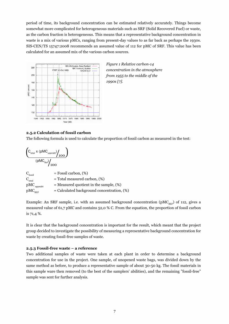
The quotient of the 14C/12C isotopes in the atmosphere has been measured since the 1950s, and shown in Error! Reference source not found. as pMC (Percentage Modern Carbon). The clear peak in the middle of the 1960s was caused by atmospheric nuclear weapons tests, after which the relative atmospheric concentration of carbon-14 declined. pMC in a fossil material has a value of zero, while that in young biomass (such as grass or food) has a value equivalent to the present-day atmospheric value, i.e. 107. Older biomass – e.g. 40 years or 20 years – will show respective pMC values of 131 and 114 (Figure 1). If the material is relatively homogeneous (e.g. a homogeneous biofuel), and has grown during a limited

7

period of time, its background concentration can be estimated relatively accurately. Things become somewhat more complicated for heterogeneous materials such as SRF (Solid Recovered Fuel) or waste, as the carbon fraction is heterogeneous. This means that a representative background concentration in waste is a mix of various pMCs, ranging from present-day values to as far back as perhaps the 1930s. SIS-CEN/TS 15747:2008 recommends an assumed value of 112 for pMC of SRF. This value has been calculated for an assumed mix of the various carbon sources.

2.5.2 Calculation of fossil carbon The following formula is used to calculate the proportion of fossil carbon as measured in the test:

Cfossil = Fossil carbon, (%)Ctotal = Total measured carbon, (%)pMC uppmätt = Measured quotient in the sample, (%)pMCREF = Calculated background concentration, (%)

Example: An SRF sample, i.e. with an assumed background concentration (pMCREF) of 112, gives a measured value of 61,7 pMC and contains 52,0 % C. From the equation, the proportion of fossil carbon is 71,4 %.

It is clear that the background concentration is important for the result, which meant that the project group decided to investigate the possibility of measuring a representative background concentration for waste by creating fossil-free samples of waste.

2.5.3 Fossil-free waste – a reference Two additional samples of waste were taken at each plant in order to determine a background concentration for use in the project. One sample, of unopened waste bags, was divided down by the same method as before, to produce a representative sample of about 30-50 kg. The fossil materials in this sample ware then removed (to the best of the samplers’ abilities), and the remaining ”fossil-free” sample was sent for further analysis.

ctotal x (pmcuppmätt)

(pmcref)

/100

/100

Figure 1 Relative carbon-14 concentration in the atmosphere from 1955 to the middle of the 1990s [7].

8

2.6 The balance method The balance method is a method of calculation based on mass balances and energy balances, which together produce an overdeterminedequation system, taking operational data from the plant’s existing control system. The most important input data is the balance between oxygen consumption and carbon dioxide formation in the process. The method is based on the fact that there are several fundamental differences between how biogenic and fossil carbon react in a combustion process, which makes it possible to separate the reactions. Examples of these differences are:

Carbon / Oxygen ratio: Fossil fuels, such as plastics, have a high ratio of carbon to oxygen. In extreme cases, such as polyethene, the proportion is infinite, as polyethene does not contain any oxygen at all. A typical biomass material, on the other hand, such as cellulose (-C6H10O5)-n, can have a carbon/oxygen ratio of nearly 1.

Oxygen consumption: The higher oxygen content in a biogenic material means that it consumes less free oxygen (i.e. free oxygen in the combustion air) when it is burnt.

Energy content: Generally, fossil materials have a higher energy content, as biogenic materials contain more water and less inert material per unit of mass.

Combustion of waste produces CO2, while oxygen from the air is consumed in accordance with the two general reactions below, specific for the two types of carbon sources: A. Biomass (cellulose): (-C6H10O5-)n + 6O2 6CO2 5H2OB. Fossil (Polyethene plastic): (-CH2-CH2-)n + 3O2 2CO2 + 2H2O

There is, in other words, a difference in the amount of O2 used by the two reactions. Reaction A uses 1 mol of O2 for each mol of CO2 produced, while Reaction B uses 1,5 mol of O2 for each mol of CO2 produced, giving a difference of 50 % in O2 consumption, depending on whether it is biogenic or fossil carbon that is the source of the CO2.

Starting from the two extremes, of 100 % biogenic material and 100 % fossil carbon material, we can calculate theoretical values of calorific value (HVwaste, kj/kg) and oxygen consumption (O2

Cwaste). A

plausibility test to check whether the calculated values are reasonable – i.e. whether they lie within the limits of what is possible – can also be performed.

Information on the following process parameters is required in order to perform the calculations: Continuous input data • O2 and CO2 concentrations in the flue gas (actual value, dry, %)• Waste quantities (tonne/h)• Masses of bottom ash, filter ash and filter cake • Flue gas quantity (Nm3/h) • Steam production (tonne/h)• Steam pressure and temperature (bar and °C)• Feed water temperature (°C)• Quantity of additional fuel (oil [tonne/h], gas [Nm3/h] or [for example] sludge [tonne/h]).

Of these parameters, it is the measured O2 and CO2 concentrations in the flue gas that are the most important for the calculations.

9

Predefined input data• Water content in the bottom ash (slag), %• Water content in the fly ash, %• Slag content in the waste, excluding metals, %• Energy efficiency of the boiler, (%)• O2 content of the combustion air, %. (Normally atmospheric air, but there are occasions when it is

sometimes enriched or changed.)

See Appendix II for further information on the balance method.

Ramböll AB performed all balance method calculations, using the BIOMA© program.

2.7 The sorting analysis method 2.7.1 Sorting analyses Four of the plants (Renova, Sysav, Fortum Högdalen and Tekniska Verken) performed their own sorting analyses in accordance with Avfall Sverige’s instructions for sorting analyses [8]. The results were then used as input for calculation of fossil carbon proportions.

The sorting analyses divided up the waste into the following nine primary fractions, with the plastics and ‘Other’ fractions being further divided into secondary fractions: • Biological waste (“Biowaste”) • Paper• Plastics:

• Soft plastics • Expanded plastics foam• Hard plastics packaging • Other plastics

• Glass • Metal • Other inorganic • Hazardous waste • Electrical and electronic waste • Other:

• Woods • Textiles • Absorbent hygiene products • Miscellaneous

The sorting analyses were performed by plant personnel or sub-contractors at each plant, with the subsequent calculations performed by Profu, using its models.

10

2.7.2 The calculation method The model links each fraction from the sorting analysis to an assumed chemical composition of the fraction. In this project, this information has been taken from Profu’s “Avfalls-Atlas3” data base, which contains chemical analyses of various waste fractions such as paper, plastics and glass. In this way, a description of the following parameters can be built up for each fraction: • Moisture content• Dry solids content (TS)• Carbon content (C) as % of dry solids (both biogenic and fossil contents)• Hydrogen content (H) as % of dry solids• Oxygen content (O) as % of dry solids• Nitrogen content (N) as % of dry solids• Sulphur content (S) as % of dry solids• Ash as % of dry solids

Combining data on the composition of each sorting analysis (percentage by weight) and the chemical composition of each fraction enables the chemical composition of the waste as a whole to be calculated, from which the biogenic and fossil carbon proportions can be determined. If it is assumed that all carbon is oxidised to carbon dioxide, then the biogenic, fossil and total emissions of carbon dioxide can be calculated.

An effective calorific value of the entire body of waste was also calculated in order to be able to relate emissions to the delivered quantity of energy from the waste.

See Appendix III for further information.

3 Waste Atlas.

11

3 results

3.1 Chemical characterisation of waste A chemical characterisation of all the waste samples taken from the seven combustion plants over a ten-month period was prepared for evaluation. Some of the plants burned only MSW, while some of the others burned (in some cases) waste containing an admixture of up to 79 % of waste from business/commercial sources. However, despite these relatively large differences in the waste fractions, the results of the chemical characterisation show relatively little spread. The main parameters, such as carbon, oxygen and hydrogen, show a relative standard deviation of less than 10 %, while more product-specific elements such as sulphur and iron exhibit a higher standard spread. Together, the 42 samples had an average moisture content of 38 (SD5,9) %, and an effective calorific value of 11 (SD1,5) MJ/kg. The results from selected parameters are shown in the three diagrams below. All data can also be found in tabular form in Appendix 14.

Figure 2 Calculated average values, with standard deviation, for the 42 analysed samples of waste. Concentrations are expressed as percentage of dry solids by weight.

Figure 3 Calculated average values, with standard deviation, for the 42 analysed samples of waste. Concentrations are expressed as percentage of dry solids by weight.

Figure 4 shows the average composition of the waste mixture as burnt in Sweden. As expected, the clearly dominating elements are carbon, oxygen, hydrogen, silicon and calcium. Proportions of other elements do not exceed 1 %.

Figure 4 The calculated average composition of waste burnt in Sweden. Values are expressed in percentage by weight of dry solids.

12

3.2 Determination of fossil carbon in waste by chemical analysis The quantity of fossil carbon in the waste was determined by analysis of the solid waste (a total of 42 samples, being six samples from each plant), and by sampling the flue gases (a total of 21 samples, being three samples from each plant). The six solid waste samples were taken at times spread over the whole sampling period, such that both summer and winter fuels were represented (see the sampling plan in Table 2). Figure 5 shows the results from both measurements, expressed as the proportion of fossil carbon in the total carbon quantity, which can also be read as the proportion of fossil CO2 in the total CO2 emission.

All the results can also be found in Appendix V, expressed as fossil carbon kg/Gj and as fossil carbon per tonne of waste.

Figure 5 The proportion of fossil carbon or CO2 in the total quantity of carbon in waste burnt in Sweden. The proportion of waste from business sources varies from 0 to 79 % among the various samples. Blue diamonds indicate the results from solid waste sampling, and the red squares indicate the results from flue gas sampling. All data has been calculated with an assumed background value of 107 pMC.

Two of the results – one flue gas sample and one solid waste sample – are clearly deviant, and have therefore been excluded from further calculations. Statistical analysis of the results shows that there is no link between the date of sampling and the proportion of fossil carbon, but there is a weak correlation with whether the waste consists of MSW alone, or whether it includes waste from commercial sources. However, there is no correlation with the proportion of admixture of waste from commercial sources.

The results of the solid waste sample analyses indicate a mean value of 36 % (SD7) of fossil carbon in the total carbon quantity in the samples, which is the same as saying that the waste contains a total of 10 % of fossil carbon by weight. Mean value calculations of the flue gas analyses give approximately the same results; that 38 % (SD5) of the CO2 has a fossil origin.

3.2.1 Background concentration in the waste As part of the work of the project, a further 14 samples (two from each plant) were taken, and the fossil material in them sorted and removed from the samples before they were analysed. This was done in order to try to create a fossil-free waste sample that could be used to give a measure of the background concentration of fossil carbon in the heterogeneous biogenic waste fraction/ Section (2.5.1) (above) describes how the background concentration was calculated.

Table 4 shows the measured levels of background concentrations , from which it can be seen that all the samples exhibit a lower value than that of the present-day atmosphere (107 pMC). This indicates that it is most likely that all the samples are contaminated with fossil material, and that sorting to remove such material was not entirely successful. Another hypothesis, although less likely, is that all the waste samples contain high proportions of biomass that are older than the 1960 value (Figure 1).

13

Table 4 Background concentrations (pMC quotient of carbon-14 and carbon-12) in waste samples from which fossil material has been removed. sample 1 sample 2

101,4 ±0,5 104,6 ±0,3

104,7 ±0,4 104,2 ±0,3

91,7 ±0,5 101,0 ±0,3

102,5 ±0,5 98,5 ±0,3

102,0 ±0,5 102,2 ±0,5

90,7 ±0,4 105,4 ±0,3

103,2 ±0,3 n.Dn.D.: no data, as the sample was destroyed before the analysis was concluded.

As we cannot be certain that our measured background concentrations are correct, their values will not be used in the calculations of the proportion of fossil carbon in waste. Unless otherwise stated, all results have been calculated using a background level of 107 pMC, as recommended in the standard (SIS-CEN 15747).

3.2.2 Calculation of fossil carbon in waste with different background concentrations The final reported fossil concentrations depend on the background concentration with which the sample is compared. Figure 6 shows the significance of the reported fossil carbon proportions for two different pMC levels. The two levels can be regarded as representing minimum and maximum levels of fossil carbon in waste, as probably not all biomass is “young” biomass (food waste), and the proportion of wood waste fractions is hardly exceeds the value in an SRF mixture. The reported value increased by a little over two percentage points if the background value for SRF is used instead of 107 pMC as given in the standard.

Figure 6 The significance of comparison background concentration measurements for the reported fossil concentration. The average values from the solid waste samples (blue diamonds) and the flue gas samples (red squares) are shown for two different background concentrations.

3.3 Four methods of determination of the fossil carbon content of waste In addition to determining the proportion of fossil carbon in waste burnt as fuel in Sweden today, the work of the project also aimed at evaluating the advantages and drawbacks of four different methods of determination of fossil content.

3.3.1 Comparison of solid fuel sampling and flue gas sampling The two methods are both based on the collection of samples and subsequent isotope analysis for determination of the proportion of fossil carbon. In order to be able to compare the two methods, the sampling was planned so that, as far as possible, the two types of samples (solid waste and flue gases) were taken at the same time.

Figure 7 shows the difference between the results from the parallel samplings on three occasions in each plant. A systematic difference between the results from the two methods can be clearly seen. At low concentrations of fossil carbon, the solid waste sampling method shows lower concentrations, while at

14

high concentrations it shows higher proportions than the results from flue gas sampling. This systematic error between the two methods was not noted when only the average values and standard deviation were compared, as the systematic errors at the lower and higher concentrations cancelled each other out. Which of the two methods can therefore be regarded as giving the most correct result value?

Figure 7 Differences in measured concentrations between the solid samples and the simultaneous flue gas samples, plotted against the measured concentrations in the solid waste samples. Yellow circles show values from fluidised bed boilers burning crushed waste, while the black rhomboids show values from grate boilers burning untreated waste.

Based on the material that we have obtained in this project, we feel that the flue gas methods gives the most correct measure of the proportion of fossil carbon. This is because: • in comparison with sampling of solid waste fuels, flue gas sampling collects from a relatively

homogeneous source, which reduces the potential for error; • the method provides a figure for the quantity of fossil carbon emitted from the plant.

As yet, we have no reasonable explanation for the cause of the systematic error: this would need to be further investigated in a project intended specifically to find the answer. Data from this present project does not show any systematic link to the proportion of commercial waste or to pre-treated or untreated waste. The results from this statistical analysis of the two different methods of measurement show how important it is that methods should be carefully compared with each other in order to reveal any errors.

The total uncertainty of measurement in the two methods is an estimate of the random and systematic errors in the sub-areas shown in Figure 8. The total uncertainty of measurement of the flue gas sampling method in this project is estimated as 3 % of fossil carbon, as against the considerably higher uncertainty value of 14 % given by the solid fuel method, due to the systematic error in that method.

Figure 8 The total uncertainty of measurement in a method consists of estimates of the random and systematic uncertainties in the three defined sub-areas.

Taking samples of solid waste is a relatively complicated process that requires considerable resources in terms of personnel and equipment when dealing with unprocessed waste. Sampling waste that has been processed and crushed is not particularly complicated or demanding of resources, as the samples can be taken from a falling stream of waste, which also simplifies the taking of a collection of many small samples over a longer period of time and then adding them together. However, all solid waste samples require further treatment and sample preparation before their fossil carbon contents can be analysed. One advantage of sampling solid wastes is that it permits other chemical characterisation of the waste, and also allows samples to be kept for future analyses.

osäkerheter relaterad till hur

väl proverna representerar hela avfallet i sverige?

osäkerheter relaterade till

provtagning och neddelning.

osäkerheter relaterade till bestämning av

fossilt kol.

15

By comparison, sampling flue gases is relatively simple to do, but it needs to be done by someone who knows how to work in the way specified by the relevant standard. In addition, the plant must have suitable access points for sampling the flue gases. The gas is collected in a sampling bag, which can then be sent off for analysis without any pretreatment. The drawbacks of this method are that the boiler must be operating in a relatively stable mode while the samples are being taken, as the sampling method is dependent on a steady flue gas flow. In addition, there is a slight risk of the sample being lost when being sent for analysis, unless double samples are taken.

When all is said and done, the various methods cost about the same if it is borne in mind that the services of a consultant are used for flue gas sampling and that more of the company’s own personnel are involved in sampling sold waste materials. The cost of taking samples of waste in a plant where the waste is fragmented before combustion is considerably less; only about a little over a third of the cost of sampling untreated waste. The cost of analysis for determining the proportion of fossil carbon can probably be substantially reduced if a simpler method of analysis – liquid scintillation – is used instead of AMS. However, although its performance is not as good as AMS, and so it is no longer used for archaeological dating, it would probably be sufficiently accurate for determining the proportion of fossil carbon in fuels.

3.3.2 The balance method The balance method was evaluated at two plants: Renova, where the BIOMA© program was installed for three months, and at Sysav, where previously logged data was used for post-collection processing by the program. The results from, and experience of using, the balance method are described below.

3.3.2.1 Experience from Renova, Göteborg As the program was installed at the plant, it enabled the project to obtain experience of how the software works under real conditions for three months.

Figure 9 presents the results from BIOMA© as weekly mean values of the proportion of fossil CO2 in the flue gases, together with the estimated proportion of the waste being from non-domestic sources. It can be seen that five values of calculated fossil carbon content differ from the others: they occurred during the weeks when a replacement instrument for oxygen and carbon dioxide measurements was being used. The accuracy of these two parameters is particularly important for the results, as the calculations are largely based on carbon/oxygen ratios. The replacement instrument that was used measured an oxygen content that was, on average, about 0,2 percentage points higher than the reading from the normal instrument, while its carbon dioxide measurement was about 0,9 percentage points lower than that from the normal instrument. These relatively small differences in measured values had a very considerable effect on the calculated value of fossil carbon in the flue gases (Figure 9). A check calculation, using corrected measured data, returned calculated values of fossil content to the normal levels,

Figure 9 The proportion of fossil carbon dioxide in the flue gases as weekly average values, as calculated by the BIOMA© program (green triangles) and approximate proportion of commercial waste in the waste mix (blue dots), plotted against week numbers.

16

It can also be seen from Figure 9 that the proportion of fossil carbon in the flue gases exhibits a declining trend from winter to summer, which also coincides with a lower proportion of waste from business sources in the mix.

A brief overview of the user-friendliness of the program The software licence was restricted, which meant that Renova did not have access to all the essential functions during the test period. One of the effects of this was that the proportion of fossil carbon was not reported on-line by the software, but had to calculated afterwards by Ramböll and the University of Vienna (which had developed the program). In its present version, the program is intended primarily to indicate the proportion of non-fossil energy. It would be desirable for the proportion of fossil carbon to be calculated on-line, and for the results to be included in the automatic reports that the program can produce. Further, if the program is to be useable, it is essential that the licensing aspects between the three parties (the waste combustion plant, Ramböll and the University of Vienna) should be cleared up.

If the software is to be used to calculate the direct fossil carbon emissions from a plant, it is important that the plant has checked that the necessary input data is available in the correct format and that it is of good quality. The apparently minor changes in the oxygen and carbon dioxide concentrations caused by the use of the spare instrument during the test period resulted in a doubling in the calculated value of fossil carbon proportion, which indicates that the method is very sensitive to the quality and values of the input data.

The additional value of using the program is that, in addition to being told the proportion of fossil carbon dioxide, users are also told what proportion of the energy being produced derives from fossil carbon. This is information that is of interest for further discussions on guarantees of origin and on electricity certificates. The software also delivers a probability value for the measured values, reflecting the quality of the data produced by the plant’s instruments.

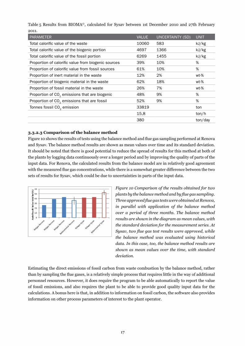
3.3.2.2 Experience from Sysav in MalmöTable 5 shows the results of the calculations, based on logged process data from Sysav for the period from 1st December 2010 to 27th February 2011, showing that 52 % of CO2 emissions during that period were fossil-sourced. However, the uncertainty of the results is relatively large, due to unknown uncertainties in the input data from the plant. The weight of the waste fuel, for example, has not been measured by/from the crane: instead, the total quantity of waste has been calculated from weighing scale data, with the quantity being supplied to the boiler being estimated visually, giving an estimated uncertainty of 8 %. In addition, uncertainties of how the steam has been used in the process introduce further uncertainties to the calculations.

17

Table 5 Results from BIOMA©, calculated for Sysav between 1st December 2010 and 27th February 2011. parameter Value uncertainty (sD) unit

total calorific value of the waste 10060 583 kJ/kg

total calorific value of the biogenic portion 4697 1366 kJ/kg

total calorific value of the fossil portion 6269 1455 kJ/kg

proportion of calorific value from biogenic sources 39% 10% %

proportion of calorific value from fossil sources 61% 10% %

proportion of inert material in the waste 12% 2% wt-%

proportion of biogenic material in the waste 62% 18% wt-%

proportion of fossil material in the waste 26% 7% wt-%

proportion of co2 emissions that are biogenic 48% 9% %

proportion of co2 emissions that are fossil 52% 9% %

tonnes fossil co2 emission 33819 ton

15,8 ton/h

380 ton/day

3.3.2.3 Comparison of the balance method Figure 10 shows the results of tests using the balance method and flue gas sampling performed at Renova and Sysav. The balance method results are shown as mean values over time and its standard deviation. It should be noted that there is good potential to reduce the spread of results for this method at both of the plants by logging data continuously over a longer period and by improving the quality of parts of the input data. For Renova, the calculated results from the balance model are in relatively good agreement with the measured flue gas concentrations, while there is a somewhat greater difference between the two sets of results for Sysav, which could be due to uncertainties in parts of the input data.

Figure 10 Comparison of the results obtained for two plants by the balance method and by flue gas sampling. Three approved flue gas tests were obtained at Renova, in parallel with application of the balance method over a period of three months. The balance method results are shown in the diagram as mean values, with the standard deviation for the measurement series. At Sysav, two flue gas test results were approved, while the balance method was evaluated using historical data. In this case, too, the balance method results are shown as mean values over the time, with standard deviation.

Estimating the direct emissions of fossil carbon from waste combustion by the balance method, rather than by sampling the flue gases, is a relatively simple process that requires little in the way of additional personnel resources. However, it does require the program to be able automatically to report the value of fossil emissions, and also requires the plant to be able to provide good quality input data for the calculations. A bonus here is that, in addition to information on fossil carbon, the software also provides information on other process parameters of interest to the plant operator.

18

3.3.3 The sorting analysis method A sorting analysis was also performed at four of the plants on about 500 kg of mixed waste. After the analysis was performed, the sample was remixed and a representative quantity was sent for further chemical analysis of its fossil carbon content. This procedure, of simultaneous sampling, provides a direct comparison of test methods, as two different methods of determining fossil carbon were used on the same waste sample from the process. Table 6 shows the results of these sorting analyses in terms of the main fractions into which the waste was sorted. Unfortunately, the results from one of the four plants could not be used for further calculations, as some of the fractions had not been separated in a comparable manner.

Table 6 Results from sorting analyses of mixed waste from the waste combustion plants renoVa fortum teKnisKa VerKen

type of waste 40-45 % domestic waste and 55-60 % commercial waste

100 % domestic waste 100 % domestic waste

composition (%)

bio-wastea 24,8 % 14,6% 31,4%

paper 20,8 % 37,6% 23,2%

plasticsb 15,8 % 25,7% 13,8%

Glass 1,8 % 3,4 % 1,4%

metal 3,8 % 3,1 % 2,8%

other inorganic 3,0 % 0,4 % 2,7%

hazardous waste 0,1 % 0,1 % 0,1%

electrical and electronic 0,6 % 0,1 % 0,3%

otherc 29.3 %

15,1% 24,5%

a) at tekniska Verken, this fraction was divided into food waste and garden waste. b) in all three sorting analyses, this fraction was divided into soft plastics, foamed plastics, hard plastic packaging and other plastics. c) in all three sorting analyses, this fraction was divided into wood, textiles, nappies, sanitary prod-ucts and similar, and miscellaneous. see appendix iii for all data on secondary fractions.

Data from the three sorting analyses was then used as input for further calculations of fossil carbon contents (Table 7). It can be seen that the calculated fossil CO2 emissions are clearly linked to the measured proportions of plastics in the sorting analyses. The results of the sorting analyses as shown in Table 6 show that Fortum’s waste had by far the greatest plastics content, which is reflected in Table 7 by Fortum having by far the highest fossil CO2 emission.

Fortum’s waste clearly differs from the two other combustion plant wastes in terms of its plastics concentrations. Where there are less differences between the results of the sorting analyses in terms of their plastics contents, as is the case for Renova and Tekniska Verken, the composition of the rest of the waste plays an important part in deciding the fossil carbon content. An important reason for the differences between Renova and Tekniska Verken is that, in Göteborg, the ‘Other’ fraction consisted largely of wood (in which the carbon is treated as 100 % biogenic), while the same fraction in Tekniska Verken was dominated by nappies, sanitary products etc., in which 64 % of the carbon is treated as fossil-sourced.

19

Table 7 Proportion of fossil carbon, calculated using sorting analysis data as the input renoVa fortum teKnisKa VerKen

fossil carbon as proportion of total carbon (percentage by weight)

31 48 38

fossil carbon per tonne of waste (percentage by weight)

9,5 15 9,4

fossil carbon (kg/GJ) 8,1 12 10

fossil co2 (tonne/tonne of waste) 0,35 0,54 0,34

fossil co2 (kg/GJ) 30 43 36

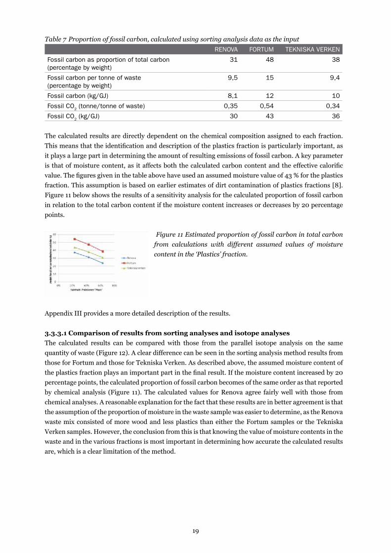
The calculated results are directly dependent on the chemical composition assigned to each fraction. This means that the identification and description of the plastics fraction is particularly important, as it plays a large part in determining the amount of resulting emissions of fossil carbon. A key parameter is that of moisture content, as it affects both the calculated carbon content and the effective calorific value. The figures given in the table above have used an assumed moisture value of 43 % for the plastics fraction. This assumption is based on earlier estimates of dirt contamination of plastics fractions [8]. Figure 11 below shows the results of a sensitivity analysis for the calculated proportion of fossil carbon in relation to the total carbon content if the moisture content increases or decreases by 20 percentage points.

Figure 11 Estimated proportion of fossil carbon in total carbon from calculations with different assumed values of moisture content in the ‘Plastics’ fraction.

Appendix III provides a more detailed description of the results.

3.3.3.1 Comparison of results from sorting analyses and isotope analyses The calculated results can be compared with those from the parallel isotope analysis on the same quantity of waste (Figure 12). A clear difference can be seen in the sorting analysis method results from those for Fortum and those for Tekniska Verken. As described above, the assumed moisture content of the plastics fraction plays an important part in the final result. If the moisture content increased by 20 percentage points, the calculated proportion of fossil carbon becomes of the same order as that reported by chemical analysis (Figure 11). The calculated values for Renova agree fairly well with those from chemical analyses. A reasonable explanation for the fact that these results are in better agreement is that the assumption of the proportion of moisture in the waste sample was easier to determine, as the Renova waste mix consisted of more wood and less plastics than either the Fortum samples or the Tekniska Verken samples. However, the conclusion from this is that knowing the value of moisture contents in the waste and in the various fractions is most important in determining how accurate the calculated results are, which is a clear limitation of the method.

20

Figure 12 Comparison of the proportions of fossil carbon in waste, as given by the sorting analysis method calculations (yellow dots) and corresponding isotope analyses (blue rhomboids) of solid waste. The grey triangle indicates the average value, with standard deviation, of the flue gas samples taken from the same plant.

One advantage of the sorting analysis method is that, once the necessary basic work has been done in the model, it is straightforward to enter the sorting analysis results and obtain output results. In comparison with the other methods evaluated in this project, the cost of the actual evaluation method itself is probably quite low. However, the overall cost of the method is relatively high, as sorting analyses have to be performed at frequent intervals in order to ensure that the samples are representative of the waste being burnt.

3.3.4 Evaluation of all four methods in one plant All four methods were evaluated at one plant, although based on different numbers of actual individual tests. Another difference is that two of the methods – solid waste and flue gas – are based on isotope analysis, while the two other sorting analyses and the balance method are based on a number of assumptions in the models that then perform the calculations. Figure 13 shows a summary of the results obtained from the different methods tested at Renova in Göteborg. The five differing measured values for the balance method are due to measurement errors. It can be seen from the figure that the samples were taken on three different times: around Week 5, Week 15 and after Week 25. The results from the different methods at the different sampling times do not differ very much from each other.

Figure 13 Proportion of fossil carbon in relation to total carbon in the waste mix, as calculated at Renova by four methods. Bottom scale: week number. The three measured values shown for Week 0 are for waste samples taken in September, October and December of the previous year. The five differing values from the balance method are the result of an incorrectly calibrated instrument.

It is difficult directly to compare the results from the four methods as, in addition to their estimates of direct fossil carbon emissions, they also provide other information that is of value to the plant operator. The choice of method can therefore by influenced by circumstances other than those of direct determination of fossil carbon emissions. The following is a comparison of the methods in respect of their estimated uncertainty of measurement, resource requirements and user-friendliness.

Solid fuel sampling Uncertainty of measurement: The total uncertainty of measurement for determination of the proportion of fossil carbon, including the systematic error, is estimated as amounting to 14 % of fossil carbon.

21

Resources: For a plant burning untreated waste, this sampling method requires relatively substantial resources in terms of personnel for sampling, and space and equipment for sampling and division of the waste. However, the method is considerably simpler for a plant burning crushed waste, requiring only one person who, at regular intervals during the sampling period, abstracts samples from the falling stream of waste in the plant. The costs for sampling and analysis of untreated waste are estimated as about SEK 20 000 – 30 000 per sample, while those for crushed waste are estimated as a maximum of SEK 10 000 per sample. User-friendliness: Sampling of untreated waste is a relatively labour-intensive process, but it can be done if the plant has the necessary space and equipment to do so. Sampling of crushed waste is a more user-friendly and simpler process. Advantages of both types of waste are that sampling also offers the opportunity of chemical characterisation of the waste, and that a prepared sample can easily be saved for a long period of time for sometime future analyses. An important drawback of the method, however, is that it includes an unexplained systematic measurement error. In addition, regardless of whether it is taken from pretreated waste or not, the sample must be further prepared for laboratory testing before its fossil carbon content can be determined.

Flue gas sampling Uncertainty of measurement: The total uncertainty of measurement for determination of the proportion of fossil carbon is estimated as amounting to 3 % of fossil carbon. Resources: Sampling requires the knowledge and ability to perform the work in accordance with the requirements of the relevant standards, together with availability of the necessary physical equipment. In addition, the plant must have a suitable accessible sampling point in the flue gas duct downstream of the flue gas cleaning. The estimated costs for sampling and analysis are at least SEK 20 000 per sample: this cost includes the services of an measurements consultant to do the sampling. User-friendliness: This sampling is relatively user-friendly if the plant has the resources required by the standard. The advantage of the method is that it produces a sample that is ready for analysis of the proportion of fossil carbon. Its drawbacks are that the combustion process must be able to maintain a relatively constant flow, and that there is a risk of the sample being lost in transit on its way to the laboratory, unless two sets of samples are taken. It is also difficult to save samples for sometime future analysis.

The balance methodUncertainty of measurement: This method has not been evaluated for a sufficiently long period of time in this project to enable uncertainty of measurement of the proportion of fossil carbon to be estimated. Resources: The method requires the plant to invest in and install software that can perform the calculations. Good quality of the measurements of CO2 and O2 concentrations in the flue gases is also necessary if the results are to be reliable. User-friendliness: Once the program has been installed, and all automatic calculation procedures are working, this is a very user-friendly method. An additional benefit is that other interesting energy parameter values from the process can be calculated at the same time. The drawback that we have found during this project is that the program is not yet fully developed to the point that it can perform on-line calculations of the proportion of fossil carbon in the waste.

22

The sorting analysis method Uncertainty of measurement: Not enough sorting analyses have been carried out in this project to enable the method’s uncertainty of measurement of the proportion of fossil carbon to be estimated. However, the results are very dependent on accurate knowledge of the moisture content of each fraction. A sensitivity analysis of the effect of varying the moisture content of the plastics fraction by 20 percentage points showed major variations in the results. Resources: Sorting analysis of mixed waste is demanding of personnel resources, and the plant must also have access to suitable premises for the purpose. To calculate the proportion of fossil carbon requires the use of mathematical models for the purpose. The cost of performing a sorting analysis and associated evaluation of the proportion of fossil carbon by modelling is estimated as amounting to about SEK 25 000 - 30 000 per sample.User-friendliness: Sampling, i.e. sorting analysis of mixed waste, is a labour-intensive process, more or less necessitating the waste to be untreated if a sorting analysis is to be feasible. However, once the results of the sorting analyses are available, the subsequent modelling is user-friendly and straightforward if those doing the work are familiar with the model. In order to reduce the uncertainty of measurement of this method, it is recommended that the moisture content of (particularly) the plastic fractions should be determined. The advantage of the model is that it also provides information on the composition of the waste. Its drawbacks are that it requires a relatively large labour input, and that it is associated with considerably uncertainties of results.

23

4 conclusions

Composition of the waste Despite substantial differences, ranging from 0 to 79 %, in the admixture of commercial waste among the MSW being used as fuel by the plants in this project, the final mixes of waste exhibit a relatively similar chemical composition. As expected, the predominant elements are carbon, oxygen, hydrogen, silicon and calcium, while all other elements occur at less than 1 % concentration. The relative spread of the dominant elements is about 10 %.

What proportion of the waste burnt as fuel in Sweden is fossil? The direct emission of fossil carbon was measured both by sampling of the solid waste and by sampling of the flue gases at seven waste combustion plants over a ten-month period. The results from calculating the average values from the 42 solid waste samples show that 36 (SD7) % of the carbon is of fossil origin, equivalent to a fossil carbon concentration in a sample mix of about 10 % by weight. The results from the 21 flue gas samples show almost the same result: namely, that 38 (SD5) % of the carbon in the waste is of fossil origin.

In simple terms, this can be expressed as saying that about one third of the carbon in the waste burnt as fuel in Sweden is of fossil origin.

What are the advantages and drawbacks of the various methods of determination? Table 8 is an overall presentation of the advantages and drawbacks of solid waste sampling, flue gas sampling, the balance method and the sorting analysis method for determining the proportion of fossil carbon in waste, as investigated in this project.

Table 8 Presentation of the advantages and drawbacks of the methods investigated. The prices shown are only indicative, and could be changed.

methoDuncertainty of measurement resources

aDVantaGes / DrawbacKs

waste1 >14 % fossil carbon material resources: considerable. cost: >20 – 30 000 seK/sample

permits further characterisation.

waste2 >14 % fossil carbon material resources: modest. cost: <10 000 seK/sample

systematic meas-urement error.

flue gas >3 % fossil carbon material resources: modest. cost: >20 – 30 000 seK/sample

simple sampling. / only one sample.

balance method insufficient data. material resources: modest. cost: no information on cost per sample.

user-friendly. / requires good quality data.

sorting analysis insufficient data, but probably >20 % fossil carbon.

material resources: considerable. cost: >25- 30 000 seK/sample

permits further characterisation. / considerable uncertainty of measurement.

1. untreated waste 2. crushed waste 3. initial cost of about seK 230 000 for software, which includes the user licence, calculation for

one boiler, and training. subsequent cost, about seK 40 000 per year.

24

5 continued work

It was noted, within the framework of this project, that there was a systematic error in the method based on sampling of solid waste, that did not occur in the flue gas sampling method. It has not been possible to find a reasonable explanation for this error from the material available today. It would be very interesting to investigate this further, in the form of a project intended to find an answer to this question.

One possible approach would be that of simultaneous sampling of solid waste and flue gases in a plant burning known mixtures, e.g. with 0 %, 50 % and 100 % fossil carbon materials.

25

6 references

1. Ministry of Finance; ”A burning tax? – Taxation of waste used as fuel” [in Swedish]. Swedish Government Official Report no. 2005:23.

2. Ministry of Finance; ”Tax back” [in Swedish]. Swedish Government Official Report no. 2009:12.3. Ministry of Finance; “The Act (1994:1776) Concerning Tax on Energy” [in Swedish], 1994.4. Profu; ”CO2 emissions from Swedish waste combustion” [in Swedish], 2003. 5. RVF; ”Waste combustion – Greenhouse gas emissions compared with other waste treatments and

other energy production” [in Swedish], 2003:12.6. Wikström-Blomqvist, EB., Franke, J., Johansson, I., ”Characterisation of solid non-homogeneous

waste as fuel – The effect of methods of sampling and sample preparation” [in Swedish], Swedish Thermal Engineering Research Association, Report no. 1036, 2007.

7. Wikipedia, http://en.wikipedia.org/wiki/Radiocarbon_dating#cite_note-11, diagram downloaded 2011-11-21.

8. RVF; ”A sorting analysis manual for domestic waste” [in Swedish], 2005:19.

26

27

aPPendix i – fuel samPling

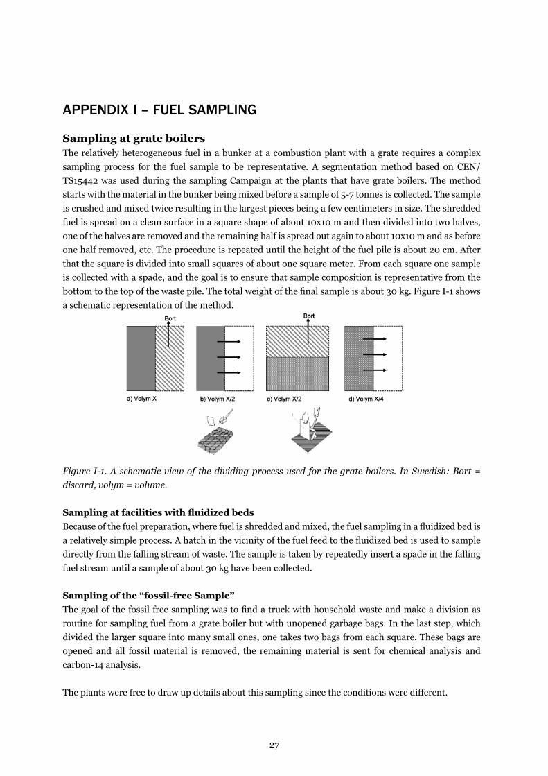
Sampling at grate boilersThe relatively heterogeneous fuel in a bunker at a combustion plant with a grate requires a complex sampling process for the fuel sample to be representative. A segmentation method based on CEN/TS15442 was used during the sampling Campaign at the plants that have grate boilers. The method starts with the material in the bunker being mixed before a sample of 5-7 tonnes is collected. The sample is crushed and mixed twice resulting in the largest pieces being a few centimeters in size. The shredded fuel is spread on a clean surface in a square shape of about 10x10 m and then divided into two halves, one of the halves are removed and the remaining half is spread out again to about 10x10 m and as before one half removed, etc. The procedure is repeated until the height of the fuel pile is about 20 cm. After that the square is divided into small squares of about one square meter. From each square one sample is collected with a spade, and the goal is to ensure that sample composition is representative from the bottom to the top of the waste pile. The total weight of the final sample is about 30 kg. Figure I-1 shows a schematic representation of the method.

Figure I-1. A schematic view of the dividing process used for the grate boilers. In Swedish: Bort = discard, volym = volume.

Sampling at facilities with fluidized bedsBecause of the fuel preparation, where fuel is shredded and mixed, the fuel sampling in a fluidized bed is a relatively simple process. A hatch in the vicinity of the fuel feed to the fluidized bed is used to sample directly from the falling stream of waste. The sample is taken by repeatedly insert a spade in the falling fuel stream until a sample of about 30 kg have been collected.

Sampling of the “fossil-free Sample”The goal of the fossil free sampling was to find a truck with household waste and make a division as routine for sampling fuel from a grate boiler but with unopened garbage bags. In the last step, which divided the larger square into many small ones, one takes two bags from each square. These bags are opened and all fossil material is removed, the remaining material is sent for chemical analysis and carbon-14 analysis.

The plants were free to draw up details about this sampling since the conditions were different.

28

fuel

sam

ple

sam

ple

1s

ampl

e 2

sam

ple

3s

ampl

e 4

sam

ple

5s

ampl

e 6

sam

plin

g w

eek

39, 2

010

41, 2

010

50, 2

010

5, 2

011

14, 2

011

26, 2

011

sha

re o

f co

mm

erci

al w

aste

65 %

63 %

67 %

64 %

fue

l sam

ple

64 %

flu

e G

as

sam

ple

62 %

fue

l sam

ple

52 %

flu

e G

as

sam

ple

45 %

fue

l sam

ple

48 %

flu

e G

as

sam

ple

sim

ulta

neou

s flu

e ga

s sa

mpl

e-

--

yes

yes

yes

oth

er in

form

atio

nth

e w

hole

pro

ject

gr

oup

join

ed in

to

obse

rve

a sa

mpl

ing

fuel

sam

ple

ca 5

h

com

bust

ion,

flu

e G

as s

ampl

e 24 h

fuel

sam

ple

ca 5

h

com

bust

ion,

flu

e G

as s

ampl

e 24 h

fuel

sam

ple

ca 5

h

com

bust

ion,

flu

e G

as s

ampl

e 24 h

fos

sil

fr

ee s

ampl

es

ampl

e 1

sam

ple

2

sam

plin

g w

eek

14, 2

011

26, 2

011

sha

re o

f co

mm

erci

al w

aste

sim

ulta

neou

s sa

mpl

ings

fuel

sam

ple

flue

Gas

sam

ple

sor

ting

anal

ysis

fuel

sam

ple

flue

Gas

sam

ple

oth

er in

form

atio

nth

e fo

ssil

free

sam

ple

was

mix

ed u

sing

the

fos

sil f

ree

mat

eria

ls fro

m t

he

sort

ing

anal

ysis

R

enov

a

29

fuel

sam

ple

sam

ple

1s

ampl

e 2

sam

ple

3s

ampl

e 4

sam

ple

5s

ampl

e 6

sam

plin

g w

eek

43, 2

010

50, 2

010

3, 2

011

8, 2

011

19, 2

011

25, 2

011

sha

re o

f co

mm

erci

al

was

te42 %

30 %

44 %

60 %

37 %

36 %

sim

ulta

neou

s flu

e ga

s sa

mpl

e-

--

yes

yes

yes

oth

er in

form

atio

n*22 %

woo

d ca

me

in

to t

he b

unke

r, 165

7

tonn

es c

ame

in d

urin

g th

e sa

mpl

ing

time.

4

tonn

es w

ere

extr

acte

d.

shr

edde

d 1 t

ime.

onl

y th

ree

divi

sion

s du

e to

sm

all s

ampl

e vo

lum

e.

one

of th

e pr

ojec

t le

ader

s w

as p

rese

nt

for

the

sam

plin

g.

32 %

woo

d ca

me

in t

o th

e bu

nker

, 1358 t

onne

s ca

me

in d

urin

g th

e sa

mpl

ing

time.

4.6

ton

nes

wer

e ex

trac

ted

17 %

woo

d ca

me

in t

o th

e bu

nker

, to

nnes

cam

e in

dur

ing

the

sam

plin

g tim

e.

4.3

ton

nes

wer

e ex

trac

ted

6 %

woo

d ca

me

in t

o th

e bu

nker

, 1726 t

onne

s ca

me

in

durin

g th

e sa

mpl

ing

time.

6.3

to

nnes

wer

e ex

trac

ted

the

sam

ple

was

del

iver

ed in

tw

o se

para

te b

oxes

to

the

anal

ysis

labo

rato

ry s

o th

is

sam

ple

have

tw

o re

port

s.

1.2

m3 o

il w

as u

sed

a su

ppor

ting

fuel

dur

ing

the

flue

G

as s

ampl

ing.

0 %

woo

d ca

me

in t

o th

e bu

nker

, to

nnes

cam

e in

dur

ing

the

sam

plin

g tim

e.

5.3

ton

nes

wer

e ex

trac

ted

the

sam

ple

was

del

ayed

to

the

ana

lysi

s la

bora

tory

0 %

woo

d ca

me

in

to t

he b

unke

r, 711

tonn

es c

ame

in

durin

g th

e sa

mpl

ing

time.

4 t

onne

s w

ere

extr

acte

d

the

4 t

onne

s ar

e m

ost

prob

ably

not

re

pres

enta

tive

for

the

711 t

onne

s. 1

8

% o

f th

e 711 t

onne

s co

nsis

ted

of s

lf.

*th

e sa

mpl

es w

ere

all p

erfo

rmed

the

sam

e w

ay:

Day

1: w

aste

was

sam

pled

fro

m t

he b

unke

r be

twee

n 8-1

5.

at 1

5.3

0 o

ne s

coop

of

ca 4

ton

nes

was

ext

ract

ed.

Day

2: th

e w

aste

was

shr

edde

d tw

ice

and

divi

ded

indo

ors.

the

flue

gas

sam

plin

g w

as p

erfo

rmed

fro

m 0

9:0

0 d

ay 1

to

09

:00

day

2.

fos

sil

fr

ee s

ampl

es

ampl

e 1

sam

ple

2

sam

plin

g w

eek

11

25

sha

re o

f co

mm

erci

al w

aste

036%

sim

ulta

neou

s sa

mpl

ings

-fu

el s

ampl

efl

ue G

as s

ampl

es

ortin

g an

alys

is

oth

er in

form

atio

no

ne t

ruck

with

was

te f

rom

bot

h ho

useh

olds

and

ind

ustr

ies

was

use

d. r

epre

sent

ativ

e fo

r m

alm

ö ci

ty.

the

sam

ple

extr

acte

d fr

om t

he b

unke

r di

dn’t c

onta

in m

uch

ms

w o

r fo

ssil

free

mat

eria

ls. n

ot r

epre

sent

ativ

e.

Sys

av

30

fuel

sam

ple

sam

ple

1s

ampl

e 2

sam

ple

3s

ampl

e 4

sam

ple

5s

ampl

e 6

sam

plin

g w

eek

44

49

10

11

13

24

sha

re o

f co

mm

erci

al w

aste

48 %

63 %

66 %

63 %

68 %

57 %

sim

ulta

neou

s flu

e ga

s sa

mpl

e-

-ye

s-

yes

yes

oth

er in

form

atio

ns

tart

sam

plin

g of

fue

lm

onda

y 101102 a

t 06.0

0en

d sa

mpl

ing

of f

uel

tues

day

101103 a

t 12.0

0

tim

e fo

r ex

trac

tion

from

bun

ker:

tues

day

101103 a

t 12.3

0to

tal w

eigh

t ca

7

tonn

es

shr

edde

d 2 t

imes

.

one

of th

e pr

ojec

t le

ader

s w

as p

rese

nt

for

the

sam

plin

g.

sta

rt s

ampl

ing

of f

uel

mon

day

101206 a

t 06.0

0en

d sa

mpl

ing

of f

uel

wed

nesd

ay 1

01208 a

t 12.0

0

tim

e fo

r ex

trac

tion

from

bun

ker:

wed

nesd

ay 1

01208 a

t 13.3

0to

tal w

eigh

t ca

6,7

to

nnes

shr

edde

d 2 t

imes

.

sta

rt s

ampl

ing

of f

uel

tues

day

110308 a

t 06.0

0en

d sa

mpl

ing

of f

uel

thur

sday

110310 a

t 12.0

0

sta

rt t

ime

for

flue

gas

sam

plin

g:

wed

nesd

ay 1

10309 a

t 10.0

0en

d tim

e fo

r flu

e ga

s sa

mpl

ing:

thur

sday

110310 a

t 10.0

0

tim

e fo

r ex

trac

tion

from

bun

ker:

thur

sday

110310 a

t 13.0

0to

tal w

eigh

t ca

6.5

to

nnes

shr

edde

d 2 t

imes

.

no

oil w

as u

sed

durin

g th

e flu

e ga

s sa

mpl

ing.

sta

rt s

ampl

ing

of f

uel

mon

day

11

03

14

at

06.0

0en

d sa

mpl

ing

of f

uel

wed

nesd

ay 1

10

31

6 a

t 12.0

0

tim

e fo

r ex

trac

tion

from

bun

ker:

wed

nesd

ay 1

10

31

6 a

t 13.0

0to

tal w

eigh

t ca

7.2

to

nnes

shr

edde

d 2

tim

es.

our

cra

ne o

pera

tor

thou

ght

the

fuel

was

ve

ry li

ght.

he

need

ed

3 f

ull s

coop

s to

get

th

e rig

ht a

mou

nt (

ca

7 t

onne

s) o

f w

aste

(p

revi

ousl

y 2

sco

ops

was

eno

ugh)

.

sta

rt s

ampl

ing

of f

uel

mon

day

11

03

28

at

06

.00

end

sam

plin

g of

fue

lw

edne

sday

11

03

30

at

12

.00

sta

rt t

ime

for

flue

gas

sam

plin

g:

tues

day

11

03

29

at

09

.00

end

time

for

flue

gas

sam

plin

g:w

edne

sday

11

03

30

at

09

.00

tim

e fo

r ex

trac

tion

from

bun

ker:

wed

nesd

ay 1

10

33

0 a

t 1

3.0

0to

tal w

eigh

t ca

6,9

ton

shr

edde

d 2

tim

es.

no

oil w

as u

sed

durin

g th

e flu

e ga

s sa

mpl

ing.

ligh

t fu

el t

his

time

as w

ell,

3 s

coop

s ne

cess

ary.

sta

rt s

ampl

ing

of f

uel

mon

day

11

06

13

at

06

.00

end

sam

plin

g of

fue

lw

edne

sday

11

06

15

at

12

.00

sta

rt t

ime

for

flue

gas

sam

plin

g:

tues

day

11

06

14

at

08

.00

end

time

for

flue

gas

sam

plin

g:w

edne

sday

11

06

15

at

08

.00

tim

e fo

r ex

trac

tion

from

bun

ker:

wed

nesd

ay 1

10

61

5 a

t 1

3.0

0to

tal w

eigh

t ca

5.7

to

nnes

shr

edde

d 2

tim

es.

no

oil w

as u

sed

durin

g th

e flu

e ga

s sa

mpl

ing.

Um

eå E

ner

gi

31

fos

sil

fr

ee s

ampl

es

ampl

e 1

sam

ple

2

sam

plin

g w

eek

14

20

sha

re o

f co

mm

erci

al

was

te0 %

0 %

sim

ulta

neou

s sa

mpl

ings

--

oth

er in

form

atio

no

ne t

ruck

load

of

ms

w w

as c

hose

n (1

10406). t

he t

ruck

con

tain

ed

ms

w fro

m h

ouse

s an

d ap

artm

ents

in t

he n

eigh

borh

oods

röd

äng

and

Väst

ersl

ätt

in u

meå

. fo

od w

aste

sho

uld

have

bee

n se

para

ted

but

we

foun

d it

in c

a 50 %

of th

e ba

gs. th

e tr

uck

cont

aine

d ca

5

tonn

es o

f m

sw

.

2 b

ags

wer

e ta

ken

from

eve

ry o

ther

squ

are,

44 b

ags

in t

otal

.

one

tru

ck lo

ad o

f m

sw

was

cho

sen

(110517). t

he t

ruck

con

tain

ed

ms

w a

nd foo

d w

aste

fro

m h

ouse

s an

d ap

artm

ents

in t

he

neig

hbor

hood

rob

erts

fors

out

side

um

eå. th

e tr

uck

cont

aine

d ca

3.9

ton

nes.

2 b

ags

wer

e ta

ken

from

eve

ry o

ther

squ

are,

30 b

ags

in t

otal

.

For

tum

Hög

dal

enfu

el s

ampl

es

ampl

e 1

sam

ple

2s

ampl

e 3

sam

ple

4s

ampl

e 5

sam

ple

6

sam

plin

g w

eek

44, 2

010

50, 2

010

4, 2

011

12, 2

011

17, 2

011

21, 2

011

sha

re o

f co

mm

erci

al

was

te0 %

0 %

0 %

0 %

0 %

0 %

sim

ulta

neou

s flu

e ga

s sa

mpl

e-

--

yes

yes

yes

oth

er in

form

atio

no

ne o

f th

e pr

ojec

t le

ader

s w

as p

rese

nt for

the

sa

mpl

ing.

fos

sil

fr

ee s

ampl

es

ampl

e 1

sam

ple

2

sam

plin

g w

eek

12, 2

011

17, 2

011

sha

re o

f co

mm

erci

al w

aste

sim

ulta

neou

s sa

mpl

ings

fuel

sam

ple

flue

Gas

sam

ple

fuel

sam

ple

flue

Gas

sam

ple

oth

er in

form

atio

n

32

fuel

sam

ple

sam

ple

1s

ampl

e 2

sam

ple

3s

ampl

e 4

sam

ple

5s

ampl

e 6

sam

plin

g w

eek

3, 2

011

8, 2

011

12, 2

011

15, 2

011

20, 2

011

23, 2

011

sha

re o

f co

mm

erci

al w

aste

0 %

0 %

0 %

0 %

0 %

0 %

sim

ulta

neou

s flu

e ga

s sa

mpl

e-

--

yes

yes

yes

oth

er in

form

atio

ns

tart

sam

plin

g of

fue

lm

onda

y 110117 a

t 07.0

0en

d sa

mpl

ing

of f

uel

wed

nesd

ay 1

10119 a

t 12.0

0

tim

e fo

r ex

trac

tion

from

bun

ker:

wed

nesd

ay 1

10119 a

t 09.0

0to

tal w

eigh

t ca

10

tonn

es

shr

edde

d 1 t

ime.

one

of th

e pr

ojec

t le

ader

s w

as p

rese

nt

for

the

sam

plin

g.

sta

rt s

ampl

ing

of f

uel

mon

day

110221 a

t 07.0

0en

d sa

mpl

ing

of f

uel

wed

nesd

ay 1

10223 a

t 12.0

0

tim

e fo

r ex

trac

tion

from

bun

ker:

wed

nesd

ay 1

10223 a

t 09.0

0to

tal w

eigh

t ca

10

tonn

es

shr

edde

d 2 t

imes

.

sta

rt s

ampl

ing

of f

uel

mon

day

110321 a

t 07.0

0en

d sa

mpl

ing

of f

uel

wed

nesd

ay 1

10323 a

t 12.0

0

tim

e fo

r ex

trac

tion

from

bun

ker:

wed

nesd

ay 1

10323 a

t 09.0

0to

tal w

eigh

t ca

10

tonn

es

shr

edde

d 2 t

imes

.

sta

rt s

ampl

ing

of f

uel

thur

sday

11

04

07

at

07.0

0en

d sa

mpl

ing

of f

uel

wed

nesd

ay 1

10

41

3 a

t 12.0

0

tim

e fo

r ex

trac

tion

from

bun

ker:

wed

nesd

ay 1

10

41

3 a

t 09.0

0to

tal w

eigh

t ca

10

to

nnes

shr

edde

d 2

tim

es.

sta

rt t

ime

for

flue

gas

sam

plin

g:

wed

nesd

ay 1

10

40

7 a

t 12.0

0en

d tim

e fo

r flu

e ga

s sa

mpl

ing:

thur

sday

11

04

08

at

10.0

0

sho

rter

sam

plin

g tim

e du

e to

ope

ratio

nal

prob

lem

s.

no

oil w

as u

sed

durin

g th

e flu

e ga

s sa

mpl

ing.

sta

rt s

ampl

ing

of f

uel

thur

sday

11

05

12

at

07

.00

end

sam

plin

g of

fue

lw

edne

sday

11

05

18

at

12

.00

tidp

unkt

då

avfa

ll ta

gits

ur

bunk

erw

edne

sday

11

05

18

at

09

.00

tota

l wei

ght

ca 1

0

tonn

es

shr

edde

d 2

tim

es.

sta

rt t

ime

for

flue

gas

sam

plin

g:

wed

nesd

ay 1

10

51

8 a

t 1

0.0

0en

d tim

e fo

r flu

e ga

s sa

mpl

ing:

thur

sday

11

05

19

at

10

.00

now

usi

ng li

ne 2

in

stea

d of

2.

no

oil w

as u

sed

durin

g th

e flu

e ga

s sa

mpl

ing.

sta

rt s

ampl

ing

of f

uel

thur

sday

11

06

02

at

07

.00

end

sam

plin

g of

fue

lw

edne

sday

11

06

08

at

12

.00

tidp

unkt

då

avfa

ll ta

gits

ur

bunk

erw

edne

sday

11

06

08

at

09

.00

tota

l wei

ght

ca 1

0

tonn

es

shr

edde

d 2

tim

es.

sta

rt t

ime

for

flue

gas

sam

plin

g:

thur

sday

11

06

09

at

11

.00

end

time

for

flue

gas

sam

plin

g:fr

iday

11

06

10

at

11

.00

0.4

mw

h of

oil

was

us

ed d

urin

g th

e flu

e ga

s sa

mpl

ing.

Tek

nis

ka V

erke

n

33

fuel

sam

ple

sam

ple

1s

ampl

e 2

sam

ple

3s

ampl

e 4

sam

ple

5s

ampl

e 6

sam

plin

g w

eek

3, 2

011

8, 2

011

12, 2

011

15, 2

011

20, 2

011

23, 2

011

sha

re o

f co

mm

erci

al w

aste

0 %

0 %

0 %

0 %

0 %

0 %

sim

ulta

neou

s flu

e ga

s sa

mpl

e-

--

yes

yes

yes

oth

er in

form

atio

ns

tart

sam

plin

g of

fue

lm

onda

y 110117 a

t 07.0

0en

d sa

mpl

ing

of f

uel

wed

nesd

ay 1

10119 a

t 12.0

0

tim

e fo

r ex

trac

tion

from

bun

ker:

wed

nesd

ay 1

10119 a

t 09.0

0to

tal w

eigh

t ca

10

tonn

es

shr

edde

d 1 t

ime.

one

of th

e pr

ojec

t le

ader

s w

as p

rese

nt

for

the

sam

plin

g.

sta

rt s

ampl

ing

of f

uel

mon

day

110221 a

t 07.0

0en

d sa

mpl

ing

of f

uel

wed

nesd

ay 1

10223 a

t 12.0

0

tim

e fo

r ex

trac

tion

from

bun

ker:

wed

nesd

ay 1

10223 a

t 09.0

0to

tal w

eigh

t ca

10

tonn

es

shr

edde

d 2 t

imes

.

sta

rt s

ampl

ing

of f

uel

mon

day

110321 a

t 07.0

0en

d sa

mpl

ing

of f

uel

wed

nesd

ay 1

10323 a

t 12.0

0

tim

e fo

r ex

trac

tion

from

bun

ker:

wed

nesd

ay 1

10323 a

t 09.0

0to

tal w

eigh

t ca

10

tonn

es

shr

edde

d 2 t

imes

.

sta

rt s

ampl

ing

of f

uel

thur

sday

11

04

07

at

07.0

0en

d sa

mpl

ing

of f

uel

wed

nesd

ay 1

10

41

3 a

t 12.0

0

tim

e fo

r ex

trac

tion

from

bun

ker:

wed

nesd

ay 1

10

41

3 a

t 09.0

0to

tal w

eigh

t ca

10

to

nnes

shr

edde

d 2

tim

es.

sta

rt t

ime

for

flue

gas

sam

plin

g:

wed

nesd

ay 1

10

40

7 a

t 12.0

0en

d tim

e fo

r flu

e ga

s sa

mpl

ing:

thur

sday

11

04

08

at

10.0

0

sho

rter

sam

plin

g tim

e du

e to

ope

ratio

nal

prob

lem

s.

no

oil w

as u

sed

durin

g th

e flu

e ga

s sa

mpl

ing.

sta

rt s

ampl

ing

of f

uel

thur

sday

11

05

12

at

07

.00

end

sam

plin

g of

fue

lw

edne

sday

11

05

18

at

12

.00

tidp

unkt

då

avfa

ll ta

gits

ur

bunk

erw

edne

sday

11

05

18

at

09

.00

tota

l wei

ght

ca 1

0

tonn

es

shr

edde

d 2

tim

es.

sta

rt t

ime

for

flue

gas

sam

plin

g:

wed

nesd

ay 1

10

51

8 a

t 1

0.0

0en

d tim

e fo

r flu

e ga

s sa

mpl

ing:

thur

sday

11

05

19

at

10

.00

now

usi

ng li

ne 2

in

stea

d of

2.

no

oil w

as u

sed

durin

g th

e flu

e ga

s sa

mpl

ing.

sta

rt s

ampl

ing

of f

uel

thur

sday

11

06

02

at

07

.00

end

sam

plin

g of

fue

lw

edne

sday

11

06

08

at

12

.00

tidp

unkt

då

avfa

ll ta

gits

ur

bunk

erw

edne

sday

11

06

08

at

09

.00

tota

l wei

ght

ca 1

0

tonn

es

shr

edde

d 2

tim

es.

sta

rt t

ime

for

flue

gas

sam

plin

g:

thur

sday

11

06

09

at

11

.00

end

time

for

flue

gas

sam

plin

g:fr

iday

11

06

10

at

11

.00

0.4

mw

h of

oil

was

us

ed d

urin

g th

e flu

e ga

s sa

mpl

ing.

fos

sil

fr

ee s

ampl

es

ampl

e 1

sam

ple

2

sam

plin

g w

eek

9, 2

011

13, 2

011

sha

re o

f co

mm

erci

al

was

te0 %

0 %

sim

ulta

neou

s sa

mpl

ings

fuel

sam

ple

fuel

sam

ple

oth

er in

form

atio

no

ne t

ruck

load

of

ms

w w

as c

hose

n (m

onda

y 110228). t

he t

ruck

co

ntai

ned

ms

w fro

m h

ouse

s an

d ap

artm

ents

som

ewhe

re in

li

nköp

ing.

the

was

te is

not

sor

ted.

1-2

bag

s w

ere

take

n fr

om e

ach

squa

re, c

a 50 b

ags

in t

otal

.

one

tru

ck lo

ad o

f m

sw

was

cho

sen

(mon

day

110328). t

he t

ruck

co

ntai

ned

ms

w fro

m h

ouse

s an

d ap

artm

ents

som

ewhe

re in

li

nköp

ing.

the

was

te is

not

sor

ted.

1-2

bag

s w

ere

take

n fr

om e

ach

squa

re, c

a 50 b

ags

in t

otal

.

EO

n H

änd

elöv

erke

tfu

el s

ampl

es

ampl

e 1

sam

ple

2s

ampl

e 3

sam

ple

4s

ampl

e 5

sam

ple

6

sam

plin

g w

eek

45, 2

010

49, 2

010

5, 2

011

11, 2

011

18, 2

011

23, 2

011

sha

re o

f co

mm

erci

al

was

te20 %

30 %

40 %

40 %

34 %

40 %

sim

ulta

neou

s flu

e ga

s sa

mpl

e-

--

yes

yes

yes

oth

er in

form

atio

nal

l fue

l sam

ples

are

ex

trac

ted

from

a s

trea

m o

f fa

lling

was

te.

1816 k

g of

oil

was

us

ed d

urin

g th

e flu

e ga

s sa

mpl

ing.

sam

plin

g fr

om2011-0

3-1

4 k

l 16:0

0to

2011-0

3-1

5 k

l 16:0

0

no

oil w

as u

sed

durin

g th

e flu

e ga

s sa

mpl

ing.

sam

plin

g fr

om2011-0

5-0

2 k

l 15:0

0to 2011-0

5-0

3 k

l 15:0

0

no

oil w

as u

sed

durin

g th

e flu

e ga

s sa

mpl

ing.

sam

plin

g fr

om2011-0

6-0

7 k

l 15:0

0to 2011-0

6-0

8 k

l 15:0

0

fos

sil

fr

ee s

ampl

es

ampl

e 1

sam

ple

2

sam

plin

g w

eek

13

25

sha

re o

f co

mm

erci

al w

aste

sim

ulta

neou

s sa

mpl

ings

--

oth

er in

form

atio

n

34

fuel

sam

ple

sam

ple

1s

ampl

e 2

sam

ple

3s

ampl

e 4

sam

ple

5s

ampl

e 6

sam

plin

g w

eek

45, 2

010

49, 2

010

5, 2

011

14, 2

011

20, 2

011

26 a

nd 3

4, 2

011

sha

re o

f co

mm

erci

al w

aste

79 %

79 %

70 %

75 %

73 %

72%

(v.

26) an

d 78%

(v.

34)

sim

ulta

neou

s flu

e ga

s sa

mpl

e-

-ye

sye

s-

yes,

v.2

6

oth

er in

form

atio

nth

e fu

el s

ampl

e w

as c

olle

cted

in

a fa

lling

str

eam

du

ring

24h.

one

su

b-sa

mpl

e w

as

extr

acte

d ev

ery

seco

nd h

our.

the

tota

l sam

ple

wei

ght

was

30-4

0 k

g.

the

fuel

sam

ple

was

col

lect

ed in

a

falli

ng s

trea

m

durin

g 24h.

one

su

b-sa

mpl

e w

as

extr

acte

d ev

ery

seco

nd h

our.

the

tota

l sam

ple

wei

ght

was

30-4

0 k

g.

the

fuel

sam

ple

was

co

llect

ed in

a f

allin

g st

ream

dur

ing

24h.

o

ne s

ub-s

ampl

e w

as

extr

acte

d ev

ery

seco

nd

hour

. th

e to

tal s

ampl

e w

eigh

t w

as 3

0-4

0 k

g.

no

oil w

as u

sed

durin

g th

e flu

e ga

s sa

mpl

ing.

the

fuel

sam

ple

was

co

llect

ed in

a f

allin

g st

ream

dur

ing

24

h.

one

sub

-sam

ple

was

ex

trac

ted

ever

y se

cond

ho

ur.

the

tota

l sam

ple

wei

ght

was

30

-40

kg.

Dur

ing

the

24

h fl

ue

gas

sam

ple

0.1

mw

oil

was

use

d a

supp

ortin

g fu

el.

the

fuel

sam

ple

was

co

llect

ed in

a f

allin

g st

ream

dur

ing

24

h.

one

sub

-sam

ple

was

ex

trac

ted

ever

y se

cond

ho

ur.

the

tota

l sam

ple

wei

ght

was

30

-40

kg.

the

fuel

sam

ple

was

co

llect

ed in

a f

allin

g st

ream

du

ring

24

h. o

ne s

ub-s

ampl

e w

as e

xtra

cted

eve

ry s

econ

d ho

ur.

the

tota

l sam

ple

wei

ght

was

30

-40

kg.

the

fuel

sam

ple

from

wee

k 2

6 w

as d

estr

oyed

in a

n ac

cide

ntal

fire

. th

e flu

e ga

s sa

mpl

ing

from

wee

k 2

6

incl

uded

7.5

mw

oil

as a

su

ppor

ting

fuel

.

the

first

”sam

ple

6”

that

was

ext

ract

ed in

wee

k 26 w

as lo

st in

an

acci

dent

. a

new

sam

ple

was

ext

ract

ed in

wee

k 3

4.

fos

sil

fr

ee s

ampl

es

ampl

e 1

sam

ple

2

sam

plin

g w

eek

23

-

sam

plin

g w

eek

-

sim

ulta

neou

s sa

mpl

ings

--

oth

er in

form

atio

n-

sam

ple

2 w

as lo

st in

an

acci

dent

.

Bor

ås E

ner

gi o

ch M

iljö

35

aPPendix ii – more about the balance method

Additional information on the balance methodThe Balance method is based on the mathematical solution of five theoretic balance equations, one energy balance equation (for mass, element and energy), and measured data. The measured data is conventional measurement data available on waste combustion plants (for example, flue gas volume, O2-, and CO2-concentrations, steam production, ash and slag production).

The equations solved are the following:1. Mass balance: mB + mF + mI + mw = 11. Ash balance: mI = awaste

1. Carbon balance: cB*mB + cF* mF = Cwaste

1. Energy balance: HVB*mB + HVF*mF - 2.45*mW = HVwaste

1. O2-balance: O2C

,B*mB + O2C

,F*mF = O2C

Waste

2. The difference O2-comsumption: CO2-production: ΔOCB*mB + ΔOCF = ΔOCwaste

mB the share of biogenic material in the waste, %mF the share of fossil material in the waste, %mI the share of inert material in the waste, %mw the share of water in the waste, %awaste the mass of ash in the waste, kgcB the carbon share in biogenic material, g/kg ash freecF the carbon share in fossil material, g/kg ash freeCwaste the carbon share in the waste, g/kg ash freeHVB the lower heating value of biogenic material, kJ/kgHVF the lower heating value of fossil material, kJ/kgHVwaste the lower heating value of waste, kJ/kgO2

C,B the oxygen share in biogenic material, %

O2C,

F the oxygen share in fossil material = %O2

CWaste the oxygen share in waste, %

ΔOCB the difference between oxygen consumption and CO2-production for the biogenic shareΔOCF the difference between oxygen consumption and CO2-production for the fossil shareΔOCwaste the difference between oxygen consumption and CO2-production for the waste

The following is taken from the combustion plant: awaste the mass of ash in the waste, kgCwaste the carbon share in the waste, g/kg ash freeHVwaste the lower heating value of waste, kJ/kgO2

CWaste the oxygen share in waste, %

ΔOCwaste the difference between oxygen consumption and CO2-production for the waste

36

The unknown parameters from the equations are the mass fractions of inert, biogenic, and fossil material as well as the share of water (mi, mB, mF, and mW). The coefficients in the equations for these parameters (HVB, CB, etc) can be extracted from the chemical composition of the fuel (here: waste). The chemical composition is described in the table below. A more detailed description of the equations and the method to solve them can be found in Fellner et al. and I patent A539/2005, see the reference list below.

Table II-1. Chemical composition of the biogenic and the fossil share of waste

sharec

g/kg ash freeh

g/kg ash frees

g/kg ash freen

g/kg ash freeo

g/kg ash free

mean stD mean stD mean stD mean stD mean stD

biogenic 483.3 3.2 65.0 0.8 1.2 0.3 8.0 2.9 441.4 5.3

fossil 768.6 20.2 109.0 7.0 3.0 1.1 13.3 5.5 87.7 21.8stD = standard deviation

Excluding the combustion of organic material the method also take into consideration reactions involving inorganic elements, for example, CaCO3 decomposes to CaO + CO2, or the oxidation of aluminum or iron.

1. Fellner, J., Cencic, O. und Rechberger, H., 2007. A New Method to Determine the Ratio of Electricity Production from Fossil and Biogenic Sources in Waste-to-Energy Plants. Environmental Science und Technology 41, 7, 2579-2586.

2. Fellner, J., Cencic, O. und Rechberger, H., 2005. Verfahren zur Ermittlung der Anteile biogener und fossiler Energietrager sowie biogener und fossiler Kohlendioxidemissionen beim Betrieb of Verbrennungsanlagen (Bilanzenmethode). Osterreichisches Patent A539/2005, Wien.

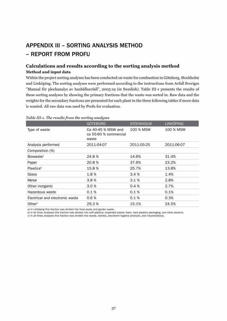
37

aPPendix iii – sorting analysis method

– rePort from Profu

Calculations and results according to the sorting analysis methodMethod and input dataWithin the project sorting analyses has been conducted on waste for combustion in Göteborg, Stockholm and Linköping. The sorting analyses were performed according to the instructions from Avfall Sveriges ”Manual för plockanalys av hushållsavfall”, 2005:19 (in Swedish). Table III-1 presents the results of these sorting analyses by showing the primary fractions that the waste was sorted in. Raw data and the weights for the secondary fractions are presented for each plant in the three following tables if more data is wanted. All raw data was used by Profu for evaluation.

Table III-1. The results from the sorting analysesGöteborG stocKholm linKöpinG

type of waste ca 40-45 % msw and ca 55-60 % commercial waste

100 % msw 100 % msw

analysis performed 2011-04-07 2011-05-25 2011-06-07

composition (%)

biowastea 24.8 % 14.6% 31.4%

paper 20.8 % 37.6% 23.2%

plasticsb 15.8 % 25.7% 13.8%

Glass 1.8 % 3.4 % 1.4%

metal 3.8 % 3.1 % 2.8%

other inorganic 3.0 % 0.4 % 2.7%

hazardous waste 0.1 % 0.1 % 0.1%

electrical and electronic waste 0.6 % 0.1 % 0.3%

otherc 29.3 % 15.1% 24.5%a) in linköping this fraction was divided into food waste and garden waste , b) in all three analyses this fraction was divided into soft plastics, expanded plastic foam, hard plastics packaging, and other plastics, c) in all three analyses this fraction was divided into woods, textiles, absorbent hygiene products, and miscellaneous.

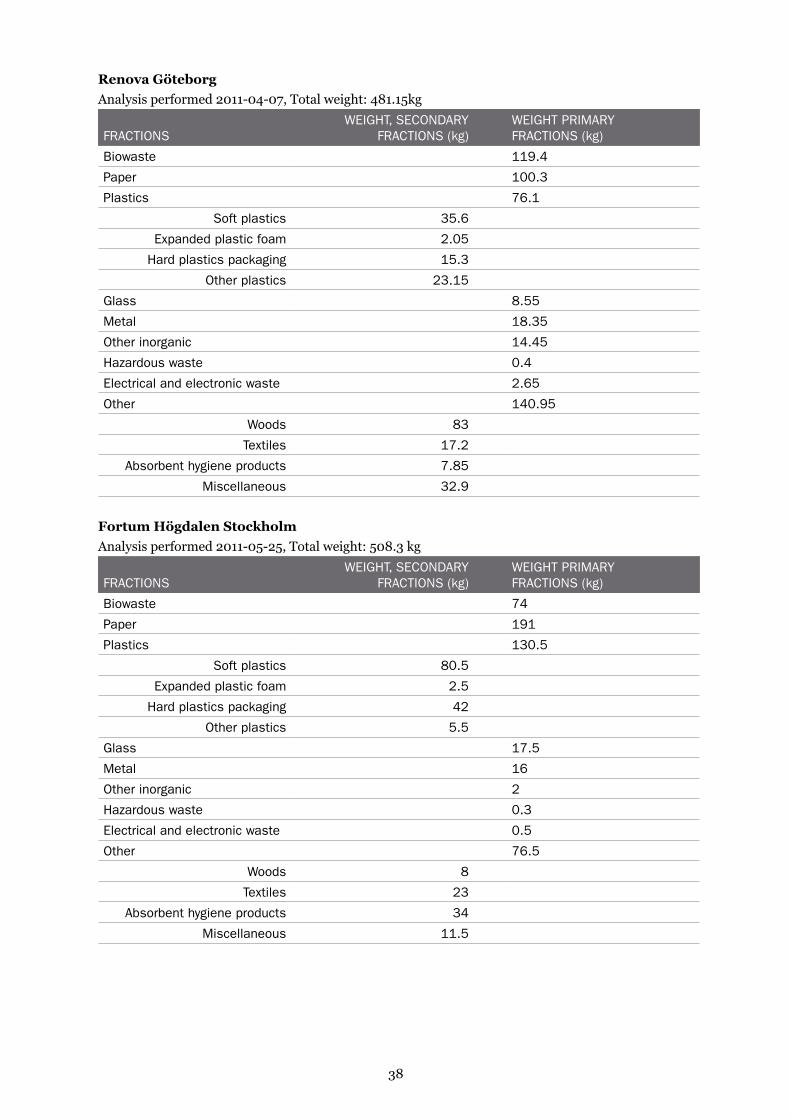
38

Renova GöteborgAnalysis performed 2011-04-07, Total weight: 481.15kg

fractionsweiGht, seconDary

fractions (kg)weiGht primary fractions (kg)

biowaste 119.4

paper 100.3

plastics 76.1

soft plastics 35.6

expanded plastic foam 2.05

hard plastics packaging 15.3

other plastics 23.15

Glass 8.55

metal 18.35

other inorganic 14.45

hazardous waste 0.4

electrical and electronic waste 2.65

other 140.95

woods 83

textiles 17.2

absorbent hygiene products 7.85

miscellaneous 32.9

Fortum Högdalen StockholmAnalysis performed 2011-05-25, Total weight: 508.3 kg

fractionsweiGht, seconDary

fractions (kg)weiGht primary fractions (kg)

biowaste 74

paper 191

plastics 130.5

soft plastics 80.5

expanded plastic foam 2.5

hard plastics packaging 42

other plastics 5.5

Glass 17.5

metal 16

other inorganic 2

hazardous waste 0.3

electrical and electronic waste 0.5

other 76.5

woods 8

textiles 23

absorbent hygiene products 34

miscellaneous 11.5

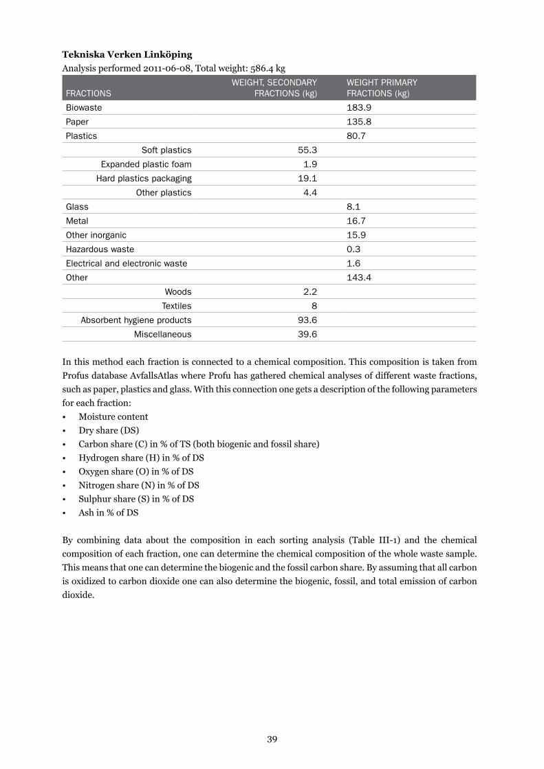
39

Tekniska Verken LinköpingAnalysis performed 2011-06-08, Total weight: 586.4 kg

fractionsweiGht, seconDary

fractions (kg)weiGht primary fractions (kg)

biowaste 183.9

paper 135.8

plastics 80.7

soft plastics 55.3

expanded plastic foam 1.9

hard plastics packaging 19.1

other plastics 4.4

Glass 8.1

metal 16.7

other inorganic 15.9

hazardous waste 0.3

electrical and electronic waste 1.6

other 143.4

woods 2.2

textiles 8

absorbent hygiene products 93.6

miscellaneous 39.6

In this method each fraction is connected to a chemical composition. This composition is taken from Profus database AvfallsAtlas where Profu has gathered chemical analyses of different waste fractions, such as paper, plastics and glass. With this connection one gets a description of the following parameters for each fraction:• Moisture content• Dry share (DS)• Carbon share (C) in % of TS (both biogenic and fossil share)• Hydrogen share (H) in % of DS• Oxygen share (O) in % of DS• Nitrogen share (N) in % of DS• Sulphur share (S) in % of DS• Ash in % of DS

By combining data about the composition in each sorting analysis (Table III-1) and the chemical composition of each fraction, one can determine the chemical composition of the whole waste sample. This means that one can determine the biogenic and the fossil carbon share. By assuming that all carbon is oxidized to carbon dioxide one can also determine the biogenic, fossil, and total emission of carbon dioxide.

40

To relate the emission to the energy in the waste a lower heating value (LHV) is calculated. An equation (from ECN (2011)), is initially used to decide the higher heating value (HHV) per TS.

HHVMilne = 0.341·C + 1.322·H - 0.12·O - 0.12·N + 0.0686·S - 0.0153·Ash [MJ/kg DS]

A LHV for the whole material, including moisture (w = moisture in %) is gained from the following equation:

LHV = (HHV – 2.442·8.936·H/100) ·(1-w/100) – 2.442·w/100 [MJ/kg]

ResultsTable III-2 shows the results according to this method. With this method the fossil emissions of CO2 is often increased with the share of plastics in the waste. The sorting analyses (Table III-1) shows that out of these three analyses the share of the plastic fraction was higher in Stockholm than in the two other cities, which can be seen in Table III-2 with high emissions for Stockholm.

When the difference of the plastics shares between the analyses is smaller, like between Göteborg and Linköping, the rest of the waste plays an important part when determining which waste mixture that gives the highest emissions of fossil CO2. The plastics share is somewhat higher in Göteborg but still the emissions (tonnes CO2/tonnes waste) is approximately the same as for Linköping. One important explanation to this is that in Göteborg the main share of the fraction “Other” consisted of wood (where the carbon is 100 % biogenic), whereas the main share in Linköping was absorbent hygiene products (where 64 % of the carbon is fossil). This means:

• The fraction ”others” barely gave any increase in fossil carbon in Göteborg but a significant contribution in Linköping, thus showing approximately the same emissions in total due to Göteborgs higher share of plastics.

• That the waste in Linköping, according to the calculations, had a higher moisture share (which was further increased by a high share of biowaste), giving a lower LHV and therefore a higher fossil carbon and CO2 / GJ waste. The higher moisture content also gave a lower total carbon share, increasing the share of fossil carbon in the total carbon.

Table III-2 Results according to the sorting analyses methodGöteborG stocKholm linKöpinG

share of fossil carbon of total carbon (wt-%) 31 48 38

share of fossil carbon per tonnes waste (wt-%/tonnes)

9.5 15 9.4

fossil carbon (kg/GJ) 8.1 12 10

fossil co2 (tonnes/tonnes avfall) 0.35 0.54 0.34

fossil co2 (kg/GJ) 30 43 36

41

Discussion about pros and cons of the sorting analyses methodAn advantage with this method is that when all the basic work is done (calculations structure, deciding what chemical composition each fraction should have etc.) it is easy to insert the result from the sorting analyses to get the calculated results. The method is easily adapted to the sorting analyses data available. In comparison with the other methods in this study the total cost for the evaluation itself is low, but the total cost could increase dramatically depending on how often the sorting analyses have to be performed to get a representative overview of the waste that is going to be burnt. This is a disadvantage/challenge for the method. The sorting analyses in this study were performed on 480-590 kg waste. Even though this is a relatively large amount of waste, it only represent 0.03-0.05 % of the amounts that were combusted on the same day as the sorting analyses were performed . This means that it is extremely important that the extracted portion of waste (for example, from a bunker) used for analysis really reflects the composition of the whole waste bunker.

Another disadvantage/challenge is whether the chemical composition that is assigned to each fraction gives a correct description of the current fraction. In these calculations the description of the plastic fraction especially important since it plays such an important role when it comes to the resulting emission of fossil CO2. One other important parameter is the moisture content, since it affects both the carbon share (higher moisture content leads to lower carbon share) and the LHV (higher moisture content leads to lower LHV). In the calculations an assumed moisture content of 43 % was used for the plastic fraction (from RVF (2005)). A sensitivity analysis is shown in Figure III-1, based on how the total carbon share (wt-%) would change if the moisture content would be 20 percentages lower or higher than the assumed value (ie a moisture content of 23 % and 63 %, respectively).

Figure III-1. Resulting share of carbon with three different moisture contents of the fraction plastics. Renova = Göteborg, Fortum = Stockholm, Tekniska Verken = Linklöping. (y-axis = Share of the total carbon (wt-%), x-axis = The moisture content in the plastic fraction (%)).

ReferencesECN (2011) PHYLLIS the composition of biomass and waste, http://www.ecn.nl/phyllis/RVF (2005) Manual för plockanalys av hushållsavfall, RVF Utveckling, rapport 2005:19Avfall Sverige (2011) Svensk Avfallshantering 2011

42

aPPendix iv - results from the chemical analysis of

the waste fuel from all Plants

The tables below present the raw data from the chemical analysis of all six samples at all seven plants.

Renovasample as receiVeD sample 1 sample 2 sample 3 sample 4 sample 5 sample 6

moisture, wt-% 36 36,5 42,5 27,7 30,1 37

ash, wt-% 13,2 14,2 16 19,4 16,6 12,4

c, wt-% 29,9 28,1 24,2 31,1 31,9 30,5

h , wt-% 8,1 7,8 7,8 7 7,5 8,2

n, wt-% 0,6 0,64 0,53 0,79 0,62 0,67

s, wt-% 0,21 0,17 0,5 0,54 0,3 0,14

cl, wt-% 0,58 0,54 0,5 0,7 0,6 0,89

higher heating valueat a constant volume, mJ/kg

12,86 11,78 10,29 13,39 13,73 13,08

lower heating value at a constant pressure, mJ/kg

11,09 10,07 8,59 11,87 12,11 11,29

Dry sample sample 1 sample 2 sample 3 sample 4 sample 5 sample 6

ash, wt-% 20,7 22,3 27,9 26,8 23,8 19,6

s, wt-% 0,32 0,85 0,86 0,74 0,43 0,22

cl, wt-% 0,91 0,27 0,86 0,96 0,85 1,4

c, wt-% 46,7 44,2 42,1 43,1 45,6 48,4

s, wt-% 6,5 5,9 5,3 5,4 5,9 6,5

n, wt-% 0,94 1,0 0,91 1,1 0,89 1,1

higher heating valueat a constant volume, mJ/kg

20,11 18,55 17,90 18,52 19,64 20,75

lower heating value at a constant pressure, mJ/kg

18,71 17,27 16,76 17,36 18,37 19,34

al, wt-% 1,28 1,21 1,68 1,02 1,37 0,98

si, wt-% 4,38 5,57 5,59 4,64 4,74 3,92

fe, wt-% 0,86 0,61 1,57 1,22 0,83 0,79

ti, wt-% 0,24 0,26 0,20 0,25 0,21 0,22

mn, wt-% 0,02 0,02 0,03 0,02 0,02 0,02

mg, wt-% 0,33 0,42 0,40 0,37 0,34 0,26

ca, wt-% 2,75 3,00 3,52 3,04 3,14 2,34

ba, wt-% 0,05 0,03 0,11 0,06 0,06 0,05

na, wt-% 0,75 1,06 0,86 0,71 0,71 0,76

K, wt-% 0,35 0,42 0,45 0,36 0,34 0,39

p, wt-% <0,02 0,16 0,07 0,07 0,09 0,14

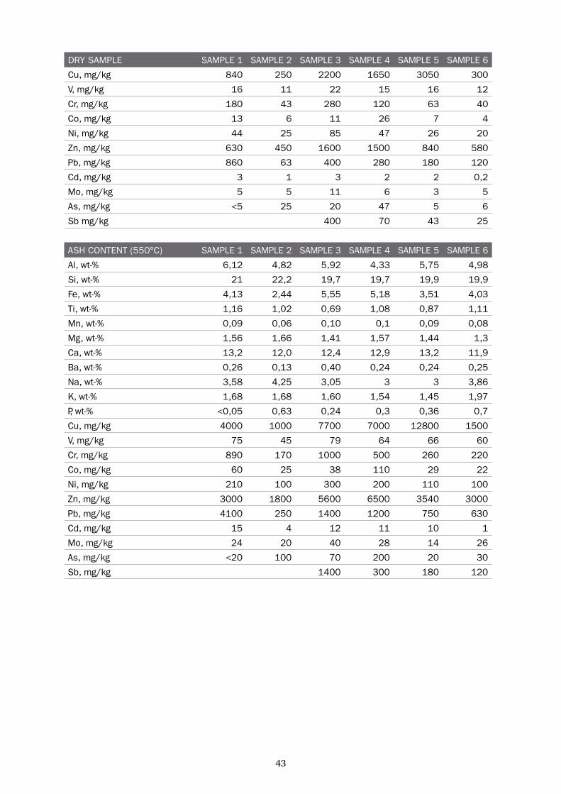
43

Dry sample sample 1 sample 2 sample 3 sample 4 sample 5 sample 6

cu, mg/kg 840 250 2200 1650 3050 300

V, mg/kg 16 11 22 15 16 12

cr, mg/kg 180 43 280 120 63 40

co, mg/kg 13 6 11 26 7 4

ni, mg/kg 44 25 85 47 26 20

Zn, mg/kg 630 450 1600 1500 840 580

pb, mg/kg 860 63 400 280 180 120

cd, mg/kg 3 1 3 2 2 0,2

mo, mg/kg 5 5 11 6 3 5

as, mg/kg <5 25 20 47 5 6

sb mg/kg 400 70 43 25

ash content (550°c) sample 1 sample 2 sample 3 sample 4 sample 5 sample 6

al, wt-% 6,12 4,82 5,92 4,33 5,75 4,98

si, wt-% 21 22,2 19,7 19,7 19,9 19,9

fe, wt-% 4,13 2,44 5,55 5,18 3,51 4,03

ti, wt-% 1,16 1,02 0,69 1,08 0,87 1,11

mn, wt-% 0,09 0,06 0,10 0,1 0,09 0,08

mg, wt-% 1,56 1,66 1,41 1,57 1,44 1,3

ca, wt-% 13,2 12,0 12,4 12,9 13,2 11,9

ba, wt-% 0,26 0,13 0,40 0,24 0,24 0,25

na, wt-% 3,58 4,25 3,05 3 3 3,86

K, wt-% 1,68 1,68 1,60 1,54 1,45 1,97

p, wt-% <0,05 0,63 0,24 0,3 0,36 0,7

cu, mg/kg 4000 1000 7700 7000 12800 1500

V, mg/kg 75 45 79 64 66 60

cr, mg/kg 890 170 1000 500 260 220

co, mg/kg 60 25 38 110 29 22

ni, mg/kg 210 100 300 200 110 100

Zn, mg/kg 3000 1800 5600 6500 3540 3000

pb, mg/kg 4100 250 1400 1200 750 630

cd, mg/kg 15 4 12 11 10 1

mo, mg/kg 24 20 40 28 14 26

as, mg/kg <20 100 70 200 20 30

sb, mg/kg 1400 300 180 120

44

Sysavsample as receiVeD sample

1sample

2sample

3sample

4asample

4bsample

5sample

6

moisture, wt-% 39,0 40,1 38,9 38,3 41 24,4 21,5

ash, wt-% 11,7 11,1 14,6 16,5 15,1 13,2 31,5

c, wt-% 28,8 26,1 26,4 26,4 25,6 38,4 30,8

h , wt-% 8,1 7,7 7,7 7,8 7,8 7,6 6,4

n, wt-% 0,70 0,76 0,59 0,82 0,88 0,66 0,82

s, wt-% 0,24 0,12 0,26 0,35 0,28 0,28 0,27

cl, wt-% 0,36 0,19 0,32 0,68 0,5 0,61 0,72

higher heating valueat a constant volume, mJ/kg

12,44 10,98 11,06 11,73 10,86 17,1 12,7

lower heating value at a constant pressure, mJ/kg

10,68 9,29 9,37 10,03 9,16 15,46 11,31

Dry sample sample 1

sample 2

sample 3

sample 4a

sample 4b

sample 5

sample 6

ash, wt-% 19,1 18,5 23,9 26,8 25,6 17,4 40,1

s, wt-% 0,39 0,19 0,43 0,57 0,47 0,37 0,35

cl, wt-% 0,6 0,32 0,52 1,1 0,84 0,8 0,92

c, wt-% 47,2 43,5 43,2 42,9 43,4 50,7 39,3

s, wt-% 6,2 5,4 5,6 5,7 5,5 6,4 5,1

n, wt-% 1,1 1,3 0,96 1,3 1,5 0,87 1

higher heating valueat a constant volume, mJ/kg

20,39 18,33 18,1 19,01 18,4 22,61 16,18

lower heating value at a constant pressure, mJ/kg

19,05 17,15 16,89 17,78 17,21 21,23 15,08

al, wt-% 0,86 0,84 1,1 1,28 1,2 1,1 1,79

si, wt-% 4,56 4,44 5,61 5,28 5,29 3,06 7,24

fe, wt-% 0,72 0,93 0,85 0,98 1,06 0,7 5,68

ti, wt-% 0,20 0,14 0,19 0,38 0,44 0,19 0,36

mn, wt-% 0,02 0,02 0,02 0,03 0,03 0,01 0,06

mg, wt-% 0,28 0,26 0,32 0,36 0,35 0,26 0,49

ca, wt-% 2,34 1,89 2,92 3,25 3,12 2,31 3,1

ba, wt-% 0,03 0,03 0,08 0,07 0,07 0,08 0,28

na, wt-% 0,71 0,72 0,7 0,64 0,62 0,44 1,1

K, wt-% 0,39 0,42 0,46 0,4 0,4 0,23 0,5

p, wt-% 0,02 0,10 0,13 0,09 0,1 0,07 0,12

cu, mg/kg 1100 280 1550 1640 510 2080 6400

V, mg/kg 15 11 20 12 14 10 20

cr, mg/kg 57 57 52 96 58 250 200

co, mg/kg 7 7 5 10 11 40 20

ni, mg/kg 41 13 19 110 43 100 330

Zn, mg/kg 850 640 1090 1900 910 950 15000

pb, mg/kg 1830 90 110 120 160 120 1000

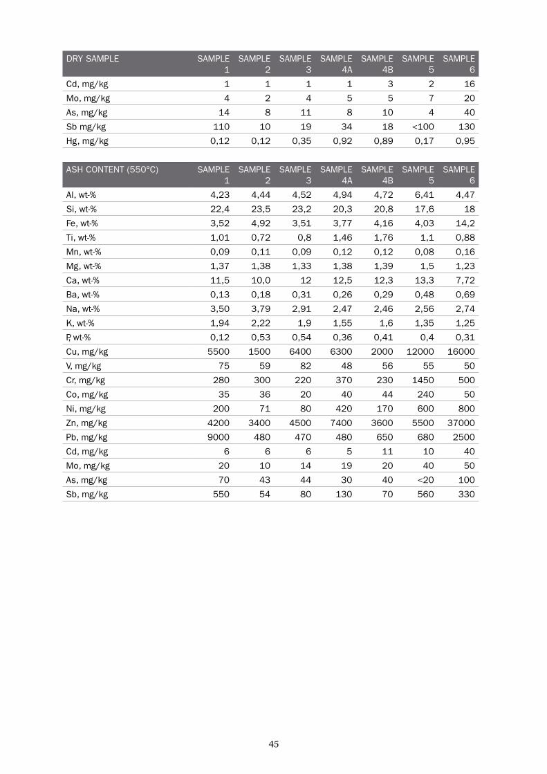
45

Dry sample sample 1

sample 2

sample 3

sample 4a

sample 4b

sample 5

sample 6

cd, mg/kg 1 1 1 1 3 2 16

mo, mg/kg 4 2 4 5 5 7 20

as, mg/kg 14 8 11 8 10 4 40

sb mg/kg 110 10 19 34 18 <100 130

hg, mg/kg 0,12 0,12 0,35 0,92 0,89 0,17 0,95

ash content (550°c) sample 1

sample 2

sample 3

sample 4a

sample 4b

sample 5

sample 6

al, wt-% 4,23 4,44 4,52 4,94 4,72 6,41 4,47

si, wt-% 22,4 23,5 23,2 20,3 20,8 17,6 18

fe, wt-% 3,52 4,92 3,51 3,77 4,16 4,03 14,2

ti, wt-% 1,01 0,72 0,8 1,46 1,76 1,1 0,88

mn, wt-% 0,09 0,11 0,09 0,12 0,12 0,08 0,16

mg, wt-% 1,37 1,38 1,33 1,38 1,39 1,5 1,23

ca, wt-% 11,5 10,0 12 12,5 12,3 13,3 7,72

ba, wt-% 0,13 0,18 0,31 0,26 0,29 0,48 0,69

na, wt-% 3,50 3,79 2,91 2,47 2,46 2,56 2,74

K, wt-% 1,94 2,22 1,9 1,55 1,6 1,35 1,25

p, wt-% 0,12 0,53 0,54 0,36 0,41 0,4 0,31

cu, mg/kg 5500 1500 6400 6300 2000 12000 16000

V, mg/kg 75 59 82 48 56 55 50

cr, mg/kg 280 300 220 370 230 1450 500

co, mg/kg 35 36 20 40 44 240 50

ni, mg/kg 200 71 80 420 170 600 800

Zn, mg/kg 4200 3400 4500 7400 3600 5500 37000

pb, mg/kg 9000 480 470 480 650 680 2500

cd, mg/kg 6 6 6 5 11 10 40

mo, mg/kg 20 10 14 19 20 40 50

as, mg/kg 70 43 44 30 40 <20 100

sb, mg/kg 550 54 80 130 70 560 330

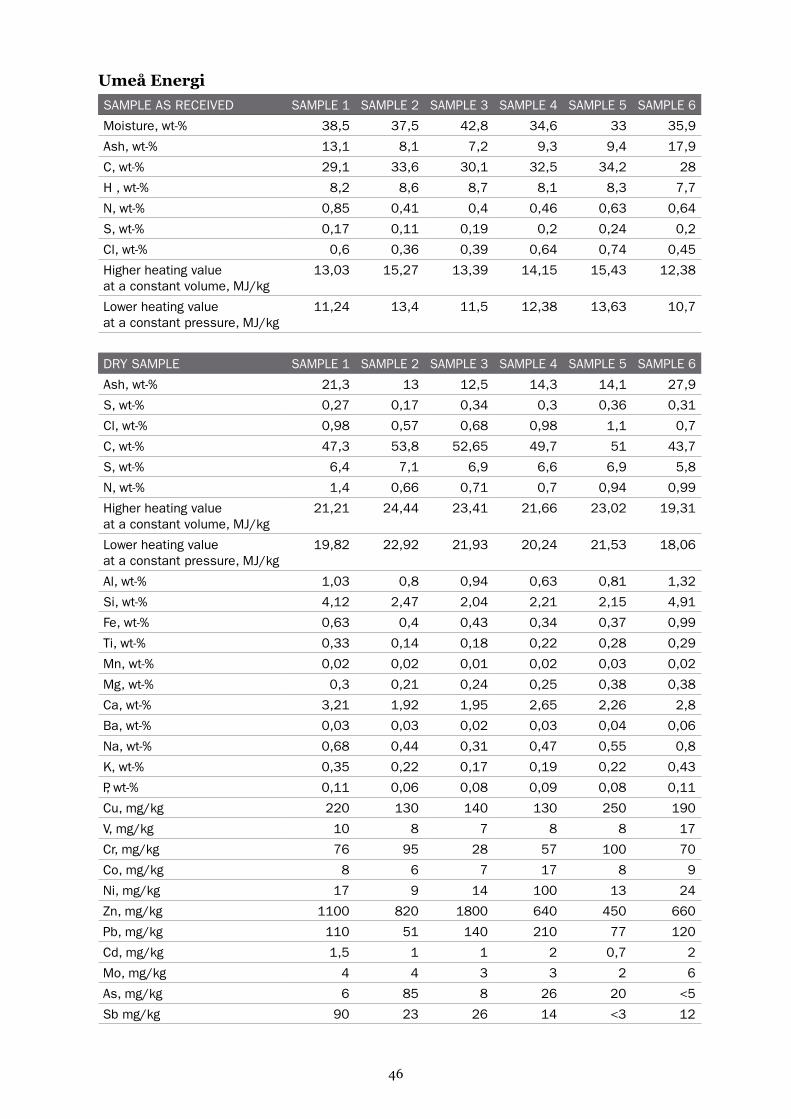
46

sample as receiVeD sample 1 sample 2 sample 3 sample 4 sample 5 sample 6

moisture, wt-% 38,5 37,5 42,8 34,6 33 35,9

ash, wt-% 13,1 8,1 7,2 9,3 9,4 17,9

c, wt-% 29,1 33,6 30,1 32,5 34,2 28

h , wt-% 8,2 8,6 8,7 8,1 8,3 7,7

n, wt-% 0,85 0,41 0,4 0,46 0,63 0,64

s, wt-% 0,17 0,11 0,19 0,2 0,24 0,2

cl, wt-% 0,6 0,36 0,39 0,64 0,74 0,45

higher heating valueat a constant volume, mJ/kg

13,03 15,27 13,39 14,15 15,43 12,38

lower heating value at a constant pressure, mJ/kg

11,24 13,4 11,5 12,38 13,63 10,7

Dry sample sample 1 sample 2 sample 3 sample 4 sample 5 sample 6

ash, wt-% 21,3 13 12,5 14,3 14,1 27,9

s, wt-% 0,27 0,17 0,34 0,3 0,36 0,31

cl, wt-% 0,98 0,57 0,68 0,98 1,1 0,7

c, wt-% 47,3 53,8 52,65 49,7 51 43,7

s, wt-% 6,4 7,1 6,9 6,6 6,9 5,8

n, wt-% 1,4 0,66 0,71 0,7 0,94 0,99

higher heating valueat a constant volume, mJ/kg

21,21 24,44 23,41 21,66 23,02 19,31

lower heating value at a constant pressure, mJ/kg

19,82 22,92 21,93 20,24 21,53 18,06

al, wt-% 1,03 0,8 0,94 0,63 0,81 1,32

si, wt-% 4,12 2,47 2,04 2,21 2,15 4,91

fe, wt-% 0,63 0,4 0,43 0,34 0,37 0,99

ti, wt-% 0,33 0,14 0,18 0,22 0,28 0,29

mn, wt-% 0,02 0,02 0,01 0,02 0,03 0,02

mg, wt-% 0,3 0,21 0,24 0,25 0,38 0,38

ca, wt-% 3,21 1,92 1,95 2,65 2,26 2,8

ba, wt-% 0,03 0,03 0,02 0,03 0,04 0,06

na, wt-% 0,68 0,44 0,31 0,47 0,55 0,8

K, wt-% 0,35 0,22 0,17 0,19 0,22 0,43

p, wt-% 0,11 0,06 0,08 0,09 0,08 0,11

cu, mg/kg 220 130 140 130 250 190

V, mg/kg 10 8 7 8 8 17

cr, mg/kg 76 95 28 57 100 70

co, mg/kg 8 6 7 17 8 9

ni, mg/kg 17 9 14 100 13 24

Zn, mg/kg 1100 820 1800 640 450 660

pb, mg/kg 110 51 140 210 77 120

cd, mg/kg 1,5 1 1 2 0,7 2

mo, mg/kg 4 4 3 3 2 6

as, mg/kg 6 85 8 26 20 <5

sb mg/kg 90 23 26 14 <3 12

Umeå Energi

47

ash content (550°c) sample 1 sample 2 sample 3 sample 4 sample 5 sample 6

al, wt-% 4,72 5,94 7,68 4,41 5,81 5,49

si, wt-% 18,9 18,4 16,7 15,5 15,4 20,4

fe, wt-% 2,88 2,96 3,54 2,39 2,64 4,12

ti, wt-% 1,5 1,3 1,51 1,5 2 1,2

mn, wt-% 0,09 0,13 0,11 0,13 0,19 0,09

mg, wt-% 1,38 1,56 1,96 1,75 2,76 1,57

ca, wt-% 14,8 14,3 16 18,5 16,1 11,6

ba, wt-% 0,15 0,21 0,13 0,2 0,26 0,25

na, wt-% 3,12 3,25 2,54 3,3 3,92 3,31

K, wt-% 1,6 1,68 1,38 1,32 1,56 1,8

p, wt-% 0,52 0,42 0,68 0,64 0,55 0,47

cu, mg/kg 1000 1000 1140 900 1800 780

V, mg/kg 44 62 60 60 54 70

cr, mg/kg 350 710 230 400 700 290

co, mg/kg 35 42 57 120 56 38

ni, mg/kg 80 67 120 700 94 100

Zn, mg/kg 5000 6100 14600 4500 3200 2750

pb, mg/kg 500 38 1130 1500 550 500

cd, mg/kg 7 8 12 11 5 9

mo, mg/kg 20 28 30 20 15 27

as, mg/kg 30 630 60 180 140 <20

sb, mg/kg 400 170 210 100 <120 50

48

sample as receiVeD sample 1 sample 2 sample 3 sample 4 sample 5 sample 6

moisture, wt-% 45,2 46,5 47,5 43,3 45,9 44,2

ash, wt-% 10,7 10,8 9,7 11,8 11,1 11,2

c, wt-% 25 24,5 25 26,6 24,4 25,8

h , wt-% 8,5 8,5 8,7 8,4 8,3 8,4

n, wt-% 0,66 0,71 0,57 0,64 0,66 0,59

s, wt-% 0,09 0,08 0,09 0,12 0,05 0,07

cl, wt-% 0,4 0,3 0,46 0,48 0,33 0,48

higher heating valueat a constant volume, mJ/kg

11,09 10,81 11,22 12,02 10,81 11,8

lower heating value at a constant pressure, mJ/kg

9,23 8,96 9,32 10,18 9 9,97

Dry sample sample 1 sample 2 sample 3 sample 4 sample 5 sample 6

ash, wt-% 19,6 20,2 18,5 20,8 20,6 20,1

s, wt-% 0,16 0,15 0,17 0,21 0,09 0,12

cl, wt-% 0,73 0,56 0,88 0,84 0,61 0,86

c, wt-% 45,6 45,8 47,6 47 45,1 46,2

s, wt-% 6,4 6,2 6,6 6,4 5,9 6,2

n, wt-% 1,2 1,3 1,1 1,1 1,2 1

higher heating valueat a constant volume, mJ/kg

20,25 20,19 21,38 21,21 19,99 21,17

lower heating value at a constant pressure, mJ/kg

18,88 18,86 19,97 19,83 18,72 19,83

al, wt-% 1,31 1,07 0,84 1,05 0,68 1,03

si, wt-% 4,23 4,38 3,28 4,4 4,79 5,1

fe, wt-% 0,42 0,35 0,43 0,64 0,21 0,39

ti, wt-% 0,13 0,13 0,13 0,14 0,1 0,13

mn, wt-% 0,02 0,02 0,01 0,02 0,01 0,01

mg, wt-% 0,25 0,3 0,22 0,26 0,26 0,28

ca, wt-% 2,86 3,02 2,64 2,89 3,35 3,16

ba, wt-% 0,02 0,02 0,04 0,02 0,02 0,02

na, wt-% 0,95 1,12 0,86 0,92 1,32 1,19

K, wt-% 0,38 0,38 0,3 0,34 0,37 0,41

p, wt-% 0,16 0,15 0,16 0,17 0,18 0,12

cu, mg/kg 990 660 250 220 47 590

V, mg/kg 7 8 6 7 1 8

cr, mg/kg 53 50 59 60 77 80

co, mg/kg 4 32 5 6 4 4

ni, mg/kg 25 280 12 14 100 10

Zn, mg/kg 950 840 480 420 260 450

pb, mg/kg 500 65 36 75 30 110

cd, mg/kg 0,6 0,9 0,4 1 0,2 0,7

mo, mg/kg 2 3 <2 3 <3 2

as, mg/kg 6 <4 <4 <5 <5 5

sb mg/kg 116 18 22 25 <5 30

Fortum Högdalen

49

ash content (550°c) sample 1 sample 2 sample 3 sample 4 sample 5 sample 6

al, wt-% 6,2 4,97 4,68 5,05 3,01 4,45

si, wt-% 20,1 20,3 18,2 21,1 21,2 22

fe, wt-% 2 1,62 2,39 3,09 0,92 1,67

ti, wt-% 0,3 0,6 0,71 0,66 0,46 0,57

mn, wt-% 0,08 0,08 0,06 0,07 0,03 0,06

mg, wt-% 1,19 1,41 1,25 1,26 1,16 1,2

ca, wt-% 13,6 14 14,7 13,9 14,8 13,7

ba, wt-% 0,09 0,08 0,22 0,1 0,07 0,11

na, wt-% 4,51 5,21 4,76 4,42 5,85 5,15

K, wt-% 1,81 1,78 1,64 1,66 1,66 1,78

p, wt-% 0,75 0,69 0,88 0,82 0,81 0,53

cu, mg/kg 4700 3060 1380 1040 210 2600

V, mg/kg 35 36 32 33 15 33

cr, mg/kg 250 230 330 290 340 340

co, mg/kg 20 150 28 28 18 16

ni, mg/kg 120 1300 66 70 470 24

Zn, mg/kg 4500 3900 2700 2000 1160 1950

pb, mg/kg 2400 300 200 360 140 460

cd, mg/kg 3 4 2 6 1 3

mo, mg/kg 10 15 <10 14 <10 10

as, mg/kg 30 <20 <20 <20 <20 22

sb, mg/kg 550 83 120 120 <20 130

50

sample as receiVeD sample 1 sample 2 sample 3 sample 4 sample 5 sample 6

moisture, wt-% 40,2 46 45,3 42,4 46,7 37,8

ash, wt-% 14,3 9,4 9 9,6 12,2 11,1

c, wt-% 25,4 26,1 26,2 27,8 23,2 29,7

h , wt-% 8 8,6 8,6 8,2 8,4 8,2

n, wt-% 0,74 0,69 0,64 0,79 0,73 0,73

s, wt-% 0,12 0,16 0,08 0,08 0,1 0,21

cl, wt-% 0,39 0,37 0,35 0,39 0,32 0,5

higher heating valueat a constant volume, mJ/kg

11,02 11,53 11,8 12,17 10,08 13,33

lower heating value at a constant pressure, mJ/kg

9,28 9,64 9,93 10,37 8,25 11,54

Dry sample sample 1 sample 2 sample 3 sample 4 sample 5 sample 6

ash, wt-% 24 17,4 16,5 16,6 22,8 17,8

s, wt-% 0,21 0,31 0,15 0,14 0,18 0,19

cl, wt-% 0,66 0,68 0,63 0,68 0,6 0,8

c, wt-% 42,5 48,4 48 48,3 43,5 47,7

s, wt-% 5,8 6,6 6,5 6,1 6 6,4

n, wt-% 1,2 1,3 1,2 1,4 1,4 1,2

higher heating valueat a constant volume, mJ/kg

18,43 21,37 21,58 21,15 18,9 21,41

lower heating value at a constant pressure, mJ/kg

17,17 19,96 20,18 19,82 17,62 20,03

al, wt-% 1,18 1,09 0,92 1 1,51 0,85

si, wt-% 5,07 3,57 3,15 3,62 5,26 3,27

fe, wt-% 0,52 0,56 0,36 0,35 0,79 0,47

ti, wt-% 0,16 0,17 0,16 0,13 0,13 0,18

mn, wt-% 0,02 0,02 0,01 0,01 0,15 0,01

mg, wt-% 0,33 0,3 0,23 0,22 0,28 0,24

ca, wt-% 3,12 2,69 2,72 2,47 2,82 2,69

ba, wt-% 0,06 0,02 0,01 0,01 0,02 0,01

na, wt-% 1,1 0,83 0,8 0,79 1,2 0,81

K, wt-% 0,48 0,34 0,42 0,4 0,59 0,37

p, wt-% 0,23 0,13 0,2 0,14 0,18 0,17

cu, mg/kg 230 380 110 270 120 210

V, mg/kg 9 11 6 6 11 6

cr, mg/kg 24 90 23 40 47 30

co, mg/kg 3 4 4 7 5 6

ni, mg/kg 11 30 12 10 15 10

Zn, mg/kg 250 250 380 300 1250 280

pb, mg/kg 43 32 34 45 140 28

cd, mg/kg 1 0,8 0,7 0,4 <0,3 2

mo, mg/kg 2 2 2 2 2 3

as, mg/kg 5 <4 <4 <4 10 <4

sb mg/kg 92 16 26 9 <5 11

Tekniska Verken

51

ash content (550°c) sample 1 sample 2 sample 3 sample 4 sample 5 sample 6

al, wt-% 4,9 5,81 5,44 5,55 6,04 4,79

si, wt-% 21 19 18,5 20 21,1 18,4

fe, wt-% 2,17 2,98 2,15 1,93 3,16 2,66

ti, wt-% 0,65 0,9 0,92 0,74 0,52 0,99

mn, wt-% 0,07 0,1 0,06 0,07 0,61 0,07

mg, wt-% 1,39 1,61 1,35 1,19 1,13 1,33

ca, wt-% 12,9 14,3 16 13,6 11,3 15,1

ba, wt-% 0,26 0,11 0,8 0,07 0,07 0,06

na, wt-% 4,55 4,4 4,68 4,36 4,8 4,57

K, wt-% 2,01 1,83 2,5 2,24 2,35 2,07

p, wt-% 0,97 0,69 1,18 0,8 0,73 0,97

cu, mg/kg 950 2030 660 1500 470 1200

V, mg/kg 38 57 36 36 44 36

cr, mg/kg 100 480 130 220 190 170

co, mg/kg 12 23 24 40 22 36

ni, mg/kg 46 160 70 53 60 60

Zn, mg/kg 1030 1340 2200 1700 5000 1600

pb, mg/kg 180 170 200 250 560 160

cd, mg/kg 4 4 4 2 <1 12

mo, mg/kg 10 13 12 10 10 20

as, mg/kg 20 <20 <20 <20 40 <20

sb, mg/kg 380 84 150 50 <20 60

52

sample as receiVeD sample 1 sample 2 sample 3 sample 4 sample 5 sample 6

moisture, wt-% 35,6 41,8 40,1 39,2 33,8 32,1

ash, wt-% 13 11,2 12,2 10,3 15,6 16

c, wt-% 30,3 26,2 27,3 30,2 29,8 30,9

h , wt-% 8 8,2 8 8,3 7,6 7,6

n, wt-% 0,8 0,71 0,68 0,5 0,69 0,94

s, wt-% 0,29 0,22 0,43 0,31 0,48 0,58

cl, wt-% 0,6 0,24 0,43 0,57 0,72 0,5

higher heating valueat a constant volume, mJ/kg

13,66 11,2 11,99 13,52 12,98 13,59

lower heating value at a constant pressure, mJ/kg

11,93 9,42 10,24 11,72 11,33 11,94

Dry sample sample 1 sample 2 sample 3 sample 4 sample 5 sample 6

ash, wt-% 20,2 19,2 20,3 17 23,5 23,5

s, wt-% 0,46 0,37 0,72 0,51 0,72 0,85

cl, wt-% 0,93 0,41 0,72 0,93 1,1 0,73

c, wt-% 47,1 45,1 45,5 49,7 45 45,5

s, wt-% 6,2 6 6 6,4 5,7 5,9

n, wt-% 1,2 1,2 1,1 0,82 1 1,4

higher heating valueat a constant volume, mJ/kg

21,2 19,22 20,01 22,23 19,61 20,3

lower heating value at a constant pressure, mJ/kg

19,87 17,92 18,72 20,84 18,38 18,76

al, wt-% 2,26 0,93 0,92 1,04 1,16 1,34

si, wt-% 4,14 3,94 3,76 2,63 4,73 5,06

fe, wt-% 0,66 0,46 0,57 0,58 0,92 0,9

ti, wt-% 0,19 0,12 0,24 0,24 0,2 0,21

mn, wt-% 0,02 0,02 0,02 0,02 0,02 0,02

mg, wt-% 0,38 0,46 0,36 0,33 0,31 0,37

ca, wt-% 3,16 2,59 3,26 2,8 2,96 3,6

ba, wt-% 0,03 0,03 0,02 0,02 0,03 0,04

na, wt-% 0,69 0,81 0,69 0,45 0,7 0,75

K, wt-% 0,28 0,33 0,35 0,23 0,42 0,38

p, wt-% 0,01 0,11 0,12 0,11 0,11 0,05

cu, mg/kg 2000 720 110 920 400 300

V, mg/kg 14 9 12 10 13 20

cr, mg/kg 250 170 90 170 330 100

co, mg/kg 6 8 5 9 10 10

ni, mg/kg 39 743 23 50 120 40

Zn, mg/kg 830 550 860 1020 660 1000

pb, mg/kg 680 690 2000 110 200 180

cd, mg/kg 4 2 2 2 7 4

mo, mg/kg 6 3 5 10 22 9

as, mg/kg 25 59 16 10 10 25

sb mg/kg 50 22 60 50 120 40

Eon Händelöverket

53

ash content (550°c) sample 1 sample 2 sample 3 sample 4 sample 5 sample 6

al, wt-% 10,9 4,73 4,24 6,13 4,65 5,33

si, wt-% 19,9 20 17,4 15,5 19 20,2

fe, wt-% 3,17 2,33 2,63 3,44 3,69 3,58

ti, wt-% 0,93 0,6 1,1 1,38 0,82 0,84

mn, wt-% 0,08 0,09 0,09 0,11 0,09 0,1

mg, wt-% 1,81 2,32 1,65 1,97 1,23 1,48

ca, wt-% 15,2 13,2 15,1 16,5 11,9 14,4

ba, wt-% 0,16 0,17 0,11 0,14 0,13 0,16

na, wt-% 3,34 4,12 3,18 2,62 2,82 3

K, wt-% 1,37 1,66 1,61 1,36 1,67 1,52

p, wt-% 0,05 0,54 0,54 0,65 0,44 0,21

cu, mg/kg 9600 3650 4900 5400 1600 1200

V, mg/kg 65 45 55 60 50 80

cr, mg/kg 1200 850 410 980 1340 400

co, mg/kg 30 41 23 50 40 40

ni, mg/kg 190 220 100 300 470 160

Zn, mg/kg 4000 2800 4000 6000 2700 4100

pb, mg/kg 3300 3500 9300 640 820 700

cd, mg/kg 18 8 11 12 29 15

mo, mg/kg 30 15 24 60 90 37

as, mg/kg 120 300 76 60 40 100

sb, mg/kg 240 110 280 300 500 160

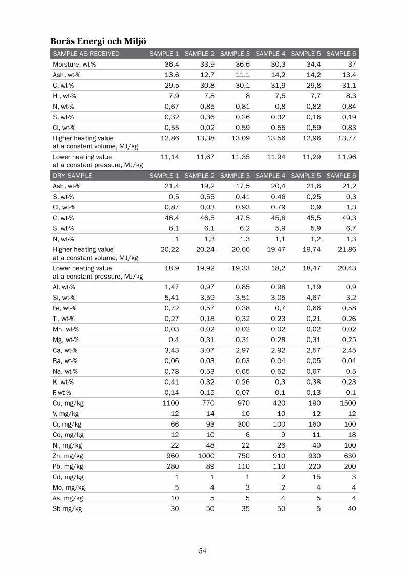
54

sample as receiVeD sample 1 sample 2 sample 3 sample 4 sample 5 sample 6

moisture, wt-% 36,4 33,9 36,6 30,3 34,4 37

ash, wt-% 13,6 12,7 11,1 14,2 14,2 13,4

c, wt-% 29,5 30,8 30,1 31,9 29,8 31,1

h , wt-% 7,9 7,8 8 7,5 7,7 8,3

n, wt-% 0,67 0,85 0,81 0,8 0,82 0,84

s, wt-% 0,32 0,36 0,26 0,32 0,16 0,19

cl, wt-% 0,55 0,02 0,59 0,55 0,59 0,83

higher heating valueat a constant volume, mJ/kg

12,86 13,38 13,09 13,56 12,96 13,77

lower heating value at a constant pressure, mJ/kg

11,14 11,67 11,35 11,94 11,29 11,96

Dry sample sample 1 sample 2 sample 3 sample 4 sample 5 sample 6

ash, wt-% 21,4 19,2 17,5 20,4 21,6 21,2

s, wt-% 0,5 0,55 0,41 0,46 0,25 0,3

cl, wt-% 0,87 0,03 0,93 0,79 0,9 1,3

c, wt-% 46,4 46,5 47,5 45,8 45,5 49,3

s, wt-% 6,1 6,1 6,2 5,9 5,9 6,7

n, wt-% 1 1,3 1,3 1,1 1,2 1,3

higher heating valueat a constant volume, mJ/kg

20,22 20,24 20,66 19,47 19,74 21,86

lower heating value at a constant pressure, mJ/kg

18,9 19,92 19,33 18,2 18,47 20,43

al, wt-% 1,47 0,97 0,85 0,98 1,19 0,9

si, wt-% 5,41 3,59 3,51 3,05 4,67 3,2

fe, wt-% 0,72 0,57 0,38 0,7 0,66 0,58

ti, wt-% 0,27 0,18 0,32 0,23 0,21 0,26

mn, wt-% 0,03 0,02 0,02 0,02 0,02 0,02

mg, wt-% 0,4 0,31 0,31 0,28 0,31 0,25

ca, wt-% 3,43 3,07 2,97 2,92 2,57 2,45

ba, wt-% 0,06 0,03 0,03 0,04 0,05 0,04

na, wt-% 0,78 0,53 0,65 0,52 0,67 0,5

K, wt-% 0,41 0,32 0,26 0,3 0,38 0,23

p, wt-% 0,14 0,15 0,07 0,1 0,13 0,1

cu, mg/kg 1100 770 970 420 190 1500

V, mg/kg 12 14 10 10 12 12

cr, mg/kg 66 93 300 100 160 100

co, mg/kg 12 10 6 9 11 18

ni, mg/kg 22 48 22 26 40 100

Zn, mg/kg 960 1000 750 910 930 630

pb, mg/kg 280 89 110 110 220 200

cd, mg/kg 1 1 1 2 15 3

mo, mg/kg 5 4 3 2 4 4

as, mg/kg 10 5 5 4 5 4

sb mg/kg 30 50 35 50 5 40

Borås Energi och Miljö

55

ash content (550°c) sample 1 sample 2 sample 3 sample 4 sample 5 sample 6

al, wt-% 6,27 5,03 4,55 5,61 5,62 5,04

si, wt-% 23 18,6 18,8 17,5 22 17,8

fe, wt-% 3,05 2,94 2,03 4 3,12 3,25

ti, wt-% 1,14 0,96 1,72 1,31 0,98 1,46

mn, wt-% 0,12 0,1 0,09 0,11 0,12 0,11

mg, wt-% 1,72 1,58 1,65 1,6 1,48 1,4

ca, wt-% 14,6 15,9 15,9 16,8 12,1 13,7

ba, wt-% 0,25 0,15 0,17 0,21 0,24 0,22

na, wt-% 3,32 2,74 3,48 2,96 3,15 2,8

K, wt-% 1,73 1,64 1,4 1,7 1,78 1,3

p, wt-% 0,61 0,8 0,39 0,6 0,62 0,55

cu, mg/kg 4600 4000 5200 2400 890 8600

V, mg/kg 50 74 51 60 57 65

cr, mg/kg 280 480 1600 580 740 580

co, mg/kg 50 53 34 50 50 100

ni, mg/kg 95 250 120 150 190 570

Zn, mg/kg 4100 5200 4000 5250 4400 3500

pb, mg/kg 1200 460 570 620 1050 1100

cd, mg/kg 5 7 8 12 70 15

mo, mg/kg 23 19 14 14 18 20

as, mg/kg 45 25 25 20 20 25

sb, mg/kg 130 260 190 280 20 220

56

aPPendix v - determination of fossil carbon

In the tables below the results from Betalab Analtyics carbon-14 analysis of the project’s solid samples and flue gas samples are presented. The results from Betalab (“The share of fossil carbon in total carbon content (%)”, column 3, and “The share of fossil carbon in the flue gas, contemporary samples (%)”, column 7) are calculated with a background value of 107 pMC. Other results in the tables are calculated using the individual chemical analyses are given in Appendix IV.

Further down in the Appendix are two graphs that present the data and how they relate to the two standard values that have been used and discussed by the authorities and industry. Both standard values are calculated from the same basic data in the RVF Report 2003:13. Interestingly, it is noted that the results of this project is less than one norm value and higher than the other. This result suggests that some of these earlier standard values must be calculated wrong.

renoVa share of com-mercial waste

share of fossil

carbon per total car-

bon (%)

fossil car-bon in the

fuel (%)

fossil car-bon

(KG co2/GJ)

fossil car-bon, aVeraGe

moisture content 40 %

(%/tonnes waste)

share of fossil car-bon in the flue Gas, parallel

samplinG (%)

sample 1 65 38 11 38 10 -

sample 2 63 29 8 30 7 -

sample 3 67 32 8 33 8 -

sample 4 63 33 10 32 7 39

sample 5 60 38 12 37 9 43

sample 6 30 33 10 33 9 26

sysaV share of com-mercial waste

share of fossil

carbon per total car-

bon (%)

fossil car-bon in the

fuel (%)

fossil car-bon

(KG co2/GJ)

fossil car-bon, aVeraGe

moisture content 40 %

(%/tonnes waste)

share of fossil car-bon in the flue Gas, parallel

samplinG (%)

sample 1 42 29 8 29 8 -

sample 2 30 10 3 10 3 -

sample 3 44 28 7 29 7 -

sample 4a 60 37 10 36 9 8

sample 4b 60 34 9 35 9 as above*

sample 5 37 53 20 48 12 42

sample 6 36 46 14 46 8 43* sample 4 was delivered in two separate boxes on two separate days and was analyzed as two separate samples.

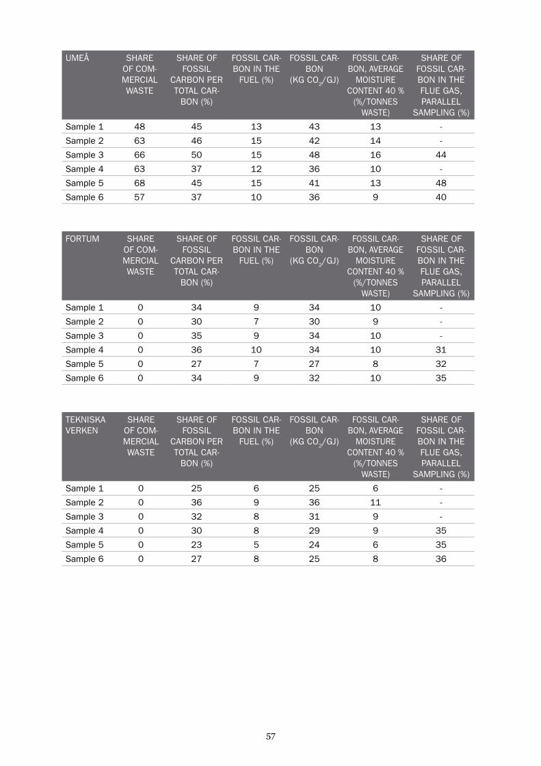
57

umeå share of com-mercial waste

share of fossil

carbon per total car-

bon (%)

fossil car-bon in the

fuel (%)

fossil car-bon

(KG co2/GJ)

fossil car-bon, aVeraGe

moisture content 40 %

(%/tonnes waste)

share of fossil car-bon in the flue Gas, parallel

samplinG (%)

sample 1 48 45 13 43 13 -

sample 2 63 46 15 42 14 -

sample 3 66 50 15 48 16 44

sample 4 63 37 12 36 10 -

sample 5 68 45 15 41 13 48

sample 6 57 37 10 36 9 40

fortum share of com-mercial waste

share of fossil

carbon per total car-

bon (%)

fossil car-bon in the

fuel (%)

fossil car-bon

(KG co2/GJ)

fossil car-bon, aVeraGe

moisture content 40 %

(%/tonnes waste)

share of fossil car-bon in the flue Gas, parallel

samplinG (%)

sample 1 0 34 9 34 10 -

sample 2 0 30 7 30 9 -

sample 3 0 35 9 34 10 -

sample 4 0 36 10 34 10 31

sample 5 0 27 7 27 8 32

sample 6 0 34 9 32 10 35

teKnisKa VerKen

share of com-mercial waste

share of fossil

carbon per total car-

bon (%)

fossil car-bon in the

fuel (%)

fossil car-bon

(KG co2/GJ)

fossil car-bon, aVeraGe

moisture content 40 %

(%/tonnes waste)

share of fossil car-bon in the flue Gas, parallel

samplinG (%)

sample 1 0 25 6 25 6 -

sample 2 0 36 9 36 11 -

sample 3 0 32 8 31 9 -

sample 4 0 30 8 29 9 35

sample 5 0 23 5 24 6 35

sample 6 0 27 8 25 8 36

58

eon hänDel-öVerKet

share of com-mercial waste

share of fossil

carbon per total car-

bon (%)

fossil car-bon in the

fuel (%)

fossil car-bon

(KG co2/GJ)

fossil car-bon, aVeraGe

moisture content 40 %

(%/tonnes waste)

share of fossil car-bon in the flue Gas, parallel

samplinG (%)

sample 1 20 40 12 37 11 -

sample 2 30 26 7 27 7 -

sample 3 40 34 9 33 9 -

sample 4 40 48 14 45 14 36

sample 5 34 33 10 32 8 37

sample 6 40 44 14 42 11 41

borås en-erGi och milJö

share of com-mercial waste

share of fossil

carbon per total car-

bon (%)

fossil car-bon in the

fuel (%)

fossil car-bon

(KG co2/GJ)

fossil car-bon, aVeraGe

moisture content 40 %

(%/tonnes waste)

share of fossil car-bon in the flue Gas, parallel

samplinG (%)

sample 1 79 39 12 38 10 -

sample 2 79 33 10 32 9 -

sample 3 70 38 11 37 10 39

sample 4 75 31 10 30 7 34

sample 5 73 30 9 29 8 -

sample 6* - - - - - 43

sample 6 78 46 14 44 13 -*the first”sample 6” that was extracted was lost in an accidental fire. there is no parallel flue gas sample for the last solid sample.

59

The figure shows the amount of fossil CO2 per GJ of fuel. The red line corresponds to the standard value (25kg/GJ) that have been discussed and used by authorities to date. This standard value is calculated from the previous sorting analysis studies of RVF Report 2003:12. (Y-axis = Calculated fossil CO2 (kg/GJ), x-axis = share of commercial waste, (%))

The figure shows the proportion of fossil carbon per tonnes waste. The red line corresponds to the standard value (12.6% / tonnes waste) that have been discussed and used by authorities to date. This standard value is calculated from the previous sorting analysis studies of RVF Report 2003:12.(Y-axis =The share of fossil carbon per tonnes of waste (%/tonnes), x-axis = share of commercial waste, (%))

raPPorter från avfall sverige 2012

avfall sveriges utvecklingssatsning u2012:01 avfallsavgifter 2010. insamling och behandling av hushållsavfall - former och utförande u2012:01 bestämning av andel fossilt kol i avfall som förbränns i sverigeu2012:03 fosforfällor. fosforfiltermaterial - ett hushållsavfallu2012:04 internationellt intresse för svenska avfallslösningaru2012:05 Determination of the fossil carbon content in combustible municipal solid waste in sweden

avfall sveriges utvecklingssatsning, biologisk behandling

avfall sveriges utvecklingssatsning, dePonering

avfall sveriges utvecklingssatsning, avfallsfÖrbrÄnningf2012:01 primärenergi i avfall och restvärmef2012:02 ackumulering av metaller i vegetation på geotekniska askkonstruktioner

avfall sverige utveckling u2012:05

issn 1103-4092

©avfall sverige ab

adress

telefon

fax

e-post

hemsida

prostgatan 2, 211 25 malmö

040-35 66 00

040-35 66 26

info@avfallsverige.se

www.avfallsverige.se

“Vi är Sveriges största miljörörelse. Det är Avfall Sveriges

medlemmar som ser till att svensk avfallshantering

fungerar - allt från renhållning till återvinning. Vi gör det

på samhällets uppdrag: miljösäkert, hållbart och långsik-

tigt. Vi är 15 000 personer som arbetar tillsammmans

med Sveriges hushåll och företag.”