determination of explosive energy partition values in …
TRANSCRIPT
University of Kentucky University of Kentucky
UKnowledge UKnowledge
Theses and Dissertations--Mining Engineering Mining Engineering
2015
DETERMINATION OF EXPLOSIVE ENERGY PARTITION VALUES IN DETERMINATION OF EXPLOSIVE ENERGY PARTITION VALUES IN
ROCK BLASTING THROUGH SMALL-SCALE TESTING ROCK BLASTING THROUGH SMALL-SCALE TESTING
Joshua Calnan University of Kentucky, [email protected]
Right click to open a feedback form in a new tab to let us know how this document benefits you. Right click to open a feedback form in a new tab to let us know how this document benefits you.
Recommended Citation Recommended Citation Calnan, Joshua, "DETERMINATION OF EXPLOSIVE ENERGY PARTITION VALUES IN ROCK BLASTING THROUGH SMALL-SCALE TESTING" (2015). Theses and Dissertations--Mining Engineering. 24. https://uknowledge.uky.edu/mng_etds/24
This Doctoral Dissertation is brought to you for free and open access by the Mining Engineering at UKnowledge. It has been accepted for inclusion in Theses and Dissertations--Mining Engineering by an authorized administrator of UKnowledge. For more information, please contact [email protected].

STUDENT AGREEMENT: STUDENT AGREEMENT:
I represent that my thesis or dissertation and abstract are my original work. Proper attribution
has been given to all outside sources. I understand that I am solely responsible for obtaining
any needed copyright permissions. I have obtained needed written permission statement(s)
from the owner(s) of each third-party copyrighted matter to be included in my work, allowing
electronic distribution (if such use is not permitted by the fair use doctrine) which will be
submitted to UKnowledge as Additional File.
I hereby grant to The University of Kentucky and its agents the irrevocable, non-exclusive, and
royalty-free license to archive and make accessible my work in whole or in part in all forms of
media, now or hereafter known. I agree that the document mentioned above may be made
available immediately for worldwide access unless an embargo applies.
I retain all other ownership rights to the copyright of my work. I also retain the right to use in
future works (such as articles or books) all or part of my work. I understand that I am free to
register the copyright to my work.
REVIEW, APPROVAL AND ACCEPTANCE REVIEW, APPROVAL AND ACCEPTANCE
The document mentioned above has been reviewed and accepted by the student’s advisor, on
behalf of the advisory committee, and by the Director of Graduate Studies (DGS), on behalf of
the program; we verify that this is the final, approved version of the student’s thesis including all
changes required by the advisory committee. The undersigned agree to abide by the statements
above.
Joshua Calnan, Student
Dr. Braden T. Lusk, Major Professor
Dr. Braden T. Lusk, Director of Graduate Studies

DETERMINATION OF EXPLOSIVE ENERGY PARTITION VALUES IN ROCK BLASTING THROUGH SMALL-SCALE TESTING
DISSERTATION
A dissertation submitted in partial fulfillment of the requirements for the degree of Doctor of Philosophy in the
College of Engineering at the University of Kentucky
By
Joshua Thomas Calnan
Lexington, Kentucky
Director: Dr. Braden T. Lusk, Professor of Mining Engineering
Lexington, Kentucky
2015
Copyright © Joshua Thomas Calnan 2015
ABSTRACT OF DISSERTATION
DETERMINATION OF EXPLOSIVE ENERGY PARTITION VALUES IN ROCK BLASTING THROUGH SMALL-SCALE TESTING
Blasting is a critical part of most mining operations. The primary function of blasting is to fragment and move rock. For decades, attempts have been
made at increasing the efficiency of blasting to reduce costs and increase production. Most of these attempts involve trial and error techniques that focus on changing a single output. These techniques are costly and time consuming
and it has been shown that as one output is optimized other outputs move away from their optimum level. To truly optimize a blasting program, the transfer of
explosive energy into individual components must be quantified. Explosive energy is broken down into five primary components: rock fragmentation, heave, ground vibration, air blast, and heat. Fragmentation and heave are considered
beneficial components while the remaining are considered waste. Past energy partitioning research has been able to account for less than 30% of a blast’s total
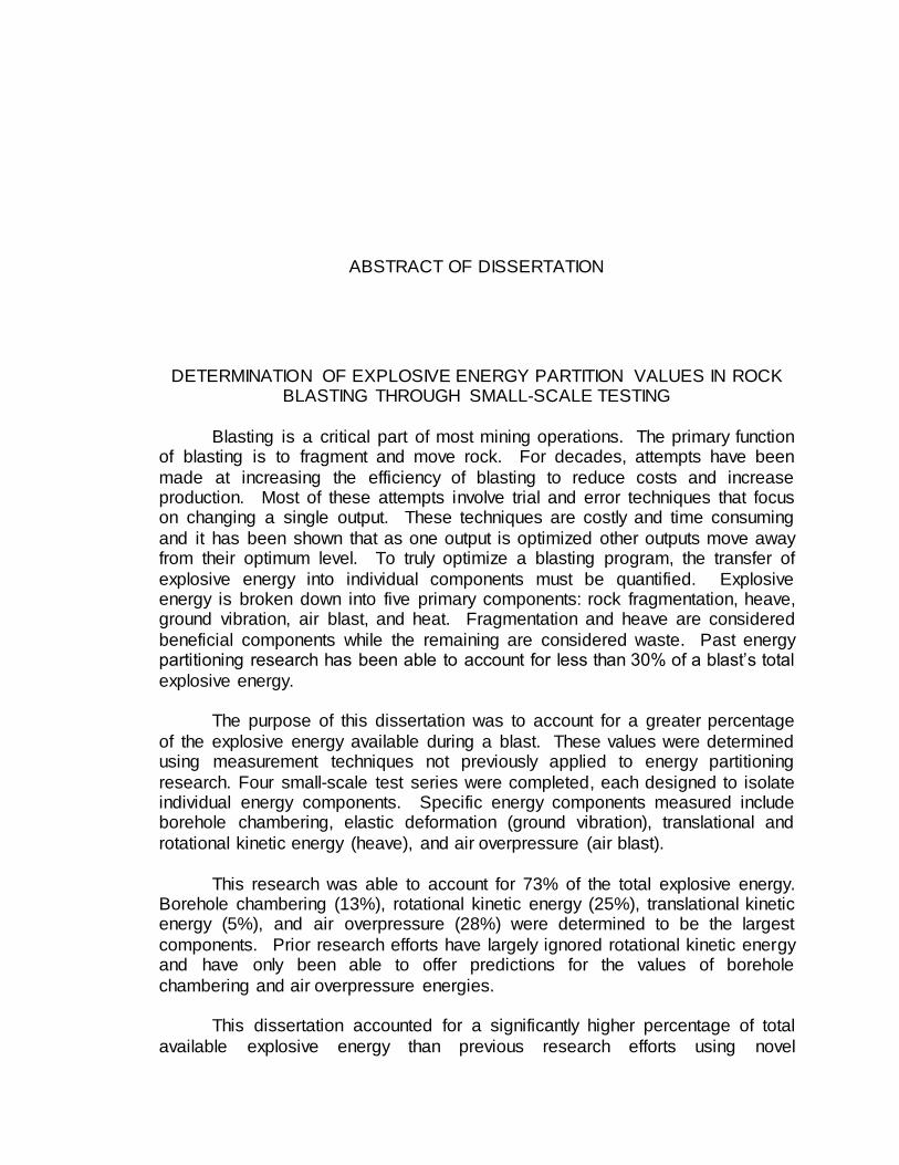
explosive energy. The purpose of this dissertation was to account for a greater percentage
of the explosive energy available during a blast. These values were determined using measurement techniques not previously applied to energy partitioning
research. Four small-scale test series were completed, each designed to isolate individual energy components. Specific energy components measured include borehole chambering, elastic deformation (ground vibration), translational and
rotational kinetic energy (heave), and air overpressure (air blast).
This research was able to account for 73% of the total explosive energy. Borehole chambering (13%), rotational kinetic energy (25%), translational kinetic energy (5%), and air overpressure (28%) were determined to be the largest
components. Prior research efforts have largely ignored rotational kinetic energy and have only been able to offer predictions for the values of borehole
chambering and air overpressure energies. This dissertation accounted for a significantly higher percentage of total
available explosive energy than previous research efforts using novel

measurement techniques. It was shown that borehole chambering, heave, and air blast are the largest energy components in a blast. In addition to quantifying
specific energy partitions, a basic goal programming objective function was proposed, incorporating explosive energy partitioning and blasting parameters
into a framework that can be used for future energy optimization.
KEYWORDS: Rock Blasting, Energy Partitioning, Optimization, Explosives, Goal Programming
Joshua Thomas Calnan
12/11/2015

DETERMINATION OF EXPLOSIVE ENERGY PARTITION VALUES IN ROCK BLASTING THROUGH SMALL-SCALE TESTING
By
Joshua Thomas Calnan
Dr. Braden T. Lusk
Director of Dissertation
Dr. Braden T. Lusk
Director of Graduate Studies
12/11/2015

iii
Acknowledgements
I would like to thank my wife, Courtney, for her love, support, and patience
throughout this process. Without her encouragement I would not have made it
through this process. Thank you to parents, Cori and Tom, for their continued
support, emotionally and financially, through all of these years of college. I would
also like to thank my brothers, Todd and Adam, for providing their sarcastic
comedic relief when I needed it most. A big thanks goes to my grandparents,
Roger and Ann, and Tom and Doris, for their phone calls to see how things were
going and to offer words of encouragement.
Thank you to all of the members of the University of Kentucky Explosives
Research Team (UKERT), especially Paul Sainato, Brendan McCray, Lizzie
Maher, and Kylie Larson-Robl. Without the long hours that they put in helping
me, my research would never have gotten done.
I would like to thank the facility and stuff of the University of Kentucky Mining
Engineering Department, especially Ed Thompson and Megan Doyle for lending
a helping hand over the past few years.
Finally, I would like to thank my advisor, Dr. Braden Lusk, and the rest of my
dissertation committee, Dr. Kyle Perry, Dr. Jhon Silva, Dr. Chad Wedding, and
Dr. Sebastian Bryson. Their knowledge and support was vital to the completion
of this dissertation.

iv
TABLE OF CONTENTS
Acknowledgements ......................................................................................................... iii List of Tables .....................................................................................................................vi
List of Figures ..................................................................................................................vii Chapter 1. Introduction.................................................................................................. 1 Chapter 2. Review of Literature ................................................................................... 4
2.1 Introduction to Blasting and Key Terms ......................................................... 4 2.1.1 General Blasting Guidelines ..................................................................... 7
2.2 Energy Partitioning .......................................................................................... 10 2.2.1 Explosive Energy Determination............................................................ 14 2.2.2 Fragmentation Energy ............................................................................. 15
2.2.3 Seismic Energy ......................................................................................... 20 2.2.4 Kinetic Energy ........................................................................................... 20
2.2.5 Air Blast Energy ........................................................................................ 22 2.2.6 Energy Measurement Values ................................................................. 22
2.3 Borehole Physics and Cavity Expansion Analysis ..................................... 23
2.3.1 Borehole Physics...................................................................................... 24 2.3.2 Cavity Expansion Analysis Applied to Blasting ................................... 27
2.4 Optimization Methods ..................................................................................... 29 2.4.1 Goal Programming ................................................................................... 30 2.4.2 Mine Scheduling Optimization (MSO) ................................................... 32
2.4.3 Coupled Expert System........................................................................... 33 2.4.4 Mine-to-Mill Methodology ........................................................................ 35
Chapter 3. Test Rationale and Methodology ........................................................... 38 Chapter 4. Fully Confined Chambering Tests ......................................................... 43
4.1 Methodology ..................................................................................................... 43
4.2 Instrumentation ................................................................................................ 44 4.3 Explosive Charge............................................................................................. 49
4.4 Chambering Test Results............................................................................... 50 4.4.1 Chambering Calculations ........................................................................ 51 4.4.2 Supplemental Borehole Chambering Testing and Calculations ....... 54
4.4.3 Pressure Shell Energy Calculations ...................................................... 55 4.4.4 Conclusions ............................................................................................... 61
Chapter 5. Stemming Tests........................................................................................ 63 5.1 Methodology ..................................................................................................... 63 5.2 Instrumentation ................................................................................................ 64
5.3 Explosive Charge............................................................................................. 67 5.4 Stemming Test Results................................................................................... 67
Chapter 6. Strain Mapping and Strain Energy......................................................... 71 6.1 Methodology & Instrumentation .................................................................... 71 6.2 Strain Mapping Results................................................................................... 73
Chapter 7. Concrete Block Testing ........................................................................... 83 7.1 Methodology ..................................................................................................... 83
7.2 Instrumentation ................................................................................................ 83 7.3 Explosive Charge............................................................................................. 87

v
7.4 Block Testing Results ..................................................................................... 87 7.4.1 Kinetic Energy ........................................................................................... 87
7.4.2 Fracture Energy ........................................................................................ 94 7.4.3 Air Overpressure ....................................................................................102
7.4.4 Strain ........................................................................................................105 7.5 Borehole Chambering ...................................................................................107 7.6 Conclusions ....................................................................................................109
Chapter 8. Goal Programming Framework ............................................................113 Chapter 9. Conclusions and Future Work ..............................................................117
9.1 Conclusions ....................................................................................................117 9.2 Summary of Novel Contributions ................................................................120 9.3 Future Work ....................................................................................................120
Appendices……………………………………………………………………………125 A. Borehole Chambering Tests – Maximum Values ..........................................125
B. Borehole Chambering Tests – Air Overpressure Energy Plots ...................127 C. Stemming Tests – Maximum Values ...............................................................132 D. Strain Mapping Tests – Elastic Deformationa Enery Calculations .............135
E. Strain Mapping Tests – Air Overpressure Energy Plots ...............................137 F. Concrete Block Tests – UCS Tests for Concrete...........................................143
G. Concrete Block Tests – Three-Point Beam Fracture Plots ..........................145 Bibliography...................................................................................................................149 Vita…………..................................................................................................................156

vi
LIST OF TABLES
Table 2.1: Scaled Distance Equations (adapted from Lusk, 2011) ........................ 10 Table 4.1: Summary of volume data for borehole chambering tests ..................... 52
Table 4.2: Normalized before and after volume data .............................................. 52 Table 4.3: Summary of borehole chambering energy values ................................. 54 Table 4.4: Summary of Supplemental Borehole Volumes....................................... 55
Table 4.5: Summary of maximum pressure and time of arrival (TOA) .................. 57 Table 4.6: Summary of pressure shell energy calculations for initial test series . 60
Table 4.7: Summary of strain results from chambering tests .................................. 62 Table 5.1: Summary of stemming test results ........................................................... 68 Table 6.1: Summary of strain mapping results .......................................................... 74
Table 6.2: Summary of calculated strain energy for a confined borehole ............. 77 Table 6.3: Summary of air overpressure calculations for confined borehole ....... 78
Table 6.4: Weight total air overpressure energy for confined tests ........................ 79 Table 6.5: Energy transferred to stemming ejection during confined tes t............. 80 Table 6.6: Total energy measured from confined borehole..................................... 81
Table 7.1: Summary of fragment masses .................................................................. 88 Table 7.2: Summary of Translational Kinetic Energy Calculations ........................ 89
Table 7.3: Summary of Angular Velocities ................................................................. 92 Table 7.4: Summary of Moment of Inertia and Rotational Kinetic Energy ............ 92 Table 7.5: Summary of newly created surface area ................................................. 96
Table 7.6: Summary of beam dimensions for three-point bending tests............... 98 Table 7.7: Summary of specific fracture energy results .........................................101
Table 7.8: Fracture energy determination for each block test...............................101 Table 7.9: Block primary facture length and shell surface area ............................104 Table 7.10: Summary of overpressure and wave velocity .....................................104
Table 7.11: Calculated air overpressure energy .....................................................105 Table 7.12: Maximum transverse strain and respective strain energy value .....106
Table 7.13: Strain energy values for block tests .....................................................107 Table 7.14: Block borehole chambering profiles .....................................................108 Table 7.15: Calculated explosive energy partition values in Joules ....................110

vii
LIST OF FIGURES
Figure 1.1: Explosive Energy Components.................................................................. 2 Figure 2.1: Key blasting parameters (Lusk, 2011) ...................................................... 6
Figure 2.2: Typical hole pattern layouts (Lusk, 2011) ................................................ 7 Figure 2.3: Typical powder factor ranges based on application (Lusk, 2011) ........ 8 Figure 2.4: Non-ideal detonation and energy partitioning........................................ 25
Figure 4.1: Plan view of setup for chambering test series ....................................... 44 Figure 4.2: Typical free-field pencil sensor setup ..................................................... 45
Figure 4.3: PCB strain sensor adhered to the rock surface .................................... 46 Figure 4.4: Seismograph setup .................................................................................... 48 Figure 4.5: Test arena and instrumentation setup for chambering test series ..... 49
Figure 4.6: Illustration of pressure shell radius, surface area, and volume .......... 56 Figure 4.7: Pressure versus time data for energy calculations............................... 58
Figure 4.8: Time scale converted to distance plot .................................................... 59 Figure 4.9: Final data plot after conversion to Pressure-Area vs. Distance ......... 59 Figure 5.1: Free-field pencil sensor stand with attached velocity screen.............. 65
Figure 5.2: Strain gauge setup for stemming tests ................................................... 66 Figure 5.3: Plan view of sensor configuration for stemming tests .......................... 66
Figure 5.4: Air overpressure versus elastic deformation ......................................... 69 Figure 5.5: Air overpressure at sensor 4 versus strain measured at sensor 6 .... 70 Figure 5.6: Air blast versus strain plot......................................................................... 70
Figure 6.1: Instrumentation setup for strain mapping ............................................... 72 Figure 6.2: Plan view of strain mapping test setup ................................................... 73
Figure 6.3: Shock waves intersecting strain gauges ................................................ 74 Figure 6.4: Strain with respect to distance from borehole ....................................... 76 Figure 6.5: Revised pressure shell shape .................................................................. 79
Figure 7.1: Strain sensor mounting locations ............................................................ 84 Figure 7.2: Velocity screen position for block testing ............................................... 85
Figure 7.3: Overview of test setup for block testing .................................................. 86 Figure 7.4: Plan view of block testing setup............................................................... 86 Figure 7.5: Frame grab from high speed video ......................................................... 89
Figure 7.6: 3D rendering of major fragments ............................................................. 91 Figure 7.7: Detailed view of fragment and associated output from Creo .............. 91
Figure 7.8: Fractured wedge reassembled ............................................................... 95 Figure 7.9: Small fragments from Test 2 .................................................................... 96 Figure 7.10: Three-point bending test setup .............................................................. 99
Figure 7.11: Sample beam with fracture extending from starter notch.................. 99 Figure 7.12: Load versus displacement for concrete beam sample ....................100
Figure 7.13: Dust and gases (highlighted) venting from primary fracture plane 103 Figure 7.14: Primary fracture plane for block tests .................................................103 Figure 7.15: Summary of Block 1 energy partitioning percentages .....................110
Figure 7.16: Summary of Block 2 energy partitioning percentages .....................111 Figure 7.17: Summary of Block 3 energy partitioning percentages .....................111
Figure 7.18: Average energy partitioning percentages for block tests ................112 Figure 9.1: Summary of explosive energy components and respective values .119
1
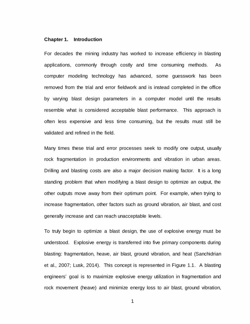
Chapter 1. Introduction
For decades the mining industry has worked to increase efficiency in blasting
applications, commonly through costly and time consuming methods. As
computer modeling technology has advanced, some guesswork has been
removed from the trial and error fieldwork and is instead completed in the office
by varying blast design parameters in a computer model until the results
resemble what is considered acceptable blast performance. This approach is
often less expensive and less time consuming, but the results must still be
validated and refined in the field.
Many times these trial and error processes seek to modify one output, usually
rock fragmentation in production environments and vibration in urban areas.
Drilling and blasting costs are also a major decision making factor. It is a long
standing problem that when modifying a blast design to optimize an output, the
other outputs move away from their optimum point. For example, when trying to
increase fragmentation, other factors such as ground vibration, air blast, and cost
generally increase and can reach unacceptable levels.
To truly begin to optimize a blast design, the use of explosive energy must be
understood. Explosive energy is transferred into five primary components during
blasting: fragmentation, heave, air blast, ground vibration, and heat (Sanchidrian
et al., 2007; Lusk, 2014). This concept is represented in Figure 1.1. A blasting
engineers’ goal is to maximize explosive energy utilization in fragmentation and
rock movement (heave) and minimize energy loss to air blast, ground vibration,

2
and heat. Optimizing explosive energy use will result in better performing blasts
(i.e. increased fragmentation and acceptable air blast), in addition to cost
reduction and increased profits.
Figure 1.1: Explosive Energy Components
Although explosive energy partitioning has been studied in the past (Berta, 1990;
Spathis, 1999; Ouchterlony et al., 2003; Sanchidrian et al., 2007) a significant
portion of the total explosive energy has not been accounted for. These past
studies have examined full-scale blasts, relying primarily on traditional blast
instrumentation equipment such as seismographs which, although ideal for
documenting a blast for regulatory compliance, are not well suited for a refined
Explosive Energy
Ground Vibration
Air Blast
MovementFragmentation
Heat

3
assessment of explosive energy components. Components such as rotational
kinetic energy, air blast, and permanent deformation of the borehole have largely
been ignored during these past research efforts.
The problem of optimizing one output or goal without adversely affecting other
variables is not limited to the explosives industry. In fact, this problem can be
found in almost every industry. To deal with this problem, a form of computer
programming was developed called goal programming. Goal programming (GP)
is a programming technique used to find an optimum solution for complex
problems containing many variables and conflicting objectives.
The primary focus of the research presented in this dissertation is to examine
each of the explosive energy components more closely, with the goal of
accounting for greater portions of the total explosive energy. This is
accomplished through a number of small-scale test series designed to isolate
specific components, using laboratory equipment better suited to collect data at
the necessary level of fidelity. This dissertation also introduces the concept of
using goal programming as a means of explosive energy optimization in the rock
blasting environment.
Copyright © Joshua Thomas Calnan 2015

4
Chapter 2. Review of Literature
2.1 Introduction to Blasting and Key Terms
The primary function of blasting is to fragment and move rock so that it can be
efficiently handled by equipment such as loaders, shovels, haul trucks, etc.
Good blasting practices effectively fragment and move rock while also limiting
ground vibration, air overpressure, fly rock, and toxic gas emissions. The
blasting program must maintain production rates and remain cost effective.
Fragmentation requirements vary from mine to mine based on haulage
equipment and use of the blasted material. In the Appalachian Region, blasted
overburden is typically hauled to dump sites via haul truck to be used as fill for
reclamation activities. Other effects, including cost and environmental impact,
must also be considered (Johnson et al., 2013).
Since this dissertation will focus heavily on blast design and variation of
parameters, a brief overview of key terms and general blasting guidelines is
provided.
One of the most critical terms to understand in blasting is powder factor. Powder
factor is a ratio of the amount of explosives used to break a given amount of
rock. The definition of powder factor varies based on the function the explosive
serves.
When mining ore, the definition of powder factor is given as:
𝑃𝐹 =𝑙𝑏 𝑜𝑓 𝑒𝑥𝑝𝑙𝑜𝑠𝑖𝑣𝑒
𝑡𝑜𝑛𝑠 𝑜𝑓 𝑜𝑟𝑒 (2.1)

5
When removing waste rock (overburden) powder factor is defined as:
𝑃𝐹 =𝑙𝑏 𝑜𝑓 𝑒𝑥𝑝𝑙𝑜𝑠𝑖𝑣𝑒
𝑐𝑢𝑏𝑖𝑐 𝑦𝑎𝑟𝑑𝑠 𝑜𝑓 𝑟𝑜𝑐𝑘 (2.2)
For the remainder of this dissertation, the second definition of powder factor will
be used. Other key terms are defined below and in Figure 2.5.
Face Height (L) – the height of the free face.
Burden (B) – the distance from a row of holes to the free face. This is the
amount of material that must be moved by a row of loaded holes.
Spacing (S) – the distance between holes in a row.
Hole Depth (H) – the depth of the hole below the surface, including subdrill (J).
Stemming Height (T) – the amount of material, usually drill cuttings or gravel,
placed in the borehole to contain the explosive energy.
Powder Column (PC) – the height of the explosive column within the borehole.
The powder column is generally the face height + subdrill depth – stemming
height.

6
Figure 2.1: Key blasting parameters (Lusk, 2011)
Boreholes are typical laid out on one of three patterns; square, rectangular, and
staggered. These patterns are illustrated in Figure 2.6. Square patterns have
equal burden and spacing while in a rectangular pattern the spacing is generally
greater than the burden. In a staggered pattern, each row of holes is offset
relative to the row of holes in front of it.
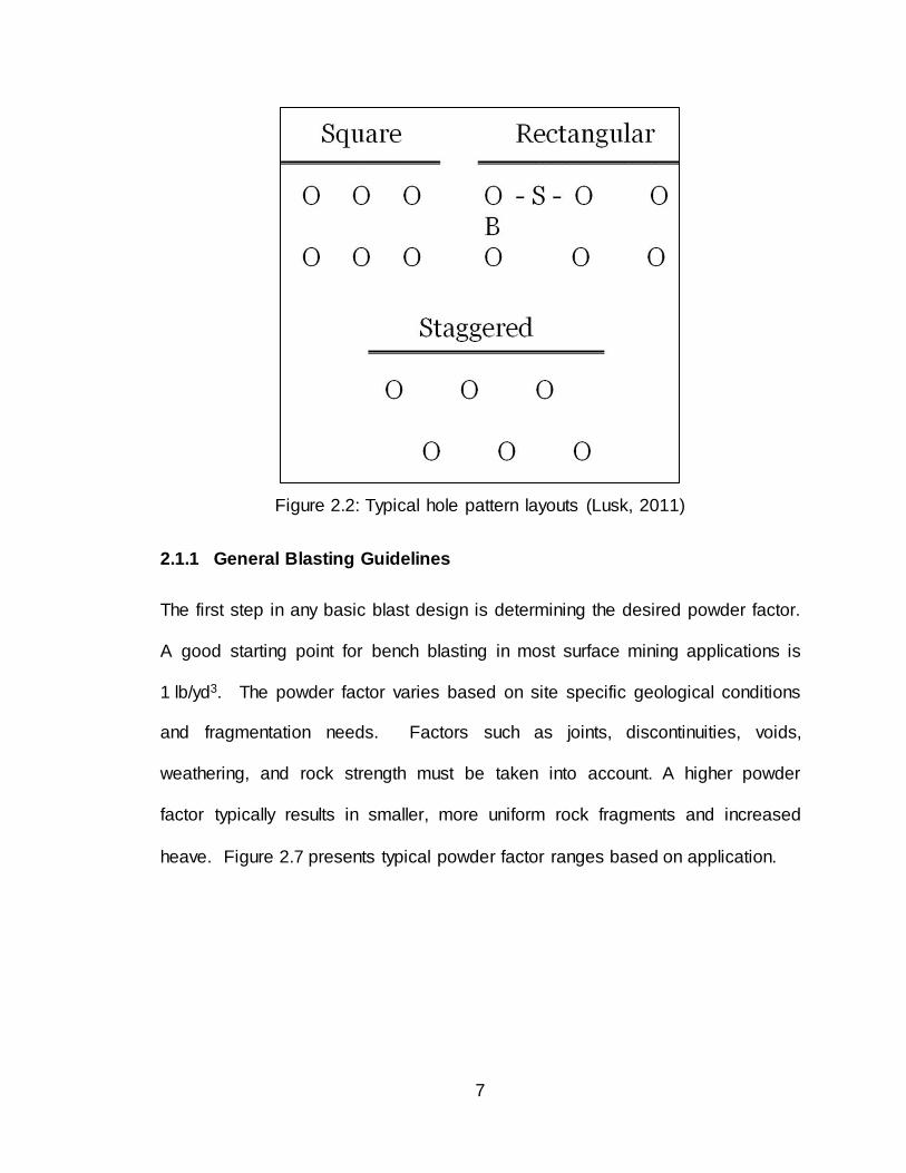
7
Figure 2.2: Typical hole pattern layouts (Lusk, 2011)
2.1.1 General Blasting Guidelines
The first step in any basic blast design is determining the desired powder factor.
A good starting point for bench blasting in most surface mining applications is
1 lb/yd3. The powder factor varies based on site specific geological conditions
and fragmentation needs. Factors such as joints, discontinuities, voids,
weathering, and rock strength must be taken into account. A higher powder
factor typically results in smaller, more uniform rock fragments and increased
heave. Figure 2.7 presents typical powder factor ranges based on application.

8
Figure 2.3: Typical powder factor ranges based on application (Lusk, 2011)
Ash’s Burden Factor Equation (2.3) is used as a starting point to determine the
optimal burden, taking into account the type of explosive being used and the
density of the rock being blasted.
𝐾𝐵 = 30(𝑆𝐺𝑒𝑥/1.4)13⁄ (160/𝑊𝑡𝑟𝑘)
13⁄ (2.3)
𝑆𝐺𝑒𝑥 = 𝑆𝑝𝑒𝑐𝑖𝑓𝑖𝑐 𝑔𝑟𝑎𝑣𝑖𝑡𝑦 𝑜𝑓 𝑒𝑥𝑝𝑙𝑜𝑠𝑖𝑣𝑒 (𝑔
𝑐𝑐) (2.4)
𝑊𝑡𝑟𝑘 = 𝑈𝑛𝑖𝑡 𝑤𝑒𝑖𝑔ℎ𝑡 𝑜𝑓 𝑟𝑜𝑐𝑘 (𝑙𝑏
𝑐𝑢𝑏𝑖𝑐 𝑓𝑡) (2.5)
After determining the burden factor (𝐾𝐵), the burden is calculated using the
diameter of the explosive (𝑑𝑥). For packaged products, the diameter of the
explosive is the diameter of the package, and for bulk products, such as

9
ammonium nitrate/fuel oil (ANFO), the diameter is taken as the diameter of the
borehole.
𝐵 = 𝑑𝑥 × 𝐾𝐵 (2.6)
Ash’s Spacing Relationship serves as a guideline for determining the hole to hole
spacing of a pattern in relation to the burden.
𝑆 = 𝐵 × (1.4 𝑡𝑜 2) (2.7)
As a generalized rule of thumb, when utilizing ANFO as the explosive product, it
can be assumed that:
𝐵 = 24 × ℎ𝑜𝑙𝑒 𝑑𝑖𝑎𝑚𝑡𝑒𝑟 (2.8)
S = 36× ℎ𝑜𝑙𝑒 𝑑𝑖𝑎𝑚𝑡𝑒𝑟 (2.9)
Emulsions and emulsion/ANFO blends have a higher specific gravity than ANFO
and therefore do not require as tight of a pattern to achieve the required powder
factor. As a result, the generalized rule of thumb for burden and spacing when
using these products is:
𝐵 = 30 × ℎ𝑜𝑙𝑒 𝑑𝑖𝑎𝑚𝑡𝑒𝑟 (2.10)
S = 42× ℎ𝑜𝑙𝑒 𝑑𝑖𝑎𝑚𝑡𝑒𝑟 (2.11)
A general rule of thumb for determining face height is 100 to 120 times the hole
diameter.
Scaled distance must be taken into account when determining the maximum
amount of explosives that can be detonated within a single delay period. This is
done in an effort to limit ground vibrations that could cause damage to nearby
structures. Table 2.1 summarizes the scaled distance equations based on
distance from the blasting site to the nearest structure. As shown in this table,

10
the scaled distance equation varies based on distance and becomes more
stringent as distance increases. The primary reason for this is that as blast
induced ground vibrations travel through the earth their frequency decreases.
Built structures have a low resonance frequency and are more susceptible to
damage caused by these lower frequency ground vibrations.
Table 2.1: Scaled Distance Equations (adapted from Lusk, 2011)
Distance (D) from the blasting site in feet
Scaled Distance Equation
0 to 300 𝑊 = (𝐷 50⁄ )2
301 to 5,000 𝑊 = (𝐷 55⁄ )2
5,001+ 𝑊 = (𝐷 60⁄ )2
W = the maximum weight of explosives that can be detonated within any eight (8) millisecond period.
D = the distance, in feet, from the blasting site
2.2 Energy Partitioning
Explosive energy is transformed into five primary components in a rock blasting
environment. Two of these components, kinetic energy (rock movement) and
fracture energy (fragmentation) are beneficial, while explosive energy transferred
to seismic energy (ground vibration), air blast, and heat can be considered
waste.
Extensive work has been completed in recent years in an attempt to better
understand energy partitioning. Spathis (1999) calculated the amount of energy
being transformed into kinetic energy, fracture energy, and seismic energy. He
also recommended the use of energy balance in blast designs to increase
efficiency as future work. The idea of energy balance involves optimizing the use

11
of the explosive energy available to achieve desirable results, rather than simply
increasing the total amount of explosive energy. Ouchterlony et. al. (2003 and
2004), and Sanchidrian et al., (2007) have also conducted work similar to that of
Spathis (1999). Their works will be discussed in more detail throughout this
chapter.
While a significant amount of information has been uncovered through these
publications, many questions are left unanswered. One of the largest obstacles
is the number of variables that must be considered in an experiment. Below are
examples of some of the components where energy is absorbed in the blasting
process. By no means is this list complete, but it serves as a useful starting point
(Berta, 1990; Lusk, 2014; Ouchterlony et al., 2004; Sanchidrian et al., 2007;
Spathis, 1999).
Immediately In and Around Borehole
Chambering of the borehole
Crushing (fines)
Friction
Heat
In the Surrounding Rock Mass
Elastic and Plastic Deformation from tensile and compression forces
Micro-cracks
Macro-cracks
Formation of large fragments (greater than 1mm)
Formation of fines (smaller than 1mm)
Backbreak
Friction and impact between fragments
Movement of fragments

12
Lost into the atmosphere (outside immediate blasting zone)
Heat
Fumes
Airblast
Ground Vibration
Fracture and kinetic energies are relatively easy to measure because the end
result can be seen through rock fragmentation and movement. However, energy
transferred into elastic and plastic deformation of the rock, heat transfer to the
rock, and enthalpy of the venting gases are not as easily measured (Sanchidrian
et al., 2007).
Sanchidrian et al. (2007) conducted extensive work in an attempt to quantify the
energy components in rock blasting. In doing so, a number of useful equations
were identified. The first equation, and likely the most important, is the energy
balance equation expressed as:
𝐸𝐸 = 𝐸𝐹 + 𝐸𝑆 + 𝐸𝐾 + 𝐸𝑁𝑀 (2.12)
where 𝐸𝐸 is the explosive energy, 𝐸𝐹 is the fragmentation energy, 𝐸𝑆 is the
seismic energy, 𝐸𝐾 is the kinetic energy, and 𝐸𝑁𝑀 is energy forms not measured
such as air blast and heat.
Fragmentation energy can be calculated using the equation:
𝐸𝐹 = 𝐴𝐹𝐺𝐹 (2.13)
where 𝐺𝐹 is the specific fracture energy calculated from experimental
fragmentation tests and 𝐴𝐹 is the surface area of the fragments created by the
13
blast. The surface area of the fragments can be approximated based on the
muckpile size distribution using the simplified equation:
𝐴 = 6𝑉∫𝑓(𝑥)
𝑥𝑑𝑥
∞
0
(2.14)
where 𝑥 is the diameter or edge length of the particles, 𝑉 is the volume of the
fragmented rock, and 𝑓(𝑥) is the density function of the fragment size
distribution.
The calculation of seismic energy is more complicated and requires a number of
approximations and before finally reaching the following equation:
𝐸𝑆 = 4𝜋𝑟2𝜌𝑐𝐿 ∫ 𝑣2𝑑𝑡
∞
0
(2.15)
where 𝑟 is the radius of the surface across which the total power is acting, 𝜌 is
the rock density, 𝑐𝐿 is the longitudinal wave velocity, 𝑣 is the magnitude of the
vector sum of the velocities using a unique wave velocity.
The kinetic energy of rock displaced by a blast hole is given as:
𝐸𝐾 =1
2𝑆𝐵ℎ ∫ 𝜌(𝑦)𝑉0
2(𝑦)𝑑𝑦𝐻
0
(2.16)
where 𝑆 is the spacing between holes, 𝐵ℎ is the burden, 𝐻 is the bench height,
𝜌(𝑦) is the rock density (taking into account the variability throughout the height
of the profile), and 𝑉0 (𝑦) is initial velocity of the rock face at different heights.

14
2.2.1 Explosive Energy Determination
There is no universally accepted way to assess explosive energy. Explosive
energy determination can be separated into two categories: experimental testing,
and thermodynamic detonation code modeling. Each method has its own
intrinsic flaws.
The two most commonly utilized experimental tests are the cylinder test and the
underwater test. During cylinder tests, a copper cylinder is packed with an
explosive charge. Upon detonation, the velocity of the fragments are calculated
and equated to useful work using the Gurney equation (Gurney, 1943; Nyberg et
al., 2003). This test is particularily useful for energy determination related to
munitions and to some extent energy transferred to a borehole, but it fails to fully
capture the energy lost to heat and gas formation. The underwater test also has
its own flaws. During these tests, an explosive charge is detonated underwater,
resulting in a rapidly expanding gas bubble. The bubble expands until the
pressure within falls below the equilibrium hydrostatic pressure of the
surrounding water. The bubble then collapses until the pressure again rises
above the equilibrium hydrostatic pressure. This process repeats until the gases
vent to the atmosphere. The time between the initial expansion and the
subsequent collapse is used to determine the explosive energy. The primary
concern with this test methodology is that it fails to take into account the effects
of confinement on the explosive (Mohanty, 1999).

15
A number of ideal detonation codes are commercially available for explosive
energy modeling. In the work highlighted by Sanchidrian (2007), the W-Detcom
code is used. Other thermodynamic codes include CHEETAH and its
predecessor, TIGER (both developed by Lawrence Livermore National
Laboratory). These codes predict the velocity of detonation and heat of
detonation assuming an ideal, complete detonation of the product. For high
explosives (i.e. PETN and RDX), the experimental values generally agree with
the predicted values. However, for many commercial explosives (i.e. ANFO and
emulsions), the predicted values are higher than the experimental values
because the product does not detonate ideally. Partial reaction models are being
implemented into thermodynamic code. In these models, the assumption is
made that the explosive product is not ideally detonating. The results from these
models are in better agreement with experimental results for commercial
explosives (Sanchidrian and Lopez, 2006).
The advantage of using heat of detonation calculated by thermodynamic code
versus useful work captured by experimental tests, is that heat of detonation fully
accounts for all of the energy available during detonation, whereas experimental
tests only account for a portion of the energy based on a specific detonation
parameter.
2.2.2 Fragmentation Energy
Many blasting engineers view fragmentation as a simple process. The shock
front caused by detonation of the explosive transmits compression waves
through the rock mass until they reach the free-face where they are then

16
reflected, causing the pre-conditioned rock to fail in tension. The expanding
gases further exploit the existing cracks and increase fragmentation. To an
extent, this statement is true; however, the process is much more complex with
different reaction zones, each having their own microscopic and macroscopic
events taking place.
The fragmentation process is comprised of two processes taking place during the
detonation of an explosive. First, the shock phase pressurizes a volume of rock,
leading to the compression waves that are transmitted to the free-face before
being reflected, causing the rock to fracture in tension. Next, the gas pressure
caused by the detonation of the explosive increases in the borehole and is
sustained until the point at which fractures open and allow for the expansion and
venting of the gases.
Sellers (2013) states that in massive rock masses radial cracks are prevalent.
However, in highly jointed rock masses, radial fracturing is not evident. Instead,
the joints open. It is not surprising that in a massive deposit, fractures will form
radiating away from the borehole, while in jointed rock, the expanding gases will
exploit weaknesses already present. It is difficult to create a smaller mean
particle size in highly jointed rock because the gases are able to vent through
these joints rather than produce new cracks (Lusk, 2014).
Fragmentation energy can be broken down into a number of components. Not all
of the fragmentation energy goes directly into creating new visible fragments. It
is hypothesized that a great deal of energy is absorbed by the rock through

17
plastic and elastic deformation, both in compression and in tension. The exact
amount of energy absorbed during this process is unknown. Most literature only
considers the formation of macro-cracks, or the large cracks that lead to the
formation of individual fragments. Work by Hamdi et al. (2001) introduces the
idea of also considering the energy requirements for the formation of micro-
cracks. Although these micro-cracks result in a very limited increase of the
surface area individually, the large number of them results in a significant
increase in surface area overall. Based on additional work completed by Hamdi
et al. (2008), micro-cracks account for up to 11% of the explosive energy,
whereas the macro-cracks account for only 6%.
Determination of the fragmentation energy is a rather intense process that
requires a significant amount of pre-blast preparation. Calculation of the
fragmentation energy relies solely on the amount of new surface area created
within the rock. Therefore, it is critical to know the surface area of existing cracks
and joints within the rock mass prior to blasting. This is completed through an
extensive geological survey of the rock mass discontinuities. Joints are mapped
and the block sizes and surface area calculated. After the blast, the fragment
sizes are determined using image analysis software.
Fragmentation is measured using image analysis software such as Split Desktop
(Split Engineering, 2001), Fragscan (Schleifer and Tessier, 2000); and WipFrag
(Wipware, 2015). Each of these software packages is able to estimate the
fragment size distributions by analyzing digital images of the rock in the
muckpile, primary crusher hopper, or haul truck. These packages work well for

18
determining the size distribution of larger particles, but fall short when
determining the amount of fines. Therefore, correction factors are often applied
to account for the fines.
In the work completed by Hamdi et al. (2008), the fragments sizes were
continually monitored as the fragments travelled along a conveyor. In a coal
mining operation this is not possible, since muck is almost always transported via
truck. Instead, extensive photography of the muckpile in various stages of
removal is required.
After the fragmentation distribution curves have been created, the fragmentation
energy can be determined using the surface area of the fragments, the volume of
rock blasted, and the specific fracture energy (Sanchidrian et al.,2007).
Sanchidrian et al. (2007) uses Rittinger’s law as the basis for specific energy
calculations due to the large amount of fines in a blast. Rittinger’s law states that
the amount of energy required to mechanically crush fragments is directly
proportional to the amount of new surface area created. Rittinger’s law has
commonly been used to calculate energy requirements for large mills, and the
author is skeptical that this method is directly applicable to fragmentation energy.
Sanchidrian et al. (2007) also fails to take into account the surface area of micro-
cracks. The Rittinger coefficient may be applicable for calculation of the fines
immediately around the borehole in the crush-zone.
Hamdi et al. (2008) utilizes Griffiths theory for the basis of his calculations.
Griffiths theory is commonly associated with the fracture of brittle materials and is
19
used to determine the magnitude of tensile stress required to create new
fractures. The equation presented by Hamdi et al. (2008) is:
𝐸𝑚𝑓 = 𝑐𝑓𝐷𝐴 (2.17)
where 𝐸𝑚𝑓 is the macro-fragmentation energy, 𝑐𝑓 is the specific fracture energy,
and DA is the new blast-induced surface area.
Specific fracture energy (𝑐𝑓) is a function of the fracture toughness (𝐾𝐼𝐶), the rock
density (𝑞), and the P-wave velocity (𝑐). Specific fracture energy is calculated
using the following formula:
𝑐𝑓 =𝐾𝐼𝐶
2
2 ∗ 𝑞 ∗ 𝑐2 (2.18)
Specific fracture energy is determined experimentally using the Wedge Splitting
Test (Moser, 2003; Moser et al, 2003) or the Three-Point Bending Test (RILEM
Committee FMC-50, 1985).
Back breakage is fracturing of the remaining rock mass immediately surrounding
the blasted area and is not accounted for in any of these studies. Back break
affects a relatively small volume of the rock mass on the backside of the blast in
comparison to the blasted material. Therefore, if current results hold true (stating
that fragmentation only accounts for a limited amount of energy, say 5%), then
back break may be negligible and can be discounted.

20
2.2.3 Seismic Energy
Calculation of seismic energy is far from a simple and exact process as
highlighted by Sanchidrian et al. (2007), Ouchterlony et al. (2004), and Silva
(2015). To calculate seismic energy a significant number of simplifying
assumptions are required to equate particle velocity to stress which is then used
to calculate energy flow past a given point. To make these assumptions, wave
velocities about the three primary axes (longitudinal, transverse, and vertical)
must be know. This analysis is also dependent upon density of the rock material
(Sanchidrian et al., 2007).
To further complicate matters, seismographs, which are commonly used to
monitor ground vibrations, are not ideally suited for energy calculations. It is not
uncommon for seismic energies to vary significantly from one seismograph to
another (Sanchidrian et al., 2007). Ouchterlony et al. (2004) expands on this
concern, stating that seismographs are ill-suited for energy calculations because
content is filtered and surface mounting distorts the frequency. He recommends
using triaxial accelerometers mounted in the bottom of boreholes.
2.2.4 Kinetic Energy
Kinetic energy can be calculated based on rock movement. This is done by
tracking a target point as it moves using high-speed photography. The
displacement and subsequent velocity can be tracked manually through a frame-
by-frame visual analysis, or by using a software package such as Motion Tracker
2D (Blasting Analysis International, 2001). Once the movement of the rock is

21
known, the kinetic energy can be calculated using basic physics (Sanchidrian et
al., 2007).
The methods for determining energy absorption in movement are based on the
fact that explosive energy is converted to kinetic energy within the rock mass.
However, calculations for energy lost to movement have been greatly
oversimplified to this point. Current methods rely on the face velocity as a means
of determining the kinetic energy of the rock mass using the classic physics
equation 𝐾𝐸 =1
2𝑚𝑣2. The problem with this approach is that the rock mass does
not have a constant velocity from the face to the borehole. Ouchterlony et al.
(2004) proposed that the velocity is highest at the face and falls to near zero at
the borehole. The author strongly disagrees with this theory and believes that
the velocity is nearly constant throughout the profile with slightly higher velocities
at the face than near the borehole due to collisions.
Another major problem with this simplification is that inelastic collisions are
constantly taking place between fragments. Although momentum is conserved in
an inelastic collision, kinetic energy is not. This energy is lost to additional
fragmentation, heat, friction, and sound.
Finally, only translational kinetic energy has been considered to this point.
Rotational kinetic energy has largely been ignored during previous work. Based
on field experience and video analysis of previous blasts, the author believes that
for many typical bench blasting scenarios using short delays, rotation of
fragments is small in comparison to translation of fragments. However, during

22
blasts utilizing slower timing, fragment rotation is prevalent and should be
considered.
2.2.5 Air Blast Energy
Typically, air blast magnitude and frequency is only considered for limiting
damage to nearby structures and regulatory compliance. The author could not
find any instances where the portion of energy lost to air blast has been directly
measured in a blasting environment. However, the energy of open air explosions
has been studied significantly in the past using the principle of shock front
velocity. It is most famously demonstrated by Enrico Fermi, who used falling
paper carried by the blast wave to approximate the nuclear yield of the United
States’ first nuclear bomb at the Trinity Test in 1945. The technology used to
measure the change in pressure and time of arrival has been improved since
Fermi’s effort, but the theory and application remain unchanged as shown in
Hoffman’s (2009) work. Pairs of pressure sensors mounted collinearly are used
to measure the peak overpressure and shock wave velocity as it passes a given
point. This data is then be used to calculate the volume of air compressed by the
shock front. From this, the energy of the blast can be calculated.
2.2.6 Energy Measurement Values
In the work conducted by Sanchidrian et al. (2007), the measured energy values
varied significantly. All energy values were expressed as a percentage of the
total estimated explosive energy. Fracture energy accounted for 3-7%, seismic
energy 1-4%, and kinetic energy 5-16%. From this, it was determined that only

23
8% to 26% of the explosive energy was measured. It was hypothesized that
30% of the explosive energy was lost to gasses venting to the atmosphere with
the remaining 40-60% being transferred to rock deformation and heat transfer.
Ouchterlony et al. (2003) determined that 60-70% of the total explosive energy is
transferred to the rock mass, with the remaining percentages transferred to the
atmosphere and not performing useful work. They found that seismic energy
varied from 3-12% and kinetic energy varied from 3-16%.
Hamdi (2008) states that 11% of the energy is transmitted to formation of micro-
cracks and 6% is transmitted to formation of macro-cracks.
2.3 Borehole Physics and Cavity Expansion Analysis
Traditionally, energy partitioning analysis has modeled the response of rock to
blasting as elastic. It has been known for some time that this model is incorrect,
but no better models existed (Cunningham et al., 2007). Work by Cunningham et
al. (2007) has significantly changed the way energy partitioning in blasting is
viewed through the application of Cavity Expansion Analysis (CEA) and hyper-
velocity penetrators to blasting.
During detonation of a borehole, permanent enlargement of the hole, (called
chambering) results from the shock-driven, non-elastic deformation of the
surrounding rock. This chambering effect has been documented on many
occasions where the blast has failed to sufficiently create fragmentation
(Cunningham et al., 2007; Szendrei and Cunningham, 2003). However, most
24
blasting engineers never witness this phenomenon, as a result of the complete
destruction of the borehole during the blast.
To an extent, the fundamentals of blasting are not understood. There is still
debate as to whether or not VoD of an explosive plays a significant role in the
fragmentation and heave of the rock. It is also unknown how energy is
transferred from the explosive to the rock mass immediately surrounding the
borehole, as the failure mode in the rock mass varies based on whether the
explosive VoD is higher or lower than the sound velocity (Cp) and shear wave
velocity (Cs). It is possible that CEA may provide a means of definitively
answering these questions.
2.3.1 Borehole Physics
Commercial explosives detonate in a non-ideal manner. A significant portion of
the detonation reaction takes place after the Chapman-Jouguet (C-J), or sonic
plane. This results in a lower detonation pressure and velocity, but a longer
pressure duration in the borehole if the stemming holds and burden is competent.
This detonation process can be broken down into two phases, the “Shock
Energy” phase and “Heave Energy” phase. The reaction taking place ahead of
the C-J plane which sustains the shock front is the Detonation Driving Zone
(DDZ). The expanding reaction zone behind the C-J plane results in the shock
phase of the detonation process. Chambering occurs during this stage. The
borehole expands until the detonation pressure and borehole wall resistance are
at equilibrium (Cunningham, 2003). This phase is energy intensive and not only
enlarges the borehole, but also significantly weakens the nearby rock

25
(Cunningham et al., 2007). The energy associated with the elastic straining of
the rock is also part of the Shock Energy phase. Following the equilibrium point
is the heave phase. During this phase, no further expansion of the borehole
takes place. Instead, the more commonly witnessed effects, fragmentation and
movement, take place (Cunningham, 2003). Figure 2.4 illustrates this concept
graphically.
Figure 2.4: Non-ideal detonation and energy partitioning (from Cunningham, 2003)
Confinement plays a significant role in the non-ideal detonation process. It
influences the detonation pressure by draining energy from the DDZ and the
shock energy by dictating to what extent the borehole expands before the
equilibrium point is reached. The effect that confinement and non-ideal
detonation have on one another is very much a two-way reaction; therefore,

26
modeling the situation is complex. Cunningham (2003) had limited success
modeling this reaction using Vixen_n detonation code. The most notable
problem with creating a working model is the inability to gather data on the
interaction between the detonation wave and the borehole wall as a result of the
high rates at which the process occurs and its destructiveness.
As discussed by Ouchterlony et al. (2004), only a fraction of the explosive energy
is transferred to the rock mass. The energy transferred to the rock mass is called
the relative work capacity, or utilization ratio. Based on the work by Ouchterlony
et al. (2004), its value varies from approximately 40-50% for ANFO and 60-70%
for gassed emulsions, when compared to the total explosive energy. The rest of
the energy is lost to heat, both in the rock and in the air, fumes, and airblast.
Weight strength is based on the explosion pressure Eo (or possibly a lower value,
based on the assumption that at some point the gas pressure stops doing useful
work).
Velocity of Detonation (VoD) is often used in the field as a means of calculating
borehole pressure, with the belief that higher borehole pressures are a result of
higher energy values and more work will be done on the surrounding rock mass
(Saharan, 2006). However, the theory behind this thought process is flawed
because most commercial explosives do not detonate ideally. VoD is a function
of the Detonation Driving Zone (DDZ) and is essentially only a snapshot of a
piece of the detonation process. VoD fails to capture the energy release and
sustained pressure behind the DDZ in a non-ideal detonation that ultimately
leads to greater work being done (Cunningham, 2006).

27
2.3.2 Cavity Expansion Analysis Applied to Blasting
Cunningham (2003 and 2007) sought to work around the previously discussed
uncertainties with high-velocity penetrators. The science behind high-velocity
penetrators is heavily documented, in large part to military research, and the
process of crater formation is well understood. Although on the surface
explosive detonation and high-velocity penetrators may seem rather different, the
fundamentals are common. Both result in the rapid expansion of a cavity through
the introduction of a dynamic energy source. The science behind the
development of high-velocity penetrators will not be discussed in detail here, as
the end results are all that is of importance. For further information on high-
velocity impact cratering, read Cunningham’s work (2003 and 2007).
Cavity Efficiency, Ev, given in units of kJ/cm3 or GPa (1kJ/cm3 = 1GPa) is defined
as:
𝐸𝑣 =𝐸∆𝑉⁄ (2.18)
where E is the kinetic energy of the penetrator and ΔV is the change in volume of
the cavity. This linear relationship is similar to the Livingston Theory of Cratering
in blasting which relates the mass of explosives required to create a crater of a
given volume. However, in this case, no free-face is required.
Cavity Efficiency can be further defined as:
𝐸𝑣 =𝐸∆𝑉⁄ = 𝜎 ∗ [√
𝜌𝑝𝜌𝑡+ 2+ √
𝜌𝑡𝜌𝑝] (2.19)
28
where 𝜎 is the yield strength (Unconfined Compressive Strength, UCS) of the
target material around the expanding cavity, 𝜌𝑝 is the density of the penetrator,
and 𝜌𝑡 is the density of the target. In all cases, the yield strength of the target
material is found to be constant at around 25% of the energy/volume content
(Cunningham, 2003). Based on these results, it can be concluded that the
pressure needed to open a cavity is approximately four times larger than the
UCS of the material.
The maximum radius of expansion for a cavity can be defined as:
𝑎𝑚𝑎𝑥𝑟𝑝
= √𝜌𝑡2𝜎(
𝑉𝑝
1 +√𝜌𝑡 𝜌𝑝⁄ )
(2.20)
where 𝑎𝑚𝑎𝑥 is the maximum cavity radius as a result of a penetrator with a given
radius (𝑟𝑝), 𝜌𝑝 is density, and 𝑉𝑝 is volume. 𝜌𝑡 is rock density and 𝜎 is rock
strength as before.
Cavity Efficiency is characteristic of the target material, with very little
dependency on the density of the projectile or the velocity at which is impacts the
target. Cunningham has stated that crater blasting in a monolithic block of
concrete requires a powder factor of about 0.5 kg/m3, which is equivalent to an
energy factor of approximately 0.0015 kJ/cm3. Cavity expansion in the same
block would require an energy factor of 0.3 kJ/cc (or about 200 times that
required to fragment a mass to the free faces). This indicates that a significant
portion of energy is used close to the borehole.

29
After a thorough review of past hyper-velocity penetrator effects on rock,
Cunningham (2003) concluded that the energy required to expand a cavity in
massive rock is about 1 kJ per cubic centimeter of volume created, and therefore
boreholes undergoing expansion by detonation pressures must absorb similar
amounts of energy. This can account for up to 25% of energy.
According to Satapathy and Bless (2000), there are four response zones
surrounding an expanding cavity.
1. Cylindrical borehole cavity (expanded borehole)
2. Zone of failed material (crush zone)
3. Zone of radial cracking
4. Zone of elastic deformation
The size of each zone and the cavity expansion pressure are dependent upon
rock properties readily found in the lab, including Young’s Modules (E), Poisson’s
ratio (ν), Uniaxial Compressive Strength (Q), Tensile Strength (T), Mohr-Coulomb
parameters, and cohesion and friction angles.
2.4 Optimization Methods
There are numerous optimization methods used within the mining industry, but
very few have been applied to blasting. The methods that have been applied to
blasting fail to consider all of the applicable variables and none of these methods
consider using explosive energy partitioning as a means of optimizing blasting.
The optimization methods most applicable to optimization of blasting practices

30
are goal programming, Mine Scheduling Optimization (MSO), coupled expert
system, and the Mine-to-Mill method.
2.4.1 Goal Programming
Goal programming is a multi-objective programming technique. It is an extension
of linear programming, used to resolve complex decision-making problems that
contain a number of variables and conflicting objectives or goals. Goals are
certain desirable conditions that must be met as closely as possible. Each goal
has a specific value or range of acceptable values (Charnes & Cooper, 1977).
Goal programming was first introduced in a paper by Charnes et al. (1955).
Their publication considered the compensation of executives. Goal programming
is the most widely used multi-objective decision-making technique. The primary
difference between linear programming and goal programming is that linear
programming attempts to solve for one objective, while goal programming solves
for many objectives (Tamiz et al., 1998).
Interactive goal programming algorithms are becoming more common, allowing
for greater flexibility in goal programming models. These algorithms allow the
decision maker to set target values and weights that produce the best solution
based on the decision maker’s preferences (Tamiz et al., 1998).
Goal Programming problems begin as a mathematical program with a number of
inequalities stating the required goals or objectives. The function being
maximized or minimized is called the objective function. Constraints are added to
place restrictions on the variables. For example, the price of a product cannot be

31
negative. All constraints and the objective function must be linear in nature
(Miller, 2007).
The general form of a mathematical program is:
optimize: 𝑧 = 𝑓(𝑥1,𝑥2,… , 𝑥𝑛)
subject to: 𝑔1(𝑥1,𝑥2, … , 𝑥𝑛) 𝑔2(𝑥1,𝑥2, … , 𝑥𝑛)
⋮ 𝑔𝑚(𝑥1,𝑥2, … ,𝑥𝑛)
}≤=≥{
𝑏1𝑏2⋮𝑏𝑚
The terms 𝑔1, 𝑔2 ,… , 𝑔𝑚 are functions of the variables 𝑥1,𝑥2, … , 𝑥𝑛. On the right
hand side 𝑏1, 𝑏2, …, 𝑏𝑚 are all constraints. The objective function,𝑓, is subject to
m constraints and there are n variables (Grayson, 2005).
The mathematical program can be re-written in matrix form for simplification. The
standard matrix form is:
optimize: 𝑧 = 𝑪𝑇𝑿
subject to: 𝑨𝑿= 𝑩
with: 𝑿 ≥ 𝟎
where,
𝑪𝑇𝑿 = 𝑐1𝑥1 + 𝑐2𝑥2 + ⋯+ 𝑐𝑛𝑥𝑛
A is an m x n matrix, X is an n x 1 matrix consisting of n variables, and B is an
m x 1 matrix.
If x satisfies the constraints AX = B and x ≥ 0, then x is considered a feasible
solution. When x achieves the goal of maximizing or minimizing the objective
function, it is then considered an optimal solution (Miller, 2007).
32
Linear programming and goal programming have long been applied to problems
in the mining industry, as demonstrated by Hewlett (1961). Since 1961, models
have improved efficiency in the mining of a wide variety of materials including:
copper, coal, diamonds, gold, iron, lignite, limestone, potassium, and zinc. In
addition, LP and GP have seen extensive use in blending problems in oil refining,
food processing, paper manufacturing, and cement producing industries
(Gershon, 1982). Optimization models have also been used to meet the BTU,
sulfur, and ash content requirements for coal shipments (Kim et al., 1981;
Gershon, 1981; Hooban & Camozzo, 1981).
There has been significant work in the area of production planning and
scheduling, but most models are site specific and do not provide enough
generality to be useful in other applications (Gershon, 1982). This work includes
determination of optimum cut-off grades by Redenno (1979), refining and
process control by Nelle (1962) and Sarmiento and Delgado (1979), ultimate pit
limit by Johnson (1969) and Meyer (1969), and strategic planning by Albach
(1967) and Jordi and Currin (1979).
2.4.2 Mine Scheduling Optimization (MSO)
Many aspects of mining have previously been modeled independently using
linear programming. Since optimization of one aspect of mine operation may
result in a negative effect on another, independent models often conflict. Work
presented by Gerson (1982) sought to change this, with introduction of the Mine
Scheduling Optimization (MSO) concept. MSO uses a mathematical model to
optimize the mining process as a whole, from mine to plant to market. It also

33
incorporates long, intermediate, and short range planning. MSO considers
ultimate pit limit, blending, transportation, and production scheduling in one
model. The concept emerged following the request of a major copper producer
that required a linear programming scheduler. The MSO model was tested using
data from the previously mentioned copper producer, a coal company, and a
cement producer. In the case of the coal company, data from six of its mines
were modeled using MSO. The goal of the modeling was to produce as many
BTU’s as possible with minimum operating costs, while still meeting sulfur and
ash content requirements.
Unlike previous models, MSO is designed to be applied to any kind of open-pit
mining operation. This is accomplished using a “core model” that remains mostly
unchanged between applications. The core model includes the ultimate pit limit,
production scheduling, and transportation problems; however, one exception is
the lack of blending considerations, since blending requirements can vary
significantly. As a result, the blending portion may need to be reconstructed for
each application. Different assumptions and restrictions are fed into the core
model for short and long term planning. The short-term model is linked to the
long-term model to ensure long-term optimization (Gershon, 1982).
2.4.3 Coupled Expert System
The concept of linking multiple smaller linear programming models together to
optimize the entirety of the mining process has continually developed. One
example of model linking is provided by Smith and Hautala (1991) in their
publication on a blasting coupled expert system at the University of Idaho. A

34
coupled expert system combines the reasoning power and knowledge of a
blasting engineer with mathematical calculations to minimize cost. The goal of
this was to optimize all mine operations influenced by blasting. This modeling
couples quantitative numeric optimization, used for minimizing cost, and
qualitative symbolic modeling, used to define “trouble-free” blasting. Smith and
Hautala (1991) recognized the importance of blasting on the down-stream costs
of mining including the following: loading, hauling, cleanup, crushing, and
grinding.
According to Smith and Hautala (1991), an optimal blast is one that produces
good fragmentation and is also trouble free, meaning it has acceptable back
break, vibration, oversize, and flyrock. Their work considered a number of ways
to model fragmentation, including physics-based models like BLASPA, finite
difference models by Sandia and Los Alamos National Labs, and empirical
models such as the Kuz-Ram equations. Ultimately, Smith and Hautala (1991)
chose to incorporate the fragmentation distributions provided by the Kuz-Ram
equations into the model.
The goal of the optimization model by Smith and Hautala (1991) is to find the
fragmentation distribution resulting in the lowest drilling, blasting, loading,
hauling, and crushing costs. The objective function of this model is as follows:
𝑀𝑖𝑛 𝑍 = 𝐶𝑑(𝐷, 𝐵, 𝑆) + 𝐶𝑏(𝑊, 𝑃) + 𝐶𝑙(𝐹(𝑑, 0))+ 𝐶ℎ(𝐹(𝑑, 0))+ 𝐶𝑚(𝐹(𝑑, 𝑡))
such that ℎ𝑗(𝑥)+ 𝑈 ≥ 0
where 𝑥 = {𝐷, 𝐵, 𝑆,𝑊, 𝑃} is the vector of blast design variables which are
constrained to lie within acceptable limits defined by constant U.

35
𝐹(𝑑, 0) is the fragmentation distribution as determined using the Kuz-Ram
equations as identified in constraint form
𝐶𝑑(𝐷, 𝐵, 𝑆) is the drilling cost as a function of borehole diameter (D), burden
(B), and spacing (S)
𝐶𝑏 (𝑊, 𝑃) is the blasting cost which is primarily a function of weight of
explosive (W) and price of explosive (P)
𝐶𝑙(𝐹(𝑑, 0)), 𝐶ℎ(𝐹(𝑑, 0)), 𝐶𝑚(F(d,t)) are the loading, hauling and crushing
costs which are primarily influenced by the fragmentation as that point in the
milling circuit
Input data for these variables, such as costs and fill factors, come from a variety
of reference manuals including the Mine Engineers Handbook and a surface
mining manual, both of which are generic in nature.
2.4.4 Mine-to-Mill Methodology
One of the most well-known holistic optimization systems currently used in the
mining industry is the Mine-to-Mill process developed at the Julius Krutschnitt
Mineral Research Centre (JKMRC) in Queensland, Australia. This methodology
aims to reduce energy consumption by optimizing all steps of the particle size
reduction process (Adel et al., 2005). Mine-to-Mill optimization has been applied
to gold, copper, and lead/zinc operations. Operations have seen increases in
throughput from 5-18% and cost reductions of approximately 10% (Atasoy et al.,
2001; Grundstrom et al., 2001; Hart, et al., 2001; Karageorgos et al., 2001;
Paley and Kojovic, 2001; Valery et al., 2001).
36
The Mine-to Mill optimization methodology includes a number of critical steps as
highlighted by Adel (Adel, et al., 2005) below.
Characterization of appropriate in-situ ore properties
Modeling and simulation of the performance of each step
Simulation of the conditions to achieve overall optimum performance
Implementation of a strategy to achieve optimum performance
Tracking and measurement of the ore and its properties throughout the
various processes
As has been stated previously, trial-and-error techniques are difficult and
expensive in a mining environment. The use of modeling and simulation is often
quicker and cost effective. The Mine-to-Mill methodology applies JKSimBlast for
blasting simulation. JKSimBlast has the ability to analyze and evaluate energy,
scatter, vibration, fragmentation, damage and cost (Adel, et al., 2005). This
simulation software uses the Crush Zone Model (CZM) (Kanchibotla et al., 1999)
to model blast fragmentation. CZM uses a semi-mechanistic approach to
calculate the volume of crushed material around each borehole, thus estimating
the amount of fines in the fragment size distribution. The Kuz-Ram model is
used to predict the coarse material in the size distribution (Adel et al., 2005).
JKSimMet is a mineral processing simulation package used by the Mine-to-Mill
methodology to track particle break-down throughout the processing plant.
Using this methodology, a detailed site survey is conducted to collect data about
a specific mining operation. Blasting related data includes blast design, rock
characteristics through core sample testing, and explosive characteristics
including determination of velocity of detonation (VoD). Collected data is fed into

37
JKSimBlast. The blasting parameters are varied to create differing fragmentation
size distributions. These fragment size distributions are then input into
JKSimMet, along with processing plant parameters. The information is
processed and analyzed to construct improved operating strategies.
The operating strategies are then implemented and re-analyzed to quantify
improvements. Improvements are typically quantified using a side-by-side
comparison, first using the old blasting method and standard operating
procedures (SOPs), then followed by the new blasting method and SOPs
established using the Mine-to-Mill optimization methodology. The energy
consumption and throughput can be directly compared in this manner. (Adel et
al., 2005; Adel et al., 2006).
Copyright © Joshua Thomas Calnan 2015

38
Chapter 3. Test Rationale and Methodology
Small-scale testing was conducted at the University of Kentucky Explosives
Research Team’s (UKERT) underground laboratory located in Georgetown, KY.
The purpose of this testing was to better define energy partition component
values by isolating specific components for measurement. The main energy
components considered for testing in this dissertation include air overpressure
(air blast), fragmentation, kinetic energy (heave), elastic deformation (ground
vibration), and borehole enlargement.
Section 2.2.1 discusses the various ways that explosive energy is calculated. In
energy partitioning research, all of the energy released during a confined
detonation much be considered. Therefore, it would not be appropriate to use
values gained from underwater or cylinder testing. Instead, heat of detonation is
appropriate for use here because it encompasses all of the energy released
during detonation. The explosive product used for this testing is PETN, a
commercially available high explosive. The assumption will be made that the
PETN is detonating close to ideally. This assumption is discussed more in
Section 4.3 where the explosive charge makeup is detailed.
Significant work has been done in the past to determine the amount of energy
required to fragment rock as shown in Section 2.2.2. Where this work falls short
is in the measurement of the new surface area created during a blast, mostly due
to the inability to accurately capture fines through photographic analysis. This
testing uses small-scale tests coupled with a low powder factor to produce a

39
manageable number of fragments. The new surface area created by these
fragments can then be directly measured.
The current methodology used to estimate energy to ground vibration is full of
simplifying assumptions and approximations. This, coupled with the known
limitations of seismographs discussed in Section 2.2.3, leads to results that are
likely imprecise. A new methodology using strain measurement is proposed. By
definition, strain is change in length (deformation) over length. Deformation can
be thought of as the displacement of particles. The derivative of displacement
with respect to time is velocity. Particle velocity is commonly the metric used for
measurement of ground vibration. Following this line of thought, it is possible to
measure the energy commonly associated with ground vibration by measuring
the deformation of the rock mass using strain gauges. This thought process is
further supported by the work of Sanchidrian et al. (2007) where they state that
shock waves propagate as plastic and elastic waves. These waves are
witnessed as ground vibrations. In solid mechanics, elastic deformation (strain)
energy is the potential energy of an elastic object undergoing deformation
caused by an applied load. In this case, the applied load is the compression and
tension waves caused by the detonation of a charge in the borehole, the elastic
object is the rock mass, and the energy transmitted to the rock mass is measured
through deformation. Based on this reasoning, there is sufficient evidence to say
that ground vibration energy and elastic deformation energy are equivalent and
can be measured using strain gauges.

40
The current methodologies for calculating translational kinetic energy discussed
in Section 2.2.4 are considered adequate. One area of concern is the velocity
profile of the fragmented particles from the free face to the borehole. In an
optimized situation, the velocity would be highest at the face and be near zero at
the borehole. This would indicate that energy was not wasted on excessive
heave of the material. However, this is rarely the case as shown by the “power
trough” commonly witnessed along the backside of a muckpile. Because very
few blast act ideally, the assumption will be made for this dissertation that the
translational velocity profile is consistent from the face to the borehole.
There is no methodology currently in place to calculate rotational kinetic energy
of fragments. To accurately calculate rotational kinetic energy, the angular
velocity and the moment of inertia about the axis of rotation must be known. For
this testing, high-speed video is used to determine the angular velocity and the
moment of inertia for each fragment will be calculated using 3D modeling
software.
The methodology used to calculate explosive energy yield from an open air blast
was discussed in Section 2.2.5. This methodology has been proven reliable over
the years and will used in this testing to calculate the explosive energy
transmitted to air overpressure. For the sake of clarity, this dissertation will use
air overpressure rather than air blast to describe the energy transmitted to the air.
Air blast only includes the audible portion of energy transmitted, while air
overpressure encompasses all of the energy transmitted to the air.

41
The information gained from cavity expansion analysis (CEA) discussed in
Section 2.3 is used to calculate the amount of energy transmitted to deformation
of the rock mass in the immediate vicinity of the borehole. According to CEA, the
amount of energy absorbed during borehole enlargement is directly proportional
to the change in borehole volume.
The testing for this dissertation consisted of four individual test series: fully
confined chambering, stemming, strain mapping, and block tests. During the first
three test series, heave and fragmentation were eliminated from the energy
partitioning equation (Eq. 2.12) by conducting the tests in massive limestone.
Therefore, a substantial portion of the explosive energy was transferred to air
overpressure and elastic deformation. During the last test series, heave and
fragmentation were reintroduced into the equation by conducting the tests in
concrete blocks.
The primary purpose of the fully confined chambering test series was to
measure borehole enlargement. To do this, four holes were drilled in the
massive limestone floor of the test arena. The volume of each hole was
measured before and after an explosive charge was detonated in the hole. The
secondary purpose of this series was to test the air overpressure measurement
methodology.
The stemming and strain mapping tests reused two of the four holes. The
purpose of the stemming test series was to show a correlation between air
overpressure and elastic deformation when the type of stemming material was

42
varied. The strain mapping tests consisted of a strain gauge sensor array to
illustrate how strain levels decay with respect to distance. It also served to help
explain the strain measurement anomalies found in the stemming tests.
The concrete block testing series was a small-scale effort to measure a
significant portion of the energy partitioning components minus heat. Three tests
were conducted on 4’ x 4’ x 4’ concrete blocks. Four pressure sensors were
positioned around the block to capture air overpressure. A velocity screen and
high-speed camera were used to calculate translational and rotational kinetic
energy. Three strain gauges were adhered to the top of the block to measure
elastic deformation. Finally, the fragments were collected and the new surface
area was measured to calculate fragmentation energy.
At the completion of these tests series a significant portion of the total explosive
energy could be accounted for. The test methodologies developed during this
dissertation are shown to be sensitive enough to capture changes in the balance
between the four primary energy components measured and this methodology
can be applied to full-scale testing with some slight changes.
Copyright © Joshua Thomas Calnan 2015

43
Chapter 4. Fully Confined Chambering Tests
4.1 Methodology
The purpose of the chambering tests and subsequent fully confined test series
was two-fold. First, it allowed for the measurement of borehole enlargement, or
chambering. Second, by conducting the tests in massive limestone,
fragmentation and heave (to an extent) were removed from the partition
equation. Therefore, all explosive energy must then be transferred into
deformation of the surrounding rock mass, air overpressure, and stemming
ejection.
Four holes, labeled 1-4, were drilled in the floor of the test arena at a radius of
10.33 feet from a central point. Holes were placed at a 90 degree angle from
one another. The central point would later serve as the geophone mounting
location. This layout is shown in Figure 4.1.
Holes were drilled using a hammer drill with a 7/8 inch bit to a depth of
approximately 30 inches. A 7/8 inch diameter bit was chosen to allow adequate
space for insertion of multiple strands of detonating cord, a detonator, and VoD
probe cable. The volume of each hole was measured before testing and then
again after to check for borehole enlargement. Compressed air was used to
remove any drill cuttings from the hole prior to the initial volume measurement,
and then again after the test to remove any fine material created by the blast.
Dry sand and water were used to measure the volume of the holes.
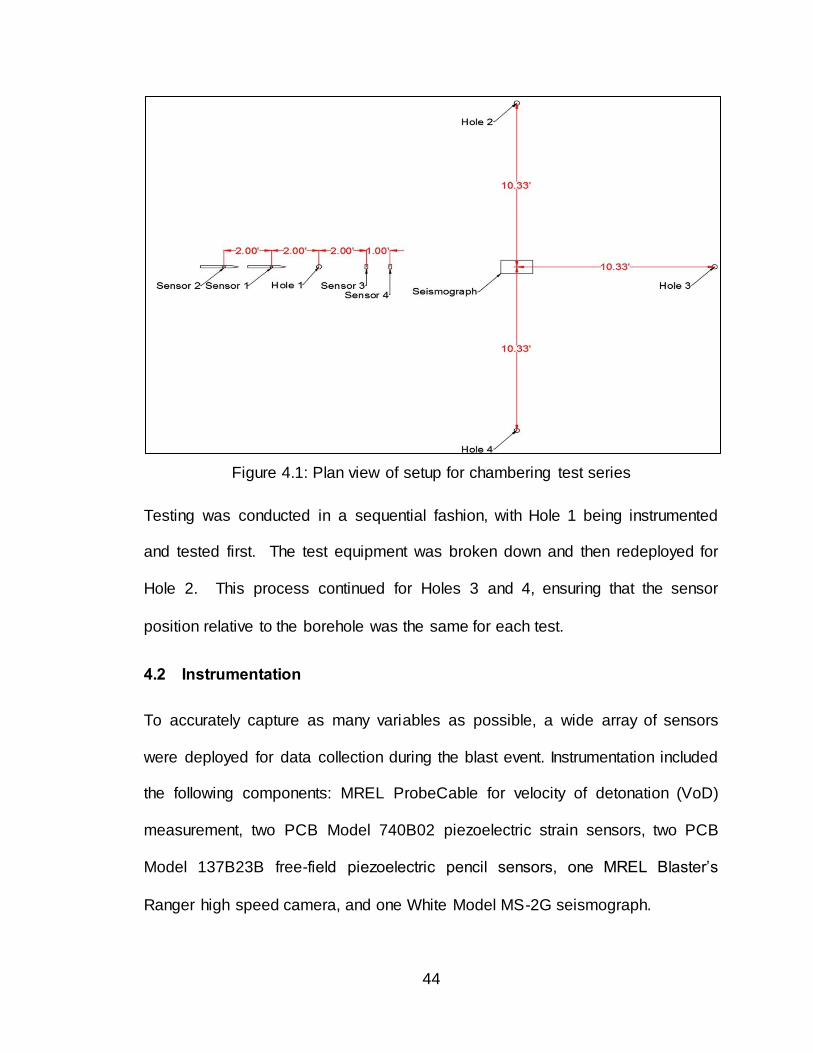
44
Figure 4.1: Plan view of setup for chambering test series
Testing was conducted in a sequential fashion, with Hole 1 being instrumented
and tested first. The test equipment was broken down and then redeployed for
Hole 2. This process continued for Holes 3 and 4, ensuring that the sensor
position relative to the borehole was the same for each test.
4.2 Instrumentation
To accurately capture as many variables as possible, a wide array of sensors
were deployed for data collection during the blast event. Instrumentation included
the following components: MREL ProbeCable for velocity of detonation (VoD)
measurement, two PCB Model 740B02 piezoelectric strain sensors, two PCB
Model 137B23B free-field piezoelectric pencil sensors, one MREL Blaster’s
Ranger high speed camera, and one White Model MS-2G seismograph.
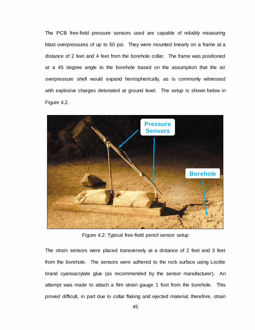
45
The PCB free-field pressure sensors used are capable of reliably measuring
blast overpressures of up to 50 psi. They were mounted linearly on a frame at a
distance of 2 feet and 4 feet from the borehole collar. The frame was positioned
at a 45 degree angle to the borehole based on the assumption that the air
overpressure shell would expand hemispherically, as is commonly witnessed
with explosive charges detonated at ground level. The setup is shown below in
Figure 4.2.
Figure 4.2: Typical free-field pencil sensor setup
The strain sensors were placed transversely at a distance of 2 feet and 3 feet
from the borehole. The sensors were adhered to the rock surface using Loctite
brand cyanoacrylate glue (as recommended by the sensor manufacturer). An
attempt was made to attach a film strain gauge 1 foot from the borehole. This
proved difficult, in part due to collar flaking and ejected material; therefore, strain
Pressure Sensors
Borehole

46
measurements close to the hole were not recorded for this series. A PCB strain
sensor adhered to the rock surface is shown in Figure 4.3.
Figure 4.3: PCB strain sensor adhered to the rock surface
The White seismograph was positioned at the center of the test arena, 10.33 feet
from the borehole. A scaled distance of 50 was calculated using the following
equation:
𝑆𝐷 =𝐷
√𝑊 (4.1)
where SD is scaled distance, D is the distance from the charge to the
seismograph, and W is the weight of the charge.
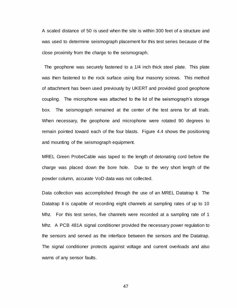
47
A scaled distance of 50 is used when the site is within 300 feet of a structure and
was used to determine seismograph placement for this test series because of the
close proximity from the charge to the seismograph.
The geophone was securely fastened to a 1/4 inch thick steel plate. This plate
was then fastened to the rock surface using four masonry screws. This method
of attachment has been used previously by UKERT and provided good geophone
coupling. The microphone was attached to the lid of the seismograph’s storage
box. The seismograph remained at the center of the test arena for all trials.
When necessary, the geophone and microphone were rotated 90 degrees to
remain pointed toward each of the four blasts. Figure 4.4 shows the positioning
and mounting of the seismograph equipment.
MREL Green ProbeCable was taped to the length of detonating cord before the
charge was placed down the bore hole. Due to the very short length of the
powder column, accurate VoD data was not collected.
Data collection was accomplished through the use of an MREL Datatrap II. The
Datatrap II is capable of recording eight channels at sampling rates of up to 10
Mhz. For this test series, five channels were recorded at a sampling rate of 1
Mhz. A PCB 481A signal conditioner provided the necessary power regulation to
the sensors and served as the interface between the sensors and the Datatrap.
The signal conditioner protects against voltage and current overloads and also
warns of any sensor faults.

48
Figure 4.4: Seismograph setup
The MREL Blaster’s Ranger high-speed camera was used to collect video of the
experiment. In the past, high-speed video has proven useful in documenting
explosive tests, especially when unexpected problems arise. The frame rate was
set to 250 frames per second. This rate provided a good balance of speed and
image quality given the lighting available.
Figure 4.5 provides an overview of the test arena and instrumentation setup.
The data acquisition equipment is placed inside of a steel pipe to protect it from
possible flying material. The high speed camera is placed adjacent to the data
acquisition equipment. Also shown are the three high intensity lights needed to
illuminate the test arena for high-speed video.

49
Figure 4.5: Test arena and instrumentation setup for chambering test series
4.3 Explosive Charge
All tests were conducted using 18 inches of 200 grain detonating cord and an
electric detonator, yielding 0.043 pounds of PETN high explosive. For the first
two tests, the detonating cord was left as a single 18” strand. The charge was
coupled using moist sand and stemmed using 10 inches (Hole 1) and 11.5
inches (Hole 2) of 1/4 inch gravel. This stemming method proved to be
ineffective, with significant flaking occurring around the collar of the borehole.
This result was not completely unexpected. The general rule of thumb for
stemming size states that the material should be no greater than 1/8 of the hole
diameter, and the stemming height should be at least 24 times the hole diameter.
In this case, the stemming should be no greater than 1/8 inch in size and
stemming height should be 21 inches.
Pressure
Sensors
Data
Acquisition
High-speed
Camera
Borehole

50
For the remaining two tests, the test procedure was modified to more closely
following the general rules of thumb for blasting. Detonating cord was cut into
two, nine-inch lengths, thereby decreasing the powder column height, increasing
the amount of stemming, and keeping the overall explosive charge weight
constant. These changes increased the stemming height to 19.75 (Hole 3) and
20.5 inches (Hole 4). In addition to the increased stemming height, dry, general
purpose sand was used as a stemming material, instead of the fine gravel. While
the stemming was still ejected for these two tests, damage to the borehole collar
during the blast was significantly reduced, indicating that less of the energy was
escaping the borehole through stemming ejection, and was being contained
deeper within the hole.
Reported experimental heat of detonation values for PETN vary from 5,730 kJ/kg
(Scilly, 1995) to 6,404 kJ/kg (Meyer, 1987). As a result, the expected detonation
energy ranges between 114.6 kJ and 128.1 kJ for this test series. For this test
series and subsequent test series, the available detonation energy value used for
calculation of percentages will be at the low end of published values. This
assumption is made because individual strands of detonating cord were bundled
together, resulting in a less energetic event when compared to using a bulk
product.
4.4 Chambering Test Results
Data analysis of the chambering test series provided useful information. Based
on the data collected, it is possible to analyze borehole enlargement and

51
calculate energy loss to air overpressure. When directly compared there does
not appear to be an association between air overpressure and strain. However,
when taking into account other factors, such as stemming type and borehole
condition, a trend does appear. This trend is discussed later in Section 4.4.5
“Conclusions.”
Experts in the field of ground vibration have previously discussed their
apprehension towards using seismographs to accurately measure ground
vibration at a level needed for calculating energy because of the content filtering
and distortion of frequency along the ground surface (Ouchterlony, 2004; Lusk,
2014). For thoroughness, a seismograph was used during this test series.
However, the seismographs inherent limitations coupled with a small charge size
yielded inconclusive ground vibration results for this test series.
4.4.1 Chambering Calculations
The primary purpose of the initial test series was to determine the amount of
energy transferred to borehole enlargement or chambering. As discussed
previously, this was accomplished by measuring the before and after volumes of
the borehole using sand and water.
Table 4.1 summarizes the volume data collected. The initial hole depths are
within a narrow range of 29.75 inches to 30.25 inches. The hole depths after
testing varied considerably more, from 27.75 inches to 29.63 inches. This
change can be attributed to flaking of the borehole collar and highly compacted
debris in the bottom of the borehole. In all instances, the borehole depth

52
decreased (most notably on Holes 1 and 2, a result of severe collar damage).
For comparison purposes, the theoretical volume of each hole is calculated,
using the before and after depths while assuming a consistent diameter of 7/8
inch. In all cases, the measured volume is approximately 10% greater than the
calculated volume. This is due to slight variations in hole diameter incurred
during the drilling process.
Table 4.1: Summary of volume data for borehole chambering tests
Before After Calculated
Hole
Depth
(in)
Sand Volume
(mL)
Water Volume
(mL)
Depth
(in)
Sand Volume
(mL)
Water Volume
(mL)
Before Volume
(mL)
After Volume
(mL)
1 29.75 - 320 28.50 340 350 293 281
2 30.25 330 330 27.75 290 300 298 273 3 30.00 320 325 29.63 330 330 296 292
4 30.13 330 330 29.50 320 325 297 291
As a result of the change in borehole depth, it is incorrect to directly compare the
before and after volumes of each hole. Therefore, the data is normalized by
dividing the measured volume in mL by the hole depth in inches. The normalized
data is now presented in terms of mL/inch, allowing for direct comparison.
Normalized data is shown in Table 4.2.
Table 4.2: Normalized before and after volume data
mL/inch (Sand) mL/inch (Water) Hole Before After % Diff Before After % Diff
1 10.76* 11.83 9.47* 10.76 12.39 14.11
2 10.91 10.45 -4.29 10.91 10.81 -0.90 3 10.67 11.14 4.33 10.83 11.14 2.78
4 10.95 10.85 -0.98 10.95 11.02 0.57 *Assuming an initial volume of 320mL

53
The percent difference between the before and after normalized values range
from -4.29% to 9.47% for sand and -0.90% to 14.11%. for water. The presence
of negative normalized volume changes indicates that experimental error is
present. A likely source of this error is the precision of the measuring devices
used. In this case, a standard tape measure and wooden dowel rod were used to
measure the hole depth and a 1000mL graduated cylinder was used to measure
the volume of material (sand or water) being poured in the hole.
The higher percent difference realized for Hole 1 is not believed to be completely
accurate. The hole did not hold water, unlike the other three holes. Lack of
water retention is a strong indication that a void or fracture in the rock mass was
exploited during the test.
To minimize the effect of experimental error, the average change in volume/inch
was calculated. This change was determined to be 0.24 mL/in and 0.48 mL/in
when using the sand measurement and water measurement, respectively,
resulting in an overall average volume change of 0.36 mL/in. This value was
multiplied by the original hole depth to calculate total change in volume per hole.
The assumption that 1 kJ is required to expand a borehole one milliliter (1 cc)
was used. Therefore, the change in volume in mL is equivalent to the energy lost
to borehole chambering in kJ. The results are summarized in Table 4.3.
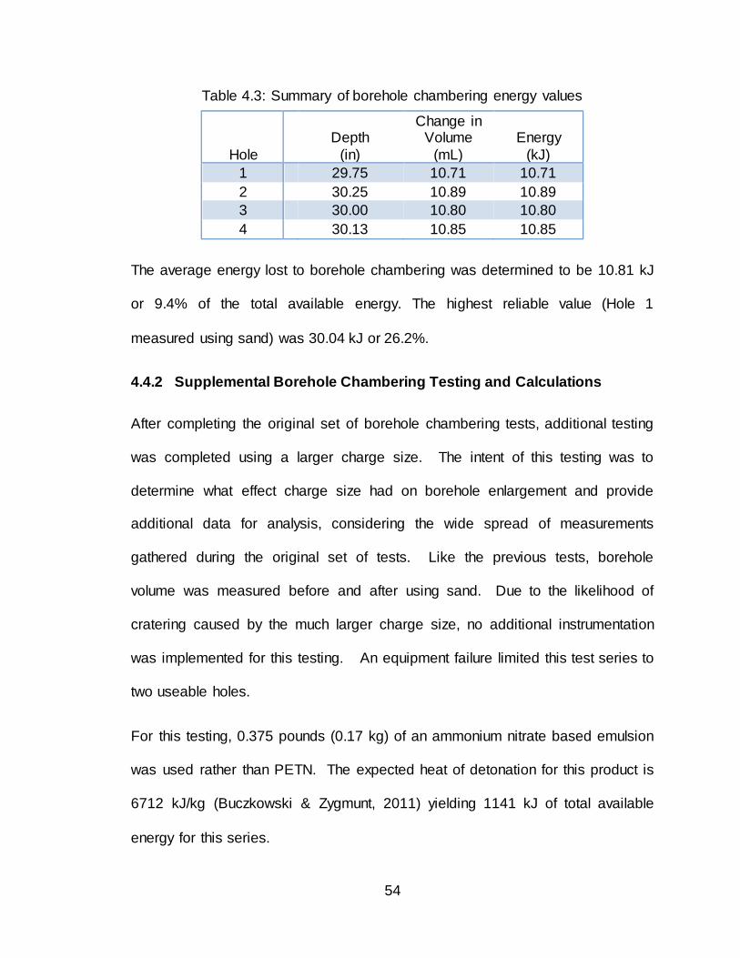
54
Table 4.3: Summary of borehole chambering energy values
Hole
Depth
(in)
Change in Volume
(mL)
Energy
(kJ)
1 29.75 10.71 10.71
2 30.25 10.89 10.89
3 30.00 10.80 10.80
4 30.13 10.85 10.85
The average energy lost to borehole chambering was determined to be 10.81 kJ
or 9.4% of the total available energy. The highest reliable value (Hole 1
measured using sand) was 30.04 kJ or 26.2%.
4.4.2 Supplemental Borehole Chambering Testing and Calculations
After completing the original set of borehole chambering tests, additional testing
was completed using a larger charge size. The intent of this testing was to
determine what effect charge size had on borehole enlargement and provide
additional data for analysis, considering the wide spread of measurements
gathered during the original set of tests. Like the previous tests, borehole
volume was measured before and after using sand. Due to the likelihood of
cratering caused by the much larger charge size, no additional instrumentation
was implemented for this testing. An equipment failure limited this test series to
two useable holes.
For this testing, 0.375 pounds (0.17 kg) of an ammonium nitrate based emulsion
was used rather than PETN. The expected heat of detonation for this product is
6712 kJ/kg (Buczkowski & Zygmunt, 2011) yielding 1141 kJ of total available
energy for this series.

55
The original and post-blast borehole depths and volumes are presented in Table
4.4. Hole 6 remained intact following the test. Hole 5 experienced significant
cratering and fragmentation to a depth of approximately 11.5 inches leaving the
bottom 18.25 inches with no visible damage.
Table 4.4: Summary of Supplemental Borehole Volumes
Before After
Hole Depth
(in) Volume
(mL)
Normalized
Volume (mL/in)
Depth (in)
Volume (mL)
Normalized
Volume (mL/in)
5 31.875 346 10.85 18.25 308 16.87
6 31.75 338 10.64 32.75 572 17.47
Average 31.81 342 10.75 25.50 440 17.17
The normalized volume change for Hole 5 was 6.02 mL/in resulting in a net
volume change of 192 mL. Hole 6 normalized volume change was slightly higher
at 6.83 mL/in, netting a volume change of 217 mL. Applying the same
assumption that 1 kJ is required to create 1 mL change in volume, it was
determined that 192 kJ or 16.8% of the total available energy was transferred to
borehole chambering for Hole 5. 217 kJ or 19.0% of the total available energy
was transferred to chambering for Hole 6.
4.4.3 Pressure Shell Energy Calculations
Calculating explosive energy based on pressure front velocity is not a novel idea
as shown by the work of Hoffman et al. (2009). Using pairs of sensors placed
around a blast, the velocity and duration (or thickness) of the expanding pressure
shell can be calculated. Each pair of sensors is a known distance from the blast
allowing for the determination of the radius, surface area, and volume of the
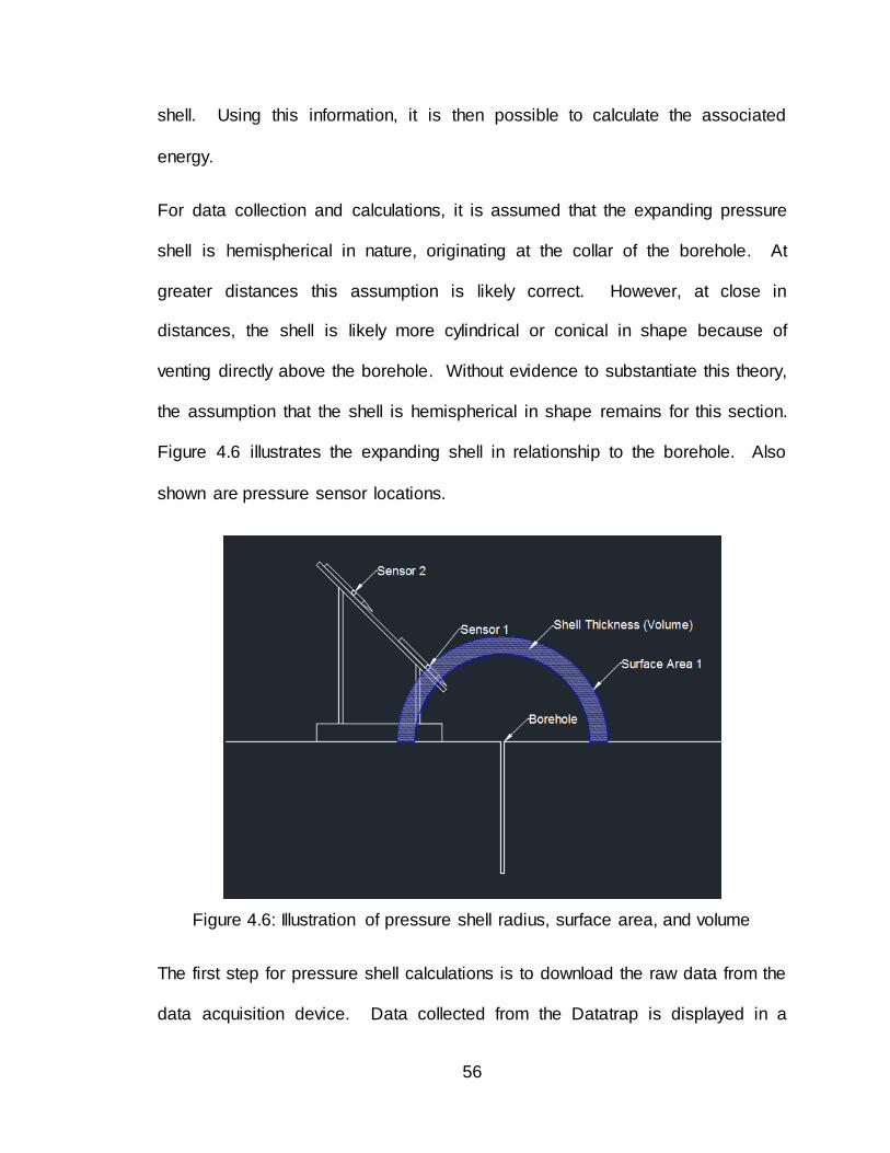
56
shell. Using this information, it is then possible to calculate the associated
energy.
For data collection and calculations, it is assumed that the expanding pressure
shell is hemispherical in nature, originating at the collar of the borehole. At
greater distances this assumption is likely correct. However, at close in
distances, the shell is likely more cylindrical or conical in shape because of
venting directly above the borehole. Without evidence to substantiate this theory,
the assumption that the shell is hemispherical in shape remains for this section.
Figure 4.6 illustrates the expanding shell in relationship to the borehole. Also
shown are pressure sensor locations.
Figure 4.6: Illustration of pressure shell radius, surface area, and volume
The first step for pressure shell calculations is to download the raw data from the
data acquisition device. Data collected from the Datatrap is displayed in a

57
voltage versus time format. A sensor specific calibration factor is applied to the
data to convert the voltage readings to pressure (PSI). The maximum pressure
and time at which the peak pressure occurred is recorded for both sensors.
From this information, the time necessary for the pressure wave to travel from
Sensor 1 to Sensor 2 can be determined. Since the distance between the two
pencil sensors is a known distance of 2 feet, it is then possible to calculate the
wave velocity. Table 4.5 provides a summary of the maximum pressure, time of
arrival (TOA), time difference, and wave velocity for each hole. For this test
series, the TOA was taken as the time at which the maximum pressure was
reached. Note that wave velocity is presented in English and Metric units to
facilitate future calculations. Figure 4.7 shows a typical Pressure vs. Time plot
for this test series. For simplicity, pressure data is converted from PSI to kPa and
calculations are completed using metric units.
Table 4.5: Summary of maximum pressure and time of arrival (TOA)
Sensor 1 (2 ft.) Sensor 2 (4 ft.) Wave
Hole Pressure
(PSI) Pressure
(kPa) TOA (ms)
Pressure (PSI)
Pressure (kPa)
TOA (ms)
Time Diff
(ms) Velocity
(fps) Velocity (m/ms)
1 2.125 14.65 3.77 0.759 5.481 5.67 1.90 1052 0.3205
2 4.864 33.54 2.90 2.548 17.57 4.55 1.65 1208 0.3683
3 4.351 30.00 4.82 1.875 12.93 6.68 1.86 1075 0.3277
4 3.283 22.63 4.75 1.529 10.54 6.46 1.71 1171 0.3569

58
Figure 4.7: Pressure versus time data for energy calculations
After the wave velocity is calculated, time (ms) is converted to distance (m). This
is done by multiplying the time scale and the calculated wave velocity. This
conversion is necessary to determine the thickness of the pressure shell. Figure
4.8 shows the converted plot.
The pressure data is next multiplied by the surface area of the pressure shell. In
this case, it is the surface area of a hemisphere, with a radius equal to the
distance from the borehole collar to the sensor. This distance is 2 feet (0.61 m)
for Sensor 1 and 4 feet (1.22 m) for Sensor 2. These conversions result in a
Pressure-Area (kPa-m2) versus Distance (m) plot, as shown in Figure 4.9.
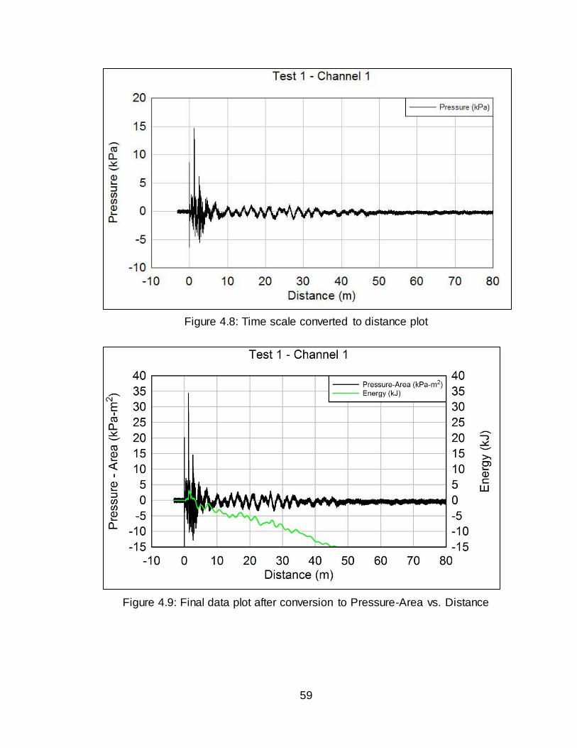
59
Figure 4.8: Time scale converted to distance plot
Figure 4.9: Final data plot after conversion to Pressure-Area vs. Distance

60
The plot is then integrated and the maximum value taken as the pressure shell
energy. This procedure is repeated for the data recorded at both sensors, with
the assumption that the wave velocity is the same at Sensors 1 and 2. Table 4.6
summarizes the data and energy calculations. Area 1 is the area of the
hemisphere as the pressure shell approaches Sensor 1, and Energy 1
represents the calculated energy based on the data provided by Sensor 1. Area
2 and Energy 2 represent the same conditions for Sensor 2.
Table 4.6: Summary of pressure shell energy calculations for initial test series
Hole Time Diff
(ms) Velocity (m/ms)
Area 1 (m2)
Energy 1 (kJ)
Area 2 (m2)
Energy 2 (kJ)
1 1.902 0.3205
2.335
3.148
9.340
7.321
2 1.655 0.3683 3.508 26.732 3 1.860 0.3277 8.341 17.080
4 1.708 0.3569 6.855 15.580
Hole to Hole differences in energy can be explained by variations in the
effectiveness of the stemming and borehole condition. However, differences in
energy from between sensors indicate that the assumption of the hemispheric
pressure shell expansion is not completely correct. In order for this assumption
to hold true, Energy 1 and Energy 2 should be roughly equivalent, with Energy 2
being slightly less due to other environmental losses. Although the overpressure
decreases from Sensor 1 to 2, the area being affected increases significantly.
Without additional data to further refine the shape of the pressure shell, future
calculations will use the assumption that the pressure shell created by venting
gases is hemispherical in shape. Peak pressure values are shown in Appendix A
and air overpressure energy plots from Tests 1 – 4 are in Appendix B.

61
4.4.4 Conclusions
Borehole chambering results varied significantly. Using normalized values to
mitigate experimental error, the average energy transferred to borehole
chambering for Holes 1-4 was 9.4%. For the larger charge size in Holes 5 and 6,
the energy transfer was determined to be roughly 18%.
This test series demonstrated that there is merit to the methodology used for
calculating energy transferred to air overpressure. At first glance, the energy
values summarized in Table 4.5 appear to be sporadic. However, when
analyzing the test series as a whole, by taking into account stemming material
and borehole condition, patterns emerge.
Following testing, Hole 1 would not retain water, indicating that cracks were
present. Cracks allowed the expanding gases to vent into the surrounding rock
mass, rather than into the atmosphere. Hole 2 was stemmed using fine gravel,
which held poorly, allowing the gasses to quickly vent to the atmosphere. Holes
3 and 4 used wet sand, which provided more resistance to venting, thus
transmitting more energy to the surrounding rock mass. These observations are
further reinforced by the strain data results, summarized in Table 4.7. Hole 1 had
the lowest strain values and Holes 3 and 4 had the highest.

62
Table 4.7: Summary of strain results from chambering tests
Sensor 3 (2 ft.) Sensor 4 (3 ft.)
Hole Strain (µε)
Strain (µε)
1 49.82 23.62
2 71.70 16.67 3 99.46 26.29
4 90.89 29.36
The total available explosive energy for this test series is 114.6 kJ. Energy
transferred to air overpressure ranged from a minimum of 6.39% (Hole 1) to a
maximum of 14.9% (Hole 2). These values are understated because of the
positioning of the free-field pressure sensors, which failed to capture a portion of
the higher overpressures venting vertically from the borehole. Future tests will
feature pressure sensors mounted directly above the borehole.
Copyright © Joshua Thomas Calnan 2015
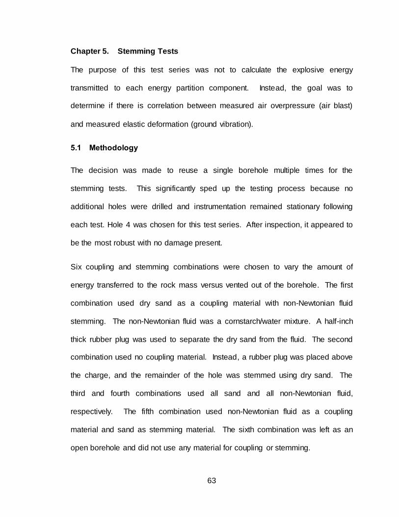
63
Chapter 5. Stemming Tests
The purpose of this test series was not to calculate the explosive energy
transmitted to each energy partition component. Instead, the goal was to
determine if there is correlation between measured air overpressure (air blast)
and measured elastic deformation (ground vibration).
5.1 Methodology
The decision was made to reuse a single borehole multiple times for the
stemming tests. This significantly sped up the testing process because no
additional holes were drilled and instrumentation remained stationary following
each test. Hole 4 was chosen for this test series. After inspection, it appeared to
be the most robust with no damage present.
Six coupling and stemming combinations were chosen to vary the amount of
energy transferred to the rock mass versus vented out of the borehole. The first
combination used dry sand as a coupling material with non-Newtonian fluid
stemming. The non-Newtonian fluid was a cornstarch/water mixture. A half-inch
thick rubber plug was used to separate the dry sand from the fluid. The second
combination used no coupling material. Instead, a rubber plug was placed above
the charge, and the remainder of the hole was stemmed using dry sand. The
third and fourth combinations used all sand and all non-Newtonian fluid,
respectively. The fifth combination used non-Newtonian fluid as a coupling
material and sand as stemming material. The sixth combination was left as an
open borehole and did not use any material for coupling or stemming.
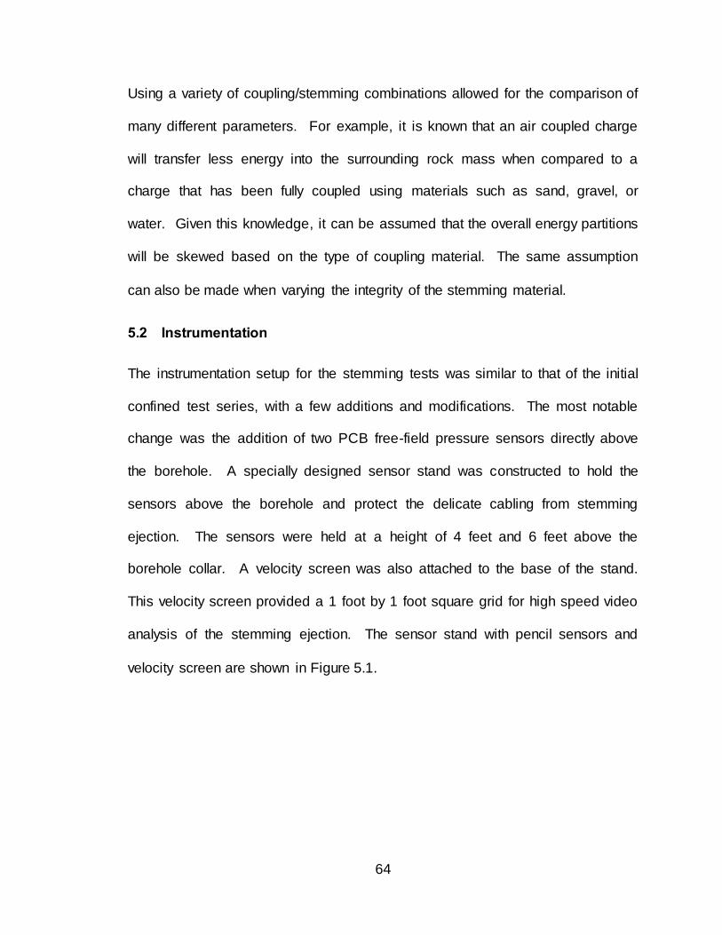
64
Using a variety of coupling/stemming combinations allowed for the comparison of
many different parameters. For example, it is known that an air coupled charge
will transfer less energy into the surrounding rock mass when compared to a
charge that has been fully coupled using materials such as sand, gravel, or
water. Given this knowledge, it can be assumed that the overall energy partitions
will be skewed based on the type of coupling material. The same assumption
can also be made when varying the integrity of the stemming material.
5.2 Instrumentation
The instrumentation setup for the stemming tests was similar to that of the initial
confined test series, with a few additions and modifications. The most notable
change was the addition of two PCB free-field pressure sensors directly above
the borehole. A specially designed sensor stand was constructed to hold the
sensors above the borehole and protect the delicate cabling from stemming
ejection. The sensors were held at a height of 4 feet and 6 feet above the
borehole collar. A velocity screen was also attached to the base of the stand.
This velocity screen provided a 1 foot by 1 foot square grid for high speed video
analysis of the stemming ejection. The sensor stand with pencil sensors and
velocity screen are shown in Figure 5.1.

65
Figure 5.1: Free-field pencil sensor stand with attached velocity screen
Two film strain gauges were added to the setup as well. These gauges were
adhered to the rock surface, following the manufacturer’s recommendations in
transverse and longitudinal orientations. The distance from the borehole to the
center of these strain gauges was 1 foot. The two PCB strain sensors remained
at 2 feet and 3 feet. The strain gauge setup is shown in Figure 5.2, with the film
strain gauges highlighted by a yellow circle and the two PCB strain sensors
highlighted by smaller red circles. Figure 5.3 illustrates the instrumentation setup
in plan view.
Velocity
Screen
Pressure
Sensors
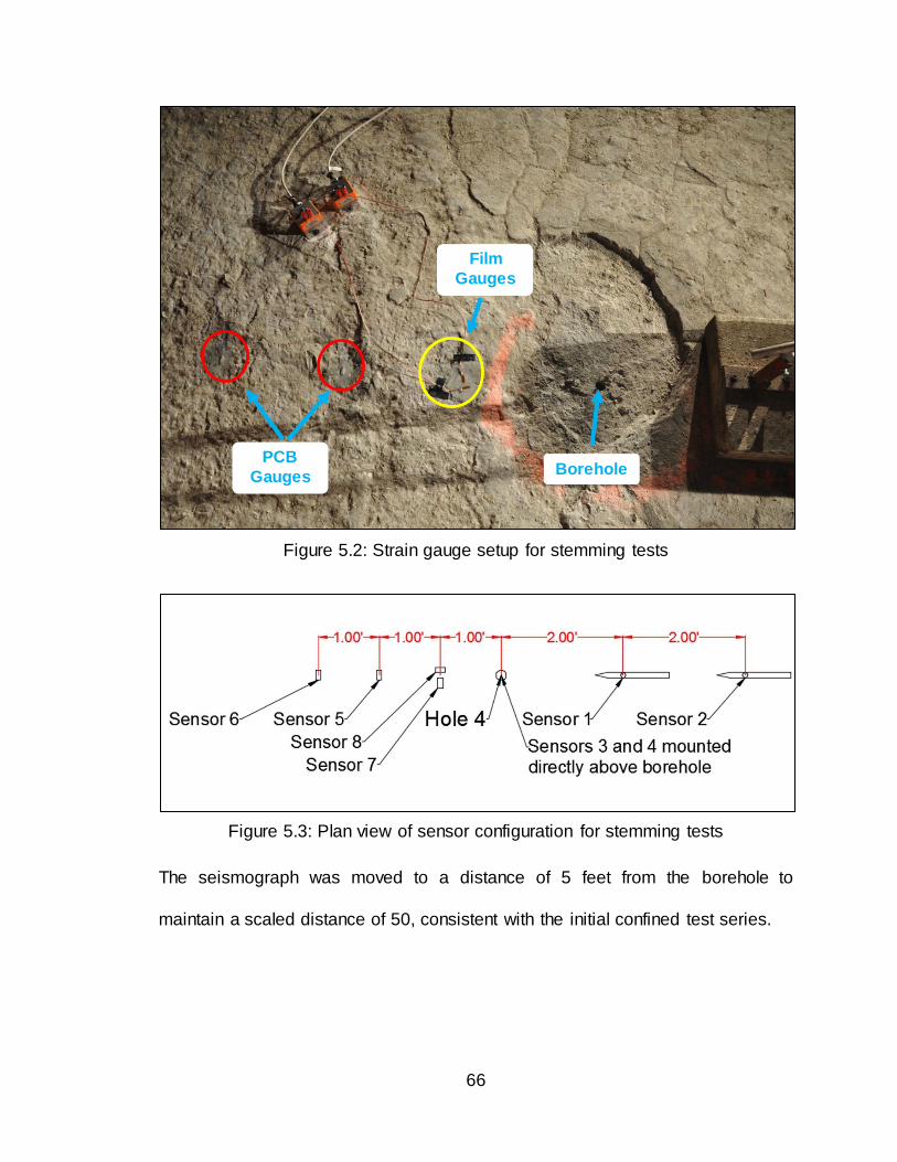
66
Figure 5.2: Strain gauge setup for stemming tests
Figure 5.3: Plan view of sensor configuration for stemming tests
The seismograph was moved to a distance of 5 feet from the borehole to
maintain a scaled distance of 50, consistent with the initial confined test series.
Film
Gauges
PCB
Gauges Borehole

67
5.3 Explosive Charge
The first round of stemming tests (five tests) was conducted using 18 inches of
25 grain detonating cord cut into two, nine-inch lengths. This resulted in a
charge weight of 0.0053 pounds. The detonating cord was initiated using an
electric detonator. Following this round of tests, the charge size was increased
to 16 inches of 50 grain detonating cord, cut into four, four-inch lengths for a
charge weight of 0.0095 pounds (including detonator). This decision was made
after reviewing the data from the first round of tests. On many instrumentation
channels, the signal to noise ratio was very low, making it difficult to discern
useable results from noise. By increasing the charge size, the magnitude of the
results (strain, overpressure, and vibration values) was also increased. This
improved the signal to noise ratio, facilitating data analysis and greater
measurement accuracy. The charge size was not increased substantially, in
order to prevent the explosive energy from overwhelming any differences that
would otherwise be noticed between coupling/stemming combinations.
Referencing the published values, the total explosive energy expected for this
test series is 28.83 kJ.
5.4 Stemming Test Results
A total of 18 stemming tests were conducted, three for each of the six
coupling/stemming material combinations. The average values recorded for
each of the combinations is summarized in Table 5.1. The performance of each
combination will not be discussed in detail because that is beyond the scope of

68
this dissertation. Instead, this section will focus on the correlation between
measured air overpressure and measured elastic deformation.
Strain gauges on channels 5-7 were positioned perpendicular to the borehole
(transverse) and the strain gauge on channel 8 was positioned longitudinally.
Analysis of the data from gauges closest to the borehole (7 and 8) indicated a
flaw in the test methodology. Poisson’s ratio was calculated to range from 0.78
to 1.04 (well above the upper limit of 0.5 and accepted values of 0.2-0.3 for
limestone). These results are a strong indication that the strain gauges in close
proximity to the borehole were not oriented correctly. This belief is that at
distances less than one borehole length, the waves are propagating primarily in
the vertical (Z) direction and are not accurately captured using surface mounted
strain gauges. Additional tests in Chapter 6 support this belief.
Table 5.1: Summary of stemming test results
Sensor Number 1
(2 ft) 2
(4 ft) 3
(4 ft) 4
(6 ft) 5
(2 ft) 6
(3 ft) 7
(1 ft) 8
(1 ft) Seismo
(5 ft)
Coupling/Stemming Material
Pressure (PSI)
Strain (μϵ)
Trans. (μϵ)
Long. (μϵ)
Acoustic (dB)
Sand/Cornstarch 0.89 0.49 1.74 1.13 12.88 2.88 172.45 186.75 139
Air/Sand 0.77 0.48 2.19 1.28 14.16 2.14 107.78 103.19 141
Sand 0.57 0.67 2.31 1.58 16.13 2.41 93.93 113.59 133
Cornstarch 0.28 0.32 0.36 0.40 54.25 10.75 125.88 161.34 130
Air 2.94 1.21 2.64 1.36 8.72 1.54 235.97 248.74 146
Cornstarch/Sand 0.08 0.13 0.08 0.08 43.69 19.36 -- -- NV
The data collected during this test series shows that the test methodology
described provides a high enough fidelity to detect shifts in the air overpressure
and elastic deformation balance. The air overpressure from sensors 1-4 and
strain from sensors 5 and 6 are summed and compared. Strain data from
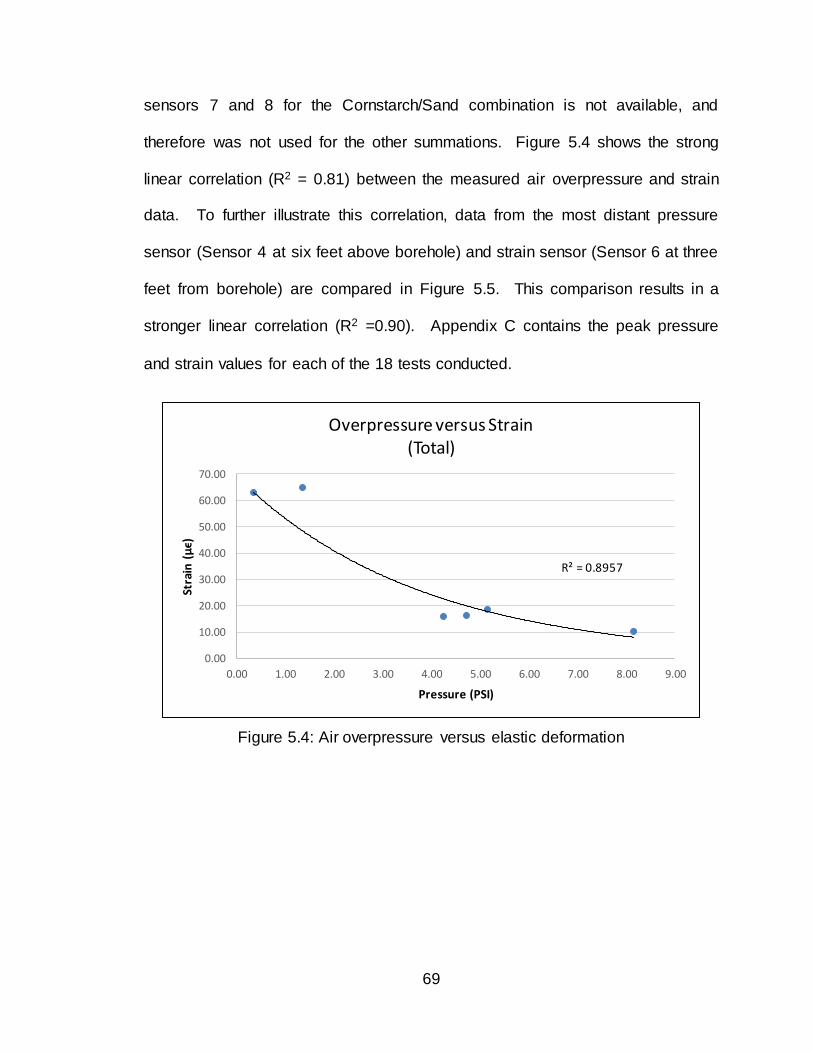
69
sensors 7 and 8 for the Cornstarch/Sand combination is not available, and
therefore was not used for the other summations. Figure 5.4 shows the strong
linear correlation (R2 = 0.81) between the measured air overpressure and strain
data. To further illustrate this correlation, data from the most distant pressure
sensor (Sensor 4 at six feet above borehole) and strain sensor (Sensor 6 at three
feet from borehole) are compared in Figure 5.5. This comparison results in a
stronger linear correlation (R2 =0.90). Appendix C contains the peak pressure
and strain values for each of the 18 tests conducted.
Figure 5.4: Air overpressure versus elastic deformation
R² = 0.8957
0.00
10.00
20.00
30.00
40.00
50.00
60.00
70.00
0.00 1.00 2.00 3.00 4.00 5.00 6.00 7.00 8.00 9.00
Stra
in (μϵ)
Pressure (PSI)
Overpressure versus Strain(Total)

70
Figure 5.5: Air overpressure at sensor 4 versus strain measured at sensor 6
Comparison of air blast measured using the seismograph unit at five feet versus
the strain recorded at sensors 5 and 6 does not show as strong of a correlation
as previous comparisons. This is shown in Figure 5.6
Figure 5.6: Air blast versus strain plot
Copyright © Joshua Thomas Calnan 2015
R² = 0.9264
0.00
5.00
10.00
15.00
20.00
25.00
0.00 0.20 0.40 0.60 0.80 1.00 1.20 1.40 1.60 1.80
Stra
in (μϵ)
Pressure (PSI)
Overpressure (Sensor 4) versus Strain (Sensor 6)
R² = 0.7365
0.00
10.00
20.00
30.00
40.00
50.00
60.00
70.00
128.00 130.00 132.00 134.00 136.00 138.00 140.00 142.00 144.00 146.00 148.00
Stra
in (μϵ)
Airblast (dB)
Airblast vs Strain

71
Chapter 6. Strain Mapping and Strain Energy
6.1 Methodology & Instrumentation
Following the stemming test series previously completed, another test series was
needed to determine at what distance the waves transition from propagating
primarily in the vertical direction to propagating primarily in the axial (longitudinal)
direction, making it acceptable to use surface mounted strain gauges for energy
measurement. The instrumentation used for this test series was similar to the
stemming tests, with the addition of two PCB strain gauges to the sensor array.
Following the extensive number of tests conducted using Hole 4, the decision
was made to conduct the strain testing on Hole 3. Like Hole 4, Hole 3 was drilled
in competent rock. Strain sensors were adhered to the rock surface at distances
of 1 foot, 2 feet, 4 feet, and 6 feet from the center of the borehole. The sensors
were first mounted transversely, and then after five test re-oriented longitudinally.
Free-field pencil sensors were again positioned at a 45 degree angle to the
borehole and directly above the borehole. The high-speed camera, set at 500
frames per second, and velocity screen were used to determine stemming
ejection velocity. Figure 6.1 shows this instrumentation setup. The orange hash
marks on the rock floor demarcate 1 foot intervals, and the blue circles highlight
the location of the PCB strain sensors. Figure 6.2 shows the setup in plan view.
Again, 16 inches of 50 grain detonating cord was initiated using an electric
detonator, yielding a theoretical heat of detonation value of 28.83 kJ.
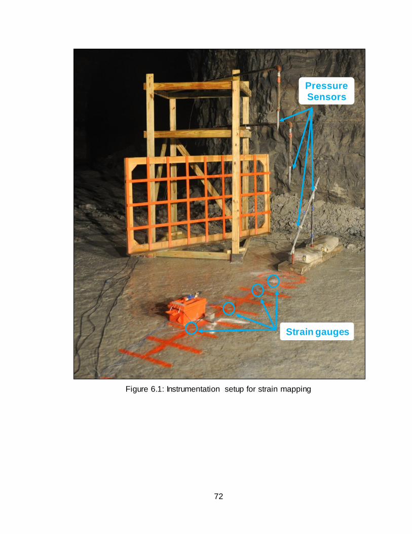
72
Figure 6.1: Instrumentation setup for strain mapping
Strain gauges
Pressure Sensors

73
Figure 6.2: Plan view of strain mapping test setup
6.2 Strain Mapping Results
Five tests for each strain gauge orientation were conducted. The averages for
each location and orientation are summarized in Table 6.1. The calculated
Poisson’s ratio for each location is also shown. Like the stemming test results in
the previous chapter, the calculated ratio for the sensors closest to the borehole
(1 ft. and 2 ft.) are well outside the conventional limit of 0.5. This is a strong
indication that compression and tension waves are propagating primarily in the
vertical direction at these distances. Poisson’s ratio at the 4 ft. and 6 ft. points
level out at reasonable values of 0.33 and 0.34, respectively. This indicates that
the waves are moving primarily in the longitudinal direction. It should be noted
that this is a dynamic reading and therefore, Poisson’s ratio is expected to be
higher than in static tests.

74
Table 6.1: Summary of strain mapping results
Distance from Borehole
Orientation 1 ft 2 ft 4 ft 6 ft
Transverse (µϵ) 29.24 18.36 4.63 3.62
Longitudinal (µϵ) 31.96 9.15 14.13 10.50
Poisson’s Ratio 0.91 2.01 0.33 0.34
It is believed that close to the borehole, the waves are moving outward from the
point of origin in a spherical manner and intersecting the rock surface (and strain
gauges) at steep angles. As the waves continue to move outward, they become
more planar and the interaction with the surface becomes shallower. At this
point, the primary wave direction is more accurately captured by the longitudinal
strain gauges. For this test series, the transition zone from spherical to planar
takes place between 2 ft. and 4 ft. from the borehole. This idea is shown
graphically in Figure 6.3. The magenta line is propagation and intersection of the
wave as it reaches the strain gauge at a distance of 1 ft. from the borehole. This
is followed by the red line at 2 ft., green line at 4 ft., and blue line at 6 ft.
Figure 6.3: Shock waves intersecting strain gauges

75
With these findings in mind, the recommendation is made that for instrument
mounting locations at a distance less than the borehole depth, the vertical
component must be instrumented to accurately calculate the strain/ground
vibration energy component. This can be accomplished one of two ways. The
first is to use a triaxial accelerometer. The second method is to affix a strain
gauge vertically to the side of a second borehole. For distances from the
borehole exceeding the depth of the borehole, the use of strain gauges mounted
transversely and longitudinally is advised. At these distances the vertical
component can be estimated using basic solid mechanics principles.
The transverse strain measurements from each test were plotted with respect to
distance to illustrate how strain decays with distance. Figure 6.4 illustrates the
relationship between transverse strain measurement and distance. Strain is
highest near the borehole and rapidly decays with distance, similar to air
overpressure.

76
Figure 6.4: Strain with respect to distance from borehole
In addition to providing valuable data for mapping strain levels around the
borehole, this test series also provided data that can be used for calculating
energy lost to strain, air overpressure, and stemming ejection. For each of the
five tests with transversely mounted strain gauges, the maximum strain level was
plotted and a “Power” trend line fitted, similar to Figure 6.2. From this, the strain
level at any distance could be estimated.
Strain energy is calculated using the following equation:
𝑈 =1
2𝑉𝐸휀2 (6.1)
where U is strain energy, V is volume, E is Young’s Modulus, and ε is strain. For
this Limestone material, Young’s Modulus is 59.91 GPa and the dynamic
R² = 0.9096
0
10
20
30
40
50
60
70
80
90
0 1 2 3 4 5 6 7 8 9
Stra
in (μϵ)
Distance (ft)
Strain vs Distance

77
Poisson’s ratio is 0.33, therefore the strain levels are assumed to be equal in the
transverse and vertical directions and three times greater in the axial direction.
The strain energy is assumed to propagate out from the borehole
hemispherically. Therefore, the volume of rock affected by a given strain level is
a hemispherical shell with an outer radius equal to the distance from the borehole
to the point of interest and an inner radius equal to the distance from the
borehole to the previous point of interest. Radii and their respective volumes
from 0.1 ft. to 60 ft. were used for calculation of strain energy. The energies from
each affected volume was summed and tabulated in Table 6.2.
Table 6.2: Summary of calculated strain energy for a confined borehole
Test
Transverse
(J)
Axial
(J)
Vertical
(J)
Total
(J)
Percentage of Total
Energy
1 174.25 522.75 174.25 871.25 3.0%
2 111.16 333.48 111.16 555.8 1.9%
3 84.35 253.05 84.35 421.75 1.4%
4 232.01 696.03 232.01 1160.05 4.0%
5 91.47 274.41 91.47 457.35 1.6%
Strain energy values ranged from 456.35 J (1.6%) to 1160.05 J (4.0%) for
individual tests. Using the values and resulting equation presented in Figure 6.4,
the average strain energy for the entire test series is 514.74 J or 1.8% of the total
explosive energy available. The values used for completion of this calculation
are shown in their entirety in Appendix D.
Air overpressure energy was calculated using the same methodology previously
discussed in Chapter 4. Two energy calculations were made for each test. One

78
using the pressures and wave velocities from the sensors mounted at a 45
degree angle, and the other using the data from the sensors mounted directly
above the borehole. These energy values are shown in Table 6.3.
Table 6.3: Summary of air overpressure calculations for confined borehole
Side sensors Top Sensors
Test
Time Diff (ms)
Velocity (m/ms)
Surface Area (m2)
Energy (kJ) Test
Time Diff
(ms) Velocity (m/ms)
Surface Area (m2)
Energy (kJ)
1 2.087 0.2920
2.335
2.466 1 1.771 0.3442
9.34
9.137
2 1.751 0.3481 1.084 2 1.781 0.3423 8.526
3 1.764 0.3456 1.022 3 1.789 0.3407 8.588
4 1.757 0.3470 0.914 4 1.760 0.3464 8.069
5 1.771 0.3442 1.429 5 1.731 0.3522 8.447
A significant portion of the air overpressure energy is being directed upward,
rather than outward in a uniform hemispherical shape at the distances measured
in these tests. This is supported by the higher wave velocities experienced at the
sensors directly above the borehole and the gas cloud seen escaping the
borehole after stemming ejection when reviewing the high-speed video data.
Also, peak pressures seen at sensor 1 (2 ft. from borehole at 45 degree angle)
and sensor 4 (6ft. directly above the borehole) were both around 0.5 psi. As a
result, it would not be correct to equally weight the top and side values to find the
average energy for each test. Instead, a weight of 25% will be assigned to the
side and 75% to the top. Table 6.4 summarizes the weighted values. Figure 6.5
illustrates the predicted pressure shell shape in relationship to the borehole and
pressure sensors.

79
Table 6.4: Weight total air overpressure energy for confined tests
Test
Side Weighted
Energy - 25% (kJ)
Top Weighted
Energy - 75% (kJ)
Total
Energy (kJ)
Percentage of Total
Available Energy
1 0.616 6.853 7.469 25.9
2 0.271 6.395 6.666 23.1
3 0.255 6.441 6.696 23.2
4 0.228 6.052 6.280 21.8
5 0.357 6.335 6.692 23.2
Figure 6.5: Revised pressure shell shape

80
Total air overpressure values were consistent using this methodology, ranging
from 6280 J (21.8%) to 7469 J (25.9%). The overall average of the total energy
lost to air overpressure is 6761 J or 23.5% of the total available explosive energy.
Air overpressure energy plots for Tests 1-5 are presented in Appendix E.
Energy lost to stemming ejection was calculated using the basic physics
equation:
𝐾𝐸 = 1
2𝑚𝑣2 (6.2)
Mass was taken as the mass of sand used to stem the hole during each test and
velocity was calculated using high-speed video. The results of these calculations
are show below in Table 6.5.
Table 6.5: Energy transferred to stemming ejection during confined test
Test Velocity
(m/s) Mass (kg)
Energy (J)
Percentage
of Total Energy
1 50.8 0.475 613 2.1
2 50.8 0.477 616 2.1
3 61 0.477 887 3.1
4 50.8 0.469 605 2.1
5 61 0.477 887 3.1
Calculated energy values ranged from 605 J (2.1%) to 887 J (3.1%). This
amount of energy is significant considering the relatively small mass of the
material being ejected.
The total amount of energy measured and the respective percentage of total
available energy for each of the five tests is summarized below in Table 6.6.
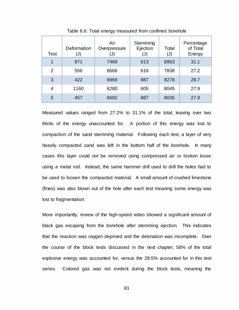
81
Table 6.6: Total energy measured from confined borehole
Test
Deformation
(J)
Air Overpressure
(J)
Stemming Ejection
(J)
Total
(J)
Percentage of Total
Energy
1 871 7469 613 8953 31.1
2 556 6666 616 7838 27.2
3 422 6969 887 8278 28.7
4 1160 6280 605 8045 27.9
5 457 6692 887 8036 27.9
Measured values ranged from 27.2% to 31.1% of the total, leaving over two
thirds of the energy unaccounted for. A portion of this energy was lost to
compaction of the sand stemming material. Following each test, a layer of very
heavily compacted sand was left in the bottom half of the borehole. In many
cases this layer could not be removed using compressed air or broken loose
using a metal rod. Instead, the same hammer drill used to drill the holes had to
be used to loosen the compacted material. A small amount of crushed limestone
(fines) was also blown out of the hole after each test meaning some energy was
lost to fragmentation.
More importantly, review of the high-speed video showed a significant amount of
black gas escaping from the borehole after stemming ejection. This indicates
that the reaction was oxygen deprived and the detonation was incomplete. Over
the course of the block tests discussed in the next chapter, 58% of the total
explosive energy was accounted for, versus the 28.5% accounted for in this test
series. Colored gas was not evident during the block tests, meaning the

82
detonation was closer to ideal. Considering the same explosive products and
similar test methodologies were used, the author believes that a considerable
amount of the explosives total available energy was lost to incomplete detonation
and not transferred to measureable components
Copyright © Joshua Thomas Calnan 2015

83
Chapter 7. Concrete Block Testing
7.1 Methodology
The purpose of the concrete block testing was to reintroduce the fragmentation
and movement components of energy partitioning into the test series. Concrete
block testing more closely resembles scenarios typically encountered during rock
blasting, by allowing the material to fragment towards three free-faces. The
concrete blocks measured 4 feet in length, width, and height and were composed
of a medium strength concrete mix containing no course aggregates.
Two blocks were available for testing purposes. For each test, a 7/8 inch hole
was drilled to a depth of 10 inches with a burden of 10 inches from both side free
faces. The first block was used for one test, and the second block was used for
two tests, with holes being drilled and detonated on opposing corners.
7.2 Instrumentation
The same equipment used in previous tests was applied here also, but in a
different configuration. In summary: a total of four PCB free-field pressure
sensors, four PCB strain sensors, one MREL high-speed camera, one PCB
signal conditioner, and one MREL data acquisition system were used.
Two PCB free-field pressure sensors were placed at a height of 4 feet and 6 feet,
directly above the borehole, using the wood sensor tower (raised four feet using
metal scaffolding). The two remaining pressure sensors were placed 2 feet and
4 feet from the side of the block to capture gases venting from fractures. Due to

84
the high probably of damage from flying debris, no sensors were placed directly
in front of the block.
Strain sensors were adhered to the concrete block surface in 1 foot intervals.
Prior to adhering sensors to the block, the surface was smoothed using an
electric grinder and then lightly scuffed using sandpaper. After analyzing data
from the first test, the decision was made to no longer place a sensor at 4 feet,
due to abnormal readings. The abnormal readings were likely caused by the
sensor’s close proximity to the back corner of the block. This position resulted in
significant reflection of the waves. Figure 7.1 shows the position of the strain
sensors relative to the borehole collar.
Figure 7.1: Strain sensor mounting locations
Strain
Gauges
Borehole

85
The velocity screen, containing a 1 foot by 1 foot grid, was placed parallel to the
expected direction of fragment heave. The high speed camera was arranged
perpendicular to the screen at a height of 4.5 feet. The corner of the block was
painted with a grid and dots to aid in the tracking of fragments. Velocity screen
positioning and the painted block corner are shown in Figure 7.2.
Figure 7.2: Velocity screen position for block testing
Figure 7.3 shows an overview of the testing setup, and Figure 7.4 shows the test
setup in plan view.

86
Figure 7.3: Overview of test setup for block testing
Figure 7.4: Plan view of block testing setup
Pressure
Sensors
Velocity
Screen
87
7.3 Explosive Charge
The explosive charge remained consistent with the stemming and strain
attenuation tests (four strands of 50 grain detonating cord cut to 4 inches in
length) to allow for a direct comparison of energy component percentages. The
borehole was 7/8 inch diameter and drilled to a depth of 10 inches for each of the
three tests. The explosive charge was coupled with sand and then stemmed with
6 inches of sand.
The burden to both free faces and hole depth were chosen to be 10 inches to
provide a powder factor of 0.5 lbs/yd3. It was predicted that this powder factor
would fragment the corner of the block without resulting in excessive material
heave.
Referencing the published values, the total explosive energy expected for this
test series is between 28.83 kJ.
7.4 Block Testing Results
7.4.1 Kinetic Energy
Kinetic energy of a moving fragment must be broken down into two components:
translational kinetic energy and rotational kinetic energy. The determination of
translation kinetic energy is straightforward and is found with the basic physics
equation:
𝐾𝐸𝑡𝑟𝑎𝑛𝑠𝑙𝑎𝑡𝑖𝑜𝑛𝑎𝑙 = 1
2𝑚𝑣2 (7.1)

88
where m is the mass of the object (kg) and v is velocity of the object (m/s). For
these calculations, the mass of all sizeable fragments was recorded and
summarized. Small fragments were placed in a bucket and weighed together.
To account for the loss of fines and other unrecoverable fragments, 5% was
added to the total weight. These results are summarized bellowed in Table 7.1.
Test Blocks 1 and 3 had similar fragment masses of 125.00 kg and 117.21 kg,
respectively. The mass of fragments from Test Block 2 was approximately 25%
higher at 150.79 kg.
Table 7.1: Summary of fragment masses
Fragment Mass
(kg)
Fragment Number Block 1 Block 2 Block 3
Small 7.89 4.26 4.54 1 10.18 64.93 28.12
2 3.18 55.72 78.97 3 41.75 18.69 -
4 3.02 - - 5 53.02 - -
Total 119.05 143.61 111.63 Total * 1.05 125.00 150.79 117.21
The translational velocity of the fragments was calculated after reviewing the high
speed video taken of each test. Each discernible fragment was tracked
throughout the video and the number of frames it took for the center of the
fragment to travel a distance of one foot was noted. All video was recorded at a
rate of 500 frames per second, meaning that one frame was equivalent to a time
of 2 milliseconds. With this information at hand, it was possible to calculate the
fragment velocity in terms of feet per second (and then finally meters per
second). There was little variability (±1 frame) in individual fragment velocity
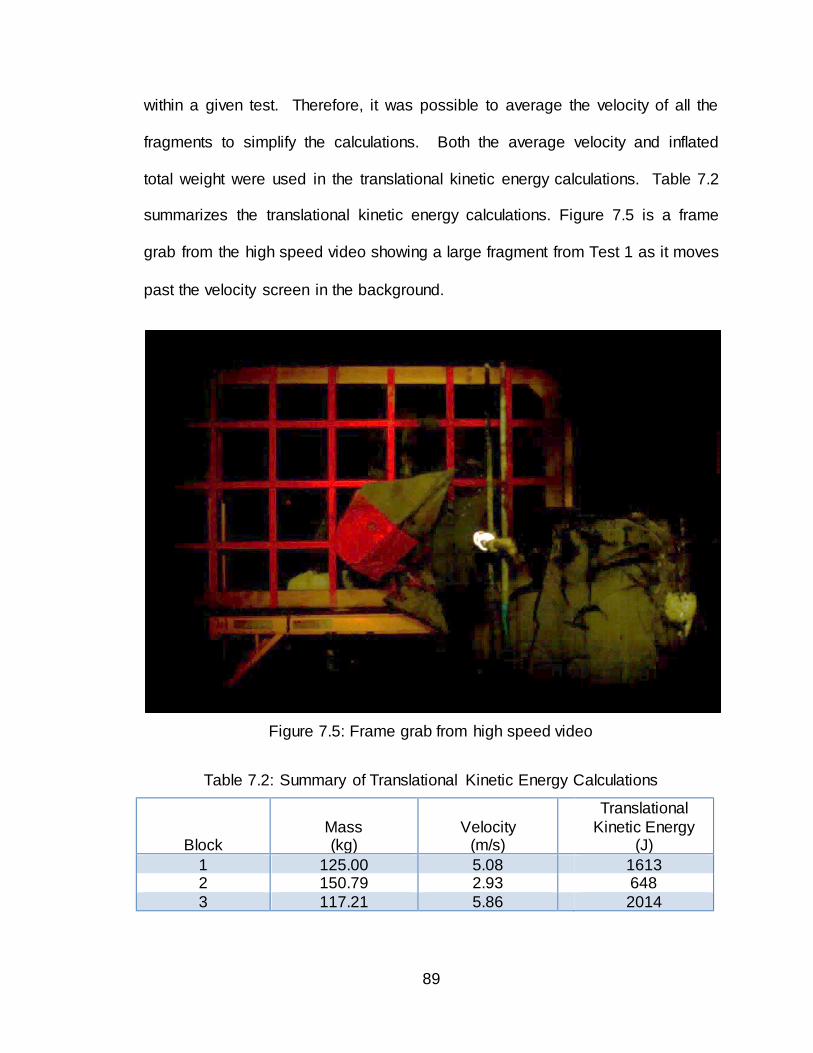
89
within a given test. Therefore, it was possible to average the velocity of all the
fragments to simplify the calculations. Both the average velocity and inflated
total weight were used in the translational kinetic energy calculations. Table 7.2
summarizes the translational kinetic energy calculations. Figure 7.5 is a frame
grab from the high speed video showing a large fragment from Test 1 as it moves
past the velocity screen in the background.
Figure 7.5: Frame grab from high speed video
Table 7.2: Summary of Translational Kinetic Energy Calculations
Block
Mass (kg)
Velocity (m/s)
Translational
Kinetic Energy (J)
1 125.00 5.08 1613 2 150.79 2.93 648
3 117.21 5.86 2014

90
Although block 3 had the lowest fragment mass, calculations showed that it had
the highest amount of translational kinetic energy. Block 2 showed the opposite
outcome, yielding the largest fragment mass, but the lowest velocity. As a result,
block 2 possessed translational kinetic energy much lower than the other two
tests.
Determination of the rotational kinetic energy for each test was not as
straightforward. Unlike translational velocity which only requires two pieces of
information that can be determined easily (mass and velocity), rotational kinetic
energy requires the moment of inertia and angular velocity of each fragment.
The formula used for calculating rotational kinetic energy is:
𝐾𝐸𝑟𝑜𝑡𝑎𝑡𝑖𝑜𝑛𝑎𝑙 =1
2𝐼𝜔2 (7.2)
where I is moment of inertia about the rotational axis and ω is the angular
velocity of the object. Due to the irregularity of the fragments in all three
dimensions, hand calculation of the moment of inertia was impractical. Instead,
fragments were transformed into a 3D point cloud using a Maptek laser scanner.
This point cloud was meshed and imported into Creo 3D modeling software,
where the moment of inertia for each fragment was calculated about its principal
axes. A 3D rendering of the major fragments is shown in Figure 7.6. The output
from Creo is shown in Figure 7.7.

91
Figure 7.6: 3D rendering of major fragments
Figure 7.7: Detailed view of one major fragment and associated output from Creo
Without the aid of 3D motion tracking software, determination of angular velocity
through the use a single high-speed video angle is subjective and inexact to an
Center of
Gravity

92
extent. Like with any blast, the fragments in these tests tumbled about multiple
axes, rather than rotating about a single axis. However, after carefully studying
each high-speed video on a frame-by-frame basis the author feels confident that
angular velocities presented are a good estimation of the true values.
In cases where a fragment was not rotating about a single primary axis, but
rather between two primary axes, the average moment of inertia for these two
axes was used in calculations. Tables 7.3 and 7.4 summarize the velocities,
moments of inertia, and resulting rotational kinetic energy.
Table 7.3: Summary of Angular Velocities
Angular Velocity (frames per 360)
Angular Velocity (radians / sec)
Fragment # Block 1 Block 2 Block 3 Block 1 Block 2 Block 3
1 216 376 184 133 76 156
2 -- 468 320 -- 49 89.5
3 400 164 -- 72 112 --
4 -- -- -- -- -- --
5 300 -- -- 95 -- --
Table 7.4: Summary of Moment of Inertia and Rotational Kinetic Energy
Moment of Inertia (kg-m2) Rotational Kinetic Energy (J)
Fragment # Block 1 Block 2 Block 3 Block 1 Block 2 Block 3
1 0.0934 0.7155 0.3819* 821 4236 4629*
2 -- 1.2449 1.6004 -- 2332 6414
3 0.7819 0.0884 -- 2005 1348 --
4 -- -- -- -- -- --
5 0.6792 -- -- 3097 -- --
The moment of inertia and therefore rotational kinetic energy was not calculated
for Fragments 2 and 4 from Block 1. Each of these fragments weighed less than
10 kg and were not easily trackable in the high speed video. Due to their relative
93
small mass it is assumed that their effect on the overall rotational kinetic energy
is negligible. It should also be noted that Fragment 1 from Block 3 was sacrificed
as part of the specific fracture energy determinations discussed in the next
section. As a result, a 3D point cloud for this fragment was not created. Instead
a rough approximation was created using 3D modeling software based on
measurements gathered from studying the high-speed video. The moment of
inertia for this model was used during calculations.
The rotational kinetic energy results follow the same basic trend as the
translational kinetic energy with Block 3 having the highest energy results and
Block 2 having the lowest. The total rotational energy for Block 1 was 5923 J or
21% of the total energy. Values for Blocks 2 and 3 were 7916 J (27.5%) and
11043 J (38.3%), respectively.
As is shown by these calculations, rotational kinetic energy represents a
significant portion of the overall available energy and must not be ignored during
future energy partitioning work.
In full-scale tests, it is probable that the translational kinetic energy to rotational
kinetic energy balance will shift towards translational kinetic energy. With this
test configuration, much of the energy was concentrated high in the block, which
could significantly influence the rotation of the fragments. In full-scale testing the
energy will be more evenly distributed about the test area, resulting in more
translation and less rotation. Confinement of the material and timing sequence
will also play a role in this balance and is discussed in the next chapter.

94
7.4.2 Fracture Energy
The biggest hurdle in calculating fracture energy is accurately determining the
new surface area created. This holds true for full-scale blasts and for small-scale
testing such as this. A number of different methods were used to calculate the
new surface area for this testing. In each of the three tests, a large wedge
shaped portion was broken off of the corner of the block, fragmenting into a
number of pieces. The larger pieces were collected and the wedge was
reassembled. The fracture lines were then labeled to prevent the same fracture
plane from being measured twice. Figure 7.8 shows one of these wedges
reassembled with the fractures labeled.
The surface area of each of these large fractures was measured as accurately as
possible using a tape measure. To account for the surface roughness, the
measured surface area was multiplied by an adjustment factor of 25%. Multiple
fragments were spot checked using the Maptek 3D laser scanner and modeling
software to ensure that the calculations completed using the tape measure and
adjustment factor were accurate.

95
Figure 7.8: Fractured wedge reassembled with fractures labeled for measurement
Smaller fragments were spread out on a table for photographic analysis using
WipFrag software. WipFrag is a commercially available fragmentation analysis
software commonly used in the blasting industry to estimate particle size
distribution within a muck pile. Using a standard tennis ball as a scale within
each picture, the software was then used to determine the size of each particle.
Figure 7.9 shows the small fragments collected from Test 2. The fines in the
upper left-hand corner are a result of the fragments grinding against each other
in a bucket and were not included in the surface area determination.

96
Figure 7.9: Small fragments from Test 2
Table 7.5: Summary of newly created surface area
Joint Block 1
(in2)
Block 2 (in2)
Block 3 (in2)
Wedge 2142
881
1050
1 152.5
14
110.25
2 45.5
117
38.5
3 20.25
214.75
26
4 92.5
23
9
5
21
18
6
17.5
7
13
8
13.5
9
22.75
10
6.5
Total 2452.75
1270.75
1325
Total*1.25 3066
1588
1656
97
The next piece of information required to determine energy partitioned to
fragmentation is specific fracture energy. Use of the specific fracture energy was
chosen over other methods such as the Rittinger coefficient used by Sanchidrian
et al. (2007) because of the lack of fines and because it was possible to directly
measure the new surface area created. Specific fracture energy is calculated
using the following equation:
𝐺𝐹 =1
(𝐷− 𝑎)𝐵∫𝑃𝑑𝛿 (7.3)
where 𝐺𝐹 is specific fracture energy, D is depth of the sample beam, 𝑎 is the
starter notch depth, B is beam thickness, P is applied load, and 𝛿 is the
displacement of the applied load.
To determine the specific fracture energy, multiple three-point bend tests were
conducted on concrete samples. The test methodology took into consideration
RILEM 50-FMC (1985) and ASTM C 293-02 (ASTM International, 2002) test
standards as well as recent works published by Abdalla and Karihaloo (2003)
and Karihallo et al. (2003). Six concrete beams with rectangular cross-sections
of varying size were cut from the center of one of the larger fragments. ASTM C
293-02 (2002) recommends the depth of the sample be three times its span
length for a standard three-point bend test and the RILEM (1982) document
recommends the span be eight times its depth for samples with a maximum
aggregate size less than 16mm. Revised recommendations by Karihallo et. al.
(2003) suggest the sample span be four times greater than the depth. Based on
these recommendations and the amount of intact material available, a span to
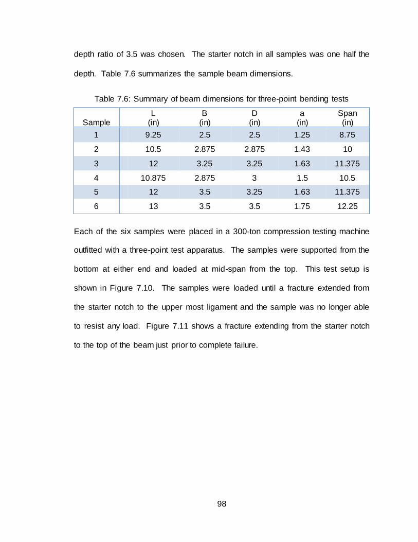
98
depth ratio of 3.5 was chosen. The starter notch in all samples was one half the
depth. Table 7.6 summarizes the sample beam dimensions.
Table 7.6: Summary of beam dimensions for three-point bending tests
Sample L
(in) B
(in) D
(in) a
(in) Span (in)
1 9.25 2.5 2.5 1.25 8.75
2 10.5 2.875 2.875 1.43 10
3 12 3.25 3.25 1.63 11.375
4 10.875 2.875 3 1.5 10.5
5 12 3.5 3.25 1.63 11.375
6 13 3.5 3.5 1.75 12.25
Each of the six samples were placed in a 300-ton compression testing machine
outfitted with a three-point test apparatus. The samples were supported from the
bottom at either end and loaded at mid-span from the top. This test setup is
shown in Figure 7.10. The samples were loaded until a fracture extended from
the starter notch to the upper most ligament and the sample was no longer able
to resist any load. Figure 7.11 shows a fracture extending from the starter notch
to the top of the beam just prior to complete failure.

99
Figure 7.10: Three-point bending test setup
Figure 7.11: Sample beam with fracture extending from starter notch
For each test, a plot of the displacement versus measured applied load was
created. This plot was integrated using DPlot and the maximum energy content

100
value found. One of these plots is shown in Figure 7.12. The plots for the other
five sample can be found in Appendix G.
Table 7.7 provides a summary of the maximum sustained load for each sample,
fracture area size, maximum energy content, and finally the energy required to
create one square meter of new fracture area. In finding the average energy
required to create new fracture area, results from Sample 1 were discarded. This
sample was the smallest in size and showed small voids through the fracture
plane which can explain the very low energy content value. Results from Sample
2-6 were used and an average energy of 74.30 J was found.
Figure 7.12: Load versus displacement for concrete beam sample

101
Table 7.7: Summary of specific fracture energy results
Sample Max Load
(lbf)
Fracture Area (in2)
Fracture Area (m2)
Energy Content (N-m)
Energy (J/m2)
1 18.9 3.13 0.0020 0.0241 11.93
2 206 4.11 0.0027 0.1638 61.76
3 363 5.30 0.0034 0.3320 97.15
4 294 4.31 0.0028 0.1686 60.59
5 390 5.70 0.0037 0.2258 61.36
6 363 6.13 0.0040 0.3581 90.64
Table 7.8 summarizes the new surface area created during each of the three
block tests along with the total portion of energy going to fracturing the block
during the tests.
Table 7.8: Fracture energy determination for each block test
Test
New Surface
Area (in2)
New Surface
Area (m2)
Specific Fracture
Energy (J/m2)
Fracture
Energy (J)
1 3066 1.978
74.30
147
2 1588 1.025 76
3 1656 1.069 79
Test block 1 had the largest amount of new surface area created at 1.98 m2 and
therefore saw the highest fracture energy component at 147 J. Test blocks 2 and
3 had roughly the same amount of new fracture area created and therefore
similar fracture energy components of 76 J and 79 J, respectively. By
comparison, fracture energy is small, ranging from 0.2% to 0.5% for this testing.
These values are significantly lower than values reported by others. The cause
102
of this is not a result of the test methodology, but rather the configuration of the
blast itself. It is expected that fractures will readily develop towards the free
faces when there is little confinement, as is the case with this testing. Holes will
more confinement will see fragmentation values higher than those recorded here.
7.4.3 Air Overpressure
Air overpressure energy for the block tests was calculated the same way for this
test series as previous test series, with the exception of the surface area
calculation. Rather than assuming the gases vented hemispherically from the
borehole, the assumption was made that the gases vented along the primary
fracture plane. This assumption was validated after reviewing high-speed video.
In the video it was made clear by the dust being ejected from the top of the block
and along the fracture lines on the side of the block, that gases were venting
along the length of the fracture plane. Figure 7.13 is a frame grab from the high-
speed video with the venting dust and gas highlighted within the blue ovals.
The primary fracture plane is the main fracture between the fragmented wedge
portion and the remaining block. Figure 7.14 illustrates this primary fracture
plane. The edge lengths (top, left side, and right side) of the fracture plane were
measured for each block and multiplied by the edge length of an arch having a
radius of curvature equal to the distance to the nearest pressure sensor (2 feet
for the sides, and 4 feet for the top). This resulted in a pressure shell shaped like
an arched tunnel along each fracture, rather than a single hemisphere. The
primary fracture lengths and shell surface areas are summarized in Table 7.9.

103
Figure 7.13: Dust and gases (highlighted) venting from primary fracture plane
Figure 7.14: Primary fracture plane for block tests

104
Table 7.9: Block primary facture length and shell surface area
Primary Fracture Lengths
(in)
Surface Area of Shell
(in2)
Surface Area of Shell
(m2)
Test
Top Sides Top Sides Top Sides
1
34.0 61.5 10254 9274 6.62 5.98
2
41.0 92.0 12365 13873 7.39 8.59
3
39.0 75.5 11762 11385 7.59 7.35
Test 2 saw pressures significantly higher at all sensors in comparison to tests 1
and 3. This coupled with a primary fracture length of 133 inches, resulted in the
total energy lost to air overpressure for test 2 equaling 11.62 kJ or 40.3% of the
total available energy. The total energy lost to air overpressure for tests 1 and 3
was 8.151 kJ (28.3%) and 4.557 kJ (15.8%), respectively. Table 7.10
summarizes the pressure and peak pressure time of arrival (TOA) for each
sensor along with the calculate wave velocity. Table 7.11 summarizes the values
used for calculation of the air overpressure energy and the calculated air
overpressure energy for each test.
Table 7.10: Summary of overpressure and wave velocity
Sensor 1 Sensor 2 1 to 2
Test Pressure
(PSI) TOA (ms)
Pressure (PSI)
TOA (ms)
Velocity (fps)
1 0.260 3.778 0.158 5.494 1166
2 0.787 3.640 0.554 5.402 1135
3 0.129 4.498 0.079 6.229 1155
Sensor 3 Sensor 4 3 to 4
Test Pressure
(PSI) TOA (ms)
Pressure (PSI)
TOA (ms)
Velocity (fps)
1 0.415 4.782 0.255 6.531 1144
2 1.576 4.163 0.875 5.894 1155
3 0.360 5.134 0.220 6.901 1132

105
Table 7.11: Calculated air overpressure energy
Test
Time Diff
(ms)
Velocity
(m/ms)
Top Area
(m2)
Top Energy
(kJ)
1
1.749 0.3485 6.62 5.861
2
1.731 0.3522 7.39 7.825
3
1.767 0.3450 7.59 2.767
Test
Time Diff (ms)
Velocity (m/ms)
Side Area (m2)
Side Energy (kJ)
1
1.716 0.3552 5.98 2.290
2
1.762 0.3460 8.56 3.799
3
1.731 0.3522 7.35 1.790
The average air overpressure energy for these tests was 8110 J or 28.1%. This
value coincides well with the prediction made by Sanchidrian et al. (2007) of
30%.
7.4.4 Strain
Earlier chapters discussed the assumptions and care that must be taken to
calculate strain energy using surface mounted strain gauges. Block tests
introduce additional factors that must be considered. In the previous confined
tests, the holes were drilled in massive limestone. Therefore, reflections were
not an issue. In the case of these block tests, there were a total of six free faces
in close proximity to the explosive charge and strain gauges. Extra care must be
taken to isolate the primary wave values from the reflected wave values when
analyzing the data. Due to the 4th strain gauges close proximity to the back
corner of the block (less than 6 inches), it was not possible to separate the
primary wave values from the reflected wave value. The data from this sensor
was not useable for analysis.

106
The data from the remaining three sensors is provides enough information to
make a rough approximation of the strain energy for each test. Strain energy is
again calculated using the following equation:
𝑈 =1
2𝑉𝐸휀2 (7.4)
where U is strain energy, V is volume, E is Young’s Modulus, and ε is strain. For
this approximation the Poisson’s ratio is assumed to be 0.33, and therefore the
strain levels are assumed to be equal in the transverse and z directions and
three times greater in the axial direction. To determine the volume affected by a
given strain level, the block was divided into three areas, one for each of the
three strain gauges. Strain was assumed to be uniform throughout the depth of
the block within each area. The volume influenced by values recorded at strain
sensors 1 and 2 is 0.55 m3 for each. The volume influenced by sensor 3 is 0.71
m3. Based on laboratory tests, the Young’s Modulus for the concrete is
15.18x10⁹ N/m2. Table 7.12 summarizes the maximum strain values recorded at
each sensor location and energy calculated for the transverse component at that
location. Finally Table 7.13 shows the transverse, axial, and vertical strain
energy values, along with the total strain energy for each test.
Table 7.12: Summary of maximum transverse strain value and respective strain
energy value
Strain Energy - Transverse Component
Test Strain 1
(µϵ) Energy 1
(J) Strain 2
(µϵ) Energy 2
(J) Strain 3
(µϵ) Energy 3
(J)
Total
Energy (J)
1 46.34 8.97 36.90 5.69 31.35 5.30 19.95 2 41.37 7.15 36.30 5.50 29.87 4.81 17.46
3 39.28 6.44 32.72 4.47 26.43 3.77 14.68

107
Table 7.13: Strain energy values for block tests
Test
Transverse
Energy (J)
Axial
Energy (J)
Vertical
Energy (J)
Total
Energy (J)
Percentage of Total
Available Energy
1 19.95 59.85 19.95 99.8 0.35
2 17.46 52.38 17.46 87.3 0.30
3 14.68 44.04 14.68 73.4 0.25
The strain energy is minimal for these block tests. Like the fragmentation
energy, this is due to the nature of block testing and limited confinement, rather
than the test methodology itself. Increased confinement would increase the total
strain energy. This is shown clearly when comparing the values from these block
tests to the values calculated in the confined test series. The average strain
energy calculated during block testing was 86.8 J. The average strain energy
calculated during the confined tests, using an identical charge, was eight times
greater at 693.2 J.
7.5 Borehole Chambering
During each of the three block tests, the borehole was split vertically from top to
bottom, leaving an intact cross-section in the un-fragmented portion of the block.
This made measurement of the borehole chambering a straightforward process.
The original borehole diameter was assumed to be constant at 0.880 inches from
collar to bottom. The post-blast borehole was profiled in one inch increments
from the collar to the bottom. The diameter of each of the boreholes remained
constant for the first few inches before reaching the largest diameter 2 inches
from the bottom of the borehole. This coincides with the midpoint of the 4 inch

108
explosive charge that was placed in the bottom of the borehole. Table 7.14
presents the borehole profiles along with the volume change for each hole.
Table 7.14: Block borehole chambering profiles
Diameter (in)
Depth (in)
Block 1
Block 2
Block 3
0 0.880 0.880 0.880
1 0.880 0.880 0.880
2 0.916 0.920 0.880
3 0.916 0.920 0.880
4 0.916 0.920 0.880
5 0.927 0.930 0.920
6 0.927 0.950 0.940
7 0.977 1.000 0.940
8 1.052 1.044 1.010
9 0.994 0.960 1.010
10 0.916 0.920 0.950
Volume
Change (in3)
0.8855 0.8983 0.8926
Volume Change
(cm3) 14.51 14.72 14.63
The volume change was consistent from block to block, ranging from 14.51 cm3
to 14.72 cm3. Unlike the borehole chambering tests conducted in massive
limestone, the generalized assertion made by Ouchterlony et al. (2004) that
1 cm3 change in volume requires 1 kJ of energy does not stand. The physical
characteristics of the medium strength concrete used in this testing are
considerably different than massive limestone. In addition to their generalized
assertion, Ouchterlony et al. (2004) also stated that the cratering efficiency (the

109
energy required to increase the volume of the cavity) for rock is between 4.0 and
4.3 times its static unconfined compressive strength (UCS). The UCS of the
concrete material used in this testing was 9059 psi or 0.0625 GPa. These test
results can be found in Appendix F. Based on this information, the energy
required to expand the borehole volume by 1 cm3 is 0.25 kJ. Therefore, the
energy transferred to borehole chambering in Block 1 was 3.638 kJ or 12.58% of
the total available energy. Blocks 2 and 3 had similar results with 3.680 kJ
(12.76%) and 3.658 kJ (12.61%) transferred to chambering, respectively.
7.6 Conclusions
Kinetic energy and air overpressure energy are the largest components in the
energy partitioning equation. Based on the data collected, there is a direct
correlation between kinetic energy and air overpressure. When air overpressure
is lower, kinetic energy is higher and vice versa. Due to the limited number of
fragments created during this testing, it is not possible to determine if there is a
direct correlation between fragmentation energy and other components from this
testing. The same can be said for strain energy. However, based on previous
field experience, the author believes that as air overpressure energy increases,
fragmentation and strain energies tend to decrease.
Table 7.15 summarizes the calculated values the energy partitioning components
measured for each test along with the average value. Figures 7.15 – 7.17
summarize the data for blocks 1 – 3 as a percentage of the total explosive
energy available, conservatively estimated to be 28.83 kJ. Figure 7.18 illustrates
the average values from the three tests.
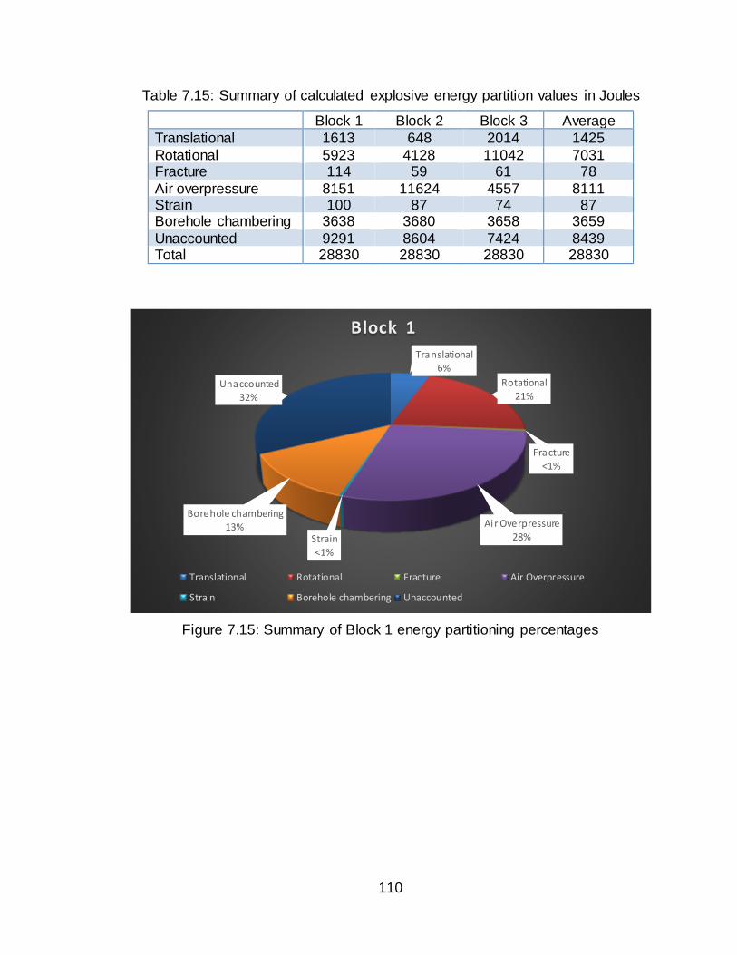
110
Table 7.15: Summary of calculated explosive energy partition values in Joules
Block 1 Block 2 Block 3 Average
Translational 1613 648 2014 1425
Rotational 5923 4128 11042 7031 Fracture 114 59 61 78
Air overpressure 8151 11624 4557 8111 Strain 100 87 74 87 Borehole chambering 3638 3680 3658 3659
Unaccounted 9291 8604 7424 8439 Total 28830 28830 28830 28830
Figure 7.15: Summary of Block 1 energy partitioning percentages
Translational6%
Rotational21%
Fracture
<1%
Air Overpressure28%Strain
<1%
Borehole chambering13%
Unaccounted32%
Block 1
Translational Rotational Fracture Air Overpressure
Strain Borehole chambering Unaccounted
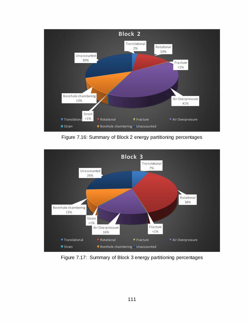
111
Figure 7.16: Summary of Block 2 energy partitioning percentages
Figure 7.17: Summary of Block 3 energy partitioning percentages
Translational2% Rotational
14%
Fracture<1%
Air Overpressure41%
Strain<1%
Borehole chambering13%
Unaccounted30%
Block 2
Translational Rotational Fracture Air Overpressure
Strain Borehole chambering Unaccounted
Translational7%
Rotational38%
Fracture<1%
Air Overpressure16%
Strain<1%
Borehole chambering13%
Unaccounted26%
Block 3
Translational Rotational Fracture Air Overpressure
Strain Borehole chambering Unaccounted

112
Figure 7.18: Summary of average energy partitioning percentages for block tests
These results show that slightly over one quarter (28%) of the total explosive
energy was lost to air overpressure. Slightly less than one third of the energy
was transmitted to kinetic energy (5% translational and 25% rotational). 13% of
the energy was transferred to enlargement of the borehole. The remainder of the
energy went into elastic deformation (<1%), fragmentation (<1%), or was not
accounted for (39%). The portion not accounted for includes, but is not limited
to: heat, fume formation, and micro-cracks.
Copyright © Joshua Thomas Calnan 2015
Translational5%
Rotational25%
Fracture<1%
Air Overpressure28%
Strain<1%
Borehole chambering13%
Unaccounted
29%
Average
Translational Rotational Fracture Air Overpressure
Strain Borehole chambering Unaccounted

113
Chapter 8. Goal Programming Framework
The primary objective of most mining operations is to minimize overall operating
costs. It is important to optimize blasting practices because blasting directly
effects all of the downstream processes include loading, hauling, and processing
of the material. Generally, as drilling and blasting costs increase, loading,
hauling, and processing costs decrease as a result of increased fragmentation.
This generalization is based on site specific conditions and goals of the final use
of the fragmented material.
Drilling and blasting costs are largely dependent on the parameters of the shot
including burden, spacing, hole depth and diameter, and physical properties of
the rock. These parameters dictate the amount of drilling and explosive product
required. The type of explosive product and initiation system also effect the
blasting cost. Loading costs are affected by fragmentation and heave. Material
that is poorly fragmented and “tight” results in excessive equipment wear (both
for the loaders and haul trucks) and digs slower. From a blasting perspective,
haulage is most heavily affected by fragmentation. A decrease in mean particle
size results in higher volume and tonnage per truck load. Site specific conditions
such as haul road topography, haul distance, and maximum truck payload must
also be considered. Like haulage costs, processing costs are most affected by
fragmentation, but are very site specific and the end product must be taken into
account.
Based on the conclusions reached in earlier chapters of this dissertation, a
significant portion of the total explosive energy can be lost to air overpressure.

114
By decreasing the amount of energy lost to overpressure, more energy is shifted
to other beneficial partitions, specifically: heave, and fragmentation. However,
this shift may also send additional energy to ground vibration which must be
balanced.
Air overpressure levels are a function of confinement and are primarily impacted
by the amount of burden and the effectiveness of the stemming material.
Rotational and translational kinetic energy are affected by the geometry of the
shot (effective burden and timing). Slowing timing and lack of confinement will
favor rotational kinetic energy. Faster timing and greater confinement will favor
translational kinetic energy. Fragmentation and elastic deformation are
influenced by burden, stemming effectiveness, physical properties of the rock,
and timing sequence. Expansion of the borehole is controlled by confinement
and physical properties of the rock. Energy lost to heat is assumed to be a
property of the explosive and not influenced by the design of the blast in most
cases. However, poor performance and low order detonation can occur with loss
of confinement, resulting in less efficient use of the explosive energy and
production of toxic byproducts. Energy not measured includes any components
that currently cannot be accounted for including friction and fume creation.
A basic goal programming framework can be created with the objective of
lowering overall operating costs. The framework must take into the factors just
discussed. The objective function with respect to blast design and energy
partitioning is therefore expressed as:
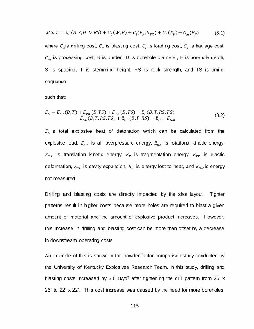
115
𝑀𝑖𝑛 𝑍 = 𝐶𝑑(𝐵,𝑆, 𝐻, 𝐷, 𝑅𝑆) + 𝐶𝑏(𝑊, 𝑃) + 𝐶𝑙(𝐸𝐹 ,𝐸𝑇𝐾) + 𝐶ℎ(𝐸𝐹)+ 𝐶𝑚(𝐸𝐹) (8.1)
where 𝐶𝑑is drilling cost, 𝐶𝑏 is blasting cost, 𝐶𝑙 is loading cost, 𝐶ℎ is haulage cost,
𝐶𝑚 is processing cost, B is burden, D is borehole diameter, H is borehole depth,
S is spacing, T is stemming height, RS is rock strength, and TS is timing
sequence
such that:
𝐸𝐸 = 𝐸𝐴𝑂 (𝐵, 𝑇) + 𝐸𝑅𝐾 (𝐵,𝑇𝑆) + 𝐸𝑇𝐾(𝐵, 𝑇𝑆) + 𝐸𝐹(𝐵, 𝑇,𝑅𝑆, 𝑇𝑆)+ 𝐸𝐸𝐷(𝐵,𝑇, 𝑅𝑆, 𝑇𝑆) + 𝐸𝐶𝐸(𝐵,𝑇, 𝑅𝑆) + 𝐸𝐻 +𝐸𝑁𝑀
(8.2)
𝐸𝐸 is total explosive heat of detonation which can be calculated from the
explosive load, 𝐸𝐴𝑂 is air overpressure energy, 𝐸𝑅𝐾 is rotational kinetic energy,
𝐸𝑇𝐾 is translation kinetic energy, 𝐸𝐹 is fragmentation energy, 𝐸𝐸𝐷 is elastic
deformation, 𝐸𝐶𝐸 is cavity expansion, 𝐸𝐻 is energy lost to heat, and 𝐸𝑁𝑀 is energy
not measured.
Drilling and blasting costs are directly impacted by the shot layout. Tighter
patterns result in higher costs because more holes are required to blast a given
amount of material and the amount of explosive product increases. However,
this increase in drilling and blasting cost can be more than offset by a decrease
in downstream operating costs.
An example of this is shown in the powder factor comparison study conducted by
the University of Kentucky Explosives Research Team. In this study, drilling and
blasting costs increased by $0.18/yd3 after tightening the drill pattern from 26’ x
26’ to 22’ x 22’. This cost increase was caused by the need for more boreholes,

116
increased explosives consumption, and hauling in gravel to use as stemming
material instead of drilling cuttings. The tighter pattern increased the total
amount of explosive energy and the more effective stemming reduced air
overpressure, resulting in improved fragmentation. The average particle size
(D50) decreased from 24” to 17”.
These changes decreased load cycle times and increased tonnage per truck
load, allowing more material to be moved per shift. As a result, loading and
haulage costs were decreased by $0.21/yd3, yielding a $0.03/yd3 decrease in
overall operating costs. This study was conducted at an open-pit coal mine
where the overburden was removed and taken to a dumpsite. Had this been a
mine where the blasted material was processed further, additional cost savings
would likely be noticed.
Improved performance can be seen through increasing the total amount
explosive energy (i.e. increasing the powder factor by changing the shot layout).
However, if the energy is partitioned poorly, a significant amount of the useful
energy is going to wasteful byproducts. An alternative is to tailor the blast
parameters and site conditions to better utilize the explosive energy available.
This includes using best practices to stem the holes, cleaning up benches to
prevent excessive toe burden, and selecting a timing sequence that results in
acceptable fragmentation and heave, but limits ground vibration.
Copyright © Joshua Thomas Calnan 2015
117
Chapter 9. Conclusions and Future Work
9.1 Conclusions
The focus of this dissertation was to further the understanding of explosive
energy partitioning, through small-scale testing of various independent energy
components. An innovative test methodology was constructed that has not been
previously used in explosive energy partition testing. This methodology
accounted for significantly more of the available energy than previous research
efforts.
The confined borehole chambering test series values ranged from an average of
9.4% of the total explosive energy for the small PETN charge to 17.9% for the
larger emulsion charge.
The stemming tests proved that different types of stemming do in fact affect the
amount of energy transferred to air overpressure and elastic deformation
components. When these two components were isolated, there was a definitive
correlation between the two. As air overpressures increased, the measured
strain levels decreased, and vice versa. Following the abnormal results recorded
at the strain gauges nearest the borehole, additional strain mapping tests were
conducted. During these tests, it was discovered that the tension and
compression waves travel primarily in the vertical direction until they reach a
distance greater than the borehole depth, making surface mounted strain gauges
ineffective in this zone. Instead, surface mounted triaxial accelerometers or
strain gauges mounted vertically in an adjacent borehole are recommended.
118
Outside of this zone, surface mounted strain gauges positioned transversely and
longitudinally may be used to calculate strain energy. Using a strain attenuation
curve developed during the strain mapping tests, the strain energy was
calculated to be 2% of the total available explosive energy. Also during the
course of these tests, black gases escaping the borehole were evident on the
high-speed video, a sign of incomplete detonation. Only 28.5% of the total
available energy was measured during this testing versus the 58% measured
during the block testing using similar methodology. Therefore, the conclusion
was reached that a substantial portion of the explosive energy was not
transferred to measurable work due to incomplete detonation in this test series.
The concrete block tests reintroduced heave and fragmentation into the test
matrix and sought to replicate a full-scale blast as closely as possible. During
this test series values for air overpressure, rotational and translational kinetic,
fragmentation, elastic deformation, and borehole chambering energies were
calculated. It was determined that, although it has largely been ignored before,
rotational kinetic energy can account for a significant portion of the total available
energy; 25% in the case of this testing. During the concrete block testing, air
overpressure energy was calculated at 28% of the available energy. This
coincides closely with the prediction made by Sanchidrian et al. (2007) of 30%.
The direct correlation between air overpressure and kinetic energy was clearly
shown during this testing. As one component increased, the other decreased.
Also, this testing showed increased confinement does have a significant impact
on measured strain energy. Strain energy measured during the concrete block

119
tests was one sixth the value measured during the strain mapping tests. Finally,
through this test series it was determined that borehole chambering accounts for
13% of the total available energy. This value falls within the range previously
determined in the confined borehole chambering tests.
Figure 9.1 summarizes the values found for each of the components studied over
the course of this research. In total, 71% of the explosive energy was accounted
for. This is substantially more than previous research efforts.
Figure 9.1: Summary of explosive energy components and respective values
Explosive Energy
Elastic Deformation
(2%)
Air Overpressure
(28%)
Translational Kinetic Energy
(5%)
Rotational Kinetic Energy
(25%)
Fragmentation
(1%)
Heat and Not Measured
Components
(27%)
Borehole Chambering
(13%)
120
9.2 Summary of Novel Contributions
The following is a summary of novel contributions provided by this dissertation
research.
Determined that energy absorbed by borehole chambering accounts for
approximately 13% of the explosive’s heat of detonation
Proposed and implemented an alternative method for measuring ground
vibration energy by using strain gauges to measure elastic deformation
Determined that air overpressure energy accounts for 28% of the
explosive’s heat of detonation
Showed that rotational kinetic energy can be a significant component of
energy partitioning and must be considered
Expanded upon the energy balance equation and applied this equation to
goal programming
9.3 Future Work
It is recommended that additional full-scale testing be conducted to further the
understanding of energy partitioning in blasting and continue building upon the
current energy balance equation and goal programming objective function for
optimizing blasting to decrease overall operating costs.
Ideally, gaining a complete data set for each blast in a test series is preferred. A
data set consists of a pre-blast survey to gain an understanding of the geological
conditions and the blast design parameters, blast data collection to capture
ground vibration and elastic deformation, air overpressure, and fragment velocity,
121
and finally a post-blast survey to document fragmentation. Due to the complexity
of the problem at hand, a complete data set is not likely, especially when
considering that a borehole must not be destroyed in order to accurately
calculate the energy lost to cratering and the crush zone. An alternative is to
conduct multiple tests using samples from a single rock mass.
The first step in the testing process is to complete a very detailed site survey to
fully characterize the rock mass being blasted. Until a better methodology is
proven, estimation of energy lost to fragmentation is calculated based on the
evaluation of new surface area created. This requires a thorough understanding
of the current geological conditions to calculate the surface area of the
discontinuities already present in the rock mass. A couple of methods come to
mind; the first being the use of the SIMBLOC discontinuities network simulation
program that is used to model the rock mass. This method requires field
measurement of discontinuities, azimuth of the dip vectors, the dip angle, the
half-trace, and the spacing (Hamdi, 2007). The second being the use of a 3D
laser profiler and associated processing software, in this case a Maptek 8800
scanner and i-Site Studio software. Using the 3D laser profiler, a high resolution
point cloud is created and processed via spherical triangulation. Strike and dip
can then be determined. From this, joint systems can be analyzed (Maptek,
2011, 2014). Laboratory tests will be needed to determine rock strength
properties including Young’s Modulus, compressive strength, tensile strength,
and specific fracture energy.

122
A detailed blast design survey must be conducted to accurately gauge the blast
parameters. Simply assuming the shot is laid out per the blast design is not
acceptable. Burden, spacing, hole depth, bench height, powder column, and
stemming height must all be measured and recorded. It is important to record
the type of stemming, the explosive products, initiation system, and timing. Due
to the variation in timing associated with nonel detonators, it is highly
recommended to use an electronic detonation system (Lusk, 2012). This will
remove unknowns associated with the variation in timing delay. Slight variations
in blast design may very well likely provide insight to differences in energy
partition results from test to test.
High-speed photography is a crucial part of blast instrumentation because
multiple variables can be analyzed using a single video. The video is used to
calculate fragment velocity, size, and trajectory, all of which are used to calculate
energy transferred to movement. Video is also used to verify timing and
calculate duration of confinement prior to venting as a result of stemming ejection
or cracks opening to the free-face. This information is used to aid in the
approximation of energy transmitted to the rock versus vented to the
atmosphere.
There is some debate as to the velocity profile from the face to the borehole.
Sanchidrian et al. (2007) assumes the velocity is constant from the face to the
borehole while Ouchterlony et al. (2004) proposes a range from highest at the
face to almost zero at the borehole. High-speed photography can be used to
solve this problem by mounting a protected high-speed camera over a borehole.

123
The biggest challenge with this methodology is scale. It would be difficult to
safely mount a high-speed camera above a production hole and as shown by this
dissertation research, small-scale testing may not yield the number of fragments
necessary to accurately determine the velocity gradient.
Seismographs can provide valuable data for blasting operations granted they are
properly calibrated, this test series being no different. One problem encountered
with seismographs, is that even when properly calibrated, two seismographs still
may not provide the same results. As discussed previously, an alternative is to
use triaxial accelerometers attached to a data acquisition device. To date, there
is no widely accepted way of calculating energy lost to ground vibration or elastic
deformation. Previous authors on the subject who have proposed methods for
measuring this energy admit that their attempts require refinement before
providing accurate results.
A widely known short-coming of fragmentation analysis using imaging techniques
is the lack of fines determination. This presents a significant problem because it
is believed that up to 90% of the new surface area created may be from fines
(Ouchterlony et al., 2004). To overcome this problem, three solutions are
available. The first is to conduct a detailed imaging analysis throughout the
muckpile as is traditionally done with extra efforts being made to capture the
fines. The second method is to perform a sieve analysis of the muckpile. This
method is time and cost prohibitive in a production environment. The third
solution is a combination of the previous two. Pairing imaging analysis, and data
collected from sieving representative muckpile samples, it may be possible to

124
derive a correlation between mean particle size and the amount of fines
generated for a specific blast.
These recommendations, coupled with the present knowledge base will provide
the information needed to begin creating a goal programming model that can be
implemented in the blasting industry. This model will not only optimize explosive
energy use, but also minimize overall operating costs by tailoring the blast
parameters to meet the specific needs of the mine, reducing downstream costs.
Copyright © Joshua Thomas Calnan 2015

125
APPENDIX A
BOREHOLE CHAMBERING TEST SERIES – MAXIMUM VALUES
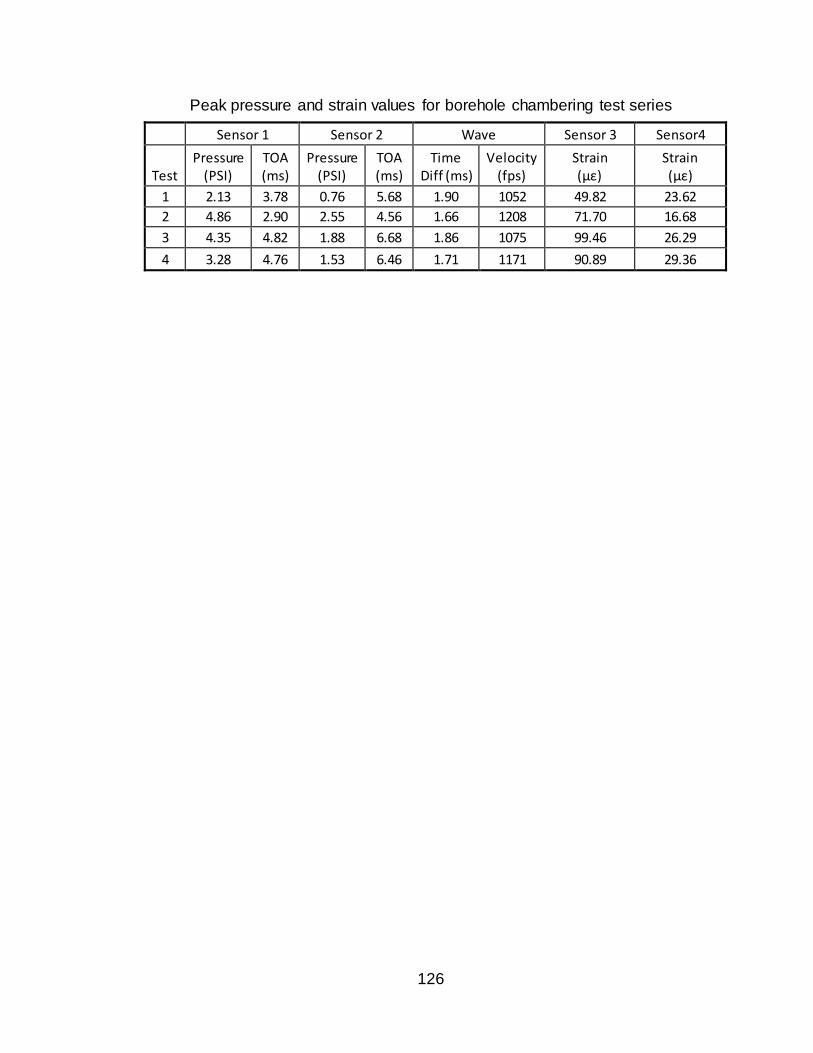
126
Peak pressure and strain values for borehole chambering test series
Sensor 1 Sensor 2 Wave Sensor 3 Sensor4
Test Pressure
(PSI) TOA (ms)
Pressure (PSI)
TOA (ms)
Time Diff (ms)
Velocity (fps)
Strain (µε)
Strain (µε)
1 2.13 3.78 0.76 5.68 1.90 1052 49.82 23.62
2 4.86 2.90 2.55 4.56 1.66 1208 71.70 16.68
3 4.35 4.82 1.88 6.68 1.86 1075 99.46 26.29
4 3.28 4.76 1.53 6.46 1.71 1171 90.89 29.36

127
APPENDIX B
BOREHOLE CHAMBERING TEST SERIES – AIR OVERPRESSURE ENERGY
PLOTS

128

129

130

131

132
APPENDIX C
STEMMING TEST SERIES – MAXIMUM VALUES

133
Sand/Cornstarch
1 2 3 4 5 6 7 8 Seismograph
Test Pressure
(PSI) Pressure
(PSI) Pressure
(PSI) Pressure
(PSI) Strain (µε)
Strain (µε)
Trans (µε)
Long (µε)
Acoustic (dB)
Radial (in/s)
Vert (in/s)
Trans (in/s)
1 1.224 0.687 2.284 1.411 16.28 4.04 62.36 69.309 138 0.01 0.01 0
2 0.891 0.496 1.536 1.590 15.03 2.64 159.36 154.79 139 0.005 0.005 0.005
3 0.551 0.277 1.391 0.385 7.32 1.96 295.63 336.15 141 0 0.005 0.005
Avg 0.889 0.487 1.737 1.129 12.88 2.88 172.45 186.75 139.33 0.005 0.007 0.003
Air/Sand
1 2 3 4 5 6 7 8 Seismograph
Test Pressure
(PSI) Pressure
(PSI) Pressure
(PSI) Pressure
(PSI) Strain (µε)
Strain (µε)
Trans (µε)
Long (µε)
Acoustic (dB)
Radial (in/s)
Vert (in/s)
Trans (in/s)
1 1.709 0.759 2.442 0.812 21.42 2.06 93.54 88.946 145 0 0.01 0.01
2 0.069 0.412 1.783 1.638 13.39 2.48 70.444 65.843 137 0.005 0.005 0.005
3 0.524 0.256 2.331 1.405 7.68 1.87 159.36 154.79 142 0 0.005 0.005
Avg 0.767 0.476 2.185 1.285 14.16 2.14 107.78 103.19 141.33 0.002 0.007 0.007
Sand
1 2 3 4 5 6 7 8 Seismograph
Test Pressure
(PSI) Pressure
(PSI) Pressure
(PSI) Pressure
(PSI) Strain (µε)
Strain (µε)
Trans (µε)
Long (µε)
Acoustic (dB)
Radial (in/s)
Vert (in/s)
Trans (in/s)
1 0.516 0.306 1.212 1.425 34.34 3.17 69.289 101.65 128 0 0 0
2 0.419 1.345 1.803 1.445 7.53 2.27 147.82 159.41 137 0.005 0.005 0.005
3 0.780 0.356 3.925 1.873 6.54 1.80 64.67 79.705 133 0.005 0.005 0.005
Avg 0.572 0.669 2.314 1.581 16.13 2.41 93.93 113.59 132.67 0.003 0.003 0.003
Cornstarch
1 2 3 4 5 6 7 8 Seismograph
Test Pressure
(PSI) Pressure
(PSI) Pressure
(PSI) Pressure
(PSI) Strain (µε)
Strain (µε)
Trans (µε)
Long (µε)
Acoustic (dB)
Radial (in/s)
Vert (in/s)
Trans (in/s)
1 0.288 0.356 0.395 0.558 57.03 10.10 92.385 152.48 133 0.01 0.04 0.02
2 0.322 0.306 0.374 0.227 55.56 8.66 105.09 138.62 130 0.005 0.055 0.01
3 0.233 0.284 0.306 0.413 50.17 13.51 180.15 192.91 127 0.01 0.045 0.01
Avg 0.281 0.315 0.358 0.399 54.25 10.75 125.88 161.34 130.00 0.008 0.047 0.013
134
Air
1 2 3 4 5 6 7 8 Seismograph
Test Pressure
(PSI) Pressure
(PSI) Pressure
(PSI) Pressure
(PSI) Strain (µε)
Strain (µε)
Trans (µε)
Long (µε)
Acoustic (dB)
Radial (in/s)
Vert (in/s)
Trans (in/s)
1 2.000 1.013 3.019 1.431 12.10 1.78 168.6 248.36 146 0.01 0.01 0.01
2 2.375 0.957 1.830 1.025 6.47 1.59 321.04 274.92 147 0.005 0.015 0.005
3 4.440 1.664 3.074 1.618 7.58 1.24 218.26 222.94 145 0.005 0.015 0.005
Avg 2.938 1.211 2.641 1.358 8.72 1.54 235.97 248.74 146.00 0.007 0.013 0.007
Cornstarch/Sand 1 2 3 4 5 6
Test Pressure
(PSI) Pressure
(PSI) Pressure
(PSI) Pressure
(PSI) Strain (µε)
Strain (µε)
1 0.094 0.136 0.079 0.068 49.67 28.23 2 0.066 0.115 0.079 0.075 42.26 15.40 3 0.072 0.129 0.072 0.083 39.13 14.44 Avg 0.077 0.127 0.077 0.076 43.69 19.36
135
APPENDIX D
STRAIN MAPPING TEST SERIES – AVERAGE ELASTIC DEFORMATION
ENERGY CALCULATIONS

136
Distance (ft)
Affected Area (ft3)
Affected Area (m3)
Strain (µε)
Strain (ε)
Young's Modulus
Transverse Energy
(J)
Axial Energy
(J)
Vertical Energy
(J)
0.1 0.079 0.00 590.40 0.00059 5.99E+10 23.36 70.08 23.36
0.25 0.411 0.01 185.76 0.000186 5.99E+10 12.03 36.09 12.03
0.5 1.47 0.04 77.45 7.75E-05 5.99E+10 7.48 22.44 7.48
0.75 2.46 0.07 46.43 4.64E-05 5.99E+10 4.50 13.50 4.50
1 3.43 0.10 32.30 3.23E-05 5.99E+10 3.03 9.10 3.03
2 23.57 0.67 13.47 1.35E-05 5.99E+10 3.63 10.88 3.63
3 39.27 1.11 8.07 8.07E-06 5.99E+10 2.17 6.51 2.17
4 63.35 1.79 5.61 5.61E-06 5.99E+10 1.69 5.08 1.69
5 127.76 3.62 4.24 4.24E-06 5.99E+10 1.95 5.84 1.95
6 190.59 5.40 3.37 3.37E-06 5.99E+10 1.83 5.50 1.83
7 265.99 7.53 2.77 2.77E-06 5.99E+10 1.73 5.20 1.73
8 353.95 10.02 2.34 2.34E-06 5.99E+10 1.65 4.94 1.65
9 454.48 12.87 2.02 2.02E-06 5.99E+10 1.57 4.71 1.57
10 567.59 16.07 1.77 1.77E-06 5.99E+10 1.50 4.51 1.50
15 4974.18 140.85 1.06 1.06E-06 5.99E+10 4.73 14.20 4.73
20 9686.62 274.29 0.74 7.37E-07 5.99E+10 4.46 13.38 4.46
25 15969.7 452.21 0.56 5.56E-07 5.99E+10 4.19 12.56 4.19
30 23823.8 674.61 0.44 4.42E-07 5.99E+10 3.94 11.82 3.94
40 77492.3 2194.33 0.31 3.07E-07 5.99E+10 6.20 18.61 6.20
50 127758 3617.70 0.23 2.32E-07 5.99E+10 5.82 17.46 5.82
60 190590 5396.90 0.18 1.84E-07 5.99E+10 5.48 16.44 5.48
SUM 102.95 308.85 102.95

137
APPENDIX E
STRAIN MAPPING TEST SERIES – AIR OVERPRESSURE ENERGY PLOTS

138

139

140
141
142
143
APPENDIX F
CONCRETE BLOCK TEST SERIES – UNCONFINED COMPRESSIVE STRENGTH FOR CONCRETE BLOCK

144

145
APPENDIX G
CONCRETE BLOCK TEST SERIES – CONCRETE THREE POINT BENDING TEST / FRACTURE ENERGY PLOTS

146

147
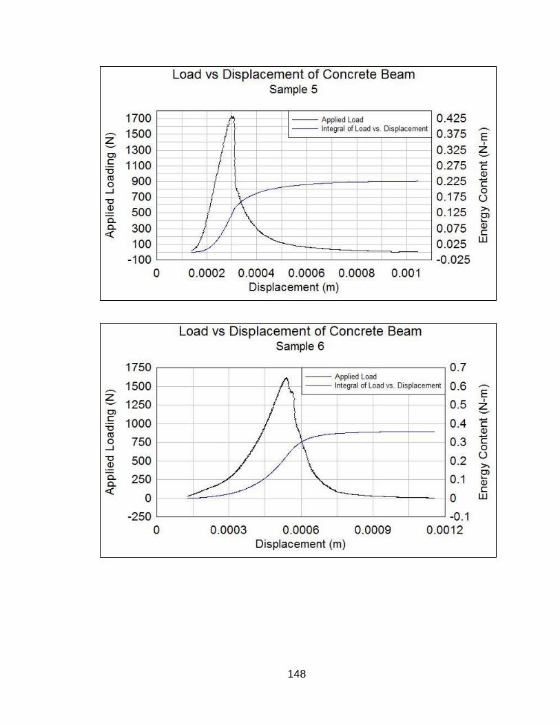
148

149
Bibliography
Abdalla, H., & Karihaloo, B. (2003). Determination of size-independent specific fracture energy of concrete from three-point bend and wedge splitting
tests. Magazine of Concrete Research, 133-141.
Adel, G., Smith, B., Kojovic, T., Thornton, D., & Richardson, J. M. (2005). Mine-
to-Mill Optimization of Aggregate Production. 2005 SME Annual Meeting. Salt Lake City, UT: SME.
Adel, G., Smith, B., Kojovic, T., Thornton, D., & Richardson, J. M. (2006). Application of Mine-to-Mill Optimization to the Aggregate Industry. 2006
SME Annual Meeting. St. Louis, MO: SME.
Albach, H. (1967). Long Range Planning in Open-Pit Mining. Management
Science, B549-568.
Amador, F., & Romero, C. (1989). Redundancy in lexicographical goal programming: An emperical approach. European Journal of Operational Research, 347-354.
ASTM International. (2002). C 293 - 02 Standard Test Method for Flexural Strength of Concrete (Using Simple Beam with Center-Point Loading).
Atasoy, Y., Valery, W., & Skalski, A. (2001). Primary Versus Secondary Crushing
at St. Ives (WMC) SAG Mill Circuit. SAG 2001 (pp. 248-261). Vancouver, Canada: University of British Columbia.
Berta, G. L. (1990). L'esplosivo strumento di lavoro. Italesplosivi, 31-64.
Blasting Analysis International. (2001). Motion Tracker 2D Program User's
Manual. Allentown, Pennsylvania: Blasting Analysis International.
Bronson, R., & Naadimuthu, G. (1997). Schuam's Outline of Theory and Problems of Operations Research (2nd ed.). New York: McGraw-Hill.
Buczkowski, D., & Zygmunt, B. (2011). Detonation Properties of Mixtures of Ammonium Nitrate Based Fertilizers and Fuels. Central European Journal of Energetic Materials, 99-106.
Charnes, A., & Cooper, W. W. (1961). Management Models and Industrial
Applications of Linear Programming. New York: Wiley.
Charnes, A., & Cooper, W. W. (1977). Goal programming and multiple objective
optimizations. European Journal of Operational Research, 39-54.
Charnes, A., Cooper, W. W., & Furguson, R. (1955). Optimal estimation of
executive compensation by linear programming. Management Science, 138-151.

150
Cunningham, C. (1991). The assessment of detonation codes for blast engineering. San Diego, CA: International Society of Explosives
Engineers.
Cunningham, C. (2001). The Energy of Detonation: A Fresh Look at Pressure in the Blasthole. Proceedings EXPLO 2001 (pp. 105-110). Melbourne: The Australasian Institute of Mining and Metallurgy.
Cunningham, C. (2003). Breakthrough in the portrayal of explosive energy. International Society of Explosives Engineers.
Cunningham, C. (2005). The Kuz-Ram fragmentation model - 20 years on.
Brighton Conference Proceedings, R. Holmber et al (pp. 201-210). European Federation of Explosives Engineers.
Cunningham, C. (2006). Blasthole Pressure: What it really means and how we should use it. Journal of Explosives Engineering.
Cunningham, C., & Szendrei, T. (2004). Cavity expansion by hypervelocity impact applied to blasthole expansion by detonation. Journal of Explosives
Engineering.
Cunningham, C., Sellers, E., & Szendrei, T. (2007). Cavity expansion energy
applied to rock blasting. Vienna Conference Proceedings (pp. 27-38). European Federation of Explosvies Engineers.
Flavell, R. B. (1976). A new goal programming formulation. Omega, 731-732.
Gershon, M. (1981). Model Choice in Multiobjective Decision Making in Water and Mineral Resource Systems. Tucson, Arizona: Dept. of Hydrology and Water Resources, University of Arizona.
Gershon, M. (1982). A Linear Programming Approach to Mine Scheduling
Optimization. 17th Application of Computers and Operations Research in the Mineral Industry (pp. 483-492). Colorado: APCOM.
Gheibie, S., Aghababaei, H., Hoseinie, S. H., & Pourrahimian, Y. (2009). Modified Kuz-Ram fragmentation model and its use at the Sungun Copper Mine. International Journal of Rock Mechanics and Mining Sciences 46,
967-973.
Grayson, R. L. (2005). Mi Eng 403 Lecture Optimization Applications in Mining. Rolla, Missouri: University of Missouri-Rolla Department of Mining Engineering.
Grundstrom, C., Kanchibotla, S. S., Jankovic, A., & Thornton, D. M. (2001). Blast
Fragmentation for Maximizing the SAG Mill Throughput at Porgera Gold Mine. 27th Annual Conference of Explosives and Blasting Techniques (pp. 383-399). Orlando, FL: ISEE.
151
Gurney, R. (1943). The Initial Velocities of Fragments from Bombs, Shells, and Grenades. In BRL Report No. 405.
Hamdi, E. e. (2008). Fragmentation Energy in Rock Blasting. Geotech. Geol.
Eng., 133-146.
Hamdi, E., Mouza, J. d., & Fleurisson, J. A. (2001). Evaluation of the part of
blasting energy used for rock mass fragmentation. Fragblast, 180-193.
Hannan, E. L. (1980). Nondominance in goal programming. Canadian Journal of
Operation Research and Information Processing, 300-309.
Hart, S., Valery, W., Clements, B., Reed, M., Song, M., & Dunne, R. (2001). Optimization of the Cadia Hill SAG Mill Circuit. SAG 2001 (pp. 11-30). Vancouver, Canada: Univeristy of British Columbia.
Hewlett, R. F. (1961). Mathematical Models and Their Application to Production Problems. 1st Computers and Computer Applications in the Mineral
Industry (pp. 1-23). Tuscon, Arizona: APCOM.
Hoffman, J., Lusk, B., & Perry, K. (2009). Investigations of shock tunnel dynamics and energy realization. Blasting and Fragmentation, 207-226.
Hoffman, J., Lusk, B., & Perry, K. (2009). Investigations of shock tunnel dynamics and energy realization. Blasting and Fragmentation, 207-226.
Hooban, M., & Camozzo, R. (1981). Blending of Coal With a Small Computer. Coal Age, 102-104.
Ignizio, J. P. (1976). Goal Programming and Extensions. Lexington, MA: Lexington Books.
Johnson, C., Lusk, B., Hoffman, J., & Rathbun, J. (2013). Surface Coal Mine Blasting Optimization and Mitigation of Environmental Impacts: Mine to
Fill. Environmental Considerations in Energy Production. Littleton, CO: SME.
Johnson, T. B. (1969). Optimum Production Scheduling. 8th Internation Symposium on Computers and Operations Research, (pp. 539-562). Salt
Lake City, Utah.
Jordi, K. C., & Currin, D. C. (1979). Goal Programming for Strategic Planning. 16th Application of Computers and Operations Research in the Mineral Industry (pp. 269-303). Tucson, Arizona: APCOM.
Kanchibotla, S. S., Valery, W., & Morrell, S. (1999). Modeling fines in blast fragmentation and its impact on curshing and grinding. Proceedings of
Explo'99 - A Conference on Rock Breaking (pp. 137-144). Kalgoorlie, Australia: The Australasian Institute of Mining and Metallurgy.

152
Karageorgos, J., Skrypniuk, J., Valery, W., & Ovens, G. (2001). SAG Milling at the Fimiston Plant (KCGM). SAG 2001 (pp. 109-124). Vancouver,
Canada: University of British Columbia.
Karihaloo, B., Abdalla, H., & Imjai, T. (2003). A simple method for determining the true specific fracture energy of concrete. Magazine of Concrete Research, 471-481.
Kim, Y. C., Knudsen, H. P., & Baafi, E. Y. (1981). Goal Programming for Strategic Planning. 16th Application of Computers and Operations
Research in the Mineral Industry (pp. 269-303). Tuscon, Arizona: APCOM.
Kristiansen, J., Kure, K., Vestre, J., & Bergqvist, I. (1990). An Investigation of Heave and Fragmentation Related to Explosive Properties. Proceedings FRAGBLAST '90, (pp. 83-90). Brisbane.
La Rosa, D., & Thornton, D. (2011). Blast Movement Modelling and
Measurement. Proceedings 35th APCOM Symposium (pp. 297-309). Wollongong, NSW: APCOM.
Lee, S. M. (1972). Goal Programming for Decision Analysis. Philidelphia: Auerbach.
Lewis, C. (2008). Linear Programming: Theory and Application. Walla Walla, WA: Whitman College Mathematics Department.
Lilly, P. A. (1986). An Emperical Method of Assessing Rock Mass Blastability. Large Open Pit Mining Conference. Parkville, Vic: The AusIMM/IE Aust
Newman Combined Group.
Lopez, L. M. (2002). On explosive useful work and rock mass fragmentation
energy. Journal of Explosives Engineering, 175.
Lusk, B. (2011, Fall). Blast Design Basics. In MNG 331. Lexington, KY: University of Kentucky Mining Engineering Dept.
Lusk, B. (2014, September). Personal Discussion.
Meyer, M. (1969). Applying Linear Programming to the Design of Ultimate Pit
Limits. Management Science, B121-135.
Meyer, R. (1987). Explosives 3rd Edition. Weinheim, Germany: VCH-Verlag.
Miller, S. J. (2007). An Introduction to Linear Programming. Providence, RI:
Mathematics Department, Brown University.
Mohanty, B. (1999). Explosives Performance - The Underwater Test Revisited.
Proceedings Explo '99 (pp. 131-137). Kalgoorlie: The Australasian Institute of Mining and Metallurgy.
153
Nelle, P. B. (1962). Ore Blending and Process Control. 2nd Mathematical Techniques and ComputerApplications in Mining, (pp. 02-016). Tucson,
Arizona.
Nyberg, U., Arvanitidis, I., Olsson, M., & Ouchterlony, F. (2003). Large Size Cylinder Expansion Tests on ANFO and Gassed Bulk Emulsion Explosives. Proceedings of the Second World Conference on Explosives
and Blasting Techniques (pp. 181-191). Prague: Balkema.
Olsson, M., Nie, S., Bergqvist, I., & Ouchterlony, F. (2001). What Causes Cracks
in Rock Blasting. Proceedings EXPLO 2001 (pp. 191-196). Melbourne: The Australasian Institute of Mining and Metallurgy.
Onederra, I., Esen, S., & Jankovic, A. (2004). Estimation of fines generated by blasting - application for the mininbg and quarrying industries. Mining
Technology.
Ouchterlony, F. (2004). Where does the explosive energy in rock blasting rounds go? Lulea University of Technology.
Ouchterlony, F., Nyberg, U., & Olsson, M. (2003). The Energy Balance of Production Blasts at Norkalk's Klinthagen Quarry. Proceedings of the Second World Conference on Explosives and Blasting (pp. 193-203).
Prague: Balkema.
Paley, N., & Kojovic, T. (2001). Adjusting blasting to increase SAG mill throughput at the Red Dog mine. 27th ISEE Annual Conference (pp. 65-80). Orlando, FL: ISEE.
RILEM Committee FMC-50. (1985). Determination of the fracture energy of mortar and concrete by means of the three-point bend tests on notched
beams. Materials and Structures, 285-290.
Romero, C. (1991). Handbook of Critical Issues in Goal Programming. Oxford: Pergamon Press.
Rudenno, V. (1979). Determination of Optimum Cutoff Grades. 16th Application of Computers and Operations Research in the Mineral Industry (pp. 261-
268). Tucson, Arizona: APCOM.
Saharan, M. R., Mitri, H. S., & Jethwa, J. L. (2006). Rock fracturing by explosive
energy: review of state-of-the-art. Fragblast, 61-81.
Sanchidrian, J. A., & Lopez, L. M. (2006). Calculation of the Energy of Explosives
with a Partial Reaction Model. Comparison with Cylinder Test Data. Propellants, Explosives, Pyrotechnics 31, No.1, 25-32.
Sanchidrian, J. A., Segarra, P., & Lopez, L. M. (2007). Energy components in rock blasting. International Journal of Rock Mechanics and Mining
Sciences 44, 130-147.

154
Sanchidrian, J. A., Segarra, P., & Lopez, L. M. (2007). Energy Components in Rock Blasting. International Journal of Rock Mechanics & Mining
Sciences, 130-147.
Sanchidrian, J. A., Segarra, P., & Lopez, L. M. (2007). On specific surface and fragmentation energy of blasted rock. Vienna Conference Proceedings (pp. 63-73). European Federation of Explosives Engineers.
Sarmiento, D., & Delgado, G. (1979). A Mathematical Model for a Refinery Process - Centromin's Plant of Zinc. 16th Application of Computers and
Operations Research in the Mineral Industry (pp. 261-268). Tucson, Arizona: APCOM.
Satapathy, S., & Bless, S. (1995). Cavity Expansion Analysis of Brittle Materials. Austin, TX: Institute for Advanced Technology The University of Texas at
Austin.
Satapathy, S., & Bless, S. (2000). Cavity Expansion Resistance of Brittle Materials Obeying a Two-Curve Pressure-Shear Behavior. Journal of Applied Physics, 4004-4012.
Schleifer, J., & Tessier, B. (2000). Fragmentation Assessment Using the Fragscan System: Quality of a Blast. Proceedings of the First World
Conference on Explosives and Blasting Technique (pp. 111-115). Munich: Balkema.
Scilly, N. (1995). Measurement of the Explosive Performance of High Explosives. Journal of Loss Prevention in the Process Industries, 265-273.
Sellers, E. e. (2013). What Broke the Burden? Improving our understanding of burden breakout. International Society of Explosives Engineers.
Silva, J. (2015). Personal Discussion.
Singh, S. e. (2006). A comparison between seived, predicted and measured blast fragmentation results. Journal of Explosives Engineering.
Smith, M., & Hautala, R. (1991). A Coupled Expert System Approach to Blast Optimization and Fragmentation Modeling. 1991 SME Annual Meeting.
Denver, Colorado: SME.
Spathis, A. (2013). Innovations in blast measurement: Reinventing the past. Rock Fragmentation by Blasting, 23-39.
Spathis, A. T. (1999). On the energy efficiency of blasting. Proceedings of the Sixth International Symposium on Rock Fragmentation by Blasting (pp.
81-90). Johannesburg: The South African Institute of Mining and Metallurgy.
155
Split Engineering. (2001). Split-Desktop Software Manual. Tucson, Arizona: Split Engineering, LLC.
Tamiz, M., & Jones, D. F. (1996). Goal programming and pareto efficiency.
Journal of Information and Optimization Sciences, 291-307.
Tamiz, M., Jones, D., & Romero, C. (1998). Goal programming for decision
making: An overview of the current state-of-the-art. European Journal of Operation Research, 569-581.
Udy, L., & Lownds, C. M. (1990). The Partition of Energy in Blasting with Non-Ideal Explosives. FRAGBLAST, 37-43.
Valery, W., Morrell, S., Kojovic, T., Kanchibotla, S. S., & Thornton, D. M. (2001). Modeling and Simulation Techniques Applied for Optimization of Mine to
Mill Operations and Case Studies. VI Southern Hemisphere Meeting on Mineral Technology (pp. 107-116). Rio de Janeiro, Brazil: CETEM/MCT.
Zimmerman, H. J. (1983). Using fuzzy sets in operational research. European Journal of Operational Research, 201-206.
156
Vita
Joshua Thomas Calnan was born in Oneida, New York and moved to Statesville,
North Carolina at the age of 13. After finishing high school in 2006, he attended
Mitchell Community College (MCC) in Statesville, NC, where he received his
Associate of Science degree. During his time at MCC he held two summer
internships with the NASA Robotics Academy and was a key member in the
foundation of the college’s rocketry team. He received his B.S. in Civil
Engineering from the University of Kentucky in December 2010 and M.S. in
Mining Engineering from the University of Kentucky in May 2013. While in
graduate school, he has been a research assistant for Dr. Braden Lusk and a
member of the University of Kentucky Explosives Research Team (UKERT). He
has been a student member of ISEE and SME since 2011. In addition to his
research duties with UKERT, he has been a subject matter expert for the Bureau
of Alcohol, Tobacco, Firearms, and Explosives (ATF). He has also co-authored
numerous local and international conference papers.
Joshua Thomas Calnan