1

DETERMINATION OF DELAYED NEUTRON PARAMETERS AND URANIUM CONTENT OF A SAMPLE

Cs. Sükösd, L. Balázs Department of Nuclear Techniques,

Budapest University of Technology and Economics

1. Introduction

During the fission process, the 235U nucleus first absorbs a neutron, so a 236U compound nucleus is formed in an excited state. This is unstable, and undergoes fission into two medium-sized fission fragments1. Additionally, a few neutrons are also emitted (for the 235U the average number of emitted neutrons is 2,47). More than 99% of these neutrons are emitted very shortly (within 10-12 s) after the fission. These neutrons are called prompt neutrons. In some cases neutrons are emitted ‘longer time’ after the fission process (sometimes several minutes later), these are called delayed neutrons. Although their ratio to the prompt neutrons is small (for the 235U they represent only 0,64% of the total fission neutrons), they are very important for controlling the nuclear chain reaction.

In the first part of this measurement we shall determine some basic parameters of the delayed neutrons. In the second part we use the method of the delayed neutron-detection to determine the uranium content of samples (e.g. ores, soil etc.).

2. Theoretical summary

There are several hundreds of ways for the 236U compound nucleus to fission. One of these possibilities is the following:

235 236 90 143 3nU n U Kr Ba+ ® ® + +*

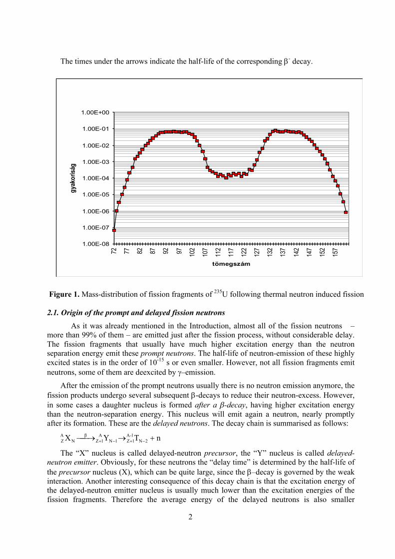
The number of the possible fission fragments is very large. Fig. 1. shows the mass-

distribution of the fission fragments. Please note that the ordinate is in logarithmic units. The curve shows two maxima: one around A = 95 and another one around A = 140. The fission fragments have excess neutrons as compared to the stable nuclei with the same atomic number. In most cases they undergo several subsequent b--transitions for „adjusting” their neutron/proton ratio. As an example, the fragment-pair above decays as follows:

( )90 90 90 90 9033 2 28 64

Krs

Rb Sré v

Yh

Zr stabilb b b b- - - -

,7 min

( )143 143 143 143 1430 5 12 33 13

Ba La Ceh d

Nd stabilb b b b- - - -

, min minPr

,7

1 The nuclei that are formed just after the fission process (within 10-14s) are called fission fragments. These fast moving nuclei slow down by colliding with the nuclei of the fuel material, then pick-up electrons, and finally become neutral atoms. Since they are radioactive, they undergo several decays, and form other atoms. These latter are called fission products.

2

The times under the arrows indicate the half-life of the corresponding b- decay.

1.00E-08

1.00E-07

1.00E-06

1.00E-05

1.00E-04

1.00E-03

1.00E-02

1.00E-01

1.00E+0072 77 82 87 92 97 102

107

112

117

122

127

132

137

142

147

152

157

tömegszám

gyakoriság

Figure 1. Mass-distribution of fission fragments of 235U following thermal neutron induced fission 2.1. Origin of the prompt and delayed fission neutrons

As it was already mentioned in the Introduction, almost all of the fission neutrons – more than 99% of them – are emitted just after the fission process, without considerable delay. The fission fragments that usually have much higher excitation energy than the neutron separation energy emit these prompt neutrons. The half-life of neutron-emission of these highly excited states is in the order of 10-15 s or even smaller. However, not all fission fragments emit neutrons, some of them are deexcited by g–emission.

After the emission of the prompt neutrons usually there is no neutron emission anymore, the fission products undergo several subsequent b-decays to reduce their neutron-excess. However, in some cases a daughter nucleus is formed after a b-decay, having higher excitation energy than the neutron-separation energy. This nucleus will emit again a neutron, nearly promptly after its formation. These are the delayed neutrons. The decay chain is summarised as follows:

nTYX 2N1-A1Z1N

A1Z

βN

AZ +®¾®¾ -+-+

The “X” nucleus is called delayed-neutron precursor, the “Y” nucleus is called delayed-neutron emitter. Obviously, for these neutrons the “delay time” is determined by the half-life of the precursor nucleus (X), which can be quite large, since the b–decay is governed by the weak interaction. Another interesting consequence of this decay chain is that the excitation energy of the delayed-neutron emitter nucleus is usually much lower than the excitation energies of the fission fragments. Therefore the average energy of the delayed neutrons is also smaller

3

(300÷600 keV) than the one of prompt neutrons (2 MeV in average).

The total yield of the fission neutrons (average number of neutrons, n) is the sum of the yield of the prompt and the delayed neutrons (np, and nd):

n n n= +p k

The delayed-neutron fraction is defined as:

bnn

= k . (1)

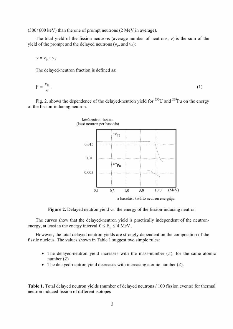
Fig. 2. shows the dependence of the delayed-neutron yield for 235U and 239Pu on the energy

of the fission-inducing neutron.

0,1 0,3 1,0 3,0 10,0 (MeV)

a hasadást kiváltó neutron energiája

239Pu

235U

0,015

0,01

0,005

késõneutron-hozam(késõ neutron per hasadás)

Figure 2. Delayed neutron yield vs. the energy of the fission-inducing neutron

The curves show that the delayed-neutron yield is practically independent of the neutron-energy, at least in the energy interval 0 4£ £E MeVn .

However, the total delayed neutron yields are strongly dependent on the composition of the fissile nucleus. The values shown in Table 1 suggest two simple rules:

• The delayed-neutron yield increases with the mass-number (A), for the same atomic

number (Z) • The delayed-neutron yield decreases with increasing atomic number (Z).

Table 1. Total delayed neutron yields (number of delayed neutrons / 100 fission events) for thermal neutron induced fission of different isotopes

4

Fissile nucleus nd (neutron/100 fissions)

233U 235U

238U*

0,667+0,0029 1,621+0,05 4,39+0,10

239Pu 240Pu* 241Pu

242Pu*

0,628+0,038 0,95+0,08 1,52+0,11 2,21+0,26

*Data for fast-neutron induced fission. 2.2. The delayed neutron groups

Nuclear physicists have identified so far more than 66 delayed neutron precursor nuclei.2 Their half-lives range between 0,12 s and 78 s, therefore their delayed neutrons appear with considerably differing delay times. A correct treatment of the delayed neutrons in reactor-kinetic calculations would consider each precursor nucleus with its own half-life and yield. However two problems arise when proceeding in this way:

• The calculation scheme becomes complicated because of the large number of the precursor nuclei;

• The decay scheme, half-life and yield are not well known for every precursor nucleus.

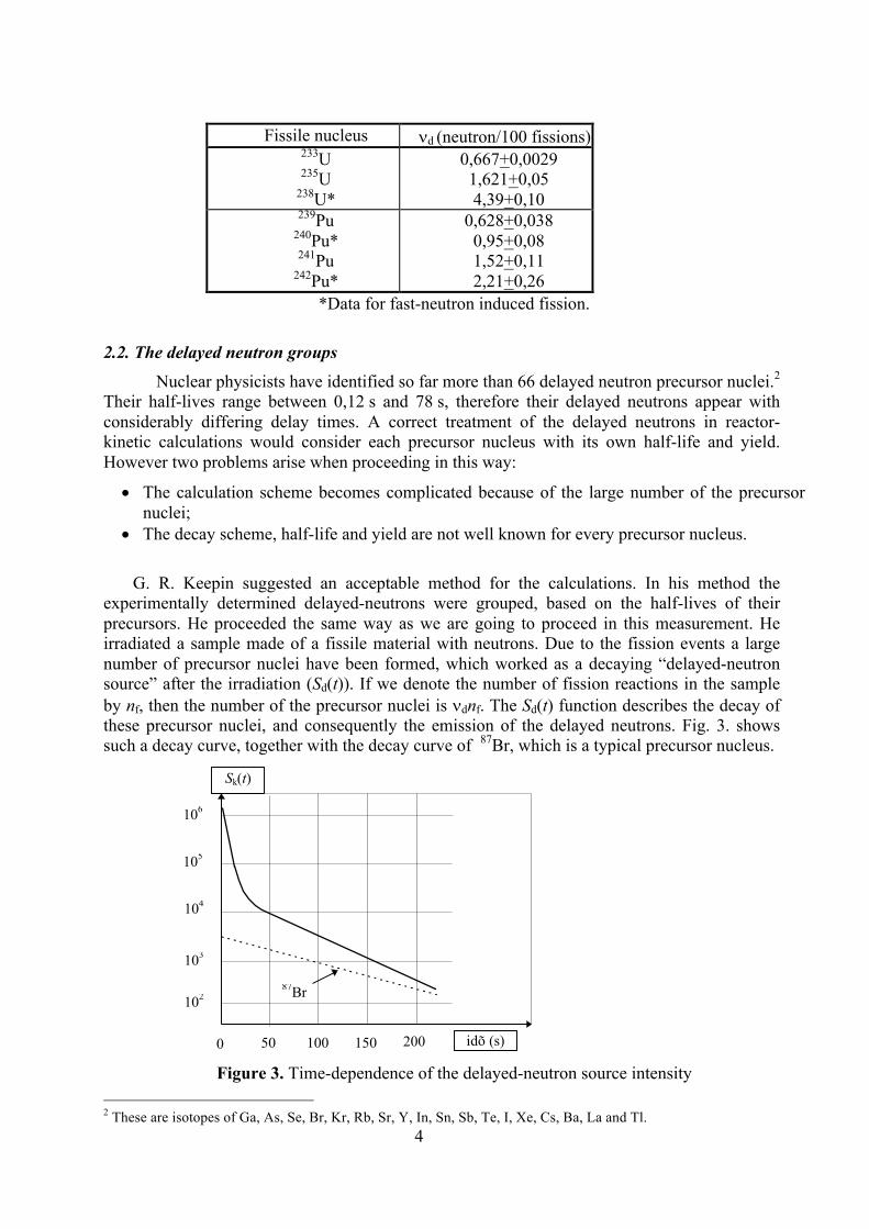
G. R. Keepin suggested an acceptable method for the calculations. In his method the experimentally determined delayed-neutrons were grouped, based on the half-lives of their precursors. He proceeded the same way as we are going to proceed in this measurement. He irradiated a sample made of a fissile material with neutrons. Due to the fission events a large number of precursor nuclei have been formed, which worked as a decaying “delayed-neutron source” after the irradiation (Sd(t)). If we denote the number of fission reactions in the sample by nf, then the number of the precursor nuclei is ndnf. The Sd(t) function describes the decay of these precursor nuclei, and consequently the emission of the delayed neutrons. Fig. 3. shows such a decay curve, together with the decay curve of 87Br, which is a typical precursor nucleus.

87Br

idõ (s)

Sk(t)

106

105

104

103

102

0 50 100 150 200 Figure 3. Time-dependence of the delayed-neutron source intensity

2 These are isotopes of Ga, As, Se, Br, Kr, Rb, Sr, Y, In, Sn, Sb, Te, I, Xe, Cs, Ba, La and Tl.

5

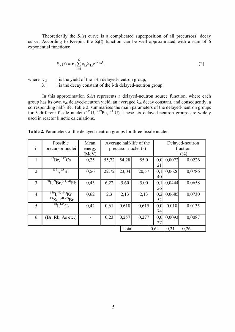
Theoretically the Sd(t) curve is a complicated superposition of all precursors’ decay

curve. According to Keepin, the Sd(t) function can be well approximated with a sum of 6 exponential functions:

S t n ek f kii

kitki( ) =

=

-å n l l

1

6, (2)

where ndi : is the yield of the i-th delayed-neutron group, ldi : is the decay constant of the i-th delayed-neutron group

In this approximation Sd(t) represents a delayed-neutron source function, where each group has its own ndi delayed-neutron yield, an averaged ldi decay constant, and consequently, a corresponding half-life. Table 2. summarises the main parameters of the delayed-neutron groups for 3 different fissile nuclei (235U, 239Pu, 233U). These six delayed-neutron groups are widely used in reactor kinetic calculations. Table 2. Parameters of the delayed-neutron groups for three fissile nuclei

i

Possible precursor nuclei

Mean energy (MeV)

Average half-life of the precursor nuclei (s)

Delayed-neutron fraction

(%) 1 87Br, 142Cs 0,25 55,72 54,28 55,0 0,0

21 0,0072 0,0226

2 137I, 88Br 0,56 22,72 23,04 20,57 0,140

0,0626 0,0786

3 138I,89Br,(93,94)Rb 0,43 6,22 5,60 5,00 0,126

0,0444 0,0658

4 139I,(93,94)Kr 143Xe,(90,92)Br

0,62 2,3 2,13 2,13 0,252

0,0685 0,0730

5 140I,145Cs 0,42 0,61 0,618 0,615 0,074

0,018 0,0135

6 (Br, Rb, As etc.) - 0,23 0,257 0,277 0,027

0,0093 0,0087

Total 0,64 0,21 0,26

6

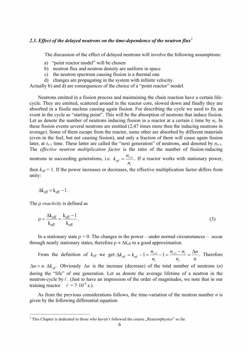
2.3. Effect of the delayed neutrons on the time-dependence of the neutron flux3

The discussion of the effect of delayed neutrons will involve the following assumptions: a) “point reactor model” will be chosen b) neutron flux and neutron density are uniform in space c) the neutron spectrum causing fission is a thermal one d) changes are propagating in the system with infinite velocity.

Actually b) and d) are consequences of the choice of a “point reactor” model.

Neutrons emitted in a fission process and maintaining the chain reaction have a certain life-cycle. They are emitted, scattered around in the reactor core, slowed down and finally they are absorbed in a fissile nucleus causing again fission. For describing the cycle we need to fix an event in the cycle as “starting point”. This will be the absorption of neutrons that induce fission. Let us denote the number of neutrons inducing fission in a reactor at a certain ti time by ni. In these fission events several neutrons are emitted (2,47 times more then the inducing neutrons in average). Some of them escape from the reactor, some other are absorbed by different materials (even in the fuel, but not causing fission), and only a fraction of them will cause again fission later, at ti+1 time. These latter are called the “next generation” of neutrons, and denoted by ni+1. The effective neutron multiplication factor is the ratio of the number of fission-inducing

neutrons in succeeding generations, i.e. i

ieff n

nk 1+= . If a reactor works with stationary power,

then keff = 1. If the power increases or decreases, the effective multiplication factor differs from unity:

Dk keff eff= -1 . The r reactivity is defined as

r = =-Dk

kkk

eff

eff

eff

eff

1. (3)

In a stationary state r = 0. The changes in the power – under normal circumstances – occur

through nearly stationary states, therefore r » Dkeff to a good approximation.

From the definition of keff we get:nn

nnn

nn

kki

ii

i

ieffeff

D=

-=-=-=D ++ 11 11 . Therefore

effknn D×=D . Obviously nD is the increase (decrease) of the total number of neutrons (n) during the “life” of one generation. Let us denote the average lifetime of a neutron in the neutron-cycle by ! . (Just to have an impression of the order of magnitudes, we note that in our training reactor ! = 7·10-5 s.).

As from the previous considerations follows, the time-variation of the neutron number n is given by the following differential equation:

3 This Chapter is dedicated to those who haven’t followed the course „Reactorphysics” so far.

7

dndt

n keff=D!

. (4)

Supposing that Dkeff is constant in time we get:

n t n tk

teff( ) ( )exp( )= 0D!

. (5)

Here n(0) is the number of the neutrons in t = 0 time.

The reactor period (T) is defined as a time-interval, where the neutron-number changes by a factor of e (e = 2,7172…). According to (5) this means:

Tkeff

=!

D. (6)

The time-dependence of the neutron-numbers can be expressed using the reactor period too:

n t n t etT( ) ( )= 0 . (5a)

Within the framework of the one-group theory the (5) equations are also valid

(approximately) for the neutron density, the neutron flux and for the reactor power as well. In a reactor operating stationary with constant power n(t) = n(0) = const., i.e. T is

infinity. The period is a very important quantity for the safety of a reactor with varying power level. Handling the period-trip has to be built-in in the reactor-protection system of every reactor, which shuts down the reactor immediately if the reactor period becomes too small (compared to the possibilities of the reactor control systems). If this did not exist, period times smaller than 7÷10 s would represent highly dangerous states.

To show the importance of the delayed neutrons let us determine the period when the reactivity is r = 0,25%4, and only prompt neutrons are considered. Since Dkeff » r = 0,0025, according to (6) we get for the period:

Tk

seff

= = =!

D00

0,00007,0025

,028 .

(Here we used ! = 7·10-5 s that is a typical value for our reactor). This means that the neutron number increases during 1 s to

n sn

e ess( )

(, ,1

0)3 10

10 028 35 7 15= = = × .

4 The reactivity (which is a dimensionless number) is often expressed in %. For example r = 0,25% means, that r = 0,0025 (i.e. according to (3) keff » 1,0025).

8

Obviously, there is no control mechanism (containing mechanical parts) that could follow

this very rapid increase. However, the delayed neutrons could – under special circumstances – “slow down” this pace, and so they enable the control of the reactors.

In order to explain the effect of delayed neutrons we simplify our treatment. We take into account only one – “averaged” – delayed neutron group5. Averaging the half-lives (for 235U) in Table 2. we get 9 s. This means that the six decay constants in (2) will be substituted by only one averaged decay constant:

l = = -log,077

29

0 1

ss .

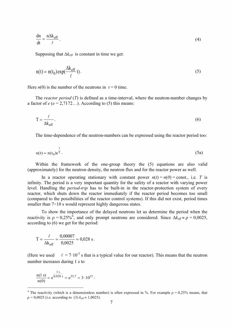
Eq. 4. should be modified, since the delayed neutrons have another life-time than the prompt neutrons. Therefore the delayed-neutron fraction (β) has to be subtracted from the term containing an average ! lifetime, and has to be added with their own life-time.

Let us denote the number of precursor nuclei in time t by C(t). Therefore the delayed neutron production rate will be ( )lC t . Thus we get for the modified form of Eq. (4):

dndt

n keff=D!

(7a)

The first term on the right side expresses the neutron-multiplication due to the prompt

neutrons, whereas the second term shows the effect of the delayed neutrons. This equation has to be completed by another equation describing the variation of the number of precursor nuclei:

( )dCdt

C t nkeff= - +lb!

. (7b)

Here the first term on the right side describes the decrease due to the decays, the second

term describes the fact that the precursor nuclei are created by the fission events. Note that this is exactly the term that modified the first term on the right side in Eq. (7a).

Now let us examine how the delayed neutrons affect the reactor period! Like we did for

(5a), the solution of the (7) system of equations is searched in the form:

( )n t n et T= 0 and ( )C t C et T= 0 .

Substituting this into (7), we get for T:

5 Detailed treatment see in Reference [4].

9

( )rb

bl

= ++

! kT Teff 1

1, (8)

where we used the reactivity defined in (3). (When we derive similar equations considering

all the 6 delayed neutron groups, we get the so-called inhour equation.)

Equation (8) is a quadratic equation for the T period (by constant reactivity):

rbl

rb

lb b

Tk

Tkeff eff

2 1 0+ - -æ

èç

ö

ø÷ - =

! ! . (9)

Let us denote the two roots by T1 and T2. Using these roots, the time-dependence of the

neutron numbers can be written down as

( )n t n e n et T t T= +1 21 2 , (10)

where the n1 and n2 constants depend on the initial conditions. The constants appearing in

(9) are all positive, except the reactivity, which can be positive, negative or zero. If the r reactivity is negative (i.e. keff < 1, the reactor is subcritical), all three coefficients in Eq. (9) are negative. This means that both roots are negative,6 which implies that the neutron number – irrespective of the (10) initial conditions – decreases in time. If the r reactivity is positive (i.e. keff > 1, the reactor is supercritical), the first coefficient in Eq. (9) is positive, the third one is still negative. Depending on the actual value of the reactivity the second coefficients can be negative or positive. However in both cases one of the roots is negative and the other one is positive. Let us denote the positive root by T1. After sufficiently long time (t) Eq. (10) goes over into

( )n t n et T» 1

1 (t >> T2), (11)

since the term with the negative root vanishes. The number of neutrons increases exponentially in a supercritical reactor even in the presence of the delayed neutrons! However, the time-constant of this exponential increase is crucial! Let us assume the following numerical values:

b = 0,0064; ! = 7·10-5 s; r = 0,0025; l = -0 1,077 s ; keff = 1,0025.

Substituting these into Eq. (9) we get T1 = 20,31 s, which is substantially larger than the 0,028 s that we obtained without the presence of the delayed neutrons. This numerical example shows clearly the essential feature: the delayed neutrons cause an increase in the reactor period so that it makes possible the safe control of the reactor with external devices.

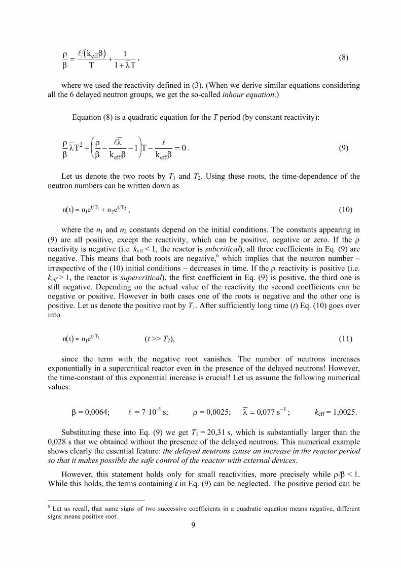
However, this statement holds only for small reactivities, more precisely while r/b < 1. While this holds, the terms containing l in Eq. (9) can be neglected. The positive period can be

6 Let us recall, that same signs of two successive coefficients in a quadratic equation means negative, different signs means positive root.

10

written approximately as:

T1 »-b rrl

. (r/b < 1) (12a)

This approximation gives T1 = 20,26 s in the above numerical example, i.e. the

approximation is sufficiently correct. The situation changes dramatically when r/b > 1. In this case the coefficient of the second term in Eq. (9) becomes positive, and the positive root of the equation should be approximated by a different formula:7

( )Tkeff

1 » -!r b

. (r/b > 1) (12b)

For example if r/b = 1,1 (keff = 1,0071) according to the formula (12b) we get T1 = 0,109 s,

which means that the reactor becomes uncontrollable again. (The exact value is T1 = 0,099 s.) Our results show that the reactor is controllable while r/b < 1, i.e. keff < 1+b (approximately). With other words: the necessary condition of the controllability is that the reactor be subcritical without the delayed neutrons. When the reactor becomes supercritical without the delayed neutrons (i.e. if r/b > 1), the reactor becomes uncontrollable and a reactor excursion occurs. Such a reactor state is called prompt supercritical state, and it is considered as a severe reactor accident.

As from the above discussion follows, the delayed-neutron ratio (b) plays an important role in controlling the chain reaction. Because of this fact it is chosen as the unit of the reactivity. The name of this unit is dollar ($). The reactivity of a reactor is 1 $, if r/b = 1. As we have shown, this reactor state should be avoided, therefore in the praxis the hundredth of this unit is usually used, which is called cent. The reactivity of a reactor is one cent, if r/b = 0,01.

3. Determination of the parameters of delayed neutron groups

3.1. Equipment and materials needed for the measurement

• Reactor and pneumatic sample transporting system; • Uranium foil in small polyethylene container (rabbit) for the pneumatic transport system • Measuring vessel filled with moderator (paraffin); • 6 neutron-detectors (3He); • Electronic devices (power supply, amplifier, discriminator); • Computer with multichannel analyser card (used in multiscaler – time-analyser mode). 3.2. Procedure

The natural uranium foil will be transported into the core of the reactor by the pneumatic transport system. The reactor operates at 1 kW thermal power. After a certain irradiation time the sample will be automatically transported out of the reactor core, to the measuring place (transportation time is about 3 s). An optical sensor picks up the time when the sample leaves the reactor core. This signal can be used as “start” signal for the measurement.

7 To derive the approximation formulas is a useful exercise for the reader in order to check whether he/she had well understood the mathematical treatment so far.

11

The measuring place consists of a vessel filled with paraffin moderator. In the holes of the moderator 6 parallel-connected (3He filled) neutron-detectors are placed. The moderator is needed for slowing down the neutrons, since the detectors are sensitive mainly for thermal neutrons. The time for slowing down the neutrons is negligibly small (about. 1 µs) compared to the delay time of the delayed neutrons.

The neutron detectors send pulses to the accompanying electronic devices. These pulses will be first amplified then sorted by a discriminator. It is important to adjust the discrimination level correctly. Since the detectors are proportional chambers filled with 3He gas, they detect not only the neutrons but also g-photons. Additionally – like every electronic device – the detectors also have noise. With adjusting the discrimination level, the “background” due to the electronic noise and the g-events can be well reduced. A simple procedure to adjust the discrimination level is to search the maximal discrimination level where the counting rate is still not too low, and then choose the discrimination level the 1/8-th of this value.

A better method would be to analyse the pulse-height distribution of the detectors (a pulse-height analyser will be needed), and identify the amplitude-region that corresponds to the neutrons. This best can be done using a neutron source. Gating the analyser with the discriminator output pulses, the discrimination level can be adjusted so that only the pulses coming from the neutrons go through the discriminator.

The selected pulses will be counted in the multichannel analyser card during a certain time-interval (dwell-time). In this measurement 1 s dwell-time is recommended. During the dwell time the incoming pulses are counted, and when this time-period is over, the accumulated count will be stored in the computers memory (the memory array containing these data is called “channels”). Since the “longest-lived” delayed-neutron group has a half-life of about 54 s, it is reasonable to measure the neutrons only until about 320 s (6 half-lives of the longest group). The “decay-curve” of the delayed neutrons is represented then as an array of 320 integer numbers (counts). The first number corresponds to the incoming counts in the first second after the start pulse, the second number represents those counted during the second time-interval, and so on. (Usually the first three-four numbers should be near zero, since the sample did not arrive to the measuring place.) This array of numbers can be saved in a file, can be printed out, or examined using different software of the analysing computer.

3.3. Data processing – uncertainty estimation The decay-curve of the delayed neutrons can be approximated – according to Keepin – with

a sum of 6 exponential functions. The aim of the data processing is to determine the half-lives and the relative intensities of these groups (to measure the parameters of Table 2.). Since the half-lives of the groups 4,5,6 are smaller than 3 s (the time of flight of our pneumatic rabbit system), we will determine the parameters of groups 1,2 and 3 only.

Thus we have our “theoretical decay function” S t n ek f kii

kitki( ) =

=

-å n l l

1

6. (For the simplicity

here we omitted the index “d” referring to the delayed neutrons). Our detector detects only a portion of these emitted neutrons. This is determined by the overall detection efficiency (e). Our multiscaler analyser “integrated” the detected signals during Dt dwell-time, starting at time tk. So we have our “theoretical guess” for the detected counts:

å ò=

-D+ ¢¢×=

3

1

)(i

k

k

iiifth

ttt tdtevnkN lle .

The integral is easy to evaluate and we get:

12

åå==

-×=-×÷øö

çèæ D--××=

3

1

3

111)(

i

kii

ki

i

i

iiifth

teatetevnkN llll

le . (13)

Here we introduced ÷øö

çèæ D--×××= tevna i

ifile 1 .

According to (13) we have 6 parameters to determine ai and li , i = 1..3. The “simplest” procedure will be to use a fit program to determine these 6 parameters so, that the “theoretical” Nth(k) values fit best the “measured” Nm(k) values. However, since 3 parameters are in the exponent, we will need a weighted non-linear least-square fit procedure to find the appropriate solution.

However, we will use another – more conventional – method, because it is instructive. The main idea is the following:

If there was only one exponential, a simple linear regression fit could be used, since the logarithm of the counts is a linear function of the time tk: kth takN ×-= lln)(ln . From the slope the l decay constant, from the interception the logarithm of the a parameter could be simply determined. The problem is, that our data are a sum of exponentials, so logarithmic transformation will not lead to a simple linear expression. Let us now sort the li-s in ascending

order, i.e. l1< l2< l3. After a certain time we surely have tetete 321 lll ->>->>- , which means that in the sum (13) the second and third terms can be neglected, and only the first term should be kept. With other words, after a certain time only the group with the longest half-live remains, so we have only one exponential, and can use the simple linear regression fit to determine its parameters! (This can also be clearly seen on Fig. 3, which shows the decay curve on a semi-logarithmic scale. After about 50-60 s the transformed curve may be approximated well by linear function).

Once we have the parameters for the first group, we know already its contribution! So we can calculate:

kmm

teakNkN 11

)2( )()( l-×-= .

Of course these data should be fitted with a sum of two exponentials. But here we again use

the previous argument: after a certain time we have: tete 32 ll ->>- , i.e. only the term containing a2 and l2 remains. And this is only one exponential:

km takN 22)2( ln)(ln l-= . From here a2 and l2 can easily be determined. Now we know

already four parameters, so we can calculate again:

kkmm

teateakNkN 22

11

)3( )()( ll -×--×-= .

These data should be fitted with one remaining exponential, which is an easy task again, so finally a3 and l3 are also determined.

Summarised: step by step deducing consecutively always the longest exponential components from the measured values, the half-lives and relative percentages of the first three delayed neutron groups can be determined.

We should keep in mind that this procedure – though simple and easy to carry out – gives only approximate values for the parameters, since the logarithm operation transforms also the statistical deviations of the measured points from the “theoretical” values. Additionally, the

13

several successive subtractions increase the uncertainties of the later defined parameters. With this method it is also relatively hard to determine the uncertainties of the parameters.

More precise values can be extracted with a weighted non-linear least-squares fit using the whole original data set. Such procedures usually need a set of initial values for the parameters, which should be “not too far” from the best values. (If the initial values are too far, the iterative procedure converges only slowly if it converges at all.) To determine such an initial parameter set the above simple procedure can be well used.

4. Determination of uranium concentration of unknown samples

In this measurement the natural uranium concentration (in mass %) will be determined in a

sample (ore, soil, etc.). 4.1. Equipment and materials needed for the measurement

• Equipment used in the determination of the delayed neutron parameters (see. 3.1); • Analytical scales; • Small polyethylene containers (rabbits) for the pneumatic transporting system; • Reactor and pneumatic transporting system; • Two uranium standards calibrated by the IAEA.

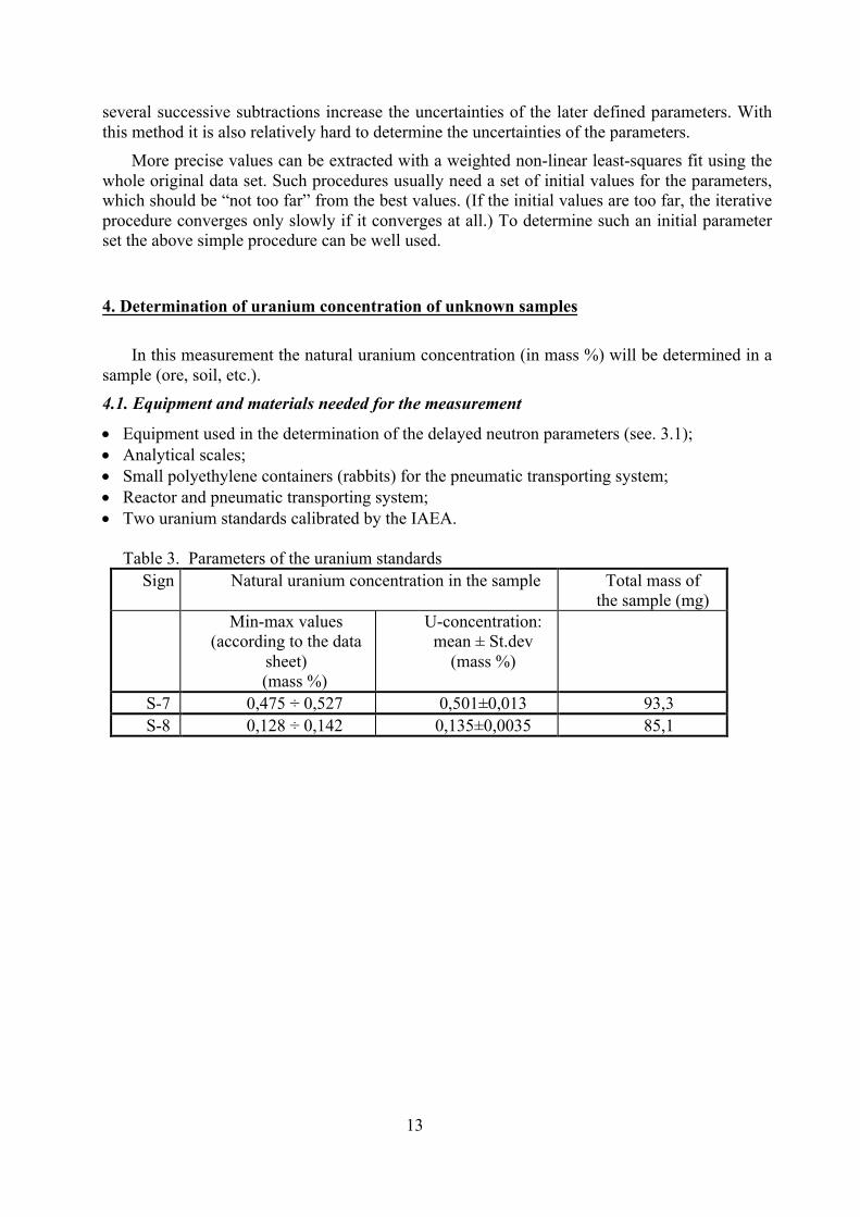
Table 3. Parameters of the uranium standards

Sign Natural uranium concentration in the sample Total mass of the sample (mg)

Min-max values (according to the data

sheet) (mass %)

U-concentration: mean ± St.dev

(mass %)

S-7 0,475 ÷ 0,527 0,501±0,013 93,3 S-8 0,128 ÷ 0,142 0,135±0,0035 85,1

14

4.2. Procedure

The determination of the uranium-content is based on the measurement of the relative delayed-neutron intensity. This is a fast, precise, sensitive and non-destructive method. Because of the simplicity of the method it is widely used for series-analysis of ores, or soil samples.

The uranium-content of an unknown sample will be determined by comparing its delayed-neutron intensity with two uranium-standards of the IAEA. Also the standard deviation of the measured values should be calculated as well as the detection limit of the measurement. Our unknown sample is a small piece of rock containing pitchblende.

The unknown sample is transported into the reactor core by the pneumatic transport system, and it is irradiated in the reactor. The thermal power of the reactor is about 10 kW. The measuring equipment is the same as previously (see Chapter 3.2.). The main idea of the measurement is that Equ. (2) describes the decay curve of the delayed neutrons both in the standards and in the unknown sample, only the nf parameters can be different. It follows, that any portion of the decay curve is suitable to compare the two samples. Theoretically the data in only one single channel could be used, but adding several channels together could reduce the relative statistical fluctuations of the data.

In the choice of the region where the contents of the channels will be added (called region of interest, ROI), the following considerations should be kept in mind:

Both the standards and the unknown sample may contain oxygen. This can be disturbing, since the 17N nucleus can be formed in the 17O(n,p)17N reaction. This is a neutron-emitter, and has a half-life of 4,1 s. Since the oxygen-content can be different from sample to sample (and not known), it is advisable to wait until these neutrons “disappear”. So we choose about 20 s cooling time before starting to add the counts. As can be seen from Table 2. the 3,4,5,6 delayed-neutron groups also disappear at the end of this cooling time. Hence, the determination of the uranium content will be based on the measurement of the 2. delayed-neutron group (half-life 22,72 s). Sensitivity is only little improved by a counting time longer than 1 minute. A longer counting time increases the background contribution more than that of the useful information. Therefore the suggested region of interest is between 20 and 80 seconds.

Because the determination is focussed on groups with longer half-lives no irradiation time longer than twice or three times the half-life should be chosen. This time is sufficient for activation without causing significant background activity.

In order to determine the standard deviation and to calculate the detection limit the “background” should also be measured. We irradiate an empty “rabbit”, and measure the background in the previously determined region of interest (i.e. between 20 and 80 s). 4.3. Data processing – uncertainty estimation Measuring one single standard

Let us denote by Nx and Nstd the sum of the counts in the region of interest (from 20 to 80 s) for the sample and for the standard:

15

N nx i xi

==å ,20

80, N nstd i std

i=

=å ,20

80, (15)

where ni,x és ni,std are the content of the i-th channel of the unknown sample and the standard, respectively. The background count will be calculated similarly:

H hx i xi

==å ,20

80, (16)

where hi,x is the content of the i-th channel at the measurement of the background for the unknown sample. If we measure the standard and the unknown sample close in time, it can be assumed that the backgrounds are the same. However, to keep the mathematical treatment as general as possible, we allow that the standard has a separate background, Hstd .

We assume that the net number of counts is proportional to the uranium content of the sample. This latter is the product of the mass of the sample (m) and the uranium concentration (C). So we have N – H = a·m·C, from where we get:

N Hm

aC-= , (17)

Here a is an (unknown) proportionality constant depending on the actual circumstances of

the measurement. Naturally Eq. (17) holds not for the measured data but only for their expectation values. Using Eq. (17) for the measured data of the standard we get an estimated value for the unknown a parameter:

~a N Hm Cstd std

std std=

- , (18)

Cstd is the uranium-concentration of the selected standard, as it can be found in the data-sheet (mass %, see Table 3.). Using this value, the uranium-concentration of the unknown sample can be estimated as

C N Hm axx x

x=

-~ . (19)

If we measure only one standard, this formula means the end of the data processing. However, we still have to calculate the standard deviation of the determined value.

Since the precision of the mass-determination (weighting) is much higher than the other

16

sources of uncertainty, we neglect the uncertainties of the mx and mstd masses.

The statistics of the counts follow the Poisson distribution, so for the standard deviation of the background-subtracted counts we have

sstd std stdN H2 » + and sx x xN H2 » + . (20)

Therefore the standard deviation of the estimated value of the a parameter (18):

( )s

sa

std std

std std

C

stda N H

N H Cstd2 2

2

2

2=+

-+

æ

èçç

ö

ø÷÷

~ , (21a)

and that of the uranium concentration calculated using (19):

( )s

sC x

x x

x x

ax

C N H

N H a2 2

2

2

2=+

-+

æ

èçç

ö

ø÷÷~ . (21b)

The (21) formulas can be simply deduced using basic mathematical statistics, so we don’t

elaborate them further here. However, the reader is encouraged to show their validity.

Measuring two standards

When we measure both standards, more than one data processing procedures can be used. The simplest way is to estimate the a parameter from both measurements independently:

~a N Hm Cii i

i i=

- , (i = 1, 2) (22)

where the index “i” denotes the data for the individual standards. The standard deviations can also be estimated like we did in (21a) :

( )s

sai i

i i

i i

Ci

ia N H

N H C2 2

2

2

2=+

-+

æ

èçç

ö

ø÷÷

~ . (i = 1, 2) (23)

The final value of the a parameter will be the weighted average of these two values:

17

~~

aai ai

i

aii

= =

=

å

å

s

s

2

1

2

2

1

21

, (24a)

and its standard deviation becomes:

ss

a

aii

2

2

1

21

1=

=å

. (24b)

We get a less heuristic estimation if we use a linear regression based on the (17) formula. This means that we search the minimum of the

Q w N Hm

aCii i

ii

i=

--

æèç

öø÷

=å

2

1

2 (25a)

expression in function of a, where the “weights” can be expressed with the standard deviations of the measured quantities:

w N Hm

aii i

iCi

- =+

+12

2 2s . (25b)

The solution of the minimum problem can be easily obtained:

~aw C N H

m

w C

i ii i

ii

i ii

=

-

=

=

å

å

1

2

2

1

2 , (26a)

and its standard deviation becomes:

sai i

iw C

2

2

1

21

=

=å

. (26b)

Note, that the wi weights also depend on the a parameter according to (25b), therefore the

18

use of (26a) needs iteration.8 The method according to (24a) needs no such iteration.

To determine the unknown uranium concentration we need to use the (19) and the (21b) formulas, irrespective whether we choose the (22)÷(24) formulas or the (25)÷(26) ones. The two methods are equivalent. The reader is encouraged to show this mathematically. (Hint: in the (23) formula – and only there – change ~ai

2 to ~a2 , then it is easy to show with simple algebra that (24a) and (24b) gives the same result as (26a) and (26b). Question: why is this sufficient to demonstrate the equivalence of the two estimations?

Detection limit

When defining the detection limit we have to assure – based on statistical arguments – that the net count (used for the calculation of the uranium content) is significantly larger than the background. With other words, we have to decide whether there is an effect or not, and we also have to give a quantitative argument for this decision.

In the decision we can commit two types of error. The first is called “error of first kind”, where we assume that some part of the measured intensity comes from the uranium content of the sample, but in reality it is only a positive fluctuation of the background. (We assume that there is an effect, but in reality there is none). The error of second kind is, when we assume that the measured intensity is only the fluctuation of the background, but in reality it comes from the uranium content. (We assume that there is no effect, but in reality there is one).

To avoid the error of first kind we require that the useful effect exceed the standard deviation of the background by a certain amount:

L k k Nc h h1 1 1= =s .

Here k1 is dependent on the significance level required. (For example k = 1,645 represents 95% significance level and k = 2,33 assures 99% significance. This means that in the first case the probability of committing an error of first kind is 5%, and in the second case it is only 1%. However these values are valid for a background having a normal distribution.)

The probability of the error of second kind can be formulated using a concrete counter-

hypothesis. We assume a net effect (Lc2), which has to exceed the previously defined Lc1 level so, that even negative fluctuations cannot bring Lc2 below Lc1. This means:

L L kc c L hc2 1 22 22= + +s s .

Here k2 is again dependent on the significance level required. If we take k2 = k1 (this is not always the case, since the risk of the two errors can be different), then we have for the number of counts significantly exceeding the background:

8 The main behaviour of this iteration depends strongly on the values of the standard deviations. The reader is encouraged to experiment with it using the concrete experimental data. General tendency is, that the weighting according to (25b) tends to decrease the estimated value of a.

19

L k k k Nc c h22

122L 2= + = +

This quantity has to be compared to the number of counts measured with the standard to get the detection limit for the uranium concentration.

Choosing a 95% significance level (k = 1,645) we get: L k k k Nc c h22

122L 2= + = + .

This is the so-called Currie detection limit.

5. References

1. G. R. Keepin: Physics of Nuclear Reactors, Addison-Wesley Publishing Co., Massachusetts (1965)

2. G. R. Keepin: Interpretation of Delayed Neutron Phenomena, J. Nucl. Energy, 7, 13 (1958) 3. G. R. Keepin, T. F. Wimmet, R. K. Zeigler: Delayed Neutron from Fissionable Isotopes of

Uranium, Plutonium and Thorium, Phys. Rev., 107, 1044 (1957) 4. W.M. Stacey: Nuclear Reactor Physics (John Wiley &Sons Inc., 2001) 6. Knowledge check (questions)

1. What are the delayed neutrons? 2. What is the origin of the delayed neutrons? 3. What nuclei are called delayed neutron precursors? 4. What are the prompt neutrons? 5. What is the origin of the prompt neutrons? 6. What is the difference between the average energy of the prompt and delayed neutrons? 7. What is called reactor period? 8. What role do the delayed neutrons play in the control of the nuclear chain reaction? 9. Describe the procedure for measuring the essential parameters of the delayed neutron groups! 10. How are the delayed neutrons grouped? What physical parameter is the most important when

grouping the delayed neutrons? 11. Describe the procedure for measuring the uranium concentration of unknown samples!