4

_ DETERMINATION OF CORRECTIONS TO

FLOW DIRECTION MEASUREMENTS OBTAINED WITH A

WING-TIP MOUNTED SENSOR

By

Thomas Martin Moul

B.S. May 1977, University of Virginia

(_ASA-C_- 1744 12) DETI_MI_IIIC_ OF . N85-I£$62CCBBEC_ICBS TO _LCB DIH_C_IC_ _ASUBP_BN_S

OB£&INED IIZB A WING-2I_ MCI:_T]_E SE_50_

._.5. Thesis (George _ashingtcn Univ.) $I p Unclas

HC A05/8_ &Ol CSCI 01_ G3/C2 18137

A Thesis submitted to

_h. Faculty of

The Graduate School of Engineering and Applied Science

of the George Washington University in partial satisfaction

of the requirements for the degree of Master of Science

August 1983

1985010653

https://ntrs.nasa.gov/search.jsp?R=19850010653 2018-05-03T13:49:00+00:00Z

-.ABSTRACT

i An iovestigation into the nature of corrections for flow directionmeasurements obtained with a wing-tip mounted sensor has been conducted. I

Corrections for the angles of attack and sideslip, measured by sensorsT_

mounted in front of each wing tip of a general aviation airplane, have been

determined. These flow corrections have been obtained from both wind-

tunnel and flight tests over a large angle-of-attack range. Both the

angle-of attack and angle-of-sideslip flow corrections were found to be

substantial. The corrections were a function Gf the angle of attack and

angle of sideslip. The effects of wing configuration changes, small

changes in Reynolds number, and spinning rotation on the angle-of-attack

flow correction were found to be small. The angle-of-attack flow correc-

tion determlned from the static wind-tunnel tests agreed reasonably well

with the correction determined from flight tests.

Xi

, ®

1985010653-002

ACKNOWLEDGEMENTS

The author wishes to thank the National Aeronautics and Space|

Administration for providlng the opportunity to perform this research, pre- I!

pare this thesis, and complete all the other requirements for this degree.

The author is grateful to Professor John P. Campbell who acted as my acade-

mlc and thesis advisor. His guidance and encouragement have been instru-

mental in the successful completion of my degree program. I would also

like to thank Mr. William P. Gilbert for his timely review of the thesis

and his helpful comments and Ms Nadine E. McHatton for her speedy prepara-

tion of +his document. Special thanks also go to Mr. Eric C. Stewart for

his advlc= and encouragement, Mr. Kenneth E. Glover for supplying me with

the spin flight-test data used in this thesis, and Mr. Randy So Hultberg

for supplying me with the rotary-balance da_a used in this thesis.

Finally, I would like to thank Dr. Vladislav Klein and Dr. Michael K. Myers

for reviewing my thesis and serving on my thesis defense committee.

iii

®_m

1985010653-003

TABLE OF CONTENTS

Page

TITLE ................................................................. i

ABSTRACT ............................................................. ii

ACKNOWL EDGEMENTS .................................................... Iii

TABLE OF CONTENTS .................................................... iv

LIST OF TABLES ........................................................ v

LIST OF FIGURES ...................................................... vi

LIST OF SYMBOLS ...................................................... ix

Chapter

I INTRODUCT ION ................................................. I

I I TEST CONFIGURATIONS .......................................... 4

I II DATA ACQUISITION EQUIPMENT ................................... 6

IV TEST TECHNIQUES AND TEST CONDITIONS ......................... 10

V ANALYSIS TECHNIQUES ......................................... 13

VI RESULTS AND DISCUSSION ...................................... 22

VII SUMMARY OF RESULTS .......................................... 31

APPENDIX ............................................................. 32

REFERENCES ........................................................... 39

TABLES ............................................................... 41

FIGURES .............................................................. 43

iv

q

• • * J

1985010653-004

LIST OF TABLES

Page

I. Characteristics of research airplane ............................ 41 I

F2. Measurement list for research airplane .......................... 42

v

jj

1985010653-005

LIST OF FIGURES

Page

_. Spln research airplane in flight ................................. 44

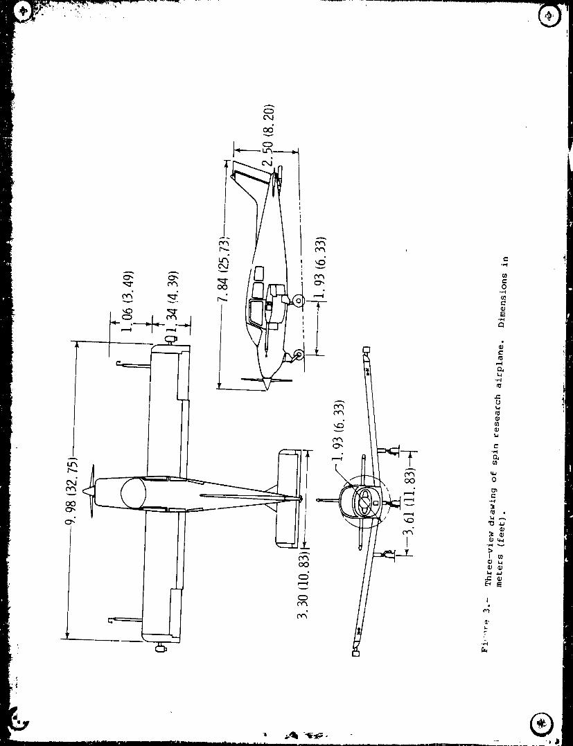
3. Three-view drawing of spin research airplane. Dimensions in meters(feet) ........................................................... 45

4. Wing leading-edge droop modification ............................. 46

5. Dimensions of the I/6-scale model in centimeters (inches) ........ 47

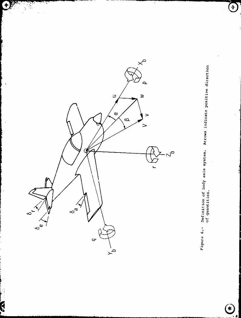
6. Definition of body axis system. Arrows indicate positive direction ofquantities ........................................................ 48

7. Flow direction sensor used in the wind-tunnel tests .............. 49

a. Photograph of the flow direction sensor.

b. Dimensions (in cm) of the flow direction sensor.

8. Flow dlrection and velocity sensor used in the flight tests ...... 50

9. Model mounted In the 12-foot low-speed wind tunnel ............... 51

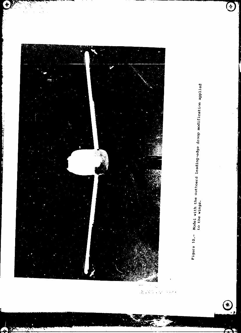
10. Model with the outboard leading-edge droop modification applied to thewings ............................................................ 52

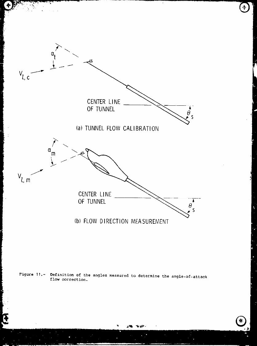
11. Definition of the angles measured to determine the angle-of-attackflow correction .................................................. 53

12. Model mounted on the rotary-balance apparatus in the spin tunnel . 54

13. Definition of the angle-of--attack and angle-of-sideslip

flow correction ................................................ 55

a. Definition of the angle-of-attack flow correction.

b. Definition of the angle-of-sideslip flow correction.

14. Longitudinal force and moment data for the model ................. 56

- 15. Resultant-force coefficient data for the model ................... 57

16. Tne effect of leading-edge modifications on the lift coefficient

of the model .................................................... 58

17. The effect of the Reynolds number on the lift coefficient of

the model ..................................................... 59

vi

1985010653-006

18. The true versus the measured angle of attack from the staticw ind-t,'nnel tests ................................................ 60

19. The angle-of-attack flow correction determined from the static

wind-tunnel t_sts ................................................ 61i

20. The effect of the outboard droop leading-edge modification on the iangle-of-attack flow correction determined from the static wind- rtunnel tests ..................................................... 62

21. The effect of the full-span droop leading-edge modification on the

angle-of-attack flow correction determined from the static wind-tunnel tests ..................................................... 63

22. T_e effect of aileron deflections on the angle-of-attack flowcorrection determined from the static wind-tunnel tests .......... 64

23. The effect of the outboard droop modification and an aileron

deflection on the angle-of-attack flow correction determined from

the static wind-tunnel tests ..................................... 65

24. The effect of the Reynolds number on the angle-of-attack flowcorrection determined from the static wind-tunnel tests .......... 66

25. The effect of the sensor location on the angle-of-attack flowcorrection determined from the static wind-tunnel tests .......... 67

26. The effect of the sideslip ang on the angle-of-attack flowcorrection determined from the static wind-tunnel tets ........... 68

27. The angle-of-sideslip flow correction determined from the staticwind-tunnel tests ................................................ 69

28. The effect of the full-span _roop leading-edge modification on the

angle-of-sideslip flow correction deterqined from the static wind-

tunnel tests ..................................................... 70

29. The effect of the sideslip angle on the angle-of-sideslip flowcorrection determine4 from the static wind-tunnel tests .......... 71

-- 30. The effect of the angle of attack on the angle-of-sideslip flowcorrection determined from the static wind-tunnel tests .......... 72

31. The effect of rotation on the angle-of-attack flow correction

,2 determined in the spin tunnel. Determined from different rates of

i_ rotation at Utcg = 40° 73, e toeeoeee.eee..oeoeeo, o.0o0o..o ....Qeeeeee.

i 32. The effect of rotation on the angle-of-attack flow correction

determined in the spin tunnel. Determined from different angle-of-attazkr__ settings at _b/2V = - .3 ......................................... 74

_, vii

1985o10653,oo7

33. Comparison of the angle-of-attack flow correction determined from

static windutunnel tests und from level flight tests ............. 75

34. Comparison of the angle-of-attack flow correction determined from

static wind-tunnel tests and from two approximate methods used during

steady spins .................................................... 76 J

35. Comparison of the angle-of-attack flow correction determine _ from

static wind-tunnel tests and from a steady spin analysis

technique ....................................................... 77

36. Instantaneous arrangement of ground axis system .................. 78

37. Relationship between resultant acceleration and resultantrotation vectors ................................................. 79

viii

1985010653-008

LIST OF SYMBOLS

A resultant acceleration, g units

T ,-_n_r,f,lg_l _r_l_r_inn, m/s_c 2 (ft/s_c2_"'C ..................... ' ' ' ' m

AX, A Z linear accelerations along the Xg, Zg ground axes, g units

aw acceleration along velocity vector, g units

ax, ay, az linear accelerations along the Xb, Yb' Zb body axes, g units

b wing span, m (ft)

C constant, I (I + ay sin B)COS 8

CD drag coefflcient, Drag/q_S

CL lift coefficient, Lift/q=S

/ 2 2CR resultant-fo:ce coefficient, CD + CL

Cm pltching-moment coefflcient, positive nose up, Pitching moment/q=S_

wing mean aerodynamic chord, m (ft)

Fw force along velocity vector, N (ib)

g acceleration due to gravity, m/sec 2 (ft/sec2)

h altitude, m (ft)

altitude rate, m/sec (ft/sec)

^ ^ ^

I, J, K unit vectors along the Xg, Yg, Zg ground axes^ ^ ^

i, j, k unit vectors along the Xb, Yb' Zb body axes

m/

i, j, k direction componentu of Xg in the body axes

Lbw transformation matrix from wind axes to body axes

£j, mj, nj direction cosines in the body axis system of the J ground axis

/ t /

Zj, mj, nj direction cosines in the ground axis system of the j body axis

m mass, kg (slugs)

p, q, r angular velocity about the Xb, Yb' Zb body axes, rad/sec (deg/sec)

q_ free-stream dynamic pressure, Pa (Ib/ft 2)

ix

1985010653-009

Rn Reynolds number, V_

Rs radius of the spin, m (ft)

S wing area, m 2 (ft 2)

U, V, W linear velocities along the Xg, Yg, Zg ground axes, m/sec i(ft/sec)

u, v, w linear velocities along the Xb, Yb' Zb body axes, m/s£c (ft/sec)

V total velocity, m/sec (ft/sec)

V total velocity vector, m/sec (ft/sec)

Vl,c local flow velocity w_ch the boom and flow direction sensor in thecalibration apparatus, m/sec (ft/sec)

V£, m local flow velocity with the boom and flow direction sensor mounted

on the model, m/sec (ft/sec)

W weight, N(ib)

Xb' Yb' Zb body axes

Xq, Yg, Zg ground axes__l

Xg vector along the Xg ground axis

x, y, z distance along Xb, Yb' Zb body axes, from cg to flow directionsensors, m (ft)

angle of attack, rad (deg)

am measured angle of attack, rad (deg)

a t true angle of attack, rad (deg)p

B angle of sideslip, rad (deg)

Bm measured angle of sideslip, rad (deg)

8t true angle of sideslip, rad (deg)

Y flight path angle, rad (deg)

helix angle of flight path measured from the vertical, tad(deg)

_a aileron deflection, rad (deg)

x

.................. m ... _ ..A_ _ ........ inn m ,m ,mmmim,, ,i m --- -- I ........ b

1985010653-010

_e elevator deflection, rad (deg)

_r rudder deflectlon, rad (deg)

E_ angle-of-attack flow correction, rad (R_g)l

E_ angle-of-sideslipcorrection, rad (deu_ W

flow

0 airplane pitch attitude, rad (deg)

Vl

@s wind tunnel mounting strut angle, rad (deg)

U angle between flight path and Xb body axis, rad (deq)

'_ klnematic viscosity, m2/sec (ft2/sec)

angle between resultant acceleration and resultant rotationvectors, rad (deg)

angular velocity about spin axis, rad/sec (deg/sec)

. angular velocity vector, rad/sec (deg/sec)

____b spln coefficient, positive for clockwise spins2V

Subscripts

b body axis system

cg at the center-of-gravity location

g ground axis system

£ left

m measured

r right

s at the sensor location

i t true9.

w wind axis system

Abbreviations

cg center of gravityi

psf, ib/ft 2

psi ib/in 2

xi

1985010653-011

CHAPTER I

INTRODUCTION

_ ........................... _ions it is u_Le, de_irabie to

reduce the flight data to a form that can be compared directly with wind-

tunnel data or theoretical predictions. An essential flight quantity for

this comparison is the true angle of attack of the airplane. Typically,

the angle of attack during flight tests is measured with a self-alining

vane or flow direction sensor (ref. I). The sensor is often mounted on

booms ahead of the wing near each wing tip and measures the local flow

direction. To determine the true angle of attack of the airplane, correc-

tions must be applied to this measured local flow direction (called the

measured angle of attack herein) to account for the change in the flow

direction at the sensor locatio: aue to the presence of the airplane.

For airplanes in the normal, unstalled flight regime, this flow correc-

tion may be easily detezmined both experimentally from flight tests and

theoretically (ref. 2). Experimentally, when an airplane is in steady,

straight and level flight the true angle of attack is given either by the

pitch attitude measurement os by the inverse sine of the longitudinal acce-

leration measurement (refs. 3 and 4). Theoretically, the flow correction

in front of the wing may be determined using lifting line theory (refs. 5

and 6).

However, at angles of attack above the stall these methods are no longer

usable. The flight test technique cannot be used because the airplane can

no longer achieve steady level flight at angles of attack above the stall.

Also, the lifting llne theory is no longer valid due to the separated flow

over the wing. In fact, the nature of the flow correction at these large

angles of attack is not well known.

®

1985010653-012

I One field of study here the knowledge of t_,is correction at l_rge

angles of attack is needed is in spin-fllght testing. The NASA Langley

i Research Center is conducting a comp_ehe_l_ive stall/spin investigation of

I_ general aviation airplanes to help improve their safe_y. The program

includes the use of full-scale and radio-controlled model flight tests,

static wind-t_:nnel tests of full-scale airplaDps and models, spin-tunnel

tests, rotary-balance tests, and computer sim_lation studies (fig. I). At

the large angles of attack encountered during the stall/spin flight tests,

the flow correction is substantial and, therefore, it must be applied to

the flight data to enable correlation with data from other phases of the

stall/spln program (ref. 7). Also, any theoretical appLoach to the

stall/spin problem would require the true angle of attack to be known.

Thus, an understarding of the flow correction at large angles of attack is

important in the study of the general aviation stall/spin p_oblem.

Preliminary investigations into the nature of the flow correction at

large angles of attack have shown that the correction can be substantial

(refs. 8 and 9). These reports looked only briefly at the flow correction

encountered on one of the research airplanes involved irl the Langley

stall/spin program. It was deemed necessary to undertake a more thorough

study into the basic nature of the flow correction. It was also desirable

to expand the data base for the stail/spill program by obtaining flow

correction data for another research airplane utilized in the program.

This thesis presents the results of a study to determine the flow

correction to be applied to the measurement of the angles of attack and

sideslip over a large angle-of-attack range. This work includes the deter-

mination of the flow correction from both wind-tunnel and flight tests of

--2--

" "' 19850 i 0653-01

one of the general aviation research airplanes utilized in the Langley

stall/spin program.

A I/6-scale model of the general aviation research airFlane was testedi

by the author in a low-speed wind tunnel at _he Langley Research Center.

The model was tested over a large angle-of-attack range and the effects on

the flow correction due to changes in flow parameters and configuration

changes were determined. The same model was also tested on the rotary-

balance apparatus located in the Langley Spin Tunnel. The author analyzed

this data to evaluate the effect of rotation on the flow correction.

The general aviation research airplane was flown in both level flight

and spinning flight as part of the Langley stall/spin program. The author

used the data from the level flight tests to determine a low angle-of-

attack flow correction. Data from many different spin flight tests were

analyzed by the author. The author applied two approximete methods and a

more complete analytical method to determine the flow correction during

these spins. The angle-of-attack flow correction determined by using these

methods is presented herein. However, the methods did not satisfactorily

determine the angle-of-sideslip flow correction; therefore, no data are

presented for this parameter.

-3-

®_ _ 'b J

1985010653-014

i

CHAPTER 2

TEST CONFIGURATIONS

Flight Test Airplane|

A single-engine, low wing, general aviation spin research airplane (fig. i

T2) was used in the flight tests reported herein. A three-view drawing of

the airplane is shown in figure 3. Some of the pertinent physical charac-

teristics of the airplane are given in Table I.

The airplane was equipped with two spin recovery systems. The primary

spin recovery system utilized hydrogen peroxide rockets mounted on each

wing tip (ref. 10). The research pilot could select which rocket to fire

7 to produce an unbalanced yawing moment to oppose the _pin aerodynamic

[_ moments. The rockets could also be fired in a direction to enhance the

aerodynamic moments in order to transition the airplane to a higher angle-

of-attack spin mode. The airplane was also equipped with a spin recovery

parachute.

Many modifications to the wing and body were flight tested to evaluate

their effect on the spin characteristics of the airplane. One of the wing

modifications was found to improve the stall/spin characterist_.-e of th_

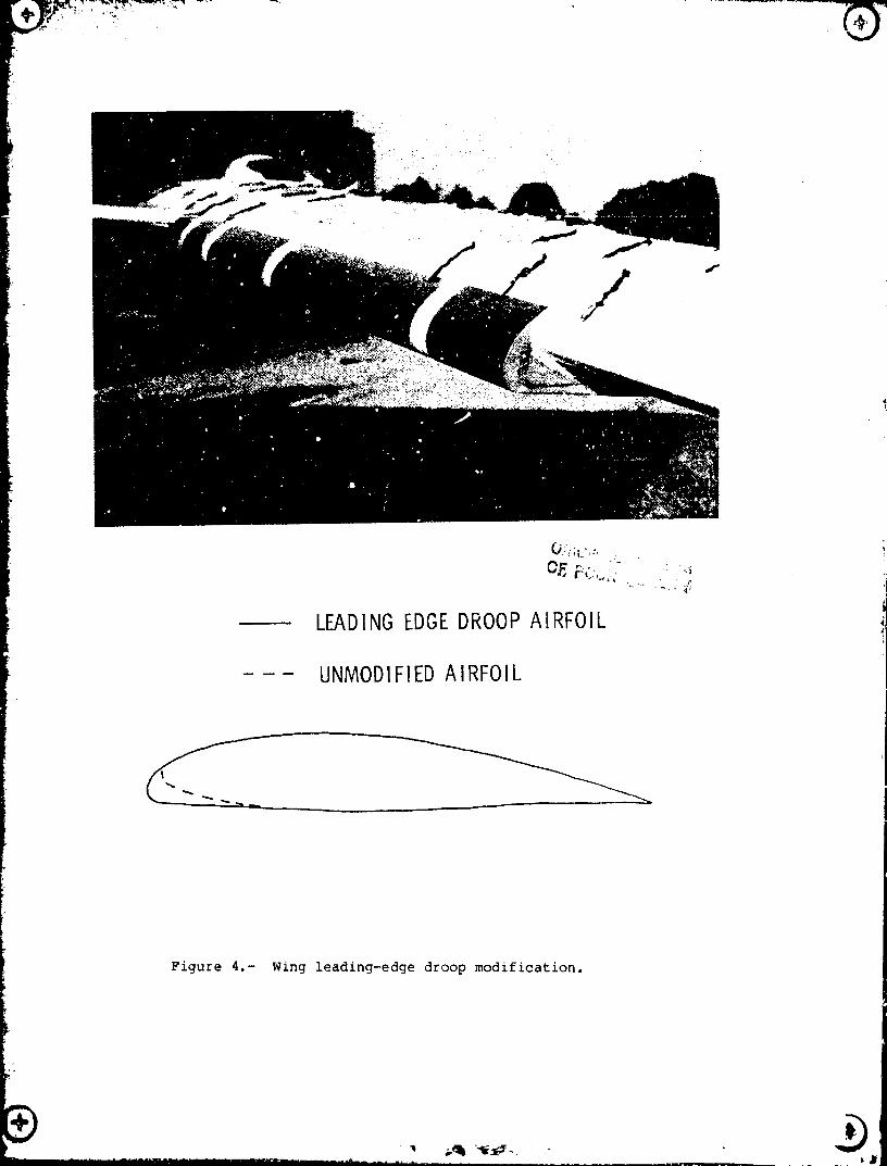
airplane (ref. 11). This modification consisted of a glove over the for-

ward part of the airfoil which provided a 3-percent chord extension and a

droop which increased the leading-edge camber and radius (fig. 4). This

leading-edge modification could be added to the full span of the airplane

wing, but was segmented so that different spanwise lengths could also be

tested.

-4-

1985010653-015

t

Wind-Tunnel Model

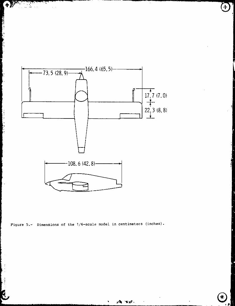
The I/6-scale model of the spin research airplane was tested in the

12-foot low-speed wind _ inn_1 ann in *h= _p_- _....cl "_ _ _'_ Langley

Research Center. The model was constructed of fiberglass, wood, and alumi-

num. The model did not have landing gear and had the propeller removed for

the tests. The rear fuselage sectioD, including the horizontal and ver-

_ " tical tails, was removed to facilitate mounting the model in the 12-foot

wind tunnel. A drawing of the model as tested in the 12-foot tunnel is

shown in figure 5. In the _pl_1 tL,nnel, the model was tested with both the

horizontal and vertical tail_ oi_.

The model had movable ailerons allowing deflections of up to ±25 °. A

_ scaled version of the leading-edge droop modification tested in flight

could be applied to the forward portion of the model airfoil. This droop

modification was also segmented so different spanwise lengths could be

i' tested.

m5_

ri®

19" 010653-016

CHAPTER 3

DATA ACQUISITION EQUIPMENT

Equipment Used in Wind-Tunnel Tests

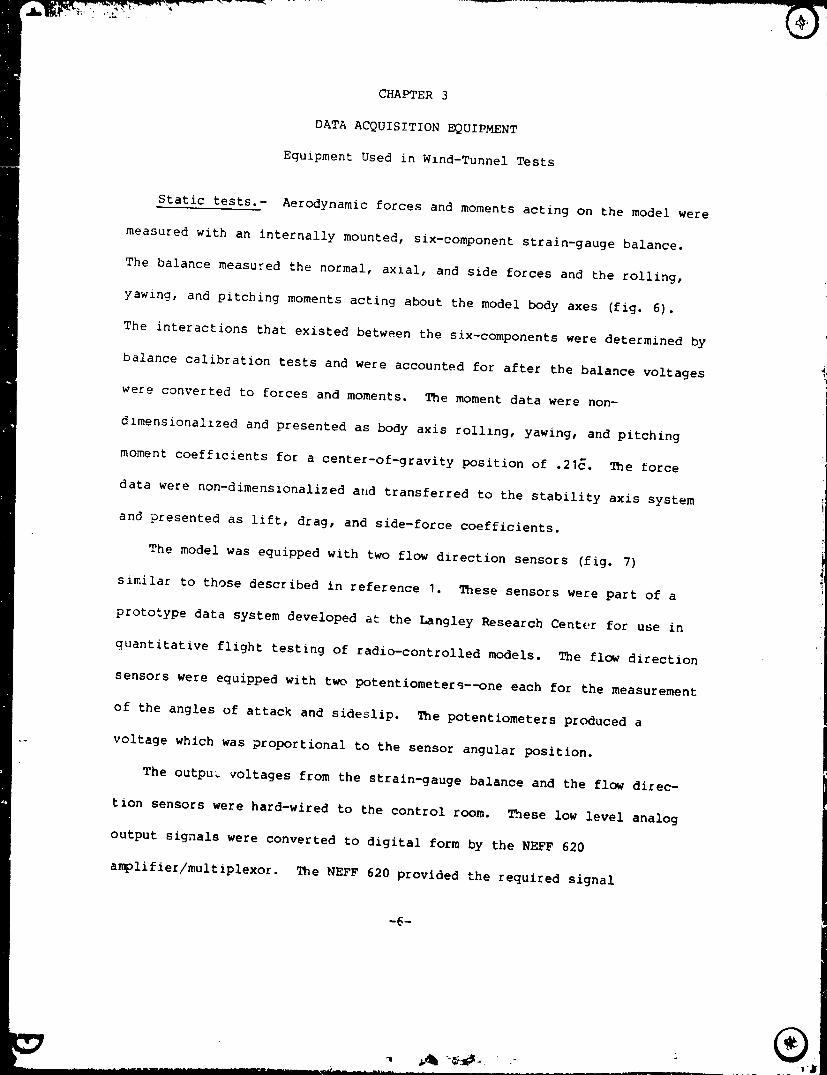
Static tests.- Aerodynamic forces and moments acting on the model were

measured with an internally mounted, six-component strain-gauge balance.

The balance measured the normal, axial, and side forces and the rolling,

yawing, and pitching moments acting about the model body axes (fig. 6).

The interactions that existed between the six-components were determined by

balance calibration tests and were accounted for after the balance voltages

were converted to forces and moments. The moment data were non-

d imensionallzed and presented as body axis rolling, yawing, and pitching

moment coefficients for a center-of-gravity position of .215. The force

data were non-dimensionalized alld transferred to the stability axis system

and presented as lift, drag, and side-force coefficients.

The model was equipped with two flow direction sensors (fig. 7)

similar to those described in reference I. These sensors were part of a

prototype data system developed at the Langley Research Center for use in

quantitative flight testing of radio-controlled models. The flow direction

sensors were equipped with two potentiometers--one each for the measurement

of the angles of attack and sideslip. The potentiometers produced a

_ voltage which was proportional to the sensor angular position.

The outpu_ voltages from the strain-gauge balance and the flow direc-

tion sensors were hard-wired to the control room. These low level analog

output signals were converted to digital form by the NEFF 620

amplifier/multiplexor. _ne NEFF 620 provided the required signal

--6--

®i,

198501065-3-017

ii_ conditioning, amplification, filtering, and multiplexing. The digital out-r-

i put from the NEFF 620, in 16-bit binary word format, was fed into a

i HP-9845B mlni-computer, At each test condition, the measured parameters

I! were sampled 100 times over a period of about 21 seconds. The computer

averaged these 100 measurements and converted the average to engineering

_ units. Print-outs and plots of the data were available on the CRT display

_. and/or the prin_er. The reduced data were stored on a magnetic tape.

I The flow direction sensors were mounted on a 6.44 mm (.25 in.) diameter

cylindrical rod which positioned them in front of each wing tip. The sen-

sor pivot was located 17.7 cm (6.97 in.) or .79c in front of the leading

edge of the wing. The pivot was located 73.5 cm (28.9 in.) outboard from

the center line of the model. The sensors were instrumented to measure the

local angles of attack and sideslip.

The flow direction sensors were thoroughly calibrated once they were

installed on the model in the tunnel. Both the angle-of-attack and angle-of-

sideslip sensors were calibrated using a specially designed calibration

protractor. These calibrations were checked daily for changes in the zero

values. Under these closely controlled conditions, the angle-of-attack

measurements were repeatable within I°. Because the sideslip potentiometer

was smaller and less sophisticated than the angle-of-attack potentiometer,

the angle-of-sideslip measurements were repeatable to within only 2°.

Rotar[ tests.- A six-component strain-gauge balance was used to

measure the forces and moments acting on the model while subjected to rota-

tional flow conditions. As in the static tests, the strain-gauge balance

measured the forces and moments acting abeut the model body axes. Again,

the data were adjusted to account for the balance interactions. The data

-7-

1985010653'018

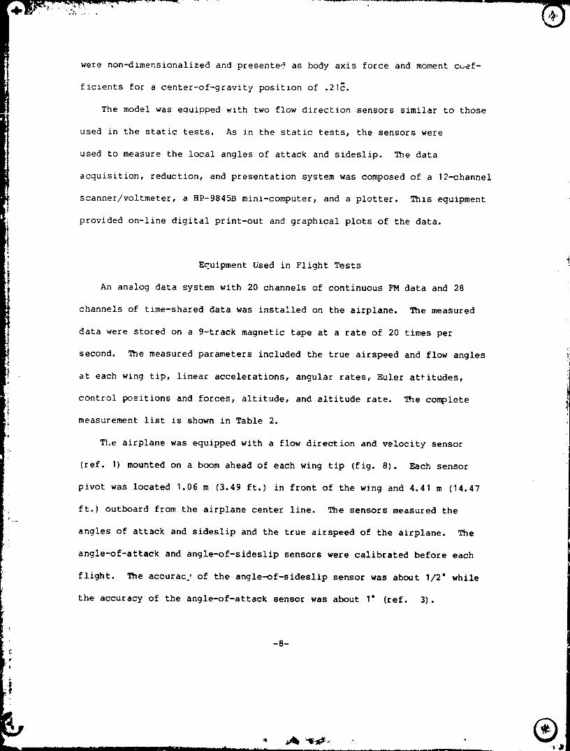
were non-dimensionalized and presented as body axis force and moment cuef-

ficients for a center-of-gravity position of .21_.

The model was equipped with two flow direction sensors similar to those

used in the static tests. As in the static tests, the sensors were

used to measure the local angles of attack and sideslip. The data

acquisition, reduction, and presentation system was composed of a 12-channel

scanner/voltmeter, a HP-9845B mini-computer, and a plotter. This equipment

provided on-line digital print-out and graphical plots of the data.

Equipment Used in Flight Tests I

,q

An analog data system with 20 channels of continuous FM data and 28

I

channels of time-shared data was installed on the airplane. The measured

data were stored on a 9-track magnetic tape at a rate of 20 times per

second. The measured parameters included the true airspeed and flow angles

wing tip, linear accelerations, angular rates, Euler attitudes,at each

control positions and forces, altitude, and altitude rate. The complete:Ii

measurement list is shown in Table 2.

TLe airplane was equipped with a flow direction and velocity sensor

(ref. I) mounted on a boom ahead of each wing tip (fig. 8). Each sensor

pivot was located 1.06 m (3.49 ft.) in front of the wing and 4.41 m (14.47

ft.) outboard from the airplane center line. The sensors measured the

angles of attack and sideslip and the true airspeed of the airplane. The

angle-of-attack and angle-of-sideslip sensors were calibrated before each

flight. The accuracy of the angle-of-sideslip sensor was about I/2" while

the accuracy of the angle-of-attack sensor was about I" (ref. 3).

-8-

i

1985010653-019

Linear accelerations were measured by a triad of accelerometers mounted

on the floor near the airplane center-of-gravity location. Angular rates

were _o _........a_=u by three rate gyros mounted orthogonally on a two-level

i instrumentation rack The rack was located behind the front seats and alsoL

i contained the attitude gyros, signal conditioning equipment, power

supplies, and tape recorder.

®

" 1985010663-020

CHAPTER 4

TEST TECHNIQUES AND TESTS CONDITIONS

Wind-Tunnel Tests

Static tests.- The I/6-scale model of the research airplane was tested RTI

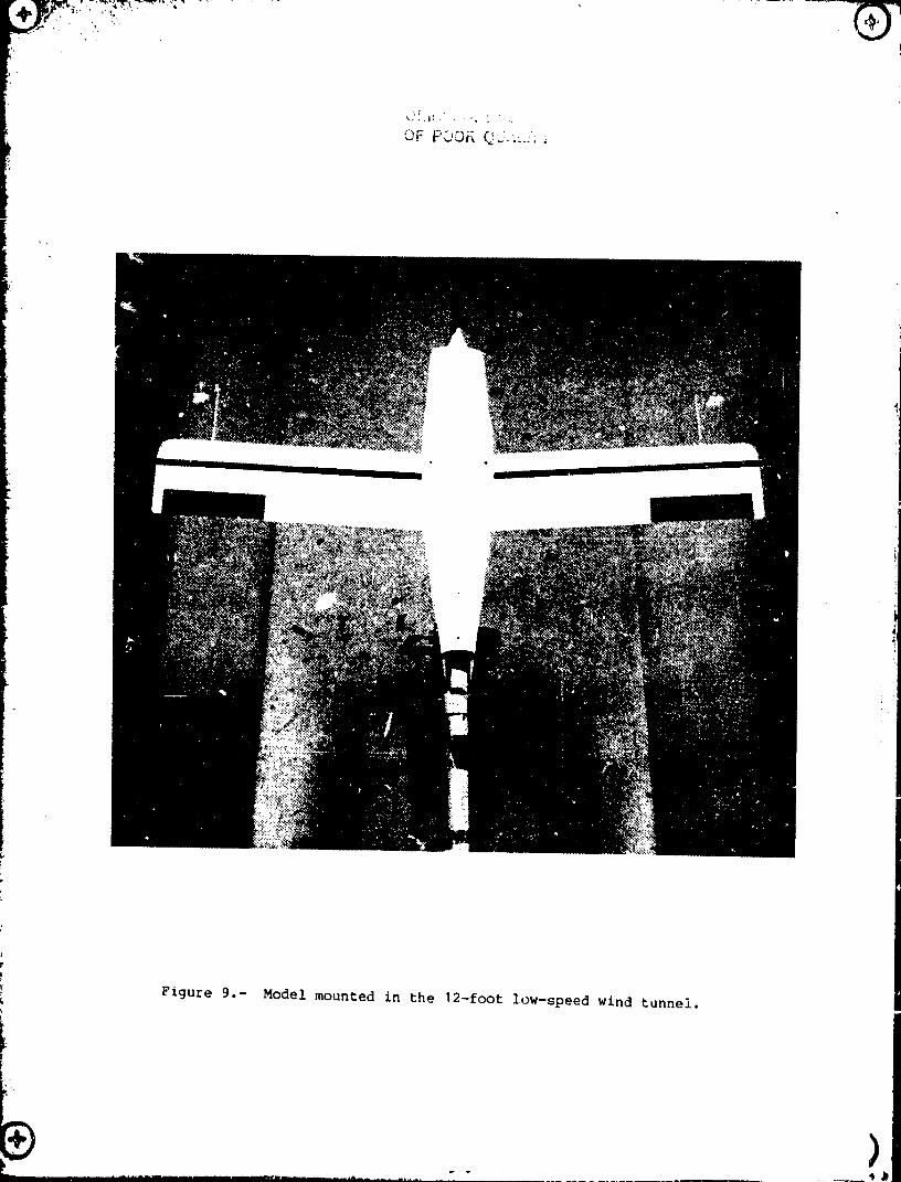
at the Langley Research Center in the 12-foot low-speed wind tunnel which

has a 3.66 m (12 ft.) octagonal test section. Figure 9 shows the model

mounted in the wind tunnel. Most of the tests were conducted at a free

stream dynamic pressure of 4 psf which corresponded to a Reynolds number of

0.27 x 106 , based on the mean aerodynamic c_,ord of the wing. Data were

obtained over an angle-of-attack range from 0" to 85" and an angle-of-

sideslip range from -20 ° to 20 °. No corrections were made to the data for

jet boundary, blockage, or wall effects. Because the force and moment data

were used only to show trends, the data were not corrected for upwash

(about 2 ° for this test).

The leading-edge droop modification discussed previously was tested in

two lengths. The outboard droop extended from 57- to 95-percent b/2 on

each wing and the full-span droop extended from the fuselage to 95-percent

b/2 on each wing. Figure 10 shows the outboard droop leading-edge modifi-

cation attached to the model. The effects of aileron deflections, sensor

location, angle of sideslip, and Reynolds number on the flow correction

were also investigated.

To account for flow irregularities in the tunnel, a calibration was

conducted. To accomplish this, the boom and sensor were removed from the

model and placed in a calibration apparatus. This apparatus positioned the

boom and sensor at the same point in the tunnel as they were when mounted

on the model. With the model out of the tunnel and the boom and sensor in

-10-

1985010653-021

i ii m tl)!

bration setup, the sensor measured the true or free-stream angles

to ?0 ° and at angles of attack from 0 ° to 85 °.

After the calibration runs were made, the boom and the sensor were

mounted on the model and the model tests were started. In this con-

figuration the sensor gave the - _sured angles of attack and sideslip as a

function o[ the mounting strut angle (fig. 11(b)).

Rotary tests.- The I/6-scale model of the research airplane was also

tested in the Langley Spin Tunnel using the rotary-balance apparatus (fig.

12 and ref. 12). The tests were conducted at an airstream velocity of 7.6

m/sec (25 ft/sec) which corresponded to a ReynolCs number of .12 x 106

based on the mean aerodynamic chord of the wing. The model was tested over

an angle-of-attack range from 8" to 90 ° at a zero sideslip angle. At each

angle of attack both static and rotary data were obtained. The rates of

rotation included _b values of .I, .2, .3, .4, .5, .6, .7, .8, and .9 in2V

both clockwise and counter-clockwise directions.

A calibration to account for flow irregularities in the spin tunnel was

not conducted. It '_as felt that a flow calibration was not as necessary in

the spin tunnel as it was in the 12-foot low-speed wind tunnel. This was

due to the fact that during the rotary tests, data were taken as the flow

direction sensors swept around the tunnel, thus helping to average out the

i flow irregularities. One data point was the average of 80 measurements.

P

That is, 8 measurements were taken during each revolution for a _otal of 10

revolutions. Also, the static data were the average of 4 measurements,

each taken with the model rotated 90+ from the previous orientation.

-11-

®

1985010653-022

<i Flight Tests

Level flight tests.- The spin research airplane was flown in steady,

;_ s_raight and level flight at different airspeeds to obtain an airspeed and

angle-of-attack calibration. Data were taken at airspeeds ranging from the

maximum cruise speed to the minimum speed at which the airplane could main-

ii tain steady, level flight. At each airspeed the airplane was flown in

opposite directions and the results of the two runs were aveLaged. The

flight was made on a calm day at an altitude close to sea level. From

these runs a low angle-of-attack flow correction was determined.

Spin flight tests.- The research airplane was flight tested as part of

the Langley Research Center's general aviation stall/spin program. The

spin flight tests were conducted at the NASA Wallops Flight Center. Each

spin attempt was started at an altitude above 2438 m (8,000 ft.), often

close to 3048 m (10,000 ft.). Spins were entered by slowly decelerating at

idle power to a 1-g wings-level stall. At the stall break, prospin rudder

was applied followed by ailerons against the spin once the wing had dropped

90 °. On some of the spin flights the rocket system was actually fired in a

pro-spin direction. This was done to increase the spin rate of the

airplane in order to look for high angle-of-attack spin modes. During the

spin research program the airplane was flown with different center-of-

gravity locations and with a number of different leading-edge modifica-

tions. Data from many different steady spins were used to determine the

true angle of attack in the spin.

®ii

1985010653-023

CHAPTER 5

ANALYSIS TECHNIQUES

Static Wind-Tunnel Tests

To determine the flow correction, data from the desired model-in dataV

run as well as data from the appropriate calibration run were used. Tne

angle-of-attack flow correction, Ee, was the difference between the

measured and the true angles of attack at a particular strut angle (fig.

13(a)), that is

ea = _m - _t (I)

For data analysis, the angle-of-attack flow correction (e_), was plotted

against the measured angle of attack (am).

Initially, the flow correction was plotted against the measured angle

of attack for both the right and left sensors separately. Bowever, this

data showed some differences between the flow correction from the right

sensor and the flow correction from the left sensor. This difference could

be due to an asymmecrlc model, an asymmetric mounting of the sensors, a

difference between the sensors, or a difference in the flow field from one

side of the model to the other. Asymmetries in the model or between the

flow sensors were not suspected so the most likely explanation was a dif-

ference in the flow field. This explanation was backed up by an earlier,

unpublished flow survey of the tunnel. The survey showed as much as 2"

angularity difference between the point in the tunnel where the righ_ sen-

sor was located and the point where the left sensor was positioned. PartI

of this difference was accounted for by the model-out calibration runs.

However, once the model was mounted in the tunnel the flow angularity could

-13-

!

possibly change from the angularity that was measured during the calibra-

tlon runs. To take care of this difference the flow correction from the

right sensor was averaged with the flow correction from the left sensor.

Thls average flow correction was then plotted against the average of the

measured angles of attack from the right and left sensors.

To look at the effect of the angle of sideslip on the flow correction,

the flow correction from the right sensor was plotted against the measured

angle of attack from the right sensor. In this case, data from the right

sensor were used because the tunnel survey showed that the flow quality was

better on the right side of the tunnel.

The angle-of-sideslip flow correction was determined in a manner simi-

lar to the method used in the calculation of the angle-of-attack flow

correction. That is, the angle-of-sideslip flow correction, eS' was the

dlfference between the measured and the true angles of sideslip at a par-

ticular strut angle (figure 13(b)):

e_ = 8m - 8t (2)

The angle-of-sideslip flow correction was also averaged, but in a

slightly different manner. As the angle of attack increased, the noses of

the sideslip sensors had a tendency to point toward the center line of the

airplane. This represented a positive sideslip inc_ement for the left sen-

sor ap] a negative sideslip increment for the right sensor. Thus, if the

angle-of-sideslip flow correction from both sensors was simply averaged,

_[ the resulting correction would be close to zero. To determine the magni-

i tude of the angle-of-sideslip flow correction,the correction from the right

! sensor was subtracted from the correction measured by the left sensor and

f the result was divided in half. That is:

-i -_-

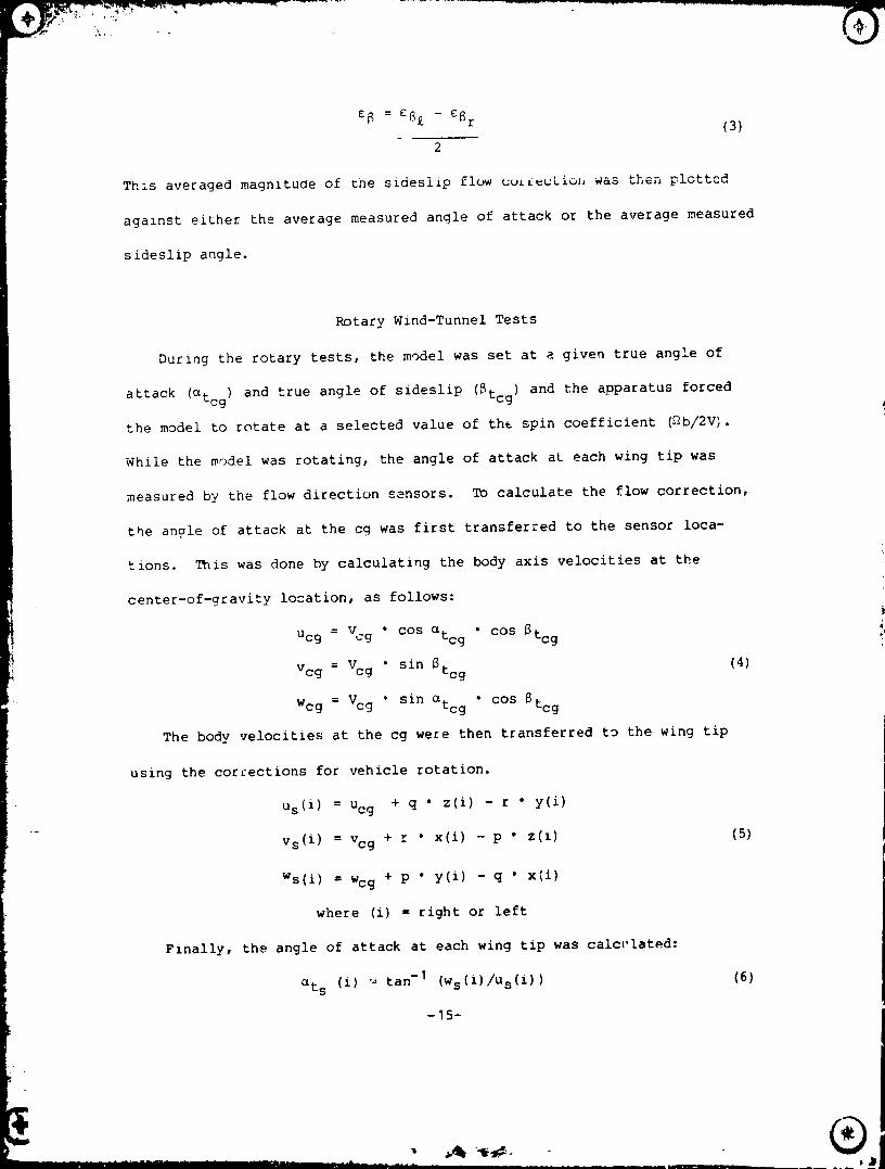
_ = E_ - _r (3)

2

This averaged magnitude of the sideslip flow _ULL_cLioJ_ was then _._v__^_^_

against either the average measured angle of attack or the average measured

sideslip angle.

Rotary Wind-Tunnel Tests

During the rotary tests, the model was set at a given true angle of

attack (_tcg) and true angle of sideslip (_tcg) and the apparatus forced

the model to rotate at a selected value of th% spin coefficient (_b/2V).

While the model was rotating, the angle of attack at each wing tip was

measured by the flow direction sensors. To calculate the flow correction,

the angle of attack at the cg was first transferred to the sensor loca-

tions. ThiS was done by calculating the body axis velocities at the

center-of-gravity location, as follows:

i

Ucg = Vcg • cos atcg • cos _tcg _

Vcg = Vcg • sin 8tcg (4)

Wcg = Vcg • sin Utcg cos 8tcg

The body velocities at the cg were then transferred to the wing tip

using the corrections for vehicle rotation.

Us(i) = Ucg + q • z(i) - r • y(i)

Vs(i) = Vcg + r • x(i) - p • z(i) (5)

Ws(i) = Wcg + p • y(i) - q • x(i)

where (i) = right or left

Finally, the angle of attack at each wing tip was calcL'lated:

ets (i) _ tan -I (Ws(i)/us(i)) (6)

-15-

- ®

............. l I

':1985010653-026

i

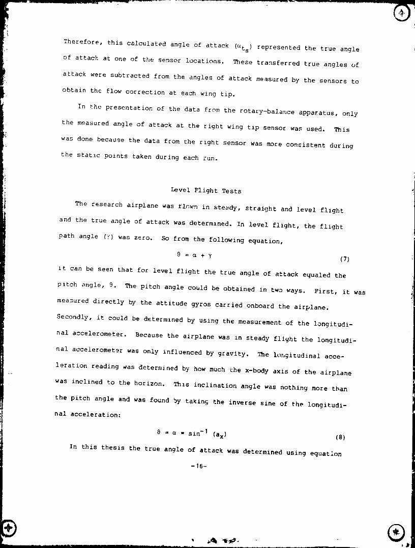
Therefore, this calculated angle of attack (_ts) represented the true angle

of attack at one of the sensor locations. These transferred true angles of!

attack were subtracted from the angles of attack measured by the sensors to

!,_! obtain the flow correction at each wing tip.

In the presentation of the data from the rotary-balance apparatus, only

the measured angle of attack at the right wing tip sensor was used. This

was done because the data from the right sensor was more consistent during

the statlc points taken during each _un. 1

Level Flight Tests

The research airplane was flown in steady, straight and level flight

and the true angle of attack was determined. In level flight, the flight

path angle (Y) was zero. So from the following equation, j

0 = _ + ¥ (7)

it can be seen that for level flight the true angle of attack equaled the

!

pitch angle, 9. The pitch angle could be obtained in two ways. First, it was

measured directly by the attitude gyros carried onboard the airplane.

Secondly, it could be determined by using the measurement of the longitudi-

nal accelerometer. Because the airplane was In steady flight the longitudi-

nal acceierometer was only influenced by gravity. The lon_itudinal acce-

leration reading was determined by how much £he x-body axis of the airplaneL_

was inclined to the horizon. This inclination angle was nothing more than

the pitch angle and was found by taking the inverse sine of the longitudi-

nal acceleration:

8 = e _ sin -/ (ax) (8)

In this thesis the true angle of attack was determined using equation

-16-

®

19-85010653-027

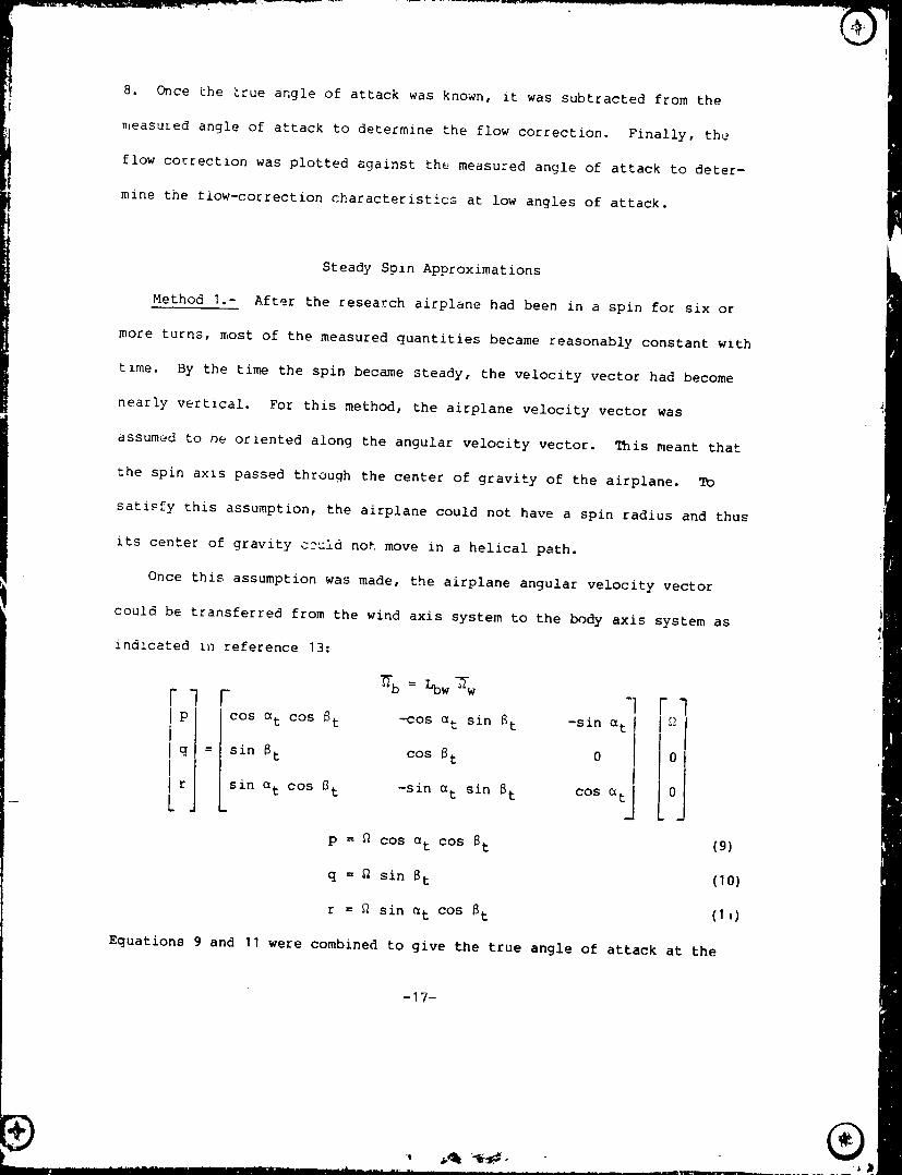
8. Once the _rue angle of attack was known, it was subtracted from the

measuLed angle of attack to determine the flow correction. Finally, the

flow correction was plotted against the measured angle of attack to deter-

mine the flow-correction characteristics at low angles of attack.

Steady Spin Approximations

Method I.- After the research airplane had been in a spin for six or

more turns, most of the measured quantities became reasonably constant with

time. By the time the spin became steady, the velocity vector had become

nearly vertical. For this method, the airplane velocity vector was

assumed to be oriented along the angular velocity vector. This meant that

the spin axis passed through the center of gravity of the airplane.

satisfy this assumption, the airplane could not have a spin radius and thus

its center of gravity c__ula not move in a helical path.

Once this assumption was made, the airplane angular velocity vector

could be transferred from the wind axis system to the body axis system as

ind!cated in reference 13:

--F7 [ - "7I P cos a t COS St -COS e t sin 8t -sin at

iI q = sin St cos 8t 0 0

II r sin a t cos 8 t -sin a t sin St cos _t 0

- [

p = _ cos _t cos Bt (9)

q = _ sin 8t (10)

r = _ sin c*t cos St (I ,)

Equations 9 and 11 were combined to give the true angle of attack at the

-17-

6 53- 02'8

f gravity of the airplane in a steady spin:

I a = tan-1(_ 1 (12)

tcg /

The equatioi_s for the angular rates could also be used to compute a

true angle of sideslip at the center of gravity of the airplane in a steady

spin. Equations 9 and 10 were combined to yield:

_tcg = tan -I atcg (I3)P

To determine the flow correction, the measured angles of attack at the wing

tips were transformed to the center-of-gravity location. This was done by

first converting the flow direction and velocity sensor readings into body

velocity components, yielding:

Us(i) = Vm(i) • cos am(i) • cos Bin(i)

vs(i) = Vm(i) • sin Bm(i) (14)

Ws(i ) = Vm(i) • sin am(i) • cos 8re(i)

where (i) = right or left

The body velocities at the wing tip were transferred to the center-of-

gravity location using the corrections for vehicle rotation as follows: I

Ucg(i) = Us(i) + r • y(i) - q ° z(i) Ii

Vcg(i) = Vs(i) + p " z(i) - r • x (i) (15)

Wcg(i) = Ws(i) + q • x(i) - p • y(i)

The body velocities at the center-of-gravity location were first

averaged an4 then were reconstructed into the desired information. This

proceeded as follows:

Ucg = Ucg (L) + Ucg (R)2

-18-

®

;1§85'010653-029

/' =

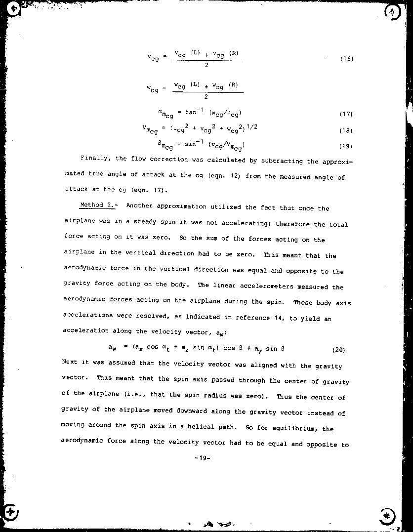
Vcg Vcg (L) + Vcg (R) (16)2

w = Wcg (L) + Wcg (R)2

amcg = tan -I (Wcg/Ucg) (17)

= ,_ 2 + + 1/2 (18)Vmcg , c9 Vcg 2 Wcg2)

_mcg = sin -I (Vcg/Vmcg) (19)

Finally, the flow correction was calculated by subtracting the approxi-

mated true angle of attack at the cg (eqn. 12) from the measured angle of

attack at the cg (egn. 17).

Method 2.- Another approximation utilized the fact that once the

airplane was in a steady spin it was not accelerating; therefore the total

force acting on zt was zero. So the sum of the forces acting on the

airplane in the vertical direction had to be zero. This meant that the

aerodynamic force in the vertical direction was equal and opposite to the

gravity force acting on the body. The linear accelerometers measured the

aerodynamic forces acting on the airplane during the spin. These body axis

accelerations were resolved, as indicated in reference 14, to yield an

acceleration along the velocity vector, aw:

aw = (ax cos _t + az sin et) cos _ + ay sin 8 (20)

Next it was assumed that the velocity vector was aligned with the gravity

vector. Th_s meant that the spin axis passed through the center of gravity

of the airplane (i.e., that the spin radius was zero). Thus the center of

gravity of the airplane moved downward along the gravity vector instead of

moving around the spin axis in a helical path. So for equilibrium, the

aerodynamic force along the velocity vector had to be equal and opposite to

-19-

........ ,i I I

1985010653-030

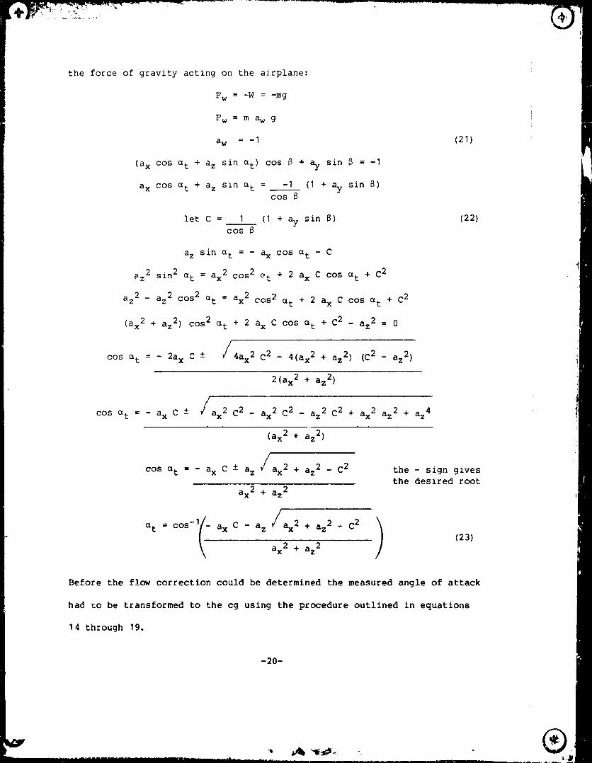
the force of gravity acting on the airplane:

Fw = -W = -mg

Fw= m awgmm

aw = -I (21) l

(ax cos a t + az sin at) cos 8 + ay sin _ = -I

ax cos a t + az sin at = -I (I + ay sin 8)cos

let C = I (I + ay sin 8) (22)cos 8

az sin at = - ax cos a t - C

_z 2 sin2 at = ax2 c°s2 _t + 2 ax C cos a t + C 2

az2 - az2 cos2 at = ax2 cos 2 at + 2 ax C cos a t + C2

(ax2 + az 2) cos 2 a t + 2 ax C cos at + C2 - az2 = 0

cos a t = - 2ax C + /4ax2 C 2 - 4(ax2 + az 2) (C2 - az 2)

2(ax 2 + az 2)

cos a t = - ax C + /ax2 C 2 - ax2 C2 - az2 C 2 + ax2 az 2 + az 4

(ax 2 + az 2)

cos at = - ax C + az /ax2 + az 2 - C2 the - sign givesthe desired root

ax2 + az 2

. (23)

ax2 + az2

Before the flow correction could be determined the measured angle of attack

had to be transformed to the cg using the procedure outlined in equations

14 through 19.

-20-

1985010653-031

_' Steady Sp_p _alysls

_ method to calculate the flow direction angles during a steady spin

;! detailed manner in the Appendix. The method used the linear accelerations,

i} body angular rates, and the vertical velocity to compute the true angles of

attack and sideslip at the airplane cg. Again, to calculate the flow

_ correction, the measured angles of attack and sideslip had to be trans-

i_ formed to the cg as indicated above.

:i4

_' -21-

r

[- q®--_- ___ ill ml_l I ............... nil -- , ........ _

.... .., .... iI ......... - .A .. "-

1985010653-032

CHAPTER 6

RESULTS AND DISCUSSION

Static Wind-Tunnel T_ts

• Force and moment data.- The force and moment characteristics of the

L

basic model are shown in figure 14. The model exhibits lift and drag

characteristics typical of general aviation airplanes. The lift curve

i! reaches a maximum value at an angle of attack of 12 °. After the stall the

! lift curve slope becomes negative and the lift curve reaches a local mini-

_ mum at an anqle of attack of 20" The lift curve exhibits a local maximum_! - .

at an angle of attack between 30 ° and 40 ° after which the lift coefficient

decreases continuously up to 85 ° angle of attack. The stall can also be

determined from the drag curve as evidenced by the large increase in slope

at an angle of attacL _ 12 °. The drag coefficient continually increases

from 0 ° :o 85 ° ang_ of attack. The pitching-moment coefficient shows the

configuration is unstabl_ up t _ t_e stall angle of attack. However, this

is to be expected since the model ,_a£ tested without a horizontal tail.

The resultant-force cc_fficient, fig, 15, is a combination of the lift

and drag coefficients. It exhibits the decrease in lift after the stall as

well as the large rise in the drag coefficient at the larger angles of

attack.

Figure 16 compares the lift coefficient data for the basic con-

L figuration with that for the model with the outboard droop and the full-

span droop leading-edge modifications. The configuration with the

outboard-droop modification exhibits similar stall characteristics but

increased lift in the middle of the angle-of-attack range, when compared

with the basic configuration. The full-span droop leadlng-edge modifica-

_t

-22-

®

1985010653-033

tion increases both the maximum lift coefficient attainable and the stall

angle of attack. The full-span drooped wing produces more lift than the

basic wing over an angle-of-attack range from 10" to 50 °. These lift coef-

ficient trends for the model with the two different leading-edge modifica- I

!tions are similar to the data for the same modiflcations tested on a dif-

ferent configuration in reference 16.

The effect of small changes of the Reynolds number on the lift coefficient

of the model is shown in figure 17. The data show the well known increase of

llft coefficient with Reynolds number (ref. 17).

Basic angle-of-attack flow correction.- A plot of the true angle of

attack versus the measured angle of attack for the basic model at zero

sideslip is shown in figure 18. The flow correction is the difference bet-

ween the data and the a t = am line. The data was fit with a regression

analysis program which gave the following Ist order fit:

a t = -1.22 + .870 um (24)

The correlation coefficient was 0.9994 which indicates that the regression

equation fit the data very well. Therefore, knowing the measured angle of

attack of an airplane in flight, this regression equation may be used to

determine the true angle of attack of the airplane.

The flow correction corresponding to the data from figure 18 is plotted

against the measured angle of attack in figure 19. The data show a reduc-

tion in the flow correction after the stall angle of attack. This reduc-

tion is due to the loss of llft on the wing after the stall. At an angle of

attack of about 20", the flow correction starts to inc: _; ;e again. This

increase occurs at almost the same angle of attack that the lift coefficient

[I begins increasing age_n. The flow correction reaches a maximum of slightly more

_| -23-

t ®

than 12° at a measured angle of attack of abou_ 95 ° It appears that the flow

correction is dependent on the drag as well as the lift because the general

shape of the flow correction curve resembles the shape of the resultant-force

I coefficient shown in figure 15.

• From this flow correction data it may be seen that for an airplane in a

i

flat spin (an angle of attack near 90°), using the measured angle of attack

instead of the true angle of attack results in an error of 15%.

Effect of wing configuration changes.- During the course of the

stall/spin program, many wing modifications were evaluated as to the degree

of spin resistance they provided. Also, the effect of the controls on the

spin entry, developed spin and recovery was evaluated. The addition of

modifications to the wing or the deflection of the ailerons will change the

flow over the wing and therefore could possibly change the flow correction.

A number of tests were run to evaluate the effect of wing modifications and

aileron deflections on the flow correction.

The effect on the flow correction of adding the outboard drc_p to the

wing is shown in figure 20. The modification increases the flow correction

slightly between 15" and 35 ° measured angle of attack. Tnis may be due to

the fact that the w_ng with the outboard droop modification produces a

larger lift coefficient than the unmodified wing over this angle-of-attack

range. This increased lift would cause increased upwash at the sensor

location, which would increase the flow correction.

Adding the full-span droop to the model effects the flow correction as

shown in figure 21. Again the flow correction is increased between 15" and

35 ° angle of attack. This increase may also be due to the larger lift coef-

ficient produced by the wing with the full-span droop over this angle-of-

attack range._ -24-

I II _n ,,,,,,,

1985010653-035

[ The drooped leadlng-edge modlflcations tested all seem to change the

flow correction. However, the differences were never larger than I" and m

often much less. The _t vs am data for the full-span droop modification I

rwere fit with the nth order regression program, resulting in the following

flt:

at = -1.49 + .870 Sm (25)

The coefflcients for the regression equation for the full-span droop data

were very similar to the coefficients for the basic data (egn. 24). Thus,

for the purposes of correcting the measured angles of attack in flight, the

drooped leading-edge modifications cause only a slight change in the

correction equation.

The effect of aileron deflection on the flow correction is shown in

figure 22. Deflecting the ailerons full down slightly increases the flow

correction while a full-up deflection slightly decreases the flow correc-

tion. This change in the flow correction could be related to the fact that

the deflection of the ailerons probably alters the lift on the wing.

One test was run with the ailerons deflected full up at the same time

the outboard-droop modification was mounted on the wing. The flow correc-

tion for this configuration is shown in figure 23. Again, the flow correc-

tion is changed slightly which is likely related to the change of flow over

the wing due to the wing modifications.

Effect of Reynolds number.- The effect of the test Reynolds ,_umber on

the flow correction is shown in figure 24. The tunnel was r1_n at dynamic

pressures of 3, 4, and 5 which resulted in Reynolds numbers of .23 x 106 ,

.27 x 106 and .30 x 106 , respectively. The flow correction appears to

increase as the Peynolds number increases. This is most likely related to

-25-

D

1985010653'036

the increase of lift coefficient with Reynolds number as shot;n in figure

17.

Effcct of senso_ luc_hiun.- For one test, the flow direction sensors

were moved forward until the pivot point was 23.7 cm (9.35in.) or 1.06 c in

front of the wing. As can be seen in figure 25 this change decreased the

flow correction. This is as expected because as the sensors are moved for-

ward, the influence of the wing on the flow at the sensors is reduced.

This sensor location is the same distance (measured in wing chords) in

front of the wing as the sensor used in the tests reported in reference 9.

In both tests the airfoils used were 60 series airfoils and both tests

exhibited a maximum flow correction of about 10° at a measured angle of

attack of 90° . This indicates that the flow correction is not affected by

small changes in the airfoil section.

Effect of angle of sideslip.- The effect of the angle of sideslip on

the angle-of-attack flow correction was also investigated. Figure 26 shows

the flow correction as a function of the measured angle of attack for the

right flow direction sensor. At angles of attack larger than 50 °, the flow

correction is reduced for positive angles of sideslip and is increased for

negative angles of sideslip. Apparently, the lift at the right wing tip is

increased for negative sideslip angles and decreased for positive sideslip

angles. Reference 17 shows similar trends, indicating that as the sweep

angle of a wing is increased, the lift is shifted from the upstream to the

downstream areas of the wing. However, this sweep effect would be expected

to occur primarily at angles of attack below the stall and therefore may

not exist at the larger angles of attack where the flow correction is

affected by the angle of sideslip.

-26-

....+.++.

.................... -= ................ 1985--01065303/

Basic angle-of-sideslip flow correction.- The flow correction to be

! applied to the angle-of-sideslip measurements, is shown in figure 27, as a

function of the average measured angle of attack. This figure shows that

i the sldesilp flow correction is also signlficant. The correction reaches a I

Imaximum of about 7° at the large measured angles of attack. This means

r

i that at the sensor location the local flow is skewed outboard by up to 7°

at each wlng tip. So if there is a need to know the angle cf sideslip in a

i spin accurately, the angle of sideslip flow correction should be _plied to

I the measured sideslip angles. To correct the measured sideslip angles the

average angle-of-sideslip flow correction presented in figure 27, should be

added to the measured sideslip angle at the right sensor and subtracted

i from the measured sideslip angle at the left sensor.

Effect of full-span droop modification.- The effect on the sideslip

i flow correction of adding the £ull-span droop leading-edge modification to[

! the model is shown in figure 28. The main difference is that the addition

of the wing modification reduces the sideslip flow correction over anr

angle-of-attack range from 15" to 40 °. The model has more lift in this

angle-of-attack range with the leading-edge modification on the wing. This

increases the wing loading and may tend to reduce the spanwise flow, thus

reducing the sideslip flow correction in this region.

Effect of angle of sideslip.- Figure 29 shows the effect of the angleL-

of sideslip on the sideslip flow correction as a function of the measured

angle of attack. The main effect of sideslipping the model is to reduce

the sideslip flow correction at large angles of attack.

Effect of angle of attack.- The variation of the sideslip flow

correction with the measured angle of sideslip, for different angles of

-27-

1985010653-038

attack, is shown in figure 30. At low angles of attack the sideslip flox,

correction is basically unchang£_ by the angle of sideslip. However, at

larger angles of attack,the sideslip flow correction exhibits a stronq

dependence on the sideslip angle. Again, it can be seen that the sideslip

flow correction increases wlth the angle of attack.

Rotary Wind-Tunnel Tests

The previous section presented the results of the flow correction

determined by static wind-tunnel teJts. This flow correction could be

applied to angle-of-attack data measured onboard an airplane during a spin.

Since the spin is an unsteady, rotational flight condition, however, it is

possible that a statically determined flow correction would not be adequate

in this situation. To determine if the static correction could be used,

the effect of rotation on the flow correction was investigated.

For this investigation the rotary-balance apparatus in the Langley Spin

Tunnel was used. The rotary-balance apparatus was found to have some

freedom of movement in the pitch direction. This freedom of movement

resulted in inaccurate data for the large rotation rates at the large

angles of attack. To avoid this region of uncertainty, data for lower

angles of attack and lower spin rates were used.

The first set of data used was from a run made with the model set at a

true angle of attack of 40" with ratrs of rotation from _bof -.8 to .8.2V

By using data over the full range of rotation, the measured angle of attack

at the right sensor varied from about 10" to 90° . In figure 31, this flow

correction data is compared with the static flow correction obtained in the

spin tunnel. _ithough there is consi@erable scatter in the data, the two

sets of data agree fairly well.-28-

............ -......... 1+85010653'039

from 20 to 90 . Thzs also resulted in a measured

angle-of-attack ranqe at thp right _cnso_ _Lom i0_ to 90 _. The flow

correction for this method is shown in figure 32 along with the spin tunnel

static flow correction. Again, there is some scatter in the data but the

two data sets show the same trend. From the data presented in figures 31

and 32, it appears that the presence of rotation does net greatly affect

the statically determined flow correction.

Level Flight Tests

The airplane was flown in steady, StLaight and level flight to de_r-

mine a low angle of attack flow correction. This data was not available

for the basic airplane so data taken with the outboard droop modification

on the wing were used. Figure 33 shows the comparison of the static wind-

tunnel data to the low angle of attack flight data. It can be seen that

i the wind-tunnel and flight data are in general agreement in this angle-of-

attack range.

Spin Flight Tests

Data from 15 steady spins were analyzed using the two approximate

methods and the method described in the Appendix. Some spins with dif-

ferent leading-edge modifications were used in order to find different spin

modes to cover a range of measured angles of attack. Data were also used

from spins where the rockets were fired in a pro-spin direction to obtain

spin modes at large angles of attack.

Steady spin approximations.- The two approximate techniques, used to

-29-

i

i

1985010653-0

estimate the true angle of attack of the airplane in a spin, were used with

some success. Figure 34 shows the angle-of-attack flow correction deter-

mined from the two techniques. The data shown are th_ re_u!ts for the best

8 spins for each method. The data show a reasonable amount of scatt;r

indicating that these methods probably should not be used if accurate

results are needed. However, these methods do indicate the trends of the

data. So if no wind-tunnel data are available these methods could be use4

to get an estimate of the angle-of-attack flow correction. Method #I did

not give satisfactory results for the sideslip angle during tne spin;

therefore, no angle-of-sideslip flow correction data are presented.

Steady spin analysis.- The angle-of-attack flow correction, determined

using the steady spin analysis, is shown in figure 35. The data shown are

the results of the analysis applied to 9 steady spins. The steady spin

analysis seemed to better determine the angle-of-attack flow correction

than _he approximat[ methods. In fact, it is encouraging that the wind-

tunr_l data agree with the flight data as well as they do. In general the

method did not give reasonable results for the angle-of-sideslip flow

correction; thus no data are presented.

-30-

1985010653-041

CHAPTER 7

SUMMARY OF RESULTS

The results of this investigation, te detcrmine corLections for £1ow

directlon measurements, may be s'_amarized as follows:

i I. The flow corrections to be applied to both the measured angle of

ii attack and measured angle of sidesllp were found to be substantial.

! 2. The a_gle-of-attack flow correction appee: s to be a function of the

I aerodynamic forces acting on the model.L_ 3. The effects of wing configuration changes and small Reynolds number

changes on the angle-of-attack flow correction were found to be small.

4. The angle of sideslip had a significant effect on both the angle-

of-attack and angle-of-sideslip flow corrections at large angles of attack.

5. me presence of spinning rotation did not appreciably alter the

angle-of-attack flow correction.

6. The angle-of-attack flow correction determined from the static

wind-tunnel tests was in agreement with the correction determined in level

flight.

7. The approximate analytical methods used to determine the flow

correction during steady spins did not appear to be as promising as the

more complete spin analysis techniques.

_ 8. If wind-tunnel data is not available, it would be preferable to use

results from any of the three methods to estimate the angle-of-attack flow

correction in a spin than to not apply a correction at all.

-31-

' ....................... 1-9 653 042-- IIII

, APPENDIX

CALCULATION OF FLOW DIRECTION ANGLES

a set of relations may be developed which can be used to calculate the

! angles of attack and sideslip of an airplane in a steady spin. This methodL

was p_oposed in reference 15 and is rederived here in a more complete

manner. This method utilizes the linear accelerations, angular rates, and

I the vertical velocity to compute the true angle of attack and true angle of

sideslip at the center-of-gravity location of the airplane.Because some of the measurements are made with respect to the airplane

body axes (the linear accelerations and angular rates) and others with

respect to the ground axes (the vertical velocity), the relationship bet-

ween tl,- two axis systems must be determined.

The ground axis system has its origin at the center-of-gravity location

of the a=rplane. _ne Zg axis point& vertically downward and is aligned with •

the gravity vector. The Xg axis is in the horizontal plane and points

!through the spin axis. The Yg axis is in the horizontal plane and is

mutually perpendicular to the Xg and Zg axes. The ground axis systems turns

with the center-of-gravity location of the airplane as the airplane travels

in a helical path about the spin axis. Figure 36 shows an instantaneous

arrangement of the ground axis system.

The angular velocity _f the airplane about the spin axis in the body

axis system may be determined from the body angular rates as shown=

_=p_+q_ +r _

I_I = /p2 + q2 + r 2

-32-

= """" ' ............ 1985010653-043

IBut the spin axis is vertical in the ground axis system, therefore:

_:I_I_

For an equilibrium spin, the resultant force or resultant acceleration

vector must be located in the XaZ a plane. Figure 37 shows the relationshipm

between the resultant acceleration and resultant rotation vectors. The f

resultant acceleration may be determined by the measured body linear

accelerations:

A = ax i + ay ]+ az

By using the Law of Cosines, the angle between the resultant acceleration

and the resultant rotation vectors may be found as follows:

1_-_12=1_12 +1_12-21_1.1_1cos_

X. _-_-. _-- A • n +e -_- =*. A+n • n- 2J_-J" I'n-I cos _

2A • n --2IXl" Jn'lcoso

cos a = p (ax) + q (ay) + r (az)

I;I.i_I

Once a is known, the resultant acceleration vector can be transferred into the

ground axis system:

IXxi"IXlsin

-33-

1985010653-044

IXzl--IXlcos

Since the airplane is in eqiulibrium, the aerodynamic acceleration in

the vertical direction must be equal and opposite to the acceleration ofTI

gravity, in other words:

IAzI:Ig

The center of gravity of the airplane exhibits a circular motion in the

Xg Yg plane; thus the velocity in this plane is in the Yg direction only

(i.e., U = 0). Also, the aerodynamic acceleration in the Xg direction must

be equal to the centrifugal acceleration in order for the airplane to be in

equilibrium:

•_ IXxlg_Ac

A--c = v 2

Rs

v =IrlR s

Ac=I_I2Rs2 "IAxlg

R s

Rs:IXxlg

I_I2

% °vl_lRs"IXxIgRs

vl_l-l_xlg-34-

1985010653-045

m

I AX, l.gV =

171

IVl / u2 2 2+V +W

W=-h,U=0

IV l =/ 2 " 2V + (-h)¢

tan-'(v)_hNext, we define a vector, Xg, which is parallel to the }'_. axis and

intersects the resultant acceleration vector at unit distance from origin

(see figure 37):

_J

Xg = A -cos a T[

IXl l_f

The direction comLzonents of Xg in the body axes are:

i = ax - cos o p

I_I 171

aj --_/_- cos (7__g_

IXl I_I

ak = z - cos (7 r

171 i_f

: -35-

i'

1985010653-046

I

f_gl=/Iif_ +jji_+Iki_

The

Yg axis is mutually perpepdicular to the Xg and Zc axes an| its']

_ direction may be fuund by the deflnltion of orthogonality: J^ ^

I " J= 0

^ ^

J " J = I

^

K " J-- 0

The directen cosines of the Yg axis in the body axes are found by the

solution of the following direction cosine equation:

m _ m q

£X mx nx £YI 0i

£y my ny my l = II

£Z mz nz ny I 0,m

Using Cramer's rule of determinants

I mx nx£y = _ = m Z nx - mX nZI mz nZ

q k j r£Y = _i - _/

I_-lIxgl Ixgfi_J

£X nx Imy = = £X nz - £Z nxl_z nzl

-36-

.... m ,mm,i ram, ,, ................ • x.......

1985010653-047

V

my = _ - _/

_ ny ! £x mXl= - [" ZZ mx - £X mz

! IZZ mZIi"

. _P__i i __9_ny =

! 11 x-g'l tx-g'llrrl

Next the direction cosines in the ground axis system are determined.

The direction cosines of the flight path are:

£v=0

I ----+mv - sin 6 - for right spins

+ for left spins

J

_V = COS

The direction cosines of the Yb body axis are:

£y = mx

ny = ± mz + for right spins- for left spins

The direction of the cosines of the Xb body axis are:

£x = £X

nx = ± £Z + for right spins- for left spins

-37-

®

1985010653-048

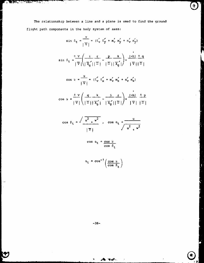
The relationship between a line and a plane is used to find the ground

flight path components in the body system of axes:

u

cos _ = = (Zv Zx + mv + nv nx)

Ivl

> ......... _ _ (;h__) ± pCOS _ = - +

IVl I_llx_"l I_g'll_l IVl I_1

2 2 uu w

cos at + , cos s t _ 2 2iv I u + w

COS ut = cos

cos 6t

_t.co.-,(oo._>oo6,_

-38-

I

'b

1985010653-049

REFERENCES

I. Kershner, David: Miniature Flow-Direction and Airspeed Sensor for

Airplane and Radio-Controlled Models in Spin Studies. NASA TP1467, 1979.

2. Alford, William J., Jr.: Theoretical and Experimental Investigation

of the Subsonic-Flow Fields Beneath Swept and Unswept Wings with

Tables of Vortex-Induced Velocities. NASA TN 3738, 1956.

3. Sliwa_ Steven M.: A Study of Data Extraction Techniques for Use in

General Aviation Aircraft Spin Research. Master's Thesis, GeorgeWashington University, September 1978.

4. Gracey, William: Summary of Methods of Measuring Angle of Attack onAircraft. NASA TN 4351, 1958.

5. Ribner, Herbert S.: Notes on the Propeller and Slipstream in Relationto Stability. NACA WR L-25, 1944.

_ 6. Milne-Thomson, L. M.: Theozetical Aerodynamics. Fourth Ed. DoverPublications, Inc., 1966.

7. Bowman, James S.; Stough, H. Paul; Burk, Sanger M.; and Patton, James

M.: Correlation of Model and Airplane Spin Characteristics for a

Low-Wing General Aviation Airplane. AIAA Paper No. _8-1977, August1978.

8. Moul, Thomas M.: Wind-Tunnel Investigation of the Flow Correction for

a Model-Mounted Angle of Attack Sensor at Angles of Attack From -10 °

_ to 110 °. NASA TM 80189, 1979.

9. Moul, Thomas M.; and Taylor, Lawrence W., Jr.: Determination of an

Angle of Attack Sensor C_rrection for a General Aviation Airplane at

Large Angles of Attack as Determined from Wind Tunnel and FlightTests. AIAA Paper No. 80-1845, August 1980.

10. O'Bryan, Thomas C.; Gcode, Maxwell W.; Gregory, Frederick D.; and

Mayo, Marna H.: Description of an Experimental (Hydrogen Peroxide)

Rocket System and Its Use in Measuring Aileron and Rudder

Effectiveness of a Light Airplane. NASA TP 1647, 1980.

11. Staff of the Langley Research Center: Exploratory Study of the

Effects of Wing Leading-Edge Modifications on the Stall/Spin

Behavior of a Light General Aviation Airplane. NASA TP 1589, 1979.

12. Mulcay, William J.; and Rose, Robert A.: Rotary-Balance Data for a

Typical Single-Engine General Aviation Design for an Angle-of-Attack

Range of 8" to 90"; I - Low-Wing Model C. }_SA CR 3200, 1980.

-39-

1985010653-050

13. Etkl_:, Bernard: Dynamics of Atmospheric Flight. John Wiley and Sons,

Inc., 1972.

14. Gainer, Thomas G.; and Hoffman, Sherwood: Summary of Transformation

Equations and Equations of Motion Used in Free-Flight and Wind-

Tunnel Data Reduction and Analysis. NASA SP-3070, 1972.

15. SOUI_, Hartley A.; and Scudder, Nathan F.: A Method of "_ightMeasurement of Spins. NACA Report No. 377, 1931. Yl

16. Newsom, William A., Jr.; Satran, Dale R.; and Johnson, Joseph L., Jr.:

Effects of Wing Leading-Edge Modifications on a Full-Sca e, Low-Wing

General Aviation Airplane--Wind-Tunnel Investigation of High Angle of

Attack Aerodynamic Characteristics. NASA TP 2011, 1982.

17. Hoerner, Sighard F.: Fluid-Dynamic Lift. Hoerner Fluid Dynamics,1975.

-40-

1985010653-051

TABLE I.- CHARACTERISTICS OF RESEARCH AIRPLANE

Maximum gross mass (normal category), kg (ibm) ............. 1110 (2450)

Engine kW (hp) ............................................... 130 (180)

Propeller di_,u_te[, m (ft) ................................... 1.93 (6.33)

Length, m (ft) ............................................... 7.84 (25.73)

Height, m (ft) ............................................... 2.50 (8.20)

Wing airfoil ................................................ NACA 632 A415

WingWing area,span, mm2(ft)(ft2)........................... . .".............. ..'''" 9.9813.56 (32.75)(146)

Wing chord, m (ft) ........................................... 1.34 (4.39)

Wing mean aerodynamic chord, m (ft) .......................... 1.34 (4.39)

Aspect ratio ................................................. 7.35

Dihedral, deg ................................................ 6.5

Aileron span, m (ft) ......................................... 1.64 (5.38)

Aileron area (each), m 2 (ft 2) ................................ 0.64 (6.93)

Aileron chord, m (ft) ........................................ 0.39 (1.29)

Vertical tail airfoil .............................. NACA 631 A012 modifiedVertical tail area, m2 (f_2) ............................ 1.36 (14.6)

Rudder area, m2 (ft 2) .......... i _.i.. . _ _ 0.43 (4.62)

Horizontal tail airfoil ............................ NACA 631 A012 modifiedHorizontal tail area, m 2 (ft 2) ............................... 2.51 (27.0)

Tail length (quarter chord of wing to quarter chord of vertical

tail), m (ft) ............................................... 4.14 (13.6)

Location of flow direction and velocity sensor pivot point:

Outboard from airplane center line, m (ft) ............... 4.41 (14.47)

Forward from leading edge of wing, m (ft) ................ 1.06 (3.49)

Maximum control deflections:

Ailerons, deg .......................................... 20 up, 10 down

Elevator, deg ........................................... 15 up, 2 down

Rudder, deg ......................................... 25 right, 25 left

-41-

f

TABLE II.- MEASUREMENT LIST FOR RESEARCH AIRPLANE

Measurement Range

Airspeed (rlght and left), m/sec (mph) .............. 0 to 89.4 (0 to 200) NAngle of attack (right and left), deg ......................... -30 to 150 v!Angle of sideslip (right and left), deg .............................. +60

Altitude, m (ft) ............................. -150 to 2896 (-500 to 9500)

X-axis acceleration, g units .......................................... +I

Y-axis acceleration, g units .......................................... -+I

Z-axis acceleration, g units ..................................... -6 to 3

Pitch rate, deg/sec ................................................. -+100

Roll rate, deg/sec .................................................. +290

Yaw rate, deg/sec ................................................... +290

Pltch attitude, deg .................................................. -+90

Roll attltude, deg .................................................. +180

Yaw attitude, deg ................................................... -+180

Stabilator deflector, deg ....................................... -16 tc 3

Aileron deflection (right and left), deg ................ 23 up to 10 downRudder deflection, deg ............................................... +30

Trim tab deflection, deg ....................................... -18 to 13

Flap deflection, deg ............................................. 0 to 35

Throttle, percent ............................................... 0 to 100 I_

Longitudinal wheel force, N (ib) ............................. +445 (+100)

Lateral wheel force, N (ib) ................................... +156 (-+35)

Rudder pedal force_ N (ib) ................................... -+667 (+150)

Engine speed, rpm .............................................. 0 to 2900

Rocket chamber pressure (right and left), MPa (psi) .. 0 to 2.07 (0 to 300)

Rate of climb, m/sec (ft/min) .............................. -+10.2 (-+2000)

Total temperature, °C (OF) .......................... -18 to 38 (0 to 100)

Impact pressure, kPa (psi) .......................... 0 to 3.45 {0 to .5)

/

®

1985010653-053

1985010653-054

o, (9

]9850]0653-055

,.'-!

1985010653-056

• . . ,,[,

LEADINGEDGEDROOPAIRFOIL

UNMODIFIEDAIRFOIL

Figure 4.- Wing leading-edge droop modification.

1985010653-057

i_

_ -- _--- 73.5 (28.9)----_ 166.4(65.5) "[

117.7(7.O)

22.3 (8.8)_ I ! I __L

i 108.6(42.8) _i

Figure 5.- Dimensions of the I/6-scale model in centimeters (inches).

1985010653-058

7

®

1985010653-059

(a) Photograph of the flow direction sensor.

6.9 =I

I_ 4.8 _II _---2.5 ---_

V

c45°.

(b) Dimensions (in cm) of the flow direction sensor.

Figure 7.- Flow direction sensor used in the wind-tunnel tests.

............... tc=- - ---a ...... II'l II ill i i , , ,, i .... d i ..... _ -- -- " _ _

1985010653-060

Figure 8.- Flow direction and velocity sensor used in the fligh_ tests.

.... . • * %

1985010653-061

OF POOii C_'..L'-,-.L_

Figure 9.- Model mounted in the 12-foot low-speed wind tunnel.

)" " ......._J

1985010653-062

, i! _'_/ ¸, _ 'v ¸ * "; _

®

1985010653-063

am

V[, m''_

OFTUNNEL _8 ,_S

(b) FLOWDIRECTIONMEASUREMENT

Figure 11.- Definition of the angles measured to determine the angle-of-attackflow correction.

1985010653-064

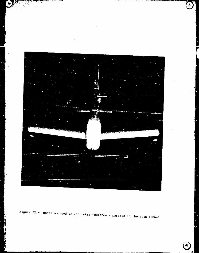
; Figure 12.- Model mounted on _he rotary-balance apparatus in the spin tunnel.f

i

®

1985010653-065

Vl, c Vl, m Vl, m Vl, c

Pl sp_

(b) Definition of the angle-of-sideslip flow correction.

Figure 13.- Definition of the angle-of-attack and angle-of-sideslip

flow correction.

1985010653-066

1.2

1.0 CCL, CD L

.8

I I I I I I I0 I0 20 30 40 50 60 70 80 90

a, deg

Figure 14.- Longitudinal force and moment data for the model.

1985010653-067

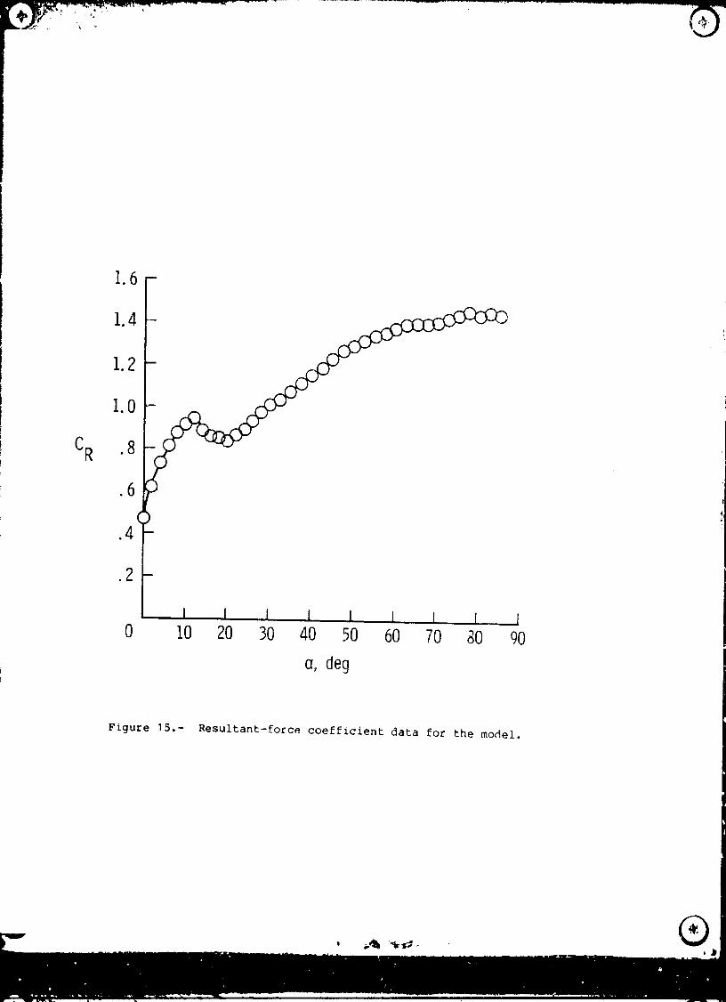
1.6F1.4

1.2

1.0

CR .8

.6

.4-

.2-

, I I ill [ I I 1 [ I0 10 20 30 40 50 60 70 30 90

a, deg

Figure 15.- Resultant-force coefficient data for the model.

1985010653-068

1985010653-069

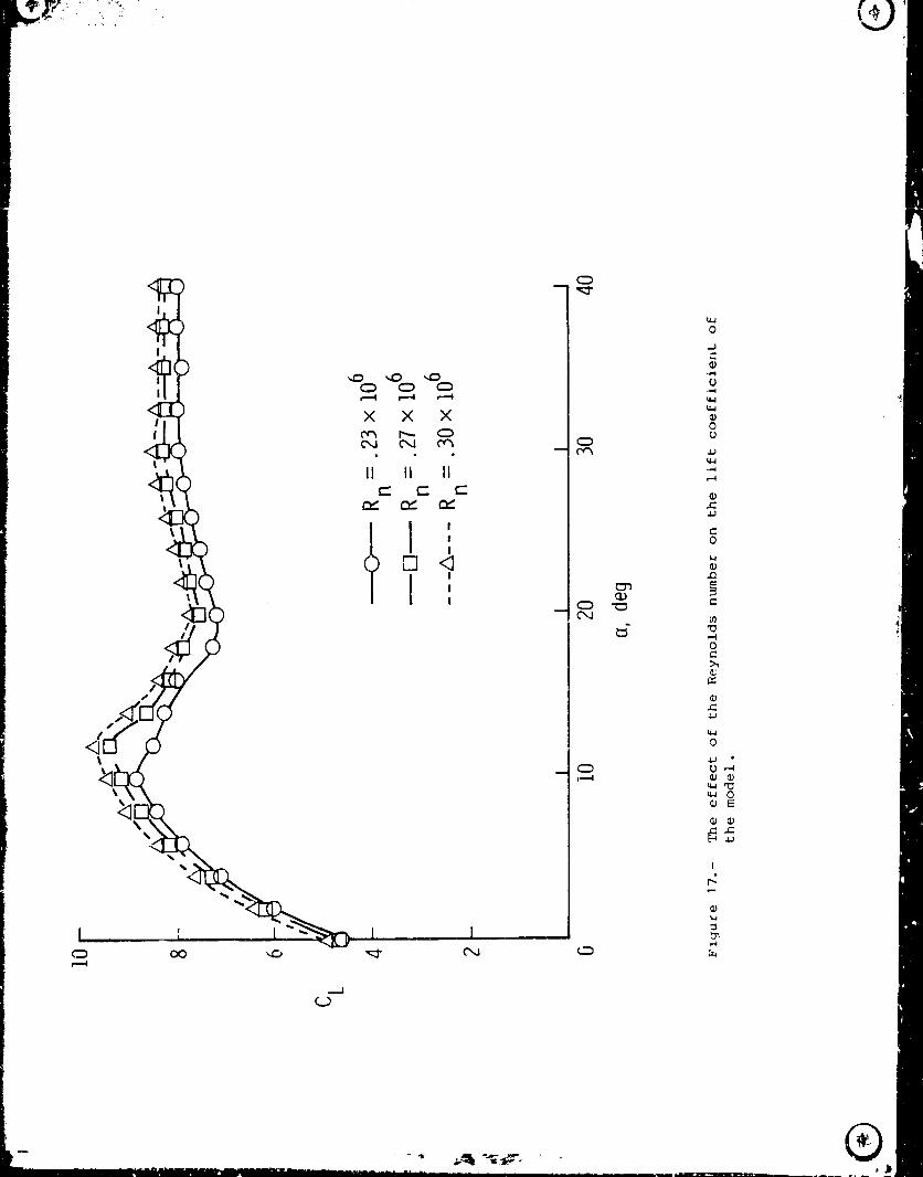
i

1985010653-070

1_ _ " •., :_ ,-.-_ .....

1985010653-071

®

1985010653-072

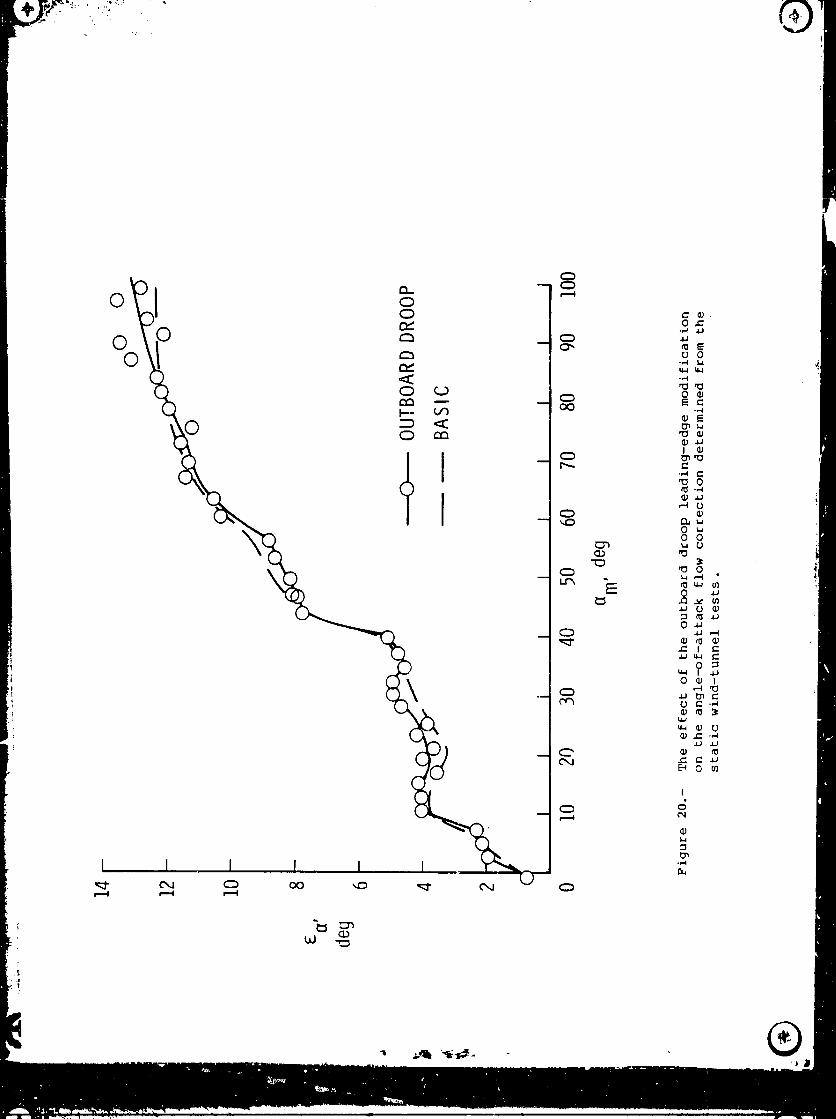
1985010653-073

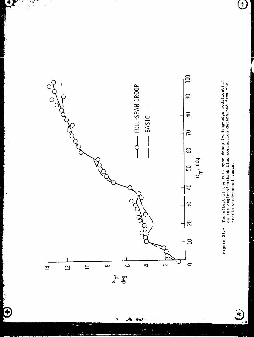
1985010653-074

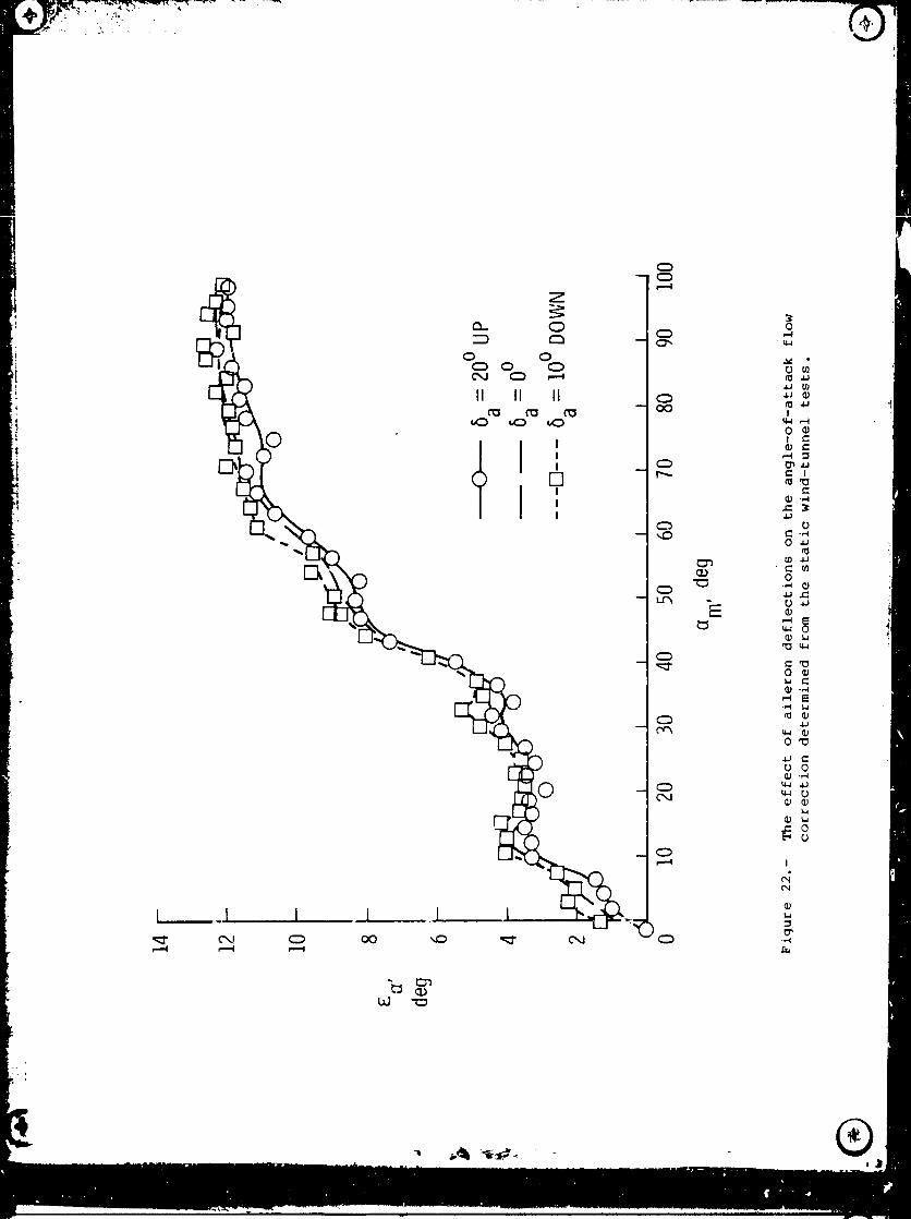
1985010653-075

1985010653-076

"J _

1985010653-077

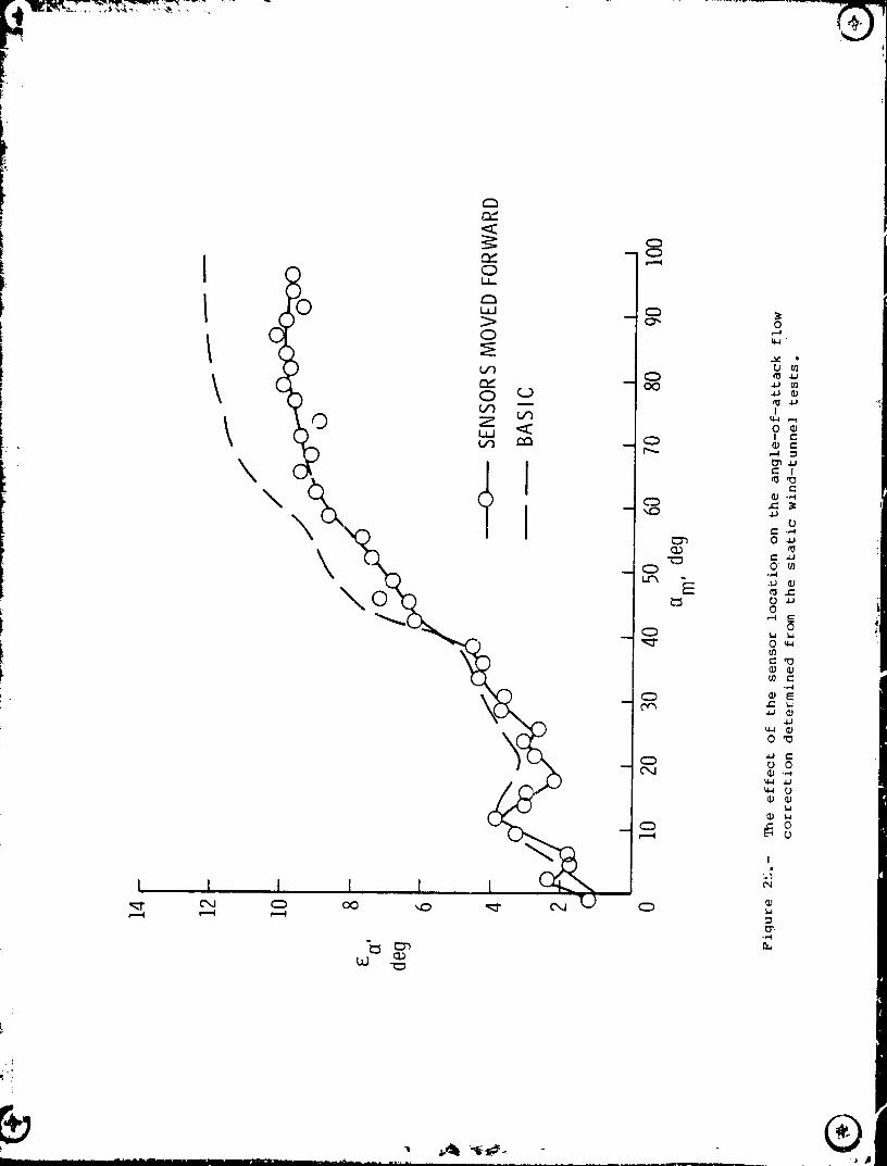
1985010653-078

_,_,_F,_. i,_,,:I̧ -,-

0--CD

r_

1985010653-080

I °

_J

1985010653-081

.i

®

1985010653-082

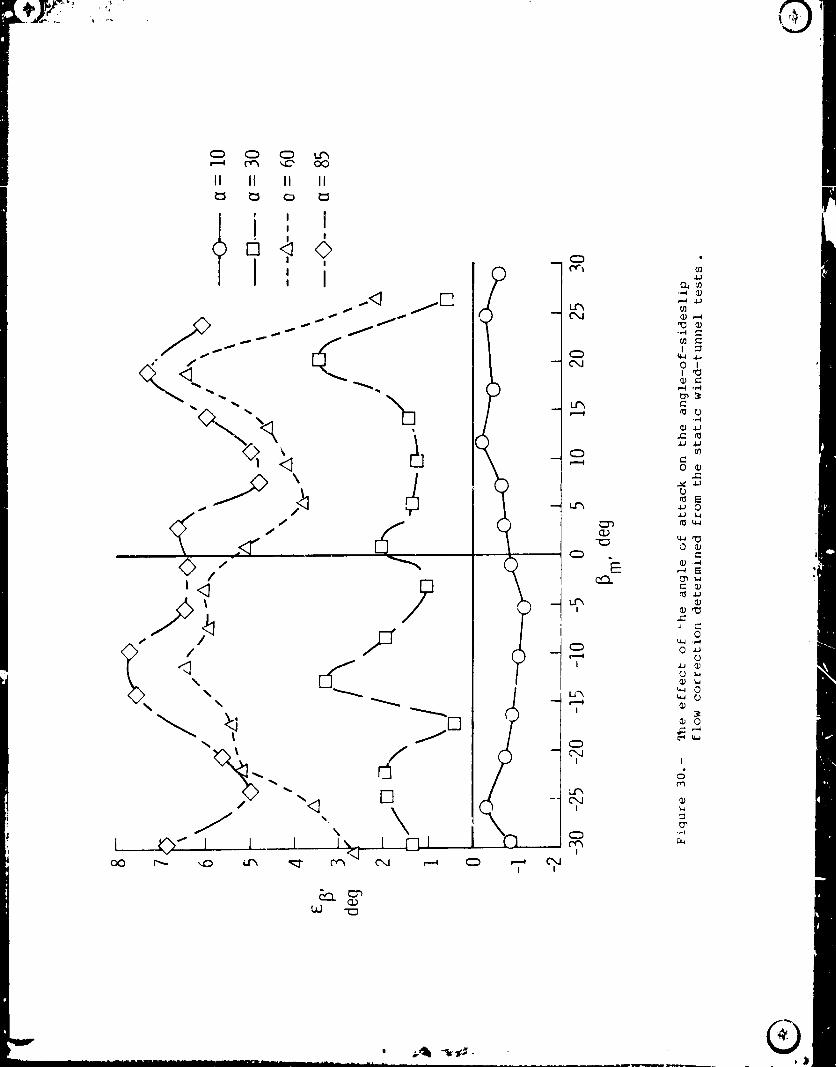
- ®' _ "_- . ...................... _ .... -_- ,iil| ii i_ _ _'

1985010653-083

_

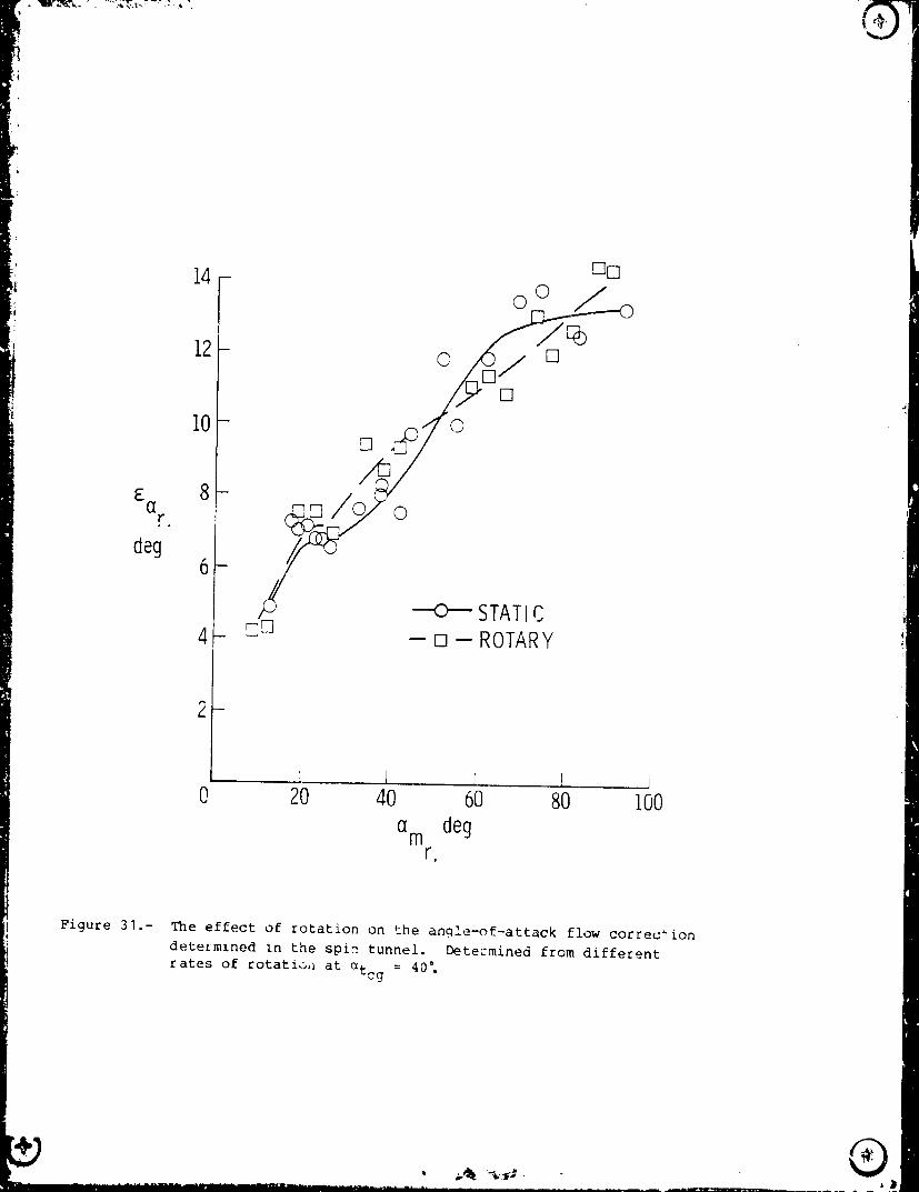
, I I I , ! ,,i0 20 40 60 80 I00

am degr,

Figure 31.- The effect of rotation on the angle-of-attack flow correction

determined in the spin tunnel. Detezmined from different

rates of rotatio,i at _tcg 40°.

®, _._ _-..#.",

1985010653-084

I _ I I i0 20 40 60 80 i00

am degr,

i

_,, Figure 32.- _he effect of roLation on the angle-of-attack =_low correction

determined in the spin tunnel. I_.termined from different

" angle-of-attack settings at :2b/EV = - .3.

i

1985010653-0,

4- O

l

E,

deg 09 --

STATICWIND-TUNNELDATA1 -

O_ --E:I---- LOWa FLIGHTDATA/

0 l 1 1 _j-5 0 5 I0 15

am, deg

Figure 33.- Comparison of the angle-of-attack flow correction determined f_omstatic wind-tunnel tests and from level flight tests.

1985010653-086

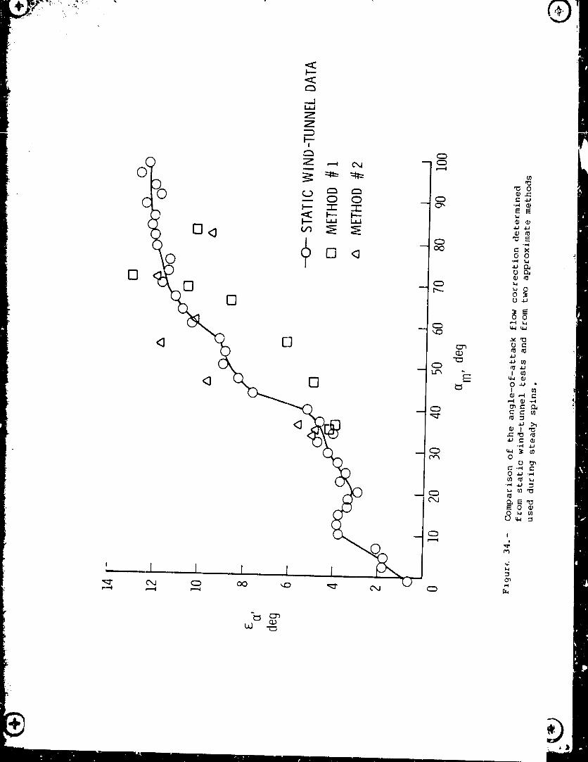
1985010653-087

(_

1985010653-088

I_ _ SPIN AX!St i

/

/

/

X

g _ CYLINDERON WHICHFLIGHTPATHLIES

CENTEROFCENTEROF

GRAVITY "-- _ yg ROTATION

--- FLIGHTPATHT

Zg

/

..- - +--j:.1

Figure 36.- Instantaneous arrangement of ground axis system.

1985010653-089

CENTEROFGRAVITY

,..,_Xg

- =1

COS_

Zg

Figure 37.- Relationship between resultant acceleration and resultantrotation vectors.

(9

1985010653-090