detection of natural gas pipeline defects using magnetic...
TRANSCRIPT
Detection of Natural Gas Pipeline Defects using Magnetic Flux Leakage Measurements
1Control and Intelligent Processing Center of Excellence, School of ECE, College of Engineering, University of Tehran, Iran
2Segal Pardazesh Engineering Co., Tehran, Iran
[email protected], [email protected], [email protected], [email protected], [email protected] Abstract: Magnetic Flux Leakage (MFL) testing is the most widely used non-destructive techniques for the in-service inspection of oil and gas pipelines. This study presents novel approaches to detect defects by employing MFL signals. Estimating the number of defects, locations, and orientations from measurements is a typical inverse problem in electromagnetic non-destructive evaluations (NDE). A detection algorithm on axial flux is proposed for defect detection based on image processing approaches and morphological methods. Finally, the efficacy and accuracy of the proposed algorithm is validated through examinations on simulated defects and real experimental MFL data. Simulated defects are generated in presence of multiple uncertainties and noises; including the variation of the pipeline thickness, sensors liftoff, magnetization level, and shape irregularity. Keywords: MFL, defect detection, image processing, axial flux, radial flux, non-destructive testing.
1. Introduction Natural gas is transported in most countries through a
vast network of buried and aboveground pipelines. The reliable supply and transportation of product in a safe and cost-effective manner is a primary goal of most pipeline operating companies and managing the integrity of the pipeline is paramount in maintaining this objective. However, with the influence of the long-term wear-out and variable surrounding conditions, the pipeline will always be deformed and corroded. If the situation is severe, it will cause oil-gas leakage, in turn; this will bring difficult problems to the safe operation [1-3]. So it is essential to have an effective method and means to inspect and appraise oil-gas pipelines regularly.
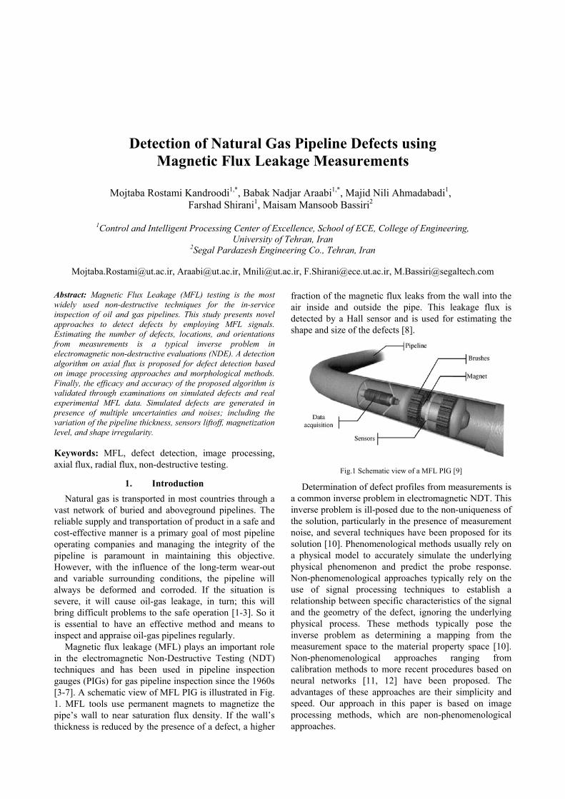
Magnetic flux leakage (MFL) plays an important role in the electromagnetic Non-Destructive Testing (NDT) techniques and has been used in pipeline inspection gauges (PIGs) for gas pipeline inspection since the 1960s [3-7]. A schematic view of MFL PIG is illustrated in Fig. 1. MFL tools use permanent magnets to magnetize the pipe’s wall to near saturation flux density. If the wall’s thickness is reduced by the presence of a defect, a higher
fraction of the magnetic flux leaks from the wall into the air inside and outside the pipe. This leakage flux is detected by a Hall sensor and is used for estimating the shape and size of the defects [8].
Fig.1 Schematic view of a MFL PIG [9]
Determination of defect profiles from measurements is a common inverse problem in electromagnetic NDT. This inverse problem is ill-posed due to the non-uniqueness of the solution, particularly in the presence of measurement noise, and several techniques have been proposed for its solution [10]. Phenomenological methods usually rely on a physical model to accurately simulate the underlying physical phenomenon and predict the probe response. Non-phenomenological approaches typically rely on the use of signal processing techniques to establish a relationship between specific characteristics of the signal and the geometry of the defect, ignoring the underlying physical process. These methods typically pose the inverse problem as determining a mapping from the measurement space to the material property space [10]. Non-phenomenological approaches ranging from calibration methods to more recent procedures based on neural networks [11, 12] have been proposed. The advantages of these approaches are their simplicity and speed. Our approach in this paper is based on image processing methods, which are non-phenomenological approaches.
Mojtaba Rostami Kandroodi1,*, Babak Nadjar Araabi1,*, Majid Nili Ahmadabadi1, Farshad Shirani1, Maisam Mansoob Bassiri2

MFL non-destructive evaluation of pipelines typically generates about 150 GB of data for every 100 km of pipeline inspected [3, 13-14]. Since the volume of MFL data is huge, traditional methods involving manual inspection of the data can be very time consuming. Moreover, the performance is depended on skills, training, emotional status, and the level of fatigue of analysts. Contrast to traditional non-automatic methods, the gas pipeline inspection industry is keenly interested in automatic methods for analyzing MFL data in order to improve accuracy and decrease turnaround time between actual pigging and the delivery of inspection results.
This paper proposes an approach for defect detection by employing MFL signals. The number of defects is achieved via a proposed image-based detection algorithm on axial flux. Also, locations and orientations of defects are achieved via this algorithm. The proposed algorithm is validated through examinations on simulated defects and real experimental MFL PIG data.
The rest of this paper is organized as follows. Section 2 gives an overview of the MFL PIG hardware and principle of it. Simulation and real defect databases are described in Section 3. Section 4 explains the proposed algorithm for defect detection. Section 5 discusses the results achieved via implementing the proposed method on simulated and real data sets. Section 6 concludes the paper indicating major achievements and discusses further scopes of works in this field.
2. MFL PIG Tool In this section, a MFL PIG tool is described. First, the
physical construction of the PIG tool is explained. Moreover, the technique of measuring MFL signals is presented. 2.1 Description of MFL PIG hardware
Pipeline inspection gauge (PIG) is a tool which is sent down to a pipeline by a launcher and the pressure of the product in the pipeline is used for pushing it along down the pipe until it reaches the receiving trap at the end of each run.
An Intelligent MFL PIG, the highly sophisticated instrument, includes mechanics, electronics, electromagnets, and sensory parts. Various sensors collect several forms of data such as magnetic flux, temperature, speed, etc. during the trip through the pipeline.
For the first time in Islamic Republic of Iran, a MFL PIG tool is designed and constructed with collaboration of Segal Pardazesh Part Co. and University of Tehran. It is constructed for inspection the 30 inch pipelines. The constructed MFL PIG is demonstrated in Fig. 2.
The designed MFL PIG body consists of two parts, front and rear. The front body contains batteries, data acquisition, electronics board, gyroscope sensors, Coil type sensors, and cup. The rear body contains magnets, brushes, odometer system, and Hall Effect sensors.
In next subsection, the MFL principle is explained.
Fig. 2 The MFL PIG designed and constructed with collaboration of Segal Pardazesh Part Co. and University of Tehran.
2.2 MFL Principle
The MFL PIG inspection is based on utilizing a known external magnetic field onto a ferromagnetic material and measuring the response via Hall sensors. By navigating the MFL tool into the pipeline, a magnetic circuit is created between the pipe wall and the tool. Brushes act as a transmitter of magnetic flux from the tool into the pipe wall. The high magnetic field saturates a piece of the pipe wall where is between two poles of magnets.
A volumetric wall loss in the pipeline wall acts as a region of high magnetic reluctance causing an increased magnetic leakage field. If the wall’s thickness is reduced in presence of a defect, a higher fraction of the magnetic flux leaks from the wall into the space inside and outside the pipe, allowing the defect to be detected in presence of increasing in leakage magnetic flux density.
Sensors array is placed at the center of the poles in the magnetic circuit to ensure that it is located in the most uniform part of the field. It records anomalies and changes in the magnetic field in both axial and radial directions with sufficient density to recognize even very small pipeline metal defects. The signals from the sensors are sampled and recorded on memory board as the PIG moves through the pipeline. Once the PIG is retrieved at the end of the inspection run, the stored signals are then processed. Fig. 3 depicts how a defect disturbs magnetic flow.
Fig.3 Sensor detection of magnetic flux leakage from an anomaly in pipe wall
In this work, as mentioned above, the MFL signals are
recorded in both axial and radial directions. The number of Hall Effect sensors is 448 for each direction. In addition, 88 coil type sensors are applied to discriminate between internal and external defects.
In the next section, experimental database collected by the MFL PIG is described. Moreover, the simulation database studied in this work is explained.

3. Database Description Defect database studied in this paper have two parts.
One is the simulated data, and the other is the real experiments data. 3.1 Simulated data
To accurately estimate the characteristics of defects, at the first, features of MFL signals should be investigated. So, artificial defects with various characteristics are simulated via COMSOL software.
The number of simulated defects is 477. They can be geometrically categorized in four classes; general, pitting, axial grooving, and circumferential grooving. 217 defects are ellipse shape that simulated in nominal conditions. 50 defects are simulated in different orientation with pipeline axis. 90 defects are simulated with different sensors lift-off. 80 defects are simulated at four pipe wall thicknesses. 40 defects have irregular geometrical profiles to study the effect of defect shape irregularity in MFL flux. Notice that all data simulated in presence of white noise.
3.2 Real Experiments data
The database is collected from inspection of pilot setup via intelligent MFL PIG. This pilot setup is provided by Iranian Gas Transmission Co. and designed for testing MFL PIGs. This setup contains 40 defects with different length, width, and depth in four classes that mentioned above. Experimental tests have been done under real conditions, noises and uncertainties. All experiments data are achieved by utilizing the MFL PIG constructed by cooperation between Segal Pardazesh Co. and University of Tehran on the pilot setup.
A real ellipse shape defect on the pilot setup is demonstrated in Fig. 4. The distinctive response in both axial and radial directions for this real is illustrated in Fig. 5.
In the next section the defect detection algorithm is presented.
4. Defect Detection Algorithm In this section, an automatic method based on image
processing techniques is proposed to detect metal loss defects. As mentioned before, the volume of MFL data is huge. Automatic defect detection is an important strategy to solve the problems with huge data. Hence, in this work, an automatic method is proposed to improve accuracy and decrease turnaround time between actual pigging and the delivery of inspection results.
In this work, MFL non-destructive evaluation of pipelines typically generates about 150 GB of data for every 100 km of pipeline inspected. Since a large volume of the MFL signal from a run usually contains the information that some of them are not corresponding to metal loss defects, separating only those parts of the MFL signal that contains the beneficial information about pipe
features or metal loss defects is necessary to decrease computational processing time and to increase computational efficiency. In this section, an algorithm is proposed to separate the mentioned parts of the MFL signal.
Fig.4 Ellipse shape defect on test pilot setup. (Length=85mm, Width=53mm, Depth=6.08mm or 36.9% wall loss).
0 50 100 150 200 250
0
200
400
6009
10
11
12
13
14
15
16
Pipe Axis (mm)
Axial Component
Circu. Axis (mm)
Sig
nal A
mpl
itude
(m
T)
Fig.5 (a) Axial component of MFL signal under the ellipse shape defect.
0 50 100 150 200 250
0
200
400
600-6
-4
-2
0
2
4
6
Pipe Axis (mm)
Radial Component
Circu. Axis (mm)
Sig
nal A
mpl
itude
(m
T)
Fig.5 (b) Radial component of MFL signal under the ellipse shape defect.
The algorithm is developed with considering seven steps in greater details as follows.

Input data: Row sensory data To ascertain the completeness and quality of the run,
the raw MFL data are first scanned for preliminary information on the quality, continuity, and duration of stored data.
As the largest pipeline length is 12m, we are interested that every part of the data contains data between two circular welds. The algorithm processes the row sensory data parts for one pipeline length in each run of the algorithm.
Pre-Processing First, data of each sensor are corrected with calibration
information achieved in prior experiments. Second, sensor alignments are carried out to arrange sensor blocks. After that, data are normalized such that malfunctions of Hall-Effect transducers during inspection and the variations in sensor lift-off alignment are corrected in this step. Let Si be the signal from the ith element in the sensor array on the PIG and N represent the total number of sensors in the array. The signal from a bad sensor is simply replaced by interpolating the signals from neighbouring sensors. If mi is the mean value of the signal measured by ith sensor, then the normalized data is obtained as:
Si =1,2,...,N( ) = Si + m−mi( ) (1)
where m denotes the median of all signal means. Finally in pre-processing step, the data is filtered to
eliminate noise due to sensor bounce, non-uniform pipe thickness, etc. The achieved signal can be used as the gray-scaled or coloured image for automatic detection in the next steps of the algorithm. A sample MFL image of the real data is illustrated in Fig. 6 (a).
Background and Wall Thickness Estimation In this step, 2D sliding window is defined on the data
such that it completely contains all data of the Hall Effect sensors and one pipeline length for estimating axial flux signal background. The median of the data on the sliding window is calculated as the signal background of the signal. By studying the simulation data, it was observed that the following relation between the wall thickness and background exists:
WT Bα β= + (2) where WT is the wall thickness and B is the background. α and β are the constant parameters obtained by the Least Square algorithm on the simulation data. Therefore, the wall thickness is estimated via the calculated background as Eq. (2).
Threshold and Binary Image In this step, a threshold on the data is defined to
investigate about existing defects. To define the threshold, first, by studying the simulation data, the minimum peak of the detectable defects is determined. Then, considering the background estimated in the previous step and the minimum peak obtained from the simulation study, the threshold is determined.
As the data is a 2D signal or an image, the threshold is applied to all pixels of the image. If the pixel intensity is higher than the threshold, then the pixel intensity will be set to one. The intensity of other pixels will be equal to zero. So, a binary image is made via applying the threshold on the MFL image, see Fig. 6 (b).
Binary Image Closing As mentioned in the previous step, intensity of some
pixels is equal to one. It means that they are maybe corresponding to defects existence. Defects on the pipeline create continuous objects in the binary image. Hence, narrow breaks and small holes on the objects of the binary images should be eliminated.
To fill gaps, closing as the morphological operation is carried out via a disc shape structural element that the radius of it is five pixels. As the radius of the element is small, narrow breaks, long thin gulfs, and small holes are only fused, see Fig. 6 (c).
Image Dilation The MFL signal information corresponding to binary
image objects usually does not contain all signal features required for estimating the characteristics of defects. Required information can be completed by using the MFL signals corresponding to vicinity of binary image objects. Hence, expanding object area in binary image without considering the position of other objects is not efficient.
In this step, the area of objects is expanded using dilation as the morphological operation. A rectangular shape structural element is used for dilating objects. Dimensions of the structural element are defined such that objects of a cluster defect are merged and the area obtained after using this element contains the required information; see Fig. 6 (d).
After dilating the binary image, locations of the objects are found in the next step of the algorithm.
Connected Components and Defect Map Extraction of connected components is used for the
automated image analysis in binary images. As mentioned before, objects in binary image are corresponding to defect areas. To find locations of objects areas, connected components are extracted and then the MFL signals corresponding to obtained areas should be separated from the signals for the next processing. In this algorithm, 8-adjacency is used. Connected components of the dilated binary image shown in Fig. 6 (d) are extracted and illustrated in Fig. 6 (e). Moreover, the MFL signal corresponding to the extracted connected components is illustrated in Fig. 6 (f).
The MFL signal separated in the previous step contains the axial and radial components information. As it is corresponding to a defect, the number of defects, locations, and orientations of defects are estimated. So, a defect map of the pipeline is accessible.

Axial Component
Pipe Axis (mm)
Circ
u. A
xis
(mm
)
0 50 100 150 200 250
0
200
400
600
800
1000
Binary Image
Pipe Axis (mm)
Circ
u. A
xis
(mm
)
0 50 100 150 200 250
0
200
400
600
800
1000
Closed Binary Image
Pipe Axis (mm)
Circ
u. A
xis
(mm
)
0 50 100 150 200 250
0
200
400
600
800
1000
(a) (b) (c) Dilated Binary Image
Pipe Axis (mm)
Circ
u. A
xis
(mm
)
0 50 100 150 200 250
0
200
400
600
800
1000
Detected Area as a Defect
Pipe Axis (mm)
Circ
u. A
xis
(mm
)
0 50 100 150 200 250
0
200
400
600
800
1000
Axial Component of Detected Area
Pipe Axis (mm)
Circ
u. A
xis
(mm
)
50 100 150 200 250
300
400
500
600
700
(d) (e) (f) Fig.6 Sequence of algorithm steps on a real defect. (a) Original MFL signal, (b) Binary image (c) Closed binary image
(d) Dilated image and bounding box of extracted connected components, (e) Detected area as a defect, (f) Signal of detected area
5. Results and Discussion The proposed defect detection algorithm is tested on
the simulated defects and real experimental MFL PIG data presented in section 3 to confirm the validity of the algorithm. Numerical results are reported on Table 1. A sample of the detected defect is demonstrated in Section 4 for the visual explanation of the algorithm steps. By using the proposed algorithms on the real MFL PIG data, a defect map for Gas pipeline defects in our pilot setup is achieved. The pilot setup length is 24m. Piece of the defect map for 3.3m of the Gas pipeline length is demonstrated in Fig. 7.
Table 1 Numerical Results
Defect Sample Rate of success (%) Error (%) Simulation 477 100 0 Experimental 40 100 0
Results confirm that the proposed automatic method can effectively detect defects estimate the number of defects, locations, and orientations. It is investigated that separated signals, which are detected defects, contains all signal features required for estimating the characteristics of defects. Primary study on the separated signal used for estimating lengths, widths, and depths of defects certifies that the required information is on the signals. In future works, developing algorithms for estimating defect characteristics will be presented.
6. Conclusion In this study, a defect detection algorithm was
developed. Based on image processing and morphological approaches, defects are detected by employing MFL signals. Presented algorithm estimates the number of defects, locations, and orientations. Moreover, it is an automatic estimator for the signal background and wall thickness.
Axial Component
Pipe Axis (mm)
Circ
u. A
xis
(mm
)
0 500 1000 1500 2000 2500 3000
0
500
1000
1500
2000
(a)
Connected Components in Binary Image
Pipe Axis (mm)
Circ
u. A
xis
(mm
)
0 500 1000 1500 2000 2500 3000
0
500
1000
1500
2000
(b)
Defect Map
Pipe Axis (mm)
Circ
u. A
xis
(mm
)
0 500 1000 1500 2000 2500 3000
0
500
1000
1500
2000
(c) Fig.7 Piece of the obtained defect map for 3.3m of the Gas pipeline length, (a) MFL signal for 3.3m of the pipeline length, (b) detected
areas on the binary image, (c) defect map.

In contrast to traditional and broadly manual methods, the algorithm is an automatic intelligent procedure for defect detection using MFL signals. Traditional methods analyse signals of each sensor individually, but the proposed algorithm analyses 2D signals. Our method can be applied for detecting defects in a variety of pipelines. Moreover, the algorithm is robust versus noise and uncertainties such as variation of wall thickness, sensors lift-off, shape irregularity, etc. Results verify the effectiveness of the method to detect pipeline defects.
Acknowledgements
Authors are much grateful to Mr. B. Khoshnoud, an employee of Segal Pardazesh Part Co., for his contributions in constructive discussions. Authors would like to acknowledge Ms. A. Nakhaei, an employee of Segal Pardazesh Part Co., for generating simulation data by COMSOL Software.
References
[1] Raymond G. Rempel, “Anomaly Detection using Magnetic Flux Leakage Technology”, in Proc. 2005 the Rio Pipeline Conference and Exposition.
[2] Qi Jiang, Qingmei Sui, Nan Lu, Paschalis Zachariades, Jihong Wang, “Detection and Estimation of Oil-Gas Pipeline Corrosion Defects”, in Proc. 2006 the 8th International Conference on Systems Engineering, pp. 173-177.
[3] Muhammad Afzal, Satish Udpa, “Advanced signal processing of magnetic flux leakage data obtained from seamless gas pipeline”, NDT&E International, Vol. 35, pp. 449-457, 2002.
[4] Yong Li, John Wilson, Gui Yun Tian, “Experiment and simulation study of 3D magnetic field sensing for magnetic flux leakage defect characterization”, NDT&E International, Vol. 40, pp. 179-184, 2007.
[5] Pohl R, Erhard A, Montag HJ, Thomas HM, Wu stenberg H., “NDT techniques for railroad wheel and gauge corner inspection”, NDT&E International, Vol. 37, No. 2, pp. 89-94, 2004.
[6] Drury JC, Marino A., “A comparison of the magnetic flux leakage and ultrasonic methods in the detection and measurement of corrosion pitting in ferrous plate and pipe”, in Proc. 2000 15th World Conference on Nondestructive Testing,.
[7] Sophian A, Tian GY, Zairi S., “Pulsed magnetic flux leakage probe for crack detection and characterization”, Sensors and Actuators A: Physical, Vol. 125, No. 2, pp.186-191, 2006.
[8] Reza K. Amineh, Slawomir Koziel, Natalia K. Nikolova, John W. Bandler, and James P. Reilly, “A space mapping methodology for defect characterization from magnetic flux leakage measurements”, IEEE Trans. on Magnetics, Vol. 44, No. 8, pp. 2058-2065, 2008.
[9] A.A. Carvalho, J.M.A. Rebello, L.V.S. Sagrilo, C.S. Camerini, I.V.J. Mirand, “MFL signals and artificial neural networks applied to detection and classification of pipe weld defects”, NDT&E International, Vol. 39, pp. 661-667, 2006.
[10] Tariq Khan and Pradeep Ramuhalli, “A Recursive Bayesian Estimation Method for Solving Electromagnetic Nondestructive Evaluation Inverse Problems”, IEEE Trans. on Magnetics, Vol. 44, No. 7, pp.1845-1855, 2008.
[11] P. Ramuhalli, L. Udpa, and S. Udpa, “Electromagnetic NDE signal inversion using function approximation neural networks,” IEEE Trans. on Magnetics, Vol. 38, No. 6, pp. 3633–3642, 2002.
[12] P. Ramuhalli, L. Udpa, and S. Udpa, “Neural network algorithm for electromagnetic NDE signal inversion”, Electromagnetic Nondestructive Evaluation, IOS Press, pp. 121-128, 2001.
[13] Haines H, Porter P, Barkdull L, Afzal M, Lee J. “Advanced magnetic flux leakage signal analysis for detection and sizing of pipeline corrosion”, 3rd edition, Pipe line & Gas industry, Vol. 82,. pp. 49-63, 1999.
[14] Afzal M, Kim J, Udpa S, Udpa L, Lord W., “Enhancement and detection of mechanical damage MFL signals from gas pipeline inspection”, Review of progress in quantitative nondestructive evaluation, Vol. 18A, pp. 805-812, 1999.