detecting motion from a moving platform; phase 2

AFRL-RX-TY-TR-2011-0096-02

DETECTING MOTION FROM A MOVING PLATFORM; PHASE 2: LIGHTWEIGHT, POW POWER ROBUST MEANS OF REMOVING IMAGE JITTER

John F. O’Brien John E. McInroy

University of Wyoming 1000 East University Avenue Laramie, WY 82072

Contract No. FA4819-07-C-0010 November 2011

DISTRIBUTION A: Approved for public release; distribution unlimited. 88ABW-2012-2229, 13 April 2012

AIR FORCE RESEARCH LABORATORY MATERIALS AND MANUFACTURING DIRECTORATE

Air Force Materiel Command United States Air Force Tyndall Air Force Base, FL 32403-5323

DISCLAIMER

Reference herein to any specific commercial product, process, or service by trade name,

trademark, manufacturer, or otherwise does not constitute or imply its endorsement,

recommendation, or approval by the United States Air Force. The views and opinions of

authors expressed herein do not necessarily state or reflect those of the United States Air

Force.

This report was prepared as an account of work sponsored by the United States Air Force.

Neither the United States Air Force, nor any of its employees, makes any warranty,

expressed or implied, or assumes any legal liability or responsibility for the accuracy,

completeness, or usefulness of any information, apparatus, product, or process disclosed, or

represents that its use would not infringe privately owned rights.

Standard Form 298 (Rev. 8/98)

REPORT DOCUMENTATION PAGE

Prescribed by ANSI Std. Z39.18

Form Approved OMB No. 0704-0188

The public reporting burden for this collection of information is estimated to average 1 hour per response, including the time for reviewing instructions, searching existing data sources, gathering and maintaining the data needed, and completing and reviewing the collection of information. Send comments regarding this burden estimate or any other aspect of this collection of information, including suggestions for reducing the burden, to Department of Defense, Washington Headquarters Services, Directorate for Information Operations and Reports (0704-0188), 1215 Jefferson Davis Highway, Suite 1204, Arlington, VA 22202-4302. Respondents should be aware that notwithstanding any other provision of law, no person shall be subject to any penalty for failing to comply with a collection of information if it does not display a currently valid OMB control number. PLEASE DO NOT RETURN YOUR FORM TO THE ABOVE ADDRESS. 1. REPORT DATE (DD-MM-YYYY) 2. REPORT TYPE 3. DATES COVERED (From - To)

4. TITLE AND SUBTITLE 5a. CONTRACT NUMBER

5b. GRANT NUMBER

5c. PROGRAM ELEMENT NUMBER

5d. PROJECT NUMBER

5e. TASK NUMBER

5f. WORK UNIT NUMBER

6. AUTHOR(S)

7. PERFORMING ORGANIZATION NAME(S) AND ADDRESS(ES) 8. PERFORMING ORGANIZATION REPORT NUMBER

9. SPONSORING/MONITORING AGENCY NAME(S) AND ADDRESS(ES) 10. SPONSOR/MONITOR'S ACRONYM(S)

11. SPONSOR/MONITOR'S REPORT NUMBER(S)

12. DISTRIBUTION/AVAILABILITY STATEMENT

13. SUPPLEMENTARY NOTES

14. ABSTRACT

15. SUBJECT TERMS

16. SECURITY CLASSIFICATION OF: a. REPORT b. ABSTRACT c. THIS PAGE

17. LIMITATION OF ABSTRACT

18. NUMBER OF PAGES

19a. NAME OF RESPONSIBLE PERSON

19b. TELEPHONE NUMBER (Include area code)

30-NOV-2011 Final Technical Report 03-SEP-2007 -- 02-NOV-2011

Detecting Motion from a Moving Platform; Phase 2: Lightweight, Low Power Robust Means of Removing Image Jitter

FA4819-07-C-0010

0909999F

GOVT

F0

QF503003

O'Brien, John F.; McInroy, John E.

University of Wyoming 1000 East University Avenue Laramie, WY 82072

Air Force Research Laboratory Materials and Manufacturing Directorate Airbase Technologies Division 139 Barnes Drive, Suite 2 Tyndall Air Force Base, FL 32403-5323

AFRL/RXQES

AFRL-RX-TY-TR-2011-0096-02

Distribution Statement A: Approved for public release; distribution unlimited.

Ref Public Affairs Case # 88ABW-2012-2229, 13 April 2012. Document contains color images.

The University of Wyoming has formed a robotics initiative consisting of three distinct parts. “Biomimetic Vision Sensor,” (AFRL-RX-TY-TR-2011-0096-01) develops a novel computer vision sensor based upon the biological vision system of the common housefly, Musca domestica. “Lightweight, Low Power Robust Means of Removing Image Jitter,” (AFRL-RX-TY-TR-2011-0096-02) develops an optimal platform stabilization mechanism for motion detection and target tracking using recent advances in the area of Parallel Kinematic Machines (PKMs). “Unification of Control and Sensing for More Advanced Situational Awareness,” (AFRL-RX-TY-TR-2011-0096-03) develops a multi-purpose planning scheme that effectively solves patrolling and constrained sensor planning problems for a large-scale multi-agent system.

vibration isolation; precise pointing; robotic patrolling

U U U UU 57

Jeffrey S. Wit

Reset

i Distribution A. Approved for public release; distribution unlimited. 88ABW-2012-2229, 13 April 2012

TABLE OF CONTENTS

LIST OF FIGURES ........................................................................................................................ ii 1. EXECUTIVE SUMMARY .................................................................................................1 2. INTRODUCTION ...............................................................................................................2 3. METHODS, ASSUMPTIONS, AND PROCEDURE .........................................................3 3.1. Kinematics of the PUS-RR Mechanism ..............................................................................3 3.2. Inverse Kinematics of the PUS-RR .....................................................................................3 3.3. Workspace of PUS-RR ........................................................................................................4 3.4. Actuators and Sensor Description ........................................................................................7 4. RESULTS AND DISCUSSION ..........................................................................................8 4.1. Closed Loop Control (Phase 1: Nyquist-Stable Control with Nonlinear Dynamic

Compensation) ...................................................................................................................12 4.2. Nyquist Stable Controller Design ......................................................................................17 4.2.1. Effects of Saturation ..........................................................................................................19 4.2.2. Absolute Stability and the Popov Criterion .......................................................................19 4.2.3. Nonlinear Dynamic Compensator......................................................................................20 4.2.4. Closed Loop Experiments ..................................................................................................22 4.3. Closed Loop Control (Phase 2: Camera Tracking Using Modified Command Feed-

forward)..............................................................................................................................27 4.3.1. Camera System ..................................................................................................................28 4.3.2. Plant Identification .............................................................................................................31 4.3.3 Command Feed-forward Control Design..............................................................................35 5. CONCLUSIONS................................................................................................................43 6. REFERENCES ..................................................................................................................44 LIST OF SYMBOLS, ABBREVIATIONS, AND ACRONYMS ................................................45

ii Distribution A. Approved for public release; distribution unlimited. 88ABW-2012-2229, 13 April 2012

LIST OF FIGURES

Page Figure 1. PUS-RR Parallel Robotic Architecture ............................................................................3 Figure 2. Triangle Made by the PUS Links .....................................................................................4 Figure 3. PUS-RR Singular Configuration ......................................................................................4 Figure 4. Prismatic Joint Displacement ...........................................................................................5 Figure 5. Prismatic Universal Joint Angle .......................................................................................6 Figure 6. End Effector Sphere Joint Angle ......................................................................................6 Figure 7. PUS-RR Parallel Robot Assembly ...................................................................................7 Figure 8. PUS-RR Plant Frequency Response. The left column are the responses to the

prismatic actuator, the right are the responses to the revolute actuator. ..............................8 Figure 9. X-axis Plant, Loop Transmission with Vibration Suppression Compensator and

Sensitivity Frequency Response Functions .......................................................................10 Figure 10. X-axis Vibration Suppression Compensator Frequency Response Function ...............10 Figure 11. Y-axis Plant, Loop Transmission with Vibration Suppression Compensator and

Sensitivity Frequency Response Functions .......................................................................11 Figure 12. Time Domain System Response to White Noise Band—Limited to 10 Hz in Open

and Closed Loop ................................................................................................................12 Figure 13. PUS-RR Parallel Robot with a Laser Sensor ...............................................................13 Figure 14. Quiescent Sensor Noise Power Spectrum Densities ....................................................14 Figure 15. PUS-RR Plant Frequency Response .............................................................................15 Figure 16. AFSG Controller Design ..............................................................................................16 Figure 17. Nyquist-stable System ..................................................................................................18 Figure 18. Modified Nyquist Plots for Absolute Stability Analysis ..............................................20 Figure 19. Equivalent Systems for the NS with NDC Controller ..................................................21 Figure 20. NDC Design .................................................................................................................22 Figure 21. Disturbance Generating Signal Used in Closed Loop Tests ........................................24 Figure 22. Open vs. Closed Loop Power Spectrum Densities .......................................................25 Figure 23. NS vs. NS with NDC vs. ASFG Controller Design Comparison .................................26 Figure 24. Plant Response to White Noise Stimulus of Differing Amplitude ...............................26 Figure 25. Command Feed-forward ...............................................................................................27 Figure 26. RR-PRR Parallel Mechanism with a Camera ...............................................................27 Figure 27. Sensor Sub-system........................................................................................................28 Figure 28. Nominal Z-axis Plant Model ........................................................................................30 Figure 29. Sensor Frequency Response Showing Linear Phase Change with Frequency .............31 Figure 30. Frequency Response of Y-axis to Varying Amplitude White Noise over

Frequency Range of Interest ..............................................................................................32 Figure 31. PRRR Plant Response Plot and Loop Transmission ....................................................33 Figure 32. RR Loop Transmission with Feedback Controller Designed for the High

Amplitude Input Stimulus ..................................................................................................34 Figure 33. MIMO Nyquist Array Showing Diagonal Dominance ................................................34 Figure 34. Plot of Diagonal Nyquist Response Plots with Gersgorin Discs ..................................35 Figure 35. Close Loop Response of the X-axis Showing Both Feedback and Modified

Command Feed-forward (W) .............................................................................................36 Figure 36. Modified Command Feed-forward Block Diagram with Time Delay .........................37 Figure 37. Bode Diagram for Modified Command Feed-forward Modifier Block .......................37

iii Distribution A. Approved for public release; distribution unlimited. 88ABW-2012-2229, 13 April 2012

Figure 38. Bode Diagram for Modified Command Feed-forward Comparison of Addition of Lead Compensator .............................................................................................................38

Figure 39. Phase Advance ..............................................................................................................39 Figure 40. Plot of |N| ......................................................................................................................40 Figure 41. Tracking Performance with Input Sine Reference at Various Frequencies .................41 Figure 42. Tracking Performance with Input Triangle Reference at Various Frequencies ...........42

1 Distribution A. Approved for public release; distribution unlimited. 88ABW-2012-2229, 13 April 2012

1. EXECUTIVE SUMMARY

The University of Wyoming has formed a robotics initiative consisting of three distinct parts. A complete, stand-alone final technical report is presented for each phase. Phase 1 was managed by Dr. Cameron Wright, Phase 2 by Dr. John O’Brien, and Phase 3 by Dr. John McInroy. The overall project was coordinated by the Robotics Initiative Manager, Dr. John McInroy. Phase 1, “Biomimetic Vision Sensor,” AFRL-RX-TY-TR-2011-0096-01 summarizes the development of a novel computer vision sensor based upon the biological vision system of the common housefly, Musca domestica. Several variations of this sensor were designed, simulated extensively, and hardware prototypes were constructed and tested. Initial results indicate much greater sensitivity to object motion than traditional sensors, and the promise of very high speed extraction of key image features. The main contributions of this research include: (1) characterization of the image information content presented by a biomimetic vision sensor, (2) creation of algorithms to extract pertinent image features such as object edges from the sensor data, (3) fabrication and characterization of sensor prototypes, (4) creation of an automated sensor calibration subsystem, (5) creation of a light adaptation subsystem to permit use of the sensor in both indoor and outdoor real-world environments. Phase 2, “Lightweight, Low Power Robust Means of Removing Image Jitter,” AFRL-RX-TY-TR-2011-0096-02, develops an optimal platform stabilization mechanism for motion detection and target tracking using recent advances in the area of Parallel Kinematic Machines (PKMs). Novel PKM architectures have been developed for high performance disturbance rejection and target tracking. Nonlinear feedback control has been successfully implemented on this hardware allowing for maximum feedback and stability despite the presence of nonlinearities in the feedback loop. Modified command feed-forward has been successfully implemented on these PKMs that provide high performance tracking despite significant non-minimum phase delay. The combination of these new PKMs and advanced control methods is a substantial new Air Force capability for future unmanned ground vehicle applications. Phase 3, “Unification of control and sensing for more advanced situational awareness,” AFRL-RX-TY-TR-2011-0096-03, develops a multi-purpose planning scheme that effectively solves patrolling and constrained sensor planning problems for a large-scale multi-agent system. This situation arises when some mobile-robots are performing a patrolling mission, and, at the same time, gathering visual data from pre-defined objects in the map. The proposed technique doesn't directly tackle the merged problem with the complicated cost function. Instead, it suggests a sequential scheme that considerably simplifies the main multi-objective problem, and makes it easier to make a compromise. The simulation confirms the effectiveness of the proposed multi-objective multi-agent planning scheme for different size systems. This report covers Phase 2, “Lightweight, Low Power Robust Means of Removing Image Jitter,” AFRL-RX-TY-TR-2011-0096-02.


2. INTRODUCTION

Robot kinematic research has increasingly focused on parallel mechanisms, where the end-effector connects to the base via multiple kinematic chains. This trend is driven by stringent task space accuracies required for precision machining, micro-assembly, and accurate pointing applications that common serial chain mechanisms are ill-equipped for due to their intrinsic flexibility and accuracy reductions due to cumulative joint error. The complexity of singularity analysis [1-3] and limited workspace are some of the more severe drawbacks of parallel robots. In contrast to serial chain manipulators, singularities in parallel mechanisms have different manifestations. This issue has been studied in the multi-finger grasping context in [4],[5] and more recently for general parallel mechanisms in [6],[7]. In [7], the singularities are separated into two broad classifications: end-effector and actuator singularities. The former is comparable to the serial arm case, where the end-effector loses a degree-of-freedom in the Cartesian task space. The latter is defined when a certain task wrench cannot be resisted by active joint torques or, equivalently, the task frame can move even when all the active joints are locked. These are called the unstable configurations in [7] which correspond to unstable grasps in multi-finger grasp literature. The existence of unstable singularities must be determined before the mechanism is built. Six- degrees of freedom (DOF) parallel mechanisms commonly consist of six parallel chains, each having one actuator. The Gough-Stewart [8] platform has six parallel prismatic legs connecting the end-effector to the base. Six-legged mechanisms tend to have small workspaces, a characteristic that can be improved if the number of legs is reduced. The use of Gough-Stewart Platforms with compliant voice coil actuators for six-axis vibration suppression applied to the Space Interferometry Mission is reported in [9]. Vibration suppression is provided at low frequency by active voice coil control and at high frequency by passive isolation. This technology is modified to provide a fault tolerant precision pointing functionality in addition to six-axis vibration isolation in [10]. The voice coil actuators provide high-bandwidth positioning, and precision flexures are used in place of standard passive joints to provide linear motion to very small displacements. The small workspace and very high bandwidth disturbance rejection these actuators provide is well suited for space-borne applications. This paper summarizes the design and initial test results of a limited-DOF parallel mechanism with high-force, compliant voice coil actuators for vibration suppression. The parallel machine architecture and its kinematic analysis are presented. Dynamic test data for the voice coil actuator is provided. The experimentally acquired plant frequency responses are reported for the 2-axis pointing problem. A fourth-order pointing controller is designed, and closed loop vibration suppression performance is presented.


3. METHODS, ASSUMPTIONS, AND PROCEDURE

A diagram of the PUS-RR (prismatic, universal, spherical-revolute, revolute) mechanism is shown in Figure 1. The base and the end effector are connected by two legs. The leg connecting points 0 and E has the following architecture: an active revolute joint connected to the base followed by a passive revolute joint. The leg connecting points B and E has the following architecture: a prismatic actuator, which changes the distance between point 1 and E followed by a passive universal joint at point 1, a passive spherical joint at point 2 which is rigidly connected to the end effector at point E. A wrench applied at the end effector is resisted by the mechanism’s structure and active joint forces. The leg connecting points 0 and E allows for yaw rotation of the end effector only, and the leg connecting points B and E allows for pitch rotation on the end effector only through changing the length of the prismatic actuator between points B and 1. The University of Wyoming has constructed a prototype PUS-RR for vibration isolation applications. The architecture’s simplicity allows for quick and inexpensive machining and fabrication work. The detailed hardware description follows.

Figure 1. PUS-RR Parallel Robotic Architecture

3.1. Kinematics of the PUS-RR Mechanism

The position kinematics of the mechanism must be understood before control synthesis so that individual joint commands can be generated as a function of pose error. The velocity kinematics must also be solved so that the existence of singularities that cannot be compensated by automatic control can be identified, and the mechanism architecture suitably modified to eliminate them. 3.2. Inverse Kinematics of the PUS-RR

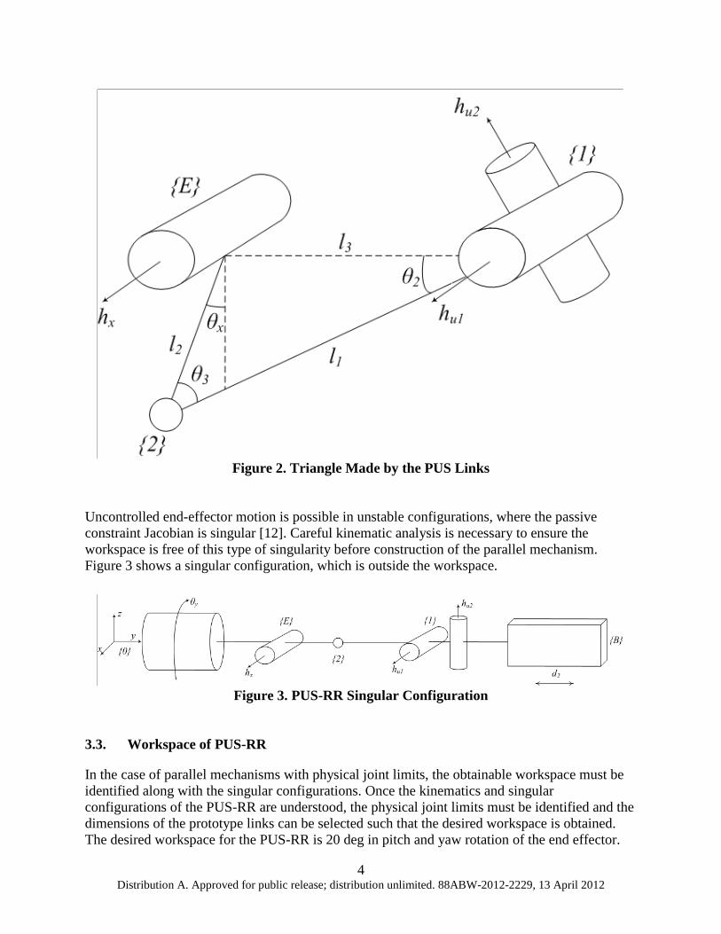
The PUS-RR kinematics is decoupled, allowing separate control of x-axis rotation (prismatic arm) and y-axis rotation (revolute arm). The inverse kinematic solution for the y-axis rotation is simply the revolute motor rotation matching the desired y-axis angle. To find the required prismatic arm position for a desired end-effector x-axis rotation angle, the triangle made by the PUS links and variable side l_3 shown in Figure 2 is analyzed. Remaining angles are found using the sine law.


Figure 2. Triangle Made by the PUS Links

Uncontrolled end-effector motion is possible in unstable configurations, where the passive constraint Jacobian is singular [12]. Careful kinematic analysis is necessary to ensure the workspace is free of this type of singularity before construction of the parallel mechanism. Figure 3 shows a singular configuration, which is outside the workspace.

Figure 3. PUS-RR Singular Configuration

3.3. Workspace of PUS-RR

In the case of parallel mechanisms with physical joint limits, the obtainable workspace must be identified along with the singular configurations. Once the kinematics and singular configurations of the PUS-RR are understood, the physical joint limits must be identified and the dimensions of the prototype links can be selected such that the desired workspace is obtained. The desired workspace for the PUS-RR is 20 deg in pitch and yaw rotation of the end effector.


The physical joint limits for the prototype have been identified as 75 deg of rotation in the universal joint with respect to both the h_{u1} and h_{u2} axis at 1 and 17 deg of rotation in the spherical joint at 2. The lengths of l_{1} and l_{2} are modified until the end effector can be moved through the entire desired workspace. The architecture of the PUS-RR prototype is selected as l_2=2cm, l_1=5cm and with a right angle spherical joint at point 2. The prismatic joint displacement as a function of end-effector position is shown in Figure 4, the universal joint displacement in Figure 5 and the spherical joint in Figure 6, respectively. The Figures show that the obtained workspace for end effector is 17 deg of yaw rotation with a displacement of 1.5 cm of the prismatic actuator. The end effector can rotate 28 deg (pitch rotation) and is limited by the throw of the spherical joint located at point 2.

Figure 4. Prismatic Joint Displacement


Figure 5. Prismatic Universal Joint Angle

Figure 6. End Effector Sphere Joint Angle


3.4. Actuators and Sensor Description

The first phase of experiments involves the development of a 2-axis, closed-loop vibration suppression control system using the PUS-RR parallel mechanism using high-bandwidth, large force prismatic actuator and a DC brushless high speed servo motor. This prototype parallel mechanism is shown in the 0-configuration in Figure 7. The following subsections detail the actuators, sensor, and single-axis tests.

Figure 7. PUS-RR Parallel Robot Assembly

The prismatic actuator is a voice coil connected mechanically in series with two helical springs for self centering when not powered. The voice coil is capable of 300N of force and the maximum displacement is 4 cm. The actuator connects to the end effector by a universal joint and spherical joint (PUS). On the other side, the revolute motor is connected to the end effector through a passive revolute joint (RR). The revolute motor is a standard NEMA 23 motor by Technic. This motor provides adequate holding torque and acceleration, and has an integrated closed loop controller commercially available that interfaces with the motor's encoder. The controller is the SSt-Eclipse, a high bandwidth digital vector servo drive. This drive features controls for position, velocity and torque/force feedback loops. The drive is in torque mode for these experiments. Two-axis vibration suppression is the goal of the first closed loop experiments using the PUS-RR parallel architecture. Two Analog Devices ADXRS610 300 deg single-axis gyroscope sensors are used to measure the pitch and yaw angular velocities of the end effector. The ADXRS610 300 deg has an operational bandwidth of 360 Hz.


4. RESULTS AND DISCUSSION

The PUS-RR is a two-axis sensor pointing and vibration suppression system. For these initial experiments, vibration suppression is the only control goal. A loop-shaping approach is used for control design, as it is quite effective at allowing the designer to maximize feedback at the frequencies of interest while taking into consideration the limitations presented by plant dynamics, sensor noise, sources of non-minimum phase, etc. The decade of 1-10 Hz is targeted for maximum disturbance rejection. For aggressive control applications such as this one, developing a plant model with sufficient fidelity is very difficult. Thus, control design is performed using experimentally obtained frequency response functions. To identify the plant frequency responses, it is driven with band-limited white noise and the response as measured by the gyro sensors is recorded. Data is acquired using an Agilent VXI platform and the plant frequency responses are derived using Applied Physics SignalCalc 6.0 software. The 2 × 2 plant frequency responses are shown in Figure 8.

Figure 8. PUS-RR Plant Frequency Response. The left column are the responses to the

prismatic actuator, the right are the responses to the revolute actuator. The plant frequency response magnitudes are shown in Figure 8. The plots on the diagonal are the x and y-axis responses to their respective actuator inputs. The off-diagonal plots are the cross-coupled responses. While the plant is 2 × 2, the first generation design is two independent


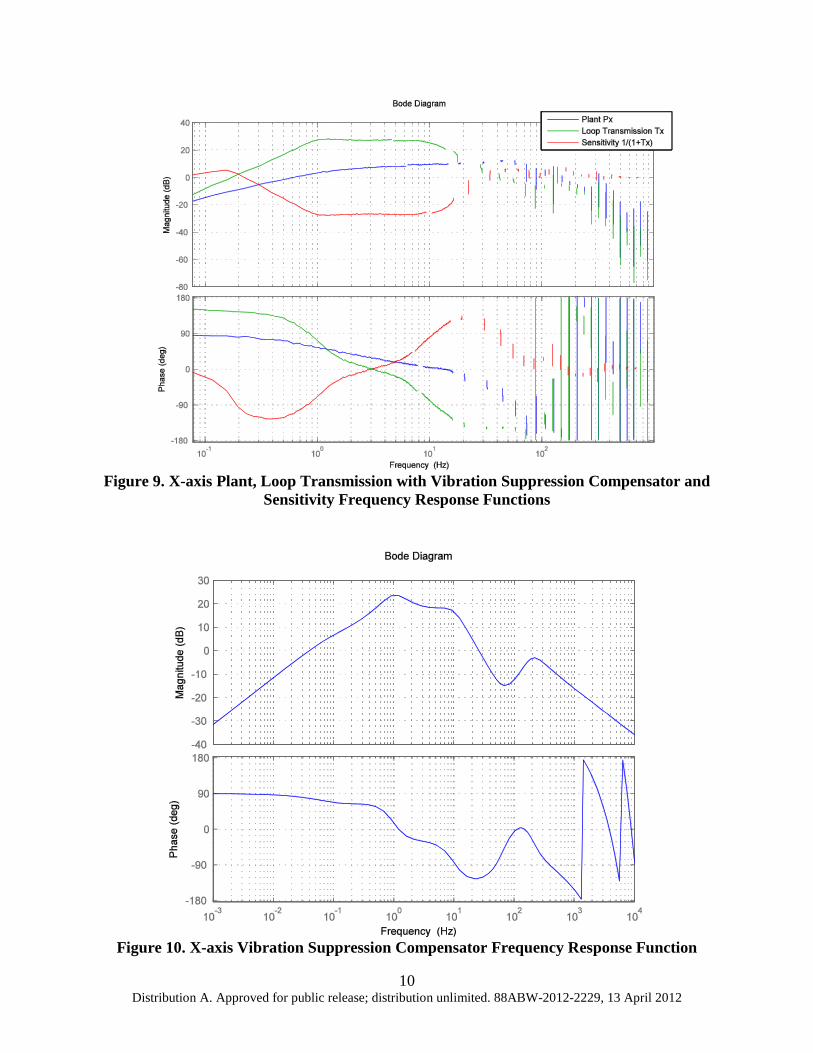
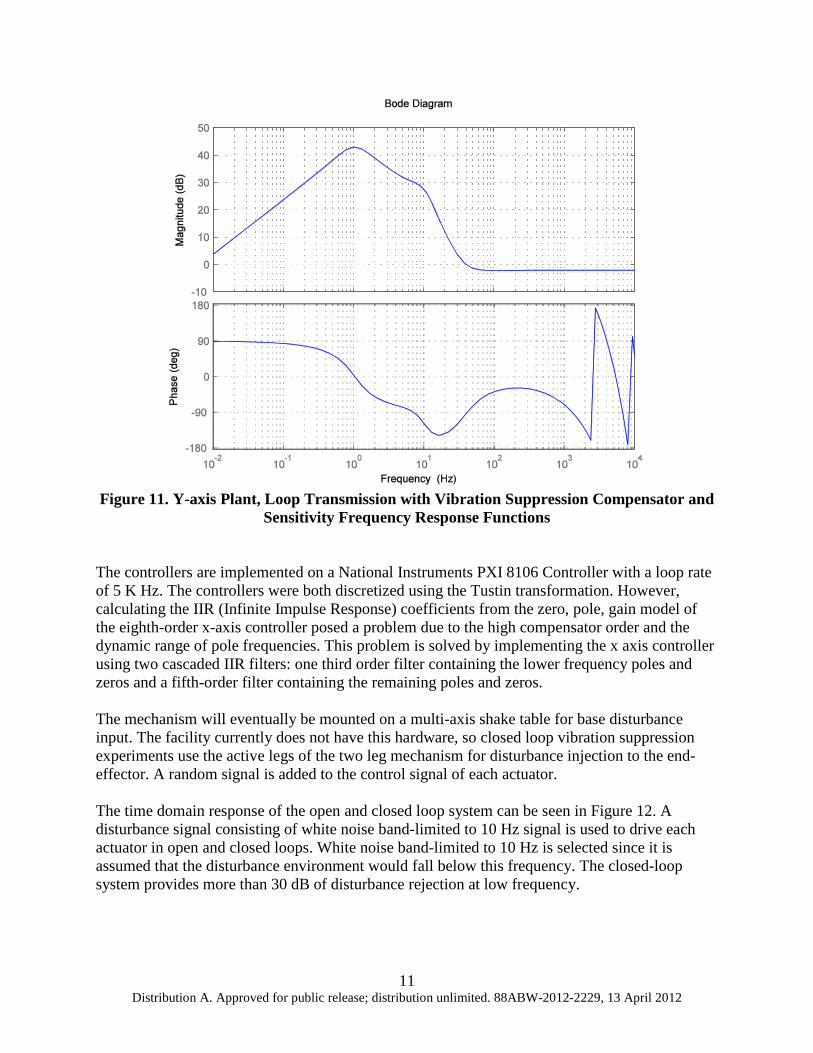
SISO controllers (off-axis moduli are not excessive). There are several aspects of the system that limit the effective bandwidth, and thus available feedback. The controllers are implemented digitally with a sample rate of 5k Hz. It takes 0.2ms for the analog gyro signals to be digitized, processed, and then converted back to analog. This time delay results in non-minimum phase that is linearly proportional to frequency. The gyro signals are biased by voltage around 2.5V that can drift with temperature fluctuations. As such, band pass controller designs were adopted. Design of both controllers is discussed in the following two subsections. The plant frequency response for the x-axis, P_x, can be seen in the top left plot in Figure 8. The slope of the plant modulus is approximately 20dB/dec from 0 Hz to 2 Hz, 0dB/dec from 2 Hz to 65 Hz, and -40dB/dec afterwards. The helical springs are responsible for the flexible modes seen around 90 Hz and 150 Hz. The controller, C_x, was carefully designed to produce the loop transmission T_x and sensitivity S_x shapes seen in Figure 9. The controller offers a maximum of 28 dB of disturbance rejection over the target decade of 1-10 Hz. The x-axis controller is an eighth order compensator as seen in Figure 9. An eighth order controller is required to produce the desired T_x and S_x. A zero at 2 Hz and conjugate zero pair at 65 Hz effectively straightens the corners seen in the original plant. An origin zero together with conjugate pole pairs at 1 Hz and 10 Hz create the general band pass shape of T_x. A first order lead filter around 0.1 Hz ensures that there is around 30 degrees of phase margin at the first crossover. Likewise, a Bode step [15] from 100 Hz to 400 Hz is required to achieve a similar phase margin around the second crossover at 50 Hz. This step is created by a conjugate zero pair at 90 Hz with a single pole and conjugate pole pair at 200 Hz. The plant frequency response for the y-axis, P_y, is shown in the bottom right plot in Figure 8. The slope of the plant modulus is approximately 20dB/dec from 0 Hz to 10 Hz and -20dB/dec afterwards. Flexible body dynamics associated with the sensor cables are more pronounced for the y axis and are responsible for the mode around 630 Hz. There is also only slight coupling to one of the helical spring resonances around 150 Hz. The lack of flexible modes made design of the y axis controller simpler than that of the x axis controller, and also allowed for nearly 6dB more negative feedback in the frequencies of interest. Design of the y axis controller proceeded similar to that of C_x. A zero was placed at the origin for a band pass loop transmission, and conjugate pole pairs at 1 Hz and 10 Hz define the corners of the functional bandwidth. A zero at 16 and zero pair at 35 Hz flattens the loop gain resulting in a Bode step from approximately 200 Hz to 630 Hz. The phase at 630 Hz is nearly -75 degrees so that this mode could cross the 0dB line without threatening closed loop stability. If this mode had been gain stabilized as opposed to phase stabilized, then the second crossover frequency would be lower, as well as the amount of available feedback between 1 Hz and 10 Hz. The resulting loop transmission T_y and sensitivity S_y functions can be seen in Figure 11. The controller provides a maximum of 34 dB of disturbance rejection over the target decade of 1-10 Hz. The y-axis controller is a forth order compensator and is seen in Figure 10.


Figure 9. X-axis Plant, Loop Transmission with Vibration Suppression Compensator and

Sensitivity Frequency Response Functions

Figure 10. X-axis Vibration Suppression Compensator Frequency Response Function


Figure 11. Y-axis Plant, Loop Transmission with Vibration Suppression Compensator and

Sensitivity Frequency Response Functions The controllers are implemented on a National Instruments PXI 8106 Controller with a loop rate of 5 K Hz. The controllers were both discretized using the Tustin transformation. However, calculating the IIR (Infinite Impulse Response) coefficients from the zero, pole, gain model of the eighth-order x-axis controller posed a problem due to the high compensator order and the dynamic range of pole frequencies. This problem is solved by implementing the x axis controller using two cascaded IIR filters: one third order filter containing the lower frequency poles and zeros and a fifth-order filter containing the remaining poles and zeros. The mechanism will eventually be mounted on a multi-axis shake table for base disturbance input. The facility currently does not have this hardware, so closed loop vibration suppression experiments use the active legs of the two leg mechanism for disturbance injection to the end-effector. A random signal is added to the control signal of each actuator. The time domain response of the open and closed loop system can be seen in Figure 12. A disturbance signal consisting of white noise band-limited to 10 Hz signal is used to drive each actuator in open and closed loops. White noise band-limited to 10 Hz is selected since it is assumed that the disturbance environment would fall below this frequency. The closed-loop system provides more than 30 dB of disturbance rejection at low frequency.


Figure 12. Time Domain System Response to White Noise Band—Limited to 10 Hz in Open

and Closed Loop 4.1. Closed Loop Control (Phase 1: Nyquist-Stable Control with Nonlinear Dynamic

Compensation)

Nonlinear control increases the available feedback for a given bandwidth restriction. The approach provides substantial roll reduction improvement compared to linear controllers. A Nyquist-stable pointing control system with nonlinear dynamic compensation applied to a limited DOF PKM is described in this paper. Despite a 0 dB crossover restriction less than 100 Hz, the controller provides nearly 40 dB of feedback over a 10 Hz functional bandwidth and satisfies the conditions of absolute stability in actuator saturation. During these experiments, it became apparent that friction forces heavily influence the system dynamics for small displacements and velocities. In order to better observe what was happening, another sensor was added to the robot to directly measure the position of the end effector. This was accomplished by attaching a mirrored surface to the end effector so that a stationary laser beam would be reflected onto a photodiode position sensing detector (PSD). This paper documents the control experiments that were performed using this new sensor. The plant is a PUS-RR parallel robot shown in Figure 13. One kinematic path consists of an active prismatic actuator, universal joint and sphere joint (PUS), while the other is an active revolute joint in series with a pin joint (RR).


Figure 13. PUS-RR Parallel Robot with a Laser Sensor

The prismatic actuator is powered by a linear voice coil manufactured by BEI Kimco Magnetics Division, model number LA28-43-000A. It is capable of around 300 N of force and 3 cm of displacement. The coil is mechanically in series with helical springs that provide a restoring force to keep the end effector centered when unpowered. The coil is driven by an AE Techron LV608 Linear Power Amplifier operating in a voltage controlled voltage source mode with a gain of 30 V/V. The revolute actuator is a standard NEMA 23 sized electric motor by Techic driven by an SSt-Eclipse digital controller running in torque control mode. This DOF is not used for the control experiments described in this paper. Attached to the end-effector are two microelectromechanical system (MEMS) gyros used to measure the angular rate about the two DOFs. These Analog Devices ADXRS610 300 deg single axis gyroscope sensors have an operational bandwidth of 360 Hz. They work by measuring the deflection experienced by a proof mass resonating at 14 k Hz caused by the Coriolis effect. This deflection measurement is amplified and demodulated to provide a voltage output proportional to the angular rate. The quiescent noise power spectrum of the gyro, with a peak at 14 k Hz, can be seen in Figure 14. A time delay of around 0.75 ms 1/(1.4 k Hz) is also observed, and it is suspected that this is introduced by the demodulation. Such non-minimum phase delay limits the attainable bandwidth, and thus is not used for closed loop experimentation.


Figure 14. Quiescent Sensor Noise Power Spectrum Densities

A Helium Neon (HeNe) laser is used in conjunction with an ON-TRAK Photonics OT-324 Position Sensitive Detector (PSD) to measure the end effector position. The stationary HeNe laser emits a 632.8 nm beam that is directed by an adjustable steering mirror towards the end effector. A mirror attached to the end effector deflects the beam onto the bare duolateral photodiode sensor of the PSD. The PSD sensing amplifier reports the position of the laser beam on the two dimensional sensor as two analog voltages within 10 V. Figure 14 shows the quiescent noise power spectrum of the position sensor along one axis. There are peaks in the position sensors spectra at 120 Hz, 240 Hz, and 360 Hz. These harmonics are likely caused by a 120 Hz voltage ripple on the high voltage DC line powering the laser that results from rectifying the 60 Hz AC power. The higher operational bandwidth of nearly 15 k Hz and lower noise characteristics make the PSD better suited than the gyro for the control experiments discussed in this paper. The system is stimulated by driving the prismatic actuator with band-limited Gaussian noise for the purpose of system identification. The stimulus and PSD signals are digitized and recorded using an Agilent VXI system. The data capture and processing is performed using the SignalCalc 6.2 software suite from DataPhysics. Stimuli of varying amplitudes and bandwidth are applied and the corresponding coherence and plant transfer functions are calculated. A nominal pole-zero-gain (PZK) model of the plant is developed by the manual placement of poles and zeros to sufficiently match those transfer functions with the highest coherence. This 15th order nominal model P(s) is plotted along with the experimentally acquired data in Figure 15.


Figure 15. PUS-RR Plant Frequency Response

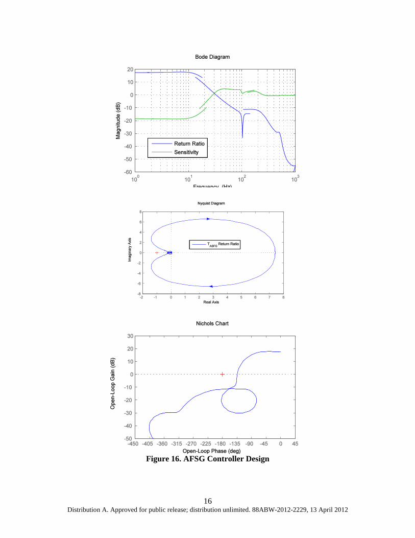
The plant transfer function is low pass as expected. The plant modulus is relatively flat with a value around 48 dB from 0 Hz to around 4 Hz, at which point it begins to roll off at approximately 6 dB/oct. At 80 Hz the slope transitions to nearly 18 dB/oct as there are two conjugate pole pairs and one very lightly damped conjugate zero pair around this frequency. There are interlaced pole then zero pairs around 440 Hz and 840 Hz. There are consecutive pole pairs at 1 k Hz and 1.3 k Hz, whose addition total phase contribution of 360 deg places a hard upper limit on control bandwidth and thus the amount of available feedback. The phase contributions of the well damped poles and lightly damped poles around 80 Hz likewise limit control bandwidth as described later. An absolutely stable fixed gain (ASFG) controller is designed to serve as a baseline for comparison to the nonlinear controller described later. The design goal is to maximize vibration suppression at frequencies below 10 Hz while remaining absolutely stable. This is accomplished by carefully shaping the compensator to obtain the return ratio seen in Figure 16. Similar to the development of the nominal plant model, the PZK model is designed by manually placing poles and zeros.


Figure 16. AFSG Controller Design


A zero at 4 Hz and a conjugate pair of zeros at 80 Hz compensate for the corners found in the original plant. A pair of conjugate poles placed at 11 Hz define the corner of the functional bandwidth around 10 Hz. A pair of zeros at 100 Hz together with pairs of poles at 160 Hz and 220 Hz define the Bode step. A lead filter with a zero at 60 Hz and pole at 100 Hz, together with the Bode step, provide sufficient phase advance around the crossover point. Thus a gain margin of at least 10 dB and a phase margin of nearly 50 deg is maintained. This may seem excessive, but it allows us to demonstrate absolute stability (AS). A major factor limiting bandwidth is the lightly damped zeros and heavily damped poles around 80 Hz. The phase lag of the poles is more pronounced than the phase lead of the zeros at frequencies below 80 Hz. Thus the phase sharply drops to nearly 180 deg around 80 Hz. There is also uncertainty in the exact frequency and Q factor of this mode, as it varied between different system identification experiments. Thus the mode is gain stabilized in order to retain adequate phase margins. The return ratio crosses 0 dB around 33 Hz and the resulting 7th order controller provides nearly 18 dB of negative feedback below 10 Hz. 4.2. Nyquist Stable Controller Design

A high performance Nyquist stable (NS) controller C_{NS}(s) is also designed with the goal of maximizing disturbance rejection at frequencies below 10 Hz. This controller need only satisfy the Nyquist stability criterion, and not the more restrictive conditions for absolute stability. Since the plant is open loop stable, the Nyquist plot of the return ratio T_{NS}(s) must not encircle the -1 critical point. Satisfying the Nyquist stability criterion ensures the closed loop stability of the system without saturation. A high performance Nyquist stable (NS) controller C_{NS}(s) is also designed with the goal of maximizing disturbance rejection at frequencies below 10 Hz. By definition, the return ratio of a Nyquist stable system has a modulus greater than unity and phase less than 180 degrees over some interval of frequencies. Furthermore, since the plant is open loop stable, the Nyquist plot of the return ratio T_{NS}(s) must not encircle the -1 critical point. As opposed to the ASFG, however, the NS controller by itself is not required to be AS.

C_{NS} is designed by carefully shaping the return ratio by direct placement of poles and zeros. A zero at 4 Hz compensates for the bend in the original plant. Conjugate pole pairs were placed at 6.75 Hz and 10 Hz to fix the functional bandwidth at 10 Hz. The pole pair at 10 Hz and a zero pair at 15 Hz were lightly damped in order to provide the sharp transitions seen in the slope of the return ratio at 10 Hz and 15 Hz. It is this steep slope and accompanying phase lag that allows us to attain nearly 20 dB more negative feedback than with the ASFG controller. A pair of zeros at 60 Hz and a pair of poles at 200 Hz flatten the response to produce a Bode step. A two octave wide lead filter centered at 100 Hz further flattens the response and adds phase lead. The loop is shaped such that the positive feedback never exceeds 6 dB. The loop transmission function is shown in Figure 17. The resulting 7th order compensator provides nearly 38 dB of disturbance rejection below 10 Hz. This is an order of magnitude greater than the ASFG controller. The 0 dB crossover frequency is also slightly higher at 44.5 Hz. The return ratio satisfies the Nyquist stability criterion and the


system without saturation is stable in closed loop. However, no physically realizable system behaves linearly under all conditions. The saturation of large signals is inevitable considering the finite nature of real world systems.

Figure 17. Nyquist-stable System


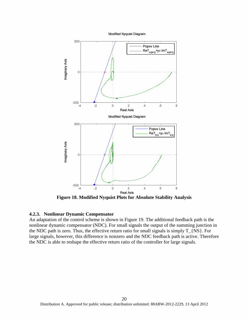
4.2.1. Effects of Saturation The plant possesses several saturation mechanisms: the controller analog output voltage is limited to 10 V, the maximum power output of the Techron amplifier is only a few hundred watts, the stroke of the prismatic actuator is physically limited, and the laser beam can only be deflected a few degrees before it misses the target PSD sensor. To investigate the effects of saturation on the closed loop system without driving the hardware to its physical operating limits, an additional saturation with an adjustable threshold is added to the controller output. The values of t_{sat} used during closed loop experimentation are sufficiently low so that this link will saturate before any of the other sources of saturation mentioned above. Describing functions (DF) and harmonic analysis can be useful for approximating the behavior of a nonlinear link in a linear feedback system. Consider a sinusoid of amplitude E fed into a saturation block. For a small amplitude sinusoid, E < t_{sat}, the saturation link is equivalent to a unity gain. For a large amplitude sinusoid, E > t_{sat}, the output is a waveform of reduced amplitude but of the same frequency and phase of the input. Thus a saturation link can effectively reduce the loop gain for large signals. Consider the Nichols plots for the ASFG and NS controllers. One can see that a broadband reduction of the return ratio moduli would result in the plots shifting down along the amplitude axis. Since |T_{NS}|>0 dB at some frequencies where arg(T_{NS})<-180 deg reducing the gain will eventually result in an encirclement of the critical point, and the Nyquist criterion would no longer be satisfied. This is not the case for ASFG controller. The greater disturbance rejection performance of the NS controller thus comes at the expense of potential stability issues. This is the motivation for development of the nonlinear dynamic compensation (NDC). Consider the Nichols plots for the ASFG and NS. A broadband reduction of the return ratio moduli would result in the plots shifting down along the amplitude axis. Since |T_{NS}|>0 dB at some frequencies where arg(T_{NS})<-180 deg, reducing the gain will eventually result in an encirclement of the critical point and the Nyquist criterion would no longer be satisfied. This is not the case for the ASFG controller. 4.2.2. Absolute Stability and the Popov Criterion A linear time invariant (LTI) system in feedback with a nonlinearity n(e) is said to be absolutely stable (AS) if it is asymptotically globally stable for any n(e) satisfying the sector condition. All of the poles of T_{ASFG} have negative real parts and Figure 18 clearly shows the modified Nyquist plot for T_{ASFG} lying to the right of a Popov line with slope q^{-1} = 375. Thus the Popov criterion is satisfied and the ASFG control system truly is absolutely stable. T_{NS} is also open loop stable, but by the definition of Nyquist stable there exists an w_0 such that arg(T_{NS}(j omega_0)) = -180 deg and |T_{NS}(j omega_0)| > 1. Therefore Re[ (1+qjomega_0) T_{NS}(jomega_0) ] = -|T_{NS}(jomega_0)| < -1 and the NS control system cannot satisfy the Popov criterion.


Figure 18. Modified Nyquist Plots for Absolute Stability Analysis

4.2.3. Nonlinear Dynamic Compensator An adaptation of the control scheme is shown in Figure 19. The additional feedback path is the nonlinear dynamic compensator (NDC). For small signals the output of the summing junction in the NDC path is zero. Thus, the effective return ratio for small signals is simply T_{NS}. For large signals, however, this difference is nonzero and the NDC feedback path is active. Therefore the NDC is able to reshape the effective return ratio of the controller for large signals.


Figure 19. Equivalent Systems for the NS with NDC Controller

The purpose of the NDC is to obtain an AS equivalent return ratio T_{EQ}. Thus T_{ASFG} can serve as a target for T_{EQ}. For a given desired equivalent return ratio T_{EQ}^D = T_{ASFG} and T_{NS}, a target NDC design T_{NDC}^D is ((T_{NS}- T_{EQ}^D)/(1+ T_{EQ}^D))=(( T_{NS}- T_{ASFG})/(1+ T_{ASFG})). The order of the resulting T_{NDC}^D is quite high, and its implementation could pose serious challenges. Therefore, a lower order NDC is sought. A reduced order NDC is thus developed by the manual placement of poles and zeros. An iterative approach is indicated here as the resulting equivalent return ratio T_{EQ} will differ from T_{EQ}^D, and AS will have to be verified. The resulting 9th order T_{NDC} and 40th order T_{NDC}^D are plotted in Figure 20.


Frequency

Figure 20. NDC Design Well damped pole pairs at 6.75 Hz and 250 Hz in combination with lightly damped poles at 10 Hz and 400 Hz capture the sharp bends in T_{NDC}^D seen around these frequencies. Likewise, well damped zeros at 12.3 Hz and lightly damped zeros at 20 Hz produce the remaining corner. A pole around 35 Hz together with a zero around 282 Hz helps match the modulus slope between these frequencies. The equivalent return ratio is T_{EQ} = ((T_{NS} - T_{NDC})(1+ T_{NDC})). The modified Nyquist plot of T_{EQ} is shown in Figure 18 and lies entirely to the right of the Popov line with slope q^{-1}=375. T_{EQ} is Hurwitz, therefore the combined NS with NDC controller is AS. 4.2.4. Closed Loop Experiments All control design work is performed using MATLAB and the Control Systems Toolbox. The continuous time PZK models of the final control designs are discretized using Tustin's method. The poles and zeros were grouped to form a cascade of second order systems. This approach of PZK design lessens the effects of finite precision arithmetic and round off errors. Custom software developed with National Instruments LabWindows/ CVI executes on a National Instruments PXI 8106 Real Time Controller. The program implements the 7th order C_{ASFG}, 7th order C_{NS}, and 9th order T_{NDC} at a loop rate of 10 k Hz. It should be noted the digitizing, processing, and outputting of signals must take no longer than 1/10 k Hz =0.1 ms. This worst case time delay is included in the controller models during the design phase. However, a 0.1 ms time delay only contributes 3.6 deg of non-minimum phase at 100 Hz and 36 deg at 1 k Hz. Thus it is not a major limiting factor in maximizing the crossover frequency. Companion software running on a Windows XP machine allows for loops to be open and closed, disturbances enabled or disabled, and saturation thresholds and proportional gains to be adjusted in real time.


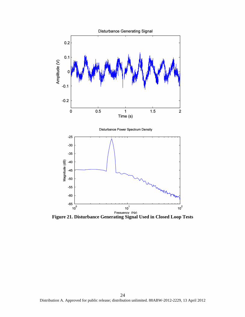
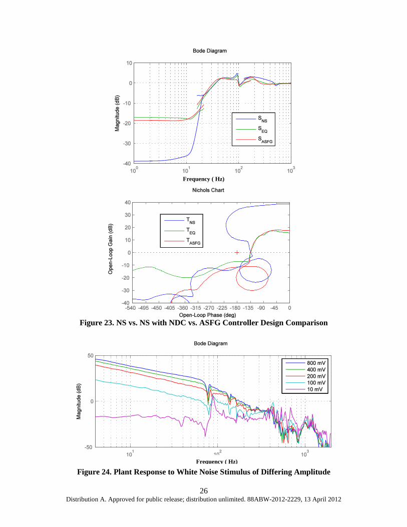
4.2.4.1. Disturbance Environment While it would be desirable to mount the mechanism on a shake table, the facility does not currently have this hardware. The robot is rigidly mounted to an air suspended optics table, so the prismatic actuator itself is used for disturbance injection. A disturbance signal is simply added to the output of the controller before it is fed to the Techron amplifier input. A plot of the disturbance generating signal with its power spectral density (PSD) is shown in Figure 21. The signal is generated by passing white noise through a 10 Hz first-order, low-pass filter and summing it with a 5 Hz sinusoidal tone. The performance of both the ASFG and the NS with NDC controllers are verified in closed loop tests. The disturbance source described above is used in all cases, but t_{sat} is varied. A threshold of 150 mV is sufficiently high to ensure that control effort saturation seldom occurs. In this small signal regime, the NDC is inactive and the effective return ratio of the NS with NDC controller is T_{NS}. This is evidenced by nearly 40 dB of disturbance rejection below 10 Hz as seen in the power spectral density plot in Figure 22. A saturation threshold of 50 mV is sufficiently low to saturate the control effort some of the time. In this large signal scenario, the NDC link is active and reduces the effective return ratio to a less aggressive loop shape as shown in Figure 23. Comparing the performance of the ASFG controller between the small and large signal cases, we see that its effectiveness was also reduced in the saturated case. The first half of Figure 23 demonstrates the unstable nature of the NS controller without the NDC. With t_{sat} = 100 mV, the NS controller without NDC is able to operate stably for some time until the control effort saturates. After this initial saturation, the control output oscillates wildly, ensuring further saturation. Two different control strategies are applied to the prismatic axis of a limited DOF PKM, and their performance in closed loop is demonstrated. The goal is to maximize the amount of negative feedback for disturbance rejection in the frequency interval from 0 Hz to 10 Hz. The linear controller C_{ASFG} is shown to be absolutely stable and provides nearly 18 dB of feedback over the frequencies of interest. The high performance nonlinear controller consisting of a Nyquist stable controller C_{NS} with nonlinear dynamic compensation T_{NDC} is also shown to be absolutely stable. In the small signal case the NDC with NS is able to provide 38 dB disturbance rejection below 10 Hz. This is an order of magnitude better than the ASFG controller. In the large signal case, i.e. when the control signal saturates, the nonlinear controller is able to perform at least as well as the fixed gain controller.


Figure 21. Disturbance Generating Signal Used in Closed Loop Tests


Figure 22. Open vs. Closed Loop Power Spectrum Densities


Frequency ( Hz)

Figure 23. NS vs. NS with NDC vs. ASFG Controller Design Comparison

Figure 24. Plant Response to White Noise Stimulus of Differing Amplitude Frequency ( Hz)


4.3. Closed Loop Control (Phase 2: Camera Tracking Using Modified Command Feed-forward)

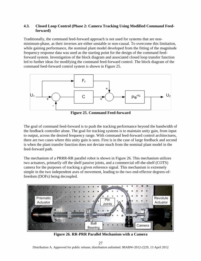
Traditionally, the command feed-forward approach is not used for systems that are non-minimum-phase, as their inverses are either unstable or non-causal. To overcome this limitation, while gaining performance, the nominal plant model developed from the fitting of the magnitude frequency response data was used as the starting point for the design of the command feed-forward system. Investigation of the block diagram and associated closed loop transfer function led to further ideas for modifying the command feed-forward control. The block diagram of the command feed-forward control system is shown in Figure 25.

Figure 25. Command Feed-forward

The goal of command feed-forward is to push the tracking performance beyond the bandwidth of the feedback controller alone. The goal for tracking systems is to maintain unity gain, from input to output, across the desired frequency range. With command feed-forward control architectures, there are two cases where this unity gain is seen. First is in the case of large feedback and second is when the plant transfer function does not deviate much from the nominal plant model in the feed-forward path. The mechanism of a PRRR-RR parallel robot is shown in Figure 26. This mechanism utilizes two actuators, primarily off the shelf passive joints, and a commercial off-the-shelf (COTS) camera for the purposes of tracking a given reference signal. This mechanism is extremely simple in the two independent axes of movement, leading to the two end-effector degrees-of-freedom (DOFs) being decoupled.

Figure 26. RR-PRR Parallel Mechanism with a Camera


The mechanism consists of two closed kinematic paths. One kinematic path consists of a prismatic actuator, a passive ball bearing revolute joint and two passive revolute pin joints (PRRR). The other kinematic path is a revolute actuator in series with a single passive pin joint (RR). This architecture has two decoupled DOFs for the camera movement. These are designated the X-Axis in the prismatic direction of movement and the Y-Axis in the revolute direction of movement. Analysis using a 2 × 2 multiple-input, multiple-output MIMO Nyquist array and Gershgorin discs shows diagonal dominance of the plant, verifying that the two axes are decoupled, and stability of the 2 × 2 multivariable system. 4.3.1. Camera System The primary sensor used in this experiment is a COTS camera. Target tracking software that utilizes the camera output is hosted on a standard x86 based PC, and target tracking results are conveyed to the stabilization robot's control system via analog voltages produced by a data acquisition card. Very simple image processing software capable of tracking a bright dot produced by a laser or oscilloscope has been implemented to test the camera's viability as a real-time sensor. Figure 27 shows the block diagram of the sensor system.

Figure 27. Sensor Sub-system

The FL3-FW-03S1C (Flea3) is a compact (29 × 29 × 30 mm and 58 g) IEEE 1394b interface camera manufactured by Point Grey Research. The Flea3 incorporates a Sony ICX618 1/4-in CCD image sensor that can capture color video at up to 60 frames per second (fps) and monochrome video at up to 120 fps. A Pentax C60402KP C-mount lens is mated to the Flea3's interchangeable lens mount. This lens is designed for an effective focal length (EFL) of 4.2 mm when used with a 1/2-in CCD. When the crop factor of the smaller 1/4-in CCD is taken into account, an EFL of approximately 7.5 mm results in a 27 deg horizontal field of view. The camera is attached to the robot using a custom machined holder.


A standard industrial box PC is used to capture and process the imagery coming from the Flea3 over the IEEE 1394b bus. The PC is an Advantech ARK-3420 (ARK) which has a 1.6 GHz Core2 Duo Intel processor, 4 gigabytes of RAM, and two PCI expansion slots. The PCI expansion slots are populated with a dedicated IEEE 1394b interface and an Adlink DAQ-2501 data acquisition card. Two of the DAQ-2501's four available 12-bit D/A channels are used to produce voltages corresponding to the X/Y coordinates of the target as measured by the image processing software. Ubuntu Linux 9.04 (kernel version 2.6.28) is used as the operating system on the PC. The libdc1394 library is used to capture imagery which is streamed over the IEEE 1394b bus, and the Adlink DAQ is controlled with drivers provided by the manufacturer. For the purposes of this experiment the simplest possible imagery suffices to demonstrate the tracking performance of the robot, and for this reason a method of generating a controllable point target is required. To enable comparison of commanded target position and tracked target position it is desirable to simply control the target with applied voltages. Two possible methods of generating a target dot which can be positioned using voltages are considered. Either system can use the same simple method of target detection discussed below or upon further investigation it was decided that the high price and complexity of galvanometer based systems was not warranted. Using the oscilloscope as a target generator simplifies many aspects of data collection and the fact that it is a calibrated instrument allows for reasonable confidence that the geometry commanded is the geometry realized on the screen. For the target type described a simple method of detecting and localizing the target is to regard the location of the brightest point in the image as the target location and to simply use the pixel position of this maximum as an estimate of the target location. Other methods of target detection such as searching the image for pixels whose value is above some threshold require either strict control of the lighting in the laboratory or more complex, and therefore slower, image processing to compensate for variations in the light level of the room and the target intensity.


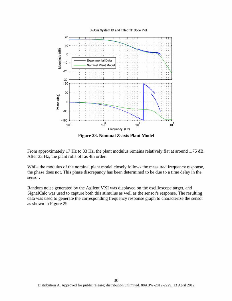
Figure 28. Nominal Z-axis Plant Model

From approximately 17 Hz to 33 Hz, the plant modulus remains relatively flat at around 1.75 dB. After 33 Hz, the plant rolls off as 4th order. While the modulus of the nominal plant model closely follows the measured frequency response, the phase does not. This phase discrepancy has been determined to be due to a time delay in the sensor. Random noise generated by the Agilent VXI was displayed on the oscilloscope target, and SignalCalc was used to capture both this stimulus as well as the sensor's response. The resulting data was used to generate the corresponding frequency response graph to characterize the sensor as shown in Figure 29.


Figure 29. Sensor Frequency Response Showing Linear Phase Change with Frequency

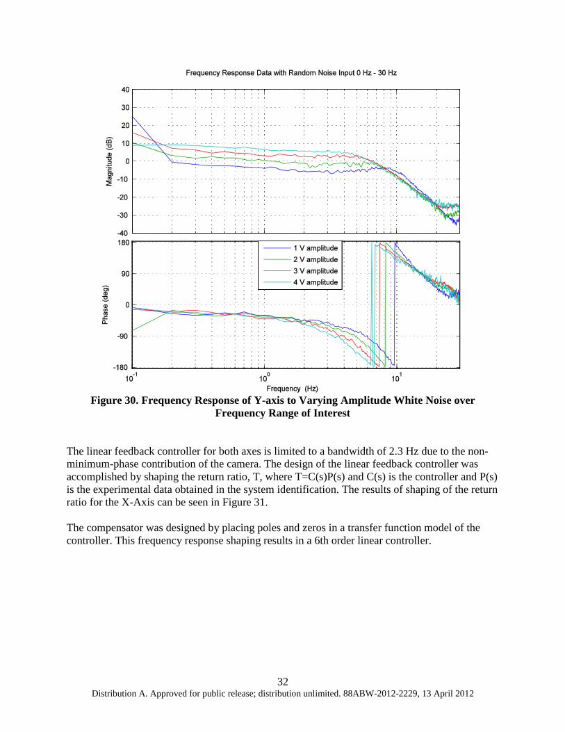
The magnitude response of the sensor is relatively constant, while the phase decreases linearly with frequency which indicates a time delay in the camera system. There is a measured phase shift of 180 deg at 27 Hz, and therefore a phase shift of 360 deg at 54 Hz. This corresponds to a time delay of 18.5 ms, or approximately two inter-frame periods at 110 fps. This large time delay in the sensor is the primary limiting factor of the controller bandwidth and provides the motivation for exploring the application of the command feed-forward method to this control problem. 4.3.2. Plant Identification Random white noise over the frequency range, from 0.01 Hz to 30 Hz, of interest is used to stimulate the revolute actuator. This stimulus was injected at four different amplitudes, from 1 volt RMS to 4 volts RMS, to fully identify the response of the Y-Axis. This revolute axis is inherently nonlinear as shown in Figure 30. It can be seen that not only does the modulus of the response varies with varying input amplitudes, but there are two poles that shift out in frequency with lower amplitude input stimuli. The control design procedure for the tracking system begins with the design of a SISO linear feedback controller. Next a command feed-forward controller is designed based only on the nominal minimum-phase plant model. Lastly, an additional block is designed in cascade with the command feed-forward block to locally compensate for non-minimum-phase to obtain the final, modified command feed-forward control system while maintaining the condition of causality. The modified command feed-forward system is designed to track an image feature at frequencies below 20 Hz, while remaining stable with adequate gain and phase margins.


Figure 30. Frequency Response of Y-axis to Varying Amplitude White Noise over

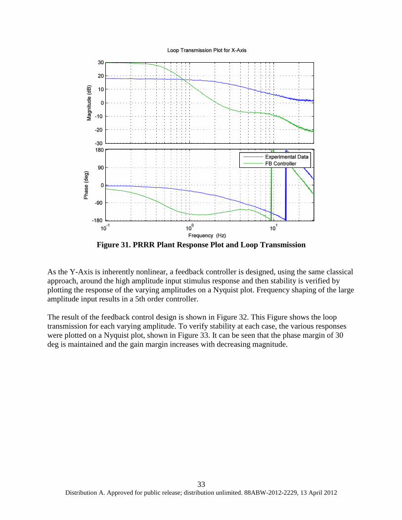
Frequency Range of Interest The linear feedback controller for both axes is limited to a bandwidth of 2.3 Hz due to the non-minimum-phase contribution of the camera. The design of the linear feedback controller was accomplished by shaping the return ratio, T, where T=C(s)P(s) and C(s) is the controller and P(s) is the experimental data obtained in the system identification. The results of shaping of the return ratio for the X-Axis can be seen in Figure 31. The compensator was designed by placing poles and zeros in a transfer function model of the controller. This frequency response shaping results in a 6th order linear controller.


Figure 31. PRRR Plant Response Plot and Loop Transmission

As the Y-Axis is inherently nonlinear, a feedback controller is designed, using the same classical approach, around the high amplitude input stimulus response and then stability is verified by plotting the response of the varying amplitudes on a Nyquist plot. Frequency shaping of the large amplitude input results in a 5th order controller. The result of the feedback control design is shown in Figure 32. This Figure shows the loop transmission for each varying amplitude. To verify stability at each case, the various responses were plotted on a Nyquist plot, shown in Figure 33. It can be seen that the phase margin of 30 deg is maintained and the gain margin increases with decreasing magnitude.


Figure 32. RR Loop Transmission with Feedback Controller Designed for the High

Amplitude Input Stimulus

Figure 33. MIMO Nyquist Array Showing Diagonal Dominance


After designing the linear feedback control, the assumption that the plant is sufficiently decoupled is verified by showing the diagonal dominance of the plant, justifying the design of each linear feedback controller as an independent SISO controller. A MIMO Nyquist array plot of the system is shown in Figure 34. The small magnitude of the off diagonal plots verifies diagonal dominance of the plant, justifying the design of each feedback as independent SISO controllers for the two axes.

Figure 34. Plot of Diagonal Nyquist Response Plots with Gersgorin Discs

4.3.3 Command Feed-forward Control Design To increase the effectiveness of the feed-forward block, while having a pure time delay in the plant, the closed loop transfer function must be broken into two parts. For the case of a minimum phase, proper plant, P(s), the feed-forward term, F_{f}, would be an inversion of the plant. However, in the case of a strictly proper plant and the presence of a time delay, the feed-forward term is no longer a simple inversion. Additional poles are placed in the feed-forward block, F_{f}, to make it proper. Previously, the plant model for the PRRR-PR system was shown to have a relative degree of four. Therefore, four zeros were added well beyond the bandwidth of the feedback controller. These zeros were all placed at nearly two decades beyond the bandwidth. The effects of the time delay are more difficult to overcome. Minimizing the integral of the absolute value of the sum of the feed-forward term, feedback term and negative 1over the frequency interval of interest causes the closed loop response to approach the highest tracking performance possible. Many variables go into the development of the closed loop transfer function, causing this process of minimizing alpha to be done manually by adding an additional block in cascade to the nominal inverse plant model in the feed-forward path. The additional block in the feed-forward path is used to improve tracking response from 2 Hz to 20 Hz, extending the tracking bandwidth beyond that of the linear feedback controller alone to achieve the tracking goal. Through several iterations, the closed loop response was shaped to


maintain close to unity gain from 0 Hz to 20 Hz while not violating causality. The results are shown in Figure 35.

Figure 35. Close Loop Response of the X-axis Showing Both Feedback and Modified

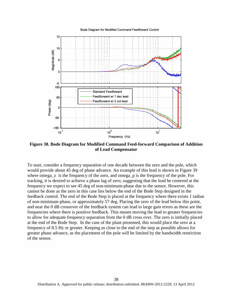
Command Feed-forward (W) A systematic approach is taken to develop the modification of the command feed-forward path to locally compensate for some of the non-minimum-phase. This approach looks at a finite band of frequencies of interest, in this case 2 Hz to 20 Hz, and adds an additional compensator block, call it C_2, to the feed-forward path. The block diagram for this new modified command feed-forward control is shown in Figure 36. The first step in this design is the placement of a first order lead. Two major considerations go into the placement of the lead. First, the lead should be placed sufficiently far from the cross over frequency of the feedback system. Second, it is important to consider the amount of phase advance that can be achieved based on the bandwidth limitations imposed by time delay. The frequency response of the lead implemented is shown in Figure 37. The input-output frequency responses using standard command feed-forward, and modified feed-forward with a 1 decade and 2 octave leads are shown in Figure 38.


Figure 36. Modified Command Feed-forward Block Diagram with Time Delay

Figure 37. Bode Diagram for Modified Command Feed-forward Modifier Block


Figure 38. Bode Diagram for Modified Command Feed-forward Comparison of Addition

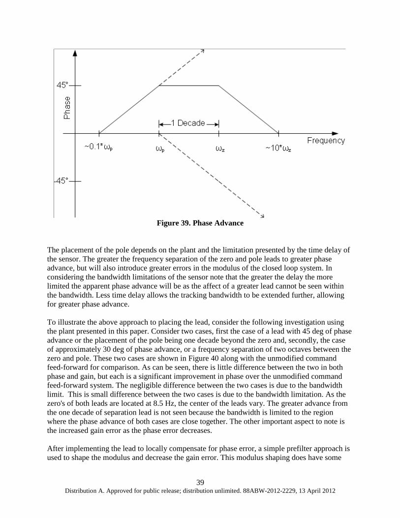
of Lead Compensator To start, consider a frequency separation of one decade between the zero and the pole, which would provide about 45 deg of phase advance. An example of this lead is shown in Figure 39 where omega_z is the frequency of the zero, and omega_p is the frequency of the pole. For tracking, it is desired to achieve a phase lag of zero, suggesting that the lead be centered at the frequency we expect to see 45 deg of non-minimum-phase due to the sensor. However, this cannot be done as the zero in this case lies below the end of the Bode Step designed in the feedback control. The end of the Bode Step is placed at the frequency where there exists 1 radian of non-minimum-phase, or approximately 57 deg. Placing the zero of the lead below this point, and near the 0 dB crossover of the feedback system can lead to large gain errors as these are the frequencies where there is positive feedback. This means moving the lead to greater frequencies to allow for adequate frequency separation from the 0 dB cross over. The zero is initially placed at the end of the Bode Step. In the case of the plant presented, this would place the zero at a frequency of 8.5 Hz or greater. Keeping as close to the end of the step as possible allows for greater phase advance, as the placement of the pole will be limited by the bandwidth restriction of the sensor.


Figure 39. Phase Advance

The placement of the pole depends on the plant and the limitation presented by the time delay of the sensor. The greater the frequency separation of the zero and pole leads to greater phase advance, but will also introduce greater errors in the modulus of the closed loop system. In considering the bandwidth limitations of the sensor note that the greater the delay the more limited the apparent phase advance will be as the affect of a greater lead cannot be seen within the bandwidth. Less time delay allows the tracking bandwidth to be extended further, allowing for greater phase advance. To illustrate the above approach to placing the lead, consider the following investigation using the plant presented in this paper. Consider two cases, first the case of a lead with 45 deg of phase advance or the placement of the pole being one decade beyond the zero and, secondly, the case of approximately 30 deg of phase advance, or a frequency separation of two octaves between the zero and pole. These two cases are shown in Figure 40 along with the unmodified command feed-forward for comparison. As can be seen, there is little difference between the two in both phase and gain, but each is a significant improvement in phase over the unmodified command feed-forward system. The negligible difference between the two cases is due to the bandwidth limit. This is small difference between the two cases is due to the bandwidth limitation. As the zero's of both leads are located at 8.5 Hz, the center of the leads vary. The greater advance from the one decade of separation lead is not seen because the bandwidth is limited to the region where the phase advance of both cases are close together. The other important aspect to note is the increased gain error as the phase error decreases. After implementing the lead to locally compensate for phase error, a simple prefilter approach is used to shape the modulus and decrease the gain error. This modulus shaping does have some


affect on the phase, but much of the additional phase advance is maintained. Still, it is important to look at the effects on both gain and phase when shaping this modified command feed-forward control. This trade off is directly seen in the previously derived alpha error quantity. The end of the design is an iterative approach. After the above basic guidelines for placement, small changes are made to the lead and filters to achieve the smallest alpha quantity as possible by hand. For the plant presented, the final design for this new block, C_2, includes a lead, with a zero at 9 Hz and a pole at 18 Hz, to locally compensate for some of the non-minimum-phase and a sixth order combination of notch filters.

Figure 40. Plot of |N|

Additionally, the values for N(jw) are plotted in Figure 40 to show the effects of the modified command feed-forward controller. By integrating the norm of the N(jw) function over the desired tracking bandwidth of 0 Hz to 20 Hz, we obtain a value for alpha for both the feedback and modified command feed-forward systems. The feed-forward has an error value of 11.25 while the modified command feed-forward has an error value of 1.53. Thus the addition of the modified command feed-forward controller provides 7.35 times the performance of the feedback control alone. Several time domain tests were completed to compare the closed loop tracking performance of both the linear feedback control system and the modified command feed-forward control system.


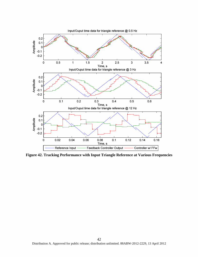
Two different reference signals are used for these tests: an internally generated continuous sine reference and an externally generated discontinuous triangle reference. The first reference trajectory for testing the tracking performance is a sine reference signal generated discretely on the NI machine. The program provides the ability to vary the amplitude, frequency and phase of the reference sine. The performance was tested at three different frequencies to verify performance. The results of these tests are shown in Figure 41. Similarly, the tracking performance of a discontinuous reference signal was tested. This reference trajectory consists of an externally generated triangle wave provided by an Agilent 33120 Function Generator input into the NI machine. The function generator provides the ability to vary the amplitude and frequency of the reference signal. The discontinuous tracking performance was tested at three varying frequencies, 0.5 Hz, 3 Hz, and 12 Hz. These results can be seen in Figure 42. These closed loop results verify the improvement of the target tracking, the extension of the tracking bandwidth out to 20 Hz, and the ability to track discontinuous reference signals by implementing the modified command feed-forward control.

Figure 41. Tracking Performance with Input Sine Reference at Various Frequencies


Figure 42. Tracking Performance with Input Triangle Reference at Various Frequencies


5. CONCLUSIONS

Tracking systems used on military unmanned ground vehicles must be lightweight, rugged and have very high performance. Commercial, off-the-shelf articulation systems are too fragile, and common control techniques (e.g. proportional-integral-derivative) have insufficient performance. To provide solutions to this challenging problem, novel PKM architectures and control approaches have been developed for high performance disturbance rejection and target tracking related specifically to Air Force unmanned ground vehicle systems. The RR-PUS and RR-PRRR (“Prismatic/revolute orienting apparatus,” US Patent application No. 13,099,299, May 2011) two DOF PKMs, developed at the University of Wyoming, are stiff, rugged and fast articulation systems that are easily manufactured. Extremely aggressive control systems have been designed providing very large disturbance rejection and tracking accuracy. Nonlinear feedback control has been successfully implemented on this hardware allowing for maximum feedback and stability despite the presence of nonlinearities in the feedback loop. This type of control has been implemented only on a small number of real systems. A new modification of command feed-forward control has been successfully implemented on these PKMs that provides high performance tracking despite significant non-minimum phase delay due to tracking camera time delay. The combination of these new PKMs and advanced control methods is a substantial new Air Force capability for future unmanned ground vehicle applications.


6. REFERENCES

1. Merlet, J. P., "Parallel manipulators: state of the art and perspective", IMACS/SICE International Symposium on Robotics, Mechatronics, and Manufacturing Systems, pg 403-408, Kobe, JP, 1992.

2. Merlet, J. P., "Parallel Manipulators 2: The Theory, Singular Configurations, and Grassman Geometry", INRIA Research Report, pg 791, Feb 1988.

3. Merlet, J. P.,"Singular configurations of parallel manipulators and Grassmann geometry", International Journal of Robotics Research, Vol 8 No 5, pg 45-56, 1989.

4. Bicchi, A. and Balluchi, D.,"On the mobility and manipulability of general multiple limb robots," Robotics and Automation, IEEE Transactions on}, Vol 11, No 2, pg 215-228, April 1995.

5. Chiacchio, P. and Chiaverini, S. and Sciavicco, L.,"Global task space manipulability ellipsoids for multiple-arm systems," Robotics and Automation, IEEE Transactions on, Vol 7, No 5, pg 678-685, Oct 1991.

6. Park, F. C. and Kim, J. W., "Manipulability and singularity analysis of multiple robot systems:a geometric approach," Robotics and Automation, 1998 IEEE International Conference on, Vol 2, pg 1032-1037, May 1998.

7. O'Brien, J. F. and Jafari, F. and Wen, J. T., "Determination of Unstable Singularities in Parallel Robots with N-arms," Robotics, IEEE Transactions on, Vol 22, No 1, pg 160-168, 2006.

8. Stewart, D.,"A platform with six degrees of freedom," UK Institution of Mechanical Engineers Proceedings}, Vol 180, No 15, 1966.

9. O'Brien, J.F., Neat, G.W., Calvet, R.J., and von Flotow, A., "Six-Axis vibration isolation system for spaceborne interferometers," Proceedings of the SPIE International Symposium on AeroSense, Conference on Spaceborne Interferometry, vol. 1947, pp. 199-197, Orlando, FL, April 1995.

10. McInroy, J. E. and O'Brien, J. F. and Neat, G. W.,"Precise, fault tolerant pointing using a Stewart platform," Mechatronics, IEEE/ASME Transactions on, Vol 4, No 1, pg 91-95, Mar 1999.

11. Carruthers, D.J., O’Brien, J.F., McInroy, J.E., and Yang, Y., “Development of a Voice Coil-Actuated Limited-DOF Parallel Mechanism for Vibration Suppression,” Journal of Systems and Control Engineering, February 2009.

12. Nelson, J., Carruthers, D. O’Brien, J. and McInroy J., “Design and Control of a 2-DOF Parallel Mechanism Using Prismatic and Revolute Actuators, IASTED International Conference on Robotics and Applications, ,Cambridge, MA, Nov 2010.

13. Carruthers, D, and O’Brien, J, “Two Degree-of-Freedom Parallel Mechanisms for Vibration Suppression and Tracking,” SPIE Symposium on Smart Structures and Materials, San Diego, March 2011.

14. Parkins, J.A. and O’Brien, J.F., “A Modified Command Feedforward Tracking Control System Applied to the PRRR-RR Parallel Mechanism,” Symposium on SPIE Smart Structures and Materials, San Diego, March 2012.

15. Lurie, B, Enright, P, “Classical Feedback Control,” Marcel Dekker, 2000.


LIST OF SYMBOLS, ABBREVIATIONS, AND ACRONYMS

AC alternating current arg argument ASFG absolutely stable fixed gain C_x compensator x CCD charged-coupled device cm centi-meters COTS commercial of the shelf D/A digital to analog dB decibels DC direct current deg degrees DF describing function DOF degree of freedom EFL effective focal length F feed-forward system fps frames per second HeNe helium neon Hz Hertz IIR infinite impulse response k Hz kilo-Hertz MIMO multiple input, multiple output mm millimeters ms milli-seconds mV milli-volts N Newtons N(jomega) feed-forward performance function NEMA national electrical manufactures association P_x plant x PKM parallel kinematic machine PRRR-RR prismatic revolute revolute revolute-revolute revolute PSD position sensitive detector PUS-RR prismatic universal spherical-revolute revolute PZK pole zero gain (K) Q quality factor rad radians rms root mean square s seconds S_x sensitivity x SISO single input, single output T_x loop transmission x t_sat saturation threshold V volts

detecting motion from a moving platform; phase 2

Documents