detecting stalled or slow-moving vehicles at night by optical sensing
TRANSCRIPT
Detecting stalled or slow-moving vehicles at nightby Optical Sensing - a feasibility study
by
Olufeni Okelana
A thesis submitted to the Graduate Faculty ofAuburn University
in partial fulfillment of therequirements for the Degree of
Master of Science
Auburn, AlabamaDecember 13, 2014
Keywords: Collision avoidance, Night vehicle, Optical sensing
Copyright 2014 by Olufeni Okelana
Approved by
John Hung, Chair, Professor of Electrical and Computer EngineeringMichael Baginski, Associate Professor of Electrical and Computer Engineering
Shiwen Mao, McWane Associate Professor of Electrical and Computer Engineering
Abstract
In developing countries and areas without adequate infrastructure, a system that can
work towards automobile accident reduction without heavy infrastructural dependence or
in-vehicle installation will have a shorter implementation time and thereby function sooner.
Road studs are a common feature used for road delineation at night. Incorporating intel-
ligence into road studs to detect stalled or slowly-moving vehicles can greatly reduce fatal
night car accidents, which have a much higher frequency rate than those occurring during
the day. This research aims at investigating its feasibility through optical sensing.
ii

Acknowledgments
The author would like to thank all those who contributed towards the successful com-
pletion of this research. First, I would like to thank Dr. Hung for his patience and guidance
all through the research, particularly for times when we had to collect data by the roadside
at night. I would also like to thank Dr. S. Mao and Dr. M. Baginski for ensuring a thorough
grasp of the theoretical part of the research.
I would also like to thank all my friends who gave me necessary moral support and
assistance to pull through successfully.
Finally, I would like to thank my parents (in the US and Africa) and my siblings for
their love, financial and moral support, which contributed immensely towards the overall
success of my graduate program.
iii
Table of Contents
Abstract . . . . . . . . . . . . . . . . . . . . . . . . . . . . . . . . . . . . . . . . . . . ii
Acknowledgments . . . . . . . . . . . . . . . . . . . . . . . . . . . . . . . . . . . . . . iii
List of Figures . . . . . . . . . . . . . . . . . . . . . . . . . . . . . . . . . . . . . . . vi
List of Tables . . . . . . . . . . . . . . . . . . . . . . . . . . . . . . . . . . . . . . . . ix
1 Introduction . . . . . . . . . . . . . . . . . . . . . . . . . . . . . . . . . . . . . . 1
1.1 Background . . . . . . . . . . . . . . . . . . . . . . . . . . . . . . . . . . . . 1
1.2 Purpose . . . . . . . . . . . . . . . . . . . . . . . . . . . . . . . . . . . . . . 4
1.3 Scope . . . . . . . . . . . . . . . . . . . . . . . . . . . . . . . . . . . . . . . 5
1.4 Document Layout . . . . . . . . . . . . . . . . . . . . . . . . . . . . . . . . . 5
2 Literature Review . . . . . . . . . . . . . . . . . . . . . . . . . . . . . . . . . . . 6
2.1 Causes of Car Crashes[2] . . . . . . . . . . . . . . . . . . . . . . . . . . . . . 6
2.1.1 Driver related causes . . . . . . . . . . . . . . . . . . . . . . . . . . . 6
2.1.2 Vehicle related causes . . . . . . . . . . . . . . . . . . . . . . . . . . . 6
2.1.3 Environment related causes . . . . . . . . . . . . . . . . . . . . . . . 8
2.2 Car Crashes at Night . . . . . . . . . . . . . . . . . . . . . . . . . . . . . . . 8
2.2.1 Disuse of Restraints(seat-belts) . . . . . . . . . . . . . . . . . . . . . 8
2.2.2 High Blood Alcohol Concentration (BAC) Levels . . . . . . . . . . . 9
2.2.3 Speeding . . . . . . . . . . . . . . . . . . . . . . . . . . . . . . . . . . 9
2.3 Reaction and Stopping Time/Distance . . . . . . . . . . . . . . . . . . . . . 11
2.3.1 Reaction Time/Distance . . . . . . . . . . . . . . . . . . . . . . . . . 12
2.3.2 Stopping/Braking Distance . . . . . . . . . . . . . . . . . . . . . . . 13
2.4 Advanced Driver Assistance Systems (ADAS) . . . . . . . . . . . . . . . . . 17
2.4.1 Cruise Control . . . . . . . . . . . . . . . . . . . . . . . . . . . . . . 17
iv

2.4.2 Adaptive Cruise Control . . . . . . . . . . . . . . . . . . . . . . . . . 17
2.4.3 Precrash Systems [35] . . . . . . . . . . . . . . . . . . . . . . . . . . 20
2.4.4 Lane Departure Warning (LDW)Systems [35] . . . . . . . . . . . . . 20
2.4.5 Blind Spot Information System (BLIS) [35] . . . . . . . . . . . . . . . 21
2.4.6 Autonomous Parking Assistance System . . . . . . . . . . . . . . . . 21
2.4.7 Drowsiness Detection System [35] . . . . . . . . . . . . . . . . . . . . 21
2.5 Intelligent Transportation Systems (ITS) . . . . . . . . . . . . . . . . . . . . 21
2.6 Road Studs . . . . . . . . . . . . . . . . . . . . . . . . . . . . . . . . . . . . 24
2.7 Vehicle Detection Systems . . . . . . . . . . . . . . . . . . . . . . . . . . . . 27
2.8 Vehicle Headlamp . . . . . . . . . . . . . . . . . . . . . . . . . . . . . . . . . 29
3 Materials and Methods . . . . . . . . . . . . . . . . . . . . . . . . . . . . . . . . 32
3.1 Experiment Setup . . . . . . . . . . . . . . . . . . . . . . . . . . . . . . . . . 32
3.2 Procedure . . . . . . . . . . . . . . . . . . . . . . . . . . . . . . . . . . . . . 34
4 Results and Discussion . . . . . . . . . . . . . . . . . . . . . . . . . . . . . . . . 36
4.1 Parking Lot Experiments . . . . . . . . . . . . . . . . . . . . . . . . . . . . . 36
4.1.1 Variation of Voltage Output with Distance from Optical Sensor . . . 36
4.1.2 Output waveforms at varying vehicle speeds . . . . . . . . . . . . . . 36
4.2 Traffic Light Experiments . . . . . . . . . . . . . . . . . . . . . . . . . . . . 39
4.2.1 Light sensor mounted by 4-lane road on curb . . . . . . . . . . . . . . 39
4.2.2 Light sensor mounted in middle of outer lane on white stop line . . . 43
5 Conclusions and Recommendations . . . . . . . . . . . . . . . . . . . . . . . . . 46
Bibliography . . . . . . . . . . . . . . . . . . . . . . . . . . . . . . . . . . . . . . . . 48
Appendices . . . . . . . . . . . . . . . . . . . . . . . . . . . . . . . . . . . . . . . . . 51
A PDV-9008 Light Dependent Resistor (LDR) Specifications [12] . . . . . . . . . . 52
B ADC-200 PC Oscilloscope/Datalogger [24] . . . . . . . . . . . . . . . . . . . . . 54
C Tektronix P2200 Passive Probe Electrical Characteristics [13] . . . . . . . . . . 56
v
List of Figures
1.1 Reaction and Braking Distance . . . . . . . . . . . . . . . . . . . . . . . . . . . 3
2.1 Passenger Vehicle Occupant Fatalities in 2005 by Time of Day and Restraint Use 9
2.2 Passenger Vehicle Occupant Fatalities in 2005 by Time of Day and the BAC Level
in the Crash . . . . . . . . . . . . . . . . . . . . . . . . . . . . . . . . . . . . . . 11
2.3 Passenger Vehicle Occupant Fatalities in 2005 by Time of Day and Speeding . . 11
2.4 Stopping Distance against Initial Velocity at constant deceleration of 32ft/s2 . 14
2.5 Effect of Gradient/Slope on Braking/Stopping Distance . . . . . . . . . . . . . 15
2.6 Adaptive Cruise Control (ACC) system on the 2012 Audi A8 . . . . . . . . . . 19
2.7 Ford’s Active Park Assist System . . . . . . . . . . . . . . . . . . . . . . . . . . 22
2.8 Intelligent Transportation System (ITS) . . . . . . . . . . . . . . . . . . . . . . 23
2.9 Basic Components of a Solar LED Road Stud . . . . . . . . . . . . . . . . . . . 25
2.10 Two-Lane Road Well-Delineated by LED Road Studs . . . . . . . . . . . . . . . 25
2.11 System Layout of Remotely Controllable Wireless Road Stud Network . . . . . 26
2.12 Road Nail System . . . . . . . . . . . . . . . . . . . . . . . . . . . . . . . . . . 27
2.13 Basic Components of a Car Headlamp . . . . . . . . . . . . . . . . . . . . . . . 30
vi
2.14 Comparison of Halogen and HID lamp light patterns . . . . . . . . . . . . . . . 31
3.1 Experiment Setup . . . . . . . . . . . . . . . . . . . . . . . . . . . . . . . . . . 32
3.2 Optical Sensor Circuit . . . . . . . . . . . . . . . . . . . . . . . . . . . . . . . . 33
3.3 Experiment setup for sensor output with varying distance . . . . . . . . . . . . 34
3.4 Experiment setup at traffic light . . . . . . . . . . . . . . . . . . . . . . . . . . 35
4.1 Variation of voltage output with distance from headlight . . . . . . . . . . . . . 37
4.2 Light sensor output for vehicle moving at 5mph . . . . . . . . . . . . . . . . . . 38
4.3 Light sensor output for vehicle moving at 10mph . . . . . . . . . . . . . . . . . 38
4.4 Light sensor output for vehicle moving at 20mph . . . . . . . . . . . . . . . . . 39
4.5 Light sensor output at traffic light (40Hz sampling frequency) . . . . . . . . . . 40
4.6 Light sensor output at traffic light (100Hz sampling frequency) . . . . . . . . . 41
4.7 Light sensor output at traffic light (200Hz sampling frequency) - 1st run . . . . 41
4.8 Light sensor output at traffic light (200Hz sampling frequency) - 2nd run . . . . 42
4.9 Light sensor output at traffic light (200Hz sampling frequency) - 3rd run . . . . 42
4.10 Light sensor output at traffic light (200Hz sampling frequency) - 4th run . . . . 43
4.11 Light sensor output from mid-lane position - 1st run . . . . . . . . . . . . . . . 44
4.12 Light sensor output from mid-lane position - 2nd run . . . . . . . . . . . . . . . 45
4.13 Light sensor output from mid-lane position - 3rd run . . . . . . . . . . . . . . . 45
vii
5.1 Model of proposed intelligent road stud . . . . . . . . . . . . . . . . . . . . . . . 47
A.1 PDV-9008 package . . . . . . . . . . . . . . . . . . . . . . . . . . . . . . . . . . 53
B.1 ADC-200 PC Oscilloscope / Datalogger . . . . . . . . . . . . . . . . . . . . . . 55
C.1 Derating curve for determining maximum input voltage . . . . . . . . . . . . . . 57
C.2 P2200 probe input impedance and phase vs. frequency graph . . . . . . . . . . 58
C.3 The Tektronix P2200 passive probe . . . . . . . . . . . . . . . . . . . . . . . . . 58
viii
List of Tables
2.1 Reasons for Car Crashes attributed to Drivers[2] . . . . . . . . . . . . . . . . . 7
2.2 Reasons for Car Crashes attributed to Vehicles[2] . . . . . . . . . . . . . . . . . 7
2.3 Reasons for Car Crashes attributed to the Environment[2] . . . . . . . . . . . . 8
2.4 The ABCs of BAC - A Guide to understanding Blood Alcohol Concentration andAlcohol Impairment [3] . . . . . . . . . . . . . . . . . . . . . . . . . . . . . . . . 10
2.5 Car Manufacturers ACC sensor type and year first offered[35] . . . . . . . . . . 18
2.6 Car Manufacturers Lane Departure Warning (LDW) System trade names [35] . 20
2.7 In-roadway Vehicle Detectors and Applications [26] . . . . . . . . . . . . . . . . 28
2.8 Over-roadway Vehicle Detectors and Applications [26] . . . . . . . . . . . . . . 28
A.1 PDV-9008 Absolute Maximum Rating (230C) . . . . . . . . . . . . . . . . . . . 53
A.2 Electro-Optical Characteristics Rating (230C) . . . . . . . . . . . . . . . . . . . 53
B.1 ADC-200 PC Oscilloscope/Datalogger Specifications . . . . . . . . . . . . . . . 55
C.1 Electrical Characteristics . . . . . . . . . . . . . . . . . . . . . . . . . . . . . . . 57
ix
Chapter 1
Introduction
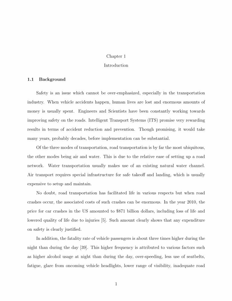
1.1 Background
Safety is an issue which cannot be over-emphasized, especially in the transportation
industry. When vehicle accidents happen, human lives are lost and enormous amounts of
money is usually spent. Engineers and Scientists have been constantly working towards
improving safety on the roads. Intelligent Transport Systems (ITS) promise very rewarding
results in terms of accident reduction and prevention. Though promising, it would take
many years, probably decades, before implementation can be substantial.
Of the three modes of transportation, road transportation is by far the most ubiquitous,
the other modes being air and water. This is due to the relative ease of setting up a road
network. Water transportation usually makes use of an existing natural water channel.
Air transport requires special infrastructure for safe takeoff and landing, which is usually
expensive to setup and maintain.
No doubt, road transportation has facilitated life in various respects but when road
crashes occur, the associated costs of such crashes can be enormous. In the year 2010, the
price for car crashes in the US amounted to $871 billion dollars, including loss of life and
lowered quality of life due to injuries [5]. Such amount clearly shows that any expenditure
on safety is clearly justified.
In addition, the fatality rate of vehicle passengers is about three times higher during the
night than during the day [39]. This higher frequency is attributed to various factors such
as higher alcohol usage at night than during the day, over-speeding, less use of seatbelts,
fatigue, glare from oncoming vehicle headlights, lower range of visibility, inadequate road
1
signs, etc. Hence, any effective measure towards reducing vehicle passenger fatality at night
will greatly reduce the overall fatality rate of vehicle accidents.
Since the invention of the automobile in the 18th century, the automobile has evolved
over the years in terms of its operation. Of particular interest are some of the safety features
aimed towards preventing accidents and minimizing injuries and loss of life, when accidents
occur. Safety features in today’s cars vary a great deal, usually depending on the cost of the
car. However, features such as front airbags, seatbelts with pretensioners,etc., are standard
across board. A more detailed review on some of these features is presented in the next
chapter.
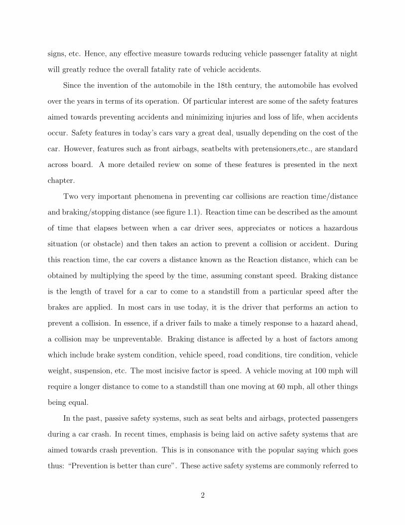
Two very important phenomena in preventing car collisions are reaction time/distance
and braking/stopping distance (see figure 1.1). Reaction time can be described as the amount
of time that elapses between when a car driver sees, appreciates or notices a hazardous
situation (or obstacle) and then takes an action to prevent a collision or accident. During
this reaction time, the car covers a distance known as the Reaction distance, which can be
obtained by multiplying the speed by the time, assuming constant speed. Braking distance
is the length of travel for a car to come to a standstill from a particular speed after the
brakes are applied. In most cars in use today, it is the driver that performs an action to
prevent a collision. In essence, if a driver fails to make a timely response to a hazard ahead,
a collision may be unpreventable. Braking distance is affected by a host of factors among
which include brake system condition, vehicle speed, road conditions, tire condition, vehicle
weight, suspension, etc. The most incisive factor is speed. A vehicle moving at 100 mph will
require a longer distance to come to a standstill than one moving at 60 mph, all other things
being equal.
In the past, passive safety systems, such as seat belts and airbags, protected passengers
during a car crash. In recent times, emphasis is being laid on active safety systems that are
aimed towards crash prevention. This is in consonance with the popular saying which goes
thus: “Prevention is better than cure”. These active safety systems are commonly referred to
2
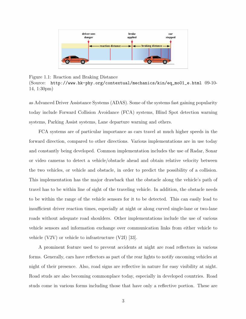
Figure 1.1: Reaction and Braking Distance(Source: http://www.hk-phy.org/contextual/mechanics/kin/eq_mo01_e.html 09-10-14, 1:30pm)
as Advanced Driver Assistance Systems (ADAS). Some of the systems fast gaining popularity
today include Forward Collision Avoidance (FCA) systems, Blind Spot detection warning
systems, Parking Assist systems, Lane departure warning and others.
FCA systems are of particular importance as cars travel at much higher speeds in the
forward direction, compared to other directions. Various implementations are in use today
and constantly being developed. Common implementation includes the use of Radar, Sonar
or video cameras to detect a vehicle/obstacle ahead and obtain relative velocity between
the two vehicles, or vehicle and obstacle, in order to predict the possibility of a collision.
This implementation has the major drawback that the obstacle along the vehicle’s path of
travel has to be within line of sight of the traveling vehicle. In addition, the obstacle needs
to be within the range of the vehicle sensors for it to be detected. This can easily lead to
insufficient driver reaction times, especially at night or along curved single-lane or two-lane
roads without adequate road shoulders. Other implementations include the use of various
vehicle sensors and information exchange over communication links from either vehicle to
vehicle (V2V) or vehicle to infrastructure (V2I) [33].
A prominent feature used to prevent accidents at night are road reflectors in various
forms. Generally, cars have reflectors as part of the rear lights to notify oncoming vehicles at
night of their presence. Also, road signs are reflective in nature for easy visibility at night.
Road studs are also becoming commonplace today, especially in developed countries. Road
studs come in various forms including those that have only a reflective portion. These are
3
popularly known as “cat’s eyes”. Other forms include those that are solar-powered with
Light Emitting Diodes (LEDs) [20]. Whenever road studs are used, they are usually few
meters apart, within line of sight of each other. LED road studs provide illumination visible
from up to 900m, compared to reflective cat’s eye which is limited to 90m [28]. The major
purpose of the road studs is for lane delineation purposes. Recently, other features/functions
are being included in them to improve vehicle safety on the roads. Some of these include
vehicle detection, incident detection, hazard warning and weather monitoring [9]. LED road
studs with added functions are commonly referred to as Intelligent Road Studs (IRS). IRS are
usually hard-wired to other systems to enable them function appropriately. Unfortunately,
this limits their use to areas where adequate infrastructure is available. In developing coun-
tries, advanced infrastructure is not always available and there is the need for a solution
that is both flexible and easy to install in terms of cost and complexity [20]. Vehicles can be
detected using magnetic field disturbances in the earth’s surface caused by metals present in
the vehicles [4][18]. A shortcoming of this approach can be caused by large vehicles passing
close to the sensors, thereby leading to false readings. Also, the earth’s magnetic field could
vary from time to time [27].
To further improve the reliability and accuracy of this detection method in IRS at night,
lights from vehicles can be detected through optical means.
1.2 Purpose
This report is aimed at presenting results and findings arising from investigating the
possibility of detecting stalled or slowly moving vehicles at night with minimum infrastruc-
tural dependence through measuring the variation of headlight intensity of the concerned
vehicles. This possibility is being investigated as it is mandatory all over the world for car
vehicles to have their headlights on at night and under low-lighting conditions. This makes
it theoretically possible to detect the presence of a car through the use of a light detector
at night. This detection method may be included in IRS that can detect vehicles through
4
magnetic field sensing, which coupled with wireless communication ability, can be used in
implementing an effective FCA system.
1.3 Scope
In carrying out the study and experiments, only cars, small trucks and sport-utility
vehicles were utilized for the experiments. Experiments were carried out under dry conditions
with minimal light reflection from road surfaces. Some of the experiment runs were carried
out near traffic lights where moving cars and stopped vehicles could easily be observed. Fog,
rain or other low visibility environmental conditions were not considered for the experiments.
1.4 Document Layout
This thesis is organized into five chapters, followed by a bibliography and a set of
appendices. Chapter 2 provides background information on road crashes and its higher
frequency at night. It also briefly describes some of the current ways of accident prevention.
The second subsection gives a brief description of accident causes, including why accidents
could occur more frequently at night. Also, the concepts of Reaction and Stopping distances
are further explained. ADAS and vehicle detection systems are also briefly described. The
car headlight beam is also described.
Chapter 3 explains the materials used for the experiments and the methods employed.
Chapter 4 provides the results of the experiments and discusses them.
Chapter 5 provides a conclusion and future work.
5
Chapter 2
Literature Review
Since the invention of the motor vehicle, scientists and engineers have been constantly
working towards its development to improve its efficiency, reliability and safety. Safety is a
very important aspect as “every year nearly 36,000 people are killed and more than 3.5 million
people are injured in motor vehicle crashes, making it the leading cause of unintentional
injuries and death for people between the ages of 1 and 33”[7].
In this chapter, causes of car crashes are briefly discussed.
2.1 Causes of Car Crashes[2]
Factors that could lead to a car crash can be grouped into three major categories,
namely: Driver, Vehicle and Environment.
2.1.1 Driver related causes
These can be further classified into recognition, decision, performance and non-performance
errors. As shown in Table 2.1, it can be observed that recognition error has the highest per-
centage of 40.6%, followed by decision error. Hence, if a driver recognizes a hazard in time,
a crash may be avoided.
2.1.2 Vehicle related causes
These are crashes which occur as a result of failure of some part(s) of the vehicle(s)
involved. These are as shown in Table 2.2. It is clearly seen that the most frequent vehicle
related cause is tire failure.
6

Table 2.1: Reasons for Car Crashes attributed to Drivers[2]Reason for Crash Weight (%)
Recognition Error
Inadequate Surveillance 20.3Internal Distraction 10.7External Distraction 3.8Inattention (i.e. daydreaming,etc.) 3.2Other/unknown recognition error 2.5Subtotal 40.6
Decision Error
Too fast for conditions 8.4Too fast for curve 4.9False assumption of other’s action 4.5Illegal maneuver 3.8Misjudgment of gap or other’s speed 3.2Following too closely 1.5Aggressive driving behavior 1.5Other/unknown decision error 6.2Subtotal 34.1
Performance Error
Overcompensation 4.9Poor directional control 4.7Other/unknown performance error 0.4Panic/freezing 0.3Subtotal 10.3
Non-Performance Error
Sleep, actually asleep 3.2Heart attack or other physical impairment 2.4Other/unknown critical nonperformance 1.6Subtotal 7.1
Other/unknown driver error 7.9Total 100
Table 2.2: Reasons for Car Crashes attributed to Vehicles[2]Reason for Crash Weight (%)Tires failed or degraded/wheels failed 43.3Brakes failed/degraded 25.0Other vehicle failure/deficiency 20.8Steering/suspension/transmission/engine failed 10.5Unknown 0.5Total 100
7
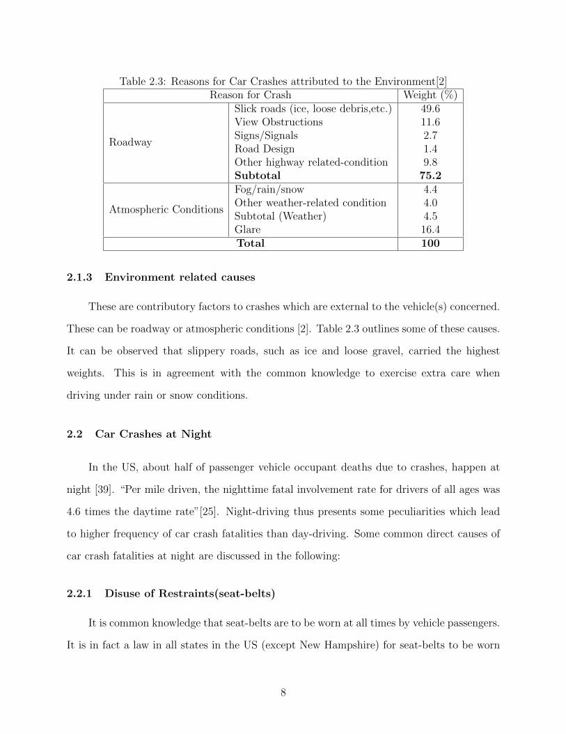
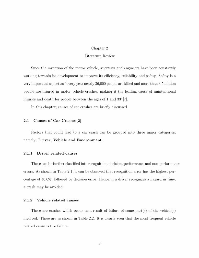
Table 2.3: Reasons for Car Crashes attributed to the Environment[2]Reason for Crash Weight (%)
Roadway
Slick roads (ice, loose debris,etc.) 49.6View Obstructions 11.6Signs/Signals 2.7Road Design 1.4Other highway related-condition 9.8Subtotal 75.2
Atmospheric Conditions
Fog/rain/snow 4.4Other weather-related condition 4.0Subtotal (Weather) 4.5Glare 16.4Total 100
2.1.3 Environment related causes
These are contributory factors to crashes which are external to the vehicle(s) concerned.
These can be roadway or atmospheric conditions [2]. Table 2.3 outlines some of these causes.
It can be observed that slippery roads, such as ice and loose gravel, carried the highest
weights. This is in agreement with the common knowledge to exercise extra care when
driving under rain or snow conditions.
2.2 Car Crashes at Night
In the US, about half of passenger vehicle occupant deaths due to crashes, happen at
night [39]. “Per mile driven, the nighttime fatal involvement rate for drivers of all ages was
4.6 times the daytime rate”[25]. Night-driving thus presents some peculiarities which lead
to higher frequency of car crash fatalities than day-driving. Some common direct causes of
car crash fatalities at night are discussed in the following:
2.2.1 Disuse of Restraints(seat-belts)
It is common knowledge that seat-belts are to be worn at all times by vehicle passengers.
It is in fact a law in all states in the US (except New Hampshire) for seat-belts to be worn
8
Figure 2.1: Passenger Vehicle Occupant Fatalities in 2005 by Time of Day and Restraint Use(Source: http://www-nrd.nhtsa.dot.gov/Pubs/810637.PDF 09-10-14, 1:30pm)
when operating a motor vehicle [8]. A study carried out in 2005 by the National Highway
Traffic Safety Administration (NHTSA) showed that about 64% of people killed through car
crashes at night did not use restraints (see Figure 2.1) [39]. In contrast, less than half of such
people failed to use restraints during daytime. This could be due to the relative difficulty of
being observed by law enforcement officers at night, than during the day.
2.2.2 High Blood Alcohol Concentration (BAC) Levels
Blood Alcohol Concentration can be defined as the quantity of alcohol contained in a
person’s blood, measured in weight per unit volume. At times, this measurement is converted
to a percentage. Alcohol easily affects a person’s sense of reasoning and judgment as it travels
directly to the brain through blood [30].
Figure 2.2 shows Car Crash Deaths by time of day and BAC. It can be clearly observed
that alcohol use contributed to more deaths at night than during the day. Table 2.4 shows
the way people typically react to some BAC levels. It can be clearly observed that the higher
the alcohol concentration level in a driver’s blood, the higher is the likelihood of a car crash.
2.2.3 Speeding
We live in a fast-paced society where people want things done quickly. Unfortunately,
this does not usually turn out well when it comes to driving a motor vehicle. Driving a
9
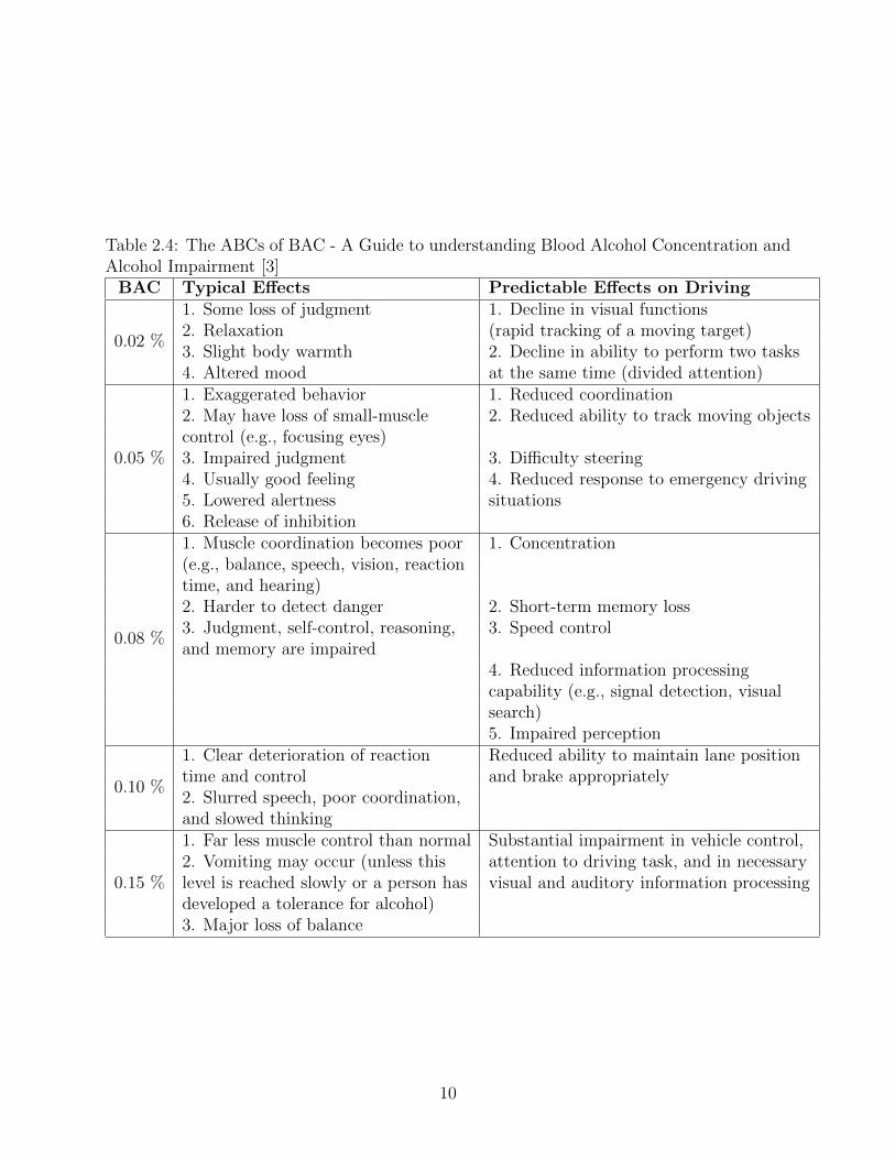
Table 2.4: The ABCs of BAC - A Guide to understanding Blood Alcohol Concentration andAlcohol Impairment [3]
BAC Typical Effects Predictable Effects on Driving
0.02 %
1. Some loss of judgment 1. Decline in visual functions2. Relaxation (rapid tracking of a moving target)3. Slight body warmth 2. Decline in ability to perform two tasks4. Altered mood at the same time (divided attention)
0.05 %
1. Exaggerated behavior 1. Reduced coordination2. May have loss of small-muscle 2. Reduced ability to track moving objectscontrol (e.g., focusing eyes)3. Impaired judgment 3. Difficulty steering4. Usually good feeling 4. Reduced response to emergency driving5. Lowered alertness situations6. Release of inhibition
0.08 %
1. Muscle coordination becomes poor 1. Concentration(e.g., balance, speech, vision, reactiontime, and hearing)2. Harder to detect danger 2. Short-term memory loss3. Judgment, self-control, reasoning, 3. Speed controland memory are impaired
4. Reduced information processingcapability (e.g., signal detection, visualsearch)5. Impaired perception
0.10 %
1. Clear deterioration of reaction Reduced ability to maintain lane positiontime and control and brake appropriately2. Slurred speech, poor coordination,and slowed thinking
0.15 %
1. Far less muscle control than normal Substantial impairment in vehicle control,2. Vomiting may occur (unless this attention to driving task, and in necessarylevel is reached slowly or a person has visual and auditory information processingdeveloped a tolerance for alcohol)3. Major loss of balance
10

Figure 2.2: Passenger Vehicle Occupant Fatalities in 2005 by Time of Day and BAC Levelin the Crash(Source: http://www-nrd.nhtsa.dot.gov/Pubs/810637.PDF 09-10-14, 1:45pm)
Figure 2.3: Passenger Vehicle Occupant Fatalities in 2005 by Time of Day and Speeding(Source: http://www-nrd.nhtsa.dot.gov/Pubs/810637.PDF 09-10-14, 1:45pm)
motor vehicle at high speeds can be fatal. In fact, “Speeding is one of the most prevalent
causes of car accidents today according to the U.S. Department of Transportation”[31].
In the year 2005, speeding accounted for about 37% of car-crash deaths at night com-
pared to about 21% of such death during the day (see Figure 2.3).
2.3 Reaction and Stopping Time/Distance
These two concepts were introduced in Chapter 1 and would be further explained here.
As mentioned earlier, speed directly affects both reaction and stopping distances. The faster
a vehicle moves, the more distance it covers within a unit time. For example, a vehicle trav-
eling at 70 miles per hour (mph) covers 31.29 meters (m) in a second, while one traveling at
100 mph covers 44.70 m in a second.
11
2.3.1 Reaction Time/Distance
It is necessary for a car driver to respond to a road hazard in a timely manner to prevent
a crash. The time that elapses between when the driver sees or appreciates a hazard and
actually responds is known as Reaction time. During this time, it is generally assumed that
the speed of the vehicle remains constant. Hence, multiplying the speed by the reaction
time yields the Reaction distance. This is a very important factor in FCA system design, as
it contributes towards the computation of Time-to-Collision (TTC) and Safety braking dis-
tances, which are two quantities that FCA systems use in deciding whether there is a hazard
ahead of a traveling vehicle or not [6]. Reaction time/distance of a driver to a particular
situation depends on a lot of factors, among which includes:
- Various available alternatives: In case a driver traveling along a road needs to respond
urgently to a situation, the time it takes to analyze the situation and its alternatives will
affect the eventual reaction. For example, a driver suddenly encountering a road blockage
may decide to try to avoid it or try to stop without a collision [38].
- Ease of distinction between various situations: In this case, the ability to differ-
entiate the various happenings in the vicinity of the driver will likely affect the eventual
response/reaction time. As an illustration, a driver who fixates his eyes on a semi-truck
about to join a major highway may not see that the vehicles ahead are slowing down as a
result of a speed zone ahead and thus have his or her available reaction time shortened [38].
- Accuracy of the reaction outcome: Depending on the resulting action, a driver may
take a while to figure it out. In a situation where a car is following another too closely, if
the one ahead suddenly slows down, the driver behind may be unable to respond accurately
by also braking and this could result in a crash [38].
- Thinking involved[38]: The length of time a driver needs to think about a situation will
directly affect the corresponding reaction.
- Past experience of the driver: A driver who has been previously exposed to various
situations when driving, is likely to react/respond faster upon encountering similar situations
12
than one who is not as exposed.
- Current state of mind and health of the driver:A distracted driver is not likely to
react as quickly as one who is focused. In addition, a healthy and fit driver is likely to react
faster than one who is not.
Reaction times vary from person to person, and also the situation but benchmarks of 1.5
seconds and 2.5 seconds are used for road design considerations and car-crash investigations
[1]. In [6], Reaction time was broken into three components namely Reflection time , Judg-
ment time and Action time, with corresponding time ranges of (0.44-0.52 seconds),(0.15-0.25
seconds) and (0.15-0.4 seconds) respectively.
Pressure Buildup Distance/Time
Due to the fact that there is some free pedal play in most vehicle brake pedals, this
factor may also be considered before braking commences. “The pressure buildup distance is
the distance of vehicle travel during the initiation of braking action to the full setup of the
braking pressure”[6]. The value of this time may range from 0.3 to 0.75 seconds [6].
2.3.2 Stopping/Braking Distance
After the driver upon appreciating a hazard ahead, has decided to stop the vehicle and
pressure is fully built in the brake system, the time that elapses between when the vehicle
starts braking and eventually stops is the Stopping/braking time. The vehicle covers a
certain distance during this time referred to as the braking distance. Factors which affect a
vehicle’s stopping distance include:
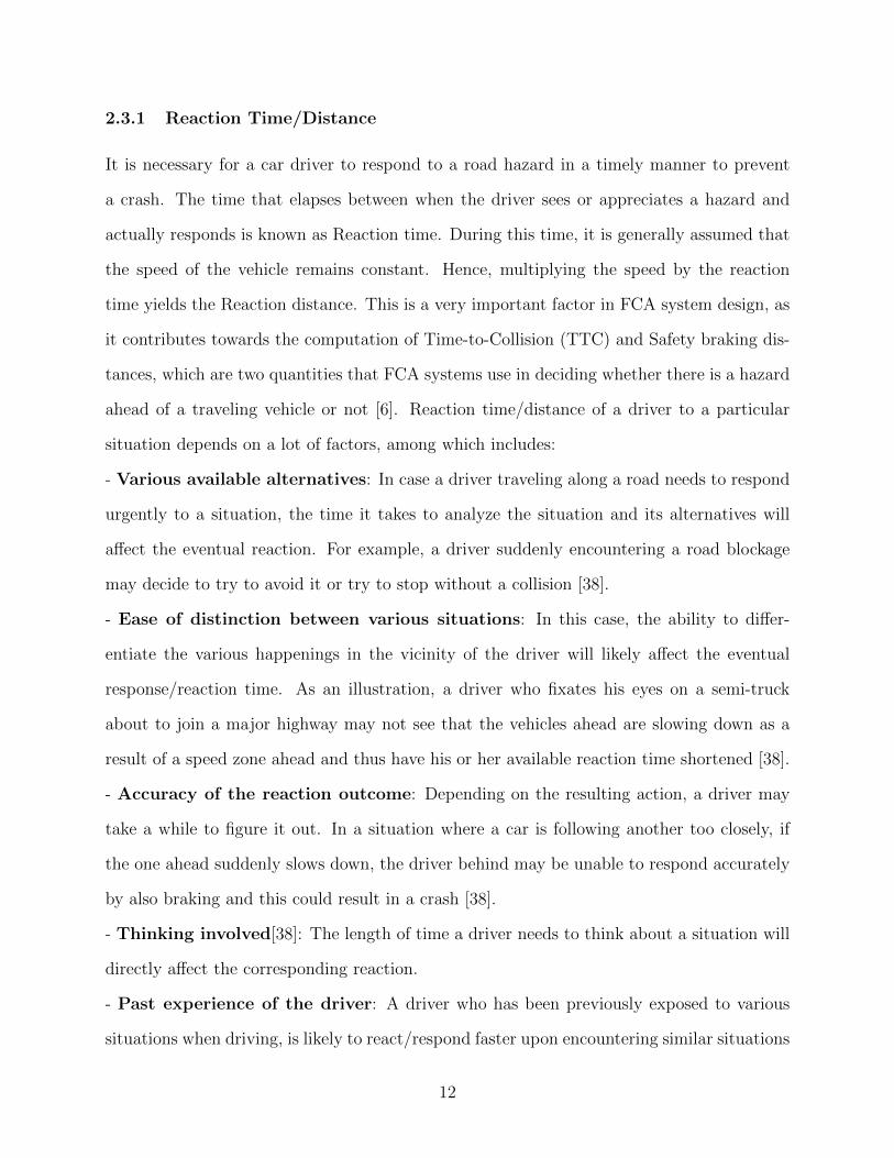
- Speed [11]: The higher the speed of a vehicle, the longer the stopping/braking distance
will be, given a constant deceleration. This can be deduced from the mechanics equation:
v2 = u2 + 2as (2.1)
13
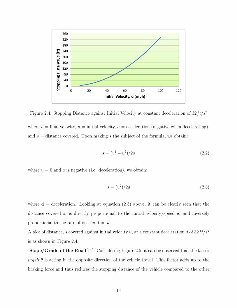
Figure 2.4: Stopping Distance against Initial Velocity at constant deceleration of 32ft/s2
where v = final velocity, u = initial velocity, a = acceleration (negative when decelerating),
and s = distance covered. Upon making s the subject of the formula, we obtain:
s = (v2 − u2)/2a (2.2)
where v = 0 and a is negative (i.e. deceleration), we obtain:
s = (u2)/2d (2.3)
where d = deceleration. Looking at equation (2.3) above, it can be clearly seen that the
distance covered s, is directly proportional to the initial velocity/speed u, and inversely
proportional to the rate of deceleration d.
A plot of distance, s covered against initial velocity u, at a constant deceleration d of 32ft/s2
is as shown in Figure 2.4.
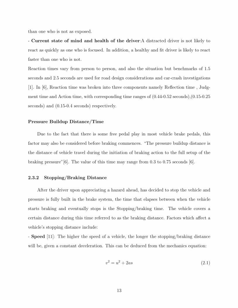
-Slope/Grade of the Road[11]: Considering Figure 2.5, it can be observed that the factor
mgsinθ is acting in the opposite direction of the vehicle travel. This factor adds up to the
braking force and thus reduces the stopping distance of the vehicle compared to the other
14
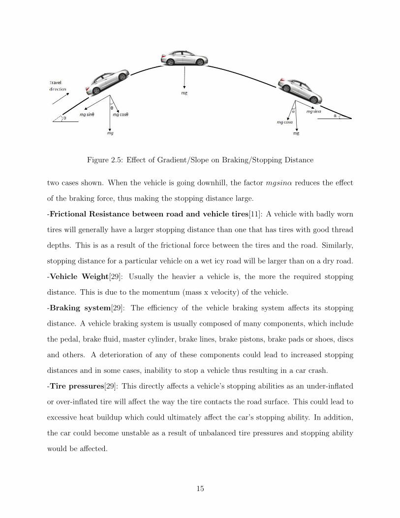
Figure 2.5: Effect of Gradient/Slope on Braking/Stopping Distance
two cases shown. When the vehicle is going downhill, the factor mgsinα reduces the effect
of the braking force, thus making the stopping distance large.
-Frictional Resistance between road and vehicle tires[11]: A vehicle with badly worn
tires will generally have a larger stopping distance than one that has tires with good thread
depths. This is as a result of the frictional force between the tires and the road. Similarly,
stopping distance for a particular vehicle on a wet icy road will be larger than on a dry road.
-Vehicle Weight[29]: Usually the heavier a vehicle is, the more the required stopping
distance. This is due to the momentum (mass x velocity) of the vehicle.
-Braking system[29]: The efficiency of the vehicle braking system affects its stopping
distance. A vehicle braking system is usually composed of many components, which include
the pedal, brake fluid, master cylinder, brake lines, brake pistons, brake pads or shoes, discs
and others. A deterioration of any of these components could lead to increased stopping
distances and in some cases, inability to stop a vehicle thus resulting in a car crash.
-Tire pressures[29]: This directly affects a vehicle’s stopping abilities as an under-inflated
or over-inflated tire will affect the way the tire contacts the road surface. This could lead to
excessive heat buildup which could ultimately affect the car’s stopping ability. In addition,
the car could become unstable as a result of unbalanced tire pressures and stopping ability
would be affected.
15
-Suspension system[29][14]: The suspension system of a car is made up of components such
as shock absorbers, control arms, stabilizer bars/links, bushings, subframe supports, etc. All
these components ensure that the vehicle is well supported and stable when driven. Failure
of any of these components could lead to instability and thus increase stopping distance
of the vehicle. As an illustration, a worn out shock absorber could affect the way the tire
contacts the road and thus affect the stopping ability of the vehicle.
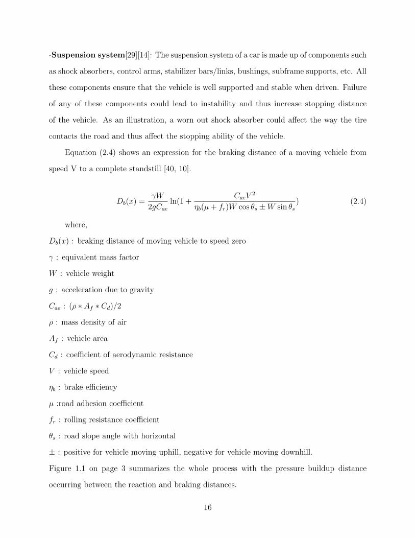
Equation (2.4) shows an expression for the braking distance of a moving vehicle from
speed V to a complete standstill [40, 10].
Db(x) =γW
2gCae
ln(1 +CaeV
2
ηb(µ+ fr)W cos θs ±W sin θs) (2.4)
where,
Db(x) : braking distance of moving vehicle to speed zero
γ : equivalent mass factor
W : vehicle weight
g : acceleration due to gravity
Cae : (ρ ∗ Af ∗ Cd)/2
ρ : mass density of air
Af : vehicle area
Cd : coefficient of aerodynamic resistance
V : vehicle speed
ηb : brake efficiency
µ :road adhesion coefficient
fr : rolling resistance coefficient
θs : road slope angle with horizontal
± : positive for vehicle moving uphill, negative for vehicle moving downhill.
Figure 1.1 on page 3 summarizes the whole process with the pressure buildup distance
occurring between the reaction and braking distances.
16
2.4 Advanced Driver Assistance Systems (ADAS)
Embedded systems can be found in many electronic devices and can be found in vir-
tually all new cars today. In cars, this takes the form of Electronic Control Units (ECUs)
which control specific functions in the car. Some of these systems found in cars include
air-conditioning systems (climate control), security alarm systems, comfort modules, power
and memory seats, supplemental restraint systems (SRS) and others. Real-time car systems
aimed at preventing or avoiding accidents are known as Advanced Driver Assistance Systems
(ADAS)[35]. Some ADAS systems help prevent major accidents while others help prevent
minor ones. The following sections describe some of these systems in more detail.
2.4.1 Cruise Control
Cruise control is a feature found on some vehicles that keeps the vehicle moving at a
particular speed (set by the driver) without throttle input from the driver. In earlier vehicles,
this was controlled by the use of a mechanical device called a Centrifugal governor [37]. In
recent vehicles, this is controlled electronically through an embedded system. Two main
benefits of this kind of system are reduction of driver fatigue on long drives, and increased
fuel economy [35].
2.4.2 Adaptive Cruise Control
With the Cruise control system, the vehicle would maintain the set speed regardless of
the external conditions of the car and could be cancelled by either pressing the brake pedal
or pressing the cancel button. Recent developments have led to Adaptive Cruise Control
(ACC) systems.
In the ACC system, the vehicle has a range of sensors which detect other vehicles coming
within their range. The system responds by autonomously applying the brakes and reducing
acceleration in order to follow a vehicle ahead at a user-defined time-gap or distance [35].
17
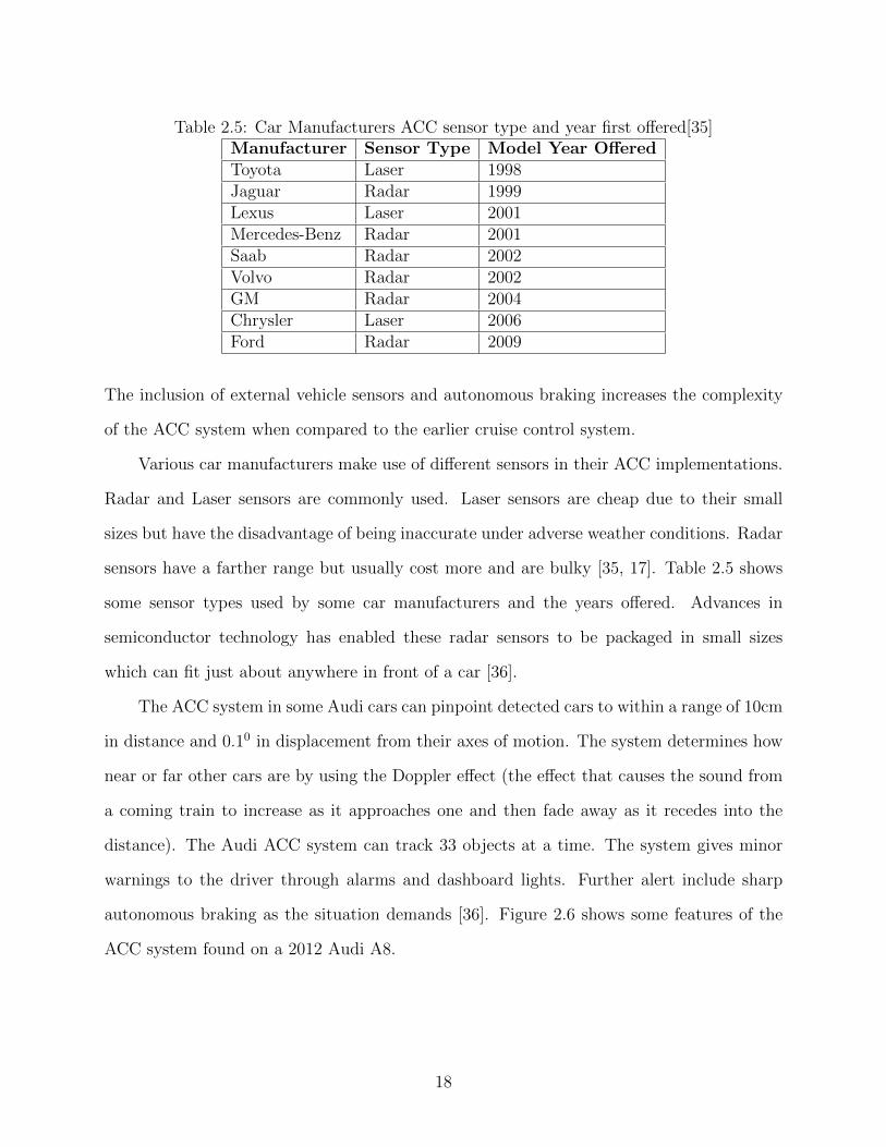
Table 2.5: Car Manufacturers ACC sensor type and year first offered[35]Manufacturer Sensor Type Model Year OfferedToyota Laser 1998Jaguar Radar 1999Lexus Laser 2001Mercedes-Benz Radar 2001Saab Radar 2002Volvo Radar 2002GM Radar 2004Chrysler Laser 2006Ford Radar 2009
The inclusion of external vehicle sensors and autonomous braking increases the complexity
of the ACC system when compared to the earlier cruise control system.
Various car manufacturers make use of different sensors in their ACC implementations.
Radar and Laser sensors are commonly used. Laser sensors are cheap due to their small
sizes but have the disadvantage of being inaccurate under adverse weather conditions. Radar
sensors have a farther range but usually cost more and are bulky [35, 17]. Table 2.5 shows
some sensor types used by some car manufacturers and the years offered. Advances in
semiconductor technology has enabled these radar sensors to be packaged in small sizes
which can fit just about anywhere in front of a car [36].
The ACC system in some Audi cars can pinpoint detected cars to within a range of 10cm
in distance and 0.10 in displacement from their axes of motion. The system determines how
near or far other cars are by using the Doppler effect (the effect that causes the sound from
a coming train to increase as it approaches one and then fade away as it recedes into the
distance). The Audi ACC system can track 33 objects at a time. The system gives minor
warnings to the driver through alarms and dashboard lights. Further alert include sharp
autonomous braking as the situation demands [36]. Figure 2.6 shows some features of the
ACC system found on a 2012 Audi A8.
18
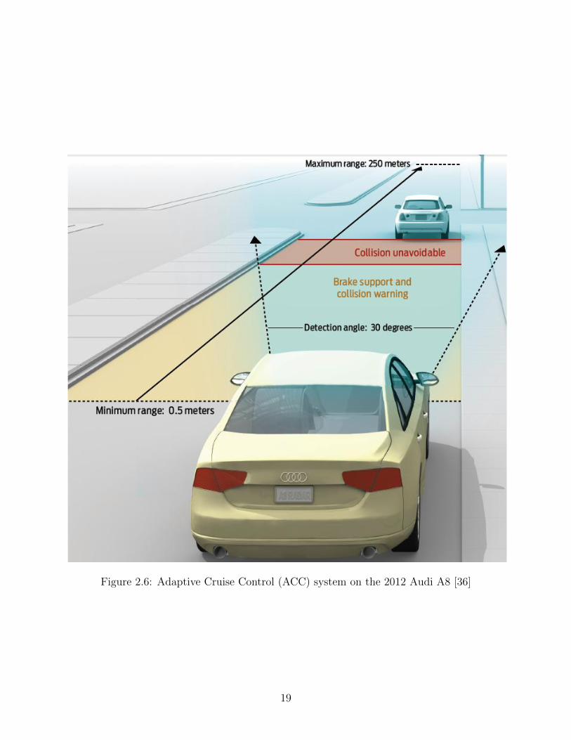
Figure 2.6: Adaptive Cruise Control (ACC) system on the 2012 Audi A8 [36]
19
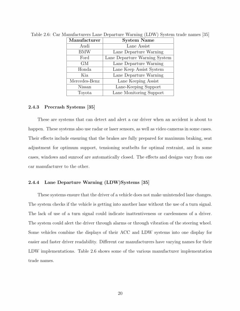
Table 2.6: Car Manufacturers Lane Departure Warning (LDW) System trade names [35]Manufacturer System Name
Audi Lane AssistBMW Lane Departure WarningFord Lane Departure Warning SystemGM Lane Departure Warning
Honda Lane Keep Assist SystemKia Lane Departure Warning
Mercedes-Benz Lane Keeping AssistNissan Lane-Keeping SupportToyota Lane Monitoring Support
2.4.3 Precrash Systems [35]
These are systems that can detect and alert a car driver when an accident is about to
happen. These systems also use radar or laser sensors, as well as video cameras in some cases.
Their effects include ensuring that the brakes are fully prepared for maximum braking, seat
adjustment for optimum support, tensioning seatbelts for optimal restraint, and in some
cases, windows and sunroof are automatically closed. The effects and designs vary from one
car manufacturer to the other.
2.4.4 Lane Departure Warning (LDW)Systems [35]
These systems ensure that the driver of a vehicle does not make unintended lane changes.
The system checks if the vehicle is getting into another lane without the use of a turn signal.
The lack of use of a turn signal could indicate inattentiveness or carelessness of a driver.
The system could alert the driver through alarms or through vibration of the steering wheel.
Some vehicles combine the displays of their ACC and LDW systems into one display for
easier and faster driver readability. Different car manufacturers have varying names for their
LDW implementations. Table 2.6 shows some of the various manufacturer implementation
trade names.
20
2.4.5 Blind Spot Information System (BLIS) [35]
Blind spots are areas on the sides of a vehicle that cannot be seen by the driver through
the mirrors, but only by turning the head away from the front of the car to the sides. The
system was first introduced by Volvo. It usually notifies the driver of a vehicle in the blind
spot through visual and/or audible alerts. Common implementations make use of sensors
mounted in the rear wheel wells, bumper sensors and cameras mounted in the side mirrors.
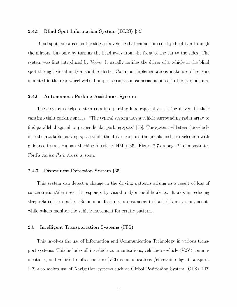
2.4.6 Autonomous Parking Assistance System
These systems help to steer cars into parking lots, especially assisting drivers fit their
cars into tight parking spaces. “The typical system uses a vehicle surrounding radar array to
find parallel, diagonal, or perpendicular parking spots” [35]. The system will steer the vehicle
into the available parking space while the driver controls the pedals and gear selection with
guidance from a Human Machine Interface (HMI) [35]. Figure 2.7 on page 22 demonstrates
Ford’s Active Park Assist system.
2.4.7 Drowsiness Detection System [35]
This system can detect a change in the driving patterns arising as a result of loss of
concentration/alertness. It responds by visual and/or audible alerts. It aids in reducing
sleep-related car crashes. Some manufacturers use cameras to tract driver eye movements
while others monitor the vehicle movement for erratic patterns.
2.5 Intelligent Transportation Systems (ITS)
This involves the use of Information and Communication Technology in various trans-
port systems. This includes all in-vehicle communications, vehicle-to-vehicle (V2V) commu-
nications, and vehicle-to-infrastructure (V2I) communications /citeetsiintelligenttransport.
ITS also makes use of Navigation systems such as Global Positioning System (GPS). ITS
21
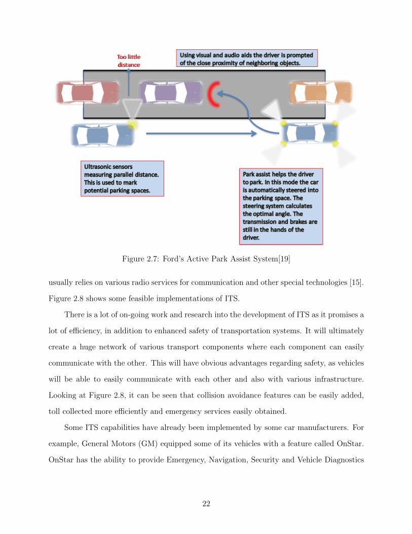
Figure 2.7: Ford’s Active Park Assist System[19]
usually relies on various radio services for communication and other special technologies [15].
Figure 2.8 shows some feasible implementations of ITS.
There is a lot of on-going work and research into the development of ITS as it promises a
lot of efficiency, in addition to enhanced safety of transportation systems. It will ultimately
create a huge network of various transport components where each component can easily
communicate with the other. This will have obvious advantages regarding safety, as vehicles
will be able to easily communicate with each other and also with various infrastructure.
Looking at Figure 2.8, it can be seen that collision avoidance features can be easily added,
toll collected more efficiently and emergency services easily obtained.
Some ITS capabilities have already been implemented by some car manufacturers. For
example, General Motors (GM) equipped some of its vehicles with a feature called OnStar.
OnStar has the ability to provide Emergency, Navigation, Security and Vehicle Diagnostics
22
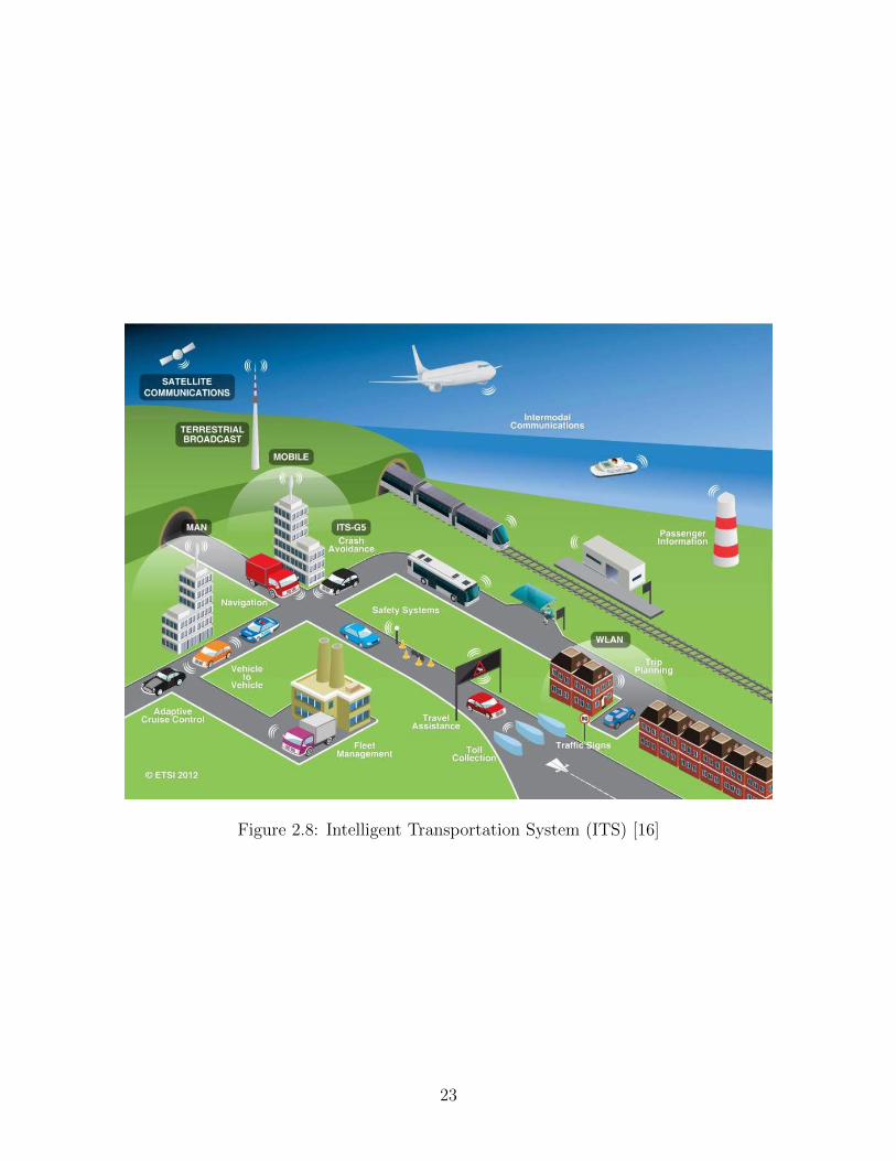
Figure 2.8: Intelligent Transportation System (ITS) [16]
23
features as necessary for the car user [22]. Automatic tolling systems have also been installed
on some major US highways.
ITS systems promise very good results when implementation levels are high. This could
take a couple of decades as research is still ongoing to develop some key components of the
various subsystems. For instance, various implementations of Inter-Vehicle Communications
(V2V) are still being experimented upon.
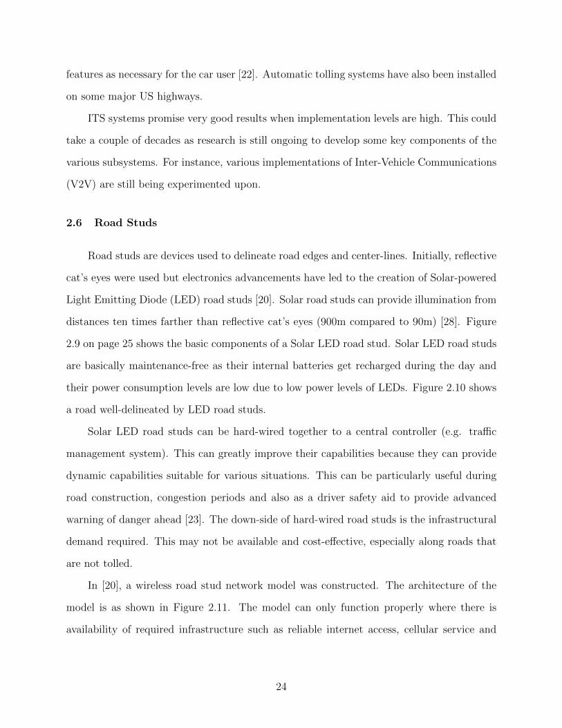
2.6 Road Studs
Road studs are devices used to delineate road edges and center-lines. Initially, reflective
cat’s eyes were used but electronics advancements have led to the creation of Solar-powered
Light Emitting Diode (LED) road studs [20]. Solar road studs can provide illumination from
distances ten times farther than reflective cat’s eyes (900m compared to 90m) [28]. Figure
2.9 on page 25 shows the basic components of a Solar LED road stud. Solar LED road studs
are basically maintenance-free as their internal batteries get recharged during the day and
their power consumption levels are low due to low power levels of LEDs. Figure 2.10 shows
a road well-delineated by LED road studs.
Solar LED road studs can be hard-wired together to a central controller (e.g. traffic
management system). This can greatly improve their capabilities because they can provide
dynamic capabilities suitable for various situations. This can be particularly useful during
road construction, congestion periods and also as a driver safety aid to provide advanced
warning of danger ahead [23]. The down-side of hard-wired road studs is the infrastructural
demand required. This may not be available and cost-effective, especially along roads that
are not tolled.
In [20], a wireless road stud network model was constructed. The architecture of the
model is as shown in Figure 2.11. The model can only function properly where there is
availability of required infrastructure such as reliable internet access, cellular service and
24
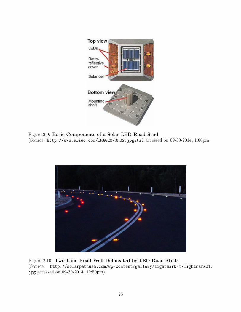
Figure 2.9: Basic Components of a Solar LED Road Stud(Source: http://www.sliwo.com/IMAGES/SRS2.jpgits) accessed on 09-30-2014, 1:00pm
Figure 2.10: Two-Lane Road Well-Delineated by LED Road Studs(Source: http://solarpathusa.com/wp-content/gallery/lightmark-t/lightmark01.
jpg accessed on 09-30-2014, 12:50pm)
25

Figure 2.11: System Layout of Remotely Controllable Wireless Road Stud Network [20]
power. This may not be available along some roads, especially in developing countries, thus
rendering the system unusable in such areas.
In [34], an intelligent system that makes use of Solar LED road studs connected wirelessly
was developed. Each road stud has an infra-red sensor and light sensor to detect the presence
of vehicles. Once an oncoming vehicle is detected, the road stud switches from a power-saving
mode to an active mode. In the active mode, the LED (red in this case) is switched on and
then a message is sent to the next node (road stud) for it to also be lit. This message is sent
in a forward direction along the car line of travel for the corresponding road studs to be lit.
The road stud LEDs go off after a definite time period. The system is as shown in Figure
2.12. This system provides clear lane delineation as the car travels and also conserves power
by lighting only when a vehicle is detected. However, the system does not provide advanced
26
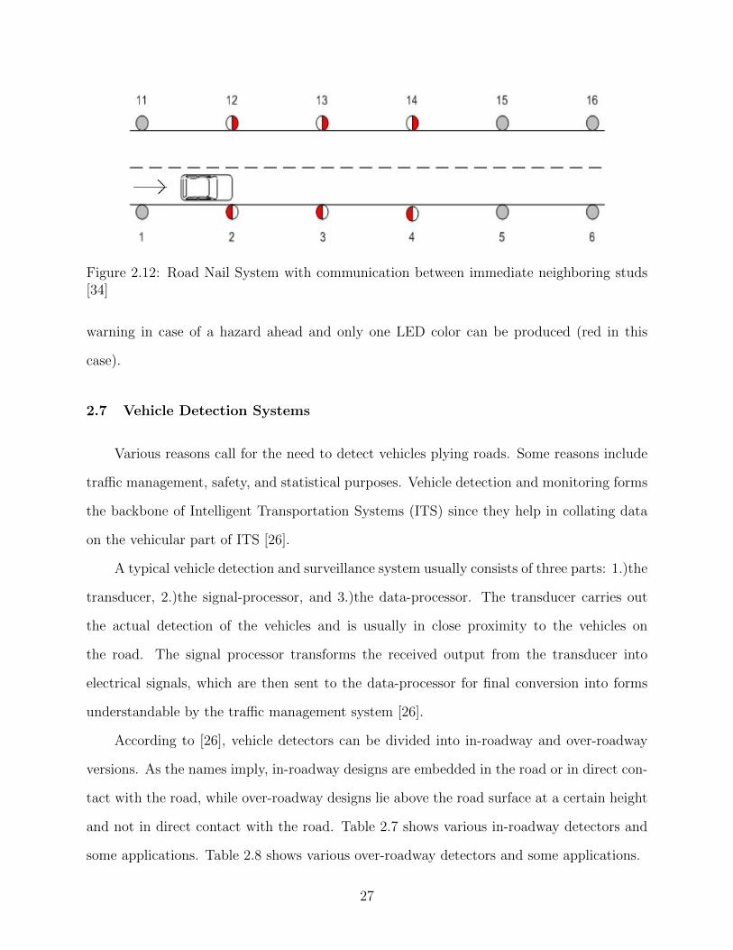
Figure 2.12: Road Nail System with communication between immediate neighboring studs[34]
warning in case of a hazard ahead and only one LED color can be produced (red in this
case).
2.7 Vehicle Detection Systems
Various reasons call for the need to detect vehicles plying roads. Some reasons include
traffic management, safety, and statistical purposes. Vehicle detection and monitoring forms
the backbone of Intelligent Transportation Systems (ITS) since they help in collating data
on the vehicular part of ITS [26].
A typical vehicle detection and surveillance system usually consists of three parts: 1.)the
transducer, 2.)the signal-processor, and 3.)the data-processor. The transducer carries out
the actual detection of the vehicles and is usually in close proximity to the vehicles on
the road. The signal processor transforms the received output from the transducer into
electrical signals, which are then sent to the data-processor for final conversion into forms
understandable by the traffic management system [26].
According to [26], vehicle detectors can be divided into in-roadway and over-roadway
versions. As the names imply, in-roadway designs are embedded in the road or in direct con-
tact with the road, while over-roadway designs lie above the road surface at a certain height
and not in direct contact with the road. Table 2.7 shows various in-roadway detectors and
some applications. Table 2.8 shows various over-roadway detectors and some applications.
27
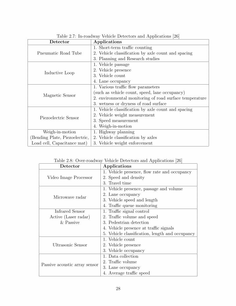
Table 2.7: In-roadway Vehicle Detectors and Applications [26]Detector Applications
Pneumatic Road Tube1. Short-term traffic counting2. Vehicle classification by axle count and spacing3. Planning and Research studies
Inductive Loop
1. Vehicle passage2. Vehicle presence3. Vehicle count4. Lane occupancy
Magnetic Sensor
1. Various traffic flow parameters(such as vehicle count, speed, lane occupancy)2. environmental monitoring of road surface temperature3. wetness or dryness of road surface
Piezoelectric Sensor
1. Vehicle classification by axle count and spacing2. Vehicle weight measurement3. Speed measurement4. Weigh-in-motion
Weigh-in-motion 1. Highway planning(Bending Plate, Piezoelectric, 2. Vehicle classification by axlesLoad cell, Capacitance mat) 3. Vehicle weight enforcement
Table 2.8: Over-roadway Vehicle Detectors and Applications [26]Detector Applications
Video Image Processor1. Vehicle presence, flow rate and occupancy2. Speed and density3. Travel time
Microwave radar
1. Vehicle presence, passage and volume2. Lane occupancy3. Vehicle speed and length4. Traffic queue monitoring
Infrared Sensor 1. Traffic signal controlActive (Laser radar) 2. Traffic volume and speed
& Passive 3. Pedestrian detection4. Vehicle presence at traffic signals5. Vehicle classification, length and occupancy
Ultrasonic Sensor1. Vehicle count2. Vehicle presence3. Vehicle occupancy
Passive acoustic array sensor
1. Data collection2. Traffic volume3. Lane occupancy4. Average traffic speed
28
Magnetic Sensor Detector
In the design of a vehicle detector system that requires very little infrastructural depen-
dence, over-roadway detectors are not usually considered because of their large dependence
on infrastructure (power, mounting poles, communications lines, etc.). From the variety of
in-road detectors, the only feasible option that can cover vast road areas is the Magnetic sen-
sor type, as used in [18]. There is a large variety of magnetic sensor technologies. A detailed
review can be found in [21]. [27] provides more information on the Anisotropic Magnetore-
sistive (AMR) magnetic sensor, which can be easily suited for vehicle detection with little
infrastructural dependence, as shown in [18]. Some of the drawbacks of the AMR sensor are
its temperature dependence, sensitivity to orientation, noise and amplifier requirement. To
overcome these drawbacks, circuit complexity has to be increased to ensure accuracy, at the
cost of increased power requirements [27].
2.8 Vehicle Headlamp
All motorized vehicles are mandated to have headlamps mounted in front of them to
provide light for night-driving or as daytime running lights (DRL) to provide presence-
awareness to other road users during the day. Engineers have constantly been working on
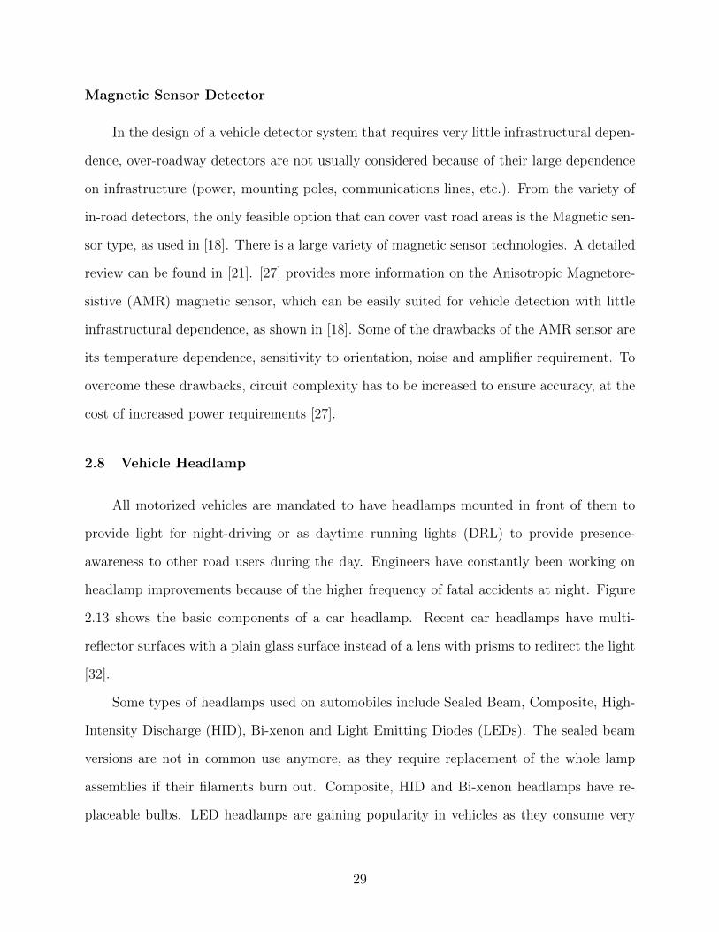
headlamp improvements because of the higher frequency of fatal accidents at night. Figure
2.13 shows the basic components of a car headlamp. Recent car headlamps have multi-
reflector surfaces with a plain glass surface instead of a lens with prisms to redirect the light
[32].
Some types of headlamps used on automobiles include Sealed Beam, Composite, High-
Intensity Discharge (HID), Bi-xenon and Light Emitting Diodes (LEDs). The sealed beam
versions are not in common use anymore, as they require replacement of the whole lamp
assemblies if their filaments burn out. Composite, HID and Bi-xenon headlamps have re-
placeable bulbs. LED headlamps are gaining popularity in vehicles as they consume very
29
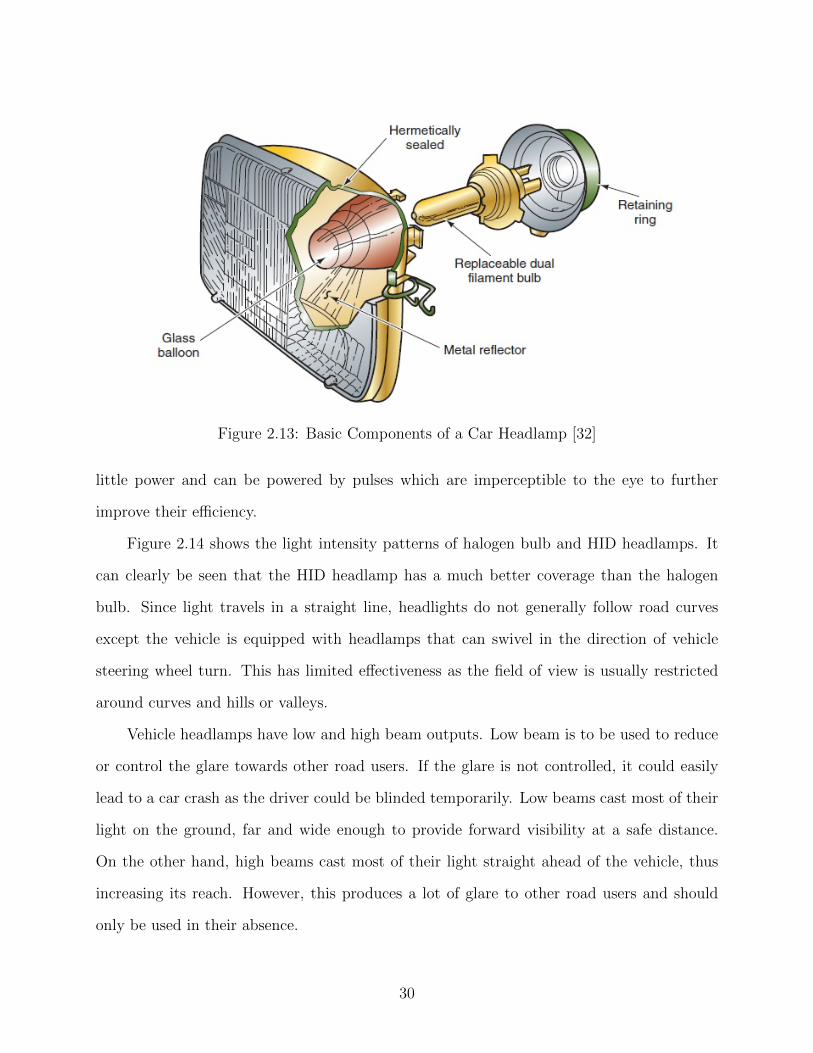
Figure 2.13: Basic Components of a Car Headlamp [32]
little power and can be powered by pulses which are imperceptible to the eye to further
improve their efficiency.
Figure 2.14 shows the light intensity patterns of halogen bulb and HID headlamps. It
can clearly be seen that the HID headlamp has a much better coverage than the halogen
bulb. Since light travels in a straight line, headlights do not generally follow road curves
except the vehicle is equipped with headlamps that can swivel in the direction of vehicle
steering wheel turn. This has limited effectiveness as the field of view is usually restricted
around curves and hills or valleys.
Vehicle headlamps have low and high beam outputs. Low beam is to be used to reduce
or control the glare towards other road users. If the glare is not controlled, it could easily
lead to a car crash as the driver could be blinded temporarily. Low beams cast most of their
light on the ground, far and wide enough to provide forward visibility at a safe distance.
On the other hand, high beams cast most of their light straight ahead of the vehicle, thus
increasing its reach. However, this produces a lot of glare to other road users and should
only be used in their absence.
30
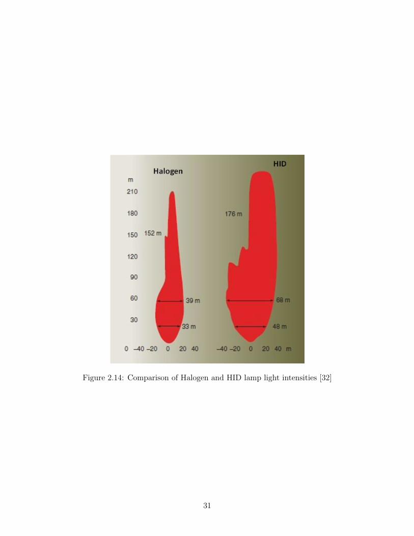
Figure 2.14: Comparison of Halogen and HID lamp light intensities [32]
31
Chapter 3
Materials and Methods
3.1 Experiment Setup
The main reason for this study was the determination of the feasibility of accurately
detecting a slow-moving or stalled vehicle at night, through optical sensing, by using only
the vehicle headlights. Other methods as mentioned in the previous chapter can be employed
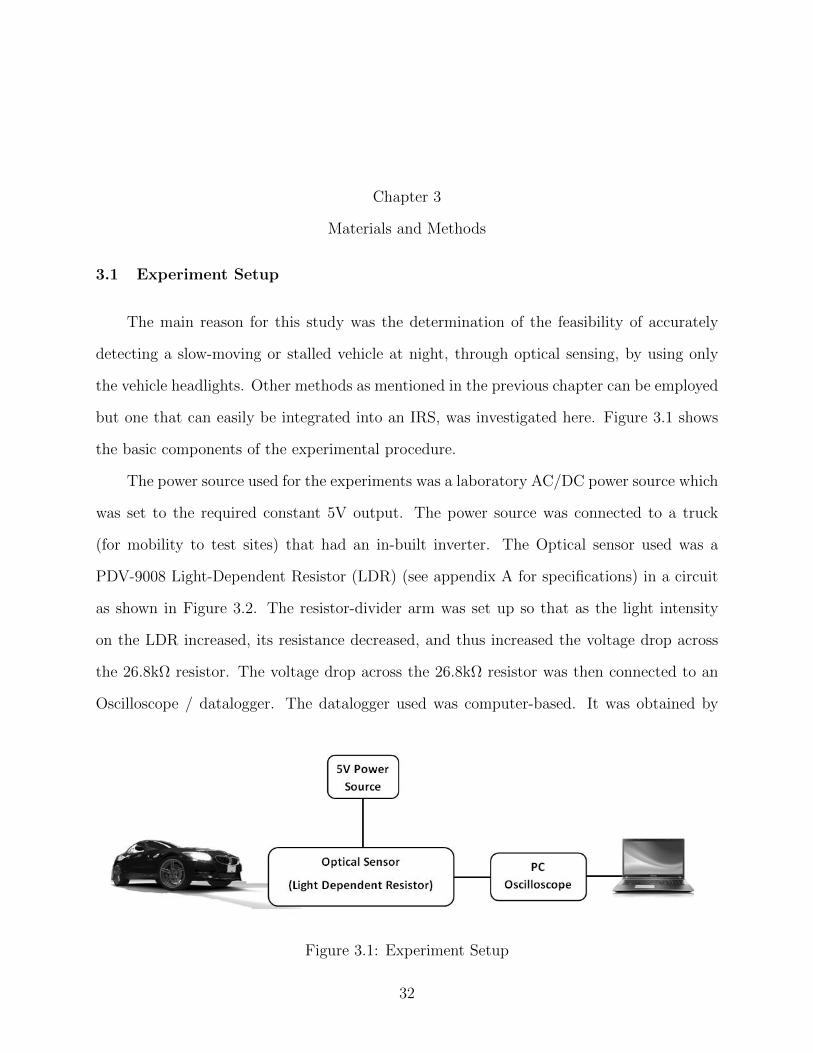
but one that can easily be integrated into an IRS, was investigated here. Figure 3.1 shows
the basic components of the experimental procedure.
The power source used for the experiments was a laboratory AC/DC power source which
was set to the required constant 5V output. The power source was connected to a truck
(for mobility to test sites) that had an in-built inverter. The Optical sensor used was a
PDV-9008 Light-Dependent Resistor (LDR) (see appendix A for specifications) in a circuit
as shown in Figure 3.2. The resistor-divider arm was set up so that as the light intensity
on the LDR increased, its resistance decreased, and thus increased the voltage drop across
the 26.8kΩ resistor. The voltage drop across the 26.8kΩ resistor was then connected to an
Oscilloscope / datalogger. The datalogger used was computer-based. It was obtained by
Figure 3.1: Experiment Setup
32
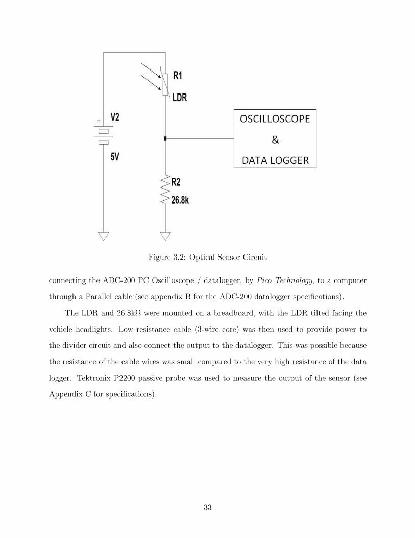
Figure 3.2: Optical Sensor Circuit
connecting the ADC-200 PC Oscilloscope / datalogger, by Pico Technology, to a computer
through a Parallel cable (see appendix B for the ADC-200 datalogger specifications).
The LDR and 26.8kΩ were mounted on a breadboard, with the LDR tilted facing the
vehicle headlights. Low resistance cable (3-wire core) was then used to provide power to
the divider circuit and also connect the output to the datalogger. This was possible because
the resistance of the cable wires was small compared to the very high resistance of the data
logger. Tektronix P2200 passive probe was used to measure the output of the sensor (see
Appendix C for specifications).
33
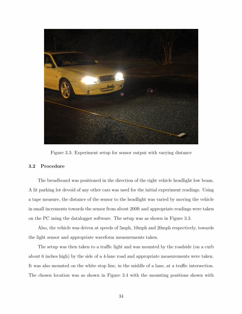
Figure 3.3: Experiment setup for sensor output with varying distance
3.2 Procedure
The breadboard was positioned in the direction of the right vehicle headlight low beam.
A lit parking lot devoid of any other cars was used for the initial experiment readings. Using
a tape measure, the distance of the sensor to the headlight was varied by moving the vehicle
in small increments towards the sensor from about 200ft and appropriate readings were taken
on the PC using the datalogger software. The setup was as shown in Figure 3.3.
Also, the vehicle was driven at speeds of 5mph, 10mph and 20mph respectively, towards
the light sensor and appropriate waveform measurements taken.
The setup was then taken to a traffic light and was mounted by the roadside (on a curb
about 6 inches high) by the side of a 4-lane road and appropriate measurements were taken.
It was also mounted on the white stop line, in the middle of a lane, at a traffic intersection.
The chosen location was as shown in Figure 3.4 with the mounting positions shown with
34
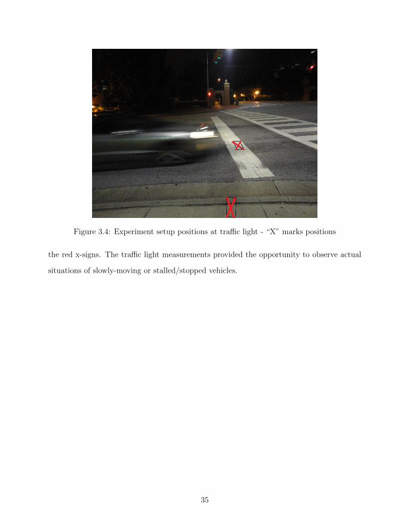
Figure 3.4: Experiment setup positions at traffic light - “X” marks positions
the red x-signs. The traffic light measurements provided the opportunity to observe actual
situations of slowly-moving or stalled/stopped vehicles.
35
Chapter 4
Results and Discussion
4.1 Parking Lot Experiments
4.1.1 Variation of Voltage Output with Distance from Optical Sensor
The result was as shown in Figure 4.1 on page 37 at a sampling rate of 200Hz. It can
be observed that the voltage output initially increased at a steady rate till it reached its
peak (about 2.6V) at around 20ft. This was due to the fact that the car headlights being
at a height of about 3.5 ft off the ground, do not fully shine on the sensor until the car was
backed off from the sensor a distance of about 20ft. After 20ft, the light intensity diminishes
and then falls off as the car recedes further. The small increments as the voltage output
dropped from its peak value are due to light reflecting off the ground surface and light from
the 2nd headlight reaching the sensor. At 190ft away from the sensor, the output voltage
was measured to be 0.100V. With the headlights set to full beam at 190ft, the output voltage
was measured to be 1.118V. This difference in output clearly shows the effect of using low
and high beams during night driving.
At 120ft away, the voltage measurement was about 0.24V. This clearly indicates that
the sensor could pick up the presence of a vehicle about 120ft away on a level and straight
road.
4.1.2 Output waveforms at varying vehicle speeds
Results obtained were as shown in Figures 4.2, 4.3 and 4.4 for speeds of 5mph, 10mph
and 20mph respectively. Upon comparing Figures 4.2, 4.3 and 4.4, it can be observed that
the tooth-like portions are identical except that the widths of the bases reduced as the speed
36
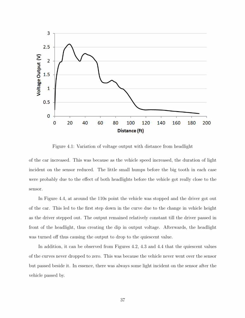
Figure 4.1: Variation of voltage output with distance from headlight
of the car increased. This was because as the vehicle speed increased, the duration of light
incident on the sensor reduced. The little small humps before the big tooth in each case
were probably due to the effect of both headlights before the vehicle got really close to the
sensor.
In Figure 4.4, at around the 110s point the vehicle was stopped and the driver got out
of the car. This led to the first step down in the curve due to the change in vehicle height
as the driver stepped out. The output remained relatively constant till the driver passed in
front of the headlight, thus creating the dip in output voltage. Afterwards, the headlight
was turned off thus causing the output to drop to the quiescent value.
In addition, it can be observed from Figures 4.2, 4.3 and 4.4 that the quiescent values
of the curves never dropped to zero. This was because the vehicle never went over the sensor
but passed beside it. In essence, there was always some light incident on the sensor after the
vehicle passed by.
37

Figure 4.2: Light sensor output for vehicle moving at 5mph
Figure 4.3: Light sensor output for vehicle moving at 10mph
38
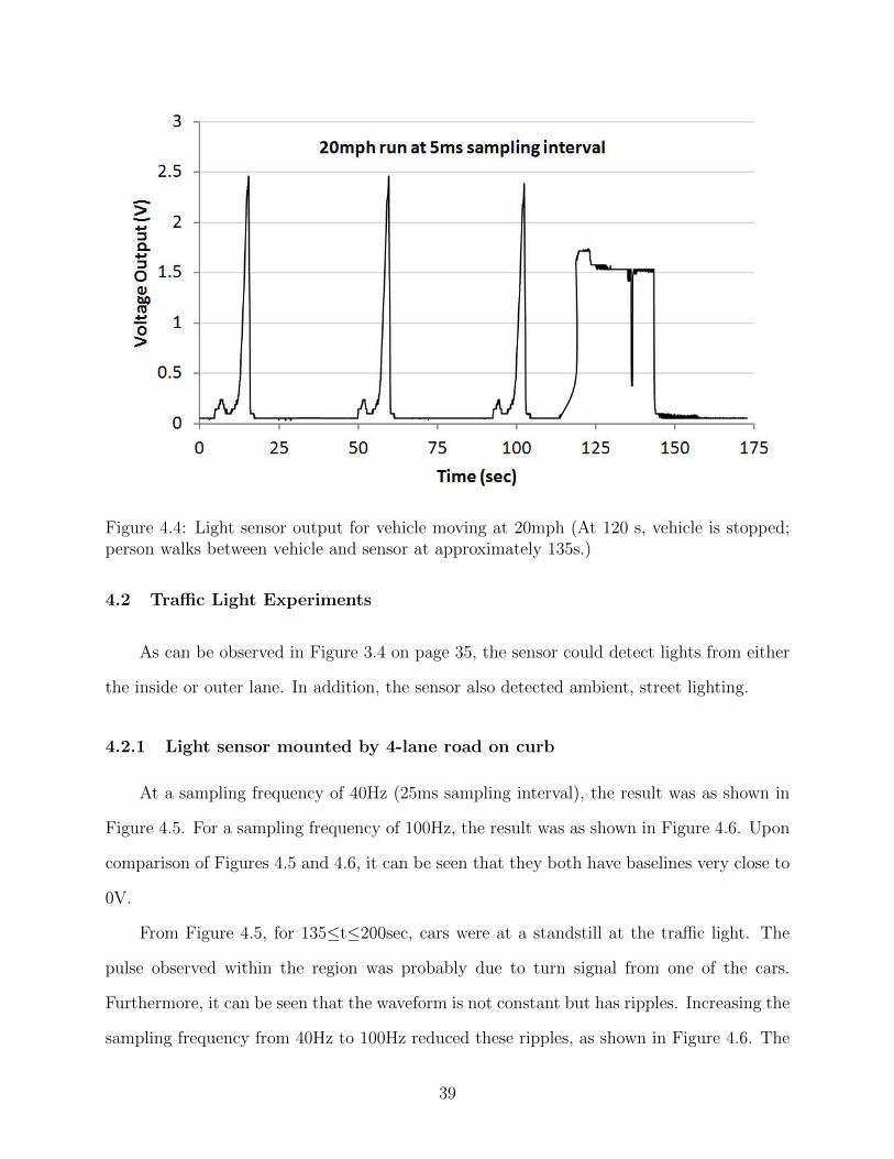
Figure 4.4: Light sensor output for vehicle moving at 20mph (At 120 s, vehicle is stopped;person walks between vehicle and sensor at approximately 135s.)
4.2 Traffic Light Experiments
As can be observed in Figure 3.4 on page 35, the sensor could detect lights from either
the inside or outer lane. In addition, the sensor also detected ambient, street lighting.
4.2.1 Light sensor mounted by 4-lane road on curb
At a sampling frequency of 40Hz (25ms sampling interval), the result was as shown in
Figure 4.5. For a sampling frequency of 100Hz, the result was as shown in Figure 4.6. Upon
comparison of Figures 4.5 and 4.6, it can be seen that they both have baselines very close to
0V.
From Figure 4.5, for 135≤t≤200sec, cars were at a standstill at the traffic light. The
pulse observed within the region was probably due to turn signal from one of the cars.
Furthermore, it can be seen that the waveform is not constant but has ripples. Increasing the
sampling frequency from 40Hz to 100Hz reduced these ripples, as shown in Figure 4.6. The
39
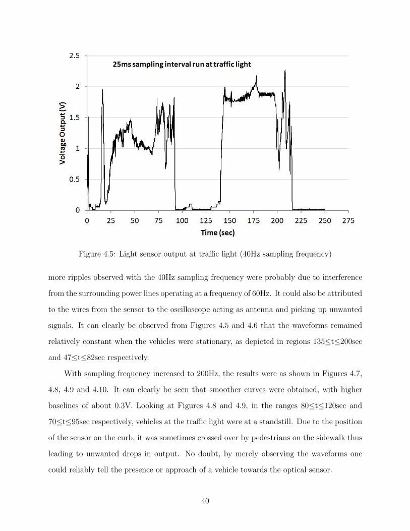
Figure 4.5: Light sensor output at traffic light (40Hz sampling frequency)
more ripples observed with the 40Hz sampling frequency were probably due to interference
from the surrounding power lines operating at a frequency of 60Hz. It could also be attributed
to the wires from the sensor to the oscilloscope acting as antenna and picking up unwanted
signals. It can clearly be observed from Figures 4.5 and 4.6 that the waveforms remained
relatively constant when the vehicles were stationary, as depicted in regions 135≤t≤200sec
and 47≤t≤82sec respectively.
With sampling frequency increased to 200Hz, the results were as shown in Figures 4.7,
4.8, 4.9 and 4.10. It can clearly be seen that smoother curves were obtained, with higher
baselines of about 0.3V. Looking at Figures 4.8 and 4.9, in the ranges 80≤t≤120sec and
70≤t≤95sec respectively, vehicles at the traffic light were at a standstill. Due to the position
of the sensor on the curb, it was sometimes crossed over by pedestrians on the sidewalk thus
leading to unwanted drops in output. No doubt, by merely observing the waveforms one
could reliably tell the presence or approach of a vehicle towards the optical sensor.
40

Figure 4.6: Light sensor output at traffic light (100Hz sampling frequency)
Figure 4.7: Light sensor output at traffic light (200Hz sampling frequency) - 1st run
41
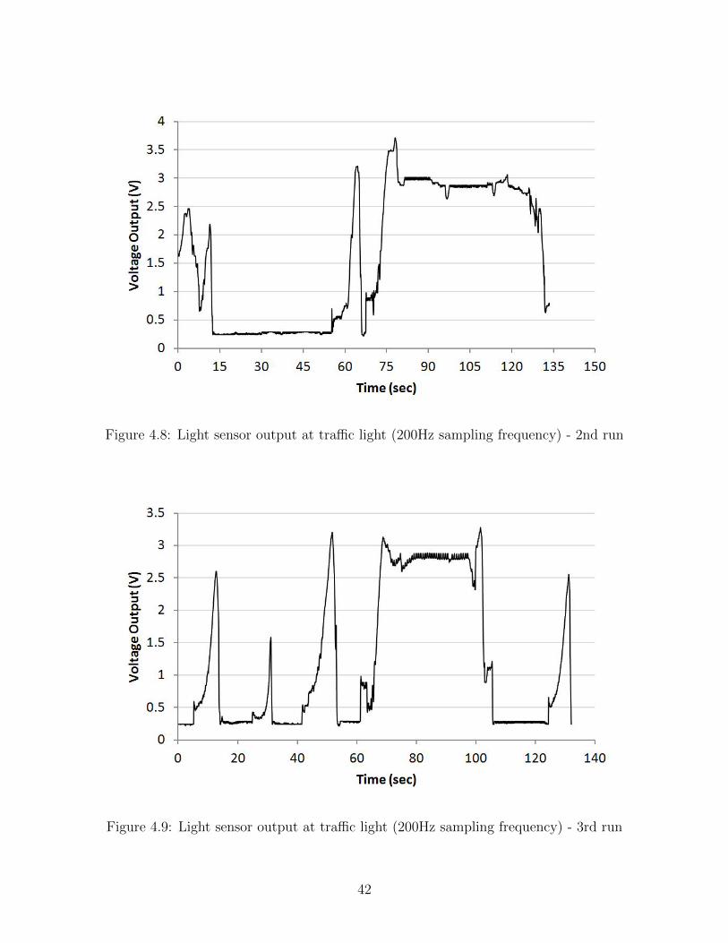
Figure 4.8: Light sensor output at traffic light (200Hz sampling frequency) - 2nd run
Figure 4.9: Light sensor output at traffic light (200Hz sampling frequency) - 3rd run
42
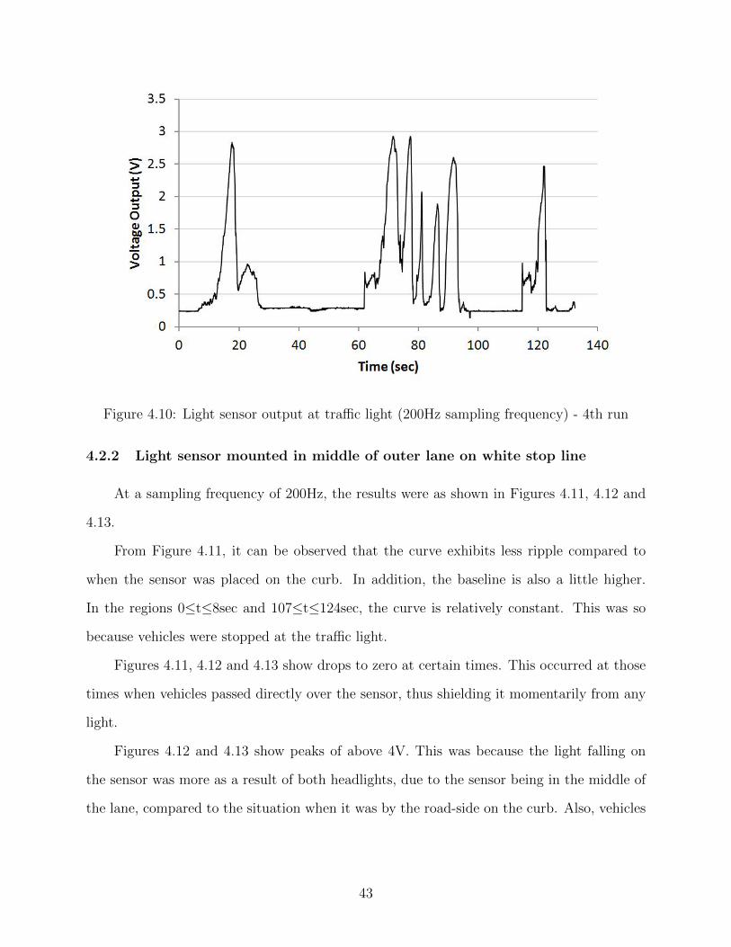
Figure 4.10: Light sensor output at traffic light (200Hz sampling frequency) - 4th run
4.2.2 Light sensor mounted in middle of outer lane on white stop line
At a sampling frequency of 200Hz, the results were as shown in Figures 4.11, 4.12 and
4.13.
From Figure 4.11, it can be observed that the curve exhibits less ripple compared to
when the sensor was placed on the curb. In addition, the baseline is also a little higher.
In the regions 0≤t≤8sec and 107≤t≤124sec, the curve is relatively constant. This was so
because vehicles were stopped at the traffic light.
Figures 4.11, 4.12 and 4.13 show drops to zero at certain times. This occurred at those
times when vehicles passed directly over the sensor, thus shielding it momentarily from any
light.
Figures 4.12 and 4.13 show peaks of above 4V. This was because the light falling on
the sensor was more as a result of both headlights, due to the sensor being in the middle of
the lane, compared to the situation when it was by the road-side on the curb. Also, vehicles
43
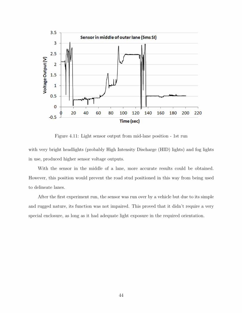
Figure 4.11: Light sensor output from mid-lane position - 1st run
with very bright headlights (probably High Intensity Discharge (HID) lights) and fog lights
in use, produced higher sensor voltage outputs.
With the sensor in the middle of a lane, more accurate results could be obtained.
However, this position would prevent the road stud positioned in this way from being used
to delineate lanes.
After the first experiment run, the sensor was run over by a vehicle but due to its simple
and rugged nature, its function was not impaired. This proved that it didn’t require a very
special enclosure, as long as it had adequate light exposure in the required orientation.
44
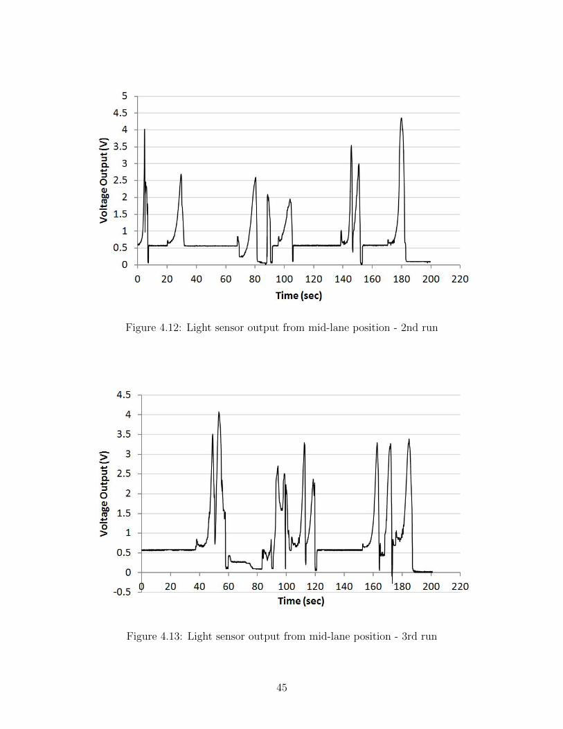
Figure 4.12: Light sensor output from mid-lane position - 2nd run
Figure 4.13: Light sensor output from mid-lane position - 3rd run
45
Chapter 5
Conclusions and Recommendations
No doubt, the experiment setup was able to detect the presence of vehicles through
their headlight beams. It was also observed that the width of the pulses corresponded to the
speeds of the vehicles. In situations where the sensor output was relatively constant, it can
be concluded with much certainty that the vehicle was not moving.
An intelligent prototype needs to be further developed, incorporating the decision el-
ement that determines if the detected vehicle is either stopped or moving too slowly for
the particular roadway, and also the required action to be taken. In the case of LED road
studs, this action could take the form of flashing red or amber LEDs on the road studs. The
prototype can be implemented using a microcontroller embedded in a road stud, with solar
charging capabilities for power. Afterwards, a communication protocol could be designed
to pass on the detection information to other road studs, perhaps a certain number of hops
away or a particular distance, in order to provide advanced warning of the obstacle (vehicle)
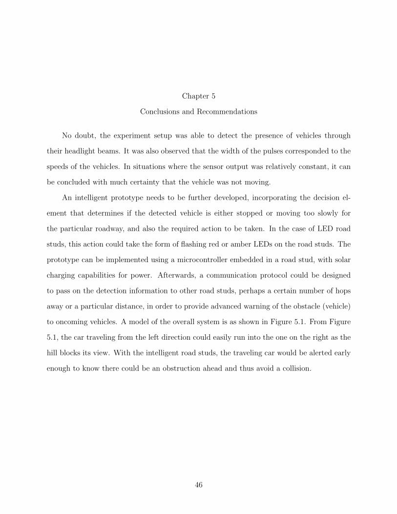
to oncoming vehicles. A model of the overall system is as shown in Figure 5.1. From Figure
5.1, the car traveling from the left direction could easily run into the one on the right as the
hill blocks its view. With the intelligent road studs, the traveling car would be alerted early
enough to know there could be an obstruction ahead and thus avoid a collision.
46
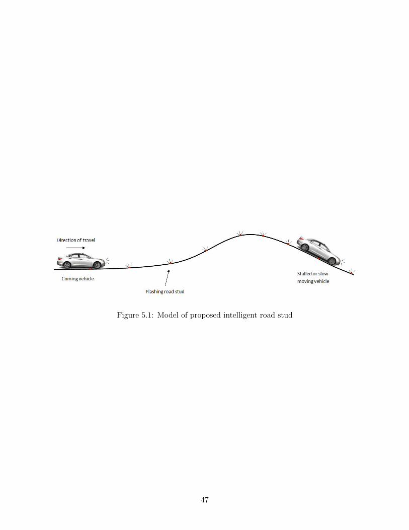
Figure 5.1: Model of proposed intelligent road stud
47
Bibliography
[1] Crash Reconstruction Basics for Prosecutors - Targeting Hardcore Impaired Drivers.American Prosecutors Research Institute, 2003 p 24.
[2] National Highway Traffic Safety Administration. National motor vehicle crash causationsurvey - report to congress(dot hs 811 059). Technical report, US Dept. of Transporta-tion, 2008.
[3] National Highway Traffic Safety Administration. The abcs of bac - a guide to under-standing blood alcohol concentration and alcohol impairment http://www.nhtsa.gov/links/sid/ABCsBACWeb/page2.htm accessed on 09-14-2014, 8.55pm, Sept 2014.
[4] F. AHDI, M.K. KHANDANI, M. HAMEDI, and A. HAGHANI. Traffic data collectionand anonymous vehicle detection using wireless sensor networks, May 2012.
[5] L.J. Blincoe, T. R. Miller, E. Zaloshnja, and B. A. Lawrence. The economic and soci-etal impact of motor vehicle crashes. National Highway Traffic Safety Administration,Washington, DC, 2014.
[6] Y. Chen, K. Shen, and S Wang. Forward collision warning system considering bothtime-to-collision and safety braking distance. In 2013 IEEE 8th Conference on IndustrialElectronics and Applications (ICIEA).
[7] National Safety Council. Motor vehicle safety, automobile safety, roadsafety issues http://www.nsc.org/safety_home/MotorVehicleSafety/Pages/
MotorVehicleSafety.aspx accessed on 09-26-2014, 9.12pm, Sept 2014.
[8] National Safety Council. Seat belt safety, seat belt laws http://www.nsc.org/
safety-road/DriverSafety/Pages/SeatBelts.aspx accessed on 09-17-2014, 6.28pm,Sept 2014.
[9] C.B. Crawford and V.P.A. Doran. Trial and evaluation of intelligent road studs forhazard warning, 2004.
[10] R.V. Dukkipati, J. Pang, M.S. Qatu, and Z. Shuguang. Road Vehicle Dynamics. SAEInternational, 2008.
[11] K. Hunter-Zaworski, J. Fowler, and T. Bardwell. Braking distance http:
//www.webpages.uidaho.edu/niatt_labmanual/chapters/geometricdesign/
theoryandconcepts/brakingdistance.htm accessed on 09-22-2014, 1:08pm.
48
[12] Advanced Photonix Inc. Cds photoconductive photocells pdv-p9008 http:
//advancedphotonix.com/wp-content/uploads/PDV-P9008.pdf accessed on 09-25-2014, 7:20pm.
[13] Tektronix Inc. P2200 200 mhz 1x/10x passive probe http://www.tek.com/manual/
p2200-200-mhz-1x-10x-passive-probe accessed on 09-30-2014, 10:20pm.
[14] Tenneco Automotive Inc. The hidden danger of worn out shock absorbers http://
www.tenneco.com/the_hidden_danger_of_worn_out_shock_absorbers accessed on09-22-2014, 11:58pm, March 2000.
[15] European Telecommunications Standards Institute. Etsi - intelligent trans-port http://www.etsi.org/index.php/technologies-clusters/technologies/
intelligent-transport accessed on 09-29-2014, 12:10am, September 2014.
[16] European Telecommunications Standards Institute. Etsi - intelligent transportation sys-tem http://www.etsi.org/images/files/membership/ETSI_ITS_09_2012.jpg ac-cessed on 09-29-2014, 12:10am, September 2014.
[17] W.D. Jones. Keeping cars from crashing, ieee spectrum vol. 38 iss. 9, pp 40-45, Septem-ber 2001.
[18] A.N. Knaian. A wireless sensor network for smart roadbeds and intelligent transporta-tion systems, June 2000.
[19] Clemson University Vehicular Electronics Laboratory. Parking systems http://www.
cvel.clemson.edu/auto/systems/parking.html accessed on 09-29-2014, 2:13pm,September 2014.
[20] J.H. Le Roux, A. Barnard, and M.J. Booysen. Remotely controllable wireless road studnetwork. In , editor, Proceeding of the 16th International IEEE Annual Conference onIntelligent Transportation Systems (ITSC 2013), The Hague, The Netherlands, October6-9, 2013.
[21] J.E. Lenz. A review of magnetic sensors. In IEEE, editor, Proceedings of the IEEE (Vol.78, Issue 6 pp. 973-989, Jun 1990.
[22] OnStar LLC. Auto security — car safety — navigation system — onstar https://www.onstar.com/web/portal/home?g=1 accessed on 09-29-2014, 12:50am, September 2014.
[23] Clearview Traffic Group Ltd. Irs2 hardwired intelligent road studshttp://www.clearviewtraffic.com/astucia/products-astucia/art/56/
irs2-hardwired-intelligent-road-studs.htm accessed on 09-30-2014, 1:20pm.
[24] Pico Technology Ltd. Adc-200 series user’s guide - pico technology http://www.
picotech.com/document/pdf/adc2xx-en-3.pdf accessed on 10-09-2014, 10:40pm.
[25] D.L. Massie and K.L. Campbell. Analysis of accident rates by age, gender, and timeof day based on the 1990 nationwide personal transportation survey. Technical report,Transportation Research Institute, University of Michigan, Ann Arbor, Michigan, 1993.
49
[26] L.E.Y. Mimbela, L.A.K. Klein, and P Kent. A summary of vehicle detection andsurveillance technologies used in intelligent transportation systems, August 31,2007.
[27] K. Mohamadabadi. Anisotropic Magnetoresistance Magnetometer for inertial navigationsystems. PhD thesis, Ecole Polytechnique, Nov. 2013.
[28] G. Muspratt. Five ways to make night-time driving safer with astucia active road studs,Dec. 2012.
[29] J. Neilsen. Stopping distance - safe drive training http://www.sdt.com.au/
safedrive-directory-STOPPINGDISTANCE.htm accessed on 09-22-2014, 1:08pm, 2014.
[30] The University of North Carolina Highway Safety Research Center. Hsrc: Blood al-cohol concentration (bac) http://www.hsrc.unc.edu/safety_info/alcohol/blood_
alcohol_concentration.cfm accessed on 09-16-2014, 3.22pm, Sept 2014.
[31] Michael Pines. Drivers.com: Top 3 causes of car accidents in america http://www.
drivers.com/article/1173 accessed on 09-14-2014, 7.32pm, Sept 2014.
[32] Auto System Pro. Headlights - lighting circuits http://autosystempro.com/
headlights/ accessed on 10-8-2014, 10:20pm.
[33] B. Roessler and K. Fuerstenberg. First european strep on cooperative intersectionsafety, intersafe-2. In 2010 13th International IEEE Annual Conference on IntelligentTransportation Systems, 2010.
[34] D. Samardzija, E. Kovac, D. Isailovi, B. Miladinovic, N. Teslic, and M. Katona. Roadnail: Intelligent road marking system. In IEEE, editor, 2011 IEEE International Con-ference on Consumer Electronics (ICCE), 9-12 Jan 2011.
[35] A. Shaout, D. Colella, and S. Awad. Advanced driver assistance systems - past, presentand future. In IEEE, editor, Computer Engineering Conference (ICENCO), 2011 Sev-enth International, 27-28 Dec 2011.
[36] R. Stevenson. A driver’s sixth sense, ieee spectrum vol. 48 iss. 10, pp 50-55, October2011.
[37] M. Tatum. What is cruise control http://www.wisegeek.com/
what-is-cruise-control.htm accessed on 10-02-2014, 10.48am, June 2003.
[38] T.J. Triggs and W.G. Harris. Reaction time of drivers to road stimuli. Technical report,Human Factors Group, Department of Psychology, Monash University, Victoria 3800,Australia, June 1982 pp 4-5.
[39] C. Varghese and U. Shankar. Passenger vehicle occupant fatalities by day and night -a contrast (dot hs 810 637). NHTSA Traffic Safety Facts - Research Note, 2007.
[40] J.Y. Wong. Theory of Ground Vehicles, 3rd ed. John Wiley & Sons, Inc., 2001.
50

Appendices
51
Appendix A
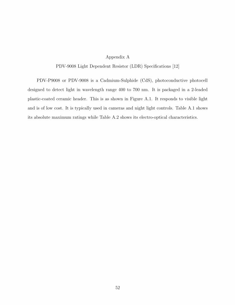
PDV-9008 Light Dependent Resistor (LDR) Specifications [12]
PDV-P9008 or PDV-9008 is a Cadmium-Sulphide (CdS), photoconductive photocell
designed to detect light in wavelength range 400 to 700 nm. It is packaged in a 2-leaded
plastic-coated ceramic header. This is as shown in Figure A.1. It responds to visible light
and is of low cost. It is typically used in cameras and night light controls. Table A.1 shows
its absolute maximum ratings while Table A.2 shows its electro-optical characteristics.
52
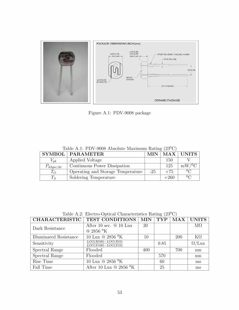
Figure A.1: PDV-9008 package
Table A.1: PDV-9008 Absolute Maximum Rating (230C)SYMBOL PARAMETER MIN MAX UNITS
Vpk Applied Voltage 150 VPd∆po/∆t Continuous Power Dissipation 125 mW/0CTO Operating and Storage Temperature -25 +75 0CTS Soldering Temperature +260 0C
Table A.2: Electro-Optical Characteristics Rating (230C)CHARACTERISTIC TEST CONDITIONS MIN TYP MAX UNITS
Dark ResistanceAfter 10 sec. @ 10 Lux 20 MΩ@ 2856 0K
Illuminated Resistance 10 Lux @ 2856 0K 10 200 KΩ
Sensitivity LOG(R100)−LOG(R10)LOG(E100)−LOG(E10)
0.85 Ω/Lux
Spectral Range Flooded 400 700 nmSpectral Range Flooded 570 nmRise Time 10 Lux @ 2856 0K 60 msFall Time After 10 Lux @ 2856 0K 25 ms
53
Appendix B
ADC-200 PC Oscilloscope/Datalogger [24]
The ADC-200 PC Oscilloscope belongs to a family of high-speed analogue-to-digital
converters (ADCs). It has 4 signal connectors and a 12V DC power socket. The 4 signal
connectors are composed of 2 input channels (female BNC connectors), a parallel port and
an external trigger (female BNC connector). It can be used as a PC-based oscilloscope /
spectrum analyzer with appropriate software or as a datalogger with the Picolog software.
Also, its driver software can be used to develop programs to collect and analyze data from
the unit. Its specifications are shown in Table B.1. A picture of the ADC-200 is as shown
in Figure B.1.
54
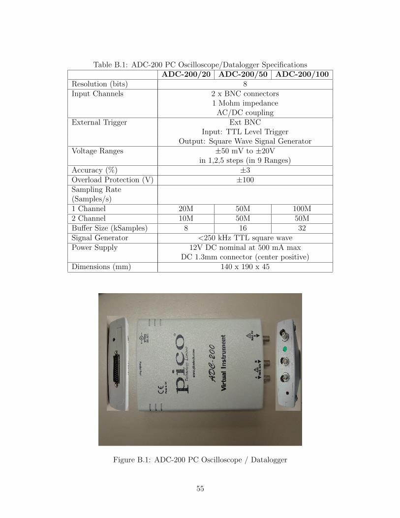
Table B.1: ADC-200 PC Oscilloscope/Datalogger SpecificationsADC-200/20 ADC-200/50 ADC-200/100
Resolution (bits) 8Input Channels 2 x BNC connectors
1 Mohm impedanceAC/DC coupling
External Trigger Ext BNCInput: TTL Level Trigger
Output: Square Wave Signal GeneratorVoltage Ranges ±50 mV to ±20V
in 1,2,5 steps (in 9 Ranges)Accuracy (%) ±3Overload Protection (V) ±100Sampling Rate(Samples/s)1 Channel 20M 50M 100M2 Channel 10M 50M 50MBuffer Size (kSamples) 8 16 32Signal Generator <250 kHz TTL square wavePower Supply 12V DC nominal at 500 mA max
DC 1.3mm connector (center positive)Dimensions (mm) 140 x 190 x 45
Figure B.1: ADC-200 PC Oscilloscope / Datalogger
55

Appendix C
Tektronix P2200 Passive Probe Electrical Characteristics [13]
The Tektronix P2200 passive probe has a male BNC plug on one end, a probe attenu-
ation switch for selecting either 10X or 1X attenuation factor, a hook tip and ground lead.
Its electrical characteristics are shown in Table C.1. Figures C.1 and C.2 show its operating
curves. Figure C.3 shows a sample Tektronix P2200 probe.
56
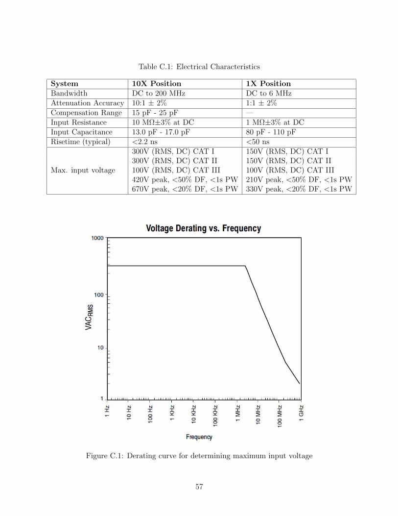
Table C.1: Electrical Characteristics
System 10X Position 1X PositionBandwidth DC to 200 MHz DC to 6 MHzAttenuation Accuracy 10:1 ± 2% 1:1 ± 2%Compensation Range 15 pF - 25 pF —Input Resistance 10 MΩ±3% at DC 1 MΩ±3% at DCInput Capacitance 13.0 pF - 17.0 pF 80 pF - 110 pFRisetime (typical) <2.2 ns <50 ns
Max. input voltage
300V (RMS, DC) CAT I 150V (RMS, DC) CAT I300V (RMS, DC) CAT II 150V (RMS, DC) CAT II100V (RMS, DC) CAT III 100V (RMS, DC) CAT III420V peak, <50% DF, <1s PW 210V peak, <50% DF, <1s PW670V peak, <20% DF, <1s PW 330V peak, <20% DF, <1s PW
Figure C.1: Derating curve for determining maximum input voltage
57
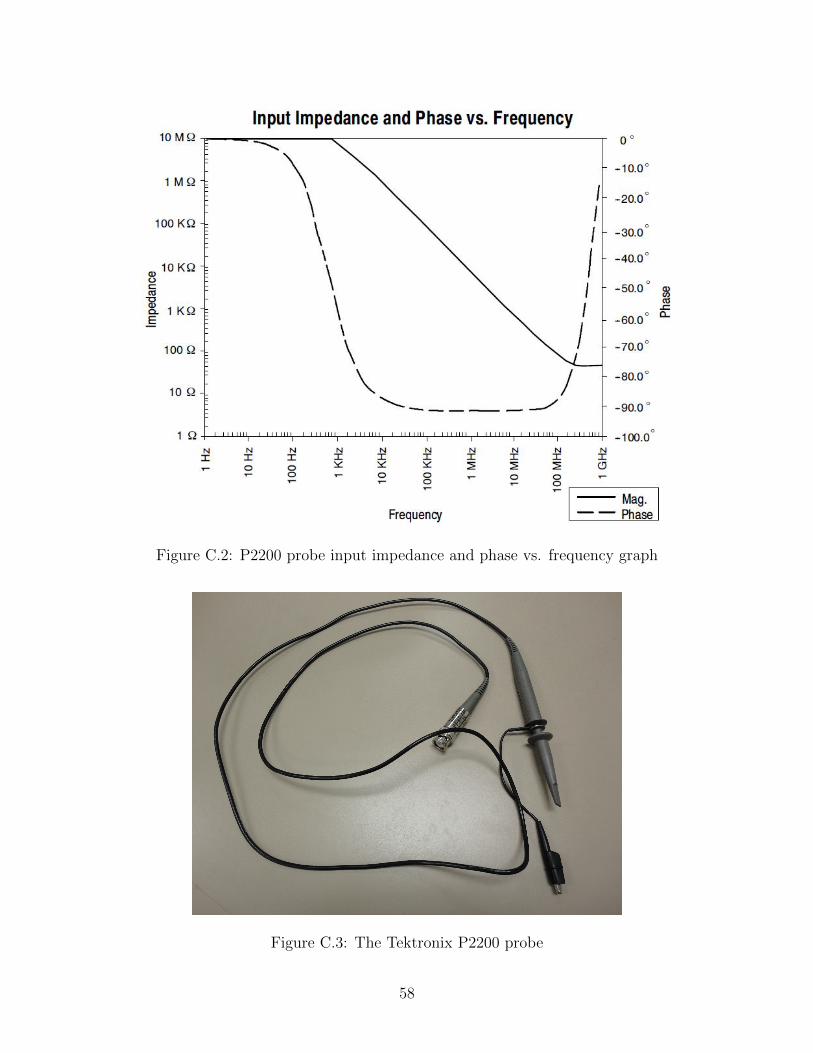
Figure C.2: P2200 probe input impedance and phase vs. frequency graph
Figure C.3: The Tektronix P2200 probe
58