detecting a stochastic gravitational wave …quency. virtually 100% of the white dwarf binaries in...
TRANSCRIPT

DETECTING A STOCHASTIC GRAVITATIONAL WAVE BACKGROUND
WITH SPACE-BASED INTERFEROMETERS
by
Matthew Raymond Adams
A dissertation submitted in partial fulfillmentof the requirements for the degree
of
Doctor of Philosophy
in
Physics
MONTANA STATE UNIVERSITYBozeman, Montana
August, 2014

c© COPYRIGHT
by
Matthew Raymond Adams
2014
All Rights Reserved

ii
DEDICATION
To my wife Liz and our three children Millie, Amy, and Nicholas for their unendingsupport and encouragement.

iii
ACKNOWLEDGEMENTS
Firstly, I’d like to acknowledge and thank Neil Cornish for being a superb
graduate advisor. I am particularly grateful for his patience and continued
help over the past couple of years as this thesis and its defense were delayed
several times. I appreciate his guidance and teaching in the classroom and in
my research in helping me understand and enjoy the field of gravitational wave
astronomy.
I also appreciate the invaluable insight and help the members of my graduate
committee have provided along the way and through the various delays over the
past couple of years. They have always been willing to meet and reschedule. I
appreciate the numerous faculty members who have taught me in courses and
enhanced my knowledge of physics. I also thank Margaret Jarrett for continually
supporting me and making sure all the logistical i’s were dotted and t’s crossed.
I thank my parents for instilling a scientific curiosity in me when I was
young and for always encouraging me in my schooling and other endeavors. I
thank Eric Swager for first opening my eyes to the joy of physics and for David
Cinabro for working with me at Wayne State and sparking my interest in gravity
through our particle physics research.
Lastly, I thank my wife, Liz, and our children for their support and patience
during the graduate school process. We were married in the midst of the process
and I appreciate Liz’s help raising our young family while I finished my graduate
degree. Liz may be more excited to see me graduate than I myself am, and I
am indebted to her for her selfless support.

iv
TABLE OF CONTENTS
1. INTRODUCTION ........................................................................................1
2. SPACE-BASED GRAVITATIONAL WAVE DETECTORS .............................9
2.1 Noise..................................................................................................... 112.2 Simulated Data...................................................................................... 172.3 Detector Response to a Gravitational Wave Signal ................................... 192.4 Null Channel for Unequal Arm LISA....................................................... 22
3. COSMOLOGICAL SOURCES OF GRAVITATIONAL WAVES .................... 26
3.1 Characterizing a Gravitational Wave Background..................................... 273.2 Bounds.................................................................................................. 29
3.2.1 BBN .............................................................................................. 303.2.2 COBE and WMAP......................................................................... 323.2.3 LIGO and PTA Bounds .................................................................. 33
3.3 Sources of Gravitational Waves ............................................................... 343.3.1 Amplification of Quantum Fluctuations ........................................... 343.3.2 Reheating....................................................................................... 383.3.3 Phase Transitions ........................................................................... 383.3.4 Cosmic Strings ............................................................................... 39
3.4 Model ................................................................................................... 393.5 Simulated Data...................................................................................... 40
4. ASTROPHYSICAL GRAVITATIONAL WAVE FOREGROUNDS ................ 42
4.1 Sources of Astrophysical Stochastic Signals.............................................. 424.2 White Dwarf Population Model .............................................................. 43
4.2.1 Modeling Individual White Dwarf Binaries ....................................... 444.2.2 Modeling the Galactic Distribution .................................................. 45
4.3 Confusion Foreground Model .................................................................. 464.4 Simulated Data...................................................................................... 51
5. ANALYSIS TECHNIQUES ......................................................................... 53
5.1 Bayesian Basics...................................................................................... 545.1.1 Gravitational Wave Applications ..................................................... 56
5.1.1.1 Parameter Estimation and Model Selection ............................... 575.2 MCMC Techniques ................................................................................ 58
5.2.1 Metropolis Hastings ........................................................................ 59

v
TABLE OF CONTENTS – CONTINUED
5.2.2 Parallel Tempering.......................................................................... 60
5.2.3 Thermodynamic Integration ............................................................ 615.3 Hierarchical Bayes.................................................................................. 64
5.3.1 Toy Model I ................................................................................... 665.3.1.1 Numerical Simulation .............................................................. 68
5.3.2 Toy Model II .................................................................................. 705.3.2.1 Approximating the Likelihood .................................................. 72
6. GRAVITATIONAL WAVE ASTRONOMY APPLICATIONS ........................ 75
6.1 Measurement of Galaxy Distribution Parameters ..................................... 756.1.1 White Dwarf Likelihood .................................................................. 786.1.2 Prior and Hyperparameters ............................................................. 796.1.3 Results........................................................................................... 806.1.4 Approximating the Likelihood ......................................................... 836.1.5 Conclusion ..................................................................................... 86
6.2 Separating a Background from Instrument Noise...................................... 876.2.1 Stochastic Likelihood ...................................................................... 87
6.2.1.1 Mock LISA Data Challenge Training Data Results .................... 906.2.2 Detection Limits............................................................................. 926.2.3 The Role of Null Channels and 4-link Operation............................... 94
6.3 Including the Galactic Foreground .......................................................... 986.3.1 Bayesian Model Selection .............................................................. 1026.3.2 Comparison to MLDC................................................................... 1036.3.3 Analysis with a Galactic Foreground.............................................. 1046.3.4 Conclusion ................................................................................... 108
7. CONCLUSIONS ....................................................................................... 110
REFERENCES CITED.................................................................................. 112
APPENDIX A: Noise Cross-spectra ............................................................... 125

vi
LIST OF TABLESTable Page
6.1 Galaxy Distribution Parameter MAP Values ......................................... 84
6.2 Prior Ranges for Model Parameters ...................................................... 89

vii
LIST OF FIGURESFigure Page
2.1 Schematic of the proposed LISA satellites. Each of the three satelliteshas two proof masses, shown as boxes. .................................................. 10
2.2 Depiction of light travel times for two signals that can be combinedto create a TDI channel. For the general case of an unequal arminterferometer, the delay corresponds to the light travel time to go upand down each of two adjacent arms..................................................... 13
2.3 Our model for the noise in the A and T channels compared to smoothedspectra formed from the MLDC training data. ...................................... 18
2.4 The sensitivity curve for the A, E, and T channels, showing the insen-sitivity of the T channel to a gravitational wave signal........................... 22
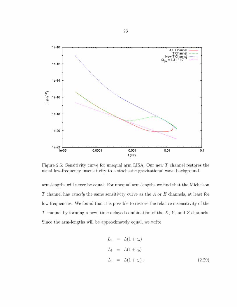
2.5 Sensitivity curve for unequal arm LISA. Our new T channel restoresthe usual low-frequency insensitivity to a stochastic gravitational wavebackground. ........................................................................................ 23
4.1 The time domain noise, galaxy, and stochastic background signal com-ponents for the X-channel. They have been bandpass filtered between0.1 and 4 mHz. We show that we are able to detect a scale invariantbackground with Ωgw = 5 · 10−13, which is well below the instrumentnoise and galaxy levels. ........................................................................ 47
4.2 Several galaxy realizations showing the scatter in the modulation levelsthroughout the year compared to the galaxy used in our simulations.The points are scaled by the first Fourier coefficient, C0. ........................ 49
4.3 Several galaxy realizations showing the scatter in the Fourier coef-ficients for different galaxy realizations. The ±3σ upper and lowerbounds are used as the prior range on the Fourier coefficients in ouranalysis............................................................................................... 50
4.4 Our smoothed, simulated data with the model overlaid in black (solid). .. 51
5.1 The marginalized PDF for α. The injected value is indicated by thevertical black line. ............................................................................... 69
5.2 MAP values for 30 different simulations of the toy model. The redcurve includes noise in the simulated signal and converges to α0 asexpected. The blue curves does not include noise in the simulationand converges to α2
0 − β2. .................................................................... 70

viii
LIST OF FIGURES – CONTINUEDFigure Page
5.3 MAP values for 30 different realizations of the toy model II. Using thefull likelihood (red) the MAP values converge to the injected value, butwith the Fisher Matrix approximation to the likelihood (blue) there isa bias. ................................................................................................ 72
5.4 PDFs for the prior hyperparameter α and the noise level β for toymodel II. Both are individually constrained in this model. The injectedvalues are shown by the black lines. ...................................................... 73
6.1 The percentage of sources which are detectable as a function of fre-quency. Virtually 100% of the white dwarf binaries in the Milky Wayabove 4 mHz would be detected by LISA............................................... 77
6.2 The chirp mass distribution of the 5000 binaries used in our simula-tions is shown in red. The green distribution shows the MAP valuesof the recovered chirp mass for each binary, and the blue shows themodel (Eq. 6.3) using the MAP values for the chirp mass prior hyper-parameters. The brightest binaries accurately capture the chirp massdistribution, which serves as a useful prior for sources whose chirpmasses are not so well determined. ....................................................... 81
6.3 PDFs for the four galaxy model hyperparameters. The red is for asimulation using 100 binaries, the green 1000 binaries, and the blue5000 binaries. The black lines show the true values of the distributionfrom which the binaries were drawn...................................................... 82
6.4 PDFs for the three chirp mass model hyperparameters and the FWHMof the distribution. The red is for a simulation using 100 binaries, thegreen 1000 binaries, and the blue 5000 binaries. .................................... 83
6.5 PDFs from a simulation using 5000 binaries for the four galaxy modelhyperparameters using the full likelihood (red), a Fisher approximationin d (green), and a Fisher approximation in 1/d (blue)........................... 85
6.6 MAP values and corresponding averages from a simulation using 5000binaries for the four galaxy model hyperparameters using the full like-lihood (red), a Fisher Matrix approximation parameterized with d(green), and a Fisher Matrix approximation using 1/d (blue). ................ 86

ix
LIST OF FIGURES – CONTINUEDFigure Page
6.7 Histograms showing the PDFs for the position noise levels, scaled bythe nominal level, Eq. 2.10. On the left are the sums along each arm,and on the right are the differences. The vertical lines denote theinjected values..................................................................................... 91
6.8 Histograms showing the PDFs for the position noise levels, scaled bythe nominal level, Eq. 2.11. On the left are the sums along each arm,and on the right are the differences. The vertical lines denote theinjected values..................................................................................... 92
6.9 PDF for the gravitational wave background level (scaled up by 1013).The vertical line denotes the injected values. ......................................... 93
6.10 PDF for the gravitational wave background slope. ................................. 94
6.11 Bayes factor showing the detectability versus background level. Thecurve shows the average values of the scattered points. .......................... 95
6.12 Bayes factors for the X, Y, and Z channels. ........................................... 96
6.13 The PDFs for the 6 constrained noise parameter combinations for theAET channels. The position noise parameters are on the left and theacceleration noise parameters on the right. The black (solid) verticallines show the injected values. The blue (dashed) PDFs include slopefitting and the red (solid) PDFs do not. ................................................ 99
6.14 The constrained position (left) and acceleration (right) noise param-eters for X. The black (solid) vertical lines show the injected values.The blue (dashed) PDFs include slope fitting and the red (solid) PDFsdo not. ............................................................................................. 100
6.15 The stochastic gravitational wave background level, Ωgw, and slopeparameter, m, for AET. The black (solid) vertical lines show the in-jected values. The blue (dashed) PDFs include slope fitting and thered (solid) PDFs do not. .................................................................... 101
6.16 The stochastic gravitational wave background level, Ωgw, and slopeparameter, m, for X. The black (solid) vertical lines show the injectedvalues. The blue (dashed) PDF includes slope fitting and the red (solid)PDF does not.................................................................................... 102

x
LIST OF FIGURES – CONTINUEDFigure Page
6.17 The first three (left) and last three (right) Fourier coefficients for theA-channel. The first coefficients are well constrained while the laterones are not. The blue (dashed) PDFs include slope fitting and thered (solid) PDFs do not. .................................................................... 103
6.18 The first three (left) and last three (right) Fourier coefficients for theX-channel. The blue (dashed) PDFs include slope fitting and the red(solid) PDFs do not........................................................................... 104
6.19 A comparison of the Bayes factors for the MLDC data and for oursimulated data without a galaxy. The lower panel includes slope fitting.A Bayes factor of 30 is considered a strong detection. .......................... 105
6.20 A comparison of Bayes factors for data without the galaxy vs. datawith the galaxy included. Including the galaxy does not significantlydecrease our detection ability. The lower panel includes slope fitting..... 106
6.21 A comparison of Bayes Factors for the full AET vs. running on the lowfrequency end of the spectrum, single weeks of data, and a stochasticbackground with a spectral shape identical to the galaxy spectrum usedin this paper. We see that both the spectral shape and the galaxysignal modulation help separate the three model components. Thelower panel includes slope fitting. ....................................................... 108

xi
ABSTRACT
The detection of a stochastic background of gravitational waves could significantlyimpact our understanding of the physical processes that shaped the early Universe.The challenge lies in separating the cosmological signal from other stochastic processessuch as instrument noise and astrophysical foregrounds. One approach is to build twoor more detectors and cross correlate their output, thereby enhancing the commongravitational wave signal relative to the uncorrelated instrument noise. When onlyone detector is available, as will likely be the case with space based gravitational waveastronomy, alternative analysis techniques must be developed. Here we develop anend to end Bayesian analysis technique for detecting a stochastic background witha gigameter Laser Interferometer Space Antenna (LISA) operating with both 6- and4-links. Our technique requires a detailed understanding of the instrument noiseand astrophysical foregrounds. In the millihertz frequency band, the predominateforeground signal will be unresolved white dwarf binaries in the galaxy. We considerhow the information from multiple detections can be used to constrain astrophysicalpopulation models, and present a method for constraining population models usinga Hierarchical Bayesian modeling approach which simultaneously infers the sourceparameters and population model and provides the joint probability distributions forboth. We find that a mission that is able to resolve ∼ 5000 of the shortest period bi-naries will be able to constrain the population model parameters, including the chirpmass distribution and a characteristic galaxy disk radius to within a few percent.This compares favorably to existing bounds, where electromagnetic observations ofstars in the galaxy constrain disk radii to within 20%. Having constrained the galaxyshape parameters, we obtain posterior distribution functions for the instrument noiseparameters, the galaxy level and modulation parameters, and the stochastic back-ground energy density. We find that we are able to detect a scale-invariant stochasticbackground with energy density as low as Ωgw = 2× 10⁻¹³ for a 6-link interferometerand Ωgw = 5× 10⁻¹³ for a 4-link interferometer with one year of data.

1
CHAPTER 1
INTRODUCTION
Einstein’s theory of general relativity, published in 1915 [1], is currently our best
and most complete theory of the gravitational interaction. General relativity accounts
for several problems that arose in Newtonian gravity, including the perihelion preces-
sion of Mercury [2, 3]. General relativity also correctly predicts the bending of light
by massive objects [3], which was experimentally verified in 1919 [4], and predicts the
existence of gravitational waves [5, 6, 7]. To date, gravitational waves have not been
directly detected.
Hulse and Taylor discovered the binary pulsar, PSR1913+16, in 1974 [8] which led
to indirect evidence for gravitational wave radiation. General relativity predicts that
the orbit of a binary system will gradually decay due to energy loss from departing
gravitational waves. Hulse and Taylor’s measurements of the binary pulsar show that
the decay of the orbit agrees exquisitely with Einstein’s predictions [9]. They were
awarded the Nobel Prize in 1993 for their work.
The first direct detections of gravitational waves are expected to be made within
a few years by either the Laser Interferometer Gravitational Wave Observatory
(LIGO) [10, 11] or by a collaboration of pulsar timing arrays (PTAs) known as the
International Pulsar Timing Array (IPTA) [12]. The members of IPTA are the Euro-
pean Pulsar Timing Array (EPTA) [13], the North American Nanohertz Observatory
for Gravitational Waves (NANOGrav) [14], and the Parkes Pulsar Timing Array
(PPTA) [15]. Later detections could be made by space-based gravitational wave
detectors such as the European mission, the New Gravitational Wave Observatory
(NGO), which is nicknamed evolved LISA (eLISA) [16] since it was derived from

2
the joint NASA-ESA mission, the Laser Interferometer Space Antenna (LISA) [17].
We expect these missions to detect gravitational waves from binary systems, merg-
ers of compact objects, and burst sources such as supernovae, but one of the most
exciting potential discoveries for gravitational wave observatories is the detection of
a stochastic gravitational wave background. Just as studies of the cosmic microwave
background (CMB) have revolutionized our understanding of cosmology, the detection
of a gravitational wave background would provide unique insight into the processes
that shaped the early Universe.
Most of our current knowledge about the early Universe comes from measurements
of the CMB. Before the detection of the CMB, we were limited in our ability to test
and constrain models of the early history of the Universe. The detection of the CMB
opened the field of cosmology as a full fledged observational science [18]. Using data
from first the Cosmic Background Explorer (COBE) [19], then the Wilkinson Mi-
crowave Anisotropy Probe (WMAP) [20], and most recently the Planck mission [21],
we are able to test, constrain, and rule out various theories of the origins of our
Universe. Most notably, the CMB observations provided evidence for the Big Bang
and ruled out steady state models of the Universe. Recently, the Background Imag-
ing of Cosmic Extragalactic Polarization (BICEP2) experiment reported detection
of B-mode polarization in the CMB and attributed it to primordial gravitational
waves [22, 23]. This would be the first direct measurements supporting inflation and
primordial gravitational waves, but others have put forth an alternative explanation
and find the BICEP2 measurements to be consistent with dust polarization [24, 25].
Further measurements are needed to confirm the results.
Despite the success of CMB science, there is a limit to how far back we can look
in time with electromagnetic radiation. At what is known as the surface of last
scattering, the Universe was so dense and energetic, that photons were not able to

3
propagate freely. When atoms formed, light and matter decoupled and the Universe
became transparent. When we observe the CMB, we are observing the Universe at
the time of this decoupling, approximately 400,000 years after the Big Bang.
Inflation is one of the most successful models of the early Universe. It is hypothe-
sized to have occurred within a fraction of the first second of the Universe, long before
the time of the surface of last scattering. Inflation was proposed by Alan Guth in
1981 [26] as a possible solution to the horizon and flatness problems in cosmology.
Inflation suggests that the Universe underwent a period of exponential expansion
that can account for the large scale smoothness we observe today. Because inflation
happened so early in the history of the Universe, we only indirectly observe its affects
in the CMB. We are currently unable to directly probe back in time to the era of
inflation.
However, Big Bang and inflationary models also predict residual gravitational
wave radiation. Gravitational waves couple very weakly to matter and we do not
expect that they will be appreciably dampened or scattered as they propagate across
the Universe. We could potentially detect gravitational waves from the inflationary
epoch and see back in time farther than we’ve ever been able to see, opening a new
window to the early Universe [27, 28, 29, 30, 31, 32].
Primordial gravitational waves from the early Universe may be detectable by cur-
rent and future gravitational wave observatories. LIGO [33] and PTAs [34] have al-
ready set bounds on the energy density in a stochastic gravitational wave background
in their respective wavebands. In this dissertation we show that complementary
bounds can be set in the millihertz waveband with a space-based interferometer.
The challenge in detecting a primordial stochastic gravitational wave background
is that we expect other stochastic signals to compete with and possibly overwhelm
any primordial signals. Even if there is a primordial signal of sufficient strength to be

4
detected, it must be modeled and distinguished from the other stochastic signals. In
this dissertation, we develop several techniques for modeling and separating the vari-
ous stochastic signals that could appear in a space-based gravitational wave detector’s
data.
There are two types of stochastic signals that we must contend with: instru-
ment noise and astrophysical foregrounds. When multiple independent detectors are
available, as is the case with the ground based interferometers, the signal from one
interferometer can be used as a (noise corrupted) template for a second interfer-
ometer. The common gravitational wave signal will combine coherently, while the
contributions from instrument noise will average to zero [35, 36, 37]. Terrestrial
detectors such as LIGO and PTAs use this technique to separate stochastic signals
from stochastic instrument noise [38, 36, 39]. The LSC for example, has detectors in
Italy; Hanford, Washington; and Livingston, Louisiana. The noise at one site, will
be uncorrelated from the noises at the other two sites. Likewise, PTAs can correlate
data from multiple pulsars.
With prospects for only one space-based detector in the foreseeable future, we
will not be able to cross correlate between detectors. For space-based gravitational
wave interferometry, we need to develop other techniques for separating instrument
noise and stochastic signals. In this dissertation, we develop a technique that can
successfully distinguish between instrument noise and stochastic signals with only one
space-based detector [40, 41]. The key to our technique is that the noise and stochastic
signals manifest differently in the detector. The transfer functions have different
spectral shapes, which gives sufficient leverage to separate the various components.
The original measurement of the CMB by Penzias and Wilson did not use cross
correlation either. Penzias and Wilson made their measurements with the Horn an-
tenna in Holmdel, New Jersey. They were actually not even looking for the CMB, but

5
were interested in detecting radio waves reflected from echo balloon satellites. These
faint signals required a very sensitive instrument.
The Horn antenna, designed to detect these faint radio signals, was cooled to 4
degrees Kelvin. Penzias and Wilson accounted for all known noise sources includ-
ing radar and radio broadcasting interference. However, their measurements still
contained an extra white noise. They dutifully cleaned the instrument by removing
some nesting pigeons and their droppings, but the extra signal remained. It was
isotropic and present day and night. Finally, because they were confident that they
understood the noise in their detector, Penzias and Wilson were convinced that the
signal was not an instrument artifact. Because of its isotropy, they deduced that it
did not come from the Earth, solar system, or even our own galaxy.
Dicke, Peebles, and Wilkinson (DPW) at Princeton University were looking for
the CMB at the same time Penzias and Wilson made their discovery. Penzias and
Wilson were alerted to the work by Dicke, Peebles, and Wilkinson and contacted
them with their results. DPW realized they had been scooped, but the two groups
released publications together in 1965 with their findings and interpretation [42, 43].
The relevant, key point to our study is that Penzias and Wilson understood their
instrument noise well enough that they were able to confidently say that the extra
signal was not instrument noise. We follow a similar approach in this dissertation and
show that a detailed understanding of the instrument noise allows us to distinguish
it from stochastic signals.
This approach is more difficult in ground based interferometry. The LSC deals
with terrestial noise sources that require more complex noise models. In space, we
expect the noise to be linear and more easily modeled. With an adequate noise model,
spectral templates provide a very powerful method for seperating the components that
allows us to detect stochastic signals to levels that put them below the instrument

6
noise. While it is in principle possible for the various contributions to the instrument
noise to have spectra that mimic the geometrical transfer funtions of the signal, or
vice-versa, in practice the signal and noise transfer functions are so complex and
distinct that this situation should never arise.
Not only do we need to account for instrument noise, but there will likely be
astrophysical stochastic foregrounds that may mask an underlying primordial back-
ground. The sources that we need to be aware of depend on the frequency band of
interest. In the very low frequency PTA band, supermassive black hole binaries are
expected to overwhelm any primordial stochastic signal [44, 45, 46, 47, 34], and in the
LIGO band, neutron star binaries could be a limiting factor [48, 49, 38]. Proposed
spaced based gravitational wave detectors will operate in the milliHertz frequency
range. Of the three frequency regimes, the most certain foreground source will be
white dwarf binaries in the Milky Way in the milliHertz band [50, 51, 52]. Several
bright white dwarf binaries have already been optically detected. The brightest of
these would be easily detectable with proposed space-based detectors [53, 54]. In
total, several thousands of white dwarf binaries will be individually resolvable [55].
The rest will form a confusion foreground that could overwhelm any extragalactic
stochastic signals if not properly modeled. It is also possible that extreme-mass-ratio
inspirals (EMRIs) [56] of compact objects or binary black hole systems [57] could
form stochastic foregrounds in the milliHertz band.
There is an old joke in astrophysics that with one source you have a discovery,
and with two you have a population. This joke will be all too true in gravitational
wave astronomy as we are seeking our first discovery and subsequently will have only
a very small sample of sources. However, as we discover more and more sources it
becomes possible to constrain astrophysical population models.

7
Inferring the underlying population model, and the attendant astrophysical pro-
cesses responsible for the observed source distribution, from the time series of a grav-
itational wave detector is the central science challenge for a future space mission. It
folds together the difficult task of identifying and disentangling the multiple over-
lapping signals that are in the data, inferring the individual source parameters, and
reconstructing the true population distributions from incomplete and imperfect infor-
mation. Until recently, studies of milli-Hertz gravitational wave science have either
focused on making predictions about the source populations, or have looked at de-
tection and parameter estimation for individual sources. These types of studies have
featured heavily in the science assessment of alternative space-based gravitational
wave mission concepts, where metrics such as detection numbers and histograms of
the parameter resolution capabilities for fiducial population models were used to rate
science performance (see eg. Ref. [58]). These are certainly useful metrics, but they
only tell part of the story. A more powerful and informative measure of the science
capabilities is the ability to discriminate between alternative population models.
The past few years have seen the first studies of the astrophysical model selection
problem in the context of space-based gravitational astronomy. Gair and collabo-
rators [59, 60, 61, 62] have looked at how EMRI formation scenarios and massive
black hole binary assembly scenarios can be constrained by GW observations using
Bayesian model selection with a Poisson likelihood function. Plowman and collabo-
rators [63, 64] have performed similar studies of black hole population models using
a frequentist approach based on error kernels and the Kolmogorov-Smirnov test. Re-
lated work on astrophysical model selection for ground based detectors can be found
in Refs. [65, 66].
In this dissertation, we show how observations of individual white dwarf binaries
can be used to simultaneously infer the parameters of individual binaries and to

8
model the population of binaries throughout the galaxy. The constraints placed on
the shape of the galaxy from the bright binaries can then be used to model the leftover,
confusion foreground of unresolved binaries. We fold the model of the galaxy into our
analysis of stochastic signals and show that we are able to detect a relatively very
weak, underlying stochastic background, even in the presence of the strong galactic
foreground.
The remainder of the dissertation is organized as follows. In Chapter 2, we discuss
two current proposals for space-based gravitational wave detectors, LISA and eLISA.
We derive the detector noise functions and the signal transfer functions. We also
discuss the sensitivity for the missions. In Chapter 3, we discuss various sources and
formation mechanisms for gravitational waves in the early Universe. We show how to
model a stochastic gravitational wave background and show how one manifests in a
detector. We derive expressions used for simulating stochastic background data. In
Chapter 4, we discuss astrophysical foregrounds in the millihertz frequency band. We
show how to model individual white dwarf binaries, the galaxy population distribu-
tion, and a confusion foreground of sources. We also discuss how we simulated white
dwarf data for our studies. Chapter 5 gives a brief primer on Bayesian data analysis
and details the specific techniques we use. In particular we develop a Hierarchical
Bayesian algorithm for simultaneously doing parameter estimation of white dwarf
binaries and population model studies. In Chapter 6, we present our results and
show that we are able to detect a stochastic gravitational wave background that is
much weaker than the instrument noise or galactic foreground. We discuss these
results and mention future lines of work in Chapter 7.

9
CHAPTER 2
SPACE-BASED GRAVITATIONAL WAVE DETECTORS
The only space-based mission currently under active development is the Euro-
pean Space Agency (ESA) mission, evolved LISA (eLISA), which is derived from the
NASA-ESA mission, the Laser Interferometer Space Antenna (LISA). The first NASA
white paper on LISA was published in 1998 [67] and research on the mission progressed
over the next 15 years [17]. After the James Webb Space Telescope [68] took most of
the funding at NASA, the original LISA partnership was dissolved. However, ESA
began development of eLISA, which has now moved into mission phase. Since the
missions are so similar, we present results for both types of instruments throughout
this dissertation. The basic detector theory presented here also applies to any other
space-based interferometer.
The LISA mission concept is a constellation composed of three satellites in an
approximately equilateral triangle configuration (Fig. 2.1). Laser beams are trans-
mitted between each pair of satellites, and interferometry signals are formed using
these beams. Each of the three satellites has two proof masses, one for each of the
two incoming laser beams. Laser beams are transmitted in both directions between
adjacent satellite pairs. This gives six laser links between the satellites and we refer
to LISA as a 6-link configuration. Gravitational waves are detected as variations in
the light travel time, or equivalently, the distance, between the proof masses along
each arm of the interferometer.
The eLISA mission also has 3 satellites, but there are active laser links along only
two arms, making eLISA a 4-link mission. This, along with lower mass satellites
and drift away orbits, creates a savings in mission cost, making eLISA a much more

10
X
ZY
a
b
c
Figure 2.1: Schematic of the proposed LISA satellites. Each of the three satelliteshas two proof masses, shown as boxes.
practical mission financially. Additionally, eLISA will have shorter armlengths, which
will shift its sensitivity curve to higher frequencies.
The derivations and equations below are correct for both a LISA mission and an
eLISA mission. We need only plugin in the appropriate arm length and nominal noise
levels to switch between the missions. Much of this work was done in support of the
LISA mission, and we use the values appropriate for LISA in our analysis. LISA,
being a 6-link mission has the benefit of redundancy. If one link were to fail, LISA
could still operate as a 4-link mission like eLISA. As one would expect, the extra
links also make LISA a more sensitive instrument. We do analysis for both 6-link and
4-link LISA configurations to show the effectiveness of the extra arm link in detecting
a stochastic gravitational wave background.

11
These differences in arm length and noise levels affect the sensitivity of the two
missions and the number of sources that can be detected. The two missions have
different peak frequencies, with eLISA’s being five times higher than LISA’s. The
shift in frequency will slightly affect which sources are available to each misssion as
well. For example, both missions will detect at least some of the galactic white dwarf
binaries in our galaxy. However, most of these binaries will be at lower frequency,
and eLISA will miss out on these lower frequency sources.
With only a single detector planned for the foreseeable future, the key to detecting
a stochastic background will be a detailed understanding of the instrument noise and
instrument response to gravitational wave signals. Luckily, in space-based interfer-
ometry, the noise is more manageable than for a terrestial detector like LIGO. We can
reasonably expect through a combination of preflight testing, on-orbit commissioning
studies, and theoretical modeling to have a solid understanding of the instrument
noise. We rely on knowing the spectral shape of the noise and that it is different than
any expected stochastic signals. While the instrument noise spectra could in principle
conspire to mimic the geometrical transfer functions of the signal, or vice-versa, this
is unlikely to occur in practice as the signal and noise models have very distinct and
complicated transfer functions. In the rest of this chapter we develop the formalism
for a LISA detector and derive the instrument noise and detector response functions.
2.1 Noise
Noise enters a LISA measurement when the proof masses move in response to local
disturbances, and in the process of measuring the phase of the laser light. The various
LISA noise sources are discussed in several references [17, 69, 70]. As is commonly
done, we group all the noise sources into two categories, position and acceleration.

12
Each proof mass will have a position and an acceleration noise associated with it,
making a total of six position and six acceleration noise levels for a 6-link mission, or
four of each for a 4-link mission.
We start by writing down the phase output Φij(t), for the link connecting space-
craft i and j:
Φij(t) = Ci(t− Lij)− Cj(t) + ψij(t) + npij − xij · (~naij(t)− ~naji(t− Lij)) (2.1)
Here the Ci are the laser phase noises, ψij is the gravitational wave strain, and npij
and ~naij denote the position and acceleration noise. A Michelson signal can be formed
at any of the three vertices by combining the phase at that detector with the time
delayed signal from the two detectors at the ends of the two adjacent arms. For
example, if we label the spacecraft 1, 2, and 3, the Michelson signal at spacecraft 1
is given by:
M1(t) = Φ12(t− L12) + Φ21(t)− Φ13(t− L13)− Φ31(t). (2.2)
The laser phase noise would easily overwhelm any gravitational wave signals if
left unchecked. However, the phase noise is canceled using clever combinations of the
three Michaelson interferometry channels. This technique, developed by Armstrong,
Estabrook, and Tinto, is known as Time Delay Interferometry (TDI) [71, 72].
Fig. 2.2, adapted from Ref. [73], shows how the laser phase noise is canceled. The
key is to combine two time delayed signals at each vertex such that the time delays
are equal for each signal. Eq. 2.1 shows the two laser phase terms that need to be
canceled. Eq. 2.2 shows how the terms are canceled in the equal arm case. Since
all the Lij are equal, the same phase noise terms enter into the Φ21(t) and Φ31(t)

13
Figure 2.2: Depiction of light travel times for two signals that can be combined tocreate a TDI channel. For the general case of an unequal arm interferometer, thedelay corresponds to the light travel time to go up and down each of two adjacentarms.
terms, but with different signs. The same is true of the time delayed terms in Eq. 2.2.
The unequal arm case is only slightly trickier. Each beam must travel down each
of the adjacent arms such that the light travel time is equal for the two beams. For
simplicity, we show here the equal arm case, but comment later on how to adapt some
of our results to the unequal arm case.
The TDI channels which cancel laser phase noise for an equal arm LISA (Lij =
L = 5 · 106 km) are formed by subtracting a time delayed Michelson signal as follows:
X(t) = M1(t)−M1(t− 2L). (2.3)

14
The three TDI channels are commonly referred to as X, Y , and Z corresponding to
the signals extracted from spacecrafts 1, 2, and 3 respectively. The Y and Z channels
are given by permuting indices in the X channel expression. Moving to the frequency
domain, the signal at vertex 1 can be written as
X(f) = 2i sin
(f
f∗
)ef/f∗
[ef/f∗(np13 − n
p12) + np31 − n
p21
]+4i sin
(2f
f∗
)e2f/f∗
[(na12 + na13)− (na21 + na31) cos
(f
f∗
)]. (2.4)
Here f/f∗ = c/(2πL), npij is the position noise for the link between spacecraft i and
j, and naij is the acceleration noise level.
We form cross spectral densities between TDI channel pairs. For the X-channel,
we get
〈XX∗p 〉 = 4 sin2
(f
f∗
)(S p
12 + S p21 + S p
13 + S p31 ) (2.5)
and
〈XX∗a〉 = 16 sin2
(f
f∗
)(S a12 + S a
13 + (S a21 + S a
31 ) cos2
(f
f∗
))(2.6)
where Sij(f) = 〈nij(f)n∗ij(f)〉. In forming the spectral density, we separated out
the position and acceleration noise contributions of Eq. 2.4 into 〈XX∗p 〉 and 〈XX∗a〉
respectively. The gravitational wave strain has disappeared from our equations as it
is assumed to be uncorrelated with the noise and will have an expectation value of
zero when multiplied by anything other than itself.
The six cross spectral densities that can be formed for a 6-link mission, or the single
cross spectra for a 4-link mission are our model templates for the noise. The model
parameters are the twelve (6-link) or eight (4-link) noise spectral density levels, Sij,
which we assume fully describe the instrument noise. In reality, it may be necessary

15
to include additional parameters in the noise model to account for uncertainties in
the spectral shape of the individual noise spectra. However, if the a priori known
distributions on these additional parameters are narrowly peaked, there will be little
impact on our ability to detect a stochastic background signal.
Alternative combinations of the phase measurements can be used to derive noise
orthogonal TDI variables [74]. We use a different set of TDI variables formed from
combinations of the X, Y , and Z channels:
A =1
3
(2X − Y − Z
)E =
1√3
(Z − Y
)T =
1
3
(X + Y + Z
). (2.7)
We calculate the six cross-spectral densities for these channels in the appendix. As an
example, we quote here the position and acceleration noise contributions to 〈AA∗〉:
⟨AA∗p
⟩=
4
9sin2
(f
f∗
)cos
(f
f∗
)[4(Sp21 + Sp12 + Sp13 + Sp31)− 2(Sp23 + Sp32)
]+5(Sp21 + Sp12 + Sp13 + Sp31) + 2(Sp23 + Sp32)
(2.8)
and
〈AA∗a〉 =16
9sin2
(f
f∗
)(cos
(f
f∗
)[4(Sa12 + Sa13 + Sa31 + Sa21)− 2(Sa23 + Sa32)
]+ cos
(f
f∗
)[3
2(Sa12 + Sa13 + Sa23 + Sa32) + 2(Sa31 + Sa21)
]+
9
2(Sa12 + Sa13) + 3(Sa31 + Sa21) +
3
2(Sa23 + Sa32)
. (2.9)
.

16
Models for the TDI cross-spectra have previously been considered in the context
of LISA instrument noise determination [75], and the insensitivity of certain TDI
variables to gravitational wave signals have been put forward as a technique for
discriminating between a stochastic background and instrument noise [71, 72, 75].
Our approach extends the noise characterization study of Sylvestre and Tinto [75]
to include the signal cross-spectra, and improves upon the simple estimator used by
Hogan and Bender [76] by using an optimal combination of all six cross-spectra. Our
approach is able to detect stochastic signals buried well below the instrument noise.
For this study we adopted the model used for the Mock LISA Data Challenges
(MLDC) [77]. The position noise affecting each proof mass is assumed to be white,
with a nominal spectral density of
Sp(f) = 4× 10−42 Hz−1. (2.10)
The acceleration noise is taken as white above 0.1 mHz, with a red component be-
low this frequency. Integrated to give an effective position noise, the proof mass
disturbances on each test mass have a nominal spectral density of
Sa(f) = 9× 10−50
(1 +
(10−4 Hz
f
)2)(
mHz
2πf
)4
Hz−1. (2.11)
The precise level of each contribution is to be determined from the data. A more
realistic model for the noise contributions would include a parameterized model for
the frequency dependence, with the model parameters to be inferred from the data.
Allowing for this additional freedom would weaken the bounds that can be placed on
the contribution from the stochastic background.

17
2.2 Simulated Data
In this study, we use both our own simulated data as well as data provided as part
of the MLDC. We simulated our data using a combination of LISA Simulator [78, 79]
and our own codes. We create a 1-year long data set sampled every 10 seconds. We
chose the low sampling rate for computational expediency. The galaxy signal, which
we describe in Chapter 4, only extends to 3 mHz and a stochastic gravitational wave
background falls well below the noise shortly thereafter. With a faster sampling rate,
we could extend to higher frequencies. We would better constrain the position noise,
but our results would be otherwise unaffected.
In comparison, in the third round of the MLDC, Challenge 3.5 provides an ap-
proximately 3-week long data set of 221 samples with 1 second sampling. A scale
invariant isotropic background was simulated with a frequency spectrum of f−3. The
background was injected with a level that is ∼ 10 times the nominal noise levels at
1 mHz, giving a range of Ωgw = 8.95 × 10⁻¹² − 1.66 × 10⁻¹¹ for the energy density
in gravitational waves relative to the closure density per logarithmic frequency in-
terval [77]. The MLDC noise levels were randomly chosen for each component with
power levels that range within ±20% of their nominal values, given in Eqs. 2.10
and 2.11. We use the same noise model to create our noise realizations. The noise
amplitudes are randomly drawn from strain spectral densities.
nBij =
√Sij
2δ (2.12)
where δ is a unit standard deviate and B signifies either the real or imaginary part.
As the LISA spacecraft orbit, the distance between them fluctuates by approxi-
mately 3%. To simplify our analysis we assume an equal arm rigid LISA constellation.

18
This is not a bad approximation over short periods of time compared to the yearly
orbit of the constellation. The MLDC data was less than a month long. We look
at year long observation times when including the galactic foreground signal, but we
break the year up into 50 segments in our model. Each segment is approximately
one week in length. The arm lengths will not change appreciably over that amount
of time. Additionally, the galactic foreground signal is also approximately constant
over a one week period.
Fig. 2.3 compares our model spectra to simulated LISA noise spectra from the
MLDC training data. We show the strain spectral density in the TDI A and T
channels. The E channel is almost identical to the A channel.
Figure 2.3: Our model for the noise in the A and T channels compared to smoothedspectra formed from the MLDC training data.

19
2.3 Detector Response to a Gravitational Wave Signal
In this section we re-derive the LISA response to a stochastic gravitational wave
background. The details for how to calculate the detector response are given in
Ref. [79]. We include here the main results needed to simulate our data. We later
extend this calculation to take into account the effect of unequal arm-lengths. We
begin by expanding the gravitational wave background in plane waves:
hij(t, ~x) =∑P
∫ ∞−∞
df
∫dΩh(f, Ω)e−2πf(t−Ω·~x)εPij(Ω). (2.13)
Here the εij are the components of the polarization tensor and P sums over the two
polarizations. The polarization tensors are formed by using the basis vectors u and
v and the sky location vector Ω,
u = cos θ cosφx+ cos θ sinφy − sin θz
v = sinφx− cosφy
Ω = sin θ cosφx+ sin θ sinφy + cos θz. (2.14)
The polarization tensors are formed as
ε+(Ω, ψ) = e+(Ω) cos(2ψ)− e×(Ω) sin(2ψ) (2.15)
and
ε×(Ω, ψ) = e+(Ω) sin(2ψ) + e×(Ω) cos(2ψ) (2.16)

20
where ψ is the polarization angle and e+ and e× are given by:
e+ = u⊗ u− v ⊗ v (2.17)
and
e× = u⊗ v + v ⊗ u . (2.18)
The single arm detector tensor is given by:
D(Ω, f) =1
2(rij ⊗ rij)T (rij · Ω, f) (2.19)
where rij is an arm vector and T is the single arm transfer function given by
T = sinc
(f
2f∗
(1− Ω · rij(ti)
))exp
(if
2f∗(1− Ω · rij)
). (2.20)
The signal is a convolution of the detector tensor with the gravitational waveform,
s(t) = D(Ω, f) : h(f, t). (2.21)
In general, the gravitational waveform is given by a combination of the two po-
larizations:
h = h+ε+ + h×ε
× (2.22)
where ε+,× are the basis tensors for the wave’s orientation with respect to the detector.
We can absorb the basis tensors into the detector tensor function to get the beam
pattern functions:
F P (Ω, f) = D(Ω, f) : eP (Ω) . (2.23)

21
We then rewrite the signal as
s(t) = h+F+ + h×F
×. (2.24)
Now h+ and h× depend only on the source parameters and we can plug in different
wave templates. We show in later chapaters how h+ and h× are generated for the
galaxy and stochastic background.
The detector response functions are
Rij(f) =∑P
∫dΩ
4πF Pi (Ω, f)F P ∗
j (Ω, f). (2.25)
In general, the integral in Eq. 2.25 must be performed numerically, though we can
develop analytic expressions in the low frequency limit using the Taylor expansion:
RAA = REE = 4 sin2
(f
f∗
)[3
10− 169
1680
(f
f∗
)2
+85
6048
(f
f∗
)4
(2.26)
− 178273
159667200
(f
f∗
)6
+19121
24766560000
(f
f∗
)8
+ ...
]
and
RTT = 4 sin2
(f
f∗
)[1
12096
(f
f∗
)6
− 61
4354560
(f
f∗
)8
+ ...
]. (2.27)
The A, E, and T channels were created to be noise orthogonal, but they also happen
to be signal orthogonal in the equal arm case. All of the cross terms in the response
function RAE, RAT , etc. are zero in the equal arm-length limit. Sensitivity curves for
the various channels are generated by plotting
hK =
√SKK(f)
RKK(f)(2.28)

22
where SKK and RKK are the noise and signal spectral densities in the K channel.
Fig. 2.4 shows the sensitivity curves for the A,E, and T channels along with a scale
invariant gravitational wave background with Ωgw = 10−10. We see that the T channel
is insensitive to the gravitational wave background for f < f∗.
Figure 2.4: The sensitivity curve for the A, E, and T channels, showing the insensi-tivity of the T channel to a gravitational wave signal.
2.4 Null Channel for Unequal Arm LISA
The various null channels that have been identified for LISA - the symmetric
Sagnac channel, the Sagnac T channel, and the Michelson T channel - are null only
if the arm-lengths of the detector are equal. The orbits of the LISA spacecraft cause
the arm-lengths to vary by a few percent over the course of a year. In practice the
23
Figure 2.5: Sensitivity curve for unequal arm LISA. Our new T channel restores theusual low-frequency insensitivity to a stochastic gravitational wave background.
arm-lengths will never be equal. For unequal arm-lengths we find that the Michelson
T channel has exactly the same sensitivity curve as the A or E channels, at least for
low frequencies. We found that it is possible to restore the relative insensitivity of the
T channel by forming a new, time delayed combination of the X, Y , and Z channels.
Since the arm-lengths will be approximately equal, we write
La = L(1 + εa)
Lb = L(1 + εb)
Lc = L(1 + εc) , (2.29)

24
with |εi| 1. Here an “a” subscript denotes the “12” arm, “b” the “23” arm, and
“c” the “13” arm. In the frequency domain we define a modified T channel:
T =1
3(X + αY + βZ) , (2.30)
where α and β are factors that will restore the signal insensitivity of the T channel.
Working to leading order in εi and expanding α and β in a Taylor series in f/f∗, we
are able to set the response function RTT to zero out to order f 8 (the same as in the
equal arm-length limit) with the coefficients
α = 1 + ε
[j0 + ij1
(f
f∗
)+ j2
(f
f∗
)2
+ j4
(f
f∗
)4]
β = 1 + ε
[k0 + k2
(f
f∗
)2]
(2.31)
where j0, j1, j2, j4, k0, and k2 are given by:
j0 = εa − εb
j1 =
√1
2(εa − εb)2 +
1
2(εb − εc)2 +
1
2(εa − εc)2
j2 =1
3(εb − εa)
j4 =17
3780(εb + εc − 2εa)
k0 = εc − εb
k2 =1
3(εb − εc) . (2.32)
The α and β coefficients define delay operators in the time domain.
Fig. 2.5 shows the sensitivity curves for unequal arm LISA. We see that at low
frequencies, the original T channel has identical sensitivity to the A and E channels,
25
while the new T channel restores the usual low-frequency insensitivity to a stochastic
gravitational wave background.

26
CHAPTER 3
COSMOLOGICAL SOURCES OF GRAVITATIONAL WAVES
The detection of the cosmic microwave background (CMB) revolutionized the field
of cosmology. We expect the detection of a primordial stochastic gravitational wave
background to similarly open a window of exploration and provide new information
about the early Universe and inflation. Because the Universe was opaque to elec-
tromagnetic radiation before the surface of last scattering, there is large uncertainty
in the processes that ocurred during early epochs. This uncertainty leads to mul-
tiple viable models of early Universe processes that are not yet well constrained by
data. Different models lead to different amounts of gravitational wave production
and potentially different spectra. Just as detecting the CMB supported Big Bang
cosmology over a steady state model, detecting a primordial stochastic gravitational
wave background will allow us to constrain and estimate early Universe parameters
and rule out models inconsistent with the data.
Despite this current uncertainty, there are features of a stochastic background that
would be common to all models. We can reasonably expect that the background will
be stationary, isotropic, and Gaussian. We can infer the isotropy of the background
from measurements of the CMB. WMAP data shows that the CMB is isotropic to
within approximately 1 part in 105. Stationarity is implied because the time scales
on which a stochastic background could change are much longer than the time scales
on which we might observe the background. Gaussianity is implied largely by the
central limit theorem. A detailed discussion of these assumptions is given in [39, 80].
As discussed in [28], a stochastic background from the early Universe is expected to
extend over a very large waveband. LIGO, PTAs, and space-based missions can offer

27
complementary observations of the background at different frequencies. Detecting
a primordial background across a wide band would help pin down a model for the
production of gravitational waves in the early Universe. While the background may
be too low to detect with first generation detectors, upper bounds can be set that
will potentially rule out some models. In the remainder of this chapter, we discuss
how to characterize a background, existing bounds on the strength of a stochastic
background, several production mechanisms, and show how we model and simulate
data for our studies.
3.1 Characterizing a Gravitational Wave Background.
We will discuss several production mechanisms below, but regardless, we can use
the plane wave approximation to characterize the incoming radiation at our detector.
The radiation is typically characterized by its energy density, ρgw. However, we will
be comparing a stochastic signal to instrument noise, and the instrument noise is not
characterized by its energy density, but rather by the strain spectral noise density, Sn.
We need to compute the strain spectral density of the background Sh for comparison
to Sn.
We briefly summarize how to derive the relationship between Sh and ρgw following
the treatment given in [80]. Working in the transverse traceless (TT) gauge, the plane
wave expansion for gravitational waves is given by Eq. 2.13. Under the assumptions
listed above, and the further assumption that the background is unpolarized, Sh is
defined as
〈h∗A(f, Ω)h∗A′(f′, Ω′)〉 = δ(f − f ′)δ
2(Ω, Ω′)
4πδAA′
1
2Sh(f). (3.1)

28
We normalize such that when we integrate over dΩ, we get
∫dΩdΩ′〈h∗A(f, Ω)h∗A′(f
′, Ω′)〉 = δ(f − f ′)δAA′1
2Sh(f) (3.2)
where dΩ = d cos θdφ. Taking the ensemble average of Eq. 2.13 gives
〈hij(t)hij(t)〉 = 4
∫ ∞0
dfSh(f). (3.3)
We also compute the time derivative of Eq. 2.13
hij(t, ~x) =∑P
∫ ∞−∞
df
∫dΩ(−2πif)h(f, Ω)e−2πf(t−Ω·~x)εPij(Ω) (3.4)
since the energy density is given in terms of hij,
ρgw =c2
32πG〈hijhij〉. (3.5)
Combining Eqs. 3.3 and 3.5 gives
ρgw =c2
8πG
∫ f=∞
f=0
df(2πf)2Sh(f), (3.6)
which successfully relates the energy density in gravitational waves to the strain
spectral density. However, in cosmology, energy densities are typically expressed as
fractions of the critical closure density ρc,
Ωgw ≡ρgwρc. (3.7)

29
The dimensionless energy density Ωgw is defined as
Ωgw(f) ≡ 1
ρc
dρgwd log f
(3.8)
where dρgw/d log f is the energy density per logarithmic frequency interval. This
means that Ωgw will be given by
ρgw =
∫ f=∞
f=0
d(log f)dρgwd log f
. (3.9)
To relate Ωgw to Sh we change Eq. 3.6 to an integral over log f , noting that d log f =
df/f .
ρgw =c2
8πG
∫ f=∞
f=0
d(log f)f(2πf)2Sh(f). (3.10)
Comparing the integrands of Eqs. 3.9 and 3.10, we see that
Ωgw(f) =πc2
2Gf 3Sh(f) =
4π2
3H20
f 3Sh(f). (3.11)
Throughout the remainder of this dissertation, the energy density in a stochastic
gravitational wave background is characterized by Ωgw(f), with the strain spectral
density given by
Sh(f) =3H2
0
4π2
Ωgw(f)
f 3. (3.12)
3.2 Bounds
Even though we have not yet detected any gravitational waves, let alone a pri-
mordial stochastic background, we already have upper bounds on a potential back-
ground set by Big-Bang Nucleosynthesis, COBE and WMAP data, and by existing
gravitational wave missions. The bounds allow us to do gravitational wave science

30
even without detections. As the bounds improve, we will be able to rule out models
inconsistent with the data.
3.2.1 BBN
The theory of Big Bang nucleosynthesis successfully predicts the abundances of
lighter elements in the Universe like deuterium, 3He, 4He, and 7Li. Deuterium and
4He are particularly important because there doesn’t seem to be any other major
formation mechanisms for them. Stars do produce both deuterium and 4He, but in
extremely small amounts. Therefore, the amount of present day 4He gives information
about the abundance of its constituent particles, protons and neutrons, in the early
Universe.
The basic idea is that when the temperature of the Universe was approximately
T ≈ 1 MeV, there was a particle zoo in thermal equilibrium. Thermal equilibrium
here means that particle reaction rates were in equilibrium, progressing forward as
often as backward. For protons and neutrons, the reaction is
p+ e↔ n+ νe (3.13)
with reaction rate Γpe→nν . The reaction rate is given by
Γ = nσ|v| (3.14)
where n is the particle number density, σ is the cross section of the process, and
|v| is a typical velocity. Thermal equilibrium is maintained as long as Γpe→nν > H,
meaning the reaction occurs many times in one Hubble time. Once the rate falls
below the Hubble constant, the reaction is “frozen-out”. The ratio of neutrons to
protons nn/np remains constant after this point. Almost all of the neutrons present

31
at the time of freeze-out will eventually form 4He, so the present day abundance of
4He is very sensitive to the neutron to proton ratio at the time of freeze-out.
The neutron to proton ratio is related to temperature by
nn/np = eQ/T , (3.15)
where Q = mn −mp ≈ 1.3 MeV. When the Universe reaches the freeze-out tempera-
ture, Tf , the ratio is fixed and most of the neutrons later become Helium.
Gravitational waves contribute to the overall energy density of the Universe. The
freeze-out temperature depends on the energy density, and consequently the frozen-
out neutron to proton ratio is affected by the energy density in gravitational waves.
We briefly sketch out the effect of gravitational waves on nucleosynthesis here. See
[31, 28] and references therein for a fuller treatment.
The energy density of weakly-interacting gas particles is given by
ρ =g
(2π)3
∫|~p|2
3Ef(~p)d3p, (3.16)
where g is the number of internal degrees of freedom. In thermal equilibrium and in
the relativistic limit, we obtain
ρ =π2
30gT 4. (3.17)
For gravitational waves, ρgw = 2π2
30T 4.
Based on dimensional grounds, we can take
Γne−>pe = G2FT
5. (3.18)

32
At the freeze-out temperature, Γne−>pe ≈ H, where H is given by T 2f /MPl. The
relationship also depends on the particle abundances and it can be shown that
G2FT
5F ≈
(8π3g∗
90
)1/2 T 2f
MPl
. (3.19)
The freeze-out temperature Tf is sensitive to g∗ which contains contributions from
gravitational waves. Detailed calculations give the bound on the energy density in
gravitational waves as
∫ f=∞
f=0
d log fh20Ωgw(f) ≤ 5.6× 10⁻⁶(Nν − 3). (3.20)
where Nν is the effective number of neutrino species. The integral is positive definite,
which means we can also state bounds on the integrand. If the gravitational wave
background were to be narrowly peaked around a single frequency, we’d have
h20Ωgw ≤ 5.6× 10⁻⁶ (3.21)
where we have taken Nν = 4 [81].
3.2.2 COBE and WMAP
Constraints placed on the gravitational wave background from observations of the
CMB are due to what is known as the Sachs-Wolfe effect. Long wavelength gravita-
tional waves in the early Universe induced stochastic variations in the photons that
today make up the CMB. These fluctuations appear in the COBE and WMAP tem-
perature maps of the CMB. Typically, we expand the CMB temperature fluctuations
in spherical harmonics:
33
δT (Ω)
T=∞∑l=2
l∑m=−l
alm(~r)Ylm(Ω). (3.22)
The gravitational wave background Ωgw is related to the temperature fluctuations
by
Ωgw(f) <
(H0
f
)2(δT
T
). (3.23)
The range over which this is valid is
3× 10⁻¹⁸ Hz < f < 1× 10⁻¹⁶ Hz, (3.24)
with the upper end coming from the requirement that waves are outside the Hubble
radius at the time of last scattering and the lower limit from the requirement that
they be inside the Hubble radius today. The bound from COBE data is given by
Ωgw(f)h2100 < 7× 10⁻¹¹
(H0
f
)2
(3.25)
and the bound from WMAP is
Ωgw(f)h2100 < 1.6× 10⁻⁹
(H0
f
)2
, (3.26)
which are both valid inside the range given by Eq. 3.24.
3.2.3 LIGO and PTA Bounds
Existing gravitational wave detectors are not expected to be sensitive enough
to detect a primordial stochastic gravitational wave background. Regardless, LIGO
and PTAs can still place upper limits on the level of a stochastic gravitational wave

34
background. As the sensitivity of the instruments improves, the bound will become
lower and may help rule out certain models, even if a detection is not made. The
current bounds set by the LSC [33] are
Ωgw(f) = 0.33
(f
900 Hz
)3
(3.27)
with h100 = 0.72. The PTA bounds [34] are
Ωgw(1/8 yr)h2 ≤ 2.0× 10⁻⁸. (3.28)
In this dissertation we will show that a 4-link space-based interferometer is capable
of placing constraints on a background with a flat spectrum of order
Ωgw ≤ 5× 10⁻¹³. (3.29)
As mentioned before, these bounds are complementary and cover different wavebands.
3.3 Sources of Gravitational Waves
3.3.1 Amplification of Quantum Fluctuations
The amplification of quantum fluctuations is a general mechanism across different
models that can lead to gravitational wave production [82, 83]. The CMB spectrum
agrees with predictions of quantum fluctuations during inflation. These waves would
extend over a large frequency band starting at the energy scale when the fluctuation
occurred and being stretched out up to the length of the horizon during inflation.
Different models predict different amplitudes for tensor fluctuations, but the most
optimistic models give an energy density level of 10−17. This is too low for current

35
detectors to detect. Proposed future space-based missions, the Big Bang Observor
and the Deci-Hertz Interferometer Gravitational wave Observatory are specifically
designed to detect this spectrum [84, 85].
The perturbations can either be scalar perturbations, which lead to structure
formation in the Universe, or tensor perturbations, which lead to the production of
gravitational waves. The perturbations become amplified during inflation and lead
to excess particle production as inflation gives way to later phases in the history of
the Universe.
To see how gravitational waves arise from early Universe quantum fluctuations,
we start with a perturbed metric in Friedmann-Robertson-Walker (FRW) cosmology,
gµν = a2(η)(ηµν + hµν), (3.30)
where ν is conformal time and hµν is the metric perturbation. We can write the
perturbation as a mode expansion of the wavenumbers,
hab(η, ~x) =√
8πGN
∑A=+,×
∑~k
φA~k (η)ei~k·~xeAab(Ω), (3.31)
where the indices ab indicate that we are in the transverse traceless (TT) gauge.
We can linearize the Einstein equations to get a differential equation for φ [86, 28,
31],
φ′′k + 2a′
aφ′k + k2φk = 0. (3.32)
The prime denotes a derivative with respect to conformal time. If we make the
substitution
ψk(η) =1
aφk(η), (3.33)

36
Eq. 3.32 can be rearranged to give
ψ′′k +
(k2 − a′′
a
)ψk = 0, (3.34)
which we recognize as the equation for a harmonic oscillator. We can use the for-
malism of the simple harmonic oscillator to get an intuitive feel for how quantum
fluctuations become amplified. A more detailed derivation of the amplification is
given in [28, 31].
First, imagine that there are two phases in the early Universe and the the tran-
sition from phase I to phase II occurs over some time interval ∆T at time t∗. The
Hubble time is of order the time it takes for the Universe to expand appreciably, so
we can take ∆T ≈ H−1. This gives a relation between the different fluctuation modes
and the Hubble distance. If the wavelength of a mode is large, we have
2πf∗H−1∗ 1, (3.35)
where f∗ and H∗ are the frequency of the mode and the Hubble parameter at time t∗
respectively. The modes are said to be outside the horizon since their wavelength is
larger than the horizon. The evolution of the wave happens on timescales larger than
the Hubble time and the wave doesn’t have time to adjust to the changing vacuum
state. For modes whose wavelengths are smaller than the Hubble length, we have
2πf∗H−1∗ 1. (3.36)
For these modes, the evolution of the wave happens much faster than the phase
transition and they adiabatically change with the vacuum.

37
Now consider again that each mode fluctuates like a harmonic oscillator. The
creation and annihilation operators for a harmonic oscillator are defined such that
the annihilation operator acting on the ground state gives zero. If we denote the
vacuum state in phase I as |0〉I , we get
a+(k)|0〉I = a×(k)|0〉I = 0. (3.37)
The new vacuum state in phase two is |0〉II , and we need to define new creation and
annihilation operators AA(k) and A†A(k),
A+(k)|0〉II = A×(k)|0〉II = 0. (3.38)
The occupation numbers in each state must be expressed in terms of the occupation
number operator, which is in turn defined by the creation and annihilation operators
in each phase,
NI = a†a NII = A†A. (3.39)
States that change rapidly with respect to the Hubble time have time to evolve
adiabatically with the vacuum state and there is no new particle production. However,
the change for states outside the horizon is abrupt. The quantum state in phase I can’t
evolve with the vacuum state and the occupation numbers in phase II are evaluated
with the new operators, which leads to particle production. These gravitons would
lead to a stochastic gravitational wave background which is in principle observable
today.

38
3.3.2 Reheating
After inflation, all the energy density in the Universe is stored in the scalar inflaton
field. Somehow the energy needs to be removed from the inflaton field to create
the radiation and matter dominated phases of the Universe. This process is called
reheating [87, 88, 89]. In the basic reheating scenario, the inflaton decays into other
particles, including the familiar particles that will initiate nucleosynthesis. In a more
complicated scenario known as preheating [90, 91, 92, 93, 94, 95, 96, 97, 98], the
inflationary field may decay much more rapidly through parametric resonance with a
bosonic field. The decay of the inflaton field leads to the thermal bath of the Hot Big
Bang. This thermalization is non-linear. The matter and energy fluctuations during
this period create a stochastic gravitational wave background that may contribute a
signficant portion of the total primordial background.
3.3.3 Phase Transitions
Another possible source of gravitational waves is from early Universe phase tran-
sitions. A phase transition occurs when there is a symmetry breaking, such as the
electroweak symmetry. First order phase transitions offer several methods for pro-
ducing gravitational waves [99, 100], but second order phase transitions may also be
able to produce gravitational radiation [101]. Whether a transition is first order or
second order can be model dependent. Consequently, gravitational wave observations
could help differentiate amongst some of these models.
During these phase transitions, bubbles can nucleate, and then expand and collide
with one another. These collisions can be highly energetic and produce gravitational
waves. The bubbles can also interact with the surrounding plasma. As bubbles release
energy into the plasma, they cause turbulence if the plasma Reynold’s number is high
enough. If there are seed magnetic fields present in the plasma, MHD effects may
39
also come into play. As with reheating, the dynamics and turbulence leads to the
production of gravitational waves.
3.3.4 Cosmic Strings
The last potential source of early Universe gravitational waves is from cosmic
strings [102, 96, 103]. Cosmic strings are topological defects that may be formed
during phase transitions. Cosmic strings also emerge in string theory, in which case
they are referred to as cosmic super-strings.
Cosmic strings carry very high energy densities. Strings themselves will not pro-
duce gravitational waves, but they can form loops and collide with each other. During
these high energy interactions gravitational waves will be produced. The frequency
of the wave produced depends on the length of the string, so we expect that cosmic
strings would form a background over a large frequency band corresponding to a wide
variety of string lengths.
3.4 Model
We adopt here a simple model for a stochastic gravitational wave background.
More complicated models can be incorporated for the analysis, but for our present
purposes we only show that as long as the background spectrum is different than the
instrument noise and any foregrounds signals, we can differentiate it from the other
signals.
For an isotropic background, the signal cross spectra of the interferometer channels
are given by the detector response function (Eq. 2.25) and the strain spectral density
for the background,
〈Si(f), Sj(f)〉 = Sh(f)Rij(f). (3.40)

40
We only need supply Sh(f), which is dependent on the formation mechanisms. We
consider two cases, a flat spectrum where Ωgw does not depend on the frequency, and
a spectrum that allows for a power law dependence on frequency. Since we won’t
know the slope of a stochastic gravitational wave background a priori, we want the
flexibility in our model to fit for different slopes,
Ωslopegw (f) = Ωgw
(f
1mHz
)m(3.41)
In the latter case, Eq. 3.12 becomes
Sh(f) =3H2
0
4π2
Ωgw
f 3
(f
1mHz
)m. (3.42)
3.5 Simulated Data
Later, we show two studies involving simulated stochastic gravitational wave back-
ground data. In the first study, we used simulated data from the MLDC to search for
a stochastic gravitational wave background amidst instrument noise. For the second
study, we simulated our own data for the stochastic background.
The stochastic gravitational wave background is generated using Eq. 2.23. To
simulate an isotropic background, we create equal area sky pixels using the HEALpix
routines [104]. We generate N = 192 sky pixels, the same number used in the MLDC.
In each sky pixel we randomly draw plus and cross polarization amplitudes for the
stochastic background,
hBA =
√Ωgw/N
2δ, (3.43)
where A signifies the polarization plus or cross, B is the real or imaginary part, δ
is a unit standard deviate, and Ωgw is the energy density in gravitational waves per

41
logarithmic frequency interval defined above. We then fold the background into the
full data stream using Eq. 2.24.

42
CHAPTER 4
ASTROPHYSICAL GRAVITATIONAL WAVE FOREGROUNDS
In the last chapter, we discussed how to model a primordial gravitational wave
background. We also expect there to be many unresolved astrophysical foreground
sources across the wavebands spanned by current and planned gravitational wave
detectors. A superposition of many astrophysical sources forms a stochastic sig-
nal that could compete with a stochastic background. Since most models predict a
weak stochastic background, astrophysical stochastic signals will likely overwhelm a
primordial background, and must be properly modeled if we hope to separate the
astrophysical foreground from a stochastic background. Unlike a stochastic back-
ground, we do not necessarily expect astrophysical foreground signals to be isotropic,
nor do we expect them to have the same spectrum as a primordial background. The
features of the foreground signals will depend entirely on the type of source and the
population of the sources. Therefore, modeling a foreground folds together the tasks
of modeling individual sources and their population.
4.1 Sources of Astrophysical Stochastic Signals
There are several candidates for astrophysical foreground signals in the millihertz
waveband. There will almost certainly be a foreground signal from the white dwarf
binaries in our own galaxy. Many of these white dwarf binaries will be individually
resolvable [55]. The rest will form a confusion foreground that could overwhelm
any extragalactic stochastic signals if not properly modeled. We show later that
our ability to detect an isotropic stochastic gravitational wave background is not
significantly reduced when the galactic foreground is properly modeled.

43
There may also be a foreground signal from extragalactic white dwarf bina-
ries [105]. We would expect the extragalactic white dwarf signal to be fairly isotropic,
but it may be possible to see some hint of anisotropy due to the stronger signal from
nearby galaxies. Other compact objects may form confusion foregrounds including
extreme-mass-ratio inspirals (EMRIs) [56] and less certain, but still an interesting
possibility is an astrophysical foreground from inspirals of massive black hole bina-
ries [57].
In this work we will focus on the galactic white dwarf foreground only. The
analysis can easily be extended by including other foreground signals. As long as each
foreground is adequately modeled, and the spectrum is unique from other stochastic
components of the data, the addition of more foregrounds will not significantly reduce
the effectiveness of our analysis to follow.
4.2 White Dwarf Population Model
We start by modeling white dwarf binaries and their population in the galaxy.
Some of the binaries will be bright enough to be individually resolvable. Assuming
that the bright binaries have the same distribution as the dimmer binaries, we can use
the bright binaries to constrain the parameters in our population distribution model.
We show how we constrain the distribution parameters and then how we use them to
model the confusion foreground.

44
4.2.1 Modeling Individual White Dwarf Binaries
The first step is to model and regress individually resolvable binaries. The white
dwarf waveforms [106] to be used in Eq. 2.24 are:
h+(t) = A+ cos(2ψ) cos(Φ(t)) + A× sin(2ψ) sin(Φ(t))
h×(t) = −A+ sin(2ψ) cos(Φ(t)) + A× cos(2ψ) sin(Φ(t)) (4.1)
where ψ is the polarization angle and the amplitudes are given by
A+ =2G2M1M2
c4r
((πfo)
2
G(M1 +M2)
)1/3
(1 + cos2 ι)
A× =4G2M1M2
c4r
((πfo)
2
G(M1 +M2)
)1/3
cos2 ι. (4.2)
Here M1 and M2 are the white dwarf masses and ι is the inclination angle. The phase
is given by:
Φ(t) = 2πfot+ πfot2 + φo − ΦD(t) (4.3)
where fo is the instantaneous frequency, φo is the phase angle, and the modulation
frequency ΦD is:
ΦD(t) ≡ 2πfoc
k · ~xi(t). (4.4)
To leading order, the frequency evolves as
fo =96π
5(πM)5/3f 11/3
o , (4.5)
where M is the chirp mass. Later, we describe Bayesian inference techniques that
can be used to generate distribution functions for each of the parameters in Eq. 4.1,
indicating our confidence in the values of those parameters. The brightest sources

45
will be individually regressed from the data [107], and we will use the information
gained about their sky locations to constrain the shape of the galaxy distribution.
4.2.2 Modeling the Galactic Distribution
We can draw on current electromagnetic observations to choose a reasonable model
for the galaxy shape distribution. The model will be refined by the added data
obtained from gravitational wave observations. There is currently no reason to believe
that white dwarfs will have a significantly different population than other stars, but
having the flexibility to model the white dwarf distribution is wise.
We adopt a bulge plus disk model for the galaxy shape [108, 109, 110, 111].
Choosing the x-y plane as the plane of the galaxy, the density of stars in the galaxy
is given by
ρ(x, y, z) = ρ0
(A
(√πRb)3
e−r2/R2
b +1− A
4πR2dZd
e−u/Rdsech2(z/Zd)
). (4.6)
Here, r2 = x2 + y2 + z2, u2 = x2 + y2, Rb is the characteristic radius for the bulge,
and Rd and Zd are a characteristic radius and height for the disk respectively. The
quantity ρ0 is a reference density of stars and the coefficient A, which ranges between
0 and 1, weights the number of stars in the bulge versus the number in the disk.
Using the best fit sky location parameters for the bright binaries, we will map out
and constrain the white dwarf distribution throughout the galaxy. We assume the
same distribution for the unresolved sources. The more bright sources we detect, the
better contrained will be the distribution for the unresolved sources.

46
4.3 Confusion Foreground Model
Once the resolvable binaries are removed, a stochastic, confusion foreground made
from the superposition of all other binaries remains. There are two key factors in-
volved in modeling the galactic foreground. The first is the same idea alluded to
earlier. The galactic foreground has a spectral shape that is distinct from the instru-
ment noise and typical stochastic gravitational wave background models [99, 112, 113]
(it would take an extremely fine tuned and bizarre primordial signal to match the
spectral shape of the unresolved galactic foreground). The differences in spectral
shapes provide the main discriminating power amongst the three components. In ad-
dition, most of the higher frequency white dwarf binaries will be individually resolved
and regressed, meaning that the higher frequency data can be used to pin down
parameters for the noise and the stochastic background with little or no galactic
contamination.
Secondly, the galactic foreground signal is modulated with a 1-year period due to
the motion of the LISA constellation around the Sun. As LISA cartwheels around
the Sun, the beam pattern will sweep across the sky. The sweet spot of the beam
pattern will hit different parts of the galaxy at different times throughout the year.
The variation in the detector response to the galaxy throughout the year creates the
modulation in the signal. Fig. 4.1 shows the full galaxy signal for 1 year of data. The
sweet spot of the beam pattern hits near the center of the galaxy twice throughout
the year, giving the two peaks. Fig. 4.1 also shows the confusion foreground signal
after the bright binaries have been removed and the instrument noise. At certain
times throughout the year, the galactic foreground will be much stronger than the
instrument noise and a stochastic background. It may seem that the galaxy could
overwhelm any underlying signals, but as we show later, we can detect a background

47
well below the instrument noise. We will show that after properly modeling the
galactic foreground, we are able to detect a background with energy density as small
as 5× 10⁻¹³ with a 4-link interferometer, as shown in Fig. 4.1.
-1e-16
-5e-17
0
5e-17
1e-16
0 5e+06 1e+07 1.5e+07 2e+07 2.5e+07 3e+07
X(t
)
Time (s)
Full GalaxyConfusion ForegroundLISA Instrument Noise
Ωgw = 5.0 * 10-13
Figure 4.1: The time domain noise, galaxy, and stochastic background signal compo-nents for the X-channel. They have been bandpass filtered between 0.1 and 4 mHz.We show that we are able to detect a scale invariant background with Ωgw = 5 ·10−13,which is well below the instrument noise and galaxy levels.
The amount of modulation in the signal depends on the shape of the galaxy and the
distribution of white dwarf binaries throughout the galaxy. Therefore, to accurately
model the galaxy modulation, we need accurate measurements of the spatial distri-
bution of white dwarf binaries in the galaxy. One way to do this is to parameterize
the galaxy shape distribution and simultaneously fit those parameters along with the

48
noise and stochastic background parameters. In principle this works, but we find that
the confusion foreground signal can only provide very weak constraints on population
model parameters. Instead, we use the constraints placed on the galaxy distribution
model from the individually resolvable bright sources. We show later that the bright
sources constrain the shape of the galaxy to levels better than current electromagnetic
constraints. Including information from the confusion foreground does not tighten
these constraints, so we fix the distribution parameters at the maximum a posteriori
values obtained from the bright source analysis, which is described in detail in the
next chapter.
We obtain the spectral shape by generating many different galaxies using LISA
Simulator [78]. We then smooth the spectrum in the frequency domain and aver-
age the spectra from each of the different realizations. In practice, with a single
galaxy observation, we could use the residual from the bright source removal and the
information they give about the galactic model to better constrain the spectrum.
The modulation can be modeled by finding an average strain spectral density for
each segment of the year. For our approximately week long segments, the amplitude
does not change appreciably and averaging the strain in each segment gives a good
approximation to the modulation level for each week. Fig. 4.2 is made by plotting the
average amplitude of each segment versus the central time for each weekly segment.
The two peaks correspond to the peaks shown in the time domain plot, Fig. 4.1.
We see that the beam pattern slightly misses the center of the galaxy for the first
peak, but hits it almost dead on for the second peak. The amount of modulation, or
difference between the peaks and troughs, depends on the shape of the galaxy.
Even for the same galaxy parameters, different realizations of the galaxy will have
significant variation due to the placement of a finite number of stars, as shown in
Fig. 4.2. We need to account for the amount of variation that can occur from one

49
0.2
0.4
0.6
0.8
1
1.2
1.4
1.6
1.8
2
0 5 10 15 20 25 30 35 40 45 50
Avera
ge X
X(f
)
Time Segment
Different Galaxy RealizationsGalaxy Used in Analysis
Figure 4.2: Several galaxy realizations showing the scatter in the modulation levelsthroughout the year compared to the galaxy used in our simulations. The points arescaled by the first Fourier coefficient, C0.
realization to the next. If we fixed the model curve at the average value for the curves
shown in Fig. 4.2, fitting for our particular galaxy could take some power away from
a stochastic background to try to adjust for the variation from the average.
To account for the variation from one simulation to the next, we simulate many
galaxies with the same parameters. To fit the variation, we could use the 50 ampli-
tudes in the modulation curve as parameters in our model, but that is a large increase
in our parameter space. We instead use the Fourier coefficients as our model param-
eters. The modulation curve in Fig. 4.2 can be uniquely characterized by 17 Fourier
coefficients [114, 115]. Fig. 4.3 shows the Fourier coefficients for several galaxy realiza-
tions using the same shape parameters. We average the Fourier coefficients from the

50
different runs and set the prior range to be ±3σ around the average. Fig. 4.3 shows
the average coefficients, the prior range, and the coefficients from several generated
galaxies. Using the Fourier coefficients reduces the number of galaxy parameters by
more than a factor of two. In practice, the savings are even better because only the
first 5 or 6 coefficients are well constrained.
-0.8
-0.6
-0.4
-0.2
0
0.2
0.4
0.6
0.8
1
1.2
0 5 10 15 20 25 30 35 40 45 50
Fourier Coefficient Number
Average and 3 σ BoundsDifferent Realizations
Figure 4.3: Several galaxy realizations showing the scatter in the Fourier coefficientsfor different galaxy realizations. The ±3σ upper and lower bounds are used as theprior range on the Fourier coefficients in our analysis.
Fig. 4.4 shows smoothed data and our model for the various components. The
galaxy is shown during the first week of the year, when the signal is at a minimum,
and at a later time of year when the signal is near the second peak shown in Fig. 4.2.

51
As mentioned earlier, we see the difference in the spectral shapes and that the galaxy
extends over a shorter band.
1e-52
1e-50
1e-48
1e-46
1e-44
1e-42
1e-40
1e-38
1e-36
0.0001 0.001 0.01
S(f
)
f (Hz)
Smoothed Noise DataSmoothed Background Data
Smoothed Galaxy Data for 1st Week and 37th WeekModel
Figure 4.4: Our smoothed, simulated data with the model overlaid in black (solid).
4.4 Simulated Data
We produce synthetic galaxies using the catalog of binaries provided by Gijs Nele-
mans for the Mock LISA Data Challenges (MLDC), which contains approximately
29 million binaries [116, 109, 110]. We give each binary a sky location drawn from
the population distribution, Eq. 4.6. We chose A = 0.25, Rb = 500, Rd = 2500,
and Zd = 200 as done in [111]. We calculate the SNR for each binary and designate

52
sources with an SNR > 7 as bright [55]. The bright sources are used in our population
study and the remaining sources are used in the confusion foreground.

53
CHAPTER 5
ANALYSIS TECHNIQUES
The goal of our analysis is to take the models described in previous chapters and
evaluate their goodness given some data. Bayesian inference is a powerful tool for
comparing models and finding probability distributions for model parameters. Al-
though frequentist statistics are also widely used, Bayesian data analysis is becoming
more prevalent. In frequentist statistics, an experiment is repeated multiple times and
a resulting frequency distribution of outcomes for some event is constructed. Model
parameters are considered fixed, meaning we focus on the probability of the data
given those parameters. Bayesian inference reflects our belief in some model, rather
than a frequency distribution for some event. The data is considered fixed, meaning
we focus on the probability of some hypothesis or set of model parameters given the
data, and the model parameters are allowed to vary to find a best match between our
model and the data.
Bayesian inference is particularly useful in gravitational wave astronomy (and
astronomy in general). We are not able to repeat our experiments. We must take
what the Universe gives us. We do not, as of this writing, have a single direct detection
of gravitational waves. As the field matures and we make the first and then a handful
of detections, we seek to make inferences from the data with our limited information.
This is the strength of Bayesian analysis. In this chapter, we develop an end-to-end
Bayesian analysis pipeline that is able to search for, characterize and assign confidence
levels for the detection of a stochastic gravitational wave background.

54
5.1 Bayesian Basics
Bayes’ theorem can be derived from the product rule of conditional probability.
In conditional probability, for two events A and B, we may write:
p(A|B) (5.1)
which we would read as the probability of A given that B is true. Anything to the
right of the vertical bar is given as true. If we add in event C, we can write the
conditional probability of both A and B given that C is true as
p(A,B|C), (5.2)
where the comma denotes “and”. The product rule of conditional probability is
p(A,B) = p(B)p(A|B), (5.3)
which reads as the probability of A and B is the probability of B times the probability
of A given that B is true. The product is commutative and we could just as easily
have written
p(A,B) = p(A)p(B|A). (5.4)
If we add in event C as before, we can write
p(A,B|C) = p(A|C)p(B|A,C) = p(B|C)p(A|B,C). (5.5)

55
Bayes’ Theorem is a simple rearrangemenet of the product rule (Eq. 5.5).
p(B|A,C) =p(B|C)p(A|B,C)
p(A|C)(5.6)
Our goal in science is to make inferences about some hypothesis based on informa-
tion we already have and any new data we measure or observe. Let C be our existing
information, B be some hypothesis of interest, and A be our measured or observed
data. Following the treatment in [117], we can then write Bayes’ Theorem as
p(H|d, I) =p(H|I)p(d|H, I)
p(d|I)(5.7)
In words, the term on the left is the probability of our hypothesis H given our existing
information and our new data. It is called the a posteriori distribution or the posterior
probability distribution. The first term on the right, P (H|I) is the a priori or prior
probability distribution of H. It is the probability of hypothesis H based on all the
information we have available prior to collecting our new data. The term P (d|H, I) is
called the likelihood. It is the probability, or likelihood, that we would have obtained
data d given that our hypothesis H and prior information I are true. The term in
the denominator, P (d, I), is sometimes called the marginal likelihood. It serves as
a normalizing factor to ensure that the posterior distribution is a proper probability
distribution. It is the sum of all possible outcomes of the numerator.
If we consider a case with only two valid hypotheses, the marginal likelihood is
given by the law of total probability
p(d|I) = p(d|H1, I)p(H1) + p(d|H2, I)p(H2|I), (5.8)

56
which for a discrete number of hypotheses generalizes to
p(d|I) =N∑i=1
p(d|Hi, I)p(Hi, I). (5.9)
Often we will only be interested in comparing two hypotheses. In that case, we
can avoid calculating the marginal likelihood since Bayes’ theorem for two different
hypotheses and the same data will have the same marginal likelihood. Instead we
look at what is called an odds ratio between the two models. The odds ratio gives the
odds that one model is preferred above another. We take the ratio of the posterior
distributions and the marginal likelihood cancels out giving:
p(H2|d, I)
p(H1|d, I)=p(d|H2, I)
p(d|H1, I)
p(H2|I)
p(H1|I)(5.10)
The term involving the likelihoods is known as the Bayes’ factor. As discussed in
[118], the equation can be expressed in words as:
posterior odds = Bayes Factor× prior odds (5.11)
The Bayes’ factor transforms the prior odds ratio to the posterior odds ratio. For
uniform priors, the Bayes’ factor is equal to the posterior odds ratio.
5.1.1 Gravitational Wave Applications
In gravitational wave astronomy, the hypotheses we test are various models that
describe the data. Typically, a model will be a waveform that describes how the
gravitational radiation from some system depends on the parameters of that system.
For example, using general relativity we can derive the expected gravitational radia-

57
tion from a white dwarf binary system [119], and we get the equations shown earlier,
Eqs. 4.1.
5.1.1.1 Parameter Estimation and Model Selection Given some waveform, we
can use Bayes’ theorem to test which waveform parameters give the best fit to our
data. We denote all the parameters of a system with a parameter vector, ~λ. We
rewrite Bayes’ theorem using d for our data again, and our hypothesis is some model
for the gravitational waveform, which we denote as M . We have dropped all the |I)
terms and implicitly assume them for the remainder of the paper.
p(~λ|d,M) =p(d|~λ,M)p(~λ|M)
p(d|M)(5.12)
The posterior distribution gives what is called the posterior distribution function
(PDF) for each parameter. It is a distribution of the expected values for a given
parameter. The highest mode of a PDF is called the maximum a posteriori (MAP)
estimate for that parameter [55], and the width of the PDF gives the uncertainty for
the parameter. The distributions reflect our degree of belief in the set of parameters.
Generally, the model parameters can take on any values over some range. We
obtain the marginal likelihood by integrating over all possible values of ~λ,
p(d|M) =
∫d~λp(d|~λ,M)p(~λ|M). (5.13)
Notice that the marginalization over ~λ gives us the likelihood function for model M ,
p(d|M). We then use Eq. 5.10 to compare two models and evaluate which is better
supported by the data. We form the posterior odds ratio which we denote as O.
O ≡ p(M1|d)
p(M0|d)=p(d|M1)p(M1)
p(d|M0)p(M0)(5.14)

58
where we have used the indices 0 and 1 to denote the two different models M1 and
M0. The two different models may be a waveform with different numbers of pa-
rameters. For example, consider a white dwarf binary system. Most binary systems
will not have a rapidly evolving frequency. The data for some binary may be better
fit by a 7-dimensional model that excludes the frequency derivative than by the 8-
dimensional model [120]. Other examples include comparing the waveform for a black
hole system given by general relativity to the waveform from an alternative theory
of gravity [121]. Later we will compare various models for stochastic gravitational
wave data. One model contains instrument noise and a stochastic gravitational wave
background, another is instrument noise only, and a third contains the galactic con-
fusion foreground signal. Comparing two models using a Bayes’ factor is called model
selection. If model 1 has a higher posterior value, the ratio above will be greater
than one. A ratio of 1 means neither model is preferred over the other. To make a
confident detection we say that we need a Bayes’ factor of 30 or greater. Given the
example above of a model with noise only versus a model with noise and a stochastic
background, we are asking whether there is enough information in the data to state
that our signal model provides a better fit to the data than does the noise model
alone.
5.2 MCMC Techniques
In principle, all of our work is done at this point. We turn the Bayes’ theorem
crank and it returns a posterior distribution. In practice, there are often difficulties
in applying Bayes’ theorem to real world problems. As mentioned above, often the
marginal likelihood cannot be calculated analytically and can be computationally

59
expensive to calculate numerically. Instead, we use Markhov chain Monte Carlo
(MCMC) techniques to sample the posterior distribution.
5.2.1 Metropolis Hastings
The term MCMC can refer to a large range of stochastic data analaysis techniques.
In our work we use a Metropolis Hastings MCMC algorithm to explore the parameter
space of our model. We keep a sequential history of locations visited in parameter
space, which is referred to as a chain. A chain is started at some particular location in
parameter space, and the algorithm then proposes to move to a different location. We
evaluate the un-normalized posterior (likelihood × prior density) at the new location
and compare it to the un-normalized posterior at the old location using a Hastings
ratio.
Hx→y =L(~y)p(~y)q(~x|~y)
L(~x)p(~x)q(~y|~x)(5.15)
where p and q are the priors and distributions from which we draw to make our jumps
to go from position x to position y respectively. Note that the Hastings ratio is very
similar to the posterior odds ratio. The only difference is the inclusion of the jump
distributions to maintain what is called detailed balance. By forming the ratio we
are again able to avoid calculating the marginal likelihood. In the case of uniform
priors and if we draw from the same distribution, a gaussian, in both directions, our
Hastings ratio is simply the ratio of the likelihoods,
Hx→y =L(~y)
L(~x)). (5.16)
We then compare the Hastings ratio to a randomly drawn number between 0 and 1.
If the new location has a higher likelihood, the Hastings ratio will be greater than one,

60
and hence greater than the random number drawn, and the jump will be accepted.
If the new position is worse, the jump may or may not be accepted depending on
whether or not the Hastings ratio is greater than or less than the random number.
Allowing jumps to poorer likelihood values gives the algorithm a chance to explore
the whole parameter space and not get stuck on a local maximum. The time the chain
spends at each location in parameter space is the posterior weight for that location.
By histogramming the MCMC chain after it is done running, we map out the PDF
for each parameter.
5.2.2 Parallel Tempering
Given enough time, our algorithm will find the MAP values for the model param-
eters. However, the MCMC algorithm only guarantees convergence after an infinite
time. To expedite the process we use a Parallel Tempered Markhov chain Monte
Carlo (PTMCMC) [122] search. PTMCMC searches the data with multiple chains,
each at a different “heat”. The unnormalized posterior becomes
p(~λ|d) = p(d|~λ)βp(~λ) (5.17)
where β is the heat for some chain. The heats are calculated by
βi =1
(Tmax)i/NC(5.18)
where i labels the chains and NC is the total number of chains. The effect of the
heat is to “melt” or smooth the likelihood surface. The peaks in the likelihood surface
become smooth and the hotter chains don’t stick on local maxima. Chains are allowed
to propose parameter swaps, such that if a cold chain is stuck on some local maximum,
it has a chance to get moved off that local maximum by exchanging parameters with

61
a hotter chain. The maximum temperature, Tmax, is chosen such that the surface will
be smooth enough for the hottest chain to freely explore the entire prior volume.
5.2.3 Thermodynamic Integration
The Metropolis Hastings algorithm allows us to do parameter estimation with-
out having to calculate the marginal likelihood. However, as mentioned earlier, the
likelihood for a model is given by marginalizing over all model parameters ~λ. If we
want to do model selection, we need a way to calculate the marginal likelihood of
the waveforms. Luckily, not only does a PTMCMC algorithm allow us to explore the
parameter space more efficiently, it also enables us to calculate the marginal likeli-
hood so that we can do model selection. This technique is known as thermodynamic
integration [123, 124, 117, 125], which parallels techniques used in thermodynamics
as the name suggests.
Thermodynamic integration uses the chains of different heats used in parallel
tempering to calculate the marginal likelihood, which we need for the Bayes’ factor
calculation between models. To help clean up the algebra in what follows, we gen-
eralize the method with an unnormalized probability distribution q(~λ), and a true
probability distribution p(~λ) given by the normalization factor Z. This corresponds
to making the following substitions:
q(~λ) = p(d|~λ,M)p(~λ|M)
q(~λ, β) = p(d|~λ,M)βp(~λ|M)
p(~λ) = p(~λ|d,M)
Z = p(d|M) =
∫p(d|~λ,M)p(~λ|M)d~λ. (5.19)

62
Near the end of the derivation we will substitute back in the more specific distributions
to make the application to gravitational wave astronomy more clear.
It may not be possible to calculate Z directly, but we can calculate it by defining
a partition function:
Z(β) ≡∫q(~λ, β)d~λ (5.20)
where β ranges from 0 to 1. We then take the natural log of Z and differentiate with
respect to β.
∂lnZ(β)
∂β=
1
Z
∂
∂βZ =
1
Z
∂
∂β
∫q(~λ, β)d~λ (5.21)
Assuming the interchangebility of integration and differentiation, and following the
steps in [124], we get:
∂lnZ(β)
∂β=
1
Z
∂
∂β
∫q(~λ, β)d~λ
=
∫d~λ
∂
∂βq(~λ, β)
1
Z
=
∫d~λ
1
q(~λ, β)
∂
∂βq(~λ, β)
q(~λ, β)
Z
=
∫d~λ∂ ln q(~λ, β)
∂β
q(~λ, β)
Z
=
∫d~λ∂ ln q(~λ, β)
∂βp(~λ, β) (5.22)
where p(~λ, β) is the properly normalized posterior distribution. The last line is simply
the expectation value of the log term.
∂lnZ(β)
∂β= E
[∂ ln q(~λ, β)
∂β
](5.23)

63
From parallel tempering, we already have a good parameterizing factor β which
ranges from 0 to 1. Using Eqs. 5.19, Eq. 5.23 becomes
∂lnZ(β)
∂β=
⟨∂ ln
(p(d|~λ,M)βp(~λ,M)
)∂β
⟩
=
⟨∂
∂β
(ln p(d|~λ,M)β + ln p(~λ,M)
)⟩=
⟨∂
∂β
(β ln p(d|~λ,M)
)⟩=
⟨ln p(d|~λ,M)
⟩. (5.24)
Now we can integrate over β,
lnZ1 − lnZ0 =
∫ 1
0
dβ〈ln p(d|~λ,M)〉β. (5.25)
But from Eq. 5.19, we have
Zβ = pβ(d|M) =
∫(p(d|~λ,M)βp(~λ|M)). (5.26)
For β = 1, this gives Z = p(d|M), and for β = 0, lnZ0 = 0. We are left with
ln p(d|M) =
∫ 1
0
⟨ln p(d|~λ,M)
⟩dβ (5.27)
which is what we were looking for. The Bayes’ Factor is given by:
lnB10 =ln p(d|M1)
ln p(d|M0)(5.28)
The integral in Eq. 5.27 can be approximated using the chains from our parallel
tempering. We can approximate the expectation value by taking the average of

64
all likelihood values visited by each chain, and we can then perform the integral
numerically.
The above formalism gives an end-to-end algorithm for finding posterior distribu-
tions for all model parameters and for performing model selection between pairs of
models [120]. In the rest of the chapter, we develop a Hierarchical Bayesian algorithm
that also folds in the task of modeling a source population distribution.
5.3 Hierarchical Bayes
In the case of our population study, we can do parameter estimation and model
selection simulataneously using a technique known as Hierarchical Bayes. We de-
velop here a simple yet comprehensive Hierarchical Bayesian modeling approach that
uses the full multi-dimensional and highly correlated parameter uncertainties of a
collection of signals to constrain the joint parameter distributions of the underlying
astrophysical models. The method is general and can be applied to any number of
astrophysical model selection problems [126, 127, 128].
A remarkable feature of the Hierarchical Bayesian method is that in its purest form
it is completely free of selection effects such as Malmquist bias. By “purest form”
we mean where the signal model extends over the entire source population, including
those with vanishingly small signal-to-noise ratio [129]. In practice it is unclear how
to include arbitrarily weak sources in the analysis, and in any case the computational
cost would be prohibitive, so we are forced to make some kind of selection cuts on
the signals, and this will introduce a bias if left uncorrected [130].
To illustrate the Hierarchical Bayesian approach and to investigate where bias
can arise, we look at the problem of determining the population model for white
dwarf binaries in the Milky Way. Future space-based missions are expected to detect

65
thousands to tens of thousands of white dwarf binaries [62, 107, 131, 106, 132]. Here
we focus on determining the spatial distribution and the chirp mass distribution, but
in future work we plan to extend our study to include a wider class of population
characteristics such as those described in Ref. [131]. Determining the galaxy shape
using gravitational wave observations of white dwarf binaries will be an independent
measure on the shape of the galaxy to complement electromagnetic observations.
Additionally, the white dwarf binaries that are not detectable form a very bright
stochastic foreground. Accurately modeling the confusion foreground level is crucial
for the detection of extragalactic stochastic gravitational wave signals [40].
Hierarchical Bayesian modeling has been around since at least the 1950’s [133,
134, 135, 136], but it is only now becoming widely known and used. The term
“hierarchical” arises because the analysis has two levels. At the highest level are the
space of models being considered, and at the lower level are the parameters of the
models themselves. Hierarchical Bayes provides a method to simultaneously perform
model selection and parameter estimation. In this work we will consider models
of fixed dimension that can be parameterized by smooth functions of one or more
hyperparameters. The joint posterior distribution for the model parameters ~λ and
the hyperparameters ~α given data d follows from Bayes’ theorem:
p(~λ, ~α|d) =p(d|~λ, ~α)p(~λ|~α)p(~α)
p(d), (5.29)
where p(d|~λ, ~α) is the likelihood, p(~λ|~α) is the prior on the model parameters for a
model described by hyperparameters ~α, p(~α) is the hyperprior and p(d) is a normal-
izing factor
p(d) =
∫p(d, ~α)d~α =
∫p(d|~λ, ~α)p(~λ|~α)p(~α)d~λd~α . (5.30)

66
The quantity p(d, ~α) can be interpreted as the “density of evidence” for a model with
hyperparameters ~α.
As was the case when calculating the marginal likelihood, the integral marginal-
izing over the hyperparameters is often only tractable numerically, and this can be
computationally expensive. Empirical Bayes is a collection of methods that seek to
estimate the hyperparameters in various ways from the data [137, 138]. The MCMC
techniques developed above allow us to implement Hierarchical Bayesian modeling
without approximation by producing samples from the joint posterior distributions,
which simultaneously informs us about the model parameters ~λ and the hyperpa-
rameters ~α. This approach helps reduce systematic errors due to mis-modeling, as
the data helps select the appropriate model. An example of this is the use of hy-
perparameters in the instrument noise model, such that the noise spectral density is
treated as an unknown to be determined from the data [55, 139, 40]. Hierarchical
Bayesian modeling can be extended to discrete and even disjoint model spaces using
the Reverse Jump Markov chain Monte Carlo (RJMCMC) [140] algorithm. Each
discrete model can be assigned its own set of continuous hyperparameters.
5.3.1 Toy Model I
As a simple illustration of Hierarchical Bayesian modeling, consider some pop-
ulation of N signals, each described by a single parameter xi that is drawn from
a normal distribution with standard deviation α0. The measured values of these
parameters are affected by instrument noise that is drawn from a normal distribution
with standard deviation β. The maximum likelihood value for the parameters is then
xi = α0δ1 + βδ2 where the δ’s are i.i.d. unit standard deviates. Now suppose that
we employ a population model where the parameters are distributed according to a

67
normal distribution with standard deviation α. Each choice of α corresponds to a
particular model with posterior distribution
p(xi|s, α) =1
p(s, α)
N∏i=1
1
(2παβ)e−(xi−xi)2/2β2
e−x2i /2α
2
, (5.31)
and model evidence
p(s, α) =1
(√
2π√α2 + β2)N
∏i
e−x2i /2(α2+β2) . (5.32)
To arrive at a Hierarchical Bayesian model we elevate α to a hyperparameter and
introduce a hyperprior p(α) which yields the joint posterior distribution
p(xi, α|s) =p(xi|s, α)p(α)
p(s). (5.33)
Rather than selecting a single “best fit” model, Hierarchical Bayesian methods reveal
the range of models that are consistent with the data. In the more familiar, non-
hierarchical approach we would maximize the model evidence (Eq. 5.32) to find the
model that best describes the data, which is here given by
α2ME =
1
N
N∑i=1
x2i − β2. (5.34)
Since Var(xi) = α20 + β2, we have
α2ME = α2
0 ±O(√
2(α20 + β2)/
√N) . (5.35)
The error estimate comes from the sample variance of the variance estimate. In the
limit that the experimental errors β are small compared to the width of the prior α0,

68
the error in α scales uniformly as 1/√N . The scaling is more complicated when we
have a collection of observations with a range of measurement errors. Suppose that
the measurement errors are large compared to the width of the prior, and that we
have N1 observations with standard error β1, N2 observations with standard error β2,
etc., then the error in the estimate for α is
∆α2 =
(∑i
Ni
β4i
)−1/2
. (5.36)
Recalling that 1/βi scales with the signal-to-noise ratio of the observation, we see that
a few high SNR observations constrain α far more effectively than a large number of
low SNR observations.
The above calculation shows that the maximum evidence criteria provides an
unbiased estimator for the model parameter α0, but only if the measurement noise is
consistently included in both the likelihood and the simulation of the xi. Using the
likelihood from (Eq. 5.31) but failing to include the noise in the simulations leads to
the biased estimate α2ME = α2
0−β2. Conversely, including noise in the simulation and
failing to account for it in the likelihood leads to the biased estimate α2ME = α2
0 + β2.
These same conclusions apply to the Hierarchical Bayesian approach, as we shall see
shortly.
5.3.1.1 Numerical Simulation The joint posterior distribution (Eq. 5.33) can
be explored using MCMC techniques. To do this we produced simulated data with
N = 1000, α0 = 2, and β = 0.4 and adopted a flat hyperprior for α. The posterior
distribution function for α, marginalized over the xi, is shown in Fig. 5.1. The
distribution includes the injected value, and has a spread consistent with the error
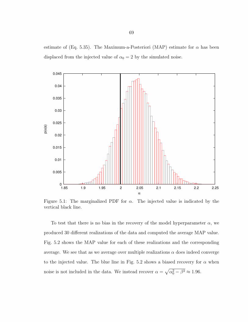
69
estimate of (Eq. 5.35). The Maximum-a-Posteriori (MAP) estimate for α has been
displaced from the injected value of α0 = 2 by the simulated noise.
0
0.005
0.01
0.015
0.02
0.025
0.03
0.035
0.04
0.045
1.85 1.9 1.95 2 2.05 2.1 2.15 2.2 2.25
p(α
|s)
α
Figure 5.1: The marginalized PDF for α. The injected value is indicated by thevertical black line.
To test that there is no bias in the recovery of the model hyperparameter α, we
produced 30 different realizations of the data and computed the average MAP value.
Fig. 5.2 shows the MAP value for each of these realizations and the corresponding
average. We see that as we average over multiple realizations α does indeed converge
to the injected value. The blue line in Fig. 5.2 shows a biased recovery for α when
noise is not included in the data. We instead recover α =√α2
0 − β2 ≈ 1.96.

70
1.8
1.85
1.9
1.95
2
2.05
2.1
2.15
2.2
0 5 10 15 20 25 30
α
Realization
MAP values with NoiseAverage of MAP values with Noise
MAP values without NoiseAverage of MAP values without Noise
Figure 5.2: MAP values for 30 different simulations of the toy model. The red curveincludes noise in the simulated signal and converges to α0 as expected. The bluecurves does not include noise in the simulation and converges to α2
0 − β2.
5.3.2 Toy Model II
The Hierarchical Bayesian approach produces un-biased estimates for the model
parameters if the signal and the noise (and hence the likelihood) are correctly modeled.
However, in some situations the cost of computing the likelihood can be prohibitive,
and it becomes desirable to use approximations to the likelihood, such as the Fisher
Information Matrix. For example, to investigate how the design of a detector influ-
ences its ability to discriminate between different astrophysical models, it is necessary
to Monte Carlo the analysis over many realizations of the source population for many
different instrument designs, which can be very costly using the full likelihood.

71
To explore these issues we introduce a new toy model that more closely resembles
the likelihood functions encountered in gravitational wave data analysis. Consider
a waveform h0 that represents a single data point (e.g. the amplitude of a wavelet
or a Fourier component), which can be parameterized in terms of the distance to
the source d0. The instrument noise n is assumed to be Gaussian with variance β2.
Here we will treat the noise level β as a hyperparameter to be determined from the
observations. Adopting a fiducial noise level β0 allows us to define a reference signal-
to-noise ratio SNR20 = h2
0/β20 . The likelihood of observing data s = h0 +n for a source
at distance d with noise level β is then
p(s|d, β) =1√2πβ
e−(s−h)2/(2β2), (5.37)
where h = (d0/d)h0. The likelihood is normally distrubuted in the inverse distance
1/d, with a maximum that depends on the particular noise realization n,
1
dML
=1 + n/(β0SNR0)
d0
. (5.38)
Now suppose that the distances follow a one-sided normal distribution p(d ≥ 0) =
2√2πβ
exp(−d2/2α20), and that we adopt a corresponding model for the distance distri-
bution with hyperparameter α and a flat hyperprior.
We simulate the data with N = 1000 sources with α0 = 2 and β = 0.05. The
values of α0 and β were chosen to give a fiducial SNR = 5 for d = 2α0. In the first of
our simulations the value of β was assumed to be known and we computed the MAP
estimates of α for 30 different simulated data sets. As shown in Fig. 5.3, the average
MAP estimate for α converges to the injected value.

72
1.75
1.8
1.85
1.9
1.95
2
2.05
2.1
0 5 10 15 20 25 30
α
Realization
MAP values Fisher LikelihoodAverage of MAP values Fisher Likelihood
MAP values Full LikelihoodAverage of MAP values Full Likelihood
Figure 5.3: MAP values for 30 different realizations of the toy model II. Using the fulllikelihood (red) the MAP values converge to the injected value, but with the FisherMatrix approximation to the likelihood (blue) there is a bias.
In contrast to the first toy model where only the combination α2+β2 is constrained
by the data, in this more realistic toy model both the noise level β and the model
hyperparameter α are separately constrained. Fig. 5.4 shows the marginalized PDFs
for both β and α. Tests using multiple realizations of the data show that the MAP
values of α and β are un-biased estimators of the injected parameter values.
5.3.2.1 Approximating the Likelihood For stationary and Gaussian instrument
noise the log likelihood for a signal described by parameters ~λ is given by
L(~λ) = −1
2(s− h(~λ)|s− h(~λ)), (5.39)

73
0
0.005
0.01
0.015
0.02
0.025
0.03
0.035
0.04
1.75 1.8 1.85 1.9 1.95 2 2.05 2.1 2.15 2.2
p(α
|s)
α
0
0.005
0.01
0.015
0.02
0.025
0.03
0.035
0.04
0.02 0.03 0.04 0.05 0.06 0.07 0.08 0.09 0.1
p(β
|s)
β
Figure 5.4: PDFs for the prior hyperparameter α and the noise level β for toy modelII. Both are individually constrained in this model. The injected values are shown bythe black lines.
where (a|b) denotes the standard noise-weighted inner product, and we have supressed
terms that depend on the noise hyperparameters. We expand the waveform h(~λ)
about the injected source parameters ~λ0 and get
h(~λ) = h(~λ0) + ∆λih,i + ∆λi∆λjh,ij +O(∆λ3) (5.40)
where ∆~λ = ~λ − ~λ0, and it is understood that the derivatives are evaluated at ~λ0.
Expanding the log likelihood we find:
L(∆~λ) = − 1
2(n|n) + ∆λi(n|h,i)
− 1
2∆λi∆λj(h,i|h,j) +O(∆λ3) . (5.41)

74
The maximum likelihood solution is found from ∂L/∂∆λi = 0, which yields ∆λiML =
(n|hj)Γij, where Γij is the inverse of the Fisher Information Matrix Γij = (h,i|h,j).
Using this solution to eliminate (n|h,i) from (Eq. 5.41) yields the quadratic, Fisher
Information Matrix approximation to the likelihood:
L(~λ) = const.− 1
2(λi − λiML)(λj − λjML)Γij . (5.42)
This form of the likelihood can be used in simulations by drawing the ∆λiML from a
multi-variate normal distribution with covariance matrix Γij.
In our toy model Γdd = SNR20β
20/(β
2d20), and L(d) = −SNR2
0β20(d−dML)2/(2β2d2
0).
The approximate likelihood follows a normal distribution in d while the full likelihood
follows a normal distribution in 1/d. For signals with large SNR this makes little
difference, but at low SNR the difference becomes significant and results in a bias in
the recovery of the model hyperparameters, as shown in Fig. 5.3. In this instance there
is a simple remedy: using u = 1/d in place of d in the quadratic approximation to the
likelihood exactly reproduces the full likelihood in this simple toy model. However,
it is not always so easy to correct the deficiencies of the quadratic Fisher Information
Matrix approximation to the likelihood.

75
CHAPTER 6
GRAVITATIONAL WAVE ASTRONOMY APPLICATIONS
In this chapter, we present several LISA and eLISA results using the Bayesian
formalism described in the previous chapter. We first show a Hierarchical Bayesian
analysis of the white dwarf binary population in the galaxy. We achieve constraints
that are applied in the subsequent analysis of stochastic signals. We then look at
the simplest case of searching for a stochastic background amidst instrument noise
only. Lastly, we fold in the added complexity of the white dwarf binary confusion
foreground signal.
6.1 Measurement of Galaxy Distribution Parameters
To illustrate how the Hierarchical Bayesian approach developed in the last chapter
can be applied to an astrophysically relevant problem, we investigate how population
models for the distribution of white dwarf binaries in the Milky Way galaxy can be
constrained by data from a space-based gravitational wave detector. Several studies
have looked at parameter estimation for individual white dwarf binaries in the Milky
Way [141, 142, 143]. We extend these studies to consider how the individual obser-
vations can be combined to infer the spatial and mass distributions of white dwarf
binaries in the Galaxy.
We present results for both LISA and eLISA missions. We focus this analysis on
short-period galactic binaries, with gravitational wave frequencies above 4 mHz. Our
conclusions for the two missions are very similar, as both are able to detect roughly
the same number of galactic binaries in the frequency bands considered here.

76
The 4 mHz lower limit is chosen to simplify the analysis in two ways. Firstly, it
avoids the signal overlap and source confusion problems that become significant at
lower frequencies [107], and secondly, it circumvents the issue of sample completeness
and Malmquist selection bias since LISA’s coverage of the galaxy is complete at high
frequencies. This claim is substantiated in Fig. 6.1 showing the cumulative percentage
of binaries detected as a function of frequency for a 4 year LISA mission. A given
frequency bin represents the percentage of binaries of that frequency and higher that
are detected. All binaries above ∼ 4 mHz are detectable by LISA, of which there are
∼ 5000.
It would be possible to extend our analysis to include all detectable white dwarf
binaries if we were to properly account for the undetectable sources. One way to do
this is to convolve the astrophysical model priors by a function that accounts for the
selection effects [130] so that we are working with the predicted observed distribution
rather than the theoretical distribution. Another approach is to marginalize over the
un-detectable signals [129].
The high frequency signals are not only the simplest to analyze, but they also tend
to have the highest signal-to-noise ratios, the best sky localization, and the best mass
and distance determination due to their more pronounced evolution in frequency.
When simulating the population of detectable sources we will assume that binaries
of all frequencies above 4 mHz are homogeneously distributed throughout the galaxy
and share the same chirp mass distribution. In reality, the population is likely to be
more heterogenous, and more complicated population models will have to be used.
Analyzing simulated data with the full likelihood is computationally taxing and,
when performing a large suite of such studies, could prove to be prohibitive. To
mitigate the cost of such analyses, we test a much faster approach (approximately
50 times faster), using the Fisher matrix approximation to the likelihood that we

77
0
10
20
30
40
50
60
70
80
90
100
0.002 0.004 0.006 0.008 0.01
Perc
enta
ge
Frequency (Hz)
Figure 6.1: The percentage of sources which are detectable as a function of frequency.Virtually 100% of the white dwarf binaries in the Milky Way above 4 mHz would bedetected by LISA.
demonstrated with a toy model in Chapter 5. We find the results are significantly
less biased by the Fisher approximation when using 1/d as the parameter that encodes
the distance to the source. This simple adjustment gives adequately reliable results in
significantly less time than the brute-force calculation, and will provide an additional,
useful metric to gauge the relative merits of proposed space-based gravitational wave
missions.

78
6.1.1 White Dwarf Likelihood
The likelihood for a single source is given by
p(s|~λ) = Ce−(s−h(~λ)|s−h(~λ))/2 . (6.1)
Here p(s|~λ) is the likelihood that the residual s− h(~x) is drawn from Gaussian noise,
where s is the data, and h(~λ) is the signal produced in the detector by a source
described by parameters ~λ. The simulated data s = h(~λ0) + n includes a waveform
h(~λ0) and a realization of the LISA instrument noise n. The normalization con-
stant C depends on the instrument noise levels, but is independent of the waveform
parameters.
The waveform for a white dwarf binary is well approximated by
h+(t) =1
d
4GMΩ2
c4
(1 + cos2 ι
2
)cos(Ωt)
h×(t) =1
d
4GMΩ2
c4cos ι sin(Ωt), (6.2)
where Ω = 2πf . Eq. 6.2 is an abbreviated form of Eq. 4.1, where we have explicitly
separated out the distance dependence in Eq. 6.2 to emphasize its importance to the
analysis here. We have 8 parameters that describe a white dwarf binary signal, the
frequency f , the distance to the source d, the chirp mass M, the inclination angle ι,
a polarization angle ψ, a phase angle ϕ0, and sky location parameters θ and φ. The
frequency evolution is given by Eq. 4.5. Sources with f T 2 SNR ∼ 1, where T is the
observation time, provide useful measurments of the chirp mass M and the distance
d [144, 145]. The strong f dependence in Eq. 4.5 is the reason why high frequency
binaries are the best candidates for placing strong constraints on the distance and
chirp mass.

79
6.1.2 Prior and Hyperparameters
The spatial density ρ, Eq. 4.6, becomes our prior distribution for the spatial
distribution of galactic binaries. The parameters of the density distribution A, Rb,
Rd and Zd become hyperparameters in the Hierarchical Bayesian analysis. Each set
of values for the four parameters corresponds to a distinct model for the shape of
the galaxy. For our simulations, we chose a galaxy with A = 0.25, Rb = 500 pc,
Rd = 2500 pc, and Zd = 200 pc.
Our ability to measure the hyperparameters of the spatial distribution depends
on how well we measure the sky location and distance for each binary. For many
sources, the distance is poorly determined because it is highly correlated with the
chirp mass. However, there are enough binaries that have sufficiently high frequency,
chirp mass and/or SNR to provide tight constraints on the chirp mass distribution.
The empirically determined chirp mass distribution can then be used as a prior for
the lower SNR, less massive, or lower frequency sources to improve their distance
constraints.
Fig. 6.2 shows the chirp mass distribution for binaries in our simulated galaxy.
We use this distribution to construct a hyperprior on the chirp mass, approximated
by the following distribution:
ρMc =C(
MM0
)−a+ a
b
(MM0
)b , (6.3)
where M0, a, and b are hyperparameters in our model. C is the normalization
constant which can be calculated analytically and is given by
C =M0πb
a+1a+b a−
a+1a+b
(a+ b) sin π(b−1)a+b
. (6.4)

80
M0 is the mode of the distribution. The hyperparameters a and b determine the
width of the distribution, which can be seen by calculating the full width at half
maximum (FWHM). It is given by
FWHM =M0
([2(b/a+ 1)]1/b − [2(a/b+ 1)]−1/a
). (6.5)
We further assume that the orbital evolution is due only to the emission of gravi-
tational waves, and is thus adequately described by Eq. 4.5. In principle, one would
want to be more careful and consider tidal effects and mass transfer [146] as possible
contributions to f . However, it is expected that the high frequency sources we are
focusing on will be mostly detached white dwarf binaries where tidal or mass transfer
effects are unlikely to be significant [147].
6.1.3 Results
We are able to efficiently calculate the full likelihood for each source (Eq. 6.1)
using the fast waveform generator developed by Cornish and Littenberg [55]. The
following results are all derived from simulations using the full likelihood. Using
the same MCMC approach from our toy models, we sample the posterior and get
PDFs for source and model parameters simultaneously. We check for convergence by
starting the chains at different locations in the prior volume and find that regardless
of starting location, the chains converge to the same PDFs.
Our procedure successfully recovers the correct chirp mass distribution, as shown
in Fig. 6.2 and is able to meaningfully constrain the parameters of the galaxy distri-
bution and chirp mass distribution models, with PDFs shown in Fig. 6.3 and Fig. 6.4
respectively.
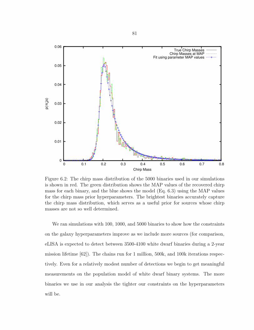
81
0
0.01
0.02
0.03
0.04
0.05
0.06
0 0.1 0.2 0.3 0.4 0.5 0.6 0.7 0.8
p(M
0|s
)
Chirp Mass
True Chirp MassesChirp Masses at MAP
Fit using parameter MAP values
Figure 6.2: The chirp mass distribution of the 5000 binaries used in our simulationsis shown in red. The green distribution shows the MAP values of the recovered chirpmass for each binary, and the blue shows the model (Eq. 6.3) using the MAP valuesfor the chirp mass prior hyperparameters. The brightest binaries accurately capturethe chirp mass distribution, which serves as a useful prior for sources whose chirpmasses are not so well determined.
We ran simulations with 100, 1000, and 5000 binaries to show how the constraints
on the galaxy hyperparameters improve as we include more sources (for comparison,
eLISA is expected to detect between 3500-4100 white dwarf binaries during a 2-year
mission lifetime [62]). The chains run for 1 million, 500k, and 100k iterations respec-
tively. Even for a relatively modest number of detections we begin to get meaningful
measurements on the population model of white dwarf binary systems. The more
binaries we use in our analysis the tighter our constraints on the hyperparameters
will be.

82
0
0.01
0.02
0.03
0.04
0.05
0.06
0.15 0.2 0.25 0.3 0.35
p(A
|s)
A Coefficient
0
0.005
0.01
0.015
0.02
0.025
350 400 450 500 550 600
p(R
b|s
)
Bulge Radius Rb
0
0.002
0.004
0.006
0.008
0.01
0.012
0.014
2400 2600 2800 3000 3200 3400
p(R
d|s
)
Disk Radius Rd
0
0.01
0.02
0.03
0.04
0.05
0.06
0.07
160 170 180 190 200 210 220 230 240 250
p(R
d|s
)
Disk Height Zd
Figure 6.3: PDFs for the four galaxy model hyperparameters. The red is for asimulation using 100 binaries, the green 1000 binaries, and the blue 5000 binaries.The black lines show the true values of the distribution from which the binaries weredrawn.
Table 1 lists the recovered MAP values and the variance of the marginalized poste-
rior distribution function for each hyperparameter. Gravitational wave observations
would be very competitive with existing electromagnetic observations in constraining
the shape of the galaxy [148, 149]. Making direct comparisons between our results
to those in the literature is complicated, as the actual values of the bulge and disk
radii are very model dependent. For example, Juric uses a model where the galaxy
is comprised of both a thin and thick disk. With GW data in hand, this comparison
could easily be made by trivially substituting the density profile used here.
What matters for this proof-of-principal study is how well the parameters can be
constrained. In the models of Juric et al., constraints for the disk radii are around

83
0
0.005
0.01
0.015
0.02
0.025 0.03
0.035
0.04
0.045
0.05
0.2 0.21 0.22 0.23 0.24 0.25
p(M
0|s
)
Chirp Mass Distribution Mode M0
0
0.005
0.01
0.015
0.02
0.025
0.03
0.05 0.06 0.07 0.08 0.09 0.1
p(F
WH
M|s
)
Chirp Mass Distribution FWHM
0
0.05
0.1
0.15
0.2
0.25
0.3
10 15 20 25 30 35 40 45 50
p(a
|s)
Chirp Mass Distribution Coefficient a
0
0.01
0.02
0.03
0.04
0.05
0.06
0.07
3 3.5 4 4.5 5
p(b
|s)
Chirp Mass Distribution Coefficient b
Figure 6.4: PDFs for the three chirp mass model hyperparameters and the FWHMof the distribution. The red is for a simulation using 100 binaries, the green 1000binaries, and the blue 5000 binaries.
20%. We find similar accuracy when using a pessimistic population of 100 systems.
Adopting a source catalog that is more consistent with theoretical predictions, we
find constraints for the disk parameters as low as 1.5% – a substantial improvement
over the state-of-the-art.
6.1.4 Approximating the Likelihood
While in this case it is very efficient, the full likelihood is nonetheless expensive
to compute, posing problems if we wish to do extensive studies of many astrophysical
models or detector configurations. For such exploratory studies, it is preferable to use
the Fisher Information Matrix approximation to the likelihood of Eq. 5.42. However,
as we saw with the toy model in Chapter 5, this can lead to biases in the recovered

84
Table 6.1: Galaxy Distribution Parameter MAP Values
100 1000 5000Parameter MAP σ MAP σ MAP σ
A 0.262 0.047 0.226 0.0157 0.249 0.0074Rb (pc) 440 58.9 490 17.1 480 8.38Rd (pc) 2465 237.5 2584 70.2 2461 32.4Zd (pc) 193 20.8 201 7.02 195 3.25
M0 0.226 0.0063 0.208 0.0018 0.205 0.00088FWHM 0.07 0.0094 0.071 0.0026 0.076 0.0014
MAP values and variances for the galaxy hyperparameters when using 100,1000 and 5000 galactic binaries in the analysis. The simulated values were A = 0.25,Rb = 500pc, Rd = 2500pc, and Zd = 200pc.
parameters. The Fisher matrix Γij is not a coordinate invariant quantity, and we
can at least partially correct the bias by reparameterizing our likelihood. Just as
in Chapter 5, instead of using the distance d as a variable, we can instead use 1/d,
which provides a much better approximation to the full likelihood. We test these
short-cuts by redoing the analysis of the galactic population using the Fisher matrix
approximation to the likelihood (both with d and 1/d as parameters) and compare
it to the results from the previous analysis using the full likelihood. Fig. 6.5 shows
PDFs for the galaxy hyperparameters using the three different methods for computing
p(d|~λ) with the full sample of 5000 binaries.
We find that the approximation using 1/d matches the full likelihood better than
the likelihood parameterized with d, however there are additional discrepancies due
to non-quadratic terms in the sky location θ, φ that we have not accounted for. The
dependence of the waveform on θ, φ is more complicated than the distance, and is
not so easily corrected by a simple reparameterization. The approximation could be

85
0
0.01
0.02
0.03
0.04
0.05
0.06
0.2 0.22 0.24 0.26 0.28 0.3
p(A
|s)
Coefficient A
0
0.005
0.01
0.015
0.02
0.025
440 460 480 500 520 540
p(R
b|s
)
Bulge Radius Rb
0
0.002
0.004
0.006
0.008
0.01
0.012
0.014
2300 2350 2400 2450 2500 2550 2600 2650 2700
p(R
d|s
)
Disk Radius Rd
0
0.01
0.02
0.03
0.04
0.05
0.06
0.07
180 190 200 210 220 230
p(Z
d|s
)
Disk Height Zd
Figure 6.5: PDFs from a simulation using 5000 binaries for the four galaxy modelhyperparameters using the full likelihood (red), a Fisher approximation in d (green),and a Fisher approximation in 1/d (blue).
improved by carrying the expansion of the likelihood beyond second order, however
this is computationally expensive and can be numerically unstable.
If we analyze several realizations of the galaxy using the three different likelihood
functions and average the results, we find the biases are persistent for the approximate
methods. Fig. 6.6 shows the MAP values and the average of the MAP values for 10
realizations of our fiducial galaxy model. The biases in the recovered disk radius and
disk height are particularly pronounced when using the Fisher Matrix approximation
to the likelihood parameterized with d.

86
0.22
0.23
0.24
0.25
0.26
0.27
0.28
0 1 2 3 4 5 6 7 8 9
Coeffic
ient A
465 470 475 480 485 490 495 500 505 510 515 520
0 1 2 3 4 5 6 7 8 9
Bulg
e R
adiu
s R
b
Realization
2300
2350
2400
2450
2500
2550
2600
2650
0 1 2 3 4 5 6 7 8 9
Dis
k R
adiu
s R
d
186
188
190
192
194
196
198
200
202
204
0 1 2 3 4 5 6 7 8 9
Dis
k H
eig
ht Z
d
Realization
Figure 6.6: MAP values and corresponding averages from a simulation using 5000binaries for the four galaxy model hyperparameters using the full likelihood (red),a Fisher Matrix approximation parameterized with d (green), and a Fisher Matrixapproximation using 1/d (blue).
6.1.5 Conclusion
In summary, when the data from a space-borne detector has been collected, the
resolvable white dwarf binaries will be regressed from the data, leaving behind a
confusion-limited foreground which will significantly contribute to the overall power
in the data around ∼ 1 mHz. The bright binaries will place tight constraints on the
distribution of white dwarf binaries throughout the galaxy. Measuring the overall
shape of the galaxy as demonstrated here will provide additional means to charac-
terize the level of the confusion noise. As we will show below, we can then use the
detailed understanding of the foreground signal to detect a stochastic gravitational
wave background at levels well below the confusion noise.
87
6.2 Separating a Background from Instrument Noise
We first show the simple case of separating a stochastic background from instru-
ment noise by applying our approach to simulated data from the third round of the
MLDC, and show that we are able to accurately recover the stochastic signal and
independently measure the position and acceleration noise levels in each arm of the
interferometer. We carry out our analysis using a noise orthogonal A,E, T set of
TDI channels. In this basis, and for equal arm-lengths, the T channel is insensitive to
gravitational wave signals at low frequencies. We show how this gives an improvement
for a 6-link detector over a 4-link configuration.
6.2.1 Stochastic Likelihood
Unlike the likelihood for white dwarf binaries, our likelihood for stochastic signals
does not include a source template h. The signal s is equal to what we call the
noise n, but here the “noise” includes contributions from instrument noise as well
as stochastic signals. For Gaussian signals and noise, the likelihood of measuring
cross-spectra < XiX∗j > is given by:
p(X|~λ) = Π1
(2π)N/2|C|eXiC
−1ij Xj (6.6)
where C is the noise correlation matrix, Xi = A,E, T, N is the number of samples
in each channel and ~λ → (Sai , Spj ,Ωgw, n) denotes the parameters in our model. The
noise correlation matrix is given by
Cij =
〈AA∗〉 〈AE∗〉 〈AT ∗〉
〈EA∗〉 〈EE∗〉 〈ET ∗〉
〈TA∗〉 〈TE∗〉 〈TT ∗〉
. (6.7)

88
For a 4-link detector, the matrix simplifies to
Cij = 〈XX∗〉 . (6.8)
In general, our model consists of the strain spectral densities for the confusion
foreground, the instrument noise, and a stochastic gravitational wave background
for each of the interferometer cross spectra (XX∗, AA∗, TT ∗, etc.). As mentioned
before, we use an equal arm, stationary approximation for the LISA arm lengths. For
a stochastic background and instrument noise only, the model is the sum of the two
individual pieces:
〈XX∗〉 = 〈XX∗noise〉+ 〈XX∗sgwb〉 . (6.9)
We compute the posterior distribution function p(Sai , Spj |xk) using the MCMC tech-
niques developed in Chapter 5.
Following the search phase, we employ the Bayesian analysis of Chapter 5 to
calculate posterior distributions for our model parameters. We also calculate a Bayes
ratio of the evidences for a model without a stochastic background and a model with
a stochastic background using thermodynamic integration. This Bayes factor for the
two models indicates our level of confidence in which model better describes the data.
For a Bayes factor of 30 or above, we can generally claim a confident detection. We
use several different stochastic background strengths to determine the lowest level
that we are confidently able to detect.
Combined with a prior for the model parameters, p(~λ), we are able to generate
samples from the posterior distributions function p(~λ|X) = p(X|~λ)p(~λ)/p(X) using
the PTMCMC algorithm from Chapter 5. Lacking a detailed instrument model or
relevant experimental data, we choose to use uniform priors for the 12 instrument

89
Table 6.2: Prior Ranges for Model Parameters
Parameter Range
Position Noise 4 · 10−43 4 · 10−41
Acceleration Noise 9 · 10−51 9 · 10−49
ln Ωgw −30.0 −24.5Ωgw 9.4 · 10−14 2.3 · 10−11
Slope -1 1
noise levels, allowing a factor of ten variation above and below the nominal levels.
Our prior ranges are given in Table 6.2. The energy density was taken to be uniform
in ln(Ωgw) across the range [−30,−24.5]. We considered two models for the spectral
slope, either assuming a scale invariant background and fixing m = 0, or allowing the
spectral index m to be uniform in the range [−1, 1].
For the proposal distribution we used a mixture of uniform draws from the full
prior range, and draws from a multivariate Gaussian distribution computed from
the Fisher Information Matrix [120]. Correlations between the parameters, and the
frequency dependence of the spectra complicate the computation of the Fisher Matrix,
but the basic idea can be understood by considering zero mean white noise with
variance σ. The relevant question is, how well can the noise level σ2 be determined
from N noise samples? The likelihood of observing the data xi is
L =1
(2π)N/2σNexp
(−∑N
i=1 x2i
2σ2
), (6.10)
which yields a maximum likelihood estimate for the noise level of σ2 =∑
i x2i /N . The
Fisher Matrix has a single element:
Γσσ = −∂2 lnL
∂σ2|ML =
N
2σ2. (6.11)

90
Thus, the error in the estimated noise level is ∆σ2 = 2σ∆σ = σ2/√N/2. We see
that the fractional error in the noise level estimate scales as the square root of the
number of data points. The same is true for the more complicated colored spectra in
our LISA noise model. Noting that the acceleration noise dominates below ∼ 1 mHz,
while the position noise dominates above ∼ 3 mHz, it follows that the effective number
of samples available to constrain the acceleration noise is of order Na ∼ 1 mHz×Tobs.
The position noise is far better constrained, with order Np ∼ fN×Tobs samples, where
fN is the Nyquist frequency of the data. We show later that only the sums of the
instrument noise levels in each arm are strongly constrained, so the Fisher matrix
approach leads to very large jumps being proposed in the noise level differences in
each arm. To maintain a good acceptance rate, we capped the variance in the weakly
constrained directions to be ten times the variance in the well constrained directions.
6.2.1.1 Mock LISA Data Challenge Training Data Results We tested our anal-
ysis technique on simulated data from the third round of the Mock LISA Data Chal-
lenge. We ran our analysis on Challenge 3.5 which is described in Section 2. Note
that we used prior ranges far wider than those described in the MLDC as we wanted
to test our approach in a more realistic setting.
We found that the signal transfer functions in the training data did not match
our analytic model. We traced the problem to the time domain filters that were
used to generate the data sets, which introduced additional transfer functions in the
frequency domain. Since the analytic form for these transfer functions has not been
published, we used the training data to estimate the transfer functions and update
our signal model.
Using the analysis from Chapter 5, we recover the PDFs for the noise parameters
and stochastic background energy density as shown in Figs. 6.7-6.10.

91
0 0.005 0.01
0.015 0.02
0.025 0.03
0.035
2.2
2.2
05
2.2
1
2.2
15
2.2
2
2.2
25
2.2
3
2.2
35
2.2
4
2.2
45
2.2
5
2.2
55
0 0.005 0.01
0.015 0.02
0.025 0.03
0.035
1.7
4
1.7
45
1.7
5
1.7
55
1.7
6
1.7
65
1.7
7
1.7
75
1.7
8
1.7
85
1.7
9
1.7
95
0 0.005 0.01
0.015 0.02
0.025 0.03
0.035 0.04
1.8
3
1.8
4
1.8
5
1.8
6
1.8
7
1.8
8
1.8
9
1.9
1.9
1
0 0.002 0.004 0.006 0.008 0.01
0.012 0.014 0.016 0.018 0.02
-2
-1.5 -1
-0.5 0
0.5 1
1.5 2
2.5
0 0.002 0.004 0.006 0.008 0.01
0.012 0.014 0.016
-1.5 -1
-0.5 0
0.5 1
1.5 2
0
0.005
0.01
0.015
0.02
0.025
-2
-1.5 -1
-0.5 0
0.5 1
1.5 2
Figure 6.7: Histograms showing the PDFs for the position noise levels, scaled by thenominal level, Eq. 2.10. On the left are the sums along each arm, and on the rightare the differences. The vertical lines denote the injected values.
We see that only the sums of the noise contributions in each arm are constrained
(the acceleration and position noise contributions can be separated though as they
have very different transfer functions). The detector is only sensitive to the change
in length for each arm, not to the movement of the individual test masses. Fig. 6.7
provides an example of this by showing that the sums Spji + Spij are well constrained,
while the differences Spji − Spij are poorly constrained. Also note that the position
noise levels are far better determined than the acceleration noise levels, as expected
from our Fisher Matrix analysis. The position noise extends over more frequency
bins, and this added information leads to tighter constraints on the uncertainty.

92
0
0.005
0.01
0.015
0.02
0.025
0.03
1.2
1.4
1.6
1.8 2
2.2
2.4
0
0.005
0.01
0.015
0.02
0.025
0.03
1.2
1.4
1.6
1.8 2
2.2
2.4
0
0.005
0.01
0.015
0.02
0.025
0.03
1.8 2
2.2
2.4
2.6
2.8 3
3.2
0 0.002 0.004 0.006 0.008 0.01
0.012 0.014 0.016 0.018 0.02
-2
-1.5 -1
-0.5 0
0.5 1
1.5 2
2.5
0
0.005
0.01
0.015
0.02
0.025
-2
-1.5 -1
-0.5 0
0.5 1
1.5 2
2.5
0
0.005
0.01
0.015
0.02
0.025
-3
-2.5 -2
-1.5 -1
-0.5 0
0.5 1
1.5 2
Figure 6.8: Histograms showing the PDFs for the position noise levels, scaled by thenominal level, Eq. 2.11. On the left are the sums along each arm, and on the rightare the differences. The vertical lines denote the injected values.
6.2.2 Detection Limits
Having established that our algorithm can faithfully recover a stochastic back-
ground level of Ωgw ∼ 10−11 with one month of data, we next turned to the problem of
determining the LISA detection limit for an approximately scale invariant stochastic
gravitational wave background. To do this we generated a new set of simulated data
sets by re-scaling the gravitational wave contribution to the MLDC training data,
and used Bayesian model selection to compared the evidence for two models, M0 -
the data is described by instrument noise alone, and M1 - the data is described by
instrument noise and a stochastic gravitational wave background. Plots of the Bayes
factor, or evidence ratio, as a function of Ωgw are shown in Fig. 6.11. We performed

93
0
0.005
0.01
0.015
0.02
0.025
0.03
105 110 115 120 125 130 135 140 145 150
Figure 6.9: PDF for the gravitational wave background level (scaled up by 1013). Thevertical line denotes the injected values.
multiple runs with different random number seeds as a way to estimate the numerical
error in our Bayes factors. Our detection confidence becomes very strong (a Bayes
factor of 30) for a background level of Ωgw = 6 × 10⁻¹³ with one month of data.
With one year of data the limit improves to Ωgw = 1.7× 10⁻¹³, based on the scaling
argument described in Section 6.2.1.
It is interesting to note that the detection limit does not change if we include the
spectral slope of the background as a model parameter. At first this seems a little
surprising, as the simulated data has a spectral slope of m = 0, so we would expect
the simpler model with m = 0 to be favored over the more complicated model with
m as a free parameter. Further investigation revealed that the more complicated
model was able to provide a slightly better fit to the data, and that this was enough

94
0
0.005
0.01
0.015
0.02
0.025
0.03
0.035
-0.1 -0.08 -0.06 -0.04 -0.02 0 0.02 0.04 0.06 0.08 0.1
Figure 6.10: PDF for the gravitational wave background slope.
to compensate for the additional complexity of the model in the calculation of the
model evidence. Our hypothesis is that our signal model is imperfect because of
the need to use numerical fits to the transfer functions introduced by the simulation
software, and that the freedom to adjust the spectral slope of the background is able
to compensate for this imperfection.
6.2.3 The Role of Null Channels and 4-link Operation
Previous analyses of stochastic background detection with LISA have emphasized
the importance of the gravitational wave insensitive null channel that can be formed
from the Sagnac or Michelson interferometry channels (to be precise these channels
are only null in the zero frequency limit, at non-zero frequencies they do respond
weakly to gravitational signals because of finite arm-length effects). Hogan and Ben-

95
Figure 6.11: Bayes factor showing the detectability versus background level. Thecurve shows the average values of the scattered points.
der showed how this null channel could be used to construct a statistic that measures
the amplitude of the stochastic background [76]. The importance of null channels has
also been emphasized in the context of searches for un-modeled gravitational wave
signals in ground and space-based detectors. For example, in the LIGO-Virgo searches
for un-modeled gravitational wave bursts, it has been shown that the sensitivity can
be improved by using the sums and differences of the output from the two (H2) and
four (H1) kilometer detectors at the Hanford site. The null channel H− = H1−H2
is insensitive to gravitational waves, and has proven useful as a tool to distinguish
between instrumental artifacts and gravitational wave signals [38, 150].
It may therefore seem a little surprising that the null “T” channel plays no priv-
ileged role in the present analysis. The reason is simple: when using a Gaussian

96
likelihood function the coordinate transformation in signal space that produces the
null channel leaves the likelihood unchanged. For example, when we repeat our anal-
ysis using the cross spectra for the X, Y, Z channels we get results that are identical
to what we found with the A,E, T channels. It is only when the instrument noise
is not well understood, and there are significant departures from stationarity and
Gaussianity that null channels become important. It would be naive to assume that
the LISA data will be perfectly stationary and Gaussian, and we expect the T -channel
will play a key role in detector characterization studies. That is our motivation for
the calculation described in the next section, where we derive a new version of the
T -channel that is insensitive to gravitational waves for unequal arm-lengths.
Figure 6.12: Bayes factors for the X, Y, and Z channels.

97
With the current baseline design for LISA, the failure of one proof mass leaves us
with a single interferometry channel. In most instances, it is then possible to configure
the array to produce a single X type TDI channel (alternatively we can work with
a single Beacon, Monitor or Relay channel). LISA has a built in redundancy that
eLISA lacks. With one channel the number of cross-spectra drops from 6 to 1, and
the null direction in signal space (the T channel) is lost. On the other hand, the
number of noise variables drops from 12 to 8 (the effective dimension of the noise
model drops from 6 to 4 since only the sums of noise contributions along each arm
can be inferred from the gravitational wave data). To study these competing effects
and to compare LISA and eLISA, we repeated our analysis using a single X type
TDI channel. We performed runs on each of the X, Y and Z channels to see how the
particular noise and signal realization in each channel impacted our ability to detect
a stochastic background signal. The results of this study are shown in Fig. 6.12.
We see that the detection threshold for a single channel is roughly a factor of two
worse than when all links are operational. This result appears to contradict the usual
statement that LISA can only detect stochastic backgrounds when the null channel is
available, but it should be remembered that we are using the very strong assumption
that the instrument noise is stationary and Gaussian, and the individual noise sources
have known spectral shape. With these assumptions we find that the high frequency
portion of the spectrum fixes the shot noise levels to very high precision, so any
deviations in the total spectrum in the 1→ 10 mHz range caused by a scale invariant
stochastic background stand out in stark relief.
In future studies it would be interesting to see how the detection limits are affected
by relaxing the assumptions in our noise model. It would also be interesting to have
a better sense of how well component level engineering models, ground testing and
in-flight commissioning studies can constrain the instrument noise model.

98
6.3 Including the Galactic Foreground
Having shown that a single space-based detector is capable of separating a stochas-
tic gravitational wave background from instrument noise, we now turn to the problem
of including the galactic white dwarf foreground in our analysis. Using the constraints
on the galaxy distrubution parameters found at the beginning of this chapter, we can
proceed to the full analysis containing a galactic white dwarf foreground. Our model,
Eq. 6.9, becomes
〈XX∗〉 = 〈XX∗noise〉+ 〈XX∗sgwb〉+ 〈XX∗galaxy〉 . (6.12)
As before, our analysis provides uncertainties for the instrument noise levels, the
galaxy shape Fourier coefficients, and the stochastic background energy density and
spectral slope.
We use the same Bayesian analysis pipeline from Chapter 5 to calculate PDFs for
our model parameters and to do Bayesian model selection. The only difference in the
likelihood arises from our treatment of the modulation. We divide the year into 50
segments and calculate the likelihood for each segment. We then take the product of
the segments to get a total posterior distribution for all the data,
p(X|~λ) =∏ 1
(2π)N/2|Cd|eX
di C
dij−1Xd
j . (6.13)
Here, d labels the time segments.
We ran our analysis for both a full 6-link LISA as well as a 4-link version. For the
6-link configuration, we use the orthogonal A, E, and T channels.

99
Figs. 6.13 and 6.14 show the posterior distributions for our noise model param-
eters. We see again that only the total noise (i.e. Sp12 + Sp21) in each interferometer
arm is well constrained.
0
0.05
-0.1
4
-0.1
3
-0.1
2
-0.1
1
-0.1
-0.0
9
-0.0
8
0
0.05
-0.3
6
-0.3
5
-0.3
4
-0.3
3
-0.3
2
-0.3
1
-0.3
0
0.05
0 0.0
1
0.0
2
0.0
3
0.0
4
0.0
5
(Sp
ij + Sp
ji - 2)/ Sp
0
0.01
0.02
0.03
-0.3
-0.2
-0.1
0 0.1
0.2
0.3
0.4
0
0.01
0.02
0.03
-0.4
-0.3
-0.2
-0.1
0 0.1
0.2
0.3
0
0.01
0.02
-0.4
-0.3
-0.2
-0.1
0 0.1
0.2
0.3
0.4
(Sa
ij + Sa
ji - 2)/ Sa
Figure 6.13: The PDFs for the six constrained noise parameter combinations for theAET channels. The position noise parameters are on the left and the accelerationnoise parameters on the right. The black (solid) vertical lines show the injected values.The blue (dashed) PDFs include slope fitting and the red (solid) PDFs do not.
For the 4-link configuration, the sum of all four noise levels is constrained. This
can be seen from Eqs. 2.5 and 2.6. The position noise extends over a larger frequency
band and is better constrained than the acceleration noise.
Figs. 6.15 and 6.16 show the posterior distributions for Ωgw for both the flat spec-
trum case and the frequency dependent case. In Fig. 6.15, the injected background
level is Ωgw = 2 · 10−13 and in Fig. 6.16 it is Ωgw = 5 · 10−13. We show later that

100
0
0.01
0.02
0.03
0.04
0.05
0.06
0.07
0.08
-0.5
4
-0.5
2
-0.5
-0.4
8
-0.4
6
-0.4
4
-0.4
2
-0.4
-0.3
8
(Sp
12 + Sp
21 + Sp
13 + Sp
31 - 4)/ Sp
0
0.005
0.01
0.015
0.02
0.025
0.03
0.035
-2 -1.5
-1 -0.5
0 0.5
1 1.5
2
(Sa
12 + Sa
21 + Sa
13 + Sa
31 - 4)/ Sa
Figure 6.14: The constrained position (left) and acceleration (right) noise parametersfor X. The black (solid) vertical lines show the injected values. The blue (dashed)PDFs include slope fitting and the red (solid) PDFs do not.
these are the lowest background levels that could be confidently detected for the AET
channels and X channel respectively.
When the proposed slope of the stochastic background matches or nearly matches
the slope for either the instrument noise or the galactic foreground, there will be
some correlation between the model parameters. This leads to greater spreads in the
PDFs of the model parameters. Figs. 6.15 and 6.16 show that the PDFs from the
model with a spectral slope are indeed broader than the PDFs for the model with
m = 0. The effect is more pronounced for the X-channel case than for AET. For
the slope parameter in the X-channel case, we even see in Fig. 6.15 that there is a
peak for m = −1. The PDF is broad enough that we wouldn’t be able to confidently
distinguish between a slope of 0 and a slope of −1. In Figs. 6.19 - 6.21, we see that this

101
0
0.01
0.02
0.03
0.04
0.05
0.06
0.07
0 2 4 6 8 10
ΩGW (1e-13)
0
0.01
0.02
0.03
0.04
0.05
0.06
0.07
0.08
0.09
-2 -1 0 1 2 3 4
Slope m
Figure 6.15: The stochastic gravitational wave background level, Ωgw, and slopeparameter, m, for AET. The black (solid) vertical lines show the injected values. Theblue (dashed) PDFs include slope fitting and the red (solid) PDFs do not.
increase in uncertainty leads to a higher upper bound on the stochastic background
level.
Figs. 6.17 and 6.18 show the PDFs for the galactic foreground model parameters.
We show the first three Fourier coefficients and the last three. The C0 coefficient sets
the DC amplitude level for the galaxy. The other Fourier coefficients determine the
shape. While there are 17 Fourier coefficients, the basic shape is determined by the
first 5 or 6 and the higher coefficients only add fine details that are not well resolved
in our analysis.

102
0
0.01
0.02
0.03
0.04
0.05
0.06
0 5 10
15
20
ΩGW (1e-13)
0
0.01
0.02
0.03
0.04
0.05
0.06
-1 0 1 2 3 4
Slope m
Figure 6.16: The stochastic gravitational wave background level, Ωgw, and slopeparameter, m, for X. The black (solid) vertical lines show the injected values. Theblue (dashed) PDF includes slope fitting and the red (solid) PDF does not.
6.3.1 Bayesian Model Selection
In Section 6.2.2, we suggested that the model with a spectral slope parameter
should always perform worse than the model without a slope. The extra degree of
freedom will allow the model to fit the data better, however, it also comes with a
penalty. In Bayesian model selection, higher dimensional models have a larger prior
volume to explore. Since the injected data had a spectral slope of m = 0, we wouldn’t
expect the model that allows for spectral slope fitting to ever outperform the model
that assumes m = 0.
However, our results above showed that both models performed comparably well.
We postulated that this was due to our having to use a numerical model for the
stochastic background spectrum. With an imperfect model, there was a benefit to

103
0 0.01 0.02 0.03 0.04 0.05 0.06
0.9
85
0.9
9
0.9
95
1 1.0
05
1.0
1
1.0
15
0 0.01 0.02 0.03 0.04 0.05 0.06
-0.1
6
-0.1
55
-0.1
5
-0.1
45
-0.1
4
-0.1
35
-0.1
3
-0.1
25
0 0.005 0.01
0.015 0.02
0.025 0.03
0.035 0.04
-0.1
3
-0.1
2
-0.1
1
-0.1
-0.0
9
-0.0
8
0 0.01 0.02 0.03 0.04 0.05 0.06 0.07 0.08
-0.0
08
-0.0
06
-0.0
04
-0.0
02
0 0.0
02
0.0
04
0.0
06
0.0
08
0 0.01 0.02 0.03 0.04 0.05 0.06 0.07 0.08
-0.0
04
-0.0
02
0 0.0
02
0.0
04
0.0
06
0 0.02 0.04 0.06 0.08 0.1
0.12
-0.0
05
-0.0
04
-0.0
03
-0.0
02
-0.0
01
0 0.0
01
0.0
02
0.0
03
0.0
04
Figure 6.17: The first three (left) and last three (right) Fourier coefficients for theA-channel. The first coefficients are well constrained while the later ones are not.The blue (dashed) PDFs include slope fitting and the red (solid) PDFs do not.
having the extra slope parameter that outweighed the penalty of having to explore
a larger prior volume. The two effects essentially canceled out. With the analytic
model used here, we find that the extra slope parameter does make a difference. In
Figs. 6.19 - 6.21, the model with spectral slope fitting always performs worse than
the model with m = 0. The effect is not large and does not significantly inflate the
bounds that could be placed on a stochastic background, which makes sense because
the single additional parameter is not a large increase in our parameter space.
6.3.2 Comparison to MLDC
As a consistency check, we compare the analytic model used with our own data, to
the numerical model used with the MLDC data. We ran our analytic model on data

104
0 0.005 0.01
0.015 0.02
0.025 0.03
0.035 0.04
0.9
8
0.9
9
1 1.0
1
1.0
2
0 0.005 0.01
0.015 0.02
0.025 0.03
0.035 0.04
0.045
-0.1
6
-0.1
55
-0.1
5
-0.1
45
-0.1
4
-0.1
35
-0.1
3
-0.1
25
0 0.005 0.01
0.015 0.02
0.025 0.03
0.035
-0.1
4
-0.1
3
-0.1
2
-0.1
1
-0.1
-0.0
9
-0.0
8
0 0.01 0.02 0.03 0.04 0.05 0.06 0.07 0.08
-0.0
08
-0.0
06
-0.0
04
-0.0
02
0 0.0
02
0.0
04
0.0
06
0.0
08
0 0.01 0.02 0.03 0.04 0.05 0.06 0.07 0.08
-0.0
04
-0.0
02
0 0.0
02
0.0
04
0.0
06
0 0.02 0.04 0.06 0.08 0.1
0.12
-0.0
05
-0.0
04
-0.0
03
-0.0
02
-0.0
01
0 0.0
01
0.0
02
0.0
03
0.0
04
Figure 6.18: The first three (left) and last three (right) Fourier coefficients for theX-channel. The blue (dashed) PDFs include slope fitting and the red (solid) PDFsdo not.
containing instrument noise and a stochastic background, but no galaxy. We find
that our results are consistent with our work on the MLDC data. We would expect
that a 1-year data set, which is ∼ 15 times longer than the ∼ 3-week MLDC data set,
should perform approximately√
15 better than the MLDC data. In Fig. 6.19, we see
that the new results agree very well with the MLDC results after taking into account
the different observation times.
6.3.3 Analysis with a Galactic Foreground
We now compare our results for the data set with no galaxy component versus
a data set that includes instrument noise, a stochastic background, and a galactic
confusion foreground. We find that our recovery of the stochastic background is not

105
0.1
1
10
100
1000
10000MLDC X Bayes
New Code XMLDC AET Bayes
New Code AET30
0.1
1
10
100
1000
10000
1e-14 1e-13 1e-12
Ba
ye
s F
acto
r
ΩGW
MLDC X BayesNew Code X
MLDC AET BayesNew Code AET
30
Figure 6.19: A comparison of the Bayes factors for the MLDC data and for oursimulated data without a galaxy. The lower panel includes slope fitting. A Bayesfactor of 30 is considered a strong detection.
significantly diminished when including the galactic foreground. Fig. 6.20 compares
the Bayes factors for the analysis without the confusion foreground to those that
contain the galaxy. The addition of the galaxy adds a small amount of uncertainty into
the posterior distributions of each parameter, and we see that the detection threshold
is slightly raised. This indicates that the correlation between the various model
components is not large and that the model is successfully distinguishing amongst
the three components.
We investigated the two effects that enable us to separate the galactic foreground
from the stochastic background, namely, the shape of the spectrum and the time
modulation of the signal throughout the year. Before, we relied solely on the discrim-

106
0.1
1
10
100
1000
10000X Without Galaxy
AET Without GalaxyX With Galaxy
AET With Galaxy30
0.1
1
10
100
1000
10000
1e-14 1e-13 1e-12
Ba
ye
s F
acto
r
ΩGW
X Without GalaxyAET Without Galaxy
X With GalaxyAET With Galaxy
30
Figure 6.20: A comparison of Bayes factors for data without the galaxy vs. datawith the galaxy included. Including the galaxy does not significantly decrease ourdetection ability. The lower panel includes slope fitting.
inating power of the different spectral shapes for the noise and stochastic background.
Fig. 6.21 shows how both the modulation and spectral shape help. To show that our
method does not depend solely on the galaxy modulation, we ran our analysis on a
single week of data. We used the first week of the year when the foreground signal
is at a minimum, and the 37th week when the foreground is at a maximum. For
one week of observation time, the foreground signal is essentially constant, and we
won’t get any information from the modulation. With only one week of data, we have
fewer data points and would expect to perform worse by a factor of approximately√
50 ' 7. The performance actually decreases by a factor of 15. Excluding the

107
modulation reduces the effectiveness of our analysis by about a factor of 2, but we
are still able to pick apart the various components in the data.
Next we showed what happens if we remove the spectral information and rely on
the time domain modulation alone. We created a stochastic background that had the
exact spectrum of the galaxy. We took the galaxy spectral shape and scaled it by the
gravitational wave energy density and the appropriate Hubble and numerical factors
from Eq. 3.12. The galaxy and artificial background spectrum are correlated to a
much greater degree in this case. We found for the X-channel that we were in general
no longer able to distinguish the galaxy from the stochastic background. However,
if the constraints on the galaxy parameters from the bright sources are sufficiently
stringent, we are still able to recover a stochastic background that has the same
spectrum as the galaxy since the galaxy distribution priors will tightly constrain the
galaxy confusion level. For the AET-channel case, the bound is weakened by almost
two orders of magnitude. However, the galaxy parameters and background are still
recovered at a level well below the instrument noise and galactic foreground. If we
are unlucky, the Universe may have produced a stochastic background with a spectral
slope that matches the galaxy or the acceleration noise. In that case, we see that we
would have much higher upper bounds for a stochastic gravitational wave background.
However, we are showing a worst case scenario where the galaxy had the exact same
spectral shape and extended over the exact same frequency band. It is very unlikely
that a stochastic background would match the galaxy or instrument noise that well.
Lastly, we ran on the low frequency end of the spectrum. The acceleration noise,
galaxy, and stochastic background dominate out to∼ 20 mHz, after which the position
noise dominates. Running on the low frequency end of the spectrum gives all of the
various signal components approximately equal weighting since they all extend over
approximately the same number of frequency bins. The background is recovered at a

108
slightly higher level, showing that we do gain by using the high frequency information
to pin down the position noise levels.
0.1
1
10
100
1000
10000Full X
Division 0Division 37
Low FrequencySame Spectrum
30
0.1
1
10
100
1000
10000
1e-14 1e-13 1e-12 1e-11
Ba
ye
s F
acto
r
ΩGW
Full XDivision 0
Division 37Low Frequency
30
Figure 6.21: A comparison of Bayes Factors for the full AET vs. running on the lowfrequency end of the spectrum, single weeks of data, and a stochastic backgroundwith a spectral shape identical to the galaxy spectrum used in this paper. We seethat both the spectral shape and the galaxy signal modulation help separate the threemodel components. The lower panel includes slope fitting.
6.3.4 Conclusion
We have shown that a single space-based detector such as LISA or eLISA is able to
detect a stochastic gravitational wave background in the presence of both instrument
noise and a strong astrophysical foreground signal. As we expect only one space
detector in the near future, this technique is important because it doesn’t rely on
cross correlation amongst multiple detectors. The levels achieved in the analysis here

109
would be the most stringent bounds placed on the energy density of a stochastic
gravitataional wave background in the millihertz frequency regime.

110
CHAPTER 7
CONCLUSIONS
This dissertation demonstrates two very promising results for space-based grav-
itational wave interferometers. We have shown that a single space-based detector
can be used to detect a stochastic gravitational wave background. Our analysis can
separate various stochastic signals and noise in the data from each other without
relying on cross correlation. The technique works for both 6-link and 4-link detector
configurations. We also develeped a general Hierarchical Bayesian method capable of
constraining the model parameters for a population of sources. In the particular case
of white dwarf binaries in the Milky Way, we can constrain the spatial distribution
of the galaxy to levels better than current electromagnetic observations using the
anticipated number of systems detectable by space-based gravitational wave detec-
tors. Even if the currently held event rates for white dwarf binaries turn out to
be optimistic by more than an order of magnitude, the constraints possible with a
gravitational wave detector are comparable to our current estimates of the Milky
Way’s shape.
We showed that after modeling the galactic foreground and instrument noise
we can detect a background of order Ωgw ∼ 10−13. This is a very optimistic
level for a gravitational wave background. Standard inflation models predict that
the background would be at a level of approximately Ωgw ∼ 10−17. However, a
LISA-like detector would set the best experimental bound in the milliHertz fre-
quency regime, and may potentially uncover phase transitions in the early Uni-
verse [28, 101, 100, 99, 112, 113], or astrophysical backgrounds from EMRIs [56],
extragalactic white dwarfs [105], or inspirals of massive black hole binaries [57]. Esti-

111
mates of the extragalactic white dwarf confusion noise [105] predict Ωgw(f) ∼ 3×10⁻¹²
at f ∼ 2 − 3mHz, which should be detectable even with the galactic foreground to
contend with. The extragalactic astrophysical foreground will likely set the floor for
detecting stochastic backgrounds of cosmological origin, preventing us from reaching
the limits that the LISA observatory is theoretically capable of.
One line of future study is to investigate how the limits shown here are affected by
weakening the assumptions that went into the instrument noise model. Another line
of future study is to include some of the other potential astrophysical foregrounds
in our analysis. We could investigate our ability to detect any anisotropies in the
extragalactic background, but neither LISA nor eLISA will have very good spatial
sky resolution for a stochastic background. Later generation detectors such as BBO
and DECIGO could achieve much better sky resolution using radiometer techniques,
and it would be interesting to investigate the sky resolution of these later generation
missions.

112
REFERENCES CITED
[1] A. Einstein. Die Feldgleichungen der Gravitation. Sitzungsberichte derKoniglich Preußischen Akademie der Wissenschaften (Berlin), Seite 844-847.,pages 844–847, 1915.
[2] A. Einstein. Erklarung der Perihelionbewegung der Merkur aus der allgemeinenRelativitatstheorie. Sitzungsber. preuss.Akad. Wiss., vol. 47, No.2, pp. 831-839,1915, 47:831–839, 1915.
[3] Albert Einstein. Relativitatstheorie. (German) [Theory of Relativity]. Die Kul-tur der Gegenwart. Ihre Entwicklung und ihre Ziele. Paul Hinneberg, ed. Part3, Mathematik, Naturwissenschaften, Medizin. Section 3, Anorganischen Natur-wissenschaften, pages 703–713. pub-TEUBNER, pub-TEUBNER:adr, 1915. SeeSchilpp number 192 for a revised edition.
[4] F. W. Dyson, A. S. Eddington, C. Davidson. A Determination of the Deflectionof Light by the Sun’s Gravitational Field, from Observations Made at the TotalEclipse of May 29, 1919. Royal Society of London Philosophical TransactionsSeries A, 220:291–333, 1920. doi:10.1098/rsta.1920.0009.
[5] Albert Einstein. Approximative Integration of the Field Equations of Gravita-tion. Sitzungsber.Preuss.Akad.Wiss.Berlin (Math.Phys.), 1916:688–696, 1916.
[6] A. Einstein. Die Grundlage der allgemeinen Relativitatstheorie. Annalen derPhysik, 354:769–822, 1916. doi:10.1002/andp.19163540702.
[7] A. Einstein. Uber Gravitationswellen. Sitzungsberichte der Koniglich Preußis-chen Akademie der Wissenschaften (Berlin), Seite 154-167., pages 154–167,1918.
[8] R.A. Hulse, J.H. Taylor. Discovery of a Pulsar in a Binary System. Astrophys.J.,195:L51–L53, 1975. doi:10.1086/181708.
[9] J.H. Taylor, J.M. Weisberg. A New Test of General Relativity: GravitationalRadiation and the Binary Pulsar PS R 1913+16. Astrophys.J., 253:908–920,1982. doi:10.1086/159690.
[10] Adhikari, Rana, et al. LSC Gravitational Wave Instrument Science White Pa-per. Available at http://www.ligo.org/about/white_paper.php, 2012.
[11] Cadonati, Laura, et al. LSC Gravitational Wave Data Analysis White Paper.Available at http://www.ligo.org/about/white_paper.php, 2012.
[12] R.N. Manchester. The International Pulsar Timing Array. 2013. arXiv:1309.7392.

113
[13] Michael Kramer, David J. Champion. The European Pulsar Timing Array andthe Large European Array for Pulsars. Class.Quant.Grav., 30:224009, 2013.doi:10.1088/0264-9381/30/22/224009.
[14] Maura A. McLaughlin. The North American Nanohertz Observatory for Grav-itational Waves. Class.Quant.Grav., 30:224008, 2013. arXiv:1310.0758,doi:10.1088/0264-9381/30/22/224008.
[15] G. Hobbs. The Parkes Pulsar Timing Array. Class.Quant.Grav., 30:224007,2013. arXiv:1307.2629, doi:10.1088/0264-9381/30/22/224007.
[16] Pau Amaro-Seoane, Sofiane Aoudia, Stanislav Babak, Pierre Binetruy,Emanuele Berti, et al. eLISA/NGO: Astrophysics and Cosmology in theGravitational-wave Millihertz Regime. GW Notes, 6:4–110, 2013. arXiv:
1201.3621.
[17] Stebbins, R., et al. Laser Interferometer Space Antenna (LISA) A Response tothe Astro2010 RFI for the Particle Astrophysics and Gravitation Panel. Avail-able at http://lisa.nasa.gov/documentation.html, 2009.
[18] E. Komatsu, et al. Five-Year Wilkinson Microwave Anisotropy Probe (WMAP)Observations: Cosmological Interpretation. Astrophys.J.Suppl., 180:330–376,2009. arXiv:0803.0547, doi:10.1088/0067-0049/180/2/330.
[19] C.L. Bennett, A. Banday, K.M. Gorski, G. Hinshaw, P. Jackson, et al. Four yearCOBE DMR Cosmic Microwave Background Observations: Maps and BasicResults. Astrophys.J., 464:L1–L4, 1996. arXiv:astro-ph/9601067, doi:10.1086/310075.
[20] G. Hinshaw, et al. Nine-Year Wilkinson Microwave Anisotropy Probe (WMAP)Observations: Cosmological Parameter Results. Astrophys.J.Suppl., 208:19,2013. arXiv:1212.5226, doi:10.1088/0067-0049/208/2/19.
[21] P.A.R. Ade, et al. Planck 2013 Results. XVI. Cosmological Parameters. 2013.arXiv:1303.5076.
[22] P.A.R. Ade, et al. BICEP2 I: Detection Of B-mode Polarization at DegreeAngular Scales. 2014. arXiv:1403.3985.
[23] P. A. R Ade, et al. BICEP2 II: Experiment and Three-Year Data Set. 2014.arXiv:1403.4302.
[24] Raphael Flauger, J. Colin Hill, David N. Spergel. Toward an Understanding ofForeground Emission in the BICEP2 Region. 2014. arXiv:1405.7351.
[25] Michael J. Mortonson, Uro Seljak. A Joint Analysis of Planck and BICEP2 BModes Including Dust Polarization Uncertainty. 2014. arXiv:1405.5857.

114
[26] Alan H. Guth. The Inflationary Universe: A Possible Solution to the Hori-zon and Flatness Problems. Phys.Rev., D23:347–356, 1981. doi:10.1103/
PhysRevD.23.347.
[27] Craig J. Hogan. Cosmological Gravitational Wave Backgrounds. 1998. arXiv:astro-ph/9809364.
[28] Michele Maggiore. Gravitational Wave Experiments and Early Universe Cos-mology. Phys.Rept., 331:283–367, 2000. arXiv:gr-qc/9909001, doi:10.1016/S0370-1573(99)00102-7.
[29] Curt Cutler, Kip S. Thorne. An Overview of Gravitational Wave Sources. pages72–111, 2013. arXiv:gr-qc/0204090, doi:10.1142/9789812776556_0004.
[30] Scott A. Hughes. Listening to the Universe with Gravitational-wave Astronomy.Annals Phys., 303:142–178, 2003. arXiv:astro-ph/0210481, doi:10.1016/
S0003-4916(02)00025-8.
[31] Alessandra Buonanno. TASI Lectures on Gravitational Waves from the EarlyUniverse. pages 855–892, 2003. arXiv:gr-qc/0303085.
[32] Sirichai Chongchitnan, George Efstathiou. Prospects for Direct Detectionof Primordial Gravitational Waves. Phys.Rev., D73:083511, 2006. arXiv:
astro-ph/0602594, doi:10.1103/PhysRevD.73.083511.
[33] J. Abadie, et al. Upper Limits on a Stochastic Gravitational-wave Backgroundusing LIGO and Virgo Interferometers at 600-1000 Hz. Phys.Rev., D85:122001,2012. arXiv:1112.5004, doi:10.1103/PhysRevD.85.122001.
[34] Frederick A. Jenet, G.B. Hobbs, W. van Straten, R.N. Manchester, M. Bailes,et al. Upper Bounds on the Low-frequency Stochastic Gravitational WaveBackground from Pulsar Timing Observations: Current Limits and FutureProspects. Astrophys.J., 653:1571–1576, 2006. arXiv:astro-ph/0609013,doi:10.1086/508702.
[35] N. Christensen. Measuring the Stochastic Gravitational Radiation Backgroundwith Laser Interferometric Antennas. Phys.Rev., D46:5250–5266, 1992. doi:
10.1103/PhysRevD.46.5250.
[36] Eanna E. Flanagan. The Sensitivity of the Laser Interferometer GravitationalWave Observatory (LIGO) to a Stochastic Background, and its Dependence onthe Detector Orientations. Phys.Rev., D48:2389–2407, 1993. arXiv:astro-ph/9305029, doi:10.1103/PhysRevD.48.2389.
[37] Neil J. Cornish, Shane L. Larson. Space Missions to Detect the Cosmic Grav-itational Wave Background. Class.Quant.Grav., 18:3473–3496, 2001. arXiv:
gr-qc/0103075, doi:10.1088/0264-9381/18/17/308.

115
[38] B.P. Abbott, et al. An Upper Limit on the Stochastic Gravitational-WaveBackground of Cosmological Origin. Nature, 460:990, 2009. arXiv:0910.5772,doi:10.1038/nature08278.
[39] Allen, Bruce. The Stochastic Gravity Wave Background: Sources and Detec-tion. 1996. arXiv:gr-qc/9604033.
[40] Matthew R. Adams, Neil J. Cornish. Discriminating Between a StochasticGravitational Wave Background and Instrument Noise. Phys.Rev., D82:022002,2010. arXiv:1002.1291, doi:10.1103/PhysRevD.82.022002.
[41] Matthew R. Adams, Neil J. Cornish. Detecting a Stochastic Gravitational WaveBackground in the Presence of a Galactic Foreground and Instrument Noise.Phys.Rev., D89:022001, 2014. arXiv:1307.4116, doi:10.1103/PhysRevD.89.022001.
[42] R. H. Dicke, P. J. E. Peebles, P. G. Roll, D. T. Wilkinson. Cosmic Black-Body Radiation. The Astrophysical Journal, 142:414–419, July 1965. doi:
10.1086/148306.
[43] A. A. Penzias, R. W. Wilson. A Measurement of Excess Antenna Temperatureat 4080 Mc/s. The Astrophysical Journal, 142:419–421, July 1965. doi:10.
1086/148307.
[44] Andrew H. Jaffe, Donald C. Backer. Gravitational Waves Probe the CoalescenceRate of Massive Black Hole Binaries. Astrophys.J., 583:616–631, 2003. arXiv:astro-ph/0210148, doi:10.1086/345443.
[45] J. Stuart B. Wyithe, Abraham Loeb. Low-frequency Gravitational Wavesfrom Massive Black Hole Binaries: Predictions for LISA and Pulsar Tim-ing Arrays. Astrophys.J., 590:691–706, 2003. arXiv:astro-ph/0211556,doi:10.1086/375187.
[46] Motohiro Enoki, Kaiki Taro Inoue, Masahiro Nagashima, Naoshi Sugiyama.Gravitational Waves from Supermassive Black Hole Coalescence in a Hierarchi-cal Galaxy Formation Model. Astrophys.J., 615:19, 2004. arXiv:astro-ph/
0404389, doi:10.1086/424475.
[47] L.P. Grishchuk. Relic Gravitational Waves and Cosmology. Phys.Usp., 48:1235–1247, 2005. arXiv:gr-qc/0504018, doi:10.1070/PU2005v048n12ABEH005795.
[48] T. Regimbau, Jose A. de Freitas Pacheco. Cosmic Background of GravitationalWaves from Rotating Neutron Stars. 2001. arXiv:astro-ph/0105260.
[49] Tania Regimbau, Jose Antonio de Freitas Pacheco. Gravitational Wave Back-ground from Magnetars. Astron.Astrophys., 447:1, 2006. arXiv:astro-ph/
0509880, doi:10.1051/0004-6361:20053702.

116
[50] P.L. Bender, D. Hils. Confusion Noise Level Due to Galactic and ExtragalacticBinaries. Class.Quant.Grav., 14:1439–1444, 1997. doi:10.1088/0264-9381/
14/6/008.
[51] Charles R. Evans, Icko Iben, Larry Smarr. Degenerate Dwarf Binariesas Promising, Detectable Sources of Gravitational Radiation. Astrophys.J.,323:129–139, 1987. doi:10.1086/165812.
[52] Bernard F. Schutz. Low Frequency Sources of Gravitational Waves: A Tutorial.1997. arXiv:gr-qc/9710079.
[53] Mukremin Kilic, Warren R. Brown, J.J. Hermes, Carlos Allende Prieto, S.J.Kenyon, et al. SDSS J163030.58+423305.8: A 40 minute Orbital Period De-tached White Dwarf Binary. 2011. arXiv:1109.6339.
[54] Warren R. Brown, Mukremin Kilic, J.J. Hermes, Carlos Allende Prieto, Scott J.Kenyon, et al. A 12 Minute Orbital Period Detached White Dwarf EclipsingBinary. 2011. arXiv:1107.2389.
[55] Neil J. Cornish, Tyson B. Littenberg. Tests of Bayesian Model SelectionTechniques for Gravitational Wave Astronomy. Phys.Rev., D76:083006, 2007.arXiv:0704.1808, doi:10.1103/PhysRevD.76.083006.
[56] Leor Barack, Curt Cutler. Confusion Noise from Extreme-Mass-Ratio Inspirals.2005. arXiv:gr-qc/0502052.
[57] A. Sesana, F. Haardt, P. Madau, M. Volonteri. The Gravitational WaveSignal from Massive Black Hole Binaries and its Contribution to the LISAData Stream. Astrophys.J., 623:23–30, 2005. arXiv:astro-ph/0409255,doi:10.1086/428492.
[58] R. T. Stebbins. Rightsizing LISA. Classical and Quantum Gravity,26(9):094014, May 2009. arXiv:0904.1029, doi:10.1088/0264-9381/26/9/094014.
[59] Jonathan R. Gair, Christopher Tang, Marta Volonteri. LISA Extreme-Mass-Ratio Inspiral Events as Probes of the Black Hole Mass Function. Phys.Rev.,D81:104014, 2010. arXiv:1004.1921, doi:10.1103/PhysRevD.81.104014.
[60] Jonathan R. Gair, Alberto Sesana, Emanuele Berti, Marta Volonteri. Constrain-ing Properties of the Black Hole Population Using LISA. Class.Quant.Grav.,28:094018, 2011. arXiv:1009.6172, doi:10.1088/0264-9381/28/9/094018.
[61] Alberto Sesana, Jonathan Gair, Emanuele Berti, Marta Volonteri. Recon-structing the Massive Black Hole Cosmic History Through Gravitational Waves.Phys.Rev., D83:044036, 2011. arXiv:1011.5893, doi:10.1103/PhysRevD.83.044036.

117
[62] Pau Amaro-Seoane, Sofiane Aoudia, Stanislav Babak, Pierre Binetruy,Emanuele Berti, et al. Low-frequency Gravitational-wave Science witheLISA/NGO. Class.Quant.Grav., 29:124016, 2012. arXiv:1202.0839, doi:
10.1088/0264-9381/29/12/124016.
[63] Joseph E. Plowman, Daniel C. Jacobs, Ronald W. Hellings, Shane L. Larson,Sachiko Tsuruta. Constraining the Black Hole Mass Spectrum with Gravita-tional Wave Observations I: The Error Kernel. 2009. arXiv:0903.2059.
[64] Joseph E. Plowman, Ronald W. Hellings, Sachiko Tsuruta. Constraining theBlack Hole Mass Spectrum with LISA Observations II: Direct Comparison ofDetailed Models. 2010. arXiv:1009.0765.
[65] Ilya Mandel. Parameter Estimation on Gravitational Waves from Multi-ple Coalescing Binaries. Phys.Rev., D81:084029, 2010. arXiv:0912.5531,doi:10.1103/PhysRevD.81.084029.
[66] R. O’Shaughnessy. Comparing Compact Binary Parameter Distributions I:Methods. 2012. arXiv:1204.3117.
[67] Bender, P.L., et al. LISA. Laser Interferometer Space Antenna for the Detectionand Observation of Gravitational Waves. An International Project in the Fieldof Fundamental Physics in Space. Pre-Phase A report. Available at http:
//relativity.livingreviews.org/refdb/record/8064, 1998.
[68] Jonathan P. Gardner, John C. Mather, Mark Clampin, Rene Doyon,Matthew A. Greenhouse, et al. The James Webb Space Telescope.Space Sci.Rev., 123:485, 2006. arXiv:astro-ph/0606175, doi:10.1007/
s11214-006-8315-7.
[69] K. Danzmann, A. Rudiger. LISA Technology - Concept, Status, Prospects.Class.Quant.Grav., 20:S1–S9, 2003.
[70] Patricia Purdue, Shane L. Larson. Spurious Acceleration Noise in SpaceborneGravitational Wave Interferometers. Class.Quant.Grav., 24:5869–5887, 2007.doi:10.1088/0264-9381/24/23/010.
[71] Massimo Tinto, J.W. Armstrong. Cancellation of Laser Noise in anUnequal-arm Interferometer Detector of Gravitational Radiation. Phys.Rev.,D59:102003, 1999. doi:10.1103/PhysRevD.59.102003.
[72] F. B. Estabrook, Massimo Tinto, J. W. Armstrong. Time Delay Analysisof LISA Gravitational Wave Data: Elimination of Spacecraft Motion Effects.Phys.Rev., D62:042002, 2000. doi:10.1103/PhysRevD.62.042002.

118
[73] Michele Vallisneri. Geometric Time Delay Interferometry. Phys.Rev.,D72:042003, 2005. arXiv:gr-qc/0504145, doi:10.1103/PhysRevD.76.
109903,10.1103/PhysRevD.72.042003.
[74] Thomas A. Prince, Massimo Tinto, Shane L. Larson, J.W. Armstrong. TheLISA Optimal Sensitivity. Phys.Rev., D66:122002, 2002. arXiv:gr-qc/
0209039, doi:10.1103/PhysRevD.66.122002.
[75] Julien Sylvestre, Massimo Tinto. Noise Characterization for LISA. Phys.Rev.,D68:102002, 2003. arXiv:gr-qc/0308085, doi:10.1103/PhysRevD.68.
102002.
[76] Craig J. Hogan, Peter L. Bender. Estimating Stochastic Gravitational WaveBackgrounds with Sagnac Calibration. Phys.Rev., D64:062002, 2001. arXiv:
astro-ph/0104266, doi:10.1103/PhysRevD.64.062002.
[77] Stanislav Babak, John G. Baker, Matthew J. Benacquista, Neil J. Cornish,Jeff Crowder, et al. The Mock LISA Data Challenges: From Challenge 1Bto Challenge 3. Class.Quant.Grav., 25:184026, 2008. arXiv:0806.2110, doi:10.1088/0264-9381/25/18/184026.
[78] Cornish, Neil J. and Rubbo, Louis J. LISA Simulator v. 2.0. Available atwww.physics.montana.edu/LISA/, 2003.
[79] Neil J. Cornish, Louis J. Rubbo. The LISA Response Function. Phys.Rev.,D67:022001, 2003. arXiv:gr-qc/0209011, doi:10.1103/PhysRevD.67.
029905,10.1103/PhysRevD.67.022001.
[80] Michele Maggiore. Gravitational Waves. Vol. 1. Oxford University Press, Ox-ford; New York, 2008.
[81] Craig J. Copi, David N. Schramm, Michael S. Turner. The Big Bang Nucle-osynthesis Limit to the Number of Neutrino Species. Phys.Rev., D55:3389–3393,1997. arXiv:astro-ph/9606059, doi:10.1103/PhysRevD.55.3389.
[82] L.P. Grishchuk. Amplification of Gravitational Waves in an Isotropic Universe.Sov.Phys.JETP, 40:409–415, 1975.
[83] Alexei A. Starobinsky. Spectrum of Relict Gravitational Radiation and theEarly State of the Universe. JETP Lett., 30:682–685, 1979.
[84] S. Kawamura, T. Nakamura, M. Ando, N. Seto, K. Tsubono, et al. The JapaneseSpace Gravitational Wave Antenna DECIGO. Class.Quant.Grav., 23:S125–S132, 2006. doi:10.1088/0264-9381/23/8/S17.
[85] E.S. Phinney, et al. NASA Mission Concept Study. 2003.

119
[86] Scott Dodelson. Modern Cosmology. Academic Press, San Diego, Calif, edition1 edition, March 2003.
[87] Lev Kofman, Andrei D. Linde, Alexei A. Starobinsky. Reheating after Inflation.Phys.Rev.Lett., 73:3195–3198, 1994. arXiv:hep-th/9405187, doi:10.1103/
PhysRevLett.73.3195.
[88] Lev Kofman, Andrei D. Linde, Alexei A. Starobinsky. Towards the Theory ofReheating after Inflation. Phys.Rev., D56:3258–3295, 1997. arXiv:hep-ph/
9704452, doi:10.1103/PhysRevD.56.3258.
[89] Juan Garcia-Bellido, Daniel G. Figueroa, Alfonso Sastre. A Gravitational WaveBackground from Reheating after Hybrid Inflation. Phys.Rev., D77:043517,2008. arXiv:0707.0839, doi:10.1103/PhysRevD.77.043517.
[90] S.Y. Khlebnikov, I.I. Tkachev. Relic Gravitational Waves Produced afterPreheating. Phys.Rev., D56:653–660, 1997. arXiv:hep-ph/9701423, doi:
10.1103/PhysRevD.56.653.
[91] Richard Easther, Eugene A. Lim. Stochastic Gravitational Wave Productionafter Inflation. JCAP, 0604:010, 2006. arXiv:astro-ph/0601617, doi:10.
1088/1475-7516/2006/04/010.
[92] Richard Easther, Jr. Giblin, John T., Eugene A. Lim. Gravitational WaveProduction at the End of Inflation. Phys.Rev.Lett., 99:221301, 2007. arXiv:
astro-ph/0612294, doi:10.1103/PhysRevLett.99.221301.
[93] Juan Garcia-Bellido, Daniel G. Figueroa. A Stochastic Background of Grav-itational Waves from Hybrid Preheating. Phys.Rev.Lett., 98:061302, 2007.arXiv:astro-ph/0701014, doi:10.1103/PhysRevLett.98.061302.
[94] Jean Francois Dufaux, Amanda Bergman, Gary N. Felder, Lev Kofman, Jean-Philippe Uzan. Theory and Numerics of Gravitational Waves from Preheatingafter Inflation. Phys.Rev., D76:123517, 2007. arXiv:0707.0875, doi:10.1103/PhysRevD.76.123517.
[95] Jean-Francois Dufaux, Gary Felder, Lev Kofman, Olga Navros. Gravity Wavesfrom Tachyonic Preheating after Hybrid Inflation. JCAP, 0903:001, 2009.arXiv:0812.2917, doi:10.1088/1475-7516/2009/03/001.
[96] Jean-Francois Dufaux, Daniel G. Figueroa, Juan Garcia-Bellido. GravitationalWaves from Abelian Gauge Fields and Cosmic Strings at Preheating. Phys.Rev.,D82:083518, 2010. arXiv:1006.0217, doi:10.1103/PhysRevD.82.083518.
[97] Zhiqi Huang. The Art of Lattice and Gravity Waves from Preheating.Phys.Rev., D83:123509, 2011. arXiv:1102.0227, doi:10.1103/PhysRevD.83.123509.

120
[98] Daniel G. Figueroa, Juan Garcia-Bellido, Arttu Rajantie. On the Transverse-Traceless Projection in Lattice Simulations of Gravitational Wave Production.JCAP, 1111:015, 2011. arXiv:1110.0337, doi:10.1088/1475-7516/2011/11/015.
[99] Chiara Caprini, Ruth Durrer, Thomas Konstandin, Geraldine Servant. Gen-eral Properties of the Gravitational Wave Spectrum from Phase Transitions.Phys.Rev., D79:083519, 2009. arXiv:0901.1661, doi:10.1103/PhysRevD.79.083519.
[100] Leonardo Leitao, Ariel Megevand, Alejandro D. Sanchez. Gravitational Wavesfrom the Electroweak Phase Transition. JCAP, 1210:024, 2012. arXiv:1205.
3070, doi:10.1088/1475-7516/2012/10/024.
[101] Jr. Giblin, John T., Larry R. Price, Xavier Siemens, Brian Vlcek. GravitationalWaves from Global Second Order Phase Transitions. JCAP, 1211:006, 2012.arXiv:1111.4014, doi:10.1088/1475-7516/2012/11/006.
[102] T.W.B. Kibble. Topology of Cosmic Domains and Strings. J.Phys., A9:1387–1398, 1976. doi:10.1088/0305-4470/9/8/029.
[103] Joey Shapiro Key, Neil J. Cornish. Characterizing the Gravitational WaveSignature from Cosmic String Cusps. Phys.Rev., D79:043014, 2009. arXiv:
0812.1590, doi:10.1103/PhysRevD.79.043014.
[104] K.M. Gorski, Eric Hivon, A.J. Banday, B.D. Wandelt, F.K. Hansen, et al.HEALPix - A Framework for High Resolution Discretization, and Fast Analysisof Data Distributed on the Sphere. Astrophys.J., 622:759–771, 2005. arXiv:
astro-ph/0409513, doi:10.1086/427976.
[105] Alison J. Farmer, E. Sterl Phinney. The Gravitational Wave Background fromCosmological Compact Binaries. Mon.Not.Roy.Astron.Soc., 346:1197, 2003.arXiv:astro-ph/0304393, doi:10.1111/j.1365-2966.2003.07176.x.
[106] Seth E. Timpano, Louis J. Rubbo, Neil J. Cornish. Characterizing the Galac-tic Gravitational Wave Background with LISA. Phys.Rev., D73:122001, 2006.arXiv:gr-qc/0504071, doi:10.1103/PhysRevD.73.122001.
[107] Jeff Crowder, Neil Cornish. A Solution to the Galactic Foreground Problemfor LISA. Phys.Rev., D75:043008, 2007. arXiv:astro-ph/0611546, doi:10.1103/PhysRevD.75.043008.
[108] Gijs Nelemans, L.R. Yungelson, S.F. Portegies Zwart. Short-periodAM CVn Systems as Optical, X-ray and Gravitational Wave Sources.Mon.Not.Roy.Astron.Soc., 349:181, 2004. arXiv:astro-ph/0312193, doi:
10.1111/j.1365-2966.2004.07479.x.

121
[109] Gijs Nelemans, Lev R. Yungelson, Simon F. Portegies Zwart, Frank Ver-bunt. Population Synthesis for Double White Dwarfs I. Close DetachedSystems. Astron.Astrophys., 365:491–507, 2001. arXiv:astro-ph/0010457,doi:10.1051/0004-6361:20000147.
[110] G. Nelemans, Simon F. Portegies Zwart, F. Verbunt, L.R. Yungelson. Pop-ulation Synthesis for Double White Dwarfs. 2. Semi-detached Systems: AMCVn Stars. Astron.Astrophys., 368:939–949, 2001. arXiv:astro-ph/0101123,doi:10.1051/0004-6361:20010049.
[111] G. Nelemans, L.R. Yungelson, Simon F. Portegies Zwart. The GravitationalWave Signal from the Galactic Disk Population of Binaries Containing TwoCompact Objects. Astron.Astrophys., 375:890–898, 2001. arXiv:astro-ph/
0105221, doi:10.1051/0004-6361:20010683.
[112] Jean-Francois Dufaux. Cosmological Backgrounds of Gravitational Waves andeLISA. 2012. arXiv:1209.4024.
[113] Pierre Binetruy, Alejandro Bohe, Chiara Caprini, Jean-Francois Dufaux. Cos-mological Backgrounds of Gravitational Waves and eLISA/NGO: Phase Tran-sitions, Cosmic Strings and Other Sources. JCAP, 1206:027, 2012. arXiv:
1201.0983, doi:10.1088/1475-7516/2012/06/027.
[114] N.J. Cornish. Making Maps with LISA. Class.Quant.Grav., 19:1279–1283, 2002.doi:10.1088/0264-9381/19/7/306.
[115] Neil J. Cornish. Mapping the Gravitational Wave Background.Class.Quant.Grav., 18:4277–4292, 2001. arXiv:astro-ph/0105374,doi:10.1088/0264-9381/18/20/307.
[116] K.A. Arnaud, S. Babak, J. Baker, M.J. Benacquista, N.J. Cornish, et al.An Overview of the Second Round of the Mock LISA Data Challenges.Class.Quant.Grav., 24:S551–S564, 2007. arXiv:gr-qc/0701170, doi:10.
1088/0264-9381/24/19/S18.
[117] P. C Gregory. Bayesian Logical Data Analysis for the Physical Sciences: AComparative approach with Mathematica Support. Cambridge University Press,Cambridge; New York, 2010.
[118] Robert E Kass, Adrian E Raftery. Bayes factors. Journal of the AmericanStatistical Association, 90(430):773–795, 1995.
[119] P.C. Peters, J. Mathews. Gravitational Radiation from Point Masses in a Ke-plerian Orbit. Phys.Rev., 131:435–439, 1963. doi:10.1103/PhysRev.131.435.

122
[120] Tyson B. Littenberg, Neil J. Cornish. A Bayesian Approach to the Detec-tion Problem in Gravitational Wave Astronomy. Phys.Rev., D80:063007, 2009.arXiv:0902.0368, doi:10.1103/PhysRevD.80.063007.
[121] Neil Cornish, Laura Sampson, Nicolas Yunes, Frans Pretorius. GravitationalWave Tests of General Relativity with the Parameterized Post-EinsteinianFramework. Phys.Rev., D84:062003, 2011. arXiv:1105.2088, doi:10.1103/PhysRevD.84.062003.
[122] Robert H Swendsen, Jian-Sheng Wang. Replica Monte Carlo Simulation of SpinGlasses. Physical Review Letters, 57(21):2607–2609, 1986.
[123] Andrew Gelman, Xiao-Li Meng. Simulating Normalizing Constants: From Im-portance Sampling to Bridge Sampling to Path Sampling. Statistical Science,pages 163–185, 1998.
[124] Nicolas Lartillot, Herve Philippe. Computing Bayes Factors Using Thermody-namic Integration. Systematic Biology, 55(2):195–207, 2006.
[125] Paul M Goggans, Ying Chi. Using Thermodynamic Integration to Calculatethe Posterior Probability in Bayesian Model Selection Problems. AIP Confer-ence Proceedings, Volume 707, pages 59–66. IOP INSTITUTE OF PHYSICSPUBLISHING LTD, 2004.
[126] Kaisey S. Mandel, W. Michael Wood-Vasey, Andrew S. Friedman, Robert P.Kirshner. Type Ia Supernova Light Curve Inference: Hierarchical BayesianAnalysis in the Near Infrared. Astrophys.J., 704:629–651, 2009. arXiv:0908.
0536, doi:10.1088/0004-637X/704/1/629.
[127] Thomas J. Loredo. Bayesian Astrostatistics: a Backward Look to the Future.2012. arXiv:1208.3036.
[128] Kunlaya Soiaporn, David Chernoff, Thomas Loredo, David Ruppert, IraWasserman. Guilt by Association: Finding Cosmic Ray Sources Using Hier-archical Bayesian Clustering. 2012. arXiv:1206.3540.
[129] C. Messenger, J. Veitch. Avoiding Selection Bias : A Unified Treatment ofThresholded Data. 2012. arXiv:1206.3461.
[130] Bernard F. Schutz. Networks of Gravitational Wave Detectors and ThreeFigures of Merit. Class.Quant.Grav., 28:125023, 2011. arXiv:1102.5421,doi:10.1088/0264-9381/28/12/125023.
[131] Samaya Nissanke, Michele Vallisneri, Gijs Nelemans, Thomas A. Prince.Gravitational-wave Emission from Compact Galactic Binaries. Astrophys.J.,758:131, 2012. arXiv:1201.4613.

123
[132] Tyson B. Littenberg. A Detection Pipeline for Galactic Binaries in LISA Data.Phys.Rev., D84:063009, 2011. arXiv:1106.6355, doi:10.1103/PhysRevD.84.063009.
[133] I. J. Good. The Estimation of Probabilities: An Essay on Modern BayesianMethods. MIT Press, Cambridge, Mass., 1965.
[134] D. V. Lindley, A. F. M. Smith. Bayes Estimates for the Linear Model. Journalof the Royal Statistical Society. Series B (Methodological), 34(1):1–41, 1972.doi:10.2307/2985048.
[135] C. N. Morris, S. L. Normand. Hierarchical Models for Combining Informationand for Meta-Analysis. A. P. Dawid J. M. Bernardo, J. O. Berger, A. F. M.Smith, editors, Bayesian Statistics 4, pages 321–344. Oxford Univeristy Press,Oxford, 1992.
[136] D. J. C. MacKay. Comparison of Approximate Methods for Handling Hyper-parameters. Neural Computation, 11(5):1035–1068, 1999.
[137] George Casella. An Introduction to Empirical Bayes Data Analysis. The Amer-ican Statistician, 39(1):83–87, 1985. doi:10.2307/2682801.
[138] Thomas A. Carlin, Bradley P.; Louis. Bayes and Empirical Bayes Methods forData Analysis. Chapman & Hall/CRC., edition second, 2000.
[139] Tyson B. Littenberg, Neil J. Cornish. Separating Gravitational Wave Signalsfrom Instrument Artifacts. Phys.Rev., D82:103007, 2010. arXiv:1008.1577,doi:10.1103/PhysRevD.82.103007.
[140] Peter J. Green, Nils Lid Hjort, Sylvia Richardson. Highly Structured StochasticSystems. Oxford University Press, July 2003.
[141] Neil J. Cornish, Shane L. Larson. LISA Data Analysis: Source Identificationand Subtraction. Phys.Rev., D67:103001, 2003. arXiv:astro-ph/0301548,doi:10.1103/PhysRevD.67.103001.
[142] Alberto Vecchio, Elizabeth D.L. Wickham. The Effect of the LISA ResponseFunction on Observations of Monochromatic Sources. Phys.Rev., D70:082002,2004. arXiv:gr-qc/0406039, doi:10.1103/PhysRevD.70.082002.
[143] Arkadiusz B laut, Stanislav Babak, Andrzej Krolak. Mock LISA Data Challengefor the Galactic White Dwarf Binaries. Phys. Rev. D, 81:063008, Mar 2010.doi:10.1103/PhysRevD.81.063008.
[144] Bernard F. Schutz. Determining the Hubble Constant from Gravitational WaveObservations. Nature, 323:310–311, 1986. doi:10.1038/323310a0.

124
[145] Ryuichi Takahashi, Naoki Seto. Parameter Estimation for Galactic Binariesby LISA. Astrophys.J., 575:1030–1036, 2002. arXiv:astro-ph/0204487, doi:10.1086/341483.
[146] Alexander Stroeer, Gijs Nelemans. The Influence of Short Term Variationsin AM CVn Systems on LISA Measurements. Mon.Not.Roy.Astron.Soc.Lett.,2009. arXiv:0909.1796.
[147] B. Willems, C.J. Deloye, V. Kalogera. Energy Dissipation through Quasi-StaticTides in White Dwarf Binaries. Astrophys.J., 713:239–256, 2010. arXiv:0904.1953, doi:10.1088/0004-637X/713/1/239.
[148] Paul J. McMillan, James J. Binney. The Uncertainty in Galactic Parameters.2009. arXiv:0907.4685.
[149] Mario Juric, et al. The Milky Way Tomography with SDSS. 1. Stellar Num-ber Density Distribution. Astrophys.J., 673:864–914, 2008. arXiv:astro-ph/
0510520, doi:10.1086/523619.
[150] Shourov Chatterji, Albert Lazzarini, Leo Stein, Patrick J. Sutton, AntonySearle, et al. Coherent Network Analysis Technique for DiscriminatingGravitational-wave Bursts from Instrumental Noise. Phys.Rev., D74:082005,2006. arXiv:gr-qc/0605002, doi:10.1103/PhysRevD.74.082005.

125
APPENDIX A
NOISE CROSS-SPECTRA

126
AA∗p =4
9sin2
(f
f∗
)cos
(f
f∗
)[4(Sp21 + Sp12 + Sp13 + Sp31
)− 2(Sp23 + Sp32
)]+5(Sp21 + Sp12 + Sp13 + Sp31
)+ 2(Sp23 + Sp32
)(A.1)
AA∗a =16
9sin2
(f
f∗
)cos
(f
f∗
)[4(Sa12 + Sa13 + Sa31 + Sa21
)− 2(Sa23 + Sa32
)]+ cos(2u)
[3
2(Sa12 + Sa13 + Sa23 + Sa32) + 2(Sa31 + Sa21)
]+
9
2(Sa12 + Sa13) + 3(Sa31 + Sa21) +
3
2(Sa23 + Sa32)
(A.2)
EE∗p =4
3sin2
(f
f∗
)Sp21 + Sp12 + Sp13 + Sp31
+(Sp23 + Sp32
)(2 + 2 cos
(f
f∗
))(A.3)
EE∗a =16
3sin2
(f
f∗
)Sa23 + Sa32 + Sa21 + Sa31 + 2 cos
(f
f∗
)(Sa23 + Sa32
)(A.4)
+ cos2
(f
f∗
)(Sa23 + Sa32 + Sa12 + Sa13
)

127
TT ∗p =4
9sin2
(f
f∗
)(2− 2 cos
(f
f∗
))(Sp13 + Sp32 + Sp21 + Sp12 + Sp31 + Sp23
)(A.5)
TT ∗a =16
9sin2
(f
f∗
)(1− 2 cos
(f
f∗
)+ cos2
(f
f∗
))(Sa12 + Sa13 + Sa31 + Sa32 + Sa23 + Sa21
)(A.6)
AE∗p = − 4
3√
3sin2
(f
f∗
)(2 cos
(f
f∗
)+ 1
)(Sp13 − S
p12 + Sp31 − S
p21
)(A.7)
AE∗a =16
3√
3sin2
(f
f∗
)2 cos
(f
f∗
)(Sa13 − Sa12 + Sa31 − Sa21
)+ cos2
(f
f∗
)(Sa13 − Sa12 + Sa23 − Sa32
)+ Sa31 − Sa21 − Sa23 + Sa32
(A.8)
AT ∗p =4
9sin2
(f
f∗
)(1− cos
(f
f∗
))(Sp12 + Sp13 + Sp21 + Sp31 − 2
(Sp32 + Sp23
))(A.9)

128
AT ∗a =16
9sin2
(f
f∗
)3
2
(Sa12 + Sa13 − Sa23 − Sa32
)+ cos
(f
f∗
)[2
(Sa23 + Sa32
)−(Sa12 + Sa13
)−(Sa31 + Sa21
)]+ cos(2u)
[(Sa31 + Sa21
)− 3
2
(Sa12 + Sa13
)− 3
2
(Sa23 + Sa32
)](A.10)
ET ∗p =4
3√
3sin2
(f
f∗
)(cos
(f
f∗
)− 1
)(Sp21 − S
p31 + Sp12 − S
p13
)(A.11)
ET ∗a =16
3√
3sin2
(f
f∗
)cos2
(f
f∗
)(Sa32 − Sa23 + Sa12 − Sa13
)+ cos
(f
f∗
)(Sa31 − Sa21 + Sa13 − Sa12
)+Sa23 − Sa32 + Sa21 − Sa31
(A.12)