detailed course plan : (module wise / lecture wise)

NPTEL – Civil Engineering – Construction Economics & Finance

Joint initiative of IITs and IISc – Funded by MHRD of 33

Construction Economics & Finance

Module 1

Engineering economics

Lecture-1

Basic principles:–

Time value of money:

The time value of money is important when one is interested either in investing or

borrowing the money. If a person invests his money today in bank savings, by next year

he will definitely accumulate more money than his investment. This accumulation of

money over a specified time period is called as time value of money.

Similarly if a person borrows some money today, by tomorrow he has to pay more money

than the original loan. This is also explained by time value of money.

The time value of money is generally expressed by interest amount. The original

investment or the borrowed amount (i.e. loan) is known as the principal.

The amount of interest indicates the increase between principal amount invested or

borrowed and the final amount received or owed.

In case of an investment made in the past, the total amount of interest accumulated till

now is given by;

Amount of interest = Total amount to be received – original investment (i.e. principal

amount)

Similarly in case of a loan taken in past, the total amount of interest is given by;

Amount of interest = Present amount owed – original loan (i.e. principal amount)

In both the cases there is a net increase over the amount of money that was originally

invested or borrowed.

When the interest amount is expressed as the percentage of the original amount per unit

time, the resulting parameter is known as the rate of interest and is generally designated

as „i‟.



The time period over which the interest rate is expressed is known as the interest period.

The interest rate is generally expressed per unit year. However in some cases the interest

rate may also be expressed per unit month.

Example: 1

A person deposited Rs.1,00,000 in a bank for one year and got Rs.1,10,000 at the end of

one year. Find out the total amount of interest and the rate of interest per year on the

deposited money.

Solution:

The total amount of interest gained over one year = Rs.1,10,000 - Rs.1,00,000 =

Rs.10,000

The rate of interest ‘i’ per year is given by;

%10100000,00,1.

000,10.(%)

Rs

Rsi

Similarly if a person borrowed Rs.1,50,000 for one year and returned back Rs.1,62,000 at

the end of one year.

Then the amount of interest paid and the rate of interest are calculated as follows;

The total amount of interest paid = Rs.1,62,000 - Rs.1,50,000 = Rs.12,000

The rate of interest ‘i’ per year is given by;

%8100000,50,1.

000,12.(%)

Rs

Rsi

Simple interest:

The interest is said to simple, when the interest is charged only on the principal amount

for the interest period. No interest is charged on the interest amount accrued during the

preceding interest periods. In case of simple interest, the total amount of interest

accumulated for a given interest period is simply a product of the principal amount, the

rate of interest and the number of interest periods. It is given by the following expression.

inPIT

Where

IT = total amount of interest

P = Principal amount



n = number of interest periods

i = rate of interest

Simple interest reflects the effect of time value of money only on the principal amount.

Compound interest:

The interest is said to be compound, when the interest for any interest period is charged

on principal amount plus the interest amount accrued in all the previous interest periods.

Compound interest takes into account the effect of time value of money on both principal

as well as on the accrued interest also.

The following example will explain the difference between the simple and the compound

interest.

Example: 2

A person has taken a loan of amount of Rs.10,000 from a bank for a period of 5 years.

Estimate the amount of money, the person will repay to the bank at the end of 5 years for

the following cases;

a) Considering simple interest rate of 8% per year

b) Considering compound interest rate of 8% per year.

Solution:

a) Considering the simple interest @ 8% per year;

Rs.800 0.08Rs.10,000 year each for interest The

The interest for each is year is calculated only on the principal amount i.e. Rs.10,000.

Thus the interest accumulated at the end of each year is constant i.e. Rs.800.

The year-by-year details about the interest accrued and amount owed at the end of each

year are shown in Table1.1.



Table 1.1 Payment using simple interest

* The amount repaid to the bank at the end of year 5 (since the person has to repay at

EOY 5).

The total amount owed at the end of each year using simple interest is graphically shown

in Fig. 1.1.

Simple interest

0

4000

8000

12000

16000

1 2 3 4 5

End of year (EOY)

To

tal

am

ou

nt

ow

ed

(R

s.)

Fig. 1.1 Total amount owed (using simple interest)

b) Considering the compound interest @ 8% per year;

The amount of interest and the total amount owed at the end of each year, considering

compound interest are presented in Table 1.2.

End of year

(EOY)

Amount of interest

(Rs.)

Total amount owed

(Rs.)

1 800 10,800

2 800 11,600

3 800 12,400

4 800 13,200

5 800 14,000*



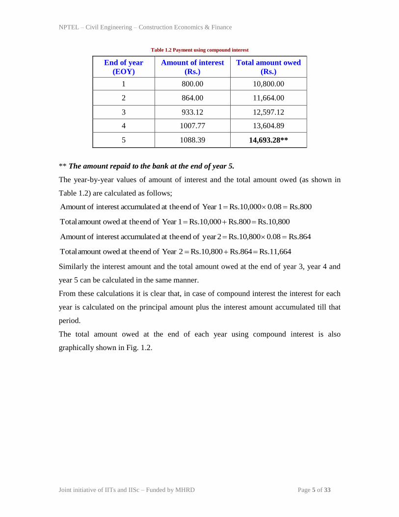
Table 1.2 Payment using compound interest

End of year

(EOY)

Amount of interest

(Rs.)

Total amount owed

(Rs.)

1 800.00 10,800.00

2 864.00 11,664.00

3 933.12 12,597.12

4 1007.77 13,604.89

5 1088.39 14,693.28**

** The amount repaid to the bank at the end of year 5.

The year-by-year values of amount of interest and the total amount owed (as shown in

Table 1.2) are calculated as follows;

Rs.8000.08Rs.10,000 1Year of end at the daccumulateinterest ofAmount

Rs.10,800 Rs.800Rs.10,000 1Year of end at the owedamount Total

Rs.8640.08Rs.10,800 2year of end at the daccumulateinterest ofAmount

Rs.11,664 Rs.864Rs.10,800 2Year of end at the owedamount Total

Similarly the interest amount and the total amount owed at the end of year 3, year 4 and

year 5 can be calculated in the same manner.

From these calculations it is clear that, in case of compound interest the interest for each

year is calculated on the principal amount plus the interest amount accumulated till that

period.

The total amount owed at the end of each year using compound interest is also

graphically shown in Fig. 1.2.



Compound interest

0

4000

8000

12000

16000

1 2 3 4 5

End of year (EOY)

To

tal

am

ou

nt

ow

ed

(R

s.)

Fig. 1.2 Total amount owed (using compound interest)

The accrued interest at the end of each year considering both simple and compound

interest is also shown in Fig. 1.3.

From Fig. 1.3, one can see that in case of simple interest, the amount of interest

accumulated each year is constant. However in case of compound interest, the interest

amount accumulated at the end of each year is not constant and increases with interest

period as evident from Fig. 1.3. Thus considering compound interest, the total amount to

be repaid at the end of year 5 is Rs.14,693.28, which is greater as compared to Rs.14,000

that is to be repaid on the basis of simple interest.



Fig. 1.3 Accumulated interest at the end of each year

0

400

800

1200

1 2 3 4 5

End of year (EOY)

Am

ou

nt

of

inte

rest

(Rs.)

Simple

Compound

Constant value



Lecture-2

Equivalence:

Equivalence indicates that different amount of money at different time periods are

equivalent by considering the time value of money. The following simple example will

explain the meaning of equivalence.

Example: 3

What are the equivalent amounts of Rs.10000 (today) at an interest rate of 10% per year

for the following cases?

a) 1 year from now (future)

b) 1 year before

Solution:

a) At interest rate of 10% per year, Rs.10000 (now) will be equivalent to Rs.11000 one

year from now as shown below;

Rs.11000 1.1010000Rs. year one of end at the daccumulateAmount

b) Similarly Rs.10000 now was equivalent to Rs.9090.90 one year ago at interest rate of

10% per year.

Rs.9090.90 10.1

10000Rs. beforeyear oneAmount

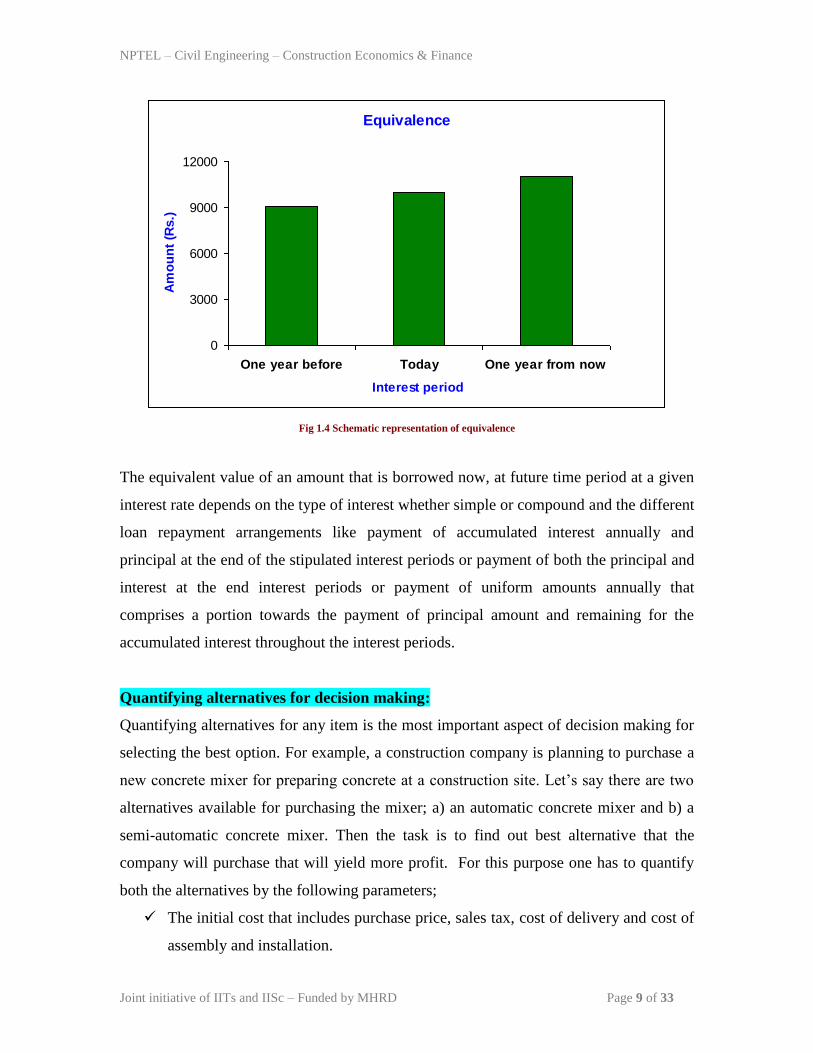
Thus due to the effect of time value of money, these amounts Rs.9090.90 (one year

before), Rs.10000 (today) and Rs.11000 (one year from now) are equivalent at the

interest rate of 10% per year. It is shown in Fig. 1.4.



Equivalence

0

3000

6000

9000

12000

One year before Today One year from now

Interest period

Am

ou

nt

(Rs.)

Fig 1.4 Schematic representation of equivalence

The equivalent value of an amount that is borrowed now, at future time period at a given

interest rate depends on the type of interest whether simple or compound and the different

loan repayment arrangements like payment of accumulated interest annually and

principal at the end of the stipulated interest periods or payment of both the principal and

interest at the end interest periods or payment of uniform amounts annually that

comprises a portion towards the payment of principal amount and remaining for the

accumulated interest throughout the interest periods.

Quantifying alternatives for decision making:

Quantifying alternatives for any item is the most important aspect of decision making for

selecting the best option. For example, a construction company is planning to purchase a

new concrete mixer for preparing concrete at a construction site. Let‟s say there are two

alternatives available for purchasing the mixer; a) an automatic concrete mixer and b) a

semi-automatic concrete mixer. Then the task is to find out best alternative that the

company will purchase that will yield more profit. For this purpose one has to quantify

both the alternatives by the following parameters;

The initial cost that includes purchase price, sales tax, cost of delivery and cost of

assembly and installation.



Annual operating cost.

Annual profit which will depend on the productivity i.e. quantity of concrete

prepared.

The expected useful life.

The expected salvage value.

Other expenditure or income (if any) associated with the equipment.

Income tax benefit

Then on the basis of the economic criteria, the best alternative is selected by calculating

the present worth or future worth or the equivalent uniform annual worth of both

alternatives by incorporating the appropriate interest rate per year and the number of

years (i.e. the comparison must be made over same number of years for both

alternatives). Then the concrete mixer with least cost or higher net income is considered

for purchase. In addition to economic parameters as mentioned above, the non-economic

parameters namely environmental, social, and legal and the related regulatory and

permitting process must also be considered for the evaluation and selection of the best

alternative. These non-economic parameters are essentially required (in addition to the

economic factors) for the selection of the best alternative for the infrastructure and heavy

construction projects like dams, bridges, roadways etc. and other publicly and privately

funded projects namely office buildings, hospitals, apartment building and shopping

malls etc. When the available alternatives exhibit the same equivalent cost or same net

income, then the non-economic parameters may play a vital role in the selection of the

best alternative. It may be noted here that the non-economic parameters cannot be

expressed in numerical values.



Lecture-3

Cash flow diagram:

The graphical representation of the cash flows i.e. both cash outflows and cash inflows

with respect to a time scale is generally referred as cash flow diagram.

A typical cash flow diagram is shown in Fig. 1.5. The cash flows are generally indicated

by vertical arrows on the time scale as shown in Fig. 1.5.

The cash outflows (i.e. costs or expense) are generally represented by vertically

downward arrows whereas the cash inflows (i.e. revenue or income) are represented by

vertically upward arrows.

In the cash flow diagram, number of interest periods is shown on the time scale. The

interest period may be a quarter, a month or a year. Since the cash flows generally occur

at different time intervals within an interest period, for ease of calculation, all the cash

flows are assumed to occur at the end of an interest period. Thus in Fig. 1.5, the numbers

on the time scale represent the end of year (EOY).

Fig 1.5 Cash flow diagram

In Fig. 1.5 the cash outflows are Rs.100000, Rs.15000 and Rs.25000 occurring at end of

year (EOY) „0‟ i.e. at the beginning, EOY „4‟ and EOY „7‟ respectively. Similarly the

cash inflows Rs.35000, Rs.80000 and Rs.45000 are occurring at EOY „3‟, EOY „6‟ and

EOY „10‟ respectively.

Compound interest factors:

The compound interest factors and the corresponding formulas are used to find out the

unknown amounts at a given interest rate continued for certain interest periods from the

100000 15000 25000

45000 80000 35000

2 3 1 4 5 6 7 8 9 10 0 Time

Cash inflow

Cash outflow

End of year 1

End of year 10

Year 1 Year 7



known values of varying cash flows. The following are the notations used for deriving

the compound interest factors.

P = Present worth or present value

F = Future worth or future sum

A = Uniform annual worth or equivalent uniform annual worth of a uniform series

continuing over a specified number of interest periods

n = number of interest periods (years or months)

i = rate of interest per interest period i.e. % per year or % per month

Unless otherwise stated, the rate of interest is compound interest and is for the entire

number of interest periods i.e. for „n‟ interest periods.

The present worth (P), future worth (F) and uniform annual worth (A) are shown in Fig.

1.6.

In this figure the present worth, P is at the beginning and the uniform annual series with

annual value „A‟ is from end of year 1 till end of year 5. Both „P‟ and „A‟ are cash

outflows. It may be noted that the uniform annual series with annual value „A‟ may be

also continued throughout the entire interest periods i.e. from beginning till end of year

10 or for some intermediate interest periods like commencing from end of year 3 till end

of year 8.

The future worth „F‟ is occurring at end of year 4 (cash outflow), at end of year 6 (cash

inflow) and at the end of year 10 (cash inflow).

Fig 1.6 Cash flow diagram showing P, F and A

F

P

2 3 1 4 5 6 7 8 9 10 0

A = Uniform annual worth

from EOY „1‟ till EOY „5”

F

F



While deriving the different compound interest factors, it is assumed that the interest is

compounded once per interest period i.e. discrete compounding. Further the cash flows

are assumed to be discrete i.e. they occur at the end of interest period.

Single payment compound amount factor (SPCAF)

The single payment compound amount factor is used to compute the future worth (F)

accumulated after “n” years from the known present worth (P) at a given interest rate ‘i’

per interest period. It is assumed that the interest period is in years and the interest is

compounded once per interest period.

The known present worth (P), unknown future worth (F) and the total interest period „n‟

years are shown in Fig. 1.7.

Fig 1.7 Cash flow diagram for ‘known P’ and ‘unknown F’

The future worth (F1) accumulated at the end of year 1 i.e. 1st year is given by;

iPiPPF 11 …………………………………. (1)

The future worth accumulated at the end of year 2 i.e. F2 will be equal to the amount that

was accumulated at the end of 1st year i.e. F1 plus the amount of interest accumulated

from end of 1st year to the end of 2

nd year on F1 and is given by;

iFiFFF 11112 ……………………….. (2)

Putting the value of F1 from equation (1) in equation (2), the value of F2 is given by;

212 1111 iPiiPiFF ………………………. (3)

Similarly, the future worth accumulated at the end of year 3 i.e. F3 is equal to the amount

that was accumulated at the end of 2nd

year i.e. F2 plus the amount of interest

accumulated from end of 2nd

year to the end of 3rd

year on F2 and is given by;

F = unknown

P = known

2 3 1 4 n-1 n 0 n-3 n-2 5

End of year

(EOY)

n-4



iFiFFF 12223 ………… (4)

Putting the value of F2 from equation (3) in equation (4), the value of F3 is given by;

32

23 1111 iPiiPiFF ………… (5)

Similarly, the future worth accumulated at the end of year 4 i.e. F4 is given by;

43

34 1111 iPiiPiFF ………… (6)

Thus the generalized formula for the future worth at the end of „n‟ years is given by;

niPF 1 …………… (7)

The factor 1n

i in equation (7) is known as the single payment compound amount

factor (SPCAF). Thus if the value of „P‟ is known, one can easily calculate the future

worth F at the end of „n‟ years at interest rate of „i‟ (per year) by multiplying the present

worth with the single payment compound amount factor.



Lecture-4

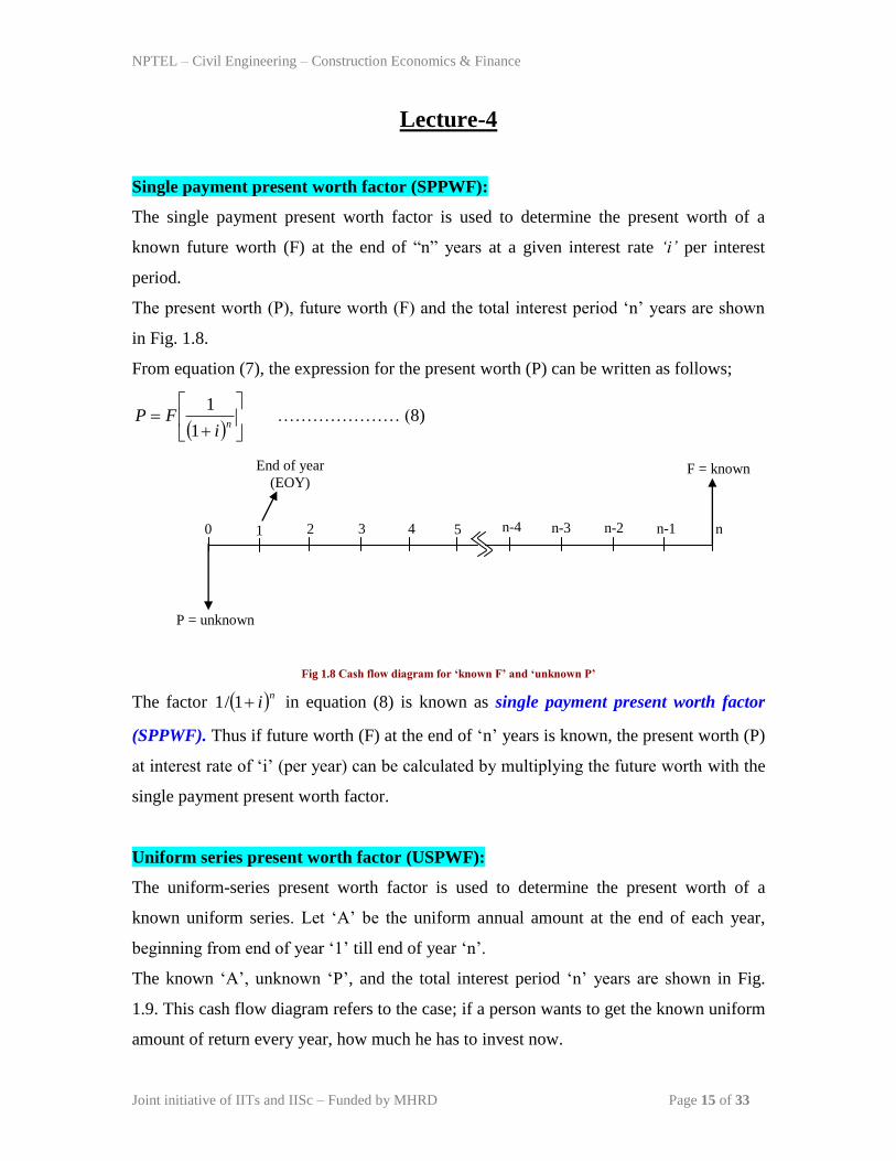
Single payment present worth factor (SPPWF):

The single payment present worth factor is used to determine the present worth of a

known future worth (F) at the end of “n” years at a given interest rate ‘i’ per interest

period.

The present worth (P), future worth (F) and the total interest period „n‟ years are shown

in Fig. 1.8.

From equation (7), the expression for the present worth (P) can be written as follows;

ni

FP1

1 ………………… (8)

Fig 1.8 Cash flow diagram for ‘known F’ and ‘unknown P’

The factor ni1/1 in equation (8) is known as single payment present worth factor

(SPPWF). Thus if future worth (F) at the end of „n‟ years is known, the present worth (P)

at interest rate of „i‟ (per year) can be calculated by multiplying the future worth with the

single payment present worth factor.

Uniform series present worth factor (USPWF):

The uniform-series present worth factor is used to determine the present worth of a

known uniform series. Let „A‟ be the uniform annual amount at the end of each year,

beginning from end of year „1‟ till end of year „n‟.

The known „A‟, unknown „P‟, and the total interest period „n‟ years are shown in Fig.

1.9. This cash flow diagram refers to the case; if a person wants to get the known uniform

amount of return every year, how much he has to invest now.

F = known

P = unknown

2 3 1 4 n-1 n 0 n-3 n-2 5

End of year

(EOY)

n-4



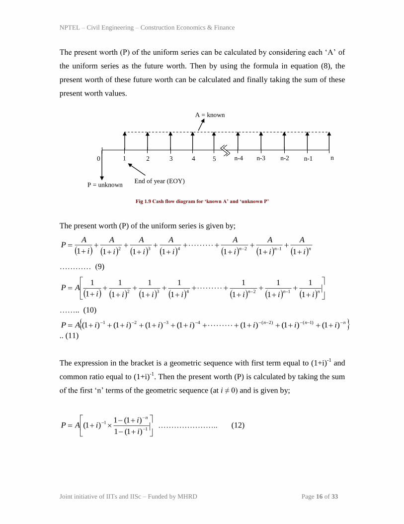
The present worth (P) of the uniform series can be calculated by considering each „A‟ of

the uniform series as the future worth. Then by using the formula in equation (8), the

present worth of these future worth can be calculated and finally taking the sum of these

present worth values.

Fig 1.9 Cash flow diagram for ‘known A’ and ‘unknown P’

The present worth (P) of the uniform series is given by;

nnni

A

i

A

i

A

i

A

i

A

i

A

i

AP

1111111 12432

………… (9)

nnniiiiiii

AP1

1

1

1

1

1

1

1

1

1

1

1

1

112432

…….. (10)

nnn iiiiiiiAP )1()1()1()1()1()1()1( )1()2(4321

.. (11)

The expression in the bracket is a geometric sequence with first term equal to (1+i)-1

and

common ratio equal to (1+i)-1

. Then the present worth (P) is calculated by taking the sum

of the first „n‟ terms of the geometric sequence (at i ≠ 0) and is given by;

1

1

)1(1

)1(1)1(

i

iiAP

n

………………….. (12)

P = unknown

2 3 1 4 n-1 n 0 n-3 n-2 5

End of year (EOY)

A = known

n-4



The simplification of equation (12) results in the following the expression;

n

n

ii

iAP

1

11 ………………………….. (13)

The factor within the bracket in equation (13) is known as uniform series present worth

factor (USPWF). Thus if the value of „A‟ in the uniform series is known, then the present

worth P at interest rate of „i‟ (per year) can be calculated by multiplying the uniform

annual amount „A‟ with uniform series compound amount factor.

The present worth (P) of a uniform annual series of known „A‟ can also be calculated in

the following manner;

Dividing both sides of equation (10) by (1+i) results in the following equation;

1154321

1

1

1

1

1

1

1

1

1

1

1

1

1

1 nnniiiiiii

Ai

P

… (14)

Subtracting equation (14) from equation (10) results in the following expression;

11

1

1

1

1 nii

Ai

PP …………….. (15)

Equation (14) can be rewritten as;

1

1

1

1

1

1 nii

Ai

iP ………………... (16)

Multiplying both sides of equation (15) by (1+i)/i and further simplification results in the

following expression for the present worth „P‟;

n

n

ii

iAP

1

11

Capital recovery factor (CRF):

The capital recovery factor is generally used to find out the uniform annual amount „A‟

of a uniform series from the known present worth at a given interest rate ‘i’ per interest

period.



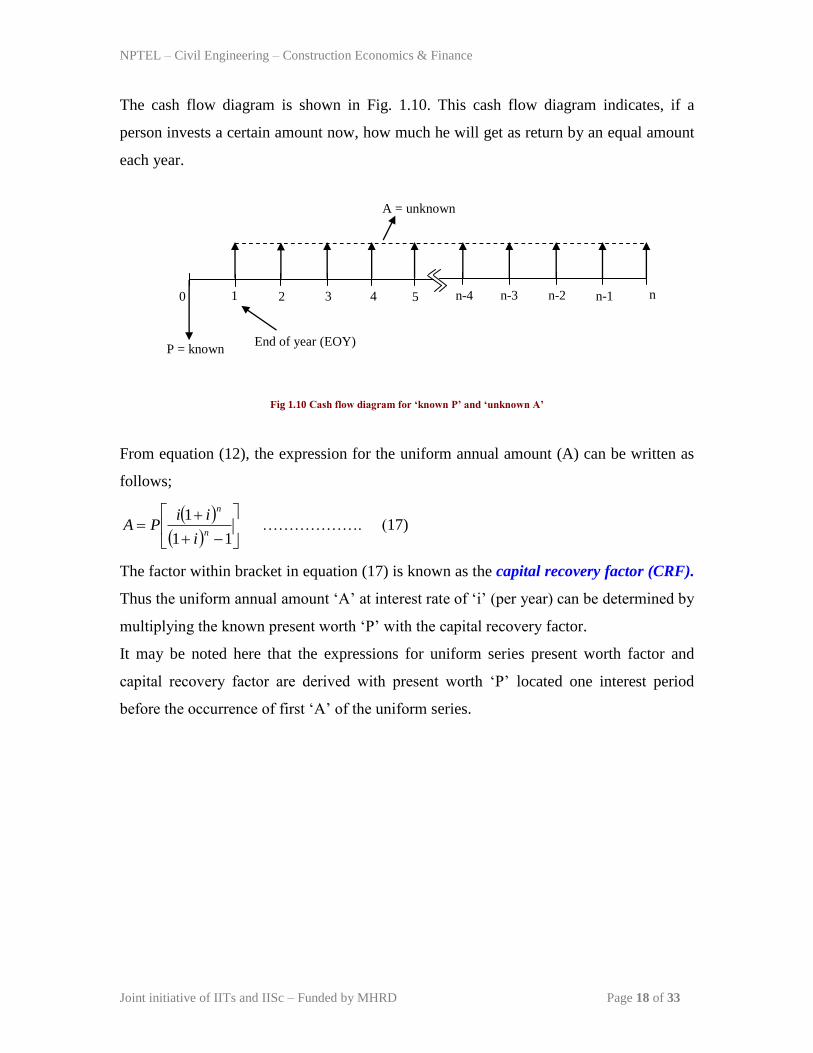
The cash flow diagram is shown in Fig. 1.10. This cash flow diagram indicates, if a

person invests a certain amount now, how much he will get as return by an equal amount

each year.

Fig 1.10 Cash flow diagram for ‘known P’ and ‘unknown A’

From equation (12), the expression for the uniform annual amount (A) can be written as

follows;

11

1n

n

i

iiPA ………………. (17)

The factor within bracket in equation (17) is known as the capital recovery factor (CRF).

Thus the uniform annual amount „A‟ at interest rate of „i‟ (per year) can be determined by

multiplying the known present worth „P‟ with the capital recovery factor.

It may be noted here that the expressions for uniform series present worth factor and

capital recovery factor are derived with present worth „P‟ located one interest period

before the occurrence of first „A‟ of the uniform series.

End of year (EOY) P = known

2 3 1 4 n-1 n 0 n-3 n-2 5

A = unknown

n-4



Lecture-5

Uniform series compound amount factor:

The uniform series compound amount factor is used to determine the future sum (F) of a

known uniform annual series with uniform amount „A‟. The cash flow diagram is shown

in Fig. 1.11. This cash flow diagram states that, if a person invests a uniform amount at

the end of each year continued for „n‟ years at interest rate of „i‟ per year, how much he

will get at the end of „n‟ years.

Putting the value of present worth (P) from equation (8) in equation (13) results in the

following;

n

n

nii

iA

iF

1

11

1

1 ………………….. (18)

i

iAF

n11

………………………… (19)

Fig 1.11 Cash flow diagram for ‘known A’ and ‘unknown F’

The factor within bracket in equation (19) is known as uniform series compound amount

factor (USCAF). Hence the future worth „F‟ can be computed by multiplying the uniform

annual amount „A‟ with the uniform series compound amount factor.

Sinking fund factor:

The sinking fund factor is used to calculate the annual amount „A‟ of a uniform series

from the known future sum „F‟. The cash flow diagram is shown in Fig. 1.12. This cash

flow diagram indicates that, if a person wants to get a known future sum at the end of „n‟

F = unknown

2 3 1 4 n-1 n

0

n-3 n-2 5

End of year (EOY)

A = known

n-4



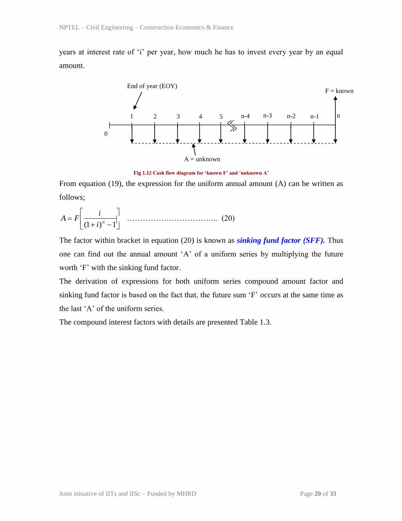
years at interest rate of „i‟ per year, how much he has to invest every year by an equal

amount.

Fig 1.12 Cash flow diagram for ‘known F’ and ‘unknown A’

From equation (19), the expression for the uniform annual amount (A) can be written as

follows;

1)1( ni

iFA …………………………….. (20)

The factor within bracket in equation (20) is known as sinking fund factor (SFF). Thus

one can find out the annual amount „A‟ of a uniform series by multiplying the future

worth „F‟ with the sinking fund factor.

The derivation of expressions for both uniform series compound amount factor and

sinking fund factor is based on the fact that, the future sum „F‟ occurs at the same time as

the last „A‟ of the uniform series.

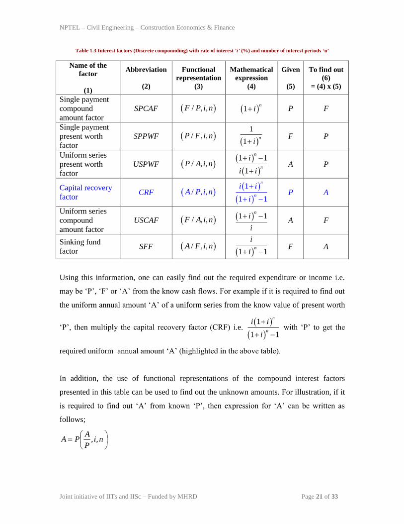
The compound interest factors with details are presented Table 1.3.

F = known

2 3 1 4 n-1 n

0

n-2 5

End of year (EOY)

A = unknown

n-4 n-3



Table 1.3 Interest factors (Discrete compounding) with rate of interest ‘i’ (%) and number of interest periods ‘n’

Name of the

factor

(1)

Abbreviation

(2)

Functional

representation

(3)

Mathematical

expression

(4)

Given

(5)

To find out

(6)

= (4) x (5)

Single payment

compound

amount factor

SPCAF / , ,F P i n 1n

i P F

Single payment

present worth

factor

SPPWF / , ,P F i n

1

1n

i F P

Uniform series

present worth

factor

USPWF / , ,P A i n

1 1

1

n

n

i

i i

A P

Capital recovery

factor CRF / , ,A P i n

1

1 1

n

n

i i

i

P A

Uniform series

compound

amount factor

USCAF / , ,F A i n 1 1n

i

i

A F

Sinking fund

factor SFF / , ,A F i n

1 1n

i

i F A

Using this information, one can easily find out the required expenditure or income i.e.

may be „P‟, „F‟ or „A‟ from the know cash flows. For example if it is required to find out

the uniform annual amount „A‟ of a uniform series from the know value of present worth

„P‟, then multiply the capital recovery factor (CRF) i.e.

1

1 1

n

n

i i

i

with „P‟ to get the

required uniform annual amount „A‟ (highlighted in the above table).

In addition, the use of functional representations of the compound interest factors

presented in this table can be used to find out the unknown amounts. For illustration, if it

is required to find out „A‟ from known „P‟, then expression for „A‟ can be written as

follows;

ni

P

APA ,,



Further the functional representation of a compound interest factor can be obtained by

multiplying the other relevant compound interest factors at a given rate of interest „i‟ and

number of interest periods „n‟ and is given as follows;

ni

P

Fni

F

Ani

P

A,,,,,, ………………………………. (21)



Lecture-6

Cash flow involving arithmetic gradient payments or receipts:

Some cash flows involve the payments or receipts in gradients by same amount. In other

words, the expenditure or the income increases or decreases by same amount. The cash

flow involving such payments or receipts is known as uniform gradient series. For

example, if the cost of repair and maintenance of a piece of equipment increases by same

amount every year till end of its useful life, it represents a cash flow involving positive

uniform gradient. Similarly if the profit obtained from an investment decreases by an

equal amount every year for a certain number of years, it indicates a cash flow involving

negative uniform gradient. The cash flow diagrams for positive gradient and negative

gradient are shown in Fig. 1.3 and Fig. 1.4 respectively.

Fig 1.13 Cash flow diagram involving a positive uniform gradient

Fig 1.14 Cash flow diagram involving a negative uniform gradient

2

0

0

3 1 4 9 10 0 8 5

End of year (EOY)

6

5000* 7000 8000 9000 10000

7

11000 12000 13000 14000

6000

* Amount in Rupees.

A positive gradient of Rs.1000.

2

0

0

3 1 4 9 10 0 8 5

End of year (EOY)

6

30000*

7

28000

* Amount in Rupees.

26000 24000 22000 20000 18000 16000 14000 12000

A negative gradient of Rs.2000.



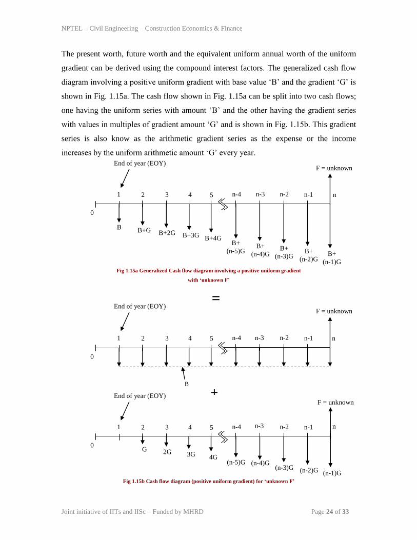
The present worth, future worth and the equivalent uniform annual worth of the uniform

gradient can be derived using the compound interest factors. The generalized cash flow

diagram involving a positive uniform gradient with base value „B‟ and the gradient „G‟ is

shown in Fig. 1.15a. The cash flow shown in Fig. 1.15a can be split into two cash flows;

one having the uniform series with amount „B‟ and the other having the gradient series

with values in multiples of gradient amount „G‟ and is shown in Fig. 1.15b. This gradient

series is also know as the arithmetic gradient series as the expense or the income

increases by the uniform arithmetic amount „G‟ every year.

Fig 1.15a Generalized Cash flow diagram involving a positive uniform gradient

with ‘unknown F’

Fig 1.15b Cash flow diagram (positive uniform gradient) for ‘unknown F’

F = unknown

2 3 1 4 n-1 n

0

n-2 5

End of year (EOY)

B

n-4 n-3

2 3 1 4 n-1 n

0

n-2 5

End of year (EOY)

n-4 n-3

G 2G 3G 4G (n-5)G (n-4)G

(n-3)G (n-2)G (n-1)G

F = unknown

=

+

F = unknown

2 3 1 4 n-1

0

n-2 5

End of year (EOY)

n-4

B B+G B+2G B+3G B+4G B+

(n-5)G

n-3

B+

(n-4)G B+

(n-3)G B+

(n-2)G B+

(n-1)G

n



The future worth of the cash flow shown in Fig. 1.15a can be obtained by finding the out

the individual future worth of the cash flows shown in Fig. 1.15b and then taking their

sum. As already stated, the future worth of the cash flow involving an uniform series can

be determined by multiplying the uniform annual amount „B‟ with the uniform series

compound amount factor. The future worth (F) of the gradient series shown in Fig 1.15b

can be determined by finding out the individual future worth of the gradient values (i.e. in

multiples of gradient amount „G‟) at the end of different years at interest rate of „i‟ per

year and then taking the sum of these individual futures values. Then „F‟ is given as

follows;

GniGniGniGn

iGiGiGiGF

nnnn

)1()1()2()1()3()1()4(

)1(4)1(3)1(2)1(

23

5432

…….

(22)

Dividing both sides of equation (22) by (1+i)n results in the following equation;

nnnn

n

i

n

i

n

i

n

i

n

iiiiG

i

F

)1(

1

1

2

1

3

1

4

1

4

1

3

1

2

1

1

1123

5432

…

…. (23)

Multiplying both sides of equation (23) by (1+i) results in the following expression;

1234

432

)1(

1

1

2

1

3

1

4

1

4

1

3

1

2

1

1

1

)1(

nnnn

n

i

n

i

n

i

n

i

n

iiiiG

i

iF

….….. (24)

Subtracting equation (23) from equation (24) results in the following expression;

nnnnnn

n

i

n

iiiii

iiiiG

i

iF

)1()1(

1

)1(

1

1

1

1

1

1

1

1

1

1

1

1

1

1

1

1

1)1(

1234

432

... (25)



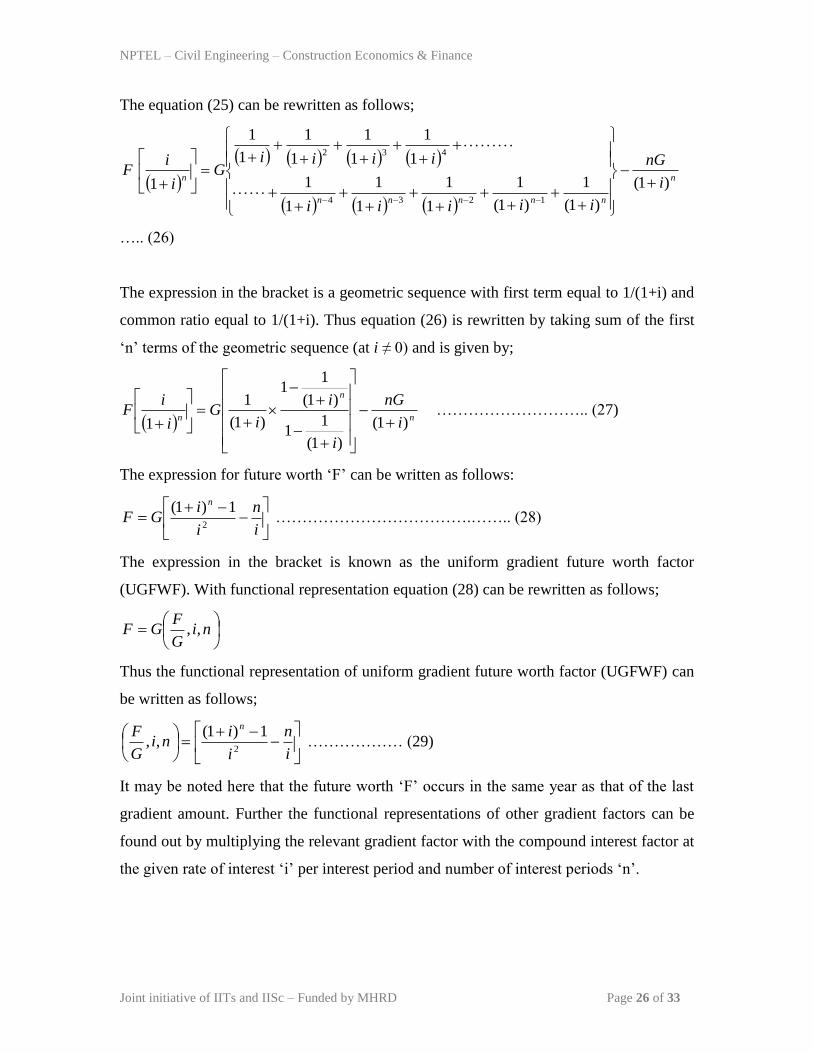
The equation (25) can be rewritten as follows;

n

nnnnn

n i

nG

iiiii

iiiiG

i

iF

)1(

)1(

1

)1(

1

1

1

1

1

1

1

1

1

1

1

1

1

1

1

11234

432

….. (26)

The expression in the bracket is a geometric sequence with first term equal to 1/(1+i) and

common ratio equal to 1/(1+i). Thus equation (26) is rewritten by taking sum of the first

„n‟ terms of the geometric sequence (at i ≠ 0) and is given by;

n

n

n i

nG

i

i

iG

i

iF

)1(

)1(

11

)1(

11

)1(

1

1

……………………….. (27)

The expression for future worth „F‟ can be written as follows:

i

n

i

iGF

n

2

1)1( ……………………………….…….. (28)

The expression in the bracket is known as the uniform gradient future worth factor

(UGFWF). With functional representation equation (28) can be rewritten as follows;

ni

G

FGF ,,

Thus the functional representation of uniform gradient future worth factor (UGFWF) can

be written as follows;

i

n

i

ini

G

F n

2

1)1(,, ……………… (29)

It may be noted here that the future worth „F‟ occurs in the same year as that of the last

gradient amount. Further the functional representations of other gradient factors can be

found out by multiplying the relevant gradient factor with the compound interest factor at

the given rate of interest „i‟ per interest period and number of interest periods „n‟.



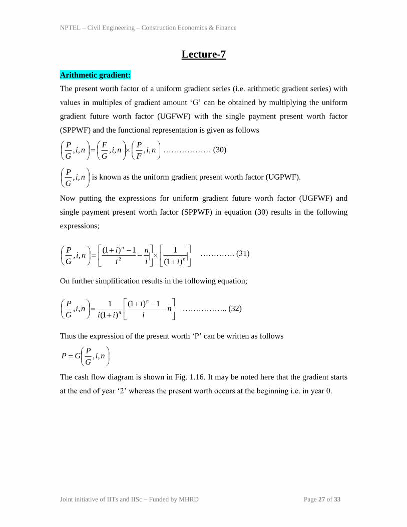
Lecture-7

Arithmetic gradient:

The present worth factor of a uniform gradient series (i.e. arithmetic gradient series) with

values in multiples of gradient amount „G‟ can be obtained by multiplying the uniform

gradient future worth factor (UGFWF) with the single payment present worth factor

(SPPWF) and the functional representation is given as follows

ni

F

Pni

G

Fni

G

P,,,,,, ……………… (30)

ni

G

P,, is known as the uniform gradient present worth factor (UGPWF).

Now putting the expressions for uniform gradient future worth factor (UGFWF) and

single payment present worth factor (SPPWF) in equation (30) results in the following

expressions;

…………. (31)

On further simplification results in the following equation;

…………….. (32)

Thus the expression of the present worth „P‟ can be written as follows

ni

G

PGP ,,

The cash flow diagram is shown in Fig. 1.16. It may be noted here that the gradient starts

at the end of year „2‟ whereas the present worth occurs at the beginning i.e. in year 0.

n

i

i

iini

G

P n

n

1)1(

)1(

1,,

n

n

ii

n

i

ini

G

P

)1(

11)1(,,

2



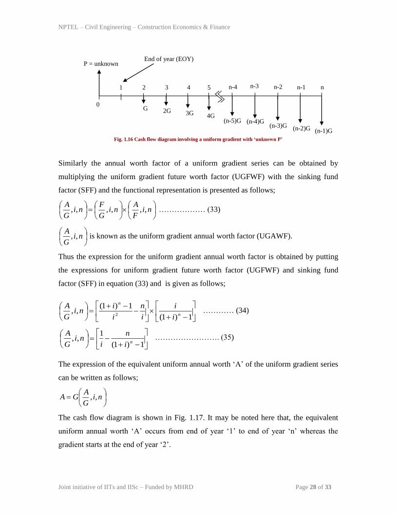
Fig. 1.16 Cash flow diagram involving a uniform gradient with ‘unknown P’

Similarly the annual worth factor of a uniform gradient series can be obtained by

multiplying the uniform gradient future worth factor (UGFWF) with the sinking fund

factor (SFF) and the functional representation is presented as follows;

ni

F

Ani

G

Fni

G

A,,,,,, ……………… (33)

ni

G

A,, is known as the uniform gradient annual worth factor (UGAWF).

Thus the expression for the uniform gradient annual worth factor is obtained by putting

the expressions for uniform gradient future worth factor (UGFWF) and sinking fund

factor (SFF) in equation (33) and is given as follows;

………… (34)

……………………. (35)

The expression of the equivalent uniform annual worth „A‟ of the uniform gradient series

can be written as follows;

ni

G

AGA ,,

The cash flow diagram is shown in Fig. 1.17. It may be noted here that, the equivalent

uniform annual worth „A‟ occurs from end of year „1‟ to end of year „n‟ whereas the

gradient starts at the end of year „2‟.

(n-1)G

2 3 1 4 n-1 n

0

n-2 5

End of year (EOY)

n-4 n-3

G 2G 3G 4G (n-5)G (n-4)G

(n-3)G (n-2)G

P = unknown

1)1(

1)1(,,

2 n

n

i

i

i

n

i

ini

G

A

1)1(

1,,

ni

n

ini

G

A



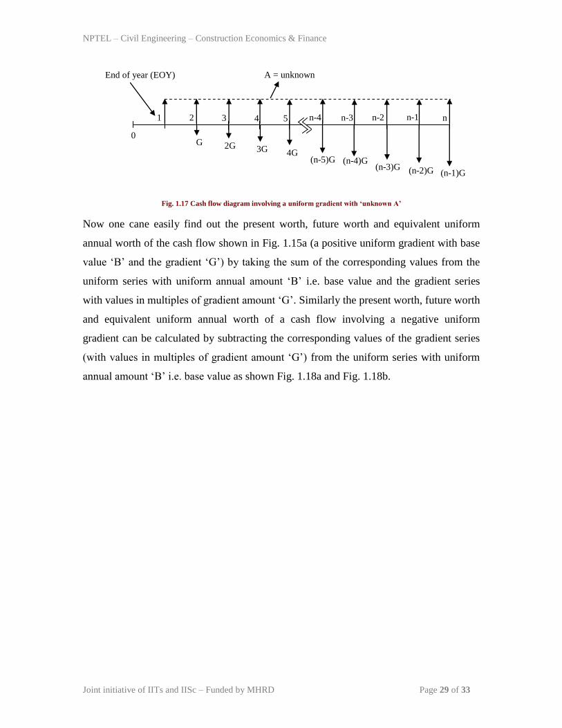
Fig. 1.17 Cash flow diagram involving a uniform gradient with ‘unknown A’

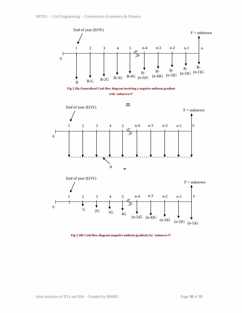
Now one cane easily find out the present worth, future worth and equivalent uniform

annual worth of the cash flow shown in Fig. 1.15a (a positive uniform gradient with base

value „B‟ and the gradient „G‟) by taking the sum of the corresponding values from the

uniform series with uniform annual amount „B‟ i.e. base value and the gradient series

with values in multiples of gradient amount „G‟. Similarly the present worth, future worth

and equivalent uniform annual worth of a cash flow involving a negative uniform

gradient can be calculated by subtracting the corresponding values of the gradient series

(with values in multiples of gradient amount „G‟) from the uniform series with uniform

annual amount „B‟ i.e. base value as shown Fig. 1.18a and Fig. 1.18b.

2 3 1 4 n-1 n

0

n-2 5

End of year (EOY)

n-4 n-3

G 2G 3G 4G (n-5)G (n-4)G

(n-3)G (n-2)G

A = unknown

(n-1)G



Fig 1.18a Generalized Cash flow diagram involving a negative uniform gradient

with ‘unknown F’

Fig 1.18b Cash flow diagram (negative uniform gradient) for ‘unknown F’

F = unknown

2 3 1 4 n-1 n

0

n-2 5

End of year (EOY)

B

n-4 n-3

2 3 1 4 n-1 n

0

n-2 5

End of year (EOY)

n-4 n-3

G 2G 3G 4G (n-5)G (n-4)G

(n-3)G (n-2)G (n-1)G

F = unknown

=

-

F = unknown

2 3 1 4 n-1

0

n-2 5

End of year (EOY)

n-4

B B-G B-2G B-3G B-4G B-

(n-5)G

n-3

B-

(n-4)G

B-

(n-3)G

B-

(n-2)G

B-

(n-1)G

n



Lecture-8

Cash flow involving geometric gradient series:

Sometimes the cash flows may have expenses or incomes being increased by a constant

percentage in the successive time periods i.e. in successive years. Such kind of cash flow

is known as geometric gradient series. The generalized cash flow diagram involving

geometric gradient series with expense or receipt „C‟ at the end of year „1” and geometric

percentage increase „g‟ is shown in Fig. 1.19.

Fig 1.19 Cash flow diagram involving geometric gradient with ‘unknown P’

The present worth (P) of the geometric gradient series can be calculated by considering

each amount as the future worth and then taking sum of these present worth values.

n

n

n

n

n

n

i

gC

i

gC

i

gC

i

gC

i

gC

i

gC

i

CP

1

1

1

1

1

1

1

1

1

1

1

1

1

1

1

2

2

3

4

3

3

2

2

…………. (36)

Equation (36) can be rewritten as follows;

n

n

n

n

n

n

i

g

i

g

i

g

i

g

i

g

i

g

iCP

1

1

1

1

1

1

1

1

1

1

1

1

1

11

1

2

2

3

4

3

3

2

2

……….… (37)

Dividing both sides of the equation (37) by (1+i) results in the following expression;

P = unknown

2 3 1 4 n-1

0

n-2 5

End of year (EOY)

n-4

C C(1+g)

2 C(1+g)

n-3 n

C(1+g)3

C(1+g)n-1

C(1+g)n-5 C(1+g)

4

C(1+g)n-4

C(1+g)n-3

C(1+g)n-2



1

12

1

3

5

3

4

2

321

1

1

1

1

1

1

1

1

1

1

1

1

1

1 n

n

n

n

n

n

i

g

i

g

i

g

i

g

i

g

i

g

iC

i

P

……….… (38)

Now multiplying both sides of equation (38) by (1+g) results in the following expression;

1

1

1

2

5

4

4

3

3

2

21

1

1

1

1

1

1

1

1

1

1

1

1

1

1

1n

n

n

n

n

n

i

g

i

g

i

g

i

g

i

g

i

g

i

gC

i

gP

……….… (39)

Subtracting equation (37) from equation (39) results in the following;

ii

gC

i

igPn

n

1

1

1

1

1 1 …………………. (40)

Equation (40) can be rewritten as follows;

ig

i

gC

P

n

n

11

1

…………….. (41)

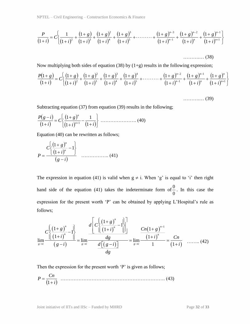
The expression in equation (41) is valid when g i. When „g‟ is equal to „i‟ then right

hand side of the equation (41) takes the indeterminate form of0

0. In this case the

expression for the present worth „P‟ can be obtained by applying L‟Hospital‟s rule as

follows;

…….. (42)

Then the expression for the present worth „P‟ is given as follows;

iCn

P

1

………………………………………………………. (43)

1

11

1 111

1 1lim lim lim

1 1

n

n nn

n n

g i g i g i

gd C

g Cn giC

i i Cndg

g i id g i

dg



Similarly the future worth and equivalent uniform annual worth of the geometric gradient

series can be obtained by multiplying its present worth „P‟ with the compound interest

factors namely single payment compound amount factor (SPCAF) and capital recovery

factor (CRF) respectively at the given rate of interest „i‟ per interest period and the

number of interest periods.

Now using the above expressions, one can easily calculate the present worth, future

worth and equivalent uniform annual worth of the cash flow involving either expenditure

or income or both increasing in the form of geometric gradient.

It may be noted here that the expressions for compound interest factors can also be

obtained by using beginning of year (interest period) convention.

The values of discrete compound interest factors at different values of interest rate and

interest period can be calculated by using the expressions of these factors as mentioned

earlier and the interest tables can thus be generated. The interest tables are available in

the relevant texts (cited in the list of references for this course). The values of different

discrete compound interest factors from these interest tables can directly be used in the

engineering economy calculations.

The use of different compound interest factors discussed so far will be illustrated by

solving various examples for comparison of different alternatives in Module 2. Further

the use of discrete compound interest factors from interest tables will also be illustrated in

Module 2.

detailed course plan : (module wise / lecture wise)

Documents