design optimization techniques for time-critical cyber-physical … · 2020. 1. 22. · design of...
TRANSCRIPT
Design Optimization Techniques for Time-Critical Cyber-PhysicalSystems
Yecheng Zhao
Dissertation submitted to the Faculty of the
Virginia Polytechnic Institute and State University
in partial fulfillment of the requirements for the degree of
Doctor of Philosophy
in
Computer Engineering
Haibo Zeng, Chair
Michael S. Hsiao
Sekharipuram S. Ravi
Binoy Ravindran
Changhee Jung
December 11, 2019
Blacksburg, Virginia
Keywords: Cyber-physical systems, Design optimization, Schedulability analysis
Copyright 2020, Yecheng Zhao

Design Optimization Techniques for Time-Critical Cyber-PhysicalSystems
Yecheng Zhao
(ABSTRACT)
Cyber-Physical Systems (CPS) are widely deployed in critical applications which are sub-
ject to strict timing constraints. To ensure correct timing behavior, much of the effort has
been dedicated to the development of validation and verification methods for CPS (e.g.,
system models and their timing and schedulability analysis). As CPS is becoming increas-
ingly complex, there is an urgent need for efficient optimization techniques that can aid the
design of large-scale systems. Specifically, techniques that can find good design options in a
reasonable amount of time while meeting all the timing and other critical requirements are
becoming vital. However, the current mindset is to use existing schedulability analysis and
optimization techniques for the design optimization of time-critical CPS. This has resulted in
two issues in today’s CPS design: 1) Existing timing and schedulability analysis are very dif-
ficult and inefficient to be integrated into well-established optimization frameworks such as
mathematical programming; 2) New system models and timing analysis are being developed
in a way that is increasingly unfriendly to optimization. Due to these difficulties, existing
practice for optimization mostly relies on meta or ad-hoc heuristics, which suffers either from
sub-optimality or limited applicability. In this dissertation, we seek to address these issues
and explore two new directions for developing optimization algorithms for time-critical CPS.
The first is to develop optimization-oriented timing analysis, that are efficient to formulate
in mathematical programming framework. The second is a domain-specific optimization
framework. The framework leverages domain-specific knowledge to provide methods that
abstract timing analysis into a simple mathematical form. This allows to efficiently handle
the complexity of timing analysis in optimization algorithms. The results on a number of case
studies show that the proposed approaches have the potential to significantly improve upon
scalability (several orders of magnitude faster) and solution quality, while being applicable
to various system models, timing analysis techniques, and design optimization problems in
time-critical CPS.

Design Optimization Techniques for Time-Critical Cyber-PhysicalSystems
Yecheng Zhao
(GENERAL AUDIENCE ABSTRACT)
Cyber-Physical Systems (CPS) tightly intertwine computing units and physical plants to
accomplish complex tasks such as control and monitoring. They are often deployed in critical
applications subject to strict timing constraints. For example, many control applications and
tasks are required to finished within bounded latencies. To guarantee such timing correctness,
much of the effort has been dedicated to studying methods for delay and latency estimation.
These techniques are known as schedulability analysis/timing analysis. As CPS becomes
increasingly complex, there is an urgent need for efficient optimization techniques that can
aid the design of large-scale and correct CPS. Specifically, techniques that can find good
design options in reasonable amount of time while meeting all the timing and other critical
requirements are becoming vital. However, most of the existing schedulability analysis are
either non-linear, non-convex, non-continuous or without closed form. This gives significant
challenge for integrating these analysis into optimization. In this dissertation, we explore
two new paradigm-shifting approaches for developing optimization algorithms for the design
of CPS. Experimental evaluations on both synthetic and industrial case studies show that
the new approaches significantly improve upon existing optimization techniques in terms of
scalability and quality of solution.
Dedication
This dissertation is dedicated to Cyber-Physical System designers and those interested in
the research of design optimization techniques for Cyber-Physical Systems
v

Acknowledgments
I would like to thank my advisor, Haibo Zeng, for his guidance, teaching, inspiration and
patience throughout my PhD study. Many of the work presented in the dissertation would
not have been done without his help and effort. I would also like to thank my PhD committee
members for their helpful comments on my research and dissertation. Finally, I want to thank
my family and my dear wife Xiaoyu Chen, for their kind support, caring, encouragement
and company all these years.
vi
Contents
List of Figures xv
List of Tables xxi
1 Introduction 1
1.1 Time-Critical Cyber-Physical Systems and Design Optimization . . . . . . . 1
1.2 Existing Approaches, Issues and Challenges . . . . . . . . . . . . . . . . . . 6
1.3 Overview of Approach and Results . . . . . . . . . . . . . . . . . . . . . . . 9
1.3.1 Developing optimization-oriented schedulability analysis . . . . . . . 9
1.3.2 Developing new domain-specific optimization framework . . . . . . . 11
1.4 Organization . . . . . . . . . . . . . . . . . . . . . . . . . . . . . . . . . . . 14
2 An Efficient Schedulability Analysis for Optimizing Systems with Adaptive
Mixed-Criticality Scheduling 21
2.1 Introduction . . . . . . . . . . . . . . . . . . . . . . . . . . . . . . . . . . . . 21
2.2 AMC Task Model and Schedulability Analysis . . . . . . . . . . . . . . . . . 25
2.3 Request Bound Function based Analysis . . . . . . . . . . . . . . . . . . . . 29
2.3.1 Sufficient Test Sets for Analysis . . . . . . . . . . . . . . . . . . . . . 34
2.3.2 Safety and Bounded Pessimism of Step 1 . . . . . . . . . . . . . . . . 36
vii
2.3.3 Exactness of Step 2 . . . . . . . . . . . . . . . . . . . . . . . . . . . . 38
2.3.4 Safety and Bounded Pessimism of Step 3 . . . . . . . . . . . . . . . . 42
2.3.5 Exactness of Step 4 . . . . . . . . . . . . . . . . . . . . . . . . . . . . 44
2.3.6 Proof of Theorem 1 . . . . . . . . . . . . . . . . . . . . . . . . . . . . 45
2.4 Schedulability Region in ILP Formulation . . . . . . . . . . . . . . . . . . . 47
2.4.1 Schedulability Region of AMC-rbf . . . . . . . . . . . . . . . . . . . . 49
2.4.2 Schedulability Region of AMC-rtb . . . . . . . . . . . . . . . . . . . . 52
2.4.3 An Illustrative Example . . . . . . . . . . . . . . . . . . . . . . . . . 54
2.5 Extension to Multiple Criticality Levels . . . . . . . . . . . . . . . . . . . . . 59
2.5.1 System Semantics . . . . . . . . . . . . . . . . . . . . . . . . . . . . 59
2.5.2 Request Bound Function based Analysis . . . . . . . . . . . . . . . . 60
2.5.3 Bounded Pessimism . . . . . . . . . . . . . . . . . . . . . . . . . . . 71
2.6 Experimental Results . . . . . . . . . . . . . . . . . . . . . . . . . . . . . . . 74
2.6.1 Comparison of Schedulability Tests . . . . . . . . . . . . . . . . . . . 75
2.6.2 Optimizing Software Synthesis of Simulink Models . . . . . . . . . . 85
2.6.3 Optimizing Task Allocation on Multicore . . . . . . . . . . . . . . . . 93
2.7 Conclusion . . . . . . . . . . . . . . . . . . . . . . . . . . . . . . . . . . . . . 100
3 The Concept of Unschedulability Core for Optimizing Real-Time Systems
with Fixed-Priority Scheduling 101
3.1 Introduction . . . . . . . . . . . . . . . . . . . . . . . . . . . . . . . . . . . . 101
viii

3.1.1 Related Work . . . . . . . . . . . . . . . . . . . . . . . . . . . . . . . 102
3.1.2 Contributions and Chapter Structure . . . . . . . . . . . . . . . . . . 104
3.2 Preliminary . . . . . . . . . . . . . . . . . . . . . . . . . . . . . . . . . . . . 105
3.3 The Concept of Unschedulability Core . . . . . . . . . . . . . . . . . . . . . 107
3.3.1 Definition of Unschedulability Core . . . . . . . . . . . . . . . . . . . 108
3.3.2 Computing Unschedulability Core . . . . . . . . . . . . . . . . . . . . 112
3.4 Unschedulability Core Guided Optimization Algorithm . . . . . . . . . . . . 115
3.4.1 Optimization Algorithm . . . . . . . . . . . . . . . . . . . . . . . . . 115
3.4.2 Advantages . . . . . . . . . . . . . . . . . . . . . . . . . . . . . . . . 120
3.5 Generalization . . . . . . . . . . . . . . . . . . . . . . . . . . . . . . . . . . . 121
3.5.1 Generalized Concept of Unschedulability Core . . . . . . . . . . . . . 121
3.5.2 Applicability and Algorithm Efficiency . . . . . . . . . . . . . . . . . 124
3.6 Examples of Application . . . . . . . . . . . . . . . . . . . . . . . . . . . . . 127
3.6.1 Optimizing Implementation of Simulink Models . . . . . . . . . . . . 127
3.6.2 Minimizing Memory of AUTOSAR models . . . . . . . . . . . . . . . 130
3.7 Experimental Evaluation . . . . . . . . . . . . . . . . . . . . . . . . . . . . . 133
3.7.1 Optimizing Implementation of Mixed-Criticality Simulink Models . . 133
3.7.2 Minimizing Memory of AUTOSAR Components . . . . . . . . . . . . 138
3.8 Conclusions . . . . . . . . . . . . . . . . . . . . . . . . . . . . . . . . . . . . 139
ix
4 Optimization of Real-Time Software Implementing Multi-Rate Synchronous
Finite State Machines 141
4.1 Introduction . . . . . . . . . . . . . . . . . . . . . . . . . . . . . . . . . . . . 141
4.1.1 Our Contributions . . . . . . . . . . . . . . . . . . . . . . . . . . . . 143
4.2 SR Models and Implementation . . . . . . . . . . . . . . . . . . . . . . . . . 144
4.2.1 SR Model Semantics . . . . . . . . . . . . . . . . . . . . . . . . . . . 144
4.2.2 Implementing SR Model: Tradeoff Analysis . . . . . . . . . . . . . . 147
4.3 Schedulability Analysis . . . . . . . . . . . . . . . . . . . . . . . . . . . . . . 150
4.4 Optimization Framework . . . . . . . . . . . . . . . . . . . . . . . . . . . . . 153
4.4.1 Overview of Optimization Framework . . . . . . . . . . . . . . . . . 155
4.4.2 Calculating Unschedulability Cores . . . . . . . . . . . . . . . . . . . 157
4.4.3 Relaxation-and-Recovery . . . . . . . . . . . . . . . . . . . . . . . . . 161
4.4.4 Schedulability-based Memoization . . . . . . . . . . . . . . . . . . . . 163
4.4.5 Discussion on Algorithm Design . . . . . . . . . . . . . . . . . . . . . 165
4.5 Experimental Evaluation . . . . . . . . . . . . . . . . . . . . . . . . . . . . . 166
4.6 Related Work . . . . . . . . . . . . . . . . . . . . . . . . . . . . . . . . . . . 172
4.7 Conclusions . . . . . . . . . . . . . . . . . . . . . . . . . . . . . . . . . . . . 174
5 The Virtual Deadline based Optimization Algorithm for Priority Assign-
ment in Fixed-Priority Scheduling 175
5.1 Introduction . . . . . . . . . . . . . . . . . . . . . . . . . . . . . . . . . . . . 175
x

5.2 System Model and Notations . . . . . . . . . . . . . . . . . . . . . . . . . . 178
5.3 Minimizing Average WCRT . . . . . . . . . . . . . . . . . . . . . . . . . . . 180
5.4 Minimizing Weighted Average WCRT . . . . . . . . . . . . . . . . . . . . . . 191
5.5 The Concept of MUDA . . . . . . . . . . . . . . . . . . . . . . . . . . . . . . 193
5.6 MUDA Guided Optimization . . . . . . . . . . . . . . . . . . . . . . . . . . 198
5.7 Experimental Results . . . . . . . . . . . . . . . . . . . . . . . . . . . . . . . 205
5.7.1 Quality of Heuristics for Min Weighted Average WCRT . . . . . . . . 206
5.7.2 Experimental Vehicle System with Active Safety Features . . . . . . 211
5.7.3 Fuel Injection System . . . . . . . . . . . . . . . . . . . . . . . . . . 212
5.8 Related Work . . . . . . . . . . . . . . . . . . . . . . . . . . . . . . . . . . . 213
5.9 Conclusion . . . . . . . . . . . . . . . . . . . . . . . . . . . . . . . . . . . . . 215
6 A Unified Framework for Period and Priority Optimization in Distributed
Hard Real-Time Systems 216
6.1 Introduction . . . . . . . . . . . . . . . . . . . . . . . . . . . . . . . . . . . . 216
6.2 Related Work . . . . . . . . . . . . . . . . . . . . . . . . . . . . . . . . . . . 218
6.3 System Model and Notation . . . . . . . . . . . . . . . . . . . . . . . . . . . 220
6.3.1 Problem Definition . . . . . . . . . . . . . . . . . . . . . . . . . . . . 223
6.4 The Concept of MUPDA . . . . . . . . . . . . . . . . . . . . . . . . . . . . . 224
6.5 MUPDA Guided Optimization . . . . . . . . . . . . . . . . . . . . . . . . . . 237
6.6 Experimental Results . . . . . . . . . . . . . . . . . . . . . . . . . . . . . . . 243
xi

6.6.1 Vehicle with Active Safety Features . . . . . . . . . . . . . . . . . . . 244
6.6.2 Distributed System with Redundancy based Fault-Tolerance . . . . . 249
6.7 Conclusion . . . . . . . . . . . . . . . . . . . . . . . . . . . . . . . . . . . . . 250
7 A Unified Framework for Optimizing Design of Real-Time Systems with
Sustainable Schedulability Analysis 253
7.1 Introduction . . . . . . . . . . . . . . . . . . . . . . . . . . . . . . . . . . . . 253
7.2 System Model . . . . . . . . . . . . . . . . . . . . . . . . . . . . . . . . . . . 255
7.3 Existing Formulation . . . . . . . . . . . . . . . . . . . . . . . . . . . . . . . 257
7.3.1 MILP Formulation Based on Response Time Analysis . . . . . . . . . 257
7.3.2 MILP Based on Request Bound Function Analysis . . . . . . . . . . 259
7.3.3 MIGP Based on Response Time Analysis . . . . . . . . . . . . . . . . 260
7.3.4 Schedulability Abstraction based on Maximal Unschedulable Period-
Deadline Assignment . . . . . . . . . . . . . . . . . . . . . . . . . . . 261
7.4 The Concept of Maximal Unschedulable Assignment . . . . . . . . . . . . . 264
7.5 Optimizing with MUA-Implied Constraints . . . . . . . . . . . . . . . . . . 270
7.6 Converting an Unschedulable Assignment to MUA . . . . . . . . . . . . . . 277
7.7 Exploring Sub-optimal Solution . . . . . . . . . . . . . . . . . . . . . . . . . 284
7.8 Applicability and Efficiency . . . . . . . . . . . . . . . . . . . . . . . . . . . 286
7.9 Experiment Result . . . . . . . . . . . . . . . . . . . . . . . . . . . . . . . . 289
7.9.1 Control Performance . . . . . . . . . . . . . . . . . . . . . . . . . . . 289
xii
7.9.2 Optimizing Energy Consumption with DVFS . . . . . . . . . . . . . 294
7.10 Conclusion . . . . . . . . . . . . . . . . . . . . . . . . . . . . . . . . . . . . . 305
8 The Concept of Response Time Estimation Range for Optimizing Systems
Scheduled with Fixed Priority 306
8.1 Introduction . . . . . . . . . . . . . . . . . . . . . . . . . . . . . . . . . . . . 306
8.2 Related Work . . . . . . . . . . . . . . . . . . . . . . . . . . . . . . . . . . . 308
8.3 System Model . . . . . . . . . . . . . . . . . . . . . . . . . . . . . . . . . . . 310
8.3.1 Response Time Dependency . . . . . . . . . . . . . . . . . . . . . . . 311
8.3.2 Real-Time Wormhole Communication in NoC . . . . . . . . . . . . . 313
8.3.3 Data-Driven Activation . . . . . . . . . . . . . . . . . . . . . . . . . 315
8.3.4 Fixed Priority Multiprocessor Scheduling . . . . . . . . . . . . . . . . 316
8.4 Response Time Estimation Range . . . . . . . . . . . . . . . . . . . . . . . . 317
8.5 MUTER-Guided Optimization Algorithm . . . . . . . . . . . . . . . . . . . 331
8.6 Exploring Potentially Feasible Solution . . . . . . . . . . . . . . . . . . . . . 339
8.7 Experimental Evaluation . . . . . . . . . . . . . . . . . . . . . . . . . . . . . 341
8.7.1 Mixed-criticality NoC . . . . . . . . . . . . . . . . . . . . . . . . . . 341
8.7.2 Data Driven Activation in Distributed Systems . . . . . . . . . . . . 346
8.7.3 Fixed Priority Multiprocessor Scheduling . . . . . . . . . . . . . . . . 350
8.8 Conclusion . . . . . . . . . . . . . . . . . . . . . . . . . . . . . . . . . . . . . 352
xiii
9 Conclusion 355
9.1 Summary . . . . . . . . . . . . . . . . . . . . . . . . . . . . . . . . . . . . . 355
9.2 Remaining Challenges and Future Work . . . . . . . . . . . . . . . . . . . . 357
9.2.1 Developing optimization-oriented schedulability analysis . . . . . . . 357
9.2.2 Developing new domain-specific optimization framework . . . . . . . 358
Bibliography 359
xiv

List of Figures
2.1 Acceptance Ratio vs. LO-crit Utilization (ULO) . . . . . . . . . . . . . . . . 76
2.2 Acceptance Ratio vs. LO-crit Utilization (ULO), Constrained Deadline . . . 77
2.3 Weighted Schedulability vs. Criticality Factor (CF) . . . . . . . . . . . . . . 77
2.4 Weighted Schedulability vs. HI-critical Task Percentage (HIP) . . . . . . . . 78
2.5 Weighted Schedulability vs. Number of Tasks (TN) . . . . . . . . . . . . . . 78
2.6 Acceptance Ratio vs. Utilization at Criticality Level (UC) . . . . . . . . . . 80
2.7 Weighted Schedulability vs. Criticality Factor (CF) . . . . . . . . . . . . . . 81
2.8 Weighted Schedulability vs. HI-critical Task Percentage (HIP) . . . . . . . . 81
2.9 Acceptance Ratio vs. Number of Tasks (TN) . . . . . . . . . . . . . . . . . . 82
2.10 Acceptance Ratio vs. Utilization at Criticality Level (UC), Constrained Dead-
line . . . . . . . . . . . . . . . . . . . . . . . . . . . . . . . . . . . . . . . . . 82
2.11 Weighted Schedulability vs. Utilization at Criticality Level (UC), HIP=70% 84
2.12 Acceptance Ratio vs. Utilization at Criticality Level (UC), UHI = 70%× UC 85
2.13 Minimized Functional Delay vs. Number of Tasks (TN) . . . . . . . . . . . . 89
2.14 Average Runtime vs. Number of Tasks (TN) . . . . . . . . . . . . . . . . . . 90
2.15 Minimized Functional Delay vs. Utilization (U) . . . . . . . . . . . . . . . . 91
2.16 Minimized Functional Delay vs. Utilization (U), Random CF . . . . . . . . . 91
xv

2.17 Minimized Functional Delay vs. Criticality Factor (CF) . . . . . . . . . . . . 92
2.18 Acceptance Ratio vs. Total System Utilization . . . . . . . . . . . . . . . . . 97
2.19 Average Runtime vs. Total System Utilization . . . . . . . . . . . . . . . . . 97
2.20 Acceptance Ratio vs. Number of Tasks . . . . . . . . . . . . . . . . . . . . . 99
2.21 Average Runtime vs. Number of Tasks . . . . . . . . . . . . . . . . . . . . . 99
3.1 Runtime vs. System Size for Implementation of Simulink Model . . . . . . . 134
3.2 Runtime vs. Utilization for Implementation of Simulink Model . . . . . . . . 136
3.3 Runtime vs. Parameter k for Implementation of Simulink Model . . . . . . . 137
3.4 Runtime vs. System Size for Memory Minimization of AUTOSAR . . . . . . 139
3.5 Runtime vs. Parameter k for Memory Minimization of AUTOSAR . . . . . 140
4.1 An example FSM. The trigger event, action, and WCET are denoted for each
transition. T (e1) = 2, T (e2) = 5. . . . . . . . . . . . . . . . . . . . . . . . . 145
4.2 An example trace of the FSM in Figure 4.1. . . . . . . . . . . . . . . . . . . 146
4.3 SR model semantics and the corresponding schedule for the case without
functional delay. . . . . . . . . . . . . . . . . . . . . . . . . . . . . . . . . . 148
4.4 SR model semantics and the corresponding schedule for the case with unit
functional delay. . . . . . . . . . . . . . . . . . . . . . . . . . . . . . . . . . 148
4.5 The overestimation (by [58]) and the exact value of rbf([2, t)) for the FSM in
Fig. 4.1. . . . . . . . . . . . . . . . . . . . . . . . . . . . . . . . . . . . . . . 153
4.6 The two-step iterative optimization framework. . . . . . . . . . . . . . . . . 156
xvi

4.7 Normalized Delay vs. Number of Blocks . . . . . . . . . . . . . . . . . . . . 168
4.8 Runtime vs. Number of Functional Blocks . . . . . . . . . . . . . . . . . . . 169
4.9 Runtime Percentage of Step 2 vs. Number of Blocks . . . . . . . . . . . . . . 170
5.1 Swapping τl with a lower priority task τs where Cl ≥ Cs, if maintaining
schedulability, reduces the average WCRT. . . . . . . . . . . . . . . . . . . . 182
5.2 The MUDA guided iterative optimization framework. . . . . . . . . . . . . . 200
5.3 Suboptimality for minimizing weighted average WCRT vs. Utilization . . . . 207
5.4 Suboptimality for minimizing weighted average WCRT vs. Number of Tasks 208
5.5 Box plots for Scaled-WCET Monotonic (P) . . . . . . . . . . . . . . . . . . . 209
5.6 Box plots for Scaled-WCET Monotonic (NP) . . . . . . . . . . . . . . . . . . 210
6.1 The MUPDA guided optimization framework. . . . . . . . . . . . . . . . . . 251
6.2 Optimized objective of IterGP. . . . . . . . . . . . . . . . . . . . . . . . . . 252
7.1 Feasibility region of deadline assignment . . . . . . . . . . . . . . . . . . . . 266
7.2 MUA-guided Iterative Optimization . . . . . . . . . . . . . . . . . . . . . . . 267
7.3 Iteration 1 . . . . . . . . . . . . . . . . . . . . . . . . . . . . . . . . . . . . . 268
7.4 Iteration 2 . . . . . . . . . . . . . . . . . . . . . . . . . . . . . . . . . . . . . 268
7.5 Iteration 3 . . . . . . . . . . . . . . . . . . . . . . . . . . . . . . . . . . . . . 268
7.6 Iteration 4 . . . . . . . . . . . . . . . . . . . . . . . . . . . . . . . . . . . . . 268
7.7 Tree representation of implied constraints . . . . . . . . . . . . . . . . . . . 272
xvii

7.8 After pruning redundant nodes . . . . . . . . . . . . . . . . . . . . . . . . . 273
7.9 Iterative optimization using BFS . . . . . . . . . . . . . . . . . . . . . . . . 275
7.10 Feasibility region of problem (7.29) . . . . . . . . . . . . . . . . . . . . . . . 279
7.11 Iteration 1 . . . . . . . . . . . . . . . . . . . . . . . . . . . . . . . . . . . . . 280
7.12 Iteration 2 . . . . . . . . . . . . . . . . . . . . . . . . . . . . . . . . . . . . . 280
7.13 Iteration 3 . . . . . . . . . . . . . . . . . . . . . . . . . . . . . . . . . . . . . 280
7.14 Iteration 4 . . . . . . . . . . . . . . . . . . . . . . . . . . . . . . . . . . . . . 280
7.15 Iteration 5 . . . . . . . . . . . . . . . . . . . . . . . . . . . . . . . . . . . . . 280
7.16 First 4 iterations of optimizing problem (7.29) using Algorithm 14 for MUA
conversion . . . . . . . . . . . . . . . . . . . . . . . . . . . . . . . . . . . . . 280
7.17 Iteration 1 . . . . . . . . . . . . . . . . . . . . . . . . . . . . . . . . . . . . . 281
7.18 Iteration 2 . . . . . . . . . . . . . . . . . . . . . . . . . . . . . . . . . . . . . 281
7.19 Iteration 3 . . . . . . . . . . . . . . . . . . . . . . . . . . . . . . . . . . . . . 281
7.20 Iterations of optimizing problem (7.29) using an improved algorithm for MUA
conversion . . . . . . . . . . . . . . . . . . . . . . . . . . . . . . . . . . . . . 281
7.21 Optimization workflow with exploration of sub-optimal solutions . . . . . . . 285
7.22 Sub-optimality by MUA-guided-BFS method . . . . . . . . . . . . . . . . 291
7.23 Improvement on objective value by MUA-guided-PA method . . . . . . . 293
7.24 Run-time . . . . . . . . . . . . . . . . . . . . . . . . . . . . . . . . . . . . . 294
7.25 Run-time by different K . . . . . . . . . . . . . . . . . . . . . . . . . . . . . 295
xviii

7.26 K = 1 . . . . . . . . . . . . . . . . . . . . . . . . . . . . . . . . . . . . . . . 296
7.27 K = 10 . . . . . . . . . . . . . . . . . . . . . . . . . . . . . . . . . . . . . . 296
7.28 K = 100 . . . . . . . . . . . . . . . . . . . . . . . . . . . . . . . . . . . . . . 296
7.29 K = 1000 . . . . . . . . . . . . . . . . . . . . . . . . . . . . . . . . . . . . . 296
7.30 Relative gap between MIGP and MUA-guided . . . . . . . . . . . . . . . 298
7.31 Relative difference between MUA-guided-O and MUA-guided . . . . . . 299
7.32 Run-time . . . . . . . . . . . . . . . . . . . . . . . . . . . . . . . . . . . . . 300
8.1 Optimal Priority Assignment Algorithm Procedure . . . . . . . . . . . . . . 332
8.2 Optimization framework with feasible solution Exploration . . . . . . . . . . 341
8.3 Timeout ratio vs. LO-criticality Utilization (Time limit = 10 minutes). . . . 344
8.4 Normalized objective vs. Number of flows (Time limit = 10 minutes). . . . . 345
8.5 Average runtime vs. Number of flows (Time limit = 10 minutes). . . . . . . 346
8.6 4 processors, 20 tasks . . . . . . . . . . . . . . . . . . . . . . . . . . . . . . . 351
8.7 8 processors, 40 tasks . . . . . . . . . . . . . . . . . . . . . . . . . . . . . . . 351
8.8 12 processors, 60 tasks . . . . . . . . . . . . . . . . . . . . . . . . . . . . . . 351
8.9 16 processors, 80 tasks . . . . . . . . . . . . . . . . . . . . . . . . . . . . . . 351
8.10 Acceptance ratio for constrained deadline system by different methods . . . 351
8.11 4 processors, 20 tasks . . . . . . . . . . . . . . . . . . . . . . . . . . . . . . . 353
8.12 8 processors, 40 tasks . . . . . . . . . . . . . . . . . . . . . . . . . . . . . . . 353
xix
8.13 12 processors, 60 tasks . . . . . . . . . . . . . . . . . . . . . . . . . . . . . . 353
8.14 16 processors, 80 tasks . . . . . . . . . . . . . . . . . . . . . . . . . . . . . . 353
8.15 Acceptance ratio for implicit deadline system by different methods . . . . . . 353
8.16 4 processors, 20 tasks . . . . . . . . . . . . . . . . . . . . . . . . . . . . . . . 354
8.17 8 processors, 40 tasks . . . . . . . . . . . . . . . . . . . . . . . . . . . . . . . 354
8.18 12 processors, 60 tasks . . . . . . . . . . . . . . . . . . . . . . . . . . . . . . 354
8.19 16 processors, 80 tasks . . . . . . . . . . . . . . . . . . . . . . . . . . . . . . 354
8.20 Average Runtime by MUTER and MUTER-NoHeu . . . . . . . . . . . . 354
xx

List of Tables
2.1 An Example Task System . . . . . . . . . . . . . . . . . . . . . . . . . . . . 54
2.2 Optimization of a Fuel Injection System . . . . . . . . . . . . . . . . . . . . 92
3.1 An Example Task System Γe . . . . . . . . . . . . . . . . . . . . . . . . . . . 107
3.2 Results on fuel injection case study . . . . . . . . . . . . . . . . . . . . . . . 137
4.1 An Example Task System Γe . . . . . . . . . . . . . . . . . . . . . . . . . . . 159
4.2 Number of action instances tested before detecting unschedulability . . . . . 171
4.3 Results on the industrial case study . . . . . . . . . . . . . . . . . . . . . . . 172
5.1 An Example Task System Γe . . . . . . . . . . . . . . . . . . . . . . . . . . . 194
5.2 Result on Min Average WCRT for the Experimental Vehicle (“N/A” denotes
no solution found) . . . . . . . . . . . . . . . . . . . . . . . . . . . . . . . . 211
5.3 Result on Min Weighted Average WCRT for the Experimental Vehicle . . . . 212
5.4 Result on Min Average WCRT for the Fuel Injection System (“N/A” denotes
no solution found) . . . . . . . . . . . . . . . . . . . . . . . . . . . . . . . . 212
5.5 Result on Min Weighted Average WCRT for the Fuel Injection System (“N/A”
denotes no solution found) . . . . . . . . . . . . . . . . . . . . . . . . . . . . 212
6.1 An Example Task System Γe . . . . . . . . . . . . . . . . . . . . . . . . . . . 226
xxi

6.2 Optimization results for the experimental vehicle with given priority assignment245
6.3 Optimization results for the experimental vehicle with given priority assign-
ment, relaxed harmonicity factor . . . . . . . . . . . . . . . . . . . . . . . . 247
6.4 Optimization results for the experimental vehicle without given priority as-
signment . . . . . . . . . . . . . . . . . . . . . . . . . . . . . . . . . . . . . . 247
6.5 Optimization results for relaxed deadline settings . . . . . . . . . . . . . . . 249
6.6 Optimization results for the fault-tolerant system with given priority assignment250
7.1 An Example Task System Γe . . . . . . . . . . . . . . . . . . . . . . . . . . . 265
7.2 Flight Management System case study . . . . . . . . . . . . . . . . . . . . . 302
7.3 Results on Flight Management System. Rate-monotonic priority assignment. 303
7.4 Results on Flight Management System. Co-optimizing priority assignment. . 304
8.1 An Example Wormhole NoC System Γe (all flows share the same link) . . . 318
8.2 Concepts Related to Response Time . . . . . . . . . . . . . . . . . . . . . . 318
8.3 Results on autonomous vehicle applications (“N/A” denotes no solution found;
Time limit = 24 hours) . . . . . . . . . . . . . . . . . . . . . . . . . . . . . . 342
8.4 Maximizing min laxity for the vehicle system . . . . . . . . . . . . . . . . . . 348
8.5 Breakdown utilization for the vehicle system (“N/A” denotes no solution
found; Time limit = 2 hours) . . . . . . . . . . . . . . . . . . . . . . . . . . 349
xxii

Chapter 1
Introduction
1.1 Time-Critical Cyber-Physical Systems and Design
Optimization
A Cyber-Physical System (CPS) is a tight integration of cyber and physical components
for accomplishing complex control tasks and interaction with the physical world. Typically,
the cyber components consist of computing platform such as CPUs, ECUs, and buses, as
well as software tasks and messages that execute on them. They control the operation
of physical components, which in return provide feedback and environmental awareness to
the cyber components through sensors. CPS is widely used in different applications and
products such as automobile, avionic, medical devices and industrial plants. The economic
and societal potential of CPS is enormous. NIST estimates that in the U.S., a mere one
percent improvement in efficiency could save $2 billion in aviation fuel costs, $4.4 billion in
power generation, and $4.2 billion in health care each year [111].
Unfortunately, we long suffered from the inadequate capability of optimization techniques
for CPS, which has left much of its potential underachieved. As observed by Sangiovanni-
Vincentelli et al., “there is a widespread consensus in the industry that there is much to gain
by optimizing the implementation phase that today is only considering a very small subset of
the design space.” [129].
1

2 Chapter 1. Introduction
Design optimization techniques are becoming vital and urgent for a number of CPS appli-
cation domains. For example, the automotive industry is pushed to adopt low-cost micro-
controllers with very limited hardware resources (typically 8 or 16-bit CPU with several
kilobytes of memory) for cost issues. Even for high-end micro-controllers (e.g., for engine con-
trol), often 32-bit CPU with 1-4 cores, the RAM memory is only several megabytes [82, 115].
Similarly, in the medical device domain, the technology innovation is largely driven by re-
duced size, weight, and power (SWaP) [23, 88]. Unmanned aerial vehicles (a.k.a. drones)
powered by batteries have a tight energy budget, hence they must carefully plan and operate
accordingly.
Furthermore, the industry is now moving towards adaptive architecture platforms recon-
figurable at runtime [141] to adequately respond to new internal and external situations,
especially because of their increasing autonomy [106, 141]. This raises an even greater chal-
lenge to optimization, as the new configuration shall be found in time comparable to the
dynamics of CPS (typically in seconds or shorter) [70, 87, 130].
Urgent and inadequate as optimization techniques may be, the design space for CPS is
arguably rather small, compared to systems we are able to successfully optimize. For ex-
ample, a modern automobile, one of the most sophisticated CPS [125], contains thousands
of software tasks, exchanging thousands of communication signals, supported by over 100
microcontrollers and dozens of in-vehicle communication buses [38, 67]. As a comparison,
over 20,000,000,000 transistors may reside in today’s highly optimized digital circuits [143].
Hence, there exist vast opportunities in developing transformative optimization techniques
to expedite the success in CPS design and operation [129, 130].
A unique challenge however, is that a CPS is typically time-critical, i.e., its functional cor-
rectness is subject to strict timing requirements. Consideration of such timing requirement
needs to be tightly incorporated into the process of design and optimization. The impor-

1.1. Time-Critical Cyber-Physical Systems and Design Optimization 3
tance of timing to CPS is well documented in various sources, including the CPS Vision
Statement from NITRD (Federal Networking & Information Technology Research & Devel-
opment) [113], various position papers from academia [11, 43, 91, 124, 129, 135, 140], and
industrial safety standards (e.g., [85, 126]). In particular, Edward Lee has put together a
strong argument that timing is a correctness criterion in CPS [92, 93].
There are plenty of reasons that CPS are time-critical. Processes in the physical environment
are unstoppable and always continue in their course of dynamic. To ensure correct and tight
interaction between the cyber and physical components, the response of cyber components
must be sufficiently prompt to match the dynamic of the physical processes. In practice, this
typically requires that tasks running on processors be properly assigned activation periods
and scheduled such that latency and deadline requirements are met. The consequences of
missing deadline can be catastrophic [34]. In addition, many design frameworks for CPS rely
on predictable timing correctness to avoid concurrency bugs [62, 77, 105].
As an example, the following gives a list of common timing-related parameters in many
control applications
• Period, which defines the activation interval for sampling input from the environment
and updating the output; The parameter is not only important for designing controllers
but also for embedded platform design in terms of task scheduling.
• Worst-case execution time (WCET), the maximum length of time a task may take to
execute;
• Response time, i.e., the time interval from a task’s activation to its completion;
• Scheduling priority, which determines the order currently released tasks are executed.
These parameters are involved in various constraints and design metrics, some of which
4 Chapter 1. Introduction
conflict with each other in a number of scenarios. The following gives a few examples of
these constraints and design metrics.
Real-time schedulability. A task must finish before the deadline. Hence the task’s worst-
case response time (WCRT) must be no larger than its deadline. Such a deadline may come
from safety requirement, but may also be inherited from the functional correctness in many
design tools (see the next item).
Functional correctness. A popular design framework for CPS is model-based design using
modeling formalisms, including synchronous reactive (SR) models (e.g., Simulink [105]) and
the logic execution time (LTE) paradigm (e.g., Giotto [77] and PTIDES [62]). A main power
of such frameworks is the models’ concurrency determinism, that is, it provides the same
deterministic behavior of the system for any order among the concurrent functional blocks.
But this comes with some real-time schedulability constraints to allow a semantics-preserving
implementation, i.e., the implementation matches the behavior of the model. Specifically,
the Simulink tool requires that each functional block shall finish before its next activation,
imposing a deadline equal to the period; the LTE paradigm defines a time window for each
software program, within which it must finish.
Safety and End-to-end Latency. In distributed system, a functionality is usually im-
plemented by multiple tasks allocated on different platforms. For example, a sensing to
actuation chain may includes real-time tasks responsible for collecting sensor data, message
passing, data processing and actuation. The total delay of the functionality, also known as
the end-to-end latency, is determined by the delay of each individual task involved on the
end-to-end path. Distributed system imposes additional timing constraints on end-to-end
latency, i.e., it must not exceed a deadline. Such timing constraint has a different nature
than the traditional notion of schedulability which focuses only on meeting deadline for an
individual task. Thus, a non-trivial problem in the design of distributed systems is assigning

1.1. Time-Critical Cyber-Physical Systems and Design Optimization 5
priorities, periods and deadlines for real-time tasks such that all end-to-end latency deadlines
are satisfied.
Real-time schedulability vs. control performance. Embedded control applications are
usually implemented as periodic task systems. It has been shown that the quality of control
performance is related to the rate of the control tasks and the delay [103, 131]. Setting
higher rate for control tasks in feedback loop usually improves responsiveness and stability,
but increases system utilization which may lead other tasks to miss deadlines. Thus, a
relevant problem in the design of embedded control applications is assigning periods to tasks
such that the control performance is optimized while meeting real-time schedulability.
Real-time schedulability vs. energy. A standard technique in today’s low-power mi-
crocontrollers is dynamic voltage and frequency scaling (DVFS) [13]. It lowers the CPU
frequency to reduce power and energy consumption, but task WCETs are consequently
longer making the system more difficult to schedule.
Real-time schedulability vs. resource consumption. In multi-tasking, it is important
to protect shared memory from race condition. For real-time system, there are three solutions
to protecting shared memory. The first is to guarantee that the execution windows of the
communicating tasks are always separated. This typically requires each task to be able
to complete before the earliest next release of other communicating tasks. The solution
introduces no overhead in resource consumption but imposes additional timing requirements.
The second solution is to use semaphore lock. A semaphore lock introduces a moderate
amount of overhead in memory consumption. But it also introduces blocking to higher
priority tasks from lower priority ones which worsens schedulability. Wait-free buffers [66] on
the other hands, introduces no blocking time but consume much more memory to implement
(each task has its own copy of the share memory). Thus, a relevant problem is to optimally
select mechanisms for protecting share memory such that schedulability is met and memory
6 Chapter 1. Introduction
consumption is minimized.
These examples show that design optimization of CPS needs to be very careful in choosing
design parameters while maintaining schedulability due to the potential conflicting require-
ments. This requires optimization algorithms to efficiently integrate schedulability analysis
into design space exploration.
1.2 Existing Approaches, Issues and Challenges
There has been a rich amount of research on the development of timing and schedulability
analysis over the past years. Most of them however, focused purely on the purpose of design
validation and did not consider the need of optimization. This has created a long-standing
lack of synergy between timing analysis and design optimization. For example, many of
the analyses are either impossible, or too inefficient, to use in well established optimization
frameworks (e.g., mathematical programming). As a result, existing practice often has to rely
on ad-hoc approaches, meta-heuristic and often times needs to additionally isolate different
decision domains to avoid scalability issues. This however, comes with either the loss of
solution quality or limited applicability. In the following, we summarize the three major
categories of existing approaches and analyze their limitations.
Problem-Specific Heuristics. The first is to develop heuristic that are strongly problem-
specific [76, 127, 156]. The major benefit of the approach is its computational tractability, as
it typically avoids the use of expensive design space exploration routines such as exhaustive
search. The average optimization quality is usually reasonable given sufficient exploitation of
problem-specific intuition. However, the approach suffers two main downsides: 1) it provides
no guarantee for finding the optimal solution or even just a feasible solution; 2) it is difficult
to generalize to a different system model or even just a different schedulability analysis.

1.2. Existing Approaches, Issues and Challenges 7
For example, [86] discusses the problem of allocating mixed-criticality tasks to multi-core
systems. It was shown that first-fit allocation strategy with decreasing-criticality ordering
of tasks gives better acceptance ratio (the percentage of systems schedulable) comparing
with decreasing-utilization ordering. However, in one of our study [164], we observed that
decreasing-criticality ordering is actually significantly worse than decreasing-utilization when
used with a more recent and accurate schedulability analysis. This reveals a critical issue in
the use of problem-specific approach in practice: It lacks the potential to catch up with new
advancement in system model and schedulability analysis research.
Meta heuristics. The second approach is to adopt meta heuristic algorithms such as
simulated annealing [22, 142] and genetic algorithm [75]. The major benefit of the approach
is their applicability to different problem settings. However, the performance is unpredictable
due to its random nature. It is also quite sensitive to problem formulation (i.e., definition
of genes) and parameter tuning, which causes issues for generalizing to different models and
analysis. It also suffers the same issue of giving no guarantee on convergence or finding a
feasible solution.
Mathematical Programming. The third approach resorts to the use of standard mathe-
matical programming framework such as convex optimization, geometric programming [42]
and integer linear programming [1, 12]. The typical practice is to formulate the given schedu-
lability analysis as mathematical programming constraints and solve the optimization prob-
lem with dedicated solvers (e.g., CPLEX, Gurobi, Matlab Optimization Toolbox). Unlike
the previous approaches, the approach is guaranteed to find globally optimal solution upon
termination. However, it suffers issues in complexity, scalability and limitation in the types
of problem settings that it can handle, as detailed in the following.
• Schedulability analysis and WCRT computation is notoriously difficult and inefficient

8 Chapter 1. Introduction
to formulate as standard mathematical programming constraints. Consider the WCRT
analysis of the most simple Liu and Layland system model.
Ri = Ci +∑
∀j∈hp(i)
⌈Ri
Tj
⌉Cj (1.1)
where Ri, Ci and Ti represents the WCRT, WCET, and period of a real-time task
indexed with i and hp(i) represents the set of higher priority tasks. It has been shown
that O(n2) number of integer variables are required to formulate the above analysis
as mixed-integer linear constraints. In a number of our studies, we observe that ILP
models using such formulation typically have difficulty scaling to systems with more
than 40 tasks. For system models with more sophisticated behaviors such as mixed-
criticality systems, their corresponding WCRT analysis usually poses an even more
severe concern in the complexity of formulation.
• Not all problem settings or schedulability analysis can be formulated in standard math-
ematical programming framework. Consider the WCRT analysis in (1.1) where both
priorities (namely hp(i)), and periods Ti are decision variables. There is no standard
mathematical programming framework that is capable of accepting such form of con-
straints. This hinders the possibility of improving quality of solution by co-optimizing
both priority and period assignments. For arbitrary deadline scheduling (deadlines are
allowed to be greater than periods), schedulability analysis requires to examine multi-
ple releases of a task for computing its WCRT. The actual number of releases necessary
to check however, is usually unknown without a complete knowledge of the parameters
such as periods. For problem settings where these parameters are part of the deci-
sion space, it is impossible to formulate the analysis in any standard mathematical
programming model.
1.3. Overview of Approach and Results 9
In this dissertation, we aim to address these issues and explore new directions for developing
optimization techniques for time-critical CPS. Our goal is to develop efficient algorithms
that find good quality and correct solution in the presence of complicated schedulability
analysis. For this purpose, we propose the following directions for developing optimization
algorithms for CPS design.
• Developing optimization-oriented timing/schedulability analysis.
• Developing new domain-specific optimization framework for time-critical CPS.
1.3 Overview of Approach and Results
In this section, we give an overview of the main ideas, the scope of application, and the
results that have been achieved for the two proposed directions.
1.3.1 Developing optimization-oriented schedulability analysis
This direction has two ideas pertaining to it. The first idea is to develop novel schedulability
analysis that is optimization friendly. Specifically, we seek to study alternative formulations
of existing schedulability analysis that are either exact or sufficient-only. The new analysis
is only marginally important for the purpose of timing analysis of a single design choice.
However, they have the potential to be much more efficient to formulate in standard math-
ematical programming framework, i.e., with a much smaller number of integer variables.
The second idea is to develop necessary-only but simple analysis. Necessary-only analysis
receives little to no attention from the research community due to the traditional emphasis
on safe timing validation. However, necessary-only analysis can be powerful for optimization

10 Chapter 1. Introduction
purpose with the following three benefits. First, necessary only analysis can be significantly
faster than exact analysis, which is beneficial to design space exploration. Second, optimizing
with necessary-only analysis will never miss the true optimal solution. Third, a close-to-exact
necessary only analysis can quickly remove large number of infeasible solutions and efficiently
narrow down the search space for finding the true optimal solution.
Below we summarize the main contribution and results achieved by techniques developed
following this direction.
• We developed a sufficient-only schedulability analysis for systems scheduled according
to Adaptive-Mixed-Criticality (AMC). The analysis is within 4% difference in accu-
racy comparing with AMC-rtb and AMC-max analysis but has much more efficient
formulation in mixed-integer-linear-programming (MILP). The analysis has achieved
the following results.
1. We applied the analysis with MILP to optimizing Simulink Synchronous Reactive
Systems. The desigion variable is priority assignment. The analysis provides 2
orders of magnitude of speedup in run-time comparing with MILP based on AMC-
rtb analysis and more than 3 orders of magnitude of speedup comparing with
Branch-and-Bound (BnB) algorithms using AMC-rtb and AMC-max analysis.
2. We applied the analysis to finding feasible task allocation on multi-processor
systems. The analysis provides 10x to 20x speedup in runtime comparing with
BnB using AMC-max and MILP based on AMC-rtb analysis.
• We develop a necessary-only analysis for systems consisting of tasks implementing Syn-
chronous Finite State Machines (FSM). The analysis is integrated in to an framework
for optimizing the software implementation of FSM systems. It contributes to 10x
speed up in runtime.

1.3. Overview of Approach and Results 11
1.3.2 Developing new domain-specific optimization framework
The issues faced by mathematical programming based approaches are mainly due to the
attempt to exactly formulate a given schedulability analysis as feasibility constraints. We
seek to break this mindset by exploring the opposite direction: we avoid directly formulating
a schedulability analysis in mathematical programming frameworks. Instead, our main idea
is to iteratively refine the feasibility region through a series of generic, simple and abstracted
form of constraints. Specifically, we propose a new optimization paradigm based on a simple
3-step iterative procedure as follows.
• Step 1. Start with a mathematical programming model without any schedulability
constraint. Solve the model only w.r.t the objective function.
• Step 2. If solver returns an unschedulable solution, learn the cause of unschedulabil-
ity and generalize it to other solutions that are similarly unschedulable. Otherwise,
terminate with the optimal solution.
• Step 3. Remove the generalized unschedulable solutions from the feasibility region
by adding an abstracted form of constraint derived from the generalization. Return to
step 1.
A main contribution of this dissertation is the development of: 1) a learning and generaliza-
tion algorithm in step 2 that word with a variety of different schedulability analysis; and 2)
a generic abstracted form of constraint in step 3 for various different optimization problems.
Domain specific knowledge, such as schedulability analysis, is embedded into the learning
and generalization algorithm. The mathematical programming solver, on the other hands,
only deals directly with the abstracted form of constraints derived from the generalization.
This significantly simplifies the formulation of mathematical programming model since the

12 Chapter 1. Introduction
underlying detail of schedulability analysis is hidden. It also addresses the issue of providing
general applicability for different schedulability analysis: If the designer chooses to use a
different system model and schedulability analysis for optimization, it is simply necessary to
plug in the new schedulability analysis for the learning and generalization routine, while the
mathematical programming model itself remains unchanged. It is also not difficult to see that
the above procedure always maintains global optimality as it only removes unschedulable
solutions from the feasibility region.
The new optimization framework runs orders of magnitudes faster than existing approaches
on various optimization problems while capable of handling a much wider variety of schedu-
lability analysis and decision variables. It is shown to be able to solve several industrial size
problems within minutes or even seconds. The framework has the potential to positively
impact current design of real-time system by offering a more agile and fluid workflow in
which designers can interact with the tools to explore system design using different system
models, schedulability analysis and design constraints. This improves the overall quality of
system design while shortening time-to-market duration. In addition, it also makes possible
the use of online optimization for finding the best system configuration (i.e., frequency level)
to match the changing dynamic in physical environment. This benefit would have been
difficult to exploit if optimization algorithms are too expensive and time consuming.
The main results achieved by techniques developed following this direction are summarized
below.
• We develop a framework for optimizing the priority assignment for systems scheduled
with fixed-priority. We applied the framework to optimizing Simulink Synchronous
Reactive System and achieve 3 to 5 orders of magnitude of speed up comparing with
MILP and BnB. We also apply the framework to minimizing memory consumption of

1.3. Overview of Approach and Results 13
AUTOSAR components and achieve 2 to 4 orders of magnitudes speed up comparing
with MILP.
• We develop a framework for optimizing the software implementation of FSM systems.
Decision variables are priority assignment. The framework provides 3 to 5 orders of
magnitude improvement in runtime and 60% improvement in quality of solution over
MILP and BnB.
• We develop a framework for optimizing priority assignment w.r.t minimizing worst-case
average/weighted average response times subject to memory and end-to-end latency
constraints. The framework provides 3 orders of magnitude improvement in run-time
comparing with MILP.
• We develop a framework for co-optimizing period and priority assignment for dis-
tributed systems subject to end-to-end latency constraints. The framework runs 10 to
100 times faster than the state-of-the-art approaches and gives 40% to 60% percent of
improvement in solution quality.
• We develop a framework for optimizing systems with sustainable schedulability anal-
ysis. We apply the framework to the problem of optimizing period and/or priority
assignment w.r.t control performance and achieve 10x to 20x improvements in run-
time and averagely 30% to 40% of improvement in quality of solution. We also apply
the framework to optimizing WCET w.r.t energy efficiency and achieve 10x to 100x
speedup and averagely 5% to 35% improvement in quality of solution.
• We develop a framework for optimizing priority assignments for systems and schedu-
lability analysis with the property of response-time dependency. We apply the frame-
work to mixed-criticality Network-on-Chip system and achieves 80%–100% improve-
ment in quality of solution comparing with BnB and MILP. We applied the framework
14 Chapter 1. Introduction
to distributed systems with data-driven activation and achieve 100x speed up in run-
time comparing with MILP. We applied the framework to fixed-priority multiprocessor
scheduling and achieve 10% to 40% improvement in acceptance ratio comparing with
state-of-the-art approaches.
1.4 Organization
The rest of the dissertation is organized as follows. Chapter 2 presents a study following
the approach of developing optimization-oriented schedulability analysis. We consider the
problem of formulating feasibility region of schedulability for use in optimization for Adap-
tive Mixed-Criticality (AMC) System [20]. State of the art schedulability analysis, known as
AMC-max, requires to examine the response time of each task in different criticality mode
change scenarios. The total number of these scenarios is usually on the order of dozens
or hundreds, which makes the analysis too complicated to formulate in standard mathe-
matical programming framework such as ILP. We developed an alternative schedulability
analysis based on request bound function. The new analysis is less efficient with bounded
pessimism comparing to the original analysis. However, it has a much simpler ILP formu-
lation. We apply the new formulation on two case studies. The first is optimization of
semantic-preserving implementation of Simulink Synchronous Reactive (SR) models, where
the proposed approach is close to optimal but runs averagely over two orders of magnitude
faster than a branch-and-bound exhaustive search algorithm and over one magnitude faster
than an ILP formulation using AMC-rtb analysis, a simpler variant of AMC-max. The sec-
ond is optimizing task allocations on multi-core platforms. The proposed approach achieves
close to optimal acceptance ratio (within 4% of sub-optimality) and is more than 10x faster
than branch-and-bound and the ILP formulation based on AMC-rtb analysis.
1.4. Organization 15
In Chapter 3, we consider the problem of optimizing priority assignment subject to schedula-
bility constraint. Specifically, the problem aims to optimally enforce a set of partial priority
orders for a set of task pairs. We introduce the concept of unschedulability core, which rep-
resents a minimal subset of partial priority orders that cannot be simultaneously satisfied
by any schedulable priority assignment. An unschedulability core implies a knapsack con-
straint that shall always be satisfied by any solution. Our main idea is to formulate the
feasibility region using the knapsack constraint implied by unschedulability cores instead of
the schedulability analysis. This significantly simplifies the mathematical model and makes
it applicable to different schedulability analysis. Our overall framework follows the 3-step
procedure introduced in Section 1.3.1. We first apply the technique to the problem of opti-
mizing semantic-preserving implementation of Simulink Synchronous Reactive (SR) models
implemented with AMC systems. It runs over 3 orders of magnitude faster than ILP using
AMC-rtb analysis and 5 orders of magnitude faster than BnB. We then extend the con-
cept and apply it to the problem of minimizing memory consumption for share memory
protection. The proposed approach runs 2 orders of magnitude faster than ILP.
In Chapter 4, we apply the technique discussed in Chapter 3 for optimizing semantic-
preserving implementation of Simulink Synchronous Reactive (SR) models implemented with
synchronous finite state machine (FSM) systems. Synchronous FSM systems consists of a set
of real-time tasks modeled by FSMs. The schedulability analysis is significantly more com-
plicated than that of Liu and Layland system and mixed-criticality system and is practically
impossible to formulate in any mathematical programming framework. However the tech-
nique discussed in Chapter 3 readily avoids the issue as it does not directly use schedulability
analysis for formulating the feasibility region but instead uses the abstraction by unschedu-
lability cores. The derivation of unschedulability cores, however, involves large number of
schedulability analysis and is the major bottleneck for efficiency. We solve the problem with

16 Chapter 1. Introduction
two strategies. The first is schedulability memoization. It exploits the reuse of result by
previous schedulability analysis. The second is a relaxation-recovery strategy that combines
the exact but expensive analysis with a necessary-only but much simpler schedulability anal-
ysis and form a hierarchical schedulability analysis algorithm. This effectively reduces the
number of times the expensive exact analysis is performed. The proposed framework runs
over 5 orders of magnitude faster than BnB and 3 orders of magnitude faster than a ILP
formulation based on an approximation analysis.
Chapter 5 considers the problem of optimizing priority assignment w.r.t minimizing aver-
age/weighted average worst-case response times of tasks. We first consider a simplified
version of the problem where schedulability is the only constraint. We show that it has
a simple optimal solution called WCET-monotonic priority assignment. We then extend
to the more general problem where additional constraints exist such as end-to-end latency
deadline and available memory. Traditionally, the general problem can only be solved using
standard mathematical programming framework that formulates the schedulability analy-
sis as feasibility constraints. This however, suffers severe scalability issues. We follow the
direction of domain-specific optimization framework. Specifically, we first reformulate the
problem as a deadline assignment optimization problem. Then we introduce the concept
of Maximal Unschedulable Deadline Assignment (MUDA), which represents an inextensible
range of deadline assignments for which no priority assignment can satisfy. A MUDA can be
computed as a generalization of a single unschedulable deadline assignment. Each MUDA
implies a disjunctive form of constraint that any schedulable deadline assignment shall sat-
isfy. Our overall idea is to use the implied disjunctive constraint instead of the schedulability
analysis for modeling the feasibility region. The proposed framework consists mainly of a
3-step iterative procedure introduced in Section 1.3.1. We first apply the framework to op-
timizing an industrial vehicle system with end-to-end latency constraints. It runs 2 to 5
1.4. Organization 17
orders of magnitude faster than ILP. We then apply the approach to optimizing a simplified
fuel-injection case study subject to available memory constraints. It runs over 2 orders of
magnitude faster than ILP.
Chapter 6 considers the problem of co-optimizing period and priority assignment for dis-
tributed real-time systems with end-to-end latency deadline constraints. Existing approaches
can only handle priority assignment and period optimization independently. When both are
decision variables, the formulation of schedulability analysis contains fractional and non-
linear forms that are too complicated to use in standard optimization framework. Our
solution is to extend the concept of MUDA proposed in Chapter 5 to include period assign-
ment. Specifically, the new concept becomes Maximal Unschedulable Period and Deadline
Assignment (MUPDA). A MUPDA similarly implies a disjunctive form of constraint that
can be used to represent the feasibility region. We then develop an algorithm that extends
the optimization framework in Chapter 5 with the new concept of MUPDA. We apply the
technique to optimizing an industrial vehicle system subject to end-to-end latency dead-
line constraints. Results show that the framework is capable of finding significantly better
solution comparing to existing approaches that separate period or priority assignment in
optimization. The framework also at the same time runs much faster.
Chapter 7 further generalizes the optimization framework discussed in Chapter 5 and Chap-
ter 6. Specifically, the we shows that as long as the schedulability analysis are sustainable
w.r.t the decision variables, we can develop a concept similar to MUDA/MUPDA and a
framework that can be used to solve the optimization problem. We introduce a new concept
Maximal-Unschedulable-Assignment (MUA) as generalization of MUDA and MUPDA. The
chapter also aims to address the following issues suffered by the techniques presented in
Chapter 5 and Chapter 6: 1) The framework is inefficient to handle objective that involves
many variables, 2) the framework relies on MILP and thus is limited only to problems with

18 Chapter 1. Introduction
linear objectives, 3) the framework does not give any feasible solution unless it solves to opti-
mality. To address these issues, we improves upon the framework by integrating three novel
techniques: 1) an algorithm that replaces MILP, 2) an improved algorithm for computing
MUA that provides faster convergence and 3) two heuristic algorithms for exploring schedu-
lable and good-quality solutions. We evaluate the generalized and improved framework on
various problems including control performance optimization and energy optimization. Re-
sults show that the framework is capable of solving optimization problems involving different
mixtures of decision variables with close-to-optimal solutions. The framework also provides
much better scalability comparing to straightforward approaches.
The types of system models and schedulability analysis considered in the above chapters
share a common helpful property: There is an efficient algorithm for checking schedulability
such as the Audsley’s algorithm. In Chapter 8, we consider the problem of optimizing pri-
ority assignment for a special type of schedulability analysis characterized by response time
dependency: schedulability of a particular task depends on the WCRT of other tasks. Unlike
previous analysis, schedulability analysis with response time dependency generally has no
efficient algorithm for finding a feasible priority assignment, which makes optimization more
challenging. Our main approach is to eliminate the dependency by diverting it instead to a
given estimation of response times for tasks. This makes Audsley’s algorithm applicable for
finding feasible priority assignments. The problem then becomes to find a safe response time
estimation. We follow the direction of domain-specific optimization framework and introduce
the concept of Maximal Unschedulable response Time Estimation Range (MUTER). It repre-
sents an inextensible range of response time estimations that are not safe. We then develop
an optimization framework following the 3-step procedure discussed in Section 1.3.1. We
apply the proposed technique to optimizing 1) mixed-criticality Network-on-Chip systems
scheduled according to wormhole protocol, 2) industrial vehicle system using event-driven

1.4. Organization 19
scheduling and 3) fixed-priority multiprocessor scheduling. Results show that the proposed
technique is capable of achieving 2 orders of magnitude speedup comparing with ILP while
capable of handling a wider range of schedulability analysis that is difficult to use in standard
mathematical programming framework.
Finally Chapter 9 concludes the dissertation, summarizes the studies presented in the dis-
sertation and discusses some remaining challenges that can be addressed in future research.
The studies presented in this dissertation have produced the following academic publications.
1. S. Bansal, Y. Zhao, H. Zeng and K. Yang. Optimal Implementation of Simulink Models
on Multicore Architectures with Partitioned Fixed Priority Scheduling. In IEEE Real-
Time Systems Symposium (RTSS), 2018.
2. Y. Zhao, G. Vinit and H. Zeng. A Unified Framework for Period and Priority Opti-
mization in Distributed Hard Real-Time Systems. In ACM International Conference
on Embedded Software (EMSOFT), 2018.
3. Y. Zhao and H. Zeng. The Concept of Response Time Estimation Range for Optimizing
Systems Scheduled with Fixed Priority. In IEEE Real-Time and Embedded Technology
and Applications Symposium (RTAS), 2018.
4. Y. Zhao and H. Zeng. The virtual deadline based optimization algorithm for prior-
ity assignment in fixed-priority scheduling. In IEEE Real-Time Systems Symposium
(RTSS), 2017. (Best Student Paper Award)
5. Y. Zhao, P. Chao, H. Zeng and Z. Gu. Optimization of real-time software implementing
multi-rate synchronous finite state machines. In ACM International Conference on
Embedded Software (EMSOFT), 2017. (Best Paper Candidate)

20 Chapter 1. Introduction
6. Y. Zhao and H. Zeng. The concept of unschedulability core for optimizing priority
assignment in real-time systems. In Conference on Design, Automation and Test in
Europe (DATE), 2017.
7. Y. Zhao and H. Zeng. An efficient schedulability analysis for optimizing systems with
adaptive mixed-criticality scheduling. Real-Time Systems, 53(4):467-525, 2017.
8. Y. Zhao and H. Zeng. The Virtual Deadline based Optimization Algorithm for Priority
Assignment in Fixed-Priority Scheduling. Real-Time Systems, 2018.
9. Y. Zhao and H. Zeng. The Concept of Unschedulability Core for Optimizing Real-Time
Systems with Fixed-Priority Scheduling. In Transaction on Computers 2018.
10. Y. Zhao and H. Zeng. Optimization techniques for time-critical cyber-physical systems.
In Proceedings of the Workshop on Design Automation for CPS and IoT. 2019.

Chapter 2
An Efficient Schedulability Analysis
for Optimizing Systems with Adaptive
Mixed-Criticality Scheduling
2.1 Introduction
The design of real-time embedded systems is often subject to many requirements and objec-
tives in addition to real-time constraints, including limited resources (e.g., memory), cost,
quality of control, and energy consumption. For example, the automotive industry is hard
pressed to deliver products with low cost, due to the large volume and the competitive in-
ternational market [38]. Similarly, the technology innovation for medical devices is mainly
driven by reduced size, weight, and power (SWaP) [23]. In these application domains, it is
important to perform design optimization in order to find the best design (i.e., optimized
according to an objective function) while satisfying all the critical requirements.
Formally, a design optimization problem is defined by decision variables, constraints, and
an objective function. The decision variables represent the set of design parameters that
the designer hope to optimize. The set of constraints represents the requirements that the
design and the choice of design parameters have to satisfied. They form the domain of the
21
22Chapter 2. An Efficient Schedulability Analysis for Optimizing Systems with Adaptive
Mixed-Criticality Scheduling
allowed values for the decision variables. The objective function represents the concerned
design metrics. In general, design optimization needs to solve an optimization problem
for decision variables w.r.t the objective function within the feasibility region. For real-
time systems, the feasibility region (also called schedulability region if concerning only real-
time schedulability) must only contain the designs that satisfy the schedulability constraints
whereby tasks complete before their deadlines.
In this chapter, we consider the design optimization for mixed-criticality systems with Adap-
tive Mixed-Criticality scheduling [20]. We briefly introduce the related work and background
below.
Real-time systems nowadays often need to integrate applications with different criticality
levels. For example, automotive safety certification standard ISO 26262 [85] specifies four
criticality levels. Likewise, in the safety standard IEC 62304 for medical device software [84],
three safety classes are defined. Mixed-Criticality Scheduling (MCS) [145] is a concept moti-
vated by integrating applications at different levels of criticality on the same computational
platform while still achieving strong temporal protection for high-criticality applications.
To achieve different levels of assurance, a task τi is characterized with multiple estimates of
WCET (Worst-Case Execution Time), one for each criticality level. For example, a task may
have a tight, optimistic estimate of WCET for LO-critical level that may be occasionally
exceeded, and a loose, pessimistic WCET for HI-critical level that should rarely, if ever, be
exceeded.
MCS has been a very active research topic in recent years, see a comprehensive review from
Burns and Davis [32]. The current research on mixed-criticality systems has introduced new
task models as well as schedulability analysis techniques. In particular, Baruah et al. [20]
consider a recurring sporadic taskset with dual-criticality and fixed task priority. They
introduce Adaptive Mixed-Criticality (AMC) scheduling on execution platforms that support
2.1. Introduction 23
runtime monitoring and enforcement of task execution time limits. In AMC, all LO-critical
tasks are dropped if any job (from any task τi) executes for more than Ci(LO), triggering
system-wide criticality change from LO to HI. Two methods for sufficient schedulability
analysis of an AMC taskset are presented, by computing each task’s worst case response
time (WCRT): AMC-rtb (for response time bound), and AMC-max1. It is proven that AMC-
max dominates AMC-rtb in terms of analysis accuracy [20].
Huang et al. [78] show that AMC provides the best schedulability compared to other pre-
emptive fixed-priority scheduling schemes, including Static Mixed-Criticality (SMC) schedul-
ing [17, 145], slack scheduling [54], and period transformation [145]. Fleming et al. [68]
extend AMC to an arbitrary number of criticality levels. AMC has been integrated with
preemption threshold [157, 159] and deferred preemption [31]. Zhao et al. [158] revise the
Priority Ceiling Protocol [71] to allow resource sharing across different criticality levels under
AMC.
In this chapter, we aim at developing efficient schedulability analysis for design optimization
of systems scheduled with AMC. The current analysis techniques of AMC [20], AMC-rtb
and AMC-max, are based on the computation of task response time. This is ill-suited for
design optimization process, as it either requires an iterative procedure to find the fixed
point of the response time formula (too slow to check a large number of design candidates),
or a large set of integer variables to define the feasibility region (see Section 2.4 for the
formulation).
Our Contributions. In this chapter, we provide an improved formulation of the feasibility
region. Our new schedulability analysis, called AMC-rbf, is based on the request bound
function (rbf) [18, 25, 95, 155]. We prove that it is guaranteed to be safe and with bounded
1We realize there is another analysis for AMC documented in [78]. We leave it out for now as it may beoptimistic [32].

24Chapter 2. An Efficient Schedulability Analysis for Optimizing Systems with Adaptive
Mixed-Criticality Scheduling
pessimism. The new analysis allows an efficient formulation of the schedulability region in
an optimization process that makes it much more scalable but with small loss of optimality.
We first evaluate the analysis accuracy of AMC-rbf with random tasksets. The experiment
demonstrates that AMC-rbf is no more than 7% worse in weighted schedulability compared
to AMC-max.
We then apply AMC-rbf to two problems of design optimization, to show its effectiveness
and applicability in optimization. The first is the software synthesis of multi-rate Simulink
models [109]. The design variables are the priority assignment of software tasks mapped from
functional blocks in Simulink models [105]. The constraints are that the system is feasible
with respect to deadline and memory resource, and preserves the communication flows with
respect to the model semantics. The objective is to minimize the functional delays to improve
control quality. The experiments using synthetic systems and an industrial case study show
that AMC-rbf based optimization algorithm provides designs within 4% of the best solution.
However, for large systems it runs one or two magnitudes faster than AMC-max or AMC-rtb
based approaches.
The second is the task allocation on multicore systems with fixed-priority partitioned schedul-
ing [86]. Here we exploit the allocation of tasks to cores as the design variables, to find a
schedulable solution. We compare with heuristics as well as two other algorithms that
exhaustively search in the design space: One is based on branch-and-bound (bnb) with
AMC-max as the schedulability test; the other adopts AMC-rtb analysis in the Integer Linear
Programming (ILP) optimization framework. The proposed AMC-rbf based optimization
procedure is only slightly worse (4% in terms of schedulable tasksets) than AMC-max, but
can scale to much larger systems.
The rest of the chapter is organized as follows. Section 2.2 summarizes the AMC task
2.2. AMC Task Model and Schedulability Analysis 25
model and the current schedulability analysis techniques AMC-rtb and AMC-max. Section 2.3
proposes the new analysis method AMC-rbf based on rbf, and proves its safety and bounded
pessimism. Section 2.4 uses an illustrative example to explain the advantages of AMC-rbf in
optimization. Section 2.5 extends the analysis AMC-rbf to systems with multiple levels of
criticality. Section 2.6 describes the experimental results before concluding the chapter in
Section 2.7.
2.2 AMC Task Model and Schedulability Analysis
In this chapter we consider mixed-criticality systems scheduled with AMC [20]. The taskset
contains a set of independent sporadic tasks Γ = τ1, τ2, .... In the following (Section 2.3–
2.4), we first consider dual-criticality systems, where the two criticality levels are denoted as
LO-critical and HI-critical (or simply LO and HI) respectively. HI is regarded as a higher level
than LO: HI > LO. In Section 2.5, we discuss the analysis for multiple levels of criticality.
They are scheduled by fixed priority on the same core. The platform can be either single-core
processor, or multicore with partitioned scheduling (so the scheduling is done independently
on each core). Each task τi has a tuple of attributes ⟨Li, Ti, Di, Ci(LO), Ci(HI), pi⟩ where
Li is its criticality level (LO or HI); Ti is its period (minimum arrival interval); Di is its
deadline, assuming Di ≤ Ti; Ci(LO) is its WCET in LO-critical mode; Ci(HI) is its WCET
in HI-critical mode (Ci(HI) = Ci(LO) if Li = LO, and Ci(LO) ≤ Ci(HI) if Li = HI); and
pi is its priority.
In AMC, jobs are dispatched for execution according to the following rules [20]:
• R1: The system has a indicator for criticality level Ψ. It is initialized to LO. The
system operates in either LO-criticality mode (Ψ = LO) or HI-criticality mode ((Ψ =
HI)) at any time instant.

26Chapter 2. An Efficient Schedulability Analysis for Optimizing Systems with Adaptive
Mixed-Criticality Scheduling
• R2: While (Ψ = LO), the waiting job of the task with highest priority is scheduled at
any time instant.
• R3: If the currently-executing job executes for more than its estimation of LO-critical
WCET without completion, then the system enters HI-critical mode, i.e., Ψ← HI.
• R4: Once (Ψ = HI), LO-critical jobs will be dropped. Hence, at each instant the
waiting job from the HI-critical task with the highest priority is selected for execution.
• R4: Once system enters HI-criticality mode (Ψ = HI), LO-critical jobs will be
dropped. Only the waiting job from the HI-critical task with the highest priority
is scheduled afterwards at any time instant.
From [20], three conditions need to be checked to verify schedulability of an AMC taskset:
▷ 1) schedulability of the stable LO-critical mode;
▷ 2) schedulability of the stable HI-critical mode;
▷ 3) schedulability of the LO-to-HI criticality change phase.
The third condition is necessary to take into consideration as it cannot be deduced from the
first and/or second condition. This is a well-known result for real-time systems that switch
between different modes of operation at runtime. Let RLOi , RHI
i , RCCi denote WCRT values
of τi under the afore-mentioned three conditions, respectively. For the two stable modes,
standard WCRT analysis equations apply:
RLOi = Ci(LO) +
∑j∈hp(i)
⌈RLO
i
Tj
⌉Cj(LO) (2.1)
RHIi = Ci(HI) +
∑j∈hpH(i)
⌈RHI
i
Tj
⌉Cj(HI) (2.2)
where hp(i) is the set of higher priority tasks than τi, and hpH(i) (hpL(i)) is the set of

2.2. AMC Task Model and Schedulability Analysis 27
HI-critical (LO-critical) tasks with priority higher than that of τi.
For WCRT during criticality change phase, Baruah et al. [20] present two sufficient analysis
techniques: AMC-rtb and AMC-max. We review them below.
AMC-rtb: For a HI-critical task τi, since the criticality change to HI-critical mode must
occur before RLOi (otherwise, τi has finished before the criticality change), its WCRT during
the criticality change phase is bounded by:
RCCi =Ci(HI) +
∑k∈hpL(i)
⌈RLO
i
Tk
⌉Ck(LO) +
∑j∈hpH(i)
⌈RCC
i
Tj
⌉Cj(HI) (2.3)
AMC-max: AMC-max reduces the pessimism of AMC-rtb by noticing that HI-critical tasks
execute with LO-critical WCETs before the criticality change. If the criticality change occurs
at time s (with s < RLOi ), then we can use Equation (2.4) to obtain WCRT RCC
i (s) for a
HI-critical task τi:
RCCi (s) = Ci(HI) + IL(s) + JH(s,RCC
i (s)) (2.4)
where IL and JH denote the interference from LO-critical tasks and HI-critical tasks respec-
tively.
Since LO-critical tasks are dropped after time s, their worst-case interference IL(s) experi-
enced by τi in time interval [0, s] is bounded by Equation (2.5), assuming that any LO-critical
job started at or before s completes its execution:
IL(s) =∑
k∈hpL(i)
(⌊s
Tk
⌋+ 1
)Ck(LO) (2.5)
For the interference function JH(s, t) from HI-critical tasks, it takes two parameters, s and
t with t > s. The concerned interval [s, t) of HI-critical mode ranges from criticality change
28Chapter 2. An Efficient Schedulability Analysis for Optimizing Systems with Adaptive
Mixed-Criticality Scheduling
time s to any time instant t. In particular, for response time based analysis, t is the response
time of the task, the variable to solve for in the iterative procedure of (2.4).
The maximum number of jobs from a HI-critical task τj that execute in HI-critical mode in
time interval [s, t) is [20]:
Nj(s, t) = min⌈
t− s− (Tj −Dj)
Tj
⌉+ 1,
⌈t
Tj
⌉(2.6)
The number of jobs from τj finished in the LO-critical mode is obtained by subtracting
Nj(s, t) from the total number of releases in an interval of length t. Therefore, the total
interference JH(s, t) from HI-critical tasks is [20]:
JH(s, t) =∑
j∈hpH(i)
Nj(s, t) · Cj(HI) +
(⌈t
Tj
⌉−Nj(s, t)
)Cj(LO)
(2.7)
The response time during criticality change for τi is
RCCi = max
∀s∈[0,RLOi )
RCC
i (s)
(2.8)
We focus on the formulation of the real-time feasibility region, i.e., the range of systems that
are deemed schedulable.
Definition 1. The feasibility region of task τi ∈ Γ is the region of the design variables within
which τi is schedulable. The feasibility region of the task set Γ is defined as the intersection
of the feasibility regions of all tasks in Γ.
The feasibility region is attached to a particular schedulability analysis (since for the same
system, different analysis techniques may return different schedulability results). For exam-
ple, the region for τi based on the AMC-max schedulability analysis, denoted as Mi, can be
2.3. Request Bound Function based Analysis 29
written as
Mi =
max(RLOi , RHI
i , RCCi ) ≤ Di
. (2.9)
where RLOi , RHI
i , and RCCi are computed in Equations (2.1), (2.2), and (2.8) respectively.
The region based on AMC-rtb can be formed in the same way except that RCCi is derived
from (2.3).
2.3 Request Bound Function based Analysis
We now develop the schedulability analysis based on request bound function [18] instead
of directly calculating the response time, for the use in optimization procedure. For any
t ≤ Di, the request bound function of task τi, denoted as τi.rbf(t), represents the cumulative
execution time requested by τi within any time interval of length t. The sum of the rbf
functions from tasks with priority higher than or equal to that of τi (including τi itself), is
denoted as Si(t). In the LO-critical mode, it takes the following form:
SLOi (t) = Ci(LO) +
∑j∈hp(i)
⌈t
Tj
⌉Cj(LO) (2.10)
The same concept applies to stable HI-critical mode and criticality change phase.
SHIi (t) = Ci(HI) +
∑j∈hpH(i)
⌈t
Tj
⌉Cj(HI) (2.11)
SCCi (s, t) = Ci(HI) + IL(s) + JH(s, t) (2.12)

30Chapter 2. An Efficient Schedulability Analysis for Optimizing Systems with Adaptive
Mixed-Criticality Scheduling
where IL(s) and JH(s, t) are defined in (2.5) and (2.7), respectively. Hence, the feasibility
region of a HI-critical task τi according to AMC-max can be re-written as
Mi = MLOi
∩MHI
i
∩MCC
i , where
MLOi =
∃t ∈ [0, Di], S
LOi (t) ≤ t
MHI
i =∃t ≤ [0, Di], S
HIi (t) ≤ t
MCC
i =∀s ∈ [0, RLO
i ), ∃t ∈ (s,Di], SCCi (s, t) ≤ t
(2.13)
Here s is the time instant for criticality change, and t is the time instant that τi completes.
The schedulability of a LO-critical task τi only concerns stable LO-mode (Mi = MLOi ). For a
HI-critical task τi, the formulation of the schedulability region, in particular MCCi in (2.13),
is complex for optimization process. First, MCCi relies on the availability of the response
time RLOi in LO-critical mode, which may be a design variable in optimization (AMC-rtb has
this difficulty as well). Second, the ∀ quantifier (on s) is preceded by the ∃ quantifier (on t),
meaning for each s, a possibly different t is needed to satisfy the schedulability constraint.
This requires many binary encoding variables in ILP [155] (see an illustrative example in
Section 2.4.3).
We now present the main result of this section, a safe approximation of the feasibility region
with bounded pessimism, but which is much more scalable than that of Equation (2.13).
Theorem 1. The feasibility region of τi based on AMC-rbf, denoted as Bi, is defined as
Bi = BCCi , where
BCCi =
∃t ∈ [0, Di], ∀s ∈ [0, t), QCC
i (s, t) ≤ t (2.14)

2.3. Request Bound Function based Analysis 31
The function QCCi (s, t) is defined for any s and t with s < t:
QCCi (s, t) = Ci(HI) + IL(s) + IH(s, t), where
IH(s, t) =∑
j∈hpH(i)
(⌈t
Tj
⌉−Mj(0, s)
)Cj(HI) +Mj(0, s)Cj(LO)
(2.15)
and the function Mj(t1, t2) is defined for any t1 and t2 with t1 ≤ t2:
Mj(t1, t2) = max⌊
t2 − t1 −Dj
Tj
⌋, 0
(2.16)
Intuitively, Mj(t1, t2) gives a lower bound on the maximum number of instances from τj that
can occur in interval [t1, t2).
Compared to Mi in (2.13), Bi is always safe with bounded pessimism:
LCCi ⊆ Bi ⊆Mi (2.17)
where LCCi derives from MCC
i by adding a positive over-approximation A(t) to SCC(s, t) for
rbf calculation during criticality change:
LCCi =
∀s ∈ [0, RLO
i ),∃t ∈ (s,Di], SCCi (s, t) + A(t) ≤ t
(2.18)

32Chapter 2. An Efficient Schedulability Analysis for Optimizing Systems with Adaptive
Mixed-Criticality Scheduling
The term A(t) above is defined as
A(t) = Y (t) + Z
Y (t) = max 0,W (t) · V +X
V =∑
j∈hp(i)
Cj(LO)
Tj
−∑
j∈hpH(i)
Cj(HI)
Tj
W (t) =
RLOi V < 0
t−RLOi otherwise
X =∑
j∈hpL(i)
Cj(LO) +∑
j∈hpH(i)
(Dj
Tj
+ 1
)(Cj(HI)− Cj(LO))
Z =∑
j∈hpH(i)
(Cj(HI)− Cj(LO))
(2.19)
The approximate region Bi can be constructed from Mi in four steps as below. The correct-
ness of Theorem 1 relies on that of the four steps. For clarity, we establish the correctness
of all four steps before formally proving Theorem 1 in Section 2.3.6.
We first elaborate the steps of constructing Bi from Mi.
• Step 1: Replace SCCi (s, t) with QCC
i (s, t);
• Step 2: Exchange the position of the ∀ quantifier and ∃ quantifier in the definition of
MCCi ;
• Step 3: Extend the interval of criticality change s from [0, RLOi ) to [0, t);
• Step 4: Eliminate MLOi and MHI
i from the definition of Bi.
In Step 1, QCCi (s, t) is derived from SCC
i (s, t) of Equation (2.12) by replacing JH(s, t) with
IH(s, t). The difference between JH(s, t) and IH(s, t) lies in the way to bound the number of
2.3. Request Bound Function based Analysis 33
instances of a HI-critical task τj that can fit into the interval [s, t) (and executes in HI-mode):
In the former, Nj(s, t) gives the upper bound, while in the latter, it relies on Mj(0, s), the
minimum number of LO instances that fit into interval [0, s) (assuming the total number of
instances is ⌈ tTj⌉).
QCCi (s, t) has a useful property that it can be written as the sum of two functions Gi(t) and
Hi(s) (as in Equation (2.21) below), which allows to study them separately. In particular, it
leads to the exchange of the ∀ and ∃ quantifiers without affecting the schedulability (Step 2).
The new schedulability region is much more efficient in ILP formulation, as the ∃ quantifier
(disjunction of constraints) is at the outermost level, largely reducing the required binary
encoding variables.
The AMC-max analysis and its direct formulation Mi require RLOi to bound the criticality
change instant s. This drawback applies to AMC-rtb as well. Section 2.4.2 demonstrates that
formulating RLOi in ILP is very expensive as it introduces a large number of integer variables
(O(n2) where n is the number of tasks). We avoid this difficulty by relaxing s from s < RLOi
to s < t (Step 3). Since any t defining BCCi satisfies t ≥ RLO
i (Lemma 5), this step gives a
safe approximation.
Remark 2.1. Similar to AMC-rtb and AMC-max [20], AMC-rbf satisfies the desired prop-
erties of Audsley’s algorithm [7], which remains optimal for finding a schedulable priority
assignment.
Remark 2.2. Note that removing the bound on criticality change s is fundamentally differ-
ent from Static Mixed-Criticality (SMC) based scheduling, another fixed priority scheduling
scheme [17]. In SMC there is no criticality change and each task τi is allowed to execute up
to Ci(Li).
Ri = Ci +∑
j∈hp(i)
⌈Ri
Ti
⌉Cj(min(Li, Lj)) (2.20)
34Chapter 2. An Efficient Schedulability Analysis for Optimizing Systems with Adaptive
Mixed-Criticality Scheduling
where HI is regarded as a higher level than LO, hence min(LO,HI) = LO.
As in the above equation, the response time analysis of SMC for a HI-critical task τi, SMC
assumes that all jobs from higher priority HI-critical task τj execute up to Cj(HI). In
contrast, AMC-rbf imposes that all jobs from τj finished before criticality change execute no
more than Cj(LO), the same as AMC-max.
In the rest of the section, we first discuss the sufficient test sets for t and s for representing
Bi. We then prove the safety and study the pessimism of each step above. Specifically, we
will show that steps 1 and 3 are the only steps that introduce bounded pessimism, while
steps 2 and 4 provide equivalent formulation of the feasibility region. Finally, we prove the
correctness of the main result Theorem 1.
2.3.1 Sufficient Test Sets for Analysis
We note that in the representation of the feasibility region, the ∃ quantifier can be equiva-
lently expressed as the min operator (as in Equation (2.21)) or logic-OR operation (∨
, as in
(2.22)). Likewise, the ∀ quantifier can be translated to the max operator or logic-AND (∧
)
operation. We rewrite Bi as:
Bi =
mint≤Di
maxs<t
Gi(t) +Hi(s)
t≤ 1
, where
Gi(t) =Ci(HI) +∑
j∈hpH(i)
⌈t
Tj
⌉Cj(HI)
Hi(s) =∑
j∈hpL(i)
(⌊s
Tj
⌋+ 1
)Cj(LO)
+∑
j∈hpH(i)
max(0,
⌊s−Dj
Tj
⌋)(Cj(LO)− Cj(HI))
(2.21)

2.3. Request Bound Function based Analysis 35
We now derive a theorem for identifying sufficient test sets of s and t for representing Bi,
assuming that Theorem 1 is correct. Note that in the definition of Bi (Equation (2.14)), we
relax the range of s from s < RLOi to s < t. This is safe since any t defining Bi satisfies
t ≥ RLOi (Lemma 5).
Theorem 2. For a HI task τi with constrained deadline, the schedulability region Bi can be
described as
Bi =
∨t∈Ti
∧s∈Si(t)
Gi(t) +Hi(s) ≤ t
, where
Ti =Di∪kTj : j ∈ hp(i), k ∈ N+, kTj ≤ Di
Si(t) =kTj : j ∈ hpL(i), k ∈ N, kTj < t
(2.22)
where N (N+) is the set of non-negative (positive) integers.
Proof. Note that Hi(s) only increases its value at the release time of jobs in hpL(i). Thus,
Si(t), which includes the integer multiples of periods for tasks in hpL(i), is sufficient for s.
We now prove the function
B(t) = maxs<t
Gi(t) +Hi(s)
t
can only achieve its minimum value at a time in Ti, hence Ti is sufficient. Consider two
consecutive points t1 < t2 in Ti ∪ 0, i.e., there is no t′ ∈ Ti such that t1 < t′ < t2. Since Ti
includes the integer multiples of periods for all higher priority tasks, it is a superset of Si(t)
for any t ∈ Ti. Hence, for any s ∈ (t1, t2), Hi(s) ≤ Hi(t1) as Hi can only decrease in the time
interval (t1, t2). Consequently,
∀t ∈ (t1, t2), maxs<t
Hi(s) = maxs<t2
Hi(s) = Hi(t1)
36Chapter 2. An Efficient Schedulability Analysis for Optimizing Systems with Adaptive
Mixed-Criticality Scheduling
Also, we have Gi(t) = Gi(t2) (Gi may only change at time t ∈ Ti). Hence,
∀t ∈ (t1, t2), B(t) > B(t2)
Since this property applies to any pair of consecutive points in Ti ∪ 0, we conclude that
only points in Ti can achieve the global minimum for B(t).
One difficulty of using the above sets Ti and Si directly for optimization is that these sets
may grow exponentially with the number of tasks, especially if the tasks have low level of
period harmony and large difference between their maximum and minimum periods. In
the non-MCS context, Zeng et al. [155] demonstrate that many of the points in the set are
redundant for defining the feasibility region and introduce algorithms to removing them. The
basic ideas can be extended to AMC-rbf and we omit the details in this chapter. Instead, we
give an illustrative example in Section 2.4.3.
2.3.2 Safety and Bounded Pessimism of Step 1
In the following, we explain the steps that lead to Theorem 1, starting from step 1 and
show their safety and correctness. Theorem 3 proves the safety and bounded pessimism
of step 1, which uses QCCi (as defined in (2.15)) in place of SCC
i in the analysis: QCCi is
more conservative than SCCi in estimating the interferences from HI-critical tasks, but the
over-estimation is bounded.
Theorem 3. ∀s < t, QCC(s, t) and SCC(s, t) satisfy
0 ≤ QCCi (s, t)− SCC
i (s, t) ≤∑
j∈hpH(i)
(Cj(HI)− Cj(LO)) (2.23)

2.3. Request Bound Function based Analysis 37
Proof. For any pair of real numbers x and y, we have [148]
⌈x⌉+ ⌈y⌉ − 1 ≤ ⌈x+ y⌉ ≤ ⌈x⌉+ ⌈y⌉ (2.24)
Also, negating the parameter in the ceiling function switches to floor and changes the
sign [148]
⌈−y⌉ = −⌊y⌋ (2.25)
Hence, if we replace y with its negation in (2.24), it is
⌈x⌉ − ⌊y⌋ − 1 ≤ ⌈x− y⌉ ≤ ⌈x⌉ − ⌊y⌋ (2.26)
In the following, we let x = tTj
, y =s−Dj
Tj. Nj(s, t) can be rewritten as
Nj(s, t) = min⌈
t− s− (Tj −Dj)
Tj
⌉+ 1,
⌈t
Tj
⌉= min ⌈x− y − 1⌉+ 1, ⌈x⌉
= min ⌈x− y⌉ , ⌈x⌉
Thus, by (2.26), Nj(s, t) is bounded as
Nj(s, t) ≤ min ⌈x⌉ − ⌊y⌋ , ⌈x⌉
= ⌈x⌉ −max ⌊y⌋ , 0
Nj(s, t) ≥ min ⌈x⌉ − ⌊y⌋ − 1, ⌈x⌉ − 1
= ⌈x⌉ −max ⌊y⌋ , 0 − 1
(2.27)

38Chapter 2. An Efficient Schedulability Analysis for Optimizing Systems with Adaptive
Mixed-Criticality Scheduling
We now rewrite the term QCCi (s, t)− SCC
i (s, t)
QCCi (s, t)− SCC
i (s, t)
= IH(s, t)− JH(s, t)
=∑
j∈hpH(i)
(⌈t
Tj
⌉−Mj(0, s)−Nj(s, t)
)(Cj(HI)− Cj(LO))
=∑
j∈hpH(i)
(⌈x⌉ −max ⌊y⌋ , 0 −Nj(s, t)) (Cj(HI)− Cj(LO))
Applying the inequations in (2.27), we can bound it as in (2.23).
2.3.3 Exactness of Step 2
Next we consider the exactness of step 2, by proving (in Theorem 7) that when using
QCCi (s, t) as the interference estimation, the two quantifiers, ∀ and ∃, can be exchanged
without affecting the feasibility region. Before presenting Theorem 7, we first look at some
properties of QCCi (s, t), which help to find a bound for such t. The following lemma states
that for any given t, the rbf in LO mode is no larger than that in criticality change.
Lemma 4. Given a HI-critical task τi, we have
∀t > 0, max∀s<t
QCCi (s, t) ≥ SLO
i (t) (2.28)
Proof. For any t > 0, choose an s∗ such that,
s∗ ∈ (T lb, t), where T lb = maxj∈hp(i)
kTj|k ∈ N, kTj < t (2.29)

2.3. Request Bound Function based Analysis 39
We now prove that QCCi (s∗, t) ≥ SLO
i (t), thus the lemma holds. For such s∗, we have
∀j ∈ hp(i),
⌈s∗
Tj
⌉=
⌈t
Tj
⌉and
⌊s∗
Tj
⌋=
⌈t
Tj
⌉− 1 (2.30)
Substituting the above equation into the definition of IL(s∗)
IL(s∗) =∑
j∈hpL(i)
(⌊s∗
Tj
⌋+ 1
)Cj(LO) =
∑j∈hpL(i)
⌈t
Tj
⌉Cj(LO) (2.31)
For IH(s∗, t), it is no smaller than the interference assuming all jobs of all tasks τj in hpH(i)
execute with Cj(LO), as Cj(HI) ≥ Cj(LO)
IH(s∗, t)
=∑
j∈hpH(i)
(⌈t
Tj
⌉−Mj(0, s
∗)
)Cj(HI) +Mj(0, s
∗)Cj(LO)
≥∑
j∈hpH(i)
⌈t
Tj
⌉Cj(LO)
(2.32)
With the above inequations (2.31) and (2.32), and also that Ci(HI) ≥ Ci(LO), it is
QCCi (s∗, t)
=Ci(HI) + IL(s∗) + IH(s∗, t)
≥Ci(LO) +∑
j∈hpL(i)
⌈t
Tj
⌉Cj(LO) +
∑j∈hpH(i)
⌈t
Tj
⌉Cj(LO)
=SLOi (t)
Consequently, max∀s<t
QCCi (s, t) ≥ QCC
i (s∗, t) ≥ SLOi (t).
Lemma 4 leads to a useful bound on any t that defines BCCi : t has to be no smaller than
RLOi .

40Chapter 2. An Efficient Schedulability Analysis for Optimizing Systems with Adaptive
Mixed-Criticality Scheduling
Lemma 5. For any t > 0 that satisfies
∀s < t,QCCi (s, t) ≤ t (2.33)
it must be t ≥ RLOi .
Proof. Prove by contradiction. Let tp < RLOi be a time instant that satisfies the condition
(2.33). Since tp < RLOi and that RLO
i is the least fixed point of SLOi (t) = t, we have
SLOi (tp) > tp ⇒ max
∀s<tpQCC
i (s, tp) ≤ tp < SLOi (tp) (2.34)
This is contradictory to Lemma 4.
We provide a stronger version of the main result in Step 2, as stated in the following theorem.
This stronger theorem will also be utilized in the proof of Theorem 1.
Theorem 6. (2.36) is a sufficient and necessary condition for representing (2.35).
∀s ∈ [0, RLOi ),∃t ∈ (s,Di], Q
CCi (s, t) + F (t) ≤ t (2.35)
∃t ∈ [0, Di], ∀s ∈ [0, RLOi ), QCC
i (s, t) + F (t) ≤ t (2.36)
where F is any function of t such that F (t) ≥ 0,∀t > 0.
Proof. Sufficiency. Assume (2.36) is satisfied and t∗ is such a time instant. Generalizing
Lemma 5 as it holds for any increase F (t) on the rbf QCCi (s, t), we have t∗ ≥ RLO
i . This
implies that
∀s ∈ [0, RLOi ),∃t = t∗ ∈ (s,Di], Q
CCi (s, t) + F (t) ≤ t (2.37)
Hence, (2.35) is satisfied.
2.3. Request Bound Function based Analysis 41
Necessity. Note that QCCi (s, t) is rewritten as QCC
i (s, t) = Gi(t) +Hi(s), where Gi(t) and
Hi(s) are defined in (2.21). We denote
sp =
sp : Hi(sp) = max
s<RLOi
Hi(s)
i.e., sp is the criticality change instant that maximizes the function Hi(s). Assume that
(2.35) is satisfied, and let tp ∈ (sp, Di] be a time instant such that QCCi (sp, tp) + F (tp) ≤ tp.
We first prove that RLOi ≤ tp. Otherwise, since RLO
i is the least fixed point for SLOi (t) = t,
tp < SLOi (tp). However, this is contradictory to the following inequation, where the last step
utilizes Lemma 4:tp ≥ Gi(tp) +Hi(sp)
= Gi(tp) + max∀s<tp
Hi(s)
= max∀s<tp
QCCi (s, tp)
≥ SLOi (tp)
(2.38)
We now prove that tp guarantees QCCi (s, tp) + F (tp) ≤ tp for any s < RLO
i , hence (2.36) is
also satisfied. This is because s < RLOi ≤ tp, and
QCCi (s, tp) = Gi(tp) +Hi(s)
≤ Gi(tp) +Hi(sp)
= QCCi (sp, tp)
≤ tp − F (tp)
(2.39)
As a special case, the following theorem shows that step 2 is exact.
Theorem 7. Given a HI-critical task τi, the two regions P = (2.40) is satisfied and Q =
42Chapter 2. An Efficient Schedulability Analysis for Optimizing Systems with Adaptive
Mixed-Criticality Scheduling
(2.41) is satisfied, both of which utilize the function QCCi (s, t) but with different orders of
the ∃ and ∀ quantifiers, are equivalent.
∀s ∈ [0, RLOi ),∃t ∈ (s,Di], Q
CCi (s, t) ≤ t (2.40)
∃t ∈ [0, Di],∀s ∈ [0, RLOi ), QCC
i (s, t) ≤ t (2.41)
Proof. It is a direct corollary of Theorem 6, by setting F (t) ≡ 0,∀t > 0.
2.3.4 Safety and Bounded Pessimism of Step 3
In this step, we relax the dependency on the availability of RLOi to bound criticality change
instant s. We demonstrate its safety and bounded pessimism in Theorem 8. Before present-
ing the theorem, we note that by Lemma 5, any t satisfying (2.41) must be t ≥ RLOi .
Theorem 8. Given a task τi, relaxing s from s ∈ [0, RLOi ) to s ∈ [0, t) in (2.41) introduces
an over-estimation ϵ that can be bounded as
0 ≤ ϵ ≤ Y (t) = max 0,W (t) · V +X (2.42)
where given a test point t ≥ RLOi , the over estimation incurred by this relaxation is defined
as
ϵ = max∀s∈[0,t)
QCCi (s, t)− max
∀s∈[0,RLOi )
QCCi (s, t) (2.43)
and W (t), V , and X are defined as in Equation (2.19).
2.3. Request Bound Function based Analysis 43
Proof. Since QCCi (s, t) = Gi(t) +Hi(s) as defined in (2.21)
ϵ = max∀s∈[0,t)
Hi(s)− max∀s∈[0,RLO
i )Hi(s)
= max0, max
∀s∈[RLOi ,t)
Hi(s)− max∀s∈[0,RLO
i )Hi(s)
(2.44)
We now derive a linear upper bound for function Hi(s). Note that
∀s,⌊s
Tj
⌋≤ s
Tj
∧ s−Dj
Tj
− 1 ≤⌊s−Dj
Tj
⌋≤Mj(0, s)
In Hi(s), we replace ⌊ sTj⌋ with s
Tj, and replace Mj(0, s) with s−Dj
Tj− 1, resulting an upper
bound on Hi(s) as follows
HUBi (s) =
∑j∈hpL(i)
(s
Tj
+ 1
)Cj(LO) +
∑j∈hpH(i)
(s−Dj
Tj
− 1
)(Cj(LO)− Cj(HI))
= s · V +X
(2.45)
Similarly, since
∀s,⌊s
Tj
⌋+ 1 ≥ s
Tj
∧ s
Tj
≥Mj(0, s)
a linear lower bound on Hi(s) is
HLBi (s) =
∑j∈hpL(i)
s
Tj
Cj(LO) +∑
j∈hpH(i)
s
Tj
(Cj(LO)− Cj(HI))
=s · V
(2.46)
With these linear upper and lower bounds on Hi(s), we have
ϵ ≤ max0, max
∀s∈[RLOi ,t)
HUBi (s)− max
∀s∈[0,RLOi )
HLBi (s)
44Chapter 2. An Efficient Schedulability Analysis for Optimizing Systems with Adaptive
Mixed-Criticality Scheduling
Since both HUBi (s) and HLB
i (s) are linear to s with the same slope V , we discuss the two
cases based on the sign of V .
Case 1: V ≥ 0. HUBi (s) and HLB
i (s) are linearly increasing with s, and
ϵ ≤ max0, HUBi (t)−HLB
i (RLOi )
= max0, (t−RLOi )V +X
(2.47)
Case 2: V < 0. HUBi (s) and HLB
i (s) are linearly decreasing with s, and
ϵ ≤ max0, HUBi (RLO
i )−HLBi (0)
= max0, RLOi · V +X
(2.48)
Combining the above two cases, Equation (2.42) is proven.
Remark 2.3. V stands for the difference between the system utilization in LO mode and
that in HI mode. If the system contains more HI-critical tasks, V is more likely to be
negative, and the error ϵ introduced in this step becomes smaller or even approaching zero.
2.3.5 Exactness of Step 4
Finally we consider step 4. We prove that MLOi and MHI
i are redundant in defining the
feasibility region Bi, thus can be safely eliminated without changing the feasibility region.
Theorem 9. Given a HI task τi, MLOi , MHI
i , and BCCi satisfy
Bi = MLOi
∩MHI
i
∩BCC
i = BCCi (2.49)

2.3. Request Bound Function based Analysis 45
Proof. It is sufficient to prove BCCi ⊆MHI
i and BCCi ⊆MLO
i . Consider any t that satisfies
QCCi (s, t) ≤ t,∀s < t. In particular, we consider s = 0 in the following equation. Because
∀j,Mj(0, 0) = 0, we have
SHIi (t) = Ci(HI) +
∑j∈hpH(i)
⌈t
Tj
⌉Cj(HI)
= Ci(HI) + IH(0, t)
≤ Ci(HI) + IL(0) + IH(0, t)
= QCCi (0, t)
(2.50)
Hence, SHIi (t) ≤ t, and consequently BCC
i ⊆MHIi .
By Lemma 4, it is SLOi (t) ≤ max
s<tQCC
i (s, t) ≤ t, which implies BCCi ⊆MLO
i .
2.3.6 Proof of Theorem 1
We now present the complete proof for Theorem 1.
Proof. This derives from the results in Theorems 3–9. We notice that Y (t) is a non-negative
function of t: ∀t, Y (t) ≥ 0.
By Theorem 3, 0 ≤ QCC(s, t)− SCC(s, t) ≤ Z, which implies:
LCCi ⊆ L(1)
∧M(1) ⊆MCC
i , where
L(1) = ∀s ∈ [0, RLOi ),∃t ∈ (s,Di], Q
CCi (s, t) + Y (t) ≤ t
M(1) = ∀s ∈ [0, RLOi ),∃t ∈ (s,Di], Q
CCi (s, t) ≤ t
Intuitively, M(1) is a smaller region than MCCi as its schedulability condition is more re-

46Chapter 2. An Efficient Schedulability Analysis for Optimizing Systems with Adaptive
Mixed-Criticality Scheduling
stricted:
QCC(s, t) ≥ SCC(s, t)
The same reason applies to derive LCCi ⊆ L(1):
QCC(s, t) + Y (t) ≤ SCC(s, t) + A(t)
By Theorem 6 where F (t) is set to be F ≡ Y (t) and F ≡ 0 respectively, and Lemma 5, we
haveL(2) = L(1)
∧M(2) = M(1), where
L(2) = ∃t ∈ [0, Di],∀s ∈ [0, t), QCCi (s, t) + Y (t) ≤ t
M(2) = ∃t ∈ [0, Di],∀s ∈ [0, t), QCCi (s, t) ≤ t
By Theorem 8, we have
L(2) ⊆ BCCi ⊆M(2)
Combining the above equations together,
LCCi ⊆ L(1) = L(2) ⊆ BCC
i ⊆M(2) = M(1) ⊆MCCi
or simply
LCCi ⊆ BCC
i ⊆MCCi (2.51)
Since BCCi ⊆MLO
i
∩MHI
i (Theorem 9) and LCCi ⊆ BCC
i , we also have
LCCi = MLO
i
∩MHI
i
∩LCC
i
2.4. Schedulability Region in ILP Formulation 47
With the above equation, Equation (2.51) is intersected with (MLOi
∩MHI
i ) to derive (2.17)
MLOi
∩MHI
i
∩LCC
i = LCCi
⊆ MLOi
∩MHI
i
∩BCC
i = Bi
⊆ MLOi
∩MHI
i
∩MCC
i = Mi
2.4 Schedulability Region in ILP Formulation
We now discuss the formulation of the feasibility region. We denote the vector of Ci of all
tasks as C, and so on. In this work, we consider criticality levels L, periods T, and deadlines
D as given parameters. The design variable X can be the WCETs C, the priority order P,
or both.
We give two example scenarios where the worst-case task execution times are design variables.
For example, for systems with dynamic voltage and frequency scaling [39], the execution time
of a task may change according to the selected clock frequency and voltage. The problem is to
minimize the energy consumed by the system while keeping all tasks schedulable. Another
scenario occurs in automotive software design on multicore systems [55]. The behaviors
associated with the functional blocks need to be mapped into tasks. A functional block with
period Ti can be mapped into any task with the same period or a submultiple of it (Tj = Ti/k,
namely, the block execute only once every k activations) on any core. Depending on the block
to task allocation, the worst case task execution times may be different.
In the following, we illustrate the formulation of schedulability region in Integer Linear
Programming (ILP) framework. In ILP, some design variables are restricted to be integers,
48Chapter 2. An Efficient Schedulability Analysis for Optimizing Systems with Adaptive
Mixed-Criticality Scheduling
and the optimization objective and constraints are linear functions of the design variables.
For simplicity, we focus on two simple cases: either WCETs C are design variables (and task
priorities P are given); or priorities P are treated as variables (and WCETs are assumed to
be constant). However, the ILP formulation can be generalized to cases that both C and P
are design variables.
We present the ILP formulation for the analysis technique AMC-rbf in Section 2.4.1. To ex-
plain the motivation of developing AMC-rbf, we provide the formulation of the schedulability
region based on AMC-rbf in Section 2.4.2. We also illustrate the ILP formulations with a
small example in Section 2.4.3.
Generally speaking, for a set of n tasks where m < n of them are HI-critical, we need at leastn(n−1)
2+ m(m−1)
2= O(n2) integer variables to encode the number of interferences in AMC-
rtb. In contrast, AMC-rbf is a much more efficient analysis for ILP: in all the experiments
on design optimization (Sections 2.6.3 and 2.6.2), it only needs no more than two binary
variables for each task, in total O(n) binary variables. Such a significant reduction in the
number of discrete decision variables leads to great savings in the runtime to solve the
optimization problem, as demonstrated in the experiments of Section 2.6.
We omit AMC-max as its ILP formulation is too complex for two reasons. Consider a HI-
critical task τi. First, it is necessary to calculate RCCi for each criticality change instant
s ≤ RLOi , where RLO
i is unknown (a design variable). Second, RCCi (s) for a given s requires
a set of integer variables to capture JH(s,RCCi (s)) as defined in (2.7). Nevertheless, all these
analysis techniques (in particular AMC-max) may be used in other optimization frameworks
such as branch-and-bound.
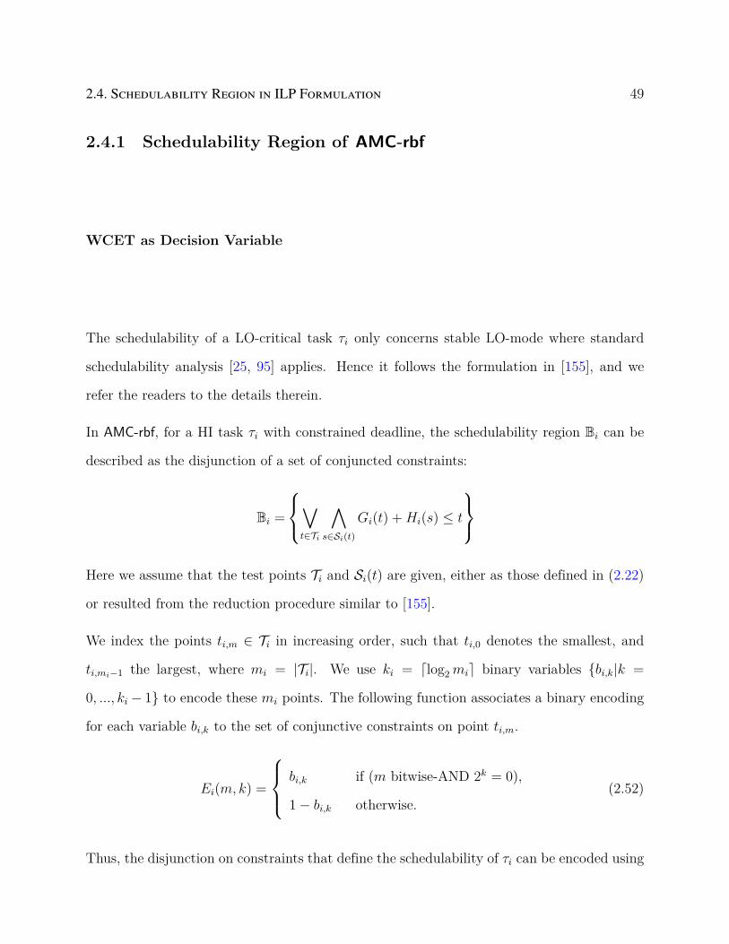
2.4. Schedulability Region in ILP Formulation 49
2.4.1 Schedulability Region of AMC-rbf
WCET as Decision Variable
The schedulability of a LO-critical task τi only concerns stable LO-mode where standard
schedulability analysis [25, 95] applies. Hence it follows the formulation in [155], and we
refer the readers to the details therein.
In AMC-rbf, for a HI task τi with constrained deadline, the schedulability region Bi can be
described as the disjunction of a set of conjuncted constraints:
Bi =
∨t∈Ti
∧s∈Si(t)
Gi(t) +Hi(s) ≤ t
Here we assume that the test points Ti and Si(t) are given, either as those defined in (2.22)
or resulted from the reduction procedure similar to [155].
We index the points ti,m ∈ Ti in increasing order, such that ti,0 denotes the smallest, and
ti,mi−1 the largest, where mi = |Ti|. We use ki = ⌈log2mi⌉ binary variables bi,k|k =
0, ..., ki− 1 to encode these mi points. The following function associates a binary encoding
for each variable bi,k to the set of conjunctive constraints on point ti,m.
Ei(m, k) =
bi,k if (m bitwise-AND 2k = 0),
1− bi,k otherwise.(2.52)
Thus, the disjunction on constraints that define the schedulability of τi can be encoded using

50Chapter 2. An Efficient Schedulability Analysis for Optimizing Systems with Adaptive
Mixed-Criticality Scheduling
the standard “big-M” formulation for conditional constraints:
∀ti,m ∈ Ti, ∀s ∈ Si(ti,m), Gi(ti,m) +Hi(s) ≤ ti,m +M
ki−1∑k=0
Ei(m, k)
ki−1∑k=0
(2k × bi,k) ≤ mi − 1
(2.53)
where M is a constant larger than any other quantity involved in the constraint, and Gi(t)
and Hi(s) are defined as (copied from (2.21))
Gi(t) =Ci(HI) +∑
j∈hpH(i)
⌈t
Tj
⌉Cj(HI)
Hi(s) =∑
j∈hpL(i)
(⌊s
Tj
⌋+ 1
)Cj(LO)
+∑
j∈hpH(i)
max(0,
⌊s−Dj
Tj
⌋)(Cj(LO)− Cj(HI))
(2.54)
The second constraint of (2.53) ensures that the binary encoding only takes values within
the maximum index of the points in Ti. This makes sure that only one of the first set of
inequalities in (2.53) is enforced.
For example, assume Ti = ti,0, ti,1, hence mi = 2. We use one binary variable bi,0 for
defining the feasibility region of task τi. Since k = 0, the function Ei(m, 0) as defined
in (2.52) becomes
Ei(m, 0) =
bi,0 if m = 0 (m bitwise-AND 20 = 0),
1− bi,0 if m = 1 (m bitwise-AND 20 = 0).(2.55)

2.4. Schedulability Region in ILP Formulation 51
According to (2.56), the formulation of the schedulability region for τi is
∀s ∈ Si(ti,0), Gi(ti,0) +Hi(s) ≤ ti,0 +M · bi,0
∀s ∈ Si(ti,1), Gi(ti,1) +Hi(s) ≤ ti,1 +M(1− bi,0)
20 · bi,0 ≤ 1
(2.56)
Task Priority as Decision Variable
The formulation in (2.53) requires the knowledge of task priority assignment as Gi(t) and
Hi(s) are defined with given information on hpH(i) and hpL(i). If the task priority assign-
ments are design variables, the above formulation is not applicable. Instead, we introduce a
set of binary variables indicating the priority order of τi and any other task τj, as follows
pj,i =
1 τj has a higher priority than τi,
0 otherwise.(2.57)
Now Gi(t) and Hi(s) can be rewritten as
Gi(t) =Ci(HI) +∑
j =i,Lj=HI
⌈t
Tj
⌉Cj(HI) · pj,i
Hi(s) =∑
j =i,Lj=LO
(⌊s
Tj
⌋+ 1
)Cj(LO) · pj,i
+∑
j =i,Lj=HI
max(0,
⌊s−Dj
Tj
⌋)(Cj(LO)− Cj(HI)) · pj,i
(2.58)
Here Gi(t) takes the sum over all other HI-critical tasks, but the interference from τj is
enforced to be zero if and only if pj,i = 0. Hi(s) is constructed in the same way.

52Chapter 2. An Efficient Schedulability Analysis for Optimizing Systems with Adaptive
Mixed-Criticality Scheduling
2.4.2 Schedulability Region of AMC-rtb
WCET as Decision Variable
Recall that AMC-rtb is formulated as follows
RLOi = Ci(LO) +
∑j∈hp(i)
⌈RLO
i
Tj
⌉· Cj(LO)
RCCi = Ci(HI) +
∑j∈hpL(i)
⌈RLO
i
Ti
⌉· Cj(LO) +
∑j∈hpH(i)
⌈RCC
i
Tj
⌉· Cj(HI)
(2.59)
We note that RHIi is always no larger than RCC
i hence it can be safely omitted in the
formulation.
To model the above computation in ILP, we introduce a set of integer variables ILOj,i ∈ N+ to
denote the term⌈RLO
i
Tj
⌉, the number of interferences from any higher priority task j ∈ hp(i)
on τi in LO-mode. Similarly, another set of variables ICCj,i ∈ N+ is used to denote the term⌈
RCCi
Tj
⌉, the number of interferences from any higher priority HI-critical task j ∈ hpH(i) on
τi during criticality change.
ILOj,i and ICCj,i can be modeled in ILP by the following constraints.
ILOj,i =
⌈RLO
i
Tj
⌉⇒
RLOj
Ti
≤ ILOj,i <RLO
j
Ti
+ 1
ICCj,i =
⌈RCC
i
Tj
⌉⇒
RCCj
Ti
≤ ICCj,i <
RCCj
Ti
+ 1
(2.60)
The response time calculation according to AMC-rtb can then be written as the following

2.4. Schedulability Region in ILP Formulation 53
constraints
RLOi = Ci(LO) +
∑j∈hp(i)
ILOj,i · Cj(LO)
RCCi = Ci(HI) +
∑j∈hpL(i)
ILOj,i · Cj(LO) +∑
j∈hpH(i)
ICCj,i · Cj(HI)
(2.61)
The above constraints contain the product of an integer variable ILOj,i and a real variable
Ci(LO), hence they are not linear. They can be linearized with additional variables [116].
All tasks have to be schedulable. This means ∀i, RLOi ≤ Di
∀i such that Li = HI, RCCi ≤ Di
(2.62)
Priority as Decision Variable
If the task priority assignments are also design variables, we use a set of binary variables pj,i
indicating the priority order of τi and any other task τj, as in (2.57).
We redefine ILOj,i by giving it a slightly different meaning: it is equal to the number of
interferences if and only if τj has a higher priority than τi. ICCj,i is similarly revised. Hence,

54Chapter 2. An Efficient Schedulability Analysis for Optimizing Systems with Adaptive
Mixed-Criticality Scheduling
(2.60) can be replaced by
ILOj,i = pj,i
⌈RLO
i
Tj
⌉⇒
RLO
j
Ti≤ ILOj,i +M(1− pj,i)
ILOj,i <RLO
j
Ti+ 1 +M(1− pj,i)
ILOj,i ≤ Mpj,i
ICCj,i = pj,i
⌈RCC
i
Tj
⌉⇒
RCC
j
Ti≤ ICC
j,i +M(1− pj,i)
ICCj,i <
RCCj
Ti+ 1 +M(1− pj,i)
ICCj,i ≤ Mpj,i
(2.63)
where M is a big enough constant. With the above changes to ILOj,i and ICCj,i , the response
time formulation remains the same as (2.61).
2.4.3 An Illustrative Example
We exemplify the two formulations using the HI-critical task τ4 in the example taskset in
Table 2.1. We assume that WCET is the decision variable and focus on AMC-rbf and AMC-rtb
only.
Table 2.1: An Example Task System
Task Criticality Period Deadline Priorityτ1 HI 10 10 1τ2 LO 10 10 2τ3 LO 18 18 3τ4 HI 30 30 4
ILP formulation for AMC-rbf. By Theorem 2, the initial set of test points for t is
T4 = 10, 18, 20, 30. The union of the criticality change instants, i.e., S4 =∪S4(t), is
0, 10, 18, 20.
For simplicity, we focus on explaining the benefit of exchanging the ∃ and ∀ quantifiers (step
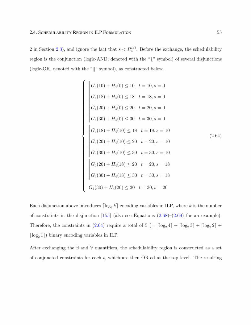
2.4. Schedulability Region in ILP Formulation 55
2 in Section 2.3), and ignore the fact that s < RLO4 . Before the exchange, the schedulability
region is the conjunction (logic-AND, denoted with the “” symbol) of several disjunctions
(logic-OR, denoted with the “||” symbol), as constructed below.
∥∥∥∥∥∥∥∥∥∥∥∥∥∥
G4(10) +H4(0) ≤ 10 t = 10, s = 0
G4(18) +H4(0) ≤ 18 t = 18, s = 0
G4(20) +H4(0) ≤ 20 t = 20, s = 0
G4(30) +H4(0) ≤ 30 t = 30, s = 0∥∥∥∥∥∥∥∥∥∥∥G4(18) +H4(10) ≤ 18 t = 18, s = 10
G4(20) +H4(10) ≤ 20 t = 20, s = 10
G4(30) +H4(10) ≤ 30 t = 30, s = 10∥∥∥∥∥∥∥G4(20) +H4(18) ≤ 20 t = 20, s = 18
G4(30) +H4(18) ≤ 30 t = 30, s = 18
G4(30) +H4(20) ≤ 30 t = 30, s = 20
(2.64)
Each disjunction above introduces ⌈log2 k⌉ encoding variables in ILP, where k is the number
of constraints in the disjunction [155] (also see Equations (2.68)–(2.69) for an example).
Therefore, the constraints in (2.64) require a total of 5 (= ⌈log2 4⌉ + ⌈log2 3⌉ + ⌈log2 2⌉ +
⌈log2 1⌉) binary encoding variables in ILP.
After exchanging the ∃ and ∀ quantifiers, the schedulability region is constructed as a set
of conjuncted constraints for each t, which are then OR-ed at the top level. The resulting

56Chapter 2. An Efficient Schedulability Analysis for Optimizing Systems with Adaptive
Mixed-Criticality Scheduling
formulation becomes: ∥∥∥∥∥∥∥∥∥∥∥∥∥∥∥∥∥∥∥∥∥∥∥∥∥∥∥∥∥∥∥∥∥∥∥∥∥∥
G4(10) +H4(0) ≤ 10 t = 10, s = 0G4(18) +H4(0) ≤ 18 t = 18, s = 0
G4(18) +H4(10) ≤ 18 t = 18, s = 10G4(20) +H4(0) ≤ 20 t = 20, s = 0
G4(20) +H4(10) ≤ 20 t = 20, s = 10
G4(20) +H4(18) ≤ 20 t = 20, s = 18
G4(30) +H4(0) ≤ 30 t = 30, s = 0
G4(30) +H4(10) ≤ 30 t = 30, s = 10
G4(30) +H4(18) ≤ 30 t = 30, s = 18
G4(30) +H4(20) ≤ 30 t = 30, s = 20
(2.65)
The constraints in (2.65) contain only one disjunction. Thus the total number of binary
encoding variables required is ⌈log2 4⌉ = 2, as opposed to 5 required by (2.64). It can be
further simplified while not affecting the feasibility region, using algorithms similar to [155].
For example, the constraint G4(10) +H4(0) ≤ 10 can be expanded as
C4(HI) + C3(LO) + C2(LO) + C1(HI) ≤ 10
The constraint is more restricted than those for
t = 30, s ∈ 0, 10, 18, 20 (2.66)
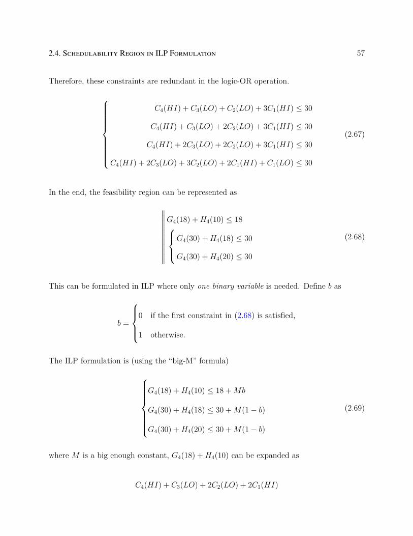
2.4. Schedulability Region in ILP Formulation 57
Therefore, these constraints are redundant in the logic-OR operation.
C4(HI) + C3(LO) + C2(LO) + 3C1(HI) ≤ 30
C4(HI) + C3(LO) + 2C2(LO) + 3C1(HI) ≤ 30
C4(HI) + 2C3(LO) + 2C2(LO) + 3C1(HI) ≤ 30
C4(HI) + 2C3(LO) + 3C2(LO) + 2C1(HI) + C1(LO) ≤ 30
(2.67)
In the end, the feasibility region can be represented as
∥∥∥∥∥∥∥∥∥∥∥G4(18) +H4(10) ≤ 18
G4(30) +H4(18) ≤ 30
G4(30) +H4(20) ≤ 30
(2.68)
This can be formulated in ILP where only one binary variable is needed. Define b as
b =
0 if the first constraint in (2.68) is satisfied,
1 otherwise.
The ILP formulation is (using the “big-M” formula)
G4(18) +H4(10) ≤ 18 +Mb
G4(30) +H4(18) ≤ 30 +M(1− b)
G4(30) +H4(20) ≤ 30 +M(1− b)
(2.69)
where M is a big enough constant, G4(18) +H4(10) can be expanded as
C4(HI) + C3(LO) + 2C2(LO) + 2C1(HI)

58Chapter 2. An Efficient Schedulability Analysis for Optimizing Systems with Adaptive
Mixed-Criticality Scheduling
and G4(30) + H4(18) and G4(30) + H4(20) are expanded as in the last two constraints in
(2.67).
ILP formulation for AMC-rtb. We now discuss the formulation for the schedulability of τ4
under AMC-rtb. First, as noted in [20], it is easy to verify that RCC4 ≥ RHI
4 and RCC4 ≥ RLO
4 .
However, to calculate RCC4 by (2.3), it is still necessary to know RLO
4 . Hence, we focus on the
formulation of RLO4 and RCC
4 . We define the set of integer variables to denote the number of
interferences from the higher priority tasks hp(4) = τ1, τ2, τ3 in LO mode, formulated as
ILO1,4 =
⌈RLO
4
T1
⌉⇒ RLO
4
T1
≤ ILO1,4 <RLO
4
T1
+ 1
ILO2,4 =
⌈RLO
4
T2
⌉⇒ RLO
4
T2
≤ ILO2,4 <RLO
4
T2
+ 1
ILO3,4 =
⌈RLO
4
T3
⌉⇒ RLO
4
T3
≤ ILO3,4 <RLO
4
T3
+ 1
Now RLO4 calculated according to (2.1) is
RLO4 = C4(LO) + ILO3,4 C3(LO) + ILO2,4 C2(LO) + ILO1,4 C1(LO)
For RCC4 calculated by (2.3), we need an additional integer variable ICC
1,4 to denote the number
of interferences by the only task τ1 in hpH(4) during criticality change phase.
ICC1,4 =
⌈RCC
4
T1
⌉⇒ RCC
4
T1
≤ ICC1,4 <
RCC4
T1
+ 1
Now RCC4 calculated according to (2.3) is
RCC4 = C4(HI) + ILO3,4 C3(LO) + ILO2,4 C2(LO) + ICC
1,4 C1(HI)
2.5. Extension to Multiple Criticality Levels 59
For AMC-rtb, in total it requires four integer variables to formulate the schedulability re-
gion of τ4 in ILP. As a comparison, it is sufficient to use only one binary variable in the
schedulability region formulation of AMC-rtb.
2.5 Extension to Multiple Criticality Levels
In this section, we discuss how the proposed analysis technique AMC-rbf can be extended
to system with multiple criticality levels. We first summarize the notation and scheduling
scheme of multi-criticality systems under AMC, then proceed to derive the corresponding
rbf based schedulability analysis.
2.5.1 System Semantics
Let Γ be a system containing K+1 criticality level where K is an arbitrary positive integer.
Let Ψk represent the k-th criticality level, k = 0, · · · , K. The higher the value of k, the
higher the criticality level. The LO criticality level, or the normal mode, is represented by
Ψ0. We use LO and Ψ0 interchangeably in the following discussion. Each task τi is affiliated
with a criticality level ΨLiand a set of WCETs Ci(Ψ0), ...Ci(ΨLi
) corresponding to each
lower or equal criticality level. We assume Ci(Ψk) ≤ Ci(Ψj) for all k < j ≤ Li. The rules of
the task dispatch under AMC policy are summarized as follows:
• The system starts with the initial criticality level of Ψ0, i.e., LO-crit mode.
• In each criticality level Ψk, only tasks with Li ≥ k are allowed to execute for up to
Ci(Ψk). Other tasks with lower criticality levels are abandoned.
• The system criticality level can only change between consecutive levels at a time.

60Chapter 2. An Efficient Schedulability Analysis for Optimizing Systems with Adaptive
Mixed-Criticality Scheduling
• Criticality change from level Ψk−1 to Ψk is triggered when a task with Li ≥ k executes
for Ci(Ψk−1) without signaling completion.
2.5.2 Request Bound Function based Analysis
Similar to dual-criticality systems, three conditions shall be checked to verify the system
schedulability for each criticality level Ψl.
• Stable LO-criticality: The system remains to be in the lowest criticality level all the
time.
• Stable Ψl criticality: The system maintains in criticality level Ψl all the time.
• Ψl criticality change phase: The system dynamically changes from LO criticality
level to Ψl criticality level during execution.
Thus correspondingly, we define three types of request bound functions for each mode at
criticality level Ψl, denoted as SLOi , SHI,Ψl
i and QCC,Ψli respectively.
SLOi is a function of time interval [0, t] and is the same for all τi and all criticality levels. It
can be formulated in the same way as in dual-criticality systems
SLOi (t) = Ci(LO) +
∑j∈hp(i)
⌈t
Tj
⌉Cj(LO) (2.70)
SHI,Ψli is a function of time interval [0, t] and can be computed by considering the execution
of τi as well as all higher priority tasks whose criticality level are higher than or equal to Ψl
2.5. Extension to Multiple Criticality Levels 61
in stable Ψl mode.
SHI,Ψli (t) = Ci(Ψl) +
K∑k≥l
∑j∈hp(i,Ψk)
⌈t
Tj
⌉Cj(Ψl) (2.71)
where hp(i,Ψk) represents the set of higher priority tasks of criticality level Ψk.
QCC,Ψli is a function of both the time interval [0, t] and the criticality change instants. In
multiple criticality systems, a criticality change phase is defined as a vector −→sl = [s1, s2, ...sl],
where sk represents the time instant of criticality change from level Ψk−1 to Ψk. For conve-
nience, we denote s0 = 0. Hence, s0 < s1 < · · · < sl < t.
Intuitively, −→sl denotes a trace of criticality change that leads from LO to criticality level Ψl.
To distinguish −→sl from the time instant sk, we refer to the former as criticality change trace,
or simply trace, and the latter as individual criticality change. To estimate the interference
from a higher priority task τj, we consider the following three cases.
Case 1: τj ∈ hp(i,Ψ0). That is, τj is a LO criticality task. τj introduces interference up to
s1, which can be computed in the same way as in dual-criticality systems.
IΨ0i,j (−→sl ) =
(⌊s1Tj
⌋+ 1
)Cj(Ψ0) (2.72)
Case 2: τj ∈ hp(i,Ψk) where 1 ≤ k = Lj < l. That is, τj is an intermediate criticality
task relative to the concerned level Ψl. τj introduces interference up to sk+1 and executes at
criticality level Ψq in each interval of [sq, sq+1), q = 0, · · · , k−1. Thus, a sufficient estimation
62Chapter 2. An Efficient Schedulability Analysis for Optimizing Systems with Adaptive
Mixed-Criticality Scheduling
of its interference can be computed by
IΨki,j (−→sl ) =
k−1∑q=0
Mj(sq, sq+1) · Cj(Ψq)
+
(⌈sk+1
Tj
⌉−
k−1∑q=0
Mj(sq, sq+1)
)Cj(Ψk)
(2.73)
Mj(t1, t2), as defined in Equation (2.16), provides an lower bound on the maximum num-
ber of instances from τj that can occur in interval [t1, t2). Hence, the term (⌈sk+1
Tj
⌉−∑k−1
q=0 Mj(sq, sq+1)) gives an upper bound on the number of instances that can occur at
τj’s criticality level Lj = k. Since the higher the criticality, the larger the WCET, this
estimation is safe.
Case 3: τj ∈ hp(i,Ψk) where k = Lj ≥ l. That is, τj at a criticality level higher than or
equal to the concerned one Ψl. It introduces interference up to t. In each interval of [sq, sq+1)
where q = 0, · · · , l− 1, it executes at criticality level Ψq. In the interval [sl, t], it executes at
criticality level Ψl. The interference can be computed as
IΨli,j (−→sl , t) =
l−1∑q=0
Mj(sq, sq+1) · Cj(Ψq)
+
(⌈t
Tj
⌉−
l−1∑q=0
Mj(sq, sq+1)
)Cj(Ψl)
(2.74)
QCC,Ψli (−→sl , t) is then obtained by summing up (2.72)–(2.74) for all higher priority tasks as
well as the execution of τi at level Ψl.
QCC,Ψli (−→sl , t) = Ci(Ψl) +
l−1∑k=0
∑j∈hp(i,Ψk)
IΨki,j (−→sl ) +
K∑k=l
∑j∈hp(i,Ψk)
IΨli,j (−→sl , t) (2.75)
We now discuss the notion of response time using the request bound functions defined above.

2.5. Extension to Multiple Criticality Levels 63
The response time in LO criticality mode and stable Ψl criticality mode, denoted respectively
as RLOi and RHI,Ψl
i , are the least fixed point solutions of the following equations respectively.
RLOi = SLO
i (RLOi )
RHI,Ψli = SHI,Ψl
i (RHI,Ψli )
(2.76)
The response time of τi in Ψl criticality change phase with the given trace −→sl , denoted as
RCC,Ψli (−→sl ), is essentially the least fixed point of the following equation
RCC,Ψli (−→sl ) = QCC,Ψl
i (−→sl , RCC,Ψli (−→sl )) (2.77)
The worst case response time of τi in Ψl criticality change mode is the maximum response
time for all possible traces
RCC,Ψli = max
−→sl∈SΨli
RCC,Ψli (−→sl ) (2.78)
where SΨli is the set of all valid −→sl , defined in Equation (2.80) below.
The worst case response time of τi at level Ψl, denoted as RΨli is the maximum of the worst
case response time in the three modes at Ψl
RΨli = maxRLO
i , RHI,Ψli , RCC,Ψl
i (2.79)
We now discuss the definition of SΨli . Similar to dual-criticality systems, in multiple criticality
systems, each individual criticality change instant sk, which triggers system criticality level
change from Ψk−1 to Ψk, must occur before RΨk−1
i . Thus SΨli can be formulated as
SΨli = −→sl | (sp ≤ sq,∀p < q)
∧(sk < R
Ψk−1
i ,∀k) (2.80)

64Chapter 2. An Efficient Schedulability Analysis for Optimizing Systems with Adaptive
Mixed-Criticality Scheduling
We now study some of the properties of QCC,Ψli (−→sl , t), by which we will build the rbf-based
analysis (Corollary 13).
Theorem 10. Given τi such that Li ≥ 1, RCC,Ψli ≥ RHI,Ψl
i for all criticality level Ψl,
l = 1, ·, Li.
Proof. Choose the criticality change trace −→s∗l = [s1, ...sl] such that sk = 0 for all k =
1, · · · , l. It is easy to verify that
⌊s1Tj
⌋= 0 ⇒ IΨ0
i,j (−→s∗l ) = Cj(Ψ0)
∀k < l,
⌈skTj
⌉= 0
∧Mj(sk, sk+1) = 0 ⇒ ∀k < l, IΨk
i,j (−→s∗l ) = 0
(2.81)
Therefore, QCC,Ψli (
−→s∗l , t) with the given trace −→s∗l = [s1, ...sl] becomes
QCC,Ψli (
−→s∗l , t) ≥ Ci(Ψl) +
K∑k=l
∑j∈hp(i,Ψk)
IΨli,j (−→s∗l , t)
= Ci(Ψl) +K∑k=l
∑j∈hp(i,Ψk)
⌈t
Tj
⌉Cj(Ψl)
= SHI,Ψli (t)
(2.82)
The above equation implies that
max−→s ∈SΨl
i (t)
QCC,Ψli (−→sl , t) ≥ SHI,Ψl
i (t), ∀t ∈ [0, RHI,Ψli ] (2.83)
Since RHI,Ψli is the least fixed point of t = SHI,Ψl
i (t), RCC,Ψli , the least fixed point of
t = max−→s ∈SΨl
i (t)
QCC,Ψli (−→sl , t) (2.84)

2.5. Extension to Multiple Criticality Levels 65
must be greater than RHI,Ψli .
Theorem 11. Given τi such that Li ≥ 1, we have RCC,Ψ1
i ≥ RLOi .
Proof. Since QCC,Ψ1
i (−→s1 , t) has the same form as QCCi (s, t) in dual-criticality system, the
proof for the theorem follows directly from Theorem 4.
Theorem 12. Given τi such that Li ≥ 2, it must be RCC,Ψki ≥ R
CC,Ψk−1
i for all k = 2, · · · , Li.
Proof. We prove the theorem by induction.
Base Case.
Consider RCC,Ψ1
i and RCC,Ψ2
i and the corresponding request bound function QCC,Ψ1
i (−→s1 , t)
and QCC,Ψ2
i (−→s2 , t). For any −→s1 = [s1] ∈ SΨ1 and t ∈ (s1, RCC,Ψ1
i ], choose −→s2 = [−→s1 , s2] that
satisfies the following
s2 ∈ [T lb, t) (2.85)
where
T lb = maxs1,maxk | k = m · Tj < t, ∀j, ∀m ∈ N+ (2.86)
and N+ is the set of positive integers.
Since RCC,Ψ1
i ≥ RLOi and RCC,Ψ1
i ≥ RHI,Ψ1
i (by Theorems 10 and 11), it is RΨ1i = RCC,Ψ1
i .
Also, since −→s1 ∈ SΨ1 , there is s1 < RLOi ≤ RΨ1
i = RCC,Ψ1
i . Thus it is always possible to
construct such an s2 for which −→s2 ∈ SΨ2(t). Note that if RCC,Ψ1
i < RLOi , t and s2 above may
not exists for −→s1 where s1 ∈ [RCC,Ψ1
i , RLOi ).
s2 selected above satisfies the following property
⌈s2Tj
⌉=
⌈t
Tj
⌉,∀j (2.87)
66Chapter 2. An Efficient Schedulability Analysis for Optimizing Systems with Adaptive
Mixed-Criticality Scheduling
Consider functions QCC,Ψ2
i (−→s2 , t) and QCC,Ψ1
i (−→s1 , t) for the above −→s1 , −→s2 and t
QCC,Ψ1
i (−→s1 , t) = Ci(Ψ1) +∑
j∈hp(i,Ψ0)
(⌊s1Tj
⌋+ 1
)Cj(LO)
+K∑k=1
∑j∈hp(i,Ψk)
Mj(0, s1)Cj(Ψ0)
+
(⌈t
Tj
⌉−Mj(0, s1)
)Cj(Ψ1)
(2.88)
QCC,Ψ2
i (−→s1 , t) = Ci(Ψ2) +∑
j∈hp(i,Ψ0)
(⌊s1Tj
⌋+ 1
)Cj(LO)
+∑
j∈hp(i,Ψ1)
Mj(0, s1) · Cj(Ψ0) +
(⌈s2Tj
⌉−Mj(0, s1)
)Cj(Ψ1)
+K∑k=2
∑j∈hp(i,Ψk)
Mj(0, s1) · Cj(Ψ0) +Mj(s1, s2) · Cj(Ψ1)
+
(⌈t
Tj
⌉−Mj(0, s1)−Mj(s1, s2)
)Cj(Ψ2)
(2.89)
Subtracting QCC,Ψ1
i (−→s1 , t) from QCC,Ψ2
i (−→s2 , t), and substituting for the relationship in (2.87),
it isQCC,Ψ2
i (−→s2 , t)−QCC,Ψ1
i (−→s1 , t)
=Ci(Ψ2)− Ci(Ψ1)
+K∑k=2
∑j∈hp(i,Ψk)
(Mj(s1, s2) +Mj(0, s1)−
⌈t
Tj
⌉)Cj(Ψ1)
+
(⌈t
Tj
⌉−Mj(0, s1)−Mj(s1, s2)
)Cj(Ψ2)
(2.90)
By the fact that ∀j, Cj(Ψ2) ≥ Cj(Ψ1), we have QCC,Ψ2
i (−→s2 , t) ≥ QCC,Ψ1
i (−→s1 , t). Also since
RCC,Ψ1
i is the least fixed point of
max−→s1∈SΨ1
i (t)
QCC,Ψ1
i (−→s1 , t) = t (2.91)

2.5. Extension to Multiple Criticality Levels 67
there is,
max−→s2∈SΨ2
i (t)
QCC,Ψ2
i (−→s2 , t) ≥ max−→s1∈SΨ1
i (t)
QCC,Ψ1
i (−→s1 , t) > t, ∀t ∈ (s1, RΨ1i ) (2.92)
which implies that RCC,Ψ2
i ≥ RCC,Ψ1
i ≥ RLOi .
Step Case.
Assumes that RCC,Ψq
i ≥ RCC,Ψq−1
i for all q = 1, · · · , k. We now show that RCC,Ψk+1
i ≥ RCC,Ψki .
For any −→sk ∈ SΨki and t ∈ (sk, R
ΨCC,k
i ], construct −−→sk+1 = [−→sk , sk+1], where sk+1 satisfies the
following
sk+1 ∈ [T lb, t) (2.93)
where
T lb = maxsk,maxn | n = m · Tj < t, ∀j, ∀m ∈ N+ (2.94)
By the inductive hypothesis, there is RCC,Ψq
i = RΨq
i ,∀q = 1, · · · , k. Since −→sk ∈ SΨk , sk <
RΨk−1
i = RCC,Ψk−1
i ≤ RCC,Ψki . Thus, it is always possible to construct such an sk+1.
Similar to the base case, sk+1 has the following property
⌈sk+1
Tj
⌉=
⌈t
Tj
⌉,∀j (2.95)
Similar to (2.90), the difference between QCC,Ψki (−→sk , t) and Q
CC,Ψk+1
i (−−→sk+1, t) can be derived
68Chapter 2. An Efficient Schedulability Analysis for Optimizing Systems with Adaptive
Mixed-Criticality Scheduling
as follows by substituting with (2.95)
QCC,Ψk+1
i (−−→sk+1, t)−QCC,Ψki (−→sk , t)
=Ci(Ψk+1)− Ci(Ψk)
+K∑
p=k+1
∑j∈hp(i,Ψp)
( k∑q=0
Mj(sq, sq+1)−⌈t
Tj
⌉)Cj(Ψk)
+
(⌈t
Tj
⌉−
k∑q=0
Mj(sq, sq+1)
)Cj(Ψk+1)
(2.96)
where s0 is defined as 0.
Because ∀j, Cj(Ψk+1) ≥ Cj(Ψk), we have QCC,Ψk+1
i (−−→sk+1, t) ≥ QCC,Ψki (−→sk , t). Since RCC,Ψk
i is
the least fixed point of
max−→sk∈S
Ψki (t)
QCC,Ψki (−→sk , t) = t (2.97)
it is
max−−→sk+1∈S
Ψk+1i (t)
QCC,Ψk+1
i (−−→sk+1, t) ≥ max−→sk∈S
Ψki (t)
QCC,Ψki (−→sk , t) > t, ∀t ∈ (sk, R
Ψki ) (2.98)
which implies that RCC,Ψk+1
i ≥ RCC,Ψki ≥ RLO
i .
The above three theorems, Theorems 10–12 imply that the worst case response time for τi
always occur in criticality change mode at τi’s highest criticality level. Thus τi is schedulable
if
RCC,ΨLii ≤ Di (2.99)
This directly implies the following corollary on rbf-based analysis for systems multiple criti-
cality levels.

2.5. Extension to Multiple Criticality Levels 69
Corollary 13. τi is schedulable if
∀−→sLi∈ SΨLi
i , ∃t ∈ (sLi, Di] s.t. Q
CC,ΨLii (−→sLi
, t) ≤ t (2.100)
where SΨLii is defined as in (2.80), repeated below.
SΨLii = −→sLi
| (sp ≤ sq,∀p < q)∧
(sk < RΨk−1
i ,∀k) (2.101)
We now prove that the ∃ and ∀ quantifiers can be exchanged without affecting the accuracy.
Theorem 14. (2.102) is a sufficient and necessary condition of (2.100).
∃t ∈ (0, Di], s.t. ∀−→sLi∈ SΨLi
i (t), QCC,ΨLii (−→sLi
, t) ≤ t (2.102)
where SΨLi (t) is refined from SΨLi (Equation (2.101)) by adding the constraint sk < t, ∀k =
1, · · · , Li.
Proof.
Sufficiency.
Let tp be the time instant that satisfies condition in (2.102). Equation (2.98) implies that
tp ≥ RΨki for all k < Li. Thus, SΨLi
i = SΨLii (tp). Clearly,
∀−→sLi∈ SΨLi
i , ∃t = tp ∈ (sLi, Di] s.t. Q
CC,ΨLii (−→sLi
, t) ≤ t (2.103)
Necessity.
Assume that (2.100) is satisfied. Since QCC,ΨLii (−→sLi
, t) is separable in −→sLiand t, it can be
70Chapter 2. An Efficient Schedulability Analysis for Optimizing Systems with Adaptive
Mixed-Criticality Scheduling
written as
QCC,ΨLii (−→sLi
, t) = H(−→sLi) +G(t) (2.104)
where H(−→sLi) and G(t) is defined as
G(t) = Ci(ΨLi) +
K∑k=Li
∑j∈hp(i,Ψk)
⌈t
Tj
⌉Cj(ΨLi
)
H(−→sLi) =
Li−1∑k=0
∑j∈hp(i,Ψk)
IΨki,j (−→sLi
) +K∑
k=Li
∑j∈hp(i,Ψk)
I′ΨLii,j (−→sLi
)
I′ΨLii,j (−→sLi
) =
Li−1∑q=0
Mj(sq, sq+1) · Cj(Ψq)−
(Li−1∑q=0
Mj(sq, sq+1)
)Cj(ΨLi
)
(2.105)
Let −→s∗Libe the criticality change trace that achieves the maximum of H(−→sLi
), i.e.,
H(−→s∗Li
) = max−→sLi
∈SΨLii
H(−→sLi) (2.106)
Let tp be a time instant that satisfies QCC,ΨLii (
−→s∗Li, tp) ≤ tp. By assumption, tp ∈ (s∗Li
, Di]
and thus −→s∗Li∈ SΨLi
i (tp). Notice that
max−→sLi
∈SΨLii (tp)
QCC,ΨLii (−→sLi
, tp) = G(tp) + max−→sLi
∈SΨLii (tp)
H(−→sLi)
= G(tp) +H(−→s∗Li
)
= QCC,ΨLii (
−→s∗Li
, tp)
(2.107)
Therefore, it is
QCC,ΨLii (−→sLi
, tp) ≤ QCC,ΨLii (
−→s∗Li
, tp) ≤ tp,∀−→sLi∈ SΨLi
i (tp) (2.108)

2.5. Extension to Multiple Criticality Levels 71
which clearly indicates that
∃t = tp ∈ (0, Di], s.t. ∀−→sLi∈ SΨLi
i (tp), QCC,ΨLii (−→sLi
, tp) ≤ tp (2.109)
Theorem 15 relaxes the constraints on the criticality change instant sk from sk < RΨk−1
i to
sk < t.
Theorem 15. τi is schedulable if
∃t ∈ (0, Di], s.t. ∀−→sLi∈ S
′ΨLii (t), Q
CC,ΨLii (−→sLi
, t) ≤ t (2.110)
where S′ΨLii (t) is defined as
S′ΨLii (t) = −→sLi
| (sp ≤ sq, ∀p < q)∧
(sk < t, ∀k) (2.111)
Proof. It is easy to see that SΨLii (t) ⊆ S′ΨLi
i (t). In fact S′ΨLii (t) is essentially a relaxation
from SΨLii (t) by removing the requirement sk < R
Ψk−1
i . Thus any time instant t that satisfies
condition (2.110) also satisfies (2.102).
2.5.3 Bounded Pessimism
We now study the boundedness of pessimism introduced by relaxation in (2.111). We provide
a high level intuition and omit the detailed proof for better readability.
Let −→s∗Libe the worst case criticality change trace in set SΨLi and
−→s′Li
be the worst case criti-
cality change trace in set S′ΨLi . When pessimism does occur due to relaxation, it can only
be the case that s∗k < RΨk−1
i ≤ s′k for some k where 1 ≤ k ≤ Li. Now consider the smallest
72Chapter 2. An Efficient Schedulability Analysis for Optimizing Systems with Adaptive
Mixed-Criticality Scheduling
of such k. In the scenario behind −→s∗Li, the system executes at Ψk−1 criticality level in interval
[s∗k−1, s∗k) and at Ψk criticality level in interval [s∗k, s′k). In the scenario represented by
−→s′Li
, the
system executes at Ψk−1 criticality level for the entire interval [s∗k−1, s′k). Comparing to −→s∗Li
,−→s′Li
introduces an extra estimation of Ψk−1-level workload in interval [s∗k, s′k) but correspond-
ingly cut away the estimation of Ψk-level workload in the same interval. Let WΨl(t1, t2)
represents the amount of workload in [t1, t2). The difference in workload estimation by −→s∗Li
and−→s′Li
in [s∗k−1, s′k) can then be represented as
WΨk−1(s∗k, s′k)−WΨk(s∗k, s
′k) (2.112)
Intuitively, the difference is clearly bounded by the amount of Ψk−1 workload that can occur
in interval [s∗k, s′k). It can also be seen that pessimism occurs mostly when lower criticality
levels have higher workload, in which case (2.112) tends to be positive. Note that in the
opposite case, both s∗k and s′k tend to be small value and thus are more likely to be smaller
than RΨk−1
i , which gives s∗k = s′k (no pessimism).
Similar to dual-criticality systems, the amount of pessimism for a given t can be quantified
as
B(t) = max−→sLi
∈S′ΨLi (t)
Hi(−→sLi
)− max−→sLi
∈SΨLi (t)
Hi(−→sLi
) (2.113)
We make use of the following relationships
s1Tj
− 1 ≤⌊s1Tj
⌋≤ s1
Tj
skTj
≤⌈skTj
⌉≤ sk
Tj
+ 1
sp − sq −Dj
Tj
− 1 ≤⌊sp − sq −Dj
Tj
⌋≤Mj(sq, sp) ≤
sp − sqTj
(2.114)

2.5. Extension to Multiple Criticality Levels 73
A linear lower bound on Hi(−→sLi
) can be constructed by substituting s1Tj−1 for the term
⌊s1Tj
⌋,
skTj
for⌈skTj
⌉, and sp−sq
Tjfor Mj(sq, sp)
HLBi (−→sLi
) =
Li∑k=1
Vk · sk (2.115)
where Vk is defined as
V1 =∑
j∈hp(i,Ψ0)
Cj(Ψ0)
Tj
∀k ≥ 2, Vk =
Li∑p=k−1
∑j∈hp(i,Ψp)
Cj(Ψk−1)
Tj
−Li∑p=k
∑j∈hp(i,Ψp)
Cj(Ψk)
Tj
(2.116)
Similarly, a linear upper bound can be constructed by substituting s1Tj
for the term⌊s1Tj
⌋,
skTj
+ 1 for⌈skTj
⌉, and sp−sq−Di
Tj− 1 for Mj(sq, sp)
HUBi (−→sLi
) =
Li∑k=1
Vk · sk +X (2.117)
where the constant X is defined as
X =
Li∑k=0
∑j∈hp(i,Ψk)
QΨki,j (2.118)

74Chapter 2. An Efficient Schedulability Analysis for Optimizing Systems with Adaptive
Mixed-Criticality Scheduling
and QΨki,j is defined as
QΨki,j =
Cj(Ψ0), k = 0
Cj(Ψk) +k−1∑q=0
Tj +Dj
Tj
(Cj(Ψq+1)− Cj(Ψq)), 1 ≤ k < Li
Li−1∑q=0
Tj +Dj
Tj
(Cj(ΨLi)− Cj(Ψq)), k = Li
(2.119)
With HUBi (−→sLi
) and HLBi (−→sLi
), B(t) can be upper bounded by
B(t) ≤ max−→sLi
∈S′ΨLi (t)
HUBi (−→sLi
)− max−→sLi
∈SΨLi (t)
HLBi (−→sLi
) (2.120)
Let −→suLiand−→slLi
be the trace that achieve the maximum of HUBi (−→sLi
) and HLBi (−→sLi
) respec-
tively. The upper bound on the amount of pessimism B(t) is the optimal value of the
following linear programming problem
maxLi∑k=1
Vk · (sui − sli) +X
s.t. suk < t, ∀k = 1..Li
sup < suq ,∀p < q
slk < mint, RΨki ,∀i = 1, · · · , Li
slp < slq,∀p < q
(2.121)
2.6 Experimental Results
In this section we present three sets of experiments to evaluate the proposed schedulability
analysis AMC-rbf. In the first set of experiments, we evaluate the accuracy of AMC-rbf by
2.6. Experimental Results 75
comparing it with AMC-max and AMC-rtb. We then extensively test the solution quality
and scalability of the optimization algorithms which use AMC-rbf to formulate schedulabil-
ity region in ILP (Integer Linear Programming) framework. This is done on two design
optimization problems. One is the software synthesis of Simulink models. The other is the
task allocation on multicore with fixed priority partitioned scheduling. All experiments are
run on a machine with a 3.40GHz quad-core processor and 8GB memory, and all ILP related
problems are solved using CPLEX [83].
2.6.1 Comparison of Schedulability Tests
We first compare the following four methods of schedulability test:
▷ AMC-max: The AMC-max method described in [20];
▷ AMC-rtb: The AMC-rtb method introduced in [20];
▷ AMC-rbf: The AMC-rbf analysis as formulated in (2.14);
▷ AMC-rbf-ub: Schedulability test assuming worst case over-approximation, i.e., LCCi de-
fined in (2.18).
Controlled LO-crit Utilization
We first generate random task systems that have controlled system utilization at LO-crit
level (ULO). Utilization of each task at LO-crit level is generated using the UUnifast-Discard
algorithm [50]. We generate random task systems that vary in several system parameters,
including system utilization at LO-crit level (ULO), criticality factor (CF, defined as C(HI)C(LO)
),
HI-critical task percentage (HIP), and number of tasks (TN). Default values of CF, HIP
and TN are set to 2.0, 50%, and 20 respectively. Periods of tasks follow the log-uniform
distribution. Audsley’s algorithm [7] is used to try to find a feasible priority assignment

76Chapter 2. An Efficient Schedulability Analysis for Optimizing Systems with Adaptive
Mixed-Criticality Scheduling
Figure 2.1: Acceptance Ratio vs. LO-crit Utilization (ULO)
for each method. If success, the taskset is considered as schedulable under that method;
otherwise, it is deemed as unschedulable. For each setting of system parameters, 1000 test
cases are generated.
Fig. 2.1 plots the acceptance ratio versus different LO-crit system utilization. It can be seen
that AMC-rbf has a very close accuracy with that of AMC-rtb, as the two curves are almost
indistinguishable. Compared to AMC-max, AMC-rbf loses some accuracy but it is always
safe as indicated by Theorem 1. On the other hand, AMC-rbf-ub provides a safe, but quite
pessimistic bound for AMC-rbf. The result similar to that of Fig. 2.1 but for tasks with
constrained deadlines (D ≤ T ), is illustrated in Fig. 2.2. The deadline of each task τi is
chosen randomly from interval [Ci(Li), Ti]. Again, this confirms that AMC-rbf provides a
close and safe approximation to AMC-max.
Experiments with other parameter settings have similar results. Figs. 2.3, 2.4 and 2.5 plot

2.6. Experimental Results 77
Figure 2.2: Acceptance Ratio vs. LO-crit Utilization (ULO), Constrained Deadline
Figure 2.3: Weighted Schedulability vs. Criticality Factor (CF)
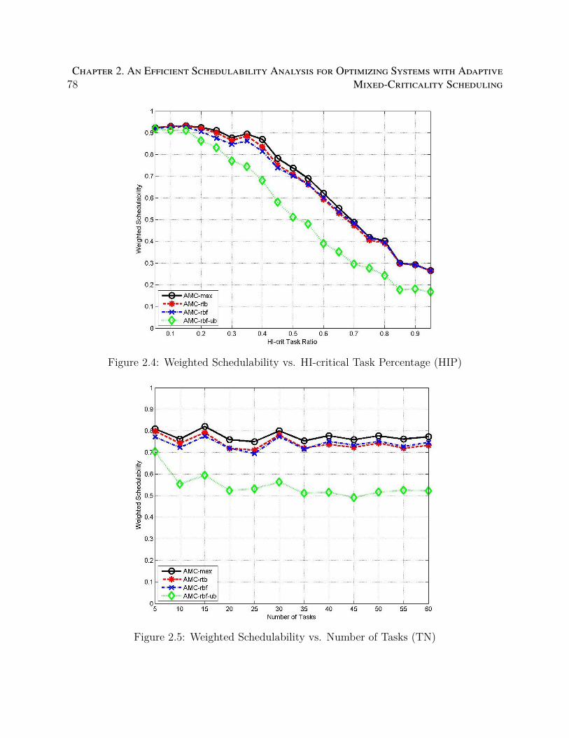
78Chapter 2. An Efficient Schedulability Analysis for Optimizing Systems with Adaptive
Mixed-Criticality Scheduling
Figure 2.4: Weighted Schedulability vs. HI-critical Task Percentage (HIP)
Figure 2.5: Weighted Schedulability vs. Number of Tasks (TN)
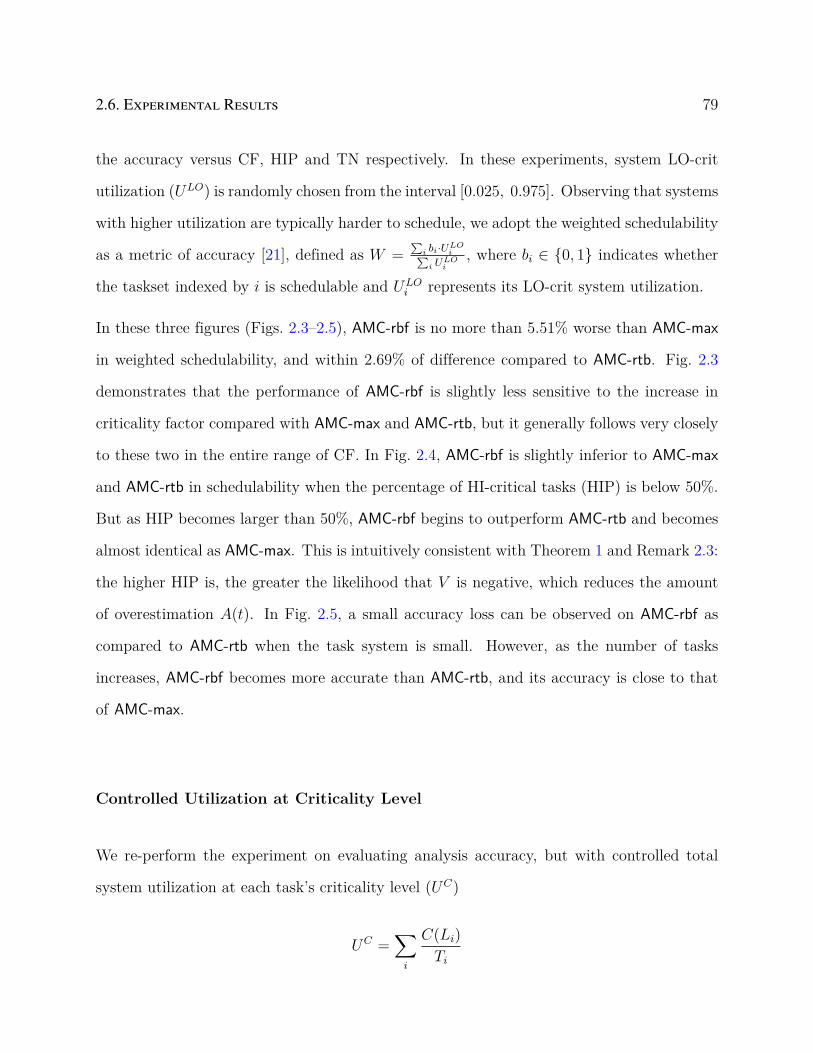
2.6. Experimental Results 79
the accuracy versus CF, HIP and TN respectively. In these experiments, system LO-crit
utilization (ULO) is randomly chosen from the interval [0.025, 0.975]. Observing that systems
with higher utilization are typically harder to schedule, we adopt the weighted schedulability
as a metric of accuracy [21], defined as W =∑
i bi·ULOi∑
i ULOi
, where bi ∈ 0, 1 indicates whether
the taskset indexed by i is schedulable and ULOi represents its LO-crit system utilization.
In these three figures (Figs. 2.3–2.5), AMC-rbf is no more than 5.51% worse than AMC-max
in weighted schedulability, and within 2.69% of difference compared to AMC-rtb. Fig. 2.3
demonstrates that the performance of AMC-rbf is slightly less sensitive to the increase in
criticality factor compared with AMC-max and AMC-rtb, but it generally follows very closely
to these two in the entire range of CF. In Fig. 2.4, AMC-rbf is slightly inferior to AMC-max
and AMC-rtb in schedulability when the percentage of HI-critical tasks (HIP) is below 50%.
But as HIP becomes larger than 50%, AMC-rbf begins to outperform AMC-rtb and becomes
almost identical as AMC-max. This is intuitively consistent with Theorem 1 and Remark 2.3:
the higher HIP is, the greater the likelihood that V is negative, which reduces the amount
of overestimation A(t). In Fig. 2.5, a small accuracy loss can be observed on AMC-rbf as
compared to AMC-rtb when the task system is small. However, as the number of tasks
increases, AMC-rbf becomes more accurate than AMC-rtb, and its accuracy is close to that
of AMC-max.
Controlled Utilization at Criticality Level
We re-perform the experiment on evaluating analysis accuracy, but with controlled total
system utilization at each task’s criticality level (UC)
UC =∑i
C(Li)
Ti

80Chapter 2. An Efficient Schedulability Analysis for Optimizing Systems with Adaptive
Mixed-Criticality Scheduling
Figure 2.6: Acceptance Ratio vs. Utilization at Criticality Level (UC)
By default, UC is a random value selected from interval [0.5, 1.6]. Utilization for each task is
then generated using UUnifast algorithm. However, the generated utilization is now treated
as the utilization of each task at its criticality level. In this way, UC is essentially the
sum of each task’s utilization at its highest criticality level, which can be greater than 1.
The corresponding utilization at lower criticality level is obtained by dividing it with the
criticality factor. For example, if a HI-crit task τi of period 10 is assigned utilization 0.4,
then Ci(HI) = 4 and Ci(LO) = 2. The other parameters are generated in the same way as
Section 2.6.1. The default value of CF, HIP and TN are set to 0.5, 50% and 20 respectively.
Periods are generated by log-uniform distribution. Deadline are set equal to period.
Figs. 2.7, 2.8 and 2.9 shows the results of the experiment that varies UL, CF, HIP, and
TN respectively, while keeping other parameters at their default configurations. Fig. 2.10
performs the same experiment as Fig. 2.6 but uses constrained deadline for each task. The
deadline are chosen randomly from interval [Ci(LO), Ti] for LO tasks and [Ci(HI), Ti] for
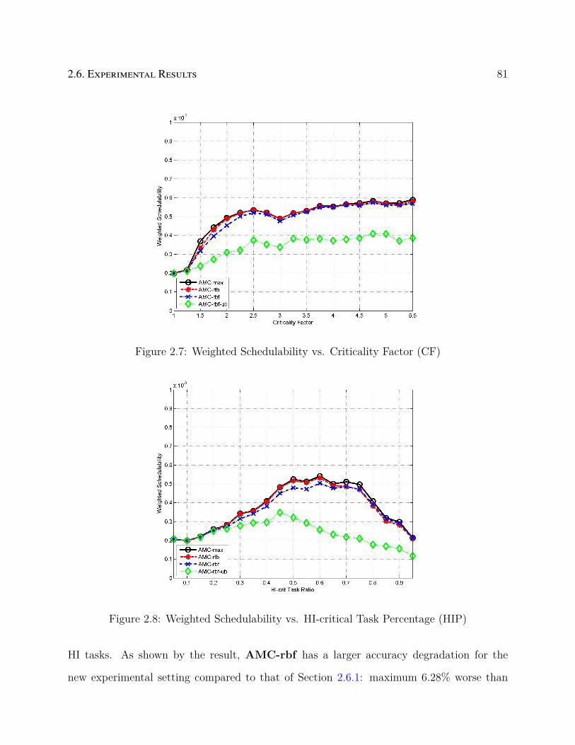
2.6. Experimental Results 81
Figure 2.7: Weighted Schedulability vs. Criticality Factor (CF)
Figure 2.8: Weighted Schedulability vs. HI-critical Task Percentage (HIP)
HI tasks. As shown by the result, AMC-rbf has a larger accuracy degradation for the
new experimental setting compared to that of Section 2.6.1: maximum 6.28% worse than

82Chapter 2. An Efficient Schedulability Analysis for Optimizing Systems with Adaptive
Mixed-Criticality Scheduling
Figure 2.9: Acceptance Ratio vs. Number of Tasks (TN)
Figure 2.10: Acceptance Ratio vs. Utilization at Criticality Level (UC), Constrained Dead-line
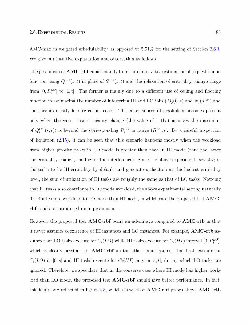
2.6. Experimental Results 83
AMC-max in weighted schedulability, as opposed to 5.51% for the setting of Section 2.6.1.
We give our intuitive explanation and observation as follows.
The pessimism of AMC-rbf comes mainly from the conservative estimation of request bound
function using QCCi (s, t) in place of SCC
i (s, t) and the relaxation of criticality change range
from [0, RLOi ] to [0, t]. The former is mainly due to a different use of ceiling and flooring
function in estimating the number of interfering HI and LO jobs (Mj(0, s) and Nj(s, t)) and
thus occurs mostly in rare corner cases. The latter source of pessimism becomes present
only when the worst case criticality change (the value of s that achieves the maximum
of QCCi (s, t)) is beyond the corresponding RLO
i in range (RLOi , t]. By a careful inspection
of Equation (2.15), it can be seen that this scenario happens mostly when the workload
from higher priority tasks in LO mode is greater than that in HI mode (thus the latter
the criticality change, the higher the interference). Since the above experiments set 50% of
the tasks to be HI-criticality by default and generate utilization at the highest criticality
level, the sum of utilization of HI tasks are roughly the same as that of LO tasks. Noticing
that HI tasks also contribute to LO mode workload, the above experimental setting naturally
distribute more workload to LO mode than HI mode, in which case the proposed test AMC-
rbf tends to introduced more pessimism.
However, the proposed test AMC-rbf bears an advantage compared to AMC-rtb in that
it never assumes coexistence of HI instances and LO instances. For example, AMC-rtb as-
sumes that LO tasks execute for Ci(LO) while HI tasks execute for Ci(HI) interval [0, RLOi ],
which is clearly pessimistic. AMC-rbf on the other hand assumes that both execute for
Ci(LO) in [0, s] and HI tasks execute for Ci(HI) only in [s, t], during which LO tasks are
ignored. Therefore, we speculate that in the converse case where HI mode has higher work-
load than LO mode, the proposed test AMC-rbf should give better performance. In fact,
this is already reflected in figure 2.8, which shows that AMC-rbf grows above AMC-rtb

84Chapter 2. An Efficient Schedulability Analysis for Optimizing Systems with Adaptive
Mixed-Criticality Scheduling
Figure 2.11: Weighted Schedulability vs. Utilization at Criticality Level (UC), HIP=70%
with higher percentage of HI tasks.
To further confirm it, we perform another two sets of experiments of varying system total
utilization. In the first set, we increase the default HIP from 50% to 70%. In the second
set we keep the HIP to be 50% but distribute 70% of the total utilization to HI tasks, i.e.,
UHI = 70%× UC where
UHI =∑
i:Li=HI
Ci(HI)
Ti
The results are respectively shown in Figs. 2.11 and 2.12, which demonstrate a closer and even
better performance of AMC-rbf than AMC-rtb. This confirms with our observation that
the proposed technique AMC-rbf is more accurate when applied to system with relatively
high HI criticality workload.

2.6. Experimental Results 85
Figure 2.12: Acceptance Ratio vs. Utilization at Criticality Level (UC), UHI = 70%× UC
2.6.2 Optimizing Software Synthesis of Simulink Models
In this experiment, we consider the optimization of minimizing the control performance in the
semantics-preserving implementation of Simulink models. We briefly describe the problem
below, and refer interested readers to [109] for more details.
A Simulink model is a Directed Acyclic Graph (DAG) where nodes represent functional
blocks and links represent data communication between functional blocks. We assume each
functional block is implemented in a dedicated task (hence use the terms functional block and
task interchangeably). The semantics-preserving implementation of the model has to match
its functional behavior. This typically requires the addition of a Rate Transition (RT) block
between a reader and a writer with different but harmonic periods, which is a special type
of wait-free communication buffers. However, the costs of RT blocks are additional memory
overheads and in some cases, functional delays in result delivering. The latter degrades
control performance. As a simple example, consider a fast reader τr and slow writer τw that
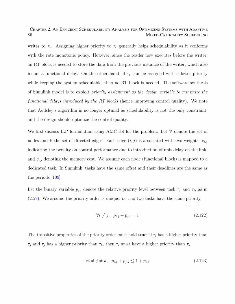
86Chapter 2. An Efficient Schedulability Analysis for Optimizing Systems with Adaptive
Mixed-Criticality Scheduling
writes to τr. Assigning higher priority to τr generally helps schedulability as it conforms
with the rate monotonic policy. However, since the reader now executes before the writer,
an RT block is needed to store the data from the previous instance of the writer, which also
incurs a functional delay. On the other hand, if τr can be assigned with a lower priority
while keeping the system schedulable, then no RT block is needed. The software synthesis
of Simulink model is to exploit priority assignment as the design variable to minimize the
functional delays introduced by the RT blocks (hence improving control quality). We note
that Audsley’s algorithm is no longer optimal as schedulability is not the only constraint,
and the design should optimize the control quality.
We first discuss ILP formulation using AMC-rbf for the problem. Let V denote the set of
nodes and E the set of directed edges. Each edge (i, j) is associated with two weights: ci,j
indicating the penalty on control performance due to introduction of unit delay on the link,
and gi,j denoting the memory cost. We assume each node (functional block) is mapped to a
dedicated task. In Simulink, tasks have the same offset and their deadlines are the same as
the periods [109].
Let the binary variable pj,i denote the relative priority level between task τj and τi, as in
(2.57). We assume the priority order is unique, i.e., no two tasks have the same priority.
∀i = j, pi,j + pj,i = 1 (2.122)
The transitive properties of the priority order must hold true: if τi has a higher priority than
τj and τj has a higher priority than τk, then τi must have a higher priority than τk.
∀i = j = k, pi,j + pj,k ≤ 1 + pi,k (2.123)
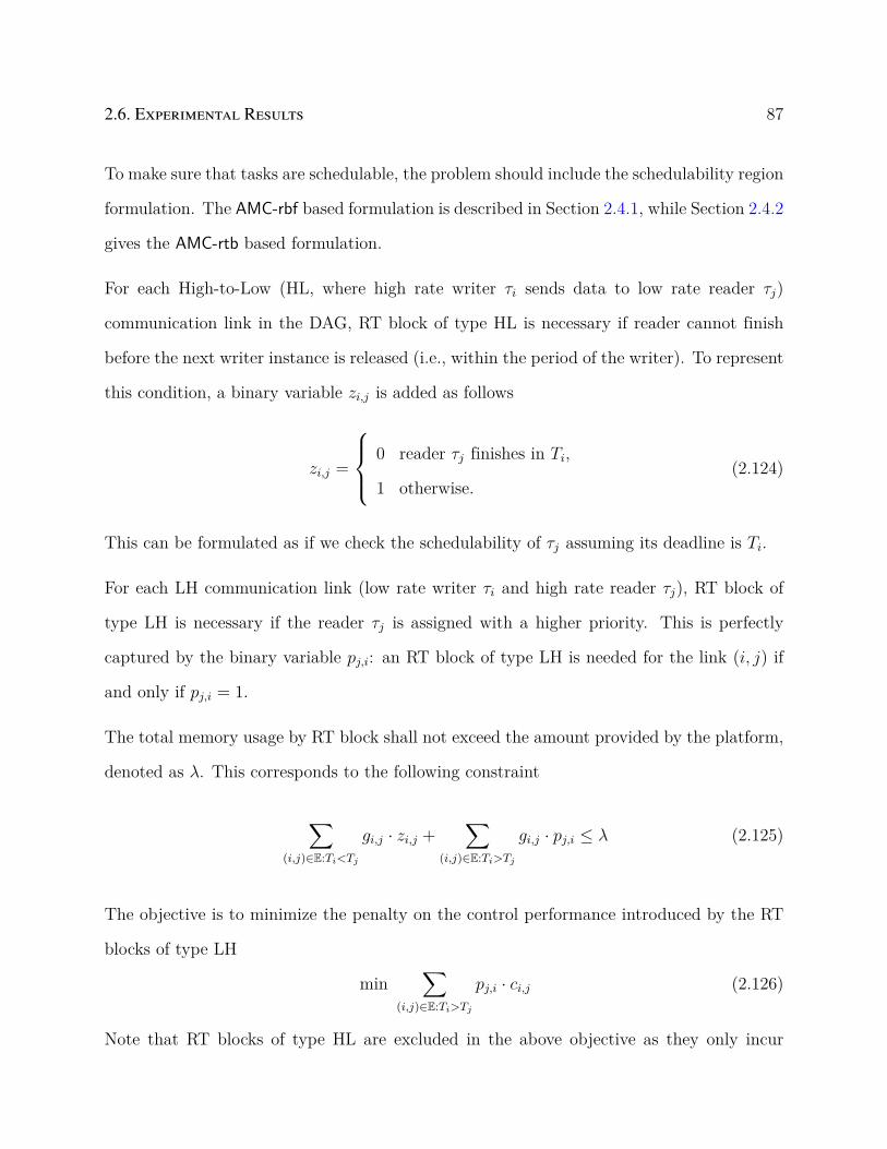
2.6. Experimental Results 87
To make sure that tasks are schedulable, the problem should include the schedulability region
formulation. The AMC-rbf based formulation is described in Section 2.4.1, while Section 2.4.2
gives the AMC-rtb based formulation.
For each High-to-Low (HL, where high rate writer τi sends data to low rate reader τj)
communication link in the DAG, RT block of type HL is necessary if reader cannot finish
before the next writer instance is released (i.e., within the period of the writer). To represent
this condition, a binary variable zi,j is added as follows
zi,j =
0 reader τj finishes in Ti,
1 otherwise.(2.124)
This can be formulated as if we check the schedulability of τj assuming its deadline is Ti.
For each LH communication link (low rate writer τi and high rate reader τj), RT block of
type LH is necessary if the reader τj is assigned with a higher priority. This is perfectly
captured by the binary variable pj,i: an RT block of type LH is needed for the link (i, j) if
and only if pj,i = 1.
The total memory usage by RT block shall not exceed the amount provided by the platform,
denoted as λ. This corresponds to the following constraint
∑(i,j)∈E:Ti<Tj
gi,j · zi,j +∑
(i,j)∈E:Ti>Tj
gi,j · pj,i ≤ λ (2.125)
The objective is to minimize the penalty on the control performance introduced by the RT
blocks of type LH
min∑
(i,j)∈E:Ti>Tj
pj,i · ci,j (2.126)
Note that RT blocks of type HL are excluded in the above objective as they only incur

88Chapter 2. An Efficient Schedulability Analysis for Optimizing Systems with Adaptive
Mixed-Criticality Scheduling
memory overhead, but no functional delay.
We consider the problem where the Simulink model contains functional blocks with different
criticality levels. To determine the task criticality level, we follow the criteria in [15]: first,
criticality (LO or HI) is randomly assigned to sink tasks in the DAG; then it is propagated
to other tasks as follows:
• If a task is the predecessor of any HI-critical block, then it is assigned a HI-critical
level as well;
• All tasks not assigned HI-critical by the above rule are assigned LO-critical level.
We vary different parameters of the task systems including system utilization in LO mode,
total number of tasks, and criticality factors. System utilization ranges from 0.5 to 0.95.
Criticality factor varies from 1.0 to 5.5. Total number of tasks ranges from 5 to 40. In each
experiment, we vary one parameter while the other two are either kept at a default value or
randomly generated.
We randomly select from a set of predefined values for task periods.
10, 20, 40, 50, 100, 200, 400, 500, 1000 (2.127)
This set contains all the period factors of the task periods for the real-world automotive
benchmark in [89]. We use TGFF [61] to generate random, acyclic task graphs. Tasks
communicating with each other have harmonic periods as required by the Simulink tool [105].
Besides the size of the communication data, which is a random value from range [1, 256], each
link is assigned with a random weight in range [1, 50] to indicate the degradation of control
performance if the reader has a higher priority. For each combination of system parameters,
1000 task systems are instantiated.
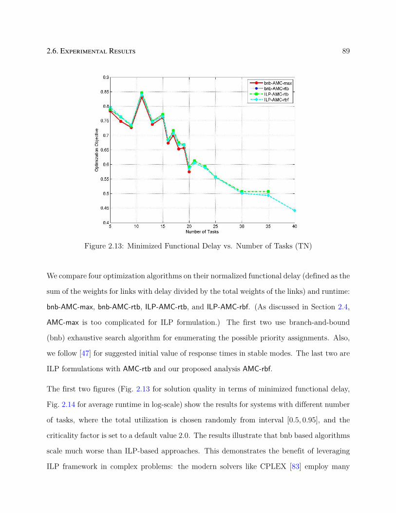
2.6. Experimental Results 89
Figure 2.13: Minimized Functional Delay vs. Number of Tasks (TN)
We compare four optimization algorithms on their normalized functional delay (defined as the
sum of the weights for links with delay divided by the total weights of the links) and runtime:
bnb-AMC-max, bnb-AMC-rtb, ILP-AMC-rtb, and ILP-AMC-rbf. (As discussed in Section 2.4,
AMC-max is too complicated for ILP formulation.) The first two use branch-and-bound
(bnb) exhaustive search algorithm for enumerating the possible priority assignments. Also,
we follow [47] for suggested initial value of response times in stable modes. The last two are
ILP formulations with AMC-rtb and our proposed analysis AMC-rbf.
The first two figures (Fig. 2.13 for solution quality in terms of minimized functional delay,
Fig. 2.14 for average runtime in log-scale) show the results for systems with different number
of tasks, where the total utilization is chosen randomly from interval [0.5, 0.95], and the
criticality factor is set to a default value 2.0. The results illustrate that bnb based algorithms
scale much worse than ILP-based approaches. This demonstrates the benefit of leveraging
ILP framework in complex problems: the modern solvers like CPLEX [83] employ many

90Chapter 2. An Efficient Schedulability Analysis for Optimizing Systems with Adaptive
Mixed-Criticality Scheduling
Figure 2.14: Average Runtime vs. Number of Tasks (TN)
sophisticated techniques and are generally much faster than plain bnb.
While both being ILP-based, ILP-AMC-rbf is about one magnitude faster than ILP-AMC-rtb
and the difference grows larger for bigger systems. This shows that AMC-rbf is much more
efficient in formulating schedulability region. Because AMC-max is more accurate than AMC-
rbf, bnb-AMC-max should always provide a better solution than AMC-rbf based approaches.
However, the maximum sub-optimality for ILP-AMC-rbf is 2.17%, which is in parity with
that of bnb-AMC-rtb or ILP-AMC-rtb (3.34%).
In the rest of the experiment, we focus on the solution quality of the algorithms. bnb-AMC-rtb
is omitted in the comparison since it always gives the same solution as ILP-AMC-rtb. Fig. 2.15
shows the results for 18-task systems with different utilizations, where the criticality factor
is set to 2.0. The normalized delay by ILP-AMC-rbf is almost the same as bnb-AMC-max
with a maximum sub-optimality of 3.14%. Fig. 2.16 performs a similar experiment but
assigns random criticality factors in the range [1.0, 5.5] for each task in the system, where
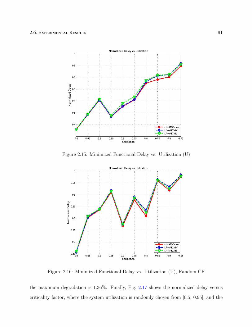
2.6. Experimental Results 91
Figure 2.15: Minimized Functional Delay vs. Utilization (U)
Figure 2.16: Minimized Functional Delay vs. Utilization (U), Random CF
the maximum degradation is 1.36%. Finally, Fig. 2.17 shows the normalized delay versus
criticality factor, where the system utilization is randomly chosen from [0.5, 0.95], and the
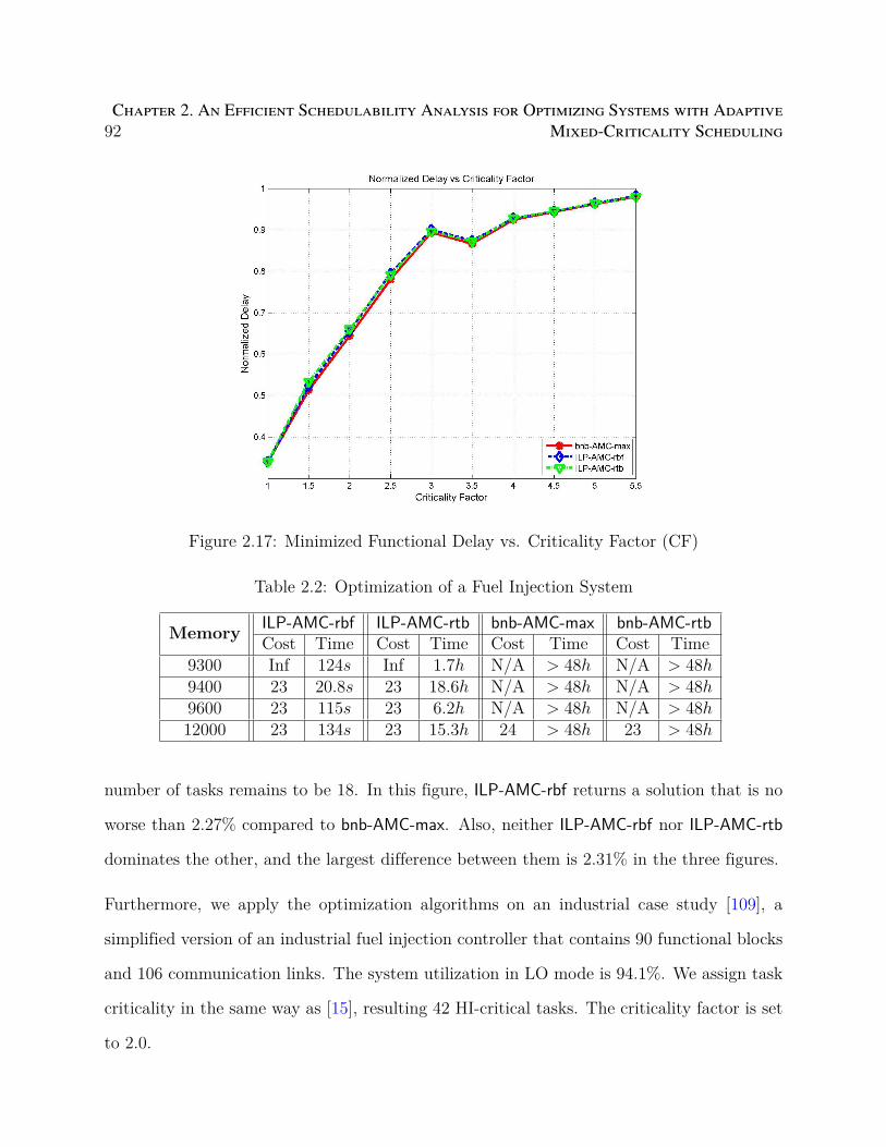
92Chapter 2. An Efficient Schedulability Analysis for Optimizing Systems with Adaptive
Mixed-Criticality Scheduling
Figure 2.17: Minimized Functional Delay vs. Criticality Factor (CF)
Table 2.2: Optimization of a Fuel Injection System
Memory ILP-AMC-rbf ILP-AMC-rtb bnb-AMC-max bnb-AMC-rtbCost Time Cost Time Cost Time Cost Time
9300 Inf 124s Inf 1.7h N/A > 48h N/A > 48h9400 23 20.8s 23 18.6h N/A > 48h N/A > 48h9600 23 115s 23 6.2h N/A > 48h N/A > 48h12000 23 134s 23 15.3h 24 > 48h 23 > 48h
number of tasks remains to be 18. In this figure, ILP-AMC-rbf returns a solution that is no
worse than 2.27% compared to bnb-AMC-max. Also, neither ILP-AMC-rbf nor ILP-AMC-rtb
dominates the other, and the largest difference between them is 2.31% in the three figures.
Furthermore, we apply the optimization algorithms on an industrial case study [109], a
simplified version of an industrial fuel injection controller that contains 90 functional blocks
and 106 communication links. The system utilization in LO mode is 94.1%. We assign task
criticality in the same way as [15], resulting 42 HI-critical tasks. The criticality factor is set
to 2.0.
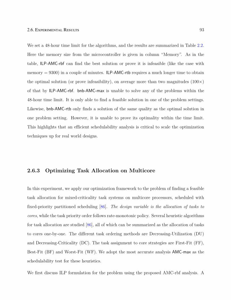
2.6. Experimental Results 93
We set a 48-hour time limit for the algorithms, and the results are summarized in Table 2.2.
Here the memory size from the microcontroller is given in column “Memory”. As in the
table, ILP-AMC-rbf can find the best solution or prove it is infeasible (like the case with
memory = 9300) in a couple of minutes. ILP-AMC-rtb requires a much longer time to obtain
the optimal solution (or prove infeasibility), on average more than two magnitudes (100×)
of that by ILP-AMC-rbf. bnb-AMC-max is unable to solve any of the problems within the
48-hour time limit. It is only able to find a feasible solution in one of the problem settings.
Likewise, bnb-AMC-rtb only finds a solution of the same quality as the optimal solution in
one problem setting. However, it is unable to prove its optimality within the time limit.
This highlights that an efficient schedulability analysis is critical to scale the optimization
techniques up for real world designs.
2.6.3 Optimizing Task Allocation on Multicore
In this experiment, we apply our optimization framework to the problem of finding a feasible
task allocation for mixed-criticality task systems on multicore processors, scheduled with
fixed-priority partitioned scheduling [86]. The design variable is the allocation of tasks to
cores, while the task priority order follows rate-monotonic policy. Several heuristic algorithms
for task allocation are studied [86], all of which can be summarized as the allocation of tasks
to cores one-by-one. The different task ordering methods are Decreasing-Utilization (DU)
and Decreasing-Criticality (DC). The task assignment to core strategies are First-Fit (FF),
Best-Fit (BF) and Worst-Fit (WF). We adopt the most accurate analysis AMC-max as the
schedulability test for these heuristics.
We first discuss ILP formulation for the problem using the proposed AMC-rbf analysis. A

94Chapter 2. An Efficient Schedulability Analysis for Optimizing Systems with Adaptive
Mixed-Criticality Scheduling
set of binary variables ai,k is defined to indicate the mapping of task τi to core k, as follows
ai,k =
1 τi is mapped to core k,
0 otherwise.(2.128)
Since each task must be mapped to exactly one core, we have the following constraints
∀i,K∑k=1
ai,k = 1 (2.129)
We add a redundant constraint that the total utilization for each core (in either LO mode
or HI mode) cannot exceed 100%. It is simple but is effective for removing obviously un-
schedulable solution.
∀k,∑i
ai,k ·Ci(LO)
Ti≤ 1
∧ ∑i:Li=HI
ai,k ·Ci(HI)
Ti≤ 1 (2.130)
The problem should also include the formulation of the schedulability region as follows.
ILP for AMC-rbf. It takes a similar form as (2.53), but the functions G and H need to be
redefined, to add the index of the core k
Gi,k(t) = Ci(HI) · ai,k +∑
j∈hpH(i)
⌈t
Tj
⌉Cj(HI) · aj,k
Hi,k(s) =∑
j∈hpL(i)
(⌊s
Tj
⌋+ 1
)Cj(LO) · aj,k
+∑
j∈hpH(i)
max(0,
⌊s−Dj
Tj
⌋)(Cj(LO)− Cj(HI)) · aj,k
(2.131)
Now the schedulability constraint (2.53) should be modified accordingly, to reflect that a
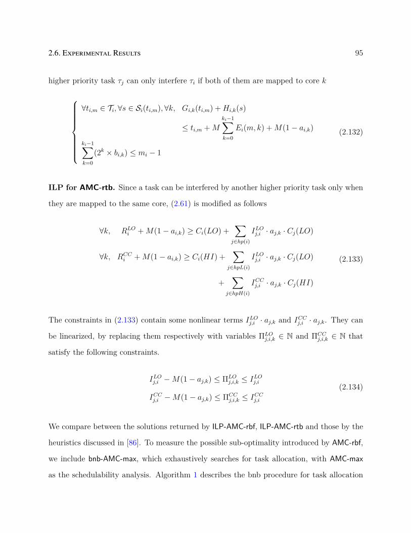
2.6. Experimental Results 95
higher priority task τj can only interfere τi if both of them are mapped to core k
∀ti,m ∈ Ti, ∀s ∈ Si(ti,m),∀k, Gi,k(ti,m) +Hi,k(s)
≤ ti,m +M
ki−1∑k=0
Ei(m, k) +M(1− ai,k)
ki−1∑k=0
(2k × bi,k) ≤ mi − 1
(2.132)
ILP for AMC-rtb. Since a task can be interfered by another higher priority task only when
they are mapped to the same core, (2.61) is modified as follows
∀k, RLOi +M(1− ai,k) ≥ Ci(LO) +
∑j∈hp(i)
ILOj,i · aj,k · Cj(LO)
∀k, RCCi +M(1− ai,k) ≥ Ci(HI) +
∑j∈hpL(i)
ILOj,i · aj,k · Cj(LO)
+∑
j∈hpH(i)
ICCj,i · aj,k · Cj(HI)
(2.133)
The constraints in (2.133) contain some nonlinear terms ILOj,i · aj,k and ICCj,i · aj,k. They can
be linearized, by replacing them respectively with variables ΠLOj,i,k ∈ N and ΠCC
j,i,k ∈ N that
satisfy the following constraints.
ILOj,i −M(1− aj,k) ≤ ΠLOj,i,k ≤ ILOj,i
ICCj,i −M(1− aj,k) ≤ ΠCC
j,i,k ≤ ICCj,i
(2.134)
We compare between the solutions returned by ILP-AMC-rbf, ILP-AMC-rtb and those by the
heuristics discussed in [86]. To measure the possible sub-optimality introduced by AMC-rbf,
we include bnb-AMC-max, which exhaustively searches for task allocation, with AMC-max
as the schedulability analysis. Algorithm 1 describes the bnb procedure for task allocation
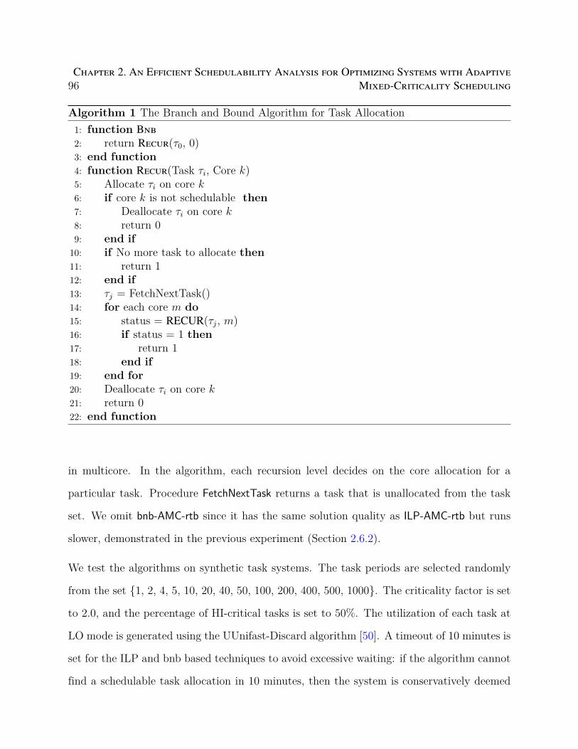
96Chapter 2. An Efficient Schedulability Analysis for Optimizing Systems with Adaptive
Mixed-Criticality Scheduling
Algorithm 1 The Branch and Bound Algorithm for Task Allocation1: function Bnb2: return Recur(τ0, 0)3: end function4: function Recur(Task τi, Core k)5: Allocate τi on core k6: if core k is not schedulable then7: Deallocate τi on core k8: return 09: end if
10: if No more task to allocate then11: return 112: end if13: τj = FetchNextTask()14: for each core m do15: status = RECUR(τj, m)16: if status = 1 then17: return 118: end if19: end for20: Deallocate τi on core k21: return 022: end function
in multicore. In the algorithm, each recursion level decides on the core allocation for a
particular task. Procedure FetchNextTask returns a task that is unallocated from the task
set. We omit bnb-AMC-rtb since it has the same solution quality as ILP-AMC-rtb but runs
slower, demonstrated in the previous experiment (Section 2.6.2).
We test the algorithms on synthetic task systems. The task periods are selected randomly
from the set 1, 2, 4, 5, 10, 20, 40, 50, 100, 200, 400, 500, 1000. The criticality factor is set
to 2.0, and the percentage of HI-critical tasks is set to 50%. The utilization of each task at
LO mode is generated using the UUnifast-Discard algorithm [50]. A timeout of 10 minutes is
set for the ILP and bnb based techniques to avoid excessive waiting: if the algorithm cannot
find a schedulable task allocation in 10 minutes, then the system is conservatively deemed
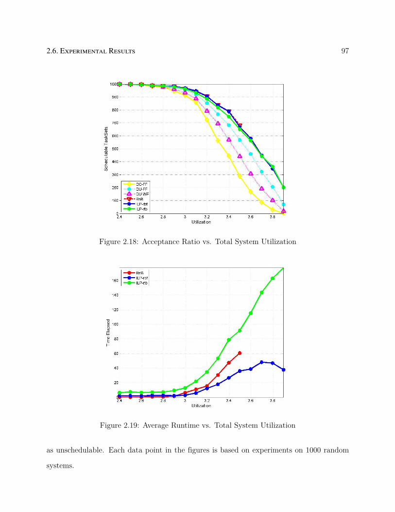
2.6. Experimental Results 97
Figure 2.18: Acceptance Ratio vs. Total System Utilization
Figure 2.19: Average Runtime vs. Total System Utilization
as unschedulable. Each data point in the figures is based on experiments on 1000 random
systems.
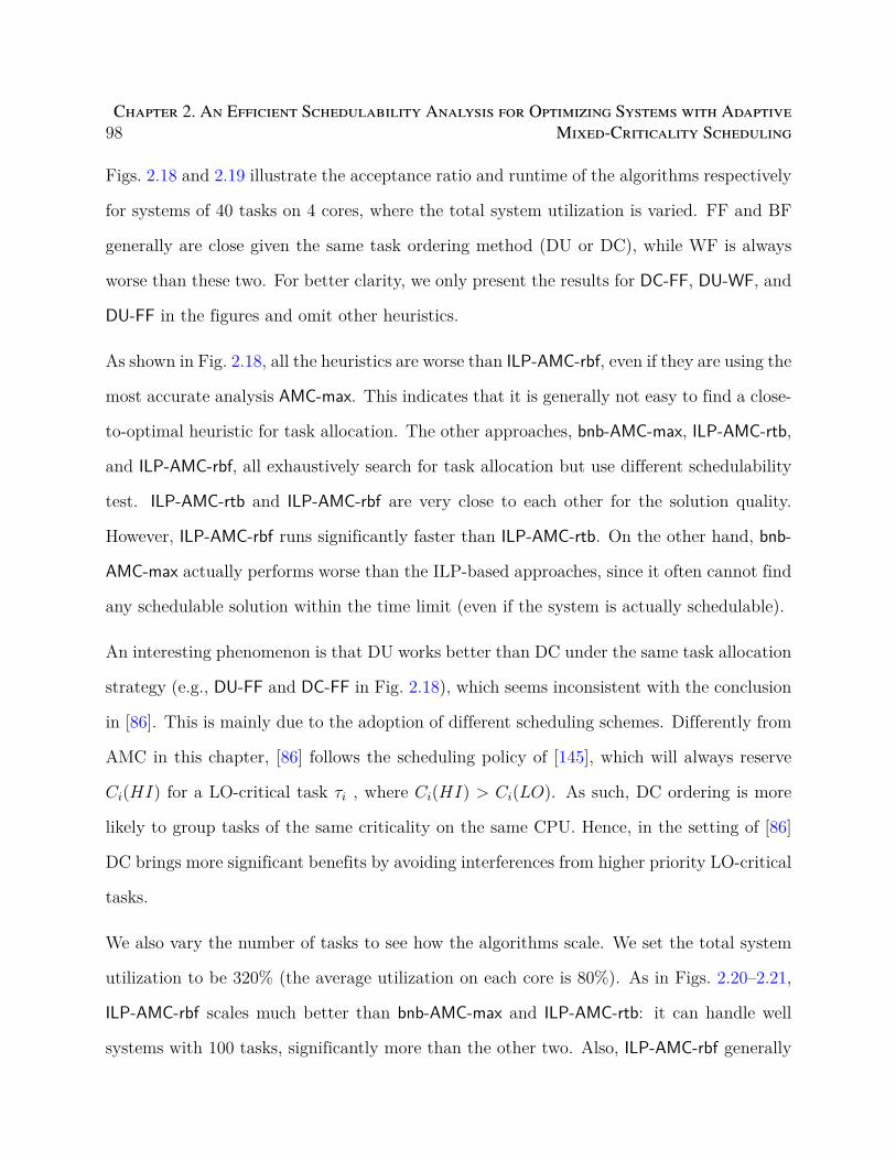
98Chapter 2. An Efficient Schedulability Analysis for Optimizing Systems with Adaptive
Mixed-Criticality Scheduling
Figs. 2.18 and 2.19 illustrate the acceptance ratio and runtime of the algorithms respectively
for systems of 40 tasks on 4 cores, where the total system utilization is varied. FF and BF
generally are close given the same task ordering method (DU or DC), while WF is always
worse than these two. For better clarity, we only present the results for DC-FF, DU-WF, and
DU-FF in the figures and omit other heuristics.
As shown in Fig. 2.18, all the heuristics are worse than ILP-AMC-rbf, even if they are using the
most accurate analysis AMC-max. This indicates that it is generally not easy to find a close-
to-optimal heuristic for task allocation. The other approaches, bnb-AMC-max, ILP-AMC-rtb,
and ILP-AMC-rbf, all exhaustively search for task allocation but use different schedulability
test. ILP-AMC-rtb and ILP-AMC-rbf are very close to each other for the solution quality.
However, ILP-AMC-rbf runs significantly faster than ILP-AMC-rtb. On the other hand, bnb-
AMC-max actually performs worse than the ILP-based approaches, since it often cannot find
any schedulable solution within the time limit (even if the system is actually schedulable).
An interesting phenomenon is that DU works better than DC under the same task allocation
strategy (e.g., DU-FF and DC-FF in Fig. 2.18), which seems inconsistent with the conclusion
in [86]. This is mainly due to the adoption of different scheduling schemes. Differently from
AMC in this chapter, [86] follows the scheduling policy of [145], which will always reserve
Ci(HI) for a LO-critical task τi , where Ci(HI) > Ci(LO). As such, DC ordering is more
likely to group tasks of the same criticality on the same CPU. Hence, in the setting of [86]
DC brings more significant benefits by avoiding interferences from higher priority LO-critical
tasks.
We also vary the number of tasks to see how the algorithms scale. We set the total system
utilization to be 320% (the average utilization on each core is 80%). As in Figs. 2.20–2.21,
ILP-AMC-rbf scales much better than bnb-AMC-max and ILP-AMC-rtb: it can handle well
systems with 100 tasks, significantly more than the other two. Also, ILP-AMC-rbf generally

2.6. Experimental Results 99
Figure 2.20: Acceptance Ratio vs. Number of Tasks
Figure 2.21: Average Runtime vs. Number of Tasks
performs better than bnb-AMC-max and ILP-AMC-rtb at larger systems as the other two often
hit the time limit and return unschedulability prematurely. The largest sub-optimality for
100Chapter 2. An Efficient Schedulability Analysis for Optimizing Systems with Adaptive
Mixed-Criticality Scheduling
ILP-AMC-rbf is at the case of systems with 20 number of tasks, where bnb-AMC-max is 4%
better in schedulable tasks. This demonstrates that AMC-rbf, while losing a small amount
of accuracy on schedulability analysis, is more scalable to large systems, hence more suitable
for optimization process.
2.7 Conclusion
In this work, we presented a schedulability analysis method based on request bound function
for AMC-scheduled mixed-criticality systems. The new analysis is safe and has bounded
pessimism compared to AMC-max, but it allows efficient formulation of the schedulability
region for optimization purposes. Experiments show that our optimization framework based
on the new analysis is able to provide close-to-optimal solutions and scale to large designs.
Chapter 3
The Concept of Unschedulability Core
for Optimizing Real-Time Systems
with Fixed-Priority Scheduling
3.1 Introduction
The design of real-time embedded systems is often subject to many requirements and ob-
jectives in addition to real-time schedulability constraints, including limited resources (e.g.,
memory), cost, quality of control, and energy consumption. For example, the automotive
industry is hard pressed to deliver products with low cost, due to the large volume and the
competitive international market [38]. Similarly, technology innovations for medical devices
are mainly driven by reduced size, weight, and power (SWaP) [23]. In these application
domains, it is important to perform design optimization in order to find the best design (i.e.,
optimized according to an objective function) while satisfying all the critical requirements.
Formally, a design optimization problem is defined by decision variables, constraints, and
an objective function. The decision variables represent the set of design parameters that
the designer hope to optimize. The set of constraints represents the requirements that the
design and the choice of design parameters have to satisfied. They form the domain of the
101

102Chapter 3. The Concept of Unschedulability Core for Optimizing Real-Time Systems
with Fixed-Priority Scheduling
allowed values for the decision variables. The objective function represents the concerned
design metrics. In general, design optimization needs to solve an optimization problem for
decision variables w.r.t the objective function within the feasibility region. For real-time
systems, the feasibility region (also called schedulability region if concerning only real-time
schedulability) must only contain the designs that satisfy the schedulability constraints where
each task completes before its deadline.
In this chapter, we consider the design optimization for real-time systems scheduled with
fixed priority. The decision variables may include task priority assignment and the selection
of mechanisms to ensure data consistency of shared variables. Besides real-time schedulabil-
ity, these problems often contain constraints or an objective function related to other metrics
(such as memory, power, thermal, etc.). Typically, this makes the problem complexity NP-
hard, including the two case studies in this chapter: the optimization of mixed-criticality
Simulink models with Adaptive Mixed Criticality (AMC) scheduling (Section 3.7.1), and
the memory minimization in the implementation of automotive AUTOSAR models (Sec-
tion 3.7.2). Below we provide a summary of related work, focusing on the underlining
approach but not intended to be complete.
3.1.1 Related Work
There is a large body of work on priority assignment for real-time systems with fixed pri-
ority scheduling. In particular, Audsley’s algorithm [8] is proven to be “optimal” for many
task models and scheduling schemes, if the designer is only concerned to find a schedulable
solution. See a recent survey by Davis et al. [53] on a complete list of applicable settings.
However, if the design optimization problem contains constraints or an objective function
related to other metrics (such as memory, power, thermal, etc.), Audsley’s algorithm is no

3.1. Introduction 103
longer guaranteed to be optimal.
In general, the current approaches for optimizing priority assignment in complex design
optimization problems (i.e., those without known polynomial-time optimal algorithms) can
be classified into three categories. The first is based on meta heuristics such as simulated
annealing (e.g., [22, 142]) and genetic algorithm (e.g., [75]). The second is to develop problem
specific heuristics (e.g., [127, 146, 156]). These two categories do not have any guarantee on
optimality.
The third category is to search for the exact optimum, often applying existing optimization
frameworks such as branch-and-bound (BnB) (e.g., [147]), or integer linear programming
(ILP) (e.g., [169]). However, this approach typically suffers from scalability issues and may
have difficulty to handle large industrial designs. For example, automotive engine control
system contains over a hundred functional blocks [120], but the ILP based approach can
only scale up to about 40 functional blocks (see Section 3.7). Furthermore, not all problems
can easily be formulated in a particular framework due to the complexity of schedulability
conditions. For example, the exact schedulability analysis for tasks with non-preemptive
scheduling requires to check all the task instances in the busy period, but the number of
instances is unknown a priori. Hence, it is difficult to formulate the exact schedulability
constraints in ILP [155].
The above existing mindset is also followed by optimization of problems with other decision
variables, such as the selection of mechanisms for protection of shared memory buffers [153],
the mapping of functional blocks to tasks [55], and the use of rate transition buffers for
semantics preservation in Simulink models [109]. Different from all existing work, our ap-
proach is to develop a domain-specific optimization framework that is optimal, scalable, yet
still applicable to a large class of real-time systems.
104Chapter 3. The Concept of Unschedulability Core for Optimizing Real-Time Systems
with Fixed-Priority Scheduling
3.1.2 Contributions and Chapter Structure
In this chapter, instead of directly reusing standard techniques (BnB, ILP, etc.), we present
customized optimization techniques for real-time systems with fixed priority scheduling.
Our framework can guarantee the optimality of the solution while drastically improving the
scalability. Specifically, we make the following contributions:
• We propose the concept of unschedulability core, an abstraction of the schedulability
conditions in real-time systems scheduled with fixed priority. It can be represented by
a set of new and compact constraints to be learned efficiently during the execution of
the optimization procedure (i.e., at runtime).
• We devise an optimization procedure that judiciously utilizes the unschedulability cores
to drastically improve the scalability.
• We use two design optimization problems to illustrate the benefit of the proposed
approach. The new unschedulability core guided optimization algorithm runs several
orders of magnitude faster than other optimal algorithms (BnB, ILP) while maintaining
the optimality of the solutions.
The rest of the chapter is organized as follows. From Section 3.2 to Section 3.4, we first con-
sider the optimization problems that assign priority orders to tasks. Specifically, Section 3.2
describes the task models and gives a formal definition of the problems that are suitable
for the proposed approach. Section 3.3 defines the concept of unschedulability core that
contains a set of partial priority orders among tasks, and studies its efficient calculation.
Section 3.4 presents the optimization procedure that leverages the unschedulability cores for
optimizing priority assignment, with proven properties on termination and optimality. In
Section 3.5, we extend the framework to optimization problems with other decision variables.
3.2. Preliminary 105
We generalize the concept of unschedulability core that allows to take problem-specific in-
terpretations. We also discuss the applicability and efficiency for the proposed optimization
framework. Section 3.6 gives two examples of application. Section 3.7 evaluates the effective-
ness of the proposed approach with industrial case studies and synthetic systems. Finally,
Section 3.8 concludes the chapter.
3.2 Preliminary
We consider a real-time system scheduled by fixed priority. It consists of a set of tasks
Γ = τ1, τ2, ...τn. Each task τi is assumed to have a unique priority πi (the higher the number,
the higher the priority) to be assigned by the designer. The concept of unschedulability core
applies to any systems scheduled with fixed priority. However, its application in design
optimization is most effective when there is a simple algorithm to determine the existence
of a schedulable priority assignment for a given task set. Hence, we consider a list of task
models and scheduling schemes where Audsley’s algorithm [8] is applicable (i.e., it can find a
schedulable priority assignment if there exists one). The list, as summarized in [53], includes
a large number of task models and scheduling schemes:
• The periodic task model, where independent tasks are scheduled on a single-core plat-
form with preemptive scheduling. Each task is characterized by a tuple of parameters:
Ti denotes the period; Di = Ti represents the implicit relative deadline; Ci denotes the
worst-case execution time (WCET).
• Tasks with arbitrary deadlines, and/or static offsets.
• Probabilistic real-time systems where task WCETs are described by independent ran-
dom variables [3].

106Chapter 3. The Concept of Unschedulability Core for Optimizing Real-Time Systems
with Fixed-Priority Scheduling
• Systems scheduled with deferred preemption [49].
• Tasks modeled as arbitrary digraphs [137], where the vertices represent different kinds
of jobs, and the edges represent the possible flows of control.
• Tasks accessing shared resources protected by semaphore locks to ensure mutual ex-
clusion.
We note that Audsley’s algorithm runs very efficiently: out of the possible n! priority as-
signments, it only needs to explore O(n2) of them.
A priority assignment can be represented using a set of binary variables P = pi,j|i =
j, τi, τj ∈ Γ denoting the partial priority orders among tasks, where pi,j is defined as
pi,j =
1 πi > πj,
0 otherwise.(3.1)
A priority assignment shall satisfy the antisymmetric and transitive properties: If τi has a
higher priority than τj (pi,j = 1), then τj has a lower priority than τi (pj,i = 0); If τi has a
higher priority than τj (pi,j = 1) and τj has a higher priority than τk (pj,k = 1), then τi must
have a higher priority than τk (pi,k = 1). These properties can be formally formulated as
Antisymmetry: pi,j + pj,i = 1, ∀i = j
Transitivity: pi,j + pj,k ≤ 1 + pi,k, ∀i = j = k(3.2)
We first focus on a design optimization problem where the decision variables X include the
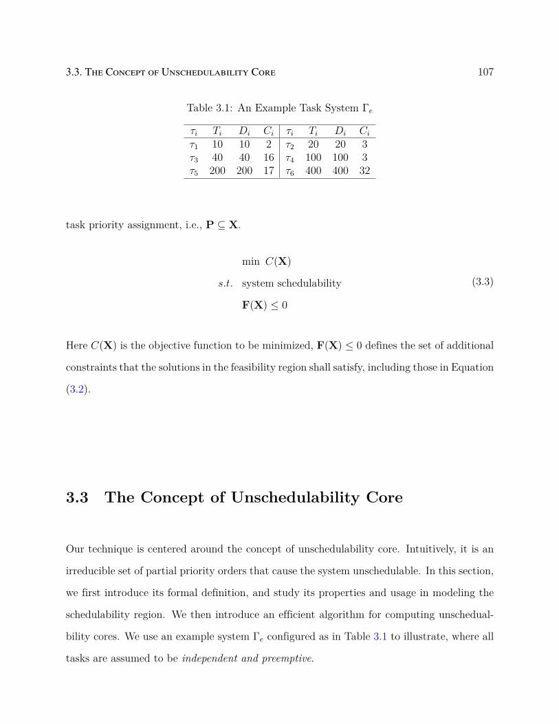
3.3. The Concept of Unschedulability Core 107
Table 3.1: An Example Task System Γe
τi Ti Di Ci τi Ti Di Ci
τ1 10 10 2 τ2 20 20 3τ3 40 40 16 τ4 100 100 3τ5 200 200 17 τ6 400 400 32
task priority assignment, i.e., P ⊆ X.
min C(X)
s.t. system schedulability
F(X) ≤ 0
(3.3)
Here C(X) is the objective function to be minimized, F(X) ≤ 0 defines the set of additional
constraints that the solutions in the feasibility region shall satisfy, including those in Equation
(3.2).
3.3 The Concept of Unschedulability Core
Our technique is centered around the concept of unschedulability core. Intuitively, it is an
irreducible set of partial priority orders that cause the system unschedulable. In this section,
we first introduce its formal definition, and study its properties and usage in modeling the
schedulability region. We then introduce an efficient algorithm for computing unschedual-
bility cores. We use an example system Γe configured as in Table 3.1 to illustrate, where all
tasks are assumed to be independent and preemptive.
108Chapter 3. The Concept of Unschedulability Core for Optimizing Real-Time Systems
with Fixed-Priority Scheduling
3.3.1 Definition of Unschedulability Core
Definition 2. A partial priority order (PPO), denoted as ri,j ≡ (πi > πj) ≡ (pi,j =
1), defines a priority order that τi has a higher priority than τj. A PPO set R =
ri1,j1 , ri2,j2 , ..., rim,jm is a collection of one or more partial priority orders that are con-
sistent with the properties in Equation (3.2). The number of elements in R is defined as its
cardinality, denoted as |R|.
Definition 3. Let Γ be a task system and R be a PPO set on Γ. Γ is R-schedulable if
and only if there exists a feasible priority assignment P that respects all elements (i.e., all
partial priority orders) in R.
For convenience, we also say that “R is schedulable” when Γ is R-schedulable, and similarly
“R is unschedulable” when Γ is not R-schedulable.
Example 3.1. Consider the system Γe in Table 3.1 and two PPO sets R1 = r1,2, r2,3,
R2 = r5,4, r4,3. Γe is R1-schedulable, since the system is schedulable under rate-monotonic
priority assignment which respects R1. However, Γe is not R2-schedulable: τ1 must have a
higher priority than τ3 (due to C3 > D1), hence assigning τ4 and τ5 with higher priority than
τ3 will make τ3 miss its deadline.
The following theorem intuitively states that if the system is schedulable for a PPO set, then
the system is also schedulable for any of its subset.
Theorem 16. Let R and R′ be two PPO sets on Γ such that R′ ⊆ R. The following always
holds
Γ is R-schedulable =⇒ Γ is R′-schedulable (3.4)
The proof is straightforward as any priority assignment satisfying R must also satisfy R′.

3.3. The Concept of Unschedulability Core 109
Applying the law of contrapositive on Theorem 16, we have that for any R′ ⊆ R,
Γ is not R′-schedulable =⇒ Γ is not R-schedulable (3.5)
We now give the definition of unschedulability core. Intuitively, it is an unschedulable PPO
set that is irreducible, such that removing any element from it allows a schedulable priority
assignment.
Definition 4. Let Γ be a task system and R be a PPO set on Γ. R is an unschedulability
core for Γ if and only if R satisfies the following two conditions:
• Γ is not R-schedulable;
• ∀R′ ⊂ R, Γ is R′-schedulable.
Remark 3.2. By Theorem 16, the second condition in Definition 4 can be replaced by
• ∀R′ ⊂ R s.t. |R′| = |R| − 1, Γ is R′-schedulable.
Example 3.3. Consider the PPO set R3 = r5,4, r4,3, r3,6, which equivalently defines the
priority order π5 > π4 > π3 > π6. Obviously, Γe is not R3-schedulable as it is not schedulable
for the subset R2 = r5,4, r4,3 of R3 (see Example 3.1). However, R3 is not an unschedu-
lability core since it has a proper subset R2 for which Γe is not schedulable. R2 is a valid
unschedulability core, as for each of its proper subset, there exists a respecting feasible pri-
ority assignment: P = [π1 > π2 > π3 > π5 > π4 > π6] respects R(1)2 = r5,4 and R(2)
2 = ∅,
and P ′ = [π1 > π2 > π4 > π3 > π5 > π6] respects R(3)2 = r4,3.
Let U denote an unschedulability core. The constraint that the PPOs in U cannot be
simultaneously satisfied is: ∑ri,j∈U
pi,j ≤ |U| − 1 (3.6)

110Chapter 3. The Concept of Unschedulability Core for Optimizing Real-Time Systems
with Fixed-Priority Scheduling
Remark 3.4. An unschedulability core U essentially gives a necessary condition for schedu-
lability, that any feasible priority assignment shall differ from U for at least one partial
priority order. Constraint (3.6) captures such requirement and is much more friendly to ILP
solver. Its coefficients on the left hand side are all small integers (0 or 1), which in many
cases makes the ILP solver more efficient [96].
We now prove that the set of all unschedulability cores is a necessary and sufficient condition
that makes the system unschedulable.
Lemma 17. Let Γ be a schedulable task system and R be a PPO set on Γ. Γ is not
R-schedulable if and only if R contains at least one unschedulability core.
Proof. “If” Part: It is straightforward by the definition of unschedulability core and the
result in Equation (3.5).
“Only If” Part: Proof by induction on the cardinality of R.
Base case. Let R be any PPO set such that |R| = 1 and Γ is not R-schedulable. The only
proper subset of R is R′ = ∅. Since Γ is schedulable, R itself is an unschedulability core.
Inductive step. Assume any PPO set of cardinality from 1 to k − 1 such that Γ is not
schedulable contains an unschedulability core. We prove that anyR of cardinality k such that
Γ is not R-schedulable shall contain an unschedulability core. By Definition 4, there must
exist R′ ⊂ R such that Γ is not R′-schedulable (otherwise, R itself is an unschedulability
core). Now we consider R′, which has a cardinality smaller than k. By the assumption for
the inductive step, R′ contains an unschedulability core, so does R.
Theorem 18. Let U denote the complete set of unschedulability cores. The exact feasibility
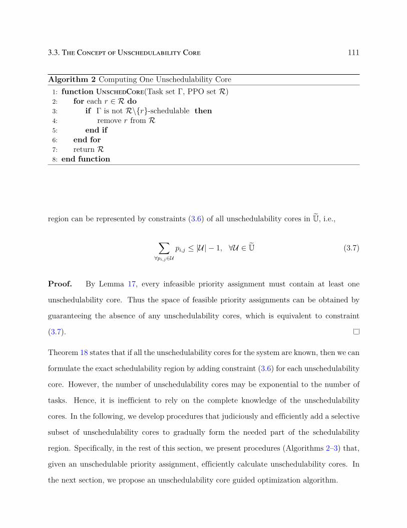
3.3. The Concept of Unschedulability Core 111
Algorithm 2 Computing One Unschedulability Core1: function UnschedCore(Task set Γ, PPO set R)2: for each r ∈ R do3: if Γ is not R\r-schedulable then4: remove r from R5: end if6: end for7: return R8: end function
region can be represented by constraints (3.6) of all unschedulability cores in U, i.e.,
∑∀pi,j∈U
pi,j ≤ |U| − 1, ∀U ∈ U (3.7)
Proof. By Lemma 17, every infeasible priority assignment must contain at least one
unschedulability core. Thus the space of feasible priority assignments can be obtained by
guaranteeing the absence of any unschedulability cores, which is equivalent to constraint
(3.7).
Theorem 18 states that if all the unschedulability cores for the system are known, then we can
formulate the exact schedulability region by adding constraint (3.6) for each unschedulability
core. However, the number of unschedulability cores may be exponential to the number of
tasks. Hence, it is inefficient to rely on the complete knowledge of the unschedulability
cores. In the following, we develop procedures that judiciously and efficiently add a selective
subset of unschedulability cores to gradually form the needed part of the schedulability
region. Specifically, in the rest of this section, we present procedures (Algorithms 2–3) that,
given an unschedulable priority assignment, efficiently calculate unschedulability cores. In
the next section, we propose an unschedulability core guided optimization algorithm.
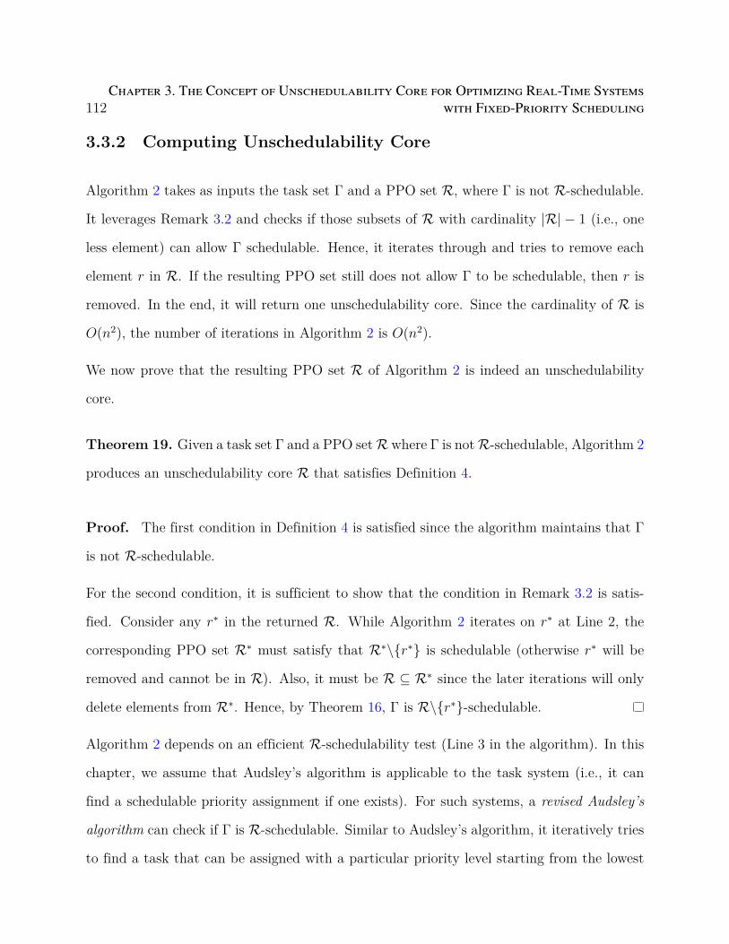
112Chapter 3. The Concept of Unschedulability Core for Optimizing Real-Time Systems
with Fixed-Priority Scheduling
3.3.2 Computing Unschedulability Core
Algorithm 2 takes as inputs the task set Γ and a PPO set R, where Γ is not R-schedulable.
It leverages Remark 3.2 and checks if those subsets of R with cardinality |R| − 1 (i.e., one
less element) can allow Γ schedulable. Hence, it iterates through and tries to remove each
element r in R. If the resulting PPO set still does not allow Γ to be schedulable, then r is
removed. In the end, it will return one unschedulability core. Since the cardinality of R is
O(n2), the number of iterations in Algorithm 2 is O(n2).
We now prove that the resulting PPO set R of Algorithm 2 is indeed an unschedulability
core.
Theorem 19. Given a task set Γ and a PPO setR where Γ is notR-schedulable, Algorithm 2
produces an unschedulability core R that satisfies Definition 4.
Proof. The first condition in Definition 4 is satisfied since the algorithm maintains that Γ
is not R-schedulable.
For the second condition, it is sufficient to show that the condition in Remark 3.2 is satis-
fied. Consider any r∗ in the returned R. While Algorithm 2 iterates on r∗ at Line 2, the
corresponding PPO set R∗ must satisfy that R∗\r∗ is schedulable (otherwise r∗ will be
removed and cannot be in R). Also, it must be R ⊆ R∗ since the later iterations will only
delete elements from R∗. Hence, by Theorem 16, Γ is R\r∗-schedulable.
Algorithm 2 depends on an efficient R-schedulability test (Line 3 in the algorithm). In this
chapter, we assume that Audsley’s algorithm is applicable to the task system (i.e., it can
find a schedulable priority assignment if one exists). For such systems, a revised Audsley’s
algorithm can check if Γ is R-schedulable. Similar to Audsley’s algorithm, it iteratively tries
to find a task that can be assigned with a particular priority level starting from the lowest
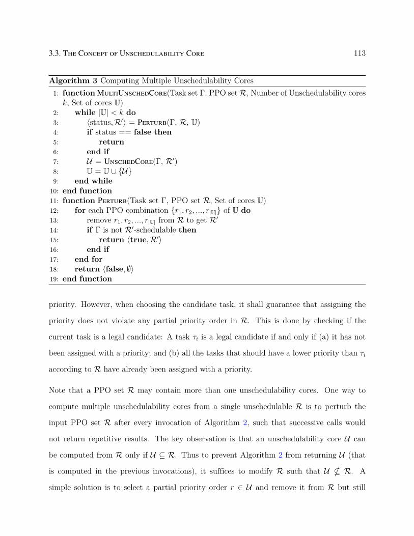
3.3. The Concept of Unschedulability Core 113
Algorithm 3 Computing Multiple Unschedulability Cores1: function MultiUnschedCore(Task set Γ, PPO setR, Number of Unschedulability cores
k, Set of cores U)2: while |U| < k do3: ⟨status,R′⟩ = Perturb(Γ, R, U)4: if status == false then5: return6: end if7: U = UnschedCore(Γ, R′)8: U = U ∪ U9: end while
10: end function11: function Perturb(Task set Γ, PPO set R, Set of cores U)12: for each PPO combination r1, r2, ..., r|U| of U do13: remove r1, r2, ..., r|U| from R to get R′
14: if Γ is not R′-schedulable then15: return ⟨true,R′⟩16: end if17: end for18: return ⟨false, ∅⟩19: end function
priority. However, when choosing the candidate task, it shall guarantee that assigning the
priority does not violate any partial priority order in R. This is done by checking if the
current task is a legal candidate: A task τi is a legal candidate if and only if (a) it has not
been assigned with a priority; and (b) all the tasks that should have a lower priority than τi
according to R have already been assigned with a priority.
Note that a PPO set R may contain more than one unschedulability cores. One way to
compute multiple unschedulability cores from a single unschedulable R is to perturb the
input PPO set R after every invocation of Algorithm 2, such that successive calls would
not return repetitive results. The key observation is that an unschedulability core U can
be computed from R only if U ⊆ R. Thus to prevent Algorithm 2 from returning U (that
is computed in the previous invocations), it suffices to modify R such that U ⊈ R. A
simple solution is to select a partial priority order r ∈ U and remove it from R but still

114Chapter 3. The Concept of Unschedulability Core for Optimizing Real-Time Systems
with Fixed-Priority Scheduling
keep the resulting R unschedulable. In this sense, given a U ⊆ R, there can be |U| different
modifications of R such that R ⊉ U (i.e., each by removing a different r ∈ U from R).
Accordingly, given a set of already computed unschedulability cores U = U1, ...U|U|, there
can be Π|U|i=1|Ui| different modifications to ensure that R ⊉ Ui,∀Ui ∈ U. It may be necessary
to examine each of them to find one modification that still maintains R to be unschedulable.
The new unschedulability core is guaranteed to be different from any Ui ∈ U.
Algorithm 3 details a procedure for computing multiple unschedulability cores from an un-
schedulable PPO set R. It takes as inputs the system Γ, a PPO set R, the desired number
of unschedulability cores k to compute, and U for storing computed unschedulability cores.
Algorithm 3 leverages a subroutine Perturb, which explores all possible PPO combinations
r1, r2, ..., r|U| consisting of one PPO ri from each unschedulability core Ui in U (Lines 12–
17). For each PPO combination, it removes the elements in the PPO combination from R
(Line 13). If any resulting PPO set is unschedulable, then the subroutine Perturb returns
true and an R′ that leads to a new unschedulability core (Lines 14–16). Otherwise, it returns
false to indicate there is no more unschedulability core.
In case Perturb returns true and an R′, Algorithm 3 uses Algorithm 2 to compute a new
unschedulability core and adds it to the set U (Lines 7–8). It iterates until k unschedulability
cores are found or there is no more unschedulability core (in which case Perturb returns
false).
3.4. Unschedulability Core Guided Optimization Algorithm 115
3.4 Unschedulability Core Guided Optimization Algo-
rithm
In this section, we develop a domain-specific optimization algorithm that leverages the con-
cept of unschedulability core. As discussed earlier, finding all the unschedulability cores
can form the complete schedulability region, but this is impractical due to their exponential
growth with the system size. However, we observe that the optimization objective may be
sensitive to only a small set of unschedulability cores. Hence, we consider the lazy constraint
paradigm that only selectively adds unschedulability cores into the problem formulation. The
paradigm starts with a relaxed problem that leaves out all the schedulability constraints.
That is, the schedulability constraints are temporarily put in a lazy constraint pool. A
constraint from the pool is added back only if it is violated by the solution returned for
the relaxed problem. In addition, instead of adding the violated schedulability constraints
back, we leverage the concept of unschedulability core to provide a much more compact
representation of these constraints. In the following, we first details the proposed algorithm
and then discusses its benefits compared with existing approaches.
3.4.1 Optimization Algorithm
The proposed procedure is summarized in Algorithm 4. It takes as inputs the task system
Γ and an integer number k which denotes the maximum number of unschedulability cores
to compute for each unschedulable solution (see Remark 3.5 below). The algorithm works
as follows.
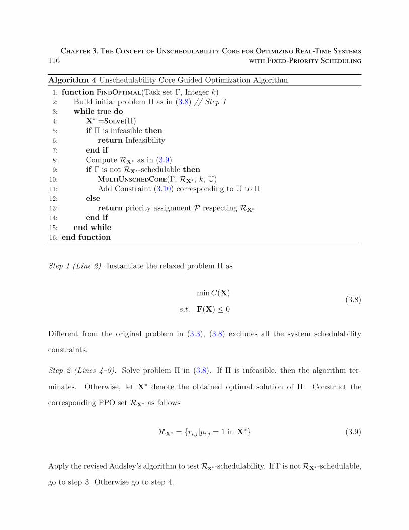
116Chapter 3. The Concept of Unschedulability Core for Optimizing Real-Time Systems
with Fixed-Priority Scheduling
Algorithm 4 Unschedulability Core Guided Optimization Algorithm1: function FindOptimal(Task set Γ, Integer k)2: Build initial problem Π as in (3.8) // Step 13: while true do4: X∗ =Solve(Π)5: if Π is infeasible then6: return Infeasibility7: end if8: Compute RX∗ as in (3.9)9: if Γ is not RX∗-schedulable then
10: MultiUnschedCore(Γ, RX∗ , k, U)11: Add Constraint (3.10) corresponding to U to Π12: else13: return priority assignment P respecting RX∗
14: end if15: end while16: end function
Step 1 (Line 2). Instantiate the relaxed problem Π as
minC(X)
s.t. F(X) ≤ 0(3.8)
Different from the original problem in (3.3), (3.8) excludes all the system schedulability
constraints.
Step 2 (Lines 4–9). Solve problem Π in (3.8). If Π is infeasible, then the algorithm ter-
minates. Otherwise, let X∗ denote the obtained optimal solution of Π. Construct the
corresponding PPO set RX∗ as follows
RX∗ = ri,j|pi,j = 1 in X∗ (3.9)
Apply the revised Audsley’s algorithm to testRx∗-schedulability. If Γ is notRX∗-schedulable,
go to step 3. Otherwise go to step 4.
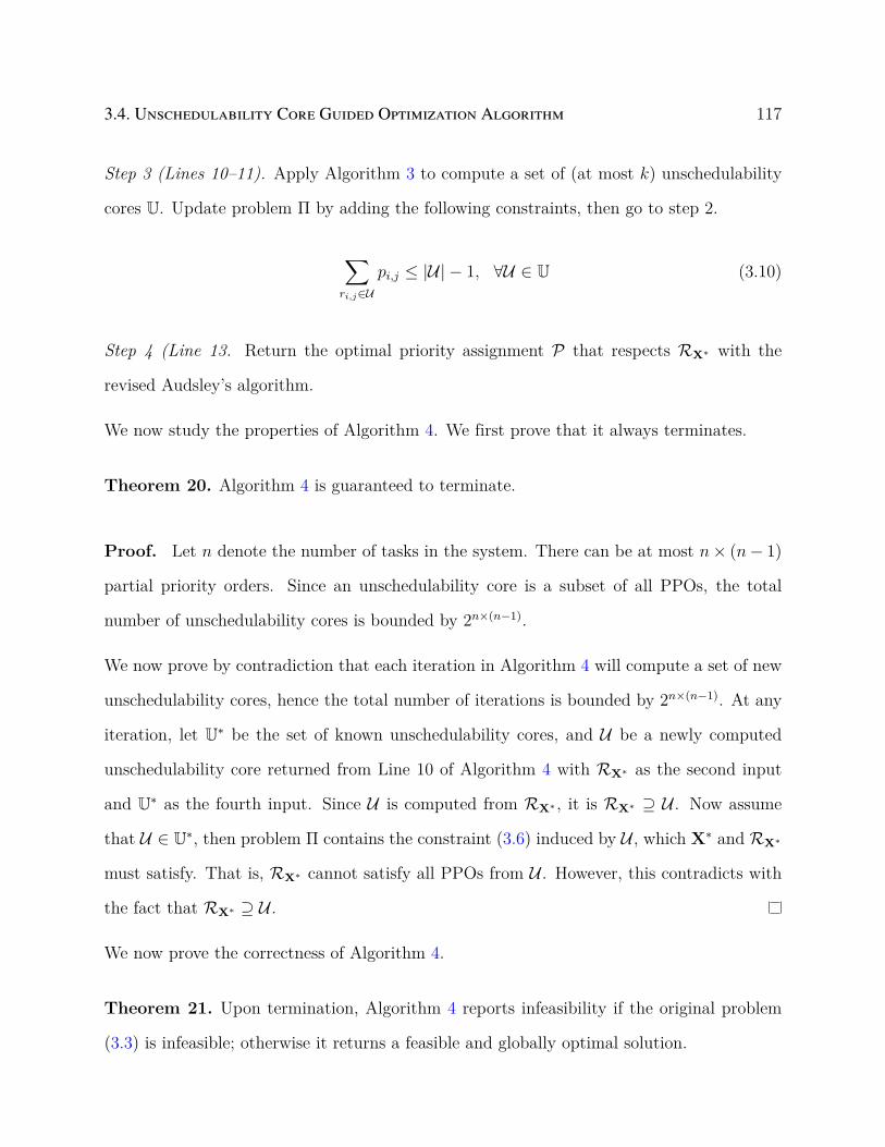
3.4. Unschedulability Core Guided Optimization Algorithm 117
Step 3 (Lines 10–11). Apply Algorithm 3 to compute a set of (at most k) unschedulability
cores U. Update problem Π by adding the following constraints, then go to step 2.
∑ri,j∈U
pi,j ≤ |U| − 1, ∀U ∈ U (3.10)
Step 4 (Line 13. Return the optimal priority assignment P that respects RX∗ with the
revised Audsley’s algorithm.
We now study the properties of Algorithm 4. We first prove that it always terminates.
Theorem 20. Algorithm 4 is guaranteed to terminate.
Proof. Let n denote the number of tasks in the system. There can be at most n× (n− 1)
partial priority orders. Since an unschedulability core is a subset of all PPOs, the total
number of unschedulability cores is bounded by 2n×(n−1).
We now prove by contradiction that each iteration in Algorithm 4 will compute a set of new
unschedulability cores, hence the total number of iterations is bounded by 2n×(n−1). At any
iteration, let U∗ be the set of known unschedulability cores, and U be a newly computed
unschedulability core returned from Line 10 of Algorithm 4 with RX∗ as the second input
and U∗ as the fourth input. Since U is computed from RX∗ , it is RX∗ ⊇ U . Now assume
that U ∈ U∗, then problem Π contains the constraint (3.6) induced by U , which X∗ and RX∗
must satisfy. That is, RX∗ cannot satisfy all PPOs from U . However, this contradicts with
the fact that RX∗ ⊇ U .
We now prove the correctness of Algorithm 4.
Theorem 21. Upon termination, Algorithm 4 reports infeasibility if the original problem
(3.3) is infeasible; otherwise it returns a feasible and globally optimal solution.

118Chapter 3. The Concept of Unschedulability Core for Optimizing Real-Time Systems
with Fixed-Priority Scheduling
Proof. Since each iteration of Algorithm 4 computes only a subset of all unschedulability
cores, the algorithm adds only a subset of the constraints in (3.7) to Π. By Theorem 18,
the feasibility region of Π is always maintained to be an over-approximation of that of the
original problem. We consider the following two cases on how Algorithm 4 terminates.
Case 1: The algorithm terminates at Line 6. This means that problem Π is infeasible. Since
the feasibility region of Π is always no smaller than that of the original problem, the original
problem must be infeasible as well.
Case 2: The algorithm exists at Line 13. Line 13 is reached only when the system is RX∗-
schedulable, which by Definition 3 is a stricter condition on schedulability. Thus the returned
P is guaranteed to be feasible. Since an optimal solution in the over-approximated region
that is also feasible must be optimal in the exact feasibility region, the returned priority
assignment is guaranteed to be optimal.
Remark 3.5. The parameter k in Algorithm 4 does not affect the optimality of the algo-
rithm, but influences its runtime. If k is too small, the algorithm may need many iterations to
terminate, which incurs solving a large number of problem Π. If k is too large, Algorithm 3
may need to explore numerous PPO combinations. In Section 3.7, we will use dedicated
experiments to study the best choice of k.
We now illustrate Algorithm 4 by applying it to the example Γe in Table 3.1, where the
parameter k is set to 1.
Example 3.6. Consider the following objective function
C(X) = −p3,1 − p4,1 − p4,2 − p4,3 − p5,4 (3.11)
The algorithm constructs the relaxed problem Π as (3.8), where F(X) ≤ 0 only contains the
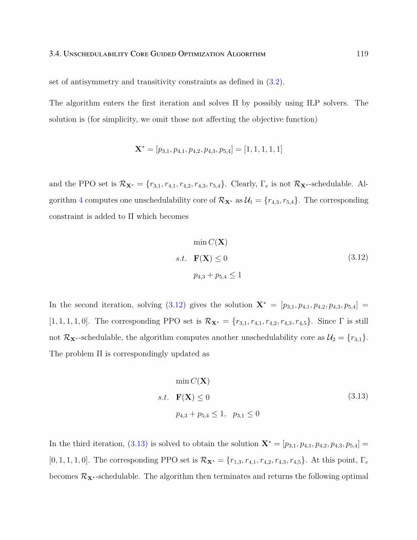
3.4. Unschedulability Core Guided Optimization Algorithm 119
set of antisymmetry and transitivity constraints as defined in (3.2).
The algorithm enters the first iteration and solves Π by possibly using ILP solvers. The
solution is (for simplicity, we omit those not affecting the objective function)
X∗ = [p3,1, p4,1, p4,2, p4,3, p5,4] = [1, 1, 1, 1, 1]
and the PPO set is RX∗ = r3,1, r4,1, r4,2, r4,3, r5,4. Clearly, Γe is not RX∗-schedulable. Al-
gorithm 4 computes one unschedulability core of RX∗ as U1 = r4,3, r5,4. The corresponding
constraint is added to Π which becomes
minC(X)
s.t. F(X) ≤ 0
p4,3 + p5,4 ≤ 1
(3.12)
In the second iteration, solving (3.12) gives the solution X∗ = [p3,1, p4,1, p4,2, p4,3, p5,4] =
[1, 1, 1, 1, 0]. The corresponding PPO set is RX∗ = r3,1, r4,1, r4,2, r4,3, r4,5. Since Γ is still
not RX∗-schedulable, the algorithm computes another unschedulability core as U2 = r3,1.
The problem Π is correspondingly updated as
minC(X)
s.t. F(X) ≤ 0
p4,3 + p5,4 ≤ 1, p3,1 ≤ 0
(3.13)
In the third iteration, (3.13) is solved to obtain the solution X∗ = [p3,1, p4,1, p4,2, p4,3, p5,4] =
[0, 1, 1, 1, 0]. The corresponding PPO set is RX∗ = r1,3, r4,1, r4,2, r4,3, r4,5. At this point, Γe
becomes RX∗-schedulable. The algorithm then terminates and returns the following optimal

120Chapter 3. The Concept of Unschedulability Core for Optimizing Real-Time Systems
with Fixed-Priority Scheduling
solution
P = [π4 > π1 > π2 > π3 > π5 > π6]
3.4.2 Advantages
We now discuss the possible limitations of standard optimization frameworks such as BnB
and ILP, before highlighting the advantages of our approach. First, a straightforward for-
mulation of the schedulability region in these standard frameworks may force to check the
schedulability of a large number of solutions, since the schedulability condition is often so-
phisticated and makes it difficult to find similarities among different solutions. Second,
the complexity of the schedulability analysis may even prevent us from leveraging existing
optimization frameworks. Consider the problem in Section 3.7.1, i.e., to optimize the mixed-
criticality Simulink models under Adaptive Mixed Criticality (AMC) scheduling [20]. The
most accurate schedulability analysis for AMC, AMC-max [20], hinders a possible formula-
tion in ILP: It requires to check, for each possible time instant c of criticality change, whether
the corresponding response time is within the deadline. However, the range of c is unknown
a priori as it depends on the task response time in LO mode.
Comparably, Algorithm 4 comes with three advantages. First, it avoids modeling the com-
plete schedulability region. Instead, it explores, in an objective-guided manner, much simpler
over-approximations that are sufficient to establish an optimal solution. Second, it hides the
complicated schedulability conditions by converting them into simple constraints induced
from unschedulability cores, where system schedulability is checked using a separate and
dedicated procedure (Line 3, Algorithm 2). This also allows to easily accommodate any
form of schedulability analysis that may be difficult to formulate in frameworks such as
ILP. Third, the conversion to unschedulability core is essentially a generalization from one
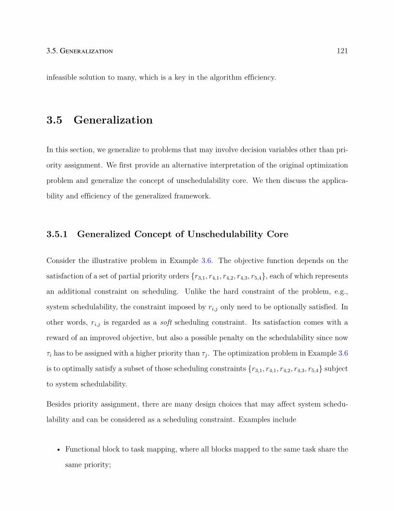
3.5. Generalization 121
infeasible solution to many, which is a key in the algorithm efficiency.
3.5 Generalization
In this section, we generalize to problems that may involve decision variables other than pri-
ority assignment. We first provide an alternative interpretation of the original optimization
problem and generalize the concept of unschedulability core. We then discuss the applica-
bility and efficiency of the generalized framework.
3.5.1 Generalized Concept of Unschedulability Core
Consider the illustrative problem in Example 3.6. The objective function depends on the
satisfaction of a set of partial priority orders r3,1, r4,1, r4,2, r4,3, r5,4, each of which represents
an additional constraint on scheduling. Unlike the hard constraint of the problem, e.g.,
system schedulability, the constraint imposed by ri,j only need to be optionally satisfied. In
other words, ri,j is regarded as a soft scheduling constraint. Its satisfaction comes with a
reward of an improved objective, but also a possible penalty on the schedulability since now
τi has to be assigned with a higher priority than τj. The optimization problem in Example 3.6
is to optimally satisfy a subset of those scheduling constraints r3,1, r4,1, r4,2, r4,3, r5,4 subject
to system schedulability.
Besides priority assignment, there are many design choices that may affect system schedu-
lability and can be considered as a scheduling constraint. Examples include
• Functional block to task mapping, where all blocks mapped to the same task share the
same priority;

122Chapter 3. The Concept of Unschedulability Core for Optimizing Real-Time Systems
with Fixed-Priority Scheduling
• The use of semaphore locks to protect shared resource, where a task suffers a blocking
time equal to the largest WCET of the critical section from lower priority tasks;
• As an alternative to semaphore locks, it is also sufficient to prove that the tasks shar-
ing the same resources do not preempt each other. However, this imposes a tighter
execution window as a task must finish before the next activation of higher priority
tasks that share the same resource.
We now introduce the general form of optimization problems that can be handled by the
proposed framework.
Definition 5. Let L = ζ1, ...ζm be a set of scheduling constraints that only need to be
optionally satisfied. The satisfaction of each constraint ζi is associated with a cost. A
scheduling constraint optimization problem is to optimally satisfy the given scheduling that
the total cost is minimized. Formally, the problem is expressed as follows
min C(b)
s.t. system schedulability
bk = 1 =⇒ ζk is enforced, ∀ζk ∈ L
(3.14)
where b = b1, ...bm is the set of binary variables that define bk for each ζk as follows
bk =
1 ζk is enforced,
0 otherwise.(3.15)
The problem considered in the previous three sections can be understood as a special instance
of (3.14) where ζk is a partial priority order. Still, for this general form of optimization
problem, the challenge mainly lies in the difficulty of efficiently formulating the feasibility

3.5. Generalization 123
region. To address this challenge, we extend the idea of schedulability region abstraction
using unschedulability core. We first establish similar concepts and properties as those in
Section 3.3.
Definition 6. A scheduling constraint set R is a set of scheduling constraints in L, i.e.,
R ⊆ L. R is said to be schedulable if and only if the following problem is feasible.
min 0
s.t. system schedulability
ζk is enforced, ∀ζk ∈ R
(3.16)
Comparing to problem (3.14), problem (3.16) removes the objective and treats all scheduling
constraints ζk inR as hard constraints. Informally, R is schedulable if and only if there exists
a feasible solution such that all scheduling constraints in R are satisfied and all tasks are
schedulable.
Theorem 22. Given two scheduling constraint sets R1 and R2 such that R1 ⊇ R2, the
following properties hold.
R1 is schedulable =⇒ R2 is schedulable
R2 is not schedulable =⇒ R1 is not schedulable(3.17)
Proof. Each element in a scheduling constraint set R imposes an additional constraint on
problem (3.16). Since R1 ⊇ R2, R1 is stricter than R2. Thus if R1 is schedulable, R2 must
also be schedulable.
Definition 7. A scheduling constraint set U is an unschedulability core if and only if the
following two conditions hold.
124Chapter 3. The Concept of Unschedulability Core for Optimizing Real-Time Systems
with Fixed-Priority Scheduling
• U is not schedulable.
• For all R ⊂ U , R is schedulable.
Intuitively, an unschedulability core refers to a minimal subset of L that can not be simul-
taneously satisfied. It implies the following constraints that must always be met.
∑∀ζk∈U
bk ≤ |U| − 1 (3.18)
We refer to (3.18) as the implied constraint by unschedulability core U . Similar to the
framework for optimizing partial priority orders, our overall idea is to use (3.18) as an
alternative form for modeling the feasibility region of (3.14). The algorithms (Algorithms 2–
4) for calculating unschedulability cores and the optimization procedure are applicable to the
new concept of unschedulability core. This comes from the general property of the scheduling
constraints as stated in Theorem 22: the system schedulability is monotonic with respect to
the set of scheduling constraints.
3.5.2 Applicability and Algorithm Efficiency
In the following, we discuss the factors that affect the algorithm efficiency of the proposed
framework and highlight where it is beneficial (i.e., much faster than existing approaches
such as ILP). We note in each iteration Algorithm 4 mainly performs two operations: the
computation of unschedulability cores (Line 10 in the algorithm) and solving the relaxed
problem Π (Line 4).
By Algorithm 2, the computation of unschedulability core can be further decomposed into
a series of schedulability test on a given scheduling constraint set R, i.e., testing the feasi-
bility of (3.16). Obviously, such a subroutine depends on the actual form of the scheduling

3.5. Generalization 125
constraint ζk and the task model. For example, the problem considered in Sections 3.2–3.4
defines ζk as a partial priority order. In this case, for many task models and scheduling
schemes as summarized in [53], schedulability of R can be tested using a revised Audsley’s
algorithm. It only needs to check O(n2) priority assignments out of the n! possible ones.
However, for some other forms of scheduling constraints or task models, the test for the
schedulability of R may be much more difficult. For example, for systems with preemp-
tion threshold scheduling [147], Audsley’s algorithm is inapplicable, and the exact test of
schedulability of R may require to check an exponential number of priority assignments.
In general, if checking the schedulability R needs to explore a large number of scheduling
constraint sets, the proposed framework may not be advantageous compared to other ap-
proaches (such as ILP). In the next section, we use two examples to illustrate how certain
scheduling constraints can be handled.
An important consideration in the development process is how the priority assignments are
stable with respect to small changes, which may arise unforeseeably. In cases where (revised)
Audsley’s algorithm is still optimal, for example, for robustness to additional interference [44],
our framework can be applied.
To compute unschedulability cores, it also relies on the schedulability analysis, i.e., to analyze
if the system is schedulable for a given valuation on the decision variables. Although our
framework is applicable for any schedulability analysis technique, its efficiency depends on
that of the schedulability analysis. In practice, the schedulability analysis is typically efficient
enough (as demonstrated in Section 3.7.1 for AMC-scheduled systems). However, it can still
be a major bottleneck. For example, the analysis of digraph real-time tasks [138] (and
similarly systems modeled with finite state machines [152]) requires to enumerate all paths
in the digraph of a higher priority task to identify its worst-case interference. In this scenario,
our framework has the flexibility, and it is usually beneficial, to optimize the implementation
126Chapter 3. The Concept of Unschedulability Core for Optimizing Real-Time Systems
with Fixed-Priority Scheduling
of schedulability analysis. For example, within one invocation of Algorithm 3, the resulting
unschedulability cores across consecutive iterations are mostly similar, suggesting that some
previous results of schedulability analysis can likely be reused. In addition, during the
computation of unschedulability cores, typically most invocations of schedulability analysis
will return unschedulability. This suggests that the use of fast, but mostly accurate necessary
only analysis may be helpful, as it can quickly detect obviously unschedulable solutions.
We apply the proposed framework in Algorithm 4 to optimizing the implementation of
synchronous finite state machines [165]. Our experimental results show that with a direct
use of the analysis technique in [152], over 95% of the total runtime is spent on schedulability
analysis. However, this bottleneck is avoided and the overall runtime is reduced by 3 orders
of magnitude, by combining a schedulability memoization technique (which exploits the
reuse of previous schedulability analysis results), and a relaxation-recovery strategy (which
leverages a simple necessary only analysis for ruling out obviously infeasible solutions).
We now discuss the difficulty of solving the relaxed problem Π. Since Π does not contain the
schedulability constraints, it opens the possibility to use appropriate mathematical program-
ming framework while adopting the most accurate, but possibly sophisticated schedulability
analysis. For example, if the objective and constraints in (3.14) are all linear (except the
schedulability constraints), then we can leverage integer linear programming solvers such as
CPLEX to solve Π. Our framework allows to combine the power of these modern solvers
(which adopt numerous highly sophisticated techniques for generic branch and cut strat-
egy) and domain-specific algorithms (such as Audsley’s algorithm for finding a schedulable
priority assignment).

3.6. Examples of Application 127
3.6 Examples of Application
In this section, we provide two examples of optimization problems that fit the proposed opti-
mization framework, both proven to be NP-hard [109, 149]. The first is optimizing semantics-
preserving implementation of Simulink models, optionally with memory constraint. The
second is minimizing memory consumption for shared resource protection, in the context of
the automotive AUTOSAR standard. In Section 3.7, we apply our framework to these two
example systems and compare with standard techniques (BnB, ILP).
3.6.1 Optimizing Implementation of Simulink Models
A Simulink model is a Directed Acyclic Graph (DAG) where nodes represent functional
blocks and links represent data communication between the blocks [109].
For simplicity and demonstration purpose only, we assume that each functional block is
implemented in a dedicated task (hence use the terms functional block and task interchange-
ably). However, it should be noted that in practice, a design may contain hundreds or
thousands of blocks and thus a more common strategy is to allocate multiple blocks to a
single task where blocks inside the task are statically scheduled. Mapping of blocks to tasks
have been studied in various works (e.g., [156]). The focus of this chapter is instead on
priority assignment. It is possible to simultaneously consider both function-to-task mapping
and priority assignment, and we leave it as future work.
The semantics-preserving implementation of a Simulink model has to match its functional
behavior. This typically requires the addition of a Rate Transition (RT) block between a
reader and a writer with different but harmonic periods, which is a special type of wait-free
communication buffers. However, the costs of RT blocks are additional memory overheads
128Chapter 3. The Concept of Unschedulability Core for Optimizing Real-Time Systems
with Fixed-Priority Scheduling
and in some cases, functional delays in result delivery. The latter degrades control perfor-
mance.
Consider a fast reader τr and slow writer τw that writes to τr. Assigning higher priority to τr
generally helps schedulability as it conforms with the rate monotonic policy. However, since
the reader now executes before the writer, an RT block is needed to store the data from the
previous instance of the writer, which also incurs a functional delay. On the other hand, if
τr can be assigned with a lower priority while keeping the system schedulable, then no RT
block is needed and no functional delay is introduced.
The software synthesis of Simulink model is to exploit priority assignment as the design
variable to minimize the weighted sum of functional delays introduced by the RT blocks
(hence improving control quality). We note that Audsley’s algorithm is no longer optimal as
system schedulability is not the only constraint. Formally, the problem can be formulated
as follows.min
∑∀(w,r)
βw,r · pr,w
s.t. system schedulability
constraints in (3.2)
(3.19)
where (w, r) represents a pair of communicating tasks, and the parameter βw,r is the penalty
on control performance if τr is assigned with a higher priority than τw.
Optionally, the implementation of Simulink models may be subject to memory constraints.
An RT block is essentially a wait-free buffer between the reader and the writer, and thus
comes with memory cost. A unit delay RT block, necessary whenever the reader task τr
has a higher priority than the writer τw, is twice the size of the protected shared variable.
For a higher priority writer and a lower priority reader, the RT block has a memory cost
of the same size as the shared variable. However, it can be avoided if we can ensure the
3.6. Examples of Application 129
absence of preemption, i.e., the lower priority reader finishes before the next activation of
the writer to ensure the absence of preemption by the writer. In Simulink, the reader and
writer tasks always have harmonic periods (one period is an integer multiple of the other)
with synchronized release offsets. Hence, it suffices to ensure that the worst-case response
time of the reader Rr satisfies Rr ≤ or,w = minTr, Tw, where or,w is the smallest offset
from an activation of τr to the next activation of τw. To summarize, an RT block can be
avoided if the following scheduling constraint is satisfied
(pw,r = 1) ∧Rr ≤ minTr, Tw (3.20)
Thus, for each writer and reader pair (τw, τr), we introduce the additional scheduling con-
straint
ζw,r ≡ constraint by (3.20) (3.21)
The associated binary variable bζw,r is defined as 1 if ζw,r is enforced and 0 otherwise. To
ensure the memory budget, we add the following constraint to the problem (3.19)
∑∀(τw,τr)
(mw,r(pw,r − bζw,r) + 2mw,r · pr,w
)≤M (3.22)
where mw,r is the size of the memory buffer shared between τw and τr, and M is the available
memory for RT blocks.
We now discuss the schedulability test for R with the newly defined scheduling constraint
(3.21). In addition to a partial priority order, it also specifies an upper-bound on the worst-
case response time of the reader tasks τr, or equivalently a virtual deadline. Thus, a given
scheduling constraint set R essentially specifies a set of partial priority orders as well as
virtual deadlines for certain reader tasks. The revised Audsley’s algorithm discussed in

130Chapter 3. The Concept of Unschedulability Core for Optimizing Real-Time Systems
with Fixed-Priority Scheduling
Section 3.3 can still be applied to test the schedulability of R: it tries to find a feasible
priority assignment respecting R where the deadline of any task τr for ζw,r ∈ R is set
to minTr, Tw. Thus the problem can be efficiently solved by the general framework in
Algorithm 4.
3.6.2 Minimizing Memory of AUTOSAR models
The second example is to minimize the memory usage of AUTOSAR components [65], where
a set of runnables (the AUTOSAR term for functional blocks) communicates through shared
buffers that shall be appropriately protected to ensure data integrity. We assume that each
runnable is implemented in a dedicated task, and use the terms runnable and task inter-
changeably. We consider the problem for the optimal selection of (a) the priority assignment
to tasks; (b) the selection of the appropriate mechanism for protecting shared buffers among
a set of possible choices, including ensuring absence of preemption, lock-based method (pri-
ority ceiling semaphore lock), and wait-free method [65]. These mechanisms are associated
with different scheduling constraints and memory costs.
1) Ensuring absence of preemption. It has no memory or timing cost, but requires that the
two communicating tasks satisfy that the lower priority task always finish before the next
activation of the higher priority task. Specifically, the minimum distance between activations
of two communicating tasks τi and τj is given by the greatest common divisor of their period,
i.e., gcd(Ti, Tj). To ensure absence of preemption, it suffices to guarantee that
Ri ≤ gcd(Ti, Tj)
Rj ≤ gcd(Ti, Tj)
(3.23)
2) Wait-free method imposes no extra timing constraints but incurs a memory cost equal to

3.6. Examples of Application 131
the size of the shared buffer.
3) Lock-based method introduces blocking delay to higher priority tasks but reduces the
memory overhead to minimal (only one-bit for implementing semaphore locks). Let s denote
the shared variable between τi and τj. The timing constraints are formally expressed as
follows Bi ≥ Cs
j , if τj has lower priority than τi
Bj ≥ Csi , if τi has lower priority than τj
(3.24)
where Bi (Bj) represents the blocking time of τi (τj), and Csi (Cs
j ) represents the worst-case
execution time of the critical section for τi (τj) to access s.
The objective is to minimize the total memory usage while ensuring system schedulability.
In the following, we show how the problem can be solved by the general framework in
Algorithm 4.
Specifically, for each pair of communicating tasks (τi, τj), we define the following scheduling
constraints for each of the three mechanisms to protect the shared variable
absence of preemption: ζai,j ≡ constraint by (3.23)
wait-free method: ζwi,j ≡ None
lock-based method: ζ li,j ≡ constraint by (3.24)
(3.25)
Note that the wait-free method does not impose an additional scheduling constraint but
comes with an additional memory cost, hence the scheduling constraint associated with ζwi,j
is empty. Also, we define the binary variables bζai,j , bζwi,j and bζli,j to denote the use of each of
132Chapter 3. The Concept of Unschedulability Core for Optimizing Real-Time Systems
with Fixed-Priority Scheduling
the mechanisms.bζai,j = 1 =⇒ ζai,j is enforced
bζwi,j = 1 =⇒ ζwi,j is enforced
bζli,j = 1 =⇒ ζ li,j is enforced
(3.26)
It is sufficient to protect each communication pair with one of the mechanisms
bζai,j + bζwi,j + bζli,j ≥ 1, ∀(τi, τj) (3.27)
The optimization objective can be written as
C(X) =∑
∀(τi,τj)
βwi,jbζwi,j + βl
i,jbζli,j (3.28)
where βwi,j and βl
i,j are the memory cost for wait-free method and lock-based method, respec-
tively. The optimization problem is to minimize the memory cost in (3.28), subject to the
constraints in (3.26), (3.27), (3.2), and system schedulability.
We now examine whether there is an efficient schedulability test for R over the schedul-
ing constraints. Constraint (3.23) is equivalent to setting a virtual deadline for τi and τj.
Constraint (3.24) specifies how blocking time should be computed. Thus a given scheduling
constraint set R essentially specifies a PPO set as well as a setting of virtual deadlines and
blocking times for associated tasks. Finding a schedulable priority assignment under the
specified setting can still be performed using the revised Audsley’s algorithm. This allows
to keep the algorithm efficiency of the general framework in Algorithm 4.
3.7. Experimental Evaluation 133
3.7 Experimental Evaluation
In this section, we present results of our experimental evaluation for the proposed technique.
We consider the two example problems discussed in the previous section.
3.7.1 Optimizing Implementation of Mixed-Criticality Simulink
Models
To demonstrate that our approach can accommodate any schedulability analysis, we consider
the problem of software synthesis for Simulink model as discussed in Section 3.6.1, but the
model contains functional blocks with different criticality levels scheduled with the Adaptive
Mixed Criticality (AMC) scheme [20]. This problem is NP-hard as the special case where all
tasks are LO-critical is proven to be NP-hard [109]. The schedulability of AMC scheduled
systems can be analyzed with two methods [20]: AMC-max and AMC-rtb. We compare the
proposed technique and a direct ILP formulation. The straightforward ILP formulation of
AMC-max is excluded due to its extreme high complexity (see Section 3.4). We also include
brute-force BnB algorithms, to evaluate the benefit from modern ILP solvers (e.g., CPLEX).
The list of compared methods includes:
• UC-AMC-max: Unschedulability core guided algorithm (Algorithm 4) with AMC-
max as schedulability analysis;
• UC-AMC-rtb: Algorithm 4 with AMC-rtb analysis;
• ILP-AMC-rtb: ILP with AMC-rtb analysis, solved by CPLEX;
• BnB-AMC-max: BnB with AMC-max analysis;
• BnB-AMC-rtb: BnB with AMC-rtb analysis.
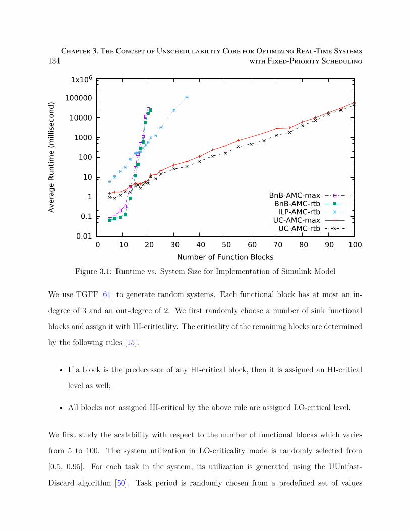
134Chapter 3. The Concept of Unschedulability Core for Optimizing Real-Time Systems
with Fixed-Priority Scheduling
0.01
0.1
1
10
100
1000
10000
100000
1x10⁶
0 10 20 30 40 50 60 70 80 90 100
Avera
ge R
unti
me (
millisecond)
Number of Function Blocks
BnB-AMC-maxBnB-AMC-rtbILP-AMC-rtb
UC-AMC-maxUC-AMC-rtb
Figure 3.1: Runtime vs. System Size for Implementation of Simulink Model
We use TGFF [61] to generate random systems. Each functional block has at most an in-
degree of 3 and an out-degree of 2. We first randomly choose a number of sink functional
blocks and assign it with HI-criticality. The criticality of the remaining blocks are determined
by the following rules [15]:
• If a block is the predecessor of any HI-critical block, then it is assigned an HI-critical
level as well;
• All blocks not assigned HI-critical by the above rule are assigned LO-critical level.
We first study the scalability with respect to the number of functional blocks which varies
from 5 to 100. The system utilization in LO-criticality mode is randomly selected from
[0.5, 0.95]. For each task in the system, its utilization is generated using the UUnifast-
Discard algorithm [50]. Task period is randomly chosen from a predefined set of values
3.7. Experimental Evaluation 135
10,20,40,50,100,200,400,500,1000. The criticality factor of HI-criticality task is uniformly
set to 2.0 (Ci(HI)Ci(LO)
= 2.0). We generate 1000 systems and report their average for each point in
the plots. We first set k to 5 in Algorithm 4 as the corresponding runtime is typically within
10% of the optimal setting. For all random systems (including those in Section 3.7.2), we
set a timeout of 900s for each problem instance for all algorithms to avoid excessive waiting.
Figure 3.1 illustrates the runtime of these methods. AMC-max based methods give slightly
better optimal solutions (no more than 5%) due to the better accuracy of AMC-max than
AMC-rtb, but they also run slower than their counterpart based on AMC-rtb (e.g., UC-
AMC-max vs. UC-AMC-rtb). The superiority of branch-and-bound based algorithms
in small-sized systems is mainly due to the overhead in ILP model construction in other
methods, which consumes a significant portion of the runtime when the ILP problem is rather
simple. The scalability for UC-AMC-rtb and UC-AMC-max is remarkably better than
that of the other methods. For example, for systems with 35 tasks, the unschedulability core
guided techniques are more than 1000 times faster compared to ILP-AMC-rtb. In addition,
UC-AMC-rtb and UC-AMC-max are quite close in their runtimes, demonstrating that
Algorithm 4 is not very sensitive to the complexity of the schedulability analysis. Finally,
ILP-AMC-rtb scales much better than BnB-AMC-rtb. This demonstrates that modern
ILP solvers, which are equipped with various sophisticated techniques, are generally more
efficient than brute force BnB.
We also evaluate the scalability of UC-AMC-max and UC-AMC-rtb with respect to
different system utilization ranging from 0.05 to 0.90. The number of functional blocks in
a system is fixed to 70 while the other parameters remain the same. The result is shown in
Figure 3.2. The optimization problem is relatively easy at very low utilization levels, as the
system is easily schedulable for most of the priority assignments. As utilization continues to
increase, the runtime grows but eventually remains at a similar value. The result illustrates

136Chapter 3. The Concept of Unschedulability Core for Optimizing Real-Time Systems
with Fixed-Priority Scheduling
0
200
400
600
800
1000
1200
1400
0 0.1 0.2 0.3 0.4 0.5 0.6 0.7 0.8 0.9
Avera
ge R
unti
me (
milis
econd)
System Utilization
UC-AMC-maxUC-AMC-rtb
Figure 3.2: Runtime vs. Utilization for Implementation of Simulink Model
that the scalability of unschedulability core guided algorithms is not sensitive to system
utilization.
We next study the effect of parameter k, the number of unschedulability cores to compute
for each infeasible solution, on the algorithm efficiency. The number of functional blocks and
system utilization are fixed to 70 and 70% respectively. The other parameters and system
generation scheme remain the same. Figure 3.3 shows the average runtime of the algorithms
UC-AMC-max and UC-AMC-rtb w.r.t. different values of k. It can be seen that the
algorithms run the fastest when k = 5. In cases with other system sizes and utilizations,
k = 5 still remains to be a good choice.
Finally, we apply the proposed technique to an industrial fuel injection controller case
study [109]. The system contains 90 functional blocks and 106 communication links. The

3.7. Experimental Evaluation 137
0 2 4 6 8 10 12 14 16 18 20
k
0
1000
2000
3000
4000
5000
6000
7000
Ru
n T
ime
(ms)
UC-AMC-rtb
UC-AMC-max
Figure 3.3: Runtime vs. Parameter k for Implementation of Simulink Model
Table 3.2: Results on fuel injection case study
Method Objective Runtime StatusUC-AMC-max 23 1.32s TerminateUC-AMC-rtb 23 0.19s TerminateILP-AMC-rtb 23 17.3h Terminate
BnB-AMC-max 23 ≥ 24h TimeoutBnB-AMC-rtb 23 ≥ 24h Timeout
total utilization in LO mode is 94.1%. We assign task criticality in the same way as the
randomly generated synthetic systems, which results in 42 HI-critical tasks. The criticality
factor is set to 2.0. We compare the same methods, and we set a time limit of 24 hours.
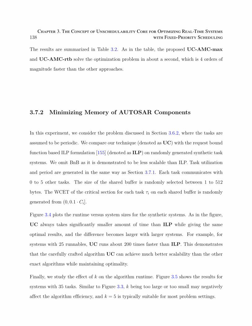
138Chapter 3. The Concept of Unschedulability Core for Optimizing Real-Time Systems
with Fixed-Priority Scheduling
The results are summarized in Table 3.2. As in the table, the proposed UC-AMC-max
and UC-AMC-rtb solve the optimization problem in about a second, which is 4 orders of
magnitude faster than the other approaches.
3.7.2 Minimizing Memory of AUTOSAR Components
In this experiment, we consider the problem discussed in Section 3.6.2, where the tasks are
assumed to be periodic. We compare our technique (denoted as UC) with the request bound
function based ILP formulation [155] (denoted as ILP) on randomly generated synthetic task
systems. We omit BnB as it is demonstrated to be less scalable than ILP. Task utilization
and period are generated in the same way as Section 3.7.1. Each task communicates with
0 to 5 other tasks. The size of the shared buffer is randomly selected between 1 to 512
bytes. The WCET of the critical section for each task τi on each shared buffer is randomly
generated from (0, 0.1 · Ci].
Figure 3.4 plots the runtime versus system sizes for the synthetic systems. As in the figure,
UC always takes significantly smaller amount of time than ILP while giving the same
optimal results, and the difference becomes larger with larger systems. For example, for
systems with 25 runnables, UC runs about 200 times faster than ILP. This demonstrates
that the carefully crafted algorithm UC can achieve much better scalability than the other
exact algorithms while maintaining optimality.
Finally, we study the effect of k on the algorithm runtime. Figure 3.5 shows the results for
systems with 35 tasks. Similar to Figure 3.3, k being too large or too small may negatively
affect the algorithm efficiency, and k = 5 is typically suitable for most problem settings.

3.8. Conclusions 139
1
10
100
1000
10000
100000
1x10⁶
0 10 20 30 40 50 60
Avera
ge R
unti
me (
millisecond)
Number of Runnables
ILPUC
Figure 3.4: Runtime vs. System Size for Memory Minimization of AUTOSAR
3.8 Conclusions
In this work, we introduce the concept of unschedulability core, a compact representation
of schedulability conditions for use in design optimization of real-time systems with fixed
priority scheduling. We develop efficient algorithms for calculating unschedulability cores
and present an unschedulability core guided optimization framework. Experiments show
that our framework can provide optimal solutions while scaling much better than standard
optimization approaches such as BnB and ILP.

140Chapter 3. The Concept of Unschedulability Core for Optimizing Real-Time Systems
with Fixed-Priority Scheduling
0 2 4 6 8 10 12 14 16 18 20
k
6
6.5
7
7.5
8
8.5
9
9.5
10
10.5
Tim
e (
s)
Figure 3.5: Runtime vs. Parameter k for Memory Minimization of AUTOSAR

Chapter 4
Optimization of Real-Time Software
Implementing Multi-Rate
Synchronous Finite State Machines
4.1 Introduction
Model-based design using formal models and associated tools provides an efficient approach
for the development of complex embedded systems. It greatly increases productivity and
reduces design errors thanks to its capability for advanced verification and validation. In
particular, the use of Synchronous Reactive (SR) models is widely adopted for software
development in the automotive and avionics industries. Tools and modeling environment
supporting SR include synchronous programming languages (e.g., Esterel [30], Lustre [74],
SIGNAL [94], and more recently, Prelude [69]) and the Simulink graphical language [105].
An SR model is a network of two types of functional blocks. Regular blocks, called Dataflow
in Simulink, are executed at their periods (integer multiples of the system-wide base period)
and perform a simple operation. Other blocks are Extended Finite State Machines, or FSMs,
which are known as Stateflow blocks in Simulink. In Stateflow blocks, a state transition and
execution of an action (a function) may be triggered by an event. In the following, we also
141
142Chapter 4. Optimization of Real-Time Software Implementing Multi-Rate Synchronous
Finite State Machines
use the terms Dataflow and Stateflow to refer to regular and FSM blocks respectively.
In this chapter, we consider the problem of optimizing the software implementation of SR
models containing both regular and FSM blocks, under preemptive fixed priority scheduling
on single-core platforms. The implementation shall (1) preserve the logical-time execution
semantics (the rate and order of execution of the blocks and the communication flows),
including the satisfaction of the timing requirement imposed by the model semantics (i.e.,
ensuring real-time schedulability1); (2) optimize some performance metric, such as a weighted
sum of the functional delays in the SR model to approximate the control quality (Section 4.2).
The past research on the optimization of SR model software implementations all have sig-
nificant drawbacks when it comes to systems with FSMs. The first approach, like those
for synchronous languages [122], works well only with single-rate systems (i.e., systems that
are triggered by events with the same rate). However, most complex control systems are
multi-rate where the trigger events have largely different rates (e.g., in automotive the de-
mand of cruise control is typically sampled at a lower rate than the acceleration pedal). The
second approach improves upon the first [58], but still treats each FSM as a regular block. It
easily generates suboptimal solutions since it substantially overestimates the workload and
is largely pessimistic in the real-time schedulability analysis.
The schedulability analysis used in the current approaches can be checked in time linear to the
number of transitions. On the contrary, the exact schedulability analysis of multi-rate FSMs
is strongly NP-complete, and requires exploring all possible transition sequences (which is
exponential in the number of transitions) in the FSM [29]. Consequently, the optimization
framework, within which the schedulability analysis serves as a subroutine to ensure the
returned solution is feasible, is very difficult to scale to large systems while maintaining
1Here the term “schedulability” refers to whether the system meets all the timing requirements, hence ithas a different meaning than what is typical of synchronous language (absence of causality loop).
4.1. Introduction 143
solution quality.
4.1.1 Our Contributions
In this chapter, we aim to improve the existing approach [58] and adopt the more accurate
schedulability analysis in [152] (see Section 4.3). The challenge is to develop an efficient
optimization framework that can accommodate the complexity of such an analysis. For this,
we develop a list of techniques as follows.
• We propose an optimization framework that judiciously combines the power of com-
mercial Integer Linear Programming (ILP) solvers for generic branch-and-bound and
the problem-specific Audsley’s algorithm for finding a feasible priority assignment.
• We utilize the concept of unschedulability core (see Section 4.4.2), to form a compact
abstraction of the schedulability condition.
• We propose two techniques to further improve scalability, one is a relaxation-and-
recovery mechanism based on a fast relaxation on schedulability analysis, the other is
memoization enhanced with schedulability conditions.
We use synthetic systems as well as an industrial case study to demonstrate that the frame-
work is optimal but runs several magnitudes faster than branch-and-bound. Also, it provides
much better solutions than the existing approach [58].
The rest of the chapter is organized as follows. Section 4.2 provides an overview on SR model
semantics and implementation. Section 4.3 summarizes the real-time schedulability analysis.
Section 4.4 proposes the optimization framework. Section 4.5 presents the experimental
results. Section 4.6 reviews the related work. Finally, Section 4.7 concludes the chapter.
144Chapter 4. Optimization of Real-Time Software Implementing Multi-Rate Synchronous
Finite State Machines
4.2 SR Models and Implementation
In this section, we briefly review the semantics and implementation of SR models that are
relevant to real-time schedulability. For a more comprehensive discussion, we refer the readers
to [36, 90].
4.2.1 SR Model Semantics
An SR model Γ is represented by a Directed Graph (V , E), where V is the set of vertices,
representing the functional blocks (or in short, blocks), and E is the set of edges or links,
representing data communication between blocks. Each link may optionally carry a unit
functional delay that impacts the model semantics (see Section 4.2.2). Each block has a set
of input and output signals. When a block is activated, it samples the input signals, processes
them, produces the result of the computation on the output ports, and (optionally) transits
to a new state. We assume that the block shall finish before its next activation, semantics
commonly followed by tools such as Prelude [69] and Simulink [105].
A Dataflow block Fi is executed at its period. Ti is the activation period of Fi, which should
be an integer multiple of the system base period Tb. Fi is also characterized by a worst case
execution time (WCET) Ci, and a deadline Di equal to its period Ti, hence matching the
Liu-Layland (LL) real-time task model [100].
A Stateflow block is a tuple F = S, sα, I,O,E,A (for ease of presentation, we drop the
index on F and its tuple elements in this paragraph), where S is the set of states, sα is
the initial state, I and O are respectively the sets of input and output signals, E is the
set of trigger events, and A is the set of transitions. Each trigger event ei ∈ E triggers a
subset of transitions. It occurs only at its period T (ei), which is an integer multiple of Tb.
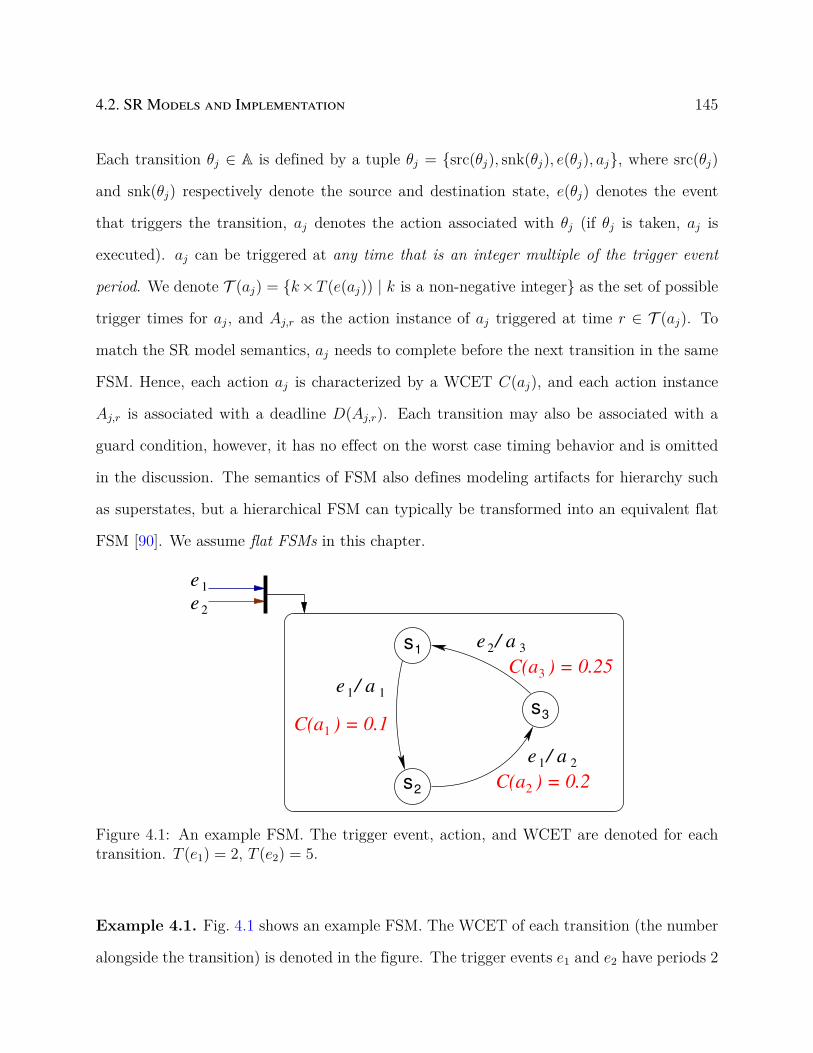
4.2. SR Models and Implementation 145
Each transition θj ∈ A is defined by a tuple θj = src(θj), snk(θj), e(θj), aj, where src(θj)
and snk(θj) respectively denote the source and destination state, e(θj) denotes the event
that triggers the transition, aj denotes the action associated with θj (if θj is taken, aj is
executed). aj can be triggered at any time that is an integer multiple of the trigger event
period. We denote T (aj) = k×T (e(aj)) | k is a non-negative integer as the set of possible
trigger times for aj, and Aj,r as the action instance of aj triggered at time r ∈ T (aj). To
match the SR model semantics, aj needs to complete before the next transition in the same
FSM. Hence, each action aj is characterized by a WCET C(aj), and each action instance
Aj,r is associated with a deadline D(Aj,r). Each transition may also be associated with a
guard condition, however, it has no effect on the worst case timing behavior and is omitted
in the discussion. The semantics of FSM also defines modeling artifacts for hierarchy such
as superstates, but a hierarchical FSM can typically be transformed into an equivalent flat
FSM [90]. We assume flat FSMs in this chapter.
s2
s3
s1
e 2
e 1
e / a 1 1
e / a 2 3
e / a 1 2
C(a ) = 0.1 1
C(a ) = 0.2 2
C(a ) = 0.25 3
Figure 4.1: An example FSM. The trigger event, action, and WCET are denoted for eachtransition. T (e1) = 2, T (e2) = 5.
Example 4.1. Fig. 4.1 shows an example FSM. The WCET of each transition (the number
alongside the transition) is denoted in the figure. The trigger events e1 and e2 have periods 2

146Chapter 4. Optimization of Real-Time Software Implementing Multi-Rate Synchronous
Finite State Machines
S1
t=0
e1/a1S2
t=2
S3 S1e1/a2
t=5
e2/a3
Figure 4.2: An example trace of the FSM in Figure 4.1.
and 5 time units respectively. Hence, they occur simultaneously every 10 units. The deadline
of A1,0, action a1 triggered at time 0, is 2, since the next transition is triggered at time 2.
Figure 4.2 shows a possible state transition trace for the example. The FSM is initially in
state S1. It executes action a1 (triggered by e1) and transits to state S2 at time t = 0 since
the trigger event e1 is present. At t = 2, event e1 becomes present again and triggers the
transition from S2 to S3. The event of e1 at t = 4 has no effect since S3 does not have any
outgoing transition triggered by it. Finally at t = 5, e2 becomes present and triggers the
transition from S3 to S1.
We consider implementing the SR model Γ on a single-core platform with preemptive fixed
priority scheduling, supported by the automotive AUTOSAR/OSEK operating systems stan-
dard, as well as the commercial code generation tools for Simulink. We assume that each
block is implemented in a dedicated software task (i.e., thread, the scheduling entity), and
use the terms task and functional block interchangeably. Hence, we also use Γ to denote the
implementing task system. Each block Fi is assigned with a unique priority πi. If Fi has
higher priority than Fj, denoted as πi > πj, Fi is always selected to execute when both are
ready.
4.2. SR Models and Implementation 147
4.2.2 Implementing SR Model: Tradeoff Analysis
The SR model semantics consist of two fundamental parts. The first is the rules dictating the
order of evaluation for the blocks. A block shall not be executed if its output depends on its
input and that the blocks driving its input has not been executed. Hence, the link between
the block and its input block represents a precedence constraint. Other blocks set their
outputs according to their current state only (along with input values acquired in previous
time steps and initial conditions specified as a block parameter) hence with no precedence
constraint on the input links.
The second is what is broadly known as the synchronous assumption. The time that the
block takes to update the outputs and the state is not relevant, provided that reactions
converge and computations complete before the next event. This corresponds to an intuitive
(but formally inaccurate) concept of instantaneous (zero-time) computations and communi-
cations.
The general conditions for a semantics-preserving implementation of SR models on a single-
core platform are discussed in [36]. Briefly speaking, in a correct implementation, the ex-
ecution order (and correspondingly the priority assignment) of the tasks implementing the
blocks is required to be in consistence with their partial order in the model. Also, the signal
values communicated among blocks in the logical time execution must be preserved in the
implementation, regardless of possible preemption or variable execution times.
The semantics-preserving implementation of SR models requires that all predecessors of a
functional block be assigned with higher priorities. This, however, may lead to system un-
schedulability. As a possible remedy, the precedence constraint can be broken by associating
a unit functional delay on the links. Specifically, if the link Ei,j = (Fi, Fj) has no delay on
it, called a feedthrough link, then there exists a precedence constraint, enforced by assigning

148Chapter 4. Optimization of Real-Time Software Implementing Multi-Rate Synchronous
Finite State Machines
higher priority to the writer Fi than the reader Fj. If the link Ei,j is associated with a unit
delay, then the precedence constraint is broken and we are free to assign a higher priority to
Fj than Fi.
T1 = 2
π1 = 2
F1 F2 F2 F2F1 F2
T2 = 1
π2 = 1
time 0 1 2 3
F1 F2
Figure 4.3: SR model semantics and the corresponding schedule for the case without func-tional delay.
T1 = 2
π1 = 1
T2 = 1
π2 = 2F1 F2
F1F2 F2 F2 F2F1
0 1 2 3 time
-1
Figure 4.4: SR model semantics and the corresponding schedule for the case with unitfunctional delay.
Fig. 4.3 illustrates a multi-rate SR model without functional delay on a low-rate-to-high-rate
edge. In the figure, F1 with period T1 = 2 produces output that is consumed by another
block F2 with period T2 = 1, without functional delay on the link. In the corresponding
schedule (bottom part of the figure), there is a precedence constraint. For example, F1 must
execute before the instance of F2 activated at the same time, such that the dataflow from F1
to F2 denoted by the dotted arrows is correct. This shall be achieved by assigning block F1
with a higher priority than F2. However, in general, the system becomes more difficult to

4.2. SR Models and Implementation 149
schedule. Intuitively, although the deadline of F1 is 2, it is required to finish with a deadline
1: the lower priority task F2, and consequently, F1 which is feeding F2, has to finish in 1
time unit after its activation.
On the contrary, Fig. 4.4 shows the model semantics and the corresponding schedule when
the edge between F1 and F2 carries a unit delay. Specifically, the instance of F2 activated
at time 2 reads the data generated by F1 activated at 0 (as opposed to F1 activated at 2 for
the case without delay). This causes an additional delay of T1 (= 2) for the dataflow from
F1 to F2. In this case, the precedence constraint from F1 to F2 is eliminated, provided that
F1 finishes before its next activation. Hence, we are free to adopt the priority assignment
that maximizes schedulability.
However, adding such functional delays comes at a cost. It generally worsens the control
performance [2, 5] since it adds delay to the feedback control loop. It also has memory
overheads since its implementation consists of a switched buffer [58]. Hence, we associate
each link Ei,j = (Fi, Fj) with a cost βi,j, to denote the penalty on control performance and/or
buffer size if Ei,j carries a unit functional delay.
Often, a correct software implementation may not be schedulable. A common strategy is
to modify the model by adding functional delays on selected links to relax the precedence
constraint. This however, may introduce performance and memory costs. The trade-off
can be formalized as the following design optimization problem: finding the schedulable
implementation that requires the minimum use of functional delays, or, as better stated, the
use of functional delays with minimum performance and/or memory penalty.

150Chapter 4. Optimization of Real-Time Software Implementing Multi-Rate Synchronous
Finite State Machines
4.3 Schedulability Analysis
We now summarize the schedulability analysis for FSMs, and highlight the significant pes-
simism in existing approaches [58, 122].
The software synthesis for synchronous languages [122] checks the schedulability by making
sure the longest chain of blocks to be executed at any cycle fits in the base period of the model.
Thus, it is only concerned with finding the action with the largest WCET for each FSM.
For example, consider an SR model containing two blocks F1 and F2, where F1 implements
the FSM in Figure 4.1, and F2 implements a Dataflow block with WCET 1 and period 100.
Hence, the system base period is 1. The analysis then checks whether the sum of the largest
WCET from F1 and F2 can fit in to a base period, i.e., if 0.25 + 1 ≤ 1. The violation of
the condition deems the system unschedulable, despite that the system utilization is very
low (lower than 26%). This approach imposes a very strong condition on schedulability and
is ill-suited for systems with largely varying rates (for example, the real-world automotive
benchmark with periods ranging from 1ms to 1000ms [89]).
The approach in [58] treats an FSM as a Dataflow block. That is, it characterizes each FSM
as an LL task [100], with a period parameter equal to the greatest common divisor (gcd) of
the event periods, a single value of WCET equal to the largest WCET among all actions,
and an implicit deadline equal to the period. This comes with two sources of pessimism: one
is the assignment of action deadline, the other is the characterization of the workload (see
Example 4.2).
Figure 4.5 shows the workload characterization by the approach for FSM in Figure 4.1. The
gcd of all event periods equals 1 and the largest WCET equals 0.25. Thus the FSM is
characterized as an LL task with period of 1 and WCET of 0.25. As proposed in [29, 152], a
more accurate characterization of the timing behavior of an FSM is to model it as a digraph

4.3. Schedulability Analysis 151
task [139].
The exact schedulability analysis is proven to be strongly NP-complete [29], by a reduction
from the schedulability of digraph tasks which is known to be NP-complete in the strong
sense [136]. Hence, there is no pseudo-polynomial time algorithm for determining the exact
schedulability of systems with synchronous FSMs unless P=NP.
We apply the sufficient-only analysis presented in [152], as it is shown to be several magni-
tudes faster than the exact analysis but is almost as accurate [29]. This allows us to compare
our optimization framework with other approaches such as branch-and-bound, as in the ex-
perimental results (Section 4.5). However, the proposed optimization framework does not
depend on the specific schedulability analysis and only uses it as a sub-routine. Thus it is
general enough to adopt other analysis techniques such as the exact analysis [29].
The exact analysis requires considering, in the worst case, the workload of each transition
sequence from every higher priority FSM [29]. The algorithm complexity is exponential in
the number of transitions. To avoid such exponential complexity, the sufficient schedulability
analysis uses one function to quantify the workload for each FSM, defined as below [152].
This reduces the complexity to be cubic in the number of transitions.
Definition 8. The request bound function (rbf) of a block F during a time interval
∆ = [s, f) where s is inclusive and f is exclusive, denoted as F.rbf(∆), is the maximum sum
of execution times by the actions of F that have their activation time within ∆.
The schedulability condition using rbf is stated as follows.

152Chapter 4. Optimization of Real-Time Software Implementing Multi-Rate Synchronous
Finite State Machines
Theorem 23. [152] The block Fi is schedulable if
∀Aj,r such that aj ∈ Fi
∧r ∈ T (aj)
∧r ∈ Si,
∀s ≤ r, ∃t ≤ D(Aj,r),∑
k∈hpe(i)
Fk.rbf([s, s+ t)) ≤ t(4.1)
Here hpe(i) = hp(i)∪Fi is the set hp(i) of blocks with higher priority than Fi plus Fi itself,
the set Si includes all the integer multiples of the event periods within the first hyperperiod
(the least common multiple of event periods for FSMs in hpe(i)) [152], and s and t are the
start and finish times of the busy period (a time interval where the CPU is always busy
executing tasks from hpe(i)) respectively. Essentially, Equation (4.1) requires to check that,
for each action instance Aj,r triggered in the first hyperperiod (the first line of the equation),
it always meets its deadline for all busy periods started before r considering the worst case
workload from tasks in hpe(i) (the second line of the equation).
We observe that the schedulability condition in Equation (4.1) has the following useful
properties. To check if Fi is schedulable, it only requires the knowledge on the set of higher
priority tasks hp(i), but not the particular priority order among tasks in hp(i), nor those with
lower priority. In addition, if the priority of Fi is raised to a higher level (hence with a smaller
set of hp(i)), the schedulability of Fi can only get better. By [53], these properties enable
to apply Audsley’s algorithm [10] to find a schedulable priority assignment. The algorithm
only needs to check O(n2) priority orders that is quadratic to the number of blocks n in the
system. In Section 4.4, we will leverage it to develop our optimization framework.
Example 4.2. For the example FSM in Fig. 4.1, the rbf([2, t)) function is illustrated in
Fig. 4.5. With the LL task model (i.e., as in the schedulability analysis of existing work [58]),
its period and deadline are 1 (the gcd of the periods of events e1 and e2), and its WCET
is 0.25 (the maximum WCET among all actions). The rbf([2, t)) function will increase at

4.4. Optimization Framework 153
t ))([2,rbf
2 63 4 5
0.2
0.4
0.6
0.8
1.0
1.2
0t7
Exact value as in this work
Overestimation by [18]
0.5
1.0
1.25
0.20.3
0.550.65
0.25
0.75
Figure 4.5: The overestimation (by [58]) and the exact value of rbf([2, t)) for the FSM inFig. 4.1.
each integer time with a step of 0.25. The rbf([2, t)) estimated by this approach [58] is
very pessimistic. For example, the exact value of rbf([2, 4)) is 0.2 as the worst case transi-
tion sequence contains only a2 triggered at time 2. However, the LL task model calculates
rbf([2, 4)) as 0.5 by assuming an action with WCET 0.25 activated at both time 2 and 3.
This is obviously impossible since a3, the action with WCET 0.25, only activates at integer
multiples of 5. Furthermore, the deadline calculated in the LL task model is overly tight.
For example, a1 is always followed by a2, both of which are triggered by e1 hence separated
by T (e1) = 2. Hence, the deadline of all instances of a1 should be 2. However, the LL task
model always assumes a deadline of 1 for a1.
4.4 Optimization Framework
The problem of optimizing software implementations of SR models involves assigning priority
orders to the tasks. We define a set of binary variables P = pi,j, where pi,j represents the
154Chapter 4. Optimization of Real-Time Software Implementing Multi-Rate Synchronous
Finite State Machines
relative priority order between tasks Fi and Fj, defined as
pi,j =
1 πi > πj,
0 otherwise.(4.2)
P shall satisfy the antisymmetry property: if Fi has a higher priority than Fj (pi,j = 1), then
Fj has a lower priority than Fi (pj,i = 0). It also shall satisfy the transitivity property: if Fi
has a higher priority than Fj (pi,j = 1) and Fj has a higher priority than Fk (pj,k = 1), then
Fi must have a higher priority than Fk (pi,k = 1).
Antisymmetry: pi,j + pj,i = 1, ∀i = j
Transitivity: pi,j + pj,k ≤ 1 + pi,k, ∀i = j = k(4.3)
The objective is to minimize the total weighted cost of the links where the writer is assigned
with a lower priority than the reader (i.e., the links associated with a unit delay) while each
task is schedulable. Thus, the problem can be formulated as
min∑
(Fi,Fj)∈E
βi,j · pi,j
s.t. Equation (4.3) is satisfied;
each task Fi is schedulable.
(4.4)
In the rest of the section, we first give an overview on the optimization framework in Sec-
tion 4.4.1, then present the three techniques for improving the scalability of the framework
in Section 4.4.2–4.4.4 respectively. In Section 4.4.5 we discuss a few key properties in the
framework and explain why it is much more efficient than standard approaches such as plain
branch-and-bound.
4.4. Optimization Framework 155
4.4.1 Overview of Optimization Framework
The optimization problem in Equation (4.4) can be regarded as the combination of two
subproblems. The first is the schedulability analysis, which checks if each task is schedulable
given a priority assignment. The second is to find a schedulable priority assignment that
minimizes a linear cost function. As elaborated in Section 4.3, the exact schedulability
analysis is strongly NP-complete. Even the sufficient-only analysis in Equation (4.1) is
still NP-complete. The second subproblem is also NP-complete, even if we assume the
schedulability analysis is simple (i.e., in constant time complexity) [57, 58]. There exists no
exact algorithm that explores only a polynomial number of priority assignments to find the
optimal one, unless P=NP. Hence, the overall problem is highly complex.
We also note that the schedulability condition may prevent us from directly leveraging some
existing optimization frameworks. The analysis in Equation (4.1) hinders a possible formu-
lation in ILP: as exemplified in Fig. 4.5, the rbf function for an FSM is generally irregular
and cannot be represented as a closed form function.
Our optimization framework combines the strength of two techniques: the commercial ILP
solver that is tuned for generic branch-and-bound based search, and the efficient (modified)
Audsley’s algorithm for checking system schedulability. Another key is to leverage and ex-
tend the concept of unschedulability core as a compact over-approximation of schedulability
region.
The framework contains two iterative steps, as illustrated in Fig. 4.6. The first step (Step
1) is an ILP formulation Π that avoids the direct formulation of Equation (4.1), the schedu-
lability conditions based on rbf functions. Initially Π only concerns the antisymmetry and
transitivity of the priority order variables P as in Equation (4.3). Gradually, it adds con-
straints on P (and implicitly the schedulability conditions) depending on the results of the
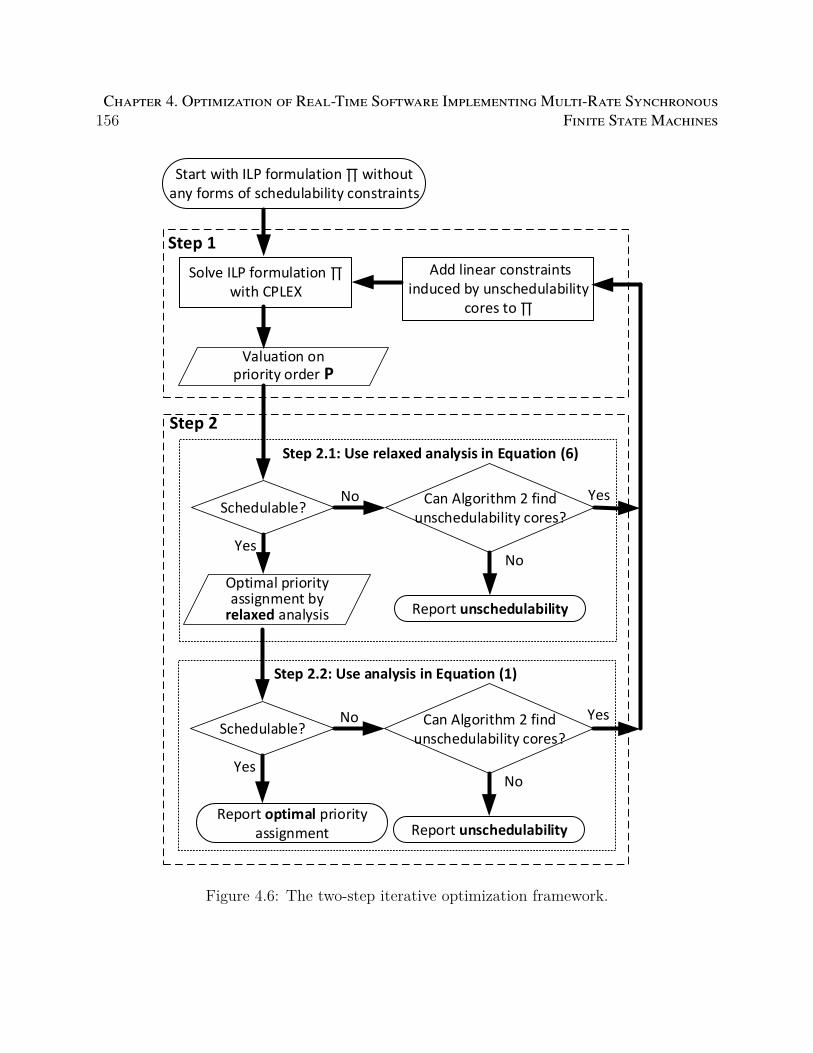
156Chapter 4. Optimization of Real-Time Software Implementing Multi-Rate Synchronous
Finite State Machines
Solve ILP formulation with CPLEX
Optimal priority assignment by relaxed analysis
Schedulable?No
Yes
Start with ILP formulation without any forms of schedulability constraints
Step 2.1: Use relaxed analysis in Equation (6)
Step 2
Can Algorithm 2 find unschedulability cores?
No
Yes
Report unschedulability
Schedulable?No
Yes
Step 2.2: Use analysis in Equation (1)
Can Algorithm 2 find unschedulability cores?
No
Yes
Report unschedulability
Valuation on priority order P
Add linear constraints induced by unschedulability
cores to
Optimal priority assignment by
relaxed analysis
Report optimal priority assignment
Step 1
Figure 4.6: The two-step iterative optimization framework.
4.4. Optimization Framework 157
second step.
Given a valuation on the priority order variables P from Step 1, the second step (Step 2)
either confirms that the tasks are schedulable, or use Algorithm 6 (see Section 4.4.2) to learn
a summation showing why they are not. In the latter case where we find that the system
is unschedulable because some tasks violate their deadlines, instead of directly adding the
schedulability conditions based on rbf for these tasks, we seek to add constraints on P as
a much more compact representation. It also tries to generalize to rule out other similar
unschedulable priority orders: as detailed in Algorithm 6, starting from an unschedulable
priority assignment (an infeasible valuation on P), it iterates through each pi,j and tries to
relax the valuation on it. If the resulting partial valuation on P still does not make the
system schedulable, then the valuation on pi,j is relaxed. In the end, it will (1) either return
a compact and general representation (defined as an unschedulability core) on why the given
valuation of P makes the system unschedulable, in the form of a linear constraint on P (see
Example 4.5 below) ; (2) or report unschedulability if the system remains unschedulable
after relaxing valuations on all pi,j. This step leverages two types of unschedulability cores,
one (as in Step 2.2) is based on the analysis in Equation (4.1), the other (as in Step 2.1) is
a generalized version based on a relaxation on Equation (4.1) (see Section 4.4.3).
4.4.2 Calculating Unschedulability Cores
The concept of unschedulability core is defined as follows [160]. Intuitively, an unschedula-
bility core is an irreducible set of partial priority orders that makes a system unschedulable.
Definition 9. [160] A partial priority order (PPO), denoted as ri,j ≡ (pi,j = 1), defines
a priority order where Fi has a higher priority than Fj. A PPO set R is a collection of
one or more PPOs that are consistent with the properties in Equation (4.3). The number of
158Chapter 4. Optimization of Real-Time Software Implementing Multi-Rate Synchronous
Finite State Machines
elements in R is defined as its cardinality, denoted as |R|.
Let Γ be a task system and R be a PPO set on Γ. Γ is R-schedulable if and only if
there exists a feasible priority assignment P that respects all the PPOs in R. R is an
unschedulability core for Γ if and only if R satisfies the following two conditions:
• Γ is not R-schedulable;
• ∀R′ ⊂ R, Γ is R′-schedulable.
Remark 4.3. The concept of unschedulability core is conceptually similar to the concept
of minimal unsatisfiability core in the context of Boolean satisfiability solvers, which
refers to a minimal unsatisfiable subset of clauses. In a similar manner, an unschedulability
core is essentially a minimal subset of priority partial orders that can not be simultaneously
satisfied by any feasible priority assignment.
In systems with FSMs, the test on R-schedulability can be performed using a revised Aud-
sley’s algorithm, detailed in Algorithm 5. It inherits the property of Audsley’s algorithm in
that it is optimal in terms of checking if there exists a schedulable priority assignment [10].
Similar to Audsley’s algorithm, it iteratively finds a task schedulable at a particular priority
level starting from the lowest priority. However, when choosing the candidate task Fi, it
shall also guarantee that assigning the current priority to Fi does not violate any PPO in R
(i.e., satisfying the condition ∄ ri,j ∈ R in Line 3). When Fi is assigned with the priority,
it shall be removed from the set of unassigned tasks (Line 6). Also, all the PPOs rj,i in R,
i.e., those requiring a higher priority than Fi for some unassigned task Fj, are satisfied and
can be removed (Line 7).
Example 4.4. We consider an example system Γe as in Table 4.1, in which all functional
blocks are of type Dataflow, but the concept applies to systems with FSMs. R1 = r2,1, r4,1

4.4. Optimization Framework 159
Algorithm 5 Algorithm for Computing Unschedulability Core1: function UnschedCore(Task set Γ, PPO set R)2: for each priority level k from lowest to highest do3: if Fi is schedulable at level k then4: assign priority level k to Fi;5: Γ = Γ\Fi;6: R = R\rj,i|Fj ∈ Γ7: continue to next priority level8: else9: return false
10: end if11: end for12: return R13: end function
Table 4.1: An Example Task System Γe
Fi Ti Di Ci
F1 10 10 2F2 20 20 3F3 40 40 16F4 100 100 6
is a valid unschedulability core, as (a) Γe is R1-unschedulable; and (b) for each of its proper
subset, there exists a respecting feasible priority assignment: P = [π2 > π1 > π3 > π4]
respects R(1)1 = r2,1 and R(2)
1 = ∅, and P ′ = [π4 > π1 > π2 > π3] respects R(3)1 = r4,1.
For FSM systems, since for any R′′ ⊆ R′, R′-schedulability implies R′′-schedulability, the
second condition in Definition 9 can be replaced by
• ∀R′ ⊂ R s.t. |R′| = |R| − 1, Γ is R′-schedulable.
The equivalence can be proved by noticing that for any R′′ ⊂ R, there must exists an R′
s.t. R′′ ⊆ R′, |R′| = |R| − 1.
Algorithm 6 gives an efficient procedure for computing unschedulability cores. It takes as
input the task set Γ and a PPO set R, where Γ is not R-schedulable. It checks if all subsets

160Chapter 4. Optimization of Real-Time Software Implementing Multi-Rate Synchronous
Finite State Machines
Algorithm 6 Algorithm for Computing Unschedulability Core1: function UnschedCore(Task set Γ, PPO set R)2: for each r ∈ R do3: if ModifiedAudsley(Γ, R\r) == false then4: remove r from R5: end if6: end for7: if R is empty then8: report Unschedulability9: else
10: return R11: end if12: end function
of R with cardinality |R| − 1 (i.e., one less element) can allow Γ schedulable by using the
function ModifiedAudsley(). Hence, it iterates through and tries to remove each element
r in R (Lines 2–6). If the resulted PPO set still does not allow Γ to be schedulable, then
r is removed (Lines 3–5). In the end, if all elements in R are removed (Line 7), it means
that the modified Audsley’s algorithm cannot find a schedulable priority assignment even
though no priority order is imposed (i.e., Line 4 is executed because ModifiedAudsley(Γ, ∅)
returns false), and Γ is unschedulable (Line 8). Otherwise, the algorithm will return one
unschedulability core (Line 10).
Let U denote an unschedulability core for Γ. The constraint that the PPOs in U cannot be
simultaneously satisfied is ∑ri,j∈U
pi,j ≤ |U| − 1 (4.5)
Example 4.5. Assume Step 1 gives a valuation on P as R = r2,1, r2,3, r2,4, r4,1, r4,3, r1,3.
This corresponds to an unschedulable priority assignment [π2 > π4 > π1 > π3]. Algorithm 6
calculates the unschedulability core R1 = r2,1, r4,1, which imposes the constraint p2,1 +
p4,1 ≤ 1. By adding this constraint back to Step 1, many unschedulable solutions besides R
are ruled out in the next iteration, such as R′ = r2,1, r2,3, r2,4, r4,1, r4,3, r3,1 (i.e., priority

4.4. Optimization Framework 161
assignment [π2 > π4 > π3 > π1]).
Remark 4.6. Our framework makes sure each call to Algorithm 6 will return a different
unschedulability core, as the input parameter R to the algorithm is a valuation on P that
respects all the previously calculated unschedulability cores. Also, the number of unschedu-
lability cores is finite, since the number of PPO sets is finite. Hence, the framework will
always terminate.
Remark 4.7. The idea of unschedulability core is critical to reduce the number of iterations
between step 1 and step 2: each time step 1 makes a mistake in that it gives an unschedulable
valuation on P, we use the efficient modified Audsley’s algorithm to generalize this mistake
as much as possible.
4.4.3 Relaxation-and-Recovery
In general, analysis based on Theorem 23 is expensive as the set Si in Equation (4.1) may
be very large. We present two techniques that effectively reduce the complexity while main-
taining optimality. The first is based on the idea of fast relaxation of the schedulability
condition, stated in the following theorem.
Theorem 24. If we use a relaxed schedulability condition in Line 4 of Algorithm 5, Algo-
rithm 6 will still return a correct unschedulability core U , in the sense that the task system
Γ is not U -schedulable.
Proof. It follows directly from the property of relaxed (necessary-only) schedulability condi-
tion: if the task set is deemed unschedulable by this relaxed condition, then it must also be
unschedulable by the accurate condition.

162Chapter 4. Optimization of Real-Time Software Implementing Multi-Rate Synchronous
Finite State Machines
We observe that the major difficulty of checking Equation (4.1) lies in the potentially large set
of action instances and busy periods to be checked. One simple but very effective relaxation
is to: a) consider only the action instances Aj,r triggered in a small subset S ′i of Si; and b)
for each action instance, consider only the busy period starting at the trigger time of Aj,r
(s = r instead of s ≤ r). This results in the following necessary condition
∀Aj,r such that aj ∈ Fi
∧r ∈ T (aj)
∧r ∈ S ′
i,
∀s = r,∃t ≤ D(Aj,r),∑
k∈hpe(i)
Fk.rbf([s, s+ t)) ≤ t(4.6)
We will show in our experimental study that, for more than 99.99% of the cases, the un-
schedulability can be detected by testing only the first three action instances in the hyper-
period using Equation (4.6).
Equation (4.6) is a relaxation of the exact schedulability condition that is much simpler to
check but still provides very close approximation. Using such a condition may give correct
schedulability analysis results in most cases while greatly improving efficiency. Due to the
necessary-only nature, the returned priority assignment (at the end of Step 2.1 in Fig. 4.6)
may not be truly schedulable. Such rare cases can be handled by adding appropriate sanity
check and recovery mechanisms to guarantee soundness. When the expected benefit from
relaxation outweighs the expected cost at recovery, an overall improvement is achieved.
The relaxation-and-recovery framework is shown in Fig. 4.6. Relaxed (necessary-only) anal-
ysis instead of the accurate analysis is used in Step 2.1. The possible false positive on
schedulability can be excluded by performing a sanity check using the accurate condition
(Step 2.2). If indeed unschedulable, the procedure computes unschedulability cores using
the accurate analysis.

4.4. Optimization Framework 163
4.4.4 Schedulability-based Memoization
We further propose schedulability-based memoization, which stores the schedulability re-
sults for previously visited priority assignments and reuses them whenever a similar scenario
reoccurs. We observe the following two properties of the schedulability condition (4.1):
• if block Fi is schedulable with higher priority task set hp(i), it is also schedulable for
any hp′(i) where hp′(i) ⊆ hp(i);
• if Fi is unschedulable with higher priority task set hp(i), it is also unschedulable for
any hp′(i) where hp′(i) ⊇ hp(i).
Thus for each FSM Fi, we maintain two lists H+i and H−
i , storing the encodings of hp(i)
under which Fi is known to be schedulable and unschedulable respectively. When performing
schedulability analysis (Line 4, Algorithm 5) with a given set hp(i) of higher priority tasks,
the procedure first checks if (a) there exists hp′(i) ∈ H+i such that hp′(i) ⊆ hp(i), or (b)
hp′(i) ∈ H−i such that hp′(i) ⊇ hp(i). In both cases the schedulability can immediately be
inferred. The actual schedulability test is performed only when it cannot find such an hp′(i).
After the schedulability with hp(i) is established, H+i and H−
i are updated accordingly to
record the new result.
The existence of such an hp′(i) is essentially a problem of subset and superset query. This can
be efficiently implemented using proper encodings of hp(i) and a data structure for H+i and
H−i that facilitates set inclusion queries. Specifically, we use a bit-vector B (implemented
as an array of integers) of length n to encode hp(i), where the m-th bit of B is set to 1
if Fm ∈ hp(i), and n is the number of tasks. The subset and superset relationship can be
efficiently tested using the following bitwise logic operations on integers, available in most
programming languages:

164Chapter 4. Optimization of Real-Time Software Implementing Multi-Rate Synchronous
Finite State Machines
• hpj(i) ⊇ hpk(i) ⇐⇒ Bj (bitwise AND) Bk = Bk;
• hpj(i) ⊆ hpk(i) ⇐⇒ Bj (bitwise OR) Bk = Bk.
This idea can be generalized to consider the dominance of a pair of FSMs with respect to
their rbf functions.
Definition 10. For two FSMs Fi and Fj, if Fi’s rbf function is always no smaller than that
of Fj, i.e.,
∀s,∀t ≥ s, Fi.rbf([s, t)) ≥ Fj.rbf([s, t)) (4.7)
then Fi is said to dominate Fj or equivalently, Fj is dominated by Fi. We denote this
relationship as Fi ⪰ Fj.
The dominance relationship between two sets of FSMs are similarly defined.
Definition 11. For two sets of FSMs h and h′, if the sum of the rbf functions of all FSMs
in h is always no smaller than that of h′, i.e.,
∀s, ∀t ≥ s,∑Fi∈h
Fi.rbf([s, t)) ≥∑Fj∈h′
Fj.rbf([s, t)) (4.8)
then h is said to dominate h′ or equivalently, h′ is dominated by h. We denote this rela-
tionship as h ⪰ h′.
Now the following properties hold for the schedulability analysis:
• if block Fi is schedulable with higher priority task set hp(i), it is also schedulable for
any hp′(i) where hp′(i) ⪯ hp(i);
• if Fi is unschedulable with higher priority task set hp(i), it is also unschedulable for
any hp′(i) where hp′(i) ⪰ hp(i).

4.4. Optimization Framework 165
The storage structure H+i and H−
i is partitioned into smaller subgroups H+,li and H−,l
i , where
l denotes the cardinality of the corresponding hp(i). When querying of subset of hp(i) in
H+i for example, the search space needs only consider those H+,l
i such that l ≤ |hp(i)|.
4.4.5 Discussion on Algorithm Design
We first remark that the proposed optimization framework is optimal: it guarantees the
optimality2 of the returned solution since it always maintains an over-approximation of the
exact feasibility region (a subset of all constraints) in Step 1. In case the system is unschedu-
lable, it will appropriately detect that since it will find the system is unschedulable with no
enforced priority orders (Algorithm 5 becomes the original Audsley’s algorithm when the
input R is empty). It also guarantees to terminate as detailed in Remark 4.6.
The current approach for complex optimal priority assignment problems (i.e., those without
known polynomial-time optimal algorithms) is to directly apply existing optimization frame-
works such as branch-and-bound (e.g., [57]) or integer linear programming (ILP) (e.g., [58]).
Comparably, the proposed framework is a few magnitudes faster for industrial case stud-
ies. As in the experimental results (Table 4.3, Section 4.5), for the plain branch-and-bound
algorithm we implement where each FSM is modeled with the accurate digraph task (i.e.,
BnB-Digraph in the table), our approach (UC-Digraph-M-RR) is 20,000× faster. If
we follow the approach in [58] and treat each FSM as an LL task, the problem can be for-
mulated in the ILP framework (i.e., ILP-LL). Still, our approach (UC-LL-M) is about
80,000× faster. This may seem surprising as modern ILP solvers such as CPLEX implement
many sophisticated techniques to efficiently search in the design space. In the following, we
provide our insights explaining this result.2Here the term “optimality” is slightly abused as the schedulability analysis in Equation (4.1) is sufficient
only. However, the optimization algorithm itself is optimal in the sense that if we replace Equation (4.1)with the exact analysis, it will return the exact optimal solution.

166Chapter 4. Optimization of Real-Time Software Implementing Multi-Rate Synchronous
Finite State Machines
Our first insight is that in a system with n blocks, although there are in total n! possible
priority assignments, typically only a small subset of all the priority order variables P are
objective-sensitive. As in Equation (4.4), only those priority orders pi,j which adhere to a
link (Fi, Fj) ∈ E affect the optimization objective.
Our second insight is that Audsley’s algorithm [10] can efficiently find a schedulable priority
assignment if there exists one [53]: it only needs to check O(n2) priority assignments out of
the n! possible ones. The intelligence in such a problem specific algorithm can be difficult to
match for generic constraint solvers like CPLEX, as evidenced in the experimental results.
Our framework is also designed to judiciously avoid the complexity of schedulability analysis
whenever possible, using the following two techniques. The first is the development of a fast
relaxation on the schedulability condition (Section 4.4.3). It quickly returns a solution that
is almost always schedulable, without using the expensive analysis of Equation (4.1). The
second is schedulability-based memoization (Section 4.4.4): the analysis is performed only
when it cannot be inferred from previous analysis results. The effectiveness of the above
two techniques is evidential in the experiments (Fig. 4.9): without these techniques, the
schedulability analysis dominates the overall runtime.
4.5 Experimental Evaluation
In this section, we conduct an experimental study to evaluate the unschedulability core (UC)
based optimization methods proposed in Section 4.4. We include a brute-force branch-and-
bound (BnB) algorithm to evaluate the algorithm efficiency, as ILP is not applicable due to
the irregularity of rbf functions for FSMs. To evaluate the benefit in solution quality from
the more accurate schedulability analysis with a digraph task model, we include the previous
approach which approximates each FSM as an LL task [58]. We omit the approach typical
4.5. Experimental Evaluation 167
of synchronous language compilers (i.e., a single-task implementation) as it is shown to be
very inefficient for multi-rate systems [58]. The list of compared methods includes:
• BnB-Digraph: BnB algorithm that uses the analysis in Equation (4.1), i.e., with a
digraph task model;
• UC-Digraph: unschedulability core (UC) based optimization with digraph task model;
• UC-Digraph-M: UC-Digraph plus memoization technique discussed in Section 4.4.4;
• UC-Digraph-M-RR: UC-Digraph-M plus relaxation-and-recovery mechanism (Sec-
tion 4.4.3);
• UC-LL-M: The same as UC-Digraph-M, but treats each FSM as an LL task;
• ILP-LL: The ILP formulation as in [58], which models each FSM as an LL task.
All ILP problems are solved with CPLEX 12.6.1. All runtimes are the wall-clock time on a
dedicated machine with a 3.40GHz quad-core processor and 8GB memory.
We first use relatively small synthetic systems to study the scalability with respect to the
number of functional blocks. We follow guidelines on the real-world automotive bench-
mark [89] to generate random systems. Each point in the plots represents the average over
1000 random systems. Each functional block has at most an in-degree of 3 and out-degree
of 2. The system utilization is fixed as 40%. 70% of the functional blocks have 1 state (i.e.,
it is a Dataflow block), 6% with 5 states, 6% with 10 states, 6% with 15 states, 6% with
20 states, 3% with 25 states, and 3% with 50 states. Each state has 3 outgoing transitions
on average. For event periods, first each FSM Fi is assigned with a base period randomly
selected from 1, 2, 5, 10, 20, 25, 50, 100, 1000, 2000, then each event in Fi is assigned with
a period by multiplying the based period with a factor randomly chosen from 1, 2, 5, 10.

168Chapter 4. Optimization of Real-Time Software Implementing Multi-Rate Synchronous
Finite State Machines
0.1
0.2
0.3
0.4
0.5
0.6
0.7
0.8
0 10 20 30 40 50 60 70 80 90 100
Norm
aliz
ed F
unct
ional D
ela
y
Number of Functional Blocks
BnB-DigraphUC-Digraph
UC-Digraph-MUC-Digraph-M-RR
ILP-LLUC-LL-M
Figure 4.7: Normalized Delay vs. Number of Blocks
We set a time limit of 1200 seconds for CPLEX to avoid excessive waiting. If the method
terminates without finding a feasible solution, the objective is set to be the sum of weights
of all communication edges.
Fig. 4.7 shows the optimized functional delay (normalized by the sum of edge weights) for
each algorithm. We note that in most cases the random systems are unschedulable without
added functional delays (i.e., with cost equal to zero). The methods with digraph-based
schedulability analysis always return the same optimized cost (except those which cannot
finish in the 1200-second time limit). The optimized cost of LL task based approaches (UC-
LL-M and ILP-LL) is) is averagely more than twice larger than that of digraph based ones,
demonstrating the significant sub-optimality from LL task based schedulability analysis in
existing work [58].

4.5. Experimental Evaluation 169
1
10
100
1000
10000
100000
1x10⁶
0 10 20 30 40 50 60 70 80 90 100
Avera
ge R
unti
me (
mili
seco
nd)
Number of Functional Blocks
BnB-DigraphUC-Digraph
UC-Digraph-MUC-Digraph-M-RR
ILP-LLUC-LL-M
Figure 4.8: Runtime vs. Number of Functional Blocks
Fig. 4.8 illustrates the runtime for each algorithm we compare. From the figure, it is clear
that the unschedulability core based methods (i.e., UC-Digraph, UC-Digraph-M, UC-
Digraph-M-RR) outperform plain BnB (BnB-Digraph). For example, for systems with
15 functional blocks, UC-Digraph is able to provide more than two magnitudes of im-
provement in runtime, and UC-Digraph-M and UC-Digraph-M-RR further improve
over UC-Digraph by more than an order of magnitude. The memoization technique makes
UC-Digraph-M 80 times faster on average than UC-Digraph for systems of 35 blocks.
The relaxation-and-recovery technique provides a speedup of about 5 to 10 times for rel-
atively large systems (with 20 blocks or more). UC-LL-M is faster than UC-Digraph-
M-RR on smaller-sized systems for its simpler analysis. However, UC-LL-M takes more
iterations to reach optimality, due to its smaller feasibility region which requires more effort
to refine, thus becoming slower than UC-Digraph-M-RR on larger systems. UC-LL-M
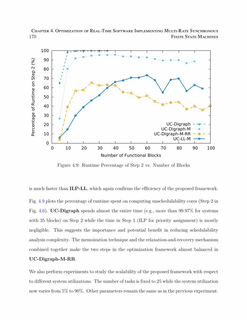
170Chapter 4. Optimization of Real-Time Software Implementing Multi-Rate Synchronous
Finite State Machines
0
10
20
30
40
50
60
70
80
90
100
0 10 20 30 40 50 60 70 80 90 100
Perc
enta
ge o
f R
unti
me o
n S
tep 2
(%
)
Number of Functional Blocks
UC-DigraphUC-Digraph-M
UC-Digraph-M-RRUC-LL-M
Figure 4.9: Runtime Percentage of Step 2 vs. Number of Blocks
is much faster than ILP-LL, which again confirms the efficiency of the proposed framework.
Fig. 4.9 plots the percentage of runtime spent on computing unschedulability cores (Step 2 in
Fig. 4.6). UC-Digraph spends almost the entire time (e.g., more than 99.97% for systems
with 35 blocks) on Step 2 while the time in Step 1 (ILP for priority assignment) is mostly
negligible. This suggests the importance and potential benefit in reducing schedulability
analysis complexity. The memoization technique and the relaxation-and-recovery mechanism
combined together make the two steps in the optimization framework almost balanced in
UC-Digraph-M-RR.
We also perform experiments to study the scalability of the proposed framework with respect
to different system utilizations. The number of tasks is fixed to 25 while the system utilization
now varies from 5% to 90%. Other parameters remain the same as in the previous experiment.
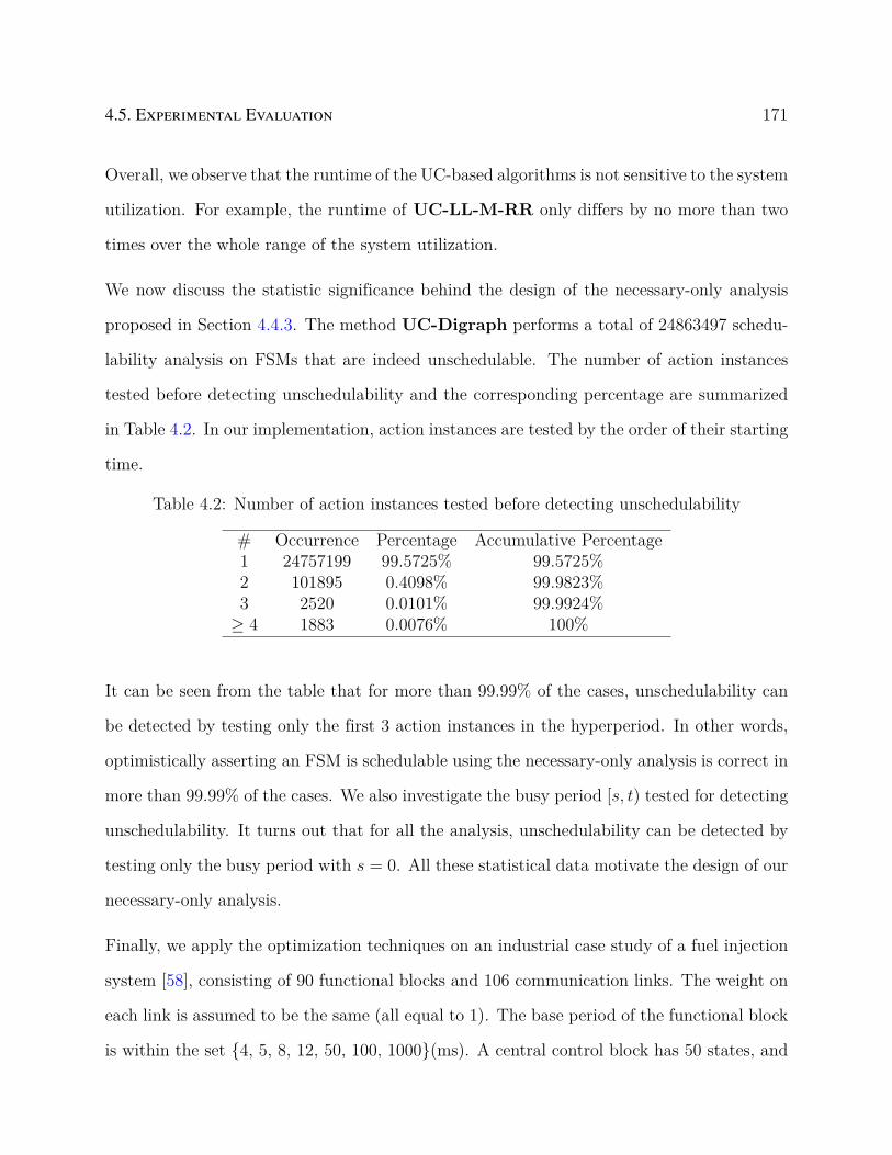
4.5. Experimental Evaluation 171
Overall, we observe that the runtime of the UC-based algorithms is not sensitive to the system
utilization. For example, the runtime of UC-LL-M-RR only differs by no more than two
times over the whole range of the system utilization.
We now discuss the statistic significance behind the design of the necessary-only analysis
proposed in Section 4.4.3. The method UC-Digraph performs a total of 24863497 schedu-
lability analysis on FSMs that are indeed unschedulable. The number of action instances
tested before detecting unschedulability and the corresponding percentage are summarized
in Table 4.2. In our implementation, action instances are tested by the order of their starting
time.
Table 4.2: Number of action instances tested before detecting unschedulability
# Occurrence Percentage Accumulative Percentage1 24757199 99.5725% 99.5725%2 101895 0.4098% 99.9823%3 2520 0.0101% 99.9924%≥ 4 1883 0.0076% 100%
It can be seen from the table that for more than 99.99% of the cases, unschedulability can
be detected by testing only the first 3 action instances in the hyperperiod. In other words,
optimistically asserting an FSM is schedulable using the necessary-only analysis is correct in
more than 99.99% of the cases. We also investigate the busy period [s, t) tested for detecting
unschedulability. It turns out that for all the analysis, unschedulability can be detected by
testing only the busy period with s = 0. All these statistical data motivate the design of our
necessary-only analysis.
Finally, we apply the optimization techniques on an industrial case study of a fuel injection
system [58], consisting of 90 functional blocks and 106 communication links. The weight on
each link is assumed to be the same (all equal to 1). The base period of the functional block
is within the set 4, 5, 8, 12, 50, 100, 1000(ms). A central control block has 50 states, and
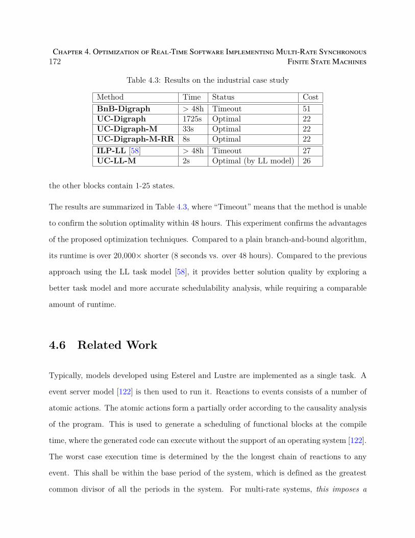
172Chapter 4. Optimization of Real-Time Software Implementing Multi-Rate Synchronous
Finite State Machines
Table 4.3: Results on the industrial case study
Method Time Status CostBnB-Digraph > 48h Timeout 51UC-Digraph 1725s Optimal 22UC-Digraph-M 33s Optimal 22UC-Digraph-M-RR 8s Optimal 22ILP-LL [58] > 48h Timeout 27UC-LL-M 2s Optimal (by LL model) 26
the other blocks contain 1-25 states.
The results are summarized in Table 4.3, where “Timeout” means that the method is unable
to confirm the solution optimality within 48 hours. This experiment confirms the advantages
of the proposed optimization techniques. Compared to a plain branch-and-bound algorithm,
its runtime is over 20,000× shorter (8 seconds vs. over 48 hours). Compared to the previous
approach using the LL task model [58], it provides better solution quality by exploring a
better task model and more accurate schedulability analysis, while requiring a comparable
amount of runtime.
4.6 Related Work
Typically, models developed using Esterel and Lustre are implemented as a single task. A
event server model [122] is then used to run it. Reactions to events consists of a number of
atomic actions. The atomic actions form a partially order according to the causality analysis
of the program. This is used to generate a scheduling of functional blocks at the compile
time, where the generated code can execute without the support of an operating system [122].
The worst case execution time is determined by the the longest chain of reactions to any
event. This shall be within the base period of the system, which is defined as the greatest
common divisor of all the periods in the system. For multi-rate systems, this imposes a
4.6. Related Work 173
very strong condition on real-time schedulability that is typically infeasible in cost-sensitive
application domains such as automotive [58].
In the commercial code generators for Simulink models (such as Simulink Coder from Math-
Works or TargetLink from dSPACE), two options are available. The first is a single-task
(executing at the base period), which is essentially the same approach as in [122]. The
second is multitask implementation scheduled with fixed-priority. Specifically, one task is
generated for each period in the model and all the tasks are scheduled by Rate Monotonic
policy. Caspi et al. [36] provide the conditions of semantics-preservation in a multi-task
implementation. Di Natale et al. [57] discuss the problem of optimizing the multitask im-
plementation of multi-rate Simulink models with respect to the control performance and
the required memory, and develop a branch-and-bound algorithm. Later in [58], an ILP
formulation is provided. Both papers [57, 58] treat each FSM as a Dataflow block, i.e., the
schedulability analysis is performed by modeling each FSM block with the Liu-Layland task
model [100]. A more accurate schedulability analysis of Stateflow models is discussed in [152]
based on an analogy with the digraph task model [137, 139]. The schedulability analysis is
tractable (i.e., pseudo-polynomial time) for bounded-utilization systems.
There are a number of papers for the implementation of SR models on architecture platforms
different than the one assumed in this chapter (i.e., single-core platform with preemptive
fixed priority scheduling). We selectively review them below. The recent synchronous lan-
guage Prelude [69, 118] defines real-time primitives to enable the programming of multi-rate
systems. It allos the designers to select mapping on to platforms scheduled with Earli-
est Deadline First (EDF), including multicore architectures [119, 123] through a number of
rules and operators. It uses a deadline modification algorithm to enforce the partial order of
execution required by the SR model semantics. [151] discusses how communication mecha-
nisms can be extended to model implementations on multicore platforms. The implemen-
174Chapter 4. Optimization of Real-Time Software Implementing Multi-Rate Synchronous
Finite State Machines
tation of Esterel/Lustre on asynchronous and distributed architectures has been discussed
in, e.g., [35, 37, 121, 144]. Specifically, techniques for generating semantics-preserving im-
plementations of synchronous models on Time-Triggered Architecture (TTA) are presented
in [35]. Desynchronization methods in distributed implementations are discussed in [37, 121].
A mapping framework from SR models to unsynchronized architecture platforms is presented
in [144], where the mapping uses intermediate layers with queues and then back-pressure
communication channels.
The multitask implementation of Stateflow blocks, i.e., decomposing each FSM into multiple
software tasks/threads, is proposed and studied in [108, 168]. We assume a dedicated task
to implement each FSM, and leave the optimization on multitask implementation to future
work.
4.7 Conclusions
In this work, we study the problem of optimizing real-time software implementing systems
modeled with synchronous finite state machines. We leverage and extend the concept of
unschedulability core, and develop a set of optimization techniques to improve the algorithm
efficiency while maintaining the solution optimality. The experimental study on synthetic
systems and an industrial case study shows that the proposed optimization framework runs
100-10000 times faster compared to conventional branch-and-bound. In the future, we plan
to develop techniques to optimize the multitask implementation for each FSM [108].
Chapter 5
The Virtual Deadline based
Optimization Algorithm for Priority
Assignment in Fixed-Priority
Scheduling
5.1 Introduction
The design optimization of real-time systems is to find, at design time, a suitable design
candidate that is (a) predictably correct, i.e., with design-time guarantees that requirements
on critical metrics (such as timing, control quality, and memory) are satisfied; and (b)
(optionally) optimal with respect to a given optimization objective function. In this chapter,
we focus on real-time systems with partitioned, fixed priority scheduling. We consider the
problems where the task priority assignment is part of the decision variables, and the task
worst-case response times (WCRTs) are involved in the design constraints and/or objective
function.
We discuss a few application scenarios. The first is the direct minimization of the average
WCRT over (a subset of) the tasks [4, 128], i.e., the system performance is measured by
175
176Chapter 5. The Virtual Deadline based Optimization Algorithm for Priority
Assignment in Fixed-Priority Scheduling
the promptness of task completion given that task schedulability is guaranteed. The second
is the design of control systems, where the control error is approximately proportional to
the response time of the controller task [27, 98]. The third is that modern cyber-physical
systems are characterized by complex functional content deployed on a distributed platform,
where timing constraints and performance metrics are expressed on end-to-end paths [41].
The worst-case end-to-end delay for each time-critical path equals the sum of the WCRTs
and periods of all tasks and messages in the path. Examples include active safety features
in automotive that spans over several Electronic Control Units (ECUs) connected by com-
munication buses such as Controller Area Network (CAN).
Since the subproblem of task WCRT calculation is shown to be NP-hard [63], the over-
all problem complexity is NP-hard. A straightforward approach is to formulate the design
optimization as a mathematical program. This approach may be appealing since modern
mathematical program solvers, such as CPLEX for Integer Linear Programs (ILP), incorpo-
rate many sophisticated techniques to efficiently prune the search space, and are typically
much better than plain branch-and-bound. However, despite the efficiency of modern solvers,
it is still very difficult to scale to large scale industrial systems.
Surprisingly, our framework runs 1,000 times faster than CPLEX while maintaining the
solution quality. The framework is carefully crafted based on a few problem-specific insights
that are difficult to match for generic constraint solvers such as CPLEX. The first is that the
WCRT calculation, although NP-hard, is actually very efficient in practice [47]. However,
the corresponding ILP formulation requires a possibly large number of integer variables (in
the order of O(n2), where n is the number of tasks) [155]. The second is that there are
algorithms which can efficiently find a schedulable priority assignment if there exists one,
such as rate monotonic policy for periodic tasks with preemptive scheduling [99] or Audsley’s
Algorithm for many task models [8], both of which run in polynomial time to the number

5.1. Introduction 177
of tasks. The intelligence in such problem specific algorithms, carefully studied by real-time
systems experts (e.g., [8, 44, 50]), may not be captured in solvers like CPLEX.
Hence, we propose an optimization framework that judiciously leverage the power of com-
mercial ILP solver (for generic branch-and-bound based search) and develop a problem-
specific algorithm (to efficiently find the optimal solution for a subproblem). We establish
an abstraction layer which hides the detail of WCRT analysis from the ILP solver but still
faithfully respects its accuracy. We envision such a drastically improved optimization capa-
bility will have profound impacts for the considered class of real-time systems. For example,
it may enable a new, agile and fluid design flow in which the designers can interact with the
optimization tools.
Specifically, our work makes the following contributions.
• We study the problem of minimum average WCRT and show that it has an efficient
optimal solution.
• We leverage the above algorithm, and introduce the concepts of virtual deadline and
Maximal Unschedulable Deadline Assignment (MUDA), the latter is a set of maximal
virtual deadlines for individual tasks and weighted sum of task WCRTs such that the
task system is unschedulable.
• We devise an optimization framework based on the concept of MUDA, which prudently
combines the efficient algorithm for calculating MUDA and ILP for generic branch-
and-bound.
• We apply our optimization framework to two industrial case studies and show that
the proposed technique runs 1, 000× faster over standard approach while maintaining
optimality.
178Chapter 5. The Virtual Deadline based Optimization Algorithm for Priority
Assignment in Fixed-Priority Scheduling
The rest of the chapter is organized as follows. Section 5.2 summarizes the task model and
optimization problem considered in this chapter. Sections 5.3 and 5.4 study the problem
of minimizing average WCRT and its weighted version, respectively. Section 5.5 introduces
the concepts of virtual deadline and MUDA, while Section 5.6 presents the optimization
framework built upon it. Section 5.7 presents the experimental results. Section 5.8 discusses
the related work. Finally, Section 5.9 concludes the chapter.
5.2 System Model and Notations
We consider a real-time system Γ containing a set of periodic or sporadic tasks τ1, τ2, · · · , τn
with constrained deadline. Each task τi is characterized by a tuple ⟨Ci, Ti, Di⟩, where Ci is
its Worst-Case Execution Time (WCET), Ti is the minimal inter-arrival time, and Di ≤ Ti is
the deadline. Without loss of generality, we assume these parameters are all positive integers.
Each task τi is assigned with a fixed priority that is subject to the designers’ decision. We
denote τi > τj if τi has higher priority than τj. We consider two possible scheduling policies:
preemptive scheduling and non-preemptive scheduling. These scheduling policies are widely
adopted in practical systems, such as the automotive AUTOSAR/OSEK real-time operating
systems (RTOS) standard, the modern RTOSes including LynxOS and QNX Neutrino, and
the Controller Area Network (CAN) protocol and its recent extension CAN-FD (CAN with
Flexible Data-rate).
For preemptive scheduling, the worst-case response time (WCRT) of task τi is the smallest
fixed point solution of the following formula
Ri = Ci +∑
∀j∈hp(i)
⌈Ri
Tj
⌉Cj (5.1)

5.2. System Model and Notations 179
where hp(i) represents the set of higher priority tasks than τi.
For non-preemptive scheduling, we adopt the following computation of WCRT that is safe
for tasks with constrained deadline [46]. Specifically, the waiting time (also called queuing
delay), the longest time that the task stays in the waiting queue before starting execution,
is calculated as
wi = max(Bi, Ci) +∑
∀j∈hp(i)
⌈wi
Tj
⌉Cj (5.2)
Here Bi denotes the maximum blocking time from lower priority tasks. The analysis is
based on the observation that τi can either suffer the blocking of a lower priority task or the
push through interference from the previous instance of the same task, but not both. For
convenience, we denote
Bi = max(Bi, Ci) = max∀j∈lp(i)∪i
Cj (5.3)
where lp(i) is the set of lower priority tasks than τi. Finally, the WCRT of a non-preemptive
task can be bounded as
Ri = Ci + wi (5.4)
The analysis in Equations (5.2)–(5.4) is only sufficient but not necessary, in the sense that
it may over-estimate the WCRT of a non-preemptive task. However, we adopt this analysis
instead of the exact one, for two reasons. One is that its accuracy is very good in practice,
especially for CAN [59]. The other is that we can derive some nice properties from such an
analysis to provide an efficient optimization algorithm (see Section 5.3).
We consider a design optimization problem where the design variables include the task
priority assignment. As part of the feasibility constraints, the tasks are required to be
schedulable. Besides, the problem also requires the precise information on the WCRTs of (a
subset of) the tasks.
180Chapter 5. The Virtual Deadline based Optimization Algorithm for Priority
Assignment in Fixed-Priority Scheduling
Formally, the problem can be expressed as the following mathematical programming problem
min∑∀i∈Ω
βi ·Ri
s.t. Tasks are schedulable
G(X) ≤ 0
(5.5)
Here X represents the vector of decision variables that include the task priority assignment
P and the task WCRTs R. The objective function is a weighted sum of the task WCRTs,
where βi ≥ 0 is the weight for task τi. G(X) ≤ 0 is the set of linear constraints on X that
the solutions in the feasibility region shall satisfy, in addition to the schedulability of each
task. For convenience, we denote Ω = τi : βi > 0, i.e., the set of tasks contributing to
the objective. We assume that G(X) is non-decreasing with task WCRTs, i.e., it imposes an
upper bound on the task WCRTs.
The problem in (5.5) is a suitable representation of a wide variety of applications. For
example, the control cost in real-time control systems depends on the WCRTs of the control
tasks, which can typically be linearized [103]. The end-to-end delay of distributed features
in automotive systems is the sum of WCRTs and periods for all tasks and messages in
the path [41], which may subject to end-to-end deadline (i.e., formulated in the constraint
G(X) ≤ 0) or serve as the objective function. In the experiments, we will illustrate with two
industrial case studies formulated in the above form.
5.3 Minimizing Average WCRT
In this section, we first study a specific instance of (5.5), known as the minimum average
WCRT problem, where all weights are the same and the constraints consist of only schedu-

5.3. Minimizing Average WCRT 181
lability of all tasks. The mathematical form of the problem is expressed as follows
min∑∀i∈Ω
Ri
s.t. Tasks are schedulable(5.6)
where Ω ⊆ Γ is the subset of tasks included in the objective for minimizing average WCRT.
In the next section, we generalize the result and design an algorithm for cases where tasks
have different weights.
We find that there is a simple optimal algorithm for (5.6), as detailed in Algorithm 7. It only
needs to explore a quadratic number O(n2) of priority orders out of the total n!, where n is
the number of tasks. This algorithm is a revision of Audsley’s algorithm [8] by augmenting
it with a simple strategy termed as “WCET Monotonic”. Similar to Audsley’s algorithm, it
iteratively assigns a task to a priority from the lowest level to the highest. At each priority
level, it checks if there is any unassigned task in Γ\Ω is schedulable (Lines 3–8). Otherwise,
it chooses the unassigned task in Ω with the longest WCET among those schedulable at this
level (Lines 9–14).
In the following, we first provide a set of sufficient conditions under which Algorithm 7 is
optimal. Consider a task system and an associated WCRT analysis M. Assume that M is
compliant with Audsley’s algorithm, i.e., it satisfies the following three conditions identified
in [50].
• The WCRT Ri of any task τi calculated by M does not depend on the relative order of
tasks in hp(i);
• Similarly, the calculation of Ri by M does not depend on the relative order of tasks in
lp(i);
• Ri is monotonically increasing with hp(i), i.e., if τi is dropped to a lower priority while

182Chapter 5. The Virtual Deadline based Optimization Algorithm for Priority
Assignment in Fixed-Priority Scheduling
Algorithm 7 Priority Assignment to Minimize Average WCRT1: function MinAvgWCRT(Task set Γ, Concerned set Ω)2: for each priority level k, from lowest to highest do3: for each unassigned τi in Γ\Ω do4: if τi is schedulable then5: Assign priority k to τi6: Continue to the next priority level7: end if8: end for9: for each unassigned τi in Ω in non-increasing WCET order do
10: if τi is schedulable then11: Assign priority k to τi12: Continue to the next priority level13: end if14: end for15: return unschedulable16: end for17: end function
τsPriority Assignment B
(Before Swapping):
Priority Assignment A(After Swapping):
τl ... ... ...
τl τs ...
HML
... ...
Higher Priority
Figure 5.1: Swapping τl with a lower priority task τs where Cl ≥ Cs, if maintaining schedu-lability, reduces the average WCRT.
the relative order of other tasks remains the same, Ri will only increase.
Now let τs and τl be any two tasks such that Cl ≥ Cs. Namely, τl is the long task and τs
is the short task. Consider any feasible priority order in which τl has higher priority than
τs. The main idea in the following theorem is to ensure that swapping the priority levels
5.3. Minimizing Average WCRT 183
of τl and τs, if schedulable, will not increase the average WCRT. We study the two priority
assignments before and after the swapping, denoted respectively as B and A in Figure 5.1.
A and B only differ in the priorities of τl and τs. The three sets of tasks H,M, and L, i.e.,
the sets of tasks with priority higher than, in between, and lower than τl and τs respectively,
remain the same.
Theorem 25. Consider a task system Γ and an associated WCRT analysis M that is compli-
ant with Audsley’s algorithm. As in Figure 5.1, we swap two tasks τs and τl with Cs ≤ Cl,
such that both A and B, the priority orders after and before swapping respectively, are
schedulable. If M additionally satisfies the following two conditions (where RAi and RB
i
denote the WCRTs of τi in priority assignments A and B respectively)
RBl +RB
s ≥ RAl +RA
s
∀τm ∈M, RBm ≥ RA
m
(5.7)
then Algorithm 7 is optimal for the problem in (5.6).
Proof. The WCRT of any task in H ∪ L remains the same, since the sets of its higher
priority and lower priority tasks are unchanged, and the analysis is compliant with Audsley’s
algorithm. This, combined with the conditions in (5.7), means that the average WCRT only
decreases after the swapping.
Now consider at any point in Algorithm 5.1 where it tries to find an unassigned task to
allocate the current priority k. Let S be the set of unassigned tasks that are schedulable at
this priority level. Further partition S into two disjoint sets C ∪ T = S where C ⊆ Ω and
T ⊆ Γ\Ω. Assume that S = ∅ (otherwise the system is unschedulable). There are two cases.
Case 1. T = ∅. We now show that for any τp ∈ T , there exists an optimal priority assign-
ment that assigns τp at the current priority level k. Consider any optimal priority assignment

184Chapter 5. The Virtual Deadline based Optimization Algorithm for Priority
Assignment in Fixed-Priority Scheduling
P that assigns a different task τq at priority k and τp at a higher priority. Construct another
priority assignment P′ by inserting τp immediately behind τq in the priority order. Since
τp /∈ Ω, the increased WCRT of τp will not affect the total cost. However all other tasks will
have equal or smaller WCRT since their priority is either shifted up by one level or remains
the same. Hence, the cost of P′ cannot be larger than that of P, indicating that P′ is also
optimal.
Case 2. T = ∅. Let τp be a task in C that has no smaller WCET than any other task in C.
Similarly, we show that there always exists an optimal priority assignment that assigns τp at
the current level k. Consider any optimal priority assignment P that assigns a different task
τq at level k and τp at a higher priority. τq has to be from C (since T = ∅), hence its WCET
cannot be smaller than τp. Now construct another priority assignment P′ by swapping τp
and τq in the priority order. Since Cp ≥ Cq, by (5.7) the cost of P′ can only be equal to or
smaller than that of P, indicating that P′ is also optimal.
The rest of the proof follows that of the Audsley’s algorithm [50], as Algorithm 7 always
constructs an optimal priority assignment by minimizing the cost at each priority level.
We now prove that the WCRT analysis methods in Equations (5.1)–(5.4) satisfy the condi-
tions in Theorem 25. We note that they are already known to be compliant with Audsley’s
algorithm [48]. For preemptive scheduling, we first observe the property of monotonicity
with priority order as formally stated in Lemma 26. We then demonstrate that the WCRT
analysis in (5.1) satisfies the conditions in (5.7), as stated in Theorem 27.
Lemma 26. In any feasible priority assignment for systems with preemptive scheduling, the
WCRT of a lower priority task τi is always no smaller than that of a higher priority task τj.

5.3. Minimizing Average WCRT 185
Proof. We define the WCRT delay function Ri(·) for τi as
Ri(x) = Ci +∑
∀k∈hp(i)
⌈Ri
Tk
⌉Ck
For τi and any higher priority task τj,
∀x > 0, Ri(x) ≥ Ci +
⌈x
Tj
⌉Cj +
∑∀k∈hp(j)
⌈x
Tk
⌉Ck
≥ Cj +∑
∀k∈hp(j)
⌈x
Tk
⌉Ck = Rj(x)
The delay function and WCRT satisfy the following property
∀x > 0,Ri(x) ≥ Rj(x) ⇒ Ri ≥ Rj (5.8)
since Ri (resp. Rj) is the first fixed point solution to the equation x = Ri(x) (resp. x =
Rj(x)).
Theorem 27. Theorem 25 holds for preemptive systems with the WCRT analysis in (5.1).
Proof. First, RBl ≥ RA
s , as RBl and RA
s have the same set of higher priority tasks H, and
Ri calculated in (5.1) is monotonically increasing with Ci.
Second, we prove RBs = RA
l . Let R∗ = minRBs , R
Al . Obviously R∗ ≤ minDs, Dl ≤
minTs, Tl. Hence, R∗ is the first fixed point solution of the following equation
R∗ = Cs + Cl +∑
∀j∈H∪M
⌈R∗
Tj
⌉Cj (5.9)

186Chapter 5. The Virtual Deadline based Optimization Algorithm for Priority
Assignment in Fixed-Priority Scheduling
We observe that R∗ is a fixed point solution to the following equation for calculating RBs
RBs = Cs +
⌈RB
s
Tl
⌉Cl +
∑∀j∈H∪M
⌈RB
s
Tj
⌉Cj (5.10)
Also, since R∗ ≤ RBs , and RB
s is the first fixed point solution to the above equation, it must
be R∗ = RBs . Likewise, R∗ = RA
l . Thus, RBs = RA
l , and RBs +RB
l ≥ RAs +RA
l .
Now consider any task τm ∈ M. By Lemma 26 and the above proven equation RBs = RA
l ,
RAm ≤ RA
l = RBs ≤ Ts. Hence, τm only suffers one interference from τs in A. Since Cl ≥ Cs,
the amount of interference from τl to τm in B will only be larger than that from τs in A.
This, combined with the fact that the set of higher priority tasks for τm only differs from τl
in B to τs in A, implies RBm ≥ RA
m.
In the following, we show that Theorem 25 also holds for the analysis in Equations (5.2)–(5.4)
for non-preemptive scheduling. We first establish a property similar to Lemma 26, but for
the waiting time calculated in (5.2). It relies on the definition of the waiting delay function
as below.
Definition 12. The waiting delay function of a task τi in systems with non-preemptive
scheduling is defined as
Wi(x) = Bi +∑
∀k∈hp(i)
⌈x
Tk
⌉Ck
Similar to (5.8), wi and Wi(x) have the following property
∀x > 0,Wi(x) ≥Wj(x) ⇒ wi ≥ wj (5.11)
Lemma 28. In any feasible priority ordering of non-preemptive systems where τi has lower
priority than τj, there is wi ≥ wj.
5.3. Minimizing Average WCRT 187
Proof. We consider τi and its immediate higher priority task τi−1.
∀x > 0, Wi(x) ≥ Bi +
⌈x
Ti−1
⌉Ci−1 +
∑∀k∈hp(i−1)
⌈x
Tk
⌉Ck
≥ Bi + Ci−1 +∑
∀k∈hp(i−1)
⌈x
Tk
⌉Ck
≥ maxBi, Ci−1+∑
∀k∈hp(i−1)
⌈x
Tk
⌉Ck
= maxBi−1, Ci−1+∑
∀k∈hp(i−1)
⌈x
Tk
⌉Ck
= Wi−1(x)
By induction, this relationship can be generalized to τi and any higher priority task τj.
Hence, the waiting time wi of τi is no smaller than that of any higher priority task.
The following two lemmas establish that the first condition in (5.7) is satisfied by the suffi-
cient WCRT analysis for non-preemptive scheduling.
Lemma 29. In Figure 5.1, it is wAl ≤ wB
s for the analysis in Equations (5.2)–(5.4) for
non-preemptive scheduling.
Proof. The waiting time wBs is computed as follows
wBs = BB
s +
⌈wB
s
Tl
⌉Cl +
∑∀j∈H
∪M
⌈wB
s
Tj
⌉Cj (5.12)
Similarly for wAl , it is computed as
wAl = BA
l +
⌈wA
l
Ts
⌉Cs +
∑∀j∈H
∪M
⌈wA
l
Tj
⌉Cj (5.13)
On the right hand side of (5.13) we substitute wAl with wB
s . Since wBs ≤ Ts, we derive the

188Chapter 5. The Virtual Deadline based Optimization Algorithm for Priority
Assignment in Fixed-Priority Scheduling
following quantity
w∗ = BAl +
⌈wB
s
Ts
⌉Cs +
∑∀j∈H
∪M
⌈wB
s
Tj
⌉Cj
= BAl + Cs +
∑∀j∈H
∪M
⌈wB
s
Tj
⌉Cj
(5.14)
We now prove that w∗ ≤ wBs . We consider the following two cases.
Case 1. max∀τj∈L
Cj ≥ Cl.
In this case, BAl = BB
s = max∀τj∈L
Cj. Also, since⌈wB
s
Tl
⌉Cl ≥ Cs, we have w∗ ≤ wB
s .
Case 2. max∀τj∈L
Cj < Cl.
In this case, there is BAl = Cl and BB
s ∈ [Cs, Cl]. Since⌈wB
s
Tl
⌉Cl ≥ Cl = BA
l and BBs ≥ Cs,
it is again w∗ ≤ wBs .
Combining the two cases, there is w∗ ≤ wBs . With wB
s ≤ Ds ≤ Ts, this means that
wBs ≥ BA
l +
⌈wB
s
Ts
⌉Cs +
∑∀j∈H
∪M
⌈wB
s
Tj
⌉Cj (5.15)
The above equation implies that the first fixed point solution of (5.13) must be no larger
than wBs , i.e., wA
l ≤ wBs .
Lemma 30. In Figure 5.1, we have wBl = wA
s for the analysis in Equations (5.2)–(5.4) for
non-preemptive scheduling.
Proof. It can be easily seen that
BBl = BA
s = max∀j∈L∪M∪τl,τs
Cj

5.3. Minimizing Average WCRT 189
Thus, wAs and wB
l are computed as the first fixed point of the same equation as below
w = max∀j∈L∪M∪τl,τs
Cj +∑∀k∈H
⌈w
Tk
⌉Ck (5.16)
This implies that wAs = wB
l .
With the above three lemmas, we now are ready to formally prove Theorem 25 for non-
preemptive scheduling.
Theorem 31. Theorem 25 holds for the analysis in Equations (5.2)–(5.4) for non-preemptive
scheduling.
Proof. By Lemma 29 and Lemma 30
RAs +RA
l − (RBs +RB
l ) = (wAl − wB
s ) + (wAs − wB
l )
≤ 0
(5.17)
This proves the first condition in (5.7) is satisfied.
Now consider τm of intermediate priority level, i.e., τm ∈ M. By Lemma 28, there is
wAm ≤ wA
l . By Lemma 29, wAm ≤ wA
l ≤ wBs ≤ Ds ≤ Ts. Therefore after swapping, τm
suffers exactly one instance of interference from τs. We use N denote the set of tasks in M
with priority higher than τm. Hence, in priority assignment A, the set of tasks with priority
higher than τm is H ∪N ∪ τs, and wAm is
wAm = BA
m +
⌈wA
m
Ts
⌉Cs +
∑∀j∈H∪N
⌈wA
m
Tj
⌉Cj
= BAm + Cs +
∑∀j∈H∪N
⌈wA
m
Tj
⌉Cj
(5.18)
Likewise, in priority assignment B, the set of tasks with priority higher than τm isH∪N∪τl,

190Chapter 5. The Virtual Deadline based Optimization Algorithm for Priority
Assignment in Fixed-Priority Scheduling
and wBm is
wBm = BB
m +
⌈wB
m
Tl
⌉Cl +
∑∀j∈H∪N
⌈wB
m
Tj
⌉Cj (5.19)
We now prove wAm ≤ wB
m, by considering the following two cases for BBm.
Case 1. Cl < BBm.
In this case, swapping Cl to a lower priority than τm does not change its blocking time, and
BAm = BB
m. From the Equations (5.18)–(5.19) for calculating wAm and wB
m, the right hand side
of the equations, i.e., the waiting time functions satisfy the property that
∀x > 0, WBm(x) = BB
m +
⌈x
Tl
⌉Cl +
∑∀j∈H∪N
⌈x
Tj
⌉Cj
≥ BAm + Cs +
∑∀j∈H∪N
⌈x
Tj
⌉Cj
= WAm(x)
Hence, by (5.11), we have wAm ≤ wB
m.
Case 2. Cl ≥ BBm.
In this case, it can only be that BAm = Cl. Also, BB
m ≥ Cs. The waiting time functions
satisfy the following equation
∀x > 0, WBm(x) = BB
m +
⌈x
Tl
⌉Cl +
∑∀j∈H∪N
⌈x
Tj
⌉Cj
≥ Cs + BAm +
∑∀j∈H∪N
⌈x
Tj
⌉Cj
= WAm(x)
Again, by (5.11), wAm ≤ wB
m.
5.4. Minimizing Weighted Average WCRT 191
Merging the above two cases, the second condition in (5.7) is also satisfied, which concludes
the proof of the theorem.
5.4 Minimizing Weighted Average WCRT
The optimality of WCET Monotonic strategy no longer holds if tasks have different weights
in problem (5.6). Consider the swapping in Figure 5.1 but the weight βl of τl is significantly
higher than other tasks. Then scheduling τl at a lower priority incurs substantial cost
that may outweigh the collective benefit from τs and tasks in M, and Theorem 25 is not
valid anymore. In this section, we propose a heuristic solution to the problem that is near
optimal as demonstrated in the experiments. It consists of two ideas. The first is a Scaled-
WCET Monotonic strategy, which mimics the WCET Monotonic strategy but divides the
task WCET by the weight and use this scaled WCET to order tasks. The second is a
refinement scheme to search for better solutions in the neighborhood.
Similar to the non-weighted case, the weighted problem can be interpreted as finding an
evaluation order for use in Line 9 of Algorithm 7, which specifies the preferred order within
the unassigned tasks to be checked for the current priority level. We introduce the concept
of scaled WCET: for each task τi, its scaled WCET Ci is defined as
Ci =Ci
βi
(5.20)
We use the non-increasing scaled WCET as the evaluation order, as it intuitively puts a task
with smaller weight or longer WCET to a lower priority.
However, the Scaled-WCET Monotonic strategy is not guaranteed to be optimal. In the rare
cases where non-trivial suboptimality occurs, we introduce a sifting adjustment scheme that
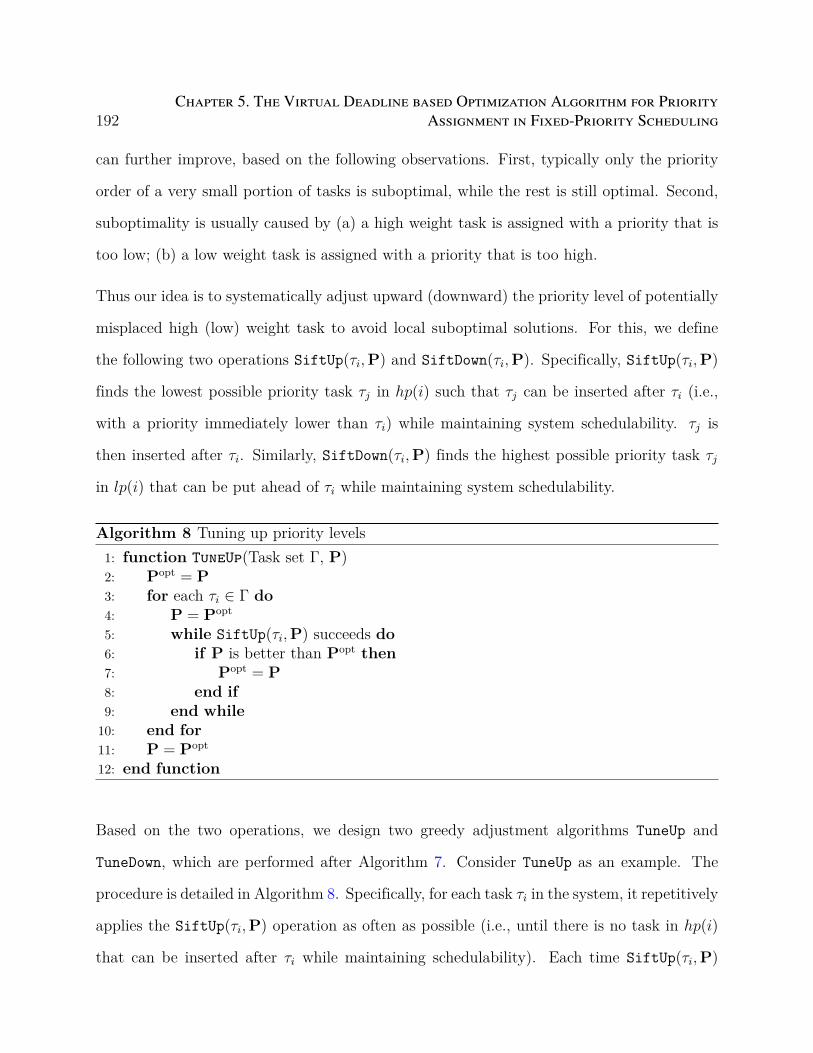
192Chapter 5. The Virtual Deadline based Optimization Algorithm for Priority
Assignment in Fixed-Priority Scheduling
can further improve, based on the following observations. First, typically only the priority
order of a very small portion of tasks is suboptimal, while the rest is still optimal. Second,
suboptimality is usually caused by (a) a high weight task is assigned with a priority that is
too low; (b) a low weight task is assigned with a priority that is too high.
Thus our idea is to systematically adjust upward (downward) the priority level of potentially
misplaced high (low) weight task to avoid local suboptimal solutions. For this, we define
the following two operations SiftUp(τi,P) and SiftDown(τi,P). Specifically, SiftUp(τi,P)
finds the lowest possible priority task τj in hp(i) such that τj can be inserted after τi (i.e.,
with a priority immediately lower than τi) while maintaining system schedulability. τj is
then inserted after τi. Similarly, SiftDown(τi,P) finds the highest possible priority task τj
in lp(i) that can be put ahead of τi while maintaining system schedulability.
Algorithm 8 Tuning up priority levels1: function TuneUp(Task set Γ, P)2: Popt = P3: for each τi ∈ Γ do4: P = Popt
5: while SiftUp(τi,P) succeeds do6: if P is better than Popt then7: Popt = P8: end if9: end while
10: end for11: P = Popt
12: end function
Based on the two operations, we design two greedy adjustment algorithms TuneUp and
TuneDown, which are performed after Algorithm 7. Consider TuneUp as an example. The
procedure is detailed in Algorithm 8. Specifically, for each task τi in the system, it repetitively
applies the SiftUp(τi,P) operation as often as possible (i.e., until there is no task in hp(i)
that can be inserted after τi while maintaining schedulability). Each time SiftUp(τi,P)
5.5. The Concept of MUDA 193
succeeds, the new priority order P is compared with the current best order Popt. If P has
a smaller cost than Popt, then Popt is updated as P. At the end of the procedure, the best
order Popt is returned. TuneDown is the same as TuneUp except that SiftUp(τi,P) is replaced
with SiftDown(τi,P) in Line 5.
5.5 The Concept of MUDA
We now consider the full version of the problem in (5.5), where there are additional linear
constraints on task WCRT besides schedulability of individual tasks. Algorithm 7 is generally
inapplicable here due to the additional constraints. A straightforward solution is to formulate
it in standard mathematical programming framework such as Integer Linear Programming
(ILP). However, this approach does not scale up to medium- or large-sized systems.
In the following, we present an efficient algorithm that runs several magnitudes faster than
ILP. It is based on the following observations. First, the major difficulty of using ILP for
solving (5.5) lies in the formulation of WCRT, which requires many integer variables [155].
However, as detailed in the previous two sections, the subproblem of finding a schedulable
priority assignment that minimizes the (weighted) average WCRT can be efficiently solved.
Thus, our main idea is to free ILP solver from the burden of computing task WCRT. The
proposed optimization framework is an iterative procedure that judiciously combines the
power of ILP solver and the algorithms in the previous two sections, Sections 5.3–5.4.
In this section, we introduce the concept of Maximal Unschedulable Deadline Assignment
(MUDA), which is used to interact between the ILP solver and the algorithms in Sections 5.3–
5.4. In the next section, we detail the MUDA guided optimization framework. Throughout
the two sections, we use the small example system in Table 5.1 with preemptive scheduling
to illustrate. The objective is to minimize the average WCRT for all tasks (i.e., all βi = 1).

194Chapter 5. The Virtual Deadline based Optimization Algorithm for Priority
Assignment in Fixed-Priority Scheduling
Table 5.1: An Example Task System Γe
τi Ti Di Ci βi
τ1 10 10 2 1τ2 20 20 3 1τ3 40 40 10 1τ4 100 100 3 1
Definition 13. A virtual deadline (VD) is a tuple ⟨τi, d⟩ where d is an integer no larger than
the deadline Di of task τi. It represents a stricter deadline requirement for τi, i.e., Ri ≤ d.
Although the concept of virtual deadline is proposed in, e.g., [14], it is used for scheduling,
i.e., to be enforced at runtime under certain scenarios. Differently, we use it purely for design
optimization, which does not affect the scheduling.
Definition 14. A weighted average deadline (WAD) is a tuple ⟨Ω, d⟩ where Ω ⊆ Γ is the
set of concerned tasks in the objective of problem (5.5), and d is an integer no larger than∑i∈Ω βi · Di. A WAD ⟨Ω, d⟩ denotes a constraint upper bounding the objective of the
optimization problem (5.5), i.e., ∑i∈Ω
βi ·Ri ≤ d (5.21)
Definition 15. A deadline assignment set R is a collection of one VD for each task τi
and one WAD, i.e., R = ⟨τ1, d1⟩ , ..., ⟨τn, dn⟩ , ⟨Ω, dΩ⟩, which represents the conjunction
(logic-AND, denoted by either the “” or the “∧” symbol) of constraints as follows
Ri ≤ di, ∀ ⟨τi, di⟩ ∈ R∑j∈Ω
βj ·Rj ≤ dΩ, ⟨Ω, dΩ⟩ ∈ R(5.22)

5.5. The Concept of MUDA 195
Example 5.1. Consider a deadline assignment set
R = ⟨τ1, 10⟩ , ⟨τ2, 20⟩ , ⟨τ3, 20⟩ , ⟨τ4, 100⟩ , ⟨Ω, 35⟩ (5.23)
It represents the conjuncted set of constraints
(R1 ≤ 10) ∧ (R2 ≤ 20) ∧ (R3 ≤ 20) ∧ (R4 ≤ 100)
∧(R1 +R2 +R3 +R4 ≤ 35)
Definition 16. R1 is said to dominateR2, denoted asR1 ⪰ R2, if and only if the constraints
represented by R1 are looser than or the same as those of R2. More specifically, the VD and
WAD in R1 are component wise no smaller than in R2. R1 is said to strictly dominate R2,
denoted as R1 ≻ R2, if R1 ⪰ R2 and at least one component in R1 is larger than R2.
Example 5.2. Consider the following deadline assignment sets
R1 = ⟨τ1, 10⟩ , ⟨τ2, 20⟩ , ⟨τ3, 20⟩ , ⟨τ4, 100⟩ , ⟨Ω, 35⟩
R2 = ⟨τ1, 10⟩ , ⟨τ2, 20⟩ , ⟨τ3, 20⟩ , ⟨τ4, 100⟩ , ⟨Ω, 40⟩
R3 = ⟨τ1, 10⟩ , ⟨τ2, 20⟩ , ⟨τ3, 40⟩ , ⟨τ4, 100⟩ , ⟨Ω, 35⟩
R4 = ⟨τ1, 10⟩ , ⟨τ2, 16⟩ , ⟨τ3, 20⟩ , ⟨τ4, 100⟩ , ⟨Ω, 170⟩
(5.24)
We have R2 ⪰ R1 and R3 ⪰ R1, since R1 denotes stricter requirements than both R2 and
R3. However, neither R4 nor R1 dominates each other, since R1 is more relaxed on the VD
of τ2, but is stricter on the WAD.
Definition 17. A system Γ is R-schedulable (or informally, R is schedulable) if there exists
a priority assignment P such that the task WCRTs satisfy the constraints represented by R.

196Chapter 5. The Virtual Deadline based Optimization Algorithm for Priority
Assignment in Fixed-Priority Scheduling
Example 5.3. Consider two deadline assignment sets as follows
R1 = ⟨τ1, 10⟩ , ⟨τ2, 20⟩ , ⟨τ3, 20⟩ , ⟨τ4, 100⟩ , ⟨Ω, 35⟩
R2 = ⟨τ1, 10⟩ , ⟨τ2, 3⟩ , ⟨τ3, 40⟩ , ⟨τ4, 100⟩ , ⟨Ω, 35⟩(5.25)
Γe is R-schedulable since in the WCET monotonic priority order τ1 > τ2 > τ4 > τ3, the task
WCRTs are R1 = 2, R2 = 5, R3 = 20, and R4 = 8, which satisfy the constraints represented
by R1. However, Γe is not R2-schedulable. This is because to satisfy R2 ≤ 3, τ2 must have
the highest priority. Also τ1 must have higher priority than τ3 (due to C3 > D1). With these
priority orders in place, the priority assignment τ2 > τ1 > τ4 > τ3 minimizes the sum (= 36)
of WCRTs, where the task WCRTs are R1 = 5, R2 = 3, R3 = 20 and R4 = 8. However, they
still violate the WAD in R2.
Obviously the following holds for deadline assignment sets with dominance relationship.
Theorem 32. If Γ is R-schedulable, it is schedulable for any R′ ⪰ R. If Γ is not R-
schedulable, it is not schedulable for any R′ ⪯ R.
Proof. This follows directly from the monotonicity of schedulability w.r.t. deadline
assignments. If the system is R-schedulable, then it is still schedulable with increased task
deadlines (i.e., with a dominating R′ ⪰ R).
Definition 18. A deadline assignment set U is a Maximal Unschedulable Deadline Assign-
ment (MUDA) if and only if
• Γ is not U -schedulable; and
• Γ is R-schedulable for any strictly dominating R ≻ U .
By Theorem 32, to verify the second condition of MUDA, it suffices to test only those Rs
that increment (i.e., increase by one) any WAD or VD in U .
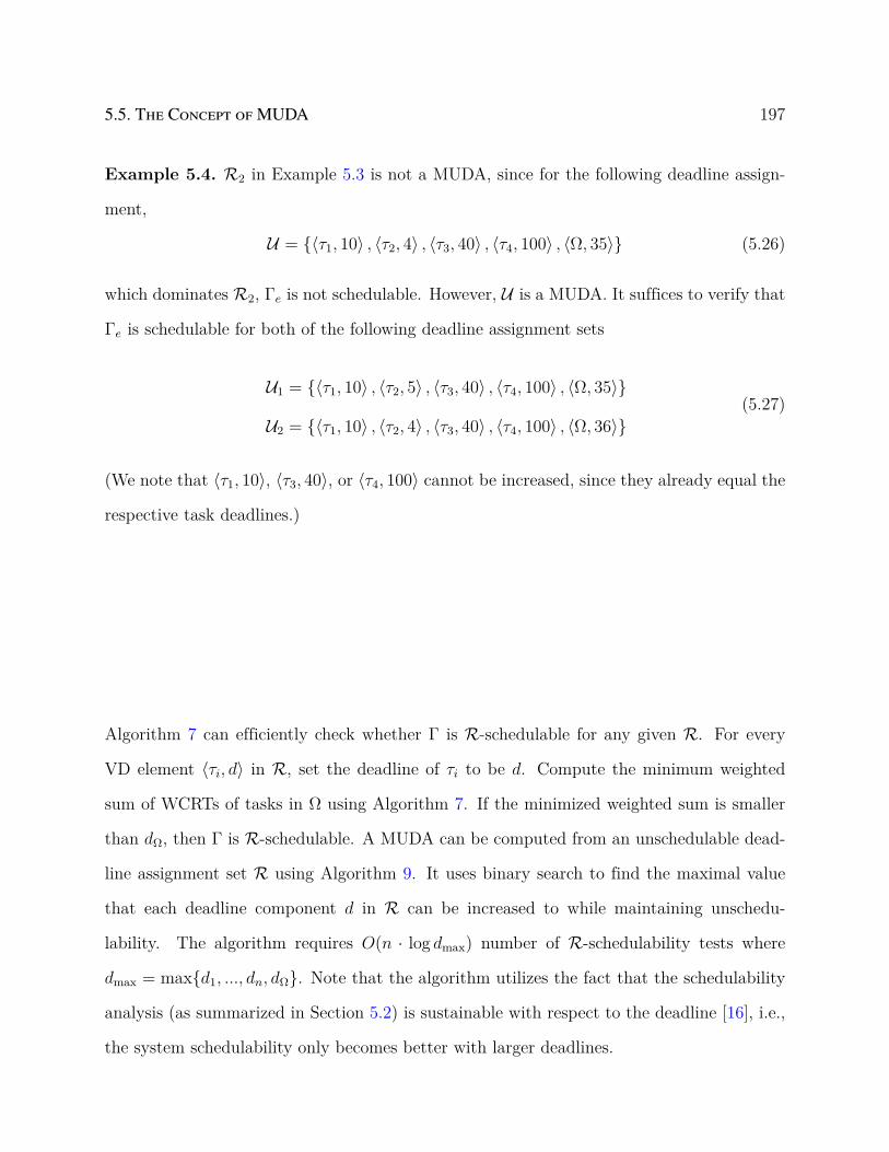
5.5. The Concept of MUDA 197
Example 5.4. R2 in Example 5.3 is not a MUDA, since for the following deadline assign-
ment,
U = ⟨τ1, 10⟩ , ⟨τ2, 4⟩ , ⟨τ3, 40⟩ , ⟨τ4, 100⟩ , ⟨Ω, 35⟩ (5.26)
which dominates R2, Γe is not schedulable. However, U is a MUDA. It suffices to verify that
Γe is schedulable for both of the following deadline assignment sets
U1 = ⟨τ1, 10⟩ , ⟨τ2, 5⟩ , ⟨τ3, 40⟩ , ⟨τ4, 100⟩ , ⟨Ω, 35⟩
U2 = ⟨τ1, 10⟩ , ⟨τ2, 4⟩ , ⟨τ3, 40⟩ , ⟨τ4, 100⟩ , ⟨Ω, 36⟩(5.27)
(We note that ⟨τ1, 10⟩, ⟨τ3, 40⟩, or ⟨τ4, 100⟩ cannot be increased, since they already equal the
respective task deadlines.)
Algorithm 7 can efficiently check whether Γ is R-schedulable for any given R. For every
VD element ⟨τi, d⟩ in R, set the deadline of τi to be d. Compute the minimum weighted
sum of WCRTs of tasks in Ω using Algorithm 7. If the minimized weighted sum is smaller
than dΩ, then Γ is R-schedulable. A MUDA can be computed from an unschedulable dead-
line assignment set R using Algorithm 9. It uses binary search to find the maximal value
that each deadline component d in R can be increased to while maintaining unschedu-
lability. The algorithm requires O(n · log dmax) number of R-schedulability tests where
dmax = maxd1, ..., dn, dΩ. Note that the algorithm utilizes the fact that the schedulability
analysis (as summarized in Section 5.2) is sustainable with respect to the deadline [16], i.e.,
the system schedulability only becomes better with larger deadlines.
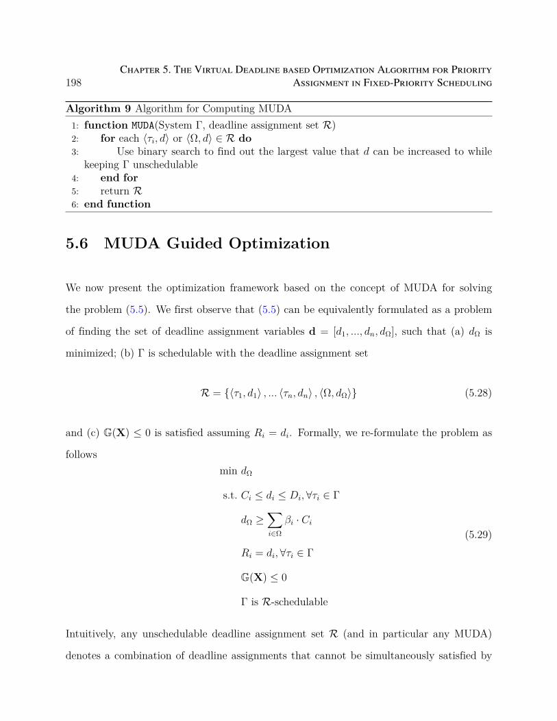
198Chapter 5. The Virtual Deadline based Optimization Algorithm for Priority
Assignment in Fixed-Priority Scheduling
Algorithm 9 Algorithm for Computing MUDA1: function MUDA(System Γ, deadline assignment set R)2: for each ⟨τi, d⟩ or ⟨Ω, d⟩ ∈ R do3: Use binary search to find out the largest value that d can be increased to while
keeping Γ unschedulable4: end for5: return R6: end function
5.6 MUDA Guided Optimization
We now present the optimization framework based on the concept of MUDA for solving
the problem (5.5). We first observe that (5.5) can be equivalently formulated as a problem
of finding the set of deadline assignment variables d = [d1, ..., dn, dΩ], such that (a) dΩ is
minimized; (b) Γ is schedulable with the deadline assignment set
R = ⟨τ1, d1⟩ , ... ⟨τn, dn⟩ , ⟨Ω, dΩ⟩ (5.28)
and (c) G(X) ≤ 0 is satisfied assuming Ri = di. Formally, we re-formulate the problem as
followsmin dΩ
s.t. Ci ≤ di ≤ Di,∀τi ∈ Γ
dΩ ≥∑i∈Ω
βi · Ci
Ri = di,∀τi ∈ Γ
G(X) ≤ 0
Γ is R-schedulable
(5.29)
Intuitively, any unschedulable deadline assignment set R (and in particular any MUDA)
denotes a combination of deadline assignments that cannot be simultaneously satisfied by

5.6. MUDA Guided Optimization 199
any feasible priority assignment. Hence, R = ⟨τ1, d∗1⟩ , · · · , ⟨τn, d∗n⟩ , ⟨Ω, d∗Ω⟩ denotes the
disjunction (logic-OR, denoted with either the “∥” or the “∨” symbol) of constraints that
any feasible deadline assignment ⟨τ1, d1⟩ , · · · , ⟨τn, dn⟩ , ⟨Ω, dΩ⟩ must satisfy
∥∥∥∥∥∥∥di > d∗i ∀ ⟨τi, d∗i ⟩ ∈ R
dΩ > d∗Ω ⟨Ω, d∗Ω⟩ ∈ R(5.30)
In this sense, any unschedulable deadline assignment set R partially shapes the feasibility
region of the problem. We call (5.30) the induced schedulability constraints by R.
The feasibility region of d = [d1, d2, ...dn, dΩ] can be defined by the set of all MUDAs of
Γ. However computing all of them is obviously impractical as the number of MUDAs is
exponential to the number of tasks. We note that in many cases, the objective is sensitive
to only a small set of MUDAs. Thus, we devise a MUDA guided optimization framework
which judiciously and gradually adds MUDAs into the problem until its optimal solution is
found. The algorithm is illustrated in Figure 5.2. The calculation of WCRT is never explicit
in the ILP formulation. Instead, it is abstracted into the form of MUDAs as an alternative
representation of the feasibility region.
Step 1–Priority Assignment Evaluation Order. In this step, we find an evaluation
order in Line 9 of Algorithm 7, which will later be used as R-schedulability test in MUDA
computation (Step 5). For the case of average WCRT, the optimal evaluation order is
WCET monotonic, i.e., in non-increasing order of task WCET. For the case of weighted
average WCRT, the algorithm in Section 5.4 is used. Specifically, we first ignore extra
design constraints and consider only schedulability. Then use the initial order by scaled-
WCET in Algorithm 7 to obtain a first solution P. Apply sifting adjustment to improve P
into P′. P′ is then used as the evaluation order in all subsequent MUDA calculations. If it
fails to find any schedulable order, the procedure terminates since the problem is infeasible.

200Chapter 5. The Virtual Deadline based Optimization Algorithm for Priority
Assignment in Fixed-Priority Scheduling
Step 3: Solve ILP formulation with CPLEX
Step 5:
Schedulable?No
Yes
Compute MUDAs with Algorithm 2 and add their induced constraints to
Step 4: Solve ILP formulation with CPLEX
Step 2: Start with ILP without any
schedulability constraints
Step 1:Obtain an evaluation order for priority
assignment
Schedulable?
Yes
Report unschedulability
Deadline assignment
Adjusted deadline assignment
No
Feasible?
Yes
Report infeasibility
No
Report optimal solution
Figure 5.2: The MUDA guided iterative optimization framework.
Step 2–Initial ILP. The initial ILP Π contains only the constraints G(X) ≤ 0, but not
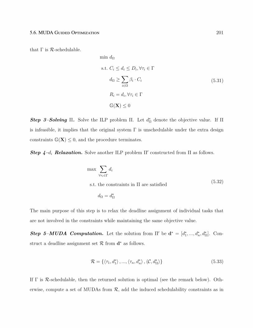
5.6. MUDA Guided Optimization 201
that Γ is R-schedulable.min dΩ
s.t. Ci ≤ di ≤ Di,∀τi ∈ Γ
dΩ ≥∑i∈Ω
βi · Ci
Ri = di,∀τi ∈ Γ
G(X) ≤ 0
(5.31)
Step 3–Solving Π. Solve the ILP problem Π. Let d∗Ω denote the objective value. If Π
is infeasible, it implies that the original system Γ is unschedulable under the extra design
constraints G(X) ≤ 0, and the procedure terminates.
Step 4–di Relaxation. Solve another ILP problem Π′ constructed from Π as follows.
max∑∀τi∈Γ
di
s.t. the constraints in Π are satisfied
dΩ = d∗Ω
(5.32)
The main purpose of this step is to relax the deadline assignment of individual tasks that
are not involved in the constraints while maintaining the same objective value.
Step 5–MUDA Computation. Let the solution from Π′ be d∗ = [d∗1, ..., d∗n, d
∗Ω]. Con-
struct a deadline assignment set R from d∗ as follows.
R = ⟨τ1, d∗1⟩ , ..., ⟨τn, d∗n⟩ , ⟨C, d∗Ω⟩ (5.33)
If Γ is R-schedulable, then the returned solution is optimal (see the remark below). Oth-
erwise, compute a set of MUDAs from R, add the induced schedulability constraints as in
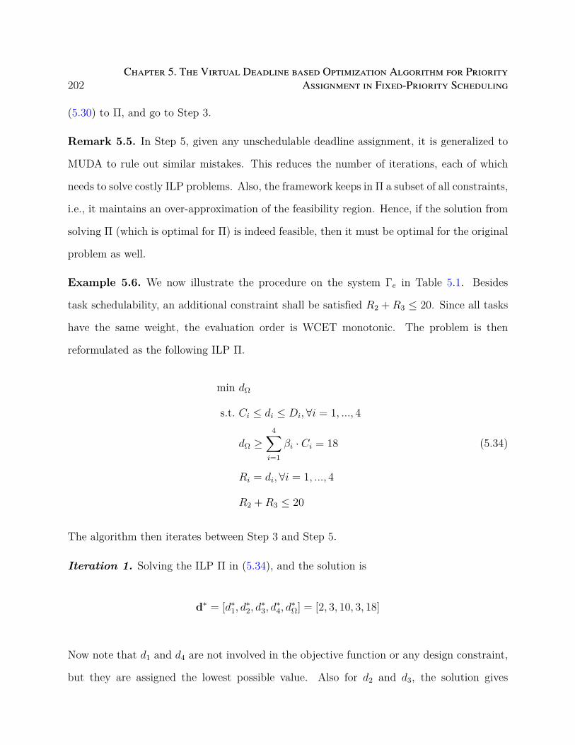
202Chapter 5. The Virtual Deadline based Optimization Algorithm for Priority
Assignment in Fixed-Priority Scheduling
(5.30) to Π, and go to Step 3.
Remark 5.5. In Step 5, given any unschedulable deadline assignment, it is generalized to
MUDA to rule out similar mistakes. This reduces the number of iterations, each of which
needs to solve costly ILP problems. Also, the framework keeps in Π a subset of all constraints,
i.e., it maintains an over-approximation of the feasibility region. Hence, if the solution from
solving Π (which is optimal for Π) is indeed feasible, then it must be optimal for the original
problem as well.
Example 5.6. We now illustrate the procedure on the system Γe in Table 5.1. Besides
task schedulability, an additional constraint shall be satisfied R2 + R3 ≤ 20. Since all tasks
have the same weight, the evaluation order is WCET monotonic. The problem is then
reformulated as the following ILP Π.
min dΩ
s.t. Ci ≤ di ≤ Di, ∀i = 1, ..., 4
dΩ ≥4∑
i=1
βi · Ci = 18
Ri = di,∀i = 1, ..., 4
R2 +R3 ≤ 20
(5.34)
The algorithm then iterates between Step 3 and Step 5.
Iteration 1. Solving the ILP Π in (5.34), and the solution is
d∗ = [d∗1, d∗2, d
∗3, d
∗4, d
∗Ω] = [2, 3, 10, 3, 18]
Now note that d1 and d4 are not involved in the objective function or any design constraint,
but they are assigned the lowest possible value. Also for d2 and d3, the solution gives

5.6. MUDA Guided Optimization 203
d2 + d3 = 13 while the maximum allowed bound for their sum is 20. Thus the deadline
assignments can be further relaxed by solving the following problem Π′ as described in
Step 4.max d1 + d2 + d3 + d4
s.t. Ci ≤ di ≤ Di,∀i = 1, ..., 4
dΩ ≥4∑
i=1
βi · Ci = 18
Ri = di,∀i = 1, ..., 4
R2 +R3 ≤ 20
dΩ = 18
(5.35)
Solving Problem (5.35) returns following adjusted solution.
d∗ = [d∗1, d∗2, d
∗3, d
∗4, d
∗Ω] = [10, 10, 10, 100, 18]
This new deadline assignment has the same d∗Ω while satisfying all the constraints in Π,
but is more relaxed in deadline assignments of individual tasks (i.e., d1–d4). Construct the
corresponding deadline assignment set R1 as
R1 = ⟨τ1, 10⟩ , ⟨τ2, 10⟩ , ⟨τ3, 10⟩ , ⟨τ4, 100⟩ , ⟨Ω, 18⟩
Since Γe is not R1-schedulable, the following two MUDAs are computed. They both are still
unschedulable, but they dominate R1 thus inducing more relaxed constraints than R1.
U1,1 = ⟨τ1, 10⟩ , ⟨τ2, 20⟩ , ⟨τ3, 40⟩ , ⟨τ4, 100⟩ , ⟨Ω, 34⟩
U1,2 = ⟨τ1, 10⟩ , ⟨τ2, 20⟩ , ⟨τ3, 19⟩ , ⟨τ4, 100⟩ , ⟨Ω, 43⟩
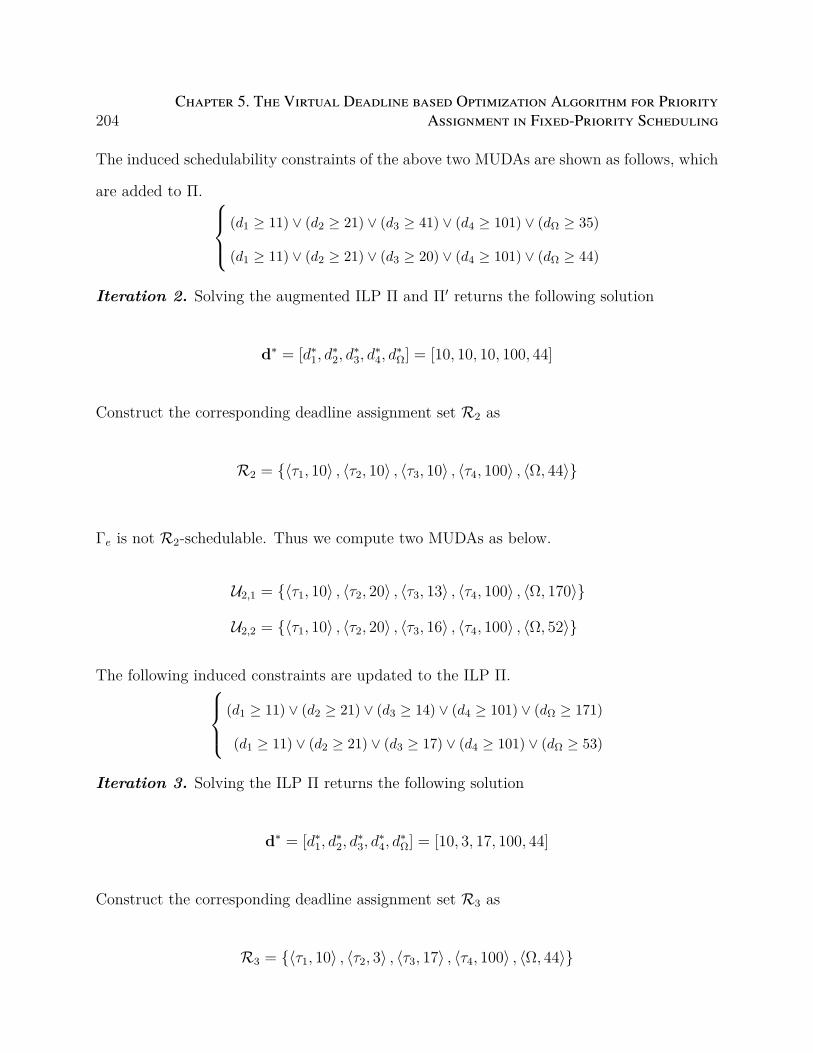
204Chapter 5. The Virtual Deadline based Optimization Algorithm for Priority
Assignment in Fixed-Priority Scheduling
The induced schedulability constraints of the above two MUDAs are shown as follows, which
are added to Π. (d1 ≥ 11) ∨ (d2 ≥ 21) ∨ (d3 ≥ 41) ∨ (d4 ≥ 101) ∨ (dΩ ≥ 35)
(d1 ≥ 11) ∨ (d2 ≥ 21) ∨ (d3 ≥ 20) ∨ (d4 ≥ 101) ∨ (dΩ ≥ 44)
Iteration 2. Solving the augmented ILP Π and Π′ returns the following solution
d∗ = [d∗1, d∗2, d
∗3, d
∗4, d
∗Ω] = [10, 10, 10, 100, 44]
Construct the corresponding deadline assignment set R2 as
R2 = ⟨τ1, 10⟩ , ⟨τ2, 10⟩ , ⟨τ3, 10⟩ , ⟨τ4, 100⟩ , ⟨Ω, 44⟩
Γe is not R2-schedulable. Thus we compute two MUDAs as below.
U2,1 = ⟨τ1, 10⟩ , ⟨τ2, 20⟩ , ⟨τ3, 13⟩ , ⟨τ4, 100⟩ , ⟨Ω, 170⟩
U2,2 = ⟨τ1, 10⟩ , ⟨τ2, 20⟩ , ⟨τ3, 16⟩ , ⟨τ4, 100⟩ , ⟨Ω, 52⟩
The following induced constraints are updated to the ILP Π.(d1 ≥ 11) ∨ (d2 ≥ 21) ∨ (d3 ≥ 14) ∨ (d4 ≥ 101) ∨ (dΩ ≥ 171)
(d1 ≥ 11) ∨ (d2 ≥ 21) ∨ (d3 ≥ 17) ∨ (d4 ≥ 101) ∨ (dΩ ≥ 53)
Iteration 3. Solving the ILP Π returns the following solution
d∗ = [d∗1, d∗2, d
∗3, d
∗4, d
∗Ω] = [10, 3, 17, 100, 44]
Construct the corresponding deadline assignment set R3 as
R3 = ⟨τ1, 10⟩ , ⟨τ2, 3⟩ , ⟨τ3, 17⟩ , ⟨τ4, 100⟩ , ⟨Ω, 44⟩
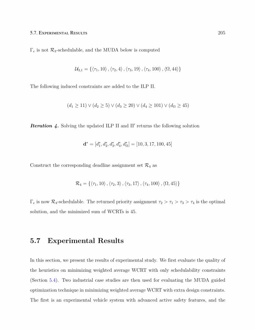
5.7. Experimental Results 205
Γe is not R3-schedulable, and the MUDA below is computed
U3,1 = ⟨τ1, 10⟩ , ⟨τ2, 4⟩ , ⟨τ3, 19⟩ , ⟨τ4, 100⟩ , ⟨Ω, 44⟩
The following induced constraints are added to the ILP Π.
(d1 ≥ 11) ∨ (d2 ≥ 5) ∨ (d3 ≥ 20) ∨ (d4 ≥ 101) ∨ (dΩ ≥ 45)
Iteration 4. Solving the updated ILP Π and Π′ returns the following solution
d∗ = [d∗1, d∗2, d
∗3, d
∗4, d
∗Ω] = [10, 3, 17, 100, 45]
Construct the corresponding deadline assignment set R4 as
R4 = ⟨τ1, 10⟩ , ⟨τ2, 3⟩ , ⟨τ3, 17⟩ , ⟨τ4, 100⟩ , ⟨Ω, 45⟩
Γe is now R4-schedulable. The returned priority assignment τ2 > τ1 > τ3 > τ4 is the optimal
solution, and the minimized sum of WCRTs is 45.
5.7 Experimental Results
In this section, we present the results of experimental study. We first evaluate the quality of
the heuristics on minimizing weighted average WCRT with only schedulability constraints
(Section 5.4). Two industrial case studies are then used for evaluating the MUDA guided
optimization technique in minimizing weighted average WCRT with extra design constraints.
The first is an experimental vehicle system with advanced active safety features, and the

206Chapter 5. The Virtual Deadline based Optimization Algorithm for Priority
Assignment in Fixed-Priority Scheduling
second is a simplified version of fuel injection system.
5.7.1 Quality of Heuristics for Min Weighted Average WCRT
In this experiment, we focus on measuring the average suboptimality by the proposed heuris-
tics in Section 5.4. We note the one in Section 5.3 is proven optimal. The following three
methods are compared.
• Scaled-WCET Monotonic: Algorithm 7, with non-increasing scaled-WCET as the
evaluation order in Line 9.
• Scaled-WCET Monotonic + Sifting: Scaled-WCET Monotonic with both Tune-down
and Tune-up adjustments applied afterwards.
• ILP: Formulating the problem as an integer linear program and solving it with CPLEX.
ILP guarantees to return global optimal solutions upon termination, which can then be used
to calculate the suboptimality of the other methods, defined as sub−optopt
× 100%, where sub
is the solution from Scaled-WCET Monotonic or Scaled-WCET Monotonic + Sifting, and
opt is the optimal solution from ILP. We use randomly generated periodic systems with
varying number of tasks and system utilization. Each task is assigned a period following
the log-uniform distribution in the range [10, 1000], and a utilization using the UUnifast-
Discard algorithm [50]. The weight for each task is a random number between 1 and 10000.
This is the typical range for coefficients of control cost [103]. We consider both preemptive
scheduling (denoted as P in the figures) and non-preemptive scheduling (denoted as NP in
the figures). Each point in the figures is the average result of 1000 randomly generated task
sets.
We first fix the number of tasks to 20 and vary the total utilization. The results are plotted
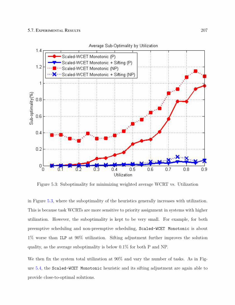
5.7. Experimental Results 207
Figure 5.3: Suboptimality for minimizing weighted average WCRT vs. Utilization
in Figure 5.3, where the suboptimality of the heuristics generally increases with utilization.
This is because task WCRTs are more sensitive to priority assignment in systems with higher
utilization. However, the suboptimality is kept to be very small. For example, for both
preemptive scheduling and non-preemptive scheduling, Scaled-WCET Monotonic is about
1% worse than ILP at 90% utilization. Sifting adjustment further improves the solution
quality, as the average suboptimality is below 0.1% for both P and NP.
We then fix the system total utilization at 90% and vary the number of tasks. As in Fig-
ure 5.4, the Scaled-WCET Monotonic heuristic and its sifting adjustment are again able to
provide close-to-optimal solutions.

208Chapter 5. The Virtual Deadline based Optimization Algorithm for Priority
Assignment in Fixed-Priority Scheduling
Figure 5.4: Suboptimality for minimizing weighted average WCRT vs. Number of Tasks
We now re-draw the above results using Tukey type box plots to illustrate the distribution
of the suboptimaltiy. Each box plot displays the distribution of suboptimality based on the
five number summary: first quartile (Q1), median (Q2), third quartile (Q3), and maximum
and minimum values that are still within the range [Q1− 1.5× (Q3−Q1), Q3+1.5× (Q3−
Q1)]. Figures 5.5 and 5.6 show the results for Scaled-WCET Monotonic. However, since
Scaled-WCET Monotonic + Sifting achieves optimality for more than 75% of the test
cases in both Figures 5.3 and 5.4 (i.e., Q1 and Q3 are both 0), its box plots appear empty
and we omit them. Instead, we only give its maximum sub-optimality. For Figure 5.3, the
maximum sub-optimality is 7% for preemptive, and 10% non-preemptive scheduling. For
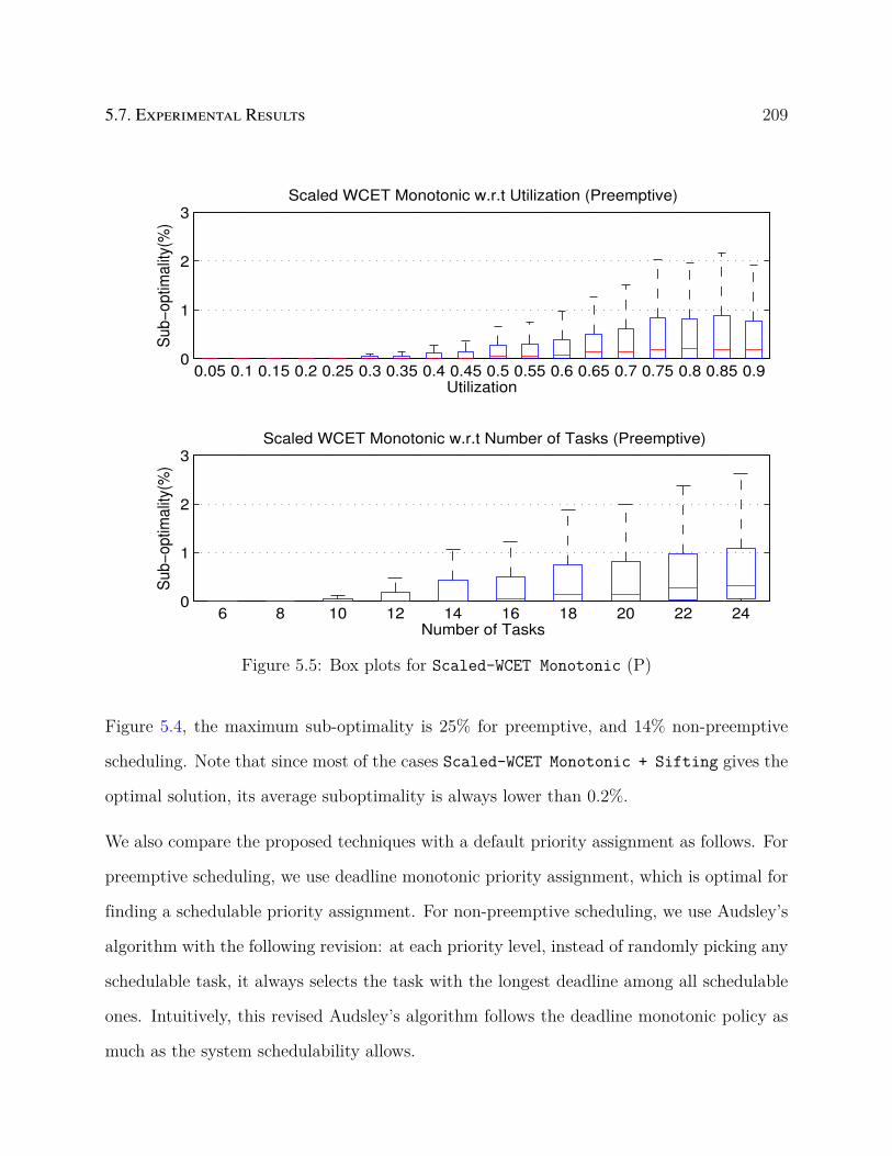
5.7. Experimental Results 209
0
1
2
3
0.05 0.1 0.15 0.2 0.25 0.3 0.35 0.4 0.45 0.5 0.55 0.6 0.65 0.7 0.75 0.8 0.85 0.9Utilization
Su
b−
op
tima
lity(
%)
Scaled WCET Monotonic w.r.t Utilization (Preemptive)
0
1
2
3
6 8 10 12 14 16 18 20 22 24Number of Tasks
Su
b−
op
tima
lity(
%)
Scaled WCET Monotonic w.r.t Number of Tasks (Preemptive)
Figure 5.5: Box plots for Scaled-WCET Monotonic (P)
Figure 5.4, the maximum sub-optimality is 25% for preemptive, and 14% non-preemptive
scheduling. Note that since most of the cases Scaled-WCET Monotonic + Sifting gives the
optimal solution, its average suboptimality is always lower than 0.2%.
We also compare the proposed techniques with a default priority assignment as follows. For
preemptive scheduling, we use deadline monotonic priority assignment, which is optimal for
finding a schedulable priority assignment. For non-preemptive scheduling, we use Audsley’s
algorithm with the following revision: at each priority level, instead of randomly picking any
schedulable task, it always selects the task with the longest deadline among all schedulable
ones. Intuitively, this revised Audsley’s algorithm follows the deadline monotonic policy as
much as the system schedulability allows.

210Chapter 5. The Virtual Deadline based Optimization Algorithm for Priority
Assignment in Fixed-Priority Scheduling
0
1
2
3
0.05 0.1 0.15 0.2 0.25 0.3 0.35 0.4 0.45 0.5 0.55 0.6 0.65 0.7 0.75 0.8 0.85 0.9Utilization
Su
b−
op
tima
lity(
%)
Scaled WCET Monotonic w.r.t Utilization (Preemptive)
0
1
2
3
6 8 10 12 14 16 18 20 22 24Number of Tasks
Su
b−
op
tima
lity(
%)
Scaled WCET Monotonic w.r.t Number of Tasks (Preemptive)
Figure 5.6: Box plots for Scaled-WCET Monotonic (NP)
The default priority assignment has substantial suboptimality. For the systems in Figure 5.3,
the default priority assignment is 57%-67% and 15%-46% worse than the optimal solution
for preemptive scheduling and non-preemptive scheduling respectively. For the systems in
Figure 5.4, the suboptimality is 30%-63% and 7%-40% for preemptive scheduling and non-
preemptive scheduling respectively. This highlights the necessity to develop a problem-
specific approach, as the default solution may be of low quality.

5.7. Experimental Results 211
Table 5.2: Result on Min Average WCRT for the Experimental Vehicle (“N/A” denotes nosolution found)
Method Objective Time StatusMUDA-Guided 305828 234.9s Terminate
ILP N/A ≥ 24h Timeout
5.7.2 Experimental Vehicle System with Active Safety Features
The first industrial case study is an experimental vehicle system with advanced active safety
features. It consists of 29 Electronic Control Units (ECUs) connected through 4 CAN buses,
92 tasks, and 192 CAN messages [41]. Tasks are preemptive and CAN messages are scheduled
non-preemptively. End-to-end delay deadlines are imposed on 12 pairs of source-sink tasks,
which contain a total of 222 unique paths. The allocation of tasks and messages onto
corresponding execution platforms are given. The problem is to find a priority assignment
that minimizes the average WCRT of all tasks and messages, subject to the end-to-end
deadline constraints and the schedulability of individual tasks/messages. As discussed in [41],
the end-to-end delay of a path is the sum of the WCRTs and periods for all tasks and messages
in the path.
We compare the proposed MUDA-based technique (denoted as MUDA-Guided) with a straight-
forward ILP formulation (denoted as ILP). The results are summarized in Table 5.2. The
proposed algorithm MUDA-Guided finds the optimal solution within just 235 seconds while
the ILP solver fails to find any feasible solution within 24 hours.
We now modify the problem to get a weighted version. Each task is assigned a weight of one
plus the number of critical paths the task is involved. This metric has the benefit of being
more aware of the critical tasks. The results are summarized in Table 5.3. Both the proposed
approach (MUDA-Guided) and ILP return the same optimal solution, however, MUDA-Guided
is 10, 000× faster.

212Chapter 5. The Virtual Deadline based Optimization Algorithm for Priority
Assignment in Fixed-Priority Scheduling
Table 5.3: Result on Min Weighted Average WCRT for the Experimental Vehicle
Method Objective Time StatusMUDA-Guided 7995881 3.36s Terminate
ILP 7995881 51616.65s Terminate
Table 5.4: Result on Min Average WCRT for the Fuel Injection System (“N/A” denotes nosolution found)
Memory MUDA-Guided ILPObjective Time Status Objective Time Status
8900 Infeasible 138.21s Terminate N/A ≥ 24h Timeout8950 14090418 183.68s Terminate N/A ≥ 24h Timeout9000 13392124 5.11s Terminate 16862700 ≥ 24h Timeout9100 13384171 1.20s Terminate 13487800 ≥ 24h Timeout
Table 5.5: Result on Min Weighted Average WCRT for the Fuel Injection System (“N/A”denotes no solution found)
Memory MUDA-Guided ILPObjective Time Status Objective Time Status
8900 Infeasible 483.87s Terminate N/A ≥ 24h Timeout8950 4.67e+10 352.34s Terminate N/A ≥ 24h Timeout9000 4.13e+10 22.62s Terminate N/A ≥ 24h Timeout9100 4.12e+10 0.95s Terminate N/A ≥ 24h Timeout
5.7.3 Fuel Injection System
The second industrial case study is the task system implementing a Simulink model of fuel
injection system [58]. It contains 90 tasks with preemptive scheduling, and 106 communica-
tion links. The communication link carries data between two tasks with harmonic periods,
as required by Simulink. The total system utilization is 94.1%. To protect the share resource
and preserve the same behavior as in the Simulink model, a wait-free buffer is introduced
whenever the executions of the writer task and the reader task may overlap. Hence, the total
memory cost incurred by the wait-free buffers is positively dependent on the task WCRTs:
the wait-free buffer is avoided if there is no preemption between the writer and reader by
ensuring the reader’s WCRT is no larger than the writer’s period [58].

5.8. Related Work 213
We consider the problem of minimizing the average and weighted average WCRT of all tasks
subject to the constraint of available memory for wait-free buffers. The weight of each task is
randomly generated between 1 and 10000. We compare the proposed approach MUDA-Guided
with an ILP formulation (denoted as ILP). To test the efficiency of the techniques under
different tightness of design constraints, we give four settings on memory constraints. The
result are summarized in Table 5.4 and Table 5.5. ILP is unable to find any feasible solution
in 24 hours except for two most relaxed memory constraint settings. On the other hand,
MUDA-Guided solves all problem settings within a few minutes, either finding a much better
solution than ILP or detecting infeasibility.
5.8 Related Work
There has been a large body of work for priority assignment in real-time systems scheduled
with fixed priority. The seminal work from Liu and Layland [99] shows that for periodic
task system where task deadline equals period, rate-monotonic (RM) priority assignment
is optimal for schedulability in the sense that there is no system that can be scheduled by
some priority assignment but not by RM. When tasks have constrained deadline (i.e., no
larger than period), deadline monotonic (DM) policy is shown to be optimal for schedula-
bility [6]. For tasks with arbitrary deadline, Audsley’s algorithm [8] guarantees to give a
feasible priority assignment if one exists. It only needs to explore a quadratic O(n2) number
of priority assignments (among the total of n!) where n is the number of tasks. Audsley’s
algorithm is optimal in terms of schedulability to a variety of task models and scheduling
policies, as summarized in the authoritative survey by Davis et al. [48]. The three necessary
and sufficient conditions for its optimality are presented in [50]. Besides schedulability, Aud-
sley’s algorithm can be revised to optimize several other objectives, including the number
214Chapter 5. The Virtual Deadline based Optimization Algorithm for Priority
Assignment in Fixed-Priority Scheduling
of priority levels [8], lexicographical distance (the perturbation needed to make the system
schedulable from an initial order) [40, 48], and robustness (ability to tolerate additional
interferences) [44].
For complex problems on priority assignment optimization where Audsley’s algorithm do
not apply, the current approaches include (a) meta heuristics such as simulated annealing
(e.g., [22, 142]) and genetic algorithm (e.g., [75]); (b) problem specific heuristics (e.g., [127,
146, 156]); and (c) directly applying existing optimization frameworks such as branch-and-
bound (BnB) (e.g., [147]) and ILP (e.g., [58, 169]). These approaches either do not have
any guarantee on solution quality, or suffer from scalability issues and may have difficulty to
handle large industrial designs. Differently, a framework based on the concept of unschedu-
lability core, i.e., the irreducible set of priority orders that cause the system unschedulable,
is proposed in [160]. However, it does not apply to problems studied in this chapter, i.e.,
those involving the task WCRTs in the objective or additional constraints.
With respect to design optimization problems which are sensitive to task response times,
a branch-and-bound algorithm is developed to optimize both priority and period assign-
ments [103]. In the paper, a linear lower bound is adopted as an approximation to response
time. The problem of optimizing period assignment for distributed systems is formulated
in geometric programming framework, where the task WCRT is approximated with a linear
function on task rates [41]. Lukasiewycz et al. [102] study the problem of ID (i.e., priority)
obfuscation for CAN messages. The optimization procedure contains a first stage of mini-
mizing the average task WCRT by formulating the problem as a Quadratically Constrained
Integer Quadratic Program. In [134], a genetic algorithm is used for the problem of priority
and period assignment that minimize the sum of end-to-end delays in networked control sys-
tems. Zhu et al. [169] consider the problem of finding task allocation and priority assignment
that maximize the minimum end-to-end laxity in distributed systems. The approach is to

5.9. Conclusion 215
divide the problem into two stages, each of which is then formulated as an ILP program. Our
approach differs from all the above in that it designs a customized optimization procedure
specialized for the minimization of (weighted) average WCRT.
5.9 Conclusion
In this chapter, we propose an optimization framework that efficiently finds a schedulable
priority assignment while minimizing the weighted average WCRT for tasks with constrained
deadlines and preemptive/non-preemptive scheduling. It significantly reduces the runtime
while the optimality is only influenced minimally or not at all as indicated in the case studies.
We plan to further investigate optimization techniques for other types of real-time systems
with different task models and scheduling policies.
Chapter 6
A Unified Framework for Period and
Priority Optimization in Distributed
Hard Real-Time Systems
6.1 Introduction
Modern embedded systems in application domains such as avionics, automotive, and smart
buildings contain complex functional contents deployed on a distributed platform. For ex-
ample, new active safety and autonomous driving features are integrated in today’s vehicles,
which collect data from 360 sensors (e.g., camera, radar, and LIDAR) to understand the
position of surrounding objects and detect hazardous conditions. Once a hazard is detected,
they inform the driver and/or provide control overlays to reduce the risk. Two examples
are adaptive cruise control and lane keeping systems. These embedded systems have the
following characteristics:
• Functional dependencies are modeled by a complex graph rather than a set of linear
transactions. At the user level, timing constraints and performance metrics are expressed
on end-to-end paths from sensors to actuators. In addition, sensor, control, and actuator
functions operate with their own periodic tasks, with constraints on periods imposed by the
216
6.1. Introduction 217
need for stability and accuracy.
• The system is inherently multi-rate, because of technological constraints (e.g. off-the-
shelf sensors operate at different rates), but also because the same inputs and outputs are
shared by multiple control functions, characterized by different control laws with their period
constraints. Merging flows with different rates and communication with oversampling/un-
dersampling are common.
In this chapter, we consider the optimization of period and priority assignment, a problem
common in the system-level design stage of such embedded systems. Specifically, given an
allocation of tasks and messages, our approach automatically determines the periods and
priorities to assign to all tasks and messages, such that hard real-time constraints including
end-to-end deadline requirements are satisfied. Clearly, the solution quality depends on both
and, ideally, the two decision variables should be optimized at once. However, in the past
this optimization problem is considered to be too large, such that an integrated problem
formulation cannot be solved in feasible time [42]. Thus, existing approaches are to optimize
periods and priorities separately and possibly iteratively.
On the contrary, we develop a unified framework capable of co-optimizing both periods and
priorities for large industrial designs. Our observation is that existing approaches try to
directly leverage standard mathematical programming frameworks such as geometric pro-
gramming (GP), but they face substantial difficulty due to the complexity of response time
analysis. Instead, we establish an abstraction layer which hides the details of response time
analysis but still faithfully respects its accuracy. This allows us to prudently combine the
power of commercial integer linear programming (ILP) solver for generic branch-and-bound
based search and customized algorithms to explore problem-specific optimization structures.
The contributions and chapter organization are as follows. Section 6.2 discusses the re-
218Chapter 6. A Unified Framework for Period and Priority Optimization in Distributed
Hard Real-Time Systems
lated work. Section 6.3 presents the system model including a summary on the analysis of
the timing metrics, and defines the optimization problem. Section 6.4 introduces a set of
concepts including Maximal Unschedulable Period and Deadline Assignment (MUPDA), to
accurately capture the real-time schedulability conditions. Section 6.5 presents an optimiza-
tion framework based on these concepts, to judiciously combine the efficient algorithm for
calculating MUPDA and ILP solver for generic branch-and-bound. Section 6.6 applies the
framework to two industrial case studies. Compared to an existing GP-based approach that
only optimizes the periods, our approach runs up to 100× faster while providing much better
solutions. Finally, the chapter is concluded in Section 6.7.
6.2 Related Work
The problem of priority assignment in hard real-time systems scheduled with fixed priority
has been studied extensively. See an authoritative survey by Davis et al. [53]. Among them,
Audsley’s algorithm [9] is optimal for finding a schedulable priority assignment for a variety of
task models and scheduling policies, as summarized in Davis et al. [53]. The three necessary
and sufficient conditions for its optimality are presented in [50]. Besides schedulability,
Audsley’s algorithm can be revised to optimize several other objectives, including the number
of priority levels [9], lexicographical distance (the perturbation needed to make the system
schedulable from an initial priority order) [40, 53], robustness (ability to tolerate additional
interferences) [44], and as a subproblem of this chapter, the average worst case response
time [161].
For complex problems on priority assignment optimization where Audsley’s algorithm do
not apply, the current approaches include (a) meta heuristics such as simulated annealing
(e.g., [22, 142, 154]) and genetic algorithm (e.g., [75, 150]); (b) problem specific heuristics

6.2. Related Work 219
(e.g., [127, 146, 156]); and (c) directly applying existing optimization frameworks such as
branch-and-bound (BnB) (e.g., [147]) and ILP (e.g., [58, 153, 155]). These approaches either
have no guarantee on solution quality, or suffer from scalability issues and may have difficulty
to handle large industrial designs.
The approaches are used for period optimization or the co-optimization of period and pri-
ority. On single-core platforms, examples include [26, 28, 104, 132]. [132] approximates
the schedulability condition with a utilization bound, hence the solution may be arbitrarily
suboptimal. Bini et al. [28] develop a branch-and-bound (BnB) based algorithm and a fast
suboptimal heuristic. In another work, Bini et al. [26] derive analytical solutions that are
specific for period assignment to optimize a particular form of control performance, and the
method relies on an approximate response time analysis. A BnB algorithm is built on top
of [26] to additionally find the best priority assignment [104]. Davare et al. [42] consider
a simpler problem than this chapter, the period optimization in distributed hard real-time
systems. They formulate it in mixed integer GP (MIGP) framework, and also propose an
iterative procedure that relies on an approximate, direct formulation in GP. This procedure
is also leveraged in several recent works on period optimization, such as [56].
Like our approach, Zhao et al. develop customized optimization procedures that are exact
and efficient [160, 161, 162]. However, these works [160, 161, 162] consider the problem of
priority assignment and assume periods are fixed. Different from all the above, we are the
first to simultaneously optimize periods and priorities in distributed hard real-time systems
with end-to-end deadline constraints. Although we also build a customized procedure, the
concepts and algorithms from [160, 161, 162] are not directly applicable.

220Chapter 6. A Unified Framework for Period and Priority Optimization in Distributed
Hard Real-Time Systems
6.3 System Model and Notation
We consider a distributed real-time system represented by a directed acyclic graph Γ =
V ,L. V = τ1, · · · , τn denotes the set of objects, each representing a scheduling entity
(i.e., task or message). L is the set of directed edges representing the communication flow
between the objects. Also, R = r1, · · · , rc is the set of (possibly heterogeneous) resources
supporting the execution of the objects, i.e., ri is a microcontroller for task execution or a
bus for message transmission. In this work, we assume that mapping of objects to resources
is fixed, and is not part of the decision variables.
An object τi is characterized by a worst-case execution time (WCET) Ci, an activation
period Ti, a deadline Di, and a scheduling priority πi. We assume that Ci, Di and Ti take
only integer values. We do not assume any particular type of resources as long as they are
scheduled with partitioned fixed priority, and the objects can be either preemptive or non-
preemptive. Such scheduling policies are widely adopted in different real-time applications
and standards, such as automotive AUTOSAR/OSEK real-time operating systems (RTOS)
standard, the modern RTOSes including LynxOS and QNX, and the Controller Area Network
(CAN) protocol and its extension CAN-FD (CAN with Flexible Data-rate). τi is schedulable
if its worst-case response time (WCRT) or simply response time, denoted as Ri, is no larger
than its deadline Di.
A directed edge ⟨τi, τj⟩ exists in L if τi writes to τj. At the start of execution, τj samples
the input of τi, which are then processed during its execution. Upon completion, the result
is delivered to its output for its successors to sample. An end-to-end path p in the system
consists of a set of directed edges connecting from a source to a sink, which represents a chain
of communicating objects. One semantics of the end-to-end latency of path p is the total
amount of time from the instant when the input data is first sampled by the source object

6.3. System Model and Notation 221
to the instant when the output is produced by the sink object. For periodic activation, the
worst case end-to-end latency is the summation of the processing latency of each object τj,
i.e.,∑
j lj where lj = Rj + Tj [42].
Intuitively, this can be understood as a scenario where τj just misses the output of τi produced
at the start of its current execution and thus has to wait until the next activation to sample
it. This introduces a sampling latency equal to the period of τj. Correspondingly, the
end-to-end latency of path pi is then [42]
Lp =∑∀j∈p
li =∑∀j∈p
(Ri + Ti) (6.1)
When communicating tasks have harmonic periods and are allocated on the same micro-
controller, the analysis can be improved assuming that the designer can select the relative
activation phase of all tasks [60]. In addition, other semantics on end-to-end latency may
exist, and we refer the readers to [64].
Each path p is characterized by an end-to-end deadline Dp requiring that Lp ≤ Dp. A correct
design of the system should satisfy not only the schedulability of each object, but also the
end-to-end deadline constraints for all paths.
We now provide a summary on the response time analysis. For fixed priority preemptive
scheduling with constrained (i.e., Di ≤ Ti) or implicit (i.e., Di = Ti) deadline, the WCRT
Ri of an object τi is the least fixed-point of the following equation
Ri = Ci +∑
∀τj∈hp(i)
⌈Ri
Tj
⌉Cj (6.2)
where hp(i) represents the set of higher priority objects allocated on the same execution
platform as τi.

222Chapter 6. A Unified Framework for Period and Priority Optimization in Distributed
Hard Real-Time Systems
For arbitrary deadline, Ri may not occur in the first instance in the busy period, and it is
necessary to check all instances in the busy period. Specifically, Ri is computed as follows
Ri(q) = (q + 1)Ci +∑
∀τj∈hp(i)
⌈Ri(q)
Ti
⌉Cj
Ri = maxqRi(q)− qTi
where q = 0...q∗ until Ri(q∗) ≤ (q∗ + 1)Ti
(6.3)
For non-preemptive scheduling, we summarize the accurate analysis and a safe approximation
proposed in [45]. Specifically, it is necessary to check all instances in the busy period even if
the object has constrained deadline. τi now suffers a worst case blocking time equal to the
maximum WCET from the lower priority objects
Bi = max∀τj∈lp(i)
Cj (6.4)
where lp(i) is the set of lower priority objects allocated on the same platform as τi. The
longest busy period tbi at the priority level of τi is the fixed point of the following equation
tbi = Bi +
⌈tbiTi
⌉Ci +
∑∀τj∈hp(i)
⌈tbiTj
⌉Cj (6.5)
The WCRT of τi is then computed as follows
wi(q) = qCi +Bi +∑
∀τj∈hp(i)
⌈wi(q)
Tj
⌉Cj
Ri = maxq=0...q∗
wi(q)− qTi + Ci where q∗ =
⌈tbiTi
⌉− 1
(6.6)
For constrained deadline, τi can either suffer the blocking of a lower priority object or the
6.3. System Model and Notation 223
push through interference from the previous instance of the same object, but not both [45].
Hence, it is sufficient to only check the first instance in the busy period
Ri = Ci + Bi +∑
∀τj∈hp(i)
⌈Ri − Ci
Tj
⌉Cj (6.7)
where Bi is defined as Bi = maxCi, Bi.
6.3.1 Problem Definition
In this chapter, we consider the design optimization problem where the decision variables
include the set of periods T and priority assignments P for all tasks/messages. The feasibil-
ity constraints include the schedulability of each task/message and the end-to-end deadline
requirements for all critical paths. Moreover, the period assignments must maintain har-
monicity for the specified pairs of objects. This can be enforced by the following constraint
Ti = hi,j · Tj, ∀ harmonicity pair τi, τj (6.8)
where hi,j represents the harmonicity factor and is integral. When hi,j is a given constant,
(6.8) is simply a linear constraint. When hi,j is also a decision variable (i.e,. the designer
is allowed to choose the harmonicity factor), (6.8) becomes a quadratic integer constraint.
Such harmonicity constraints may be motivated by the possibility to reduce the end-to-end
latency [60], but also may be imposed by development tools such as Simulink (which requires
any pair of communicating functions have harmonic periods [105]).
Also, period bounds may be specified, especially for feedback control applications
T lbi ≤ Ti ≤ T ub
i , ∀τi (6.9)
224Chapter 6. A Unified Framework for Period and Priority Optimization in Distributed
Hard Real-Time Systems
Finally, the total utilization of an execution platform rk may not exceed a specified threshold
Umaxk for future extensibility. ∑
τi∈rk
Ci
Ti
≤ Umaxk , ∀rk (6.10)
Formally, the problem can be expressed as follows.
min∀X
F (X)
s.t. Schedulability: Ri ≤ Di, ∀τi
Lp ≤ Dp, ∀p
(6.8)− (6.10)
(6.11)
where X represents the set of decision variables including the periods T and priorities P of
the tasks and messages. F (X) represents an optional objective function. In this chapter, we
consider the objective of minimizing the average WCRT over a selected set of tasks/messages
Ω, as adopted in several previous works [42, 161]
F (X) =∑∀τi∈Ω
Ri (6.12)
This metric is a quantification of the responsiveness of the selected tasks/messages. Although
our framework may be extended to other objectives, we leave it to future work.
6.4 The Concept of MUPDA
Before presenting our approach, we first discuss the challenges and the possible drawbacks
from existing exact algorithms on period optimization for distributed hard real-time sys-
tems [42]. Specifically, [42] (like many other works on design optimization of hard real-time
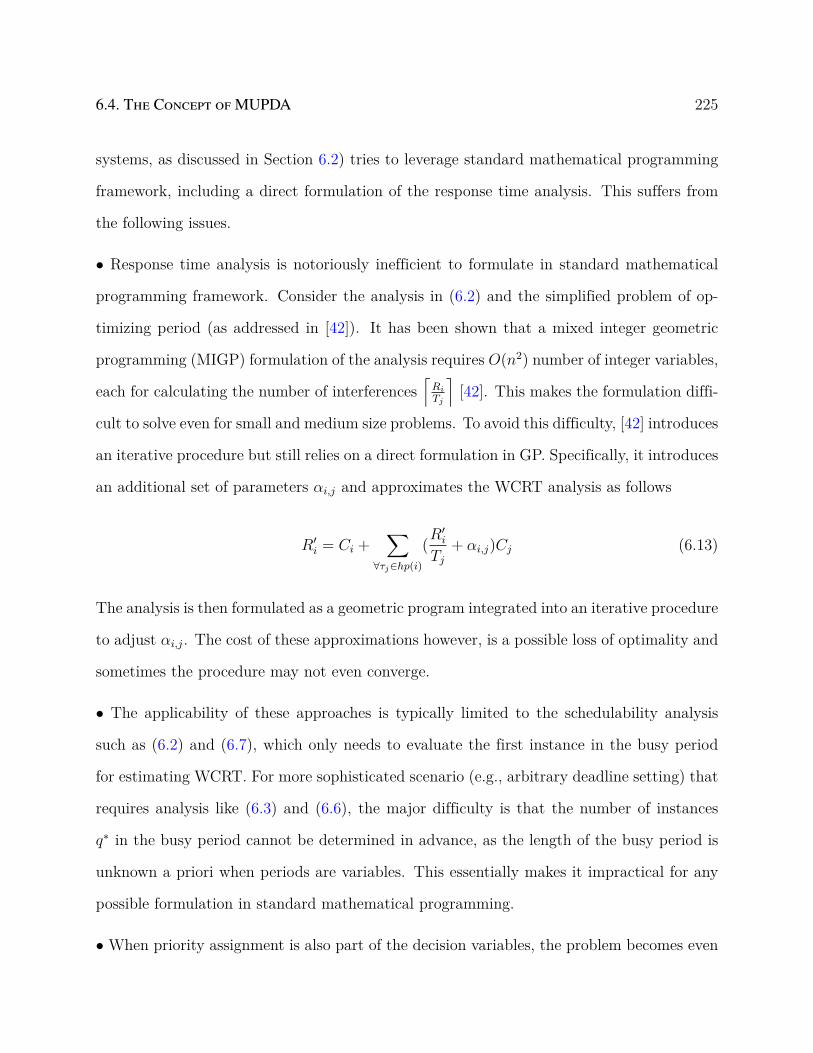
6.4. The Concept of MUPDA 225
systems, as discussed in Section 6.2) tries to leverage standard mathematical programming
framework, including a direct formulation of the response time analysis. This suffers from
the following issues.
• Response time analysis is notoriously inefficient to formulate in standard mathematical
programming framework. Consider the analysis in (6.2) and the simplified problem of op-
timizing period (as addressed in [42]). It has been shown that a mixed integer geometric
programming (MIGP) formulation of the analysis requires O(n2) number of integer variables,
each for calculating the number of interferences⌈Ri
Tj
⌉[42]. This makes the formulation diffi-
cult to solve even for small and medium size problems. To avoid this difficulty, [42] introduces
an iterative procedure but still relies on a direct formulation in GP. Specifically, it introduces
an additional set of parameters αi,j and approximates the WCRT analysis as follows
R′i = Ci +
∑∀τj∈hp(i)
(R′
i
Tj
+ αi,j)Cj (6.13)
The analysis is then formulated as a geometric program integrated into an iterative procedure
to adjust αi,j. The cost of these approximations however, is a possible loss of optimality and
sometimes the procedure may not even converge.
• The applicability of these approaches is typically limited to the schedulability analysis
such as (6.2) and (6.7), which only needs to evaluate the first instance in the busy period
for estimating WCRT. For more sophisticated scenario (e.g., arbitrary deadline setting) that
requires analysis like (6.3) and (6.6), the major difficulty is that the number of instances
q∗ in the busy period cannot be determined in advance, as the length of the busy period is
unknown a priori when periods are variables. This essentially makes it impractical for any
possible formulation in standard mathematical programming.
• When priority assignment is also part of the decision variables, the problem becomes even

226Chapter 6. A Unified Framework for Period and Priority Optimization in Distributed
Hard Real-Time Systems
Table 6.1: An Example Task System Γe
τi T lbi T ub
i Ci τi T lbi T ub
i Ci
τ1 0 10 2 τ2 0 20 3τ3 0 40 10 τ4 0 100 3
more challenging. MIGP is no longer able to handle it due to the additional constraints from
priority assignment. For example, the asymmetric constraints require that if τi has a higher
priority than τj (pi,j = 1), then τj must have a lower priority than τi (pj,i = 0) [160]. Such
constraints have the form of pi,j + pj,i = 1, which is incompatible with MIGP [107]. This
hinders the possibility of achieving significant improvement of optimization quality brought
by co-optimizing both period and priority assignment.
Instead, we propose a technique that avoids the above pitfalls in existing approaches. The
main idea is to use a set of compact constraints for schedulability that hides the details
of the underlying schedulability analysis from the mathematical programming solver. Our
approach is applicable to two scenarios. The first assumes that priority assignment is given
and periods are the decision variables. The second considers the more general problem where
both periods and priority assignments are decision variables. Both variants of the problem
can be solved by the proposed framework. For the first, the proposed technique is optimal
w.r.t. the objective function for any schedulability analysis that is sustainable w.r.t. periods
and deadlines (e.g., all the analyses summarized in Section 6.3). For the second version, the
proposed technique preserves optimality with the WCRT analysis in (6.2) and (6.7), and is
close to optimal for others.
In this section, we introduce a set of concepts for abstracting the schedulability conditions,
including Maximal Unschedulable Period-Deadline Assignment (MUPDA). MUPDA is an
extension of the concept of MUDA (maximal unschedulable deadline assignment) proposed
in [161], by adding period assignment information.
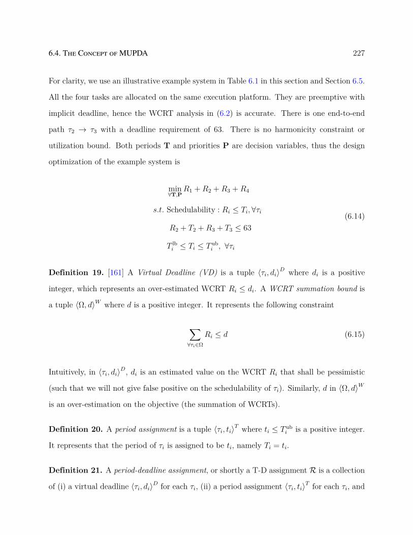
6.4. The Concept of MUPDA 227
For clarity, we use an illustrative example system in Table 6.1 in this section and Section 6.5.
All the four tasks are allocated on the same execution platform. They are preemptive with
implicit deadline, hence the WCRT analysis in (6.2) is accurate. There is one end-to-end
path τ2 → τ3 with a deadline requirement of 63. There is no harmonicity constraint or
utilization bound. Both periods T and priorities P are decision variables, thus the design
optimization of the example system is
min∀T,P
R1 +R2 +R3 +R4
s.t. Schedulability : Ri ≤ Ti,∀τi
R2 + T2 +R3 + T3 ≤ 63
T lbi ≤ Ti ≤ T ub
i , ∀τi
(6.14)
Definition 19. [161] A Virtual Deadline (VD) is a tuple ⟨τi, di⟩D where di is a positive
integer, which represents an over-estimated WCRT Ri ≤ di. A WCRT summation bound is
a tuple ⟨Ω, d⟩W where d is a positive integer. It represents the following constraint
∑∀τi∈Ω
Ri ≤ d (6.15)
Intuitively, in ⟨τi, di⟩D, di is an estimated value on the WCRT Ri that shall be pessimistic
(such that we will not give false positive on the schedulability of τi). Similarly, d in ⟨Ω, d⟩W
is an over-estimation on the objective (the summation of WCRTs).
Definition 20. A period assignment is a tuple ⟨τi, ti⟩T where ti ≤ T ubi is a positive integer.
It represents that the period of τi is assigned to be ti, namely Ti = ti.
Definition 21. A period-deadline assignment, or shortly a T-D assignment R is a collection
of (i) a virtual deadline ⟨τi, di⟩D for each τi, (ii) a period assignment ⟨τi, ti⟩T for each τi, and

228Chapter 6. A Unified Framework for Period and Priority Optimization in Distributed
Hard Real-Time Systems
(iii) a WCRT summation bound ⟨Ω, dΩ⟩W . Namely, R can be expressed as
R = ⟨τ1, d1⟩D .. ⟨τn, dn⟩D , ⟨τ1, t1⟩T .. ⟨τn, tn⟩T , ⟨Ω, dΩ⟩W
The following definition gives a partial order relationship among period-deadline assignments.
Definition 22. R1 is said to dominate R2, denoted as R1 ⪰ R2, if the following conditions
hold.di ≥ d′i, ∀ ⟨τi, di⟩
D ∈ R1, ⟨τi, d′i⟩D ∈ R2
ti ≥ t′i, ∀ ⟨τi, ti⟩T ∈ R1, ⟨τi, t′i⟩
T ∈ R2
dΩ ≥ d′Ω, ⟨Ω, dΩ⟩W ∈ R1, ⟨Ω, d′Ω⟩
W ∈ R2
(6.16)
Equivalently, R1 ⪰ R2, if and only if R1 is component-wise no smaller than R2. R1 is said
to strictly dominate R2, denoted as R1 ≻ R2, if R1 ⪰ R2 and R1 = R2.
Example 6.1. Consider the following T-D assignments for Γe
R1 =⟨τ1, 10⟩D , ⟨τ2, 20⟩D , ⟨τ3, 40⟩D , ⟨τ4, 100⟩D
⟨τ1, 10⟩T , ⟨τ2, 20⟩T , ⟨τ3, 40⟩T , ⟨τ4, 100⟩T , ⟨Ω, 170⟩W
R2 =⟨τ1, 10⟩D , ⟨τ2, 15⟩D , ⟨τ3, 40⟩D , ⟨τ4, 100⟩D
⟨τ1, 10⟩T , ⟨τ2, 20⟩T , ⟨τ3, 40⟩T , ⟨τ4, 100⟩T , ⟨Ω, 170⟩W
R3 =⟨τ1, 10⟩D , ⟨τ2, 20⟩D , ⟨τ3, 30⟩D , ⟨τ4, 100⟩D
⟨τ1, 10⟩T , ⟨τ2, 20⟩T , ⟨τ3, 40⟩T , ⟨τ4, 100⟩T , ⟨Ω, 170⟩W
R1 ⪰ R2 and R1 ⪰ R3, as the virtual deadlines, period assignments and WCRT summation
bound in R1 is component wise no smaller than those of R2 and R3. Also, neither R2 ⪰ R3
nor R3 ⪰ R2: compared to R2, R3 has a larger virtual deadline on τ2 but a smaller virtual
deadline on τ3. Thus, Definition 22 defines a partial order among all T-D assignments.

6.4. The Concept of MUPDA 229
Definition 23. Let R = ⟨τ1, d1⟩D , ... ⟨τn, dn⟩D, ⟨τ1, t1⟩T ,...⟨τn, tn⟩T , ⟨Ω, dΩ⟩W be a T-D as-
signment. The system Γ is R-schedulable, or informally R is schedulable, if and only if there
exists a priority assignment such that (i) Ti = ti,∀ ⟨τi, ti⟩T ∈ R; (ii) Ri ≤ di,∀ ⟨τi, di⟩D ∈ R;
and (iii)∑
τi∈ΩRi ≤ dΩ. That is, R is schedulable if and only if there exists a priority assign-
ment that respects all the assignments on periods, virtual deadlines, and WCRT summation
bound in R.
Example 6.2. Consider the following T-D assignments
R1 =⟨τ1, 10⟩D , ⟨τ2, 20⟩D , ⟨τ3, 40⟩D , ⟨τ4, 100⟩D
⟨τ1, 10⟩T , ⟨τ2, 20⟩T , ⟨τ3, 40⟩T , ⟨τ4, 100⟩T , ⟨Ω, 170⟩W
R2 =⟨τ1, 10⟩D , ⟨τ2, 15⟩D , ⟨τ3, 2⟩D , ⟨τ4, 100⟩D
⟨τ1, 10⟩T , ⟨τ2, 20⟩T , ⟨τ3, 40⟩T , ⟨τ4, 100⟩T , ⟨Ω, 170⟩W
R3 =⟨τ1, 10⟩D , ⟨τ2, 15⟩D , ⟨τ3, 2⟩D , ⟨τ4, 100⟩D
⟨τ1, 10⟩T , ⟨τ2, 20⟩T , ⟨τ3, 40⟩T , ⟨τ4, 100⟩T , ⟨Ω, 18⟩W
R1 assigns the most relaxed period, virtual deadlines and WCRT summation bound and is
schedulable by rate-monotonic priority assignment. R2 is obviously unschedulable as the
virtual deadline on τ3 cannot even accommodate its worst-case execution time. R3 differs
from R1 in the WCRT summation bound. Though individual virtual deadlines can be
satisfied for R3 by rate-monotonic priority assignment, its WCRT summation bound, which
equals the summation of WCETs of all objects, obviously cannot be satisfied for any priority
assignment. Thus R3 is also unschedulable.
We now reformulate the original problem (6.11) into the following form with the concept of
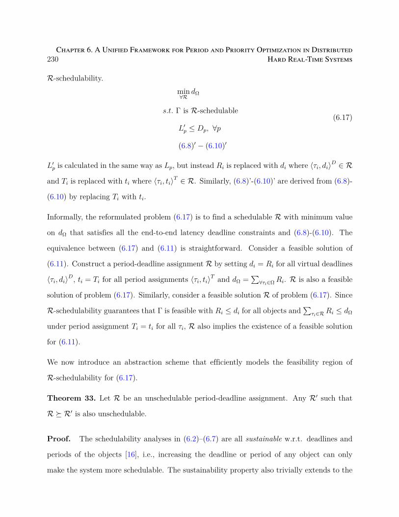
230Chapter 6. A Unified Framework for Period and Priority Optimization in Distributed
Hard Real-Time Systems
R-schedulability.min∀R
dΩ
s.t. Γ is R-schedulable
L′p ≤ Dp, ∀p
(6.8)′ − (6.10)′
(6.17)
L′p is calculated in the same way as Lp, but instead Ri is replaced with di where ⟨τi, di⟩D ∈ R
and Ti is replaced with ti where ⟨τi, ti⟩T ∈ R. Similarly, (6.8)’-(6.10)’ are derived from (6.8)-
(6.10) by replacing Ti with ti.
Informally, the reformulated problem (6.17) is to find a schedulable R with minimum value
on dΩ that satisfies all the end-to-end latency deadline constraints and (6.8)-(6.10). The
equivalence between (6.17) and (6.11) is straightforward. Consider a feasible solution of
(6.11). Construct a period-deadline assignment R by setting di = Ri for all virtual deadlines
⟨τi, di⟩D, ti = Ti for all period assignments ⟨τi, ti⟩T and dΩ =∑
∀τi∈Ω Ri. R is also a feasible
solution of problem (6.17). Similarly, consider a feasible solution R of problem (6.17). Since
R-schedulability guarantees that Γ is feasible with Ri ≤ di for all objects and∑
τi∈R Ri ≤ dΩ
under period assignment Ti = ti for all τi, R also implies the existence of a feasible solution
for (6.11).
We now introduce an abstraction scheme that efficiently models the feasibility region of
R-schedulability for (6.17).
Theorem 33. Let R be an unschedulable period-deadline assignment. Any R′ such that
R ⪰ R′ is also unschedulable.
Proof. The schedulability analyses in (6.2)–(6.7) are all sustainable w.r.t. deadlines and
periods of the objects [16], i.e., increasing the deadline or period of any object can only
make the system more schedulable. The sustainability property also trivially extends to the

6.4. The Concept of MUPDA 231
WCRT summation bound dΩ in R, hence the proof.
Theorem 33 implies that each unschedulable period-deadline assignment R captures also the
unschedulability of other period-deadline assignments R′ dominated by it. The usefulness
of the theorem is that it generalizes from one unschedulable period-deadline assignment to
a potentially large set of unschedulable ones. The following definition introduces a special
type of period-deadline assignment that is “most general” in capturing unschedulability.
Definition 24. U is a maximal unschedulable period-deadline assignment (MUPDA) if it
satisfies the following condition
• Γ is not U -schedulable;
• For all R such that R ≻ U , Γ is R-schedulable.
Example 6.3. Consider the following T-D assignments
R1 =⟨τ1, 10⟩D , ⟨τ2, 20⟩D , ⟨τ3, 10⟩D , ⟨τ4, 100⟩D
⟨τ1, 10⟩T , ⟨τ2, 20⟩T , ⟨τ3, 10⟩T , ⟨τ4, 100⟩T , ⟨Ω, 170⟩W
R2 =⟨τ1, 10⟩D , ⟨τ2, 20⟩D , ⟨τ3, 40⟩D , ⟨τ4, 100⟩D
⟨τ1, 10⟩T , ⟨τ2, 20⟩T , ⟨τ3, 16⟩T , ⟨τ4, 100⟩T , ⟨Ω, 170⟩W
R1 is unschedulable for the following reason. τ1 must have higher priority than τ3 as
C3 ≥ T ub1 . Under this constraint, the virtual deadline and period assignment for τ3 can-
not accommodate its schedulability. R2 is also unschedulable. Consider the rate-monotonic
priority assignment, known to be optimal for schedulability of individual tasks. τ2 suffers
the interference of at least two instances of τ1 and one instances of τ3. Thus R2 is at least
17. When T3 = 16, τ2 suffers one more instance of interference from τ3, which violates its
schedulability. However, If T3 is increased by one (i.e., T3 = 17), τ2 will be schedulable.

232Chapter 6. A Unified Framework for Period and Priority Optimization in Distributed
Hard Real-Time Systems
With the above result, R1 is not a MUPDA since R2 ⪰ R1 and R2 is unschedulable. R2 is
a MUPDA however, as all R ⪰ R2 (which only consist of Rs with larger period assignment
on τ3, as all other virtual deadlines, periods assignment and WCRT summation bound are
at their upper bounds) are schedulable.
Remark 6.4. A MUPDA is a maximal generalization of unschedulable period-deadline
assignment in the sense that there is no other unschedulable R that strictly dominates
U . MUPDAs are not unique: it is possible that a system Γ has multiple MUPDAs by
Definition 24.
We now show how MUPDAs can be used to derive an abstract form of schedulability con-
straint for use in problem (6.17). A MUPDA
U = ⟨τ1, d′1⟩D, ... ⟨τn, d′n⟩
D, ⟨τ1, t′1⟩
T, ... ⟨τn, t′n⟩
T, ⟨Ω, d′Ω⟩
W (6.18)
suggests that all period-deadline assignments
R = ⟨τ1, d1⟩D .. ⟨τn, dn⟩D , ⟨τ1, t1⟩T .. ⟨τn, tn⟩T , ⟨Ω, dΩ⟩W
satisfying the following constraints are unschedulable
di ≤ d′i, ∀τi
ti ≤ t′i, ∀τi
dΩ ≤ d′Ω,
(6.19)
Contra-positively, the following constraints are necessary to be satisfied for any schedulable

6.4. The Concept of MUPDA 233
Algorithm 10 Algorithm for Computing MUPDA1: function MUPDA(System Γ, Unschedulable R)2: for each element ζ ∈ R (ζ may be ⟨τi, v⟩D or ⟨τi, v⟩T or ⟨Ω, v⟩W ) do3: Use binary search to find out the largest value u that v can be increased to while
keeping R unschedulable4: Update the value of v to be u5: end for6: return R7: end function
period-deadline assignment R.
R ⪯ U ⇔ ¬
di ≤ d′i, ∀τi
ti ≤ t′i, ∀τi
dΩ ≤ d′Ω,
⇔
∥∥∥∥∥∥∥∥∥∥∥di > d′i, ∀τi
ti > t′i, ∀τi
dΩ > d′Ω,
(6.20)
where ∥ represents the logical OR (disjunction) operation.
We call (6.20) MUPDA implied constraints by U . Our general idea is to use (6.20) as the
form of constraints for shaping the feasibility region of R-schedulability in problem (6.17).
The disjunction can be formulated as integer linear constraint [160].
We now discuss how MUPDAs can be obtained given an unschedulable R. This is detailed
in Algorithm 10. Specifically, Algorithm 10 is based on the property that the schedulability
analysis is sustainable w.r.t. deadline, period, and WCRT summation. When performing
the binary search for determining the largest value u (Line 2-3) on a particular element
(virtual deadline, period assignment, or WCRT summation bound) in R, the other elements
are kept unchanged. If the system is still unschedulable even by setting v to the upper
bound, then v is updated to the upper bound. The order of visit in Line 2 may affect
the returned MUPDA in the sense that different orders may return different MUPDAs. To
compute multiple MUPDAs from a single R, it suffices to perturb R into R′ such that any

234Chapter 6. A Unified Framework for Period and Priority Optimization in Distributed
Hard Real-Time Systems
previously computed MUPDA U does not dominate R′, i.e., U ⪰ R′. This guarantees that
the MUPDA computed from R′ is different from all previous ones.
Example 6.5. We now illustrate Algorithm 10 by applying it toR1 in Example 6.3. Suppose
the algorithm iterates through each element in R1 according to the order shown in the
example. ⟨τ1, 10⟩D and ⟨τ2, 20⟩D are explored in the first two iterations, but they already at
their upper bound, thus nothing is performed. In the third iteration, the algorithm considers
⟨τ3, v⟩D where v = 10. It uses binary search to find out the maximum value v can be increased
to while maintaining unschedulability, assuming all other elements in R1 remain unchanged.
By the reasoning in Example 6.3, even if v is increased to the upper bound 40, τ2 is still
unschedulable due to ⟨τ3, 10⟩T . Thus ⟨τ3, 10⟩D is updated to ⟨τ3, 40⟩D. Similarly, when the
algorithm iterates on ⟨τ3, 10⟩T , it discovers that the system becomes schedulable after T3
is increased to 17. Thus it updates ⟨τ3, 10⟩T to ⟨τ3, 16⟩T , the largest value that maintains
unschedulability. In the end, given R1 as input, Algorithm 10 finds the MUPDA R2 shown
in Example 6.3.
Next we consider computing a second MUPDA from R1. The key is to perturb R1 into R′1
such that R′1 ⪯ R2. This can be done, for example, by setting ⟨τ3, 10⟩T in R1 to ⟨τ3, 17⟩T ,
which givesR′
1 =⟨τ1, 10⟩D , ⟨τ2, 20⟩D , ⟨τ3, 10⟩D , ⟨τ4, 100⟩D
⟨τ1, 10⟩T , ⟨τ2, 20⟩T , ⟨τ3, 17⟩T , ⟨τ4, 100⟩T , ⟨Ω, 170⟩W
R′1 is still unschedulable as the deadline assignment ⟨τ3, 10⟩D, which equals C3, is too small.
Applying Algorithm 10 gives the following MUPDA.
R′2 =⟨τ1, 10⟩
D , ⟨τ2, 20⟩D , ⟨τ3, 11⟩D , ⟨τ4, 100⟩D
⟨τ1, 10⟩T , ⟨τ2, 20⟩T , ⟨τ3, 17⟩T , ⟨τ4, 100⟩T , ⟨Ω, 170⟩W
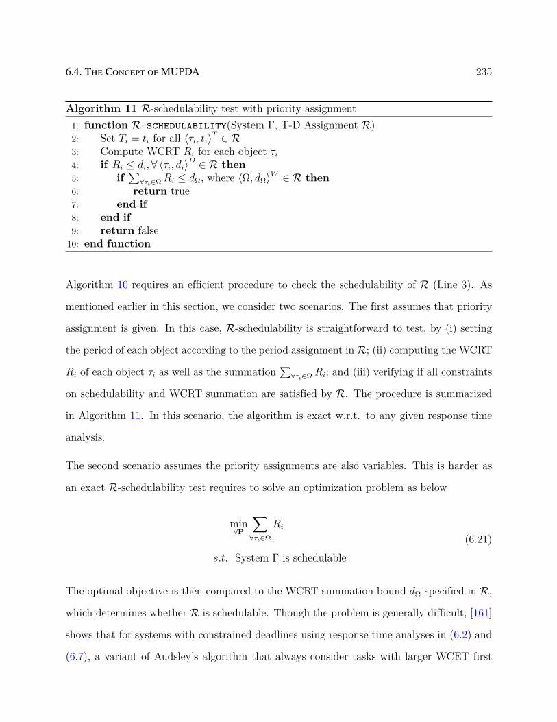
6.4. The Concept of MUPDA 235
Algorithm 11 R-schedulability test with priority assignment1: function R-schedulability(System Γ, T-D Assignment R)2: Set Ti = ti for all ⟨τi, ti⟩T ∈ R3: Compute WCRT Ri for each object τi4: if Ri ≤ di, ∀ ⟨τi, di⟩D ∈ R then5: if
∑∀τi∈Ω Ri ≤ dΩ, where ⟨Ω, dΩ⟩W ∈ R then
6: return true7: end if8: end if9: return false
10: end function
Algorithm 10 requires an efficient procedure to check the schedulability of R (Line 3). As
mentioned earlier in this section, we consider two scenarios. The first assumes that priority
assignment is given. In this case, R-schedulability is straightforward to test, by (i) setting
the period of each object according to the period assignment in R; (ii) computing the WCRT
Ri of each object τi as well as the summation∑
∀τi∈Ω Ri; and (iii) verifying if all constraints
on schedulability and WCRT summation are satisfied by R. The procedure is summarized
in Algorithm 11. In this scenario, the algorithm is exact w.r.t. to any given response time
analysis.
The second scenario assumes the priority assignments are also variables. This is harder as
an exact R-schedulability test requires to solve an optimization problem as below
min∀P
∑∀τi∈Ω
Ri
s.t. System Γ is schedulable(6.21)
The optimal objective is then compared to the WCRT summation bound dΩ specified in R,
which determines whether R is schedulable. Though the problem is generally difficult, [161]
shows that for systems with constrained deadlines using response time analyses in (6.2) and
(6.7), a variant of Audsley’s algorithm that always consider tasks with larger WCET first
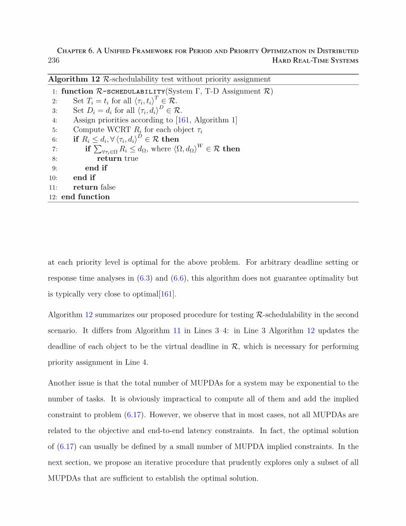
236Chapter 6. A Unified Framework for Period and Priority Optimization in Distributed
Hard Real-Time Systems
Algorithm 12 R-schedulability test without priority assignment1: function R-schedulability(System Γ, T-D Assignment R)2: Set Ti = ti for all ⟨τi, ti⟩T ∈ R.3: Set Di = di for all ⟨τi, di⟩D ∈ R.4: Assign priorities according to [161, Algorithm 1]5: Compute WCRT Ri for each object τi6: if Ri ≤ di, ∀ ⟨τi, di⟩D ∈ R then7: if
∑∀τi∈Ω Ri ≤ dΩ, where ⟨Ω, dΩ⟩W ∈ R then
8: return true9: end if
10: end if11: return false12: end function
at each priority level is optimal for the above problem. For arbitrary deadline setting or
response time analyses in (6.3) and (6.6), this algorithm does not guarantee optimality but
is typically very close to optimal[161].
Algorithm 12 summarizes our proposed procedure for testing R-schedulability in the second
scenario. It differs from Algorithm 11 in Lines 3–4: in Line 3 Algorithm 12 updates the
deadline of each object to be the virtual deadline in R, which is necessary for performing
priority assignment in Line 4.
Another issue is that the total number of MUPDAs for a system may be exponential to the
number of tasks. It is obviously impractical to compute all of them and add the implied
constraint to problem (6.17). However, we observe that in most cases, not all MUPDAs are
related to the objective and end-to-end latency constraints. In fact, the optimal solution
of (6.17) can usually be defined by a small number of MUPDA implied constraints. In the
next section, we propose an iterative procedure that prudently explores only a subset of all
MUPDAs that are sufficient to establish the optimal solution.
6.5. MUPDA Guided Optimization 237
6.5 MUPDA Guided Optimization
We now present the complete optimization framework, an iterative procedure as summarized
in Figure 6.1. The basic idea is to leverage ILP solvers for generic branch-and-bound based
search and the efficient algorithms for calculating MUPDAs. Specifically, at any point of
the procedure execution where a subset U of all MUPDAs are calculated, we partition the
problem into two parts: (i) a relaxation Π of the problem (6.17) that includes MUPDA
implied constraints from U (and implicitly part of the schedulability conditions), the end-to-
end deadline constraints, and (6.8)’–(6.9)’, which will be handled by the ILP solver; and (ii)
those constraints not included in Π, which will be handled by the algorithms in Section 6.4.
To make Π compatible with ILP, the MUPDA implied constraints, as in the form of (6.20),
can be formulated as integer linear constraints by adding a set of auxiliary binary vari-
ables [160]. Also, linearization techniques [116] can convert (6.8)’ to integer linear con-
straints.
Finally, we enforce (6.10)’ by modifying Algorithms 11 and 12. Specifically, before verifying
schedulability, the total utilization of each execution platform is checked. If any utilization
bound is violated, the system is considered to be R-unschedulable. In this sense, we extend
the definition of R-schedulability to include also the utilization bound constraints in addi-
tion to the system schedulability. We note this is consistent since (6.10)’, like the system
schedulability constraints, is also sustainable to the periods and deadlines: increasing the
periods and deadlines can only make (6.10)’ more satisfiable. In the rest of the section, we
slightly abuse the term “schedulability” to also include the utilization bound constraints.
We now detail the procedure in a step-wise manner.
Step 1-Initial Problem. The algorithm first starts with the following optimization problem
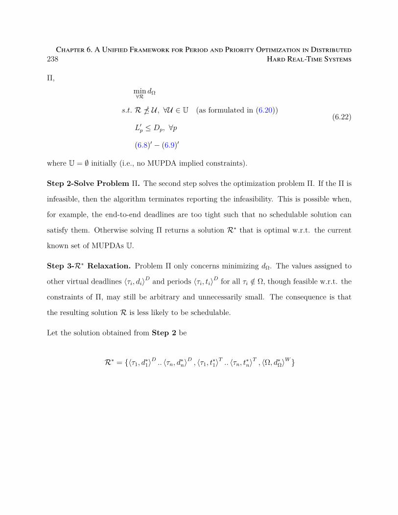
238Chapter 6. A Unified Framework for Period and Priority Optimization in Distributed
Hard Real-Time Systems
Π,min∀R
dΩ
s.t. R ⪯ U , ∀U ∈ U (as formulated in (6.20))
L′p ≤ Dp, ∀p
(6.8)′ − (6.9)′
(6.22)
where U = ∅ initially (i.e., no MUPDA implied constraints).
Step 2-Solve Problem Π. The second step solves the optimization problem Π. If the Π is
infeasible, then the algorithm terminates reporting the infeasibility. This is possible when,
for example, the end-to-end deadlines are too tight such that no schedulable solution can
satisfy them. Otherwise solving Π returns a solution R∗ that is optimal w.r.t. the current
known set of MUPDAs U.
Step 3-R∗ Relaxation. Problem Π only concerns minimizing dΩ. The values assigned to
other virtual deadlines ⟨τi, di⟩D and periods ⟨τi, ti⟩D for all τi /∈ Ω, though feasible w.r.t. the
constraints of Π, may still be arbitrary and unnecessarily small. The consequence is that
the resulting solution R is less likely to be schedulable.
Let the solution obtained from Step 2 be
R∗ = ⟨τ1, d∗1⟩D .. ⟨τn, d∗n⟩
D , ⟨τ1, t∗1⟩T .. ⟨τn, t∗n⟩
T , ⟨Ω, d∗Ω⟩W
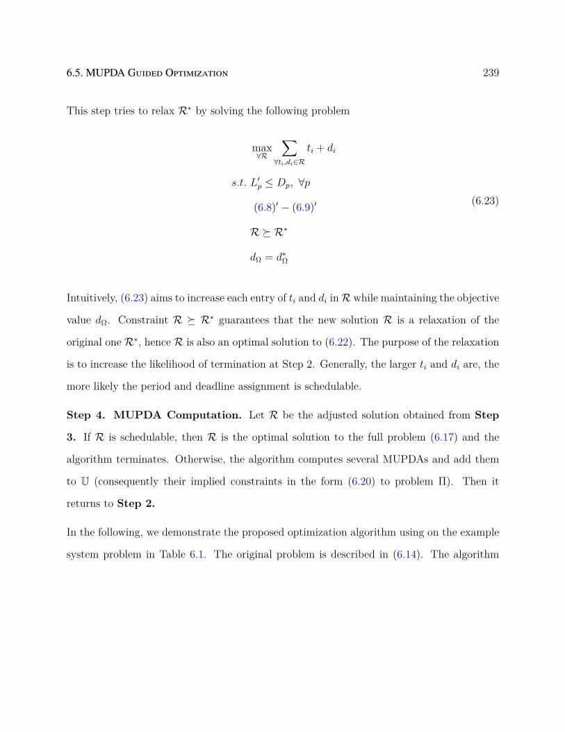
6.5. MUPDA Guided Optimization 239
This step tries to relax R∗ by solving the following problem
max∀R
∑∀ti,di∈R
ti + di
s.t. L′p ≤ Dp, ∀p
(6.8)′ − (6.9)′
R ⪰ R∗
dΩ = d∗Ω
(6.23)
Intuitively, (6.23) aims to increase each entry of ti and di inR while maintaining the objective
value dΩ. Constraint R ⪰ R∗ guarantees that the new solution R is a relaxation of the
original one R∗, hence R is also an optimal solution to (6.22). The purpose of the relaxation
is to increase the likelihood of termination at Step 2. Generally, the larger ti and di are, the
more likely the period and deadline assignment is schedulable.
Step 4. MUPDA Computation. Let R be the adjusted solution obtained from Step
3. If R is schedulable, then R is the optimal solution to the full problem (6.17) and the
algorithm terminates. Otherwise, the algorithm computes several MUPDAs and add them
to U (consequently their implied constraints in the form (6.20) to problem Π). Then it
returns to Step 2.
In the following, we demonstrate the proposed optimization algorithm using on the example
system problem in Table 6.1. The original problem is described in (6.14). The algorithm

240Chapter 6. A Unified Framework for Period and Priority Optimization in Distributed
Hard Real-Time Systems
first starts with the following initial problem Π
min∀R
dΩ
s.t. d2 + t2 + d3 + t3 ≤ 63
Ci ≤ di ≤ ti ≤ T ubi , ∀τi
(6.24)
which contains only the objective, end-to-end latency constraint, and the bounds on the
variables. The R-schedulability constraints are ignored. The algorithm then enters the
iteration in Steps 2–4.
Iteration 1. Solving the initial problem Π, we get
R∗1 = ⟨τ1, 10⟩
D , ⟨τ2, 3⟩D , ⟨τ3, 10⟩D , ⟨τ4, 100⟩D
⟨τ1, 10⟩T , ⟨τ2, 3⟩T , ⟨τ3, 10⟩T , ⟨τ4, 100⟩T , ⟨Ω, 18⟩W
The estimated end-to-end latency by the returned solution is
d2 + t2 + d3 + t3 = 26 (6.25)
which is unnecessarily smaller than the required end-to-end latency deadline. Thus the fol-
lowing relaxation is performed on R∗ to increase the period and virtual deadline assignment.
max∑∀τi
di + ti
s.t. d2 + t2 + d3 + t3 ≤ 63
di ≤ ti ≤ T ubi , ∀τi
d2 ≥ 3, t2 ≥ 3, d3 ≥ 10, t3 ≥ 10
dΩ = d∗Ω
(6.26)
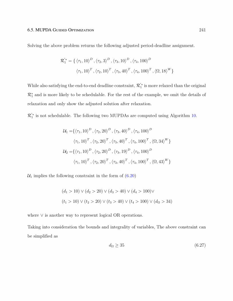
6.5. MUPDA Guided Optimization 241
Solving the above problem returns the following adjusted period-deadline assignment.
R′∗1 = ⟨τ1, 10⟩D , ⟨τ2, 3⟩D , ⟨τ3, 10⟩D , ⟨τ4, 100⟩D
⟨τ1, 10⟩T , ⟨τ2, 10⟩T , ⟨τ3, 40⟩T , ⟨τ4, 100⟩T , ⟨Ω, 18⟩W
While also satisfying the end-to-end deadline constraint,R′∗1 is more relaxed than the original
R∗1 and is more likely to be schedulable. For the rest of the example, we omit the details of
relaxation and only show the adjusted solution after relaxation.
R′∗1 is not schedulable. The following two MUPDAs are computed using Algorithm 10.
U1 =⟨τ1, 10⟩D , ⟨τ2, 20⟩D , ⟨τ3, 40⟩D , ⟨τ4, 100⟩D
⟨τ1, 10⟩T , ⟨τ2, 20⟩T , ⟨τ3, 40⟩T , ⟨τ4, 100⟩T , ⟨Ω, 34⟩W
U2 =⟨τ1, 10⟩D , ⟨τ2, 20⟩D , ⟨τ3, 19⟩D , ⟨τ4, 100⟩D
⟨τ1, 10⟩T , ⟨τ2, 20⟩T , ⟨τ3, 40⟩T , ⟨τ4, 100⟩T , ⟨Ω, 43⟩W
U1 implies the following constraint in the form of (6.20)
(d1 > 10) ∨ (d2 > 20) ∨ (d3 > 40) ∨ (d4 > 100)∨
(t1 > 10) ∨ (t2 > 20) ∨ (t3 > 40) ∨ (t4 > 100) ∨ (dΩ > 34)
where ∨ is another way to represent logical OR operations.
Taking into consideration the bounds and integrality of variables, The above constraint can
be simplified as
dΩ ≥ 35 (6.27)
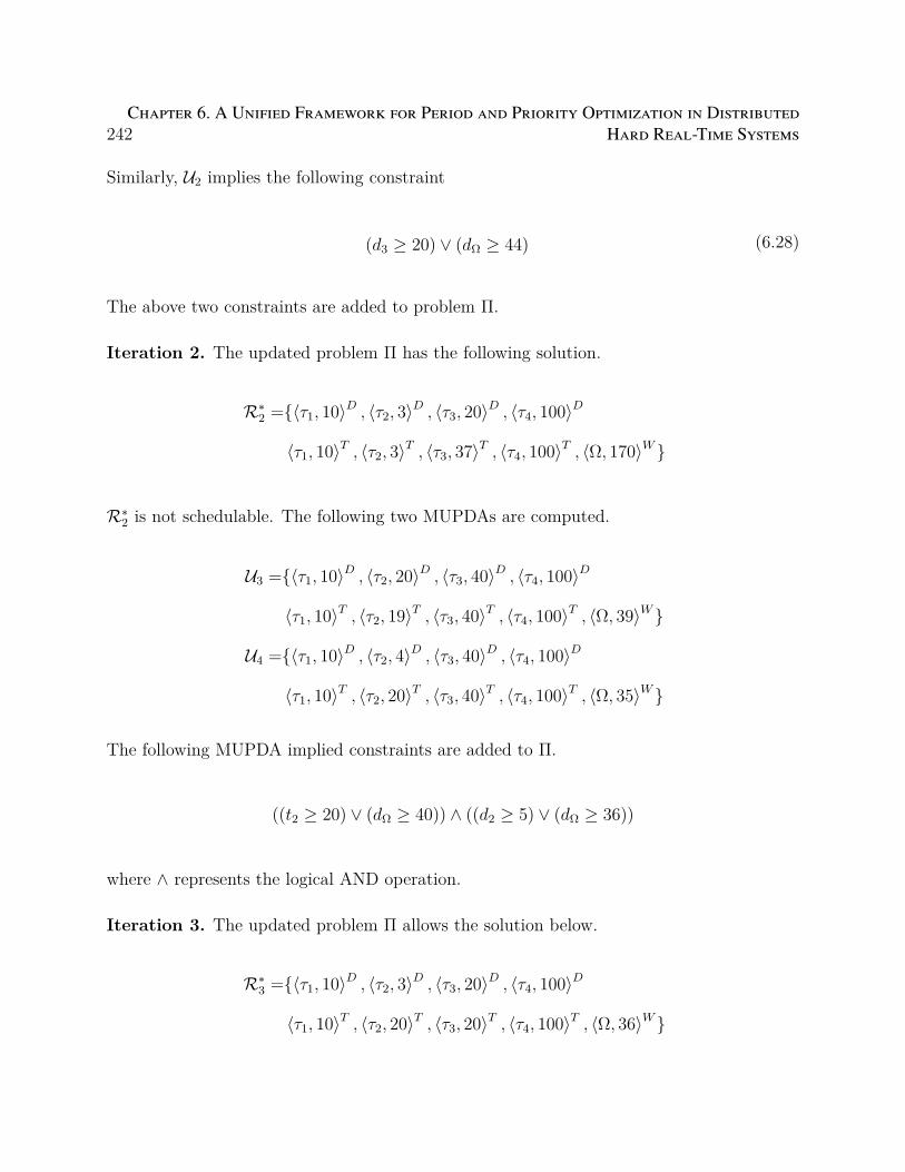
242Chapter 6. A Unified Framework for Period and Priority Optimization in Distributed
Hard Real-Time Systems
Similarly, U2 implies the following constraint
(d3 ≥ 20) ∨ (dΩ ≥ 44) (6.28)
The above two constraints are added to problem Π.
Iteration 2. The updated problem Π has the following solution.
R∗2 =⟨τ1, 10⟩
D , ⟨τ2, 3⟩D , ⟨τ3, 20⟩D , ⟨τ4, 100⟩D
⟨τ1, 10⟩T , ⟨τ2, 3⟩T , ⟨τ3, 37⟩T , ⟨τ4, 100⟩T , ⟨Ω, 170⟩W
R∗2 is not schedulable. The following two MUPDAs are computed.
U3 =⟨τ1, 10⟩D , ⟨τ2, 20⟩D , ⟨τ3, 40⟩D , ⟨τ4, 100⟩D
⟨τ1, 10⟩T , ⟨τ2, 19⟩T , ⟨τ3, 40⟩T , ⟨τ4, 100⟩T , ⟨Ω, 39⟩W
U4 =⟨τ1, 10⟩D , ⟨τ2, 4⟩D , ⟨τ3, 40⟩D , ⟨τ4, 100⟩D
⟨τ1, 10⟩T , ⟨τ2, 20⟩T , ⟨τ3, 40⟩T , ⟨τ4, 100⟩T , ⟨Ω, 35⟩W
The following MUPDA implied constraints are added to Π.
((t2 ≥ 20) ∨ (dΩ ≥ 40)) ∧ ((d2 ≥ 5) ∨ (dΩ ≥ 36))
where ∧ represents the logical AND operation.
Iteration 3. The updated problem Π allows the solution below.
R∗3 =⟨τ1, 10⟩
D , ⟨τ2, 3⟩D , ⟨τ3, 20⟩D , ⟨τ4, 100⟩D
⟨τ1, 10⟩T , ⟨τ2, 20⟩T , ⟨τ3, 20⟩T , ⟨τ4, 100⟩T , ⟨Ω, 36⟩W
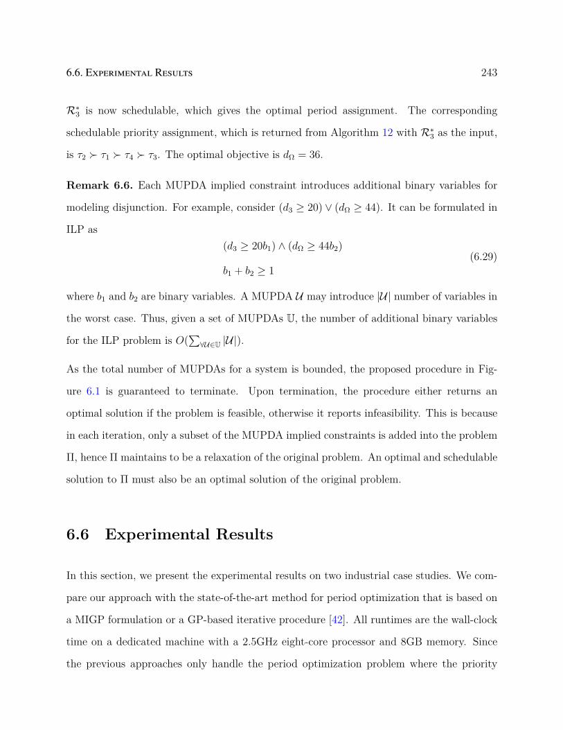
6.6. Experimental Results 243
R∗3 is now schedulable, which gives the optimal period assignment. The corresponding
schedulable priority assignment, which is returned from Algorithm 12 with R∗3 as the input,
is τ2 ≻ τ1 ≻ τ4 ≻ τ3. The optimal objective is dΩ = 36.
Remark 6.6. Each MUPDA implied constraint introduces additional binary variables for
modeling disjunction. For example, consider (d3 ≥ 20) ∨ (dΩ ≥ 44). It can be formulated in
ILP as(d3 ≥ 20b1) ∧ (dΩ ≥ 44b2)
b1 + b2 ≥ 1
(6.29)
where b1 and b2 are binary variables. A MUPDA U may introduce |U| number of variables in
the worst case. Thus, given a set of MUPDAs U, the number of additional binary variables
for the ILP problem is O(∑
∀U∈U |U|).
As the total number of MUPDAs for a system is bounded, the proposed procedure in Fig-
ure 6.1 is guaranteed to terminate. Upon termination, the procedure either returns an
optimal solution if the problem is feasible, otherwise it reports infeasibility. This is because
in each iteration, only a subset of the MUPDA implied constraints is added into the problem
Π, hence Π maintains to be a relaxation of the original problem. An optimal and schedulable
solution to Π must also be an optimal solution of the original problem.
6.6 Experimental Results
In this section, we present the experimental results on two industrial case studies. We com-
pare our approach with the state-of-the-art method for period optimization that is based on
a MIGP formulation or a GP-based iterative procedure [42]. All runtimes are the wall-clock
time on a dedicated machine with a 2.5GHz eight-core processor and 8GB memory. Since
the previous approaches only handle the period optimization problem where the priority
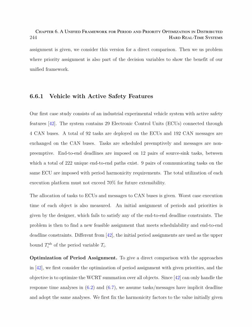
244Chapter 6. A Unified Framework for Period and Priority Optimization in Distributed
Hard Real-Time Systems
assignment is given, we consider this version for a direct comparison. Then we us problem
where priority assignment is also part of the decision variables to show the benefit of our
unified framework.
6.6.1 Vehicle with Active Safety Features
Our first case study consists of an industrial experimental vehicle system with active safety
features [42]. The system contains 29 Electronic Control Units (ECUs) connected through
4 CAN buses. A total of 92 tasks are deployed on the ECUs and 192 CAN messages are
exchanged on the CAN buses. Tasks are scheduled preemptively and messages are non-
preemptive. End-to-end deadlines are imposed on 12 pairs of source-sink tasks, between
which a total of 222 unique end-to-end paths exist. 9 pairs of communicating tasks on the
same ECU are imposed with period harmonicity requirements. The total utilization of each
execution platform must not exceed 70% for future extensibility.
The allocation of tasks to ECUs and messages to CAN buses is given. Worst case execution
time of each object is also measured. An initial assignment of periods and priorities is
given by the designer, which fails to satisfy any of the end-to-end deadline constraints. The
problem is then to find a new feasible assignment that meets schedulability and end-to-end
deadline constraints. Different from [42], the initial period assignments are used as the upper
bound T ubi of the period variable Ti.
Optimization of Period Assignment. To give a direct comparison with the approaches
in [42], we first consider the optimization of period assignment with given priorities, and the
objective is to optimize the WCRT summation over all objects. Since [42] can only handle the
response time analyses in (6.2) and (6.7), we assume tasks/messages have implicit deadline
and adopt the same analyses. We first fix the harmonicity factors to the value initially given
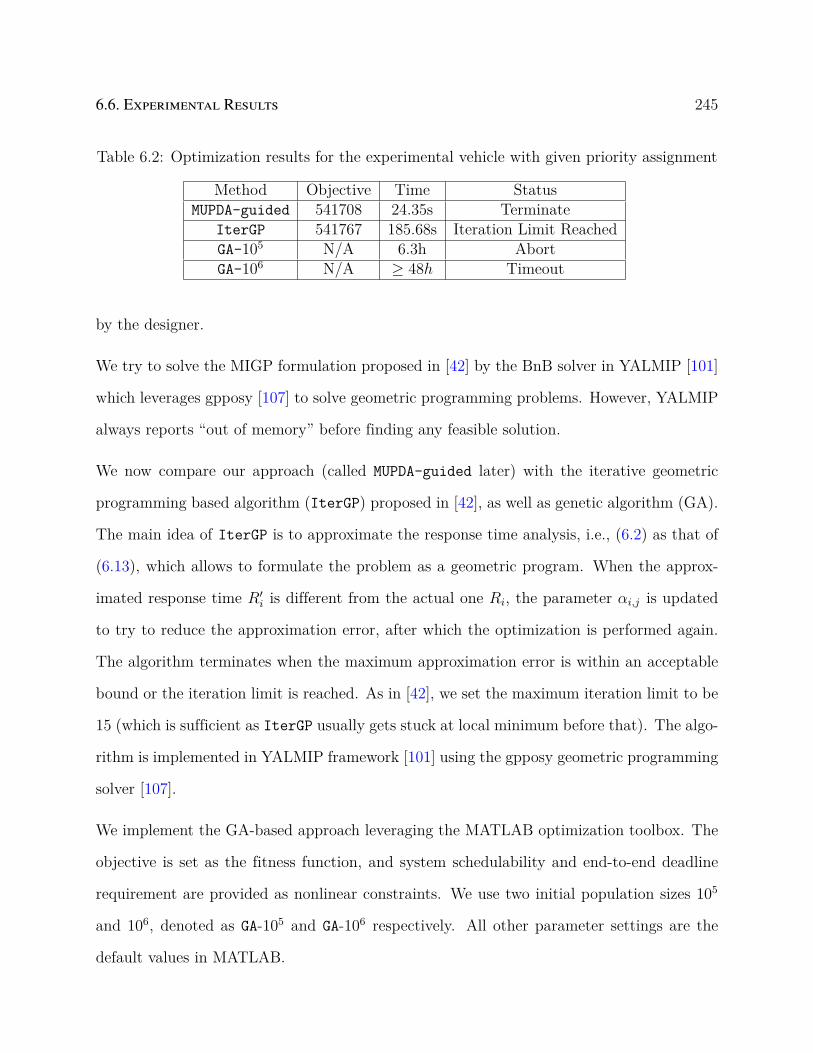
6.6. Experimental Results 245
Table 6.2: Optimization results for the experimental vehicle with given priority assignment
Method Objective Time StatusMUPDA-guided 541708 24.35s Terminate
IterGP 541767 185.68s Iteration Limit ReachedGA-105 N/A 6.3h AbortGA-106 N/A ≥ 48h Timeout
by the designer.
We try to solve the MIGP formulation proposed in [42] by the BnB solver in YALMIP [101]
which leverages gpposy [107] to solve geometric programming problems. However, YALMIP
always reports “out of memory” before finding any feasible solution.
We now compare our approach (called MUPDA-guided later) with the iterative geometric
programming based algorithm (IterGP) proposed in [42], as well as genetic algorithm (GA).
The main idea of IterGP is to approximate the response time analysis, i.e., (6.2) as that of
(6.13), which allows to formulate the problem as a geometric program. When the approx-
imated response time R′i is different from the actual one Ri, the parameter αi,j is updated
to try to reduce the approximation error, after which the optimization is performed again.
The algorithm terminates when the maximum approximation error is within an acceptable
bound or the iteration limit is reached. As in [42], we set the maximum iteration limit to be
15 (which is sufficient as IterGP usually gets stuck at local minimum before that). The algo-
rithm is implemented in YALMIP framework [101] using the gpposy geometric programming
solver [107].
We implement the GA-based approach leveraging the MATLAB optimization toolbox. The
objective is set as the fitness function, and system schedulability and end-to-end deadline
requirement are provided as nonlinear constraints. We use two initial population sizes 105
and 106, denoted as GA-105 and GA-106 respectively. All other parameter settings are the
default values in MATLAB.

246Chapter 6. A Unified Framework for Period and Priority Optimization in Distributed
Hard Real-Time Systems
The results are summarized in Table 6.2. MUPDA-guided terminates with the optimal solu-
tion after around 24 seconds. IterGP terminates with a slightly sub-optimal solution after
exceeding the limit of 15 iterations. GA-105 aborts after failing to find any feasible solution
for three generations. GA-106 on the other hand, is unable to complete the first genera-
tion within 48 hours. Figure 6.2 plots the objective value during the optimization process
of IterGP. Each data point in the plot corresponds to the objective value of a particular
iteration. The curve “Approximated GP Objective” corresponds to the objective value of
the geometric optimization, which is given by the approximated response time (6.13). The
“Actual Objective” corresponds to the objective value by the actual response time (6.2). If
the period assignment is actually infeasible (w.r.t. schedulability and end-to-end deadline
constraints), the corresponding data point is omitted in the figure, which is why for some
data points on the “Approximated GP Objective” curve, there is no corresponding one on
the “Actual Objective” curve. As shown in the figure, the solution summarized in Table 6.2
is found by IterGP after the third iteration at time 39s. However, after that IterGP oscil-
lates between a feasible and an infeasible period assignments, and cannot find any better
solution. This highlights a major drawback of IterGP: unlike MUPDA-guided, IterGP cannot
guarantee convergency.
Next, we relax the harmonicity factor hi,j from a fixed constant to an integer decision vari-
able. We omit GA for this setting since the ga function provided in MATLAB is not capable
of handling equality constraints with integer variables. The corresponding results are sum-
marized in Table 6.3. MUPDA-guided finds optimal solution after only around 6 seconds.
IterGP again starts oscillating between a feasible and infeasible solution after a few itera-
tions. The best solution it finds is at the first iteration after 52 seconds.
Optimization of Both Period and Priority. One advantage of MUPDA-guided is its
ability to optimize both periods and priority assignments. In this experiment, we ignore

6.6. Experimental Results 247
Table 6.3: Optimization results for the experimental vehicle with given priority assignment,relaxed harmonicity factor
Method Objective Time StatusMUPDA-guided 532938 6.43s Terminate
IterGP 533770 999.54s Iteration Limit Reached
Table 6.4: Optimization results for the experimental vehicle without given priority assign-ment
Harmonicity Factor Objective Time StatusFixed 300156 14.09s Terminate
Relaxed 298492 9.80s Terminate
the given priority assignment and consider it to be also part of the decision variables. All
other experimental settings remains the same as the previous one. Since the approaches
in [42] (IterGP and MIGP) are no longer applicable, we evaluate only the proposed technique
MUPDA-guided.
Table 6.4 summarizes the optimization results with fixed and relaxed harmonicity factor
settings. Comparing with the results in Table 6.2 and Table 6.3, the inclusion of priority
assignment into the decision space significantly improves the optimization results: for fixed
harmonicity factor the improvement is about 44.6%, and for relaxed harmonicity factor the
objective is about 44.0% smaller. This is expected as the design becomes much more flexible.
In summary, the results in Tables 6.2–6.4 demonstrate the three advantages of MUPDA-guided
compared to IterGP: (i) it guarantees convergency; (ii) it may run magnitudes faster (e.g.,
9.80s vs. 999.54s for the setting of relaxed harmonicity factor); (iii) it can handle the co-
optimization of both periods and priority assignments, hence has the potential to provide
substantially better solutions.
Optimization with Arbitrary Deadline Setting. Another advantage of the proposed
algorithm is its capability of accommodating schedulability analysis that may be difficult or
248Chapter 6. A Unified Framework for Period and Priority Optimization in Distributed
Hard Real-Time Systems
even impossible to use in standard mathematical programming framework, such as those in
(6.3) and (6.6) for arbitrary deadline setting. In this experiment, we seek to evaluate the
benefit brought by this feature. Intuitively, larger deadline allows more flexibility in system
design in the sense that more priority assignments would be considered schedulable compared
to constrained or implicit deadline settings. This would be beneficial, for example, when the
design objective only involves a subset of objects and other objects may be scheduled at
lower priority levels when given longer deadlines. In the following, we optimize a variant of
the original problem as follows.
• Instead of the sum of WCRTs over all objects, we now optimize the sum over only those
objects in the end-to-end paths (i.e., Ω is the set of objects in the end-to-end paths).
• The set of objects in Ω still uses implicit deadline setting. Other objects use the more
relaxed arbitrary deadline setting with response time analysis in (6.3) and (6.6). The deadline
of an object τi not in Ω is set to ρT initi , where T init
i is the initial period assignment for τi
from the designer, and ρ is a scaling factor. The higher the ρ, the more relaxed the deadline
constraint is.
Other settings remain the same with the previous experiment on optimizing both period and
priority. For simplicity, only fixed harmonicity factor setting is considered.
Table 6.5 summarizes the results of MUPDA-guided for the baseline case that all tasks/mes-
sages have implicit deadline, as well as the setting with relaxed deadlines for tasks/messages
not in the end-to-end paths. Intuitively, the modified problem places more emphasis on the
set of objects in Ω: the higher the priority that can be assigned to objects in Ω, the smaller
the objective value.
As shown in the table, the use of relaxed deadline setting does bring improvement of opti-
mization results. The larger the ρ value, the smaller the objective value. Intuitively, when

6.6. Experimental Results 249
Table 6.5: Optimization results for relaxed deadline settings
Implicit DeadlineObjective Time Status
134502 6.12s TerminateRelaxed Deadline
ρ Objective Time Status1 134502 6.06s Terminate2 128972 9.49s Terminate3 120832 7.36s Terminate
objects not in Ω are given relaxed deadlines, they are able to tolerate lower priorities, which
makes it possible to schedule objects in Ω at higher priorities. This reduces the sum of
WCRTs over Ω. However, this requires to use sophisticated analyses in (6.3) and (6.6) that
is very difficult in standard mathematical programming framework.
6.6.2 Distributed System with Redundancy based Fault-Tolerance
Our second case study is an example system used in [142]. The system is designed in a
fault-tolerant manner by replicating tasks in the original design onto different ECUs, which
results in a total of 43 tasks and 36 messages deployed onto an architecture with 8 ECUs.
However, for merely the purpose of period optimization, we do not distinguish between
original and replicated tasks and simply treat all of them as different periodic tasks in a
normal periodic task system. Initial allocation, period assignments for tasks are given, and
the initial period of each message is assumed to be the same as its source task. Tasks are
preemptive and messages are non-preemptive, with an initial priority assignment that follows
the rate-monotonic policy. End-to-end deadlines are imposed on 6 paths, which are assumed
to be the initial end-to-end latency on the path. There is no harmonicity constraint. The
utilization bound of each ECU and bus is set to 70%.
This case study is noticeably smaller than the previous one on the experimental vehicle,

250Chapter 6. A Unified Framework for Period and Priority Optimization in Distributed
Hard Real-Time Systems
Table 6.6: Optimization results for the fault-tolerant system with given priority assignment
Method Objective Time StatusMUPDA-guided 50656 0.29s Terminate
IterGP 51600 9.3s Iteration Limit ReachedMIGP 50656 13.27s Terminate
which allows the MIGP formulation for optimizing period to be solved by YALMIP. Ta-
ble 6.6 summarizes the results on the three methods (MUPDA-guided, IterGP, and MIGP) for
optimizing the period under the given rate-monotonic priority assignment. Again, IterGP
oscillates and has to settle for a suboptimal solution after 15 iterations. MUPDA-guided and
MIGP both find the optimal solution but MUPDA-guided is evidently faster. If we also include
the priority assignment as the decision variable, MUPDA-guided is the only one capable of
solving this problem. It finds a much better solution with an objective of 42740 in 0.51
second, due to the additional design space of priority assignment.
6.7 Conclusion
This chapter considers the problem of automating the period and priority assignment stage
in the design of distributed hard real-time systems. Such problems are common in a wide
variety of embedded systems application domains such as automotive and avionics. Our
approach is to develop a customized optimization procedure, that leverages the strength
of ILP solver and problem-specific algorithms. Compared to the state-of-the-art work for
solving a subproblem of optimizing period assignment only, the proposed algorithm runs
much faster while providing substantially better solutions.
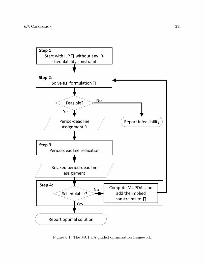
6.7. Conclusion 251
Step 2: Solve ILP formulation ∏
Step 4:
Schedulable?No
Yes
Compute MUPDAs and add the implied constraints to ∏
Step 3: Period-deadline relaxation
Step 1: Start with ILP ∏ without any R-
schedulability constraints
Period-deadline assignment R
Relaxed period-deadline assignment
Feasible?
Yes
Report infeasibility
No
Report optimal solution
Figure 6.1: The MUPDA guided optimization framework.

252Chapter 6. A Unified Framework for Period and Priority Optimization in Distributed
Hard Real-Time Systems
0 50 100 150 200 250 300
Time(s)
3.5
4
4.5
5
5.5
6
6.5
7
7.5
8
8.5
Obje
ctive V
alu
e
105
Approximated GP Objective
Actual Objective
Figure 6.2: Optimized objective of IterGP.

Chapter 7
A Unified Framework for Optimizing
Design of Real-Time Systems with
Sustainable Schedulability Analysis
7.1 Introduction
In Chapter 5, we introduce an optimization framework based on the concept of MUDA. This
has allowed us to efficiently optimize priority assignment w.r.t minimizing weighted average
response time. In Chapter 6, we blend in the parameter of period and generalize the concept
into MUPDA. This allows us to efficiently solve the more challenging problem of period
and priority assignment co-optimization w.r.t minimizing average response times. Though
effective in their targeted problem settings, the iterative optimization framework they used
suffers two major issues.
Firstly, the framework works well only when the objective function is sensitive to few vari-
ables. In particular, Chapter 5 and Chapter 6 have only considered objective functions that
contains one single decision variable. We will show later that, when the objective function is
sensitive to more variables, the number of MDUA (or MUPDA) constraints needed to defined
the optimal solution, and thus the number of iterations to terminate, grows exponentially,
253

254Chapter 7. A Unified Framework for Optimizing Design of Real-Time Systems with
Sustainable Schedulability Analysis
which significantly impact the scalability of the techniques.
Secondly, the framework relies on mixed-integer-linear-programming (MILP) for solving the
sub problem consisting of MUDA (or MUPDA) implied constraints in each iteration. This
not only restricts the applicability only to problems with linear objective functions, but also
significantly slows down the technique when the number of iterations grows high.
In this chapter, we discuss an optimization framework that improves upon the one used in
Chapter 5 and Chapter 6 and address the above issues. Specifically, we first follow the same
idea behind MUDA and MUPDA based framework, and then generalize the concept to more
parameters other than deadlines and periods. We then improve the optimization framework
by integrating the following techniques.
• A dedicated algorithm to replace MILP for solving the sub-problem in each iteration.
• An improved algorithm for computing maximal generalizations of a unschedulable so-
lution (i.e. MUDA, MUPDA in previous chapters) that provides faster convergence.
• Heuristic algorithms that explore good quality feasible solutions during optimization.
The rest of the chapter is organized as follows. Section 7.2 introduces the system model
we used for presentation and the optimization problem the chapter concerns. Section 7.3
summarizes existing approaches for solving the optimization problems and analyzes their
limitation in terms of applicability and scalability. Section 7.4 formalizes the optimization
problem and the concept of Maximal-Schedulable-Assignment (MUA) and discusses the a
general iterative optimization framework based on the concept. Section 7.5 discusses a
dedicated algorithm for solving the sub-problem consisting of MUA-implied constraints.
Section 7.6 discusses an algorithm for computing MUAs that gives faster convergence rate.
Section 7.7 discusses two heuristic algorithms for exploring good quality and schedulable
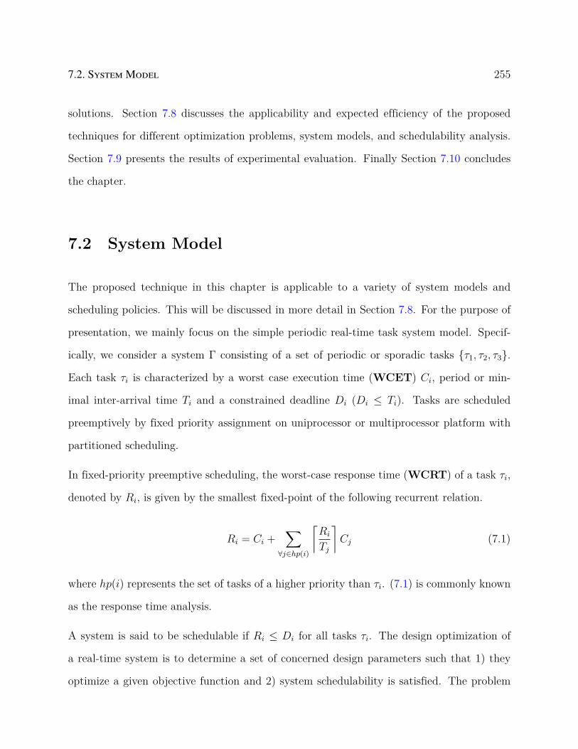
7.2. System Model 255
solutions. Section 7.8 discusses the applicability and expected efficiency of the proposed
techniques for different optimization problems, system models, and schedulability analysis.
Section 7.9 presents the results of experimental evaluation. Finally Section 7.10 concludes
the chapter.
7.2 System Model
The proposed technique in this chapter is applicable to a variety of system models and
scheduling policies. This will be discussed in more detail in Section 7.8. For the purpose of
presentation, we mainly focus on the simple periodic real-time task system model. Specif-
ically, we consider a system Γ consisting of a set of periodic or sporadic tasks τ1, τ2, τ3.
Each task τi is characterized by a worst case execution time (WCET) Ci, period or min-
imal inter-arrival time Ti and a constrained deadline Di (Di ≤ Ti). Tasks are scheduled
preemptively by fixed priority assignment on uniprocessor or multiprocessor platform with
partitioned scheduling.
In fixed-priority preemptive scheduling, the worst-case response time (WCRT) of a task τi,
denoted by Ri, is given by the smallest fixed-point of the following recurrent relation.
Ri = Ci +∑
∀j∈hp(i)
⌈Ri
Tj
⌉Cj (7.1)
where hp(i) represents the set of tasks of a higher priority than τi. (7.1) is commonly known
as the response time analysis.
A system is said to be schedulable if Ri ≤ Di for all tasks τi. The design optimization of
a real-time system is to determine a set of concerned design parameters such that 1) they
optimize a given objective function and 2) system schedulability is satisfied. The problem

256Chapter 7. A Unified Framework for Optimizing Design of Real-Time Systems with
Sustainable Schedulability Analysis
can be mathematically expressed as follow.
min F (X)
s.t. system schedulability(7.2)
X = [x1, ...xm] is the vector of decision variables that represents the decision parameters.
They may contain some or a mixture of the parameters involved in (7.1). The following
briefly summarizes these parameters and the typical optimization problems they are related
to.
• WCRT Ri. The performance of a real-time system is usually measured by the respon-
siveness of tasks. For example, control cost of real-time control applications depends
on WCRT of control tasks [104]. The end-to-end latency in distributed system depends
on WCRT of tasks involved in the end-to-end path [167].
• Period Ti. Similar as WCRT, period also affects control costs. In distributed system
with periodic activation [167], end-to-end latency additionally depends on periods of
tasks on the end-to-end path.
• WCET Ci. Platforms with dynamic voltage and frequency scaling (DVFS) allow to
adjust the execution time of tasks by adjusting the CPU clock rate. Higher clock
rate gives smaller execution time but results in of higher energy consumption. For
energy constrained devices, it is important to optimize the CPU clock rate w.r.t energy
efficiency.
• Priority Assignment. Priority assignment determines the set of hp(i) in (7.1). In the
design of Simulink Synchronous Reactive systems [109], priority assignment determines
the use of rate-transition/unit-delay blocks. The use of unit-delay blocks introduces
control cost. Therefore, it is necessary to optimize priority assignment w.r.t minimizing
7.3. Existing Formulation 257
the use of unit-delay blocks. It has also been shown that that co-optimizing parameters
Ti, Di with priority assignment yields significantly better solution than optimizing the
parameters alone [166].
7.3 Existing Formulation
Solving problem (7.2) requires an efficient algorithm for exploring the decision space defined
by schedulability constraint. Existing studies on this aspect can be largely divided into
two categories. The first aims to develop ad-hoc approaches that only target at specific
problems. The second aims to formulate the problem into a general optimization framework
(i.e. mathematical programming), which provides certain level of applicability to different
problems. The focus of this chapter is in the second category. Most of the existing work in
this category however, considers only a subset of the decision variables and certain forms of
objective functions. The following gives a summary of the main results in this category and
their limitations in terms of applicability and scalability.
7.3.1 MILP Formulation Based on Response Time Analysis
When period Ti and WCET Ci of each task are given and priority assignment is the only
decision variable, response time analysis (7.1) can be represented by a set of mixed-integer
linear programming (MILP) constraints.
The ceiling term⌈Ri
Tj
⌉can be computed by introducing an integer variable Ii,j subject to the
following constraint
Ii,j ≥Ri
Tj
(7.3)
258Chapter 7. A Unified Framework for Optimizing Design of Real-Time Systems with
Sustainable Schedulability Analysis
Priority assignment can be represented by introducing a binary variable pi,j, which represents
the partial priority order between a pair of tasks τi and τj. Specifically
pi,j =
1, τj has higher priority
0, otherwise(7.4)
With pi,j, response time analysis (7.1) can then be re-written as
Ri = Ci +∑∀j
pi,jIi,jCj (7.5)
The non-linear term pi,jIi,j can be linearized by introducing an additional variable Πi,j subject
to the following constraint
Πi,j ≥ Ii,j − (1− pi,j)M (7.6)
The response time analysis can then be expressed as the following linear form
Ri = Ci +∑∀j
Πi,jCj (7.7)
The above formulation is subject to the following limitations
• The formulation introduces large number of integer variables (up to O(n2) for Ii,j and
pi,j) and is difficult to scale to large systems.
• The formulation relies on given period Ti and WCET Ci and thus cannot be used to
optimize these parameters.

7.3. Existing Formulation 259
7.3.2 MILP Based on Request Bound Function Analysis
Request bound function rbfi(t) represents the cumulative execution request by tasks of higher
priority than τi. It is evaluated as
rbfi(t) = Ci +∑
∀j∈hp(i)
⌈t
Tj
⌉Cj (7.8)
[95] shows that the the condition of schedulability for a task τi can be expressed in terms of
the request bound function as follows
∃t ∈ Si s.t. rbfi(t) ≤ t (7.9)
where Si is a finite set of time points for evaluating the condition rbfi(t) ≤ t. A sufficient
set of Si can be computed by the technique proposed in [155].
When period Ti is given, (7.8) becomes a linear expression on priority partial orders pi,j and
WCET Cj, i.e.
rbfi(t) = Ci +∑∀j
pi,j
⌈t
Tj
⌉Cj (7.10)
The ∃ quantifier in (7.9) can be formulated as disjunctive constraints in integer programming.
For example
∃t ∈ t1, t2 s.t. rbfi(t) ≤ t⇔
∥∥∥∥∥∥∥rbfi(t1) ≤ t1
rbfi(t2) ≤ t2
(7.11)
The above formulation has much less formulation complexity comparing with the formulation
of response time analysis. It has been shown to provide significant improvement in scalability
for optimizing priority assignment [109]. The approach however, is subject to the following
limitations.

260Chapter 7. A Unified Framework for Optimizing Design of Real-Time Systems with
Sustainable Schedulability Analysis
• Due to the use with MILP, the approach can only be used to optimize linear objective
functions. This makes it impossible to apply it to problems with non-linear objectives.
For example, energy consumption is typically expressed in the following form [117]
P =∑∀i
β(C−1i )α (7.12)
Although it is theoretically possible to formulate the problem as a mixed-integer con-
vex programming (MICP), the problem is generally not well supported by available
commercial solvers.
• The formulation relies on given period Ti and does not maintains the information on
WCRT Ri. Thus it cannot be used to optimized objective functions that depend on
these parameters.
7.3.3 MIGP Based on Response Time Analysis
To address the challenge of period optimization Ti, [41] proposed a mixed-integer geometric
programming (MIGP) formulation of the response time analysis, assuming that priority
assignment is given. Specifically, the non-linear ceiling term⌈Ri
Tj
⌉is computed by introducing
an additional integer variable Ii,j subject to the following monomial constraint
RiT−1j I−1
i,j ≤ 1 (7.13)
The response time analysis can then be expressed as the following posynomial form.
Ri = Ci +∑
∀j∈hp(i)
Ii,jCj (7.14)

7.3. Existing Formulation 261
In addition to the capability of optimizing all of parameter Ri, Ti and Ci, the use of geometric
programming makes it possible to optimize a much wider range of objective functions that
can be expressed in posynomial forms. These include both linear expressions and those such
as (7.12).
The approach is subject to the following limitations
• MIGP is generally difficult to solve and scale to large design. In the original paper, [41]
proposed to solve instead the continuous relaxation of the problem and use an iterative
refinement procedure on top of it to reduce relaxation error. The issue however, is that
the algorithm does not guarantee progress or termination.
• The formulation assumes given priority assignment and therefore cannot be used to
optimize problems where priority assignment is part of the decision space.
7.3.4 Schedulability Abstraction based on Maximal Unschedula-
ble Period-Deadline Assignment
To address the challenge of co-optimizing period, WCRT and priority assignment, [166]
proposed a technique that abstracts and separates schedulability analysis from optimization.
The key observation is that response time analysis (7.1) is sustainable w.r.t to deadline Di
and period Ti. Specifically, increasing Di and Ti of tasks cannot make the system from
being schedulable to unschedulable. This property remains true regardless of whether or not
priority assignment is given. The property gives a very useful implication for characterizing
feasibility region. For example, suppose it is found that an assignment of period T1 = 10,
and deadline D2 = 20 for τ1 and τ2 respectively is unschedulable for the system. It can be
inferred that all other assignments of smaller values will be unschedulable as well. This leads
262Chapter 7. A Unified Framework for Optimizing Design of Real-Time Systems with
Sustainable Schedulability Analysis
to the following invariant.
¬
T1 ≤ 10
D2 ≤ 20
⇔
∥∥∥∥∥∥∥T1 > 10
D2 > 20
(7.15)
where symbol ∥ represents disjunction (the logical-OR relation).
Instead of directly formulating (7.1) into standard mathematical programming, [166] pro-
posed to use (7.15) as the schedulability constraint in mathematical programming. This
abstracts away the detail of schedulability analysis and thus overcomes the limitations suf-
fered by previous approaches. Similar to (7.11), (7.15) can be formulated as a disjunctive
constraint in integer programming. The higher the values on the right-hand-side, the stronger
the invariant. [166] proposes a two-step iterative procedure for optimization. Specifically,
• Step 1. Solve problem (7.2) without any schedulability constraint.
• Step 2. If the solution is schedulable, it is optimal and the algorithm terminates.
Otherwise, maximally increase the values in the solution while maintaining its un-
schedulability then add the corresponding constraint (7.15) back to problem (7.2) and
go back to Step 1.
Although originally proposed to co-optimize Di, Ti and priority assignment, the approach
can theoretically be extended to WCET Ci as well. In addition, it also provides a unique ben-
efit of accommodating different schedulability analysis given that they are sustainable w.r.t
decision variables. Experiment result reported in the chapter shows significant improvement
in both run-time and quality of solution by the proposed framework.
The approach however, is subject to the following limitations.
• The approach relies on MILP for solving the sub-problem consisting of the invariant
constraints (7.15). As a result, it is inapplicable to optimizing non-linear objectives

7.3. Existing Formulation 263
such as (7.12).
• As will be shown in the experiment, the approach is extremely inefficient when the
objective function is sensitive to many decision variables.
• Unlike many commercial mathematical programming solvers, the approach does not
give any feasible solution until it finds the optimal one. This can be undesired when
used in a time-restricted setting where termination is not likely.
In this chapter, we propose an optimization framework for solving (7.2) that aims to address
the limitations suffered by the above approaches. Specifically, at the cost of small sub-
optimality, we propose a solution that aims to achieve the following benefits.
• Capable of co-optimizing across different parameters including period Ti, WCET Ci,
WCRT Ri and priority assignment.
• Capable of optimizing a wide range of different linear and non-linear objectives.
• Capable of applying to a wide range of different schedulability analysis in addition to
(7.1).
• Provides better scalability for larger design.
The proposed approach is based on the framework developed in [166] and improved with the
following three novel techniques.
• We propose a new algorithm in place of MILP for solving the sub-problem consisting
of invariant constraint (7.15).
• We propose an improved algorithm for computing stronger invariant (7.15) from un-
schedulable solution, which gives faster convergence.
264Chapter 7. A Unified Framework for Optimizing Design of Real-Time Systems with
Sustainable Schedulability Analysis
• We enhance the framework with two heuristics that explore good-quality and schedu-
lable solutions.
In the next section, we first generalize on the core concept and optimization framework
discussed in [166]. We then discuss the design of each new technique we integrate.
7.4 The Concept of Maximal Unschedulable Assign-
ment
We first re-write problem (7.2) into the following canonical form
min F (X)
s.t. G(X) ≤ 0(7.16)
Specifically, we represent schedulability constraint as an inequality over a conceptual function
G(X). G(X) can be interpreted, for example, as
G(X) =
1, system is not schedulable
0, otherwise(7.17)
We make the following assumptions about function F (X), G(X), and variables X.
1. F (X) is non-decreasing w.r.t to the increasing of each variable xi in X.
2. G(X) is non-increasing w.r.t to the increasing of each variable xi in X.
3. Each variable xi in X takes integer values within a bounded range [lbi, ubi] (i.e, the
design parameters have finite resolution).
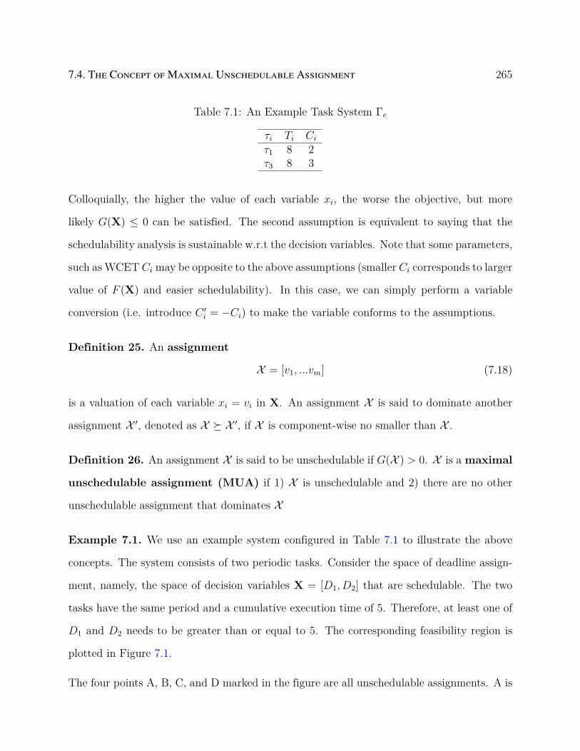
7.4. The Concept of Maximal Unschedulable Assignment 265
Table 7.1: An Example Task System Γe
τi Ti Ci
τ1 8 2τ3 8 3
Colloquially, the higher the value of each variable xi, the worse the objective, but more
likely G(X) ≤ 0 can be satisfied. The second assumption is equivalent to saying that the
schedulability analysis is sustainable w.r.t the decision variables. Note that some parameters,
such as WCET Ci may be opposite to the above assumptions (smaller Ci corresponds to larger
value of F (X) and easier schedulability). In this case, we can simply perform a variable
conversion (i.e. introduce C ′i = −Ci) to make the variable conforms to the assumptions.
Definition 25. An assignment
X = [v1, ...vm] (7.18)
is a valuation of each variable xi = vi in X. An assignment X is said to dominate another
assignment X ′, denoted as X ⪰ X ′, if X is component-wise no smaller than X .
Definition 26. An assignment X is said to be unschedulable if G(X ) > 0. X is a maximal
unschedulable assignment (MUA) if 1) X is unschedulable and 2) there are no other
unschedulable assignment that dominates X
Example 7.1. We use an example system configured in Table 7.1 to illustrate the above
concepts. The system consists of two periodic tasks. Consider the space of deadline assign-
ment, namely, the space of decision variables X = [D1, D2] that are schedulable. The two
tasks have the same period and a cumulative execution time of 5. Therefore, at least one of
D1 and D2 needs to be greater than or equal to 5. The corresponding feasibility region is
plotted in Figure 7.1.
The four points A, B, C, and D marked in the figure are all unschedulable assignments. A is
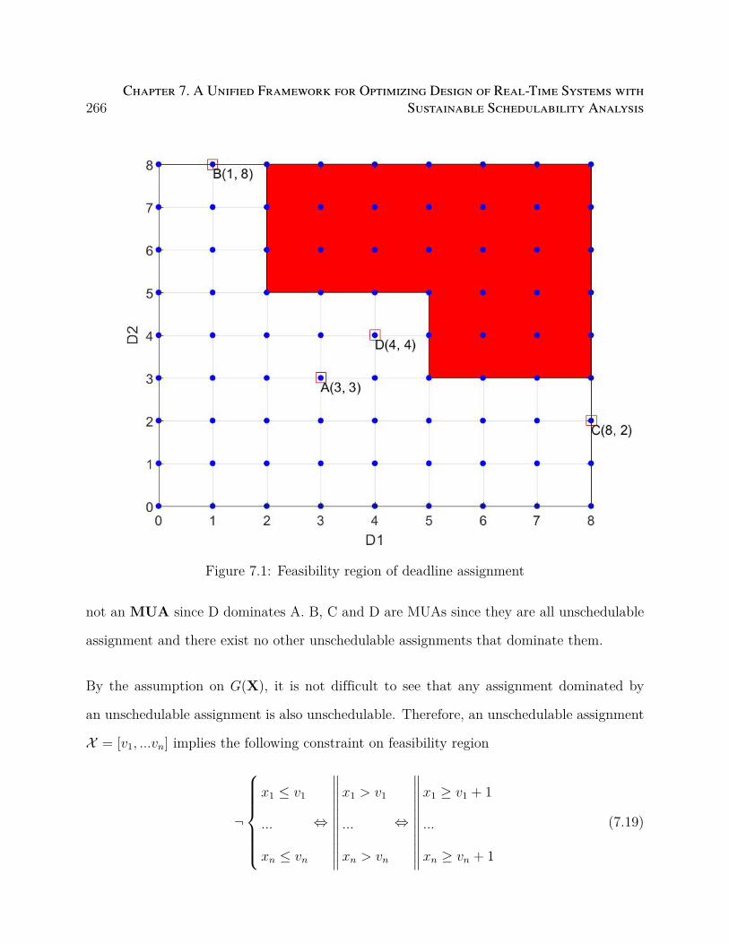
266Chapter 7. A Unified Framework for Optimizing Design of Real-Time Systems with
Sustainable Schedulability Analysis
Figure 7.1: Feasibility region of deadline assignment
not an MUA since D dominates A. B, C and D are MUAs since they are all unschedulable
assignment and there exist no other unschedulable assignments that dominate them.
By the assumption on G(X), it is not difficult to see that any assignment dominated by
an unschedulable assignment is also unschedulable. Therefore, an unschedulable assignment
X = [v1, ...vn] implies the following constraint on feasibility region
¬
x1 ≤ v1
...
xn ≤ vn
⇔
∥∥∥∥∥∥∥∥∥∥∥x1 > v1
...
xn > vn
⇔
∥∥∥∥∥∥∥∥∥∥∥x1 ≥ v1 + 1
...
xn ≥ vn + 1
(7.19)
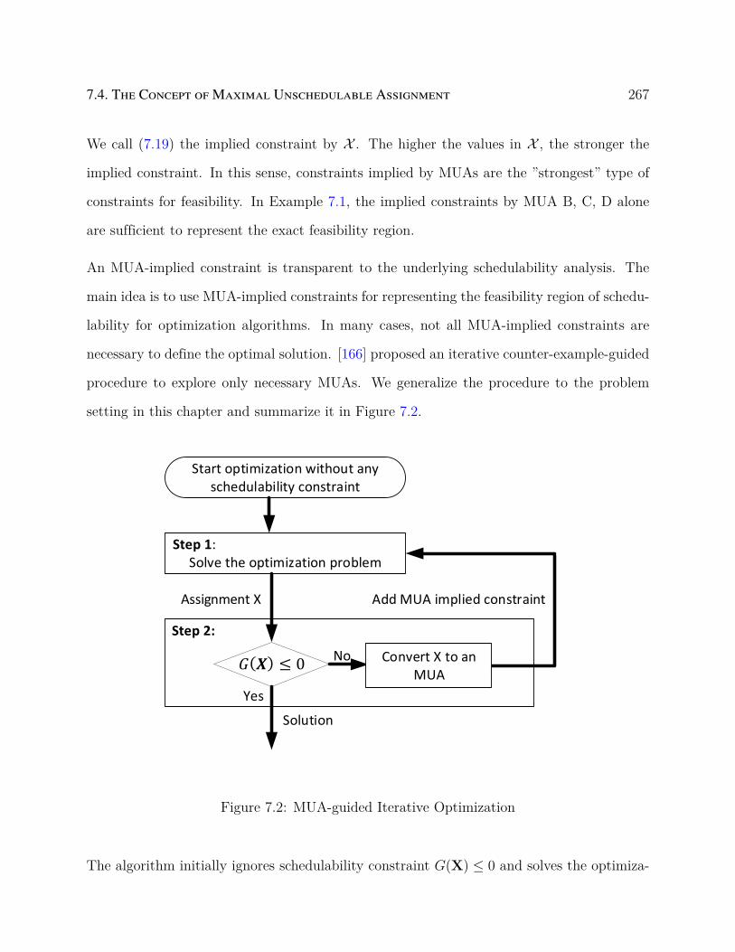
7.4. The Concept of Maximal Unschedulable Assignment 267
We call (7.19) the implied constraint by X . The higher the values in X , the stronger the
implied constraint. In this sense, constraints implied by MUAs are the ”strongest” type of
constraints for feasibility. In Example 7.1, the implied constraints by MUA B, C, D alone
are sufficient to represent the exact feasibility region.
An MUA-implied constraint is transparent to the underlying schedulability analysis. The
main idea is to use MUA-implied constraints for representing the feasibility region of schedu-
lability for optimization algorithms. In many cases, not all MUA-implied constraints are
necessary to define the optimal solution. [166] proposed an iterative counter-example-guided
procedure to explore only necessary MUAs. We generalize the procedure to the problem
setting in this chapter and summarize it in Figure 7.2.
Step 1: Solve the optimization problem
Assignment X Add MUA implied constraint
No
Yes
Convert X to an MUA
Start optimization without any schedulability constraint
Solution
Step 2:
Figure 7.2: MUA-guided Iterative Optimization
The algorithm initially ignores schedulability constraint G(X) ≤ 0 and solves the optimiza-
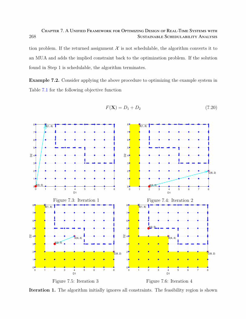
268Chapter 7. A Unified Framework for Optimizing Design of Real-Time Systems with
Sustainable Schedulability Analysis
tion problem. If the returned assignment X is not schedulable, the algorithm converts it to
an MUA and adds the implied constraint back to the optimization problem. If the solution
found in Step 1 is schedulable, the algorithm terminates.
Example 7.2. Consider applying the above procedure to optimizing the example system in
Table 7.1 for the following objective function
F (X) = D1 +D2 (7.20)
0 1 2 3 4 5 6 7 8
D1
0
1
2
3
4
5
6
7
8
D2
B(1, 8)
X(0, 0)
Figure 7.3: Iteration 1
0 1 2 3 4 5 6 7 8
D1
0
1
2
3
4
5
6
7
8D
2
C(8, 2)
B(1, 8)
X(2, 0)
Figure 7.4: Iteration 2
0 1 2 3 4 5 6 7 8
D1
0
1
2
3
4
5
6
7
8
D2
D(4, 4)
B(1, 8)
C(8, 2)
X(2, 3)
Figure 7.5: Iteration 3
0 1 2 3 4 5 6 7 8
D1
0
1
2
3
4
5
6
7
8
D2
B(1, 8)
C(8, 2)
D(4, 4)
X(2, 5)
Figure 7.6: Iteration 4
Iteration 1. The algorithm initially ignores all constraints. The feasibility region is shown
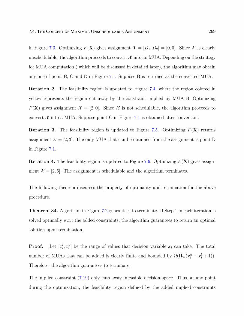
7.4. The Concept of Maximal Unschedulable Assignment 269
in Figure 7.3. Optimizing F (X) gives assignment X = [D1, D2] = [0, 0]. Since X is clearly
unschedulable, the algorithm proceeds to convert X into an MUA. Depending on the strategy
for MUA computation ( which will be discussed in detailed later), the algorithm may obtain
any one of point B, C and D in Figure 7.1. Suppose B is returned as the converted MUA.
Iteration 2. The feasibility region is updated to Figure 7.4, where the region colored in
yellow represents the region cut away by the constraint implied by MUA B. Optimizing
F (X) gives assignment X = [2, 0]. Since X is not schedulable, the algorithm proceeds to
convert X into a MUA. Suppose point C in Figure 7.1 is obtained after conversion.
Iteration 3. The feasibility region is updated to Figure 7.5. Optimizing F (X) returns
assignment X = [2, 3]. The only MUA that can be obtained from the assignment is point D
in Figure 7.1.
Iteration 4. The feasibility region is updated to Figure 7.6. Optimizing F (X) gives assign-
ment X = [2, 5]. The assignment is schedulable and the algorithm terminates.
The following theorem discusses the property of optimality and termination for the above
procedure.
Theorem 34. Algorithm in Figure 7.2 guarantees to terminate. If Step 1 in each iteration is
solved optimally w.r.t the added constraints, the algorithm guarantees to return an optimal
solution upon termination.
Proof. Let [xli, x
ui ] be the range of values that decision variable xi can take. The total
number of MUAs that can be added is clearly finite and bounded by Ω(Π∀i(xui − xl
i + 1)).
Therefore, the algorithm guarantees to terminate.
The implied constraint (7.19) only cuts away infeasible decision space. Thus, at any point
during the optimization, the feasibility region defined by the added implied constraints
270Chapter 7. A Unified Framework for Optimizing Design of Real-Time Systems with
Sustainable Schedulability Analysis
maintains to be an over-approximation of the exact feasibility region. If the optimization
problem in Step 1 is solved optimally in each iteration, the objective value is no larger
than that of the globally optimal solution. This implies that upon termination, where the
algorithm finds a schedulable solution (i.e. G(X) ≤ 0), the solution is globally optimal.
The following sections focus on two major components of the framework: 1) the algorithm
for solving the sub-optimization-problem in Step 1, and 2) the algorithm for computing an
MUA from an unschedulable assignment.
7.5 Optimizing with MUA-Implied Constraints
Step 1 in Figure 7.2 requires to solve the following optimization problem
min F (X)
s.t. constraints of form (7.19)(7.21)
[166] proposed to solve the sub-problem as an MILP. As discussed previously, this limits the
approach only to linear objective functions and suffers scalability issues when the number of
MUA-implied constraints in the problem is large. In this section, we discuss a more generic
algorithm that handles different forms of F (X) and provides much better scalability.
We first take a closer look at the form of the implied constraint (7.19).
∥∥∥∥∥∥∥∥∥∥∥∥∥∥
x1 ≥ v1 + 1
x2 ≥ v2 + 1
...
xn ≥ vn + 1
(7.22)
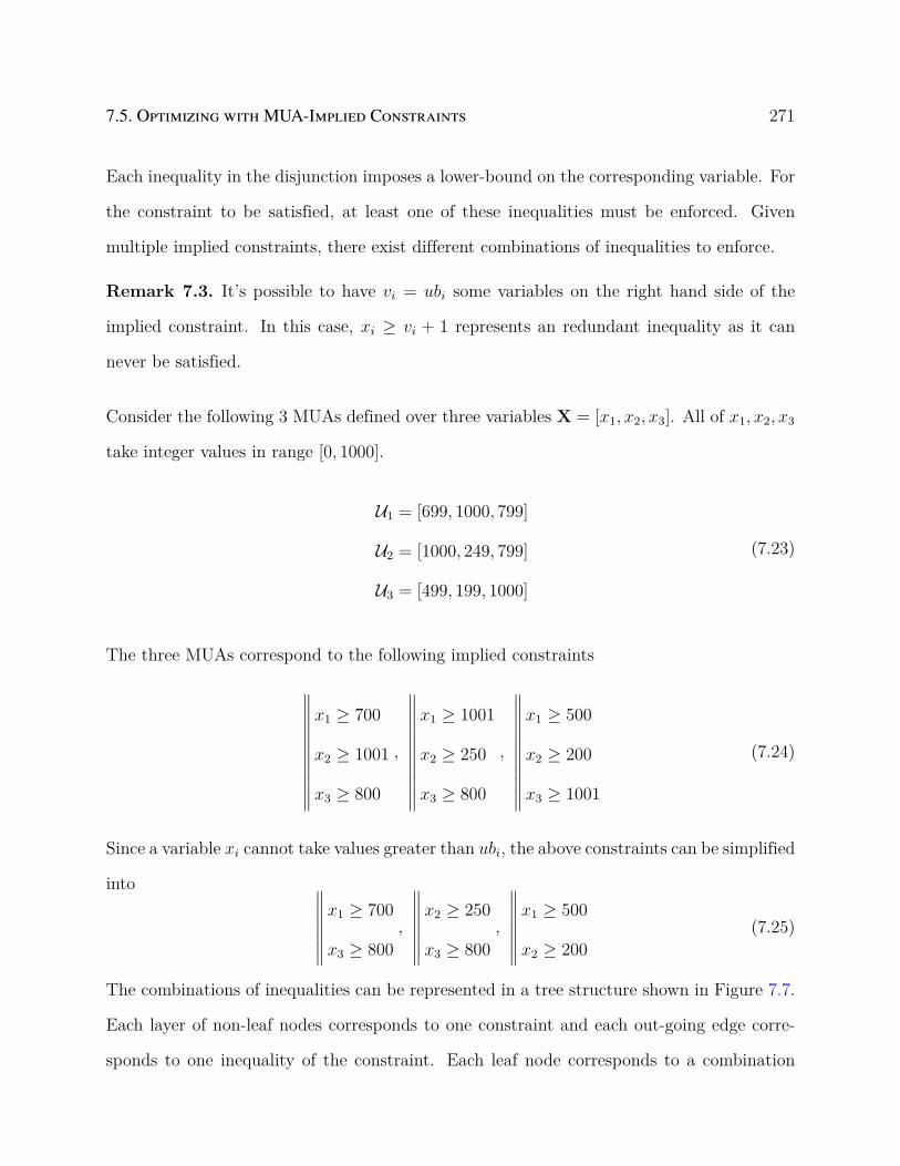
7.5. Optimizing with MUA-Implied Constraints 271
Each inequality in the disjunction imposes a lower-bound on the corresponding variable. For
the constraint to be satisfied, at least one of these inequalities must be enforced. Given
multiple implied constraints, there exist different combinations of inequalities to enforce.
Remark 7.3. It’s possible to have vi = ubi some variables on the right hand side of the
implied constraint. In this case, xi ≥ vi + 1 represents an redundant inequality as it can
never be satisfied.
Consider the following 3 MUAs defined over three variables X = [x1, x2, x3]. All of x1, x2, x3
take integer values in range [0, 1000].
U1 = [699, 1000, 799]
U2 = [1000, 249, 799]
U3 = [499, 199, 1000]
(7.23)
The three MUAs correspond to the following implied constraints
∥∥∥∥∥∥∥∥∥∥∥x1 ≥ 700
x2 ≥ 1001
x3 ≥ 800
,
∥∥∥∥∥∥∥∥∥∥∥x1 ≥ 1001
x2 ≥ 250
x3 ≥ 800
,
∥∥∥∥∥∥∥∥∥∥∥x1 ≥ 500
x2 ≥ 200
x3 ≥ 1001
(7.24)
Since a variable xi cannot take values greater than ubi, the above constraints can be simplified
into ∥∥∥∥∥∥∥x1 ≥ 700
x3 ≥ 800
,
∥∥∥∥∥∥∥x2 ≥ 250
x3 ≥ 800
,
∥∥∥∥∥∥∥x1 ≥ 500
x2 ≥ 200
(7.25)
The combinations of inequalities can be represented in a tree structure shown in Figure 7.7.
Each layer of non-leaf nodes corresponds to one constraint and each out-going edge corre-
sponds to one inequality of the constraint. Each leaf node corresponds to a combination

272Chapter 7. A Unified Framework for Optimizing Design of Real-Time Systems with
Sustainable Schedulability Analysis
of inequalities along the path from root. The combination defines a tight assignment that
satisfies all the constraints. For example, consider the left most leaf node in Figure 7.7,
which corresponds to the combination of inequalities x1 ≥ 700 ∧ x2 ≥ 250 ∧ x1 ≥ 500. The
combination defines a unique assignment X = [x1, x2, x3] = [700, 250, 0] that is minimal
w.r.t the inequalities. The assignment is sufficient to satisfy the 3 constraints. We call X
the tight assignment defined by the leaf node. Note that x1 = 750, x2 = 300, x3 = 0 is
also an assignment that satisfies the combination of inequalities. It’s not a tight assignment
however, as x1, x2 can be further decreased without violating these inequalities.
ብ𝑥1 ≥ 700𝑥3 ≥ 800
ብ𝑥2 ≥ 250𝑥3 ≥ 800
ብ𝑥1 ≥ 500𝑥2 ≥ 200
𝑥1 ≥ 700 𝑥3 ≥ 800
𝑥2 ≥ 250 𝑥3 ≥ 800 𝑥2 ≥ 250 𝑥3 ≥ 800
𝑥2 ≥ 200 𝑥1 ≥ 500𝑥2 ≥ 200 𝑥1 ≥ 500𝑥1 ≥ 500 𝑥2 ≥ 200 𝑥1 ≥ 500 𝑥2 ≥ 200
1
2 3
4 5 6 7
8 9 10 11 12 13 14 15
Figure 7.7: Tree representation of implied constraints
Some nodes in the tree are redundant, in the sense that the corresponding implied constraint
may have already been satisfied by some inequality along the path from root. For example
node 4 and 5 are redundant as inequality x1 ≥ 700 along their paths from root already
implies that the constraint is satisfied. The same goes for node 3. In this case, we can prune
away the nodes to simplify the tree to reduce the number of leaves. Figure 7.8 shows the

7.5. Optimizing with MUA-Implied Constraints 273
tree where redundant nodes are pruned away, which has much smaller number of leaves.
ብ𝑥1 ≥ 700𝑥3 ≥ 800
ብ𝑥2 ≥ 250𝑥3 ≥ 800
ብ𝑥1 ≥ 500𝑥2 ≥ 200
𝑥1 ≥ 700 𝑥3 ≥ 800
𝑥2 ≥ 250 𝑥3 ≥ 800
𝑥1 ≥ 500 𝑥2 ≥ 200
1
2
4 5
3
6 7
Figure 7.8: After pruning redundant nodes
Theorem 35. Given a set of MUA-implied constraints L = L1, ...Lq and its tree repre-
sentation, there exists a tight assignment defined by some leaf node that minimizes F (X).
Proof. Consider any assignment X that satisfies the constraints in L and that also
minimizes F (X). Since X satisfies each Li ∈ L, at least one of the inequalities in Li is
satisfied by X . Take any one of such satisfied inequality from each Li ∈ L. The combination
of these inequalities corresponds to a root to leaf path in the tree representation. Consider
the tight assignment X ′ defined by the path. It’s not difficult to see that X ⪰ X ′. Since by
assumption F (X) is non-decreasing w.r.t the increasing of each variable, there is F (X ) ≥
F (X ′). This implies that F (X ′) = F (X ) and thus X ′ minimizes F (X) as well.
Theorem 35 implies that the optimal solution of problem (7.21) can be found examining all
the tight assignments defined by the leaves. In the algorithm in Figure 7.2, new implied con-

274Chapter 7. A Unified Framework for Optimizing Design of Real-Time Systems with
Sustainable Schedulability Analysis
Algorithm 13 Incremental Breadth-First-Search (BFS)1: function IncrementalBFS(Tight Assignments by Leaves M = X1, ...Xm, New MUAU = [u1, ...un])
2: M′ = ∅3: for each assignment X = [v1, ...vn] ∈M do4: if U dominates X then5: for each ui ∈ U do6: if ui < ubi then7: set X ′ = [v1, ...vi−1, ui + 1, vi+1, ...v
′n]
8: M′ =M′ ∪ X ′9: end if
10: end for11: else12: M′ =M′ ∪ X13: end if14: end for15: return M′
16: end function
straints are continuously discovered and added to the problem. Each time a new constraint is
added, a new layer of leaf nodes is expanded from the original leaves. Observing this nature,
we uses an breadth-first-search (BFS) traversal to find the optimal solution incrementally in
each iteration.
The algorithm is summarized Algorithm 13. It takes as input 1) the set of tight assignments
M defined by the current leaves in the tree and 2) a newly computed MUA U (i.e, from
step 2 in Figure 7.2). The goal is compute the set of tight assignments M′ corresponding
to the new leaves created by the implied constraint by U . The algorithm first traverses
all the tight assignments X defined by the current leaves. If U does not dominate the tight
assignment (which implies that X satisfies the implied constraint by U), the tight assignment
is directly added to M′ as it remains to be a leaf node. This corresponds to the pruning
of redundant nodes. Otherwise, new leaves need to be created with their tight assignments
added to M′. This is performed from Line 5 to Line 10. The algorithm traverses each ui in

7.5. Optimizing with MUA-Implied Constraints 275
U . Each ui corresponds to an inequality xi ≥ ui +1 in the implied constraint. Line 6 checks
and skips redundant inequalities as discussed in Remark 7.3. For non-redundant inequality,
the algorithm creates a new assignment X ′ from X by setting the value assigned to the ith
variable to ui + 1. X ′ is then added to M′.
Figure 7.2 gives the updated procedure that uses Algorithm 13 for solving the sub-problem.
Step 1: Find assignment X in M with
minimum F(X)
Assignment XInvoke
M = IncrementalBFS(M, U)
No
Yes
Convert X to an MUA U
Solution
Step 2:
Figure 7.9: Iterative optimization using BFS
The algorithm maintains a set of tight assignments M defined by the current leaves in
the tree representation of all implied constraints. M is initialized with a single assignment
X = [lb1, ...lbn] where all variables are assigned their lower bounds. Solving the optimization
problem (7.21) is equivalent to finding the tight assignment X in M with the smallest
objective value F (X ). In Step 2, after an unschedulable assignment is converted into an
MUA, Algorithm 13 is invoked to update M.

276Chapter 7. A Unified Framework for Optimizing Design of Real-Time Systems with
Sustainable Schedulability Analysis
Example 7.4. Consider the example of (7.23) and the problem of minimizing F (X) = x1+
x2 + x3. Specifically, G(X) ≤ 0 represents the 3 constraints in (7.23). We now demonstrate
a run of the Algorithm, where U1, U2 and U3 are added sequentially in 3 iterations.
The algorithm starts with M = [0, 0, 0].
Iteration 1. Step 1 returns assignments X = [0, 0, 0]. X does not satisfied G(X ) ≤ 0 and
the algorithm coverts it into an MUA U1. After invoking Algorithm 13, M is updated to
the following
M =
[700, 0, 0]
[0, 0, 800]
(7.26)
Iteration 2. Step 1 returns assignment X = [700, 0, 0] which has the smallest objective
value. X does not satisfied G(X ) ≤ 0 and the algorithm coverts it into an MUA U2.
Invoking Algorithm 13 updates M to the following
M =
[700, 250, 0]
[700, 0, 800]
[0, 0, 800]
(7.27)
Iteration 3. Step 1 returns assignment X = [0, 0, 800]. X does not satisfied G(X ) ≤ 0
and the algorithm coverts it into an MUA U3. Invoking Algorithm 13 updates M to the
following
M =
[700, 250, 0]
[700, 0, 800]
[500, 0, 800]
[0, 200, 800]
(7.28)

7.6. Converting an Unschedulable Assignment to MUA 277
Iteration 4. Step 1 returns assignment X = [700, 250, 0] which has the smallest objective
value. X now satisfies G(X ) ≤ 0 and the algorithm terminates with the assignment.
The number of MUA-implied constraints necessary for defining the optimal solution depends
on various factors. These may include the shape of feasibility region and the number deci-
sion variables. In general, the set of necessary MUAs grows exponentially with larger size
problems and more complex feasibility region. This may lead to the following issues for
scalability.
• The total number of iterations grows exponentially.
• The size of problem (7.21) in each iteration (i.e., the size of M) may eventually grow
to an exponential size.
To alleviate the problem, we modify the algorithm into a heuristic by setting a size limit K
for M. After Algorithm 13 is invoked, we sort the assignments in M′ in ascending order
according to their objective values F (X ) and only keep the first K assignments. Problem
(7.21) in each iteration is now only solved sub-optimally due to the limit on the size of M.
However, in return, the algorithm gains better scalability. In most cases, a larger value on
K gives better solution. But extremely large K does not necessarily brings more benefit
comparing to smaller one. The best setting of K depends on the nature of the problem and
requires intuition from designer. These issues will be studied in Section 7.9.
7.6 Converting an Unschedulable Assignment to MUA
In this section, we discuss algorithms for converting an unschedulable assignment X into an
MUA U . One strategy proposed in [166] is to maximally increase each entry in X sequentially
while maintaining its unschedulability. The procedure is summarized in Algorithm 14.
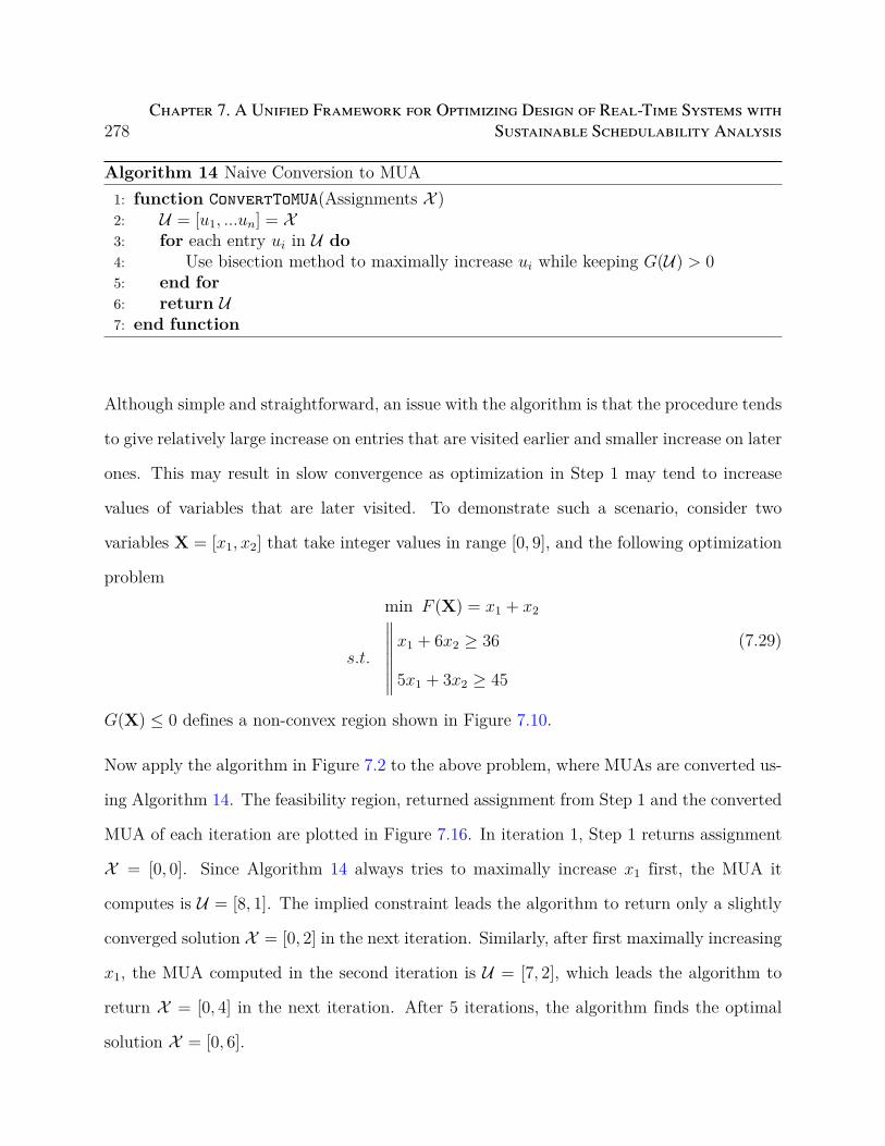
278Chapter 7. A Unified Framework for Optimizing Design of Real-Time Systems with
Sustainable Schedulability Analysis
Algorithm 14 Naive Conversion to MUA1: function ConvertToMUA(Assignments X )2: U = [u1, ...un] = X3: for each entry ui in U do4: Use bisection method to maximally increase ui while keeping G(U) > 05: end for6: return U7: end function
Although simple and straightforward, an issue with the algorithm is that the procedure tends
to give relatively large increase on entries that are visited earlier and smaller increase on later
ones. This may result in slow convergence as optimization in Step 1 may tend to increase
values of variables that are later visited. To demonstrate such a scenario, consider two
variables X = [x1, x2] that take integer values in range [0, 9], and the following optimization
problemmin F (X) = x1 + x2
s.t.
∥∥∥∥∥∥∥x1 + 6x2 ≥ 36
5x1 + 3x2 ≥ 45
(7.29)
G(X) ≤ 0 defines a non-convex region shown in Figure 7.10.
Now apply the algorithm in Figure 7.2 to the above problem, where MUAs are converted us-
ing Algorithm 14. The feasibility region, returned assignment from Step 1 and the converted
MUA of each iteration are plotted in Figure 7.16. In iteration 1, Step 1 returns assignment
X = [0, 0]. Since Algorithm 14 always tries to maximally increase x1 first, the MUA it
computes is U = [8, 1]. The implied constraint leads the algorithm to return only a slightly
converged solution X = [0, 2] in the next iteration. Similarly, after first maximally increasing
x1, the MUA computed in the second iteration is U = [7, 2], which leads the algorithm to
return X = [0, 4] in the next iteration. After 5 iterations, the algorithm finds the optimal
solution X = [0, 6].

7.6. Converting an Unschedulable Assignment to MUA 279
0 1 2 3 4 5 6 7 8 9
x1
0
1
2
3
4
5
6
7
8
9
x2
Figure 7.10: Feasibility region of problem (7.29)
We now discuss a smarter strategy of MUA conversion demonstrated in Figure 7.20. In
the first iteration, instead of first increasing x1, we simultaneously increase both x1 and
x2 while keeping the assignment in the infeasible region. This obtains MUA U = [5, 5].
The corresponding implied constraint leads the algorithm to return X = [6, 0] in the next
iteration. Similarly, in the second iteration, we simultaneously increase x1, x2 and obtain
MUA U = [8, 1]. After 3 iterations, the algorithm finds the optimal solution
The above example shows that different strategies of computing MUAs affect the rate at
which the objective value converges. Intuitively, we hope to compute MUAs whose implied
constraint give large increase on objective value. The amount of increase brought by one

280Chapter 7. A Unified Framework for Optimizing Design of Real-Time Systems with
Sustainable Schedulability Analysis
X(0, 0)
G(8, 1)
0 1 2 3 4 5 6 7 8 9
x1
0
1
2
3
4
5
6
7
8
9
x2
Figure 7.11: Iteration 1
G(8, 1)
X(0, 2)
G(7, 3)
0 1 2 3 4 5 6 7 8 9
x1
0
1
2
3
4
5
6
7
8
9
x2
Figure 7.12: Iteration 2
G(8, 1)
G(7, 3)
X(0, 4)
G(6, 4)
0 1 2 3 4 5 6 7 8 9
x1
0
1
2
3
4
5
6
7
8
9
x2
Figure 7.13: Iteration 3
G(8, 1)
G(7, 3)
G(6, 4)
X(0, 5)
G(5, 5)
0 1 2 3 4 5 6 7 8 9
x1
0
1
2
3
4
5
6
7
8
9
x2
Figure 7.14: Iteration 4
G(8, 1)
G(7, 3)
G(6, 4)
G(5, 5)
X(0, 6)
0 1 2 3 4 5 6 7 8 9
x1
0
1
2
3
4
5
6
7
8
9
x2
Figure 7.15: Iteration 5
Figure 7.16: First 4 iterations of optimizing problem (7.29) using Algorithm 14 for MUAconversion
constraint however, not only depends on itself, but also on other existing implied constraints.
This may not be known exactly until problem (7.21) is solved with the new constraint. In
this chapter, we adopt a simple strategy: we score each MUA U by the objective value it
defines alone, specificallymin F (X)
s.t. implied constraint of U :∥∥∥∥∥∥∥∥∥∥∥x1 ≥ u1 + 1
...
xn ≥ un + 1
(7.30)
Example 7.5. Consider the first iteration shown in Figure 7.11 and Figure 7.17. MUA

7.6. Converting an Unschedulable Assignment to MUA 281
X(0, 0)
G(5, 5)
0 1 2 3 4 5 6 7 8 9
x1
0
1
2
3
4
5
6
7
8
9
x2
Figure 7.17: Iteration 1
G(5, 5)
X(6, 0)
G(8, 1)
0 1 2 3 4 5 6 7 8 9
x1
0
1
2
3
4
5
6
7
8
9
x2
Figure 7.18: Iteration 2
G(5, 5)
G(8, 1)
X(0, 6)
0 1 2 3 4 5 6 7 8 9
x1
0
1
2
3
4
5
6
7
8
9
x2
Figure 7.19: Iteration 3
Figure 7.20: Iterations of optimizing problem (7.29) using an improved algorithm for MUAconversion
U1 = [8, 1] has a score of 2 as the following problem has an objective value of 2.
min F (X)
s.t.
∥∥∥∥∥∥∥x1 ≥ 9
x2 ≥ 2
(7.31)
Similarly, MUA U2 = [5, 5] has a score of 6. Thus we favor U2 over U1.
The goal is to compute an MUA of high score from an unschedulable assignment. Let us
first consider objective function F (X) of the following form
F (X) =n∑
i=1
xi (7.32)
Namely, F (X) is a summation of all decision variables.
Algorithm 15 gives an improved procedure for MUA conversion w.r.t the above form of
objective. The main difference with Algorithm 14 lies in Line 3, where the algorithm first
maximally increases all entries of U simultaneously by the same amount d while keeping U
unschedulable. Since the resulting U after Line 3 may not necessarily be an MUA, we apply
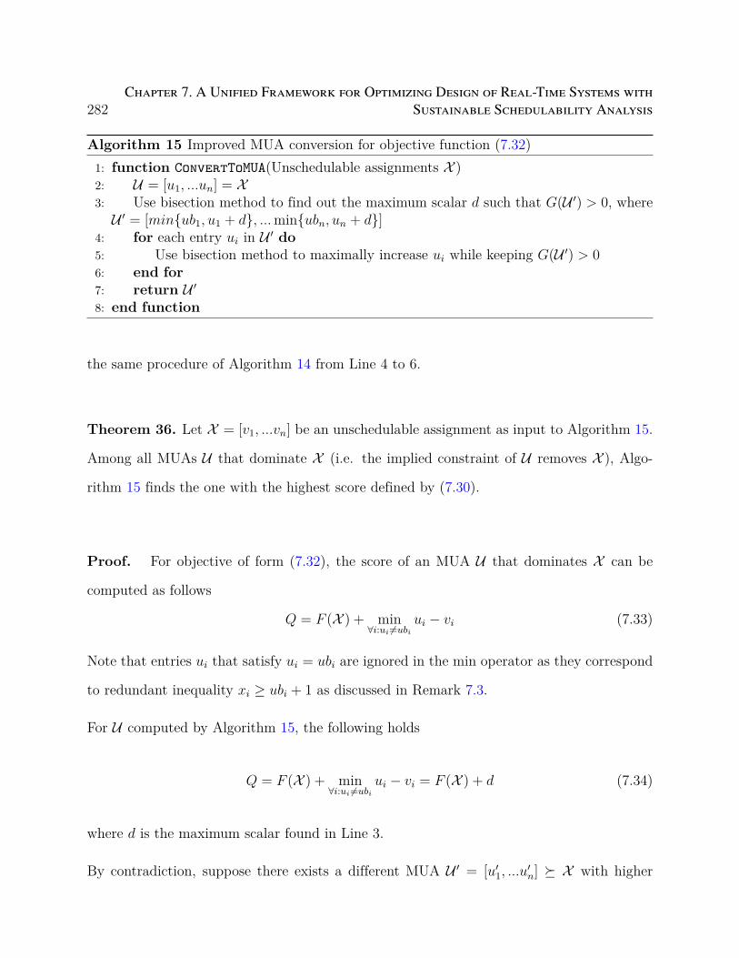
282Chapter 7. A Unified Framework for Optimizing Design of Real-Time Systems with
Sustainable Schedulability Analysis
Algorithm 15 Improved MUA conversion for objective function (7.32)1: function ConvertToMUA(Unschedulable assignments X )2: U = [u1, ...un] = X3: Use bisection method to find out the maximum scalar d such that G(U ′) > 0, whereU ′ = [minub1, u1 + d, ...minubn, un + d]
4: for each entry ui in U ′ do5: Use bisection method to maximally increase ui while keeping G(U ′) > 06: end for7: return U ′
8: end function
the same procedure of Algorithm 14 from Line 4 to 6.
Theorem 36. Let X = [v1, ...vn] be an unschedulable assignment as input to Algorithm 15.
Among all MUAs U that dominate X (i.e. the implied constraint of U removes X ), Algo-
rithm 15 finds the one with the highest score defined by (7.30).
Proof. For objective of form (7.32), the score of an MUA U that dominates X can be
computed as follows
Q = F (X ) + min∀i:ui =ubi
ui − vi (7.33)
Note that entries ui that satisfy ui = ubi are ignored in the min operator as they correspond
to redundant inequality xi ≥ ubi + 1 as discussed in Remark 7.3.
For U computed by Algorithm 15, the following holds
Q = F (X ) + min∀i:ui =ubi
ui − vi = F (X ) + d (7.34)
where d is the maximum scalar found in Line 3.
By contradiction, suppose there exists a different MUA U ′ = [u′1, ...u
′n] ⪰ X with higher
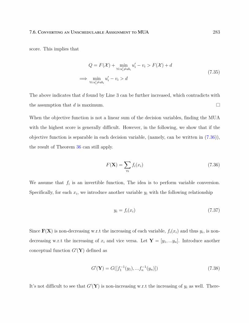
7.6. Converting an Unschedulable Assignment to MUA 283
score. This implies that
Q = F (X ) + min∀i:u′
i =ubiu′i − vi > F (X ) + d
=⇒ min∀i:u′
i =ubiu′i − vi > d
(7.35)
The above indicates that d found by Line 3 can be further increased, which contradicts with
the assumption that d is maximum.
When the objective function is not a linear sum of the decision variables, finding the MUA
with the highest score is generally difficult. However, in the following, we show that if the
objective function is separable in each decision variable, (namely, can be written in (7.36)),
the result of Theorem 36 can still apply.
F (X) =∑∀i
fi(xi) (7.36)
We assume that fi is an invertible function, The idea is to perform variable conversion.
Specifically, for each xi, we introduce another variable yi with the following relationship
yi = fi(xi) (7.37)
Since F(X) is non-decreasing w.r.t the increasing of each variable, fi(xi) and thus yi, is non-
decreasing w.r.t the increasing of xi and vice versa. Let Y = [y1, ...yn]. Introduce another
conceptual function G′(Y) defined as
G′(Y) = G([f−11 (y1), ...f
−1n (yn)]) (7.38)
It’s not difficult to see that G′(Y) is non-increasing w.r.t the increasing of yi as well. There-
284Chapter 7. A Unified Framework for Optimizing Design of Real-Time Systems with
Sustainable Schedulability Analysis
fore the original problem in (7.16) can be formulated as a problem over variable Y. Specifi-
cally,
minn∑
i=1
yi
s.t. G′(Y) ≤ 0
(7.39)
The objective function now conforms to (7.32) and thus the result of Theorem 36 applies.
(7.36) is a suitable representation for various optimization objectives including control per-
formance [103], end-to-end latency [41], energy consumption (7.12) etc. For other objectives
not conforming to (7.36), Algorithm 15 does not guarantee obtaining the MUA with highest
score, but may still be good in average as all variables are treated equally.
7.7 Exploring Sub-optimal Solution
Modern mathematical programming solvers such as CPLEX, YALMIP etc typically have the
capability to explore feasible solutions of good-quality. This allows them to return useful
result for designers to work with even when they fail to find globally optimal solution due to
time limit. The framework in Figure 7.2 however, does not give any schedulable assignment
during the optimization process until it is solved to termination. This can be undesired
when termination is not likely due to strict time limit imposed by designer. In this section,
we discuss a technique that enables the framework to explore schedulable and good-quality
solutions during the optimization process.
Our main idea is to make use of the assignment returned in Step 1 and convert it heuristically
into a good-quality schedulable assignment. The conversion can be performed concurrently
with the optimization process. Specifically, in Step 2, if X is not found to be schedulable
(G(X) > 0), we add X into a candidate set C. We introduce an procedure that runs along

7.7. Exploring Sub-optimal Solution 285
side with the iterative optimization procedure for converting each assignment in C into a
schedulable one.
Step 1: Solve the optimization problem
Assignment X Add MUA implied constraint
No
YesConvert X to an MUA
Start optimization without any schedulability constraint
Solution
Step 2:
Start
C is empty ?Optimization Terminated?
Add X to set C
No
Yes
Yes
Retrieve an assignment X from C
Make assignment X schedulable
No
Assign P=X if F(P) > F(X)
P
Figure 7.21: Optimization workflow with exploration of sub-optimal solutions
The overall work-flow is summarized in Figure 7.21. The iterative optimization procedure
is modified such that, before an unschedulable assignment X is converted to an MUA, it
add the assignment to a candidate set C. The separate procedure on the right repetitively
retrieves an assignment from C and convert it into a schedulable assignment. The schedulable
assignment with the smallest objective value processed up to the moment is stored in variable
P . When candidate set C is empty and the iterative optimization procedure terminates, the
exploration procedure terminates as well. Since the processing of each assignment in C is
independent, it is possible to use multiple instances of the exploration procedure to speed
up the process.
We now discuss the algorithm for converting an unschedulable assignment X into a schedu-
lable one. The algorithm needs to be efficient as well as aware of the objective function.
286Chapter 7. A Unified Framework for Optimizing Design of Real-Time Systems with
Sustainable Schedulability Analysis
In this chapter, we propose two algorithms for the conversion. The first is simply to scale
each variable xi by a factor α according to the following rule until the assignment becomes
schedulable.
xi = vi + (ubi − vi)α (7.40)
vi is the value currently assigned to xi. When α = 1, xi takes the upper-bound value. The
goal is to find the minimum α such that the assignment becomes schedulable after scaling.
The second algorithm is to reuse the iterative optimization procedure depicted in Figure 7.9
but with size limit K = 1 for the BFS procedure. Intuitively, this makes Figure 7.9 into a
greedy-like algorithm. Specifically, the algorithm only maintains one assignment X in M.
When X returned from Step 1 is unschedulable and an MUA U is computed from it in
Step 2, the algorithm greedily chooses one entry of X to increase such that the resulting
assignment satisfies the implied constraint of U and the corresponding objective value F (X )
is the smallest.
7.8 Applicability and Efficiency
In this section, we discuss the applicability and expected efficiency of the proposed techniques
for different system models and schedulability analysis.
The framework is applicable as long as the schedulability analysis meets the assumption
discussed in Section 7.4. In addition to (7.1), various other analysis also have such property.
These include, for example, response time analysis for sporadic tasks with arbitrary deadlines
or offsets, non-preemptive scheduling[46] etc. Sustainability for mixed-criticality scheduling
are studied in [73] and it can be shown that various analysis meet the assumptions required
by the framework.
7.8. Applicability and Efficiency 287
However, the computation complexity of these schedulability analysis can have a significant
impact on the efficiency of the technique. This is because Algorithm 15 requires to perform
schedulability analysis (for evaluating G(X) ≤ 0) for many times in order to compute an
MUA. Therefore, it is desired for the schedulability analysis to be efficient and easy to per-
form. Some schedulability analysis, although sustainable w.r.t to the design parameters, may
be computationally difficult to perform. We discuss two typical scenarios in the following.
Firstly, some schedulability analysis are inherently difficult to perform. For example, in
digragh real-time task [138] and finite state machine task model [152], each task in the system
may have different states during run time with different workload characteristics. Exact
schedulability analysis for these system requires to examine all state transition sequences
of higher priority tasks to identify the worst-case interference, which can be prohibitively
expensive when the analysis needs to be performed repetitively.
Secondly, some schedulability analysis becomes difficult under particular problem settings.
Consider analysis (7.1) in two optimization settings: 1) priority assignment is given, and 2)
priority assignment is not given and needs to co-optimized with the design parameters.
In the first setting, given an assignment on parameters Ti, Di and Ci, A schedulability anal-
ysis simply needs to compute the response time for each task and checks with the deadline.
This requires a total of O(n) number of response time calculations.
In the second setting however, schedulability analysis will need to apply Audsley’s algorithm
[8] to find if there exists a priority assignment where the system is schedulable according to
the given parameters. In the worst case, this may requires O(n2) number of response time
calculations.
While the complexity of Audsley’s algorithm is mostly acceptable in practice, issues arise
for scenarios where there does not exist an efficient algorithm like Audsley’s algorithm for

288Chapter 7. A Unified Framework for Optimizing Design of Real-Time Systems with
Sustainable Schedulability Analysis
use. Consider Data-Driven Activation model [167], where tasks executions are triggered by
arrival of data produced by other tasks. The response time analysis needs to consider the
activation jitter. Specifically
wi = Ci +∑
j∈hp(i)
⌈wi + JA
j
Tj
⌉Cj
Ri = JAi + wi
(7.41)
where wi represents the queuing delay and JAi represents the activation jitter of task τi.
Typically, JAi is determined by the response time of tasks that produce the data or activation
signal for τi. This leads to the dependency of τi’s response time on the those of other tasks,
which violates the prerequisite of Audsley’s algorithm. As a result, even though analysis
(7.41) is still sustainable w.r.t parameters such as Ci, Ti and Di, evaluating whether a given
assignment of these parameters is schedulable, in a setting where priority assignment is not
given and needs to co-optimized, is particularly difficult. For these cases, the proposed
framework is not likely going to provide much benefit. When priority assignment is given for
(7.41), schedulability analysis is much easier as it simply requires to evaluate the response
time of each task.
Therefore, the proposed technique is most suitable for problems that have the following
characteristics
• F (X) and G(X) meet the assumption discussed in Section 7.4.
• G(X) is efficient to evaluate.
• F (X) and G(X) are difficult to formulate in standard mathematical programming
frameworks.
7.9. Experiment Result 289
7.9 Experiment Result
In this section, we present results of our experiment evaluation. We mainly consider the ap-
proach depicted in Figure 7.21, where the iterative optimization procedure uses the algorithm
in Figure 7.9 with a given size limit K on M.
7.9.1 Control Performance
In this experiment, we consider the problem of optimizing control performance for a set of
periodic tasks scheduled on uniprocessor. The problem was originally introduced in [103].
System model and schedulability analysis follow that of (7.1). Decision variables include
periods and deadlines. We consider two settings, one with priority assignment may and the
other not. The objective function, which represents the control performance, are linearly
approximated as follows
F (X) =n∑
i=1
αiTi + βiDi (7.42)
[103] proposed to relax the response time analysis (7.1) by removing the ceiling operator.
In this way, when priority assignment is given, the problem can be formulated as a convex
optimization problem. [103] then uses an branch-and-bound algorithm on top of it to find
the optimal priority assignment. Although the relaxation was claimed to be a closer ap-
proximation to the actual response time in practice, it is possible that the relaxed analysis
may give unsafe solution. Thus, in this evaluation, we use the exact and safe analysis (7.1)
without any relaxation.
We evaluate on randomly generated synthetic task sets. Parameter generation uses a similar
setting as [103]. Specifically αi is randomly generated in range [1, 1000]. βi is randomly
generated in range [1, 10000]. The WCET of of each task Ci is randomly generated in range

290Chapter 7. A Unified Framework for Optimizing Design of Real-Time Systems with
Sustainable Schedulability Analysis
[1, 100]. The upper-bound for period variable Ti is set to be 5 times the sum of WCET of
all tasks, namely
T ui = 5
n∑j=1
Cj (7.43)
Intuitively, this set the lower bound on system utilization to be 20%.
We first consider the problem setting where priority assignment is randomly given and pe-
riods and deadlines are the only decision variables. The following methods are compared.
• MIGP: MIGP formulation proposed in [41]. We use geometric programming solver
gpposy [107] with the BnB (bmi) solver in YALMIP [101] for solving mixed-integer
geometric programming problems.
• MUA-guided-MILP: The proposed optimization framework, where the sub-problem
with MUA-implied constraint is solved using MILP. It is largely the same as the tech-
nique proposed in [166]. The time limit is set to 600 seconds.
• MUA-guided-BFS: The proposed optimization framework in Figure 7.21, where sub-
problem is solved using the algorithm in Figure 7.9 and K is set to 10000. The time
limit is set to 600 seconds.
The BnB (bmi) solver in YALMIP does not have a time limit setting and only allows to set
an limit on the the number of iterations. Therefore, we set a maximum iteration limit of
2000. This gives roughly a similarly amount of timeout as that of MUA-guided methods in
comparison.
When solved to optimality, MILP returns a globally optimal solution. We use it as a compar-
ison for evaluating the sub-optimality of the proposed optimization framework. Specifically,
let p1, p2 denote the objective value by MUA-guided-MILP and MUA-guided-BFS re-
spectively. The sub-optimality by MUA-guided-BFS w.r.t MUA-guided-MILP is com-
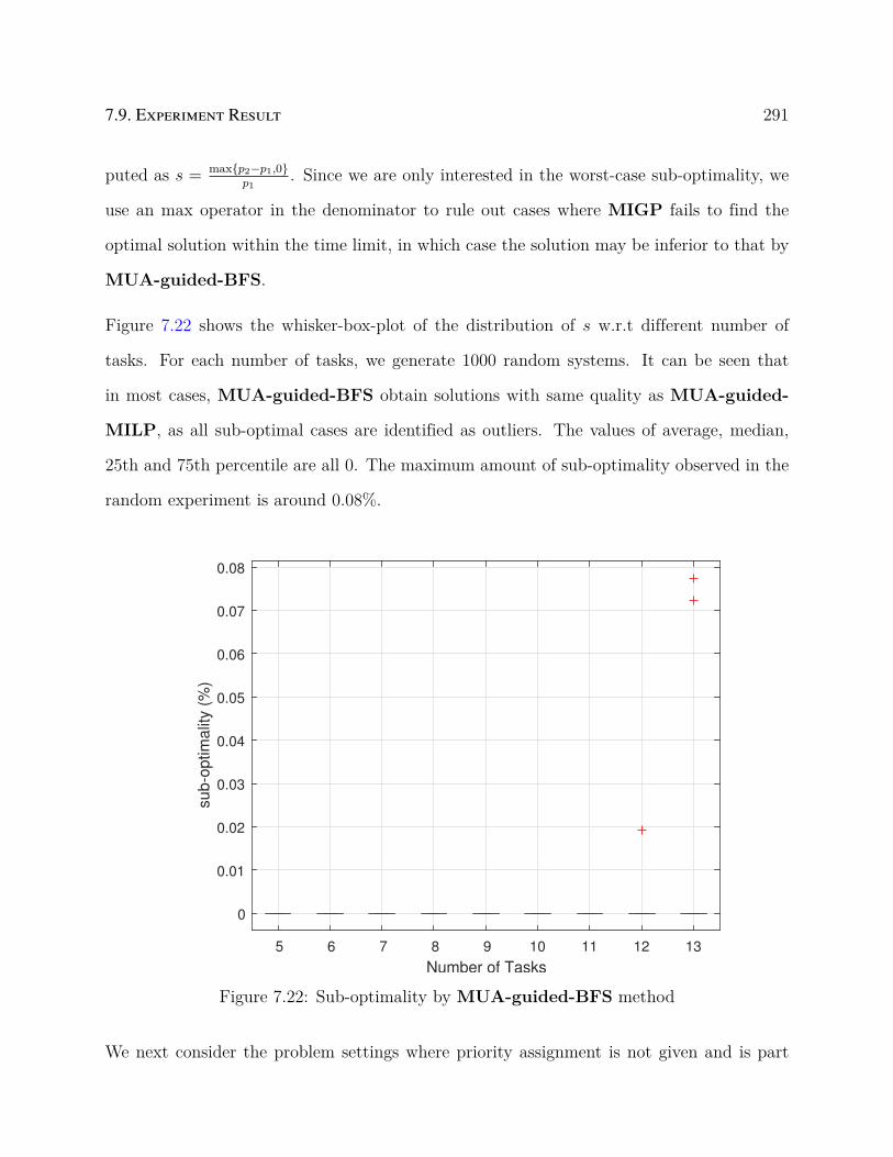
7.9. Experiment Result 291
puted as s = maxp2−p1,0p1
. Since we are only interested in the worst-case sub-optimality, we
use an max operator in the denominator to rule out cases where MIGP fails to find the
optimal solution within the time limit, in which case the solution may be inferior to that by
MUA-guided-BFS.
Figure 7.22 shows the whisker-box-plot of the distribution of s w.r.t different number of
tasks. For each number of tasks, we generate 1000 random systems. It can be seen that
in most cases, MUA-guided-BFS obtain solutions with same quality as MUA-guided-
MILP, as all sub-optimal cases are identified as outliers. The values of average, median,
25th and 75th percentile are all 0. The maximum amount of sub-optimality observed in the
random experiment is around 0.08%.
5 6 7 8 9 10 11 12 13
Number of Tasks
0
0.01
0.02
0.03
0.04
0.05
0.06
0.07
0.08
sub-o
ptim
alit
y (
%)
Figure 7.22: Sub-optimality by MUA-guided-BFS method
We next consider the problem settings where priority assignment is not given and is part
292Chapter 7. A Unified Framework for Optimizing Design of Real-Time Systems with
Sustainable Schedulability Analysis
of the decision space. We evaluate how this additional flexibility improves the optimiza-
tion result. We adapt MUA-guided-BFS for solving the new problem and denote it as
MUA-guided-PA. Since MUA-guided-MILP and MUA-guided-BFS have very simi-
lar quality of solution. We compare between MUA-guided-BFS and MUA-guided-PA
directly. Specifically, let p3 denote the objective obtained by MUA-guided-PA. We quan-
tify the improvement in solution as
d =p2 − p3
p2(7.44)
Figure 7.23 shows the whisker-box-plot of the distribution of d . It can be seen that the
treating priority assignment as decision variable significantly improves the quality of the
solution. The average amount of improvement ranges from 30% to 40% and sometimes as
large as more than 100%.
Figure 7.24 plots the run-time of all the optimization methods MIGP, MUA-guided-
MILP, MUA-guided-BFS and MUA-guided-PA. MUA-guided-MILP has the worst
scalability. This shows its inefficiency in solving problems with objective that are sensitive
to many decision variables. Both MUA-guided and MUA-guided-PA run significantly
faster than MIGP. MUA-guided-PA is slightly slower than MUA-guided due to its need
to co-optimize priority assignment. Specifically, in MUA-guided-BFS, evaluating G(X) is
simply a process of computing the response time of each task. But for MUA-guided-PA,
evaluating G(X) requires to use Audsley’s algorithm.
We next study the effect of K on MUA-guided-BFS methods in terms of their efficiency
and quality of solution. We try three other different values K = 1, 10, 100, 1000. The
corresponding configurations are denoted as MUA-K1, MUA-K10, MUA-K100 and
MUA-K1000. Figure 7.25 shows the average run-time by different configurations on K.

7.9. Experiment Result 293
5 6 7 8 9 10 11 12 13 14 15 16 17 18 19
Number of Tasks
0
10
20
30
40
50
60
70
80
90
100
Impro
vem
ent (%
)
Figure 7.23: Improvement on objective value by MUA-guided-PA method
Increasing the value of K increases the run-time. The increase mainly comes from two
factors. Firstly, Algorithm 13 requires more computation. Secondly, the sub-problem of each
iteration is solved closer-to-optimal with larger K. Therefore, the objective value converges
slower and leads to an increase in total number of iterations to terminate.
Figure 7.26 to 7.29 shows the amount of sub-optimality according to metric (7.43) by differ-
ent configurations. Generally, the higher the K, the smaller the amount of sub-optimality.
From K = 1 to K = 10000, the maximum amount of sub-optimality observed in all random
cases reduced from close to 7% down to around 0.085%.
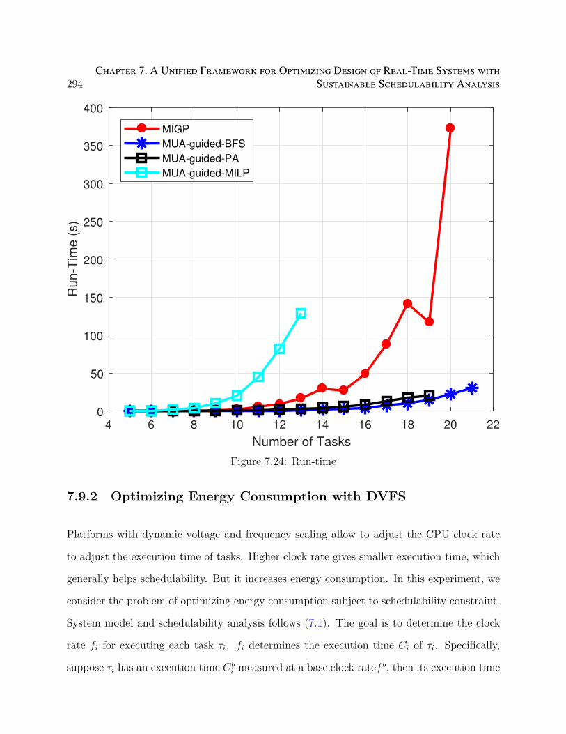
294Chapter 7. A Unified Framework for Optimizing Design of Real-Time Systems with
Sustainable Schedulability Analysis
4 6 8 10 12 14 16 18 20 22
Number of Tasks
0
50
100
150
200
250
300
350
400
Ru
n-T
ime
(s)
MIGP
MUA-guided-BFS
MUA-guided-PA
MUA-guided-MILP
Figure 7.24: Run-time
7.9.2 Optimizing Energy Consumption with DVFS
Platforms with dynamic voltage and frequency scaling allow to adjust the CPU clock rate
to adjust the execution time of tasks. Higher clock rate gives smaller execution time, which
generally helps schedulability. But it increases energy consumption. In this experiment, we
consider the problem of optimizing energy consumption subject to schedulability constraint.
System model and schedulability analysis follows (7.1). The goal is to determine the clock
rate fi for executing each task τi. fi determines the execution time Ci of τi. Specifically,
suppose τi has an execution time Cbi measured at a base clock ratef b, then its execution time
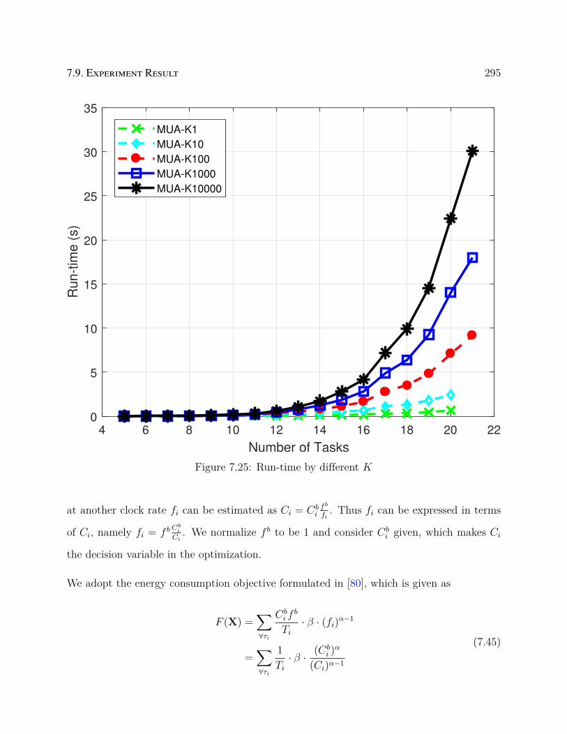
7.9. Experiment Result 295
4 6 8 10 12 14 16 18 20 22
Number of Tasks
0
5
10
15
20
25
30
35
Run-t
ime (
s)
MUA-K1
MUA-K10
MUA-K100
MUA-K1000
MUA-K10000
Figure 7.25: Run-time by different K
at another clock rate fi can be estimated as Ci = Cbifb
fi. Thus fi can be expressed in terms
of Ci, namely fi = f b Cbi
Ci. We normalize f b to be 1 and consider Cb
i given, which makes Ci
the decision variable in the optimization.
We adopt the energy consumption objective formulated in [80], which is given as
F (X) =∑∀τi
Cbi f
b
Ti
· β · (fi)α−1
=∑∀τi
1
Ti
· β · (Cbi )
α
(Ci)α−1
(7.45)
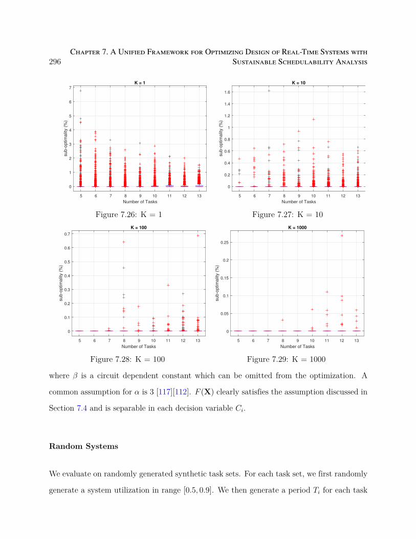
296Chapter 7. A Unified Framework for Optimizing Design of Real-Time Systems with
Sustainable Schedulability Analysis
5 6 7 8 9 10 11 12 13
Number of Tasks
0
1
2
3
4
5
6
7
sub-o
ptim
alit
y (
%)
K = 1
Figure 7.26: K = 1
5 6 7 8 9 10 11 12 13
Number of Tasks
0
0.2
0.4
0.6
0.8
1
1.2
1.4
1.6
sub-o
ptim
alit
y (
%)
K = 10
Figure 7.27: K = 10
5 6 7 8 9 10 11 12 13
Number of Tasks
0
0.1
0.2
0.3
0.4
0.5
0.6
0.7
sub-o
ptim
alit
y (
%)
K = 100
Figure 7.28: K = 100
5 6 7 8 9 10 11 12 13
Number of Tasks
0
0.05
0.1
0.15
0.2
0.25
sub-o
ptim
alit
y (
%)
K = 1000
Figure 7.29: K = 1000
where β is a circuit dependent constant which can be omitted from the optimization. A
common assumption for α is 3 [117][112]. F (X) clearly satisfies the assumption discussed in
Section 7.4 and is separable in each decision variable Ci.
Random Systems
We evaluate on randomly generated synthetic task sets. For each task set, we first randomly
generate a system utilization in range [0.5, 0.9]. We then generate a period Ti for each task

7.9. Experiment Result 297
according to log-uniform distribution from range [100, 100000], and a utilization ui for each
task using UUnifast algorithm [50]. The corresponding WCET Cbi = Ti · ui is treated as the
execution time at the base clock rate. The range of decision variable Ci is taken as [Cbi , 2C
bi ].
Specifically, the clock rate can be decreased as low as half the base clock rate. The deadline
Di of each task is generated randomly in range [Cbi , Ti]. Priorities are assigned according to
deadline monotonic assignment, which is optimal w.r.t response time analysis (7.1).
We compare between the following techniques
• MIGP: The same mixed-integer geometric programming formulation used in previous
experiment, except that decision variables becomes task execution time and objective
becomes (7.45).
• MUA-guided: The proposed technique depicted in Figure 7.21.
• MUA-guided-O: The same algorithm as MUA-guided except that MUA conver-
sion uses Algorithm 14 instead of Algorithm 15.
For each random system, we define the relative gap of method A w.r.t method B as the
relative difference in the objective value. Specifically
s =pA − pB
pB(7.46)
where pA, pB represent the objective value by method A and B respectively.
Figure 7.30 shows the whisker-box-plot of the distribution of the relative gap of MUA-
guided w.r.t MIGP for different number of tasks. It can be seen that MUA-guided finds
averagely 3% to 30% better solution than MIGP within the time limit. Figure 7.31 shows the
distribution of the relative gap of MUA-guided-O w.r.t MUA-guided. MUA-guided is
slightly better than MUA-guided-O but mostly within 5% of difference.
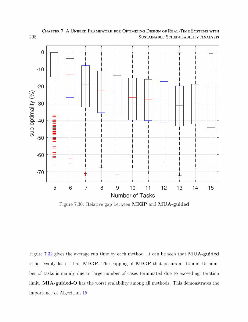
298Chapter 7. A Unified Framework for Optimizing Design of Real-Time Systems with
Sustainable Schedulability Analysis
5 6 7 8 9 10 11 12 13 14 15
Number of Tasks
-70
-60
-50
-40
-30
-20
-10
0
sub-o
ptim
alit
y (
%)
Figure 7.30: Relative gap between MIGP and MUA-guided
Figure 7.32 gives the average run time by each method. It can be seen that MUA-guided
is noticeably faster than MIGP. The capping of MIGP that occurs at 14 and 15 num-
ber of tasks is mainly due to large number of cases terminated due to exceeding iteration
limit. MIA-guided-O has the worst scalability among all methods. This demonstrates the
importance of Algorithm 15.
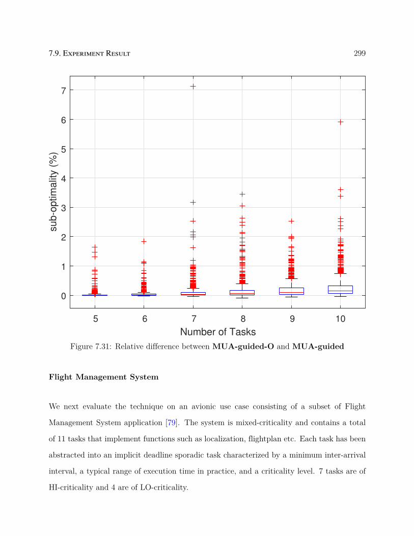
7.9. Experiment Result 299
5 6 7 8 9 10
Number of Tasks
0
1
2
3
4
5
6
7
sub-o
ptim
alit
y (
%)
Figure 7.31: Relative difference between MUA-guided-O and MUA-guided
Flight Management System
We next evaluate the technique on an avionic use case consisting of a subset of Flight
Management System application [79]. The system is mixed-criticality and contains a total
of 11 tasks that implement functions such as localization, flightplan etc. Each task has been
abstracted into an implicit deadline sporadic task characterized by a minimum inter-arrival
interval, a typical range of execution time in practice, and a criticality level. 7 tasks are of
HI-criticality and 4 are of LO-criticality.

300Chapter 7. A Unified Framework for Optimizing Design of Real-Time Systems with
Sustainable Schedulability Analysis
5 10 15 20
Number of Tasks
0
50
100
150
200
250
300
350
Run-T
ime (
s)
MIGP
MUA-guided
MUA-guided-O
Figure 7.32: Run-time
We consider fixed-priority uniprocessor scheduling according to Adaptive-Mixed-Criticality
(AMC) for these tasks. For schedulability analysis, we adopt AMC-rtb and AMC-max
response time analysis proposed in [19], both of which are sufficient analysis . The two
analysis mainly differ in the estimation of higher priority tasks interference during the time
of criticality change.
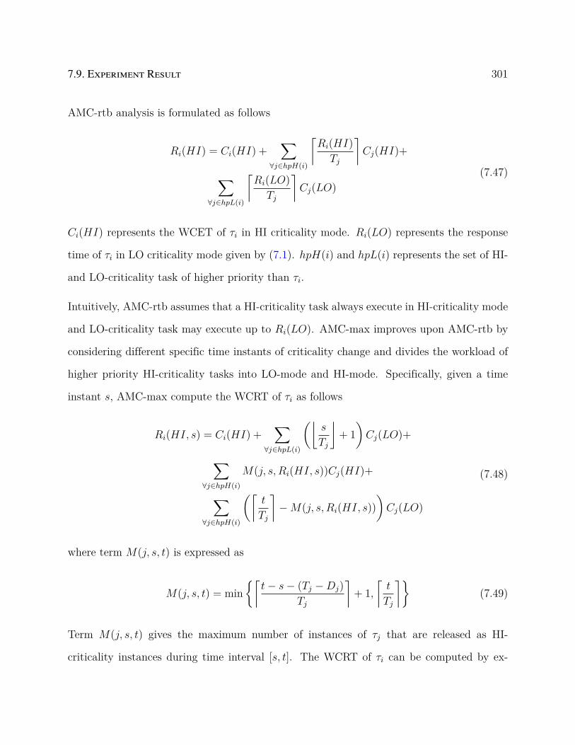
7.9. Experiment Result 301
AMC-rtb analysis is formulated as follows
Ri(HI) = Ci(HI) +∑
∀j∈hpH(i)
⌈Ri(HI)
Tj
⌉Cj(HI)+
∑∀j∈hpL(i)
⌈Ri(LO)
Tj
⌉Cj(LO)
(7.47)
Ci(HI) represents the WCET of τi in HI criticality mode. Ri(LO) represents the response
time of τi in LO criticality mode given by (7.1). hpH(i) and hpL(i) represents the set of HI-
and LO-criticality task of higher priority than τi.
Intuitively, AMC-rtb assumes that a HI-criticality task always execute in HI-criticality mode
and LO-criticality task may execute up to Ri(LO). AMC-max improves upon AMC-rtb by
considering different specific time instants of criticality change and divides the workload of
higher priority HI-criticality tasks into LO-mode and HI-mode. Specifically, given a time
instant s, AMC-max compute the WCRT of τi as follows
Ri(HI, s) = Ci(HI) +∑
∀j∈hpL(i)
(⌊s
Tj
⌋+ 1
)Cj(LO)+
∑∀j∈hpH(i)
M(j, s, Ri(HI, s))Cj(HI)+
∑∀j∈hpH(i)
(⌈t
Tj
⌉−M(j, s, Ri(HI, s))
)Cj(LO)
(7.48)
where term M(j, s, t) is expressed as
M(j, s, t) = min⌈
t− s− (Tj −Dj)
Tj
⌉+ 1,
⌈t
Tj
⌉(7.49)
Term M(j, s, t) gives the maximum number of instances of τj that are released as HI-
criticality instances during time interval [s, t]. The WCRT of τi can be computed by ex-

302Chapter 7. A Unified Framework for Optimizing Design of Real-Time Systems with
Sustainable Schedulability Analysis
Table 7.2: Flight Management System case study
τ τ1 τ2 τ3 τ4 τ5 τ6T 5000 200 1000 1600 100 1000
C(LO) [5, 40] [5, 40] [5, 40] [5, 40] [5, 40] [5, 40]HI/LO HI HI HI HI HI HI
τ τ7 τ8 τ9 τ10 τ11T 1000 1000 1000 1000 1000
C(LO) [5, 40] [50, 400] [50, 400] [50, 400] [50, 400]HI/LO HI LO LO LO LO
amining all possible time of criticality change s, namely
Ri(HI) = max∀s
Ri(HI, s) (7.50)
[19] shows that it suffices to consider only those s in interval [0, Ri(LO)) when a higher
priority LO-criticality task releases.
AMC-max has much higher computation complexity comparing to AMC-rtb. But its higher
accuracy may help find better quality solution when used in optimization. In the following,
we consider the problem of minimizing LO-mode energy consumption given by (7.45). The
decision variables are LO-mode WCET Ci(LO) of each task. The range of values for Ci(LO)
is determined as follows. We first take the upper-bound Cubi of the execution time range given
in the case study. Then we consider Ci(LO) to be freely adjustable in interval [Cubi
4, 2Cub
i ] by
CPU clock rate adjustment. For HI-criticality task, Ci(HI) is obtained by scaling Ci(LO)
by a fixed criticality factor γ, i.e. Ci(HI) = γCi(LO). The optimization problem is to find a
Ci(LO) for each task that minimizes (7.45). The parameter configuration of the case study
is summarized in Table 7.2.
We first consider the setting where priority assignment is given according by rate mono-
tonic assignment (tiers are broken by criticality level). We compare between the following
techniques

7.9. Experiment Result 303
Table 7.3: Results on Flight Management System. Rate-monotonic priority assignment.
Method γ = 3 γ = 4 γ = 5Time Objective Time Objective Time Objective
MIGP ≥ 48h 6.216e+007 ≥ 48h 8.379e+007 ≥ 48h 1.076e+008MUA-rtb-K5 0.05s 4.691e+007 0.04s 6.220e+007 0.03s 8.459e+007MUA-max-K5 0.04s 4.691e+007 0.05s 6.220e+007 0.03s 8.459e+007MUA-rtb-K500 2.40s 4.129e+007 2.04s 5.840e+007 1.76s 7.732e+007MUA-max-K500 3.18s 4.129e+007 2.64s 5.840e+007 2.14s 7.732e+007MUA-rtb-K50000 873.91s 4.108e+007 582.06s 5.803e+007 409.76s 7.723e+007MUA-max-K50000 903.10s 4.108e+007 619.86s 5.803e+007 406.59s 7.723e+007
• MIGP-AMCrtb: We use the same idea and formulate AMC-rtb analysis as mixed-
integer geometric programming.
• MUA-AMCrtb-Km: The proposed technique where schedulability analysis uses
AMC-rtb analysis and the size limit parameter K is set to m.
• MUA-AMCmax-Km: Same as MUA-AMCrtb-Km but where schedulability
analysis uses the AMC-max analysis.
Note that we do not consider using AMC-max for MIGP as the analysis is too complicated
to use in MIGP.
We run each method up to 48h. The results are summarized in Table 7.3. MIGP gets
stuck in a fairly sub-optimal solution early and cannot find better solutions even after 48
hours. Setting a higher value on K in most cases helps find better solution but at the cost
of increased runtime. Extremely high K does not necessarily bring significant improvement.
This can be seen from the results corresponding to K = 500 and K = 50000. The use of
the more accurate AMC-max analysis did not improve the quality of the solution. This is
mainly due to the rate-monotonic priority assignment. For this case, LO-criticality tasks
are mostly lower in priorities than HI-criticality tasks (except τ1, τ4 which have quite loose
deadlines). As a result, most HI-criticality tasks only suffer interference from other HI-

304Chapter 7. A Unified Framework for Optimizing Design of Real-Time Systems with
Sustainable Schedulability Analysis
Table 7.4: Results on Flight Management System. Co-optimizing priority assignment.
Method γ = 3 γ = 4 γ = 5Time Objective Time Objective Time Objective
MUA-rtb-Audsley-K5 0.14s 2.666e+007 0.09s 3.056e+007 0.09s 3.762e+007MUA-max-Audsley-K5 0.16s 2.666e+007 0.16s 2.666e+007 0.15s 2.666e+007MUA-rtb-Audsley-K500 12.16s 2.629e+007 10.20s 2.835e+007 6.55s 3.439e+007MUA-max-Audsley-K500 16.71s 2.630e+007 15.85s 2.629e+007 14.13s 2.629e+007MUA-rtb-Audsley-K50000 2356.61s 2.626e+007 1204.74s 2.832e+007 517.68s 3.415e+007MUA-max-Audsley-K50000 2734.41s 2.626e+007 2260.71s 2.626e+007 2569.84s 2.626e+007
criticality tasks. Therefore, the worst-case scenario for timing occurs when the system is
entirely in HI-criticality mode, where AMC-max and AMC-rtb aren’t much different in
accuracy.
We next consider the setting where priority assignment is not given and need to be co-
optimized with WCET. MIGP is no longer applicable and therefore we only consider meth-
ods based on the proposed optimization framework. The only modification from previous
setting is that schedulability analysis uses Audsley’s algorithm in the framework (specifically,
implementation of G(X)).
The results are summarized in Table 7.4. A number of observations can be made. First,
much better solutions are found when priority assignment is treated as a decision. The overall
objective values reduce by as much as more than half comparing to the results in Table 7.3.
This shows that co-optimizing different variables can bring significant improvement in the
solution. This is a benefit that the proposed optimization framework can provide as opposed
to traditional mathematical programmings. Secondly, the difference between AMC-rtb and
AMC-max analysis is now more noticeable. When criticality factor γ = 5, the use of AMC-
max gives more than 23% improvement over AMC-rtb. This demonstrates the benefit of
using a more accurate analysis for optimization especially in resource-stringent scenarios.
The benefit can only be achieved however, when the optimization algorithm is capable of
accommodating the analysis. This is difficult for MIGP as AMC-max is too complicated

7.10. Conclusion 305
to formulate. Thirdly, the runtime noticeably increases comparing to Table 7.3. This is
mainly because schedulability analysis now uses Audsley’s algorithm which have much higher
computation complexity.
7.10 Conclusion
In this chapter, we propose an framework for optimizing the design of real-time system with
sustainable schedulability analysis and monotonic objective functions. We study the concept
of Maximal-Unschedulable-Assignment (MUA) and show how it can be used to abstract, it-
eratively approximate and refine the feasibility region. Based on the concept, we develop an
iterative optimization procedure guided by MUAs. We discuss the design of three important
components of the optimization procedure: 1) An algorithm for solving the optimization
problem consisting of MUA-implied constraints, 2) An algorithm for computing MUAs that
gives faster convergence and 3) An algorithm for exploring good-quality schedulable solu-
tions. We perform experiments on different optimization problems with different settings and
demonstrate that the technique is capable of finding close-to-optimal solutions and providing
benefit in applicability and scalability comparing to traditional mathematical programming
based approaches.

Chapter 8
The Concept of Response Time
Estimation Range for Optimizing
Systems Scheduled with Fixed
Priority
8.1 Introduction
In real-time systems with fixed priority scheduling, appropriate priority assignment is es-
sential for judicious utilization of hardware resources [53]. This problem has attracted a
large body of research efforts. Classical results include rate-monotonic (RM) [100], deadline-
monotonic (DM) [97], and Audsley’s algorithm [9], all of which are tractable in that they only
need to check a number of priority orders polynomial in the number of tasks. In particular,
Audsley’s algorithm is shown to be optimal for finding a schedulable priority assignment for
a variety of scenarios, as long as they satisfy the conditions identified by Davis et al. [50].
The applicability of Audsley’s algorithm subsumes those of RM and DM.
However, when Audsley’s algorithm is inapplicable, there is no efficient algorithm to find the
optimal priority assignment. This may rise for two reasons. One is that the system model
306
8.1. Introduction 307
and associated schedulability analysis violate the conditions of Audsley’s algorithm. The
other is that the problem may contain constraints or an objective related to other metrics
(e.g., memory, power). The current mindset is to either invent problem specific heuristics
that may be substantially suboptimal, or directly use standard search frameworks such as
Branch-and-Bound (BnB) and Mixed Integer Linear Programming (MILP).
In this chapter, we consider a class of real-time systems where the schedulability of a task
depends not only on the set of higher/lower priority tasks but also on the response times of
other tasks. We call them systems with Response Time (RT) dependency. RT dependency
disrespects the applicable conditions of Audsley’s algorithm. We provide two examples of
such systems. The first is the real-time wormhole communication in a Network-on-Chip
(NoC) [133]. A traffic flow may suffer indirect inferences from higher priority flows that do
not directly share any communication link with it. The indirect interferences and conse-
quently the response time of the flow depend on the response times of higher priority flows.
The second is distributed systems with data-driven activation, which is broadly adopted in
application domains such as automotive [167]. A task is activated by the availability of input
data and consequently the completion of its immediate predecessor. Hence, the task has an
activation jitter that equals the response time of the immediate predecessor.
Our approach breaks through the mindset of current methods. It is suitable for design
optimization problems of systems with RT dependency that involve priority assignment as
a design variable, e.g., to find a schedulable priority assignment. Specifically, we propose
several concepts including the response time estimation range, which is used in place of the
actual response time of each task for evaluating the system schedulability. These concepts
allow to leverage Audsley’s algorithm to generalize from an unschedulable solution to many
similar ones. We then develop an optimization procedure that is guided by the proposed
concepts. The procedure is shown to provide significantly better solutions than existing

308Chapter 8. The Concept of Response Time Estimation Range for Optimizing Systems
Scheduled with Fixed Priority
heuristics. Compared to other exact algorithms based on BnB or MILP, it typically runs
many times faster.
The rest of the chapter is organized as follows. Section 8.2 discusses the related work.
Section 8.3 presents the system model. Section 8.4 introduces the concepts and discusses their
properties. Section 8.5 develops an optimization framework that leverages these concepts.
Section 8.7 presents the experimental results comparing our approach with existing methods,
before concluding the chapter in Section 8.8.
8.2 Related Work
The problem of priority assignment in real-time systems scheduled with fixed priority has
been studied extensively. See an authoritative survey by Davis et al. [53]. In particular, for
periodic tasks with implicit deadline (i.e., task deadline equals the period), RM is shown
to be optimal for schedulability in that there is no system that can be scheduled by some
priority assignment but not by RM. When tasks have constrained deadline (i.e., no larger
than period), DM is optimal for schedulability [97]. Audsley’s algorithm [9] is optimal for
finding a schedulable priority assignment for a variety of task models and scheduling policies,
as summarized in Davis et al. [53]. The three necessary and sufficient conditions for its
optimality are presented in [50]. Besides schedulability, Audsley’s algorithm can be revised to
optimize several other objectives, including the number of priority levels [9], lexicographical
distance (the perturbation needed to make the system schedulable from an initial priority
order) [40, 53], and robustness (ability to tolerate additional interferences) [44].
When Audsley’s algorithm is not directly applicable, the current approaches can be classi-
fied into three categories. The first is based on meta heuristics such as simulated annealing
(e.g., [22, 142]) and genetic algorithm (e.g., [75]). The second is to develop problem spe-
8.2. Related Work 309
cific heuristics (e.g., [127, 146, 156]). These two categories do not have any guarantee on
optimality. The third category is to search for the exact optimum, often applying standard
optimization frameworks such as BnB (e.g., [147], [51]), or MILP (e.g., [169]). However,
this approach typically suffers from scalability issues and may have difficulty to handle large
industrial designs.
Such approaches are also followed for the particular class of systems we consider, i.e., sys-
tems with RT-dependency. For the real-time wormhole communication in NoC, Shi and
Burns develop a BnB algorithm that is enhanced with some problem specific pruning tech-
niques [133]. Later Nikolić and Pinho propose a unified MILP formulation for optimizing
priority assignment and routing of traffic flows [114]. The mixed-criticality extension relies
on heuristics including DM [33]. The current work on systems with data-driven activation
either uses BnB [110] or formulates the problem in MILP [167].
Alternatively, we present efficient and exact optimization procedures that leverage Audsley’s
algorithm [160, 161]. However, these works [160, 161] are for problems where Audsley’s
algorithm is still optimal for finding a schedulable priority assignment. In this chapter, we
consider systems with RT dependency where the response time of a task also depends on
those of other tasks. This makes Audsley’s algorithm even inapplicable for schedulability.
Thus, in this work we cannot use the concepts and algorithms from [160, 161].
Our approach differs from other exact algorithms, such as [133], [114] for real-time wormhole
communication in NoC, in two significant ways. First, we transform the problem to a
search in the space of response time estimation, instead of directly searching for an optimal
priority assignment. Second, we use Audsley’s algorithm to generalize from an unschedulable
response time estimation to a maximal range. However, the approaches based on standard
optimization frameworks [133], [114] lack this problem-specific “learning” capability.

310Chapter 8. The Concept of Response Time Estimation Range for Optimizing Systems
Scheduled with Fixed Priority
8.3 System Model
We consider a real-time system Γ consisting of a set of tasks Γ = τ1, τ2, ...τn scheduled
under fixed-priority. Each task τi is characterized by a tuple ⟨Ci, Ti, Di⟩, where Ci is its
Worst Case Execution Time (WCET), Ti is the period, and Di is the deadline. Without loss
of generality, we assume these parameters are all positive integers. τi is also associated with
an activation jitter JAi and a unique priority level πi. πi > πj if τi has a higher priority than
τj. hpi = τj|πj > πi (resp. lpi = τj|πj < πi) denotes the set of tasks with priority higher
(resp. lower) than τi.
In the optimization problem, we assume the task WCET, period, and deadline are given
parameters. The decision variables include task priority assignment P. Consequently, hpi,
lpi, and the task worst case response time (or in short, response time) Ri of each task τi are
also unknown variables. The activation jitter JAi , however, may be a known parameter as
in the wormhole communication (Section 8.3.2), or an unknown variable as for the case of
data-driven activation (Section 8.3.3). The system schedulability, i.e., each task shall meet
its deadline, can be checked with an analysis that satisfies the property of RT dependency as
defined in Section 8.3.1. Besides, the optimization problem may also involve other constraints
and objective.
Formally, the optimization problem O can be written as
O : min g(X)
s.t. system schedulability
h(X) ≤ 0
(8.1)
Here X is the set of decision variables that includes the vectors of task priority assignments P
and response times R = [R1, R2, ...Rn]. h(·) is the set of constraints in addition to the system
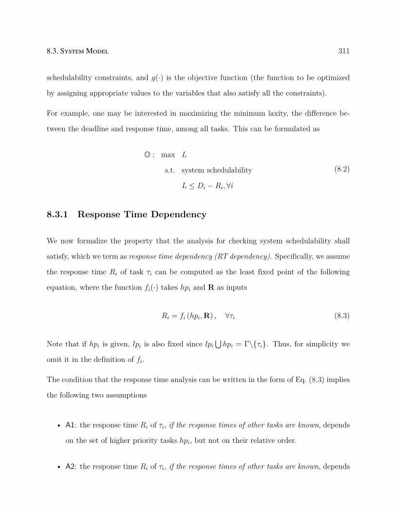
8.3. System Model 311
schedulability constraints, and g(·) is the objective function (the function to be optimized
by assigning appropriate values to the variables that also satisfy all the constraints).
For example, one may be interested in maximizing the minimum laxity, the difference be-
tween the deadline and response time, among all tasks. This can be formulated as
O : max L
s.t. system schedulability
L ≤ Di −Ri,∀i
(8.2)
8.3.1 Response Time Dependency
We now formalize the property that the analysis for checking system schedulability shall
satisfy, which we term as response time dependency (RT dependency). Specifically, we assume
the response time Ri of task τi can be computed as the least fixed point of the following
equation, where the function fi(·) takes hpi and R as inputs
Ri = fi (hpi,R) , ∀τi (8.3)
Note that if hpi is given, lpi is also fixed since lpi∪hpi = Γ\τi. Thus, for simplicity we
omit it in the definition of fi.
The condition that the response time analysis can be written in the form of Eq. (8.3) implies
the following two assumptions
• A1: the response time Ri of τi, if the response times of other tasks are known, depends
on the set of higher priority tasks hpi, but not on their relative order.
• A2: the response time Ri of τi, if the response times of other tasks are known, depends
312Chapter 8. The Concept of Response Time Estimation Range for Optimizing Systems
Scheduled with Fixed Priority
on the set of lower priority tasks lpi, but not on their relative order.
We suppose (8.3) further satisfies two additional assumptions.
• A3: the response time Ri of τi is monotonically non-decreasing with the set of higher
priority tasks hpi. Specifically, given two sets of tasks hpi and hp′i such that hpi ⊆ hp′i,
the response time Ri with hp′i as the higher priority tasks is no smaller than that with
hpi.
• A4: the response time Ri of τi is monotonically non-decreasing with the increase of the
response time Rj of any other task τj.
We now give the formal definition of RT dependency.
Definition 27. The response time analysis of a real-time system Γ is said to be response
time dependent (RT dependent) if it satisfies the above four assumptions A1-A4.
Remark 8.1. Assumptions A1-A4 are desired properties for calculating Ri, i.e., the least
fixed point solution to Eq. (8.3) where the input is the sets of higher/lower priority tasks
and their response times, and the output is Ri.
As a more compact representation, let hp be the vector of higher priority task sets, and
f(hp,R) be a vector of functions over hp and R. The response times of all tasks in the
system are computed as the least fixed point of the following equation
R = f(hp,R) (8.4)
We note that a response time analysis with RT dependency in general violates the applica-
bility of Audsley’s algorithm. Specifically, Audsley’s algorithm requires that, in addition to
A3 above, the following two conditions are satisfied [50]

8.3. System Model 313
• A1’: the response time Ri of τi depends on the set of higher priority tasks hpi, but not
on their relative order.
• A2’: the response time Ri of τi depends on the set of lower priority tasks lpi, but not
on their relative order.
To calculate Ri for τi by Eq. (8.3) in an RT dependent system, it requires the knowledge of
Rj of some other task τj. But Rj is highly dependent on the relative priority of τj, which
violates A1’-A2’. Despite this, we can still develop an efficient algorithm to optimize priority
assignment in such systems.
We provide two examples that fit this model. One is the real-time wormhole communication
in NoC [133] and its mixed-criticality extension [33] (detailed in Section 8.3.2), the other is
distributed systems with data-driven activation (Section 8.3.3).
8.3.2 Real-Time Wormhole Communication in NoC
Wormhole switching with fixed priority preemptive scheduling is a viable solution for real-
time communication in an NoC [133]. A wormhole-based NoC consists of multiple IP blocks
and routers (i.e., the nodes in the network) connected through physical links to form a grid.
Each traffic flow is transmitted through a specified path of links [133]. Here, the traffic flows
are the scheduling entity, and the physical links are the hardware resource accessed by the
traffic flows. Since a flow may access several physical links shared with other flows, priority-
based arbitration at the routers is used to provide hard real-time service guarantees [133]. In
the end, a flow suffers direct interferences, i.e., from those higher priority flows that directly
share at least one link. In addition, it may also be delayed by indirect inferences, i.e., from
those higher priority flows with no shared links. The indirect interferences are captured by
the interference jitter introduced below.

314Chapter 8. The Concept of Response Time Estimation Range for Optimizing Systems
Scheduled with Fixed Priority
The response time of traffic flow τi with constrained deadline is calculated as [133]
Ri = Ci +∑
∀τj∈shpi
⌈Ri + JA
j + J Ij
Tj
⌉Cj (8.5)
Here shpi is the set of higher priority traffic flows that share at least one link with τi. JAj is
the activation jitter inherited from its sending software task, which can be considered as a
parameter as it is independent from the priority assignment of the traffic flows. J Ij represents
the interference jitter of τj. J Ij occurs when flows with higher priority than τj share a link
with τj and thus indirectly interfere with τi. It is computed as
J Ij = Rj − Cj (8.6)
Substitute (8.6) into (8.5), there is
Ri = Ci +∑
∀τj∈shpi
⌈Ri + JA
j +Rj − Cj
Tj
⌉Cj (8.7)
We now show that the response time analysis in Eq. (8.7) satisfies the four assumptions
A1-A4. Note that the set shpi is solely dependent on the set of higher priority flows hpi, as
it is the intersection of hpi and the fixed set of flows sharing a link with τi. For A1 and A2,
if the response time Rj of all other tasks τj are known, the fixed point solution of Eq. (8.7)
depends only on the set shpi but not on other design variables. For A3, since only the
response times of tasks in shpi contribute positively to the right hand side of (8.7), a larger
hpi (and consequently a larger shpi) will only make Ri larger. Likewise, in the right hand
side of (8.7), the response time Rj of any other task τj has an coefficient that is either zero
(in case it is not in shpi) or positive (in case it belongs to shpi), A4 is also satisfied.

8.3. System Model 315
Hence, the analysis in Eq. (8.7) is RT dependent. However, Audsley’s algorithm is not
applicable even for finding a schedulable priority order [133]. Similarly, the NoC system
with mixed-criticality traffic flows also relies on a response time analysis that violates the
conditions for Audsley’s algorithm but satisfies A1-A4 [33].
8.3.3 Data-Driven Activation
Data-driven activation is an activation model in distributed systems such as automotive
applications [167]. In this model, task executions and message transmissions are triggered
by the arrival of input data. Hence, each task/message τi is characterized by a period Ti,
an activation jitter JAi , and a deadline that is relative to the arrival time (i.e., the expected
activation time). In a communication chain, the activation jitter inherits the worst case
response time of the immediate predecessor: if τj is triggered by the arrival of data sent
by τk, then JAj = Rk. This dependency is often referred to as jitter propagation. Note
that the direct communication happens only between a task and another task/message,
but not between two messages. However, indirect communication, and consequently jitter
propagation dependency, may still exist between two messages.
With respect to the scheduling policy, tasks and messages are both assigned with a fixed
priority. However, tasks are preemptive while messages are non-preemptive (like in the
Controller Area Network bus). For a task/message τi, the queuing delay wi is defined as
the worst case delay from τi’s activation to its completion. The response time Ri of τi with
preemptive scheduling and constrained deadline is
wi = Ci +∑
j∈hp(i)
⌈wi + JA
j
Tj
⌉Cj
Ri = JAi + wi
(8.8)

316Chapter 8. The Concept of Response Time Estimation Range for Optimizing Systems
Scheduled with Fixed Priority
When there is direct or indirect communication from τj to τi sharing the same resource (CPU
or bus), JAi and consequently Ri rely on the exact value of Rj. The response time for non-
preemptive scheduling or tasks with arbitrary deadlines requires to evaluate all instances in
the busy period [167]. Still, they satisfy the properties of RT dependency.
The end-to-end latency Lp of a path p is the sum of the queuing delays of all tasks/messages
on p
Lp =∑
∀τj on path p
wi (8.9)
Lp shall be no larger than the end-to-end deadline Dp of p.
8.3.4 Fixed Priority Multiprocessor Scheduling
Multiprocessor platforms are becoming increasingly popular in the design of real-time sys-
tem. Here we consider systems that contains a set of periodic (or sporadic) task. Each task is
characterized by a period Ti, deadline Di and worst-case execution time Ci. Tasks are sched-
uled on a multiprocessor platform consisting of M processors by fixed priority assignment.
Specifically, at any time instant, the waiting task with the highest priority is scheduled on
an idle processor. A number of studies have been performed for its schedulability analysis.
We consider the well known GSYY analysis introduced in [72] for its good trade-off between
computation complexity and accuracy. The analysis is summarized in the following.
Ri = Ci +∑
∀j∈hp(i)
INCi (τj, Ri) +
∑∀j∈M(i)
ICIi (τj, Ri)− INC
i (τj, Ri) (8.10)
hp(i) represents the set of tasks of higher priority than τi. INCi (τj, Ri) represents the amount
of non-carry-in interference by τj and ICIi represents the amount of carry-in interference by
τi. M(i) is a set of at most M − 1 higher priority tasks that have the highest value of

8.4. Response Time Estimation Range 317
ICIi (τj, Ri) − INC
i (τj, Ri). Specifically, a higher priority task can either introduce carry-in
or non-carry-in interference. There can be at most M − 1 higher priority tasks that have
carry-in interference. Therefore,the worst-case scenario occurs when these M − 1 tasks are
those with the greatest difference between carry-in and non-carry-in interference.
We mainly concern term ICIi (τj, t) in (8.10), which‘is formulated as follows
ICIi (τj, t) =
[[WCI
k (τj, t)]]t−Cj+1
0
WCIi (τj, t) =
⌊[[t− Cj]]0
Tj
⌋Cj + Cj + α
α = [[[[t− Cj]] mod Tj − (Tj −Rj)]]Cj
0
(8.11)
From the expression of α, it can be seen that the amount of carry-in interference introduced
by task τj depends on its worst-case response time Rj. The larger the Ri, the higher the
interference. Therefore, the worst-case response time of the lower priority task τi depends
on those of the higher priority tasks.
8.4 Response Time Estimation Range
The response time analysis in Eq. (8.3) does not satisfies the conditions of Audsley’s algo-
rithm. However, it has a useful property as in the assumptions A1-A2: if the response times
of other tasks are appropriately estimated, then Ri only requires the knowledge on the set of
higher/lower priority tasks, but not on the relative order in them. This, combined with A3,
allows to leverage Audsley’s algorithm assuming we can appropriately estimate the response
times.
Hence, the main idea of our optimization framework is to use a separate procedure to search
for an appropriate response time estimation. Before presenting the details of the optimization
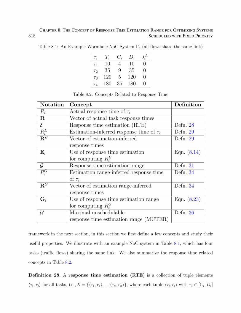
318Chapter 8. The Concept of Response Time Estimation Range for Optimizing Systems
Scheduled with Fixed Priority
Table 8.1: An Example Wormhole NoC System Γe (all flows share the same link)
τi Ti Ci Di JAi
τ1 10 4 10 0τ2 35 9 35 0τ3 120 5 120 0τ4 180 35 180 0
Table 8.2: Concepts Related to Response Time
Notation Concept DefinitionRi Actual response time of τiR Vector of actual task response timesE Response time estimation (RTE) Defn. 28RE
i Estimation-inferred response time of τi Defn. 29RE Vector of estimation-inferred Defn. 29
response timesEi Use of response time estimation Eqn. (8.14)
for computing REi
G Response time estimation range Defn. 31RG
i Estimation range-inferred response time Defn. 34of τi
RG Vector of estimation range-inferred Defn. 34response times
Gi Use of response time estimation range Eqn. (8.23)for computing RG
i
U Maximal unschedulable Defn. 36response time estimation range (MUTER)
framework in the next section, in this section we first define a few concepts and study their
useful properties. We illustrate with an example NoC system in Table 8.1, which has four
tasks (traffic flows) sharing the same link. We also summarize the response time related
concepts in Table 8.2.
Definition 28. A response time estimation (RTE) is a collection of tuple elements
⟨τi, ri⟩ for all tasks, i.e., E = ⟨τ1, r1⟩ , ... ⟨τn, rn⟩, where each tuple ⟨τi, ri⟩ with ri ∈ [Ci, Di]
8.4. Response Time Estimation Range 319
represents that the response time of τi is estimated to be ri.
The following concept defines the way how a response time estimation is used during opti-
mization. Essentially, given an RTE E , we define the estimation-inferred response time of
task τi as the least fixed point to Eq. (8.3) assuming the response times of other tasks follow
the estimated value in E .
Definition 29. Given a priority assignment P and a response time estimation as follows,
E = ⟨τ1, r1⟩ , ... ⟨τn, rn⟩ (8.12)
the estimation-inferred response time of task τi, denoted as REi , is the least fixed point
solution of the following equation
REi = fi(hpi,Ei) (8.13)
Here Ei is a vector constructed as follows: the i-th entry of Ei is the variable REi , and the
j-th entry for any j = i takes the corresponding given value rj in E , i.e.,
Ei = [r1, ..., REi , ..., rn] (8.14)
The vector of estimation-inferred response times is denoted as RE.
Remark 8.2. With a given RTE E , the calculation of estimation-inferred response time REi
for task τi only depends on the set of higher priority tasks, but not on their relative order.
Also, given a priority assignment, the actual response time is generally different from the
estimation-inferred response time. This is illustrated in the following example.
Example 8.3. Assume the priority order is π1 > π2 > π3 > π4 for the system in Table 8.1.
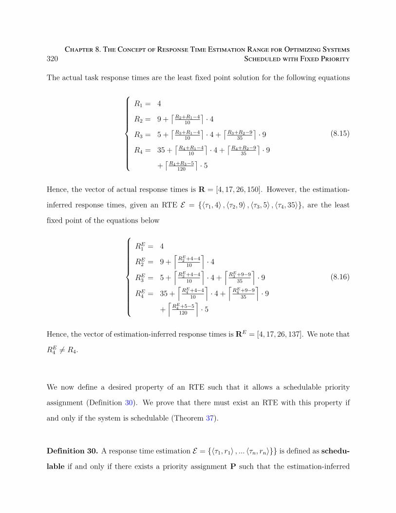
320Chapter 8. The Concept of Response Time Estimation Range for Optimizing Systems
Scheduled with Fixed Priority
The actual task response times are the least fixed point solution for the following equations
R1 = 4
R2 = 9 +⌈R2+R1−4
10
⌉· 4
R3 = 5 +⌈R3+R1−4
10
⌉· 4 +
⌈R3+R2−9
35
⌉· 9
R4 = 35 +⌈R4+R1−4
10
⌉· 4 +
⌈R4+R2−9
35
⌉· 9
+⌈R4+R3−5
120
⌉· 5
(8.15)
Hence, the vector of actual response times is R = [4, 17, 26, 150]. However, the estimation-
inferred response times, given an RTE E = ⟨τ1, 4⟩ , ⟨τ2, 9⟩ , ⟨τ3, 5⟩ , ⟨τ4, 35⟩, are the least
fixed point of the equations below
RE1 = 4
RE2 = 9 +
⌈RE
2 +4−4
10
⌉· 4
RE3 = 5 +
⌈RE
3 +4−4
10
⌉· 4 +
⌈RE
3 +9−9
35
⌉· 9
RE4 = 35 +
⌈RE
4 +4−4
10
⌉· 4 +
⌈RE
4 +9−9
35
⌉· 9
+⌈RE
4 +5−5
120
⌉· 5
(8.16)
Hence, the vector of estimation-inferred response times is RE = [4, 17, 26, 137]. We note that
RE4 = R4.
We now define a desired property of an RTE such that it allows a schedulable priority
assignment (Definition 30). We prove that there must exist an RTE with this property if
and only if the system is schedulable (Theorem 37).
Definition 30. A response time estimation E = ⟨τ1, r1⟩ , ... ⟨τn, rn⟩ is defined as schedu-
lable if and only if there exists a priority assignment P such that the estimation-inferred

8.4. Response Time Estimation Range 321
response times are component-wise no larger than E . That is, E is schedulable if and only if
∃P s.t. ∀i = 1..n, REi = fi(hpi,Ei) ≤ ri (8.17)
Theorem 37. A system Γ has a schedulable priority assignment if and only if there exists
a schedulable RTE E .
Proof. “Only If” part. Let P be a schedulable priority assignment of Γ and R =
[R1, ...Rn] be the actual response time under P. Take ri = Ri for each ⟨τi, ri⟩ in E . Then E
and P satisfy Eq. (8.17), where the estimation-inferred response time for any τi is REi = ri.
Hence, E is schedulable.
“If” part. Let E and P be the response time estimation and priority assignment that
satisfy the condition (8.17). By (8.17), RE is component-wise no larger than E , or RE ≤ E .
Hence, for any τi, RE is component-wise no larger than Ei, i.e., RE ≤ Ei. Combine the
monotonicity of fi with respect to the task response times (assumption A4) and Eq. (8.17),
there is
∀i, fi(hpi,RE) ≤ fi(hpi,Ei) = REi ≤ ri (8.18)
Now consider the vector function f(hp,R), there is
f(hp,RE) ≤ RE ≤ E (8.19)
This implies that the least fixed point of (8.4), i.e., the actual response times R, must be
component-wise no larger than RE and consequently E . Hence, Γ is schedulable with P.
Remark 8.4. This chapter focuses on developing optimization algorithms while assuming
a given schedulability analysis (that satisfies A1-A4). Hence, the notions of “schedulability”
(e.g., Definition 30 and Theorem 37) and “optimality” (e.g., Figure 8.1 and Theorem 40)
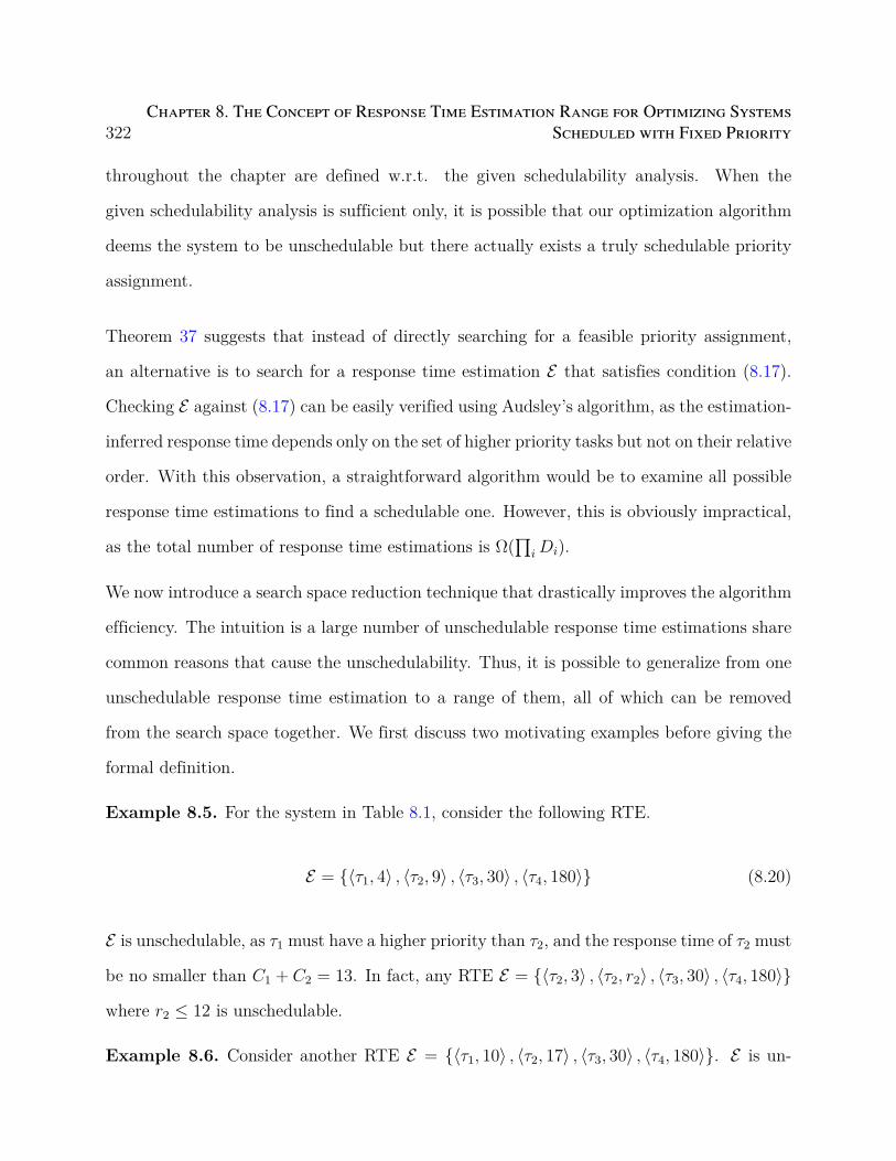
322Chapter 8. The Concept of Response Time Estimation Range for Optimizing Systems
Scheduled with Fixed Priority
throughout the chapter are defined w.r.t. the given schedulability analysis. When the
given schedulability analysis is sufficient only, it is possible that our optimization algorithm
deems the system to be unschedulable but there actually exists a truly schedulable priority
assignment.
Theorem 37 suggests that instead of directly searching for a feasible priority assignment,
an alternative is to search for a response time estimation E that satisfies condition (8.17).
Checking E against (8.17) can be easily verified using Audsley’s algorithm, as the estimation-
inferred response time depends only on the set of higher priority tasks but not on their relative
order. With this observation, a straightforward algorithm would be to examine all possible
response time estimations to find a schedulable one. However, this is obviously impractical,
as the total number of response time estimations is Ω(∏
i Di).
We now introduce a search space reduction technique that drastically improves the algorithm
efficiency. The intuition is a large number of unschedulable response time estimations share
common reasons that cause the unschedulability. Thus, it is possible to generalize from one
unschedulable response time estimation to a range of them, all of which can be removed
from the search space together. We first discuss two motivating examples before giving the
formal definition.
Example 8.5. For the system in Table 8.1, consider the following RTE.
E = ⟨τ1, 4⟩ , ⟨τ2, 9⟩ , ⟨τ3, 30⟩ , ⟨τ4, 180⟩ (8.20)
E is unschedulable, as τ1 must have a higher priority than τ2, and the response time of τ2 must
be no smaller than C1 + C2 = 13. In fact, any RTE E = ⟨τ2, 3⟩ , ⟨τ2, r2⟩ , ⟨τ3, 30⟩ , ⟨τ4, 180⟩
where r2 ≤ 12 is unschedulable.
Example 8.6. Consider another RTE E = ⟨τ1, 10⟩ , ⟨τ2, 17⟩ , ⟨τ3, 30⟩ , ⟨τ4, 180⟩. E is un-
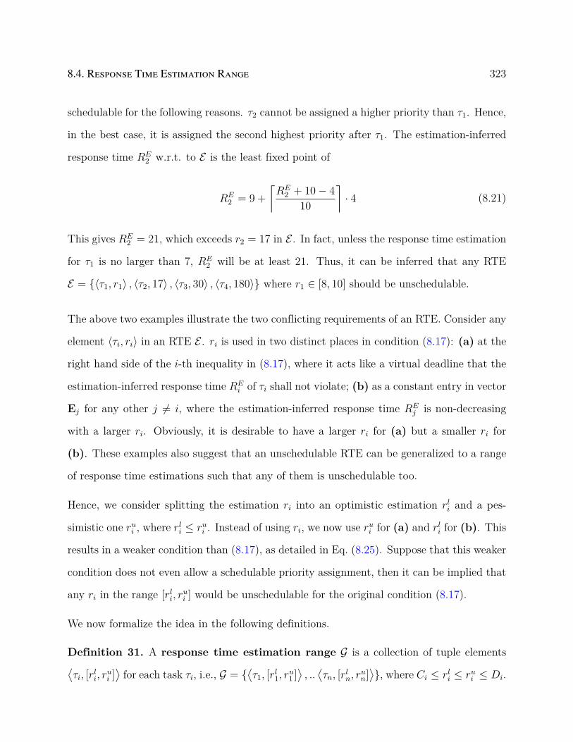
8.4. Response Time Estimation Range 323
schedulable for the following reasons. τ2 cannot be assigned a higher priority than τ1. Hence,
in the best case, it is assigned the second highest priority after τ1. The estimation-inferred
response time RE2 w.r.t. to E is the least fixed point of
RE2 = 9 +
⌈RE
2 + 10− 4
10
⌉· 4 (8.21)
This gives RE2 = 21, which exceeds r2 = 17 in E . In fact, unless the response time estimation
for τ1 is no larger than 7, RE2 will be at least 21. Thus, it can be inferred that any RTE
E = ⟨τ1, r1⟩ , ⟨τ2, 17⟩ , ⟨τ3, 30⟩ , ⟨τ4, 180⟩ where r1 ∈ [8, 10] should be unschedulable.
The above two examples illustrate the two conflicting requirements of an RTE. Consider any
element ⟨τi, ri⟩ in an RTE E . ri is used in two distinct places in condition (8.17): (a) at the
right hand side of the i-th inequality in (8.17), where it acts like a virtual deadline that the
estimation-inferred response time REi of τi shall not violate; (b) as a constant entry in vector
Ej for any other j = i, where the estimation-inferred response time REj is non-decreasing
with a larger ri. Obviously, it is desirable to have a larger ri for (a) but a smaller ri for
(b). These examples also suggest that an unschedulable RTE can be generalized to a range
of response time estimations such that any of them is unschedulable too.
Hence, we consider splitting the estimation ri into an optimistic estimation rli and a pes-
simistic one rui , where rli ≤ rui . Instead of using ri, we now use rui for (a) and rli for (b). This
results in a weaker condition than (8.17), as detailed in Eq. (8.25). Suppose that this weaker
condition does not even allow a schedulable priority assignment, then it can be implied that
any ri in the range [rli, rui ] would be unschedulable for the original condition (8.17).
We now formalize the idea in the following definitions.
Definition 31. A response time estimation range G is a collection of tuple elements⟨τi, [r
li, r
ui ]⟩
for each task τi, i.e., G = ⟨τ1, [r
l1, r
u1 ]⟩, ..⟨τn, [r
ln, r
un]⟩, where Ci ≤ rli ≤ rui ≤ Di.

324Chapter 8. The Concept of Response Time Estimation Range for Optimizing Systems
Scheduled with Fixed Priority
It represents a range of possible estimation values for the actual response time Ri of each
task τi.
Note that in the definition, we restrict [rli, rui ] of each task τi to be within [Ci, Di], as the
response time Ri of τi for any schedulable system shall be in that range.
Definition 32. A response time estimation E is said to be contained in a response time
estimation range G, denoted as E ∈ G, if and only if for each ⟨τi, ri⟩ in E , the corresponding
range⟨τi, [r
li, r
ui ]⟩
in G satisfies ri ∈ [rli, rui ].
Example 8.7. Consider the following response time estimations and response time estima-
tion range.E1 = ⟨τ1, 4⟩ , ⟨τ2, 13⟩ , ⟨τ3, 30⟩ , ⟨τ4, 180⟩
E2 = ⟨τ1, 4⟩ , ⟨τ2, 17⟩ , ⟨τ3, 30⟩ , ⟨τ4, 180⟩
G = ⟨τ1, [4, 9]⟩ , ⟨τ2, [9, 16]⟩ , ⟨τ3, [5, 120]⟩ , ⟨τ4, [35, 180]⟩
E1 ∈ G, as each response time estimated in E1 is contained in the corresponding range in G.
E2 /∈ G, as the response time estimation of τ2 is 17, outside the corresponding range in G.
Definition 33. G1 is a subset of G2, or equivalently G2 is a superset of G1, denoted as
G1 ⊆ G2, if and only if for each⟨τi, [r
li1, r
ui1]⟩
in G1, the corresponding⟨τi, [r
li2, r
ui2]⟩
in G2
satisfies rli2 ≤ rli1 and rui2 ≥ rui1. G1 is a strict subset of G2, denoted as G1 ⊂ G2, if and only
if G1 ⊆ G2 and G1 = G2.
Example 8.8. For the response time estimation ranges below
G1 = ⟨τ1, [4, 10]⟩ , ⟨τ2, [13, 17]⟩ , ⟨τ3, [5, 30]⟩ , ⟨τ4, [35, 180]⟩
G2 = ⟨τ1, [4, 10]⟩ , ⟨τ2, [9, 17]⟩ , ⟨τ3, [5, 30]⟩ , ⟨τ4, [35, 180]⟩
obviously G1 ⊆ G2 since each element in G2 is a superset of the corresponding one in G1.

8.4. Response Time Estimation Range 325
Definition 34. Given a response time estimation range G = ⟨τ1, [r
l1, r
u1 ], ..[r
ln, r
un]⟩, and a
priority assignment P, the estimation range-inferred response time of τi, denoted as
RGi , is the least fixed point of the following equation
RGi = fi(hpi,Gi) (8.22)
where Gi is a vector constructed by taking the i-th entry as variable RGi and any other j-th
entry as the value rlj from G
Gi = [rl1, ..., RGi , ..., r
ln] (8.23)
The vector of estimation range-inferred response times is denoted as RG.
Intuitively, due to property A4, the estimation range-inferred response time is essentially the
smallest estimation inferred response time that can possibly be obtained for E ∈ G, as shown
in the following equation.
∀E ∈ G, ∀i, ∀j = i, rj ≥ rlj
⇒ ∀E ∈ G, ∀i, REi ≥ RG
i (by property A4)(8.24)
Also, given an estimation range, the analysis of estimation range-inferred response times
depends only on the set of higher priority tasks but not on their relative order, hence it is
compliant with Audsley’s algorithm.
We now define the schedulability of a response time estimation range as follows.
Definition 35. A response time estimation range G = ⟨τ1, [r
l1, r
u1 ]⟩, ...⟨τn, [r
ln, r
un]⟩ is said
to be schedulable if
∃P s.t. ∀i = 1, RGi = fi(hpi,Gi) ≤ rui (8.25)

326Chapter 8. The Concept of Response Time Estimation Range for Optimizing Systems
Scheduled with Fixed Priority
Condition (8.25) is weaker than (8.17): it allows rli to be smaller than rui , hence easier to be
satisfied than (8.17). Like (8.17), (8.25) can be verified efficiently using Audsley’s algorithm.
The usefulness of the concept is shown in the following theorem, which demonstrates that
an unschedulable response time estimation range implies all its contained response time
estimations are unschedulable.
Theorem 38. Given an unschedulable response time estimation range
G = ⟨τ1, [r
l1, r
u1 ]⟩, ...⟨τn, [r
ln, r
un]⟩ (8.26)
any response time estimation E ∈ G is unschedulable.
Proof. Let E = ⟨τ1, r1⟩ , ... ⟨τn, rn⟩ be any response time estimation contained in G. If G
is unschedulable, then for any priority assignment P, there exists a task τi such that
RGi ≥ rui ⇒ RE
i ≥ rui [by Eq. (8.24)]
⇒ REi ≥ ri (since E ∈ G)
(8.27)
Hence, E is also unschedulable.
Unlike the case of unschedulable response time estimation range, its schedulable version is
less useful in the sense that the contained RTE may or may not be schedulable. We illustrate
in the following example.
Example 8.9. Consider the following two response time estimation ranges
G1 = ⟨τ1, [4, 10]⟩ , ⟨τ2, [9, 16]⟩ , ⟨τ3, [5, 120]⟩ , ⟨τ4, [35, 180]⟩
G2 = ⟨τ1, [4, 10]⟩ , ⟨τ2, [9, 35]⟩ , ⟨τ3, [5, 120]⟩ , ⟨τ4, [35, 180]⟩
G1 is unschedulable by reasons similar to those in Example 8.6. Specifically, τ1 has to have
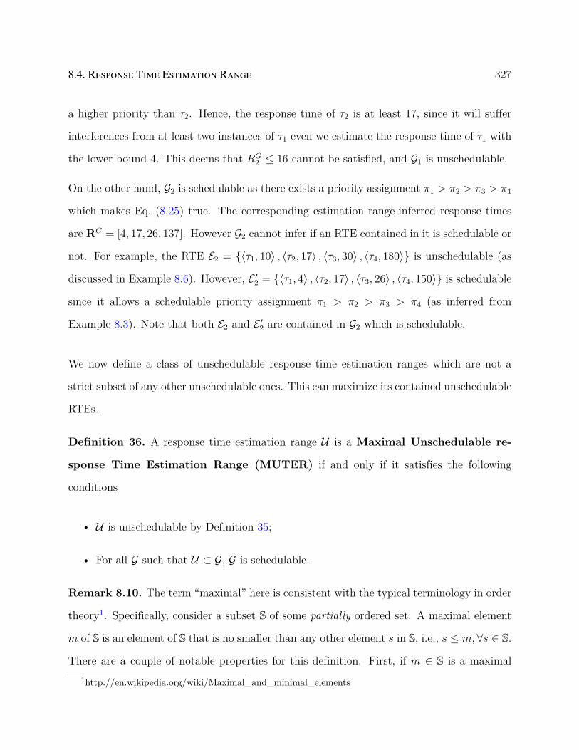
8.4. Response Time Estimation Range 327
a higher priority than τ2. Hence, the response time of τ2 is at least 17, since it will suffer
interferences from at least two instances of τ1 even we estimate the response time of τ1 with
the lower bound 4. This deems that RG2 ≤ 16 cannot be satisfied, and G1 is unschedulable.
On the other hand, G2 is schedulable as there exists a priority assignment π1 > π2 > π3 > π4
which makes Eq. (8.25) true. The corresponding estimation range-inferred response times
are RG = [4, 17, 26, 137]. However G2 cannot infer if an RTE contained in it is schedulable or
not. For example, the RTE E2 = ⟨τ1, 10⟩ , ⟨τ2, 17⟩ , ⟨τ3, 30⟩ , ⟨τ4, 180⟩ is unschedulable (as
discussed in Example 8.6). However, E ′2 = ⟨τ1, 4⟩ , ⟨τ2, 17⟩ , ⟨τ3, 26⟩ , ⟨τ4, 150⟩ is schedulable
since it allows a schedulable priority assignment π1 > π2 > π3 > π4 (as inferred from
Example 8.3). Note that both E2 and E ′2 are contained in G2 which is schedulable.
We now define a class of unschedulable response time estimation ranges which are not a
strict subset of any other unschedulable ones. This can maximize its contained unschedulable
RTEs.
Definition 36. A response time estimation range U is a Maximal Unschedulable re-
sponse Time Estimation Range (MUTER) if and only if it satisfies the following
conditions
• U is unschedulable by Definition 35;
• For all G such that U ⊂ G, G is schedulable.
Remark 8.10. The term “maximal” here is consistent with the typical terminology in order
theory1. Specifically, consider a subset S of some partially ordered set. A maximal element
m of S is an element of S that is no smaller than any other element s in S, i.e., s ≤ m,∀s ∈ S.
There are a couple of notable properties for this definition. First, if m ∈ S is a maximal1http://en.wikipedia.org/wiki/Maximal_and_minimal_elements
328Chapter 8. The Concept of Response Time Estimation Range for Optimizing Systems
Scheduled with Fixed Priority
element of S, then for all s ∈ S such that m ≤ s, it must be m = s. Second, it is possible
that there are many maximal elements of S, since S does not impose a total order.
For the concept of response time estimation range, we shall treat the subset relationship in
Definition 33 as a partial order, i.e., G1 is no larger than G2 if G1 ⊆ G2. Let S be the set of all
unschedulable response time estimation ranges. A MUTER U by Definition 36 is essentially
a “maximal” element of S. Since the partial order in Definition 33 does not form a total
order among response time estimation ranges, there may be multiple maximal elements of
S, i.e., multiple MUTERs.
Example 8.11. Consider the response time estimation ranges
G3 = ⟨τ1, [4, 10]⟩ , ⟨τ2, [9, 13]⟩ , ⟨τ3, [5, 120]⟩ , ⟨τ4, [35, 180]⟩
and G1, the latter is defined in Example 8.9. Though both G1 and G3 are unschedulable, G3
is not a MUTER since G3 ⊂ G1. G1 is a MUTER since increasing ru2 from 16 to 17 will make
it schedulable, and the other bounds in G1 cannot be expanded either: the lower bound rli is
equal to the smallest value Ci, and the upper bound rui is the same as the largest value Di.
Intuitively, consider two unschedulable response time estimation ranges G1 and G2 such that
G1 ⊆ G2. G1 is redundant in the presence of G2, since the latter contains all unschedulable
RTEs contained in G1. In this sense, a MUTER U is more useful than any of its subset
G (i.e., G ⊆ U), since it is more efficient than G in capturing unschedulable RTEs. In the
optimization algorithm design, this allows to rule out the most unschedulable RTEs with
the fewest number of unschedulable response time estimation ranges.
An unschedulable RTE E = ⟨τ1, r1⟩ , ... ⟨τn, rn⟩ can be generalized into a MUTER by
Algorithm 16. We assume that the initial input E satisfies ri ∈ [Ci, Di] for each task τi. We
will later show in Section 8.5 how it can be guaranteed. The algorithm first converts the
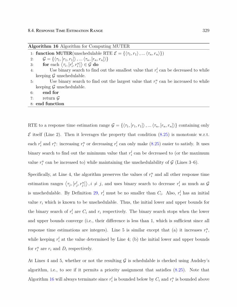
8.4. Response Time Estimation Range 329
Algorithm 16 Algorithm for Computing MUTER1: function MUTER(unschedulable RTE E = ⟨τ1, r1⟩ , ... ⟨τn, rn⟩)2: G = ⟨τ1, [r1, r1]⟩ , ... ⟨τn, [rn, rn]⟩3: for each
⟨τi, [r
li, r
ui ]⟩∈ G do
4: Use binary search to find out the smallest value that rli can be decreased to whilekeeping G unschedulable.
5: Use binary search to find out the largest value that rui can be increased to whilekeeping G unschedulable.
6: end for7: return G8: end function
RTE to a response time estimation range G = ⟨τ1, [r1, r1]⟩ , ... ⟨τn, [rn, rn]⟩ containing only
E itself (Line 2). Then it leverages the property that condition (8.25) is monotonic w.r.t.
each rli and rui : increasing rui or decreasing rli can only make (8.25) easier to satisfy. It uses
binary search to find out the minimum value that rli can be decreased to (or the maximum
value rui can be increased to) while maintaining the unschedulability of G (Lines 3–6).
Specifically, at Line 4, the algorithm preserves the values of rui and all other response time
estimation ranges⟨τj, [r
lj, r
uj ]⟩, i = j, and uses binary search to decrease rli as much as G
is unschedulable. By Definition 29, rli must be no smaller than Ci. Also, rli has an initial
value ri which is known to be unschedulable. Thus, the initial lower and upper bounds for
the binary search of rli are Ci and ri respectively. The binary search stops when the lower
and upper bounds converge (i.e., their difference is less than 1, which is sufficient since all
response time estimations are integers). Line 5 is similar except that (a) it increases rui ,
while keeping rli at the value determined by Line 4; (b) the initial lower and upper bounds
for rui are ri and Di respectively.
At Lines 4 and 5, whether or not the resulting G is schedulable is checked using Audsley’s
algorithm, i.e., to see if it permits a priority assignment that satisfies (8.25). Note that
Algorithm 16 will always terminate since rli is bounded below by Ci and rui is bounded above
330Chapter 8. The Concept of Response Time Estimation Range for Optimizing Systems
Scheduled with Fixed Priority
by Di.
We now formally prove that Algorithm 16 always returns a correct MUTER according to
Definition 36.
Theorem 39. Given an unschedulable response time estimation E = ⟨τ1, r1⟩ , ... ⟨τn, rn⟩,
Algorithm 16 correctly computes a MUTER G.
Proof. We show that the returned response time range G satisfies the two conditions in
Definition 36. First, G is initially unschedulable, and Algorithm 16 updates G only if G is
maintained to be unschedulable. Thus, the returned G is guaranteed to be unschedulable.
We prove the second condition by contradiction. Let G ′ be an unschedulable response
time estimation range such that G ′ is a strict superset of the returned G, i.e., G ⊂ G ′.
Hence, there must exist a task τi such that the corresponding response time range element⟨τi, [r
li(G ′), rui (G ′)]
⟩in G ′ strictly contains the one
⟨τi, [r
li(G), rui (G)]
⟩in G. That is, at least
one of the two conditions rli(G ′) < rli(G) and rui (G) < rui (G ′) is satisfied. Now consider the
resulting response time estimation range Gi after⟨τi, [r
li, r
ui ]⟩
is processed by Algorithm 16.
Since the algorithm only expands G during each iteration, it must be Gi ⊆ G ⊂ G ′. We con-
struct another response time estimation range G ′i such that (a) for each j = i, rlj(G ′i) = rlj(Gi)
and ruj (G ′i) = ruj (Gi); (b) rli(G ′i) = rli(G ′) and rui (G ′i) = rui (G ′). Obviously Gi ⊂ G ′i ⊆ G ′. This
contradicts with the fact that Gi is the result after⟨τi, [r
li, r
ui ]⟩
is maximally expanded.
In Algorithm 16, Audsley’s algorithm is called each time we try to check if G is schedulable.
It is known that Audsley’s algorithm only needs to explore O(n2) priority orders out of the
n! possible ones, where n is the number of tasks [53]. For each task τi, the binary searches at
Lines 4–5 make O(logDi) function calls to Audsley’s algorithm, since there are at most Di
possible integer values for both rli and rui . Hence, Algorithm 16 checks a total of O(n2 logD)
priority orders to calculate a MUTER, where D =∏
iDi.

8.5. MUTER-Guided Optimization Algorithm 331
8.5 MUTER-Guided Optimization Algorithm
We now present an optimization algorithm that leverages the concepts of RTE and MUTER.
We observe that in many optimization problems for systems with an RT-dependent response
time analysis, finding a schedulable priority assignment is a major difficulty since there
is no known tractable procedure like Audsley’s algorithm. As in Theorem 37, finding a
schedulable priority assignment is equivalent to finding a schedulable RTE. The latter has
the promise to be more scalable for the following unique capability from Algorithm 16:
given an unschedulable RTE it can efficiently generalize to a set of MUTERs, each of which
contains a maximal range of unschedulable RTEs.
Hence, we design the optimization algorithm that leverages the power of Algorithm 16.
Specifically, instead of solving the original problem O directly, we start with a relaxed prob-
lem X that leaves out all the system schedulability constraints. Solving this relaxed problem
will return an RTE that is driven by other constraints and the objective. If the RTE is
unschedulable, we use Algorithm 16 to generalize to a set of MUTERs. We then add the
corresponding constraints to X to rule out similar unschedulable RTEs, and solve it again.
The iterative procedure will end if the returned RTE is schedulable, which is guaranteed to
be an optimal solution of the original problem, or the problem is deemed to be infeasible
(see Theorem 40 below).
The procedure is illustrated in Figure 8.1. It contains an initial Step 1 that checks if the
most relaxed response time estimation range is schedulable. If yes, it enters the iterations
between Step 2 (solving the relaxed problem X) and Step 3 (computing MUTERs). We
explain each step in details below.
Step 1. Let RLi and RU
i denote the smallest and largest values for the response time of
each task τi in any schedulable priority assignment. In this chapter we take RLi = Ci and

332Chapter 8. The Concept of Response Time Estimation Range for Optimizing Systems
Scheduled with Fixed Priority
Solve relaxed problem X
Step 3:
Schedulable?No
Yes
Compute k MUTERs with Algorithm 1 and add implied
constraints to problem X
Determine smallest and largest values for each Ri. Construct G M .
G M Schedulable?
Yes
Report unschedulability
Returned RTE
No
Feasible?
Yes
Report infeasibility
No
Report optimal solution
Step 2:
Step 1:
Figure 8.1: Optimal Priority Assignment Algorithm Procedure

8.5. MUTER-Guided Optimization Algorithm 333
RUi = Di. The first step simply evaluates whether the response time estimation range
GM = ⟨τ1, [C1, D1]⟩ , ... ⟨τn, [Cn, Dn]⟩ is schedulable. Any schedulable RTE E must satisfy
E ∈ GM . If GM is not schedulable, then the system must be unschedulable by any priority
assignment, as proven in Theorem 38.
Step 2. The second step searches for a response time estimation that has not been deemed
unschedulable by the currently computed MUTERs. This is done by solving a relaxed
problem X consisting of no schedulability conditions but the implied constraints by the
computed MUTERs. Specifically, for each MUTER U = ⟨τ1, [r
l1, r
u1 ]⟩, ...⟨τn, [r
ln, r
un]⟩, by
Theorem 38 any schedulable RTE E = ⟨τ1, r1⟩ , ... ⟨τn, rn⟩ cannot be contained in U . This
implies the following constraint
E /∈ U ⇔ ¬
rl1 ≤ r1 ≤ ru1
...
rln ≤ rn ≤ run
⇔
∥∥∥∥∥∥∥∥∥∥∥r1 < rl1∥r1 > ru1
...
rn < rln∥rn > run
(8.28)
where ¬, , and ∥ represent the logic-NOT, logic-AND, and logic-OR operations, respectively.
Thus, X is essentially a mathematical programming problem consisting of the objective and
the design constraints h(·) in O, while replacing the system schedulability constraints with
those of (8.28) implied by all currently computed MUTERs. X also includes the response
time estimations of all tasks [r1, ...rn] as the additional design variables, as well as their
initial bounding constraints Ci ≤ ri ≤ Di, ∀i. Formally, problem X can be expressed as
X : min g(X)
s.t. Implied constraints (8.28), ∀ U ∈ U
Ci ≤ ri ≤ Di,∀i
h(X) ≤ 0
(8.29)
334Chapter 8. The Concept of Response Time Estimation Range for Optimizing Systems
Scheduled with Fixed Priority
where U is the set of currently known MUTERs.
In this chapter, we assume g(·) and h(·) are both linear functions of X, hence X can be solved
using MILP solvers such as CPLEX. Note that the logical disjunction constraint in (8.28)
can be formulated in MILP using “big-M” method. For example,
∥∥∥∥∥∥∥r1 < rl1
r1 > ru1
⇔
r1 < rl1 +M · b1
r1 > ru1 −M · (1− b1)
(8.30)
Here b1 is an auxiliary binary variable, defined as 0 if r1 < rl1, 1 if r1 > ru1 . M is a sufficiently
large constant such as D1.
If X is infeasible (i.e., no solution satisfies all constraints in X), then the system cannot be
schedulable by any RTE (see Theorem 40 below). Otherwise, solving X will return an RTE
(composed of the solution values assigned to the decision variables [r1, ...rn]) that respects
all the implied constraints by the known MUTERs.
Step 3. This step evaluates the schedulability of the RTE E returned in Step 2, i.e., whether
it satisfies Eq. (8.25). If yes, then E is optimal, and the associated priority assignment P
is an optimal priority assignment (proven in Theorem 40). Here P can be obtained as a
byproduct of applying Audsley’s algorithm in checking E against the condition (8.25).
If E is unschedulable, it is generalized into at most k MUTERs using Algorithm 16, where
k is a predefined parameter. The implied constraints from these newly discovered MUTERs
are then added to the problem X, and we enter the next iteration. In our experiments, we
find that k = 5 is a good setting in most cases. Since problem X contains the constraints
Ci ≤ ri ≤ Di,∀i, the RTE E = ⟨τ1, r1⟩ , ... ⟨τn, rn⟩ from Step 2, which is the input to
Algorithm 16 for computing MUTERs, must satisfy the prerequisite ri ∈ [Ci, Di],∀i.
The following theorem formally proves the correctness of the proposed algorithm in Fig-
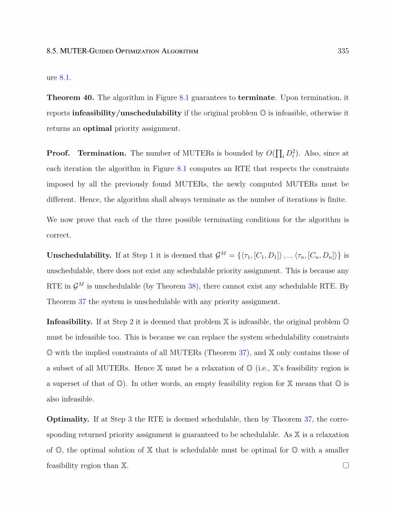
8.5. MUTER-Guided Optimization Algorithm 335
ure 8.1.
Theorem 40. The algorithm in Figure 8.1 guarantees to terminate. Upon termination, it
reports infeasibility/unschedulability if the original problem O is infeasible, otherwise it
returns an optimal priority assignment.
Proof. Termination. The number of MUTERs is bounded by O(∏
i D2i ). Also, since at
each iteration the algorithm in Figure 8.1 computes an RTE that respects the constraints
imposed by all the previously found MUTERs, the newly computed MUTERs must be
different. Hence, the algorithm shall always terminate as the number of iterations is finite.
We now prove that each of the three possible terminating conditions for the algorithm is
correct.
Unschedulability. If at Step 1 it is deemed that GM = ⟨τ1, [C1, D1]⟩ , ... ⟨τn, [Cn, Dn]⟩ is
unschedulable, there does not exist any schedulable priority assignment. This is because any
RTE in GM is unschedulable (by Theorem 38), there cannot exist any schedulable RTE. By
Theorem 37 the system is unschedulable with any priority assignment.
Infeasibility. If at Step 2 it is deemed that problem X is infeasible, the original problem O
must be infeasible too. This is because we can replace the system schedulability constraints
O with the implied constraints of all MUTERs (Theorem 37), and X only contains those of
a subset of all MUTERs. Hence X must be a relaxation of O (i.e., X’s feasibility region is
a superset of that of O). In other words, an empty feasibility region for X means that O is
also infeasible.
Optimality. If at Step 3 the RTE is deemed schedulable, then by Theorem 37, the corre-
sponding returned priority assignment is guaranteed to be schedulable. As X is a relaxation
of O, the optimal solution of X that is schedulable must be optimal for O with a smaller
feasibility region than X.

336Chapter 8. The Concept of Response Time Estimation Range for Optimizing Systems
Scheduled with Fixed Priority
Although the algorithm in Figure 8.1 is guaranteed to terminate, in the worst case it may
require to compute all MUTERs. Consequently it needs O(∏
i D2i ) number of iterations
between Steps 2 and 3, as each iteration computes a constant number of distinct MUTERs.
Also, in each iteration it needs to solve an MILP problem X. In the end, the algorithm still
has an exponential worst case complexity, like those of the other exact algorithms based on
BnB and a single MILP formulation.
We now demonstrate the algorithm by applying it to the problem of finding a schedulable
priority assignment for the example system in Table 8.1. The parameter k is set to 3.
Example 8.12. As the first step, we construct GM as
GM = ⟨τ1, [4, 10]⟩ , ⟨τ2, [9, 35]⟩ , ⟨τ3, [5, 120]⟩ , ⟨τ4, [35, 180]⟩
GM is schedulable as it satisfies Eq. (8.25). The algorithm then enters an iterative procedure
between Step 2 and Step 3.
Iteration 1. The relaxed problem X is constructed by leaving out all schedulability con-
straints. Hence, X only contains the constraints that the response time estimation is in the
range defined by GM
X : min 0
s.t. 4 ≤ r1 ≤ 10
9 ≤ r2 ≤ 35
5 ≤ r3 ≤ 120
35 ≤ r4 ≤ 180
(8.31)
Solving X returns the following response time estimation
E = ⟨τ1, 4⟩ , ⟨τ2, 9⟩ , ⟨τ3, 5⟩ , ⟨τ4, 35⟩

8.5. MUTER-Guided Optimization Algorithm 337
which is obviously unschedulable since the response time is estimated to be the WCET for
each task. The following 3 MUTERs are computed
U1 = ⟨τ1, [4, 10]⟩ , ⟨τ2, [9, 35]⟩ , ⟨τ3, [5, 120]⟩ , ⟨τ4, [35, 136]⟩
U2 = ⟨τ1, [4, 10]⟩ , ⟨τ2, [9, 25]⟩ , ⟨τ3, [5, 25]⟩ , ⟨τ4, [35, 180]⟩
U3 = ⟨τ1, [4, 8]⟩ , ⟨τ2, [9, 35]⟩ , ⟨τ3, [5, 8]⟩ , ⟨τ4, [35, 180]⟩
By (8.28), U1 implies the following constraints
∥∥∥∥∥∥∥∥∥∥∥∥∥∥
r1 < 4 ∥ r1 > 10
r2 < 9 ∥ r2 > 35
r3 < 5 ∥ r3 > 120
r4 < 35 ∥ r4 > 136
which can be simplified as follows considering that (8.31) shall be satisfied as well
r4 ≥ 137
Similarly, we can find the implied constraints for all three MUTERs. Below we give their
simplified version, which is then added to X
U1 : r4 ≥ 137
U2 : r2 ≥ 26 ∥ r3 ≥ 26
U3 : r1 ≥ 8 ∥ r3 ≥ 8

338Chapter 8. The Concept of Response Time Estimation Range for Optimizing Systems
Scheduled with Fixed Priority
Iteration 2. Solving the updated problem X returns the solution below
E = ⟨τ1, 4⟩ , ⟨τ2, 9⟩ , ⟨τ3, 26⟩ , ⟨τ4, 137⟩
E is unschedulable, and the MUTER below is computed
U4 = ⟨τ1, [4, 10]⟩ , ⟨τ2, [9, 16]⟩ , ⟨τ3, [5, 120]⟩ , ⟨τ4, [35, 180]⟩
The following implied constraint is added to problem X
r2 ≥ 17
Iteration 3. Solving X returns the following solution
E = ⟨τ1, 4⟩ , ⟨τ2, 26⟩ , ⟨τ3, 26⟩ , ⟨τ4, 137⟩
E is still unschedulable. We compute the following MUTER
U5 = ⟨τ1, [4, 10]⟩ , ⟨τ2, [13, 35]⟩ , ⟨τ3, [5, 120]⟩ , ⟨τ4, [35, 149]⟩
which implies the constraint below to be added to X
r2 ≤ 12 ∥ r4 ≥ 150
Iteration 4. Solving X now returns the following solution
E = ⟨τ1, 4⟩ , ⟨τ2, 26⟩ , ⟨τ3, 26⟩ , ⟨τ4, 150⟩

8.6. Exploring Potentially Feasible Solution 339
At this point, E becomes schedulable w.r.t. condition (8.25), and the associated schedulable
priority assignment is
π1 > π3 > π2 > π4
8.6 Exploring Potentially Feasible Solution
Modern mathematical programming solvers such as CPLEX often come with various tech-
niques for exploring good-quality feasible solutions. Even though the solver may not be able
to find the globally optimal solution within the time limit, it may still returned feasible so-
lutions during the process which can be useful to the designers. In this section, we enhance
the proposed framework with a similar capability. Specifically, we integrate an algorithm
for exploring solutions that are potentially feasible with good quality.
Our main intuition is that as more and more MUTER implied constraint are added to the
problem, the resulting RTE obtained in Step 2 becomes closer to the one that is schedulable
and optimal. Therefore, our main idea is to relax the RTE obtained from step 2 into a
number of response time estimation ranges Gs that are schedulable by Definition 35. If the
corresponding priority assignment in condition (8.25) is truly schedulable for the original
system, we keep the priority assignment as a feasible solution. If the optimization algorithm
terminates due to timing out, the feasible solutions with the best objective value is returned.
One way to obtain relaxed and schedulable response time estimation ranges is through
MUTER computations. Specifically, consider Line 4 and 5 in Algorithm 16, which use
binary search to find the minimum/maximum unschedulable lower-bound/upper-bound. In
the typical process of binary update, it is possible that G becomes schedulable at some point,
in which case it can be taken as one schedulable and relaxed response time estimation ranges.
The corresponding priority assignment derived from condition (8.25) can then be checked
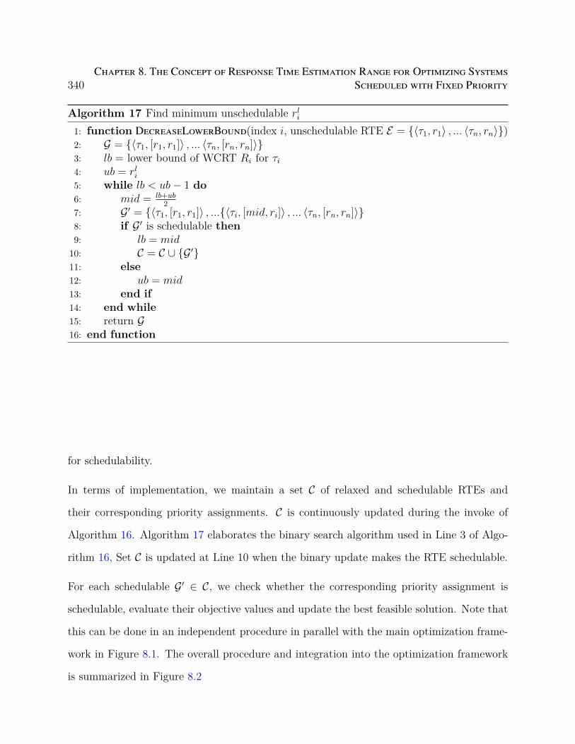
340Chapter 8. The Concept of Response Time Estimation Range for Optimizing Systems
Scheduled with Fixed Priority
Algorithm 17 Find minimum unschedulable rli
1: function DecreaseLowerBound(index i, unschedulable RTE E = ⟨τ1, r1⟩ , ... ⟨τn, rn⟩)2: G = ⟨τ1, [r1, r1]⟩ , ... ⟨τn, [rn, rn]⟩3: lb = lower bound of WCRT Ri for τi4: ub = rli5: while lb < ub− 1 do6: mid = lb+ub
2
7: G ′ = ⟨τ1, [r1, r1]⟩ , ...⟨τi, [mid, ri]⟩ , ... ⟨τn, [rn, rn]⟩8: if G ′ is schedulable then9: lb = mid
10: C = C ∪ G ′11: else12: ub = mid13: end if14: end while15: return G16: end function
for schedulability.
In terms of implementation, we maintain a set C of relaxed and schedulable RTEs and
their corresponding priority assignments. C is continuously updated during the invoke of
Algorithm 16. Algorithm 17 elaborates the binary search algorithm used in Line 3 of Algo-
rithm 16, Set C is updated at Line 10 when the binary update makes the RTE schedulable.
For each schedulable G ′ ∈ C, we check whether the corresponding priority assignment is
schedulable, evaluate their objective values and update the best feasible solution. Note that
this can be done in an independent procedure in parallel with the main optimization frame-
work in Figure 8.1. The overall procedure and integration into the optimization framework
is summarized in Figure 8.2
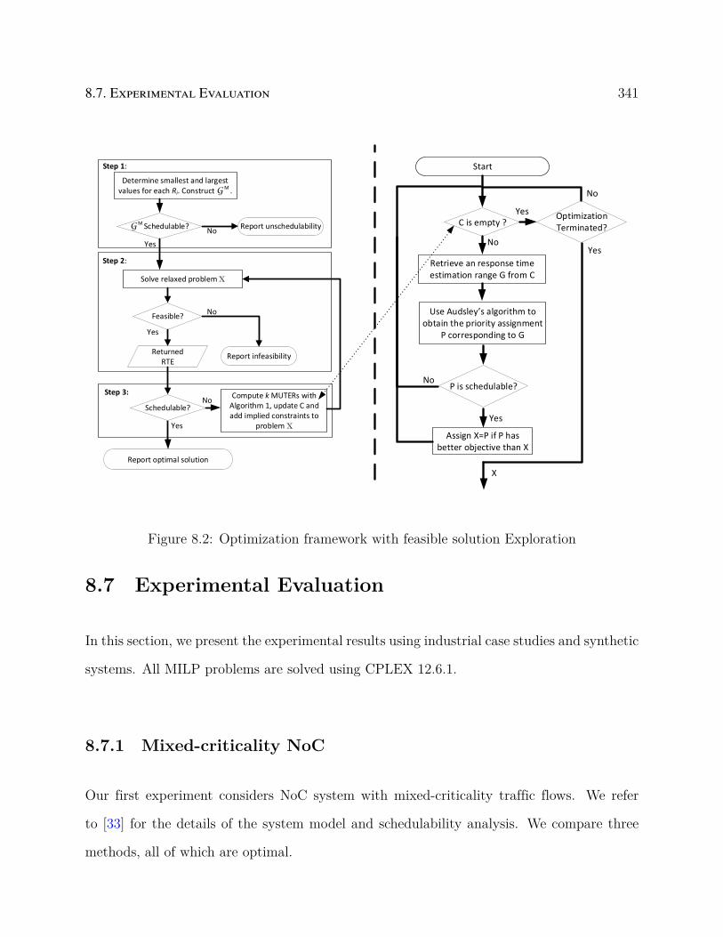
8.7. Experimental Evaluation 341
Solve relaxed problem X
Step 3:
Schedulable?No
Yes
Compute k MUTERs with Algorithm 1, update C and add implied constraints to
problem X
Determine smallest and largest values for each Ri. Construct G M .
G M Schedulable?
Yes
Report unschedulability
Returned RTE
No
Feasible?
Yes
Report infeasibility
No
Report optimal solution
Step 2:
Step 1: Start
C is empty ?Optimization Terminated?
No
Yes
Yes
Retrieve an response time estimation range G from C
Use Audsley’s algorithm to obtain the priority assignment
P corresponding to G
No
Assign X=P if P has better objective than X
X
P is schedulable?
Yes
No
Figure 8.2: Optimization framework with feasible solution Exploration
8.7 Experimental Evaluation
In this section, we present the experimental results using industrial case studies and synthetic
systems. All MILP problems are solved using CPLEX 12.6.1.
8.7.1 Mixed-criticality NoC
Our first experiment considers NoC system with mixed-criticality traffic flows. We refer
to [33] for the details of the system model and schedulability analysis. We compare three
methods, all of which are optimal.

342Chapter 8. The Concept of Response Time Estimation Range for Optimizing Systems
Scheduled with Fixed Priority
Table 8.3: Results on autonomous vehicle applications (“N/A” denotes no solution found;Time limit = 24 hours)
U(LO)Enhanced-BnB MUTER-guided MILP
Objective Time Status Objective Time Status Objective Time Status1.357 40713 ≥ 24h Timeout 51309 1.7s Terminate 51309 51743.02s Terminate1.404 40835 ≥ 24h Timeout 50318 2.21s Terminate 50318 21789.89s Terminate1.451 5765 ≥ 24h Timeout 49328 35.54s Terminate 49328 ≥ 24h Timeout1.497 N/A ≥ 24h Timeout 47204 49569.68s Terminate 47204 6835.83s Terminate1.544 N/A ≥ 24h Timeout Infeasible 141.85s Terminate Infeasible 28.12s Terminate
• Enhanced-BnB: An enhanced branch-and-bound procedure proposed in [133]. The
branching order is optimized such that the likely schedulable priority assignments are
explored first.
• MILP: A unified MILP formulation solved by CPLEX, as detailed in [163].
• MUTER-guided: The proposed method in Section 8.5.
We first evaluate them on a case study of autonomous vehicle applications [33]. The case
study consists of 38 flows deployed on a 4×4 NoC, 6 of which are of HI-criticality. Each flow
is characterized by the data size, the source and destination processors, and the criticality
factor (Ci(HI)/Ci(LO)) if it is of HI-criticality. Since the utilization and WCET of the flows
are not given, we generate a set of systems where we set U(LO), the total system utilization
at LO-criticality mode, to be a particular value. The utilization of each flow is then assigned
proportional to the product of its data size and route length. Besides system schedulability,
we consider the objective of maximizing the minimum laxity among all flows, as defined in
Eq. (8.2). The time limit is set to 24 hours.
The results are summarized in Table 8.3. As in the table, when the system utilization is
relatively low such that the system is easily schedulable, MUTER-guided is over 1000×
faster than both Enhanced-BnB and MILP. However, when the system utilization is
around the borderline of being schedulable (as in the last two rows of the table), MUTER-
guided requires many iterations to refine the schedulability region. It becomes about 10×

8.7. Experimental Evaluation 343
slower than MILP (but still faster than Enhanced-BnB).
This motivates us to do a more systematic evaluation using randomly generated synthetic
systems with different utilization levels and number of flows. We first try to identify the
typical borderline utilization around which the problem is difficult to solve, using the
following settings. In this experiment, we are only concerned to find a schedulable priority
assignment. The system uses a 4×4 NoC platform. The periods of flows are selected from
the interval [1, 1000] following the log-uniform distribution. The criticality factor of HI-
criticality flows are set to be 2. We generate 1000 random systems for each value on the
system utilization in LO-criticality mode U(LO). The LO-criticality utilizations of individual
flows are generated using the UUnifast algorithm. Each system contains 40 flows, 20 of which
are of HI-criticality. The source, destination, and routing of each flow are generated following
the stress test scheme in [81]. The time limit is set to 10 minutes to avoid excessive waiting.
As in Table 8.3, the methods typically require a much longer time if they cannot finish in
10 minutes.
Figure 8.3 shows the portion of systems that incur a timeout for each method, for systems
with utilization within 50%-130%. For the purpose of finding the borderline utilization, this
range is sufficient, since the systems with utilization at 50% are always easily schedulable,
and those at 130% are mostly easily unschedulable. As indicated from the figure, the timeout
ratio is different at different utilization, but the utilization around 80%–95% has the highest
timeout ratio for all three methods. For systems with other numbers of flows the “borderline
utilization” is similarly around 80%–95%. Note that in this case study, there are totally 32
physical links shared by 38 traffic flows, and each flow may require multiple physical links
to transmit. This means that unlike the case of software tasks running on a uniprocessor,
the system may still be schedulable with a utilization higher than 100%. The difficulty of
this borderline utilization can be intuitively explained as follows. The priority assignment
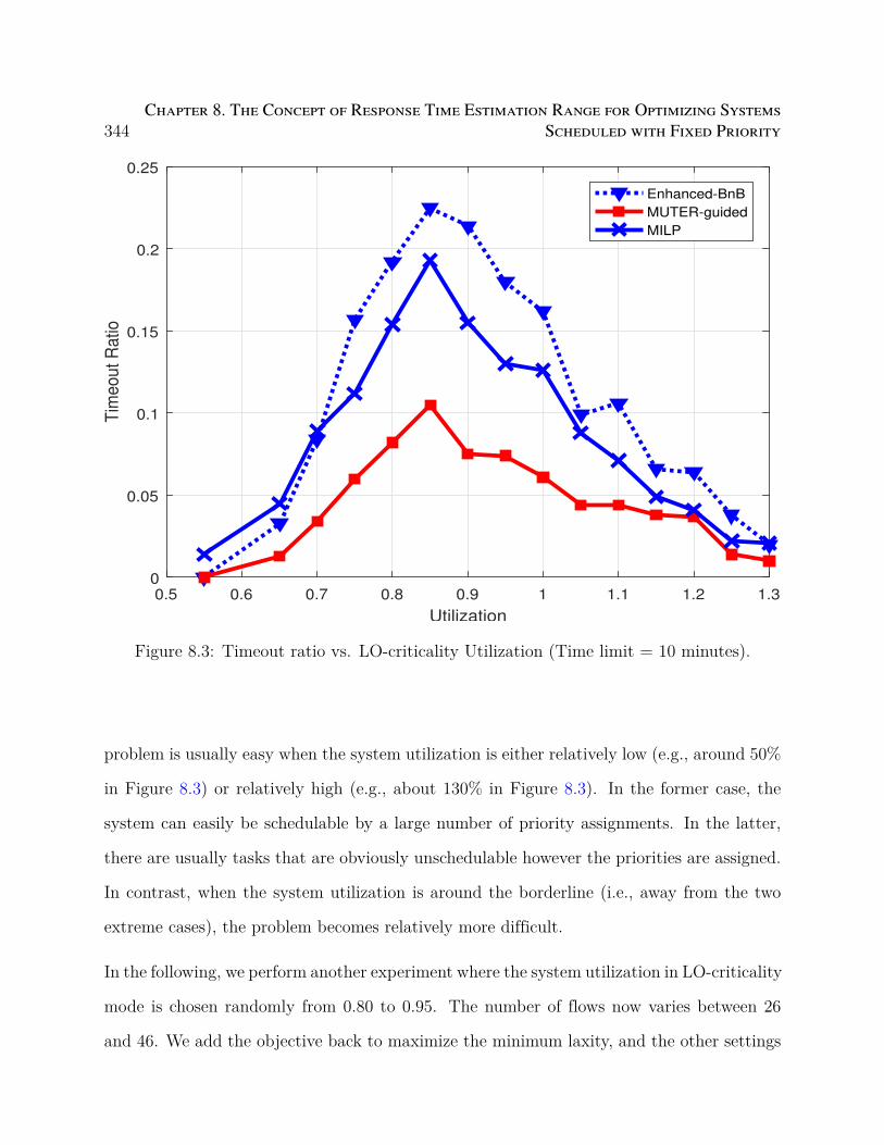
344Chapter 8. The Concept of Response Time Estimation Range for Optimizing Systems
Scheduled with Fixed Priority
0.5 0.6 0.7 0.8 0.9 1 1.1 1.2 1.3
Utilization
0
0.05
0.1
0.15
0.2
0.25
Tim
eout R
atio
Enhanced-BnB
MUTER-guided
MILP
Figure 8.3: Timeout ratio vs. LO-criticality Utilization (Time limit = 10 minutes).
problem is usually easy when the system utilization is either relatively low (e.g., around 50%
in Figure 8.3) or relatively high (e.g., about 130% in Figure 8.3). In the former case, the
system can easily be schedulable by a large number of priority assignments. In the latter,
there are usually tasks that are obviously unschedulable however the priorities are assigned.
In contrast, when the system utilization is around the borderline (i.e., away from the two
extreme cases), the problem becomes relatively more difficult.
In the following, we perform another experiment where the system utilization in LO-criticality
mode is chosen randomly from 0.80 to 0.95. The number of flows now varies between 26
and 46. We add the objective back to maximize the minimum laxity, and the other settings
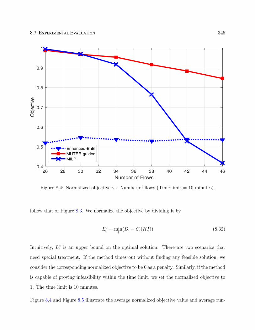
8.7. Experimental Evaluation 345
26 28 30 32 34 36 38 40 42 44 46
Number of Flows
0.4
0.5
0.6
0.7
0.8
0.9
1
Obje
ctiv
e
Enhanced-BnB
MUTER-guided
MILP
Figure 8.4: Normalized objective vs. Number of flows (Time limit = 10 minutes).
follow that of Figure 8.3. We normalize the objective by dividing it by
Lui = min
i(Di − Ci(HI)) (8.32)
Intuitively, Lui is an upper bound on the optimal solution. There are two scenarios that
need special treatment. If the method times out without finding any feasible solution, we
consider the corresponding normalized objective to be 0 as a penalty. Similarly, if the method
is capable of proving infeasibility within the time limit, we set the normalized objective to
1. The time limit is 10 minutes.
Figure 8.4 and Figure 8.5 illustrate the average normalized objective value and average run-

346Chapter 8. The Concept of Response Time Estimation Range for Optimizing Systems
Scheduled with Fixed Priority
26 28 30 32 34 36 38 40 42 44 46
Number of Flows
0
50
100
150
200
250
300
350
400
450
Tim
e(s
)
Enhanced-BnB
MUTER-guided
MILP
Figure 8.5: Average runtime vs. Number of flows (Time limit = 10 minutes).
time of each method, respectively. MUTER-guided demonstrates much better optimiza-
tion quality than both Enhanced-BnB and MILP, especially for large systems. In general,
this is because Enhanced-BnB and MILP have higher timeout ratios and are often only
able to find suboptimal solutions within the time limit. Hence, on average MUTER-guided
has the promise to be more scalable than Enhanced-BnB and MILP.
8.7.2 Data Driven Activation in Distributed Systems
In this experiment, we evaluate the proposed method on an industrial experimental vehicle
system with advanced active safety features [42]. The system consists of 29 Electronic
Control Units (ECUs) connected through 4 CAN buses, 92 tasks, and 192 CAN messages.
8.7. Experimental Evaluation 347
End-to-end deadlines are imposed on 12 pairs of source-sink tasks, which contain a total
of 222 unique paths. The allocation of tasks and messages onto corresponding execution
resources are given.
We compare the following three methods
• MILP-Approx: Formulating the problem as a single MILP and solving it with
CPLEX, where the response time analysis is approximate [167].
• MUTER-Accurate: The proposed technique using the accurate response time anal-
ysis.
• MUTER-Approx: Same as MUTER-Accurate but using the approximation anal-
ysis.
The accurate analysis is too complex to be formulated in MILP, since it needs to check all
the instances in the busy period, the length of which is unknown a priori. Hence, for tasks
with preemptive scheduling, an approximate analysis is proposed [167] which enforces the
deadline to be no larger than the period. This makes it safe to only ensure the first instance
in the busy period is schedulable. For messages with non-preemptive scheduling, we enforces
constrained deadline to allow to adopt a similar analysis from [45].
We first consider the objective of maximizing the minimum laxity among all paths. The
laxity of an end-to-end path is computed as the difference between the end-to-end latency
deadline and the actual end-to-end latency. Formally, the objective is max minp(Dp − Lp),
where p represents a path and Lp is defined in (8.9).
The results of the experiment are summarized in Table 8.4. As in the table, all three
methods are capable of finding the optimal solution (which happens to be the same with
either the accurate analysis or the approximate analysis). However, the proposed MUTER

348Chapter 8. The Concept of Response Time Estimation Range for Optimizing Systems
Scheduled with Fixed Priority
Table 8.4: Maximizing min laxity for the vehicle system
Method MILP-Approx MUTER-Approx MUTER-AccurateObjective 90466 90466 90466
Runtime (s) 596.72 4.68 9.00
based technique runs much faster than a single MILP formulation.
Next we study the problem of finding the breakdown utilization of each resource (ECU or
bus), which is defined as the maximum value the utilization of the resource can be scaled to
such that the system is still feasible (in terms of both schedulability of individual tasks/mes-
sages and end-to-end path deadlines) assuming the utilization of other resources remains
the same. For MUTER-Approx and MUTER-Accurate, the breakdown utilization is
computed by a binary search on top of them. The binary search stops when the upper-bound
and lower-bound are within 3%. A time limit of 2 hours is set for each ECU/Bus to prevent
excessive waiting.
We summarize the runtime and breakdown utilization in Table 8.5. MUTER-Accurate
and MUTER-Approx both can finish within the time limit for each ECU/Bus. For MILP-
Approx, it occasionally fails to finish in two hours. As highlighted in red bold fonts in the
table, MUTER-Accurate is capable of tolerating noticeably higher utilization than the
other two techniques for a number of resources, due to the accurate response time analysis.
This demonstrates that the approximate analysis may lead to substantially suboptimal so-
lutions. The MUTER-guided framework is mostly about two magnitudes faster than MILP.
Furthermore, unlike MILP, it is more flexible in terms of the adopted schedulability analysis,
as it uses a generic procedure to check the system schedulability.
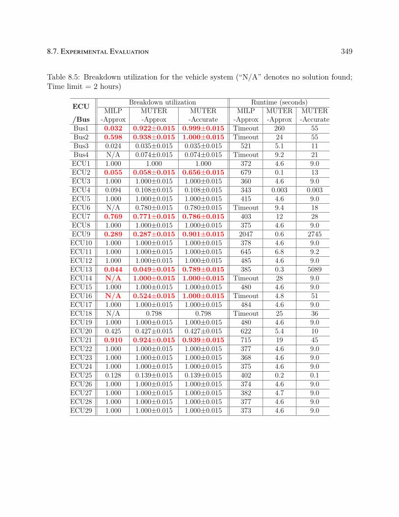
8.7. Experimental Evaluation 349
Table 8.5: Breakdown utilization for the vehicle system (“N/A” denotes no solution found;Time limit = 2 hours)
ECU Breakdown utilization Runtime (seconds)MILP MUTER MUTER MILP MUTER MUTER
/Bus -Approx -Approx -Accurate -Approx -Approx -AccurateBus1 0.032 0.922±0.015 0.999±0.015 Timeout 260 55Bus2 0.598 0.938±0.015 1.000±0.015 Timeout 24 55Bus3 0.024 0.035±0.015 0.035±0.015 521 5.1 11Bus4 N/A 0.074±0.015 0.074±0.015 Timeout 9.2 21ECU1 1.000 1.000 1.000 372 4.6 9.0ECU2 0.055 0.058±0.015 0.656±0.015 679 0.1 13ECU3 1.000 1.000±0.015 1.000±0.015 360 4.6 9.0ECU4 0.094 0.108±0.015 0.108±0.015 343 0.003 0.003ECU5 1.000 1.000±0.015 1.000±0.015 415 4.6 9.0ECU6 N/A 0.780±0.015 0.780±0.015 Timeout 9.4 18ECU7 0.769 0.771±0.015 0.786±0.015 403 12 28ECU8 1.000 1.000±0.015 1.000±0.015 375 4.6 9.0ECU9 0.289 0.287±0.015 0.901±0.015 2047 0.6 2745ECU10 1.000 1.000±0.015 1.000±0.015 378 4.6 9.0ECU11 1.000 1.000±0.015 1.000±0.015 645 6.8 9.2ECU12 1.000 1.000±0.015 1.000±0.015 485 4.6 9.0ECU13 0.044 0.049±0.015 0.789±0.015 385 0.3 5089ECU14 N/A 1.000±0.015 1.000±0.015 Timeout 28 9.0ECU15 1.000 1.000±0.015 1.000±0.015 480 4.6 9.0ECU16 N/A 0.524±0.015 1.000±0.015 Timeout 4.8 51ECU17 1.000 1.000±0.015 1.000±0.015 484 4.6 9.0ECU18 N/A 0.798 0.798 Timeout 25 36ECU19 1.000 1.000±0.015 1.000±0.015 480 4.6 9.0ECU20 0.425 0.427±0.015 0.427±0.015 622 5.4 10ECU21 0.910 0.924±0.015 0.939±0.015 715 19 45ECU22 1.000 1.000±0.015 1.000±0.015 377 4.6 9.0ECU23 1.000 1.000±0.015 1.000±0.015 368 4.6 9.0ECU24 1.000 1.000±0.015 1.000±0.015 375 4.6 9.0ECU25 0.128 0.139±0.015 0.139±0.015 402 0.2 0.1ECU26 1.000 1.000±0.015 1.000±0.015 374 4.6 9.0ECU27 1.000 1.000±0.015 1.000±0.015 382 4.7 9.0ECU28 1.000 1.000±0.015 1.000±0.015 377 4.6 9.0ECU29 1.000 1.000±0.015 1.000±0.015 373 4.6 9.0

350Chapter 8. The Concept of Response Time Estimation Range for Optimizing Systems
Scheduled with Fixed Priority
8.7.3 Fixed Priority Multiprocessor Scheduling
In this experiment, we apply the proposed technique to the problem of finding a feasible
priority assignment for fixed priority multiprocessor scheduling using response time analysis
(8.10). We evaluate the performance on randomly generated synthetic task systems with
different number of tasks, processors and system utilization. The period of each task in a
system is generated randomly from interval [100, 100000] according to log-uniform distribu-
tion. Utilization of each task is generated using UUnifast-Discard algorithm. We compare
between the following methods
• MUTER-guided: The proposed optimization framework in Figure 8.2
• DA: Deadline analysis proposed in [24] plus Audsley’s algorithm for priority assign-
ment
• DkC: A heuristic priority assignment algorithm proposed in [52] using (8.10) as
schedulability analysis.
Intuitively, DA uses a less accurate analysis but which has can be used with the optimal
Audsley’s algorithm for priority assignment. DkC uses a more accurate analysis but can
only be used with a heuristic priority assignment which is generally not optimal. MUTER-
guided on the other hands, uses both the more accurate analysis and is optimal in finding
a schedulable priority assignment if one exists.
The above methods are compared in terms of acceptance ratio, which is defined as the
number of systems deemed schedulable by the method over the total number of systems.
Figures 8.6 to 8.9 show the results by different methods for systems with different number of
cores, number of tasks and utilization. Each data points in the system is the average based
on 1000 randomly generated systems. It can be seen that MUTER-guided is noticeably
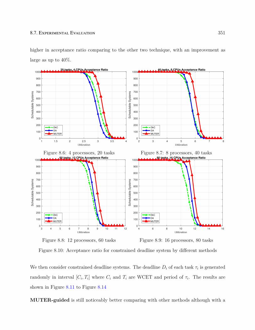
8.7. Experimental Evaluation 351
higher in acceptance ratio comparing to the other two technique, with an improvement as
large as up to 40%.
1 1.5 2 2.5 3 3.5 4
Utilization
0
100
200
300
400
500
600
700
800
900
1000
Sch
ed
ula
ble
Syste
ms
20 tasks, 4 CPUs Acceptance Ratio
DkC
DA
MUTER
Figure 8.6: 4 processors, 20 tasks
2 3 4 5 6 7 8
Utilization
0
100
200
300
400
500
600
700
800
900
1000
Sch
ed
ula
ble
Syste
ms
40 tasks, 8 CPUs Acceptance Ratio
DkC
DA
MUTER
Figure 8.7: 8 processors, 40 tasks
3 4 5 6 7 8 9 10 11 12
Utilization
0
100
200
300
400
500
600
700
800
900
1000
Schedula
ble
Syste
ms
60 tasks, 12 CPUs Acceptance Ratio
DkC
DA
MUTER
Figure 8.8: 12 processors, 60 tasks
4 6 8 10 12 14 16
Utilization
0
100
200
300
400
500
600
700
800
900
1000
Schedula
ble
Syste
ms
80 tasks, 16 CPUs Acceptance Ratio
DkC
DA
MUTER
Figure 8.9: 16 processors, 80 tasks
Figure 8.10: Acceptance ratio for constrained deadline system by different methods
We then consider constrained deadline systems. The deadline Di of each task τi is generated
randomly in interval [Ci, Ti] where Ci and Ti are WCET and period of τi. The results are
shown in Figure 8.11 to Figure 8.14
MUTER-guided is still noticeably better comparing with other methods although with a

352Chapter 8. The Concept of Response Time Estimation Range for Optimizing Systems
Scheduled with Fixed Priority
relatively smaller amount comparing with implicit deadline setting. This is mainly because
the overall schedulability is worse for constrained deadline setting. The two experiments
demonstrate the importance of combining both accurate schedulability analysis and priority
assignment algorithm that can accommodate the analysis
To evaluate the benefit of feasible solution exploration technique used in Figure 8.2, we com-
pare with another method MUTER-NoHeu, that uses only the framework in Figure 8.1.
Figure 8.20 shows the average run-time by MUTER and MUTER-NoHeu.
8.8 Conclusion
In this chapter, we study the optimization of real-time systems where the response time of a
task not only depends on the set of higher/lower priority tasks but also on the response times
of other tasks. We introduce a set of concepts, including the response time estimation range
that replaces the actual response time of each task for checking the system schedulability. We
develop an optimization framework which builds upon such concepts and leverages Audsley’s
algorithm to generalize from an unschedulable solution to many similar ones. Experimental
results on two example systems show that the proposed technique is potentially much faster
than exhaustive search algorithms based on BnB or MILP.
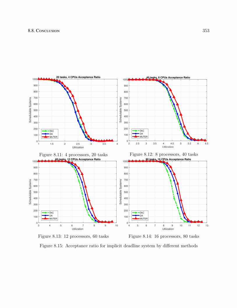
8.8. Conclusion 353
1 1.5 2 2.5 3 3.5 4
Utilization
0
100
200
300
400
500
600
700
800
900
1000
Sch
ed
ula
ble
Syste
ms
20 tasks, 4 CPUs Acceptance Ratio
DkC
DA
MUTER
Figure 8.11: 4 processors, 20 tasks
2 2.5 3 3.5 4 4.5 5 5.5 6 6.5
Utilization
0
100
200
300
400
500
600
700
800
900
1000
Schedula
ble
Syste
ms
40 tasks, 8 CPUs Acceptance Ratio
DkC
DA
MUTER
Figure 8.12: 8 processors, 40 tasks
3 4 5 6 7 8 9 10
Utilization
0
100
200
300
400
500
600
700
800
900
1000
Schedula
ble
Syste
ms
60 tasks, 12 CPUs Acceptance Ratio
DkC
DA
MUTER
Figure 8.13: 12 processors, 60 tasks
4 5 6 7 8 9 10 11 12 13
Utilization
0
100
200
300
400
500
600
700
800
900
1000
Schedula
ble
Syste
ms
80 tasks, 16 CPUs Acceptance Ratio
DkC
DA
MUTER
Figure 8.14: 16 processors, 80 tasks
Figure 8.15: Acceptance ratio for implicit deadline system by different methods

354Chapter 8. The Concept of Response Time Estimation Range for Optimizing Systems
Scheduled with Fixed Priority
1 1.5 2 2.5 3 3.5 4
Utilization
0
2000
4000
6000
8000
10000
12000
14000
16000
Run-t
ime(m
s)
20 tasks, 4 CPUs MUTER Runtime
MUTER
MUTER-NoHeu
Figure 8.16: 4 processors, 20 tasks
2 3 4 5 6 7 8
Utilization
0
0.5
1
1.5
2
2.5
3
3.5
Run-t
ime(m
s)
104 40 tasks, 8 CPUs MUTER Runtime
MUTER
MUTER-NoHeu
Figure 8.17: 8 processors, 40 tasks
3 4 5 6 7 8 9 10 11 12
Utilization
0
0.5
1
1.5
2
2.5
3
3.5
4
4.5
Run-t
ime(m
s)
104 60 tasks, 12 CPUs MUTER Runtime
MUTER
MUTER-NoHeu
Figure 8.18: 12 processors, 60 tasks
4 6 8 10 12 14 16
Utilization
0
1
2
3
4
5
6
Ru
n-t
ime
(ms)
104 80 tasks, 16 CPUs MUTER Runtime
MUTER
MUTER-NoHeu
Figure 8.19: 16 processors, 80 tasks
Figure 8.20: Average Runtime by MUTER and MUTER-NoHeu
Chapter 9
Conclusion
9.1 Summary
In this dissertation, we propose and discuss two paradigm-shifting directions for developing
optimization algorithms for the design of time-critical Cyber Physical Systems. We present
a number of studies to demonstrate and explain the use of these two directions, thoughts and
principles for algorithm development in different problem settings and the potential benefit
it can bring.
Specifically, the first direction is to develop optimization-oriented schedulability analysis
that have an efficient formulation in existing mathematical programming framework. We
present a study in Chapter 2 that considers the problem of efficiently formulating the fea-
sibility region of schedulability for adaptive mixed-criticality systems. We develop a new
schedulability analysis based on request bound function. The new analysis is much more
efficient to be formulated as mixed-integer linear programming in the sense that the number
of binary and integer variables needed is much smaller. The new formulation shows signifi-
cant improvement in optimizing implementation of Simulink SR model and task allocation
for multiprocessor platforms.
We then use the remaining chapters to discuss the second approach: developing domain-
specific optimization framework. The overall idea is to abstract the feasibility region of
355

356 Chapter 9. Conclusion
schedulability into a simple and uniform mathematical form that can be formulated effi-
ciently in mathematical programming framework, which separates optimization and schedu-
lability analysis. We first present a study in Chapter 3 that discusses the concept of
unschedulability-core and how it can be used as an alternative and much simpler repre-
sentation of the schedulability region. We then develop an iterative optimization framework
guided by unschedulability-core. The technique gives significant improvement in runtime
and scalability comparing to mathematical programming approach. In Chapter 4, We apply
the technique to optimizing Finite State Machine systems, which has a much more difficult
schedulability analysis. We show that the proposed optimization framework is flexible for
integrating different techniques to improve efficiency. Specifically, We show how schedulabil-
ity memoization and hierarchical relaxation can be seamlessly integrated into the framework
to significantly improve efficiency.
In Chapter 5 and Chapter 6, we extend the concept of unschedulability core to MUDA
and MUPDA and correspondingly generalize the iterative optimization framework. This
allows the framework to solve challenging optimization problems that involve response time,
period and priority assignment co-optimization. Evaluation on several industrial case studies
demonstrates that the technique provides significant benefits in runtime, applicability and
solution quality.
We further generalize the framework in Chapter 7 such that it is applicable to all problems
where decision variables are sustainable w.r.t. the schedulability analysis and objective
functions are monotonic w.r.t decision variables. This allows the framework to solve problems
that involve much more complicated objective functions. Evaluation on synthetic system and
industrial case studies demonstrate significant improvement in terms of runtime, applicability
to different schedulability analysis and solution quality.
Finally, in Chapter 8, we consider a type of schedulability analyses characterized by re-
9.2. Remaining Challenges and Future Work 357
sponse time dependency. For these analyses, the well known Audsley’s algorithm cannot be
applied to find feasible priority assignment, which undermines the applicability of the pro-
posed iterative optimization framework. We take a different perspective and reformulate the
problem into finding a schedulable response time estimation. We introduce a new concept
called maximal unschedulable response time estimation range, which largely follows the same
underlying principle as MUDA, and develop a similar iterative optimization framework for
solving the optimization problems that use such type of schedulability analysis. Evaluation
on random system and industrial case study demonstrate noticeable improvement in terms
of acceptance ratio, scalability, solution quality and runtime.
9.2 Remaining Challenges and Future Work
The studies presented in this dissertation demonstrate the relevance and effectiveness of the
new directions for developing algorithms for design optimization of CPS. However, challenges
and issues still exist and the need for more research into the realm of CPS design optimization
continues to be vital. In this section, we summarize the main issues regarding the two
proposed directions that can be addressed in future work.
9.2.1 Developing optimization-oriented schedulability analysis
The major limitation of this direction is that it is not always possible to find an alternative
schedulability analysis that is optimization friendly. This is because some system models
and scheduling policies are inherently difficult to formulate. Consider the task graph and
finite state machine system mentioned in Chapter 4. These system models are developed in
a way that inherently requires to exhaustively examine all state transition paths to identify

358 Chapter 9. Conclusion
the worst-case workload. Such a characteristic eventually leads to the extreme difficulty
in developing schedulability analyses that are efficient for optimization without introducing
significant pessimism. This again refers back to the major issue suffered by design optimiza-
tion of CPS discussed in Chapter 1: System model and schedulability analysis have long
been developed in a way without any consideration of the need for optimization. Therefore,
a possible direction in CPS design is to integrate the need of optimization early into the
development of system model and formulation of schedulability analysis.
9.2.2 Developing new domain-specific optimization framework
Developing domain-specific optimization framework alleviates the issue suffered by the first
direction to some extent by abstracting and separating schedulability analysis away from
optimization algorithms. The key to achieving scalability in this approach is that schedula-
bility analysis, which is extensively used in computing domain specific abstraction, needs to
be highly efficient. This however, can be difficult to achieve for some problem settings. A no-
table example here is task allocation in partitioned scheduling on multiprocessor platforms.
Consider the experimental vehicle system case study discussed in Chapter 5. In the case
study, task allocation is assumed to be given and fixed. This makes schedulability analysis
a lot easier as it is essentially the same as uni-processor scheduling with multiple indepen-
dent processors. However, if task allocation is not given, schedulability analysis becomes
extremely difficult, as it is first necessary to find a proper allocation, which is generally
an NP-hard problem for most task models. As a result, the second direction is typically
inapplicable to problems that involves task allocation. The use of multi-processor platform
is becoming wide-spread in CPS. A framework/approach that can efficiently integrate task-
allocation and schedulability analysis into optimization is critical to the design of CPS in
the future.
Bibliography
[1] Benny Akesson, Anna Minaeva, Premysl Sucha, Andrew Nelson, and Zdenek Hanzálek.
An efficient configuration methodology for time-division multiplexed single resources.
In Real-Time and Embedded Technology and Applications Symposium (RTAS), 2015
IEEE, pages 161–171. IEEE, 2015.
[2] Z. Al-bayati, H. Zeng, M. Di Natale, and Z. Gu. Multitask implementation of syn-
chronous reactive models with earliest deadline first scheduling. In IEEE Symposium
on Industrial Embedded Systems, 2013.
[3] Sebastian Altmeyer, Liliana Cucu-Grosjean, and Robert I. Davis. Static probabilistic
timing analysis for real-time systems using random replacement caches. Real-Time
Syst., 51(1):77–123, January 2015.
[4] K-E Arzén, Anton Cervin, Johan Eker, and Lui Sha. An introduction to control and
scheduling co-design. In IEEE Conference on Decision and Control, 2000.
[5] Karl J. Åström and Björn Wittenmark. Computer-controlled Systems (3rd Ed.).
Prentice-Hall, Inc., 1997. ISBN 0-13-314899-8.
[6] N. Audsley, A. Burns, M. Richardson, and A. Wellings. Hard real-time scheduling: the
deadline-monotonic approach. In IEEE Workshop on Real-Time Operating Systems
and Software, 1991.
[7] N. Audsley, A. Burns, M. Richardson, K. Tindell, and A. J. Wellings. Applying
new scheduling theory to static priority pre-emptive scheduling. Software Engineering
Journal, 8:284–292, 1993.
359
360 BIBLIOGRAPHY
[8] N.C. Audsley. On priority assignment in fixed priority scheduling. Information Pro-
cessing Letters, 79(1):39 – 44, 2001.
[9] N.C. Audsley. On priority assignment in fixed priority scheduling. Information Pro-
cessing Letters, 79(1):39 – 44, 2001.
[10] Neil Audsley. Optimal priority assignment and feasibility of static priority tasks with
arbitrary start times. Technical Report YCS 164, Department of Computer Science,
University of York, UK, 1991.
[11] P. Axer et al. Building timing predictable embedded systems. ACM Trans. Embed.
Comput. Syst., 13(4):82:1–82:37, March 2014.
[12] Akramul Azim, Gonzalo Carvajal, Rodolfo Pellizzoni, and Sebastian Fischmeister.
Generation of communication schedules for multi-mode distributed real-time applica-
tions. In Design, Automation and Test in Europe Conference and Exhibition (DATE),
2014, pages 1–6. IEEE, 2014.
[13] Mario Bambagini, Mauro Marinoni, Hakan Aydin, and Giorgio Buttazzo. Energy-
aware scheduling for real-time systems: A survey. ACM Trans. Embed. Comput. Syst.
(TECS), 15(1):7:1–7:34, January 2016. ISSN 1539-9087.
[14] S. Baruah, V. Bonifaci, G. D’Angelo, H. Li, A. Marchetti-Spaccamela, S. van der Ster,
and L. Stougie. The preemptive uniprocessor scheduling of mixed-criticality implicit-
deadline sporadic task systems. In Euromicro Conference on Real-Time Systems, 2012.
[15] Sanjoy Baruah. Implementing mixed-criticality synchronous reactive programs upon
uniprocessor platforms. Real-Time Syst., 50(3):317–341, 2014.
[16] Sanjoy Baruah and Alan Burns. Sustainable scheduling analysis. In IEEE Real-Time
Systems Symposium, 2006.
BIBLIOGRAPHY 361
[17] Sanjoy Baruah and Alan Burns. Implementing mixed criticality systems in ada. In
Reliable Software Technologies-Ada-Europe 2011, pages 174–188. Springer, 2011.
[18] Sanjoy K. Baruah. Dynamic- and static-priority scheduling of recurring real-time tasks.
Real-Time Syst., 24(1):93–128, January 2003.
[19] Sanjoy K Baruah, Alan Burns, and Robert I Davis. Response-time analysis for mixed
criticality systems. In 2011 IEEE 32nd Real-Time Systems Symposium, pages 34–43.
IEEE, 2011.
[20] S.K. Baruah, A. Burns, and R.I. Davis. Response-time analysis for mixed criticality
systems. In 32nd IEEE Real-Time Systems Symposium, 2011.
[21] Andrea Bastoni, Björn Brandenburg, and James Anderson. Cache-related preemption
and migration delays: Empirical approximation and impact on schedulability. In 6th
Workshop on Operating Systems Platforms for Embedded Real-Time Applications, pages
33–44, 2010.
[22] I. Bate and P. Emberson. Incorporating scenarios and heuristics to improve flexibility
in real-time embedded systems. In IEEE Real-Time and Embedded Technology and
Applications Symposium, 2006.
[23] Kateryna Bazaka and Mohan V Jacob. Implantable devices: issues and challenges.
Electronics, 2(1):1–34, 2012.
[24] Marko Bertogna, Michele Cirinei, and Giuseppe Lipari. Schedulability analysis of
global scheduling algorithms on multiprocessor platforms. IEEE Transactions on par-
allel and distributed systems, 20(4):553–566, 2008.
[25] Enrico Bini and Giorgio C. Buttazzo. Schedulability analysis of periodic fixed priority
systems. IEEE Trans. Comput., 53(11):1462–1473, 2004.

362 BIBLIOGRAPHY
[26] Enrico Bini and Anton Cervin. Delay-aware period assignment in control systems. In
IEEE Real-Time Systems Symposium, 2008.
[27] Enrico Bini and Anton Cervin. Delay-aware period assignment in control systems. In
IEEE Real-Time Systems Symposium, 2008.
[28] Enrico Bini and Marco Di Natale. Optimal task rate selection in fixed priority systems.
In IEEE Real-Time Systems Symposium, 2005.
[29] Blind. Exact and approximate methods for response time analysis of tasks implement-
ing synchronous finite state machines. submitted, 2017.
[30] Frédéric Boussinot and Robert De Simone. The esterel language. Proceedings of the
IEEE, 79(9):1293–1304, 1991.
[31] A. Burns and R. Davis. Adaptive mixed criticality scheduling with deferred preemp-
tion. In IEEE Real-Time Systems Symposium, 2014.
[32] Alan Burns and Robert I. Davis. A survey of research into mixed criticality systems.
ACM Comput. Surv., 50(6):82:1–82:37, November 2017.
[33] Alan Burns, James Harbin, and Leandro Indrusiak. A wormhole noc protocol for mixed
criticality systems. In IEEE Real-Time Systems Symposium, 2014.
[34] Giorgio C Buttazzo. Hard real-time computing systems: predictable scheduling algo-
rithms and applications, volume 24. Springer Science & Business Media, 2011.
[35] P. Caspi, A. Curic, A. Maignan, C. Sofronis, S. Tripakis, and P. Niebert. From simulink
to scade/lustre to tta: A layered approach for distributed embedded applications. In
ACM Conf. Language, Compiler, and Tool for Embedded Systems, 2003.
BIBLIOGRAPHY 363
[36] P. Caspi, N. Scaife, C. Sofronis, and S. Tripakis. Semantics-preserving multitask im-
plementation of synchronous programs. ACM Trans. Embed. Comput. Syst., 7(2):1–40,
2008.
[37] Paul Caspi and Albert Benveniste. Time-robust discrete control over networked loosely
time-triggered architectures. In IEEE Conf. Decision & Control, 2008.
[38] Shiladri Chakraborty. Keynote talk: Challenges in automotive cyber-physical systems
design. In 25th International Conference on VLSI Design (VLSID), pages 9–10. IEEE,
2012.
[39] Youngjin Cho, Younghyun Kim, Yongsoo Joo, Kyungsoo Lee, and Naehyuck Chang.
Simultaneous optimization of battery-aware voltage regulator scheduling with dynamic
voltage and frequency scaling. In ACM/IEEE International Symposium on Low Power
Electronics and Design, pages 309–314, Aug 2008.
[40] Yanching Chu and Alan Burns. Flexible hard real-time scheduling for deliberative ai
systems. Real-Time Systems, 40(3):241–263, 2008.
[41] Abhijit Davare, Qi Zhu, Marco Di Natale, Claudio Pinello, Sri Kanajan, and Alberto
Sangiovanni-Vincentelli. Period optimization for hard real-time distributed automotive
systems. In ACM/IEEE Design Automation Conference, 2007.
[42] Abhijit Davare, Qi Zhu, Marco Di Natale, Claudio Pinello, Sri Kanajan, and Alberto
Sangiovanni-Vincentelli. Period optimization for hard real-time distributed automotive
systems. In Design Automation Conference, 2007.
[43] Abhijit Davare, Douglas Densmore, Liangpeng Guo, Roberto Passerone, Alberto L.
Sangiovanni-Vincentelli, Alena Simalatsar, and Qi Zhu. metroII: A design environment

364 BIBLIOGRAPHY
for cyber-physical systems. ACM Trans. Embed. Comput. Syst. (TECS), 12(1s):49:1–
49:31, March 2013.
[44] R. Davis and A. Burns. Robust priority assignment for fixed priority real-time systems.
In IEEE Real-Time Systems Symposium, 2007.
[45] Robert Davis, Alan Burns, Reinder Bril, and Johan Lukkien. Controller area network
schedulability analysis: Refuted, revisited and revised. Real-Time Systems, 35(3):
239–272, 2007.
[46] Robert Davis, Alan Burns, Reinder Bril, and Johan Lukkien. Controller area network
(can) schedulability analysis: Refuted, revisited and revised. Real-Time Systems, 35
(3):239–272, 2007.
[47] Robert Davis, Attila Zabos, and Alan Burns. Efficient exact schedulability tests for
fixed priority real-time systems. IEEE Transactions on Computers, 57(9):1261–1276,
2008.
[48] Robert Davis, Liliana Cucu-Grosjean, Marko Bertogna, and Alan Burns. A review of
priority assignment in real-time systems. J. Syst. Archit., 65(C):64–82, April 2016.
ISSN 1383-7621.
[49] Robert I Davis and Marko Bertogna. Optimal fixed priority scheduling with deferred
pre-emption. In IEEE Real-Time Systems Symposium, 2012.
[50] Robert I. Davis and Alan Burns. Priority assignment for global fixed priority pre-
emptive scheduling in multiprocessor real-time systems. In IEEE Real-Time Systems
Symposium, 2009.
[51] Robert I Davis and Alan Burns. On optimal priority assignment for response time

BIBLIOGRAPHY 365
analysis of global fixed priority pre-emptive scheduling in multiprocessor hard real-
time systems. University of York, UK, Tech. Rep YCS-2010, 451, 2010.
[52] Robert I Davis and Alan Burns. Improved priority assignment for global fixed priority
pre-emptive scheduling in multiprocessor real-time systems. Real-Time Systems, 47
(1):1–40, 2011.
[53] Robert I. Davis, Liliana Cucu-Grosjean, Marko Bertogna, and Alan Burns. A review
of priority assignment in real-time systems. J. Syst. Archit., 65(C):64–82, April 2016.
[54] Dionisio De Niz, Karthik Lakshmanan, and Ragunathan Rajkumar. On the scheduling
of mixed-criticality real-time task sets. In 30th IEEE Real-Time Systems Symposium,
pages 291–300, 2009.
[55] Peng Deng, Qi Zhu, Fabio Cremona, Marco Di Natale, and Haibo Zeng. A model-
based synthesis flow for automotive cps. In ACM/IEEE International Conference on
Cyber-Physical Systemsn, April 2015.
[56] Peng Deng, Qi Zhu, Abhijit Davare, Anastasios Mourikis, Xue Liu, and Marco Di Na-
tale. An efficient control-driven period optimization algorithm for distributed real-time
systems. IEEE Transactions on Computers, 65(12):3552–3566, 2016.
[57] M. Di Natale and V. Pappalardo. Buffer optimization in multitask implementations
of simulink models. ACM Trans. Embed. Comput. Syst., 7(3):1–32, 2008.
[58] M. Di Natale, L. Guo, H. Zeng, and A. Sangiovanni-Vincentelli. Synthesis of multi-
task implementations of simulink models with minimum delays. IEEE Trans. Industrial
Informatics, 6(4):637–651, 2010.
[59] Marco Di Natale and Haibo Zeng. Practical issues with the timing analysis of the
366 BIBLIOGRAPHY
controller area network. In IEEE Conference on Emerging Technologies & Factory
Automation, 2013.
[60] Marco Di Natale, Paolo Giusto, Sri Kanajan, Claudio Pinello, and Patrick Popp. Op-
timizing end-to-end latencies by adaptation of the activation events in distributed
automotive systems. In Society of Automotive Engineers World Congress, 2007.
[61] Robert P Dick, David L Rhodes, and Wayne Wolf. TGFF: task graphs for free. In 6th
international workshop on Hardware/software codesign, 1998.
[62] John Eidson, Edward A. Lee, Slobodan Matic, Sanjit Seshia, and Jia Zou. Distributed
real-time software for cyber-physical systems. Proceedings of the IEEE, 100(1):45 – 59,
January 2012.
[63] Friedrich Eisenbrand and Thomas Rothvoß. Static-priority real-time scheduling: Re-
sponse time computation is np-hard. In IEEE Real-Time Systems Symposium, 2008.
[64] Nico Feiertag, Kai Richter, Johan Nordlander, and Jan Jonsson. A compositional
framework for end-to-end path delay calculation of automotive systems under different
path semantics. In IEEE Real-Time Systems Symposium, 2009.
[65] Alberto Ferrari, Marco Di Natale, Giacomo Gentile, Giovanni Reggiani, and Paolo
Gai. Time and memory tradeoffs in the implementation of autosar components. In
Conference on Design, Automation and Test in Europe, 2009.
[66] Alberto Ferrari, Marco Di Natale, Giacomo Gentile, Giovanni Reggiani, and Paolo
Gai. Time and memory tradeoffs in the implementation of autosar components. In
Proceedings of the Conference on Design, Automation and Test in Europe, pages 864–
869. European Design and Automation Association, 2009.
BIBLIOGRAPHY 367
[67] B. Fleming. An overview of advances in automotive electronics. IEEE Vehicular
Technology Magazine, 9(1):4–9, March 2014.
[68] Tim Fleming and Alan Burns. Extending mixed criticality scheduling. In Workshop
on Mixed Criticality Systems (WMC), 2013.
[69] J. Forget, F. Boniol, D. Lesens, and C. Pagetti. A multi-periodic synchronous data-flow
language. In IEEE High Assurance Systems Engineering Symposium, 2008.
[70] M. Garcia-Valls, D. Perez-Palacin, and R. Mirandola. Time-sensitive adaptation in
cps through run-time configuration generation and verification. In IEEE 38th Annual
Computer Software and Applications Conference, pages 332–337, July 2014.
[71] J. B. Goodenough and L. Sha. The priority ceiling protocol: A method for minimizing
the blocking of high priority ada tasks. Ada Lett., VIII(7):20–31, June 1988.
[72] Nan Guan, Martin Stigge, Wang Yi, and Ge Yu. New response time bounds for fixed
priority multiprocessor scheduling. In 2009 30th IEEE Real-Time Systems Symposium,
pages 387–397. IEEE, 2009.
[73] Zhishan Guo, Sai Sruti, Bryan C Ward, and Sanjoy Baruah. Sustainability in mixed-
criticality scheduling. In 2017 IEEE Real-Time Systems Symposium (RTSS), pages
24–33. IEEE, 2017.
[74] N. Halbwachs, P. Caspi, P. Raymond, and D. Pilaud. The synchronous data flow
programming language lustre. Proceedings of the IEEE, 79(9):1305–1320, 1991.
[75] A. Hamann, M. Jersak, K. Richter, and R. Ernst. Design space exploration and system
optimization with symta/s - symbolic timing analysis for systems. In IEEE Real-Time
Systems Symposium, 2004.
368 BIBLIOGRAPHY
[76] Qiushi Han, Ming Fan, Linwei Niu, and Gang Quan. Energy minimization for fault
tolerant scheduling of periodic fixed-priority applications on multiprocessor platforms.
In Proceedings of the 2015 Design, Automation & Test in Europe Conference & Exhi-
bition, pages 830–835. EDA Consortium, 2015.
[77] T. A. Henzinger, B. Horowitz, and C. M. Kirsch. Giotto: a time-triggered language
for embedded programming. Proceedings of the IEEE, 91(1):84–99, Jan 2003.
[78] Huang-Ming Huang, Christopher Gill, and Chenyang Lu. Implementation and evalua-
tion of mixed-criticality scheduling approaches for sporadic tasks. ACM Transactions
on Embedded Computing Systems, 13(4s):126, 2014.
[79] Pengcheng Huang, Georgia Giannopoulou, Nikolay Stoimenov, and Lothar Thiele.
Service adaptions for mixed-criticality systems. In 2014 19th Asia and South Pacific
Design Automation Conference (ASP-DAC), pages 125–130. IEEE, 2014.
[80] Pengcheng Huang, Pratyush Kumar, Georgia Giannopoulou, and Lothar Thiele. En-
ergy efficient dvfs scheduling for mixed-criticality systems. In Proceedings of the 14th
International Conference on Embedded Software, page 11. ACM, 2014.
[81] L. Indrusiak, J. Harbin, and A. Burns. Average and worst-case latency improvements in
mixed-criticality wormhole networks-on-chip. In Euromicro Conference on Real-Time
Systems, 2015.
[82] Microcontroller. Infineon. [Online] http://www.infineon.com/microcontrollers. Re-
trieved in January 2019.
[83] CPLEX Optimizer. International Business Machines Corporation, . [Online]
http://www.ibm.com/software/commerce/optimization/cplex-optimizer/.

BIBLIOGRAPHY 369
[84] IEC 62304:2006 Medical device software - Software life cycle processes. International
Electrotechnical Commission, . [Online] https://webstore.iec.ch/publication/6792.
[85] ISO 26262-1:2011(en) Road vehicles – Functional safety – Part 1:
Vocabulary. International Standardization Organization, . [Online]
https://www.iso.org/obp/ui/#iso:std:iso:26262:-1:ed-1:v1:en.
[86] O.R. Kelly, H. Aydin, and Baoxian Zhao. On partitioned scheduling of fixed-priority
mixed-criticality task sets. In IEEE International Conference on Trust, Security and
Privacy in Computing and Communications (TrustCom), Nov 2011.
[87] K. D. Kim and P. R. Kumar. Cyber-physical systems: A perspective at the centennial.
Proceedings of the IEEE, 100:1287–1308, May 2012.
[88] John Koon. Overview of the Medical Semiconductor Market and Applications. Infineon.
[Online] http://medsmagazine.com/2012/04/overview-of-the-medical-semiconductor-
market-and-applications/. Retrieved in January 2019.
[89] Simon Kramer, Dirk Ziegenbein, and Arne Hamann. Real world automotive bench-
marks for free. In International Workshop on Analysis Tools and Methodologies for
Embedded and Real-time Systems (WATERS), 2015.
[90] Edward Lee and Pravin Varaiya. Structure and Interpretation of Signals and Systems,
2nd Edition. LeeVaraiya.org, 2011.
[91] Edward A. Lee. Cyber physical systems: Design challenges. In International
Symposium on Object/Component/Service-Oriented Real-Time Distributed Computing
(ISORC), May 2008.
[92] Edward A Lee. Computing needs time. Communications of the ACM, 52(5):70–79,
2009.
370 BIBLIOGRAPHY
[93] Edward A Lee. CPS foundations. In 47th ACM/IEEE Design Automation Conference
(DAC), 2010.
[94] P. LeGuernic, T. Gautier, M. Le Borgne, and C. Le Maire. Programming real-time
applications with signal. Proceedings of the IEEE, 79(9):1321–1336, 1991.
[95] J.P. Lehoczky, L. Sha, and Y. Ding. The rate monotonic scheduling algorithm: Ex-
act characterization and average case behavior. In 10th IEEE Real-Time Systems
Symposium, 1989.
[96] Adam N. Letchford and Andrea Lodi. Strengthening chvátal-gomory cuts and gomory
fractional cuts. Oper. Res. Lett., 30(2):74–82, April 2002.
[97] Joseph Y-T Leung and Jennifer Whitehead. On the complexity of fixed-priority
scheduling of periodic, real-time tasks. Performance evaluation, 2(4):237–250, 1982.
[98] Bo Lincoln and Anton Cervin. Jitterbug: A tool for analysis of real-time control
performance. In IEEE Conf. Decision and Control, 2002.
[99] C. L. Liu and James W. Layland. Scheduling algorithms for multiprogramming in a
hard-real-time environment. J. ACM, 20(1):46–61, January 1973. ISSN 0004-5411.
doi: 10.1145/321738.321743. URL http://doi.acm.org/10.1145/321738.321743.
[100] C. L. Liu and James W. Layland. Scheduling algorithms for multiprogramming in a
hard-real-time environment. J. ACM, 20(1):46–61, January 1973.
[101] J. Löfberg. Yalmip : A toolbox for modeling and optimization in matlab. In IEEE
Symposium on Computer Aided Control Systems Design, 2004.
[102] Martin Lukasiewycz, Philipp Mundhenk, and Sebastian Steinhorst. Security-aware
obfuscated priority assignment for automotive can platforms. ACM Trans. Des. Autom.
Electron. Syst., 21(2):1–27, January 2016.

BIBLIOGRAPHY 371
[103] G.. Mancuso, Enrico Bini, and Gabriele Pannocchia. Optimal priority assignment to
control tasks. ACM Trans. Embed. Comput. Syst., 13(5s):1–17, 2014.
[104] Giulio Mancuso, Enrico Bini, and Gabriele Pannocchia. Optimal priority assignment
to control tasks. ACM Trans. Embedded Computing Systems, 13(5s):161, 2014.
[105] The MathWorks Simulink and StateFlow User’s Manuals. MathWorks. [Online]
http://www.mathworks.com.
[106] Mischa Möstl, Johannes Schlatow, Rolf Ernst, Nikil D. Dutt, Ahmed Nassar, Amir-
Mohammad Rahmani, Fadi J. Kurdahi, Thomas Wild, Armin Sadighi, and Andreas
Herkersdorf. Platform-centric self-awareness as a key enabler for controlling changes
in CPS. Proceedings of the IEEE, 106(9):1543–1567, Sept 2018.
[107] Almir Mutapcic, Kwangmoo Koh, Seungjean Kim, and Stephen Boyd. Ggplab version
1.00: a matlab toolbox for geometric programming, January 2006.
[108] M. Di Natale and H. Zeng. Task implementation of synchronous finite state machines.
In Conference on Design, Automation Test in Europe, 2012.
[109] M. Di Natale, L. Guo, H. Zeng, and A. Sangiovanni-Vincentelli. Synthesis of multi-
task implementations of simulink models with minimum delays. IEEE Trans. Industrial
Informatics, 6(4):637–651, 2010.
[110] Marco Di Natale, Wei Zheng, Claudio Pinello, Paolo Giusto, and Alberto L.
Sangiovanni-Vincentelli. Optimizing end-to-end latencies by adaptation of the acti-
vation events in distributed automotive systems. In IEEE Real-Time and Embedded
Technology and Applications Symposium, 2007.
[111] Cyber Physical Systems Program. National Institute of Standards and Technology

372 BIBLIOGRAPHY
(NIST), September 2016. [Online] www.nist.gov/programs-projects/cyber-physical-
systems-program. Retrieved in January 2019.
[112] Andrew Nelson, Orlando Moreira, Anca Molnos, Sander Stuijk, Ba Thang Nguyen,
and Kees Goossens. Power minimisation for real-time dataflow applications. In 2011
14th Euromicro Conference on Digital System Design, pages 117–124. IEEE, 2011.
[113] Cyber Physical Systems Vision Statement. The Networking and Information Technol-
ogy Research and Development (NITRD) Program, June 2015.
[114] Borislav Nikolić and Luís Miguel Pinho. Optimal minimal routing and priority as-
signment for priority-preemptive real-time nocs. Real-Time Systems, 53(4):578–612,
2017.
[115] NXP Automotive MCUs and MPUs. NXP Semiconductor. [Online]
www.nxp.com/docs/en/product-selector-guide/BRAUTOPRDCTMAP.pdf. Re-
trieved in January 2019.
[116] Muhittin Oral and Ossama Kettani. A linearization procedure for quadratic and cubic
mixed-integer problems. Oper. Res., 40(S1):109–116, January 1992.
[117] Santiago Pagani and Jian-Jia Chen. Energy efficiency analysis for the single frequency
approximation (sfa) scheme. ACM Transactions on Embedded Computing Systems
(TECS), 13(5s):158, 2014.
[118] C. Pagetti, J. Forget, F. Boniol, M. Cordovilla, and D. Lesens. Multi-task implemen-
tation of multi-periodic synchronous programs. Discrete Event Dynamic Systems, 21
(3):307–338, 2011.
[119] C. Pagetti, D. Saussié, R. Gratia, E. Noulard, and P. Siron. The ROSACE case study:

BIBLIOGRAPHY 373
From simulink specification to multi/many-core execution. In IEEE Real-Time and
Embedded Technology and Applications Symposium, 2014.
[120] M. Panic, S. Kehr, E. Quiñones, B. Boddecker, J. Abella, and F. J. Cazorla. Runpar:
An allocation algorithm for automotive applications exploiting runnable parallelism
in multicores. In 2014 International Conference on Hardware/Software Codesign and
System Synthesis (CODES+ISSS), pages 1–10, Oct 2014.
[121] D. Potop-Butucaru, B. Caillaud, and A. Benveniste. Concurrency in synchronous
systems. In Int. Conf. Application of Concurrency to System Design, 2004.
[122] D. Potop-Butucaru, S. A. Edwards, and G. Berry. Compiling Esterel. Springer, 2007.
[123] W. Puffitsch, E. Noulard, and C. Pagetti. Mapping a multi-rate synchronous lan-
guage to a many-core processor. In IEEE Real-Time and Embedded Technology and
Applications Symposium, 2013.
[124] R. Rajkumar, Insup Lee, Lui Sha, and J. Stankovic. Cyber-physical systems: The next
computing revolution. In 47th ACM/IEEE Design Automation Conference (DAC),
June 2010.
[125] S. Ramesh. Automobile: Aircraft or smartphone? modeling challenges and oppor-
tunities in automotive systems (keynote). In 2015 ACM/IEEE 18th International
Conference on Model Driven Engineering Languages and Systems (MODELS), page 3,
Sept 2015.
[126] DO-178C Software Considerations in Airborne Systems and Equipment Certification.
RTCA.
[127] M. Saksena and Yun Wang. Scalable real-time system design using preemption thresh-
olds. In IEEE Real-Time Systems Symposium, 2000.

374 BIBLIOGRAPHY
[128] Soheil Samii, Yanfei Yin, Zebo Peng, Petru Eles, and Yuanping Zhang. Immune genetic
algorithms for optimization of task priorities and flexray frame identifiers. In IEEE
Conf. Embedded and Real-Time Computing Systems and Applications, 2009.
[129] A. Sangiovanni-Vincentelli, W. Damm, and R. Passerone. Taming dr. frankenstein:
Contract-based design for cyber-physical systems. European Journal of Control, 18(3):
217–238, 2012.
[130] S. A. Seshia, S. Hu, W. Li, and Q. Zhu. Design automation of cyber-physical systems:
Challenges, advances, and opportunities. IEEE Transactions on Computer-Aided De-
sign of Integrated Circuits and Systems (TCAD), PP(99):1–15, 2017.
[131] D. Seto, J. P. Lehoczky, L. Sha, and K. G. Shin. On task schedulability in real-time
control systems. In 17th IEEE Real-Time Systems Symposium, pages 13–21, Dec 1996.
doi: 10.1109/REAL.1996.563693.
[132] Danbing Seto, John P. Lehoczky, and Lui Sha. Task period selection and schedulability
in real-time systems. In IEEE Real-Time Systems Symposium, 1998.
[133] Zheng Shi and Alan Burns. Priority assignment for real-time wormhole communication
in on-chip networks. In IEEE Real-Time Systems Symposium, 2008.
[134] M. Shin and M. Sunwoo. Optimal period and priority assignment for a networked
control system scheduled by a fixed priority scheduling system. International Journal
of Automotive Technology, 8:39–48, 2007.
[135] J. Sifakis. Rigorous design of cyber-physical systems. In International Conference on
Embedded Computer Systems (SAMOS), July 2012.
[136] M. Stigge and W. Yi. Hardness results for static priority real-time scheduling. In
Euromicro Conference on Real-Time Systems, 2012.

BIBLIOGRAPHY 375
[137] Martin Stigge and Wang Yi. Combinatorial abstraction refinement for feasibility anal-
ysis of static priorities. Real-Time Systems, 51(6):639–674, 2015.
[138] Martin Stigge and Wang Yi. Combinatorial abstraction refinement for feasibility anal-
ysis of static priorities. Real-time systems, 51(6):639–674, 2015.
[139] Martin Stigge, Pontus Ekberg, Nan Guan, and Wang Yi. The digraph real-time task
model. In IEEE Real-Time and Embedded Technology and Applications Symposium,
2011.
[140] J. Sztipanovits, X. Koutsoukos, G. Karsai, N. Kottenstette, P. Antsaklis, V. Gupta,
B. Goodwine, J. Baras, and Shige Wang. Toward a science of cyber-physical system
integration. Proceedings of the IEEE, 100(1):29–44, Jan 2012.
[141] The AUTOSAR Adaptive Platform. [online:] https://www.autosar.org/
standards/adaptive-platform/.
[142] K. Tindell, A. Burns, and A. Wellings. Allocating hard real-time tasks: An np-hard
problem made easy. Real-Time Syst., 4(2):145–165, 1992.
[143] Transistor count. [online:] https://en.wikipedia.org/wiki/Transistor_count.
[144] S. Tripakis, C. Pinello, A. Benveniste, A. Sangiovanni-Vincent, P. Caspi, and M. Di Na-
tale. Implementing synchronous models on loosely time-triggered architectures. IEEE
Transactions on Computers, 57(10):1300–1314, 2008.
[145] S. Vestal. Preemptive scheduling of multi-criticality systems with varying degrees of
execution time assurance. In 28th IEEE Real-Time Systems Symposium, Dec 2007.
[146] Chao Wang, Zonghua Gu, and Haibo Zeng. Global fixed priority scheduling with pre-
emption threshold: Schedulability analysis and stack size minimization. IEEE Trans-
actions on Parallel and Distributed Systems, 27(11):3242–3255, 2016.
376 BIBLIOGRAPHY
[147] Yun Wang and M. Saksena. Scheduling fixed-priority tasks with preemption threshold.
In International Conference on Real-Time Computing Systems and Applications, 1999.
[148] Floor and ceiling functions. Wikipedia. [Online]
https://en.wikipedia.org/wiki/Floor_and_ceiling_functions.
[149] E. Wozniak, A. Mehiaoui, C. Mraidha, S. Tucci-Piergiovanni, and S. Gerard. An opti-
mization approach for the synthesis of autosar architectures. In 18th IEEE Conference
on Emerging Technologies Factory Automation, Sept 2013.
[150] Ernest Wozniak, Marco Di Natale, Haibo Zeng, Chokri Mraidha, Sara Tucci-
Piergiovanni, and Sebastien Gerard. Assigning time budgets to component functions
in the design of time-critical automotive systems. In ACM/IEEE International Con-
ference on Automated Software Engineering, 2014.
[151] H. Zeng and M. Di Natale. Mechanisms for guaranteeing data consistency and time
determinism in autosar software on multicore platforms. In IEEE Symposium on
Industrial Embedded Systems, 2011.
[152] H. Zeng and M. Di Natale. Schedulability analysis of periodic tasks implementing
synchronous finite state machines. In Euromicro Conference on Real-Time Systems,
2012.
[153] H. Zeng and M. Di Natale. Efficient implementation of autosar components with
minimal memory usage. In IEEE International Symposium on Industrial Embedded
Systems, 2012.
[154] H. Zeng, A. Ghosal, and M. Di Natale. Timing analysis and optimization of flexray dy-
namic segment. In 10th IEEE International Conference on Computer and Information
Technology, pages 1932–1939, June 2010.

BIBLIOGRAPHY 377
[155] Haibo Zeng and Marco Di Natale. An efficient formulation of the real-time feasibility
region for design optimization. IEEE Transactions on Computers, 62(4):644–661, April
2013.
[156] Haibo Zeng, Marco Di Natale, and Qi Zhu. Minimizing stack and communication
memory usage in real-time embedded applications. ACM Trans. Embed. Comput.
Syst., 13(5s):149:1–149:25, July 2014.
[157] Qingling Zhao, Zonghua Gu, and Haibo Zeng. PT-AMC: Integrating Preemption
Thresholds into Mixed-Criticality Scheduling. In Conference on Design, Automation
and Test in Europe, 2013.
[158] Qingling Zhao, Zonghua Gu, and Haibo Zeng. HLC-PCP: A Resource Synchronization
Protocol for Certifiable Mixed Criticality Scheduling. IEEE Embedded Systems Letters,
6(1):8–11, March 2014.
[159] Qingling Zhao, Zonghua Gu, and Haibo Zeng. Design optimization for autosar mod-
els with preemption thresholds and mixed-criticality scheduling. Journal of Systems
Architecture, 72:61–68, 2017.
[160] Y. Zhao and H. Zeng. The concept of unschedulability core for optimizing priority
assignment in real-time systems. In Conference on Design, Automation and Test in
Europe, 2017.
[161] Y. Zhao and H. Zeng. The virtual deadline based optimization algorithm for priority
assignment in fixed-priority scheduling. In IEEE Real-Time Systems Symposium, 2017.
[162] Y. Zhao and H. Zeng. The concept of response time estimation range for optimizing
systems scheduled with fixed priority. In IEEE Real-Time and Embedded Technology
and Applications Symposium, 2018.

378 BIBLIOGRAPHY
[163] Y. Zhao and H. Zeng. The concept of response time estimation range for optimizing
systems scheduled with fixed priority. Technical report, Department of Electrical and
Computer Engineering, Virginia Tech, 2018. URL https://github.com/zyecheng/
MUTER/blob/master/ZhaoReport2018.pdf.
[164] Yecheng Zhao and Haibo Zeng. An efficient schedulability analysis for optimizing
systems with adaptive mixed-criticality scheduling. Real-Time Systems, 53(4):467–
525, 2017.
[165] Yecheng Zhao, Chao Peng, Haibo Zeng, and Zonghua Gu. Optimization of real-time
software implementing multi-rate synchronous finite state machines. ACM Trans. Em-
bed. Comput. Syst., 16(5s):175:1–175:21, September 2017.
[166] Yecheng Zhao, Vinit Gala, and Haibo Zeng. A unified framework for period and
priority optimization in distributed hard real-time systems. IEEE Transactions on
Computer-Aided Design of Integrated Circuits and Systems, 37(11):2188–2199, 2018.
[167] Wei Zheng, Marco Di Natale, Claudio Pinello, Paolo Giusto, and Alberto Sangiovanni
Vincentelli. Synthesis of task and message activation models in real-time distributed
automotive systems. In Conference on Design, Automation & Test in Europe, 2007.
[168] Q. Zhu, P. Deng, M. Di Natale, and H. Zeng. Robust and extensible task implementa-
tions of synchronous finite state machines. In Conference on Design, Automation Test
in Europe, 2013.
[169] Qi Zhu, Haibo Zeng, Wei Zheng, Marco Di Natale, and Alberto L. Sangiovanni-
Vincentelli. Optimization of task allocation and priority assignment in hard real-time
distributed systems. ACM Trans. Embedded Comput. Syst., 11(4):85:1–85:30, 2012.