Computers and Structures 89 (2011) 1712–1724

Contents lists available at ScienceDirect

Computers and Structures

journal homepage: www.elsevier .com/locate/compstruc

Design optimization of laminated composites using a new variantof simulated annealing

Mustafa Akbulut, Fazil O. Sonmez ⇑Department of Mechanical Engineering, Bogazici University Istanbul, Bebek 34342, Turkiye

a r t i c l e i n f o a b s t r a c t

Article history:Received 6 July 2010Accepted 25 April 2011Available online 12 June 2011

Keywords:Laminated compositesOptimal designGlobal optimizationSimulated annealingClassical lamination theory

0045-7949/$ - see front matter � 2011 Elsevier Ltd. Adoi:10.1016/j.compstruc.2011.04.007

⇑ Corresponding author. Tel.: +90 212 359 7196; faE-mail address: sonmezfa@boun.edu.tr (F.O. Sonm

The aim of this study is to minimize the thickness (or weight) of laminated composite plates subject toboth in-plane and out-of-plane loading. A new variant of the simulated annealing algorithm is proposedto optimize the lay-up design. Fiber orientation angle and number of plies in each lamina are used asdesign variables. Considering static failure as the critical failure mode, the maximum stress and Tsai–Wu criteria are used together to predict failure. Numerical results show that the optimization methodol-ogy proposed in this study can find the globally optimum laminate designs even with a high number ofdesign variables.

� 2011 Elsevier Ltd. All rights reserved.

1. Introduction

Use of composite materials has been increasing steadily in aero-space, automotive and other engineering applications due to theirhigh specific stiffness and strength. However, because of their highcost, the composite structures should be optimized to make thebest use of material. In this way, composite materials may becomefeasible alternatives as a replacement for conventional homoge-neous materials in many applications. For this purpose, manyresearchers conducted studies to minimize the material use incomposite structures by optimizing fiber orientations, laminathickness, stacking sequence, or geometric parameters.

While minimizing the weight or thickness of composite struc-tures, the designers need to consider all the design parameters,loading conditions, failure modes and computational assumptions.In typical engineering applications, composite structures are undervarious types of loading conditions, not only in-plane loads butalso out-of-plane loads such as auto-body chassis or airplanefuselage and wings. In this respect, a model accounting for onlyin-plane loads fails to capture the physics of the phenomena; asa result it is essential to consider all the loading types in the anal-ysis and design optimization of composite plates. However, in mostof the studies on the optimization of laminated composite platesonly in-plane loads were considered. The studies accounting forout-of-plane loads [1–36], either being bending and/or twistingmoments [1–6,13,16,19,20,24,25,27,32,35,36] or transverse loads[7–12,14,15,17,18,20–23,26,28–31,33,34], were relatively rare. In

ll rights reserved.

x: +90 212 287 2456.ez).

some of these studies the objective was to minimize thickness[2,12,15,17–19,21,22,28], weight [3,6–8,11,20,35], cost and weight[29,30,36], thickness and change in the strain energy [4], or maxi-mize the static strength of composite laminates for a given thick-ness [5,14,16,18,25,26,30,34], strength-to-weight ratio [5],stiffness [1,5,7,9–11,13,17,22,27,31], energy absorption capacity[33] twisting angle at plate tip to reduce aerodynamic loading[24], or maximizing static strength while minimizing weight[32]. In the present study, laminate thickness was minimized;but by modifying the objective function, the same optimizationprocedure can be applied to design optimization problems inwhich different criteria are used for the effectiveness of the lami-nate design. Although plain laminates are considered in this study,the algorithm can be applied to hybrid laminates or sandwichplates by introducing minor changes to the optimization algo-rithm. Because, coupling between bending and extension is not de-sired in most of the applications of composite materials, onlysymmetric laminates are considered in this study. In rare applica-tions like fan or helicopter blades, favorable use of the coupling canbe made [37]. The extension of the structural analysis method forsuch applications is straightforward.

In order to evaluate the objective and constraint functions andthus estimate the structural performance of the candidate optimaldesigns generated during the optimization process, structural anal-ysis of the laminate should be carried out. The most frequentlyadopted approach is to use either the classical lamination theory(CLT) [1–6,16,24,25,27,29,31,32,35,36], or finite element method(FEM) [8–12,14,15,17,19–22,26,28,30,33,34]. For laminates havingrelatively simple geometries such as smooth rectangular or circularplates without any discontinuities like holes and having small

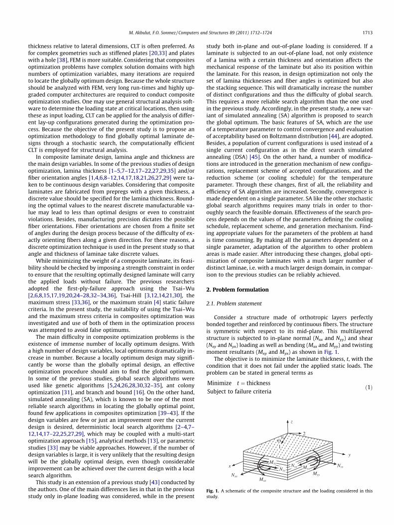
Fig. 1. A schematic of the composite structure and the loading considered in thisstudy.

M. Akbulut, F.O. Sonmez / Computers and Structures 89 (2011) 1712–1724 1713

thickness relative to lateral dimensions, CLT is often preferred. Asfor complex geometries such as stiffened plates [20,33] and plateswith a hole [38], FEM is more suitable. Considering that compositesoptimization problems have complex solution domains with highnumbers of optimization variables, many iterations are requiredto locate the globally optimum design. Because the whole structureshould be analyzed with FEM, very long run-times and highly up-graded computer architectures are required to conduct compositeoptimization studies. One may use general structural analysis soft-ware to determine the loading state at critical locations, then usingthese as input loading, CLT can be applied for the analysis of differ-ent lay-up configurations generated during the optimization pro-cess. Because the objective of the present study is to propose anoptimization methodology to find globally optimal laminate de-signs through a stochastic search, the computationally efficientCLT is employed for structural analysis.

In composite laminate design, lamina angle and thickness arethe main design variables. In some of the previous studies of designoptimization, lamina thickness [1–5,7–12,17–22,27,29,35] and/orfiber orientation angles [1,4,6,8–12,14,17,18,21,26,27,29] were ta-ken to be continuous design variables. Considering that compositelaminates are fabricated from prepregs with a given thickness, adiscrete value should be specified for the lamina thickness. Round-ing the optimal values to the nearest discrete manufacturable va-lue may lead to less than optimal designs or even to constraintviolations. Besides, manufacturing precision dictates the possiblefiber orientations. Fiber orientations are chosen from a finite setof angles during the design process because of the difficulty of ex-actly orienting fibers along a given direction. For these reasons, adiscrete optimization technique is used in the present study so thatangle and thickness of laminae take discrete values.

While minimizing the weight of a composite laminate, its feasi-bility should be checked by imposing a strength constraint in orderto ensure that the resulting optimally designed laminate will carrythe applied loads without failure. The previous researchersadopted the first-ply-failure approach using the Tsai–Wu[2,6,8,15,17,19,20,24–28,32–34,36], Tsai-Hill [3,12,14,21,30], themaximum stress [33,36], or the maximum strain [4] static failurecriteria. In the present study, the suitability of using the Tsai–Wuand the maximum stress criteria in composites optimization wasinvestigated and use of both of them in the optimization processwas attempted to avoid false optimums.

The main difficulty in composite optimization problems is theexistence of immense number of locally optimum designs. Witha high number of design variables, local optimums dramatically in-crease in number. Because a locally optimum design may signifi-cantly be worse than the globally optimal design, an effectiveoptimization procedure should aim to find the global optimum.In some of the previous studies, global search algorithms wereused like genetic algorithms [5,24,26,28,30,32–35], ant colonyoptimization [31], and branch and bound [16]. On the other hand,simulated annealing (SA), which is known to be one of the mostreliable search algorithms in locating the globally optimal point,found few applications in composites optimization [39–43]. If thedesign variables are few or just an improvement over the currentdesign is desired, deterministic local search algorithms [2–4,7–12,14,17–22,25,27,29], which may be coupled with a multi-startoptimization approach [15], analytical methods [13], or parametricstudies [33] may be viable approaches. However, if the number ofdesign variables is large, it is very unlikely that the resulting designwill be the globally optimal design, even though considerableimprovement can be achieved over the current design with a localsearch algorithm.

This study is an extension of a previous study [43] conducted bythe authors. One of the main differences lies in that in the previousstudy only in-plane loading was considered, while in the present

study both in-plane and out-of-plane loading is considered. If alaminate is subjected to an out-of-plane load, not only existenceof a lamina with a certain thickness and orientation affects themechanical response of the laminate but also its position withinthe laminate. For this reason, in design optimization not only theset of lamina thicknesses and fiber angles is optimized but alsothe stacking sequence. This will dramatically increase the numberof distinct configurations and thus the difficulty of global search.This requires a more reliable search algorithm than the one usedin the previous study. Accordingly, in the present study, a new var-iant of simulated annealing (SA) algorithm is proposed to searchthe global optimum. The basic features of SA, which are the useof a temperature parameter to control convergence and evaluationof acceptability based on Boltzmann distribution [44], are adopted.Besides, a population of current configurations is used instead of asingle current configuration as in the direct search simulatedannealing (DSA) [45]. On the other hand, a number of modifica-tions are introduced in the generation mechanism of new configu-rations, replacement scheme of accepted configurations, and thereduction scheme (or cooling schedule) for the temperatureparameter. Through these changes, first of all, the reliability andefficiency of SA algorithm are increased. Secondly, convergence ismade dependent on a single parameter. SA like the other stochasticglobal search algorithms requires many trials in order to thor-oughly search the feasible domain. Effectiveness of the search pro-cess depends on the values of the parameters defining the coolingschedule, replacement scheme, and generation mechanism. Find-ing appropriate values for the parameters of the problem at handis time consuming. By making all the parameters dependent on asingle parameter, adaptation of the algorithm to other problemareas is made easier. After introducing these changes, global opti-mization of composite laminates with a much larger number ofdistinct laminae, i.e. with a much larger design domain, in compar-ison to the previous studies can be reliably achieved.

2. Problem formulation

2.1. Problem statement

Consider a structure made of orthotropic layers perfectlybonded together and reinforced by continuous fibers. The structureis symmetric with respect to its mid-plane. This multilayeredstructure is subjected to in-plane normal (Nxx and Nyy) and shear(Nxy and Nyx) loading as well as bending (Mxx and Myy) and twistingmoment resultants (Mxy and Myx) as shown in Fig. 1.

The objective is to minimize the laminate thickness, t, with thecondition that it does not fail under the applied static loads. Theproblem can be stated in general terms as

Minimize t ¼ thicknessSubject to failure criteria

ð1Þ

1714 M. Akbulut, F.O. Sonmez / Computers and Structures 89 (2011) 1712–1724

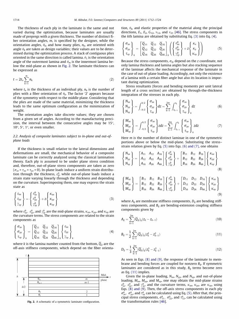
The thickness of each ply in the laminate is the same and notvaried during the optimization, because laminates are usuallymade of prepregs with a given thickness. The number of distinct fi-ber orientation angles, m, is specified by the designer, while theorientation angles, hk, and how many plies, nk, are oriented withangle hk are taken as design variables; their values are to be deter-mined during the optimization process. A stack of contiguous pliesoriented in the same direction is called lamina. h1 is the orientationangle of the outermost lamina and hm is the innermost lamina be-low the mid-plane as shown in Fig. 2. The laminate thickness canbe expressed as

t ¼ 2to

Xm

k¼1

nk ð2Þ

where to is the thickness of an individual ply, nk is the number ofplies with a fiber orientation of hk. The factor ‘2’ appears becauseof the symmetry with respect to the middle plane. Considering thatthe plies are made of the same material, minimizing the thicknessleads to the same optimum configuration as the minimization ofweight.

The orientation angles take discrete values; they are chosenfrom a given set of angles. According to the manufacturing preci-sion, the interval between the consecutive angles may be 15�,10�, 5�, 1�, or even smaller.

2.2. Analysis of composite laminates subject to in-plane and out-of-plane loads

If the thickness is small relative to the lateral dimensions anddeformations are small, the mechanical behavior of a compositelaminate can be correctly analyzed using the classical laminationtheory. Each ply is assumed to be under plane stress conditionand, therefore, out-of-plane stress components are taken as zero(rzz = sxz = syz = 0). In-plane loads induce a uniform strain distribu-tion through the thickness, e0

ij, while out-of-plane loads induce astrain state varying linearly through the thickness and dependingon the curvature. Superimposing them, one may express the strainstate as

exx

eyy

cxy

8><>:

9>=>; ¼

e0xx

e0yy

c0xy

8><>:

9>=>;þ z

jxx

jyy

jxy

8><>:

9>=>; ð3Þ

where e0xx; e0

yy, and c0xy are the mid-plane strains, jxx, jyy, and jxy are

the curvature terms. The stress components are related to the straincomponents as

rxx

ryy

sxy

8><>:

9>=>;

k

¼Q 11 Q 12 Q16

Q 12 Q 22 Q26

Q 16 Q 26 Q66

264

375

k

exx

eyy

cxy

8><>:

9>=>;

k

ð4Þ

where k is the lamina number counted from the bottom, Qij are theoff-axis stiffness components, which depend on the fiber orienta-

h

h/2

12

mm-1

θ1

θ2

θm-1

θm

Mid-

plane x

z

Fig. 2. A schematic of a symmetric laminate configuration.

tion, hk, and elastic properties of the material along the principaldirections, E1, E2, G12, m12, and m21 [46]. The stress components inthe kth lamina are obtained by substituting Eq. (3) into Eq. (4).

rxx

ryy

sxy

8><>:

9>=>;

k

¼Q 11 Q 12 Q 16

Q 12 Q 22 Q 26

Q 16 Q 26 Q 66

264

375

k

e0xx

e0yy

c0xy

8><>:

9>=>;þ z

jx

jy

jxy

8><>:

9>=>;

0B@

1CA ð5Þ

Because the stress components, rij, depend on the z coordinate, notonly lamina thickness and lamina angles but also stacking sequenceof the laminae affects the mechanical response of the laminate inthe case of out-of-plane loading. Accordingly, not only the existenceof a lamina with a certain fiber angle but also its location is impor-tant during optimization.

Stress resultants (forces and bending moments per unit laterallength of a cross section) are obtained by through-the-thicknessintegration of the stresses in each ply.

Nxx

Nyy

Nxy

8><>:

9>=>; ¼

Z h=2

�h=2

rxx

ryy

sxy

8><>:

9>=>;dz ¼

X2m

k¼1

Z zk

zk�1

rxx

ryy

sxy

8><>:

9>=>;

k

dz ð6Þ

Mxx

Myy

Mxy

8><>:

9>=>; ¼

Z h=2

�h=2

rxx

ryy

sxy

8><>:

9>=>;zdz ¼

X2m

k¼1

Z zk

zk�1

rxx

ryy

sxy

8><>:

9>=>;

k

zdz ð7Þ

Here m is the number of distinct laminae in one of the symmetricportions above or below the mid-plane. Substituting the stress–strain relation given by Eq. (5) into Eqs. (6) and (7), one obtains

Nxx

Nyy

Nxy

8><>:

9>=>; ¼

A11 A12 A16

A12 A22 A26

A16 A26 A66

264

375

e0xx

e0yy

c0xy

8><>:

9>=>;þ

B11 B12 B16

B12 B22 B26

B16 B26 B66

264

375

jxx

jyy

jxy

8><>:

9>=>;ð8Þ

Mxx

Myy

Mxy

8><>:

9>=>; ¼

B11 B12 B16

B12 B22 B26

B16 B26 B66

264

375

e0xx

e0yy

c0xy

8><>:

9>=>;þ

D11 D12 D16

D12 D22 D26

D16 D26 D66

264

375

jxx

jyy

jxy

8><>:

9>=>;ð9Þ

where Aij are membrane stiffness components, Dij are bending stiff-ness components, and Bij are bending-extension coupling stiffnesscomponents given by

Aij ¼X2m

k¼1

ðQ ijÞkðzk � zk�1Þ ð10Þ

Bij ¼12

X2m

k¼1

ðQ ijÞkðz2k � z2

k�1Þ ð11Þ

Dij ¼13

X2m

k¼1

ðQ ijÞkðz3k � z3

k�1Þ ð12Þ

As seen in Eqs. (8) and (9), the response of the laminate to mem-brane and bending forces are coupled for nonzero Bij. If symmetriclaminates are considered as in this study, Bij terms become zeroas Eq. (11) implies.

Given the in-plane loading, Nxx, Nyy, and Nxy, and out-of-planeloading, Mxx, Myy, and Mxy, one may obtain the mid-plane strainse0

xx; e0yy, and c0

xy, and the curvature terms, jxx, jyy, are jxy, usingEqs. (8) and (9). Then, the off-axis stress components in each plyrk

xx; rkyy, and sk

xy can be calculated using Eq. (5). After that, the prin-cipal stress components, rk

11; rk22, and sk

12, can be calculated usingthe transformation rules [46].

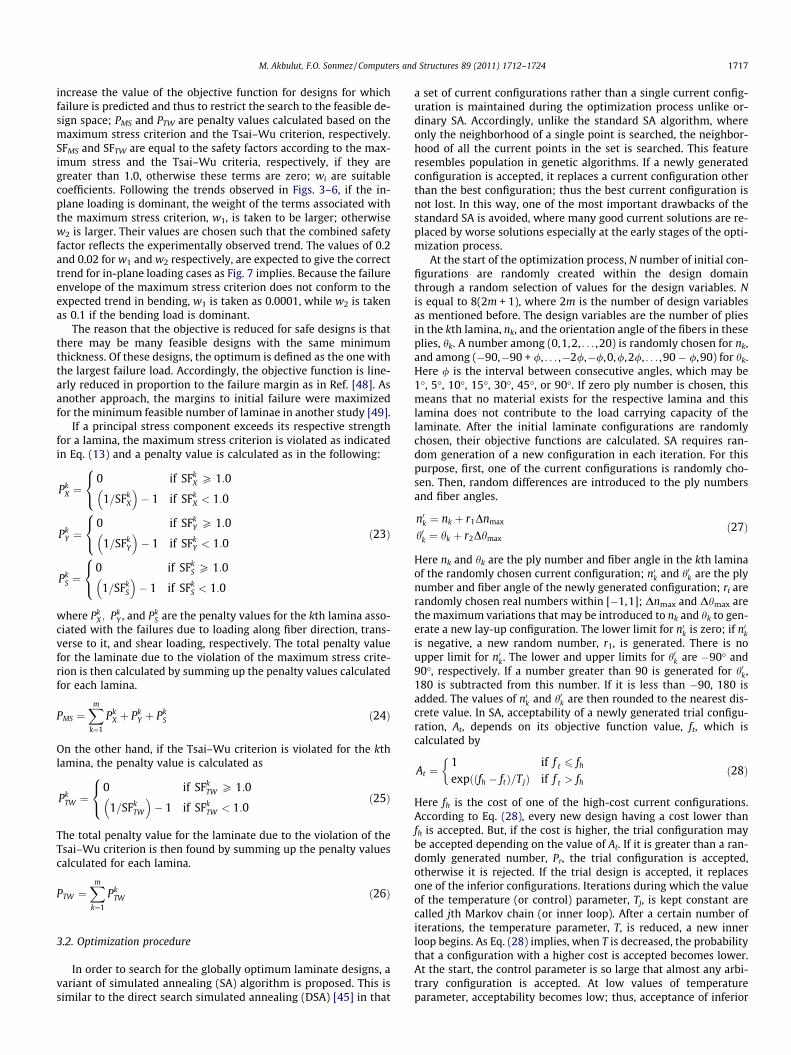
Fig. 3. Safety factors calculated using the maximum stress criterion for a laminatesubjected to uniaxial loading (only Nxx – 0) for a range of fiber orientation angles, h.

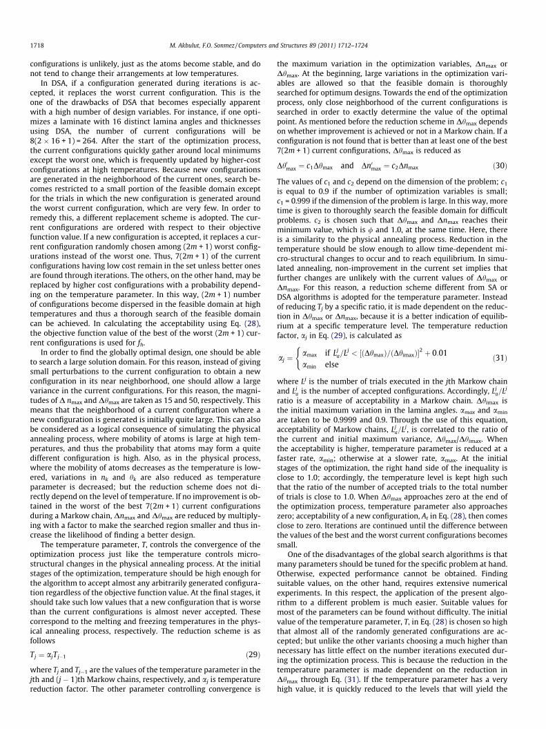
Fig. 4. Safety factors calculated using the maximum stress criterion for a laminatesubjected to one component of bending moment (only Mxx – 0) for a range of fiberorientation angles, h.

M. Akbulut, F.O. Sonmez / Computers and Structures 89 (2011) 1712–1724 1715

Based on the principal stress components, rk11; rk

22, and sk12, one

may judge whether the kth ply will fail or not using appropriatestatic failure criteria.

2.3. Static failure criteria

During weight minimization of a composite structure, strengthconstraints should be imposed, because decreasing the number ofload carrying plies eventually leads to failure. Whenever a new lay-up design is generated by the search algorithm during optimiza-tion, its feasibility regarding load-carrying capacity should bechecked. In this study, only the static failure modes are assumedto be critical for the laminate. The other failure modes, fatigue,low stiffness, buckling, delamination, resonance etc. are assumedto be not critical.

One of the commonly used approaches to estimate the load car-rying capability of a laminate design is to use a limit theory such asthe maximum stress criterion. According to this criterion, failure ispredicted whenever one of the principal stress components ex-ceeds its respective strength. The failure envelope for a ply underin-plane normal and shear stresses is then defined by the followinginequalities:

r11 < Xt and r11 > Xc and r22 < Yt andr22 > Yc and js12j < S ð13Þ

where ‘‘X’’ and ‘‘Y’’ symbolize the strengths along the fiber directionand transverse to it, respectively; the subscripts ‘‘t’’ and ‘‘c’’ denotethe tensile and compressive strengths; S is the ultimate in-planeshear strength of the laminate under pure shear loading. Adoptingthe first – ply – failure criterion, the whole laminate is consideredto have failed, if one of these inequalities is not satisfied for anyone of the laminae.

The safety factor of a structure is an indication of its load carry-ing capacity. Values less than 1.0 indicate failure. In order to calcu-late the safety factor of a laminate based on the maximum stresscriterion, first, the principal stresses ðrk

11; rk22, and sk

12Þ in eachlamina are determined; the safety factor for each failure mode iscalculated; then the minimum of them is denoted as the safety fac-tor of the lamina, SFk

MS.

SFkMS ¼min of

SFkX ¼

Xt=r11 if r11 > 0Xc=r11 if r11 < 0

�

SFkY ¼

Yt=r22 if r22 > 0Yc=r22 if r22 < 0

�

SFkS ¼ S=js12j

8>>>>>><>>>>>>:

ð14Þ

Then, the minimum of the lamina safety factors, SFkMS, is denoted as

the safety factor of the laminate SFMS.

SFMS ¼min of SFkMS for k ¼ 1;2; . . . ;m� 1;m ð15Þ

Fig. 3 shows the safety factors calculated using this criterion fora laminate subjected to uniaxial loading (only Nxx – 0) for a rangeof fiber orientation angles, h. Two different laminate lay-up config-urations are considered. One is a balanced and symmetric lami-nate, [h25/�h25]s, the other is a unidirectional laminate, [h50]s. Thegraph indicates the change in the safety factor with orientation an-gle h. One may observe that for the balanced laminate, [h25 /�h25]s

under uniaxial loading (Nxx = 9.8 MPa m), the criterion correctlypredicts that the laminate is strongest for h = 0�, in which fibersare oriented along the loading direction. The safety factor for thiscase, which is 1.01, is the highest of all. However, for the unidirec-tional laminate, [h50]s, the criterion falsely predicts the highestsafety factor for h = 5�. This means that an optimization processin which failure is assessed based on the maximum stress criterionmay stick to a spurious optimum design for an unbalanced lami-

nate. On the other hand, as Fig. 4 shows, the highest safety factorsare calculated at angles other than h = 0� for a laminate subjectedto bending moment Mxx. Therefore the maximum stress criterionby itself is not suitable for a general laminate design optimizationprocedure.

The general form of the Tsai–Wu failure criterion for orthotro-pic materials under 2D stress state is expressed as [46,47]

r211

XtjXcjþ r2

22

YtjYcjþ s2

12

S2 �r11r22ffiffiffiffiffiffiffiffiffiffiffiffiffiffiffiffiffiffiffiffiXtXcYtYcp þ 1

Xt� 1jXcj

� �r11

þ 1Yt� 1jYcj

� �r22 < 1 ð16Þ

The left hand side of the equality in Eq. (16) is called failure index. Ifit is less than 1.0, the structure will not fail; the closer it is to zero,the safer will be the laminate. In this study, safety factor is used asan indication of the strength of the laminate instead of failure index.The safety factor for the kth lamina, SFk

TW , according to the Tsai–Wucriterion is defined as the multiplier of the stress components atlamina k, rk

ij, that makes the right hand side of Eq. (16) equal to1.0. Eq. (16) then becomes

aðSFkTWÞ

2 þ bðSFkTWÞ � 1 ¼ 0 ð17Þ

where

a ¼ ðrk11Þ

2

XtjXcjþ ðr

k22Þ

2

Yt jYcjþ ðs

k12Þ

2

S2 � ðrk11Þðrk

22ÞffiffiffiffiffiffiffiffiffiffiffiffiffiffiffiffiffiffiffiffiXtXcYtYcp ð18Þ

Fig. 6. Safety factor calculated using the Tsai–Wu criterion for a laminate subjectedto one component of bending moment (only Mxx – 0) for a range of fiber orientationangles, h.

Fig. 7. Safety factor calculated using both criteria for a unidirectional laminate anda balanced laminate subjected to uniaxial loading (only Nxx – 0) for a range of fiberorientation angles, h.

1716 M. Akbulut, F.O. Sonmez / Computers and Structures 89 (2011) 1712–1724

b ¼ 1Xt� 1jXcj

� �rk

11 þ1Yt� 1jYcj

� �rk

22 ð19Þ

The root of Eq. (17) gives the safety factor. Because a negative safetyfactor is not physically meaningful, the absolute value of the firstroot is considered as the actual safety factor.

SFkTW ¼

�bþffiffiffiffiffiffiffiffiffiffiffiffiffiffiffiffib2 þ 4a

p2a

���������� ð20Þ

Then, the minimum of SFkTW is chosen as the safety factor of the

laminate

SFTW ¼min of SFkTW for k ¼ 1;2; . . . ;m� 1;m ð21Þ

Fig. 5 shows the safety factor calculated using the Tsai–Wu cri-terion for two laminates subjected to uniaxial loading (onlyNxx – 0). For the unidirectional laminate, [h50]s, the criterion cor-rectly predicts that the laminate is strongest for h = 0�. The safetyfactor quickly decays with increasing h. However, for the balancedlaminate, [h25/�h25]s, the criterion falsely estimates the highestsafety factor as 1.087 at h = 10�. Actually, the laminate is expectedto become weaker and weaker when h is increased. One may con-clude that the Tsai–Wu criterion may also lead to false optimumdesigns in an optimization process. Another known optimum de-sign is [45n/�45n]s for the loading Nxx = Nyy = Nxy, which both crite-ria correctly predict. As opposed to the maximum stress criterion,the Tsai–Wu criterion correctly estimates that the laminate isstrongest for h = 0� if it is subjected to bending moment Mxx asshown in Fig. 6.

Considering the predictions of these two failure criteria for thetwo different laminate designs under two different loading condi-tions, each criterion seems to compensate the shortcomings of theother. If one of them incorrectly predicts the trend of strength for agiven laminate configuration, the other correctly predicts. Byenforcing the satisfaction of both criteria and calculating the safetyfactor using both criteria, one may correctly find the optimum de-signs. As Fig. 7 shows, a combined safety factor better conforms tothe trend of the in-plane laminate strength, which continuouslydecreases when the angle between the fibers and the load axis getslarger. The combined safety factor is obtained by adding 90% and10% of the safety factors calculated according to the maximumstress and the Tsai–Wu criteria, respectively. In this study, boththe maximum stress and the Tsai–Wu criteria are used to assessthe load bearing capacity of composite laminates with the expecta-tion that false optimum designs will be avoided for any laminateconfiguration.

Fig. 5. Safety factor calculated using the Tsai–Wu criterion for a laminate subjectedto uniaxial loading (only Nxx – 0) for a range of fiber orientation angles, h.

3. Methodology

3.1. Formulation of the objective function

When the load on a laminate is increased, only some of the pliesmay fail while the rest of the plies continue to resist the appliedload. If the load is further increased, progressively more and moredamage is induced until the whole laminate fails. In this study fail-ure of a single ply is considered as signaling inception of the failureof the whole structure. Accordingly, the first-ply failure approach isadopted in the design optimization and safety of each lamina in alaminate design generated during the optimization process ischecked using the Tsai–Wu and the maximum stress failure crite-ria. Failure is predicted if one of the inequalities in Eqs. (13) and(16) is not satisfied for any one of the laminae. In that case, a pen-alty value is calculated and added to the cost function. The overallcost function may then be expressed as

F ¼ 2to

Xm

k¼1

nk þw1PMS þw2PTW �w1SFMS �w2SFTW ð22Þ

where the first term represents the total thickness of the compositestructure as given in Eq. (2); nk is the number of plies in the kth lam-ina, in which the orientation angle is hk; m is the total number oflaminae below or above the mid-plane of the laminate; the secondand the third terms represent the penalty values introduced to

M. Akbulut, F.O. Sonmez / Computers and Structures 89 (2011) 1712–1724 1717

increase the value of the objective function for designs for whichfailure is predicted and thus to restrict the search to the feasible de-sign space; PMS and PTW are penalty values calculated based on themaximum stress criterion and the Tsai–Wu criterion, respectively.SFMS and SFTW are equal to the safety factors according to the max-imum stress and the Tsai–Wu criteria, respectively, if they aregreater than 1.0, otherwise these terms are zero; wi are suitablecoefficients. Following the trends observed in Figs. 3–6, if the in-plane loading is dominant, the weight of the terms associated withthe maximum stress criterion, w1, is taken to be larger; otherwisew2 is larger. Their values are chosen such that the combined safetyfactor reflects the experimentally observed trend. The values of 0.2and 0.02 for w1 and w2 respectively, are expected to give the correcttrend for in-plane loading cases as Fig. 7 implies. Because the failureenvelope of the maximum stress criterion does not conform to theexpected trend in bending, w1 is taken as 0.0001, while w2 is takenas 0.1 if the bending load is dominant.

The reason that the objective is reduced for safe designs is thatthere may be many feasible designs with the same minimumthickness. Of these designs, the optimum is defined as the one withthe largest failure load. Accordingly, the objective function is line-arly reduced in proportion to the failure margin as in Ref. [48]. Asanother approach, the margins to initial failure were maximizedfor the minimum feasible number of laminae in another study [49].

If a principal stress component exceeds its respective strengthfor a lamina, the maximum stress criterion is violated as indicatedin Eq. (13) and a penalty value is calculated as in the following:

PkX ¼

0 if SFkX P 1:0

1=SFkX

� �� 1 if SFk

X < 1:0

8<:

PkY ¼

0 if SFkY P 1:0

1=SFkY

� �� 1 if SFk

Y < 1:0

8<:

PkS ¼

0 if SFkS P 1:0

1=SFkS

� �� 1 if SFk

S < 1:0

8<:

ð23Þ

where PkX ; Pk

Y , and PkS are the penalty values for the kth lamina asso-

ciated with the failures due to loading along fiber direction, trans-verse to it, and shear loading, respectively. The total penalty valuefor the laminate due to the violation of the maximum stress crite-rion is then calculated by summing up the penalty values calculatedfor each lamina.

PMS ¼Xm

k¼1

PkX þ Pk

Y þ PkS ð24Þ

On the other hand, if the Tsai–Wu criterion is violated for the kthlamina, the penalty value is calculated as

PkTW ¼

0 if SFkTW P 1:0

1=SFkTW

� �� 1 if SFk

TW < 1:0

8<: ð25Þ

The total penalty value for the laminate due to the violation of theTsai–Wu criterion is then found by summing up the penalty valuescalculated for each lamina.

PTW ¼Xm

k¼1

PkTW ð26Þ

3.2. Optimization procedure

In order to search for the globally optimum laminate designs, avariant of simulated annealing (SA) algorithm is proposed. This issimilar to the direct search simulated annealing (DSA) [45] in that

a set of current configurations rather than a single current config-uration is maintained during the optimization process unlike or-dinary SA. Accordingly, unlike the standard SA algorithm, whereonly the neighborhood of a single point is searched, the neighbor-hood of all the current points in the set is searched. This featureresembles population in genetic algorithms. If a newly generatedconfiguration is accepted, it replaces a current configuration otherthan the best configuration; thus the best current configuration isnot lost. In this way, one of the most important drawbacks of thestandard SA is avoided, where many good current solutions are re-placed by worse solutions especially at the early stages of the opti-mization process.

At the start of the optimization process, N number of initial con-figurations are randomly created within the design domainthrough a random selection of values for the design variables. Nis equal to 8(2m + 1), where 2m is the number of design variablesas mentioned before. The design variables are the number of pliesin the kth lamina, nk, and the orientation angle of the fibers in theseplies, hk. A number among (0,1,2, . . . ,20) is randomly chosen for nk,and among (�90,�90 + /, . . . ,�2/,�/,0,/,2/, . . . ,90 � /,90) for hk.Here / is the interval between consecutive angles, which may be1�, 5�, 10�, 15�, 30�, 45�, or 90�. If zero ply number is chosen, thismeans that no material exists for the respective lamina and thislamina does not contribute to the load carrying capacity of thelaminate. After the initial laminate configurations are randomlychosen, their objective functions are calculated. SA requires ran-dom generation of a new configuration in each iteration. For thispurpose, first, one of the current configurations is randomly cho-sen. Then, random differences are introduced to the ply numbersand fiber angles.

n0k ¼ nk þ r1Dnmax

h0k ¼ hk þ r2Dhmaxð27Þ

Here nk and hk are the ply number and fiber angle in the kth laminaof the randomly chosen current configuration; n0k and h0k are the plynumber and fiber angle of the newly generated configuration; ri arerandomly chosen real numbers within [�1,1]; Dnmax and Dhmax arethe maximum variations that may be introduced to nk and hk to gen-erate a new lay-up configuration. The lower limit for n0k is zero; if n0kis negative, a new random number, r1, is generated. There is noupper limit for n0k. The lower and upper limits for h0k are �90� and90�, respectively. If a number greater than 90 is generated for h0k,180 is subtracted from this number. If it is less than �90, 180 isadded. The values of n0k and h0k are then rounded to the nearest dis-crete value. In SA, acceptability of a newly generated trial configu-ration, At, depends on its objective function value, ft, which iscalculated by

At ¼1 if f t 6 fh

expððfh � ftÞ=TjÞ if f t > fh

�ð28Þ

Here fh is the cost of one of the high-cost current configurations.According to Eq. (28), every new design having a cost lower thanfh is accepted. But, if the cost is higher, the trial configuration maybe accepted depending on the value of At. If it is greater than a ran-domly generated number, Pr, the trial configuration is accepted,otherwise it is rejected. If the trial design is accepted, it replacesone of the inferior configurations. Iterations during which the valueof the temperature (or control) parameter, Tj, is kept constant arecalled jth Markov chain (or inner loop). After a certain number ofiterations, the temperature parameter, T, is reduced, a new innerloop begins. As Eq. (28) implies, when T is decreased, the probabilitythat a configuration with a higher cost is accepted becomes lower.At the start, the control parameter is so large that almost any arbi-trary configuration is accepted. At low values of temperatureparameter, acceptability becomes low; thus, acceptance of inferior

1718 M. Akbulut, F.O. Sonmez / Computers and Structures 89 (2011) 1712–1724

configurations is unlikely, just as the atoms become stable, and donot tend to change their arrangements at low temperatures.

In DSA, if a configuration generated during iterations is ac-cepted, it replaces the worst current configuration. This is theone of the drawbacks of DSA that becomes especially apparentwith a high number of design variables. For instance, if one opti-mizes a laminate with 16 distinct lamina angles and thicknessesusing DSA, the number of current configurations will be8(2 � 16 + 1) = 264. After the start of the optimization process,the current configurations quickly gather around local minimumsexcept the worst one, which is frequently updated by higher-costconfigurations at high temperatures. Because new configurationsare generated in the neighborhood of the current ones, search be-comes restricted to a small portion of the feasible domain exceptfor the trials in which the new configuration is generated aroundthe worst current configuration, which are very few. In order toremedy this, a different replacement scheme is adopted. The cur-rent configurations are ordered with respect to their objectivefunction value. If a new configuration is accepted, it replaces a cur-rent configuration randomly chosen among (2m + 1) worst config-urations instead of the worst one. Thus, 7(2m + 1) of the currentconfigurations having low cost remain in the set unless better onesare found through iterations. The others, on the other hand, may bereplaced by higher cost configurations with a probability depend-ing on the temperature parameter. In this way, (2m + 1) numberof configurations become dispersed in the feasible domain at hightemperatures and thus a thorough search of the feasible domaincan be achieved. In calculating the acceptability using Eq. (28),the objective function value of the best of the worst (2m + 1) cur-rent configurations is used for fh.

In order to find the globally optimal design, one should be ableto search a large solution domain. For this reason, instead of givingsmall perturbations to the current configuration to obtain a newconfiguration in its near neighborhood, one should allow a largevariance in the current configurations. For this reason, the magni-tudes of D nmax and Dhmax are taken as 15 and 50, respectively. Thismeans that the neighborhood of a current configuration where anew configuration is generated is initially quite large. This can alsobe considered as a logical consequence of simulating the physicalannealing process, where mobility of atoms is large at high tem-peratures, and thus the probability that atoms may form a quitedifferent configuration is high. Also, as in the physical process,where the mobility of atoms decreases as the temperature is low-ered, variations in nk and hk are also reduced as temperatureparameter is decreased; but the reduction scheme does not di-rectly depend on the level of temperature. If no improvement is ob-tained in the worst of the best 7(2m + 1) current configurationsduring a Markow chain, Dnmax and Dhmax are reduced by multiply-ing with a factor to make the searched region smaller and thus in-crease the likelihood of finding a better design.

The temperature parameter, T, controls the convergence of theoptimization process just like the temperature controls micro-structural changes in the physical annealing process. At the initialstages of the optimization, temperature should be high enough forthe algorithm to accept almost any arbitrarily generated configura-tion regardless of the objective function value. At the final stages, itshould take such low values that a new configuration that is worsethan the current configurations is almost never accepted. Thesecorrespond to the melting and freezing temperatures in the phys-ical annealing process, respectively. The reduction scheme is asfollows

Tj ¼ ajTj�1 ð29Þ

where Tj and Tj�1 are the values of the temperature parameter in thejth and (j � 1)th Markow chains, respectively, and aj is temperaturereduction factor. The other parameter controlling convergence is

the maximum variation in the optimization variables, Dnmax orDhmax. At the beginning, large variations in the optimization vari-ables are allowed so that the feasible domain is thoroughlysearched for optimum designs. Towards the end of the optimizationprocess, only close neighborhood of the current configurations issearched in order to exactly determine the value of the optimalpoint. As mentioned before the reduction scheme in Dhmax dependson whether improvement is achieved or not in a Markow chain. If aconfiguration is not found that is better than at least one of the best7(2m + 1) current configurations, Dhmax is reduced as

Dh0max ¼ c1Dhmax and Dn0max ¼ c2Dnmax ð30Þ

The values of c1 and c2 depend on the dimension of the problem; c1

is equal to 0.9 if the number of optimization variables is small;c1 = 0.999 if the dimension of the problem is large. In this way, moretime is given to thoroughly search the feasible domain for difficultproblems. c2 is chosen such that Dhmax and Dnmax reaches theirminimum value, which is / and 1.0, at the same time. Here, thereis a similarity to the physical annealing process. Reduction in thetemperature should be slow enough to allow time-dependent mi-cro-structural changes to occur and to reach equilibrium. In simu-lated annealing, non-improvement in the current set implies thatfurther changes are unlikely with the current values of Dhmax orDnmax. For this reason, a reduction scheme different from SA orDSA algorithms is adopted for the temperature parameter. Insteadof reducing Tj by a specific ratio, it is made dependent on the reduc-tion in Dhmax or Dnmax, because it is a better indication of equilib-rium at a specific temperature level. The temperature reductionfactor, aj in Eq. (29), is calculated as

aj ¼amax if Lj

a=Lj < ðDhmaxÞ=ðDhimaxÞ½ �2 þ 0:01amin else

(ð31Þ

where Lj is the number of trials executed in the jth Markow chainand Lj

a is the number of accepted configurations. Accordingly, Lja=Lj

ratio is a measure of acceptability in a Markow chain. Dhimax isthe initial maximum variation in the lamina angles. amax and amin

are taken to be 0.9999 and 0.9. Through the use of this equation,acceptability of Markow chains, Lj

a=Lj, is correlated to the ratio ofthe current and initial maximum variance, Dhmax/Dhimax. Whenthe acceptability is higher, temperature parameter is reduced at afaster rate, amin; otherwise at a slower rate, amax. At the initialstages of the optimization, the right hand side of the inequality isclose to 1.0; accordingly, the temperature level is kept high suchthat the ratio of the number of accepted trials to the total numberof trials is close to 1.0. When Dhmax approaches zero at the end ofthe optimization process, temperature parameter also approacheszero; acceptability of a new configuration, At in Eq. (28), then comesclose to zero. Iterations are continued until the difference betweenthe values of the best and the worst current configurations becomessmall.

One of the disadvantages of the global search algorithms is thatmany parameters should be tuned for the specific problem at hand.Otherwise, expected performance cannot be obtained. Findingsuitable values, on the other hand, requires extensive numericalexperiments. In this respect, the application of the present algo-rithm to a different problem is much easier. Suitable values formost of the parameters can be found without difficulty. The initialvalue of the temperature parameter, T, in Eq. (28) is chosen so highthat almost all of the randomly generated configurations are ac-cepted; but unlike the other variants choosing a much higher thannecessary has little effect on the number iterations executed dur-ing the optimization process. This is because the reduction in thetemperature parameter is made dependent on the reduction inDhmax through Eq. (31). If the temperature parameter has a veryhigh value, it is quickly reduced to the levels that will yield the

M. Akbulut, F.O. Sonmez / Computers and Structures 89 (2011) 1712–1724 1719

required acceptability ratio, Lja=Lj. The initial value of the maximum

variation that may be introduced to the optimization variables,Dhimax, is another parameter affecting convergence. Its value ischosen based on the extent of the solution domain. Its value shouldbe chosen as high as possible in order to search the solution do-main thoroughly. For the present problem, the initial value ofDhmax is chosen as 50�, knowing that the upper and lower limitsof h are 90� and �90�. The value of factor c1 in Eq. (30) dependson the difficultly of the problem. The higher the number, the moreiterations are executed. If the number of variables is four or lessthan four, 0.9 is a suitable value. If the number of variables is 16or more, a much slower reduction in the maximum variation is re-quired; a number as high as 0.999 permits a thorough search of thesolution domain. The only parameter that requires numericalexperiments to determine its value is c1.

Table 1Dependence of the optimal designs on the chosen failure criteria for the loadingNxx = 10 � 106, Nyy = Nxy = 0 N/m, and for two distinct fiber angles. Mxx = Myy = M-xy = 0 Nm/m.

Failure criteria usedto check feasibility

Optimallay-up

Totalnumber ofplies

Safety factorfor Tsai–Wu

Safety factorfor max. str.

Only Tsai–Wucriterion

[�925/1022]s

94 1.0007 0.9142

Only max stresscriterion

[551]s 102 0.6688 1.0168

Both Tsai–Wu andmax. stress

[051]s 102 1.0091 1.0091

Table 2Dependence of the optimal designs on the chosen failure criteria for the loadingMxx = 15, Myy = Mxy = 0 kNm/m, and for two distinct fiber angles. Nxx = Nyy = Nxy = 0 N/m.

Failure criteriaused to checkfeasibility

Optimallay-up

Totalnumberof plies

Safetyfactor forTsai–Wu

Safetyfactor formax. str.stress

Only Tsai–Wu criterion [315/�1028]s 86 1.1124 1.0115Only max stress

criterion[�124/439]s 86 1.0102 1.0563

Both Tsai–Wu and max.stress

[221/�1622]s 86 1.1124 1.0123

Table 3The optimum lay-ups for the loading Mxx = 15, Myy = Mxy = 0 kNm/m for variousnumbers of distinct fiber angles.

Number ofdistinctfiberangles

Optimum lay-up sequences

Totalnumberof plies

Safetyfactorfor Tsai–Wu

Safetyfactor formax.stress

1 [043]s 86 1.0325 1.03252 [221/�1622]s 86 1.1124 1.01234 [02/�69/78/624]s 86 1.1164 1.01228 [02/�63/�75/631/�142]s 86 1.1165 1.012216 [0/�52/�64/77/64/�512/712/261]s 86 1.1165 1.0122

4. Numerical results and discussions

The numerical results were obtained for a graphite/epoxy mate-rial, T300/5308, with the following material properties:E11 = 40.91 GPa, E22 = 9.88 GPa, G12 = 2.84 GPa, m12 = 0.292,XT = 779 MPa, XC = �1134 MPa, YT = 19 MPa, YC = �131 MPa,S = 75 MPa. Thickness of the plies is 0.127 mm.

4.1. Dependence of the optimum designs on the failure criterion

The results of the optimization process depend on the failurecriterion. Table 1 shows the optimal designs obtained by applyingthe aforementioned optimization procedure using different failurecriteria. The loading is uniaxial (Nxx = 10 � 106 N/m) and two dis-tinct fiber orientations are used. The interval between the anglesis taken to be 1�. If only the Tsai–Wu criterion is used, the optimaldesign is almost balanced and the angle imparting the higheststrength is predicted around ±10�, conforming to the trend shownin Fig. 5, which is obtained using only a single angular parameter, h.According to the maximum stress criterion, however, this configu-ration is unsafe. If only the maximum stress criterion is used, theoptimal laminate is unidirectional with 5� fiber orientation angle,conforming to the trend shown in Fig. 3. According to the Tsai–Wu criterion, however, this design is highly nonconservative.These results imply that relying on just one failure criterion maylead to spurious optimal designs. If the Tsai–Wu and maximumstress criteria are used together, the optimal lay-up design agreeswith the empirical observations; i.e. a laminate under uniaxialloading is strongest if all the fibers are aligned along the load direc-tion. Table 2 shows the optimal designs of laminates under bend-ing loading for various uses of failure criteria. The optimumlaminates are not unidirectional according to both criteria. For[043]s, the safety factor is 1.0325. The optimum designs, on theother hand, have a higher safety factor. When both criteria areused, the optimal design has a safety factor (1.1124) very closeto that of the optimal design found by using only the Tsai–Wu cri-terion; but the safety factor based on the maximum stress criterionis larger (1.0123 in comparison to 1.0115) even though its weight,w1 Eq. (22), is very small. One may conclude that use of the twofailure criteria together shows a potential in compositeoptimization.

4.2. Optimum designs for different numbers of distinct laminae

For some out-of-plane loading cases, the optimal lay-ups havingminimum thickness were obtained using the Tsai–Wu and maxi-mum stress criteria together in order to see the effectiveness ofthe optimization algorithm proposed in this study. A range of val-ues were tried for the number of distinct laminae. Tables 3–6 show

the optimum angles, the number of plies oriented along theseangles, and the total number of plies for laminates subjected tovarious out-of-plane loads. For the cases presented in the tables,in-plane loads are zero, Nxx = Nyy = Nxy = 0 N/m, unless otherwisestated. Since stacking sequence affects the laminate response forout-of-plane loading, only the adjacent plies are shown by a singlesymbol, e.g. [90/90/02/0/903/0]s may be shown as [902/03/903/0]s,but not as [905/04]s, because they lead to different stress and strainstates under the same out-of-plane loading. Furthermore, if theoptimum number of plies in a lamina is found to be zero, it isnot shown in the results because no material exists in that lamina.

For biaxial bending (Mxx = 15, Myy = 15, Mxy = 0), quite a numberof multiple globally optimum lay-up configurations were found asshown in Table 4. For two distinct fiber angles, the optimizationalgorithm found [�9027/0150]s, [�8927/1150]s, . . . , [�127/89150]s, [027/90150]s, [127/�89150]s, . . . , [9027/0150]s as optimal configurations; allof them had the same objective function value. This means thatthe strength of a laminate having [�9027/0150]s lay-up is the samefor all biaxial bending loads having equal magnitude applied alongany arbitrary x–y directions. For this loading case, tensile stressestransverse to the fibers are critical. Because for all these lay-ups,[h27/90 + h150]s, transverse tensile stress in the outermost ply isthe same, they have the same safety factor, and thus the same

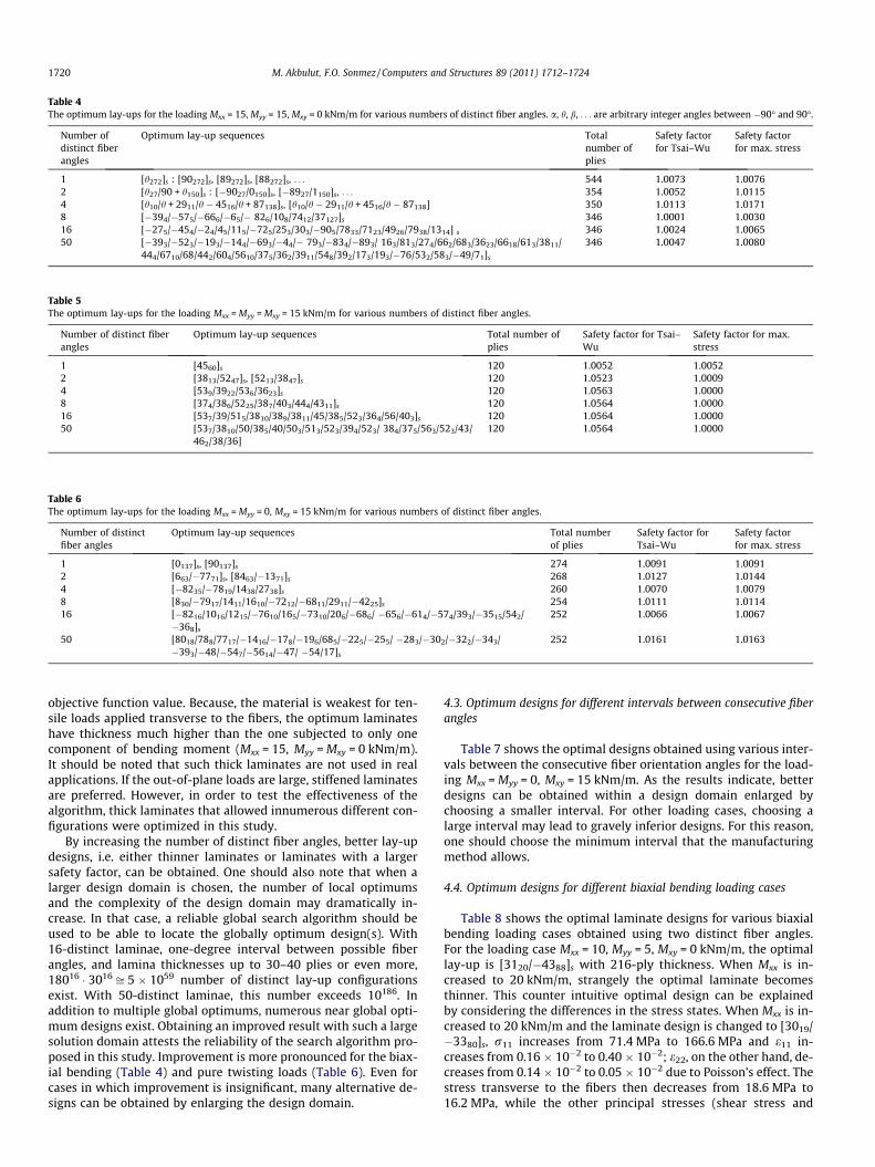
Table 4The optimum lay-ups for the loading Mxx = 15, Myy = 15, Mxy = 0 kNm/m for various numbers of distinct fiber angles. a, h, b, . . . are arbitrary integer angles between �90� and 90�.

Number ofdistinct fiberangles

Optimum lay-up sequences Totalnumber ofplies

Safety factorfor Tsai–Wu

Safety factorfor max. stress

1 [h272]s : [90272]s, [89272]s, [88272]s, . . . 544 1.0073 1.00762 [h27/90 + h150]s : [�9027/0150]s, [�8927/1150]s, . . . 354 1.0052 1.01154 [h10/h + 2911/h � 4516/h + 87138]s, [h10/h � 2911/h + 4516/h � 87138] 350 1.0113 1.01718 [�394/�575/�666/�65/� 826/108/7412/37127]s 346 1.0001 1.003016 [�275/�454/�24/45/115/�725/253/303/�905/7833/7123/4926/7938/1314] s 346 1.0024 1.006550 [�393/�523/�193/�144/�693/�44/� 793/�834/�893/ 163/813/274/662/683/3623/6618/613/3811/

444/6710/68/442/604/5610/375/362/3911/548/392/173/193/�76/532/583/�49/71]s

346 1.0047 1.0080

Table 5The optimum lay-ups for the loading Mxx = Myy = Mxy = 15 kNm/m for various numbers of distinct fiber angles.

Number of distinct fiberangles

Optimum lay-up sequences Total number ofplies

Safety factor for Tsai–Wu

Safety factor for max.stress

1 [4560]s 120 1.0052 1.00522 [3813/5247]s, [5213/3847]s 120 1.0523 1.00094 [539/3922/536/3623]s 120 1.0563 1.00008 [374/386/5225/387/403/444/4311]s 120 1.0564 1.000016 [537/39/515/3810/389/3811/45/385/523/364/56/403]s 120 1.0564 1.000050 [537/3810/50/385/40/503/513/523/394/523/ 384/375/563/523/43/

462/38/36]120 1.0564 1.0000

Table 6The optimum lay-ups for the loading Mxx = Myy = 0, Mxy = 15 kNm/m for various numbers of distinct fiber angles.

Number of distinctfiber angles

Optimum lay-up sequences Total numberof plies

Safety factor forTsai–Wu

Safety factorfor max. stress

1 [0137]s, [90137]s 274 1.0091 1.00912 [663/�7771]s, [8463/�1371]s 268 1.0127 1.01444 [�8235/�7819/1438/2738]s 260 1.0070 1.00798 [830/�7917/1411/1610/�7212/�6811/2911/�4225]s 254 1.0111 1.011416 [�8216/1016/1215/�7610/165/�7310/206/�686/ �656/�614/�574/393/�3515/542/

�368]s

252 1.0066 1.0067

50 [8018/788/7717/�1416/�178/�196/685/�225/�255/ �283/�302/�322/�343/�393/�48/�547/�5614/�47/ �54/17]s

252 1.0161 1.0163

1720 M. Akbulut, F.O. Sonmez / Computers and Structures 89 (2011) 1712–1724

objective function value. Because, the material is weakest for ten-sile loads applied transverse to the fibers, the optimum laminateshave thickness much higher than the one subjected to only onecomponent of bending moment (Mxx = 15, Myy = Mxy = 0 kNm/m).It should be noted that such thick laminates are not used in realapplications. If the out-of-plane loads are large, stiffened laminatesare preferred. However, in order to test the effectiveness of thealgorithm, thick laminates that allowed innumerous different con-figurations were optimized in this study.

By increasing the number of distinct fiber angles, better lay-updesigns, i.e. either thinner laminates or laminates with a largersafety factor, can be obtained. One should also note that when alarger design domain is chosen, the number of local optimumsand the complexity of the design domain may dramatically in-crease. In that case, a reliable global search algorithm should beused to be able to locate the globally optimum design(s). With16-distinct laminae, one-degree interval between possible fiberangles, and lamina thicknesses up to 30–40 plies or even more,18016 � 3016 ffi 5 � 1059 number of distinct lay-up configurationsexist. With 50-distinct laminae, this number exceeds 10186. Inaddition to multiple global optimums, numerous near global opti-mum designs exist. Obtaining an improved result with such a largesolution domain attests the reliability of the search algorithm pro-posed in this study. Improvement is more pronounced for the biax-ial bending (Table 4) and pure twisting loads (Table 6). Even forcases in which improvement is insignificant, many alternative de-signs can be obtained by enlarging the design domain.

4.3. Optimum designs for different intervals between consecutive fiberangles

Table 7 shows the optimal designs obtained using various inter-vals between the consecutive fiber orientation angles for the load-ing Mxx = Myy = 0, Mxy = 15 kNm/m. As the results indicate, betterdesigns can be obtained within a design domain enlarged bychoosing a smaller interval. For other loading cases, choosing alarge interval may lead to gravely inferior designs. For this reason,one should choose the minimum interval that the manufacturingmethod allows.

4.4. Optimum designs for different biaxial bending loading cases

Table 8 shows the optimal laminate designs for various biaxialbending loading cases obtained using two distinct fiber angles.For the loading case Mxx = 10, Myy = 5, Mxy = 0 kNm/m, the optimallay-up is [3120/�4388]s with 216-ply thickness. When Mxx is in-creased to 20 kNm/m, strangely the optimal laminate becomesthinner. This counter intuitive optimal design can be explainedby considering the differences in the stress states. When Mxx is in-creased to 20 kNm/m and the laminate design is changed to [3019/�3380]s, r11 increases from 71.4 MPa to 166.6 MPa and e11 in-creases from 0.16 � 10�2 to 0.40 � 10�2; e22, on the other hand, de-creases from 0.14 � 10�2 to 0.05 � 10�2 due to Poisson’s effect. Thestress transverse to the fibers then decreases from 18.6 MPa to16.2 MPa, while the other principal stresses (shear stress and

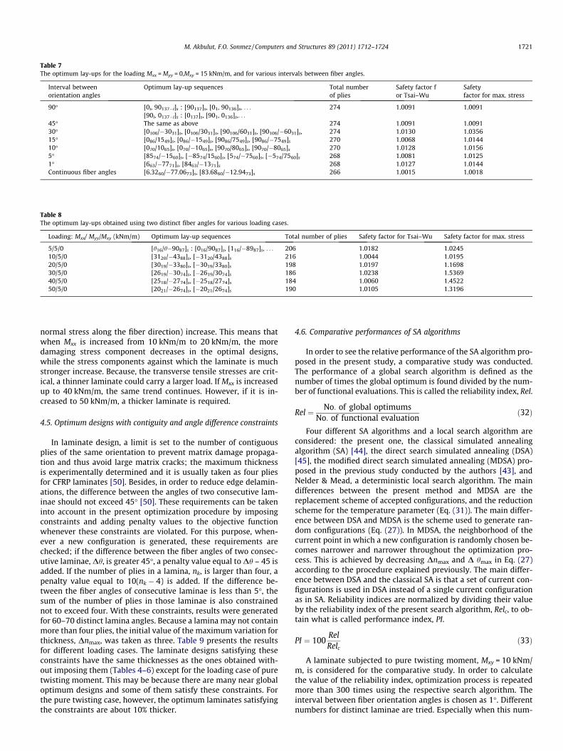
Table 7The optimum lay-ups for the loading Mxx = Myy = 0,Mxy = 15 kNm/m, and for various intervals between fiber angles.

Interval betweenorientation angles

Optimum lay-up sequences Total numberof plies

Safety factor for Tsai–Wu

Safetyfactor for max. stress

90� [0i, 90137�i]s : [90137]s, [01, 90136]s, . . . 274 1.0091 1.0091[90i, 0137�i]s : [0137]s, [901, 0136]s,. . .

45� The same as above 274 1.0091 1.009130� [0106/�3031]s, [0106/3031]s, [90106/6031]s, [90106/�6031]s, 274 1.0130 1.035615� [086/1549]s, [086/�1549]s, [9086/7549]s, [9086/�7549]s 270 1.0068 1.014410� [070/1065]s, [070/�1065]s, [9070/8065]s, [9070/�8065]s 270 1.0128 1.01565� [8574/�1560]s, [�8574/1560]s, [574/�7560]s, [�574/7560]s 268 1.0081 1.01251� [663/�7771]s, [8463/�1371]s 268 1.0127 1.0144Continuous fiber angles [6.3260/�77.0673]s, [83.6860/�12.9473]s 266 1.0015 1.0018

Table 8The optimum lay-ups obtained using two distinct fiber angles for various loading cases.

Loading: Mxx/ Myy/Mxy (kNm/m) Optimum lay-up sequences Total number of plies Safety factor for Tsai–Wu Safety factor for max. stress

5/5/0 [h16/h�9087]s : [016/9087]s, [116/�8987]s, . . . 206 1.0182 1.024510/5/0 [3120/�4388]s, [�3120/4388]s 216 1.0044 1.019520/5/0 [3019/�3380]s, [�3019/3380]s 198 1.0197 1.169830/5/0 [2619/�3074]s, [�2619/3074]s 186 1.0238 1.536940/5/0 [2518/�2774]s, [�2518/2774]s 184 1.0060 1.452250/5/0 [2021/�2674]s, [�2021/2674]s 190 1.0105 1.3196

M. Akbulut, F.O. Sonmez / Computers and Structures 89 (2011) 1712–1724 1721

normal stress along the fiber direction) increase. This means thatwhen Mxx is increased from 10 kNm/m to 20 kNm/m, the moredamaging stress component decreases in the optimal designs,while the stress components against which the laminate is muchstronger increase. Because, the transverse tensile stresses are crit-ical, a thinner laminate could carry a larger load. If Mxx is increasedup to 40 kNm/m, the same trend continues. However, if it is in-creased to 50 kNm/m, a thicker laminate is required.

4.5. Optimum designs with contiguity and angle difference constraints

In laminate design, a limit is set to the number of contiguousplies of the same orientation to prevent matrix damage propaga-tion and thus avoid large matrix cracks; the maximum thicknessis experimentally determined and it is usually taken as four pliesfor CFRP laminates [50]. Besides, in order to reduce edge delamin-ations, the difference between the angles of two consecutive lam-inae should not exceed 45� [50]. These requirements can be takeninto account in the present optimization procedure by imposingconstraints and adding penalty values to the objective functionwhenever these constraints are violated. For this purpose, when-ever a new configuration is generated, these requirements arechecked; if the difference between the fiber angles of two consec-utive laminae, Dh, is greater 45�, a penalty value equal to Dh – 45 isadded. If the number of plies in a lamina, nk, is larger than four, apenalty value equal to 10(nk � 4) is added. If the difference be-tween the fiber angles of consecutive laminae is less than 5�, thesum of the number of plies in those laminae is also constrainednot to exceed four. With these constraints, results were generatedfor 60–70 distinct lamina angles. Because a lamina may not containmore than four plies, the initial value of the maximum variation forthickness, Dnmax, was taken as three. Table 9 presents the resultsfor different loading cases. The laminate designs satisfying theseconstraints have the same thicknesses as the ones obtained with-out imposing them (Tables 4–6) except for the loading case of puretwisting moment. This may be because there are many near globaloptimum designs and some of them satisfy these constraints. Forthe pure twisting case, however, the optimum laminates satisfyingthe constraints are about 10% thicker.

4.6. Comparative performances of SA algorithms

In order to see the relative performance of the SA algorithm pro-posed in the present study, a comparative study was conducted.The performance of a global search algorithm is defined as thenumber of times the global optimum is found divided by the num-ber of functional evaluations. This is called the reliability index, Rel.

Rel ¼ No: of global optimumsNo: of functional evaluation

ð32Þ

Four different SA algorithms and a local search algorithm areconsidered: the present one, the classical simulated annealingalgorithm (SA) [44], the direct search simulated annealing (DSA)[45], the modified direct search simulated annealing (MDSA) pro-posed in the previous study conducted by the authors [43], andNelder & Mead, a deterministic local search algorithm. The maindifferences between the present method and MDSA are thereplacement scheme of accepted configurations, and the reductionscheme for the temperature parameter (Eq. (31)). The main differ-ence between DSA and MDSA is the scheme used to generate ran-dom configurations (Eq. (27)). In MDSA, the neighborhood of thecurrent point in which a new configuration is randomly chosen be-comes narrower and narrower throughout the optimization pro-cess. This is achieved by decreasing Dnmax and D hmax in Eq. (27)according to the procedure explained previously. The main differ-ence between DSA and the classical SA is that a set of current con-figurations is used in DSA instead of a single current configurationas in SA. Reliability indices are normalized by dividing their valueby the reliability index of the present search algorithm, Relc, to ob-tain what is called performance index, PI.

PI ¼ 100RelRelc

ð33Þ

A laminate subjected to pure twisting moment, Mxy = 10 kNm/m, is considered for the comparative study. In order to calculatethe value of the reliability index, optimization process is repeatedmore than 300 times using the respective search algorithm. Theinterval between fiber orientation angles is chosen as 1�. Differentnumbers for distinct laminae are tried. Especially when this num-

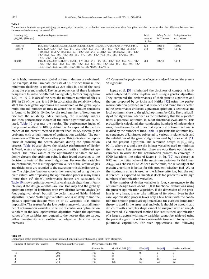
Table 9The optimum laminate designs satisfying the contiguity constraint, i.e. no lamina may contain more than four plies, and the constraint that the difference between twoconsecutive laminae may not exceed 45�.

Loading: Mxx

/Myy/Mxy (kNm/m)Optimum lay-up sequences Total

numberof plies

Safety factorfor Tsai–Wu

Safety factor formax. stress

15/15/15 [533/38/373/514/383/523/384/533/394/512/384/533/413/362/514/374/55/392/552/47/44/53/452]s 120 1.0564 1.000015/15/0 [234/404/474/22/�104/�164/�112/�254/�314/�394/�844/ �703/�854/�734/�814/�863/893/

�804/884/�852/874/�874/ 864/�834/�594/�36/�543/�774/813/�63/�804/864/72/ �882/�823/793/�894/�724/�893/�483/�26/�662/�574/ �202/�634/�792/�752/�382/�674/904/�593/�474/�302/ �142/�202]s

348 1.0107 1.0132

0/0/15 [584/262/564/28/544/313/514/463/68/�67/�314/�642/ �34/�353/�603/�404/�484/�433/�484/�424/�494/�434/ �484/�434/�503/�424/�494/�433/�484/�423/�534/�452/ �394/�494/�423/�543/�463/�403/�52/�683/�453/�81/ 73/�86/71/793/�662/752]s

280 1.0043 1.014

1722 M. Akbulut, F.O. Sonmez / Computers and Structures 89 (2011) 1712–1724

ber is high, numerous near global optimum designs are obtained.For example, if the laminate consists of 16 distinct laminae, theminimum thickness is obtained as 206 plies in 18% of the runsusing the present method. The layup sequences of these laminatedesigns are found to be different having safety factors ranging from1.001 to 1.012. In 80% of the runs, the minimum number of plies is208; in 2% of the runs, it is 210. In calculating the reliability index,all of the near global optimums are considered as the global opti-mum and the number of runs in which the minimum thicknessis found to be 206 is divided by the total number of iterations tocalculate the reliability index. Similarly, the reliability indicesand then performance indices of the other algorithms are calcu-lated. Table 10 presents the results. The performance index ofthe present method is 100 by definition. As expected the perfor-mance of the present method is better than MDSA especially forproblems with a high number of optimization variables. The per-formances of DSA and SA are rather poor. This indicates the impor-tance of reducing the search domain during the optimizationprocess. Table 10 also shows the relative performance of Nelder& Mead, which is applied to the problem with a multi-start ap-proach. The initial values of the optimization variables are ran-domly chosen; the optimum point is then found according to thedecision criteria of the search algorithm. Because the variablesare continuous, the resulting optimum values of the lamina anglesand thicknesses are rounded to the nearest permissible discrete va-lue. The objective function value is then reevaluated using the dis-crete values. After repeating the optimization process many times(more than 105 times), performance indices are calculated. AsTable 10 shows optimization with a local search algorithm is feasi-ble only if the design variables are few. One may find the globallyoptimum design of laminates with two distinct lamina angles (orfour design variables); but still the performance of Nelder & Meadalgorithm is poor. With eight variables, one is unlikely to find theglobally optimum design; with 16 or 32 variables, it is almostimpossible. The reason for the low performance with a small num-ber of optimization variables is the use of continuous optimizationvariables in the local optimization algorithm. When the optimumvalues of the variables are rounded to the nearest discrete values,either constraints are violated or objective function valueincreases.

Table 10Comparison of the performances of various simulated annealing algorithms and a local se

Number of distinct fiber angles Minimum number of plies Performance

Present SA

16 206 1008 208 1004 212 1002 218 100

4.7. Comparative performances of a genetic algorithm and the presentSA algorithm

Lopez et al. [51] minimized the thickness of composite lami-nates subjected to static in-plane loads using a genetic algorithm.They compared the performances of their genetic algorithm andthe one proposed by Le Riche and Haftka [52] using the perfor-mance criterion provided in that reference and found theirs better.In the performance criterion, a practical optimum is defined as thelocal optimum close to the global optimum by 0.1%. Then, reliabil-ity of the algorithm is defined as the probability that the algorithmfinds a practical optimum in 6000 functional evaluations. Thisprobability is calculated after conducting hundreds of independentruns; then the number of times that a practical optimum is found isdivided by the number of runs. Table 11 presents the optimum lay-up sequences of laminates subjected to various in-plane loads andthe reliabilities of the genetic algorithm used by Lopez et al. [51]and the present algorithm. The laminate design is [02q/±45r/902s]s, where q, r, and s are the integer variables used to minimizethe thickness. This means that there are only three optimizationvariables. In order for the optimization process to converge in6000 iterations, the value of factor c1 in Eq. (30) was chosen as0.82 and the initial value of the maximum variation for thickness,Dnmax, was chosen as 12. As seen in the table, the reliability of thepresent algorithm is better for this problem whether Tsai–Wu orthe maximum stress is used as the failure criterion; but the realdifference is expected to manifest itself for problems with highnumbers of optimization variables.

If the number of design variables is four, convergence to theoptimum design takes about 10,000 functional evaluations usingthe present optimization algorithm. If the dimension of the prob-lem is very large, it may take millions of iterations. Even in thatcase, optimization process takes only a few hours with the condi-tion that smooth panels are optimized and the classical laminationtheory is used in the structural analysis. It should be noted that astructure with a complex shape cannot be analyzed with an analyt-ical method. If a numerical method like FEM is used, optimizationof a large structure with many variables cannot be achieved usingthe present algorithm within a reasonable time with today’s com-putational capabilities. For such applications, the following

arch algorithm.

Index (PI)

Modified DSA [43] DSA [45] SA [44] Nelder and Mead

62 0 0 085 1 0 098 33 15 0.5105 50 22 32

Table 11Comparison of the reliabilities of the genetic algorithm used by Lopez et al. [51] and the present algorithm.

Nxy (N/mm) Optimum lay-up sequences Failure Criterion⁄ Safety factor Reliability

Ref. [51] Present

0 [±4517]s, [010/±457/9010]s, . . . MS 1.0455 1.00 1.000 The same TW 1.1599 0.99 1.00100 [±4517]s MS 1.0245 1.00 1.00100 The same TW 1.1412 1.00 1.00250 [018//9016]s,[016//9018]s MS 1.0117 0.77 0.84250 The same TW 1.0161 0.32 0.59500 [±4518]s MS 1.0041 0.96 1.00500 The same TW 1.1243 1.00 1.001000 [±4520]s MS 1.0209 0.96 1.001000 The same TW 1.1302 0.41 1.00

⁄ MS and TW denote the maximum stress criterion and Tsai–Wu criterion, respectively.

M. Akbulut, F.O. Sonmez / Computers and Structures 89 (2011) 1712–1724 1723

multilevel optimization procedure is suggested: First, the wholestructure is analyzed using FEM and the stress states at criticallocations are determined. Given the stress components at eachlayer, rk

xx; rkyy, and sk

xy, the stress resultants, Nij, Mij, are calculatedusing Eqs. (6) and (7), Then, the lamina angles and thicknesses areoptimized using the present optimization algorithm. When thelaminate design is changed, stiffness properties of the structureand thus stress state also change. For this reason, the analysis ofthe whole structural is carried out again. This procedure is re-peated until convergence.

5. Conclusions

In this study, a methodology is presented to optimize compositelaminates subjected to both in-plane and out-of-plane loading forminimum thickness. A variant of the simulated annealing algo-rithm is proposed to search the globally optimum design(s). Manymultiple global or near global optimums were found to exist. Thealgorithm proved to be more reliable in locating these designs inthe benchmark tests compared to the other SA algorithms and agenetic algorithm recently proposed. The search algorithm yieldedconsistent and reliable results in all the optimization runs.

By increasing the number of distinct lamina angles and therange of values they may take, one obtains a larger design domain,i.e. more lay-up configurations become possible. In this way, thecomplexity of the design domain and the number of local minimagreatly increase; but existence of a better global optimum becomesalso more likely. In this study, up to fifty distinct lamina thick-nesses and lamina angles with 1� angle increments were used asdesign variables to optimize laminates. To the knowledge of theauthors, optimization with such a large solution domain was notattempted in the previous studies. With a larger domain, it waspossible to obtain better optimum designs. Unlike in-plane load-ing, using two or three distinct lamina angles is not sufficient toobtain the best possible design for laminates under out-of-planeloading. For all the out-of-plane loading cases considered in thisstudy, optimum lay-up configurations with 16-distinct laminaeturned out to be better than the ones with 8-distinct laminae.

Results were also obtained by imposing contiguity constraint,i.e. no lamina may contain more than four plies, and the constraintthat the difference between two consecutive laminae may not ex-ceed 45�. In many of the loading cases, it was possible to find a near– global optimum design satisfying these constraints. In one case, athicker laminate was required to satisfy them.

When the maximum stress or Tsai–Wu failure criterion is usedindividually, an optimization algorithm may lead to false optimaldesigns because of the particular features of their failure enve-lopes. On the other hand, when they are used together, false opti-mums may be avoided. For some cases, the best orientation angles

according to one criterion may be quite unsafe according to theother. These designs can be avoided by using both criteria.

In some loading cases, the optimal designs can be counter intu-itive. Sometimes, when one component of loading is increased, it ispossible to find a thinner laminate design that can carry the ap-plied load. Therefore, a design process for composite materialsshould not be based on intuition or experience.

If the available fiber orientations are scarce, quite inferior de-signs may be obtained. This is the case, if only 0�, ±45�, and 90� an-gles are allowed. For this reason, the interval between theconsecutive angles should be selected as small as the manufactur-ing precision allows.

Acknowledgment

This paper is based on the work supported by TUBITAK (The Sci-entific and Technological Research Council of Turkey) with thecode number 106M301.

References

[1] Tauchert TR, Adibhatla S. Design of laminated plates for maximum stiffness.J Compos Mater 1984;18:58–69.

[2] Massard TN. Computer sizing of composite laminates of strength. J ReinforcedPlast Compos 1984;3:300–27.

[3] Martin PMJW. Optimum design of anisotropic sandwich panels with thin faces.Eng Optim 1987;11:3–12.

[4] Watkins RI, Morris AJ. A multicriteria objective function optimization schemefor laminated composites for use in multilevel structural optimizationschemes. Comput Methods Appl Mech Eng 1987;60:233–51.

[5] Callahan KJ, Weeks GE. Optimum design of composite laminates using geneticalgorithms. Compos Eng 1992;2(3):149–60.

[6] Fang C, Springer GS. Design of composite laminates by a Monte Carlo method.J Compos Mater 1993;27(7):721–53.

[7] Adali S, Summers EB, Verijenko VE. Minimum weight and deflection design ofthick sandwich laminates via symbolic computation. Compos Struct1994;29:145–60.

[8] Soerio AV, Antonio CAC, Marques AT. Multilevel optimization of laminatedcomposite structures. Struct Optim 1994;7:55–60.

[9] Kam TY, Lai FM. Maximum stiffness design of laminated composite plates via aconstrained global optimization approach. Compos Struct 1995;32:391–8.

[10] Huang C, Kroplin B. On the optimization of composite laminated plates. EngComput 1995;12:403–14.

[11] Huang C, Kröplin B. Optimum design of composite laminated plates via amulti-objective function. Int J Mech Sci 1995;37:317–26.

[12] Soares CMM, Correia VF, Mateus H, Herskovits J. A discrete model for theoptimal design of thin composite plate – shell type structures using a two –level approach. Compos Struct 1995;30:147–57.

[13] Avalle M, Belingardi G. A theoretical approach to the optimization of flexuralstiffness of symmetric laminates. Compos Struct 1995;31:75–86.

[14] Song SR, Hwang W, Park HC. Optimum stacking sequence of compositelaminates for maximum strength. Mech Compos Mater 1995;31(3):290–300.

[15] Kam TY, Lai FM, Liao SC. Minimum weight design of laminated compositeplates subject to strength constraint. AIAA J 1996;34(8):1699–708.

[16] Todoroki A, Sasada N, Miki M. Object-oriented approach to optimize compositelaminated plate stiffness with discrete ply angles. J Compos Mater1996;30:1020–41.

1724 M. Akbulut, F.O. Sonmez / Computers and Structures 89 (2011) 1712–1724

[17] Walker M, Reiss T, Adali S. Optimal design of symmetrically laminated platesfor minimum deflection and weight. Compos Struct 1997;39:337–46.

[18] Soares CMM, Soares CAM, Correia VMF. Optimization of multilaminatedstructures using higher-order deformation models. Comput Methods ApplMech Eng 1997;149:133–52.

[19] Haridas B, Rule WK. A modified interior penalty algorithm for the optimizationof structures subjected to multiple independent load cases. Comput Struct1997;65(1):69–81.

[20] Yamazaki K, Tsubosaka N. A stress analysis technique for plate and shell built-up structures with junctions and its application to minimum-weight design ofstiffened structures. Struct Optim 1997;14:173–83.

[21] Abu-Odeh AY, Jones HL. Optimum design of composite plates using responsesurface method. Compos Struct 1998;43:233–42.

[22] Lombardi M, Haftka RT. Anti-optimization technique for structural designunder load uncertainties. Comput Methods Appl Mech Eng 1998;157:19–31.

[23] Verijenko VE, Summers EB, Adali S. Minimum stress design of transverselyisotropic sandwich plates based on higher-order theory. Struct Optim1998;15:114–23.

[24] Soremekun G, Gurdal Z, RT Haftka, Watson LT. Composite laminate designoptimization by genetic algorithm with generalized elitist selection. ComputStruct 2001;79:131–43.

[25] Kere P, Koski J. Multicriterion stacking sequence optimization scheme forcomposite laminates subjected to multiple loading conditions. Compos Struct2001;54:225–9.

[26] Park JH, Hwang JH, Lee CS, Hwang W. Stacking sequence design of compositelaminates for maximum strength using genetic algorithms. Compos Struct2001;52:217–31.

[27] Bruyneel M, Fleury C. Composite structures optimization using sequentialconvex programming. Adv Eng Softw 2002;33:697–711.

[28] Walker M, Smith RE. A technique for the multiobjective optimisation oflaminated composite structures using genetic algorithms and finite elementanalysis. Compos Struct 2003;62:123–8.

[29] Kasprzak J, Ostwald M. Multicriterion optimization of hybrid composite plateswith various supports under transverse load. Proc Appl Math Mech2005;5:747–8.

[30] Deka DJ, Sandeep G, Chakraborty D. Multiobjective optimization of laminatedcomposites using finite element method and genetic algorithm. J ReinforcedPlast Compos 2005;24(3):273–85.

[31] Aymerich E, Serra M. An ant colony optimization algorithm for stackingsequence design of composite laminates. Comput Mode Eng Sci2006;13(1):49–65.

[32] Pelletier JL, Vel SS. Multi-objective optimization of fiber reinforced compositelaminates for strength, stiffness and minimal mass. Comput Struct2006;84:2065–80.

[33] Jadhav P, Mantena PR. Parametric optimization of grid-stiffened compositepanels for maximizing their performance under transverse loading. ComposStruct 2007;77:353–63.

[34] Kim JS. Development of a user-friendly expert system for composite laminatedesign. Compos Struct 2007;79:76–83.

[35] Park CH, Lee WI, Han WS. Improved genetic algorithm for multidisciplinaryoptimization of composite laminates. Comput Struct 2008;86:1894–903.

[36] Omkar SN, Khandelwal R, Yathindra S, Naik GN, Gopalakrishnan S. Artificialimmune system for multi-objective design optimization of compositestructures. Eng Appl Artif Intell 2008;21:1416–29.

[37] Matsuzaki R, Todoroki A. Stacking-sequence optimization using fractal branch-and-bound method for unsymmetrical laminates. Compos Struct2007;78:537–50.

[38] Khosravi P, Sedaghati R. Design of laminated composite structures foroptimum fiber direction and layer thickness, using optimality criteria. StructMultidisplinary Optim 2008;36:159–67.

[39] Rao AN, Ratnam C, Srinivas J, Premkumar A. Optimum design of multilayercomposite plates using simulated annealing. Proc Inst Mech Eng. Part L: J Mat:Des Appl 2002;216(3):193–7.

[40] Sciuva MD, Gherlone M, Lomario D. Multiconstrained optimization oflaminated and sandwich plates using evolutionary algorithms and higher-order plate theories. Compos Struct 2003;59:149–54.

[41] Erdal O, Sonmez FO. Optimum design of composite laminates for maximumbuckling load capacity using simulated annealing. Compos Struct2005;71:45–52.

[42] Moita JMS, Correia VMF, Martins PG. Optimal design in vibration control ofadaptive structures using a simulated annealing algorithm. Compos Struct2006;75:79–87.

[43] Akbulut A, Sonmez FO. Optimum design of composite laminates for minimumthickness. Comput Struct 2008;86:1974–82.

[44] Kirkpatrick S, Gelatt CD, Vecchi MP. Optimization by simulated annealing.Science 1983;220:671–80.

[45] Ali MM, Törn A, Viitanen S. A direct search variant of the simulated annealingalgorithm for optimization involving continuous variables. Comput Oper Res2002;29:87–102.

[46] Jones RM. Mechanics of composite materials. 2nd ed. Taylor & Francis; 1999.[47] Gürdal Z, Haftka RT, Hajela P. Design and optimization of laminated composite

materials. John Wiley & Sons; 1999.[48] Le Riche R, Haftka RT. Improved genetic algorithm for minimum thickness

composite laminate design. Compos Eng 1995;5(2):143–61.[49] Kere P, Lyly M, Koski J. Using multicriterion optimization for strength design of

composite laminates. Compos Struct 2003;62:329–33.[50] Irisarri FX, Bassir DH, Carrere N, Maire JF. Multiobjective stacking sequence

optimization for laminated composite structures. Compos Sci Technol2009;69:983–90.

[51] Lopez RH, Luersen MA, Cursi ES. Optimization of laminated compositesconsidering different failure criteria. Compos: Part B 2009;40:731–40.

[52] Le Riche R, Haftka R. Improved genetic algorithm for minimum thicknesscomposite laminate design. Compos Eng 1995;5(2):143–61.