Design Optimisation of Surface Mounted PermanentMagnet Synchronous Motors for In-wheel Electric

Vehicle Applications

Soumya Bandyopadhyay

Master of Science Thesis

Supervisor:Dr.ir. H. Polinder

Ir. Martin van der Geest

DC systems, Energy conversion & StorageDepartment of Electrical Sustainable Energy

Faculty of Electrical Engineering, Mathematics and Computer ScienceDelft University of Technology

June 25, 2015

Acknowledgements

I would first and foremost like to thank my supervisor Dr. Henk Polinder who has shown immensepatience and support for me during this thesis. He was always available for any kind of questions anddiscussions. His phenomenal passion and understanding of the subject is a big motivation and inspi-ration for me.I would also like to thank Martin van der Geest who has been a great support in carrying out this thesiswork. His immense knowledge in machine design and sharp analytical skills inspired me to challengemy boundaries to become a better researcher. He has always been ready to discuss my questions anddoubts and has been very helpful throughout the whole duration of this thesis. A special thanks to Dr.Domenico Lahaye for his support and encouragement for both computational and writing part of thisthesisMy thesis was supported by E-Traction B.V and the team there has been very helpful and always pro-vided me with everything I needed for my thesis work. I would take this opportunity to thank Ir. PeterPaul vand der Ven who has always helped me and acknowledged my demand for more time on thetest bench. I wish him luck and success for his future endeavours.Many thanks to my fellow master students of the student room who have made this hectic monthsbearable and fun-filled. Thanks to them I never really had to work alone.I would also like to thank my friends in Delft Jaggu, Avinash, Anil, Udai, Debu, Benji, Harsha, Muru fortheir support, encouragement and most importantly making this last two years memorable.I can’t thank my family enough for their faith in me. Thanks Mom-Dad and sister Anisha for yourconstant encouragement and support. Last but not the least I would like to thank Tuli for her con-stant support and encouragement, particularly the toughest and testing times during the course ofthis thesis.

Abstract

The drive to reduce CO2 emissions through alternative energy resources has been one of the pioneer-ing studies of this century. This has led to a lot of research and innovation in the transportation sector.After nearly a century with the internal combustion(IC) engine dominating this sector, it now appearsthat the Electric Vehicle Technology is on the edge of experiencing rapid growth in both developedand developing vehicle markets. Hence the research for electric vehicles with efficient drive systemswith electric motors, especially Permanent Magnet Motors has received a lot of attention lately.

This thesis investigates the opportunities for improvements on an existing design of Surface MountedPermanent Magnet Synchronous motor(SPMSM) for better performance of Electric vehicles alongwith detailed comparison of dynamic performance with existing class of motors.

The initial part of the thesis is dedicated to modelling of a Permanent Magnet Synchronous Motor tobe used as an in-wheel motor in an Electric Bus. A 2-Dimensional machine model is developed usingFinite Element methods (FEM) which forms the basis of study of the steady state and dynamic Elec-tromagnetic behaviour of the machine. Furthur a Lumped Circuit Parameter Thermal Model is de-veloped to understand the steady state and transient thermal behaviour of the machine. This projectis executed in collaboration with the Dutch Electric vehicle company,E-Traction. The developed ma-chine models are validated with experiments on their testbench motor.

In the second stage of the Thesis new designs of Fractional Slot Concentrated Winding(FSCW) PMSMare made with pre-defined targets and design choices. The existing design as well as the new ones areoptimised using multi-objective Particle Swarm Optimisation Technique to ensure higher Efficiency& Boost Torque capability. The thesis also investigates the performance of FSCW PMSM with differentwinding schemes or slot/pole combinations. Finally the thesis culminates with a detailed comparativeanalysis of all the optimal machines with different winding schemes.

Contents

Acknowledgements

Abstract

1 Introduction 11.1 Background . . . . . . . . . . . . . . . . . . . . . . . . . . . . . . . . . . . . . . . . . . . . . . 1

1.1.1 In-Wheel Hub Motor Technology . . . . . . . . . . . . . . . . . . . . . . . . . . . . . . 11.1.2 Permanent Magnet Machines in E-Vehicles . . . . . . . . . . . . . . . . . . . . . . . 31.1.3 Types of PM synchronous machines . . . . . . . . . . . . . . . . . . . . . . . . . . . . 3

1.2 Research Focus . . . . . . . . . . . . . . . . . . . . . . . . . . . . . . . . . . . . . . . . . . . . 51.3 Thesis Objective . . . . . . . . . . . . . . . . . . . . . . . . . . . . . . . . . . . . . . . . . . . . 51.4 Research Approach and Thesis layout . . . . . . . . . . . . . . . . . . . . . . . . . . . . . . . 61.5 Contributions . . . . . . . . . . . . . . . . . . . . . . . . . . . . . . . . . . . . . . . . . . . . . 8

2 Numerical Modelling of PMSM 112.1 Introduction . . . . . . . . . . . . . . . . . . . . . . . . . . . . . . . . . . . . . . . . . . . . . . 112.2 Finite Element Method . . . . . . . . . . . . . . . . . . . . . . . . . . . . . . . . . . . . . . . . 12

2.2.1 Basic Theory . . . . . . . . . . . . . . . . . . . . . . . . . . . . . . . . . . . . . . . . . . 122.2.2 FE Model for PM machines . . . . . . . . . . . . . . . . . . . . . . . . . . . . . . . . . 122.2.3 Flowchart for analysis and design of PMSM . . . . . . . . . . . . . . . . . . . . . . . 13

2.3 Design details of existing PMSM . . . . . . . . . . . . . . . . . . . . . . . . . . . . . . . . . . 142.3.1 Geometry . . . . . . . . . . . . . . . . . . . . . . . . . . . . . . . . . . . . . . . . . . . 142.3.2 Winding distribution . . . . . . . . . . . . . . . . . . . . . . . . . . . . . . . . . . . . . 142.3.3 Material Properties . . . . . . . . . . . . . . . . . . . . . . . . . . . . . . . . . . . . . . 16

2.4 Electromagnetic Analysis of PMSM . . . . . . . . . . . . . . . . . . . . . . . . . . . . . . . . 182.4.1 Flux Linkage & Back-EMF . . . . . . . . . . . . . . . . . . . . . . . . . . . . . . . . . . 192.4.2 Inductance . . . . . . . . . . . . . . . . . . . . . . . . . . . . . . . . . . . . . . . . . . . 212.4.3 Electromagnetic Torque Characteristics . . . . . . . . . . . . . . . . . . . . . . . . . . 21

2.5 Estimation of Losses in PM Synchronous motors . . . . . . . . . . . . . . . . . . . . . . . . 222.5.1 Stator Losses . . . . . . . . . . . . . . . . . . . . . . . . . . . . . . . . . . . . . . . . . . 232.5.2 Rotor Losses . . . . . . . . . . . . . . . . . . . . . . . . . . . . . . . . . . . . . . . . . . 262.5.3 Summary of Losses . . . . . . . . . . . . . . . . . . . . . . . . . . . . . . . . . . . . . 27

2.6 Thermal Analysis using Circuit Thermal Model . . . . . . . . . . . . . . . . . . . . . . . . . 282.6.1 Background and Motivation . . . . . . . . . . . . . . . . . . . . . . . . . . . . . . . . 282.6.2 Lumped Circuit Thermal model . . . . . . . . . . . . . . . . . . . . . . . . . . . . . . 292.6.3 Summary of Assumptions . . . . . . . . . . . . . . . . . . . . . . . . . . . . . . . . . . 322.6.4 Steady state thermal analysis . . . . . . . . . . . . . . . . . . . . . . . . . . . . . . . . 332.6.5 Transient thermal analysis . . . . . . . . . . . . . . . . . . . . . . . . . . . . . . . . . 34

2.6.6 Comparison with experimental results . . . . . . . . . . . . . . . . . . . . . . . . . . 342.7 Conclusions . . . . . . . . . . . . . . . . . . . . . . . . . . . . . . . . . . . . . . . . . . . . . . 35

3 Experimental Validation FE Machine Model 373.1 Introduction . . . . . . . . . . . . . . . . . . . . . . . . . . . . . . . . . . . . . . . . . . . . . . 373.2 Methodology and Experiments . . . . . . . . . . . . . . . . . . . . . . . . . . . . . . . . . . . 37

3.2.1 Testbench . . . . . . . . . . . . . . . . . . . . . . . . . . . . . . . . . . . . . . . . . . . 383.2.2 Open Circuit Test . . . . . . . . . . . . . . . . . . . . . . . . . . . . . . . . . . . . . . . 383.2.3 Short Circuit Test . . . . . . . . . . . . . . . . . . . . . . . . . . . . . . . . . . . . . . . 383.2.4 Load Test . . . . . . . . . . . . . . . . . . . . . . . . . . . . . . . . . . . . . . . . . . . . 39

3.3 Experimental Validation . . . . . . . . . . . . . . . . . . . . . . . . . . . . . . . . . . . . . . . 403.3.1 Back-EMF Experimental Validation . . . . . . . . . . . . . . . . . . . . . . . . . . . . 403.3.2 Validation of Electromagnetic Torque . . . . . . . . . . . . . . . . . . . . . . . . . . . 413.3.3 Experimental Validation Resistance and Inductance . . . . . . . . . . . . . . . . . . 423.3.4 Validation of Efficiency and Losses . . . . . . . . . . . . . . . . . . . . . . . . . . . . . 43

3.4 Conclusion . . . . . . . . . . . . . . . . . . . . . . . . . . . . . . . . . . . . . . . . . . . . . . . 46

4 Design Optimization of PM Synchronous Machines 474.1 Introduction . . . . . . . . . . . . . . . . . . . . . . . . . . . . . . . . . . . . . . . . . . . . . . 474.2 Definitions and Terminology . . . . . . . . . . . . . . . . . . . . . . . . . . . . . . . . . . . . 484.3 Advantages and Drawbacks of Concentrated windings . . . . . . . . . . . . . . . . . . . . . 494.4 Optimal slot/pole combinations . . . . . . . . . . . . . . . . . . . . . . . . . . . . . . . . . . 50

4.4.1 Selection Criteria . . . . . . . . . . . . . . . . . . . . . . . . . . . . . . . . . . . . . . . 504.4.2 Comparative analysis of concentrated winding schemes . . . . . . . . . . . . . . . 514.4.3 Summary . . . . . . . . . . . . . . . . . . . . . . . . . . . . . . . . . . . . . . . . . . . . 53

4.5 Optimization Strategy to compare different PM machine designs . . . . . . . . . . . . . . 544.5.1 Background . . . . . . . . . . . . . . . . . . . . . . . . . . . . . . . . . . . . . . . . . . 544.5.2 Basics of Particle Swarm Optimization . . . . . . . . . . . . . . . . . . . . . . . . . . 544.5.3 Multi-objective PSO and Pareto Fronts . . . . . . . . . . . . . . . . . . . . . . . . . . 554.5.4 Optimisation Targets . . . . . . . . . . . . . . . . . . . . . . . . . . . . . . . . . . . . . 574.5.5 Optimization Variables . . . . . . . . . . . . . . . . . . . . . . . . . . . . . . . . . . . 594.5.6 Given Constants . . . . . . . . . . . . . . . . . . . . . . . . . . . . . . . . . . . . . . . 614.5.7 Optimisation Constraints . . . . . . . . . . . . . . . . . . . . . . . . . . . . . . . . . . 61

4.6 Conclusion . . . . . . . . . . . . . . . . . . . . . . . . . . . . . . . . . . . . . . . . . . . . . . . 62

5 Results & Comparison of Optimal Machine Designs 655.1 Introduction . . . . . . . . . . . . . . . . . . . . . . . . . . . . . . . . . . . . . . . . . . . . . . 655.2 Results of optimization . . . . . . . . . . . . . . . . . . . . . . . . . . . . . . . . . . . . . . . . 65

5.2.1 2D Pareto and Derived Fronts . . . . . . . . . . . . . . . . . . . . . . . . . . . . . . . . 665.2.2 Effect of Design Variables . . . . . . . . . . . . . . . . . . . . . . . . . . . . . . . . . . 68

5.3 Optimisation of existing PMSM design . . . . . . . . . . . . . . . . . . . . . . . . . . . . . . 685.3.1 Background . . . . . . . . . . . . . . . . . . . . . . . . . . . . . . . . . . . . . . . . . . 685.3.2 Methodology . . . . . . . . . . . . . . . . . . . . . . . . . . . . . . . . . . . . . . . . . 715.3.3 Reduction of Torque ripple . . . . . . . . . . . . . . . . . . . . . . . . . . . . . . . . . 74

5.4 Comparison of Optimal Machine Designs . . . . . . . . . . . . . . . . . . . . . . . . . . . . 755.4.1 Selection of Optimal machines . . . . . . . . . . . . . . . . . . . . . . . . . . . . . . . 765.4.2 Design Details . . . . . . . . . . . . . . . . . . . . . . . . . . . . . . . . . . . . . . . . . 765.4.3 Back-EMF characteristics . . . . . . . . . . . . . . . . . . . . . . . . . . . . . . . . . . 785.4.4 Torque Characteristics . . . . . . . . . . . . . . . . . . . . . . . . . . . . . . . . . . . . 805.4.5 Losses and Efficiency . . . . . . . . . . . . . . . . . . . . . . . . . . . . . . . . . . . . 82

5.4.6 Thermal Behaviour . . . . . . . . . . . . . . . . . . . . . . . . . . . . . . . . . . . . . . 845.5 Summary and Discussions . . . . . . . . . . . . . . . . . . . . . . . . . . . . . . . . . . . . . 86

6 Conclusion and Recommendations 896.1 Conclusions . . . . . . . . . . . . . . . . . . . . . . . . . . . . . . . . . . . . . . . . . . . . . . 896.2 Future Work and Recommendations . . . . . . . . . . . . . . . . . . . . . . . . . . . . . . . . 90

Bibliography 93

Chapter 1

Introduction

This chapter presents an introduction to the field of research. Then the need for such research is justifiedby recent trends and developments. After a holistic view of the whole field of research, the problemstatement is formulated. Finally the chapter culminates in a brief outline of the thesis.

1.1 Background

1.1.1 In-Wheel Hub Motor Technology

Electric vehicle technology has been widely considered as the future of worldwide automobile in-dustry. The virtues of low noise pollution and very fast torque response seems make E-vehicle (EV)technology indisputable. However the present performance of an Electric Vehicle in terms of driv-ing range and cost of infrastructure are far from being competitive to those Internal Combustion en-gine (ICE) vehicles. With limited onboard energy storage the need arises to build more efficient, lightweight,compact electric propulsion systems so as to maximize driving range per charge.There are basically two ways to achieve high power density and high efficiency drives. The first tech-nique(fig 1.1) involves employing high speed motors, so that motor volume and weight reduces sig-nificantly for same rated output power. However mechanical losses incurred by the clutch,gears etc.during power transmission from motor to wheel reduces overall efficiency. A simple yet elegant solu-tion to the above problem involves employing high-torque, low speed motors directly mounted insidethe wheel (Figure 1.2), known as In-wheel motors or hub motors [1]. By applying wheel motors in EVstraditional power transmission such as clutch, reduction, differential gears can be eliminated thusminimizing transmission losses and improving operation efficiency [2], [3]. The biggest advantages ofusing in-wheel electric motor are following:

• Precise Torque Control of individual wheels

• Optimisation of Space

• Direct Drive leading to Optimal Efficiency operation

• Reduction of Power Electronic Converter rating

Considering the advantages of in-wheel motor numerous vehicle manufacturers are developing vehi-cles with in-wheel motor drives [4],[5]. Even though this kind of motor drives being mainly suitablefor off-road applications [6], gradually they are coming into commercial on-road applications as well.

1

Figure 1.1: Classic Electric Vehicle with single motor drive [4]

Figure 1.2: Modern Electric Vehicle with in-wheel motor direct drive [4]

(a) External rotor in-wheel PM motor by Protean Electric (b) Exploded 3-D view of in-wheel PM motor

Figure 1.3: Outer Rotor in-wheel PM synchronous motor of Electric Protean ford truck

2

Figure 1.3 depicts an outer rotor PM machine which is used in an electric truck developed by ProteanElectric.

However in-wheel motors suffers from a drawback of having large unsprung mass which deteri-orates ride comfort and reduces the road holding capability of the car. There are solutions to thisproblem in literature [7], but it is beyond the scope of this thesis.Different electric motors can be used for this EV in-wheel application. However the focus of this thesisis entirely on Permanent magnet synchronous motors.In the next subsection the merits of permanentmagnet synchronous machines as in-wheel hub motor will be analysed.

1.1.2 Permanent Magnet Machines in E-Vehicles

The main requirements of in-wheel motors are good peak torque capability at low speeds, wide speedrange, high efficiency, high power density so as to reduce motor weight. A low motor weight is verymuch essential to maintain vehicle dynamic performance due to low unsprung mass. Hence, highefficiency to weight ratio is an important criteria to select suitable electric motors. Several types ofmotors as in-wheel motors satisfying the above criteria have been reported in literature including thefollowing machine types:

• Induction motor [8] [9]

• PM synchronous motor [10]

• PM brushless DC motor (BLDC) [11] [12]

• Switched reluctance motor (SRM) [13].

In depth comparative analysis of aforesaid electric motor drives in EV application is beyond thescope of this thesis. Interested readers can have a look at [14] [15]. As already mentioned, the re-search focus of this thesis is exclusively on PM synchronous motors because its high power densityand efficiency, smooth torque characteristics and ease of control. Since magnetic field is excited byhigh-energy permanent magnets, power density is high, and hence, the overall weight and volumecan be greatly reduced. Because of absence of rotor copper windings and rotor copper losses, the ef-ficiency of PM synchronous machines is inherently high.

1.1.3 Types of PM synchronous machines

There are various types of PM synchronous machines in the market these days and many ways toclassify them. Here the focus on classification is based on the following design choices:

Exterior rotor PMSM and Interior rotor PMSM

The relative placement of rotor with respect to the stator leads to two different machine topologiesnamely Exterior Rotor PMSM and Interior rotor PMSM.The interior rotor PM motor is widely used forall types of application and since the static part is placed externally, it provides safety for its users aswell. However for applications in Electric Vehicle as wheel motors, exterior rotor PM motor has certainadvantages:

• Ease of integration as vehicle tire rests on outer moving rotor

• Larger air gap diameter than interior rotor PM machines with same rated power and volumeleading to higher torque density

3

(a) Distributed winding with q = 1 (b) Concentrated winding with q = 0.5

Figure 1.4: Comparison of basic stator winding schemes [24]

Surface Mounted Magnet Rotor(SPM) and Interior Buried Magnet rotor(IPM)

The surface mounted PM machine(SPM) is of simple structure, thus widely used in many applica-tions including Electric vehicles [16]. Interior Permanent magnet(IPM) rotor machines are also fa-mous in EV application because of their extra torque capability due to reluctance.In addition to thatIPM machines provide inherent protection of buried magnets from demagnetization [17]. Literatureon comparison between SPM and IPM topologies [18] [19] [20]for EV applications shows comparableperformances.

Distributed winding and Concentrated Winding Stator

Before going into in-depth comparative analysis the aforesaid winding schemes, the definitions ofdistributed winding and concentrated winding configurations (Figure 1.4) used in the thesis must behighlighted.The term "distributed windings" refers to overlapping windings with slots per pole perphase (q) greater than or equal to 1. The term "concentrated winding" refers to non-overlappingwindings with q less than 0.5. So in a PM machine with concentrated windings, q will always be afraction(discussed in detail in chapter 4).In general, a distributed winding PM machine has lower harmonic content in its winding MMF dis-tribution (fig: 1.5) which leads to lower rotor eddy current losses than its concentrated winding coun-terpart . But concentrated winding machines have smaller end windings than distributed windingmachines.Thus PM machines with concentrated windings have higher power densities due to lowercopper weights and higher efficiencies due to lower copper losses for same output power rating [21][22].Concentrated winding PM machines are easier to manufacture due to their simplicity of implementa-tion and also can be made cheaper with automation. Due to their non-overlapping winding schemethey also have a higher fault tolerant capability [21]. Even though significant research on comparativeanalysis of concentrated winding and distributed winding topologies can be found in literature, veryfew can be found with respect to Electric vehicle as application [23].Therefore, in this thesis PM machine with both concentrated winding stator and distributed windingstator will be considered for in depth research of their suitability analysis for EV application.

4

Figure 1.5: Comparison of concentrated winding mmf with distributed winding mmf

1.2 Research Focus

This thesis exclusively focuses on the design optimisation of Permanent magnet synchronous ma-chines for in-wheel motor applications in electric vehicles. Out of many types of PM synchronousmachines, this thesis deals with surface mounted exterior rotor PM synchronous machines (SPMSM).This type of motor has been chosen because it fits the criteria for electric vehicle applications viz. highefficiency, high torque density and ease of control.However these motors are heavy and expensive due to use of distributed windings (high number ofoverlapping coils) and costly PM material. Therefore it is evident that research needs to be done withthe aim of reducing the active weight of the machine without affecting overall performance. In thatrespect, an important feature of this whole research is the use of fractional slot concentrated windingmachine instead of distributed winding stator in PMSM so as to reduce copper weight and manufac-turing cost.

1.3 Thesis Objective

This thesis originates from a research initiative by E-Traction ( Dutch Electric bus company).It is moti-vated by the scope of improvement on the dynamic performance of their existing Permanent MagnetSynchronous machine with distributed winding stator (table 1.1). As already highlighted in section 1.2,in general this kind of machine is heavy and expensive. The existing design also suffers from the samedrawback. In addition to that, the peak torque capability of the machine is lower than the requiredperformance specifications. Also the electrical efficiency of the machine in its operating range is nothigh enough given the overall size of the machine. These above drawbacks presents a good opportu-nity to analyse and improve on the current machine design. Therefore the main objective of the thesiscan be formulated as:"How far the performance of the PMSM can be improved in terms of peak torque capability, active motorweight and electrical efficiency?"

5

Parameters ValueRated Output Power (kW) 100

Rated Speed (rpm) 350Rated Current/Maximum Current (A) 200/500Rated Torque/Maximum Torque (Nm) 2750/6000

Outer rotor diameter(m) 0.535Stack Length (m) 0.3

Airgap Length (mm) 2Winding Type Distributed

Number of slots/poles 93/30Insulation Class F

Table 1.1: Specifications of E-Traction’s PM machine

In order to achieve the above goals, the objective has been broken down into a number of subsidiaryobjectives which are described below:

• Develop an accurate electromagnetic model of the existing PMSM (with distributed windingscheme).

• Develop a lumped circuit parameter thermal model coupled with aforesaid electromagneticmodel to take thermal constraints into account.

• Validation of aforesaid models with experiments.

• Develop segmented or fractional electromagnetic FEM model for PMSM with Fractional slotconcentrated winding scheme, computationally suitable for design optimisation.

• Design optimisation of suitable machine configurations using Multi-Objective optimisation al-gorithm.

• Compare performance of optimal new machine designs with existing permanent magnet syn-chronous machine performance

It must be noted that this thesis is limited to design optimization, electromagnetic aspects and thethermal model of the motor. The mechanical aspects of the motor along with design of controllersand converters are beyond the scope of the research.

1.4 Research Approach and Thesis layout

This section describes the approach or methodology taken in this thesis. In order to achieve the ob-jectives mentioned above, this Master thesis is organized as shown in the flowchart in Figure 1.6. Thefollowing is a summary of contents of each chapter,

Chapter 2: FEM Electromagnetic Model and Thermal model

The first step taken in the thesis is to create a 2-D transient automated FEM model of the existingPMSM which takes magnetic saturation and rotor motion into account for better accuracy. Equationsfor calculating Flux linkage, Back-EMF, Electromagnetic Torque and electrical losses from flux density

6

Figure 1.6: Outline of this thesis

7

distribution in different parts of the machine are given. The transient FEM model is mainly used todetermine the eddy current losses in the rotor magnets. This model forms a very effective tool to studythe expected behaviour of a PMSM and its inner intricate fields. The last section of this chapter de-scribes the development of a lumped circuit parameter thermal model to take the thermal constraintinto account.

Chapter 3: Experimental Validation of Models

The goal of this chapter is to validate the accuracy of the FEM simulated results by comparing themwith experimental results on the existing PM machine. The non-linear dynamic FEM model is val-idated on basis of a) Back-EMF shape and magnitude b) Electromagnetic Torque vs Iq current be-haviour c) Machine phase resistance and Synchronous Inductance d) Electrical Efficiency at differentcurrent loading. Simulation and experimental results show good agreement.Successful validation described in this chapter paves the way for design optimization of new machinesusing the existing FEM model.

Chapter 4: Design optimization of Concentrated winding PMSM using Multi-Objective ParticleSwarm Algorithm

This chapter describes how the validated FEM model is extended to create a fractional slot Concen-trated winding(FSCW) Permanent magnet machine model with well defined design choices. Variousslot/pole combinations are investigated on their relevant merits for in-wheel motor application forE-vehicles. The chapter also describes how the previous FEM model is improved in terms of ease ofcomputation using winding and geometrical symmetry to make it suitable for design optimization.Inthe final section of this chapter,the design optimization of the FEM model using multi-objective Parti-cle swarm optimization technique is discussed in detail along with choice of well defined optimizationtargets and variables.

Chapter 5: Comparative analysis of Optimal machine configurations

In this chapter, in-depth post processing of optimisation results from the previous chapter is doneto compare optimal machines with different winding schemes and discuss their suitability for usingthem in in-wheel hub motor application. This chapter also investigates the influence and sensitivityof optimisation variables on the machine performance targets.

Chapter 6: Conclusions and recommendations on future work

In the last thesis chapter, theoretical and practical work presented in the thesis are revisited and eval-uated. Important conclusions are drawn with respect to the validation of the developed models, per-formance and applicability of the new optimised machine designs. The chapter lists the main contri-butions of the thesis and gives recommendations for future research work on this field.

1.5 Contributions

This thesis entirely focuses on Permanent Magnet Synchronous machines as in-wheel motor in Elec-tric vehicle applications. Some interesting scientific insights which are not extensively covered in lit-erature are gained during this thesis. They are as follows:

8

• In-depth comparative analysis of both distributed winding PMSM with various concentratedwinding PMSM topologies with respect to their suitability in EV application.

• New insights into using marginally unbalanced winding schemes to significantly increase PMmachine performance in electric vehicles.

• Methods of optimising asymmetrical and computationally heavy FEM machine models usingsymmetrical models with reasonable accuracy but saving large computational power, efficiencyand time.

The aforesaid contributions will be discussed in detail in the final chapter of this thesis and attacheddraft scientific papers in the appendix.

9

10

Chapter 2

Numerical Modelling of PMSM

The aim of this chapter is to introduce numerical modelling procedure for direct drive PMSM. Finiteelement method (FEM) is used to model the electromagnetic behaviour of the machine. After a brief dis-cussion on background theory,some results obtained from FE modelling of a current PMSM design arepresented. The chapter also discusses a lumped circuit model used for modelling the thermal behaviourof the machine. Finally the chapter ends with results obtained from combining the aforesaid electro-magnetic and the thermal machine models to present a holistic thermo-electromagnetic performanceof PMSM.

2.1 Introduction

The aim of this thesis as discussed in the previous chapter is to critically analyse the performance of anexisting PMSM and subsequently investigate the possibility of better machine designs with improvedperformance. This requires an in depth understanding on the effect of various design parameterson the performance of PMSM, which can be acquired by creating an accurate and flexible machinemodel. When starting with such a detailed analysis and design of PM synchronous machines, there aremany modelling approaches which can be applied. Two popular choices are the Analytical methodsand the Finite Element method (FEM).Finite element(FE) methods are being used extensively these days to simulate complex geometriesand scenarios which are difficult to solve analytically. The analytical methods are limited in capturingthe following effects:

a Complexity of geometry

b Material non-linearity and anisotropy

c Interlinked transient effects like thermo-electric ,motional effects etc.

The mathematical complexity of analytical models and the inaccuracy due to simplified assumptionshas made FE methods popular nowadays. The scope of this thesis is limited to use of 2-D FE methodfor analysing PMSM designs.The first section of this chapter provides some background information on FEM and an overview ofthe steps involved. In the next section the details of the existing PMSM are given, which will be used toillustrate the FE modelling procedure. The results obtained from the FE model of the existing designare discussed in the following section. It must be noted that the FE machine model only analyses the

11

electromagnetic behaviour of the machine. To gain insights into the holistic thermo-electromagneticperformance of the machine a circuit thermal model(combined with electromagnetic model) of thePMSM is built. The thermal model uses the losses predicted by the electromagnetic model to simulateth thermal behaviour of the machine. Details on thermal modelling procedure and assumptions arediscussed in the penultimate section of this chapter. Finally, the importance and contribution of thischapter with respect to the overall goal of this thesis is discussed in the conclusion.

2.2 Finite Element Method

In this section basic theory of FEM and general procedure of setting up a FEM problem for PM ma-chines are briefly described. The mathematics behind FEM are not discussed here as it has beenwidely published. Interested readers can check the following references for more details(reference onbianchi book,lahaye notes)

2.2.1 Basic Theory

In essence, the Finite element method is a numerical technique to solve Partial Differential Equa-tions(PDEs). In FEM the solution of PDEs is based on either complete elimination of equations orbreaking them into Ordinary Differential Equations(ODEs). These ODEs are then solved numericallyby discretizing the space into smaller sub domains and solving them locally.

2.2.2 FE Model for PM machines

An in-depth treatment of the FEM model for PM machines is not presented in this thesis since it iswidely published in books and literature [25]. Readers interested in detailed FEM modelling of PMmachines can look in these references [26] [27] [28]. Instead of detailed description, only the basicsteps in the process of solving a magnetics problem in PM machines using FEM are briefly describedin the following.

Problem Definition

In this step it has to be determined what the problem actually is, along with the required input data tosolve the problem. Most of the performance parameters of PMSM like electromagnetic torque, lossesetc. are dependent on the interactions of the stator and rotor magnetic field within the PM machine.This requires knowledge on the magnetic field distribution in the machine leading to the question :

"How are the magnetic fields distributed within the PM machine?"

To provide an answer to the above problem statement we need data about the parameters of the mag-netic circuits in the machine like net magneto motive force(mmf) and effective reluctance offered bythe magnetic path. In terms of machine parameters we need the data on geometrical dimensions,winding distribution and magnetic properties of the materials used in the machine.

Creating the model

When all the relevant data has been collected the FEM model can be built. The user creates the geom-etry, selects the equation(s) to be solved and assigns constraints and driving sources. The governingelectromagnetic field equation in 2-D FEM model for PMSM can be written as :

5× (µ−1(5× ~Az − ~Br ))+σ∂~Az

∂t= ~Js,z −σ5ϕ (2.1)

12

where ~Az is the magnetic vector potential in the z-direction, ~Br is the vector remnant flux densityof the magnets, ~Js,z is the current density of the external source in z-direction,ϕ is the electric scalarpotential,µ is the permeability of the material and σ is the electrical conductivity. If non-linear mate-rials are used µ is a function of flux density.To be able to provide an accurate solution to the above problem, magnetic saturation of stator androtor iron are taken into account. Also to take into account for rotor motion, the Arbitrary LagrangianEulerian(ALE) method [29]is used. For more details on building model for PM machines refer to[26][27].

Generating a mesh

FEM approximates the problem locally on elements with a fixed shape. In this step an approximationof the geometry is created using those elements; the result is called the mesh (Figure 2.1 (a)). Thenumber of mesh points influences the accuracy of the numerical calculations. If the meshes are fine(high degrees of freedom) the accuracy of computation is high but computational time is high as well.Normally the FEM program is made in compromise between accuracy and time-consumption. Thefollowing steps are necessary to ensure good balance of computational accuracy and time needed forFEM simulation of outer rotor PM Synchronous machines.

• Fine mesh in air gap for accurate torque computation

• Fine mesh in rotor back iron and magnets to catch induced eddy currents

• Relatively coarser mesh in other domains to reduce computation time

Solving the model

After the mesh has been generated the model can be solved. With the FEM this comes down to solvinga large set of linear equations. A static or transient solver can be used depending upon the require-ments of the simulation. In general, using a transient solver can be time consuming since it solves fora sequence of system equations whereas a static solver solves for only one.

Post-processing

The computed solution may not directly provide an answer to the problem. The results are furtherprocessed in this step to yield the desired answers in a form engineers can understand.In case of PM machines FEM solves equation 2.1 for the magnetic vector potentials ~Az (Figure 2.1 (b)).This plot of ~Az is further post-processed to deduce the flux density, back-emf and flux linkage, elec-tromagnetic torque, eddy current loss and stator iron loss. More detailed results on post-processingwill be presented in upcoming sections of this chapter.

2.2.3 Flowchart for analysis and design of PMSM

The whole concept of described above is presented in the flowchart in figure 2.1. According to theflowchart the FEM software is coupled with MATLAB and the program runs on MATLAB. The machineinput data includes dimensions, material properties etc. MATLAB creates the geometry and also setsup the entire FE model including assigning domain physics and boundary conditions. The FEM soft-ware solves the model and sends it back to MATLAB for post processing. Until now, a non-linear 2-DFEM machine model is built which also includes rotor motion. This FE machine model will now beused to analyse the electromagnetic behaviour of the current PMSM design. Before showing the FEresults, the design details of the current machine will be presented in the next section.

13

(a) Finite Element Meshing (b) Solution Plot of Magnetic Vector Potential (contourplot) and Magnetic Flux density (surface Plot)

Figure 2.1: Finite Element Modelling of Surface PM Synchronous Machine

2.3 Design details of existing PMSM

Important specifications of the existing PM machine have already been presented in Chapter 1 (Ta-ble 1.1). In this section, the relevant design details will be presented. The aim of this section is to pro-vide the pertinent input data to solve the electromagnetic FEM problem as discussed in section 2.2.2.

2.3.1 Geometry

In Figure 2.3, an exploded view of the current PMSM design is shown. There is an outer rim on therotor back iron (figure 2.4), to provide good fit inside the wheel and to protect the PM machine frommechanical vibrations. This kind of outer rim over the rotor back-iron is generally not seen in standarddesigns.

2.3.2 Winding distribution

The details on winding distribution of the current PMSM design are presented in Table 4.1. It is afractional slot distributed winding with slot/pole/phase (q) equal to 1.03. This winding distribution isdifferent from traditional integer slot distributed symmetrical and balanced winding schemes.The star of slots method [30] [31] is used to analyse the winding distribution. The winding factors ofthe working harmonics (15th) are calculated to be 0.9536, 0.9536 and 0.9530 for phases u, v and wrespectively, resulting in a unbalance degree of 0.0388 %.

14

Start

Input Machine Data

Matlab Program

FEM software

Output data

Store Data

End

Slot/Pole combination, dimensions of tooth & pole,

air gap length, material properties etc.

Coupling of Matlab & FEM software(COMSOL)

Magnetic vector potential, flux density, Back-emf,

electromagnetic torque,cogging torque,iron

losses etc.

Solving electromagnetic field problem as defined in script

Create machine geometry, assigning physics &

boundary conditions + Post-processing

Pos

t-P

roce

ssin

g

Figure 2.2: Flowchart for analysis and design of PM machines based on FEM

15

RotorIron

Magnets

StatorWinding

Stator Core

CoolantHousing

CoolantBush

Figure 2.3: 3-D exploded view of current PMSM design

Winding Parameters DetailsPhases 3

Winding Layers 2Number of slots 93Number of Poles 30

Coils 87×1 and 3×2Turns per coil 2

Coil Connection seriesWinding Pitch 3

Connection Type Star

Table 2.1: Specifications of Winding Distribution

2.3.3 Material Properties

Permanent Magnet material

Sintered Neodymium-Iron-Boron (NdFeB) magnets (Type N38H) are used as permanent magnets inthe current PMSM design. The demagnetization characteristics (2nd quadrant of BH curve) at roomtemperature is shown in figure 2.5. The slope of the characteristic B(H) is approximated by the per-meability of the magnet. In this thesis, the effect of temperature on BH characteristics of the magnet

16

Outer RimRotor Back-Iron

Stator Teeth

MagnetsCooling Jacket

Figure 2.4: 2-D cross-sectional view of current PMSM design

is not considered.Relevant material properties of N38H magnets are presented in Table 2.2.

Type of Properties Parameters ValuesBr , Residual flux density 1.235 (T)

Magnetic µr , Relative permeability 1.04HcB , Coercivity -939 (kA/m)

B Hmax , Maximum energy Product 300 (kJ/m3)

Thermal Tc , Curie Temperature 330o CMechanical δ, Density 7.5 g/cm3

Electrical ρ , Electric resistivity 180 µΩ.cm

Table 2.2: Material properties of Permanent Magnet

Stator and rotor iron data

Figure 2.4 shows the three different parts of the machine which are responsible for carrying the mag-netic flux created by driving sources like permanent magnets and currents in stator slots. They arenamely - a) stator teeth and yoke iron b) rotor back-iron c) outer rim iron. Table 2.3 presents theirmaterial types and properties. The following remarks complete the table :

• The stator is made of laminated steel with well defined BH characteristics (see figure 2.6 [a])supplied by the manufacturer.

• The rotor back-iron BH characteristic(see figure 2.6 [b]) only extends to flux density of 0.4 T.

17

Figure 2.5: 2-D cross-sectional view of current PMSM design

• Magnetic properties of the outer rim iron are unknown.

Since the equivalent magnetic circuit path is comprised of the stator iron, airgap , rotor back ironand outer rim, incomplete magnetic characteristics of rotor back-iron and outer rim may result in bigdeviations of FE results from the real machine. This will be discussed in detail in next chapter whenwe compare the FE results and the experimental results on the actual machine. For now to continuesolving the electromagnetic FEM problem the following assumptions are made:

• The rim iron is assumed to be linear with µr = 1000.

• The rotor back-iron BH curve is extrapolated to higher values of magnetic flux density using anasymptotic curve extension technique (see figure 2.7).

Now the data required to solve the electromagnetic problem is obtained. The machine geometry de-tails are taken into account in the FEM model along with the magnetic characteristics of the materialused with some reasonable assumptions. With all this information obtained, the FEM model is cre-ated and solved as discussed in section 2.2.2. In the upcoming section the results obtained from theFE machine model will be analysed.

2.4 Electromagnetic Analysis of PMSM

In this section the results obtained from the FE model of the current PMSM designs will be presentedand analysed. As already discussed in section 2.2.2 the FEM software solves for the vector magneticpotential (~Az ) in the PM machine which in itself doesn’t provide much insights into the performanceof the machine. Some post-processing needs to be performed to extract performance parameters likeback-emf, electromagnetic torque, loss distribution, inductance etc. In the following paragraphs thesepost-processing results will be discussed along with the results.

18

Parameters Stator Iron Rotor Back Iron Rim Iron

Material Magnetic Steel Structural Steel Structural Steel(Laminated)

Type M 350-50A ADI-1000 S355J2C

BH characteristics see figure 2.6 (a) see figure 2.6 (b) Unknown

Table 2.3: Material Properties of different types of iron used in the current PMSM design

101

102

103

104

105

106

107

0

0.5

1

1.5

2

2.5

3

3.5

4

Magnetic Field [A/m]

Flu

x D

en

sit

y (

T)

101

102

103

104

105

106

1070

1000

2000

3000

4000

5000

6000

7000

8000

9000

10000R

ela

tive P

erm

eab

ilit

y [

µr]

(a) Stator Iron Characteristics(M 350-50A)

102

103

104

0

0.1

0.2

0.3

0.4

0.5

Magnetic Field [A/m]

Flu

x D

en

sit

y [

T]

102

103

1040

10

20

30

40

50

60

70

80

90

100

Rela

tive P

erm

eab

ilit

y (

µr )

(b) Rotor Back-Iron Characteristic (ADI-1000)

Figure 2.6: Plot of BH characteristics(blue) and relative permeability(green) of used Iron in stator androtor

0 2 4 6 8 10 12 14 16 18

x 104

0

0.2

0.4

0.6

0.8

1

1.2

1.4 BH Curve extended to saturation

H (A/m)

B(T

)

Extrapolated to Saturation

OriginalData

(a)

0 1 2 3 4 5 6 7 8

x 104

0

10

20

30

40

50

60

70

80µ

r (incremental) Extended

H(A/m)

µr (

inc

)

µr (Extended)

µr (Original)

(b)

Figure 2.7: (a)Extended BH Curve (ADI-1000) (b)Plot of Incremental µr = ∆Bµ0∆H of extended BH curve

2.4.1 Flux Linkage & Back-EMF

The flux linkage φ through a turn of a winding of any phase and the induced emf E of a turn can becalculated in 2-D FEM as ,

φ= L

Aw

[ÏΩ+

Az dΩ−ÏΩ−

Az dΩ]

(2.2)

E =−∂φ∂t

(2.3)

19

where L is the length of the conductor, Ω+ and Ω− are integration areas corresponding to the go andreturn sides of equivalent conductors of the stator windings and Aw is the cross section area of theequivalent conductor.Figure 2.8(a) shows the induced emf waveforms of all phases at rated speed of the existing PMSM .Figure 2.8(b) shows the harmonic content of the waveform which reveals the presence of significantthird harmonic (45th harmonic in this case, 15th being the working harmonic for this machine with30 poles). This can be explained by the combined effect of slot harmonics and magnetic saturation ofsteel. However the 3rd harmonic is not expected to be present in line-line back-emf measurementsin the actual machine(discussed in detail in Chapter 3). Figure 2.9 shows the linear variation of rmsvalue of back-emf with rotor speed .It must be noted that these back-emf results are obtained after taking some assumptions (see 2.3.3)

0 5 10 15 20 25−300

−200

−100

0

100

200

300

Time (ms)

Back−

EM

Fp

hase (

V)

Phase U

Phase V

Phase W

(a) Phase back-EMF waveforms at 350 rpm (b) Harmonic Spectrum of Back-EMF

Figure 2.8

0 50 100 150 200 250 300 350 400 450 5000

50

100

150

200

250

300

Speed (rpm)

Ba

ck

−E

MF

ph

ase,r

ms

Figure 2.9: Plot of back-emf versus rotor speed

due to lack of magnetic data on rim and back iron. In addition to that, the magnets are skewed in theactual machine (figure 2.3). Since a 2D FEM model is used, non-skewed magnets are assumed.The influence of those assumptions on the accuracy of FE results with respect to the experimentaldata obtained from the actual machine will be discussed in the next chapter where the FE results areexperimentally validated.

20

2.4.2 Inductance

Multiple approaches are possible when it comes to computation of inductance of PM synchronousmachine, depending on desired level of accuracy.

• Based on magnetic energy, with field sources like permanent magnets, winding disabled. Thismethod is fast as it needs one static FE simulation. However this method isn’t accurate enoughwhen saturation has to be taken into account.

• Change of linked flux due to an applied current [32]:

L = φI −φo

I

where φI and φo are the flux with and without current I, respectively. This allows saturation dueto the magnets to be taken into account, thus increasing accuracy. However this method doesn’ttake the end-winding inductance into account.

• Computation in dq frame based on change of linked flux. This approach is relevant in case ofsalient pole PM machines.

The change of linked flux method is used to compute the inductance of the machine. Since this ma-chine has 5 mm thick surface mounted magnets with µr = 1.05 (very close to air) and 2 mm airgap ,saliency can be safely ignored.The computed synchronous inductance of the existing PMSM is 0.746 mH. The following remarks com-plete the result:

• The inductance of the end-windings is not taken into account by this method.

• Since a 2-D FE model is used the influence of skewing on inductance is ignored.

2.4.3 Electromagnetic Torque Characteristics

There are multiple methods based on finite element solutions which can be used for calculation ofelectromagnetic torque of PM synchronous machines[33]. Some of them are described below:

• Maxwell Stress Tensor (MST)

• Magnetic Co-energy or Virtual Work method

In depth comparative analysis of accuracy of the above methods can be found in literature [34] [33].In this thesis, a different version of MST is used to calculate the torque of the machine. Its is calledMaxwell Stress harmonic Filter(HFT) method. It is based on Maxwell stress tensor theory and thefiltered contributions due to harmonics of magnetic vector potential (~Az ). Detailed mathematics be-hind this method can be found in the this reference [35].

Torque versus Current characteristics

Figure 2.10 (a) shows the variation of mean electromagnetic torque with varying q-current (maximumtorque production when load angle is 0 i.e I = Iq ). It can be seen that at lower values of current thetorque-current profile is linear. However the effect of iron saturation can be seen at higher values ofcurrent.

21

Torque Ripple

Ripple in electromagnetic torque can be due to the following factors[36] [37]:

• Cogging Torque (independent of load)

• Stator and rotor field spatial harmonics (dependent on load)

Cogging torque results from the interaction of permanent magnet field and stator slot openings andit is normally independent of any excitation in the stator windings. However during saturation in sta-tor teeth at high stator currents, cogging torque increases due to higher effective slot openings[33].The amplitude and frequency of cogging torque depends on the lowest common multiple (LCM) ofnumber of slots and poles. In general higher the LCM, lower the cogging torque. In this machine thenumber of slots is 93 and the number of poles is 30 which results in a LCM of 930 which is reasonablyhigh. Figure 2.10 (c) shows the variation of cogging torque with rotor angle. The peak to peak coggingtorque amplitude is 12 Nm which is very desirable for EV applications. This low cogging torque is dueto the uncommon slot/pole combination here which results in high values of LCM(slot number,polenumber) thus reducing cogging torque. This may explain the choice of an unconventional slot/polecombination in this current PMSM.

During on-load condition, torque ripple (Figure 2.10 [c]) is due to the combination of cogging andspace harmonics in the airgap field. Figure 2.10 [c] highlights the fact that the current PMSM designhas a low relative torque ripple of 1.1% when the machine is supplied with rated current. The har-monic content of the torque waveform is shown in Figure 2.10 [d] which reveals the presence of 6thharmonic. The following remarks complete the electromagnetic torque analysis:

• In this 2D FEM model, the skewing of the magnets are not taken into account. Due to thisskewing the torque ripple and the mean electromagnetic torque are expected to be lower in thereal machine.

• It is assumed that the PMSM is supplied by perfectly sinusoidal currents. However in reality, in-verter output current contains ripples which give rise of time harmonics, which in combinationwith space harmonics of airgap field can cause more torque ripple.

• The 6th harmonic in the torque waveform is created because of the interaction between the 5thharmonic of the back-emf and the fundamental component of the current [38].

In the upcoming section, the method of estimating losses in various parts of the machine will be brieflydescribed.

2.5 Estimation of Losses in PM Synchronous motors

The losses in PMSM are grouped and subdivided into the following:

1. Stator losses

(a) Iron Losses

• Hysteresis Loss

• Eddy current loss

(b) Copper Losses

2. Rotor Losses

22

0 100 200 300 400 500 600 700 8000

1000

2000

3000

4000

5000

6000

7000

8000

q−Current (Arms

)

Me

an

Ele

ctr

om

ag

ne

tic

To

rqu

e (

Nm

)

(a) Variation of Mean Electromagnetic Torque with Iq

0 3 6 9 12 15 18 21 24−10

−8

−6

−4

−2

0

2

4

6

8

10

Rotor Angle ( mech °)

No

−L

oa

d T

orq

ue

(N

m)

(b) Cogging Torque vs rotor angle at 50 rpm

0 3 6 9 12 15 18 21 242000

2200

2400

2600

2800

3000

Rotor Angle (mech °)

Ele

ctr

om

ag

ne

tic

To

rqu

e (

Nm

)

Rated Torque

(c) Electromagnetic Torque versus rotor angle at Ir ated

−2 0 2 4 6 8 10 12 14 16

−3

−2

−1

0

1

2

3

4

Harmonic

log

10(T

orq

ue)

(d) Logarithmic space harmonic spectrum of rated Electromag-netic Torque

Figure 2.10: Electromagnetic Torque Characteristics of current PMSM design

(a) Magnet Eddy current losses

(b) Rotor back iron eddy current losses

3. Windage or friction losses

Estimation of windage and friction losses are beyond the scope of this thesis. Brief description onestimation of the all the other losses with the help of finite element methods are described below.

2.5.1 Stator Losses

The stator losses consist of copper losses in stator windings due to joule heating and losses in thelaminated iron.

Copper Losses

Copper loss is the loss due to current going though stator windings. It further consists of I 2R jouleheating losses and stray load loss. Stray load losses are due to

• Skin effect

23

• Proximity effect

The diameter of the copper wires used in the slots is 1 mm and the frequency of current used is less

than 125 Hz, which results in a skin depth ( δ=√

1π f µσ ) of 6 mm which is higher than the wire diame-

ter. Therefore additional losses due to skin effect are negligible. Losses due to proximity effect are alsoignored.

The joule heating loss is given by Pcu = 3I 2R, where I is the rms phase current and R is the dc resistanceof the phase windings. Basic geometrical calculations in FEM are used to estimate the resistance ofper phase winding. Figure 2.11 shows the 2-D layout of the slot windings in stator. The following stepsare taken to estimate the copper losses and phase resistance at a certain current (Ir ms and assumingnumber of turns per coil, N =1 ) :

1. Volume of materials in a slot is estimated by calculating the effective slot area (Asl ot ) in FEMgeometry and multiplying with axial length which in case is the length of the machine.

2. Copper volume in a slot is obtained by multiplying slot area with the fill factor (40% in thiscurrent machine ) to get the effective winding area (Aw = Asl ot× fill factor ) and the machinelength (L).

3. End winding copper volume is estimated by calculating the volume of the copper bundle com-ing out of one slot and entering another slot after crossing the winding pitch (3 slots in thisdesign).

4. The current density in a slot is estimated by J = Ir msAw

A/m2.

5. The loss density is calculated as PCu,l ossdensi t y = J 2 ×ρCu W/m3.

6. The total copper loss is then PCu,loss = PCu,l ossdensi t y×(total copper volume).

7. Phase resistance is then estimated as R = PCu,loss

3× I 2r ms

.

It must be noted that ρCu is not a constant. It is an increasing function of copper temperature (ρCu =f (T )).Therefore, for accurate estimation of copper losses, information on winding copper tempera-ture is a must.Assuming a winding temperature of 80o C, the copper losses and the phase resistance at rated currentare presented in table 2.4.

Copper Loss Detail Units ValuesRph mΩ 37

End-Winding Copper Loss kW 1.4Slot winding Copper loss kW 3.07

Total Copper loss kW 4.47

Table 2.4: Copper Losses and phase resistance at rated load

Iron Losses

The iron losses in stator consist of the following:

24

Tooth

Slot Wedge

Conductors

SlotLiner

Potting

InterphaseLiner

Figure 2.11: Stator teeth and slot windings

• Hysteresis Loss (Ph)

• Eddy Current Loss (Pe )

The total loss in stator iron at a given frequency(f) and peak magnetic flux density(B) can be writtenlike the following:

Pi r on = kh f αBβ+ke f 2B 2 (2.4)

where kh , ke are hysteresis and eddy current loss coefficients which depend on the type of materialand laminations used. The laminations used in stator iron are of type M350-50A (see table 2.3). Mate-rial loss data for this kind of lamination is provided by the manufacturer. Basic curve fitting techniquesare used to extract the material coefficients (kh ,ke ,α,β). Table 2.5 shows the values of the extracted co-efficients. Figure 2.12 shows the variation of iron losses(W/kg) with flux density at different frequen-cies. With all the material loss data in place, the computation of iron losses in the current machine is

Lamination Coefficients Valueskh 6.41×10−4

ke 7.58×10−6

α 1.795β 2.53

Table 2.5: Material Coefficients for M350-50A laminations

described in the following steps:

1. The whole stator is divided into small grids to capture the local field behaviour.

2. From static 2-D FEM simulations, the maximum flux density fields are extracted in each of thosegrids (figure 2.13 [a]).

25

0 0.5 1 1.5 2 2.5 3

10−2

100

102

104

Flux Density [T]

Iro

n L

os

se

s [

W/k

g]

50 Hz

100 Hz

200 Hz

400 Hz

1000 Hz

2500 Hz

Figure 2.12: Iron losses versus flux density at different frequencies for lamination type M350-50A

3. The extracted B-fields are then converted to iron losses [W/kg] using equation 2.4 at the operat-ing frequency.

4. Total losses are computed by multiplying the weight of stator iron with the sum of iron losses[W/kg] in all the grids [figure 2.13 (b)].

x [m]

y [

m]

0 0.05 0.1 0.15 0.2 0.250

0.05

0.1

0.15

0.2

0.25

0

0.5

1

1.5

2

2.5

[ T ]

(a) Plot of flux density fields (B)

x [m]

y [

m]

0 0.05 0.1 0.15 0.2 0.250

0.05

0.1

0.15

0.2

0.25

0

5

10

15

20

25

30

35

40

W/kg

(b) Plot of iron lamination loss density (W/kg)

Figure 2.13: Extraction of flux density fields and computation of stator iron losses

2.5.2 Rotor Losses

Generally in low speed machines,the rotor losses due to induced eddy currents and hysteresis in therotor back-iron and the magnets are not significant with respect to the total machine loss [39]. How-ever, removing the heat from the rotor to ensure reasonable operating temperatures of its componentsis more difficult than removing the heat from the stator. Therefore, accurate prediction of the eddycurrent losses is needed especially in the magnets due to possible demagnetization of the magnets athigh temperatures.Due to lack of manufacturer data, the hysteresis loss in the rotor back-iron is neglected along with

26

eddy current loss. In this thesis, only the magnet eddy current losses will be considered. The majorcauses of magnet eddy current losses are due to the following:

1. No load eddy losses due to stator slot openings

2. On-load eddy losses due to space harmonics in winding MMF

3. On-load eddy losses due to time harmonics in phase currents (not considered here)

A time-stepping (transient) solver is used to estimate the eddy current losses in the magnets. The eddycurrent density and instantaneous eddy current loss are calculated using the following equations:

~Jz =σ~Ez (2.5)

Pedd (t ) = LÏ

Sρ|Jz |2dS (2.6)

where, S and L are the cross section area and the length of the conducting region (magnets) in thez-direction. ρ is the electrical resistivity of the magnets used (see table 2.2). Figure 2.14 shows themagnet eddy current losses with time at rated current and rated speed of the machine. It can be seenthat the eddy loss waveforms are not smooth. This is due to use of limited number of time steps in thetransient solver to reduce computation time.

0 1 2 3 4 5 6 7 8 9 10 11

40.6

40.8

41

41.2

41.4

41.6

41.8

Time [ms]

Ed

dy c

urr

en

t lo

sses in

mag

nets

[W

att

s]

Mean magnet eddy current loss

Instanteneous magnet eddy current loss

Figure 2.14: Eddy current losses in magnet during rated operating condition

2.5.3 Summary of Losses

In the previous sections, the computation techniques of different losses in PM synchronous machineswith finite element method are discussed. Then the methods are applied on the current PMSM designto compute the losses in the machine at different operating points of torque and speed. Figure 2.15shows the variation of PMSM losses with rotor speed at 25%, 50%, 75% and 100% of the rated loadcurrent. The following remarks complete this information provided in the figure 2.15:

• Eddy current losses in magnets are ignored because of their huge computation time and rela-tively small values with respect to other machine losses.

27

• Copper losses are computed assuming a constant winding copper temperature of 80o C.

• Losses during low speeds (≤ 40 rpm) are not shown in the graph.

0 50 100 150 200 250 300 350 400 450

1000

2000

3000

4000

5000

6000

7000

Variation of Losses at Iload

= 50,100,150,200 A

Speed [rpm]

To

tal L

osses [

W]

Iload

= 50 A

Iload

= 100 A

Iload

= 150 A

Iload

= 200 A

Figure 2.15: Variation of total PMSM losses with rotor speed at different current loading

Now we have built a machine model using finite element method to estimate the electromagneticperformance of the existing PM machine. As already discussed, to make a complete machine modelwe also need to take the thermal constraint into account. The following section is devoted to build athermal model of the machine coupled to the electromagnetic model to analyse the thermo-electricperformance of the machine.

2.6 Thermal Analysis using Circuit Thermal Model

In the previous sections, an electromagnetic FEM machine model is developed and used to analysethe electromagnetic behaviour of the existing PM synchronous machine. It is also used to calculatethe losses in the current PM synchronous machine. In this section, how these losses influence thethermal behaviour of the current PMSM design will be analysed.Organization: Initially, the reason for using a thermal model along with an electromagnetic modelwill be discussed. In addition to that, the motivations for using a circuit thermal model to analyse thethermal behaviour of PM machine will be discussed.In the next section, some basic concepts of lumped circuit thermal model will be highlighted.Then theassumptions and boundary conditions needed to solve the thermal model will be briefly described. Inthe final part of this section, the electromagnetic and the thermal model will be combined to simulatethe steady state and transient thermal behaviour of the machine. Few thermal tests are performed onthe machine to check the accuracy of the thermal model.

2.6.1 Background and Motivation

Why do we need a thermal model? High temperatures due to machine losses (thermal sources) candamage the winding insulation and demagnetize the magnets. Therefore, a good estimate of tem-

28

peratures at different hotspots in the machine is needed to take the thermal constraint into accountduring machine design. Thats why a thermal model is necessary to check whether the desired operat-ing torque-speed points are thermally viable or not.

Why a lumped circuit thermal model? The lumped circuit thermal model is known to be an effec-tive and accurate methodology to estimate temperatures in electrical machines [40] [41]. It is easyand quite flexible in terms of changing the parameters of the thermal model. Numerical methodslike FEM thermal simulations and Computational Fluid dynamics (CFD) are also accurate, but verytime consuming. An exact computation of the heat transfer co-efficients could require a series of CFDcalculations [42] [43], which requires large computational effort and expertise in CFD. However, theevaluation of convection coefficients can also be done using the empirical equations using Taylor’snumber and Nusselt number found in literature [40] [44] . Therefore a lumped circuit thermal modelin combination with the above analytical methods are used for thermal analysis of PM machines inthis thesis.

2.6.2 Lumped Circuit Thermal model

A lumped circuit parameter thermal model is the thermal counterpart to electrical network analysiswith the following equivalences: Temperature to voltage, power to current and thermal resistance toelectrical resistance. A detailed modelling of lumped circuit thermal model is not provided here since itcan be widely found in literature [26][45] [46]. In this thesis some basic steps to determine the requiredthermal parameters in the lumped circuit model will be discussed. Lumped circuit analysis involvesthe determination of heat sources, thermal resistances and heat capacities of the lumped elements.To create a lumped circuit thermal model of an electrical machine the following steps are taken:

• The machine geometry is divided into grids of squares(discretization).

• In a lumped thermal circuit, it is possible to lump together components within a single grid andrepresent a single node in the thermal network.

• The smaller the size of the grids, higher the number of nodes which leads to accurate results butat the same time reduces speed of computation.

• The losses derived from the electromagnetic model are uniformly divided and modelled as heatflux in these nodes representing a grid.

• Appropriate boundary conditions at different surfaces using flow analysis are assigned to com-plete the model.

• In addition to the heat load, a heat capacity in individual nodes is also computed to allow tran-sient computations.

In the upcoming sections, methods of estimation of the lumped circuit parameters (eg. heat sources,thermal resistances, boundary conditions) required to solve the thermal network will be briefly dis-cussed along with corresponding assumptions to reduce complexity of the model.

Heat Sources

The following losses of the PMSM will be considered as heat sources in the lumped circuit thermalnetwork:

1. Stator Iron losses

29

2. Winding Copper losses

3. Magnet Eddy current losses

The losses will be uniformly divided into the grids of the machine where they will act as heat sources.

However, the joule losses in the windings are dependent on the temperature of copper since copperresistivity increases with temperature. Thats why the heat flux due to copper losses in the windings ismodelled as a Temperature Dependent Heat source expressed in the following equation

P = P0(1+KT (T −T0)) (2.7)

where P0 is the constant heat flux at T0 (reference temperature), T is the node temperature of the LPnetwork, KT is the temperature co-efficient of copper wire. This temperature dependent heat fluxmethod increases the accuracy of the thermal circuit model.

Determination of thermal resistances

Accurate estimation of the thermal resistances is very much required to build an accurate circuit ther-mal model.In this section, different types of thermal resistances in an outer rotor PM machine will bediscussed along with their estimation methods. The circuit thermal model of an electrical machinecan be divided into two distinct parts:

Heat Conduction in solid partsThe thermal circuit parameters pertaining to heat conduction are determined from dimensionaland material data from the manufacturer. Uncertainties arise due to unknown boundaries andmixed material conductivities. In case of PM machines, the following parts of the machine areassociated with heat conduction (figure 2.16):

• Stator Iron (Yoke and tooth)

• Winding copper and insulation

• Rotor iron and magnets

Conduction thermal resistances can be calculated using the following equation:

Rcond = L

k A(2.8)

where L(in meters) is the path length, A(in sq.m) is path area and k (in Watt/meter/oC) is thethermal conductivity of the material. In most cases L and A can be easily obtained from geom-etry.However, uncertainties arise due to mixed material conductivities like in winding slots wherethere are copper wires, insulation and potting compound. For estimation of the equivalent ther-mal parameters of impregnated windings the methods described in [47] are used.

Heat Convection and radiation from surfacesIn general convection co-efficients are hard to predict accurately due to strong non-linear air-flow at high speeds and material surface composition. However empirical equations based onNusselt’s number can be used to predict them with reasonable accuracy. The following parts ofthe machine are associated with heat convection and radiation (figure 2.16):

• Airgap between rotor and stator

30

• Outer rotor surface to ambient

In this thesis, heat transfer due to radiation will not be considered. Convection thermal resis-tances can be calculated using the following equation:

Rconv = 1

h Ac(2.9)

where h is the convection heat transfer co-efficient from a surface and Ac is the effective area ofconvection. Methods of computing of h will be discussed in the next section.

Convection

Conduction

CoolingJacket

Ambient Tempareture

Figure 2.16: Types of heat transfer in existing PMSM design

The thermal properties of the solid materials are relatively well known and can be used directly to de-termine the lumped thermal resistances. Making the thermal circuit for conductive parts is straight-forward. However handling the boundary conditions is a a bit tricky due to difficulty of estimationof heat transfer co-efficient h at the boundaries. In the next section the handling of the boundaryconditions will be discussed.

Boundary Conditions

In the current PMSM design three distinct boundaries for convective heat transfer exists. They are asfollows:

1. Outer rotor and ambient

2. Airgap between stator and moving rotor.

3. Between inner stator yoke and cooling jacket (figure 2.4 and figure 2.16).

In the following paragraphs the methods of handling different boundary conditions will be discussed:

Heat transfer between Inner stator and cooling jacketHeat transfer between the stator inner yoke and cooling jacket is due to both conduction andconvection depending on the fit between the aluminium and stator iron surfaces. In this the-sis, the main interest lies in the steady state behaviour of the machine during analysis and de-sign optimization. Therefore, assuming a constant temperature at the stator and cooling jacket

31

boundary is an acceptable approach, since a lower temperature with those conditions will mostlikely also imply a lower temperature with an actual cooling system. For thermal analysis of thecurrent machine the constant boundary temperature is assumed to be 65oC .

Heat Transfer between tooth surface and airgapIt is assumed that the heat transfer from tooth surface to the airgap is entirely due to convectionand in the radial direction. The convection coefficient (h) depends on the airgap length, lengthof rotor and kinematic viscosity of the streaming fluid (air). There are many methods that canbe found on literature trying to estimate the convective heat transfer coefficient from stator torotor [44] [46].In this research, the empirical equations based on Taylor-Couette flow or Taylor Vortex flow(Pyrrohen [48]) will be used to estimate the convective heat transfer coefficient (h). The basicsteps of estimation of h are summarized below:

• The Taylor number (Ta) in the airgap is calculated. This number describes the influenceof air flow vortices or eddies on the heat transfer characteristics in airgap.

• A modified Taylor number (Tam = TaFg

) is calculated taking into account the geometrical

properties (described by Fg ) of the electric machine. Tam gives an estimate on the type offluid flow in the airgap: laminar or turbulent.

• Nusselt’s number (Nu) is calculated depending on the range of Tam or the type of fluidflow in the airgap.

• The mean convective heat transfer co-efficient (h) from the tooth surface is then calculatedto be

h = Nukai r

δ(2.10)

where kai r is the thermal conductivity of air and δ is the radial length of the airgap.

Heat Transfer between outer rotor and ambient temperatureA similar approach is taken while estimating the convective heat transfer co-efficient from theouter rotor surface to the ambient. The ambient node outside the rotor is taken to be at a con-stant temperature of Tamb = 293 K or 20oC .

2.6.3 Summary of Assumptions

In the previous sections, all the thermal parameters (heat sources,thermal resistances,boundary con-ditions) required to solve the lumped thermal network are estimated. However, for ease of modellingsome assumptions are made during the process of setting up the model. It is important to summarizethe assumptions before discussing the results obtained from the model:

1. A 2-D lumped circuit model is built to reduce complexity.

2. To reduce computation time, thermal network for only half tooth and half slot winding is made.

3. Heat Sources

• Copper losses, stator iron losses and magnet eddy losses are considered as heat sources inthe thermal circuit model.

• Heat flux from copper losses is modelled as a temperature dependent heat source withreference temperature T0 = 20oC .

32

• Uniformity of heat load for all active grids in the thermal network.

• Heat flow is considered only in the radial and tangential direction.

4. Determination of thermal resistances

• Uniformity of physical properties within each grid.

• Thermal resistances due to radiation are negligible.

5. Boundary Conditions

• Stator and cooling jacket boundary temperature assumed to be constant at 65oC .

• Convective heat transfer co-efficients in both stator-rotor airgap and rotor-ambient arecalculated using Taylor-Couette flow equations [48].

• Ambient temperature is taken to be constant at Tamb = 20oC .

2.6.4 Steady state thermal analysis

Why do we need a steady state thermal model? A steady state thermal model is needed to checkwhether the desired operating points of the machine with continuous operating cycle are thermallyviable or not. Figure 2.17 shows the results of thermal simulation of the existing PMSM at one of themany desired operating point [Torque = 2000 Nm, Speed =50 rpm]. The magnitude of different typesof losses of the PMSM at this operating point is reported in table 2.6.Assuming reasonable accuracy of the thermal model, from the temperature distribution at different

0.400.23

0.522.132.13

0.47

0.502.132.13

0.48

0.492.132.13

0.50

0.482.132.13

0.51

0.472.132.13

0.53

0.452.132.13

0.54

0.442.132.13

0.56

0.432.132.13

0.57

0.412.132.13

0.590.402.132.13

0.610.392.132.13

0.630.382.132.13

1.491.170.100.025.67 5.679.209.200.045.67 5.679.209.200.045.67 5.679.209.200.045.67 5.679.209.20

2.5844.62

5.1789.25

5.1789.25

5.1789.25

5.1789.25

5.1789.25

5.1789.25

5.1789.25

5.1789.25

5.1789.25

5.1789.25

5.1789.25

44.625.175.1789.25

5.1789.25

5.1789.25

5.1789.25

5.1789.25

5.1789.25

5.1789.25

5.1789.25

5.1789.25

5.1789.25

5.1789.25

44.625.175.1789.25

5.1789.25

5.1789.25

5.1789.25

5.1789.25

5.1789.25

5.1789.25

5.1789.25

5.1789.25

5.1789.25

5.1789.25

44.625.175.17

89.255.17

89.255.17

89.255.17

89.255.17

89.255.17

89.255.17

89.255.17

89.255.17

89.255.17

89.255.17

89.25

44.6244.6244.6244.62

1.022.022.012.001.00

1.026.416.442.02 6.472.01 6.502.001.00

1.026.416.442.02 6.472.01 6.502.001.00

1.026.416.442.02 6.472.01 6.502.001.00

0.661.301.281.270.63

0.660.640.651.30 0.661.28 0.661.270.63

0.660.640.651.30 0.661.28 0.661.270.63

0.660.640.651.30 0.661.28 0.661.270.63

336.57336.57336.57336.57

148.57946.75946.75946.75946.75

364.34364.34364.34

364.34

366

367

367

367368369

366

367368369

366

366367368

365

366367368

365

365366367

363

364365366

362

362363364

360

360361362

358

358359360

356

356357358

353

353354354

350

350350350

342338

342342

338 342344

345

342338 342

344345342338 342

344345

341338 342

344345

351356360363365367368369370371371371352358362364367369370371372373373372352359363366368370371373374374374373

352359363366369371372373374375375374

370371372373

320

320

320

320

320320320320319

320320320320319

320320320320319

320320320320319

319319319319319

319319319319319

319319319319

319

319319319319319

293344

T (K)

293

303

313

324

334

344

354

365

375

Figure 2.17: Steady State node temperatures of current PMSM at a continuous operation at Torque =2000 Nm and Speed = 50 rpm

nodes of the PM machine it can be concluded that the operating point of 2000 Nm torque and 50 rpmspeed is well within thermal limits since the maximum winding temperature is 102 oC which is belowthe temperature limit of class F insulation (150 oC ).

33

Type of Loss (kW) ValuesCopper Loss 2.51

Stator Iron Loss 0.003Magnet Eddy loss 0.004

Total losses 2.517

Table 2.6: Various losses of existing PMSM at operating point of 2000 Nm Torque and 50 rpm speed

2.6.5 Transient thermal analysis

Why do we need transient thermal simulation? During boost operation in EV applications, the PMmachine is supplied with large current (more than its current rating) to generate high torque for ashort period of time. The insulations in the machine, especially the winding insulations are severelystressed during this type of operation. Therefore, a transient thermal simulation is required to esti-mate the overloading capabilities of an electric machine without causing a thermal runaway.Lumped circuit thermal model can be modified to simulate transient thermal behaviour of electricmachines. The heat capacities calculated during setting up the model (section 2.6.2) are used to sim-ulate the transient thermal behaviour of the current machine.Figure 2.18 (b) shows the result of a transient thermal behaviour of the current PM machine duringboost operation. The torque-speed profile during this operation is shown in Figure 2.18 (a). Torqueand speed are expressed in their per units with respect to their rated values. The simulation shows amaximum increase of 50oC in the slot winding for boost operation for close to 1 min.

0 20 40 60 80 100 120 140 160 180 2000

0.5

1

1.5

2

2.5

Time [s]

To

rqu

e [

pu

]

0 20 40 60 80 100 120 140 160 180 2000

0.1

0.2

0.3

0.4

0.5

Sp

ee

d [

pu

]

Speed

Torque

(a) Torque-Speed profile during boost operation

0 20 40 60 80 100 120 140 160 180 200

10

20

30

40

50

60

70

80

Time (s)

T (

°C)

TSlot, max

Tslot, mean

TIron, max

(b) Thermal behaviour of various parts of the machine

Figure 2.18: Results of transient thermal simulation of current PMSM during boost operation [Tboost

= 2.2×Tr ated , ωboost = 0.3×ωr ated ]

2.6.6 Comparison with experimental results

In this section, the accuracy of the thermal models will be tested. Extensive validation of the thermalmodel is not in the scope of the thesis since the main objective is to improve the electromagneticperformance of the machine. Therefore, in-depth experimental validation of the FE machine modelis done in the next chapter. For validation of the thermal model, one steady state thermal test and onetransient thermal test is done on the existing machine.

34

Steady State Model Validation

A steady state thermal test is performed on the existing PM machine at the torque-speed operatingpoint of 2000 Nm- 50rpm. Results on thermal behaviour of the machine predicted by the circuit ther-mal model at the same operating point are already highlighted in section 2.6.4. Table 2.7 shows thecomparison between the simulation and experiment results. The following remarks complete the in-

Simulation Experiment

Coolant Temperature (o C) 65 (assumed constant) 61

Slot Windings (o C) 98 (mean), 102 (max) 96

Table 2.7: Comparison of simulation and experimental temperatures at steady state of existing PMSMdesign

formation provided in Table 2.7:

• Coolant temperature in the circuit thermal model is assumed to be constant at 65oC (see bound-ary conditions in section 2.6.2).

• Three PT-100 sensors are used to measure temperatures in the three phases of the test machine.They showed same temperatures as expected. However, the exact locations of the sensors areunknown.

• Only winding temperature is measured, since it is thermally the weakest point of the machine.

• The relative error in simulation and experiment is only 2%, which validates the accuracy of thethermal model in predicting steady state temperatures.

Transient Model Validation

A fast transient test is performed on the existing design to measure the temperature rise in the copper.The same test setup discussed in the steady state experiment is used. Maximum current is applied bythe inverter to the machine for almost 60 s and the results of simulation and experiment are shown infigure 2.19. It can be concluded from the results that the thermal transient model is under predictingthe transient temperature rise of the machine. The hotspot temperature from the simulation showslower temperature rise with respect to the experimental results. In addition to that, the location of thesensors is unknown. Therefore, it may even be possible that the sensor is located in the end-windings(easy to install) where winding temperatures are expected to be higher since it is located far from thecooling source.Considering the above uncertainties it can be concluded that the results of the thermal transientmodel may not depict the real thermal performance of the machine and in reality it may have highertemperature rise.

2.7 Conclusions

The overall goal of this thesis as discussed in the previous chapter is to analyse an existing designof PM synchronous machine and investigate further improvements on the existing design . For that

35

0 20 40 60 80 100 120 140 160 180 2000

10

20

30

40

50

60

70

80

90

100

110

120

Time (s)

Tem

pera

ture

(° C

)

0 20 40 60 80 100 120 140 160 180 2000

50

100

150

200

250

300

350

400

450

500

550

600

Cu

rren

t (A

rms)

Boost Current

Experiment

Tslot,mean

Tslot,max

Figure 2.19: Comparison of experimental and simulation results of transient thermal test on existingPM design

purpose, a 2-D non-linear Finite Element machine model (electromagnetic) is built to analyse anddesign of PM machines. The model is then used to analyse the electromagnetic behaviour of the ex-isting PMSM design. Back-emf, electromagnetic torque characteristics and different electrical lossesobtained from the FE results are discussed in detail.

In the final part of the chapter, a lumped circuit thermal model is built to take into account the ther-mal constraint into design and analysis of PM machines. Losses estimated from the electromagneticmodel are used as heat sources in the circuit thermal model. Variation of copper losses with temper-ature is taken into account to improve accuracy of the thermal model. The thermal model is used tosimulate the steady state and transient thermal behaviour of the machine. The results are also vali-dated with experiments.

The machine model built in this chapter is quite flexible and efficient for the analysis and design ofPM machines. In the upcoming chapters the machine model will be used for design optimisation toinvestigate the possibility of better designs in terms of different performance parameters. However,the results obtained from the FE model need to be validated with experimental results to increase con-fidence on the model before using it for design optimisation. In the next chapter, the accuracy of themodel will be tested extensively with experimental results obtained on the existing PMSM design.

36

Chapter 3

Experimental Validation FE MachineModel

This chapter aims at validating the FE machine model. The concept and methodology are explainedfirst. Thereafter, the framework for carrying out various types of experiments is presented.This is fol-lowed by detailed comparative analysis of the experimental and simulation results.The deviations inresults are documented and the reasons for the deviation are brought out.

3.1 Introduction

The main goal of this thesis is to improve the performance of an existing PM synchronous machinewith the help of design optimisation. For that purpose a machine model based on Finite Elementanalysis is developed in Chapter 2. The existing PMSM design is then analysed using the FE machinemodel. The FE analysis gave deep insights into the performance of the PM machine in terms of itselectromagnetic torque capability, efficiency etc. But the results obtained need to be validated withexperiments to develop confidence on the model before using it for design optimisation. This under-lines the importance of this chapter with respect to the overall goal of this research.

In this chapter experimental results of the existing PMSM design is used to validate the results of theFE model, which is also based on the same machine. Note that the material used for stator cores andback-iron of rotor of the machine are analysed and studied beforehand. Detailed specifications of themachine are presented in Chapter 2.

Organization of this chapter: Section 3.2 describes the test facilities, methodology along with the ex-periments done to validate the FE model. Section 3.3 compares the experimental results with the FEresults to judge the accuracy and usefulness of the machine model. Finally section 3.4 concludes thechapter discussing the importance of a validated machine model, thus laying out the platform fordesign optimisation.

3.2 Methodology and Experiments

In this section the test facilities will be discussed to paint a clear picture of the relation between theexperiments conducted and the results obtained.The FE machine model will be validated on 4 different criteria-

37

1. Back-EMF Characteristics

2. Electromagnetic Torque Characteristics

3. Resistance and Inductance

4. Efficiency and Losses

3.2.1 Testbench

The testbench consists of two identical PMSM on the same shaft along with a torque sensor, LEM Cur-rent Sensors on each of the three phases, Speed Encoder and PT-100 thermal sensor in the windingsall connected to an external data acquisition system through a CAN Bus connector. One machine isused in Speed Control and the other one is used in current or Torque Control. The measurement testsdone on the machine are the following -

1. Open Circuit Test

2. Short Circuit Test

3. Load Test

The idea is to extract the parameters of the machine individually using these combination of tests. Abrief description of the tests are given in the following subsections.

3.2.2 Open Circuit Test

EB

LsRs

Vt

Figure 3.1: No-Load 1-phase Equivalent Circuit of PMSM

Steady state operation under open circuit condition of a Synchronous machine can be analysedwith the aid of synchronous phasor based machine model as shown in Figure 3.1.

3.2.3 Short Circuit Test

A brief analysis of the quasi-steady state operation under short circuited operation may be under-taken with the aid of synchronous, phasor based machine model from Figure 3.1 by setting | Vt |= 0as shown in Figure 3.2. The short circuit test is mainly conducted to extract the machine parametersnamely, phase resistance(Rph ) and synchronous phase inductance (Ls ). If the rotor flux linkage is

38

isc

EB

LsRs

Figure 3.2: 1-Phase Equivalent Short Circuit of PMSM

represented by phasor ψ f then the short circuit current amplitude (|isc |) and the machine torque Te

may be rewritten as-

|isc | =ωsψ f√

R2s +ω2

s L2s

(3.1)

|Te | =3i 2

sc Rs

ωs=

3ωs Rsψ2f

R2s +ω2

s L2s

(3.2)

By differentiating Equation 3.2 with respect to ωs The maximum short circuit machine torque Te oc-

curs whendTe

dωs= 0, which is also known as the Impedance matching point i.e,ωs = Rs

Ls. The maximum

machine torque becomes |Te,max | =3ψ2

f

2Lsand the current asymptotes to |i sc

s | = ψ fp2Ls

.

These equations will be used for calculating the resistance and inductance of the existing PMSM de-sign from the short circuit test results.

3.2.4 Load Test

EB

Lsil oadRs

Vt

Figure 3.3: Load 1-phase Equivalent Circuit of PMSM

The test machine is loaded with an identical PM synchronous machine. One machine is in speedcontrol and the other one is in torque control mode. During this load test voltage,current,torque andspeed are measured by in-built test-bench sensors, which send the data to an external data acquisitionsoftware which post-processes the data and shows the values of efficiency and losses.

39

3.3 Experimental Validation

3.3.1 Back-EMF Experimental Validation

In this section, the back emf characteristics predicted by the FE machine model will be compared tothe back-emf waveforms extracted from experiments. As already reported in section 2.4.1, to computethe flux linkage and back-emf of any PM machine, details about the geometry, winding distributionand magnetic properties of different flux carrying iron parts of the machine need to be known. Forthe existing PM machine most of the required data was obtained except for the magnetic properties ofrotor iron. Some assumptions (section 2.3.3 ) were taken to mitigate the lack of data problem. Table 3.1presents the assumptions taken in the previous chapter.

Problem Area Description Solution/Assumption

Rotor back-iron BH characteristics incomplete BH Curve extension (Figure 2.7)

Outer rim iron BH characteristics unknown Linear BH curve (µr = 1000 )

Table 3.1: Assumptions taken to solve the FE machine model

Results on back-emf characteristics obtained from FE model using the above assumptions are al-ready presented in Figure 2.8. However, those results cannot be properly validated with experimentalresults on the existing PMSM design due to the uncertainties involved because of assumed magneticproperties of some iron parts in the machine model.It is difficult to get rid of the uncertainties due to assumed magnetic properties which may vary a lotfrom the magnetic properties of the irons used in the real machine . For that reason, it is decided totune the model in such a way that it generate results close to the experimental results of the actualmachine. The relative permeability µr of outer rim iron is used as the tuning parameter.

Tuning of FE machine model

A sweep of the single phase back-emf (Eb) of the machine model is simulated with changing relativepermeability µr of outer rim iron with values ranging from 5 to 1000 as seen in Figure 3.4 at the ratedspeed of the machine. From the results obtained from the open circuit test on the machine the singlephase back-emf at rated speed was already known to be 178.92 V. From the sweep plot (Figure 3.4) thevalue of µr of the rim iron at which the simulated back-emf comes closest to the experimental valueis chosen for the tuned model.The back-emf of the machine model matches the experimental back-emf result at µr,r i m of 15. To ac-count for reduction of back-emf due to skewed rotor magnets in the actual machine, the 2D-machinemodel is tuned with µr,r i m of 20 which gives 3% higher back-emf than the real machine.

Comparison of experimental results with simulation

The results obtained from simulation of the tuned model and experiments on the real machine areshown in Figure 3.5. The results show good match between the shape and values of the back-emffrom the model and the experiments. Figure 3.5 [b] also shows good agreement between the back-emf constant of machine model and the real machine. The following remarks completes the back-emfvalidation:

40

• The neutral point of the star connected testbench machine was inaccessible. Therefore, theexperimental back-emf waveforms are all based on line-line measurements.

• The results on single phase back-emf obtained from FE simulations in section 2.4.1 showedpresence of significant 3rd harmonic in the waveform. This couldn’t be validated with line-lineback-emf measurements.

• Assumptions based on magnetic properties are tuned to make the machine model match exper-imental results closely. All the simulation results in the upcoming sections are based on thesenew assumptions.

100

101

102

103

160

165

170

175

180

185

190

195

µr(rim)

Back−

EM

F P

hase

Figure 3.4: Sweep of rated Back-Emf against relative permeability µr of Rim Iron

4 6 8 10 12 14 16−200

−150

−100

−50

0

50

100

150

200

Time (ms)

Back−

EM

Fp

h (

V)

Back−EMF Validation at 350 RPM

Experiment

Simulation

(a)

0 100 200 300 400 5000

50

100

150

200

250

Rotor Speed (rpm)

Back−

EM

Fp

h r

ms

Back−EMF vs Rotor Speed

Phase EMF,Experiment

Phase−EMF,Simulation

(b)

Figure 3.5: Comparison of simulation and experimental results of a) L-L Back-EMF shape at ratedrotor speed b) Back-EMF(rms) versus rotor speed

3.3.2 Validation of Electromagnetic Torque

A torque test is performed on the test machine which measures the torque generated at different val-ues of q-current (Iq,r ms ) at a fixed speed of 50 rpm. It must be noted that the assumptions (Table 3.1)taken to solve the FE model for computation of back-emf are also valid here. To test the accuracy ofthe assumptions, the torque test has been performed on the machine with and without the outer rim.

41

Figure 3.6 shows the comparison of torque characteristics of the FE machine model and the actual ma-chine with and without the outer rim. The following remarks complete the experimental validation oftorque:

• The FE model torque characteristics show good agreement with experimental results. Based onthe results it can be concluded, that the assumptions regarding magnetic properties may not befar away from reality.

• Figure 3.6 [b] shows that the torque obtained from the FE model in the boost region (high cur-rent region) is close to the experimental result. Since the goal of the thesis is to improve the boosttorque of the current machine it is imperative to have a machine model which can accuratelypredict the torque in this highly saturated operating points.

0 50 100 150 200 250 3000

500

1000

1500

2000

2500

3000

3500

4000

q−Current (Arms

)

Ele

ctr

om

ag

ne

tic

To

rqu

e (

Nm

)

Simulation

Experiment

(a) Torque versus Current without outer rim

0 100 200 300 400 500 600 700 8000

1000

2000

3000

4000

5000

6000

7000

8000

q−Current (Arms

)

Ele

ctr

om

ag

ne

tic

To

rqu

e (

Nm

)

Simulation

Experiment

(b) Torque versus Current with outer rim

Figure 3.6: Comparison of simulation and experimental results of Electromagnetic Torque character-istics

3.3.3 Experimental Validation Resistance and Inductance

In this part,two essential machine parameters namely, Phase Resistance (Rs ) and Phase SynchronousInductance (Ls ) obtained from FEM simulations will be validated with experimental results. Thephase resistance of the test machine is calculated in section 2.5.1. The inductance is computed us-ing change of linked flux method in section 2.4.2.Results obtained from performing a short circuit test on the test machine will be analysed to obtainthe experimental values of Rs and Ls using the Impedance Matching method explained in section 3.2.3The experimental short circuit results are shown in figure 3.7. To obtain the experimental values of Rs

and Ls the following equations of short circuit current and short circuit torque are used:

isc |Tmax =ψ fp2Ls

(3.3)

T maxe =

3ψ2f

2Ls(3.4)

i maxsc = ψ f

Ls(3.5)

42

where isc |Tmax is the short circuit phase current when the short circuit torque is maximum (T maxe ).

i maxsc is the maximum current during short circuit. The above equations are already derived in sec-

tion 3.2.3.

50 100 150 200 250 300 3500

100

200

300

400

500

600

Speed(RPM)

Short Circuit Current

I sc (

A)

isc

= 383 A

ωr = R

s/L

s

Imax

sc = 541 A

(a)

0 50 100 150 200 250 3000

500

1000

1500

2000

2500

3000

Short Circuit Torque

Speed(RPM)

To

rqu

e(N

m)

ωr = 34 rpm

Tmax

= 2764 Nm

(b)

Figure 3.7: Experimental Short Circuit Characteristics a) Current vs Speed b) Torque vs Speed

The respective values of Tmax , I maxsc and ωr (impedance matching speed) of both simulation and

experimental results are compared in Table 3.2. It can be seen that the experimental results agree withthe simulations. The 10% deviation in the absolute value of Synchronous phase inductance (Ls ) is dueto the limitation of the method used to estimate the inductance. The change of Linked flux methodof computing the inductance in 2D FEM models does not take the inductance of end-windings intoaccount. This limitation is already reported in section 2.4.2.

Method Flux Linkage ψ f (Wb) I maxsc (A) Resistance(Rs ) (mΩ) Inductance(Ls ) (mH)

Simulation 0.468 567.2 37 0.748Experiment 0.452 542.3 44.1 0.832

Table 3.2: Comparison of values of phase resistance and inductance obtained from model simulationand short circuit experiment

Finally, it is wise to consider the influence of some non-linear factors which influence the results ob-tained. The values of machine resistance and inductance vary over the whole operating range of themachine depending on factors like temperature and saturation of iron. This makes it hard to definemachine characteristics with a single pair of values of resistance and inductance. Taking that into ac-count,the values machine parameters from simulation and experiment still agree with each other withreasonable accuracy.

3.3.4 Validation of Efficiency and Losses

In the final section of this chapter, the efficiencies or losses predicted by the FE machine model willbe compared to the experimentally obtained efficiency results. The efficiencies of both the simulationand experiments will be compared at 25%,50%,75% and 100% of the rated load current (Ir ated = 200A),over a speed range. As already discussed in detail in the previous chapter (see section 2.5) the mainlosses in any PM machine can be divided into the following category -

• Copper Losses (Pcu)

43

• Rotor and stator Iron Losses (PFe )

• Friction and Windage losses (P f r i c )

As already reported there, the FE machine model is not equipped to predict the friction and windagelosses. Therefore, for proper comparison of machine model efficiency and experimental efficiency itis necessary to extract the friction losses (P f r i c ) of the existing motor.

Extraction of Friction losses

Ideally friction and windage losses can extracted by performing a no-load test on the machine withreplacing the actual stator with a dummy rotor. It is well known that during open-circuit or no-loadtest the losses in the machine is mainly comprised of no-load iron losses and friction losses as shownin the following equation:

Pnl ,loss = P f r i c +Pnl ,Fel oss(3.6)

If a dummy rotor (rotor with non-magnetized magnets) is used instead of the real rotor, Pnl ,Felossbe-

comes zero due to absence of any kind of magnetic flux and the computation of the no-load lossesgives the estimate of friction and windage losses. However, this method wasn’t feasible with the exist-ing testbench setup. Therefore, a different way to estimate the no-load iron losses must be found.One way of estimating the no-load iron losses can be using the FE machine model to simulate theno-load losses. Since the iron losses computed by the FE machine model are based on lamination lossdata supplied by the manufacturers, they can be assumed to be reasonably accurate. The friction andwindage losses of the actual machine are then obtained by subtracting the no-load Iron losses (esti-mated from model ) from the total no-load losses from the experiment.Figure 3.8 shows the derived friction losses in the test machine using the aforesaid method. Now thatwe have estimated the friction losses of the actual machine it is possible to extract the electrical lossesin the test machine for a fair comparison with the same losses estimated by the FE machine model.

60 80 100 120 140 160 180 200 2200

500

1000

1500

2000

2500

3000Friction & Windage Losses

Rotor Speed(rpm)

Lo

ss(W

att

s)

Open Circuit

Friction & windage Losses

No−Load Iron Losses(Model)

Figure 3.8: Extraction of friction and windage losses from no-load test

Comparison with experimental results

The electrical efficiency curves of the test machine are determined from the load test experiments(section 3.2.4). Figure 3.9 compares the experimental results with the FE machine model efficiencyresults . The following remarks and inferences complete the information provided by the efficiencygraphs:

44

40 60 80 100 120 140 160 180 200 2200

10

20

30

40

50

60

70

80

90

100

Speed [rpm]

Eff

icie

nc

y (

%)

Simulation

Experiment

(a) Electrical efficiency versus speed at 50 A

40 60 80 100 120 140 160 180 200 2200

10

20

30

40

50

60

70

80

90

100

Speed [rpm]

Eff

icie

nc

y (

%)

Simulation

Experiment

(b) Electrical efficiency versus speed at 100 A

60 80 100 120 140 160 180 200 2200

10

20

30

40

50

60

70

80

90

100

Speed [ rpm ]

Eff

icie

nc

y (

%)

Simulation

Experiment

(c) Electrical efficiency versus speed at 150 A

40 60 80 100 120 140 160 180 200 2200

10

20

30

40

50

60

70

80

90

100

Speed [rpm]

Eff

icie

nc

y (

%)

Simulation

Experiment

(d) Electrical efficiency versus speed at 200 A

Figure 3.9: Comparison of efficiency results from FE model and experiments

• It must be noted that the experimental efficiencies are computed automatically by an externalsoftware after processing sensor from the test machine (details in section 3.2.1).

• There were some data logging issues at lower values of speeds which explains the lack of effi-ciency experimental data below 60 rpm speed.

• It can be seen from the efficiency graphs that at lower values of current ( 50A, 100 A), the effi-ciencies predicted by the FE model are quite in agreement with the experimental results.

• The deviation of efficiency results are primarily seen at lower values of speed at relatively highvalues of current (figure 3.9 [c][d] ).

• The deviations can be explained if the limitations of a 2-D FE model combined with the unde-sired influence of different assumptions like material magnetic properties are considered. Inaddition to that, there is a good possibility that the machine parameters used in the FE modelare quite different from that of the test machine. For instance, accurate modelling of the cop-per losses are very much dependent on a correct value of resistance of the machine which mayhave changed during experimental setup . That may have caused the lower efficiencies at highervalues of current.

45

• The deviations at lower values of speed may be due to inaccuracies in the method used for esti-mation of friction losses.

3.4 Conclusion

The aim of this chapter is to establish the veracity and confidence on the FE machine model builtin the previous chapter. For that purpose, a framework for carrying out experiments in order to val-idate the FE machine model has been presented. These experiments are conducted and the resultsare compared with that of the FE simulation results. An open circuit test is carried out to extract theback-emf characteristics of the test machine. The back-emf shape and magnitude of the test machineand results from the model are found to be quite in agreement. A torque test is performed to investi-gate the torque characteristics of the existing PMSM. The results show very small deviations from theFE model simulations. In the short circuit test, the machine parameters resistance and inductanceare derived and compared to the model results for validation. The results of comparison are analysedand possible reasons of minor deviations are explained. Finally, the efficiency and loss model of thesimulation is validated with the load test experimental results. The efficiency curves from experimentand simulation showed good match at lower values of current. The deviations in the results at highermachine currents are analysed and possible reasons are discussed.

With successful experimental validation it can be concluded that this FE machine model can be usedeffectively to predict performances of Surface Mounted Permanent Magnet machines (PMSM).Thispaves the way for using this FE machine model to design new machines and optimize them for bestpossible performance. Given the accuracy of the FE model in predicting machine performance, it canbe inferred that the new machines designed and optimized using this model will give more or lesssimilar performance in real life.

46

Chapter 4

Design Optimization of PMSynchronous Machines

This chapter aims to use the previously validated FE machine model for design optimization to inves-tigate the possibility of new machine designs with improved performance. Fractional slot concentratedwinding schemes are introduced and the suitability of various slot/pole combinations is analysed in de-tail. The purpose is to present a complete picture of design selection. This chapter also discusses thestrategy for optimisation along with its finer details. The validated FE model is used for design optimi-sation. The overall goal is to draw some trends and guidelines on design optimisation of PMSM withdifferent winding schemes for Electric vehicles.

4.1 Introduction

This chapter provides the framework and methodology for investigation of new machine designs withthe main goal of improving on pre-defined performance targets. As discussed in Chapter 1 (sec-tion 1.2) the research focus is entirely on design of surface mounted PM synchronous machines withconcentrated and distributed windings. For that purpose some background analysis on concentratedwindings is presented in this chapter. This information might be trivial for machine designers but forgeneral readers and students this information is included. Various slot/pole combinations are inves-tigated with respect to their suitability for E-vehicles which require light motors with smooth torque,good torque density and high efficiency. Some of them are chosen for design optimisation of new PMmachines. The validated FE machine model coupled with an optimisation algorithm is used for de-sign optimisation.Organization of this chapter: In the initial sections, the motivations for using concentrated windings inPM machine design are touched upon. A brief comparative analysis with distributed winding schemesis also presented. In concentrated winding stators, a lot of combinations of slot and pole number arepossible. Performing design optimisation on all of them is time consuming and a quite inefficientway of designing machines. Therefore, only a few slot/pole combinations are selected for design opti-misation after thorough analysis. Section 4.5 discusses the strategy of design optimisation of electricmachines with in depth analysis justifying the choice of optimisation algorithm, variables, targets andconstraints. Finally some conclusions are drawn at the end of the chapter.

47

4.2 Definitions and Terminology

The choice of stator winding schemes in PM machines has been a matter of in-depth research forlong, as it can also be found widely in literature regardless of the type of application. In literature,windings are divided into several categories like overlapping/non-overlapping windings or fractionalslot/integer slot windings or concentrated/distributed windings. In this thesis a unique approach toclassify winding distributions adopted by Germishuizen [49] will be used. The paper suggests a clas-sification scheme which is based on the classical winding properties, i.e. slots per pole and phase andcoil pitch. Some winding topologies derived using this aforesaid scheme are discussed in the follow-ing:

Fractional Slot and Integer Slot windingsInferences on machine performance due to different winding distributions can be drawn with reason-able approximation if the value of slot/pole/phase or ’q’ is known which is defined as

q = Qs

2mp= qn

qd(4.1)

where Qs is the number of slots, p is the number of pole pairs, m is the number of phases and qnqd

isthe reduced form of q. For the case where qd equals one, q is an integer and the winding is called anintegral slot winding. When qd is greater than one, it is called a fractional slot winding. The reducedform of q can be interpreted as follows. Each phase has qn slots that are distributed over qd poles.

Concentrated and Distributed windingsIn this thesis the term "concentrated windings" refers to non-overlapping windings with slot/pole/phase(q) É 0.5 and in the same logic the term "distributed windings" mean overlapping windings with q Ê 1.It should be noted that concentrated windings is always fractional slot winding (q É 0.5), but dis-tributed windings may or may not be fractional slot windings depending winding configuration.

Figure 4.1 (a) shows a classic non-overlapping single layer concentrated winding. Figure 4.1 (b) de-picts a double layer overlapping distributed winding with coil pitch greater than one. In this windingit is quite evident that coil endings do overlap.

Single and Double layer windingsAny three phase winding can be characterized by its number of slots per pole per phase (q) as dis-cussed above. However when comparing different winding schemes, this number alone is insufficientas it does not take into account the number of winding layers. Generally Single layer (Fig. 4.1a) andDouble layer windings (Fig. 4.1b) are used in electric machines.These windings are differentiated by the number of coils (Qc ) compared to the number of statorslots(Qs ). When Qs = 2Qc it is a single layer winding and when Qs =Qc it’s a double layer winding.In this thesis only double layer windings will be investigated due to its following advantages over singlelayer windings:

• Shorter end-windings

• Less space harmonics in airgap MMF

• Smaller Torque ripple and less rotor eddy current losses

48

(a) Single Layer Concentrated Winding (b) Double Layer Distributed Winding

Figure 4.1: Non-overlapping and Overlapping windings [49]

4.3 Advantages and Drawbacks of Concentrated windings

There are several advantages of using fractional slot concentrated windings (FSCW) instead of tradi-tional integer slot distributed winding. Most prominent reasons are highlighted below:

Reduction of Torque Ripple By choosing slot/pole combinations which decrease the recurring inter-actions between rotor PMs and stator slots which is responsible for cogging torque [50][51] [52].

Reduction of Copper losses For instance the non-overlapping windings have low end-winding lengths,yielding both copper weight and Joule losses to be reduced for a given torque [53].

Increase of Power Density for same rating Reduction of copper weight due to smaller end-windingsleading to lower overall machine weight and higher power density[21] [22] [54].

Increase of Fault tolerant capability Due to non-overlapping nature of the winding scheme whichhinders propagation of fault [55] [56].

Increase of Flux weakening capability In general, due to higher phase inductance as compared to in-teger slot winding, concentrated winding PM machines can have wide speed ranges of constantpower operation [24] [57].

Ease of manufacturing and cheaper Due to simpler winding layout than traditional lap winding it iseasier to manufacture. On top of that the prospect of using automation for wounding coils canreduce cost.

However there are some notable drawbacks in fractional slot concentrated windings which can befound in literature, like the following:

• Some slot/pole combinations exhibit low winding factor [53] [58]

• High THD in MMF distribution [59]

• MMF sub harmonics causes additional rotor eddy losses and torque ripple.[60]

As a consequence, it is imperative to properly investigate different slot/pole combinations in depthfor selection of only those combinations which maximize the advantages and minimize the parasitic

49

effects.In this research field there are several authors who have investigated on solutions with a par-ticular number of poles and slots of different winding types and consequently drawn guidelines andeffective rules for designing fractional slot concentrated machines [61] [62].In the next section a brief summary of winding properties will be discussed and various slot/pole com-binations will be analysed on basis of parameters like fundamental winding factor, Total harmonicdistortion (THD) of MMF etc. After an in-depth comparative study the most suitable slot/pole com-binations will be chosen for the design optimization.

4.4 Optimal slot/pole combinations

4.4.1 Selection Criteria

As already reported, there are numerous possible slot/pole combinations [27] in concentrated wind-ing scheme. One of the goals of this chapter is to determine the most suitable slot/pole combina-tions for EV type application. For that purpose some performance evaluation parameters must bedefined to objectively compare different winding schemes. Usually, the main requirements for PMSMintended for electric vehicles could be divided into three parts [63]:

I High Electromagnetic Torque

II Low Harmonics and Sub-harmonics content in MMF

III Low Torque Ripple

In the coming paragraphs the dependence of above mentioned performance parameters on windingproperties will be briefly highlighted.

Electromagnetic Torque

The higher the fundamental winding factor (kw1) the higher the induced EMF and thus higher themean electromagnetic torque for a given number of series turns of coil per phase and current loading.Machines with low winding factor use the winding turns ineffectively and thus have a low pull outtorque. To compensate for this a high current or more number of turns have to be used which mayresult in stator leakage inductance dominating machine behaviour [62].

Harmonics and Sub-harmonics

The MMF distribution produced by 3-phase windings are never really a pure sinusoid and they con-tain harmonics asynchronous to the working harmonic (ν= p). These harmonics induce iron losses inthe machine especially in the rotor. They are also responsible for distortion of EMF waveform. Thuschoosing a winding topology with lowest harmonic distortion is wise. In general the main windingfactors such as 1st,3rd,5th and 7th have enough information to decide whether that particular wind-ing scheme is suitable or not [61].However in Fractional Slot-PMSM, the airgap MMF has also harmonics with order lower than thefundamental, also known as the sub-harmonics [64]. Because of their higher wavelength and higherrotational speed compared to fundamental harmonic the flux lines of sub harmonics penetrate deeplyinto the rotor, consequently causing much higher losses than harmonics of other orders[65]. This cor-roborates the fact that MMF distribution of windings is of huge importance while comparing differentslot/pole combinations.

50

Torque Ripple

There are two main sources of torque ripple produced by a PM machine:

• Cogging Torque

• Distortion in airgap flux density waveform

The choice of slot/poles has a direct effect on cogging torque since it traces its origins to the interac-tion of permanent magnets on rotor and stator teeth. One way to reduce cogging torque is to ensurethat the lowest common multiple (LCM) of number of slots and poles to be as high as possible.Tominimize the load component of torque ripple it is wise to select a winding scheme with a clean MMFspectrum i.e, low harmonic content.

Based on the above analysis, it can be concluded that those winding schemes which have the fol-lowing characteristics need to be selected for the new designs:

• High winding factor (kw )

• Large LCM (slots,poles)

• Low harmonic content in MMF spectrum

An increase in the number of poles results in increased torque/amp capability as well as increasedfundamental frequency of the current waveform, thus a trade-off exists between low speed and highspeed power losses . The number of slots is typically chosen based upon the fundamental windingfactor (kw,1) and the lowest common multiple (LCM) between the number of poles and slots. Thewinding factor provides a measure of the utilization of the air-gap flux and hence directly affects thetorque constant while the LCM gives the number of cogging periods per mechanical revolution; a highLCM suggests a low cogging torque amplitude. In the next paragraph, these selection criteria will beapplied on some conventional concentrated winding schemes to select the suitable ones.

4.4.2 Comparative analysis of concentrated winding schemes

In this part,a comparative study on various slot/pole combinations is carried out and after carefulconsiderations some basic slot/pole combinations are chosen. There are numerous possible slot/polecombinations in concentrated windings. A detailed comparative analysis of all the combinations isbeyond the scope of this thesis. Instead, the following slot/pole combinations will be considered: 3/2,3/4 , 9/8, 12/10 and 12/14. Most of these winding schemes are quite popular and widely reported inliterature. In addition to that, their FE models are computationally quite favourable, which is a bigplus in design optimization.In Table 4.1 their winding characteristics are highlighted. For more insight on the performance of thepossible slot/pole combinations, the MMF harmonic spectrum of all the chosen combinations arehighlighted on Figure 4.2. The following remarks and inferences complete the information given inTable 4.1 and Figure 4.2

• The 6/2 slot/pole combination is that of an integer slot distributed winding scheme. It is in-cluded to compare the winding characteristics of concentrated and distributed winding schemes.

• It can be seen that slot/pole combinations like 9/8,12/10,12/14 exhibit high fundamental wind-ing factor compared to 3/2 , 3/4. Therefore they are expected to have high mean electromagnetictorque with same current loading and number of winding turns.

51

Table 4.1: Comparison of winding properties of different winding schemes

Basic Slot/PoleCombination

Slots/pole/phase

(q)Winding Type

Number ofWinding Layers

WindingFactor (kw )

Number ofSub-harmonics in

MMF spectrum

3/2 0.5 Concentrated 2 0.866 03/4 0.25 Concentrated 2 0.866 16/2 1 Distributed 1 1 09/8 0.38 Concentrated 2 0.945 2

12/10 0.4 Concentrated 2 0.933 112/14 0.29 Concentrated 2 0.933 2

(a) 3 slots-2 poles MMF spectrum (b) 3 slots-4 poles MMF spectrum

(c) 6 slots-2 poles MMF spectrum (d) 9 slots-8 poles MMF spectrum

(e) 12 slots-10 poles MMF spectrum (f) 12 slots-14 poles MMF spectrum

Figure 4.2: Comparison of MMF harmonic spectrum of different slot/pole combinations

52

• The integer slot winding of slot/pole combination of 6/2 has the least harmonic content in itsMMF distribution. Its fundamental winding factor is 0.866 which due to short pitching.

• The harmonic spectra of slot/pole combination of 9/8 and 12/14 contain two sub-harmonicswhich deteriorates the machine performance during load.

• Due to its high fundamental winding factor and relatively low harmonic distortion in MMFwaveform, research on 12/10 slot-pole combination is widely reported in literature [66] [67] [68].

Based on the above inferences and the winding selection criteria, these winding schemes are analysedand the suitable ones are selected for the new designs. Table 4.2 presents the suitable designs andprovides arguments against the rejected winding schemes.

Table 4.2: Winding choices for new designs and justifications

Basic WindingConfiguration

Optimal DesignChoice?

Remarks

3/2 Yes -

3/4 No

1. Presence of sub-harmonic of significant amplitudein MMF harmonic spectrum which can causesignificant rotor losses.2. Large number of poles which leads to high operatingfrequencies thus leading to high iron losses in stator and rotor.3. Low winding factor leading to reducedelectromagnetic torque.

6/2 Yes -

9/8 No1. High harmonic content in MMF waveform.2. Presence of two sub-harmonics in MMFspectrum leading to high rotor losses.

12/10 Yes -

12/14 No

1. High harmonic content in MMF waveform.2. Presence of two sub-harmonics in MMFspectrum leading to high rotor losses.3. Large number of poles which leads to highoperating frequencies thus leading to highiron losses in stator and rotor.

4.4.3 Summary

In this section, an in-depth analysis of properties of different winding schemes or slot/pole combi-nations has been presented. Their suitability in Electric vehicle applications has been evaluated us-ing performance parameters like electromagnetic Torque, torque ripple, harmonic distortion of back-EMF waveform etc. derived from the winding properties. After careful analysis a few slot/pole combi-nations are considered for a new PM synchronous machine design optimisation which will be elabo-rated on in the next sections.

53

4.5 Optimization Strategy to compare different PM machine designs

Like any other scientific optimisation problem, design optimisation of machines also consists of twoparts: a model to analyse the problem and an optimisation algorithm to carry out the actual optimisa-tion problem. The previous chapters are dedicated to build and validate a 2-D machine model basedon Finite Element method. The aim of this section is to combine the FE machine model with a flexibleoptimisation algorithm suitable for design optimisation of machines.

4.5.1 Background

A wide range of optimization algorithms can be used to optimize machines. However the selection ofa suitable algorithm is very important due to expensive cost functions, huge computation time andnoisy results associated with FE machine models. These requirements usually leads to the selection ofan evolutionary algorithm [69]. In machine optimization two most popular evolutionary algorithmsare:

• Genetic Algorithms (GA)

• Particle Swarm Optimization (PSO)

Design optimisation of machines using both PSO and GA has been reported in literature[70][71].Attempts to compare the two methods for design optimisation of machines can also be found inliterature[71][72][73]. In this thesis PSO algorithm will be used for design optimisation.

Why use Particle Swarm Optimization? This algorithm is selected due to its superior performanceover GA in terms of potentially less function calls and higher robustness to algorithm coefficientswhich leads to high computational efficiency. Therefore, where time is a limiting factor especiallyin case of computationally heavy FE machine models, PSO algorithm seems to be a better choice.

Single-Objective or Multi-Objective Optimisation? There are many performance parameters to com-pare machine designs. As already discussed in this thesis, high peak torque capability, high efficiency,low motor weight, minimal torque pulsations are some the few parameters to compare and selectsuitable machines for EV applications. In addition to that, some of the performance parameters aremutually conflicting in nature. This effectively rules out single objective design optimisation and com-parison of machines. Nowadays with steady increase of computer speeds it is possible to optimisemachines with multiple targets. In this thesis, multi-objective PSO is used to optimize machines. Thisapproach leads to Pareto Optimal fronts which provides an efficient means for comparison of differ-ent machine designs.In the next section, the PSO algorithm used in this thesis is explained. Detailed discussion on optimi-sation targets, variables, constants and constraints are also documented at the end of this section.

4.5.2 Basics of Particle Swarm Optimization

Particle Swarm Optimization(PSO) was invented by Kennedy and Eberhart[74] while attempting tosimulate the choreographed motion of swarm of birds as a part of a study investigating the notion of"collective intelligence" in biological population. In PSO, a set of randomly generated solutions (ini-tial swarm) propagates in the design space towards the optimal solution over a number of iterations(moves) based on large amount of information about the design space that is assimilated and sharedby all members of the swarm. The basic concepts of PSO will be discussed nextAny search algorithm is characterized by two properties: capability of Exploration and capability ofExploitation. Exploration is the ability of a search algorithm to explore different region of the search

54

space in order to locate a good optimum. Exploitation, on the other hand, is the ability to concentratethe search around a promising area in order to refine a candidate solution. The original PSO algo-rithm is an iterative algorithm which uses a collection "particles" to explore the fitness landscape ofa particular problem. With each iteration the particles moves through the fitness landscape based onit’s current fitness value as well as those nearby particles and the swarm as a whole. The followingequations defines the basic algorithm:

vn = mvn−1 + c1r1(xpbest −xn−1)+ c2r2(xg best −xn−1) (4.2)

xn = xn−1 + vn (4.3)

where x and v vectors store information about the position and velocity of a particle and n is the itera-tion step. Acceleration coefficients c1 and c2, together with random vectors r1,r2 control the stochasticinfluence of the algorithm. Vectors xpbest and xg best store the personal and global best positions in thesearch space for each particle in the swarm and is updated after every iteration step. They act as twoessential reasoning capabilities for the swarm particles to explore and exploit the search hyperspace.It must be noted that the main tuning parameters of the algorithm are the following:

• Accelaretion co-efficients, c1,c2

• Mass of particle, m

However, the aforesaid PSO algorithm is only suitable for single-objective optimisation problem. Tothis end, a multi-objective variant of PSO (MPSO) is used for design optimisation of machines. In thenext part, basics of MPSO will be reported.

4.5.3 Multi-objective PSO and Pareto Fronts

PSO seems particularly suitable for Multi-objective optimisation due to its high speed of convergencethat the basic single-objective optimisation algorithm presents. Due to its similarity to evolutionaryalgorithms, a Pareto ranking scheme [75] is an efficient way to extend the approach to handle multi-objective optimisation problems.To properly explain Pareto dominance the following mathematical definitions are useful:

Global MinimumGiven a function f: Ω ⊆ ℜ, for ~x ∈ Ω, the value f(~x∗) >−∞ is called the global minimum if andonly if

∀~x ∈Ω : f (~x∗) ≤ f (~x) (4.4)

Then~x∗ is the global minimum solution, f is the objective function and the setΩ is the feasibleregion within the whole search space S.

General Multi-objective Optimization problem (MOP)Find the vector~x∗ = [x∗

1 , x∗2 , ..., x∗

n ]T which will satisfy m inequality constraints, p equality con-straints

gi (~x) Ê 0 i = 1,2, ...,m (4.5)

hi (~x) = 0 i = 1,2, ..., p (4.6)

and will optimize the vector function

~f (~x) = [ f1(~x), f2(~x), ..., fk (~x)]T (4.7)

where~x=[x1, x2, ..., xn]T is the vector of deciding variables.

55

Pareto OptimalityA point~x∗ ∈Ω is Pareto Optimal if for every~x ∈Ω and I =1,2,...,k either

∀i∈I ( fi (~x) = fi (~x∗)) (4.8)

or there is at least one i ∈ I such thatfi (~x) > fi (~x∗) (4.9)

In words, it means that ~x∗ is Pareto optimal if there exists no feasible vector ~x which woulddecrease some criterion without causing a simultaneous increase in at least one other criterion.

Pareto DominanceA vector ~u = (u1, ...,uk ) is said to dominate ~v = (v1, ..., vk ) if and only if u is partially less than v,i.e,

∀i∈1,...,k ui ≤ vi (4.10)

Pareto Optimal SetFor a given MOP ~f (x), the Pareto optimal set(P∗) is defined as

P∗ := x ∈Ω|¬∃x ∈Ω ~f (x) ¹ ~f (x) (4.11)

Pareto FrontFor a given MOP ~f (x) and Pareto optimal set(P∗) , the Pareto front (PF∗) is defined as

PF∗ := ~u = ~f = ( f1(x), ..., fk (x))|x ∈ P∗ (4.12)

The procedure of generating a Pareto front is to compute the feasible points Ω and their correspond-ing f(Ω). With enough of these points it is possible to produce a Pareto front. Pareto optimal solutionsare also known as no-inferior or efficient solutions; their corresponding vectors termed as nondomi-nated. With the help of Pareto fronts and Pareto optimality the trade off between optimisation targetscan be visualized. Figure 4.3 shows an example of a 2-D Pareto front where x has to be minimized andy has to be maximized. The trade-off between x and y is quite visible.The historical record of best solutions found by a particle is used to store these nondominated solu-

tions generated in the past(notion of elitism in evolutionary algorithms). The combination of globalattraction mechanisms and historical archive of non-dominated vectors would lead convergence to-wards globally non-dominated or Pareto optimal solutions. The modified PSO algorithm for multi-objective optimisation problems is shown in Figure 4.8.

Limiting Solution space

Since optimising machines using FE models is quite a computationally heavy approach, exploring theentire solution space for optimal designs will take a lot of time to find optimal solutions. Therefore,it is better to limit the solution space to interesting areas. In case of machine design, certain parts ofthe solutions space, such as highly inefficient and/or heavy designs are not in line with our interest.To save valuable computation time, the global target is confined only to highly efficient and/or lighterdesigns. However, selecting a too narrow solution space can hinder the optimisation process.

Search Space and Boundaries

Like any other engineering optimisation problem, machine design also has restrictions practicallyon every design parameter. Thus, limiting the search space becomes necessary. In addition to that,

56

X

Y

Figure 4.3: Pareto Optimal solutions on Pareto Front (red line)

certain combination of parameter values (within individual search limits) can create geometricallyinfeasible designs. This limits the search space further. Proper feasibility checks must be implementedto discard any infeasible design to save computing time.There are various ways of ensuring that particles remain within the defined search space. One way toimplement is to place the particles violating the search space boundaries back on the border of thesearch space. Several variations of this approach can be found in literature [69][75].In the next section the relevant targets of the optimisation of PM machines for EV application will bedetermined.

4.5.4 Optimisation Targets

For most applications, efficiency and weight of the PM machine is of paramount importance. In caseof EV applications the main requirements from the PM motors also include high torque capabilitiesalong with high efficiencies and low weight. It must be noted that choice of optimisation targets isnot only limited to the above parameters. However too many optimisation targets can be counter-productive in case of machines since most of the targets are mutually conflicting for example, effi-ciency and weight, High torque capabilities and efficiencies etc. Thats why choosing suitable targetsfor machine optimisation is very critical. After careful considerations of the above factors, the follow-ing optimisation targets are chosen:

• Minimize Machine Weight

• Maximize Peak Torque capability at lower speeds

• Maximize Part-load Efficiency

In the next paragraphs the motivations for choosing these targets will be explained in detail.

57

Machine Weight

The choice of minimizing machine weight as an optimisation target is quite straight forward. Totalmachine weight is comprised of the weights of the stator laminations, solid rotor , permanent magnetsand the copper used in windings. A light motor with approximately same performance has a lot ofadvantages over a heavier motor, like the following:

1. Easy for transport and installation.

2. Reduced cost due to less material requirement especially permanent magnets and copper whichcontribute considerably to the overall motor cost.

3. For in-wheel motor application light motors are always preferred for better road holding capa-bility of the EV [7].

Peak Torque Capability

Peak electromagnetic torque at lower speeds is one of the most important performance parameter ofcomparing PM machines for EV applications. Machine performance is limited by three factors-

• Thermal limit due to failure of winding insulation at high temperatures during high currentloading.

• Magnetic saturation due to non-linear BH curves of iron used in stator laminations.

• Mechanical limit due to failure of bearings or damage of winding insulation due to mechanicalvibrations.

Peak torque capability of a PM machine at low speeds is heavily dependent on the thermal and mag-netic limits of the machine. At low speeds, PMSM has to provide high torque for acceleration ofEV.Thus huge amount of currents will be necessary which results in high copper losses, thus leadingto high temperatures in slots which in turn may cause winding insulation failure. In addition to that,high currents in windings will definitely saturate the stator iron. Depending on the level of saturationthe amount of current required to produce a certain peak torque. For high level of saturation the hugecurrent necessary to produce the required torque may not be provided as the current is limited by thetransient thermal behaviour of the machine and also the inverter current rating.After careful investigation of the existing PMSM drive, the optimisation target is set to maximise thepeak torque capability of the design at a maximum current of 750 Ar ms (inverter current rating) for 30s.

Part Load Efficiency

As already highlighted, the machine efficiency is one of the most important performance parameters.Generally the efficiency of the PMSM at its rated operating point is a good measure for comparing dif-ferent machine designs. However this method is not suitable for comparing machine performancesin EV applications, since the motors are used for a wide range of operating points depending on thedriving cycle. So optimising a machine design to provide maximum efficiency at its rated operatingpoint can be counter-productive.To improve the overall efficiency of an electric vehicle for a fixed driving cycle, electric motor can bedesigned from the view of efficiency map so that the motor can often work in the maximum efficiencyarea [76] [77]. A similar approach is taken in this thesis. Since the motor will be used in E-buses forpublic transportation (defined driving cycle), the design can be done in a way to achieve high effi-ciency while satisfying the required torque-speed operating range [16].

58

0 50 100 150 200 250 300 350 4000

5

10

15Frequency of Occurrence of Current

Current RMS(A)

Perc

en

tag

e O

ccu

ren

ce(%

)

(a) Distribution of requested current from motor drive

0 1000 2000 3000 4000 50000

5

10

15Frequency of Occurrence of Torque

Torque(Nm)

Perc

en

tag

e O

ccu

ren

ce(%

)

(b) Distribution of requested torque from motor

Figure 4.4: Statistical distribution of absolute torque and current requested in a drive cycle

After some data analysis on the driving cycle log data of the E-bus, a distribution of operating pointsis extracted. With this information one can get an insight in which operating areas are used more fre-quently than other areas and thus the motor can be designed to achieve maximum efficiency in thoseareas .The distribution of absolute current requested by the in-wheel motor from the drive is shown in Fig-ure 4.4 a. The torque distribution in Figure 4.4 b is similar to the current distribution which is quiteexpected. In both figures of the current and torque the regenerative currents and torques are used alot. This can be explained by the settings for the brake and pedal release brake currents. This currentsand torques are the same at every pedal release or brake action.Figure 4.5 show the wheel speed distribution which almost resembles a normal distribution. Thetorque and speed distribution has to be combined to get better insight on the operating regions. Thiscan be done using a joint probability density function(pdf) as shown in figure 4.6. These PDFs has aprobability of occurrence of a certain area and the integral of the total area should be 1. By studyingthe pdf the most used operating range is found to be the following:

Torque 1500 Nm

Speed Range 150-200 rpm

Based on the above analysis the design optimization of the PMSM will be done to achieve the highestefficiency on the above torque-speed operating range. The target of optimisation is then to maximizethe average weighted efficiency(ηwei g hted ) of the machine in that range.

ηwei g hted = w1η150 +w2η160 +w3η170 +w4η180 +w5η190 +w6η200

w1 +w2 +w3 +w4 +w5 +w6(4.13)

where η150 is defined as the electrical efficiency of the motor at 150 rpm and 1500 Nm torque. In thesame way, η160...η200 are defined. The values of the individual weights wi (i = 1, ...,6) are dependenton the probability of occurrence and the output power of the machine at that operating point.Thus the target of the optimisation is to maximise the weighted efficiency (ηwei g hted ) for the mostprobable torque-speed operating range.

4.5.5 Optimization Variables

The design variables of the optimisation are the number of poles, number of slots , geometrical prop-erties (fig 4.7) that define the stator teeth, the magnets, the outer rotor diameter, the airgap length, the

59

0 50 100 150 200 250 300 3500

1

2

3

4

5

6

7Frequency of Occurrence of Wheel Speed

Wheel Speed[RPM]

Pe

rcen

tag

e O

cc

ure

nce

(%)

Figure 4.5: Distribution of occurrence of wheel speed of the electrical machine

50 100 150 200 250 300 350

500

1000

1500

2000

2500

3000

3500

4000

4500

5000

5500

Speed(Rpm)

To

rqu

e(N

m)

Joint Probability Density Function

0

1

2

3

4

5

6

x 10−6

Figure 4.6

thickness of stator and rotor yoke and the machine stack length. The design variables and their rangesare given in Table 4.3.

The following remarks complete the table

60

Variables Symbol RangeNumber of poles p 24 ≤ p ≤ 80Number of slots Qs Qs = f (p)

Rotor Diameter(mm) Dor Dor ≤ 275Rotor yoke thickness(mm) hr y 10 ≤ hr y ≤ 30

Airgap Length (mm) δ 1.5 ≤ δ≤ 3Magnet thickness (mm) lm 3 ≤ lm ≤ 8

Magnet Span(%) αm 40 ≤αm ≤ 96Stator Slot opening relative kopen 0.15 ≤ kopen

Slot height (mm) hs 20 ≤ hs ≤ 50Slot base span (%) αsl ot 40 ≤αm ≤ 60

Stator yoke thickness (mm) hs y 5 ≤ hs y ≤ 20Machine Stack length(m) L L ≤ 0.3

Table 4.3: Design variable and their ranges

• The number of slots Qs depends on the slot/pole combination used for the particular optimisa-tion run and the number of poles which will be selected by the PSO algorithm.

• The number of poles is not an optimization variable for the distributed winding scheme of 6/2.It is fixed at 30, resulting in a machine with slot/pole combination of 90/30. The motivations ofusing this approach will be thoroughly discussed in the next chapter.

• The relative slot opening (kopen) is defined as kopen = bs

bs +btwhere bs is the slot opening and

bt is the stator tooth width as shown in figure 4.7.

• The term magnet span (αm) is defined as the percentage of the rotor area covered by magnetsassuming the absence magnet skewing and with magnets of singular axial segment.

• The upper limit on magnet thickness (lm) and magnet span (αm) is set to avoid too high fluxleakage between two neighbouring magnets.

• The upper limits on outer rotor diameter (Dor ) and machine stack length (L) is due to the di-mensional restrictions fitting the motor in the hub of the wheel.

4.5.6 Given Constants

The constants given in table 4.4 are used in design procedure. The considered permanent magnetmaterial is Sintered Neodynium-Iron-Boron (NdFeB).

4.5.7 Optimisation Constraints

The design constraints are described in table 4.5. They are chosen to guarantee good performancein EV application. In addition to these constraints, it is checked in every design that the permanentmagnets are not subject to too high negative magnetic field that may reduce their flux density andirreversibly damage them.

61

Figure 4.7: Geometry of outer rotor surface mounted PM synchronous machine

Materials Type PropertiesBr = 1.235T

Permanent Magnets N-38H µr = 1.05ρ = 180µΩ.cm

Non-Linear BH curveStator and Rotor Iron M350-50 Iron Density = 7650kg /m3

Solid RotorNon-Overlapping Fill factor( fs ) = 55 %

Fractional-Slot Winding Concentrated 2-layer(q ≤ 0.5) Slot/pole combinations = 3/2,3/4, 12/10,12/14

Overlapping Fill factor( fs ) = 40 %Integer-Slot Winding Distributed 2-layer

(q = 1.0) Slot/pole combinations = 6/2

Table 4.4: Assumed material properties

4.6 Conclusion

In this chapter, an in-depth analysis in fractional-slot concentrated winding PMSM has been per-formed in relevance to their suitability for application in Electric vehicle. Different slot/pole combi-nations are studied in detail in terms of winding properties like winding factors, MMF harmonics etc.Basic slot/pole combinations 3/2 and 12/10 are selected for the new machine designs. The motiva-tions of selecting those winding schemes are also discussed. To get a broader picture of performanceof selected concentrated winding schemes, an integer slot distributed winding with slot/pole combi-nation of 6/2 is also considered for design optimisation.For proper comparison between the machine designs with the selected winding topologies, an opti-misation approach is required. Any engineering related optimisation approach consists of two parts:models to describe the problem and an algorithm to control the optimisation. The models used inthis chapter are based on the 2D non-linear FEA machine model which was described in chapter 2

62

Objective of Constraint Description Numerical LimitsOperation under Boost current for 30 s(Iboost ) Iboost ≥ 800A

thermal limit Steady state temperature rise (∆T oC ) ∆T ≤ 30o C

EV performance Relative Torque Ripple(%) ≤ 10%

Limit the machine weight Focusing design on certain weight range 160 ≤ mtot ≤ 240kg

VI-rating of inverter kept constantInverter Size Maximum Current (Imax ) Imax = 750 A

Back-Emf constant (kb) kb É 4.86 Vs/ph/rad

Table 4.5: Constraints of Optimisation

and subsequently validated in chapter 3. The optimisation algorithm used here is PSO. The algorithmis selected because it is gradient free and potentially requires very few function calls.In the final sections of the chapter,after careful investigation the targets of design optimisation arechosen along with the variables of optimisation(table 4.3 and figure 4.7). The properties of the ma-terials used in the machine design are shown in table 4.4 which are assumed to be constant duringan optimisation run. To ensure required overall performance of the design results some optimisationconstraints are chosen (table 4.5).This chapter is very important with respect to the overall research approach taken in this thesis. It setsup the platform for comparison of various machine designs by combining machine models and anoptimisation algorithm. In the next chapter the results of the optimisation will be discussed in detail .

63

Figure 4.8: Multi-objective PSO algorithm

64

Chapter 5

Results & Comparison of OptimalMachine Designs

This chapter presents a detailed comparative analysis of various machine designs obtained from de-sign optimization discussed in the previous chapter. The Pareto plots of different machine designs arepresented and discussed in detail. This chapter also describes a novel method of design optimizationof machines with asymmetrical winding schemes like the existing PM design. The overall goal of thischapter is to present the main contributions of this thesis work and analyse their standing with respectto the thesis objective.

5.1 Introduction

The Pareto fronts obtained from the design optimization procedure discussed in Chapter 4 are pre-sented here. The results are analysed and conclusions based on the overall performance of PM ma-chines with different winding schemes are drawn. In the next section, a novel methodology of opti-mizing asymmetrical winding machines is described. The results obtained by applying the methodon the existing PM design are also reported.In section 5.4, the optimal designs obtained from the optimization are compared based on some per-formance parameters and few of them are selected for further analysis. The electromagnetic and ther-mal performance of the selected machine designs are compared with the performance of the existingPMSM. Based on the results obtained from this comparative analysis, conclusions are drawn and thegoals of the thesis work are revisited.

5.2 Results of optimization

Since there are three targets of the optimization, the optimization procedure returned a 3D Paretofront with boost torque, efficiency and weight as its axes. However, its hard to visualize and identifythe underlying design trends from a 3D Pareto front. Therefore, sub-fronts of two targets will be pre-sented in 2D plots and analysed individually. To gain more insight into the optimization process somesecondary plots derived from the main pareto fronts will also be presented in figure 5.2. To identifydesign trends, plots of design parameters of the optimal machines are shown in Figure 5.3.

65

5.2.1 2D Pareto and Derived Fronts

The results obtained from optimization should be carefully analysed before drawing scientific con-clusions based on it. The optimization procedure generates a lot of data and a significant time mustbe devoted into post-processing those results to investigate possibilities of errors. Errors in machinemodels can lead the optimization algorithm into solving an entirely different problem leading to erro-neous results.Figure 5.1 shows the resulting Pareto fronts of maximum efficiency and maximum torque plottedagainst the design active weight. The pareto front shown in figure 5.1 (a) is in line with expectation. Allthe winding schemes show similar trend i.e, increasing efficiency with heavier machine designs. Thisis expected as for fixed machine ratings, heavier machines can operate at lower flux densities and cur-rent densities. Since machine losses vary with the square of fluxes and currents, in heavier machinesthe losses are reduced leading to higher efficiencies [78]. The trade off between these two opposingoptimisation targets can easily be visualized in the Pareto plot in Figure 5.1 (a).

120 140 160 180 200 220 240

90

91

92

93

94

95

96

97

98

Weight (kg)

Eff

icie

ncy

(%

)

93/30

90/30

3/2

12/10

(a) Maximum PL-Efficiency versus Weight

120 140 160 180 200 220 240

5000

6000

7000

8000

9000

10000

11000

12000

Weight (kg)

Bo

ost

To

rqu

e C

ap

ab

ilit

y (

Nm

)

93/30

90/30

3/2

12/10

(b) Maximum Torque versus Weight

Figure 5.1: 2D Pareto Fronts of optimization targets

Studying all the results carefully the following observations are made:

• The plots shown in figure 5.1 are side views of the main 3D Pareto front. It must be noted thata design which lies in the maximum efficiency front doesn’t necessarily have maximum boosttorque as well.

• Among the winding schemes chosen, the 3/2 combination seems like the least efficient one es-pecially for heavier designs. Analysing the individual loss components, this seems to be causedby extra stator iron losses. It can be explained if the following reasons are considered: (1) 3/2machines have high number of poles (see figure 5.3 (f)) which lead to high electrical frequen-cies and thus higher iron losses. (2) The fundamental winding factor of 3/2 scheme is the lowestamong the windings discussed. Therefore, if compared to a 6/2 design (kw = 1) with same back-emf constant, the 3/2 winding scheme needs more overall flux thus leading to extra iron losses.

• In general, the copper losses of the different winding schemes follow the same trend. The dis-tributed winding scheme seems to have higher copper losses than its concentrated windingcounterpart, which can be attributed to increased amount of copper needed due to longer endwinding lengths in distributed winding machines. The current PMSM design has even highercopper losses and lower iron losses than the optimal machines of all the winding schemes. Itcan be inferred that the existing machine will have good efficiencies at high speed-low torqueoperating points.

66

120 140 160 180 200 220 240

0.4

0.6

0.8

1

1.2

1.4

1.6

Weight (kg)

Co

pp

er l

oss

es (

kW

)

93/30

90/30

3/2

12/10

(a) Copper Losses

100 120 140 160 180 200 220 240 260

300

400

500

600

700

800

900

1000

1100

Weight (kg)

Iro

n l

oss

es (

W)

93/30

90/30

3/2

12/10

(b) Iron Losses

100 120 140 160 180 200 220 240 260

0

5

10

15

20

25

30

Weight (kg)

Rel

ati

ve

torq

ue

rip

ple

(%

)

93/30

90/30

3/2

12/10

(c) Torque Ripple

120 140 160 180 200 220 240

100

200

300

400

500

600

700

800

Weight (kg)

L−

M f

or

giv

en t

urn

s (µ

H)

93/30

90/30

3/2

12/10

(d) Synchronous Inductance

Figure 5.2: Plot of derived parameters of optimal machine designs

• The tendency of most of the optimal concentrated winding machines is to stick to lighter de-signs unlike distributed winding machines. This maybe due to high number of pole pairs of theconcentrated winding designs which lead to higher electrical frequencies leading to higher ironlosses which is further aggravated by increase of machine iron weight.

• There is no apparent trend in the Pareto front of boost torque versus weight. This is because ofthe back-emf constraint in the design optimisation algorithm. Since the inverter voltage ratingis constant, the limit on the machine back-emf constant is necessary to keep the speed range ofthe new designs similar to the current one.

• The Pareto front of the boost torque shows possibility of significant improvement on the maxi-mum torque capability of the existing PMSM design. However, other performance parametersof the optimal designs have to thoroughly analysed as well.

• The torque ripple of winding schemes 3/2, 6/2 winding schemes have no specific trend. Onlythe 12/10 winding scheme provides optimal machines with consistently low torque ripple, con-sistent with literature [79]. The existing PM design also has a very low torque ripple as alreadyhighlighted and analysed in Chapter 2 (section 2.4.3).

• Figure 5.2 (d) shows the synchronous inductance per turn of the optimal machines. The induc-tances of 12/10 machines are among the lowest. This can lead to high ripples in the currentwaveform drawn by the machine from the inverter. It also negatively affects its capability oflimiting the short-circuit current and flux weakening capabilities of the machines.

67

• The reason for lower inductance can be attributed to the fact that the optimizer was trying to in-crease the boost torque capability for a given current rating. This is obtained with large magnetvolumes and short air gaps leading to high fluxes. This may lead to reduction of machine phaseinductance [78].

Based on the findings above, it can be concluded that the optimization algorithm can correctly detecttrends and the results obtained can be used to fairly compare various machine designs. In the nextsection, the effect of design parameters on the optimal machine designs will be analysed.

5.2.2 Effect of Design Variables

The design variables of the optimisation must be chosen in such a way, that during the optimizationruns, they shouldn’t run into the search space boundaries. It means that the defined design space istoo small and optimal machine designs may be out of the solution space as well. On the flip side, ifthis shows that there are no results in certain part of the search space, that part can be omitted fromfuture optimization runs for faster convergence and thus saving a lot of valuable time. The followinginferences can be drawn after studying carefully the trends shown by various design parameters infigure 5.3:

• From the plots it can be seen that some design variables like machine outer radius, physical airgap are definitely running into the boundaries of the search space. However, these constraintshas to be strict from the mechanical point of view.

• The tendency of the design particles to run towards maximum outer radius limit is expectedas the torque capability of machines is directly proportional to the air gap diameter of the ma-chines.

• The 12/10 designs seems to prefer open slots whereas 3/2 and 6/2 prefer semi-closed slots. Theeffect of

In accordance with the thesis objective, in-depth research has been carried out to explore the possi-bility of superior machine designs. PM machines with both fractional slot concentrated windings andinteger slot distributed windings are optimized and the results are presented in the form of 2-D Paretoplots. From the plots, the improvement in performance of the optimal machines with respect to theexisting design can be easily visualized. However, detailed analysis needs to be performed individu-ally on selected machines before acknowledging the possibility that the optimal machines have trulysuperior performance.Before going into in-depth analysis of the optimal machines, a novel methodology of optimising theexisting machine design will be discussed in detail in the next section.

5.3 Optimisation of existing PMSM design

5.3.1 Background

Until now, we have only considered design optimization of machines with conventional winding con-figurations like 3/2, 6/2 and 12/10 . Optimising machine designs with this configurations is relativelyeasy since the whole machine performance can be analysed by only extracting the magnetic field dis-tribution of a fraction of the machine. The magnetic field distribution of the entire machine can beeasily obtained by repeating the pattern of the fractional part of the machine. For example, if wewant to analyse a machine 72 slots and 48 poles with conventional concentrated winding distribution,analysing a machine model with conventional 3 slots and 2 poles is enough. The solved magnetic field

68

100 120 140 160 180 200 220 240 260

210

220

230

240

250

260

270

280

Weight (kg)

Ou

ter

rad

ius

(mm

)

93/30

90/30

3/2

12/10

(a) Outer radius

100 120 140 160 180 200 220 240 260

220

240

260

280

300

320

Weight (kg)

Ma

chin

e le

ng

th (

mm

)

93/30

90/30

3/2

12/10

(b) Machine stack length

120 140 160 180 200 220 240

1.4

1.6

1.8

2

2.2

2.4

2.6

2.8

Weight (kg)

Ph

ysi

cal

air

ga

p (

mm

)

93/30

90/30

3/2

12/10

(c) Physical Airgap

100 120 140 160 180 200 220 240 260

4.5

5

5.5

6

6.5

7

7.5

8

8.5

Weight (kg)

Ma

gn

et t

hic

kn

ess

(mm

)

93/30

90/30

3/2

12/10

(d) Magnet Thickness

100 120 140 160 180 200 220 240 260

10

20

30

40

50

60

70

80

90

Weight (kg)

Slo

t O

pen

ing

Rel

ati

ve(

%)

93/30

90/30

3/2

12/10

(e) Relative Slot Opening

100 120 140 160 180 200 220 240 260

20

30

40

50

60

70

Weight (kg)

Po

les

93/30

90/30

3/2

12/10

(f) Number of Poles

Figure 5.3: Comparison of Derived Pareto Fronts of symmetric 90/30 machine with asymmetric 93/30machine

of the 3/2 combination can be repeated for 24 sectors and thus we get the field distribution of the en-tire 72 slot/48 pole machine.This methodology saves a lot of computation power and valuable time of the designer. This is onlypossible because of the symmetrical nature of the winding topology. Design optimization of elec-tric machines using this methodology is widely reported in literature [16] [80] . Unfortunately, thismethod cannot be applied for design optimization of the existing PMSM design with 93 slots and 30poles. The machine has an asymmetrical and marginally unbalanced winding distribution. Detailsabout the winding distribution is reported in Chapter 2 (see section 2.3.2). Absence of winding sym-

69

metry makes it difficult to optimise the 93/30 machine designs using Finite Element methods whichare already computationally heavy. Table 5.1 presents the computational details of solving FE ma-chine models with different winding schemes.The following remarks and inferences complete the information provided in the table:

Slot/PoleNumber

Basic Slot/PoleCombination

Number ofsymmetrical

sectors

Avg. Degrees ofFreedom (DOF)

Avg. Computationtime of single design

(mins)90/60 3/2 30 4000 1.590/30 6/2 15 8000 396/80 12/10 8 12000 593/30 93/30 1 1,30,000 45

Table 5.1: Comparison of FE machine models with different winding schemes

• The solution time and memory requirements are strongly related to the number of degrees offreedom (DOF) in the FE machine model.

• It must be noted that the information provided in the table is strictly based on the type of FEmodel built in this thesis. The absolute values of time and degrees of freedom will vary depend-ing on complexity of the magnetics problem and mesh density required to solve the problem. Italso depends on the speed and memory of the computers used for optimization.

• If the problem complexity and mesh density is assumed to be constant for all the machinemodels, the relative percentage change of DOFs and computational time between the wind-ing schemes is proportional to the complexity of the geometry which in general increases withincrease in number of slots and poles.

• The solution time can be reduced significantly if a linear FE machine model is considered. How-ever, accurate calculation of peak torque (optimization target) demands a non-linear FE modelsince at high currents magnetic saturation of iron plays a significant role which cannot be ig-nored.

• It can be seen from the table, the 3/2 slot-pole combination is computationally most favourableamong the combinations presented in the table. It is hardly a surprise since it has the lowestnumber of slots and poles with respect to other winding schemes.

• Machines with slot/pole combinations 3/4 and 12/14 have more or less same degrees of free-dom and solution time as 3/2 and 12/10 respectively. For that reason, their computational datais not highlighted in the table.

• In this thesis, the PSO algorithm solved for 20 particles (designs in this problem) per iterationwith a minimum of 100 iterations. That means at least 2000 designs need to be analysed. Thiseffectively rules out optimising the existing design which will take months to generate the Paretofronts of the optimization targets.

Taking all the above information into account, it can be concluded that optimising the 93/30 PMSMwith asymmetrical winding design using FE analysis on the entire machine geometry is not feasibleand probably not an efficient approach. However, in this thesis a methodology of optimising asym-metric machine designs has been proposed. This method will be presented and the results obtainedwill be analysed in the upcoming sections.

70

5.3.2 Methodology

In the previous section, it has been established that optimization of asymmetrical machines with largeslots and poles is infeasible mainly due to the large computation times associated with it. In this thesis,a novel methodology has been proposed to tackle this problem. The methodology has been presentedin the following steps:

1. Select a symmetrical machine which is closest to the original asymmetrical one in terms ofwinding characteristics and slot/pole combination.

2. Use the symmetry of the selected machine and optimise the design with all the same optimiza-tion targets, settings, variables and constraints which are originally intended for the asymmet-rical machine.

3. Generate Pareto fronts of the optimization targets and select randomly a bunch of optimal par-ticles or designs.

4. Make modifications on the selected designs of the symmetrical machine to create designs of theasymmetrical machine.

5. Analyse the modified asymmetrical designs using Finite element models and extract all the rel-evant performance data.

6. Plot the performance data of the asymmetrical machines and compare their positions with re-spect to the Pareto front of the optimal symmetrical designs.

7. If the positional deviations of the asymmetrical machine designs are consistent with respect tothe Pareto front of the symmetrical machines, it can concluded with reasonable certainty thatthe asymmetrical machine designs are pareto optimal designs as well.

Now the methodology proposed will be applied on the existing design. In-depth design detail of thedesign is already presented in Chapter 2 (see section 2.3). The current design has 93 slots and 30 poles.Distributed winding scheme with slot/pole/phase (q) 1.03 is used. The application of the proposedmethod on the existing asymmetrical design is reported in a step by step synopsis in the followingparagraphs:

Step 1: Selection of Symmetrical Machine

In accordance with the proposed method the nearest symmetrical winding machine with closest wind-ing distribution is 90/30. Table 5.2 presents the winding characteristics of both the machines. Fromthe information provided in the table, it can be concluded that the in general winding characteris-tics of the 90/30 machine is close to that of the 93/30 machine. With 5% higher winding factor themain electromagnetic performance parameters like linked flux, torque, back-emf etc. of the 90/30machines are expected to be follow the same trend with respect to that of the 93/30 machines.Now that we have selected a symmetrical machine, in the next step the results of design optimizationwill be presented in the next step.

Step 2: Design Optimization of the Symmetrical Machine

The selected symmetrical design is a conventional integer slot distributed winding machine with basicwinding configuration of 6/2 with 15 symmetrical sectors. Design optimization of this machine isalready discussed in Chapter 4 (see section 4.4). The optimization targets, variables , constants andconstraints are also presented in detail. The pareto fronts of the optimization targets are presented inthe next step.

71

90/30 93/30

Basic Slot/PoleCombination

6/2 93/30

SymmetricalSectors

15 1

Slots/pole/phase(q)

1 1.03

Type ofWinding

Distributed Distributed

Number of WindingLayers

2 2

Slot Span 3 3Winding

Factor (kw )1 0.9536

Table 5.2: Comparison of machines with slot/pole combination 90/30 and 93/30

Step 3: Pareto Fronts of Optimal Machines

The Pareto fronts of the optimization targets of the 90/30 or 6/2 machine are already presented in theprevious section. They are presented here as well to describe the methodology. Figure 5.4 shows thePareto fronts of efficiency and boost torque of the optimal 90/30 machines. The front is representedby 167 particles or optimal designs. Out of these 40 particles are selected in random (25% of frontparticles). In the next step, these selected 90/30 designs will be modified to create 93/30 designs withminute geometrical modifications.

120 140 160 180 200 220 240

91

91.5

92

92.5

93

93.5

94

94.5

95

95.5

96

Weight [kg]

Part

− L

oad

Eff

icie

ncy

[%

]

90/30

(a) Maximum Efficiency versus Weight

120 140 160 180 200 220 240

7500

8000

8500

9000

9500

10000

10500

Weight [kg]

Boost

Torq

ue

[Nm

]

90/30

(b) Maximum Torque versus Weight

Figure 5.4: 2-D Pareto fronts of integer slot distributed winding 90/30 PM machine

Step 4: Conversion from 90/30 design to 93/30 design

Minor geometrical modifications are needed to convert the 90/30 machine geometry to the 93/30one.The following steps are taken to modify the 90/30 design to a 93/30 design:

1. The rotor geometry remains same since both the designs have the same number of poles.

72

2. The vertical stator dimensions like outer radius,inner radius, slot height and yoke thickness willalso remain same.

3. The tangential dimensions like tooth width, absolute slot opening width, slot width will be mod-ified to fit the extra slots.

4. Once the stator geometry with 93 slots is obtained, the asymmetrical winding distribution of theexisting PM design is implemented.

Once the modified asymmetrical designs are obtained, they are analysed using the FE machine model.The results are presented and analysed in the upcoming steps.

Step 5,6,7: FE Analysis of Asymmetric Designs and Comparison with Symmetric Designs

In this part, the performance of the modified asymmetrical machines with respect to the optimal sym-metric machines is compared. Figure 5.5 shows the plots of the modified 93/30 machines with respectto the Pareto fronts of the optimised 90/30 machines. The results are briefly discussed in the following:

• Figure 5.5 (a)shows the plot of the maximum efficiency of the modified 93/30 machines withrespect to the Pareto fronts of the optimised 90/30 machines. It can be seen, that the generaltrend of the 93/30 machines follows that of the Pareto fronts of the symmetrical 90/30 machines.

• Figure 5.5 (b) shows the comparison of the boost torque capability of the 93/30 and the 90/30machines. In general, the 90/30 optimal designs have slightly higher boost torques which isexpected given that it has 5% higher winding factor (kw ) which leads to higher flux linkage (seefigure 5.5 (c)), thus higher torque for a given current.

• The copper losses at an operating point of 1500 Nm torque is shown in Figure 5.5 (d) for both themachines. The plots show increase in the copper losses of the modified 93/30 machines. Thiscan be explained by taking the increase of linked flux into consideration. With the increase oflinked flux due to high fundamental winding factor, the 90/30 machines need lower current toproduce the same torque given by the proportionality, Te ∝λI where λ is the linked flux and I isthe current. With the reduction of required current, the copper losses are also decreasing. Thisalso explains the reduction of the efficiency of the 93/30 machines with respect to the optimal90/30 machines.

• Figure 5.5 (f) shows the iron losses of both the machines at an operating speed of 200 rpm. Giventhat the amount of iron and magnet material used in both the machines are exactly the same,the iron losses are expected to be in the same range as well. However, the plot shows that the93/30 machine has in general lower iron losses than its 90/30 counterpart. This needs furtherinvestigation.

• Figure 5.5 (d) shows the comparison of the relative torque ripple of the 93/30 machines andthe 90/30 machines. It can be seen, that the torque ripple has reduced significantly. Detailedanalysis is presented in the next section.

Considering the results obtained by applying the proposed methodology, it seems like it can be a veryefficient way of design optimization of asymmetrical machines. However, to conclude with certaintythat the method works, the results obtained must be checked and analysed in detail.

73

120 140 160 180 200 220 240

90

91

92

93

94

95

96

97

Weight (kg)

Eff

icie

ncy

(%)

90/30 optimal designs

93/30 derived designs

(a) Maximum Efficiency versus Weight

120 140 160 180 200 220 240

7500

8000

8500

9000

9500

10000

Weight (kg)

Bo

ost

To

rqu

e C

ap

ab

ilit

y (

Nm

)

90/30 optimal designs

93/30 derived designs

(b) Boost Torque versus Weight

120 140 160 180 200 220 240

400

420

440

460

480

500

520

540

Weight (kg)

Lin

ked

ma

gn

et f

lux

(m

Wb

)

90/30 optimal designs

93/30 derived designs

(c) Linked Flux versus Weight

120 140 160 180 200 220 240

0.8

1

1.2

1.4

1.6

1.8

2

Weight (kg)

Cop

per

loss

es (

kW

)

90/30 optimal designs

93/30 derived designs

(d) Copper Losses versus Weight

120 140 160 180 200 220 240

300

350

400

450

500

550

Weight (kg)

Iro

n l

oss

es (

W)

90/30 optimal designs

93/30 derived designs

(e) Iron Losses versus Weight

120 140 160 180 200 220 240

0

5

10

15

20

25

30

Weight (kg)

Rel

ati

ve

torq

ue

rip

ple

(%

)

90/30 optimal designs

93/30 derived designs

(f) Relative Torque ripple versus Weight

Figure 5.5: Comparison of Derived Pareto Fronts of symmetric 90/30 machine with asymmetric 93/30machine

5.3.3 Reduction of Torque ripple

The significant reduction of torque ripple in the modified 93/30 machines can be explained if the ef-fect of slot/pole combinations on cogging torque is considered. In Chapter 2 (see section 2.4.3), thelow cogging torque characteristics of the existing PM design (93 slots, 30 poles) has been presented. Itis also inferred as a probable motivation for choosing this unconventional slot/pole combination.

74

Low cogging torque in machine designs with unconventional slot-pole combinations has been a sub-ject of research for sometime [79]. In-depth analysis is beyond the scope of this thesis. Instead somebasic analytical expressions for cogging torque will be used to explain the low torque ripple of 93/30machines with respect to 90/30 machines.Cogging torque can be expressed in the general form [36]:

Tc =∞∑

i=1,2,3,..Ki sin(i Ncθ) (5.1)

where the fundamental order of the waveform Nc is lowest common multiple of number of slots Qs

and number of poles 2p, θ is the mechanical angle between stator and rotor.Ki is the amplitude of thei-th cogging harmonic waveform which can be represented in the following equation:

Ki = sin(iπNc /Qs )

iπNc /Qs(5.2)

It must be noted that above equations are based on the assumption of absence of skewing in eithermagnets or slots. It can be seen in equation 5.2 that the amplitude of the cogging torque is inverselyproportional to Nc which is LCM (Qs ,2p). The value for Nc for the 93/30 machine is 930 which is almost10 times higher than that of Nc for the 90/30 machine. Therefore, it can be concluded the coggingtorque for the modified 93/30 machines will definitely be lower than their symmetrical counterparts90/30.Since cogging torque is a significant part of the overall torque ripple in PM synchronous machines[38], it is not surprising to see significant reduction of torque ripple in the modified 93/30 machines.

Inferences

The aim of this proposed methodology is to present an efficient way to optimize asymmetrical wind-ing machines. In general, design optimization of this kind of machines using FE analysis combinedwith an automated optimization algorithm takes large computation power and time. The methodproposed in this thesis tackles the problem by converting the asymmetrical design to its closest sym-metrical design which is computationally more favourable due to its symmetry. The method claimsthat the optimal designs obtained from design optimization of the symmetrical machines will also re-main an optimal design after converting them back to their asymmetrical counterpart.The results obtained by applying the methodology on the existing PM design seems to agree with theabove prediction. The results clearly show that the asymmetrical machines derived from the optimalsymmetrical machines represent an optimal front of their own. The main advantage of this method-ology is the significant reduction of solution time required to optimize an asymmetrical machine.Therefore, it can be concluded with reasonable certainty that the proposed method is an computa-tionally efficient way of optimizing asymmetrical machines. In the next section, the optimal machinedesigns of slot/pole combinations 3/2,12/10 and 93/30 will be further analysed and their performancewith respect to the existing design will be compared.

5.4 Comparison of Optimal Machine Designs

It has already been highlighted that the 2D Pareto plots show only the maximum achievable perfor-mance in one parameter, ignoring the performance in other parameters. Machines that perform wellin the plots highlighted here, may not perform so well when all the parameters are considered. There-fore, several constraints are selected on the performance targets to filter out the most feasible designs.It can be inferred that the percentage of particles that satisfy all the constraints gives a clear indication

75

on the feasibility of machine designs with the specific winding scheme.

5.4.1 Selection of Optimal machines

Table 5.3 shows the criteria that are used, number of particles meeting the criteria individually and thenumber of particles meeting all criteria simultaneously. It must be noted that this is not really an effi-cient way of presenting the results of the optimization since a lot of information is lost. However, thisapproach allows a fast comparison of individual machine designs therefore concluding on their suit-ability for this kind of applications. The following inferences can be drawn based on the informationprovided in the table:

MachineType

InitialParticles

Weight<220 kg

η

>95%Tboost

>9000 NmTorque Ripple

<5%Back-Emf

<1 puIntersect

3/2 96 93 36 39 28 67 612/10 189 188 178 38 117 183 22

6/2 167 165 90 133 3 110 193/30 40 37 15 13 40 22 0

Table 5.3: Selection Criteria of Optimal machine designs

• PM machines with winding scheme 12/10 show considerably more potential than the otherwinding schemes with most of the particles meeting the individual criteria and almost 15% ofthe particles on the front satisfying all the stringent criteria.

• The 3/2 design performs well in most of the criteria. However, the efficiency performance ofthis machine is inferior to the other designs as highlighted by the smaller fraction of particlessatisfying the efficiency criteria.

• The distributed winding machines with 6/2 winding scheme seems to perform well in almost allthe criteria. However, its poor torque ripple performance makes this design effectively infeasibleand thus omitted from further analysis.

• The 93/30 machines are obtained by modifying the geometry and winding distribution optimal90/30 machines. Even though not a single machine design satisfies all the criteria, the overallperformance of this design in individual criteria still remains promising. Therefore, some strin-gent criteria are relaxed to obtain some feasible designs for further analysis.

Based on the selection technique above, some promising designs of the individual winding schemesare selected for further analysis. The aim of this approach is to deeply analyse the performance of theindividual designs and to compare them to the existing PMSM design. If they perform better than theexisting design on most or all of the performance parameters, it can be concluded that machine de-signs with better performance than the existing machine are possible. This will complete the objectiveof the thesis.

5.4.2 Design Details

In this section, detailed design data of the selected optimal machine designs will be presented. Thecorresponding data of the existing PM machine will also be highlighted for comparative study. Ta-ble 5.4 shows the slot/pole configurations and the phase resistance and inductance of the selected

76

machines. Table 5.5 presents the details of the relevant dimensions of various parts of the machines.The relevant dimensions are also highlighted in Figure 5.6 for easy reference. Table 5.6 presents thedistribution of the active weights of the selected machines.

Machine TypeSlot/Pole

CombinationPhase

Resistance (Ω)Phase

Inductance (mH)3/2 75/50 0.0267 0.182

12/10 72/60 0.0204 0.17393/30 93/30 0.031 0.388

93/30 Current 93/30 0.037 0.746

Table 5.4: Machine Parameters

Figure 5.6: Geometry of a general outer rotor surface mounted PM synchronous machine

After careful analysis of the information provided in the above tables the following inferences aredrawn:

• Significant reduction of weight has been achieved in the concentrated winding designs withrespect to the existing distributed winding design. After reviewing the individual componentweights, it looks like the main reason for weight reduction is in stator iron.

• The copper weight of the concentrated winding designs is also low, which mainly caused dueto reduction of end winding copper weight. Thats why the phase resistance of the concentratedwindings as shown in Table 5.4 are also lower compared to the distributed winding designs.

• The reduction of stator iron weight of the optimized 93/30 machines with respect to the existing93/30 is significant.

• All the optimal machine designs have higher permanent magnet weight with respect to the cur-rent design. It is not surprising, since one of the optimization targets was to increase the boosttorque capability which may lead to use of more magnet material.

77

GeometricalData

Current Design93/30

Optimized93/30

Optimized3/2

Optimized12/10

MainDimensions

Outer Radius (m) 0.275 0.272 0.267 0.271Inner Radius (m) 0.19 0.209 0.216 0.218

Machine Length (m) 0.3 0.257 0.299 0.272Airgap Length (mm) 2 1.6 1.5 1.5

RotorDimensions

Yoke Thickness (mm) 20 10 11 11Magnet Thickness (mm) 5 7.8 7.6 7.9

Magnet Span (%) 84 90 73.46 88.4

StatorDimensions

Yoke Thickness (mm) 12.5 10 10 12Slot Height (mm) 40 33.5 21 21Slot Width (mm) 6.5 7.4 8.9 10.4Slot Opening (%) 98 23.3 56.6 39.2

Table 5.5: Geometrical dimension data of the selected machines

MachinePart

Current Design93/30

Optimized93/30

Optimized3/2

Optimized12/10

Stator Iron (kg) 117 75 72 70Rotor Iron (kg) 49 35 45 40

PermanentMagnet (kg)

15 21 20 22

Copper inWinding slot (kg)

30 27 20 21

End WindingCopper (kg)

14 14.4 4 5

TOTAL 225 174 161 158

Table 5.6: Distribution of active weight of the selected machines

In the upcoming section, the main electromagnetic characteristics of the optimal machine designswill be discussed.

5.4.3 Back-EMF characteristics

Since the VI rating of the inverter is assumed to be constant in all the optimization runs, a constraintwas put on the back-emf constant of the designed machines. Therefore, all the selected machines arechosen with back emf constant close to that of the original machine. The back-emf characteristicsof the optimal machine designs are shown in Table 5.7. The corresponding back-emf waveforms andthe harmonic spectrum of the individual machine designs are presented in Figure 5.7 and Figure 5.8.Studying all the information provided in the above table and the figures the following conclusions canbe drawn:

• The distributed winding machines have very high THD in their phase back emf waveformsmainly due to the presence of significant 3rd harmonics as seen in their harmonic spectrum.But this 3rd harmonic will be cancelled out in line-line back-emf.

• The optimized 93/30 machine has higher THD than the existing PM design. This can be ex-plained if the airgap length of both the machines are considered. The optimized machine has

78

Machine TypeSlot/Pole

Combination

Back-EMFConstant

(pu)

Total HarmonicDistortion (%)

3/2 75/50 0.99 3.3712/10 72/60 0.99 2.1593/30 93/30 1.02 19.8

93/30 Current 93/30 1 16.9

Table 5.7: Back-EMF Characteristics of the optimal machine designs

0 5 10 15−250

−200

−150

−100

−50

0

50

100

150

200

250

Time (ms)

Back−

EM

Fp

hase

(a) Phase Back-EMF waveform of existing PM design

1 2 3 4 5 6 7 80

50

100

150

200

250

300

Harmonic Order

Vo

ltag

e (

V)

(b) Harmonic spectrum Back-emf (existing design)

0 2 4 6 8 10 12−250

−200

−150

−100

−50

0

50

100

150

200

250

Time(ms)

Back−

EM

Frm

s (

V)

(c) Phase Back-EMF waveform of optimized 93/30 design (d) Harmonic spectrum Back-emf (optimized 93/30)

Figure 5.7: Comparison of Back-EMF waveforms and harmonic content of the selected machine de-signs with distributed winding scheme

an airgap length of 1.5 mm whereas the original machine has aa 2mm long airgap which maylead to increase of 3rd harmonic content.

• The THD of the back-emf waveforms of the concentrated winding machine is much lower thanthe distributed winding machines. However, their harmonic spectrum has some 5th harmonicin it, which can combine with time harmonics of the inverter current and produce torque ripple.In depth analysis of the effect of time harmonics in current on machine performance is beyondthe scope of this thesis.

In the next section, the electromagnetic torque characteristics of the selected machines are discussed.

79

0 1 2 3 4 5 6−250

−200

−150

−100

−50

0

50

100

150

200

250

Time (ms)

Back−

EM

Fp

hase (

V)

(a) Phase Back-EMF waveform of optimized 72/60 design (b) Harmonic spectrum Back-emf (72/60)

0 1 2 3 4 5 6 7−250

−200

−150

−100

−50

0

50

100

150

200

250

Time (ms)

Back−

EM

Fp

hase (

V)

(c) Phase Back-EMF waveform of optimized 75/50 design (d) Harmonic spectrum Back-emf (75/50)

Figure 5.8: Comparison of Back-EMF waveforms and harmonic content of the selected machine de-signs with concentrated winding scheme

5.4.4 Torque Characteristics

As already discussed, the back-emf constant of the selected machines are similar. Therefore, thetorque per amps is more or less the same for all the machine. However, the target of the optimiza-tion was to increase the boost torque capability of the machines at the maximum inverter currentrating. The effect of saturation plays a big role here. During analysis of the existing machine design,it was observed that the machine runs into saturation at high currents thus reducing its boost torquecapabilities. This was also validated with experimental results in Chapter 3. That’s the motivation forchoosing boost torque as an optimization target. Figure 5.9 shows the electromagnetic torque char-acteristics of the optimal machine designs with respect to the current design. The ripple in the loadtorque of different machines are shown in Figure 5.10. Finally the information provided in the fig-ures are consolidated and presented in Table 5.8. The following remarks and inferences complete theinformation provided in the above table and figures :

• The linear torque line represents the variation of torque with machine current if the effect of sat-uration is ignored. This basically signifies the maximum possible torque produced by a machinefor a fixed back-emf constant at a certain inverter current with linear magnetic properties.

• There has been significant improvement in the boost torque characteristics of the optimizedmachine designs. The concentrated winding combinations of 12/10 and 3/2 show lower satura-tion at high currents compared to the distributed winding .

80

0 100 200 300 400 500 600 700 8000

2000

4000

6000

8000

10000

12000

Current (Arms

)

Mean

Ele

ctr

om

ag

neti

c T

orq

ue (

Nm

)

93/30 Current

3/2 Optimized

12/10 Optimized

93/30 Optimized

Linear Model

Figure 5.9: Comparison of boost torque of optimal machines of different winding schemes

0 2 4 6 8 10 12 14 16 181440

1460

1480

1500

1520

1540

1560

Time (ms)

To

rqu

e (

Nm

)

(a) Optimal 93/30 machine

0 1 2 3 4 51460

1470

1480

1490

1500

1510

1520

1530

Time (ms)

To

rqu

e (

Nm

)

(b) Optimal 75/50 design

0 2 4 6 8 10 12 14 16 18

1,515

1,510

1,505

1,500

1,495

1,490

1,485

1,480

Time (ms)

To

rqu

e (

Nm

)

(c) Existing PM design 93/30

0 1 2 3 4 51460

1470

1480

1490

1500

1510

1520

1530

Time (ms)

To

rqu

e (

Nm

)

(d) Optimal 72/60 design

Figure 5.10: Comparison of Load torque characteristics of the selected machine designs

• The relative torque ripple of the optimized machines are also comparable to that of the existingmachine. A lot of numerical noise is present in the torque graphs shown in Figure 5.9.

81

Design TypeSlot/Pole

CombinationTorque Rippleat 1500 Nm(%)

Maximum Torque(Nm)

Boost TorqueIncrement (%)

Current Design 93/30 1.16 7860 -93/30 93/30 2.66 8650 1012/10 72/60 1.67 9680 23

3/2 75/50 2.0 9750 24

Table 5.8: Electromagnetic Torque Characteristics of selected machine designs

• Based on the results obtained it can be concluded that the goal of increasing the boost torquewith respect to the current design has been fulfilled

In the next section, results for another important optimization target namely the efficiency will bediscussed.

5.4.5 Losses and Efficiency

Till now results of two optimization targets (weight and boost torque) has been presented for the se-lected machine designs. Based on the results obtained it can be concluded that the selected machinedesigns are lighter and definitely better performing in terms of boost torque capability. However, be-fore concluding that these designs are really better than the existing design the losses and efficiencyof the selected designs must be compared as well.The efficiency maps of the selected machines are shown in Figure 5.11. The maximum mechanicalpower operating points are shown with the help of the green line in the efficiency maps. The followinginferences are drawn based on the information provided by the efficiency maps:

• It can be seen that the distributed winding machines tend to be more efficient than the concen-trated winding machines at higher speed and low torque regions. However the trend reverses ifthe operating points shift towards high torque, low speed regions.

• Given the high phase resistances of the distributed winding machines, it is not surprising toexpect low efficiencies at operating points with high torques which demand high currents.

• Due to high iron losses in the concentrated winding machines , their efficiency at high speedsare lower than the distributed winding designs.

• Rotor losses due to magnet eddy current loss and back-iron loss are not considered in efficiencycalculation.

To get a better picture of the efficiency performance of the machines three operating points are chosenon the constant power curve(100 kW) as shown in the Torque-Speed characteristics in Figure 5.12. Thetorque-speed values of the operating points are presented in Table 5.9. The efficiencies of the machine

Operatingpoint

Torque (Nm) Speed (rpm)Mechanical Power

(kW)

1 6366 150 1002 3183 300 1003 2122 450 100

Table 5.9: Constant power operating points of torque speed curve

82

95

94

95.595

9492

90

80

70

60

50

40

30

20

10

95

94

95.595

9492

90

80

70

60

50

40

30

20

10

10

10

20

20

30

30

40

40

40

50

50

5050

60

60

60

6060

70

70

70

707070

80

80

80

80

808080

90

90

90

909090

92

92

92

929292

94

94

94

949494

95

95

95

9595

9595.5

95.5

95.5

95.595.5

95.5

10

20

30

40

50

60

70

80

90

9294

9595.5

94

95

Speed (rpm)

To

rqu

e (

Nm

)

50 100 150 200 250 300 350 400 450

1000

2000

3000

4000

5000

6000

7000

8000

9000

10

20

30

40

50

60

70

80

90

(a) Efficiency map of existing 93/30 design

95

94

95.5

95.5

95

9492

9080

70

60

50

4030

20

10

95

94

95.5

95.5

95

9492

9080

70

60

50

4030

20

10

10

10

20

20

30

30

30

40

40

4040

50

50

505050

60

60

606060

70

70

707070

80

80

80

808080

90

90

90

909090

92

92

92

929292

94

94

94

9494

9495

95

95

9595

95

95.595.5

95.5

95.5

95.5

10

20

3040

50

60

70

80 90

9294

95

95.5

95.5

94

95

Speed (rpm)

To

rqu

e (

Nm

)

50 100 150 200 250 300 350 400 450

1000

2000

3000

4000

5000

6000

7000

8000

9000

10

20

30

40

50

60

70

80

90

(b) Efficiency map of optimised 93/30 design

95

95

94

95.595

95.5

95

9492

90

80

70

60

50

40

30

2010

95

95

94

95.595

95.5

95

9492

90

80

70

60

50

40

30

2010

10

10

20

20

20

30

30

3030

40

40

404040

50

50

505050

60

60

606060

70

70

707070

80

80

808080

90

90

90

9090

9092

92

92

92

9292

94

94

94

9494

94

959595

95

95

95.595.5

95.5

95

1020

30

40

50

60

70

80

90

9294

95

95.5

9595.5

94

95

95

Speed (rpm)

Torq

ue (

Nm

)

50 100 150 200 250 300 350 400 450

1000

2000

3000

4000

5000

6000

7000

8000

9000

10

20

30

40

50

60

70

80

90

(c) Efficiency map of 75/50 design

9594

95

94

95.59594

95.5

95

94

92

90

80

70

60

50

40

30

20

10

9594

95

94

95.59594

95.5

95

94

92

90

80

70

60

50

40

30

20

10

10

10

20

20

2020

30

30

3030

40

40

404040

50

50

505050

60

60

606060

70

70

707070

80

80

808080

90

90

90

9090

9092

92

92

92

9292

94

94

94

94

94

94

95

9595

95

95

95.5

95.5

94

10

20

30

40

50

60

70

80

90

92

94

95

95.5

949595.5

94

95

9495

Speed (rpm)

To

rqu

e (

Nm

)

50 100 150 200 250 300 350 400 450

1000

2000

3000

4000

5000

6000

7000

8000

9000

10

20

30

40

50

60

70

80

90

(d) Efficiency map of 72/60 design

Figure 5.11: Efficiency maps of selected designs over Torque-Speed range (green curve representsmaximum output power of 100 kW)

0 100 200 300 400 5000

2000

4000

6000

8000

10000

Speed (rpm)

To

rqu

e (

Nm

)

100 kW Power

Operating Point 1

Operating Point 2

Operating Point 3

Figure 5.12: Torque Speed curve of constant power of 100 kW and chosen operating points

83

MachineType

Slot/PoleCombination

Operating Point 1 Operating Point 2 Operating Point 3Cu loss Fe loss η Cu loss Fe loss η Cu loss Fe loss η

CurrentDesign

93/30 30.5 0.4 76.4 5.5 0.7 94.2 2.4 1.2 96.5

93/30 93/30 21.9 0.6 81.8 4.6 0.9 94.8 2.0 1.8 96.33/2 75/50 16.7 0.9 85 3.8 1.5 95.0 1.6 3 95.5

12/10 72/60 13.6 1.1 87.1 3.1 1.8 95.3 1.4 3.8 95

Table 5.10: Efficiency (%) and Loss distribution (kW) of different machines at different operatingpoints

at these three operating points are presented in table 5.11. It can be inferred from the informationprovided in the table that the current machine design performs better than the optimal designs at highspeeds and low torques as already predicted. However, the optimal machine designs perform betterthan the existing machine at operating points with middle to lower speed range and high torque.Therefore it can be concluded that the optimal machines are better than the current design in termsof machine active weight, boost torque capability and in par with the efficiency performance of theexisting design. In the next section, the thermal behaviour of the machines will be analysed.

5.4.6 Thermal Behaviour

The thermal behaviour of the machines will be analysed in two stages. Initially their steady state be-haviour at a certain continuous operating point will be analysed. Then their transient thermal be-haviour at maximum inverter current will be presented.

Steady State Behaviour

The rise in steady state temperature was taken as one of the constraints of the optimization (Table 4.5).Therefore, all the optimal machine designs have steady state thermally stable behaviour.To check the selected thermal behaviour of the selected machines a single operating point on thetorque speed curve are selected at 1000 Nm torque and 350 rpm speed. Table 5.11 shows the distribu-tion of losses in the selected machines.The steady state temperatures of the selected machines at thisoperating point are shown in Table 5.12. The following remarks complete the information provided

MachineType

Slot/PoleCombination

T = 1000 NmS = 350 rpm

Copper Loss Iron Loss Efficiency3/2 75/50 0.4 1.8 94.2

12/10 72/60 0.3 2.3 93.393/30 optimal 93/30 0.5 1.1 95.993/30 Original 93/30 0.6 0.8 96.5

Table 5.11: Loss distribution(kW) of the selected machines at the operating point of 1000Nm /350 rpm

in the above tables:

• The stator coolant temperature is assumed to be constant at value of 65o C.

• The temperature of the copper for all the machines remains well below the critical temperatureof Class F insulation.

84

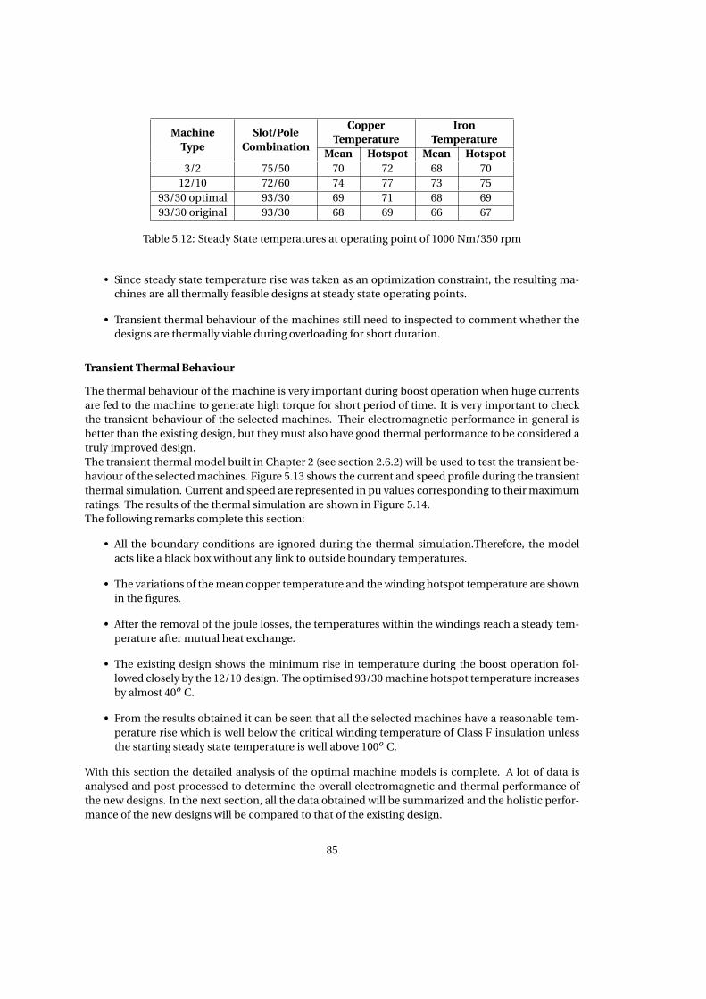
MachineType

Slot/PoleCombination

CopperTemperature

IronTemperature

Mean Hotspot Mean Hotspot3/2 75/50 70 72 68 70

12/10 72/60 74 77 73 7593/30 optimal 93/30 69 71 68 6993/30 original 93/30 68 69 66 67

Table 5.12: Steady State temperatures at operating point of 1000 Nm/350 rpm

• Since steady state temperature rise was taken as an optimization constraint, the resulting ma-chines are all thermally feasible designs at steady state operating points.

• Transient thermal behaviour of the machines still need to inspected to comment whether thedesigns are thermally viable during overloading for short duration.

Transient Thermal Behaviour

The thermal behaviour of the machine is very important during boost operation when huge currentsare fed to the machine to generate high torque for short period of time. It is very important to checkthe transient behaviour of the selected machines. Their electromagnetic performance in general isbetter than the existing design, but they must also have good thermal performance to be considered atruly improved design.The transient thermal model built in Chapter 2 (see section 2.6.2) will be used to test the transient be-haviour of the selected machines. Figure 5.13 shows the current and speed profile during the transientthermal simulation. Current and speed are represented in pu values corresponding to their maximumratings. The results of the thermal simulation are shown in Figure 5.14.The following remarks complete this section:

• All the boundary conditions are ignored during the thermal simulation.Therefore, the modelacts like a black box without any link to outside boundary temperatures.

• The variations of the mean copper temperature and the winding hotspot temperature are shownin the figures.

• After the removal of the joule losses, the temperatures within the windings reach a steady tem-perature after mutual heat exchange.

• The existing design shows the minimum rise in temperature during the boost operation fol-lowed closely by the 12/10 design. The optimised 93/30 machine hotspot temperature increasesby almost 40o C.

• From the results obtained it can be seen that all the selected machines have a reasonable tem-perature rise which is well below the critical winding temperature of Class F insulation unlessthe starting steady state temperature is well above 100o C.

With this section the detailed analysis of the optimal machine models is complete. A lot of data isanalysed and post processed to determine the overall electromagnetic and thermal performance ofthe new designs. In the next section, all the data obtained will be summarized and the holistic perfor-mance of the new designs will be compared to that of the existing design.

85

0 50 100 150 2000

0.2

0.4

0.6

0.8

1

Time (s)

Cu

rren

t (p

u)

0 50 100 150 2000

0.5

1

1.5

Sp

eed

(p

u)

Figure 5.13: Current and speed profile during boost operation

0 20 40 60 80 100 120 140 160 180 200

20

25

30

35

40

45

50

55

Time (s)

T (

°C)

Tslot,max

Tslot,mean

(a) Transient temperature rise of 3/2 design

0 20 40 60 80 100 120 140 160 180 200

20

25

30

35

40

45

50

Time (s)

T (

°C)

Tslot,max

Tslot,mean

(b) Transient temperature rise of 12/10 design

0 20 40 60 80 100 120 140 160 180 200

20

25

30

35

40

45

Time (s)

T (

°C)

Tslot,max

Tslot,mean

(c) Transient temperature rise of existing 93/30 design

0 20 40 60 80 100 120 140 160 180 200

20

25

30

35

40

45

50

55

60

Time (s)

T (

°C)

Tslot,max

Tslot,mean

(d) Transient temperature rise of optimized 93/30 design

Figure 5.14: Winding temperature rise of selected designs during maximum torque operation for 30s

5.5 Summary and Discussions

This chapter discussed and compared the electromagnetic and thermal performance of optimal ma-chine designs with different winding schemes for application as in-wheel motors for Electric Vehicles.

86

The Pareto fronts of different winding schemes are used to compare the performance and suitabilityof the designs in EV applications.To get more insight into design trends and behaviour of individual winding families, some designs areselected and analysed in detail.The performance of the existing PMSM design is used as a benchmarkto evaluate the holistic performance of the new designs. The results obtained from the analysis of theoptimal designs are presented in Table 5.13. The following inferences are drawn based on the results

PropertiesExistingDesign

93/30 3/2 12/10

DesignDetails

Slot/Pole Combination 93/30 93/30 75/50 72/60Active Weight (kg) 226 174 161 158Outer radius (m) 0.275 0.27 0.27 0.27Stack Length (m) 0.3 0.26 0.3 0.27

Airgap Length (mm) 2 1.6 1.5 1.5

MachineParameters

Phase Resistance (mΩ) 37 31 26 21Phase Inductance (µH) 746 388 182 173

Back-EMF (pu) 1 1.02 1 1

ElectromagneticPerformance

Boost Torque (kNm) 7.8 8.7 9.8 9.7Torque Ripple (%) 1.2 2.6 1.7 2.1

Part-Load Efficiency (%) 94.9 95.3 95.1 95.2Thermal

PerformanceTemperature Rise

at Boost Operation25 40 32 22

Table 5.13: Comparison of design details and overall performance of Optimal machines with differentwinding schemes

in the table:

• It can be seen from the information provided in the table that, the new designs have muchimproved electromagnetic performance with respect to the current design. All the new designsirrespective of winding schemes have improved boost torque capabilities which was one of themajor performance issues with current design.

• The active weights of the new designs are also lower than the existing designs. This is mainlydue to reduction of overall stator iron weight.

• The part-load efficiency shown in the table was one of the targets of optimization. It is definedas the weighted sum of the efficiencies ( (equation 4.13)) at the most frequent torque-speed op-erating points. The new designs have comparable part-load efficiencies with the existing design.

• The torque ripple of the optimal designs are also comparable to the existing PMSM design. InEV type applications, a low torque ripple is desirable.

• The phase resistances of the concentrated winding machines are lower compared to the dis-tributed winding machines. This is due to lower end winding lengths compared to distributedwinding machines. This leads to lower copper losses as shown in the results. This findings arein line with research work reported in literature[22] [54].

• The concentrated winding machines seem to have lower phase inductance than the distributedwinding machines. This suggest high flux levels during normal machine operation. The highamount of permanent magnet material and short air gap of the concentrated winding machinedesigns also suggest the same thing.

87

• Lower inductance may cause higher inverter current ripples which is detrimental to overall ma-chine performance. It also increases the current rating of the inverter if flux weakening opera-tion is needed at high speed operating points. To increase the inductance of the machines thenumber of turns can increased, however it will reduce the speed range of the machine for a givenDC link voltage.

• Among all the optimal designs with different winding schemes, the 12/10 PM machine seemsto have the better overall performance compared to the other machines. This is in line withresearch work reported in literature [66] [67] [68].

88

Chapter 6

Conclusion and Recommendations

This chapter summarizes the findings and contributions of this thesis.

6.1 Conclusions

Designing electric machines is a complex process and takes a lot of iterations to arrive at an optimaldesign. The framework of machine design can be different for different kinds of application. It basi-cally emphasizes on the fact that there is no "perfect or best machine". The performance of a machinecannot be possibly judged by a single parameter like efficiency or torque etc. It is judged on a combi-nation of many different performance parameters which vary widely with application type.Given this background, it is very important to get a clear idea of the machine requirements dependingon the type of application. This thesis is focused on designing electric machines for in-wheel applica-tion in EVs. The design scope was narrowed down to direct drive Surface mounted permanent magnetsynchronous machines. For EV application, the performance parameters are mainly - high torque ca-pabilities, high efficiencies , light designs, low torque ripple among many others. This thesis focuseson designing optimal machines which satisfies all the requirement. It must be noted that it is highlyunlikely that a single design will satisfy all the requirements in best possible way. In the following textthe overall flow and culmination of the entire thesis work will be presented chapter wise:

Chapter 1In this chapter, the motivations for this thesis work are discussed in detail. The relevant designtrends reported in literature are highlighted. The main goal of the thesis is to investigate thepossibility of good machine designs with optimum performances for electric vehicles. An ex-isting PM design is selected as a benchmark to compare and evaluate the performance of newdesigns. This chapter brings out limitations and challenges of current technology which arehelpful in forming the thesis objective.

Chapter 2This chapter is dedicated to describe the modelling procedure to predict electromagnetic be-haviour of PM machines. Finite Element method is used for this purpose. The motivations forchoosing FE modelling procedure are also discussed. The FE model is applied to analyse theperformance of the existing design. The results obtained gave a fair idea about the opportuni-ties of improvements in the new designs with respect to the current one.To get an idea about the holistic performance of the PM machines , a lumped circuit thermalmodel is built in this chapter and combined with the FE model to get accurate simulation re-sults.

89

Chapter 3Experiments to validate FE machine model developed in chapter 2 are presented in this chapter.Since experiments are the most close to actual situation in the real machine, they can be used forvalidation. From the obtained results, it is seen that the FE model simulation results are not farfrom the experimental results. The extent of deviation of simulation results from experimentalvalues is documented and reasons are deduced. This is a contribution of this chapter.

Chapter 4This chapter uses the previously validated FE machine model for design optimization to in-vestigate the possibility of new machine designs with improved performance. Fractional slotconcentrated winding schemes are introduced and the suitability of various slot/pole combina-tions is analysed in detail. Design choices are also justified in detail.Based on the obtained FE results of the existing PM machine the performance targets of new de-signs are determined along with the identification of relevant design variables and constraints.This chapter combines the FE machine model with multi-objective Particle Swarm Optimiza-tion algorithm to set up an automated design optimization to create optimal machine designs.The main contribution of this chapter is that it draws some design trends about choosing opti-mal winding schemes for PM machines for EV application. It also presents some insights aboutselection of design variables and most importantly the right choices of optimization targets.

Chapter 5This chapter presents the results of the optimization procedure discussed in chapter 4. A com-parative analysis of the results is also reported. Based on that numerous conclusions are drawnon different winding schemes and about their suitability for EV applications. The following mainconclusions are drawn based on the findings:

• For the same torque/amp requirement, concentrated winding PM machines tend to havelower efficiencies for heavy designs mainly due to large iron losses. Therefore, most opti-mal concentrated winding machines generally have lighter designs.

• The 12/10 slot/pole combination seems to be most suitable for this application among theselected slot/pole combinations. A major fraction of all the optimal designs of this windingscheme satisfied most of the pre-defined performance requirements.

• The goal of the thesis is achieved in this chapter. After careful and in-depth analysis newmachine designs are obtained whose performance seemed better than the existing ma-chine on various fields like boost torque capability and reduced weight.

Apart from the above findings, the most important contribution of this thesis is a novel method-ology of design optimization of machines with asymmetrical winding . The results obtained afterapplying the method seemed to be in agreement with the expectations of the proposed idea.

6.2 Future Work and Recommendations

Over the course of this thesis a number of possible avenues of further investigation have been identi-fied. First, more winding schemes must be included in the design optimization procedure to generatemore design trends to get a complete picture of the design choices, so that a machine designer cantake well informed design choices which can save a lot of time.

Second, throughout the whole thesis the goal of the design optimization was to improve machineperformance with fixed VI rating of the inverter. This restricts the design space a lot. It would be very

90

interesting to see the results of design optimization if minimization of inverter size is also included asanother target of the optimization. Using number of turns per coil as an optimization variable thereare good chances of designing machines with high back-emf to provide good starting torque and toinclude flux weakening to increase its speed range.

Finally, this thesis focuses on a machine with an unbalanced and asymmetrical winding scheme. How-ever, their overall performance is discovered to be quite impressive with many advantages over con-ventional winding machines. There are very few literature on this type of windings and especially noton design optimization of machines with this kind of windings.

.

91

92

Bibliography

[1] D. Luque, E. Ruppert, N. Bianchi, and M. Castiello, “Analysis of a three-phase in-wheel electricmotor,” Universities Power Engineering Conference (UPEC), 2009 Proceedings of the 44th Interna-tional, no. 1, pp. 1–5, 2009.

[2] K. J. Tseng and G. H. Chen, “Computer-aided design and analysis of direct-driven wheel motordrive,” IEEE Transactions on Power Electronics, vol. 12, no. 3, pp. 517–527, 1997.

[3] H. C. Lovatt, D. Elton, L. Cahill, D. H. Huynh, A. Stumpf, A. Kulkarni, A. Kapoor, M. Ektesabi,H. Mazumder, T. Dittmar, and G. White, “Design procedure for low cost, low mass, direct drive,in-wheel motor drivetrains for electric and hybrid vehicles,” IECON Proceedings (Industrial Elec-tronics Conference), pp. 4558–4562, 2011.

[4] M. Jain and S. S. Williamson, “Suitability analysis of in-wheel motor direct drives for electric andhybrid electric vehicles,” 2009 IEEE Electrical Power and Energy Conference, EPEC 2009, 2009.

[5] C. Espanet, F. Dubas, H. M. Mai, D. Chamagne, R. Bernard, and P. Bigot, “In-wheel motor for asmall hybrid electric vehicle: design, realization and experimental characterization,” 2012 IEEEEnergy Conversion Congress and Exposition (ECCE), pp. 892–898, 2012.

[6] S. Zhitkova, M. Felden, D. Franck, and K. Hameyer, “Design of an electrical motor with wide speedrange for the in-wheel drive in a heavy duty off-road vehicle,” in 2014 International Conferenceon Electrical Machines (ICEM), pp. 1076–1082, 2014.

[7] Y. Tang, J. J. H. Paulides, I. J. M. Besselink, F. Gardner, and E. A. Lomonova, “Indirect drive in-wheelsystem for HEV/EV traction,” in 2013 World Electric Vehicle Symposium and Exhibition (EVS27),pp. 1–9, IEEE, Nov. 2013.

[8] A. Benoudjit and N. Nait Said, “New dual-airgap axial and radial-flux induction motor for onwheel drive electric propulsion systems,” in POWERCON ’98. 1998 International Conference onPower System Technology. Proceedings (Cat. No.98EX151), vol. 1, pp. 615–619, IEEE.

[9] F. Xu and L. Shi, “Characteristics analysis of multiple in-wheel-induction-motors drive system,”in 2011 IEEE International Conference on Industrial Technology, pp. 121–126, IEEE, Mar. 2011.

[10] Y. Fan, X. Han, Z. Xue, and H. Jiang, “Design, analysis and control of a permanent magnet in-wheel motor based on magnetic-gear for electric vehicles,” 2011 International Conference onElectrical Machines and Systems, pp. 1–6, 2011.

[11] Y.-P. Yang, Y.-P. Luh, and C.-H. Cheung, “Design and Control of Axial-Flux Brushless DC WheelMotors for Electric Vehicles—Part I: Multiobjective Optimal Design and Analysis,” IEEE Transac-tions on Magnetics, vol. 40, pp. 1873–1882, July 2004.

93

[12] M. Miyamasu and K. Akatsu, “Efficiency comparison between Brushless dc motor and Brush-less AC motor considering driving method and machine design,” in IECON 2011 - 37th AnnualConference of the IEEE Industrial Electronics Society, pp. 1830–1835, IEEE, Nov. 2011.

[13] P. Luk and P. Jinupun, “An In-Wheel Switched Reluctance Motor for Electric Vehicles,” in 2006CES/IEEE 5th International Power Electronics and Motion Control Conference, vol. 3, pp. 1–5,IEEE, Aug. 2006.

[14] M. Yildirim, M. Polat, and H. Kurum, “A survey on comparison of electric motor types and drivesused for electric vehicles,” in 2014 16th International Power Electronics and Motion Control Con-ference and Exposition, pp. 218–223, IEEE, Sept. 2014.

[15] G. Nanda and N. Kar, “A Survey and Comparison of Characteristics of Motor Drives Used in Elec-tric Vehicles,” in 2006 Canadian Conference on Electrical and Computer Engineering, pp. 811–814,IEEE, 2006.

[16] J. Wang, X. Yuan, and K. Atallah, “Design Optimization of a Surface-Mounted Permanent-MagnetMotor With Concentrated Windings for Electric Vehicle Applications,” IEEE Transactions on Ve-hicular Technology, vol. 62, pp. 1053–1064, Mar. 2013.

[17] Ki-Chan Kim and Ki-Yong Sung, “Performance analysis of interior permanent magnet syn-chronous motor for electric vehicle considering magnetic saturation effect,” in Digests of the 201014th Biennial IEEE Conference on Electromagnetic Field Computation, pp. 1–2, IEEE, 2010.

[18] A. Vagati, G. Pellegrino, and P. Guglielmi, “Comparison between SPM and IPM motor drives forEV application,” in The XIX International Conference on Electrical Machines - ICEM 2010, pp. 1–6,IEEE, Sept. 2010.

[19] S. Yang, N. J. Baker, C. Hilton, G. Sooriyakumar, and A. Fraser, “Cost Reduction of a PermanentMagnet In-wheel Electric Vehicle Traction Motor r,” 2014.

[20] D. Evans, Z. Azar, L. Wu, and Z. Zhu, “Comparison of optimal design and performance of PM ma-chines having non-overlapping windings and different rotor topologies,” 5th IET InternationalConference on Power Electronics, Machines and Drives (PEMD 2010), no. c, pp. WE311–WE311,2010.

[21] A. EL-Refaie, “Fractional-Slot Concentrated-Windings Synchronous Permanent Magnet Ma-chines: Opportunities and Challenges,” IEEE Transactions on Industrial Electronics, vol. 57,pp. 107–121, Jan. 2010.

[22] D. G. Dorrell, M.-F. Hsieh, M. Popescu, L. Evans, D. A. Staton, and V. Grout, “A Review ofthe Design Issues and Techniques for Radial-Flux Brushless Surface and Internal Rare-EarthPermanent-Magnet Motors,” IEEE Transactions on Industrial Electronics, vol. 58, pp. 3741–3757,Sept. 2011.

[23] C. M. Cho, J. H. Sim, and K. H. Nam, “Comparative study of EV propulsion motors for A-classvehicles,” 2011 International Conference on Electrical Machines and Systems, ICEMS 2011, pp. 1–3, 2011.

[24] A. M. El-Refaie, T. M. Johns, P. J. McCleer, and J. W. McKeever, “Experimental verification of opti-mal flux weakening in surface PM machines using concentrated windings,” Conference Record -IAS Annual Meeting (IEEE Industry Applications Society), vol. 2, no. 3, pp. 1050–1057, 2005.

[25] D. Lahaye, “Finite Element Modeling for Electrical Energy Applications Introduction,” 2012.

94

[26] H. VuXuan, D. Lahaye, H. Polinder, and J. a. Ferreira, “Improved model for design of perma-nent magnet machines with concentrated windings,” 2011 IEEE International Electric Machines& Drives Conference (IEMDC), pp. 948–954, 2011.

[27] A. Jassal, Eddy Current Loss Modeling for Design of PM Generators for Wind Turbines. PhD thesis,TU Delft, 2014.

[28] M. V. D. Geest, E. P. Processing, and C. Science, “Rotor losses in the HISPEM,” 2011.

[29] M. Jabbar, H. Phyu, Z. Liu, and C. Bi, “Modeling and Numerical Simulation of a BrushlessPermanent-Magnet DC Motor in Dynamic Conditions by Time-Stepping Technique,” IEEE Trans-actions on Industry Applications, vol. 40, pp. 763–770, May 2004.

[30] A. O. D. Tommaso and F. Genduso, “A Novel Improved Matlab-based Software for the Electric andMagnetic Analysis and Design of Rotating Electrical Machines,” pp. 1–7, 2015.

[31] A. O. Di Tommaso, F. Genduso, and R. Miceli, “A software for the evaluation of winding factor har-monic distribution in high efficiency electrical motors and generators,” in 2013 Eighth Interna-tional Conference and Exhibition on Ecological Vehicles and Renewable Energies (EVER), pp. 1–6,IEEE, Mar. 2013.

[32] K. J. Meessen, P. Thelin, J. Soulard, and E. a. Lomonova, “Inductance Calculations of Permanent-Magnet Synchronous Machines,” IEEE Transactions on Magnetics, vol. 44, no. 10, pp. 2324–2331,2008.

[33] D. Gerling, “Comparison of Different FE Calculation Methods for the Electromagnetic Torque ofPM Machines,” NAFEMS Seminar: Numerical Simulation of Electromechanical Systems, pp. 1–8,2005.

[34] F. Henrotte and K. Hameyer, “Computation of electromagnetic force densities: Maxwell stresstensor vs. virtual work principle,” Journal of Computational and Applied Mathematics, vol. 168,no. 1-2, pp. 235–243, 2004.

[35] M. Popescu, “Prediction of the electromagnetic torque in synchronous machines throughMaxwell stress harmonic filter (HFT) method,” Electrical Engineering, vol. 89, no. 2, pp. 117–125,2006.

[36] Z. Q. Zhu and D. Howe, “Influence of design parameters on cogging torque in permanent magnetmachines,” Energy Conversion, IEEE Transactions on, vol. 15, no. 4, pp. 407–412, 2000.

[37] U. D. B. Muenchen, D. Neubiberg, A. Ag, and D. Ingolstadt, “Torque Ripple Reduction in Perma-nent Magnet Synchronous Machines with Concentrated Windings and Pre-Wound Coils,” vol. 1,2014.

[38] J. Song-Manguelle, G. Ekemb, S. Schroder, T. Geyer, J. M. Nyobe-Yome, and R. Wamkeue, “Analyt-ical expression of pulsating torque harmonics due to PWM drives,” 2013 IEEE Energy ConversionCongress and Exposition, ECCE 2013, pp. 2813–2820, 2013.

[39] C. Huynh, L. Zheng, and D. Acharya, “Losses in High Speed Permanent Magnet Machines Usedin Microturbine Applications,” Journal of Engineering for Gas Turbines and Power, vol. 131, no. 2,p. 022301, 2009.

[40] A. Boglietti, A. Cavagnino, and D. Staton, “Determination of Critical Parameters in Electrical Ma-chine Thermal Models,” IEEE Transactions on Industry Applications, vol. 44, no. 4, pp. 1150–1159,2008.

95

[41] S. K. Chowduury, B. Dutta, and D. Bhowmik, “Lumped Parameter Thermal Model for InductionMachine,” vol. 3, no. 1, pp. 175–180, 2014.

[42] J. Nerg, M. Rilla, and J. Pyrhonen, “Thermal Analysis of Radial-Flux Electrical Machines With aHigh Power Density,” IEEE Transactions on Industrial Electronics, vol. 55, pp. 3543–3554, Oct.2008.

[43] D. A. Howey, A. S. Holmes, and K. R. Pullen, “Measurement and CFD Prediction of Heat Transfer inAir-Cooled Disc-Type Electrical Machines,” IEEE Transactions on Industry Applications, vol. 47,pp. 1716–1723, July 2011.

[44] D. a. Howey, P. R. N. Childs, and A. S. Holmes, “Air-gap convection in rotating electrical ma-chines,” IEEE Transactions on Industrial Electronics, vol. 59, no. 3, pp. 1367–1375, 2012.

[45] A. Tassi, G. Zanocchi, and D. Staton, “FEM and lumped circuit thermal analysis of external rotormotor,” IECON Proceedings (Industrial Electronics Conference), pp. 4825–4828, 2006.

[46] X. Zhang, W. Li, S. Cheng, J. Cao, and C. Zhu, “Thermal analysis of solid rotor in PMSM used forEV,” 5th IEEE Vehicle Power and Propulsion Conference, VPPC ’09, pp. 1637–1642, 2009.

[47] N. Simpson, R. Wrobel, and P. H. Mellor, “Estimation of Equivalent Thermal Parameters of Im-pregnated Electrical Windings,” IEEE Transactions on Industry Applications, vol. 49, pp. 2505–2515, Nov. 2013.

[48] J. Pyrhönen, T. Jokinen, and V. Hrabovcová, Design of Rotating Electrical Machines. 2008.

[49] J. J. Germishuizen and M. J. Kamper, “Classification of symmetrical non-overlapping three-phasewindings,” 19th International Conference on Electrical Machines, ICEM 2010, 2010.

[50] J. a. Güemes, a. M. Iraolagoitia, P. Fernández, and M. P. Donsión, “Comparative study of PMSMwith integer-slot and fractional-slot windings,” 19th International Conference on Electrical Ma-chines, ICEM 2010, 2010.

[51] Z. Zhu and D. Howe, “Influence of design parameters on cogging torque in permanent magnetmachines,” 2000.

[52] N. Bianchi and S. Bolognani, “Design techniques for reducing the cogging torque in surface-mounted PM motors,” IEEE Transactions on Industry Applications, vol. 38, pp. 1259–1265, Sept.2002.

[53] N. Bianchi, S. Bolognani, and P. Frare, “Design Criteria for High-Efficiency SPM SynchronousMotors,” IEEE Transactions on Energy Conversion, vol. 21, pp. 396–404, June 2006.

[54] B. Mecrow, A. Jack, D. Atkinson, S. Green, G. Atkinson, A. King, and B. Green, “Design and Test-ing of a Four-Phase Fault-Tolerant Permanent-Magnet Machine for an Engine Fuel Pump,” IEEETransactions on Energy Conversion, vol. 19, pp. 671–678, Dec. 2004.

[55] A. Jack, B. Mecrow, and J. Haylock, “A comparative study of permanent magnet and switchedreluctance motors for high-performance fault-tolerant applications,” IEEE Transactions on In-dustry Applications, vol. 32, no. 4, pp. 889–895, 1996.

[56] N. Bianchi, M. Pre, G. Grezzani, and S. Bolognani, “Design considerations on fractional-slot fault-tolerant synchronous motors,” in IEEE International Conference on Electric Machines and Drives,2005., pp. 902–909, IEEE, 2005.

96

[57] A. El-Refaie and T. Jahns, “Comparison of synchronous PM machine types for wide constant-power speed operation: converter performance,” IET Electric Power Applications, vol. 1, p. 217,Mar. 2007.

[58] F. Magnussen and C. Sadarangani, “Winding factors and Joule losses of permanent magnet ma-chines with concentrated windings,” in IEEE International Electric Machines and Drives Confer-ence, 2003. IEMDC’03., vol. 1, pp. 333–339, IEEE, 2003.

[59] E. Fornasiero, N. Bianchi, and S. Bolognani, “Slot harmonic impact on rotor losses in fractional-slot permanent-magnet machines,” IEEE Transactions on Industrial Electronics, vol. 59, no. 6,pp. 2557–2564, 2012.

[60] S.-H. H. S.-H. Han, W. Soong, and T. Jahns, “An Analytical Design Approach for Reducing StatorIron Losses in Interior PM Synchronous Machines During Flux-Weakening Operation,” 2007 IEEEIndustry Applications Annual Meeting, pp. 103–110, 2007.

[61] H. Dogan, F. Wurtz, A. Foggia, and L. Garbuio, “Analysis of slot-pole combination of fractional-slots PMSM for embedded applications,” International Aegean Conference on Electrical Machinesand Power Electronics, ACEMP 2011 and Electromotion 2011 Joint Conference, pp. 611–615, 2013.

[62] H. Jussila, P. Salminen, M. Niemelä, and J. Pyrhönen, “Guidelines for designing concentratedwinding fractional slot permanent magnet machines,” POWERENG 2007 - International Confer-ence on Power Engineering - Energy and Electrical Drives Proceedings, pp. 191–194, 2007.

[63] H. Dogan, F. Wurtz, A. Foggia, and L. Garbuio, “Performance analysis and comparison of threeIPMSM with high homopolar inductance for electric vehicle applications,” 2011.

[64] N. Bianchi, S. Bolognani, and E. Fomasiero, “A General Approach to Determine the Rotor Lossesin Three-Phase Fractional-Slot PM Machines,” in 2007 IEEE International Electric Machines &Drives Conference, vol. 1, pp. 634–641, IEEE, May 2007.

[65] Y. Liu, “Critical wavelength of eddy currents and its influence on harmonic losses in solid poles,”19th International Conference on Electrical Machines, ICEM 2010, no. 1, pp. 1–6, 2010.

[66] H. V. Xuan, D. Lahaye, H. Polinder, and J. A. Ferreira, “Influence of slot/pole number combinationon performances of permanent magnet machines with concentrated windings for ship applica-tion,” in 2011 International Conference on Electrical Machines and Systems, pp. 1–6, IEEE, Aug.2011.

[67] Z. Q. Zhu, Z. P. Xia, L. J. Wu, and G. W. Jewell, “Influence of slot and pole number combina-tion on radial force and vibration modes in fractional slot PM brushless machines having single-and double-layer windings,” 2009 IEEE Energy Conversion Congress and Exposition, ECCE 2009,pp. 3443–3450, 2009.

[68] J. Goss, D. Staton, R. Wrobel, and P. Mellor, “Brushless AC interior-permanent magnet motordesign: Comparison of slot/pole combinations and distributed vs. concentrated windings,” 2013IEEE Energy Conversion Congress and Exposition, ECCE 2013, pp. 1213–1219, 2013.

[69] M. van der Geest, H. Polinder, and J. a. Ferreira, “Optimization and comparison of electrical ma-chines using particle swarm optimization,” XXth International Conference on Electrical Machines(ICEM), 2012.

[70] N. Bianchi and S. Bolognani, “Design optimisation of electric motors by genetic algorithms,” IEEETransactions on Electric Power Applications, no. 5, 1998.

97

[71] Y. Duan and R. G. Harley, “A Novel Method for Multiobjective Design and Optimization of ThreePhase Induction Machines,” IEEE Transactions on Industry Applications, vol. 47, pp. 1707–1715,July 2011.

[72] Y. Duan, R. Harley, and T. Habetler, “Comparison of Particle Swarm Optimization and GeneticAlgorithm in the design of permanent magnet motors,” 2009 IEEE 6th International Power Elec-tronics and Motion Control Conference, vol. 3, pp. 822–825, 2009.

[73] R. Hassan and B. Cohanim, “A comparison of particle swarm optimization and the genetic algo-rithm,” 1st AIAA multidisciplinary design optimization specialist conference, pp. 1–13, 2005.

[74] J. Kennedy and R. Eberhart, “Particle swarm optimization,” Neural Networks, 1995. Proceedings.,IEEE International Conference on, vol. 4, pp. 1942–1948 vol.4, 1995.

[75] C. a. C. Coello, G. T. Pulido, and M. S. Lechuga, “Handling multiple objectives with particle swarmoptimization,” Evolutionary Computation, IEEE Transactions on, vol. 8, no. 3, pp. 256–279, 2004.

[76] Z. Li and A. Miotto, “Concentrated-winding fractional-slot synchronous surface PM motor designbased on efficiency map for in-wheel application of electric vehicle,” 2011 IEEE Vehicle Power andPropulsion Conference, VPPC 2011, 2011.

[77] J. Goss, R. Wrobel, P. Mellor, and D. Staton, “The design of AC permanent magnet motors forelectric vehicles: A design methodology,” Proceedings of the 2013 IEEE International Electric Ma-chines and Drives Conference, IEMDC 2013, pp. 871–878, 2013.

[78] M. van der Geest, An Integral Approach to Design High Performance Permanent Magnet Syn-chronous Machines. PhD thesis, 2015.

[79] M. Valavi, A. Nysveen, R. Nilssen, R. D. Lorenz, and T. Rø lvåg, “Influence of pole and slot combi-nations on magnetic forces and vibration in low-speed PM wind generators,” IEEE Transactionson Magnetics, vol. 50, no. 5, 2014.

[80] C. C. Hwang, C. M. Chang, and P. L. Li, “Design optimization for cogging torque minimization andefficiency maximization of a high-speed PM motor,” Proceedings of the International Conferenceon Power Electronics and Drive Systems, pp. 938–943, 2009.

98