design of divertor impurity monitoring - ipen.br filedesign of divertor impurity monitoring -...
TRANSCRIPT
JAERI-Tech98-047
JAERI-Tech--98-047
JP9901026
DESIGN OF DIVERTOR IMPURITY MONITORINGSYSTEM FOR ITER (II)
November 1998
Tatsuo SUGIE, Hiroaki OGAWA,
Atsushi KATSUNUMA', Mitsumasa MARUO+,
Yoshio KITA *, Katsuyuki EBISAWA,
Toshiro ANDO and Satoshi KASAI
3 0 - 08Japan Atomic Energy Research Institute

(T319-1195
- (T319-H95
This report is issued irregularly.Inquiries about availability of the reports should be addressed to Research
Information Division, Department of Intellectual Resources, Japan Atomic EnergyResearch Institute, Tokai-mura, Naka-gun, Ibaraki-ken T319—1195, Japan.
©Japan Atomic Energy Research Institute, 1998

JAERI-Tech 98-047
Design of Divertor Impurity Monitoring System for ITER (II)
Tatsuo SUGIE, Hiroaki OGAWA, Atsushi KATSUNUMA * ,
Mitsumasa MARUO * , Yoshio KITA * * , Katsuyuki EBISAWA
Toshiro ANDO + and Satoshi KASAI+ +
Department of Fusion Plasma Research
Naka Fusion Research Establishment
Japan Atomic Energy Research Institute
Naka-machi, Naka-gun, Ibaraki-ken
(Received October 1 ,1998)
The divertor impurity monitoring system of ITER has been designed. The main
functions of this system are to identify impurity species and to measure the two-
dimensional distributions of the particle influxes in the divertor plasmas. The wavelength
range is 200 nm to 1000 nm. The viewing fans are realized by molybdenum mirrors
located in the divertor cassette. With additional viewing fans seeing through the gap
between the divertor cassettes, the region approximately from the divertor leg to the x-
point will be observed. The light from the divertor region passes through the quartz
windows on the divertor port plug and the cryostat, and goes through the dog-leg optics
in the biological shield. Three different type of spectrometers : ( i ) survey
spectrometers for impurity species monitoring, (ii) filter spectrometers for the particle
influx measurement with the spatial resolution of 10 mm and the time resolution of 1 ms
and (iii) high dispersion spectrometers for high resolution wavelength measurements
are designed. These spectrometers are installed just behind the biological shield (for X <
This design work was carried out under the ITER EDA task agreement of design task (TaskAgreement number : S 91 TD21 95-01-20 FJ and S 91 TD31 95-08-04 FJ) .
+ Department of ITER Project+ + Department of Fusion Engineering Research
* Nikon Corporation
* * Toshiba Corporation

JAERI-Tech 98-047
450 nm) to prevent the transmission loss in fiber and in the diagnostic room (for X ^
450 nm) from the point of view of accessibility and flexibility. The optics have been
optimized by a ray trace analysis. As a result, 10-15 mm spatial resolution will be
achieved in all regions of the divertor.
In addition, the measurable limit, the neutron and y -ray irradiation effect on
windows, a calibration method, an alignment method, a remote handling method and a
data acquisition method are considered.
Keywords : ITER, ITER EDA, Divertor, Impurity, Impurity Monitor, Spectroscopy, Design,
Optics, Visible Ray, Filter

JAERI-Tech 98-047
( E )
( 1 9 9 8 ^ 10 M 1
T E
lOOOnm
lms
o ( i )
, (iii) -T *->-*
i:
U
Task Agreemen t Number :S91
TD21-95-01-20 FJ , &D?S91TD31-95-08-04 FJ
++ +** *

JAERI-Tech 98-047
t y mm
IV
JAERI-Tech 98-047
Contents
1. Introduction 1
2. Requirements 2
3. Concept of Measuring Method and Composition 4
4. Conceptual Arrangement 6
4.1 Magnetic Field and Shielding for Detector 6
4.2 First Mirror 11
4.3 Baffle Plate in the Viewing Slot 12
4.4 Optical Fiber 16
4.5 Conceptual Arrangement 17
5. Optical Design 18
5.1 Design Concept and Viewing Fans in the Divertor Channel 18
5.2 Optics • 23
5.3 Spectrometer 92
5.4 Estimation of Number of Photons Coming into the Detector 124
5.5 Calibration System 130
5.6 Alignment System 132
6. Mechanical Design 137
6.1 Optics 137
6.2 Spectrometer 152
6.3 Analysis of the Electromagnetic Force during the Disruption 157
6.4 Analysis of the Nuclear Heating for Mirrors in the Divertor Cassette 161
6.5 Remote Handling for Mirrors in the Divertor Cassette 163
7. Neutron and y -ray Irradiation Effect 167
8. Control and Data Acquisition 168
8.1 Concept of control and Data Acquisition 168
8.2 Items of Control for the Divertor Impurity Monitoring System 170
8.3 Data Acquisition and Processing 173
9. Space Requirement 187
10. Further Work, and Necessary R & D 189
11. Rearrangement of Mirrors for New Divertor Cassette 190
12. Conclusion 192
Acknowledgment 193
Appendix 194

JAERI-Tech 98-047
i . tic&M l2. ITER^hCO^J^ 2
3. Ml£Wt&ki'X;rJ»mj$. 4
4. m^St 64. 1 M^$lt±ifs«^->-^ K 6
4.2 7°7XV>PJ-[p]ff 1 5 7 - 11
4.3 I f f X n 5/ M*9/*y y^Wl 12
4.4 * 7 7 ^ f ^ - 16
4.5 «iSgO#X.^ 17
5. ^ l £ f + 18
5.1 mW^tLUtPJ^-VJj^y hrt^lllf 18
5.2 %^lh 23
5.3 ft%%s 92
5.4 &mmzxz>%=?-!®L<r>nm 1245. 5 i iJ tK^ 130
5.6 %mm.mm 1326 . WMLWL^c 137
6. 1 %¥%, 137
6.2 j ^ % ^ • 152
6. 3 7 ° 7 ^ V • Vs4 ^ 7 7 ° v / a >-^<DMBJJ 157
6.4 #>('<— $>13± y h r t ? y~~<D&%ffl, 161
6.5 mmmmcx^y^f^-^^^y hfo^y-ottm 1637. mmmfctt-tz>tip&*kymmtt<D&m 1678. fflffl - f—^^m^ 168
8. 1 fflffl • X —^^a^OSt^^H- 1688.2 ^J l^ 1 ! ! 170
8.3 "r — Zl&M ' faM<DfflL& 173
9 . £fe^m 187
10. $-&<DWtflrftMk >&g*£R&D 189
11. I f f^V/^-^^i ry hJd^1-5^7-©SBBB 190
12. $.blsb 192
• 193
194
VI
JAERI-Tech 98-047
1. Introduction
The main functions of this system are to identify impurity species and tomeasure the two-dimensional distributions of the particle influxes in thedivertor plasmas. The expected impurities are carbon, tungsten, beryllium andcopper originating from the divertor target plate and from the surface of the firstwall in the main chamber. Neon and other impurity gases injected into theplasma for radiation cooling in the divertor will also be observed. Thewavelength range is 200 nm to 1000 nm. This system, which is one of the mostimportant diagnostic systems for plasma control, is included in the start-up set ofITER diagnostics [1].
The temperature of the divertor plasma is lower than that of the mainplasma. Many spectral lines originating from neutral and ionized atoms andmolecules are emitted in the ultraviolet and visible region as well as in thevacuum ultraviolet region. These spectral lines have information of plasma-wallinteraction. In existing tokamaks, visible spectroscopy is used extensively to studydivertor plasmas and also edge plasmas, because the apparatus of visiblespectroscopy is relatively simple compared to that of the vacuum ultravioletspectroscopy which needs a vacuum extension and a pumping device. Forexample, impurity species identification, particle influx measurements andstudies of the impurity generation and particle recycling mechanism [2,3,4,5,6,7]have been carried out in various tokamaks. Electron temperature and densitymeasurements [8] and ion temperature measurements have been also attempted.These techniques will be able to extrapolate to ITER divertor diagnostics except inthe very high electron density and low temperature region where therecombination process is dominant.
In this report, the conceptual design and the detailed optical design of thedivertor impurity monitoring system are described. In addition, the measurablelimit, the neutron and y-ray irradiation effect on windows, a calibration methodand an alignment method are considered. The conceptual design for the dataacquisition system is also reported.
References
[1] A. E. Costley, K. Ebisawa, P. Edmond, et al., Overview of the ITER diagnostic system, inProceedings of the International Workshop on "Diagnostics for Experimental Fusion Reactors"(1997).
[2] K. H. Behringer, Spectroscopic studies of plasma-wall interaction and impurity behavior intokamaks, /. Nucl. Mater, 145-147: 145 (1987).
[3] H. Kubo, M. Shimada, T. Sugie, et al., Impurity generation mechanism and remote radiativecooling in JT-60U divertor discharges, /. Nucl. Mater, 196-198: 71 (1992).
-I

JAERI-Tech 98-047
[4] P. Bogen, D. Rusbiildt, Velocity distribution of carbon and oxygen atoms in front of a tokamaklimiter, /. Nucl. Mater, 196-198: 179 (1992).
[5] D. Reiter, P. Bogen, U. Samm, Measurement and monte carlo computations of Ha profiles infront of a TEXTOR limiter, /. Nucl. Mater, 196-198: 1059 (1992).
[6] B. Unterberg, H. Knauf, P. Bogen, et al., /. Nucl. Mater, 220-222: 462 (1992).[7] H. Kubo, T. Sugie, H. Takenaga, et al., High resolution visible spectrometer for divertor study
in JT-60U, Fusion Eng. Design, 34-35: 277 (1997).[8] B. Schweer, G. Mank, A. Pospieszczyk, Electron temperature and electron density profiles
measured with a thermal He-beam in the plasma boundary of TEXTOR, /. Nucl. Mater, 196-198: 174 (1992).
2. Requirements
The identification and monitoring of the impurity species, and the two-dimensional measurement of particle influxes in the divertor plasma are veryimportant for ITER plasma control. The requirements for the divertor impuritymonitoring system are shown in the section 5.5 of the ITER design descriptiondocument (DDD) and other papers [1,2,3,4]- As shown in the section 5.5.E.04 [5] ofthe DDD, the objective of the divertor impurity monitoring system is to obtainspatially resolved measurements from the plasma in the divertor channel toidentify and quantify the impurity species. The wavelength range of 200-1000 nmand two-dimensional measurement in the poloidal plane are required.
The more detailed requirements for parameters to be measured, parameterranges, spatial resolutions, time resolutions and accuracies are summarized inTable 2-1.
Table 2-1. Target requirements for impurity monitoring system [2, 3,4,5].
• Impurity Species Monitor
Parameter Parameter range Spatial res. Time res. Accuracy
BeCCuN e
influxinfluxinfluxinflux
TBDTBDTBDTBD
Several pointTBD
Several pointTBD
10 ms10 ms10 ms10 ms
10 % (rel.)10 % (rel.)10 % (rel.)10 % (rel.)
Key Divertor Parameter
Parameter Parameter range Spatial res. Time res. Accuracy
"Ionization front" position 0 - 2 m •10 cm l m s 10%
O

JAERI-Tech 98-047
Table 2-1. Target requirements for impurity monitoring system (continued).
• Impurity and D, T Influx in Divertor
Parameter Parameter range Spatial res. Time res. Accuracy
rD ,rT
Divertor Helium Density
1017 -1022 at/sec 10 mm1019 -1025 at/sec 10 mm
lmslms
0.1 -100.01 - 0.1
100 ms100 ms
• Ion Temperature in Divertor
30%30%
Parameter
x/nD, nH/riD in Divertor
Parameter
Parameter range
1017-1020m-3
Parameter range
Spatial
Spatial
res.
res.
Time res.
l m s
Time res.
Accuracy
20%
Accuracy
20%20%
Parameter Parameter range Spatial res. Time res. Accuracy
Ti 1-200 eV 10 cm (along legs) 1 ms0.3 cm (across legs)
20%
References
[1] A. E. Costley, et al., ITER Diagnostic System, in: ITER Design Description Document, (1996).[2] A. E. Costley, et al., ITER Diagnostic System, in: ITER Design Description Document, (1998).[3] A. E. Costley, et al., in: Diagnostics for Experimental Thermonuclear Fusion Reactors (Plenum
Press, New York, 1998) 41.[4] V. S. Mukhovatov, et al., in: Diagnostics for Experimental Thermonuclear Fusion Reactors
(Plenum Press, New York, 1998) 25.[5] K. Ebisawa, Divertor Impurity Monitoring System, ia-.ITER Design Description Document, (1998).
- 3 -

JAERI-Tech 98-047
3. Consept of measuring method and composition
In order to realize the required measurements, the divertor impuritymonitoring system has three different types of spectrometers; one for eachfunction.
The first are visible survey spectrometers for impurity species monitoringand particle influx measurements with a time resolution of 10 ms. Thesespectrometers have more than 12 lines of sight in the divertor legs. The spectrallines emitted from 200 nm to 1000 nm will be measured simultaneously.
The second are filter spectrometers for two-dimensional measurements ofparticle influxes with the spatial resolution of -10 mm and the time resolution of1 ms. These spectrometers have almost 500 lines of sight and will be able tomeasure over 12 spectral lines for every line of sight simultaneously. Theionization front and helium density will also be measured by thesespectrometers. The measurement of electron density and the electrontemperature will be attempted.
The third are high dispersion spectrometers for measuring the iontemperature, the particle energy distribution and the ratios of tritium density todeuterium density (nx/no) and hydrogen density to deuterium density (nn/no)in the divertor plasma. The ion temperature will be derived from the Dopplerbroadening of impurity lines. The ratios of nj /no and nn/nD will be estimatedfrom the intensity ratios of tritium Ta to deuterium Da and hydrogen Ha todeuterium Da respectively.
The functions and outline specifications of each spectrometer aresummarized in Table 3-1.
Table 3-1 Functions and outline specifications of proposed spectrometers.
• Visible survey spectrometerParameters to be measured: Impurity species, Impurity and D/T influxWavelength range: 200 nm -1000 nm (simultaneously)Wavelength resolution: ~0.1nmTime resolution: 10 msSpatial resolution: ~ 12 sight lines for divertor legs
• Filter spectrometerParameters to be measured: 2-dimensional impurity and D/T influx, Ionizationfront, Helium density, ( ne, Te )Wavelength range: 200 nm -1000 nm (~ 12 lines)Wavelength resolution: ~lnmTime resolution: 1 msSpatial resolution: ~10mm
- 4 -

JAERI-Tech 98-047
Table 3-1 Functions and outline specifications of proposed spectrometers (continued).
• High dispersion spectrometerParameters to be measured: n j /nD and nfi/nD ratio, Ion temperature, Particle
energy distributionWavelength range: 200ran-1000ranWavelength resolution: < 0.01 ranTime resolution: 10 msSpatial resolution: ~ 12 sight lines for divertor legs
- 5 -

JAERI-Tech 98-047
4. Conceptual arrangement
The arrangement of the Divertor Impurity Monitoring System has beenconsidered from the point of view of magnetic environment, first-mirrormaterial, neutral particle bombardment on the first mirror and transmissivity ofoptical fiber as described below. The irradiation effect of neutron and y-ray on awindow is described in section 7.
4.1 Magnetic field and shielding for detector
Magnetic shield is necessary to the detector which has a image intensifiersuch as a micro channel plate (MCP). The divertor impurity monitoring systemhas been planned to use such detector. It is necessary to shield the detector fromthe strong magnetic field induced by the poloidal coils. The permissible magneticflux density of the detector, which already surrounded by the magnetic shieldmaterials, is about 0.01 T (100 G).
If the detector is set in the divertor diagnostic shield block located in thedivertor port as shown in Fig. 4.1-1, the estimated magnetic flux density at thedetector will reach around 1 T [1].
Fig. 4.1-1 Cross section of ITER Fig. 4.1-2 Magnetic field induced by poloidal coils.
- 6 -

JAERI-Tech 98-047
4.1.1 Magnetic field induced by poloidal coils
The magnetic field induced by the poloidal coils calculated by Dr A.Portone(Naka JWS) is shown in Fig.4.1-2 along the major radius on Z=-5 and -6. Thedetector will be set somewhere along the line. If we set the detector in thediagnostic shield block located in the divertor port, the magnetic flux density isestimated around IT at the position of the detector (Z=-5 ~ -6 m, R=13 ~ 14 m).
4.1.2. Rough estimation of magnetic shield
Here, we consider single layer shielding, because we assume the detector isalready surrounded by the shielding materials (such as iron and Mumetal)against the magnetic flux density of 100 G.
The magnetic flux density in a shielding material Bm should be less thanthe value of the saturation magnetic flux density Bsat-
< (4.1-1)
If we use the cylindrical model and assumethat the magnetic field lines in the region oftwice diameter of shielding material come intothe shielding material as shown in Fig.4.1-3, themagnetic flux density in a shielding material
isB m = Bout x 2D / 2t
= Bout x (Din+2t) / t. (4.1-2)
Here, Bout is the magnetic flux density of Fig. 4.1-3 Concept of magneticouter region of the shield, and D, Din / and t are e g'
the outer diameter, inner diameter andthickness of the shield material.
From the equation (4.1-1) and (4.1-2), we can estimate the required thicknessof shielding material as a function of BOut-
We assume;i) shielding material: soft iron Fe, which has a large value of the saturation
magnetic field Bsat = 21.5 kG,ii) inner diameter Din = 15 cm, and 10 cm.
7 -

JAERI-Tech 98-047
Table tD i n (cm)
151515151515101010101010
t.1-1 The required thickness t of the shielding material.Bout (kG)
1086421
1086421
t(cm)100.021.8
9.54.41.70.8
66.714.56.33.01.10.5
D(cm)215.058.633.923.918.416.5
143.339.122.615.912.311.0
t8o (cm)
no solution100.017.36.52.31.0
no solution66.711.54.31.50.7
D80 (cm)no solution
215.049.628.019.517.0
no solution143.333.118.713.011.3
The result is shown in Table 4.1-1. In the table, t is the required thicknessand tso is the thickness in case we permit 80% of the saturation magnetic field,because of uncertainties.
From this table, the reasonable limit of BOut is expected around 4 -6 kG. This
value is correspond to the position of the cryostat wall as shown in Fig. 4.1-2.
4.1.3. Inner magnetic flux density
If we assume the spherical model, inner magnetic flux density Bin is
Bin =(9/2)xBout /(n(l-Din3/D3)). (4.1-3)
The shielding factor S is
1/S = Bin / Bout = (9/2) / (^i(l-Din3/D3)).
(]X : permeability, 300 for soft iron)
(4.1-4)
The inner magnetic flux density Bin and the value 1/S is plotted in Fig. 4.1-4and 5. From these figure, it is difficult to reduce the magnetic flux density of 1 T toless than 100 G. The reasonable limit of Bout is also expected around 4 -6 kG.
- 8 -

JAERI-Tech 98-047
0.06
0.05
~ 0.04o
CD0.03
0.02
0.01
0
I I I
•—\-pem
i-i i-
i I I
3a£ii!y>?3i
•::::I:::I::::I:::::
•r-i—i
,...i '.....•.....)0* |....*....
••"t r-"i
i i i
*•->-•«
,...#....»
»••••;•-?t-f-t
....I....! ! . . . .• • • • ? • • • * • • • • • • -
' • • ' • ; : • • " •
8 0 '
0.2 0.4 0.6 0.8
Fig. 4.1-4 Shielding characteristic: B m /B o u t vs D m / D .
1000
oc 100
CO
100.1
|x = 300 (for soft iron)Djn=15cm
• • • « < • • • • • • • •
° o o crnoooo o o o
10t(cm)
100 1000
A
D
•O
*
Bout=8
Bout=6
Bout=4
B - 2" o u t * •
Bwl=1
DkGkG
kGkGkGkG
Fig. 4.1-5 Inner magnetic flux density Bjn vs thickness t of shielding material.
- 9 -

JAERI-Tech 98-047
4.1.4. Conclusion
From the results of section 4.1.2 and 4.1.3, it seems that there is no feasibilityfor setting the detector in the diagnostic shield block located in the divertor port.It is better to set the detector, at least, behind the cryostat from the magneticshield's point of view.
References
[1]: Calculation by Dr A.Portone (Naka JWS).
10 -

JAERI-Tech 98-047
4.2 First mirror
Because of intense nuclear radiation the first mirror should be metallic [1].The reflectivity of molybdenum (Mo), tungsten (W), copper (Cu) and aluminum(Al) are shown in Fig. 4.2-1 as a function of the wavelength [2]. In the region of200 - 500 ran, the reflectivity of Mo is better than that of Cu and W. In the regionof 500 - 1000 ran, Cu is better than Mo and W. The reflectivity of Al is high from200 nm to 1000 nm. The sputtering yield of Mo with deuterium is almost 1/40 ofthat of Cu and Al at the deuterium energy of 200 eV [3]. Therefore, we selectedmolybdenum as the material of the first mirror in the divertor cassette. On theother hand, it is better to use aluminum for the mirror located behind thebiological shield.
1
0.8 -
£* 0.6>o
CC
0.2
1 1 '
;
•
1 / K
f v- ••
i • • • i • • •
•
••
mm
1 . • . 1 . . •
•
-
W
MoCuAl
-
-
i . . .
200 400 600Wavelength (nm)
800 1000
Fig.4.2-1 The reflectivity of molybdenum (Mo), copper (Cu) and aluminum (Al) vswavelength.
References
[1] D. V. Orlinski, Radiation hardening of diagnostic components, in: Diagnostics forExperimental Thermonuclear Fusion Reactors, P. E. Stoott, G. Gorini and E. Sindoni, ed.,Plenum Press, New York (1996).
[2] J. H. Weaver and H. P. R. Frederikse, Optical properties of metals and semiconductors, in: CRCHandbook of Chemistry and Physics, D. R. Lide, ed., CRC Press, Boca Raton (1994).
[3] Y. Yamamura, H. Tawara, Energy dependence of ion-induced sputtering yields from monatomicsolids at normal incidence, Report NIFS-DATA-23 (1995).
- 11

JAERI-Tech 98-047
4.3 Baffle plate in the viewing slot
The bombardment of charge exchanged neutral particles on the first mirroris a serious problem during the plasma disruption and the shots because theparticles degrade the performance of the mirror especially in the shortwavelength region. Another serious problem is adhesion of the dust on themirror surface.
The baffle plates have been considered to reduce the number of particlesbombing the first mirror during the disruptions and the shots by decreasing thesolid angle of the mirror [1]. The baffle plates will be installed in the viewing slotwithout scraping away the optical pass, except where the baffle plate is exist, asshown in Fig. 4.3-1.
In the present design, the intervals between the viewing channels arearound 5 mm near the first mirror. It is difficult to install the baffle plate for eachviewing channels (sight lines). Therefore, it is reasonable to install the baffle plateevery ~5 channels. In this case, about 23 sheets of baffle plates will be installed inthe each viewing fan.
Baffle Plates
Fig. 4.3-1 Baffle plates are installed in the viewing slot without scraping away the optical
pass, except where the baffle plate is exist to reduce the number of particles bombing
the first mirror during the disruption.
There are four viewing fans in the each viewing slot as shown in the section5.2 and Table 5.2-1. For example, viewing fans of OV1, OV2, OH/L and OH/Uobserve outer divertor region through a same viewing slot (see Fig. 5.1-2 ~ 5.1-7).Since the baffle plates divide one viewing slot to 96 individual slots, the particle
- 12 -
JAERI-Tech 98-047
flux on to the first mirror will become ~ 1/100 by decreasing the solid angle of themirror. The baffle plates for each viewing fans are shown in Fig. 4.3-2(a), (b) and(c).
The lifetime will become 100 times longer, but it is difficult to estimate theactual lifetime, because the estimation of the particle source from the divertor isvery difficult and has a large uncertainty. Following considerations and R & Dshould be necessary.
i) Particle flux estimation as a function of energy in the divertor.ii) Experimental data of candidates for the first mirror concerning the
degradation by neutral particle bombardment especially at the lowenergy region,
iii) Test of the baffle method in the present tokamaks.
In addition, following other methods should be considered,i) Shutter in front of the mirror in order to block off the particle just
during the disruption, the boronization and other wall conditionings,ii) Strong gas puff into the divertor just during the disruption in order to
decrease the energy of the disrupted particles.iii) Strong gas puff to the mirror in order to blow the dust off the mirror.iv) In-situ coating of the mirror,v) R & D of mirror materials.
References
[1] G. Vayakis 'Effect of disruptions on optical components in the divertor', ITER EDA Interofficememorandum, March 26,1996.
- 13 -

JAERI-Tech 98-047
Fig. 4.3-2(a) There are two viewing fans named OV. 23 sheeets of baffle plates are installedin the each viewing fan OV.
- 14 -

JAERI-Tech 98-047
Fig. 4.3-2(b) 23 sheeets of baffle plates are installed in the viewing fan OH/Upper.
r
Fig. 4.3-2(c) 23 sheeets of baffle plates are installed in the viewing fan OH/Lower.
15 -
JAERI-Tech 98-047
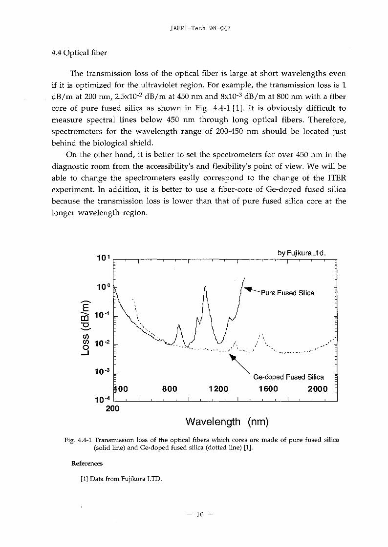
4.4 Optical fiber
The transmission loss of the optical fiber is large at short wavelengths evenif it is optimized for the ultraviolet region. For example, the transmission loss is 1dB/m at 200 ran, 2.5xl0"2 dB/m at 450 nm and 8xlO'3 dB/m at 800 nm with a fibercore of pure fused silica as shown in Fig. 4.4-1 [1]. It is obviously difficult tomeasure spectral lines below 450 nm through long optical fibers. Therefore,spectrometers for the wavelength range of 200-450 nm should be located justbehind the biological shield.
On the other hand, it is better to set the spectrometers for over 450 nm in thediagnostic room from the accessibility's and flexibility's point of view. We will beable to change the spectrometers easily correspond to the change of the ITERexperiment. In addition, it is better to use a fiber-core of Ge-doped fused silicabecause the transmission loss is lower than that of pure fused silica core at thelonger wavelength region.
byFujkuraLtd.
10
10
-3
-4
Fused Slica
ioo 800 1200Ge-doped Fused Silica
1600 2000
200
Wavelength (nm)
Fig. 4.4-1 Transmission loss of the optical fibers which cores are made of pure fused silica(solid line) and Ge-doped fused silica (dotted line) [1].
References
[1] Data from Fujikura LTD.
- 16 -

JAERI-Tech 98-047
4.5 Conceptual arrangement
From the considerations above, the conceptual arrangement shown in Fig.4.5-1 has been chosen. The light from the divertor region passes through thequartz windows on the divertor port plug and the cryostat, and goes through thedog-leg optics in the biological shield. The light is then focused on the ends of thefiber bundle by collecting and focusing optics. The fiber bundle guides the light tothe spectrometers. The spectrometers with the wavelength region below 450 nmare installed just behind the biological shield to minimize the transmission lossin fiber. On the other hand, the light with X > 450 nm is guided by long opticalfibers to the spectrometers which are located remotely in the diagnostic room inorder to have good accessibility. We will be able to change the spectrometerseasily corresponding to the change of the experiment.
The spectrometers for 200 - 450 nm and the local controller are installed on amovable trolley so that they can be removed in a short time before the divertormaintenance.
< Tcp view> Optical Fber Bundle
Coftecthg & FoeusingGpties
Spectrometers(200 -450nm)
^To Dagnostb Room{>450nm)
Terminal Box
LocalControlbr
Movable Trolley
Cryostat BiologicalShield
Fig.4.5-1 Conceptual arrangement of Divertor Impurity Monitoring System.
- 17 -

JAERI-Tech 98-047
5. Optical design
5.1 Design concept and viewing fans in the divertor channel
The two-dimensional measurement in the poloidal plane is performed withtwo viewing fans, which intersect, namely OV and OH for the outer divertorregion, and IV and IH for the inner region. These viewing fans are realized bymetallic mirrors (made of molybdenum) located in the divertor cassette as shownin Figure 5.1-1. This viewing system is called '2-D viewing system'.
The region from approximately up the divertor leg to the x-point will beobserved with the additional viewing fans named XL and XU through the gapbetween the divertor cassettes. This viewing system is called 'X-point viewingsystem'.
The number of lines of sight for each viewing fan is given in Table 5.1-1.The 10 mm spatial resolution will be realized by filter spectrometers. The detailedlines of sight are also shown in Fig. 5.1-2, 3, 4, 5, 6 and 7. The each viewing fans ofOH and IH is composed of two sub-viewing fans called OH/Lower andOH/Upper, and IH/Lower and IH/Upper respectively, in order to realize therequired spatial resolution.
Cut out< Top view >
XU, XL
Inner Divertor Outer Divertor< Side view >
Mo-miiror
Fig. 5.1-1 Viewing fans in the divertor cassette. The additional viewing fans XL and XU observethe region near the top of the divertor leg to the x-point through the gap between thedivertor cassette.
- 18 -

JAERI-Tech 98-047
Table 5.1-1 Number of lines of sight for spectrometers in each viewing fan.
Viewing fan Visible survey spectrometer Filter spectrometer High dispersion spectrometer
<2-D viewing system>OV >4 >100 >4OH - >100IV >4 >100 >4IH - >100
<X-point viewing system>XL >2 >50 >2XU >2 >50 >2
- 19 -
JAERI-Tech 98-047
tne image or m e oocical fleer ounoie
70aa from tne center of m e vessel
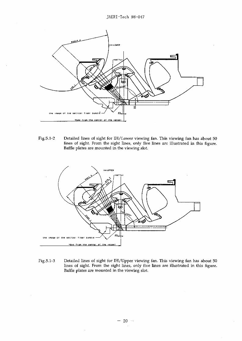
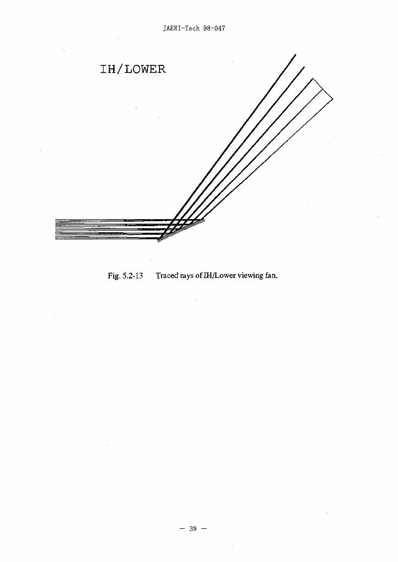
Fig.5.1-2 Detailed lines of sight for IH/Lower viewing fan. This viewing fan has about 50lines of sight. From the sight lines, only five lines are illustrated in this figure.Baffle plates are mounted in the viewing slot.
cne image of tne ooticai fioer curtate
7044 from tne center of the vessel .
Fig.5.1-3 Detailed lines of sight for IH/Upper viewing fan. This viewing fan has about 50lines of sight. From the sight lines, only five lines are illustrated in this figure.Baffle plates are mounted in the viewing slot.
- 20 -

JAERI-Tech 98-047
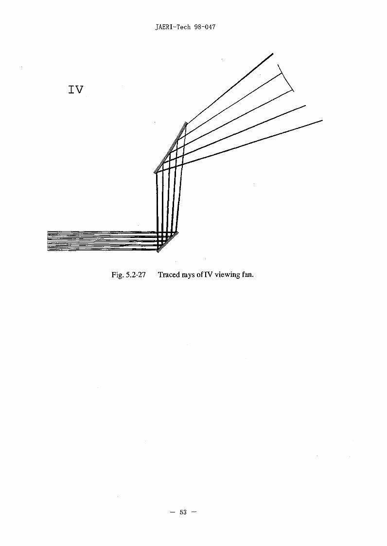
Fig.5.1-4 Detailed lines of sight for IV viewing fan. This viewing fan has about 100 lines ofsight. From the sight lines, only five lines are illustrated in this figure. Baffleplates are mounted in the viewing slot.
Fig.5.1-5 Detailed lines of sight for OV viewing fan. This viewing fan has about 100 lines ofsight. From the sight lines, only five lines are illustrated in this figure. Baffleplates are mounted in the viewing slot.
- 21 -
JAERI-Tech 98-047
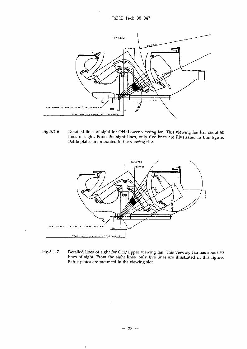
Fig.5.1-6 Detailed lines of sight for OH/Lower viewing fan. This viewing fan has about 50lines of sight. From the sight lines, only five lines are illustrated in this figure.Baffle plates are mounted in the viewing slot.
Che image of the ootlcal fiDer bundle S
7044 from the center of The vessel
Fig.5.1-7 Detailed lines of sight for OH/Upper viewing fan. This viewing fan has about 50lines of sight. From the sight lines, only five lines are illustrated in this figure.Baffle plates are mounted in the viewing slot.
- 22 -
JAERI-Tech 98-047
5.2 Optics
5.2.1 Optical penetration and collecting optics
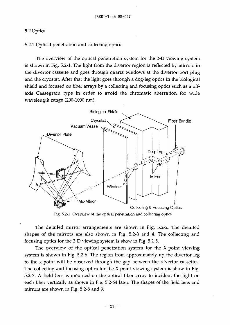
The overview of the optical penetration system for the 2-D viewing systemis shown in Fig. 5.2-1. The light from the divertor region is reflected by mirrors inthe divertor cassette and goes through quartz windows at the divertor port plugand the cryostat. After that the light goes through a dog-leg optics in the biologicalshield and focused on fiber arrays by a collecting and focusing optics such as a off-axis Cassegrain type in order to avoid the chromatic aberration for widewavelength range (200-1000 nm).
Biological Shield
Fiber Bundle
'Mo-Mirror ^Collecting & Focusing Optics
Fig. 5.2-1 Overview of the optical penetration and collecting optics
The detailed mirror arrangements are shown in Fig. 5.2-2. The detailedshapes of the mirrors are also shown in Fig. 5.2-3 and 4. The collecting andfocusing optics for the 2-D viewing system is show in Fig. 5.2-5.
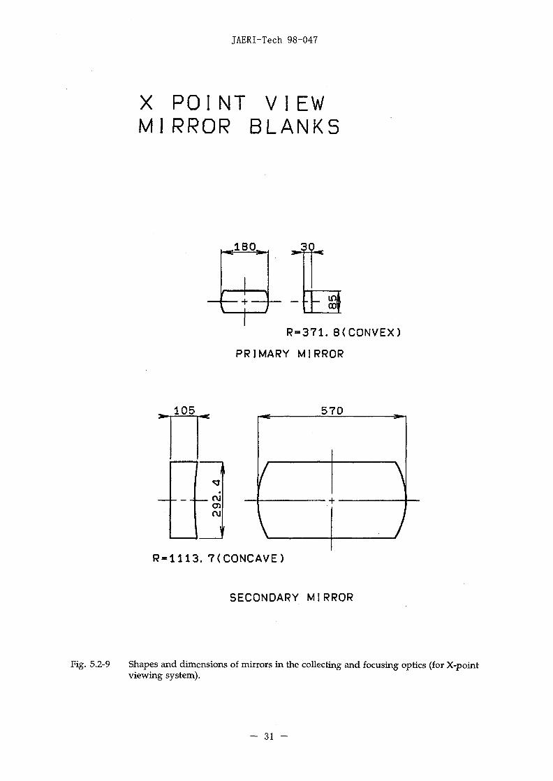
The overview of the optical penetration system for the X-point viewingsystem is shown in Fig. 5.2-6. The region from approximately up the divertor legto the x-point will be observed through the gap between the divertor cassettes.The collecting and focusing optics for the X-point viewing system is show in Fig.5.2-7. A field lens is mounted on the optical fiber array to incident the light oneach fiber vertically as shown in Fig. 5.2-64 later. The shapes of the field lens andmirrors are shown in Fig. 5.2-8 and 9.
23

to -STANDARD LINE7044mm fromthe center of the vess
o
tooo
IV ovFig. 5.2-2 Detailed mirror arrangement for 2-D viewing system in the divertor cassette.

JAERI-Tech 98-047
H/UPPER
. 1H/LOWER
IV
15
03
Rj-1089. 7
. 7
Rxoo
R-^1358. 0
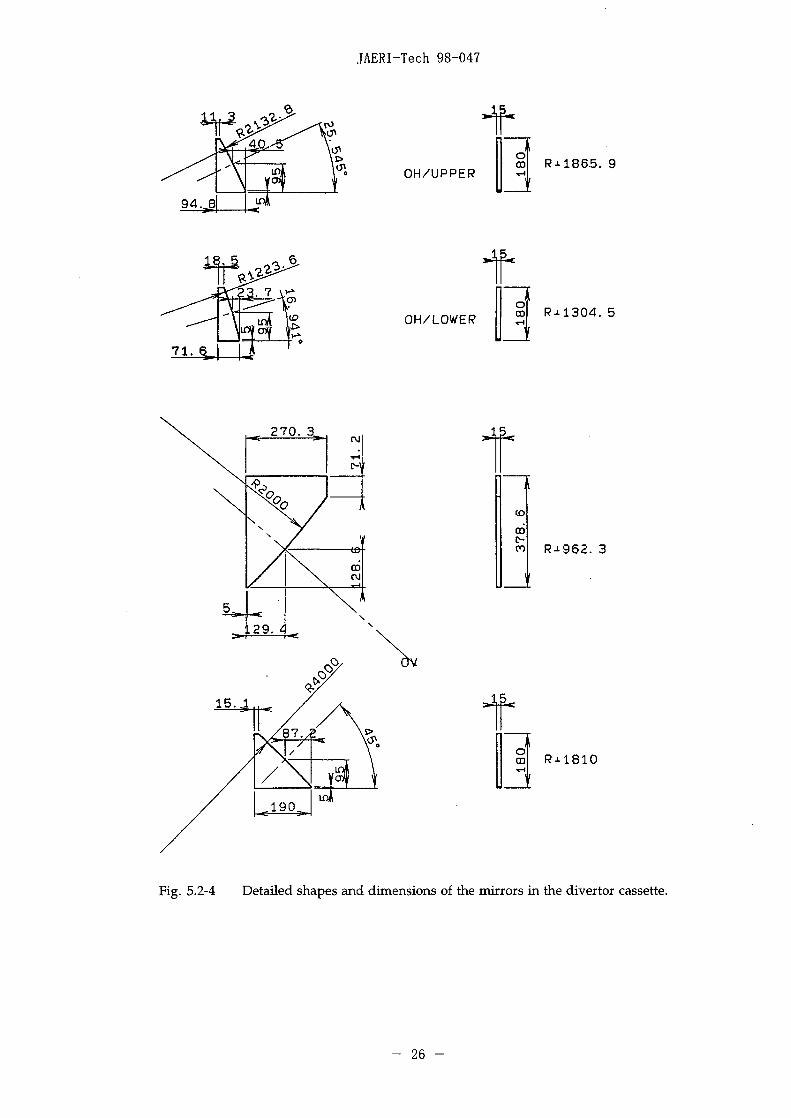
Fig. 5.2-3 Detailed shapes and dimensions of the mirrors in the divertor cassette.
- 25 -
JAERI-Tech 98-047
OH/UPPERoo R-^1865. 9
OH/LOWER R J - 1 3 0 4 . 5
toCO
cn R J - 9 6 2 . 3
Fig. 5.2-4 Detailed shapes and dimensions of the mirrors in the divertor cassette.
- 26 -

-CO-AXISOF THE TWO OFF-AXIS MIRRORS
CO
LIGHT SORCE & TI LT DETECTOR L IGHT COLLECTOR
13600 FROM S.
FOR THE DIVERTOR OPTICSPT1CAL FIBER ^BUNDLE
EXIT PUPIL 0-38mm(MAX)
-APERTURE STOP0=200
0-300(290)
-9CDO
toooo
1363. 76
Fig. 5.2-5 Collecting and focusing optics for 2-D viewing system.

AA"
/ " •
X P O I N T VIEW
•APERUTURE STOP
IS)00
12707from the aperture stoo
APERTURE STOP
opUca! p e — sys.en,
3TO
O
CDO
COi
o

X POINT VIEW OPTICS
SECONDARY MIRROR
to
I
APERTURE STOP0-6512700mm FROM OBJECT
0-AXIS OF THE MIRRORS
ELD LENS ANDOPTJCAL FIBER BUNDLE
1821.11
pat—i
iCDO
00
O
-0
-PRIMARY MIRROR
Fig. 5.2-7 Collecting and focusing optics for X-point viewing system.

X POINT VIEWFIELD LENS & OPTICAL FIBER BUNDLE
CO
o
OPTICAL AXIS
i—JCDO
00I
o
FIELD LENS
•-OPTICAL FIBER BUNDLEENTRANCE SURFACE
Fig. 5.2-8 Shapes and dimensions of field lens in the collecting and focusing optics (for X-point viewing system).
JAERI-Tech 98-047
X POINT VIEWMIRROR BLANKS
30
R=371. 8(CONVEX)
PRIMARY MIRROR
570
R-1113.7(CONCAVE)
SECONDARY MIRROR
Fig. 5.2-9 Shapes and dimensions of mirrors in the collecting and focusing optics (for X-pointviewing system).
- 31 -

JAERI-Tech 98-047
5.2.2 Fiber array
The light from the divertor region is focused on a optical-fiber array tomeasure spatial distribution of spectral emissions at the divertor with theresolution of about 10 mm. Each optical fiber has a core diameter of 200 |im anda clad diameter of 250 |im. The arrangement of the optical-fibers are shown inFig.5.2-10 and 11. Fig. 5.2-10 is the plan view of the fiber arrangement for 2-Dviewing system. Fig. 5.2-11 is the front view. Each viewing fan has 360 (120 x 3)optical fibers. Total number of fibers is 2,880.
For the X-point viewing system, 480 optical-fibers will be arranged totally.The distributions of optical fibers are summarized in Table 5.2-1, 2, 3 and 4
for all of this system, for visible survey spectrometers, for filter spectrometersand for high dispersion spectrometers respectively.
Table 5.2-1 Distribution of optical fibers for Divertor Impurity Monitoring System.Viewing fan
IH/L
IH/U
IV2
IV1
OV1
OV2
OH/L
OH/U
Subtotal
XU
XL
Subtotal
Total
Number of fibersin bundle
120x3
120x3
120x3
120x3
120x3
120x3
120x3
120x3
2880
TBD
TBD
vss0
0
4x16
4x16
0
0
128
2x16
2x16
64
192
FS
50x4
50x4
100x4
100x4
50x4
50x4
1600
50x4
50x4
400
2000
HDS
0
0
4x2+4x2
4x2+4x2
0
0
32
2 x 4
2 x 4
16
48
Subtotal
200
200
480
480
200
200
1760
240
240
480
2240
32 -

JAERI-Tech 98-047
Table 5.2-2 Distribution of optical fibers for Visible Survey Spectrometer.
No. of VSS
No.lNo.2No.3No.4No.5No.6No.7No.8No.9
No. 10No.llNo.12No.13No.14No.15No.16Total
Capacity
2020
202020202020
2020202020
202020
320
Viewing fanIH/L
0
0000
00
000000
000
0
IH/U
0
0000000
00000
0000
IV2/IV1
4444444
444444
444
64
OV1/OV2
4
444444
444
4444
4464
OH/L
00000000
00000
0000
OH/U
0
0000000
000000
000
xu2222222
222222
22232
XL
22222
22
222222
222
32
Total
1212121212
1212121212121212
121212
192
Table 5.2-3 Distribution of optical fibers for Filter Spectrometer.
NameUV
VIS-1VIS-2VIS-3Total
Capacity400
400400400
1600
Viewing fanIH/L
50505050200
IH/U50
505050
200
IV2/IV1100100100100400
OV1/OV2100
100100100
400
OH/L5050
5050
200
OH/U50505050
200
Total400400400400
1600
NameUV
VIS-1VIS-2VIS-3Total
Capacity4004004004001600
Viewing fanXU
50505050200
XL
50505050
200
Total100100100100400
Table 5.2-4 Distribution of optical fibers for High Dispersion Spectrometer.
NameBlueRed
Total
Capacity121224
Viewing fanIH/L
000
IH/U000
IV2/IV1448
OV1/OV244
8
OH/L000
OH/U000
XU224
XL
224
Total121224
- 33 -

IGO
CENTER OF THE CYLINDER OPTICAL FIBER BUNDLE
i-3too
COI
O
CO-AXIS OF THE TWO OFF-AXIS MIRRORS\
Fig. 5.2-10 Plan view of fiber arrangement for 2-D viewing system.

JAERI-Tech 98-047
OPTICAL F IBER 8UNOLE
CORE
CLAD
PTiCAL FIBER
3 LINES OF THE 120 OPTICAL FIBEBSFOR ONE VIEW
Fig. 5.2-11 Front view of fiber arrangement for 2-D viewing system. Each viewing fan has 360(120 x 3) optical fibers. Total number of fibers is 2,880.
- 35 -
JAERI-Tech 98-047
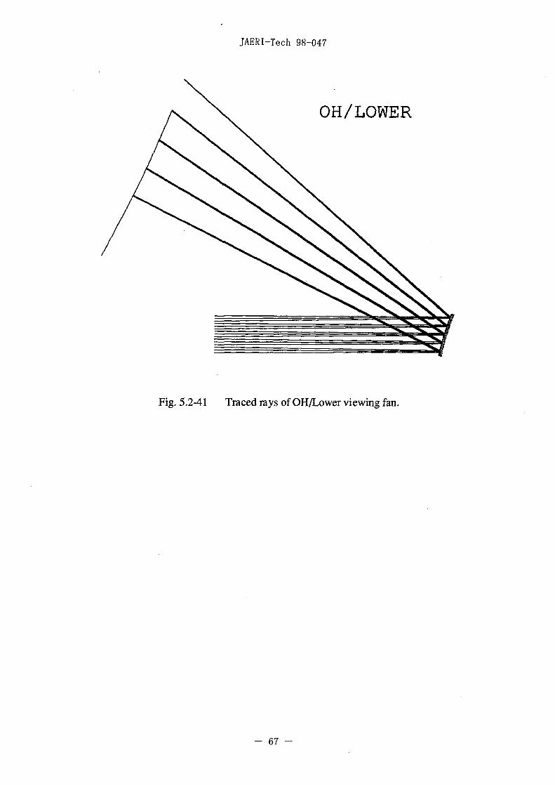
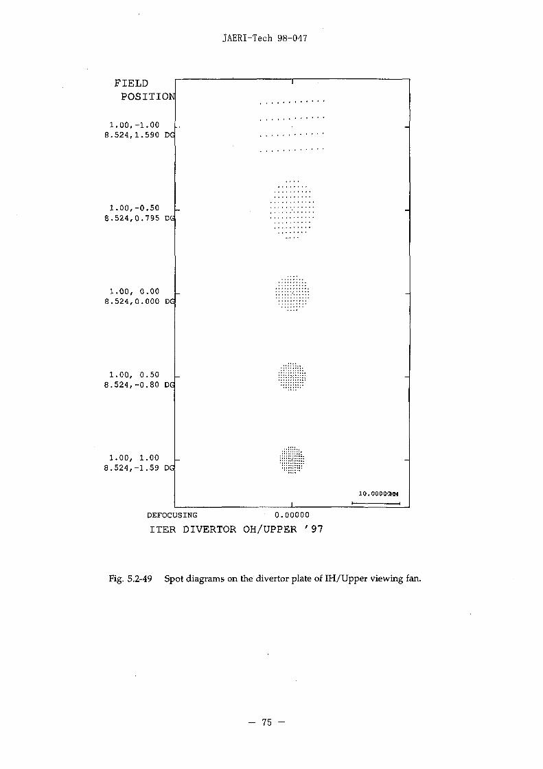
5.2.3 Ray trace analysis
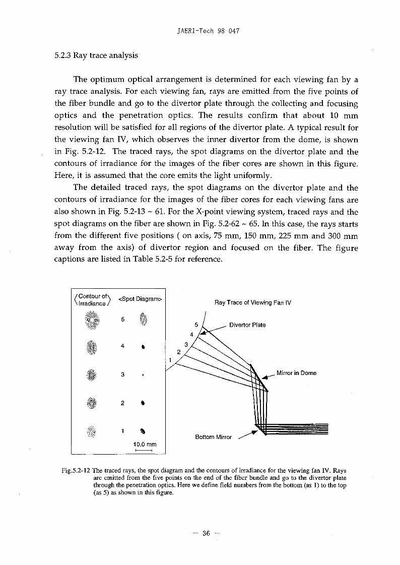
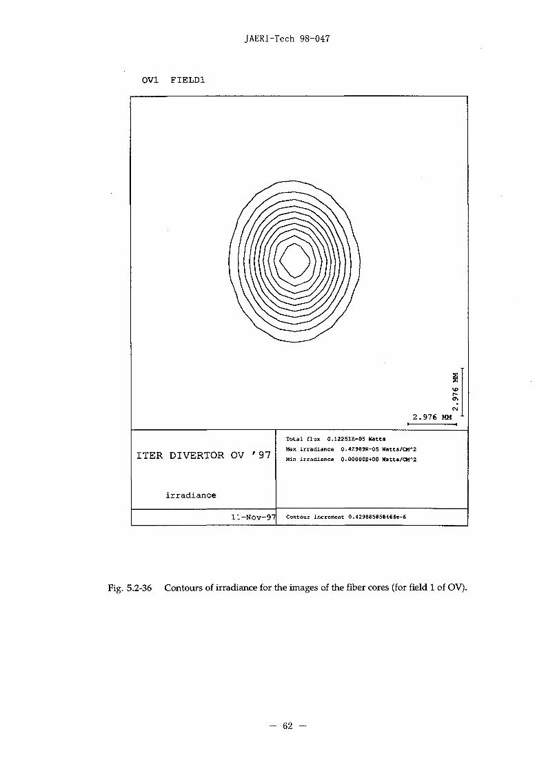
The optimum optical arrangement is determined for each viewing fan by aray trace analysis. For each viewing fan, rays are emitted from the five points ofthe fiber bundle and go to the divertor plate through the collecting and focusingoptics and the penetration optics. The results confirm that about 10 mmresolution will be satisfied for all regions of the divertor plate. A typical result forthe viewing fan IV, which observes the inner divertor from the dome, is shownin Fig. 5.2-12. The traced rays, the spot diagrams on the divertor plate and thecontours of irradiance for the images of the fiber cores are shown in this figure.Here, it is assumed that the core emits the light uniformly.
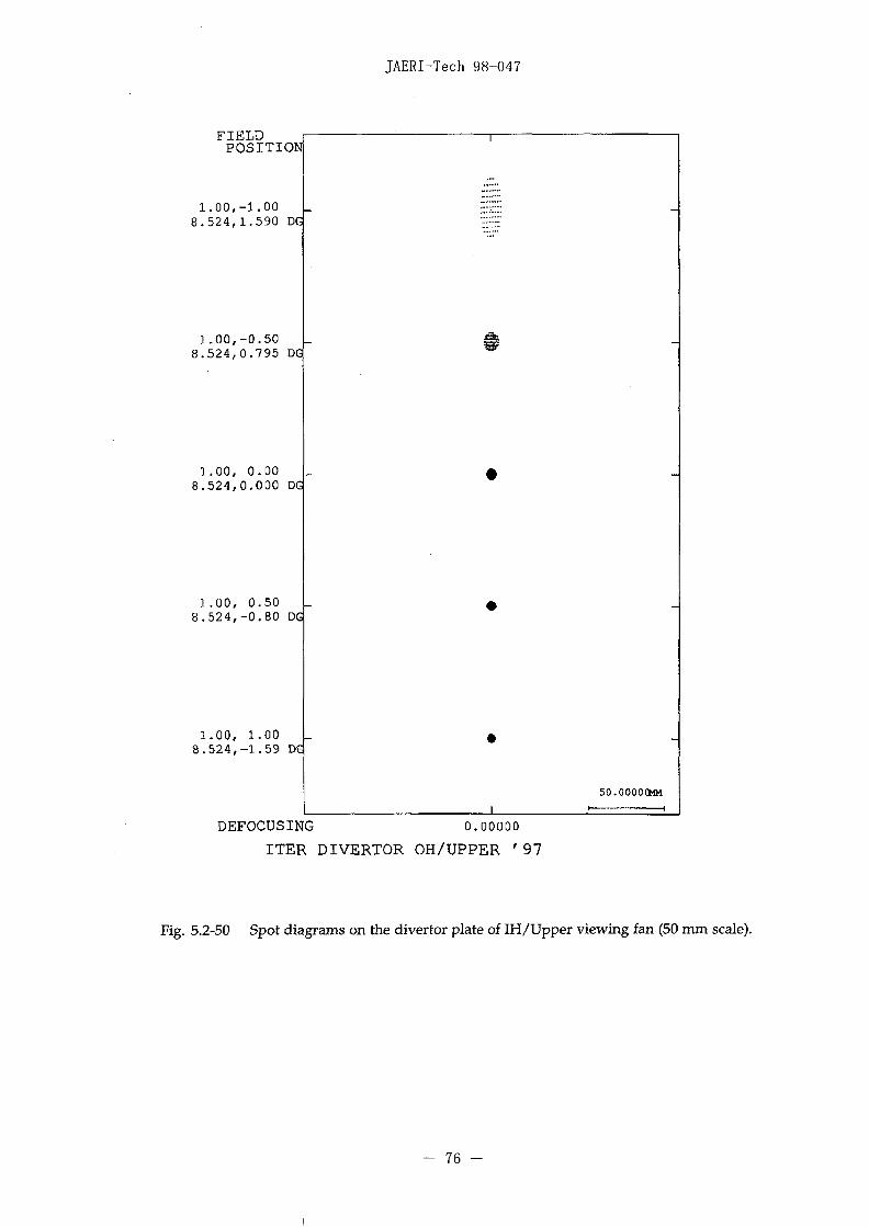
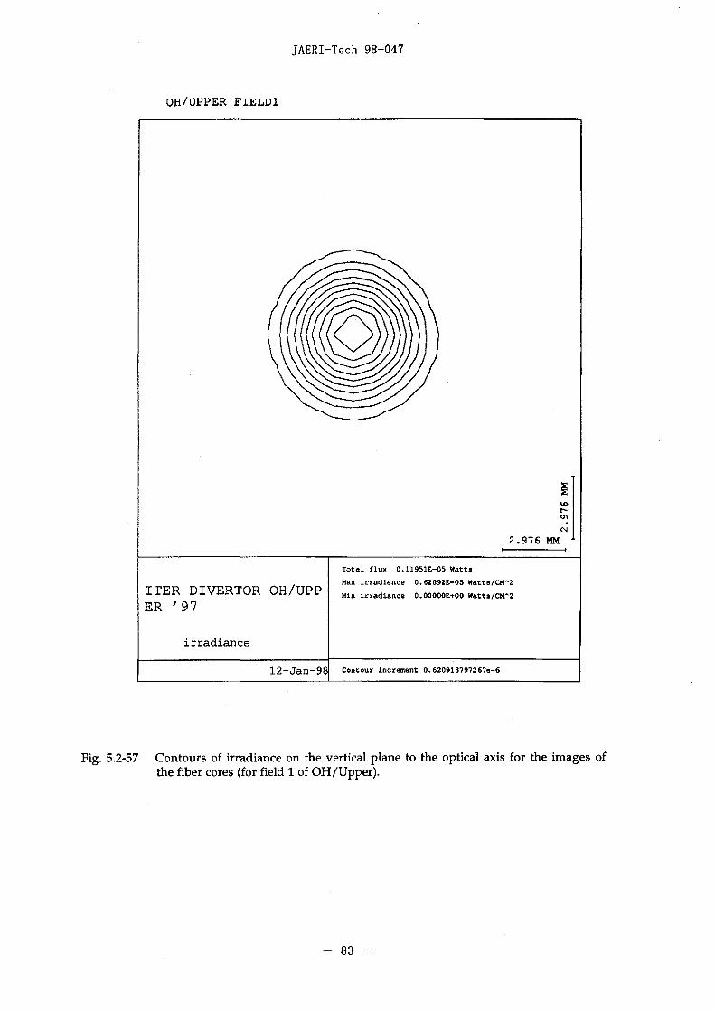
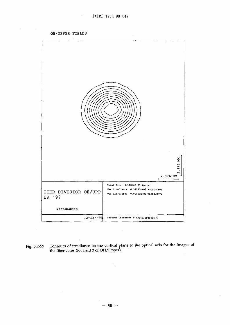
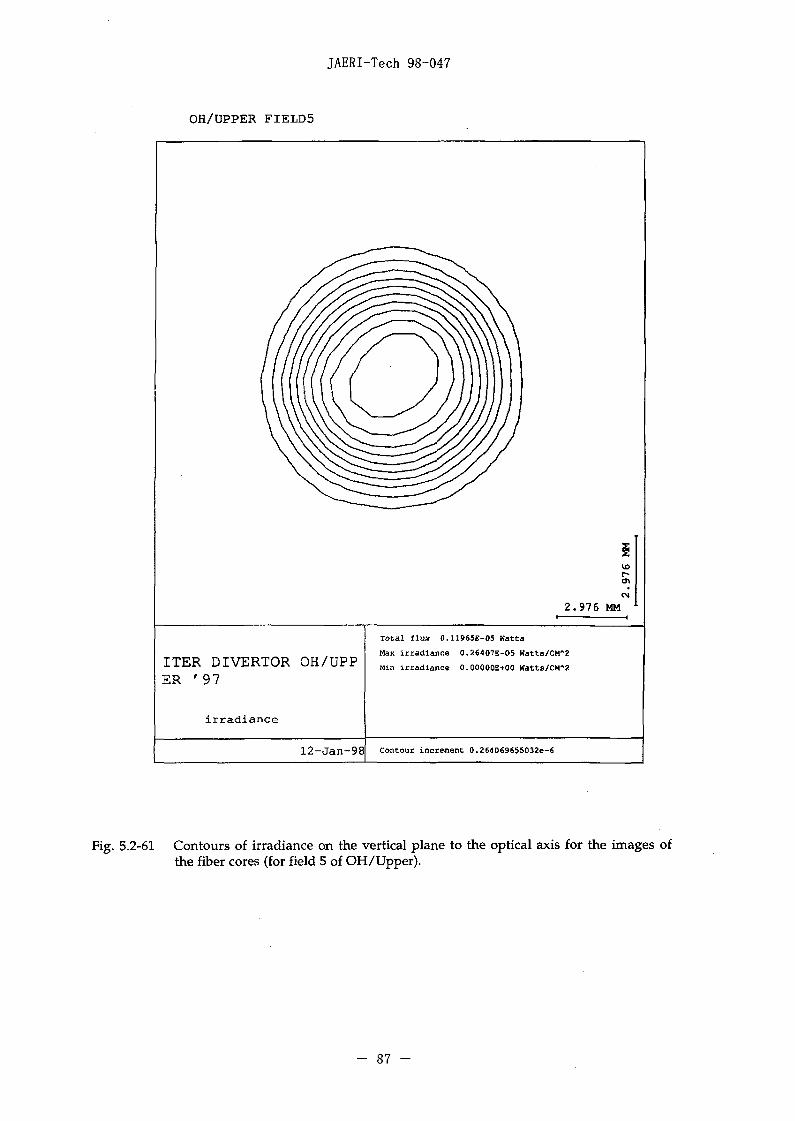
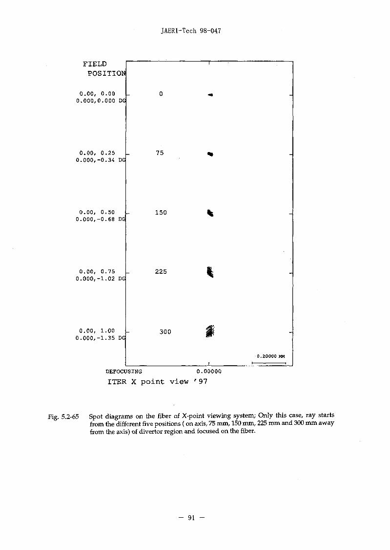
The detailed traced rays, the spot diagrams on the divertor plate and thecontours of irradiance for the images of the fiber cores for each viewing fans arealso shown in Fig. 5.2-13 ~ 61. For the X-point viewing system, traced rays and thespot diagrams on the fiber are shown in Fig. 5.2-62 ~ 65. In this case, the rays startsfrom the different five positions ( on axis, 75 mm, 150 mm, 225 mm and 300 mmaway from the axis) of divertor region and focused on the fiber. The figurecaptions are listed in Table 5.2-5 for reference.
/ Contour of\ < S p o t Diagram>\ Irradiance/
f
10.0 mm
Ray Trace of Viewing Fan IV
Divertor Plate
. Mirror in Dome
Bottom Mirror
Fig.5.2-12 The traced rays, the spot diagram and the contours of irradiance for the viewing fan IV. Raysare emitted from the five points on the end of the fiber bundle and go to the divertor platethrough the penetration optics. Here we define field numbers from the bottom (as 1) to the top(as 5) as shown in this figure.
- 36 -
JAERI-Tech 98-047
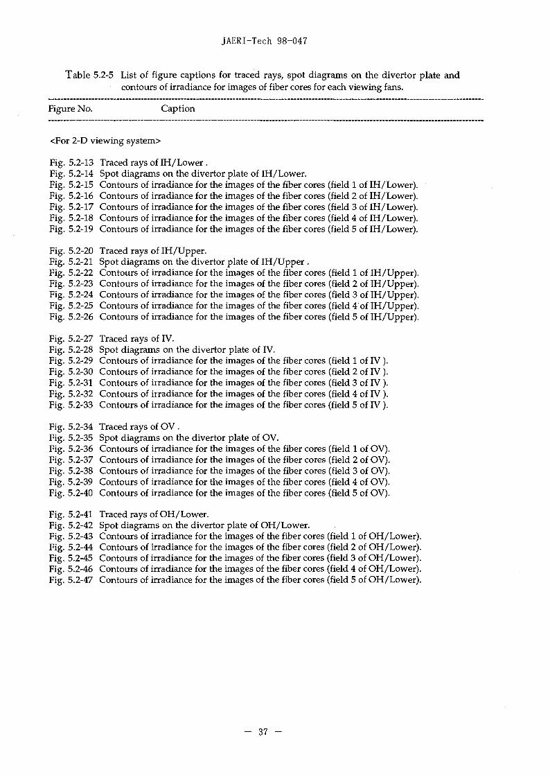
Table 5.2-5 List of figure captions for traced rays, spot diagrams on the divertor plate andcontours of irradiance for images of fiber cores for each viewing fans.
Figure No. Caption
<For 2-D viewing system>
Fig. 5.2-13 Traced rays of IH/Lower .Fig. 5.2-14 Spot diagrams on the divertor plate of IH/Lower.Fig. 5.2-15 Contours of irradiance for the images of the fiber cores (field 1 of IH/Lower).Fig. 5.2-16 Contours of irradiance for the images of the fiber cores (field 2 of IH/Lower).Fig. 5.2-17 Contours of irradiance for the images of the fiber cores (field 3 of IH/Lower).Fig. 5.2-18 Contours of irradiance for the images of the fiber cores (field 4 of IH/Lower).Fig. 5.2-19 Contours of irradiance for the images of the fiber cores (field 5 of IH/Lower).
Fig. 5.2-20 Traced rays of IH/Upper.Fig. 5.2-21 Spot diagrams on the divertor plate of IH/Upper .Fig. 5.2-22 Contours of irradiance for the images of the fiber cores (field 1 of IH/Upper).Fig. 5.2-23 Contours of irradiance for the images of the fiber cores (field 2 of IH/Upper).Fig. 5.2-24 Contours of irradiance for the images of the fiber cores (field 3 of IH/Upper).Fig. 5.2-25 Contours of irradiance for the images of the fiber cores (field 4 of IH/Upper).Fig. 5.2-26 Contours of irradiance for the images of the fiber cores (field 5 of IH/Upper).
Fig. 5.2-27 Traced rays of IV.Fig. 5.2-28 Spot diagrams on the divertor plate of IV.Fig. 5.2-29 Contours of irradiance for the images of the fiber cores (field 1 of IV ).Fig. 5.2-30 Contours of irradiance for the images of the fiber cores (field 2 of IV ).Fig. 5.2-31 Contours of irradiance for the images of the fiber cores (field 3 of IV ).Fig. 5.2-32 Contours of irradiance for the images of the fiber cores (field 4 of IV ).Fig. 5.2-33 Contours of irradiance for the images of the fiber cores (field 5 of IV ).
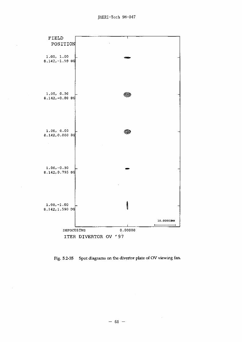
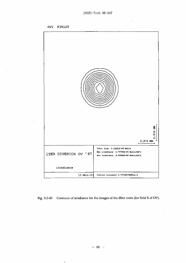
Fig. 5.2-34 Traced rays of OV .Fig. 5.2-35 Spot diagrams on the divertor plate of OV.Fig. 5.2-36 Contours of irradiance for the images of the fiber cores (field 1 of OV).Fig. 5.2-37 Contours of irradiance for the images of the fiber cores (field 2 of OV).Fig. 5.2-38 Contours of irradiance for the images of the fiber cores (field 3 of OV).Fig. 5.2-39 Contours of irradiance for the images of the fiber cores (field 4 of OV).Fig. 5.2-40 Contours of irradiance for the images of the fiber cores (field 5 of OV).
Fig. 5.2-41 Traced rays of OH/Lower.Fig. 5.2-42 Spot diagrams on the divertor plate of OH/Lower.Fig. 5.2-43 Contours of irradiance for the images of the fiber cores (field 1 of OH/Lower).Fig. 5.2-44 Contours of irradiance for the images of the fiber cores (field 2 of OH/Lower).Fig. 5.2-45 Contours of irradiance for the images of the fiber cores (field 3 of OH/Lower).Fig. 5.2-46 Contours of irradiance for the images of the fiber cores (field 4 of OH/Lower).Fig. 5.2-47 Contours of irradiance for the images of the fiber cores (field 5 of OH/Lower).
- 37

JAERI-Tech 98-047
Table 5.2-5 List of figure captions for traced rays, spot diagrams on the divertor plate andcontours of irradiance for images of fiber cores for each viewing fans (continued).
Figure No. Caption
Fig. 5.2-48 Traced rays of OH/Upper.Fig. 5.2-49 Spot diagrams on the divertor plate of IH/Upper.Fig. 5.2-50 Spot diagrams on the divertor plate of IH/Upper (50 mm scale).Fig. 5.2-51 Spot diagrams on the vertical plane to the optical axis of IH/Upper.Fig. 5.2-52 Contours of irradiance for the images of the fiber cores (field 1 of OH/Upper).Fig. 5.2-53 Contours of irradiance for the images of the fiber cores (field 2 of OH/Upper).Fig. 5.2-54 Contours of irradiance for the images of the fiber cores (field 3 of OH/Upper).Fig. 5.2-55 Contours of irradiance for the images of the fiber cores (field 4 of OH/Upper).Fig. 5.2-56 Contours of irradiance for the images of the fiber cores (field 5 of OH/Upper).Fig. 5.2-57 Contours of irradiance on the vertical plane to the optical axis for the images
of the fiber cores (field 1 of OH/Upper).Fig. 5.2-58 Contours of irradiance on the vertical plane to the optical axis for the images
of the fiber cores (field 2 of OH/Upper).Fig. 5.2-59 Contours of irradiance on the vertical plane to the optical axis for the images
of the fiber cores (field 3 of OH/Upper).Fig. 5.2-60 Contours of irradiance on the vertical plane to the optical axis for the images
of the fiber cores (field 4 of OH/Upper).Fig. 5.2-61 Contours of irradiance on the vertical plane to the optical axis for the images
of the fiber cores (field 5 of OH/Upper).
< For X-point viewing system>
Fig. 5.2-62 Traced rays of X-point viewing system (side view).Fig. 5.2-63 Traced rays of X-point viewing system (plan view).Fig. 5.2-64 Traced rays of X-point viewing system (at field lens).Fig. 5.2-65 Spot diagrams on the fiber of X-point viewing system; Only this case, ray
starts from the different five positions ( on axis, 75 mm, 150 mm, 225 mm and300 mm away from the axis) of divertor region and focused on the fiber.
- 38 -
JAERI-Tech 98-047
IH/LOWER
Fig. 5.2-13 Traced rays of IH/Lower viewing fan.
- 39 -

JAERI-Tech 98-047
FIELDPOSITION
1.00, 1.006.181,-1.59 DG
1.00, 0.506.181,-0.80 Dd
1.00, 0.006.181,0.000 Dd
1.00,-0.506.181,0.797 Dd
1.00,-1.006.181,1.593 DGi
DEFOCUSING 0.00000
ITER DIVERTOR IH/LOWER '97
Fig. 5.2-14 Spot diagrams on the divertor plate of IH/Lower viewing fan.
- 40 -
JAERI-Tech 98-047
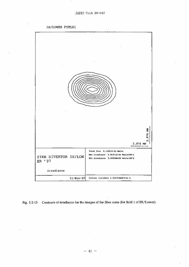
IH/LOWER FIELD1
2 . 9 7 6 MM
ITER DIVERTOR IH/LOWER ' 9 7
irradiance
Total flux 0.12221E-05 Watts
Max irradiance 0.91071E-05 Hatta/CM*2
Min irradiance 0.OQOO0E+O0 Watta/CM"2
ll-Nov-97 Contour increment 0.910710866719e-6
Fig. 5.2-15 Contours of irradiance for the images of the fiber cores (for field 1 of IH/Lower).
41
JAERI-Tech 98-047
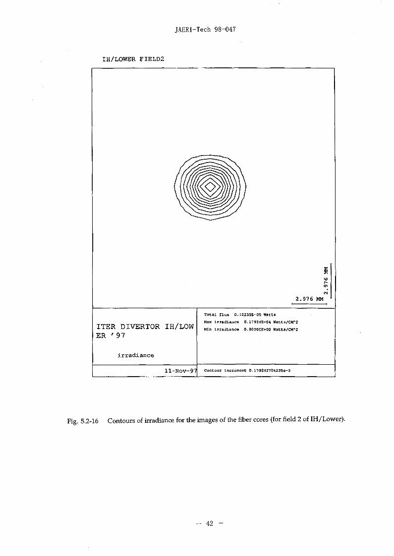
IH/LOWER FIELD2
2 . 9 7 6 MM
ITER DIVERTOR IH/LOWER ' 9 7
irradiance
Total flux 0.12235E-05 »»tts
Max irradiancs 0.17924E-04 Watts/CM'2
Min irradiance O.00OO0E+0O Matts/CM»2
ll-Nov-97 Contour increment 0. n924270«35e-5
Fig. 5.2-16 Contours of irradiance for the images of the fiber cores (for field 2 of IH/Lower).
- 42 -

JAERI-Tech 98-047
IH/LOWER FIELD3
2.976 MM
ITER DIVERTOR IH/LOWER ' 9 7
irradiance
Total flux 0.12235E-05 Watts
Max irradianee 0.13321E-04 WattB/CJT2
Min irradiance O.OOOOOE+00 Hatts/CM"2
ll-Nov-97 Contour increment O.13321454162e-5
Fig. 5.2-17 Contours of irradiance for the images of the fiber cores (for field 3 of IH/Lower).
- 43 -

JAERI-Tech 98-047
IH/LOWER FIELD4
CM
2 .976 MM
ITER DIVERTOR IH/LOWER ' 9 7
irradiance
Total flux 0.12236E-05 Watts
Max irradiance O.G4543E-O5 Katts/CM"2
Min irradiance O.O0OO0E+00 WatWCM*2
ll-Nov-97 Contour increment 0.6454299068S4e-6
Fig. 5.2-18 Contours of irradiance for the images of the fiber cores (for field 4 of IH/Lower).
44 -

JAERI-Tech 98-047
IH/LOWER FIELD5
2 .976 MM
ITER DIVERTOR IH/LOWER ' 9 7
irradiance
Total f lux 0.12211E-05 Watts
Max Irradiance 0.36971E-05 Natt9/CM"2
Min irradiance 0.OO000E+OO tfatt»/CM*2
l l -Nov-97 Contour increment 0.3691149395S2a-6
Fig. 5.2-19 Contotirs of irradiance for the images of the fiber cores (for field 5 of IH/Lower).
- 45 -

JAERI-Tech 98-047
IH/UPPER
Fig. 5.2-20 Traced rays of IHAJpper viewing fan.
- 46 -

JAERI-Tech 98-047
FIELDPOSITION]
1.00 , -1 .006-575,1.592 DG
1.00 , -0 .506.575,0 .796 DG
1.00, 0.006.575,0 .000 DG
1.00, 0.506 .575 , -0 .80 DG
1.00, 1.006 .575 , -1 .59 DG
DEFOCUSING 0.00000
ITER DIVERTOR IH/UPPER '97
Fig. 5.2-21 Spot diagrams on the divertor plate of IH/Upper viewing fan.
- 47 -

JAERI-Tech 98-047
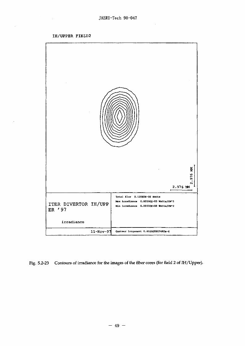
IH/UPPER FIELD1
2 .976 MM
ITER DIVERTOR IH/UPPER ' 9 7
irradiance
Total flux 0.12047E-OS KattS
Max irradiance O.S3610E-05 Watts/CM"2
Min irradlanca O.0O000E+0O Watts/CM'2
l l-Nov-97 Contour Increment 0.536095626S56e-6
Fig. 5.2-22 Contours of irradiance for the images of the fiber cores (for field 1 of IH/Upper).
- 48 -
JAERI-Tech 98-047
IH/UPPER FIELD2
2 . 9 7 6 MM
ITER DIVERTOR IH/UPPER ' 9 7
irradiance
Total flux 0.12060K-0S Watta
Max lrradiancB 0.8S590E-05 H»tts/CW2
Min irradianca O.00000E+O0 Hatts/CMA2
l l -Nov-97 Contour increment 0.855900907482e-6
Fig. 5.2-23 Contours of irradiance for the images of the fiber cores (for field 2 of IH/Upper).
49

JAERI-Tech 98-047
IH/UPPER FIELD3
2 . 9 7 6 MM
ITER DIVERTOR IH/UPPER ' 9 7
irradiance
Total flux 0.12064E-05 Watts
Max irradiance 0.99565E-05 Watts/CH*2
Min irradiance O.OOOOOE+00 W»tts/CM*2
H-Nov-97 Contour increment 0.995648292701e-6
Fig. 5.2-24 Contours of irradiance for the images of the fiber cores (for field 3 of IH/Upper).
- 50 -

JAERI-Tech 98-047
IH/UPPER FIELD4
2.976 MM
ITER DIVERTOR IH/UPPER ' 9 7
irradiance
Total flux 0.12060E-05 Watta
Max irradiance O.68505E-O5 Hatts/CM"2
Min irradiance 0.OO0O0E+OO Matts/CM"2
ll-Nov-97 Contour increment 0.<8S04562023e-6
Fig. 5.2-25 Contours of irradiance for the images of the fiber cores (for field 4 of IH/Upper).
- 51 -

JAERI-Tech 98-047
IH/UPPER FIELD5
2 .976 MM
ITER DIVERTOR IH/UPPER ' 9 7
irradiance
Total flux 0.12047E-05 Watts
Max irradiance 0.39718E-05 Watta/CMA2
Min irradiance O.00000E+OO Watta/CMA2
l l -Nov-97 Contour increment 0.39717738786^-6
Fig. 5.2-26 Contours of irradiance for the images of the fiber cores (for field 5 of IH/Upper).
- 52 -
JAERI-Tech 98-047
IV
Fig. 5.2-27 Traced rays of IV viewing fan.
- 53 -

JAERI-Tech 98-047
FIELDPOSITION
1 .00 , -1 .006 .961 ,1 .590 DG
1.00 , -0 .506 .961 ,0 .795 DG
1.00, 0.006 .961 ,0 .000 DG
1.00, 0.506 . 9 6 1 , - 0 . 8 0 DG
1.00, 1.006 . 9 6 1 , - 1 . 5 9 DG
DEFOCUSING 0.00000
ITER DIVERTOR IV ' 97
Fig. 5.2-28 Spot diagrams on the divertor plate of IV viewing fan.
- 54 -

JAERI-Tech 98-047
IV1 FIELD1
2.976 MM l
ITER DIVERTOR IV ' 9 7
irradiance
Total flux 0.12288E-05 Wstta
Max irradiance O.88B41E-O5 WattB/CM"2
Hin irradiance O.O0000E+OO Katts/CM*2
ll-Nov-97 Contour increment 0.886413806298O-6
Fig. 5.2-29 Contours of irradiance for the images of the fiber cores (for field 1 of IV ).
- 55 -

JAERI-Tech 98-047
IVI FIELD2
2 .976 MM
ITER DIVERTOR IV ' 97
irradiance
Total flux 0.12308E-05 Watts
Max irradianee 0.11366E-04 Hatt»/CM*2
Kin irradiance O.O00O0E+0O Watts/CM1^
ll-Nov-97 Contour increment 0.113663134016e-5
Fig. 5.2-30 Contours of irradiance for the images of the fiber cores (for field 2 of IV ).
- 56 -

JAERI-Tech 98-047
IV1 FIELD3
2 .976 MM
ITER DIVERTOR IV ' 97
irradiance
Total flux 0.12308E-05 Vtatts
Max irradiance O.11894E-O4 Watts/OTZ
Hin irradiance O.0O000B+0O Watts/CM'2
l l -Nov-97 Contour increment 0.1189390786756-5
Fig. 5.2-31 Contours of irradiance for the images of the fiber cores (for field 3 of IV ).
- 57 -

JAERI-Tech 98-047
IV1 FIELD4
CM
2.976 MM
ITER DIVERTOR IV ' 97
irradiance
Total flux 0.122 92E-05 Watt*
Max ixradiance 0.86353E-0S Hatt8/CM"2
Mln irradiance O.0O000E+00 Watta/CM"2
ll-Nov-97 Contour increment 0.8G3529294293e-6
Fig. 5.2-32 Contours of irradiance for the images of the fiber cores (for field 4 of IV ).
- 58 -

JAERI-Tech 98-047
IV1 FIELD5
/// \\\\v
2 .9 7 6 MM
ITER DIVERTOR IV ' 9 7
irradiance
Total flux 0.94533E-06 Watts
Max irradiance 0.25369E-05 Watt«/CM*2
Min irradiance O.OOOOOE+00 Watt3/CM*2
ll-Nov-97 Contour increment 0.253686550877e-6
Fig. 5.2-33 Contours of irradiance for the images of the fiber cores (for field 5 of IV ).
- 59 -

JAERI-Tech 98-047
OV
Fig. 5.2-34 Traced rays of OV viewing fan.
- 60
JAERI-Tech 98-047
FIELDPOSITION
1.00, 1.008.142,-1.59 DG
1.00, 0.508.142,-0.80 DG
1.00, 0.008.142,0.000 DG
1.00,-0.508.142,0.795 DG
1.00,-1.008.142,1.590 DG
DEFOCUSING 0.00000
ITER DIVERTOR OV ' 9 7
Fig. 5.2-35 Spot diagrams on the divertor plate of OV viewing fan.
61 -
JAERI-Tech 98-047
OV1 FIELD1
2.976 MM
ITER DIVERTOR OV ' 97
irradiance
ll-Nov-97
Total flux 0.12251E-05 Watts
Max irradiance 0-42969E-05 Natt5/CH^2
Min irradiance O.O0OO0E+0O Watt8/CMA2
Contour increment 0.42988565846Ge-6
Fig. 5.2-36 Contours of irradiance for the images of the fiber cores (for field 1 of OV).
- 62

JAERI-Tech 98-047
OV1 FIELD2
2.976 MM
ITER DIVERTOR OV ' 9 7
irradiance
Total flux 0.12285E-05 Watts
Max irradiance 0.63544E-05 »atts/CM*2
Mir irradiance 0.O00O0E+00 Watta/CH*2
ll-Nov-97 Contour increment 0.635437174878e-6
Fig. 5.2-37 Contours of irradiance for the images of the fiber cores (for field 2 of OV).
- 63 -

JAERI-Tech 98-047
OV1 FIELD3
2 .976 MM
ITER DIVERTOR OV ' 97
irradiance
Total flux 0.1230SE-0S Watts
Max irradiance 0.71589E-05 Watts/CM*2
Min irradiance O.OOOOOE+00 Hatts/CM*2
ll-Nov-97 Contour increment 0.71589039407£e-6
Fig. 5.2-38 Contours of irradiance for the images of the fiber cores (for field 3 of OV).
- 64 -

JAERI-Tech 98-047
OV1 FIELD4
2 .976 MM
ITER DIVERTOR OV ' 97
irradiance
Total flux 0.12300E-05 Watto
Max irradiance O.77556E-05 Hatt3/CM"2
Min irradianoe O.0OO00E+0O Watts/CM'2
ll-Nov-97 Contour Increment 0.77556035194e-6
Fig. 5.2-39 Contours of irradiance for the images of the fiber cores (for field 4 of OV).
65 -
JAERI-Tech 98-047
OV1 FIELDS
2 . 9 7 6 MM
ITER DIVERTOR OV ' 9 7
irradiance
Total flux 0.12261E-0S Watts
Max irradiance 0.75755B-05 Katts/CM"2
Min irradiance O.OO0O0E+DO Watts/CMA2
Contour increment 0.757549798891e-6
Fig. 5.2-40 Contours of irradiance for the images of the fiber cores (for field 5 of OV).
- 66
JAERI-Tech 98-047
OH/LOWER
Fig. 5.2-41 Traced rays of OH/Lower viewing fan.
- 67

JAERI-Tech 98-047
FIELDPOSITION!
1 .00 , -1 .008.934,1 .592 DG
1.00 , -0 .508 .934 ,0 .796 DG
1.00, 0.008.934,0 .000 DG
1.00, 0.508 .934 , -0 .80 DG
1.00, 1.008 .934 , -1 .59 DG
DEFOCUSING 0.00000
ITER DIVERTOR OH/LOWER '97
Fig. 5.2-42 Spot diagrams on the divertor plate of OH/Lower viewing fan.
- 68 -
JAERI-Tech 98-047
OH/LOWER FIELD1
2.976 MM
ITER DIVERTOR OH/LOWER ' 9 7
irradiance
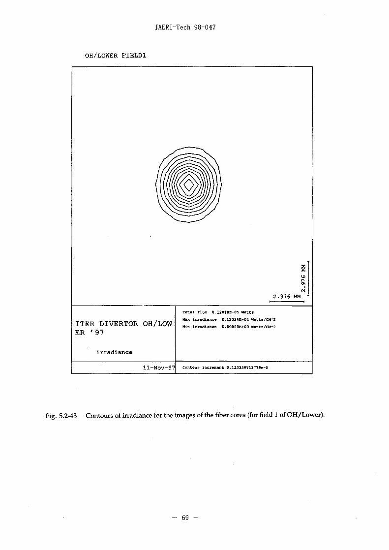
Total flux 0.12018Z-05 Watts
Max irradiance 0.12336E-04 Watts/CM*2
Bin irradiance O.0OO0OE+O0 Katts/CM'2
ll-Nov-9"7 Contour increment 0.1233597im9e-5
Fig. 5.2-43 Contours of irradiance for the images of the fiber cores (for field 1 of OH/Lower).
69 -

JAERI-Tech 98-047
OH/LOWER FIELD2
N
2.976 MM
ITER DIVERTOR OH/LOWER ' 9 7
irradiance
Total flux O.12O4BE-05 Watts
Max irradiance 0.12063E-04 Watta/CM"2
Min irradiance O.OOOOOE+00 Watt»/CMA2
ll-Nov-97 Contour increment 0.120633922052e~5
Fig. 5.2-44 Contours of irradiance for the images of the fiber cores (for field 2 of OH/Lower).
70 -
JAERI-Tech 98-047
OH/LOWER FIELD3
2 .976 MM
ITER DIVERTOR OH/LOWER ' 9 7
irradiance
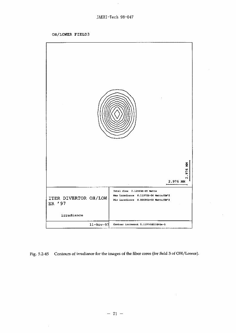
Total flux 0.12065E-05 watts
Max irradiance 0.11975E-04 W»tt»/CMA2
Min i r r a d i a n c a O.OOOOOE+00 Hatts/CHA2
l l -Nov-97 Contour increment 0.119745811844«-5
Fig. 5.2-45 Contours of irradiance for the images of the fiber cores (for field 3 of OH/Lower).
- 71 -

JAERI-Tech 98-047
OH/LOWER FIELD4
ID
OS
CM
2 .976 MM
ITER DIVERTOR OH/LOWER ' 97
irradiance
Total flux 0.12058E-OS Watts
Max irradiance 0.12241E-04 Wotts/CM*2
Min irradiance O.OO00OE+O0 Watts/CM"2
ll-NOV-97 Contour increment 0.12240S01S19e-5
Fig. 5.2-46 Contours of irradiance for the images of the fiber cores (for field 4 of OH/Lower).
- 72
JAERI-Tech 98-047
OH/LOWER FIELDS
2.976 MM
ITER DIVERTOR OH/LOWER ' 9 7
irradiance
ll-Nov-97
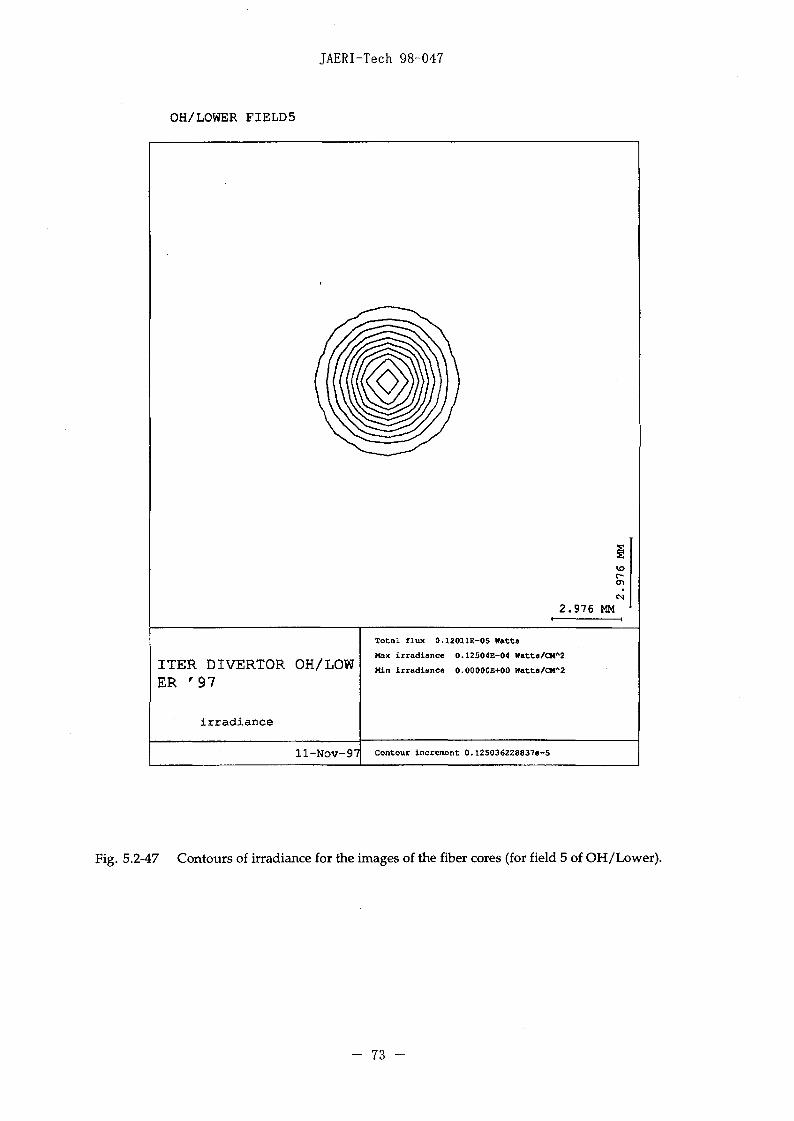
Total flux 0.12011E-05 W»tta
Max ixradiance O.12504E-O4 Watt»/CM*2
Hln irradiance O.OOOOOS+00 Hatt«/CHA2
Contour Increment 0.125036228837e-5
Fig. 5.2-47 Contours of irradiance for the images of the fiber cores (for field 5 of OH/Lower).
- 73 -

JAERI-Tech 98-047
OH/UPPER
Fig. 5.2-48 Traced rays of OH/Upper viewing fan.
- 74
JAERI-Tech 98-047
FIELDPOSITION
1.00, -1 .008.524,1.590 DG
1.00, -0 .508.524,0 .795 DG
1.00, 0.008.524,0.000 DG
1.00, 0.508 .524 , -0 .80 DG
1.00, 1.008 .524 , -1 .59 DG
DEFOCUSING 0.00000
ITER DIVERTOR OH/UPPER ' 9 7
Fig. 5.2-49 Spot diagrams on the divertor plate of IH/Upper viewing fan.
75 -
JAERI-Tech 98-047
FIELDPOSITION
1.00, -1 .003.524,1.590 DG
1.00 , -0 .505.524,0.795 DG
1.00, 0-008.524,0.000 DG
1.00, 0.508 .524 , -0 .80 DG
1.00, 1.008 .524 , -1 .59 DG
DEFOCUSING 0.00000
ITER DIVERTOR OH/UPPER ' 97
Fig. 5.2-50 Spot diagrams on the divertor plate of IH/Upper viewing fan (50 mm scale).
- 76 -

JAERI-Tech 98-047
FIELDPOSITION
1.00 , -1 .008.524,1 .590 DG
1.00, -0 .508.524,0 .795 DG
1.00, 0.008.524,0.000 DG
1.00, 0.508 .524 , -0 .80 DG
1.00, 1.003.524,-1 .59 DG
DEFOCUSING 0.00000
ITER DIVERTOR OH/UPPER ' 97
Fig. 5.2-51 Spot diagrams on the vertical plane to the optical axis of IH/Upper viewing fan.
- 77 -

JAERI-Tech 98-047
OH/UPPER FIELD1
2 .9 7 6 MM
ITER DIVERTOR OH/UPPER ' 9 7
irradiance
Total flux 0.12017E-05 Watts
Max Irradiance 0.50660E-05 Watts/CMA2
Min Irradiance O.OOOOOE+00 Hatta/CM"2
ll-Nov-97 Contour incrament 0.5066Q1338657e-6
Fig. 5.2-52 Contours of irradiance for the images of the fiber cores (for field 1 of OH/Upper).
- 78 -

JAERI-Tech 98-047
OH/UPPER FIELD2
2 .976 MM
ITER DIVERTOR OH/UPPER ' 9 7
irradiance
Total flux 0.120S3E-OS Hatts
Max irradiance 0.43201E-0S Watta/CM"2
Min irradiance O.O0000E+O0 Watta/CMA2
ll-Nov-97 Contour increment 0.432O13O2446Se-6
Fig. 5.2-53 Contours of irradiance for the images of the fiber cores (for field 2 of OH/Upper).
- 79 -

JAERI-Tech 98-047
OH/UPPER FIELD3
VDI -
2 . 9 7 6 MM
ITER DIVERTOR OH/UPPER ' 9 7
irradiance
Total flux O.12071E-05 Watts
Max irradiance 0.27669E-0S Watt»/CH"2
Hin irradiance O.0O0O0E+O0 Watt*/CM"-2
ll-Nov-97 Contour increment 0.276687472933e-6
Fig. 5.2-54 Contours of irradiance for the images of the fiber cores (for field 3 of OH/Upper).
- 80

JAERI-Tech 98-047
OH/UPPER FIELD4
2 .976 MM
ITER DIVERTOR OH/UPPER ' 9 7
irradiance
Total flux 0.12060E-05 Watts
Max irradiance 0.13463E-05
Min irradiance 0.00000E+00 Watts/CM'Z
Contour increment 0.134628280088-6
Fig. 5.2-55 Contours of irradiance for the images of the fiber cores (for field 4 of OH/Upper).
- 81 -

JAERI-Tech 98-047
OH/UPPER FIELD5
8.929 KM
ITER DIVERTOR OH/UPPER ' 9 7
irradiance
Total flux 0.12017E-05 Watts
Max irradiance 0.21318E-06 Hatts/CH*2
Mir) irradiance 0.OO000E+O0 Watt a/CMA 2
ll-Nov-97 Contour increment 0.21317«747366e-7
Fig. 5.2-56 Contours of irradiance for the images of the fiber cores (for field 5 of OH/Upper).
- 82
JAERI-Tech 98-047
OH/UPPER FIELD1
2.976 MM
ITER DIVERTOR OH/UPPER ' 9 7
irradiance
Total flux 0.11951E-05 Watts
Max irradiance 0.62092B-O5 Katts/CM-2
Min irradiance 0.O000OE+OO Matts/CM-2
12-Jan-98 Contour increment 0.620918797267e-6
Fig. 5.2-57 Contours of irradiance on the vertical plane to the optical axis for the images ofthe fiber cores (for field 1 of OH/Upper).
- 83 -

JAERI-Tech 98-047
OH/UPPER FIELD2
2.976 MM
ITER DIVERTOR OH/UPPER ' 97
irradiance
Total flux 0.11996E-05 Watts
Max irradiance 0.61645E-05 Watts/CM"2
Min irradianca 0.O0000E+OO Watta/CM*2
12-Jan-98 Contour increment 0.616448630803e-6
Fig. 5.2-58 Contours of irradiance on the vertical plane to the optical axis for the images ofthe fiber cores (for field 2 of OH/Upper).
- 84 -
JAERI-Tech 98-047
OH/UPPER FIELD3
2 . 9 7 6 MM
ITER DIVERTOR OH/UPPER ' 9 7
irradiance
Total flux 0.12010E-05 Watts
Max irradiance 0.52945E-05 Watts/CMA2
Min irradiance O.OOOOOE+OD Watts/CMA2
12-Jan-98 Contour increment 0.529452393039O-6
Fig. 5.2-59 Contours of irradiance on the vertical plane to the optical axis for the images ofthe fiber cores (for field 3 of OH/Upper).
- 85

JAERI-Tech 98-047
OH/UPPER FIELD4
1 0I—CT1
2 .976 MM
ITER DIVERTOR OH/UPPER ' 97
irradiance
Total flux 0.12002E-05 Watts
Max irradiance 0.36144E-05 Watts/CM"2
Min irradiance 0.OOOOOE+00 Watts/CM'2
12-Jan-98 Contour increment 0.3€1439418d39e-6
Fig. 5.2-60 Contours of irradiance on the vertical plane to the optical axis for the images ofthe fiber cores (for field 4 of OH/Upper).
- 86 -
JAERI-Tech 98-047
OH/UPPER FIELD5
2 . 9 7 6 MM
ITER DIVERTOR OH/UPPER ' 9 7
irradiance
Total flux 0.11965E-05 KattaMax irradiance 0.26407E-O5 Hatts/CM*2Min irradiance 0.00000E+00 Katts/CMA2
12-Jan-98 Contour increment 0.264D69655032e-6
Fig. 5.2-61 Contours of irradiance on the vertical plane to the optical axis for the images ofthe fiber cores (for field 5 of OH/Upper).
- 87 -

JAERI-Tech 98-047
Fig. 5.2-62 Traced rays of X-point viewing system (side view).

JAERI-Tech 98-047
Fig. 5.2-63 Traced rays of X-point viewing system (plan view).
- 89

JAERI-Tech 98-047
Fig. 5.2-64 Traced rays of X-point viewing system (at field lens).
- 90 -
JAERI-Tech 98-047
FIELDPOSITION
0.00, 0.000.000,0.000 DG
0.00, 0.250.000,-0.34 DG
0.00, 0.500 . 0 0 0 , - 0 . 6 8 DG
0.00, 0.750 .000 , -1 .02 DG
0.00, 1.000 . 0 0 0 , - 1 . 3 5 DG
DEFOCUSING 0-00000
ITER X point view ' 97
Fig. 5.2-65 Spot diagrams on the fiber of X-point viewing system; Only this case, ray startsfrom the different five positions (on axis, 75 mm, 150 mm, 225 mm and 300 mm awayfrom the axis) of divertor region and focused on the fiber.
- 91

JAERI-Tech 98-047
5.3 Spectrometer
Spectrometers have been designed in accordance with the required functionsas shown in Table 3-1.
5.3.1 Spectrometer for species monitor (Visible Survey Spectrometer)
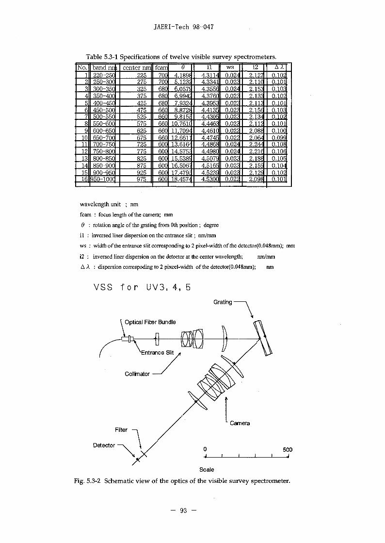
The spectral lines in the wavelength range of 200 - 1000 nm are observedsimultaneously by sixteen grating spectrometers as shown in Table 5.3-1. Eachspatial line of sight has sixteen fibers and each fiber guides the light to thespectrometer as shown in Fig. 5.3-1. The light from over twelve spatial lines ofsight are observed by each spectrometer simultaneously. Here, it is assumed thatspectral lines are detected by an ICCD detector with 1024 x 512 pixels (imagingarea: 2.5 cm x 1.25 cm). If we use a larger detector, the number of spectrometerswill be decreased.
The schematic view of the optics of the visible survey spectrometer isshown in Fig.5.3-2. The optical fiber array which has twelve fibers is mounted onthe entrance slit. The light is collimated by lenses and dispersed by grating andfocused by camera lens on a detector through a filter.
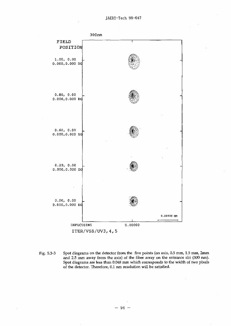
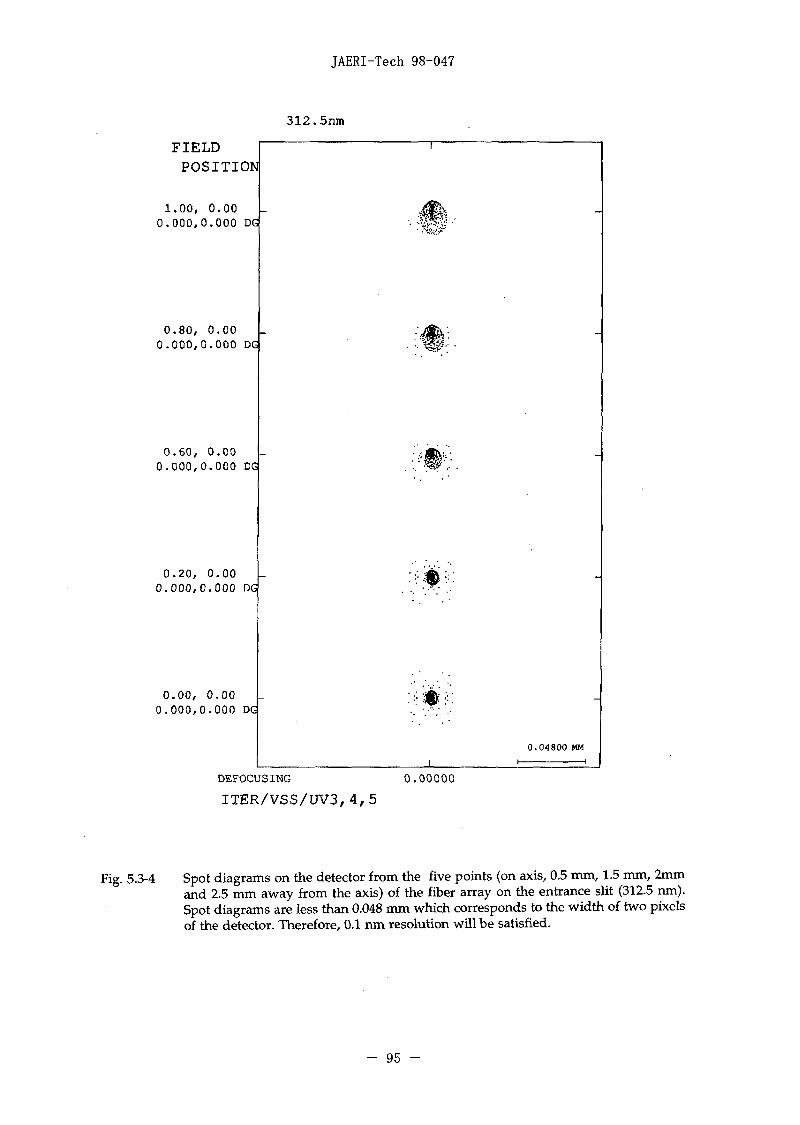
The ray trace analysis has been carried out. Rays are emitted from the fivepoints (on axis, 0.5 mm, 1.5 mm, 2 mm and 2.5 mm away from the axis) of thefiber array on the entrance slit. The spot diagrams on the detector for those pointsare shown in Fig. 5.3-3,4, 5, 6 and 7. These spot diagrams shows the resolution isless than 0.048 mm which corresponds to the width of two pixels of the detector.Therefore, 0.1 nm resolution will be satisfied.
X-pointviewingsystem
Optical fiber bundle
2-D viewingewe+prn
Movable trolley in the pit
| No. 1 | | No. 4 |
| No. 2 | | No. 5 |
No. 3 |
Diagnostics room
| No. 6 | | No. 12 |
| No. 7 | | No. 13 |
| No. 8 | | No. 14 |
| No. 9 | | No. 15 |
| No. 10 | | No. 16 |
| No. 11 |
Fig. 5.3-1 Arrangement of visible survey spectrometers. There are sixteen spectrometers (No. 1~ No. 16). Five spectrometers for UV region are located on the movable trolley inthe pit and other spectrometers are set in the diagnostics room.
- 92 -
JAERI-Tech 98-047
Table 5.3-1
No.123456789
10111213141516
band nr220-25C250-30C300-35C350-400400-450450-50C500-55C550-600600-65C650-70C700-75C750-800800-850850-900900-95C
950-100C
i
Specifications of
center nm225275325375425475525575625675725775825875925975
fcatn700700680680680660660660660660600600600600600600
twelve i
e4.189*5.123S6.057'6.994^7.932'8.872?9.815E
10.76K11.709'12.661113.61&14.575E15.538516.506717.479E18.457'
/isible survey spectrometers.i l
4.31144.33414.355€4.376C4.39524.41354.430E4.44624.461C4.47454.48684.498C4.507E4.51654.523S4.5300
ws0.02'0.02c0.02^0.02c0.02c0.02c0.02c0.02G0.02;0.02;0.02'0.02'0.02:0.02c0.02c0.02;
i22.1272. IK2.15c2.13c2.11c2.15(2.13'2.1122.08E2.06'2.24<2.2U2.18E2.15E2.12£2.098
AA0.1020.1010.10c0.1020.1010.1020.1020.1010.10C0.09<0.10Eo.ioe0.10J0.10'0.1020.101
wavelength unit ; nm
fcam : focus length of the camera; mm
9 : rotation angle of the grating from Oth position ; degree
11 : inversed liner dispersion on the entrance slit; nm/mm
ws : width of the entrance slit corresponding to 2 pixel- width of the detector(0.048mm); mm
12 : inversed liner dispersion on the detector at the center wavelength; nm/mm
A A : dispersion correspoding to 2 pixcel-width of the detector(0.048mm); nm
V S S T o r U V 3 , 4 , 5
Grating
Detector
Scale
Fig. 5.3-2 Schematic view of the optics of the visible survey spectrometer.
- 93 -
JAERI-Tech 98-047
300nm
FIELDPOSITION
1.00, 0.000.000,0 .000 DG
0.80, 0.000.000,0 .000 DG
0 . 6 0 , 0 . 000 . 0 0 0 , 0 . 0 0 0 DG
0.20, 0.000.000,0 .000 DG
0.00, 0.000.000,0 .000 DG
mm,
"••'/>•.?••"
$k
0.04800 MM
DEFOCUSING
ITER/VSS/UV3,4,5
0.00000
Fig. 5.3-3 Spot diagrams on the detector from the five points (on axis, 0.5 mm, 1.5 mm, 2mmand 2.5 mm away from the axis) of the fiber array on the entrance slit (300 nm).Spot diagrams are less than 0.048 mm which corresponds to the width of two pixelsof the detector. Therefore, 0.1 nm resolution will be satisfied.
- 94 -
JAERI-Tech 98-047
312.5nm
FIELDPOSITION
1 .00 , 0 . 0 00 . 0 0 0 , 0 . 0 0 0 DG
0.80, 0.000.000,0.000 DG
0.60, 0.000.000,0 .000 DG
0.20, 0.000.000,0.000 DG
0 . 0 0 , 0 . 0 00 . 0 0 0 , 0 . 0 0 0 DG
DEFOCUSING
ITER/VSS/UV3,4, 50.00000
Fig. 5.3-4 Spot diagrams on the detector from the five points (on axis, 0.5 mm, 1.5 mm, 2mmand 2.5 mm away from the axis) of the fiber array on the entrance slit (312.5 run).Spot diagrams are less than 0.048 mm which corresponds to the width of two pixelsof the detector. Therefore, 0.1 nm resolution will be satisfied.
- 95 -
JAERI-Tech 98-047
325nm
FIELDPOSITION
1.00, 0 .000 . 0 0 0 , 0 . 0 0 0 DG
0 . 8 0 , 0 .000 . 0 0 0 , 0 . 0 0 0 DG
0 . 6 0 , 0 .000 . 0 0 0 , 0 . 0 0 0 DG
0 . 2 0 , 0 .000 . 0 0 0 , 0 . 0 0 0 DG
0.00, 0.000.000,0.000 DG
DEFOCUSING
ITER/VSS/UV3,4,50.00000
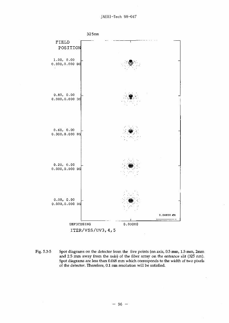
Fig. 5.3-5 Spot diagrams on the detector from the five points (on axis, 0.5 mm, 1.5 mm, 2mmand 2.5 mm away from the axis) of the fiber array on the entrance slit (325 nm).Spot diagrams are less than 0.048 mm which corresponds to the width of two pixelsof the detector. Therefore, 0.1 nm resolution will be satisfied.
- 96 -

JAERI-Tech 98-047
337.5nm
FIELDPOSITION!
1.00, 0 .000 . 0 0 0 , 0 . 0 0 0 DG
0 . 8 0 , 0 .000 . 0 0 0 , 0 . 0 0 0 DG
0 . 6 0 , 0 .000 . 0 0 0 , 0 . 0 0 0 DG
0 . 2 0 , 0 .000 . 0 0 0 , 0 . 0 0 0 DG
0 . 0 0 , 0 .000 . 0 0 0 , 0 . 0 0 0 DG
DEFOCUSING
ITER/VSS/UV3,4,50.00000
Fig. 5.3-6 Spot diagrams on the detector from the five points (on axis, 0.5 mm, 1.5 mm, 2mmand 2.5 mm away from the axis) of the fiber array on the entrance slit (337.5 nm).Spot diagrams are less than 0.048 mm which corresponds to the width of two pixelsof the detector. Therefore, 0.1 nm resolution will be satisfied.
- 97 -

JAERI-Tech 98-047
350nm
FIELD I"POSITION
1.00, o.oo0.000,0 .000 DG
0 . 8 0 , 0 . 0 00 . 0 0 0 , 0 . 0 0 0 DG
0 . 6 0 , 0 .000 . 0 0 0 , 0 . 0 0 0 DG
0 . 2 0 , 0 .000 . 0 0 0 , 0 . 0 0 0 DG
0 . 0 0 , 0 . 000 . 0 0 0 , 0 . 0 0 0 DG
0.O4800 MM
I 1
DEFOCUSING
ITER/VSS/UV3,4,5
0.00000
Fig. 5.3-7 Spot diagrams on the detector from the five points (on axis, 0.5 mm, 1.5 mm, 2mmand 2.5 mm away from the axis) of the fiber array on the entrance slit (350 nm).Spot diagrams are less than 0.048 mm which corresponds to the width of two pixelsof the detector. Therefore, 0.1 nm resolution will be satisfied.
- 98 -

JAERI-Tech 98-047
5.3.2 Filter optical system for influx measurement (Filter Spectrometer)
There are two sets of filter spectrometers. One is the set for the viewing fansOV, OH, IV and IH (2-D viewing system). Another is the set for the viewing fansXL and XU (X-point Viewing system). Each set has four spectrometers and eachspectrometer can observe three different spectral lines simultaneously. Thespectrometer for the wavelength region of 200 - 450 nm is set on the movabletrolley just behind the biological shield. The other spectrometers for thewavelength range 450 - 1000 nm are installed in the diagnostic room as shown inFig.5.3-8. The number of lines of sight and fibers are shown in Table 5.2-3. The setfor the viewing fans of OV, OH, IV and IH has 400 lines of sight and each line ofsight has four fibers in order to guide the light to each spectrometer.
Bio-Shield
forXL, XU
< Pit >200-450 nm
< Diagnostic Ftoom >>450 nm
forOV,OH,IV, IH
\ Fiber Bundle (100 Fibers)
• Fiber Bundle (400 Fibers)
Fig.5.3-8 Arrangement of filter spectrometers. Each spectrometer measures three spectrallines.
The optical design has been carried out for twelve selected lines here:
1) Ha+Da+Toc, 2) Hel: 667.8 nm,4) Hel: 728.1 nm, 5) Hell: 468.6 nm,7) Belli: 372.0, 372.1 and 372.3 nm,9)CII : 657.8 nm, 10) CV : 227.1 nm,12) Nel: 640.2 and 640.1 nm.
3) Hel: 706.5 and 706.6 nm,6) Bell: 313.0 and 313.1 nm,8) BelV : 465.9 nm,11) Cul: 521.8 and 522.0 nm,
These spectral lines are measured by four spectrometers as the combinationof Table 5.3-2.
- 99 -

227.091 run313.041 ran372.085 ran
465.854 ran521.9136 ran657.810 ran
468.5682 ran656.1032 ran706.5449 ran
640.1661 ran667.8157 ran728.1349 ran
CVBellBelli
BelVCulCII
HellHa, Da, TaHel
NelHelHel
JAERI-Tech 98-047
Table 5.3-2 Spectrometer and the filter combination.
Spectrometer Filter No. Central wavelength of filter Target line
UV 123
VIS1 456
VIS2 789
VIS3 101112
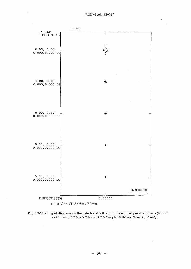
As an example, the schematic view of the filter spectrometer for 200 - 450nm is shown in Fig. 5.3-9. The light emitted from the optical fiber bundle, whichis composed of 400 fibers, passes through a collimator. After that, the light of arequired wavelength region is reflected by a dichroic mirror. It passes through aband-pass filter (full width of half maximum: ~1 nm) corresponding to theselected spectral line and is focused on a 2-dimensional detector by a camera. Thelight penetrating the dichroic mirror goes to the next dichroic mirror. Theoutline of the filter spectrometer is summarized in Table 5.3-3. The spotdiagrams on the detector at 229 nm, 300 nm and 450 nm and the contours ofirradiance for the image of the fiber cores are shown in Fig. 5.3-10(a), ll(a), 12(b)and Fig. 5.3-10(b), ll(b), 12(b). Here, it is assumed that the cores emit the lightuniformly. The diameters of the contours, which irradiances are 1/10 ofmaximum one, are about 230 |0.m. This shows that the resolved measurementfor each images of 400 fiber cores is possible by a two-dimensional detector if thefiber cores are set at intervals of >230 (im.
The arrangement of the dichroic mirrors and band-pass filters is shown inFig.5.3-13. The reflection rate of the dichroic mirrors and the transmissivities ofthe band-pass filter are designed as shown in Fig. 5.3-14 ~ 18.
Table 5.3-3 Outline of filter spectrometer.
Focal length of collimator 170 mmDiameter of collimated light 70 mmFocal length of camera 170 mmNA 0.2 (same as fiber's NA)
- 100 -

FS for uvIAMERA
:AM£RA
ANDPASS FILTER
> •
ixo3"
00
O
•-OPTICAL FIBER BUNDLE
I I I I500
I
Fig.5.3-9 Schematic view of the filter spectrometer for 200 - 450 nm.

JAERI-Tech 98-047
229nm
FIELDPOSITION
0 . 0 0 , 1.000 . 0 0 0 , 0 . 0 0 0 DG
0 . 0 0 , 0 . 8 30 . 0 0 0 , 0 . 0 0 0 DG
0 . 0 0 , 0 . 6 70 . 0 0 0 , 0 . 0 0 0 DG
0 . 0 0 , 0 .500 . 0 0 0 , 0 . 0 0 0 DG
0 . 0 0 , 0 . 0 00 . 0 0 0 , 0 . 0 0 0 DG
DEFOCUSING 0.00000
ITER/FS/UV/f=170mm
Fig. 5.3-10(a) Spot diagrams on the detector at 229 nm for the emitted point of on axis (bottomone), 1.5 mm, 2 mm, 2.5 mm and 3 mm away from the optical axis (top one).
- 102 -

JAERI-Tech 98-047
229nm y»0mm 229nm y-2mm
i
oITER/FS/UV/f=170mm
irradiance
£
3O
0.07626 Hff
IUr. : n « l i i . i » 0.H6O1E-3O W«tti/CH*2
H;n ir:.»di*.-i=« 0.3D000E*D0 W.ces/CM-J
22?nm y»2.5mmy - j
• ITER/FS/UV/f=170mm
Fig. 5.3-10(b) Contours of irradiance for the image of the fiber cores at 229 nm for the cores of onaxis (0 mm), 2 mm, 2.5 mm and 3 mm away from the optical axis.
- 103 -
JAERI-Tech 98-047
300nmFIELD
POSITION
0 . 0 0 , 1.000 . 0 0 0 , 0 . 0 0 0 DG
0 . 0 0 , 0 . 8 30 . 0 0 0 , 0 . 0 0 0 DG
0 . 0 0 , 0 .670 . 0 0 0 , 0 . 0 0 0 DG
0 . 0 0 , 0 . 5 00 . 0 0 0 , 0 . 0 0 0 DG
0 . 0 0 , 0 . 0 00 . 0 0 0 , 0 . 0 0 0 DG
DEFOCUSING 0.00000
ITER/FS/UV/f=170mm
Fig. 5.3-ll(a) Spot diagrams on the detector at 300 nm for the emitted point of on axis (bottomone), 1.5 mm, 2 mm, 2.5 mm and 3 mm away from the optical axis (top one).
- 104 -

JAERI-Tech 98-047
300nm y-Omm 300nm y=2mm
ITER/FS/UV/f=170mm
irradiance
*. Jun
m, ^ u u . ).!•....«.» .«>./«-!
300nm y=2.5mm300nm y«3mm
0.07626 M&"
ITER/FS/UV/f=l70mm
irradiance
H-n ; r n d H n : « O.00C3OE'OO K»cta/CM-2
632
Fig. 5.3-ll(b) Contours of irradiance for the image of the fiber cores at 300 nm for the cores of onaxis (0 mm), 2 mm, 2.5 mm and 3 mm away from the optical axis.
- 105

JAERI-Tech 98-047
FIELDPOSITION
0 . 0 0 , 1.000 . 0 0 0 , 0 . 0 0 0 DG
0 . 0 0 , 0 .830 . 0 0 0 , 0 . 0 0 0 DG
0.00, 0.670.000,0 .000 DG
0 . 0 0 , 0 .500 . 0 0 0 , 0 . 0 0 0 DG
0 . 0 0 , 0 .000 . 0 0 0 , 0 . 0 0 0 DG
DEFOCUSING 0.00000
I T E R / F S / U V / f = 1 7 0 m m
Fig. 5.3-12(a) Spot diagrams on the detector at 450 run for the emitted point of on axis (bottomone), 1.5 mm, 2 mm, 2.5 nun and 3 mm away from the optical axis (top one).
- 106 -

JAERI-Tech 98-047
450nm v-0mm 450nm y»2mm
ITER/FS/UV/f=170mm
0.07626 MS"
•J50nm y™2.5mm
ITER/FS/UV/f=170mm
3
0.07626 Mff
i;i»J:.»r.c. O.JOOOOEtC ITER/FS/UV/f-170mm O.OOQ0OE*OU tUtt*/CM~I
2-Jun-9S cw
Fig. 5.3-12(b) Contours of irradiance for the image of the fiber cores at 450 nm for the cores of onaxis (0 mm), 2 mm, 2.5 mm and 3 mm away from the optical axis.
- 107 -

uv
JAERI-Tech 98-047
BPF2
VIS1
BPF4
DCM4 DCM5
BPF9
VIS2BPF8
20
20 •H -• 8
VIS3
BPF7
10 or 11
DCM6 DCM7
BPFIO or 11
BPF11 or 10
11 or 10
DCM8 DCM9
BPF12
Fig, 5.3-13 Arrangement of the dichroic mirros and band-pass filters of filter spectrometers.
- 108 -

JAERI-Tech 98-047
100.0
90.0 "
50.0
5 . 0
1
111
T 100.0
D e m S 5 . o
200. 221. 3 1 3 . 312.
HAVE LENGTH (NM)
— 50.0
5.0
0.0
1
IIIi1 !
ilfllI 1 \1 1 1
\
\
\ _— ——-'
0CM2
200. 227. 313. 312.
WAVE LENGTH (NH)
DCI
313, 372.
HAVE LENGTH (NM)
95.0
90.0 \
\
V • •
DCM4
161. S22.
HAVE LENGTH (NM)
651. 700.
100.0
95.0
90,0
10.0
s.o0.0
r
ir 'r
\
100.095.090.0
10.0
S.O
0.0
f
(11
1
f
11 / X\/ V — ~
467. S22.
HAVE LENGTH (NH)
6S7. 700. 6 5 7 . 7 0 1 .
HAVE LENGTH (NH)
Fig. 5.3-14 Desugned reflection rate of the dichroic mirros for numer 1, 2,3,4,5 and 6.
109

JAERI-Tech 98-047
A ^ r\ r\/ \ / \ / \ / \ r\
\j V v \/ \/ \
1
... D
656. 706.
HAVE LENGTH (NM)
10.0
5.0
0.0
\ / \ _
v/ ^^^—\ ^—-.
/— DCM8
G40. 6SS.
HAVE LENGTH (NM)
100.095.090^0
50.0
10.05.0
/
1jJ
^ — •1O0.O
95.0
90.0
_ 50.0
s
—-v.
\
\\
/ \/ "*>
DCM9'
E00. 640 . 667. 1ZB.
HAVE LENGTH (NM)
600. 640 . 667. 728.
HAVE LENGTH (NW1
Fig. 5.3-15 Desugned reflection rate of the dichroic mirros for numer 7, 8,9 and 9*.
- 110 -

JAERI-Tech 98-047
Ch. 1 BPF1
100.095.090.0
5.00.0
/
/
/
\
\
\
226.09 226.59 227.09 227.59 228.09
Ch. 2 BPF2100.095.090.0
HAVE LENGTH (NM)312.07 312.57 313.07 313.57 314.07
HAVE LENGTH (NM)
Ch.3 8PF3Ch. 4 BPF4
371.17 371.67 372.17 372.67 373.17WAVE LENGTH (NM)
100.095.090.0
/
'
/—-—
/
/
— — \
\
\
\
~ ~ —
464.85 465.35 465.85 466.35 466.85WAVE LENGTH (NM)
Ch.4 BPF4 Ch. 6 BPF6100.095.090.0 / • —
/
/
-
1 N
\
\
464.85 465.35 465.85 466.35 466.85WAVE LENGTH (NM)
100.095.090.0
... — . — '
r! \
'^~~—— 1
656.81 657.31 657.81 658.31 658.81WAVt LbNGTil (NM)
Fig. 5.3-16 Desugned transmissivities of the band-pass filters for numer 1,2,3,4,5 and 6.
- I l l -

JAERI-Tech 98-047
Ch. 1Ch. 1
100.095.090.0
£ 50.0
10.05.00.0 k ^, / ~ \ . / - —-—•
100.095.090.0
- — — " • • -—-V--—-^ - ^ — - — . — • —•
HAVE LENGTH (NM)
300. 4 00. 500. 600. 700. 800. 900. 1000.
WAVE LENGTH (NM)
Cfl.2 Ch.2100.095.090.0
10.05.00.0
A —-——— —
100.095.090.0
10.05.0
WAVE LENGTH (NM) WAVE LENGTH (NM)
Ch.3100.C95.03C.0
JO.O5.C0.C
Ch.3100.095.090.0
10.05.00.0
WAVE LENGTH WAVE LENGTH (NM)
Fig. 5.3-17 Desugned total transmissivities of the channel number of 1, 2 and 3.
112 -

JAERI-Tech 98-047
95.0 •90.0
50. C
10.05.0
Ch
1
J 1
4
200. 300. 400. 500. 600. 700. 800. 900. 1000.
WAVE LENGTH (KK)
Ch.5100.095.090.0
I . »200. 300. 400. 500. 600. 100. 800. 900. -1000.
HAVE LENGTH (NM)
Ch.6
95.090.0
50.0
10.05.00.0
1
L200. 300. 100. 500- 600. 700- 800. 900. 1000.
HAVE LENGTH (NM)
Fig. 5.3-18 Desugned total transmissivities of the channel number of 4, 5 and 6.
- 113 -

JAERI-Tech 98-047
5.3.3 High dispersion spectrometer for line shape measurement
The high dispersion spectrometer is a Littrow type spectrometer with anechelle grating as shown in Fig. 5.3-19. The light emitted from the optical fiberbundle, which is composed of 12 fibers, passes through a relay optics where ordersorting filter is inserted on the optical pass. After that, the image of the fiberbundle is focused on a entrance slit of the Littrow type spectrometer. Thespecification of the high dispersion spectrometer is summarized in Table 5.3-4.Two set of this spectrometer are set in the diagnostic room. One is used in theshorter wavelength range and another is used in the longer wavelength region.
Table 5.3-4 Specification of high dispersion spectrometer.
Wavelength rangeResolving powerOptical fiber bundleMagnification of relay opticsLength of entrance slitFocal length of Littrow lensEffective diameter of Littrow lensBlazing angle of echelle grating
Number of grooves of echelle grating
DetectorAngle between axis of Littrow lens
and incident axis
450nm-1000nmX/Ak ~ 50000 (A*. ~ 0.01 ran)12 fibers (0.25 mm x 12 = 3 mm length)3.7>12mm990 mm-110 mm70.45 degree (for shorter wavelength range)71.8 degree (for longer wavelength range)52.676 I/mm (for shorter wavelength range)31.6 I/mm (for longer wavelength range)1024 x 512 pixels (0.024 pitch)
1.8 degrees
The dispersion of the spectrometer for shorter wavelength range iscalculated as Table 5.3-5.
Table 5.3-5 Dispersion of the high dispersion spectrometer for shorter wavelength range.
Dispersion at the entrance slitSlit width correspond to 0.01 runWidth of image of entrance slit (0.131 mm)
on detector
0.0763 nm/mm (at 500 ran; order of 72nd)0.131 mm
0.108 mm (4.52 pixels)
The result of ray trace analysis for relay optics is shown in Fig.5.3-20. In thiscase, rays are emitted from three positions (on axis, 4.55 mm away from axis and6,6 mm away from axis) of the entrance slit. The spot diagrams for compositionof 450 nm, 500 nm, 650 nm, 750 nm and 1000 nm on the fiber bundle are shownin this figure. The result shows the relay optics has a good performance.
The spot diagrams of the spectrometer for 72nd of 500.102 nm, 500.558 nm,501.008 nm, 501.451 nm, 501.888 nm and 502.319 nm on the detector are shown in
- 114 -

JAERI-Tech 98-047
Fig.5.3-21, 22, 23, 24, 25 and 26. Rays are emitted from five points (from thebottom in the figures; on axis, 1 mm away from axis, 2 mm away from axis, 3mm away from axis and 4 mm away from axis) of the entrance slit. The resultsshows the widths of spots are sufficiently less than that of pixel of the detector.
115 -

HDS
-PLANE MIRROR
DETECTOR
.?.*
-ENTRANCE SLIT
-RELAY OPTICS
JRDER SORTING FILTER
DPTICAL FIBER BUNDLE
LJTTROW LENS
ENTRANCE PUP\l
CHELLE GRATING
0 5001 - 4 - - I - I I 1
3CDO
ooIo
Fig. 5.3-19 Schematic view of high dispersion spectrometer (Littiow type spectrometer with an echelle grating ).

JAERI-Tech 98-047
FIELDPOSITION
0 . 0 0 , 1.000 . 0 0 0 , 0 . 6 5 1 DG
0 . 0 0 , 0 . 700 . 0 0 0 , 0 . 4 5 6 DG
0 . 0 0 , 0 . 000 . 0 0 0 , 0 . 0 0 0 DG II
0.05000 MM
DEFOCUSING 0.00000
ITER/RELAY OPTICS FOR HDS ' 97
Fig. 5.3-20 Ray trace analysis for relay optics. Rays are emitted from three positions (from thebottom; on axis, 4.55 mm away from axis and 6,6 mm away from axis) of the entranceslit. The spot diagrams for composition of 450 nm, 500 nm, 650 nm, 750 nm and 1000nm on the fiber bundle are shown here.
- 117 -
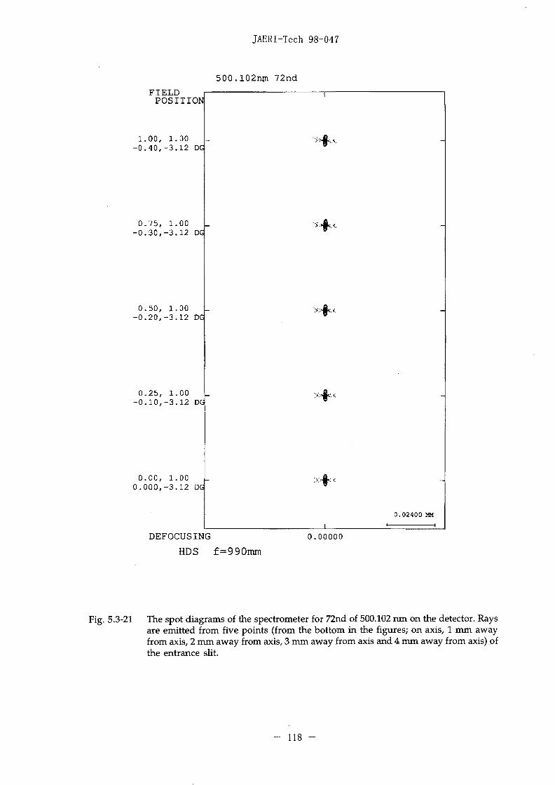
JAERI-Tech 98-047
500.102ntn 72ndFIELD
POSITION
1.00, 1.00-0 .40 , -3 .12 DG
0.75, 1.00-0 .30 , -3 .12 DG
0.50, 1.00-0 .20 , -3 .12 DG
0.25, 1.00- 0 . 1 0 , - 3 . 1 2 DG
0.00, 1.000 .000 , -3 .12 DG
DEFOCUSING
HDS f=990mm
0.00000
Fig. 5.3-21 The spot diagrams of the spectrometer for 72nd of 500.102 run on the detector. Raysare emitted from five points (from the bottom in the figures; on axis, 1 mm awayfrom axis, 2 mm away from axis, 3 mm away from axis and 4 mm away from axis) ofthe entrance slit.
- 118
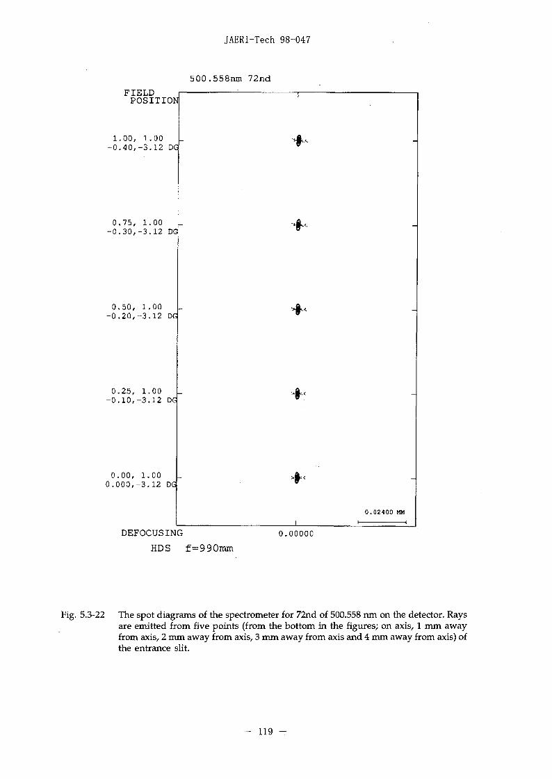
JAERI-Tech 98-047
500.558nm 72ndFIELD
POSITION
1.00, 1.00-0 .40 , -3 .12 DG
0.75 , 1.00-0 .30 , -3 .12 DG
0.50, 1.00-0 .20 , -3 .12 DG
0.25, 1.00- 0 . 1 0 , - 3 . 1 2 DG
0.00, 1.000 .000 , -3 .12 DG
DEFOCUSING
HDS f=990mm0.00000
Fig. 5.3-22 The spot diagrams of the spectrometer for 72nd of 500.558 nm on the detector. Raysare emitted from five points (from the bottom in the figures; on axis, 1 mm awayfrom axis, 2 mm away from axis, 3 mm away from axis and 4 mm away from axis) ofthe entrance slit.
- 119 -
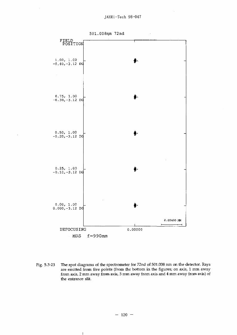
JAERI-Tech 98-047
501.008nm 72nd
FIELDPOSITION
1.00, 1.00-0 .40 , -3 .12 DG
0.75 , 1.00- 0 . 3 0 , - 3 . 1 2 DG
0.50, 1.00-0 .20 , -3 .12 DG
0.25, 1.00- 0 . 1 0 , - 3 . 1 2 DG
0.00, 1.000 .000 , -3 .12 DG
DEFOCUSING
HDS f=990mm0.00000
Fig. 5.3-23 The spot diagrams of the spectrometer for 72nd of 501.008 nm on the detector. Raysare emitted from five points (from the bottom in the figures; on axis, 1 mm awayfrom axis, 2 mm away from axis, 3 mm away from axis and 4 mm away from axis) ofthe entrance slit.
- 120 -

JAERI-Tech 98-047
501.451nm 72ndFIELD
POSITION
1.00, 1.00- 0 . 4 0 , - 3 . 1 2 DG
0.75 , 1.00- 0 . 3 0 , - 3 . 1 2 DG
0.50, 1.00- 0 . 2 0 , - 3 . 1 2 DG
0.25 , 1.00-0 .10 , -3 .12 DG
0.00, 1.000 .000 , -3 .12 DG
DEFOCUSING
HDS f=990mm0.00000
Fig. 5.3-24 The spot diagrams of the spectrometer for 72nd of 501.451 nm on the detector. Raysare emitted from five points (from the bottom in the figures; on axis, 1 mm awayfrom axis, 2 mm away from axis, 3 mm away from axis and 4 mm away from axis) ofthe entrance slit.
- 121 -

JAERI-Tech 98-047
501.888nm 72ndFIELD
POSITION
1.00, 1.00- 0 . 4 0 , - 3 . 1 2 DG
0.75 , 1.00- 0 . 3 0 , - 3 . 1 2 DG
0.50, 1.00- 0 . 2 0 , - 3 . 1 2 DG
0.25 , 1.00- 0 . 1 0 , - 3 . 1 2 DG
0.00, 1.000 .000 , -3 .12 DG
DEFOCUSING
HDS f=990mm0.00000
Fig. 5.3-25 The spot diagrams of the spectrometer for 72nd of 501.888 nm on the detector. Raysare emitted from five points (from the bottom in the figures; on axis, 1 mm awayfrom axis, 2 mm away from axis, 3 mm away from axis and 4 mm away from axis) ofthe entrance slit.
- 122 -

JAERI-Tech 98-047
502.319nm 72nd
FIELDPOSITION]
1.00, 1.00- 0 . 4 0 , - 3 . 1 2 DG
0.75 , 1.00- 0 . 3 0 , - 3 . 1 2 DG
0.50, 1.00- 0 . 2 0 , - 3 . 1 2 DG
0.25 , 1.00- 0 . 1 0 , - 3 . 1 2 DG
0.00, 1.000 .000 , -3 .12 DG
0.02400 MM
_L
DEFOCUSING
HDS f=990mm0.00000
Fig. 5.3-26 The spot diagrams of the spectrometer for 72nd of 502.319 nm on the detector. Raysare emitted from five points (from the bottom in the figures; on axis, 1 mm awayfrom axis, 2 mm away from axis, 3 mm away from axis and 4 mm away from axis) ofthe entrance slit.
- 123 -

JAERI-Tech 98-047
5.4 Estimation of number of photons coming into the detector
5.4.1 Collecting performance and transmissivity
The numbers of photons Nd (photons-s"1) incident on the detector is(see next appendix)
Nd = Idiv • Tpe- Tf • T s p • ftd • Sd
= Idiv • Tpe- Tf- T s p Qf-Sf, (5.4-1)
where Idiv is the intensity of the spectral line emitted in the divertor, Tpe is thetransmissivity of the optics from the divertor to the end of the fiber, Tf is thetransmissivity of the fiber to the spectrometer, Tsp is the transmissivity of thespectrometer, £2f is the effective solid angle on to the fiber and Sf is the area of thefiber core as shown in Fig. 5.4-1.
<Divertor>
•div
PenetrationOptics
NA=0.2
Optical fiber
TfDetector
Fig. 5.4-1 Transmission pass of the system.
Q.t, Sf and Tpe x Tsp for the filter spectrometers with the viewing fans ofOV, OH, IV and IH are 3.8 x 10"3 sr, 1.26 xlO"7m2 and 0.06 - 0.15 respectively. Onthe other hand, Qf and Tpe x Tsp for the filter spectrometers with the viewingfans of XL and XU are 5.1 x 10"2 sr and 0.12 - 0.24 while Sf remains 1.26 xlO"7 m2.
The summary of the trasmissivity of the penetration optics and of thespectrometers are tabulated in Table 5.4-1, 2,3, and 4.
- 124

JAERI-Tech 98-047
Table 5.4-1 Trasmissivity of penetration optics (from divertor to the end of fiber)Wavelength (nm)
Al
MoSiO2
200 300 400 500 600 700 800 900| 1000Reflectivity or Transmissivity of each material (for one surface)
0.930.650.96
0.930.6
0.96
0.920.550.96
0.920.590.97
0.920.570.97
0.9
0.570.97
0.870.550.97
0.890.6
0.97
0.940.810.97
IH/OH viewIV/OV view
Transmissivity of Penetration Optics (from divertor to fiber)0.410.27
0.370.22
0.350.19
0.370.22
0.350.2
0.330.19
0.280.15
0.330.2
0.560.45
XL/XU view 0.59 0.58| 0.58| 0.59 0.57 0.54 0.47 0.52 0.65
IH/OH: 1 surface of Mo. 4 surfaces of Al, 4 surfaces of SiO2IV/OV: 2 surfaces of Mo. 4 surfaces of Al, 4 surfaces of SiO2XL/XU: 4 surfaces of Al, 6 surfaces of SiO2
No.1
2
345
6789
1011
12
13141516
Table 5.4-2
Band (nm)200 - 250250 - 300300 - 350350-400400 - 450450 - 500500-550550 - 600600 - 650650-700700 - 750750 - 800800 - 850850 - 900900-950950 -1000
Trasmissivity of Visible survey spectrometer.TransmissiviCollimator
0.850.850.850.850.850.850.850.850.850.850.850.850.850.850.850.85
tyGrating
0.50.5
0.50.60.6
0.60.60.60.6
0.60.60.6
0.60.60.60.6
Camer0.850.850.850.850.850.850.850.850.850.850.850.850.850.850.850.85
SlitWidth (mm)
0.02370.02340.02370.02340.02310.02340.02310.02280.02250.02210.024
0.02370.02330.02290.02260.0222
Transmissivityof Slit
0.150.150.150.150.150.150.150.140.140.140.150.150.150.150.140.14
TotalTransmissivity
0.050.050.050.060.060.060.060.060.060.060.070.070.060.060.060.06
Slit width correspond to 0.1 nm of wavelength.
125 -

JAERI-Tech 98-047
Table 5.4-3 Trasmissivity of Filter spectrometer.
No.1
23
456
7
8
9
101112
Wavelength (nm)227.091313.041372.085
465.854521.9136
657.81
468.5682656.1032706.5449
640.1661667.8157728.1349
A0.90.850.8
0.90.850.8
0.9
0.850.8
0.7
0.60.9
B?
0.60.6
0.70.6
0.6
0.7
0.6
0.6
0.7
0.60.7
C0.8
0.850.9
0.980.980.98
0.980.980.98
0.980.980.98
D7
0.430.43
0.620.5
0.47
0.620.5
0.47
0.480.350.62
E
0.960.940.92
0.980.970.96
0.980.970.96
0.980.970.96
F0.60.6
0.6
0.880.880.88
0.880.880.88
0.880.880.88
G
0.80.80.8
0.880.880.88
0.880.880.88
0.880.880.88
TotalTransmissivity
?0.2
0.19
0.470.380.35
0.470.380.35
0.360.270.46
A: Design value of filter surface transmissivityB: Diffusive loss coefficient of filter surface (rough estimate)C: inner transmissivity in the filter-layers (rough estimate)D: A x B x CE: Transmissivity of the filter blank (do not include filter surfaces ).F: Transmissivity of collimatorG: Transmissivity of camera
Table 5.4-4 Trasmissivity of High dispersion spectrometer.
SpectrometerShorter RegionLonger Region
Relay Optics0.920.92
Order SortingFilter
0.70.7
Littorow(Double pass)
0.880.88
Grating0.50.5
Slit0.210.23
TotalTransmissivity
0.060.06
Setting angle of grating:for Shorter Region : 70.45 degreefor Longer Region: 71.8 degree
Slit width (for X/AX = 50000 )for Shorter Region : 0.122 mmfor Longer Region: 0.133 mm
- 126 -

JAERI-Tech 98-047
5.4.2 Intensity estimation of spectral lines in the divertor
The particle influx F is given by
T = 47tKI, (5.4-2)
where K is the number of ionization events per photon for the observed linewith the intensity of I.
The required range to be measured for the deuterium total influx is 1019 -1025 at-s"1 as shown in Table 1. Since the power deposition area on the divertortargets is about 10 m2, the measurable range of the deuterium influx density F tothe divertor is 1018 - 1024 at-m^.s"1. In a similar way, the influx density to bemeasured for carbon and beryllium are 1016-1021 atm^.s"1.
We estimated the intensities of Da, CII(3s-3p, 657.8 nm) and BeII(2s-2p,313.06 nm) lines for each required influx density region using equation (5.4-2)under the conditions of electron density of lxlO19 - lxlO22 m~3 and electrontemperature of 1 - 50 eV. These values are expected for ITER divertor plasmas.The values of K are calculated in references [1], [2], [3] for wide ranges of electrondensity and temperature.
The calculated results are shown in Fig.5.4-2.
5.4.3 Measurable limit
If we assume the lower limit of the number of photons is 1000 photonms"1
at the detector, the measurable intensity limit in the divertor derived fromequation (5.4-1) is about 1.4xlO16 - 3xlO16 photonm^-sr^s"1 for the optics ofviewing fans of OV, OH, IV and IH. From Fig. 5.4-2, it is expected that themeasurable limits for influxes will be different depending on the electron densityand temperature. For example, it is difficult to measure the carbon influx densityof lxlO16 mr2^"1 for Te=5eV. Also, it is difficult to distinguish between lineemission and bremsstrahlung emission by filter spectrometers. The calculatedline intensities of the bremsstrahlung emission (Zeff=1.5, Te= 5-50 eV) are alsoshown in Fig. 5.4-2. Here, we have assumed that the integrated length is 5 cm andthe wavelength band width is 1 nm which is the same as that of the band passfilter of the spectrometer. In the high density region, it is necessary to confirm thebremsstrahlung component by survey spectrometers. In addition, free-boundcontinuum originated recombination will be important in the low temperatureand high density region.
- 127 -
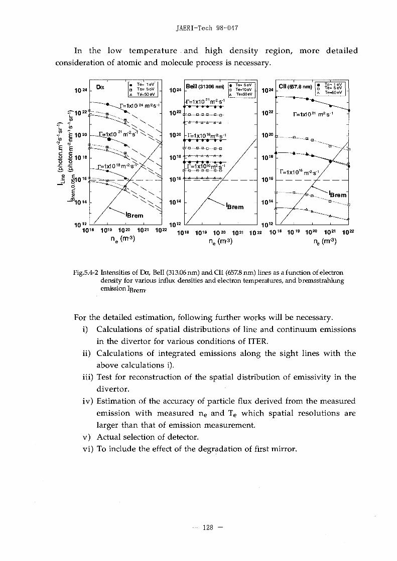
JAERI-Tech 98-047
In the low temperature and high density region, more detailedconsideration of atomic and molecule process is necessary.
102" - 1Q24
_ E P .
10 1 2
Bell (31306 nm)
r=1x10²¹nrv2-s-1
3 " © 0—EJ-E -E3--0-
^r=ix1018m-2s-1
r=1x10¹⁶m2s"1
ETS B-B-fl B-Q-
( Te= 5eVa Te=i0eVa Te=50eV
-
-
3 r e m ;
1018 1019 1 020 1021
102« -
- 102 2 -
- 102 0
1 ( ) 2 2
ne (m-3) (rrr3)
Fig.5.4-2 Intensities of EXx, Bell (313.06 nm) andCII (657.8 nm) lines as a function of electrondensity for various influx densities and electron temperatures, and bremsstrahlungemission Iurem-
For the detailed estimation, following further works will be necessary,i) Calculations of spatial distributions of line and continuum emissions
in the divertor for various conditions of ITER.ii) Calculations of integrated emissions along the sight lines with the
above calculations i).iii) Test for reconstruction of the spatial distribution of emissivity in the
divertor.iv) Estimation of the accuracy of particle flux derived from the measured
emission with measured ne and Te which spatial resolutions arelarger than that of emission measurement,
v) Actual selection of detector,vi) To include the effect of the degradation of first mirror.
- 128 -

JAERI-Tech 98-047
References
[1] L. C. Johnson and E. Hinnov, Ionization, recombination, and population of excited levels inhydrogen plasma, /. Quant. Spectrosc. Radial. Transfer, 13: 333 (1973).
[2] K. Behringer, H. P. Summers, B. Denne, et al., Spectroscopic determination of impurity influxfrom localized surfaces, Plasma Phys. Cont. Fusion, 14: 2059 (1989).
[3] H. P. Summers, W. J. Dickson, A. Boileau, et al., Spectral emission from beryllium in plasma,Plasma Phys. Contr. Fusion, 34: 325 (1992).
- 129 -

JAERI-Tech 98-047 S 55 TD 02 FJ (5.5.E.04)
5.5 Calibration system
Before the installation of the diagnostic divertor cassette and thepenetration optics, the sensitivity calibration will be carried out by arranging thereal components in the same arrangement as the real optics with standard lightsources set in the divertor. After the installation, the standard light will be setbehind the biological shield. The light will be applied to the molybdenum CCRsthrough the same optics as used for the measurements. The CCR will be installedin the pocket which is free from neutral particle bombardment and from dustdeposition. The spectral intensity of the reflected light from the CCR will bemonitored by a spectrometer in order to monitor the degradation of thepenetration optics. Schematic view of the calibration system (surrounded bydoted line) is shown in Fig. 5.5-1.
CCR
Collecting & FdcusinOptics,
PenetrationOptics
Half Mirto
Detector 1,2:Spectrometer with auto-changeable grating &detector vs wavelength
Detecton2
Mirror
Li'ght Sourse 2
_v
Detector 1
Optical FiberBundle
Liglpt Sourse 1
Spectrometers
Fig, 5.5-1 Schematic view of the calibration system (surrounded by doted line).
It will be a problem that only a few areas of the optics will be calibratedactually by this method. The degradation of other area will be assumed as same asthe calibrated area. This problem should be resolved and demonstrated bymockup equipment. The details of the calibration method are still underdevelopment.
For the signal to noise ratio during the calibration, the ratio will beimproved by increasing the integration time longer than that of plasmameasuring phase (for example 1 ms for filter spectrometer). It will be necessary to
- 130 -

JAERI-Tech 98-047
estimate the signal to noise ratio with actual light sources, optics and detectorsduring the calibration.
In addition, it will be necessary to consider other calibration methods. Forexample, it is better to install the light source at the divertor during thecalibration remotely.
- 131

JAERI-Tech 98-047
5.6 Alignment system
The alignment of the optical axis will be carried out by moving the collectingoptics it self for large movement and by moving the optical fiber bundle for smallmovement. The mirrors in the labyrinth will not be moved except installationphase.
The alignment will be carried out with a laser, a diffuser, a plane mirror anda corner cube reflector (CCR) mounted between the line of sight in the divertorcassette. The laser is shone through the optical axis of the system and the positionof light spots created by the diffuser, the plane mirror and the CCR are monitoredwith a CCD camera as shown in Fig. 5.6-1. The diffuser is used to adjust the shiftof the axis and the plane mirror is used to adjust the tilt of the axis. The CCR isused for reference.
Opticsin Divertor Cassette
CCR
Collecting & FocusingOptics
DiffuserPlane Mirror
CCD
on CCD
Mirror
S from Plane Mirror
from CCR
Fig. 5.6-1 Concept of alignment system.
The detailed arrangement of alignment system for axis-tilting is shown inFig.5.6-2. The light source and the detector is also shown in Fig. 5.6-3. Thearrangement of alignment system for the axis-shift is shown in Fig.5.6-4.
i) Illumination optics (see Fig.5.6-2)The laser light is focused on the plane mirror where is the focal point of the
collecting optics. The laser beam is radiated with the diameter of 193 mm fromthe collecting optics on to the mirrors located in the divertor cassette. The focallength of the collecting optics is 1380 mm.
ii) Alignment system for axis-tilting (see Fig.5.6-3)The reflected lights from the plane mirror and the CCR on the divertor
cassette are focused on the plane mirror in the collecting optics and detected bythe detector (CCD camera).
- 132 -

JAERI-Tech 98-047
The distance D between the spot from the CCR and that from the planemirror is written as
D = foo (5.6-1)where f is the focal length and (0 is the angle between the beam from the CCR andthat from the plane mirror. If the axis-tilting is 1' (1/60 degree; oo = 2.91 x 10~4 rad),D becomes 0.401 mm at the plane mirror in the collecting optics. The distancebecomes 0.167 nnm on the detector because the magnification from the planemirror to the detector is designed as 0.416. If the axis-tilting is 0.5 degree, thedistanse on the detector becomes 5.01 mm.
iii) Alignment system for the axis-shift (see Fig. 5.6-4)The light from the diffuser mounted on the divertor cassette focused on the
plane mirror at the optical fiber bundle and focused on the detector (CCD camera)by a relay optics. The magnification from the diffuser to the detector is 1/5. If theshift is 1 cm, the sift of the spot becomes 2 mm on the detector.
- 133 -

-CO-AXIS \OF THE TWO OFF-AXIS MIRRORS v
;LIGHT SORCE & T ILT DETECTOR L I G H T C O L L E C T O R
FOR THE GMVERTOR OPTICS
PTICAL FIBER \BUNDLE
EXIT PUPIL 0=38mm(MAX)
APERTURE STOP0=200
PLANE MIRRORat FOCAL POINT OF COLLECTING OPTICS
0=300(290)
tn
- 3(tloXXto00
o
Fig. 5.6-2 Detailed arrangement of alignment system for axis-tilting.

LASER DIODE HEADBEAM SPLITTER
—3CDocrtooooj
DETECTOR
Fig. 5.6-3 Light source and the detector for tilt alignment.

AUTO ALIGNMENT SYSTEMSHIFT DETECTOR
-PLANE
I
CO
I
)—HI
COO
001
o4
Fig. 5.6-4 Arrangement of alignment system for the axis-shift.

JAERI-Tech 98-047
6. Mechanical design
6.1 Optics
6.1.1 Over view and arrangement
The over views and arrangements of this system in the pit and in thediagnostic room are shown in Fig. 6.1-1, 2, 3 and in Fig. 6.1-4, 5 respectively. Thesystem has two viewing systems. One is a viewing system through the optics inthe divertor cassette and another is a viewing system through the gap betweenthe divertor cassette. Those are called '2-D viewing system' and 'X-point viewingsystem' respectively. Each viewing system has a dog-leg optics in the biologicalshield to prevent neutron and y-ray stream.
Spectrometers for the wavelength region from 200 nm to 450 nm and theirlocal controller are mounted on the movable trolley in the pit as shown in Fig.6.1-2 and 3. An optical terminal box and a electrical terminal box are set besidethe spectrometers in the pit. Through these terminal boxes, optical fibers andelectrical wires are connected with the spectrometers and the electricalcomponents set in the diagnostics room.
Spectrometers for the wavelength region from 450 nm to 1000 nm, theirlocal controller and a main control and data acquisition system are set in thediagnostic room as shown in Fig. 6.1-4 and 5.
6.1.2 Optics in the divertor cassette
The optics in the divertor cassette described in section 5.1. is realized bymirrors made of molybdenum. Mirrors in the bottom of the divertor cassette arearranged in a box as shown in Fig.6.1-6 and mounted on the divertor cassettefrom the bottom. Mirrors in the divertor dome are arranged on a plate as shownin Fig.6.1-7 and mounted in the dome from the top before setting the dome.
6.1.3 Dog-leg optics
The drawing of the dog-leg optics for 2-D viewing system is shown in Fig.6.1-8 and 9. The components of the dog-leg optics are mounted in the biologicalshield from the outside. After the adjustment of optical axes, the crevice is filledup with concrete blocks except optical pass.
- 137 -

JAERI-Tech 98-047
The drawing for X-point viewing system is shown in Fig.6.1-10.
6.1.4 Collecting and focusing optics
The collecting and focusing optics for 2-D viewing system and for X-pointviewing system are shown in Fig. 6.1-11 and 12 respectively.
6.1.5 Alignment system
The arraignment system for optical axes is shown in Fig. 6.1-13. A lightsource for arraignment is mounted on the box of collecting and focusing optics.The light is introduced into the optical axis by a movable plane mirror which isinserted in the optical axis. The light from the optics in the divertor is detected byCCD camera mounted near the light source for adjustment of tilt. The shift of theoptical axis is detected by a CCD camera mounted near the block of fiber arrays.
- 138 -

Mirrors in Divertor Cassette Dog-leg Optics
7044
CO i r ro rs in Dol
12326
11696
1.1150
Col l e c t i n g fi F o c u s i n g O p t i cfor X - p o i n t V i e w
iCD
o
to
o
1000 2000 3000 4000C o l l e c t i n g & F o c u s i n g O p t i c s
f o r 2 - D V i e w
Fig.6.1-1 Over view of the Divertor Impurity Monitoring System in the pit.

til Hi mi HI
oI
- aCDo
00
O
1000 2100 3000 (COB 5001
Fig.6.1 -2 Plan view of the Divertor Impurity Monitoring System in the pit.
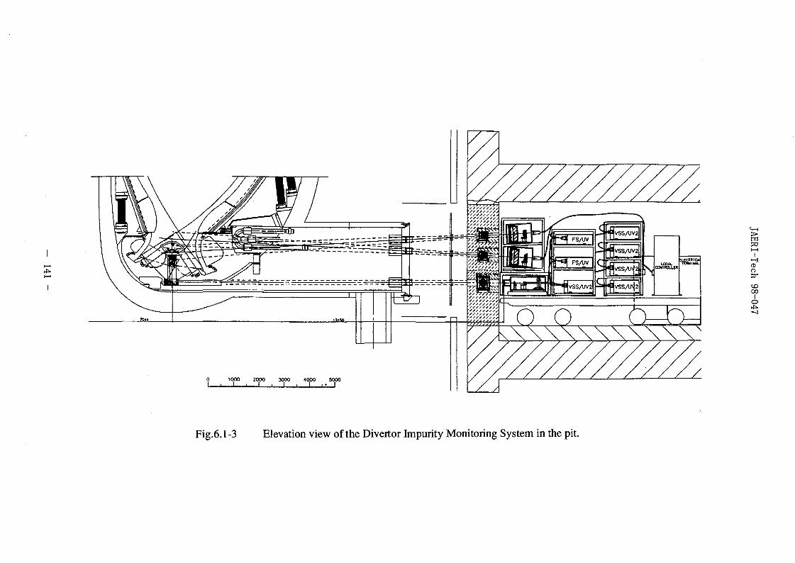
0 1000 2000 MOO 4000 50i
>CD
CDo
CO
o
Fig.6.1-3 Elevation view of the Divertor Impurity Monitoring System in the pit.

Cable Box
Fiber Box F i Her Cable
to
I
Data Acqu i s i t i on
msoi—i
-3CDO
rtoooo
Fig.6.1 -4 Plan view of the Divertor Impurity Monitoring System in the diagnostic room.

Cable Box
F i barFiber Box Data AcquIs i t i on
-3
to00
Io
Fig.6.1-5 Elevation view of the Divert or Impurity Monitoring System in the diagnostic room.

>m50
3CDO
o
Fig.6.1 -6 Mirror arrangement at the bottom of the divertor cassette.

JAERI-Tech 98-047
"il• ' I
344
V / / /// //////
//////A / / / /
o00
Fig.6.1-7 Mirror arrangement in the dome of the divertor cassette.
- 145 -

JAERI-Tech 98-047
\\\\\wwwwwwwww
W \ V
I/3
6fl
2
2
60
09' ' OSS OOL
i
1
0 0
oss ooc
146 -

JAERI-Tech 98-047
1CO
Ml
%
si
o
•8
061S2g
-£-
£ -
147 -
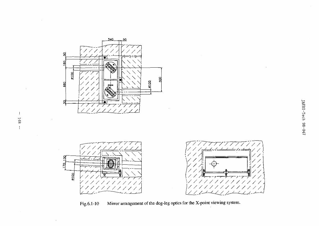
340
00
I
CDPC
I
CDO
nrtooo
V//////////A/ / / / • / / / / / / /
Fig.6.1-10 Mirror arrangement of the dog-leg optics for the X-point viewing system.

JAERI-Tech 98-047
OPTICAL FIBER BUNDLE
LIGHT SORCE & T I L T DETECTOR
PLANE MIRROR
APERTURE STOP
ooto
oin10
-i-SB
rim
280 1400
Fig.6.1-11 Collecting and focusing optics for the 2-D viewing system.
- 149 -
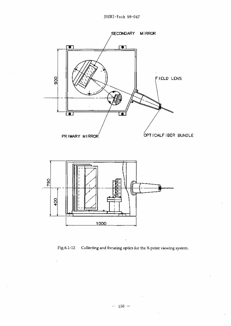
JAERI-Tech 98-047
SECONDARY MIRROR
m
FIELD LENS
PRIMARY MIRROR OPT I CALF IBER BUNDLE
Fig.6.1-12 Collecting and focusing optics for the X-point viewing system.
150 -

LIGHT SORCE & TILT DETECTOR OPTICAL FIBER BUNDLE
so
CD
otoooo
Fig.6.1-13 Alignment system in the Collecting and focusing optics for the 2-D viewing system.

JAERI-Tech 98-047
6.2 Spectrometer
6.2.1 Visible survey spectrometer
A general view of the visible survey spectrometer for UV region is shownin Fig.6.2-1.
6.2.2 Filter spectrometer
A general views of the filter spectrometer for UV and for visible region are
shown in Fig.6.2-2 and 3 respectively.
6.2.3 High dispersion spectrometer
A general view of the high dispersion spectrometer for UV region is shownin Fig.6.2-4.
- 152 -

JAERI-Tech 98-047
SHUTTER
OPTICAL FIBER BUNDLE / COLL IMATOR GRATING
ENTRANCE SL IT
DETECTOR
CAMERA
VSS f o r UV
Fig.6.2-1 Visible survey spectrometer for UV region.
- 153 -

JAERI-Tech 98-047
BANDPASS FILTER
DETECTOR
CAMERABANDPASS FILTER
COLL IMATOR
DETECTOR
OPTICAL FIBER BUNDLEDICHROIC MIRROR
CAMERA
XZJ cffl
1500
FS for UV
Fig.6.2-2 Filter spectrometer for UV region.
- 154 -
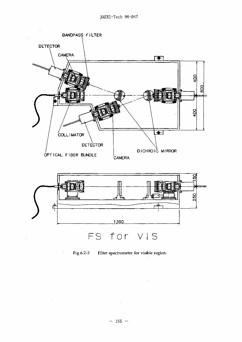
JAERI-Tech 98-047
BANDPASS FILTER
DETECTOR
CAMERA
COLLIMATOR
DETECTOR
OPTICAL FIBER BUNDLEDICHROIC MIRROR
CAMERA
F S f o r v i sFig.6.2-3 Filter spectrometer for visible region.
- 155 -

JAERI-Tech 98-047
ENTRANCE PUPIL
PLANE MIRROR ECHELLE GRATING
ORDER SORTING FILTER ENTRANCE SLITRELAY OPTICS
OPTICAL FIBER BUNDLE
HDS
Fig.6.2-4 High dispersion spectrometer.
- 156

JAERI-Tech 98-047
6.3 Analysis of the electromagnetic force during the disruption
Rapid decay of the plasma current during the disruption affects a large stresson the optical component. Here, we estimate an electromagnetic force on themirror base which is located in the divertor cassette. In this estimation,followings are assumed;
(1) Toroidal magnetic field during the disruption is 5.8 T at the mirror.(2) Plasma current of 21 MA creates a poloidal magnetic field of 0.84 T at the
mirror base which is located 5 m away from the plasma center.(3) The mirror base, which is made of stainless steel, is 50 mm wide, 413 mm
long and 30 mm thick as shown in Fig. 6.3-1.(4) The mirror base is inclined at 50 degrees against the poloidal field as shown
in Fig. 6.3-1.
The electromagnetic force wasestimated by using a simple modelcalculation. The results are shown inFig. 6.3-2, 3 and 4 in case of the currentdecay time of 10 ms, 5 ms and 1 ms.Maximum values of the force, theinduced current and the moment arealso summarized in Table 6.3-1.
As the result, the electromagneticforce on the mirror base is 67 N in caseof the current decay time of 10 ms. Evenif the decay time was 1 ms, it becomesonly 440 N. These results indicate thatthe electromagnetic force on the mirrorbase is not a serious problem.
30.
E30
Fig.6.3-1 The electromagnetic force on thebase of the mirror is calculated.The considered object is shown bythick solid lines.
Table 6.3-1 Summary of calculated force, induced current and torque.
Plasma Current Decay Time 10 ms 5 ms 1 ms
Maximum
Maximum
Maximum
Force
Induced
Torque
Current
67
430
21
N
A
Nm
124
800
38
N
A
Nm
440
2900
138
N
A
Nm
- 157
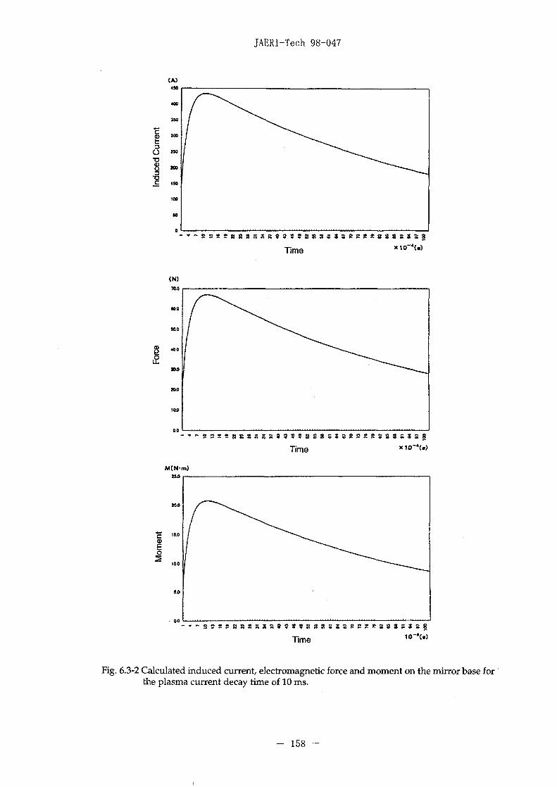
JAERI-Tech 98-047
Time " " " * < • >
Time *io-c>
Time
Fig. 6.3-2 Calculated induced current, electromagnetic force and moment on the mirror base forthe plasma current decay time of 10 ms.
- 158

JAERI-Tech 98-047
Time x 1 0 ' *c '>
Time x10"4<«)
Time
Fig. 6.3-3 Calculated induced current, electromagnetic force and moment on the mirror base forthe plasma current decay time of 5 ms.
- 159

JAERI-Tech 98-047
o
Time xio"4(«)
Time >do-4{.)
; i ; K « ; : t s : ; i ; s
Fig. 6.3-4 Calculated induced current, electromagnetic force and moment on the mirror base forthe plasma current decay time of 1 ms.
- 160 -

JAERI-Tech 98-047
6.4 Analysis of the nuclear heating for mirrors in the divertor cassette
The temperature rise of the mirror located in the divertor dome isestimated by a simple model calculation as a function of nuclear-heating value.The calculation was carried out under the following assumption.
(1) The mirror has a triangle shape as 525x352x391 mm as shown in Fig. 6.4-1.(2) Heat is transmitted only by conduction.(3) The temperature distribution of the triangle is approximated by that of a
fan-shape as shown in Fig. 6.4-1.
The temperature distribution T(r) is approximately written as
T(r) = T Tfa 2 -w 4A,
(6.4-1)
where Tw is a temperature of the bottom of the triangle, y is a nuclearheating value, A, is a thermal conductivity, rw is a length of the oblique side of thefan and r is a distance from the top of the triangle (see Fig. 6.4-1). From theequation (6.4-1), the temperature difference AT between the top and the bottomof the triangle is
AT = (6.4-2)
T=T,w
Fig. 6.4-1 Schematic view of the mirrors in the dome and a triangle which is used in thecalculation.
The calculated results are shown in Fig. 6.4-2 and 3, and summarized inTable 6.4-1. Fig. 6.4-2 is AT as a function of nuclear heating value and Fig. 6.4-3 isthe temperature distribution T(r) as a function of r. Since the nuclear heating
- 161 -

JAERI-Tech 98-047
value y at the mirror is expected to be 0.2 W/cm, the temperature difference ATbetween the top and the bottom of the mirror becomes 94 degrees formolybdenum and 861 degrees for stainless steal. It suggests that the molybdenummirror has no problem but the base of the mirror which is made of stainless stealhas a problem. Therefore, the base should be made of the material which has ahigher thermal conductivity such as aluminum/copper alloy.
Table 6.4-1 Calculated results of temperature difference AT between the top and thebottom of the mirror for different nuclear heating.
Nuclear heating(W/cnV3)
AT for molybdenum(degree)
AT for stainless steal(degree)
0.2.0.40.60.81.0
94188281375469
8611723
(2584)(3445)(4307)
15
4500
4000
3500
3000
2500
H 2000
1500
1000
500
00 02 0.4 0.6 OS 1
Nuclear heating A (W/cnf^)
Fig.6.4-2 Calculated results of ATas a functionof nuclear heating value.
—
^ —
/
- Molybdenum
- Stainless Steal
//
//
//
/
//
- — • — '
Fig. 6.4-3 Temperature distribution T(r)as a function of r.
- 162 -

JAERI-Tech 98-047
6.5 Remote handling for mirrors in the divertor cassette
The concept of remote handling for mirrors in the divertor cassette isillustrated in Fig. 6.5-1 and 2. The support tools are mounted on the mirror boxas shown in Fig.6.5-1. The mirror box is installed in the dome by remotehandling tool before installation of the dome as shown in Fig.6.5-2. The mirrorbox for the bottom of the divertor cassette is installed from the bottom. Theremote handling method is still under consideration.
If it is able to set mirrors in a mono-module, the installation and remotehandling from the bottom of the divertor cassette will become simple as shownin Fig. 6.5-3. Further work is needed about this method.
- 163 -
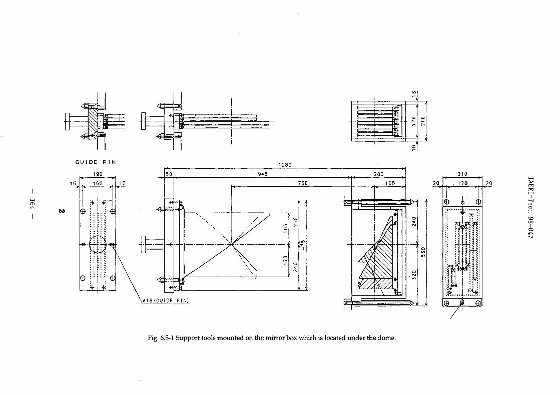
1280
20
210
, 170 20 CDSO
- 3
O
rtoCO
Io
Fig. 6.5-1 Support tools mounted on the mirror box which is located under the dome.

I
HOOK
HAND
POWER MANIPULATOR
IMPACT WRENCH
i
CDO
00
o
Fig. 6.5-2 Concept of remote handling method.

JAERI-Tech 98-047
1LD—CJJ
i
1
Fig. 6.5-3 Remote handling concept from the bottom. Mirrors are mounted in a mono-module.
- 166 -
JAERI-Tech 98-047
7. Neutron and y-ray irradiation effect
The neutron flux and y-ray dose rate at the port plug are calculated to be2x1013 m-2-s'l and 200 Gy/h [1] respectively. The windows located at the port plugare shielded by water cooled stainless steel tubes as shown in Fig.4.5-1. Theneutron flux and y-ray dose rate at the windows are expected to be 6x10^1 m~2-s~land 3 Gy/h. The degradation of trasmissivity (A>350 nm) of fused silica KU is lessthan 5 % (for 8 mm thickness) at the neutron fluence of 10^1 m~2 and the y-raydose of 107 Gy [2,3]. At 200 nm, the degradation is 17 % (for 8 mm thickness) at they-ray dose of 10^ Gy.
From these consideration, the windows will survive during ITER operation(50,000 shots x 1000 sec) for the wavelength region of A>350 nm.
For the wavelength region of 200 - 350 nm, the windows will surviveagainst the y-ray irradiation. For the neutron irradiation, more carefulconsideration is necessary.
References
[1] R. T. Santro, H. Iida, V. Khripunov, Neutron and gamma-ray flux and dose rate levels in thecryostat and gallery cells. Impact on electronic instrumentation, ITER Internal ReportNA:NAG-31-16-05-97 (1997).
[2]. D. V. Orlinski, Radiation hardening of diagnostic components, in: Diagnostics forExperimental Thermonuclear Fusion Reactors, P. E. Stoott, G. Gorini and E. Sindoni, ed.,Plenum Press, New York (1996).
[3]. S. Yamamoto, The present status and future plan of task T246, in Technical Meeting onIrradiation Tests on Diagnostic Components based on the T246 task agreement, Garching(1997).
- 167 -
JAERI-Tech 98-047
8. Control and data acquisition
Here, the control system of the Divertor Impurity Monitoring System and
the data acquisition system are described.
8.1 Concept of control and data acquisition
The basic concepts are as follows.1) The control system should be composed of wide used equipment.2) The data should be acquired with a fast sampling mode and a slow
sampling mode during each ITER shot to reduce the amount of data.3) The equipment control and the data acquisition should be realized by a
local control system and a data acquisition system. Only the selectedand/or processed data should be forwarded to COD AC.
4) The plasma parameter such as electron temperature and densitymeasured by the other diagnostics should be necessary. It should beable to get those data through COD AC.
5) Real time data acquisition and processing should be considered for
plasma control.
The block diagram of the control and the data acquisition system is
illustrated in Fig. 8.1-1.
- 168 -
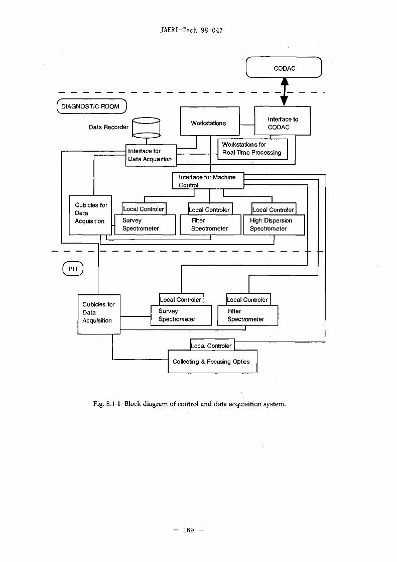
JAERI-Tech 98-047
CODAC
I DIAGNOSTIC ROOM
Data RecorderWorkstations
Interface forData Acquisition
Interface toCODAC
JLWorkstations forReal Time Processing
Interface for MachineControl
Cubicles forDataAcquisition
JLocal Controler
SurveySpectrometer
ocal Controler
FilterSpectrometer
J
1Local Controler
High DispersionSpectrometer
Cubicles forDataAcquisition
Local Controler
SurveySpectrometer
Local Controler
FilterSpectrometer
_T
Local Controler
Collecting & Focusing Optics
Fig. 8.1-1 Block diagram of control and data acquisition system.
- 169 -
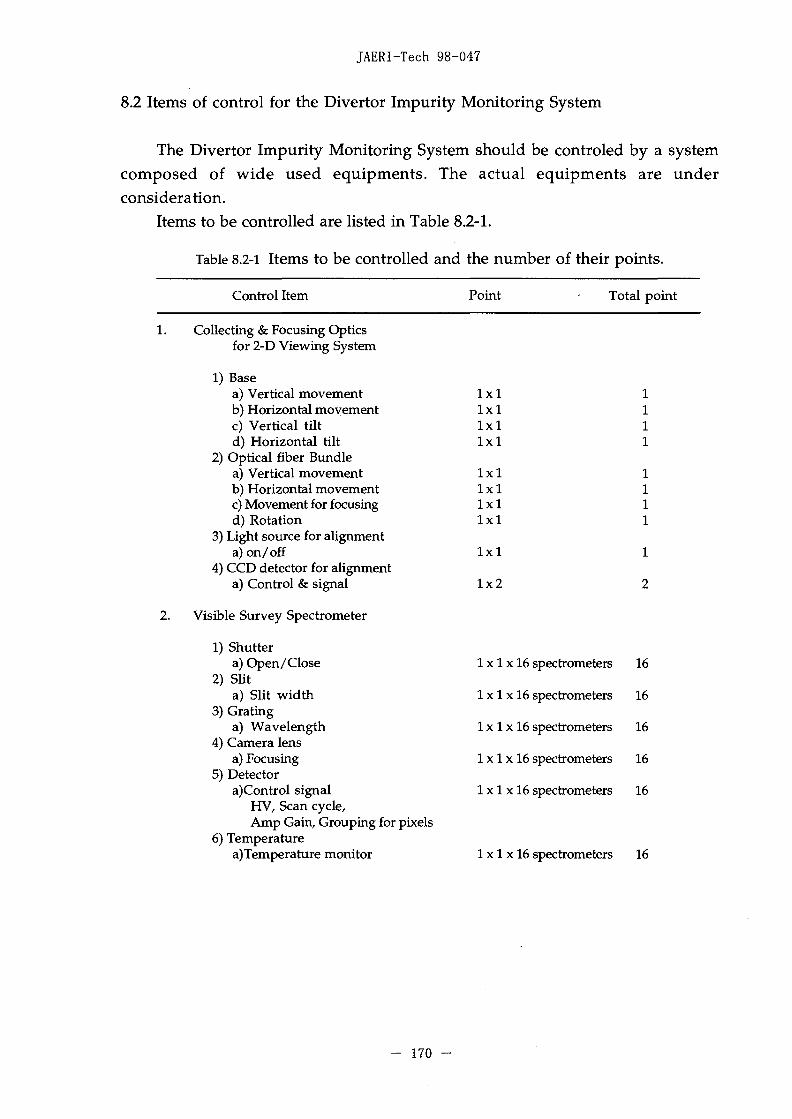
JAERI-Tech 98-047
8.2 Items of control for the Divertor Impurity Monitoring System
The Divertor Impurity Monitoring System should be controled by a systemcomposed of wide used equipments. The actual equipments are underconsideration.
Items to be controlled are listed in Table 8.2-1.
Table 8.2-1 Items to be controlled and the number of their points.
1.
2.
Control Item
Collecting & Focusing Opticsfor 2-D Viewing System
1) Basea) Vertical movementb) Horizontal movementc) Vertical tiltd) Horizontal tilt
2) Optical fiber Bundlea) Vertical movementb) Horizontal movementc) Movement for focusingd) Rotation
3) Light source for alignmenta) on/off
4) CCD detector for alignmenta) Control & signal
Visible Survey Spectrometer
1) Shuttera) Open/Close
2) Slita) Slit width
3) Gratinga) Wavelength
4) Camera lensa) Focusing
5) Detectora)Control signal
HV, Scan cycle,Amp Gain, Grouping for pixels
6) Temperaturea)Temperature monitor
Point Total point
l x ll x ll x ll x l
l x ll x ll x ll x l
l x l
1x2
1 x 1 x 16 spectrometers
1 x 1 x 16 spectrometers
1 x 1 x 16 spectrometers
1 x 1 x 16 spectrometers
1 x 1 x 16 spectrometers
1 x 1 x 16 spectrometers
1111
1111
1
2
16
16
16
16
16
16
- 170 -

JAERI-Tech 98-047
Table 8.2-1 Items to be controlled and the number of their points (continued-1).
5.
Control Item Point Total point
Filter Spectrometer
1) Shuttera) Open/Close
2) Camera lensa) Focusing
3) Detectora)Control signal
HV, Scan cycle,Amp Gain, Grouping for pixels
4) Temperaturea)Temperature monitor
High Dispersion Spectrometer
1) Shuttera) Open/Close
2) Slita) Slit width
3) Band-pass filtera) Replacing
4) Gratinga) Wavelength
5) Littrow lensa) Focusing
6) Detectora)Control signal
HV, Scan cycle,Amp Gain, Grouping for pixels
7) Temperaturea)Temperature monitor
Collecting & Focusing Opticsfor X-point Viewing System
1x1x8 spectrometers 8
1x3x8 spectrometers 24
1x3x8 spectrometers 24
1x1x8 spectrometers 8
1x1x2 spectrometers 2
1x1x2 spectrometers 2
1x1x2 spectrometers 2
1x1x2 spectrometers 2
1x1x2 spectrometers 2
1x1x2 spectrometers 2
1x1x2 spectrometers 2
1) Basea) Vertical movementb) Horizontal movementc) Vertical tiltd) Horizontal tilt
2) Optical fiber Bundlea) Vertical movementb) Horizontal movementc) Movement for focusingd) Rotation
3) Light source for alignmenta) on/off
4) CCD detector for alignmenta) Control & signal
1x1x2 views1x1x2 views1x1x2 views1x1x2 views
1x1x2 views1x1x2 views1x1x2 views1x1x2 views
1x1x2 views
1x2x2 views
2222
2222
2
4
- 171 -

JAERI-Tech 98-047
Table 8.2-1 Items to be controlled and the number of their points (continued-2).
Control Item Point Total point
6. Calibration system (2-D viewing)
3
4
2222
1) Mirror for light sourcea) in/out
2) Light sourcea) on/off, control
2) Detector (with monochromator)a) Wavelengthb)HVc) Amp Gaind) Rotation
3) Shuttera) on/off
1 x 3
1 x 2
1 x 21x21 x 21 x 2
1 x 2
- 172 -
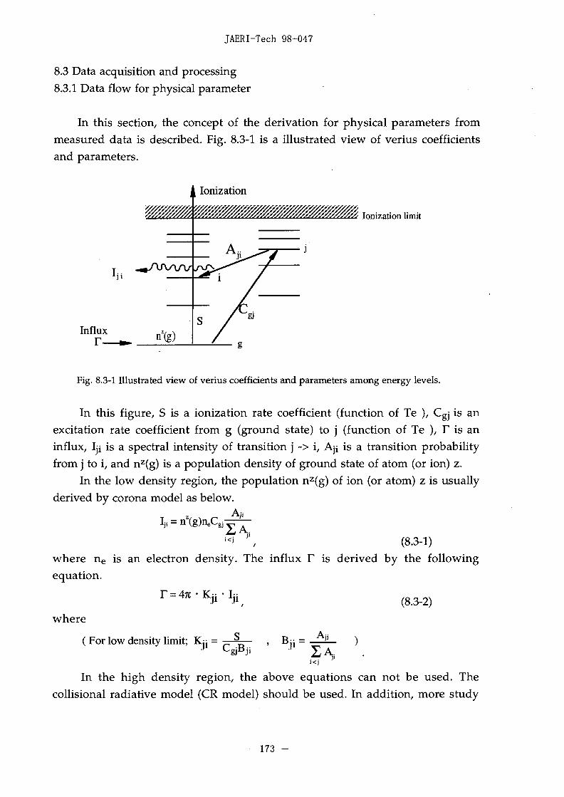
JAERI-Tech 98-047
8.3 Data acquisition and processing8.3.1 Data flow for physical parameter
In this section, the concept of the derivation for physical parameters frommeasured data is described. Fig. 8.3-1 is a illustrated view of verius coefficientsand parameters.
Ionization
Ionization limit
Fig. 8.3-1 Illustrated view of verius coefficients and parameters among energy levels.
In this figure, S is a ionization rate coefficient (function of Te ), Cgj is anexcitation rate coefficient from g (ground state) to j (function of Te ), T is aninflux, Iji is a spectral intensity of transition j -> i, Ajj is a transition probabilityfrom j to i, and nz(g) is a population density of ground state of atom (or ion) z.
In the low density region, the population nz(g) of ion (or atom) z is usuallyderived by corona model as below.
Iji = nz(g)neCgj-=r^-
j<i \ (8.3-1)where n e is an electron density. The influx T is derived by the followingequation.
(8.3-2)
where
(For low density limit; K:J = BJi =AH
In the high density region, the above equations can not be used. Thecollisional radiative model (CR model) should be used. In addition, more study
- 173 -
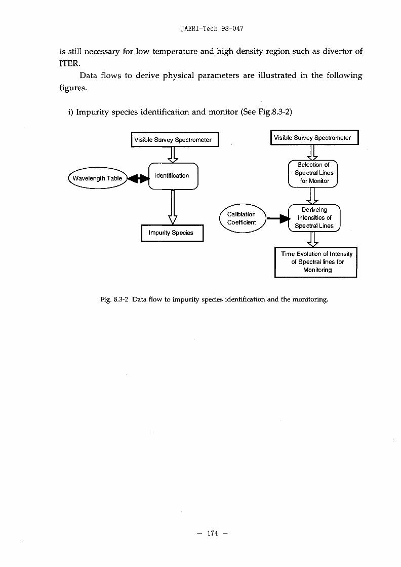
JAERI-Tech 98-047
is still necessary for low temperature and high density region such as divertor ofITER.
Data flows to derive physical parameters are illustrated in the followingfigures.
i) Impurity species identification and monitor (See Fig.8.3-2)
Visible Survey Spectrometer
(Wavelength Table^)^W Identification
VImpurity Species
Visible Survey Spectrometer
Selection ofSpectral Lines
for Monitor
XDeriveing
Intensities ofSpectral Lines
Time Evolution of Intensityof Spectral lines for
Monitoring
Fig. 8.3-2 Data flow to impurity species identification and the monitoring.
- 174 -
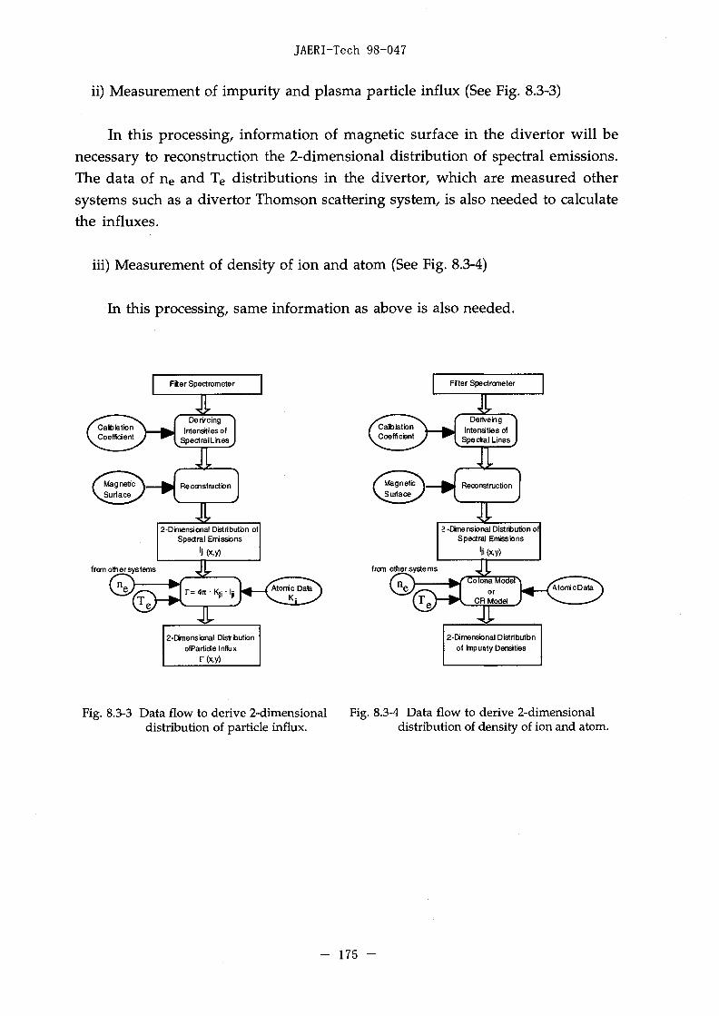
JAERI-Tech 98-047
ii) Measurement of impurity and plasma particle influx (See Fig. 8.3-3)
In this processing, information of magnetic surface in the divertor will benecessary to reconstruction the 2-dimensional distribution of spectral emissions.The data of ne and Te distributions in the divertor, which are measured othersystems such as a divertor Thomson scattering system, is also needed to calculatethe influxes.
iii) Measurement of density of ion and atom (See Fig. 8.3-4)
In this processing, same information as above is also needed.
DervemgIntensities of
SpectralLhes
2-Drnensional Distributor! ofSpectral Emissions
') <x,y)
from othersystems
2-Dimensbnal DistbutionofParticle Influx
r (x,y)
DerrvengIntensities of
Special Lines
2 -Dimensional Distribution ofSpectral Emissions
from othersystems
2-Dmensbnal Distributor!of tapurity Densities
Fig. 8.3-3 Data flow to derive 2-dimensional Fig. 8.3-4 Data flow to derive 2-dimensionaldistribution of particle influx. distribution of density of ion and atom.
- 175 -
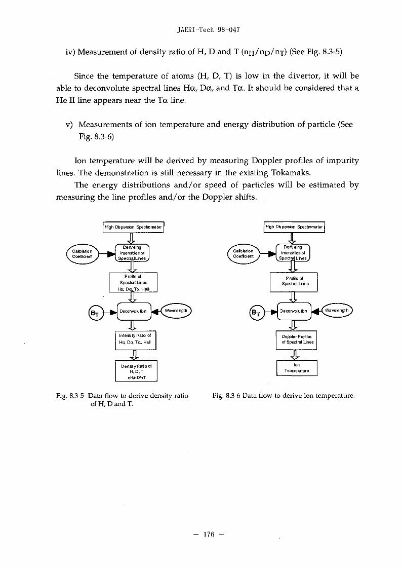
JAERI-Tech 98-047
iv) Measurement of density ratio of H, D and T nx) (See Fig. 8.3-5)
Since the temperature of atoms (H, D, T) is low in the divertor, it will beable to deconvolute spectral lines Ha, Da, and Ta. It should be considered that aHe II line appears near the Ta line.
v) Measurements of ion temperature and energy distribution of particle (SeeFig. 8.3-6)
Ion temperature will be derived by measuring Doppler profiles of impuritylines. The demonstration is still necessary in the existing Tokamaks.
The energy distributions and/or speed of particles will be estimated bymeasuring the line profiles and/or the Doppler shifts.
High Dispersion Spectrometer
A.Derveing
Intenatiesof..Spectral Lines
Prof leafSpectral Lines
Ha, Da, Tec, Hell
Fig. 8.3-5 Data flow to derive density ratioof H, D and T.
DeriveingIntensities of
Spectral Lines
Oeconvolutbn L ^ - l Wavelength
Fig. 8.3-6 Data flow to derive ion temperature.
- 176 -

JAERI-Tech 98-047
vi) Measurement of ionization front (See Fig. 8.3-7)
Ionization front of each outer and inner divertor will be determined bydetecting the channel which has a maximum intensity respectively.
Filter Spectrometer
XDerweing
Intensities of Da
A.(Detect the Channels which have
Maximum Intensity for each outeiand inner divertor legs
lonization Front
Fig. 8.3-7 Data flow to derive ionization front.
vii) Measurements of ne and Te
The electron density ne and temperature Te will be measured by line ratiomethod in the divertor.
For example, rie and Te were measured by following lines [1].ne: Hel (667.8151nm: 2p iP0 - 3d *D) / Hel (728.1349 nm: 2p lp° - 3s XS)Te: Hel (728.1349 nm: 2p !p° - 3s IS) / Hel (706.519, 706.5707 nm: 2p 3Po - 3s
3S)Concerning this method, it should be necessary more detailed study and
demonstration in the existing Tokamaks.
References
[1] B. Schweer, G. Mank, A. Pospieszczyk, Electron temperature and electron density profilesmeasured with a thermal He-beam in the plasma boundary of TEXTOR, /. Nucl. Mater, 196-198: 174 (1992).
177

JAERI-Tech 98-047
8.3.2 Data from detector
i) Visible survey spectrometerEach visible survey spectrometer has an intensified CCD detector which has
1024 x 512 pixels (~ 25 mm x 12.5 mm) in this design. The wavelength regionfrom 200 nm to 1000 nm will be measured by 16 visible spectrometers. If we usethe detector which has 2048 x 512 pixels, the number of spectrometers will bedecreased to 8.
The spectral lines from the different sight lines are imaged on the detectoras shown in Fig. 8.3-8. 12 sight lines (maximum number is 20 optically) will beobserved by each detector. The signals of the same line, which corresponds tosame wavelength, are added as shown in Fig. 8.3-9. These signals from the 12sight lines are sent to the data acquisition system of this system.
That is,1024 x 12 sight lines = 12,288 data /one scan for each spectrometer,
12,288 x 16 spectrometers = 196,608 data / one scan for this system.The amount of the data will be very large if we got the data every 10 ms
during ITER shot of 1000 s. Here we assume the data will be sent to the dataacquisition system and COD AC as follows.
To the data acquisition system;-10 ms sampling Total 100 s during the ITER shot-100 ms sampling Total 900 s during the ITER shot
196,608 x (100/0.01) + 196,608 x (900/0.1) = 3.7 x 10 9 data/shot= 3.7 G data/shot
To COD AC;- Time evolutions of selected 50 spectral lines.
50 x 12 sight lines x ((100/0.01) + (900/0.1)) = 1.14 x 10 7 (11.4 M) data/shot
- 178 -

JAERI-Tech 98-047
Fiber ends are set along the entrance slit
OOooooooooooo
spectral lines
IlllllllllilllllllllllllllllllllllllllllllllllllllllllllllfflllllllllIlllllllllJIIIIIIIIIIIIIIIIIflllllllllllllllllllllllllllllllllllllllllIlllllllllllllllllllllllllllllllllllllllllllllllllllllllllllllllllllllIlllllllllllllllllllllilllllllllllllllllllllllllllllllllllllllllllillliiiiiiiiiiiiiiiiiiiiiiiiiiiiiiiiiiiiiiiiiiiiiiiiiiiiiiiiiiiiiiiiiiiinIlllllllllllllllllllllllllllilllllllllllllllllllllllllllllllllllllllllIlllilllllllllllllllllllllllllllllllllllllllllllllllllllllllllllllllllIlllllllllllllllllllllllllllllllllilllllllllllllllllllllilllllllllllllIlllllllllllllllllllllllllllllllllllllllllllllllllllllllllllllllllllllIlllllllllllllllllllllllllllllllllilllllllllllllllflllllllllllllllllllIlllllllllllllllllllllllllllllllllllllllllllllllllllllllllllllllllllllIlllllllllllllllllllllllllllllllllllllllllllllllllllllllillllllllllllliiiiiiiiiiiiiiiiiiiiiiiiiiiiiiiiiiiiiiiiiiiiiiiiiiiiiiiiiiiiiiiiiiiin
1024 pixel(correspond to wavelength)
512 pixels
1Fig. 8.3-8 The spectral lines from the different sight lines are imaged on the detector. 12 sight
lines (maximum number is 20 optically) will be observed by each detector.
Add alongthis direction
Spectral lineson the detector
1 LJ n Added signal
Fig. 8.3-9 The signals of the same line, which corresponds to same wavelength, are added.These signals from the 12 sight lines are sent to the data acquisition system of thissystem.
- 179 -

JAERI-Tech 98-047
ii) Filter spectrometer
The filter spectrometer system is composed of two groups of filterspectrometers as shown in Fig. 8.3-10. Each group has 4 spectrometers and eachspectrometer observes 3 spectral lines. The group for viewing fans of XL and XUobserves 12 spectral lines from 100 sight lines simultaneously. The group forviewing fans of IV, IH, OV and OH observes 12 spectral lines from 400 sight linessimultaneously. An intensified CCD detector (or MOS detector) which has 512 x512 pixels will be used in this design.
A filtered spectral line from the different sight lines are imaged on thedetector as shown in Fig. 8.3-11. 400 or 100 sight lines will be observed by eachdetector. The signals from pixels corresponding to the same sight line are addedand the added data will be sent to the data acquisition system of this system.
That is,12 x (400 + 100) sight lines = 6,000 data /one scan,The amount of the data will be very large if we got the data every 1 ms
during ITER shot of 1000 s. Here we assume the data will be sent to the dataacquisition system and COD AC as follows.
To the data acquisition system and to CODAC;-1 ms sampling Total 100 s during the ITER shot-100 ms sampling Total 900 s during the ITER shot
6000 x (100/0.001) + 6000 x (900/0.1) = 6.54 x 10 8 data/shot= 654 M data/shot
In addition, the data from the filter spectrometer should be sent to CODACby real time processing system every 100 ms for plasma control.
- 180 -
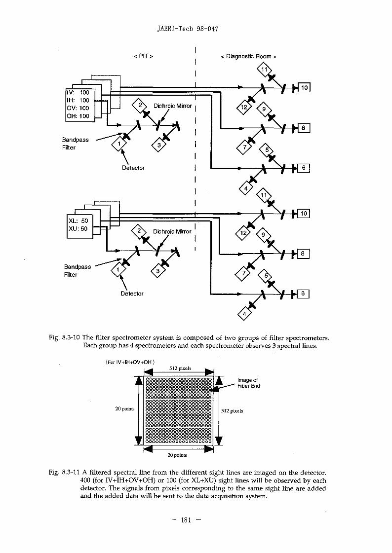
JAERI-Tech 98-047
<PIT> < Diagnostic Room >
JL
IV: 100IH: 100OV: 100OH: 100
BandpassFilter
X
XL: 50XU:50
BandpassFilter
2 \ Dichroic Mirror
\ \
Detector
Detector
Fig. 8.3-10 The filter spectrometer system is composed of two groups of filter spectrometers.Each group has 4 spectrometers and each spectrometer observes 3 spectral lines.
(For IV+IH+OV+OH)512 pixels
20 points
Image ofFiber End
512 pixels
20 points
Fig. 8.3-11 A filtered spectral line from the different sight lines are imaged on the detector.400 (for IV+IH+OV+OH) or 100 (for XL+XU) sight lines will be observed by eachdetector. The signals from pixels corresponding to the same sight line are addedand the added data will be sent to the data acquisition system.
- 181 -

JAERI-Tech 98-047
iii) High dispersion spectrometer
Each high dispersion spectrometer has an intensified CCD detector whichhas 1024 x 512 pixels (~ 25 mm x 12.5 mm) in this design. There are twospectrometers in this system.
The spectral lines from the different sight lines are imaged on the detectoras shown in Fig. 8.3-12. 12 sight lines (maximum number is 20 optically) will beobserved by each detector. The signals of the same line, which corresponds tosame wavelength, are added as shown in Fig. 8.3-13. These signals from the 12sight lines are sent to the data acquisition system of this system.
That is,1024 x 12 sight lines = 12,288 data /one scan for each spectrometer,12,288 x 2 spectrometers = 24,576 data / one scan for this system.The amount of the data will be very large if we got the data every 10 ms
during ITER shot of 1000 s. Here we assume the data will be sent to the dataacquisition system and COD AC as follows.
To the data acquisition system;-10 ms sampling Total 100 s during the ITER shot-100 ms sampling Total 900 s during the ITER shot
24,576 x (100/0.01) + 24,576 x (900/0.1) = 4.7 x 10 8 data/shot= 470 M data/shot
To CODAC;
- Time evolutions of Ti and the ratio of nn, np and nj.(to be considered)
- 182 -
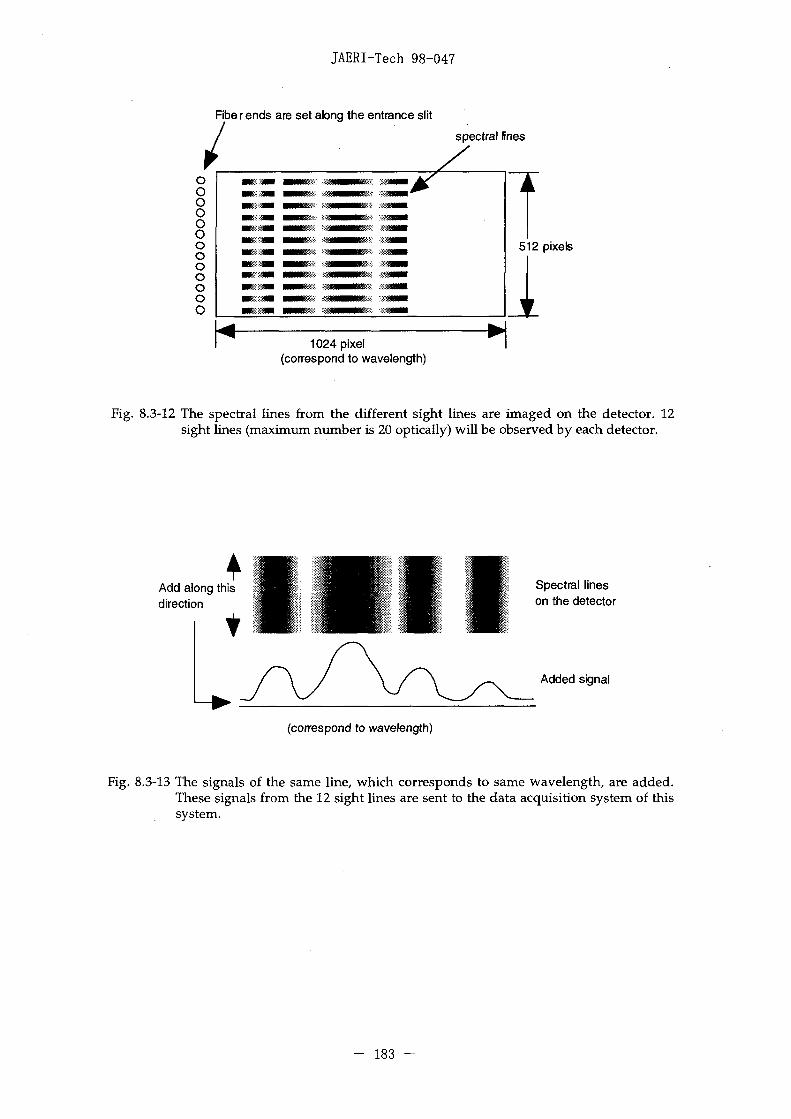
JAERI-Tech 98-047
Fiber ends are set along the entrance slit
spectra! lines
1024 pixel(correspond to wavelength)
512 pixels
Fig. 8.3-12 The spectral lines from the different sight lines are imaged on the detector. 12sight lines (maximum number is 20 optically) will be observed by each detector.
Add along thisdirection
Spectral lineson the detector
Added signal
(correspond to wavelength)
Fig. 8.3-13 The signals of the same line/ which corresponds to same wavelength, are added.These signals from the 12 sight lines are sent to the data acquisition system of thissystem.
- 183 -
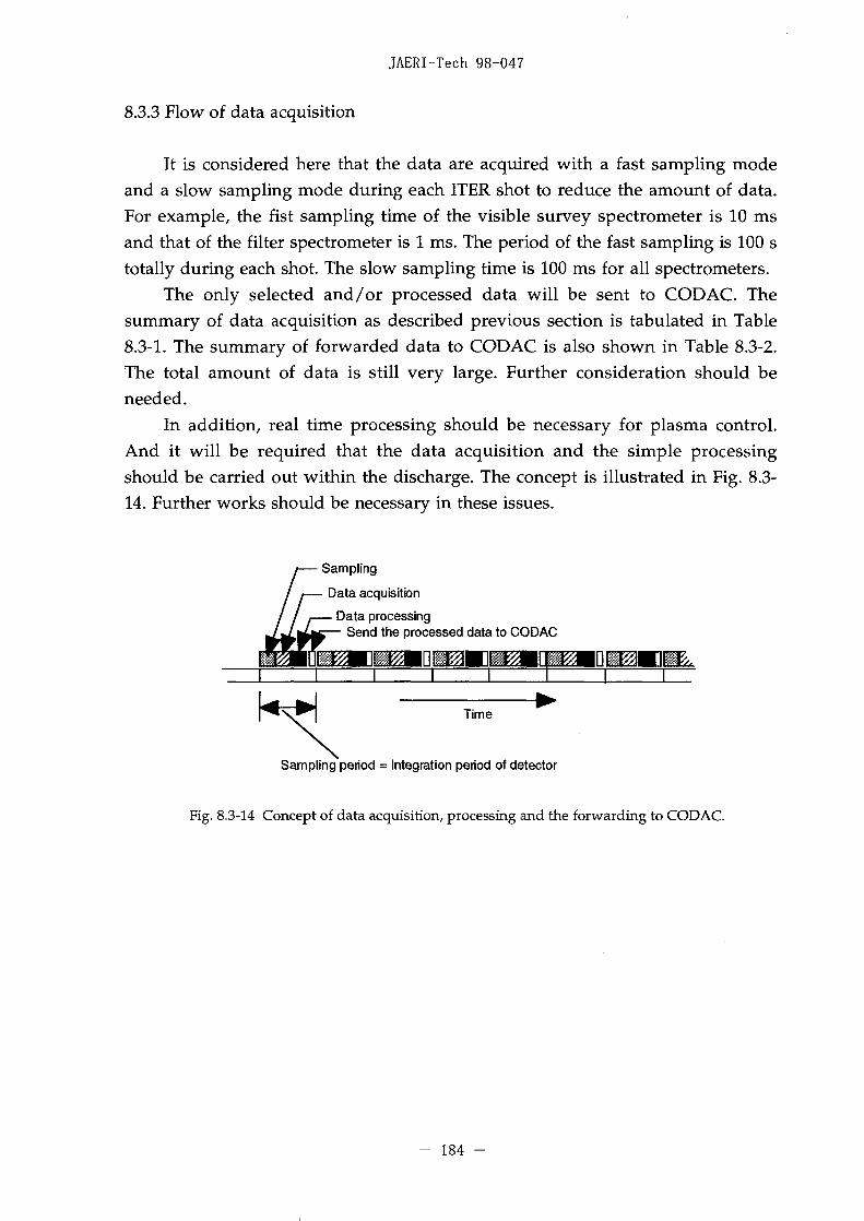
JAERI-Tech 98-047
8.3.3 Flow of data acquisition
It is considered here that the data are acquired with a fast sampling modeand a slow sampling mode during each ITER shot to reduce the amount of data.For example, the fist sampling time of the visible survey spectrometer is 10 msand that of the filter spectrometer is 1 ms. The period of the fast sampling is 100 stotally during each shot. The slow sampling time is 100 ms for all spectrometers.
The only selected and/or processed data will be sent to CODAC. Thesummary of data acquisition as described previous section is tabulated in Table8.3-1. The summary of forwarded data to CODAC is also shown in Table 8.3-2.The total amount of data is still very large. Further consideration should beneeded.
In addition, real time processing should be necessary for plasma control.And it will be required that the data acquisition and the simple processingshould be carried out within the discharge. The concept is illustrated in Fig. 8.3-14. Further works should be necessary in these issues.
Sampling
Data acquisition
Data processingSend the processed data to CODAC
Sampling period = Integration period of detector
Fig. 8.3-14 Concept of data acquisition, processing and the forwarding to CODAC.
- 184 -

Table 8.3-1 Summary of data acquisition for each spectrometers.
00en
Spectro-meter
VSS
HDS
FS
ViewingFan
IVOVXL
XU
Numberof sight
lines
442
2
Numberof
spectro-meters
16
Number ofwavelengthchannels/sight line
1024
Numberof
data/scan
65,5366533632,768
32,768
Sub Total
IV
OVXLXU
SubTotal
IVIHOVOHXL
XU
SubTotal
Total
12
4
42
2
12
100100100
1005050
500
16
2
2
1
1
1024
1024
1024
12
12
12
196,608
8,1928,1924,0964,096
24,576
1,2001,2001,200
UOO600
600
6,000
Fastsamplingtime (ms)
101010
10
10
10
101010
10
11111
1
1
Num. of data/1000s
(only withfast samp.)
6.55E+096.55E+093.28E+09
3.28E+09
1.97E+10
8.19E+088.19E+08
4.10E+084.10E+08
2.46E+09
1.20E+091.20E+091.20E+09
1.20E+096.00E+08
6.00E+08
6.00E+09
2.81E+10(-28 G)
Period offast
samplingwindow (s)
100
100100
100
100
100
100100100
100
100
100100100100100
100
Number ofdata for fastsampling
6.55E+08
6.55E+O83.28E+08
3.28E+08
1.97E+09
8.19E+078.19E+07
4.10E+074.10E+07
2.46E+08
1.20E+081.20E+081.2OE+O8
1.20E+086.00E+07
6.00E-fO7
6.00E+08
slowsamplingtime(ms)
100
100100
100
100100100100
100
100
100100100100100
100
Period ofslow
sampling(s)
900
900900
900
900900900900
900
900
900900
900900
900
900
Number ofdata for
slowsampling
5.90E+085.90E+082.95E+08
2.95E+08
1.77E+09
737E+07
737E+073.69E+07
3.69E+07
2.21E+08
1.08E+07
1.08E4O71.08E+07
1.08E+075.40E+065.40E+06
5.40E+07
Number ofdata /1000s(with fast &slow samp.)
1.25E+091.25E+09
6.23E+086.23E+08
3.74E+09
1.56E4081.56E+087.78E+07
7.78E+07
4.67E+08
1.31E+08
1.31E+081.31E+08
1.31E+08654E+07
6.54E+07
6.54E+08
4.86E+09(-4.9 G)
>CDWt-H- 3
otr
oCO
o

Table 8.3-2 Summary of forwarded data to COD AC.
00
Spectro-meter
vss
HDS
FS
Viewing Fan
IV
OVXL
xu
Numberof sight
lines
4
4
2
2
Number ofspectral line to
CODAC
5050
5050
Sub Total
IVOVXL
XU
SubTotal
IV
IHOVOH
XLXU
Sub Total
Total
12
44
22
12
100100
100100
5050
500
50
2048(1024x2
=2048)
2
1212
121212
12
72
Fastsamplingtime (ms)
1010
10
10
10
10
101010
10
11
1111
1
Number ofdata /1000 s
2.00E+072.00E+07
1.00E+07
1.00E+07
6.00E+07
(60 M)8.19E+088.19E+084.10E+084.10E+08
2.46E+09
(2.46 G)1.20E+09
1.20E+091.20E+09
1.20E+096.00E+086.00E+08
6.00E+09
8.52E+09(-6.06G)
Period of fastsampling
window (s)
100
100
100
100
100
100100100100
100
100
100100
100100100
100
Number ofdata for fast
sampling
2.00E+06
2.00E+061.00E+06
1.00E+06
6.00E+06
8.19E+078.19E+074.10E+074.10E+07
2.46E+08
1.20E+081.20E+08
1.20E+08
1.20E+086.00E+076.00E+07
6.00E+08
slowsamplingtime (ms)
100100100
100
100100100100
100
100100
100
100100100
100
Period ofslow
sampling (s[
900
900
900
900
900
900900900
900
900
900
900
900900900
900
Number ofdata for slow
sampling
1.80E+O61.8OE+O69.00E+05
9.00E+05
5.40E+06
7.37E+077.37E+073.69E+073.69E+07
2.21 E+08
1.08E+071.08E+07
1.08E+07
1.08E+075.40E+06
5.4OE+O6
5.40E+07
Number of data/1000s
3.80E+O63.8OE+O6
1.90E+06
1.90E+06
1.14E+07
(11.4M)1.56E+08
1.56E+087.78E+077.78E+07
4.67E+08
(467 M)1.31 E+08
1.31E+08
1.31E+081.31E+O8
6.54E+076.54E+07
6.54E+08
(654 M)
1.13E+09(-1.13 G)
CDo
ooi
o

JAERI-Tech 98-047
9. Space requirement
In the pit, spectrometers and local controllers are mounted on the movabletrolley and cubicles for data acquisitions are set behind the shielding wall asshown in Fig. 9.1
a*
as
187 -
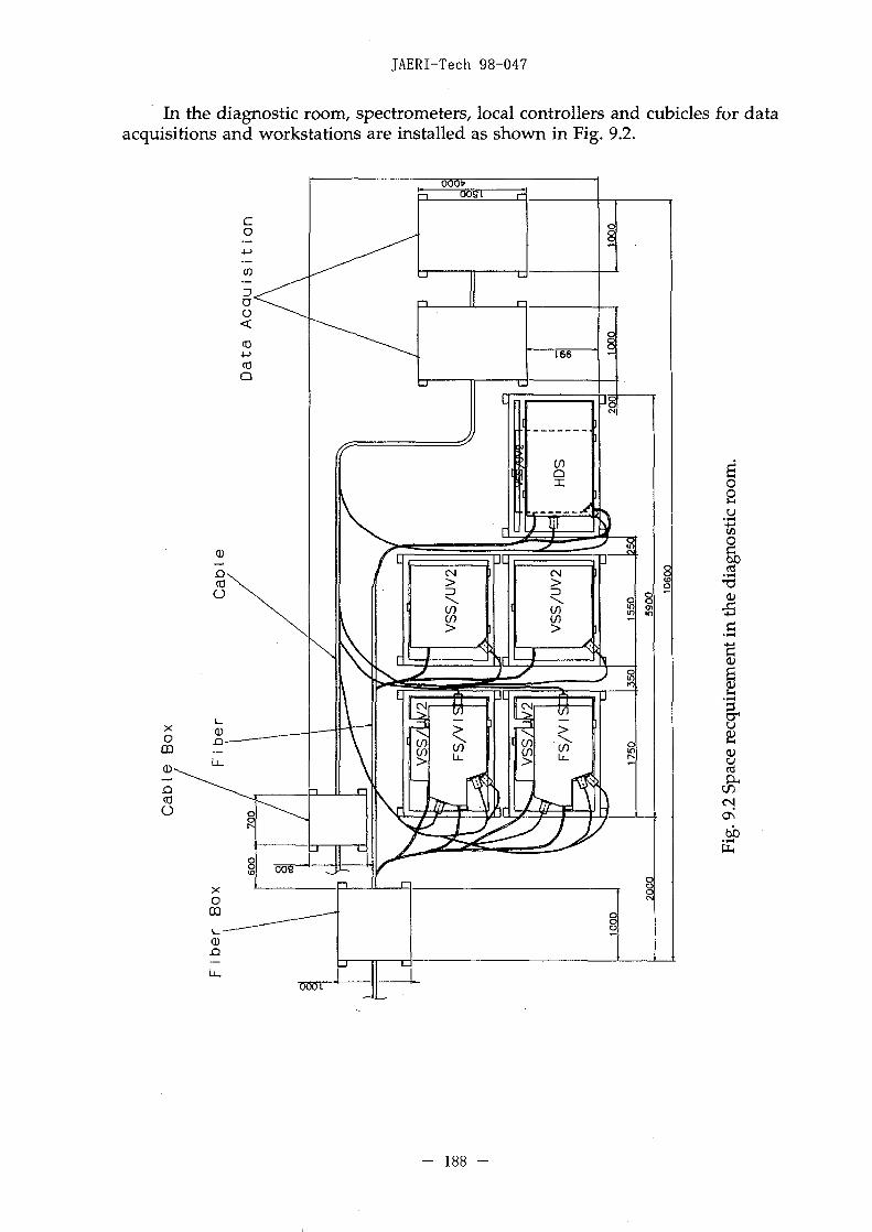
JAERI-Tech 98-047
In the diagnostic room, spectrometers, local controllers and cubicles for dataacquisitions and workstations are installed as shown in Fig. 9.2.
so2.aI
the
0)
a,C/5
ON
"33ST
- 188 -

JAERI-Tech 98-047
10. Further work, and necessary R & D
Further works and necessary R & D were described in the each sections.Those are summarized in this section as follows.
i) First mirror in the divertor cassette:- Particle flux estimation as a function of energy in the divertor.- Experimental data of candidates for the first mirror concerning the
degradation by neutral particle bombardment especially at the low energyregion.
- Test of the baffle method in the present tokamaks.- Shutter in front of the mirror in order to block off the particle just during
the disruption, the boronization and other wall conditionings.- Strong gas puff into the divertor just during the disruption in order to
decrease the energy of the disrupted particles.- Strong gas puff to the mirror in order to blow the dust off the mirror.- In-situ coating of the mirror.- R & D of mirror materials.
ii) Optical design- Detailed design for new divertor cassette.- Design of new viewing fans.- Detailed design of calibration system.- Detailed design of alignment system.
iii) Mechanical design- More detailed design of interface with other equipment.- Remote handling equipment
iv) Detector- Detector selection and design.- R & D if necessary.
v) Data acquisition and processing- Reconsideration for concept of data acquisition and processing.- Detailed design.- Interface with CODAC.- Data acquisition and processing for plasma control.
vi) Physics- Study of atomic and molecular process in the low temperature and high
temperature plasma such as ITER divertor.
- 189 -

JAERI-Tech 98-047
11. Rearrangement of mirrors for new divertor cassette.
The design of the rearrangement of mirrors in the divertor cassette wascarried out for the new divertor cassette as shown in Fig. 11-1.
The new divertor cassette [1] has liners between divertor legs and the firstmirrors. The gap of 7 mm between each liners is narrow to measure spectral linesthrough the gap. In order to get a suitable viewing slot for measurement, one ofthe liners is removed for each viewing fans. There are four viewing slots forinner and outer divertor measurement. The gap of each viewing slot is 30 mm asshown in Fig. 11-2.
The optical design will be necessary for this new arrangement. It is,however, expected that the optical performance will not change so much, sincethe rearrangement is not so big.
Liner
Mirror
Fig. 11-1 Mirror arrangement and viewing fans for new divertor cassette.
LinerMirrorSide
•V iew ing Sto
•Viewing Slot
us;
OuterDivertorSide
Fig. 11-2 Horizontal section of liners. Each viewing slot is realized by removing one sheet of liner.There are two viewing slots for outer divertor. The width of the viewing slot is 30 mm.The viewing slots for inner divertor are realized by same structure as outer one.
- 190 -
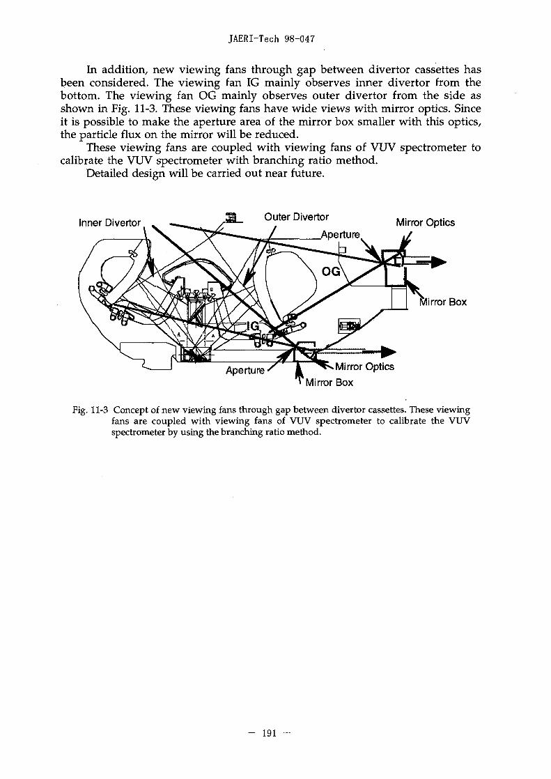
JAERI-Tech 98-047
In addition, new viewing fans through gap between divertor cassettes hasbeen considered. The viewing fan IG mainly observes inner divertor from thebottom. The viewing fan OG mainly observes outer divertor from the side asshown in Fig. 11-3. These viewing fans have wide views with mirror optics. Sinceit is possible to make the aperture area of the mirror box smaller with this optics,the particle flux on the mirror will be reduced.
These viewing fans are coupled with viewing fans of VUV spectrometer tocalibrate the VUV spectrometer with branching ratio method.
Detailed design will be carried out near future.
Inner Divertor Outer Divertor
ApertureMirror Optics
irror Box
Mirror Optics
Mirror Box
Fig. 11-3 Concept of new viewing fans through gap between divertor cassettes. These viewingfans are coupled with viewing fans of VUV spectrometer to calibrate the VUVspectrometer by using the branching ratio method.
- 191

JAERI-Tech 98-047
12. Conclusion
The objectives of the divertor impurity monitoring system (WBS 5.5.E.04)are to identify impurity species and to measure those quantities and influxeswith spatial resolution in the divertor. The system has been designed here in thewave length region of 200 - 1000 nm in accordance with the work order and therequirements of the design description document (DDD).
Main results are as follows.
1) System should be composed of three kind of spectrometers such as a visiblesurvey spectrometer, a filter spectrometer and a high dispersion spectrometer.
2) Spectrometers should be located outside the cryostat from the magnetic shieldpoint of view.
• Spectrometers for the wavelength range of 200 - 450 nm should be sit on amovable trolley in the pit to prevent the transmission loss of fiber.
• Spectrometers for over 450 nm should be set in the diagnostic room fromthe accessibility's and flexibility's point of view.
3) In order to realize 2D measurements on the poloidal plane both in outer andinner divertor region, four viewing fans are proposed with mirror optics inthe divertor cassette.
4) The region from approximately up the divertor leg to the x-point will beobserved with the additional viewing fans through the gap between thedivertor cassettes.
5) The ray trace analysis shows that the 10-mm spatial resolution in the all regionof the divertor will be achieved.
6) Visible survey spectrometers, filter spectrometers and high dispersionspectrometers are designed.
7) It is difficult to measure deuterium influx lower than 1019 (at/ 'm^-sec1) in ahigh electron density region. Continuum radiation such as bremsstrahlungand recombination emission is large in the dense and cold plasmas.
8) The windows on the divertor port plug will be survive against neutron and y-ray flux. For the short wavelength region, more detailed consideration isnecessary.
9) Mechanical designs have been carried out for the optical penetration system,spectrometers, remote handling concept, electromagnetic force, nuclearheating and so on.
10) Concept of control and data acquisition are considered.
- 192 —

JAERI-Tech 98-047
11) Space requirements are listed.12) Further design works and necessary R & D are listed.13) Estimated cost is listed.14) Rearrangements of mirrors mounted in the divertor cassette were carried out
for a new divertor cassette.
Acknowledgment
The authors are grateful to Drs A. Costley, S. Yamamoto, L. de Kock, C.Walker, V. Mukhovatov, H. Iida, H. Nakamura and the members of ITER EDAJoint Central Team for their fruitful discussions and cooperation. We would liketo express our gratitude to Drs T. Tsnemarsu and T. Shoji for thier continuousencouragement to this work.
This paper has been prepared as an account of work assigned to the JapaneseHome Team under Task Agreement numbers S 91 TD21 95-01-20 FJ and S 91TD31 95-08-04 FJ within the Agreement among the European Atomic EnergyCommunity, the Government of Japan, the Government of the RussianFederation, and the Government of the United States of America on Cooperationin the Engineering Design Activities for the International ThermonuclearExperimental Reactor ("ITER EDA Agreement") under the auspices of theInternational Atomic Energy Agency (IAEA).
193 -
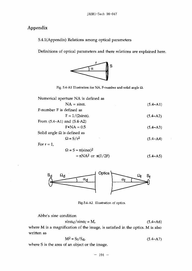
JAERI-Tech 98-047
Appendix
5.4.1 (Appendix) Relations among optical parameters
Definitions of optical parameters and there relations are explained here.
Fig. 5.4-Al Illustration for NA, F-number and solid angle £2.
Numerical aperture NA is defined asNA = sinoc.
F-number F is defined as
F = l/(2sina).From (5.4-A1) and (5.4-A2)
F«NA = 0.5Solid angle Q. is defined as
For r = 1,
= S ~ 7t(sina)2
or 7i(l/2F)
(5.4-A1)
(5.4-A2)
(5.4-A3)
(5.4-A4)
(5.4-A5)
s d Q dOptics
Of Sf
Fig.5.4-A2 Illustration of optics.
Abbe's sine condition
sinocd/sinaf = M, (5.4-A6)where M is a magnification of the image, is satisfied in the optics. M is alsowritten as
M2 = Sf/Sd/ (5.4-A7)where S is the area of an object or the image.
- 194 -
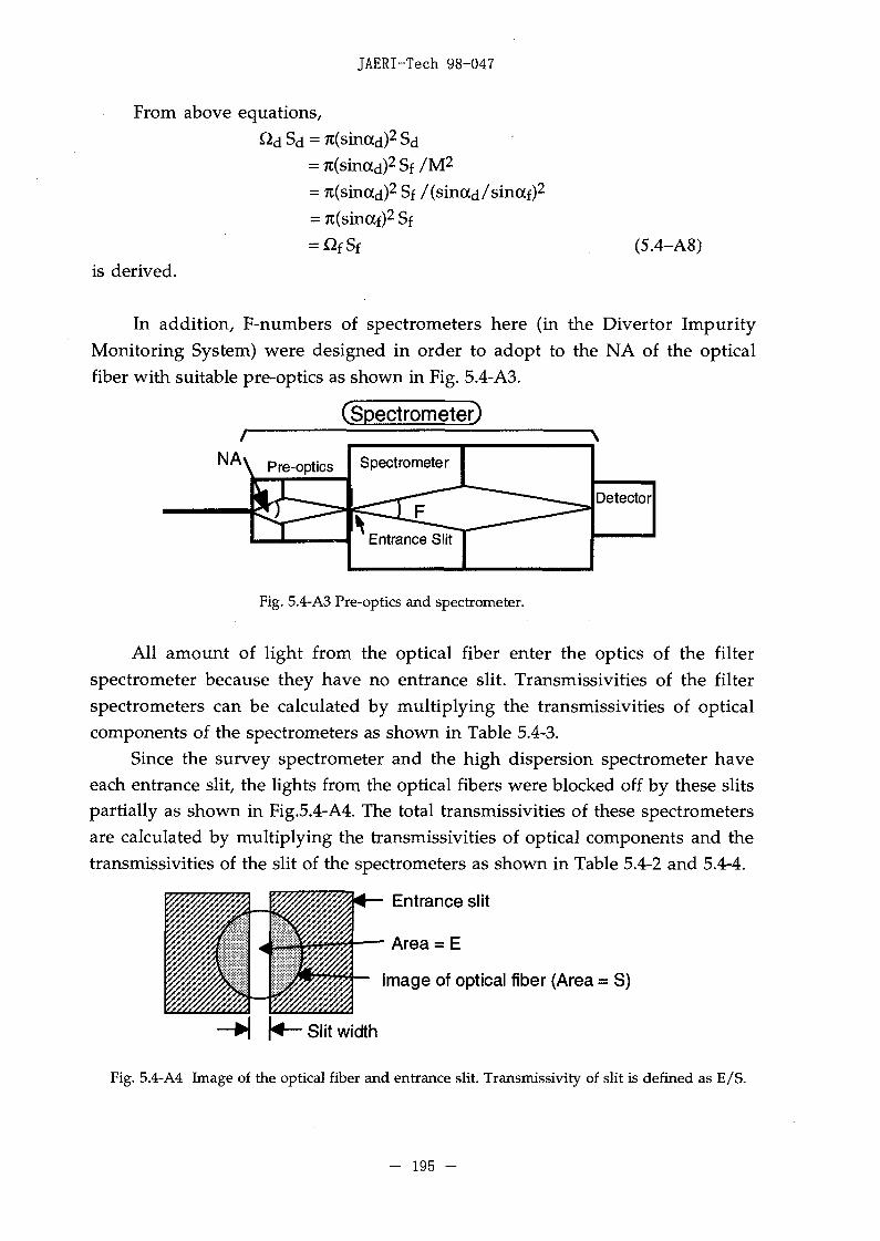
JAERI-Tech 98-047
From above equations,
Qd Sd = rc(sinad)2 Sd= 7c(sinad)
2 Sf /US?
= Ti(sinad)2 Sf /(sinad/sinaf)2
= Tt(sinaf)2 Sf
(5.4-A8)is derived.
In addition, F-numbers of spectrometers here (in the Divertor ImpurityMonitoring System) were designed in order to adopt to the NA of the opticalfiber with suitable pre-optics as shown in Fig. 5.4-A3.
(Spectrometer)
Detector
Fig. 5.4-A3 Pre-optics and spectrometer.
All amount of light from the optical fiber enter the optics of the filterspectrometer because they have no entrance slit. Transmissivities of the filterspectrometers can be calculated by multiplying the transmissivities of opticalcomponents of the spectrometers as shown in Table 5.4-3.
Since the survey spectrometer and the high dispersion spectrometer haveeach entrance slit, the lights from the optical fibers were blocked off by these slitspartially as shown in Fig.5.4-A4. The total transmissivities of these spectrometersare calculated by multiplying the transmissivities of optical components and thetransmissivities of the slit of the spectrometers as shown in Table 5.4-2 and 5.4-4.
Entrance slit
Area = E
Image of optical fiber (Area = S)
Slit width
Fig. 5.4-A4 Image of the optical fiber and entrance slit. Transmissivity of slit is defined as E/S.
- 195 -

ssK
n̂ft¥A
% it
¥ B
SU
Si
msftft
+
T
ii
7
-
y
IV
y
i?
X X 7
fth
'' 7
t"
T
rVs T
A
Ty
7
y
y
IS ^
mkgsAK
molcd
radsr
GE
I
ft
S
iftm.in.
y 9'
m
•> 7 X
x *
7y
j . - ;l/
•y h
— • y
iv h
7 7 K— A
: - / y x
HzNPaJWcVFas
WbTH°Clmlx
BqGySv
s -m-kg/s2
N/m2
N-mJ/sA-sW/AC/VV/AA/VV-sWb/m2
Wb/A
cd-srlm/m2
s—
J/kgJ/kg
'J
ftfif,
•y h
B
y
a
§2 ^
min, h, d
1, Lt
eVu
leV=1.60218xl0-"J
1 u= 1.66054x10"" kg
SM
£ ft-̂ y ? " x h D —
/< -
'ft
* ^ 'J\s y Y *f
7
u
A
y
71/
7U
-
y
KA
12 ^
Ab
barGalCiR
r a d
r e m
1 A=0.1 nm=10"'°m
lb=100fm2=10"2Sm2
lbar=0.1MPa=10sPa
1 Ci=3.7xlO'°Bq
lR=2.58xlO-'C/kg
1 rad = lcGy = 10"2Gy
1 rem=lcSv=10"2Sv
1 0 "
1 0 "
10 1 2
10'106
103
102
10'
io-10"2
10"3
10"6
10"'
io-2
10""10-8
X
*
f
•f"-b
• 7
^~
t"
7
T
sans? •*»•
?
7
#
'ft
•
i/
y f-'j
A ^7 O
/
i A h
b
12 ^
EPTGM
k
h
da
d
c
m
li
n
Pfa
(a)1. 1 - 5 li rUKWilSJ ® 5 Kg. HIS
1985^fiJff(Cj;5o fcfc'L. 1 eV
to J; tf 1 u ©<tfi CODATA CD 1986£p«St
2. J V, T-'
-C
3. bar IJ,
2 Oil
, barntoj;
N( = 10sdyn)
1
9.80665
4.44822
kgf
0.101972
1
0.453592
lbf
0.224809
2.20462
1
lPa-s(N-s/m2)=10P(*TX)(g/(cm-s))
lmVs=10'St(x h - ?
E MPa( = 10bar)
1
0.0980665
0.101325
1.33322 x 10-"
6.89476 x 10"3
kgf /cm2
10.1972
1
1.03323
1.35951 x 10"3
7.03070 x 10"2
a t m
9.86923
0.967841
1
1.31579 x 10"3
6.80460 x lO"2
mmHg(Torr)
7.50062 x 10³
735.559
760
1
51.7149
Ibf/in2(psi)
145.038
14.2233
14.6959
1.93368 xlO"2
1
X
IV
1
<±
fl:
J (=10 'erg)
1
9.80665
3.6 xlO6
4.18605
1055.06
1.35582
1.60218x10-'
kgf-m
0.101972
1
3.67098 x 10 s
0.426858
107.586
0.138255
1.63377 xlO'2 0
kW- h
2.77778x10"
2.72407 x 10"'
1
1.16279 x 10"'
2.93072 x lO"
3.76616 x 10"'
4.45050 x 10"26
cal(Itaffi)0.238889
2.34270
8.59999 xlO5
1
252.042
0.323890
3.82743 x 10~M
Btu
9.47813x10-
9.29487 x 10⁻³
3412.13
3.96759 x 10⁻³
1
1.28506 xlO"3
1.51857 xlO-22
ft • Ibf
0.737562
7.23301
2.65522 x 10⁶
3.08747
778.172
1
1.18171 x l O " "
eV
6.24150x10"
6.12082x10"
2.24694 xlO2B
2.61272x10"
6.58515 x 10²'
8.46233x10"
1
lcal = 4.18605 J(atHtt-)
= 4.184J (jSMfcfO
= 4.1855 J (15 °C)
= 4.1868 J(Bf$MM&
= 75 kgf-m/s
= 735.499 W
Bq
3.7 x 10"
Ci
2.70270x10-"
1
m.Gy
i
0.01
rad
100
1
C/kg
2.58 x 10-
R
3876
1
1
0.01
rem
100
1
26BSS)
