design of a neuromemristive echo state network architecture
TRANSCRIPT

Rochester Institute of Technology Rochester Institute of Technology
RIT Scholar Works RIT Scholar Works
Theses
8-2015
Design of a Neuromemristive Echo State Network Architecture Design of a Neuromemristive Echo State Network Architecture
Qutaiba Mohammed Saleh
Follow this and additional works at: https://scholarworks.rit.edu/theses
Recommended Citation Recommended Citation Saleh, Qutaiba Mohammed, "Design of a Neuromemristive Echo State Network Architecture" (2015). Thesis. Rochester Institute of Technology. Accessed from
This Thesis is brought to you for free and open access by RIT Scholar Works. It has been accepted for inclusion in Theses by an authorized administrator of RIT Scholar Works. For more information, please contact [email protected].

Design of a Neuromemristive Echo StateNetwork Architecture
by
Qutaiba Mohammed Saleh
A Thesis Submitted in Partial Fulfillment of the Requirements for the Degree of Master ofScience
in Computer Engineering
Supervised by
Associate Professor Dr. Dhireesha KudithipudiDepartment of Computer EngineeringKate Gleason College of Engineering
Rochester Institute of TechnologyRochester, New York
August 2015
Approved by:
Dr. Dhireesha Kudithipudi, Associate ProfessorThesis Advisor, Department of Computer Engineering
Dr. Andres Kwasinski, Associate ProfessorCommittee Member, Department of Computer Engineering
Dr. Ray Ptucha, Assistant ProfessorCommittee Member, Department of Computer Engineering
Thesis Release Permission Form
Rochester Institute of TechnologyKate Gleason College of Engineering
Title:
Design of a Neuromemristive Echo State Network Architecture
I, Qutaiba Mohammed Saleh, hereby grant permission to the Wallace Memorial Library
to reproduce my thesis in whole or part.
Qutaiba Mohammed Saleh
Date

iii
Dedication
To my beloved family, for all of your support along the way.

iv
Acknowledgments
I am grateful for my thesis advisor Dr. Dhireesha Kudithipudi. I could not have achieved
this without her invaluable motivation, patience, and dedication to this work. I also thank
Dr. Andres Kwasinski and Dr. Ray Ptucha for serving on my thesis committee and their
insightful comments and encouragement. Furthermore, I thank the rest of the department
faculty and staff for their support through my study.
I thank my labmates Cory Merkel, Colin Donahue, James Manatzaganian, Levs Dolgovs,
and James Thesing for their guidance and the stimulating discussions. Finally, I would
like to thank the Iraqi Ministry of Higher Education and Scientific Research for the full
scholarship to complete my Master study.

v
AbstractDesign of a Neuromemristive Echo State Network Architecture
Qutaiba Mohammed Saleh
Supervising Professor: Dr. Dhireesha Kudithipudi
Echo state neural networks (ESNs) provide an efficient classification technique for spa-
tiotemporal signals. The feedback connections in the ESN enable feature extraction in
both spatial and temporal components in time series data. This property has been used
in several application domains such as image and video analysis, anomaly detection, and
speech recognition. The software implementations of the ESN demonstrated efficiency in
processing such applications, and have low design cost and flexibility. However, hardware
implementation is necessary for power constrained resources applications such as therapeu-
tic and mobile devices. Moreover, software realization consumes an order or more power
compared to the hardware realization. In this work, a hardware ESN architecture with neu-
romemristive system is proposed. A neuromemristive system is a brain inspired computing
system that uses memristive devises for synaptic plasticity. The memristive devices in
neuromemristive systems have several interesting properties such as small footprint, sim-
ple device structure, and most importantly zero static power dissipation. The proposed
architecture is reconfigurable for different ESN topologies. 2-D mesh architecture and
toroidal networks are exploited in the reservoir layer. The relation between performance
of the proposed reservoir architecture and reservoir metrics are analyzed. The proposed
architecture is tested on a suite of medical and human computer interaction applications.
The benchmark suite includes epileptic seizure detection, speech emotion recognition, and
electromyography (EMG) based finger motion recognition. The proposed ESN architecture
demonstrated an accuracy of 90%, 96%, and 84% for epileptic seizure detection, speech
emotion recognition and EMG prosthetic fingers control respectively.

vi
Contents
Dedication . . . . . . . . . . . . . . . . . . . . . . . . . . . . . . . . . . . . . . iii
Acknowledgments . . . . . . . . . . . . . . . . . . . . . . . . . . . . . . . . . iv
Abstract . . . . . . . . . . . . . . . . . . . . . . . . . . . . . . . . . . . . . . . v
1 Introduction . . . . . . . . . . . . . . . . . . . . . . . . . . . . . . . . . . . 11.1 Motivation . . . . . . . . . . . . . . . . . . . . . . . . . . . . . . . . . . . 11.2 List of Objectives . . . . . . . . . . . . . . . . . . . . . . . . . . . . . . . 31.3 Summary . . . . . . . . . . . . . . . . . . . . . . . . . . . . . . . . . . . 4
2 Background and Related Work . . . . . . . . . . . . . . . . . . . . . . . . 52.1 Introduction to Echo State Networks . . . . . . . . . . . . . . . . . . . . . 5
2.1.1 Training Algorithm . . . . . . . . . . . . . . . . . . . . . . . . . . 62.1.2 Training Example . . . . . . . . . . . . . . . . . . . . . . . . . . . 8
2.2 Related work . . . . . . . . . . . . . . . . . . . . . . . . . . . . . . . . . 102.2.1 Applications . . . . . . . . . . . . . . . . . . . . . . . . . . . . . 102.2.2 Epileptic Seisure Detection . . . . . . . . . . . . . . . . . . . . . . 102.2.3 Emotion Recognition . . . . . . . . . . . . . . . . . . . . . . . . . 112.2.4 Electromyography . . . . . . . . . . . . . . . . . . . . . . . . . . 122.2.5 Hardware Reservoir Models . . . . . . . . . . . . . . . . . . . . . 13
2.3 Summary . . . . . . . . . . . . . . . . . . . . . . . . . . . . . . . . . . . 16
3 Circuit Models . . . . . . . . . . . . . . . . . . . . . . . . . . . . . . . . . 173.1 Memristive Devices . . . . . . . . . . . . . . . . . . . . . . . . . . . . . . 173.2 Synapse circuit models . . . . . . . . . . . . . . . . . . . . . . . . . . . . 203.3 Neuron circuit models . . . . . . . . . . . . . . . . . . . . . . . . . . . . . 213.4 Summary . . . . . . . . . . . . . . . . . . . . . . . . . . . . . . . . . . . 23
4 Proposed Topology and Architectures . . . . . . . . . . . . . . . . . . . . . 244.1 ESN Topologies . . . . . . . . . . . . . . . . . . . . . . . . . . . . . . . . 24
vii
4.1.1 Random Topology . . . . . . . . . . . . . . . . . . . . . . . . . . 244.1.2 Ring Topology . . . . . . . . . . . . . . . . . . . . . . . . . . . . 244.1.3 Proposed Hybrid Topology . . . . . . . . . . . . . . . . . . . . . . 26
4.2 Proposed Architectures . . . . . . . . . . . . . . . . . . . . . . . . . . . . 274.2.1 Neuron Box . . . . . . . . . . . . . . . . . . . . . . . . . . . . . . 274.2.2 2-D Mesh Architecture for Ring and Random Topologies . . . . . . 284.2.3 Toroidal Architecture for Hybrid Topology . . . . . . . . . . . . . 32
4.3 Simulation Platform . . . . . . . . . . . . . . . . . . . . . . . . . . . . . . 354.4 Summary . . . . . . . . . . . . . . . . . . . . . . . . . . . . . . . . . . . 36
5 Benchmarks and Validation . . . . . . . . . . . . . . . . . . . . . . . . . . 385.1 Epileptic Seizure Detection . . . . . . . . . . . . . . . . . . . . . . . . . . 38
5.1.1 EEG Dataset . . . . . . . . . . . . . . . . . . . . . . . . . . . . . 385.1.2 Feature Extractor . . . . . . . . . . . . . . . . . . . . . . . . . . . 40
5.2 Emotion Recognition . . . . . . . . . . . . . . . . . . . . . . . . . . . . . 405.2.1 Speech Emotion Dataset . . . . . . . . . . . . . . . . . . . . . . . 415.2.2 Feature Extractor . . . . . . . . . . . . . . . . . . . . . . . . . . . 41
5.3 Electromyography . . . . . . . . . . . . . . . . . . . . . . . . . . . . . . . 445.3.1 EMG Dataset . . . . . . . . . . . . . . . . . . . . . . . . . . . . . 445.3.2 Feature Extractor . . . . . . . . . . . . . . . . . . . . . . . . . . . 45
5.4 Summary . . . . . . . . . . . . . . . . . . . . . . . . . . . . . . . . . . . 46
6 Results and Performance Analysis . . . . . . . . . . . . . . . . . . . . . . . 486.1 Applications . . . . . . . . . . . . . . . . . . . . . . . . . . . . . . . . . . 48
6.1.1 Epileptic Seizure Detection . . . . . . . . . . . . . . . . . . . . . . 486.1.2 Emotion Recognition . . . . . . . . . . . . . . . . . . . . . . . . . 496.1.3 Prosthetic Fingers Control . . . . . . . . . . . . . . . . . . . . . . 52
6.2 Reservoir Metrics . . . . . . . . . . . . . . . . . . . . . . . . . . . . . . . 556.2.1 Kernel quality . . . . . . . . . . . . . . . . . . . . . . . . . . . . . 556.2.2 Lyapunov’s Exponent . . . . . . . . . . . . . . . . . . . . . . . . . 57
6.3 Power . . . . . . . . . . . . . . . . . . . . . . . . . . . . . . . . . . . . . 586.4 Summary . . . . . . . . . . . . . . . . . . . . . . . . . . . . . . . . . . . 60
7 Conclusions and Future Work . . . . . . . . . . . . . . . . . . . . . . . . . 617.1 Conclusions . . . . . . . . . . . . . . . . . . . . . . . . . . . . . . . . . . 617.2 Future Work . . . . . . . . . . . . . . . . . . . . . . . . . . . . . . . . . . 62
A Derivation for Hybrid Topology . . . . . . . . . . . . . . . . . . . . . . . . 63

viii
Bibliography . . . . . . . . . . . . . . . . . . . . . . . . . . . . . . . . . . . . 65

ix
List of Tables
5.1 Frequency bands of Mel triangular filters. The start and end frequencies inthis table represent bi and di in equation 5.2 respectively. . . . . . . . . . . 43
x
List of Figures
2.1 An Echo State Network consists of three layers: input layer, reservoir layerand output layer . . . . . . . . . . . . . . . . . . . . . . . . . . . . . . . . 6
2.2 Echo State Networks abstract structure. How signals propagate through theESN and the effects of different weight sets in the network. . . . . . . . . . 7
2.3 Signals propagation through the tested ESN over time. The plots shows (a)input sinusoid test signal, (b) reservoir layer responses to this signal, (c)output signal of the ESN and (d) final classification signal. . . . . . . . . . 9
2.4 Training and testing classification accuracies of the sinusoid signal versesdifferent threshold values. The maximum accuracy achieved for both train-ing and testing is 98%. . . . . . . . . . . . . . . . . . . . . . . . . . . . . 10
2.5 (a) Graph representation of a random reservoir. Edges represent memristorsand nodes represent neurons in the reservoir. (b) Circuit representation [29]. 14
2.6 Reservoir architecture as presented in [5]. It is a regular mesh networkconnecting a number of nodes using memristors as links. . . . . . . . . . . 15
3.1 Relations between the four fundamental two-terminal circuit elements: re-sistor, inductor, capacitor, and memristor. . . . . . . . . . . . . . . . . . . 18
3.2 Charge vs voltage of a piecewise linear memristor model. . . . . . . . . . . 193.3 (a) Inhibitory memristive synapse circuit and (b) excitatory memristive
synapse circuit. These circuits are inspired by the function of biologicalinhibitory (e.g. GABAergic) and excitatory (e.g. glutamatergic) synapseswith ionotropic receptors [39]. . . . . . . . . . . . . . . . . . . . . . . . . 20
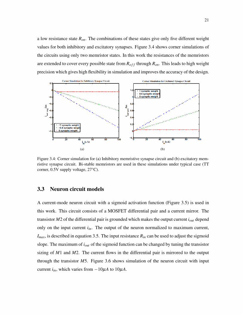
3.4 Corner simulation for (a) Inhibitory memristive synapse circuit and (b) ex-citatory memristive synapse circuit. Bi-stable memristors are used in thesesimulations under typical case (TT corner, 0.5V supply voltage, 27°C). . . . 21
3.5 Neuron circuit for the reservoir layer of the ESN with a sigmoid activationfunction [39]. . . . . . . . . . . . . . . . . . . . . . . . . . . . . . . . . . 22
3.6 Simulation of the neuron circuit under typical case (TT corner, 0.5V supplyvoltage, 27°C). Input current iin varies form −10µA to 10µA. . . . . . . . . 22
xi
4.1 (a) ESN architecture with ring reservoir topology. Each reservoir node has2 inputs and one output. (b) ESN architecture with center node topology.Reservoir nodes are connected to one center node that works as a hub. (c)ESN architecture with hybrid topology. Each node has 3 inputs and oneoutput. . . . . . . . . . . . . . . . . . . . . . . . . . . . . . . . . . . . . . 25
4.2 A neuron box of a ring topology ESN that has one input node and oneoutput node. The neuron box contain one reservoir layer node, one in-put synapse, one output synapse, and one reservoir synapse connecting thereservoir layer node with the previous node. . . . . . . . . . . . . . . . . . 28
4.3 Internal structure of one cell. It contains one neuron box surrounded byfour muxes and one four channel switch. These muxes and switches areused to control the routing of the links in the network. . . . . . . . . . . . . 30
4.4 Complete system depiction of ESN architecture. The reservoir is imple-mented in 2-D mesh network with reconfigurable switches (colored or-ange) enabling dynamic configuration of different ESN topologies. Thecross-connectors (colored green) are used to connect the input and outputlayers to the reservoir layer. . . . . . . . . . . . . . . . . . . . . . . . . . . 31
4.5 Block level representations of the two ESN topologies. (a) Random topol-ogy and (b) Two way ring topology. . . . . . . . . . . . . . . . . . . . . . 32
4.6 Implementations of (a) Ring and (b) Random reservoir topologies on 2d-mesh network. . . . . . . . . . . . . . . . . . . . . . . . . . . . . . . . . . 32
4.7 Implementing the hybrid topology as four rings. The rings are color coddedbased on figure 4.1. Purple ring is used for the connections between theinput layer and the reservoir layer. Green ring is used for the ring topologyconnections. Red ring is used for the center node connections. Orange ringis used for the connections between the reservoir layer and the output layer. 33
4.8 6x6 doubly twisted toroidal network. The figure shows two rings connec-tions are embedded in the architecture. One ring uses the horizontal linkswhile the other uses the vertical links. . . . . . . . . . . . . . . . . . . . . 34
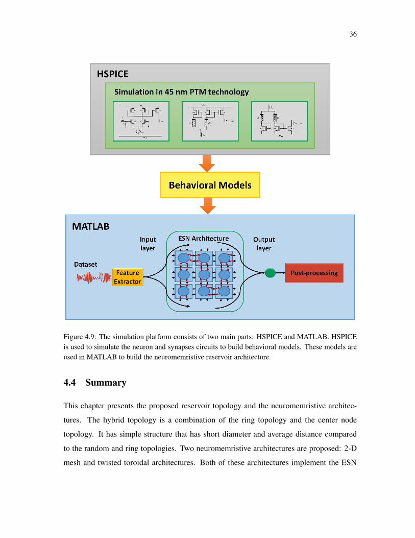
4.9 The simulation platform consists of two main parts: HSPICE and MAT-LAB. HSPICE is used to simulate the neuron and synapses circuits to buildbehavioral models. These models are used in MATLAB to build the neu-romemristive reservoir architecture. . . . . . . . . . . . . . . . . . . . . . 36
xii
5.1 Electrode placements as explained in [3]. (a) (the first white figure only)Standardized surface electrode placement scheme used to collect normalEEG signals of set A. (b) (three gray shaded figures) Scheme of electrodesimplanted symmetrically into the hippocampal formation of the brain. Thisscheme was used to collect seizure EEG signals of set E. . . . . . . . . . . 39
5.2 Five second time series EEG signal samples for (a) Normal case and (b)Seizure case. . . . . . . . . . . . . . . . . . . . . . . . . . . . . . . . . . 39
5.3 Mel scale generated using equation 5.1. . . . . . . . . . . . . . . . . . . . 425.4 Block diagram of the feature extractor used in this work. The input is an
audio signal and the final output is the energy corresponding to the emotioncontents of the input signal. . . . . . . . . . . . . . . . . . . . . . . . . . . 42
5.5 Ten randomly chosen final emotion features for neutral and anger statuses.The length of each of the signal depends on the length of the actual inputaudio signal to the feature extractor. . . . . . . . . . . . . . . . . . . . . . 44
5.6 (a) Surface electrode placement on the forearm. (b) Five classes of individ-ual finger movements used in this work [27]. . . . . . . . . . . . . . . . . . 45
5.7 EMG signal samples of individual finger movements for (a) Thumb, (b)Index, (c) Middle, (d) Ring, and (e) Little. . . . . . . . . . . . . . . . . . . 47
6.1 Epileptic seizure detection accuracy versus the reservoir size and alpha for(a) Ring topology with maximum accuracy of 86% and (b) Hybrid topologywith maximum accuracy of 90%. . . . . . . . . . . . . . . . . . . . . . . . 49
6.2 The effects of the number of nodes within the reservoir and the degree ofconnectivity of those nodes on the testing accuracy at Alpha ≈0.25. Thebest accuracy is observed at ≈190 nodes and ≈ 20% connectivity. . . . . . 50
6.3 The short memory parameter Alpha verses testing accuracy at 190 reservoirnodes with 20% connectivity. Best accuracy is observed at Alpha ≈0.25. . . 50
6.4 Signal propagation through ESN for speech emotion recognition at (a) Testexpected, output signal Vs threshold, and test predicted. . . . . . . . . . . . 51
6.5 The classification accuracy of ideal hardware behavior model of the ESNwith 190 reservoir nodes at 20% degree of connectivity and Alpha ≈0.25The best test accuracy is 96.5%. . . . . . . . . . . . . . . . . . . . . . . . 52
6.6 The effects of the number of nodes within the reservoir and alpha on thetesting accuracy of finger motion recognition using hybrid topology. . . . . 53
6.7 Confusion matrix of fingers classification from surface EMG signals using300 nodes hybrid reservoir for (a) training with accuracy of 87% and (b)testing with accuracy of 84%. . . . . . . . . . . . . . . . . . . . . . . . . . 53
xiii
6.8 Classification accuracy of individual finger motion. The accuracy is in arange from 88% to 95%. . . . . . . . . . . . . . . . . . . . . . . . . . . . 54
6.9 Kernel results vs different reservoir sizes for hybrid topology reservoir test-ing (a) EEG and (b) EMG signals. . . . . . . . . . . . . . . . . . . . . . . 56
6.10 Lyapunov’s exponent results vs different reservoir sizes for hybrid topologyreservoir testing (a) EEG and (b) EMG signals. . . . . . . . . . . . . . . . 58
6.11 Power consumption vs reservoir size of three ESN topologies: one wayring, two way ring, and hybrid. The ring topology has lower power con-sumption compared to the other topologies. . . . . . . . . . . . . . . . . . 59
6.12 Power consumption vs reservoir size of four ESN topologies: one way ring,two way ring, hybrid, and random. The random topology has higher powerconsumption compared to the other topologies. . . . . . . . . . . . . . . . 60
1
Chapter 1
Introduction
1.1 Motivation
Spatiotempporal signals have been widely used in various of applications such as speech
recognition, video and music editing, and bio-signal processing. These signals are pro-
cessed based on their behavior in time series windows. For example, the goal of speech
recognition is translating an audio signal into text. Observing the signal at a specific time
does not provide enough information for translation. Taking multiple measurements of the
signal in a time series window provides the required information to describe the speech.
Reservoir computing has been heavily used in processing spatiotemporal signals. The re-
current connections of the reservoir layer enable extracting desired features within a time
frame [36]. These random connections make the state of the reservoir layer oscillate at
the edge of chaos [7], which is region of dynamic systems that operates at the boundary
between chaotic and non-chaotic behavior [34]. This property has been utilized in several
reservoir computing models.
Echo State Network (ESN) is a type of reservoir computing neural network in which
the reservoir state depends on current the input and all the previous inputs to the reser-
voir layer [23]. It has a simple training algorithm compared to other types of recurrent
neural networks [34]. The software implementations of the ESNs are effective in diverse
The words ESN and Reservoir are used interchangeably in this document.
2
applications offering low cost and flexible designs. These software ESN models are imple-
mented on conventional computing systems (such as Von Neumann systems). Such sys-
tems demand large area to fit the design and consume considerable power to run different
components on the chip. Primarily, Von Neumann systems are not design for processing
limited resources applications such as body sensors, therapeutic, and mobile devices. Such
applications require processing models that have low power consumption, small area and
high processing speed. For example in smart phones, power consumption is critical [11].
Supporting such devices with large batteries may solve the power consumption problem
in some applications. However, this solution can not be considered for therapeutic and
body sensors where the device is physically attached to the patients. These devices also
require real-time processing speed to detect any event in the tested bio-signals and take the
appropriate action.
A custom hardware implementation of ESN is preferred to meet these requirements.
Several approaches to implement hardware neural networks have been presented. Like the
software implementation, the digital hardware approach has flexibility and ease of imple-
mentation. It also partially satisfies some of the critical requirements addressed before.
The neuromorphic computing approach can more effectively meet these requirements. It is
a non-conventional system built of mixed signal hardware circuits inspired by the human
brain [38]. Neuromophic designs have several appealing properties over the traditional
CMOS implementations in terms of power consummation, area, speed, and cost [19]. It
also offers highly parallel architectures. Neuromemristive systems are a class of mero-
morphic computing [2]. It uses memristive devices for synapses implementations. The
memristor is a passive electrical component that has a variable resistance depending of the
internal state [13]. The resistance values of the devices are changed based on the duration
and amount of current flow through it. This memory property is used to save the weight
value or strength of the synaptic connection in neuromorphic designs.
Building a neuromorphic architecture model of ESN using memrisive devices will sat-
isfy the requirements of low power consumption, small area and high processing speed.
Such an architecture fills a knowledge gap in hardware reservoir designs, which operate in

3
real-time with limited power resource applications. Medical devices are in the top of list
of applications that can benefit from these systems. These devices are used by wide range
of medical professionals to diagnose diverse set of diseases and infections such as epilep-
tic seizure, neuromuscular diseases, kinesiology, motor control disorders, and emotional
disorders.
1.2 List of Objectives
• Develop a software ESN model for baseline analysis.
• Design a hardware neuromemristive ESN model, with varying reservoir topologies
(random, ring, and hybrid).
– Design an ESN model using memristive-based synapse circuits as building blocks.
– Design a novel hybrid reservoir topology.
– Implement the neuromemristive reservoir on a set of different reservoir topolo-
gies.
– Optimize this model for parameters such as reservoir layer size, degree of con-
nectivity, and alpha.
– Analyze the correlation between reservoir metrics and performance.
• Hardware architecture for the memristive reservoir.
– A homogeneous, scalable, and reconfigurable architecture that is used as a plat-
form to implement the reservoir.
– Two architectures are used to design this platform: Mesh networks and doubly
twisted toroidal networks.
• Use the proposed neuromemristive architecture to build complete processing plat-
forms for three applications:
– Epileptic seizure detection using Electroencephalogram signals (EEG).

4
– Speech emotion recognition. Use speech to detect two emotions: neutral and
anger.
– Prosthetic finger control using surface electromyogram signals (EMG).
1.3 Summary
The reset of this document is outlined as follows: Chapter 2 gives an introduction of ESN
and its training algorithm and demonstrates an example. It also presents the related work
in the literature. Chapter 3 discusses the memristive synapse and neuronal circuits used in
this work. Chapter 4 presents the proposed neuromemristive architecture and the modified
novel hybrid reservoir topology. Chapter 5 describes the benchmarks that are used to test
the proposed architecture and the feature extractors. The simulation results obtained from
applying these benchmarks and the metrics analysis are presented in Chapter 6. Chapter 7
discusses conclusions and future work.

5
Chapter 2
Background and Related Work
2.1 Introduction to Echo State Networks
Echo State Network (ESN) is a class of reservoir computing model presented by Jaeger
et al. in 2001 [21]. ESNs are considered as partially-trained artificial neural networks
(ANNs) with a recurrent network topology. They are used for spatiotemporal signal pro-
cessing problems. The ESN model is inspired by the emerging dynamics of how the brain
handles temporal stimuli. It consists of an input layer, a reservoir layer and an output layer
(see Figure 2.1). The reservoir layer, is the heart of the network, with rich recurrent con-
nections. These connections are randomly generated and each connection has a random
weight associated with it. Once generated, these random weights are never changed during
training or testing phases of the network. The output layer of the ESN linearly combines
the desired output signal from the rich variety of excited reservoir layer signals. The cen-
tral idea is that only the network to the output layer connection weights have to be trained,
using simple linear regression algorithms. Another reservoir model, known as liquid state
machine, provides a biologically plausible model for generating computations in cortical
microcircuits. In contrast, ESN provides a high performance mathematical framework for
solving a number of engineering tasks. Specifically, they can be applied to recurrent ar-
tificial neural networks without internal noise. ESNs have simplified training algorithms
compared to other recurrent ANNs and are more efficient than kernel-based methods (e.g.:
Support Vector Machines) due to their ability to incorporate temporal stimuli. Because of
its recurrent connections, the output of the reservoir depends on the current input state and
all previous input states within the system memory. The recurrent network topology of the
reservoir enables feature extraction of spatiotemporal signals. This property has been used

6
in several application domains such as image and video analysis, anomaly detection, and
speech recognition.
Figure 2.1: An Echo State Network consists of three layers: input layer, reservoir layer and outputlayer
2.1.1 Training Algorithm
Three main sets of weights are associated with the ESNs (Figure 2.2). The weights at the
input and reservoir layers are randomly generated. These layers are used to extract temporal
features of the input signal. They can be thought of as an internal pre-process step that
prepares the signal for the actual processing layer where the classification is learned at the
readout layer. Figure 2.2 also shows the propagation of the signals through the ESNs. The
input signal to the ESN u[n] is pre-processed at the input and reservoir layers to extract the
temporal featured signal x[n] which is fed to the readout layer to complete the classification
process. Considering that the input and reservoir layers are not actual parts of this process,
their weights are not trained which makes training the ESNs much easier than other types
of recurrent neural networks.
The goal of the training algorithm is to calculate the weights at the output layer based

7
Figure 2.2: Echo State Networks abstract structure. How signals propagate through the ESN andthe effects of different weight sets in the network.
on the dynamic response (states) of the reservoir layer [22]. The states of the reservoir
layer are calculated based on the input vectors and the weights of the input and reservoir
layer as shown in (2.1).
x[n+1] = f res (Winu[n+1]+Wxx[n]) (2.1)
where u[n] is the ESN input, Win is the weight matrix between the input layer and reservoir
layer, Wx is the weight matrix between the neurons within the reservoir layer, and f res is
the reservoir layer’s activation function.
The states of the reservoir layer for all input vectors are used as an input to a supervised
training to calculate the output weights Wout. There are several linear regression methods
to calculate the weights at the output layer. This work uses normal equation to implement
the supervised training of the ESN (2.2).
Wout = (YX′)(XX′)−1 (2.2)
where X is a matrix concatenating all states of the reservoir layer and Y is a matrix of all
training outputs.
The process for training the ESN can be explained through the following steps:
1. At initialization, randomly generate the weights for the input and reservoir layers
(Win and Wx)
2. Drive the next input vector u[n+1] to the input layer

8
3. Calculate the response of the reservoir layer by 2.1
4. Save the response in a matrix (X)
5. Repeat step 2-4 for all input vectors
6. Calculate output weights based on normal equation 2.2
Once the weights of the output layer are calculated, the network is ready and the state
of the reservoir layer is used to calculate the output of the network as shown in (2.3).
y[n+1] = f out (Woutx[n+1]) (2.3)
where y[n+1] is the output of the network, Wout is the weight matrix at the readout layer
and f out is the readout layer’s activation function.
2.1.2 Training Example
This example elucidates how an ESN can be trained to classify temporal signals. A single-
channel sinusoid input signal u(n) = sin(2πFn) is used. This signal periodically oscillates
at two different frequencies F1 and F2. The ESN in this example is used to classify the input
sinusoid signal based on its frequency. For such problem, a single output unit is enough to
represent the two classes F1 and F2. Since the problem is simple and has uncomplicated
features based on which the decision is made, a small reservoir layer is used. The network
used consists of single input unit, 20 reservoir units and a single output unit. The values
of the signal frequencies F1 and F2 are 4 and 2 Hz respectively. The signal is sampled at a
rate of 100 Hz. The target output of the network is −1 for F1 and 1 for F2. The algorithm
described in the previous section is used to train the network for this classification problem.
Figure 2.3 shows the propagation of the signal through the ESN starting from the input
tested signal Figure 2.3(a). It also shows the responses of the reservoir layer to this input
signal figure 2.3(b). As can be seen, the reservoir layer’s response varies based on the input
signal in both frequency and amplitude. The variations of the signals at the output of the
reservoir layer represent extracted features based on which classification decision is made

9
at the output layer. Figure 2.3(c) is the output signal at the output layer. This signal is
compared to some threshold value to generate the final output as seen in figure 2.3(d).
(a)
(b)
(c)
(d)
Figure 2.3: Signals propagation through the tested ESN over time. The plots shows (a) input sinu-soid test signal, (b) reservoir layer responses to this signal, (c) output signal of the ESN and (d) finalclassification signal.

10
Different threshold values are used to increase the classification accuracy. Figure 2.4
shows the training and testing accuracy vs. different threshold values. The maximum accu-
racy achieved is 98%. This example is a simple demonstration of how ESNs are powerful
at processing temporal signals.
Figure 2.4: Training and testing classification accuracies of the sinusoid signal verses differentthreshold values. The maximum accuracy achieved for both training and testing is 98%.
2.2 Related work
2.2.1 Applications
The software implementations of the ESN have been effective at diverse applications such
as emotion recognition [52], forecasting of water inflow for a hydropower plant [49], nat-
ural language analysis [57], motion identification [20], speech recognition [54], and many
more applications (see [35] for a review). The previous work on the applications used in
this project is explored in the next sections.
2.2.2 Epileptic Seisure Detection
Epileptic Seizure detection is one of the biomedical applications that was implemented us-
ing ESNs. Epileptic seizures are chronic disorders of the central nervous system, where

11
one in 26 people will develop this disorder at sometime in their life [1]. It can be often
detected through analysis of electroencephalogram (EEG) signals. A software ESN model
for epileptic seizure detection is presented in [8]. The reservoir layer in the design consists
of 200 randomly connected neuronal nodes with 90% connectivity. The EEG dataset used
for testing purposes was taken from rats which have behavioral similarity with human EEG
signals. The input signal is pre-processed before it is fed to the actual ESN. Similarly, the
output signal of the ESN passes through a post process stage before the final decision is
made. This model showed fast and accurate results compared to other methods that use non
ESN techniques. The results in this work showed that ESNs are more effective in process-
ing EEG signals for epileptic seizure detection. However, the software model presented
in this work has high number of neuronal nodes with high degree of connectivity. These
two properties are not desired for hardware implementations [48]. On the other hand the
pre-process stage and its relation with the reset of the model was not fully explained in the
paper. A full system level implementation with design details are not presented. Moreover,
the EEG signals used for validation were confidential data and can not be compound or
used by other researchers.
2.2.3 Emotion Recognition
In emotion recognition, the emotional status of a human like anger, fear, happiness etc
are detected. Human-computer interaction is an application of emotion recognition [15].
Using this property, computers can have better interaction with human. Using speech for
emotion recognition requires lower computational resources compared to other inputs as
facial expressions.
The software ESN model introduced in [52] uses features like energy, pitch and speech
spectral base features to recognize emotions. The Mel Frequency Cepstral Coefficients
(MFCC) are used for emotional feature extraction. The extracted features are used to train
the ESN network. A reservoir layer of 500 neuronal nodes with 50% degree of connec-
tivity is used in this ESN. The model was able to detect two different emotional statuses
(natural and anger) with an accuracy of 99%. This accuracy was achieved in real-time

12
speed. The results proved that ESNs are a viable option for emotion recognition. These re-
sults can be tested considering that the dataset used is publicly available. The pre-process
stage (feature extractor) is also well explained while exhibiting all similar techniques in
the literature. The paper showed that the recognition speed was fast enough to be used
in real-time applications without explaining the characteristics of the computing system
used in the experiment. The work presented in this paper can be improved to detect more
emotional statuses so that it can be considered as a stand-alone recognition system. The
ESN model presented in this paper has acceptable degree of connectivity for a hardware
implementation. The pre-process stage can be also considered for such implementation.
2.2.4 Electromyography
Electromyography (EMG) is a biosignal collected by measuring muscles potential activ-
ities. EMG signals are recorded using electrodes sensors. With the advances of signal
processing techniques, EMG signals have been used for several medical applications such
as neuromuscular disorder diagnosis and prosthetic devices control. Processing of EMG
signals can be summarized into three steps: signals decomposition, feature extraction, and
signal classification [46].
Several traditional statistical techniques have been used for EMG signal processing
such as Linear Discrimination Analysis (LDA), Quadratic Discriminant Analysis (QDA),
Gaussian Mixture Models (GMM), Hidden Markov Models (HMM), and k-Nearest neigh-
bor classifier (refer to [61] for more examples). Khushaba et al. [27] used support vector
machine (SVM), k-Nearest neighbor, and extreme learning machine (ELM) to classify fif-
teen finger movements of the upper limbs. Artificial neural network classifier models have
also been used for EMG signals. These models include MLP, back-propagation network,
conic section function neural network, and fuzzy clustering neural network [24]. Subasy
et al. used neural networks to detect two types of neuromuscular disorders: myopathy and
neurogenic disease [56]. The classification accuracy of EMG signals are 90.7% and 88%
for feedforward error back-propagation (FEB) and wavelet neural networks (WNN) re-
spectively. This work classifies EMG signals based on finger motions for prosthetic finger
13
control. To the best of my knowledge, not only is this the first work presenting a neu-
romemristive architecture to classify EMG signals but it also the first work processing this
class of signals using reservoir computing.
2.2.5 Hardware Reservoir Models
Software implementations proved that ESNs are efficient in different application domains.
However, the software models are not efficient for embedded and low-end processing en-
vironments, where power dissipation is critical to the operation of the devices. A few
research groups presented hardware ESN models based on memristive devices. Next are
two examples that used memristive devices to build reservoir models.
Kulkarni et al. in [29] presented a memristor-based reservoir model. The memristive
devices in this model are used as building blocks to construct the reservoir layer. They
are considered as bi-directional connections that are randomly connected based on graph
theory approach to generate different reservoir topologies. In this architecture, each mem-
ristive device represents an edge that connects two nodes or vertices in the graph Figure
2.5(b). Except for a self loop connection, each node can be connected to any other node
in the graph. The existence of a connection between two nodes means a new memristive
device is added to the circuit. The responses of the reservoir are taken from these nodes.
Figure 2.5(b) shows a circuit representation of reservoir generated base on graph theory.
The reservoir layer was modeled in Ngspice while the output layer was trained using ge-
netic algorithm. The work presents a generic reservoir model. While it provides a good
explanation of the theoretical algorithm to establish the reservoir topology, it gives no spec-
ification of the type of the reservoir (example Liquid State Machine (LSM) or ESN) where
each reservoir type has its own characteristics in terms of weight generation and activation
functions. It neither gives details of the circuits at the output layer nor how the weight
values have been trained. At the same time no power or performance measurements were
presented in this work. Except for some simple classification problems, the model was not
used for a specific application.

14
(a) (b)
Figure 2.5: (a) Graph representation of a random reservoir. Edges represent memristors and nodesrepresent neurons in the reservoir. (b) Circuit representation [29].
Burger et al. presented a structured memristive reservoir architecture in [5]. The mem-
ristive devices are connected as a mesh network. The effect of process variations of the
devices is used to set the random weight values of the reservoir synapses. The device-to-
device variation gives each memristor its unique maximum and minimum resistances and
threshold voltages. The topology consists of a matrix of nodes that are connected by mem-
ristors as a mesh network Figure 2.6. One of the nodes is selected to be an input node that
is used to feed the input signal into the reservoir. The rest of the nodes are used as outlets
where the response of the reservoir is measured. As in any reservoir computing model,
the response of the reservoir layer is used to train the output layer. The output layer is
implemented in software as step function perceptrons. Genetic algorithm is used to train
the output layer to overcome the problem of local minima in a given search space.
Five different sizes of reservoirs were simulated to study the relationship between reser-
voir size, number of memristive devices, and the performance. The performance of this

15
work is compared with the performance of the model presented in [29] which uses a ran-
dom reservoir topology. In this experiment, both mesh and random architectures use the
process variation to generate the weights of the reservoir layer. These architectures were
trained to classify a frequency modulated signal that has two frequencies. The experiment
revealed that the reservoir is tolerant to the process variation. It also showed that increas-
ing the size of the reservoir improves the variation tolerance and decreases the error rate
for both mesh and random architectures. The overall performance of the two tested archi-
tectures have the same response toward changing the degree of variation and size of the
reservoir but in general the regular mesh architecture showed better performance compared
to the random architecture.
Figure 2.6: Reservoir architecture as presented in [5]. It is a regular mesh network connecting anumber of nodes using memristors as links.
This work presents a homogeneous architecture that was analyzed for different parame-
ters. It uses, however, a simple classification problem. More complicated applications that
has high impacts on industry and human life could have been used to validate the architec-
ture. Such applications empower the architecture and present it as a possible solution for
daily faced problems. No metrics are used to analyze the effectiveness of the reservoir in

16
any of these works.
2.3 Summary
ESN is a class of reservoir computing, which processes information based on its behavior
history. This property presents ESN as a powerful candidate for processing spatiotemporal
signals. Epileptic seizure detection and speech emotion recognition are two examples ap-
plied on software ESN models. Hardware ESN, however, is not a well explored area. There
is a few memristive based ESN architectures presented in the literature. These architectures
were not tested on vital well defined applications. This work presents a neuromemristive
ESN architecture and uses it for epileptic seizure detection, speech recognition, and EMG
signals processing. To the best of my knowledge, this is the first ESN model that processes
EMG and combines it with EEG and speech emotion recognition.

17
Chapter 3
Circuit Models
From a circuit point of view, an ESN consists of a number of neurons connected by a
set of synapses in a specific pattern. Therefore, the primitives required to build an ESN
processing system are:
• Architectural topology of the reservoir
• Input and output processing layers
• Memristive synapse circuit models
• Neuron circuit models
This chapter introduces the circuits models used in this research. These models are used
as building blocks for the proposed ESN architecture. They were designed by Mr. Cory
Merkel, a Phd student in the NanoComputing research lab (RIT), in previous collaborated
works [16, 39, 50].
3.1 Memristive Devices
Memristor is a two-terminal non-volatile variable resistor. It was first proposed in 1971
by Leon Chua [14] as a missing non-linear passive basic electrical component to be added
to the three components resistor, capacitor, and inductor. Chua stated that there are six
mathematical relations between the four fundamental circuit variables: voltage (v), current
(i), charge (q), and flux (φ ). Figure 3.1 shows these relations. The memristor relates electric
charge q(t) and magnetic flux linkage φm(t) equation 3.1.

18
Figure 3.1: Relations between the four fundamental two-terminal circuit elements: resistor, induc-tor, capacitor, and memristor.
f (φm(t),q(t)) = 0 (3.1)
A memristor is characterized by its function that shows how the rate of change of charge
and flux leakage depend on the state of the memristor [13] as shown in equation 3.2.
M(q) =dφm
dq(3.2)
Taking the time integral of this equation and substituting the flux as the time integral of
the voltage and the charge as time integral of the current leaves us with resistance value as
in equation 3.3. This equation shows that the resistance value of the memristor depends on
the period of time and amount of current flow through the memristor.
M(q(t)) =V (t)(t)
(3.3)
In 2008, Strukov et al. presented the first applicable memristor model using vacancy-
doped titanium dioxide thin films [55]. Several other variations of memristor models have
been presented. Each has diffenrent method to describe the memristive switching such as
tunneling barrier modulation [43] and controlling the spin of electrons [41].

19
The resistance of memristor can be changed by applying voltage to its terminals. In the
ideal memrsitor, any applied voltage should change the resistance. However in fabricated
memristor models, the resistance is changed only when the applied voltage increases above
a certain write threshold. Figure 3.2 shows the behavior of a piecewise memristor model
vs voltage.
Figure 3.2: Charge vs voltage of a piecewise linear memristor model.
This figure shows that the charge linearly reacts to the voltage changes lower the write
voltage. However, it dramatically changes ones the applied voltage increases above the
write voltage. The write threshold divides the voltage scale of memristors into two regions:
read and write. In the write region, the resistance of the memristor is changed to a desired
value. The memristor retains this resistance state as long as no high voltage is applied. In
the read region, the memristor acts as a linear resistor. This memory property is used to save
synaptic weight values in synapse circuits [17, 44]. Memristors also have other attractive
characteristics such as small footprint, simple device structure, and most importantly zero
static power dissipation[30].

20
3.2 Synapse circuit models
Two synapse circuits are used in this work. The inhibitory synapse (Figure 3.3(a)) draws
current away from a post-synaptic neuron, similar to GABAergic synapse in the biological
brain. The excitatory synapse (Figure 3.3(b)) supplies current to the post-synaptic neu-
ron, similar to glutamatergic synapse in the biological brain. In both the inhibitory and
excitatory synapses, two memristors are used to save the weight value. Each memristor is
connected to a diode connected transistor. The two memristors in parallel divide the input
current based on the memristors conductance. Consequently the synaptic weight is given
as a ratio of conductances as in equation 3.4.
w−(+) =G2(4)
G1(3)+G2(4)(3.4)
where G = 1/R, is the conductance of memristors in figure 3.3.
The output current of the synapse circuits is driven through a current mirror, transistor
M3 and M6 for the inhibitory and excitatory synapses respectively. The output currents
inhibit or excite the post-synaptic neuron as shown in figure 3.3.
(a) (b)
Figure 3.3: (a) Inhibitory memristive synapse circuit and (b) excitatory memristive synapse circuit.These circuits are inspired by the function of biological inhibitory (e.g. GABAergic) and excitatory(e.g. glutamatergic) synapses with ionotropic receptors [39].
These circuits were originally designed based on bi-stable memristors where resistance
values are assumed to be on one of the two extreme values, a high resistance state Ro f f and
21
a low resistance state Ron. The combinations of these states give only five different weight
values for both inhibitory and excitatory synapses. Figure 3.4 shows corner simulations of
the circuits using only two memristor states. In this work the resistances of the memristors
are extended to cover every possible state from Ro f f through Ron. This leads to high weight
precision which gives high flexibility in simulation and improves the accuracy of the design.
(a) (b)
Figure 3.4: Corner simulation for (a) Inhibitory memristive synapse circuit and (b) excitatory mem-ristive synapse circuit. Bi-stable memristors are used in these simulations under typical case (TTcorner, 0.5V supply voltage, 27°C).
3.3 Neuron circuit models
A current-mode neuron circuit with a sigmoid activation function (Figure 3.5) is used in
this work. This circuit consists of a MOSFET differential pair and a current mirror. The
transistor M2 of the differential pair is grounded which makes the output current iout depend
only on the input current iin. The output of the neuron normalized to maximum current,
Imax, is described in equation 3.5. The input resistance Rin can be used to adjust the sigmoid
slope. The maximum of iout of the sigmoid function can be changed by tuning the transistor
sizing of M1 and M2. The current flows in the differential pair is mirrored to the output
through the transistor M5. Figure 3.6 shows simulation of the neuron circuit with input
current iin, which varies from −10µA to 10µA.

22
iout
Imax≈
0 , iin <− s
12 −√
aiinRin√
1−a(iinRin)2 , |iin| ≤s
1 , iin >s
(3.5)
where a = βn/2Imax, s =√
2Vov/Rin, and Vov is the gate overdrive voltage defined as
Vov=VGS−Vt .
iin
Rin
VDD
-VSS
iout
Imax
M3 M4
M1 M2
M5
Figure 3.5: Neuron circuit for the reservoir layer of the ESN with a sigmoid activation function [39].
Figure 3.6: Simulation of the neuron circuit under typical case (TT corner, 0.5V supply voltage,27°C). Input current iin varies form −10µA to 10µA.

23
3.4 Summary
Memristor is a programmable resistor that changes its resistance based on its internal state.
It has two voltages ranges: read and write. Applying write voltage updates the resistance
while the read voltage has no effect on the resistance. Memristors are used as memory
elements in synapse circuits. In this work two synapses, excitatory and inhibitory, are used.
Each synapse uses two memristors to save weight values. The neuron circuits used in this
architecture are composed of current-mode designs,which are inherently low power. These
synapses and a current mode neuron circuit are used as building blocks for the proposed
neuromemristive ESN architecture. The next chapter introduces this architecture.

24
Chapter 4
Proposed Topology and Architectures
4.1 ESN Topologies
Topology is defined as the interconnection pattern within the reservoir layer nodes. Sev-
eral topologies for reservoir were presented in the literature [48]. This work particularly
explores the random and ring topologies. It also presents a novel hybrid topology that
minimize the required hardware resources.
4.1.1 Random Topology
The original ESN uses fully or randomly connected reservoir layer topologies [21]. The
shape of these topologies and their degree of connectivity are defined by the reservoir layer
weight matrix Wx where the weights of the unconnected links are set to zero. Such a
random method to generate topologies for the reservoir layer has design constraints. It
requires several trials to find the appropriate topology for an application. It is hard to
regenerate these connections dynamically; it requires saving all the connections. There
is no proofs that the generated pattern will be the best choice for the target application
[48]. Moreover, the highly connected random topology is too complex to be implemented
in hardware. The routing complexity, area overhead, and power consumption are signifi-
cantly higher in hardware. For these reasons, simple reservoir topologies are desirable for
hardware implementation of the ESN.
4.1.2 Ring Topology
The ring topology presented in [48] has a simple and hardware friendly structure. The
nodes of the reservoir layer are connected in a ring shape where the output of each node is

25
connected to only the neighboring node (Figure 4.1(a)). Equation 4.1 is used to calculate
the state of a single node x(s) in the reservoir layer at a certain time step n. This equation
can be generalized to calculate the state of the entire reservoir layer as shown in equation
4.2.
x(s)[n] = f res(Win(s)U[n]+Wring(s)x(s−1)[n−1]) (4.1)
where x(s)[n] is the state of node s at time step n. Win(s) is the input weight associated
with the node s. U[n] is the input at time step n. Wring(s) is the reservoir weight between
the nodes s and s−1. x(s−1)[n−1] is the state of the node s−1 at the previous time step
n−1.
X[n] = f res(Winu[n]+Wring�
X[n−1]�
) (4.2)
where X[n] is the state of all nodes in the reservoir layer at time step n. Win is the input
weights matrix. Wring is the reservoir weight vector (one weight for each node).�
X[n−1]�
refers to the state of all nodes in the reservoir layer at time step n−1 rotated by one.
(a) Ring (b) Center Node (c) Hybrid
Figure 4.1: (a) ESN architecture with ring reservoir topology. Each reservoir node has 2 inputs andone output. (b) ESN architecture with center node topology. Reservoir nodes are connected to onecenter node that works as a hub. (c) ESN architecture with hybrid topology. Each node has 3 inputsand one output.
This topology provides low degree of connectivity in the network but has undesirable
properties for the reservoir network. It has high network diameter and average distance.
For a ring reservoir layer that has N number of nodes the diameter is N−1 and the average
distance is 23N. This means that the output effect of node 1 requires N−1 time steps to
reach the node N. This high diameter may cause delay in the response of the reservoir to

26
any changes in the input. Such delay is undesirable in real-time information processing
applications.
4.1.3 Proposed Hybrid Topology
Simple updates to the ring topology can fix the high diameter and average distance values.
Adding different shortcut links in the reservoir layer may decrease these values but it will
make the network unbalanced, where the distance between the nodes will vary depending
on its location from the shortcut links. Uniform connection links should be added to achieve
constant distance between all nodes. Combining the ring topology, shown in figure 4.1(a),
with the center node topology, shown in figure 4.1(b), may give the network the balanced
uniformed shortcut links that increase the connections between nodes and improve network
properties. Figure 4.1(c) shows the proposed hybrid reservoir topology. This topology has
low diameter and average distance compared to the ring topology. The diameter is 2 and
the average distance is less than 2. In this way the reservoir is tightly connected and more
sensitive to the changes to the input of the network. Equation 4.3 is used to calculate the
state of the reservoir layer of the hybrid topology.
X[n] = f res(Winu[n]+WdownXc+Wring�
X[n−1]�
) (4.3)
where Wdown is the weight vector of synapses from the center node to the reservoir layer
nodes. Xc is the state of the reservoir node. For further explanation, the mathematical
derivation for the hybrid reservoir topology is shown in appendix A.
In terms of complexity, the hybrid topology has two extra synapses per node compared
to the ring topology. These synapses connect the nodes of the reservoir layer with the center
node. The idea behind using the center node is to provide each node in the reservoir layer
with information about the state of the whole reservoir. It emulates the fully connected
topology in which each node has full access to all nodes within the reservoir layer.
27
4.2 Proposed Architectures
4.2.1 Neuron Box
The neuron box is a container for the functional components in the ESN. Each neuron box
contains one reservoir layer node and all the actively corelated synapses. These boxes are
the building blocks of the proposed architectures that provide flexibility, reconfigurability
and scalability.
In the ESN, there are three types of nodes: input layer nodes, reservoir layer nodes, and
output layer nodes. These nodes are connected by three types of synapses: input layer to
reservoir layer, reservoir layer synapses which connect the nodes within the reservoir layer,
and reservoir layer to output layer synapses. In addition to these types, a few ESN models
have additional types of synapses such as input layer to output layer synapses and feedback
synapses from output layer back to reservoir layer. The ESN model in this work uses only
the first three types of synapses. It can be noticed from the structure of the ESN that all
three types of synapses are connected to the nodes in the reservoir layer, which represents
a bridge between the input and the output layers.
The neuron box wraps one reservoir node and all the synapses that are connected to it
in one frame. Figure 4.2 shows a neuron box for the ring topology ESN. As seen in this
figure, the neuron box contains one neuron (reservoir layer node), one input synapse, one
output synapse, and one reservoir synapse. The neuron box includes only input reservoir
synapses. For this reason, there is only one reservoir synapse in the ring topology neuron
box where the other synapse is included in the neuron box of the next node in the ring
structure. The size of the neuron box depends on the number of synapses in the network
and the size of the circuits of these synapses and the reservoir layer node. The neuron box
does not includes the input nor output nodes because they are linear neurons and can be
represented behaviorally.
Dividing an ESN into neuron boxes produce a number of homogeneous blocks that have
the same number of ports, size, and structure. The number of these boxes is equal to the
number of the reservoir layer nodes. Using neuron boxes simplifies the connectivity prob-
lem of the ESN. It can be thought of as a number of nodes (neuron boxes) that should be

28
Figure 4.2: A neuron box of a ring topology ESN that has one input node and one output node.The neuron box contain one reservoir layer node, one input synapse, one output synapse, and onereservoir synapse connecting the reservoir layer node with the previous node.
connected according to a connection pattern. This makes the neuromemristive ESN archi-
tectures easier to implement, measure, and evaluate. Neuron boxes also provide scalability
where a new neuron box is added to the architecture for each new reservoir node.
4.2.2 2-D Mesh Architecture for Ring and Random Topologies
In this work, hardware ESN model is built based on analog neuron and synapses circuits.
These circuits are designed based on the assumption that they are always connected, which
requires dedicated links to connect the circuits. This constraint is the main challenge for any
proposed interconnect network. Moreover, the proposed architecture should have recon-
figurability and scalability to implement several reservoir topologies with different sizes.
These properties can be achieved with the neuron box and the appropriate interconnect
network that has a flexible routing mechanism.

29
The proposed architecture uses 2-D mesh network topology to connect the neuron
boxes. Similar network has been used for self-reconfigurable connectivity for FPGAs
in [58]. A 2-D cellular automata is used where the routing between cells is decided by
the cellular rules. The architecture proposed in this work is inspired by the network pre-
sented in [58]. In this architecture, each neuron box is connected to four neighboring boxes
through full duplex links. The neighboring boxes are annotated north (N) south (S) east
(E) west (W). This architecture allows any arbitrary connection between any two boxes in
the network. Depending on the width of the links between the boxes, there could be some
constraints to the possible connections. There are no constraints for the first connection,
however, the more the connections added to the network, the more constraints are placed.
The connection pattern between the neuron boxes is controlled by a set of multiplexers
and switches that are added to each neuron box to form one cell in the 2-D mesh network.
Figure 4.3 shows the internal architecture of one cell.
The states of these Mux’s and switches are controlled by a memory register that is also
included in the cell, where each cell requires seventeen bits. These bits are distributed
between the Mux’s (three bits for each Mux) and the switch which requires five bits. The
connections between the cells are established according to the values of these bits which
provide the required recofigurability to implement different ESN topologis. The registers
of all cells in the network are serially connected. At the start-up time, the values of the bits
are streamed to the registers. A bit file of the desired configuration for the entire network
can be generated offline. This file is reusable for multiple implementations.
In the ESN model used in this work, the input layer and output layer are fully connected
to the reservoir layer. These connections are never changed regardless of the ESN topol-
ogy. An extra layer of cross-connectors are added to the 2-D mesh network to connect the
input and output layers to the reservoir layer. Figure 4.4 shows a full ESN processing sys-
tem that uses the proposed architecture. This figure shows an array of neuron boxes (blue
balls) which form the heart of the architecture. The connections within the reservoir layer
of the ESN are implemented using a 2-D mesh network through the routing switches (or-
ange boxes) that are attached to the neuron boxes. The connections between the reservoir

30
Figure 4.3: Internal structure of one cell. It contains one neuron box surrounded by four muxes andone four channel switch. These muxes and switches are used to control the routing of the links inthe network.
layer and the input and output layers are implemented through the cross-connectors (green
balls). The ESN system also contains pre-processing and post-processing steps. The pre-
processing is the feature extractor while the post-processing is the circuitry used for the
final output decision of the system. The post-processing could be a simple threshold circuit
or a winner-take all circuit.
Two reservoir topologies were implemented using the 2-D mesh architecture: random
and two way ring topologies. An example of the random topology is shown in figure
4.5(a). The two way ring topology, which is shown in figure 4.5(b), is a modified version
of the ring topology that is discussed earlier in this chapter. It consists of two rings of
connections. In this topology, node N in the reservoir layer has access to the outputs of
both N−1 and N +1 nodes. The extra ring is used to increase the connectivity within the

31
Figure 4.4: Complete system depiction of ESN architecture. The reservoir is implemented in 2-D mesh network with reconfigurable switches (colored orange) enabling dynamic configuration ofdifferent ESN topologies. The cross-connectors (colored green) are used to connect the input andoutput layers to the reservoir layer.
reservoir layer which impact the delay in the response of the ESN to the changes in the
inputs. Figure 4.6 shows the implementation of the reservoir layers for these topologies
on the 2-D mesh architecture. The random connections implemented on the 2-D mesh
in figure 4.6(a) do not correspond to the random connections of the random topology in
figure 4.5(a). The random and the two way ring topologies are used for speech emotion
recognition and epileptic seizure detection applications respectively.

32
(a) (b)
Figure 4.5: Block level representations of the two ESN topologies. (a) Random topology and (b)Two way ring topology.
(a) (b)
Figure 4.6: Implementations of (a) Ring and (b) Random reservoir topologies on 2d-mesh network.
4.2.3 Toroidal Architecture for Hybrid Topology
The hybrid topology consists of four main groups of synaptic links: input set, output set,
ring set, and center node set. The input and output synapses are fully connected to the
reservoir. This means that the same signals are distributed for all nodes in the reservoir
layer. One connection link that passes through all nodes in the reservoir layer in a ring
shape can be used to distribute these signals. Since the center node is linear, which makes

33
it a simple node that works according to Kirchhoff’s current law, its connections can also be
implemented as a ring (Figure 4.7). In this way, four rings can implement all the required
connections of the hybrid topology as shown in figure 4.7. The rings in this figure are color
coded to be consistent with figure 4.1(c) that shows the hybrid topology.
Figure 4.7: Implementing the hybrid topology as four rings. The rings are color codded basedon figure 4.1. Purple ring is used for the connections between the input layer and the reservoirlayer. Green ring is used for the ring topology connections. Red ring is used for the center nodeconnections. Orange ring is used for the connections between the reservoir layer and the outputlayer.
Combining the neuron box with the ring connection patterns for the hybrid topology,
produces a simple homogeneous architecture. With a suitable connection width, the 2-
D mesh architecture can be used to implement the hybrid topology. However, using a
reconfigurable architecture like the 2-D mesh for the static hybrid topology is inefficient
utilization of the routing resources available in the 2-D mesh architecture. Instead, any
static architecture that satisfies the four ring connections can be used.
In this work, the doubly twisted toroidal network is used to implement the hybrid topol-
ogy. It has been used for several interconnection implementations. Martinez et al. [37]
presented a modern modeling for twisted toroidal networks with the Gaussian integers.
Beivide et al. [4] used twisted toroidal network for SIMD and MIMD architectures. Yang
et al. [62] used a diagonal twisted toroidal network for massively parallel computer net-
works.

34
The doubly twisted toroidal network topology has the same array structure that tradi-
tional toroidal networks have with one extra connection for each row in the array. The idea
is to add a ”twist” to the regular toroidal network. In the toroidal network, the opposite
nodes at the beginning and end of each row and column are connected together while in the
doubly twisted network, the last node at each row of the network is connected to the first
node in the next row. The same twist connections are added in the vertical direction for the
columns [53] [10]. Figure 4.8 shows an example of a doubly twisted network.
Figure 4.8: 6x6 doubly twisted toroidal network. The figure shows two rings connections are em-bedded in the architecture. One ring uses the horizontal links while the other uses the vertical links.
The nodes in the doubly twisted toroidal network represent neuron boxes of the hybrid
topology. Four rings are required to connect these boxes. However, only two rings con-
nections are embedded in the toroidal network as seen in figure 4.8. One ring uses the

35
horizontal links while the other uses the vertical links. For this reason multichannel links
are used in the doubly twisted toroidal network to increase the number of the embedded
rings. This architecture is simple compared to the 2-D mesh architecture in term of the
required resources, where no muxes, switches, or memory registers are used to route the
signals. Consequently, it loses the reconfigurability property that the 2-D mesh has. On
the other hand, scalability is still provided by the twisted toroidal architecture where any
reservoir size can be implemented on this architecture.
4.3 Simulation Platform
The platform is the methodology used to simulate the proposed neuromemristive architec-
tures. It consists of two parts MATLAB and HSPICE (Figure 4.9). A MATLAB script
is used to generate HSPICE netlist for the synapses and neuron circuits. These netlists
are simulated in HSPICE using 45 nm technology. The results are analyzed to build an
ideal behavioral model of these circuits. Based on these models, the whole system was
emulated in MATLAB, for a realistic simulation. The behavioral models are used to build
an entire ESN system. The system includes managing the dataset, pre-processing (feature
extractor), the neuromemristive reservoir architecture, and the post-processing. Three in-
dependent ESN systems are built for the three applications that are targeted in this work:
epileptic seizure detection, speech emotion recognition and electromyography based finger
recognition. Using this approach the systems are analyzed in detail to find the appropriate
parameters to enhance the accuracy. The datasets and the feature extractors of the three
applications are discussed in chapter 5 of this document. The results are presented and
analyzed in chapter 6 of this document.
36
Figure 4.9: The simulation platform consists of two main parts: HSPICE and MATLAB. HSPICEis used to simulate the neuron and synapses circuits to build behavioral models. These models areused in MATLAB to build the neuromemristive reservoir architecture.
4.4 Summary
This chapter presents the proposed reservoir topology and the neuromemristive architec-
tures. The hybrid topology is a combination of the ring topology and the center node
topology. It has simple structure that has short diameter and average distance compared
to the random and ring topologies. Two neuromemristive architectures are proposed: 2-D
mesh and twisted toroidal architectures. Both of these architectures implement the ESN

37
as a number of homogeneous neuron boxes. Each neuron box contain a reservoir node
and the synapses associated with it. The 2-D mesh architecture uses muxes and switches
to establish the connections between neuron boxes. This architecture has reconfigurability
and scalability properties that gives the architecture the ability to implement different sizes
and topologies of the ESN. The twisted toroidal architecture is used for the hybrid topology
ESN.

38
Chapter 5
Benchmarks and Validation
5.1 Epileptic Seizure Detection
Epileptic seizure is a chronic disorder of the central nervous system. It is the fourth most
common neurological disorder affecting 50 million people across the world [33]. Detecting
epileptic seizures has several therapeutic applications, i) serves as an early alert system to
preclude any unwanted exertion; ii) controlled delivery of drugs to reduce side effects; iii)
continual monitoring for proactive intervention for anti-epileptic drug failures. Seizure, an
aberration in the brain activity, can be often detected through analysis of electroencephalo-
gram (EEG) signals. EEG signals are measured using surface or implanted electrodes in
the tested region of the brain. The dataset used in this work is discussed in the next section.
5.1.1 EEG Dataset
The EEG dataset used was presented in [3]. It consists of 500 single-channel EEG segments
of 23.6 sec. The dataset was divided into five sets (denoted A-E), each set contains 100 EEG
segments. These segments were selected and cut form multichannel EEG records. Set A
and E of this dataset are used in this work. Set A contains EEG recordings of five healthy
volunteers in a relaxed state. Surface electrodes are used to collect the data in this set. The
electrodes are placed according to a standardized electrode placement scheme as shown
in figure 5.1(a). The signals were collected from all these electrodes where each segment
contains data of one electrode. Set E contains seizure activity segments taken from five
epilepsy patients during presurgical evaluation. Depth electrodes implanted symmetrically
into the hippocampal formations of the brain were used to collect the data as shown in figure
5.1(b). Figures 5.2(a) and 5.2(b) show EEG signal samples of normal and seizure cases

39
respectively. Signals in this dataset were recorded using the same 128-channel amplifier
system. A 12 bit analog-to-digital converter is used to sample the signals at a rate of 173.61
Hz.
(a) (b)
Figure 5.1: Electrode placements as explained in [3]. (a) (the first white figure only) Standardizedsurface electrode placement scheme used to collect normal EEG signals of set A. (b) (three grayshaded figures) Scheme of electrodes implanted symmetrically into the hippocampal formation ofthe brain. This scheme was used to collect seizure EEG signals of set E.
(a)
(b)
Figure 5.2: Five second time series EEG signal samples for (a) Normal case and (b) Seizure case.

40
5.1.2 Feature Extractor
Before feeding the input EEG signals into the ESN, desired features that contains informa-
tion about seizures should be extracted. Four band pass filters are used as feature extractors
in [9]. These filters cover the frequency range from 1 to 30 Hz. The output of these filters
combined with the first derivative of the original EEG signals are used as feature candi-
dates. A forward feature selection algorithm is used to choose some of these features.
Continuous Wavelet Transform (CWT) formula is used to compose 16-channel EEG sig-
nals in [60]. This method is preferred over Fourier Transform because it can increase the
frequency resolution in the frequency band of interest without affecting the time resolution.
This work uses single channel EEG signals. A simplified feature extractor is considered. It
normalizes input EEG segments and takes their absolute values. Such preprocessing step
is desirable for hardware processing systems.
5.2 Emotion Recognition
With the advent of brain inspired computing systems, there is significant attention being
given to speech emotion recognition. It is well-known that speech signals are the fastest
and most effective method of communication among humans and believed to facilitate bet-
ter human-computer interaction [15]. Speech emotion recognition will be particularly ben-
eficial in applications where the response of the machine is based on the detected emotion,
examples include therapeutic devices, autonomous driving systems, monitoring emotions
in critical decision making environments, and personalized advertisements. Moreover us-
ing speech for emotion recognition requires fewer computational resources compared to
other signals such as facial expressions. Based on the physiological studies it has been
demonstrated that the sympathetic nervous system is stimulated with the expression of dif-
ferent emotions (joy, fear, and anger) and the parasympathetic nervous system is triggered
for emotions such as sadness. The result is altered heart rate, blood pressure, respiratory
movements, and muscle tremor, which in turn effect the energy, frequency, and pitch of the
speech. It is also easier to collect the speech input signals compared to ECG/EKG signals
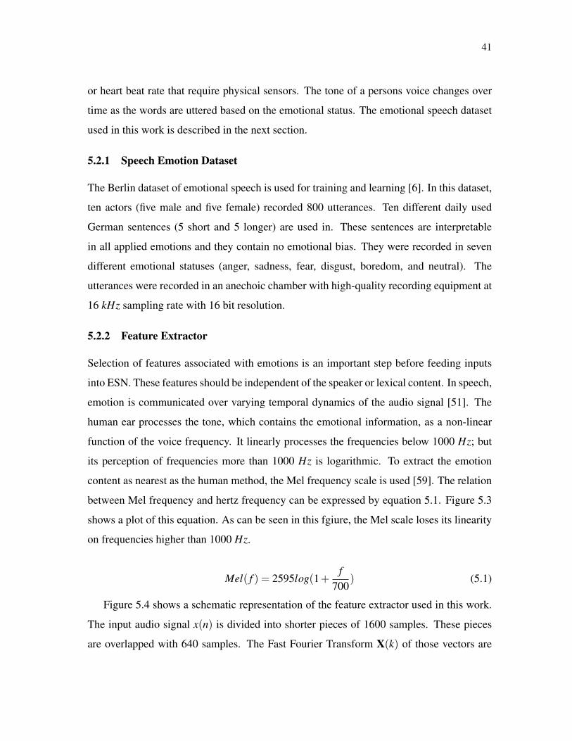
41
or heart beat rate that require physical sensors. The tone of a persons voice changes over
time as the words are uttered based on the emotional status. The emotional speech dataset
used in this work is described in the next section.
5.2.1 Speech Emotion Dataset
The Berlin dataset of emotional speech is used for training and learning [6]. In this dataset,
ten actors (five male and five female) recorded 800 utterances. Ten different daily used
German sentences (5 short and 5 longer) are used in. These sentences are interpretable
in all applied emotions and they contain no emotional bias. They were recorded in seven
different emotional statuses (anger, sadness, fear, disgust, boredom, and neutral). The
utterances were recorded in an anechoic chamber with high-quality recording equipment at
16 kHz sampling rate with 16 bit resolution.
5.2.2 Feature Extractor
Selection of features associated with emotions is an important step before feeding inputs
into ESN. These features should be independent of the speaker or lexical content. In speech,
emotion is communicated over varying temporal dynamics of the audio signal [51]. The
human ear processes the tone, which contains the emotional information, as a non-linear
function of the voice frequency. It linearly processes the frequencies below 1000 Hz; but
its perception of frequencies more than 1000 Hz is logarithmic. To extract the emotion
content as nearest as the human method, the Mel frequency scale is used [59]. The relation
between Mel frequency and hertz frequency can be expressed by equation 5.1. Figure 5.3
shows a plot of this equation. As can be seen in this fgiure, the Mel scale loses its linearity
on frequencies higher than 1000 Hz.
Mel( f ) = 2595log(1+f
700) (5.1)
Figure 5.4 shows a schematic representation of the feature extractor used in this work.
The input audio signal x(n) is divided into shorter pieces of 1600 samples. These pieces
are overlapped with 640 samples. The Fast Fourier Transform X(k) of those vectors are

42
Figure 5.3: Mel scale generated using equation 5.1.
passed to eight triangular Mel-Filters. The limits of the filters are selected to mimic the
human auditory system. The same frequency bands in [52] are used for the Mel-Filters in
this work. Table 5.1 shows these bands. The frequency responses of these triangular filters
are calculated based on equation 5.2.
Figure 5.4: Block diagram of the feature extractor used in this work. The input is an audio signaland the final output is the energy corresponding to the emotion contents of the input signal.

43
Band Start Freq. (Hz) End Freq. (Hz)1 32 5782 257 9643 578 15014 966 22175 1501 31806 2217 44337 3180 69728 4433 8256
Table 5.1: Frequency bands of Mel triangular filters. The start and end frequencies in this tablerepresent bi and di in equation 5.2 respectively.
Hi[k] =
2(k−bi)
(di−bi)−(ci−bi), if bi ≤ k ≤ ci
2(di−k)(di−bi)−(di−ci)
, if ci ≤ k ≤ di
0, otherwise
(5.2)
where i is the index of the filter, Hi is the frequency response of the ith filter. bi, ci and di
are the start, center and end limits of the ith filter.
The amplitude spectrum of the signals analyzed by the Mel-Filter is calculated based
on the responses of the frequency of the filter bands and the absolute value of the FFT H[k]
(Equaion 5.3). This process ends with eight different signals and each signal is analyzed
with FFT to calculate the final features. Based on the length and overlapped values of the
input pieces, the extraction frequency is 25 Hz.
m(i) =K
∑k=0
Hi[k] |X [k]| (5.3)
Figure 5.5 shows the final features of ten neutral and ten anger statuses. It shows that
the response of the third through eighth Mel-Filter bands for the neutral status is very low
while the anger status shows high responses at these bands. This difference is the key to
the classification.
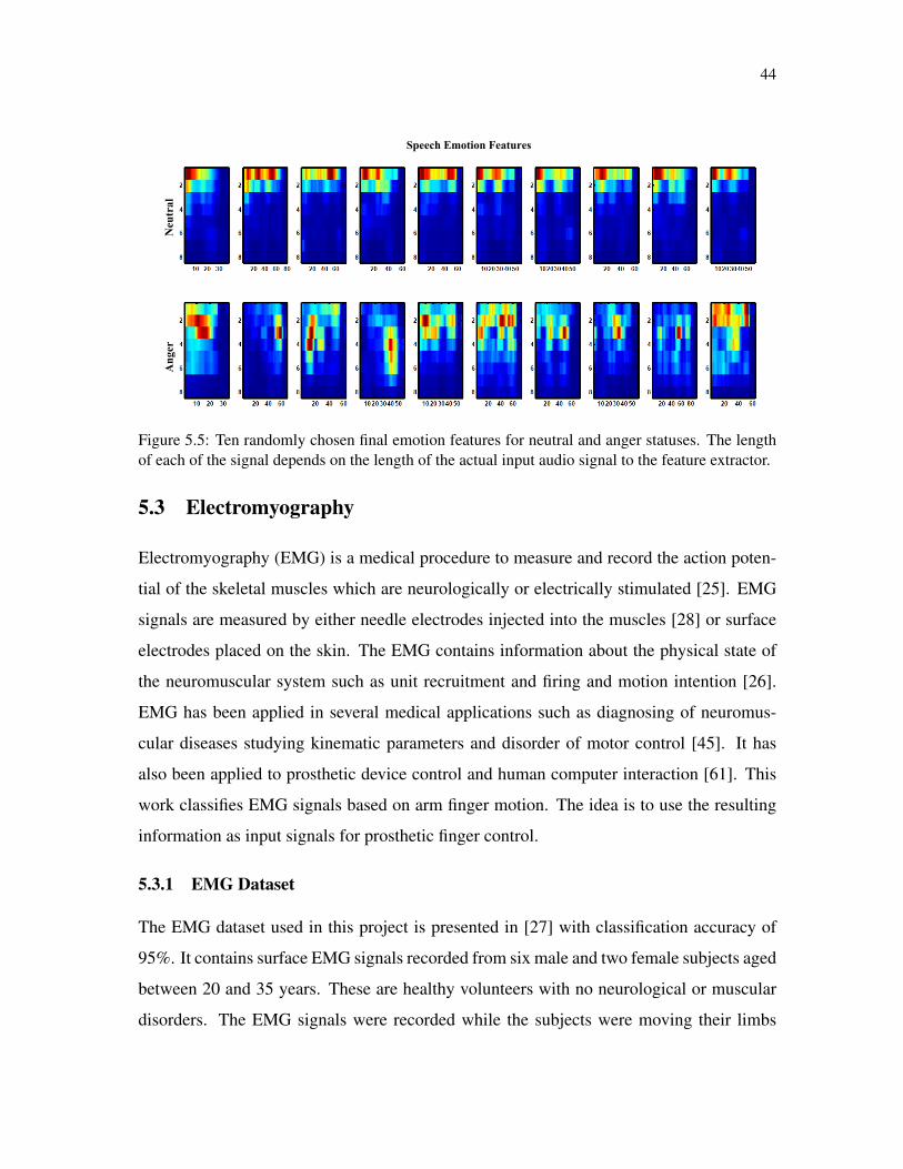
44
Ang
erN
eutr
al
Speech Emotion Features
Figure 5.5: Ten randomly chosen final emotion features for neutral and anger statuses. The lengthof each of the signal depends on the length of the actual input audio signal to the feature extractor.
5.3 Electromyography
Electromyography (EMG) is a medical procedure to measure and record the action poten-
tial of the skeletal muscles which are neurologically or electrically stimulated [25]. EMG
signals are measured by either needle electrodes injected into the muscles [28] or surface
electrodes placed on the skin. The EMG contains information about the physical state of
the neuromuscular system such as unit recruitment and firing and motion intention [26].
EMG has been applied in several medical applications such as diagnosing of neuromus-
cular diseases studying kinematic parameters and disorder of motor control [45]. It has
also been applied to prosthetic device control and human computer interaction [61]. This
work classifies EMG signals based on arm finger motion. The idea is to use the resulting
information as input signals for prosthetic finger control.
5.3.1 EMG Dataset
The EMG dataset used in this project is presented in [27] with classification accuracy of
95%. It contains surface EMG signals recorded from six male and two female subjects aged
between 20 and 35 years. These are healthy volunteers with no neurological or muscular
disorders. The EMG signals were recorded while the subjects were moving their limbs

45
and fingers according to a predefined procedure. Eight surface EMG electrodes were used
to collect the data. The electrodes were placed across the circumference of the forearm as
shown in figure 5.6(a). The signals were amplified to a total gain of 1000. They are sampled
using 12-bits ADC at sampling rate of 4 kHz. The signals are band filtered between 20 and
450 Hz. The dataset is divided into 15 classes based on finger movements. It contains
3 EMG segments of each subject per class. Five classes representing individual finger
movements are used in this project. Figure 5.6(b) shows these classes. The idea is to
classify EMG signals based on finger motions. Figure 5.7 shows EMG signal samples of
individual finger movements for the five classes used in this work.
(a)
(b)
Figure 5.6: (a) Surface electrode placement on the forearm. (b) Five classes of individual fingermovements used in this work [27].
5.3.2 Feature Extractor
Different feature extractors have been used in EMG signal analysis. Two step feature ex-
tractor is used in [27], the first step is mutual information evaluation function, which re-
duces the uncertainty of one random variable, given information of another random vari-
able. The output of this function is projected on principle components analysis (PCA).
Zhang et al. [63] used sampling entropy (SampEN) analysis for detecting onset muscles
activity. SampEn is a modified version of approximate entropy introduced in 2000 by
Richamn and Moorman [47]. It measures the complexity and randomness of physiological
time-series signals independently from length of data segment under test. Pinymork et al.

46
[42] used fifty time and frequency domains features to classify ten upper limb motions.
Results showed that SampEn has the best accuracy compared to other features that were
investigated such as ApEn waveform length (WL), root mean square (RMS), and cepstral
coefficients (CC). This work uses SampEn analysis as feature extractor of EMG before
feeding signals to the ESN. The input EMG segments are divided into short windows of
length 250 ms with 125 ms intervals. The same parameters for SampEn in [42] are used in
this work. The Matlab code for SampEn is developed by Kijoon Lee [31].
5.4 Summary
Three bio-signal benchmarks are used to test the proposed architecture. The EEG sig-
nals are used for epileptic seizures detection, which has several medical applications. The
speech emotion recognition is mainly useful for applications that require human computer
interaction. The EMG signals are used to test electrical activity of skeletal muscles. In
this work EMG signals are used for motion detection. The datasets of these benchmarks
and their feature extractors are described in this chapter. Next chapter presents the results
obtained from applying these signals onto the proposed neuromemristive reservoir archi-
tecture.

47
(a)
(b)
(c)
(d)
(e)
Figure 5.7: EMG signal samples of individual finger movements for (a) Thumb, (b) Index, (c)Middle, (d) Ring, and (e) Little.

48
Chapter 6
Results and Performance Analysis
6.1 Applications
6.1.1 Epileptic Seizure Detection
Two hundred EEG segments (160 for training and 40 for testing) are used for epileptic
seizure detection. The normalized absolute values of these segments are fed into the ESN.
The output of the ESN is compared against a threshold value to calculate the final binary
output.
Two ESN topologies are used for epileptic seizure detection: ring topology and hybrid
topology. Several simulations were conducted for each topology to find the best reservoir
size and alpha value that give the highest classification accuracy. Figure 6.1(b) shows the
testing accuracy vs reservoir size and alpha for the rign and random topologies. In the two
topologies, the accuracy increases as the reservoir size increases. However, the accuracy
stabilizes within a range once the reservoir size exceeds 100 nodes. Changing alpha value
does not have as much affect on the accuracy. In general, alpha value of 0.5 works for the
two topologies. The maximum accuracy achieved is ≈86% and ≈90% for the ring and
hybrid topology respectively. The extra synaptic connection within the reservoir layer is
behind this increase in the accuracy. These connections increase the interaction between
reservoir nodes and provide more information about the overall situation of the reservoir to
each node which increases the response of the reservoir to the changes in the input.
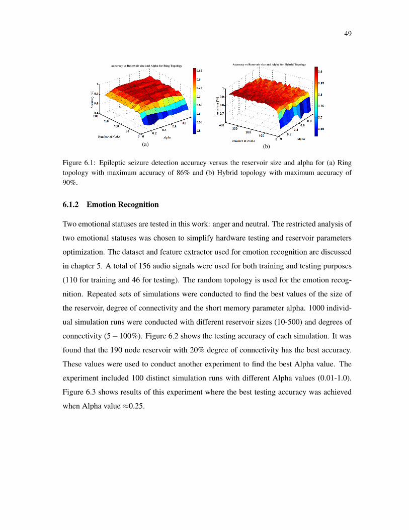
49
Accuracy vs Reservoir size and Alpha for Ring Topology
(a)
Accuracy vs Reservoir size and Alpha for Hybrid Topology
(b)
Figure 6.1: Epileptic seizure detection accuracy versus the reservoir size and alpha for (a) Ringtopology with maximum accuracy of 86% and (b) Hybrid topology with maximum accuracy of90%.
6.1.2 Emotion Recognition
Two emotional statuses are tested in this work: anger and neutral. The restricted analysis of
two emotional statuses was chosen to simplify hardware testing and reservoir parameters
optimization. The dataset and feature extractor used for emotion recognition are discussed
in chapter 5. A total of 156 audio signals were used for both training and testing purposes
(110 for training and 46 for testing). The random topology is used for the emotion recog-
nition. Repeated sets of simulations were conducted to find the best values of the size of
the reservoir, degree of connectivity and the short memory parameter alpha. 1000 individ-
ual simulation runs were conducted with different reservoir sizes (10-500) and degrees of
connectivity (5−100%). Figure 6.2 shows the testing accuracy of each simulation. It was
found that the 190 node reservoir with 20% degree of connectivity has the best accuracy.
These values were used to conduct another experiment to find the best Alpha value. The
experiment included 100 distinct simulation runs with different Alpha values (0.01-1.0).
Figure 6.3 shows results of this experiment where the best testing accuracy was achieved
when Alpha value ≈0.25.

50
Number of Nodes Connectivity[%]
Acc
urac
y [%
]
Accuracy vs Reservoir Nodes and Connectivity
Figure 6.2: The effects of the number of nodes within the reservoir and the degree of connectivity ofthose nodes on the testing accuracy at Alpha ≈0.25. The best accuracy is observed at ≈190 nodesand ≈ 20% connectivity.
Alpha Value
Figure 6.3: The short memory parameter Alpha verses testing accuracy at 190 reservoir nodes with20% connectivity. Best accuracy is observed at Alpha ≈0.25.
One readout layer node was sufficient to classify the two emotional status (Neutral and
Anger). The output of this node is compared against a threshold value to calculate the
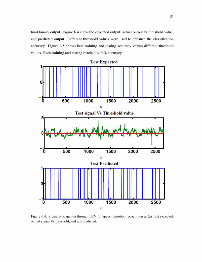
51
final binary output. Figure 6.4 show the expected output, actual output vs threshold value,
and predicted output. Different threshold values were used to enhance the classification
accuracy. Figure 6.5 shows best training and testing accuracy versus different threshold
values. Both training and testing reached ≈96% accuracy.
(a)
(b)
(c)
Figure 6.4: Signal propagation through ESN for speech emotion recognition at (a) Test expected,output signal Vs threshold, and test predicted.
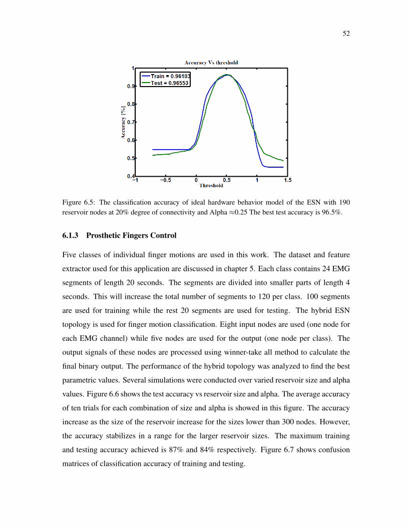
52
Figure 6.5: The classification accuracy of ideal hardware behavior model of the ESN with 190reservoir nodes at 20% degree of connectivity and Alpha ≈0.25 The best test accuracy is 96.5%.
6.1.3 Prosthetic Fingers Control
Five classes of individual finger motions are used in this work. The dataset and feature
extractor used for this application are discussed in chapter 5. Each class contains 24 EMG
segments of length 20 seconds. The segments are divided into smaller parts of length 4
seconds. This will increase the total number of segments to 120 per class. 100 segments
are used for training while the rest 20 segments are used for testing. The hybrid ESN
topology is used for finger motion classification. Eight input nodes are used (one node for
each EMG channel) while five nodes are used for the output (one node per class). The
output signals of these nodes are processed using winner-take all method to calculate the
final binary output. The performance of the hybrid topology was analyzed to find the best
parametric values. Several simulations were conducted over varied reservoir size and alpha
values. Figure 6.6 shows the test accuracy vs reservoir size and alpha. The average accuracy
of ten trials for each combination of size and alpha is showed in this figure. The accuracy
increase as the size of the reservoir increase for the sizes lower than 300 nodes. However,
the accuracy stabilizes in a range for the larger reservoir sizes. The maximum training
and testing accuracy achieved is 87% and 84% respectively. Figure 6.7 shows confusion
matrices of classification accuracy of training and testing.

53
Figure 6.6: The effects of the number of nodes within the reservoir and alpha on the testing accuracyof finger motion recognition using hybrid topology.
(a) (b)
Figure 6.7: Confusion matrix of fingers classification from surface EMG signals using 300 nodeshybrid reservoir for (a) training with accuracy of 87% and (b) testing with accuracy of 84%.
Some applications of human computer interaction may require recognition of one finger
motion. For instance, a signal that can be used to control an on/off button. In such applica-
tion, the classification problem is simplified; instead of recognizing which exact finger is
moving, this application test for movement of a specific finger. The idea is to answer the
question: is finger X is moving or not? regardless of the situation of other fingers. This can

54
be implemented using different post processing step. Instead of winner-take all, a threshold
comparator can be used for each output node. In this application the accuracy increase to a
range from 88% to 95%. Figure 6.8 shows the classification accuracy vs different threshold
value for the five classes. Each class has different threshold value that gives the maximum
accuracy.
Figure 6.8: Classification accuracy of individual finger motion. The accuracy is in a range from88% to 95%.

55
6.2 Reservoir Metrics
The performance of the reservoir is dependent on the randomly generated weights of the
reservoir and several other parameters such as alpha and reservoir size. Finding the best
values for these parameters has been an open question. The over all performance of the
reservoir has been used to study effect of these parameters. This requires a complete train-
ing of the reservoir for a specific application, which takes long time and requires more
processing resources. Further more the best parameter values may vary depending on the
targeted application. More general metrics that are independent from the target output are
required to test the reservoir. These reservoir metrics are measurements of the quality of the
reservoir. Several metrics have been proposed in the literature [40, 18]. Chrol-Cannon et al.
[12] compared the ability of four reservoir metrics to measure the performance of several
reservoir topologies. The reservoir metrics used in this study are: class separation, kernel
quality, Lyapunove’s exponent, and spectral radius. Results showed that kernel quality and
Lyapunove’s exponent strongly correlate with reservoir performance. These two metrics
are used in this work for the hybrid topology while processing two types of data: EEG and
EMG. They are used to study the effect of reservoir size on the quality of the reservoir. The
test is implemented over varied reservoir sizes 10 to 100 node. To study the stabilization of
these metrics hundred trials are used for each size.
6.2.1 Kernel quality
Kernel quality is a measure of linear separation property of the reservoir. It is first presented
in [32] and proposed by Chrol-Cannon et al. [12] as a reservoir metric. The reservoir
response to the whole set of input vectors is used to calculate this metric. The whole
reservoir states are concatenated in a matrix M where each column in M represents reservoir
response to one input vector. The kernel quality is calculated by taking the rank of this
matrix. It represents the network freedom to represent each input stimulus differently. The
target kernel value is equal to the size of the reservoir which means that each reservoir node
generate its unique response that can’t be regenerated by using linear combinations of the
responses of the other nodes.
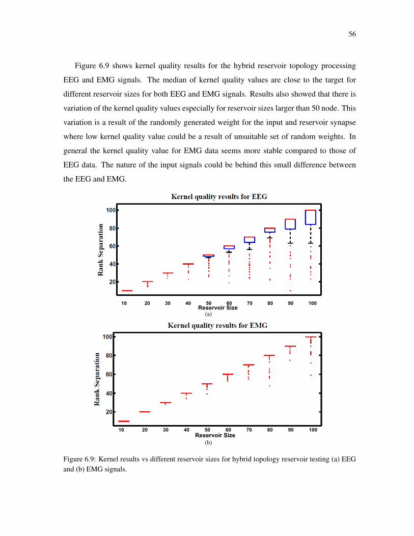
56
Figure 6.9 shows kernel quality results for the hybrid reservoir topology processing
EEG and EMG signals. The median of kernel quality values are close to the target for
different reservoir sizes for both EEG and EMG signals. Results also showed that there is
variation of the kernel quality values especially for reservoir sizes larger than 50 node. This
variation is a result of the randomly generated weight for the input and reservoir synapse
where low kernel quality value could be a result of unsuitable set of random weights. In
general the kernel quality value for EMG data seems more stable compared to those of
EEG data. The nature of the input signals could be behind this small difference between
the EEG and EMG.
10 20 30 40 50 60 70 80 90 100 Reservoir Size
(a)
10 20 30 40 50 60 70 80 90 100 Reservoir Size
(b)
Figure 6.9: Kernel results vs different reservoir sizes for hybrid topology reservoir testing (a) EEGand (b) EMG signals.

57
6.2.2 Lyapunov’s Exponent
Lyapunov’s exponent is a measure of the chaos in the dynamic response of the reservoir.
This metric was formulated in [18]. Equation 6.1 is used to calculate Lyapunov’s exponent
value. Positive values of this metric represent the chaotic dynamic region while negative
values represent the stable region. Since the optimal reservoir performance occurs at the
edge of chaos, Lyapunove’s exponent of zero is desirable.
λ (t) = kN
∑n=1
ln
∥∥∥x j(t)− x j(t)
∥∥∥∥∥∥u j(t)−u j(t)∥∥∥ (6.1)
where u j(t) is an input to the reservoir at time step t. u j(t) is the nearest neighbor to u j(t).
x j(t) and x j(t) are the reservoir response to u j(t) and u j(t) respectively.
Figure 6.10 shows Lyapunov’s exponent results for the hybrid reservoir topology pro-
cessing EEG and EMG signals. Results showed that the values of this metric are higher
than zero for EEG signals while it showed that they are around zero for EMG signals. This
means that the hybrid topology has more chaotic response to the EEG signals compared
to the response of the EMG signals. It also showed that the size of the reservoir process-
ing the EEG signals has low effect on the value of Lyaponv’s exponent compared to the
reservoir processing the EMG signals. As in kernel quality, there is variation in the values
of Lyapunov’s exponent and this is also attributed to the random weights of the input and
reservoir synapses.

58
10 20 30 40 50 60 70 80 90 100 Reservoir Size
(a)
10 20 30 40 50 60 70 80 90 100 Reservoir Size
(b)
Figure 6.10: Lyapunov’s exponent results vs different reservoir sizes for hybrid topology reservoirtesting (a) EEG and (b) EMG signals.
6.3 Power
Power dissipation of four different reservoir topologies is analyzed. The average dynamic
power dissipation is measured in HSPICE for small size reservoirs. The maximum cur-
rent Imax used in the simulation is 10µA. These measurements are quantitatively scaled for

59
larger reservoir sizes. Figure 6.11 shows the power dissipation of three reservoir topolo-
gies, one way ring, two way ring, and hybrid, over different reservoir sizes. The power
dissipation of the three topologies is in tens mile watts. Results showed that the one way
ring topology has lower power consumption compared to the two way ring and hybrid
topologies. This is attributed to the small number of synapses that the one way ring topol-
ogy has where each reservoir layer node has only one synapse. Results also showed that
the relation between power dissipation of these topologies and reservoir size is linear. This
implies that there is no power dissipation overhead for increasing the size of the reservoir.
Figure 6.12 shows the power results for four reservoir topologies: one way ring, two way
ring, hybrid and random. The random topology has higher power dissipation (in order of
several watts) because it has high number of synapses compared to the other topologies. It
also showed that the power dissipation of the random topology is exponentially related to
the size of the reservoir. For this reason the random topology is not desired for the hard-
ware implementation. The power consumption of these topologies can be reduced using
subthreshold designs and other power reduction techniques.
Figure 6.11: Power consumption vs reservoir size of three ESN topologies: one way ring, two wayring, and hybrid. The ring topology has lower power consumption compared to the other topologies.

60
Figure 6.12: Power consumption vs reservoir size of four ESN topologies: one way ring, two wayring, hybrid, and random. The random topology has higher power consumption compared to theother topologies.
6.4 Summary
Three reservoir topologies, ring, hybrid, and random are used for the three applications
implemented in this work. The ring and hybrid topologies are used for epileptic seizure de-
tection. The maximum accuracy achieved using the ring and hybrid reservoir topologies is
86% and 90% respectively. The random topology is used for the emotion recognition with
accuracy of 96%. The hybrid topology is used for prosthetics finger control with accuracy
of 84%. Reservoir quality is analyzed for the hybrid topology using two reservoir met-
rics: kernel quality and Lyapunov’s exponent. Results showed that the hybrid topology has
more stable response to the EMG signals compared to the response to the EEG signals. The
power dissipation of different reservoir topologies is also analyzed. Results showed that the
one way ring topology has lower power consumption compared to the other topologies. It
also showed that the random topology has very high power consumption which makes it
undesirable topology for hardware implementation.

61
Chapter 7
Conclusions and Future Work
7.1 Conclusions
This thesis work proposed a neuromemristive ESN architecture. ESN is a recurrent neural
network that has simplified training algorithm. It has been applied to several spatiotemporal
recognition problems. The untrained recurrent connections within the ESN are used as filter
for extraction of features in the temporal domain. The output of this filter is used to train
the output layer of the ESN using linear regression. The proposed ESN neurmemristive
architecture is useful for power constrained devices. Mixed-signal circuits have high design
cost, but are the prime choice for realizing ESNs. The proposed architecture uses the 2-D
mesh network and doubly twisted toroidal network as interconnection platforms. Several
ESN topologies are implemented on the proposed architecture. The work also proposed a
hybrid ESN topology that has low number of synapses and high connectivity. The choice
between the ESN topologies is determined by the accuracy of the the target application,
input data stream, and hardware resource availability.
Three medical and human computer interaction applications are used to test the pro-
posed architecture. The architecture achieved an accuracy of 90%, 96%, and 84% for
epileptic seizure detection, speech emotion recognition and prosthetic fingers control. The
quality of the ESN is analyzed using kernel quality and Lyapunov’s exponent metrics. The
power consumption of different ESN topologies is also analyzed. The power dissipation
of the one way ring, two way ring, and hybrid topology is in tens mile watts. The ran-
dom topology has higher power consumption compared to the ring and hybrid topologies.
In general, for the applications tested in this work ESN performance is comparable to the
state-of-the-art.

62
7.2 Future Work
The architecture proposed in this work can be used for applications in other therapeutic sys-
tems and body sensors such as diagnose of neuromuscular disease, analysis of ECG/EKG
signals, and prediction of epileptic seizures. Such power constrained devices are on the top
of list of applications that can benefits from the neuromemristive architectures. Further-
more, the applications used in this work can be expanded. For instance, more emotional
statuses can be used in the speech emotion recognition instead of only two statuses. Com-
bined finger motions can be added to the prosthetic finger control. Other ESN topologies
can be explored to increase the accuracy of the system and reduce hardware requirements.
Training circuitry for the memristors can be incorporated in this system. Such circuits
can be used for on chip training. To reduce the power consumption of the architecture,
other synapse and neuron circuit models can be used. These new circuit models can directly
replace the current circuits where the proposed architecture is not constrained to specific
circuits. Subthreshold designs and other power reduction techniques are also a suggested
to reduce the power consumption. The proposed architecture can be expanded for other
types of reservoirs such as liquid state machine.

63
Appendix A
Derivation for Hybrid Topology
A.1 is the traditional equation to calculate the state of the reservoir
X(n+1) = f res (Winu[n+1]+Wxx[n]) (A.1)
The second part of this equation Wxx(n) represents the interconnections within the
reservoir layer. This part can be used to calculate the state of the reservoir layer indepen-
dently from the input layer. In other words, if there are R nodes in the reservoir layer, this
part can be modified to calculate the state of one node in the reservoir layer x(s) as shown
in equation A.2. For derivation purposes, equation A.2 neglects the reservoir activation
function f res and the input to the network u.
x(s) =R
∑r=1
Wx(s)(r)x(r) (A.2)
Wx in equation A.2 can be divided into two groups: W1x and W2x. As shown in
equation A.3.
x(s) =R
∑r=1
W1x(s)W2x(r)x(r) (A.3)
⇒ x(s) = W1x(s)R
∑r=1
W2x(r)x(r) (A.4)
A.4 can be divided into two parts as shown in equation A.5 and A.6.
Xc =R
∑r
W2x(r)x(r) (A.5)
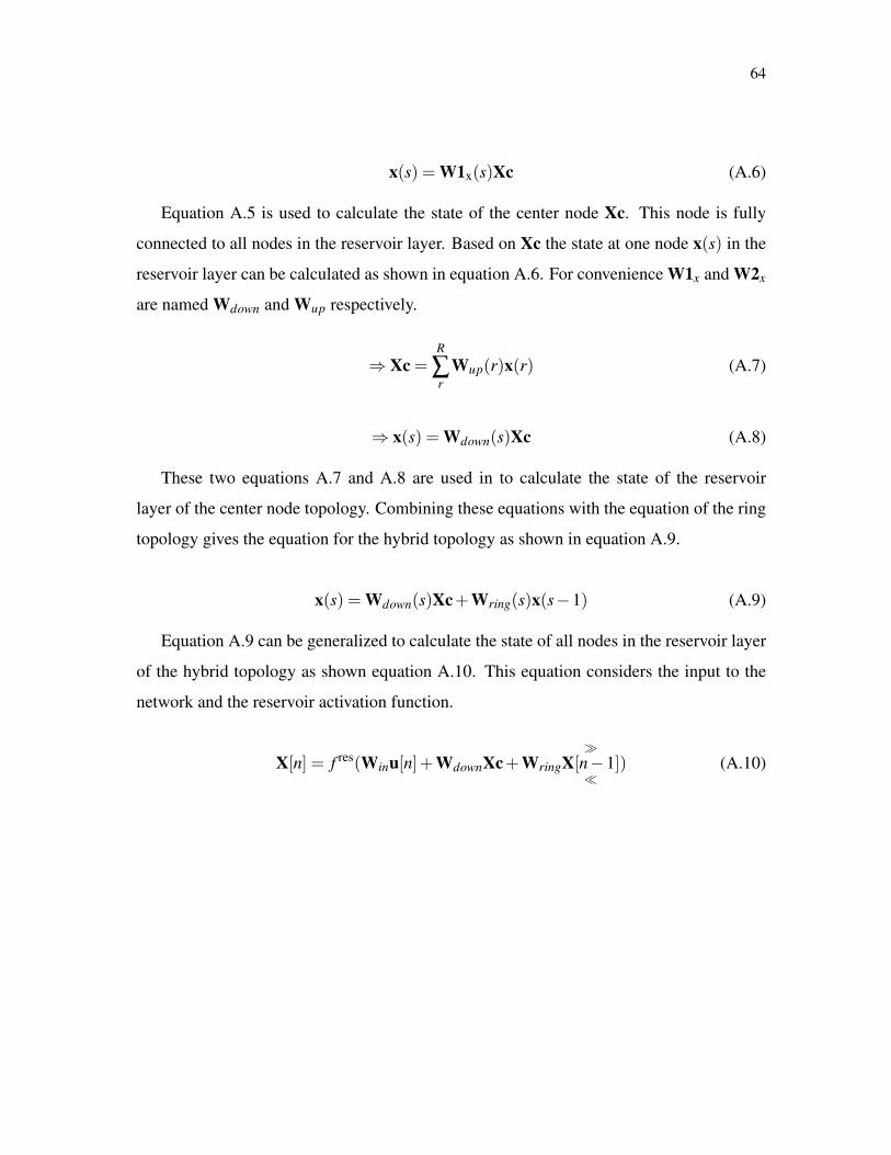
64
x(s) = W1x(s)Xc (A.6)
Equation A.5 is used to calculate the state of the center node Xc. This node is fully
connected to all nodes in the reservoir layer. Based on Xc the state at one node x(s) in the
reservoir layer can be calculated as shown in equation A.6. For convenience W1x and W2x
are named Wdown and Wup respectively.
⇒ Xc =R
∑r
Wup(r)x(r) (A.7)
⇒ x(s) = Wdown(s)Xc (A.8)
These two equations A.7 and A.8 are used in to calculate the state of the reservoir
layer of the center node topology. Combining these equations with the equation of the ring
topology gives the equation for the hybrid topology as shown in equation A.9.
x(s) = Wdown(s)Xc+Wring(s)x(s−1) (A.9)
Equation A.9 can be generalized to calculate the state of all nodes in the reservoir layer
of the hybrid topology as shown equation A.10. This equation considers the input to the
network and the reservoir activation function.
X[n] = f res(Winu[n]+WdownXc+Wring�
X[n−1]�
) (A.10)

65
Bibliography
[1] An introduction to epilepsy. http://www.epilepsy.com/.
[2] Towards intelligent computing with neuromemristive circuits and systems, 2014.
[3] Ralph G. Andrzejak, Klaus Lehnertz, Florian Mormann, Christoph Rieke, PeterDavid, and Christian E. Elger. Indications of nonlinear deterministic and finite-dimensional structures in time series of brain electrical activity: Dependence onrecording region and brain state. Phys. Rev. E, 64:061907, Nov 2001.
[4] Ramon Beivide, Enrique Herrada, Jose L Balcazar, and Jesus Labarta. Optimizedmesh-connected networks for simd and mimd architectures. In Proceedings of the14th annual international symposium on Computer architecture, pages 163–170.ACM, 1987.
[5] J. Burger and C. Teuscher. Variation-tolerant computing with memristive reservoirs.In Nanoscale Architectures (NANOARCH), 2013 IEEE/ACM International Sympo-sium on, pages 1–6, July 2013.
[6] Felix Burkhardt, Astrid Paeschke, Miriam Rolfes, Walter F Sendlmeier, and BenjaminWeiss. A database of german emotional speech. In Interspeech, volume 5, pages1517–1520, 2005.
[7] Lars Busing, Benjamin Schrauwen, and Robert Legenstein. Connectivity, dynamics,and memory in reservoir computing with binary and analog neurons. Neural compu-tation, 22(5):1272–1311, 2010.
[8] Pieter Buteneers, Benjamin Schrauwen, David Verstraeten, and Dirk Stroobandt.Epileptic seizure detection using reservoir computing. In 19th Annual Workshop onCircuits, Systems and Signal Processing, 2008.
[9] Pieter Buteneers, David Verstraeten, Pieter van Mierlo, Tine Wyckhuys, DirkStroobandt, Robrecht Raedt, Hans Hallez, and Benjamin Schrauwen. Automatic de-tection of epileptic seizures on the intra-cranial electroencephalogram of rats usingreservoir computing. Artificial intelligence in medicine, 53(3):215–223, 2011.

66
[10] Jose M Camara, Miquel Moreto, Enrique Vallejo, Ramon Beivide, Jose Miguel-Alonso, Carmen Martınez, and Javier Navaridas. Twisted torus topologies for en-hanced interconnection networks. Parallel and Distributed Systems, IEEE Transac-tions on, 21(12):1765–1778, 2010.
[11] Aaron Carroll and Gernot Heiser. An analysis of power consumption in a smartphone.In USENIX annual technical conference, pages 1–14, 2010.
[12] Joseph Chrol-Cannon and Yaochu Jin. On the correlation between reservoir metricsand performance for time series classification under the influence of synaptic plastic-ity. PLoS ONE, 9(7):e101792, 07 2014.
[13] Leon Chua. Resistance switching memories are memristors. Applied Physics A,102(4):765–783, 2011.
[14] L.O. Chua. Memristor-the missing circuit element. Circuit Theory, IEEE Transactionson, 18(5):507–519, Sep 1971.
[15] Roddy Cowie, Ellen Douglas-Cowie, Nicolas Tsapatsoulis, George Votsis, StefanosKollias, Winfried Fellenz, and John G Taylor. Emotion recognition in human-computer interaction. Signal Processing Magazine, IEEE, 18(1):32–80, 2001.
[16] Colin Donahue, Cory Merkel, Qutaiba Saleh, Levs Dolgovs, Yu Kee Ooi, DhireeshaKudithipudi, and Bryant Wysocki. Design and analysis of neuromemristive echo statenetworks with limited-precision synapses. page Under print, 2015.
[17] Idongesit E. Ebong and Pinaki Mazumder. CMOS and memristor-based neural net-work design for position detection. Proceedings of the IEEE, 100(6):2050–2060, June2012.
[18] Thomas E Gibbons. Unifying quality metrics for reservoir networks. In Neural Net-works (IJCNN), The 2010 International Joint Conference on, pages 1–7. IEEE, 2010.
[19] Jennifer Hasler and Bo Marr. Finding a roadmap to achieve large neuromorphic hard-ware systems. Frontiers in neuroscience, 7, 2013.
[20] K Ishu, Tijn van Der Zant, Vlatko Becanovic, and P Ploger. Identification of mo-tion with echo state network. In OCEANS’04. MTTS/IEEE TECHNO-OCEAN’04,volume 3, pages 1205–1210. IEEE, 2004.
[21] Herbert Jaeger. The echo state approach to analysing and training recurrent neuralnetworks – with an erratum note. Bonn, Germany: German National Research Centerfor Information Technology GMD Technical Report, 148:34, 2001.

67
[22] Herbert Jaeger. Adaptive nonlinear system identification with echo state networks. InAdvances in neural information processing systems, pages 593–600, 2002.
[23] Herbert Jaeger. Tutorial on training recurrent neural networks, covering BPPT, RTRL,EKF and the” echo state network” approach. GMD-Forschungszentrum Information-stechnik, 2002.
[24] Bekir Karlik, M Osman Tokhi, and Musa Alci. A fuzzy clustering neural networkarchitecture for multifunction upper-limb prosthesis. Biomedical Engineering, IEEETransactions on, 50(11):1255–1261, 2003.
[25] Kevin G Keenan, Dario Farina, Roberto Merletti, and Roger M Enoka. Influenceof motor unit properties on the size of the simulated evoked surface emg potential.Experimental brain research, 169(1):37–49, 2006.
[26] KevinG. Keenan, Dario Farina, Roberto Merletti, and RogerM. Enoka. Influenceof motor unit properties on the size of the simulated evoked surface emg potential.Experimental Brain Research, 169(1):37–49, 2006.
[27] Rami N Khushaba and Sarath Kodagoda. Electromyogram (emg) feature reductionusing mutual components analysis for multifunction prosthetic fingers control. InControl Automation Robotics & Vision (ICARCV), 2012 12th International Confer-ence on, pages 1534–1539. IEEE, 2012.
[28] Norito Kokubun, Masahiro Sonoo, Tomihiro Imai, Yumiko Arimura, SatoshiKuwabara, Tetsuo Komori, Masahito Kobayashi, Takahide Nagashima, YukiHatanaka, Emiko Tsuda, et al. Reference values for voluntary and stimulated single-fibre emg using concentric needle electrodes: a multicentre prospective study. ClinicalNeurophysiology, 123(3):613–620, 2012.
[29] Manjari S Kulkarni and Christof Teuscher. Memristor-based reservoir computing. InNanoscale Architectures (NANOARCH), 2012 IEEE/ACM International Symposiumon, pages 226–232. IEEE, 2012.
[30] Duygu Kuzum, Shimeng Yu, and HS Philip Wong. Synaptic electronics: materials,devices and applications. Nanotechnology, 24(38):382001, 2013.
[31] Kijoon Lee. Sample entropy, 2012. http://www.mathworks.com/matlabcentral/fileex-change/35784-sample-entropy.
[32] Robert Legenstein and Wolfgang Maass. Edge of chaos and prediction of computa-tional performance for neural circuit models. Neural Networks, 20(3):323–334, 2007.
68
[33] Matilde Leonardi and T Bedirhan Ustun. The global burden of epilepsy. Epilepsia,43(s6):21–25, 2002.
[34] Mantas LukosEvicIus and Herbert Jaeger. Reservoir computing approaches to recur-rent neural network training. Computer Science Review, 3(3):127–149, 2009.
[35] Mantas Lukosevicius, Herbert Jaeger, and Benjamin Schrauwen. Reservoir comput-ing trends. KI-Kunstliche Intelligenz, 26(4):365–371, 2012.
[36] Wolfgang Maass, Thomas Natschlger, and Henry Markram. Real-time computingwithout stable states: A new framework for neural computation based on perturba-tions. Neural Computation, 14(11):2531 – 2560, 2002.
[37] Carlos Martinez, Ramon Beivide, Esteban Stafford, Miquel Moreto, and Ernst MGabidulin. Modeling toroidal networks with the gaussian integers. Computers, IEEETransactions on, 57(8):1046–1056, 2008.
[38] C. Mead. Neuromorphic electronic systems. Proceedings of the IEEE, 78(10):1629–1636, Oct 1990.
[39] Cory Merkel, Qutaiba Saleh, Colin Donahue, and Dhireesha Kudithipudi. Memristivereservoir computing architecture for epileptic seizure detection. Procedia ComputerScience, 41(0):249 – 254, 2014. 5th Annual International Conference on BiologicallyInspired Cognitive Architectures, 2014 {BICA}.
[40] David Norton and Dan Ventura. Improving liquid state machines through iterativerefinement of the reservoir. Neurocomputing, 73(16):2893–2904, 2010.
[41] Yu V Pershin and Massimiliano Di Ventra. Spin memristive systems: Spin memoryeffects in semiconductor spintronics. Physical Review B, 78(11):113309, 2008.
[42] Angkoon Phinyomark, Franck Quaine, Sylvie Charbonnier, Christine Serviere,Franck Tarpin-Bernard, and Yann Laurillau. Emg feature evaluation for improv-ing myoelectric pattern recognition robustness. Expert Systems with Applications,40(12):4832–4840, 2013.
[43] Matthew D Pickett, Dmitri B Strukov, Julien L Borghetti, J Joshua Yang, Gregory SSnider, Duncan R Stewart, and R Stanley Williams. Switching dynamics in titaniumdioxide memristive devices. Journal of Applied Physics, 106(7):074508, 2009.
[44] Jeyavijayan Rajendran, Harika Manem, Ramesh Karri, and Garrett S. Rose. Anenergy-efficient memristive threshold logic circuit. IEEE Transactions on Comput-ers, 61(4):474–487, 2012.

69
[45] M.B.I. Reaz, M.S. Hussain, and F. Mohd-Yasin. Techniques of emg signal analysis:detection, processing, classification and applications. Biological Procedures Online,8(1):11–35, 2006.
[46] MBI Reaz, MS Hussain, and Faisal Mohd-Yasin. Techniques of emg signal analysis:detection, processing, classification and applications. Biological procedures online,8(1):11–35, 2006.
[47] Joshua S Richman and J Randall Moorman. Physiological time-series analysis usingapproximate entropy and sample entropy. American Journal of Physiology-Heart andCirculatory Physiology, 278(6):H2039–H2049, 2000.
[48] Ali Rodan and Peter Tino. Minimum complexity echo state network. Neural Net-works, IEEE Transactions on, 22(1):131–144, 2011.
[49] Rodrigo Sacchi, Mustafa C Ozturk, Jose C Principe, Adriano AFM Carneiro, andIvan Nunes da Silva. Water inflow forecasting using the echo state network: a brazil-ian case study. In Neural Networks, 2007. IJCNN 2007. International Joint Confer-ence on, pages 2403–2408. IEEE, 2007.
[50] Qutaiba Saleh, Cory Merkel, Dhireesha Kudithipudi, and Bryant Wysocki. Memris-tive computational architecture of the echo state networks for real-time speech emo-tion recognition. page Under print, 2015.
[51] Klaus R Scherer, Tom Johnstone, and Gundrun Klasmeyer. Vocal expression of emo-tion. Handbook of affective sciences, pages 433–456, 2003.
[52] Stefan Scherer, Mohamed Oubbati, Friedhelm Schwenker, and Gunther Palm. Real-time emotion recognition from speech using echo state networks. In Artificial neuralnetworks in pattern recognition, pages 205–216. Springer, 2008.
[53] Carlo H Sequin. Doubly twisted torus networks for vlsi processor arrays. In Proceed-ings of the 8th annual symposium on Computer Architecture, pages 471–480. IEEEComputer Society Press, 1981.
[54] Mark D Skowronski and John G Harris. Automatic speech recognition using a pre-dictive echo state network classifier. Neural networks, 20(3):414–423, 2007.
[55] Dmitri B Strukov, Gregory S Snider, Duncan R Stewart, and R Stanley Williams. Themissing memristor found. Nature, 453(7191):80–3, May 2008.

70
[56] Abdulhamit Subasi, Mustafa Yilmaz, and Hasan Riza Ozcalik. Classification of emgsignals using wavelet neural network. Journal of neuroscience methods, 156(1):360–367, 2006.
[57] Matthew H Tong, Adam D Bickett, Eric M Christiansen, and Garrison W Cot-trell. Learning grammatical structure with echo state networks. Neural Networks,20(3):424–432, 2007.
[58] Andres Upegui and Eduardo Sanchez. Evolving hardware with self-reconfigurableconnectivity in xilinx fpgas. In Adaptive Hardware and Systems, 2006. AHS 2006.First NASA/ESA Conference on, pages 153–162. IEEE, 2006.
[59] Y. Li X. Jiang. A kind of audio data retrieval method based on mfcc[j]. Computerand Digtal Engineering, 36(9):19–21, 2008.
[60] Petros Xanthopoulos, Steffen Rebennack, Chang-Chia Liu, Jicong Zhang, GregoryHolmes, Basim Uthman, and Panos Pardalos. pages 14–19, 2010.
[61] Hong-Bo Xie, Tianruo Guo, Siwei Bai, and Socrates Dokos. Hybrid soft computingsystems for electromyographic signals analysis: a review. Biomedical engineeringonline, 13:8, 2014.
[62] Yulu Yang, Akira Funahashi, Akiya Jouraku, Hiroaki Nishi, Hideharu Amano, andToshinori Sueyoshi. Recursive diagonal torus: an interconnection network for mas-sively parallel computers. Parallel and Distributed Systems, IEEE Transactions on,12(7):701–715, 2001.
[63] Xu Zhang and Ping Zhou. Sample entropy analysis of surface emg for improvedmuscle activity onset detection against spurious background spikes. Journal of Elec-tromyography and Kinesiology, 22(6):901–907, 2012.