design of a high intensity ultrasound dispersion cellri&dsh7rzq synopsis the aim of this project...
TRANSCRIPT

Univers
ity of
Cap
e Tow
n
Design of a High Intensity Ultrasound
Dispersion Cell
Clinton Foster
Supervisor: Dr J. Tapson
Co-supervisor: Dr BJ.P. Mortimer
Submitted to the Faculty of Electrical Engineering, University of Cape Town in
fulfilment of the requirements for the Degree Masters of Science in Engineering.
Cape Town, November 2002
The copyright of this thesis vests in the author. No quotation from it or information derived from it is to be published without full acknowledgement of the source. The thesis is to be used for private study or non-commercial research purposes only.
Published by the University of Cape Town (UCT) in terms of the non-exclusive license granted to UCT by the author.
Univers
ity of
Cap
e Tow
n

Univers
ity of
Cap
e Tow
n
Acknowledgments
First and foremost , I would like to thank Christ for every good thing given to me. For
every honourable, loving and great thing in me, I give praise and credit to Christ
Jesus.
I would also like to thank the following people for their help with this project:
Dr. John Tapson for his role in supervising the project, his encouragement and proof
reading of this dissertation.
Dr. Bruce Mortimer for his encouragement, interest and advice for the duration of the
project.
Mr. Henry Milner for his initiation of the project and his advice on the chemistry
involved as well as the loan of valuable equipment.
Mr. Casius Gourgel for his help with testing and excellence in his work .
Mr. Brett Wilson, Mr. Stanley Adams, Mr. Willem Kriege and Mr. Jacque Wheeler
for their advice, interest and assistance in numerous areas.
Mrs. Jacki Mun-Gavin for her tireless efforts in proof reading this dissertation,
without her assistance this project would not have been completed.
Table olcolltenrs 11

Univers
ity of
Cap
e Tow
n
Declaration
The content of this thesis is my own work if not otherwise referenced and has not
been submitted for any other academic qualification or examination. The opinions
expressed herein are my own and not necessarily that of the University.
Clinton Foster
TaMe ofc Ollf(>nts III

Univers
ity of
Cap
e Tow
n
Synopsis
The aIm of this project was to provide detailed research on the factors causmg
mechanical damage in a high power ultrasound environment, and to give
recommendations for the production of an ultrasonic dispersion cell with a removable
treatment vessel. The primary mechanism for causing this dispersion was cavitation: a
void of air or vapour in a liquid mediwn that grows and collapses in an intense
ultrasonic sound field. The secondary mechanism was a phenomenon called acoustic
streaming which provides a macro mixing effect, also caused by intense ultrasound.
Streaming and, even more so, cavitation were difficult to measure and for this reason
a refinement of a method to map cavitation fields with aluminium foil was developed.
This involved using digital image processing to extract quantitative information from
damaged foil samples.
A large portion of the project focused on the overcommg of absorption and
subsequent rapid attenuation of sound between the transducer (ultrasonic source) and
the treatment vessel. This absorption was due to a number of interrelated factors:
reflection of sound at material boundaries; cavitation clouds causing sound scattering;
energy absorption; and conventional absorption in liquids due to viscous damping. A
number of strategies were employed to overcome this absorption problem: the use of
increased static pressure to suppress cavitation in certain areas; the use of multiple
transducers; and, as a result, multiple paths for the sound to enter the vessel. A
combination of static pressure and multiple transducers were also tested. A number of
different media were tested for their ability to transmit sound and an optimum
solution was recommended. Streaming and the physical constraints affecting
streaming in the treatment vessel were tested to give a practical guide to the factors
producing streaming. Then, as the temperature of the liquid affects absorption,
cavitation threshold, and the ability of a solvent to dissolve, a look at the thermal
aspects of the system was discussed .
In conclusion it was found that the acoustic power delivered to the receptor vessel
could be increased by the use of increased static pressure to limit the cavitation
Table o/confenls IV
Synopsis
The aim of this project was to provide detailed research on the factors causmg
mechanical damage in a high power ultrasound environment, and to give
recommendations for the production of an ultrasonic dispersion cell with a removable
treatment vessel. The primary mechanism for causing this dispersion was cavitation: a
void of air or vapour in a liquid mediwn that grows and collapses in an intense
ultrasonic sound field. The secondary mechanism was a phenomenon called acoustic
streaming which provides a macro mixing effect, also caused by intense ultrasound.
Streaming and, even more so, cavitation were difficult to measure and for this reason
a refinement of a method to map cavitation fields with aluminium foil was developed.
This involved using digital image processing to extract quantitative information from
damaged foil samples.
A large portion of the project focused on the overcommg of absorption and
subsequent rapid attenuation of sound between the transducer (ultrasonic source) and
the treatment vessel. This absorption was due to a number of interrelated factors:
reflection of sound at material boundaries; cavitation clouds causing sound scattering;
energy absorption; and conventional absorption in liquids due to viscous damping. A
number of strategies were employed to overcome this absorption problem: the use of
increased static pressure to suppress cavitation in certain areas; the use of multiple
transducers; and, as a result, multiple paths for the sound to enter the vessel. A
combination of static pressure and multiple transducers were also tested. A number of
different media were tested for their ability to transmit sound and an optimum
solution was recommended. Streaming and the physical constraints affecting
streaming in the treatment vessel were tested to give a practical guide to the factors
producing streaming. Then, as the temperature of the liquid affects absorption,
cavitation threshold, and the ability of a solvent to dissolve, a look at the thermal
aspects of the system was discussed.
In conclusion it was found that the acoustic power delivered to the receptor vessel
could be increased by the use of increased static pressure to limit the cavitation
Table of'contents IV

Univers
ity of
Cap
e Tow
n
(where it was not needed) reduce the scattering beam,
produced positive results. use of multiple transducers also produced good results
when compared to same vessel with only one emitting sound.
Unfortunately, the was not evident multiple transducer
vessel.
Through the factors affecting
streaming and type of system were and an optimised
system was achieved.
o['colltenrs v
it was not
was not
were an
was
v

Univers
ity of
Cap
e Tow
n
Table of Contents
Acknowledgments
Declaration
Synopsis
1 Introduction
1.1 Previous Wark
1.2 Scope and Limitations
1.3 Structure of the Thesis
2 Literature Review
2.1 An Overview of Ultrasonics
2.2 Cavitation
2.2.1 Cavitation Threshold
2.2.2 Cavitation Strength
2.3 Streaming
2.3.1 Radiation Pressure
2.3.2 Acoustic Streaming
Reflections & Transmission of Sound
2.3.3 Reflection at Material Interfaces
2.3.4 Refraction at Material Interfaces
2.3.5 Absorption in Non-Cavitating Liquids
2.4 Transducers
2.4.1 Simple Harmonic Motion and Resonance
2.4.2 Equivalent Circuits
2.4.3 Types ofTransducers
2.4.4 The Piezoelectric Effect
2.4.5 Transducer Construction
2.4.6 Transducer Efficiency
2.4.7 Amplitude Measurement Methods
Table oj'contenfs
Page
ii
iii
iv
1
2
3
5
5
6
6
7
10
10
JJ
12
12
14
15
16
16
20
22
22
23
25
26
VI
Table (:ontents
1 1
1.1
1.2 2
1.3 3
2 5
2.1 5
6
2.2.1 6
2.2 7
2.3 10
2.3../ 10
2. 11
12
2.3.3
2.3.4 at 14
2.3.5 in 15
16
2.4.1 16
2.
2.4.3
2.4.4
2.4.5 23
2.4.6
2.4.7 26
contenrs

Univers
ity of
Cap
e Tow
n
1 Heal Flow
Liquids
2. equivalent circuits 30
3 Experimental Method
3.1 31
3.2 Foil Method
3.3 Digital 33
3.3.1 Analysis and Areas 34
3.3.2 Analysis and
3.3.3 Mean Deviation on 37
3.4 Streaming 38
3.5 Temperature 39
4 Static 40
Design of 40
4.1.1 Design and 41
4.1.2 Plastic Bottle 44
4.1.3 Comparison between Glass and New 44
4.2 Pressure Effects on Transducer 46
4.2.1 Pressure Effect on Power 46
4.2.2 Pressure Effect on Resonant 47
4.3 Static Pressure Effect on Disruption
4.4 Differential Pressure Testing
4.4.1 Effects of Water Level Variations
4.5 Conclusion 51
5 Tri-Reactor Vessel
5.1 Experimental Apparatus
Design and Construction 53
J
Selection
Modes
comcms Vll
3
4
5
J
1.5.2
253
254
3.1
3.2
3.3
3.3.1
3.
3.3.3
3.4
4.1
4.1.1
4.
4.J.3
.1
1
5.1
J
comcms
'1
"
3.1
3
Areas
3
38
51
53

Univers
ity of
Cap
e Tow
n
5.3 Mapping the Sound Field
5.3.1 Focusing 57
Optimising the Receptacle 58
5.4.1 ofMultiple Transducer on Receptacle Disruption 59
5.4.2 Plastic 60
5.4.3 Receptacle material 61
5. 63
5.4.5 Triangular Receptacle 63
5.5 Pressurizing 64
1 Effects on 64
5.5.2 Effects on Power 65
5.5.3 Differential FrL>(>(>1JrO Effects 66
5.6 Comparison between Tri-reactor and Vibracel Unit
Conclusion 68
6 Transmission Media 69
6.1 Acoustic 69
6.1.1 Theoretical Calculations 70
6.1.2 Attenuation the System 71
6.1.3 Affect ofsolutes on Vapour 73
6.2 Transmission Media
6.2.1 of Various Media 74
6.2.2 Optimising Solution 75
7 77
7.1 Test Conditions
Intensity 80
7.3 Distance Transducer 81
7.4 Bottle
83
Conclusion 83
8 Shocking 84
8.1 Test Conditions 84
8.2 Temperature on Cavitation 86
contents
6
7
8
5.3
5.3.1
5,4
5.4.1
5.
5.4.3
5.
5.
1
552
3
5.7
6.1
6.1.1
6.1.2
6.1.3
7.1
.1
6J2
8.1
contents
on
on
on
on
57
75
80
81

Univers
ity of
Cap
e Tow
n
8.3 Use of Analogue Computers in Temperature Calculations
8.4 Temperature Profiles
8.4.1 Varying Volume Ratios
8.4.2 Equivalent Circuits
8.4.3 Ultrasonic Energy Effects
9 Conclusion & Future Recommendations
10 References
Appendix A
Appendix B
Appendix C
Appendix D
87
88
88
90
91
93
95
I
II
III
IV
To bl(! 0/collten!s IX
8.3 Use of Analogue Computers in Temperature Calculations
8.4 Temperature Profiles
8.4.1 Varying Volume Ratios
8.4.2 Equivalent Circuits
8.4.3 Ultrasonic Energy Effects
9 Conclusion & Future Recommendations
10 References
Appendix A
Appendix B
Appendix C
Appendix D
Table> o/contents
87
88
88
90
91
93
95
I
II
III
IV
IX

Univers
ity of
Cap
e Tow
n
1 Introduction
The object of this thesis was to investigate the factors contributing to and influencing
ultrasonic dispersion, in an attempt to optimise both the cavitation and streaming
effect associated with high power acoustics. This was done with the intention of
designing and building an ultrasonic dispersion cell with a removable treatment vessel
for the processing of a wide range of organic samples, thereby providing a stable,
controllable platfonn for biochemical researchers.
In this context, dispersion is defined as a process where a solid is dissolved or at least
broken down to small particles typically in a liquid medium. This has many industrial
applications; high power ultrasound is being used to homogenise or mix paints, in
breaking of micro-organism cells and as a catalyst to chemical reaction (due to the
thorough micro-mixing properties of high intensity ultrasound).
1.1 Previous Work
This project was based on and a continuation of research by Ricardo de Quieros into
ultrasonic dispersion. It is therefore important that the key issues of his findings are
briefly discussed: [12J
A wide variety of ultrasonic apparatus and sources were experimented with, revealing
the need for a high power (above 200 Watts) and high intensity system. The
importance of delivering high intensity acoustic energy to the receptor vessel was
obvious. A serious power saturation problem became evident during his research
(where an increase in the acoustic power above 80 Watt would not increase the
acoustic intensity in the receptor vessel). Mr De Quieros found that a commercial
unit, the VCX500 manufactured by Vibracel, provided a flexible powerful (up to 500
introductioll
u
1,1 Previ
was
A
was to
an
s Work
[ 12J
on
It is
an Increase
a
Introduction
This \;v'as
high'
sources were
200 Watts) and
a id is
a
to
a
or at
to
are
was
to

Univers
ity of
Cap
e Tow
n
Watts) system in which to conduct optimisation experiments and, as a result, that
became the main ultrasonic source used in this project. [12]
There is much work on the effect of high power ultrasound and the many areas that
have been advance by using ultrasonic properties. C. Suri (et al) present a system that
has similarities to this project in that the streaming properties are used to mix liquids
in a chemical reaction vessel, therefore acting as a catalyst. The streaming is
generated with the use of two transducers in different planes and measured with the
aid of an iodide solution, a laser and a receiver diode arrangement. This system,
however, only uses the streaming effects of high frequency ultrasound and therefore
does not consider cavitation. [13]
N.A. Tsochatzidis (et al) describe a method of cavitation cloud measurement where a
laser is passed through the cavitation cloud, using Doppler shift to give velocity and
cavitation bubble average size. [14] Yet another advanced method of cavitation cloud
measurement makes use of X-ray equipment to take snap shots of cavitation fields.
[15] Although these methods of measurement are complex and costly, they show the
cutting edge in ultrasonic effect measurement.
1.2 Scope and Limitations
This project was primarily concerned with the investigation into the effects of
cavitation and streaming in terms of their ability to disperse or process a wide variety
of biological samples for research purposes. The intention of the project was not to
investigate the effects of ultrasound on biological samples but to provide a stable,
well-defined platform so that experts in their respective fields can conduct research
using high power ultrasound. In order to achieve this, both the cavitation and the
streaming effects need to be consistently reproduced and the factors influencing them
need to be well understood within the context of the project. The requirement that the
treatment vessel should be removable is what sets this project apart from a typical
ultrasonic cleaning bath, and significantly complicates the design. A major limitation
on this design is the FDA's (Food and Drug Administration's) rules and regulations on
/ntrodUCI ion 2

Univers
ity of
Cap
e Tow
n
pennissible materials and other possible contaminating effects on the orgamc
samples, as it is envisaged that this device will be used, among other things, in the
food industry. In the original design requirements the removable processing vessel
was to be of a small volume, less than one hundred millilitres.
1.3 Structure of the Thesis
Introduction: An explanation of the project's main research objectives, restrictions
and scope, as well as a short review of previous, (including the most recent) work in
the field.
Literature review: This chapter contains a comprehensive review of previously done
work relating to this project, including both theory and practical tests done with
specific application to this project.
Experimental Methods: This chapter contains infonnation on the basic experimental
set-up that explains methods of quantifying both streaming and cavitation fields. It
also considers the mean error or accuracy involved in these methods.
Static Pressure: This chapter looks at the construction/adaptation of an ultrasonic
vessel to study the effects of static pressure on cavitation threshold and its disruptive
ability. Included is a discussion on the effects of static pressure on the transducer and
electronics.
Tri-reactor VesseJ: This chapter looks at the design and testing of a three-transducer
bath with the intention of gauging the effectiveness of using multiple transducers in a
dispersion system. The combination of static pressure and the multiple transducers is
also investigated.
Transmission Media: This chapter considers a wide variety of materials for their
acoustic transmission of high power ultrasound. This was primarily aimed at
IIltroc/uclion 3
pennissible materials and other possible contaminating effects on the orgamc
samples, as it is envisaged that this device will be used, among other things, in the
food industry. In the original design requirements the removable processing vessel
was to be of a small volume, less than one hundred millilitres.
1.3 Structure of the Thesis
Introduction: An explanation of the project's main research objectives, restrictions
and scope, as well as a short review of previous, (including the most recent) work in
the field.
Literature review: This chapter contains a comprehensive review of previously done
work relating to this project, including both theory and practical tests done with
specific application to this project.
Experimental Methods: This chapter contains infonnation on the basic experimental
set-up that explains methods of quantifying both streaming and cavitation fields. It
also considers the mean error or accuracy involved in these methods.
Static Pressure: This chapter looks at the construction/adaptation of an ultrasonic
vessel to study the effects of static pressure on cavitation threshold and its disruptive
ability. Included is a discussion on the effects of static pressure on the transducer and
electronics.
Tri-reactor Vessel: This chapter looks at the design and testing of a three-transducer
bath with the intention of gauging the effectiveness of using multiple transducers in a
dispersion system. The combination of static pressure and the multiple transducers is
also investigated.
Transmission Media: This chapter considers a wide variety of materials for their
acoustic transmission of high power ultrasound. This was primarily aimed at
I II troc/uC: l ion 3

Univers
ity of
Cap
e Tow
n
cavitation suppression but also attempted to match acoustic impedances as best as
possible for real liquids.
Streaming: This chapter investigates the factors affecting acoustic streaming in the
receptor vessel, in telTIlS of its velocity and magnitude and the factors which affect
them.
ThelTIlal Shocking: This chapter looks at the uses of rapid temperature cycling to
assist in the dispersion process. A method of estimating real temperature profiles
based on measured temperatures is presented.
Conclusion and Future Recommendations: A review of relevant findings and how
they affect the design of an ultrasonic dispersion unit as a whole, as well as other
possible areas for further research.
ilztroductioll 4
cavitation suppression but also attempted to match acoustic impedances as best as
possible for real liquids.
Streaming: This chapter investigates the factors affecting acoustic streaming in the
receptor vessel, in tenns of its velocity and magnitude and the factors which affect
them.
Thennal Shocking: This chapter looks at the uses of rapid temperature cycling to
assist in the dispersion process. A method of estimating real temperature profiles
based on measured temperatures is presented.
Conclusion and Future Recommendations: A review of relevant findings and how
they affect the design of an ultrasonic dispersion unit as a whole, as well as other
possible areas for further research.
f Iltrod liCli 011 4
Univers
ity of
Cap
e Tow
n
2 Literature Review
chapter ofa of the done by in the of ultrasound
and relevant areas. It with a overview and background into
ultrasound then to the fundamental of power
ultrasonics, with the core being on cavitation and streaming. It is then followed
by an investigation into reflection and transmission of sound at material boundaries
and materials respectively. modes operation vanous
related properties are discussed, since transducers form an integral part of
any ultrasound Lastly, a thermal theory was presented, as temperature
an important role in a solvent's ability to as well as affecting cavitation.
2.1 An Overview of Ultrasonics
Ultrasound, simply, is a sound wave whose frequency is too for the human
auditory system to hear typically from 18 kHz upwards into the MHz range and
beyond. Over ultrasound been many new applications
including imaging as as mechanical water purification,
distance measuring food and many other areas that are still nrrH't>C'C'
developed. [3] [I
Literature Review 5
consists a of
an s to as as
1 u
a is too
water
areas are
[1
5

Univers
ity of
Cap
e Tow
n
2.2 Cavitation
already mentioned, streaming perform an In somc
a disruptive force required to samples,
while the streaming quality. create an
effective homogenisation Both cavitation and occur at similar
acoustic intensities, but they are distinctly terms of the
factors that influence and occurrence. This the
factors causing cavitation the physical properties contributing to strength. It
then goes on to radiation pressure and the factors acoustic
streaming. [2] [1]
2.2.1 Cavitation
Cavitation, loosely is a rupture or cavity IS a liquid when the
tensile force on liquid molecules is larger than vapour cavities
subsequently violently, sending out shock waves and powerful micro
jetting destructive to erode metal jetting defines a
situation collapses from one side a of high velocity
liquid and out the other side. [20]
The to initiate cavitation would have to of the order of 1000 atm
for water in However, the minute gas bubbles and
impurities liquids provide a which a cavity can form at
much lower These gas bubbles or cavitation nuclei
and are source of most common cavitations. in the ultrasonic
context is provided by an oscillating sound which creates a sinusoidal by
During the rarefaction vapour filled bubble
In bubble then, (during the stage) collapses due to
by surface tension bubble closed. The pressure
cavitation occurs at is equation below. [4]
Review 6
2 avitation
1
and are
context is
to
11
macro mIx
occurrence.
or
to
most common
occurs at is
an some
create an
It
a !
a
a
atm
at
6

Univers
ity of
Cap
e Tow
n
Equation 2-1p - p + P + P _ 2(J"~ rhres - sal _ vap storie gas / RO
Where (J" is surface tension and Ro is initial bubble radius. This shows that an increase
in vapour pressure ( P.UI_ vap) or static pressure (~lGliC ) increases the threshold pressure
(~hres). The increasing of threshold pressure has the effect of suppressing cavitation.
However, if one increases the sound pressure above the threshold pressure, the liquid
will again begin to cavitate. The simultaneous increasing of both the sound and
threshold pressure would not cause an increase in cavitation strength, as one would
expect. The factors influencing cavitation strength will be discussed in the next
section. [4]
The equation:
~hres =O.7(Tboil - T) + 1 [Atm] Equation 2-2
gIves an estimate of threshold pressure as a function of liquid temperature. It is
interesting to note that the boiling point (Tboil ) is used in the calculation, implying that
if one increases the boiling point of a liquid it will raise the threshold pressure. This
correlates with the above reference to saturated vapour pressure because boiling point
is linked to vapour pressure. Thus it can be seen how temperature, vapour pressure
and static or atmospheric pressure affect the cavitation threshold. [2J
2.2.2 Cavitation Strength
The strength of cavitation, among other things, is proportional to the ratio of
maximum bubble radius over initial bubble radius Rmax [2]. This makes sense when Ro
looking at where the energy that is released during a cavitation comes from. It
originates primarily from surrounding liquid rushing into the cavity. The larger the
cavity radius just before collapse and the less gas in the initial bubble, the larger the
Literature Review 7
p - p + P + P _ 2(J" ~ rhres - sal _ vap slat;c g as / Ro
Equation 2-1
Where (J" is surface tension and Ro is initial bubble radius. This shows that an increase
in vapour pressure ( P.UI_ vap) or static pressure (P.WliC) increases the threshold pressure
(~hres). The increasing of threshold pressure has the effect of suppressing cavitation.
However, if one increases the sound pressure above the threshold pressure, the liquid
will again begin to cavjtate. The simultaneous increasing of both the sound and
threshold pressure would not cause an jncrease in cavitation strength, as one would
expect. The factors influencing cavitation strength will be discussed in the next
section. [4]
The equation:
~hres = O.7(Tboil - T) + 1 [Atm] Equation 2-2
gIves an estimate of threshold pressure as a function of liquid temperature. It is
interesting to note that the boiling point (Tboil ) is used in the calculation, implying that
jf one increases the boiling point of a liquid it will raise the threshold pressure. This
correlates with the above reference to saturated vapour pressure because boiling point
is linked to vapour pressure. Thus it can be seen how temperature, vapour pressure
and static or atmospheric pressure affect the cavitation threshold. [2]
2.2.2 Cavitation Strength
The strength of cavitation, among other things, is proportional to the ratio of
maximum bubble radius over initial bubble radius Rmax [2]. This makes sense when Ro
looking at where the energy that is released during a cavitation comes from. It
originates primarily from surrounding liquid rushing into the cavity. The larger the
cavity radius just before collapse and the less gas in the initial bubble, the larger the
Literature Review 7
Univers
ity of
Cap
e Tow
n
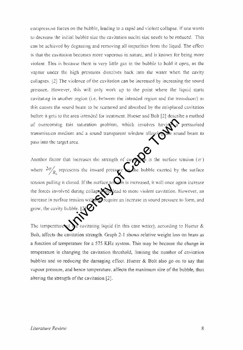
compressive forces on bubble, leading to a rapid and violent col If one wants
to the initial bubble size cavitation nuclei size to be reduced. This
can be and removing all impurities from the liquid. The
is that the cavitation becomes more vaporous in nature, and is known for more
violent. This is because there is very little gas in bubble to hold it open, as the
vapour under high pressures dissolves back the water when the cavity
collapses. The violence of the cavitation can be increased by increasing the sound
However, will only work up to the point where liquid starts
cavitating in another (i.e. between intended region and the as
this causes the sound beam to be by the cavitation
h",+",..", it to the area intended for treatment. Hueter and Bolt [2] a method
of this saturation problem, which involves having a pressurised
transmission medium and a sound transparent window allowing the sound beam to
into target area.
factor that of cavitation is the tension (a)
where inward on the bubble by the p-v,>rt",·t1
tension pulling it If the surface tension is it will once again increase
the involved during collapse and to more violent cavitation. However, an
increase in surface tension will also require an sound to form,
the bubble. [2]
The temperature of the cavitating liquid (in this case water), according to &
the cavitation strength. Graph 1 shows weight on brass as
a function of temperature for a be because the change in
temperature is changing the cavitation threshold, the number of cavitation
bubbles and so reducing the damaging effect. Hueter & Bolt go on to that
vapour hence the maximum of the bubble, thus
the strength the cavitation [2].
Literature Review 8
to
can
.IS
tension
mcrease
a
on
area.
to a
a
an
case
a1
IS
to
to
one wanis
more
starts
as
to
(0')
m.crease
, an
as
m
8

Univers
ity of
Cap
e Tow
n
60
50
lO
o
(\
/ ,
1/v \
'" '"r---20 30 40 50 60 70 80 90 100
Temperature, 'C
Graph 2-1 Relative Weight Loss in Cavitation Erosion as a Function of Temperature [2]
Pg 235
M. H. Entezari (et al), using the oxidation of iodine to measure cavitation intensity in
a 20 KHz system, found the cavitation strength to falloff with an increase of
temperature, and attributed this to more vaporous type cavitation occurring at lower
temperatures. M. H. Entezari (et al) also present a graph of similar shape to that in
Graph 2-1 for a 900KHz system, showing the effect of different frequencies on
cavitation strength where temperature is concerned. Based on these findings a lower
temperature would be better for violent cavitation at 20Khz. [19]
M. H. Entezari (et al) conducted tests varying the gas content of the liquid, using the
same iodine oxidation rate as an indicator, concluding that the effect of introducing
gas had little effect at 20 kHz [19]. This finding is contrasted by other researchers'
findings that state that the introduction of gas bubbles reduces the vaporous type
cavitation. [2]
Literature Review 9

Univers
ity of
Cap
e Tow
n
2.3 Streaming
As already mentioned, acoustic streaming is responsible for mixing and stirring in the
treatment vessel. Obviously, the more pronounced the streaming effect, the better, as
this will cause a more thorough mixing and stirring action.
2.3.1 Radiation Pressure
There are many possible causes of radiation pressure and, subsequently, streaming,
but in this environment it is most likely a combination of Radiation and Oseen forces.
Radiation forces are primarily due to the scattering of sound waves on impurities and,
of course, cavitation bubbles. Oseen forces are generated by ultrasonic wave
distortion, which is due to non-linearities in the liquid (caused by cavitation, among
other things). The drag coefficients of the two forces, which give a measure of the
radiating force, are as follows : [2]
Radiation Forces 1.2(kr)4 Equation 2-3
Equation 2-4 Oseen Forces
where k is OJ/ (Frequency over sound velocity), r is the particle radius, c2 = u 2 j is/ c j uo
the fractional second harmonic content (amount of the wave which has distorted to its
second harmonic) and cp is the phase shift between the fundamental and the second
harmonic.
Literature Review 10
2.3 Streaming
As already mentioned , acoustic streaming is responsible for mixing and stirring in the
treatment vessel. Obviously, the more pronounced the streaming effect, the better, as
this will cause a more thorough mixing and stirring action.
2.3.1 Radiation Pressure
There are many possible causes of radiation pressure and, subsequently, streaming,
but in this environment it is most likely a combination of Radiation and Oseen forces.
Radiation forces are primarily due to the scattering of sound waves on impurities and,
of course, cavitation bubbles. Oseen forces are generated by ultrasonic wave
distortion, which is due to non-linearities in the liquid (caused by cavitation, among
other things). The drag coefficients of the two forces , which give a measure of the
radiating force, are as follows: [2]
Radiation Forces 1.2(kr)4 Equation 2-3
Oseen Forces Equation 2-4
where k is OJI (Frequency over sound velocity), r is the particle radius, c2 = u2 / is I c / uo the fractional second hannonic content (amount of the wave which has distorted to its
second hannonic) and qJ is the phase shift between the fundamental and the second
hannonic .
Literature Review 10

Univers
ity of
Cap
e Tow
n
2.3.2 Acoustic Streaming
streaming is simply reaction of a fluid to forces discussed above. The
fluid is also by factors such as viscosity, density physical
vessel. becomes a complex problem
that is case "' ....0" .... The the Radiation an
idea of the factors influencing streaming. In Shutilov [4] and Beyer [8] it is that
the is proportional to the total acoustic absorption coefficient of fluid.
with Oseen as the harmonic distortion is a form of absorption
in the liquid.
Shutilov [4] gives the following equation for calculating this
2-5[4] pg 1
an unbounded situation is given by:
2
-"--~c- [4] 2-6
3poco
(et al) gives a simplified equation streaming velocity
Equation 2-7[18]
both fl and are the coefficient intensity, R is
radius, Po IS mean density, IS mean P the
power, Ya coefficient, and a is the absorption coefficient
amount and of is proportional to This is unfortunate
because cavitation is more pronounced at low ifone more
acoustic streaming and can afford to reduce the cavitation this could by
increasing the frequency of the sound wave. [19] It is must also be that
increases the absorption, and the streaming
but decreases and that
velocity is proportional to acoustic [4] [1
Literature 11
2
a to
an
3S IS a
2-5
an IS
a
[1 2-7
are IS R is
a IS
more
wave. [19] It is must
IS to [1
11

Univers
ity of
Cap
e Tow
n
Reflections &Transmission of Sound
The transmission of sound is of great importance in terms of the delivery of maximum
acoustic intensity, as well as the use of reflection boundaries as a mechanism for
creating standing waves. This section begins with a discussion of sound wave
reflection at material interfaces or boundaries and then goes on to look at some of the
factors influencing the absorption in liquids that are not cavitating.
2.3.3 Reflection at Material Interfaces
The explanation of reflection and transmission, for the time being, will be restricted to
orthogonal incident waves, but will be extended to other angles of incidence. As is
well known, sound waves, such as a loud shout, are reflected off cliff faces, echoing
back. The precise amount of sound energy that is reflected by and transmitted through
a medium interface can be calculated using the two media's acoustic impedances.
The accoustic impedance (Z) is calculated from two physical properties, namely the
product of density (P) and sound speed (c). This is very useful if one wants to
manipulate the amount of reflection/transmission at medium interfaces. There are four
variables that can be tuned: density and sound speed for both of the media.
z =pc Equation 2-8
Literature Review 12
Reflections & Transmission of Sound
The transmission of sound is of great importance in terms of the delivery of maximum
acoustic intensity, as well as the use of reflection boundaries as a mechanism for
creating standing waves. This section begins with a discussion of sound wave
reflection at material interfaces or boundaries and then goes on to look at some of the
factors influencing the absorption in liquids that are not cavitating.
2.3.3 Reflection at Material Interfaces
The explanation of reflection and transmission, for the time being, will be restricted to
orthogonal incident waves, but will be extended to other angles of incidence. As is
well known, sound waves, such as a loud shout, are reflected off cliff faces, echoing
back. The precise amount of sound energy that is reflected by and transmitted through
a medium interface can be calculated using the two media's acoustic impedances.
The accoustic impedance (Z) is calculated from two physical properties, namely the
product of density (P) and sound speed (c). This is very useful if one wants to
manipulate the amount of reflection/transmission at medium interfaces. There are four
variables that can be tuned: density and sound speed for both of the media.
z =pc Equation 2-8
Literature Review 12

Univers
ity of
Cap
e Tow
n
Figure 2-1 shows an wave by , the reflected wave
transmitted wave
Material 1
Boundary
Material 2
2-1 Sound Wave Reflection and Transmission [8] 48
The amount energy reflected is calculated by
Equation 2-9 [8J Pg 49
and amount of energy IS by
Equation 2-10 [8J Pg 49
Although above discussion is limited to orthogonal wave material boundaries, the
two equations may still used for magnitude calculations for the orthognal
in the next the angles are as shown in the
following sub-section.
Review 13
Univers
ity of
Cap
e Tow
n
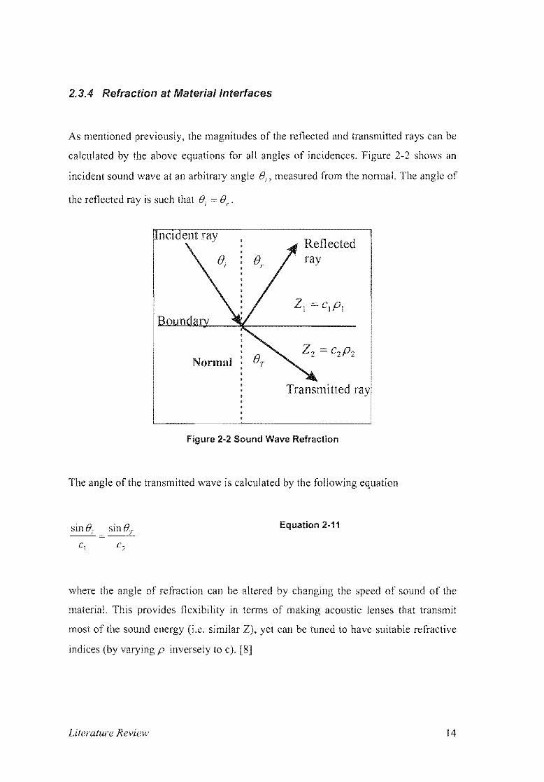
2.3.4 Refraction at Material Interfaces
As mentioned the magnitudes of the reflected and transmitted rays can be
calculated by the above for all of Figure an
incident sound wave at an angle ();, measured from the nonnal. The
ray IS that (); =
Normal
Transmitted
2-2 Sound Wave Refraction
of the wave is calculated by the following equation
2-11
where the of refraction can altered by changing the of sound the
This flexibility tenns of acoustic that transmit
most the sound (i.e. similar can be to have suitable refractive
indices (by varying p to c). [8]
Literature 14

Univers
ity of
Cap
e Tow
n
5 Absorption in Non-Cavitating Liquids
The absorption of in a non-cavitating liquid is by frictional
or viscous damping consequently,
I = -2ax Equation 2-12 x
of sound as a function distance x, which is an exponential
falloff where by sum the
friction the liquid and the conduction as below:
Equation 2-13
Where Internal friction according to Stokes is
8 Equation 2-14 a = ---'- 128 r 3
and Conduction (Kirchoff)
2J[ 2cKTa 2 Equation 2-15
a, = N
0 • [3J Pg 129
In the above equations co is 11 is viscosity, c is velocity, p is
the K is thernlal T the in Kelvin, a the thern1al
coefficient expansion, A the wavelength, the mechanical equivalent heat and
specific heat of the liquid. A a would result a rapid falloff
intensity as waves travel a liquid. To the m liquid
sound frequency and viscosity should reduced, the sound speed and density
should be increased, among other
Literature 15
5
IS
or
2m 2-12
as a IS an
sum
as
(l::::: 2-13
IS
8 2-14 - ................................... , ... . 3
2-15
co IS 11 IS C IS P IS
15

Univers
ity of
Cap
e Tow
n
2.4 Transducers
Transducers are responsible for the generation ultrasonic energy or, more
the conversion energy from one form to another (in this case to
mechanical energy). Modern use a complex combination of
materials to create an ultrasonicelectrical and
source. It is therefore important that of simple
harmonic motion and resonance, the implications transducers, and the use of
equivalent circuits for a simple analysis transducers. In addition to this, various
types of transducers are discussed, operation of piezoelectric materials is then
explained and, finally, a few critical properties of transducers are mentioned.
2.4.1 Simple Harmonic Motion and Resonance
In order to explain harmonic motion and to create an intuitive understanding of
how a system would a basic example of a mass on the end of a will
be to lay a foundation.
K
2·3 Mass and Spring [2] Pg 14
In the system shown in Figure above, are two potential forces exerted
on the mass: firstly, force by the spring which is proportional to the
displacement, but in the opposite direction to displacement as defined by the
equation = - Ku ,where is Hooke's spring constant as defined law
U IS secondly, the force as a result of acceleration that is the
same direction as the acceleration as defined by the equation F = ma where m is the
]6Literature
Univers
ity of
Cap
e Tow
n
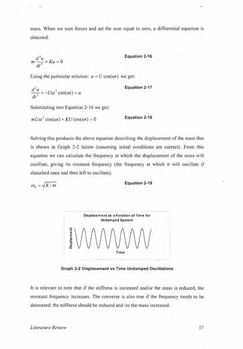
mass. When we sum forces and set the sum equal to zero, a differential equation is
obtained:
d 2 u m-
2dt +Ku = 0
Equation 2-16
Using the particular solution: u = U cos(UJt) we get:
d 2
~ dt
= -UUJ 2 cos(UJt) = a Equation 2-17
Substituting into Equation 2-16 we get:
Equation 2-18 mUUJ 2 cos(UJt) + KU cos(UJt) = 0
Solving this produces the above equation describing the displacement of the mass that
is shown in Graph 2-2 below (assuming initial conditions are correct) . From this
equation we can calculate the frequency at which the displacement of the mass will
oscillate, giving its resonant frequency (the frequency at which it will oscillate if
disturbed once and then left to oscillate).
Equation 2-19
Displacement as a Function of Time for Undamped System
Time
I ..
Graph 2-2 Displacement vs Time Undamped Oscillations
'E Ql
E o .!l! Q. VI
i5
It is relevant to note that if the stiffness is increased and/or the mass is reduced, the
resonant frequency increases. The converse is also true if the frequency needs to be
decreased: the stiffness should be reduced and lor the mass increased.
Literature Review 17

Univers
ity of
Cap
e Tow
n
However, IS not a realistic solution, as it not include velocity
as friction or This which is proportional
to direction of the velocity, is then introduced the
equation
Figure 2-4 Mass, Damper and Spring [2] Pg 14
Equation 2-20 + R", + Ku = 0
dt
Which can be solved to give
2-21u U cos(cot)e-X1
It is once again to characteristic equation, which is a sinusoid falling
off exponentially as in Graph 2-3 below, where
R K=~ Equation 2·22
2m
and resonant IS
Equation 2·23
or more fully
Equation 2-24
This implies a o1"''''''P'> in resonant when frictional force is
the mass will frequency as the ~ term will dominate Again, m
( 1 )2over the l- term.
Literature Review 18

Univers
ity of
Cap
e Tow
n
i--DisPlacment as a Function of Time for a
I Damped system
-t: Q)
E CJ
.!!! c. III
is
Time
Graph 2-3 Displacement as a Function of Time for a Damped System
If we look at the frequency response in Graph 2-4 for an arbitrary system the effect of
stiffness, mass and damping become clear.
,I ~ I
Amplitude as a Function of Frequency
OJ!
Stiffness Dominated
Dominated
Frequency
Mass Dominated
Graph 2-4 Frequency Response [2] Pg 18
We now have a more rea1istic model for explaining resonance in solids as most
material characteristics can be approximated by viewing them as a set of springs,
masses and damping forces. However, this is not entirely accurate as factors such as
Passion's ratio and non-linearities in the materials' stress/strain curves have not been
taken into account. Including these factors in the analysis would prove to be very
time-consuming and this added computation would not necessarily assist in a practical
understanding of this project. As a result the fore-mentioned factors will not be dealt
with in detail.
Literature Review 19

Univers
ity of
Cap
e Tow
n
2.4.2 Equivalent Circuits
are generally driven by an electrical source that sees the transducer as an
electrical this reason it IS useful to be able to express the mechanical
parameters and properties of the in terms equivalent.
can also serve to extend one's understanding of the if one at
the electrical circuit 73.
Figure 2·5 Mechanical System [2] Pg 14
du f 2·25 m +ru+K udt =
dt
characteristic differential equation that describes the above of a
mechanical shown again In 2·5 can also expressed
as an equivalent electrical of an inductor, and resistor as
shown in Figure gives a list their
equivalent electrical (Note that a mechanical IS
as a electrical and vice versa.)
Figure 2-6 Electrical [2] Pg 14
Equation 2·26L-+Ri+~ fidt
dl C
Literature Review
2.4.2
can
m~+ru+
as an
as a
L-+ 1
+-C
an source
reason it IS
Il1 terms
of
K
2·5 Mechanical
a
Electrical sV'UF!lm
sees as an
ifone at
14
2·25
a
as
I.S
14
2-26

Univers
ity of
Cap
e Tow
n
Mechanical Electrical
Mass
Compliance*
Resistance
Velocity
Force
Displacement
Impedance
Inductance
Capacitance
Resistance
Current
Voltages I
Charge
Impedance
Table 2-1 Equivalent Parameters [5] Pg 75
This use of equivalent circuits enables the use of powerful electrically based circuit
theory to solve and explain the mechanical system. Similarly, the electrical power
being dehvered to the transducer and other factors can be used to calculate acoustic
power from electro-mechanical efficiency that is again electrically calculated from the
impedance.
• Compliance is the reciprocal of sti ffness.
Literature Review 21

Univers
ity of
Cap
e Tow
n
2.4.3 Types of Transducers
Ultrasonic waves are primarily generated with electro-mechanical transducers such as
those piezoelectric that are discussed in the section below. However,
there are other ultrasound generators, namely whistles and sirens, which use entirely
means to create tensile high enough to cause cavitation. These are
generally used in high industrial Another common electro
mechanical method of ultrasound is with usc a magneto-strictive
transducer that usc of the properties of certain metals to create
a mechanical vibration. were very common in the 1 but they have now
been superseded in most areas piezoelectric technology and will not be
investigated further in this thesis.
2.4.4 The Piezoelectric Effect
Piezoelectric transducers have found wide acceptance because their ability to
convert electrical energy to mechanical energy at high efficiencies as as being
able to reverse the process to convert energy electrical energy
at high [5] transducers have been common use for
over forty and as a there are many commercial transducers on the market.
2.4.4.1 How Piezoelectric Materials Function
The internal mechanisms that glve materials their are
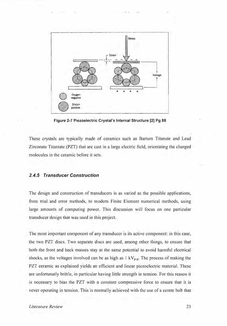
illustrated in Figure where the crystalline structure is shown. When a stress is
applied to the crystal a change in dimensions, known as strain, results. This has the
effect of squashing the lattice so that more positive molecules (in this are at
bottom the of molecules are at the creating a potentia]
difference the two of the The converse of is also
true: if a is placed on the crystal surfaces, it pulls molecules to compress
the resulting in a strain, which in tum would cause a stress if the were
fixed to supports.
Literature Review
Jneans to create
a
1I1 most areas
m
convert
to convert
at
over as a are
.... "'Ir."'II.l
true:
a turn
structure is
cause a stress
as
are
to create
now
II not
to
common use
on
are
a stress is
were
Univers
ity of
Cap
e Tow
n
Stress
C=:=:;:;;;:::=:=J - ~f~~rac:::in_==_~~I
Oxygen negative
Silicon positive
Voltage
~~~ + + + +
Figure 2-7 Piezoelectric Crystal's Internal Structure [2] Pg 88
These crystals are typically made of ceramics such as Barium Titanate and Lead
Zirconate Titantate (PZT) that are cast in a large electric field, orientating the charged
molecules in the ceramic before it sets.
2.4.5 Transducer Construction
The design and construction of transducers is as varied as the possible applications,
from trial and error methods, to modem Finite Element numerical methods, using
large amounts of computing power. This discussion will focus on one particular
transducer design that was used in this project.
The most important component of any transducer is its active component: in this case,
the two PZT discs. Two separate discs are used, among other things, to ensure that
both the front and back masses stay at the same potential to avoid harmful electrical
shocks, as the voltages involved can be as high as 1 kY p_p' The process of making the
PZT ceramic as explained yjelds an efficient and linear piezoelectric material. These
are unfortunatly brittle, in particular having little strength in tension. For this reason jt
is necessary to bias the PZT with a constant compressive force to ensure that it is
never operating in tension. Thjs is normally achieved with the use of a centre bolt that
Literature Review 23

Univers
ity of
Cap
e Tow
n
clamps the crystals and provides a fixing point for the front and back mass. (See the
exploded assembly in Figure 2-8.)
The front and back masses are designed to assist the PZT to resonate at the correct
frequency and, in the case of the front mass, to provide an emitting surface that can
support the high stresses in both compression and tension that are involved at high
powers. This transducer is face-mounted on a thin steel plate and it is, therefore, not
necessary to have nodal point (point of little or no movement on the transducer)
mountings, which simplifies the design greatly.
Centre Bolt
Back mass
Crystal
Conducting rIng
Crystal
Figure 2-8 Transducer Assembly
Literature Review 24

Univers
ity of
Cap
e Tow
n
2.4.6 Transducer Efficiency
If one looks at an equivalent circuit for a typical transducer as in Figure 2-9, the LCR
series circuit can be seen. This is named the 'motional arm ' because it represents the
mechanical part of the transducer. The power dissipated in the 'motional arm' is the
same as mechanical power of the transducer. If one applied a mechanical load to the
transducer it can be seen as an electrical load in the 'motional arm', which would
result in an increase in resistance of the 'motional arm'. This increase in resistance
can be used as a coupling factor (to the load) and so give the efficiency of the
transducer. Equation 2-29 calculates this increase as a ratio giving efficiency
(assuming Ri does not change significantly in water). [5]
R,
x,
Figure 2·9 Transducer Equivalent circuit showing Internal Losses [5] Pg 86
Ri represents internal mechanical losses, Rr the radiation resistance and Xr is the
radiation reactance of the water (load). Re and Co are the clamped admittance where
the losses are directly proportional to the applied voltage. [5]
Equation 2-27
1Gair =
R;
Equation 2·28
Mechanical - acoustic efficiency
Equation 2·29
Literature Review 25
Univers
ity of
Cap
e Tow
n
2.4.7 Amplitude Measurement Methods
reproducible ultrasonic intensities are required, it is important to
maintain constant amplitude at the emitting surface of a transducer. It is therefore
to measure amplitude. can achieved very accurately with a
microscope, but this method of measurement does not lend itself to a practical/real
measurement or to feedback systems. It is for this reason that designers
use current amplifiers. In the equivalent it can
be seen that equivalent m terms is velocity. Using
velocity for amplitude measurement seems incorrect, however if one the
current it will give transducer displacement. a result the current can used as a
relatively good approximation amplitude. If a device is said to be current
feedback it implies that it controls the power being transmitted to transducer by
looking at the current. This is the mechanism that the Vibracel ultrasonic source uses
to control amount being to the to maintain a set
amplitude.
Literature Review 26
7
to measure
measurernent
rneasurernenl or to
use current
seen
current It
to
current
amount
n1.easurement seems
arc
to
it 1S
current can
to
to
to
to
a
it can
as a
current
source uses
a set

Univers
ity of
Cap
e Tow
n
2.5 Thermal Considerations
In a project of nature where temperature is critical in terms its effect on
threshold, ability of a solvent to dissolve, to some extent to the
operation of transducers, it is important to understand the which
is reduced, maintained and In this we have a situation where the
ultrasonic transducers are putting into a which most results in
heating. It is important to understand difference between heating and
temperature. Heating is the or source that causes a In
I.e. flow of thermal energy out of a will cause a decrease
are three can transmi tted:
convection, conduction and and conduction will be Ul""UClCl\.'U
below, as are the two transfer that will be encountered
this project. Another important of materials that will be discussed is
capacity or a measure of the "energy required to temperature a unit mass
of a substance one degree"
1 Thermal Conduction, Heat Flow
Thermal conduction is the whereby energy from one to
always a higher temperature to a lower temperature. This is usually
through some fonn of transmitting conductivity a material is
the of theand so an indication of its ability to transmit
hot material.
Equation 2-30
A therate, k/ is thermal conductivity Q is heat
area through which the is passing, the thickness the material and
temperature
Literature

Univers
ity of
Cap
e Tow
n
In looking at the equation for heat transfer through an object, it can be seen that an
object of high thermal conductivity, large transmitting surface area, low thickness and
high temperature gradient or temperature difference produces a large heat flow. To
give an indication of the conductivity of certain relevant materials the table below is
provided. [6].
Material Thermal Conductivity W Im.k
Aluminium 237
Titanium 46.73
Glass 1.4
Poly Propylene 0.15
Water 0.613
Air 0.026
Table 2-2 Table of Thermal Conductivity [6] Pg 107
2.5.2 Convection in Liquids
Convection is similar to conduction in that it transfers its heat energy to a fluid using
conduction, and then the fluid moves to a cold surface and heat energy from the fluid
is transferred for a second time through conduction to the cold surface. There have
been equations derived to calculate the heat transfer through convection. However,
these are less exact than the equations for conduction. The reason for this is that the
convection coefficient can vary from 50 to 1000 for free convection of liquids
depending on many geometrical factors . This gives a huge variation in heat transfer,
but still, the general underlying effects and principles can be extracted from equations
for convection heat flow below.
Equation 2-31 Q conl' =hA(T, - Tf )
Where Q is heat energy transfer rate, h is the thermal convection coefficient, A the
exposed area, Tr and r: the temperature of the fluid and solid respectively.
Literature Review 28

Univers
ity of
Cap
e Tow
n
From the equation it can be seen that the higher the convection coefficient, the larger
the area, and the larger the temperature difference between the solid and the fluid, the
higher the heat transfer through convection will be. Although very little can be
ascertained from the coefficient, there is a clear advantage of introducing forced
convection as the coefficient can go as high as 20,000. This is not an immediately
obvious effect of acoustic streaming but an extremely important one nonetheless, as
the acoustic streaming provides forced convection.
2.5.3 Heat Capacity
As already mentioned the heat capacity is a measure of a material's ability to absorb
energy for a certain increase in temperature. This mechanism will not be discussed in
detail but this effect needs to be kept in mind when using temperature increase as a
measure of acoustic power. This is particularly relevant between two different devices
as they may be made of different materials with different heat capacity, causing a
large error in the results.
!Material Specific Heat (J/(kg.K))
Aluminium 910
Titanium 532
Glass 837
!poly Propylene 1800
,Water 4190
'Air 0 .026
Table 2-3 Table of Specific Heat [6] Pg 107
Literature Review 29

Univers
ity of
Cap
e Tow
n
2.5.4 Thermal equivalent circuits
Once again equivalent circuits can be used to solve thermal systems using electrical
analysis techniques and analogue computers. The thermal and electrical systems are
more similar than the mechanical and electrical systems, in that a parallel thermal
system has an electrical circuit where the equivalent components are also in parallel.
Table 2-4 gives the thermal and electrical equivalent physical parameters.
Thermal Electrical
Temperature Voltage
Heat flow ( Q ) Current
Mass. heat capacity Capacitance
Conductivity . Area Resistance
Table 24 Equivalent Thermal Parameters
Literature Review 30

Univers
ity of
Cap
e Tow
n
3.1
3 Experimental Method
This chapter and methods measurement and presentation
of the results. it looks at the typical set-up used in this project
( transducers, solvents etc.) work done by Mr
Quieros.[12] It discusses the use of foil cavitation
and the software used to analyse the damaged samples. it
looks at accuracy and reliability of the processor method as a
The method and analyse vessels is then briefly
the measurement of m the thennal IS
as the use of equivalent to accurately estimate the
mental Set-up
will consider the physical of a typical or base most
in this project. The relevant then explain the slight
was a continuation of a review of the previous and
Mr De Quieros is A wide variety baths with
}'xperimental Method 31
measurement
as use
3.1
II the
a
IS
rneasurement
to
a or
A
it
IS
real
most
3

Univers
ity of
Cap
e Tow
n
frequencies from 20 - 30kHz, horns, and cup horns (20 kHz) were experimented with,
using a number of different receptor vessels of differing size, shape and material in
various orientations. Based on the conclusion and recommendations of Mr De
Quieros, a good set-up had been achieved, but needed further optimisation. This
recommended set-up, which was used as a basis for this project, consisting of a
titanium 64mm diameter cup hom manufactured by Vibracel with a 500 Watt
amplifier - transducer combination. The cup that contained the transmission fluid was
made of glass and fixed to the hom by a plastic screw-in lug. The receptor vessel was
placed vertically in the cup hom with the base as close as possible to the emitting
surface of the transducer (typically with a Imm gap). The receptor vessel
reconunended was a SOml polypropylene pill bottle. Various solvent and transmission
media levels (height above the emitting-face) were experimented with, resulting in the
finding that a level of 30-3Smm was optimum for disruption. As temperature plays an
important role where cavitation and chemical reactions are concerned, it was decided
to use a cooling arrangement where the transmission medium would also serve the
function of cooling. The temperature in the receptacle started at 23°C and was held
below 39°C (this was part of the design requirements) by
circulating the cooling fluid and limiting the sonification
time. This cooling method unfortunately introduced a
number of minute bubbles or cavitation nuclei that can
alter the cavitation threshold slightly. In this project, this
problem was solved by ensuring that the flow rate, and
hence the introduction of cavitation nuclei, was held
constant for all tests.
Figure 3-1 shows a typical set-up. [12] (Scale drawings
of the hom can be found in Appendix D).
Figure 3-1 Vibracel Cup Horn Assembly
For the majority of tests Mr De Quieros followed a method of inserting a piece of
aluminium foil to the sound field for a specified length of time (typically for 30
Experimental Method 32
frequencies from 20 - 30kHz, horns, and cup horns (20 kHz) were experimented with,
using a number of different receptor vessels of differing size, shape and material in
various orientations. Based on the conclusion and recommendations of Mr De
Quieros, a good set-up had been achieved, but needed further optimisation. This
recommended set-up, which was used as a basis for this project, consisting of a
titanium 64mm diameter cup hom manufactured by Vibracel with a 500 Watt
amplifier - transducer combination. The cup that contained the transmission fluid was
made of glass and fixed to the hom by a plastic screw-in lug. The receptor vessel was
placed vertically in the cup hom with the base as close as possible to the emitting
surface of the transducer (typically with a Imm gap). The receptor vessel
recommended was a SOml polypropylene pill bottle. Various solvent and transmission
media levels (height above the emitting-face) were experimented with, resulting in the
finding that a level of 30-3Smm was optimum for disruption. As temperature plays an
important role where cavitation and chemical reactions are concerned, it was decided
to use a cooling arrangement where the transmission medium would also serve the
function of cooling. The temperature in the receptacle started at 23 T and was held
below 39°C (this was part of the design requirements) by
circulating the cooling fluid and limiting the sonification
time. This cooling method unfortunately introduced a
number of minute bubbles or cavitation nuclei that can
alter the cavitation threshold slightly. In this project, this
problem was solved by ensuring that the flow rate, and
hence the introduction of cavitation nuclei, was held
constant for all tests.
Figure 3-1 shows a typical set-up. [12] (Scale drawings
of the hom can be found in Appendix D).
Figure 3-1 Vibracel Cup Horn Assembly
For the majority of tests Mr De Quieros followed a method of inserting a piece of
aluminium foil to the sound field for a specified length of time (typically for 30
Experimental Method 32
Univers
ity of
Cap
e Tow
n
seconds), sonicating it, and the foil for visual of the
cavitation damage. was a substantial body of work and provided a from
further experimentation could be conducted.
3.2 Foil Method
Cavitation fields are unfortunately extremely difficult to measure due to
their chaotic nature and rapid variation. A method of taking a image"
of the cavitation to effectively accumulate or average in which the
cavitation is IS This foil technique of the destructive
ability of a field involves inserting a of aluminium foil into
the cavitation The cavitation damage to the
foil, either totally the foil, or partially it to appear
pitted and bubbled. foil unfortunately field and for this
reason the foil must be extremely thin foiL 1.1 references to
other methods on cavitation measurement.)
3.3 Digital Image Processing
When that were damaged or partially destroyed by ultrasonic
cavitation, it was an accurate, means of analysing the foil
samples was what was representing the area
of was destroyed or damaged. methods of doing this
would Image processor, as areas manually would
extremely time-consuming and error prone. use of relative weight loss in
in Heuter and Bolt [2] does not information about areas that
were but only about the mass removed the sample.
It was to use Matlab™'s digital toolbox to calculate Pf",,"P£1
to master are examples and help with similar
Method
a
3 Foil Method
are to measure to
a
into
reason 1.1 conta to
on rncasurement. )
3 ital I p ng
were or
area
areas
were
It was to
to master are
Univers
ity of
Cap
e Tow
n
problems on the Internet. Although these programs are very powerful, it simplifies the
programming to give the image processor data that can be easily manipulated, and for
this reason the foil samples were placed with their dull side facing the digital image
scanner, and using black paper as a backing. This black background was selected to
ensure that there was an adequate intensity level difference between the intact foil,
and areas that had been destroyed. The reason for facing the dull side of the foil up
was because the flat sections of the shiny surface in the digital scanner would tend to
come out very white or bright and distorted the images' intensity level gradients. In
order to explain the process of extracting a value for the damaged, as well as the
destroyed areas, as mask images and as a percentage of the total original foil area, an
example will be used.
Figure 3-2 Original normalized image
Figure 3-2 shows a processed foil sample after scanning. The destroyed and damaged
areas can be seen clearly.
3.3.1 Analysis and Extraction of Damaged Areas
In order to extract the damage areas, the program is required to generate a mask that
covers the pitted foil yet excludes the black background and the smooth foil that is
undamaged. The area of interest can be seen to contain rapidly varying intensities,
which implies many local maxima and minima or edges in the intensity profile. A
function that places a pixel at the position of each edge is used to get the following
image shown in Figure 3-3.
Experimental Method 34

Univers
ity of
Cap
e Tow
nFigure 3-3 Edge Detected Image
This edge detection is extremely effective in finding the damaged area if one visually
compares this image to the original in Figure 3-2; however the number of white pixels
doesn't represent the damaged area. This can be corrected by filling in the regions
between closely positioned pixels. Dilating each pixel and so grouping the pixels
works well; however in that case the white areas exaggerate the damaged area. An
erode function is employed to correct this exaggeration without ungrouping the pixels.
Figure 3-4 shows the final mask that represents the damaged area. It can be confirmed
by detailed visual comparison that this gives an accurate mask of the damaged areas.
Figure 3-4 Final Damaged Foil Mask Image
Experimental Method 35
Figure 3-3 Edge Detected Image
This edge detection is extremely effective in finding the damaged area if one visually
compares this image to the original in Figure 3-2; however the number of white pixels
doesn't represent the damaged area. This can be corrected by filling in the regions
between closely positioned pixels. Dilating each pixel and so grouping the pixels
works well; however in that case the white areas exaggerate the damaged area. An
erode function is employed to correct this exaggeration without ungrouping the pixels.
Figure 3-4 shows the final mask that represents the damaged area. It can be confirmed
by detailed visual comparison that this gives an accurate mask of the damaged areas.
Figure 3-4 Final Damaged Foil Mask Image
Experimental Method 35

Univers
ity of
Cap
e Tow
n
3.3.2 Analysis and Extraction of Destroyed Areas
The extraction of the destroyed area is marginally easier than that of the damaged
area. Once again starting with the nonnalized image in Figure 3-2, a mask needs to be
generated that will represent the black background where the foil is destroyed only.
An obvious solution is to carry out a threshold detection, which involves taking the
intensities above the threshold value and setting them to 255 or white, and similarly
setting those below the threshold value to 0 or black. A threshold value of 51 ensured
that the entire black region was included and resulted in the threshold image in Figure
3-5.
Figure 3·5 Threshold Image
This threshold image represents the entire destroyed area, but unfortunately it includes
the dark areas of the damaged regions . This can, as before, be corrected by the
grouping strategy explained in the previous section, however in this case the erode
function was carried out first, and then the dilate function, because of the inverted
colours. The result is the final destroyed mask shown in Figure 3-6 below.
Experimental Method 36
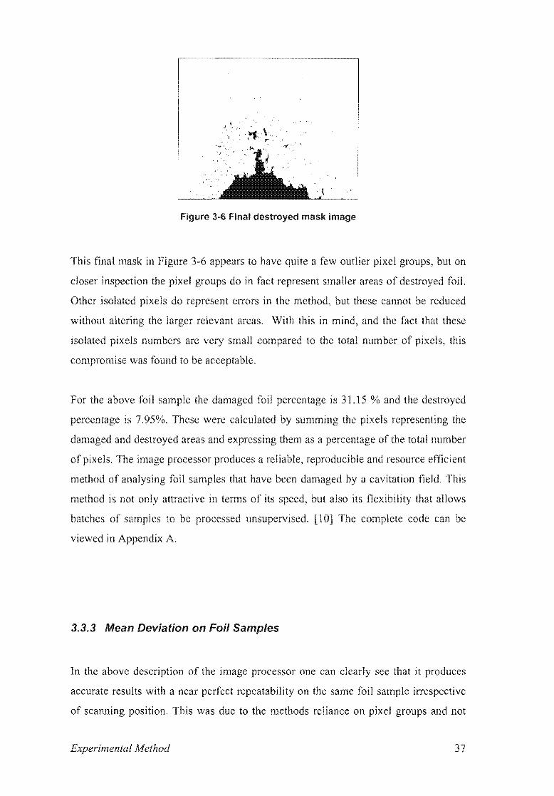
Univers
ity of
Cap
e Tow
n
Figure 3-6 Final destroyed mask image
This mask in Figure appears to have quite a outlier pixel groups, but on
closer inspection the pixel groups do in fact represent areas destroyed foil.
Other isolated pixels do l"pn,l"P"pnT errors in the method, but these cannot be
without altering larger areas. With in mind, the
isolated pixels are small to the total num ber of this
compromise was found to be acceptable.
For the above foil sample damaged percentage is 31.15 % and destroyed
percerlta~~e is 7.95%. were calculated by the representing the
damaged and destroyed areas and expressing as a oel'cent3lge of total number
pixels. produces a reliable, reproducible and resource efficient
method of analysing foil samples that have been damaged by a cavitation This
method is not only attractive terms of but also its flexibility that allows
batches samples to processed unsupervised. [10] complete code can be
in Appendix A.
3.3.3 Mean Deviation on Foil Samples
In the above description the processor one can see it produces
accurate results with a near perfect repeatability on the same
scanning position. This was to the methods reliance on pixel groups and not
Method

Univers
ity of
Cap
e Tow
n
individual pixels for All scans were done at the same resolution for
consistency in the image errors m in this
thesis the inconsistency of the cavitation which is rather
chaotic. errors obtained in this thesis not necessarily
a of the foil the chaotic nature the cavitation
fields. Nonetheless, a measure to be established validation
of in the chapters. A series test were on samples under
conditions to the standard and give a in which
vary due to errors. It was found that this standard deviation was 0.08 of
means that was 69% certainty that a value of X would in the
± X times by 0.08, as many the foil tests were in very similar
experimental set-ups to tests where mean deviation was
3.4 Streaming
In to measure various parameters associated with, influencing
streaming, a method visualizing the patterns recording
was are various methods of doing using a wide of
to visualise streaming effects. this project
solvents are and for reason it would good sense to use water
Experimental Method 38
x
a measure
to errors. It was
to measure
a
was
camera
to tests
I scans were at same
mean was
sense to use \vater
a

Univers
ity of
Cap
e Tow
n
Figure 3-7 Streaming Pattern of Water visualized by Aluminium Powder Cloud
These 5-second MPEG movie clips were stepped through frame-by-frame to extract
information such as the extent and velocity of the streaming patterns. (Appendix C
shows a progression of the movie frame-by-frame).
3.5 Temperature Measurements
Temperature measurements for most of the project were taken with the use of a
conventional laboratory thermometer. These are acceptable for static temperatures
and will not be discussed further. However, the measurement of dynamic or time
varying temperatures such as those used in the temperature profiles need to be
considered for their accuracy. These measurements are distorted in that the
temperature probe (in this case a LM35 electronic thermal reference) has a small heat
capacity, and hence there wiJl be a time-lag between the real temperature and the
measured temperature. This can be compensated for if the thermal system is
expressed in terms of its electrical equivalent and the temperature probe is modelled
as a low-pass filter. The actual temperature can then be calculated from the measured
temperature. This is useful if a certain organic sample can be damaged at a
particularly high temperature, because the real maximum temperature of the solvent
can be accurately estimated from the measured temperature. (The exact method was
explained more completely in the section entitled Thermal Shocking.)
Experimental Method 39
Figure 3-7 Streaming Pattern of Water visualized by Aluminium Powder Cloud
These 5-second MPEG movie clips were stepped through frame-by-frame to extract
infonnation such as the extent and velocity of the streaming patterns. (Appendix C
shows a progression of the movie frame-by-frame).
3.5 Temperature Measurements
Temperature measurements for most of the project were taken with the use of a
conventional laboratory thennometer. These are acceptable for static temperatures
and will not be discussed further. However, the measurement of dynamic or time
varying temperatures such as those used in the temperature profiles need to be
considered for their accuracy. These measurements are distorted in that the
temperature probe (in this case a LM35 electronic thennal reference) has a small heat
capacity, and hence there will be a time-lag between the real temperature and the
measured temperature. This can be compensated for if the thennal system is
expressed in tenns of its electrical equivalent and the temperature probe is modelled
as a low-pass filter. The actual temperature can then be calculated from the measured
temperature. This is useful if a certain organic sample can be damaged at a
particularly high temperature, because the real maximum temperature of the solvent
can be accurately estimated from the measured temperature. (The exact method was
explained more completely in the section entitled Thermal Shocking.)
Experimental Method 39

Univers
ity of
Cap
e Tow
n
4 Static Pressure
chapter is with the of or atmospheric on
cavitation with to its strength, and ultimately ability to
solids. A to be out in an environment in which the
pressure the water could varied while enabling an intensity
to into (2]
two parts: the design and construction pressure apparatus,
together with comparisons and the original cup horn
In tests including done by Mr de Quieros [12]); and
secondly, a description of the tests and conclusions drawn them.
1 Design of the Pressure Apparatus
In addition to the primary of the pressure, new vessel had to
made of lightweight so as not to overload the transducer, yet
enough to withstand up to two of internal and one Bar external
or negative pressure. needed to constructed in such a way that
internal was easily accessible for checking and replacing test samples etc.
important requirement that was not immediately obvious was that all the air
to be from the to ensure that water not
breathe' while cavitating absorb minute amounts of into the water, allowing
more easily). It was also necessary to make provision for internal
connections that were to hold the test in place.
Static Pressure 40
4 Pressure
IS or on
[ 12
a tests
1 n of p re Appa
new to
so as not to
or
etc.
that was not
to be not
were to test

Univers
ity of
Cap
e Tow
n
4.1.1 Design and Experimental Conditions
The first and most pressing concern was the seal around the hom and whether it
would stand up to the high pressures involved. To simulate the glass cup's fixing
point to the transducer a piece of steel tube was machined to the same shape as the
glass cup. Another piece of steel was machined to the same shape as the plastic lug as
shown in Figure 4-1. However, there was no thread on either of these new
components, as this would have significantly increased the cost and time of
machining. The method of tightening or compressing the rubber o-rings can be seen in
Figure 4-2, where tapered slots in the PVC piping provided a primitive yet effective
thread. This method of compressing the o-rings and fixing the vessel to the hom only
work if the other socket was firmly fixed to the PVC piping. This was achieved by
making the outer diameter of the component slightly larger than that of the pipe,
giving an interference fit that was also glued for added strength.
Transducer
Figure 4-1 Pressure Apparatus Cross Section,
showing the method of sealing the vessel.
The PVC piping was chosen because it was
easy to work with, and has the added benefit of
being a glue-on, off-the-shelf component that is
able to handle the high pressures involved .
Figure 4-2 shows the grey plastic converter and
the steel screw-in end cap. The 3mm nut and
bolt internal connectors can be seen protruding
from the grey converter. A scale drawing of the
apparatus can be found in Appendix D.
Figure 4-2 Assembled Apparatus Showing the Assembled Apparatus
Static Pressure 41
4.1.1 Design and Experimental Conditions
The first and most pressing concern was the seal around the hom and whether it
would stand up to the high pressures involved. To simulate the glass cup's fixing
point to the transducer a piece of steel tube was machined to the same shape as the
glass cup. Another piece of steel was machined to the same shape as the plastic lug as
shown in Figure 4-1 . However, there was no thread on either of these new
components, as this would have significantly increased the cost and time of
machining. The method of tightening or compressing the rubber o-rings can be seen in
Figure 4-2, where tapered slots in the PVC piping provided a primitive yet effective
thread. This method of compressing the o-rings and fixing the vessel to the hom only
work if the other socket was finnly fixed to the PVC piping. This was achieved by
making the outer diameter of the component slightly larger than that of the pipe,
giving an interference fit that was also glued for added strength.
Figure 4-1 Pressure Apparatus Cross Section,
showing the method of sealing the vessel.
The PVC piping was chosen because it was
easy to work with, and has the added benefit of
being a glue-on, off-the-shelf component that is
able to handle the high pressures involved .
Figure 4-2 shows the grey plastic converter and
the steel screw-in end cap. The 3mm nut and
bolt internal connectors can be seen protruding
from the grey converter. A scale drawing of the
apparatus can be found in Appendix D.
Figure 4-2 Assembled Apparatus Showing the Assembled Apparatus
Static Pressure 41

Univers
ity of
Cap
e Tow
n
The pump used to pressurise the vessel was a hand pump rated at 30 Bar positive
pressure and 5 Bar negative pressure, with a built in pressure sensor and digital
display. (See Figure 4-3). Although the
negative pressure was never a priority, this
extra capability provided additional insight into
the effect of static pressure on cavitation. As
mentioned before, it was important that the
water under pressurisation was not able to
'breathe' or be in contact with air during
sonification. However, the pump only
functioned in air, and for this reason the
air/water separation reservoir needed to be
constructed. This was simply a vessel that was
half-full of water, with two connecting points,
one at the top for the air or pump connection,
and the other at the bottom for the wet or
reaction vessel connection.
Figure 4-3 Pressure Pump
Ensuring that the cavitating liquid did not breathe also meant that sources of other
dissolved gases needed to be limited. For this reason, distilled water was used as the
coupling/cooling fluid. That, though, meant that the coupling fluid would get hot (up
to 30°C after a few 10 second tests). This was solved by replacing the coupling fluid
with the same fluid but at a temperature of 23 °C. The transducer was then briefly
turned on to allow any air trapped by the changing of the fluids to be released. This
air was then vented, and the vessel was pressurised for the various tests. The liquid in
the receptor vessel was also replaced to both ensure a constant temperature for each
experiment as well as to clean the vessel of destroyed pieces of aluminium foil. As in
other experiments, the receptor vessel was fixed 1 mm above the emitting-face of the
transducer to minimise acoustic absorption.
Static Pressure 42
The pump used to pressurise the vessel was a hand pump rated at 30 Bar positive
pressure and 5 Bar negative pressure, with a built in pressure sensor and digital
Figure 4-3 Pressure Pump
display. (See Figure 4-3). Although the
negative pressure was never a priority, this
extra capability provided additional insight into
the effect of static pressure on cavitation. As
mentioned before, it was important that the
water under pressurisation was not able to
'breathe' or be in contact with air during
sonification. However, the pump only
functioned in air, and for this reason the
air/water separation reservoir needed to be
constructed. This was simply a vessel that was
half-full of water, with two connecting points,
one at the top for the air or pump connection,
and the other at the bottom for the wet or
reaction vessel connection.
Ensuring that the cavitating liquid did not breathe also meant that sources of other
dissolved gases needed to be limited. For this reason, distilled water was used as the
coupling/cooling fluid. That, though, meant that the coupling fluid would get hot (up
to 30°C after a few 10 second tests). This was solved by replacing the coupling fluid
with the same fluid but at a temperature of 23°C. The transducer was then briefly
turned on to allow any air trapped by the changing of the fluids to be released. This
air was then vented, and the vessel was pressurised for the various tests. The liquid in
the receptor vessel was also replaced to both ensure a constant temperature for each
experiment as well as to clean the vessel of destroyed pieces of aluminium foil. As in
other experiments, the receptor vessel was fixed 1 mm above the emitting-face of the
transducer to minimise acoustic absorption.
Static Pressure 42
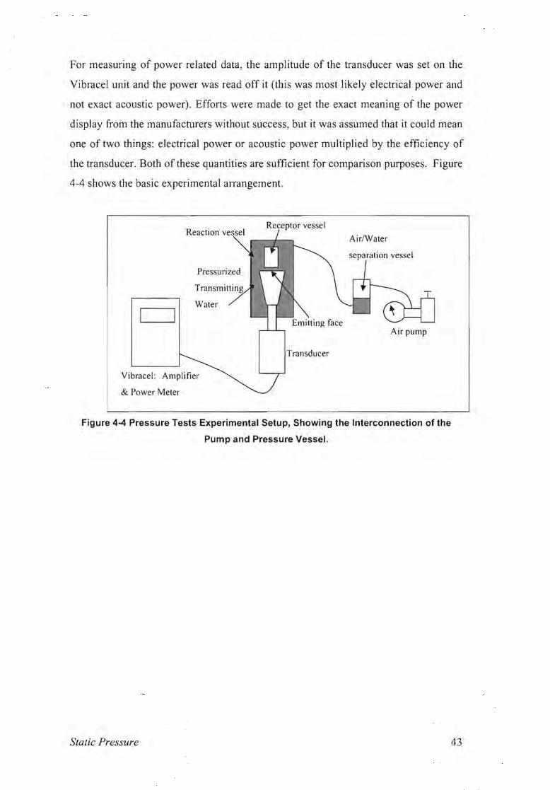
Univers
ity of
Cap
e Tow
n
For measuring of power related data, the amplitude of the transducer was set on the
Vibracel unit and the power was read off it (this was most likely electrical power and
not exact acoustic power) . Efforts were made to get the exact meaning of the power
display from the manufacturers without success, but it was assumed that it could mean
one of two things: electrical power or acoustic power multiplied by the efficiency of
the transducer. Both of these quantities are sufficient for comparison purposes. Figure
4-4 shows the basic experimental alTangement.
Air/Water
Receptor vessel
Emitting face
Transducer
Vibracel: Amplifier
& Power Meter
Air pump
Figure 4-4 Pressure Tests Experimental Setup, Showing the Interconnection of the
Pump and Pressure Vessel.
Static Pressure 43

Univers
ity of
Cap
e Tow
n
4.1.2 Plastic Bottle Sealing
The plastic bottles were sealed for reasons that will be explained later in this chapter.
These bottles, once sealed, were required to withstand an external pressure of up to
1.5 Bars without allowing any water to seep or leak into the bottle. Various adhesives
were tried without success, even for pressures as low as 0.5 Bar. The solution finally
implemented was a technique found in the gas and oil industry for joining large
plastic piping sections. [17] This involved winding a resistive wire around the lid of
the bottle, closing it, and applying a large current through the winding causing it to
heat up and melt the lid on to the rest of the bottle. The wire then remained inside the
seal and the loose ends were
trimmed. This provided an excellent
seal that was extremely difficult to
break open, even by hand after the
tests for inspection of the foil
sample.
Figure 4-5 Plastic Bottle being Sealed
4.1.3 Comparison between Glass and New Pressure Vessel
In order to compare the results obtained in the pressure vessel, with those of the glass
vessel and with those of previous work done with the glass cup hom, a conversion
factor or relationship between the two vessels needed to be experimentally obtained.
The first method of comparing the two vessels consisted of recording electrical power
input (displayed by the Vibracel amplifier) into the transducer for various amplitudes.
This would give a measure of the resistive force in the new vessel compared to that of
the glass vessel, as the Vibracel adjusts its power to maintain a steady amplitude using
current feedback. From the graph of Amplitude vs. Power in Graph 4-1 below, a
slight power offset of 2.8 Watts can be seen between the two vessels, which could be
explained by the fact that the pressure vessel was slightly heavier than the glass cup
hom.
Static Pressure 44
4.1.2 Plastic Bottle Sealing
The plastic bottles were sealed for reasons that will be explained later in this chapter.
These bottles, once sealed, were required to withstand an external pressure of up to
1.5 Bars without allowing any water to seep or leak into the bottle. Various adhesives
were tried without success, even for pressures as low as 0.5 Bar. The solution finally
implemented was a technique found in the gas and oil industry for joining large
plastic piping sections. [17] This involved winding a resistive wire around the lid of
the bottle, closing it, and applying a large current through the winding causing it to
heat up and melt the lid on to the rest of the bottle. The wire then remained inside the
Figure 4-5 Plastic Bottle being Sealed
seal and the loose ends were
trimmed. This provided an excellent
seal that was extremely difficult to
break open, even by hand after the
tests for inspection of the foil
sample.
4.1.3 Comparison between Glass and New Pressure Vessel
In order to compare the results obtained in the pressure vessel, with those of the glass
vessel and with those of previous work done with the glass cup hom, a conversion
factor or relationship between the two vessels needed to be experimentally obtained.
The first method of comparing the two vessels consisted of recording electrical power
input (displayed by the Vibracel amplifier) into the transducer for various amplitudes.
This would give a measure of the resistive force in the new vessel compared to that of
the glass vessel, as the Vibracel adjusts its power to maintain a steady amplitude using
current feedback. From the graph of Amplitude vs. Power in Graph 4-1 below, a
slight power offset of 2.8 Watts can be seen between the two vessels, which could be
explained by the fact that the pressure vessel was slightly heavier than the glass cup
hom.
Static Pressure 44

Univers
ity of
Cap
e Tow
n
Amplitude vs Power
400 y =4.3464x - 67.768 --Glass
~ 300 - -- Plastidsteel ~ 200 ~ Y=2.9x - 54.3 o PlastidSteelc.. 100
1bar
o 20 40 60 80 100
Ampltude (%)
Graph 4-1 Amplitude vs Electrical Power, showing The Average Power Consumed over
a Ten Second Period for Various Amplitude Settings for the Different Vessel.
It can also been noted from the linear trend lines fitted to the data series that the
gradient for the pressure vessel is about 10% larger than that of the glass vessel. This
may be because as the amplitude is increased the plastic approaches a non-linear
region of its stress-strain curve, and it begins to absorb more energy.
It is also interesting to note the third (upper) data series in Graph 4-1 above, where
the external pressure was increased to 1 Bar and the power at 100% amplitude
subsequently doubled. As an increasing power implies an increasing destructive
capability, this was a very positive and exciting result.
While the amplitude-power relationship between the two vessels gives a reasonable
comparison in terms of the electrical energy used, it was also necessary to conduct
some tests that compared the destructive capabilities of the two vessels, as this was
one of the goals of this research. As a result, a series of tests was conducted, again
using the foil method. This time, however, the foil was placed directly into the vessel
without first being inserted into a bottle. Tests were done under open or atmospheric
conditions for both the vessels, using degassed water at the same temperatures (23°C)
and heights above the transducer (35mm) and subsequently very similar volumes of
Static Pressure 45

Univers
ity of
Cap
e Tow
n
water. The idea was to set all conditions to be identical to ensure that the results
would only reflect differences between the two vessels.
The amounts of damaged and destroyed foil were calculated with the Matlab™ based
image processor. A disruption index was calculated using a weighted sum of these
two values (weighted I :2) to place an emphasis on the value representing the area of
destroyed foil (as this area represents greater destructive forces). These two disruptive
indexes were compared firstly as a function of amplitude, and then as a function of
power. This revealed that the pressure vessel at similar amplitudes produced 74.8% ±
2.9% of the disruption of the glass vessel, and at similar power levels the pressure
vessel produced 63 % ± 2.5 % of the disruption of the glass vessel. This implies that
the new pressure vessel is 63% ± 2.5% as efficient as the glass vessel. Again, this was
most likely due to the fact that the pressure vessel was heavier, and consisted of more
lossy material than glass. This was not a problem as long as the inefficiency or
conversion factor between the glass cup's horn and the pressure vessel was kept in
mind when comparing results.
4.2 Pressure Effects on Transducer
Varying the static pressure of a liquid under high power sound waves significantly
affects the cavitation strength and bubble size, as well as the load that the transducer
has to drive . This section investigates the effects of static pressure variation on the
transducer and the way in which it responds.
4.2.1 Pressure Effect on Power
In Graph 4-2 of Pressure vs. Power, the power (This was average power over 10
seconds) required to drive the transducer was recorded while increasing the pressure.
This once again showed that the increase in pressure results in a higher power being
required to maintain specific amplitudes : in this case, at a 50% amplitude setting.
Static Pressure 46
water. The idea was to set all conditions to be identical to ensure that the results
would only reflect differences between the two vessels.
The amounts of damaged and destroyed foil were calculated with the Matlab™ based
image processor. A disruption index was calculated using a weighted sum of these
two values (weighted I :2) to place an emphasis on the value representing the area of
destroyed foil (as this area represents greater destructive forces). These two disruptive
indexes were compared firstly as a function of amplitude, and then as a function of
power. This revealed that the pressure vessel at similar amplitudes produced 74.8% ±
2.9% of the disruption of the glass vessel, and at similar power levels the pressure
vessel produced 63 % ± 2.5 % of the disruption of the glass vessel. This implies that
the new pressure vessel is 63% ± 2.5% as efficient as the glass vessel. Again, this was
most likely due to the fact that the pressure vessel was heavier, and consisted of more
lossy material than glass. This was not a problem as long as the inefficiency or
conversion factor between the glass cup's horn and the pressure vessel was kept in
mind when comparing results.
4.2 Pressure Effects on Transducer
Varying the static pressure of a liquid under high power sound waves significantly
affects the cavitation strength and bubble size, as well as the load that the transducer
has to drive. This section investigates the effects of static pressure variation on the
transducer and the way in which it responds.
4.2.1 Pressure Effect on Power
In Graph 4-2 of Pressure vs. Power, the power (This was average power over 10
seconds) required to drive the transducer was recorded while increasing the pressure.
This once again showed that the increase in pressure results in a higher power being
required to maintain specific amplitudes: in this case, at a 50% amplitude setting.
Static Pressure 46

Univers
ity of
Cap
e Tow
n
Pressure vs Power
140
40 ·
20
{) -L
-1 -0.5 o 0.5 1.5
Pressure (Bar)
Graph 4-2 Power Variation with Pressure where The Pressure was expressed as
Differential Pressure where 0 Bar is Atmospheric Pressure.
By increasing the static pressure one Increases the cavitation threshold pressure,
subsequently suppressing the cavitation as implied by
Equation 2-1. Cavitation has the effect of unloading the transducer because of the
compressibility of the cavitation bubbles and the energy being dissipated throughout
the liquid by the heating and shockwave effects of the cavitation. It was therefore
evident that an increased static pressure would mean an increased load and therefore
an increase in the power required to drive the transducer.
4.2.2 Pressure Effect on Resonant Frequency
In addition to the power changing in response to pressure, a frequency change was
also noticed for different pressures. Graph 4-3 below shows how the Vibracel unit
tracked the resonant frequency as the pressures increased. This change in resonant
frequency was most likely due to the resistive forces increasing, from a reduction in
cavitation (i.e. transducer, vessel, water and cavitation bubbles) as a result of
pressunslng.
Static Pressure 47

Univers
ity of
Cap
e Tow
n---
Pressure vs. Frequency
20.1 ,-----------------------------------------------~ _ 20.05 N :I: 20 .::t:. - 19.95
o ~ t: Q) 19.85 :J C" 19.8 ~ 19.75
U. 19.7 _L-_______~--~---~--~---~---~
0.00 0.20 1.20 1.40 1.60
~--
-
-1 -------"""""-"'"
19.9 +--- --
-+-----------J_-----"'='-'----'-'~
0.40 0.60 0.80 1.00
Pressure (Bar)
Graph 4-3 Pressure vs. Frequency, Showing the Drop in Frequency as Differential
Pressure was Increased.
Although the frequency variation is less than 1.5 % over a 1.4 Bar range, the Q of
most transducers, (including this one) is high, reiterating the need for a PLL (Phase
Lock Loop) to track the resonate frequency. Fortunately a PLL was included in the
Vibracel amplifier.
4.3 Static Pressure Effect on Disruption
Once again the foil test was used to establish the disruptive capabilities of cavitation.
This time, however, the pressure was varied in order to find the static pressure that
produced the most damaging cavitation in water. This test was initially done over a
broad range with a resolution of 1 Bar. Once the general area in which the highest
cavitation occurred was found, more accurate tests with a resolution of 0.1 Bar were
done to establish the exact optimised pressure.
Static Pressure 48
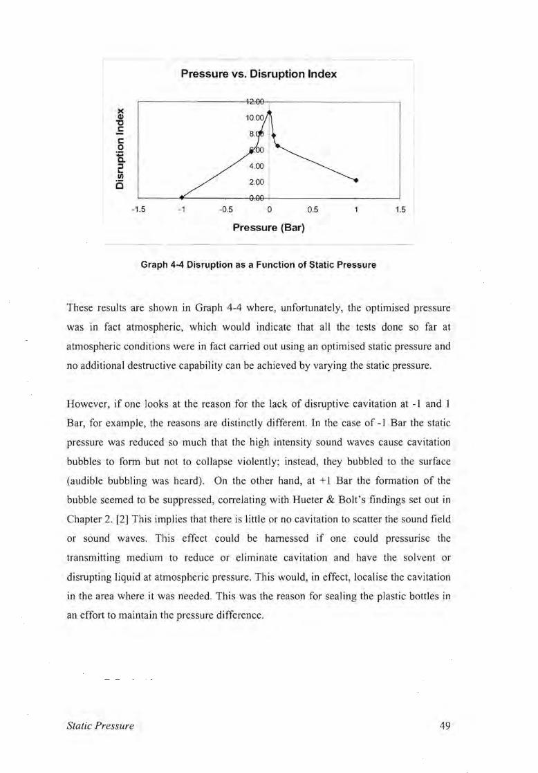
Univers
ity of
Cap
e Tow
n
Pressure vs. Disruption Index
4.00
2.00 1
I -1.5 -1 -0.5 o 0.5 1.5
Pressure (Bar)
Graph 4-4 Disruption as a Function of Static Pressure
These results are shown in Graph 4-4 where, unfortunately, the optimised pressure
was in fact atmospheric, which would indicate that all the tests done so far at
atmospheric conditions were in fact carried out using an optimised static pressure and
no additional destructive capability can be achieved by varying the static pressure.
However, if one looks at the reason for the lack of disruptive cavitation at -I and I
Bar, for example, the reasons are distinctly different. In the case of -I Bar the static
pressure was reduced so much that the high intensity sound waves cause cavitation
bubbles to form but not to collapse violently; instead, they bubbled to the surface
(audible bubbling was heard). On the other hand, at +1 Bar the formation of the
bubble seemed to be suppressed, correlating with Hueter & Bolt's findings set out in
Chapter 2. [2] This implies that there is little or no cavitation to scatter the sound field
or sound waves. This effect could be harnessed if one could pressurise the
transmitting medium to reduce or eliminate cavitation and have the solvent or
disrupting liquid at atmospheric pressure. This would, in effect, localise the cavitation
in the area where it was needed. This was the reason for sealing the plastic bottles in
an effort to maintain the pressure difference.
SIalic Pressure 49

Univers
ity of
Cap
e Tow
n
4.4 Differential Pressure Testing
This section sets out to prove and optimise the previously explained principal of using
a differential pressure to increase and localise the cavitation in the receptor vessel.
Once again, all the factors affecting cavitation were set constant, so that the results
would reflect only the changes in differential pressure. Tests were done, all with the
internal pressure at atmospheric pressure, as this had already been found to be the
optimum pressure for the most destructive cavitation. The pressure for the
transmitting medium was then varied from 0 through to 0.75 Bar gauge pressure. Foil
samples and image processing were again used to quantify the amount of disruption;
the results are shown in Table 4-1 below.
IPressure ratio % Destroyed % Damaged Disruption Index I
P/O 1.88 26.10 9.95 ± 0.795
0 / 0.25 13.73 19.63 15.70 ± 1.26
K> / 0.75 24.63 19.75 23 .00 ± 1.84
Table 4-1 Differential Pressure Results
This revealed some very positive results where the theory above was confinned, and
the percentage damage was increased by 2.5 times from % to 0/0.75 (receptacle
pressure/external pressure).
4.4.1 Effects of Water Level Variations
The effects of the water level variations in the receptacle were once again quantified
using the foil and image processor technique to give the results in Table 4-2. It is
apparent from Table 4-2 that a water level (inside the receptor) of 20mm gives the
maximum disruption by a significant margin . This is most likely due to the fact there
is a small volume being subjected to ultrasound, creating high-density high energy
levels. The reason for a water level of 10mm not having a higher disruption index
could be explained by the small contact surface area, and a liquid level being too low
Static Pressure 50

Univers
ity of
Cap
e Tow
n
to create standing waves. The 20mm level simply constitutes an optimal operating
point between the two effects, and thus results in the most destructive cavitation.
Water level % Destroyed % Damaged IDisruption Index
10mm 32.02 11.32 25.12 ± 2
20mm 57.39 10.29 41.69 ± 3.3
30mm 11.64 28.90 17.40 ± 1.3
40mm 4.69 20.65 10.01 ± 0.8
Table 4-2 Disruption as a Function of Receptacle Water Level
4.5 Conclusion
The effects of pressure or, more specifically, the effects of differential pressure, have
obvious advantages in terms of a disruption system. On the other hand, the time taken
to complete a single pressure differential experiment was well over twenty minutes
due to the complex mechanisms that provide the seals for these relatively high
pressures. Although the differential pressure has obvious benefits, it also provides
significant complications and, as a result, increased costs of making a system that
would include this differential pressure technique.
Static Pressure 51

Univers
ity of
Cap
e Tow
n
Tri..Reactor Vessel
In the prevIous the sound intensity to was
increased with an static pressure; was
consuming and complex. This chapter will consider a method of transmitting
increased acoustic intensity to the receptacle. This method involves the use of
multiple m an ultrasonic bath set-up. In an attempt to overcome the
saturation most acoustic energy was through a single path
to the transducers were fixed to a bath (hence the Tri-
Reactor name) and a variety of receptacles, prism vessel, were
tested in this new the interests of static pressure on
the multiple baths was also of the
chapter. Finally, a comparison between this new and the 500 Watt Vibracel (in
tenns power and its destructive capability) as well as its ability to
biological was discussed.
5.1 Experimental Apparatus
The for chapter varied from rest project primanly in tenns
the method of driving the transducers. 5-1 shows the basic
the signal generator, transfonner and power meter.
was used to increase the of the amplifier to enable
to and the loaded with the correct Once
were cooled by circulation of cooling
liquid which also as transmission medium. rate of flow of
water was 250ml Imin.
Reactor Vesse!
... Reactor
to
terms
v./as
1
rest
to
as
water was
I'< '-',U,','FlY Vesse!
to
as well as
was
to overcome
a
to
rate
were
on
tenns

Univers
ity of
Cap
e Tow
n
Cooling
C) 0 water in
Impedance
matching
Transfonner Cooling
Signal 104 kW Power water Ollt
Generator Meter
23.45 0
Figure 5-1 Experimental Set-up, Showing the Tri-Reactor and its Electrical Connections
to the Power Meter and Amplifier
5.2 Design and Construction
5.2.1 Geometry
The design requirements were that a number of transducers needed to act on a volume
of liquid as small as possible; however, each transducer needed to be mounted on a
1OOx] OOmm stainless steel plate to enable the chosen square transducer to resonate
adequately. The obvious choice would be to use two transducers facing one another
in a bath that has a rectangle shape in the top view; however, this was avoided
because of multimode resonance being set up between the two transducers . The next
option was to construct a triangular prism bath and use three transducers, one on each
of the triangular faces. The advantage of the equilateral triangular shape was that it
has a higher surface area to volume ratio than other regular polygons of a higher
order. As a result, a triangular prism with sides of 100mm by IOOmm was
constructed from stainless steel (to reduce pitting under heavy cavitation). To further
Tri - Reactor Vessel 53

Univers
ity of
Cap
e Tow
n
secure the bond of the glue that couples the transducer to the bath, threaded studs
were welded to the bath ' s walls to provide a screw-on fixing point for the transducers.
In order to facilitate pressurising, the wall thickness of the triangular bath was set to
2.1 mm. This was slightly above
the manufacturer's recommended
thickness for the mounting plate of
a transducer, thus a resistance
against the plate flexing too much
under pressure was required and a
compromise was made. In addition
to this, a flange, lid and rubber
seal were constructed that could
handle pressure in excess of 2 Bar.
Figure 5-2 Top view of Tri-reactor, Showing a Top View of the Bath and Three
Transducers (Dimensioned drawing in Appendix D).
The transducers used were designed by MP Interconsulting, Switzerland, using PZT-8
or better quality, piezoceramic material with aircraft grade aluminium and a centre
bolt. Figure 2-8 shows an exploded view of the transducer where the two sandwiched
PZT disks and their orientation can clearly be seen. Detailed scaled drawings of both
the transducer and the triangular bath can be found in Appendix D.
5.2.2 Transducer Selection
The transducer selection was critical in terms of resonant frequency, and the
impedance characteristics at that resonant frequency, as it would simplify the system
greatly to have all three transducers running at the same frequency on the same
amplifier and, if possible, in parallel. Fortunately, a number of these square
transducers were available for testing. The impedance characteristic as a function of
frequency was attained using a network analyser. The resonant frequencies and their
associated maximum conductance (G) were graphed for easy visual selection of
similar transducers.
Tri - Reactor Vessel 54
secure the bond of the glue that couples the transducer to the bath, threaded studs
were welded to the bath's walls to provide a screw-on fixing point for the transducers.
In order to facilitate pressurising, the wall thickness of the triangular bath was set to
2.1 mm. This was slightly above
the manufacturer's recommended
thickness for the mounting plate of
a transducer, thus a resistance
against the plate flexing too much
under pressure was required and a
compromise was made. In addition
to this, a flange, lid and rubber
seal were constructed that could
handle pressure in excess of 2 Bar.
Figure 5-2 Top view of Tri-reactor, Showing a Top View of the Bath and Three
Transducers (Dimensioned drawing in Appendix D).
The transducers used were designed by MP Interconsulting, Switzerland, using PZT-8
or better quality, piezoceramic material with aircraft grade aluminium and a centre
bolt. Figure 2-8 shows an exploded view of the transducer where the two sandwiched
PZT disks and their orientation can clearly be seen. Detailed scaled drawings of both
the transducer and the triangular bath can be found in Appendix D.
5.2.2 Transducer Selection
The transducer selection was critical in terms of resonant frequency, and the
impedance characteristics at that resonant frequency, as it would simplify the system
greatly to have all three transducers running at the same frequency on the same
amplifier and, if possible, in parallel. Fortunately, a number of these square
transducers were available for testing. The impedance characteristic as a function of
frequency was attained using a network analyser. The resonant frequencies and their
associated maximum conductance (G) were graphed for easy visual selection of
similar transducers.
Tri - Reactor Vessel 54
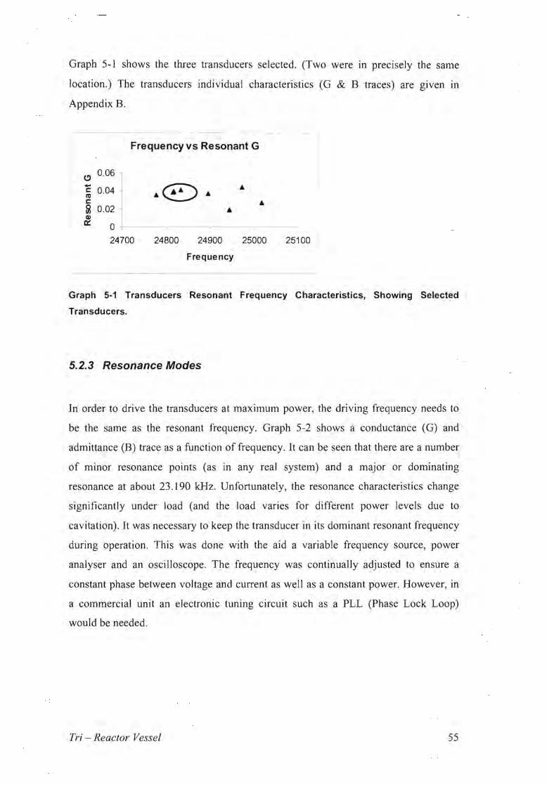
Univers
ity of
Cap
e Tow
n
Graph 5-1 shows the three transducers selected. (Two were in precisely the same
location.) The transducers individual characteristics (G & B traces) are given in
Appendix B.
Frequency vs Resonant G
0.06C)-c: 0.04 • ell
•·0·c: •~ 0.02
Q)
~ 0 1 24700 24800 24900 25000 25100
Frequency
Graph 5-1 Transducers Resonant Frequency Characteristics, Showing Selected
Transducers.
5.2.3 Resonance Modes
In order to drive the transducers at maximum power, the driving frequency needs to
be the same as the resonant frequency. Graph 5-2 shows a conductance (G) and
admittance (B) trace as a function of frequency. It can be seen that there are a number
of minor resonance points (as in any real system) and a major or dominating
resonance at about 23.190 kHz. Unfortunately, the resonance characteristics change
significantly under load (and the load varies for different power levels due to
cavitation). It was necessary to keep the transducer in its dominant resonant frequency
during operation. This was done with the aid a variable frequency source, power
analyser and an oscilloscope. The frequency was continually adjusted to ensure a
constant phase between voltage and current as well as a constant power. However, in
a commercial unit an electronic tuning circuit such as a PLL (Phase Lock Loop)
would be needed.
Tri - Reactor Vessel 55

Univers
ity of
Cap
e Tow
n
Triangular Bath - Transducer 1,2&3 in Parallel Frequency vs B & G
0.08 . 0.04
0.07 0.03
0.06 . 0.02 Ui'
F 0.05 0.01 EG .l::s 0.04 a ~
m :s0.03 -0.01 l!)
0.02 -0.02
0.01 B . -0.03
0·, -0.04 22400 22600 22800 23000 23200 23400 23600 23800 24000 24200
Frequency (Hz)
Graph 5-2 Frequency vs. G & B
Using Graph 5-2 and the graph of the unloaded system it was possible to calculate the
electromechanical efficiency using the following equation:
= Go;r - Glaad Equation 2-29 17 mo G.
OIr
This gave an efficiency of 89%. However, this value did not apply to the system
under load and at high power; it only gave an estimation of the efficiency. The
loading condition was with the vessel filled with water, and the unloaded values were
taken while the vessel was empty with the aid of a network analyser. Graph 5-3 shows
the dynamic impedance as the power was increased, all the time ensuring that the
system was in maximum resonance by tuning the frequency appropriately.
RMS Power \oS Impedance
1000.00 ,.-----'in E 800.00.r:.
~Q. 600.00 ....
B •c: 400.00ra "0 • • t • •• •• •III a. 200.00 E
0.00 '--~--~-~--------1
0.00 100.00 200.00 300.00 400.00 500.00 600.00
Power RMS (W)
Graph 5-3 Dynamic Impedance of all Three Transducers in parallel as a Function of
Power
Tri - Reactor Vessel 56

Univers
ity of
Cap
e Tow
n
It was evident that the transducer electrical-mechanical characteristics vary
considerably under load, further enforcing the need for electronic control In a
commercial unit for both frequency and power.
5.3 Mapping the Sound Field
Before tests with receptacles could begin, an idea of the sound field and focal points
needed to be established. Once again, foil samples were inserted into the vessel and
subjected to ultrasonic radiation. The foil samples were secured on a plastic and wire
rig at various levels throughout the bath. These foil samples were then scanned and
process in Matlab™ to give images below, where the black areas show the destroyed
foil and the grey areas the damaged foil.
Figure 5-3 Cavitation Field Cross-section for 40 & 50 mm Above the Base, Showing the
areas of Cavitation Damage and Advantages of the Digital Image Processor.
5.3.1 Focusing
Figure 5-3 above shows the areas of damage on the foil samples placed midway up
the bath (on the centre line of the transducer). This was the level at which the most
disruption occurred and areas of high cavitation intensity can be seen clearly. It is
evident from these images that there is a large amount of focusing and as a result
destructive energy at the centre of the triangle. This makes intuitive sense in that the
three ultrasonic waves all converge at this point, and because the waves are in phase
Tri - Reactor Vessel 57

Univers
ity of
Cap
e Tow
n
due to all the transducers being in phase, the amplitudes of the waves are added by the
principal of superposition to create an intensity level in theory roughly three times the
surrounding area. In addition to the central focal point, lines can be seen running
from the centre to the comers of the triangle. This can be explained in much the same
way, however it is Jess dramatic because
now only two of the waves are in phase
along these lines. If one of the transducers
is switched off, it can be seen that the lines
from the centre to the comers are created by
the two transducers closest to the line as
shown in
Figure 5-4.
\.. .. .
Figure 5-4 Focusing of Two Transducers, where the upper and lower left transducers
were active and the right transducer was off.
5.4 Optimising the Receptacle
In order to compare this new reactor vessel with previously used equipment it was
necessary to optimise the disruption in this particular set-up. This was done with a
series of receptacles of various sizes, shapes, materials and volume levels. It was
obvious from the mapping of the sound field that the centre of the vessel is the region
with the highest sound intensities, and for this reason all receptacles will be placed in
the centre and at a height that would insure that the centre of the solvent volume is
subjected to the most intense radiation. From the previous section this was found to be
mid way up the bath, along the centre line of the transducers. The following tests were
done in a similar way to the other foil based tests in this project by placing the foil
vertically orientated in the receptacle and sonicating for five seconds. The receptacles
were once again made of polypropylene.
Tri - Reactor Vessel 58
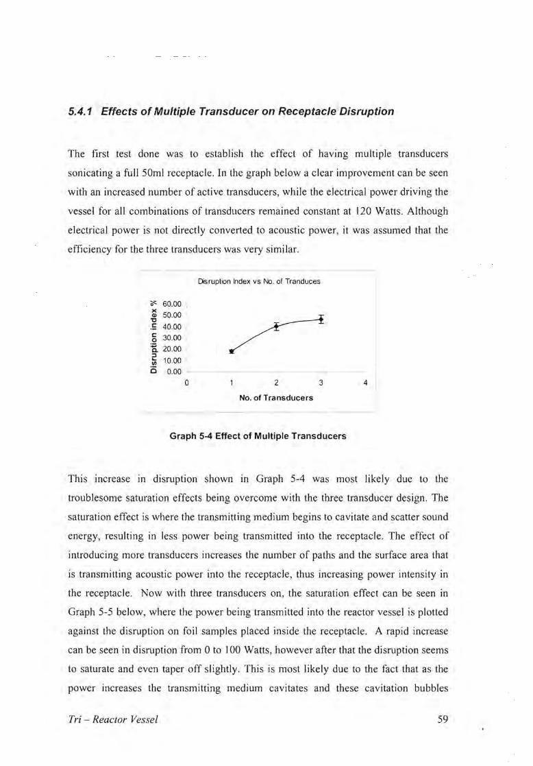
Univers
ity of
Cap
e Tow
n
5.4.1 Effects of Multiple Transducer on Receptacle Disruption
The first test done was to establish the effect of having mUltiple transducers
sonicating a full 50ml receptacle. In the graph below a clear improvement can be seen
with an increased number of active transducers, while the electrical power driving the
vessel for all combinations of transducers remained constant at 120 Watts. Although
electrical power is not directly converted to acoustic power, it was assumed that the
efficiency for the three transducers was very similar.
Disruption Index vs No, of Tranduces
'" 60.00 , ~ 50.00 I 'C c: 40.00
g 30,00
a 20,00 ::J ~ 10.00 is 0.00
o 2 3
No. of Transducers L _________
Graph 5-4 Effect of Multiple Transducers
This increase in disruption shown in Graph 5-4 was most likely due to the
troublesome saturation effects being overcome with the three transducer design. The
saturation effect is where the transmitting medium begins to cavitate and scatter sound
energy, resulting in Jess power being transmitted into the receptacle. The effect of
introducing more transducers increases the number of paths and the surface area that
is transmitting acoustic power into the receptacle, thus increasing power intensity in
the receptacle. Now with three transducers on, the saturation effect can be seen in
Graph 5-5 below, where the power being transmitted into the reactor vessel is plotted
against the disruption on foil samples placed inside the receptacle. A rapid increase
can be seen in disruption from 0 to 100 Watts, however after that the disruption seems
to saturate and even taper off slightly. This is most likely due to the fact that as the
power increases the transmitting medium cavitates and these cavitation bubbles
Tri - Reactor Vessel 59

Univers
ity of
Cap
e Tow
n
absorb and scatter much of the sound energy as found In the chapter on static
pressure. [2]
"0 50c:::
c::: 40 0 30
:0:
20 I
Power vs Disruption
>< Q) 60
Co ::J I 10 III
C 0
0.0 100.0 200.0 300.0 400.0 500.0 600.0
Power (Watts)
Graph 5-5 Disruption as a Function of Power, where the Saturation can Clearly be seen,
the Disruption Levels off and Becomes Less as the Power is Increased.
5.4.2 Plastic Receptacles
In this test electrical power being delivered to the vessel remains constant, as well as
fixing any other factors that could influence disruption such as temperature, geometry,
receptacle position, etc. Various sizes of bottle and volume of solvent were tried, and
the results are shown in the table below. The disruptive index per unit volume is of
particular interest as this shows a measure of the sound intensity per unit volume of
the solvent.
Tri - Reactor Vessel 60

Univers
ity of
Cap
e Tow
n
iSolvent
(ml) Foil
4.7
0.1
9.2
1.3
5.6
0.2
13.6
43.0 3.1 ± 0.24
15.0 5.3 0.42
51.5
13.3 ± 0.54
100
10.1
0.8 :
8.2
3.2 ±
36.0 1.1 ± 0.09
10.7 1.4±0.0
0.04
Table 5·1 Disruption Results for Plastic Bottles
From the 1, it can seen that small bottles with low produced
the most disruption as was however when considering the disruption of
organic materials, solvent saturation needs to into consideration. could
mean that volumes of solvent would need to used, and a compromise
need to be between disruptive required and the amounts of solvent
to fully the compound decision by the end
5.4.3 Receptacle material
The glass receptacle tests were carried out in exactly the same manner as plastic
and although similar can be seen, confirming the small low volume
recommendation, the disruption is significantly lower when compared to that
with plastic This confirms conclusions made by Mr. De
Quieros [I and the of sound transmission solid/liquid interfaces that
IS a use In this context. (Graph 5-6 shows a theoretical
calculation of sound from water through to water
Tri - Reactor Vessel 61
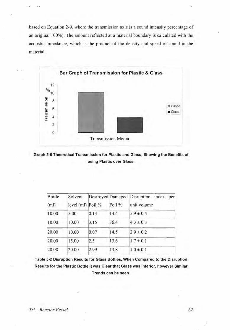
Univers
ity of
Cap
e Tow
n
based on Equation 2-9, where the transmission axis is a sound intensity percentage of
an original 100%). The amount reflected at a material boundary is calculated with the
acoustic impedance, which is the product of the density and speed of sound in the
material.
Bar Graph of Transmission for Plastic & Glass
12
%10
c::: 0 8 'il!
[J Aastic1 6~ • GlassIc:::
III 4 ~... I
2 -i
0
Transmission Media
Graph 5-6 Theoretical Transmission for Plastic and Glass, Showing the Benefits of
using Plastic over Glass.
Bottle
(ml)
Solvent
level (ml)
Destroyed
Foil %
Damaged
Foil %
Disruption index per
unit volume
10.00 5.00 0.13 14.4 5.9 ± 0.4
10.00 10.00 3.15 36.4 4.3 ± 0.3
20.00 10.00 0.07 14.5 2.9 ± 0.2
20.00 15.00 2.5 13 .6 1.7 ± 0.1
20.00 20.00 2.99 13.8 1.0 ± 0.1
Table 5-2 Disruption Results for Glass Bottles, When Compared to the Disruption
Results for the Plastic Bottle it was Clear that Glass was Inferior, however Similar
Trends can be seen.
Tri - Reactor Vessel 62
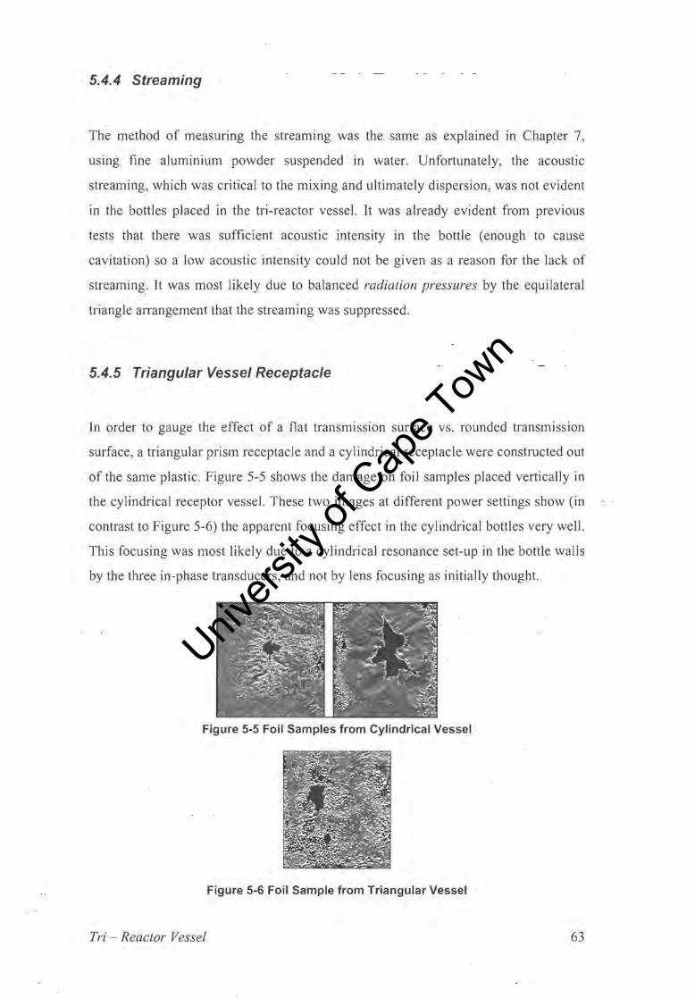
Univers
ity of
Cap
e Tow
n
5.4.4 Streaming
The method of measuring the streaming was the same as explained in Chapter 7,
using fine aluminium powder suspended in water. Unfortunately, the acoustic
streaming, which was critical to the mixing and ultimately dispersion, was not evident
in the bottles placed in the tri-reactor vessel. It was already evident from previous
tests that there was sufficient acoustic intensity in the bottle (enough to cause
cavitation) so a low acoustic intensity could not be given as a reason for the lack of
streaming. It was most likely due to balanced radiation pressures by the equilateral
triangle arrangement that the streaming was suppressed.
5.4.5 Triangular Vessel Receptacle
In order to gauge the effect of a flat transmission surface vs. rounded transmission
surface, a triangular prism receptacle and a cylindrical receptacle were constructed out
of the same plastic. Figure 5-5 shows the damage on foil samples placed vertically in
the cylindrical receptor vessel. These two images at different power settings show (in
contrast to Figure 5-6) the apparent focusing effect in the cylindrical bottles very well.
This focusing was most likely due to a cylindrical resonance set-up in the bottle walls
by the three in-phase transducers, and not by lens focusing as initially thought.
Figure 5-5 Foil Samples from Cylindrical Vessel
Figure 5-6 Foil Sample from Triangular Vessel
Tri - Reactor Vessel 63

Univers
ity of
Cap
e Tow
n
5.5 Pressurizing
To confinn the results found in Chapter 4 on Static Pressure, tests on both the
apparatus and whether the cavitation was suppressed by the static pressure increase
were carried out. Firstly, tests were done on the apparatus to gauge the effects of static
pressure on the resonance frequency and power. These results were found to confinn
those in Chapter 4 and are discussed below.
5.5.1 Pressure Effects on Resonant Frequency
The resonance frequency once again dropped slightly with an increase in pressure,
shown in Graph 5-7, which again shows a linear trend. However, it must be noted that
the gradient was double that obtained with the Vibracel unit.
Pressure vs Resonant Frequency
r=-:.~
• 0 22.20 y = -O.4815x + 22.236 22.10
' ~~:~~ 21 .80 L .~~~----~----------------------------~
-0.4 -0.2 0.0 0.2 0.4 0.6 0.8 1.0 1.2
Pressure (Bar)
Graph 5-7 Graph of Pressure vs. Resonant Frequency, Showing the Frequency
Decreasing with an Increase of Differential Pressure
Tri - Reactor Vessel 64

Univers
ity of
Cap
e Tow
n
5.5.2 Pressure Effects on Power
In Graph 5-8 below shows the triangular bath electrical power as a function of
pressure. Although similar to the Vibracel unit in that power increased with an
increase in pressure, the increase was remarkably less when compared to the same
increases in pressure in the Vibracel. This was due to the different methods in which
the transducers are controlled. The transducers in the triangular bath were simply
driven at a constant voltage, which in contrast to the Vibracel unit involves no active
feedback. The Vibracel unit uses a method of current feedback, presumably to
maintain near constant amplitude on the tip of the transducer. This results in the
Vibracel unit delivering more power to the transducer when under load (i.e. static
pressure) to ensure that the amplitude on the transducer remains constant.
Graph 5-8 RMS Electrical Power as a Function of Pressure, where the Power Increases
Slightly with an Increase of Differential Pressure.
Tri - Reactor Vessel 65

Univers
ity of
Cap
e Tow
n
Differential Pressure Effects
Tests similar to those Chapter 4 differential pressure were out on
triangular reactor vessel. Although the in Table directly
with in Chapter the ratio of any of the sums over 0/0
differential pressure disruption . can enable a comparison those in '-'UU.IJ,vl
It was Increase increase of
differential was In reactor vessel as
it was the Vibracel unit. This be due to two possible firstly, use
of transducers in overcoming the problematic saturation effect In
transmitting medium rendering the static pressure less and secondly, the
previously mentioned Jack of control and resulting relative power in the
triangular vessel when compared to Vibracel as the was
Destroyed Damaged Disruption
Index
17.8±lA
20.0 ± 1.6
60.7
0/0.75 40.9
Table 5-3 Differential Pressure Results
Tri - Reactor Vessel 66

Univers
ity of
Cap
e Tow
n
5.6 Comparison between Tri ..reactor and Vibracel Unit
order to gauge the a comparison between the
the Vibracel unit, three were compared. Firstly, simply at
the electrical power being into the system gives us an
of the transducer. this is extremely inaccurate as are many
inefficiencies in the of ultrasound to the
transducers. The second method somewhat overcomes this problem by
disruption within the (which is common to both and
comparing the power at which disruption saturates, a high indicating a nrHllpr
better design in tenns disruptive power to the third is
simply """" .... <1 tenns of how the end product is to function
i.e. its ability to solids.
When comparing which was driven at Watts (max. at 0 Bar)
and the Vibracel unit at 190 Watts (max. at 0 it tri-reactor
vessel has a advantage over the Vibracel unit to tri-reactor delivering
more power.
Looking at the disruption as function of a maximum at
300 be seen; however it 80% of the saturation value
at comparing this to the Vibracel unit the disruption saturates
at about 100 80% of its reaching a maximum value at just over 40
Watts, it can UI.A.lUI..,,",U that the is more effective at delivering
power to
Compari n Tri and Vib I Unit
to a
at
or
is common to
a
IS
IS to
was at (max. at 0
at 0 tri··-reactor
over unit to
rnore
as a at
at saturates
at
IS more P1"1"Pl't.uP at
nrnHPT to
Univers
ity of
Cap
e Tow
n
5.7 Conclusion
The saturation problem was overcome, which was one of the main reasons for the
construction of this multiple transducer bath. Based on the findings, it was evident
that the use of multiple transducers increased the transmission to the vessel by about
threefold. The effects of static pressure were confirmed on both the apparatus and
cavitating liquid, and the advantages of differential pressure were shown once again.
It was also recommend that a PLL be used in a final product to control frequency and,
hence, the systems power. The tri-reactor can unfortunately not be recommended for a
disruption cell as its tendency to suppress streaming caused the system to be
ineffective. However, if a fourth transducer was placed at the bottom of the bath it
could possibly unbalance the radiation pressures and result in streaming.
Tri - Reactor Vessel 68

Univers
ity of
Cap
e Tow
n
6 Transmission Media
This considers use of liquids as a for the of
high power ultrasound to The goal was to the
the transmission medium by some other means time-consuming
static pressure method. This chapter at acoustic attenuation, due
firstly to sound waves reflected at boundaries in theory, and secondly,
to the effects of cavitation absorbing and the sound energy in the actual
This was followed by a the effect a broad
cross of liquids as media were In
terms of the attenuation the sound travelling through them an optimum solution
a transmission medium was found.
6.1 Acoustic Attenuation
As mentioned, attenuation was believed to come from two sources:
the scattering effect of cavitation, and reflection at material boundaries.
there is a third source of namely VISCOUS This needs to
into account when considering oils as media that significantly
higher than water or water-based solutions. [2]
Transmission Mediums 69
to
cross
temlS
a
1 Acou
(j 'fralls111ission Media
use as a
an
Attenu
was to come two sources:
water or
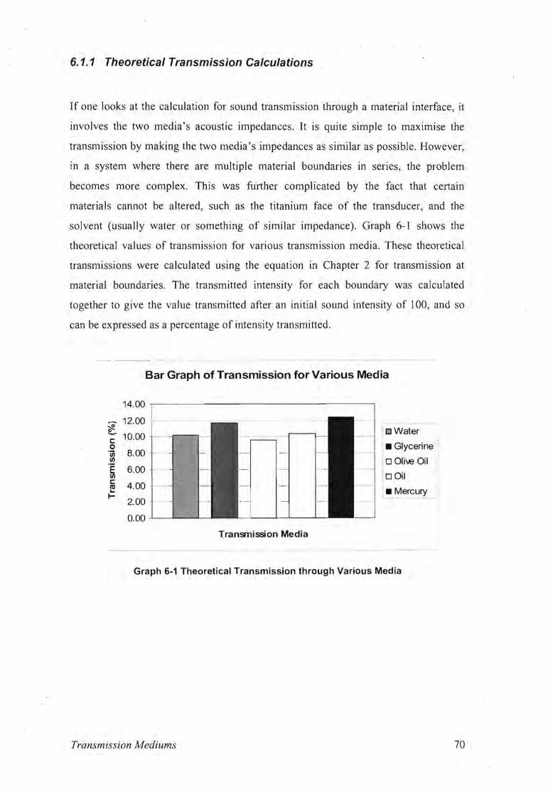
Univers
ity of
Cap
e Tow
n
6.1.1 Theoretical Transmission Calculations
If one looks at the calculation for sound transmission through a material interface, it
involves the two media's acoustic impedances. It is quite simple to maximise the
transmission by making the two media's impedances as similar as possible. However,
in a system where there are multiple material boundaries in series, the problem
becomes more complex. This was further complicated by the fact that certain
materials cannot be altered, such as the titanium face of the transducer, and the
solvent (usually water or something of similar impedance). Graph 6-1 shows the
theoretical values of transmission for various transmission media. These theoretical
transmissions were calculated using the equation in Chapter 2 for transmission at
material boundaries. The transmitted intensity for each boundary was calculated
together to give the value transmitted after an initial sound intensity of 100, and so
can be expressed as a percentage of intensity transmitted.
---_. _-
Bar Graph of Transmission for Various Media
Transmission Media
Graph 6-1 Theoretical Transmission through Various Media
14.00 -,--- ------------------,
12.00 ~ ~ c:: 1 0.00 -4-~r---I-o .~
·e II)c:: ~ I
8.00
6.00
4.00
2.00
0.00 -'--_.L_-"__
o Water
• Glycerine '
oOIi\€ Oil
oOil
• Mercury
Transmission Mediums 70

Univers
ity of
Cap
e Tow
n
6.1.2 Attenuation in the System
Looking at the tests done on the actual system, a number of interesting observations
can be made. Graph 6-2 and Graph 6-3 show the sound intensity as a function of
distance from the transducer. These values were taken with the use of a custom built
PZT hydrophone. The intensities were expressed as a voltages as these graphs only
serve as comparative and not absolute references. The Vibracel device was used
again, with the amplitude set to 50% giving an average power of 70 Watts . The
temperature was maintained at a constant 23 °C by circulating water. The water leveJ
was maintained at 35mm above the transducer face for both receptor vessel and the
coolant.
Without receptor vessel
Hydrophone
Coolant
- --- Di lance fro
tra sducer
Coolant
With receptor vessel
Hydrophone
Coolant
Receptor vessel o t
-+---Di ' ance from '---_....
sducer
Coolant
In
Figure 6-1 Apparatus used to Measure Attenuation over Distance
Two sets of readings were taken: one without the receptor vessel present, and the
other with the receptor vessel present. The experimental set-up is shown in Figure
6-1. Graph 6-2 shows the sound intensity as a decaying exponential with a sinusoid
superimposed on top of it. This demonstrates very well the exponential decay of a
sound wave in a lossy medium, as well as the standing waves that are set-up in the
Transmission Mediums 71
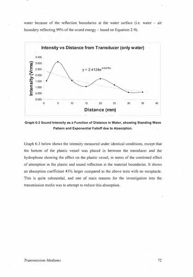
Univers
ity of
Cap
e Tow
n
water because of the reflection boundaries at the water surface (i.e. water - aIr
boundary reflecting 99% of the sound energy - based on Equation 2-9) .
Intensity vs Distance from Transducer (only water)
3.500
(i) 3.000
E 2.500 y = 2.4124e-00376x > - 2.000 ~...
1.500 tJ)
~ 1.000... c: 0.500
0.000 ---
o 5 10 15 20 25 30 35 40
L Distance (mm)
Graph 6-2 Sound Intensity as a Function of Distance in Water, showing Standing Wave
Pattern and Exponential Falloff due to Absorption.
Graph 6-3 below shows the intensity measured under identical conditions, except that
the bottom of the plastic vessel was placed in between the transducer and the
hydrophone showing the effect on the plastic vessel, in tenns of the combined effect
of absorption in the plastic and sound reflection at the material boundaries. It shows
an absorption coefficient 43% larger compared to the above tests with no receptacle.
This is quite substantial, and one of main reasons for the investigation into the
transmission media was to attempt to reduce this absorption .
Transmission Mediums 72

Univers
ity of
Cap
e Tow
n
-----
----
Intensity vs Distance from Transducer (Water & Plastic Receptcale)
tJ) 4.000
E 3.500
> 3.000- 2.500 O0534xY= 2.41 e- .~
~ 2.000 .
tJ) 1.500 -----~r::::
Q) -1.000 ~ 0.500r::::
0.000
0 5 10 15 20 25 30 35 40
Distance(mm)
Graph 6-3 Sound Intensity as a Function of Distance in Receptacle, As above but
showing a Smaller Intensity.
6.1.3 Affect of solutes on Vapour Pressure
In order to fully understand the results presented in the next section, a review of
Raoult's Law follows:
The vapour pressure increase of the solvent, LJP, of a solution equals the vapour
pressure of the pure solvent, Po, times the mole fraction of solute, X, in the
solvent.[f f} Pg 497
I.e. LJP = PoX
This implies that the addition of a solute or salt to the transmission medium has the
effect of increasing the vapour pressure and, consequently, the threshold pressure,
causing a suppression of cavitation amongst other things.
Transmission Mediums 73

Univers
ity of
Cap
e Tow
n
6.2 Transmission Media
The transmission media that were expected to work well, based on reflection
calculations, were those with acoustic impedances of between 1.7 and 27.3 MRayls,
having a low viscosity and high vapour pressures. However, a wide cross-section of
liquids were chosen for testing to confirm the above assumptions.
6.2.1 Testing of Various Media
The tests carried out on the media used the standard set-up described in Chapter 3
with a few modifications. The first being that the medium could not be circulated, as
there was not sufficient quantities to do so. This meant that the same liquid was used
for successive tests, making cooling it necessary. This was achieved by inserting a
copper pipe coil through which cooling water was passed, acting as a heat transfer
mechanism, cooling the medium down to 23 °C before each test. The amplitude setting
put at 100% gave a power of about 160 Watts. The gap between the transducer
emitting-face and the receptacle was 1 mm and the transition medium and water in the
receptacle was at a level of 35mm above the transducer emitting-face. Once again the
foil sample was placed in the receptor vessel with a vertical orientation.
Graph 6-4 below shows the disruptive index for the media tested. Water was the
medium used in all previous tests, implying that we needed a medium that produced
higher disruptive indices in order to increase the transmission. (These results were the
average of three foil tests).
Transmission Mediums 74
6.2 Transmission Media
The transmission media that were expected to work well, based on reflection
calculations, were those with acoustic impedances of between 1.7 and 27.3 MRayls,
having a low viscosity and high vapour pressures. However, a wide cross-section of
liquids were chosen for testing to confirm the above assumptions.
6.2.1 Testing of Various Media
The tests carried out on the media used the standard set-up described in Chapter 3
with a few modifications. The first being that the medium could not be circulated, as
there was not sufficient quantities to do so. This meant that the same liquid was used
for successive tests, making cooling it necessary. This was achieved by inserting a
copper pipe coil through which cooling water was passed, acting as a heat transfer
mechanism, cooling the medium down to 23 °C before each test. The amplitude setting
put at 100% gave a power of about 160 Watts . The gap between the transducer
emitting-face and the receptacle was 1 mm and the transition medium and water in the
receptacle was at a level of 35mm above the transducer emitting-face. Once again the
foil sample was placed in the receptor vessel with a vertical orientation.
Graph 6-4 below shows the disruptive index for the media tested. Water was the
medium used in all previous tests, implying that we needed a medium that produced
higher disruptive indices in order to increase the transmission. (These results were the
average of three foil tests).
Transmission Mediums 74

Univers
ity of
Cap
e Tow
n------
Bar Graph of Disruption for Transmitting Mediums
40.00
35.00 @ '0 30.00 c
25.00 c 0:a 20.00
15.002 (/)
(5 10.00
5.00
0.00 .
Transmitting Medium
[iJ Water
[l 50% glycerine
• Olive Oil
o Isolation Oil
o eaa...,1.8&03 rroVm
Graph 6-4 Bar Graph of Transmitting Media (at 23°C)
Once again, in Graph 6-4, it can be seen that both the oils perfonned very badly even
though they suppressed the cavitation, as visually confinned. It was evident that the
viscosity caused large absorption of sound energy. The medium labelled "50%
Glycerine" consisted of a 50% water, 50% glycerine mixture and produced a slightly
worse disruption index than water due to the presence of cavitation (as much as in
pure water), and the high viscosity media apparently absorbing more energy than
lower viscosity media. The one medium that increased the transmission, with a
disruption index of 27% higher than water, was the CaCl2 solution. This was most
likely because the vapour pressure was increased according to Raoults' Law, as the
cavitation could visually be seen to have reduced significantly. However, the
concentration of 1.8 x 10-03 mol/ml was randomly chosen and needed optimisation.
6.2.2 Optimising CaCI2 Solution Concentration
Using the same experimental set-up as above, a set of foil tests were conducted with
varying molar concentration of CaCh in water.
Transmission Mediums 75

Univers
ity of
Cap
e Tow
n
Disruption vs. Transrrission Medium Conce ntration
20
18 )( Q) "0 16s::
.. s:: 0 14 Co 2 12IIJ
is 10
8
0
-
-
0.0005 0.001 0.0015 0.002 0.0025 0.003 0.0035 0.004
Concentration (mol/ml)
Graph 6-5 Concentration Optimisation (at 23°C), showing the Optimum Molar
Concentration in terms of Transmission.
Graph 6-5 shows a band between 0.001 and 0.003 mol/ml with an average disruptive
index of 22% larger than that of plain water. This region has a few other maximums
but these are probably extremes caused by random errors. It was nonetheless obvious
that the transmission falls off rapidly for concentrations above 0.003 mol/m!. This is
possibly an increased viscosity causing the medium to absorb energy, thereby
reducing the transmission.
Transmission Mediums 76

Univers
ity of
Cap
e Tow
n
7 Streaming
As mentioned before, the of acoustic provide a mixing stirring
action. It was desirable to maximise these mixing to improve the dispersion
and therefore it was critical that the factors influencing streaming are
discussed and quantified in context a disruption cell. chapter looks at the
streaming set up in and these are affected factors
such as amplitude (or acoustic the water between transducer and
the the SIze, final1y, the volume of liquid
1 Test Conditions
The tests conducted in this chapter were under the conditions that produced
disruption as set out in previous namely a 50ml plastic bottle 1 mm
above the transducer, and water both inside and outside receptacle. The of
the coolant/transmission was set at 35mm above transducer face. Only
the under was to see effect on acoustic
streaming patterns of the tests that were done the same basic
shown Figure 1.
Streaming 77
1 Test d
tests In
as set out H1
1.
7 S
m
s
\vcrc
was set at
a
on
same
are
Imm

Univers
ity of
Cap
e Tow
n
Reaction vessel
Digital Camera
Cooling water out
Vibracel Amplifier
& power meter
[f-+ L.:~
Cooling water in
Transducer
Figure 7-1 Streaming Measurement Apparatus, showing the Physical Arrangement of
the Apparatus.
Receptacle
Transducer
Figure 7-2 Typical Streaming Pattern, where the Curved Lines and Arrows Represent
the Path and Direction of the Streaming Water.
In Figure 7-2 the position of the transducer is shown, where the rectangle labelled
"receptacle" above the transducer represents a cross section of the cylindrical receptor
vessel with a typical streaming pattern. These streaming patterns were particularly
suited to dispersion of solids due to the fact that the solvent flows to the centre of the
Streaming 78

Univers
ity of
Cap
e Tow
n
bottle. This moved solids to the regions of high intensity ultrasound (the centre of the
vessel). Only once the solid was damaged or lightened sufficiently would it be lifted
and removed by the streaming forces.
The streaming was predominantly symmetrical around a vertical line in the centre of
the vessel. As mentioned in Chapter 3, the patterns were analysed with the aid of
aluminium powder in water and a digital video camera. Using a personal computer to
step through the video frame-by-frame , it was possible to obtain the velocity of the
streaming with reasonable accuracy and visually quantify the extent of the streaming.
Figure 7-3 Frame 18, shows the Aluminium being Picked up by the Streaming.
Figure 7-4 Frame 22, shows the Distance the Particles of Aluminium have Travelled
between the Two Frames.
In Figure 7-3 Frame 18 and Figure 7-4 Frame 22 it can be seen how the velocity
measurements were taken: divide Lly by the time between Frame 18 and 22 based on
the fixed frame rate of 14.5 frames per second.
Streaming 79

Univers
ity of
Cap
e Tow
n
7.2 Acoustic Intensity
Graph 7-1 was obtained usmg the above method to measure the velocity of the
streaming and varying the amplitude of the transducer. This displays an apparent
linear relationship between velocity and amplitude. Amplitude is also related to
intensity in this context due to the transducer load being consistent. These results are
confinned by the Equation 2-6 Vo = I OR 2~2 where the streaming velocity (v ) iso3poco
linearly proportional to sound intensity (10)' Based on the results , it can be confinned
that the increase of acoustic intensity causes an increase in streaming velocity for this
particular arrangement.
Amplitude vs Velocity
0.70
0.60 · • ~ 0.50 E .s 04 0
z'0 0.30 .2 ~ 0.20
0.10
0.00 +1 ----.
o 20 40 60 80 100 120
Amplitude (%)
Graph 7-1 Streaming Velocity as a Function of Amplitude, where the Streaming
Velocity seems to Increase Linearly with Amplitude.
The 'Glass vessel' trace in Graph 4-1 shows the relationship between amplitude and
power for the Vibracel unit, which can be used to calculate the power values in the
above Graph 7-\.
Streaming
I
80

Univers
ity of
Cap
e Tow
n
------
7.3 Distance from Transducer
Looking at the results obtained from varying the gap between the receptacle and the
transducer in Graph 7-2, yet another interesting phenomenon related to acoustic
intensity can be seen. Graph 7-2 shows the velocity decaying exponentially as the gap
was increased. This was not a direct streaming effect but rather confirmation that the
water gap between the vessel and transducer absorbs the sound energy exponentially
as a function of distance (Equation 2-12). This again confirms and correlates with the
test results for destruction of the foil samples. Graph 7-2 shows that the larger the
acoustic intensity (or the closer the receptacle vessel to the transducer), the more
pronounced the streaming effects.
Water Gap vs Velocity
0.70
0.60 • ::§' 0.50 I E E.. 0.40
~ '0 0.30 o ~ 0.20
0.10 .
0.00 -
o 2 3 4 5 6 7 8
Gap (mm) _. __ 1
Graph 7-2 Streaming Velocity as a function of Transducer - Receptacle Distance,
Showing a more Violent Streaming action for Small Transducer Receptacle Gaps.
Streaming 81
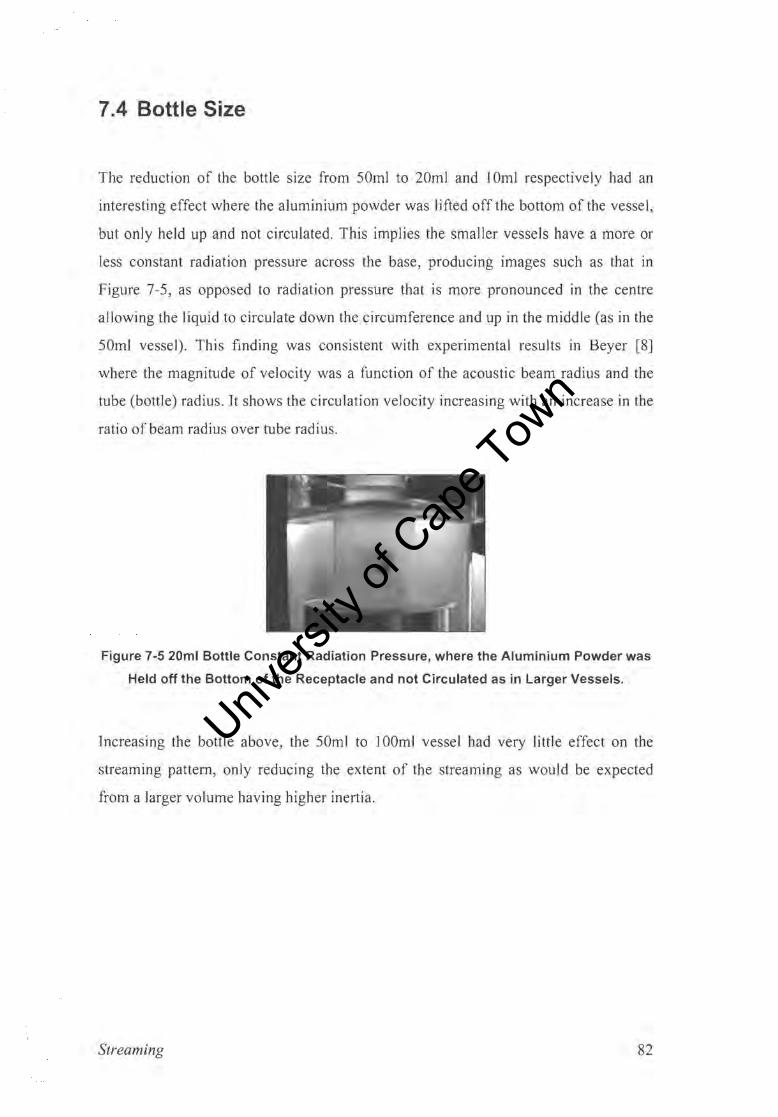
Univers
ity of
Cap
e Tow
n
7.4 BoUie Size
The reduction of the bottle size from 50ml to 20ml and IOml respectively had an
interesting effect where the aluminium powder was lifted off the bottom of the vessel ,
but only held up and not circulated. This implies the smaller vessels have a more or
less constant radiation pressure across the base, producing images such as that in
Figure 7-5, as opposed to radiation pressure that is more pronounced in the centre
allowing the liquid to circulate down the circumference and up in the middle (as in the
50ml vessel). This finding was consistent with experimental results in Beyer [8]
where the magnitude of velocity was a function of the acoustic beam radius and the
tube (bottle) radius. It shows the circulation velocity increasing with an increase in the
ratio of beam radius over tube radius.
Figure 7-5 20m I Bottle Constant Radiation Pressure, where the Aluminium Powder was
Held off the Bottom of the Receptacle and not Circulated as in Larger Vessels.
Increasing the bottle above, the 50ml to lOOml vessel had very little effect on the
streaming pattern, only reducing the extent of the streaming as would be expected
from a larger volume having higher inertia.
Streaming 82
7.4 BoUie Size
The reduction of the bottle size from 50ml to 20ml and lOml respectively had an
interesting effect where the aluminium powder was lifted off the bottom of the vessel,
but only held up and not circulated. This implies the smaller vessels have a more or
less constant radiation pressure across the base, producing images such as that in
Figure 7-5, as opposed to radiation pressure that is more pronounced in the centre
allowing the liquid to circulate down the circumference and up in the middle (as in the
50ml vessel). This finding was consistent with experimental results in Beyer [8]
where the magnitude of velocity was a function of the acoustic beam radius and the
tube (bottle) radius. 1t shows the circulation velocity increasing with an increase in the
ratio of beam radius over tube radius.
Figure 7-5 20m I Bottle Constant Radiation Pressure, where the Aluminium Powder was
Held off the Bottom of the Receptacle and not Circulated as in Larger Vessels.
Increasing the bottle above, the 50ml to 100ml vessel had very little effect on the
streaming pattern, only reducing the extent of the streaming as would be expected
from a larger volume having higher inertia.
Streaming 82

Univers
ity of
Cap
e Tow
n
7.5 Volume Levels
As was expected, the variation of water level in the vessel had very little effect in
tenns of the extent of the streaming as a function of the total volume. However, it was
noticed that the streaming velocity increased slightly with an increase of volume. It
was also noticed that the volume level of 10ml in the SOml container deviated from
the typical streaming pattern set out in the beginning of this chapter by being visibly
more chaotic in nature. The apparent radiation pressure (based on the initial velocity)
at the bottom of the vessel seemed to increase with an increase of volume, possibly
because the loading of the system caused the acoustic intensity at the vessel base to
increase. This effect cannot be used successfully however, as an increase of volume
would dilute the streaming and, more importantly, reduce the cavitation density which
would be undesirable.
7.6 Conclusion
Based on the tests conducted, it was clear that streaming, or more precisely radiation
pressure, was proportional to acoustic intensity, thus agreeing with the theory [4]. The
presence of a volume large enough to enable circulation was important.
Streaming 83
7.5 Volume Levels
As was expected, the variation of water level in the vessel had very little effect in
terms of the extent of the streaming as a function of the total volume. However, it was
noticed that the streaming velocity increased slightly with an increase of volume. It
was also noticed that the volume level of 10ml in the SOml container deviated from
the typical streaming pattern set out in the beginning of this chapter by being visibly
more chaotic in nature. The apparent radiation pressure (based on the initial velocity)
at the bottom of the vessel seemed to increase with an increase of volume, possibly
because the loading of the system caused the acoustic intensity at the vessel base to
increase. This effect cannot be used successfully however, as an increase of volume
would dilute the streaming and, more importantly, reduce the cavitation density which
would be undesirable.
7.6 Conclusion
Based on the tests conducted, it was clear that streaming, or more precisely radiation
pressure, was proportional to acoustic intensity, thus agreeing with the theory [4]. The
presence of a volume large enough to enable circulation was important.
Streaming 83

Univers
ity of
Cap
e Tow
n
8 Thermal Shocking
chapter was concerned with the use thermal cycling to increase dissolving
qualities of the solvent as well as increasing the disruptive force of the cavitation. It
looks at the dependence of violent cavitation on temperature. the of
solvents at different and finally the temperature
calculations, thermal of the
8.1 Test Conditions
A fluid (on loan industry) provided a and accurate means of
adding the solvent in correct volumes, at a set temperature and at the right time
intervals. The fluid consisted of two pump, storage and del
one the hot solvent one for cold solvent. unit's delivery system and
environment is In Figure 8-2.
shocking 84
8 Shocking
was use to
It
1 Cond
A a accurate means
at
one
IS
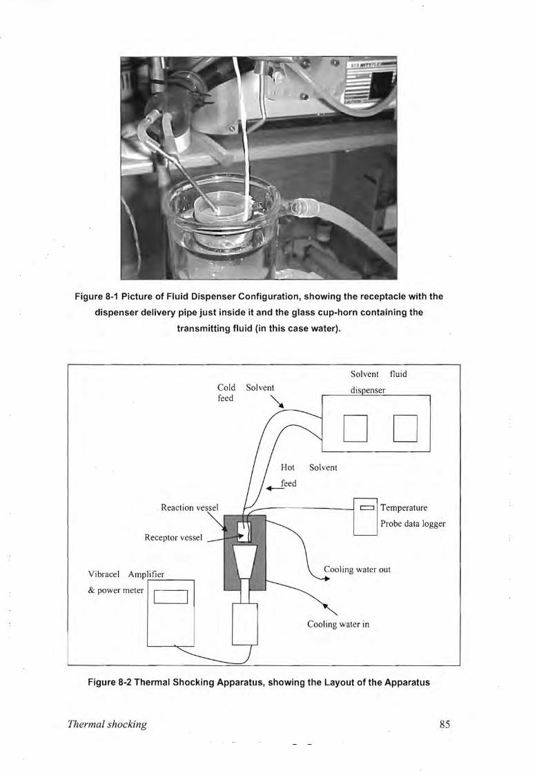
Univers
ity of
Cap
e Tow
nFigure 8-1 Picture of Fluid Dispenser Configuration, showing the receptacle with the
dispenser delivery pipe just inside it and the glass cup-horn containing the
transmitting fluid (in this case water).
Solvent fluid
Cold Solvent feed ~
D D Hot Solvent
Reaction c:=:J Temperature
Probe data logger
Receptor vessel _-<a...::'>L--1
Cooling water out Vibracel Ampl,ifi_le_r__--,
& power meter
Cooling water in
Figure 8-2 Thermal Shocking Apparatus, showing the Layout of the Apparatus
Thermal shocking 85

Univers
ity of
Cap
e Tow
n
••
8.2 Effects of Temperature on Cavitation
lO r-----------------------------,
"'.1S ~~ ~
~ ""'",~","0 e IL ~'-" C
~ ~ 10 ~,•e ~> ~ '" ..
c:;.;; 0- 5 -.
o ~----~----~----~----~----~
o 10 20 30 50
Temperature ("C)
Figure 1 Va·fialion Wrlh temperlilUrO of the rale of SOfIochemical oxidalio,n of iodide using 20kHz irradiation WiLh an X-large tip . (A) 21 W: (-I-) 32 W; (.) 42 W; (.) 56 W; {y) 72 W. Each point
Graph 8-1 Iodine oxidation as a result of cavitation as a function of Temperature [19],
showing fall-off in oxidation with and increase of temperature.
Graph 8-1 from Entezari and Kruus, shows the cavitation in terms of iodine oxidation
as a function of temperature for a system using ultrasound at 20 KHz. It clearly
shows a decrease in cavitation for an increase in temperature, and for this reason the
temperature needs to be controlled quite accurately. (These values are not necessarily
the case with water but show the importance of thermal control.) It must also be noted
that samples may be sensitive to high temperatures and an easy method of
calculating/measuring the real temperature is required. [19]
Increasing the temperature of the solvent increases the dissolving of the organic solid.
The benefits of a high temperature solvent are obvious and therefore the temperature
Thermal shocking 86
Univers
ity of
Cap
e Tow
n
needs to be allowed to rise as high as possible, but without reducing the cavitation too
much. For these reasons it was essential to understand the thermal system.
8.3 Use of Analogue Computers in Temperature
Calculations
Analogue computers were used to accurately predict the real temperatures of the
solvent base on the measured temperatures, as well as predicting temperatures of
untested situations. These analogue computers were electrical in origin yet provide a
fast, flexible method of solving differential equations. The thermal system can be
modelled in electrical terms using the equivalent parameters set out in Chapter 2. This
enables the real temperature sensor to be modelled and actual dynamic temperature
profiles can be calculated.
Thermal shocking 87

Univers
ity of
Cap
e Tow
n
8.4 Temperature Profiles
Temperature profiles were measured with an LM35T electronic temperature probe
that was inside the treatment vessel. The treatment vessel (50ml polyprop.) was then
placed in the Vibracel 68mm cup hom along with the transmitting fluid (water at
23°C) providing cooling as well as acoustic transmission. The cooling fluid was
circulated to ensure that the temperature of 23°C was maintained. (Flow rate for this
was 250mllmin). Graph 8-2 shows a typical temperature profile record, where the
effects of adding the hot and cold water can each be clearly seen.
Temperature Profile Inside Bottle
~___....... / Cold added
E20
(!!. 10 ·1
'Hot added
0 -
o 10 20 30 40 50 60
Time (s)
Cl) 50 I
-=40 ro Q; 30
a.
Graph 8-2 Typical Temperature Profile, showing the Change in Temperature over Time
as the Hot Water was Added and then the Cold.
8.4.1 Varying Volume Ratios
To fully understand the effect of different volumes and temperatures of the solvent
being added to the container, a set of tests were carried out and the temperature
profiles were recorded. Using the apparatus as described and shown in Figure 8-1,
Graph 8-3 shows the effect of varying the ratio of hot (90°C) and cold (23°C) water
while keeping the final volume at 30ml.
Thermal shocking 88

Univers
ity of
Cap
e Tow
n
Thermal Profile for Varying Volume Ratios I (hot/cold m I)
_ 80 -
o 70 J- --'
Q) 10 -5/25 ~--
..... 0 .,.
o 10 20 30 40 50 60
Time (s) _I
Q) 60 ,
~ 50 j-~ 40 l Q) 30 -· a.E 20
-25/5
-20/10
15/15
- 10/20
Graph 8-3 Thermal Profiles for Varying Ratios, where the 25/5 .. etc. Represents the
Volume of Hot Water 1the Volume of Cold Water.
To get the profile above, the hot water (the so1vent in this case) was introduced first
and, after a delay of 15 seconds, the cold water was added. Graph 8-3 gives a fair
indication of the temperatures involved and shows that the temperature apparently
doesn't go above 70°C. As was presumed, the larger the amount of hot water
introduced, the higher the temperature throughout the profile, and, subsequently, the
final temperature (after 50 seconds) was higher.
Thermal shocking 89

Univers
ity of
Cap
e Tow
n
8.4.2 Equivalent Circuits
Based on the above tests with variable volume ratios, the effectiveness of equivalent
circuits in calculating the temperature profiles can be seen. Figure 8-3 below shows an
equivalent circuit (analogue computer) that was used to calculate the profiles. The
various subsections of the circuit can be seen, along with their thermal equivalents.
Ultrasonic Res tHe~ Energy Hot & cold water Prohe
r---------,~ ~--------------------------: I I
I
Plastic hottle ,_ - - - - - - - - - - - - - I I
I:~ ~--------~--~-'~_,----~~._~r_,:~~2Dk~.
~------ --~
10k , 104&-nF
'~V
[ill I
2,3V I ~I
I
Figure 8-3 Thermal System Equivalent Circuit
The hot and cold water are represented as capacitors (heat storage) charged to a
specific voltage (temperature), using switches to introduce the capacitance (water
volume) to the system at the correct time. The plastic bottle was represented as a
capacitor (heat capacity) and a resistor (thermal conduction) to a voltage source (the
cooling liquid), and the temperature probe, as mentioned already, was modelled as a
low pass filter. The ultrasonic energy (heating) is represented as a current source. The
two probes, one in the plastic bottle box and the other in the temperature probe box,
were used to produce real time traces of the real and the measured or apparent
temperature.
Graph 8-4 displays these traces where the components were tuned to simulate the 5ml
hot and 25m] cold settings. It was interesting to note that the real temperature was
quite different in shape and magnitude to the measured value . This discrepancy in the
profiles was due to the time lag or slow response of the temperature sensor in
registering the measured temperature.
Thermal shocking 90

Univers
ity of
Cap
e Tow
n
Theoretical Thermal Profile for 5ml Hot 125 Cold Water
U 7
~ 6 J i5l 5G>f7~L --l'v1easured 1/~ : ___-=:::=~_____-
L- Real
1ii 2...
~ 0
1
JI- -'-----
o 10 20 30 40 50
Time (5)
Graph 8-4 Theoretical Thermal Profile for 5ml hot I 25 ml cold.
This shows the temperature at which the liquid in the receptacle was initially at, just
after t=O seconds, and the discrepancy between the measured and real values. Anyone
wanting to use this thermal shocking needs to realise that for all the simulations done,
the maximum real temperature was about 20% higher than the maximum measured
temperature owing to the time constant of the temperature sensor. This is important in
terms of raising the temperature above a value that would suppress cavitation and/or
damage the sample in some undesirable way.
8.4.3 Ultrasonic Energy Effects
Tests done up to this point have been with the transducer switched off so as to
simplify the analysis until the system was well understood. The effect of switching on
the transducer can be seen below in Graph 8-5 where the ultrasound introduces
heating energy into the system, thereby raising the thermal profile. This can be
simulated by modelling the heat energy as a current source.
Thermal shocking 91

Univers
ity of
Cap
e Tow
n
- ----
Thermal Profile Showing Ultrasonic Tranducer Effect
7o,-----------------------------------.
tf 60-Q) 50... .a 40 - 10/20 ~ Q) 30 - TX on 10/20 I c.E20 Q)
I- 10
o · ,~----------~----------~----------~
o 10 20 30 40 50 60
Time (s)
-
-
Graph 8-5 Effect of Introducing Ultrasonic Energy, where the Introduction of Ultrasonic
Energy causes a Noticeable Increase on Temperature
It must be noted that for the profiles shown above the transducer has the effect of
increasing the temperature by 10°C. This must be taken into account and compensated
for. Graph 8-6 shows the temperature profile generated using the analogue computer
simulating the transducer being switched on. The maximum temperature can be seen
to be the same for real and measured case; however, it shows the difference in time
duration at that maximum temperature. This effect still needs to be considered by the
end user as the time at the maximum temperature is roughly 50 % longer than that
implied by the measured profile.
Theoretical temperature profile for 10ml hot 120ml cold (Transducer on)
U 7 .--------------------------~--------~ VI}:IC- -- - - ~;;;::_- - -=-L- -
I-Real I~4
~ 3 - tv1easured ! - I:::I
E 2 CI>
~ 1 ~O-'----------------------,---------------l
o 5 10 15 20 25 30 35
Time(s)
Graph 8-6 Theoretical Temperature Profile (Transducer Switched on)
Thermal shocking 92

Univers
ity of
Cap
e Tow
n
9 Conclusion & Future Recommendations
The factors influencing cavitation, streaming and ultimately dispersion were
investigated and optimized to produce a number of useful methods or apparatus, as
outlined below.
The use of a digital image processor for the analysis of foil samples to give both
numerical area values for damaged and destroyed foil, and to show spatial distribution
of the cavitation field, proved to be invaluable. It made possible large numbers of tests
due to its speed and need for little user intervention, while still maintaining
consistency and accuracy throughout the testing.
The problem of acoustic saturation at high powers was overcome in a number of
ways. Firstly, the static pressure or the differential pressure method provided an
increase in destruction (cavitation damage) of 250 ± 20% in the Vibracel unit and 139
± 11 % in the tri-reactor bath. The reason for the tri-reactor having a lesser increase in
destruction with the differential pressure method was because the saturation effect
was already partially overcome by the use of multiple transducers. The use of three
transducers, and hence three paths for the acoustic energy to travel through, provided
an increase of destruction by 240 ± 19.2% compared to the same apparatus with only
one transducer active but at the same power as the three transducers. The combined
effect of differential pressure and the use of three transducers provided an increase of
330 ± 26% in destruction. The third method of reducing saturation was the use of a
salt solution, to raise the cavitation threshold by limiting cavitation that absorbs
energy in the transmission medium. This only increased the destruction by 122 ± 9%
but could be used in conjunction with the above pressure differential methods.
The investigation into streaming provided important infonnation on acoustic
streaming in the context of a small vessel. The tri-reactor unfortunately didn't produce
Conclusion & Future Recommendations 93

Univers
ity of
Cap
e Tow
n
any notable streaming effect, making it a very poor option due to the lack of macro
mixing. However, future work may look into making an unbalanced multiple
transducer bath. It might also be an option to sometimes drive only one transducer on
the tri-reactor vessel, to unbalance the acoustic field. It must be noted that for the cup
hom set-up, the streaming was proportional to sound intensity and that the vessel
needs to be over 30ml in volume to allow significant streaming.
Thermal shocking provided additional dispersion capability by increasing the
cavitation strength, as well as increasing the ability of the solvent to dissolve. The use
of equivalent circuits to estimate the real temperature profiles can be used to decide
on the fluid dispenser settings, so as not to exceed the critical temperature of the
specific organic compound.
In conclusion, the differential pressure, multiple transducers and salt solution
provided an increase in acoustic intensity in the receptacle, which was the goal of the
research. However, the combined effect of combining the salt solution with the
pressure and multiple transducers is suggested for future work. Although the
streaming was quantified for the existing system, more work could be done to
increase the streaming amount and violence, particularly in the multiple transducer
environment.
Conclusion & Future Recommendations 94

Univers
ity of
Cap
e Tow
n
10 References
I. Sonochemistry, T J ina,,,,,, , 1990.
& Bolt, Wiley & Inc., 1955.
3. Ultrasonics, Ludwig Bergmann, Bell & Ltd, 1938
4. Fundament Physics of Ultrasound, Shutilov, Gourdon Breach Science
Publishers, 1988.
5. Transducers, D. University
1991.
6. Thermodynamics, Third edition, Cengel & Boles, McGraw
J P Perkins, Sonic Systems, application notes, 2002 (* on a paper
presented at Sonochemistry Symposium, Annual Chemical Congress, held
at Warwick University, UK, 11 April 1
8. Nonlinear Robert T Beyer, Brown 1974
9. University Physics ninth edition, & Addison Wesley
Publishing, 1996.
10. MatJab™ to Analyse Damaged by Ultrasonic Cavitation, C
J Tapson, B Mortimer, 2002.
11. General Chemistry, Fourth Edition, Ebbing, Houghton Mifflin Company,
1991.
12. Solid Drugs, De Quieros, Cape
2002.
13. Chaotic mixing generated by acoustic C. Suri, K. Takenaka,
Yanagida, Y. Kojima, Koyama, Ultrasonics 40 (2002)
14. Determination of velocity, and concentration of ultrasonic cavitation
bubbles by the phase-Doppler N.A. Guiraud, A.M.
Wilhelm, H. Delmas, Chemical Science 56 (2001) 1831-1840
Reference
L
4.
5
6.
7. J P
8.
9.
10.
11.
12.
13.
at
J
o
TJ , 1
I 8
c
1.
1) 1 1-1

Univers
ity of
Cap
e Tow
n
IS. Measurements within cloud cavitation by means of X-ray attenuation device,
G. Barouch, S. Legoupil, B. Stutz, R. Woo, Nuclear Instruments and Methods
in Physics Research B, 2003.
16. Sonochemistry and sonoprocessing: the link, the trends and (probably) the
future, Timothy 1. Mason, Ultrasonics Sonochemistry 10 (2003) 175-179.
17. Polyethylene Joining Procedures, Plastic Pipe Institute, The Society of Plastic
Industry, Inc. 1998.
18. A new ultrasonic method for fluid property measurement, S.O. Dymling, H.
W. Person, T.G. Hertz, and K. Lindstrom, Ultrason. Med. BioI. Vol. 17,497
500, 1991.
19. Effect of frequency on sonochemical reactions II. Tempertature and intensity
effects, Mohammad H. Entezari and Peeter Kruus, Ultrasonics Sonochemistry
Vol3 (1996), Pg 19-24 ,1996.
20. http: //pl uto.apJ . washington.edu/harlett2/artgwww /acoustic/medicallli tho.html,
2002.
Reference 96
IS. Measurements within cloud cavitation by means of X-ray attenuation device,
G. Barouch, S. Legoupil, B. Stutz, R. Woo, Nuclear Instruments and Methods
in Physics Research B, 2003.
16. Sonochemistry and sonoprocessing: the link, the trends and (probably) the
future, Timothy 1. Mason, Ultrasonics Sonochemistry 10 (2003) 175-179.
17. Polyethylene Joining Procedures, Plastic Pipe Institute, The Society of Plastic
Industry, Inc. 1998.
18. A new ultrasonic method for fluid property measurement, S.O. Dymling, H.
W. Person, T.G. Hertz, and K. Lindstrom, Ultrason. Med. BioI. Vol. 17,497-
500, 1991.
19. Effect of frequency on sonochemical reactions II. Tempertature and intensity
effects, Mohammad H. Entezari and Peeter Kruus, Ultrasonics Sonochemistry
Vol3 (1996), Pg 19-24 ,1996.
20. http: //pluto.apl . washington.edu/harlett2/artgwww lacoustic/medicallli tho.html,
2002.
Reference 96

Univers
ity of
Cap
e Tow
n
Appendix A Image Processor Code Function
function r foil(file,si)
1m imread(fiJe) %Loading the [m,n] size(lm); % getting size of image figure, imshow(lm), titleCoriginal % show
% ----------------------------- --- --------------- % damaged foil computation
ladj imadjust(lm, [], (0 1 % nonnalize
% imshow(ladj), title('scaled image); % show
ledge 'sobel', (2 * .1 I»; % detection
%figure, % show image
SE ones( 6,2); % setting up dilate matrix
ledgedil dilate(Iedge, % to group foil
imshow(Jedgedil), 'dilated gradient mask); % show image
seD ones(3, I); % setting up erode matrix I final % areas to size lfinal erode(lfinal,seD);
imshow(lfinal), mask); % show
Dam = 100*(sum«sum(IfinaJ»)))/(si); % calculating percentage of black to the total
% ---- --------_. ---_. ---------------------------- % ,,,,,,,·r"'.'/1 foil computation
lth = im2bw(lm,O.2); % the to reveal black destroyed areas
% title( Threshold % show image
seD ones(3,1); Itherode erode(lth,seD); % reduce outlier
%figure, imshow(ltherode), titleCeroded % show
Itherode = dilate(ltherode, SE, , I); % Dilating to original size figure, imshow(ltherode), tille(Deslroyed image mask); % show image
Des = JOO*(m*n)-(sum«sum(Itherode»))))/(si); % calculating percentage of black to the total
r (Des Dam]; % returning Destroyed and damaged as a percentage
A I
Processor CodeF'tmction
function r
'); show
detection
SF h... :.~ up dilate rnalrix
',1 ); % to group foil
'dilal.cd
areas to size
percentage of
foil
.Ilh to reveal black ""':"rr,,,," areas
% reduce outlier
% show
size
of black to the total
r % and as a
A I

Univers
ity of
Cap
e Tow
n
--- ----- ---
- ----
III
Appendix B
-
1.00E-02
8.00E-03
6.00E-03
III 4 .00E-03
200E-03
O.OOE+OO
20 -2 .00E-03
-
00 21000 22000 23000 24000 25000 26000 27000 28
1.40E-02
1.20E-02 .
1.00E-02 .
8.00E-03
6.00E-03 ·
4.00E-03
2.00E-03
Triangular bath - Transducer 1- empty B & G vs Frequency
0.008
0.006
0.004
0 .002
0 C)
-0002
-0.004
-0.006 00 -0008
0.011.60E-02
Frequency
Triangular bath - Transducer 2- empty B & G vs Frequency
0.008
.. 0.006
. 0.004
0.002
0 C)
-0.002
-0.004
-0.006
O.OOE+OO -0.008 0 21000 22000 23000 24000 2'5000 2600 ClQ)01-200E-o'?P
Frequency
Triangular bath - Transducer 3 - empty B & G vs Frequency
Frequency
0.01200E-02
1.50E-02 0.005
1.00E-02 0 C)
5 .00E-03 -0.005
-0.01O.OOE+OO
00 21000 22000 23000 24000 25000 26000 27000 2820 00
-5.00E-03 ·0.015
Appendix B
III
II

Univers
ity of
Cap
e Tow
n
Appendix C
Appendix C III
Appendix C
Appendix C III

Univers
ity of
Cap
e Tow
n
Appendix D
~
~
- -
i
I
(Y)
\Ll
50 , 4 I. .1
.q
o If)
50,4
Appendix D IV

Univers
ity of
Cap
e Tow
n
~;:;;;,,,~\' .. ( I~~~
/ I
1/I
1/l
\ \
\\\/1'<(~~. if 7!
I I
I
I 93,16
113,86
C
I I
I
1
\;./\
96,54
/ /;;="
// .;
Appendix D v

Univers
ity of
Cap
e Tow
n
Appendix D VI