Design of a dynamic simulation system for VR

applications

Jan Bender

Abstract

A dynamic simulation system for VR applications consists of multipleparts. The first task that must be accomplished is the generation of com-plex dynamic models. A 3D modelling tool is required that supports thedefinition of joint constraints and dynamic parameters. For the dynamicsimulation of the generated models a modular simulator is required. Thissimulator must handle constrained models, detect and resolve collisions re-garding dynamic and static friction, manage user interactions and providethe possibility of extensions. It also requires an interface for the output ofthe simulation data. There exist several different methods for the dynamicsimulation of joint constraints, for collision detection and for the handling ofcollisions and resting contacts with friction. The simulation system shouldsupport multiple of these methods and provide the possibility to exchangethem at runtime.

1 Introduction

The design of a dynamic simulation system is a complex task. Such a systemmust include a tool which allows the creation of complex dynamic models. Adynamic model consists of bodies, constraints, external forces and torques as well assimulation parameters like the time step size. A body can have multiple geometriesand a set of dynamic parameters like its mass or its velocity. The geometries areused for the determination of the inertia tensor, the graphical output and for thecollision detection. The geometries for the graphical output and for the collisiondetection can be different. For the real-time simulation of a body with a high-resolution mesh often a low-resolution mesh is used for the collision detection inorder to increase the performance.

Today there exist many 3D modelling tools and some of them even support thecreation and simulation of dynamic models, like e. g. Autodesk Maya [Aut08]. Theproblem is that these dynamic models are often only supported by the built-in

1

simulator of the corresponding modelling tool. The free modelling tool Blender[Ble08] is an exception because it is able to export models using the exchangeformat COLLADA [Col08] which also supports dynamics.

Since dynamic simulation has a long history of research, many different methodsexist for the dynamic simulation of joints, the collision detection and the collisionresponse. Therefore a simulation system must have a modular design in order tosupport multiple methods at the same time. A modular design also provides thepossibility of extending the simulator by new methods. The extensibility of thesimulation system is an important feature. The extension by new methods is oneimportant part but it is also required that the user can extend the functionalityof the simulator easily. Additionally the user must be able to manipulate thesimulation by changing parameters and by directly interacting with the simulationobjects.

For the research of the impulse-based dynamic simulation method [BS06,Ben07a,Ben07b] a simulation system was developed that is introduced in the following sec-tions. This simulation system consists of two parts. The first part is an extensionfor the 3D modelling tool Maya1. Maya is used to create all geometries which arerequired in a dynamic model. The dynamic parameters of the bodies and all con-straints between the bodies can be defined by the developed extension. The secondpart of the simulation system is a modular simulator. This simulator provides thepossibility to simulate dynamic models using different methods for the handlingof constraints, the collision detection and the collision resolution. The resultingsimulation data is used for the graphical output, for plotting certain values or forthe generation of photo-realistic videos. During a simulation the user can interactwith the dynamic models.

2 Dynamic simulation

This section gives a short introduction to the dynamic simulation of multi-bodysystems. The simulator that is introduced in section 4 supports the simulation ofparticles and rigid bodies. Each rigid body in a three-dimensional world has sixdegrees of freedom: three translational and three rotational ones. A particle hasonly three translational degrees of freedom, since it has no volume. A particle isdefined by:

• its mass m,

• its position x(t) and

1Maya from Autodesk is a tool for the modelling of complex geometries and the creation ofanimations.

2

• its velocity v(t).

A rigid body has the following additional parameters to define its rotational mo-tion:

• the inertia tensor J,

• an unit quaternion q(t) that describes the rotation of the body [Sho85] and

• the angular velocity ω(t).

Constraints can be defined for these bodies in order to simulate joints, restingcontacts or to interact with the bodies.

Joint constraints are holonomic constraints which decrease the degrees of freedomin a dynamic model permanently. Constraints for the velocities of the bodies arenon-holonomic constraints. The introduced simulation system supports severaldifferent constraint types:

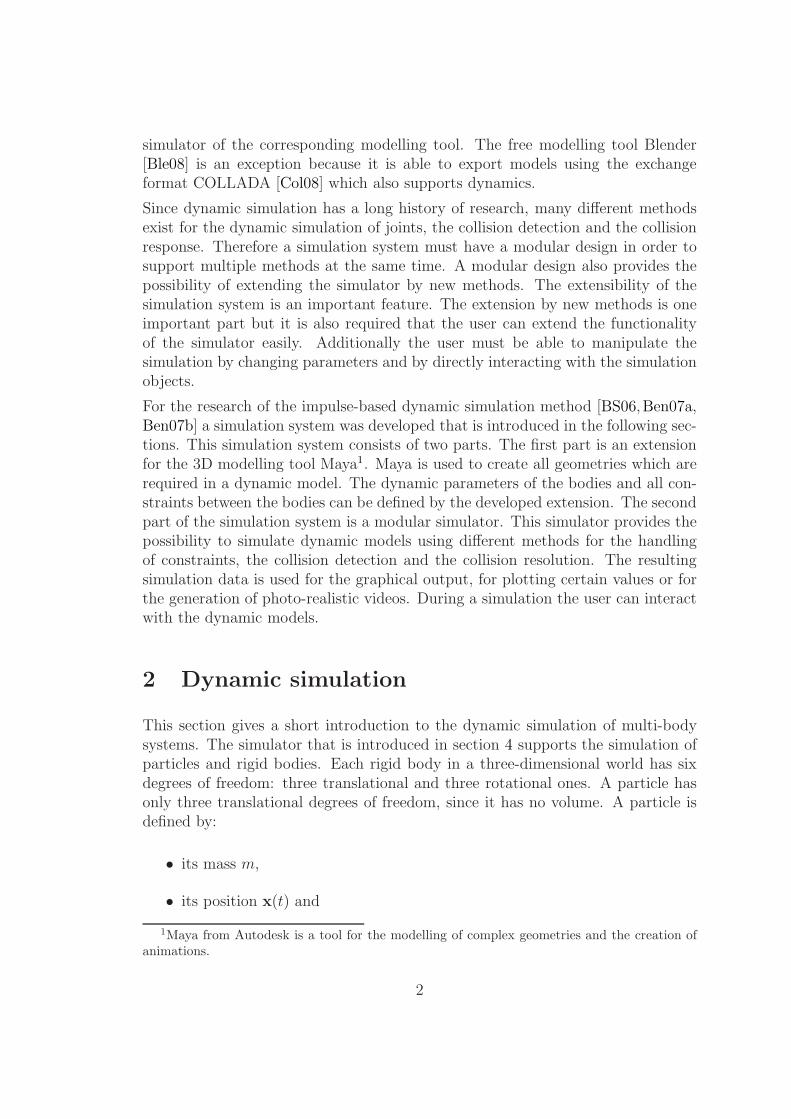
Ball joint A ball joint links two bodies together in one point (see figure 1). Thiskind of joint removes three translational degrees of freedom, since a relativetranslational motion of the bodies in the joint point is not possible. A balljoint is defined by the position of its joint point.

Figure 1: Ball joint

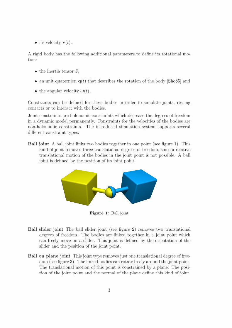
Ball slider joint The ball slider joint (see figure 2) removes two translationaldegrees of freedom. The bodies are linked together in a joint point whichcan freely move on a slider. This joint is defined by the orientation of theslider and the position of the joint point.

Ball on plane joint This joint type removes just one translational degree of free-dom (see figure 3). The linked bodies can rotate freely around the joint point.The translational motion of this point is constrained by a plane. The posi-tion of the joint point and the normal of the plane define this kind of joint.

3

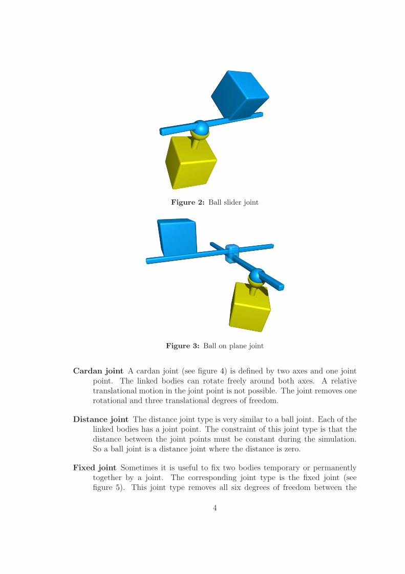
Figure 2: Ball slider joint

Figure 3: Ball on plane joint

Cardan joint A cardan joint (see figure 4) is defined by two axes and one jointpoint. The linked bodies can rotate freely around both axes. A relativetranslational motion in the joint point is not possible. The joint removes onerotational and three translational degrees of freedom.

Distance joint The distance joint type is very similar to a ball joint. Each of thelinked bodies has a joint point. The constraint of this joint type is that thedistance between the joint points must be constant during the simulation.So a ball joint is a distance joint where the distance is zero.

Fixed joint Sometimes it is useful to fix two bodies temporary or permanentlytogether by a joint. The corresponding joint type is the fixed joint (seefigure 5). This joint type removes all six degrees of freedom between the

4

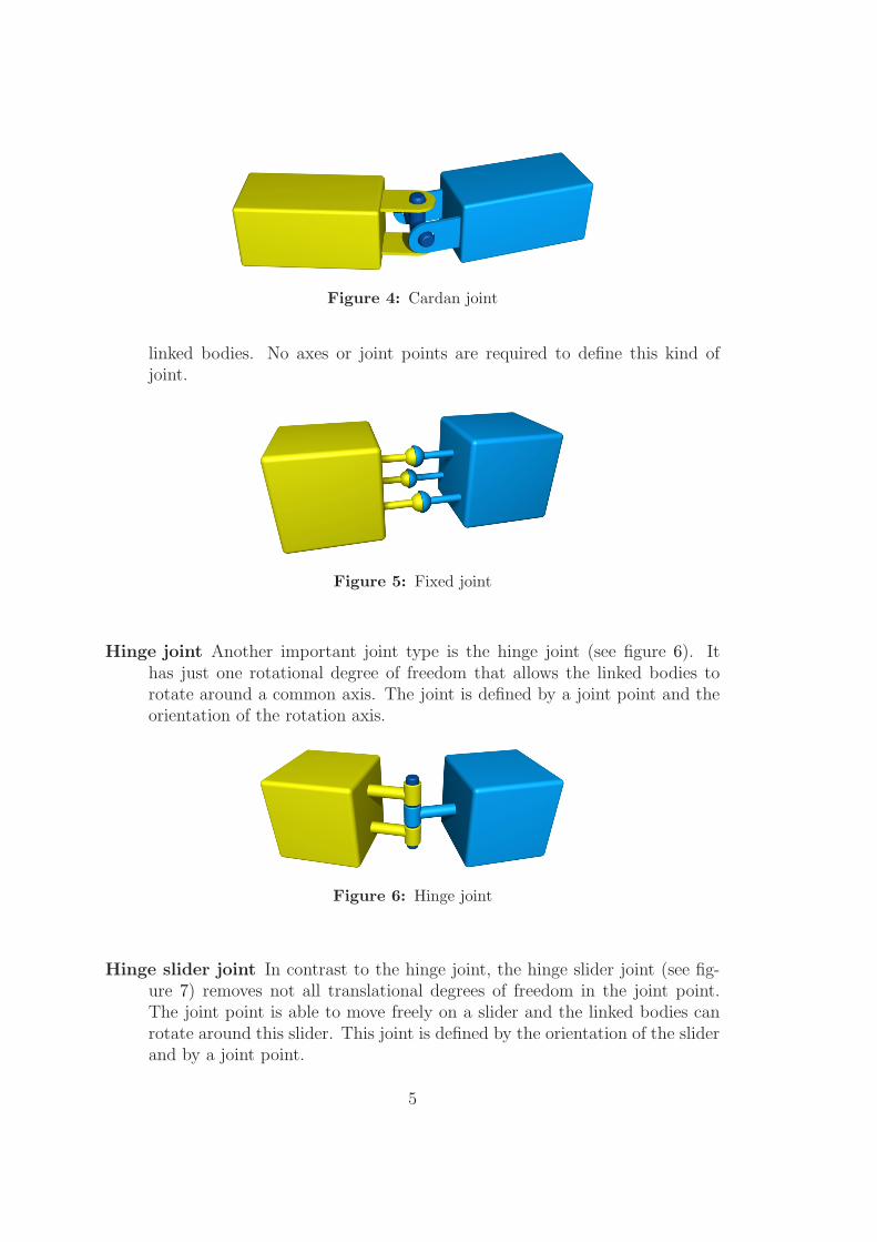
Figure 4: Cardan joint

linked bodies. No axes or joint points are required to define this kind ofjoint.

Figure 5: Fixed joint

Hinge joint Another important joint type is the hinge joint (see figure 6). Ithas just one rotational degree of freedom that allows the linked bodies torotate around a common axis. The joint is defined by a joint point and theorientation of the rotation axis.

Figure 6: Hinge joint

Hinge slider joint In contrast to the hinge joint, the hinge slider joint (see fig-ure 7) removes not all translational degrees of freedom in the joint point.The joint point is able to move freely on a slider and the linked bodies canrotate around this slider. This joint is defined by the orientation of the sliderand by a joint point.

5

Figure 7: Hinge slider joint

Motor hinge joint The motor hinge joint is an angular servo motor. The jointconstraint is the same as the one of a hinge joint. Additionally an externaltorque acts on the linked bodies in order to simulate the motor. The mag-nitude of this torque is determined by a PID controller to reach a certainangular velocity or angle.

Motor slider joint Another servo motor joint is the motor slider joint. Usingthis joint type a linear servo motor is simulated. The required constraint isthe same as the one of a slider joint. To simulate the motor an external forceacts on the linked bodies. If a certain position or linear velocity should bereached, the magnitude of the force is determined by a PID controller.

Point velocity constraint A point velocity constraint is a non-holonomic con-straint. In contrast to a holonomic constraint it does not reduce the degreesof freedom of the dynamic model. The point velocity constraint is definedby two points, one for each of its bodies. The velocities of these points mustbe equal to satisfy the constraint.

This kind of constraint is very useful, if the motion of a body should becontrolled by another one. For example this can be used to control themotion of a body by the mouse pointer. A static body is introduced atthe position of the pointer. The static body is linked by a point velocityconstraint with the body which should be controlled. So user interactionscan be easily realised using velocity constraints.

Slider joint Another holonomic constraint is the slider joint (see figure 8). Thelinked bodies can only move on the defined slider. This joint type removesthree rotational degrees of freedom and two translational ones. The joint isdefined by the orientation of the slider and a joint point.

Spring A spring (see figure 9) does not define a constraint but the simulator in-troduced in the following handles springs very similar to joint constraints.

6

Figure 8: Slider joint

Springs also link two bodies together but they use forces instead of a con-straint.

Figure 9: Spring

Constraints for the simulation of collisions and resting contacts with friction areintroduced automatically by the simulation system.

3 Modelling

This section introduces the modelling system. The first task of the modelling pro-cess is the creation of three-dimensional objects. The second task is the definitionof dynamic parameters, joints and other constraints.

The modelling of three-dimensional bodies is a complex task which is accomplishedusing the 3D modelling tool Maya (see figure 10). Autodesk Maya provides an ownsimulation system that supports the simulation of rigid bodies. In this simulationsystem each rigid body has a set of physical parameters which can be definedby the user. So Maya already supports the definition of dynamic parameters foreach body. But the actual version of the simulation system can only handle a fewjoint constraints. Because of that an extension of Maya was developed in order to

7

Figure 10: Design of a dynamic model using Autodesk Maya

support the definition of all possible joint constraints easily. This extension wasimplemented using the scripting language MEL2.

Each object in Maya can have additional attributes that are defined by the user.For the implementation of the required extension these user-defined attributes arevery useful. An attribute is added to each object of the dynamic model in orderto define its type. The extension supports the following object types:

• settings object that stores the settings of a simulation method, a collisiondetection method or collision resolution method,

• rigid body or particle,

• geometry of a body,

• geometry for the collision detection,

• joint constraint, e. g. ball joint, hinge joint or slider joint,

2MEL is a shortcut for ”Maya Embedded Language”

8

• position of a joint point and

• orientation of a joint axis.

Each simulation, collision detection and collision response method has several pa-rameters. These parameters can be defined by a settings object. Such an objecthas no geometry and just stores the user-defined settings for the simulation. If nosettings object is created the simulator uses default settings.

At the moment the simulation system supports two kinds of bodies: particles andrigid bodies. A particle is a point with a mass that has no volume. Becauseof this, it has just translational parameters in the dynamic simulation. A rigidbody has translational and rotational parameters (see section 2). Particles andrigid bodies have additional parameters that define the coefficients of dynamicand static friction and the coefficient of restitution.

A body can have multiple geometries. The first geometry and the mass of a rigidbody are used by the simulator to compute the inertia tensor of the body. Theinertia tensor is determined by using the algorithm that was published by BrianMirtich [Mir96]. The geometries are also required for the collision detection of thesimulator, if the corresponding body has no special collision geometry. Otherwisethe additional geometries are only needed for the visualisation of the body.

A collision geometry can be defined by the user, if he wants to use different ge-ometries for the collision detection and for the graphical output. This feature isvery helpful to increase the performance of the collision detection by using low-resolution collision geometries. Each particle or rigid body can have multipleindependent collision geometries. These special geometries can be used to define adecomposition of a non-convex body into convex parts. Collision geometries thatbelong to the same body can never collide with each other because their relativeposition stays constant over time. Because of this, there is no collision detectionnecessary between these collision geometries. It is also possible to explicitly ex-clude pairs of bodies from the collision detection process in order to improve theperformance of the simulation. For example, this is done automatically for staticbodies, since they cannot collide.

Each joint object has at least two additional attributes which define the bodies thatare linked by the joint. Except the fixed joint (see section 2) all joint types requiresome attributes to define the positions of their joint points and the orientationsof their joint axes. Other properties like the maximum torque of a motor hingejoint or the parameters of its corresponding PID controller are also defined by suchattributes.

The modelling of joints should be a simple and intuitive task for the user. Becauseof this, the developed extension provides a graphical representation for each jointtype. To create a joint, the user have first to select the two bodies which shouldbe linked together. Then he chooses the desired joint type and a graphical repre-

9

sentation of the joint appears between the bodies. The user can manipulate thisgraphical joint object in a simple way by moving its points or rotating its axes.Joint objects of different types are shown in figure 11.

Figure 11: Ball joint, hinge joint, cardan joint and slider joint as jointobjects in Maya

Some joint types like a spring or a motor hinge joint have additional attributes.These attributes are automatically added to the joint object. So the user can easilydefine the properties of a joint by using the GUI of Maya.

After creating a dynamic model the user can export it in a XML3 file. This filecontains the geometries of all bodies, all joints and the values of their attributes.

The representation of a rigid body in XML looks like this:

<RigidBody name="SphereBody">

<Mass value="1"/>

<Dynamic value="1"/>

<InitialVelocity value="5 0 0"/>

<InitialSpin value="0 1 0"/>

<ImpulsePosition value="0 0 0"/>

<Impulse value="0 0 0"/>

<Geometry type="Sphere">

<Transformation value="1 0 0 0

0 1 0 0

0 0 1 0

-1.75 -0.7 0.9 1"/>

<Color value="0.5 0.5 0.5 1"/>

<Radius value="0.3"/>

</Geometry>

<Collision value="1">

<Bounciness value="0.6"/>

3XML is a shortcut for ”‘Extensible Markup Language”’. XML provides the possibility tosave data in a tree structure.

10

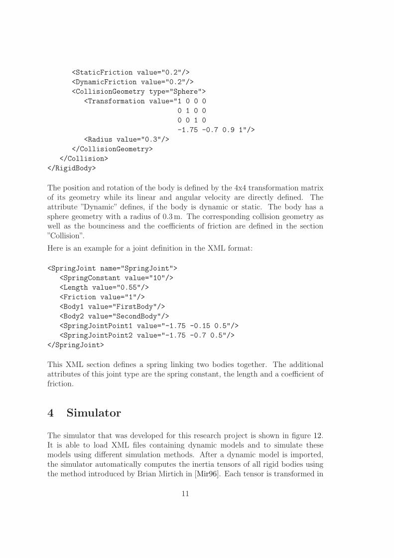
<StaticFriction value="0.2"/>

<DynamicFriction value="0.2"/>

<CollisionGeometry type="Sphere">

<Transformation value="1 0 0 0

0 1 0 0

0 0 1 0

-1.75 -0.7 0.9 1"/>

<Radius value="0.3"/>

</CollisionGeometry>

</Collision>

</RigidBody>

The position and rotation of the body is defined by the 4x4 transformation matrixof its geometry while its linear and angular velocity are directly defined. Theattribute ”Dynamic” defines, if the body is dynamic or static. The body has asphere geometry with a radius of 0.3m. The corresponding collision geometry aswell as the bounciness and the coefficients of friction are defined in the section”Collision”.

Here is an example for a joint definition in the XML format:

<SpringJoint name="SpringJoint">

<SpringConstant value="10"/>

<Length value="0.55"/>

<Friction value="1"/>

<Body1 value="FirstBody"/>

<Body2 value="SecondBody"/>

<SpringJointPoint1 value="-1.75 -0.15 0.5"/>

<SpringJointPoint2 value="-1.75 -0.7 0.5"/>

</SpringJoint>

This XML section defines a spring linking two bodies together. The additionalattributes of this joint type are the spring constant, the length and a coefficient offriction.

4 Simulator

The simulator that was developed for this research project is shown in figure 12.It is able to load XML files containing dynamic models and to simulate thesemodels using different simulation methods. After a dynamic model is imported,the simulator automatically computes the inertia tensors of all rigid bodies usingthe method introduced by Brian Mirtich in [Mir96]. Each tensor is transformed in

11

Figure 12: Simulator

a diagonal matrix by a principal axis transformation [GPS01]. Then the simulationcan start.

In this section first the modular architecture of the simulator is explained in detail.Afterwards the possibilities for user interaction in the simulator are described.

4.1 Architecture of the simulator

The simulator is written in C++. The graphical user interface is implementedusing the open-source library wxWidgets [wxW08] which is a widget toolkit forcross-platform applications. Because of that the simulator can be compiled ondifferent platforms. This was successfully tested on Microsoft Windows and Unixplatforms.

The architecture of the simulation system is shown in figure 13. Bodies and jointsare defined and modified using the introduced extension of Maya. During the sim-ulation the user is able to change all dynamic parameters like positions, velocitiesetc. by the graphical user interface or by a Python script. This user interaction isdescribed in detail in section 4.2. The simulator consists of different independentmodules for the simulation and for the graphical output. This modular architec-ture has the following advantages. Different simulation methods can be integrated

12

easily in the simulation system. The resulting simulation data can be exportedand visualised in multiple ways.

Maya Simulator OpenGL

Gnuplot

MEL

Python

GUI

model output

executescripts

userinput

Figure 13: Architecture of the simulation system

4.1.1 Modules

Some parts of the simulator were designed as independent modules with a well-defined interface. Such modules are used for:

• the simulation of joints,

• the collision detection,

• the collision response,

• the simulation of external forces and

• the output of the resulting simulation data.

The simulation system should support different methods for the dynamic simu-lation of joint constraints. Therefore it is important that these methods can beeasily exchanged during runtime. Another important feature of the simulator is thesimultaneous simulation with different methods. This is possible, if the model issubdivided into independent chains of linked bodies. Each chain can be simulatedby a different method which allows the direct comparison of simulation methods.In contrast to this the methods used for collision detection and collision and con-tact handling must always be exchanged for the whole model because in this caseno independent subsets of the model can be determined.

13

The generation of external forces was also realised by different modules. For ex-ample, gravity is simulated using such a module. Multiple force modules can beactive at the same time. Each module knows all bodies that are influenced by itsforce field. The force modules are called in each simulation step to generate theexternal forces and torques for the bodies. These forces can depend on the actualstate of the model or on user inputs. Therefore user interaction with the modelis implemented as a force module. Force modules can also be used to realise PIDcontrollers for servo motors.

The last kind of module is used for the output of simulation data. At the momentthe simulation system has three different modules of this kind. The first moduleis responsible for the 3D visualisation of the dynamic model. It uses OpenGL forthe visualisation. This module is called by a timer to render the actual state of themodel. At the same time the mouse and keyboard inputs of the user are handled.Like this the user can navigate through the scene and interact with the model (seesection 4.2). The other two modules are called after each simulation step. Oneis able to export the simulation data in a file and to plot this data set using theopen-source program ”Gnuplot”. The other one writes the data to a MEL file inorder to export the whole simulation to Autodesk Maya. The MEL file contains allgeometries, all motion data, the positions of the joint points, the velocity vectorsand some more information. Maya can be used to create photo-realistic animationsfrom the simulation data.

4.1.2 Multi-threading

The simulation of dynamic models takes much computation time. A simulationstep of a very complex model can take multiple seconds. It is essential that thegraphical user interface (GUI) and the simulation runs in their own threads. Oth-erwise the user is not able to interact with the simulator during a simulation step.Figure 14 shows the subdivision of the simulator in a GUI thread and a simulationthread. A data storage and a command list is used for the subdivision. Whena simulation parameter is changed by the user during runtime, a correspondingchange command is inserted in the command list. Before each simulation stepall commands in the list are executed and removed from the list. In this way itis guaranteed that the parameters are only changed between the simulation stepswhich prevents the simulation from unstable states. After a simulation step theactual data of the model (e.g. the positions and velocities of the bodies) is copiedto the data storage. The data of the storage is used by the GUI and the outputmodules. By using the command list and the data storage it is prevented that athread reads data which is changed by another thread at the same time.

14

GUI command list

OpenGL output

Gnuplot output

MEL output

data storageget

data

simulation

addcommand

get command& execute

GUI thread simulation thread

storedata

simulationstep

Figure 14: The threads of the simulator

4.2 Interaction

At runtime, the user can interact with the joints and bodies in the simulationby changing their parameters or by applying impulses or external forces. Thesimulator provides different dialogs to change the parameters of the bodies, themotors and the springs. It is even possible to program a chronological sequencefor the target values of a servo motor. In this way, e.g. a simple robot can becontrolled. All parameters for the different modules described above can also beset by using the graphical user interface. The user has also the possibility to pause,to resume or to slow down the simulation.

The motion of a body can be influenced by changing its parameters. This is nota very intuitive way of interaction and the simulation can become unstable, if thechosen parameters are unsuitable. Because of this, two different ways of interactionwere developed. Both provide the possibility to interact directly with a body byusing the mouse pointer.

The user can select a point on a body that he wants to push or to pull by an impulse.After selecting a point the user can control the magnitude and the direction of theimpulse by moving the mouse. At the end he can decide, if he wants to push orpull the body by a left or right mouse click. The impulse changes the velocity ofthe body directly.

If the position or rotation of a body should be changed during the simulation,all constraints of this body must be regarded. Therefore the translational androtational parameters must not be changed directly. For this kind of interactionthe simulator provides the possibility to select a body with the mouse and changeits position and rotation parameter by using velocity constraints. After selecting

15

a body the user can control its motion directly by manipulators (see figure 15). A

(a) Translation (b) Rotation

Figure 15: Manipulators for controlling the translation and rotation of abody

manipulator can be selected by the mouse. As long as the mouse button is pressedthe translation or rotation of the body will be controlled by the mouse movement.The control is realised as a velocity constraint for the body. That means that thebody will follow the mouse cursor as long as its position constraints allow thismotion.

5 Extensibility

The simulator provides two different possibilities for extensions. The first one isthe implementation of new modules (see section 4.1.1). The second possibility isthe extension by Python scripts. For the simulator an interface was implementedthat allows the user to execute own scripts at runtime.

New methods for the simulation of joints, for collision detection, for collision reso-lution or for the generation of external forces can be integrated in the simulator asa module. Such a module can be linked statically or dynamically, when the simu-lator starts. In this way the modules can be exchanged easily and the methods canbe developed independently from the simulation system. The development of newmodules also provides the possibility to compare different methods in the samesimulator.

Programs written in the scripting language Python can be executed by the simu-lator. These scripts can access and change all parameters of the bodies, the jointsand the different modules. There are two ways to execute a Python script in the

16

simulator. Either the script is called manually by the user or it is executed auto-matically by an event callback. For example, a script method can be called aftereach simulation step in order to manipulate the simulation parameters or to exportthe simulation data. Each part of the simulation system can be controlled by suchscript programs.

6 Conclusion and future work

In this report the design of a new dynamic simulation system for VR applications ispresented. The system consists of a modelling tool and a simulator. An extensionwas written for Maya that allows the creation of dynamic models. These modelsare exported as XML file for the simulator.

During a simulation the user has different possibilities to interact with the simu-lated model. He can manipulate the dynamic parameters directly, apply impulsesor use manipulators that influence the bodies by using a velocity constraint.

The simulation system has a modular architecture in order to support multiplesimulation methods. Due to this architecture an extension by new methods canbe done easily. The simulator supports modules for the simulation of joints, thecollision detection, the collision response, the simulation of external forces and theoutput of the simulation data. The Python interface of the simulator is anotherpossibility for extending the simulator. Scripts can be loaded and executed atruntime in order to manipulate the simulation or to control the functions thesimulator.

17

18

References

[Aut08] Autodesk. Maya, 2008. http://www.autodesk.com/maya.

[Ben07a] Jan Bender. Impulsbasierte Dynamiksimulation von Mehrkorpersyste-men in der virtuellen Realitat. PhD thesis, University of Karlsruhe,Germany, February 2007.

[Ben07b] Jan Bender. Impulse-based dynamic simulation in linear time. ComputerAnimation and Virtual Worlds, 18(4-5):225–233, 2007.

[Ble08] Blender, 2008. http://www.blender.org.

[BS06] Jan Bender and Alfred Schmitt. Fast dynamic simulation of multi-bodysystems using impulses. In Virtual Reality Interactions and PhysicalSimulations (VRIPhys), pages 81–90, Madrid (Spain), November 2006.

[Col08] Collada, 2008. http://www.khronos.org/collada.

[GPS01] Herbert Goldstein, Charles P. Poole, and John L. Safko. Classical Me-chanics. Addison Wesley, 3rd edition, 2001.

[Mir96] Brian V. Mirtich. Fast and accurate computation of polyhedral massproperties. Journal of Graphics Tools: JGT, 1(2):31–50, 1996.

[Sho85] Ken Shoemake. Animating rotation with quaternion curves. In SIG-GRAPH ’85: Proceedings of the 12th annual conference on Computergraphics and interactive techniques, pages 245–254. ACM Press, 1985.

[wxW08] wxWidgets, 2008. http://www.wxwidgets.org.

19