design, fabrication and characterization of mems
TRANSCRIPT

Design, Fabrication and Characterization of
MEMS Gyroscopes Based on Frequency
Modulation
by
Dawit Effa
A thesis
presented to the University of Waterloo
in fulfillment of the
thesis requirement for the degree of
Doctor of Philosophy
in
Mechanical and Mechatronics Engineering (Nanotechnology)
Waterloo, Ontario, Canada, 2018
© Dawit Effa 2018

ii
Examining Committee Membership
The following served on the Examining Committee for this thesis. The decision of the
Examining Committee is by majority vote.
External Examiner Professor Edmond Cretu
Electrical and Computer Engineering
Supervisors Professor Eihab Abdel-Rahman
System Design Engineering
Professor Mustafa Yavuz
Mechanical and Mechatronics Engineering
Internal Member Professor Baris Fidan
Mechanical and Mechatronics Engineering
Professor Amir Khajepour
Mechanical and Mechatronics Engineering
Professor Raafat Mansour
Electrical and Computer Engineering
Professor Gregory Glinka
Mechanical and Mechatronics Engineering
Other Member(s) Professor Siva Sivoththaman
Electrical and Computer Engineering

iii
Author’s Declaration
I hereby declare that I am the sole author of this thesis. This is a true copy of the thesis, including any
required final revisions, as accepted by my examiners.
I understand that my thesis may be made electronically available to the public.

iv
Abstract
Conventional amplitude modulated (AM) open loop MEMS gyroscopes experience a significant
performance trade-off between having a large bandwidth or high sensitivity. It is impossible to
improve both metrics at the same time without increasing the mass of the gyroscope or introducing a
closed loop (force feedback) system into the device design. Introducing a closed loop system or
increasing the proof mass on the other hand will surge power consumption. Consequently, it is
difficult to maintain consistently high performance while scaling down the device size. Furthermore,
bias stability, bias repeatability, reliability, nonlinearity and other performance metrics remain
primary concerns as designers look to expand MEMS gyroscopes into areas like space, military and
navigation applications. Industries and academics carried out extensive research to address these
limitations in conventional AM MEMS gyroscope design.
This research primarily aims to improve MEMS gyroscope performance by integrating a frequency
modulated (FM) readout system into the design using a cantilever beam and microplate design. The
FM resonance sensing approach has been demonstrated to provide better performance than the
traditional AM sensing method in similar applications (e.g., Atomic Force Microscope). The
cantilever beam MEMS gyroscope is specifically designed to minimize error sources that corrupt the
Coriolis signal such as operating temperature, vibration and packaging stress. Operating temperature
imposes enormous challenges to gyroscope design, introducing a thermal noise and drift that degrades
device performance. The cantilever beam mass gyroscope system is free on one side and can therefore
minimize noise caused by both thermal effects and packaging stress. The cantilever beam design is
also robust to vibrations (it can reject vibrations by sensing the orthogonally arranged secondary
gyroscope) and minimizes cross-axis sensitivity. By alleviating the negative impacts of operating
environment in MEMS gyroscope design, reliable, robust and high-performance angular rate
measurements can be realized, leading to a wide range of applications including dynamic vehicle
control, navigation/guidance systems, and IOT applications. The FM sensing approach was also
investigated using a traditional crab-leg design. Tested under the same conditions, the crab-leg design
provided a direct point of comparison for assessing the performance of the cantilever beam
gyroscope.
v
To verify the feasibility of the FM detection method, these gyroscopes were fabricated using
commercially available MIDIS™ process (Teledyne Dalsa Inc.), which provides 2 μm capacitive
gaps and 30 μm structural layer thickness. The process employs 12 masks and hermetically sealed
(10mTorr) packaging to ensure a higher quality factor. The cantilever beam gyroscope is designed
such that the driving and sensing mode resonant frequency is 40.8 KHz with 0.01% mismatch.
Experimental results demonstrated that the natural frequency of the first two modes shift linearly with
the angular speed and demonstrate high transducer sensitivity. Both the cantilever beam and crab-leg
gyroscopes showed a linear dynamic range up to 1500 deg/s, which was limited by the experimental
test setup. However, we also noted that the cantilever beam design has several advantages over
traditional crab-leg devices, including simpler dynamics and control, bias stability and bias
repeatability. Furthermore, the single-port sensing method implemented in this research improves the
electronic performance and therefore enhances sensitivity by eliminating the need to measure
vibrations via a secondary mode. The single-port detection mechanism could also simplify the IC
architecture.
Rate table characterization at both high (110 oC) and low (22 oC) temperatures showed minimal
changes in sensitivity performance even in the absence of temperature compensation mechanism and
active control, verifying the improved robustness of the design concept. Due to significant die area
reduction, the cantilever design can feasibly address high-volume consumer market demand for low
cost, and high-volume production using a silicon wafer for the structural part. The results of this work
introduce and demonstrate a new paradigm in MEMS gyroscope design, where thermal and vibration
rejection capability is achieved solely by the mechanical system, negating the need for active control
and compensation strategies.
vi
Acknowledgements
First, I would like to express my sincere gratitude to my advisor, Prof. Eihab Abdel-Rahman and
Prof. Mustafa Yavuz. Thank you for your guidance and support throughout the various stages of the
dissertation. Thanks are due to my friends and members of the entire Advanced Micro and Nano
Device Lab group, for valuable insights that enriched my work over the last few years. Very special
thanks go to Dr. Sangtak Park and Mahmoud Khater for providing with invaluable advice and
comments on my study and research.
I would also like to thank CMC Microsystems for supporting this work and providing us with the
necessary device fabrication and packaging resource, without which my research progress in this
subject would not have been possible. I would like to also acknowledge the extensive test equipment
supports provided by CMC Microsystems including rate table and other signal measurement
equipment’s.
I would like also to thank Prof. Raafat Mansour and his team from Center for Integrated RF
Engineering lab for allowing the use of additional test equipment. I whole heartily thank Prof. Steve
Lambert and Oscar Nespoli for making my study possible while I was working at the University of
Waterloo.
I would like to extend my gratitude to my committee members Prof. Edmond Cretu, Prof. Baris Fidan,
Prof. Amir Khajepour, Prof. Raafat Mansour, Prof. Gregory Glinka, for making time in their busy
schedules to serve on my dissertation committee. Thank you for taking an interest in my work and
serving on my PhD defense committee.
I would like to express my gratitude to Page Burton for their invaluable help with the editing of this
Thesis.

vii
Dedication
To Isabel, Michaela and Nathaniel!
viii
Table of Contents
Examining Committee Membership ...................................................................................... ii
Author’s Declaration ............................................................................................................. iii
Abstract ................................................................................................................................. iv
Acknowledgements ............................................................................................................... vi
Dedication ............................................................................................................................ vii
Table of Contents ................................................................................................................ viii
List of Figures ...................................................................................................................... xii
Nomenclature ...................................................................................................................... xvi
List of Abbreviations .......................................................................................................... xix
Chapter I..................................................................................................................................1
Introduction .............................................................................................................................1
1.1 Overview of MEMS Gyroscope ...................................................................................2
1.2 Gyroscope Performance Metrics ..................................................................................4
1.2.1 Angular Random Walk (deg/Hz) ......................................................................5
1.2.2 Rate Random Walk (deg/s/Hz) .........................................................................5
1.2.3 Bias (deg/s) .......................................................................................................6
1.2.4 Power on Bias Drift (deg/s) ............................................................................6
1.2.5 Bias Stability (deg/s) ......................................................................................7
1.2.6 Nonlinearity (ppm) ...........................................................................................7
1.2.7 Resolution (deg/sHz) ......................................................................................7
1.2.8 Sensitivity (mV/(deg/s) or LSB/ (deg/s)) .....................................................7
ix
Hysteresis (deg/s) ....................................................................................................8
1.2.10 Bandwidth (Hz) ..............................................................................................9
1.2.13 Operating Temperature Range (˚C) ................................................................9
1.2.14 Shock Survivability ......................................................................................10
1.3 Review of MEMS Gyroscope .................................................................................10
1.4. Current State of the Art .............................................................................................11
1.5 Motivation and Objectives of the Thesis ....................................................................16
1.5.1 Research Contribution ....................................................................................18
1.6 Research Outline ........................................................................................................18
Chapter II ..............................................................................................................................20
Frequency Modulated MEMS Gyroscope ............................................................................20
2.1 Resonance and Resonant Sensing ..............................................................................20
2.2 Frequency-Based Detection of Angular Rate .............................................................21
2.3 Kinematics Analysis of the Cantilever Beam MEMS gyroscope ..............................23
2.3.1 MEMS Gyroscope Frequency Modulation Detection Approach ...................30
2.4 Electrical Excitation and Detection ...........................................................................31
2.4.1 Primary Mode Excitation Method ............................................................................33
2.4.2 Drive and Sense Motion Detection ................................................................38
2.4.2.1 Single port actuation and detection with DC bias .......................................40
2.5 Effects of Capacitive Excitation and Detection .........................................................44
2.5.1 Spring Softening .............................................................................................44
Chapter III .............................................................................................................................46
MEMS Gyroscope Dynamic Behavior Modeling and Analysis ...........................................46
3.1 Kinetics Modeling and Assumptions .........................................................................48

x
3.1.2 Strain-Curvature Relations .............................................................................53
3.2 Equations of Motion and Boundary Conditions .........................................................54
3.2.1 Kinetic Energy of the System ..................................................................................55
3.2.2 Potential Energy ......................................................................................................58
3.3 Extended Hamilton's Principle ...................................................................................61
3.6 Finite Element Simulations and Results .....................................................................80
3.6.1 Cantilever Beam Gyroscope FEA Analysis ...................................................80
3.6.2 Crab Leg FEA Analysis (Device 2) ...............................................................86
Chapter IV .............................................................................................................................92
Analysis of Thermal Noise in Frequency-Modulated Gyroscopes .......................................92
4.1 Thermal Noise in MEMS Gyroscope .........................................................................93
4.2 Thermal Noise in Frequency-Modulated Gyroscopes ................................................95
4.2 Analysis of Stability and Device Performance of the Cantilever Gyroscopes ...........97
4.2.1 Allan variance .................................................................................................97
Chapter V ............................................................................................................................100
Prototypes Fabrication and Device Characterization ..........................................................100
5.1 Prototypes Fabrication MIDIS™ Process .......................................................102
5.2 Experimental Characterization .................................................................................112
5.2.1 Single port Actuation and Detection ............................................................114
5.2.2 Crab-Leg Characterization ...........................................................................119
5.4 Temperature Effects on Cantilever vs Crab Leg .............................................125
5.5 Noise Analysis ..........................................................................................................128
Chapter VI ...........................................................................................................................132
xi
Summary and Conclusions .................................................................................................132
6.1 Contributions and Outcome of This Work ...............................................................133
6.2 Recommendations for Future Work .........................................................................134
References ......................................................................................................................136
Appendix A: MEMS Gyroscope Model Using MATLAB / Simulink ..........................142
Appendix B: Fabrication process flow ...........................................................................145
Appendix C: Mask Design Layouts of MIDIS™ ...........................................................147
Appendix D: Device Design Parameter and Test Results ..............................................148
xii
Figure 1.1: Comparison of the optical vs. mechanical gyroscope ..........................................2
Figure 1.2: A typical crab leg MEMS gyroscope 3D model ..................................................3
Figure 1.3: Sample Plot of Allan Variance Analysis Results [6] ...........................................5
Figure 1.4: Bias error output for zero input rate .....................................................................6
Figure 1.5: Thermal Hysteresis of gyroscope .........................................................................8
Figure 1.6: Frequency response curve of a resonator .............................................................9
Figure 1.7: AM vibrating MEMS gyroscope block diagram ................................................12
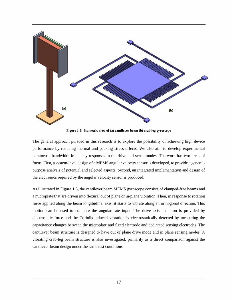
Figure 1.9: Isometric view of (a) cantilever beam (b) crab leg gyroscope ..........................17
Figure 2.1: Functional block diagram of resonant sensing ...................................................20
Figure 2.2: Functional block diagram of FM MEMS gyroscope..........................................21
Figure 2.3: Perspective view of the cantilever beam MEMS gyroscope ..............................22
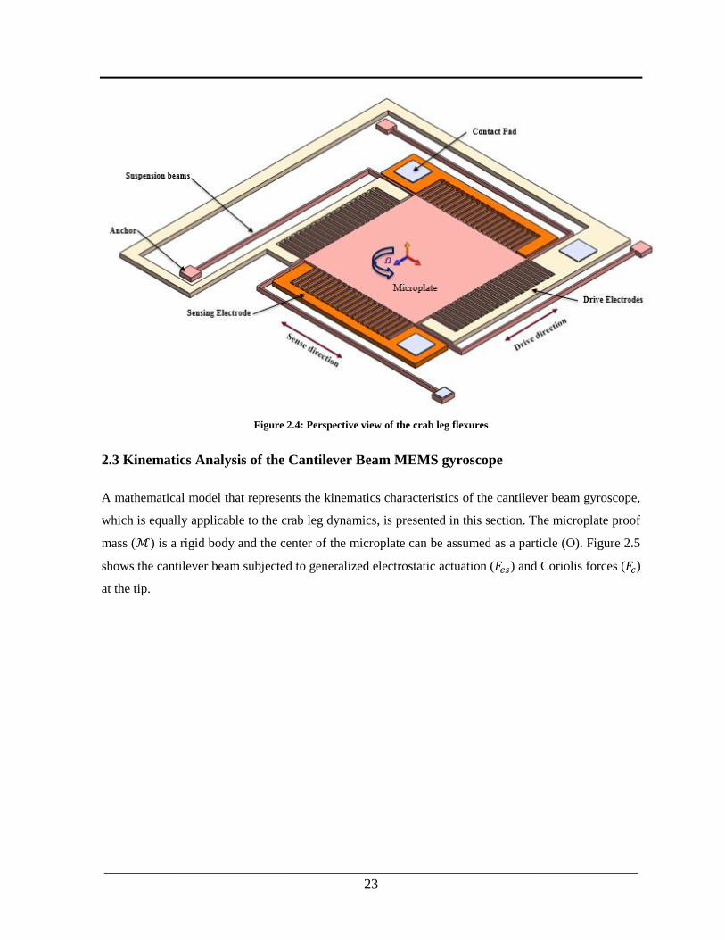
Figure 2.4: Perspective view of the crab leg flexures ...........................................................23
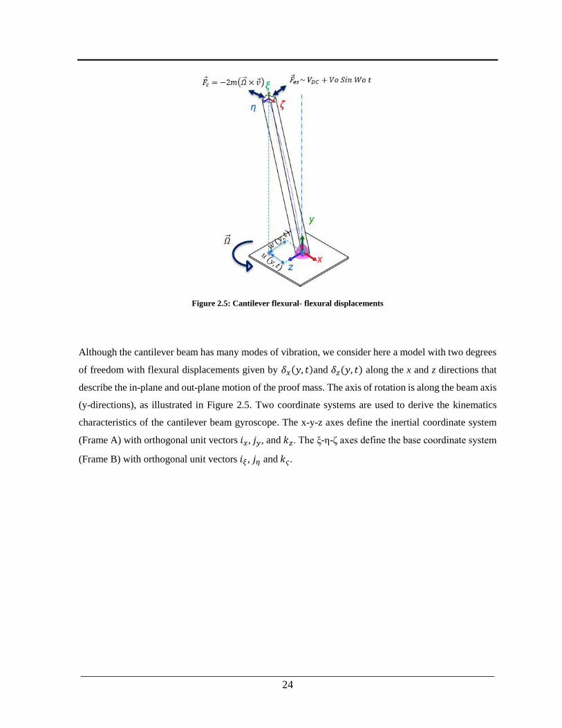
Figure 2.5: Cantilever flexural- flexural displacements .......................................................24
Figure 2.6: Particle O moving in non-inertial Frame B with respect to inertial Frame A. ...25
Figure 2.7: Simplified lumped-mass model of a vibrating MEMS gyroscope .....................28
Figure 2.8: A parallel-plate electrostatic actuator and detection electrodes .........................32
Figure 2.9: A parallel plate electrostatic actuator .................................................................34
Figure 2.10: Crab leg comb finger actuator and sensor electrodes .......................................35
Figure 2.11: Single Port actuation and sensing .....................................................................37
Figure 2.12: Cantilever beam MEMS gyroscope actuation circuit.......................................38
Figure 2.13: Comb finger model for 3D electrostatic force analysis ....................................39
Figure 2.14: Cantilever beam MEMS gyroscope sensing circuit .........................................40
Figure 3.1: Schematic of the cantilever beam .......................................................................46
Figure 3.2: Cantilever 1 design parameter ............................................................................47
Figure 3.3: Cantilever beam flexural-flexural deflection .....................................................49
List of Figures

xiii
Figure 3.4: Rigid body rotations of beam .............................................................................50
Figure 3.5: A segment of the neutral axis local coordinate system ......................................52
Figure 3.6: Initial and deformed positions of an arbitrary point P.......................................53
Figure 3.7: Load acting on the cantilever beam ....................................................................55
Figure 3.8: Variation of the static deflection in the drive with the DC voltage ....................70
Figure 3.9: Variation of the static deflection in the sense direction with the DC voltage ....71
Figure 3.10: Variation of the first natural frequency with the DC voltage for cantilever 1
gyroscope (drive) ..................................................................................................................75
Figure 3.11: Variation of the first natural frequency with the DC voltage for Cantilever 1
gyroscope (sense) ..................................................................................................................75
Figure 3.12: System output response plot for the drive mode ..............................................79
Figure 3.13: System output response plot for the Sense mode .............................................79
Figure 3.14: Meshed element of the cantilever beam gyroscope ..........................................81
Figure 3.15: Variation of the static deflection with the DC voltage .....................................82
Figure 3.16: Deformed shape of the cantilever beam gyroscope ..........................................83
Figure 3.17: First mode shape of the cantilever beam ..........................................................85
Figure 3.18. Second mode shape of the cantilevered beam. .................................................85
Figure 3.19. Third mode shape of the cantilevered beam. ....................................................86
Figure 3.20: Crab leg gyroscope design parameter ..............................................................87
Figure 3.21: Meshed crab leg gyroscope ..............................................................................88
Figure 3.22: Static deflection and deformed shape of the crab-leg gyroscope .....................89
Figure 3.23: The first mode shape of crab-leg gyroscope (z-axis) .......................................90
Figure 3.24: The second mode shape of crab-leg gyroscope (x-axis) ..................................90
Figure 3.25: The third mode shape of crab-leg gyroscope (y-axis) ......................................91
Figure 4.1: Allan Variance flow chart ..................................................................................98
Figure 4.2: Sample Plot of Allan Variance Analysis Results [5] .........................................99
Figure 5.1: A 3D model of the structure of the cantilever beam element ...........................101

xiv
Figure 5.2: A comb finger electrode and other structural parts for the crab leg beam
element ................................................................................................................................102
Figure 5.3: Substrates assembly process .............................................................................103
Figure 5.4: Handle wafer patterning to a depth of 20μm using mask 95 cavity .................105
Figure 5.5: Device layer is patterned using a combination of mask 32 and 37 ..................106
Figure 5.6: crab-leg sense and drive electrodes defined using mask 32 and 37 .................106
Figure 5.7: Second bonding plane definition using mask 34 to creates a 2μm deep spacer
between device TSV wafers................................................................................................107
Figure 5.8: Second bonding plane definition using mask 34 ..............................................107
Figure 5.9: Cross-section view of final stack ......................................................................108
Figure 5.10: Second bonding plane definition using mask 34 ............................................108
Figure 5.11: Second bonding plane definition using mask 34 ............................................109
Figure 5.12: Process cross-section with substrates and masks identification .....................109
Figure 5.13: Photograph of vacuum packaged test chip along with a 1 cent coin ..............112
Figure 5.14: Sensing circuit to detect the frequency difference between driving and sensing
side resonance .....................................................................................................................113
Figure 5.15: Illustration of the device characterization setup .............................................114
Figure 5.16: The experimental setup for device characterization using SR850c lock
amplifier ..............................................................................................................................115
Figure 5.17: Actuation and Sensing circuit for device characterization in the in-plan
direction (x-axis) .................................................................................................................116
Figure 5.18: Measured frequency response for Cantilever 1 gyroscope in the drive
direction ..............................................................................................................................117
Figure 5.19: zicontrol screen shot for the cantilever beam design 3 ..................................119
Figure 5.20: Electrical connection for frequency response test for Device #2 ...................120
Figure 5.21: Measured frequency response for Crab leg (Device #2) drive mode .............121
Figure 5.22: zicontrol screen shot of the test device #2 ......................................................122

xv
Figure 5.23: The experimental illustration for rate table (rate table not shown here) ........123
Figure 5.24: The experimental setup for rate-table characterization ..................................124
Figure 5.25: Measured frequency response for Cantilever beam (Device #1) ...................125
Figure 5.28: Measured frequency shift as a function of time for the cantilever beam
gyroscopes...........................................................................................................................128
Figure 5.29: Measured frequency shift as a function of time for the crab leg gyroscopes .129
Figure 5:30: Measured Allan variance comparison between cantilever beam FM
gyroscopes...........................................................................................................................130
Figure 5.31: Measured Allan variance comparison between crab leg FM gyroscopes ......131
xvi
Nomenclature
Symbol Quantity Description Units
𝑐 Coriolis force N
𝑚 Mass per unit length cantilever beam gyroscope Kg/m
Ω Input angular rate O/sec (DPS)
θ Angular displacement Deg. (O)
𝑑 Actuation velocity of the proof mass m/s
𝑅𝑚 Motional impedance
𝑔𝑜 Initial capacitor gap 𝜇𝑚
𝐿𝑠𝑚 Suspended mass length 𝜇𝑚
𝑏𝑠𝑚 Suspended mass width 𝜇𝑚
𝜌 Density Kg/m3
E Young’s modules Pascal
Poisson's ratio -
ℳ Suspended microplate mass Kg
𝑤𝑏 Cantilever beam width 𝜇𝑚
𝑡𝑏 Cantilever beam thickness 𝜇𝑚
L Cantilever beam length 𝜇𝑚
𝑉𝐴𝐶 AC voltage Voltage
𝑉𝐷𝐶 DC voltage Voltage
𝐹𝑒𝑠 Electrostatic actuation force N
𝛿𝑥(𝑦, 𝑡) Sense direction deflection of the microplate 𝜇𝑚
𝛿𝑧(𝑦, 𝑡) Drive direction deflection of the microplate 𝜇𝑚
𝑟𝐴 Position vector relative to inertial frame A 𝜇𝑚
𝑟𝐵 Position vector relative to base frame B 𝜇𝑚
𝑟𝐴/𝐵 Position vector relative to rotating frame 𝜇𝑚
𝐴 Absolute velocity of particle with respect to the inertial reference 𝜇𝑚/𝑠
xvii
𝑟𝐴 Acceleration of particle with respect to the inertial reference 𝜇𝑚/𝑠2
𝐹𝑓𝑖𝑐𝑡 Fictitious force N
휁𝑑 Damping ratio of the drive direction -
휁𝑠 Damping ratio of the sense direction -
𝜔𝑛𝑑 Natural frequencies of the drive direction KHz
𝜔𝑛𝑠 Natural frequencies of the sense direction KHz
Ω Angular acceleration 𝑑𝑒𝑔./𝑠2
∆𝜔Ω Difference between the drive and sense natural frequencies 𝑑𝑒𝑔./𝑠
𝑉𝑒𝑥𝑐(𝑡) Excitation voltage V
𝐶 Capacitance F
𝐴 Electrode area 𝜇𝑚2
휀𝑜 Permittivity of vacuum F/m
휀𝑟 Relative permittivity of the insulator between the plates F/m
Q Quality factor -
𝐸𝑒𝑠 Total energy J
𝜔𝑒𝑥𝑐 Excitation frequency Hz.
𝐶𝑝 Parasitic capacitance F
𝐶𝑚 (𝑡) Capacitance of the electrostatic transducer F
𝑖(𝑡) Electric current A
𝑉𝑝𝑖 Pull-in voltage V
𝑘 Spring stiffness 𝑁/𝑚
A Peak amplitude of the harmonic signal
𝑘𝑒𝑓𝑓 Effective spring constant 𝑁/𝑚
𝑘𝑒𝑠 Electrostatic spring constant 𝑁/𝑚
[𝑇] Transformation matrix -
𝜓 Transformation angle 𝑑𝑒𝑔
휃 Transformation angle 𝑑𝑒𝑔
𝜙 Transformation angle 𝑑𝑒𝑔

xviii
𝜌(𝑠, 𝑡) Curvature vector -
𝑒 Strain -
𝑇𝑡𝑟 Kinetic energy due to translation displacement J
𝑇𝑟𝑜𝑡 Kinetic energy due to rotation J
T Total Kinetic energy J
U Total Potential energy J
𝑥(𝐿, 𝑡)𝑦 Angular speed of the suspended mass in the sense direction (x-axis) 𝑑𝑒𝑔./𝑠
𝑧(𝐿, 𝑡)𝑦 Angular speed of the suspended mass in the drive direction (z-axis) 𝑑𝑒𝑔./𝑠
𝜎ij Stress Pa
휀ij Strain -
𝛿ℒ Lagrangian density -
𝛿𝑊𝑁𝐶 Virtual work done by non-conservative forces J
𝐿1 Crab leg beam length 1 𝜇𝑚
𝐿2 Crab leg beam length 2 𝜇𝑚
𝑤𝑏𝑤 Crab leg beam width 𝜇𝑚
𝑡𝑏 (𝑡𝑝) Crab leg beam thickness 𝜇𝑚
𝐿𝑐𝑝 Crab leg microplate length 𝜇𝑚
𝑤𝑝 Crab leg microplate width 𝜇𝑚
E Young’s modules MPa
T Time constant
xix
List of Abbreviations
Symbol Description
𝐵𝑊 Bandwidth
SF Scale factor
FR Full-scale range
AFM Atomic force Microscope
FM Frequency modulation
DSP Digital signal processing
SNR Signal to noise ratio
LPF Law pass filter
ARW Angular Radom Walk
RRW Rate Random Walk
PLL Phase locked loop
AGC Automatic gain control
PID Proportional integral derivative
TIA Transimpedance amplifiers
VCO Voltage controlled oscillator
MIDIS MEMS Integrated Design for Inertial Sensors
TSV Through-Silicon Via
DRIE Deep Reactive Ion Etching
SOIMUMPS Silicon-On-Insulato Multiple User Platform
AVAR Allan variance
FEM Finite Element Method
APDL Parametric Design Language of ANSYS
PDE Partial Differential Equation
ODE Ordinary Differential Equation
DPS Degree per second
___________________________________________________________________________
1
CHAPTER I
Introduction
Micro-Electromechanical Systems (MEMS) are miniaturized devices that combine integrated electrical
circuit and micromechanical components through microfabrication technology. The advent of MEMS
technology has directly enabled the development of low-cost, low-power sensors and actuators, which
are rapidly replacing their macroscopic scale equivalents in many traditional applications most notably,
inertial measurement units (IMU). MEMS inertial sensors, comprised of gyroscopes and accelerometers,
are used to measure the rotation rate, angle or acceleration of a body with respect to an inertial reference
frame. In recent years, the MEMS inertial sensor market has benefitted significantly from the rise of
mobile communication platforms, the Internet of Things (IOT), automotive, augmented reality (AR) and
gaming [1-3]. Consequently, MEMS gyroscopes now comprise one of the fastest growing segments of
the MEMS sensor market [4].
Conventional vibratory MEMS gyroscope designs have a proof mass suspended above the substrate by
a suspension system consisting of flexible beams, typically formed in the same structural layer as the
proof mass. A rotational motion perpendicular to the sensor’s drive axis produces a DC voltage
proportional to the rate of rotation due to the Coriolis forces acting on the sense direction. However, the
Coriolis force detection method is very sensitive to change in the environment (such as temperature and
stress due to package) and asymmetries in the mechanical transducer because the rate signal is derived
from the sense axis. Furthermore, parasitic coupling between the drive and sense axes introduces
unwanted bias (offset) errors due to deterministic or stochastic noise sources.
In this study, we focused on vibratory MEMS gyroscopes designed to measure the Coriolis Effect
induced by rotation using the frequency modulation (FM) detection technique. Moreover, we
investigated the first implementation of a cantilever beam MEMS gyroscope. An introduction to
vibratory MEMS gyroscope technology is presented in this chapter including device classification and
performance metrics. A detailed review of prior research carried out by the academic and industrial
research communities in the conventional MEMS gyroscope design is presented, while emerging, non-

___________________________________________________________________________
2
conventional MEMS gyroscope technologies are briefly covered. The chapter concludes with the
motivation, objectives and general layout of the thesis research.
1.1 Overview of MEMS Gyroscope
Gyroscope devices are typically categorized by the actuation and sensing method employed, either
mechanical or optical. Mechanical gyroscopes apply the conservation of angular momentum stored in a
vibrating system, whereas optical gyroscopes use the Sagnac effect experienced by counter-propagating
laser beams in a ring cavity or a fiber optic coil [5-7]. The Sagnac effect is a special relativistic
phenomenon that manifests itself as a phase shift proportional to the rotation rate in a closed-loop
interferometer. Optical gyroscopes are typically used for industrial, military and high-tactical grade
applications and generally provide good performance. A summary of the comparison between
mechanical and optic sensing approaches is presented in Figure 1.1.
Figure 1.1: Comparison of the optical vs. mechanical gyroscope
___________________________________________________________________________
3
MEMS vibratory gyroscopes measure angular rotations about specific axes with respect to an inertial
reference frame and have found broad application in automotive (rollover detection, anti-sliding control,
and GPS), consumer electronics (game consoles, camera image stabilization, cell phone, and 3-D mouse)
and medical device applications. Rate gyroscopes measure angular velocity while whole angle
gyroscopes measure the rotation angle.
Currently, MEMS gyroscope lag behind optical gyroscope technology in critical performance metrics
such angle random walk (ARW) and bias stability, which are extremely important performance criteria
for stabilization and positioning systems required for navigation and tactical applications. MEMS entry
into these markets is also hampered by the thermal sensitivity of MEMS gyroscopes and inertial systems,
which directly impacts their bias and sensitivity [6]. This research aimed to improve these critical
performance barriers - specifically bias stability and thermal sensitivity - by implementing the FM
detection method and innovative cantilever beam MEMS gyroscope design.
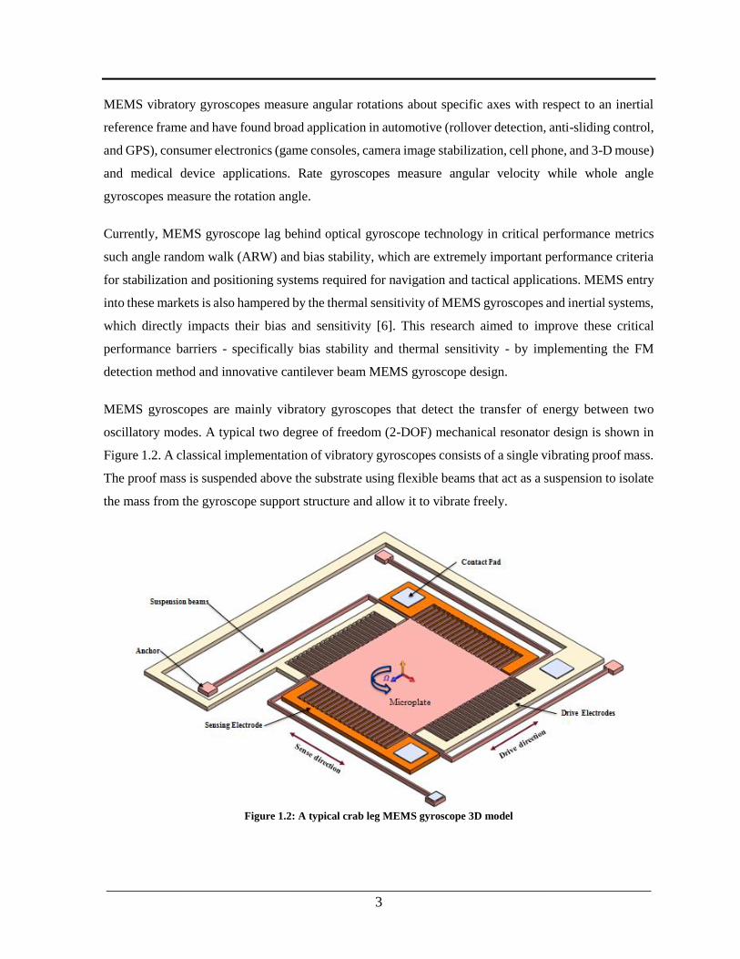
MEMS gyroscopes are mainly vibratory gyroscopes that detect the transfer of energy between two
oscillatory modes. A typical two degree of freedom (2-DOF) mechanical resonator design is shown in
Figure 1.2. A classical implementation of vibratory gyroscopes consists of a single vibrating proof mass.
The proof mass is suspended above the substrate using flexible beams that act as a suspension to isolate
the mass from the gyroscope support structure and allow it to vibrate freely.
Figure 1.2: A typical crab leg MEMS gyroscope 3D model

___________________________________________________________________________
4
The proof mass is driven into resonance along the drive axis using drive electrodes. When the sensor
rotates in the orthogonal direction of the drive axis, a Coriolis force perpendicular to the drive axis and
the angular rotation axis is induced on the proof mass. In the sense direction, the displacement of the
proof mass is detected using sense electrodes.
The Coriolis force is oscillatory in nature since it’s coupled with the drive motion, and thus the driving
frequency of the gyroscope will ideally match with the sensing resonant frequency. If the proof mass is
not excited at the right frequency, then the displacement in the sensing direction will be significantly
reduced there by affecting its sensitivity. However, slight shifts in the resonant frequencies can improve
the gyroscope bandwidth [8]. Hence, there is always a trade-off between the bandwidth and the
sensitivity for conventional open-loop MEMS gyroscope technologies. The design can be optimized,
however, depending on the application requirements.
Drive mode oscillations are typically range from 5 to 40 kHz with a typical amplitude of about 0.5 to
1.5 𝜇𝑚, depending on the application. Therefore, the peak oscillation velocity (𝑑) is about 0.06 m/s.
The Coriolis force is proportional to the vibrating mass, the drive velocity, and the input angular speed.
For MEMS gyroscopes, typical values are used to estimate the Coriolis force in Eq. (1.1), which is on
the order of a pico-Newton. Assuming a spring stiffness for the sensing mode of 1 N/m, the sensed
displacement is about 10 pm. Thus, capacitive sensing methods are required to detect very small forces
(motion).
𝑐 = −2𝑚( × 𝑑) ∝ 10−12 × 102 × 10−2~𝑝𝑁 (1.1)
where 𝑐, 𝑚, Ω, and 𝑑 represent the Coriolis force, the mass, the angular speed and the velocity of a
proof mass, respectively.
1.2 Gyroscope Performance Metrics
MEMS gyroscope performance, particularly with respect to Angular Random Walk (ARW), bias
stability and drift metrics, are crucial to their real-world application. This section briefly covers the most
basic performance metrics for MEMS gyroscopes.
___________________________________________________________________________
5
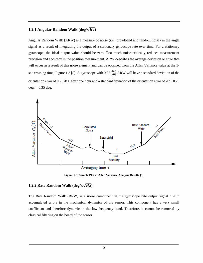
1.2.1 Angular Random Walk (deg/√𝑯𝒛)
Angular Random Walk (ARW) is a measure of noise (i.e., broadband and random noise) in the angle
signal as a result of integrating the output of a stationary gyroscope rate over time. For a stationary
gyroscope, the ideal output value should be zero. Too much noise critically reduces measurement
precision and accuracy in the position measurement. ARW describes the average deviation or error that
will occur as a result of this noise element and can be obtained from the Allan Variance value at the 1-
sec crossing time, Figure 1.3 [5]. A gyroscope with 0.25 deg
√𝐻𝑧 ARW will have a standard deviation of the
orientation error of 0.25 deg. after one hour and a standard deviation of the orientation error of √2 · 0.25
deg. = 0.35 deg.
Figure 1.3: Sample Plot of Allan Variance Analysis Results [5]
1.2.2 Rate Random Walk (deg/s/√𝑯𝒛)
The Rate Random Walk (RRW) is a noise component in the gyroscope rate output signal due to
accumulated errors in the mechanical dynamics of the sensor. This component has a very small
coefficient and therefore dynamic in the low-frequency band. Therefore, it cannot be removed by
classical filtering on the board of the sensor.
___________________________________________________________________________
6
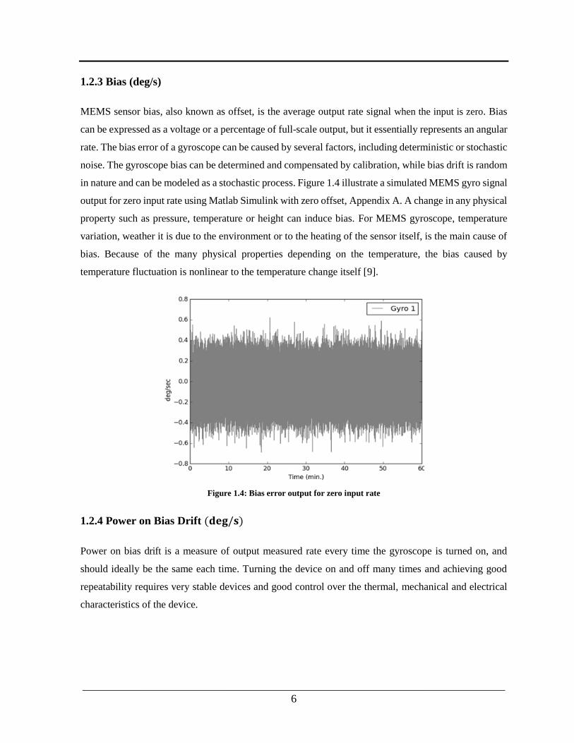
1.2.3 Bias (deg/s)
MEMS sensor bias, also known as offset, is the average output rate signal when the input is zero. Bias
can be expressed as a voltage or a percentage of full-scale output, but it essentially represents an angular
rate. The bias error of a gyroscope can be caused by several factors, including deterministic or stochastic
noise. The gyroscope bias can be determined and compensated by calibration, while bias drift is random
in nature and can be modeled as a stochastic process. Figure 1.4 illustrate a simulated MEMS gyro signal
output for zero input rate using Matlab Simulink with zero offset, Appendix A. A change in any physical
property such as pressure, temperature or height can induce bias. For MEMS gyroscope, temperature
variation, weather it is due to the environment or to the heating of the sensor itself, is the main cause of
bias. Because of the many physical properties depending on the temperature, the bias caused by
temperature fluctuation is nonlinear to the temperature change itself [9].
Figure 1.4: Bias error output for zero input rate
1.2.4 Power on Bias Drift (𝐝𝐞𝐠/𝐬)
Power on bias drift is a measure of output measured rate every time the gyroscope is turned on, and
should ideally be the same each time. Turning the device on and off many times and achieving good
repeatability requires very stable devices and good control over the thermal, mechanical and electrical
characteristics of the device.
___________________________________________________________________________
7
1.2.5 Bias Stability (𝐝𝐞𝐠/𝐬)
Bias stability is a measure of the gyroscope’s output stability over a length of time, and is a fundamental
performance metric for all gyroscopes types including fibre optic gyroscope (FOG), ring laser
gyroscope (RLG), and MEMS. Bias stability is measured after the device is turned on and for a particular
length of time. This variable provides a measure of the drift of the output offset value over time. Bias
instability is best measured using the Allan Variance measurement technique, Figure 1.3. Many applications,
including autonomous vehicle navigation, require higher bias stability for excellent performance.
1.2.6 Nonlinearity (ppm)
Gyroscopes output a voltage proportional to the input angular rate. Nonlinearity measures how the
outputted voltage close to linearity to the actual angular rate. Nonlinearity measured as a percentage
error from a linear fit over the full-scale range or an error in parts per million (ppm). For MEMS
gyroscope, the output linearity affected by physical property such as pressure or temperature.
Additionally, packaging stress play a critical role in nonlinearity.
1.2.7 Resolution (𝐝𝐞𝐠/𝐬
√𝑯𝒛)
Gyroscope resolution defines the minimum change in input required to produce a measurable change in
output. The white noise of the device limits the resolution; therefore, the resolution can be determined
by measuring the standard deviation of the white noise.
1.2.8 Sensitivity (mV/(𝐝𝐞𝐠/𝒔) or LSB/ (𝐝𝐞𝐠/𝒔))
Sensitivity defines the relationship between the input rotation rate, in degree per second (deg
√𝐻𝑧), and the
gyroscope's output voltage change. A device’s sensitivity can vary due to many factors as the output
signal may be sensitive to environmental conditions and other undesirable inputs. Some common
secondary inputs include temperature, pressure, and humidity. Sensitivity can be used to convert the
gyroscope’s output voltage signal into angular velocity.
𝑆𝑓 = (𝛺+𝛺0)
(1.2)
where is the output signal,
___________________________________________________________________________
8
Sf is the sensitivity,
𝛺 is the applied rate and
𝛺0 is the Zero-rate offset (ZRO).
The ZRO is the gyroscope measured rate when no rate is applied.
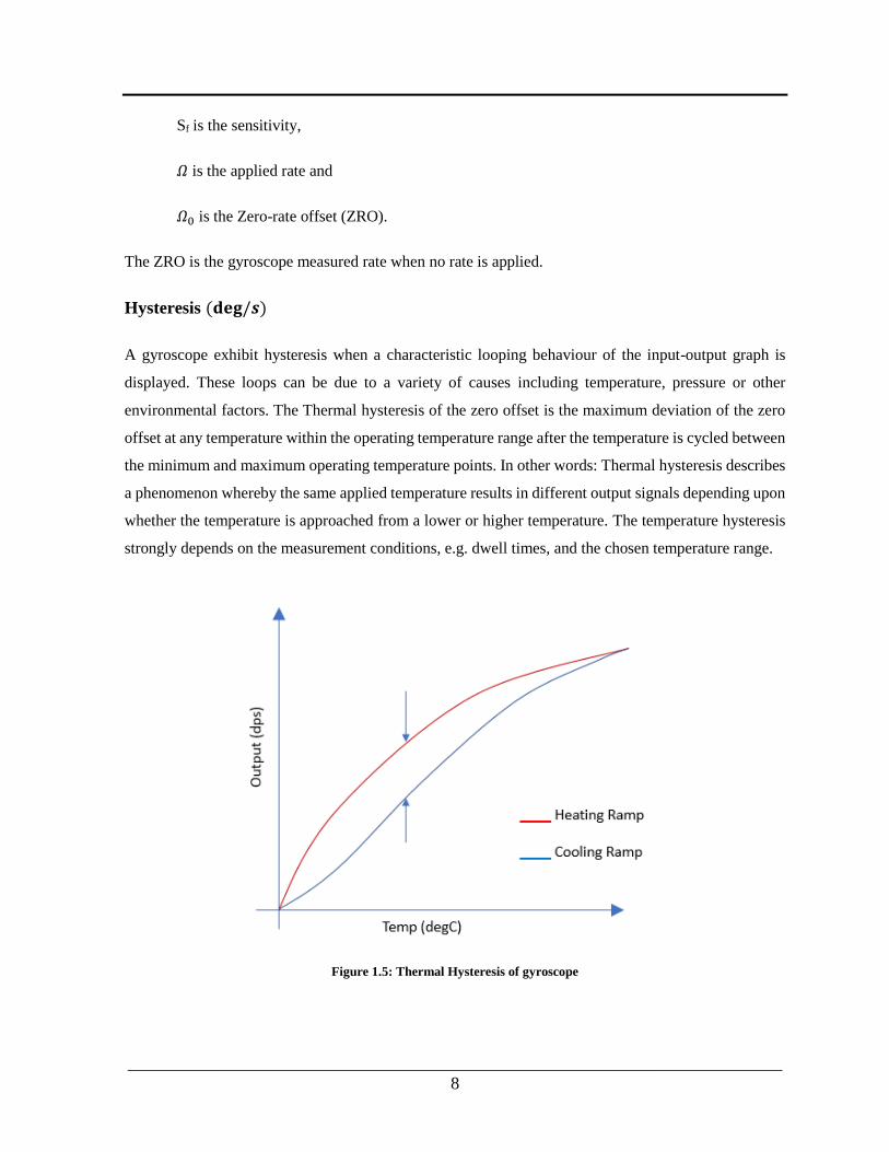
Hysteresis (𝐝𝐞𝐠/𝒔)
A gyroscope exhibit hysteresis when a characteristic looping behaviour of the input-output graph is
displayed. These loops can be due to a variety of causes including temperature, pressure or other
environmental factors. The Thermal hysteresis of the zero offset is the maximum deviation of the zero
offset at any temperature within the operating temperature range after the temperature is cycled between
the minimum and maximum operating temperature points. In other words: Thermal hysteresis describes
a phenomenon whereby the same applied temperature results in different output signals depending upon
whether the temperature is approached from a lower or higher temperature. The temperature hysteresis
strongly depends on the measurement conditions, e.g. dwell times, and the chosen temperature range.
Figure 1.5: Thermal Hysteresis of gyroscope
___________________________________________________________________________
9
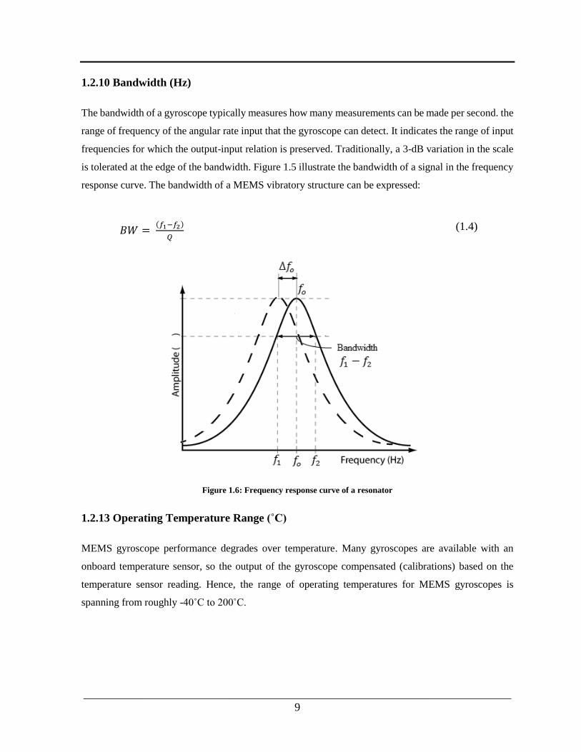
1.2.10 Bandwidth (Hz)
The bandwidth of a gyroscope typically measures how many measurements can be made per second. the
range of frequency of the angular rate input that the gyroscope can detect. It indicates the range of input
frequencies for which the output-input relation is preserved. Traditionally, a 3-dB variation in the scale
is tolerated at the edge of the bandwidth. Figure 1.5 illustrate the bandwidth of a signal in the frequency
response curve. The bandwidth of a MEMS vibratory structure can be expressed:
𝐵𝑊 = (𝑓1−𝑓2)
𝑄 (1.4)
Figure 1.6: Frequency response curve of a resonator
1.2.13 Operating Temperature Range (˚C)
MEMS gyroscope performance degrades over temperature. Many gyroscopes are available with an
onboard temperature sensor, so the output of the gyroscope compensated (calibrations) based on the
temperature sensor reading. Hence, the range of operating temperatures for MEMS gyroscopes is
spanning from roughly -40˚C to 200˚C.
___________________________________________________________________________
10
1.2.14 Shock Survivability
In systems where both linear acceleration and angular rotation rate are measured, it is important to know
how much force the gyroscope can withstand without failing. This is typically measured in g’s (1g =
earth’s acceleration due to gravity), and occasionally the time with which the maximum g-force can be
applied before the unit fails is also given.
1.3 Review of MEMS Gyroscope
A wide range of MEMS gyroscope designs, fabrication methods, and control systems have been
developed over the last two decades. This section highlights major progress made during this period.
Draper Labs demonstrated the first MEMS gyroscope in 1991, utilizing a double-gimbal single crystal
silicon structure suspended by torsional flexures with a resolution of 4 deg/s
√𝐻𝑧 over 60Hz bandwidth [9].
Since then, various MEMS gyroscopes designs fabricated with a wide range of topologies, fabrication
process, integration approaches, and detection techniques have emerged [10].
In 1993, Draper Labs reported tuning fork gyroscopes with 1 deg/s
√𝐻𝑧 resolution at 60Hz bandwidth using
a silicon-on-glass fabrication technique to reduce parasitic capacitances. In 1996, the Berkeley Sensor
and Actuator Center (BSAC) developed an integrated z-axis vibratory rate gyroscope with a resolution
of 1 deg/s
√𝐻𝑧 using a surface micromachining process. This z-axis gyroscope had a single proof mass driven
in-plane at resonance. Electrostatic frequency tuning of sense-modes was successfully demonstrated to
enhance sensitivity by minimizing mode mismatching. Furthermore, the quadrature error nullifying
technique was employed to compensate for structural imperfections caused by fabrication tolerances.
In 1997, BSAC developed an x-y dual input axis gyroscope with a 2μm quad symmetric circular
oscillating polysilicon rotor disc. This gyroscope utilizes torsional drive-mode excitation and two
orthogonal torsional sense-modes to achieve a resolution of 0.24 deg/s
√𝐻𝑧. Subsequent electrostatic tuning
of the device resulted in higher performance, at 0.05 deg/s
√𝐻𝑧 resolution, but at the expense of high cross
axis sensitivity [9-10].
In 2000, Seoul National University reported a hybrid surface-bulk micromachining (SBM) process with
deep reactive ion etching (DRIE) to fabricate high aspect ratio structures with large sacrificial gaps in a
single wafer. A new isolation method using sandwiched oxide, polysilicon and metal films was
___________________________________________________________________________
11
developed for electrostatic actuation and capacitive sensing. This 40μm thick single crystal silicon
MEMS gyroscope demonstrated a resolution of 0.0025 deg/s
√𝐻𝑧 at 100Hz bandwidth [11].
In 2001, Carnegie-Mellon University (CMU) employed a mask-less post-CMOS micromachining
process to develop a lateral-axis integrated gyroscope with a resolution of about 0.5 deg/s
√𝐻𝑧 [12]. The
lateral-axis gyroscope had a 5μm thick structure with out of plane actuation and was fabricated using
Agilent’s three-metal 0.5μm CMOS process. CMU also fabricated an 8μm thick z-axis integrated
gyroscope with dimensions 410×330μm2 using a six-copper layer and 0.18μm CMOS process [13]. This
device showed a sensitivity of 0.8μV/o/s and a resolution of 0.5 deg/s
√𝐻𝑧.
In 2003, CMU demonstrated a DRIE CMOS-MEMS lateral axis gyroscope with dimensions 1×1 mm2
and a measured resolution of 0.02 deg/s
√𝐻𝑧 at 5Hz. This device was fabricated by post-CMOS
micromachining using interconnect metal layers to mask the structural etch steps. The device was built
with on-chip CMOS circuitry and demonstrated in-plane vibration and out of plane Coriolis acceleration
detection [14].
In 2004, Middle East Technical University (METU), Turkey, presented a symmetrical and decoupled
surface MEMS gyroscope fabricated by electroforming thick Nickel on a glass substrate. A capacitive
interface circuit, which was fabricated using a 0.8μm CMOS process, was hybrid connected to the
gyroscope, where the circuit had an input capacitance lower than 50fF and a sensitivity of 33mV/fF.
Calculations on measured resonance values suggested that the fabricated gyroscope, which had a 16μm
thick structural layer, provides a resolution of 0.004 deg/s
√𝐻𝑧 [15].
There are still active research and development from other key player to address the market need for
emerging new application such as IOT and augmented reality. Various design methods and fabrication
processes have been explored to improve the certain performance metrics especially bias instability and
ARW to increase MEMS gyroscopes robustness.
1.4. Current State of the Art
Gyroscopes are classified into three different categories based on their performance: rate-grade, tactical-
grade, and inertial grade devices. Table 1.2 summarizes the performance metrics for each category. Over
the past decade, much of the effort in developing MEMS gyroscopes has concentrated on rate grade
___________________________________________________________________________
12
devices, primarily because of their use in consumer electronics and automotive applications. Depending
on the application, automotive systems generally require a full-scale range of at least 50 - 300 deg/s and
a resolution of about 0.5 - 0.05 deg/s in a bandwidth of less than 100 Hz [22].
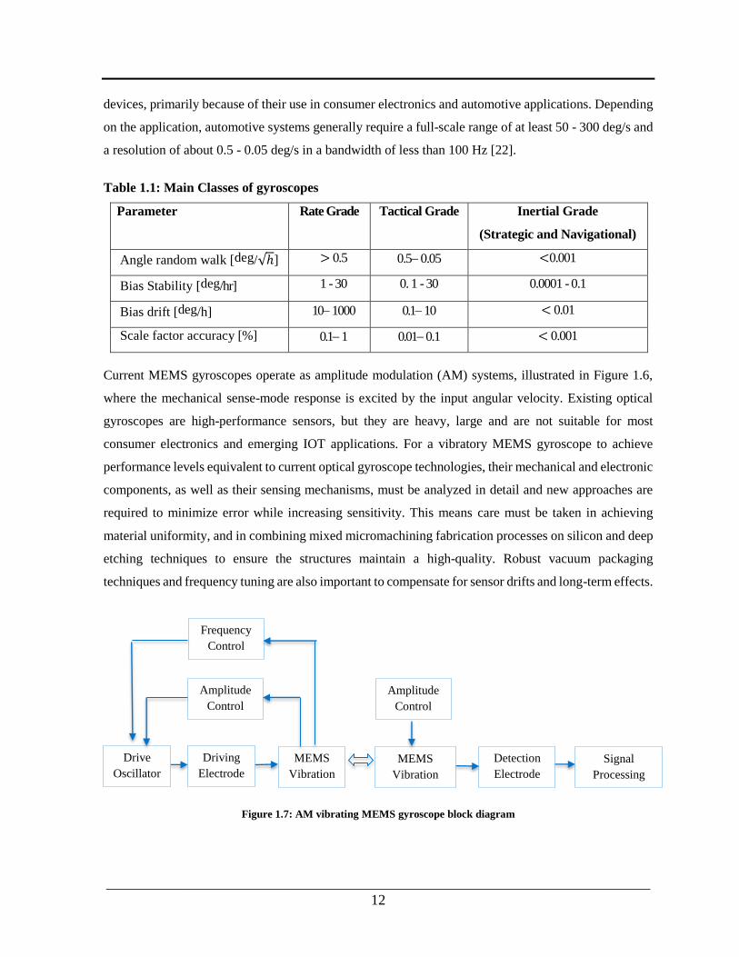
Table 1.1: Main Classes of gyroscopes
Parameter Rate Grade Tactical Grade Inertial Grade
(Strategic and Navigational)
Angle random walk [deg/√ℎ] > 0.5 0.5 0.05 <0.001
Bias Stability [deg/hr] 1 - 30 0. 1 - 30 0.0001 - 0.1
Bias drift [deg/h] 10 1000 0.1 10 < 0.01
Scale factor accuracy [%] 0.1 1 0.01 0.1 < 0.001
Current MEMS gyroscopes operate as amplitude modulation (AM) systems, illustrated in Figure 1.6,
where the mechanical sense-mode response is excited by the input angular velocity. Existing optical
gyroscopes are high-performance sensors, but they are heavy, large and are not suitable for most
consumer electronics and emerging IOT applications. For a vibratory MEMS gyroscope to achieve
performance levels equivalent to current optical gyroscope technologies, their mechanical and electronic
components, as well as their sensing mechanisms, must be analyzed in detail and new approaches are
required to minimize error while increasing sensitivity. This means care must be taken in achieving
material uniformity, and in combining mixed micromachining fabrication processes on silicon and deep
etching techniques to ensure the structures maintain a high-quality. Robust vacuum packaging
techniques and frequency tuning are also important to compensate for sensor drifts and long-term effects.
Figure 1.7: AM vibrating MEMS gyroscope block diagram
Drive
Oscillator
Driving
Electrode
MEMS
Vibration
MEMS
Vibration
Detection
Electrode
Signal
Processing
Amplitude
Control
Frequency
Control
Amplitude
Control

___________________________________________________________________________
13
All conventional MEMS gyroscopes are based on Coriolis Effect amplitude modulation (AM)
gyroscopes. In this case, the input angular rate is amplitude-modulated by the drive mode velocity signal.
They need high quality factors (Q) to improve the sensitivity, resulting in a constraint between Q factor
and bandwidth. Moreover, AM sensors are also extremely sensitive to the value of the sense mode Q
factor which will result in scale factor drifts caused by the ambient temperature and pressure. Even
though an extensive variety of MEMS gyroscope designs and operation principles exists, achieving
robustness against fabrication variations and imperfection as well as environmental fluctuations remain
as one of the greatest challenges in high-performance MEMS gyroscope development. The limitations
of the micromachining technologies define the performance and robustness of the device. Conventional
gyroscopes design based on matching the drive and sense mode resonant frequencies are sensitive to
variations in oscillatory system parameters, which affect device performance. Thus, realizing stable and
reliable vibratory MEMS gyroscopes has proven extremely challenging, primarily due to the high
sensitivity of the dynamical system response to fabrication and environmental variations. To overcome
this challenge, a thorough understanding of all aspects of sensor production including MEMS
fabrication, design, and backend operations is required. Moreover, these critical aspects must be
mutually optimized to be universally adopted in the cost sensitive, high volume, consumer electronics
market, which is the primary driver for MEMS gyroscope innovation.
In this study, we investigated frequency modulated MEMS gyroscopes that exploit changes in the natural
frequency of the proof mass vibrations to measure rotation rate, which theoretically reduces the effect
of noise. The FM technique measures the angular rate by detecting the difference between the
frequencies of two closely spaced global vibration modes, as illustrated in Figure 1.7. The FM approach
has already been implemented in other MEMS sensors including atomic force Microscopes (AFM),
pressure sensors and mass sensors.

___________________________________________________________________________
14
Figure 1.8: FM vibrating MEMS gyroscope block diagram
Although MEMS gyroscopes have been the subject of intensive research for several years and the
frequency sensing approach has been shown to address some of the key limitations of existing MEMS
sensors designs, the technique remains under-utilized in MEMS gyroscope research [16-18]. Seshia et
al. reported an integrated microelectromechanical resonant gyroscope, but they did not give the dynamic
characteristics of the resonant gyroscope in detail [20]. Moussa H. and Bourquin R [23] introduced the
theory for direct frequency output vibratory gyroscopes, but they were concerned with gyroscope
designs where the vibratory mode was out of the plane. Other studies have investigated the resonant
gyroscope, but they all focus on improving the quality factor (for higher sensitivity), the driving control,
or the fabrication process [26-28].
Zotov et al. proposed an angular rate sensor based on mechanical frequency modulation (FM) of the
input rotation rate to solve the contradiction between the gain–bandwidth and dynamic range, [29]. The
sensor consists of a symmetric, ultra-high Q, silicon micromachined Quadruple Mass Gyroscope (QMG)
and a new quasi-digital signal processing scheme which takes advantage of a mechanical FM effect. The
input angular rate is only proportional to the frequency split. The gyroscope comprises four identical
symmetrically decoupled tines with linear coupling flexures as well as a pair of anti-phase
synchronization lever mechanisms for both the x- and the y-modes. The complete x-y symmetrical
structure improves robustness against the fabrication imperfections and frequency drifts.

___________________________________________________________________________
15
Li et al. proposed a double-ended tuning fork (DETF) gyroscope, which utilizes resonant sensing as the
basis for Coriolis force detection instead of displacement sensing [30]. The device is fabricated by the
silicon on glass (SOG) micro fabrication technology. The gyroscope consists of two proof masses, a pair
of DETF resonators and two pairs of lever differential mechanisms. The lever differential mechanism is
responsible for the transmission of the differential Coriolis forces into one common force acting in the
longitudinal direction of the DETF. When the two masses move toward each other or away from each
other, the opposite Coriolis forces from the two masses are transferred to one common force. The
common mode acceleration error is cancelled because the transferred force is differential. The rotation
rate applied to the device can be estimated by demodulating the DETF resonant frequency and detecting
the resonant frequency difference.
However, the effect of temperature and packaging stress on device performance remains a major
challenge in MEMS gyroscope design. The present study focused on addressing this issue by
implementing a novel free end cantilever beam design and the FM sensing approach. The FM sensing
method has proven to be highly sensitive, provide good linearity, low noise and low power in other
applications [24]. We also investigated for the first time the cantilever beam implementation and single
port excitation and sensing scheme. The cantilever structure was designed to provide good control over
the thermal, mechanical, and electrical characteristics, thereby dramatically improving bias stability.
The free end cantilever structure minimizes the effects of packaging and thermal stresses. Specifically,
the design helps eliminate thermally induced strain between the supporting beam and the substrate, and
reduces the impact of packaging sensitivity. The cantilever beam gyroscope could also be aligned in an
orthogonal direction to develop a multi-axis device, which helps to reject external vibrations since the
cantilever beam does not move in response to linear acceleration in the beam’s longitudinal axis. The
single port sensing design also eliminates any cross talk between the drive mode and sense modes of the
gyroscope caused by manufacturing misalignment (i.e., the design minimizes cross-axis sensitivity). The
single-port MEMS FM gyroscope (signal processing) design could also be simplified and the electronics,
signal processing electronics (IC architecture) and backend operations improved. The single port
cantilever beam gyroscope design minimizes the error sources that corrupt the Coriolis signal and
simplifies the IC architecture.
___________________________________________________________________________
16
1.5 Motivation and Objectives of the Thesis
There is a growing demand for high-performance MEMS gyroscopes which can’t be satisfied with either
optical or currently existing gyroscope technologies. The need for smaller and lighter gyroscopes has
been partly met by advances in MEMS design and fabrication. To maximize the device performance in
conventional AM MEMS gyroscopes, resonance is used to enhance the response gain, and hence the
sensitivity of the device, by matching the resonant frequencies of the drive and the sense-mode.
However, bias stability, reliability, and other performance metrics remain major concerns as designers
look to expand MEMS gyroscopes into a broader range of applications, such as navigation, which require
an extended time use of the sensor.
In view of the above-mentioned issues, the current state of vibratory rate MEMS gyroscopes requires an
order of magnitude improvement in performance and robustness. Hence, more research is needed to
investigate angular rate sensing mechanisms including the feasibility of frequency modulated
gyroscopes. Industries and academic research groups developing gyroscopes often focus on fabricating
devices or theoretical work on control algorithms and lack the expertise to implement effective readout
and control hardware.
The aim of this work is to design thermally stable and robust MEMS gyroscopes using a frequency
modulation method, and by means of theoretical and experimental approaches. Two major design
concepts, a novel cantilever beam design and traditional crab leg configuration, are explored to achieve
a dynamical system with a wide bandwidth frequency response, Figure 1.8. We aim to develop, for the
first time, a cantilever beam gyroscope that employs a transfer of energy identification technique to
estimate the natural frequency deviation with the angular velocity input. The design goals of our
cantilever MEMS gyroscope are to build a small sensor with a very low angle drift and bias instability,
which requires devices with low stress and high-quality factors, wide dynamic range (capable of accurate
measurements at both low and high rotation rates), and wide bandwidth to match the maneuverability of
small vehicles.
___________________________________________________________________________
17
Figure 1.9: Isometric view of (a) cantilever beam (b) crab leg gyroscope
The general approach pursued in this research is to explore the possibility of achieving high device
performance by reducing thermal and packing stress effects. We also aim to develop experimental
parametric bandwidth frequency responses in the drive and sense modes. The work has two areas of
focus. First, a system-level design of a MEMS angular velocity sensor is developed, to provide a general-
purpose analysis of potential and selected aspects. Second, an integrated implementation and design of
the electronics required by the angular velocity sensor is produced.
As illustrated in Figure 1.8, the cantilever beam MEMS gyroscope consists of clamped-free beams and
a microplate that are driven into flexural out of plane or in-plane vibration. Then, in response to rotation
force applied along the beam longitudinal axis, it starts to vibrate along an orthogonal direction. This
motion can be used to compute the angular rate input. The drive axis actuation is provided by
electrostatic force and the Coriolis-induced vibration is electrostatically detected by measuring the
capacitance changes between the microplate and fixed electrode and dedicated sensing electrodes. The
cantilever beam structure is designed to have out of plane drive mode and in plane sensing modes. A
vibrating crab-leg beam structure is also investigated, primarily as a direct comparison against the
cantilever beam design under the same test conditions.

___________________________________________________________________________
18
1.5.1 Research Contribution
The objective of this research is to develop new dynamical sensing systems and structural designs for
resonant MEMS vibratory gyroscope technologies using standard, low-cost, commercially available
MEMS processes. The proposed research objectives are to:
Demonstrate the MEMS gyroscope operation in the frequency modulation mode and investigate
the modal frequencies of the MEMS gyroscope,
Derive the mathematical model of the beam-rigid body gyroscope considering the static behavior
of the beam-rigid body MEMS gyroscope and study the reduced-order nonlinear behavior of the
system,
Analyze the nonlinear behavior using Finite Element software (ANSYS) and compare the results
of the method with the analytical and numerical results,
Develop the mechanical-thermal noise analysis for a frequency modulated MEMS gyroscope
Design and fabricate a prototype MEMS gyroscope to demonstrate the frequency modulated
MEMS gyroscope concept,
Develop a characterization method that measures the frequency of the MEMS gyroscope’s two
modes
1.6 Research Outline
This work is organized into six chapters to provide the scope of work. In chapter one, the working
principles, types and applications of vibratory MEMS gyroscopes are introduced and comprehensively
described. A review of MEMS gyroscope sensing methods along with the prior research work carried
out by academic and industrial research groups are provided. Following the literature review, the
research method is presented, including an overview of the research problems, as well as research
objectives and the research motivation.
Chapter two covers the basics of the FM MEMS gyroscope concept and analysis of frequency modulated
mathematical modeling. A detailed review of frequency modulated MEMS sensor implementation is
given. The principles of operation and benefits of the FM gyroscope design is introduced along with
related design parameters and characteristics. Throughout the FM sensing approach review, the
frequency sensing method is proved to have better sensitivity and higher accuracy on micro-
displacement measurement compared to the AM method. This provides the development background
___________________________________________________________________________
19
and methods to significantly improve the performance of MEMS gyroscope systems. Towards the end
of the chapter, the frequency excitation and detection approach, as well as gyroscope testing and
characterization, are briefly discussed.
Chapter three comprehensively covers the dynamics of the cantilever beam MEMS gyroscope, taking
into account its systematic design implementation. A comprehensive theoretical description is provided,
and relevant dynamics and mechanical design considerations of the cantilever beam models are
discussed in detail. Optimization, as well as simulation methodology in ANSYS, are also developed.
The main emphasis of this work is to demonstrate the optimization of gyroscopes within the design rules
of standards for Teledyne Dalsa MEMS Integrated Design for Inertial Sensors (MIDIS™), where we
fabricate prototype device.
In chapter four, the noise analysis for frequency modulated MEMS gyroscope structures and noise-based
optimization are briefly discussed. Chapter five discusses fabrication methods for MEMS vibration
structures, including a cantilever beam and crab leg MEMS gyroscope fabrication process. These
vibration structures are further described based on operation principles and functions introduced in
chapter two. Prototype fabrication using the MIDIS™ process is also investigated. Finally, a testing
methodology along with the electrical circuit, control, and sensing design is devised and test result
presented.
The last chapter provides a list of major contributions and some suggestions for improving the
performance of MEMS gyroscope design. To sum up the structure of this thesis, it defines a problem
and discusses alternative methods to fine tune the final structure of the gyroscope.

___________________________________________________________________________
20
CHAPTER II
Frequency Modulated MEMS Gyroscope
2.1 Resonance and Resonant Sensing
The resonance sensing concept is fundamental to understanding the operation of frequency modulated
MEMS gyroscope systems. Resonance is a term used to describe a system’s enhanced response at a
certain characteristic natural frequency determined by parameters of the system. The specific frequency
is one where the system retains input energy with minimum loss. Resonance can be observed in
mechanical, optical and electronic systems as well as in systems that interconvert energy between these
energy domains. At a microscopic scale, operating systems at resonance enhances the effects of small
forces and the device’s signal to noise ratio. A general functional block diagram of the resonant sensing
approach is illustrated in Figure 2.1.
Figure 2.1: Functional block diagram of resonant sensing
The resonant characteristics of a mechanical system can be changed either by modulating the spring
constant (stiffness) or the effective mass of the resonating system. Typically, a shift in either of these
quantities can be monitored as a change in the resonant amplitude, frequency or phase [21-22]. A change
in resonant characteristics can be monitored using several different techniques such as capacitive, optical
and piezoresistive sensing. Generally, measuring the change in resonance frequency provides a highly

___________________________________________________________________________
21
sensitive instrument and has the potential to address a large dynamic range [22-23]. The resonance
frequency sensing approach has been implemented in numerous MEMS devices including Atomic Force
Microscopy (AFM) and pressure sensors.
2.2 Frequency-Based Detection of Angular Rate
In conventional AM gyroscope designs, the primary mode drives at a constant amplitude and frequency
along the drive axis. When the gyroscope is subjected to an angular rotation, a Coriolis force is generated
along the sense axis, whose magnitude is proportional to the oscillation velocity of the drive axis and
the magnitude of the input angular rate that is being measured. The sense direction motion magnitude is
amplified according to the mechanical quality factor and the rate signal detected along the sense mode
of vibration by reading the amplitude changes. In this work, we primarily focused on the FM approach,
which tracks the instantaneous frequency of the drive and sense oscillation. The functional block
diagram of the FM method is given in Figure 2.2.
Figure 2.2: Functional block diagram of FM MEMS gyroscope
In this study, the FM approach was implemented, using cantilever beam and crab-leg MEMS gyroscope
configurations, to detect the applied rotation rate using the shift in natural frequency of the first two
close modes. A schematic of the Cantilever beam MEMS vibratory gyroscope is shown in Figure 2.3,
which includes two parallel sidewall electrodes (the right side removed here for clarity) and the drive
electrode. The cantilever beam is attached to a rotating base and it has a uniform cross section. At the
free end, a proof mass (M) is attached, which is electrically coupled to the drive and sense electrodes.
The suspended mass is driven to vibration along the z-axis by applying AC excitation and DC
polarization voltage between the parallel plate (proof mass and stationary drive electrodes). When the
cantilever beam gyroscope rotates around the y-axis, the Coriolis acceleration induced by the input

___________________________________________________________________________
22
rotation rate causes the beam to transfer energy from the drive-mode (z-direction) to the sense-mode (x-
direction). The input angular rate can be measured by analyzing the shift in the natural frequencies of
these two modes.
Figure 2.3: Perspective view of the cantilever beam MEMS gyroscope
A crab-leg MEMS gyroscope system was also developed and experimentally investigated to evaluate
the performance advantage(s) of the new cantilever design. Traditional crab-leg flexure structures were
designed within plane motion for both drive and sensing modes. In this design, we used a comb drive
(set of parallel plates) for sensing and driving the gyroscope. In Figure 2.4, a schematic drawing of the
crab-leg gyroscope is illustrated where the actuation takes place in the z-direction. When the angular
rate is applied along the y-axis, the Coriolis force is induced and sensing happens in the x-direction.
𝜴
___________________________________________________________________________
23
Figure 2.4: Perspective view of the crab leg flexures
2.3 Kinematics Analysis of the Cantilever Beam MEMS gyroscope
A mathematical model that represents the kinematics characteristics of the cantilever beam gyroscope,
which is equally applicable to the crab leg dynamics, is presented in this section. The microplate proof
mass (ℳ) is a rigid body and the center of the microplate can be assumed as a particle (O). Figure 2.5
shows the cantilever beam subjected to generalized electrostatic actuation (𝐹𝑒𝑠) and Coriolis forces (𝐹𝑐)
at the tip.
___________________________________________________________________________
24
Figure 2.5: Cantilever flexural- flexural displacements
Although the cantilever beam has many modes of vibration, we consider here a model with two degrees
of freedom with flexural displacements given by 𝛿𝑥(𝑦, 𝑡)and 𝛿𝑧(𝑦, 𝑡) along the x and z directions that
describe the in-plane and out-plane motion of the proof mass. The axis of rotation is along the beam axis
(y-directions), as illustrated in Figure 2.5. Two coordinate systems are used to derive the kinematics
characteristics of the cantilever beam gyroscope. The x-y-z axes define the inertial coordinate system
(Frame A) with orthogonal unit vectors 𝑖𝑥, 𝑗𝑦, and 𝑘𝑧. The ξ-η-ζ axes define the base coordinate system
(Frame B) with orthogonal unit vectors 𝑖𝜉, 𝑗𝜂 and 𝑘𝜍.
___________________________________________________________________________
25
Figure 2.6: Particle O moving in non-inertial Frame B with respect to inertial Frame A.
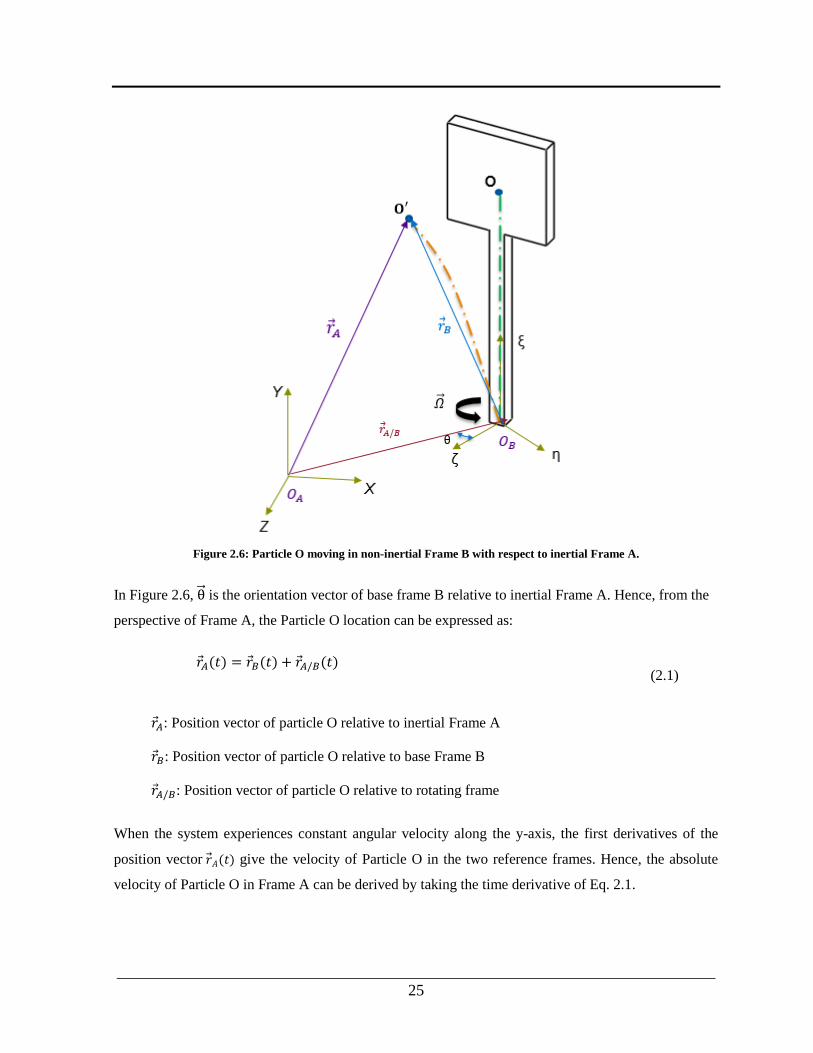
In Figure 2.6, θ is the orientation vector of base frame B relative to inertial Frame A. Hence, from the
perspective of Frame A, the Particle O location can be expressed as:
𝑟𝐴(𝑡) = 𝑟𝐵(𝑡) + 𝑟𝐴/𝐵(𝑡)
(2.1)
𝑟𝐴: Position vector of particle O relative to inertial Frame A
𝑟𝐵: Position vector of particle O relative to base Frame B
𝑟𝐴/𝐵: Position vector of particle O relative to rotating frame
When the system experiences constant angular velocity along the y-axis, the first derivatives of the
position vector 𝐴(𝑡) give the velocity of Particle O in the two reference frames. Hence, the absolute
velocity of Particle O in Frame A can be derived by taking the time derivative of Eq. 2.1.

___________________________________________________________________________
26
𝐴(𝑡) = 𝐵(𝑡) + (Ω × 𝑟𝐴/𝐵(𝑡)) + 𝐴/𝐵(𝑡) (2.2)
where Ω: Angular velocity of rotating Frame B given by Ω = θ
The absolute acceleration of Particle O in the inertial reference frame A can be derived by taking second
derivatives of Eq. (2.2).
𝑟𝐴 (𝑡) = 𝑟𝐵
(𝑡) + (Ω × 𝑟𝐴/𝐵) + (Ω × (Ω × 𝑟𝐴/𝐵)) + (2Ω × 𝐴/𝐵(𝑡)) (2.3)
where 𝑟𝐴 (𝑡) is the linear acceleration of Particle O with respect to the inertial reference frame A,
𝑟𝐵 (𝑡) is the acceleration of the particle with respect to the rotating Frame B
(Ω × 𝑟𝐴/𝐵) is angular acceleration induced by tangential acceleration
(Ω × (Ω × 𝑟𝐴/𝐵)) is the centripetal acceleration
(2Ω × 𝐴/𝐵(𝑡)) is the Coriolis acceleration
The Coriolis acceleration terms (2Ω × 𝐴/𝐵(𝑡)) couple the drive and sense direction (z and x-axis) and
allow the vibrating structure to act as a gyroscope. In Eq. 2.3, the Coriolis term states that an oscillating
structure that undergoes a rotation will experience an acceleration that is proportional to the rotation rate
in a direction that is orthogonal to both the rotation axis and the direction of motion. That is if the
microplate moves along the z-axis and rotates about the y-axis, it will accelerate along the x-axis as
observed in Frame B. Once that acceleration is detected and converted into a meaningful medium such
as voltage, it is possible to determine the original rotation rate. The absolute acceleration vector for the
x and z-acceleration components are then obtained as
𝑟𝑥 (𝑡) = − 𝑧Ω − 𝑥Ω2 − 2Ωz
𝑟𝑧 (𝑡) = − 𝑥Ω − 𝑧Ω2 − 2Ωx
(2.4)

___________________________________________________________________________
27
Equation 2.3 summarizes all the acceleration terms of a moving Particle O. The force terms of this
acceleration can be along with the system damping and stuffiness can be written as:
𝐹𝐴 = (𝑚𝑟𝐵 (𝑡) + (𝑚Ω × 𝑟𝐴/𝐵) + (Ω × 𝑚(Ω × 𝑟𝐴/𝐵)) + 2𝑚( Ω × 𝐴/𝐵(𝑡))) +
+𝑐𝐵(𝑡) + 𝑘𝐵(𝑡)
(2.5)
The fictitious force component in Eq. 2.5 includes
𝐹𝑓𝑖𝑐𝑡 = (𝑚Ω × 𝑟𝐴/𝐵)⏟ tangential force
+ (Ω × 𝑚(Ω × 𝑟𝐴/𝐵))⏟ centripetal force
+ 2𝑚( Ω × 𝐴/𝐵(𝑡))⏟ Coriolis force
(2.6)
Hence, from Eq. 2.6 the Coriolis force is a part of the fictitious force used to describe the motion of
objects observed in a rotating non-inertial reference frame. The tangential and centripetal force
components which couple the two axes are undesirable and are a source of offset in a rate gyroscope and
drift in a rate-integrating gyroscope. For a constant angular rate input Ω = 0 and for very small angular
rate, the centripetal force terms become negligible compared to the Coriolis force. Hence the Coriolis-
induced motion is sensed for obtaining the angular rate; the corresponding rotation angle is obtained by
integration.
A simple conceptual vibratory gyroscope is illustrated in Figure 2.7. A 2-DOF spring mass damper
system is typically used to model the proof mass of the vibrating gyroscope. The governing equations
of the vibratory gyroscope can be expressed as a second order spring mass damper system. The model
includes a vibrating mass ℳ and two spring-damper systems.
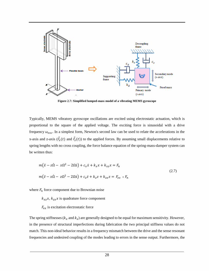
___________________________________________________________________________
28
Figure 2.7: Simplified lumped-mass model of a vibrating MEMS gyroscope
Typically, MEMS vibratory gyroscope oscillations are excited using electrostatic actuation, which is
proportional to the square of the applied voltage. The exciting force is sinusoidal with a drive
frequency 𝜔𝑒𝑥𝑐. In a simplest form, Newton's second law can be used to relate the accelerations in the
x-axis and z-axis (𝑟𝑥 (𝑡) and 𝑟𝑧
(𝑡)) to the applied forces. By assuming small displacements relative to
spring lengths with no cross coupling, the force balance equation of the spring-mass-damper system can
be written thus:
𝑚( − 𝑧Ω − 𝑥Ω2 − 2Ωz) + 𝑐𝑥 + 𝑘𝑥𝑥 + 𝑘𝑥𝑧𝑥 = 𝐹𝑛
𝑚( − 𝑥Ω − 𝑧Ω2 − 2Ωx) + 𝑐𝑧 + 𝑘𝑧𝑧 + 𝑘𝑧𝑥𝑧 = 𝐹𝑒𝑥 + 𝐹𝑛
(2.7)
where 𝐹𝑛 force component due to Brownian noise
𝑘𝑥𝑧𝑥, 𝑘𝑧𝑥𝑥 is quadrature force component
𝐹𝑒𝑥 is excitation electrostatic force
The spring stiffnesses (𝑘𝑥 and 𝑘𝑧) are generally designed to be equal for maximum sensitivity. However,
in the presence of structural imperfections during fabrication the two principal stiffness values do not
match. This non-ideal behavior results in a frequency mismatch between the drive and the sense resonant
frequencies and undesired coupling of the modes leading to errors in the sense output. Furthermore, the

___________________________________________________________________________
29
fabrication imperfections of gyroscope such as non-symmetrical structures or the defect make
anisoelasticity stiffness components (𝑘𝑥z and 𝑘z𝑥). Hence, this introduce extra motions on the sense axis
without input rates applied. Thus, the Coriolis force and the extra motion which is coupled from the z-
axis drive can be both observed on x-axis. This extra x-axis deflection is proportional with the z-axis
displacement and it is named as quadrature coupling.
Figure 2.8: lumped mass model without and with Quadrature coupling due to anisoelasticity terms
Quadrature term included in the sense direction cannot be separated by amplitude detection only. To
distinguish the Coriolis force and the quadrature term, the phase relationship between the two can be
used since there is a 90-degree phase difference between the velocity and displacement on the drive axis.
Equation 2.7 can be reformulated into a more convenient form, to emphasize the main parameters. If we
divide by the mass of the movable structure, we get:
+ 2휁𝑑𝜔𝑛𝑑 + (𝜔𝑛𝑑2 − Ω2)𝑥 − 2Ωz − 𝑧Ω = 𝜔𝑛𝑠
2 𝑋𝑑𝑒𝑗𝜔𝑡
+ 2휁𝑠𝜔𝑛𝑠 + (𝜔𝑛𝑠2 − Ω2)𝑧 − 2Ωx − 𝑥Ω = 𝜔𝑛𝐷
2 𝑍𝑠𝑒𝑗𝜔𝑡
(2.8)
where, 𝜔𝑛𝑑 and 𝜔𝑛𝑠 are the natural frequencies of the drive and sense direction,
휁𝑑 and 휁𝑠 are the damping ratio of the drive and sense direction
𝑋𝑑 and 𝑍𝑠 are the excitation force amplitudes
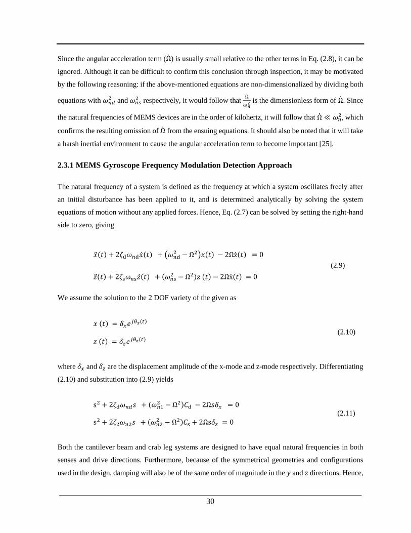
___________________________________________________________________________
30
Since the angular acceleration term (Ω) is usually small relative to the other terms in Eq. (2.8), it can be
ignored. Although it can be difficult to confirm this conclusion through inspection, it may be motivated
by the following reasoning: if the above-mentioned equations are non-dimensionalized by dividing both
equations with 𝜔𝑛𝑑2 and 𝜔𝑛𝑠
2 respectively, it would follow that Ω
𝜔𝑛2 is the dimensionless form of Ω. Since
the natural frequencies of MEMS devices are in the order of kilohertz, it will follow that Ω ≪ 𝜔𝑛2, which
confirms the resulting omission of Ω from the ensuing equations. It should also be noted that it will take
a harsh inertial environment to cause the angular acceleration term to become important [25].
2.3.1 MEMS Gyroscope Frequency Modulation Detection Approach
The natural frequency of a system is defined as the frequency at which a system oscillates freely after
an initial disturbance has been applied to it, and is determined analytically by solving the system
equations of motion without any applied forces. Hence, Eq. (2.7) can be solved by setting the right-hand
side to zero, giving
(𝑡) + 2휁d𝜔𝑛d(𝑡) + (𝜔𝑛d2 − Ω2)𝑥(𝑡) − 2Ωz(𝑡) = 0
(𝑡) + 2휁s𝜔𝑛s(𝑡) + (𝜔𝑛s2 − Ω2)𝑧 (𝑡) − 2Ωx(𝑡) = 0
(2.9)
We assume the solution to the 2 DOF variety of the given as
𝑥 (𝑡) = 𝛿𝑥𝑒𝑗𝜃𝑥(𝑡)
𝑧 (𝑡) = 𝛿𝑧𝑒𝑗𝜃𝑧(𝑡)
(2.10)
where 𝛿𝑥 and 𝛿𝑧 are the displacement amplitude of the x-mode and z-mode respectively. Differentiating
(2.10) and substitution into (2.9) yields
s2 + 2휁d𝜔𝑛𝑑𝑠 + (𝜔𝑛12 − Ω2)𝐶d − 2Ω𝑠𝛿𝑥 = 0
s2 + 2휁2𝜔𝑛2𝑠 + (𝜔𝑛22 − Ω2)𝐶s + 2Ωs𝛿𝑧 = 0
(2.11)
Both the cantilever beam and crab leg systems are designed to have equal natural frequencies in both
senses and drive directions. Furthermore, because of the symmetrical geometries and configurations
used in the design, damping will also be of the same order of magnitude in the 𝑦 and 𝑧 directions. Hence,
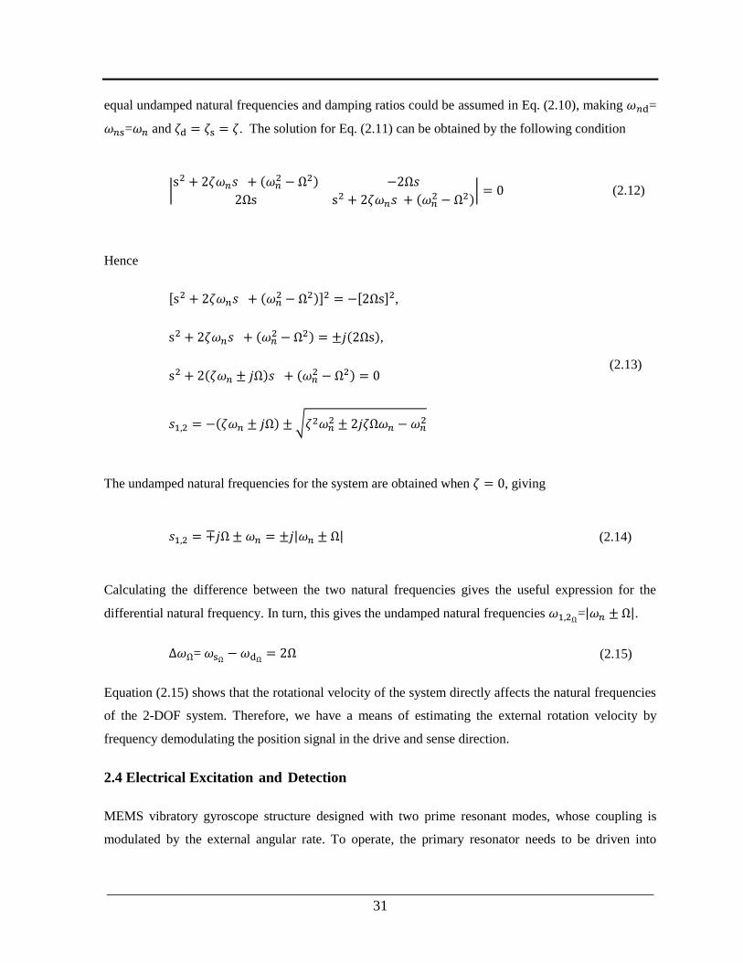
___________________________________________________________________________
31
equal undamped natural frequencies and damping ratios could be assumed in Eq. (2.10), making 𝜔𝑛d=
𝜔𝑛s=𝜔𝑛 and 휁d = 휁s = 휁. The solution for Eq. (2.11) can be obtained by the following condition
|s2 + 2휁𝜔𝑛𝑠 + (𝜔𝑛
2 − Ω2) −2Ω𝑠
2Ωs s2 + 2휁𝜔𝑛𝑠 + (𝜔𝑛2 − Ω2)
| = 0 (2.12)
Hence
[s2 + 2휁𝜔𝑛𝑠 + (𝜔𝑛2 − Ω2)]2 = −[2Ωs]2,
s2 + 2휁𝜔𝑛𝑠 + (𝜔𝑛2 − Ω2) = ±𝑗(2Ωs),
s2 + 2(휁𝜔𝑛 ± 𝑗Ω)𝑠 + (𝜔𝑛2 − Ω2) = 0
𝑠1,2 = −(휁𝜔𝑛 ± 𝑗Ω) ± √휁2𝜔𝑛
2 ± 2𝑗휁Ω𝜔𝑛 − 𝜔𝑛2
(2.13)
The undamped natural frequencies for the system are obtained when 휁 = 0, giving
𝑠1,2 = ∓𝑗Ω ± 𝜔𝑛 = ±𝑗|𝜔𝑛 ± Ω| (2.14)
Calculating the difference between the two natural frequencies gives the useful expression for the
differential natural frequency. In turn, this gives the undamped natural frequencies 𝜔1,2Ω=|𝜔𝑛 ±Ω|.
∆𝜔Ω= 𝜔sΩ −𝜔dΩ = 2Ω (2.15)
Equation (2.15) shows that the rotational velocity of the system directly affects the natural frequencies
of the 2-DOF system. Therefore, we have a means of estimating the external rotation velocity by
frequency demodulating the position signal in the drive and sense direction.
2.4 Electrical Excitation and Detection
MEMS vibratory gyroscope structure designed with two prime resonant modes, whose coupling is
modulated by the external angular rate. To operate, the primary resonator needs to be driven into
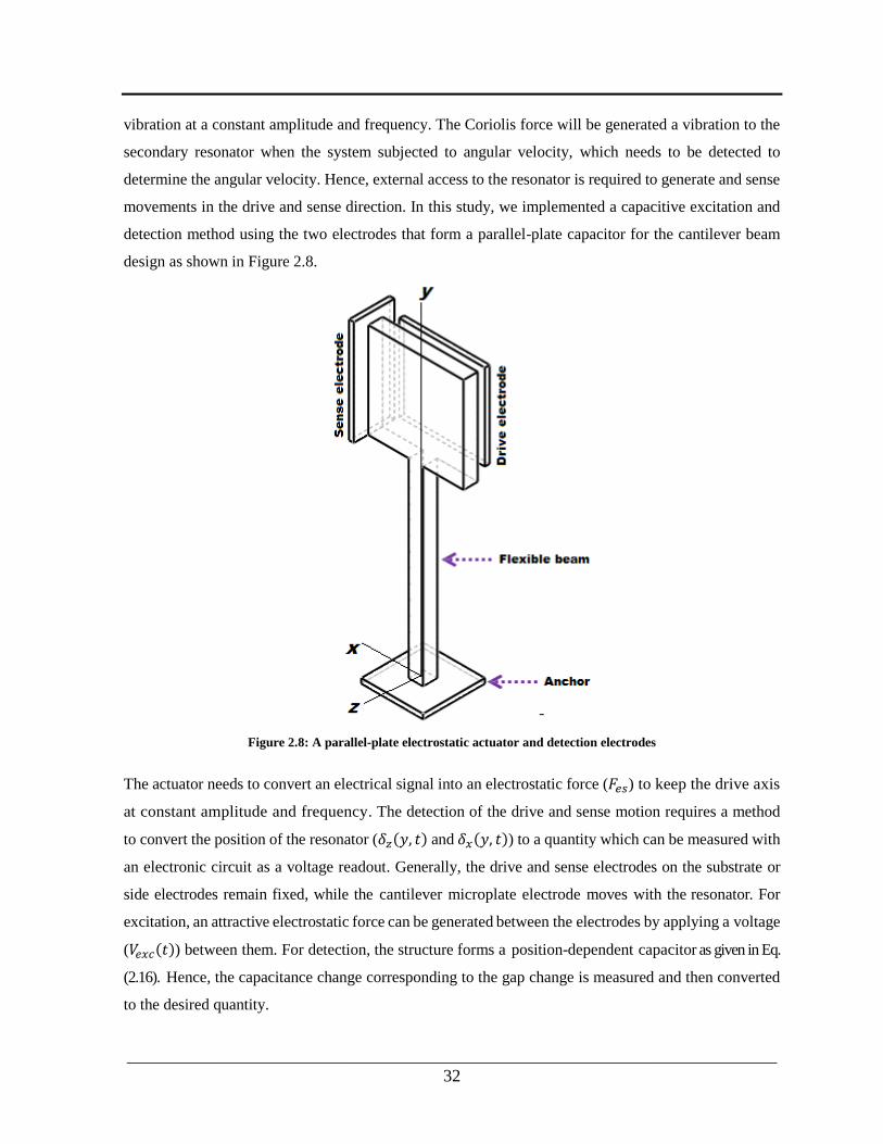
___________________________________________________________________________
32
vibration at a constant amplitude and frequency. The Coriolis force will be generated a vibration to the
secondary resonator when the system subjected to angular velocity, which needs to be detected to
determine the angular velocity. Hence, external access to the resonator is required to generate and sense
movements in the drive and sense direction. In this study, we implemented a capacitive excitation and
detection method using the two electrodes that form a parallel-plate capacitor for the cantilever beam
design as shown in Figure 2.8.
Figure 2.8: A parallel-plate electrostatic actuator and detection electrodes
The actuator needs to convert an electrical signal into an electrostatic force (𝐹𝑒𝑠) to keep the drive axis
at constant amplitude and frequency. The detection of the drive and sense motion requires a method
to convert the position of the resonator (𝛿𝑧(𝑦, 𝑡) and 𝛿𝑥(𝑦, 𝑡)) to a quantity which can be measured with
an electronic circuit as a voltage readout. Generally, the drive and sense electrodes on the substrate or
side electrodes remain fixed, while the cantilever microplate electrode moves with the resonator. For
excitation, an attractive electrostatic force can be generated between the electrodes by applying a voltage
(𝑉𝑒𝑥𝑐(𝑡)) between them. For detection, the structure forms a position-dependent capacitor as given in Eq.
(2.16). Hence, the capacitance change corresponding to the gap change is measured and then converted
to the desired quantity.

___________________________________________________________________________
33
𝐶 =𝐴휀𝑜휀𝑟
𝑔𝑜 + 𝛿𝑥(𝑦, 𝑡) (2.16)
where 휀𝑜 and 휀𝑟 is the absolute and relative permittivity of the insulator between the plates, 휀𝑟 for
vacuum or air is 1
𝑔𝑜 is the initial gap between the electrodes (fixed and moving plates)
𝐴 is the area of the sense electrode
The MEMS gyroscope control system must ensure that the amplitude and frequency remain constant in
either the drive axis or in both the drive and sensing axes, depending on the operation modes. Excitation
and detection can be designed to operate in either open-loop or closed loop modes. The main advantage
of open-loop systems is that, by comparison with other modes, the circuitry used to operate the
gyroscope is relatively simple (i.e., there is no control action in the sense axis) and, thus, easy to
implement. However, under an open-loop mode of operation, the gyroscope’s angular rate scale factor
is very sensitive to fabrication defects and environment variations, and cannot be held constant over any
appreciable bandwidth. Therefore, open-loop systems are limited to applications which require low-cost
and low-performance gyroscopes.
In the closed-loop mode of operation, both the drive and sense direction amplitude and frequency are
continuously monitored and amplitude driven to zero. Therefore, the bandwidth and dynamic range of
the gyroscope can be greatly increased, extending far beyond what can be achieved with open-loop-
based systems. However, under the conventional closed-loop mode of operation, it is difficult to ensure
a constant noise performance in the face of environmental variations such as temperature changes.
Moreover, there are practical difficulties in designing a feedback controller that keeps the closed-loop
system both stable and sufficiently robust for gyroscopes with high-quality factors (Q). Therefore, the
application areas for the conventional closed-loop mode of operation are those which allow for medium-
cost and medium-performance (large bandwidth, but limited resolution) gyroscopes.
2.4.1 Primary Mode Excitation Method
There are many actuation methods available to MEMS technologies, including electrostatic,
piezoelectric, thermal, and magnetic techniques. Among them, electrostatic actuation is the most
common for MEMS resonator systems, owing to their easy integration and implementation. The
cantilever beam parallel-plate electrostatic actuation comprises an attractive force generated by applying
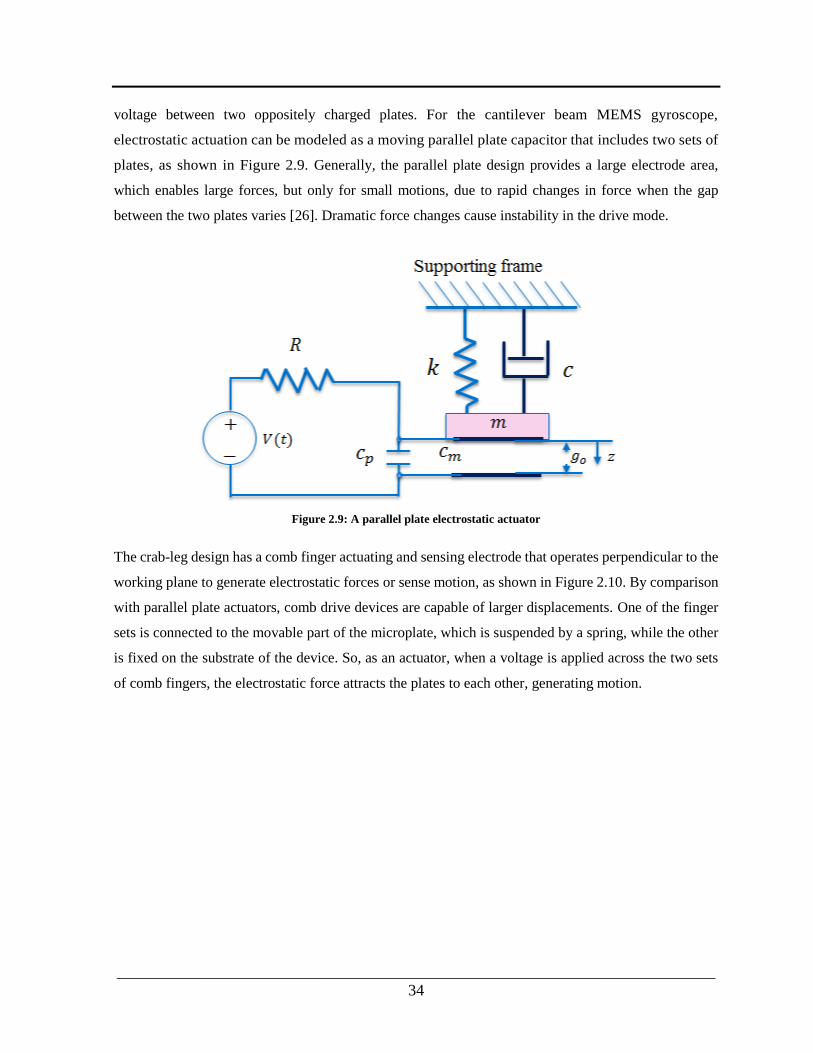
___________________________________________________________________________
34
voltage between two oppositely charged plates. For the cantilever beam MEMS gyroscope,
electrostatic actuation can be modeled as a moving parallel plate capacitor that includes two sets of
plates, as shown in Figure 2.9. Generally, the parallel plate design provides a large electrode area,
which enables large forces, but only for small motions, due to rapid changes in force when the gap
between the two plates varies [26]. Dramatic force changes cause instability in the drive mode.
Figure 2.9: A parallel plate electrostatic actuator
The crab-leg design has a comb finger actuating and sensing electrode that operates perpendicular to the
working plane to generate electrostatic forces or sense motion, as shown in Figure 2.10. By comparison
with parallel plate actuators, comb drive devices are capable of larger displacements. One of the finger
sets is connected to the movable part of the microplate, which is suspended by a spring, while the other
is fixed on the substrate of the device. So, as an actuator, when a voltage is applied across the two sets
of comb fingers, the electrostatic force attracts the plates to each other, generating motion.
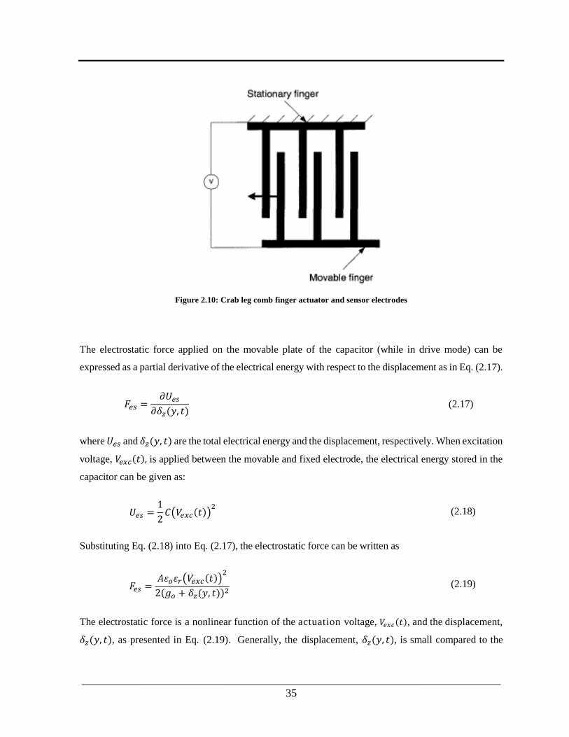
___________________________________________________________________________
35
Figure 2.10: Crab leg comb finger actuator and sensor electrodes
The electrostatic force applied on the movable plate of the capacitor (while in drive mode) can be
expressed as a partial derivative of the electrical energy with respect to the displacement as in Eq. (2.17).
𝐹𝑒𝑠 =𝜕𝑈𝑒𝑠
𝜕𝛿𝑧(𝑦, 𝑡) (2.17)
where 𝑈𝑒𝑠 and 𝛿𝑧(𝑦, 𝑡) are the total electrical energy and the displacement, respectively. When excitation
voltage, 𝑉𝑒𝑥𝑐(𝑡), is applied between the movable and fixed electrode, the electrical energy stored in the
capacitor can be given as:
𝑈𝑒𝑠 =1
2𝐶(𝑉𝑒𝑥𝑐(𝑡))
2 (2.18)
Substituting Eq. (2.18) into Eq. (2.17), the electrostatic force can be written as
𝐹𝑒𝑠 =𝐴휀𝑜휀𝑟(𝑉𝑒𝑥𝑐(𝑡))
2
2(𝑔𝑜 + 𝛿𝑧(𝑦, 𝑡))2
(2.19)
The electrostatic force is a nonlinear function of the actuation voltage, 𝑉𝑒𝑥𝑐(𝑡), and the displacement,
𝛿𝑧(𝑦, 𝑡), as presented in Eq. (2.19). Generally, the displacement, 𝛿𝑧(𝑦, 𝑡), is small compared to the

___________________________________________________________________________
36
initial gap (𝑔𝑜), thus the force can be linearized by taking the first two terms of the Taylor series of Eq.
(2. 19). Hence, the force can be written as:
𝐹𝑒𝑠 ≈𝐴휀𝑜휀𝑟𝑉𝑒𝑥𝑐(𝑡)
2
2(𝑔𝑜)2
+𝐴휀𝑜휀𝑟𝑉𝑒𝑥𝑐(𝑡)
2
(𝑔𝑜)3
. 𝛿𝑧(𝑦, 𝑡) (2.20)
The first term of the series can be interpreted as a displacement-independent attractive electrostatic force,
which is used to excite the resonator, while the second term is a repulsive force with a linear dependency
with the displacement. Equation (2.20) also indicates that the electrostatic force is proportional to the
square of the excitation voltage, which may include DC and AC components [26].
𝑉𝑒𝑥𝑐(𝑡) = 𝑉𝐷𝐶 + 𝑉𝐴𝐶 . 𝑆𝑖𝑛(𝜔𝑒𝑥𝑐𝑡) 2.21
where 𝑉𝐷𝐶 and 𝑉𝐴𝐶 are the DC and AC components of the excitation voltage, respectively, and 𝜔𝑒𝑥𝑐 is the
frequency at which the excitation is performed. To achieve a maximum displacement with a given
excitation force the excitation is normally performed at the mechanical resonance frequency of the
MEMS structure. Hence, the resulting force is proportional to:
𝐹𝑒𝑠~(𝑉𝐷𝐶 + 𝑉𝐴𝐶 . 𝑆𝑖𝑛(𝜔𝑒𝑥𝑐𝑡))2
𝐹𝑒𝑠~ (𝑉𝐷𝐶)2 + 2𝑉𝐷𝐶𝑉𝐴𝐶 . 𝑆𝑖𝑛(𝜔𝑒𝑥𝑐𝑡) + (𝑉𝐴𝐶)
2𝑆𝑖𝑛2(𝜔𝑒𝑥𝑐𝑡)
𝐹𝑒𝑠~ (𝑉𝐷𝐶)2 +
(𝑉𝐴𝐶)2
2+ 2𝑉𝐷𝐶𝑉𝐴𝐶 . 𝑆𝑖𝑛(𝜔𝑒𝑥𝑐𝑡) −
(𝑉𝐴𝐶)2
2𝐶𝑜𝑠(2𝜔𝑒𝑥𝑐𝑡)
2.22
From Eq. (2.22), it can be seen that there are forces generated at DC, 𝜔𝑒𝑥𝑐, and 2𝜔𝑒𝑥𝑐. In single-ended
excitation schematically illustrated in Figure 2.11, the force generated at DC causes a static displacement
of the gyroscope. The latter two of these forces can be used to excite the primary resonator of the
gyroscope. If the excitation frequency is chosen to be equal to the natural frequency of the resonator,
i.e 𝜔𝑒𝑥𝑐 = 𝜔𝑛𝑑, then the resulting force component exciting the drive mode at its resonance frequency
would be

___________________________________________________________________________
37
𝐹𝑒𝑠~2𝑉𝐷𝐶𝑉𝐴𝐶 . 𝑆𝑖𝑛(𝜔𝑛𝑑𝑡) 2.23
Figure 2.11: Single Port actuation and sensing
On the other hand, if the excitation frequency is chosen to be half of the natural frequency of the
resonator, i.e that 𝜔𝑒𝑥𝑐 =𝜔𝑛𝑑
2, then the resulting force component exciting the primary resonator would
be
𝐹𝑒𝑠~ −(𝑉𝐴𝐶)
2
2𝐶𝑜𝑠(𝜔𝑛𝑑𝑡) 2.24
This result implies that excitation of the resonator can be performed either at the resonance frequency,
in which case the force is proportional to the product of the DC and AC components of the excitation
voltage or at half the resonance frequency, in which case the force is proportional to the AC component
squared. In our experimental investigation, we have used both approaches depending on the excitation
voltage requirement of a given prototype device.
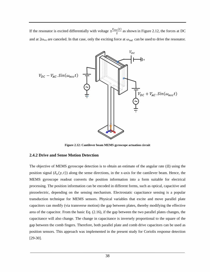
___________________________________________________________________________
38
If the resonator is excited differentially with voltage ±𝑉𝑒𝑥𝑐(𝑡)
2 as shown in Figure 2.12, the forces at DC
and at 2exc are canceled. In that case, only the exciting force at 𝜔𝑛𝑑 can be used to drive the resonator.
Figure 2.12: Cantilever beam MEMS gyroscope actuation circuit
2.4.2 Drive and Sense Motion Detection
The objective of MEMS gyroscope detection is to obtain an estimate of the angular rate (Ω) using the
position signal (𝛿𝑥(𝑦, 𝑡)) along the sense directions, in the x-axis for the cantilever beam. Hence, the
MEMS gyroscope readout converts the position information into a form suitable for electrical
processing. The position information can be encoded in different forms, such as optical, capacitive and
piezoelectric, depending on the sensing mechanism. Electrostatic capacitance sensing is a popular
transduction technique for MEMS sensors. Physical variables that excite and move parallel plate
capacitors can modify (via transverse motion) the gap between plates, thereby modifying the effective
area of the capacitor. From the basic Eq. (2.16), if the gap between the two parallel plates changes, the
capacitance will also change. The change in capacitance is inversely proportional to the square of the
gap between the comb fingers. Therefore, both parallel plate and comb drive capacitors can be used as
position sensors. This approach was implemented in the present study for Coriolis response detection
[29-30].
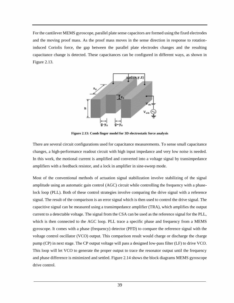
___________________________________________________________________________
39
For the cantilever MEMS gyroscope, parallel plate sense capacitors are formed using the fixed electrodes
and the moving proof mass. As the proof mass moves in the sense direction in response to rotation-
induced Coriolis force, the gap between the parallel plate electrodes changes and the resulting
capacitance change is detected. These capacitances can be configured in different ways, as shown in
Figure 2.13.
Figure 2.13: Comb finger model for 3D electrostatic force analysis
There are several circuit configurations used for capacitance measurements. To sense small capacitance
changes, a high-performance readout circuit with high input impedance and very low noise is needed.
In this work, the motional current is amplified and converted into a voltage signal by transimpedance
amplifiers with a feedback resistor, and a lock in amplifier in sine-sweep mode.
Most of the conventional methods of actuation signal stabilization involve stabilizing of the signal
amplitude using an automatic gain control (AGC) circuit while controlling the frequency with a phase-
lock loop (PLL). Both of these control strategies involve comparing the drive signal with a reference
signal. The result of the comparison is an error signal which is then used to control the drive signal. The
capacitive signal can be measured using a transimpedance amplifier (TRA), which amplifies the output
current to a detectable voltage. The signal from the CSA can be used as the reference signal for the PLL,
which is then connected to the AGC loop. PLL trace a specific phase and frequency from a MEMS
gyroscope. It comes with a phase (frequency) detector (PFD) to compare the reference signal with the
voltage control oscillator (VCO) output. This comparison result would charge or discharge the charge
pump (CP) in next stage. The CP output voltage will pass a designed low-pass filter (LF) to drive VCO.
This loop will let VCO to generate the proper output to trace the resonator output until the frequency
and phase difference is minimized and settled. Figure 2.14 shows the block diagrams MEMS gyroscope
drive control.
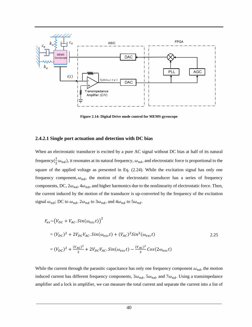
___________________________________________________________________________
40
Figure 2.14: Digital Drive mode control for MEMS gyroscope
2.4.2.1 Single port actuation and detection with DC bias
When an electrostatic transducer is excited by a pure AC signal without DC bias at half of its natural
frequency(1
2𝜔𝑛𝑑), it resonates at its natural frequency, 𝜔𝑛𝑑, and electrostatic force is proportional to the
square of the applied voltage as presented in Eq. (2.24). While the excitation signal has only one
frequency component, 𝜔𝑛𝑑, the motion of the electrostatic transducer has a series of frequency
components, DC, 2𝜔𝑛𝑑, 4𝜔𝑛𝑑, and higher harmonics due to the nonlinearity of electrostatic force. Then,
the current induced by the motion of the transducer is up-converted by the frequency of the excitation
signal 𝜔𝑛𝑑; DC to 𝜔𝑛𝑑, 2𝜔𝑛𝑑 to 3𝜔𝑛𝑑, and 4𝜔𝑛𝑑 to 5𝜔𝑛𝑑.
𝐹𝑒𝑠~(𝑉𝐷𝐶 + 𝑉𝐴𝐶 . 𝑆𝑖𝑛(𝜔𝑒𝑥𝑐𝑡))2
= (𝑉𝐷𝐶)2 + 2𝑉𝐷𝐶𝑉𝐴𝐶 . 𝑆𝑖𝑛(𝜔𝑒𝑥𝑐𝑡) + (𝑉𝐴𝐶)
2𝑆𝑖𝑛2(𝜔𝑒𝑥𝑐𝑡)
= (𝑉𝐷𝐶)2 +
(𝑉𝐴𝐶)2
2+ 2𝑉𝐷𝐶𝑉𝐴𝐶 . 𝑆𝑖𝑛(𝜔𝑒𝑥𝑐𝑡) −
(𝑉𝐴𝐶)2
2𝐶𝑜𝑠(2𝜔𝑒𝑥𝑐𝑡)
2.25
While the current through the parasitic capacitance has only one frequency component 𝜔𝑛𝑑, the motion
induced current has different frequency components, 3𝜔𝑛𝑑, 5𝜔𝑛𝑑, and 7𝜔𝑛𝑑. Using a transimpedance
amplifier and a lock in amplifier, we can measure the total current and separate the current into a list of
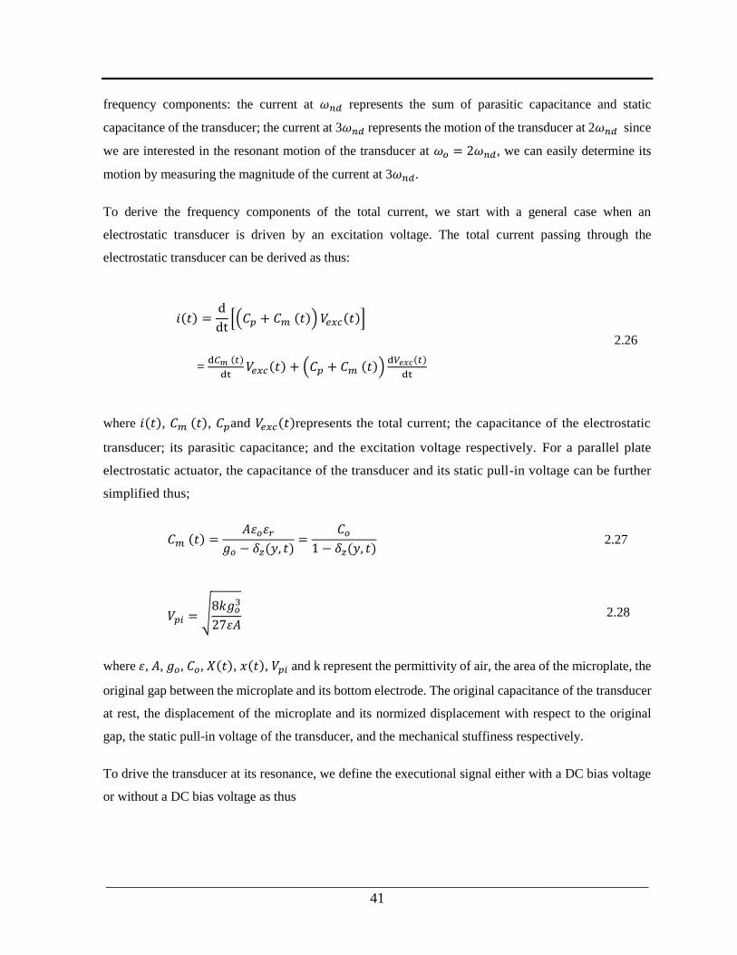
___________________________________________________________________________
41
frequency components: the current at 𝜔𝑛𝑑 represents the sum of parasitic capacitance and static
capacitance of the transducer; the current at 3𝜔𝑛𝑑 represents the motion of the transducer at 2𝜔𝑛𝑑 since
we are interested in the resonant motion of the transducer at 𝜔𝑜 = 2𝜔𝑛𝑑, we can easily determine its
motion by measuring the magnitude of the current at 3𝜔𝑛𝑑.
To derive the frequency components of the total current, we start with a general case when an
electrostatic transducer is driven by an excitation voltage. The total current passing through the
electrostatic transducer can be derived as thus:
𝑖(𝑡) =d
dt[(𝐶𝑝 + 𝐶𝑚 (𝑡)) 𝑉𝑒𝑥𝑐(𝑡)]
= d𝐶𝑚 (𝑡)
dt𝑉𝑒𝑥𝑐(𝑡) + (𝐶𝑝 + 𝐶𝑚 (𝑡))
d𝑉𝑒𝑥𝑐(𝑡)
dt
2.26
where 𝑖(𝑡), 𝐶𝑚 (𝑡), 𝐶𝑝and 𝑉𝑒𝑥𝑐(𝑡)represents the total current; the capacitance of the electrostatic
transducer; its parasitic capacitance; and the excitation voltage respectively. For a parallel plate
electrostatic actuator, the capacitance of the transducer and its static pull-in voltage can be further
simplified thus;
𝐶𝑚 (𝑡) =𝐴휀𝑜휀𝑟
𝑔𝑜 − 𝛿𝑧(𝑦, 𝑡)=
𝐶𝑜1 − 𝛿𝑧(𝑦, 𝑡)
2.27
𝑉𝑝𝑖 = √8𝑘𝑔𝑜
3
27휀𝐴 2.28
where 휀, 𝐴, 𝑔𝑜, 𝐶𝑜, 𝑋(𝑡), 𝑥(𝑡), 𝑉𝑝𝑖 and k represent the permittivity of air, the area of the microplate, the
original gap between the microplate and its bottom electrode. The original capacitance of the transducer
at rest, the displacement of the microplate and its normized displacement with respect to the original
gap, the static pull-in voltage of the transducer, and the mechanical stuffiness respectively.
To drive the transducer at its resonance, we define the executional signal either with a DC bias voltage
or without a DC bias voltage as thus
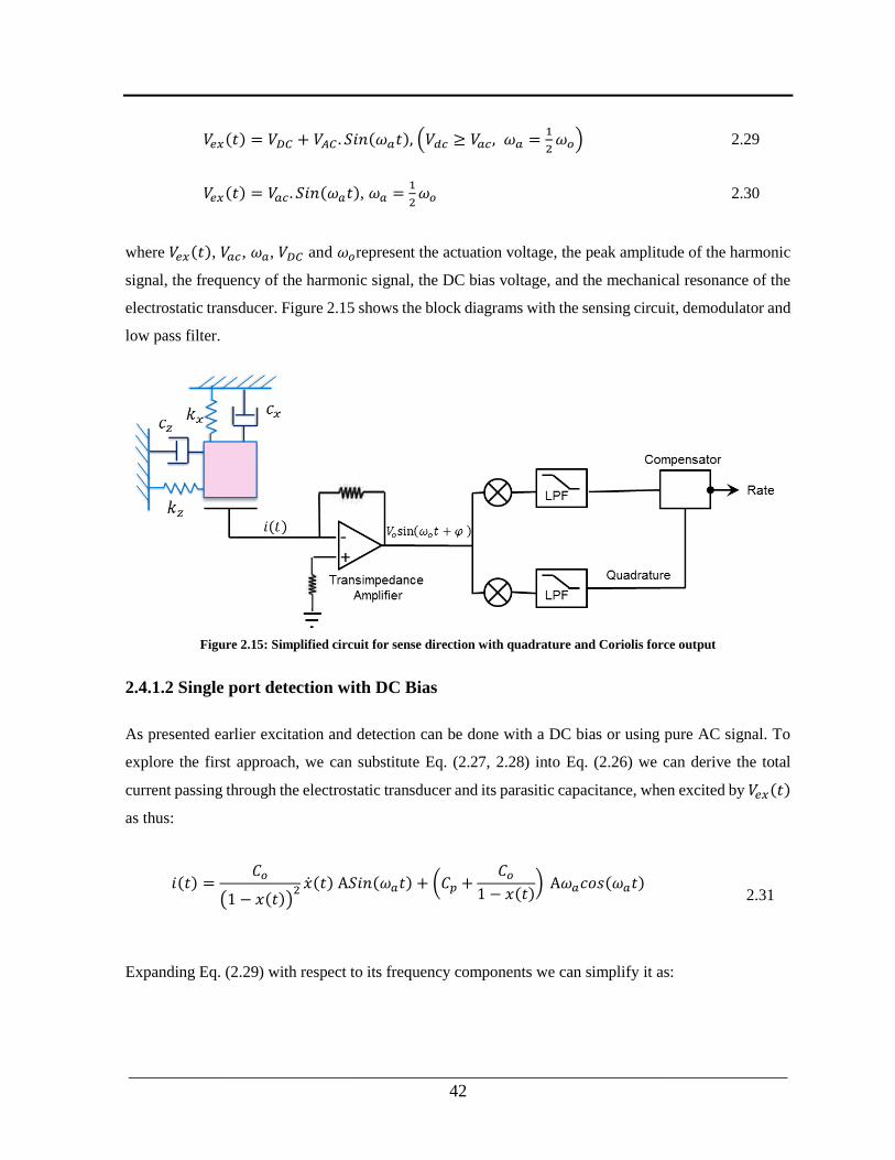
___________________________________________________________________________
42
𝑉𝑒𝑥(𝑡) = 𝑉𝐷𝐶 + 𝑉𝐴𝐶 . 𝑆𝑖𝑛(𝜔𝑎𝑡), (𝑉𝑑𝑐 ≥ 𝑉𝑎𝑐, 𝜔𝑎 =1
2𝜔𝑜) 2.29
𝑉𝑒𝑥(𝑡) = 𝑉𝑎𝑐. 𝑆𝑖𝑛(𝜔𝑎𝑡), 𝜔𝑎 =1
2𝜔𝑜 2.30
where 𝑉𝑒𝑥(𝑡), 𝑉𝑎𝑐, 𝜔𝑎, 𝑉𝐷𝐶 and 𝜔𝑜represent the actuation voltage, the peak amplitude of the harmonic
signal, the frequency of the harmonic signal, the DC bias voltage, and the mechanical resonance of the
electrostatic transducer. Figure 2.15 shows the block diagrams with the sensing circuit, demodulator and
low pass filter.
Figure 2.15: Simplified circuit for sense direction with quadrature and Coriolis force output
2.4.1.2 Single port detection with DC Bias
As presented earlier excitation and detection can be done with a DC bias or using pure AC signal. To
explore the first approach, we can substitute Eq. (2.27, 2.28) into Eq. (2.26) we can derive the total
current passing through the electrostatic transducer and its parasitic capacitance, when excited by 𝑉𝑒𝑥(𝑡)
as thus:
𝑖(𝑡) =𝐶𝑜
(1 − 𝑥(𝑡))2 (𝑡) A𝑆𝑖𝑛(𝜔𝑎𝑡) + (𝐶𝑝 +
𝐶𝑜1 − 𝑥(𝑡)
) A𝜔𝑎𝑐𝑜𝑠(𝜔𝑎𝑡) 2.31
Expanding Eq. (2.29) with respect to its frequency components we can simplify it as:

___________________________________________________________________________
43
𝑖(𝑡) =𝐶𝑜
(1 − 𝑥(𝑡))2 (𝑡) A𝑆𝑖𝑛(𝜔𝑎𝑡) + (𝐶𝑝 +
𝐶𝑜1 − 𝑥(𝑡)
) A𝜔𝑎𝑐𝑜𝑠(𝜔𝑎𝑡) 2.32
Since the first term of Eq. (2.32) represents the current due to the parasitic capacitance. We can determine
the parasitic capacitance by measuring the magnitude of the current at 𝜔𝑎. The second term of Eq. (2.32)
represents the current induced by the displacement of the transducer; and the third term represents the
current caused by the displacement and velocity of the transducer. Since the transducer is excited at its
resonance, 𝑥(𝑡) can be assumed to be the harmonic motion at 𝜔𝑎 such as D. cos (𝜔𝑎𝑡) the second
term can be expanded using the Tayler series. The third term of Eq. (2.30) can be expanded into Eq.
(2.32) as thus:
𝐶𝑜
(1 − 𝑥(𝑡))2 (𝑡) = (𝐶𝑜 + 2𝐶𝑜𝑥(𝑡) + 3𝐶𝑜𝑥
2(𝑡) + 𝑂𝑥3(𝑡))(𝑡)
= −𝐶𝑜𝐷𝜔𝑜𝑠𝑖𝑛(𝜔𝑜𝑡) + 2𝐶𝑜𝐷2𝜔𝑜𝑐𝑜𝑠(𝜔𝑜𝑡)𝑠𝑖𝑛(𝜔𝑜𝑡)
− 3𝐶𝑜𝐷3𝜔𝑜𝑐𝑜𝑠
2(𝜔𝑜𝑡)𝑠𝑖𝑛(𝜔𝑜𝑡)
= −𝐶𝑜𝐷𝜔𝑜𝑠𝑖𝑛(𝜔𝑜𝑡) + 𝐶𝑜𝐷2𝜔𝑜𝑠𝑖𝑛(2𝜔𝑜𝑡)
−3
4𝐶𝑜𝐷
3𝜔𝑜(𝑠𝑖𝑛(𝜔𝑜𝑡) + 𝑠𝑖𝑛(3𝜔𝑜𝑡))
2.33
Substituting Eq. (2.31) and Eq. (2.32) into Eq. (30), we simplifying it
𝑖(𝑡) ≈ A𝜔𝑜(𝐶𝑝 + 𝐶𝑜) × cos(𝜔𝑜𝑡) +3
4A𝜔𝑎𝐶𝑜𝐷 × cos(3𝜔𝑎𝑡) +
3
4A𝜔𝑎𝐶𝑜𝐷
2
× cos(5𝜔𝑎𝑡)
2.34
As presented in Eq. (2.33), we can determine the parasitic capacitance of the electrostatic transducer by
measuring the magnitude of the current at 𝜔𝑎. To determine the magnitude of the resonant motion at
2𝜔𝑎 we can measure the magnitude of the current at 3𝜔𝑎.
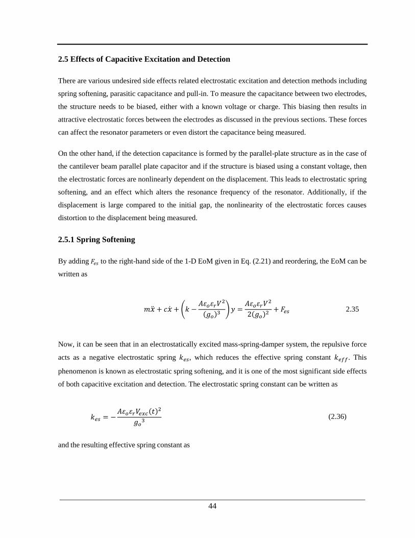
___________________________________________________________________________
44
2.5 Effects of Capacitive Excitation and Detection
There are various undesired side effects related electrostatic excitation and detection methods including
spring softening, parasitic capacitance and pull-in. To measure the capacitance between two electrodes,
the structure needs to be biased, either with a known voltage or charge. This biasing then results in
attractive electrostatic forces between the electrodes as discussed in the previous sections. These forces
can affect the resonator parameters or even distort the capacitance being measured.
On the other hand, if the detection capacitance is formed by the parallel-plate structure as in the case of
the cantilever beam parallel plate capacitor and if the structure is biased using a constant voltage, then
the electrostatic forces are nonlinearly dependent on the displacement. This leads to electrostatic spring
softening, and an effect which alters the resonance frequency of the resonator. Additionally, if the
displacement is large compared to the initial gap, the nonlinearity of the electrostatic forces causes
distortion to the displacement being measured.
2.5.1 Spring Softening
By adding 𝐹𝑒𝑠 to the right-hand side of the 1-D EoM given in Eq. (2.21) and reordering, the EoM can be
written as
𝑚+ 𝑐+ (𝑘 −𝐴휀𝑜휀𝑟𝑉
2
(𝑔𝑜)3 )𝑦 =
𝐴휀𝑜휀𝑟𝑉2
2(𝑔𝑜)2+ 𝐹𝑒𝑠 2.35
Now, it can be seen that in an electrostatically excited mass-spring-damper system, the repulsive force
acts as a negative electrostatic spring 𝑘𝑒𝑠, which reduces the effective spring constant 𝑘𝑒𝑓𝑓. This
phenomenon is known as electrostatic spring softening, and it is one of the most significant side effects
of both capacitive excitation and detection. The electrostatic spring constant can be written as
𝑘𝑒𝑠 = −𝐴휀𝑜휀𝑟𝑉𝑒𝑥𝑐(𝑡)
2
𝑔𝑜3
(2.36)
and the resulting effective spring constant as
___________________________________________________________________________
45
𝑘𝑒𝑓𝑓 = 𝑘 + 𝑘𝑒𝑠 = 𝑘 −𝐴휀𝑜휀𝑟𝑉𝑒𝑥𝑐(𝑡)
2
𝑔𝑜3
(2.37)
As a result of the electrostatic spring softening, the resonance frequency is reduced to
𝜔0 = √𝑘𝑒𝑓𝑓
𝑚=√𝑘 −
𝐴휀𝑜휀𝑟𝑉𝑒𝑥𝑐(𝑡)2
𝑔𝑜3
𝑚
(2.38)
Therefore, the mechanical spring constant reduced by the square of the voltage applied to the electrodes.
Because of the inherent nonlinearity of the parallel-plate actuator, its applicability may be limited when
large relative displacements need to be generated.
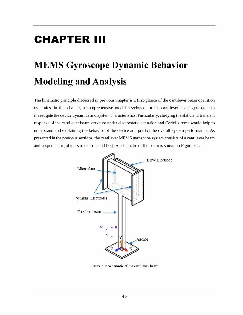
___________________________________________________________________________
46
CHAPTER III
MEMS Gyroscope Dynamic Behavior
Modeling and Analysis
The kinematic principle discussed in previous chapter is a first-glance of the cantilever beam operation
dynamics. In this chapter, a comprehensive model developed for the cantilever beam gyroscope to
investigate the device dynamics and system characteristics. Particularly, studying the static and transient
response of the cantilever beam structure under electrostatic actuation and Coriolis force would help to
understand and explaining the behavior of the device and predict the overall system performance. As
presented in the previous sections, the cantilever MEMS gyroscope system consists of a cantilever beam
and suspended rigid mass at the free end [33]. A schematic of the beam is shown in Figure 3.1.
Figure 3.1: Schematic of the cantilever beam
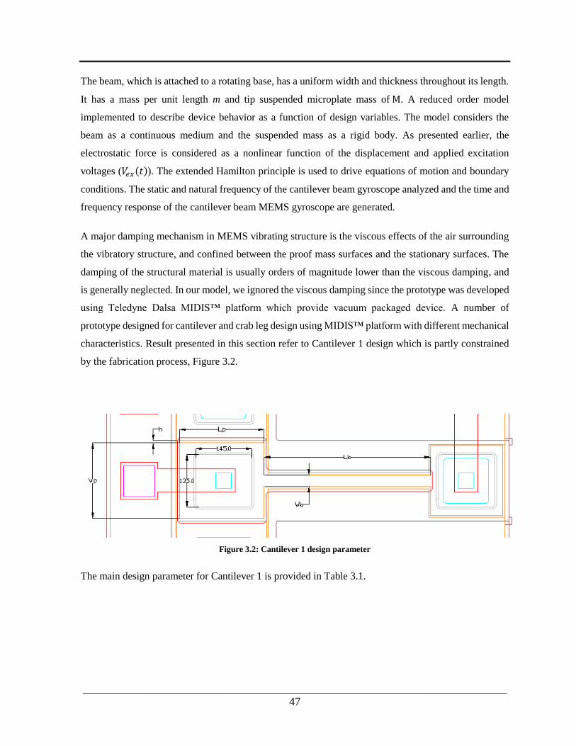
___________________________________________________________________________
47
The beam, which is attached to a rotating base, has a uniform width and thickness throughout its length.
It has a mass per unit length m and tip suspended microplate mass of M. A reduced order model
implemented to describe device behavior as a function of design variables. The model considers the
beam as a continuous medium and the suspended mass as a rigid body. As presented earlier, the
electrostatic force is considered as a nonlinear function of the displacement and applied excitation
voltages (𝑉𝑒𝑥(𝑡)). The extended Hamilton principle is used to drive equations of motion and boundary
conditions. The static and natural frequency of the cantilever beam gyroscope analyzed and the time and
frequency response of the cantilever beam MEMS gyroscope are generated.
A major damping mechanism in MEMS vibrating structure is the viscous effects of the air surrounding
the vibratory structure, and confined between the proof mass surfaces and the stationary surfaces. The
damping of the structural material is usually orders of magnitude lower than the viscous damping, and
is generally neglected. In our model, we ignored the viscous damping since the prototype was developed
using Teledyne Dalsa MIDIS™ platform which provide vacuum packaged device. A number of
prototype designed for cantilever and crab leg design using MIDIS™ platform with different mechanical
characteristics. Result presented in this section refer to Cantilever 1 design which is partly constrained
by the fabrication process, Figure 3.2.
Figure 3.2: Cantilever 1 design parameter
The main design parameter for Cantilever 1 is provided in Table 3.1.
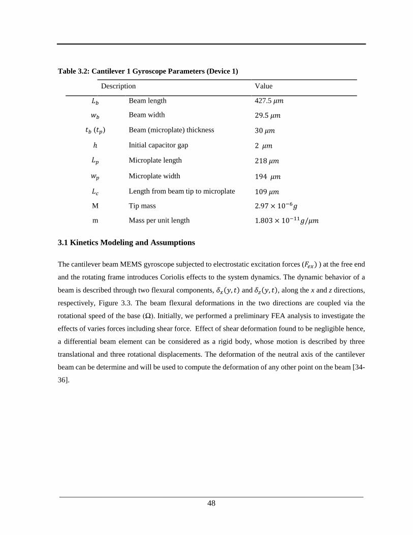
___________________________________________________________________________
48
Table 3.2: Cantilever 1 Gyroscope Parameters (Device 1)
Description Value
𝐿𝑏 Beam length 427.5 𝜇𝑚
𝑤𝑏 Beam width 29.5 𝜇𝑚
𝑡𝑏 (𝑡𝑝) Beam (microplate) thickness 30 𝜇𝑚
ℎ Initial capacitor gap 2 𝜇𝑚
𝐿𝑝 Microplate length 218 𝜇𝑚
𝑤𝑝 Microplate width 194 𝜇𝑚
𝐿𝑐 Length from beam tip to microplate 109 𝜇𝑚
M Tip mass 2.97 × 10⁻⁶𝑔
m Mass per unit length 1.803 × 10⁻¹¹𝑔/𝜇𝑚
3.1 Kinetics Modeling and Assumptions
The cantilever beam MEMS gyroscope subjected to electrostatic excitation forces (𝐹𝑒𝑥) ) at the free end
and the rotating frame introduces Coriolis effects to the system dynamics. The dynamic behavior of a
beam is described through two flexural components, 𝛿𝑥(𝑦, 𝑡) and 𝛿𝑧(𝑦, 𝑡), along the x and z directions,
respectively, Figure 3.3. The beam flexural deformations in the two directions are coupled via the
rotational speed of the base (Ω). Initially, we performed a preliminary FEA analysis to investigate the
effects of varies forces including shear force. Effect of shear deformation found to be negligible hence,
a differential beam element can be considered as a rigid body, whose motion is described by three
translational and three rotational displacements. The deformation of the neutral axis of the cantilever
beam can be determine and will be used to compute the deformation of any other point on the beam [34-
36].

___________________________________________________________________________
49
Figure 3.3: Cantilever beam flexural-flexural deflection
To model the dynamic behavior of the cantilever beam and suspended mass system, two coordinate
systems are introduced, Figure 3.4. The inertial coordinate system (x-y-z) is aligned with the local
curvilinear coordinate system (ξ-η-ζ) in the undeformed configuration. Three counter clockwise rigid
body rotations are used to describe the motion of the beam’s cross section at arc length ℓ, from the
undeformed to get to the deformed state. The Euler angles 𝜓, 휃, and 𝜙 are used to describe these
rotations. First the x-y-z system is rotated about the y-axis, then about 휂′, the new position of the y-axis,
and finally about the ξ-axis. The unit vectors of the ξ-η-ζ coordinate system are related to unit vectors
of the x-y-z coordinate system through a transformation matrix [T], which is the product of three
transformation matrices, one for each rigid body rotation [37-39].

___________________________________________________________________________
50
Figure 3.4: Rigid body rotations of beam
In general, each cross section of the beam experiences an elastic displacement of its centroid C and a
rotation. The displacement components of the centroid C, with respect to the x, y, and z axes at the arc
length ℓ and time t are denoted by 𝛿𝑥(𝑠, 𝑡), 𝛿𝑦(𝑠, 𝑡), and 𝛿𝑧(𝑠, 𝑡), respectively.
[
𝑖𝑥𝑗
𝑧
] = [𝑇] [
𝑖𝜉𝑗
𝜍
] = [𝑇𝜓][𝑇𝜃][𝑇𝜙] [
𝑖𝑗
𝜍
] (3.1)
The three individual transformation matrices and the transformation matrix [𝑇] are then
[𝑇𝜓] = [𝑐𝑜𝑠𝜓 𝑠𝑖𝑛𝜓 0−𝑠𝑖𝑛𝜓 𝑐𝑜𝑠𝜓 00 0 1
],[𝑇𝜃] = [𝑐𝑜𝑠 휃 0 −𝑠𝑖𝑛 휃0 1 0
𝑠𝑖𝑛 휃 0 𝑐𝑜𝑠 휃],[𝑇𝜙] = [
1 0 00 𝑐𝑜𝑠𝜙 𝑠𝑖𝑛𝜙0 −𝑠𝑖𝑛𝜙 𝑐𝑜𝑠𝜙
] (3.2)
___________________________________________________________________________
51
[𝑇] = [
𝑐𝑜𝑠𝜓 𝑐𝑜𝑠휃 𝑐𝑜𝑠휃𝑠𝑖𝑛𝜓 −𝑠𝑖𝑛휃−𝑠𝑖𝑛𝜓𝑐𝑜𝑠𝜙 + 𝑠𝑖𝑛𝜙𝑠𝑖𝑛휃𝑐𝑜𝑠𝜓 𝑐𝑜𝑠𝜙𝑐𝑜𝑠𝜓 + 𝑠𝑖𝑛𝜙𝑠𝑖𝑛휃𝑠𝑖𝑛𝜓 𝑠𝑖𝑛𝜙𝑐𝑜𝑠휃𝑠𝑖𝑛𝜙𝑠𝑖𝑛𝜓 + 𝑐𝑜𝑠𝜙𝑠𝑖𝑛휃𝑐𝑜𝑠𝜓 −𝑠𝑖𝑛𝜙𝑐𝑜𝑠𝜓 + 𝑐𝑜𝑠𝜙𝑠𝑖𝑛휃𝑠𝑖𝑛𝜓 𝑐𝑜𝑠𝜙𝑐𝑜𝑠휃
] (3.3)
The absolute angular velocity of the local coordinate system 𝑥′-𝑦′-𝑧′ is obtained from Figure 3.4
𝜔(𝑦, 𝑡) = 𝑒𝑧 + 𝑒𝑦′ + 𝑒𝜉 (3.4)
The expressions for 𝑒𝑧, and 𝑒𝑦′ are obtained from the transformation matrices in Eq. (3.2) and Eq. (3.3).
𝑒𝑧 = −𝑠𝑖𝑛휃𝑒𝜉 + 𝑠𝑖𝑛𝜙𝑐𝑜𝑠휃𝑒𝜂 + 𝑐𝑜𝑠𝜙𝑐𝑜𝑠휃𝑒𝜍 (3.5)
𝑒𝑦′ = 𝑐𝑜𝑠𝜙𝑒𝜂 − 𝑠𝑖𝑛𝜙𝑒𝜍 (3.6)
Substituting Eq. (3.5) and (3.6) into Eq. (3.4) yields
𝜔(ℓ, 𝑡) = ( − 𝑠𝑖𝑛휃)𝑒𝜉 + (𝑠𝑖𝑛𝜙𝑐𝑜𝑠휃 + 휃𝑐𝑜𝑠𝜙)𝑒𝜂 + (𝑐𝑜𝑠𝜙𝑐𝑜𝑠휃 − 휃𝑠𝑖𝑛𝜙)𝑒𝜍 (3.7)
where the dots ( )denotes the partial derivative with respect to time t and 𝑒𝑖 is a unit vector, and i = x,
y, z, ξ, θ, ζ indicates the direction of the unit vector. The curvature components can be obtained from the
angular velocity components by replacing the time derivatives in Eq. (3.7) with spatial derivatives.
Hence the curvature vector is given by
𝜌(𝑠, 𝑡) = (𝜙′ − 𝜓′𝑠𝑖𝑛휃)𝑒𝜉 + (𝜓′𝑠𝑖𝑛𝜙𝑐𝑜𝑠휃 + 𝜙′𝑐𝑜𝑠𝜙)𝑒𝜂 + (𝜓
′𝑐𝑜𝑠𝜙𝑐𝑜𝑠휃 − 𝜙′𝑠𝑖𝑛𝜙)𝑒𝜍 (3.8)
The inextensibility condition expresses that the elongation of the neutral axis during the vibration is
ignorable. Figure 3.5 shows a segment of the neutral axis of the cantilever beam. Segment CD is in the
undeformed configuration while C*D* is in the deformed configuration. The strain at point C is given
by

___________________________________________________________________________
52
𝑒 =𝑑𝑠∗ − 𝑑𝑠
𝑑𝑠= √(1 + 𝛿𝑥
′)2+ (𝛿𝑦
′)2+ (𝛿𝑧
′)2− 1 (3.9)
Since the beam is assumed to be inextensional, the strain along the neutral axis is zero. Therefore Eq.
(3.9) becomes.
1 = (1 + 𝛿𝑥′)2+ (𝛿𝑦
′)2+ (𝛿𝑧
′)2 (3.10)
Equation (3.10) is referred to as the inextensionality constraint.
Figure 3.5: A segment of the neutral axis local coordinate system
Figure 3.4 can be used to determine the expressions for the angles ψ and θ in terms of the spatial
derivatives of the transverse displacements. These expressions will be helpful in the simplification of
the equations of motion later on. The relationships for 𝜓 and 휃 are then
𝑡𝑎𝑛 𝜓 =𝛿𝑦′
1 + 𝛿𝑥′ 𝑡𝑎𝑛 휃 =
−𝛿𝑧′
√(1 + 𝛿𝑥′)2+ (𝛿𝑦
′)2
(3.11)
Equation (3.11) indicates 𝜓 and 휃 are dependent on the spatial derivatives of the displacement
components 𝛿𝑥, 𝛿𝑦 and 𝛿𝑧. Therefore, there are only four independent variables for this problem,
namely𝛿𝑥, 𝛿𝑦, 𝛿𝑧, and 𝜙

___________________________________________________________________________
53
3.1.2 Strain-Curvature Relations
Consider the cross section of the cantilever beam at the center of the suspended mass on the neutral axis,
Figure 3.5. The figure shows the beam cross section at arclength s for both the deformed and undeformed
configurations. An arbitrary point P in the undeformed beam cross section moves to point P* in the
deformed cross section, with the displacement components of C being (𝛿𝑥, 𝛿𝑦, 𝛿𝑧) in the (x, y, z) system.
The coordinates of P∗ relative to C∗ are still (η, ζ) because of the assumption of a rigid body motion
where the shape of the cross section remains intact after bending. The position vectors of P and P∗ can
be defined as
𝑟𝑃 = 𝑂𝐶 + 𝐶𝑃 = 𝑠𝑒𝑥 + 휂𝑒𝑦 + 휁𝑒𝑧 (3.12)
𝑟𝑃∗ = 𝑂𝐶∗ + 𝐶∗𝑃∗ = (𝑠 + 𝑢) 𝑒𝑥 + 𝑣𝑒𝑦 +𝑤𝑒𝑧 + 휂𝑒𝜂 + 휁𝑒𝜁 (3.13)
Figure 3.6: Initial and deformed positions of an arbitrary point P
The distance differentials for points P and P* are given by
___________________________________________________________________________
54
𝑑𝑟𝑃 = 𝑑𝑠𝑒𝑥 + 𝑑휂𝑒𝑦 + 𝑑휁𝑒𝑧 (3.14)
𝑑𝑟𝑃∗ = 𝑑𝑠𝑒𝜁 + 휂𝑑𝑒𝜂 + 𝑑휂𝑒𝜂 + 휁𝑑𝑒𝜁 + 𝑑휁𝑒𝜁 (3.15)
with the first term in Eq. (3.15) given by
𝑑𝑠𝑒𝜁 = (1 + 𝛿𝑥′)𝑑𝑠𝑒𝑥 + 𝛿𝑦
′𝑑𝑠𝑒𝑦 + 𝛿𝑧′𝑑𝑠𝑒𝑧= 𝐶∗𝐷∗ (3.16)
which is obtained directly from Figure 3.5. Eq. (3.14) and (3.15) are used to obtain
𝑑𝑟𝑃∗ . 𝑑𝑟𝑃∗ − 𝑑𝑟𝑃 . 𝑑𝑟𝑃 = 2(휁𝜌𝜂 − 휂𝜌𝜉)𝑑𝑠2 − 2휁𝜌𝜉𝑑𝑠𝑑휂 + 2휂𝜌𝜉𝑑𝑠𝑑휁 (3.17)
The difference of the squared distance differentials is related to the Green's strain tensor by
𝑑𝑟𝑃∗ . 𝑑𝑟𝑃∗ − 𝑑𝑟𝑃 . 𝑑𝑟𝑃 = 2[𝑑𝑠 𝑑휂 𝑑휁]. [휀𝑖𝑗]. [𝑑𝑠 𝑑휂 𝑑휁]𝑇 (3.18)
The components of the strain tensor in terms of the curvature are found by expanding the right-hand side
of Eq. (3.18) and comparing it to the right-hand side of Eq. (3.17).
휀11 = 휁𝜌𝜂 − 휂𝜌𝜉, 𝛾12 = 2휀12 = −휁𝜌𝜉 , 𝛾13 = 2휀13 = 휂𝜌𝜉, 휀22 = 휀23 = 휀33 = 0 (3.19)
3.2 Equations of Motion and Boundary Conditions
The extended Hamilton principle is used to derive the nonlinear partial-differential equations of motion.
The equations describe the flexural-flexural motion of the cantilever beam. The Lagrangian of motion 𝑙
is given as:
𝛿𝑙 = T − U (3.20)
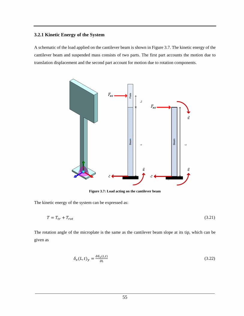
___________________________________________________________________________
55
3.2.1 Kinetic Energy of the System
A schematic of the load applied on the cantilever beam is shown in Figure 3.7. The kinetic energy of the
cantilever beam and suspended mass consists of two parts. The first part accounts the motion due to
translation displacement and the second part account for motion due to rotation components.
Figure 3.7: Load acting on the cantilever beam
The kinetic energy of the system can be expressed as:
𝑇 = 𝑇𝑡𝑟 + 𝑇𝑟𝑜𝑡 (3.21)
The rotation angle of the microplate is the same as the cantilever beam slope at its tip, which can be
given as
𝛿𝑥(𝐿, 𝑡)𝑦 =𝜕𝛿𝑥(𝐿,𝑡)
𝜕𝐿 (3.22)
___________________________________________________________________________
56
𝛿𝑧(𝐿, 𝑡)𝑦 =𝜕𝛿𝑧(𝐿,𝑡)
𝜕𝐿
The angular speed of the microplate in the sense and drive direction can be expressed as 𝑥(𝐿, 𝑡)𝑦
and 𝑧(𝐿, 𝑡)𝑦, where the dot ( ) denote the partial derivatives with respect to time (t). Furthermore, the
kinetic energy of the cantilever beam and microplate due to translation is given by
𝑇𝑡𝑟 =1
2𝜌𝐴∫((𝑥 (𝑦, 𝑡))
2+ (𝑧(𝑦, 𝑡) )
2) 𝑑𝑦
𝑙
0
+1
2𝜌𝐴Ω2∫((𝛿𝑥 (𝑦, 𝑡))
2 + (𝛿𝑧(𝑦, 𝑡) )2)𝑑𝑦
𝑙
0
+ 𝜌𝐴∫Ω(𝛿𝑥 (𝑦, 𝑡)𝑧 (𝑦, 𝑡) − 𝛿𝑧(𝑦, 𝑡)𝑥 (𝐿, 𝑡)) 𝑑𝑦
𝑙
0
+ 1
2𝑀 ((𝑥 (𝐿, 𝑡))
2+ (𝑧 (𝐿, 𝑡))
2)
+ 𝑀Ω(𝛿𝑥(𝐿, 𝑡)𝑧 (𝐿, 𝑡) − 𝛿𝑧(𝐿, 𝑡)𝑥 (𝐿, 𝑡))
+𝑀Ω2
2((𝛿𝑥(𝐿, 𝑡))
2+ (𝛿𝑧(𝐿, 𝑡))
2)
(3.23)
where 𝛿𝑥(y, t) and 𝛿𝑧 (y, t) be the differential beam element displacement at location y and time t in the
x and z axis respectively
𝑥 (𝑦, 𝑡) and 𝑧 (𝑦, 𝑡) are translational velocities of the differential beam element
Ω is the angular velocities
𝜌𝐴 is the 𝑚ass per unit length
𝛿𝑥(𝑦, 𝑡)𝑦 =𝜕𝛿𝑥(𝑦,𝑡)
𝜕𝑦 and 𝛿𝑧 (𝑦, 𝑡) 𝑦 =
𝜕𝛿𝑧 (𝑥,𝑡)
𝜕𝑦 are the slope at location y and time t
𝛿𝑥(𝑦, 𝑡)𝑦𝑦 =𝜕2𝛿𝑥(𝑦,𝑡)
𝜕𝑦2 and 𝛿𝑧 (𝑥, 𝑡) 𝑦𝑦 =
𝜕2𝛿𝑧 (𝑦,𝑡)
𝜕𝑦2 curvature at location y and time t
The kinetic energy also includes energy due to rotation of the differential element

___________________________________________________________________________
57
𝑇𝑟𝑜𝑡 =1
2∫[𝜔𝜉𝑡 (𝑦, 𝑡) + 𝜔𝜂𝑡 (𝑦, 𝑡)][𝐽][𝜔𝜉𝑡 (𝑦, 𝑡) + 𝜔𝜂𝑡 (𝑦, 𝑡)]
𝑇𝑑𝑦
𝑙
0
𝑇𝑟𝑜𝑡 = Ω2∫𝐽 [(𝛿𝑥(𝑦, 𝑡)𝑦)
2+ (𝛿𝑧(𝑦, 𝑡)𝑦)
2] 𝑑𝑦
𝑙
0
+1
2∫𝐽 [(𝑥 (𝑦, 𝑡)𝑦)
2+ (𝑧 (𝑦, 𝑡)𝑦)
2] 𝑑𝑦
𝑙
0
+ Ω∫𝐽[(𝛿𝑥 (𝑦, 𝑡)𝑦𝑧 (𝑦, 𝑡)𝑦 − 𝛿𝑧 (𝑦, 𝑡)𝑦𝑥 (𝑦, 𝑡)𝑦)]𝑑𝑦
𝑙
0
+ 𝐿𝑐𝐽Ω2
(3.24)
where [𝐽] is the distributed inertia matrix.
In order to have matching natural frequency for the first two mode the cantilever beam is designed to
have symmetrical cross-section. Furthermore, the product mass moments of inertia 𝐽𝑖𝑗, 𝑖 ≠ 𝑗, are zero
because a principal coordinate system is being used. Hence, using the notation 𝐽𝜉 = 𝐽11, 𝐽𝜂 = 𝐽22
and 𝐽𝜍 = 𝐽33, the inertia matrix [𝐽] is given by
[𝐽] = [
𝐽𝜉 0 0
0 𝐽𝜂 0
0 0 𝐽𝜍
] = 𝜌
[ ∬(휂2 + 휁2)
𝐴
𝑑휂𝑑휁 0 0
0 ∬휁2
𝐴
𝑑휂𝑑휁 0
0 0 ∬휂2
𝐴
𝑑휂𝑑휁]
(3.25)
Substituting Eq. (3.24) into Eq. (3.23), and adding Eq. (3.22) to the resulting expression provides the
total kinetic energy of the system.
___________________________________________________________________________
58
𝑇 =1
2𝜌𝐴∫((𝑥 (𝑦, 𝑡))
2+ (𝑧(𝑦, 𝑡) )
2) 𝑑𝑦
𝑙
0
+1
2𝜌𝐴Ω2∫((𝛿𝑦 (𝑦, 𝑡))
2+ (𝛿𝑧(𝑦, 𝑡) )
2)𝑑𝑦
𝑙
0
+ 𝜌𝐴∫Ω(𝑦 − 𝑧)𝑑𝑦
𝑙
0
+ 1
2𝑀 ((𝑥 (𝐿, 𝑡))
2+ (𝑥 (𝐿, 𝑡))
2)
+ 𝑀Ω(𝛿𝑥(𝐿, 𝑡)𝑧 (𝐿, 𝑡) − 𝛿𝑧(𝐿, 𝑡)𝑥 (𝐿, 𝑡)) +𝑀Ω2
2
+ Ω2∫𝐽 [(𝛿𝑥 (𝑦, 𝑡)𝑦)2+ (𝛿𝑧 (𝑦, 𝑡)𝑦)
2] 𝑑𝑦
𝑙
0
+1
2∫𝐽 [(𝑥 (𝑦, 𝑡)𝑦)
2+ (𝑧 (𝑦, 𝑡)𝑦)
2] 𝑑𝑦
𝑙
0
+ Ω∫𝐽[(𝛿𝑥 (𝑦, 𝑡)𝑦𝑧 (𝑦, 𝑡)𝑦 − 𝛿𝑧 (𝑦, 𝑡)𝑦𝑥 (𝑦, 𝑡)𝑦)]𝑑𝑦
𝑙
0
+ 𝐿𝑐𝐽Ω2
(3.26)
3.2.2 Potential Energy
The potential energy (𝑈) of the system include the cantilever beam strain energy and the electrostatic
potential energy of the electrostatic field between electrodes and the microplate. The strain energy of the
beam is calculated using the strain tensor (𝑈𝑠𝑡) components from Eq. (3.19). Hence, the total strain
energy for the cantilever beam can be expressed as:
𝑈𝑠 =1
2∫ [∬(𝜎11휀11 + 𝜎12
𝑏𝛾12𝑏 + 𝜎13
𝑏𝛾12𝑏)
𝐴
𝑑휂𝑑휁] 𝑑ℓ
𝑙
0
(3.27)
Silicon wafer is used to fabricate the structural element of the sensor and a linear relationship between
the stress and the strain is assumed. Therefore, Hooke's law can be used to relate the stress to the strain.
𝜎11 ≈ 𝐸휀11 𝜎12 ≈ 𝐺𝛾12 𝜎13 ≈ 𝐺𝛾13 (3.28)
휀11 = 휁𝜌𝜂 − 휂𝜌𝜉
___________________________________________________________________________
59
Substituting the strain tensor components from the previous section into Eq. (3.27) and Eq. (3.28), and
noting that the cross section is symmetric about the 휂 and 휁 axes, the strain energy is written as
𝑈𝑠𝑡 =1
2∫(𝐷𝜉𝜌𝜉
2 + 𝐷𝜁𝜌𝜁2)𝑏𝑑ℓ
𝑙
0
(3.29)
where 𝐷𝜉, and 𝐷𝜁 are the flexural rigidities of the x and z axis respectively. The potential energy is then
𝑈𝑠𝑡 =1
2∫(𝐸𝐼𝜉𝛿𝑥(𝑦, 𝑡)𝑦𝑦 + 𝐸𝐼𝜂𝛿𝑧(𝑦, 𝑡)𝑦𝑦)𝑑𝑦
𝑙
0
𝑈𝑠𝑡 =E
2∫(𝐼𝑦𝛿𝑥(𝑦, 𝑡)𝑦𝑦
2 + 𝐼𝑧𝛿𝑧(𝑦, 𝑡)𝑦𝑦2)𝑑𝑦
𝑙
0
(3.30)
The electrostatic force applied underneath the microplate produces a potential energy that can be
expressed
𝑈𝐸 = −ε𝐴𝑑2(𝑉𝐷𝐶 + 𝑉𝐴𝐶(𝑡))𝑑
2∫
1
g𝑑 − 𝛿𝑥(𝐿, 𝑡) − 𝛿𝑥(𝐿, 𝑡)𝑦𝑑𝑦
2𝐿𝐶
0
−ε𝑎𝑠2(𝑉𝐷𝐶 + 𝑉𝐴𝐶(𝑡))𝑠
2∫
1
g𝑠 − 𝛿𝑧(𝐿, 𝑡) − 𝛿𝑧(𝐿, 𝑡)𝑦𝑑𝑦
2𝐿𝐶
0
=ε𝐴𝑝
2𝛿𝑥(𝐿, 𝑡)𝑦(𝑉𝐷𝐶 + 𝑉𝐴𝐶(𝑡))𝑑
2 𝑙𝑛[g𝑑 − 𝛿𝑥(𝐿, 𝑡) − 𝛿𝑥(𝐿, 𝑡)𝑦]|0
2𝐿𝐶
+ε𝑎𝑠
2𝛿𝑧(𝐿, 𝑡)𝑦(𝑉𝐷𝐶 + 𝑉𝐴𝐶(𝑡))𝑠
2 𝑙𝑛[g𝑠 − 𝛿𝑧(𝐿, 𝑡) − 𝛿𝑧(𝐿, 𝑡)𝑦]|0
2𝐿𝐶
=ε𝐴𝑑
2𝛿𝑥(𝐿, 𝑡)𝑦(𝑉𝐷𝐶 + 𝑉𝐴𝐶(𝑡))𝑑
2 𝑙𝑛 [
g𝑑 − 𝛿𝑥(𝐿, 𝑡) − 2𝐿𝐶 𝛿𝑥(𝐿, 𝑡)𝑦
g𝑑 − 𝛿𝑥(𝐿, 𝑡)]
+ε𝑎𝑠
2𝛿𝑧(𝐿, 𝑡)𝑦(𝑉𝐷𝐶 + 𝑉𝐴𝐶(𝑡))𝑠
2 𝑙𝑛 [
g𝑠 − 𝛿𝑧(𝐿, 𝑡) − 2𝐿𝐶 𝛿𝑧(𝐿, 𝑡)𝑦
g𝑠 − 𝛿𝑧(𝐿, 𝑡)]
(3.31)
where ε is the permittivity of free space

___________________________________________________________________________
60
(𝑉𝐷𝐶 + 𝑉𝐴𝐶(𝑡))𝑑 and (𝑉𝐷𝐶 + 𝑉𝐴𝐶(𝑡))𝑠 are the combination of DC and AC voltages applied
between the drive and sense electrodes, respectively.
𝐴𝑑 and 𝐴𝑠effective area of the drive and sense electrode direction respectively.
Here, the sensing axis also applied with a feedback voltage for closed loop design consideration. Then
the total potential energy is given by
U = 𝑈𝑠𝑡 + 𝑈𝐸 (3.32)
= (E
2∫ 𝐼𝑥𝛿𝑥(𝑦, 𝑡)𝑦𝑦
2 +
𝑙
0
𝐼𝑧𝛿𝑧(𝑦, 𝑡)𝑦𝑦2𝑑𝑦)
+ (ε𝑎𝑑
2𝛿𝑥(𝐿, 𝑡)𝑦(𝑉𝐷𝐶 + 𝑉𝐴𝐶(𝑡))𝑑
2 𝑙𝑛 [
g𝑑 − 𝛿𝑥(𝐿, 𝑡) − 2𝐿𝐶 𝛿𝑥(𝐿, 𝑡)𝑦
g𝑑 − 𝛿𝑥(𝐿, 𝑡)]
+ε𝑎𝑠
2𝛿𝑧(𝐿, 𝑡)𝑦(𝑉𝐷𝐶 + 𝑉𝐴𝐶(𝑡))𝑠
2 𝑙𝑛 [
g𝑠 − 𝛿𝑧(𝐿, 𝑡) − 2𝐿𝐶 𝛿𝑧(𝐿, 𝑡)𝑦
g𝑠 − 𝛿𝑧(𝐿, 𝑡)])
(3.33)
Equations (3.26) and (3.32) are substituted into Eq. (3.20) to obtain the final expression for the
Lagrangian. The inextensionality constraint in Eq. (3.10) must be maintained during the variational
process. The Lagrangian density is then
___________________________________________________________________________
61
𝛿ℒ =1
2𝜌𝐴∫((𝑥 (𝑦, 𝑡))
2+ (𝑧(𝑦, 𝑡) )
2) 𝑑𝑦
𝑙
0
+1
2𝜌𝐴Ω2∫((𝛿𝑥 (𝑦, 𝑡))
2 + (𝛿𝑧(𝑦, 𝑡) )2)𝑑𝑦
𝑙
0
+ 𝜌𝐴∫Ω(𝑥 − 𝑧)𝑑𝑦
𝑙
0
+ 1
2𝑀 ((𝑥 (𝐿, 𝑡))
2+ (𝑥 (𝐿, 𝑡))
2)
+𝑀Ω(𝛿𝑥(𝐿, 𝑡)𝑧 (𝐿, 𝑡) − 𝛿𝑧(𝐿, 𝑡)𝑥 (𝐿, 𝑡)) +𝑀Ω2
2((𝛿𝑥(𝐿, 𝑡))
2+ (𝛿𝑧(𝐿, 𝑡))
2)
+ Ω2∫𝐽 [(𝛿𝑥 (𝑦, 𝑡)𝑦)2+ (𝛿𝑧 (𝑦, 𝑡)𝑦)
2] 𝑑𝑦
𝑙
0
+1
2∫ 𝐽 [(𝑥 (𝑦, 𝑡)𝑦)
2+ (𝑧 (𝑦, 𝑡)𝑦)
2] 𝑑𝑦
𝑙
0
+ Ω∫ 𝐽[(𝛿𝑥 (𝑦, 𝑡)𝑦𝑧 (𝑦, 𝑡)𝑥 − 𝛿𝑧 (𝑦, 𝑡)𝑦𝑥 (𝑦, 𝑡)𝑥)]𝑑𝑦
𝑙
0
+ 𝐿𝑐𝐽Ω2
−1
2∫(𝐸𝐼𝜉𝛿𝑦(𝑦, 𝑡)𝑦𝑦
𝑙
0
+ 𝐸𝐼𝜂𝛿𝑧(𝑦, 𝑡)𝑦𝑦)𝑑𝑦ε𝐴𝑑
2𝛿𝑥(𝐿, 𝑡)𝑦(𝑉𝐷𝐶
+ 𝑉𝐴𝐶(𝑡))𝑑2 𝑙𝑛 [
g𝑑 − 𝛿𝑥(𝐿, 𝑡) − 2𝐿𝐶 𝛿𝑥(𝐿, 𝑡)𝑦
g𝑑 − 𝛿𝑦(𝐿, 𝑡)]
+ε𝐴𝑠
2𝛿𝑧(𝐿, 𝑡)𝑦(𝑉𝐷𝐶 + 𝑉𝐴𝐶(𝑡))𝑠
2 𝑙𝑛 [
g𝑠 − 𝛿𝑧(𝐿, 𝑡) − 2𝐿𝐶 𝛿𝑧(𝐿, 𝑡)𝑦
g𝑠 − 𝛿𝑧(𝐿, 𝑡)]
(3.34)
3.3 Extended Hamilton's Principle
The MEMS cantilever beam gyroscope is subjected to non-conservative forces such as viscous damping
and Coriolis forces. Therefore, the extended Hamilton's principle is used to derive the equations of
motion. This approach permits the derivation of the equations of motion from a definite integral
involving kinetic energy and the virtual work performed by the applied forces. Appropriate boundary
conditions are also produced as part of the derivation. The extended Hamilton's principle can be stated
as

___________________________________________________________________________
62
𝛿𝐼 = ∫(𝛿ℒ + 𝛿𝑈𝑛𝑐)𝑑𝑡
𝑡2
𝑡1
= 0 (3.35)
where 𝛿ℒ is the virtual change in mechanical energy
𝛿𝑈𝑛𝑐 is the virtual work done by non-conservative forces
𝑡1, 𝑡2 are times at which the configuration of the system is assumed to be known
𝛿( ) Symbol denoting the first variation, or virtual change, in the quantity in brackets
Replacing the Lagrangian components and taking the time integral, the overall dynamics can be
expressed:
___________________________________________________________________________
63
∫ 1
2𝜌𝐴∫((𝑥 (𝑦, 𝑡))
2+ (𝑧(𝑦, 𝑡) )
2)𝑑𝑦
𝑙
0
𝑡2
𝑡1
+1
2𝜌𝐴Ω2∫((𝛿𝑥 (𝑦, 𝑡))
2 + (𝛿𝑧(𝑦, 𝑡) )2)𝑑𝑦
𝑙
0
+ 𝜌𝐴∫Ω(𝑥 − 𝑧)𝑑𝑦
𝑙
0
+ 1
2𝑀 ((𝑥 (𝐿, 𝑡))
2+ (𝑧 (𝐿, 𝑡))
2)
+𝑀Ω(𝛿𝑥(𝐿, 𝑡)𝑧 (𝐿, 𝑡) − 𝛿𝑧(𝐿, 𝑡)𝑥 (𝐿, 𝑡))
+𝑀Ω2
2((𝛿𝑥(𝐿, 𝑡))
2+ (𝛿𝑧(𝐿, 𝑡))
2)
+ Ω2∫𝐽 [(𝛿𝑥 (𝑦, 𝑡)𝑦)2+ (𝛿𝑧 (𝑦, 𝑡)𝑦)
2] 𝑑𝑦
𝑙
0
+1
2∫ 𝐽 [(𝑥 (𝑦, 𝑡)𝑦)
2+ (𝑧 (𝑦, 𝑡)𝑦)
2] 𝑑𝑦
𝑙
0
+ Ω∫𝐽[(𝛿𝑥 (𝑦, 𝑡)𝑦𝑧 (𝑦, 𝑡)𝑦 − 𝛿𝑧 (𝑦, 𝑡)𝑦𝑥 (𝑦, 𝑡)𝑦)]𝑑𝑦
𝑙
0
+ 𝐿𝑐𝐽Ω2
−1
2∫(𝐸𝐼𝜉𝛿𝑥(𝑦, 𝑡)𝑦𝑦
𝑙
0
+ 𝐸𝐼𝜂𝛿𝑧(𝑦, 𝑡)𝑦𝑦)𝑑𝑦ε𝑎𝑑
2𝛿𝑥(𝐿, 𝑡)𝑥(𝑉𝐷𝐶
+ 𝑉𝐴𝐶(𝑡))𝑑2 𝑙𝑛 [
g𝑑 − 𝛿𝑥(𝐿, 𝑡) − 2𝐿𝐶 𝛿𝑥(𝐿, 𝑡)𝑦
g𝑑 − 𝛿𝑥(𝐿, 𝑡)]
+ε𝑎𝑠
2𝛿𝑧(𝐿, 𝑡)𝑦(𝑉𝐷𝐶
+ 𝑉𝐴𝐶(𝑡))𝑠2 𝑙𝑛 [
g𝑠 − 𝛿𝑧(𝐿, 𝑡) − 2𝐿𝐶 𝛿𝑧(𝐿, 𝑡)𝑦
g𝑠 − 𝛿𝑧(𝐿, 𝑡)] 𝑑𝑡 = 0
(3.36)
Utilizing the expressions for kinetic and potential energies, different components of Eq. (3.36) can be
expressed as follows.
Kinetic energy is given by
___________________________________________________________________________
64
∫ 𝛿𝑇𝑑𝑡
𝑡2
𝑡1
= ∫ 1
2𝜌𝐴∫((𝑥 (𝑦, 𝑡))
2+ (𝑧(𝑦, 𝑡) )
2) 𝑑𝑦
𝑙
0
𝑡2
𝑡1
+1
2𝜌𝐴Ω2∫((𝛿𝑥 (𝑦, 𝑡))
2 + (𝛿𝑧(𝑦, 𝑡) )2)𝑑𝑦
𝑙
0
+ 𝜌𝐴∫Ω(𝑥 − 𝑧)𝑑𝑦
𝑙
0
+ 1
2𝑀 ((𝑥 (𝐿, 𝑡))
2+ (𝑧 (𝐿, 𝑡))
2)
+ 𝑀Ω(𝛿𝑥(𝐿, 𝑡)𝑧 (𝐿, 𝑡) − 𝛿𝑧(𝐿, 𝑡)𝑥 (𝐿, 𝑡))
+𝑀Ω2
2((𝛿𝑥(𝐿, 𝑡))
2+ (𝛿𝑧(𝐿, 𝑡))
2)
+ Ω2∫𝐽 [(𝛿𝑥 (𝑦, 𝑡)𝑦)2+ (𝛿𝑧 (𝑦, 𝑡)𝑦)
2] 𝑑𝑦
𝑙
0
+1
2∫𝐽 [(𝑥 (𝑦, 𝑡)𝑦)
2+ (𝑧 (𝑦, 𝑡)𝑦)
2] 𝑑𝑦
𝑙
0
+ Ω∫𝐽[(𝛿𝑥 (𝑦, 𝑡)𝑦𝑧 (𝑦, 𝑡)𝑦 − 𝛿𝑧 (𝑦, 𝑡)𝑦𝑥 (𝑦, 𝑡)𝑦)]𝑑𝑦
𝑙
0
+ 𝐿𝑐𝐽Ω2𝑑𝑡 = 0
(3.37)
∫ 𝛿𝑈𝑑𝑡
𝑡2
𝑡1
=1
2∫(𝐸𝐼𝜉𝛿𝑥(𝑦, 𝑡)𝑦𝑦
𝑙
0
+ 𝐸𝐼𝜂𝛿𝑧(𝑦, 𝑡)𝑦𝑦)𝑑𝑦ε𝑎𝑑
2𝛿𝑥(𝐿, 𝑡)𝑦(𝑉𝐷𝐶
+ 𝑉𝐴𝐶(𝑡))𝑑2 𝑙𝑛 [
g𝑑 − 𝛿𝑥(𝐿, 𝑡) − 2𝐿𝐶 𝛿𝑥(𝐿, 𝑡)𝑦
g𝑑 − 𝛿𝑥(𝐿, 𝑡)]
+ε𝑎𝑠
2𝛿𝑧(𝐿, 𝑡)𝑦(𝑉𝐷𝐶 + 𝑉𝐴𝐶(𝑡))𝑠
2 𝑙𝑛 [
g𝑠 − 𝛿𝑧(𝐿, 𝑡) − 2𝐿𝐶 𝛿𝑧(𝐿, 𝑡)𝑦
g𝑠 − 𝛿𝑧(𝐿, 𝑡)] 𝑑𝑡
(3.38)

___________________________________________________________________________
65
In order to simplify the solution approach, the equation of motion and boundary conditions are non-
dimensionalized.
𝐸𝐼𝑥𝛿𝑥(𝑦, 𝑡)𝑦𝑦𝑦𝑦 + 𝑐𝑥(𝑦, 𝑡) + 𝜌𝐴𝑥(𝑦, 𝑡) − 2𝜌𝐴Ω𝑧(𝑦, 𝑡) − 𝜌𝐴Ω𝛿𝑧(𝑦, 𝑡) − 𝜌𝐴Ω2𝛿𝑥(𝑦, 𝑡) +
2𝑗𝑥Ω2𝛿𝑥(𝑦, 𝑡)𝑦𝑦 − 𝑗𝑥Ω𝛿𝑧(𝑦, 𝑡)𝑦𝑦−𝑗𝑥𝑥(𝑦, 𝑡)𝑦𝑦 = 0
(3.39)
𝐸𝐼𝑧𝛿𝑧(𝑦, 𝑡)𝑦𝑦𝑦𝑦 + 𝑐𝑧(𝑦, 𝑡) + 𝜌𝐴𝑧(𝑦, 𝑡) − 2𝜌𝐴Ω𝑥(𝑦, 𝑡) − 𝜌𝐴Ω𝛿𝑥(𝑦, 𝑡)
− 𝜌𝐴Ω2𝛿𝑧(𝑦, 𝑡)+𝑗𝑧Ω2𝛿𝑧(𝑦, 𝑡)𝑦𝑦 + 𝑗𝑧Ω𝛿𝑥(𝑦, 𝑡)𝑦𝑦−𝑗𝑧𝑧(𝑦, 𝑡)𝑦𝑦 = 0
𝜌𝐴𝑥(𝑦, 𝑡) + 𝑐𝑥(𝑦, 𝑡) + 𝐷𝜁𝛿𝑥(𝑦, 𝑡)𝑦𝑦𝑦𝑦
= 2𝜌𝐴Ω𝑧(𝑦, 𝑡) + 𝜌𝐴Ω𝛿𝑧(𝑦, 𝑡) + 𝜌𝐴Ω2𝛿𝑥(𝑦, 𝑡) − 2𝑗𝑥Ω
2𝛿𝑥(𝑦, 𝑡)𝑦𝑦
+ 𝑗𝑥Ω𝛿𝑧(𝑦, 𝑡)𝑦𝑦+𝑗𝑥𝑥(𝑦, 𝑡)𝑦𝑦
𝜌𝐴𝑧(𝑦, 𝑡) + 𝑐𝑧(𝑦, 𝑡) + 𝐷𝜁𝛿𝑧(𝑦, 𝑡)𝑦𝑦𝑦𝑦
= 2𝜌𝐴Ω𝑥(𝑦, 𝑡) + 𝜌𝐴Ω𝛿𝑥(𝑦, 𝑡) + 𝜌𝐴Ω2𝛿𝑧(𝑦, 𝑡) − 2𝑗𝑧Ω
2𝛿𝑧(𝑦, 𝑡)𝑦𝑦
+ 𝑗𝑧Ω𝛿𝑥(𝑦, 𝑡)𝑦𝑦+𝑗𝑧𝑧(𝑦, 𝑡)𝑦𝑦
(3.40)
The boundary conditions at the fixed end (𝑦 = 0) are no deflection and zero slope as shown below
respectively:
𝛿𝑥(0, 𝑡) = 0 𝛿𝑧(0, 𝑡) = 0
(3.41) 𝛿𝑥(0, 𝑡)𝑦 = 0 𝛿𝑧(0, 𝑡)𝑦 = 0
The boundary conditions at the end of the cantilever beam (𝑦 = 𝐿) are moment and shear balances as
shown below, respectively.

___________________________________________________________________________
66
𝐸𝐼𝑦𝛿𝑦(𝐿, 𝑡)𝑦𝑦 = −𝑀𝐿𝐶 𝑥(𝐿, 𝑡) − (𝑀𝐿𝐶2 + 𝐽)𝑥(𝐿, 𝑡)𝑦
+ε𝑎𝑑
2(𝛿𝑥(𝐿, 𝑡)𝑦)2 (𝑉𝐷𝐶 + 𝑉𝐴𝐶(𝑡))𝑑
2 [
2𝐿𝐶𝛿𝑥(𝐿, 𝑡)𝑦
g𝑑 − 𝛿𝑦(𝐿, 𝑡) − 2𝐿𝐶𝛿𝑥(𝐿, 𝑡)𝑦
− 𝑙𝑛 [g𝑑 − 𝛿𝑥(𝐿, 𝑡)
g𝑑 − 𝛿𝑥(𝐿, 𝑡) − 2𝐿𝐶𝛿𝑥(𝐿, 𝑡)𝑦]]
𝐸𝐼𝑧𝛿𝑧(𝐿, 𝑡)𝑦𝑦 = −𝑀𝐿𝐶 𝑥(𝐿, 𝑡) − (𝑀𝐿𝐶2 + 𝐽)𝑥(𝐿, 𝑡)𝑦
+ε𝑎𝑑
2(𝛿𝑥(𝐿, 𝑡)𝑦)2 (𝑉𝐷𝐶 + 𝑉𝐴𝐶(𝑡))𝑑
2 [
2𝐿𝐶𝛿𝑥(𝐿, 𝑡)𝑦
g𝑑 − 𝛿𝑦(𝐿, 𝑡) − 2𝐿𝐶𝛿𝑥(𝐿, 𝑡)𝑦
− 𝑙𝑛 [g𝑑 − 𝛿𝑥(𝐿, 𝑡)
g𝑑 − 𝛿𝑥(𝐿, 𝑡) − 2𝐿𝐶𝛿𝑥(𝐿, 𝑡)𝑦]]
𝐸𝐼𝑦𝛿𝑦(𝐿, 𝑡)𝑦𝑦𝑦 = 𝑀 𝑥(𝐿, 𝑡) − 𝑀Ω2𝛿𝑥(𝑦, 𝑡) − 2𝑀Ω 𝑧(𝑦, 𝑡) − 𝑀Ω 𝛿𝑧(𝑦, 𝑡)
+ 𝐽𝑥 Ω𝛿𝑧(𝐿, 𝑡)𝑥 + 2𝐽𝑥Ω2 𝛿𝑥(𝐿, 𝑡)𝑦 + 𝐽𝑥 𝑥(𝐿, 𝑡)𝑦
− ε𝑎𝑑
2𝛿𝑥(𝐿, 𝑡)𝑦(𝑉𝐷𝐶 + 𝑉𝐴𝐶(𝑡))𝑑
2[
1
g𝑑 − 𝛿𝑥(𝐿, 𝑡) − 2𝐿𝐶𝛿𝑥(𝐿, 𝑡)𝑦
− 1
g𝑑 − 𝛿𝑥(𝐿, 𝑡)]
𝐸𝐼𝑧𝛿𝑧(𝐿, 𝑡)𝑦𝑦𝑦 = 𝑀 𝑧(𝐿, 𝑡) − 𝑀Ω2𝛿𝑧(𝑦, 𝑡) − 2𝑀Ω 𝑥(𝑦, 𝑡) − 𝑀Ω 𝛿𝑥(𝑦, 𝑡)
+ 𝐽𝑧 Ω𝛿𝑥(𝐿, 𝑡)𝑦 + 2𝐽𝑧Ω2 𝛿𝑧(𝐿, 𝑡)𝑦 + 𝐽𝑧 𝑧(𝐿, 𝑡)𝑦
− ε𝑎𝑑
2𝛿𝑥(𝐿, 𝑡)𝑦(𝑉𝐷𝐶)𝑠
2[
1
g𝑑 − 𝛿𝑥(𝐿, 𝑡) − 2𝐿𝐶𝛿𝑥(𝐿, 𝑡)𝑦−
1
g𝑑 − 𝛿𝑥(𝐿, 𝑡)]
(3.42)
where the moment of inertia of the suspended mass about its point of connection with the microbeam is
given by 𝑀𝐿𝐶2 + 𝐽 =
3
4𝑀𝐿𝐶
2
In non-dimensional forms of the equations of motion become
___________________________________________________________________________
67
𝛿𝑥(𝑦, 𝑡)𝑦𝑦𝑦𝑦 + 𝑥(𝑦, 𝑡) + 𝑥(𝑦, 𝑡) − 21
𝑑Ω𝑧(𝑦, 𝑡) −
1
𝑑Ω𝛿𝑧(𝑦, 𝑡) − Ω
2𝛿𝑥(𝑦, 𝑡)
+ 2𝐽𝑥Ω2𝛿𝑥(𝑦, 𝑡)𝑦𝑦 −
𝐽𝑥𝑑Ω𝛿𝑧(𝑦, 𝑡)𝑦𝑦 − 𝐽𝑥𝑥(𝑦, 𝑡)𝑦𝑦 = 0
(3.43)
𝛿𝑧(𝑦, 𝑡)𝑦𝑦𝑦𝑦 + 𝑐𝑧(𝑦, 𝑡) + 𝑧(𝑦, 𝑡) − 2Ω𝑥(𝑦, 𝑡) − Ω𝛿𝑥(𝑦, 𝑡) − Ω2𝛿𝑧(𝑦, 𝑡)
+ 2𝐽𝑧Ω2𝛿𝑧(𝑦, 𝑡)𝑦𝑦 − 𝐽𝑧𝑑 Ω𝛿𝑥(𝑦, 𝑡)𝑦𝑦−𝐽𝑧𝑧(𝑦, 𝑡)𝑦𝑦 = 0
(3.44)
The cantilever beam dynamics depends on three factors: beam resistance to bending, inertia due to
movement, and electrostatic force. For convenience, we introduce the following non-dimensional
parameters:
𝔵 =𝑦
L 𝔩 =
𝐿𝑐L
𝔱 =𝑡
T 𝔶 =
𝛿𝑥(𝑦, 𝑡)
𝑔𝑦 𝔷 =
𝛿𝑧(𝑦, 𝑡)
𝑔𝑦
𝔱 = 𝒯t ω𝑥 =
Ω
𝒯 𝔪 =
M
𝜌𝐴L 𝖏 =
j
𝜌𝐴𝐿2 Ω =
Ω
𝒯
𝔠 = c𝐿2
√EI𝜌𝐴 Ω =
Ω
𝒯
𝔱 = 𝒯t Ω =
Ω
𝒯 Ω =
Ω
𝒯
𝜶𝒖 =ε𝑎𝑑L
4
2𝐸𝐼𝑑2
Where T is a time constant defined by T = √𝜌𝐴𝐿4
EI.
We decompose
𝔶𝑦𝑦𝑦𝑦 + + = 21
𝑑Ω𝑧(𝑦, 𝑡) +
1
𝑑Ω𝛿𝑧(𝑦, 𝑡) + Ω
2𝛿𝑥(𝑦, 𝑡) − 2𝐽𝑥Ω2𝛿𝑥(𝑦, 𝑡)𝑦𝑦
+𝐽𝑥𝑑Ω𝛿𝑧(𝑦, 𝑡)𝑦𝑦 + 𝐽𝑥𝑥(𝑦, 𝑡)𝑦𝑦
(3.45)
___________________________________________________________________________
68
𝔷𝑦𝑦𝑦𝑦 + 𝑐 + = 2Ω𝑥(𝑦, 𝑡) + Ω𝛿𝑥(𝑦, 𝑡) + Ω2𝛿𝑧(𝑦, 𝑡) − 2𝐽𝑧Ω
2𝛿𝑧(𝑦, 𝑡)𝑦𝑦
+ 𝐽𝑧𝑑 Ω𝛿𝑥(𝑦, 𝑡)𝑦𝑦+𝐽𝑧𝑧(𝑦, 𝑡)𝑦𝑦
(3.46)
Subject to the following boundary conditions:
At 𝔵 = 0 𝔶 (0, 𝔱) = 0
(𝔶 (0, 𝔱))𝑦= 0
(3.47)
At 𝔵 = 1
𝔶 (1, 𝔱)𝑦𝑦 = M𝑁𝛼1(𝑉𝐷𝐶)𝑑
2
(𝛿𝑧(1)𝑦)2 [
γ𝛿𝑧(1)𝑦
1 − 𝛿𝑧(1) − γ𝛿𝑧(1)𝑦
− 𝑙𝑛 (1
1 − 𝛿𝑧(1) − γ𝛿𝑧(1)𝑦)]
𝔶 (1, 𝔱)𝑦𝑦𝑦 =𝛼1(𝑉𝐷𝐶)𝑑
2
(𝛿𝑧(1)𝑦)2 [
γ𝛿𝑧(1)𝑦
1 − 𝛿𝑧(1) − γ𝛿𝑧(1)𝑦−
1
1 − 𝛿𝑧(1)]
(3.48)
The microbeam deflection due to electric force include the sum of a static component as a result of the
DC voltage, denoted by 𝛿𝑧𝑠 () and a dynamic component because of the AC voltage, denoted by
𝛿𝑧𝑑 (, ); that is
𝛿𝑧(, ) = 𝛿𝑧𝑠 (y) + 𝛿𝑧𝑑 (, ) (3.49)
3.3.1 Static Deflection Analysis
The static analysis aims at computing the static deflection of the center of the microplate as the MEMS
gyroscope is actuated using a constant voltage ( V𝑑𝑐) dropping the AC voltage. Hence, there will not be
a dynamic behaviour in this situation and the beam is at static equilibrium. Furthermore, the angular rate
is set to zero (Ω = 0) to uncouple the equation of motions in the sense and drive direction. Therefore,
the static analysis in both drive and sense direction would have the same approach. Here, we present the
static deflection in the drive direction is governed by
___________________________________________________________________________
69
(𝛿𝑧𝑠(, 𝑡))𝑦𝑦𝑦𝑦 − Ω2𝛿𝑧(, 𝑡) + 2𝐽𝑧Ω
2𝛿𝑧(, 𝑡)𝑦𝑦 = 0
(𝔶𝑠(𝔵, 𝔱))𝑦𝑦𝑦𝑦 −ω𝑥2𝔶(𝔵, 𝔱) + 2𝖏𝑦ω𝑥
2𝔶(, 𝔱)𝑦𝑦 = 0
(3.50)
Subject to the following boundary conditions:
At 𝔵 = 0 𝔶𝑧𝑠 (0, 𝔱) = 0
(𝔶𝑧𝑠(0, 𝔱))𝑦 = 0
(3.51)
At 𝔵 = 1
(𝔶𝑧𝑠 (1, 𝔱))𝑦𝑦 = −M𝑁𝛼1(𝑉𝐷𝐶)𝑑
2
(𝛿𝑧(1)𝑦)2 [
γ𝛿𝑧(1)𝑦
1 − 𝛿𝑧(1) − γ𝛿𝑧(1)𝑦
− 𝑙𝑛 (1
1 − 𝛿𝑧(1) − γ𝛿𝑧(1)𝑦)]
(𝔶𝑧𝑠 (1, 𝔱))𝑦𝑦𝑦 =𝛼1(𝑉𝐷𝐶)𝑑
2
(𝛿𝑧(1)𝑦)2 [
γ𝛿𝑧(1)𝑦
1 − 𝛿𝑧(1) − γ𝛿𝑧(1)𝑦−
1
1 − 𝛿𝑧(1)]
(3.52)
Dropping all terms related to time variation, the general solution to the modified Eq. (1) is a third-degree
polynomial:
𝛿𝑧𝑠() = 𝐴3 +𝐵2 + 𝐶 + 𝐷 (3.53)
where 𝛿𝑧𝑠() is the normalized static deflection at the normalized position along the beam. We also
drop any time variation terms in the BC’s;
Using the fixed end boundary conditions Eq. (3.51) in Eq. (3.53), the constants C and D vanish. Since
both 𝛿𝑧𝑠(1)and (𝛿𝑧𝑠)𝑦(1) and are actually functions of A and B, then the BCs will yield two non-linear
algebraic equations for every VDC.

___________________________________________________________________________
70
6𝐴 + 2𝐵 =
𝛼1𝑉𝐷𝐶2
(3𝐴 + 2𝐵)2[
𝛾(3𝐴 + 2𝐵)
1 − 𝐴 − 𝐵 − 𝛾(3𝐴 + 2𝐵)− 𝑙𝑛 (
1 − 𝐴 − 𝐵
1 − 𝐴 − 𝐵 − 𝛾(3𝐴 + 2𝐵))]
6𝐴 =𝛼1𝑉𝐷𝐶
2
3𝐴 + 2𝐵[
1
1 − 𝐴 − 𝐵 − 𝛾(3𝐴 + 2𝐵)−
1
1 − 𝐴 − 𝐵]
(3.54)
Equation (3.54) can be solved numerically for A and B to provide the static deflection as function of
voltage. For the cantilevers 1 geometric and physical parameters described earlier in this chapter, the
result is shown in Figure 3.8. The result displays variation of the static deflection of the cantilevers beam
and microplate system with the applied DC voltage. It is composed of two branches: a lower branch
corresponds to stable equilibria, whereas the upper branch corresponds to unstable equilibria. Figure 3.8
also shows that beyond a critical voltage VP, there are no equilibria. This critical point, known as the
pull-in point, corresponds to VP = 45.295 Volts and a maximum deflection of 0.2837 nm. We prepared
a mathematic reduced order model to simulate the cantilever beam gyroscope and the result is presented
in the next section, Appendix B.
Figure 3.8: Variation of the static deflection in the drive with the DC voltage
VDC 𝑉𝑝𝑖, the solution to system (4.22) yields two distinct values for A and B
10 20 30 40Vdc V
5. 10 7
1. 10 6
1.5 10 6
zs m

___________________________________________________________________________
71
Figure 3.9 displays the maximum static deflection (𝛿𝑥𝑠()) in the sense directions with the DC voltage.
The resulting curve is typical for electrostatic actuators with lower and upper branches of solutions
corresponding, respectively, to stable and unstable equilibria of the micro-beam. The pull-in voltage is
45.61V and the associated deflection 0.24 nm. For our application, one needs to avoid the occurrence of
pull-in and then select an operating voltage less than 45.61V.
Figure 3.9: Variation of the static deflection in the sense direction with the DC voltage
Very close pull-in voltage and deflection was attained using FEA analysis. Also, we note that the
symmetric configuration considered here results in the static deflection in the drive and sense directions
being identical 𝛿𝑥𝑠() = 𝛿𝑧𝑠() for the same DC voltage. From a design standpoint, this presents a
desirable outcome since a match between the DC forces and static deflections on the sense and drive
directions can be obtained. This would eliminate spurious torsional motions and leads to a match
between the natural frequencies in the sense and drive directions.
3.3.2 Natural Frequencies and Mode Shapes
The modal analysis transforms the general motions equations of the beam from a Partial Differential
Equation (PDE) to an Ordinary Differential Equation (ODE) problem. The dynamic behaviour of the
beam is analyzed around a static operating point as the sum of several mode shapes, where each shape
represents the typical response of the beam to an excitation at a given frequency. The effect of each
10 20 30 40Vdc V
5. 10 7
1. 10 6
1.5 10 6
xs m
___________________________________________________________________________
72
mode on the general motion of the beam decreases with the increase of the frequency associated to the
mode. In this particular case, it is sufficient to consider the first three modes to have a good knowledge
of the displacement of the beam. The first two modes are desired to have very close natural frequency
to each other whereas the third mode is intended to have a wider different from the two to avoid energy
transfer.
Initially, the general motion equations need to be linearized around a given static operating point, that
is, around a constant input voltage VDC. Substituting Eq. (3.20) into Equations (3.18 - 3.19) and
expanding the nonlinear electrostatic force using Taylor series about 𝛿𝑧(𝑦, 𝑡) = 0 yields the dynamics of
the cantilevers beam and microplate system about its static equilibrium:
𝑧(𝑦, 𝑡) + 𝑧(𝑦, 𝑡) + 𝛿𝑧(𝑦, 𝑡)𝑦𝑦𝑦𝑦 − 𝐽𝑧𝑧(𝑦, 𝑡)𝑦𝑦 = 0 (3.55)
We drop the nonlinear forcing and damping terms in Equations (3.55), (3.26), and (3.27) and obtain the
following linear eigenvalue problem
(𝛿) + (𝛿) = 0 (3.56)
Subject to the following boundary conditions:
𝛿 (0, ) = 0
𝛿 (0, ) = 0
(3.57)
𝛿𝑑(1, )𝑥𝑥 = −𝐶𝑦(1, ) −
4
3𝐶2𝑦(1, )𝑥+𝛼1𝑉𝐶𝐷
2 (𝛾2
(1− (1,))(1− (1,))𝛿𝑦 (1, ))
𝛿z𝑑 (1, ) =
(3.58)
We solve Eq. (3.29) and (3.30) for the mode shapes and corresponding natural frequencies for a given
static deflection𝑤𝑠 (𝑥). To this end, we let
___________________________________________________________________________
73
𝛿𝑧(𝑦, 𝑡)𝑦𝑦𝑦𝑦 + 𝑧(𝑦, 𝑡) + 𝑧(𝑦, 𝑡) − 21
𝑑Ω𝑧(𝑦, 𝑡) −
1
𝑑Ω𝛿𝑧(𝑦, 𝑡) − Ω
2𝛿𝑧(𝑦, 𝑡)
+ 2𝐽𝑧Ω2𝛿𝑧(𝑦, 𝑡)𝑦𝑦 −
𝐽𝑧𝑑Ω𝛿𝑧(𝑦, 𝑡)𝑦𝑦 − 𝐽𝑧𝑧(𝑦, 𝑡)𝑦𝑦 = 0
(3.59)
𝛿𝑧 (, ) = 𝜉()𝑒𝑖𝜔 (3.60)
where 𝜉() is the mode shape and is its corresponding non-dimensional natural frequency.
Substituting Equation (3.32) into Equations (3.29) and (3.30) yields the following eigenvalue problem:
𝜉𝑖𝑣() + 𝜉𝑖𝑖() − 𝜔𝜉() = 0 (3.61)
and the associated boundary conditions are
𝜉(0) = 0
𝜉′(0) = 0
𝜉′′(1) = 𝑐𝜔2𝜉(1) +
4
3𝑐2𝜔2𝜉′(1) + 𝛼1𝑉𝐷𝐶
2 (𝐶1𝜉(1) + 𝐶2𝜉′(1))
𝜉′′′(1) = −𝜔2𝜉(1) − 𝑐𝜔2𝜉′(1) − 𝛼1𝑉𝐷𝐶
2 (𝐶3𝜉(1) + 𝐶4𝜉′(1))
(3.62)
The general solution of Eq. (4.33) can be expressed as
𝜉(𝑦) = 𝜆1𝑐𝑜𝑠𝛽𝑦 + 𝜆2𝑠𝑖𝑛𝛽𝑦 + 𝜆3𝑐𝑜𝑠ℎ𝛽𝑦 + 𝜆4𝑠𝑖𝑛ℎ𝛽𝑦 (3.63)
where the coefficients 𝜆𝑖are functions of the applied voltage and 𝛽 = √𝜔 . Using the first two boundary
conditions in Eq. 3.34, we eliminate two of the unknowns, say 𝜆3 and 𝜆4 . This yields two linear algebraic
equations in 𝜆1 and 𝜆2, which can be written in the following matrix form:

___________________________________________________________________________
74
[𝑁] 𝜆1𝜆2 = 0 with [𝑁] = [
𝑛11 𝑛12𝑛21 𝑛22
] (3.64)
and
𝑛11 = 𝛽2(𝑐𝑜𝑠𝛽 + 𝑐𝑜𝑠ℎ𝛽) + (𝑐𝑜𝑠𝛽 − 𝑐𝑜𝑠ℎ𝛽)(𝑐𝛽
4 + 𝛼1𝑉𝐷𝐶2 𝐶1)
− 𝛽(𝑠𝑖𝑛𝛽 + 𝑠𝑖𝑛ℎ𝛽) (4
3𝑐2𝛽4 + 𝛼1𝑉𝐷𝐶
2 𝐶2)
𝑛12 = 𝛽2(𝑠𝑖𝑛𝛽 + 𝑠𝑖𝑛ℎ𝛽) + (𝑠𝑖𝑛𝛽 − 𝑠𝑖𝑛ℎ𝛽)(𝑐𝛽
4 + 𝛼1𝑉𝐷𝐶2 𝐶1)
+ 𝛽(𝑐𝑜𝑠𝛽 + 𝑐𝑜𝑠ℎ𝛽) (4
3𝑐2𝛽4 + 𝛼1𝑉𝐷𝐶
2 𝐶2)
𝑛21 = −𝛽2(𝑠𝑖𝑛𝛽 + 𝑠𝑖𝑛ℎ𝛽) + (𝑐𝑜𝑠𝛽 − 𝑐𝑜𝑠ℎ𝛽)(𝛽4 + 𝛼1𝑉𝐷𝐶
2 𝐶3)
+ 𝛽(𝑠𝑖𝑛𝛽 + 𝑠𝑖𝑛ℎ𝛽)(𝑐𝛽4 + 𝛼1𝑉𝐷𝐶
2 𝐶1)
𝑛22 = 𝛽3(𝑐𝑜𝑠𝛽 + 𝑐𝑜𝑠ℎ𝛽) − (𝑠𝑖𝑛𝛽 − 𝑠𝑖𝑛ℎ𝛽)(𝛽4 + 𝛼1𝑉𝐷𝐶
2 𝐶3)
+ 𝛽(𝑐𝑜𝑠𝛽 − 𝑐𝑜𝑠ℎ𝛽)(𝑐𝛽4 + 𝛼1𝑉𝐷𝐶
2 𝐶1)
(3.65)
Setting the determinant of the two by two matrix equal to zero leads to the characteristic equation
det(N)=0 of the cantilever and microplate system. Solving the characteristic equation, we obtain an
infinite number of natural frequencies for a given DC voltage. In Figure 3.10 show variation of the first
natural frequency 𝜔 with the applied voltage
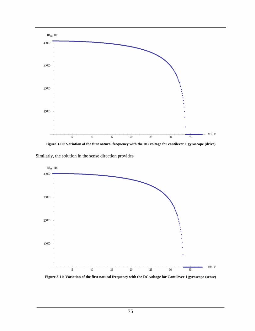
___________________________________________________________________________
75
Figure 3.10: Variation of the first natural frequency with the DC voltage for cantilever 1 gyroscope (drive)
Similarly, the solution in the sense direction provides
Figure 3.11: Variation of the first natural frequency with the DC voltage for Cantilever 1 gyroscope (sense)
5 10 15 20 25 30 35Vdc V
10000
20000
30000
40000
Wnd Hz
5 10 15 20 25 30 35Vdc V
10000
20000
30000
40000
Wns Hz

___________________________________________________________________________
76
It follows from Figure 3.10 and 3.11 that increasing the applied DC voltage leads to a sharp drop in the
first natural frequency followed by the pull-in instability. A numeral model also developed and
implemented to study the dynamic behavior of the cantilever beam. The equations of motion derived in
the previous section is simplified to include nonlinear effects up to order three. This is accomplished by
expanding each term in the equations into a Taylor series and discarding terms of order greater than
three. The simplification is necessary to enable the use of the equations to study the motion of the beam
using numerical techniques. The simplification process begins by obtaining the order three Taylor series
expansions of u', ψ, and θ. These are derived using the Taylor series expansion of arctan (x)
𝑡𝑎𝑛−1𝑦 = 𝑦 −1
3𝑦3 +⋯ (3.66)
which is combined with Eq. (3.10) and (3.11) to get
𝛿𝑥(𝑦, 𝑡)𝑦𝑦𝑦𝑦
(𝛿𝑥(𝑦, 𝑡)𝑦)2
𝛿𝑥(𝑦, 𝑡)𝑦 = [1 − (𝛿𝑥(𝑦, 𝑡)𝑦)2− (𝛿𝑧(𝑦, 𝑡)𝑦)
2]
12− 1
=1
2[(𝛿𝑥(𝑦, 𝑡)𝑦)
2− (𝛿𝑧(𝑦, 𝑡)𝑦)
2] + ⋯
(3.67)
𝜓 = 𝑡𝑎𝑛−1𝛿𝑥(𝑦, 𝑡)𝑦
1 + 𝛿𝑥(𝑦, 𝑡)𝑦
= 𝑡𝑎𝑛−1 𝛿𝑥(𝑦, 𝑡)𝑦 [1 − (𝛿𝑥(𝑦, 𝑡)𝑦)2− (𝛿𝑧(𝑦, 𝑡)𝑦)
2]−1/2
= 𝛿𝑥(𝑦, 𝑡)𝑦 [1 +1
6(𝛿𝑥(𝑦, 𝑡)𝑦)
2+1
2(𝛿𝑧(𝑦, 𝑡)𝑦)
2] + ⋯
(3.68)
휃 = 𝑡𝑎𝑛−1𝛿𝑧(𝑦, 𝑡)𝑦
[1 − (𝛿𝑦(𝑦, 𝑡)𝑦)2− (𝛿𝑥(𝑦, 𝑡)𝑦)
2]1/2
= 𝑡𝑎𝑛−1 −𝛿𝑧(𝑦, 𝑡)𝑦 [1 − (𝛿𝑧(𝑦, 𝑡)𝑦)2]−1/2
= 𝛿𝑧(𝑦, 𝑡)𝑦 [1 +1
6(𝛿𝑧(𝑦, 𝑡)𝑦)
2] + ⋯
(3.69)
The order three expansions for the angle of twist is obtained from the twisting curvature 𝜌𝜉. The order
three equations of motion for the flexural-flexural-torsional vibration of a cantilever beam.
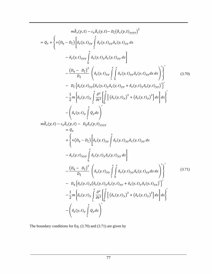
___________________________________________________________________________
77
𝑚𝑥(𝑦, 𝑡) − 𝑐𝑥𝑧(𝑦, 𝑡)− 𝐷𝜁(𝛿𝑥(𝑦, 𝑡)𝑦𝑦𝑦𝑦)2
= 𝑄𝑣 + +(𝐷𝜂 − 𝐷𝜁) [𝛿𝑧(𝑦, 𝑡)𝑦𝑦∫𝛿𝑧(𝑦, 𝑡)𝑦𝑦𝛿𝑥(𝑦, 𝑡)𝑦𝑦
𝑠
𝑙
𝑑𝑠
− 𝛿𝑧(𝑦, 𝑡)𝑦𝑦𝑦∫𝛿𝑧(𝑦, 𝑡)𝑦𝛿𝑥(𝑦, 𝑡)𝑦𝑦
𝑠
0
𝑑𝑠]
−(𝐷𝜂 − 𝐷𝜁)
2
𝐷𝜉 (𝛿𝑧(𝑦, 𝑡)𝑦𝑦∫∫𝛿𝑥(𝑦, 𝑡)𝑦𝑦𝛿𝑧(𝑦, 𝑡)𝑦𝑦𝑑𝑠
𝑠
0
𝑠
𝑙
𝑑𝑠)
′
′
− 𝐷𝜁 𝛿𝑧(𝑦, 𝑡)𝑦𝑦(𝛿𝑥(𝑦, 𝑡)𝑦𝛿𝑥(𝑦, 𝑡)𝑦𝑦 + 𝛿𝑧(𝑦, 𝑡)𝑦𝛿𝑧(𝑦, 𝑡)𝑦𝑦)′′
−1
2𝑚 𝛿𝑥(𝑦, 𝑡)𝑦∫
𝜕2
𝜕𝑡2[∫ [ (𝛿𝑥(𝑦, 𝑡)𝑦)
2+ (𝛿𝑧(𝑦, 𝑡)𝑦)
2] 𝑑𝑠
𝑠
0
]
𝑠
𝑙
𝑑𝑠
′
− (𝛿𝑥(𝑦, 𝑡)𝑦∫𝑄𝑦𝑑𝑠
𝑠
𝑙
)
′
(3.70)
𝑚𝑧(𝑦, 𝑡) − 𝑐𝑧𝑧(𝑦, 𝑡) − 𝐷𝜂𝛿𝑧(𝑦, 𝑡)𝑦𝑦𝑦𝑦= 𝑄𝑧
+ +(𝐷𝜂 − 𝐷𝜁) [𝛿𝑥(𝑦, 𝑡)𝑦𝑦∫𝛿𝑧(𝑦, 𝑡)𝑦𝑦𝛿𝑥(𝑦, 𝑡)𝑦𝑦
𝑠
𝑙
𝑑𝑠
− 𝛿𝑥(𝑦, 𝑡)𝑦𝑦𝑦∫𝛿𝑥(𝑦, 𝑡)𝑦𝛿𝑧(𝑦, 𝑡)𝑦𝑦
𝑠
0
𝑑𝑠]
−(𝐷𝜂 − 𝐷𝜁)
2
𝐷𝜉 (𝛿𝑥(𝑦, 𝑡)𝑦𝑦∫∫𝛿𝑥(𝑦, 𝑡)𝑦𝑦𝛿𝑧(𝑦, 𝑡)𝑦𝑦𝑑𝑠
𝑠
0
𝑠
𝑙
𝑑𝑠)
′
′
− 𝐷𝜂 𝛿𝑧(𝑦, 𝑡)𝑦(𝛿𝑥(𝑦, 𝑡)𝑦𝛿𝑥(𝑦, 𝑡)𝑦𝑦 + 𝛿𝑧(𝑦, 𝑡)𝑦𝛿𝑧(𝑦, 𝑡)𝑦𝑦)′′
−1
2𝑚 𝛿𝑧(𝑦, 𝑡)𝑦∫
𝜕2
𝜕𝑡2[∫ [ (𝛿𝑥(𝑦, 𝑡)𝑦)
2+ (𝛿𝑧(𝑦, 𝑡)𝑦)
2] 𝑑𝑠
𝑠
0
]
𝑠
𝑙
𝑑𝑠
′
−(𝛿𝑧(𝑦, 𝑡)𝑦∫𝑄𝑦𝑑𝑠
𝑠
𝑙
)
′
(3.71)
The boundary conditions for Eq. (3.70) and (3.71) are given by
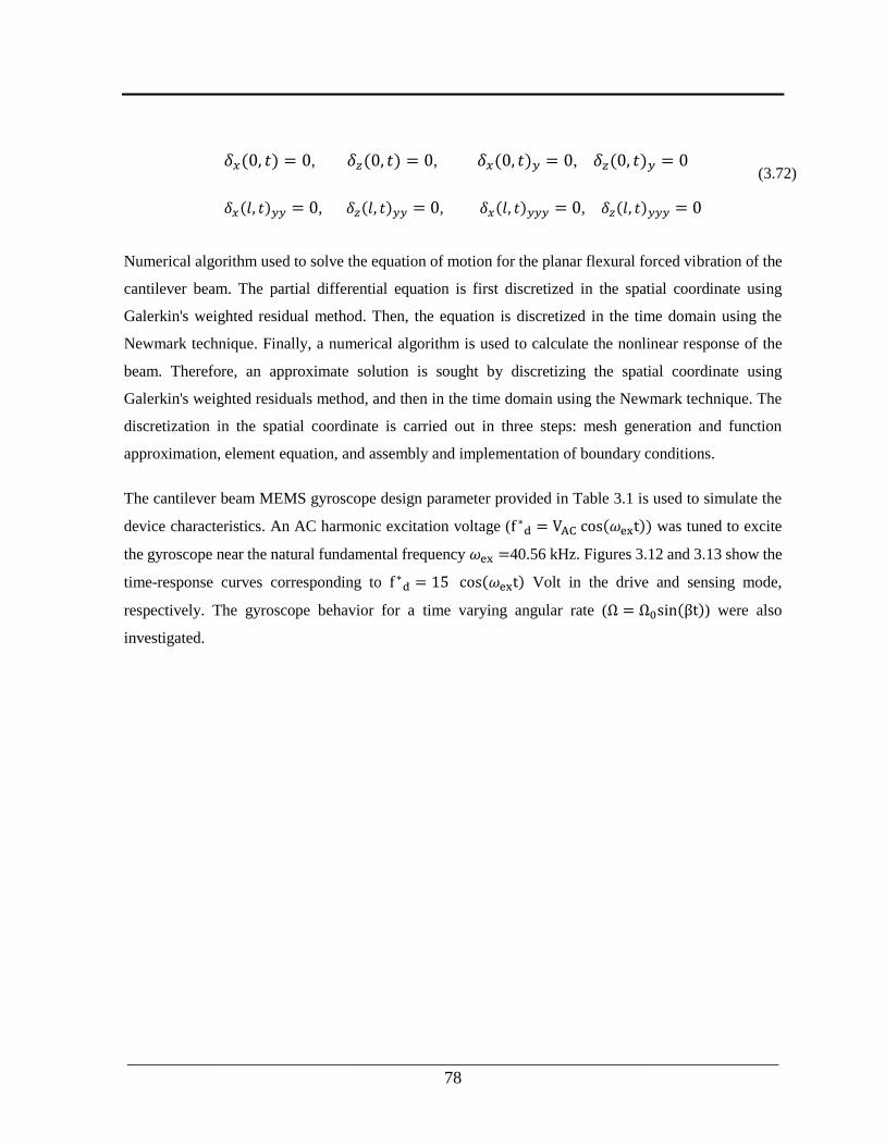
___________________________________________________________________________
78
𝛿𝑥(0, 𝑡) = 0, 𝛿𝑧(0, 𝑡) = 0, 𝛿𝑥(0, 𝑡)𝑦 = 0, 𝛿𝑧(0, 𝑡)𝑦 = 0
𝛿𝑥(𝑙, 𝑡)𝑦𝑦 = 0, 𝛿𝑧(𝑙, 𝑡)𝑦𝑦 = 0, 𝛿𝑥(𝑙, 𝑡)𝑦𝑦𝑦 = 0, 𝛿𝑧(𝑙, 𝑡)𝑦𝑦𝑦 = 0
(3.72)
Numerical algorithm used to solve the equation of motion for the planar flexural forced vibration of the
cantilever beam. The partial differential equation is first discretized in the spatial coordinate using
Galerkin's weighted residual method. Then, the equation is discretized in the time domain using the
Newmark technique. Finally, a numerical algorithm is used to calculate the nonlinear response of the
beam. Therefore, an approximate solution is sought by discretizing the spatial coordinate using
Galerkin's weighted residuals method, and then in the time domain using the Newmark technique. The
discretization in the spatial coordinate is carried out in three steps: mesh generation and function
approximation, element equation, and assembly and implementation of boundary conditions.
The cantilever beam MEMS gyroscope design parameter provided in Table 3.1 is used to simulate the
device characteristics. An AC harmonic excitation voltage (f ∗d = VAC cos(𝜔ext)) was tuned to excite
the gyroscope near the natural fundamental frequency 𝜔ex =40.56 kHz. Figures 3.12 and 3.13 show the
time-response curves corresponding to f ∗d = 15 cos(𝜔ext) Volt in the drive and sensing mode,
respectively. The gyroscope behavior for a time varying angular rate (Ω = Ω0sin(βt)) were also
investigated.
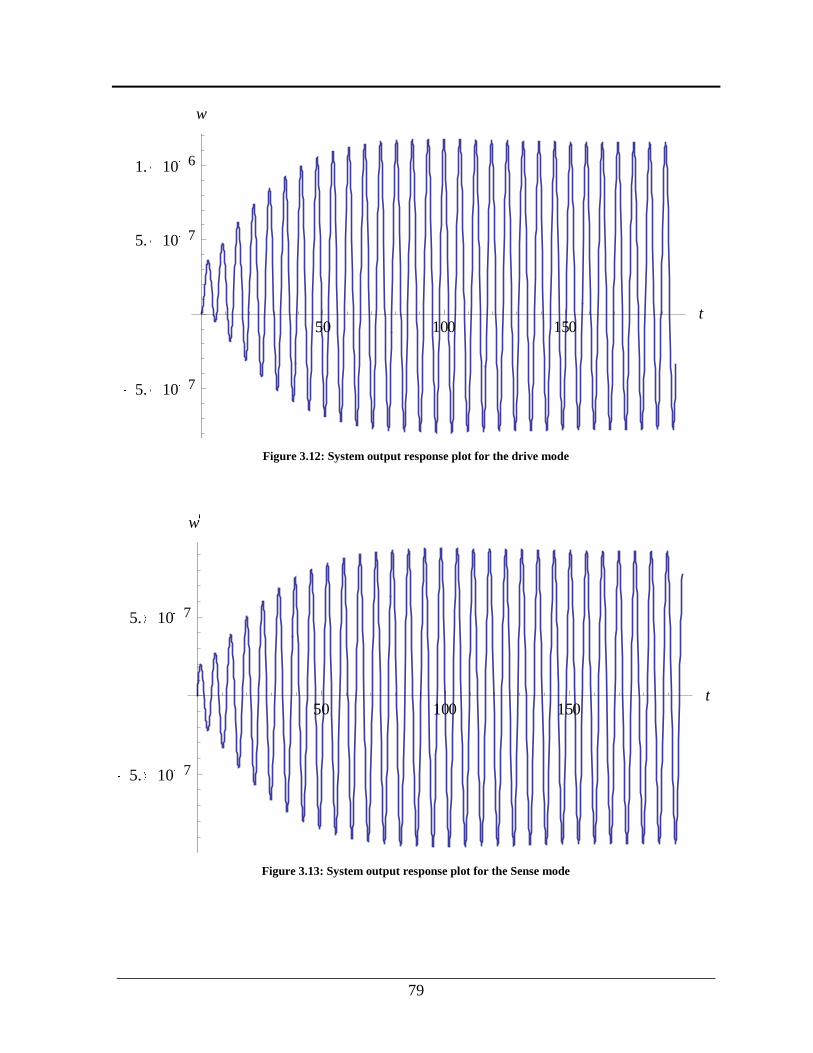
___________________________________________________________________________
79
Figure 3.12: System output response plot for the drive mode
Figure 3.13: System output response plot for the Sense mode
50 100 150t
5. 10 7
5. 10 7
1. 10 6
w
50 100 150t
5. 10 7
5. 10 7
w

___________________________________________________________________________
80
3.6 Finite Element Simulations and Results
The gyroscope dynamic analysis for the cantilever beam gyroscope in previous section established the
relationship between device characteristic such as device resonant frequency, displacement and
capacitance sensitivity with various design parameters such as material properties of the beam structure
and beam geometry (length, width and beam thickness).
In this section, a finite element model developed for the cantilever beam and crab leg design presented.
A commercial CAD software, SolidWorks was used to develop the 3D model. For parametric finite
element model of the cantilever beam and crab leg, Parametric Design Language of ANSYS (APDL) is
used. For static and modal analysis, a number of parameters (geometric, material, analysis options, etc)
can easily, change to account for different prototype sample developed, Appendix G. variables are taken
as parameters and they can be changed interactively. Boundary and loading conditions are described for
each analysis in the other subsections. In the next section analysis and result preformed for Cantilever 1
and Crab leg 2 is presented.
3.6.1 Cantilever Beam Gyroscope FEA Analysis
In this section, Finite Element Analysis (FEA) for the cantilever beam MEMS gyroscope design is
presented. As the MEMS structure moves due to electrostatic excitation force, the electrostatic field
distribution will change. Hence, a coupled electrostatic‐structural analysis was implemented that allows
the actual electrostatic actuation of a MEMS device to be simulated, capturing the interdependencies of
these two physics.
The full cantilever beam model was used for static and modal analysis since the model is small enough
to run with available computational resource and does not need simplification. The FEA analysis
presented here does not take into account the effect of gravity condition. Both the cantilever beam and
crab leg 3D model developed using SolidWork and imported to ANSYS. In this analysis, shell elements
were used for the microplate. A shell element is the combination of the bending element and the
membrane element. At each node, the shell element has both translational DOFs and rotational DOFs in
each direction. When the structure's thickness is far less than the other dimensions, shell elements can
usually give more accurate results than solid elements. A tetrahedral solid element were also used for
the cantilever beam, Figure 3.14.
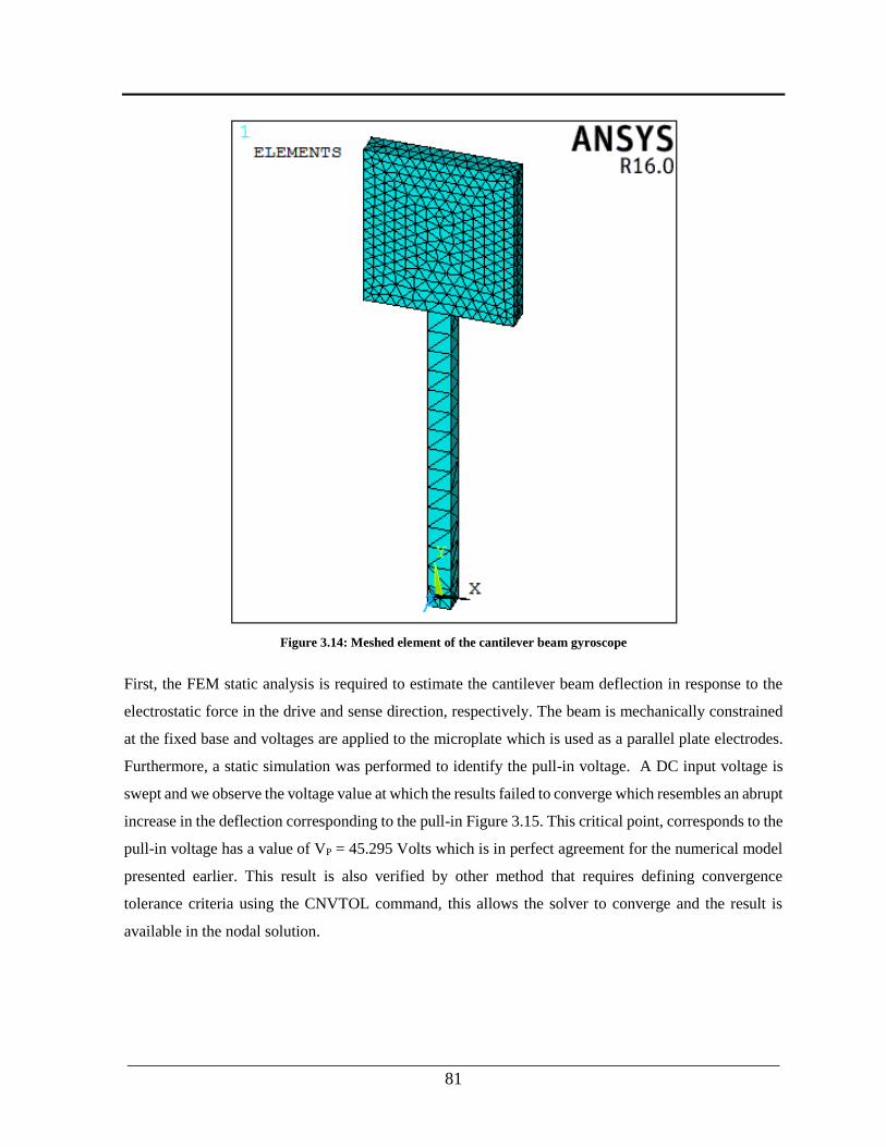
___________________________________________________________________________
81
Figure 3.14: Meshed element of the cantilever beam gyroscope
First, the FEM static analysis is required to estimate the cantilever beam deflection in response to the
electrostatic force in the drive and sense direction, respectively. The beam is mechanically constrained
at the fixed base and voltages are applied to the microplate which is used as a parallel plate electrodes.
Furthermore, a static simulation was performed to identify the pull-in voltage. A DC input voltage is
swept and we observe the voltage value at which the results failed to converge which resembles an abrupt
increase in the deflection corresponding to the pull-in Figure 3.15. This critical point, corresponds to the
pull-in voltage has a value of VP = 45.295 Volts which is in perfect agreement for the numerical model
presented earlier. This result is also verified by other method that requires defining convergence
tolerance criteria using the CNVTOL command, this allows the solver to converge and the result is
available in the nodal solution.
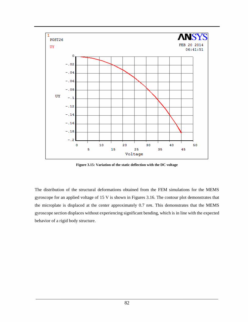
___________________________________________________________________________
82
Figure 3.15: Variation of the static deflection with the DC voltage
The distribution of the structural deformations obtained from the FEM simulations for the MEMS
gyroscope for an applied voltage of 15 V is shown in Figures 3.16. The contour plot demonstrates that
the microplate is displaced at the center approximately 0.7 n𝑚. This demonstrates that the MEMS
gyroscope section displaces without experiencing significant bending, which is in line with the expected
behavior of a rigid body structure.
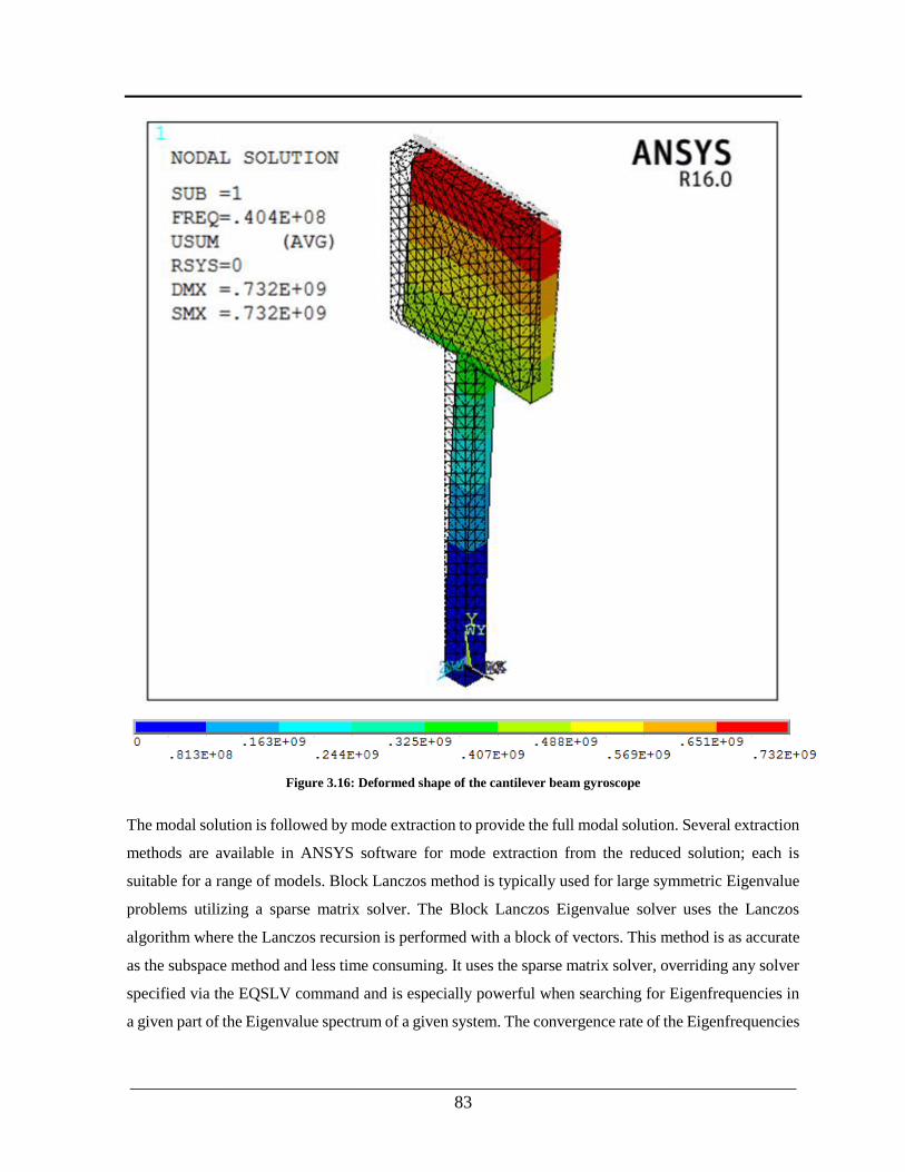
___________________________________________________________________________
83
Figure 3.16: Deformed shape of the cantilever beam gyroscope
The modal solution is followed by mode extraction to provide the full modal solution. Several extraction
methods are available in ANSYS software for mode extraction from the reduced solution; each is
suitable for a range of models. Block Lanczos method is typically used for large symmetric Eigenvalue
problems utilizing a sparse matrix solver. The Block Lanczos Eigenvalue solver uses the Lanczos
algorithm where the Lanczos recursion is performed with a block of vectors. This method is as accurate
as the subspace method and less time consuming. It uses the sparse matrix solver, overriding any solver
specified via the EQSLV command and is especially powerful when searching for Eigenfrequencies in
a given part of the Eigenvalue spectrum of a given system. The convergence rate of the Eigenfrequencies

___________________________________________________________________________
84
will be about the same when extracting modes in the midrange and higher end of the spectrum as when
extracting the lowest modes.
The application of DC bias voltage at the device electrodes produces electrostatic forces which creates
stresses in the beam and affects the natural frequencies. The prestressed modal analysis was performed
in two steps: The first step was a static analysis with the DC bias voltage applied and prestressing active
(PSTRES, ON) as preformed in the previous section. The second step was a modal analysis with the
prestressing still active. The DC bias voltage was applied using the distributed array of TRANS126
elements. With a 0V bias, the problem is solved without the inclusion of “spring softening” effects. For
the static prestress analysis, a DC bias voltage ranging from 0-45 Volts was applied across the
TRANS126 elements.
A modal analysis is used to determine the structure vibration characteristics of natural frequencies and
mode shapes. We extracted the first 3 vibration modes of this gyroscope to decide which two modes are
the driving modes and sensing mode of the gyroscope. The shape and values of the mode frequency
versus voltage curves are approximately the same over the course up to the pull in voltage. The deformed
shapes of the first three modes are shown in Figures 3.17 through 3.19 for the cantilever beam gyroscope.
These include the first out of plane mode shapes and frequencies, second in plan mode and the third
torsional mode. From the simulated results, the first two set frequencies are 40.4 kHz and 40.8 kHz.
Therefore, the resonant frequency of the driving mode is 40.4 kHz; and the resonant frequency of the
sensing mode is 40.8 kHz. In general, ANSYS predicts a slight higher modal frequency than reduced
order model solution in the drive direction. This slight difference can be explained by the effect of pre-
stress consideration including in our ANSYS simulation.

___________________________________________________________________________
85
Figure 3.17: First mode shape of the cantilever beam
Figure 3.18. Second mode shape of the cantilevered beam.
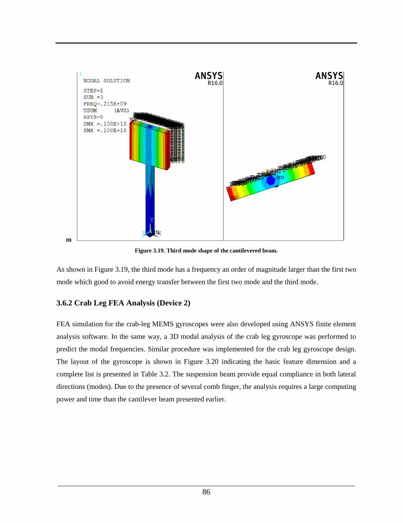
___________________________________________________________________________
86
m
Figure 3.19. Third mode shape of the cantilevered beam.
As shown in Figure 3.19, the third mode has a frequency an order of magnitude larger than the first two
mode which good to avoid energy transfer between the first two mode and the third mode.
3.6.2 Crab Leg FEA Analysis (Device 2)
FEA simulation for the crab-leg MEMS gyroscopes were also developed using ANSYS finite element
analysis software. In the same way, a 3D modal analysis of the crab leg gyroscope was performed to
predict the modal frequencies. Similar procedure was implemented for the crab leg gyroscope design.
The layout of the gyroscope is shown in Figure 3.20 indicating the basic feature dimension and a
complete list is presented in Table 3.2. The suspension beam provide equal compliance in both lateral
directions (modes). Due to the presence of several comb finger, the analysis requires a large computing
power and time than the cantilever beam presented earlier.
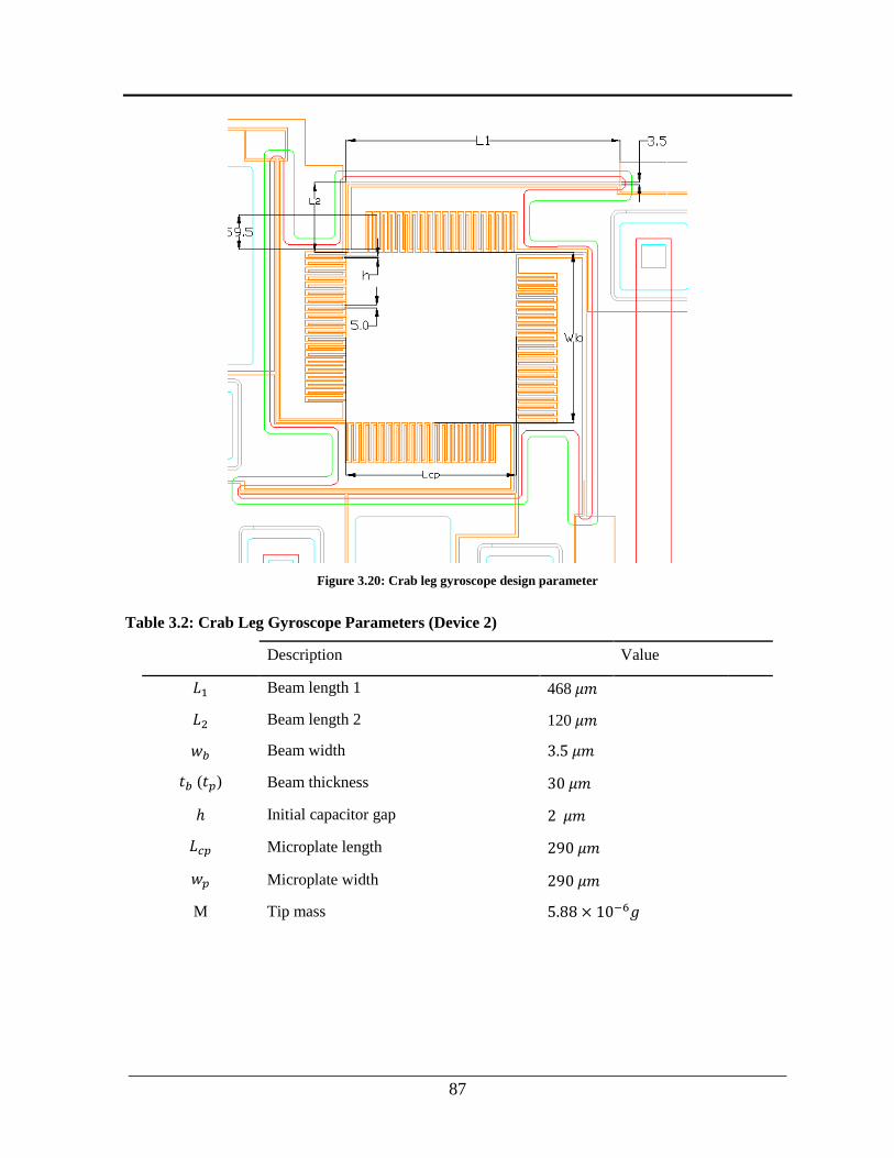
___________________________________________________________________________
87
Figure 3.20: Crab leg gyroscope design parameter
Table 3.2: Crab Leg Gyroscope Parameters (Device 2)
Description Value
𝐿1 Beam length 1 468 𝜇𝑚
𝐿2 Beam length 2 120 𝜇𝑚
𝑤𝑏 Beam width 3.5 𝜇𝑚
𝑡𝑏 (𝑡𝑝) Beam thickness 30 𝜇𝑚
ℎ Initial capacitor gap 2 𝜇𝑚
𝐿𝑐𝑝 Microplate length 290 𝜇𝑚
𝑤𝑝 Microplate width 290 𝜇𝑚
M Tip mass 5.88 × 10⁻⁶𝑔
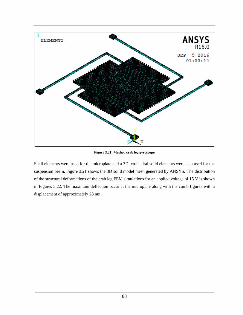
___________________________________________________________________________
88
Figure 3.21: Meshed crab leg gyroscope
Shell elements were used for the microplate and a 3D tetrahedral solid elements were also used for the
suspension beam. Figure 3.21 shows the 3D solid model mesh generated by ANSYS. The distribution
of the structural deformations of the crab leg FEM simulations for an applied voltage of 15 V is shown
in Figures 3.22. The maximum deflection occur at the microplate along with the comb figures with a
displacement of approximately 28 n𝑚.
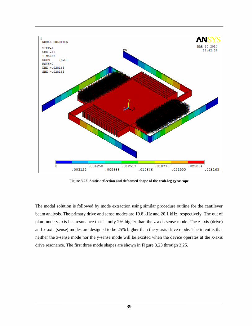
___________________________________________________________________________
89
Figure 3.22: Static deflection and deformed shape of the crab-leg gyroscope
The modal solution is followed by mode extraction using similar procedure outline for the cantilever
beam analysis. The primary drive and sense modes are 19.8 kHz and 20.1 kHz, respectively. The out of
plan mode y axis has resonance that is only 2% higher than the z-axis sense mode. The z-axis (drive)
and x-axis (sense) modes are designed to be 25% higher than the y-axis drive mode. The intent is that
neither the z-sense mode nor the y-sense mode will be excited when the device operates at the x-axis
drive resonance. The first three mode shapes are shown in Figure 3.23 through 3.25.

___________________________________________________________________________
90
Figure 3.23: The first mode shape of crab-leg gyroscope (z-axis)
Figure 3.24: The second mode shape of crab-leg gyroscope (x-axis)
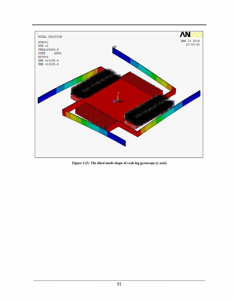
___________________________________________________________________________
91
Figure 3.25: The third mode shape of crab-leg gyroscope (y-axis)

___________________________________________________________________________
92
CHAPTER IV
Analysis of Thermal Noise in Frequency-
Modulated Gyroscopes
Noise in MEMS gyroscopes can be introduced from electrical and mechanical sources. Mechanical noise
is usually more significant and presented as Brownian motion and is analyzed extensively for AM
modulated gyroscope. A MEMS gyroscope, the mass-spring-damper system is dissipative systems
exhibits thermal noise. Thermal noise in MEMS gyroscopes arise due to molecular agitation inside beam
springs, actuation and sense structures, suspended mass and the surrounding environment. The cantilever
fluctuates with respect to the rest position due to the random impacts of the surrounding molecules. In
the same way, the cantilever dissipates the stored mechanical energy through its interaction with the
surrounding thermal bath. This relationship between the thermal forces and the dissipation of mechanical
energy is described by the fluctuation-dissipation theorem, which is usually applied to determine the
electrical noise across a resistor. Thermodynamics sets the ultimate sensitivity of beam springs based
MEMS devices in general.
The fluctuation-dissipation theorem in statistical physics for predict the behavior of non-equilibrium
thermo-dynamical systems. These systems involve the irreversible dissipation of energy into heat from
their reversible thermal fluctuations at thermodynamic equilibrium. The fluctuation-dissipation theorem
applies both to classical and quantum mechanical systems. The fluctuation-dissipation theorem relies on
the assumption that the response of a system in thermodynamic equilibrium to a small applied force is
the same as its response to a spontaneous fluctuation. Therefore, the theorem connects the linear response
relaxation of a system from a prepared non-equilibrium state to its statistical fluctuation properties in
equilibrium. Often the linear response takes the form of one or more exponential decays.
Previously research has been done on thermal noise for amplitude modulated MEMS gyroscope [28].
This chapter presents analysis of thermal noise for frequency modulation MEMS gyroscope. Hence, we
investigate the effect of thermal noise on the natural frequency of the MEMS gyroscope since the
rotation rate is measured by detecting the shift in the natural frequencies of two closely spaced global

___________________________________________________________________________
93
vibration modes. We analyzed analytical expressions for the effect of thermal noise on the frequency
modulation MEMS gyroscope and compare the output signals due to both the rotation rate and thermal
noise.
4.1 Thermal Noise in MEMS Gyroscope
Temperature fluctuation generate noise in electrical or mechanical system. Commonly in large-scale
sensors this kind of noise is usually neglected. However, as a device size reduced, thermal noises become
significant and cause performance degradation [45]. Generally, MEMS gyroscopes are limited by
electrical noise and systematic errors, but for such small mechanical structures and low values of
displacement in the sensing direction, thermal noise should be considered as the theoretical sensitivity
limiting factor. Mechanical thermal noise occurs due to vibrations of atoms in the materials from which
a device is made and the environment in which the device operates.
There are three primary works that investigated the thermal noise properties of amplitude modulated
MEMS gyroscope [51-52]. The first studied the effect of mechanical thermal fluctuations on a vibrating-
mass surface-micromachined gyroscope [53]. It was found that the mechanical–thermal noise source
represents a practical sensitivity limit in the gyroscope and is likely to restrict their performance [54].
In chapter two, we modeled the MEMS gyroscope as a 2-DOF spring-mass-damper. The mechanisms
that couple these thermal vibrations to the mechanical of interest are the energy dissipation mechanisms.
The interaction of molecules with flexible parts of the sensing elements immersed in a gaseous or a
liquid medium can be described by the equation of a harmonic oscillator as follows
𝑚( − 𝑦Ω − 𝑥Ω2 − 2Ωy) + (𝑐 + 𝛿) + (𝑘 + 𝜑)𝑥 = 𝐹𝑒𝑥𝑡(𝑡) + 𝐹𝑡ℎ(𝑡)
𝑚( − 𝑥Ω − 𝑦Ω2 − 2Ωx) + 𝑐 + 𝑘𝑦 = 𝐹𝑡ℎ(𝑡)
(4.1)
where Fext(t) is the deterministic excitation force, Fth(t) is the stochastic force excited from the
surrounding molecules on the flexible part of the sensor, m is the mass, 𝑐 is the damping constant, and
𝑘 is the spring constant. 𝛿 and 𝜑 are the variation of the damping and spring constant due to
imperfection of micro-fabrication.
The magnitude of Fext(t) in the drive direction is sufficiently large enough to neglect the thermal noise
effect in this direction. Therefore, our investigation focuses the thermal noise effect in the sense
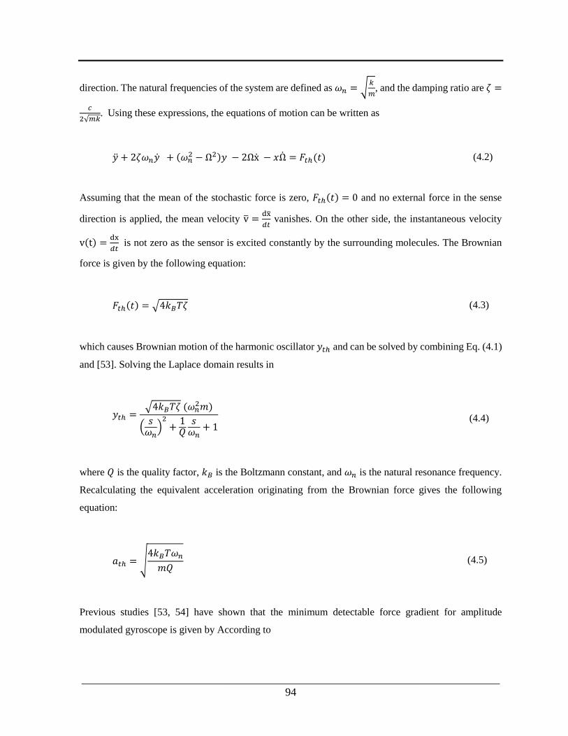
___________________________________________________________________________
94
direction. The natural frequencies of the system are defined as 𝜔𝑛 = √𝑘
𝑚, and the damping ratio are 휁 =
𝑐
2√𝑚𝑘. Using these expressions, the equations of motion can be written as
+ 2휁𝜔𝑛 + (𝜔𝑛2 − Ω2)𝑦 − 2Ωx − 𝑥Ω = 𝐹𝑡ℎ(𝑡) (4.2)
Assuming that the mean of the stochastic force is zero, 𝐹𝑡ℎ(𝑡) = 0 and no external force in the sense
direction is applied, the mean velocity v =dx
𝑑𝑡 vanishes. On the other side, the instantaneous velocity
v(t) =dx
𝑑𝑡 is not zero as the sensor is excited constantly by the surrounding molecules. The Brownian
force is given by the following equation:
𝐹𝑡ℎ(𝑡) = √4𝑘𝐵𝑇휁 (4.3)
which causes Brownian motion of the harmonic oscillator 𝑦𝑡ℎ and can be solved by combining Eq. (4.1)
and [53]. Solving the Laplace domain results in
𝑦𝑡ℎ =√4𝑘𝐵𝑇휁 (𝜔𝑛
2𝑚)
(𝑠𝜔𝑛)2+1𝑄𝑠𝜔𝑛+ 1
(4.4)
where 𝑄 is the quality factor, 𝑘𝐵 is the Boltzmann constant, and 𝜔𝑛 is the natural resonance frequency.
Recalculating the equivalent acceleration originating from the Brownian force gives the following
equation:
𝑎𝑡ℎ = √4𝑘𝐵𝑇𝜔𝑛𝑚𝑄
(4.5)
Previous studies [53, 54] have shown that the minimum detectable force gradient for amplitude
modulated gyroscope is given by According to
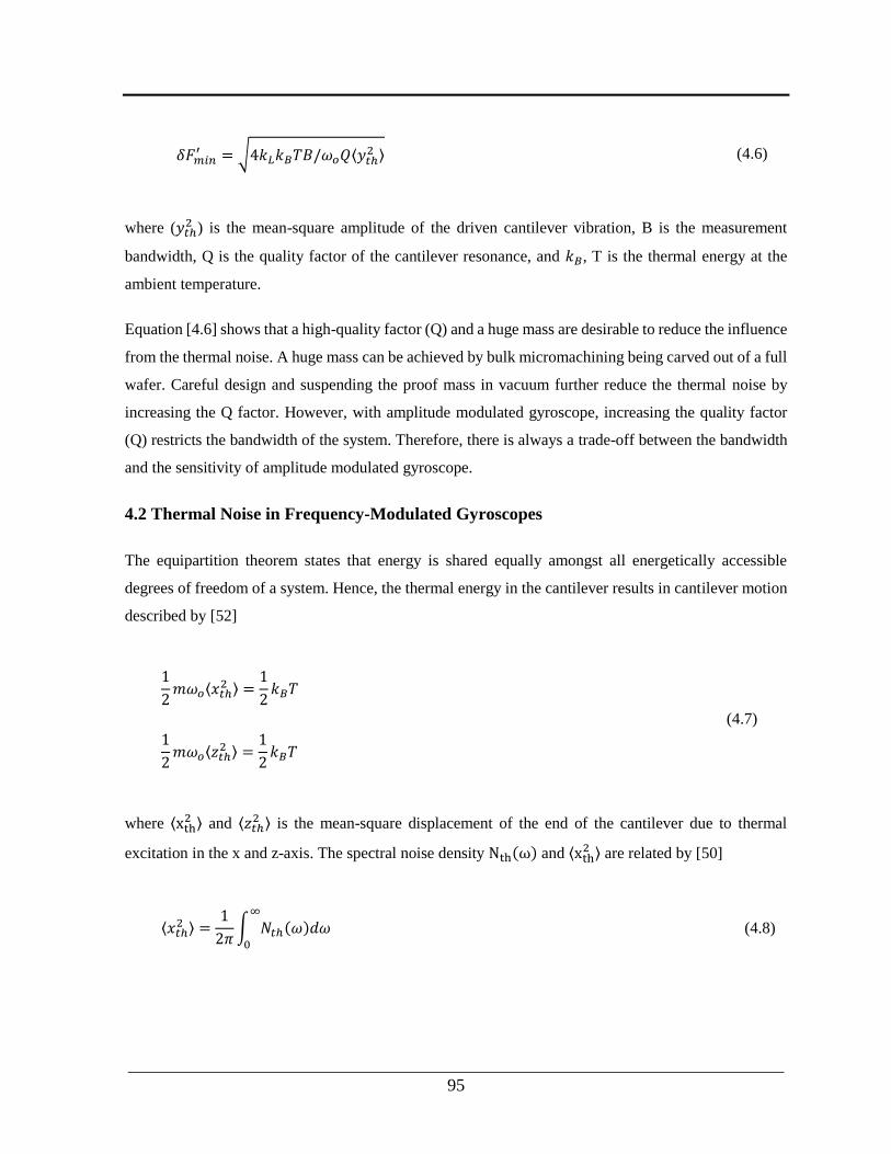
___________________________________________________________________________
95
𝛿𝐹𝑚𝑖𝑛′ = √4𝑘𝐿𝑘𝐵𝑇𝐵/𝜔𝑜𝑄⟨𝑦𝑡ℎ
2 ⟩ (4.6)
where (𝑦𝑡ℎ2 ) is the mean-square amplitude of the driven cantilever vibration, B is the measurement
bandwidth, Q is the quality factor of the cantilever resonance, and 𝑘𝐵, T is the thermal energy at the
ambient temperature.
Equation [4.6] shows that a high-quality factor (Q) and a huge mass are desirable to reduce the influence
from the thermal noise. A huge mass can be achieved by bulk micromachining being carved out of a full
wafer. Careful design and suspending the proof mass in vacuum further reduce the thermal noise by
increasing the Q factor. However, with amplitude modulated gyroscope, increasing the quality factor
(Q) restricts the bandwidth of the system. Therefore, there is always a trade-off between the bandwidth
and the sensitivity of amplitude modulated gyroscope.
4.2 Thermal Noise in Frequency-Modulated Gyroscopes
The equipartition theorem states that energy is shared equally amongst all energetically accessible
degrees of freedom of a system. Hence, the thermal energy in the cantilever results in cantilever motion
described by [52]
1
2𝑚𝜔𝑜⟨𝑥𝑡ℎ
2 ⟩ =1
2𝑘𝐵𝑇
1
2𝑚𝜔𝑜⟨𝑧𝑡ℎ
2 ⟩ =1
2𝑘𝐵𝑇
(4.7)
where ⟨xth2 ⟩ and ⟨𝑧𝑡ℎ
2 ⟩ is the mean-square displacement of the end of the cantilever due to thermal
excitation in the x and z-axis. The spectral noise density Nth(ω) and ⟨xth2 ⟩ are related by [50]
⟨𝑥𝑡ℎ2 ⟩ =
1
2𝜋∫ 𝑁𝑡ℎ(𝜔)𝑑𝜔∞
0
(4.8)

___________________________________________________________________________
96
⟨𝑧𝑡ℎ2 ⟩ =
1
2𝜋∫ 𝑁𝑡ℎ(𝜔)𝑑𝜔∞
0
and 𝑁𝑡ℎ(𝜔) can be further described by
𝑁𝑡ℎ(𝜔) = |𝐺(𝜔)|2Ψ𝑡ℎ(𝜔) (4.9)
where |𝐺(𝜔)|2 is the response function of the cantilever (damped harmonic oscillator) given by
|𝐺(𝜔)|2 =1/𝑚2
(𝜔02 −𝜔2)2 + (𝜔0𝜔/𝑄)
2 (4.10)
and Ψ𝑡ℎ(𝜔)is the thermal white noise drive given by
Ψ𝑡ℎ(𝜔) = 4𝑚𝜔0𝑘𝐵𝑇/𝑄 (4.11)
If we ignore noise components with a modulation frequency on the order of the oscillator linewidth and
less, we may write an approximate expression for the spectral noise density Nth in each sideband in terms
of the modulation frequency as follows:
𝑁𝑡ℎ(𝜔𝑚𝑜𝑑) = K𝐵𝑇/𝑚𝜔𝑜𝑄𝜔𝑚𝑜𝑑2 (4.12)
The phase noise energy is given by Nop(𝜔𝑚𝑜𝑑) =𝑘𝑙𝑁𝑡ℎ(𝜔𝑚𝑜𝑑)/2) and the mean-square frequency
modulation due to this noise source is given by
⟨(𝛿𝜔d)2⟩ = ∫
2𝐸𝑝(𝜔𝑚𝑜𝑑)
𝐸𝐶𝑓𝑚𝑜𝑑2 𝑑𝑓𝑚𝑜𝑑
𝜔𝑚𝑜𝑑
(4.13)
This is in case where it is necessary to calculate the effective frequency deviation over some finite
baseband bandwidth say

___________________________________________________________________________
97
where 𝛿𝑓 is the mean-square frequency modulation due to this noise source C, is the oscillator energy
(carrier power) given by C = EC = 𝑘𝑙𝑥𝑜𝑠𝑐2 ) over the bandwidth of measurement
Integrating Eq. (12) over the bandwidth of measurement, the minimum detectable frequency shift of a
cantilever beam oscillator incorporated in a self-oscillating system with positive feedback has been
estimated.
𝛿𝜔s = √𝜔sΩ𝑘𝐵𝑇𝐵
𝑘𝑄⟨𝑥𝑜𝑠𝑐2 ⟩
𝛿𝜔d = √𝜔dΩ𝑘𝐵𝑇𝐵
𝑘𝑄⟨𝑧𝑜𝑠𝑐2 ⟩
(4.14)
As presented in chapter two, we can determine input angular rate by taking the difference between the
two natural frequencies i.e 𝜔dΩ −𝜔sΩ = 2Ω.. Since similar design parameter were used for the drive
and sense direction, the two mode will have the same shift in resonance frequency due to thermal effect.
The thermally induced change in resonance frequency therefore cancel each other with not output effect
on the output reading. Therefore, the frequency modulated detection method allows the sensitivity to be
increased by using a very high Q without sacrificing bandwidth or dynamic range. With very low
damping, noise in the amplitude modulated can play a significant role in reducing system sensitivity.
4.2 Analysis of Stability and Device Performance of the Cantilever Gyroscopes
Two main parameters representing the performance of MEMS gyroscope is the angle random walk and
the bias instability. These two parameters can be obtained by the Allan variance method or by power
spectral density. In the following section, the Allan variance method describe for ARW and bias stability
analysis.
4.2.1 Allan variance
Allan variance is a statistical measurement used to characterize and identify noise related error sources
and their contribution to the overall noise statistics. It is defined as one half of the time average of the
squares of the differences between successive readings of the frequency deviation sampled over a given
sampling period. This is a time-domain analysis method of the stochastic process of the sensor
measurements which investigates the errors as a function of averaging times. Allan variance analysis is
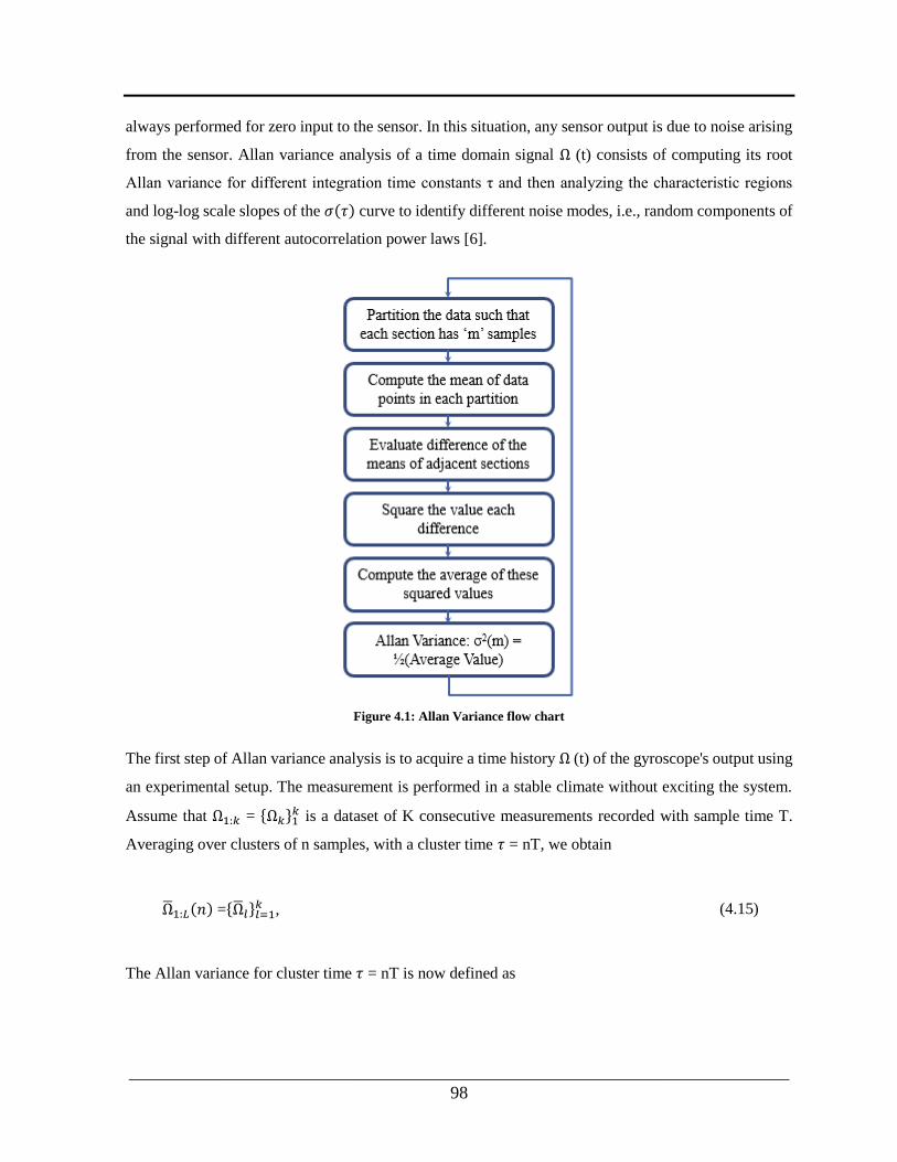
___________________________________________________________________________
98
always performed for zero input to the sensor. In this situation, any sensor output is due to noise arising
from the sensor. Allan variance analysis of a time domain signal Ω (t) consists of computing its root
Allan variance for different integration time constants τ and then analyzing the characteristic regions
and log-log scale slopes of the 𝜎(𝜏) curve to identify different noise modes, i.e., random components of
the signal with different autocorrelation power laws [6].
Figure 4.1: Allan Variance flow chart
The first step of Allan variance analysis is to acquire a time history Ω (t) of the gyroscope's output using
an experimental setup. The measurement is performed in a stable climate without exciting the system.
Assume that Ω1:𝑘 = Ω𝑘1𝑘 is a dataset of K consecutive measurements recorded with sample time T.
Averaging over clusters of n samples, with a cluster time 𝜏 = nT, we obtain
Ω1:𝐿(𝑛) =Ω𝑙𝑙=1𝑘 , (4.15)
The Allan variance for cluster time 𝜏 = nT is now defined as
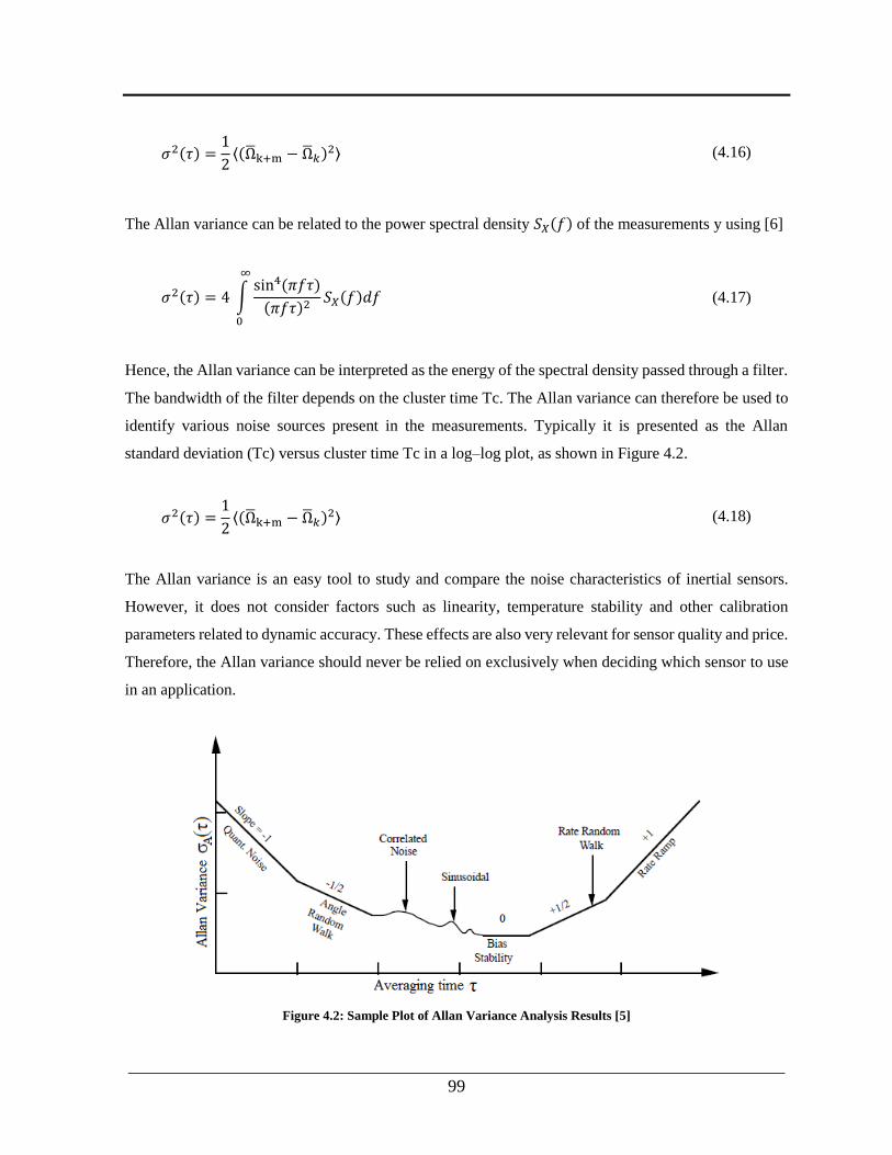
___________________________________________________________________________
99
𝜎2(𝜏) =1
2⟨(Ωk+m − Ω𝑘)
2⟩ (4.16)
The Allan variance can be related to the power spectral density 𝑆𝑋(𝑓) of the measurements y using [6]
𝜎2(𝜏) = 4 ∫sin4(𝜋𝑓𝜏)
(𝜋𝑓𝜏)2
∞
0
𝑆𝑋(𝑓)𝑑𝑓 (4.17)
Hence, the Allan variance can be interpreted as the energy of the spectral density passed through a filter.
The bandwidth of the filter depends on the cluster time Tc. The Allan variance can therefore be used to
identify various noise sources present in the measurements. Typically it is presented as the Allan
standard deviation (Tc) versus cluster time Tc in a log–log plot, as shown in Figure 4.2.
𝜎2(𝜏) =1
2⟨(Ωk+m − Ω𝑘)
2⟩ (4.18)
The Allan variance is an easy tool to study and compare the noise characteristics of inertial sensors.
However, it does not consider factors such as linearity, temperature stability and other calibration
parameters related to dynamic accuracy. These effects are also very relevant for sensor quality and price.
Therefore, the Allan variance should never be relied on exclusively when deciding which sensor to use
in an application.
Figure 4.2: Sample Plot of Allan Variance Analysis Results [5]
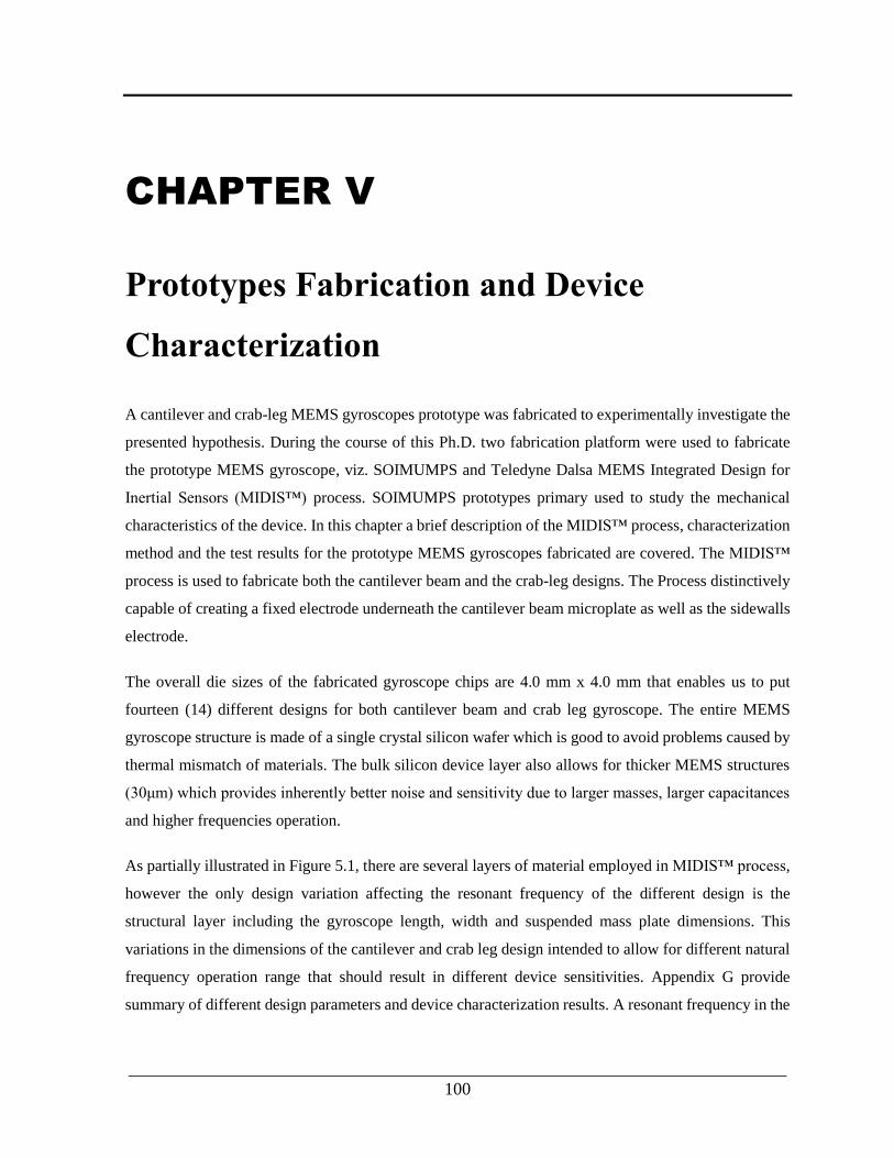
___________________________________________________________________________
100
CHAPTER V
Prototypes Fabrication and Device
Characterization
A cantilever and crab-leg MEMS gyroscopes prototype was fabricated to experimentally investigate the
presented hypothesis. During the course of this Ph.D. two fabrication platform were used to fabricate
the prototype MEMS gyroscope, viz. SOIMUMPS and Teledyne Dalsa MEMS Integrated Design for
Inertial Sensors (MIDIS™) process. SOIMUMPS prototypes primary used to study the mechanical
characteristics of the device. In this chapter a brief description of the MIDIS™ process, characterization
method and the test results for the prototype MEMS gyroscopes fabricated are covered. The MIDIS™
process is used to fabricate both the cantilever beam and the crab-leg designs. The Process distinctively
capable of creating a fixed electrode underneath the cantilever beam microplate as well as the sidewalls
electrode.
The overall die sizes of the fabricated gyroscope chips are 4.0 mm x 4.0 mm that enables us to put
fourteen (14) different designs for both cantilever beam and crab leg gyroscope. The entire MEMS
gyroscope structure is made of a single crystal silicon wafer which is good to avoid problems caused by
thermal mismatch of materials. The bulk silicon device layer also allows for thicker MEMS structures
(30μm) which provides inherently better noise and sensitivity due to larger masses, larger capacitances
and higher frequencies operation.
As partially illustrated in Figure 5.1, there are several layers of material employed in MIDIS™ process,
however the only design variation affecting the resonant frequency of the different design is the
structural layer including the gyroscope length, width and suspended mass plate dimensions. This
variations in the dimensions of the cantilever and crab leg design intended to allow for different natural
frequency operation range that should result in different device sensitivities. Appendix G provide
summary of different design parameters and device characterization results. A resonant frequency in the

___________________________________________________________________________
101
range between 38 kHz to 45 kHz designed for the cantilever beam gyroscope. The cantilever beam
MEMS gyroscope design uses side wall as well as a bottom parallel plate electrode to drive and sustained
oscillation and to sense the Coriolis oscillation. In Figure 5.1 different colors are used for the structural
layer for visibility of the different structural parts.
Figure 5.1: A 3D model of the structure of the cantilever beam element
For the crab leg design a comb drive and sensing electrode constructed from an array of two side by side
beams. Figures 5.2 represent the structure of the drive and sense electrode and other features for the
cantilever and crab leg design.

___________________________________________________________________________
102
Figure 5.2: A comb finger electrode and other structural parts for the crab leg beam element
5.1 Prototypes Fabrication MIDIS™ Process
Teledyne Dalsa MIDIS™ platform is mixed micromachining process for manufacturing inertial sensors
which is capable of integrating the MEMS device with CMOS. In this process, major micromachining
techniques includes surface and bulk machining, Through Silicon Via (TSV) with metal plugs (ISDP),
anhydrous HF Release, thick polymers, and wafer bonding. The MIDIS™ platform also provides wafer
level packaging with high-vacuum sealing that allows a high quality factor (Q) for the MEMS inertial
sensors. The process makes use of three starting silicon substrates that includes Handle, Membrane, and
TSV as shown in Figure 5.3.
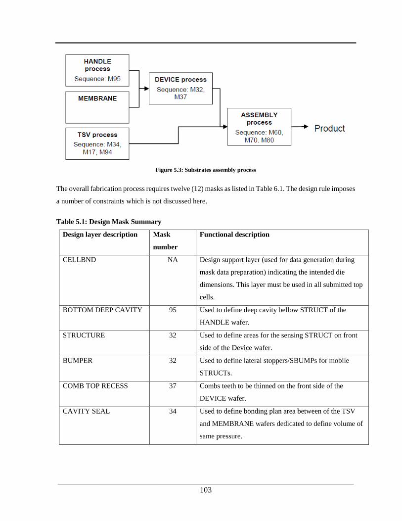
___________________________________________________________________________
103
Figure 5.3: Substrates assembly process
The overall fabrication process requires twelve (12) masks as listed in Table 6.1. The design rule imposes
a number of constraints which is not discussed here.
Table 5.1: Design Mask Summary
Design layer description Mask
number
Functional description
CELLBND NA Design support layer (used for data generation during
mask data preparation) indicating the intended die
dimensions. This layer must be used in all submitted top
cells.
BOTTOM DEEP CAVITY 95 Used to define deep cavity bellow STRUCT of the
HANDLE wafer.
STRUCTURE 32 Used to define areas for the sensing STRUCT on front
side of the Device wafer.
BUMPER 32 Used to define lateral stoppers/SBUMPs for mobile
STRUCTs.
COMB TOP RECESS 37 Combs teeth to be thinned on the front side of the
DEVICE wafer.
CAVITY SEAL 34 Used to define bonding plan area between of the TSV
and MEMBRANE wafers dedicated to define volume of
same pressure.
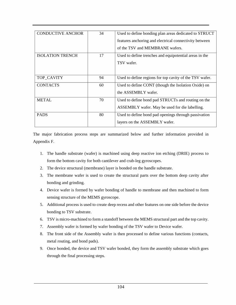
___________________________________________________________________________
104
CONDUCTIVE ANCHOR 34 Used to define bonding plan areas dedicated to STRUCT
features anchoring and electrical connectivity between
of the TSV and MEMBRANE wafers.
ISOLATION TRENCH 17 Used to define trenches and equipotential areas in the
TSV wafer.
TOP_CAVITY 94 Used to define regions for top cavity of the TSV wafer.
CONTACTS 60 Used to define CONT (though the Isolation Oxide) on
the ASSEMBLY wafer.
METAL 70 Used to define bond pad STRUCTs and routing on the
ASSEMBLY wafer. May be used for die labelling.
PADS 80 Used to define bond pad openings through passivation
layers on the ASSEMBLY wafer.
The major fabrication process steps are summarized below and further information provided in
Appendix F.
1. The handle substrate (wafer) is machined using deep reactive ion etching (DRIE) process to
form the bottom cavity for both cantilever and crab-leg gyroscopes.
2. The device structural (membrane) layer is bonded on the handle substrate.
3. The membrane wafer is used to create the structural parts over the bottom deep cavity after
bonding and grinding.
4. Device wafer is formed by wafer bonding of handle to membrane and then machined to form
sensing structure of the MEMS gyroscope.
5. Additional process is used to create deep recess and other features on one side before the device
bonding to TSV substrate.
6. TSV is micro-machined to form a standoff between the MEMS structural part and the top cavity.
7. Assembly wafer is formed by wafer bonding of the TSV wafer to Device wafer.
8. The front side of the Assembly wafer is then processed to define various functions (contacts,
metal routing, and bond pads).
9. Once bonded, the device and TSV wafer bonded, they form the assembly substrate which goes
through the final processing steps.
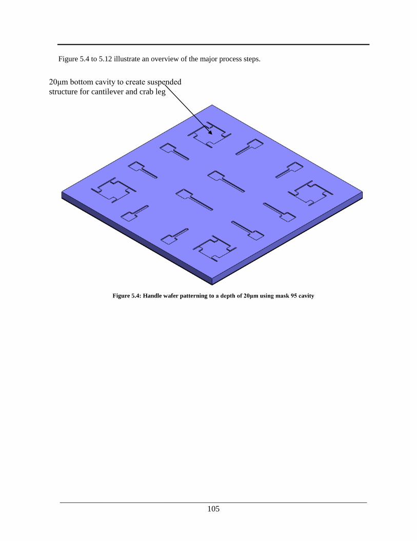
___________________________________________________________________________
105
Figure 5.4 to 5.12 illustrate an overview of the major process steps.
Figure 5.4: Handle wafer patterning to a depth of 20μm using mask 95 cavity
20μm bottom cavity to create suspended
structure for cantilever and crab leg

___________________________________________________________________________
106
Figure 5.5: Device layer is patterned using a combination of mask 32 and 37
Figure 5.6: crab-leg sense and drive electrodes defined using mask 32 and 37

___________________________________________________________________________
107
Figure 5.7: Second bonding plane definition using mask 34 to creates a 2μm deep spacer between device TSV wafers
Figure 5.8: Second bonding plane definition using mask 34

___________________________________________________________________________
108
Figure 5.9: Cross-section view of final stack
.
Figure 5.10: Second bonding plane definition using mask 34
Cross section of crab
leg figure electrodes
Electrical
contact
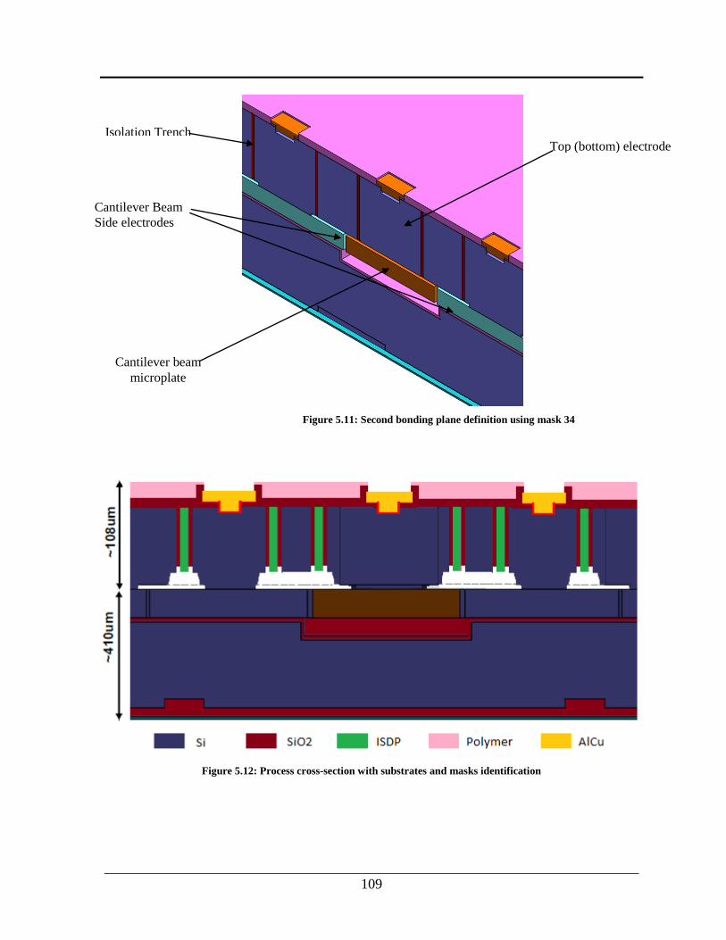
___________________________________________________________________________
109
Figure 5.11: Second bonding plane definition using mask 34
Figure 5.12: Process cross-section with substrates and masks identification
Top (bottom) electrode
Cantilever Beam
Side electrodes
Isolation Trench
Cantilever beam
microplate
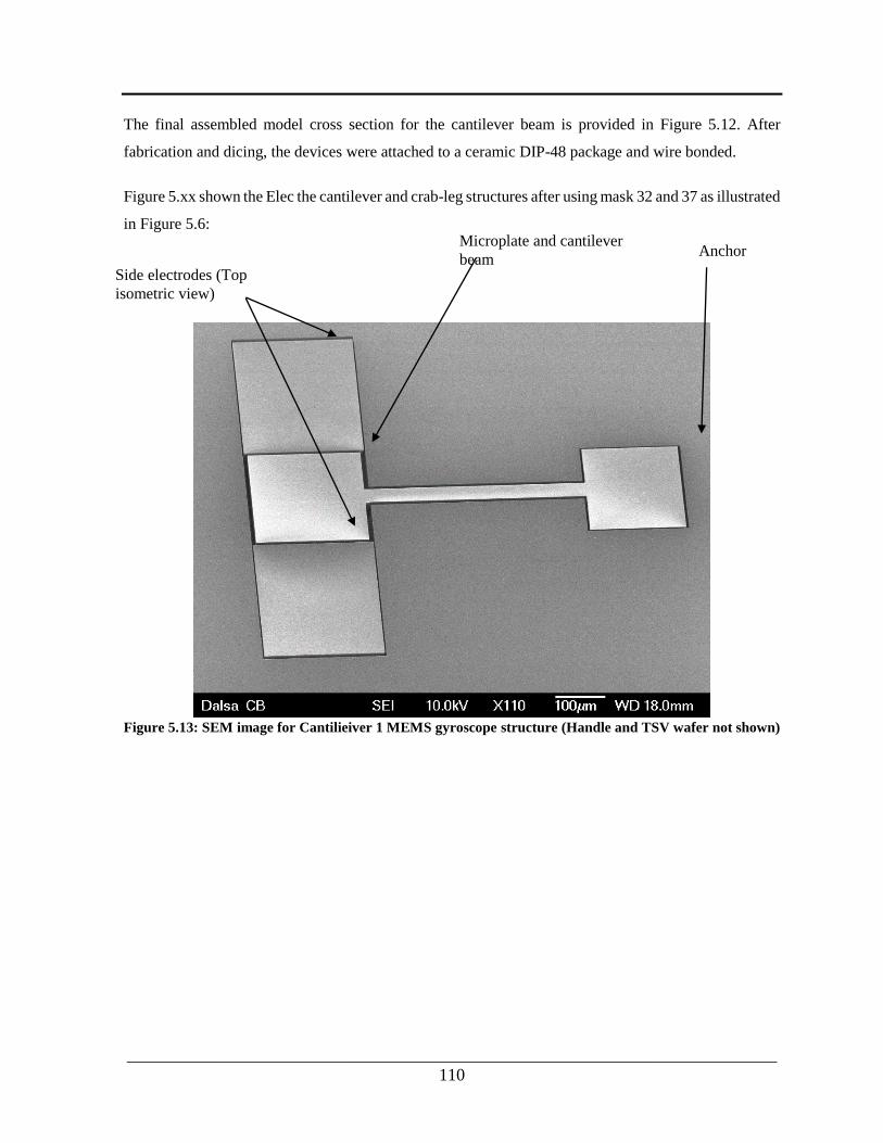
___________________________________________________________________________
110
The final assembled model cross section for the cantilever beam is provided in Figure 5.12. After
fabrication and dicing, the devices were attached to a ceramic DIP-48 package and wire bonded.
Figure 5.xx shown the Elec the cantilever and crab-leg structures after using mask 32 and 37 as illustrated
in Figure 5.6:
Figure 5.13: SEM image for Cantilieiver 1 MEMS gyroscope structure (Handle and TSV wafer not shown)
Side electrodes (Top
isometric view)
Microplate and cantilever
beam Anchor
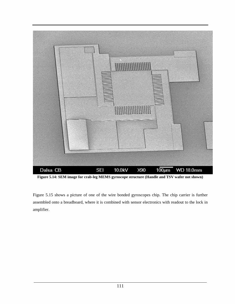
___________________________________________________________________________
111
Figure 5.14: SEM image for crab-leg MEMS gyroscope structure (Handle and TSV wafer not shown)
Figure 5.15 shows a picture of one of the wire bonded gyroscopes chip. The chip carrier is further
assembled onto a breadboard, where it is combined with sensor electronics with readout to the lock in
amplifier.
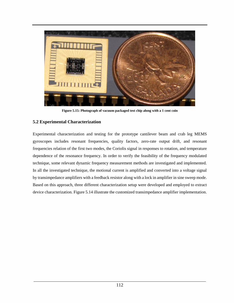
___________________________________________________________________________
112
Figure 5.15: Photograph of vacuum packaged test chip along with a 1 cent coin
5.2 Experimental Characterization
Experimental characterization and testing for the prototype cantilever beam and crab leg MEMS
gyroscopes includes resonant frequencies, quality factors, zero-rate output drift, and resonant
frequencies relation of the first two modes, the Coriolis signal in responses to rotation, and temperature
dependence of the resonance frequency. In order to verify the feasibility of the frequency modulated
technique, some relevant dynamic frequency measurement methods are investigated and implemented.
In all the investigated technique, the motional current is amplified and converted into a voltage signal
by transimpedance amplifiers with a feedback resistor along with a lock in amplifier in sine sweep mode.
Based on this approach, three different characterization setup were developed and employed to extract
device characterization. Figure 5.14 illustrate the customized transimpedance amplifier implementation.
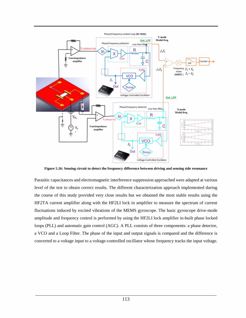
___________________________________________________________________________
113
Figure 5.16: Sensing circuit to detect the frequency difference between driving and sensing side resonance
Parasitic capacitances and electromagnetic interference suppression approached were adapted at various
level of the test to obtain correct results. The different characterization approach implemented during
the course of this study provided very close results but we obtained the most stable results using the
HF2TA current amplifier along with the HF2LI lock in amplifier to measure the spectrum of current
fluctuations induced by excited vibrations of the MEMS gyroscope. The basic gyroscope drive-mode
amplitude and frequency control is performed by using the HF2LI lock amplifier in-built phase locked
loops (PLL) and automatic gain control (AGC). A PLL consists of three components: a phase detector,
a VCO and a Loop Filter. The phase of the input and output signals is compared and the difference is
converted to a voltage input to a voltage-controlled oscillator whose frequency tracks the input voltage.

___________________________________________________________________________
114
5.2.1 Single port Actuation and Detection
The single port excitation and detection technique discussed in chapter 2 is implemented to characterize
the natural frequency, quality factor and rate table test of the prototype devices. Hence, the frequency
response measurement is performed for the drive and sense modes by electrostatically exciting the
system with a sine wave in frequency sweep mode, and capacitive detecting the response simultaneously
using a single port. Swept frequency gain phase analysis was performed using a lock in amplifier which
sweeps the source frequency and records both the amplitude and phase of the received signal. The
excitation and detection are both performed through the electrodes patterned on the structural and TSV
wafers. Figure 5.15 and 5.16 show illustration of the characterization setup and pictures of the
experimental setup for measuring the frequency response.
Figure 5.17: Illustration of the device characterization setup
First characterization was performed to determine the natural frequency for all prototypes developed.
The designed natural frequency values together with the actual device character provide a reference
value where we measure the frequency fluctuation to relate with the input angular rate. The test results
also provide an insight about the process variations and the quality factor of the resonator.
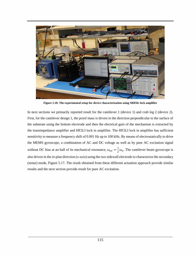
___________________________________________________________________________
115
Figure 5.18: The experimental setup for device characterization using SR850c lock amplifier
In next sections we primarily reported result for the cantilever 1 (device 1) and crab leg 2 (device 2).
First, for the cantilever design 1, the proof mass is driven in the direction perpendicular to the surface of
the substrate using the bottom electrode and then the electrical gain of the mechanism is extracted by
the transimpedance amplifier and HF2LI lock in amplifier. The HF2LI lock in amplifier has sufficient
sensitivity to measure a frequency shift of 0.001 Hz up to 100 kHz. By means of electrostatically to drive
the MEMS gyroscope, a combination of AC and DC voltage as well as by pure AC excitation signal
without DC bias at an half of its mechanical resonance, 𝜔𝑒𝑥 =1
2𝜔𝑜. The cantilever beam gyroscope is
also driven in the in-plan direction (x-axis) using the two sidewall electrode to characterize the secondary
(sense) mode, Figure 5.17. The result obtained from these different actuation approach provide similar
results and the next section provide result for pure AC excitation.
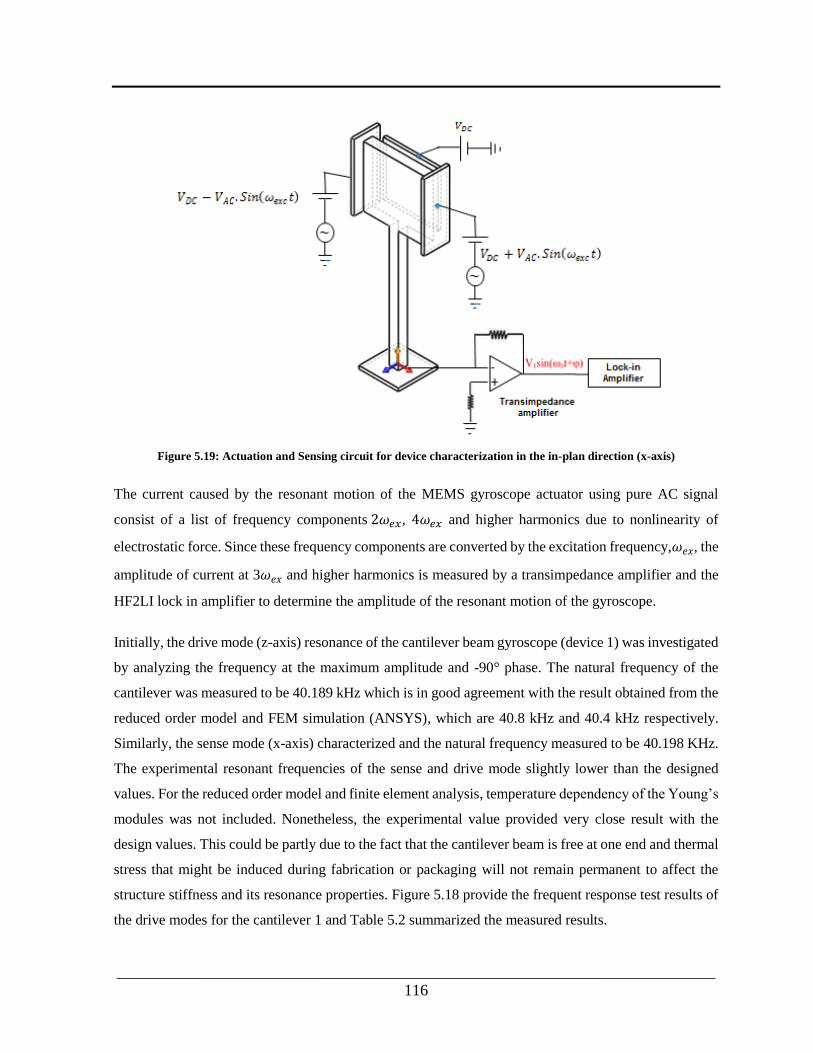
___________________________________________________________________________
116
Figure 5.19: Actuation and Sensing circuit for device characterization in the in-plan direction (x-axis)
The current caused by the resonant motion of the MEMS gyroscope actuator using pure AC signal
consist of a list of frequency components 2𝜔𝑒𝑥, 4𝜔𝑒𝑥 and higher harmonics due to nonlinearity of
electrostatic force. Since these frequency components are converted by the excitation frequency,𝜔𝑒𝑥, the
amplitude of current at 3𝜔𝑒𝑥 and higher harmonics is measured by a transimpedance amplifier and the
HF2LI lock in amplifier to determine the amplitude of the resonant motion of the gyroscope.
Initially, the drive mode (z-axis) resonance of the cantilever beam gyroscope (device 1) was investigated
by analyzing the frequency at the maximum amplitude and -90° phase. The natural frequency of the
cantilever was measured to be 40.189 kHz which is in good agreement with the result obtained from the
reduced order model and FEM simulation (ANSYS), which are 40.8 kHz and 40.4 kHz respectively.
Similarly, the sense mode (x-axis) characterized and the natural frequency measured to be 40.198 KHz.
The experimental resonant frequencies of the sense and drive mode slightly lower than the designed
values. For the reduced order model and finite element analysis, temperature dependency of the Young’s
modules was not included. Nonetheless, the experimental value provided very close result with the
design values. This could be partly due to the fact that the cantilever beam is free at one end and thermal
stress that might be induced during fabrication or packaging will not remain permanent to affect the
structure stiffness and its resonance properties. Figure 5.18 provide the frequent response test results of
the drive modes for the cantilever 1 and Table 5.2 summarized the measured results.

___________________________________________________________________________
117
Figure 5.20: Measured frequency response for Cantilever 1 gyroscope in the drive direction
Table 5.2: Testing and simulation results of the fundamental parameters of cantilever 1
Test Parameter Drive mode Sense mode
ROM/FEA ROM/FEA
Actuation Voltage 15 Vpp 15 Vpp
Sweep frequency 38 kHz to 42 kHz 38 kHz to 42 kHz
Parasitic capacitance 3.5 pF 3.5 pF
Natural frequency 40.189 kHz 40.8/40.4 kHz 41.191 KHz 40.8/40.4 kHz
Qaulity factor ~1850 ~1800
Pull-in voltage 45.0 V 45.25 /45.2 V 41.191 V 45.25 /45.2 V
___________________________________________________________________________
118
The quality factor characterization provided different results through the course of the test due to
potential device leaking or outgassing. Initially, the cantilever drive mode quality (Q) factors found to
be above 1850 and start to decrease as the time progress. In order to investigate the quality factor issue
a second version of both the cantilever and crab leg design is currently in fabrication.
A series of other cantilever prototype designs were also tested and the first to mode natural frequencies
in the z and x directions are well matched with less than 0.1% deviation with the design values. All the
other cantilever beam gyroscope design characterized and test results are summarized in Appendix G.
The measured natural frequencies are in good agreement with simulated result using the reduced order
model. Figure 5.19 show the zicontrol software screen shot for cantilever beam device #3 which has the
same geometric dimension as device #1 except its length, which is 388𝜇𝑚. The resonance frequent
measured to be 45.050 kHz in a good agreement with the design values, Appendix G. The zicontrol
software conveniently used to setup test parameters for the HF2TA current amplifier and HF2LI lock in
amplifier using the graphical window interface, as shown in Figure 5.19.

___________________________________________________________________________
119
Figure 5.21: zicontrol screen shot for the cantilever beam design 3
5.2.2 Crab-Leg Characterization
A similar single port test setup and procedure was adapted for the crab leg characterization. The crab-
leg gyroscopes natural frequencies and quality factor were characterized in the sense and drive direction
using the comb finger drive and sense electrodes. The drive mode was electrostatically excited with an
actuation voltage, Ves(t) = Vpp· Sin (ωexc t), in a swept mode, produced by HF2LI lock in amplifier
internal signal generator. This is done exciting the crab-leg gyroscopes with a pure AC signal over a
range of sweep frequencies and recording the amplitude vs. frequency and phase vs. frequency curves,
Figure 5.20.
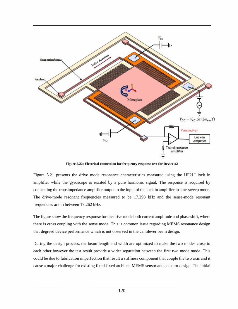
___________________________________________________________________________
120
Figure 5.22: Electrical connection for frequency response test for Device #2
Figure 5.21 presents the drive mode resonance characteristics measured using the HF2LI lock in
amplifier while the gyroscope is excited by a pure harmonic signal. The response is acquired by
connecting the transimpedance amplifier output to the input of the lock in amplifier in sine-sweep mode.
The drive-mode resonant frequencies measured to be 17.293 kHz and the sense-mode resonant
frequencies are in between 17.262 kHz.
The figure show the frequency response for the drive mode both current amplitude and phase shift, where
there is cross coupling with the sense mode. This is common issue regarding MEMS resonance design
that degreed device performance which is not observed in the cantilever beam design.
During the design process, the beam length and width are optimized to make the two modes close to
each other however the test result provide a wider separation between the first two mode mode. This
could be due to fabrication imperfection that result a stiffness component that couple the two axis and it
cause a major challenge for existing fixed-fixed architect MEMS sensor and actuator design. The initial

___________________________________________________________________________
121
quality factor of the drive mode is measured to be 3000 and as in the case of the cantilever beam the
quality factor degrade over the course of this work.
Figure 5.23: Measured frequency response for Crab leg (Device #2) drive mode
Figure 5.22 show the zicontrol software screen shot for crab leg Device #2, which is also plotted in
figure 5.21. As shown in Figure 5.21, the quality factor degraded to 313 indicating an order of magnitude
reduction.
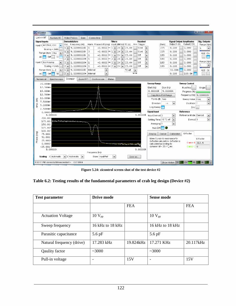
___________________________________________________________________________
122
Figure 5.24: zicontrol screen shot of the test device #2
Table 6.2: Testing results of the fundamental parameters of crab leg design (Device #2)
Test parameter Drive mode Sense mode
FEA FEA
Actuation Voltage 10 Vpp 10 Vpp
Sweep frequency 16 kHz to 18 kHz 16 kHz to 18 kHz
Parasitic capacitance 5.6 pF 5.6 pF
Natural frequency (drive) 17.283 kHz 19.824kHz 17.271 KHz 20.117kHz
Qaulity factor ~3000 ~3000
Pull-in voltage - 15V - 15V

___________________________________________________________________________
123
Similarly for the finite element analysis, temperature dependency of the Young’s modules was not
included. However, the experimental result provided a slightly more variation with the design result
compared with the cantilever beam. This could be due to packaging or thermally induced stress that
occurred in fixed-fixed MEMS structure that we initially outline to address. The reduced order model
and FEM analysis result verified using the other twelve (12) other cantilever and crab leg designs and
the result are summarized in Appendix G.
5.3 Rate Table Test
Similarly, single port excitation and sensing approach were used for the prototype gyroscope rate table
test. The prototype gyroscope and signal detecting electronics were mounted on an ARMS-200 Rotary
Motion Simulator which is controlled by Soloist HLe controller. HF2LI used for single and double mode
detection which offers key features including a built-in signal modulation and demodulation at several
frequencies in parallel and incorporate PLLs and PID for frequency amplitude control an. Single port
connection of the HF2LI is illustrated in Figure 5.23. A series of test were performed both for the
cantilever and crab leg MEMS gyroscope input rate ranging from 0 to 1500 deg/sec, limited by ARMS-
200 Rotary Motion rate table.
Figure 5.25: The experimental illustration for rate table (rate table not shown here)
For the drive-mode control, the oscillation of the vibratory gyroscope is maintained at resonance by
means of a PLL. The drive-mode of the gyroscope is connected to input and output of the HF2LI.
Furthermore, the mechanical amplitude is kept constant using a PID controller. For electrostatic
actuation, an offset (VOffset) is applied to the drive signal. This offset was added with function generator

___________________________________________________________________________
124
or by using the Add connector on the HF2LI front panel, depending on the voltage requirement for the
cantilever beam gyroscope.
Figure 5.26: The experimental setup for rate-table characterization
In this test results, the microplate is driven by a pure AC signal without DC bias, which is amplified by
the high voltage amplifier, Tabor 9400. While both sidewall electrodes are grounded, its bottom
electrode is connected to the virtual ground of the transimpedance amplifier to measure the current
flowing through the microplate and the bottom electrode. The amplitude of the current and phase shift
measured by the lock in amplifier, Zurich Instrument HF2LI. The spectrum analyzer, Agilent N9010A,
is also used to observe the frequency components of the measured current in real time.
Current signal output from the device was processed in real-time using the HF2TA current amplifier
along with HF2LI lock in amplifier. The shift in the resonant frequency of the cantilever-based
gyroscope due to angular speed is measured. As theoretically expected for a single-axis gyroscope, the
shift in the natural frequency for both the drive and sense axis measured to be linearly proportional to
the input rate, Figure 5.25. At the rotational speed of 1500 deg/sec along the drive axis, the shift in the
resonant frequency was found to be 4.2 Hz. The FM gyroscope demonstrates less than 0.05 %
nonlinearity throughout the entire range.
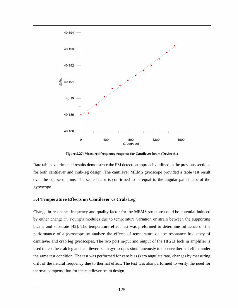
___________________________________________________________________________
125
Figure 5.27: Measured frequency response for Cantilever beam (Device #1)
Rate table experimental results demonstrate the FM detection approach outlined in the previous sections
for both cantilever and crab-leg design. The cantilever MEMS gyroscope provided a table test result
over the course of time. The scale factor is confirmed to be equal to the angular gain factor of the
gyroscope.
5.4 Temperature Effects on Cantilever vs Crab Leg
Change in resonance frequency and quality factor for the MEMS structure could be potential induced
by either change in Young’s modules due to temperature variation or strain between the supporting
beams and substrate [42]. The temperature effect test was preformed to determine influence on the
performance of a gyroscope by analyze the effects of temperature on the resonance frequency of
cantilever and crab leg gyroscopes. The two port in-put and output of the HF2LI lock in amplifier is
used to test the crab leg and cantilever beam gyroscopes simultaneously to observe thermal effect under
the same test condition. The test was performed for zero bias (zero angulate rate) changes by measuring
drift of the natural frequency due to thermal effect. The test was also performed to verify the need for
thermal compensation for the cantilever beam design.
___________________________________________________________________________
126
The actuation and sense method implemented in the previous section were used to drive the gyroscope
for testing its resonant frequency and the quality factor under the temperature change from 22 °C (room
temperature) to 110 °C using the open loop testing scheme using the following procedure
1. The gyroscope and the circuit are statically mounted on the hot plate during the course of
measurement
2. The temperature value of the hot plate raised from 22 °C to 110 °C in 10 °C increment
3. The temperature at each sampling point is maintained for 25 minutes before testing to ensure
that the temperature on the hotplate and the gyroscope is fully heated uniformly.
4. Additional external temperature measurement was done using Infrared thermal measurement
unit to insure uniform thermal distribution
5. The lock in amplifier (or function generator) provides the sinusoidal signal to drive the
gyroscope, as in the previous cases.
6. Both the crab-leg and cantilever beam gyroscope current output is connected to the current and
lock in amplifier.
7. By sweeping the frequency of excitation signal, the frequency response of vibrating amplitude
and frequency recorded, so its peak of the frequency response is just the resonant frequency
(𝜔𝑛) and its quality factor Q can be measured directly from the HF2LI lock in amplifier
Test result provided in Table 5.4 indicate that the natural frequency shift. Experiment data analyzed
while the sample gyroscope excited with a pure harmonic signal at 10 Vpeak. We used a 5th order
polynomial to fit the measurement data in order to find the resonant frequencies and the quality factors
of cantilever and crab-leg gyroscope at different temperature oC. So, based on these experiment data, the
mechanical resonance and the quality factor of the gyroscope slightly decrease as its temperature
increases.
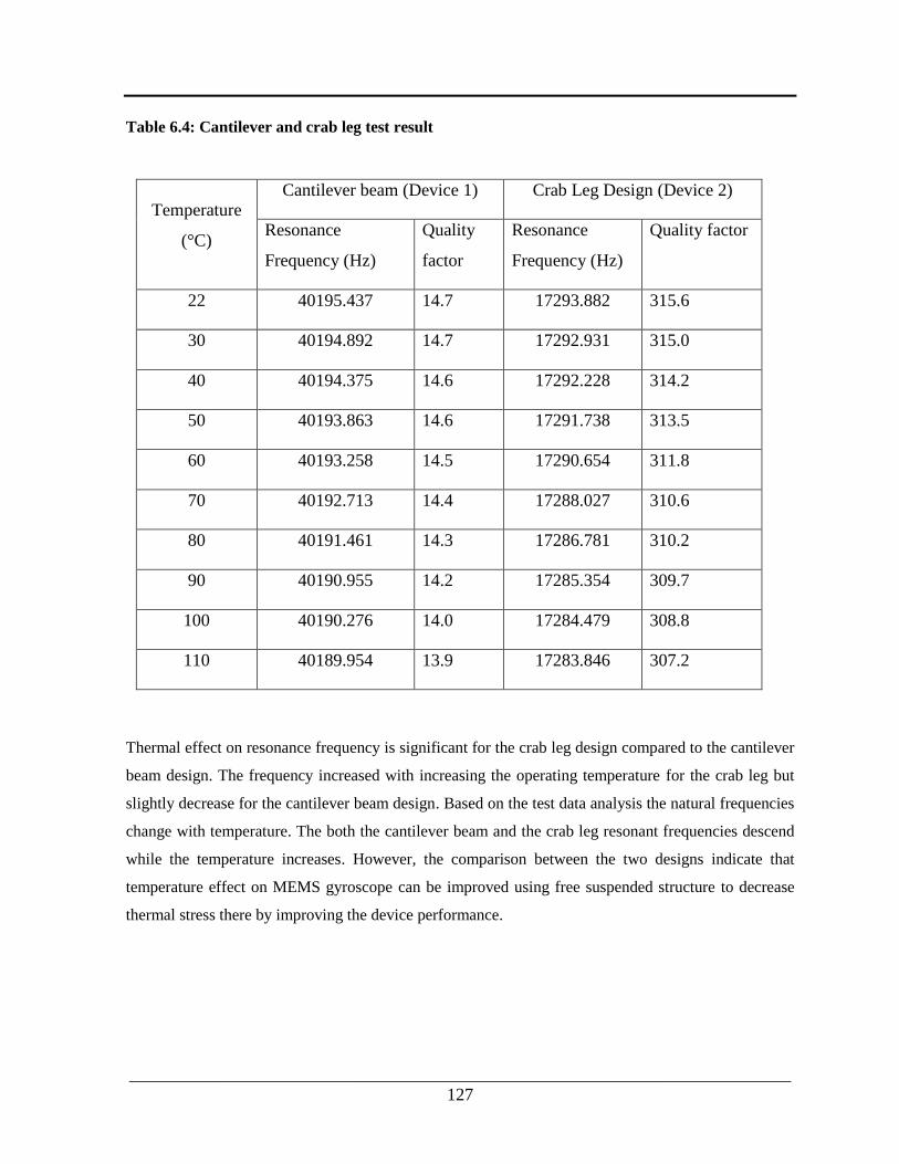
___________________________________________________________________________
127
Table 6.4: Cantilever and crab leg test result
Temperature
(°C)
Cantilever beam (Device 1) Crab Leg Design (Device 2)
Resonance
Frequency (Hz)
Quality
factor
Resonance
Frequency (Hz)
Quality factor
22 40195.437 14.7 17293.882 315.6
30 40194.892 14.7 17292.931 315.0
40 40194.375 14.6 17292.228 314.2
50 40193.863 14.6 17291.738 313.5
60 40193.258 14.5 17290.654 311.8
70 40192.713 14.4 17288.027 310.6
80 40191.461 14.3 17286.781 310.2
90 40190.955 14.2 17285.354 309.7
100 40190.276 14.0 17284.479 308.8
110 40189.954 13.9 17283.846 307.2
Thermal effect on resonance frequency is significant for the crab leg design compared to the cantilever
beam design. The frequency increased with increasing the operating temperature for the crab leg but
slightly decrease for the cantilever beam design. Based on the test data analysis the natural frequencies
change with temperature. The both the cantilever beam and the crab leg resonant frequencies descend
while the temperature increases. However, the comparison between the two designs indicate that
temperature effect on MEMS gyroscope can be improved using free suspended structure to decrease
thermal stress there by improving the device performance.
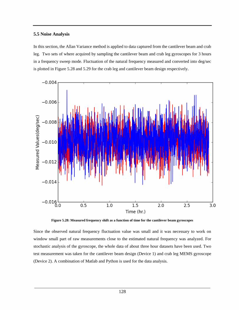
___________________________________________________________________________
128
5.5 Noise Analysis
In this section, the Allan Variance method is applied to data captured from the cantilever beam and crab
leg. Two sets of where acquired by sampling the cantilever beam and crab leg gyroscopes for 3 hours
in a frequency sweep mode. Fluctuation of the natural frequency measured and converted into deg/sec
is plotted in Figure 5.28 and 5.29 for the crab leg and cantilever beam design respectively.
Figure 5.28: Measured frequency shift as a function of time for the cantilever beam gyroscopes
Since the observed natural frequency fluctuation value was small and it was necessary to work on
window small part of raw measurements close to the estimated natural frequency was analyzed. For
stochastic analysis of the gyroscope, the whole data of about three hour datasets have been used. Two
test measurement was taken for the cantilever beam design (Device 1) and crab leg MEMS gyroscope
(Device 2). A combination of Matlab and Python is used for the data analysis.
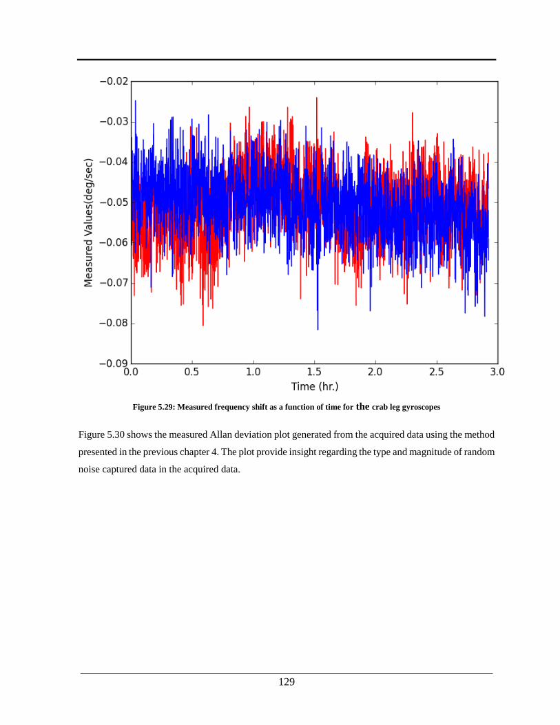
___________________________________________________________________________
129
Figure 5.29: Measured frequency shift as a function of time for the crab leg gyroscopes
Figure 5.30 shows the measured Allan deviation plot generated from the acquired data using the method
presented in the previous chapter 4. The plot provide insight regarding the type and magnitude of random
noise captured data in the acquired data.

___________________________________________________________________________
130
Figure 5:30: Measured Allan variance comparison between cantilever beam FM gyroscopes
From figure 5.30 the Angular Radom Walk (ARW) and the bais instability identifiable by a slope of
−1/2 and the graph low point respectively. The ARW of the cantilever beam and crab leg gyroscopes are
is 0.24 and 1.25 deg/h/√Hz, respectively. The bias stabilities of the cantilever beam and crab leg
gyroscopes are 30 and 69 /hr at 100 and 27 s averaging time, respectively. Noise performance of the
FM sensor is limited by the frequency stability of the two modes of vibration in the gyroscope. The
cantilever beam measured with better ARW as well as bias stabilities providing further advantage over
the fixed-fixed type of the crab leg design.
100
101
102
103
101
102
103
Overlapping Allan Deviation: lt data (2 Hz)
[sec]
Ove
rla
pp
ing
y(
)

___________________________________________________________________________
131
Figure 5.31: Measured Allan variance comparison between crab leg FM gyroscopes
100
101
102
103
101
102
103
Overlapping Allan Deviation: lt data (2 Hz)
[sec]
Ove
rla
pp
ing
y(
)
___________________________________________________________________________
132
CHAPTER VI
Summary and Conclusions
Two MEMS gyroscope devices were developed based the FM detection method, one a novel cantilever
beam design and the other a traditional crab-leg technology. The crab-leg gyroscope served as a direct
comparison against the cantilever beam design, providing baseline performance data under the same test
conditions. A new methodology for the design and analysis of FM MEMS gyroscopes was formulated
and applied to the design and fabrication of both prototypes. The design emphasis was on the
investigation of device dynamics and demonstration of the proof of concept. The working principle and
dynamic output characteristics of the FM detection method for MEMS gyroscope devices were
introduced, providing a theoretical basis for analyzing the dynamic frequency output characteristics of
resonant vibratory gyroscopes.
The cantilever beam and a crab-leg designs were modeled and analyzed, along with suspended mass. A
nonlinear model of the cantilever beam MEMS gyroscope was presented, considering electrostatic and
Coriolis forces. The system governing equations were solved using a reduced order model, and FEM
simulation was performed to verify the result. The effects of changing input excitation parameters on
the performance of the gyroscope were investigated.
Based on the design, a prototype device was fabricated using the Teledyne Dalsa MEMS Integrated
Design for Inertial Sensors (MIDIS™) Process. Furthermore, three different characterization and test
setups were investigated and implemented for resonance operation of the drive and sense mode
resonator. A frequency measurement method based on dynamic output characteristics was implemented
to investigate the modulated output signal of the resonant vibratory gyroscope. A characterization and
control system for MEMS gyroscopes was performed mainly using commercially available hardware
and software.
The results of the proof of concept analysis and the advantages of cantilever beam gyroscopes over
traditional fixed-fixed designs are discussed in chapter five. The resulting benefits include simpler
dynamics and control, improved scale factor stability over micromechanical gyroscopes utilizing open-
___________________________________________________________________________
133
loop displacement sensing, and large dynamic range. The cantilever beam MEMS gyroscope also
demonstrated lower angular random walk and bias instability, which helps minimize error sources that
corrupt the Coriolis signal. Thermal testing of the sample device demonstrated that the amplitude and
frequency fluctuant for both cantilever and crab leg design. However, the cantilever beam gyroscope
performed much better and was less affected by thermal change to the environment. Addressing thermal
effects in MEMS gyroscope design could potentially yield reliable, robust and high-performance
devices, leading to a wide range of applications including dynamic vehicle control, automotive safety
systems, navigation/guidance systems, and interactive consumer electronics.
While it was not experimentally verified, the cantilever beam MEMS gyroscope design is expected to
reject vibrations (by sensing the orthogonally arranged secondary gyroscope), which is one of the major
sources of error for MEMS devices. This is mainly because the cantilever cannot vibrate along the
longitudinal direction, a phenomenon that can be used to improve device performance by measuring
orthogonally arranged cantilever gyroscopes and adapt sensor fusion. The single port detection FM
detection method was reported for the first time in this work, and showed a clear benefit to determining
the input rate angle (by observing a single axis (drive) motion output), which could potentially solve
cross-axis sensitivity (a common MEMS gyroscope error source).
6.1 Contributions and Outcome of This Work
This study explored novel sensing and design concepts for MEMS gyroscopes that provide inherent
robustness against structural and thermal parameter variations, and require less demanding active
compensation schemes. This work focuses on system level contributions to the characterization and
control of MEMS gyroscopes. The primary contributions include:
Investigation of the natural frequency shift sensing method for MEMS cantilever beam
gyroscopes. The mathematical model of the cantilever beam carrying a rigid body is developed.
To derive the mathematical model, the kinetic energy of the structure under spatial rotation and
deformation is computed.
Demonstration of MEMS gyroscope operation in frequency modulation mode and investigation
of the MEMS gyroscope modal frequencies. The application of the proposed system in the
frequency-modulation mode is demonstrated by experimental method the input rotation rate as
the function of the modal frequencies. In practice, the modal frequencies are measured and the
rotation rate is computed from the equation.
___________________________________________________________________________
134
Mathematical models for the beam-rigid body gyroscope, considering the static behaviour of
the beam-rigid body MEMS gyroscope and study the reduced-order nonlinear behaviour of the
system,
Analysis of the device’s nonlinear behaviour using Finite Element software (ANSYS) and
comparison to the results of the method with the reduced order model results. A finite element
analysis of the structure provides an insight to the performance and design of the MEMS sensor
and result in a better design before going to the experimentation phase.
The impact of mechanical-thermal noise effects on frequency modulated MEMS gyroscopes
was studied.
The fabrication and experimental verification of the cantilever beam MEMS gyroscope,
demonstrating the frequency modulated MEMS gyroscope concept. The results provide a basis
for further improvement of the design and performance of the beam-based rotation rate sensors.
Development of a characterization method that measures the frequency of the MEMS
gyroscope’s two modes
6.2 Recommendations for Future Work
We implemented the single port FM detection and control system using commercially available
hardware and software. An off the shelf HF2TA current amplifier and HF2LI lock in amplifier were
used to measure the spectrum of current fluctuations, allowing us to obtain the most stable test results.
The characterization setup could potentially be improved by using PCB board design with a stable
transimpedance amplifier with a similar gain as the HF2TA current amplifier. Furthermore, future
research must be undertaken to develop FM detection circuitry using CMOS-based single mode
detection architecture for commercialization and batch fabrication.
Temperature remains one of the major challenges impeding MEMS inertial sensor performance. While
the cantilever design demonstrated improved performance for thermal fluctuation, additional innovative
structural designs, operational principles and fabrication processes could be explored to ultimately
develop a navigation-grade MEMS gyroscope unit. During the course of this study various fabrication
techniques were explored, including those for cantilever beam designs with large suspended masses, to
enhance the sensor robustness and increase capacitive sensitivity (by increasing area). We also
___________________________________________________________________________
135
developed a microfabrication process for the new design architecture, but could not implement it due to
limited fabrication access. This work could be significantly advanced in collaboration with industry,
enabling realization of a robust design that could potentially provide inherently better noise and
sensitivity due to larger masses and larger capacitances.
A thorough design optimization was performed to find the best parameters for selecting a fabrication
platform for our cantilever gyroscope, ensuring the best system performance is obtained. This work
could benefit with a system level optimization study, taking broader gyroscope performance metrics into
account. In conclusion, this study presents one possible method to improve MEMS gyroscope
performance using structural design and sensing approach technical.
___________________________________________________________________________
136
References
[1] N. Yazdi, F. Ayazi, and K. Najafi "Micromachined Inertial Sensors" Proceeding of IEEE, Vol.
86, No. 8, August 1998, pp. 136-147.
[2] C. Acar and A. M. Shkel "Structural design and experimental characterization of torsional
micromachined gyroscopes with non-resonant drive mode" Journal of micromechanics and
microengineering, 14 (2004) 15-25.
[3] H. Xie and G. K. Fedder "Integrated Microelectromechanical Gyroscopes" Journal of Aerospace
Engineering, Vol. 16, No. 2, April 2003, pp. 65-75.
[4] N. Barbour, and G. Schmidt "Inertial Sensor Technology Trends" IEEE Sensors Journal, Vol. 1,
No. 4, Dec 2001, pp. 332-339.
[5] IEEE-952 "IEEE Standard Specification Format Guide and Test Procedure for Single-Axis
Interferometric Fiber Optic Gyros" December 2008.
[6] P. Greiff, B. Boxenhorn, T. King, and L. Niles "Silicon monolithic micromechanical gyroscope"
Tech. Dig. 6th Int. Conf. Solid-State Sensors and Actuators, San Francisco, CA, June 1991, pp.
966-968.
[7] G. B. Malykin "The Sagnac effect: correct and incorrect explanations" Physics-Uspekhi 43, 1229–
1252 (2000).
[8] E. Alper and T. Akin "A symmetric surface micromachined gyroscope with decoupled oscillation
modes" Sensors and Actuators, (2004) 347-358.
[9] Y. S. Hong, J. H. Lee and S. H. Kim "A lateraly driven symmetric micro resonator for gyroscopic
applications" Journal of Micromachining and Microengineering, 10 (2000) 452-458.
[10] C. Jeong "A study on resonant frequency and Q factor tunings for MEMS vibratory gyroscopes"
Journal of micromechanics and microengineering, 14 (2004) 1530-1536.
[11] M. Esmaeili, N. Jalili, and M. Durali "Dynamic modeling and performance evaluation of a
vibrating beam microgyroscope under general support motion" Journal of Sound and Vibration
301 (2007) 146–164
[12] G.L. Anderson "Natural frequencies of a cantilever with an asymmetrically attached tip mass"
AIAA Journal 16 (1978) 281–282.
___________________________________________________________________________
137
[13] M.R.M. Crespo da Silva and C.C. Glynn "Nonlinear Flexural-Flexural-Torsional Dynamics of
Inextensional Beams: I. Equations of Motion" Journal of Structural Mechanics, 6(4), 437-448.
[14] Bhadbhade V. and Jalili N "Modeling and Vibration Analysis of Cantilever-based Rocking Mass
Gyroscope" Proceedings of 2006 ASME International Mechanical Engineering Congress &
Exposition, Chicago, IL.
[15] Takaway T., Fukudaz T. and Takadaz T "Flexural–Torsion Coupling Vibration Control of Fiber
Composite Cantilevered Beam by Using Piezoceramic Actuators" Smart Materials and Structures,
6, 477-484.
[16] M. W. Putty and K. Najafi "A micromachined vibrating ring gyroscope" Tech. Dig. Solid-State
Sens. Actuator Workshop, Hilton Head Island, SC, June 1994, pp. 213-220.
[17] Hopkin, I. D. "Vibrating gyroscopes (automotive sensors)". IEEE Colloquium on Automotive
Sensors. Digest No. 1994/170. Solihull, UK, Sept. 1994, pp. 1-4.
[18] Tanaka, K., Mochida, Y., Sugimoto, S., Moriya, K., Hasegawa, T., Atsuchi, K., and Ohwada, K.
"A micromachined vibrating gyroscope". Proc., Eighth IEEE Int. Conf. on Micro Electro
Mechanical Systems (MEMS ’95), Amsterdam, Netherlands, Jan. 1995, pp. 278-281.
[19] Clark, W. A., Howe, R. T., and Horowitz, R. "Surface micromachined Z-axis vibratory rate
gyroscope" Technical Digest. Solid-State Sensor and Actuator Workshop, Hilton Head Island,
S.C., June 1996, pp. 283-287.
[20] A. Seshia, R. Howe, and S. Montague, “An Integrated Microelectromechanical Resonant-Output
Gyroscope” IEEE MEMS 2002, Las Vegas, NV, pp. 722-726, 2002.
[21] Juneau, T., Pisano, A. P., and Smith, J. H. "Dual axis operation of a micromachined rate
gyroscope" Proc., IEEE 1997 Int. Conf. on Solid State Sensors and Actuators (Tranducers ’97),
Chicago, June 1997, pp. 883-886.
[22] Lutz M., Golderer W., Gerstenmeier J., Marek J., Maihofer B., Mahler S., Munzel H., and Bischof
U. "A precision yaw rate sensor in silicon micromachining" Transducers 1997, Chicago, IL, June
1997, pp. 847-850.
[23] Moussa, H. and Bourquin, R.: "Theory of direct frequency output vibrating gyroscopes" IEEE
Sensors Journal, vol. 6, pp. 310-315, 2006.

___________________________________________________________________________
138
[24] Albrecht T. R., Gru¨tter P., Horne D., and Rugar D., "Frequency modulation detection using
high‐Q cantilevers for enhanced force microscope sensitivity" Journal of Applied Physics.
69(2), 668 (1991).
[25] Abe, M., Shinohara, E., Hasegawa, K., Murata, S. and Esashi, M. "Trident-type tuning fork silicon
gyroscope by the phase difference detection. In: Proceedings of the 13th IEEE International
Conference on Microelectromechanical Systems" pp. 508- 513. 2000.
[26] Sangtak Park, Mahmoud Khater, David Effa, Eihab Abdel-Rahman, and Mustafa Yavuz
"Detection of Cyclic-Fold Bifurcation in Electrostatic Transducers by Motion-Induced Current"
Journal of Micromechanics and Microengineering, Volume 27, Number 8, 2017.
[27] John, J., Jakob, C., Vinay, T. and Qin, L. "Phase differential angular rate sensor concept and
analysis" IEEE Sensors Journal, vol. 4, pp. 471-478, 2004.
[28] Yang, H., Bao, M., Yin, H. and Shen, S. "Two-dimensional excitation operation mode and phase
detection scheme for vibratory gyroscopes" Journal of Micromechanics and Microengineering,
vol. 12, pp. 193-197, 2002.
[29] S.A. Zotov, I.P. Prikhodko, A.A. Trusov, and A.M. Shkel, “Frequency Modulation Based Angular
Rate System” Proc. IEEE MEMS, Cancun, Mexico, January 23 - 27, 2011.
[30] Xie, L.; Xiao, D.; Wang, H.; Wu, X.; Li, S. Sensitivity Analysis and Structure Design for Tri-
Mass Structure Micromachined Gyroscope. In Proceedings of the 2009 4th IEEE International
Conference on Nano/Micro Engineered and Molecular Systems, Shenzhen, China, 5–8 January
2009; pp. 126–129.
[31] D. R. Sparks, S. R. Zarabadi, J. D. Johnson, Q. Jiang, M. Chia, O. Larsen, W. Higdon, and P.
Castillo-Borelley. "A CMOS integrated surface micromachined angular rate sensor: It’s
automotive applications" Tech. Dig. 9th Int. Conf. Solid-State Sensors and Actuators
(Transducers’97), Chicago, IL, June 1997, pp. 851-854.
[32] Y. Oh, B. Lee, S. Baek, H. Kim, J. Kim, S. Kang, and C. Song. "A surface micromachined tunable
vibratory gyroscope" Proc. IEEE Micro Electro Mechanical Systems Workshop (MEMS’97),
Japan, 1997, pp. 272-277.
[33] D. Effa, Eihab Abdel-Rahman, and Mustafa Yavuz, "Cantilever Beam Microgyroscope Based on
Frequency Modulation" IEEE/ASME International Conference on Advanced Intelligent
Mechatronics, July 9-12, 2013 Wollongong, Australia.

___________________________________________________________________________
139
[34] K. Y. Park, C. W. Lee, Y. S. Oh, and Y. H. Cho. "Laterally oscillated and force-balanced micro
vibratory rate gyroscope supported by fish hook shape springs" Proceeding IEEE Micro-Electro
Mechanical Systems Workshop (MEMS’97), Japan, 1997, pp. 494-499.
[35] Kourepenis, J. Bernstein, J. Connely, R. Elliot, P. Ward, and M. Weinberg. "Performance of
MEMS inertial sensors" Proceeding IEEE Position Location and Navigation Symposium, 1998,
pp. 1-8.
[36] Mochida, Y., Tamura, M., and Ohwada, K. "A micromachined vibrating rate gyroscope with
independent beams for the drive and detection modes" Proceeding Twelfth IEEE Int. Conf. on
Micro Electro Mechanical Systems (MEMS ’99), Orlando, FL, Jan. 1999, pp. 618-623.
[37] Funk, K., Emmerich, H., Schilp, A., Offenberg, M., Neul, R., and Larmer, F. "A surface
micromachined silicon gyroscope using a thick polysilicon layer" Proceeding Twelfth IEEE Int.
Conf. on Micro Electro Mechanical Systems (MEMS ’99), Orlando, FL, Jan. 1999, pp. 57-60.
[38] Park, K. Y., Jeong, H. S., An, S., Shin, S. H., and Lee, C. W. "Lateral gyroscope suspended by
two gimbals through high aspect ratio ICP etching" Proceeding IEEE 1999 Int. Conf. on Solid
State Sensors and Actuators (Tranducers ’99), Sendai, Japan, June 1999, pp. 972-975.
[39] S. Lee, S. Park, J. Kim, and D. Cho. "Surface/bulk micromachined single crystalline-silicon
micro-gyroscope" IEEE/ASME Journal of Microelectromechanical Systems, Vol.9, No.4 Dec.
2000, pp. 557-567.
[40] Jiang, X., Seeger, J. I., Kraft, M., and Boser, B. E. "A monolithic surface micromachined Z-axis
gyroscope with digital output" Digest of Technical Papers, 2000 Symposium on VLSI Circuits,
Honolulu, June 2000, pp. 16-19.
[41] H. Xie and G. K. Fedder. "A CMOS-MEMS lateral-axis gyroscope" Proceeding 14th IEEE Int.
Conf. Microelectromechanical Systems, Interlaken, Switzerland, Jan. 2001, pp. 162-165.
[42] H. Luo, X. Zhu, H. Lakdawala, L. R. Carley, and G. K. Fedder. "A copper CMOS- MEMS z-axis
gyroscope" Proceeding 15th IEEE Int. Conf. Microelectromechanical Systems, Las Vegas, NV,
Jan. 2001, pp. 631-634.
[43] D. Effa, Eihab Abdel-Rahman, and Mustafa Yavuz, "Analysis of Thermal Noise in Frequency-
Modulated Gyroscopes" IEEE/ASME International Conference on Advanced Intelligent
Mechatronics, November 9-12, 2014 Montreal, Canada.
___________________________________________________________________________
140
[44] W. Geiger, W.U. Butt, A. Gaisser, J. Fretch, M. Braxmaier, T. Link, A. Kohne, P. Nommensen,
H. Sandmaier, and W. Lang. "Decoupled Microgyros and the Design Principle" Sensors and
Actuators A (Physical), Vol. A95, No.2-3, Jan. 2002, pp. 239-249.
[45] J. A. Geen, S. J. Sherman, J. F. Chang, and S. R. Lewis. "Single-chip surface micromachining
integrated gyroscope with 50 deg/hour root Allan variance" Dig. IEEE Int. Solid-State Circuits
Conf., San Francisco, CA, Feb. 2002, pp.426-427.
[46] Seshia, A. A., Howe, R. T., and Montague, S. "An integrated microelectromechanical resonant
output gyroscope" Proc., The Fifteenth IEEE Int. Conf. on Micro Electro Mechanical Systems
(MEMS 2002), Las Vegas, Jan. 2002, pp. 722-726.
[47] G. He and K. Najafi. "A single crystal silicon vibrating ring gyroscope" Proceeding the Fifteenth
IEEE Int. Conf. on Micro Electro Mechanical Systems (MEMS 2002), Las Vegas, Jan. 2002, pp.
718-721.
[48] H. Xie and G. K. Fedder. "Fabrication, Characterization, and Analysis of a DRIE CMOS-MEMS
Gyroscope" IEEE Sensors Journal, Vol. 3, No. 5, 2003, pp. 622-631.
[49] T. J. Brosnihan, J. M. Bustillo, A. P. Pisano, and R. T. Howe. "Embedded interconnect and
electrical isolation for high-aspect-ratio, SOI inertial instruments" Transducers 1997, Chicago, IL,
June 1997, pp. 637-640.
[50] W.A. Clark, R.T. Howe, and R. Horowitz. "Surface Micromachined Z-Axis Vibratory Rate
Gyroscope" Proceedings of Solid-State Sensor and Actuator Workshop, June 1994.
[51] Shkel, R. Horowitz, A. Seshia, S. Park and R.T. Howe. "Dynamics and Control of Micromachined
Gyroscopes" American Control Conference, CA, 1999.
[52] S. Park and R. Horowitz. "Adaptive Control for Z-Axis MEMS Gyroscopes" American Control
Conference, Arlington, VA, June 2001.
[53] R.P. Leland. "Adaptive Tuning for Vibrational Gyroscopes" Proceedings of IEEE Conference on
Decision and Control, Orlando, FL, Dec. 2001.
[54] C.W. Dyck, J. Allen, and R. Hueber. "Parallel Plate Electrostatic Dual Mass Oscillator"
Proceedings of SPIE SOE, CA, 1999.
[55] X. Li, R. Lin, and K.W. Leow. "Performance-Enhenced Micro-Machined Resonant Systems with
Two-Degrees-of-Freedom Resonators" Journal of Micromech, Microeng, Vol. 10, 2000, pp. 534-
539.

___________________________________________________________________________
141
[56] T. Usada. "Operational Characteristics of Electrostatically Driven Torsional Resonator with Two-
Degrees-of-Freedom" Sensors and Actuators A, Vol. 64, 1998, pp. 255-257.

___________________________________________________________________________
142
Appendix A: MEMS Gyroscope Model Using MATLAB / Simulink
MEMS gyroscope was modeled in Matlab/SIMULINK which performance of the proposed processing
chain has been simulated. The general view of MEMS gyroscope Simulink model includes value input
boxes representing geometrical dimensions, material properties and load acceleration and measured
properties. The input to the system is the rotation rate which was given in terms of degree/sec. The input
is given to the MEMS module. The MEMS block is designed with the help of gyro specifications natural
frequency and damping, which generates the amount of motion in the sense direction producing sensed
angular rate. The model includes a bias error block to compensate deterministic or stochastic noise
factors. The signal is introducing with white noise that generate random drift error. This would have
added Angular Random Walk (ARW) and The Rate Random Walk (RRW). The simulation also contains
several blocks including sensitivity and digital low pass filter. Sample signal output plotted blow for 0
rate inputs.

___________________________________________________________________________
143

___________________________________________________________________________
144

___________________________________________________________________________
145
Appendix B: Fabrication process flow
Design Layer Cell Boundary (M83): Design support layer (used for data generation during mask data
preparation) indicating the intended die dimensions.
Design Layer Bottom Deep Cavity (M95) Used to define deep cavity bellow structure of the handle
wafer.
Design Layer Structure (M32) Used to define areas for the sensing structure on front side of the DEVICE
wafer.
Design Layer Comb Top Recess (M37) Combs teeth to be thinned on the front side of the Device wafer.
Design Layer Bumper (M34) Used to define lateral stoppers/SBUMPs for mobile STRUCTs.
Device top cavity is defined using mask 94 (20μm head space). Mask 17 is used to define connection
vias (TSVs) followed my mask 60 for contacts (not shown) and mask 70 to define interconnects. TSV
wafer upper cavity (30μm high) using M94 Fabrication of TSV using M17 followed by contacts using
M60 (not shown) Handle/Device wafer + TSV wafer bond. Interconnects using M70 & M80
Design Layer Conductive Anchor (M155) Used to define bonding plan areas dedicated to structure
features anchoring and electrical connectivity between of the TSV and Membrane wafers.
Design Layer Isolation Trench (M56) Used to define trenches and equipotential areas in the TSV wafer.
Design Layer Top Cavity (M96) used to define regions for top cavity of the TSV wafer.
Design Layer Contacts (M60) used to define CONT (though the Isolation Oxide) on the assembly wafer.
Design Layer Metal (M70) used to define bond pad structure and routing on the assembly wafer. May
be used for die labelling.
Design Layer PADS (M80) used to define bond pad openings through passivation layers on the assembly
wafer.

___________________________________________________________________________
146
Process cross-section view of the developed includes the material legend (Crab leg).
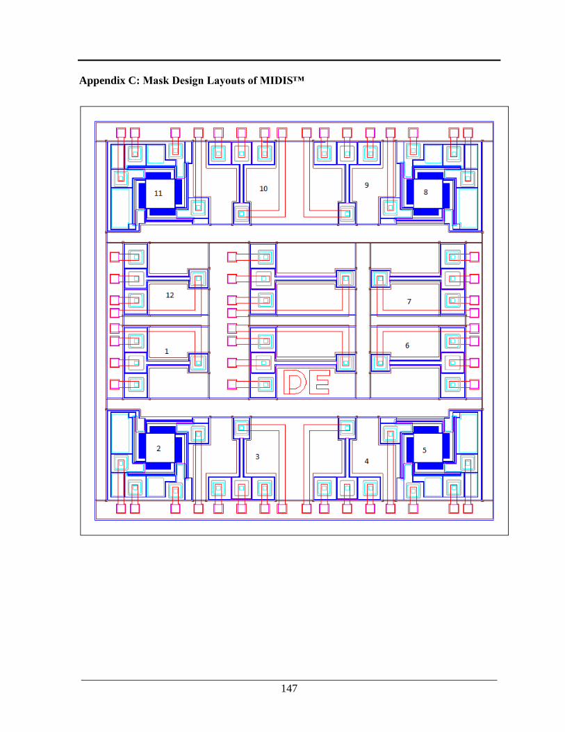
___________________________________________________________________________
147
Appendix C: Mask Design Layouts of MIDIS™

___________________________________________________________________________
148
Appendix D: Device Design Parameter and Test Results
Device 1 & 12: Cantilever Beam Gyroscope
Description Value
𝐿𝑏 Beam length 427.5 𝜇𝑚
𝑤𝑏 Beam width 29.5 𝜇𝑚
𝑡𝑏 (𝑡𝑝) Beam (microplate) thickness 30 𝜇𝑚
ℎ Initial capacitor gap 2 𝜇𝑚
𝐿𝑝 Microplate length 218 𝜇𝑚
𝑤𝑝 Microplate width 194 𝜇𝑚
𝐿𝑐 Length from beam tip to microplate 109 𝜇𝑚
M Tip mass 2.97 × 10⁻⁶𝑔
Test Parameters and Results
Test Parameter Drive mode Sense mode
ROM/FEA ROM/FEA
Actuation Voltage 15 Vpp 15 Vpp
Sweep frequency 38 to 42 kHz 38 to 42 kHz
Parasitic capacitance 3.5 pF 3.5 pF
Natural frequency 40.189 kHz 40.8/40.4 kHz 41.191 KHz 40.8/40.4 kHz
Qaulity factor ~1850 ~1800
Pull-in voltage 45.0 V 45.25 /45.2 V - 45.25 /45.2 V

___________________________________________________________________________
149
Device 2, 5, 8 & 11: Crab leg Gyroscope
Description Value
𝐿1 Beam length 1 468 𝜇𝑚
𝐿2 Beam length 2 120 𝜇𝑚
𝑤𝑏 Beam width 10𝜇𝑚
𝑡𝑏 (𝑡𝑝) Beam thickness 30 𝜇𝑚
ℎ Initial capacitor gap 2 𝜇𝑚
𝐿𝑐𝑝 Microplate length 290 𝜇𝑚
𝑤𝑝 Microplate width 290 𝜇𝑚
M Tip mass 5.88 × 10⁻⁶𝑔
Test Parameters and Results
Test parameter Drive mode Sense mode
FEA FEA
Actuation Voltage 10 Vpp 10 Vpp
Sweep frequency 16 to 18 kHz 16 to 18 kHz
Parasitic capacitance 5.6 pF 5.6 pF
Natural frequency
(drive)
17.283 kHz 19.824kHz 17.271 KHz 20.117kHz
Qaulity factor ~3000 ~3000
Pull-in voltage - 15V - 15V
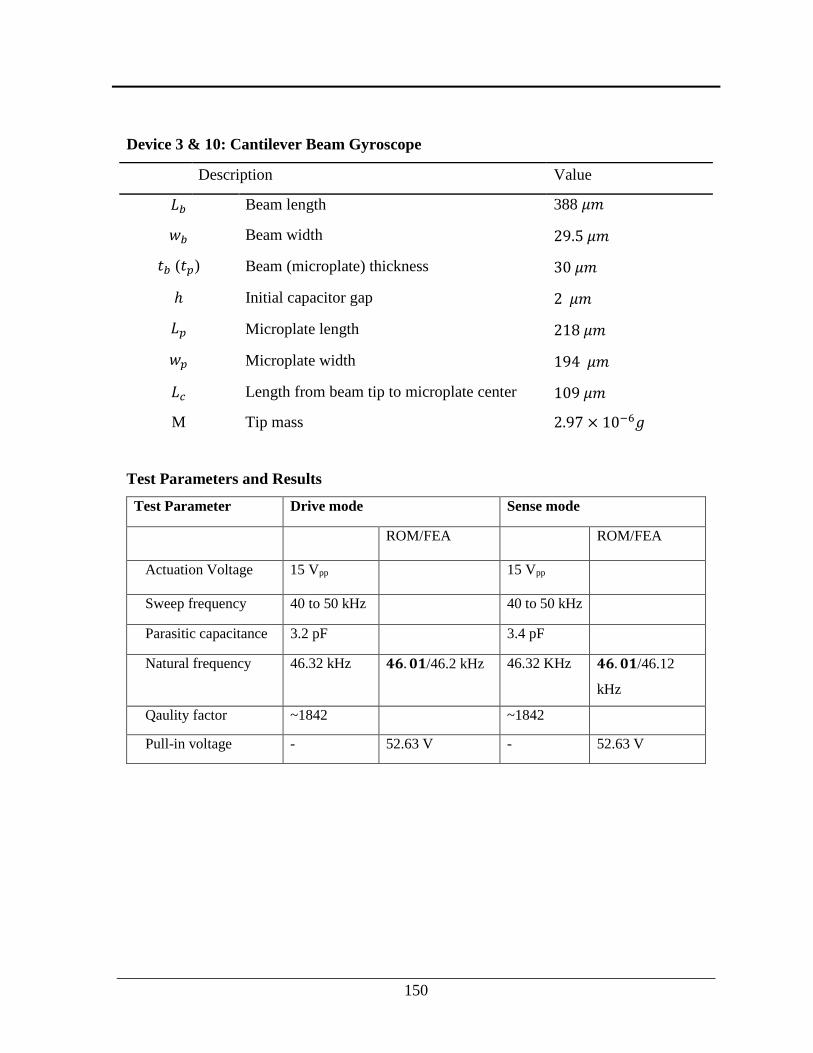
___________________________________________________________________________
150
Device 3 & 10: Cantilever Beam Gyroscope
Description Value
𝐿𝑏 Beam length 388 𝜇𝑚
𝑤𝑏 Beam width 29.5 𝜇𝑚
𝑡𝑏 (𝑡𝑝) Beam (microplate) thickness 30 𝜇𝑚
ℎ Initial capacitor gap 2 𝜇𝑚
𝐿𝑝 Microplate length 218 𝜇𝑚
𝑤𝑝 Microplate width 194 𝜇𝑚
𝐿𝑐 Length from beam tip to microplate center 109 𝜇𝑚
M Tip mass 2.97 × 10⁻⁶𝑔
Test Parameters and Results
Test Parameter Drive mode Sense mode
ROM/FEA ROM/FEA
Actuation Voltage 15 Vpp 15 Vpp
Sweep frequency 40 to 50 kHz 40 to 50 kHz
Parasitic capacitance 3.2 pF 3.4 pF
Natural frequency 46.32 kHz 𝟒𝟔. 𝟎𝟏/46.2 kHz 46.32 KHz 𝟒𝟔. 𝟎𝟏/46.12
kHz
Qaulity factor ~1842 ~1842
Pull-in voltage - 52.63 V - 52.63 V
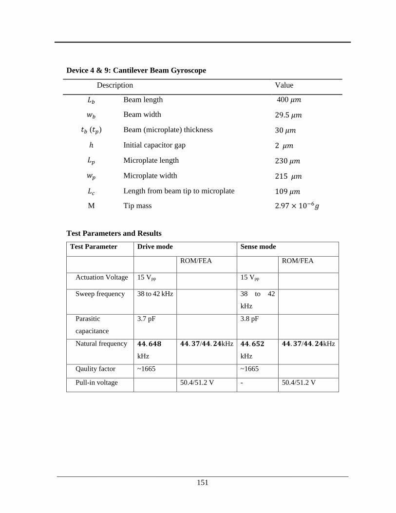
___________________________________________________________________________
151
Device 4 & 9: Cantilever Beam Gyroscope
Description Value
𝐿𝑏 Beam length 400 𝜇𝑚
𝑤𝑏 Beam width 29.5 𝜇𝑚
𝑡𝑏 (𝑡𝑝) Beam (microplate) thickness 30 𝜇𝑚
ℎ Initial capacitor gap 2 𝜇𝑚
𝐿𝑝 Microplate length 230 𝜇𝑚
𝑤𝑝 Microplate width 215 𝜇𝑚
𝐿𝑐 Length from beam tip to microplate 109 𝜇𝑚
M Tip mass 2.97 × 10⁻⁶𝑔
Test Parameters and Results
Test Parameter Drive mode Sense mode
ROM/FEA ROM/FEA
Actuation Voltage 15 Vpp 15 Vpp
Sweep frequency 38 to 42 kHz 38 to 42
kHz
Parasitic
capacitance
3.7 pF 3.8 pF
Natural frequency 𝟒𝟒. 𝟔𝟒𝟖
kHz
𝟒𝟒. 𝟑𝟕/𝟒𝟒. 𝟐𝟒kHz 𝟒𝟒. 𝟔𝟓𝟐
kHz
𝟒𝟒. 𝟑𝟕/𝟒𝟒. 𝟐𝟒kHz
Qaulity factor ~1665 ~1665
Pull-in voltage 50.4/51.2 V - 50.4/51.2 V

___________________________________________________________________________
152
Device 6 & 7: Cantilever Beam Gyroscope
Description Value
𝐿𝑏 Beam length 621 𝜇𝑚
𝑤𝑏 Beam width 29.5 𝜇𝑚
𝑡𝑏 (𝑡𝑝) Beam (microplate) thickness 30 𝜇𝑚
ℎ Initial capacitor gap 2 𝜇𝑚
𝐿𝑝 Microplate length 239.5 𝜇𝑚
𝑤𝑝 Microplate width 196 𝜇𝑚
𝐿𝑐 Length from beam tip to microplate center 119.75 𝜇𝑚
M Tip mass 3.28 × 10⁻⁶𝑔
Test Parameters and Results
Test Parameter Drive mode Sense mode
ROM/FEA ROM/FEA
Actuation Voltage 15 Vpp 15 Vpp
Sweep frequency 35 to 40 kHz 35 to 40 kHz
Parasitic capacitance 4.2 pF 4.0 pF
Natural frequency 37.53 kHz - 37.53 KHz -
Qaulity factor ~1850 ~1800
Pull-in voltage - 40.26 V - 40.26 V
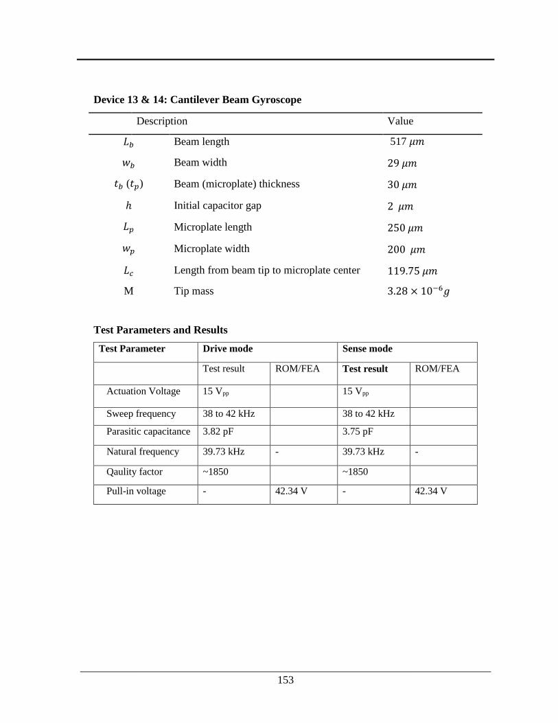
___________________________________________________________________________
153
Device 13 & 14: Cantilever Beam Gyroscope
Description Value
𝐿𝑏 Beam length 517 𝜇𝑚
𝑤𝑏 Beam width 29 𝜇𝑚
𝑡𝑏 (𝑡𝑝) Beam (microplate) thickness 30 𝜇𝑚
ℎ Initial capacitor gap 2 𝜇𝑚
𝐿𝑝 Microplate length 250 𝜇𝑚
𝑤𝑝 Microplate width 200 𝜇𝑚
𝐿𝑐 Length from beam tip to microplate center 119.75 𝜇𝑚
M Tip mass 3.28 × 10⁻⁶𝑔
Test Parameters and Results
Test Parameter Drive mode Sense mode
Test result ROM/FEA Test result ROM/FEA
Actuation Voltage 15 Vpp 15 Vpp
Sweep frequency 38 to 42 kHz 38 to 42 kHz
Parasitic capacitance 3.82 pF 3.75 pF
Natural frequency 39.73 kHz - 39.73 kHz -
Qaulity factor ~1850 ~1850
Pull-in voltage - 42.34 V - 42.34 V