design and power management of an...
TRANSCRIPT

DESIGN AND POWER MANAGEMENT OF AN OFFSHORE MEDIUM VOLTAGE DC MICROGRID REALIZED THROUGH HIGH VOLTAGE POWER ELECTRONICS TECHNOLOGIES AND CONTROL
by
Brandon Michael Grainger
B.S. in Mechanical Engineering, University of Pittsburgh, 2007
M.S. in Electrical Engineering, University of Pittsburgh, 2011
Submitted to the Graduate Faculty of
Swanson School of Engineering in partial fulfillment
of the requirements for the degree of
Doctor of Philosophy
University of Pittsburgh
2014
UNIVERSITY OF PITTSBURGH
SWANSON SCHOOL OF ENGINEERING
This dissertation was presented
by
Brandon Michael Grainger
It was defended on
July 7th, 2014
and approved by
Gregory F. Reed, PhD, Professor
Department of Electrical and Computer Engineering
George L. Kusic, PhD, Associate Professor Department of Electrical and Computer Engineering
Zhi-Hong Mao, PhD, Associate Professor
Department of Electrical and Computer Engineering
Thomas E. McDermott, PhD, Assistant Professor Department of Electrical and Computer Engineering
William E. Stanchina, PhD, Professor
Department of Electrical and Computer Engineering
William W. Clark, PhD, Professor Department of Mechanical Engineering and Materials Science
Marius Rosu, PhD, Electromechanical Lead Product Manager, ANSYS Inc.
Dissertation Director: Gregory F. Reed, PhD, Professor Department of Electrical and Computer Engineering
ii

Copyright © by Brandon M. Grainger
2014
iii

The growth in the electric power industry’s portfolio of Direct Current (DC) based generation
and loads have captured the attention of many leading research institutions. Opportunities for
using DC based systems have been explored in electric ship design and have been a proven,
reliable solution for transmitting bulk power onshore and offshore. To integrate many of the
renewable resources into our existing AC grid, a number of power conversions through power
electronics are required to condition the equipment for direct connection. Within the power
conversion stages, there is always a requirement to convert to or from DC.
The AC microgrid is a conceptual solution proposed for integrating various types of
renewable generation resources. The fundamental microgrid requirements include the capability
of operating in islanding mode and/or grid connected modes. The technical challenges associated
with microgrids include (1) operation modes and transitions that comply with IEEE1547 without
extensive custom engineering and (2) control architecture and communication. The Medium
Voltage DC (MVDC) architecture, explored by the University of Pittsburgh, can be visualized as
a special type of DC microgrid.
This dissertation is multi-faceted, focused on many design aspects of an offshore DC
microgrid. The focal points of the discussion are focused on optimized high power, high
frequency magnetic material performance in electric machines, transformers, and DC/DC power
converters – all components found within offshore, power system architectures. A new
DESIGN AND POWER MANAGEMENT OF AN OFFSHORE MEDIUM VOLTAGE DC MICROGRID REALIZED THROUGH HIGH VOLTAGE POWER ELECTRONICS TECHNOLOGIES AND CONTROL
Brandon M. Grainger, PhD
University of Pittsburgh, 2014
iv

controller design based upon model reference control is proposed and shown to stabilize the
electric motor drives (modeled as constant power loads), which serve as the largest power
consuming entities in the microgrid. The design and simulation of a state-of-the-art multilevel
converter for High Voltage DC (HVDC) is discussed and a component sensitivity analysis on
fault current peaks is explored. A power management routine is proposed and evaluated as the
DC microgrid is disturbed through various mode transitions. Finally, two communication
protocols are described for the microgrid – one to minimize communication overhead inside the
microgrid and another to provide robust and scalable intra-grid communication.
The work presented is supported by Asea Brown Boveri (ABB) Corporate Research
Center within the Active Grid Infrastructure program, the Advanced Research Project Agency –
Energy (ARPA-E) through the Solar ADEPT program, and Mitsubishi Electric Corporation
(MELCO).
v

TABLE OF CONTENTS
NOMENCLATURE ................................................................................................................. XIX
ACKNOWLEDGMENTS .................................................................................................... XXIII
1.0 INTRODUCTION................................................................................................................ 1
1.1 MOTIVATION FOR RESEARCH PURSUITS ................................................ 2
1.1.1 Electric Ship Design......................................................................................... 3
1.1.2 Explorations in Offshore Wind Generation Potential and Oil Drilling Reservoirs ........................................................................................................ 5
1.1.3 Challenges and Opportunities with Microgrids ........................................... 8
1.1.4 Increased Interest in Microgrid Operations for AC and DC Architectures …………………………………………………………………………………9
1.1.5 Microgrid Hierarchical Control Terminology ............................................ 11
1.2 SIGNIFICANCE AND CONTRIBUTIONS .................................................... 13
1.3 DISSERTATION OUTLINE ............................................................................. 18
2.0 POWER DENSITY IMPROVEMENTS UTILIZING HIGH FREQUENCY MAGNETIC NANOCOMPOSITE MATERIALS IN POWER APPLICATIONS .... 20
2.1 MOTIVATION FOR DESIGNING BIDIRECTIONAL CHARGERS WITH
HIGH FREQUENCY MAGNETIC COMPONENTS .................................... 23
2.2 OPTIMIZING BIDIRECTIONAL CHARGER MAGNETIC DESIGN FOR KILOWATT SCALE POWER APPLICATIONS USING ANSYS .............. 26
2.2.1 Analytical Methodology for Optimizing Transformer Parameters .......... 26
vi

2.2.2 Optimal Ferrite Core Transformer Parameters Analyzed through ANSYS PExprt ............................................................................................................ 30
2.2.3 Optimal HTX-012B Nanocomposite Core Transformer Parameters
Analyzed through ANSYS PExprt .............................................................. 34
2.2.4 Results Comparison between Analytical Ferrite Core, Computer Simulated Ferrite Core, and Computer Simulated Nanocomposite Core 41
2.3 ELECTRIC MACHINE POWER DENSITY IMPROVEMENT USING
NANOCOMPOSITE MATERIALS ................................................................. 42
2.3.1 Power Density Improvement of Induction Motors Utilizing HTX-012B: Design Considerations .................................................................................. 43
2.3.2 Power Density Improvement of Induction Motors Utilizing HTX-012B:
Motor Optimization Study ........................................................................... 47
2.4 APPROXIMATE UTILITY SCALE TRANSFORMER CORE SIZE REDUCTION EMPLOYING NANOCOMPOSITE MAGNETIC MATERIALS ...................................................................................................... 51
3.0 MODULAR MULTILEVEL CONVERTER BASED HIGH VOLTAGE DC
MODELING, COMPONENT SENSITIVITY ANALYSIS, AND SCALING APPROXIMATIONS ........................................................................................................ 55
3.1 MODULAR MULTILEVEL CONVERTER MODELING AND CONTROL
…………………………………………………………………………………..60
3.1.1 Generalized Mathematical Model of the MMC Converter ....................... 61
3.1.2 MMC Converter Inner Loop Controllers: Current Regulators and Tuning ............................................................................................................ 63
3.1.3 MMC Converter Outer Loop Controllers: AC and DC Regulators ........ 65
3.1.4 Capacitor Balancing Algorithm ................................................................... 66
3.1.5 System Parameters and Dynamic Performance Evaluation...................... 67
3.2 MODULAR MULTILEVEL CONVERTER COMPONENT SENSITIVITY ANALYSIS ON FAULT CURRENTS .............................................................. 71
3.2.1 Transformer Impedance Impact on Peak DC Current ............................. 73
3.2.2 Bypass Switch Impact on Peak DC Current ............................................... 73
vii

3.2.3 Reactor Impact on Peak DC Current .......................................................... 74
3.3 ELECTRIC CHARACTERISTIC PREDICTION WITH REDUCED SUBMODULE COUNT IN CONVERTER ARMS......................................... 76
4.0 MODEL REFERENCE CONTROLLER DESIGN FOR STABILIZING CONSTANT
POWER LOADS IN A MEDIUM VOLTAGE DC MICROGRID .............................. 78
4.1 FUNDAMENTALS OF BIDIRECTIONAL DC/DC CONVERTERS .......... 80
4.1.1 Converter Dynamics ...................................................................................... 82
4.1.2 System Description with Constant Power Load Assumption .................... 83
4.2 STABILITY ASSESSMENTS USING MODEL REFERENCE CONTROL THEORY ............................................................................................................. 85
4.2.1 Attempt to Stabilize Plant with PD Controller ........................................... 85
4.2.2 Model Reference Control Definitions and Assumptions ............................ 88
4.2.3 Attempt to Stabilize Second-Order Plant with Model Reference Control 90
4.2.4 Stabilized Third Order Plant with Model Reference Control ................... 91
4.3 COMPENSATOR DESIGN AND PARAMETER SELECTION .................. 93
4.3.1 Simulation Results – Control Block Diagram Response ............................ 94
4.3.2 Simulation Results – Circuit Response ........................................................ 98
5.0 MODELING AN OFFSHORE MEDIUM VOLTAGE DC MICROGRID ............... 102
5.1 FULL CONVERTER WIND TURBINE MODEL ........................................ 102
5.1.1 Simplified Model of a Permanent Magnet Synchronous Machine ......... 103
5.1.2 Aerodynamic Model of Wind Source ......................................................... 104
5.1.3 Maximum Power Point Tracking Control Implementation .................... 105
5.1.4 Wind Turbine Model Validation ................................................................ 107
5.2 POWER ELECTRONIC CONVERTER MODELING ............................... 109
viii

5.2.1 Mathematical Modeling of Power Electronic Converters: The Average Model ............................................................................................................ 109
5.2.2 Average Model of Pulse Width Modulated Rectifier with Open Loop PQ
Control ......................................................................................................... 113
5.2.3 Average Model Implementation of Neutral Point Clamped Converter in Simulink ....................................................................................................... 118
5.2.4 Average Model of Bidirectional DC/DC Converter ................................. 119
5.3 VARIABLE FREQUENCY DRIVE MODEL ............................................... 121
5.3.1 Machine Current Control ........................................................................... 123
5.4 SYSTEM PARAMETERS AND ASSEMBLED DC MICROGRID VALIDATION................................................................................................... 125
5.4.1 System Power Balance and DC/DC Converter Power Handling Capability ………………………………………………………………………………127
5.4.2 Motor Drive Responses ............................................................................... 130
6.0 DYNAMIC POWER MANAGEMENT AND DC/DC CONVERTER CURRENT SHARING EVALUATION UNDER VARIOUS MODE TRANSITIONS ................ 135
6.1.1 Power Management Routine ...................................................................... 136
6.1.1 DC/DC Converter Dynamic Response under a Grid Disconnection ...... 139
6.1.2 DC/DC Converter Dynamic Response under a Grid Connection ........... 144
7.0 CONSIDERATIONS FOR DESIGNING THE COMMUNICATION NETWORK ARCHITECTURE OF THE OFFSHORE DC MICROGRID ................................... 146
7.1 COMMUNICATION NETWORKS ............................................................... 147
7.1.1 Microgrid Communication Network ......................................................... 148
7.1.2 Wide-Area Control Network ...................................................................... 151
7.2 PERFORMANCE ANALYSIS OF THE DISTRIBUTED COMMUNICATION ARCHITECTURE ...................................................... 152
7.2.1 Availability and Reliability ......................................................................... 153
ix

7.2.2 Packet Size and Overhead .......................................................................... 154
7.2.3 Transmission Delays .................................................................................... 154
7.2.4 Security ......................................................................................................... 155
8.0 CONCLUSIONS AND FUTURE WORK ..................................................................... 157
APPENDIX A ............................................................................................................................ 161
APPENDIX B ............................................................................................................................ 165
APPENDIX C ............................................................................................................................ 168
Permanent Magnet Synchronous Generator (PMSG) Implementation in Simulators ................................................................................................................. 168
APPENDIX D ............................................................................................................................ 173
BIBLIOGRAPHY ..................................................................................................................... 176
x

LIST OF TABLES
Table 2.1: Geometrical Relationships Associated with Transformer Core ................................. 27
Table 2.2: Optimal Core Results for DAB Benchmark Case with Available Commercial Core Metrics [51] ............................................................................................................... 29
Table 2.3: Ferrite Material Properties .......................................................................................... 30
Table 2.4: Top Ten Core Solutions Rated for 1 kW Utilizing Ferrite Core ................................ 31
Table 2.5: Dimensions, Mass, and Permeability of Experimentally Tested Cores ...................... 35
Table 2.6: Core Loss Measurements at Varying Frequencies and Induction Levels for Experimental Toroids.................................................................................................. 35
Table 2.7: Steinmetz Coefficients Associated with Tested Cores ............................................... 36
Table 2.8: HTX-012B Nanocomposite Material Properties ........................................................ 40
Table 2.9: Top Ten Core Solutions Rated for 1 kW Utilizing Nanocomposite HTX-012B ....... 40
Table 2.10: Comparison of Optimized Core Results ................................................................... 41
Table 2.11: Motor Geometric Variables ...................................................................................... 48
Table 2.12: Motor Constraints ..................................................................................................... 48
Table 2.13: Two Pole Motor Output ............................................................................................ 48
Table 2.14: Eight Pole Motor Output .......................................................................................... 48
Table 2.15: Parameters Associated with Core and Winding Loss Calculation ........................... 52
Table 2.16: System Constraints to Optimize 100 kW Transformer............................................. 53
xi

Table 2.17: Transformer Optimization Results with Varying Frequency ................................... 53
Table 3.1: HVDC System Parameters for a US Market Installation ........................................... 68
Table 3.2: Circuit Breaker and BPS Operating Sequence after Fault Occurs ............................. 72
Table 4.1: Cable Parameters ........................................................................................................ 84
Table 4.2: Rated System Parameters ........................................................................................... 95
Table 5.1: Wind Turbine and Permanent Magnet Synchronous Machine Parameters [96] ...... 103
Table 5.2: Operating States of Pulse Width Modulated Boost Rectifier ................................... 114
Table 5.3: Induction Machine Parameters [76] .......................................................................... 131
Table 5.4: Predicted Motor Simulation Results .......................................................................... 134
Table 7.1: Telecommunication Protocols and Media Options for Microgrid and Wide-Area Networks [117] ......................................................................................................... 153
xii

LIST OF FIGURES
Figure 1.1: Electric Ship Power System Architecture [5] .............................................................. 4
Figure 1.2: Semi-Submersible Drilling Rig [7] ............................................................................. 6
Figure 1.3: Location of Oil Drilling Opportunities between 2012 and 2017 [5] ........................... 7
Figure 1.4: Available Wind Generation Onshore and Offshore in the United States [9] .............. 7
Figure 1.5: Offshore Platforms – Siemens Offshore Design (Left), [10]& ABB Offshore Design (Right), [11] ................................................................................................................. 7
Figure 1.6: Block Diagram of Microgrid Control Layers Operating in Unison [27] .................. 12
Figure 1.7: Hierarchical Control Architectures for an AC and DC Microgrid [28] .................... 12
Figure 1.8: DC Microgrid - Local Wind Power being supplied to Offshore Platform ................ 14
Figure 2.1: 2010 Power Electronic Opportunities for Improvements [34] .................................. 21
Figure 2.2: Offshore Medium Voltage DC Microgrid Emphasizing Magnetic Intensive Areas . 22
Figure 2.3: Bidirectional DC/DC Converter Topology ............................................................... 24
Figure 2.4: Voltage and Current Waveforms of DAB DC/DC while Operating in Charging (Buck) Mode .............................................................................................................. 25
Figure 2.5: Single-phase Transformer Core for Dual-Active Bridge Converter [46] .................. 27
Figure 2.6: Magnetics 0P44125UC [54] ...................................................................................... 29
Figure 2.7: Optimal Manufacturer Core Volume Solutions ........................................................ 31
Figure 2.8: Notable Parameters associated with the ETD49 Ferrite Core Design for the 1 kW DAB ......................................................................................................................... 32
xiii

Figure 2.9: ETD49 Core: Simulation Results and Manufactured Component from Magnetics [56] ........................................................................................................................... 33
Figure 2.10: Cross Section of 72 Windings Configured in Two Parallel Turns around ETD49
Core .......................................................................................................................... 34
Figure 2.11: Core Loss for Annealed, Impregnated, and Impregnated Cut Cores (f = 20kHz) [57].................................................................................................................................. 37
Figure 2.12: Core Loss for Annealed, Impregnated, and Impregnated Cut Cores (f = 50kHz) .. 37
Figure 2.13: Core Loss for Annealed, Impregnated, and Impregnated Cut Cores (f = 100kHz) 38
Figure 2.14: Core Loss for Annealed, Impregnated, and Impregnated Cut Cores (B = 0.1T) .... 38
Figure 2.15: Steinmetz Coefficients Provided by PExprt for HTX-012B Based on Experimental Loss Data ................................................................................................................. 39
Figure 2.16: Notable Parameters associated with the ETD49 Nanocomposite Core Design for the
1 kW DAB ............................................................................................................... 40
Figure 2.17: Size Reduction of 10 kW PPMT Motor Using HTX-005C Fe-Co Nanocomposite Material [59] ........................................................................................................... 42
Figure 2.18: B-H Curve for HTX-012B ...................................................................................... 43
Figure 2.19: M600-50A B-H Curve [62] ..................................................................................... 45
Figure 2.20: Core Loss Data for M600-50A [62] ........................................................................ 45
Figure 2.21: Machine Power Factor Adjustments as Number of Machine Poles Increase [63] .. 46
Figure 2.22: Motor Geometry, Winding Configuration and Slot Dimensions ............................ 47
Figure 2.23: Two Pole Motor Flux Distribution .......................................................................... 49
Figure 2.24: Eight Pole Motor Flux Distribution......................................................................... 49
Figure 2.25: Two Pole Motor Torque vs. Speed Curve ............................................................... 50
Figure 2.26: Eight Pole Motor Torque vs. Speed Curve .............................................................. 50
Figure 2.27: C-Core Transformer Design [64] ............................................................................ 51
Figure 2.28: Core Volume vs. Frequency for 100 kW Rated Transformer Core ........................ 54
xiv

Figure 3.1: Planned HVDC Installations within North America through 2019 .......................... 55
Figure 3.2: Planned HVDC Installations in China through 2020 [67] ........................................ 56
Figure 3.3: Definition of a Multilevel Inverter [68] .................................................................... 57
Figure 3.4: Modular Multilevel Converter Topology .................................................................. 58
Figure 3.5: Multi-Terminal DC Application within the Offshore DC Microgrid Environment .. 59
Figure 3.6: Submodule States of the Modular Multilevel Converter .......................................... 60
Figure 3.7: Circuit Synthesis of 6 Cell per Arm MMC Converter .............................................. 61
Figure 3.8: Current Controller of MMC Converter ..................................................................... 64
Figure 3.9: Illustration of Modulated Case with Third Harmonic Injection [77] ........................ 65
Figure 3.10: THD Voltage Distortion Limits [82] ....................................................................... 68
Figure 3.11: Top-Level View of HVDC Model Development in PSCAD .................................. 69
Figure 3.12: HVDC Model Waveforms: (a) DC voltage (b) Capacitor Voltage Ripple, (c) ∆-side AC Voltage / Y-Side AC Voltage / Reference Signal and (d) Power Flow .. 70
Figure 3.13: Pole-to-Pole Fault in a Monopolar HVDC System ................................................. 71
Figure 3.14: Transformer Reactance Impact on Peak DC Current .............................................. 73
Figure 3.15: Bypass Switch Speed Impact on Peak DC Current ................................................. 74
Figure 3.16: DC Line Inductor Impacts on Peak DC Current ..................................................... 75
Figure 3.17: Asymmetrical Arm Reactor Impact on Peak DC Current ....................................... 75
Figure 3.18: Comparison between Electrical Characteristics for 6 and 10 Cell MMC Converter Systems ................................................................................................................... 77
Figure 4.1: Model Reference Controller Design Application within the Offshore DC Microgrid
Environment ............................................................................................................. 79
Figure 4.2: Dual Active Bridge Bidirectional DC/DC Converter................................................ 80
Figure 4.3: Current Traces of DAB DC/DC Converter ............................................................... 81
Figure 4.4: Operating Waveforms of the Dual Active Bridge DC/DC Converter ....................... 82
xv
Figure 4.5: System Model for Studying CPL Scenario ............................................................... 83
Figure 4.6: Simplified System Model for Evaluating CPL Scenario (Third Order System) ....... 84
Figure 4.7: Pole-zero plot associated with unstable output impedance for various constant power loads ........................................................................................................................... 85
Figure 4.8: Second-order System Model of a Simplified Motor Drive Model (Second-Order).. 86
Figure 4.9: PD Control of Plant ................................................................................................... 86
Figure 4.10: Controller Structure to Stabilize Constant Power Load [93] .................................. 89
Figure 4.11: Pole Placement of the Reference Model ................................................................. 94
Figure 4.12: Pole-zero plot for unstable plant with lumped network capacitors (right) and neglected (left) ........................................................................................................ 96
Figure 4.13: Pole-zero Plot for Model, M(s)................................................................................ 96
Figure 4.14: Simulation Model of Designed Control Structure Utilizing Model Reference Control .................................................................................................................... 97
Figure 4.15: Closed Loop Controller Performance Based Upon Model Reference Control Design
.................................................................................................................................. 97
Figure 4.16: Closed Loop Controller Performance Based Upon PD Design .............................. 97
Figure 4.17: Circuit Diagram for Proving Model Reference Control Capability ........................ 98
Figure 4.18: Circuit Response with Step Change in DC/DC Converter Control Input at 0.5 seconds ................................................................................................................... 99
Figure 4.19: Average Circuit Model Representation of Plant Model under Study ................... 100
Figure 4.20: Comparison of Circuit Simulation and Control Block Diagram Response........... 101
Figure 5.1: Offshore Wind Turbine Collection System ............................................................. 102
Figure 5.2: Maximum Power Point Tracking Implementation and Control of Wind Turbine .. 105
Figure 5.3: Wind Turbine Controller Responses ....................................................................... 107
Figure 5.4: Wind Turbine Aerodynamic Responses and Output Power .................................... 108
Figure 5.5: Simplified Half-Bridge Inverter .............................................................................. 109
xvi

Figure 5.6: Switched Equivalent Circuit Model of the Half-Bridge Converter ......................... 110
Figure 5.7: Averaged Equivalent Circuit of the Half-Bridge Converter ................................... 113
Figure 5.8: Pulse Width Modulated Boost Rectifier .................................................................. 114
Figure 5.9: Average Model of Pulse Width Modulated Inverter/Rectifier ................................ 117
Figure 5.10: Open Loop PQ Regulator of Pulse Width Modulated Boost Rectifier ................. 117
Figure 5.11: Average Model of Neutral Point Clamped Converter ........................................... 118
Figure 5.12: Detailed and Average Model Output Voltage Waveform of NPC Inverter .......... 119
Figure 5.13: Average Model of Bidirectional DC/DC Converter.............................................. 120
Figure 5.14: Illustration of Detailed and Average Model Currents for the Bidirectional DC/DC Converter .............................................................................................................. 120
Figure 5.15: Variable-Frequency Voltage Sourced Converter for Controlling Induction Machine
................................................................................................................................ 121
Figure 5.16: Magnetization Current Alignment in a dq Axis Frame ......................................... 123
Figure 5.17: Machine Current Control ....................................................................................... 125
Figure 5.18: Interconnected DC Based Microgrid Computer Model ........................................ 126
Figure 5.19: Generation Sources in Microgrid .......................................................................... 128
Figure 5.20: Bus DC Voltages and Currents in DC Microgrid.................................................. 128
Figure 5.21: dq Flux Linkages of Wind Turbine Generator after Grid Disconnect .................. 129
Figure 5.22: dq Current Regulation of Induction Motors .......................................................... 131
Figure 5.23: Axes Orientation for Current Controller and Motor ............................................. 132
Figure 5.24: Relationship between the dq and abc Quantities for Generating and Motoring Operation[97] ......................................................................................................... 132
Figure 5.25: dq Stator Currents and Motor Torque ................................................................... 134
Figure 5.26: Motor Load Power and Modulation Index of Motor Inverters ............................. 134
Figure 6.1: Power Signals and Coordination through Centralized Computer ........................... 136
xvii

Figure 6.2: Power Management Routine for Adjusting DC/DC Converters in Microgrid ........ 137
Figure 6.3: Microgrid Computer Model with Implementation of Power Management Scheme 138
Figure 6.4: System Generation Response During a Grid Disconnect ........................................ 140
Figure 6.5: DC/DC Converter Duty Cycle Response ................................................................ 140
Figure 6.6: DC Bus Voltages and Current Flows in Case of Grid Disconnect .......................... 141
Figure 6.7: Zoomed-In Intervals of Figure 6.6 Providing Finer Electrical Characteristics ....... 141
Figure 6.8: Output Currents of DC/DC Converters for Grid Disconnect Scenario – 60% / 40 % Weighting ............................................................................................................... 142
Figure 6.9: Wind Generator Currents and Grid Connected Converter Current for Grid
Disconnect Scenario............................................................................................... 143
Figure 6.10: System Generation Response During a Grid Connection ..................................... 145
Figure 6.11: Duty Cycles and Output Currents of DC/DC Converters – 60% / 40% Weighting .............................................................................................................................. 145
Figure 7.1: Architecture of Microgrid Communication Networks ............................................ 148
Figure 7.2: Secondary Controller's Inside and Outside Communication Cycles ....................... 150
Figure 7.3: Architecture of Wide-Area Communication Network ............................................ 151
Figure 8.1: Portable Motor Units (Left) and Motor Control Center (Right) ............................. 159
Figure 8.2: LVRT Requirement per Appendix G of FERC's LGIA .......................................... 160
xviii

NOMENCLATURE
x Average DC Value x~ Small Signal AC Value x Dimensional Vector x Phasor
*x Complex Conjugate A Area Swept by Wind Turbine Blades Ac Cross Sectional Area of Transformer Ai Equipment Availability At Transformer Thermal Area Aw Window Area of Transformer B Magnetic Induction Bs Saturation Magnetic Induction BTx Transformer Magnetic Induction C Capacitance Cdc DC/DC Converter Output Capacitor Cp Power Coefficient of Wind Turbine D Diode Erms RMS Transformer Voltage F Machine Friction Factor Fr Litz Wire Loss Factor G(s) Closed Loop Transfer Function H Magnetic Field Strength I General DC Current Ig DC/DC Converter Input Current IL Inductor Current J Machine Moment of Inertia KDC DC/DC Converter Plant Gain KP Proportional Gain of DC/DC Converter Controller KD Derivative Gain of DC/DC Converter Controller Kpc Proportional Gain of HVDC Converter Kic Integral Gain of HVDC Converter L General Inductance Lds Permanent Magnet Machine Direct Axis Inductance Lqs Permanent Magnet Machine Quadrature Axis Inductance
xix

Lm Induction Machine Magnetizing Inductance Ls HVDC Converter Arm Inductance LTx Transformer Inductance M Mutual Inductance M(s) Reference Model Transfer Function N Turns Ratio of Transformer, Submodules per HVDC Converter Arm P Real Power, Machine Poles
)(ˆ sP Plant Transfer Function PL Power Loss PT Turbine Power Pc Core Loss Pt Terminal Power Ps Sending Power Q Reactive Power, Semiconductor Module R Resistance, Length of Wind Turbine Blade S Apparent Power T Transpose Te Electrical Torque Tm Mechanical Torque Trise Temperature Rise of Transformer Ts Switching Period T(θ) Park Transformation V General DC Voltage, Transformer Volume VH Medium Voltage DC Bus Voltage VL Offshore Production Platform DC Bus Voltage VLL Line-to-Line Voltage VW Wind Velocity Vc Core Volume Vg DC/DC Converter Input Voltage Vp Primary Side Voltage Vs Secondary Side Voltage, Stator Voltage Vr Rotor Voltage Vt Terminal Voltage Vsm Submodule Voltage X Reactance Y Wye side of Transformer, Constant Power Load Z Total Impedance Zout Output Impedance a Width of Main Flux Path in Transformer ah Fourier Coefficient bh Fourier Coefficient ax Polynomial Coefficients of Reference Model Numerator, )(ˆ snm ; x = 0,1,2,3…n b Width of the Transformer Window bx Polynomial Coefficients of Reference Model Denominator, )(ˆ sdm ; x = 1,2,3…n
xx

d Transformer Thickness, General Duty Cycle dc Copper Wire Diameter dd Direct Axis Duty Cycle dq Quadrature Axis Duty Cycle dh DC/DC Converter Duty Cycle
)(ˆ sd p Plant Denominator f System Frequency f0 Ratio between Model and Plant Gains fs Switching Frequency fabc Variable f in abc frame fdqk Variable f in dq frame h Height of Half of the Transformer Window, harmonic number i AC Current id Direct axis current ik AC Current in Converter Arm k iq Quadrature Axis Current is Stator Current ir Rotor Current imr Machine Magnetizing Current k Steinmetz Relationship Gain, Field Distribution Constant km Reference Model Gain kα Scaling factor of DC/DC Converter No. 1 kβ Scaling factor of DC/DC Converter No. 2 kp Plant Gain l Magnetic Effective Length lo Mean Length per Turn l1 Transformer Width l2 Transformer Thickness l3 Transformer Height m Modulation Index md Direct Axis Modulation Index mq Quadrature Axis Modulation Index n Turns Ratio of DC/DC Converter, Wire Strands, Multilevel Converter Levels
)(ˆ snp Plant Numerator )(ˆ snm Reference Model Numerator
px Polynomial Coefficients of Plant Denominator, )(ˆ sd p ; x = 0,1,2,3…n qx Polynomial Coefficients of Plant Numerator, )(ˆ snp ; x = 1,2,3…n
)(ˆ sr Reference Model Input s Laplace Operator, Switching Function, Switch t Ribbon thickness, Time u Phase voltage of HVDC Converter, Control signal ud Direct Axis Control Input uq Quadrature Axis Control Input
)(ˆ su Control System Input
xxi

v AC voltage vd Direct Axis Voltage vq Quadrature Axis Voltage
)(ˆ sy p Plant Output )(ˆ sym Reference Model Output
α Steinmetz Exponent on Frequency β Steinmetz Exponent on Induction, Wind Turbine Pitch Angle δ Phase of Voltage λ Flux or Tip Speed Ratio of Wind Turbine λd Direct Axis Flux λq Quadrature Axis Flux λopt Optimal Tip Speed Ratio λm Permanent Magnet Flux λs Stator Flux λr Rotor Flux µ Permeability ω Circular Frequency ω1 Model Pole Location ωe Excitation Frequency ωn Natural Frequency ωo Nominal Frequency ωr Rotor Mechanical Speed ϕ Phase Delay, Transformer Geometric Constant ρ Resistivity, Air Density, Angle between Rotor and Stator Machine Axis ρ Copper Resistivity σ Total Leakage Factor σs Stator Leakage Factor σr Rotor Leakage Factor θ Phase of Impedance, System Angle θr Rotor Angle τ Closed Loop Transfer Function Time Constant τs Stator Time Constant ζ Damping Coefficient Δ Delta side of transformer Φ HVDC Converter Energy Ratio
xxii

ACKNOWLEDGMENTS
The race towards achieving an advanced engineering degree is not a simple task but requires
perseverance and endurance to breakthrough life’s challenges and trials to reach the end goal.
The path towards completion cannot be achieved without the support of others because the
journey, without question, is an emotional rollercoaster with heights and valleys.
Acknowledgments are meant to show gratitude to those who have encouraged or supported my
efforts and are not listed in any particular order.
First, I want to thank my parents – Douglas and Nancy Grainger – who didn’t have the
same opportunities as I had growing up and ensured that I received a solid education and
supported my efforts along the way. The drive, undistracted attention and focus, and
perfectionist mentality comes from my dad and the ability to organize, manage, and listen comes
from my mom – all qualities that are valuable in engineering.
Second, I want to thank the financial support from ABB Corporate research, ARPA-E,
and MELCO. From ABB, special thanks go to Dr. Le Tang and Dr. Zhenyuan “John” Wang
from the United States and Dr. Jan Svensson from Vasteras, Sweden who funded our efforts at
the university in medium voltage DC microgrids. From ARPA-E, Dr. Tim Heidel who program
managed the research efforts being done on the advanced magnetic material development. From
MELCO, Ryo Yamamoto for partnering with Pitt, funding and encouraging our HVDC research
and development, and touring me around Japan to see MELCO’s engineering facilities. I also
xxiii

want to thank the Richard K. Mellon foundation for providing substantial funds in supporting the
Center for Energy at Pitt and awarding me one of the first endowed graduate student fellowships.
A special thank you to Dr. Gregory Reed for selecting me as his first PhD student in 2009
to help build the electric power program; instilling in my mentality the importance of
networking; relationship building; and close collaboration with industry. As our relationship
grew, the faculty/student hierarchy began to dissolve and, from my viewpoint, we became
engineering colleagues using each other’s strengths to reach a common goal. Using a very
untraditional academic model, the opportunities, engineering skillsets, and company interactions
have molded me into, spoken humbly, a sought-after engineer who has the analytical foundation
and communication attributes to be successful in this field all in thanks to his guidance.
Thanks to Dr. Zhi-Hong Mao for his willingness to meet often to discuss control theory,
listen to my thoughts and concerns, and enhanced my research abilities over the years and to Dr.
Thomas McDermott for always having his office door open for “on-the-fly” technical
discussions. Thanks to Dr. George Kusic, Dr. William Stanchina, Dr. William Clark, and Dr.
Marius Rosu for serving as committee members.
I want to thank many of my friends who have helped pave the success of the electric
power engineering research group since its initiation and who really have / make the group
something special. Past and present members include Hashim Al-Hassan, Ansel Barchowsky,
Dr. Hussain Bassi, Alvaro Cardoza, Dr. Shimeng Huang, Dr. Bob Kerestes, Dr. Raghav Khanna,
Dr. Matthew Korytowski, Patrick Lewis, Rusty Scioscia, Zachary Smith, Adam Sparacino and
Dr. Emmanuel Taylor. Also, thanks to Velin Kounev for partnering with me and applying his
communications knowledge to solving microgrid communication issues.
xxiv

Special recognition to various members of Pitt’s staff including Danielle Ilchuk, Suzan
Dolfi, James Lyle, Bill McGahey and Sandy Weisburg for making the Center for Energy and
ECE Department operate as smooth as possible on a daily basis and Paul Kovach for helping to
publically market our research program and team.
Engineering difficulty arises not because of the nature of the work but strictly because
engineers and scientists have finite minds attempting to understand one, infinite mind. For
nothing could explain how the equations, from the perspective of man, eloquently break down,
when used correctly, to predict the phenomena of this world without acknowledging a higher,
creative power who designed this world. All the engineer does is invents or manipulates what
has already been created. With this perspective, I express sincere thanks to God who knows the
plans for my life and secures my future.
A thank you is in order for Godly men in the faith who have prayed for me and serve as
weekly encouraging mechanisms during weekly studies. These men include Dr. Stephen
Wilson, Scott Marton, Ojo Nwabara, Don Schell, Warren Keyes, Paul Dougherty, Vince
Schmidt, Terry Colabrese, Todd Lewandowski, Paul De La Torre, and others. Special
recognition goes to Dr. Stephen Wilson for two years of prayer support for my future
employment endeavors.
Finally, great appreciation is expressed towards those organizations and individuals
within those organizations that continuously help to support, volunteer their time, and train the
next generation of electric power engineers at the University of Pittsburgh.
Brandon M. Grainger
xxv

1.0 INTRODUCTION
Corporate research centers, universities, power equipment vendors, end-users and other market
participants around the world are beginning to explore and consider the use of DC in future
transmission and distribution system applications. Recent developments and trends in electric
power consumption indicate an increasing use of DC-based power and constant-power loads. In
addition, growth in renewable energy resources requires DC interfaces for optimal integration.
A strong case is being made for intermeshed AC and DC networks, with new concepts emerging
at the medium voltage level for Medium Voltage DC (MVDC) infrastructure developments.
At the turn of the 20th century, the use of AC transmission, as opposed to DC, was a
justifiable decision for many reasons. Looking toward the future of transmission and
distribution, this decision must be reevaluated, in light of the changes taking place throughout the
United States electric grid at all levels – generation, transmission and distribution, and end-use.
In 2006, EPRI presented a number of valid arguments that strengthened the case for DC
infrastructure in the 21st century [1]. Modern advances in the transportation industry have often
come through the application of electronics (electric vehicles and magnetic levitation trains, for
example). These innovations utilize DC power, requiring an AC to DC conversion within the
current grid infrastructure. We are living in the emerging era of the microgrid, composed of
distributed generation (such as photovoltaic systems) and energy storage systems that produce
DC power. Finally, solutions for integrating renewable energy with storage devices are
1

attempting to be developed at the utility scale to deliver DC power. These advances will make
utility scale energy storage more economical and efficient.
Power electronics technology is an efficient, powerful, and reliable solution for
integrating large amounts of renewable generation into existing grid infrastructure. Increased
renewable integration with aggressive growth targets is a mandate set forth by the United States
government with a deadline in 2030. Growing developments in the area of power electronics,
including the application of novel semiconductor devices and materials, have unlocked the
potential for higher capacity, faster switching, lower-loss conversion, inversion, and rectification
devices. In recent years the advent of silicon carbide solid state electronic devices, which have
lower switching and conduction losses compared to silicon devices, have made DC/AC
conversion more promising in the near-term timeframe. Virtually all voltage and current ratings
are possible by utilizing series and parallel combinations of discrete semiconductors. All of
these factors combine to form an opportunity for the development and further deployment of DC
technology throughout the electric grid at all levels.
1.1 MOTIVATION FOR RESEARCH PURSUITS
Before a problem statement is defined, it is important to investigate areas where DC technology
is currently being utilized. Electric ship design, trends and exploration in offshore renewable
energy integration (specifically wind power) in the United States, and the concept of the
microgrid is lightly defined in this section. Utilizing the local, offshore wind power to supply
power to the offshore production platforms is a new concept being explored and explained in this
section as well.
2

1.1.1 Electric Ship Design
The concept of an integrated power system (IPS) is familiar terminology for the Office of Naval
Research and research groups within universities [2],[3]. A generic layout of an electric ship
using a DC backbone is provided in Figure 1.1. The idea of IPS is to enable all the energy
generated to be used by all the ship systems. Earlier IPS concepts showed that the energy within
the ship propulsion system would be enough to supply traditional ship operation needs so that
service generators could be eliminated, yielding significant fuel savings. Efficient use of
generated energy is important, but another critical factor in ship design is space savings.
Traditionally, every marine load or load circuit was interfaced with a transformer strictly for
galvanic isolation. Transformers have two main functions in addition to providing galvanic
isolation – impedance matching and voltage scaling [4]. Although vital and a workhorse of past
and current electric power systems, transformers rated for 60 Hz are large and heavy. For these
reasons, research organizations like the Advanced Research Projects Agency – Energy (ARPA-
E) are providing funds for investigating new magnetic materials for transformer cores so the unit
can operate at much higher frequencies. The size and weight of the transformer is inversely
proportional to the operating frequency.
Historically, DC has had protection issues limiting DC distribution systems to a
maximum rating of 1,000 V level on naval ships. Traditional electromechanical switchgear is
slow and DC voltage collapse can be much faster than AC collapse. Amongst power engineering
professionals, it is well known that AC circuit breakers make use of zero crossing points to clear
faults, but in DC systems there are no zero crossings. Today, solid-state devices and power
converters are making DC a more attractive and feasible option. Rectifier and inverter sets found
in today’s modern motor drives have the capability of identifying faults in microseconds. Motor
3

controllers handle faults, maintain the DC link between the rectifier and inverter in various
circumstances, and monitor over-voltage and under-voltage while using appropriate protection
schemes for a specific occurrence. If the technology and knowledge within the motor drives
industry is mapped to future DC architectures, it is expected that the same benefits in controller
performance and protection will be inherit in these systems.
Figure 1.1: Electric Ship Power System Architecture [5]
4
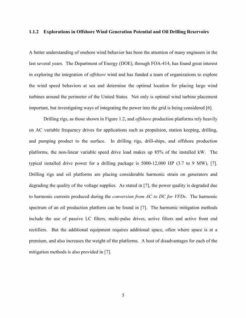
1.1.2 Explorations in Offshore Wind Generation Potential and Oil Drilling Reservoirs
A better understanding of onshore wind behavior has been the attention of many engineers in the
last several years. The Department of Energy (DOE), through FOA-414, has found great interest
in exploring the integration of offshore wind and has funded a team of organizations to explore
the wind speed behaviors at sea and determine the optimal location for placing large wind
turbines around the perimeter of the United States. Not only is optimal wind turbine placement
important, but investigating ways of integrating the power into the grid is being considered [6].
Drilling rigs, as those shown in Figure 1.2, and offshore production platforms rely heavily
on AC variable frequency drives for applications such as propulsion, station keeping, drilling,
and pumping product to the surface. In drilling rigs, drill-ships, and offshore production
platforms, the non-linear variable speed drive load makes up 85% of the installed kW. The
typical installed drive power for a drilling package is 5000-12,000 HP (3.7 to 9 MW), [7].
Drilling rigs and oil platforms are placing considerable harmonic strain on generators and
degrading the quality of the voltage supplies. As stated in [7], the power quality is degraded due
to harmonic currents produced during the conversion from AC to DC for VFDs. The harmonic
spectrum of an oil production platform can be found in [7]. The harmonic mitigation methods
include the use of passive LC filters, multi-pulse drives, active filters and active front end
rectifiers. But the additional equipment requires additional space, often where space is at a
premium, and also increases the weight of the platforms. A host of disadvantages for each of the
mitigation methods is also provided in [7].
5

Figure 1.2: Semi-Submersible Drilling Rig [7]
Today, domestic offshore oil drilling takes place in the Gulf of Mexico and Northern
Alaska, as shown in Figure 1.3. The eastern seaboards, from North Carolina through Maine, are
locations with the greatest potential for offshore oil and gas drilling. Considering a few results in
Figure 1.4 from the Department of Energy wind turbine placement study mentioned earlier
showing available wind generation along the east coast, readers will observe a strong overlap
between high wind penetration and oil drilling areas approved by the United States government
when comparing Figure 1.3 and Figure 1.4.
The offshore production platform is an opportunity for a more innovative application
while taking advantage of the offshore wind turbine power generation locally. The directions
that many manufacturers of power system equipment are exploring with offshore technologies,
Figure 1.5, to harness and transmit electric power provides further encouragement that the
direction proposed is viable [8].
6

Figure 1.3: Location of Oil Drilling Opportunities between 2012 and 2017 [5]
Figure 1.4: Available Wind Generation Onshore and Offshore in the United States [9]
Figure 1.5: Offshore Platforms – Siemens Offshore Design (Left), [10]& ABB Offshore Design (Right), [11]
7

1.1.3 Challenges and Opportunities with Microgrids
The MVDC architecture, [1], [5], has often been referred to as a type of microgrid upon first
view. The microgrid concept was first proposed in 2002 as a better way to implement the
emerging potential of distributed generation. During disturbances, the generation and
corresponding loads can separate from the disturbed grid, maintain service, and not harm the
overall grid’s integrity. As pointed out by [12], the difficult task is to achieve the microgrid
functionality without extensive custom engineering and still have high system reliability and
generation placement flexibility.
The fundamental microgrid requirements include the capability of operating in islanding
and/or grid connected modes with high stability, mode switching with minimum load disruption
and shedding during transitions, and after a transition, stabilize in a certain amount of time. The
high-level technical challenges associated with microgrids include (1) operation modes and
transitions that comply with IEEE1547 (Standard for Interconnecting Distributed Resources with
Electric Power Systems), [13], and (2) control architecture and communication. For the case of
an AC based microgrid, the following items are considered by various research teams:
• Islanding mode:
Frequency and Voltage Stability, Optimal Power Flow
• Grid to Islanding mode:
Transition and Stabilization, Minimum load shedding and disruption
• Islanding to Grid mode:
Re-synchronization and Re-connection, Minimum impact on sensitive loads and
electronics as transients evolve during state transitions
Key research and development needs are centered upon operational inverter improvements
(harsh environment design, robust operation during fault conditions, improved overload, volume
8

and weight reduction) and improved system yields (micro and mini converters). A listing of
topics referred to as advanced concepts provided in [14] focused on (1) an integrated storage
inverter, (2) direct medium voltage inverter design and (3) DC microgrid subsystems. These
components are extremely important but protection is also one of the most vital challenges facing
the deployment of microgrids.
1.1.4 Increased Interest in Microgrid Operations for AC and DC Architectures
A plug-and-play property of the microgrid is defined as a unit (either generation source or load)
that can be placed at any point without re-engineering the system or controls. Ideally, the
microgrid should maintain system operation even if one component is lost [12] and operate
without communications [15] because of the long distance between generation units [16].
The ability of the microgrid to transition to an islanded state smoothly or automatically
reconnect to the bulk power delivery system (and vice versa) is an important operational property
[12]. This feature also supports the fact that the reference frequency in a microgrid application is
not fixed and depends on the magnitude of the load and power frequency curves of the sources
[15]. These transitions from one system state to another will be referred to as a mode transition
throughout this dissertation. Other transition modes are application specific. Handling internal
fault ride-through in the case of wind turbine systems is a prime example. The authors in [17]
designed a phase-locked loop controller for grid failure detection and automatic mode switching
between stand-alone and grid-connected modes for a 11 kW, full converter, wind turbine. In
[18], the authors investigated parallel microgrid inverters with the design challenge of ensuring
precision power flow control, current sharing between the converters and smooth transition
between grid-tie and islanding modes. An adaptive droop control method is formulated for
9

inverters operating in grid-connected and islanded modes in [19] and a control strategy to handle
transient disturbances and faults in [20].
Most of the research conducted so far has concentrated on AC microgrids [21]. The DC
microgrid has a similar network structure compared to a single phase AC microgrid. The
fundamental differences include the existence of a frequency component and reactive power flow
control is not necessary in a DC system. Power flow is controlled by voltage droops in AC
[22],[23],[24],[25] and DC systems [26]. Droop control is extensively found in the literature and
is worthy of explaining here. Consider a two generator system with grid impedance, Z, between
both units. The apparent power, S, flowing from the reference generator to the next can be
described with (1.1). The real and reactive power components from (1.1) are described by (1.2)
and (1.3), respectively.
−=
−===+ − θ
δ
j
j
ZeeVVV
ZVVVIVSjQP 21
1
*21
1*
1 (1.1)
)cos(cos 212
1 δθθ +−=ZVV
ZVP (1.2)
)sin(sin 212
1 δθθ +−=ZVV
ZVQ (1.3)
Utilizing the fact, jXRZe j +=θ , (1.2) and (1.3) can be rewritten as (1.4) and (1.5).
( )[ ]δδ sincos 22122
1 XVVVRXR
VP +−+
= (1.4)
( )[ ]δδ cossin 21222
1 VVXRVXR
VQ −+−+
= (1.5)
10

Relationships (1.4) and (1.5) can be simplified to (1.6) and (1.7). By utilizing a small angle
approximation and neglecting line resistance; one arrives at (1.8) and (1.9).
12 sin
VRQXPV −
=δ (1.6)
121 cos
VXQRPVV +
=− δ (1.7)
21VVXP
≅δ (1.8)
121 V
XQVV ≅− (1.9)
From (1.8) and (1.9), the angle δ can be controlled by regulating P and the voltage V1 is
controllable through Q. Control of the frequency dynamically controls the power angle and thus,
the real power flow. By adjusting P and Q, frequency and amplitude of the grid voltage are
determined.
1.1.5 Microgrid Hierarchical Control Terminology
Only a few works conceived the microgrid as a whole problem taking into account the different
control levels. In the literature, [27] and [28] provide exceptional overviews of the three control
layers within microgrids – primary control, secondary control, and tertiary control. The primary
control – droop control discussed earlier – is often used to emulate physical behaviors to make
the system stable and more damped. The primary control maintains voltage and frequency
11

stability of the microgrid prior to islanding. The secondary control ensures that the electrical
signals through the microgrid are within the required values compensating voltage and frequency
deviations toward zero when necessary caused by the operation of the primary controls. Finally,
the tertiary layer controls the power flow between the microgrid and main grid. Figure 1.6 is an
illustration showing the interoperability of the primary, secondary, and tertiary control within a
microgrid set-up. Figure 1.7 shows the reduced controller complexity for a DC microgrid with
respect to an AC microgrid.
Figure 1.6: Block Diagram of Microgrid Control Layers Operating in Unison [27]
Figure 1.7: Hierarchical Control Architectures for an AC and DC Microgrid [28]
12

1.2 SIGNIFICANCE AND CONTRIBUTIONS
With improvements in power electronics technology, renewable energy resources are
experiencing wider adoption and commercial facilities are considering new infrastructure options
with the vast increase in IT hardware. These movements are allowing research teams to propose
ideas centered around high and low voltage DC grids. As examples, reference [29] studied a
multi-terminal HVDC system for transferring power between (1) one wind farm to two grid
connected points and (2) multiple wind turbines to one grid connected point. Reference [30]
studied the eight different operation modes within a DC data center environment. Variable wind
turbines and energy storage systems coupled through a DC microgrid are explored in [21]. The
microgrid, currently, is also being considered for more efficient disaster recovery [31], [32].
With the motivation and current industry/academia pursuits established, one main goal of
this study is to investigate offshore, power management strategies within a medium voltage DC
microgrid as various network components transition from one state (grid-connected or islanded)
to another while adequately serving critical industrial processes. The approach is to understand
that there are research needs at the power system level but determine a remedy for the problem at
the component/equipment level. For this reason, detailed model development in ANSYS PExprt,
PSCAD/EMTDC, and Matlab/Simulink is required. The chosen package is dependent on the
problem being evaluated in the forthcoming chapters.
The DC microgrid developed and analyzed throughout this dissertation is found in Figure
1.8. The main source of generation serving the offshore production platform composed of
electric motor drives includes offshore wind power, potential utility feed from an onshore
substation, and backup generators on the platform. Interfacing many of the generation sources
13

and loads are a number of power electronic interfaces – one key component being the
bidirectional DC/DC converter.
Figure 1.8: DC Microgrid - Local Wind Power being supplied to Offshore Platform
The research contributions, from the author’s perspective, include the following:
• Proposed offshore DC and, potentially, practical microgrid architecture that utilizes offshore
renewables to supply the local load. Average models of all components assembling the
microgrid are mathematically provided and combined to form the overall architecture in the
Matlab/Simulink environment.
• Performance evaluation of new magnetic materials utilized in high frequency and high power
environments showing size reductions of these magnetic components (bidirectional chargers,
transformers, and electric machines) that will indeed be utilized in the offshore production
14

platform or other environments where size and weight restrictions are common. This
optimized analysis is conducted in ANSYS PExprt or RMxprt.
• The offshore microgrid offers an opportunity for a multi-terminal application that will be
explained in Chapter 3. Therefore, a model of a high voltage DC system utilizing modular
multilevel converters is developed in PSCAD/EMTDC to evaluate component sensitivities
on peak DC fault currents. Physical systems of this size and power rating are difficult for
any computer to simulate, thus, discussions are presented on how to scale computer models,
from a system energy perspective, to predict electrical quantities of interest.
• Constant power loads are inherently unstable and common in power systems. The electric
motor drives are constant power consuming entities due to their speed regulation. This work
lays out the mathematical details showing that PD controllers, traditionally used for
stabilizing systems, are inadequate and proposes a model reference control design ensuring
stability. Although the analysis is based on linear methods (small perturbations from the
operating point), the control architecture can be readily upgraded to include adaptation
capabilities following model reference adaptive control (MRAC) design – a discussion point
in the future work.
• Our objective is to develop a simplified power management strategy between the available
renewable generation and onshore utility to provide adequate power to the platform under
various mode transitions while still maintaining continuous and seamless power to the
electric machines. Although wind turbines out at sea have higher output power potential for
transmission compared to onshore wind turbines, the engineer cannot say with 100%
confidence that the critical load can always be served by the wind generation alone. In
15

systems like Figure 1.8, the available power production is also a system constraint. At times,
the wind potential may be too high allowing for power to be transferred to the utility and at
other times too low requiring the wind turbines to disconnect and allow the utility and onsite
diesel generation to supply the critical motor loads. Ultimately, our desire is to use the diesel
generation supply at a minimum.
• Finally, communication protocols are described and proposed. One protocol is for within the
microgrid itself and another protocol for communication between other microgrids in the
same geographical location. This portion of the dissertation required discussions between
electrical engineers and telecommunication engineers speaking the same dialogue showing
that the microgrid problem is truly multidisciplinary in nature.
The proposed research objectives will have a number of profound impacts and technological
advancements in the following areas listed, in no particular order:
1. Enhancement in DC System Operation and Understanding. Changes being made to the power
system architecture and layout are drastic with increased renewable generation penetration and
power electronic equipment. From previous sections, strong arguments have been made that
support new developments in DC areas. As many have been focused on improving AC
architectures, this body of work shall go beyond the norm and enhance the engineering
community’s knowledge in DC microgrid operation.
2. Microgrids: Conceptual to Practical. Throughout the last decade, the microgrid was
conceptualized as a potential solution to improve power system reliability by having the ability
to detach from the main grid under a major disturbance. Usually, microgrids have some kind of
16

connection with a larger electrical network but this is not necessarily always the case. This
dissertation has distinct applications to help improve disaster relief procedures, future military
operating bases used for short time periods, and in non-developed nations where a strong electric
grid is non-existent.
3. Numerical Insights into Advantages of MVDC compared to MVAC. Pursuing DC system
design is a challenge when the legacy of the electric power industry has primarily been based on
AC. This dissertation area will try to disclose some of the advantages that have been
hypothesized, through a simulation environment, or perhaps reveal the challenges with DC based
grids.
4. Diagnosis of Power Electronic Operation and Equipment Interaction in a DC Environment.
Presently 30% of all electric power generated uses power electronics technologies somewhere
between the point of generation and end-use. By 2030, 80% of all electric power will flow
through power electronics, [33]. The need to understand how equipment, like power electronics,
in the grid responds, interacts and delivers power to changing loads due to operational mode
transitions is a valuable exploratory effort because this will be a future scenario that will need to
be handled appropriately both in AC and DC system design.
5. Exploratory Offshore Renewable Generation Utilization. Traditionally, engineers have
strictly focused on transporting offshore renewable energy, specifically wind power, to the shore
and utilizing the remaining power, after losses have been considered, to power equipment on
land. The system described in the proposal body is a unique application that uses offshore wind
generation, locally, to power an offshore production platform (a heavy industrial environment).
Although conceptual at first, the oil and gas industry could potentially benefit from this study.
17

As stated earlier, many global manufacturers are pursuing initiatives and funding offshore power
equipment design.
6. Evolving Application for High Voltage DC. The increasing need for high voltage, grid-scale
power electronics (HVDC & FACTS) and growth is astonishing. Also, multi-terminal HVDC is
a concept that has been proposed but, in practice, has not been implemented to date. The
medium voltage DC concept is an application of a multi-terminal scenario and microgrid
packaged into one unit which will be explored.
1.3 DISSERTATION OUTLINE
This dissertation provides a thorough treatment (but not complete!) for an offshore, medium
voltage DC microgrid power system design. This dissertation is organized in 7 chapters, as
follows:
Chapter 2 looks into power density improvements for electric machines, transformers and
bidirectional DC/DC converters utilizing novel nanocomposite magnetic materials capable of
performing at high switching frequency. The analysis is conducted in various ANSYS packages.
Chapter 3 investigates the design of a modular multilevel converter based HVDC system
with key analysis focused upon component sensitivities to system fault currents. Scaling the
HVDC system for large submodule count per inverter arm is also emphasized. The analysis is
conducted in PSCAD/EMTDC.
Chapter 4 presents the argument that the motor drives on the offshore platform can be
modeled as constant power loads. First, it is shown that traditional proportional-derivative
18

control cannot be used to stabilize constant power loads and a new, small signal model reference
control is analytically derived for stabilizing the constant power load. The analysis is primarily
conducted in Matlab/Simulink.
Chapter 5 explores the detail model development for all components of the DC microgrid
power system described in Chapter 1 including wind turbine models, detailed variable frequency
electric drive model, average converter models, and associated controls for each component.
Model development was entirely developed in Matlab/Simulink using the SimPowerSystems
toolbox.
Chapter 6 presents a power management routine implemented within the model
developed in Chapter 5. A few mode transitions are evaluated and results presented including
grid connected to islanding mode and islanding to grid connected mode. Low voltage ride
through studies conducted with the wind generation is considered a future work item. Emphasis
is placed on the behavior of the components on the offshore platform and behavior of the
bidirectional DC/DC converters in the model.
Chapter 7 demonstrates the necessary communication requirements for the offshore DC
microgrid. A multi-disciplinary partnership was established between the research groups of the
electric power initiative in the Swanson school of engineering and the department of
telecommunications to adequately research this microgrid problem. Lite details are only
provided for completeness with more extensive results published collaboratively between both
parties.
Chapter 8 concludes the dissertation by summarizing the major takeaways of this
document while also providing a few suggestions for future work including experimental
verification in the electric power systems laboratory at the University of Pittsburgh.
19

2.0 POWER DENSITY IMPROVEMENTS UTILIZING HIGH FREQUENCY
MAGNETIC NANOCOMPOSITE MATERIALS IN POWER APPLICATIONS
The need for the advancement of soft magnetic materials for applications in high-frequency,
medium-voltage, MW-scale power electronics and grid integration technology is conveyed by
recent DOE reports [34]. Figure 2.1 provides a comprehensive summary of the power electronic
programs that the Advanced Research Project Agency – Energy (ARPA-E) has found interest in
funding. Increases in DC power conversion and DC loads also motivate research into new
topologies containing high-frequency DC-to-DC power converters. The soft magnetics used in
these power electronics can occupy significant space, require extensive cooling, and limit
designs [35]. Operation at higher frequencies allows for reductions in converter size and weight
[36],[37]. Current commercial magnetic core materials are limited by low saturation inductions,
in the case of ferrites, or limited to low-frequency applications because of unacceptable losses at
high frequencies, in the case of silicon steels. Nanocomposites contain both the soft magnetic
strengths of amorphous core materials with the more attractive saturation inductions of
crystalline metals, a combination naturally well suited for high-frequency converter applications
[37],[38].
The operation of power converters at higher frequencies is limited by increased losses, a
trend accounted for by the Steinmetz Equation, (2.1), which relates the operating frequency, f,
and saturation induction, Bs, to power loss. In (2.1), the material-dependent, empirically-found
20

βαBkfPL = (2.1)
Steinmetz Coefficients, α(~2) β(~1-2), account for all core losses, in which hysteretic, anomalous
and conventional eddy current losses are predominant. Eddy current losses depend on electrical
resistivity, sample geometry, and dimensions. The operating frequency of a transformer can be
chosen by considering the tradeoffs at high switching frequencies, namely, reduced converter
size at the expense of reduced efficiency.
Exhaustive development of nanocomposites, such as FINEMET, NANOPERM, and
HITPERM, has shifted focus to optimizing these materials’ properties specifically for their use in
state-of-the-art power converters, [39],[40],[41]. Combinations of compositional additions and
novel processing techniques have produced nanocomposites with permeability, μ > 105,
saturation induction, Bs > 1.6T, resistivity, ρ > 150μΩ-cm, thickness, t < 15 μm, temperature
stability up to 300oC, and overall core losses less than 20 W/kg at 10 kHzT, a unit convention set
by the ARPA-E. Note that T in the metric is Tesla.
Figure 2.1: 2010 Power Electronic Opportunities for Improvements [34]
The unique material properties possessed by nanocomposites also present challenges.
Converter designs developed for ferrites or silicon steels may not be the ideal designs for new
21

nanocomposites. With currently available soft magnetic materials, thermal management
requirements limit converter power density below levels that could otherwise be achieved with
advanced switching circuits [35]. The research presented here is focused on a HTX-012B, a
novel nanocomposite magnetic material whose iron based chemistry has been optimized to have
low coercivity and low permeability. The material’s performance will be evaluated in three
major power engineering applications including electric machines, transformers, and
bidirectional chargers with higher emphasis on the latter two applications. Continuing with the
offshore medium voltage DC microgrid theme, the yellow encircled components found in Figure
2.2 can take advantage of these high frequency magnetic materials.
AC / DCThree LevelMultilevel Rectifier
(NPC)
+ -
MVDCCollection Platform
5 MW Supply
AC / DCThree LevelMultilevel Rectifier
(NPC)
DC Cable
Breakers
MPPT EnabledPMSG Based
PMSG Based
Off-Shore Oil Drilling Platform
Voltage Regulator
AC / DCThree LevelMultilevel Rectifier
(NPC)
PMSG Based
AC / DCThree LevelMultilevel Rectifier
(NPC)
PMSG Based
5 MW Supply
5 MW Supply
5 MW Supply
MPPT Enabled
MPPT Enabled
MPPT Enabled
DC / DCConverter
DC Cable
DC Cable
DC Cable
DC Cable
DC / ACThree LevelMultilevel Inverter
(NPC)
#1 #2AC Cable
Wind Generation(Off-Shore)
~- M
~- M
~- M
~- M
~- M
~- M
+ -
DC / DCConverterDC Cable
Diesel Generator
Magnetic Design
Magnetic Design
Magnetic Design
Figure 2.2: Offshore Medium Voltage DC Microgrid Emphasizing Magnetic Intensive Areas
22

2.1 MOTIVATION FOR DESIGNING BIDIRECTIONAL CHARGERS WITH
HIGH FREQUENCY MAGNETIC COMPONENTS
The topology chosen for the DC/DC converter first proposed in [42] is the dual active bridge
(DAB) DC/DC converter. Multiple configurations have been proposed with two of the most
common provided in Figure 2.3. Half-bridge converters, as shown in Figure 2.3 (a) consist of a
single phase leg in parallel with a split capacitor bus. These converters have been applied in
uninterruptible power supply systems, electric vehicle applications, and photovoltaic arrays.
Although the half-bridge converters offer a reduced switch count in comparison to the full-bridge
configuration, their primary drawback is the size and cost of the DC capacitors (C1-C4) required.
Half-bridge topology ratings are limited to below 400 V and 2 kW, which is not applicable for a
medium voltage design (kV rating) [42],[43].
The single phase, full-bridge, DAB topology found in Figure 2.3 (b) is very attractive
because of its zero-voltage switching capability, low component stresses (increased phase legs),
high-power density applications [42],[44],[45],[46] and accommodates voltage levels up to 1 kV
and higher [47]. The configuration has found widespread use in shipboard power systems
because of its galvanic isolation property between two voltage levels through a transformer [48].
In recent literature, [49] explored controller designs for varying loads with the full-bridge DAB
operating in the megahertz operating regime while maintaining high efficiency operation. The
ARPA-E has also funded work to investigate bidirectional, battery-to-grid charger applications
using GaN devices [50]. With growing trends towards higher switching frequency based
bidirectional charger applications which utilize transformers, the motivation is set to perform an
analysis using ANSYS PExprt to quantify the potential benefits of using HTX-012B in the
charger transformer.
23
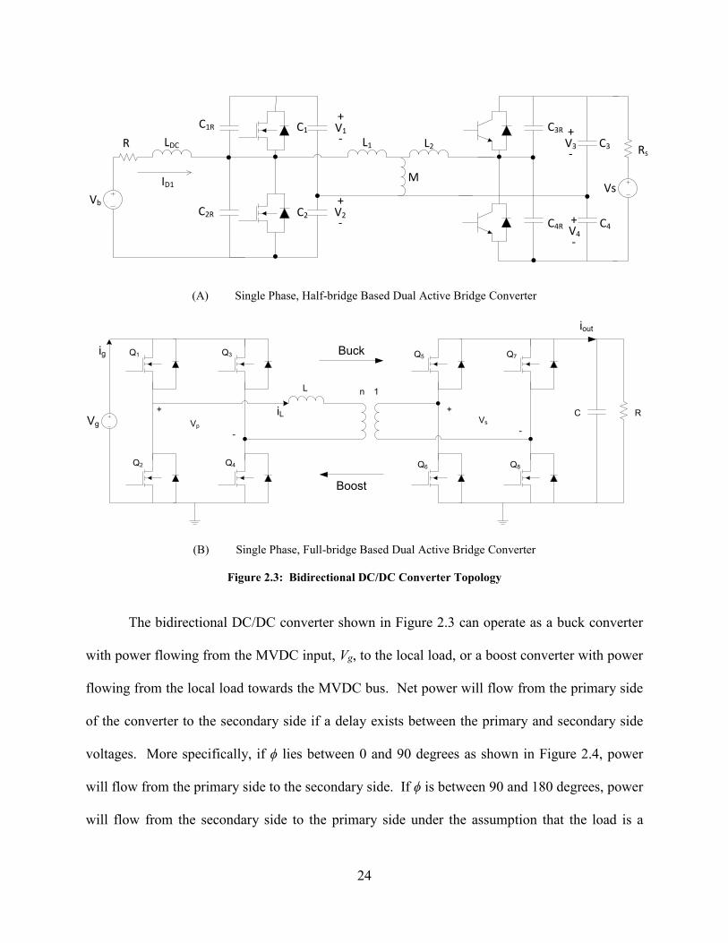
Vb
Vs
Rs
M
L1 L2
C1
C2
C3
C4
C1R
C2R
C3R
C4R
LDC
V1
V2
V3
V4
+
-
+
-
+
-
+
-
R
ID1
(A) Single Phase, Half-bridge Based Dual Active Bridge Converter
Vg
Q1
Q2
Q3
Q4
Q5
Q6
Q7
Q8
L 1n
+ +
- -Vp
Vs
ig
iL
iout
C R
Boost
Buck
(B) Single Phase, Full-bridge Based Dual Active Bridge Converter
Figure 2.3: Bidirectional DC/DC Converter Topology
The bidirectional DC/DC converter shown in Figure 2.3 can operate as a buck converter
with power flowing from the MVDC input, Vg, to the local load, or a boost converter with power
flowing from the local load towards the MVDC bus. Net power will flow from the primary side
of the converter to the secondary side if a delay exists between the primary and secondary side
voltages. More specifically, if ϕ lies between 0 and 90 degrees as shown in Figure 2.4, power
will flow from the primary side to the secondary side. If ϕ is between 90 and 180 degrees, power
will flow from the secondary side to the primary side under the assumption that the load is a
24

voltage source like a battery. The waveforms illustrated are ideal and neglect the resonant
transitions that may occur between the substrate capacitances of the semiconductors and line
inductance. The numbers associated with each of the four intervals shown in Figure 2.4
correspond to the active switches shown in Figure 2.3.
+Vg
-Vg
ωt
Vp
+V
-V
ωt
Vs
ωt
IL
ωt
Ig
π+φ0 πφ
1467
58
14
58
23
67
23
+Ip
-Ip
+Ip
-Ip
Figure 2.4: Voltage and Current Waveforms of DAB DC/DC while Operating in Charging (Buck) Mode
25

2.2 OPTIMIZING BIDIRECTIONAL CHARGER MAGNETIC DESIGN FOR
KILOWATT SCALE POWER APPLICATIONS USING ANSYS
With the understanding of the DAB circuit behavior, procedures for evaluating the magnetic
performance of HTX-012B against traditional ferrites using ANSYS PExprt are explored. A
benchmark circuit platform used for the analysis is taken from [46],[51]. The single phase DAB
converter was experimentally prototyped and rated for 300 V input, 1-to-1 turns ratio, 20 kHz
operating frequency, and 1 kW rated output power.
2.2.1 Analytical Methodology for Optimizing Transformer Parameters
Consider the single phase core found in Figure 2.5. The graphic shows appropriate dimensions
from the front and side views of the transformer core with windings appropriately colored – a is
the width of the main flux path, b is the width of the transformer window, h is the height of half
of the transformer window, and thickness d.
Traditionally, modeling every winding associated with the core is not of interest unless
AC resistance is of concern resulting in model approximations [52]. For the analysis presented,
it is assumed that (1) the windings are fully filled in the window area of the core and (2) the
volume model of the transformer can be simplified by assuming the coils are densely packed
(high fill factor). The volume of the transformer (core + windings) can be expressed with the
geometric parameters of the latter paragraph as shown in Table 2.1.
The cost function (transformer volume), optimized variables (geometric dimensions of
transformer) and constraints of interest are listed as (2.2). The design constraints are functions of
the geometric dimensions of the transformer as well as driving frequency as indicated by (2.3),
26

Table 2.1: Geometrical Relationships Associated with Transformer Core
Geometric Property Mathematical Relationship with Geometric Dimensions
Cross Sectional Area adAc =
Window Area bhAw 2=
Mean Length per Turn )(2 dbalo ++=
Transformer Width )(21 bal +=
Transformer Thickness bdl +=2
Transformer Height hal 223 +=
Transformer Volume 321 lllV =
Core Volume hbddhabaVc 2)22)(2( −++=
Transformer Thermal Area )(2 323121 llllllAt ++=
Figure 2.5: Single-phase Transformer Core for Dual-Active Bridge Converter [46]
27

(2.4), and (2.5). Equation (2.3) is the transformer universal EMF equation assuming the core is
driven by a sinusoid, (2.4) is the standard Steinmetz relationship describing transformer core loss
for nanocomposite materials, (2.5) is a relationship describing transformer winding losses [35],
and (2.6) is an estimate on the temperature rise within the core, [53]. Note that α, β, and k are
standard Steinmetz coefficients, l is a magnetic effective length, and ϕ is a geometric constant.
Equation (2.2) through (2.6) establishes the basis for an optimization problem with given
constraint that can be solved using Matlab optimization algorithms. The benchmark results for
our study are provided in Table 2.2 - both numerical results and available core selected, [51].
maxmax ; TTBB riseTx << (2.2)
fNadEB rms
π22
max = (2.3)
βα BkfVP corecore = (2.4)
cwinding A
lN
lBP ρµφ
= max
21
(2.5)
826.0
450
+=
t
windingcorerise A
PPT (2.6)
The existing literature provides a nice basis for sizing cores of any size. However, the
research team in [51] had to select a bobbin from a different manufacturer with given design
constraints. Utilizing ANSYS PExprt, a solution was found that achieves a smaller magnetics
volume with parts (core and bobbin) that can be purchased from the same manufacturer. This
analysis will be shown next.
28

Table 2.2: Optimal Core Results for DAB Benchmark Case with Available Commercial Core Metrics [51]
Transformer Property Optimized Numerical Result (Single Phase)
Commercial Core (Magnetics: 0P44125UC)
Volume (mm3) 85376 105204
Bmax(T) 0.3 0.25
Core Loss (W) 1.79 2.16
Winding Loss (W)
Total Loss (W)
Transformer Turns
a (mm)
b (mm)
d (mm)
h (mm)
7.02
8.81
82
11.7
13.0
13.0
21.6
2.84
5.0
78
11.94
18.8
11.94
15.9
Figure 2.6: Magnetics 0P44125UC [54]
29

2.2.2 Optimal Ferrite Core Transformer Parameters Analyzed through ANSYS PExprt
The transformer core uses P material that is commonly used for low to medium frequency
general-purpose power converters and is engineered for lowest loss at 95°C, [55]. The
parameters required by the software are provided in Table 2.3. AWG22 gauge wire was chosen
for this application. With a 300 V peak-to-peak, 20 kHz square wave voltage defined having a
duty cycle of 50%, the computer software is able to optimize a transformer core rated for 1 kW
using stock libraries. PExprt optimizes based on reducing the total system loss associated with
the core and windings towards a minimum. The vendors incorporated into the program include
AVX, Electrical Steel, Epcos, Ferroxcube, Magnetics, Metglas, Micrometals, Steward, and TDK.
Only one stock library can be selected to be evaluated per solution set, thus, Magnetics was
chosen. The top ten cores selected for a 1 kW rated core are provided in Table 2.4. Figure 2.7
provides the volume for each core relative to each other for the ten proposed solutions.
Table 2.3: Ferrite Material Properties
Ferrite Material Property Quantity
Core Resistivity 5 Ω-m
Relative Permittivity 10000
Initial Permeability 2500
Magnetic Flux Density Saturation
Steinmetz Coefficient α
Steinmetz Coefficient β
Steinmetz Coefficient k
0.375 T
2.1
2.65
0.0015 kW/m3
30

Table 2.4: Top Ten Core Solutions Rated for 1 kW Utilizing Ferrite Core
Core Name Volume (mm3) Turns Temperature
(oC) Parallel Turns Power Losses (W)
ETD49 24510 72 58.91 2 5.2485 ETD49 24510 72 74.55 1 8.3685 EC70 39621 55 42.84 2 4.6319 EC70 39261 55 51.26 1 7.2212
EE45528 43050 44 50.03 2 5.4129 EE47228 50416 42 45.32 2 5.0993 EE47228 50416 42 54.36 1 7.7417 ETD59 51152 42 42.92 2 4.7803 ETD59 51152 42 50.65 1 7.3051
EE48020 68265 42 43.71 2 6.1329
1 2 3 4 5 6 7 8 9 10Solution Volumes 24510 24510 39621 39621 43050 50416 50416 51152 51152 68265
0
10000
20000
30000
40000
50000
60000
70000
80000
Volu
me
(mm
3 )
Optimal Manufacturer Core Volume Solutions
Figure 2.7: Optimal Manufacturer Core Volume Solutions
31

The advantages of operating at higher switching frequency include component volume
reductions resulting in improved power density, one of the key drivers behind the ARPA-E
program. Hence, the core volume, total loss, and number of wire turns around the core are
parameters of interest in this analysis with core volume being of highest priority. Evaluating the
solutions in Table 2.4, the core selected for the 1 kW application is the ETD49. Two solutions
are associated with the ETD49 core – the solution with 5.25 W total loss, 2 parallel turns, and
maximum temperature rise of 58.91oC is chosen. Other valuable parameters associated with this
design including current density and maximum flux density are included in Figure 2.8.
Figure 2.8: Notable Parameters associated with the ETD49 Ferrite Core Design for the 1 kW DAB
The dimensions associated with the core and bobbin is provided in Figure 2.9. Figure 2.9
(a) provides the dimensions of the bobbin, Figure 2.9 (b) provides the dimensions of the core,
Figure 2.9 (c) and (d) provide the schematic and dimensions associated with a readily available
core from Magnetics, respectively. A cross sectional view of the core with winding arrangement
is found in Figure 2.10. This schematic is the geometry that can be used to conduct a finite
element analysis upon if quantities such as current density distribution, flux distribution, power
loss vs. time, and other variables that might be of interest.
32

(A) PExprt Bobbin Dimensions (B) PExprt Core Dimensions
(C) Magnetics Manufactured Core (D) 2014 Manufactured Core Dimensions
Figure 2.9: ETD49 Core: Simulation Results and Manufactured Component from Magnetics [56]
33

Figure 2.10: Cross Section of 72 Windings Configured in Two Parallel Turns around ETD49 Core
2.2.3 Optimal HTX-012B Nanocomposite Core Transformer Parameters Analyzed through ANSYS PExprt
HTX-012B is a material whose chemistry has been optimized for high switching frequency,
tunable permeability depending on desired application, capable of operating at high temperature
(above 200oC), and designed for high power applications (kW to MW scale magnetic core
designs). A few disadvantages of the material are that the alloy saturates between 1 and 1.2 T
and is mechanically brittle. Throughout this section, the same analysis is conducted as in Section
2.2.2 except the ferrite has been replaced with HTX-012B.
Before the magnetic material could be evaluated in a charger application, loss
characteristics of various cores had to be obtained experimentally as a function of frequency and
34

induction level. Once these parameters were obtained, the Steinmetz coefficients could be
evaluated and used as inputs into the software.
Six circular cores made of HTX-012B were manufactured, annealed, then impregnated,
and tested by technicians at Spang & Company – Magnetics division. Two sets of cores were
fabricated – uniform cores and cut cores having outside diameters of 1.25 inch (small), 2.81 inch
(medium), and 6.25 inch (large). As the cores were scaled, the ratio between the inside and
outside diameter was fixed at 0.80 to reduce flux crowding. The size of the cut in the cores is
0.002 inches. General properties associated with the cores are provided in Table 2.5 with core
loss measurements associated with the cores for three different frequencies in Table 2.6.
Table 2.5: Dimensions, Mass, and Permeability of Experimentally Tested Cores
Table 2.6: Core Loss Measurements at Varying Frequencies and Induction Levels for Experimental Toroids
35

The core loss results of Table 2.6 have been plotted to show various trends as the cores
are geometrically scaled. Figure 2.11, Figure 2.12, and Figure 2.13 are the core loss results for
fixed frequency excitation of 20 kHz, 50 kHz, and 100 kHz, respectively. Figure 2.14 are the
results for fixed induction. A few trends can be observed. Consider Figure 2.11 although the
following observation can be seen in Figure 2.12 and Figure 2.13. The annealed core loss
remains constant (left to right in the plots) as the size of the cores increases for a given
frequency. This is not the case for the cores that were impregnated and impregnated with cut.
For the latter core conditions, the losses increase with increasing core size. Interestingly, the
losses are lower in magnitude for the large cores compared to the small and medium-sized cores.
This trend is related to the mechanical stress states of the cores. Consider the loss trends from
top to bottom for each figure. As induction levels increase, losses consistently increase. Finally,
consider when the applied induction level is fixed and frequency varies as shown in Figure 2.14.
The losses measured appear to be independent of core size and consistent from core to core if
applied induction is fixed and frequency is varied. The experimentally determined Steinmetz
coefficients based off of this data is provided in Table 2.7.
Table 2.7: Steinmetz Coefficients Associated with Tested Cores
36

Small Medium Large0
0.5
1
1.5
2
Loss
(W/k
g)
Core Loss Results under B=0.1T / f = 20kHz Stimulus
AnnealedImpregnatedImpregnated Cut
Small Medium Large0
2
4
6
8Core Loss Results under B=0.2T / f = 20kHz Stimulus
Loss
(W/k
g)
Small Medium Large0
10
20
30
40Core Loss Results under B=0.5T / f = 20kHz Stimulus
Loss
(W/k
g)
Figure 2.11: Core Loss for Annealed, Impregnated, and Impregnated Cut Cores (f = 20kHz) [57]
Small Medium Large0
0.5
1
1.5
2
Loss
(W/k
g)
Core Loss Results under B=0.05T / f = 50kHz Stimulus
AnnealedImpregnatedImpregnated Cut
Small Medium Large0
2
4
6
8
Loss
(W/k
g)
Core Loss Results under B=0.1T / f = 50kHz Stimulus
Small Medium Large0
10
20
30
Loss
(W/k
g)
Core Loss Results under B=0.2T / f = 50kHz Stimulus
Figure 2.12: Core Loss for Annealed, Impregnated, and Impregnated Cut Cores (f = 50kHz)
37

Small Medium Large0
0.5
1
1.5
Loss
(W/k
g)
Core Loss Results under B=0.025T / f = 100kHz Stimulus
AnnealedImpregnatedImpregnated Cut
Small Medium Large0
2
4
6
Loss
(W/k
g)
Core Loss Results under B=0.05T / f = 100kHz Stimulus
Small Medium Large0
5
10
15
20
Loss
(W/k
g)
Core Loss Results under B=0.1T / f = 100kHz Stimulus
Figure 2.13: Core Loss for Annealed, Impregnated, and Impregnated Cut Cores (f = 100kHz)
Annealed-Small Annealed-Medium Annealed-Large0
5
10
15
Loss
(W/k
g)
Changes in Core Loss with Varying Applied Frequency at Fixed Induction Level (B=0.1T)
20kHz50kHz100kHz
Impregnated-Small Impregnated-Medium Impregnated-Large0
5
10
15
20
Loss
(W/k
g)
Impregnated_Cut-Small Impregnated_Cut-Medium Impregnated_Cut-Large0
5
10
15
20
Loss
(W/k
g)
Figure 2.14: Core Loss for Annealed, Impregnated, and Impregnated Cut Cores (B = 0.1T)
38

The next task at hand is to introduce the material properties from the tested cores into the
simulation software. The bobbin for the core (Figure 2.9) will likely have an outside diameter of
36 mm (1.41 inches). From the experimental cores, Core #2 has an outside diameter of 1.25
inches and a measured permeability of 2,843. This permeability value is relatively close to the
ferrite design. The experimental core loss information of Core #2 at (20 kHz, 0.1 T), (20 kHz,
0.2 T), (50 kHz, 0.1 T), (50 kHz, 0.2 T) from Table 2.6 were inputs into the core loss definition
and Steinmetz coefficients extracted as shown in Figure 2.15. For Core #2, the effective area of
the core is 0.657 cm2.
Figure 2.15: Steinmetz Coefficients Provided by PExprt for HTX-012B Based on Experimental Loss Data
The remaining material definition parameters are provided in Figure 2.8. Although
permeability is a function of frequency, it is assumed that the permeability is relatively constant
for the frequency range of operation. For very high switching frequencies, this assumption is not
valid,[58].
39

Table 2.8: HTX-012B Nanocomposite Material Properties
HTX-012B Material Property Quantity
Core Resistivity 1 Ωm
Relative Permittivity 10000
Initial Permeability 2843
Magnetic Flux Density Saturation 1.08 T
Table 2.9: Top Ten Core Solutions Rated for 1 kW Utilizing Nanocomposite HTX-012B
Core Name Volume (mm3) Turns Temperature
(oC) Parallel Turns Power Losses (W)
EE44022 23321 40 66.08 2 5.9785 ETD49 24510 49 56.98 2 5.1987 ETD49 24510 40 68.78 1 7.5634 EC70 39621 46 47.43 2 5.6100 EC70 39621 37 57.28 1 8.4266
EE45528 43050 37 53.17 2 6.0570 EE47228 50416 39 47.94 2 5.7826 ETD59 51152 41 45.34 2 5.3978 ETD59 51152 33 54.41 1 8.1681
EE48020 68265 42 45.95 2 6.8988
Figure 2.16: Notable Parameters associated with the ETD49 Nanocomposite Core Design for the 1 kW DAB
40

The top ten optimized core results for a 1 kW DAB core utilizing HTX-012B is provided
in Table 2.9 with other parameters of interest associated with the core in Figure 2.16. For
reasons listed previously, the best suitable design is the ETD49 core using two parallel turns.
Although the same core is utilized in this design compared with the ferrite design, there are some
advantages to using the HTX-012B material that will be pointed out in the next section.
2.2.4 Results Comparison between Analytical Ferrite Core, Computer Simulated Ferrite Core, and Computer Simulated Nanocomposite Core
Table 2.10 provides a side by side comparison of the ferrite core results (benchmark) with the
results when utilizing HTX-012B in the core. Realize that the analytical result is an
approximation from the originally proposed geometry whereas PExprt provides a more formal
solution from a larger family of core shapes and sizes that are widely available for purchase. By
utilizing a nanocomposite material, the losses are more evenly distributed between the core and
windings. The number of turns required to achieve the DAB ratings (1 kW, 300 V, 20 kHz) is
reduced in comparison to the ferrite design as well as the core’s magnetizing inductance. The
ferrite material does not exhibit any noticeable advantage in comparison to HTX-012B from an
electrical engineering design perspective. Note that economics have not been taken into account.
Table 2.10: Comparison of Optimized Core Results
Transformer Property Analytical Result (Square Core)
Optimized / Commercial Ferrite Core
Optimized / Commercial
HTX-012B Core Volume (mm3) 85376 24510 24510
Bmax(T) 0.3 0.242 0.355 Core Loss (W)
Winding Loss (W) Total Loss (W)
Turns Core Temperature (oC)
1.79 7.02 8.81 82 --
0.924 4.324 5.249
72 53.04
2.516 2.683 5.199
49 52.74
41

2.3 ELECTRIC MACHINE POWER DENSITY IMPROVEMENT USING
NANOCOMPOSITE MATERIALS
Colleagues on the ARPA-E project have explored a new class of Fe-Co based amorphous and
nanocomposite materials in permanent magnet machine applications. Co-rich compositions offer
the benefits of Fe-rich alloys but are not nearly as brittle and offer an alternative for high
frequency operation when material strength is critical, [59]. Frequencies in excess of 1000 Hz
can be achieved. However, Co-rich materials have lower saturation inductions, which ultimately
impact overall torque production from a machine.
Novel materials contribute to improved machine power density but also novel motor
architectures. Reference [59] chose the Parallel Path Magnetic Technology (PPMT) architecture
because peak power density can be achieved with little or no rare earth material. For 10 kW
rated machines, the team showed that a 70% size reduction can be achieved if HTX-005C (novel
Fe-Co nanocomposite material) was utilized in comparison to M-19 G29 (non-oriented silicon
steel) while using 83% less rare earth permanent magnet. Reductions are shown in Figure 2.17.
Light Grey: HTX-005 soft magnet; Dark Grey: NdFeB hard magnet
Figure 2.17: Size Reduction of 10 kW PPMT Motor Using HTX-005C Fe-Co Nanocomposite Material [59]
42

2.3.1 Power Density Improvement of Induction Motors Utilizing HTX-012B: Design Considerations
All machine designs require mechanical, electrical, and thermal analysis. Although HTX-012B
is an iron rich alloy, the intent is to show power density improvements for induction motor
applications. The B-H loop associated with HTX-012B is provided in Figure 2.18.
0 10 20 30 40 50 60 70 800
0.2
0.4
0.6
0.8
1
1.2
1.4
H (A/m)
B (T
)
B-H Curve for HTX-012B
Figure 2.18: B-H Curve for HTX-012B
To observe possible power density improvements for induction motors, an example
motor model is selected from the ANSYS RMxprt motor library. The model reflects an existing
motor and ensures validity of the operational characteristics for the base case. By increasing the
driving frequency of the motor, the motor’s size can be decreased, as described by Faraday’s
Law. This is shown mathematically for a toroidal core assuming a sinusoidal current excitation
and constant voltage in (2.7) – both the cross sectional area, A, and driving frequency, ω, are
inversely proportional to each other. Note that N and l are the number of turns and effective
43

length, respectively. When increasing the driving frequency without changing any other
parameters of the motor, the mechanical speed of the motor increases proportionally. For this
reason, the number of poles of the motor must be altered in order to maintain the same
mechanical speed. This concept is described by (2.8) where P is the number of pole pairs and ωe
and ωr is notation for the excitation frequency and rotor frequency, respectively.
)cos(2
tIl
ANdtdIL
dtdBNAV o ωωµ−
=−=−= (2.7)
2/P
er
ωω = (2.8)
The number of poles of the original motor is reduced from 8 poles to 2 poles. The
voltage, driving frequency (50 Hz), and rated speed are all kept constant. A second motor model
is then created with all the same characteristics; however, the driving frequency is changed to
200 Hz requiring an increase in pole number to keep the same rotational speed between both
cases. The number of poles was altered to 8 for the second case.
The nanocomposite material, HTX-012B, replaces the stator material but not the rotor
material for both motor models to maintain mechanical integrity. The original motor model
utilizes an electric steel listed as M19-24G in the rotor. Because the original motor model is only
rated for 50 Hz operation we cannot be sure the loss data for M19-24G is valid for higher
frequencies. For this reason, a new material, M600-50A is used to replace M19-24G in the rotor.
The core loss/material data and B-H curves were obtained from [60],[61],[62] and can be seen in
Figure 2.19 and Figure 2.20, respectively. The core loss data for M600-50A is represented by
the dashed lines in Figure 2.20.
44

With the new materials in the rotor and stator, a non-linear optimization algorithm is
performed on the geometry of the 8 pole motor. Parameters such as the outer diameter of the
stator, air gap size, slot length, and a general scaling factor are allowed to vary so as to decrease
the overall size of the motor. The objective of the algorithm is to reduce size while keeping the
efficiency and power factor high. In addition, the algorithm is run to keep the output power and
the rotational speed for the 8 pole design, the same as the 2 pole design.
Figure 2.19: M600-50A B-H Curve [62]
Figure 2.20: Core Loss Data for M600-50A [62]
45

When increasing the number of poles, it is critical to take into account how the
magnetizing current, and therefore, the power factor (P.F.) are both impacted. As the number of
poles in a motor increases, the magnetic flux has less distance to travel to get from one end of a
pole to the other. There is an inverse relationship between the number of poles and the necessary
thickness or width of the return path in the stator core. If the thickness is not increased, flux
crowding will occur and will diminish the motor’s ability to produce torque; additionally the
magnetizing current will also increase. This increases the full load current and, therefore, the
primary I2R losses. In order to maintain the same output power, the current through the rotor
cannot diminish. Therefore, the stator current must increase to provide more magnetizing
current. As the magnetizing current increases, the power factor of the motor decreases. The
machine power factor trend as machine poles increase is shown in Figure 2.21, [63].
Figure 2.21: Machine Power Factor Adjustments as Number of Machine Poles Increase [63]
46

2.3.2 Power Density Improvement of Induction Motors Utilizing HTX-012B: Motor Optimization Study
The motor model for this study is depicted in Figure 2.22 and the geometric data is listed in
Table 2.11. The geometry and winding configuration is fixed for the 2 pole design operating at
1.3 kW, 50 Hz and 2800 RPM. In order to run an optimization algorithm for the 8 pole design,
adjustable parameters are assigned to the dimensions of the rotor and stator outer diameters, rotor
and stator slots, motor length, and a scaling factor for the motor at a whole. Every geometric
variable of the motor was multiplied by the scaling factor except for the stacking factor and the
number of slots. This scaling factor was used to allow the optimization algorithm to change the
motor’s size. These variables and their constraints are listed in Table 2.12. A nonlinear
optimization algorithm is run to reduce the size of the motor while keeping the same output
power and rotational speed. The constraints of the optimization algorithm are as follows:
Efficiency > 77%; Power Factor > 0.93; Slot fill factor < 79%. These constraints were chosen to
make the machine power factor the highest priority.
Figure 2.22: Motor Geometry, Winding Configuration and Slot Dimensions
47

Table 2.11: Motor Geometric Variables Parameter Stator Rotor Outer Diameter (mm) Inner Diameter (mm) Length (mm) Stacking Factor Number of Slots Hs0 (mm) Hs01 (mm) Hs1 (mm) Hs2 (mm) Bs0 (mm) Bs1 (mm) Bs2 (mm)
210 148 250 0.92 48 0.8 NA 1.05 12.9 2.8 4.9 6.7
147.3 48
250 0.92 44 0.5 0
1.2 12 1
5.2 3.5
Table 2.12: Motor Constraints Parameter Min Max Outer Diameter Stator (mm) Outer Diameter Rotor (mm) Length (mm) Hs2 Stator (mm) Hs2 Rotor (mm) Scaling Factor
190 137 125
4 4
0.4
210 147.9 375 14 14 1
Operating characteristics for the two pole and eight pole motor are provided in Table 2.13
and Table 2.14, respectively. A 56% size reduction and a 57% reduction in weight can be
visually seen through the magnetic field plots shown in Figure 2.23 and Figure 2.24 for the two
pole and eight pole machine, respectively. While there is a 7.6% reduction in power factor
between these models, the output power, rated torque, and efficiency are all similar. Figure 2.25
Table 2.13: Two Pole Motor Output Machine Parameter Quantity
Outer Diameter Stator (mm) Outer Diameter Rotor (mm) Length (mm) Hs2 Stator (mm) Hs2 Rotor (mm) Scaling Factor Stator Ohmic Loss (W) Rotor Ohmic Loss (W) Iron-Core Loss (W) Output Power (W) Input Power (W) Efficiency Power Factor Rated Torque (N-m) Rated Speed (RPM) Rated Slip Stator Phase Current (A) Magnetizing Current (A) Rotor Phase Current (A) Total Net Weight (kg) Total Size (m3)
210 147.3 250 14 12 1 21.965 29.444 0.000564 1300.1 1519.94 85.53 0.967 4.222 2940.52 0.01982 1.3668 0.2922 1.329 54.987 0.00866
Table 2.14: Eight Pole Motor Output Parameter Quantity Outer Diameter Stator (mm) Outer Diameter Rotor (mm) Length (mm) Hs2 Stator (mm) Hs2 Rotor (mm) Scaling Factor Stator Ohmic Loss (W) Rotor Ohmic Loss (W) Iron-Core Loss (W) Output Power (W) Input Power (W) Efficiency Power Factor Rated Torque (N-m) Rated Speed (RPM) Rated Slip Stator Phase Current (A) Magnetizing Current (A) Rotor Phase Current (A) Total Net Weight (kg) Total Size (m3)
196.6 147.9 125 14 8.55 1 9.87 10.4 0.0011288 1299.3 1490.02 87.1997 0.8931 4.16534 2978.72 0.007 1.451 0.4377 1.3378 23.448 0.00379
48

Figure 2.23: Two Pole Motor Flux Distribution
Figure 2.24: Eight Pole Motor Flux Distribution
49

and Figure 2.26 show a reduction in the maximum torque for the motor from 40 Nm to 37.2 Nm;
however, rated torque remains the same. If HTX-012B is used in the stator, simulations show
improved power density and improved operating efficiency, with a minimal loss in power factor.
0.00 500.00 1000.00 1500.00 2000.00 2500.00 3000.00Speed (rpm)
-10.00
0.00
10.00
20.00
30.00
40.00
50.00
Torq
ue (N
.m)
m1Curve Info
Torque
Name X Ym1 1680.0000 40.0265
Figure 2.25: Two Pole Motor Torque vs. Speed Curve
0.00 500.00 1000.00 1500.00 2000.00 2500.00 3000.00Speed (rpm)
-5.00
5.00
15.00
25.00
35.00
Torq
ue (N
.m)
m1Curve Info
TorqueName X Y
m1 2550.0000 37.2410
Figure 2.26: Eight Pole Motor Torque vs. Speed Curve
.
50

2.4 APPROXIMATE UTILITY SCALE TRANSFORMER CORE SIZE REDUCTION
EMPLOYING NANOCOMPOSITE MAGNETIC MATERIALS
The optimization objective of any transformer design is decided by the application of the power
transformer and specification of the design. Various factors such as the weight, volume of the
transformer, cost, minimum loss, or combination of all four are often considered. Design
constraints are from the limit of the magnetic, electrical, and mechanical properties of the
materials used in transformers. Usually system constraints include the maximum flux density,
maximum allowable temperature rise and sometimes current density as shown previously. The
objective of this brief section is to optimize a 100 kW transformer core and quantify volume
reductions with increased switching frequency. The C-core design to be optimized is shown in
Figure 2.27 (dark gray component).
Figure 2.27: C-Core Transformer Design [64]
51

The design details of the 100 kW, 13.8 kV (primary) / 7.7 kV (secondary) rated
transformer will be kept to a minimal. The transformer is to operate with an efficiency greater
than 99% with a power factor of 0.93 and weighing 15 lbs. There are 8 primary circuits and 1
secondary all using multi-filar windings. All winding groups are in parallel to one another. On
the primary side and secondary side, 12 AWG Litz wire and 22 AWG magnet wire is used,
respectively.
The loss model associated with the Litz wire is described by (2.9) and (2.10), [65]. In
(2.10), ω is the transformer driving frequency, µo is the permeability constant, N is the
transformer turns, n is the number of strands, dc is the diameter of the copper strand, k is a factor
accounting for field distribution in multi-winding transformers, ρc is the resistivity of copper at
100oC, and bc is the depth of the core window. Data contributing to core loss or winding loss
computation utilized in the optimization algorithm is provided in Table 2.15.
dcacrLitzLoss RIFP 2, = (2.9)
22
622222
7681
cc
cor b
kdnNFρ
µωπ+= (2.10)
Table 2.15: Parameters Associated with Core and Winding Loss Calculation
Loss Variable Value Steinmetz Coefficient, α Steinmetz Coefficient, β Steinmetz Coefficient, k Number of Turns, N Number of Strands, n Diameter of Strand, dc Resistivity of Copper, ρc Transformer Depth, bc Litz Wire DC Resistance, Rdc Solid Wire DC Resistance, Rdc
1.695 1.967
0.787 W/kg 32 420
0.000102 m 23x10-9 Ω-m
0.110 m 0.323 Ω 0.0104 Ω
52

Table 2.1 provides the geometric relationships associated with the transformer and (2.3)
through (2.6) describe the physics associated with the transformer. Equations (2.3) through (2.6)
are function of system frequency and core geometry. The system constraints provided in Table
2.16 and latter relationships establish the necessary mathematics to optimize the transformer
core, as was demonstrated in the charger application. The Matlab optimization toolbox was
utilized to optimize the core volume and the codes that were written are provided in Appendix A.
The frequency of the core varied from 1000 Hz to 40 kHz resulting in six sets of results for six
distinct frequencies. These results are provided in Table 2.17. A plot of core volume versus
frequency is also provided in Figure 2.28.
Table 2.16: System Constraints to Optimize 100 kW Transformer
Loss Variable Value BTx Tmax
a b d h N
0.65 T to 0.75 T 150oC
0.008 to 0.08 m 0.04 to 0.36 m
0.008 to 0.08 m 0.09 to 0.51 m
25 to 32
Table 2.17: Transformer Optimization Results with Varying Frequency
Case Number 1 2 3 4 5 6 BTx (T) 1.90 0.75 0.75 0.75 0.73 0.67
Trise (oC) 13.63 41.40 59.70 88.53 116.29 134.33 Irms,primary 1.25 1.25 1.25 1.25 1.25 1.25 Pcore (W) 113.24 13.23 26.87 64.77 111.80 150.30
Pwinding (W) 89.85 89.85 89.85 89.86 89.87 89.88 Powerloss (W) 203.09 103.09 116.72 154.63 201.68 240.18
a (m) 0.080 0.041 0.022 0.011 0.008 0.008 b (m) 0.263 0.040 0.040 0.040 0.040 0.040 d (m) 0.080 0.080 0.075 0.075 0.075 0.075 h (m) 0.146 0.090 0.090 0.090 0.090 0.090
N 32 32 32 32 31 26 Vcore (m3) 0.1064 0.0050 0.0032 0.0024 0.0021 0.0021
Frequency (Hz) 1000.00 5000.00 10000.00 20000.00 30000.00 40000.00
53

0.0050
0.0032
0.00240.0021 0.0021
0.0000
0.0010
0.0020
0.0030
0.0040
0.0050
0.0060
0.00 5000.00 10000.00 15000.00 20000.00 25000.00 30000.00 35000.00 40000.00 45000.00
Core
Vol
ume
(m3 )
Frequency (Hz)
Transformer Core Volume vs Operating Frequency Fixed Flux Ranging between 0.65 and 0.75
Figure 2.28: Core Volume vs. Frequency for 100 kW Rated Transformer Core
54

3.0 MODULAR MULTILEVEL CONVERTER BASED
HIGH VOLTAGE DC MODELING, COMPONENT SENSITIVITY ANALYSIS, AND
SCALING APPROXIMATIONS
There are a number of advantages associated with Voltage-source converter High Voltage DC
(VSC-HVDC) technology including: (1) more efficient power transfer over long distances, (2)
carrying capacity of up to 2 to 5 times that of an AC line of similar voltage, (3) interconnection
of two AC systems, where AC lines would not be possible due to stability problems or both
systems having different nominal frequencies (as in Japan), (4) underwater power transfer if
cables are longer than 50 km and (5) rapid and accurate power flow control, [66]. For these
reasons, it’s not surprising to see the number of planned installations taking place in North
America and China as shown in Figure 3.1 and Figure 3.2, respectively.
Figure 3.1: Planned HVDC Installations within North America through 2019
55

Figure 3.2: Planned HVDC Installations in China through 2020 [67]
Multilevel converters are power conversion systems composed of an array of power
semiconductors and capacitive voltage sources that, when properly controlled, can generate a
multiple-step voltage waveform with variable and controllable frequency, phase and amplitude
[68]. The number of levels, n, of a converter is defined as the number of steps or constant
voltage values that can be generated by the converter between the output terminal and any
internal reference node (the DC-link node) within the converter.
A qualification of a multilevel converter to be referred to as being multilevel is that each
phase of the converter has to generate at least three different voltage levels. Figure 3.3 contains
three inverter structures. The topology on the far left is an inverter, but it is not a multilevel
inverter because the output is that of a classical voltage source inverter. The middle and far right
topologies are three and five-level topologies and are classified as multilevel inverters.
56

Figure 3.3: Definition of a Multilevel Inverter [68]
The number of levels is always defined by the number found in the line-to-neutral voltage
output, which are equally distant from each other. When considering a three-phase system, the
levels of one phase are combined with those of the other phases generating (2n – 1) voltage
levels in the line-to-line voltage waveform, where n is the phase to neutral voltage levels. The
levels that are produced by the inverter add a new degree of freedom, from the control
perspective, giving more alternatives to generate the desired output waveform. For this reason,
multilevel inverters have the capability of improving power quality resulting in lower voltage
distortion and reduced dv/dt [68].
The modular multilevel converter (MMC) topology design for an HVDC converter
station is shown in Figure 3.4. The topology boasts a number of advantages over traditional
multilevel designs including its high modularity in hardware and software, low generation of
harmonics, lower switching frequency of semiconductor devices, easily scalable, and, most
importantly, a stronger approximation of a sinusoidal output with increasing submodules [69].
57

An extensive literature review on the MMC topology, modulation, and control is provided in
[70], controller design in [71], and protection needs given a pole-to-pole fault occurrence in [72].
Missing from the literature is a sensitivity analysis of the various components that make
up the converter topology and their impacts on system currents and fault currents. The study
presented in this chapter focuses on (i) the arm reactor, Ls, sizing and configuration layout
(symmetrical vs. asymmetrical) depicted in Figure 3.4, (ii) transformer impedance, and (iii)
bypass switch (BPS) speed of response on fault current magnitudes.
Transformer
Arm reactance
Vdc
Cable
Cable
Submodule
Phase A Phase B Phase C
Vdc/2
Phase Voltage Upper Arm
uk1
Ls
LsLs
Ls
Ls
Ls
Cell Capacitor
Bypass Switch
IGBTFWD
Phase Voltage Lower Arm
uk2
ik
ik1
ik2
+
-
O
Figure 3.4: Modular Multilevel Converter Topology
58

Many research teams have also investigated approaches for simulating systems with
hundreds of submodules per converter arm, [73],[74]. In this work, 10 submodules per arm are
used to perform the majority of the sensitivity analysis. Reasons for this will be stated. A
transient analysis of a 6 submodule per arm system with appropriately sized capacitors will be
shown to predict circuit phenomena comparable to a 10 submodule per arm design.
Although the system ratings of a HVDC system are on the order of 100’s of kilovolts and
100’s of megawatts, the presence of the multi-terminal “HVDC” concept is an apparent
characteristic of the offshore medium voltage DC microgrid concept as shown in Figure 3.5.
AC / DCThree LevelMultilevel Rectifier
(NPC)
+ -
MVDCCollection Platform
5 MW Supply
AC / DCThree LevelMultilevel Rectifier
(NPC)
DC Cable
Breakers
MPPT EnabledPMSG Based
PMSG Based
Off-Shore Oil Drilling Platform
Voltage Regulator
AC / DCThree LevelMultilevel Rectifier
(NPC)
PMSG Based
AC / DCThree LevelMultilevel Rectifier
(NPC)
PMSG Based
5 MW Supply
5 MW Supply
5 MW Supply
MPPT Enabled
MPPT Enabled
MPPT Enabled
DC / DCConverter
DC Cable
DC Cable
DC Cable
DC Cable
DC / ACThree LevelMultilevel Inverter
(NPC)
#1 #2AC Cable
Wind Generation(Off-Shore)
~- M
~- M
~- M
~- M
~- M
~- M
+ -
DC / DCConverterDC Cable
Diesel Generator
Multi-Terminal HVDC Application
Figure 3.5: Multi-Terminal DC Application within the Offshore DC Microgrid Environment
59

3.1 MODULAR MULTILEVEL CONVERTER MODELING AND CONTROL
The MMC in Figure 3.4 consists of n series-connected half-bridge submodules on each of the six
arms, two arms per phase. For the validated model presented, the number of submodules, or n, is
10. For the entire HVDC system, there are 120 submodules. Each MMC submodule consists of
a half bridge cell where its output voltage is either equal to its capacitor voltage or zero
depending on the switching states (two states). The two switches per submodule are
complimentary in nature. The submodule voltage Vsm takes on the value of 0 volts or the voltage
on the capacitor depending upon which switch is ON and which is OFF. Figure 3.6 demonstrates
this submodule operation. The operation directly depends upon the binary input to the IGBT
switches (S1 and S2) specific to each submodule. When Vsm = VC the submodule as a whole is
considered ON. When Vsm = 0 the submodule is considered OFF.
S1
S2
VcS1 ONS2 OFF
Vsm
+
-Vsm=Vc
VcVsm
+
-
S1
S2
S1 OFFS2 ONVsm=0
Figure 3.6: Submodule States of the Modular Multilevel Converter
Circuit synthesis of the MMC topology is worthy of noting. Consider a theoretical
example system with 6 submodules (n = 6), the system is considered a 7 voltage level system (n
+ 1). To achieve Level 7 all upper switches of one arm must be turned ON (Vsm = VC) while all
lower switches of the same arm must be turned OFF (Vsm = 0). To achieve Level 6, the first 5
upper switches closest to the arm reactor must be turned ON and one lower switch closest to the
arm reactor must be turned ON with all other switches OFF. Figure 3.7 provides a visual aid of
these voltage level changes on the Phase A branch of the MMC. This pattern continues until the
approximate sinusoidal waveform is established based upon 7 levels.
60

Transformer
Arm reactance
Vdc/2
Vdc/3
Vdc/6
0
Phase A Phase A Phase A Phase A
Level 7 Level 6 Level 5 Level 4
Figure 3.7: Circuit Synthesis of 6 Cell per Arm MMC Converter
3.1.1 Generalized Mathematical Model of the MMC Converter
In Figure 3.4, ik1 and ik2 represent the upper and lower arm currents of phase-k (k = a, b, c) with
their sum being composed of the total line current, ik. Mathematically, this is expressed as (3.1).
kkk iii =+ 21 (3.1)
61

Because the capacitors within the top arm and bottom arm are never equally balanced for
all system conditions, a current difference can exist that circulates through each phase. This
current difference is expressed as (3.2). The circulating currents within the three phases must
sum to zero as described by (3.3). The circulating currents have no effect on the DC or AC-side
of the converter but perform a role in the sizing of the MMC components and capacitor ripple,
[71].
2
21 kkkz
iii −= (3.2)
0=++=∑ kckbkakz iiii (3.3)
Writing Kirchoff’s voltage law for phase-k in Figure 3.4, equations (3.4) and (3.5) can be
deduced for the upper and lower converter arms, respectively. Note that point “O” is a fictitious
dc-side mid-point associated with vo. This term can often be neglected if the system is balanced.
Also, uk is the terminal voltage associated with the AC-side of the converter.
dt
diLLuVvu kTxsk
dcok
11 )2(
2+=
−+− (3.4)
dtdiLLuVvu k
Txskdc
ok2
2 )2(2
+=
+−− (3.5)
The sum of (3.4) and (3.5) divided by 2 leads to (3.6). Equation (3.6) describes the dynamics of
the MMC converter on the AC-side for any phase-k, [75], with the transformer inductance, LTx,
assumed to be much larger than the arm inductances. Utilizing Park’s transformation, (3.7), the
dq-axis relationships can be shown to be (3.8). In (3.8), f can be three phase voltage or current.
dtdiLuvuuuuu k
Txokkokk
k =−−=
+
−− )(
212 (3.6)
62

( ) ( )
( )( )( )
++
−−
=3/2cos3/2sin
3/2cos3/2sin
cossin
32
πθπθ
πθπθ
θθ
θT (3.7a)
∫=t
dtt0
)(ωθ (3.7b)
( ) abcdqk fTf θ= (3.7c)
dTx
dTx
qd v
Lu
Li
dtdi 11
−+= ω
qTx
qTx
dq v
Lu
Li
dtdi 11
−+−= ω
(3.8)
3.1.2 MMC Converter Inner Loop Controllers: Current Regulators and Tuning
Inner loop current controls are found on the sending end and receiving end converters in the
HVDC system. On the sending end converter, the outer loop provides DC voltage regulation. On
the receiving end, the outer loop regulates real power flow. The equations expressed by (3.8) are
coupled together but can be decoupled through a change of variable. Defining (3.9) and
substituting into (3.8), the result can be shown to be (3.10). Equation (3.10) represents two first-
order, decoupled subsystems with inputs being id and iq.
( ) ( )( )∫ −+−−+= dtiikiikLiuv drefdicdrefdpcqdd ,,ω
( ) ( )( )∫ −+−−−= dtiikiikLiuv qrefqicqrefqpcdqq ,,ω
(3.9)
( ) ( )∫ −+−= dtiikiikdtdiL drefdicdrefdpc
d,,
( ) ( )∫ −+−= dtiikiikdtdi
L qrefqicqrefqpcq
,,
(3.10)
63

Throughout the analysis, it has been assumed that line resistance, R, is small. If R were
considered, (3.10) would be appropriately adjusted as shown with (3.11). The closed loop
transfer function can be shown to be (3.12) if the gains are chosen to be kpc = L / τ and kic = R / τ.
The time constant, τi, ranges between 1 and 5 milliseconds, [75],[76]. The current regulator for
each converter station is found in Figure 3.8.
( ) ( )∫ −+−=+ dtiikiik
dtdiLRi drefdicdrefdpc
dd ,,
( ) ( )∫ −+−=+ dtiikiikdtdi
LRi qrefqicqrefqpcq
q ,,
(3.11)
siisG
irefd
d
τ+==
11)(
,
(3.12)
idref1
id1
iq1
iqref1
VC1 VC2 VCN
uq1
vq,ref
LTxω1
LTxω1
Third Harmonic Injection
ud1
vd,ref
vref,a
Pulse Width ModulationAnd
Capacitor Balancing Algorithm
PLL
ua1 ub1 uc1
PI
PI
θ1 = ω1t
. . .Gating Signals
to MCC
-
-
+
+
- -
+
+
-+
vref,b
vref,c
Figure 3.8: Current Controller of MMC Converter
64

To obtain the desired DC voltage, it may be required to increase the fundamental line-to-
line voltage by adding a third harmonic component to the three-phase sinusoidal modulating
wave without causing overmodulation. This technique is illustrated in Figure 3.9. Essentially,
the peak fundamental component can be higher than the peak triangular carrier wave, which
boosts the fundamental voltage. At the same time, the modulated wave can be kept lower than
the carrier signal avoiding problems caused by overmodulation. This technique is referred to as
third harmonic injection, [77]. The reference signal generated is a combination of the three-
phase sinusoidal modulated wave signal generated by the current controller based upon vd,ref and
vq,ref and a signal composed of a third harmonic.
Figure 3.9: Illustration of Modulated Case with Third Harmonic Injection [77]
3.1.3 MMC Converter Outer Loop Controllers: AC and DC Regulators
The outer control loops in the HVDC model include the AC voltage regulator and DC voltage
regulator. The adjusted error difference established by the PI controller between the measured
line-to-ground voltage on the wye-side of the transformer and reference is regulated to establish
iq,ref. AC voltage regulation is a feature of both converter stations. The adjusted error difference
65

established by the PI controller between the measured DC voltage and reference is regulated to
establish id,ref for only one converter station. Mathematically, the latter is described by (3.13).
Stronger mathematical details for tuning the DC regulators are provided in [71],[78]. For our
application, kpdc = 10 and kidc = 200.
( ) ( )∫ −+−= dtVVkVVki drefdidcdrefdpdcrefd ,,, (3.13)
In the monopolar HVDC system, one converter acts as the sending end and the other as
the receiving end at any given time. The converter controlled by the DC voltage regulator can be
seen as the sending end. The receiving end must then be controlled by a real power regulator,
ensuring proper power transfer through the system. The id,ref command for the receiving end
converter is described by (3.14), [79].
d
refrefd u
Pi
5.1, = (3.14)
3.1.4 Capacitor Balancing Algorithm
A problem that arises if left unaddressed is a voltage imbalance between the various capacitors in
a given arm. This is due to the different rates at which the capacitors are switched, resulting in
more charge being stored in the capacitors that are switched the least frequently. To remedy this
problem, an algorithm was implemented based on that demonstrated in [71], which relies on the
selection of cells based on capacitor voltage and the direction of current flow. The strategy can
be separated into three distinct portions: determination of the number of conducting cell
capacitors per arm, sorting of cells based on capacitor voltage, and selection of the conducting
cells based on current direction.
66

3.1.5 System Parameters and Dynamic Performance Evaluation
Megawatt scale HVDC systems require hundreds of submodules per arm. The key challenge for
systems of this size is simulating all power semiconductor switching events without exhausting
computational resources. A detailed article written by an IEEE task force addresses various
average models associated with the MMC, [80]. Since fault studies are critical for evaluating
protection design, a detailed switching model of the modular multilevel converter is required.
The primary objective from this point forward is to adequately scale the system down from
hundreds of submodules per converter arm to about ten submodules per arm. This is done by
equating the energies of both systems and scaling the capacitance accordingly.
The ratio of the total energy stored and the rated capacity of the converter should be
maintained when converter parameters are scaled. The ratio of the total capacitor energy to the
rated capacity of the converter, Φ, is listed as (3.15). With the understanding that the DC voltage
is evenly distributed between each submodule, the energy stored per arm is defined by (3.16).
Finally, the ratio, Φ, can be shown to be (3.17). Note that the number of arms is 6 for three
phase systems and the number of cells per arm is defined as N. Variable S is the system apparent
power. Ratio Φ must be maintained while parameters C, N, VDC, and S are varied allowing
(3.18) to be written. As long as the large scale system parameters are known, (3.18) can be used
to determine the necessary capacitance for an adequately scaled simulation model.
=Φ (Number of arms)(Number of cells per arm)(Energy stored per arm)
Rated Capacity of Converter (3.15)
2
21
=
NVCE DC
Arm (3.16)
NSCVDC
23=Φ (3.17)
67

22
22,2
11
21,1 33
SNVC
SNVC DCDC ==Φ (3.18)
A deeper treatment on energy storage requirements in modular multilevel converters can be
found in [81] and similar capacitor sizing analysis as presented here in [73].
In order to select the number of submodules, the following criteria are considered. First,
the total harmonic distortion (THD) measured on the wye-side of the transformer must be below
the limits set by IEEE 519-1992. If the THD was found to be too high through simulation
studies, the number of cells would need to be increased. Second, the capacitor voltage ripple
must be less than 10%. The THD voltage distortion limits are found in Figure 3.10. Ten cells
per arm was found to be adequate. The HVDC system parameters are found in Table 3.1.
Table 3.1: HVDC System Parameters for a US Market Installation
Parameter Numerical Quantity Tx Primary Winding Tx Secondary Winding Transformer Reactance Transformer MVA Rating X/R Ratio of Transformer Rated System Capacity Rated DC Voltage Nominal Frequency Switching Frequency Submodule Capacitor Arm Reactor Cable Length
500 kV - Wye 500 kV - Delta 0.25 p.u. 1050 MVA 100 1000 MW +/- 500 kV 60 Hz 2.5 kHz 300 µF 0 to 100 mH 800 to 1200 km
Figure 3.10: THD Voltage Distortion Limits [82]
68

Figure 3.11 provides a schematic layout of the HVDC model developed in
PSCAD/EMTDC. The cable parameters are taken from [83]. System dynamic / steady-state
results are provided in Figure 3.12. Although attempts were made to initialize the system at
steady-state (charging capacitors with ideal sources, controller reference points, etc.), reviewers
will still notice some initial dynamics occurring from 0 to 1.0 seconds into the simulation.
PSCAD does not initially compute the steady-state solution but always starts from 0 in its
computational procedures. All results from 0 to 1.0 seconds should be ignored. A commanded
step change at 2.6 seconds is initiated by the author.
Figure 3.11: Top-Level View of HVDC Model Development in PSCAD
The DC voltage over the course of the simulation can be seen in Figure 3.12(a) and
capacitor ripple in Figure 3.12(b). It is clear that after the initial transient, the DC voltage settles
near the demanded 1000 kV value and, after a reference change, to 1050 kV at 2.6 seconds. The
DC steady-state error was calculated to be 0.6% and calculation of the voltage fluctuation on the
capacitors was found to be 1.39%. Note that both quantities are well below their specified limits
mentioned earlier.
69

Figure 3.12(c) shows that the HVDC system model is working satisfactorily – all
circuitry, capacitor balancing algorithm, and system controls. Note that the slight phase shift
between the grid side and the ∆-side is expected due to the Y-∆ transformer (30 degree phase
shift). According to IEEE 519-1992, the total harmonic distortion (THD) at the point of
interconnection can be no more than 1.5%. Utilizing 10 cells per arm for the base case, the grid
side AC voltage THD was found to be 0.49%. The final portion of this analysis presents the
power flow characteristics. The steady-state DC power flow is 1000 MW as expected and shown
in Figure 3.12(d).
DC Voltage Reference and Output
time 0.00 0.50 1.00 1.50 2.00 2.50 3.00 3.50 4.00
0.0
0.2k
0.4k
0.6k
0.8k
1.0k
1.2k
Volta
ge [k
V]
V dc V_dc_ref
AC Grid Voltage, Converter Output, and Reference
time 2.440 2.450 2.460 2.470 2.480
-500 -400 -300 -200 -100
0 100 200 300 400 500
V [k
V]Ea1 V1a1 Va_ref
(a) (c)
Capacitor Voltage
time 1.900 2.000 2.100 2.200 2.300 2.400 2.500 2.600
90.0 92.0 94.0 96.0 98.0
100.0 102.0 104.0 106.0 108.0 110.0
Volta
ge [k
V]
Vcup1
DC Real Power
time 0.00 0.50 1.00 1.50 2.00 2.50 3.00 3.50 4.00
0.0 1.0k2.0k3.0k4.0k5.0k6.0k7.0k8.0k9.0k
10.0k
P [M
W]
P_DC
(b) (d)
Figure 3.12: HVDC Model Waveforms: (a) DC voltage (b) Capacitor Voltage Ripple, (c) ∆-side AC Voltage / Y-Side AC Voltage / Reference Signal and (d) Power Flow
70

3.2 MODULAR MULTILEVEL CONVERTER COMPONENT SENSITIVITY
ANALYSIS ON FAULT CURRENTS
When considering system faults, the pole-to-ground DC-link fault is more likely compared to the
pole-to-pole DC-link fault. However, the pole-to-pole fault is more critical in the symmetrical
monopole HVDC configuration and needs evaluated for worst case peak currents, [72]. The
pole-to-pole fault is located in Figure 3.13. The important features of Figure 3.13 for the
explanation to follow include the bypass switch (BPS) and AC circuit breaker – the two
mechanisms of mechanical protection in the circuit. Some details of the analysis are purposely
omitted with only observations noted.
Transformer
Arm reactance
Vdc
Overhead Line
Submodule
Phase A Phase B Phase C
Phase Voltage Upper Arm
uk1
Ls
LsLs
Ls
Ls
Ls
Cell Capacitor
Bypass Switch
IGBTFWD
Phase Voltage Lower Arm
uk2
ik
ik1
ik2
+
-
O
AC
AC Breaker
Overhead Line
Figure 3.13: Pole-to-Pole Fault in a Monopolar HVDC System
71

When a fault is identified in the system, the AC circuit breaker (ACCB) and BPS are
introduced into the circuit and converter controllers do not regulate any longer but gate block.
Assume the HVDC system is operating at steady-state and suddenly a pole-to-pole fault occurs.
The first action of the controllers is to gate block (microsecond time scale), the BPS close on all
submodules to protect the semiconductors (millisecond time scale), and finally the ACCB open
on both ends of the system isolating the unit from the rest of the grid. For pole-to-ground faults,
the bypass switches are not needed since a natural ground occurs for current to flow towards.
For the pole-to-pole fault, bypass switches are necessary because the current is continuously
circulating through the unit. The component operating sequences are provided in Table 3.2.
Table 3.2: Circuit Breaker and BPS Operating Sequence after Fault Occurs
Fault Voltage Source Converter 1 Voltage Source Converter 2
ACCB BPS Controller ACCB BPS Controller
OFF Close Open DC Regulation Close Open Power
Regulation
ON Close Open DC Regulation Close Open Power
Regulation ON Close Open GB Close Open GB ON Close Close GB Close Close GB ON Open Close GB Open Close GB ON Open Close GB Open Close GB
The analysis presented from this point forward shows the sensitivity of transformer
reactance, BPS speed response, and lumped inductance (arm and DC line reactance) on fault
current magnitudes. A 25% transformer reactance, 0 mH DC line reactance, 10% arm reactance
along the lower arms (asymmetric configuration), and 10 ms BPS operation speed is utilized to
establish the base case DC peak current of 13.4 kA. The overhead line parameters associated
with the study are taken from [84] and an electro-geometric model was built within PSCAD.
Only pole-to-pole fault studies are evaluated and peak DC currents emphasized. Other variables
72

often considered by manufacturers include (1) the time to reach the maximum peak current, (2)
rate of change in the current, (3) peak currents through the submodule diodes, and (4) I2T for the
diodes.
3.2.1 Transformer Impedance Impact on Peak DC Current
The transformer reactance was varied from 10% to 25% per unit impedance with increments of
5% resulting in four cases. The peak DC currents for the four scenarios evaluated are provided
in Figure 3.14. From experience, transformers within the United States market typically are
designed for 25% impedance. These results support this design criteria. Peak DC current when
pole-to-pole faults are applied are quite sensitive to the transformer impedance rating.
Figure 3.14: Transformer Reactance Impact on Peak DC Current
3.2.2 Bypass Switch Impact on Peak DC Current
The BPS speed of operation was varied from 5 ms to 11 ms. The peak DC currents for the seven
scenarios evaluated are provided in Figure 3.15. Intuitively, these results make sense. The
longer the BPS is inactive in the circuit, the more time the DC current has to reach its peak
73

potential. The purpose of the BPS is to protect the submodules by introducing an alternative
path (short circuit) for the current to flow. The faster the BPS can be introduced into the
network, the quicker the transient current can be suppressed resulting in a faster decay towards
zero from which system restart could then be achieved. Peak DC current when pole-to-pole
faults are applied are quite sensitive to BPS operation speed.
Figure 3.15: Bypass Switch Speed Impact on Peak DC Current
3.2.3 Reactor Impact on Peak DC Current
There are two reactor sets introduced into the MMC HVDC converter design – arm reactors
placed either in an asymmetrical configuration (only along the bottom arm of each phase) or
symmetrical configuration (both upper and lower arm placement) and the DC line reactors.
Figure 3.16 provides the sensitivity results on the DC positive rail current if the DC line reactor
varies from 0 to 100 mH. Similarly, Figure 3.17 provides the peak DC current results if the arm
reactor varies from 5% to 10% per unit impedance. Interestingly, the peak DC currents are
insensitive to changes in arm reactor size. Before the onset of the study, it is well known that
DC line reactors contribute to fault current control – hence the name current limiting reactors
(CLR) – and was conducted for completeness.
74

Figure 3.16: DC Line Inductor Impacts on Peak DC Current
Figure 3.17: Asymmetrical Arm Reactor Impact on Peak DC Current
Other exhaustive system studies on circuit component sensitivites can be evaluated
including impacts of increasing overhead line length, system strength, and many others. These
were conducted but only the most dramatic results from particular system components have been
shown. Although not related to high power design (utility scale), a nice study was conducted in
[85] showing the fault current dependence on cable length, chosen bus voltage, and number of
interconnected sources within a meshed DC system.
75

3.3 ELECTRIC CHARACTERISTIC PREDICTION WITH REDUCED
SUBMODULE COUNT IN CONVERTER ARMS
Utilizing the case with 10% reactor sizing with asymmetrical arm configuration, no DC line
reactors, and a line-to-line fault applied, the task at hand is to draw comparisons of peak DC
current transients and HVDC power flow dynamics for both a 6 and a 10 cell per arm system.
Indirectly, the capacitor value also changes with the number of cells utilized per arm.
Recall that the THD level on the wye-side of the transformer is of greatest importance –
remaining below the set value provided by IEEE 519-1992 while minimizing submodules but
predicting peak currents adequately. For the 6 cell and 10 cell system, the submodule
capacitance is 180uF and 300uF, respectively. The arm reactor is the same in both cases. A
line-to-line fault occurs at 3.1 seconds and the sequence of circuit operations described by Table
3.2 occurs throughout the simulation time. The solution time step for both simulations is set to
10 microseconds and channel plot time to 25 microseconds.
Comparing the peak DC fault current flowing through the HVDC overhead line model
and power flow dynamics, the 6 cell system strongly predicts the same transient behavior in
comparison to the 10 cell system. The 6 cell system also serves as a suitable approximation for
the system dynamics but the THD levels are higher than the maximums set by IEEE standards.
76

AC Real Power
time 3.060 3.080 3.100 3.120 3.140 3.160 3.180 3.200 3.220 3.240
-0.6k
-0.4k
-0.2k
0.0
0.2k
0.4k
0.6k
0.8k
1.0kP
[MW
]Real P1 Real P2
10 Cell Per Arm Power Flow
Dynamics after Fault
AC Real Power
time 3.060 3.080 3.100 3.120 3.140 3.160 3.180 3.200 3.220 3.240
-0.6k
-0.4k
-0.2k
0.0
0.2k
0.4k
0.6k
0.8k
1.0k
P [M
W]
Real_P1 Real_P2
6 Cell Per Arm Power Flow Dynamics after Fault
DC Current of Converter 1
time 3.00 3.50 4.00 4.50 5.00
-15.0
-10.0
-5.0
0.0
5.0
10.0
15.0
DC C
urre
nt [k
A]
I_DC_p I_DC_n
10 Cell Per Arm DC Voltage Decay after Fault
DC Current of Converter 1
time 3.00 3.50 4.00 4.50 5.00
-20.0
-15.0
-10.0
-5.0
0.0
5.0
10.0
15.0
20.0
DC C
urre
nt [k
A]
I DC p I DC n
6 Cell Per Arm DC Voltage Decay after Fault
Figure 3.18: Comparison between Electrical Characteristics for 6 and 10 Cell MMC Converter Systems
77

4.0 MODEL REFERENCE CONTROLLER DESIGN FOR STABILIZING
CONSTANT POWER LOADS IN A MEDIUM VOLTAGE DC MICROGRID
Constant power loads (CPL) exhibit negative incremental impedance characteristics contributing
to destabilizing effects in power systems [86]. Power electronic converters and motor drives,
when tightly regulated, behave as CPLs. For the case of a motor drive, the inverter drives the
motor and tightly regulates the speed to achieve constant speed. Assuming a linear relationship
between torque and speed, motor torque will remain constant resulting in constant power
consumption by the motor. For CPLs, the instantaneous value of impedance is positive (V/I >
0), but the incremental impedance is always negative (dV/dI < 0). In the literature, the latter is
referred to as negative incremental impedance instability [86],[87],[88].
As pointed out in [87], CPL induced instability or oscillations can be resolved by
modifying the DC system’s hardware structure, by adding resistors, filters, or energy storage
elements, but approaches based on feedback control can offer more practical and efficient
solutions. In addition to linear controllers featured by simple architectures and designs, many
research teams have chosen nonlinear based control approaches to stabilize CPL scenarios to
avoid limitations of linearization (operating closely to the system equilibrium point) and large-
signal stability is guaranteed [88]. The primary nonlinear approaches include the use of
Lyapunov-based design, hysteresis control, nonlinear passivity-based techniques, and boundary
control. However, some of the disadvantages of these techniques include the use of
78

proportional-derivative (PD) controllers which can be sensitive to noise, current and voltage
transient overshoots, and difficulty with implementation.
In this chapter, a model reference controller is proposed for stabilizing CPLs. Model
reference control has the advantages of allowing the designer to select the pole and zero
placements to adequately tune system behavior. The controlled closed-loop system with
naturally unstable plant replicates the dynamic system behavior of the designed reference model
to ensure stable output. Moreover, this control architecture can be readily upgraded to include
adaptation capabilities following model reference adaptive control (MRAC) design.
This chapter provides a review of the fundamentals of bidirectional DC/DC converters
and develops the plant model to be controlled through model reference control approaches. An
in-depth treatment of how model reference control techniques can be used to stabilize CPLs
through the design of a controller compensator for a third-order plant model will be analytically
shown. Finally, a demonstration of the closed loop response showing compensator performance
through a Matlab/Simulink simulation using the proposed control scheme will be provided. A
diagram emphasizing the focus of this chapter is highlighted in Figure 4.1.
AC / DCThree LevelMultilevel Rectifier
(NPC)
+ -
MVDCCollection Platform
5 MW Supply
AC / DCThree LevelMultilevel Rectifier
(NPC)
DC Cable
Breakers
MPPT EnabledPMSG Based
PMSG Based
Off-Shore Oil Drilling Platform
Voltage Regulator
AC / DCThree LevelMultilevel Rectifier
(NPC)
PMSG Based
AC / DCThree LevelMultilevel Rectifier
(NPC)
PMSG Based
5 MW Supply
5 MW Supply
5 MW Supply
MPPT Enabled
MPPT Enabled
MPPT Enabled
DC / DCConverter
DC Cable
DC Cable
DC Cable
DC Cable
DC / ACThree LevelMultilevel Inverter
(NPC)
#1 #2AC Cable
Wind Generation(Off-Shore)
~- M
~- M
~- M
~- M
~- M
~- M
+ -
DC / DCConverterDC Cable
Diesel Generator
Model Reference Controller
Design
Figure 4.1: Model Reference Controller Design Application within the Offshore DC Microgrid Environment
79

4.1 FUNDAMENTALS OF BIDIRECTIONAL DC/DC CONVERTERS
The dual active bridge DC/DC converter shown in Figure 4.2 was first proposed in [42]. The
converter topology has grown in popularity as demand in bidirectional power flow capability has
increased in research pursuits such as battery charger applications for electric vehicles. Research
teams have devised new control techniques for improving system efficiencies [49] and using
state of the art semiconductor devices for high frequency operation of the topology [89].
Research efforts have been primarily centered upon low power applications. In this work, we
utilize the dual active bridge as an interface between two medium voltage (kV) DC busses.
Vg
Q1
Q2
Q3
Q4
Q5
Q6
Q7
Q8
LTx 1n+ +
- -Vp Vs
ig
iL
iout
C R
+
-Vo
Figure 4.2: Dual Active Bridge Bidirectional DC/DC Converter
The current traces and operating waveforms of the dual active bridge DC/DC converter
are provided in Figure 4.3 and Figure 4.4, respectively. Plots correspond to the primary side
voltage, Vp, secondary side voltage, Vs, inductor current, IL, and input current, Ig. The active
devices within the circuit for each subinterval are labeled according to the convention found in
Figure 4.2. The most notable characteristic is the phase delay, ϕ, between both bridges, which
controls the allowable power flow in the circuit. The relationship between the phase delay and
duty cycle, dh, is described by (4.1). Note that Ts is the switching period.
2
shTd=φ (4.1)
80

C1
n:1LTx
VHV
+
-
S1
S4
S3
S2
S5
S8
S7
S6
C2 VLV
+
-
(A) Vp = Vg ; Vs = V
C1
n:1LTx
VHV
+
-
S1
S4
S3
S2
S5
S8
S7
S6
C2 VLV
+
-
(B) Vp = -Vg; Vs = V
C1
n:1LTx
VHV
+
-
S1
S4
S3
S2
S5
S8
S7
S6
C2 VLV
+
-
(C) Vp = -Vg; Vs = -V
Figure 4.3: Current Traces of DAB DC/DC Converter
81

+Vg
-Vg
ωt
Vp
+V
-V
ωt
Vs
ωt
IL
ωt
Ig
π+φ0 πφ
1467
58
14
58
23
67
23
+Ip
-Ip
+Ip
-Ip
Figure 4.4: Operating Waveforms of the Dual Active Bridge DC/DC Converter
4.1.1 Converter Dynamics
The average inductor current can be described by (4.2), [90]. The output voltage as a function of
the converter duty cycle and output impedance, Zout, of the converter is described by (4.3). If we
apply a small perturbation to both the output voltage,V̂ , and duty cycle, hd̂ , of (4.3) and
linearize, the linear small signal transfer function between the output voltage and duty cycle can
82

be shown to be (4.4) where KDC denotes )2/()21( TxhsDC LdTnV − . Equation (4.4) is the plant that
will be shown to be naturally unstable.
)1(2 hh
Tx
sDCavg dd
LTnVI −= (4.2)
outhhTx
sDCoutavg Zdd
LTnVZIV )1(
2−== (4.3)
outDCouthTx
sDC
h
ZKZdL
TnVdV
≡−= )21(2ˆ
ˆ (4.4)
4.1.2 System Description with Constant Power Load Assumption
Figure 4.5 is a key segment of the overall power system found in Figure 4.1 and will be studied
thoroughly in this work. Starting from left to right, the medium voltage DC bus has been
replaced with an ideal voltage source (assuming a well regulated DC bus) and a bidirectional
DC/DC converter interfaces the medium voltage DC bus with the induction motor inverter. A 7.2
kV rated, single core, XLPE insulated, PVC sheathed, unarmoured cable bridges the power
converters and is modeled as a coupled pi circuit as shown [91].
DC / ACConverterDC
DC / DCConverter
Cable
d 1
CableMVDC
Pmeasured
Figure 4.5: System Model for Studying CPL Scenario
As described in [92], a common constant power load is a DC/AC inverter that drives an
electric motor and tightly regulates the speed of the machine to be constant. Assuming a linear
relationship between torque and speed, for every speed there is one and only one torque. For
83

constant speed, torque will be constant as well as power. Therefore, the motor/inverter
combination presents a constant power load characteristic to the DC/DC converter. With the
understanding that the average current of the bidirectional DC/DC converter can be described by
(4.2) and assuming that the DC/AC inverter and motor can be approximately represented as a
constant power load (whose time constant is much smaller than that of the DC/DC converter),
Figure 4.5 can be simplified to Figure 4.6.
Iavg
Constant Power Load
R L
C1 C2 -YV+-
Figure 4.6: Simplified System Model for Evaluating CPL Scenario (Third Order System)
The output impedance associated with the simplified system model is described by (4.5)
where the circuit parameters are defined in Figure 4.6. The pole-zero placements of the naturally
unstable transfer function is found in Figure 4.7. For higher power applications, the poles and
zeros shift further into the unstable region of the complex plane. Line parameters used for this
observation are provided in Table 4.1.
( )( ) ( ) ( ) 1
)(
2112
1213
21
22
2
−+−+−+−+−+
=sYCRCYCsLCYCRCsYCLC
RYsLYRCYsLCZout (4.5)
Table 4.1: Cable Parameters
Parameter Numerical Quantity Line Resistance, R Line Inductance, L
Line Capacitance, 2C1,2 Cable Distance
0.0176 Ω/km 0.248 mH/km 0.923 µF/km
0.005 km (16 feet)
84

Pole-Zero Map
Real Axis (seconds-1)
Imag
inar
y A
xis
(sec
onds
-1)
0 1 2 3 4 5 6 7 8 9 10
x 106
-3
-2
-1
0
1
2
3x 10
7
Y = 25 ohmY = 50 ohmY = 75 ohm
Figure 4.7: Pole-zero plot associated with unstable output impedance for various constant power loads
4.2 STABILITY ASSESSMENTS USING MODEL REFERENCE
CONTROL THEORY
Based on the previous analysis, the task at hand is to design a controller compensator. Power
system engineers are accustomed to using some form of PID controller. The integral (I) control is
often used to eliminate steady-state error, while derivative (D) control to improve stability and
system damping. This section will first show that the proportional derivative (PD) controller
cannot achieve satisfactory steady-state performance and stable response at the same time. The
principles of model reference control (MRC) are used to stabilize the CPL scenario.
4.2.1 Attempt to Stabilize Plant with PD Controller
To appreciate the damping control effect of a PD controller, we first consider a simplified
second-order model of the plant. Because the distance between the DC/DC converter and motor
85

inverter is short (application being on an offshore platform), the cable can be approximated with
a line resistance and inductance in series (Figure 4.8), [93]. Noting the output capacitor of the
dual active bridge DC/DC converter, the system model can be approximated as a second-order
system with output impedance transfer function described by (4.6), where Z2,out represents the
simplified second-order output impedance, the meaning of KDC is given in (4.4), and the other
circuit parameters are defined in Figure 4.6. The line resistance is assumed to be small.
1
)(ˆˆ
2,2 +−−
==YCsLCs
YLsKsZKdV
DCoutDCh
(4.6)
Iavg
Constant Power Load
R L
C -YV+-
Figure 4.8: Second-order System Model of a Simplified Motor Drive Model (Second-Order)
The first choice of controller compensator would be the PD controller because this type
of compensation provides a phase lead, which creates a stabilizing effect. Generally for a
second-order plant, the derivative (D) part of the PD control can act on the damping component
of the closed-loop system and thus stabilize the plant. Figure 4.9 shows a diagram with PD
control in the closed loop.
+- )(ˆ)(ˆ
sdsV
h
hd̂ V̂refV̂PD Controller Plant
sKK DP +
Figure 4.9: PD Control of Plant
86

The closed-loop transfer function of the system in Figure 4.9 can be written as (4.8)
where a standard PD compensator of the form KP + KDs is used to control the plant in (4.6), and
KP and KD are the proportional and derivative gains, respectively. A couple of observations can
be made on the performance of the PD control. First, under the premise of stability, from (4.9),
as KP increases the damping ratio, ς, increases. As KD increases, the natural frequency, ωn, and
damping ratio decrease. This behavior of PD control is different from the conventional effect of
PD control when applied to a stable and minimum-phase plant where, for example, bigger KD
and KP usually achieve larger damping ratio and higher natural frequency, respectively. From
(4.10), as KP increases the natural frequency decreases.
The DC gain of the system is listed as (4.11a). In order for the closed-loop system to be
stable, both (4.9) and (4.10) need to be greater than 0, i.e., KDCKPL ˗ KDCKPY ˗ YC > 0 and
KDCKPY < 1. However, as KDCKPY < 1, the system’s DC gain is always negative. Therefore, the
PD controller here cannot achieve satisfactory steady-state performance while maintaining
system stability.
( )( )
( )YKKsYCYKKLKKsLCLKKYLssKKK
sVsV
PDCDDCpDCDDC
DPDC
ref −+−−++−+
=1)()()(ˆ
)(ˆ2
(4.8)
LCLKKYCYKKLKK
DDC
DDCPDCn +
−−=ςω2 (4.9)
LCLKKYKK
DDC
pDCn +
−=
12ω (4.10)
YKKYKK
DCPDC
pDCGain −
−=
1 (4.11a)
87

We now consider the third-order model of the plant including the line resistance R and an
added capacitor C2 in parallel with the constant power load. It can be derived that the DC gain of
the closed-loop system with PD control equals (4.11b).
1)()(−−
−=
RYKKRYKK
DCPDC
pDCGain (4.11b)
Under the premise of stability (here a necessary condition for stability is KDCKP(Y ˗ R) > 1), the
system’s DC gain is always greater than 1. Therefore, the PD controller still cannot achieve
satisfactory steady-state performance even with a capacitor added in parallel to the constant
power load.
4.2.2 Model Reference Control Definitions and Assumptions
Thus far, it has been shown that the plant cannot be controlled satisfactorily using a traditional
PD controller. Our objective is to design a controller such that the behavior of the controlled
plant remains close to the behavior of a desirable reference model, M(s), despite uncertainties or
variations in the plant parameters. Before establishing the mathematical details, a few
assumptions need to be described based upon the plant and reference model. First, the plant is a
single-input, single-output, linear time-invariant system described by (4.12). Note that pn̂ and
pd̂ are monic polynomials of order m and n, respectively. The plant is strictly proper, minimum
phase, and not assumed to be stable. The gain of the plant, kp > 0. Second, the reference model
is described by (4.13) with numerator and denominator polynomials that are monic, coprime and
of the same order as the plant. The reference model is stable, minimum phase with km > 0.
)(ˆ)(ˆ
)(ˆ)(ˆ)(ˆ
sd
snksP
susy
p
pp
p == (4.12)
88

)(ˆ)(ˆ
)(ˆ)(ˆ)(ˆ
sdsn
ksMsrsy
m
mm
m == (4.13)
To achieve our control objective, we consider the controller structure found in Figure
4.10 where f0 is a scalar, )(ˆ sc , )(ˆ sd ,and )(ˆ sλ are polynomials of degrees n-2, n-1, and n-1,
respectively.
)(ˆ sP
)(ˆ)(ˆ
ssc
λ
)(ˆ)(ˆ
ssd
λ
+ur yp
fo
)(ˆ sP)(ˆ)(ˆ
)(ˆ
scss−λ
λ
)(ˆ)(ˆ
ssd
λ
+ur yp
fo
Figure 4.10: Controller Structure to Stabilize Constant Power Load [94]
The closed loop transfer function between the output, yp, and input, r, can be shown to be
(4.14). Note that (4.14b) can be obtained if (4.12) is substituted into (4.14a). It is possible to
make (4.14) equal to )(ˆ sM if and only if (4.15) is satisfied. If satisfied, there exists unique f0*,
)(ˆ* sc , and )(ˆ* sd such that the transfer function in (4.14) equals )(ˆ sM described by (4.13),
assuming that pn̂ and pd̂ are coprime [94].
)(ˆ)(ˆ)(ˆ
)(ˆ1
)(ˆ)(ˆ)(ˆ
)(ˆ
)()(
sPscs
sd
sPscs
sf
srsy o
p
−−
−=
λ
λλ
(4.14a)
89

( ) )(ˆ)(ˆ)(ˆ)(ˆ)(ˆ)(ˆ)(ˆ
)()(
sdsnksdscssnskf
srsy
ppp
ppop
−−=λ
λ (4.14b)
( ) )(ˆ)(ˆ)(ˆ)()(ˆ)(ˆ)(ˆ)(ˆ ** sdsns
kk
fsdsnksdscs mpom
poppp λλ =−− (4.15)
The unique solutions of these polynomials can be determined with (4.16). The expression for
)(0̂ sλ is an arbitrary Hurwitz polynomial of degree n-m-1 and q(s) is the quotient obtained when
dividing md̂0̂λ by pd̂ of degree n-m-1.
))(ˆ)(ˆ)(ˆ)(ˆ(1)(ˆ* sdssdsqk
sd mopp
λ−= (4.16a)
)(ˆ)(ˆ)(ˆ)(ˆ* snsqssc p−= λ (4.16b)
p
mo k
kf =* (4.16c)
4.2.3 Attempt to Stabilize Second-Order Plant with Model Reference Control
Consider the second order plant associated with the output impedance of the system of Figure 4.8
listed as (4.17). The plant takes on the form of (4.18).
1
)()(ˆ2,2 +−
−==
YCsLCsYLsKsZsP DCout (4.17)
o
op
p
pp psps
qsk
sd
snksP
+−−
==1
2)(ˆ)(ˆ
)(ˆ (4.18)
The zero of (4.18) is not of minimum phase because the zero is located in the right half of the
complex plane. The model that is chosen is listed as (4.19). One advantage of the control
structure chosen (Figure 4.10) is that the forward block cancels the zeros of )(ˆ sP and replaces
them with the zeros of )(ˆ sM .
90

o
om
m
mm bsbs
ask
sdsn
ksM++
+==
12)(ˆ
)(ˆ)(ˆ (4.19)
Utilizing the procedures outlined in the previous section, polynomials (4.20), (4.21),
(4.22), and (4.23) can be written. One will notice that (4.21) introduces negative feedback terms.
omo assnss +== )(ˆ)(ˆ)(ˆ λλ (4.20)
[ ]
o
oop
mopp
dsd
pbsbpk
ddqk
sd
+=
−++−
=
−=
*1
11
*
)()(1
)ˆˆˆˆ(1)(ˆ λ
(4.21)
oooop qaqsasnqssc +=−−+=−= )()(ˆˆ)(ˆ)(ˆ* λ (4.22) The feedforward block of Figure 4.10 is listed as (4.23). Comparing (4.17) and (4.18), qo = Y/L
resulting in an unstable compensator since qo > 0.
o
o
qsas
scss
−+
=− )(ˆ)(ˆ
)(ˆ
λλ
(4.23)
4.2.4 Stabilized Third Order Plant with Model Reference Control
Utilizing the short line modeling assumption has resulted in an unstable compensator design.
The third order plant model, (4.5), will be used, which introduces additional capacitance into the
system (coupled pi network). Our plant is now described by (4.24).
o
op
p
pp pspsps
qsqsksd
snksP
−++++
==1
22
31
2
)(ˆ)(ˆ
)(ˆ (4.24)
1/ CKk DCp ≡ ( )YCLCp 210 /1≡ )/()( 20 YLCRYq −≡ ( ) ( )YCLCYCRCYCp 212111 /+−≡
)/()( 221 YLCLYRCq −≡ ( ) ( )YCLCLCYCRCp 211212 /−≡
91

In order to use model reference control, the plant needs to be minimum phase (but not
necessarily stable). Therefore, both q0 and q1 must be greater than 0. While q0 > 0 is easily
satisfied as the line resistance R is usually very small or ignorable, the condition q1 > 0 imposes a
constraint on the use of capacitor C2, the value of which should be lower bounded by L/(RY).
When these conditions are satisfied, we can consider a reference model described by (4.25).
o
om
m
mm bsbsbs
asask
sdsn
ksM+++
++==
12
23
12
)(ˆ)(ˆ
)(ˆ (4.25)
Using the model reference controller structure as in Figure 4.10 and following the procedures as
in the previous section, we can determine )(ˆ sλ , )(ˆ* sd and )(ˆ* sc to be (4.26), (4.27), and (4.28),
respectively.
omo asassnss ++== 1
2)(ˆ)(ˆ)(ˆ λλ (4.26)
( )[ ]
o
oop
mopp
dsdsd
pbsbpsbpk
ddqk
sd
++=
+−−+−=
−=
*1
2*2
112
22
*
)()(1
)ˆˆˆˆ(1)(ˆ λ
(4.27)
( ) ( ) ooop cscqaqasnqssc +=−+−=−= *
111* ˆˆ)(ˆ)(ˆ λ (4.28)
The controller compensator is listed as (4.29) and is clearly stable if the parameters ao, a1, bo, b1,
and b2 are chosen appropriately.
o
o
qsqsasas
scss
++++
=− 1
21
2
)(ˆ)(ˆ)(ˆ
λλ (4.29)
92

4.3 COMPENSATOR DESIGN AND PARAMETER SELECTION
To select the parameters of the reference model, we consider the following criteria. First, the DC
gain of the reference model equals 1, so that the output voltage is able to follow the reference
voltage with no steady-state error. Second, the reference model is stable with desired transient
characteristics, e.g., with sufficiently small rise time, settling time, and percentage overshoot.
To meet the first criterion, the reference model’s DC gain should satisfy
0,:
1)0(ˆ
>
==
ii
o
om
baStabilitybakM
If km=1, then ao = bo. For the system to be critically damped, (4.30) must be satisfied.
To meet the second criterion, we follow the guideline of [95] and choose the pole locations as
shown in Figure 4.11. The third order denominator of the reference model is chosen to be
composed of a stable real pole and a complex conjugate pair as described by (4.31). We choose
not to place all the poles at one point or within a very small region, because otherwise the
controlled system tends to have slow response and use large control signals. Instead, we place
the poles 30 degrees apart on a circle of radius ω1. Using (4.31), bo, b1, and b2 can be solved for
as shown in (4.32).
oaa 21 = (4.30)
)23
23)(
23
23)(( 11111 ωωωωω jsjss −++++ (4.31)
)3)(( 2
112
1 ωωω +++ sss
obsbsbssss +++=+++++ 12
233
121
21
211
3 )3()3( ωωωωω (4.32)
93

ωj
σ
X
X
X30o
1ω−
123ωj
123ωj
Figure 4.11: Pole Placement of the Reference Model
After determining the denominator of (4.25), we choose the numerator parameters as
shown in (4.33). These parameters ensure that )(ˆ)(ˆ)(ˆ 0 snss mλλ = is critically damped.
1101
310 22 , ωωω === aaa (4.33)
4.3.1 Simulation Results – Control Block Diagram Response
The parameters associated with the system are provided in Table 4.2. For this study, the
bidirectional converter is rated for 200 kW corresponding to a transformer leakage inductance of
5.21 mH. Demanded power, Prms, is 100 kW, and the DC bus ripple (ΔVDC) was chosen to be +/-
4.5% of nominal DC voltage. The equivalent lumped capacitance on the output of the
bidirectional DC/DC converter was calculated with (4.34), [96]. This capacitance is an electric
circuit model constraint. To maintain system stability, (4.35) must be satisfied.
94

mF
VVPC
dcdcLine
rmseqv 62.3=
∆>ω
(4.34)
mFRYLC 41.12 => (4.35)
Table 4.2: Rated System Parameters
Parameter Numerical Quantity Transformer Turns, n Leakage Inductance, LT Duty Cycle, dh DC Bus Voltage, VDC Switching Frequency, fs Line Resistance, R Line Inductance, L Line Capacitance, 2C1,2 Lumped Capacitance, C1 Lumped Capacitance, C2 Cable Distance Constant Power Load, Y Line Frequency Complex pole frequency, ω1
5 5.208 mH
0.1464 1 kV 3 kHz
0.0176 Ω/km 0.248 mH/km 0.923 µF/km
13.26 mF 5 mF
0.1 km 10 ΩDC
377 rad/s 3500 rad/s
With all necessary parameters defined, the pole-zero plot for the plant transfer function,
(4.5), is plotted in Figure 4.12. Figure 4.12 also shows the impacts of the lumped capacitance on
the overall system stability. The additional capacitance in the network helps shift the poles and
zeros of the plant transfer function but doesn’t completely help stabilize the plant. The pole-zero
plot for the reference model, )(ˆ sM , is provided in Figure 4.13. Because the zero is placed far
along the real-axis, the pole placements are a bit skewed. For this reason, point identifiers are
included showing that the poles conform to the design methodology found in Figure 4.11.
95

0 2 4 6 8 10 12 14 16 18
x 105
-1.5
-1
-0.5
0
0.5
1
1.5x 10⁶ Pole-Zero Map
Real Axis (seconds-1)
Imag
inar
y A
xis
(sec
onds
-1)
Pole-Zero Map
Real Axis (seconds-1)
Imag
inar
y A
xis
(sec
onds
-1)
-30 -25 -20 -15 -10 -5 0 5 10-4000
-3000
-2000
-1000
0
1000
2000
3000
4000
Figure 4.12: Pole-zero plot for unstable plant with lumped network capacitors (right) and neglected (left)
Pole-Zero Map
Real Axis (seconds-1)
Imag
inar
y A
xis
(sec
onds
-1)
-2.5 -2 -1.5 -1 -0.5 0
x 105
-2000
-1500
-1000
-500
0
500
1000
1500
2000
System: sys2Pole : -3.03e+03 + 1.75e+03iDamping: 0.866Overshoot (%): 0.433Frequency (rad/s): 3.5e+03
System: sys2Pole : -3.5e+03Damping: 1Overshoot (%): 0Frequency (rad/s): 3.5e+03
System: sys2Zero : -2.07e+05 + 0.00249iDamping: 1Overshoot (%): 0Frequency (rad/s): 2.07e+05
Figure 4.13: Pole-zero Plot for Model, M(s)
The closed loop Matlab/Simulink block diagram representation of the CPL scenario
being evaluated with controller design using model reference control techniques is provided in
Figure 4.14. A step response of the closed-loop block diagram response of Figure 4.14 is
provided in Figure 4.15. The Matlab script used to populate the parameters associated with the
block diagram is provided in Appendix B.
96

Figure 4.14: Simulation Model of Designed Control Structure Utilizing Model Reference Control
0.5 0.51 0.52 0.53 0.54 0.55-1.5
-1
-0.5
0
0.5
1
1.5
Time(secs)
Dha
t
0.498 0.5 0.502 0.504 0.506 0.5081.2
1.25
1.3
1.35
Time(secs)
Out
put V
olta
ge (P
er U
nit)
Figure 4.15: Closed Loop Controller Performance Based Upon Model Reference Control Design
As a basis of comparison, if a PD compensator were selected to regulate the plant, the
expected closed loop response is provided in Figure 4.16. The noticeable observation is that the
PD controller cannot stabilize the output voltage. Using model reference control design ensures
that a very smooth, well performing system response is achieved.
0 0.25 0.5 0.75 1 1.25 1.5 1.75 2 2.25 2.5 2.75 30
0.5
1
1.5
2
Time(secs)
Out
put V
olta
ge (P
er U
nit)
Figure 4.16: Closed Loop Controller Performance Based Upon PD Design
97

4.3.2 Simulation Results – Circuit Response
To ensure that the plant is adequately modelled, the model reference control design is evaluated
in SimPowerSystems using the circuit layout found in Figure 4.17. Figure 4.17 is a modified
version of Figure 4.5 with control blocks emphasized and the electric machine replaced with a
dynamic constant power load. The DC/DC converter output voltage is regulated with the model
reference controller and the inverter output voltage is regulated with a traditional dq control
scheme where each axis is regulated with a PI controller. Table 4.2 provides all the parameters
associated with the circuit model.
DC / ACConverterDC
DC / DCConverter VDC
Dynamic Load
C 1 C 2
R L
)(ˆ)(ˆ)(ˆ
scss−λ
λ
)(ˆ)(ˆ
ssd
λ
+r
fo
dhat
VDC
Voltage Regulator
Vabc,inv
Vabc,inv
mVd,ref
Vabc,pu
Vabc,pu
dhat
Imeas
Model Reference Controller
Figure 4.17: Circuit Diagram for Proving Model Reference Control Capability
Initially, the input into the controller, r, is set to 1200 V and a step change of 100 V is
applied at 0.5 seconds into the simulation. The d-axis reference voltage is set to 1.0 per unit for
the inverter. The DC bus voltage, DC/DC output current, power consumed by the dynamic load,
and modulation index of the inverter are all provided in Figure 4.18.
98

0.2 0.4 0.6 0.8 10
200
400
600
800
1000
1200
1400
Time(secs)
Vol
tage
(V)
0.2 0.4 0.6 0.8 10
20
40
60
80
100
Time(secs)
DC
/DC
Out
put C
urre
nt (A
)
0.2 0.4 0.6 0.8 10
50
100
150
200
Time(secs)
Pow
er (k
W)
0.2 0.4 0.6 0.8 10.4
0.6
0.8
1
Time(secs)
Mod
ulat
ion
Inde
x
Figure 4.18: Circuit Response with Step Change in DC/DC Converter Control Input at 0.5 seconds
From the simulation results, a few observations can be observed. First, the power
provided to the dynamic load is always held constant at 150 kW – if the DC bus voltage rises, the
current compensates accordingly. The derivation of the output impedance, (4.5), assumed
constant load impedance, Y, of 10Ω corresponding to 100 kW of DC power. This load value is
with respect to the DC side of the inverter. The relationship between the DC side impedance of
the inverter, RDC, and AC side impedance, RAC, is described by (4.36). Substituting appropriate
values into (4.36), one can show that 150 kW is the appropriate AC power to be absorbed by the
load at all times. This is only the case if the inverter has a neutral point clamped topology which
will be described more thoroughly in the following chapter.
99

ACDC PP =
( )
AC
DC
AC
LL
DC
DC
RmV
RV
RV 222 612.0
==
( )2612.0 mRR AC
DC =
(4.36)
The second observation is the ripple on the voltage. The average model circuit
representation of the plant under study is shown in Figure 4.19 with capacitors that impact the
ripple voltage. These capacitors provide the energy storage necessary to balance instantaneous
power delivered to the dynamic load. Mathematical details of these average models are provided
in Chapter 5. Notice that both power converters have Norton equivalents and if transformed into
Thevenin equivalents, capacitors C1 and C2 would be in series. With this concept in mind and
from (4.34), the simulated ripple can be verified as shown in (4.37).
ma(t)Vdc/2
mb(t)Vdc/2
mc(t)Vdc/2
∑ == DCDCDCAC IVPP
ia
IDC
ib
ic
C2
R L
Vdc-+
Isec
)1(2 hh
sDCavg dd
LTnVI −=VDC
nII ondaryprimary /sec=Isec
C1 Vdc-+
va,vb,vc
ia,ib,ic
VDC
Inverter
DC/DC Converter
Figure 4.19: Average Circuit Model Representation of Plant Model under Study
VVmFsrad
kWVC
PVdceqvLine
rmsdc 10.92
)1200)(62.3)(/377(150
===∆ω
(4.37)
100

Finally, Figure 4.20 provides a comparison of the circuit simulation result and control
block diagram response showing that the plant model derived adequately reflects the dynamics
of the circuit behavior. The control block diagram voltage response is not a simple step change
but, if zoomed around the control input step time (see Figure 4.15), one will see a very fast
control response. The small signal duty cycle response between both exhibits the same transient
frequency with the big difference being the observed ripple in the circuit simulation response.
The average value of the small signal duty cycle for the circuit simulation converges to the
control diagram response as in the case with the DC/DC converter output voltage.
0.2 0.3 0.4 0.5 0.6 0.7 0.8 0.9 11000
1100
1200
1300
1400
1500
Time(secs)
DC
/DC
Out
put V
olta
ge (V
)
0.5 0.51 0.52 0.53 0.54 0.55 0.56-10
-5
0
5
10
Time(secs)
Dha
t
0.5 0.51 0.52 0.53 0.54 0.55 0.56-1.5
-1
-0.5
0
0.5
1
1.5
Time(secs)
Dha
t
Circuit SimulationControl Block Diagram
Circuit Simulation Control Block Diagram
Figure 4.20: Comparison of Circuit Simulation and Control Block Diagram Response
101

5.0 MODELING AN OFFSHORE MEDIUM VOLTAGE DC MICROGRID
The purpose of this section is to provide the mathematical details associated with the various
renewable, power electronic, and electric drive models that combine to form the overall DC
microgrid model. Throughout the chapter, figures are provided in each subsection showing that
the models have been adequately implemented in Matlab/Simulink. Detailed schematics of some
of the Simulink models are provided in Appendix C for the curious student.
5.1 FULL CONVERTER WIND TURBINE MODEL
The wind collection system that was modeled within the Matlab/Simulink environment is
composed of 1 wind turbine which will be represented by an aerodynamic model, permanent
magnet synchronous generator (PMSG), and a three-level neutral point clamped rectifier that
generates the required DC bus voltage. A schematic representation is found in Figure 5.1. Table
5.1 provides the wind turbine and PMSG parameters used for modeling.
+ -MVDC
AC / DCThree Level
Multilevel Rectifier(NPC)
5 MW Supply
DC Cable
Breakers
MPPT EnabledPMSG Based
+-DC
Infinite Bus
Figure 5.1: Offshore Wind Turbine Collection System
102

Table 5.1: Wind Turbine and Permanent Magnet Synchronous Machine Parameters [97]
Wind Turbine Parameters PMSG parameters Rate power P 5 MW Rate power P 5 MW
Rated rotor speed nr 14.8 rpm Rated voltage (L-L RMS) 3.3 kV Rotor diameter D 116 m Rated current (RMS) 0.92 kA
Hub height 138 m Power factor 0.95 Hub height mean speed 11.8 m/s Phase resistor Rs 50 mΩ
Cut in wind speed 2.5 m/s d-axis inductance Lmd+Lσ 3.5218 mH Cut out wind speed 25 m/s q-axis inductance Lmq+Lσ 3.5218 mH Rated wind speed 11.8 m/s PM flux 14.3522Wb
Optimum tip speed ratio 7.6179 Number of pole pairs 118 Maximum power coefficient Cp 0.4746 Inertia factor 2.5e5 kg.m2
Air density 1.225 kg/m3 Friction factor 2.26e4 N.m.s
5.1.1 Simplified Model of a Permanent Magnet Synchronous Machine
A standard set of electrical equations, with respect to the dq rotor reference frame, describing the
permanent magnet synchronous machine are displayed as (5.1) with output torque listed as (5.2).
Note that Ls is the stator leakage inductance, λm is the permanent magnet flux of constant
magnitude, ω is the rotor speed, P is the number of pole pairs, F is a friction factor, and J the
moment of inertia of the machine [98]. This model described by (5.1) and (5.2) assumes that
saturation is neglected, induced emf’s are sinusoidal, the Eddy currents and hysteresis losses are
negligible, and there are no field current dynamics. Finally, the mechanical equation, based on
Newton’s second law, of the machine is listed as (5.3).
qsrd
sdsd iLdtdiLiRV ω−+= (5.1a)
mrdsrq
sqsq iLdtdi
LiRV λωω +++= (5.1b)
103

( )( )qdqsdsqmem iiLLiPT −+= λ22
3
(5.2)
dtdJFTT r
rmeωω =−− (5.3)
5.1.2 Aerodynamic Model of Wind Source
The wind source power can be computed with (5.4), which is derived from elementary fluid
mechanics. Note that Cp is termed the power coefficient, ρ is the air density, A is the area swept
by the turbine blades, VW is the velocity of the wind, β is the pitch angle and λ is the tip speed
ratio. The inputs into the aerodynamic model include the machine mechanical speed, the pitch
angle of the wind turbine system, and wind speed. With a pitch angle of zero, the wind will
generate maximum torque on the blades of the wind turbine. The rated wind speed is 11.8 m/s as
indicated in Table 5.1.
3),(21
WPT VACP λβρ= (5.4)
From a review of the literature, many definitions exist for the power coefficient because
the term is an empirical expression [99], [100], [101], [102], [103]. The definition that was
chosen for its computation comes from a laboratory validated environment and is listed as (5.5).
λββλβ 7654321 )/exp(1),( CCCCCCCC x
P +Λ−
−−−
Λ= (5.5)
In (5.5), C1 = 0.5176, C2 = 116, C3 = 0.4, C4 = 0, C5 = 5, C6 = 21, and C7 = 0.0068. The 1/Λ
term found in (5.5) is defined by (5.6).
31
035.008.0
11ββλ +
−+
=Λ
(5.6)
104

Once the power is computed, it is easy to compute the output mechanical torque by dividing by
the mechanical speed of the machine. The mechanical torque generated by the turbine serves as
an input into the mechanical equation of the PMSG, (5.3).
5.1.3 Maximum Power Point Tracking Control Implementation
According to [104], the optimal torque reference can be obtained using (5.7) through (5.9). Note
that λopt is the optimal tip speed ratio given in Table 5.1 and Cp is computed with (5.5). The
controller that implements these equations, to achieve maximum power output, is illustrated in
Figure 5.2.
2rref KT ω= (5.7)
3max,3
21
opt
pCARK
λρ= (5.8)
( )optpp CC λβ β ,| 0max, == (5.9)
M
dq
abdia,ib,icid
θmotor
++ Pulse Width
Modulator
)( mdsr iL λω +
+ - PI
vd
iq,ref
iq
iq -+vq
+ -0id
PI
)( qsr iLω
MPPT Te,ref K va,ref; vb,ref; vc,ref
ia
ib
ic
Tm
Figure 5.2: Maximum Power Point Tracking Implementation and Control of Wind Turbine
105

The controller uses field oriented control to perform the speed control of the PMSG by
decoupling the flux linkage and torque control. The flux linkage definitions are listed as (5.10)
and (5.11), [105].
mdsd iL λλ += (5.10)
qsq iL=λ (5.11) Three-phase power systems are conveniently modeled and controlled in the dq coordinate
system. The two motivations for the change of coordinates includes (1) three variables of the
original coordinate are mapped onto two variables and (2) the variables can be decoupled,
analyzed, and controlled independently. For maximum torque control applications, and referring
to (5.2), it’s always desired to drive the d-axis current to zero and maximize the q-axis current
capability. This is the reason for establishing the q-axis current reference based on the maximum
torque determined with (5.7) to (5.9). The reference torque is divided by the permanent magnet
flux, λm, and pole pairs, refer to (5.2) and note that Ld = Lq, to establish the q-axis reference
current.
The final component in the maximum power point tracking block of Figure 5.2 is the
reference signal generator output. The transformation from dq to abc components is slightly
more unique compared to any other in the overall model. The relationship between the line-to-
line output voltage and DC voltage for a neutral point clamped topology is described by (5.12).
To obtain the desired DC voltage, it may be required to increase the fundamental line-to-line
voltage by adding a third harmonic component to the three-phase sinusoidal modulating wave
without causing overmodulation [77]. The reference signal generated is a combination of the
three-phase sinusoidal modulated wave signal generated by the current controller based upon
106
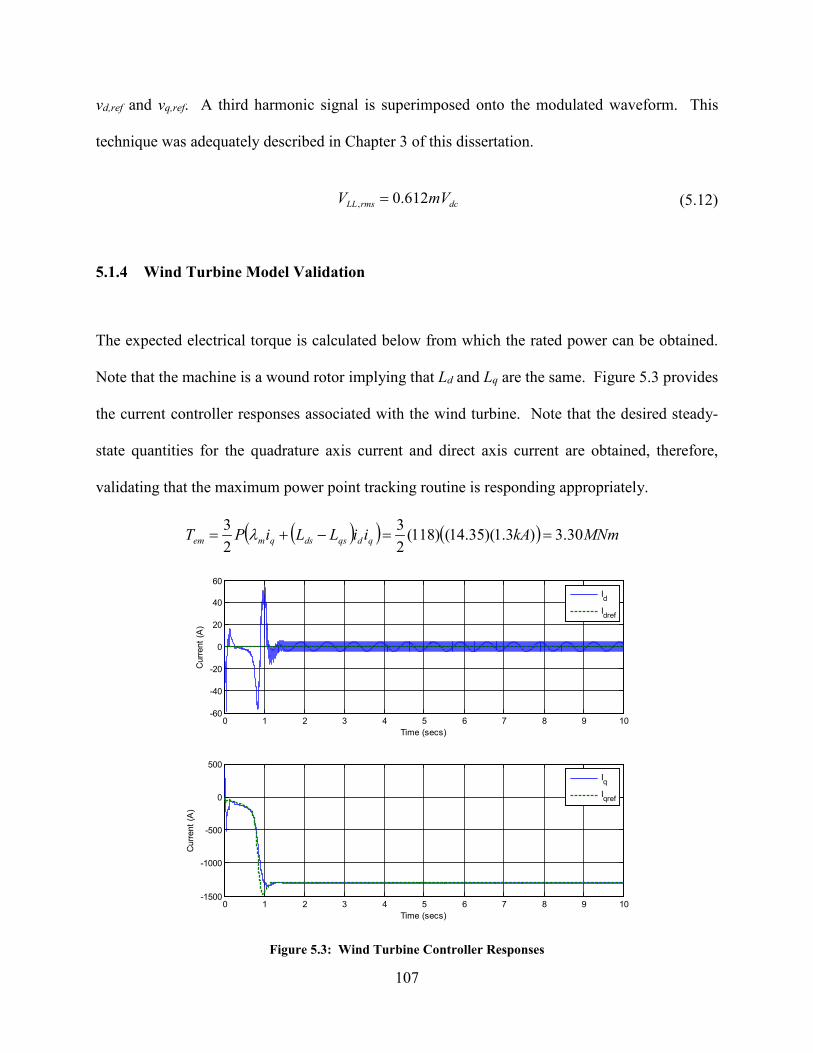
vd,ref and vq,ref. A third harmonic signal is superimposed onto the modulated waveform. This
technique was adequately described in Chapter 3 of this dissertation.
dcrmsLL mVV 612.0, = (5.12)
5.1.4 Wind Turbine Model Validation
The expected electrical torque is calculated below from which the rated power can be obtained.
Note that the machine is a wound rotor implying that Ld and Lq are the same. Figure 5.3 provides
the current controller responses associated with the wind turbine. Note that the desired steady-
state quantities for the quadrature axis current and direct axis current are obtained, therefore,
validating that the maximum power point tracking routine is responding appropriately.
( )( ) ( ) MNmkAiiLLiPT qdqsdsqmem 30.3)3.1)(35.14()118(23
23
==−+= λ
0 1 2 3 4 5 6 7 8 9 10-60
-40
-20
0
20
40
60
Time (secs)
Cur
rent
(A)
0 1 2 3 4 5 6 7 8 9 10-1500
-1000
-500
0
500
Time (secs)
Cur
rent
(A)
IdIdref
IqIqref
Figure 5.3: Wind Turbine Controller Responses
107

Figure 5.4 provides a few illustrations showing that the power coefficient and tip speed
ratio achieve their optimal settings provided in Table 5.1. With all components and controls
synchronized, the desired output power of the wind turbine is achieved as shown below.
0 1 2 3 4 5 6 7 8 9 100
0.2
0.4
0.6
0.8
Time (secs)
Pow
er C
oeffi
cien
t, C p
0 1 2 3 4 5 6 7 8 9 100
2
4
6
8
10
Time (secs)
Tip
Spe
ed R
atio
, λ
0 1 2 3 4 5 6 7 8 9 100
2
4
6x 10
6
Time (secs)
Pow
er O
utpu
t (W
)
Figure 5.4: Wind Turbine Aerodynamic Responses and Output Power
108

5.2 POWER ELECTRONIC CONVERTER MODELING
This section develops the framework for the average models of the neutral point clamped
converter, pulse width modulated boost rectifier, and the bidirectional DC/DC converter.
5.2.1 Mathematical Modeling of Power Electronic Converters: The Average Model
Figure 5.5 provides a layout of a half-bridge inverter with AC and DC side boundaries labeled in
the circuit. The analysis presented on the half-bridge inverter will be valuable for understanding
average model development of the neutral point clamped converter. A semiconductor switch, s,
is defined as two components: (1) A high power transistor, Q, and (2) an anti-parallel diode, D.
The switches are complimentary in nature as described by (5.13).
1)()( 21 ≡+ tsts (5.13) Equations (5.14)-(5.16) describe the relationships between the half-bridge converter terminal
voltages/currents and the switching functions, sn(t). The DC power, terminal power, and sending
power can be described by (5.17), (5.18), and (5.19), respectively.
VDC/2
VDC/2
Vs
R LVt Vs
0
AC S
ide
Boun
dary
Syst
em B
ound
ary
DC S
ide
Boun
dary
Vn=-VDC/2
Vp=VDC/2
Pt Ps
Ip
In
I
Q1
D1
Q2
D2
Figure 5.5: Simplified Half-Bridge Inverter
109

)()2/()()2/()( 21 tsVtsVtV DCDCt −= (5.14)
)()( 1 tisti p = (5.15)
)()( 2 tistin = (5.16)
[ ]itsts
ViViVtP DC
nnppDC )()(2
)( 21 −=+= (5.17)
[ ]itsts
VitVtP DC
tt )()(2
)()( 21 −== (5.18)
iVtP ss =)( (5.19)
Equations (5.13)-(5.19) are the mathematical relationships for a switching model of the
converter. The equivalent circuit utilizing these relations is provided in Figure 5.6. The
switching model provides insight into instantaneous currents, voltages, and power quantities but
does not easily show how the main control variables (one being the modulation index) impact
these electrical quantities.
VDC/2
VDC/2
Vs
R L Vs
0
AC S
ide
Boun
dary
Syst
em B
ound
ary
DC S
ide
Boun
dary
Vn=-VDC/2
Vp=VDC/2
Pt Ps
Ip
In
I
Ip(t)
In(t)
+-
Vt(t)
Figure 5.6: Switched Equivalent Circuit Model of the Half-Bridge Converter
110

The procedure for determining an average model of a circuit is straightforward. The AC
side current must satisfy (5.20). The terminal voltage, because it is periodic, can be described
with a Fourier series as shown with (5.21) revealing an average term and the high frequency
signal components. The terminal voltage is of utmost importance because this parameter
dynamically determines the amount of power flowing from the AC side boundary towards the
system boundary.
st VtVtRiti
dtdL −=+ )()()( (5.20)
[ ]∑∫∞
=
++=10
)sin()cos()(1)(h
shsh
T
ts
t thbthadVT
tVs
ωωττ (5.21)
Substituting (5.21) into (5.20), one arrives at (5.22). The current, i(t), can be decomposed
the same way. Upon doing so, (5.22) can be decomposed into a set of relationships providing the
average model, (5.23a) and high frequency periodic model (5.23b). In general, any periodic
signal can be averaged using (5.24). Assuming the audience is familiar with pulse width
modulation routines in power electronic circuits, (5.24) is only valid if the frequency of the
carrier waveform is sufficiently larger than that of the modulating waveform.
[ ]∑∫
∞
=
++
−=+
10
)sin()cos()(1)()(h
shshs
T
ts
thbthaVdVT
tRitidtdL
s
ωωττ (5.22)
s
T
ts
VdVT
iRidtdL
s
−=+ ∫ ττ )(1
0
(5.23a)
[ ]∑
∞
=
+=+1
)sin()cos(~~h
shsh thbthaiRidtdL ωω (5.23b)
ττ dxT
txs
s
T
Ttt
s
)(1)( ∫−
= (5.24)
111

Applying (5.24) to (5.14) through (5.19), one arrives at the averaged set of equations, (5.25)-
(5.30) describing the average model of the half-bridge converter. The switching functions, s1
and s2, are pulsed signals of unity amplitude and duty cycle, d, and are complimentary in nature.
dts =)(1 (5.25a)
dts −= 1)(2 (5.25b)
)12(
2)( −= d
VtV DC (5.26)
dIi p = (5.27)
Idi n )1( −= (5.28)
IdV
P DCDC )12(
2−= (5.29)
IdV
P DCt )12(
2−= (5.30)
The modulation index, m, is the amplitude ratio between the reference and carrier signals
of the pulse width modulation strategy. The duty cycle, d, is related to the modulation index, m,
by (5.31). Substituting (5.31) into (5.26)-(5.30), one arrives at (5.32) through (5.35).
12 −= dm (5.31)
2DC
tVmV = (5.32)
Imi p
+
=2
1 (5.33)
Imi n
−
=2
1 (5.34)
tDC
DC PIV
mP ==2
(5.35)
112

Utilizing the relationships previously derived, one arrives at the average circuit model of Figure
5.7. Classic references on power electronic circuit averaging are provided in the references
as[76], [106], and [107].
VDC/2
VDC/2
Vs
R L Vs
0
AC S
ide
Boun
dary
Syst
em B
ound
ary
DC S
ide
Boun
dary
Vn=-VDC/2
Vp=VDC/2
Pt Ps
Ip
In
I
+-
imip
+
=2
1
imin
−
=2
1
2DC
tVmV =
Figure 5.7: Averaged Equivalent Circuit of the Half-Bridge Converter
5.2.2 Average Model of Pulse Width Modulated Rectifier with Open Loop PQ Control
Consider the pulse width modulated boost rectifier in Figure 5.8 with power devices represented
by single pole, double throw switches. Each switch, s, can take on two positions.
Mathematically, two binary values are used to describe their position (1-top or 0-bottom) during
circuit operation. The instantaneous voltages and currents in terms of the switch states are
defined by (5.36) and (5.37).
dc
ca
bc
ab
dc
ac
cb
ba
ca
bc
ab
vsss
vssssss
vvv
=
−−−
=
(5.36)
⋅
=
c
b
aT
c
b
a
dc
iii
sss
i (5.37)
113

Table 5.2: Operating States of Pulse Width Modulated Boost Rectifier
sa sb sc sa -sb sb -sc sc –sa idc vab vbc vca 0 0 0 0 0 0 0 0 0 0 0 0 1 0 -1 1 ic 0 -vdc vdc 0 1 0 -1 1 0 ib -vdc vdc 0 0 1 1 -1 0 1 ib+ic -vdc 0 vdc 1 0 0 1 0 -1 ia vdc 0 -vdc 1 0 1 1 -1 0 ia+ic vdc -vdc 0 1 1 0 0 1 -1 ia+ib 0 vdc -vdc 1 1 1 0 0 0 ia +ib+ic 0 0 0
sa
sb
sc
va
vb
vc
RCvAB
vBC
vCA+
-
+
-+
-
ia
ib
ic
L
L
L1
0 1
0 1
0
vDC
+
-
Figure 5.8: Pulse Width Modulated Boost Rectifier
The circuit states and relationships between the DC side and AC side of the rectifier
given a specific switch outcome are provided in Table 5.2. Our objective is to replace the
outlined region of Figure 5.8 with switch dependent current sources and, ultimately, arrive at the
average circuit model. The line current and phase-to-phase current are related through (5.38).
bccaccabcbcaaba iiiiiiiii −=−=−= (5.38)
114

If we assume balanced conditions, (5.39), we can show that the phase-to-phase current is
three times the difference of any two line currents, (5.40). Writing Kirchoff’s voltage law
around the three phases of the circuit and applying Kirchoff’s current law at the capacitor node,
one can easily write the differential equations of the system listed as (5.41) and (5.42).
0=++ cabcab iii (5.39)
abbccaababbccaabba iiiiiiiiii 3)(2)( =+−=−−−=− ( )baab iii −=
31
(5.40)
+
=
−−−
+
−−−
=
ca
bc
ab
ca
bc
ab
ac
cb
ba
ac
cb
ba
CA
BC
AB
vvv
iii
dtdL
vvvvvv
iiiiii
dtdL
vvv
3 (5.41)
RCvi
Cdtdv dc
dcdc −=
1 (5.42)
If we define a few vectors by (5.43) and substitute into (5.41) and (5.42), we arrive at (5.44) and
(5.45) which conveniently describe the switching model of the pulse width modulated boost
rectifier.
≡
≡
≡
≡
ca
bc
ab
ll
ca
bc
ab
ll
ca
bc
ab
ll
CA
BC
AB
LL
sss
siii
ivvv
vvvv
v (5.43)
dcLLLLll vs
Lv
Ldtid
⋅−=
31
31
(5.44)
RCvis
Cdtdv dc
LLTdcLL
−⋅=1
(5.45)
115

Recall from Fourier analysis and the earlier subsection that the average of a signal is defined by
(5.46). If (5.44) and (5.45) are substituted into (5.46), the average model of the pulse width
modulated rectifier can be shown to be (5.47) and (5.48).
∫−
=t
Tt
dxT
tx ττ )(1)( (5.46)
dcLLLL
t
TtdcLLLL
ll vdL
vL
dvsL
vLTdt
id⋅−=⋅−= ∫
−
31
31))()(
31)(
31(1 ττττ (5.47)
RCvid
Cdtvd dc
LLTdcLL
−⋅=1
(5.48)
An important integral property, (5.49), was utilized in the equation averaging and is valid if and
only if the maximum frequency components of vdc(t) is much less than half the converter
switching frequency. The average of the switching function, s(t), is also defined as the duty
cycle, d in (5.50).
dc
t
Ttabdcabdcabab vdvsdvs
Tv ⋅=⋅≈⋅= ∫
−
τττ )()(1 (5.49)
∫−
−===t
Ttbaababab ddds
Ttsd ττ )(1)( (5.50)
Using (5.47) and (5.48), the pulse width modulated boost rectifier average model is illustrated in
Figure 5.9. For further reading on the subject, consider [108].
The most straightforward way of controlling the DC voltage output of the boost rectifier
resulting in modification to the real and reactive power references is through the control scheme
provided in Figure 5.10. For further information, consult [109].
116

CVdc
3L
daVdc
3L
dbVdc-
+-
+
Ia
Ib
daIa dbIb dcIc
3L
dcVdc-
+
Ic
Vb
Vc
-
+Va
Figure 5.9: Average Model of Pulse Width Modulated Inverter/Rectifier
abc
dq
dq
abc
kP+kI/s
kP+kI/s
PLL
vd
vd
vdvq
-vq
vq2 2+1
va,vb,vc
ia,ib,ic
Pref
Qrefid*
iq*vd vq
iq*
id
iq
θ θ
θ
+--
-
+
dd
dqda,db,dc
+
+
-
-ωLVDC
ωLVDC
id*
Σ
Σ Σ
Σ
Figure 5.10: Open Loop PQ Regulator of Pulse Width Modulated Boost Rectifier
117

5.2.3 Average Model Implementation of Neutral Point Clamped Converter in Simulink
The half-bridge converter is a basic building block for the multilevel neutral point clamped
converter. The neutral point clamped converter is utilized to interface the wind turbine to the
medium voltage DC bus bar and the bidirectional DC/DC converter to the motor drive. The
average model of the half-bridge converter was adequately discussed in Section 5.2.1. Using the
terminal voltage of the converter described by (5.32) and noting the power balance relationship
written as (5.51) that relates the AC and DC sides, Figure 5.11 provides the average circuit
model of the neutral point clamped converter. The modulation index, shown in red, is dynamic
whose value is adjusted by the control system.
ctcbtbatadcdc ivivivVi ++= (5.51)
Vdc-+
ma(t)Vdc/2
mb(t)Vdc/2
mc(t)Vdc/2
∑ == DCDCDCAC IVPP
ia
va,vb,vc
ia,ib,ic
IDC
VDC
ib
ic
Figure 5.11: Average Model of Neutral Point Clamped Converter
Figure 5.12 shows the detailed and average output voltage responses for a three level multilevel
converter – the line-to-line output has five levels as shown.
118

0.04 0.05 0.06 0.07 0.08 0.09 0.1-1000
-800
-600
-400
-200
0
200
400
600
800
1000
Time (secs)
Vol
tage
(Vol
ts)
DetailedAverage
Figure 5.12: Detailed and Average Model Output Voltage Waveform of NPC Inverter
5.2.4 Average Model of Bidirectional DC/DC Converter
The average model of the dual active bridge was covered in Chapter 4. The proof of the
relationships was not shown at the time. Consider the average DC input current of the dual
active bridge, Ig, mathematically written as (5.52), where d is the duty cycle and Ip is the peak
DC input current as was shown in Figure 4.4.
)1( dII pg −= (5.52) Equation (5.52) is in terms of the peak DC input current, Ip. Converter equations should
normally be written in terms of known parameters. Recalling that the slope of the DC input
current can be written from the constitutive relationship for the voltage across an inductor, we
can rewrite Ip in terms of the system input parameters (Vg, LTx, Ts, d). This relationship is listed
as (5.53). Substituting (5.53) into (5.52), we arrive at the average DC input current, (5.54), for
119

both the primary side current and input current of the DAB converter. Comparing (5.54) and
(4.2) and one will note similar expressions scaled by the transformer turns ratio. Figure 5.13
provides the circuit schematic of the DC/DC converter average model implemented in
Matlab/Simulink.
)
2(1 s
T
gp
dTLV
nI = (5.53)
)1)(2
(1 ddTLV
nI s
T
gg −= (5.54)
Vdc-+
Isec
)1(2 hh
sDCavg dd
LTnVI −=VDC
nII ondaryprimary /sec=Isec
Figure 5.13: Average Model of Bidirectional DC/DC Converter
4.005 4.0051 4.0052 4.0053 4.0054 4.0055 4.0056 4.0057 4.0058 4.0059 4.006-2000
-1000
0
1000
2000
Time(secs)
Cur
rent
(A)
DetailedAverage
Figure 5.14: Illustration of Detailed and Average Model Currents for the Bidirectional DC/DC Converter
120

5.3 VARIABLE FREQUENCY DRIVE MODEL
Figure 5.15 shows a schematic diagram of a variable frequency drive used to control an
induction motor/generator. The voltage sourced converter (VSC) is a three-level neutral point
clamped converter mentioned in previous sections. The objective of this section is to establish
the mathematical principles of how the machine is controlled with flux and current controllers.
A few plots showing successful model implementation into Matlab/Simulink will be provided as
done in previous sections. For a thorough treatment of the derivation refer to [76].
C1
C2
Vc1+
+-
-
Vc2
Controlled DC Bus
R L
R
L
Three Phase Voltage Sourced
Converter
Machine
Flux/Torque Controllers in dq-Frame
ABC to dq
λref Teref
md mq iqid
ᶿ
Iabc,stator
Vdc
Figure 5.15: Variable-Frequency Voltage Sourced Converter for Controlling Induction Machine
121

The equations which govern the electrical dynamics of a symmetrical three-phase AC
machine are provided in (5.55), (5.56), (5.57), and (5.58). Subscripts s, r, and m refer to the
stator, rotor, and magnetization branch, respectively in all relationships. Note that all voltages,
currents, and flux linkages denoted by λ are space vectors in the dq plane. The rotor position
with respect to the stator is represented by variable θr. Traditional leakage factors denoted by σ
are defined by (5.59), (5.60), and (5.61) for the stator, rotor, and total leakage factor,
respectively. The stator time constant is defined by (5.62).
ssss iRV
dtd
−=λ (5.55)
rrrr iRV
dtd
−=λ (5.56)
( )[ ]r
jssms ieiL r
θσλ ++= 1 (5.57)
( )[ ]s
jrrmr ieiL r
θσλ −++= 1 (5.58)
1−=m
ss L
Lσ (5.59)
1−=m
rr L
Lσ (5.60)
( )( )rs σσσ
++−=
1111 (5.61)
s
sms R
L )1( στ += (5.62)
122

5.3.1 Machine Current Control
The machine flux and torque are controlled through the direct axis and quadrature axis currents.
However, the VSC can only control the stator voltage. Therefore, one must relate the direct axis
and quadrature axis stator currents with the stator voltages. Without sharing the mathematical
abstractness of defining fictitious space phasor currents as described in [76]and [110] for the
magnetization current, it can be shown that the stator current, magnetization current and stator
terminal voltage are related by (5.63) where ρ is the angular position of the magnetization current
with respect to the stator axis. Note that the magnetization current is aligned with the direct axis
current as shown in Figure 5.16.
( )( )
sssj
mrr
sr
rsm iRVeii
dtdL
−=
+
++
−++ ρ
σσσσ ˆ
11
1111 (5.63)
isisq
isd=imrRotor axis
Stator axisθ r
ρ
Figure 5.16: Magnetization Current Alignment in a dq Axis Frame
Substituting (5.61) and (5.62) into (5.63) and dividing through by Rs, (5.64) will be obtained.
Decomposing the current and voltage space phasors into their d-axis and q-axis components,
(5.65) and (5.66), using Euler’s identity and substituting into (5.64), we arrive at (5.67) and
(5.68).
123

( ) ss
sjmrs
ss i
RVei
dtd
dtid
−=−+ ρτσστ ˆ)1( (5.64)
ρj
sqsds ejiii )( +=
(5.65)
ρjsqsds ejVVV )( +=
(5.66)
( ) sds
mrssqssd
sds V
Rdtidii
dtdi 1ˆ
1 +−−=+ τσωστστ (5.67)
( ) sqs
mrssdssqsq
s VR
iiidt
di 1ˆ1 +−−−=+ ωτσωστστ (5.68)
Equations (5.67) and (5.68) are nonlinear, coupled equations where Vsd and Vsq are inputs
and Isd and Isq are outputs that can be decoupled if (5.69) and (5.70) are defined as new control
inputs. The approach to be shared is a common technique done with three phase systems.
Substituting (5.69) and (5.70) into (5.67) and (5.68), respectively, we arrive at two first order,
single input, single output linear equations listed as (5.71) and (5.72) which are used for gain
tuning. If the PI compensator gains are chosen based upon (5.73), the closed loop transfer
function associated with (5.71) and (5.72) will contain one design variable, τi, to choose.
sds
mrssqsd V
Rdtidiu 1ˆ
)1( +−−= τσωστ (5.69)
( ) sqs
mrssdsq VR
iiu 1ˆ1 +−−−= ωτσωστ (5.70)
dsdsd
s uidt
di=+στ (5.71)
qsqsq
s uidt
di=+στ (5.72)
i
spk
τστ
= i
Ikτ1
= (5.73)
124

Figure 5.17 illustrates the current controller based upon (5.69) and (5.70) with flux
observer, [110], establishing Imr and ω setpoints. Specific features of the controller and
magnetization current considerations will be discussed more thoroughly in Chapter 6.
~- M
DC/AC
DC
+ - K(s)
Imr
Imr,optimumIsd,ref
+ -
Isd
PI + - Rs
Vdc/2
mdUd
Isq,ref
+ -
Isq
PI + + Rs
Vdc/2
mq
Uq +
Xστs Isd
Xστs Isq
ω
ω
X(1-σ)τs
ω
Imr
Current Controller
Isd
ωr
Istator (a,b,c)
Reference Signal
Machine Loss Optimization
τr (*)-1 X(sτr+1)1
Isq
+ +
ωr
ωs1 ρ
Istator (a,b,c)
dqabc
Flux Observer
Figure 5.17: Machine Current Control
5.4 SYSTEM PARAMETERS AND ASSEMBLED DC MICROGRID VALIDATION
The DC microgrid model developed in Matlab/Simulink is found in Figure 5.18. The purpose of
this section is to provide convincing arguments that the developed model is suitable for further
power management studies in Chapter 6 of this dissertation. The scenario to prove model
validation involves a grid disconnect at 4.0 seconds into the simulation. The only source of
125

generation in the model after this point comes from the wind generation and diesel generator on
the platform. For our purposes, the diesel generator is modeled as an ideal three phase voltage
source with uncontrolled rectifier connected to the offshore production platform low voltage bus.
At 1, 1.75, and 2.75 seconds, the motor drives rated for 1.68 MW each are connected into
the network by setting their power reference controls accordingly. Also on the platform is a
generic resistive load used to draw power from the diesel generator in the case for validating
when the load is higher compared to the available generation (Chapter 6). For all simulations in
this chapter, the wind speed is held constant at 11.8 m/s, the rated wind speed, and blade pitch set
to 0 degrees to extract rated power from the generator.
One of the key takeaways from this analysis is to notice how the grid power electronics
with associated controls help to isolate parts of the system network. All components are
regulated except for the bidirectional DC/DC converters which are set to deliver maximum
power to the loads equally. In chapter 6, the duty cycles dynamically change.
Wind Turbine and Control
Grid Connected Converter
Variable Frequency Motor Drives
Bidirectional DC/DC Converters
Diesel Generator / Rectifier
Figure 5.18: Interconnected DC Based Microgrid Computer Model
126

5.4.1 System Power Balance and DC/DC Converter Power Handling Capability
Figure 5.19 provides the generation source responses in the DC system. The wind turbine takes
nearly 1 second of simulation time to reach full output power and maintains steady output under
rated conditions even when the motors command power at 1, 1.75, and 2.75 seconds. The
turbine is rated for 5 MW, 5 kVdc with rectifier. The MVDC bus is slightly higher than rated as
indicated in Figure 5.20 resulting in lower machine output current creating less machine torque
(Equation 5.2). The wind power is also transmitted 10 km (6.2 miles) accounting for some
electrical loss in the line.
The center graphic in Figure 5.19 shows the real and reactive power flowing through the
grid connected, pulse width modulated rectifier. The reference power was set to 5 MW and
changed to 0 MW at 4 seconds. The reference reactive power is set to zero throughout the entire
simulation. The offshore platform generator supplies the remaining load on the platform if the
load exceeds the total generation in the network. The load resistor is set to 1 Ω for evaluation
purposes. The dynamic response of this generator is provided as the last graphic in the figure.
The currents flowing through the input of one DC/DC converter (MVDC bus side) and
output of the converter are plotted in Figure 5.20. The turns ratio, n1 / n2 = n, is equal to 2.
Using (4.2), we can predict the average DC current at the input and output of the converter. This
calculation is provided below. The ripple on the DC current is caused by the six pulse diode
bridge rectifier attached to the offshore platform DC bus. The average input current into each
DC/DC converter is 823 A resulting in a total current flow of 1646 A provided by the turbine
generator and grid connected converter equally.
Ax
ddL
TnVI hhTx
sDCavg 1646)75.0)(25.0(
)10208(2)3000/1)(5481)(2()1(
2 6 ==−= −
127

0.5 1 1.5 2 2.5 3 3.5 4 4.5 50
2
4
6
Time(secs)
Pow
er(M
W)
0.5 1 1.5 2 2.5 3 3.5 4 4.5 5-2
0
2
4
6
8
Time(secs)
Pow
er (M
W |
Mva
r)
0.5 1 1.5 2 2.5 3 3.5 4 4.5 50
2
4
6
Time(secs)
Pow
er (M
W)
Wind Power
Grid Power, PGrid Power, Q
Offshore Platform Power
Figure 5.19: Generation Sources in Microgrid
1 2 3 40.5
0.75
1
1.25
1.5
1.75
2
2.25
2.5
Time(secs)
Vol
tage
(kV
)
2.6 2.61 2.62 2.63 2.64 2.650
500
1000
1500
2000
Time(secs)
Cur
rent
(A)
1 2 3 40
1
2
3
4
5
6
7
8
Time(secs)
Vol
tage
(kV
)
2.6 2.61 2.62 2.63 2.64 2.650
500
1000
1500
2000
Time(secs)
Cur
rent
(A)
Platform Bus Voltage
Platform Side DC Current
MVDC Bus Voltage MVDC Side DC Current
Figure 5.20: Bus DC Voltages and Currents in DC Microgrid
128

To explain the voltage dip that occurs at 4 seconds on the medium voltage DC bus,
consider (5.1a) and (5.1b) – the equations governing the permanent magnet machine. Equations
(5.74a) and (5.74b) are another form of (5.1a) and (5.1b) but in terms of flux linkage, current,
and voltage. Since iq of the wind turbine is regulated to achieve maximum power extraction, the
only variable capable of changing is id to meet the load demand. If the d-axis current changes to
something other than zero, the d-axis flux linkage is altered by decreasing – Equation (5.10) –
resulting in a DC bus voltage sag as simulated. This is indeed the case as shown in Figure 5.21.
A remedy to this issue will be provided in Chapter 6 by allowing the DC/DC converter duty
cycles to change, which are currently fixed in this simulation set.
qr
ddsd dt
diRV λωλ−+= (5.74a)
drq
qsq dtd
iRV λωλ
++= (5.74b)
0 0.5 1 1.5 2 2.5 3 3.5 4 4.5 512.5
13
13.5
14
14.5
15
Time(secs)
Flux
(V-s
)
d-axis Flux
0 0.5 1 1.5 2 2.5 3 3.5 4 4.5 5-8
-6
-4
-2
0
2
Time(secs)
Flux
(V-s
)
q-axis Flux
Figure 5.21: dq Flux Linkages of Wind Turbine Generator after Grid Disconnect
129

5.4.2 Motor Drive Responses
Regulation of the magnetization current is normally exercised during the converter start-up
sequence, when the machine is at standstill, and the q-axis current is kept at zero so no machine
torque is generated. Since we are dealing with larger machines on the offshore production
platform, the rotor time constants are fairly large – on the order of 1 to 1.5 seconds. This implies
that the currents will reach steady-state in about 5τr. To obtain a faster closed-loop response, a
PI compensator, K(s), is introduced to regulate the magnetization current. The drawback of a
faster closed-loop response is that the d-axis current and reference point will create larger
transient currents strictly due to the magnitude of the rotor time constant [76].
The machine parameters for this study are provided in Table 5.3. The reference
magnetization current can be set using (5.75) under the assumption that the rotor speed regulates
closely to the rated mechanical speed which is often the case to generate maximum efficiency
out of the induction machine (η ≈ 1- s). Figure 5.22 provides the regulated d-axis current of 141
A and q-axis current of 7.3 kA for each machine. Knowing the rated torque and the machine
speed held constant at 32 rad/s, the q-axis current can be predicted with (5.76).
oms
LLrefmr L
Viωσ )1(3
2, +
= (5.75)
sqmrr
me iiLT
+
=σ12
3 (5.76)
Classic texts on machine reference theory such as [111] often designate the q-axis on the real
axis and d-axis on the imaginary axis and this is how the induction machine model in
Matlab/Simulink orients itself. For the derivation provided for the motor drive current regulator,
130

the d-axis is along the real axis and q-axis aligned to the imaginary axis. The axes orientations
are provided in Figure 5.23. This will become important when interpreting the torque direction.
Table 5.3: Induction Machine Parameters [76]
Parameter Numerical Quantity Nominal Power, P Pole Pairs Nominal Voltage, VLL Nominal Frequency, ωo Stator Resistance, Rs Rotor Resistance, Rr Magnetizing Inductance, Lm Stator Inductance, Ls Rotor Inductance, Lr Stator Leakage Factor, σs Stator Leakage Factor, σr Total Leakage Factor, σ Stator Time Constant, τs Rotor Time Constant, τr Controller Constant, τi Controller Gains, Kp; KI imr Controller Gains
1.678 MW 12
2300 V 377 rad/s 29 mΩ 22 mΩ
34.6 mH 35.2 mH 35.2 mH 0.0173 0.0173 0.0337
1.213 secs 1.6 secs
3 millisecs 13.67, 333 sec-1 79.6, 50 sec-1
0.5 1 1.5 2 2.5 3 3.5 40
100
200
300
400
Time(secs)
Cur
rent
(A)
Idref
Idmeasured
0.5 1 1.5 2 2.5 3 3.5 4
0
2000
4000
6000
8000
Time(secs)
Cur
rent
(A)
Iqref
Iqmeasured
Figure 5.22: dq Current Regulation of Induction Motors
131

C1
C2
Vc1+
+-
-
Vc2
Controlled DC Bus
R L
R
L
Three Phase Voltage Sourced
Converter
Machine Controllers
ABC to dq
λref Teref
md mq IqId
ᶿ
Iabc,stator
Vdc
q
d
d
q
Figure 5.23: Axes Orientation for Current Controller and Motor
Our job now is to map the chosen dq controller axes onto the dq machine axes. For
clarity, we will designate a subscript m for motor axis and subscript c for controller axis.
Consider Figure 5.24 with our attention on graphic (a) – representative axis for the current
controller – and graphic (c), representative axis for the motor. From this illustration we can write
(5.77) where f is either AC voltage or current.
Figure 5.24: Relationship between the dq and abc Quantities for Generating and Motoring Operation[98]
−
=
md
mq
cq
cd
ff
ff
,
,
,
,
1001
(5.77)
132

Another expression for the induction machine torque expressed in terms of the dm-axis
and qm-axis currents is listed as (5.78).
( )mdsmqsmqsmdsme iiPT ,,,,, 23 λλ −= (5.78)
Substituting (5.77) into (5.78), we arrive at a torque expression for the motor mapped into the
controller dq axis orientation.
( )cqscdscdscqsce iiPT ,,,,, 23 λλ +−= (5.79)
Recall that the controller d-axis is aligned with the magnetization current (see Figure 5.16) and
because the stator leakage inductance, Lls, is much smaller in comparison to the magnetizing
inductance, Lm, we are able to simplify (5.79) to (5.80), [112].
( ) ( ) ( )mdsmqsmcqscdsmcqscdsce iiLPiiLPiPT ,,,,,,, 23
23
23
−=== λ (5.80)
Table 5.4 provides the predicted steady-state results of the motor drive. Figure 5.25
shows the d-axis and q-axis simulated stator currents and machine electrical torque in the motor
dq frame described earlier. For motor operation, the q-axis current must lead the d-axis current,
Figure 5.24, which is indeed the case. The expected flux magnitude can be calculated with
(5.81), which is a result of equating (5.80) with (5.76). Finally, Figure 5.26 provides the total
demanded power by the motors as they command power at 1, 1.75, and 2.75 seconds. The
dynamic behavior of the inverter modulation index for one motor is also plotted. As the offshore
DC bus voltage drops due to increased load, the modulation index increases to maintain system
currents (see Figure 5.11).
mr
r
mds i
LL
P
21=λ (5.81)
133

Table 5.4: Predicted Motor Simulation Results
Prated ω Te isqLL isd = imr λds
1.678 MW 31.42 rad/s 53.4 kN 7.42 kA 141 A 0.4 V-s
0.8 0.9 1 1.1 1.2 1.3 1.4 1.5 1.60
-6-4-202468
Time(secs)
Cur
rent
(kA
)
0.8 0.9 1 1.1 1.2 1.3 1.4 1.5 1.6-8-6-4-202468
Time(secs)
Cur
rent
(kA
)
0.8 0.9 1 1.1 1.2 1.3 1.4 1.5 1.6-100
-75
-50
-25
020
Time(secs)
Torq
ue (k
Nm
)
IdStator
IqStator
Machine Torque, Te (Motoring Conv.)
Figure 5.25: dq Stator Currents and Motor Torque
0.5 1 1.5 2 2.5 3 3.5 4-6
-5
-4
-3
-2
-1
0
Time(secs)
Pow
er (M
W)
Machine Load Power
0.5 1 1.5 2 2.5 3 3.5 4-1
-0.5
0
0.5
1
Time(secs)
Mod
ulat
ion
Inde
x, m
Modulation Index
Figure 5.26: Motor Load Power and Modulation Index of Motor Inverters
134

6.0 DYNAMIC POWER MANAGEMENT AND DC/DC CONVERTER CURRENT
SHARING EVALUATION UNDER VARIOUS MODE TRANSITIONS
In traditional AC systems, power management is critical to ensure that system generation and
load are balanced so stability issues are not of concern. System frequency deviation in AC
architectures from the intended set-point (50 or 60 Hz) has often been the indicator that an issue
is arising – lower system frequency implies load is greater than available generation and high
system frequency implies available generation is greater than total load.
As mentioned in previous sections, future microgrids will have hierarchical control
structures for monitoring deviations and managing power. Figure 6.1 provides the role a central
computer will play in the microgrid studied throughout this dissertation. Available power
generation and power absorbed by the loads are measured and sent back to the central computer
in order to coordinate power flows in the network. Power flows can be altered by adjusting the
blade pitch of the wind turbine, duty cycles of the bidirectional DC/DC converters, or power
reference of the grid connected converter.
In this chapter, we will focus on the power management of the microgrid assuming ideal
communications. We will also study two mode transitions in this chapter including (1) main grid
connected to being disconnected and (2) grid disconnected to grid connected. A low voltage ride
through scenario associated within the microgrid setting is left as future work. Dynamic
behavior of the real-time DC/DC converter duty cycle adjustments is of most interest to the
135

research team and will be emphasized. The power management routine also has the capability of
scaling the amount of power flowing through each DC/DC converter. Since both converters are
sized to handle 10 MW of power in the case of converter failure, simulations can be run showing
that the power does not need to be equally shared between both components. In practice, it’s not
always guaranteed that the converters are always manufactured by the same vendor.
DC / ACConverter
DC / DCConverter
Short Cable
d 1
Short CableM
VDC
Pmeasured
“Aggregate” System (For Picture Purpose Only, 3 units will be in Simulation)
AC / DCThree LevelMultilevel Rectifier
(NPC)
+ -
5 MW SupplyBreakers
DC / DCConverter VDC
d 2
+ -5 kV 1 kV
DC / ACConverterAC
Onshore Grid
Medium Cable
Medium Cable
Measurement Coming InSignal Sent to Regulate
Figure 6.1: Power Signals and Coordination through Centralized Computer
6.1.1 Power Management Routine
The power flowing through the DC/DC converters is described by (6.1), where VH is the medium
voltage DC bus and VL is the offshore production platform bus voltage. Ptot is the total power the
converter is rated to handle – 10 MW for our system studies – and α is a scaling factor between 0
and 1. For converter sizing, this factor is set to 0.5 since two converters are assumed to be in
operation at all times.
136

)1(2 hh
Tx
sLHtot dd
LTVnVP −=α (6.1)
If (6.1) is solved for the duty cycle, dh, we arrive at (6.2). If Ptot is 10 MW; VH is 5 kV; VL is 1
kV; fs is 3 kHz; LTx is 208 µH; and α is 0.5 then n must be set to 5 to have a positive real root as a
solution to the quadratic equation. Equation (6.2) is a critical expression that is continuously
solved for to adjust the DC/DC converter duty cycles as system conditions change. In Chapter 5,
the duty cycle was fixed to validate system operation. The previous discussion is critical to
ensure that the duty cycle is below 0.5 for power to flow from generation to load.
022 =
+−
LH
sTtothh VnV
fLPdd α (6.2)
With the approach to be presented, we assume one directional power flow in the direction
of the offshore production platform and ideal communication between the central computer and
diesel generator. The inputs from the primary control into the secondary power management
scheme strictly include the machine electrical power and current, DC bus voltages, and all
system generation. The power management architecture is found in Figure 6.2.
Pmeasured,1 (X1,X2,X3) Σ
Pmeasured,N (X1,X2,X3)
kα
kβ
DC/DC Converter Power Sharing and Power Management Scheme
d 1
d 2
Equation 6.2
Equation 6.2
kα
kβ
PRef,1
PRef,2
+ - MRC
+ - MRC
d 1
d 2
kα Pmeasured,total
kβ Pmeasured,total
Poptimal,1 (X1,X2,X3)
Poptimal,N (X1,X2,X3)
OR
OR
OPEN LOOP
CLOSED LOOP
Figure 6.2: Power Management Routine for Adjusting DC/DC Converters in Microgrid
137

Starting from left to right in Figure 6.2, the total power generation on the MVDC side of
the microgrid is summed (based on system measurements) and scaled by factors kα and kβ.
These weights range from 0 to 1 depending on the power rating of the bidirectional converter.
There is one weight for each DC/DC converter. Utilizing (6.2), the duty cycle, dh, is determined
and adjusts the DC/DC converter output power. The later description can be argued to be open
loop in nature with future efforts put forth into implementing the model reference control (MRC)
design of Chapter 4 as shown in Figure 6.2. The power management routine is simple Matlab
code programmed and communicates directly with the Simulink model as shown in Figure 6.3 –
bottom left of the diagram shows a white bin with several inputs and two outputs corresponding
to the duty cycles of the DC/DC converter.
Figure 6.3: Microgrid Computer Model with Implementation of Power Management Scheme
138

6.1.1 DC/DC Converter Dynamic Response under a Grid Disconnection
The case under study in this section is very similar to the case studied in Chapter 5 but the
DC/DC converters are able to adjust their duty cycles to allow or suppress power flow depending
on load demand. The wind turbines always produce maximum power, the grid supplies 5 MW
and disconnects at 4 seconds into the simulation. The motor drives command power at 1 second,
1.75 seconds, and 2.75 seconds and are all rotating at a fixed speed of 32 rad/s (rated mechanical
speed). A 0.25 Ω resistor is attached to the offshore platform bus. The bidirectional DC/DC
converter No. 1 (closest to the generation) has a scaling factor, kα, equal to 0.6 and converter No.
2 has a scaling factor, kβ set to 0.4. This implies that 60% of the power generation will flow
through No.1 and 40% through No. 2.
Figure 6.4 provides the generation profiles as a function of time. Because the generation
supplied through the pulse width modulated rectifier completely diminishes to zero, there is not
enough power generation to supply the motor drives and the resistive load in the network, thus,
resulting an increased output from the diesel generation in the system. The dynamic behavior of
the DC/DC converter duty cycles is provided in Figure 6.5 adjusting with changes in system load
and available power generation. Sample calculations for the first time interval of Figure 6.5 are
provided below.
0)1516)(7442)(5(
)3000)(208)(2.45)(6.0(22 22 =
++−=
+−
µα MWMWddVnV
fLPdd hhLH
sTtothh
8577.01422.01., ord Noh =
0)1516)(7442)(5(
)3000)(208)(2.45)(4.0(22 22 =
++−=
+−
µα MWMWddVnV
fLPdd hhLH
sTtothh
910.0089.02., ord Noh =
139

0.5 1 1.5 2 2.5 3 3.5 4 4.5 50
1
2
3
4
5
Time(secs)
Pow
er(M
W)
Wind Power
0.5 1 1.5 2 2.5 3 3.5 4 4.5 5-2
0
2
4
6
8
Time(secs)
Pow
er (M
W |
Mva
r)
Real Power, PReactive Power, Q
0.5 1 1.5 2 2.5 3 3.5 4 4.5 50123456
Time(secs)
Pow
er (M
W)
Offshore Platform Power
Figure 6.4: System Generation Response During a Grid Disconnect
0.5 1 1.5 2 2.5 3 3.5 4 4.5 50
0.050.1
0.150.2
0.250.3
0.350.4
0.450.50.5
Time(secs)
Dut
y C
ycle
0.5 1 1.5 2 2.5 3 3.5 4 4.5 50
0.050.1
0.150.2
0.250.3
0.350.4
0.450.50.5
Time(secs)
Dut
y C
ycle
DC/DC Converter No.1
DC/DC Converter No.2
Figure 6.5: DC/DC Converter Duty Cycle Response
140

1 2 3 40.5
0.75
1
1.25
1.5
1.75
2
2.25
2.5
Time(secs)
Vol
tage
(kV
)
Platform Bus Voltage
0.5 1 1.5 2 2.5 3 3.5 40
1000
2000
3000
4000
5000
6000
Time(secs)
Cur
rent
(A)
Platform Side DC Current
1 2 3 40
1
2
3
4
5
6
7
8
Time(secs)
Vol
tage
(kV
)
MVDC Bus Voltage
0.5 1 1.5 2 2.5 3 3.5 40
250
500
750
1000
1250
1500
1750
2000
Time(secs)
Cur
rent
(A)
MVDC Side DC Current
Figure 6.6: DC Bus Voltages and Current Flows in Case of Grid Disconnect
4.2 4.22 4.24 4.26 4.28 4.30.9
0.95
1
1.05
1.1
1.15
Time(secs)
Vol
tage
(kV
)
Platform Bus Voltage
3.85 3.86 3.87 3.88 3.89 3.94000
4200
4400
4600
4800
5000
Time(secs)
Cur
rent
(A)
Platform Side DC Current
4.2 4.22 4.24 4.26 4.28 4.35.1
5.15
5.2
5.25
5.3
Time(secs)
Vol
tage
(kV
)
MVDC Bus Voltage
3.85 3.86 3.87 3.88 3.89 3.9800
850
900
950
1000
Time(secs)
Cur
rent
(A)
MVDC Side DC Current
Figure 6.7: Zoomed-In Intervals of Figure 6.6 Providing Finer Electrical Characteristics
141

Figure 6.6 provides DC bus voltages on the medium voltage bus bar and offshore
production platform bus bar as well as current flows along the rails of these busses. Constant
power load characteristics are also observed. As voltage drops because power is commanded by
the motor drives, current increases to maintain desired power to the motors. High ripple is
observed in the current as full load is brought into service at 2.75 seconds into the simulation.
Zoomed-in regions of the currents and voltages at points beyond 2.75 seconds are provided in
Figure 6.7. The characteristic pulses generated by the rectifier attached to the low voltage DC
bus are observed, which are naturally reflected onto the medium voltage DC bus through the
interfacing DC/DC converters. The scaled currents through each of the DC/DC converters are
provided in Figure 6.8. Remember, the duty cycles are a function of kα and kβ.
3.85 3.86 3.87 3.88 3.89 3.90
1000
2000
3000
4000
5000
6000
Time(secs)
Cur
rent
(A)
3.85 3.86 3.87 3.88 3.89 3.90
1000
2000
3000
4000
5000
6000
Time(secs)
Cur
rent
(A)
DC/DC Converter No.1 DC/DC Converter No.2
Figure 6.8: Output Currents of DC/DC Converters for Grid Disconnect Scenario – 60% / 40 % Weighting
kAddL
TnVI hhT
sH 64.4)273.01)(273.0()208(2
)3000/1)(5832)(5()1(2
=−=−=µ
kAddL
TnVI hhT
sH 10.3)1572.01)(1572.0()208(2
)3000/1)(5832)(5()1(2
=−=−=µ
Finally, for completeness, Figure 6.9 provides the dynamic response of the wind
generator currents, wind generator current controller, and current supplied by the grid up until
142

grid disconnection. The high ripple wind generator current is noticeable at 2.75 seconds and,
when noticed at a finer resolution, takes on similar characteristics as those shown in Figure 6.7.
0.5 1 1.5 2 2.5 3 3.5 40
500
1000
1500
2000
Time(secs)
Cur
rent
(A)
Wind Generator Current
0.5 1 1.5 2 2.5 3 3.5 4500
600
700
800
900
1000
Time(secs)
Cur
rent
(A)
Grid Current
0.5 1 1.5 2 2.5 3 3.5 4-100
-50
0
50
100
Time(secs)
Cur
rent
(A)
Idref (Wind)
Idmeasured
0.5 1 1.5 2 2.5 3 3.5 4-1500
-1400
-1300
-1200
-1100
-1000
Time(secs)
Cur
rent
(A)
Iqref (Wind)
Iqmeasured
Figure 6.9: Wind Generator Currents and Grid Connected Converter Current for Grid Disconnect Scenario
At the time this dissertation is being written, research attention has been focused upon
sharing power between parallel connected converters as presented in [113]. Future efforts will
for sure be centered upon the microgrid case, as was done in this chapter, and with a nicely
written article starting the trend in [114].
143

6.1.2 DC/DC Converter Dynamic Response under a Grid Connection
For the grid connected scenario, we consider the case when the total generation in the system
becomes much larger in comparison to the total load when the grid interfacing converter is
commanded to deliver 5 MW of power. This converter essentially transitions from a
disconnected to grid connected state. The wind turbine is continuously feeding maximum rated
power into the network and only one motor drive is active in the circuit at all times with the other
two out of service. The generic load of 0.25 Ω remains in the circuit. With this simulation
study, one can postulate that the dynamic behavior of the DC/DC converters act as an aid for
improving system stability as compared to the time to mechanically alter the blade pitch of the
wind turbines. DC/DC converter No.1 and No.2 are set to share 60% and 40% of the total
current, respectively, as in the previous section.
Figure 6.10 provides the generation profiles of the wind, power flowing through the grid
connected converter, and diesel generation power on the offshore production platform. Notice
that once the grid connected converter commands power at four seconds, the diesel generation is
no longer needed to supply the offshore load – truly an economic benefit. Figure 6.11 shows the
dynamic behavior of the DC/DC converter duty cycles. The duty cycles are initially low and,
once more generation becomes available, the duty cycles increase allowing more generation to
flow through the converter to meet the desired load. Finally, the detailed current waveforms of
each of the DC/DC converters are provided in Figure 6.11.
144

0.5 1 1.5 2 2.5 3 3.5 4 4.5 50123456
Time(secs)
Pow
er(M
W)
Wind Power
0.5 1 1.5 2 2.5 3 3.5 4 4.5 5-2-1012345678
Time(secs)
Pow
er (M
W |
Mva
r)
Real Power, PReactive Power, Q
0.5 1 1.5 2 2.5 3 3.5 4 4.5 50123456
Time(secs)
Pow
er (M
W)
Offshore Platform Power
Figure 6.10: System Generation Response During a Grid Connection
1 2 3 4 50
0.1
0.2
0.3
0.4
0.5
Time(secs)
Dut
y C
ycle
1 2 3 4 50
0.1
0.2
0.3
0.4
0.5
Time(secs)
Dut
y C
ycle
DC/DC Converter No.1 DC/DC Converter No.2
3.85 3.86 3.87 3.88 3.89 3.90
500
1000
1500
2000
2500
3000
Time(secs)
Cur
rent
(A)
3.85 3.86 3.87 3.88 3.89 3.90
500
1000
1500
2000
2500
3000
Time(secs)
Cur
rent
(A)
DC/DC Converter No.1
DC/DC Converter No.2
Figure 6.11: Duty Cycles and Output Currents of DC/DC Converters – 60% / 40% Weighting
145

7.0 CONSIDERATIONS FOR DESIGNING THE COMMUNICATION NETWORK
ARCHITECTURE OF THE OFFSHORE DC MICROGRID
Emphasis has been placed on the electrical design of the offshore microgrid to this point. The
electrical system also needs to work in tight synchronization with the signaling system provided
by the telecommunication subsystem. Fast cooperation of those systems is dependent upon
scalable and intelligently designed co-existent architectures. As discussed in previous chapters,
the microgrid control architectures can be summarized by three layers: primary, secondary, and
tertiary control. Each one of these layers is a separate physical entity that may or may not be
owned by the same operator. Each control layer must function in unison with each other in a
scalable and highly efficient manner. Designing the communication network architecture to
meet the stringent real-time operation requirements of the control layers is the focus of this
chapter.
This chapter will provide an overview of the distributed control architecture, including
the microgrid and wide-area communication networks. Telecommunication technological
options, security, and addressing protocols for the microgrid architecture will also be conveyed.
This chapter is published in [115].
146

7.1 COMMUNICATION NETWORKS
Communication network architectures are described in terms of the seven layer OSI Model
[116]. For the purposes of the following discussion, the focus is on layers two and three – Media
Access Level (MAC) and Internet Protocol (IP). The MAC layer provides the functionality to
send and receive data between a transmitter and a receiver, within the bounds of the same
network. Basic transmission error checking is provided. The IP layer builds upon, adding intra-
network addressing, substantially improved error checking, retransmission capabilities for lost
packets, congestion control, and session management (via Transmission Control Protocol (TCP)
and User Datagram Protocol (UDP)). In-depth discussion of the OSI Model and above
mentioned protocols is out of the scope of this chapter, with additional resources provided [117].
Due to the real-time, and safety critical nature of the drilling operation, the
communication network has to provide above all fast, reliable and secure service. The entire
communication network can be envisioned as two separate networks: (1) microgrid network and
(2) wide-area communication network. The microgrid network includes the DC/DC converters,
induction machines, diesel generator and respective primary and secondary controllers. The
wide-area network includes the secondary control associated with the wind turbines and tertiary
control, with the secondary control functioning as a bridge between the two networks. The
geographical distance between the elements of the wide area network can be quite high
depending on how far the wind turbines are installed from the offshore platform.
147

7.1.1 Microgrid Communication Network
The frequency of messages in the microgrid network is determined by the fastest cycle of a
subsystem element. There are three logical channels in the network including (1) induction
machine / primary controller to the secondary controller, (2) secondary controller to the DC/DC
converters, (3) secondary controller to diesel generator. These channels are pictorially shown in
Figure 7.1.
Figure 7.1: Architecture of Microgrid Communication Networks
The primary controller functions as an independent local control. The channel between
the induction machine and secondary controller has the highest frequency of messages. The
induction machine would provide torque and rotor speed measurements every 10 to 25 µs [118].
This rate is necessary to capture and address transient phenomenon due to grid islanding. The
148

two measurements provided are float values and the payload of every message is not extensive.
However, the high update rate means that the number of messages received each second is quite
high. Each measurement pair is unique to the induction machine and the number of
measurements is proportional to the number of motors in the microgrid. Given the update cycle,
the estimated number is between 5,000 and 10,000 messages per motor per second. Once the
secondary controller receives the measured values from each motor, the control calculates the
appropriate duty cycles for each of the two DC/DC converters (for this case) to alter the
demanded power flow to the machine loads. The latency between a measured torque and motor
speed and reception of the corrected control command by each DC/DC converter constitutes the
control loop delay experienced by the power system.
The secondary control would contribute significantly to the delay budget. The controller
would have to interface with the wide-area control network, employing IP addressing, resulting
in full IP Stack included in the real-time operating system and a slower runtime cycle. One way
of preventing slower runtime cycles is to have two execution cycles running in the embedded
real-time operating systems of the controller. The processes should run on two physically
separated processors communicating via shared memory channels as shown in Figure 7.2. This
would allow the inside electrical loop controller to operate at a much higher rate by only
implementing MAC layer addressing and omitting encryption/decryption operations – Steps (2)
and (6) in Figure 7.2.
149

Figure 7.2: Secondary Controller's Inside and Outside Communication Cycles
The outside network application would (1) query the outside interface (IP Layer), (2)
decrypt information, (3) read the logical channel for any message from inside the microgrid, (4)
execute control logic, (5) write to the logical channel, (6) encrypt data, and (7) write to the
outside interface at the end of its cycle. The inside loop controller would (1) receive network
messages, (3) check the logical channel for any control instruction from the tertiary controller,
(4) execute logic, (5) write messages to the tertiary controller, (7) and output messages to the
appropriate local microgrid network port.
Even by separating the controllers in order to gain performance, it is unlikely that the
inside communication cycle would be able to keep up with the 10 to 20 µs message frequency.
Without loss of generality, we assume that the inside communication execution cycle would be
of at least 10 millisecond and the outside communication cycle would be around 20 millisecond.
150

7.1.2 Wide-Area Control Network
The tertiary controller is in charge of balancing energy supply and demand between the onshore
grid, wind turbines, and one or more microgrids. In the event of insufficient wind generation, the
tertiary control would initialize the diesel generators located in various microgrids in order to
continue non-interrupted drilling operations. The tertiary controller would be distributed in
nature with each microgrid having a dedicated top level controller as illustratively shown in
Figure 7.3.
Figure 7.3: Architecture of Wide-Area Communication Network
Due to the large geographical area, the communication network would require IP
addressing and significant security protocols. Contrary to the local microgrid control network,
which creates messages at a deterministic high rate, the wide-area control network would be non-
deterministic in nature. Two major types of messages would be present: (1) keep alive between
different sub-systems, and command/failure notifications. The keep alive message would range
between milliseconds to seconds. The control and failure messages are stochastic in nature,
which may be a result of wind patterns or other natural phenomena as well as hardware and
software failures.
151

Due to the size of the wide-area communication network, security becomes an issue as
well as interconnectivity and scalability. One wind farm may be connected to two or more
offshore platforms and a tertiary control may communicate between multiple wind farms and
platforms as illustrated. Functionality provided by the IP layer would be needed here for session
establishment and maintenance. Data encryption and authentication is vital for security
protection. The network is assumed to be using UDP and not TCP as transmission protocol.
Retransmissions are not employed. In case of a lost packet, the receiver would take into account
the follow up packet. A retransmit packet will contain stale information (data too old to be acted
upon) by the time it is received. In the case of TCP, it is possible to flood the network with
retransmitted packets, creating congestion. TCP uses principle design to avoid loss in non-
critical networks. The protocol tends to be over active and too aggressive in time-critical
networks. Hence, the applications at the end points need to be robust enough in order to tolerate
packet losses, up to a safe predefined number, and continue normal operation.
7.2 PERFORMANCE ANALYSIS OF THE DISTRIBUTED COMMUNICATION
ARCHITECTURE
Communication networks are evaluated in terms of four factors – efficiency, latency, availability
and reliability, and security. In the following section, we discuss each communication
technology and evaluate its performance based on those parameters. A summary of all
communication parameters and suggested numerical quantities associated with the microgrid
power system being study are provided in Table 7.1.
152

Table 7.1: Telecommunication Protocols and Media Options for Microgrid and Wide-Area Networks [115]
7.2.1 Availability and Reliability
Availability in communication networks is the percentage of time which the network is in a
specified operational state. A simple representation of availability, shown by (7.1), is the
product of all link and equipment availability, Ai, on the communication path assuming a series
arrangement. Equation (7.1) is applied for a communication network that does not have built-in
back-up paths. For networks with more than one path between source and destination pair,
availability is determined with (7.2), where Api is the availability of the ith path.
∏=
=n
iiseries AA
1 (7.1)
∏=
−−=n
iipparallel AA
1
)1(1 (7.2)
In general, parallel networks are always more reliable, however they are much more
expensive to implement. For the availability calculation in the microgrid and wide-area
communication networks, we assume single path networks. Unlikely in reality, it is important to
analyze this base case in order to gain understanding of media options and their suitability.
153

7.2.2 Packet Size and Overhead
Efficiency is defined as the fraction of useful data bits out of the total bits transmitted. The extra
bits are control information and they are referred to as overhead. There are two communication
protocols employed in the network design: (1) inside the microgrid and (2) outside the
microgrid/inside the wide-area. The goal of the former protocol is speed and reliability,
however, some performance is sacrificed for the purposes of interoperability and security. In the
communication protocol within the microgrid we assume Ethernet is adopted and 42 bytes are
used for the payload. This is the minimum allowed by the MAC protocol. There are an
additional 42 bytes of mandatory MAC header. The overall efficiency is 50%, which is low, and
a result of the small payload of every packet. This can be corrected by buffering some
measurements, and sending them in a single packet. This however goes against the real-time
principle of the applications. Low efficiency is typical of such applications (real time audio and
video). In the wide-area network, the payload would be 512 bytes (the minimum for UDP
Packets) with additional 70 bytes of headers. The payload would also be encrypted but private
key encryption does not expand the data it encrypts. The overall efficiency is much higher,
around 90% but, with larger packet size, there would be large transmission delay.
7.2.3 Transmission Delays
There would be a number of sources of delay in the network – transmission delay, processing
delay in the intermediate notes, and encryption/decryption delay (only for the wide-area
network). From these sources, the transmission delay would be the least significant, and the
processing delay most significant. In the wide-area network, there would be a 13 µs delay for
private key encryption per message (assuming low level field programmable gate array
154

implementation of AES/Rijndael [119]), and another 4 millisecond delay [120] for authentication
of the data. Assuming the real-time system has reasonable performance, 10 milliseconds per
cycle for the inside interface [121], 15 milliseconds for the outside interface plus an additional 5
milliseconds for encryption and authentication. This would result in 10 to 11 milliseconds of
delay for one hop end-to-end delay for the microgrid network and 100 milliseconds for the wide-
area network.
7.2.4 Security
As stated previously, security results in too much overhead and delay and is unlikely to be used
in the microgrid network. The assumption here is that the microgrid network would be contained
in one physical location – the offshore platform. As such, the cyber security is replaced by
physical security (locked cabinets for the equipment and steel cable enclosures as an example).
In the tertiary network, encryption is necessary because the network has a large
geographical span, possibly connecting multiple networks owned by different operators, and
potential use of wireless communication technology. Wireless signals are easily intercepted and
fabricated and have to be encrypted to prevent malicious behavior.
There exists two encryption paradigms – public and private key encryption. The
advantage of pubic key encryption is that two parties communicating with each other have their
own separate keys. Such data encrypted by a party is also signed by that party and cannot be
later denied or produced by a third party. The downside of public key encryption is that it has
quite slow decryption and especially slow encryption procedures. For the latter reason, it is not
used for large data streams. In comparison, private key cryptography is significantly faster, up to
155

speeds of 3 Gbps [119], but both parties share the same key. Data is not signed and can be
denied or knowledge of the secret key allows a third party to join the communication undetected.
A common practice in security protocols is to use public key encryption in the initial
communication set-up, agree upon a private key, and switch to private key encryption. Since
public keys are individual, there is a need for key management intermediary, a Certificate
Authority that is in charge of distributing, renewing and retiring keys. The microgrid
communication network would have to be protected by a firewall and an intrusion detection
system (IDS). This is especially important, since inside the microgrid network there is no data
encryption. Under no conditions should an outside communication channel be allowed in those
non-encrypted networks. The secondary controller should be the only channel of communication
inside and outside the microgrid network. Deviation of this rule could result in adversary issuing
plain text control commands to the DC/DC converters and damaging the induction machines.
156

8.0 CONCLUSIONS AND FUTURE WORK
As mentioned earlier, this dissertation body is multi-faceted focusing on many areas of electrical
engineering including communications, electric motor drives and machines, microgrid design,
power magnetics, power electronics modeling and control, power system analysis, and renewable
generation. The microgrid design presented is truly multi-disciplinary requiring a diverse set of
skillsets. However, adequate engineering will not be enough to make microgrids a reality. State
incentives, scalable and economical microgrid controllers, and cheap forms of storage will help
to drive microgrid developments into the marketplace. Future natural disasters equivalent to
Superstorm Sandy could/will cause scientists and engineers, government leaders, and policy
developers to think differently about grid design to ensure grid resiliency, [122].
Various contributions can be found throughout the dissertation body and only the main
drivers of each chapter will be elaborated here. First, the case was made for a unique offshore
DC microgrid using renewable generation as its main source of power generation. The offshore
microgrid is composed of electric machines and transformers that can consume significant space
on the platforms as well as weigh down the overall structure. New classes of nanocomposite
magnetic materials that operate at high frequency/ high power have been shown with ANSYS to
reduce the magnetic volume for bidirectional DC/DC converters, power transformers, and
electric machines. Only the electrical performance has been evaluated. Further study in the
mechanical behavior of these materials is essential for electric machine applications.
157

Second, an argument was made to show that the offshore microgrid is inherently a multi-
terminal network. Multi-terminal HVDC is currently an attractive topic in the industry. A
modular multilevel converter with associated controls was simulated in PSCAD/EMTDC and a
component sensitivity analysis on peak DC fault currents showed that the bypass switch speed
and transformer impedance contribute greatly to the peak currents. Power converter scaling
methods for performing simulation studies have also been provided for other research teams.
Third, the electric motor drives in the microgrid design behave as constant power loads,
which are inherently unstable. Proportional derivative control techniques that most power
engineers are accustomed too are not adequate for stabilizing these loads and a new control
approach using model reference control design principles was shown to stabilize and dampen the
unstable plant model used in the analysis.
Fourth, a completely validated Matlab/Simulink computer model of the offshore
microgrid composed of wind turbines that maximum power point track, average power electronic
models for DC/DC converters; multilevel inverters; and rectifiers with associated control, and
variable speed electric motor drives was described. Fifth, related to the fourth takeaway, a
preliminary power management scheme was implemented that dynamically adjusts the duty
cycles of the bidirectional DC/DC converters to main balance between generation and loads. For
AC systems, frequency is an indicator of system balance. For DC systems, one could argue that
the DC/DC duty cycle serves as a similar indicator. Finally, the dissertation presented a
communication network architecture for managing power in the offshore microgrid providing a
number of technological options with theoretical bounds.
158
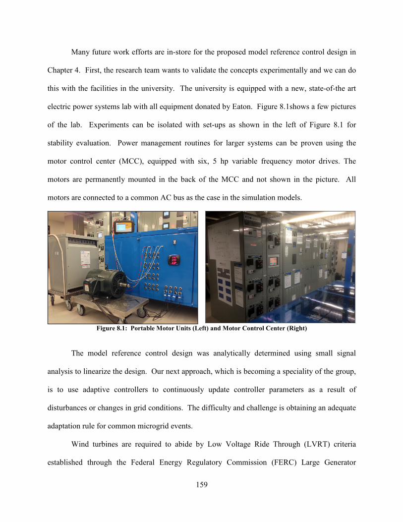
Many future work efforts are in-store for the proposed model reference control design in
Chapter 4. First, the research team wants to validate the concepts experimentally and we can do
this with the facilities in the university. The university is equipped with a new, state-of-the art
electric power systems lab with all equipment donated by Eaton. Figure 8.1shows a few pictures
of the lab. Experiments can be isolated with set-ups as shown in the left of Figure 8.1 for
stability evaluation. Power management routines for larger systems can be proven using the
motor control center (MCC), equipped with six, 5 hp variable frequency motor drives. The
motors are permanently mounted in the back of the MCC and not shown in the picture. All
motors are connected to a common AC bus as the case in the simulation models.
Figure 8.1: Portable Motor Units (Left) and Motor Control Center (Right)
The model reference control design was analytically determined using small signal
analysis to linearize the design. Our next approach, which is becoming a speciality of the group,
is to use adaptive controllers to continuously update controller parameters as a result of
disturbances or changes in grid conditions. The difficulty and challenge is obtaining an adequate
adaptation rule for common microgrid events.
Wind turbines are required to abide by Low Voltage Ride Through (LVRT) criteria
established through the Federal Energy Regulatory Commission (FERC) Large Generator
159
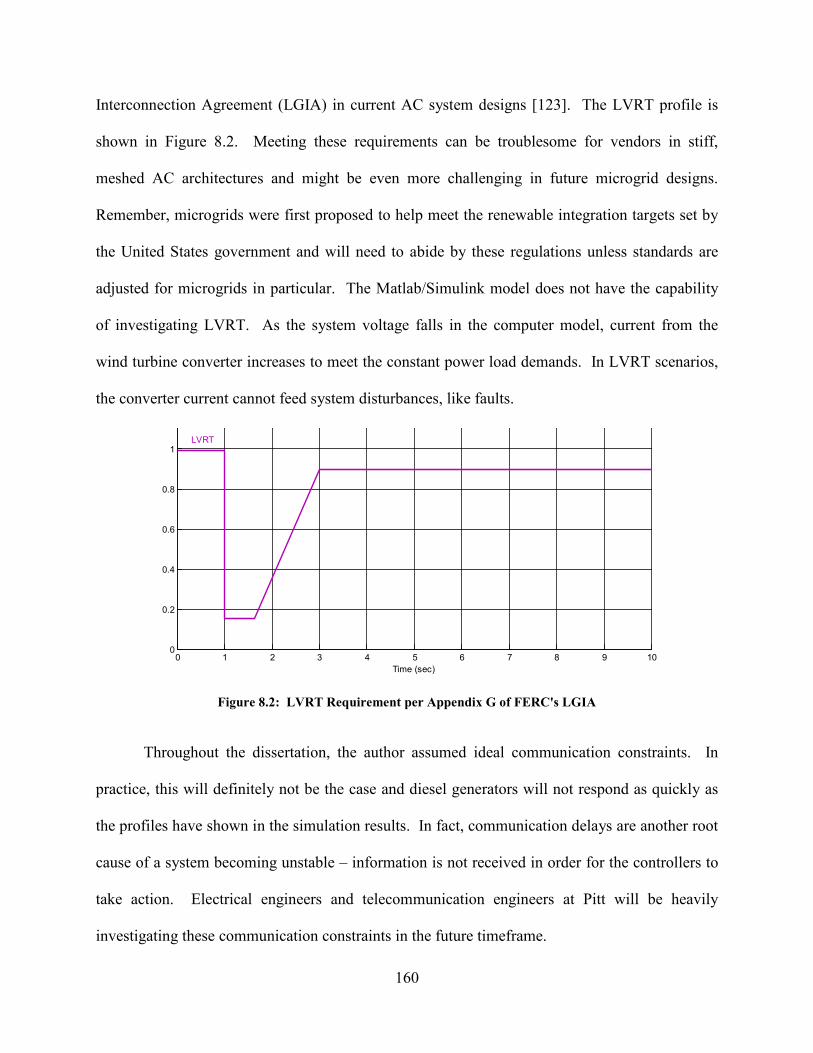
Interconnection Agreement (LGIA) in current AC system designs [123]. The LVRT profile is
shown in Figure 8.2. Meeting these requirements can be troublesome for vendors in stiff,
meshed AC architectures and might be even more challenging in future microgrid designs.
Remember, microgrids were first proposed to help meet the renewable integration targets set by
the United States government and will need to abide by these regulations unless standards are
adjusted for microgrids in particular. The Matlab/Simulink model does not have the capability
of investigating LVRT. As the system voltage falls in the computer model, current from the
wind turbine converter increases to meet the constant power load demands. In LVRT scenarios,
the converter current cannot feed system disturbances, like faults.
0 1 2 3 4 5 6 7 8 9 100
0.2
0.4
0.6
0.8
1LVRT
Time (sec)
Figure 8.2: LVRT Requirement per Appendix G of FERC's LGIA
Throughout the dissertation, the author assumed ideal communication constraints. In
practice, this will definitely not be the case and diesel generators will not respond as quickly as
the profiles have shown in the simulation results. In fact, communication delays are another root
cause of a system becoming unstable – information is not received in order for the controllers to
take action. Electrical engineers and telecommunication engineers at Pitt will be heavily
investigating these communication constraints in the future timeframe.
160

APPENDIX A
MATLAB CODE TO EVALUATE SWITCHING FREQUENCY IMPACTS ON
TRANSFORMER POWER DENSITY
161

function [c,ceq] = XfmrConstraints1(x) % Lead Graduate Student Researcher: Brandon Grainger % Undergraduate Research Assistant: Zachary Smith % January 2014 %% Objective of Function XfmrConstraints % The objective of this function is to calculate the amount of flux in the % transformer, losses in the core and windings, and temperature rise. %% Initial Conditions: %a = .028m %b = .110m %d = .028m %h = .205m %N = 32 f = 1000; % Operating frequency of transformer (Hz) Bmax = 0.75; % Maximum Flux Density (Tesla) Bmin = 0.65; % Minimum Flux Density (Tesla) Tmax = 150; % Maximum allowed temperature (Celsius) %% Declaration of Physical Properties % Geometric Properties a = x(1); % Property a in meters b = x(2); % Property b in meters d = x(3); % Property d in meters h = x(4); % Property h in meters N = x(5); % Number of turns in Primary Ac = a*d; % Cross Sectional Area (m^2) Aw = 2*b*h; % Window Area (m^2) l0 = 2*(a+b+d); % Mean Length per Turn (m) l1 = 2*a+2*b; % Transformer Width (m) l2 = d+b; % Transformer Thickness (m) l3 = 2*a+2*h; % Transformer Height (m) V = l1*l2*l3; % Transformer Core (m^3) Vc = (2*a+b)*(2*a+2*h)*d-2*h*b*d; % Core Volume (m^3) At = 2*(l1*l2+l1*l3+l2*l3); % Transformer Thermal Area (m^2) %% Variables %%%%%%% Transformer Parameters %%%%%%% circuit = 8; % Number of circuits in primary PowerT = 128340; % Power rating of the transformer W PowerFactor = 0.93; % Minimum allowable power factor STrans = PowerT/PowerFactor; % Maximum kVA of the transformer omega = 2*pi*f; % Radial Frequency Erms = 13.8*10^3; % Voltage of the transformer (Volts) Ermspri = Erms; % RMS voltage - primary winding (Volts) Irmspri = STrans/Ermspri/circuit; % RMS curr. - primary winding (Amperes) Ermssec = Ermspri*0.5580; % RMS voltage - second. winding (Volts) % (utility side) Irmssec = PowerT/Ermssec; % RMS curr. - secondary winding (Amps) % (utility side) %%%%%%%%%% Pcore Variables %%%%%%%%%%% alpha = 1.6945; beta = 1.967; k = 0.787; % W/kg %%%%%%%% Pwinding Variables %%%%%%%%%% rho = 23*10^(-9); % Electrical resistivity of copper % Ohm*m at 100degC km = 2; % Coil numbers in the transformer kAC = 1; % AC Resistance Coefficient kw = 0.1; % Fill factor of the window area mu0 = 4*pi*10^(-7); % Permeability constant (H/m) n = 420; % Number of strands in Litz wire dc = 0.00010160; % Strand diameter (m) kf = 1; % Factor accounting for field % distribution in multiwinding TXs Rs = 0.323; % Resistance of secondary wire (Ohms)
162

% 22 AWG wire Rdc = 0.0104; % DC Resistance of primary wire (Ohms) % 12 AWG wire %% Calculation of Cost Function, Losses, and Temperature Rise %%%%%%%%%% Volume of the Core %%%%%%%%%%%% Vcore = l1*l2*l3; % Cost Function (Volume in m^3) weight = 15*0.453592; % Weight of transformer in kg origVcore = 0.0177; % Initial value of transformer (m^3) density = weight/origVcore; % Density of core %%%% Magnetix Flux in the Transformer %%%% % Flux Density of the Core (T)(V*s/(m^2)) BTx= sqrt(2)*Erms/(2*pi*f*N*circuit*a*d); %%%%%%%%% Power Loss in the Core %%%%%%%%% % Calculation of Core Loss (W) Pcore = density*Vcore*(k*(f/1000)^(alpha)*BTx^(beta)); % Alternative Core Loss Equation % Pcore = Vcore*(0.0277419*(f)^(alpha)*BTx^(beta)); %%%%%%% Power Loss in the Windings %%%%%%% % Pwinding = kAC*km*kw*rho*N^2*l0/Aw; Fr = 1 + (pi*omega*mu0*N*n)^2*dc^6/(768*rho^2*b^2); Pwp = (Fr*Irmspri^2*Rdc)*circuit; % Litz Wire Winding Loss (Primary) Pws = Irmssec^2*Rs; % Solid Copper Wire Loss (Secondary) Pwinding = Pwp+Pws; % Total Winding Loss %%%%%%%%%%%% Temperature Rise %%%%%%%%%%%% Trise = 450*((Pcore+Pwinding)/(At*100*100))^(0.826); % Average Temperature Rise of the Transformer. %"At" in the Trise equation is multiplied by 10000 to get units cm^2. c(1) = BTx - Bmax; c(2) = Trise - Tmax; c(3) = -BTx + Bmin; ceq = []; %%%%%%%%%%%% Variables of Interest to Display %%%%%%%%%%%% BTx Trise Irmspri Pcore Pwinding Powerloss = (Pcore + Pwinding) efficiency = (STrans-Powerloss)/STrans a b d h N disp('excel results') disp(BTx) disp(Trise) disp(Irmspri) disp(Pcore) disp(Pwinding) disp(Powerloss) disp(efficiency) disp(a) disp(b) disp(d) disp(h) disp(N) disp(Vcore) disp(f) end
163

function [Vcore] = XfmrCost1( x ) % Lead Graduate Student Researcher: Brandon Grainger % Undergraduate Research Assistant: Zachary Smith % January 2014 %% Objective of Function XfmrCost % The objective of this function is to calculate the cost (volume) of the % transformer. %% Initial Conditions: %a = .028m %b = .110m %d = .028m %h = .205m %N = 32 %Solver: fmincon - Constrained nonlinear minimization %Algorithm: Interior point %Frequency 1000Hz %Start Point [0.028 0.110 0.028 0.205 32] %Lower Bound [0.0075 0.04 0.075 0.09 25] %Upper Bound [0.08 0.36 0.08 0.51 32] % Bmax = 0.75; % Maximum Flux Density (Tesla) % Bmin = 0.65; % Minimum Flux Density (Tesla) % Tmax = 150; % Maximum allowed temperature (Celsius) %% Declaration of Physical Properties % Geometric Properties a = x(1); % Property a in meters b = x(2); % Property b in meters d = x(3); % Property d in meters h = x(4); % Property h in meters l1 = 2*a+2*b; % Transformer Width (m) l2 = d+b; % Transformer Thickness (m) l3 = 2*a+2*h; % Transformer Height (m) %% Calculation of Cost Function %%%%%%%%%% Volume of the Core %%%%%%%%%%%% Vcore = l1*l2*l3; % Cost Function (Volume in m^3) end
164

APPENDIX B
MATLAB CODE TO EVALUATE MODEL REFERENCE CONTROLLER DESIGN
FOR CONSTANT POWER LOAD SCENARIO
165

% Brandon Grainger % June 2014 % Sponsored: ABB Corporate Research % Purpose - Stability Assessment of MRC Controller %-------------------------------------------------------------------------- % Cable Parameters % 3.6/6(7.2)kV - Single Core, XLPE Insultated, PVC Sheathed, Screened % Unarmoured cables - IEC 60502-2 % Nominal Cross Section: 1000mm^2 % Current Rating: 1340 A - Copper wire / Duct %-------------------------------------------------------------------------- clc; clear %--------------------- Cable Characteristics --------------------- % Distance d= 0.1; % DC Resistance at 20 degrees R_m = 0.0176; %ohm/km R = R_m*d; %ohm % Trefoil Formation L_m = 0.248e-3; %H/km L = L_m*d; %H % Nominal Capacity C_m = 0.923e-6; %F/km C = C_m/2*d; %%--------------------- Converter Characteristics --------------------- n = 5; Vdc = 1000; Ts = 1/3000; L_conv = 5.208e-3; dh= 0.1464; Y = (Vdc)^2/100e3 C1 = (C + (100e3/(Vdc*0.1*Vdc*377))); C1 = 13.2e-3 C2 = [(L/(R*Y))+2e-3]; C2 = 5e-3 %---------------------- Pole Placement of M(s) ------------------------ wn = 5000; wn = 3500; % Tuned for Slower Control Response Kp_PD = 1/(Y+1); % Kp < 1/Y (Constraint) Kd_PD = 1; %-------------------------------------------------------------------------- % Transfer Function Characteristics of Plant (3rd Order System) % x coefficients for numerator; y coefficients for denominator x2 = Y*C2*L; x1 = R*C2*Y-L; x0 = Y-R; y3 = L*C1*C2*Y; y2 = R*C1*C2*Y-L*C1; y1 = C1*Y-R*C1 + C2*Y; y0 = -1; G = n*Vdc*Ts*(1-2*dh)/(2*L_conv); sys=G*tf([x2 x1 x0],[y3 y2 y1 y0]) %-------------------------------------------------------------------------- % Adaptive Controller Transfer Function Characteristics
166

km = 1; G = G/100; kp = G/C1; Co = km/kp; % Compensator: Lambda / (Lambda - C_hat) w1 = sqrt(wn^3/km) % w1 is numerator coefficient of M(s) a2 = 1 % Lambda Coefficients a1 = 2*w1 a0 = w1^2 q2 = 1; % Lambda - C_hat Coefficients q1 = (R*C2*Y-L)/(L*C2*Y); % Plant Transfer Function numerator q0 = (Y-R)/(L*C2*Y); % Feedback: d_hat / Lambda b2 = sqrt(3)*wn+wn b1 = wn*wn + sqrt(3)*wn*wn b0 = km*wn*wn*wn p2 = (R*C1*C2*Y-L*C1)/(L*C1*C2*Y) p1 = (C1*Y-R*C1+C2*Y)/(L*C1*C2*Y) p0 = -1/(L*C1*C2*Y) d2 = (p2-b2)/kp % d_hat Coefficients d1 = (p1-b1)/kp d0 = -(b0+p0)/kp %-------------------------------------------------------------------------- % Zero/Pole Placement for M(s) and P(s) on Same Mapping sys2=tf([1 a1 a0],[1 b2 b1 b0]) figure iopzplot(sys) figure iopzplot(sys2) %-------------------------------------------------------------------------- % Testing Matching Equality: Variable "Right" = Variable "Left" np=tf([1 q1 q0], 1); dm = tf([1 b2 b1 b0],1); Right = np*dm aaa = -tf([1 q1 q0],1)*tf([(p2-b2) (p1-b1) -(b0+p0)],1); bbb = (tf([1 a1 a0], 1)-tf([(a1-q1) (a0-q0)], 1))*tf([1 p2 p1 -p0],1); Left = aaa+bbb %--------------------------------------------------------------------------
167

APPENDIX C
MODELING THE WIND TURBINE IN SIMULATION PLATFORMS
This appendix was written to provide an intuitive understanding of the wind turbine model
developed in this dissertation.
Permanent Magnet Synchronous Generator (PMSG) Implementation in Simulators
The outputs of the machine module shown in Figure AC.1 include the machine mechanical and
electrical speeds, measured abc currents and rotor displacement angle. These variables are
extensively used to coordinate the control between the machine and three-level, neutral point
clamped rectifier.
Permanent Magnet Machine
and Aerodynamic Model
Rotor_Angle, θr
Mechanical_Speed, ωr
Electrical_Speed, ωe
Iabc_measurements
Output Power
Figure AC.1: PMSG and Aerodynamic Model Module with Outputs
168

The blocks connected together in Figure AC.2, which are embedded in Figure AC.1, are
used to solve the mechanical equation of the machine described by (5.3). The inputs to the
equation are the mechanical torque coming from the aerodynamic model and the electromagnetic
torque coming from the electrical model of Figure AC.3. The moment of inertia of the machine,
J, is 2.5x10⁵ kgm2, the friction factor, F, is 2.26x10⁴ Nm-s, and the number of pole pairs was
chosen to be 118. Once the mechanical speed of the machine is solved for in the inner loop, the
electrical speed can be determined by multiplying by the number of pole pairs. The mechanical
speed is also integrated using the discrete time integrator, 1/s, to obtain the rotor angular
position. Three of the four outputs of Figure AC.1 come from the mechanical equation.
-+-
Moment of Inertia, J
sT1
P
Pole Pairs, P
Mechanical Torque, Tm
Electrical TorqueTe
FFriction FactorF
Mechanical_Speed, ωr
sT1
Electrical_Speed, ωe
Rotor_Angle, θr
Figure AC.2: Mechanical Equation Implementation of PMSG
Figure AC.3 provides a technique for solving the two coupled electrical equations listed
as (5.1a) and (5.1b). This set of blocks requires three inputs, which include the rotor angular
position, electrical machine speed, and the abc line-to-ground voltage measurements from the
terminals of the machine. The three-phase voltage measurement is transformed into dq
components by means of a standard Park’s transformation, listed as (A1). The block in Figure
AC.3 labeled, Script ABC to dq0 Rotor Reference, is a script that performs the transformation.
169

Note that the following trigonometric identities listed as (A2a) through (A2d) are convenient
expressions for computing the 3x3 matrix in a computer.
Script ABC to DQO
RotorReference
Id and Iq
CalculationsTorque
Calculation(Equation 5.2)
Vd
Vq
Id
Iq
va,vb,vc
Rotor_Angle, θr
Electrical_Speed, ωe Pole Pairs, P
Ld Lq
Flux, λm
Script ABC to DQO
RotorReference
Id
Iq
ia,ib,icIabc_measurements
Figure AC.3: Electrical Model Implementation of PMSG
[ ]
+−−−−
+−
=
2/12/12/1
)3
2sin()3
2sin()sin(
)3
2cos()3
2cos(cos
32)( πθπθθ
πθπθθ
θ rrr
rrr
rdqoT (A1)
)cos(
21)sin(
23)
32cos( rrr θθπθ −=− (A2a)
)cos(
21)sin(
23)
32cos( rrr θθπθ +=+ (A2b)
)cos(
23)sin(
21)
32sin( rrr θθπθ +=−− (A2c)
)cos(
23)sin(
21)
32sin( rrr θθπθ −=+− (A2d)
170

The heart of the computations occurs in the Id and Iq Calculations block found in Figure
AC.3. The inputs to this block include the dq components of the abc line-to-ground voltage
measurements as well as the calculated electrical speed from the mechanical equation of Figure
AC.2. A subsystem exists within the Id and Iq Calculations block that solves the coupled
differential equations of the electrical system listed as (5.1a) and (5.1b). The details of the
underlining system are found in Figure AC.4. The next step in the process is to compute the
electromagnetic torque of the machine. With the dq current components calculated, the torque
can be calculated using (5.2). This electromagnetic torque, Te, is fed back into the mechanical
equation model to complete the coupling between the electrical and mechanical relationships.
Equation (5.1a) Solved for d-axis
Current Component
Equation (5.1b) Solved for q-axis
Current Component
Id
Vd
Vq
Electrical_Speed ωe
Iq
Iq Id
Figure AC.4: Illustration for Solving Electrical System Differential Equations
The last step in the process is to send the dq current components through an inverse
Park’s transformation described by (A3) to obtain the abc currents. These currents are then fed
into programmable current sources, as shown in Figure AC.5, which serve as the main source of
power for the physical MVDC wind collection system. Recall that most distributed resources
171

can be modeled current fed components, [25]. The audience will notice three voltage
measurements being made in Figure AC.5. These measurements are fed into the electrical model
system equations (Figure AC.3).
[ ]
+−+
−−−
−
=−
1)3
2sin()3
2cos(
1)3
2sin()3
2cos(
1)sin(cos
32)( 1
πθπθ
πθπθ
θθ
θ
rr
rr
rr
rdqoT (A3)
ia
ib
ic
Network
va
vb
vc
Figure AC.5: Physical Machine Interconnection to the MVDC Collection System
172

APPENDIX D
SCRIPTS FOR MONITORING AND ADJUSTING POWER EXCHANGE
THROUGHOUT THE DC MICROGRID
173

% Brandon Grainger % Parameters for System Model % Sponsored: ABB Corporate Research Center % March 2014 %-------------------------------------------------------------------------- % Simulation Convergence Parameters %-------------------------------------------------------------------------- Ts=5e-5; Ts_Control=50e-6; Ts_Power=Ts; %-------------------------------------------------------------------------- % Wind Turbine System and Control Parameters %-------------------------------------------------------------------------- Radius = 58; % Unit: Meters Pairs = 118; % Unit: N/A M_Flux = 14.3522; % Unit: Webers (Vs) L_machine = 3.5218e-3; % Unit: Henry % Control Parameters Kp_Wind = 0.3; Ki_Wind = 10; %-------------------------------------------------------------------------- % Bidirectional DC/DC Converter %-------------------------------------------------------------------------- fs_DCDC = 3000; Ts_DCDC = 1/fs_DCDC; L_DCDC = 208e-6; n = 5000/7500; %-------------------------------------------------------------------------- % Bidirectional DC/DC Converter %-------------------------------------------------------------------------- % Motor Drive No.1 Parameters Rs = 29e-3; Rr = 22e-3; Lm = 34.6e-3; Lls = 0.6e-3; Llr = 0.6e-3; Ls = Lls + Lm; Ls = 35.2e-3; Lr = Llr + Lm; Lr = 35.2e-3; Prated = 1.678e6; Vrated = 2300; wo = 377; sigma_s = (Ls/Lm)-1; sigma_r = (Lr/Lm)-1; sigma = 1 - (1/((1+sigma_r)*(1+sigma_s))); Imr_ref = (sqrt(2/3)*Vrated)/(wo*Lm*(sigma_s+1)); tau_s = Lm*(1+sigma_s)/Rs; tau_r = Lm*(1+sigma_r)/Rr; tau_i = 3e-3; Kp = 1*sigma*tau_s/tau_i; Ki = 1/tau_i; % Motor Drive No.2 Parameters Rs_2 = 29e-3; Rr_2 = 22e-3; Lm_2 = 34.6e-3; Lls_2 = 0.6e-3; Llr_2 = 0.6e-3; Ls_2 = Lls_2 + Lm_2; Ls_2=35.2e-3;
174

Lr_2 = Llr_2 + Lm_2; Lr_2=35.2e-3; Prated_2 = 1.678e6; Vrated_2 = 2300; wo = 377; sigma_s_2 = (Ls_2/Lm_2)-1; sigma_r_2 = (Lr_2/Lm_2)-1; sigma_2 = 1 - (1/((1+sigma_r_2)*(1+sigma_s_2))); Imr_ref_2 = (sqrt(2/3)*Vrated_2)/(wo*Lm_2*(sigma_s_2+1)); tau_s_2 = Lm*(1+sigma_s_2)/Rs_2; tau_r_2 = Lm*(1+sigma_r_2)/Rr_2; tau_i_2 = 3e-3; Kp_2 = 1*sigma_2*tau_s_2/tau_i_2; Ki_2 = 1/tau_i_2; % Motor Drive No.3 Parameters Rs_3 = 29e-3; Rr_3 = 22e-3; Lm_3 = 34.6e-3; Lls_3 = 0.6e-3; Llr_3 = 0.6e-3; Ls_3 = Lls_3 + Lm_3; Ls_3=35.2e-3; Lr_3 = Llr_3 + Lm_3; Lr_3=35.2e-3; Prated_3 = 1.678e6; Vrated_3 = 2300; wo = 377; sigma_s_3 = (Ls_3/Lm_3)-1; sigma_r_3 = (Lr_3/Lm_3)-1; sigma_3 = 1 - (1/((1+sigma_r_3)*(1+sigma_s_3))); Imr_ref_3 = (sqrt(2/3)*Vrated_3)/(wo*Lm_3*(sigma_s_3+1)); tau_s_3 = Lm*(1+sigma_s_3)/Rs_3; tau_r_3 = Lm*(1+sigma_r_3)/Rr_3; tau_i_3 = 3e-3; Kp_3 = 1*sigma_3*tau_s_3/tau_i_3; Ki_3 = 1/tau_i_3;
175

BIBLIOGRAPHY
[1] G. F. Reed, B. M. Grainger, A. R. Sparacino, R. J. Kerestes, and M. J. Korytowski, “Advancements in medium voltage DC architecture development with applications for powering electric vehicle charging stations,” in 2012 IEEE Energytech, 2012, pp. 1–8.
[2] H. Mirzaee, S. Dutta, and S. Bhattacharya, “A medium-voltage DC (MVDC) with series active injection for shipboard power system applications,” in 2010 IEEE Energy Conversion Congress and Exposition, 2010, pp. 2865–2870.
[3] M. Bash, R. R. Chan, J. Crider, C. Harianto, J. Lian, J. Neely, S. D. Pekarek, S. D. Sudhoff, and N. Vaks, “A Medium Voltage DC Testbed for ship power system research,” in 2009 IEEE Electric Ship Technologies Symposium, 2009, pp. 560–567.
[4] T. Ericsen, “The ship power electronic revolution: Issues and answers,” in 2008 55th IEEE Petroleum and Chemical Industry Technical Conference, 2008, pp. 1–11.
[5] G. Reed, B. Grainger, A. Sparacino, and Z.-H. Mao, “Ship to Grid: Medium-Voltage DC Concepts in Theory and Practice,” IEEE Power Energy Mag., vol. 10, no. 6, pp. 70–79, Nov. 2012.
[6] ABB in the United States, “U.S. Department of Energy to fund major Offshore Wind Grid Interconnection study,” 2011. [Online]. Available: http://www.abb.us.
[7] I. C. Evans and R. Limpaecher, “High power clean DC bus generation using AC-link AC to DC power voltage conversion, DC regulation, and galvanic isolation,” in 2009 IEEE Electric Ship Technologies Symposium, 2009, pp. 290–301.
[8] F. Falco, “Subsea Technologies at the Heart of Future Oilfields,” 2014. [Online]. Available: http://www.gepowerconversion.com/inspire.
[9] E. Ibanez, T. Mai, and L. Coles, “Analyzing the Deployment of Large Amounts of Offshore Wind to Design an Offshore Transmission Grid in the United States,” in 11th Annual International Workshop on Large-Scale Integration of Wind Power into Power Systems, 2012.
[10] Siemens AG Energy Sector, “The Offshore Way: WIPOS-Wind Power Offshore Substation,” 2011. [Online]. Available: http://www.siemens.com/energy/wipos.
176

[11] P. Lundberg, M. Callavik, M. Bahrman, and P. Sandeberg, “Platforms for Change: High-Voltage DC Converters and Cable Technologies for Offshore Renewable Integration and DC Grid Expansions,” IEEE Power Energy Mag., vol. 10, no. 6, pp. 30–38, Nov. 2012.
[12] R. H. Lasseter and P. Paigi, “Microgrid: a conceptual solution,” in 2004 IEEE 35th Annual Power Electronics Specialists Conference (IEEE Cat. No.04CH37551), 2004, vol. 6, pp. 4285–4290.
[13] T. S. Basso and R. DeBlasio, “IEEE 1547 Series of Standards: Interconnection Issues,” IEEE Trans. Power Electron., vol. 19, no. 5, pp. 1159–1162, Sep. 2004.
[14] L. M. Tolbert, “Power Conversion Systems for Microgrids,” ECCE 2012 Rap Session, Raleigh, NC, 2012.
[15] S. Krishnamurthy, T. M. Jahns, and R. H. Lasseter, “The operation of diesel gensets in a CERTS microgrid,” in 2008 IEEE Power and Energy Society General Meeting - Conversion and Delivery of Electrical Energy in the 21st Century, 2008, pp. 1–8.
[16] J. M. Guerrero, J. Matas, L. Garcia de Vicuna, M. Castilla, and J. Miret, “Decentralized Control for Parallel Operation of Distributed Generation Inverters Using Resistive Output Impedance,” IEEE Trans. Ind. Electron., vol. 54, no. 2, pp. 994–1004, Apr. 2007.
[17] R. Teodorescu and F. Blaabjerg, “Flexible Control of Small Wind Turbines With Grid Failure Detection Operating in Stand-Alone and Grid-Connected Mode,” IEEE Trans. Power Electron., vol. 19, no. 5, pp. 1323–1332, Sep. 2004.
[18] D. Chen, Chien-Liang Wang, Yubin Lai, Jih-Sheng(Jason) Lee, Yuang-Shung Martin, “Design of Parallel Inverters for Smooth Mode Transfer Microgrid Applications,” IEEE Trans. Power Electron., vol. 25, no. 1, pp. 6–15, Jan. 2010.
[19] J. C. Vasquez, J. M. Guerrero, A. Luna, P. Rodriguez, and R. Teodorescu, “Adaptive Droop Control Applied to Voltage-Source Inverters Operating in Grid-Connected and Islanded Modes,” IEEE Trans. Ind. Electron., vol. 56, no. 10, pp. 4088–4096, Oct. 2009.
[20] M. A. Zamani, A. Yazdani, and T. S. Sidhu, “A Control Strategy for Enhanced Operation of Inverter-Based Microgrids Under Transient Disturbances and Network Faults,” IEEE Trans. Power Deliv., vol. 27, no. 4, pp. 1737–1747, Oct. 2012.
[21] L. Xu and D. Chen, “Control and Operation of a DC Microgrid With Variable Generation and Energy Storage,” IEEE Trans. Power Deliv., vol. 26, no. 4, pp. 2513–2522, Oct. 2011.
[22] K. De Brabandere, B. Bolsens, J. Van den Keybus, A. Woyte, J. Driesen, and R. Belmans, “A Voltage and Frequency Droop Control Method for Parallel Inverters,” IEEE Trans. Power Electron., vol. 22, no. 4, pp. 1107–1115, Jul. 2007.
177

[23] Jung-Won Kim, Hang-Seok Choi, and Bo Hyung Cho, “A novel droop method for converter parallel operation,” IEEE Trans. Power Electron., vol. 17, no. 1, pp. 25–32, 2002.
[24] J. M. Guerrero, N. Berbel, J. Matas, L. G. de Vicuna, and J. Miret, “Decentralized Control for Parallel Operation of Distributed Generation Inverters in Microgrids Using Resistive Output Impedance,” in IECON 2006 - 32nd Annual Conference on IEEE Industrial Electronics, 2006, pp. 5149–5154.
[25] J. Rocabert, A. Luna, F. Blaabjerg, and P. Rodríguez, “Control of Power Converters in AC Microgrids,” IEEE Trans. Power Electron., vol. 27, no. 11, pp. 4734–4749, Nov. 2012.
[26] I. Batarseh, K. Siri, and H. Lee, “Investigation of the output droop characteristics of parallel-connnected DC-DC converters,” in Proceedings of 1994 Power Electronics Specialist Conference - PESC’94, 1994, pp. 1342–1351.
[27] A. Bidram and A. Davoudi, “Hierarchical Structure of Microgrids Control System,” IEEE Trans. Smart Grid, vol. 3, no. 4, pp. 1963–1976, Dec. 2012.
[28] J. M. Guerrero, J. C. Vasquez, J. Matas, L. G. de Vicuna, and M. Castilla, “Hierarchical Control of Droop-Controlled AC and DC Microgrids—A General Approach Toward Standardization,” IEEE Trans. Ind. Electron., vol. 58, no. 1, pp. 158–172, Jan. 2011.
[29] J. Liang, T. Jing, O. Gomis-Bellmunt, J. Ekanayake, and N. Jenkins, “Operation and Control of Multiterminal HVDC Transmission for Offshore Wind Farms,” IEEE Trans. Power Deliv., vol. 26, no. 4, pp. 2596–2604, Oct. 2011.
[30] D. Salomonsson, L. Soder, and A. Sannino, “An Adaptive Control System for a DC Microgrid for Data Centers,” IEEE Trans. Ind. Appl., vol. 44, no. 6, pp. 1910–1917, 2008.
[31] C. Abbey, D. Cornforth, N. Hatziargyriou, K. Hirose, A. Kwasinski, E. Kyriakides, G. Platt, L. Reyes, and S. Suryanarayanan, “Powering Through the Storm: Microgrids Operation for More Efficient Disaster Recovery,” IEEE Power Energy Mag., vol. 12, no. 3, pp. 67–76, May 2014.
[32] A. Kwasinski, V. Krishnamurthy, J. Song, and R. Sharma, “Availability Evaluation of Micro-Grids for Resistant Power Supply During Natural Disasters,” IEEE Trans. Smart Grid, vol. 3, no. 4, pp. 2007–2018, Dec. 2012.
[33] “Power Electronics Research and Development Program Plan,” Office of Electricity Delivery and Energy Reliability, Washington, DC, 2011.
[34] R. Ram, “Power Electronics,” ARPA-E Pre-Summit Workshop, Washington, DC, Mar. 2010.
178

[35] A. M. Leary, P. R. Ohodnicki, and M. E. McHenry, “Soft Magnetic Materials in High-Frequency, High-Power Conversion Applications,” J. Met., vol. 64, no. 7, pp. 772–781, Jul. 2012.
[36] W. Kramer, S. Chakraborty, B. Kroposki, and H. Thomas, “Advanced Power Electronic Interfaces for Distributed Energy Systems Part 1: Systems and Topologies,” National Renewable Energy Laboratory, 2008.
[37] Q. Li, M. Lim, J. Sun, A. Ball, Y. Ying, F. C. Lee, and K. D. T. Ngo, “Technology road map for high frequency integrated DC-DC converter,” in 2010 Twenty-Fifth Annual IEEE Applied Power Electronics Conference and Exposition (APEC), 2010, pp. 533–539.
[38] M. Schaefer, G. Dietzmann, and H. Wirth, “Magnetic losses in ferrites and nanocrystalline ribbons for power applications,” J. Magn. Magn. Mater., vol. 101, no. 1–3, pp. 95–96, Oct. 1991.
[39] R. Hasegawa, “Applications of amorphous magnetic alloys in electronic devices,” J. Non. Cryst. Solids, vol. 287, no. 1–3, pp. 405–412, Jul. 2001.
[40] R. Hasegawa, “Applications of amorphous magnetic alloys,” Mater. Sci. Eng. A, vol. 375–377, pp. 90–97, Jul. 2004.
[41] M. E. McHenry, M. A. Willard, and D. E. Laughlin, Amorphous and nanocrystalline materials for applications as soft magnets, vol. 44, no. 4. 1999, pp. 291–433.
[42] R. W. A. A. De Doncker, D. M. Divan, and M. H. Kheraluwala, “A three-phase soft-switched high-power-density DC/DC converter for high-power applications,” IEEE Trans. Ind. Appl., vol. 27, no. 1, pp. 63–73, 1991.
[43] A. Pressman and K. Billings, Switching Power Supply Design. McGraw-Hill; 3rd edition, 2009.
[44] Y. Xie, J. Sun, and J. S. Freudenberg, “Power Flow Characterization of a Bidirectional Galvanically Isolated High-Power DC/DC Converter Over a Wide Operating Range,” IEEE Trans. Power Electron., vol. 25, no. 1, pp. 54–66, Jan. 2010.
[45] D. Segaran, D. G. Holmes, and B. P. McGrath, “Comparative analysis of single and three-phase dual active bridge bidirectional DC-DC converters.” pp. 1–6, 2008.
[46] J. Xue, F. Wang, D. Boroyevich, and Z. Shen, “Single-phase vs. three-phase high density power transformers,” in 2010 IEEE Energy Conversion Congress and Exposition, 2010, pp. 4368–4375.
[47] M. Pavlovsky, S. W. H. de Haan, and J. A. Ferreira, “Concept of 50 kW DC/DC converter based on ZVS, quasi-ZCS topology and integrated thermal and electromagnetic design,” in 2005 European Conference on Power Electronics and Applications, 2005, p. 9.
179

[48] I.-Y. Chung, W. Liu, M. Andrus, K. Schoder, D. A. Cartes, and M. Steurer, “Integration of a bi-directional dc-dc converter model into a large-scale system simulation of a shipboard MVDC power system,” in 2009 IEEE Electric Ship Technologies Symposium, 2009, pp. 318–325.
[49] D. Costinett, D. Maksimovic, and R. Zane, “Design and Control for High Efficiency in High Step-Down Dual Active Bridge Converters Operating at High Switching Frequency,” IEEE Trans. Power Electron., vol. 28, no. 8, pp. 3931–3940, Aug. 2013.
[50] “Gallium-Nitride Switch Technology for Bi-Directional Battery-to-Grid Charger Applications.” [Online]. Available: http://arpa-e.energy.gov/?q=arpa-e-projects/compact-interactive-electric-vehicle-charger.
[51] J. Xue, “Single-phase vs. Three-phase High Power High Frequency Transformers,” Virginia Tech, 2010.
[52] R. Prieto, J. A. Oliver, J. A. Cobos, J. Uceda, and M. Christini, “Errors obtained when 1D magnetic component models are not properly applied,” in APEC ’99. Fourteenth Annual Applied Power Electronics Conference and Exposition. 1999 Conference Proceedings, 1999, vol. 1, pp. 206–212 vol.1.
[53] W. McLyman, Transformer and Inductor Design Handbook, Fourth Edition. CRC Press; 4th edition, 2012.
[54] “0P44125UC MAGNETICS Core.” [Online]. Available: http://www.mag-inc.com/File Library/Product Datasheets/Ferrite/New Ferrite data sheets/0P44125UC.pdf.
[55] “P Material,” 2014. [Online]. Available: http://www.mag-inc.com/products/ferrite-cores/p-material.
[56] “0P44949EC ETD Core,” 2014. [Online]. Available: http://www.mag-inc.com/File Library/Product Datasheets/Ferrite/New Ferrite data sheets/0P44949EC.pdf.
[57] B. M. Grainger, O. Scioscia, T. E. McDermott, G. F. Reed, and E. Lin, “Prediction and experimental verification of core loss and temperature distribution for geometrically scaled finemet toroids using finite element analysis,” in 2014 IEEE Applied Power Electronics Conference and Exposition - APEC 2014, 2014, pp. 2615–2620.
[58] W. Shen, F. Wang, D. Boroyevich, and C. W. Tipton IV, “High-Density Nanocrystalline Core Transformer for High-Power High-Frequency Resonant Converter,” IEEE Trans. Ind. Appl., vol. 44, no. 1, pp. 213–222, 2008.
[59] J. M. Silveyra, a. M. Leary, V. DeGeorge, S. Simizu, and M. E. McHenry, “High speed electric motors based on high performance novel soft magnets,” J. Appl. Phys., vol. 115, no. 17, p. 17A319, May 2014.
180

[60] Cogent Surahammars Burks AB, “Typical Data for SURA M600-50A,” 2008. [Online]. Available: http://www.sura.se.
[61] European Steel and Alloy Grades, “Properties of Grade M600-50A,” 2013. [Online]. Available: http://www.steelnumber.com.
[62] M. Dems and K. Komeza, “Performance Characteristics of a High-Speed Energy-Saving Induction Motor With an Amorphous Stator Core,” IEEE Trans. Ind. Electron., vol. 61, no. 6, pp. 3046–3055, Jun. 2014.
[63] M. J. Melfi, “Optimum pole configuration of AC induction motors used on adjustable frequency power supplies,” in Industry Applications Society 42nd Annual Petroleum and Chemical Industry Conference, 1995, pp. 237–242.
[64] W. A. Reass, D. M. Baca, and R. F. Gribble, “Multi-Megawatt High Frequency Polyphase Nanocrystalline Transformers,” 2007. [Online]. Available: http://www.nist.gov/pml/high_megawatt/upload/2007_Reass-II.pdf.
[65] C. R. Sullivan, “Cost-constrained selection of strand diameter and number in a litz-wire transformer winding,” IEEE Trans. Power Electron., vol. 16, no. 2, pp. 281–288, Mar. 2001.
[66] G. F. Reed, B. M. Grainger, H. Bassi, E. Taylor, Z.-H. Mao, and A. K. Jones, “Analysis of high capacity power electronic technologies for integration of green energy management,” in IEEE PES T&D 2010, 2010, pp. 1–10.
[67] W. Breuer, D. Retzmann, and K. Uecker, “Highly Efficient Solutions for Smart and Bulk Power Transmission of ‘Green Energy,’” Siemens AG, Energy Sector - Power Transmission Division, 2011.
[68] J. Rodriguez, L. G. Franquelo, S. Kouro, J. I. Leon, R. C. Portillo, M. A. M. Prats, and M. A. Perez, “Multilevel Converters: An Enabling Technology for High-Power Applications,” Proc. IEEE, vol. 97, no. 11, pp. 1786–1817, Nov. 2009.
[69] B. Gemmell, J. Dorn, D. Retzmann, and D. Soerangr, “Prospects of multilevel VSC technologies for power transmission,” in 2008 IEEE/PES Transmission and Distribution Conference and Exposition, 2008, pp. 1–16.
[70] J. Wang, R. Burgos, and D. Boroyevich, “A survey on the modular multilevel converters — Modeling, modulation and controls,” in 2013 IEEE Energy Conversion Congress and Exposition, 2013, pp. 3984–3991.
[71] M. Saeedifard and R. Iravani, “Dynamic Performance of a Modular Multilevel Back-to-Back HVDC System,” IEEE Trans. Power Deliv., vol. 25, no. 4, pp. 2903–2912, Oct. 2010.
181

[72] X. Li, Q. Song, W. Liu, H. Rao, S. Xu, and L. Li, “Protection of Nonpermanent Faults on DC Overhead Lines in MMC-Based HVDC Systems,” IEEE Trans. Power Deliv., vol. 28, no. 1, pp. 483–490, Jan. 2013.
[73] J. Peralta, H. Saad, S. Dennetiere, J. Mahseredjian, and S. Nguefeu, “Detailed and Averaged Models for a 401-Level MMC–HVDC System,” IEEE Trans. Power Deliv., vol. 27, no. 3, pp. 1501–1508, Jul. 2012.
[74] U. N. Gnanarathna, A. M. Gole, and R. P. Jayasinghe, “Efficient Modeling of Modular Multilevel HVDC Converters (MMC) on Electromagnetic Transient Simulation Programs,” IEEE Trans. Power Deliv., vol. 26, no. 1, pp. 316–324, Jan. 2011.
[75] M. Guan and Z. Xu, “Modeling and Control of a Modular Multilevel Converter-Based HVDC System Under Unbalanced Grid Conditions,” IEEE Trans. Power Electron., vol. 27, no. 12, pp. 4858–4867, Dec. 2012.
[76] A. Yazdani and R. Iravani, Voltage-Sourced Converters in Power Systems: Modeling, Control, and Applications. Hoboken: Wiley, 2010.
[77] B. Wu, High-Power Converters and AC Drives. Wiley, 2006.
[78] A. Yazdani and R. Iravani, “A Unified Dynamic Model and Control for the Voltage-Sourced Converter Under Unbalanced Grid Conditions,” IEEE Trans. Power Deliv., vol. 21, no. 3, pp. 1620–1629, Jul. 2006.
[79] D. W. Novotny and T. A. Lipo, Vector Control and Dynamics of AC Drives. Oxford University Press, USA, 1996.
[80] H. Saad, J. Peralta, S. Dennetiere, J. Mahseredjian, J. Jatskevich, J. A. Martinez, A. Davoudi, M. Saeedifard, V. Sood, X. Wang, J. Cano, and A. Mehrizi-Sani, “Dynamic Averaged and Simplified Models for MMC-Based HVDC Transmission Systems,” IEEE Trans. Power Deliv., vol. 28, no. 3, pp. 1723–1730, Jul. 2013.
[81] K. Ilves, S. Norrga, L. Harnefors, and H.-P. Nee, “On Energy Storage Requirements in Modular Multilevel Converters,” IEEE Trans. Power Electron., vol. 29, no. 1, pp. 77–88, Jan. 2014.
[82] T. M. Blooming and D. J. Carnovale, “Application of IEEE STD 519-1992 Harmonic Limits,” in Conference Record of 2006 Annual Pulp and Paper Industry Technical Conference, 2006, pp. 1–9.
[83] H. Maekawa, Y. Watanabe, K. Murata, Y. Hirota, “Research and Development of DC +/- 500 kV Extruded Cables,” in Cigre Session 2002, 2002.
[84] ATCO Electric Group, “Eastern Alberta Transmission Line,” 2013. [Online]. Available: http://www.atcoelectric.com/Projects/HVDC/Eastern-Alberta-Transmission-Line.
182

[85] P. Cairoli, I. Kondratiev, and R. A. Dougal, “Coordinated Control of the Bus Tie Switches and Power Supply Converters for Fault Protection in DC Microgrids,” IEEE Trans. Power Electron., vol. 28, no. 4, pp. 2037–2047, Apr. 2013.
[86] A. Emadi, A. Khaligh, C. H. Rivetta, and G. A. Williamson, “Constant Power Loads and Negative Impedance Instability in Automotive Systems: Definition, Modeling, Stability, and Control of Power Electronic Converters and Motor Drives,” IEEE Trans. Veh. Technol., vol. 55, no. 4, pp. 1112–1125, Jul. 2006.
[87] A. Kwasinski and C. N. Onwuchekwa, “Dynamic Behavior and Stabilization of DC Microgrids With Instantaneous Constant-Power Loads,” IEEE Trans. Power Electron., vol. 26, no. 3, pp. 822–834, Mar. 2011.
[88] C. N. Onwuchekwa and A. Kwasinski, “Analysis of Boundary Control for Buck Converters With Instantaneous Constant-Power Loads,” IEEE Trans. Power Electron., vol. 25, no. 8, pp. 2018–2032, Aug. 2010.
[89] D. Costinett, H. Nguyen, R. Zane, and D. Maksimovic, “GaN-FET based dual active bridge DC-DC converter,” in 2011 Twenty-Sixth Annual IEEE Applied Power Electronics Conference and Exposition (APEC), 2011, pp. 1425–1432.
[90] H. K. Krishnamurthy and R. Ayyanar, “Building Block Converter Module for Universal (AC-DC, DC-AC, DC-DC) Fully Modular Power Conversion Architecture,” in 2007 IEEE Power Electronics Specialists Conference, 2007, pp. 483–489.
[91] International Electrotechnical Commission, “Power cables with extruded insulation and their accessories for rated voltages from 1 kV (Um = 1,2 kV) up to 30 kV (Um = 36 kV) - Part 2: Cables for rated voltages from 6 kV (Um = 7,2 kV) up to 30 kV (Um = 36 kV),” 2014.
[92] A. Emadi, B. Fahimi, and M. Ehsani, “On the Concept of Negative Impedance Instability in the More Electric Aircraft Power Systems with Constant Power Loads,” Aug. 1999.
[93] J. Glover, M. Sarma, and T. Overbye, Power System Analysis and Design, 4th ed. Thomas Learning, 2008.
[94] S. Sastry and M. Bodson, Adaptive Control: Stability, Convergence and Robustness. New York: Dover Publications, 2011.
[95] C.-T. Chen, Linear System Theory and Design, 4th ed. Oxford,UK: Oxford University Press, 2013.
[96] L. Xue, D. Diaz, Z. Shen, F. Luo, P. Mattavelli, and D. Boroyevich, “Dual active bridge based battery charger for plug-in hybrid electric vehicle with charging current containing low frequency ripple,” in 2013 Twenty-Eighth Annual IEEE Applied Power Electronics Conference and Exposition (APEC), 2013, pp. 1920–1925.
183

[97] J. Li, A. Q. Huang, S. Bhattacharya, and W. Jing, “Application of active NPC converter on generator side for MW direct-driven wind turbine,” in 2010 Twenty-Fifth Annual IEEE Applied Power Electronics Conference and Exposition (APEC), 2010, pp. 1010–1017.
[98] C.-M. Ong, Dynamic Simulations of Electric Machinery: Using Matlab/Simulink. Prentice-Hall, 1998.
[99] F. Deng and Z. Chen, “Power control of permanent magnet generator based variable speed wind turbines,” in 2009 International Conference on Electrical Machines and Systems, 2009, pp. 1–6.
[100] A. M. Howlader, N. Urasaki, T. Senjyu, A. Uehara, A. Yona, and A. Y. Saber, “Output power smoothing of wind turbine generation system for the 2-MW permanent magnet synchronous generators.” pp. 452–457, 2010.
[101] M. Fatu, C. Lascu, G.-D. Andreescu, R. Teodorescu, F. Blaabjerg, and I. Boldea, “Voltage Sags Ride-Through of Motion Sensorless Controlled PMSG for Wind Turbines,” in 2007 IEEE Industry Applications Annual Meeting, 2007, pp. 171–178.
[102] S. A. Diaz, C. Silva, J. Juliet, and H. A. Miranda, “Indirect sensorless speed control of a PMSG for wind application,” in 2009 IEEE International Electric Machines and Drives Conference, 2009, pp. 1844–1850.
[103] M. Arifujjaman, “Modeling, simulation and control of grid connected Permanent Magnet Generator (PMG)-based small wind energy conversion system,” in 2010 IEEE Electrical Power & Energy Conference, 2010, pp. 1–6.
[104] K. Johnson, L. Fingersh, M. Balas, and L. Pao, “Methods for Increasing Region 2 Power Capture on a Variable Speed HAWT,” Golden, Colorado, 2004.
[105] R. Burgos, P. Kshirsagar, A. Lidozzi, F. Wang, and D. Boroyevich, “Mathematical Model and Control Design for Sensorless Vector Control of Permanent Magnet Synchronous Machines,” in 2006 IEEE Workshops on Computers in Power Electronics, 2006, pp. 76–82.
[106] R. D. Middlebrook and S. Cuk, “A general unified approach to modelling switching-converter power stages,” Power Electron. Spec. Conf., vol. -1, pp. 18–34, 1976.
[107] S. R. Sanders, J. M. Noworolski, X. Z. Liu, and G. C. Verghese, “Generalized averaging method for power conversion circuits,” IEEE Trans. Power Electron., vol. 6, no. 2, pp. 251–259, Apr. 1991.
[108] S. Hiti, D. Boroyevich, and C. Cuadros, “Small-signal modeling and control of three-phase PWM converters,” in Proceedings of 1994 IEEE Industry Applications Society Annual Meeting, 1994, pp. 1143–1150.
184

[109] R. Teodorescu, M. Liserre, and P. Rodriguez, Grid Converters for Photovoltaic and Wind Power Systems. John Wiley and Sons, 2011.
[110] W. Leonhard, Control of Electrical Drives, 3rd ed. Springer-Verlag, 2001.
[111] P. Krause, O. Wasynczuk, and S. Sudhoff, Analysis of Electric Machinery and Drive Systems, 2nd ed. Wiley/IEEE Press, 2002.
[112] G. O. Garcia, J. C. M. Luis, R. M. Stephan, and E. H. Watanabe, “An efficient controller for an adjustable speed induction motor drive,” IEEE Trans. Ind. Electron., vol. 41, no. 5, pp. 533–539, 1994.
[113] M. N. Marwali, J.-W. Jung, and A. Keyhani, “Control of Distributed Generation Systems— Part II: Load Sharing Control,” IEEE Trans. Power Electron., vol. 19, no. 6, pp. 1551–1561, Nov. 2004.
[114] A. D. Paquette, M. J. Reno, R. G. Harley, and D. M. Divan, “Sharing Transient Loads : Causes of Unequal Transient Load Sharing in Islanded Microgrid Operation,” IEEE Ind. Appl. Mag., vol. 20, no. 2, pp. 23–34, Mar. 2014.
[115] V. Kounev, B. Grainger, G. Reed, and D. Tipper, “Analysis of an Offshore Medium Voltage DC Microgrid Environment Part II: Communication Network Architecture,” in IEEE PES T&D 2014, 2014, pp. 1–5.
[116] D. Wetteroth, OSI Reference Model for Telecommunications. McGraw-Hill, 2001.
[117] B. A. Forouzan, TCP/IP Protocol Suite, 2nd ed. New York: McGraw-Hill, 2002.
[118] P. Vas, Sensorless Vector and Direct Torque Control. New York: Oxford University Press, 1998.
[119] Ç. K. Koç and C. Paar, Eds., Cryptographic Hardware and Embedded Systems — CHES 2000, vol. 1965. Berlin, Heidelberg: Springer Berlin Heidelberg, 2000.
[120] Q. Wang, H. Khurana, Y. Huang, and K. Nahrstedt, “Time Valid One-Time Signature for Time-Critical Multicast Data Authentication,” in IEEE INFOCOM 2009 - The 28th Conference on Computer Communications, 2009, pp. 1233–1241.
[121] W. Yen, T.-Y., Wolf, “Performance estimation for real-time distributed embedded systems,” IEEE Trans. Parallel Distrib. Syst., vol. 9, no. 11, pp. 1125–1136, 1998.
[122] M. Klemun, “5 Market Trends that Will Drive Microgrids into the Mainstream,” Green Tech Grid, 2014. [Online]. Available: http://www.greentechmedia.com/articles/read/5-Market-Trends-That-Will-Drive-Microgrids-Into-the-Mainstream.
185

[123] P. Tenca, A. A. Rockhill, and T. A. Lipo, “Low Voltage Ride-Through Capability for Wind Turbines based on Current Source Inverter Topologies,” in 2007 7th International Conference on Power Electronics and Drive Systems, 2007, pp. 1115–1122.
186