Brigham Young University Brigham Young University

BYU ScholarsArchive BYU ScholarsArchive

Theses and Dissertations

2012-07-09

Design and Optimization of a Miniature Radiation Pattern Design and Optimization of a Miniature Radiation Pattern

Reconfigurable Antenna for 2.4 GHz Band and a Dual Tuned Reconfigurable Antenna for 2.4 GHz Band and a Dual Tuned

Birdcage Coil for Magnetic Resonance Imaging Birdcage Coil for Magnetic Resonance Imaging

Manoj Adhikari Brigham Young University - Provo

Follow this and additional works at: https://scholarsarchive.byu.edu/etd

Part of the Electrical and Computer Engineering Commons

BYU ScholarsArchive Citation BYU ScholarsArchive Citation Adhikari, Manoj, "Design and Optimization of a Miniature Radiation Pattern Reconfigurable Antenna for 2.4 GHz Band and a Dual Tuned Birdcage Coil for Magnetic Resonance Imaging" (2012). Theses and Dissertations. 2917. https://scholarsarchive.byu.edu/etd/2917

This Thesis is brought to you for free and open access by BYU ScholarsArchive. It has been accepted for inclusion in Theses and Dissertations by an authorized administrator of BYU ScholarsArchive. For more information, please contact scholarsarchive@byu.edu, ellen_amatangelo@byu.edu.

Design and Optimization of a Miniature Radiation Pattern Reconfigurable

Antenna for 2.4 GHz Band and a Dual Tuned Birdcage Coil

for Magnetic Resonance Imaging

Manoj Adhikari

A thesis submitted to the faculty ofBrigham Young University

in partial fulfillment of the requirements for the degree of

Master of Science

Karl F. Warnick, ChairNeal K. BangerterBrian A. Mazzeo

Department of Electrical and Computer Engineering

Brigham Young University

August 2012

Copyright c© 2012 Manoj Adhikari

All Rights Reserved

ABSTRACT

Design and Optimization of a Miniature Radiation Pattern ReconfigurableAntenna for 2.4 GHz Band and a Dual Tuned Birdcage Coil

for Magnetic Resonance Imaging

Manoj AdhikariDepartment of Electrical and Computer Engineering

Master of Science

This thesis describes development of a miniature reconfigurable antenna and opti-mization of a dual tuned birdcage coil. The design goals for the miniature reconfigurableantennas are resonance center frequency of 2.44 GHz, bandwidth of 2.4 GHz - 2.48 GHz,size of 0.8cm x 1.2cm, radiation efficiency of 70%, pattern correlation coefficient of 0.3 andinput impedance of 50 Ω. The main goals to be achieved from the birdcage coil are thebetter homogeneity and higher signal to noise ratio than the existing coil. The design andoptimization of both antenna and birdcage coil were done using simulation software andMATLAB.

Wireless communications have progressed rapidly in last decade and communicationdevices are becoming smaller and smaller. With miniaturization of devices, dimensions ofantennas need to be reduced accordingly. In recent years engineers have not only focusedon miniaturization but also on the reconfigurability of the antenna. The functionality andperformance of an antenna can be greatly improved by a reconfigurable antenna. How-ever, designing such an antenna can be a tricky task. This thesis addresses issues that arefaced during design of such miniature reconfigurable antenna. It also describes design andoptimization of such an antenna. The modeled and measured results for the miniature re-configurable antennas were very close except the built antenna requires frequency tuningand better switching technique.

Magnetic resonance imaging (MRI) is an imaging modality that provides high qualityimages. Radio frequency (RF) coils play an important role in MRI. RF coils act like anantenna that transmits RF energy and receives energy as well. The most commonly-usedRF coil for volume imaging is the birdcage coil. This thesis describes an optimization of abirdcage coil that is dual tuned for sodium and hydrogen frequencies. The modeled coil hasbetter performance compared to the existing coil.

Keywords: radiation pattern reconfigurable antenna, dual tuned birdcage coil

ACKNOWLEDGMENTS

I would like to thank Dr. Karl Warnick and Dr. Neal Bangerter for their support,

dedication and guidance. I am very grateful for their help and time to develop understanding

of the projects. I would also like to thank Dr. Brian Mazzeo for giving me guidance on editing

thesis. Finally, I would like to thank my Mom, Dad, sister and my friends for their support

and encouragement.

Table of Contents

List of Tables vi

List of Figures vii

1 Introduction 1

1.1 Thesis Contributions . . . . . . . . . . . . . . . . . . . . . . . . . . . . . . . 2

1.1.1 Miniature Radiation Pattern Reconfigurable Antenna . . . . . . . . . 2

1.1.2 Birdcage Coil . . . . . . . . . . . . . . . . . . . . . . . . . . . . . . . 3

1.2 Thesis Outline . . . . . . . . . . . . . . . . . . . . . . . . . . . . . . . . . . . 3

2 Reconfigurable Antennas 4

2.1 Introduction . . . . . . . . . . . . . . . . . . . . . . . . . . . . . . . . . . . . 4

2.2 History of Reconfigurable Antennas . . . . . . . . . . . . . . . . . . . . . . . 5

2.3 Antenna Parameters . . . . . . . . . . . . . . . . . . . . . . . . . . . . . . . 6

2.4 Challenges . . . . . . . . . . . . . . . . . . . . . . . . . . . . . . . . . . . . . 9

2.5 Antenna Design . . . . . . . . . . . . . . . . . . . . . . . . . . . . . . . . . . 10

2.6 Y-shaped Design . . . . . . . . . . . . . . . . . . . . . . . . . . . . . . . . . 12

2.6.1 Dimensions . . . . . . . . . . . . . . . . . . . . . . . . . . . . . . . . 13

2.6.2 Results . . . . . . . . . . . . . . . . . . . . . . . . . . . . . . . . . . . 13

2.7 MTM Based Design . . . . . . . . . . . . . . . . . . . . . . . . . . . . . . . . 16

2.7.1 Dimensions . . . . . . . . . . . . . . . . . . . . . . . . . . . . . . . . 18

iv

2.8 Results and Discussion . . . . . . . . . . . . . . . . . . . . . . . . . . . . . . 19

2.8.1 Antenna with Copper Bridges . . . . . . . . . . . . . . . . . . . . . . 19

2.8.2 Antenna with RF Switches . . . . . . . . . . . . . . . . . . . . . . . . 20

2.8.3 RF Switch . . . . . . . . . . . . . . . . . . . . . . . . . . . . . . . . 23

2.9 Design Challenges Encountered . . . . . . . . . . . . . . . . . . . . . . . . . 28

2.10 Summary . . . . . . . . . . . . . . . . . . . . . . . . . . . . . . . . . . . . . 31

3 Radio Frequency Coil for Magnetic Resonance Imaging 33

3.1 Introduction . . . . . . . . . . . . . . . . . . . . . . . . . . . . . . . . . . . . 33

3.2 Radio Frequency Coil . . . . . . . . . . . . . . . . . . . . . . . . . . . . . . . 35

3.3 Birdcage Coil . . . . . . . . . . . . . . . . . . . . . . . . . . . . . . . . . . . 36

3.4 Benchmark Model . . . . . . . . . . . . . . . . . . . . . . . . . . . . . . . . . 39

3.5 Optimization . . . . . . . . . . . . . . . . . . . . . . . . . . . . . . . . . . . 39

3.6 Results . . . . . . . . . . . . . . . . . . . . . . . . . . . . . . . . . . . . . . . 41

3.7 Summary . . . . . . . . . . . . . . . . . . . . . . . . . . . . . . . . . . . . . 43

4 Conclusion 48

4.1 Future Work . . . . . . . . . . . . . . . . . . . . . . . . . . . . . . . . . . . 48

Bibliography 50

v

List of Tables

2.1 Design goals for reconfigurable antenna. . . . . . . . . . . . . . . . . . . . . 10

2.2 Dimension of Y-antenna. . . . . . . . . . . . . . . . . . . . . . . . . . . . . . 14

2.3 Measured results for reconfigurable Y-antenna. . . . . . . . . . . . . . . . . . 15

2.4 Dimension of MTM based antenna. . . . . . . . . . . . . . . . . . . . . . . . 18

2.5 Measured results for reconfigurable MTM antenna without switches. . . . . . 20

2.6 Properties of different switch types. . . . . . . . . . . . . . . . . . . . . . . . 25

2.7 Control logic of switch RF1127. . . . . . . . . . . . . . . . . . . . . . . . . . 25

2.8 Switch pin description. . . . . . . . . . . . . . . . . . . . . . . . . . . . . . . 26

2.9 Measured results for reconfigurable MTM antenna with switches. . . . . . . 28

3.1 Dimension of the coil. . . . . . . . . . . . . . . . . . . . . . . . . . . . . . . . 41

vi

List of Figures

2.1 (a) The concept and (b) the cross section of MEMS reconfigurable Vee An-tenna (From: Chiao et al.[10], IEEE 1999). . . . . . . . . . . . . . . . . . . . 6

2.2 A seven-element circular array of reactively loaded parasitic dipoles for re-configurable beam steering and beam forming (From: Harrington[12], IEEE1978). . . . . . . . . . . . . . . . . . . . . . . . . . . . . . . . . . . . . . . . 7

2.3 Prototype Y-shaped antenna with copper bridges. Left: Antenna with rightbranch attached to feed (Reconfigurable state A). Right: Antenna with leftbranch attached to feed (Reconfigurable state B). . . . . . . . . . . . . . . . 11

2.4 Image of modeled Y-shaped antenna with adjusted room to fit switch and padlayout. . . . . . . . . . . . . . . . . . . . . . . . . . . . . . . . . . . . . . . . 12

2.5 Top view of prototype Y-shaped antenna with switch. . . . . . . . . . . . . . 13

2.6 Bottom view of prototype Y-shaped antenna showing decoupling capacitorsand wires to power up the switch. . . . . . . . . . . . . . . . . . . . . . . . . 14

2.7 Input reflection coefficient of Y-shaped antenna. . . . . . . . . . . . . . . . . 15

2.8 Measured gain for Y-shaped reconfigurable state A antenna . . . . . . . . . . 16

2.9 Measured gain for Y-shaped reconfigurable state A antenna . . . . . . . . . . 17

2.10 Reconfigurable state A Model in HFSS. Left parasitic connected via a thincopper wire. . . . . . . . . . . . . . . . . . . . . . . . . . . . . . . . . . . . . 18

2.11 Reconfigurable state B Model in HFSS. Right parasitic connected via a thincopper wire. . . . . . . . . . . . . . . . . . . . . . . . . . . . . . . . . . . . . 19

2.12 Comparison between measured and simulated S11 for the two antenna states. 20

2.13 Measured and simulated radiation pattern of elevation cut for the reconfig-urable antenna, showing the change in radiation pattern for the two antennastates. . . . . . . . . . . . . . . . . . . . . . . . . . . . . . . . . . . . . . . . 21

vii

2.14 Measured and simulated radiation pattern of azimuth cut. . . . . . . . . . . 21

2.15 MTM based Reconfigurable Antenna. . . . . . . . . . . . . . . . . . . . . . . 22

2.16 Measured gain for MTM reconfigurable state A antenna . . . . . . . . . . . . 23

2.17 Measured gain for MTM reconfigurable state B antenna . . . . . . . . . . . . 24

2.18 RF 1127 switch. . . . . . . . . . . . . . . . . . . . . . . . . . . . . . . . . . . 25

2.19 Top view of prototype MTM based antenna with RF switches. . . . . . . . . 27

2.20 Bottom view of prototype MTM based antenna showing decoupling capacitorsand wires to power up the switch. . . . . . . . . . . . . . . . . . . . . . . . . 27

2.21 Return loss of two reconfigurable states of MTM based antenna after RFswitches were incorporated. . . . . . . . . . . . . . . . . . . . . . . . . . . . 28

2.22 Measured gain for MTM reconfigurable state A antenna after switches wereadded. . . . . . . . . . . . . . . . . . . . . . . . . . . . . . . . . . . . . . . . 29

2.23 Measured gain for MTM reconfigurable state A antenna after switches wereadded. . . . . . . . . . . . . . . . . . . . . . . . . . . . . . . . . . . . . . . . 30

2.24 Current distribution in the antenna structure showing high current density onthe parasitic connected to the ground plane . . . . . . . . . . . . . . . . . . . 31

3.1 Magnetization in presence of static main field B0. . . . . . . . . . . . . . . . 34

3.2 B1 field applied in x-y plane that tips the magnetic vector away from z-axis. 34

3.3 Dual tuned birdcage coil. . . . . . . . . . . . . . . . . . . . . . . . . . . . . . 36

3.4 Magnetic field (A/m) in transverse plane at Sodium frequency (32.586 MHz). 37

3.5 Magnetic field (A/m) in saggital plane at Sodium frequency (32.586 MHz). . 37

3.6 Magnetic Field (A/m) in transverse plane at Hydrogen frequency (123 MHz). 38

3.7 Magnetic Field(A/m) in sagittal plane at Hydrogen frequency (123 MHz). . . 38

3.8 Two regions inside the coil. . . . . . . . . . . . . . . . . . . . . . . . . . . . 40

3.9 Simulated transverse (x-y) contour plot of magnetic field for birdcage coil atsodium frequency of 32.586 MHz. . . . . . . . . . . . . . . . . . . . . . . . . 42

viii

3.10 Simulated sagittal (x-z) contour plots of magnetic field for birdcage coil atsodium frequency (32.586 MHz). . . . . . . . . . . . . . . . . . . . . . . . . . 42

3.11 Magnetic field in transverse plane at sodium frequency showing linear mag-netic field around the center of the coil. . . . . . . . . . . . . . . . . . . . . . 43

3.12 Simulated 1D plot of magnetic field for birdcage coil at sodium frequency(32.586 MHz). . . . . . . . . . . . . . . . . . . . . . . . . . . . . . . . . . . . 44

3.13 Simulated contour plot of transverse (x-y) magnetic field at hydrogen fre-quency (123 MHz). . . . . . . . . . . . . . . . . . . . . . . . . . . . . . . . . 45

3.14 Simulated contour plots of sagittal (x-z) magnetic field at hydrogen frequency(123 MHz). . . . . . . . . . . . . . . . . . . . . . . . . . . . . . . . . . . . . 46

3.15 Magnetic field in sagittal plane at hydrogen frequency (123 MHz). . . . . . . 46

3.16 Magnetic field in transverse plane at hydrogen frequency (123 MHz). . . . . 47

3.17 Comparison of electric and magnetic field. . . . . . . . . . . . . . . . . . . . 47

ix

Chapter 1

Introduction

Simulation is a valuable tool in early product design and development. It provides an

opportunity to observe and understand behavior of the system with any changes made in a

design. Combined with optimization, it can provide high quality results in a short amount of

time. Simulation and optimization improves the performance of the design with user-selected

parameters with respect to a final result of interest. Optimization tremendously helps users

achieve the desired properties of a design. This thesis provides simulation and optimization

of two different designs in the fields of communication and biomedical imaging.

The two designs are a miniaturized, pattern-reconfigurable antenna and a birdcage

coil. Although they are completely different in design and are used for different purposes, the

process of performing simulation and optimization is the same. Initially, a design is created

with the basic structure and reasonable dimensions. The results are checked to see if the

designs show any unexpected behavior. Once results are validated, the desired constraints or

parameters are fed into the design. With good understanding of system, its properties and

parameters, a cost function is formed which is given an additional input tothe optimizing

algorithm. After several iterations optimizer gives out optimal design dimension and/or

shape that produces the optimal results. Once the optimal results are obtained, they are

used to create a prototype. In this thesis, a miniature pattern reconfigurable antenna and

birdcage coil were successfully designed and optimized to obtain desired results.

The performance of an antenna can be limited due to its inability to adapt to a new

electromagnetic environment. A reconfigurable antenna helps overcome this adjustment in-

ability and doesn’t let the performance degrade. The reconfiguration adds functionality to

the antennas. Reconfigurability is the capacity to change an individual radiator’s funda-

mental operating characteristics through electrical, mechanical, or other means [1]. Several

1

works in [2], [3] and [4] deals with designing a reconfigurable antenna. These researches only

provide the reconfigurability but not miniaturization.

The need for miniaturization of an antenna arose from the need to decrease the size of

wireless devices. Miniature antenna helps reduce the size of wireless devices significantly. [5]

provides design of a frequency reconfigurable miniature antenna but doesn’t provide pattern

reconfigurability. The limited work in radiation pattern reconfigurable antenna motivated

this project.

Birdcage coils are radio frequency coils that used in magnetic resonance imaging to

send and receive RF signals. The desired properties of the birdcage coil are resonance at

the desired frequency, good homogeneity, quadrature excitation and high signal to noise

ratio. The existing coil is based on design by [6]. This coil was dual tuned at hydrogen

and sodium frequency. Most of the coil designs are not done using simulation software.

So, it is hard to tell if the design is optimal or not. Without sacrificing a lot of time and

cost, simulation can predict if the design is performing at its optimal level. There is limited

information regarding the design and optimization of a MRI coil in commercially available

simulation software. Thus, this project was started in order to see how accurately we can

model and create a coil with optimal dimensions that produces high signal to noise ratio and

homogeneity.

1.1 Thesis Contributions

1.1.1 Miniature Radiation Pattern Reconfigurable Antenna

This thesis provides in detail the simulation and optimization of a miniature radiation

pattern reconfigurable antenna. With reconfigurable antenna pattern, an antenna can per-

form well even in an undesired electromagnetic condition. Reconfigurable miniature antenna

provides both reduction in size and reconfigurability which is highly desired for wireless

devices.

Two different antennas were created using simulation software and optimized using

MATLAB. One antenna was Y-shaped and another was modified antenna based on MTM

design [7]. Once the optimal results were acquired, prototype antenna was built and antenna

patterns were measured. The measured results were compared to the results from modeled

2

design. The measured results were in good agreement with the modeled results, which

satisfied the design goals.

1.1.2 Birdcage Coil

The goal of this project was to study if the simulation software could accurately

optimize the coil that provides high SNR and homogeneity compared to existing coil at the

desired operating frequency. A birdcage coil was designed using simulation software and

optimized using MATLAB. Birdcage coil was designed when optimal results were achieved.

A prototype coil was built using optimal dimensions. Compared with old coil, the new coil

was larger in diameter, with longer length of sodium portion and shorter length of hydrogen

portion. Measurements are currently being done at Stanford University.

1.2 Thesis Outline

This thesis is organized as follows:

Chapter 2, Reconfigurable Antennas, gives a background to basic antenna theory and

defines relevant antenna parameters. It describes developments that have been done in

miniaturization of antenna and reconfiguration of antenna characteristics. The challenges

faced by design engineers are explained in detail. It also provides design details of minia-

turized pattern reconfigurable antenna. Modeled and measured results are compared and

discussed.

Chapter 3, Birdcage Coil, gives a brief introduction to the background in magnetic

resonance imaging. It also describes the different types of the radio frequency coils used in

MRI with emphasis on birdcage coil. It gives the model optimization process and describes

results obtained from simulation.

Chapter 4, Conclusion, summarizes the important points of this thesis. A short

description of possible future work is also listed.

3

Chapter 2

Reconfigurable Antennas

2.1 Introduction

Antennas are important part of radar, wireless communication systems and anything

else that requires exchange of information via electromagnetic waves. An antenna is a trans-

ducer that converts an electromagnetic energy in space to alternating current in conductor

and vice versa. There are several fundamental types of antennas such as wire antenna such

as dipoles and monopoles, aperture antennas such as horn and slot antennas, traveling wave

antennas such as spiral and helical antennas, reflector antennas and microstrip antennas.

Reconfigurability can provide increased functionality and improved performance to

any type of antenna. Reconfigurable antennas offer the possibility of changing antenna

characteristics over time to maintain a high quality wireless communication link as the

propagation environment changes. Reconfigurability can be obtained by changing frequency

response, radiation pattern, polarization or the impedance bandwidth of an antenna [1].

Fundamentally, the reconfiguration of antenna is achieved through intentional redistribution

of currents or equivalently, the electromagnetic fields of the antenna’s effective aperture,

resulting in reversible changes in the antenna impedance and/or radiation properties [8].

To illustrate the importance of pattern reconfigurability, let us consider a situation

when a cellphone antenna is present in a noisy electromagnetic condition. This will result

in less than optimal antenna performance. If the radiation pattern of the antenna can

be changed, it could be redirected to the base station resulting in better signal to noise

ratio (SNR) performance as well as less transmit power usage resulting in better battery

performance. This is only one example of usefulness of radiation pattern reconfigurability.

Radiation pattern reconfigurability proves to be useful in various other situations in single

antenna and array antenna system. We can manipulate the radiation pattern which enables

4

avoidance of noise sources, improves beam capability of phased array systems and increases

diversity gain [9].

Reconfigurable antennas have been implemented in various ways over past 40 years.

Reconfigurable microstrip antennas, in particular, have existed for almost as long as the

microstrip antenna itself, dating back to early 1980s. Microstrip gometries are good choices

for reconfigurability because their ground plane and planar structures are well defined, which

facilitates addition of parasitic elements and its control circuitry. The structure and com-

position of microstrip antenna can be easily manipulated in various way to obtain desired

reconfigurability [2].

Not only reconfigurability but antenna miniaturization also has been an interesting

and significant topic in field of antenna design and theory. With decrease in size of commu-

nication devices like cell phones, PDAs, laptops etc, the need for small antennas is greater

than ever. Not only size of communication devices has decreased but inclusion of multiple

antenna is also desired. These days a cellular device not only has the cellular antenna but

also antenna for bluetooth, GPS and Wi-Fi. The need to fit all these different antennas in

already a small device has lead to increasing miniaturization of antennas. The continuing

growth of wireless devices continues to push the size of antenna to be smaller and smaller.

2.2 History of Reconfigurable Antennas

Early design techniques to achieve reconfigurability includes the use of circuit ele-

ments or alteration of mechanical structure [1]. More recently, antenna designers have used

electrically controlled switches like RF MEMS and PIN diodes to achieve reconfiguration

[1]. All these various techniques and approaches have contributed significantly in evolution

of reconfigurable antenna.

Chiao, et al.[10] used electrically-controlled microactuators in Vee antennas (Fig. 2.0)

to change the shape of radiation pattern. The antenna arms were moved in opposite direction

to change the angles in order to demonstrate the beam shaping capability. Nikolaou, et al.[11]

used annular slot antenna using PIN diodes to create a radiation pattern reconfigurable

antenna. Radiation pattern control was achieved by activating and deactivating shorts on

the slot.

5

Figure 2.1: (a) The concept and (b) the cross section of MEMS reconfigurable Vee Antenna(From: Chiao et al.[10], IEEE 1999).

.

One of the widely used methods to change radiation pattern is the addition of the

parasitic elements. In 1978, a reactively loaded parasitic dipole [12] was proposed by Har-

rington, which still continues to be utilized in various forms. Reactance was varied in each

parasitic element, that changed the magnitude and phase of the signal on the array elements,

resulting in beam pattern variation (Fig. 2.1).

2.3 Antenna Parameters

The following parameters are critical in defining the performance of an antenna:

Radiation pattern: Radiation pattern is the angular dependence of the field strength

transmitted by an antenna. In most cases it is measured in the far field and is represented

by a function of spherical coordinates. The average power density Sav is given as follows:

6

Figure 2.2: A seven-element circular array of reactively loaded parasitic dipoles for reconfig-urable beam steering and beam forming (From: Harrington[12], IEEE 1978).

Sav =1

2Re(E×H∗)r

=|E(r)|2

2ηr.

If we lump all the angle dependence into a new term f(θ, φ) , we can write the average

power density as:

Sav = f(θ, φ)Smax.

This angular dependency f(θ, φ) is called as radiation pattern of an antenna.

Pattern correlation coefficient : The pattern correlation coefficient is a numerical mea-

sure of how different the antennas are in terms of radiation pattern characteristics. The cor-

relation coefficient is related to the diversity gain [13] and is closely related to the received

signal correlation matrix for a propagation environment with a uniform angular distribu-

tion of multi-path arrival angles. With the lower correlation between diversity branches the

7

higher diversity gain is achieved. The correlation coefficient can be defined by the following

equation [14].

ρ12 =

∫ΩE1θE

∗2θdΩ +

∫ΩE1φE

∗2φdΩ∫

Ω[|E1θ|2 + |E1φ|2]dΩ ∗

∫Ω

[|E2θ|2 + |E2φ|2]dΩ

where Ω is the solid angle (θ,φ). E1θ and E2θ are vertical (θ) complex radiation patterns of

reconfigurable state 1 and 2, respectively. E1φ and E2φ are horizontal (φ) complex radiation

patterns of reconfigurable state 1 and 2 respectively. If the patterns are orthogonal, then

the correlation coefficient is equal to zero, meaning they are completely uncorrelated. If the

correlation coefficient is unity, the patterns are completely correlated and doesn’t provide

any diversity. The pattern correlation coefficient of 0.5 provides better diversity gain but a

coefficient of less than 0.8 can still provide good diversity gain.

E-plane cut : Radiation pattern in the plane that contains the electric field vector

radiated and the direction of maximum directivity.

H-plane cut : Radiation pattern in the plane that contains the magnetic field vector

radiated and the direction of maximum directivity.

Radiation efficiency : The ratio of the power radiated by the antenna to power sup-

plied to the antenna. Although we would like efficiency to be close to one, ohmic loss and

dielectric loss result in efficiency below one. It is expressed as

ηrad =PradPin

.

Efficiency is often quoted in terms of percentage. A high efficiency antenna radiates

most of the power and is very desirable. A low efficiency antenna does not radiate well and

most power gets lost due to ohmic and dielectric loss.

Gain Pattern: Gain Pattern is defined as the ratio of radiated power density, in a

given direction, to the radiation power density that would be obtained if power accepted by

the antenna were radiating isotropically. The power density radiated by an isotropic antenna

is

Siso =Prad4πr2

.

8

The total radiating power can be calculated as

Prad =

∫Sav(θ, φ)dS.

In equation form, gain patten is expressed as

G = ηradSav

Prad/(4πr2).

Radiation Resistance: The input resistance of an antenna can be divided into ra-

diation resistance Rrad and loss resistance Rloss. The corresponding radiated power and

dissipated power are

Prad =1

2|I0|2Rrad,

Ploss =1

2|I0|2Rloss

where I0 is the input current exciting the antenna.

In terms of antenna impedances, the antenna efficiency can be written as

ηrad =Rrad

Rrad +Rloss

.

2.4 Challenges

One of the biggest challenges any miniature antenna designer faces is to have the

antenna perform well even with the size reduction. Reducing size of an antenna is one of

the key constraints in miniature antenna design. The product of antenna efficiency and

bandwidth is proportional to the volume of the antenna. As the antenna’s size gets smaller,

the radiation resistance decreases. With smaller radiation resistance, larger input current

is needed to get same amount of radiated power as before. An antenna is made of finite

conductive material, so as the current increase, losses increase due to higher ohmic losses.

When the loss resistance Rloss gets larger, the antenna efficiency, ηrad gets smaller which

means most of power is lost and antenna does not radiate well.

9

Table 2.1: Design goals.

Bandwidth 2.4GHz-2.48GHzCenter Frequency 2.44 GHzRadiation Efficiency 70%Size 0.8cm x 1.2cmPattern CorrelationCoefficient

0.3

Substrate FR-4Input Impedance 50 Ω

The physical size of antenna is proportional to the bandwidth. With electrically small

antennas the bandwidth could get narrower than we desire. Thus, to achieve higher antenna

efficiency and wider bandwidth, the size of antenna needs to be large which is not a luxury

in miniature antenna design.

In addition to the challenges above, another challenge faced by antenna designers

is that the changing one reconfiguration characteristic could alter another characteristics.

For example, changing the radiation pattern may also change the frequency response or

bandwidth of antenna, which could be undesired for certain applications. Thus, it is critical

to consider many factors while designing a miniature reconfigurable antenna.

2.5 Antenna Design

The antenna design was done to meet goals shown in Table 2.0. It was designed

to work for industrial, scientific and medical (ISM) radio bands, since this band is most

commonly used for Wi-Fi communication. As the size of an antenna dictates the radiation

efficiency, size could only be reduced to a limit such that we still achieve good radiation

efficiency. As for our case, we wanted to achieve radiation efficiency of 70% while the size is

0.8 cm x 1.2 cm.

The substrate for the antenna was FR-4. FR-4 glass epoxy is the most commonly used

material in PCBs. It is known to provide very good electrical isolation and is inexpensive.

For our board, the dielectric constant of FR-4 was 4.4.

10

Figure 2.3: Prototype Y-shaped antenna with copper bridges. Left: Antenna with rightbranch attached to feed (Reconfigurable state A). Right: Antenna with left branch attachedto feed (Reconfigurable state B).

Since most of the microwave sources have impedance of 50 Ω, the input impedance of

antenna was also matched to 50 Ω. This impedance matching minimizes the reflection from

the antenna and hence the maximum power is transfered to antenna.

Two different designs were proposed to achieve the desired goals. One design was a

Y-shaped antenna and other was a modified design of metamaterial (MTM) structures based

on Rayspan MTM TechnologyTM [7]. The designs were done using finite element method

(FEM) based high frequency structure simulator HFSS (ANSYS Inc). HFSS is a standard

tool that performs full-wave electromagnetic simulation. The antennas were simultaneously

optimized for small size, low return loss, efficiency and high pattern reconfigurability. The

parametric optimization available in HFSS optimization package was implemented. This

optimization helps to better understand changes in the antenna parameters due to the design

variation. It also helps understand the limitation of cost function for further optimization.

Using parametric optimization, a range of suitable geometric dimension of antenna was

obtained, which gave us results within the range of antenna goals. For optimal results further

optimization was required. A genetic algorithm and Quasi-Newton methods were used. The

cost functions include the desired s11, radiation efficiency, pattern correlation coefficient and

good impedance matching performance. The best design obtained from optimization process

was used to build a prototype for purpose of testing antenna characteristics.

11

Figure 2.4: Image of modeled Y-shaped antenna with adjusted room to fit switch and padlayout.

2.6 Y-shaped Design

Reconfigurability for a Y-shaped antenna (Fig. 2.2) is achieved by altering the way

current flows in the antenna. The current arrangements in the structure of the antenna

directly determine the spatial distribution of radiation from the structure [2]. The branches

act as radiators with current flowing in either a left branch or a right branch. The switches

are placed between feed and branch. For one instance the left switch is turned on while

keeping right switch off, this causes current to flow in the left branch. For the second

instance right switch is turned on while left is turned off, which causes the current to flow

in the right branch.

The design was started with two quarter-wave length (0.25λ, λ is 5.67 cm) arms. It

is a commonly used length of a monopole that provides good radiation characteristics. Top-

load was added to the end of monopole. By adding top loading the length of the monopole is

decreased. Electrically small antennas have high quality factor (Q), which means a smaller

impedance bandwidth. Top-loading of an antenna can lower its Q and improve the impedance

12

Figure 2.5: Top view of prototype Y-shaped antenna with switch.

bandwidth. With an addition of top-load, the size of the monopole was reduced by more

than a half.

The antenna optimization factors were: the length and the width of the arms and the

top-load. The optimization process showed that a wide variety of results can be obtained.

But each result was a compromise between different desired antenna criteria. Thus, the

design with lower radiation pattern correlation was given higher preference, followed by

radiation efficiency and impedance matching.

Before switches were integrated, a copper bridge was used to act as a switch. After

the validation of modeled and measured results, the design was adjusted to fit switches. The

model is shown in Fig. 2.3 and built prototype is shown in Fig. 2.4.

2.6.1 Dimensions

Table 2.1 shows the final dimensions of the designed Y antenna. To ensure frequency

characteristics remain same between two states, the dimensions of left side and right side

structures were symmetric.

2.6.2 Results

The measurements were done for Y-shaped antenna with copper bridges in place of

real switches. The modeled and measured S11 in dB are shown in Fig. 2.6. The gain pattern

13

Figure 2.6: Bottom view of prototype Y-shaped antenna showing decoupling capacitors andwires to power up the switch.

Table 2.2: Dimension of Y-antenna.

Board Area 60mm x 47mm x 28.6milArm Length 11.26mmArm Width 1mmTop Hat Length 10mmTop Hat Width 1mm

for both states are shown in Fig. 2.7 and Fig. 2.8. Fig. 2.7(a) and Fig. 2.8(a) show the

far-field gain pattern versus space angles. Reconfigurable state A (Fig. 2.7(a)) shows the

maximum gain of 1.56 dB at azimuth angles of 60 and 340 with an elevation angle of

50. In reconfigurable state B (Fig. 2.8(a)) maximum gain moves to 150 in elevation angle.

The reconfigurable antenna B provides better gain at the space angles where reconfigurable

antenna A was not able to achieve and vice versa. At the elevation cut for φ = 90 (Fig. 2.7(b)

and Fig. 2.8(b)), it is seen that between two states, the total gain pattern shifts by 20.

Looking at the elevation cut for φ = 0 (Fig. 2.7(c) and Fig. 2.8(c)), it is seen that between

two states, the total gain pattern shifts by 120. Also, in azimuth cut for θ = 90, (Fig. 2.7(d)

and Fig. 2.8(d)), the total gain pattern shifts by 180. These large shifts in the patterns

between the two antenna reconfigurable states signify that this antenna has good pattern

reconfigurability. The more different these patterns are the better pattern reconfigurability

14

Table 2.3: Measured design results for Y- antenna.

Bandwidth 2.42 GHz-2.48 GHzCenter Frequency 2.46 GHzRadiation Efficiency 72%Pattern Correlation Coef-ficient

0.24

Input Impedance @ 2.46GHz

48 Ω

Figure 2.7: Input reflection coefficient of Y-shaped antenna.

we can obtain. The measured pattern correlation coefficient was 0.24 and maximum radiation

efficiency was 72%. The results are summarized in Table. 2.2.

After successful demonstration of very low pattern correlation while maintaining high

radiation efficiency, the next step was incorporation of switches in the antenna and adjust-

ment of the resonance frequency. But the sponsor of this project, Rayspan Inc. wanted to

prioritize development of design derived from the MTM based antenna.Thus, the final ra-

diation pattern measurements of tuned Y antennas with switches were not done and MTM

based design was initiated.

15

(a) (b)

(c) (d)

Figure 2.8: Measured gain for Y-shaped reconfigurable state A antenna. (a) Gain plot forelevation angle vs azimuthal angle.The maximum gain is 1.56 dB where as average gain is-1.329 dB. (b) Elevation plot vs θ at x-z plane for φ =90. (c) Elevation plot vs θ at y-z planefor φ =0. (d) Azimuth plot vs φ at x-y plane for θ = 90.

2.7 MTM Based Design

Reconfigurability in new modified reconfigurable MTM [7] based antenna is achieved

through parasitic coupling. The changes in radiation pattern are achieved through changes

in the coupling between the elements, which, in turn, change the effective source currents

16

(a) (b)

(c) (d)

Figure 2.9: Measured gain for Y-shaped reconfigurable state B antenna. (a) Gain plot forelevation angle vs azimuthal angle.The maximum gain is 1.864 dB where as average gain is-1.487 dB. (b) Elevation plot vs θ at x-z plane for φ =90. (c) Elevation plot vs θ at y-z planefor φ =0. (d) Azimuth plot vs φ at x-y plane for θ = 90.

on the both driven and parasitic element. The benefit of achieving reconfigurability by

parasitic tuning is that the reconfiguration elements are isolated from the radiating element.

This results in parasitics having only a small effect on operating frequency and impedance

bandwidth.

17

Table 2.4: Dimension of MTM based antenna.

Board Area 60mmx 43mm x 28.6milParasitic Length 9mmParasitic Width 0.5mmParasitic Hat Length 5mmParasitic Hat Width 5mmTotal antenna electrical size 0.19λ X 0.28λ

Figure 2.10: Reconfigurable state A Model in HFSS. Left parasitic connected via a thincopper wire.

2.7.1 Dimensions

The dimensions for the MTM-based antenna are summarized in Table 2.3.

As with the Y-antenna, to maintain the impedance bandwidth, the dimensions of the

left and right parasitic were identical. For the purpose of simulation a thin copper wire was

used to act as a switch. For reconfigurable state A, left parasitic element was connected to the

ground plane, leaving the right parasitic disconnected. For reconfigurable state B, the right

parasitic element was connected to the ground plane and left parasitic was disconnected.

18

Figure 2.11: Reconfigurable state B Model in HFSS. Right parasitic connected via a thincopper wire.

2.8 Results and Discussion

2.8.1 Antenna with Copper Bridges

Before integrating actual RF switches, prototypes were fabricated with narrow short-

ing trace of copper metal for the conducting closed state. The return loss obtained from

measurements and simulations for both configurations are shown in Fig. 2.11. The mea-

sured resonance frequency was 2.47 GHz. The elevation and azimuthal angles are defined

with the antenna axis as vertical. The measured antenna gain was 0.14 dB and 0.3 dB for

configuration states A and B, respectively. The antenna efficiency was 50%. The results in

Fig. 2.12 and Fig. 2.13 showed significant change in the radiation patterns between the two

antenna states. The measured gain plots are show in Fig. 2.15 and Fig. 2.16. Fig. 2.15(a)

and Fig. 2.16(a) show the far-field gain pattern versus space angles. Reconfigurable state A

(Fig. 2.15(a)) shows the maximum gain of 0.14 dB at azimuth angle 180 with an elevation

angle of 60. In reconfigurable state B (Fig. 2.16(a)) maximum gain moves to 10 in azimuth

angle. Looking at the elevation cut of φ = 90 (Fig. 2.15(b) and Fig. 2.16(b)), it is seen that

between two states, the total gain pattern shifts by 120. This plot also shows that using

reconfiguration state B we can get a good signal in the space angles where reconfiguration

state A was not able to receive and vice versa. Fig. 2.15(d) and Fig. 2.16(d) show the shift of

19

Figure 2.12: Comparison between measured and simulated S11 for the two antenna states.

total gain pattern by 180. These plots show that we have highly different gain patterns for

two different antenna states. These differences in pattern suggests this antenna can provide

a high pattern reconfiguration. Thus, we can expect very low radiation pattern correlation

coefficient. The radiation pattern correlation coefficient measured was 7e-4. The results are

summarized in Table. 2.4.

Table 2.5: Measured design results for MTM reconfigurable antenna with copper bridges asswitches.

Bandwidth 2.42 GHz-2.48 GHzCenter Frequency 2.46 GHzRadiation Efficiency 52%Pattern Correlation Coef-ficient

0.0007

Input Impedance @ 2.46GHz

48 Ω

2.8.2 Antenna with RF Switches

As the prototypes with copper bridges produced quality results, we implemented

actual RF switches (Fig 2.18). Since there are lot of switches in the market we looked for

the ones that are matched at 50 ohms, have low insertion loss, are easy to implement and

20

Figure 2.13: Measured and simulated radiation pattern of elevation cut for the reconfigurableantenna, showing the change in radiation pattern for the two antenna states.

Figure 2.14: Measured and simulated radiation pattern of azimuth cut.

are small as possible. Low insertion loss is important because we do not want to lose the

signal power due to the insertion of the device in the antenna.

Our first choice was a MEMS switch as they are known to have very low insertion

loss and high isolation. We purchased MEMs switches from Radant MEMs. There were not

a lot of vendors available who would sell MEMS switches in low quantity. We built a simple

microstrip line board to check the performance of MEMS switch.The switch was connected

to the board using epoxy and was connected to the microstrip line using gold bond wire. But,

21

(a) (b)

Figure 2.15: MTM based reconfigurable antennas showing 2 different states. Antenna foot-print is of length, Lant = 11mm and width, Want = 16.24mm. Ground plane is of lengthLgnd = 30mm and width Wgnd = 60mm (a) Reconfigurable state A where switch 1 is open andswitch 2 is closed.(b) Reconfigurable state B where switch 1 is closed and switch 2 is open.

we were unable to see any switching from MEMS switch. The on and off state didn’t change

with supply voltage. These switches are highly static sensitive with ESD sensitivity of 100

and there were issues with wire bonder not bonding the wire to the board properly. This

could have caused the problem with the switching. After unsuccessful multiple attempts to

get MEMS switch to work, FET switches were tried because they are not as sensitive as

MEMS and do not require high supply voltage.

We were able to see change in on and off states with the FET switches; which then

were implemented in our prototype antennas. The greatest advantage of using FET switches

is they are controlled by low voltage source of less than 3V and can be operated by batteries.

Comparison Table 2.5 describes properties of the switches that were tried.

22

(a) (b)

(c) (d)

Figure 2.16: Measured gain for MTM reconfigurable state A antenna. (a) Gain plot forelevation angle vs azimuthal angle.The maximum gain is 0.14 dB where as average gain is-2.835 dB. (b) Elevation plot vs θ at y-z plane for φ =90. (c) Elevation plot vs θ at x-z planefor φ =0. (d) Azimuth plot vs φ at x-y plane for θ = 90.

2.8.3 RF Switch

After trying different switches, RF1127 provided switching with low insertion loss

and lower voltage. It is single pole double throw switch that works from low frequency to

3.5 GHz. The single pole single throw is better type to choose but we could not find a single

23

(a) (b)

(c) (d)

Figure 2.17: Measured gain for MTM reconfigurable state B antenna. (a) Gain plot forelevation angle vs azimuthal angle.The maximum gain is 0.14 dB where as average gain is-2.835 dB. (b) Elevation plot vs θ at y-z plane for φ =90. (c) Elevation plot vs θ at x-z planefor φ =0. (d) Azimuth plot vs φ at x-y plane for θ = 90.

pole single throw switch of reasonable size for our design. The control logic for this switch

is shown in Table 2.6.

To obtain logic level of 1, control signal (V1) should be 1.8V-3.6V and for logic 0, V1

should be 0V-0.2V. In case of indeterminate states, both signal paths are ON with degraded

24

Table 2.6: Properties of different switch types.

Radant (RMSW100) RFMD (RF1127) RFMD(RF1128)

Type SPSR SPDT SPDTTechnology MEMS GaAs pHEMT GaAs pHEMTControl Voltage(on/off)

+/- 100V 0/+1.8V 0/+2.85 V

Package(mm) 1.42x1.37x0.65 2x1.3x0.4 6pinQFN

2x1.3x0.4 6pinQFN

Insertion Loss @2.4 GHz

0.16 dB 0.4 dB 0.45 dB

Required Exter-nal Components

Resistors or Induc-tors

Capacitors Capacitors

ESD 100V 250V 150 V

Table 2.7: Control logic of switch RF1127.

Logic State RF1-RFC RF2-RFC1 ON OFF0 OFF ON

performance.To accommodate for addition of switches extra pads were created in the HFSS

design. These switches needed decoupling capacitors, so capacitors were also modeled in

simulation software. The capacitance of a decoupling capacitor was 100pF.

Figure 2.18: RF 1127 switch.

25

The top view of switch is shown in Table 2.7. For the purpose of open circuit, either

RF port1 or RF port2 was left open depending on which arm we want to be disconnected.

RFC pad was connected to the the parasitic lines. The power supply voltage (VDD) was

3V.

Table 2.8: Switch pin description.

Function DescriptionRF1 RF Port1GND GroundRF2 RF Port2VDD Power SupplyRFC AntennaV1 Control Line

After the switches and capacitors were added to the prototype MTM based antenna

radiation pattern and return loss measurements were taken. The return loss plot is shown in

Fig. 2.20 and gain patterns are shown in Fig. 2.21 and Fig. 2.22. Fig. 2.21(a) and Fig. 2.22(a)

show the far-field gain pattern versus space angles. The plots do not show significant change

in the gain pattern. The maximum gain in reconfigurable state A is 3.0 dB at azimuth angle

of 280 and elevation angle of 150. The gain in reconfigurable state B is 2.22 dB at azimuth

angle of 320 and elevation angle of 150. The elevation pattern cuts for φ = 90 (Fig. 2.22(c)

and Fig. 2.21(b)) show minimal change in radiation pattern. The azimuth pattern cuts for

θ = 90 (Fig. 2.21(d) and Fig. 2.22(d)) also are very much the same. These plots show

that this antenna does not have very high pattern reconfigurability. Due to the lack of

differences in pattern, we can predict the pattern correlation coefficient to be in higher side.

As expected, the correlation coefficient was 0.8. The maximum radiation efficiency was 48%.

The bandwidth was 600 MHz with center frequency of 2.4 GHz. The results are summarized

in Table 2.8.

26

Figure 2.19: Top view of prototype MTM based antenna with RF switches.

Figure 2.20: Bottom view of prototype MTM based antenna showing decoupling capacitorsand wires to power up the switch.

27

Table 2.9: Measured design results for MTM reconfigurable antenna with RF switches.

Bandwidth 2.38 GHz-2.44 GHzCenter Frequency 2.4 GHzRadiation Efficiency 38%Pattern Correlation Coeffi-cient

0.8

Input Impedance @ 2.4GHz

50 Ω

Figure 2.21: Return loss of two reconfigurable states of MTM based antenna after RF switcheswere incorporated.

2.9 Design Challenges Encountered

The impedance bandwidth of the fabricated MTM-based antenna was not very wide.

Going back to simulation and changing the distance between radiator and parasitic element,

it was observed that the bandwidth of the antenna was increasing with increase in distance.

To understand more on this issue, we looked at the current distribution on the antenna

Fig. 2.23. Looking at the current distribution, it can be seen that current distribution

in parasitics are high, which led to higher mutual coupling between radiating element and

parasitics. This must have caused significant perturbation on the radiator. So, to improve

the bandwidth neither the structure nor dimension of parasitics needs to be changed but the

28

(a) (b)

(c) (d)

Figure 2.22: Measured gain for MTM reconfigurable state A antenna after switches wereadded. (a) Gain plot for elevation angle vs azimuthal angle.The maximum gain is 3.0 dBwhere as average gain is -4.61 dB. (b) Elevation plot vs θ at y-z plane for φ =90 . (c) Elevationplot vs θ at x-z plane for φ =0 . (d) Azimuth plot vs φ at x-y plane for θ = 90.

distance needs to be wider. When the distance between the radiating element and radiating

element was increased, the bandwidth was getting wider but the pattern correlation was

not as good as we would like. Since our requirement was bandwidth from 2.4 – 2.48 GHz

and bandwidth of designed antenna was already 2.4 – 2.46 GHz, we decided not to spent

more time on trying to widen the bandwidth. Our primary goal was to produce a pattern

29

(a) (b)

(c) (d)

Figure 2.23: Measured gain for MTM reconfigurable state A antenna after switches wereadded. (a) Gain plot for elevation angle vs azimuthal angle.The maximum gain is 2.22 dBwhere as average gain is -4.22 dB. (c) Elevation plot vs θ at y-z plane for φ =90 . ?? Elevationplot vs θ at x-z plane for φ =0 . (d) Azimuth plot vs φ at x-y plane for θ = 90.

reconfigurable miniature antenna and since bandwidth was in close range of the design goal,

preference was given to design with smaller footprint which gives a lower pattern correlation

coefficient.

Antennas with incorporated FET switch showed decrease in the radiation efficiency

and pattern correlation coefficient. Since the switch is lossy and not as conducting as a

30

Figure 2.24: Current distribution in the antenna structure showing high current density onthe parasitic connected to the ground plane .

copper bridge, it makes sense than the radiation efficiency decreases. If provided with less

lossy switch, the radiation efficiency wouldn’t have taken a hit. Also to power up the switch,

there were wires connected to the antenna. Those hanging wires could have perturbed the

radiation pattern during the measurements resulting in higher pattern correlation coefficient.

2.10 Summary

A reconfigurable miniature antenna was designed and built. The results were com-

parable to the desired design goals. The main goal of this project was to understand the

possibility of reconfigurable miniature single antenna system with good radiation efficiency.

The two different antenna were designed to fulfill the design goals.

For each design two different antennas were created, one with copper bridge acting

as a switch and an actual FET switch. The best results obtained from optimization was

31

used to create prototypes. The radiation pattern measurements were done and pattern

reconfigurability was calculated.

The results from prototype antenna with copper bridges were in good agreement with

the simulation and were close to the design goals. But, with addition of actual switches, the

results did not come out as expected. To accommodate for the switches, multiple discrete

decoupling capacitor were added and to power up the switches, wires were also attached to the

antenna. The addition of power supply wires, discrete capacitors and lossy switches degraded

the performance of the antenna. The performance of antenna could have been improved if

the switches did not require discrete capacitors and the power supply to the switch was

isolated from the antenna. If better capacitors are not available, a better capacitor and

solder models should be created in simulation and results should be reanalyzed.

Despite these issues, this project showed that a good performing antenna with pattern

reconfigurability can be built in a given small space.

32

Chapter 3

Radio Frequency Coil for Magnetic Resonance Imaging

3.1 Introduction

Magnetic resonance imaging (MRI) is an imaging process which is used to produce

detailed images of the inside of human body as well as a non biological object. It is widely

used for detection of tumors, diagnosing joint or bone problems and imaging of internal

organs. It is a powerful noninvasive imaging modality that has been growing rapidly for last

decade. MRI is popular than X-rays or computed tomography as MRI does not introduce any

ionizing radiation effects on human subject. Although MRI radiates RF, if human exposure

to RF can be reduced, it could be the safest imaging modality.

The nature of magnetic resonance is based on interaction of the atomic magnetic

moments with the magnetic fields. Atoms with an odd number of protons or neutrons

possess a small magnetic moment. The interacting magnetic fields are main magnetic field

B0, radio frequency field B1 and gradient field G. In absence of an external magnetic field,

the nuclear spin angular momentum is oriented randomly with resultant magnetic moment

being zero. Once an external field B0 is applied (along the z-axis) the magnetic moments

align in z-axis and a net magnetic moment is created along z-axis. The spin also exhibit

resonance at their Larmor frequency. The Larmor frequency can be defined in terms of

magnetic field as

ω = γB0

where γ is gyromagnetic ratio, which varies for different nuclei.

The RF magnetic field B1 is applied perpendicular to B0 field. This field forces the net

magnetization vector towards x-y plane and applies a torque that causes the magnetization

vector to rotate in the prescribed angle around the static magnetic field (Fig. 3.1). The angle

33

Figure 3.1: Magnetization in presence of static main field B0.

Figure 3.2: B1 field applied in x-y plane that tips the magnetic vector away from z-axis.

is dependent on the strength and the applied duration of B1. The frequency at which this

rotation occurs is called as Larmor frequency.

Once the tipped magnetic vector reaches the x-y plane, the B1 field is cut off, allowing

magnetization to relax back to the z-axis. During this process RF energy is released. The

34

frequency of this RF signal is same as the precession frequency. The time constant that

describes the return of magnetization vector along the z-axis is T1 and the time constant

describing the decay of magnetization vector in x-y plane is T2.

The principle components of MRI are strong magnet, transmitting and receiving RF

coil and image processing software. Out of these components, RF coils will be discussed in

detail.

3.2 Radio Frequency Coil

The purpose of RF coils is to produce RF pulses at the Larmor frequency to excite

the nuclei of the the body part being imaged and to pick up the signal emitted by excited

nuclei at the same frequency. The coils that are used to transmit are called transmit coils

and ones that are used to receive are called receive coils. Some coils can act both as a

transmit and receive. The primary considerations while designing coils are: 1) it should be

able to produce high signal to noise ratio (SNR) and 2) have a field homogeneity around the

imaging area.

Various types of RF coils have been developed since MRI became a prominent imaging

technique. These can be categorized into volume coil or surface coil. Coils like birdcage coils,

Helmholtz, saddle etc are some of the examples of volume coil and loop coils fall into surface

coil category. The volume coils are known to produce better homogeneity and surface coils

are know for higher SNR. If the RF coils do not produce the homogeneous magnetic field

across region of interest, the flip angles, which tips the atoms of the object being imaged,

will vary with the position and create a image-shading artifact. Thus, homogeneity is a big

factor in creating good quality images.

Surface coils are placed closer to the imaging subject so higher signal is received. As

these coils don’t have bigger field of view (FOV) they pick up less noise resulting in higher

SNR. They are usually used as a receivers. References [15] and [16] describe the methods to

improve SNR in surface coils

Volume coils are usually used for purpose of both transmit and receive. The volume

coils have a broad field of view with high magnetic field homogeneity. Since the imaging

area is large, the coil picks up considerably higher noise, resulting in poor SNR.

35

Figure 3.3: Dual tuned birdcage coil.

3.3 Birdcage Coil

The birdcage coils are popular choice in MRI as they have high magnetic field homo-

geneity with acceptable SNR. The first birdcage coil was designed and fabricated by Hayes

[17]. Hayes, et. al designed high pass and low pass birdcage coil. Birdcage coil consists of

two circular end rings connected by N equally spaced segments. Each segment included a

distributed capacitor. A high-pass coil has capacitors on the end ring segments, while a

low-pass coil has capacitors placed on the the legs and a band-pass coil has capacitors at the

both legs and end ring segments.

The sodium imaging has been used in the assessment of cartilage health [18], detection

of abnormal sodium levels in the kidneys [19] and assessment of tissue damage following

stroke [20]. The dual tuned birdcage coil is of particular interest because of its capability to

acquire images at both hydrogen and sodium frequencies without the need to move patient

to change the coils.

The optimization was performed on the birdcage coil designed by [6]. This birdcage

coil was a four ring coil that employs low pass structure for the middle sodium portion and

the high pass for pair of half birdcages for the outer hydrogen portion. This structure is less

lossy over traditional coils that employ frequency block traps. The optimized cage had the

same structure as [6] but with new dimensions.

36

Figure 3.4: Magnetic field (A/m) in transverse plane at Sodium frequency (32.586 MHz).

Figure 3.5: Magnetic field (A/m) in saggital plane at Sodium frequency (32.586 MHz).

37

Figure 3.6: Magnetic Field (A/m) in transverse plane at Hydrogen frequency (123 MHz).

Figure 3.7: Magnetic Field(A/m) in sagittal plane at Hydrogen frequency (123 MHz).

38

3.4 Benchmark Model

As a preliminary check to see if the coil designed will produce the results as expected,

we modeled an existing dual tuned birdcage coil (Fig. 3.2). The existing coil consists of

16 rungs which are 0.5 inch wide copper strips. The inner coil lengths of both sodium and

hydrogen were 2.65 inches. The inner radius of the coil was 3.65 inch. The capacitors for the

sodium were 80pF and hydrogen were 40pF. There were three variable caps in the sodium

coil as well as hydrogen for the purpose of tuning. Matching capacitor of 200pF was used.

The simulated results produced the magnetic field that as expected. Fig. 3.3 and

Fig. 3.4 show magnetic field in transverse and sagittal plane of this coil at frequency of

32.586 MHz. The fields distribution is not homogeneous at the center of the coil. The

magnetic strength varies from 2 A/m to 8 A/m at the ROI. This shows that there is room

for improvement in the linearity of the magnetic field. Fig. 3.5 and Fig. 3.6 show magnetic

field in transverse and sagittal plane at frequency 32.586 MHz. In case of hydrogen as well,

there is high variation in the magnetic field at the center of the coil.

3.5 Optimization

The goal of this optimization was to obtain higher SNR and better field homogeneity

for both sodium and hydrogen. Measure of homogeneity was computed using the root mean

square deviation (RMSD).

RMSD =

√∑n(Hn − Hav)2

N

where, Hn is the magnetic field at the nth location, Hav is the average magnetic field in

region of interest and N is the total number of n locations. The lower RMSD denotes lesser

difference between the magnetic field at each point in coil and the average magnetic field,

which ultimately results in better homogeneity. We used following equation as a figure of

merit for optimization of SNR

S =|E[E(r1)Sig]|2

|E[E(r2)Noise]|2

where, E(r1)Sig is a field inside the region of interest and E(r2)Noise is a field outside the

region of interest. The regions r1 and r2 are shown in Fig. 3.7. We used electric fields in the

figure of merit as it is very common in antenna systems to work with electric fields.

39

Figure 3.8: Two regions defined inside the coil.

The region of interest (ROI) is the area where we want to maximize SNR and homo-

geneity. The ROI for our design was a cylinder of diameter 16 cm and length 12 cm.

The parameters used in optimization process were width of copper tape, the lengths

of both sodium and hydrogen coil and the diameter of the coil. The small changes in copper

tape width did not have big influence in the cost function result. So, standard sized copper

tape of 0.5 inch was used. The cost function included homogeneity and S of both sodium and

hydrogen. Higher preference was given to the homogeneity and S of the sodium followed by

the homogeneity and S of the hydrogen. Since optimetrics available in HFSS does not provide

a way of optimizing fields, we had to use MATLAB to perform the optimization. Magnetic

fields and electric fields were extracted from HFSS and imported to the MATLAB. MATLAB

would then compute RMSD and S. If they were not optimal, MATLAB called a script that

would start a HFSS simulation with updated coil dimension. This process was repeated until

optimal result was achieved. A genetic algorithm was used for this optimization.

40

3.6 Results

Optimal RMSD achieved for sodium and hydrogen were 1.58 and 3.2 respectively.

This was significant improvement over existing coil with RMSD 7.9 for sodium and 5.3 for

hydrogen. The optimal S obtained for sodium and hydrogen were 2.1 and 1.6 respectively.

The existing coil had S of 1.6 and 1.2. These numbers tell us that this coil performs much

better than the existing coil. The optimal dimension of the coil is given in Table 3.0

Table 3.1: Dimensions of the coil.

Diameter 7.2 inSodium Inner length 4.6 inHydrogen Inner length 3.3 in

The simulation results for sodium frequency obtained from modeled birdcage are

shown in Fig. 3.8 and Fig. 3.9. The magnetic field is seen to be homogeneous in the center of

the coil with in the ROI. The simulated 1D plot of normalized magnetic field (Fig. 3.11) helps

look into the homogeneity clearly. We can see the the linear homogeneous region extends

from -5 cm to 5 cm in both X and Y axes. Since, the field near a conductor is stronger, we

can see the magnetic field at the ends to be higher.Fig. 3.11(c) shows the hump in the middle

with decreased field at the ends. This is due to the standing wave created in the rungs. The

contour magnetic fields for hydrogen frequency is shown in Fig. 3.12 and Fig. 3.13. These

plots show good homogeneity at the center of coil at hydrogen frequency. The image plots

Fig. 3.14 and Fig. 3.15 show the magnetic field distribution in the coil. It is seen that in

sagittal plane the field is linear along the center of coil and in transverse plane the field is

also linear in the ROI. As expected the magnetic fields are higher at the ends and decrease

as we move towards the center.

The optimal dimensions were used to built a prototype coil. The experimental studies

with the coil to determine the performance are underway in collaboration with Stanford.

41

Figure 3.9: Simulated transverse (x-y) contour plot of magnetic field for birdcage coil atsodium frequency of 32.586 MHz.

Figure 3.10: Simulated sagittal (x-z) contour plots of magnetic field for birdcage coil atsodium frequency of 32.586 MHz.

42

Figure 3.11: Magnetic field in transverse plane at sodium frequency showing linear magneticfield around the center of the coil.

3.7 Summary

A dual tuned birdcage coil was optimized and built, with experimental result under-

way. The simulation results showed better homogeneity and SNR compared to existing coil.

It is possible that a disagreement exists between results from modeled and measured coil. If

that happens there may be several reasons for the discrepancies. The cost function included

electric fields, so the next thing to try would be use of magnetic fields instead. Looking at

Fig.3.16, we can see that electric field is very low at the coil center compared to the ends.

The magnetic field at the center of the coil doesn’t drop as low as the electric field. Thus,

one can expect different results with the use of magnetic field in calculating figure of merit.

Also, a better cost function may be developed.

Studies have shown that at low frequencies most of the coil resistance comes from con-

ductor resistance and lumped components. In our experience, modeling software had issues

with accurately predicting the behavior of capacitors. Since there are multiple capacitors

present in the design, the effect could have been magnified and hence disagreement between

modeled data and measurements. The errors may also be due to the inaccurate model or the

excitation source that was used to excite the coil. The modeled coil was simulated devoid

of any external noise sources, so adding some external noise in model could help predict the

results better. In future, the designs should be tried in different simulation software and

43

(a) (b)

(c)

Figure 3.12: Simulated 1D plot of normalized magnetic field for birdcage coil at sodiumfrequency of 32.586 MHz. (a) Normalized B field along the transverse line (Y=0, Z=0). (b)Normalized B field along the transverse line (X=0, Z=0). (c) Normalized B field along thesagittal line (X=0, Y=0).

results should be compared to that of HFSS. This would help depict the accuracy of model

designed in HFSS. It might be useful to add coaxial cables on the design and see if any

significant change occurs.

44

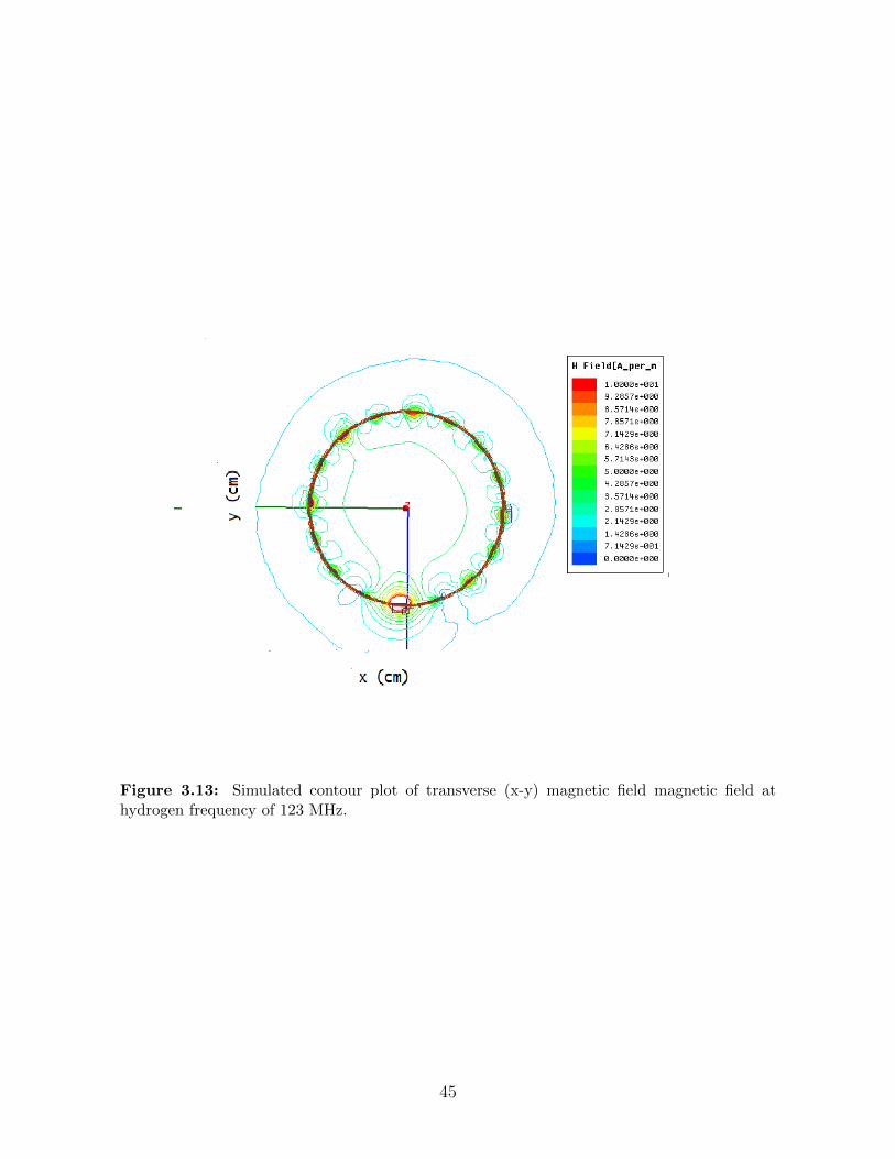
Figure 3.13: Simulated contour plot of transverse (x-y) magnetic field magnetic field athydrogen frequency of 123 MHz.

45

Figure 3.14: Simulated contour plots of sagittal (x-z) magnetic field at hydrogen frequencyof 123 MHz.

Figure 3.15: Magnetic field in sagittal plane at hydrogen frequency (123 MHz).

46

Figure 3.16: Magnetic field in transverse plane at hydrogen frequency (123 MHz).

Figure 3.17: Comparison of electric and magnetic field.

47

Chapter 4

Conclusion

This thesis has described the design and optimization of a miniature radiation pattern

reconfigurable antenna and a dual tuned birdcage coil to achieve desired results. The pattern

reconfigurable antenna was built and tested using the optimal dimension. The experimental

results for the birdcage coil are underway. The dimensions and results for reconfigurable

antenna and birdcage coil are described in Chapters 2 and 3 respectively.

Y-shaped and MTM based antennas were created and analyzed. In both structures,

the initial design was created using short copper bridge instead of actual switches. Both

of those designs performed well and were in close agreement with the model. When actual

switches were implemented instead of short copper bridges the results were still good but not

as good as the design goals. The addition of lossy switches, lossy capacitors and wires are

described as most likely culprits. Still, we showed that a miniature reconfigurable antenna

is possible and with better switches and less lossy capacitors, best results can be achieved.

A birdcage coil based on design [6] was created in simulation software and optimized.

MRI coils perform well when it provides homogeneity and high SNR at operating frequency.

This coil was optimized to perform well for resonant frequencies of sodium (32.586 MHz)

and hydrogen (132 MHz). The optimal length and diameter was used to built a prototype

coil. The prototype coil is now being tested in collaboration with Stanford University.

4.1 Future Work

The next step for the miniature pattern reconfigurable antenna would be to inte-

grate the nano switches. Nano switches are smaller in size and do not have high insertion

loss. These switches do not require decoupling capacitors; and could significantly improve

the performance of the antenna. This antenna can also be integrated to form a phased ar-

48

ray. Phased array enhances signal strength, decreases the interference and ultimately better

coverage.

In the case of the birdcage coil, experimental results need to be compared with mod-

eled results. If they are in good agreement, we can try changing the shape of the coil from

cylinder to flared ends. If there are disagreements a better model needs to be created. Model

should try to add external noises to make sure that the modeled coil will experience same

environment as the coil under test. A different simulation software should be utilized to

check the validity of the results of the current simulation software. A software that can

accurately model at low frequencies should be chosen. These implements definitely should

help debug the discrepancies between modeled and measured data.

49

Bibliography

[1] J. BernHard, Reconfigurable Antennas. Morgan and Claypool, 2007. 1, 4, 5

[2] D. Guha and Y. Antar, Reconfigurable Microstrip Antennas: New Trends, Techniques,and Applications, 1st ed. John Wiley and Sons, 2010. 2, 5, 12

[3] D. Piazza, N. Kirsch, A. Forenza, R. Heath, and K. Dandekar, “Design and evaluation ofa reconfigurable antenna array for MIMO systems,” Antennas and Propagation, IEEETransactions on, vol. 56, no. 3, pp. 869 –881, march 2008. 2

[4] P. Sooksumrarn and M. Krairiksh, “Compact pattern reconfigurable Yagi patch an-tenna,” in Microwave Conference Proceedings (APMC), 2011 Asia-Pacific, dec. 2011,pp. 729 –732. 2

[5] F. Ghanem, K. Ghanem, P. Hall, and M. Hamid, “A miniature frequency reconfigurableantenna for cognitive radios,” in Antennas and Propagation (APSURSI), 2011 IEEEInternational Symposium on, july 2011, pp. 171 –174. 2

[6] R. Watkins, E. Staroswiecki, N. Bangerter, B. Hargreaves, and G. Gold, “High SNRdual tuned sodium/proton knee coil,” in International Society for Magnetic Resonancein Medicine (ISMRM), 2010, May 2010. 2, 36, 48

[7] A. Gummalla, M. Achour, G. Poilasne, and V. Pathak, “Compact dual-band plan-armetamaterial antenna arrays for wireless lan,” IEEE Antennas andPropagation Soci-ety International Symposium, July 5-11, 2008. 2, 11, 16

[8] C. A. Balanis, Modern Antenna Handbook. John Wiley and Sons, 2008. 4

[9] M. Adhikari and K. Warnick, “Miniature radiation pattern reconfigurable antenna for2.4 GHz band,” in Antennas and Propagation Society International Symposium (AP-SURSI), 2010 IEEE, July 2010, pp. 1 –4. 5

[10] J. C. Chiao, Y. Fu, I. M. Chio, M. DeLisio, and L. Y. Lin, “MEMS reconfigurable Veeantenna,” in Microwave Symposium Digest, 1999 IEEE MTT-S International, vol. 4,1999. vii, 5, 6

[11] S. Nikolaou, B. Kim, and P. Vryonides, “Reconfiguring antenna characteristics usingPIN diodes,” in Antennas and Propagation, 2009. EuCAP 2009. 3rd European Confer-ence on, March 2009, pp. 3748–3752. 5

[12] R. Harrington, “Reactively controlled directive arrays,” Antennas and Propagation,IEEE Transactions on, vol. 26, no. 3, pp. 390–395, May 1978. vii, 6, 7

50

[13] V. Plicani, “Antenna diversity evaluation for mobile terminals,” in Antenna DiversityEvaluation for Mobile Terminals, C. I. Byrnes and A. Lindquist, Eds. North-Holland:Elsevier Science Publishers, 1986, pp. 93–105. 7

[14] A. Diallo, C. Luxey, P. Le Thuc, R. Staraj, and G. Kossiavas, “Enhanced two-antennastructures for universal mobile telecommunications system diversity terminals,” Mi-crowaves, Antennas Propagation, IET, vol. 2, no. 1, pp. 93–101, February 2008. 8

[15] Y. Li, Y. Guo, and X. Jiang, “Signal-to-noise ratio improvement by bi-2223 surface RFcoil in 0.3T MRI system,” Applied Superconductivity, IEEE Transactions on, vol. 20,no. 3, pp. 818–821, June 2010. 35

[16] R. Henry, N. Fischbein, W. Dillon, D. Vigneron, and S. Nelson, “High-sensitivity coilarray for head and neck imaging: Technical note,” American Journal of Neuroradiology,December 2001. 35

[17] C. E. Hates, W. A. Edelstein, J. F. Schenck, O. M. Mueller, and M. Eash, “An efficient,highly homogeneous radiofrequency coil for whole-body NMR imaging at 1.5T,” Journalof Magnetic Resonance, 1985. 36

[18] E. Shapiro, A. Borthakur, A. Gougoutas, and R. Reddy, “23 Na MRI accurately mea-sures fixed charge density in articular cartilage,” Magnetic Resonance Med., 2002. 36

[19] N. Maril, Y. Rosen, G. Reynolds, A. Ivanishev, L. Ngo, and R. Lenkinski, “SodiumMRI of the human kidney at 3T,” Magnetic Resonance Med., 2006. 36

[20] K. Thulborn, D. Davis, J. Snyder, H. Yonas, and A. Kassam, “Sodium MR imagingof acute and subacute stroke for assessment of tissue viability,” Neuroimaging Clin NAm., 2005. 36

51