simulation radiation pattern of different antennas - …aarora.pbworks.com/f/btp2.pdf · simulation...
TRANSCRIPT

Simulation of Radiation pattern of different antennas 1
CERTIFICATE
This is to certify that the project entitled “Simulation of Radiation patterns of different antennas” being submitted by Mr. Ankur Arora (13/EC/05), Mr. Uchit Singhal (92/EC/05), Mr. Ujjwal Nehra (93/EC/05) , Mr. Vivek Rawat (102/EC/05) of Department of Electronics and Communication Engineering , in partial fulfillment of the requirements of the award of the degree of “Bachelor of Engineering” is a record of bona-fide work carried out by them. They have worked under my guidance and supervision and fulfilled the requirements.
To the best of my knowledge, this project work has not been submitted, in part or full, to any other university or institute for award of any degree or diploma.
Dated:
Dr. HARISH PARTHASARATHY Professor, ECE division
Netaji Subhas Institute of Technology Sector-3, Dwarka
New Delhi-110045

Simulation of Radiation pattern of different antennas 2
ACKNOWLEDGEMENT
We would like to express our sincere gratitude towards our project mentor
Dr. H. Parthasarathy for providing us with his valuable time, effort, and invaluable
knowledge without which the progress of our project wouldn’t have been possible. It was
our great opportunity and experience to enrich ourselves with innovative ideas and
guidance provided by him.
We also express our regards to our colleagues who motivated us throughout the project
which led to the successful completion of the same.
ANKUR ARORA UCHIT SINGHAL (13/EC/05) (92/EC/05)
UJJWAL NEHRA VIVEK RAWAT (93/EC/05) (102/EC/05)

Simulation of Radiation pattern of different antennas 3
ABSTRACT
An Antenna is used to transmit and receive electromagnetic waves. Antennas are employed in
systems such as radio and television broadcasting, point-to-point radio communication, wireless
LAN, radar, and space exploration. Antennas usually work in air or outer space, but can also be
operated under water or even through soil and rock at certain frequencies for short distances. The
origin of the word antenna relative to wireless apparatus is attributed to Guglielmo Marconi.
There are several critical parameters affecting an antenna's performance that can be adjusted
during the design process. These are resonant frequency, impedance, gain, aperture or radiation
pattern, polarization, efficiency and bandwidth. Transmit antennas may also have a maximum
power rating, and receive antennas differ in their noise rejection properties. An antenna may be
an isotropic radiator, a dipole, yagi-uda type, horn type or patch antenna.
In this project, we have simulated the radiation pattern of horn antenna and yagi-uda antenna in
MATLAB and studied their FEKO outputs. We have designed many antennas in FEKO
environment and have made improvements in the previous designs to have better electric field
intensity and directivity. Our basic approach was to simulate the radiation pattern for a
symmetrically shaped antenna and then maximizing the output parameters by using various
techniques such as using reflector surfaces wherever the loss in antenna was due to side lobes.
Polarization of an antenna is a very important parameter in determining the loss in transmission.
In antennas matching plays a very important role in determining the final output and rain drops
due to reflection properties can lead to serious weakening of signal at high frequencies, due to
which circular polarization is generally preferred.

Simulation of Radiation pattern of different antennas 4
TABLE OF CONTENTS
CERTIFICATE ................................................................................................................................................................. 1
ACKNOWLEDGEMENT ................................................................................................................................................ 2
ABSTRACT ..................................................................................................................................................................... 3
TABLE OF CONTENTS .................................................................................................................................................. 4
LIST OF TABLES............................................................................................................................................................. 6
LIST OF FIGURES .......................................................................................................................................................... 9
INTRODUCTION.......................................................................................................................................................... 11
1.1 Introduction .............................................................................................................................................. 11
1.2 Objective ................................................................................................................................................... 12
1.4 Project Overview...................................................................................................................................... 12
1.4 Structure of the Report........................................................................................................................... 14
ANTENNA THEORY .................................................................................................................................................... 15
2.1 INTRODUCTION .............................................................................................................................................. 15
2.2 TYPES OF ANTENNA....................................................................................................................................... 16
2.3 RADIATION PATTERN ..................................................................................................................................... 17
2.4 Antenna Parameters ...................................................................................................................................... 18
PYRAMIDAL HORN..................................................................................................................................................... 21
3.1 Introduction to Horn Antenna...................................................................................................................... 21
3.2 Horn Antenna Configurations ...................................................................................................................... 22
3.3 E Plane Sectoral Horn .................................................................................................................................... 23
3.3.1 Aperture Fields ........................................................................................................................................ 23
3.3.2 Radiated Fields ........................................................................................................................................ 25
3.4 H Plane Sectoral Horn .................................................................................................................................... 26
3.4.1 Aperture Fields ........................................................................................................................................ 27
3.4.2 RADIATED FIELDS .................................................................................................................................... 28
3.5 Pyramidal Horn ............................................................................................................................................... 29
3.5.1 APERTURE FIELDS ................................................................................................................................... 31
3.5.2 RADIATED FIELDS .................................................................................................................................... 31
3.6 MATLAB Simulation........................................................................................................................................ 32

Simulation of Radiation pattern of different antennas 5
3.6.1 MATLAB CODE ......................................................................................................................................... 32
3.7 FEKO Simulation ............................................................................................................................................. 37
3.8 Results .............................................................................................................................................................. 41
YAGI UDA ANTENNA ............................................................................................................................................... 42
4.1 History .............................................................................................................................................................. 42
4.2 Introduction .................................................................................................................................................... 43
4.3 Working Principle ........................................................................................................................................... 43
4.4 Mathematical Analysis .................................................................................................................................. 46
4.5 Matlab Simulation .......................................................................................................................................... 49
4.5.1 MATLAB CODE ......................................................................................................................................... 49
4.5.2 MATLAB OUTPUTS .................................................................................................................................. 58
4.6 FEKO Simulation ......................................................................................................................................... 58
4.7 RESULTS .......................................................................................................................................................... 61
SPIRO HELICAL ANTENNA......................................................................................................................................... 62
5.1 Introduction .................................................................................................................................................... 62
5.2 Mathematical Analysis .................................................................................................................................. 63
5.3 Design Methodology ...................................................................................................................................... 65
5.3 Matlab Simulation .......................................................................................................................................... 66
5.4 Radiation Patterns .......................................................................................................................................... 68
6.1 FEKO Background .......................................................................................................................................... 72
6.2 Designs proposed in past ............................................................................................................................ 72
6.3 Antenna proposed.......................................................................................................................................... 79
Chapter7 ..................................................................................................................................................................... 88
CONCLUSION AND FUTURE WORK ......................................................................................................................... 88
7.1 CONCLUSION ................................................................................................................................................... 88
7.2 Future Work .................................................................................................................................................... 89
REFERENCES ............................................................................................................................................................... 90
APPENDICES ............................................................................................................................................................... 92
Appendix A: Transverse Electric mode .............................................................................................................. 92
Appendix B : Method Of Moments ................................................................................................................... 94
Appendix C : Radiation Equations ...................................................................................................................... 95

Simulation of Radiation pattern of different antennas 6
LIST OF PLOTS
Plot 3.1……………………………………………………………………………………………………………………………………………… 35
Plot 3.2……………………………………………………………………………………………………………………………………………… 35
Plot 3.3……………………………………………………………………………………………………………………………………………… 36
Plot 3.4……………………………………………………………………………………………………………………………………………… 37
Plot 3.5……………………………………………………………………………………………………………………………………………… 37
Plot 3.6……………………………………………………………………………………………………………………………………………… 38
Plot 3.7……………………………………………………………………………………………………………………………………………… 38
Plot 4.1……………………………………………………………………………………………………………………………………………… 56
Plot 4.2……………………………………………………………………………………………………………………………………………… 56
Plot 4.3……………………………………………………………………………………………………………………………………………… 57
Plot 4.4……………………………………………………………………………………………………………………………………………… 57
Plot 4.5……………………………………………………………………………………………………………………………………………… 58
Plot 4.6……………………………………………………………………………………………………………………………………………… 58
Plot 5.1……………………………………………………………………………………………………………………………………………… 66
Plot 5.2……………………………………………………………………………………………………………………………………………… 67
Plot 5.3……………………………………………………………………………………………………………………………………………… 67
Plot 5.4……………………………………………………………………………………………………………………………………………… 67
Plot 5.5……………………………………………………………………………………………………………………………………………… 68
Plot 5.6……………………………………………………………………………………………………………………………………………… 68
Plot 6.1……………………………………………………………………………………………………………………………………………… 71
Plot 6.2……………………………………………………………………………………………………………………………………………… 72
Plot 6.3……………………………………………………………………………………………………………………………………………… 72
Plot 6.4……………………………………………………………………………………………………………………………………………… 73

Simulation of Radiation pattern of different antennas 7
Plot 6.5……………………………………………………………………………………………………………………………………………… 74
Plot 6.6……………………………………………………………………………………………………………………………………………… 74
Plot 6.7……………………………………………………………………………………………………………………………………………… 75
Plot 6.8……………………………………………………………………………………………………………………………………………… 76
Plot 6.9……………………………………………………………………………………………………………………………………………… 76
Plot 6.10…………………………………………………………………………………………………………………………………………… 77
Plot 6.11…………………………………………………………………………………………………………………………………………… 78
Plot 6.12…………………………………………………………………………………………………………………………………………… 78
Plot 6.13…………………………………………………………………………………………………………………………………………… 79
Plot 6.14…………………………………………………………………………………………………………………………………………… 79
Plot 6.15…………………………………………………………………………………………………………………………………………… 80
Plot 6.16…………………………………………………………………………………………………………………………………………… 80
Plot 6.17…………………………………………………………………………………………………………………………………………… 81
Plot 6.18…………………………………………………………………………………………………………………………………………… 82
Plot 6.19…………………………………………………………………………………………………………………………………………… 82
Plot 6.20…………………………………………………………………………………………………………………………………………… 83
Plot 6.21…………………………………………………………………………………………………………………………………………… 83
Plot 6.22…………………………………………………………………………………………………………………………………………… 84
Plot 6.23…………………………………………………………………………………………………………………………………………… 84
Plot 6.24…………………………………………………………………………………………………………………………………………… 85
Plot 6.25…………………………………………………………………………………………………………………………………………… 85

Simulation of Radiation pattern of different antennas 8

Simulation of Radiation pattern of different antennas 9
LIST OF FIGURES
Figure 1.1 .........................................................................................................................................................
Figure 2.1………………………………………………………………………………………………………………………………….....Figure 2.2………………………………………………………………………………………………………………………………….....Figure 2.3…………………………………………………………………………………………………………………………………….. Figure 3.1……………………………………………………………………………………………………………………………………..Figure 3. 2…………………………………………………………………………………………………………………………………….Figure 3. 3.................................................................................................................. Error! Bookmark not Figure 3. 4.........................................................................................................................................................Figure 3. 5.........................................................................................................................................................Figure 3. 6.........................................................................................................................................................Figure 3. 7......................................................................................................................................................... Figure 4. 1.........................................................................................................................................................Figure 4. 2.........................................................................................................................................................Figure 4. 3.........................................................................................................................................................
Figure 4. 4.........................................................................................................................................................Figure 4. 5......................................................................................................................................................... Figure 5. 1.........................................................................................................................................................Figure 5.2………………………………………………………………………………………………………………………………….....
7 13 14 16 22 22 25 26 28 28 29 41 42 42 43 44 60 60
Figure 5.3………………………………………………………………………………………………………………………………….....Figure 5.4………………………………………………………………………………………………………………………………….....
61 61

Simulation of Radiation pattern of different antennas 10

Simulation of Radiation pattern of different antennas 11
chapter1
INTRODUCTION
1.1 Introduction
An Antenna, also known as aerial, is a transducer which is used to transmit and receive the electromagnetic waves, converting them into electric currents and vice versa. A typical antenna finds its usage in every domain of life whether it is broadcasting or space exploration. Point to point communication, wireless LAN are other important fields which can not suffice without an antenna. Antenna can be deployed in any medium whether it is air, space, soil or water. However, the range of frequencies in which it can be used efficiently narrows down in water and soil, but its advantages outcast the limitations.
While designing an antenna various parameters need to be taken care of. The important among them are the Gain, Directivity, Field Intensity, Reflector surfaces, Polarization, and bandwidth. An antenna should possess its maximum energy in the direction of main lobe while possessing a minimum of side and back lobes. For this reflector surfaces are used. Metallic surfaces act as superb reflectors, while dielectric surfaces absorb the Electromagnetic radiation falling upon them.
Various losses arise in the transmission due to mismatching and the reflections suffered by the waves in the atmosphere due to precipitation, dust, water-vapors etc. Rain drops play the most important role due to spherical symmetry, due to which circular polarization becomes a

Simulation of Radiation pattern of different antennas 12
necessity. To increase the bandwidth various methods such as use of thicker wires and combination of multiple antennas to give a single assembly is preferred. Hence, it is imperative to have a design that extends to handle these factors effectively. This report focuses on the design and architectural details of the antennas which incorporate the above mentioned features.
1.2 Objective
This project focuses on the development of antennas such that they possess a radiation pattern which provides us with the improvement in the antenna parameters such as directivity, gain , electric field intensity along the main lobe and co-existence of circular polarization. The existing designs of horn antenna and yagi-uda antenna were simulated in MATLAB and the improvements were made through FEKO.
1.3 Motivation
We wanted to build an antenna which was better than the existing designs of antenna. The improvement was made in regard to various antenna parameters whether it is gain, directivity, minimization of the side lobes, maximizing the electric field intensity, cost or bandwidth. For this, various designs were studied and the pros and cons were noted down. This was used to obtain a design which is better than all the contemporary ones for a particular antenna parameter. It could be directivity, or field intensity or polarization. FEKO provided us with an excellent platform to make changes in the existing antenna designs and study the resultant radiation pattern.
1.4 Project Overview
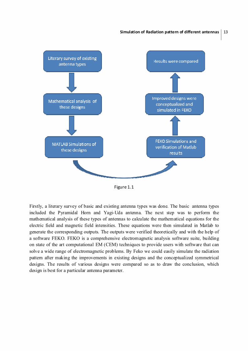
Keeping in mind the antenna parameters such as directivity, gain, polarization , bandwidth and radiation intensity , the aim was to obtain the antenna designs which excelled in any particular domain and scored well over the previous antennas. The project work has been carried out step by step using the modular approach for the benefit of clear understanding and development of efficient design. The figure below explains the basic project development life cycle.
Simulation of Radiation pattern of different antennas
13
Figure 1.1
Firstly, a literary survey of basic and existing antenna types was done. The basic antenna types included the Pyramidal Horn and Yagi-Uda antenna. The next step was to perform the mathematical analysis of these types of antennas to calculate the mathematical equations for the electric field and magnetic field intensities. These equations were then simulated in Matlab to generate the corresponding outputs. The outputs were verified theoretically and with the help of a software FEKO. FEKO is a comprehensive electromagnetic analysis software suite, building on state of the art computational EM (CEM) techniques to provide users with software that can solve a wide range of electromagnetic problems. By Feko we could easily simulate the radiation pattern after making the improvements in existing designs and the conceptualized symmetrical designs. The results of various designs were compared so as to draw the conclusion, which design is best for a particular antenna parameter.

Simulation of Radiation pattern of different antennas 14
1.4 Structure of the Report
CHAPTER 1: Gives objective, motivation behind the project, basic overview of the project and the structure of the report.
CHAPTER 2: This chapter gives a brief introduction to the antenna and various antenna parameters. It gives the different types of antenna and basic theory of radiation pattern.
CHAPTER 3: This chapter starts with an introduction to horn antenna, thereby giving detailed analysis of E-plane sectoral horn, H-plane sectoral horn, and pyramidal horn. Matlab code and outputs for the pyramidal horn and the corresponding simulation results in Feko are also there.
CHAPTER 4:. In this chapter the focus will be on yagi-uda array antenna. The mathematical analysis will be corroborated with the Matlab results. A Feko simulation will be made to showcase the various antenna parameters of the yagi uda antenna.
CHAPTER 5: In this chapter the focus will be on spiro helical antenna. The mathematical analysis results using Matlab and corresponding analysis will be done using NEC.
CHAPTER 6: In this chapter the focus will be on new designs simulation using FEKO and comparing these with previous results.
CHAPTER 7: In this chapter Conclusion and Proposed Future work will be discussed.

Simulation of Radiation pattern of different antennas
15
chapter2
ANTENNA THEORY
This chapter gives a brief introduction to the antenna and various antenna parameters. It gives the different types of antenna and basic theory of radiation pattern.
2.1 INTRODUCTION
Antenna or aerial is a means for radiating or receiving radio waves. In other words antenna is the transitional structure between free space and a guiding device. The guiding device may be a coaxial line or a waveguide and it is used to transport electromagnetic energy from the transmitting source to the antenna or from antenna to the receiver. The figure below shows the aforementioned antenna system.
Figure 2. 1

Simulation of Radiation pattern of different antennas
16
2.2 TYPES OF ANTENNA
An antenna can be of various types as discussed below:
• Wire Antenna : A wire antenna can be a straight wire (dipole), loop or helix. Loop antenna can be circular or elliptical or any other shape.
Dipole Antenna Loop Antenna
• Aperture antenna: It can be pyramidal, conical or rectangular waveguide.
• Microstrip antenna: They can be either rectangular or circular patch type antenna.
• Array antenna: These include the yagi-uda array antenna and various other antenna.
• Other antenna types: These include the reflector antennas and the lens antennas. A reflector may be with front feed, cassegrain feed or corner reflection. Lens antenna include various antenna shapes possible with convex, plane and concave surfaces.
Figure 2. 2

Simulation of Radiation pattern of different antennas 17
Pyramidal horn antenna Conical horn antenna
Rectangular patch antenna Yagi-Uda antenna
2.3 RADIATION PATTERN
In the field of antenna design the term 'radiation pattern' most commonly refers to the directional (angular) dependence of radiation from the antenna. An antenna radiation pattern is defined as a mathematical function or a graphical representation of the radiation properties of the antenna as a function of space coordinates. Mostly it is determined in the far field region and is a function of directional coordinates. Radiation property is the two or three dimensional spatial distribution of

Simulation of Radiation pattern of different antennas
18
radiated energy. It may include power flux density, radiation intensity, field strength, directivity or polarization. The spatial variation of electric or magnetic field is called field pattern.
An isotropic radiator is a theoretical point source of waves which exhibits the same magnitude or properties when measured in all directions. It has no preferred direction of radiation. It radiates uniformly in all directions over a sphere centered on the source.
A directional antenna or beam antenna is an antenna which radiates greater power in one or more directions allowing for increased performance on transmit and receive and reduced interference from unwanted sources. Directional antennas like yagi antennas provide increased performance over dipole antennas when a greater concentration of radiation in a certain direction is desired.
An omnidirectional antenna is an antenna system which radiates power uniformly in one plane with a directive pattern shape in a perpendicular plane.
Various parts of a radiation pattern are referred to as lobes, which may be either major, minor, side or back lobes.
Figure 2. 3
2.4 Antenna Parameters

Simulation of Radiation pattern of different antennas
19
2.4.1 RADIATION INTENSITY
Radiation intensity in a given direction is defined as the power radiated from an antenna per unit solid angle. The radiation from a surface has different intensities in different directions. The intensity of radiation along a normal to the surface is known as intensity of normal radiation. It is the product of radiation density and square of the distance.
2.4.2 DIRECTIVITY
Directivity of an antenna is defined as the ratio of the radiation intensity in a given direction from the antenna to the radiation intensity averaged over all directions. The average radiation intensity is equal to the total power radiated by the antenna divided by 4∏.
Where F is the radiation intensity
2.4.3 GAIN
Absolute Gain of an antenna is defined as the ratio of intensity in a given direction to the radiation intensity that would be obtained if the power accepted by the antenna were radiated isotropically.
In case of relative gain, it is the ratio of power gain in given direction to the reference direction. When the direction is not stated the power gain is usually taken in the direction of maximum radiation
G , ф = ecd 4 ∏ U ,фP
Where ecd is the antenna radiation efficiency, U is the radiation intensity and P is the total radiated power.
2.4.4 HALF POWER BEAMWIDTH
It is the angle between the two directions in which the radiation intensity is half the maximum value of beam.
Simulation of Radiation pattern of different antennas 20
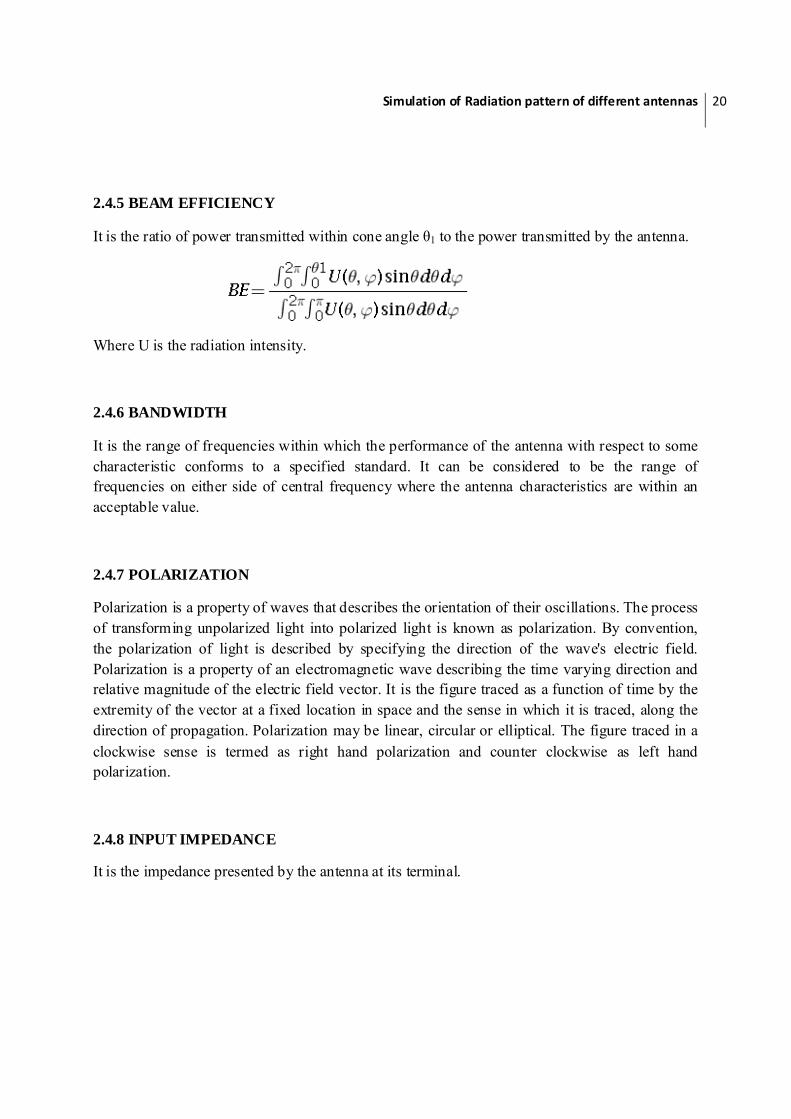
2.4.5 BEAM EFFICIENCY
It is the ratio of power transmitted within cone angle θ1 to the power transmitted by the antenna.
Where U is the radiation intensity.
2.4.6 BANDWIDTH
It is the range of frequencies within which the performance of the antenna with respect to some characteristic conforms to a specified standard. It can be considered to be the range of frequencies on either side of central frequency where the antenna characteristics are within an acceptable value.
2.4.7 POLARIZATION
Polarization is a property of waves that describes the orientation of their oscillations. The process of transforming unpolarized light into polarized light is known as polarization. By convention, the polarization of light is described by specifying the direction of the wave's electric field. Polarization is a property of an electromagnetic wave describing the time varying direction and relative magnitude of the electric field vector. It is the figure traced as a function of time by the extremity of the vector at a fixed location in space and the sense in which it is traced, along the direction of propagation. Polarization may be linear, circular or elliptical. The figure traced in a clockwise sense is termed as right hand polarization and counter clockwise as left hand polarization.
2.4.8 INPUT IMPEDANCE
It is the impedance presented by the antenna at its terminal.

Simulation of Radiation pattern of different antennas 21
chapter3
PYRAMIDAL HORN
This chapter starts with an introduction to horn antenna, thereby giving detailed analysis of E-plane sectoral horn, H-plane sectoral horn, and pyramidal horn. Matlab code and outputs for the pyramidal horn and the corresponding simulation results in Feko are also there.
3.1 Introduction to Horn Antenna
Horn antenna is the most widely used microwave antenna. It is one of the simplest antenna existing till date. The Horn Antenna, at Bell Telephone Laboratories in Holmdel, New Jersey, is listed as a National Historic Landmark because of its association with the research work of two radio astronomers, Arno Penzias and Robert Wilson. In 1965 while using the Horn Antenna, Penzias and Wilson stumbled on the microwave background radiation that permeates the universe. Cosmologists quickly realized that Penzias and Wilson had made the most important discovery in modern astronomy since Edwin Hubble demonstrated in the 1920s that the universe was expanding. The horn antenna is used in the transmission and reception of RF microwave signals and the antenna is normally used in conjunction with waveguide feeds. The horn is widely used as a feed element for large radio astronomy, satellite tracking and communication dishes. In addition to its utility as a feed for reflector and lenses, it is a common element of phased arrays also. It serves as a universal standard for calibration and gain measurements of other high power antennas. Its widespread applicability stems from its simplicity in construction, ease of excitation, versatility, large gain and preferred all over performance. Horns can be excited in any polarization or combination of polarizations.

Simulation of Radiation pattern of different antennas 22
3.2 Horn Antenna Configurations
The horn antenna gains its name from its appearance. Horn is nothing more than a hollow pipe of different cross sections which has been tapered to a larger opening. Type, direction and amount of taper can have a profound effect on the overall performance of the element as a radiator. The waveguide can be considered to open out or to be flared, launching the signal towards the receiving antenna. Flare waveguides produce a nearly uniform phase front larger than the waveguide itself. The E-plane sectoral horn is the one whose opening is flared in the direction of E field. A detailed geometry is as shown in the figure.
The H-plane sectoral horn is the one whose opening is flared in the direction of H field. A detailed geometry is as shown in the figure.
The Pyramidal horn is the one whose opening is flared in the direction of H field and E field both. A detailed geometry is as shown in the figure. Its radiation characteristics are a combination of the E and H plane sectoral horns.
While the pyramidal, E and H plane sectoral horns are usually fed by a rectangular waveguide, the conical horn is fed by a circular waveguide. Rest of the behavior is same.
E Sectoral Horn H Sectoral Horn
Conical horn Pyramidal Horn

Simulation of Radiation pattern of different antennas 23
3.3 E Plane Sectoral Horn
3.3.1 Aperture Fields
Horn being an aperture antenna, it is necessary that the tangential electric and magnetic field components over a closed surface are known, to develop an exact equivalent of it. An infinite plane coinciding with the aperture of the horn is usually selected as a closed surface. If the horn is not mounted on an infinite grounded plane, the fields outside the aperture cannot be calculated and an exact equivalent cannot be formed. However as a usual approximation we assume the fields outside the aperture to be zero.
If we treat horn as a radial waveguide, the fields at the aperture of the horn can be calculated. The fields within the horn can be expressed in terms of cylindrical transverse electric and transverse magnetic i.e. TE and TM wave functions which make use of Hankel functions. This method finds the fields not only at the aperture but also within the horn.
The lowest order mode fields at the aperture of the horn can be found very easily taking into consideration the two assumptions that,
1) Fields of the feed waveguide are those of its dominant TE10 mode. 2) Horn length is large compared to the aperture dimensions.
The field expressions are:
Ez’ = Ex’ = Hy’ = 0
Ey’(x’,y’) = E1 cos ∏ e. /
Hz’(x’,y’) = jE1 ∏
sin∏
e.
Hx(x’,y’) = - cos ∏ e.
1 = e cos e
δ(y’) = ′ρ

Simulation of Radiation pattern of different antennas
24
Here E1 is a constant; ρ is the radial distance of the point.
These primes used here correspond to fields at the aperture of the horn. These are similar to the fields of a TE10 mode for a rectangular waveguide. The complex exponential term showing the quadratic phase variation of the fields over the aperture is the only difference. These correspond to following figures.
Figure 3. 1
E Plane Sectoral Horn
Figure 3. 2
E Plane view
Simulation of Radiation pattern of different antennas 25
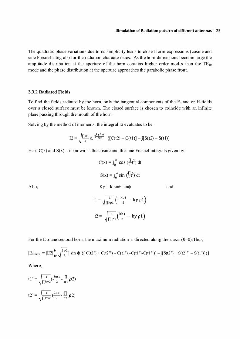
The quadratic phase variations due to its simplicity leads to closed form expressions (cosine and sine Fresnel integrals) for the radiation characteristics. As the horn dimensions become large the amplitude distribution at the aperture of the horn contains higher order modes than the TE10 mode and the phase distribution at the aperture approaches the parabolic phase front.
3.3.2 Radiated Fields
To find the fields radiated by the horn, only the tangential components of the E- and or H-fields over a closed surface must be known. The closed surface is chosen to coincide with an infinite plane passing through the mouth of the horn.
Solving by the method of moments, the integral I2 evaluates to be:
I2 = ∏ e.ρ
{[C(t2) – C(t1)] – j[S(t2) – S(t1)]
Here C(x) and S(x) are known as the cosine and the sine Fresnel integrals given by:
C(x) = cos ∏ t
2) dt
S(x) = sin ∏t2) dt
Also, Ky = k sinθ sinф and
t1 = ∏ ρ
– k ρ1
t2 = ∏ ρ
k ρ1
For the E plane sectoral horn, the maximum radiation is directed along the z axis (θ=0).Thus,
|Eθ|max = |E2| [ sin ф {[ C(t2’) + C(t2’’) – C(t1’) –C(t1’)-C(t1’’)] – j[S(t2’) + S(t2’’) – S(t1’)]}]
Where,
t1’ = ∏
(- - ∏ 2)
t2’ = ∏
( - ∏ 2)
Simulation of Radiation pattern of different antennas 26
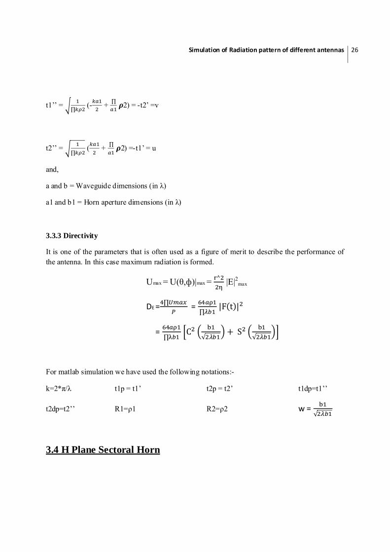
t1’’ = ∏ (- + ∏ 2) = -t2’ =v
t2’’ = ∏
( + ∏ 2) =-t1’ = u
and,
a and b = Waveguide dimensions (in λ)
a1 and b1 = Horn aperture dimensions (in λ)
3.3.3 Directivity
It is one of the parameters that is often used as a figure of merit to describe the performance of the antenna. In this case maximum radiation is formed.
Umax = U(θ,ф)|max = ^ |E|2max
DE = ∏ = ∏
|F t |
= ∏
C√
S√
For matlab simulation we have used the following notations:-
k=2*π/λ t1p = t1’ t2p = t2’ t1dp=t1’’
t2dp=t2’’ R1=ρ1 R2=ρ2 w = √
3.4 H Plane Sectoral Horn

Simulation of Radiation pattern of different antennas
27
3.4.1 Aperture Fields
Ex’ = Hy’ = 0
Ey’(x’) = E2 cos ∏ x′ δ ′
Hx’(x’) = -Eη
cos ∏ x′ δ ′
δ(x’) = ′
ρ
2 = h cos h
H Plane Sectoral Horn
Figure 3. 3

Simulation of Radiation pattern of different antennas 28
Figure 3. 4
H Plane view
3.4.2 RADIATED FIELDS
The value of integral I2 as solved by the method of moments results out to be:
I2 = ∏ρ (e.′ ρ
{[C(t2’) – C(t1’)] – j[S(t2’) – S(t1’)]} + e.′ ρ
{[C(t2’’) – C(t1’’)] –
j[S(t2’’) – S(t1’’)]})
where,
t1’ = ∏ ρ – k ′ρ2
t2’ = ∏ ρ
k ′ρ2
kx’ = k sinθ cosф + ∏
t1’’ = ∏ ρ
– k ′′ρ2
t2’’ = ∏ ρ k ′′ρ2
kx’’ = k sinθ cosф - ∏

Simulation of Radiation pattern of different antennas 29
It should be noted that for E-plane ф = ∏/2 and for H-plane ф=0. This leaves us with the value of Eф max as follows:
|Eφ|max = |E2| λ |cosφ{[ C(u) + C(v)] – j[S(u) –S(v)]}|
The net electric field thus results out to be:
|E|max = |Eθ| max |Eφ| max
= |E2| ρλ{[C(u) - C(v) +[S(u) –S(v)
3.4.3 DIRECTIVITY
The directivity value for the H plane sectoral horn antenna can be written as:
DH = ∏ = ∏ ρ {[C(u) – C(v) + [S(u) – S(v)
where,
u = √
λρ λρ
v = √
λρ λρ
3.5 Pyramidal Horn
The most widely used horn is the one which is flared in both the directions. Its radiation characteristics are essentially a combination of the E- and H- plane sectoral horns.

Simulation of Radiation pattern of different antennas
30
Figure 3. 5
Pyramidal Horn Antenna
Figure 3. 6
H Plane view

Simulation of Radiation pattern of different antennas 31
Figure 3. 7
E Plane view
3.5.1 APERTURE FIELDS
The corresponding value of electric and magnetic field components in Cartesian coordinates comes out to be:
Ey’(x’,y’) = Eo cos x′ ′
ρ / + e′
ρ / ]
Hx’(x’,y’) = -Eη
cos x′′
ρ/ + e
′
ρ/ ]
3.5.2 RADIATED FIELDS
The far zone E and H field components of a Pyramidal Horn are:-
Er = 0
Eθ = jE
∏ [sinф( 1 + cosθ ) I1I2]
Eф = j E∏
[cosф( cosθ+1 ) I1I2]
The integrals I1 and I2 after solving by method of moments are calculated to be as follows,

Simulation of Radiation pattern of different antennas 32
I1 = ∏ρ (e.′ ρ
{[C(t2’) – C(t1’)] – j[S(t2’) – S(t1’)]} + e.′ ρ
{[C(t2’’) – C(t1’’)] –
j[S(t2’’) – S(t1’’)]})
I2 = ∏ e.ρ
{[C(t2) – C(t1)] – j[S(t2) – S(t1)]
where t1, t2, t1’, t1’’, t2’, t2’’ are as specified above.
The fields radiated by a pyramidal horn are valid for all angles observation. The above equation reveals that the principal E plane pattern (Ф=π/2) is identical to the E plane pattern of an E plane sectoral horn. Similarly the H plane (Ф=0) is identical to that of an H plane sectoral horn.
3.5.3 DIRECTIVITY
The directivity for a pyramidal horn can be written as:-
Dp = ∏λ DE DH
where DE and DH are the directivities of the E and H plane sectoral horns as defined previously.
3.6 MATLAB Simulation
3.6.1 MATLAB CODE
MATLAB CODE
function []=horn; disp('E-Plane and H-Plane Horn Specifications'); R1=[]; R2=[]; R1 = input('rho1(in wavelengths) = '); R2 = input('rho2(in wavelengths) = '); a=[]; b=[]; a = input('a(in wavelengths) = '); b = input('b(in wavelengths) = '); a1=[]; b1=[]; a1 = input('a1(in wavelengths) = '); b1 = input('b1(in wavelengths) = '); u = (1/sqrt(2))*((sqrt(R2)/a1)+(a1/sqrt(R2))); v = (1/sqrt(2))*((sqrt(R2)/a1)-(a1/sqrt(R2))); u = Fresnel(u);
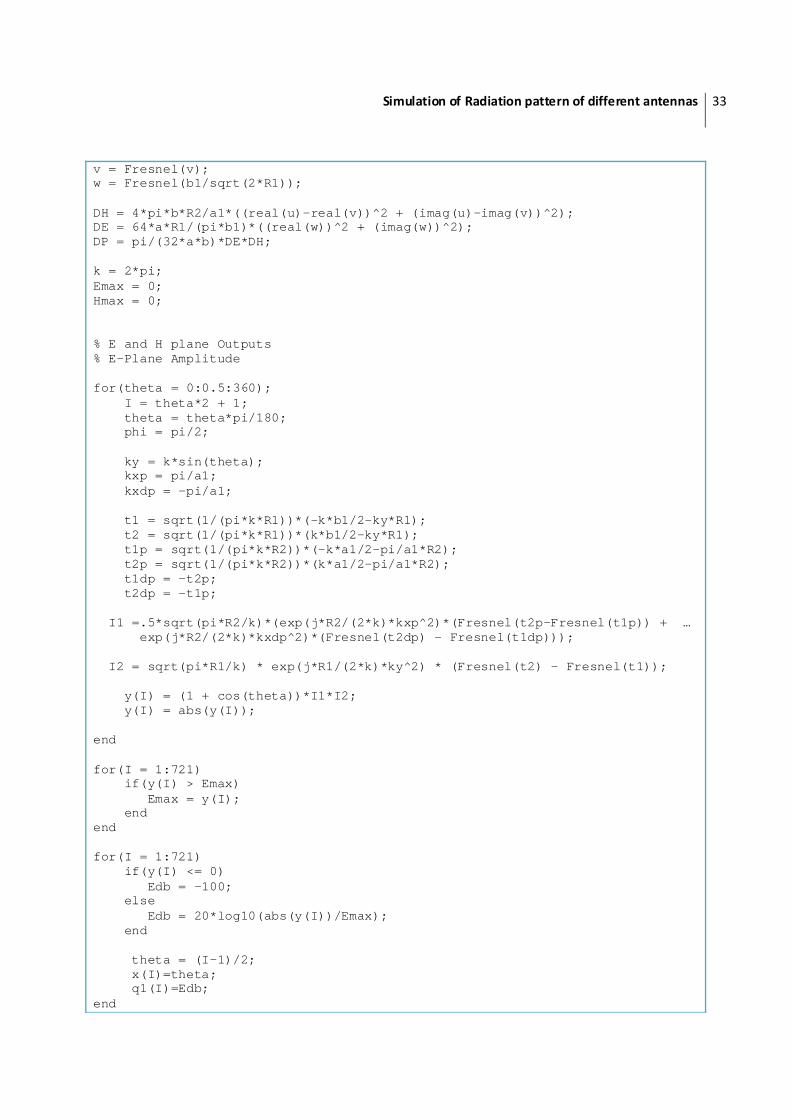
Simulation of Radiation pattern of different antennas 33
v = Fresnel(v); w = Fresnel(b1/sqrt(2*R1)); DH = 4*pi*b*R2/a1*((real(u)-real(v))^2 + (imag(u)-imag(v))^2); DE = 64*a*R1/(pi*b1)*((real(w))^2 + (imag(w))^2); DP = pi/(32*a*b)*DE*DH; k = 2*pi; Emax = 0; Hmax = 0; % E and H plane Outputs % E-Plane Amplitude for(theta = 0:0.5:360); I = theta*2 + 1; theta = theta*pi/180; phi = pi/2; ky = k*sin(theta); kxp = pi/a1; kxdp = -pi/a1; t1 = sqrt(1/(pi*k*R1))*(-k*b1/2-ky*R1); t2 = sqrt(1/(pi*k*R1))*(k*b1/2-ky*R1); t1p = sqrt(1/(pi*k*R2))*(-k*a1/2-pi/a1*R2); t2p = sqrt(1/(pi*k*R2))*(k*a1/2-pi/a1*R2); t1dp = -t2p; t2dp = -t1p; I1 =.5*sqrt(pi*R2/k)*(exp(j*R2/(2*k)*kxp^2)*(Fresnel(t2p-Fresnel(t1p)) + … exp(j*R2/(2*k)*kxdp^2)*(Fresnel(t2dp) - Fresnel(t1dp))); I2 = sqrt(pi*R1/k) * exp(j*R1/(2*k)*ky^2) * (Fresnel(t2) - Fresnel(t1)); y(I) = (1 + cos(theta))*I1*I2; y(I) = abs(y(I)); end for(I = 1:721) if(y(I) > Emax) Emax = y(I); end end for(I = 1:721) if(y(I) <= 0) Edb = -100; else Edb = 20*log10(abs(y(I))/Emax); end theta = (I-1)/2; x(I)=theta; q1(I)=Edb; end

Simulation of Radiation pattern of different antennas 34
% H-Plane Amplitude for(theta = 0:0.5:360); I = theta*2 + 1; theta = theta*pi/180; phi = 0; kxp = k*sin(theta) + pi/a1; kxdp = k*sin(theta) - pi/a1; t1 = sqrt(1/(pi*k*R1))*(-k*b1/2); t2 = sqrt(1/(pi*k*R1))*(k*b1/2); t1p = sqrt(1/(pi*k*R2))*(-k*a1/2-kxp*R2); t2p = sqrt(1/(pi*k*R2))*(k*a1/2-kxp*R2); t1dp = sqrt(1/(pi*k*R2))*(-k*a1/2-kxdp*R2); t2dp = sqrt(1/(pi*k*R2))*(k*a1/2-kxdp*R2); I1 = .5*sqrt(pi*R2/k)*(exp(j*R2/(2*k)*kxp^2)*(Fresnel(t2p)-Fresnel(t1p)) + … exp(j*R2/(2*k)*kxdp^2)*(Fresnel(t2dp) - Fresnel(t1dp))); I2 = sqrt(pi*R1/k) * exp(j*R1/(2*k)*ky^2) * (Fresnel(t2) - Fresnel(t1)); y(I) = (1 + cos(theta))*I1*I2; y(I) = abs(y(I)); end for(I = 1:721) if(y(I) > Hmax) Hmax = y(I); end end for(I = 1:721) if(y(I) <= 0) Hdb = -100; else Hdb = 20*log10(abs(y(I))/Hmax); end theta = (I-1)/2; x(I)=theta; q2(I)=Hdb; end % Figure 1 ha=plot(x,q1); set(ha,'linestyle','-','linewidth',2); hold on; hb=plot(x,q2,'r--'); set(hb,'linewidth',2); xlabel('Theta (degrees)'); ylabel('Field Pattern (dB)'); title('Horn Analysis'); legend('E-Plane','H-Plane'); grid on; axis([0 360 -60 0]);

Simulation of Radiation pattern of different antennas 35
% Figure 2 figure(2); ht1=elevation(x*pi/180,q1,-60,0,4,'b-'); hold on; ht2=elevation(x*pi/180,q2,-60,0,4,'r--'); set([ht1 ht2],'linewidth',2); legend([ht1 ht2],{'E-plane','H-plane'}); title('Field patterns'); % Directivity Output directivity = 10*log10(DP) % Fresnel Subfunction function[y] = Fresnel(x); A(1) = 1.595769140; A(2) = -0.000001702; A(3) = -6.808508854; A(4) = -0.000576361; A(5) = 6.920691902; A(6) = -0.016898657; A(7) = -3.050485660; A(8) = -0.075752419; A(9) = 0.850663781; A(10) = -0.025639041; A(11) = -0.150230960; A(12) = 0.034404779; B(1) = -0.000000033; B(2) = 4.255387524; B(3) = -0.000092810; B(4) = -7.780020400; B(5) = -0.009520895; B(6) = 5.075161298; B(7) = -0.138341947; B(8) = -1.363729124; B(9) = -0.403349276; B(10) = 0.702222016; B(11) = -0.216195929; B(12) = 0.019547031; CC(1) = 0; CC(2) = -0.024933975; CC(3) = 0.000003936; CC(4) = 0.005770956; CC(5) = 0.000689892; CC(6) = -0.009497136; CC(7) = 0.011948809; CC(8) = -0.006748873; CC(9) = 0.000246420; CC(10) = 0.002102967; CC(11) = -0.001217930; CC(12) = 0.000233939;

Simulation of Radiation pattern of different antennas 36
D(1) = 0.199471140; D(2) = 0.000000023; D(3) = -0.009351341; D(4) = 0.000023006; D(5) = 0.004851466; D(6) = 0.001903218; D(7) = -0.017122914; D(8) = 0.029064067; D(9) = -0.027928955; D(10) = 0.016497308; D(11) = -0.005598515; D(12) = 0.000838386; if(x==0) y=0; return elseif(x<0) x=abs(x); x=(pi/2)*x^2; F=0; if(x<4) for(k=1:12) F=F+(A(k)+j*B(k))*(x/4)^(k-1); end y = F*sqrt(x/4)*exp(-j*x); y = -y; return else for(k=1:12) F=F+(CC(k)+j*D(k))*(4/x)^(k-1); end y = F*sqrt(4/x)*exp(-j*x)+(1-j)/2; y =-y; return end else x=(pi/2)*x^2; F=0; if(x<4) for(k=1:12) F=F+(A(k)+j*B(k))*(x/4)^(k-1); end y = F*sqrt(x/4)*exp(-j*x); return else for(k=1:12) F=F+(CC(k)+j*D(k))*(4/x)^(k-1); end y = F*sqrt(4/x)*exp(-j*x)+(1-j)/2; return end end

Simulation of Radiation pattern of different antennas
37
3.6.2 MATLAB OUTPUT
It is very clear from the above outputs that the final radiation possesses minimum radiation intensity in the back lobe (at angle of 180 degrees) and a maximum of lobe power is concentrated in the main lobe along the axis of the horn antenna. It is a highly directive antenna with the directivity value resulting out to be :
For the input parameters:
RHO1 = 6 λ a1 = 5.5 λ a = 0.5 λ
RHO2 = 6 λ b1 = 2.75 λ b = 0.25 λ
The value of directivity given by Matlab is Dp = 76.34 but the theoretically calculated value comes out to be Dp’ = 75.54.
Therefore, error in calculation of the directivity by the Matlab program is within ± 1%.
3.7 FEKO Simulation
3.7.1 ANTENNA DESIGN
With the following Horn Antenna dimensions a solid horn was obtained:
Plot 3.1 Plot 3.2
Simulation of Radiation pattern of different antennas 38
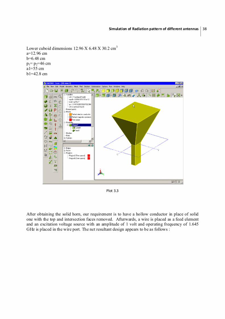
Lower cuboid dimensions 12.96 X 6.48 X 30.2 cm3 a=12.96 cm b=6.48 cm p1= p2=46 cm a1=55 cm b1=42.8 cm
Plot 3.3
After obtaining the solid horn, our requirement is to have a hollow conductor in place of solid one with the top and intersection faces removed. Afterwards, a wire is placed as a feed element and an excitation voltage source with an amplitude of 1 volt and operating frequency of 1.645 GHz is placed in the wire port. The net resultant design appears to be as follows :

Simulation of Radiation pattern of different antennas 39
Plot 3.4
The 3D far field pattern can be shown as:
Plot 3.5
3.7.2 FEKO Results
Feko Simulation result of Electric Far Field in Cartesian coordinates:

Simulation of Radiation pattern of different antennas 40
Plot 3.6
Plot 3.7
Feko Simulation result of Electric Far Field in polar coordinates:

Simulation of Radiation pattern of different antennas 41
3.8 Results
It was thus found out that the results of Matlab implementation and theoretically calculated results are within the required error limits of ±1%. It was found that the final radiation possesses minimum radiation intensity in the back lobe (at angle of 180 degrees) and a maximum of lobe power is concentrated in the main lobe along the axis of the horn antenna. Both the simulations, that of Matlab and Feko, provide us with a verification of above mentioned result.

Simulation of Radiation pattern of different antennas 42
chapter4
YAGI UDA ANTENNA
Till this point we have discussed the mathematical analysis of Horn antenna, be it E plane sectoral, H- plane sectoral or pyramidal horn. We simulated the mathematical field equations in MATLAB and compared the results with a theoretically proposed design. A Feko simulation of horn antenna was done to further strengthen the outputs of Matlab.
In this chapter the focus will be on yagi-uda array antenna. The mathematical analysis will be corroborated with the Matlab results. A Feko simulation will be made to showcase the various antenna parameters of the yagi uda antenna.
4.1 History
The Yagi-Uda antenna was invented in 1926 by Shintaro Uda of Tohoku Imperial University, Sendai, Japan, with the collaboration of Hidetsugu Yagi, also of Tohoku Imperial University.
The Yagi was first widely used during World War II for airborne radar sets, because of its simplicity and directionality. Despite its being invented in Japan, many Japanese radar engineers were unaware of the design until very late in the war, due to internal fighting between the Army and Navy. The Japanese military authorities first became aware of this technology after the Battle of Singapore when they captured the notes of a British radar technician that mentioned "yagi antenna". Japanese intelligence officers did not even recognize that Yagi was a Japanese name in this context. When questioned the technician said it was an antenna named after a Japanese professor. (This story is analogous to the story of American intelligence officers interrogating German rocket scientists and finding out that Robert Goddard was the real pioneer of rocket technology even though he was not well known in the US at that time).

Simulation of Radiation pattern of different antennas
43
4.2 Introduction
A Yagi-Uda Antenna, commonly known simply as a Yagi antenna or Yagi, is a directional antenna system consisting of an array of a dipole and additional closely coupled parasitic elements (usually a reflector and one or more directors).
The geometry of the Yagi-Uda array:
Figure 4. 1
The second dipole in the Yagi-Uda array is the only driven element with applied input/output source feed, all the others interact by mutual coupling since receive and reradiate electromagnetic energy; they act as parasitic elements by induced current. It is assumed that an antenna is a passive reciprocal device, then may used either for transmission or for reception of the electromagnetic energy: this well applies to Yagi-Uda also.
4.3 Working Principle
The simplest or minimal Yagi-Uda antenna has at least two parasitic elements behind the Driven Element (DE); the antenna with only one parasitic element as Reflector element (Ref) is generally called Yagi antenna. This happens when the electrical length of the parasitic element is greater than the driven element.
Simulation of Radiation pattern of different antennas
44
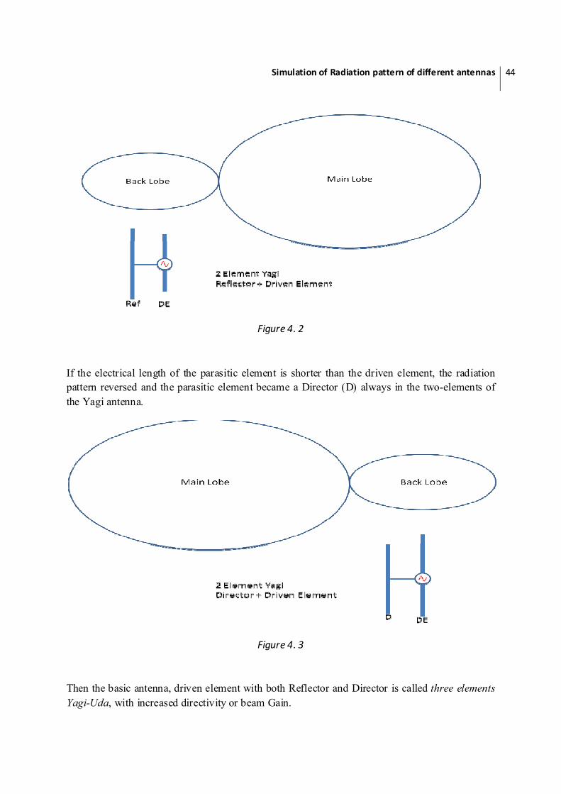
Figure 4. 2
If the electrical length of the parasitic element is shorter than the driven element, the radiation pattern reversed and the parasitic element became a Director (D) always in the two-elements of the Yagi antenna.
Figure 4. 3
Then the basic antenna, driven element with both Reflector and Director is called three elements Yagi-Uda, with increased directivity or beam Gain.

Simulation of Radiation pattern of different antennas
45
Figure 4. 4
The reflector and directors in the Yagi-Uda antenna are so coupled into parasitic mode; they mutually alter the radiation parameters of the driven element and for each element of the array. Then the physical discovery consist in the increased gain by narrowing the beam width of the dipole alone in a very genially cheap manner, by the means of simple metallic rod or tube conductors, then focus the electromagnetic energy into the desired directions.
More than one parasitic element should be axially added in the front of the driven element and each one is called director. As the reflector, the directors (D1…Dn) has not wired directly to the feed point. As the number of director grow, it increase the directivity as the beam gain of the Yagi-Uda system array.
In modern Yagi-Uda design, the parasitic elements should be applied to increase the impedance bandwidth also, much more than a single dipole alone, this is in advance to directional capability of the system to control pattern and impedance with any possible desired combination.
Yagi-Uda antennas are widely used in civilian, simple or professionals, military applications also. Yagi-Uda design is used by lot of amateur radio enthusiast all over the world in advance for any kind of wireless radio communication, television etc.

Simulation of Radiation pattern of different antennas
46
4.4 Mathematical Analysis
Figure 4. 5
The approach taken in formulating the method of solving the Yagi-Uda-type antenna problem is based on an integral equation for the electric field of the array. The point-matching technique is then used to satisfy the integra1 equation at discrete points on the axis of each element rather than attempting to satisfy this equation everywhere on the surface of every element. Thus a system of linear algebraic equations is generated in term of the complex coefficients in the Fourier series expansion of the currents on the elements. Inversion of the matrix yields the value of these coefficients from which the current distributions, phase velocity, and far-field patterns may readily be obtained. Experience has shown that if one chooses a sufficient, number of points at which to match boundary conditions, then one can obtain solutions to problems, such as this one, theretofore not easily solvable. In the case of linear elements, such as those in Fig, it has been found that an efficient representation for the current on element n is given by
In(z’) = ∑ IMmn cos 2m 1 π ′
L
Inm represent the complex current coefficient of mode m on element n and In represents the corresponding length on the n elements. This series of odd-ordered even modes is chosen such that the current goes to zero at the ends of element n. This is a suitable approximation for elements whose diameter is small in terms of the wavelength. The theory is based on Pocklington’s integral equation for total field generated be an electric current source radiating in an unbounded space as given by the following mathematical analysis.
I z′ k//
R
R dz’ = j4πωεoEz.
Simulation of Radiation pattern of different antennas 47
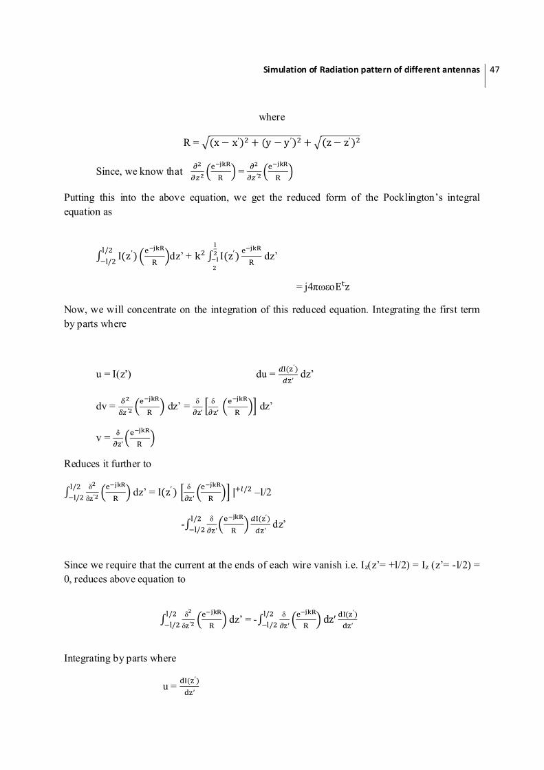
where
R = x x′ y y ′ z z′
Since, we know that R
R = ′
R
R
Putting this into the above equation, we get the reduced form of the Pocklington’s integral equation as
I z′//
R
Rdz’ + k I z′
R
R dz’
= j4πωεoE z
Now, we will concentrate on the integration of this reduced equation. Integrating the first term by parts where
u = I(z’) du = I ′
′ dz’
dv = ′
R
R dz’ = δ
′δ′
R
R dz’
v = δ′
R
R
Reduces it further to
δδ ′
//
R
R dz’ = I z′ δ
′
R
R| / –l/2
- δ′
//
R
RI ′
′ dz’
Since we require that the current at the ends of each wire vanish i.e. Iz(z’= +l/2) = Iz (z’= -l/2) = 0, reduces above equation to
δ
δ ′//
R
R dz’ = - δ
′/
/
R
Rdz′ I ′
′
Integrating by parts where
u = I ′
′

Simulation of Radiation pattern of different antennas 48
du = I ′
′ dz’
dv = δ′
R
Rdz′
v = R
R
reduces it to
δδ ′
//
R
R dz’ = I ′
′
R
R | / –l/2 + I ′
′//
R
R dz’
When this is substituted for the first term, it is further reduced to
- I ′
′
R
R | / –l/2 + k I z′ I ′
′/
/
R
R dz’ = j4πωεoE z
For small diameter wires the current on each element can be approximated by a finite series of odd-ordered even modes. Thus, the current on nth element can be written as a Fourier series expansion of following form
In(z’) = ∑ IMnm cos 2m 1 π ′
L
Where Inm represents the complex current coefficient of mode m on element n and In represents the corresponding length of the n element. Taking the Ist and Iind derivatives of above equation and substituting them results in
∑ IM nm
πI
sin 2m 1 π ′
I
R
R| k π
I
cos 2m 1 π ′I
//
R
R dz′n
= j4πωεoE z
Since the cosine is an even function, above equation can be reduced by integrating over only 0<=z’<=l/2 to
IM
nm1
2m 1 πIn
G2 x, x′ , y,y ′
z,ln2
k 2m 1 π
In
G2/
x, x′, y,y ′
z, z′n cos 2m 1
πz′nIn
dz′n
= j4πωεoE z

Simulation of Radiation pattern of different antennas 49
Where G2(x, x′, y,′,z′n
R_
R_ +
R
R
R = x x′ y y ′ + a z z′
N= 1, 2, 3,4,…..,N
N = total number of electrons
Where
R is the distance from the center of the each wire radius to center of any other wire.
The far-field pattern is given by
Eθ = ∑ E N θn = -jωAθ
Where,
Aθ = ∑ N Aθn=-μ∏
sinθ ∑ N e θ ф θ ф ∑ M Inm Z ZZ
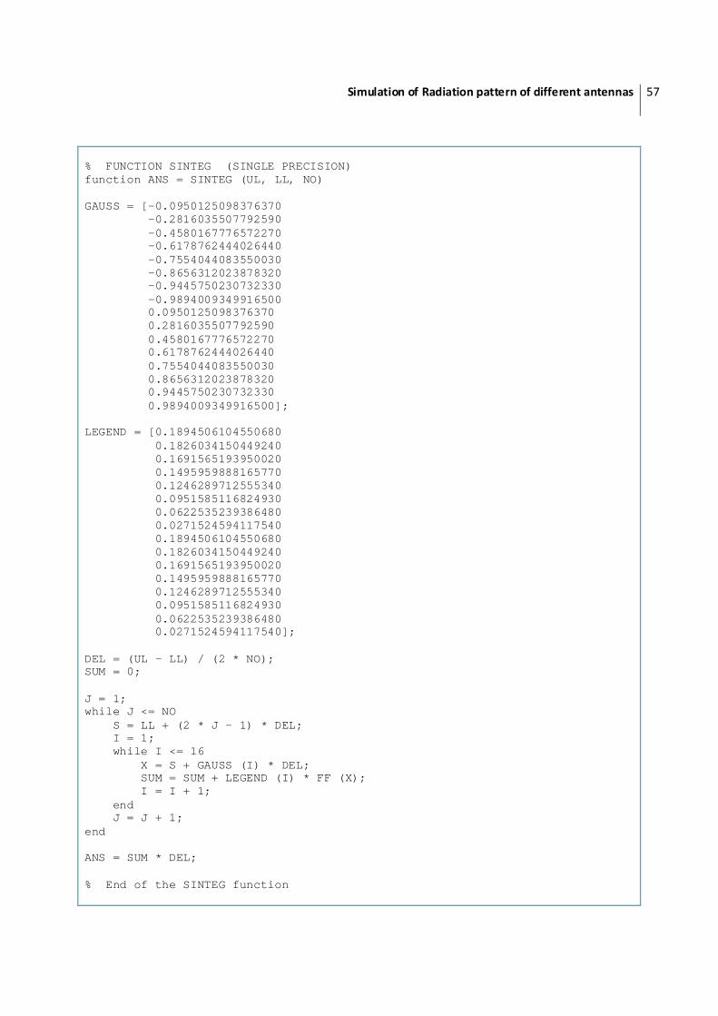
In the Matlab implementation, SINTEG function is for integration. Since integration is very difficult here, so we have used weighted method i.e. Gaussian method which states “In numerical analysis, a quadrature rule is an approximation of the definite integral of a function, usually stated as a weighted sum of function values at specified points within the domain of integration.”
4.5 Matlab Simulation
4.5.1 MATLAB CODE
MATLAB CODE
function [] = yagi_uda global MMAX NMAX Z RHO N2 NMODE L MMAX = 30; NMAX = 30; M = input ('\n NUMBER OF MODES PER ELEMENT (A POSITIVE INTEGER) = ', 's'); M = str2num (M); N = input (' NUMBER OF ELEMENTS (A POSITIVE INTEGER GREATER THAN 1) = ', 's'); N = str2num (N); % LENGTH OF THE DIRECTORS if (N > 3) fprintf (1, ' DO ALL DIRECTORS HAVE THE SAME LENGTH?\n'); ANS = input (' ANSWER: (Y OR N) ...... ', 's');

Simulation of Radiation pattern of different antennas 50
else ANS = 'N'; end if (ANS == 'Y') | (ANS == 'y') LDIR = input (' THE UNIFORM LENGTH (in WAVELENGTHS) OF THE DIRECTOR = ', 's'); LDIR = str2num (LDIR); L = LDIR * ones (1, N-2); elseif (ANS == 'N') | (ANS == 'n') a = 1; while a <= (N-2) fprintf (1, ' LENGTH (in WAVELENGTHS) OF DIRECTOR # %2d =', a); b = input (' ', 's'); b = str2num (b); L (a) = b; a = a + 1; end end % GET THE LENGTH OF THE REFLECTOR b = input (' LENGTH (in WAVELENGTHS) OF THE REFLECTOR = ', 's'); b = str2num (b); L (N-1) = b; % GET THE LENGTH OF THE DRIVEN ELEMENT b = input (' LENGTH (in WAVELENGTHS) OF THE DRIVEN ELEMENT = ', 's'); b = str2num (b); L(N) = b; % ELEMENT SEPARATION BETWEEN DRIVEN ELEMENT AND 1ST DIRECTOR b = input ('\n SEPARATION BETWEEN DRIVEN ELEMENT & 1ST DIRECTOR = ', 's'); b = str2num (b); S_1 = b; if (N > 3) fprintf (1, '\n IS THE SEPARATION BETWEEN DIRECTORS UNIFORM?\n'); ANS = input (' ANSWER: (Y OR N) ...... ', 's'); fprintf (1, '\n'); else ANS = 'N'; end % THE SEPARATION DISTANCES OF THE DIRECTORS if (ANS == 'Y') | (ANS == 'y') SDIR = input (' THE UNIFORM SEPARATION BETWEEN DIRECTORS = ', 's'); SDIR = str2num (SDIR); S = SDIR * ones (1, N-2); elseif (ANS == 'N') | (ANS == 'n') a = 2; while a <= (N-2) fprintf (1, ' SEPARATION BETWEEN DIRECTORS # %2d AND # %2d =', a-1, a);

Simulation of Radiation pattern of different antennas 51
b = input (' ', 's'); b = str2num (b); S (a) = b; a = a + 1; end end S (1) = S_1; % ELEMENT SEPARATION BETWEEN DRIVEN ELEMENT AND REFLECTOR b = input (' SEPARATION BETWEEN REFLECTOR & DRIVEN ELEMENT = ', 's'); b = str2num (b); S (N-1) = b; % RADIUS OF EACH ELEMENT b = input ('\n RADIUS (in WAVELENGTHS) FOR ALL ELEMENTS USED = ', 's'); b = str2num (b); ALPHA = b; % Initialize some variables a = 1; while a <= (N - 2) YP (a) = a * S (a); a = a + 1; end YP (N-1) = - S (N-1); YP (N) = 0; RES = 0; G2 = 0; INDEX = 0; DZ = L / (2 * M - 1); ETA = 120 * pi; MU = 4 * pi * 10 ^ (-7); C = 3 * 10 ^ 8; K = 2 * pi; RTOD = 180 / pi; DTOR = pi / 180; A = zeros (M * N, M * N); B = 1:(M*N); B = B * 0; Inm = zeros (N, M); I = 1; while I <= (M * N) IFACT = floor ((I - 1) / M); N1 = IFACT + 1; IMODE = I - IFACT * M; Z = (M - IMODE) * DZ (N1); J = 1; while J <= (M * N) JFACT = floor ((J - 1) / M); N2 = JFACT + 1;

Simulation of Radiation pattern of different antennas 52
NMODE = J - JFACT * M; if (N1 == N2) RHO = ALPHA; else RHO = YP (N1) - YP (N2); end LL = 0; UL = L (N2) / 2; RES = SINTEG (UL, LL, 10); LEN = L (N2) / 2; G2 = KERNEL (LEN); F2M = NMODE * 2 - 1; A (I, J) = ETA / (j * 8 * pi ^ 2) *((F2M * pi / L (N2)) * (-1) ^… (NMODE + 1) * G2 +(K ^ 2 - F2M ^ 2 * pi ^ 2 / L (N2) ^2) * RES); J = J + 1; end I = I + 1; end % Fill the last row of the matrix corresponding to the feeder. I = zeros (1, M * (N - 1)); J = ones (1, M); A (M * N, :) = [I J]; B (M * N) = 1; % Invert system to find current coefficients in Fourier Series expansion. ISIZE = N * M; [A, IPERM, PIVOT] = LUDEC (A, ISIZE); B = LUSOLV (A, ISIZE, IPERM, B); % CONVERT SINGLE ARRAY OF CURRENT COEFFICIENTS TO A DOUBLE ARRAY OF FORM Imn. NCUT = 0; I = 1; while I <= N J = 1; while J <= M Inm (I, J) = B (J + NCUT); J = J + 1; end NCUT = NCUT + M; I = I + 1; end % CALCULATE THE RADIATED FIELDS IN THE E-PLANE NCUT = 0; ML = 1; while ML <= 2 if (ML == 1)

Simulation of Radiation pattern of different antennas 53
PHI = 90 * DTOR; MAX = 181; else PHI = 270 * DTOR; MAX = 180; end ICOUNT = 1; while ICOUNT <= MAX waitbar(ICOUNT/MAX*ML*0.5*0.2+0.8,h); THETA = (ICOUNT - 1) * DTOR; if (THETA > pi) PHI = 270 * DTOR; end EZP = 0; I = 1; while I <= N IZP = 0; J = 1; while J <= M MODE = J; LEN = L (I); ANG = THETA; IZP = IZP + Inm(I,J)*(ZMINUS(ANG,LEN,MODE)+ ZPLUS(ANG,LEN, MODE)); J = J + 1; end AEXP = K * YP (I) * sin (THETA) * sin(PHI); EZP = EZP + L (I) * exp (j * AEXP) * IZP; I = I + 1; end ETHETA (NCUT + ICOUNT) = j * C * MU / 8 * sin (THETA) * EZP; ICOUNT = ICOUNT + 1; end NCUT = NCUT + MAX; ML = ML + 1; end % FIND THE MAXIMUM VALUE IN THE E-PLANE PATTERN EMAX = 10 ^ (-12); abs_ETHETA = abs (ETHETA); ARG = max (abs_ETHETA); if ARG > EMAX EMAX = ARG; end I = 1; while I <= 361 THETA = I - 1; ARG = abs (ETHETA (I)); if ((ARG/EMAX) > (10 ^ (-6)))

Simulation of Radiation pattern of different antennas 54
ETH (I) = 20 * log10 (ARG / EMAX); else ETH (I) = -120; end I = I + 1; end E_PLANE = ETH; EFTOB = - ETH (271); % CALCULATE THE RADIATED FIELDS IN THE H-PLANE THETA = 90 * DTOR; MAX = 361; ICOUNT = 1; while ICOUNT <= MAX PHI = (ICOUNT - 1) * DTOR; EZP = 0; I = 1; while I <= N IZP = 0; J = 1; while J <= M MODE = J; LEN = L (I); ANG = PHI; IZP = IZP + Inm(I,J)*(ZMINUS(ANG,LEN,MODE)+ZPLUS(ANG,LEN,MODE)); J = J + 1; end AEXP = K * YP (I) * sin (THETA) * sin(PHI); EZP = EZP + L (I) * exp (j * AEXP) * IZP; I = I + 1; end ETHETA (ICOUNT) = j * C * MU / 8 * sin (THETA) * EZP; ICOUNT = ICOUNT + 1; end % FIND THE MAXIMUM VALUE IN THE H-PLANE PATTERN EMAX = 10 ^ (-12); abs_ETHETA = abs (ETHETA); ARG = max (abs_ETHETA); if (ARG > EMAX) EMAX = ARG; end I = 1; while I <= 361 PHI = I - 1; ARG = abs (ETHETA (I)); if (ARG / EMAX) > (10 ^ (-6)) ETH (I) = 20 * log10 (ARG / EMAX); else

Simulation of Radiation pattern of different antennas 55
ETH (I) = - 120; end I = I + 1; end H_PLANE = ETH; HFTOB = - ETH (271); % CALCULATE THE ANTENNA DIRECTIVITY THETA = 90 * DTOR; PHI = 90 * DTOR; AZ = 0; I = 1; while I <= N IZP = 0; J = 1; while J <= M MODE = J; LEN = L (I); ANG = THETA; IZP = IZP + Inm(I,J)*ZMINUS(ANG,LEN,MODE)+ZPLUS(ANG,LEN,MODE)); J = J + 1; end AEXP = K * YP (I) * sin (THETA) * sin (PHI); AZ = AZ + L (I) * exp (j * AEXP) * IZP; I = I + 1; end UMAX = 3.75 * pi * abs (AZ) ^ 2 * sin (THETA) ^ 2; PRAD = SCINT2 (0, pi, 0, 2 * pi, N, M, Inm, YP); D0 = 4 * pi * UMAX / abs (PRAD); % BASED ON FOURIER COEFFICIENTS OF CURRENT, CALCULATE CURRENT DISTRIBUTION IL = 1; while IL <= N DZ (IL) = L (IL) / 100; I = 1; while I <= 51 Z = (I - 1) * DZ (IL); IZP = 0; J = 1; while J <= M F2M = 2 * J - 1; IZP = IZP + Inm (IL, J) * cos (F2M * pi * Z / L (IL)); J = J + 1; end CUR (I) = abs (IZP); angle = atan2 (imag (IZP), real (IZP)); PHA (I) = angle * RTOD; I = I + 1; end I = 1;

Simulation of Radiation pattern of different antennas 56
while I <= 51 Z = (I - 1) * DZ (IL); I = I + 1; end CENTER_CURRENT (IL) = CUR (1); IL = IL + 1; end I = 1; while I <= N J = 1; while J <= M CURRENT = abs (Inm (I, J)); angle_radian = atan2 (imag (Inm (I, J)), real (Inm (I, J))); ANGLE = angle_radian * RTOD; J = J + 1; end I = I + 1; end E_PLANE = E_PLANE (1:360); H_PLANE = H_PLANE (1:360); angle = 1:1:360; figure; plot (angle, E_PLANE, '-b', 'LineWidth', 2); hold on; plot (angle, H_PLANE, '--r', 'LineWidth', 2); legend ('E-Plane', 'H-Plane'); xlim ([1 360]); ylim ([-60 0]); title ('Yagi-Uda Analysis'); xlabel ('Theta(E)/Phi(H) degrees'); ylabel ('Field Pattern (dB)'); hold off; figure; INDEX = 1:1:N; if N >= 3 CENTER_CURRENT = [CENTER_CURRENT(N-1:N) CENTER_CURRENT(1:N-2)]; INDEX = [INDEX(N-1:N) INDEX(1:N-2)]; end plot (CENTER_CURRENT, 'LineWidth', 2); set (gca, 'XTick', 1:1:N); set (gca, 'XTickLabel',INDEX); title ('Current Distribution'); ylim ([0 1]); xlabel ('Element Number'); ylabel ('Element Current Amplitude'); figure; h1=elevation(angle*pi/180,E_PLANE,-40,0,5,'b'); hold on; h2=elevation(angle*pi/180,H_PLANE,-40,0,5,'r--'); set([h1 h2],'linewidth',2); legend([h1 h2],{'E-Plane','H-Plane'}); % End of the yagi_uda function
Simulation of Radiation pattern of different antennas 57
% FUNCTION SINTEG (SINGLE PRECISION) function ANS = SINTEG (UL, LL, NO) GAUSS = [-0.0950125098376370 -0.2816035507792590 -0.4580167776572270 -0.6178762444026440 -0.7554044083550030 -0.8656312023878320 -0.9445750230732330 -0.9894009349916500 0.0950125098376370 0.2816035507792590 0.4580167776572270 0.6178762444026440 0.7554044083550030 0.8656312023878320 0.9445750230732330 0.9894009349916500]; LEGEND = [0.1894506104550680 0.1826034150449240 0.1691565193950020 0.1495959888165770 0.1246289712555340 0.0951585116824930 0.0622535239386480 0.0271524594117540 0.1894506104550680 0.1826034150449240 0.1691565193950020 0.1495959888165770 0.1246289712555340 0.0951585116824930 0.0622535239386480 0.0271524594117540]; DEL = (UL - LL) / (2 * NO); SUM = 0; J = 1; while J <= NO S = LL + (2 * J - 1) * DEL; I = 1; while I <= 16 X = S + GAUSS (I) * DEL; SUM = SUM + LEGEND (I) * FF (X); I = I + 1; end J = J + 1; end ANS = SUM * DEL; % End of the SINTEG function

Simulation of Radiation pattern of different antennas 58
4.5.2 MATLAB OUTPUTS
Plot 4.1 Plot 4.2
These outputs are for the following specifications of the yagi-uda array: Spacing between reflector and feeder = 0.25 λ Number of directors = 13 Number of reflectors = 1 Number of exciters = 1 Length of reflector = 0.5 λ Length of feeder = 0.47 λ Length of each director = 0.406 λ Total elements = 15 Spacing between adjacent directors = 0.34 λ Radius of each wire = 0.003 λ Output value of directivity comes out to be ≈ 37 dB. The yagi uda turns out to be highly directive antenna with the difference between the theoretically and experimentally calculated values of directivity coming out be within reasonable error limits.
4.6 FEKO Simulation
The yagi uda antenna specifications which was simulated in FEKO:
Number of elements = 6 Number of directors = 4 Length of directors = 0.420 λ Length of reflector = 0.482 λ Length of exciter = 0.475 λ Wire radius = 0.00425 λ Spacing between directors = 0.25 λ Spacing between reflector and feed = 0.2 λ

Simulation of Radiation pattern of different antennas 59
Plot 4.3
The figure above shows the 3D far field radiation pattern for the specified yagi uda antenna at a center frequency of 826.3 MHz.
On simulating the above mentioned antenna the output values of electric field intensity and the directivity are shown by the following curves. For Electric field intensity:
Plot 4.4

Simulation of Radiation pattern of different antennas 60
For directivity ( Polar representation):
Plot 4.5
For directivity with respect to frequency :
Plot 4.6

Simulation of Radiation pattern of different antennas 61
4.7 RESULTS
It was thus found out that the results of Matlab implementation and theoretically calculated results are within the reasonable error limits. It was found that the final radiation possesses minimum radiation intensity in the back lobe (at angle of 180 degrees) and a maximum of lobe power is concentrated in the main lobe along the axis of the horn antenna. The directivity of the antenna first increases wrt frequency and then decreases as already shown. Both the simulations, that of Matlab and Feko, provide us with a verification of above mentioned result.

Simulation of Radiation pattern of different antennas
62
chapter5
SPIRO HELICAL ANTENNA
5.1 Introduction
Helical antennas find important applications in communication systems, primarily because of their circular polarization and wide bandwidth. This antenna, referred to as Spiro-Helical Antenna is made of a primary helix wound on a cylinder of larger diameter. An important advantage of this antenna is that it can be conveniently constructed. The simulation and measurement results indicate that the spiro-helical antenna indeed provides high gain and circular polarization over a wide bandwidth.
The figures shown are for the conventional helix. The first one is the normal mode helix and the latter one is axial mode helix.
Figure 5. 1 Figure 5. 2
Simulation of Radiation pattern of different antennas
63
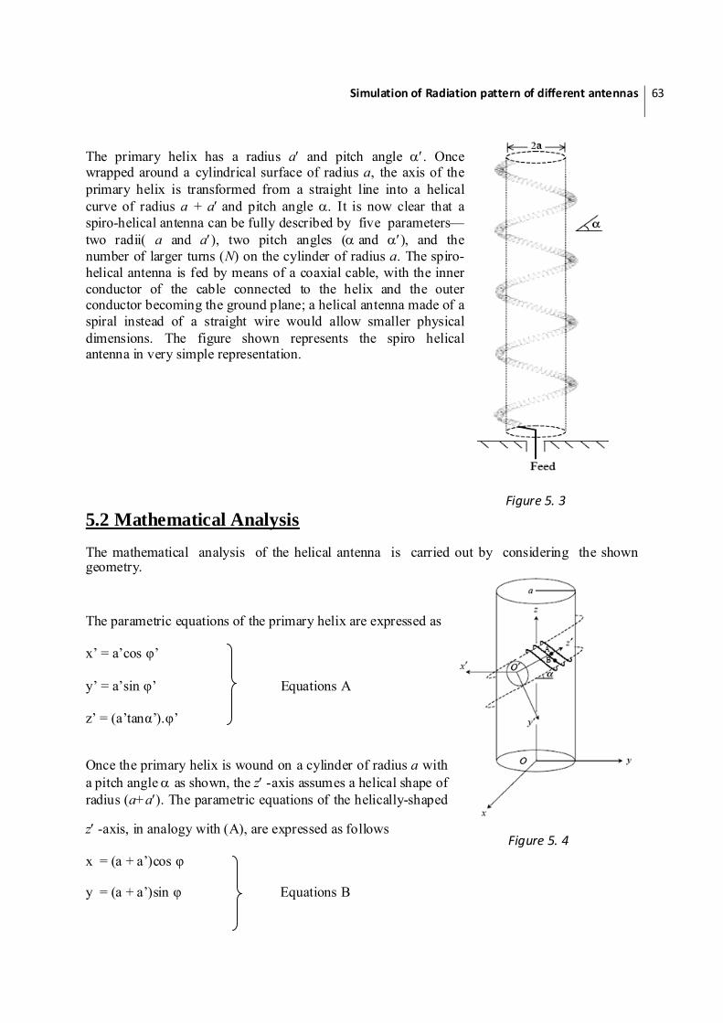
The primary helix has a radius a′ and pitch angle α′. Once wrapped around a cylindrical surface of radius a, the axis of the primary helix is transformed from a straight line into a helical curve of radius a + a′ and pitch angle α. It is now clear that a spiro-helical antenna can be fully described by five parameters—two radii( a and a′), two pitch angles (α and α′), and the number of larger turns (N) on the cylinder of radius a. The spiro-helical antenna is fed by means of a coaxial cable, with the inner conductor of the cable connected to the helix and the outer conductor becoming the ground plane; a helical antenna made of a spiral instead of a straight wire would allow smaller physical dimensions. The figure shown represents the spiro helical antenna in very simple representation.
5.2 Mathematical Analysis
The mathematical analysis of the helical antenna is carried out by considering the shown geometry.
The parametric equations of the primary helix are expressed as x’ = a’cos φ’ y’ = a’sin φ’ Equations A z’ = (a’tanα’).φ’
Once the primary helix is wound on a cylinder of radius a with a pitch angle α as shown, the z′ -axis assumes a helical shape of radius (a+a′). The parametric equations of the helically-shaped
z′ -axis, in analogy with (A), are expressed as follows x = (a + a’)cos φ
y = (a + a’)sin φ Equations B
Figure 5. 3
Figure 5. 4
Simulation of Radiation pattern of different antennas
64
z = [(a + a’) tanα].φ
Next, let us consider an arbitrary point A on the z′ -axis. The coordinates of this point are x’=0, y’=0, z’=zA and in the spiro-helical geometry are denoted as xA, yA, zA. The coordinates xA, yA, and zA, are related to each other through (B). z’A can be determined in terms of zA using the integral expression for length. That is,
z’A = (dx)2 + (dy)2 + (dz)2]1/2
= (dx/dz)2 + (dy/dz)2 + 1]1/2 dz Equations C
Using chain-rule differentiation,
= φ
φ = - (a + a’)sin φ / (a + a’) tanα = - sin φ / tanα
= φ
φ = - (a + a’)cos φ / (a + a’) tanα = - cos φ / tanα
and substituting in (C), yields z’A = (1/ tan2 α) + 1]1/2 dz
or Equations D
z’A = zA / sin α
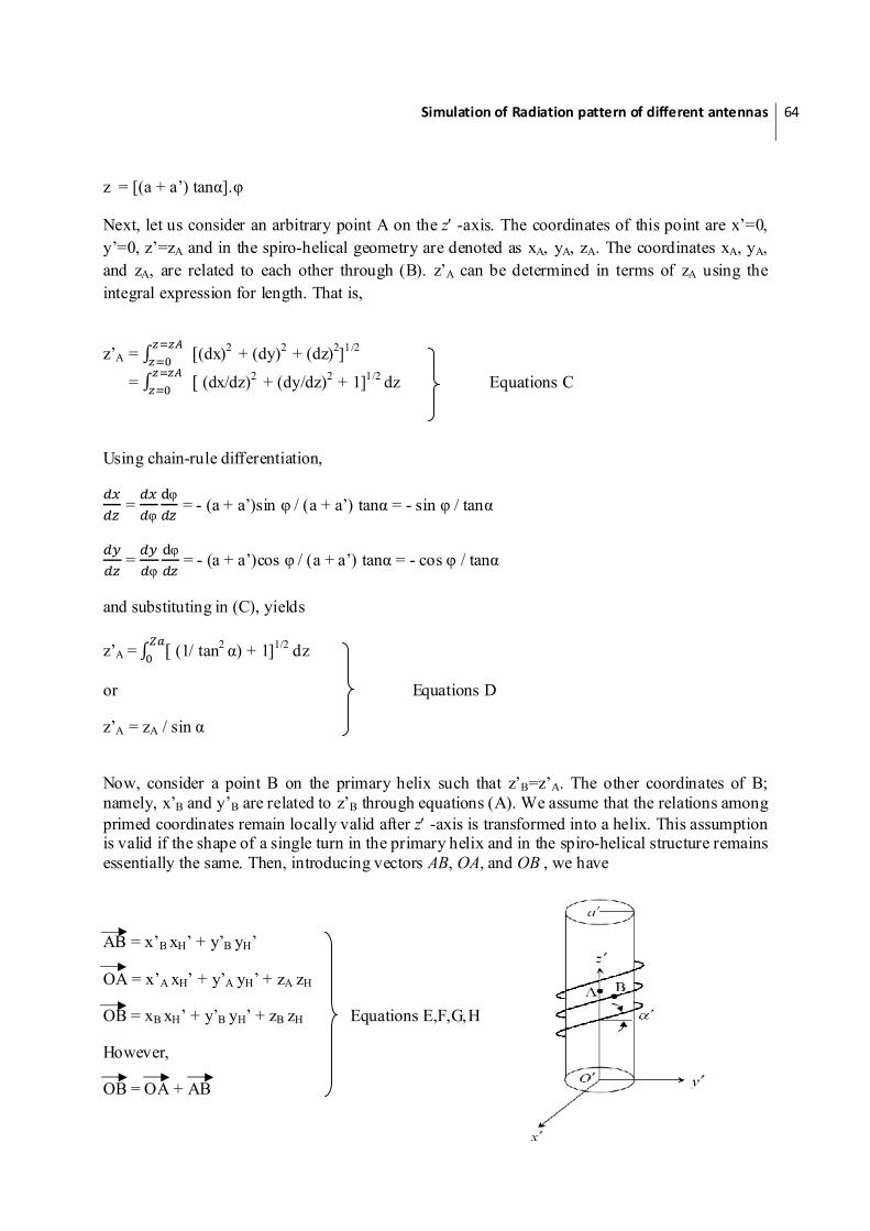
Now, consider a point B on the primary helix such that z’B=z’A. The other coordinates of B; namely, x’B and y’B are related to z’B through equations (A). We assume that the relations among primed coordinates remain locally valid after z′ -axis is transformed into a helix. This assumption is valid if the shape of a single turn in the primary helix and in the spiro-helical structure remains essentially the same. Then, introducing vectors AB, OA, and OB , we have
AB = x’B xH’ + y’B yH’
OA = x’A xH’ + y’A yH’ + zA zH
OB = xB xH’ + y’B yH’ + zB zH Equations E,F,G,H
However,
OB = OA + AB

Simulation of Radiation pattern of different antennas 65
where xH, yH, zH are the corresponding Hilbert Transforms of x, y, z respectively.
It can be shown, by inspection, that
xH’ = cos φ xH’ + sin φ yH’
yH’ = - sin α sin φ xH’ + sin α cos φ yH’ – cos α zH Equations I
zH’ = - cos α sin φ xH’ + cos α cos φ yH’ + sin α zH
Combining (E) through (I), yields
OB = xB xH’ + y’B yH’ + zB zH
= (xA + x’B cos φ - y’B sin α sin φ) xH + (yA + x’B sin φ + Equations J
y’B sin α cos φ) yH + (zA - y’B cos α) zH
Equating the like components in (J), substituting for xA, yA, and zA with the right-hand side expressions in (B), and replacing x’B and y’B with the right-hand side expressions in (A), we finally obtain x = xB = (a + a’)cosφ + a’ cosφ cos φ’ - a’ sinφ sinφ’ sinα
y = yB = (a + a’)sinφ + a’ sinφ cos φ’ - a’ cosφ sinφ’ sinα Equations K
z = zB = [(a + a’)tanα]. φ - a’ sinφ’ cosα
where,
φ = zA/ [(a + a’) tan α]
φ’ = zA/ [a’ tanα’ sin α]
zA varies in the range 0≤ zA ≤ zA max where zA max is the height of the spiro-helical antenna. It is given by,
zA max = 2πN(a + a’) tan α
5.3 Design Methodology
We have studied the radiation pattern of Spiro-helical antenna within the frequency range 1.5 GHz to 2.5 GHz. Then, we have done the mathematical analysis of its geometry. The next step
Primary Helix

Simulation of Radiation pattern of different antennas 66
was to design a Matlab code that will generate the geometry of Spiro-helical antenna. This geometry was stored in .nfm files that contained different segmentation coefficients. These files were different for different frequencies and were fed as an input to the NEC (Numerical Electromagnetic Code-2) software that will enable us to find the radiation pattern of the antenna in the desired frequency range.
5.3 Matlab Simulation
The parameter values for the investigation of spiro helical antenna are Number of turns, N=10 Frequency, 1.4 GHz ≤ f ≤ 3.5 GHz Helix pitch angle, α = 10° Spiral pitch angle, α′ = 30° Helix radius, a = 16 mm Spiral radius, a′ = 3 mm Conductor radius, ro = 0.5 mm
MATLAB CODE
clear all; a = 16; %% Radius a ap = 3; %% Radius a prime alph = 10*pi/180; %% Set angle for alpha alpha = 30*pi/180; %% Set angle for alpha prime length = 220; %% Length for number of turns sym = '_'; %% Symbol to distinguish simulation t = '10'; %% Used in filename for number of turns inc = .3; %% Increment for length begin = 1500; %% Beginning frequency last = 2500; %% Ending frequency l = 'k'; %% Color for Plot rad = .0005; %% radius of conducting wire intrvl = 50; %% Frequency interval for freq = begin:intrvl:last, c = 1; lam = .02*(3*10^8/(freq*10^6)); %% .02 times lambda f = num2str( freq/10 ); %% Simulation information rad1 = num2str ( a ); rad2 = num2str ( ap ); pitch1 = num2str ( alph*180/pi ); pitch2 = num2str ( alpha*180/pi );

Simulation of Radiation pattern of different antennas 67
radius = num2str ( rad ); filename = strcat( t, sym , f, pitch1, '.dat' ); fid = fopen(filename , 'w'); text1 = strcat('CMa=',rad1,',ap=',rad2,', alpha=',pitch1,',alphap=',. . . pitch2,',radius=',radius); text2 = strcat( 'CE',t, sym , pitch1,'.csv'); fprintf(fid, text1 ); fprintf(fid, '\r'); fprintf(fid, '\n'); fprintf(fid, text2 ); fprintf(fid, '\r'); x1(1) = 0; %% Initial values for x,y, and z y1(1) = 0; z1(1) = lam; fprintf(fid, '\nGW%3d 2%10.4f%10.4f%10.4f%10.4f%10.4f%10.4f%9.4f\r',c,x1(c),y1(c),y1(c),x1(c),y1(c),z1(c),rad); for zo = 2.7:inc:length, tmp = zo; x2 = x1(c); y2 = y1(c); z2 = z1(c); c= c+1; %% Increase counter for array phi = tmp./((a+ap) * tan(alph)); %% Calculation of Phi %% Calculation of Phi prime phip = tmp./(ap * sin(alph) * tan(alpha)); x1(c) = ((a+ap).*cos(phi) + ap.*cos(phi).*cos(phip) – . . . ap*sin(alph).*sin(phi).*sin(phip))/1000; y1(c) = ((a+ap).*sin(phi) + ap.*sin(phi).*cos(phip) + . . . ap*sin(alph).*cos(phi).*sin(phip))/1000; z1(c) = ((a+ap)*tan(alph).*phi - ap*cos(alph).*sin(phip))/1000; %% x, y, and z written in input file fprintf(fid, '\nGW%3d 1%10.4f%10.4f%10.4f%10.4f%10.4f %10.4f%9.4f\r',c,. . . x2,y2,z2,x1(c),y1(c),z1(c),rad); end %% End geometry and parameters for ground plane, %% frequency, excitation, and radiation plots. fprintf(fid,'\nGE\r'); fprintf(fid,'\nGN 1\r'); fprintf(fid,'\nFR 0 1 0 0%10.1f 0.000\r', freq); fprintf(fid,'\nEX 0 1 1 10 5.000 0.000\r'); fprintf(fid,'\nRP 0 37 37 1010 0.000 0.000 5.00010.000\r'); fprintf(fid,'\nEN'); fclose(fid); end figure(1) %% check graph of geometry to ensure number of turns plot3(x1,y1,z1,l) view(90,0)

Simulation of Radiation pattern of different antennas 68
MATLAB OUTPUT
Plot 5.1
5.4 Radiation Patterns
The radiation patterns were computed through the numerical electromagnetic code -2 software. The output patterns computed are as shown,
For the directivity with respect to frequency

Simulation of Radiation pattern of different antennas 69
Plot 5.2 Plot 5.3
Plot 5.4
The above curves are for the frequencies 1.5 GHz, 1.7 GHz, 1.9 GHz, 2.25 GHz and 2.45 GHz respectively. It is clear from the above curves that the power pattern directivity first increases with the increase in frequency, reaches a maximum value and then the pattern starts to distort that is distortion of the pattern begins.

Simulation of Radiation pattern of different antennas 70
For the Gain with respect to frequency curves
Plot 5.5 It is clear from the above plot that a peak gain of 13 dB at 2.25 GHz is there and a minimum gain of 6.8 dB at 2.4 GHz is seen. For the frequencies in between 1.55 GHz and 2.3 GHz, the gain lies between the minimum and maximum values. For the Axial Ratio with respect to frequency curves
Plot 5.6 It is observed that axial ratio is < 3 dB in frequency range 1.6 GHz < f < 2.2 GHz.

Simulation of Radiation pattern of different antennas 71
5.5 RESULTS The results of NEC-2 clearly showed that for the given antenna specifications, a peak gain of 13 dB at 2.25 GHz is there and a minimum gain of 6.8 dB at 2.4 GHz is seen. For the frequencies in between 1.55 GHz and 2.3 GHz, the gain lies between the minimum and maximum values. It is observed that axial ratio is < 3 dB in frequency range 1.6 GHz < f < 2.2 GHz.

Simulation of Radiation pattern of different antennas 72
Chapter6 FEKO Improved Designs
6.1 FEKO Background
FEKO is a full wave, MoM (method of moment) based simulation software for the analysis of electromagnetic problems such as coupling, antenna design, antenna placement analysis, micro strip design, scattering analysis, etc. It has the ability to solve electrically large problems using accurate full wave techniques. Electromagnetic fields are obtained by first calculating the electric surface currents on conducting surfaces and equivalent electric and magnetic surface current on the surface of a dielectric solid. The currents are calculated using a linear combination of basis functions, where the coefficients are obtained by solving a system of linear equations. Once the current distribution is known, further parameters can be obtained, such as near field, far field, directivity, input impedance of an antenna. Here we have used feko for analyzing various antennas introduced in past and to design new antennas which give better results in terms of better gain, directivity, better circular polarization and many other factors. The number of designs added have been abbreviated so as to maintain relevance with our designs. 6.2 Designs proposed in past
6.2.1 CROSSED DIPOLE ARRAY IN FRONT OF REFLECTOR
In mobile communication systems the position and orientation of the receiving and transmitting antennas change continually. This can effect the signal strength at the receiver, even when the antennas are

Simulation of Radiation pattern of different antennas 73
pointing at each other, as the orientation of the antennas may result in a polarization mismatch. A simple way to ensure that the polarization mismatch is not more than 3dB is to use a circularly polarized antenna at one end (e.g. transmitter) and a linearly polarized antenna at the other (e.g. receiver). However, achieving circular polarization is difficult and practically an elliptical polarization with an axial ratio close to unity is used. Here a four element crossed dipole array with reflecting metallic plate is modeled in FEKO to determine gain patterns and axial ratios.
Feko modal simulated
Dimensions Used in Paper
Frequency Range :200e6 Hz
Eps: lambda/50
L = 2*lambda
Reflector Dimensions : lambda/4 x 2*lambda
Plot 6.1
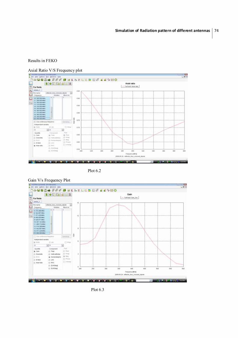
Simulation of Radiation pattern of different antennas 74
Results in FEKO
Axial Ratio V/S Frequency plot
Plot 6.2
Gain V/s Frequency Plot
Plot 6.3

Simulation of Radiation pattern of different antennas 75
6.2.2 SMALL SIZE SIERPINSKI CARPET MICROSTRIP PATCH ANTENNAS W.‐L. Chen and G.‐M. Wang
Aside from using high dielectric substrates applying shorting techniques and increasing the electrical length of the antenna by optimizing the shape there are mainly two techniques to reduce the size of an microstrip patch antenna. One is loading the edges of the patch with inductive elements and the other is inserting the capacitive elements into the patch Koch fractal shapes have been applied to the edges of the patch to reduce the size of the antenna and the essence of this technique falls into capacitive loading. By etching the patch as Sierpinski carpet of different iteration orders, the simulation results show the operating frequency of the antenna can be lowered to lower values, at the same time maintaining the bandwidth, radiation patterns comparable to that of a normal edge-fed microstrip patch Dimensions used in Paper
L= 48.0mm W= 32.4mm f =1.8GHz iteration pf 1/3 dimension are used
Plot 6.4

Simulation of Radiation pattern of different antennas
76
Simulation Results using Feko
Directivity V/S Angle Plot
Plot 6.5
Electric Far Field V/S Angle Plot
Plot 6.6
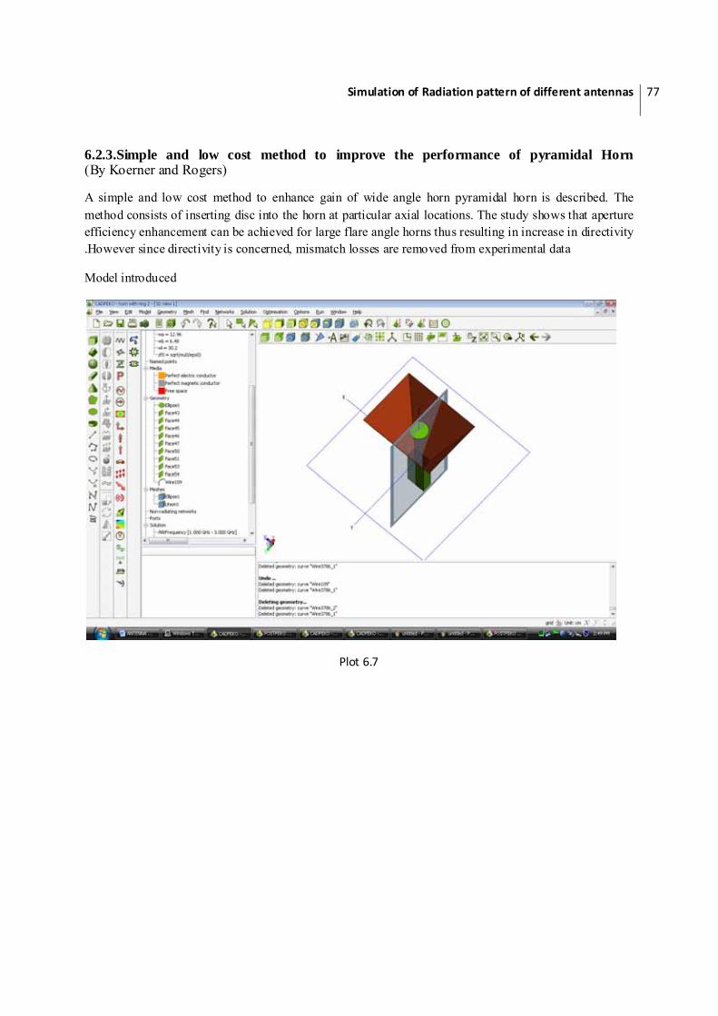
Simulation of Radiation pattern of different antennas 77
6.2.3.Simple and low cost method to improve the performance of pyramidal Horn (By Koerner and Rogers)
A simple and low cost method to enhance gain of wide angle horn pyramidal horn is described. The method consists of inserting disc into the horn at particular axial locations. The study shows that aperture efficiency enhancement can be achieved for large flare angle horns thus resulting in increase in directivity .However since directivity is concerned, mismatch losses are removed from experimental data
Model introduced
Plot 6.7

Simulation of Radiation pattern of different antennas 78
Corresponding output
Gain / Angle Plot at 2.5GHz
Plot 6.8
Directivity / Frequency plot
Plot 6.9
Yagi Uda design and simulations are already done in Matlab and Feko in Previous Chapters

Simulation of Radiation pattern of different antennas 79
6.3 Antenna proposed
Antenna Design 1
It is based on the design “Crossed Dipole Array in Front of Reflector” .As can be seen above the main lobe has a satisfactory directivity , E field but its circular polarization decreases as we move sideways and before reaching the half of beamwidth angle , circular polarization decreases by a substancial amount. Also Vertical polarization is much more than horizontal polarization, thus the medium in which it travel has a large impact on the directivity and gain. Moreover some of these are used in mobile, So there is size constrained.
In this antenna these shortcomings have been overcome
1. Improved circular polarization for large range of angle. 2. Improved circular polarization for comparatively large frequency range. 3. Size of reflector is reduced 4. Improvement in Directivity and gain
Proposed Antenna
Basic Design
Plot 6.10

Simulation of Radiation pattern of different antennas 80
Feko Output
Axial Ratio / Frequency plot
Plot 6.11
Gain / Frequency Plot
Plot 6.12

Simulation of Radiation pattern of different antennas 81
Directivity / Angle Plot
Plot 6.13
From the simulation results , the above antenna has almost 1 axial ratio and high gain or directivity in the range of frequency 200 – 450 MHz. Thus this antenna is very useful in noisy environment.
Antenna Design 2:
This Antenna Design uses Sierpinski Curve and improved version of Paper(Sierpinski patch antenna by W.-L. Chen and G.-M. Wang).Introducing slots in patch make it work at low freq without much loss in directivity and gain
Proposed model
Plot 6.14

Simulation of Radiation pattern of different antennas 82
Feko Results
Directivity /angle plot
Plot 6.15
Electric far field /angle Polar Plot
Plot 6.16

Simulation of Radiation pattern of different antennas 83
Antenna Design 3:
Antenna 3 is based on Yagi Uda antenna which has been discussed in earlier chapter. Matlab code and Feko design were also done .Here Yagi Uda antenna act as the basic model for designing antenna which has better properties.
Modified Design of Yagi Uda
Changes are made in yagi antenna taking into considerations the following Factors
1. Bandwidth 2. Directivity 3. Electric Field 4. Size Constraint 5. Gain
Design 1
Plot 6.17

Simulation of Radiation pattern of different antennas 84
Feko Results
Gain / frequency plot
Plot 6.18
Gain /angle Polar plot
Plot 6.19
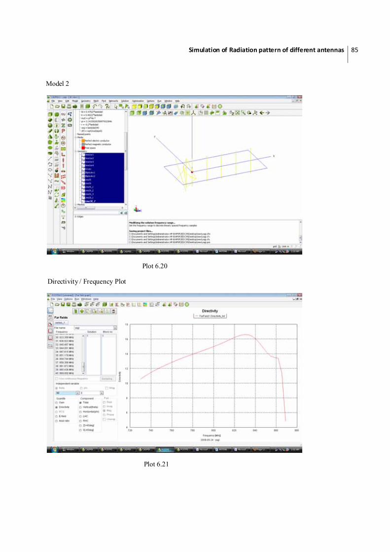
Simulation of Radiation pattern of different antennas 85
Model 2
Plot 6.20
Directivity / Frequency Plot
Plot 6.21
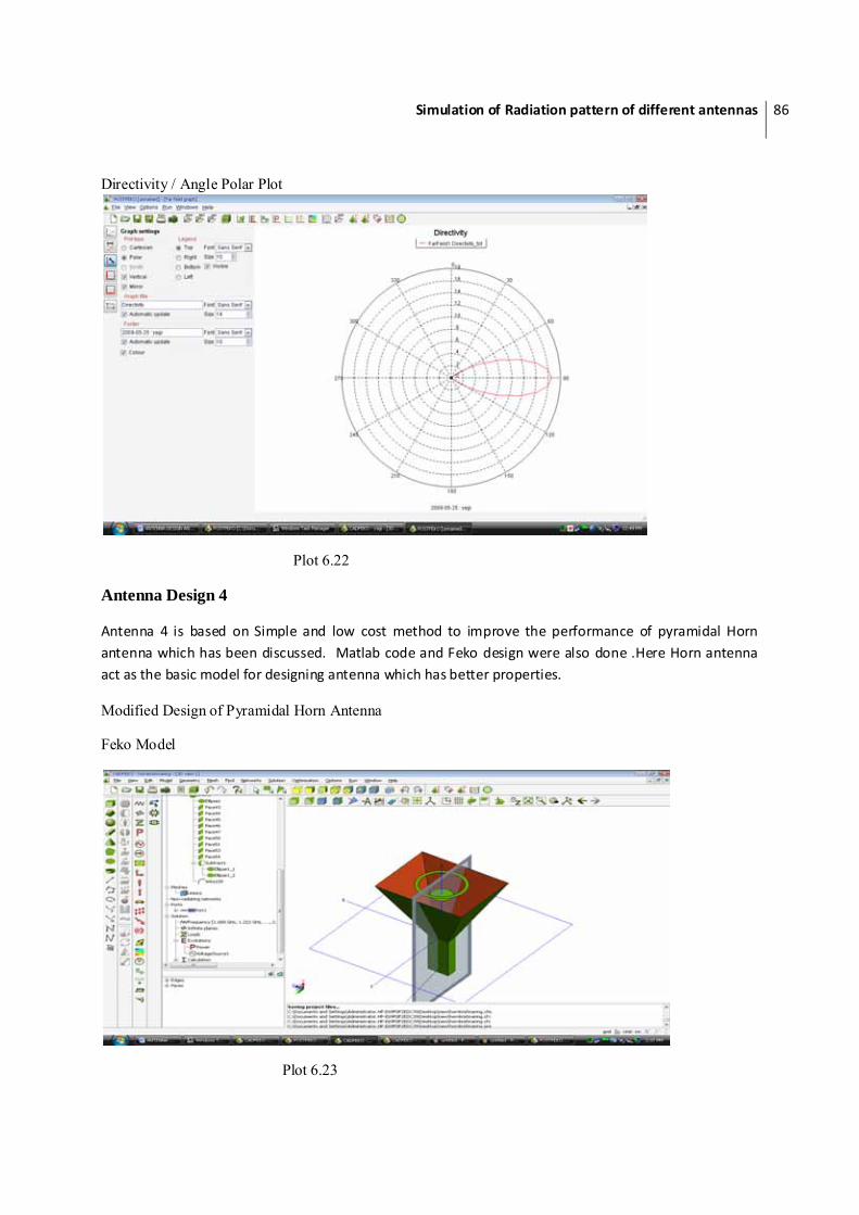
Simulation of Radiation pattern of different antennas 86
Directivity / Angle Polar Plot
Plot 6.22
Antenna Design 4
Antenna 4 is based on Simple and low cost method to improve the performance of pyramidal Horn antenna which has been discussed. Matlab code and Feko design were also done .Here Horn antenna act as the basic model for designing antenna which has better properties.
Modified Design of Pyramidal Horn Antenna
Feko Model
Plot 6.23

Simulation of Radiation pattern of different antennas 87
Directivity /Frequency Plot
Plot 6.24
Directivity / Angle plot at 2.555 Ghz frequency
Plot 6.25

Simulation of Radiation pattern of different antennas 88
Chapter7 CONCLUSION AND FUTURE WORK
7.1 CONCLUSION
While studying Pyramidal Horn antenna, it was found out that the results of Matlab implementation and theoretically calculated results are within the required error limits of ±1%. Also, it was observed that the final radiation possesses minimum radiation intensity in the back lobe (at angle of 180 degrees) and a maximum of lobe power is concentrated in the main lobe along the axis of the horn antenna. Both the simulations, that of Matlab and Feko, provide us with a verification of above mentioned result.
For Yagi-uda antenna also, the results of Matlab implementation and theoretically calculated results are within the reasonable error limits. Here also, the final radiation possesses minimum radiation intensity in the back lobe (at angle of 180 degrees) and a maximum of lobe power is concentrated in the main lobe along the axis of the antenna. The directivity of the antenna first increases with frequency and then decreases. Both the simulations, that of Matlab and Feko, proved the above mentioned result.
In the case of Spiro-helical antenna, the power pattern was observed for the frequencies 1.5 GHz, 1.7 GHz, 1.9 GHz, 2.25 GHz and 2.45 GHz respectively.
At Last new Feko designs have been simulated and their results are compared with the designs which are design wise comparable to them.

Simulation of Radiation pattern of different antennas
89
7.2 Future Work
Since till date we have designed new antennas and done their theoretical simulations but since Physical antenna results may vary from these depending on various factors.
Also there are various antenna which some of which are shown below are not giving satisfactory results and need further modification.
Due to the fact that these antenna has not been previously researched, there are still many opportunities to learn more about it. The following is a list of suggestions for future investigations of these antenna.
1. Different helical shape. The conventional helical shape determines the shape of the spiro-helical investigated here, but the spiral wire can be used to create different overall geometries as well. The wire can be wound into a tapered helical antenna, a conical helical antenna, a spherical helical antenna, or any other number of designs.
2. Gain and input impedance measurements. The measurements conducted were limited to far-field patterns only. Input impedance measurements need to be performed to have a more realistic assessment of the performance of these antennas and their practical applications.

Simulation of Radiation pattern of different antennas 90
REFERENCES
• Antenna Theory , Analysis and Design By Constantine A. Balanis • “Some data for the design of EM Horns” IRE transactions Propagat By E.H.
Braun • Antenna Engineering Handbook ( A.W. Love and T.S. Bird) • D.M. Pozar, ”Directivity of Omni directional Antennas” • R.E. Collin, “Antennas and Radio Wave Propagation” • Samuel Silver, ”Microwave antenna theory and design” • Robert S. Elliot, “Antenna theory and design” • Antenna theory and design By Stutzman Thiele • Modern Antenna Design By Thomas A. Milligan • Electromagnetic waves and antennas By S.J. Orfanidis • Antenna and EM Modeling with Matlab By Sergey N. Makarov • Antenna design and visualization using Matlab By Atef Z. Elsherbeni and
Matthew J. Inman • www.feko.info • www.en.wikipedia.org • www.mathworks.com • www.edaborad.com
• B.R. Piper, M.E. Bialkowski, "Electromagnetic Modeling of Conformal Wideband and
Multi-Band Patch Antennas by Bridging a Solid-Obect Modeler with MoM software", IEEE Antennas and Propagation Magazine, Vol. 46, No. 5, October 2004.
• S.P. Skobelev, B.-J. Ku, A.V. Shishlov, and D.-S. Ahn, "Optimal Geometry and Performance of a Dual-Mode Horn Modification," IEEE Antennas and Propagation Magazine, Vol. 43, No. 1, February 2001
• R.L. Haupt, "A Horn-Fed Reflector Optimized with a Genetic Algorithm", IEEE/ACES International Conference on Wireless Communications and Applied Computational Electromagnetics, April 2005, pp. 517-520.
• S.J. Franson, "Invited Paper - Hybrid Simulation of Electrically Large Millimeter-Wave Antennas", IEEE/ACES International Conference on Wireless Communications and Applied Computational Electromagnetics, April 2005, pp. 505-508.
• C.B. Ravipati, "Compact Circular Microstrip Antenna for Conical Patterns", Antennas and Propagation Society International Symposium, 2004.

Simulation of Radiation pattern of different antennas 91
• E. Gschwendtner, W. Wiesbeck, "Ultra-Broadband Car Antenna for Communications and Navigation Applications", IEEE Transactions on Antennas and Propagation, Vol. 51, No. 8, August 2003.
• A dual-band dual-polarized radar antenna By Yang Bochao Huang Yong Res. Inst. of Navigation Technol., Xi'an;
• Design and analysis of TEM horn antennas for ultra-wideband technology Ying Suo; Jinghui Qiu; Yeshu Yuan Electromagnetic Compatibility and 19th International Zurich Symposium on Electromagnetic Compatibility, 2008.
• Application of FDTD Method to Analyze a U-Slot Patch Antenna By S.-H. Chen and H.-Y. Chen (Taiwan)
• Novel Circularly Polarized Printed Crossed Dipole Array with Broad Axial Ratio Bandwidth By Jung-Woo Baik Kyoung-Joo Lee Won-Sang Yoon Tae-Hak Lee Young-Sik Kim Dept. of radio Commun. & Eng., Korea Univ., Seoul
• Circuit model of microstrip patch antenna on ceramic land grid array package for antenna-chip codesign of highly integrated RF transceivers By Wang, J.J.; Zhang, Y.P.; Kai Meng Chua; Lu, A.C.W.; Antennas and Propagation, IEEE Transactions on Volume 53, Issue 12, Dec. 2005 Page(s):3877 – 3883
• A model for calculating the radiation field of microstrip antennas By Hammer, P.; Van Bouchaute, D.; Verschraeven, D.; Van de Capelle, A.; Antennas and Propagation, IEEE Transactions on [legacy, pre - 1988] Volume 27, Issue 2, Mar 1979 Page(s):267 – 270 “Analysis and Simulation of a 1-18GHz Broadband Double-Ridge Horn Antenna,” By C Burns, P. Leuchtmann, R. Vahldieck, IEEE Transactions on Electromagnetic Compatibility, Vol 45, No 1, pp 55-60, Feb 2003.

Simulation of Radiation pattern of different antennas 92
APPENDICES
Appendix A: Transverse Electric mode
Waveguide differs from a transmission line in some respects. In the first place, a transmission line can support only a transverse electromagnetic (TEM) wave whereas a waveguide can support many possible field configurations. Second, at microwave frequencies (roughly 3-300 GHz), transmission lines become inefficient due to skin effect and dielectric losses; waveguides are used at that range of frequencies to obtain larger bandwidth and lower signal attenuation. Common waveguides are rectangular or circular. Consider a rectangular waveguide. We shall assume the waveguide is filled with (ρ=0, J=0) lossless dielectric material (σ = 0). After all derivation we obtain,
Exs = - µ A1
Eys = - µ A2
Hxs = - A3
Hys = - - A4
where = +
From the above equations we notice that there are different types of field patterns or configurations. Each of these distinct field patterns is called a mode. Four different mode categories can exist, we are concerned with the TE (transverse electric) mode. In the TE modes, the electric field is transverse (or normal) to the direction of wave propagation. We set Ez = 0 and determine other field components Ex, Ey, Hx, Hy, and Hz from equations and the boundary conditions. The boundary conditions are obtained from the fact that the tangential components of the electric field must be continuous at the walls of the waveguide; that is, Exs = 0 at y=0 B1 Exs = 0 at y=b B2 Eys = 0 at x=0 B3 Eys = 0 at x=a B4 From equations A and B, the boundary conditions can be written as

Simulation of Radiation pattern of different antennas 93
= 0 at y = 0
= 0 at y = b
= 0 at x = 0
= 0 at x = a
Imposing the above boundary conditions on following equation we get, Hzs (x,y,z) = (B1 coskxx + B2 sinkxx)(B3 coskyy + B4 sinkyy)
Exs = µ Ho cos sin C1
Eys = µ Ho sin cos C2
Hxs = Ho sin cos C3
Hys = Ho cos sin C4 where m = 0, 1, 2, 3, . . .; and n = 0, 1, 2, 3, . . For TE modes, (m, n) may be (0, 1) or (1, 0) but not (0,0). Both m and n cannot be zero at the same time because this will force the field components in equations C1-C4 to vanish. This implies that the lowest mode can be TEl0 or TE01, depending on the dimensions of the guide. It is standard practice to have a > b. Thus TE10 is the lowest mode and the dominant mode is the mode with the lowest cut-off frequency.

Simulation of Radiation pattern of different antennas 94
Appendix B : Method Of Moments
I z′ k//
R
Rdz’ = j4πωεoEz. ……(1)
This equation is referred to as Pocklington’s equation. It can be used to determine the equivalent filamentary line-source current of the wire, and thus current density on the wire, by knowing the incident field on the wire surface.
This equation has the form of F(g) = h. Where F is a known linear operator, h is a known excitation function and g is the response function. Our aim is to determine g once F and G are specified. The linearity of F operator makes a numerical solution possible.
In above equation, this is done by solving the integral equation using numerical techniques such as the Moment Method. This method is analytically simple and versatile. It requires that the g function be expanded as a linear combination of N terms and written as
g (z’) = a1g1(z’)+ a2g2(z’)+ ……… aNgN(z’)= ∑ angn(z’)…..(2)
Each an is an unknown constant and each gn(z’) is a known function usually known as a basis or expansion function. The domain of the g (z’) and gn(z’) functions are same. Using (2) in (1) and using the linearity of the F operator (1) reduces to
∑ an F(gn) = h……(3)
The basis functions gn are chosen so that each F(gn) can be evaluated conveniently, preferably in closed form or at the very least numerically. Now, the end task remaining is to find the an
unknown constants. Expansion of (3) leads to one equation with N unknowns. To resolve the N constants, it is necessary to have N linearly independent equations. It can be achieved by evaluating (3) at N different points. (eg. applying boundary conditions). This is referred to as point-matching or collocation. Doing this (3) takes the form of
∑ an F(gn) = hm m=1,2,…., N …….(4)
In matrix form, [Zmn] [In] = [Vm] …..(5)
Where , Zmn = F(gn) In = an Vm = hm
The unknown coefficients an can be found by solving (5) using matrix inversion techniques as
[In] = [Zmn]-1 [Vm]
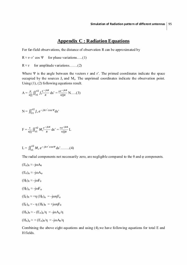
Simulation of Radiation pattern of different antennas 95
Appendix C : Radiation Equations
For far-field observations, the distance of observation R can be approximated by
R ≈ r- r’ cos Ψ for phase variations…..(1)
R ≈ r for amplitude variations…….(2)
Where Ψ is the angle between the vectors r and r’. The primed coordinates indicate the space occupied by the sources Js and Ms. The unprimed coordinates indicate the observation point. Using (1), (2) following equations result.
A = ∏ s ds’ = μ
∏ N…..(3)
N = s ′ ds’
F = ∏ s ds’ =
R
∏ L
L = s ′ ds’……..(4)
The radial components not necessarily zero, are negligible compared to the θ and φ components.
(EA)θ ≈ -jωAθ
(EA)φ ≈ -jωAφ
(HF)θ ≈ -jωFθ
(HF)φ ≈ -jωFφ
(EF)θ ≈ +η (HF)φ = -jωηFφ
(EF)φ ≈ - η (HF)θ = +jωηFθ
(HA)θ ≈ - (EA)φ/η = -jωAφ/η
(HA)φ ≈ + (EA)θ/η = -jωAθ/η
Combining the above eight equations and using (4),we have following equations for total E and H fields.

Simulation of Radiation pattern of different antennas 96
Er ≈ 0
Eθ ≈ - ∏
( Lφ + ηNθ )
Eφ ≈ +∏
( Lθ - ηNφ )
Hr ≈ 0
Hθ ≈ + ∏ ( Nφ – Lθ/η )
Hφ ≈ - ∏ ( Nθ + Lφ/η )
Using (3) and (4), we have
Nθ = x cos θ cos φ + y cos θ sin φ – z sin θ] ′ ds’
Nφ = x sin φ + y cos φ] ′ ds’
Lθ = x cos θ cos φ + y cos θ sin φ – z sin θ] ′ ds’
Lφ = x sin φ + y cos φ] ′ ds’