design and analysis of experiments with sas - bionovin · markov chain monte carlo — stochastic...
TRANSCRIPT


Design and Analysis of Experiments
with SAS

CHAPMAN & HALL/CRC Texts in Statistical Science SeriesSeries EditorsBradley P. Carlin, University of Minnesota, USAJulian J. Faraway, University of Bath, UKMartin Tanner, Northwestern University, USAJim Zidek, University of British Columbia, Canada
Analysis of Failure and Survival DataP. J. SmithThe Analysis of Time Series —An Introduction, Sixth EditionC. ChatfieldApplied Bayesian Forecasting and Time Series AnalysisA. Pole, M. West and J. HarrisonApplied Nonparametric Statistical Methods, Fourth Edition P. Sprent and N.C. SmeetonApplied Statistics — Handbook of GENSTAT Analysis E.J. Snell and H. Simpson Applied Statistics — Principles and Examples D.R. Cox and E.J. SnellApplied Stochastic Modelling, Second Edition B.J.T. MorganBayesian Data Analysis, Second Edition A. Gelman, J.B. Carlin, H.S. Stern and D.B. RubinBayesian Methods for Data Analysis, Third Edition B.P. Carlin and T.A. LouisBeyond ANOVA — Basics of Applied Statistics R.G. Miller, Jr.Computer-Aided Multivariate Analysis, Fourth Edition A.A. Afifi and V.A. ClarkA Course in Categorical Data AnalysisT. LeonardA Course in Large Sample TheoryT.S. FergusonData Driven Statistical Methods P. Sprent Decision Analysis — A Bayesian ApproachJ.Q. SmithDesign and Analysis of Experiment with SASJ. LawsonElementary Applications of Probability Theory, Second Edition H.C. Tuckwell
Elements of Simulation B.J.T. MorganEpidemiology — Study Design and Data Analysis, Second EditionM. WoodwardEssential Statistics, Fourth Edition D.A.G. ReesExtending the Linear Model with R — Generalized Linear, Mixed Effects and Nonparametric Regression ModelsJ.J. FarawayA First Course in Linear Model TheoryN. Ravishanker and D.K. DeyGeneralized Additive Models: An Introduction with RS. WoodInterpreting Data — A First Course in StatisticsA.J.B. AndersonAn Introduction to Generalized Linear Models, Third EditionA.J. Dobson and A.G. BarnettIntroduction to Multivariate Analysis C. Chatfield and A.J. CollinsIntroduction to Optimization Methods and Their Applications in Statistics B.S. EverittIntroduction to Probability with R K. BaclawskiIntroduction to Randomized Controlled Clinical Trials, Second Edition J.N.S. MatthewsIntroduction to Statistical Inference and Its Applications with R M.W. TrossetIntroduction to Statistical Methods for Clinical Trials T.D. Cook and D.L. DeMetsLarge Sample Methods in StatisticsP.K. Sen and J. da Motta SingerLinear Models with RJ.J. FarawayLogistic Regression ModelsJ.M. Hilbe

Markov Chain Monte Carlo — Stochastic Simulation for Bayesian Inference, Second EditionD. Gamerman and H.F. LopesMathematical Statistics K. Knight Modeling and Analysis of Stochastic Systems, Second EditionV.G. KulkarniModelling Binary Data, Second EditionD. CollettModelling Survival Data in Medical Research, Second EditionD. CollettMultivariate Analysis of Variance and Repeated Measures — A Practical Approach for Behavioural ScientistsD.J. Hand and C.C. TaylorMultivariate Statistics — A Practical ApproachB. Flury and H. RiedwylPólya Urn ModelsH. MahmoudPractical Data Analysis for Designed ExperimentsB.S. YandellPractical Longitudinal Data AnalysisD.J. Hand and M. CrowderPractical Statistics for Medical ResearchD.G. AltmanA Primer on Linear ModelsJ.F. MonahanProbability — Methods and MeasurementA. O’HaganProblem Solving — A Statistician’s Guide, Second Edition C. ChatfieldRandomization, Bootstrap and Monte Carlo Methods in Biology, Third Edition B.F.J. ManlyReadings in Decision Analysis S. French
Sampling Methodologies with Applications P.S.R.S. RaoStatistical Analysis of Reliability DataM.J. Crowder, A.C. Kimber, T.J. Sweeting, and R.L. SmithStatistical Methods for Spatial Data AnalysisO. Schabenberger and C.A. GotwayStatistical Methods for SPC and TQMD. BissellStatistical Methods in Agriculture and Experimental Biology, Second EditionR. Mead, R.N. Curnow, and A.M. HastedStatistical Process Control — Theory and Practice, Third Edition G.B. Wetherill and D.W. BrownStatistical Theory, Fourth EditionB.W. Lindgren Statistics for AccountantsS. LetchfordStatistics for Epidemiology N.P. JewellStatistics for Technology — A Course in Applied Statistics, Third EditionC. ChatfieldStatistics in Engineering — A Practical ApproachA.V. MetcalfeStatistics in Research and Development, Second EditionR. CaulcuttStochastic Processes: An Introduction, Second EditionP.W. Jones and P. Smith Survival Analysis Using S — Analysis of Time-to-Event DataM. Tableman and J.S. KimThe Theory of Linear ModelsB. JørgensenTime Series AnalysisH. Madsen

Texts in Statistical Science
John LawsonBrigham Young University
Provo, Utah, U.S.A.
Design and Analysis of Experiments
with SAS

Chapman & Hall/CRCTaylor & Francis Group6000 Broken Sound Parkway NW, Suite 300Boca Raton, FL 33487-2742
© 2010 by Taylor and Francis Group, LLCChapman & Hall/CRC is an imprint of Taylor & Francis Group, an Informa business
No claim to original U.S. Government works
Printed in the United States of America on acid-free paper10 9 8 7 6 5 4 3 2 1
International Standard Book Number: 978-1-4200-6060-7 (Hardback)
This book contains information obtained from authentic and highly regarded sources. Reasonable efforts have been made to publish reliable data and information, but the author and publisher cannot assume responsibility for the validity of all materials or the consequences of their use. The authors and publishers have attempted to trace the copyright holders of all material reproduced in this publication and apologize to copyright holders if permission to publish in this form has not been obtained. If any copyright material has not been acknowledged please write and let us know so we may rectify in any future reprint.
Except as permitted under U.S. Copyright Law, no part of this book may be reprinted, reproduced, transmit-ted, or utilized in any form by any electronic, mechanical, or other means, now known or hereafter invented, including photocopying, microfilming, and recording, or in any information storage or retrieval system, without written permission from the publishers.
For permission to photocopy or use material electronically from this work, please access www.copyright.com (http://www.copyright.com/) or contact the Copyright Clearance Center, Inc. (CCC), 222 Rosewood Drive, Danvers, MA 01923, 978-750-8400. CCC is a not-for-profit organization that provides licenses and registration for a variety of users. For organizations that have been granted a photocopy license by the CCC, a separate system of payment has been arranged.
Trademark Notice: Product or corporate names may be trademarks or registered trademarks, and are used only for identification and explanation without intent to infringe.
Library of Congress Cataloging‑in‑Publication Data
Lawson, John, 1947-Design and analysis of experiments with SAS / John Lawson.
p. cm. -- (Chapman & Hall/CRC texts in statistical science series)Includes bibliographical references and index.ISBN 978-1-4200-6060-7 (hard back : alk. paper)1. Experimental design. 2. SAS (Computer file) I. Title. II. Series.
QA279.L36 2010519.5’7--dc22 2009052546
Visit the Taylor & Francis Web site athttp://www.taylorandfrancis.com
and the CRC Press Web site athttp://www.crcpress.com

Contents
Preface xi
1 Introduction 11.1 Statistics and Data Collection 11.2 Beginnings of Statistically Planned Experiments 21.3 Definitions and Preliminaries 21.4 Purposes of Experimental Design 51.5 Types of Experimental Designs 61.6 Planning Experiments 71.7 Performing the Experiments 91.8 Use of SAS Software 111.9 Review of Important Concepts 121.10 Exercises 14
2 Completely Randomized Designs with One Factor 152.1 Introduction 152.2 Replication and Randomization 152.3 A Historical Example 182.4 Linear Model for CRD 192.5 Verifying Assumptions of the Linear Model 272.6 Analysis Strategies When Assumptions Are Violated 302.7 Determining the Number of Replicates 372.8 Comparison of Treatments after the F -Test 412.9 Review of Important Concepts 482.10 Exercises 50
3 Factorial Designs 533.1 Introduction 533.2 Classical One at a Time versus Factorial Plans 533.3 Interpreting Interactions 553.4 Creating a Two-Factor Factorial Plan in SAS 583.5 Analysis of a Two-Factor Factorial in SAS 603.6 Factorial Designs with Multiple Factors - CRFD 803.7 Two-Level Factorials 863.8 Verifying Assumptions of the Model 1023.9 Review of Important Concepts 106
vii
viii CONTENTS
3.10 Exercises 1083.11 Appendix–SAS Macro for Tukey’s Single df Test 112
4 Randomized Block Designs 1154.1 Introduction 1154.2 Creating an RCB in SAS 1164.3 Model for RCB 1194.4 An Example of an RCB 1214.5 Determining the Number of Blocks 1244.6 Factorial Designs in Blocks 1254.7 Generalized Complete Block Design 1284.8 Two Block Factors LSD 1314.9 Review of Important Concepts 1384.10 Exercises 1404.11 Appendix–Data from Golf Experiment 145
5 Designs to Study Variances 1475.1 Introduction 1475.2 Random Factors and Random Sampling Experiments 1485.3 One-Factor Sampling Designs 1505.4 Estimating Variance Components 1515.5 Two-Factor Sampling Designs 1615.6 Nested Sampling Experiments (NSE) 1705.7 Staggered Nested Designs 1735.8 Designs with Fixed and Random Factors 1795.9 Graphical Methods to Check Model Assumptions 1865.10 Review of Important Concepts 1945.11 Exercises 1965.12 Appendix 198
6 Fractional Factorial Designs 1996.1 Introduction 1996.2 Half-Fractions of 2k Designs 2006.3 Quarter and Higher Fractions of 2k Designs 2096.4 Criteria for Choosing Generators for 2k−p Designs 2116.5 Augmenting Fractional Factorials 2226.6 Plackett-Burman (PB) Screening Designs 2326.7 Mixed Level Factorials and Orthogonal Arrays (OA) 2386.8 Review of Important Concepts 2466.9 Exercises 248
7 Incomplete and Confounded Block Designs 2557.1 Introduction 2557.2 Balanced Incomplete Block (BIB) Designs 2567.3 Analysis of Incomplete Block Designs 259

CONTENTS ix
7.4 PBIB-BTIB Designs 2617.5 Youden Square Designs (YSD) 2657.6 Confounded 2k and 2k−p Designs 2667.7 Confounding 3 Level and p Level Factorial Designs 2807.8 Blocking Mixed-Level Factorials and OAs 2837.9 Partially Confounded Blocked Factorial (PCBF) 2907.10 Review of Important Concepts 2957.11 Exercises 298
8 Split-Plot Designs 3018.1 Introduction 3018.2 Split-Plot Experiments with CRD in Whole Plots CRSP 3028.3 RCB in Whole Plots RBSP 3098.4 Analysis Unreplicated 2k Split-Plot Designs 3188.5 2k−p Fractional Factorials in Split Plots (FFSP) 3248.6 Sample Size and Power Issues for Split-Plot Designs 3388.7 Review of Important Concepts 3398.8 Exercises 341
9 Crossover and Repeated Measures Designs 3479.1 Introduction 3479.2 Crossover Designs (COD) 3479.3 Simple AB, BA Crossover Designs for Two Treatments 3489.4 Crossover Designs for Multiple Treatments 3589.5 Repeated Measures Designs 3649.6 Univariate Analysis of Repeated Measures Design 3659.7 Review of Important Concepts 3749.8 Exercises 376
10 Response Surface Designs 38110.1 Introduction 38110.2 Fundamentals of Response Surface Methodology 38110.3 Standard Designs for Second Order Models 38510.4 Creating Standard Designs in SAS 39210.5 Non-Standard Response Surface Designs 39510.6 Fitting the Response Surface Model with SAS 40310.7 Determining Optimum Operating Conditions 41010.8 Blocked Response Surface (BRS) Designs 42110.9 Response Surface Split-Plot (RSSP) Designs 42410.10 Review of Important Concepts 43510.11 Exercises 437
11 Mixture Experiments 44311.1 Introduction 44311.2 Models and Designs for Mixture Experiments 445

x CONTENTS
11.3 Creating Mixture Designs in SAS 45211.4 Analysis of Mixture Experiment 45411.5 Constrained Mixture Experiments 46111.6 Blocking Mixture Experiments 47011.7 Mixture Experiments with Process Variables 47511.8 Mixture Experiments in Split-Plot Arrangements 48411.9 Review of Important Concepts 48711.10 Exercises 48911.11 Appendix–Example of Fitting Independent Factors 498
12 Robust Parameter Design Experiments 50112.1 Introduction 50112.2 Noise-Sources of Functional Variation 50212.3 Product Array Parameter Design Experiments 50412.4 Analysis of Product Array Experiments 51212.5 Single Array Parameter Design Experiments 52912.6 Joint Modeling of Mean and Dispersion Effects 53812.7 Review of Important Concepts 54512.8 Exercises 547
13 Experimental Strategies for Increasing Knowledge 55513.1 Introduction 55513.2 Sequential Experimentation 55513.3 One Step Screening and Optimization 55913.4 Evolutionary Operation 56013.5 Concluding Remarks 562
Bibliography 565
Index 579

Preface
After studying experimental design a researcher or statistician should be ableto: (1) choose an experimental design that is appropriate for the researchproblem at hand; (2) construct the design (including performing proper ran-domization and determining the required number of replicates); (3) executethe plan to collect the data (or advise a colleague to do it); (4) determinethe model appropriate for the data; (5) fit the model to the data; and (6)interpret the data and present the results in a meaningful way to answer theresearch question. The purpose of this book is to focus on connecting the ob-jectives of research to the type of experimental design required, describing theactual process of creating the design and collecting the data, showing how toperform the proper analysis of the data, and illustrating the interpretation ofresults. Exposition on the mechanics of computation is minimized by relyingon a statistical software package.
With the availability of modern statistical computing packages, the analysisof data has become much easier and is well covered in statistical methodsbooks. There is no longer a need to show all the computational formulasthat were necessary before the advent of modern computing, in a book onthe design and analysis of experiments. However, there is a need for carefulexplanation of how to get the proper analysis from a computer package. Thedefault analysis performed by most statistical software assumes the data havecome from a completely randomized design. In practice, this is often a falseassumption. This book emphasizes the connection between the experimentalunits, and the way treatments are randomized to experimental units, and theproper error term for an analysis of the data.
The SAS system for statistical analysis is used throughout the book toillustrate both construction of experimental designs and analysis of data. Thissoftware was chosen to be illustrated because it has extensive capabilities inboth creating designs and analyzing data, the command language has beenstable for over thirty years, and it is widely used in industry. SAS version 9.2has been used in the text, and all the SAS code for examples in the bookis available at http://lawson.mooo.com. The ods graphics used in the bookrequire version 9.2 or later. In earlier versions of SAS similar graphs can becreated with the legacy SAS/GRAPH routines and the code to do this is alsoavailable on the Web site. Examples of SAS data step programming and IMLare presented, and procedures from SAS Stat, SAS QC, and SAS OR areillustrated.
With fewer pages devoted to computational formulas, I have attempted to
xi

xii PREFACE
spend more time discussing the following: (1) how the objectives of a researchproject lead to the choice of an appropriate design, (2) practical aspects ofcreating a design, or list of experiments to be performed, (3) practical aspectsof performing experiments, and (4) interpretation of the results of a computeranalysis of the data. Items (1)-(3) can best be taught by giving many examplesof experiments and exercises that actually require readers to perform their ownexperiments.
This book attempts to give uniform coverage to experimental designs anddesign concepts that are most commonly used in practice, rather than focusingon specialized areas. The selection of topics is based on my own experienceworking in the pharmaceutical industry, and in research and development(R&D) and manufacturing in agricultural and industrial chemicals, and ma-chinery industries. At the end of each chapter a diagram is presented to helpidentify where the various designs should be used. Examples in the book comefrom a variety of application areas. Emphasis is placed on how the samplesize, the assignment of experimental units to combinations of treatment fac-tor levels (error control), and the selection of treatment factor combinations(treatment design) will affect the resulting variance and bias of estimates andthe validity of conclusions.
Intended audience This book was written for first-year graduate studentsin statistics or advanced undergraduates who intend to work in an area wherethey will use experimental designs. To be fully understood, a student usingthis book should have had previous courses in calculus, introductory statistics,basic statistical theory, applied linear models such as Kutner et al. (2004) andFaraway (2004), and some familiarity with SAS. Matrix notation for analysisof linear models is used throughout the book, and students should be familiarwith matrix operations at least to the degree illustrated in chapter 5 of Kutneret al. (2004).
However, for students from applied sciences or engineering who do not haveall these prerequisites, there is still much to be gained from this book. Thereare many examples of SAS code to create and analyze experiments as wellplentiful examples of (1) diagnosing the experimental environment to choosethe correct design, and (2) interpreting and presenting results of analysis. Onewith a basic understanding of SAS should be able to follow these examplesand modify them to complete the exercises in the book and solve problemsin their own research, without needing to understand the detailed theoreticaljustification for each procedure.
For instructors This book can be used for a one-semester or two-quartercourse in experimental design. There is too much material for a one-semestercourse, unless the students have had all the prerequisites mentioned above.The first four chapters in the book cover the classical ideas in experimentaldesign, and should be covered in any course for students without a priorbackground in designed experiments. Later chapters start with basics, butproceed to the latest research published on particular topics, and they includecode to implement all of these ideas. An instructor can pick and choose from

PREFACE xiii
these remaining topics, although if there is time to cover the whole book, Iwould recommend presenting the topics in order.
Some instructors who do not intend to cover the entire book might considercovering factorial experiments in Chapter 3, fractional factorials in Chapter 6,and response surface methods in Chapter 9, following the pattern establishedby the DuPont Strategies of Experimentation Short Courses that were devel-oped in the 1970s. I chose the ordering of chapters in the book so that variancecomponent designs in Chapter 5, would be presented before describing splitplot experiments that are so commonplace in practice. I did this because I feelit is important to understand random factors before studying designs wherethere is more than one error term.
Acknowledgments This book is the culmination of many years of thoughtprompted by consulting and teaching. I would be remiss if I did not thankMelvin Carter, my advisor at Brigham Young University (BYU) who intro-duced me to the computer analysis of experimental data over forty years ago,and whose enthusiasm about the subject of designed experiments inspired mylifelong interest in this area. I would also like to thank John Erjavec, my bossand mentor at FMC Corp., for introducing me to the ideas of Box, Hunterand Hunter long before their original book Statistics for Experimenters waspublished. I also thank the many consulting clients over the years who havechallenged me with interesting problems, and the many students who haveasked me to explain things more clearly. Special thanks to my former stu-dents Willis Jensen at Gore and Michael Joner at Procter and Gamble fortheir careful review and comments on my manuscript, and Seyed Mottagh-inejad for providing a solutions manual and finding many typos and unclearpoints in the text. Finally, I thank my wife Francesca for her never-endingsupport and encouragement during the writing of this book.
John LawsonDepartment of Statistics
Brigham Young University


CHAPTER 1
Introduction
1.1 Statistics and Data Collection
Statistics is defined as the science of collecting, analyzing and drawing con-clusions from data. Data is usually collected through sampling surveys, obser-vational studies, or experiments.
Sampling surveys are normally used when the purpose of data collection is toestimate some property of a finite population without conducting a completecensus of every item in the population. For example, if there were interest infinding the proportion of registered voters in a particular precinct that favora proposal, this proportion could be estimated by polling a random sample ofvoters rather than questioning every registered voter in the precinct.
Observational studies and experiments, on the other hand, are normallyused to determine the relationship between two or more measured quantitiesin a conceptual population. A conceptual population, unlike a finite popu-lation, may only exist in our minds. For example, if there were interest inthe relationship between future greenhouse gas emissions and future aver-age global temperature, the population, unlike registered voters in a precinct,cannot be sampled from because it does not yet exist.
To paraphrase the late W. Edwards Deming, the value of statistical meth-ods is to make predictions which can form the basis for action. In order tomake accurate future predictions of what will happen when the environmentis controlled, cause and effect relationships must be assumed. For example, topredict future average global temperature given that greenhouse gas emissionswill be controlled at a certain level, we must assume that the relationship be-tween greenhouse gas emissions and global temperature is cause and effect.Herein lies the main difference in observational studies and experiments. Inan observational study, data is observed in its natural environment, but in anexperiment the environment is controlled. In observational studies it cannotbe proven that the relationships detected are cause and effect. Correlationsmay be found between two observed variables because they are both affectedby changes in a third variable that was not observed or recorded, and anyfuture predictions made based on the relationships found in an observationalstudy must assume the same interrelationships among variables that existedin the past will exist in the future. In an experiment, on the other hand, somevariables are purposely changed while others are held constant. In that waythe effect that is caused by the change in the purposely varied variable can
1

2 INTRODUCTION
be directly observed, and predictions can be made about the result of futurechanges to the purposely varied variable.
1.2 Beginnings of Statistically Planned Experiments
There are many purposes for experimentation. Some examples include: deter-mining the cause for variation in measured responses observed in the past;finding conditions that give rise to the maximum or minimum response; com-paring the response between different settings of controllable variables; andobtaining a mathematical model to predict future response values.
Presently planned experiments are used in many different fields of applica-tion such as engineering design, quality improvement, industrial research andmanufacturing, basic research in physical and biological science, research insocial sciences, psychology, business management and marketing research, andmany more. However, the roots of modern experimental design methods stemfrom R. A. Fisher’s work in agricultural experimentation at the RothamstedExperimental Station near Harpenden, England.
Fisher was a gifted mathematician whose first paper as an undergraduateat Cambridge University introduced the theory of likelihood. He was lateroffered a position at University College, but turned it down to join the staffat Rothamsted in 1919. There, inspired by daily contact with agricultural re-search, he not only contributed to experimental studies in areas such as cropyields, field trials, and genetics, but also developed theoretical statistics at anastonishing rate. He also came up with the ideas for planning and analysis ofexperiments that have been used as the basis for valid inference and predictionin various fields of application to this day. Fisher (1926) first published hisideas on planning experiments in his paper “The arrangement of field experi-ments”; nine years later he published the first edition of his book The Designof Experiments, Fisher (1935).
The challenges that Fisher faced were the large amount of variation inagricultural and biological experiments that often confused the results, andthe fact that experiments were time consuming and costly to carry out. Thismotivated him to find experimental techniques that could:
• eliminate as much of the natural variation as possible
• prevent unremoved variation from confusing or biasing the effects beingtested
• detect cause and effect with the minimal amount of experimental effortnecessary.
1.3 Definitions and Preliminaries
Before initiating an extended discussion of experimental designs and the plan-ning of experiments, I will begin by defining the terms that will be used fre-quently.

DEFINITIONS AND PRELIMINARIES 3
• Experiment (also called a Run) is an action where the experimenter changesat least one of the variables being studied and then observes the effect ofhis or her actions(s). Note the passive collection of observational data isnot experimentation.
• Experimental Unit is the item under study upon which something is changed.This could be raw materials, human subjects, or just a point in time.
• Sub-sample, sub-unit or observational unit When the experimental unit issplit, after the action has been taken upon it, this is called a sub-sampleor sub-unit. Sometimes it is only possible to measure a characteristic sepa-rately for each sub-unit; for that reason they are often called observationalunits. Measurements on sub-samples, or sub-units of the same experimentalunit are usually correlated and should be averaged before analysis of datarather than being treated as independent outcomes. When sub-units canbe considered independent and there is interest in determining the vari-ance in sub-sample measurements, while not confusing the F -tests on thetreatment factors, the mixed model described in Section 5.8 should be usedinstead of simply averaging the sub-samples.
• Independent Variable (Factor or Treatment Factor) is one of the variablesunder study that is being controlled at or near some target value, or level,during any given experiment. The level is being changed in some system-atic way from run to run in order to determine what effect it has on theresponse(s).
• Background Variable (also called Lurking variable) is a variable that theexperimenter is unaware of or cannot control, and which could have aneffect on the outcome of the experiment. In a well-planned experimentaldesign, the effect of these lurking variables should balance out so as to notalter the conclusion of a study.
• Dependent Variable (or the Response denoted by Y ) is the characteristic ofthe experimental unit that is measured after each experiment or run. Themagnitude of the response depends upon the settings of the independentvariables or factors and lurking variables.
• Effect is the change in the response that is caused by a change in a fac-tor or independent variable. After the runs in an experimental design areconducted, the effect can be estimated by calculating it from the observedresponse data. This estimate is called the calculated effect. Before the ex-periments are ever conducted, the researcher may know how large the effectshould be to have practical importance. This is called a practical effect orthe size of a practical effect.
• Replicate runs are two or more experiments conducted with the same set-tings of the factors or independent variables, but using different experi-mental units. The measured dependent variable may differ in replicate runsdue to changes in lurking variables and inherent differences in experimentalunits.

4 INTRODUCTION
• Duplicates refer to duplicate measurements of the same experimental unitfrom one run or experiment. The measured dependent variable may varyamong duplicates due to measurement error, but in the analysis of datathese duplicate measurements should be averaged and not treated as sep-arate responses.
• Experimental Design is a collection of experiments or runs that is plannedin advance of the actual execution. The particular runs selected in an ex-perimental design will depend upon the purpose of the design.
• Confounded Factors arise when each change an experimenter makes forone factor, between runs, is coupled with an identical change to anotherfactor. In this situation it is impossible to determine which factor causesany observed changes in the response or dependent variable.
• Biased Factor results when an experimenter makes changes to an indepen-dent variable at the precise time when changes in background or lurkingvariables occur. When a factor is biased it is impossible to determine if theresulting changes to the response were caused by changes in the factor orby changes in other background or lurking variables.
• Experimental Error is the difference between the observed response fora particular experiment and the long run average of all experiments con-ducted at the same settings of the independent variables or factors. The factthat it is called “error” should not lead one to assume that it is a mistake orblunder. Experimental errors are not all equal to zero because backgroundor lurking variables cause them to change from run to run. Experimentalerrors can be broadly classified into two types: bias error and random error.Bias error tends to remain constant or change in a consistent pattern overthe runs in an experimental design, while random error changes from oneexperiment to another in an unpredictable manner and average to be zero.The variance of random experimental errors can be obtained by includingreplicate runs in an experimental design.
With these definitions in mind, the difference between observational studiesand experiments can be explained more clearly. In an observational study, vari-ables (both independent and dependent) are observed without any attemptto change or control the value of the independent factors. Therefore any ob-served changes in the response, or dependent variable, cannot necessarily beattributed to observed changes in the independent variables because back-ground or lurking variables might be the cause. In an experiment, however,the independent variables are purposely varied and the runs are conducted ina way to balance out the effect of any background variables that change. Inthis way the average change in the response can be attributed to the changesmade in the independent variables.

PURPOSES OF EXPERIMENTAL DESIGN 5
1.4 Purposes of Experimental Design
The use of experimental designs is a prescription for successful application ofthe scientific method. The scientific method consists of iterative applicationof the following steps: (1) observing of the state of nature, (2) conjecturing orhypothesizing the mechanism for what has been observed, then (3) collectingdata, and (4) analyzing the data to confirm or reject the conjecture. Statisticalexperimental designs provide a plan for collecting data in a way that they canbe analyzed statistically to corroborate the conjecture in question. When anexperimental design is used, the conjecture must be stated clearly and a list ofexperiments proposed in advance to provide the data to test the hypothesis.This is an organized approach which helps to avoid false starts and incompleteanswers to research questions.
Another advantage to using the experimental design approach is ability toavoid confounding factor effects. When the research hypothesis is not clearlystated and a plan is not constructed to investigate it, researchers tend towarda trial and error approach wherein many variables are simultaneously changedin an attempt to achieve some goal. When this is the approach, the goal maysometimes be achieved, but it cannot be repeated because it is not knownwhat changes actually caused the improvement.
One of Fisher’s early contributions to the planning of experiments was pop-ularizing a technique called randomization which helps to avoid confusionor biases due to changes in background or lurking variables. As an exampleof what we mean by bias is “The Biggest Health Experiment Ever,” Meier(1972), wherein a trial of a polio vaccine was tested on over 1.8 million chil-dren. An initial plan was proposed to offer vaccination to all children in thesecond grade in participating schools, and to follow the polio experience offirst through third graders. The first and third grade group would serve as a“control” group. This plan was rejected, however, because doctors would havebeen aware that the vaccine was only offered to second graders. There arevagaries in the diagnosis of the majority of polio cases, and the polio symp-toms of fever and weakness are common to many other illnesses. A doctor’sdiagnosis could be unduly influenced by his knowledge of whether or not apatient had been vaccinated. In this plan the factor purposely varied, vacci-nated or not, was biased by the lurking variable of doctors’ knowledge of thetreatment.
When conducting physical experiments, the response will normally varyover replicate runs due solely to the fact that the experimental units are dif-ferent. This is what we defined to be experimental error in the last section.One of the main purposes for experimental designs is to minimize the effectof experimental error. Aspects of designs that do this, such as randomiza-tion, replication and blocking, are called methods of error control. Statisticalmethods are used to judge the average effect of varying experimental factorsagainst the possibility that they may be due totally to experimental error.Another purpose for experimental designs is to accentuate the factor effects

6 INTRODUCTION
(or signal). Aspects of designs that do this, such as choice of the number andspacing of factor levels and factorial plans, are called methods of treatmentdesign. How this is done will be explained in the following chapters.
1.5 Types of Experimental Designs
There are many types of experimental designs. The appropriate one to usedepends upon the objectives of the experimentation. We can classify objec-tives into two main categories. The first category is to study the sources ofvariability, and the second is to establish cause and effect relationships. Whenvariability is observed in a measured variable, one objective of experimen-tation might be to determine the cause of that variation. But before causeand effect relationships can be studied, a list of independent variables mustbe determined. By understanding the source of variability, researchers are of-ten led to hypothesize what independent variables or factors to study. Thusexperiments to study the source of variability are often a starting point formany research programs. The type of experimental design used to classifysources of variation will depend on the number of sources under study. Thesealternatives will be presented in Chapter 5.
The appropriate experimental design that should be used to study cause andeffect relationships will depend on a number of things. Throughout the bookthe various designs are described in relation to the purpose for experimenta-tion, the type and number of treatment factors, the degree of homogeneityof experimental units, the ease of randomization, and the ability to blockexperimental units into more homogeneous groups. After all the designs arepresented, Chapter 13 describes how they can be used in sequential experi-mentation strategies where knowledge is increased through different stages ofexperimentation. Initial stages involve discovering what the important treat-ment factors are. Later, the effects of changing treatment factors are quanti-fied, and in final stages, optimal operating conditions can be determined. Dif-ferent types of experimental designs are appropriate for each of these phases.
Screening experiments are used when the researcher has little knowledge ofthe cause and effect relationships, and many potential independent variablesare under study. This type of experimentation is usually conducted early ina research program to identify the important factors. This is a critical step,and if it is skipped, the later stages of many research programs run amuckbecause the important variables are not being controlled or recorded.
After identifying the most important factors in a screening stage, the re-searcher’s next objective would be to choose between constrained optimizationor unconstrained optimization (see Lawson, 2003). In constrained optimiza-tion there are usually six or fewer factors under study and the purpose is toquantify the effects of the factors, interaction or joint effects of factors, and toidentify optimum conditions among the factor combinations actually tested.
When only a few quantitative factors are under study and curvilinear re-lationships with the response are possible, it may be possible to identify
PLANNING EXPERIMENTS 7
improved operating conditions by interpolating within the factor levels ac-tually tested. If this is the goal, the objective of experimentation is calledunconstrained optimization. With an unconstrained optimization objective,the researcher is normally trying to map the relationship between one or moreresponses and five or fewer quantitative factors.
Specific experimental design plans for each of the stages of experimentationwill be presented as we progress through the book.
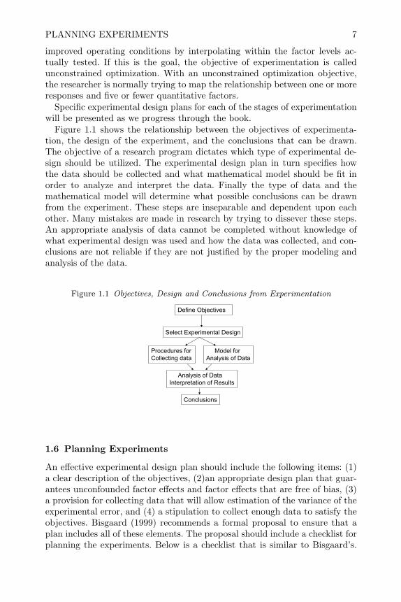
Figure 1.1 shows the relationship between the objectives of experimenta-tion, the design of the experiment, and the conclusions that can be drawn.The objective of a research program dictates which type of experimental de-sign should be utilized. The experimental design plan in turn specifies howthe data should be collected and what mathematical model should be fit inorder to analyze and interpret the data. Finally the type of data and themathematical model will determine what possible conclusions can be drawnfrom the experiment. These steps are inseparable and dependent upon eachother. Many mistakes are made in research by trying to dissever these steps.An appropriate analysis of data cannot be completed without knowledge ofwhat experimental design was used and how the data was collected, and con-clusions are not reliable if they are not justified by the proper modeling andanalysis of the data.
Figure 1.1 Objectives, Design and Conclusions from Experimentation
Define Objectives
Select Experimental Design
Procedures for Collecting data
Model for Analysis of Data
Analysis of DataInterpretation of Results
Conclusions
1.6 Planning Experiments
An effective experimental design plan should include the following items: (1)a clear description of the objectives, (2)an appropriate design plan that guar-antees unconfounded factor effects and factor effects that are free of bias, (3)a provision for collecting data that will allow estimation of the variance of theexperimental error, and (4) a stipulation to collect enough data to satisfy theobjectives. Bisgaard (1999) recommends a formal proposal to ensure that aplan includes all of these elements. The proposal should include a checklist forplanning the experiments. Below is a checklist that is similar to Bisgaard’s.

8 INTRODUCTION
Examples of some of the steps from this checklist will be illustrated in dis-cussing a simple experiment in the next section.
1. Define Objectives. Define the objectives of the study. First, this statementshould answer the question of why is the experiment to be performed.Second, determine if the experiment is conducted to classify sources ofvariability or if its purpose is to study cause and effect relationships. If itis the latter, determine if it is a screening or optimization experiment. Forstudies of cause and effect relationships, decide how large an effect shouldbe in order to be meaningful to detect.
2. Identify Experimental Units. Declare the item upon which something willbe changed. Is it an animal or human subject, raw material for some pro-cessing operation, or simply the conditions that exist at a point in timeor trial? Identifying the experimental units will help in understanding theexperimental error and variance of experimental error.
3. Define a Meaningful and Measurable Response or Dependent Variable. De-fine what characteristic of the experimental units can be measured andrecorded after each run. This characteristic should best represent the ex-pected differences to be caused by changes in the factors.
4. List the Independent and Lurking Variables. Declare which independentvariables you wish to study. Ishikawa Cause and Effect Diagrams (see SASInstitute, 2004b) are often useful at this step to help organize variablesthought to affect the experimental outcome. Be sure that the independentvariables chosen to study can be controlled during a single run, and variedfrom run to run. If there is interest in a variable, but it cannot be controlledor varied, it cannot be included as a factor. Variables that are hypothesizedto affect the response, but cannot be controlled, are lurking variables. Theproper experimental design plan should prevent uncontrollable changes inthese variables from biasing factor effects under study.
5. Run Pilot Tests. Make some pilot tests to be sure you can control and varythe factors that have been selected, that the response can be measured, andthat the replicate measurements of the same or similar experimental unitsare consistent. Inability to measure the response accurately or to control thefactor levels are the main reasons that experiments fail to produce desiredresults. If the pilot tests fail, go back to steps 2, 3 and 4. If these tests aresuccessful, measurements of the response for a few replicate tests with thesame levels of the factors under study will produce data that can be usedto get a preliminary estimate of the variance of experimental error.
6. Make a Flow Diagram of the Experimental Procedure for Each Run Thiswill make sure the procedure to be followed is understood and will bestandardized for all runs in the design.
7. Choose the Experimental Design. Choose an experimental design that issuited for the objectives of your particular experiment. This will include adescription of what factor levels will be studied and will determine how the

PERFORMING THE EXPERIMENTS 9
experimental units are to be assigned to the factor levels or combination offactor levels if there are more than one factor. One of the plans described inthis book will almost always be appropriate. The choice of the experimentaldesign will also determine what model should be used for analysis of thedata.
8. Determine the Number of Replicates Required Based on the expected vari-ance of the experimental error and the size of a practical difference, thenumber of replicate runs that will give the researcher a high probability ofdetecting an effect of practical importance.
9. Randomize the Experimental Conditions to Experimental Units. Accordingto the particular experimental design being used, there is a proscribedmethod of randomly assigning experimental conditions to experimentalunits. The way this is done affects the way the data should be analyzed,and it is important to describe and record what is done. The best way todo this is to provide a data collection worksheet arranged in the randomorder in which the experiments are to be collected. For more complicatedexperimental designs Bisgaard (1999) recommends one sheet of paper de-scribing the conditions of each run with blanks for entering the responsedata and recording observations about the run. All these sheets should thenbe stapled together in booklet form in the order they are to be performed.
10. Describe a Method for Data Analysis. This should be an outline of the stepsof the analysis. An actual analysis of simulated data is often useful to verifythat the proposed outline will work.
11. Timetable and Budget for Resources Needed to Complete the Experiments.Experimentation takes time and having a schedule to adhere to will im-prove the chances of completing the research on time. Bisgaard (1999)recommends a Gantt Chart (see SAS Institute, 2004a) which is a sim-ple graphical display showing the steps of the process as well as calendartimes. A budget should be outlined for expenses and resources that will berequired.
1.7 Performing the Experiments
In experimentation, careful planning and execution of the plan are the mostimportant steps. As we know from Murphy’s Law, if anything can go wrongit will, and analysis of data can never compensate for botched experiments.To illustrate the potential problems that can occur, consider a simple experi-menter conducted by an amateur gardener described by Box et al. (1978). Thepurpose was to determine whether a change in the fertilizer mixture wouldresult in a change in the yield of his tomato plants. Eleven tomato plants wereplanted in a single row, and the fertilizer type (A or B) was varied. The exper-imental unit in this experiment is the tomato plant plus the soil it is plantedin, and the treatment factor is the type of fertilizer applied. Easterling (2004)discusses some of the nuances that should be considered when planning and

10 INTRODUCTION
carrying out such a simple experiment. It is instructive to think about thesein context with the checklist presented in the last section.
When defining the objectives for this experiment, the experimenter needsto think ahead to the possible implications of conclusions that he can draw.In this case, the possible conclusions are (1) deciding that the fertilizer has noeffect on the yield of tomatoes, or (2) concluding that one fertilizer produces agreater yield. If the home gardener finds no difference in yield, he can choose touse the less expensive fertilizer. If he finds a difference, he will have to decideif the increase in yield offsets any increase in cost of the better fertilizer. Thiscan help him determine how large a difference in yield he should look for andthe number of tomato plants he should include in his study. The answer tothis question, which is crucial in planning the experiment, would probably bemuch different for a commercial grower than for a backyard enthusiast.
The experimental units for this experiment were defined in the paragraphabove, but in identifying them, the experimenter should consider the similarityor homogeneity of plants and how far apart he is going to place the tomatoplants in the ground. Will it be far enough that the fertilizer applied to oneplant does not bleed over and affect its neighbors?
Defining a meaningful response that can be measured may be tricky in thisexperiment. Not all the tomatoes on a single plant ripen at the same time.Thus, to measure the yield in terms of weight of tomatoes, the checklist andflow diagram describing how an experiment is conducted must be very precise.Is it the weight of all tomatoes on the plant at a certain date, or the cumulativeweight of tomatoes picked over time as they ripen? Precision in the definitionof the response and consistency in adherence to the definition when makingthe measurements are crucial.
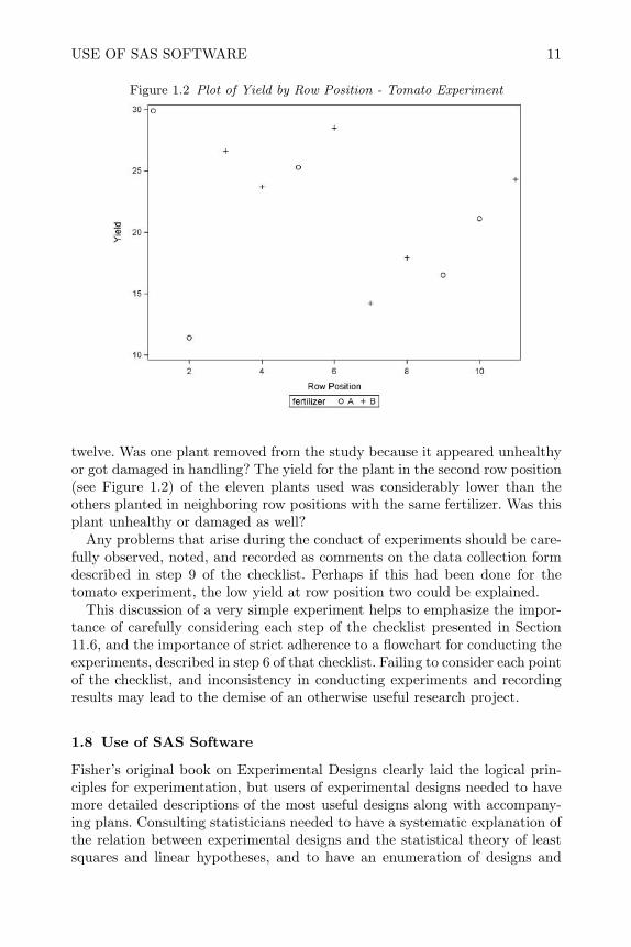
There are many possible lurking variables to consider in this experiment.Any differences in watering, weeding, insect treatment, the method and timingof fertilizer application, and the amount of fertilizer applied may certainlyaffect the yield; hence the experimenter must pay careful attention to thesevariables to prevent bias. Easterling (2004) also pointed out that the rowposition seems to have affected the yield as well (as can be seen in Figure 1.2).The randomization of fertilizers to plants and row positions should equalizethese differences for the two fertilizers. This was one of the things that Boxet al. (1978) illustrated with this example. If a convenient method of applyingthe fertilizers (such as A at the beginning of the row followed by B) hadbeen used in place of random assignment, the row position effect could havebeen mistaken for a treatment effect. Had this row position effect been knownbefore the experiment was planned, the adjacent pairs of plots could have beengrouped together in pairs, and one fertilizer assigned at random to one plot-plant in each pair to prevent bias from the row position effect. This techniqueis called blocking and will be discussed in detail in Chapter 4.
Easterling (2004) also raised the question: why were only eleven plantsused in the study (five fertilized with fertilizer A and six with fertilizer B)?Normally flats of tomato plants purchased from a nursery come in flats of
USE OF SAS SOFTWARE 11
Figure 1.2 Plot of Yield by Row Position - Tomato Experiment
twelve. Was one plant removed from the study because it appeared unhealthyor got damaged in handling? The yield for the plant in the second row position(see Figure 1.2) of the eleven plants used was considerably lower than theothers planted in neighboring row positions with the same fertilizer. Was thisplant unhealthy or damaged as well?
Any problems that arise during the conduct of experiments should be care-fully observed, noted, and recorded as comments on the data collection formdescribed in step 9 of the checklist. Perhaps if this had been done for thetomato experiment, the low yield at row position two could be explained.
This discussion of a very simple experiment helps to emphasize the impor-tance of carefully considering each step of the checklist presented in Section11.6, and the importance of strict adherence to a flowchart for conducting theexperiments, described in step 6 of that checklist. Failing to consider each pointof the checklist, and inconsistency in conducting experiments and recordingresults may lead to the demise of an otherwise useful research project.
1.8 Use of SAS Software
Fisher’s original book on Experimental Designs clearly laid the logical prin-ciples for experimentation, but users of experimental designs needed to havemore detailed descriptions of the most useful designs along with accompany-ing plans. Consulting statisticians needed to have a systematic explanation ofthe relation between experimental designs and the statistical theory of leastsquares and linear hypotheses, and to have an enumeration of designs and

12 INTRODUCTION
descriptions of experimental conditions where each design was most appropri-ate.
These needs were satisfied by Cochran and Cox (1950)’s and Kempthorne(1952)’s books. However, Cochran and Cox and Kempthorne’s books werepublished before the age of computers and they both emphasize extensive ta-bles of designs, abundant formulas and numerical examples describing meth-ods of manual analysis of experimental data and mathematical techniques forconstructing certain types of designs. Since the publication of these books,use of experimental designs has gone far beyond agricultural research whereit was initially employed, and a plethora of new books have been written onthe subject. Even though computers and software (to both design and analyzedata from experiments) are widely available, a high proportion of the morerecent books on experimental design still follow the traditional pattern estab-lished by Cochran and Cox and Kempthorne by presenting extensive tablesof designs and formulas for hand calculations and methods for constructingdesigns.
One of the objectives of this book is to break from the tradition and presentcomputer code and output in place of voluminous formulas and tables. Thiswill leave more room in the text to discuss the appropriateness of various de-sign plans and ways to interpret and present results from experiments. Theparticular computer software illustrated in this book is SAS, which was origi-nally developed in 1972. Its syntax is relatively stable and is widely used. SAShas probably the widest variety of general procedures for design of experi-ments and analysis of experimental data, including proc plan, proc factex,proc optex, and the menu driven SAS ADX for the design of experiments,and proc glm, proc varcomp, proc mixed and many other procedures for theanalysis of experimental data. These procedures are available in the SAS/Statand SAS/QC software.
1.9 Review of Important Concepts
This chapter describes the purpose for experimental designs. In order to de-termine if cause and effect relationships exist, an experimental design must beconducted. In an experimental design, the factors under study are purposelyvaried and the result is observed. This is different from observational stud-ies or sampling surveys where data is collected with no attempt to controlthe environment. In order to predict what will happen in the future, whenthe environment is controlled, you must rely on cause and effect relationships.Relationships obtained from observational studies or sampling surveys are notreliable for predicting future results when the environment is to be controlled.
Experimental designs were first developed in agricultural research, but arenow used in all situations where the scientific method is applied. The ba-sic definitions and terminology used in experimental design are given in thischapter along with a checklist for planning experiments. In practice there aremany different types of experimental designs that can be used. Which design
REVIEW OF IMPORTANT CONCEPTS 13
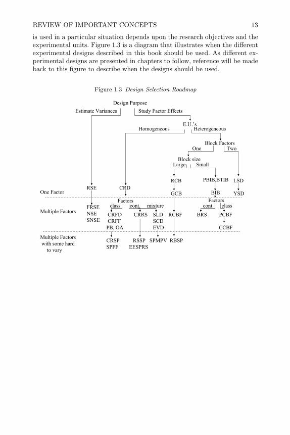
is used in a particular situation depends upon the research objectives and theexperimental units. Figure 1.3 is a diagram that illustrates when the differentexperimental designs described in this book should be used. As different ex-perimental designs are presented in chapters to follow, reference will be madeback to this figure to describe when the designs should be used.
Figure 1.3 Design Selection Roadmap
Design PurposeEstimate Variances Study Factor Effects
E.U.’s
Block Factors
One Factor
Multiple Factors
Multiple Factorswith some hard
to vary
Block size
Homogeneous Heterogeneous
Large Small
RCB
GCB
PBIB,BTIB
BIB
LSD
YSDRSE CRD
FactorsFRSENSESNSE
CRFD CRRS SLD RCBF BRS PCBFCRFF SCD
FBCCDVEAO ,BP
CRSP RSSP SPMPV RBSPSPFF EESPRS
One Two
class cont. mixture cont. classFactors

14 INTRODUCTION
1.10 Exercises
1. A series of runs were performed to determine how the wash water tem-perature and the detergent concentration affect the bacterial count on thepalms of subjects in a hand washing experiment.
(a) Identify the experimental unit.(b) Identify the factors.(c) Identify the response.
2. Explain the difference between an experimental unit and a sub-sample orsub-unit in relation to the experiments described in 1.
3. Explain the difference between a sub-sample and a duplicate in relation tothe experiment described in 1.
4. Describe a situation within your realm of experience (your work, yourhobby, or school) where you might like to predict the result of some futureaction. Explain how an experimental design, rather than an observationalstudy might enhance your ability to make this prediction.
5. Kerry and Bland (1998) describe the analysis of cluster randomized studieswhere a group of subjects are randomized to the same treatment. For ex-ample, when women in some randomly selected districts are offered breastcancer screening while women in other districts are not offered the screen-ing, or when some general practitioners are randomly assigned to receiveone or more courses of special training and the others are not offered thetraining. The response (some characteristic of the patients) in the clus-ter trials must be measured on each patient rather than the group as awhole. What is the experimental unit in this type of study? How wouldyou describe the individual measurements on patients?

CHAPTER 2
Completely Randomized Designs withOne Factor
2.1 Introduction
In a completely randomized design, abbreviated as CRD, with one treatmentfactor, n experimental units are divided randomly into t groups. Each groupis then subject to one of the unique levels or values of the treatment factor.If n = tr is a multiple of t, then each level of the factor will be applied tor unique experimental units, and there will be r replicates of each run withthe same level of the treatment factor. If n is not a multiple of t, then therewill be an unequal number of replicates of each factor level. All other knownindependent variables are held constant so that they will not bias the effects.This design should be used when there is only one factor under study and theexperimental units are homogeneous.
For example, in an experiment to determine the effect of time to rise onthe height of bread dough, one homogeneous batch of bread dough would bedivided into n loaf pans with an equal amount of dough in each. The pansof dough would then be divided randomly into t groups. Each group wouldbe allowed to rise for a unique time, and the height of the risen dough wouldbe measured and recorded for each loaf. The treatment factor would be therise time, the experimental unit would be an individual loaf of bread, andthe response would be the measured height. Although other factors, such astemperature, are known to affect the height of the risen bread dough, theywould be held constant and each loaf would be allowed to rise under the sameconditions except for the differing rise times.
2.2 Replication and Randomization
Replication and randomization were popularized by Fisher. These are thefirst techniques that fall in the category of error control that was explainedin Section 1.4.
The technique of replication dictates that r bread loaves are tested at eachof the t rise times rather than a single loaf at each rise time. By having repli-cate experimental units in each level of the treatment factor, the variance ofthe experimental error can be calculated from the data, and this variance willbe compared to the treatment effects. If the variability among the treatmentmeans is not larger than the experimental error variance, the treatment dif-ferences are probably due to differences of the experimental units assigned to
15
16 COMPLETELY RANDOMIZED DESIGNS WITH ONE FACTOR
each treatment. Without replication it is impossible to tell if treatment differ-ences are real or just a random manifestation of the particular experimentalunits used in the study. Sub-samples or duplicate measurements, described inChapter 1, cannot substitute for replicates.
The random division of experimental units into groups is called random-ization, and it is the procedure by which the validity of the experiment isguaranteed against biases caused by other lurking variables. In the bread riseexperiment randomization would prevent lurking variables, such as variabilityin the yeast from loaf to loaf and trends in the measurement technique overtime, from biasing the effect of the rise time.
When experimental units are randomized to treatment factor levels, anexact test of the hypothesis that the treatment effect is zero can be accom-plished using a randomization test, and a test of parameters in the generallinear model, normally used in the analysis of experimental data, is a goodapproximation to the randomization test.
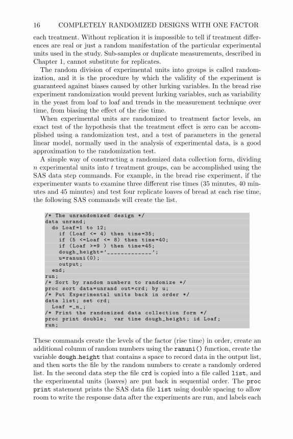
A simple way of constructing a randomized data collection form, dividingn experimental units into t treatment groups, can be accomplished using theSAS data step commands. For example, in the bread rise experiment, if theexperimenter wants to examine three different rise times (35 minutes, 40 min-utes and 45 minutes) and test four replicate loaves of bread at each rise time,the following SAS commands will create the list.
/* The unrandomized design */data unrand;
do Loaf=1 to 12;if (Loaf <= 4) then time =35;if (5 <=Loaf <= 8) then time =40;if (Loaf >=9 ) then time =45;dough_height=’_____________’;u=ranuni (0);output;
end;run;/* Sort by random numbers to randomize */proc sort data=unrand out=crd; by u;/* Put Experimental units back in order */data list; set crd;
Loaf =_n_;/* Print the randomized data collection form */proc print double; var time dough_height; id Loaf;run;
These commands create the levels of the factor (rise time) in order, create anadditional column of random numbers using the ranuni() function, create thevariable dough height that contains a space to record data in the output list,and then sorts the file by the random numbers to create a randomly orderedlist. In the second data step the file crd is copied into a file called list, andthe experimental units (loaves) are put back in sequential order. The procprint statement prints the SAS data file list using double spacing to allowroom to write the response data after the experiments are run, and labels each
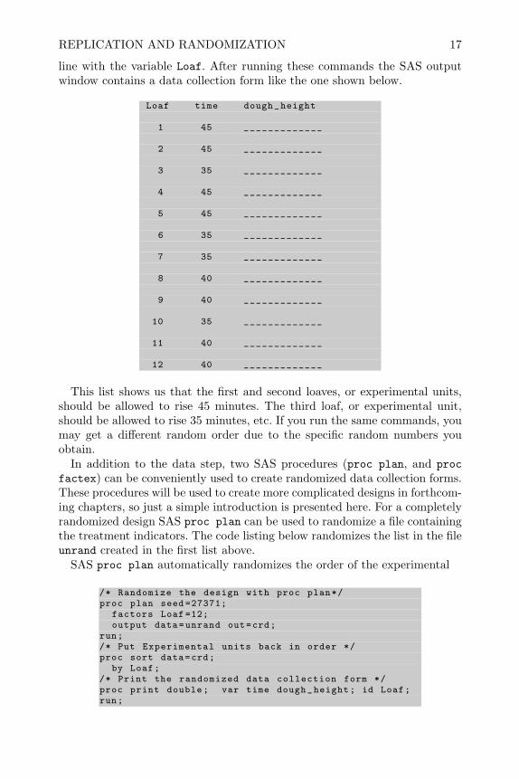
REPLICATION AND RANDOMIZATION 17
line with the variable Loaf. After running these commands the SAS outputwindow contains a data collection form like the one shown below.
Loaf time dough_height
1 45 _____________
2 45 _____________
3 35 _____________
4 45 _____________
5 45 _____________
6 35 _____________
7 35 _____________
8 40 _____________
9 40 _____________
10 35 _____________
11 40 _____________
12 40 _____________
This list shows us that the first and second loaves, or experimental units,should be allowed to rise 45 minutes. The third loaf, or experimental unit,should be allowed to rise 35 minutes, etc. If you run the same commands, youmay get a different random order due to the specific random numbers youobtain.
In addition to the data step, two SAS procedures (proc plan, and procfactex) can be conveniently used to create randomized data collection forms.These procedures will be used to create more complicated designs in forthcom-ing chapters, so just a simple introduction is presented here. For a completelyrandomized design SAS proc plan can be used to randomize a file containingthe treatment indicators. The code listing below randomizes the list in the fileunrand created in the first list above.
SAS proc plan automatically randomizes the order of the experimental
/* Randomize the design with proc plan*/proc plan seed =27371;
factors Loaf =12;output data=unrand out=crd;
run;/* Put Experimental units back in order */proc sort data=crd;
by Loaf;/* Print the randomized data collection form */proc print double; var time dough_height; id Loaf;run;

18 COMPLETELY RANDOMIZED DESIGNS WITH ONE FACTOR
units in the file crd, so no sorting by the random numbers is required. Thesecond data step puts the experimental units back in sequential order so thatthe treatment levels appear randomized in the printed data collection form.
The other alternative is to use proc factex. The lines below call procfactex to create the file crd.
/* Creates CRD in random order using proc factex */proc factex;
factors time/nlev =3;output out=crd time nvals =(35 40 45) designrep =4 randomize;
/* Add experimental unit id and space for response*/data list; set crd;
Loaf =_n_; dough_height=’_____________’;/* Print the data Collection form */proc print double; var time dough_height; id Loaf;run;
This procedure allows one to specify the level values for the factor and ran-domize the order of the list. The designrep=4 specifies that four replicateof each factor level be included in the output file. Alternatively, a random-ized list could be constructed using the =rand() function and the sort menuin an Excel spreadsheet. This would result in an electronic worksheet thatcould additionally be used to record the response data during execution ofthe experiments and later read into SAS for analysis.
2.3 A Historical Example
To illustrate the checklist for planning an experiment, consider a historicalexample taken from the 1937 Rothamstead Experimental Station Report, un-known (1937). This illustrates some of the early work done by Fisher in de-veloping the ideas of experimental design and analysis of variance for use onagricultural experiments at the research station.
Objectives The objective of the study was to compare the times of planting,and methods of applying mixed artificial fertilizers (NPK) prior to planting,on the yield of sugar beets. Normally fertilizer is applied and seeds planted asearly as the soil can be worked.
Experimental Units The experimental units were the plots of ground incombination with specific seeds to be planted in each plot of ground.
Response or Dependent Variable The dependent variable would be theyield of sugar beets measured in cwt per acre.
Independent Variables and Lurking Variables The independent vari-ables of interest were the time and method of applying mixed artificial fertil-izers. Four levels of the treatment factor were chosen as listed below:
1. (A) no artificial fertilizers applied
2. (B) artificials applied in January (plowed)
3. (C) artificials applied in January (broadcast)
4. (D) artificials applied in April (broadcast)

LINEAR MODEL FOR CRD 19
Lurking variables that could cause differences in the sugar beet yields be-tween plots were differences in the fertility of the plots themselves, differencesin the beet seeds used in each plot, differences among plots in the level of weedinfestation, differences in cultivation practices of thinning the beets, and handharvesting the beets.
Pilot Tests Sugar beets had been grown routinely at Rothamstead, andartificial fertilizers had been used by both plowing and broadcast for manycrop plants; therefore, it was known that the independent variable could becontrolled and that the response was measurable.
Choose Experimental Design The completely randomized design (CRD)was chosen so that differences in lurking variables between plots would beunlikely to correspond to changes in the factor levels listed above.
Determine the Number of Replicates A difference in yield of 6 cwtper acre was considered to be of practical importance, and based on histori-cal estimates of variability in sugar beet yields at Rothamstead, four or fivereplicates were determined to be sufficient.
Randomize Experimental Units to Treatment Levels Eighteen plotswere chosen for the experiment, and a randomized list was constructed as-signing four or five plots to each factor level.
2.4 Linear Model for CRD
The mathematical model for the data from a CRD, or completely randomizeddesign, with an unequal number of replicates for each factor level can bewritten as:
Yij = µi + εij (2.1)
where Yij is the response for the jth experimental unit subject to the ith levelof the treatment factor, i = 1, . . . , t, j = 1, . . . , ri and ri is the number ofexperimental units or replications in ith level of the treatment factor.
This is sometimes called the cell means model with a different mean, µi, foreach level of the treatment factor. The distribution of the experimental errors,εij , are mutually independent due to the randomization and assumed to benormally distributed. This model is graphically represented in Figure 2.1.
Figure 2.1 Cell Means Model
1µ 2µ 3µ 4µ

20 COMPLETELY RANDOMIZED DESIGNS WITH ONE FACTOR
An alternate way of writing a model for the data is
Yij = µ+ τi + εij . (2.2)
This is called the effects model and the τis are called the effects. τi repre-sents the difference between the long-run average of all possible experimentsat the ith level of the treatment factor and the overall average. With the nor-mality assumption Yij ∼ N(µ + τi, σ
2) or εij ∼ N(0, σ2). For equal numberof replicates, the sample means of the data in the ith level of the treatmentfactor is represented by
yi· =1ri
ri∑j=1
yij (2.3)
and the grand mean is given by
y·· =1t
t∑i=1
yi· =1n
t∑i=1
ri∑j=1
yij (2.4)
where n =∑ri. Using the method of least squares, the estimates of the cell
means are found by choosing them to minimize the error sum of squares
ssE =t∑i=1
ri∑j=1
(yij − µi)2. (2.5)
This is done by taking partial derivatives of ssE with respect to each cellmean, setting the results equal to zero, and solving each equation
∂ssE
∂µi= −2
t∑i=1
ri∑j=1
(yij − µi) = 0.
This results in the estimates:
µi = yi·.
2.4.1 Matrix Representation
Consider a CRD with t = 3 factor levels and ri = 4 replicates for i = 1, . . . , t.We can write the effects model concisely using matrix notation as:
y = Xβ + ε (2.6)
.
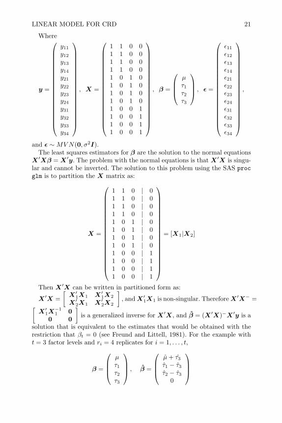
LINEAR MODEL FOR CRD 21
Where
y =
y11
y12
y13
y14
y21
y22
y23
y24
y31
y32
y33
y34
, X =
1 1 0 01 1 0 01 1 0 01 1 0 01 0 1 01 0 1 01 0 1 01 0 1 01 0 0 11 0 0 11 0 0 11 0 0 1
, β =
µτ1τ2τ3
, ε =
ε11
ε12
ε13
ε14
ε21
ε22
ε23
ε24
ε31
ε32
ε33
ε34
,
and ε ∼MVN(0, σ2I).The least squares estimators for β are the solution to the normal equations
X ′Xβ = X ′y. The problem with the normal equations is that X ′X is singu-lar and cannot be inverted. The solution to this problem using the SAS procglm is to partition the X matrix as:
X =
1 1 0 | 01 1 0 | 01 1 0 | 01 1 0 | 01 0 1 | 01 0 1 | 01 0 1 | 01 0 1 | 01 0 0 | 11 0 0 | 11 0 0 | 11 0 0 | 1
= [X1|X2]
Then X ′X can be written in partitioned form as:
X ′X =[X ′1X1 X ′1X2
X ′2X1 X ′2X2
], andX ′1X1 is non-singular. ThereforeX ′X− =[
X ′1X−11 0
0 0
]is a generalized inverse for X ′X, and β = (X ′X)−X ′y is a
solution that is equivalent to the estimates that would be obtained with therestriction that βt = 0 (see Freund and Littell, 1981). For the example witht = 3 factor levels and ri = 4 replicates for i = 1, . . . , t,
β =
µτ1τ2τ3
, β =
µ+ τ3τ1 − τ3τ2 − τ3
0

22 COMPLETELY RANDOMIZED DESIGNS WITH ONE FACTOR
2.4.2 L.S. Calculations with SAS proc glm
Table 2.1 shows the data from a CRD design for the bread rise experimentdescribed earlier in this chapter.
Table 2.1 Data from Bread Rise Experiment
Rise Time Loaf Heights35 minutes 4.5, 5.0, 5.5, 6.7540 minutes 6.5, 6.5, 10.5, 9.545 minutes 9.75, 8.75, 6.5, 8.25
Using these data we have
X ′X =
12 4 4 44 4 0 04 0 4 04 0 0 4
, X ′y =
88.021.7533.033.25
,
and
X ′X− =
0.25 −0.25 −0.25 0−0.25 0.50 0.25 0−0.25 0.25 0.50 0
0 0 0 0
, β = (X ′X)−X ′y =
8.3125−2.8750−0.06250.0000
.
The SAS commands to read in this data and compute these estimates are:
/* Reads the data from compact list */data bread;
input time h1-h4;height=h1; output;height=h2; output;height=h3; output;height=h4; output;keep time height;
datalines;35 4.5 5.0 5.5 6.7540 6.5 6.5 10.5 9.545 9.75 8.75 6.5 8.25run;/* Fits model with proc glm */proc glm;
class time;model height=time/solution;
run;
These commands read the data in a compact format, like Table 2.1, thenuse the output statement to create four lines in the file, bread, for each linein the input records. The result of the model /solution; option is:

LINEAR MODEL FOR CRD 23
Parameter Estimate
Intercept 8.312500000 Btime 35 -2.875000000 Btime 40 -0.062500000 Btime 45 0.000000000 B
We can see the estimates are the same as those shown above. These pa-rameter estimates are not unique because they depend on the ordering of theclass variable time. proc glm recognizes this and designates the estimates asbiased by following each value with a B.
2.4.3 Estimation of σ2 and distribution of quadratic forms
The estimate of the variance of the experimental error, σ2, is ssE/(n−t). It isonly possible to estimate this variance when there are replicate experiments ateach level of the treatment factor. When measurements on sub-samples or du-plicate measurements on the same experimental unit are treated as replicates,this estimate can be seriously biased.
In matrix form, ssE can be written as
ssE = y′y − β′X′y = y′(I −X(X′X)−X′)y,
and from the theory of linear models it can be shown that the ratio of ssEto the variance of the experimental error, σ2, follows a chi-square distributionwith n− t degrees of freedom, i.e., ssE/σ2 ∼ χ2
n−t.
2.4.4 Estimable Functions
A linear combination of the cell means is called an estimable function if it canbe expressed as the expected value of a linear combination of the responses,i.e.,
t∑i=1
bi(µ+ τi) = E
t∑i=1
ri∑j=1
aijYij
(2.7)
From this definition it can be seen that effects, τi, are not estimable, but acell mean, µ+τi, or a contrast of effects,
∑ciτi, where
∑ci = 0, is estimable.
In matrix notation Lβ is a set of estimable functions if each row of L is a lin-ear combination of the rows ofX, and Lβ is its unbiased estimator. Lβ followsthe multivariate normal distribution with covariance matrix σ2L′(X′X)−L,and the estimator of the covariance matrix is σ2L′(X′X)−L. For exampleusing the data from the bread rise experiment above,
L =(
0 1 −1 00 1 0 −1
). (2.8)
Lβ =(τ1 − τ2τ1 − τ3
), and Lβ =
(τ1 − τ2τ1 − τ3
)=(−2.8025−2.8750
)is a vector

24 COMPLETELY RANDOMIZED DESIGNS WITH ONE FACTOR
of contrasts of the effects. The number of degrees of freedom, or number oflinearly independent contrasts of effects in a CRD, is always the number oflevels of the treatment factor minus one, i.e., t− 1. Whenever there is a set oft− 1 linearly independent contrasts of the effects, they are called a saturatedset of estimable contrasts.
It can be shown that (Lβ)′(L(X′X)−L′)−1(Lβ) follows the noncentralchi-square distribution, χ2(p, λ) where the noncentrality parameter
λ = (σ2)−1(Lβ)′(L(X′X)−L′)−1(Lβ),
and L is the coefficient matrix for an estimable contrast like (2.8), and thedegrees of freedom p is equal to the rank of L.
Estimable contrasts can be obtained from SAS proc glm using the estimatecommand. For example to estimate the average difference in the cell means forthe first and second levels of the treatment factor, (µ+τ1)−(µ+τ2) = τ1−τ2,use the command:
estimate ’1 - 2’ time 1 -1;
where the string in quotes is the label to be used in the output, temp isthe name of the treatment factor, and the numbers 1 -1 are the contrastcoefficients, ci. The command:
estimate ’1 -2 -3’ time 1 -1 -1;
would produce no output and in the log file the message “1 -2 -3 is notestimable” would be printed, since
∑ci 6= 0.
2.4.5 Hypothesis Test of No Treatment Effects
In the model for the CRD, the statistical hypothesis of interest is H0 : µ1 =µ2 = . . . µt or τ1 = τ2 = . . . = τt versus the alternative Ha : at least twoof the τs differ. If the null hypothesis is true, the model yij = µi + εij =µ + τi + εij simplifies to yij = µ + εij which can be represented as a singlenormal distribution with mean µ and variance σ2 rather than multiple normaldistributions like those shown in Figure 2.1.
The sums of squares about the mean is ssTotal =∑ti=1
∑rij=1(yij − y··)2 =
y′y − (1′y)2/(1′1), where y·· is the grand mean and 1 is a column vector of1s. This sum of squares can be partitioned as:
ssTotal = ssT + ssE (2.9)
where ssT = β′X′y − (1′y)2/(1′1) = (Lβ)′(L(X′X)−L′)−1(Lβ), and L isthe coefficient matrix for a saturated set of estimable contrasts. This quantityis called the treatment sums of squares. Under the null hypothesis H0 : µ1 =µ2 = . . . µt, both ssT and ssE follow the chi-squared distribution. Thesesums of squares and their corresponding mean squares, which are formed bydividing each sum of squares by its degrees of freedom, are usually presented
LINEAR MODEL FOR CRD 25
in an Analysis of Variance or ANOVA table like that shown symbolically inTable 2.2.
Table 2.2 Analysis of Variance Table
Source df Sum of Squares Mean Squares F-ratioTreatment t− 1 ssT msT F = msT/msEError n− t ssE msETotal n− 1 ssTotal msTotal
Under the null hypothesis, the F-ratio msT/msE follows the F-distributionwith t − 1 and n − t degrees of freedom, and under the alternative it followsthe non-central F distribution with noncentrality parameter
λ = (σ2)−1(Lβ)′(L(X′X)−L′)−1(Lβ) =r
σ2
t∑i=1
(µi − µ·)2.
It is the generalized likelihood ratio test statistic for H0, and is the formalmethod of comparing the treatment effects to the experimental error variancedescribed in Section 2.2.
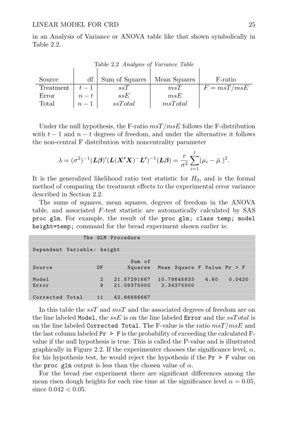
The sums of squares, mean squares, degrees of freedom in the ANOVAtable, and associated F -test statistic are automatically calculated by SASproc glm. For example, the result of the proc glm; class temp; modelheight=temp; command for the bread experiment shown earlier is:
The GLM Procedure
Dependent Variable: height
Sum ofSource DF Squares Mean Square F Value Pr > F
Model 2 21.57291667 10.78645833 4.60 0.0420Error 9 21.09375000 2.34375000
Corrected Total 11 42.66666667
In this table the ssT and msT and the associated degrees of freedom are onthe line labeled Model, the ssE is on the line labeled Error and the ssTotal ison the line labeled Corrected Total. The F-value is the ratio msT/msE andthe last column labeled Pr > F is the probability of exceeding the calculated F-value if the null hypothesis is true. This is called the P-value and is illustratedgraphically in Figure 2.2. If the experimenter chooses the significance level, α,for his hypothesis test, he would reject the hypothesis if the Pr > F value onthe proc glm output is less than the chosen value of α.
For the bread rise experiment there are significant differences among themean risen dough heights for each rise time at the significance level α = 0.05,since 0.042 < 0.05.

26 COMPLETELY RANDOMIZED DESIGNS WITH ONE FACTOR
Figure 2.2 Pr > F
9,2F
60.4== msEmsTF
042.0)6.4Pr( 9,2 =>F
2.4.6 A Word of Caution
When a completely randomized design in one factor is conducted, the modelfor analysis is Equation (2.1) or (2.2) and the correct analysis is through theanalysis of variance as shown symbolically in Table 2.2. The use of computersoftware like SAS makes it easy to analyze data and draw conclusions; however,if the experiment was not properly conducted even a sophisticated analysisof the data could be useless. The εij term in the model (2.1) or (2.2), andits associated sums of squares, ssE, represents replicate experimental units.In many cases experimenters do not have replicate experimental units in eachlevel of the treatment factor and substitute sub-samples or duplicates forthem in the analysis. In other cases the experimental units are not properlyrandomized to treatment factor levels. When this is the situation, performingthe analysis as if the design had been properly conducted may be completelywrong and misleading. Wrong conclusions can be drawn that do not hold upto later scrutiny, and a bad reputation is unfairly ascribed to statisticallydesigned experiments and statistical analyses of data.
For example, consider an experiment where a professor would like to de-termine the effect of teaching methods on student test scores. If he uses oneteaching method for the morning class, another for his evening class, and treatstest scores for individual students as replicates, the results of his analysis maybe totally wrong. This situation is similar to the cluster randomized studiesdescribed in exercise 5 of Chapter 1. The experimental unit is the class, sincehe applied the teaching method to a whole class simultaneously, and the in-dividual students are sub-samples or observational units (since he must testindividual students, not the class as a whole). The treatment effect should bejudged against the variability in experimental units or classes. The variabilityamong students in a class may be much different than variability from class

VERIFYING ASSUMPTIONS OF THE LINEAR MODEL 27
average to class average. Sub-sample observations should be averaged beforeanalysis, as explained in Section 1.3. If this were done, he would only have oneobservation per class per teaching method and no replicates for use in calcu-lating ssE in Table 2.2. There is no denominator for calculating the F -teststatistic for teaching method. If he uses the variability in students within aclass to calculate ssE, it may be too large or too small, causing him to reachthe wrong conclusion about significance of the treatment effect. Further, ifhe did not randomize which teaching method was used in the morning andevening classes, and if he has no replicate classes that were taught with thesame teaching method, his analysis is wide open to biases. Students in themorning classes may be fundamentally different than students in the eveningclasses, and any difference in average scores between the two teaching methodsmay be entirely due to differences among the two groups of students. In fact,if the professor knows there are differences in morning and evening students,he may purposely use the teaching method he wants to promote on the betterclass, thus ruining the objectivity of his research.
2.5 Verifying Assumptions of the Linear Model
The most critical assumption justifying the analysis based on the linear modelpresented in the last section is independence of the experimental error termsεij . This assumption is justified if proper randomization of the experimentalunits to treatment factor levels has been performed. No further steps areneeded to justify this assumption.
The other two assumptions for the linear model are constancy of the vari-ance of the experimental error, σ2, across all levels of the treatment factor,and normality of the experimental errors. Both of these assumptions can bevisualized in Figure 2.1.
To verify the equal variance assumption, a simple scatter plot of the responsedata versus the factor levels can be constructed. Figure 2.3 shows an exampleof this type plot for the bread rise experiment. In this plot, similarity in therange of variability in dough heights between the different levels of rise timewould justify the assumption of equal variance.
This figure was created in SAS using the commands:
proc sgplot data=bread;scatter y=Height x=Time;
run;
A similar plot that is used to check the equality of variance assumption is aplot of the residuals versus the cell means, or predicted values. The residualsare the differences of the response data and their respective cell means. Themean residual, for each level of the treatment factor, is zero. Therefore, in aplot of residuals it is easier to visualize whether the scatter or variability isequal. A common departure from equal variance occurs when the variance ofthe experimental errors increases as the mean response increases. By plotting
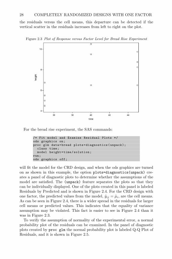
28 COMPLETELY RANDOMIZED DESIGNS WITH ONE FACTOR
the residuals versus the cell means, this departure can be detected if thevertical scatter in the residuals increases from left to right on the plot.
Figure 2.3 Plot of Response versus Factor Level for Bread Rise Experiment
For the bread rise experiment, the SAS commands:
/* Fit model and Examine Residual Plots */ods graphics on;proc glm data=bread plots=diagnostics(unpack);
class time;model height=time/solution;
run;ods graphics off;
will fit the model for the CRD design, and when the ods graphics are turnedon as shown in this example, the option plots=diagnostics(unpack) cre-ates a panel of diagnostic plots to determine whether the assumptions of themodel are satisfied. The (unpack) feature separates the plots so that theycan be individually displayed. One of the plots created in this panel is labeledResiduals by Predicted and is shown in Figure 2.4. For the CRD design withone factor, the predicted values from the model, yij = µi, are the cell means.As can be seen in Figure 2.4, there is a wider spread in the residuals for largercell means or predicted values. This indicates that the equality of varianceassumption may be violated. This fact is easier to see in Figure 2.4 than itwas in Figure 2.3.
To verify the assumption of normality of the experimental error, a normalprobability plot of the residuals can be examined. In the panel of diagnosticplots created by proc glm the normal probability plot is labeled Q-Q Plot ofResiduals, and it is shown in Figure 2.5.
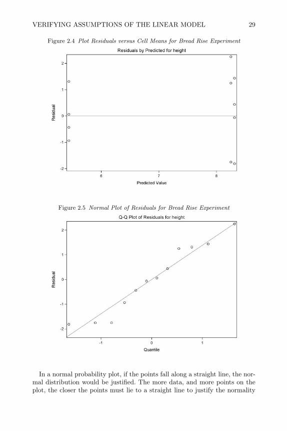
VERIFYING ASSUMPTIONS OF THE LINEAR MODEL 29
Figure 2.4 Plot Residuals versus Cell Means for Bread Rise Experiment
Figure 2.5 Normal Plot of Residuals for Bread Rise Experiment
In a normal probability plot, if the points fall along a straight line, the nor-mal distribution would be justified. The more data, and more points on theplot, the closer the points must lie to a straight line to justify the normality
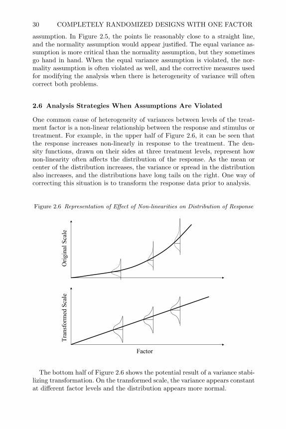
30 COMPLETELY RANDOMIZED DESIGNS WITH ONE FACTOR
assumption. In Figure 2.5, the points lie reasonably close to a straight line,and the normality assumption would appear justified. The equal variance as-sumption is more critical than the normality assumption, but they sometimesgo hand in hand. When the equal variance assumption is violated, the nor-mality assumption is often violated as well, and the corrective measures usedfor modifying the analysis when there is heterogeneity of variance will oftencorrect both problems.
2.6 Analysis Strategies When Assumptions Are Violated
One common cause of heterogeneity of variances between levels of the treat-ment factor is a non-linear relationship between the response and stimulus ortreatment. For example, in the upper half of Figure 2.6, it can be seen thatthe response increases non-linearly in response to the treatment. The den-sity functions, drawn on their sides at three treatment levels, represent hownon-linearity often affects the distribution of the response. As the mean orcenter of the distribution increases, the variance or spread in the distributionalso increases, and the distributions have long tails on the right. One way ofcorrecting this situation is to transform the response data prior to analysis.
Figure 2.6 Representation of Effect of Non-linearities on Distribution of Response
Orig
inal
Sca
leTr
ansf
orm
ed S
cale
Factor
The bottom half of Figure 2.6 shows the potential result of a variance stabi-lizing transformation. On the transformed scale, the variance appears constantat different factor levels and the distribution appears more normal.
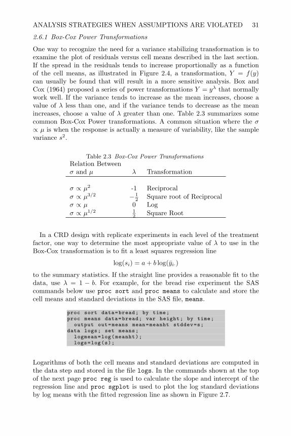
ANALYSIS STRATEGIES WHEN ASSUMPTIONS ARE VIOLATED 31
2.6.1 Box-Cox Power Transformations
One way to recognize the need for a variance stabilizing transformation is toexamine the plot of residuals versus cell means described in the last section.If the spread in the residuals tends to increase proportionally as a functionof the cell means, as illustrated in Figure 2.4, a transformation, Y = f(y)can usually be found that will result in a more sensitive analysis. Box andCox (1964) proposed a series of power transformations Y = yλ that normallywork well. If the variance tends to increase as the mean increases, choose avalue of λ less than one, and if the variance tends to decrease as the meanincreases, choose a value of λ greater than one. Table 2.3 summarizes somecommon Box-Cox Power transformations. A common situation where the σ∝ µ is when the response is actually a measure of variability, like the samplevariance s2.
Table 2.3 Box-Cox Power TransformationsRelation Betweenσ and µ λ Transformation
σ ∝ µ2 -1 Reciprocalσ ∝ µ3/2 − 1
2 Square root of Reciprocalσ ∝ µ 0 Logσ ∝ µ1/2 1
2 Square Root
In a CRD design with replicate experiments in each level of the treatmentfactor, one way to determine the most appropriate value of λ to use in theBox-Cox transformation is to fit a least squares regression line
log(si) = a+ b log(yi·)
to the summary statistics. If the straight line provides a reasonable fit to thedata, use λ = 1 − b. For example, for the bread rise experiment the SAScommands below use proc sort and proc means to calculate and store thecell means and standard deviations in the SAS file, means.
proc sort data=bread; by time;proc means data=bread; var height; by time;
output out=means mean=meanht stddev=s;data logs; set means;
logmean=log(meanht);logs=log(s);
Logarithms of both the cell means and standard deviations are computed inthe data step and stored in the file logs. In the commands shown at the topof the next page proc reg is used to calculate the slope and intercept of theregression line and proc sgplot is used to plot the log standard deviationsby log means with the fitted regression line as shown in Figure 2.7.
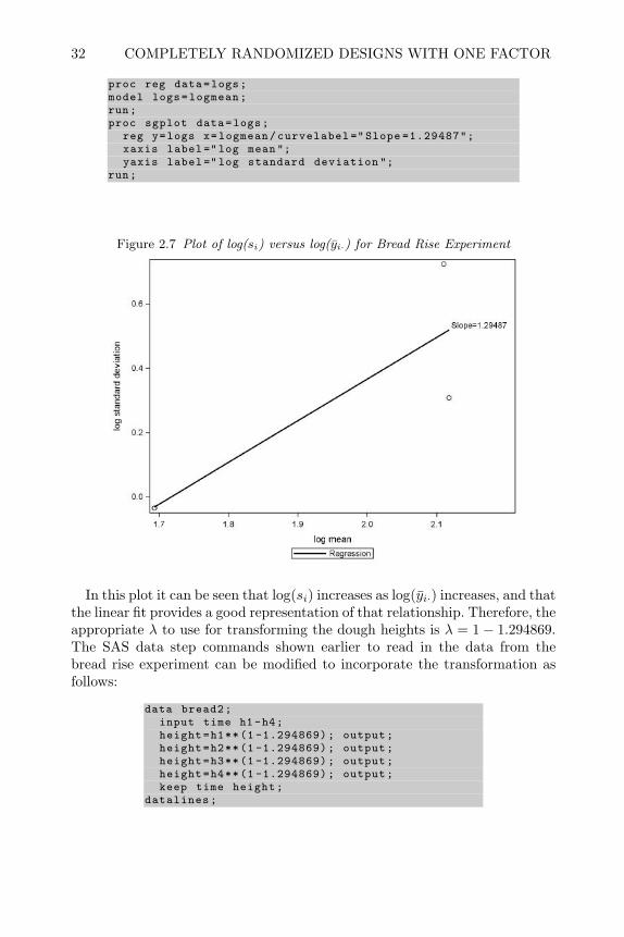
32 COMPLETELY RANDOMIZED DESIGNS WITH ONE FACTOR
proc reg data=logs;model logs=logmean;run;proc sgplot data=logs;
reg y=logs x=logmean/curvelabel =" Slope =1.29487";xaxis label="log mean";yaxis label="log standard deviation ";
run;
Figure 2.7 Plot of log(si) versus log(yi·) for Bread Rise Experiment
In this plot it can be seen that log(si) increases as log(yi·) increases, and thatthe linear fit provides a good representation of that relationship. Therefore, theappropriate λ to use for transforming the dough heights is λ = 1− 1.294869.The SAS data step commands shown earlier to read in the data from thebread rise experiment can be modified to incorporate the transformation asfollows:
data bread2;input time h1-h4;height=h1**(1 -1.294869); output;height=h2**(1 -1.294869); output;height=h3**(1 -1.294869); output;height=h4**(1 -1.294869); output;keep time height;
datalines;
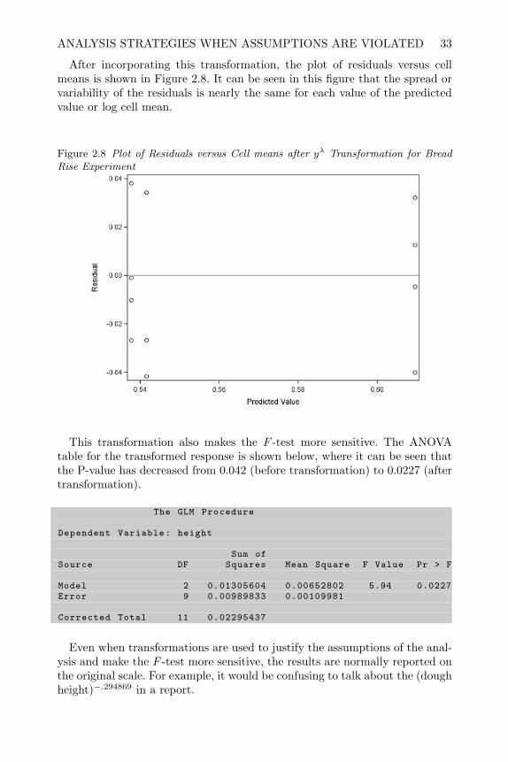
ANALYSIS STRATEGIES WHEN ASSUMPTIONS ARE VIOLATED 33
After incorporating this transformation, the plot of residuals versus cellmeans is shown in Figure 2.8. It can be seen in this figure that the spread orvariability of the residuals is nearly the same for each value of the predictedvalue or log cell mean.
Figure 2.8 Plot of Residuals versus Cell means after yλ Transformation for BreadRise Experiment
This transformation also makes the F -test more sensitive. The ANOVAtable for the transformed response is shown below, where it can be seen thatthe P-value has decreased from 0.042 (before transformation) to 0.0227 (aftertransformation).
The GLM Procedure
Dependent Variable: height
Sum ofSource DF Squares Mean Square F Value Pr > F
Model 2 0.01305604 0.00652802 5.94 0.0227Error 9 0.00989833 0.00109981
Corrected Total 11 0.02295437
Even when transformations are used to justify the assumptions of the anal-ysis and make the F -test more sensitive, the results are normally reported onthe original scale. For example, it would be confusing to talk about the (doughheight)−.294869 in a report.

34 COMPLETELY RANDOMIZED DESIGNS WITH ONE FACTOR
2.6.2 Distribution-Based Transformations
The distribution assumption for the effects model for the CRD described inSection 2.3, was Yij ∼ N(µ + τi, σ
2). However, if it is known that the datafollow some distribution other than the normal distribution, such as the Bi-nomial, Poisson or Lognormal, then it would also be known that the stan-dard deviation would not be constant. For example, if the response, Y , wasa binomial count of the number of successes in n trials, then due to the cen-tral limit theorem, Y would be approximately normal, but µY = np andσY =
√np(1− p), where p is the probability of success. In situations like this
where the distribution of the response is known to follow some specific form,then an appropriate transformation can be found to stabilize the variance.Table 2.4 shows the transformation for common situations often encountered.
Table 2.4 Response Distribution-Based Transformations
Variance in TransformationResponse Distribution Terms of Mean µ f(y)
Binomial µ(1−µ)n sin−1
√y/n (radians)
Poisson µ√y or
√y + 1
2
Lognormal cµ2 log(y)
2.6.3 Alternatives to Least Squares Analysis
When the variance of the experimental error is not constant for all levelsof the treatment factor, but it is not related to the cell means, a trans-formation will not be an appropriate way of equalizing or stabilizing thevariances. A more general solution to the problem is to use weighted leastsquares. Using weighted least squares, β is the solution to the normal equa-tions X′WXβ = X′Wy, where W is a diagonal matrix whose diagonalelements are the reciprocals of the standard deviation within each treatmentlevel. As an illustration of this method, consider the SAS commands, at thetop of the next page, for analyzing the data from the bread rise experiment.
As in the previous examples, the data is read in the same way. The sort andmeans procedures calculate the cell standard deviations and the next datastep merges these with the original data and computes the weights, w, thatare the reciprocals of the standard deviations. The weight statement, in theproc glm call, solves the weighted least squares normal equations. The resultsappear below the commands.
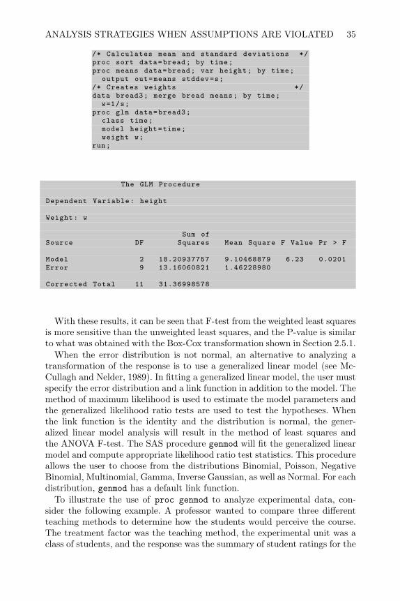
ANALYSIS STRATEGIES WHEN ASSUMPTIONS ARE VIOLATED 35
/* Calculates mean and standard deviations */proc sort data=bread; by time;proc means data=bread; var height; by time;
output out=means stddev=s;/* Creates weights */data bread3; merge bread means; by time;
w=1/s;proc glm data=bread3;
class time;model height=time;weight w;
run;
The GLM Procedure
Dependent Variable: height
Weight: w
Sum ofSource DF Squares Mean Square F Value Pr > F
Model 2 18.20937757 9.10468879 6.23 0.0201Error 9 13.16060821 1.46228980
Corrected Total 11 31.36998578
With these results, it can be seen that F-test from the weighted least squaresis more sensitive than the unweighted least squares, and the P-value is similarto what was obtained with the Box-Cox transformation shown in Section 2.5.1.
When the error distribution is not normal, an alternative to analyzing atransformation of the response is to use a generalized linear model (see Mc-Cullagh and Nelder, 1989). In fitting a generalized linear model, the user mustspecify the error distribution and a link function in addition to the model. Themethod of maximum likelihood is used to estimate the model parameters andthe generalized likelihood ratio tests are used to test the hypotheses. Whenthe link function is the identity and the distribution is normal, the gener-alized linear model analysis will result in the method of least squares andthe ANOVA F-test. The SAS procedure genmod will fit the generalized linearmodel and compute appropriate likelihood ratio test statistics. This procedureallows the user to choose from the distributions Binomial, Poisson, NegativeBinomial, Multinomial, Gamma, Inverse Gaussian, as well as Normal. For eachdistribution, genmod has a default link function.
To illustrate the use of proc genmod to analyze experimental data, con-sider the following example. A professor wanted to compare three differentteaching methods to determine how the students would perceive the course.The treatment factor was the teaching method, the experimental unit was aclass of students, and the response was the summary of student ratings for the
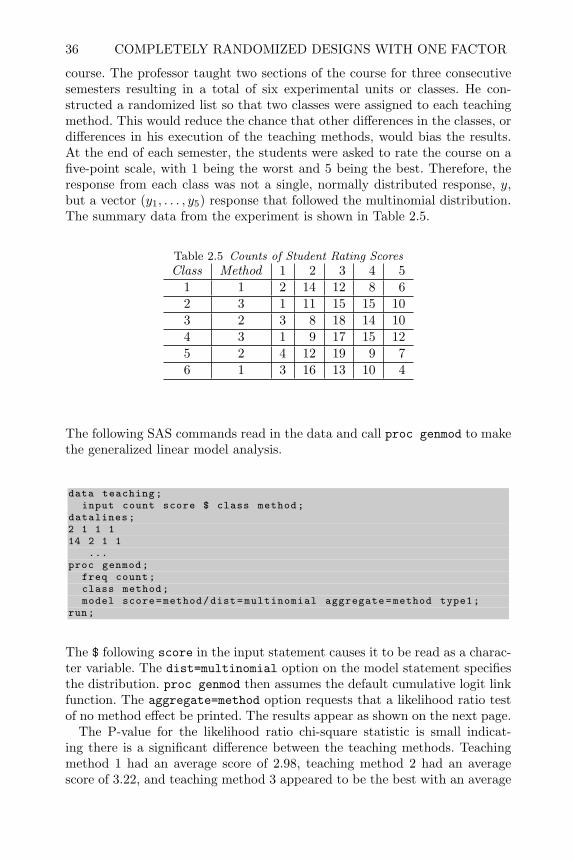
36 COMPLETELY RANDOMIZED DESIGNS WITH ONE FACTOR
course. The professor taught two sections of the course for three consecutivesemesters resulting in a total of six experimental units or classes. He con-structed a randomized list so that two classes were assigned to each teachingmethod. This would reduce the chance that other differences in the classes, ordifferences in his execution of the teaching methods, would bias the results.At the end of each semester, the students were asked to rate the course on afive-point scale, with 1 being the worst and 5 being the best. Therefore, theresponse from each class was not a single, normally distributed response, y,but a vector (y1, . . . , y5) response that followed the multinomial distribution.The summary data from the experiment is shown in Table 2.5.
Table 2.5 Counts of Student Rating ScoresClass Method 1 2 3 4 5
1 1 2 14 12 8 62 3 1 11 15 15 103 2 3 8 18 14 104 3 1 9 17 15 125 2 4 12 19 9 76 1 3 16 13 10 4
The following SAS commands read in the data and call proc genmod to makethe generalized linear model analysis.
data teaching;input count score $ class method;
datalines;2 1 1 114 2 1 1
...proc genmod;
freq count;class method;model score=method/dist=multinomial aggregate=method type1;
run;
The $ following score in the input statement causes it to be read as a charac-ter variable. The dist=multinomial option on the model statement specifiesthe distribution. proc genmod then assumes the default cumulative logit linkfunction. The aggregate=method option requests that a likelihood ratio testof no method effect be printed. The results appear as shown on the next page.
The P-value for the likelihood ratio chi-square statistic is small indicat-ing there is a significant difference between the teaching methods. Teachingmethod 1 had an average score of 2.98, teaching method 2 had an averagescore of 3.22, and teaching method 3 appeared to be the best with an average
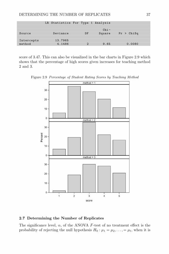
DETERMINING THE NUMBER OF REPLICATES 37
LR Statistics For Type 1 Analysis
Chi -Source Deviance DF Square Pr > ChiSq
Intercepts 13.7965method 4.1486 2 9.65 0.0080
score of 3.47. This can also be visualized in the bar charts in Figure 2.9 whichshows that the percentage of high scores given increases for teaching method2 and 3.
Figure 2.9 Percentage of Student Rating Scores by Teaching Method
2.7 Determining the Number of Replicates
The significance level, α, of the ANOVA F -test of no treatment effect is theprobability of rejecting the null hypothesis H0 : µ1 = µ2, . . . ,= µt, when it is
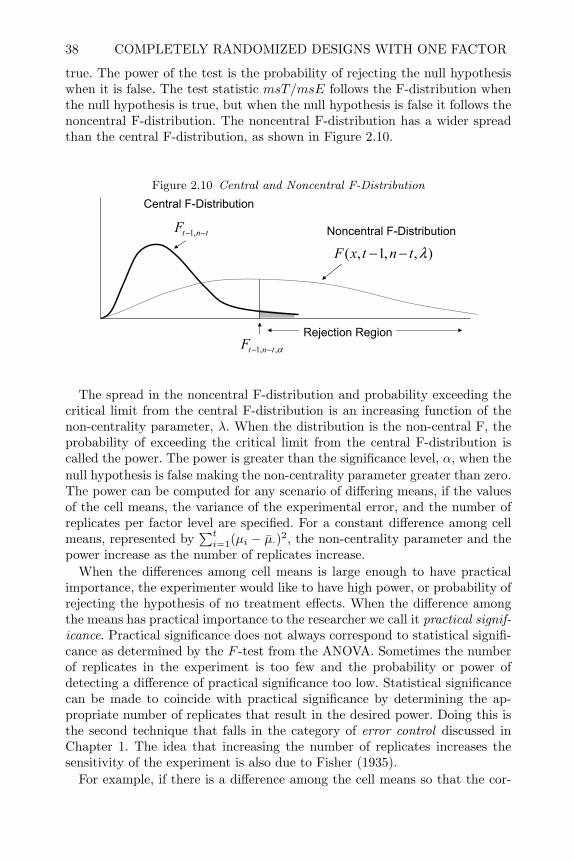
38 COMPLETELY RANDOMIZED DESIGNS WITH ONE FACTOR
true. The power of the test is the probability of rejecting the null hypothesiswhen it is false. The test statistic msT/msE follows the F-distribution whenthe null hypothesis is true, but when the null hypothesis is false it follows thenoncentral F-distribution. The noncentral F-distribution has a wider spreadthan the central F-distribution, as shown in Figure 2.10.
Figure 2.10 Central and Noncentral F-Distribution
tntF −− ,1
),,1,( λtntxF −−
α,,1 tntF −−
Central F-Distribution
Noncentral F-Distribution
Rejection Region
The spread in the noncentral F-distribution and probability exceeding thecritical limit from the central F-distribution is an increasing function of thenon-centrality parameter, λ. When the distribution is the non-central F, theprobability of exceeding the critical limit from the central F-distribution iscalled the power. The power is greater than the significance level, α, when thenull hypothesis is false making the non-centrality parameter greater than zero.The power can be computed for any scenario of differing means, if the valuesof the cell means, the variance of the experimental error, and the number ofreplicates per factor level are specified. For a constant difference among cellmeans, represented by
∑ti=1(µi − µ·)2, the non-centrality parameter and the
power increase as the number of replicates increase.When the differences among cell means is large enough to have practical
importance, the experimenter would like to have high power, or probability ofrejecting the hypothesis of no treatment effects. When the difference amongthe means has practical importance to the researcher we call it practical signif-icance. Practical significance does not always correspond to statistical signifi-cance as determined by the F -test from the ANOVA. Sometimes the numberof replicates in the experiment is too few and the probability or power ofdetecting a difference of practical significance too low. Statistical significancecan be made to coincide with practical significance by determining the ap-propriate number of replicates that result in the desired power. Doing this isthe second technique that falls in the category of error control discussed inChapter 1. The idea that increasing the number of replicates increases thesensitivity of the experiment is also due to Fisher (1935).
For example, if there is a difference among the cell means so that the cor-

DETERMINING THE NUMBER OF REPLICATES 39
rected sum of squares (css =∑ti=1(µi − µ·)2) is greater than zero, then the
power or probability of rejecting H0 : µ1 = µ2, . . . ,= µt is given by
π(λ) =∫ ∞Ft−1,t(r−1),α
F (x, t− 1, t(r − 1), λ)dx (2.10)
where Ft−1,t(r−1),α is the αth percentile of the central F distribution witht− 1 and t(r− 1) degrees of freedom, F (x, t− 1, t(r− 1), λ) is the noncentralF-distribution with non-centrality parameter λ = r
σ2
∑ti=1(µi − µ·)2. For a
fixed value of 1σ2
∑ti=1(µi− µ·)2, the non-centrality parameter, and the power
increase as a function of the number of replicates, r. This probability can becalculated for various values of r until a value is found with adequate power. Inthis way the appropriate number of replicates can be determined. The fprobfunction in SAS facilitates these computations.
In the bread rise experiment, suppose less than a three-inch difference inrisen dough heights is of no consequence. However, if changing the rise timefrom 35 minutes to 45 minutes causes a difference of more than three inchesin risen dough height, the experimenter would like to know about it, becausehe will need to monitor rise time closely in the future to produce loaves ofconsistent height. In this case we can regard ∆ = 3.0 as a practical differencein cell means. The smallest css =
∑ti=1(µi − µ·)2 could be, with at least two
cell means differing by ∆, would the case when one cell mean was ∆/2 higherthan the grand mean, a second was ∆/2 less than the grand mean, and a thirdwas equal to the grand mean. This would result in
css =t∑i=1
(µi − µ·)2 =(
∆2
)2
+ 02 +(−∆
2
)2
=(
∆2
2
)=(
32
2
)= 4.5
Assuming the variance of the experimental error σ2 = 2.1 was estimated fromthe sample variance in risen dough heights in a pilot experiment where severalloaves were allowed to rise for the same length of time, then the noncentralityfactor can be calculated as λ = r
2.1 × (4.5). The power is calculated for r =2, . . . , 6 using the SAS data step commands shown at the top of the next page.

40 COMPLETELY RANDOMIZED DESIGNS WITH ONE FACTOR
*Example power computation in SAS data step using Bread Example;data Power;do r=2 to 6;
nu1=3-1; * df for numerator;nu2=3*(r-1); * df for denomonator;alpha =.05;Fcrit=finv(1-alpha ,nu1 ,nu2); *F critical value;sigma2 =2.1;css =4.5;nc=r*(css)/sigma2;*noncentrality parameter for noncentral F;power=1-probf(Fcrit ,nu1 ,nu2 ,nc);output;
end;keep r nu1 nu2 nc power;title Power Calculation in Data Step;proc print; run;
Below are the results.
Power Calculation in Data Step
Obs r nu1 nu2 nc power1 2 2 3 4.2857 0.194802 3 2 6 6.4286 0.404193 4 2 9 8.5714 0.590344 5 2 12 10.7143 0.732895 6 2 15 12.8571 0.83299
From this we can see that with r = 5 replicates there would be a 73% chanceof detecting a difference in cell means as large as 3.0, and with r = 6 there is a83% chance. With fewer than five replicates there is at least a 40% chance thisdifference will be missed. As a rule of thumb, the number of replicates that re-sult in power between 0.80 and 0.90 is usually sufficient for most experimentalstudies.
A similar power calculation can be accomplished with the SAS AnalystSample Size tool for the One Way ANOVA, with proc power, with the procglmpower, or with the SAS Power and Sample Size Application. The interac-tive input for the SAS Analyst Sample Size tool is similar to the data stepcommands above, and the css =
∑ti=1(µi − µ·)2, must be specified. SAS
Analyst will no longer be available after SAS version 9.2.The SAS proc power, proc glmpower procedure, and the SAS Power and
Sample Size Application require the user to enter the values of the cell means,µi, that he believes exhibit a practical significance rather than the css =∑ti=1(µi − µ·)2, and σ rather than σ2. The following commands will pro-
duce an equivalent result to the data step commands above for the bread riseexperiment using proc power.

COMPARISON OF TREATMENTS AFTER THE F -TEST 41
* Eample Power Calculation Using proc power;proc power;
OneWayANOVAAlpha = 0.05GroupMeans = (-1.5 0 1.5)StdDev = 1.449Power = .NPerGroup = 2 to 6 by 1;
run;
proc glmpower allows for more complicated models and will be illustratedin Chapter 3. The SAS Power and Sample Size Application is accessed by StartI Programs I SAS I SAS Power and Sample Size I SAS Power and Sample Size3.1(or the latest release). It provides a GUI interface for proc power and procglmpower.
2.8 Comparison of Treatments after the F -Test
When the F -test for the null hypothesis H0 : µ1 = µ2 = . . . µt is rejected,it tells us that there are significant differences between at least two of thecell means, but if there are several levels of the treatment factor, it doesnot necessarily mean that all cell means are significantly different from eachother. When the null hypothesis is rejected, further investigation should beconducted to find out exactly which cell means differ. In some cases the in-vestigator will have preplanned comparisons he would like to make; in othersituations he may have no idea what differences to look for.
2.8.1 Preplanned Comparisons
Considering the treatment factor levels in the sugar beet yield experiment con-ducted at Rothamstead in 1937 and described in Section 2.3, some preplannedcomparisons that might have been of interest are:1. H0 : µ1 = 1
3 (µ2 + µ3 + µ4)2. H0 : µ2 = µ3
3. H0 : µ3 = µ4
The first comparison asks the question: Does a mix of artificial fertilizerschange yield? The second comparison asks the question: Is there a differencein yields between plowed and broadcast application of artificial fertilizer? Thethird comparison asks the question: Does timing of the application change theyield?
These hypotheses can all be expressed in the general form H0 :∑ti=1 ciµi =
0, where∑ti=1 ci = 0. Since
∑ti=1 ciµi = 0 are estimable functions, each of
these hypotheses can be tested by computing the single estimable function Lβand its standard error sLβ =
√σ2L′(X′X)−L. The ratio of the estimable
function to its standard error follows the t-distribution. The estimate com-mand in SAS proc glm performs this test. For the sugar beet experiment thecommands on the next page produce the output that follows the commands.
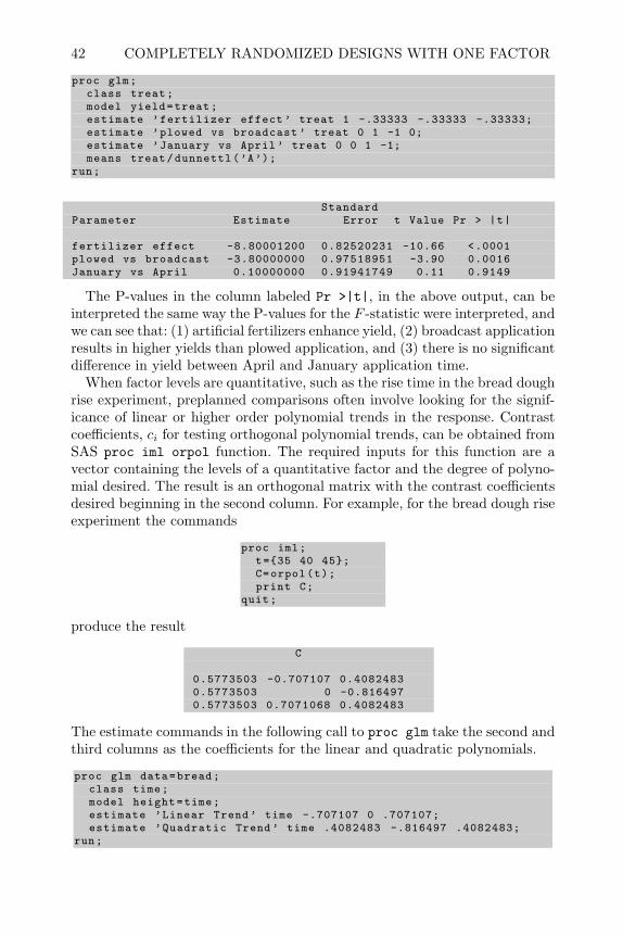
42 COMPLETELY RANDOMIZED DESIGNS WITH ONE FACTOR
proc glm;class treat;model yield=treat;estimate ’fertilizer effect ’ treat 1 -.33333 -.33333 -.33333;estimate ’plowed vs broadcast ’ treat 0 1 -1 0;estimate ’January vs April’ treat 0 0 1 -1;means treat/dunnettl(’A’);
run;
StandardParameter Estimate Error t Value Pr > |t|
fertilizer effect -8.80001200 0.82520231 -10.66 <.0001plowed vs broadcast -3.80000000 0.97518951 -3.90 0.0016January vs April 0.10000000 0.91941749 0.11 0.9149
The P-values in the column labeled Pr >|t|, in the above output, can beinterpreted the same way the P-values for the F -statistic were interpreted, andwe can see that: (1) artificial fertilizers enhance yield, (2) broadcast applicationresults in higher yields than plowed application, and (3) there is no significantdifference in yield between April and January application time.
When factor levels are quantitative, such as the rise time in the bread doughrise experiment, preplanned comparisons often involve looking for the signif-icance of linear or higher order polynomial trends in the response. Contrastcoefficients, ci for testing orthogonal polynomial trends, can be obtained fromSAS proc iml orpol function. The required inputs for this function are avector containing the levels of a quantitative factor and the degree of polyno-mial desired. The result is an orthogonal matrix with the contrast coefficientsdesired beginning in the second column. For example, for the bread dough riseexperiment the commands
proc iml;t=35 40 45;C=orpol(t);print C;
quit;
produce the result
C
0.5773503 -0.707107 0.40824830.5773503 0 -0.8164970.5773503 0.7071068 0.4082483
The estimate commands in the following call to proc glm take the second andthird columns as the coefficients for the linear and quadratic polynomials.
proc glm data=bread;class time;model height=time;estimate ’Linear Trend ’ time -.707107 0 .707107;estimate ’Quadratic Trend’ time .4082483 -.816497 .4082483;
run;
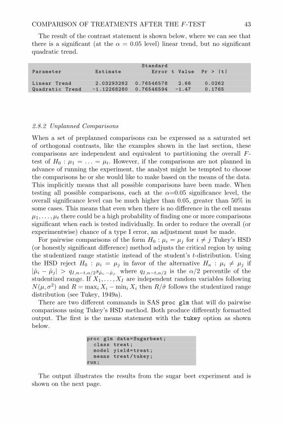
COMPARISON OF TREATMENTS AFTER THE F -TEST 43
The result of the contrast statement is shown below, where we can see thatthere is a significant (at the α = 0.05 level) linear trend, but no significantquadratic trend.
StandardParameter Estimate Error t Value Pr > |t|
Linear Trend 2.03293262 0.76546578 2.66 0.0262Quadratic Trend -1.12268280 0.76546594 -1.47 0.1765
2.8.2 Unplanned Comparisons
When a set of preplanned comparisons can be expressed as a saturated setof orthogonal contrasts, like the examples shown in the last section, thesecomparisons are independent and equivalent to partitioning the overall F -test of H0 : µ1 = . . . = µt. However, if the comparisons are not planned inadvance of running the experiment, the analyst might be tempted to choosethe comparisons he or she would like to make based on the means of the data.This implicitly means that all possible comparisons have been made. Whentesting all possible comparisons, each at the α=0.05 significance level, theoverall significance level can be much higher than 0.05, greater than 50% insome cases. This means that even when there is no difference in the cell meansµ1, . . . , µt there could be a high probability of finding one or more comparisonssignificant when each is tested individually. In order to reduce the overall (orexperimentwise) chance of a type I error, an adjustment must be made.
For pairwise comparisons of the form H0 : µi = µj for i 6= j Tukey’s HSD(or honestly significant difference) method adjusts the critical region by usingthe studentized range statistic instead of the student’s t-distribution. Usingthe HSD reject H0 : µi = µj in favor of the alternative Ha : µi 6= µj if|µi − µj | > qI,n−t,α/2sµi·−µj· where qI,n−t,α/2 is the α/2 percentile of thestudentized range. If X1, . . . , XI are independent random variables followingN(µ, σ2) and R = maxiXi −miniXi then R/σ follows the studentized rangedistribution (see Tukey, 1949a).
There are two different commands in SAS proc glm that will do pairwisecomparisons using Tukey’s HSD method. Both produce differently formattedoutput. The first is the means statement with the tukey option as shownbelow.
proc glm data=Sugarbeet;class treat;model yield=treat;means treat/tukey;
run;
The output illustrates the results from the sugar beet experiment and isshown on the next page.
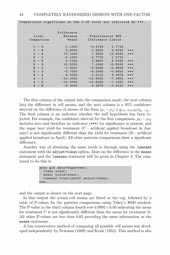
44 COMPLETELY RANDOMIZED DESIGNS WITH ONE FACTOR
Comparisons significant at the 0.05 level are indicated by ***.
Differencetreat Between Simultaneous 95%
Comparison Means Confidence Limits
C - D 0.1000 -2.5723 2.7723C - B 3.8000 0.9655 6.6345 ***C - A 10.1000 7.2655 12.9345 ***D - C -0.1000 -2.7723 2.5723D - B 3.7000 0.8655 6.5345 ***D - A 10.0000 7.1655 12.8345 ***B - C -3.8000 -6.6345 -0.9655 ***B - D -3.7000 -6.5345 -0.8655 ***B - A 6.3000 3.3122 9.2878 ***A - C -10.1000 -12.9345 -7.2655 ***A - D -10.0000 -12.8345 -7.1655 ***A - B -6.3000 -9.2878 -3.3122 ***
The first column of the output lists the comparison made, the next columnlists the difference in cell means, and the next column is a 95% confidenceinterval on the difference of means of the form |µi − µj | ± qI,n−t,0.025sµi·−µj· .The final column is an indicator whether the null hypothesis has been re-jected. For example, the confidence interval for the first comparison, µC −µDincludes zero and therefore no indicator (***) for significance is present, andthe sugar beet yield for treatment (C - artificial applied broadcast in Jan-uary) is not significantly different than the yield for treatment (D - artificialapplied broadcast in April). All other pairwise comparisons show a significantdifference.
Another way of obtaining the same result is through using the lsmeansstatement with the adjust=tukey option. More on the difference in the meansstatement and the lsmeans statement will be given in Chapter 3. The com-mand to do this is:
proc glm data=Sugarbeet;class treat;model yield=treat;lsmeans treat/pdiff adjust=tukey;
run;
and the output is shown on the next page.In this output the actual cell means are listed at the top, followed by a
table of P-values for the pairwise comparisons using Tukey’s HSD method.The P-value in the third column fourth row 0.9995>.0.05 indicating the meanfor treatment C is not significantly different than the mean for treatment D.All other P-values are less than 0.05 providing the same information as themeans statement.
A less conservative method of comparing all possible cell means was devel-oped independently by Newman (1939) and Keuls (1952). This method is also
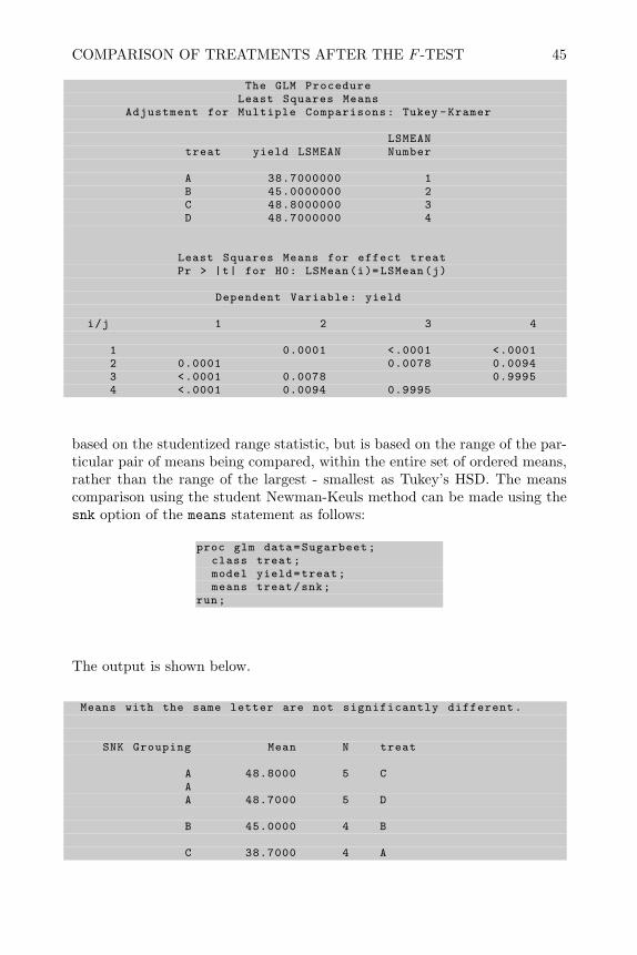
COMPARISON OF TREATMENTS AFTER THE F -TEST 45
The GLM ProcedureLeast Squares Means
Adjustment for Multiple Comparisons: Tukey -Kramer
LSMEANtreat yield LSMEAN Number
A 38.7000000 1B 45.0000000 2C 48.8000000 3D 48.7000000 4
Least Squares Means for effect treatPr > |t| for H0: LSMean(i)= LSMean(j)
Dependent Variable: yield
i/j 1 2 3 4
1 0.0001 <.0001 <.00012 0.0001 0.0078 0.00943 <.0001 0.0078 0.99954 <.0001 0.0094 0.9995
based on the studentized range statistic, but is based on the range of the par-ticular pair of means being compared, within the entire set of ordered means,rather than the range of the largest - smallest as Tukey’s HSD. The meanscomparison using the student Newman-Keuls method can be made using thesnk option of the means statement as follows:
proc glm data=Sugarbeet;class treat;model yield=treat;means treat/snk;
run;
The output is shown below.
Means with the same letter are not significantly different.
SNK Grouping Mean N treat
A 48.8000 5 CAA 48.7000 5 D
B 45.0000 4 B
C 38.7000 4 A
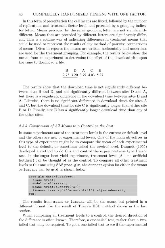
46 COMPLETELY RANDOMIZED DESIGNS WITH ONE FACTOR
In this form of presentation the cell means are listed, followed by the numberof replications and treatment factor level, and preceded by a grouping indica-tor letter. Means preceded by the same grouping letter are not significantlydifferent. Means that are preceded by different letters are significantly differ-ent. This is a concise way of indicating differences in treatment means thatcould be used to represent the results of any method of pairwise comparisonsof means. Often in reports the means are written horizontally and underlinesare used for the treatment grouping. For example, the results below show themeans from an experiment to determine the effect of the download site uponthe time to download a file.
B D A C E2.73 3.20 3.79 4.03 5.27
The results show that the download time is not significantly different be-tween sites B and D, and not significantly different between sites D and A,but there is a significant difference in the download time between sites B andA. Likewise, there is no significant difference in download times for sites Aand C, but the download time for site C is significantly longer than either siteB or D. Finally, site E has a significantly longer download time than any ofthe other sites.
2.8.3 Comparison of All Means to a Control or the Best
In some experiments one of the treatment levels is the current or default leveland the others are new or experimental levels. One of the main objectives inthis type of experiment might be to compare the mean of each experimentallevel to the default, or sometimes called the control level. Dunnett (1955)developed a method to do this and control the experimentwise type I errorrate. In the sugar beet yield experiment, treatment level (A - no artificialfertilizer) can be thought of as the control. To compare all other treatmentlevels to this one using SAS proc glm, the dunnett option for either the meansor lsmeans can be used as shown below.
proc glm data=Sugarbeet;class treat;model yield=treat;means treat/dunnett(’A’);lsmeans treat/pdiff=control(’A’) adjust=dunnett;
run;
The results from means or lsmeans will be the same, but printed in adifferent format like the result of Tukey’s HSD method shown in the lastsection.
When comparing all treatment levels to a control, the desired direction ofthe difference is often known. Therefore, a one-tailed test, rather than a two-tailed test, may be required. To get a one-tailed test to see if the experimental

COMPARISON OF TREATMENTS AFTER THE F -TEST 47
means are larger than the control means, change the means statement aboveto means treat/dunnettu(’A’); This will give a one-sided lower confidencebound on the difference in means (experimental-control). If the lower bound isgreater than zero, the experimental mean is significantly higher than the con-trol mean. The same result can be obtained from the lsmeans by changing thecommand to lsmeans treat/pdiff=controlu(’A’) cl adjust=dunnett;.To get a one-sided test of whether the experimental means are less than thecontrol, change dunnettu to dunnettl in the means statement or controlu(’A’)to controll(’A’) in the lsmeans statements.
When there is no control level of the treatment factor, there may still beinterest in comparing all treatment levels to the best level. For example in anexperiment to see the effect of the download site on the time to download afile, it may be of interest to find those sites whose download times are notsignificantly higher than the site with the minimum observed mean downloadtime. To compare all treatment levels to the observed best level and to controlthe experimentwise error rate, the MCB procedure (Hsu, 1984) turns out tobe equivalent to Dunnett’s procedure. Look at the observed cell means in thedata, determine which is the best, label the best as the control level, and usethe dunnett option. For example, in the means for the experiment to comparedownload times for different download sites shown at the end of Section 2.8.2,site B had the shortest observed download time. To compare all other sites toB use the command:
proc glm;class site;model dtime=site;means site/dunnett(’B’);
run;
Those sites that are not significantly different from B can be considered to bea subset of sites that have the fastest download times.

48 COMPLETELY RANDOMIZED DESIGNS WITH ONE FACTOR
2.9 Review of Important Concepts
In order to determine if cause and effect relationships exist and to make pre-dictions about the results of future actions, experiments must be performedwherein certain factors are purposely varied while others are held constant.The one factor design is the simplest case where one factor is varied while allother known factors are held constant.
Figure 2.11 shows a roadmap for selecting an appropriate experimentaldesign. When there is only one factor under study and experimental unitsare homogeneous, the CRD design should be used as indicated in black in thefigure. This is the only situation presented in Chapter 2. As additional designsare presented in subsequent chapters the other branches in Figure 2.10 willbe explained.
Figure 2.11 Design Selection Roadmap
Design PurposeEstimate Variances Study Factor Effects
E.U.’s
Block Factors
One Factor
Multiple Factors
Multiple Factorswith some hard
to vary
Block size
Homogeneous Heterogeneous
Large Small
RCB
GCB
PBIB,BTIB
BIB
LSD
YSDRSE CRD
FactorsFRSENSESNSE
CRFD CRRS SLD RCBF BRS PCBFCRFF SCD
PB, OA EVD CCBF
CRSP RSSP SPMPV RBSPSPFF EESPRS
One Two
class cont. mixture cont. classFactors
Fisher’s technique of randomizing experimental units to treatment levelsguarantees the long run validity of the CRD and minimizes the chance thatchanges in unknown factors or lurking variables from biasing the results. Theway a series of experiments is conducted dictates what model should be usedfor analysis.
The model for the analysis of the CRD or completely randomized for onefactor design is yij = µi + εij or yij = µ + τi + εij , where yij is the observedresponse for the jth replicate of the ith treatment level, µi is the cell mean

REVIEW OF IMPORTANT CONCEPTS 49
for the ith level, and τi is the effect. εij is the experimental error for thejth observation on treatment level i. εijs are assumed to be independent andnormally distributed with constant variance σ2. The typical analysis is to fitthe linear model by the method of least squares - maximum likelihood andperform a likelihood ratio F -test of the H0 : µ1 = . . . = µt. If the data werenot collected in a proper randomized design with replicates, analyzing data inthis way may be totally misleading.
The credibility of the conclusions of analysis depends on the degree to whichthe assumptions are valid. The independence assumption is the most criticaland it is guaranteed when replicate experimental units are randomized totreatment factor levels. The other assumptions should be checked. The con-stant variance and normality assumptions can be checked by plotting theresiduals versus cell means and by making a normal probability plot of theresiduals. If these assumptions are violated, the data should be analyzed ona transformed scale or by weighted least squares or the method of maximumlikelihood for the generalized linear model.
If a significant difference in cell means is found with the overall F -test, fur-ther investigation of the differences can be made. If comparisons are plannedin advance of running the experiment and can be described by as set of or-thogonal comparisons, the overall F -test can be partitioned to test these com-parisons. The experimentwise type I error rate for all possible comparisonsof means can be controlled by using Tukey’s HSD or the less conservativestudent Newman-Keuls method. For comparing all means to a control level,Dunnett’s method should be used and for comparing all means to the best(largest or smallest), Hsu’s MCB method should be used.

50 COMPLETELY RANDOMIZED DESIGNS WITH ONE FACTOR
2.10 Exercises
1. Consider the simple experiment described in Section 2.1 and used through-out this chapter to determine the effect of rise time on the height of breaddough. Describe the steps in the planning process for this experiment sim-ilar to what was done for this historical example in Section 2.3. Describesome of the potential problems that could occur in performing these exper-iments (similar to Section 1.7), and discuss how careful planning using thechecklist from Chapter 1 could prevent these problems.
2. Paper helicopters can be cut from one half of an 8 12 × 11 sheet of paper as
shown below.
CU
T
FOLD
4.25”
FOL
D
CUT
4”
These helicopters can be made quickly and inexpensively, and can be usedto demonstrate experimental design concepts. An experiment can be per-formed by constructing a helicopter, dropping it from a fixed height, andclocking the time it takes to rotate to the floor, as shown below, with astopwatch. The wing length could be varied by trimming some paper offthe top prior to folding the wings. Trimming some paper off would reducethe weight of the helicopter, but would also result in less surface area onthe blades. You could experiment to determine if changing the wing lengthaffects the flight time.
(a) Describe the experimental unit.(b) Explain the difference in replicates and duplicates for this situation.(c) Describe the treatment factor.(d) Describe any lurking variables that might affect the results of experi-
ments.(e) Explain why randomization would be important.

EXERCISES 51
(f) Create a randomized list of experiments for examining four wing lengthsof (4”, 4.75”, 5.5” and 6”) with eight replicate experiments in each level.
(g) Carry out the experiments and collect the data.(h) Perform an analysis of variance with your data.(i) Check the equal variance and normality assumptions with residual plots.(j) Test whether there is a significant linear or quadratic trend in flight
times as the wing length increases.
3. In Section 2.8.2 an experiment for determining the effect of the downloadsite selected upon the time to download a file was discussed. In this exper-iment:
(a) Describe the experimental unit.(b) Describe the treatment factor.(c) Describe the response.(d) Discuss the causes for experimental error in this experiment and why
the principles of replication and randomization would be important inreaching a valid conclusion.
4. In an experiment to study the effect of the amount of baking powder ina biscuit dough upon the rise heights of the biscuits, four levels of bakingpowder were tested and four replicate biscuits were made with each levelin a random order. The results are shown in the table below.
.25 tsp .5 tsp .75 tsp 1 tsp11.4 27.8 47.6 61.611.0 29.2 47.0 62.411.3 26.8 47.3 63.09.5 26.0 45.5 63.9
(a) What is the experimental unit?(b) Perform the Analysis of Variance to test the hypothesis of no treatment
effect.(c) Formulate a contrast to test the hypothesis that increase in rise height
is proportional to the increase in baking powder in the dough and testthis hypothesis.
(d) Estimate the variance of the experimental error σ2.(e) Make a plot of residuals versus predicted values and normal plot of
residuals and comment on whether the assumptions of the linear modelare justified.
(f) If the dough were made in batches and the four replicate biscuit riseheights in each column (shown in the table above) were all from thesame batch, would your answer to (a) be different? How could the databe analyzed if this were the case?
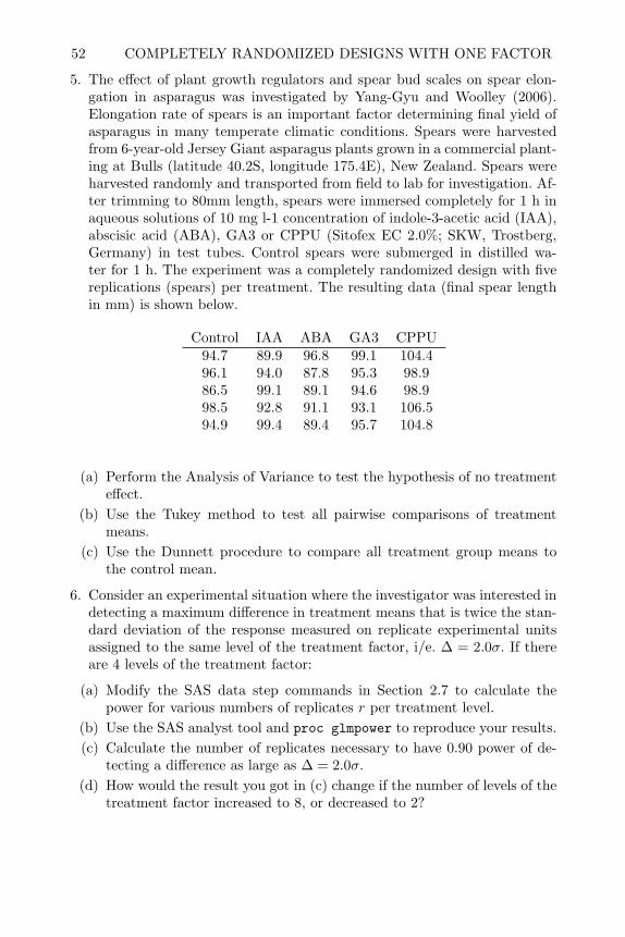
52 COMPLETELY RANDOMIZED DESIGNS WITH ONE FACTOR
5. The effect of plant growth regulators and spear bud scales on spear elon-gation in asparagus was investigated by Yang-Gyu and Woolley (2006).Elongation rate of spears is an important factor determining final yield ofasparagus in many temperate climatic conditions. Spears were harvestedfrom 6-year-old Jersey Giant asparagus plants grown in a commercial plant-ing at Bulls (latitude 40.2S, longitude 175.4E), New Zealand. Spears wereharvested randomly and transported from field to lab for investigation. Af-ter trimming to 80mm length, spears were immersed completely for 1 h inaqueous solutions of 10 mg l-1 concentration of indole-3-acetic acid (IAA),abscisic acid (ABA), GA3 or CPPU (Sitofex EC 2.0%; SKW, Trostberg,Germany) in test tubes. Control spears were submerged in distilled wa-ter for 1 h. The experiment was a completely randomized design with fivereplications (spears) per treatment. The resulting data (final spear lengthin mm) is shown below.
Control IAA ABA GA3 CPPU94.7 89.9 96.8 99.1 104.496.1 94.0 87.8 95.3 98.986.5 99.1 89.1 94.6 98.998.5 92.8 91.1 93.1 106.594.9 99.4 89.4 95.7 104.8
(a) Perform the Analysis of Variance to test the hypothesis of no treatmenteffect.
(b) Use the Tukey method to test all pairwise comparisons of treatmentmeans.
(c) Use the Dunnett procedure to compare all treatment group means tothe control mean.
6. Consider an experimental situation where the investigator was interested indetecting a maximum difference in treatment means that is twice the stan-dard deviation of the response measured on replicate experimental unitsassigned to the same level of the treatment factor, i/e. ∆ = 2.0σ. If thereare 4 levels of the treatment factor:
(a) Modify the SAS data step commands in Section 2.7 to calculate thepower for various numbers of replicates r per treatment level.
(b) Use the SAS analyst tool and proc glmpower to reproduce your results.(c) Calculate the number of replicates necessary to have 0.90 power of de-
tecting a difference as large as ∆ = 2.0σ.(d) How would the result you got in (c) change if the number of levels of the
treatment factor increased to 8, or decreased to 2?

CHAPTER 3
Factorial Designs
3.1 Introduction
In Chapter 2 we examined one-factor designs. These are useful only when onefactor is under study. When multiple factors are under study, one classicalapproach is to study each separately while holding all others constant. Fisher(1935) pointed out that this approach is useful for demonstrating known rela-tionships to students in laboratory courses where the influence of other factorsis known, but it is both inefficient and potentially misleading when it comesto discovering new knowledge through experimentation. A much better strat-egy for experimenting with multiple factors is to use a factorial design. In afactorial design the cells consist of all possible combinations of the levels ofthe factors under study. Factorial designs accentuate the factor effects, allowfor estimation of interdependency of effects (or interactions) and are the firsttechnique in the category of what is called treatment design.
By examining all possible combinations of factor levels, the number of repli-cates of a specific level of one factor is increased by the product of the numberof levels of all other factors in the design, and thus the same power or precisioncan be obtained with fewer replicates. In addition, if the effect of one factorchanges depending on the level of another factor, it will be seen in a factorialplan. This phenomenon will be missed in the classical approach where eachfactor is only varied at constant levels of the other factors. The example inthe next section will illustrate these facts.
3.2 Classical One at a Time versus Factorial Plans
In the exercises for Chapter 2, a set of experiments with paper helicopterswas described. In those experiments only one factor, the wing length, wasunder study. However, to maximize the flight time of paper helicopters, itwould be advisable to consider more than one factor. For example, considervarying wing length over 4 levels as before, and the body width over four levels,such as 4.25”, 4.0”, 3.75” and 3.5”. The left side of Figure 3.1 represents theclassical plan in which one factor is varied at a time. The circles in the diagramrepresent experiments or runs. Using this approach, the experiments acrossthe bottom of the figure would be completed by varying wing length whileholding body width constant at 3.5”. Next, the three additional experimentsup the left side of the figure would be completed by varying body width whileholding the wing length constant at its low level of 4.0”. If eight replicate runs
53
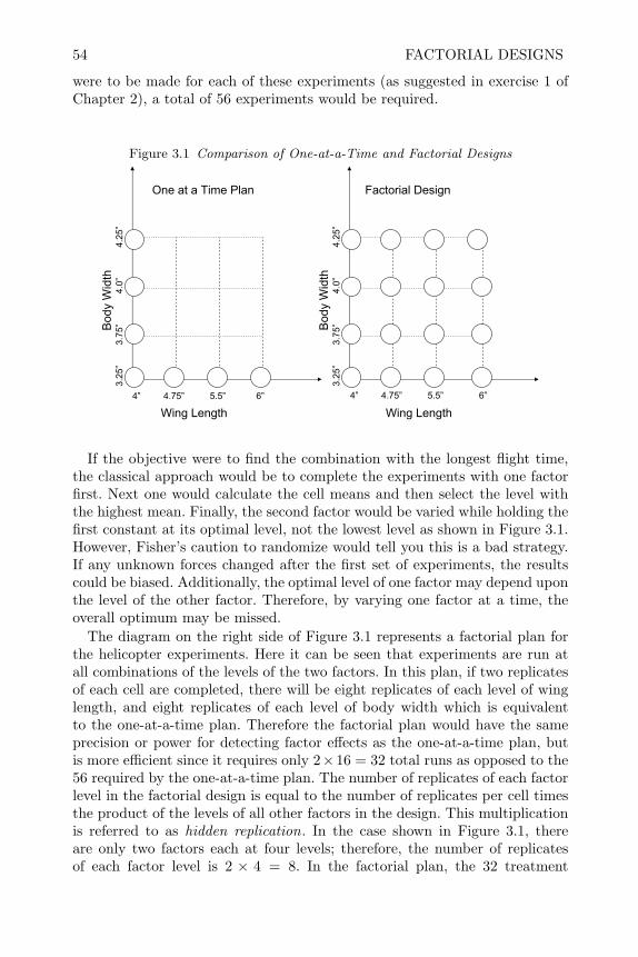
54 FACTORIAL DESIGNS
were to be made for each of these experiments (as suggested in exercise 1 ofChapter 2), a total of 56 experiments would be required.
Figure 3.1 Comparison of One-at-a-Time and Factorial Designs
One at a Time Plan Factorial Design
htgneL gniWhtgneL gniW
Bod
y W
idth
3.25
”3.
75”
4.0”
4.25
”
4” 4.75” 5.5” 6” 4” 4.75” 5.5” 6”
Bod
y W
idth
3.25
”3.
75”
4.0”
4.25
”
If the objective were to find the combination with the longest flight time,the classical approach would be to complete the experiments with one factorfirst. Next one would calculate the cell means and then select the level withthe highest mean. Finally, the second factor would be varied while holding thefirst constant at its optimal level, not the lowest level as shown in Figure 3.1.However, Fisher’s caution to randomize would tell you this is a bad strategy.If any unknown forces changed after the first set of experiments, the resultscould be biased. Additionally, the optimal level of one factor may depend uponthe level of the other factor. Therefore, by varying one factor at a time, theoverall optimum may be missed.
The diagram on the right side of Figure 3.1 represents a factorial plan forthe helicopter experiments. Here it can be seen that experiments are run atall combinations of the levels of the two factors. In this plan, if two replicatesof each cell are completed, there will be eight replicates of each level of winglength, and eight replicates of each level of body width which is equivalentto the one-at-a-time plan. Therefore the factorial plan would have the sameprecision or power for detecting factor effects as the one-at-a-time plan, butis more efficient since it requires only 2×16 = 32 total runs as opposed to the56 required by the one-at-a-time plan. The number of replicates of each factorlevel in the factorial design is equal to the number of replicates per cell timesthe product of the levels of all other factors in the design. This multiplicationis referred to as hidden replication. In the case shown in Figure 3.1, thereare only two factors each at four levels; therefore, the number of replicatesof each factor level is 2 × 4 = 8. In the factorial plan, the 32 treatment
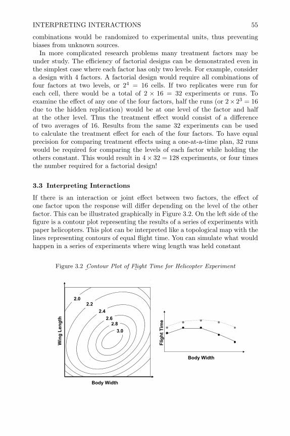
INTERPRETING INTERACTIONS 55
combinations would be randomized to experimental units, thus preventingbiases from unknown sources.
In more complicated research problems many treatment factors may beunder study. The efficiency of factorial designs can be demonstrated even inthe simplest case where each factor has only two levels. For example, considera design with 4 factors. A factorial design would require all combinations offour factors at two levels, or 24 = 16 cells. If two replicates were run foreach cell, there would be a total of 2 × 16 = 32 experiments or runs. Toexamine the effect of any one of the four factors, half the runs (or 2× 23 = 16due to the hidden replication) would be at one level of the factor and halfat the other level. Thus the treatment effect would consist of a differenceof two averages of 16. Results from the same 32 experiments can be usedto calculate the treatment effect for each of the four factors. To have equalprecision for comparing treatment effects using a one-at-a-time plan, 32 runswould be required for comparing the levels of each factor while holding theothers constant. This would result in 4× 32 = 128 experiments, or four timesthe number required for a factorial design!
3.3 Interpreting Interactions
If there is an interaction or joint effect between two factors, the effect ofone factor upon the response will differ depending on the level of the otherfactor. This can be illustrated graphically in Figure 3.2. On the left side of thefigure is a contour plot representing the results of a series of experiments withpaper helicopters. This plot can be interpreted like a topological map with thelines representing contours of equal flight time. You can simulate what wouldhappen in a series of experiments where wing length was held constant
Figure 3.2 Contour Plot of Flight Time for Helicopter Experiment
3.0
2.82.6
2.4
2.22.0
Win
g L
eng
th
Body Width
Body Width
Flig
ht
Tim
e

56 FACTORIAL DESIGNS
and body width varied by drawing a straight line parallel to the body widthaxis across the contour plot. The flight time for various runs can be read offas the label for the contour lines the straight line intersects. For example, ifwing length were held constant a value below its mid-point on the left of thecontour plot, the flight times resulting from five runs with varying body widthare represented as the black line traced on the graph at the right in Figure 3.2.If the wing length were held constant at a higher value, the grey line indicateswhat the result of a series of experiments with body width might look like.The fact that the two lines or curves on the right side of the figure are notparallel indicates there is an interaction between wing length and body width.They show that the effect of body width depends upon the wing length.
Interactions are common in the real world, but using the classical one-at-a-time strategy of experimentation tacitly assumes that interactions do notexist. To see the fallacy that results from this assumption, examine Figure 3.3,which represents what would happen if one were to search for the optimumcombination of wing length and body width.
Figure 3.3 One-at-a-Time Optimization with Paper Helicopters
3.0
2.82.6
2.4
2.22.0
Win
g L
eng
th
Body Width
2.0
2.32.82.2
2.4
2.0
2.3
2.5 2.6
The vertical set of circles are drawn at the wing length, body width combi-nations for a series of experiments that vary wing length while holding bodywidth constant. The numbers within the circles represent the resulting flighttimes. After examining the result of this series of experiments, the optimalwing length would be chosen and another series of experiments would be con-ducted by holding wing length constant at its optimal value and varying bodywidth. The results of these experiments can be visualized as the horizontal
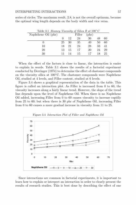
INTERPRETING INTERACTIONS 57
series of circles. The maximum result, 2.8, is not the overall optimum, becausethe optimal wing length depends on the body width and vice versa.
Table 3.1 Mooney Viscosity of Silica B at 100C
Naphthene Oil (phr) Filler (phr)0 12 24 36 48 60
0 25 30 35 40 50 6010 18 21 24 28 33 4120 13 15 17 20 24 2930 11 14 15 17 18 25
When the effect of the factors is close to linear, the interaction is easierto explain in words. Table 3.1 shows the results of a factorial experimentconducted by Derringer (1974) to determine the effect of elastomer compoundson the viscosity silica at 100C. The elastomer compounds were NaphtheneOil, studied at 4 levels, and Filler content, studied at 6 levels.
Figure 3.4 shows a graphical representation of the data in the table. Thisfigure is called an interaction plot. As Filler is increased from 0 to 60, theviscosity increases along a fairly linear trend. However, the slope of the trendline depends upon the level of Naphthene Oil. When there is no NaphtheneOil added, increasing Filler from 0 to 60 causes viscosity to increase rapidlyfrom 25 to 60; but when there is 30 phr of Naphthene Oil, increasing Fillerfrom 0 to 60 causes a more gradual increase in viscosity from 11 to 25.
Figure 3.4 Interaction Plot of Filler and Naphthene Oil
0
10
20
30
40
50
60
70
0 10 20 30 40 50 60 70
Filler
Viscosity
0 10 20 30Naphthene Oil
Since interactions are common in factorial experiments, it is important tolearn how to explain or interpret an interaction in order to clearly present theresults of research studies. This is best done by describing the effect of one
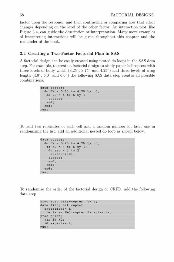
58 FACTORIAL DESIGNS
factor upon the response, and then contrasting or comparing how that effectchanges depending on the level of the other factor. An interaction plot, likeFigure 3.4, can guide the description or interpretation. Many more examplesof interpreting interactions will be given throughout this chapter and theremainder of the book.
3.4 Creating a Two-Factor Factorial Plan in SAS
A factorial design can be easily created using nested do loops in the SAS datastep. For example, to create a factorial design to study paper helicopters withthree levels of body width (3.25”, 3.75” and 4.25”) and three levels of winglength (4.0”, 5.0” and 6.0”) the following SAS data step creates all possiblecombinations.
data copter;do BW = 3.25 to 4.25 by .5;do WL = 4 to 6 by 1;output;
end;end;
run;
To add two replicates of each cell and a random number for later use inrandomizing the list, add an additional nested do loop as shown below.
data copter;do BW = 3.25 to 4.25 by .5;do WL = 4 to 6 by 1;do rep = 1 to 2;u=ranuni (0);
output;end;
end;end;
run;
To randomize the order of the factorial design or CRFD, add the followingdata step.
proc sort data=copter; by u;data list; set copter;
experiment=_n_;title Paper Helicopter Experiments;proc print;
var BW WL;id experiment;
run;

CREATING A TWO-FACTOR FACTORIAL PLAN IN SAS 59
This results in the following randomized list.Paper Helicopter Experiments
experiment BW WL1 3.25 42 3.75 63 4.25 44 4.25 65 4.25 56 3.25 57 3.75 58 3.75 69 3.75 4
10 3.75 411 3.25 612 4.25 413 3.25 514 3.75 515 4.25 616 3.25 417 4.25 518 3.25 6
This list shows that the first experiment consists of constructing a helicopterwith a body width of 3.25” and a wing length of 4”, dropping it from a fixedheight and timing its flight. The second experiment consists of constructinga helicopter with a body width of 3.75” and a wing length of 6”, dropping itfrom the same fixed height and timing its flight, etc. The randomization willhelp prevent biases from any lurking variables such as changes in air currents,changes in temperature or learning curves in dropping or timing helicopters.This randomized list could be converted to a double spaced data collectionform as shown in the example in Section 2.2.
By utilizing proc factex a more compact set of commands can be obtainedfor creating a randomized list for a factorial design. The commands below willproduce a randomized list in the file copter that is similar to that shownabove.
proc factex;factors BW WL/nlev =3;model estimate =(BW|WL);output out=copter randomize designrep =2BW nvals =(3.25 3.75 4.25) WL nvals =(4 5 6);
run;proc print data=copter;run;
The nlev=3 option on the factors statement specifies three levels for bodywidth and wing length. The default number of levels in proc factex is 2.The estimate=(BW|WL) specifies that the design should allow estimation ofthe body width and wing length main effects and their interaction. Finallythe output statement stores the list in the file. The designrep option speci-fies two replicates of each combination of factor levels, the randomize option

60 FACTORIAL DESIGNS
randomizes the order of the list and the nvals= option specifies numericalvalues for the levels of the two factors. If the levels were qualitative like (low,mid, high), the cvals=(’low’ ’mid’ ’high’) option could be used insteadof nvals. For a full factorial proc factex produces no output itself. Thereforeproc print command is used to print the randomized list.
3.5 Analysis of a Two-Factor Factorial in SAS
The mathematical model for a completely randomized two-factor factorialdesign can be written as:
yijk = µij + εijk (3.1)
where i represents the level of the first factor, j represents the level of thesecond factor, and k represents the replicate number. This model is called thecell means model and µij represents the expected response in the ijth cell.
Another way of representing the model is the effects model
yijk = µ+ αi + βj + αβij + εijk (3.2)
In this model αi, βj are the main effects and represent the difference betweenthe marginal average of all experiments at the ith level of the first factorand the overall average, and the difference between the marginal average atthe jth level of the second factor and the overall average, respectively. Theinteraction effects, αβij , represent the difference between the cell mean, µijand µ+ αi + βj .
The usual assumptions are that the experimental errors are independent andεijk ∼ N(0, σ2). The independence assumption is guaranteed if the treatmentcombinations are randomly assigned to the experimental units, and the equalvariance and normality assumptions can be verified with a residual versuspredicted plot and a normal probability plot of the residuals as described inSection 2.4.
Estimable functions, as described for the one-factor model in Section 2.3.4,are linear combinations of the cell means that can be expressed as a linearcombination of the data. For the two-factor factorial the cell means, µij =µ + αi + βj + αβij , are estimable functions but the individual effects, αi,βj , and αβij are not estimable functions. Contrasts among the effects suchas∑i ciαi, and
∑j cjβj , where
∑i ci = 0,
∑j cj = 0 and
∑i
∑j bijαβij ,
where∑i bij = 0,
∑j bij = 0 are estimable. These estimable functions and
their standard errors can be computed with the estimate command in SASproc glm. The marginal means µ+αi +αβi· and µ+βj +αβ·j are estimablefunctions and they and the cell means can be computed using the means orlsmeans statement in SAS proc glm.
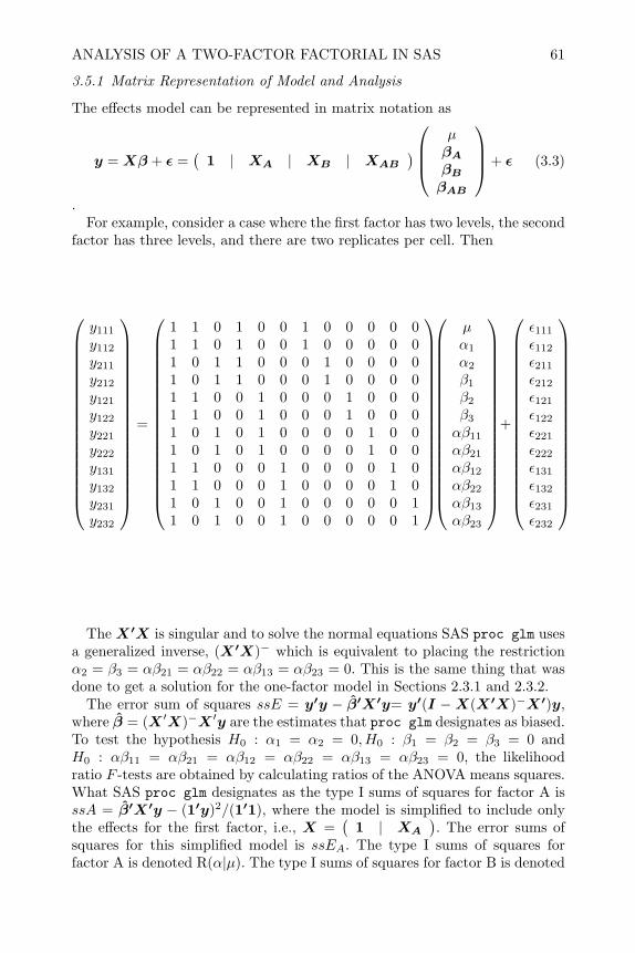
ANALYSIS OF A TWO-FACTOR FACTORIAL IN SAS 61
3.5.1 Matrix Representation of Model and Analysis
The effects model can be represented in matrix notation as
y = Xβ + ε =(
1 | XA | XB | XAB
)µβAβBβAB
+ ε (3.3)
.For example, consider a case where the first factor has two levels, the second
factor has three levels, and there are two replicates per cell. Then
y111
y112
y211
y212
y121
y122
y221
y222
y131
y132
y231
y232
=
1 1 0 1 0 0 1 0 0 0 0 01 1 0 1 0 0 1 0 0 0 0 01 0 1 1 0 0 0 1 0 0 0 01 0 1 1 0 0 0 1 0 0 0 01 1 0 0 1 0 0 0 1 0 0 01 1 0 0 1 0 0 0 1 0 0 01 0 1 0 1 0 0 0 0 1 0 01 0 1 0 1 0 0 0 0 1 0 01 1 0 0 0 1 0 0 0 0 1 01 1 0 0 0 1 0 0 0 0 1 01 0 1 0 0 1 0 0 0 0 0 11 0 1 0 0 1 0 0 0 0 0 1
µα1
α2
β1
β2
β3
αβ11
αβ21
αβ12
αβ22
αβ13
αβ23
+
ε111
ε112
ε211
ε212
ε121
ε122
ε221
ε222
ε131
ε132
ε231
ε232
The X′X is singular and to solve the normal equations SAS proc glm usesa generalized inverse, (X′X)− which is equivalent to placing the restrictionα2 = β3 = αβ21 = αβ22 = αβ13 = αβ23 = 0. This is the same thing that wasdone to get a solution for the one-factor model in Sections 2.3.1 and 2.3.2.
The error sum of squares ssE = y′y − β′X′y= y′(I −X(X′X)−X′)y,where β = (X ′X)−X ′y are the estimates that proc glm designates as biased.To test the hypothesis H0 : α1 = α2 = 0, H0 : β1 = β2 = β3 = 0 andH0 : αβ11 = αβ21 = αβ12 = αβ22 = αβ13 = αβ23 = 0, the likelihoodratio F -tests are obtained by calculating ratios of the ANOVA means squares.What SAS proc glm designates as the type I sums of squares for factor A isssA = β′X′y − (1′y)2/(1′1), where the model is simplified to include onlythe effects for the first factor, i.e., X =
(1 | XA
). The error sums of
squares for this simplified model is ssEA. The type I sums of squares forfactor A is denoted R(α|µ). The type I sums of squares for factor B is denoted
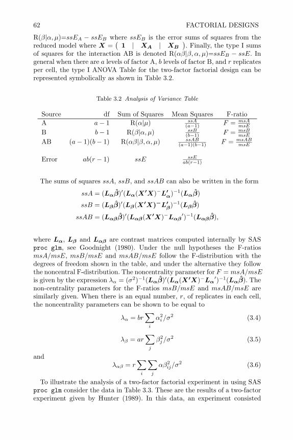
62 FACTORIAL DESIGNS
R(β|α, µ)=ssEA − ssEB where ssEB is the error sums of squares from thereduced model where X =
(1 | XA | XB
). Finally, the type I sums
of squares for the interaction AB is denoted R(αβ|β, α, µ)=ssEB − ssE. Ingeneral when there are a levels of factor A, b levels of factor B, and r replicatesper cell, the type I ANOVA Table for the two-factor factorial design can berepresented symbolically as shown in Table 3.2.
Table 3.2 Analysis of Variance Table
Source df Sum of Squares Mean Squares F-ratioA a− 1 R(α|µ) ssA
(a−1) F = msAmsE
B b− 1 R(β|α, µ) ssB(b−1) F = msB
msE
AB (a− 1)(b− 1) R(αβ|β, α, µ) ssAB(a−1)(b−1) F = msAB
msE
Error ab(r − 1) ssE ssEab(r−1)
The sums of squares ssA, ssB, and ssAB can also be written in the form
ssA = (Lαβ)′(Lα(X′X)−L′α)−1(Lαβ)
ssB = (Lββ)′(Lβ(X′X)−L′β)−1(Lββ)
ssAB = (Lαββ)′(Lαβ(X′X)−Lαβ ′)−1(Lαββ),
where Lα, Lβ and Lαβ are contrast matrices computed internally by SASproc glm, see Goodnight (1980). Under the null hypotheses the F-ratiosmsA/msE, msB/msE and msAB/msE follow the F-distribution with thedegrees of freedom shown in the table, and under the alternative they followthe noncentral F-distribution. The noncentrality parameter for F = msA/msEis given by the expression λα = (σ2)−1(Lαβ)′(Lα(X′X)−Lα′)−1(Lαβ). Thenon-centrality parameters for the F-ratios msB/msE and msAB/msE aresimilarly given. When there is an equal number, r, of replicates in each cell,the noncentrality parameters can be shown to be equal to
λα = br∑i
α2i /σ
2 (3.4)
λβ = ar∑j
β2j /σ
2 (3.5)
andλαβ = r
∑i
∑j
αβ2ij/σ
2 (3.6)
To illustrate the analysis of a two-factor factorial experiment in using SASproc glm consider the data in Table 3.3. These are the results of a two-factorexperiment given by Hunter (1989). In this data, an experiment consisted
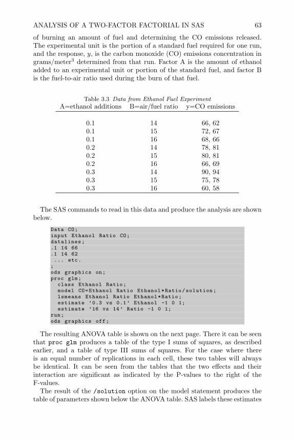
ANALYSIS OF A TWO-FACTOR FACTORIAL IN SAS 63
of burning an amount of fuel and determining the CO emissions released.The experimental unit is the portion of a standard fuel required for one run,and the response, y, is the carbon monoxide (CO) emissions concentration ingrams/meter3 determined from that run. Factor A is the amount of ethanoladded to an experimental unit or portion of the standard fuel, and factor Bis the fuel-to-air ratio used during the burn of that fuel.
Table 3.3 Data from Ethanol Fuel ExperimentA=ethanol additions B=air/fuel ratio y=CO emissions
0.1 14 66, 620.1 15 72, 670.1 16 68, 660.2 14 78, 810.2 15 80, 810.2 16 66, 690.3 14 90, 940.3 15 75, 780.3 16 60, 58
The SAS commands to read in this data and produce the analysis are shownbelow.
Data CO;input Ethanol Ratio CO;datalines;.1 14 66.1 14 62... etc.
;ods graphics on;proc glm;
class Ethanol Ratio;model CO=Ethanol Ratio Ethanol*Ratio/solution;lsmeans Ethanol Ratio Ethanol*Ratio;estimate ’0.3 vs 0.1’ Ethanol -1 0 1;estimate ’16 vs 14’ Ratio -1 0 1;
run;ods graphics off;
The resulting ANOVA table is shown on the next page. There it can be seenthat proc glm produces a table of the type I sums of squares, as describedearlier, and a table of type III sums of squares. For the case where thereis an equal number of replications in each cell, these two tables will alwaysbe identical. It can be seen from the tables that the two effects and theirinteraction are significant as indicated by the P-values to the right of theF-values.
The result of the /solution option on the model statement produces thetable of parameters shown below the ANOVA table. SAS labels these estimates
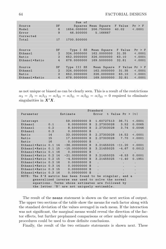
64 FACTORIAL DESIGNS
Sum ofSource DF Squares Mean Square F Value Pr > FModel 8 1654.000000 206.750000 40.02 <.0001Error 9 46.500000 5.166667CorrectedTotal 17 1700.500000
Source DF Type I SS Mean Square F Value Pr > FEthanol 2 324.0000000 162.0000000 31.35 <.0001Ratio 2 652.0000000 326.0000000 63.10 <.0001Ethanol*Ratio 4 678.0000000 169.5000000 32.81 <.0001
Source DF Type III SS Mean Square F Value Pr > FEthanol 2 324.0000000 162.0000000 31.35 <.0001Ratio 2 652.0000000 326.0000000 63.10 <.0001Ethanol*Ratio 4 678.0000000 169.5000000 32.81 <.0001
as not unique or biased as can be clearly seen. This is a result of the restrictionsα3 = β3 = αβ13 = αβ23 = αβ31 = αβ32 = αβ33 = 0 required to eliminatesingularities in X′X.
StandardParameter Estimate Error t Value Pr > |t|
Intercept 59.00000000 B 1.60727513 36.71 <.0001Ethanol 0.1 8.00000000 B 2.27303028 3.52 0.0065Ethanol 0.2 8.50000000 B 2.27303028 3.74 0.0046Ethanol 0.3 0.00000000 B . . .Ratio 14 33.00000000 B 2.27303028 14.52 <.0001Ratio 15 17.50000000 B 2.27303028 7.70 <.0001Ratio 16 0.00000000 B . . .Ethanol*Ratio 0.1 14 -36.00000000 B 3.21455025 -11.20 <.0001Ethanol*Ratio 0.1 15 -15.00000000 B 3.21455025 -4.67 0.0012Ethanol*Ratio 0.1 16 0.00000000 B . . .Ethanol*Ratio 0.2 14 -21.00000000 B 3.21455025 -6.53 0.0001Ethanol*Ratio 0.2 15 -4.50000000 B 3.21455025 -1.40 0.1951Ethanol*Ratio 0.2 16 0.00000000 B . . .Ethanol*Ratio 0.3 14 0.00000000 B . . .Ethanol*Ratio 0.3 15 0.00000000 B . . .Ethanol*Ratio 0.3 16 0.00000000 B . . .NOTE: The X’X matrix has been found to be singular , and a
generalized inverse was used to solve the normalequations. Terms whose estimates are followed bythe letter ’B’ are not uniquely estimable.
The result of the means statement is shown on the next section of output.The upper two sections of the table show the means for each factor along withthe standard deviation of the values averaged in each mean. If the interactionwas not significant, the marginal means would reveal the direction of the fac-tor effects, but further preplanned comparisons or other multiple comparisonprocedures could be used to draw definite conclusions.
Finally, the result of the two estimate statements is shown next. These
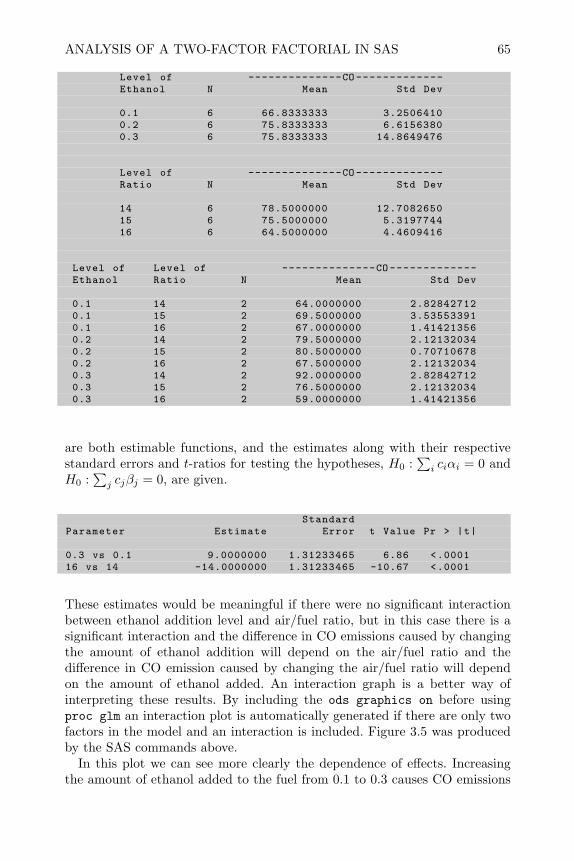
ANALYSIS OF A TWO-FACTOR FACTORIAL IN SAS 65
Level of --------------CO -------------Ethanol N Mean Std Dev
0.1 6 66.8333333 3.25064100.2 6 75.8333333 6.61563800.3 6 75.8333333 14.8649476
Level of --------------CO -------------Ratio N Mean Std Dev
14 6 78.5000000 12.708265015 6 75.5000000 5.319774416 6 64.5000000 4.4609416
Level of Level of --------------CO -------------Ethanol Ratio N Mean Std Dev
0.1 14 2 64.0000000 2.828427120.1 15 2 69.5000000 3.535533910.1 16 2 67.0000000 1.414213560.2 14 2 79.5000000 2.121320340.2 15 2 80.5000000 0.707106780.2 16 2 67.5000000 2.121320340.3 14 2 92.0000000 2.828427120.3 15 2 76.5000000 2.121320340.3 16 2 59.0000000 1.41421356
are both estimable functions, and the estimates along with their respectivestandard errors and t-ratios for testing the hypotheses, H0 :
∑i ciαi = 0 and
H0 :∑j cjβj = 0, are given.
StandardParameter Estimate Error t Value Pr > |t|
0.3 vs 0.1 9.0000000 1.31233465 6.86 <.000116 vs 14 -14.0000000 1.31233465 -10.67 <.0001
These estimates would be meaningful if there were no significant interactionbetween ethanol addition level and air/fuel ratio, but in this case there is asignificant interaction and the difference in CO emissions caused by changingthe amount of ethanol addition will depend on the air/fuel ratio and thedifference in CO emission caused by changing the air/fuel ratio will dependon the amount of ethanol added. An interaction graph is a better way ofinterpreting these results. By including the ods graphics on before usingproc glm an interaction plot is automatically generated if there are only twofactors in the model and an interaction is included. Figure 3.5 was producedby the SAS commands above.
In this plot we can see more clearly the dependence of effects. Increasingthe amount of ethanol added to the fuel from 0.1 to 0.3 causes CO emissions

66 FACTORIAL DESIGNS
Figure 3.5 Interaction Plot Ethanol and Air/Fuel Ratio
to increase linearly from 64 grams/liter to 92 grams/liter when the air/fuelratio is at its low level of 14. This is shown by the solid line with circlesrepresenting the data. However, when the air/fuel ratio is at its high levelof 16 (illustrated by the dash-dot line with ×s representing the data points),increasing the ethanol added to the fuel from 0.1 to 0.3 actually causes adecrease in CO emissions from 67 grams/liter to 59 grams/liter along a nearlylinear trend. Finally, when the air/fuel ratio is held constant at its mid-levelof 15 (illustrated by the dashed line with +s representing the data points),increasing ethanol from 0.1 to 0.2 causes CO emissions to increase by 11grams/liter; but a further increase in ethanol to 0.3 causes a decrease in COemissions of 4 grams/liter to 76.5.
The interpretation above again illustrates the principle of comparing theeffect of one factor across the levels of the other factor in order to describe aninteraction. This was done by comparing the effect of changing the ethanoladdition between the levels of air/fuel ratio. It could also be done in theopposite way. For example, the SAS code below reverses the interaction plotas shown in Figure 3.6.
ods graphics on;proc glm data=CO;
class Ratio Ethanol ;model CO= Ratio Ethanol Ratio*Ethanol;
run;ods graphics off;
In this plot the dash-dot line, with ×s representing the data points, showsthe effect of increasing air/fuel ratio when ethanol is added at the high rate
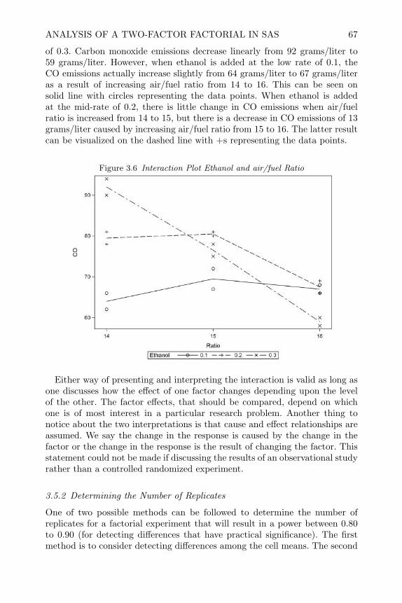
ANALYSIS OF A TWO-FACTOR FACTORIAL IN SAS 67
of 0.3. Carbon monoxide emissions decrease linearly from 92 grams/liter to59 grams/liter. However, when ethanol is added at the low rate of 0.1, theCO emissions actually increase slightly from 64 grams/liter to 67 grams/literas a result of increasing air/fuel ratio from 14 to 16. This can be seen onsolid line with circles representing the data points. When ethanol is addedat the mid-rate of 0.2, there is little change in CO emissions when air/fuelratio is increased from 14 to 15, but there is a decrease in CO emissions of 13grams/liter caused by increasing air/fuel ratio from 15 to 16. The latter resultcan be visualized on the dashed line with +s representing the data points.
Figure 3.6 Interaction Plot Ethanol and air/fuel Ratio
Either way of presenting and interpreting the interaction is valid as long asone discusses how the effect of one factor changes depending upon the levelof the other. The factor effects, that should be compared, depend on whichone is of most interest in a particular research problem. Another thing tonotice about the two interpretations is that cause and effect relationships areassumed. We say the change in the response is caused by the change in thefactor or the change in the response is the result of changing the factor. Thisstatement could not be made if discussing the results of an observational studyrather than a controlled randomized experiment.
3.5.2 Determining the Number of Replicates
One of two possible methods can be followed to determine the number ofreplicates for a factorial experiment that will result in a power between 0.80to 0.90 (for detecting differences that have practical significance). The firstmethod is to consider detecting differences among the cell means. The second

68 FACTORIAL DESIGNS
method is to consider detecting a practical size difference in the marginalmeans for the factors in the experiment.
When looking for differences among the cell means, the cells in the factorialare considered to be an unstructured group as in a one-factor design. Usingthe cell means model yijk = µij + εijk the procedure is the same as it wasdescribed for the one-factor model yij = µi + εij in Section 2.6. The non-centrality parameter for the F -test is:
λ = (r/σ2)a∑i=1
b∑j=1
(µij − µ··)2.
When looking for differences in the marginal means for the factors, thenon-centrality factor for the first main effect is:
λa = br∑i
α2i /σ
2 = br∑i
(µi· − µ··)2/σ2,
and for the second main effect the non-centrality factor is:
λb = ar∑j
β2j /σ
2 = ar∑j
(µ·j − µ··)2/σ2.
If ∆ is considered to be the size of a practical difference in cell means,then the smallest λ = r/σ2
∑ai=1
∑bj=1 (µij − µ··)2 could be with two cells
differing by at least ∆ is r∆2/2σ2. Likewise if ∆ is considered to be thesize of a practical difference in marginal means for factor A, the smallestλa = br
∑i (µi· − µ··)2/σ2 could be with two marginal means differing by at
least ∆ is br∆2/2σ2. Here again we can see the efficiency of factorial designsbecause the non-centrality factor for detecting differences in marginal factorA means is larger than the non-centrality factor for detecting differences ofcell means by a factor of, b the number of levels of factor B.
Consider the following example. A paper helicopter experiment is plannedto investigate the effects of four levels of factor A = wing length, and fourlevels of factor B = body width, upon the flight time. If pilot experimentswith nine replicates of one design resulted in flight times of 2.8, 2.6, 3.5, 3.0,3.1, 3.5, 3.2, 3.4, and 3.4 seconds. How many replicates would be required todetect a difference in flight times of 1 second with a power of .90?
From the pilot tests the variance of experimental error can be estimatedas s2 = 0.1024. If ∆ = 1.0 considered to be a practical size difference incell means, the SAS commands in Section 2.6, can be modified to give theanswer. In a 4-by-4 factorial there are 16 cells so the degrees of freedom forthe numerator is ν1 = 15, and the degrees of freedom for the denominator isν2 = 16(r − 1). The modified SAS code is shown on the next page.

ANALYSIS OF A TWO-FACTOR FACTORIAL IN SAS 69
data Power;do r=2 to 8;
nu1 =16-1; * df for numerator;nu2 =16*(r-1); * df for denominator;alpha =.05;Fcrit=finv(1-alpha ,nu1 ,nu2); *F critical value;sigma2 =.1024;css =0.5;nc=r*(css)/sigma2;*noncentrality parameter for
noncentral F;power=1-probf(Fcrit ,nu1 ,nu2 ,nc);output;
end;keep r nu1 nu2 nc power;title Power Calculation in Data Step;proc print; run;
The results below show that 6 replicates per cell would be required to obtaina power of at least 0.90.
Power Calculation in Data Step
Obs r nu1 nu2 nc power
1 2 15 16 9.7656 0.241732 3 15 32 14.6484 0.481743 4 15 48 19.5313 0.692464 5 15 64 24.4141 0.838295 6 15 80 29.2969 0.923266 7 15 96 34.1797 0.966647 8 15 112 39.0625 0.98655
If ∆ = 1.0 considered to be a practical size difference in marginal means forone of the factors, the results will be different. The degrees of freedom for thenumerator would be ν1 = 4 − 1, the degrees of freedom for the denominatorwould be ν2 = 16(r− 1) and the non-centrality factor for a main effect wouldbe λa = br∆2/2σ2 = 4r12/2(0.1024). Modifying the SAS code above we get
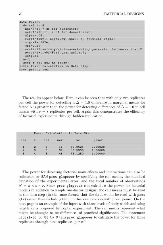
70 FACTORIAL DESIGNS
data Power;do r=2 to 4;nu1=4-1; * df for numerator;nu2 =16*(r-1); * df for denominator;alpha =.05;Fcrit=finv(1-alpha ,nu1 ,nu2); *F critical value;sigma2 =.1024;css =0.5;nc=4*r*(css)/sigma2;*noncentrality parameter for noncentral F;power=1-probf(Fcrit ,nu1 ,nu2 ,nc);output;
end;keep r nu1 nu2 nc power;
title Power Calculation in Data Step;proc print; run;
The results appear below. Here it can be seen that with only two replicatesper cell the power for detecting a ∆ = 1.0 difference in marginal means forfactor A is greater than the power for detecting differences of ∆ = 1.0 in cellmeans with r = 8 replicates per cell. Again this demonstrates the efficiencyof factorial experiments through hidden replication.
Power Calculation in Data Step
Obs r nu1 nu2 nc power
1 2 3 16 39.0625 0.998382 3 3 32 58.5938 1.000003 4 3 48 78.1250 1.00000
The power for detecting factorial main effects and interactions can also beestimated by SAS proc glmpower by specifying the cell means, the standarddeviation of the experimental error, and the total number of observationsN = a × b × r. Since proc glmpower can calculate the power for factorialmodels in addition to simple one-factor designs, the cell means must be readin the data step (in the same format that the data would be read with procglm) rather than including them in the commands as with proc power. On thenext page is an example of the input with three levels of body width and winglength for a proposed helicopter experiment. The cell means represent whatmight be thought to be differences of practical significance. The statementntotal=36 to 81 by 9 tells proc glmpower to calculate the power for threereplicates through nine replicates per cell.

ANALYSIS OF A TWO-FACTOR FACTORIAL IN SAS 71
data powglm;input BW WL cellmean;datalines;4.0 4.75 2.44.0 5.5 2.34.0 6.25 2.13.75 4.75 2.83.75 5.5 2.43.75 6.25 2.23.5 4.75 2.43.5 5.5 2.43.5 6.25 2.2proc glmpower;
class BW WL;model cellmean=BW WL BW*WL;power
stddev =0.32ntotal =36 to 81 by 9power = .;
run;
The results are shown below. The power is given for each term in the model(i.e., main effects for body width, wing length and interaction) as a functionof the total number of observations. With the cell means as specified in theinput there would be adequate power for detecting the wing length main effectwith six or more replicates per cell (i.e., ntotal ≥ 54).
The GLMPOWER Procedure
Fixed Scenario ElementsDependent Variable cellmeanError Standard Deviation 0.32Alpha 0.05
Computed PowerN Test Error
Index Source Total DF DF Power
1 BW 36 2 27 0.2422 BW 45 2 36 0.3023 BW 54 2 45 0.3614 BW 63 2 54 0.4185 BW 72 2 63 0.4726 BW 81 2 72 0.5247 WL 36 2 27 0.6598 WL 45 2 36 0.7749 WL 54 2 45 0.855
10 WL 63 2 54 0.91011 WL 72 2 63 0.94512 WL 81 2 72 0.96713 BW*WL 36 4 27 0.16514 BW*WL 45 4 36 0.20615 BW*WL 54 4 45 0.24816 BW*WL 63 4 54 0.29117 BW*WL 72 4 63 0.33518 BW*WL 81 4 72 0.378

72 FACTORIAL DESIGNS
With the ability to calculate power quickly using the probf function in thedata step or proc glmpower, it is possible to explore many potential designsbefore actually running the experiments. Questions such as, “Is it better touse three or four levels of the factors?” can be answered with respect to theeffect on the power of detecting significant differences.
3.5.3 Analysis with an Unequal Number of Replicates per Cell
Although it would be unusual to plan a factorial experiment with an unequalnumber of replicates per cell, the data from a factorial experiment may endup with an unequal number of replicates due to experiments that could not becompleted, or responses that could not be measured, or simply lost data. Aslong as the chance of losing an observation was not related to the treatmentfactor levels, the data from a factorial experiment with an unequal number ofreplicates per cell can still be analyzed and interpreted in a manner similarto the way it would be done for the equal replicate case. However, the com-putational formulas for analyzing the data differ for the case with an unequalnumber of replicates.
To illustrate why the analysis shown in Section 3.5.1 is inappropriate, con-sider again the data from the ethanol fuel experiment described in Section3.5.1. This time assume one observation in the cell where air/fuel ratio = 16and ethanol level = 0.3 was missing. Then Table 3.4 shows the data with eachresponse value written above its symbolic expected value.
Table 3.4 Fuel Experiment with Unequal Reps
air/fuel air/fuel air/fuelEthanol 14 15 16
66 72 680.1 62 67 66
µ+ α1 + β1 + αβ11 µ+ α1 + β2 + αβ12 µ+ α1 + β3 + αβ13
78 80 660.2 81 81 69
µ+ α2 + β1 + αβ21 µ+ α2 + β2 + αβ22 µ+ α2 + β3 + αβ23
90 75 600.3 94 78
µ+ α3 + β1 + αβ31 µ+ α3 + β2 + αβ32 µ+ α3 + β3 + αβ33
The marginal column means for the levels of air/fuel ratio factor computedusing the means statement as shown in Section 3.5.1 would be 78.5, 75.5 and65.8, respectively. The expected value of the marginal means for the firsttwo columns would be: µ + β1, µ + β2, since (α1 + α2 + α3)/3 = 0 and(αβ1i + αβ2i + αβ3i)/3 = 0 for i = 1, 2. However, the expected value of thelast marginal column mean would be µ+ β3 + (2α1 + 2α2 +α3)/5 + (2αβ13 +2αβ23 + αβ33)/5 and is not an unbiased estimate of µ + β3. The comparison
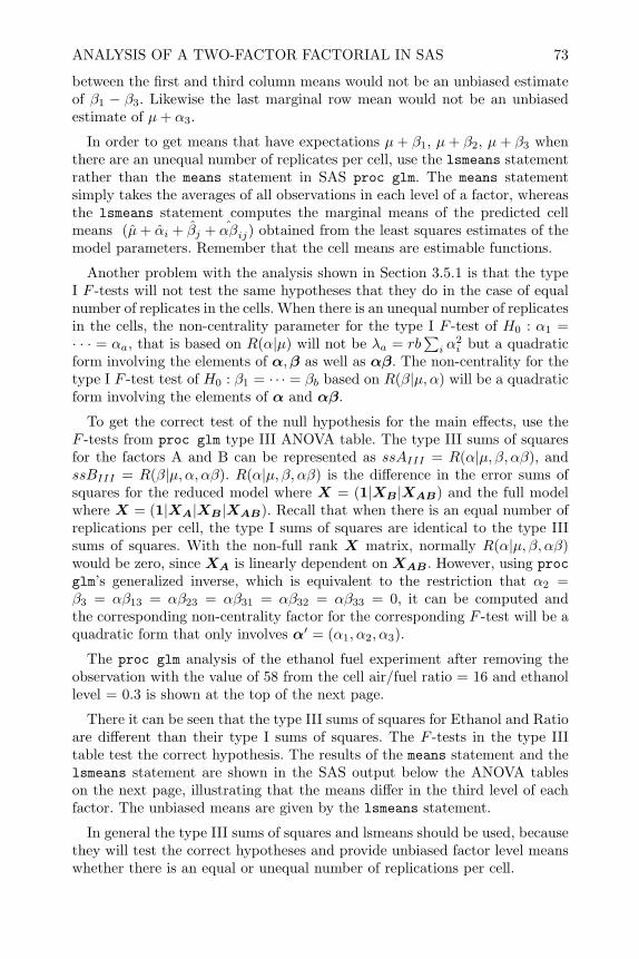
ANALYSIS OF A TWO-FACTOR FACTORIAL IN SAS 73
between the first and third column means would not be an unbiased estimateof β1 − β3. Likewise the last marginal row mean would not be an unbiasedestimate of µ+ α3.
In order to get means that have expectations µ+ β1, µ + β2, µ+ β3 whenthere are an unequal number of replicates per cell, use the lsmeans statementrather than the means statement in SAS proc glm. The means statementsimply takes the averages of all observations in each level of a factor, whereasthe lsmeans statement computes the marginal means of the predicted cellmeans (µ+ αi + βj + αβij) obtained from the least squares estimates of themodel parameters. Remember that the cell means are estimable functions.
Another problem with the analysis shown in Section 3.5.1 is that the typeI F -tests will not test the same hypotheses that they do in the case of equalnumber of replicates in the cells. When there is an unequal number of replicatesin the cells, the non-centrality parameter for the type I F -test of H0 : α1 =· · · = αa, that is based on R(α|µ) will not be λa = rb
∑i α
2i but a quadratic
form involving the elements of α,β as well as αβ. The non-centrality for thetype I F -test test of H0 : β1 = · · · = βb based on R(β|µ, α) will be a quadraticform involving the elements of α and αβ.
To get the correct test of the null hypothesis for the main effects, use theF -tests from proc glm type III ANOVA table. The type III sums of squaresfor the factors A and B can be represented as ssAIII = R(α|µ, β, αβ), andssBIII = R(β|µ, α, αβ). R(α|µ, β, αβ) is the difference in the error sums ofsquares for the reduced model where X = (1|XB|XAB) and the full modelwhere X = (1|XA|XB|XAB). Recall that when there is an equal number ofreplications per cell, the type I sums of squares are identical to the type IIIsums of squares. With the non-full rank X matrix, normally R(α|µ, β, αβ)would be zero, since XA is linearly dependent on XAB. However, using procglm’s generalized inverse, which is equivalent to the restriction that α2 =β3 = αβ13 = αβ23 = αβ31 = αβ32 = αβ33 = 0, it can be computed andthe corresponding non-centrality factor for the corresponding F -test will be aquadratic form that only involves α′ = (α1, α2, α3).
The proc glm analysis of the ethanol fuel experiment after removing theobservation with the value of 58 from the cell air/fuel ratio = 16 and ethanollevel = 0.3 is shown at the top of the next page.
There it can be seen that the type III sums of squares for Ethanol and Ratioare different than their type I sums of squares. The F -tests in the type IIItable test the correct hypothesis. The results of the means statement and thelsmeans statement are shown in the SAS output below the ANOVA tableson the next page, illustrating that the means differ in the third level of eachfactor. The unbiased means are given by the lsmeans statement.
In general the type III sums of squares and lsmeans should be used, becausethey will test the correct hypotheses and provide unbiased factor level meanswhether there is an equal or unequal number of replications per cell.
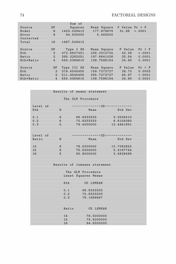
74 FACTORIAL DESIGNS
Sum ofSource DF Squares Mean Square F Value Pr > FModel 8 1423.029412 177.878676 31.98 <.0001Error 8 44.500000 5.562500CorrectedTotal 16 1467.529412
Source DF Type I SS Mean Square F Value Pr > FEth 2 472.6627451 236.3313725 42.49 <.0001Ratio 2 395.3282051 197.6641026 35.54 0.0001Eth*Ratio 4 555.0384615 138.7596154 24.95 0.0001
Source DF Type III SS Mean Square F Value Pr > FEth 2 319.4545455 159.7272727 28.72 0.0002Ratio 2 511.4545455 255.7272727 45.97 <.0001Eth*Ratio 4 555.0384615 138.7596154 24.95 0.0001
Results of means statement
The GLM Procedure
Level of --------------CO -------------Eth N Mean Std Dev
0.1 6 66.8333333 3.25064100.2 6 75.8333333 6.61563800.3 5 79.4000000 13.4461891
Level of --------------CO -------------Ratio N Mean Std Dev
14 6 78.5000000 12.708265015 6 75.5000000 5.319774416 5 65.8000000 3.4928498
Results of lsmeans statement
The GLM ProcedureLeast Squares Means
Eth CO LSMEAN
0.1 66.83333330.2 75.83333330.3 76.1666667
Ratio CO LSMEAN
14 78.500000015 75.500000016 64.8333333

ANALYSIS OF A TWO-FACTOR FACTORIAL IN SAS 75
3.5.4 Testing for Interaction with one Replicate per Cell
When there is adequate power for detecting main effects with r = 1 replicateper cell, then it would make sense to run a factorial design with only oneobservation per cell and a× b total observations. Adding one replicate to eachcell, in this case, would double the effort required, and would usually not berequired. However, with only one replicate per cell in a factorial design, thereis no way to compute the ANOVA ssE and therefore no way to make F -testson the main effects and interaction in the traditional way. If the interactionterm is assumed to be zero, then F -tests on the main effects can be madeby using the additive model yij = µ + αi + βj + εij . Even so, this could bedangerous if the interaction actually exists. There are ways to test whetherthe interaction is zero in this case.
If the levels of both factors are quantitative as in the proposed paper heli-copter experiments or the ethanol fuel experiment, the sums of squares for theinteraction term can be partitioned into orthogonal polynomial single degreesof freedom. For example, if there are three equally spaced quantitative levelsof factor A, and three equally spaced quantitative levels for factor B, thenthe sums of squares for the interaction can be partitioned into four single de-grees of freedom (namely: linear×linear, linear×quadratic, quadratic×linearand quadratic×quadratic). Using the Taylor Series philosophy that low orderpolynomials can approximate most functional relationships, the three higherorder terms might be assumed to be negligible and pooled to estimate the ssE,which could then be used as an error term to test the linear×linear portionof the interaction. This will be illustrated with the data from the ethanol fuelexperiment given in Table 3.4.
First, consider the averages of the two replicates in each cell of Table 3.3 tobe the result of a single experiment. The SAS commands shown below averagethe data in each cell to produce the file cells with one observation per cell.Fitting the model 3.2 to this data with proc glm results in an ANOVA withzero degrees of freedom for ssE, and no F -tests.
proc sort data=CO; by Ethanol Ratio;proc means noprint;
by Ethanol Ratio; var CO;output out=cells mean=COmean;
proc glm data=cells;class Ethanol Ratio;model COmean=Ethanol Ratio Ethanol*Ratio:
run;
The type III portion of the output appears on the next page.
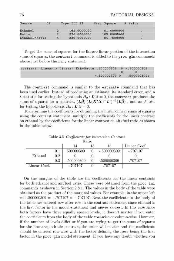
76 FACTORIAL DESIGNS
Source DF Type III SS Mean Square F Value
Ethanol 2 162.0000000 81.0000000 .Ratio 2 326.0000000 163.0000000 .Ethanol*Ratio 4 339.0000000 84.7500000 .
To get the sums of squares for the linear×linear portion of the interactionsums of squares, the contrast command is added to the proc glm commandsabove just before the run; statement:
contrast ’Linear x Linear ’ Eth*Ratio .500000309 0 -.5000003090 0 0
-.500000309 0 .500000309;
The contrast command is similar to the estimate command that hasbeen used earlier. Instead of producing an estimate, its standard error, and at-statistic for testing the hypothesis H0 : L′β = 0, the contrast produces thesums of squares for a contrast, (Lβ)′(L(X′X)−L′)−1(Lβ) , and an F -testfor testing the hypothesis H0 : L′β = 0.
To determine the coefficients for obtaining the linear×linear sums of squaresusing the contrast statement, multiply the coefficients for the linear contraston ethanol by the coefficients for the linear contrast on air/fuel ratio as shownin the table below.
Table 3.5 Coefficients for Interaction ContrastRatio
14 15 16 Linear Coef.0.1 .500000309 0 -.500000309 -.707107
Ethanol 0.2 0 0 0 00.3 -.500000309 0 .500000309 .707107
Linear Coef. -.707107 0 .707107
On the margins of the table are the coefficients for the linear contrastsfor both ethanol and air/fuel ratio. These were obtained from the proc imlcommands as shown in Section 2.8.1. The values in the body of the table wereobtained as the product of the marginal values. For example, in the upper leftcell .500000309 = −.707107 × −.707107. Next the coefficients in the body ofthe table are entered row after row in the contrast statement since ethanol isthe first factor in the model statement and moves slowest. In this case sinceboth factors have three equally spaced levels, it doesn’t matter if you enterthe coefficients from the body of the table row-wise or column-wise. However,if the number of levels differ or if you are trying to get the sums of squaresfor the linear×quadratic contrast, the order will matter and the coefficientsshould be entered row-wise with the factor defining the rows being the firstfactor in the proc glm model statement. If you have any doubt whether you
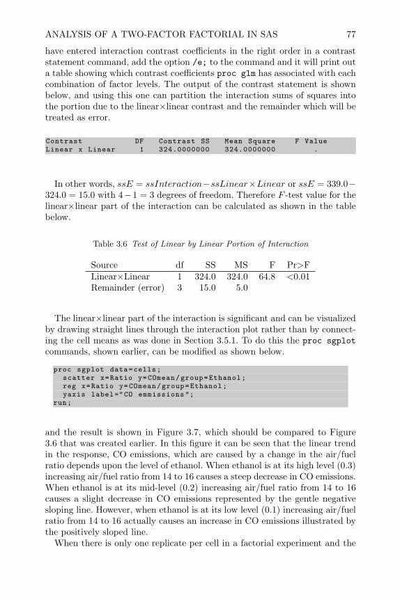
ANALYSIS OF A TWO-FACTOR FACTORIAL IN SAS 77
have entered interaction contrast coefficients in the right order in a contraststatement command, add the option /e; to the command and it will print outa table showing which contrast coefficients proc glm has associated with eachcombination of factor levels. The output of the contrast statement is shownbelow, and using this one can partition the interaction sums of squares intothe portion due to the linear×linear contrast and the remainder which will betreated as error.
Contrast DF Contrast SS Mean Square F ValueLinear x Linear 1 324.0000000 324.0000000 .
In other words, ssE = ssInteraction−ssLinear×Linear or ssE = 339.0−324.0 = 15.0 with 4−1 = 3 degrees of freedom. Therefore F -test value for thelinear×linear part of the interaction can be calculated as shown in the tablebelow.
Table 3.6 Test of Linear by Linear Portion of Interaction
Source df SS MS F Pr>FLinear×Linear 1 324.0 324.0 64.8 <0.01Remainder (error) 3 15.0 5.0
The linear×linear part of the interaction is significant and can be visualizedby drawing straight lines through the interaction plot rather than by connect-ing the cell means as was done in Section 3.5.1. To do this the proc sgplotcommands, shown earlier, can be modified as shown below.
proc sgplot data=cells;scatter x=Ratio y=COmean/group=Ethanol;reg x=Ratio y=COmean/group=Ethanol;yaxis label="CO emmissions ";
run;
and the result is shown in Figure 3.7, which should be compared to Figure3.6 that was created earlier. In this figure it can be seen that the linear trendin the response, CO emissions, which are caused by a change in the air/fuelratio depends upon the level of ethanol. When ethanol is at its high level (0.3)increasing air/fuel ratio from 14 to 16 causes a steep decrease in CO emissions.When ethanol is at its mid-level (0.2) increasing air/fuel ratio from 14 to 16causes a slight decrease in CO emissions represented by the gentle negativesloping line. However, when ethanol is at its low level (0.1) increasing air/fuelratio from 14 to 16 actually causes an increase in CO emissions illustrated bythe positively sloped line.
When there is only one replicate per cell in a factorial experiment and the

78 FACTORIAL DESIGNS
Figure 3.7 Linear by Linear Interaction Plot Ethanol and Air/Fuel Ratio
factors do not have quantitative levels, partitioning the interaction sums ofsquares into orthogonal polynomial contrasts and combining the higher orderterms as an error sums of squares may not be appropriate. However, Tukey(1949b) has developed an alternate method for testing a single degree of free-dom partitioned from interaction sums of squares. This method is equivalentto restricting the αβij in model 3.2 of Section 3.5 to be a second-degree poly-nomial function of the main effects αi and βj , (see Scheffe, 1959). By doingthis, the sums of squares
ssAB =ab[∑
i
∑j yijyi·y·j − (ssA+ ssB + aby2
··)y··]2
(ssA)(ssB)(3.7)
for testing the restricted hypothesis H0 : αβij = 0 for all i and j will haveone degree of freedom and the difference between it and the error term forthe additive model will form the error sums of squares similar to the exampleabove with quantitative factor levels.
To illustrate the use of Tukey’s single degree of freedom test for interaction,consider the data in Table 3.7, which is a portion of the data from a studyto validate an assay of viral contamination reported by Lin and Stephenson(1998). Assays of viral contamination are used to determine the presence (andamount) of a specific virus in biological products such as blood clotting FactorEight. An experiment, or run, consists of making a solution with a known viralcontamination, allowing the virus in a contaminated solution to grow, then

ANALYSIS OF A TWO-FACTOR FACTORIAL IN SAS 79
measuring the result. The experimental unit is the specific viral sample incombination with the place and time where it is allowed to grow. Factor Arepresents the sample number, or solution with which the viral sample is mixed(or spiked). Factor B represents different dilutions of the spiked sample. Themeasured response is the log10 of the plaque forming units per mL of solution.
Table 3.7 log10(PFU/mL) Assay of Viral Contamination
Sample1 2 3 4 5 6
3 1.87506 1.74036 1.79934 2.02119 1.79934 1.59106Dilution 4 1.38021 1.36173 1.25527 1.39794 1.20412 1.25527
5 0.60206 0.90309 0.95424 1.00000 0.60206 0.60206
Since factor A (sample) is not a quantitative factor it would be inappropriateto use orthogonal polynomial contrasts to partition its sums of squares or thesums of squares of its interaction with factor B (Dilution). To determine ifthe additive model yij = µ + αi + βj + εij is appropriate for this data, testto see whether there is a significant interaction using Tukey’s method. A SASmacro (shown in the appendix to this chapter) calculates the non-additivity orinteraction sums of squares, shown in Equation (3.7), and prints a report. Thecommands to read the data and call the macro are shown below. The code forthe macro, shown in the appendix, should be included above the code shownbelow. When this code is executed, the macro is called with the %tukeysdfcommand. The macro looks in a file called file1 for the variables A, B, and yto perform the calculations.
data PFU;input A B y;datalines;1 3 1.875061 4 1.38021... etc.
data file1; set PFU;%tukeysdf
The results are shown in the output shown below.
Tukey’s single df test for additivity
Source df SS MS F PR>FA 5 0.19479 0.03896B 2 3.16639 1.5832Error 10 0.12825 0.01283NonAdditivity 1 0.00688 0.00688 0.51 0.493Residual 9 0.12137 0.01349
Here it can be seen that the interaction (or non-additivity) is not significant.

80 FACTORIAL DESIGNS
Therefore, for this data, it would be appropriate to fit the additive model withthe commands proc glm; class A B; model y=A B;.
3.6 Factorial Designs with Multiple Factors - CRFD
Two-factor factorial designs are more efficient than studying each factor sep-arately in one-factor designs. Likewise, when many factors are under study,it is more efficient to study them together in a multi-factor factorial designthan it is to study them separately in groups of two using two-factor factorialdesigns. When multiple factors are studied simultaneously, the power for de-tecting main effects is increased over what it would be in separate two-factorfactorial designs. Also, the possibility of detecting interactions among any ofthe factors is possible. If the factors were studied separately in two-factor fac-torials, two-factor interactions could only be detected between factors studiedtogether in the same design. In a multi-factor factorial not only is it pos-sible to detect two-factor interactions between any pair of factors, but it isalso possible to detect higher order interactions between groups of factors. Athree-factor interaction between factors A, B and C, for example, means theeffect of factor A differs depending on the combination of levels of factors Band C. Examples of higher order interactions will be presented in examples tofollow.
The treatment combinations in a multi-factor factorial consist of all possiblecombinations of the levels of all factors. A design, along with randomizationcan be produced using nested do loops in the SAS data step or proc factexsimilar to the example shown in Section 3.4. The model for analysis is anextension of Equation (3.2), and the analysis can be made using proc glm orproc genmod similar to the examples shown earlier.
Consider an example of a multi-factor factorial design in marketing research.A company whose sales are made online through a Web page would like to in-crease the proportion of visitors to their Web site that sign up for their serviceby optimally configuring their Web page. In order to buy from the company,customers must sign up and fill out a form supplying their email address alongwith other required fields. Once a customer signs up, the company has contactinformation for their database and can email advertisements, special offers,etc. The company would like to experiment by testing different configurationsof their Web page to see if they can increase the number of visitors to theirsite that actually sign up.
The experimental units in this study will be individuals who visit the com-pany Web site. The response is binary; the customer either signs up or doesnot. The factors under study were characteristics that change the appearanceof the Web page. For example, factor A was the background alternatives forthe page with three options. Factor B was the font size in the main banner,with three levels; factor C was the text color with two alternatives; and fac-tor D was a choice between a sign-up button or link. Based on these factorsthere were 3 × 3 × 2 × 2 = 36 possible configurations of the Web page when
FACTORIAL DESIGNS WITH MULTIPLE FACTORS - CRFD 81
considering all possible combinations of the levels of each factor. A four-factorfactorial experiment would consist of randomly assigning visitors to the Website to one of the possible configurations and recording their binary response.There are lurking variables that could affect the chance that a site visitorwill sign up. For example, the position order that the link (for the company’sWeb site) comes up in a Web search for the products they sell, promotionsoffered by competitors, and attractiveness of competitors’ Web sites. Randomassignment of each sequential visitor to the site to one of the alternative con-figurations under study should minimize the chance of bias from changes inthe lurking variables over time. The probability that a site visitor would signup can be expressed by the model:
pijkl = µ+ αi + βj + αβij + γk + αγik + βγjk + αβγijk + δl + αδil
+ βδjl + αβδijl + γδkl + αγδikl + βγδjkl + αβγδijkl,(3.8)
where αi represents the effect of background choice, βj represents the effectof font size in the main banner, γk represents the effect of text color, and δlrepresents the effect of sign-up link versus button.
The experiment was conducted by constructing thirty-six Web sites con-sisting of all possible combinations of the four factors described above. Eachpotential customer who visited the company’s Web site during the trial periodwas randomly redirected to one of the thirty-six configurations. The numberof visitors nijkl to the ijklth configuration and the number that signed upxijkl was logged. xijkl is then binomially distributed
B(xijkl, nijkl, pijkl) =(nijklxijkl
)pxijklijkl (1− pijkl)(nijkl−xijkl) (3.9)
where nijkl is the number of visitors to the ijklth configured Web page duringthe testing period.
The raw data from this experiment was read into SAS using the commandson the next page.
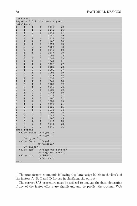
82 FACTORIAL DESIGNS
data raw;input A B C D visitors signup;datalines;1 1 1 1 1016 221 1 1 2 1145 161 1 2 1 1145 171 1 2 2 1082 191 2 1 1 1121 281 2 1 2 1103 281 2 2 1 1072 151 2 2 2 1097 331 3 1 1 1145 181 3 1 2 1137 201 3 2 1 1091 221 3 2 2 1097 322 1 1 1 1062 212 1 1 2 1093 272 1 2 1 1020 282 1 2 2 1009 272 2 1 1 1091 192 2 1 2 1133 342 2 2 1 1037 172 2 2 2 1061 282 3 1 1 1082 322 3 1 2 1010 262 3 2 1 1028 382 3 2 2 1045 303 1 1 1 1014 173 1 1 2 1100 213 1 2 1 1031 193 1 2 2 1072 213 2 1 1 1035 153 2 1 2 1038 243 2 2 1 1097 263 2 2 2 1089 223 3 1 1 1108 193 3 1 2 1119 253 3 2 1 1141 283 3 2 2 1148 35proc format;
value Backg 1=’type 1’2=’type 2’
3=’type 3’;value font 1=’small ’
2=’medium ’3=’large ’;
value sgn 1=’Sign -up Button ’2=’Sign -up Link’;
value txt 1=’black ’2=’white ’;
run;
The proc format commands following the data assign labels to the levels ofthe factors A, B, C and D for use in clarifying the output.
The correct SAS procedure must be utilized to analyze the data, determineif any of the factor effects are significant, and to predict the optimal Web

FACTORIAL DESIGNS WITH MULTIPLE FACTORS - CRFD 83
page configuration. Since the responses for the individual visitors to eachconfiguration of the Web site are Bernoulli, the aggregate response data, whichis read into SAS, is Binomial with large and approximately equal sample sizes(i.e., number of visitors to each possible Web configuration). The arcsin squareroot transformation shown in Table 2.4 of Section 2.5.2 could be applied andproc glm could be used for analysis. However, the problem with using thisprocedure is that the individual responses were summed to get the aggregateresponses, and when using these aggregate binomial responses there are noreplicate observations in any of the cells, and thus no way to calculate ssE.This would be similar to summing or averaging the replicate responses in eachcell if the data were normally distributed, leaving only one observation percell and no way to compute ssE. The alternative is to use the method ofmaximum likelihood to fit model (3.8). This can be done using proc genmod,that was described briefly in Section 2.5.3. It will automatically set σ2 = 1.0and the type III sums of squares of the form (Lβ)′(L(X′X)−L′)−1(Lβ) willbe asymptotically distributed as chi-squares under the null hypothesis. Thecommands to analyze the data using proc genmod are shown below.
proc genmod data=raw;class A B C D;model signup/visitors=A|B|C|D/ dist=bin type3 ;
run;
signup/visitors is the observed proportion signing up and the model spec-ification A|B|C|D is a shorthand for A B A*B C A*C B*C A*B*C D A*D B*DA*B*D C*D A*C*D B*C*D A*B*C*D. The option dist=bin declares the responseto be binomially distributed, and the option type3 requests a table of thetype III sums of squares and chi-square tests. The first output from procgenmod is a table of parameter estimates produced from the generalized in-verse β = (X ′X)−X ′y similar to that resulting from the /solution optionin proc glm. It is not shown here. The individual coefficients are biased andshould not be interpreted. The next section of the output is the table of typeIII analysis resulting from the type3 option and is shown on the next page.
In this output we can see that (at the α = 0.05 level of significance) factorsA (background style) and factor D (sign-up button or link) were significantalong with the three-way interaction ACD, where factor C represents the textcolor. Since there is a significant interaction, the main effects A and D cannotbe interpreted separately. Whether it is better to use a sign-up button or link

84 FACTORIAL DESIGNS
LR Statistics For Type 3 Analysis
Chi -Source DF Square Pr > ChiSq
A 2 10.21 0.0061B 2 5.91 0.0520A*B 4 6.00 0.1994C 1 2.32 0.1275A*C 2 0.84 0.6576B*C 2 4.33 0.1146A*B*C 4 2.43 0.6563D 1 5.05 0.0247A*D 2 0.04 0.9817B*D 2 4.11 0.1281A*B*D 4 5.67 0.2249C*D 1 0.12 0.7259A*C*D 2 6.06 0.0484B*C*D 2 0.06 0.9725A*B*C*D 4 2.01 0.7346
depends on whether the text color is black or white and what backgroundstyle is chosen. To interpret the three-way interaction, it is necessary to makea table of the proportion signing up in each combination of factors A, C andD and a series of interaction graphs. The SAS commands to do this are shownbelow.
data plt; set raw;p=signup/visitors;rename A=Background D=Signup C=Text_Color;
run;proc sort; by Background Text_Color Signup;proc means noprint; by Background Text_Color Signup; var p;
output out=pltint mean=pmean;proc sort; by A;proc print; run;proc sgpanel data=pltint;
panelby Background/columns =3;series x=Text_Color y=pmean/group=Signup markers;colaxis type=discrete;format Signup sgn. Text_Color txt.;
run;
proc sgpanel produces the three graphs in Figure 3.8 which show the ef-fect of factor D (text color) for each combination of the levels of factors A(background type) and C (sign-up link or button).
The common way of interpreting the interaction is to compare the effect thevariable represented on the horizontal axis between combinations of levels ofthe other factors. For this example an interpretation can be made as follows.
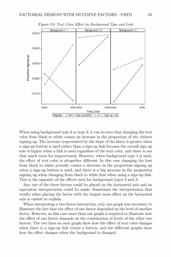
FACTORIAL DESIGNS WITH MULTIPLE FACTORS - CRFD 85
Figure 3.8 Text Color Effect by Background Type and Link
When using background type 2 or type 3, it can be seen that changing the textcolor from black to white causes an increase in the proportion of site visitorssigning up. The increase (represented by the slope of the lines) is greater whena sign-up button is used rather than a sign-up link because the overall sign uprate is higher when a link is used regardless of the text color, and there is notthat much room for improvement. However, when background type 1 is used,the effect of text color is altogether different. In this case changing the fontfrom black to white actually causes a decrease in the proportion signing upwhen a sign-up button is used, and there is a big increase in the proportionsigning up when changing from black to white font when using a sign-up link.This is the opposite of the effects seen for background types 2 and 3.
Any one of the three factors could be placed on the horizontal axis and anequivalent interpretation could be made. Sometimes the interpretation thatresults when placing the factor with the largest main effect on the horizontalaxis is easiest to explain.
When interpreting a two-factor interaction, only one graph was necessary toillustrate the fact that the effect of one factor depended on the level of anotherfactor. However, in this case more than one graph is required to illustrate howthe effect of one factor depends on the combination of levels of the other twofactors. The two lines on each graph show how the effect of text color changeswhen there is a sign-up link versus a button, and the different graphs showhow the effect changes when the background is changed.

86 FACTORIAL DESIGNS
From inspection of the three graphs, or the table of averages that could beproduced by removing the noprint option from proc means, it can be seenthat the highest proportion signing up would be for the Web page with a sign-up button, white text, and background type 2. Here it is predicted that on theaverage, slightly more than 2.7% will sign up. The font size is insignificant, soit doesn’t matter what font size is used.
3.7 Two-Level Factorials
As additional factors are added to a factorial design, the number of treatmentcombinations (runs) in the design increases exponentially. The example in thelast section contained four factors and 36 treatment combinations. If therewere five factors in a design each having four levels, the number of treatmentcombinations would be 4 × 4 × 4 × 4 × 4 = 45 = 1024 runs in the design.It can be seen that it would not take too many factors to render the designimpractical. In other words it would have too many treatment combinations torun in a reasonable period of time. However, it is better to reduce the numberof levels of each factor and stay with the factorial design using all factorsthan it is to revert to one-at-a-time or two-at-a-time experiments and lose theefficiency of factorial experiments. With separate experiments the ability todetect higher order interactions, and the ability to detect interactions betweenany pair of factors is lost. If five factors in a factorial design were studied withonly two levels each, the number of treatment combinations would be reducedto 25 = 32. For this reason factorial designs with two levels for each factor, ora two-level factorials, are popular. A shorthand for a two-level factorial withk factors is a 2k design.
In two-level factorials, if a factor has quantitative levels, the two levels aredenoted symbolically by (−) and (+), where (−) represents the lowest levelthe experimenter would consider, and (+) represents the highest level theexperimenter would consider. The high and low are usually spread out as faras feasibly possible in order to accentuate the signal or difference in responsebetween the two levels. If a factor has qualitative levels, the (−) and (+)designations are arbitrary, but the two levels chosen normally would be twothat the experimenter believes should result in the maximum difference inresponse.
3.7.1 Main Effects and Regression Slopes
The model for a factorial experiment with three factors can be written as:
yijkl = µ+ αi + βj + αβij + γk + αγik + βγjk + αβγijk + εijkl, (3.10)
where αi, βj , etc. are the effects as defined earlier. However, in the case whereeach factor has only two levels represented by (−) and (+), i, j, k, and l canbe replaced with either a (−) or (+), and α− = −α+, since α− = y−··· − y····,α+ = y+··· − y····, and y···· =
(y−··· + y+···
)/2. A similar equality will be true
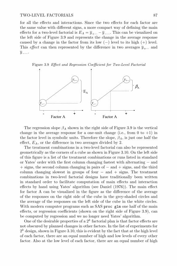
TWO-LEVEL FACTORIALS 87
for all the effects and interactions. Since the two effects for each factor arethe same value with different signs, a more compact way of defining the maineffects for a two-level factorial is EA = y+···− y−···. This can be visualized onthe left side of Figure 3.9 and represents the change in the average responsecaused by a change in the factor from its low (−) level to its high (+) level.This effect can then represented by the difference in two averages y+··· andy−···.
Figure 3.9 Effect and Regression Coefficient for Two-Level Factorial
- +Factor A
EA
- +Factor A
βA
y-···
y+···
y-···
y+···
The regression slope βA shown in the right side of Figure 3.9 is the verticalchange in the average response for a one-unit change (i.e., from 0 to +1) inthe factor level in symbolic units. Therefore the slope, βA, is just one half theeffect, EA, or the difference in two averages divided by 2.
The treatment combinations in a two-level factorial can also be representedgeometrically as the corners of a cube as shown in Figure 3.10. On the left sideof this figure is a list of the treatment combinations or runs listed in standardor Yates’ order with the first column changing fastest with alternating − and+ signs, the second column changing in pairs of − and + signs, and the thirdcolumn changing slowest in groups of four − and + signs. The treatmentcombinations in two-level factorial designs have traditionally been writtenin standard order to facilitate computation of main effects and interactioneffects by hand using Yates’ algorithm (see Daniel (1976)). The main effectfor factor A can be visualized in the figure as the difference of the averageof the responses on the right side of the cube in the grey-shaded circles andthe average of the responses on the left side of the cube in the white circles.With modern computer programs such as SAS proc glm one half of the maineffects, or regression coefficients (shown on the right side of Figure 3.9), canbe computed by regression and we no longer need Yates’ algorithm.
One of the desirable properties of a 2k factorial plan is that factor effects arenot obscured by planned changes in other factors. In the list of experiments for2k design, shown in Figure 3.10, this is evident by the fact that at the high levelof each factor, there are an equal number of high and low levels of every otherfactor. Also at the low level of each factor, there are an equal number of high
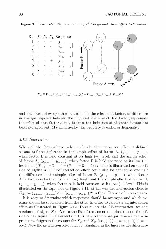
88 FACTORIAL DESIGNS
Figure 3.10 Geometric Representation of 23 Design and Main Effect Calculation
Run XA XB XC Response1 - - - y---2 + - - y+--3 - + - y-+-4 + + - y++-5 - - + y--+6 + - + y+-+7 - + + y-++8 + + + y+++ y+--
y-++
y-+-
y+++
y++-
y--+ y+-+
Factor AFa
ctor
BFact
or Cy---
EA = (y+--+ y++-+ y+-++y+++)/2 – (y---+ y-+-+ y--++ y-++)/2
and low levels of every other factor. Thus the effect of a factor, or differencein average response between the high and low level of that factor, representsthe effect of that factor alone, because the influence of all other factors hasbeen averaged out. Mathematically this property is called orthogonality.
3.7.2 Interactions
When all the factors have only two levels, the interaction effect is definedas one-half the difference in the simple effect of factor A, (y++·· − y−+··),when factor B is held constant at its high (+) level, and the simple effectof factor A, (y+−·· − y−−··), when factor B is held constant at its low (−)level, i.e.,
((y++·· − y−+··)− (y+−·· − y−−··)
)/2. This is illustrated on the left
side of Figure 3.11. The interaction effect could also be defined as one halfthe difference in the simple effect of factor B, (y++·· − y+−··), when factorA is held constant at its high (+) level, and the simple effect of factor B,(y−+·· − y−−··), when factor A is held constant at its low (−) level. This isillustrated on the right side of Figure 3.11. Either way the interaction effect isEAB = (y++··+ y−−··)/2− (y+−··+ y−+··)/2 is the difference of two averages.
It is easy to determine which responses should be averaged and which av-erage should be subtracted from the other in order to calculate an interactioneffect as illustrated in Figure 3.12. To calculate the AB interaction, we adda column of signs, XA ·XB to the list of treatment combinations on the leftside of the figure. The elements in this new column are just the elementwiseproducts of signs in the column for XA and XB (i.e., (−)(−) = +, (−)(+) = −etc.). Now the interaction effect can be visualized in the figure as the difference
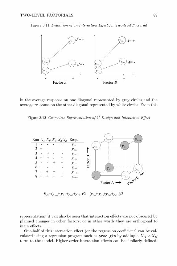
TWO-LEVEL FACTORIALS 89
Figure 3.11 Definition of an Interaction Effect for Two-level Factorial
y++··
y--··
y-+·· y+ -··y-+··
y++··
y--··
y+ -··
- + - +Factor A Factor B
B= -
B= +
A= -
A= +
in the average response on one diagonal represented by grey circles and theaverage response on the other diagonal represented by white circles. From this
Figure 3.12 Geometric Representation of 23 Design and Interaction Effect
Run XA XB XC XA⋅XB Resp.1 - - - + y---2 + - - - y+--3 - + - - y-+-4 + + - + y++-5 - - + + y--+6 + - + - y+-+7 - + + - y-++8 + + + + y+++
y+--
y-++
y-+-
y+++
y++-
y--+ y+-+
Factor A
Fact
or B
Factor Cy---
EAB=(y ---+ y++-+y--++y+++)/2 – (y+--+ y-+-+y+-++y-++)/2
representation, it can also be seen that interaction effects are not obscured byplanned changes in other factors, or in other words they are orthogonal tomain effects.
One-half of this interaction effect (or the regression coefficient) can be cal-culated using a regression program such as proc glm by adding a XA ×XB
term to the model. Higher order interaction effects can be similarly defined.

90 FACTORIAL DESIGNS
Therefore, a simpler way of writing the model for a two-level factorial is byusing the familiar regression equation,
y = β0 + βAXA + βBXB + βABXAXB + βCXC + βACXAXC + βBCXBXC
+ βABCXAXBXC + ε
(3.11)
where, the βs are one-half of the effects and XA = −1 if factor A is at itslow level and XA = +1 if factor A is at its high level. If we write this modelin matrix terms, y = Xβ + ε, the orthogonality property of the design isexpressed by the fact that the columns of theX matrix are orthogonal and theX′X matrix is diagonal with diagonal elements r2k, where r is the numberof replicates of each cell.
3.7.3 Example of a 23 Factorial
To illustrate the design and analysis of a 23 factorial experiment, consider thefollowing example (see Lawson and Erjavec, 2001). Students in a universityelectronics lab often complained that voltage measurements made on a circuitthey constructed in class were inconsistent. The lab teaching assistant (TA)decided to conduct an experiment to try to identify the source of the variation.The three factors he varied were the A=the ambient temperature where thevoltage measurement was made, B=the voltmeter warm-up time, and C=thetime the power was connected to the circuit before the measurement wastaken. The response was the measured voltage in millivolts. The two levelsfor factor A were − = 22C (room temperature) and + = 32C (close to thetemperature in some industrial settings). An oven was used and the circuitwas allowed to stabilize for at least five minutes prior to measurements. Thesettings for factors B and C were − =30 seconds or less, and + =5 minutes.The same circuit was measured for each combination of treatment factorsso the experimental unit was nothing more than the trial or point in timeat which the particular combination of treatment factor levels were appliedto make the measurement. Two replicates of each of the eight experimentalcombinations were run in a random order to help prevent biases. The resultsof the experiment are shown in Table 3.8.
In this table, the actual factor settings are shown on the left, and the coded− and + levels are shown on the right. The actual settings on the left form a listof recipes or directions for performing each experiment. The order number onthe far right next to the response was created with a random number generatorand represents the order in which the experiments should be run. The codedfactor levels are used as the independent variables in a regression program inorder to calculate the regression coefficients or half effects.
The coded factor levels can be easily calculated from the actual factor set-tings using the coding and scaling formula. In this formula we subtract themidpoint of the two factor settings, then divide by half the range. For exam-
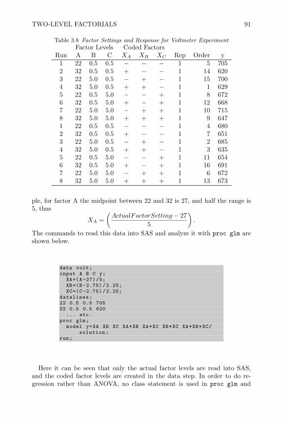
TWO-LEVEL FACTORIALS 91
Table 3.8 Factor Settings and Response for Voltmeter ExperimentFactor Levels Coded Factors
Run A B C XA XB XC Rep Order y1 22 0.5 0.5 − − − 1 5 7052 32 0.5 0.5 + − − 1 14 6203 22 5.0 0.5 − + − 1 15 7004 32 5.0 0.5 + + − 1 1 6295 22 0.5 5.0 − − + 1 8 6726 32 0.5 5.0 + − + 1 12 6687 22 5.0 5.0 − + + 1 10 7158 32 5.0 5.0 + + + 1 9 6471 22 0.5 0.5 − − − 1 4 6802 32 0.5 0.5 + − − 1 7 6513 22 5.0 0.5 − + − 1 2 6854 32 5.0 0.5 + + − 1 3 6355 22 0.5 5.0 − − + 1 11 6546 32 0.5 5.0 + − + 1 16 6917 22 5.0 5.0 − + + 1 6 6728 32 5.0 5.0 + + + 1 13 673
ple, for factor A the midpoint between 22 and 32 is 27, and half the range is5, thus
XA =(ActualFactorSetting − 27
5
).
The commands to read this data into SAS and analyze it with proc glm areshown below.
data volt;input A B C y;
XA=(A-27)/5;XB=(B -2.75)/2.25;XC=(C -2.75)/2.25;
datalines;22 0.5 0.5 70532 0.5 0.5 620
... etc.proc glm;
model y=XA XB XC XA*XB XA*XC XB*XC XA*XB*XC/solution;
run;
Here it can be seen that only the actual factor levels are read into SAS,and the coded factor levels are created in the data step. In order to do re-gression rather than ANOVA, no class statement is used in proc glm and
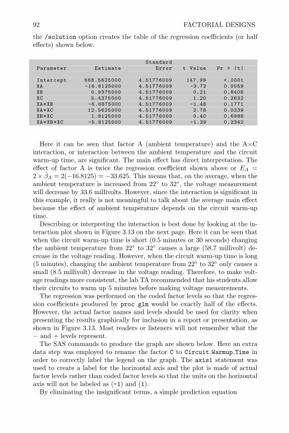
92 FACTORIAL DESIGNS
the /solution option creates the table of the regression coefficients (or halfeffects) shown below.
StandardParameter Estimate Error t Value Pr > |t|
Intercept 668.5625000 4.51776009 147.99 <.0001XA -16.8125000 4.51776009 -3.72 0.0059XB 0.9375000 4.51776009 0.21 0.8408XC 5.4375000 4.51776009 1.20 0.2632XA*XB -6.6875000 4.51776009 -1.48 0.1771XA*XC 12.5625000 4.51776009 2.78 0.0239XB*XC 1.8125000 4.51776009 0.40 0.6988XA*XB*XC -5.8125000 4.51776009 -1.29 0.2342
Here it can be seen that factor A (ambient temperature) and the A×Cinteraction, or interaction between the ambient temperature and the circuitwarm-up time, are significant. The main effect has direct interpretation. Theeffect of factor A is twice the regression coefficient shown above or EA =2× βA = 2(−16.8125) = −33.625. This means that, on the average, when theambient temperature is increased from 22 to 32, the voltage measurementwill decrease by 33.6 millivolts. However, since the interaction is significant inthis example, it really is not meaningful to talk about the average main effectbecause the effect of ambient temperature depends on the circuit warm-uptime.
Describing or interpreting the interaction is best done by looking at the in-teraction plot shown in Figure 3.13 on the next page. Here it can be seen thatwhen the circuit warm-up time is short (0.5 minutes or 30 seconds) changingthe ambient temperature from 22 to 32 causes a large (58.7 millivolt) de-crease in the voltage reading. However, when the circuit warm-up time is long(5 minutes), changing the ambient temperature from 22 to 32 only causes asmall (8.5 millivolt) decrease in the voltage reading. Therefore, to make volt-age readings more consistent, the lab TA recommended that his students allowtheir circuits to warm up 5 minutes before making voltage measurements.
The regression was performed on the coded factor levels so that the regres-sion coefficients produced by proc glm would be exactly half of the effects.However, the actual factor names and levels should be used for clarity whenpresenting the results graphically for inclusion in a report or presentation, asshown in Figure 3.13. Most readers or listeners will not remember what the− and + levels represent.
The SAS commands to produce the graph are shown below. Here an extradata step was employed to rename the factor C to Circuit Warmup Time inorder to correctly label the legend on the graph. The axis1 statement wasused to create a label for the horizontal axis and the plot is made of actualfactor levels rather than coded factor levels so that the units on the horizontalaxis will not be labeled as (-1) and (1).
By eliminating the insignificant terms, a simple prediction equation
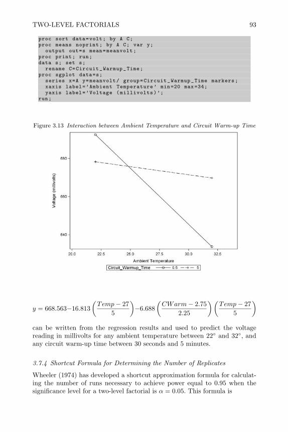
TWO-LEVEL FACTORIALS 93
proc sort data=volt; by A C;proc means noprint; by A C; var y;
output out=s mean=meanvolt;proc print; run;data s; set s;
rename C=Circuit_Warmup_Time;proc sgplot data=s;
series x=A y=meanvolt/ group=Circuit_Warmup_Time markers;xaxis label=’Ambient Temperature ’ min=20 max =34;yaxis label=’Voltage (millivolts)’;
run;
Figure 3.13 Interaction between Ambient Temperature and Circuit Warm-up Time
y = 668.563−16.813(Temp− 27
5
)−6.688
(CWarm− 2.75
2.25
)(Temp− 27
5
)can be written from the regression results and used to predict the voltagereading in millivolts for any ambient temperature between 22 and 32, andany circuit warm-up time between 30 seconds and 5 minutes.
3.7.4 Shortcut Formula for Determining the Number of Replicates
Wheeler (1974) has developed a shortcut approximation formula for calculat-ing the number of runs necessary to achieve power equal to 0.95 when thesignificance level for a two-level factorial is α = 0.05. This formula is

94 FACTORIAL DESIGNS
N = ((8σ)/∆)2 (3.12)
where σ is the standard deviation of the experimental error, ∆ is the size of apractical effect. In this case the difference in average response between the lowand high level of a factor and N = r × 2k is the total number of experimentsin the 2k factorial. Since this formula is so compact, it is easy to use on thespot in meetings where experiments are being planned. As an illustration ofits use, consider an example based on the voltage meter experiment presentedin the last section.
The lab instructor felt that the standard deviation of the experimental errorwas about σ = 15.0 and the size of practical effect was about ∆ = 30.0. σwould be known by the lab instructors experience in making repeat voltagemeasurements of the same circuit under exactly the same conditions (i.e.,factor levels), and ∆ would be known from the amount of inconsistency inmeasurements claimed by the students who were getting inconsistent readings.∆ is the size of the effect the TA would like to detect in his experiments. Usingthe shortcut formula, this says that
N = ((8× 15.0)/30.0)2 = 16
or that r = 2 replicates of each of the 23 = 8 runs should result in a powerof 0.95 for detecting effects of size 30.0 at significance level α = 0.05. If youmodify and use the SAS program for calculating the power in the data step fora factorial experiment presented in Section 3.5.2, the actual power for r = 2replicates is closer to 0.94 than 0.95. However this approximate formula isaccurate enough for most planning purposes.
The simple formula can also be used backwards by solving for ∆ as a func-tion of N , i.e., ∆ = 8×σ/
√N . That way, if an experimenter knows his budget
for experimentation, which dictates the largest N can be, he can calculate thesize of the effect ∆ that he is likely to be able to detect. If the experimenterdoes not have an accurate estimate of σ, the formula can still be used bytalking about practical effect size in units of the unknown σ. For example, ifan experimenters’ budget allows him to make at most N = 64 experiments,he can hope to detect effects that are no more than one standard deviationof the experimental error, i.e., ∆ = 8 × σ/
√64 = σ. This result will be true
regardless of the number of factors in the two-level experiment. Consequently,with 64 runs he may have one factor with r = 32 replicates of each level, orsix factors with r = 1 replicate of each of the 26 = 64 treatment combinations.
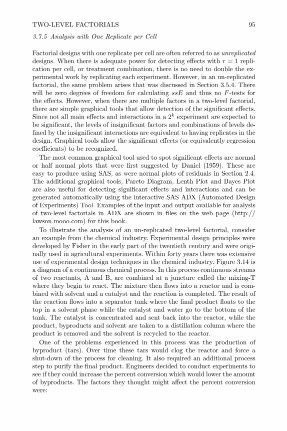
TWO-LEVEL FACTORIALS 95
3.7.5 Analysis with One Replicate per Cell
Factorial designs with one replicate per cell are often referred to as unreplicateddesigns. When there is adequate power for detecting effects with r = 1 repli-cation per cell, or treatment combination, there is no need to double the ex-perimental work by replicating each experiment. However, in an un-replicatedfactorial, the same problem arises that was discussed in Section 3.5.4. Therewill be zero degrees of freedom for calculating ssE and thus no F -tests forthe effects. However, when there are multiple factors in a two-level factorial,there are simple graphical tools that allow detection of the significant effects.Since not all main effects and interactions in a 2k experiment are expected tobe significant, the levels of insignificant factors and combinations of levels de-fined by the insignificant interactions are equivalent to having replicates in thedesign. Graphical tools allow the significant effects (or equivalently regressioncoefficients) to be recognized.
The most common graphical tool used to spot significant effects are normalor half normal plots that were first suggested by Daniel (1959). These areeasy to produce using SAS, as were normal plots of residuals in Section 2.4.The additional graphical tools, Pareto Diagram, Lenth Plot and Bayes Plotare also useful for detecting significant effects and interactions and can begenerated automatically using the interactive SAS ADX (Automated Designof Experiments) Tool. Examples of the input and output available for analysisof two-level factorials in ADX are shown in files on the web page (http://lawson.mooo.com) for this book.
To illustrate the analysis of an un-replicated two-level factorial, consideran example from the chemical industry. Experimental design principles weredeveloped by Fisher in the early part of the twentieth century and were origi-nally used in agricultural experiments. Within forty years there was extensiveuse of experimental design techniques in the chemical industry. Figure 3.14 isa diagram of a continuous chemical process. In this process continuous streamsof two reactants, A and B, are combined at a juncture called the mixing-Twhere they begin to react. The mixture then flows into a reactor and is com-bined with solvent and a catalyst and the reaction is completed. The result ofthe reaction flows into a separator tank where the final product floats to thetop in a solvent phase while the catalyst and water go to the bottom of thetank. The catalyst is concentrated and sent back into the reactor, while theproduct, byproducts and solvent are taken to a distillation column where theproduct is removed and the solvent is recycled to the reactor.
One of the problems experienced in this process was the production ofbyproduct (tars). Over time these tars would clog the reactor and force ashut-down of the process for cleaning. It also required an additional processstep to purify the final product. Engineers decided to conduct experiments tosee if they could increase the percent conversion which would lower the amountof byproducts. The factors they thought might affect the percent conversionwere:
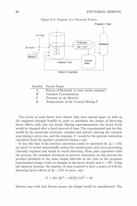
96 FACTORIAL DESIGNS
Figure 3.14 Diagram of a Chemical Process
Product + Tars
P+Solvent
Cat + H2O
A + H2O
B + H2O
Concen-trator
Solvent + Impurities
Catalyst + H2O
Distillation
Mixing T
Symbol Factor NameA Excess of Reactant A (over molar amount)B Catalyst ConcentrationC Pressure in the ReactorD Temperature of the Coated Mixing-T
Two levels of each factor were chosen that were spread apart as wide asthe engineers thought feasible in order to maximize the chance of detectingfactor effects with only two levels. During experimentation, the factor levelswould be changed after a fixed interval of time. The experimental unit for thiswould be the particular reactants, catalyst and solvent entering the reactionzone during a given run, and the response, Y , would be the percent conversioncalculated from the product produced during a run.
It was felt that if the percent conversion could be increased by ∆ = 12%(or more) it would substantially reduce the maintenance and extra processingcurrently required and would be worth detecting. From past experience withthe process, the standard deviation in percent conversion on this process forproduct produced in the same length intervals as the runs in the proposedexperimental design (with no changes in the factor levels) was σ = 6%. Usingthe shortcut formula, the number of runs required to have a power of 0.95 fordetecting factor effects of ∆ = 12% or more, was
N = (8σ/∆)2 = ((8)(6)/12)2 = 16
Sixteen runs with four factors means the design would be unreplicated. The
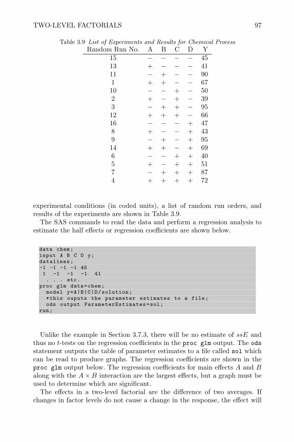
TWO-LEVEL FACTORIALS 97
Table 3.9 List of Experiments and Results for Chemical ProcessRandom Run No. A B C D Y
15 − − − − 4513 + − − − 4111 − + − − 901 + + − − 6710 − − + − 502 + − + − 393 − + + − 9512 + + + − 6616 − − − + 478 + − − + 439 − + − + 9514 + + − + 696 − − + + 405 + − + + 517 − + + + 874 + + + + 72
experimental conditions (in coded units), a list of random run orders, andresults of the experiments are shown in Table 3.9.
The SAS commands to read the data and perform a regression analysis toestimate the half effects or regression coefficients are shown below.
data chem;input A B C D y;datalines;-1 -1 -1 -1 451 -1 -1 -1 41. . . etc.
proc glm data=chem;model y=A|B|C|D/solution;*this ouputs the parameter estimates to a file;ods output ParameterEstimates=sol;
run;
Unlike the example in Section 3.7.3, there will be no estimate of ssE andthus no t-tests on the regression coefficients in the proc glm output. The odsstatement outputs the table of parameter estimates to a file called sol whichcan be read to produce graphs. The regression coefficients are shown in theproc glm output below. The regression coefficients for main effects A and Balong with the A×B interaction are the largest effects, but a graph must beused to determine which are significant.
The effects in a two-level factorial are the difference of two averages. Ifchanges in factor levels do not cause a change in the response, the effect will
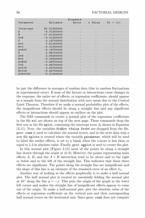
98 FACTORIAL DESIGNS
StandardParameter Estimate Error t Value Pr > |t|
Intercept 62.31250000 . . .A -6.31250000 . . .B 17.81250000 . . .A*B -5.31250000 . . .C 0.18750000 . . .A*C 0.81250000 . . .B*C -0.31250000 . . .A*B*C -0.18750000 . . .D 0.68750000 . . .A*D 2.06250000 . . .B*D -0.06250000 . . .A*B*D -0.68750000 . . .C*D -0.68750000 . . .A*C*D 2.43750000 . . .B*C*D -0.43750000 . . .A*B*C*D -0.31250000 . . .
be just the difference in averages of random data (due to random fluctuationsin experimental error). If none of the factors or interactions cause changes inthe response, the entire set of effects, or regression coefficients, should appearas a sample from the normal distribution with zero mean due to the CentralLimit Theorem. Therefore if we make a normal probability plot of the effects,the insignificant effects should lie along a straight line and any significanteffects or interactions should appear as outliers on the plot.
The SAS commands to create a normal plot of the regression coefficientsin the file sol are shown on top of the next page. These commands drop thefirst row in the file nplot, containing the intercept term β0 shown in Equation(3.11). Next, the variables StdErr tValue Probt are dropped from the file.proc rank is used to calculate the normal scores, and in the next data step anew file nplots is created where the variable parameter, which will be usedto label the outlier effects, is set to a blank when the z-score is less than orequal to 1.2 in absolute value. Finally, proc sgplot is used to create the plot.
In this normal plot (Figure 3.15) most of the points lie along a straightline drawn through the origin at (0, 0). However, the points representing maineffects A, B, and the A × B interaction tend to be above and to the rightor below and to the left of the straight line. This indicates that these threeeffects are significant. The points along the straight line are insignificant andthe slope of this line is an estimate of the standard error of an effect σβ .
Another way of looking at the effects graphically is to make a half normalplot. The half normal plot is created by essentially folding the normal plotat 45 along the line y = −x. This puts the origin of the graph in the lowerleft corner and makes the straight line of insignificant effects appear to comeout of the origin. To make a half-normal plot, plot the absolute value of theeffects or regression coefficients on the vertical axis and their correspondinghalf normal scores on the horizontal axis. Since proc rank does not compute
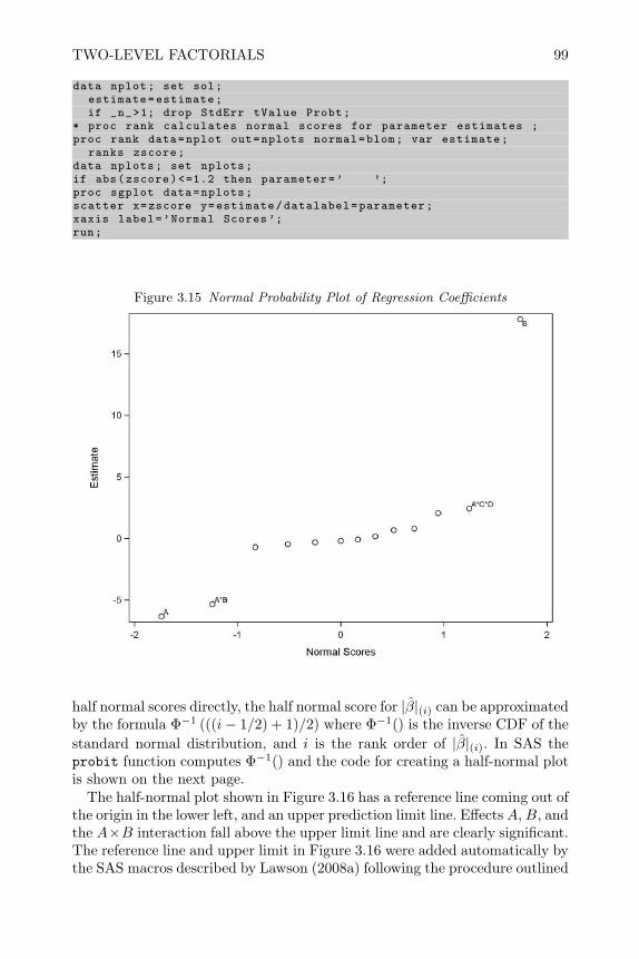
TWO-LEVEL FACTORIALS 99
data nplot; set sol;estimate=estimate;if _n_>1; drop StdErr tValue Probt;
* proc rank calculates normal scores for parameter estimates ;proc rank data=nplot out=nplots normal=blom; var estimate;
ranks zscore;data nplots; set nplots;if abs(zscore)<=1.2 then parameter=’ ’;proc sgplot data=nplots;scatter x=zscore y=estimate/datalabel=parameter;xaxis label=’Normal Scores ’;run;
Figure 3.15 Normal Probability Plot of Regression Coefficients
half normal scores directly, the half normal score for |β|(i) can be approximatedby the formula Φ−1 (((i− 1/2) + 1)/2) where Φ−1() is the inverse CDF of thestandard normal distribution, and i is the rank order of |β|(i). In SAS theprobit function computes Φ−1() and the code for creating a half-normal plotis shown on the next page.
The half-normal plot shown in Figure 3.16 has a reference line coming out ofthe origin in the lower left, and an upper prediction limit line. Effects A, B, andthe A×B interaction fall above the upper limit line and are clearly significant.The reference line and upper limit in Figure 3.16 were added automatically bythe SAS macros described by Lawson (2008a) following the procedure outlined
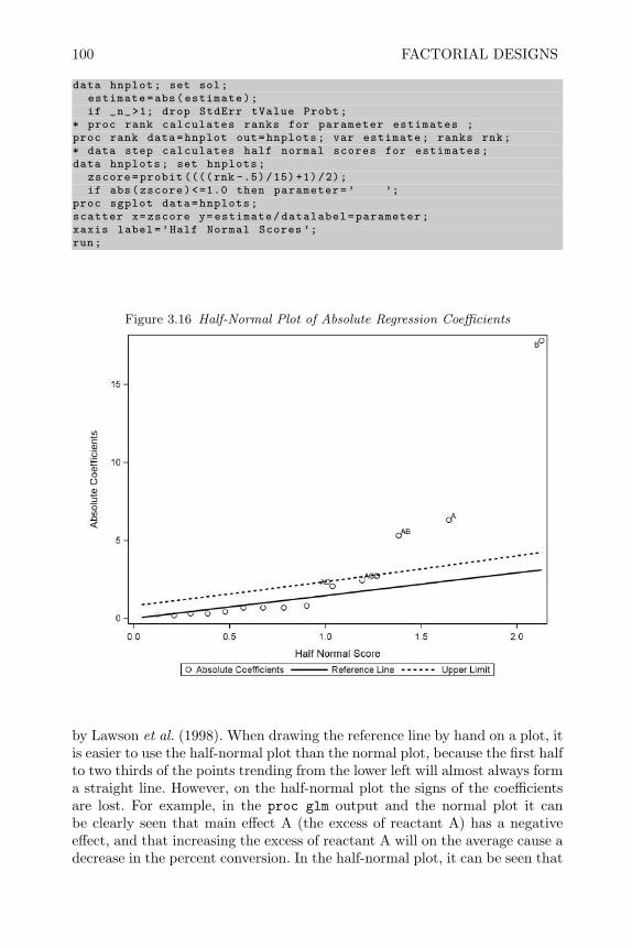
100 FACTORIAL DESIGNS
data hnplot; set sol;estimate=abs(estimate);if _n_>1; drop StdErr tValue Probt;
* proc rank calculates ranks for parameter estimates ;proc rank data=hnplot out=hnplots; var estimate; ranks rnk;* data step calculates half normal scores for estimates;data hnplots; set hnplots;
zscore=probit ((((rnk -.5)/15) +1)/2);if abs(zscore)<=1.0 then parameter=’ ’;
proc sgplot data=hnplots;scatter x=zscore y=estimate/datalabel=parameter;xaxis label=’Half Normal Scores ’;run;
Figure 3.16 Half-Normal Plot of Absolute Regression Coefficients
by Lawson et al. (1998). When drawing the reference line by hand on a plot, itis easier to use the half-normal plot than the normal plot, because the first halfto two thirds of the points trending from the lower left will almost always forma straight line. However, on the half-normal plot the signs of the coefficientsare lost. For example, in the proc glm output and the normal plot it canbe clearly seen that main effect A (the excess of reactant A) has a negativeeffect, and that increasing the excess of reactant A will on the average cause adecrease in the percent conversion. In the half-normal plot, it can be seen that
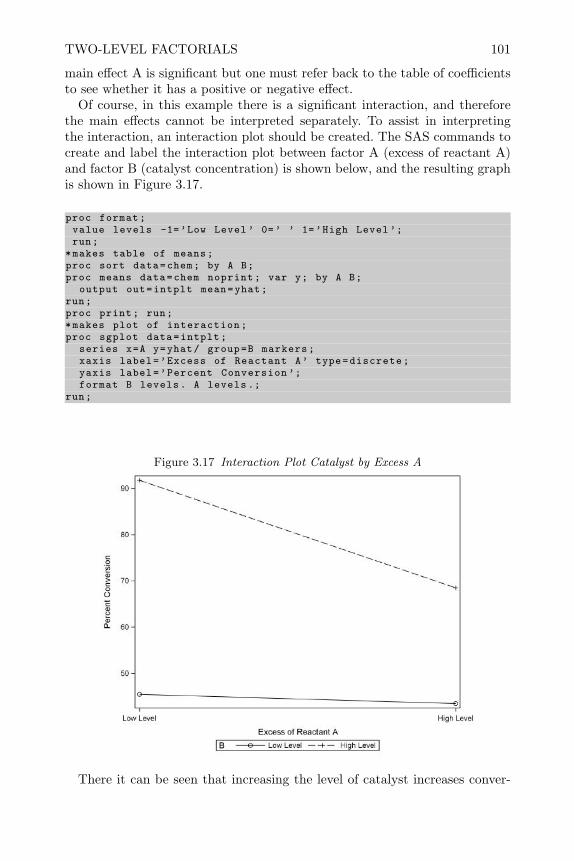
TWO-LEVEL FACTORIALS 101
main effect A is significant but one must refer back to the table of coefficientsto see whether it has a positive or negative effect.
Of course, in this example there is a significant interaction, and thereforethe main effects cannot be interpreted separately. To assist in interpretingthe interaction, an interaction plot should be created. The SAS commands tocreate and label the interaction plot between factor A (excess of reactant A)and factor B (catalyst concentration) is shown below, and the resulting graphis shown in Figure 3.17.
proc format;value levels -1=’Low Level ’ 0=’ ’ 1=’High Level’;run;
*makes table of means;proc sort data=chem; by A B;proc means data=chem noprint; var y; by A B;
output out=intplt mean=yhat;run;proc print; run;*makes plot of interaction;proc sgplot data=intplt;
series x=A y=yhat/ group=B markers;xaxis label=’Excess of Reactant A’ type=discrete;yaxis label=’Percent Conversion ’;format B levels. A levels .;
run;
Figure 3.17 Interaction Plot Catalyst by Excess A
There it can be seen that increasing the level of catalyst increases conver-
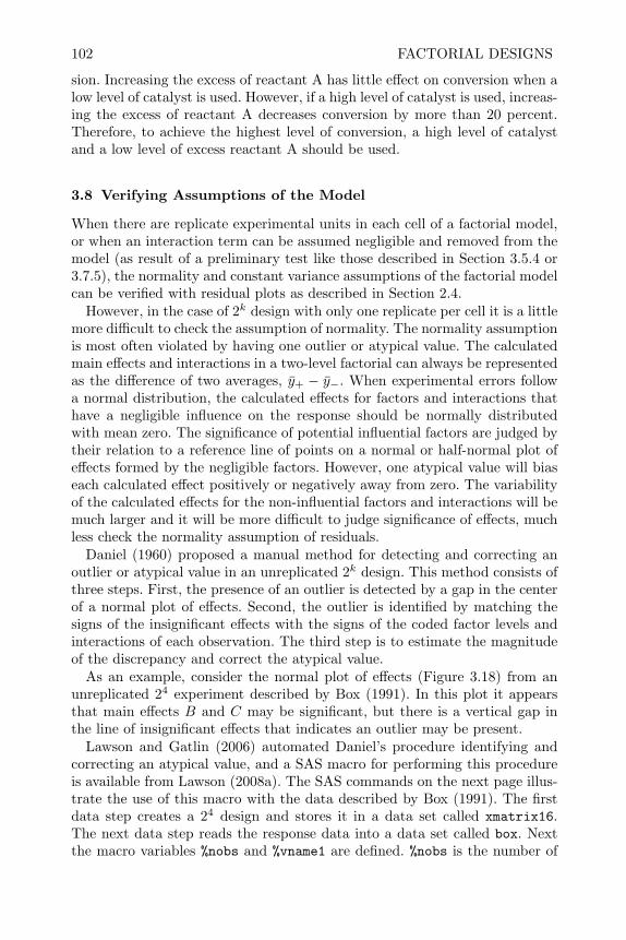
102 FACTORIAL DESIGNS
sion. Increasing the excess of reactant A has little effect on conversion when alow level of catalyst is used. However, if a high level of catalyst is used, increas-ing the excess of reactant A decreases conversion by more than 20 percent.Therefore, to achieve the highest level of conversion, a high level of catalystand a low level of excess reactant A should be used.
3.8 Verifying Assumptions of the Model
When there are replicate experimental units in each cell of a factorial model,or when an interaction term can be assumed negligible and removed from themodel (as result of a preliminary test like those described in Section 3.5.4 or3.7.5), the normality and constant variance assumptions of the factorial modelcan be verified with residual plots as described in Section 2.4.
However, in the case of 2k design with only one replicate per cell it is a littlemore difficult to check the assumption of normality. The normality assumptionis most often violated by having one outlier or atypical value. The calculatedmain effects and interactions in a two-level factorial can always be representedas the difference of two averages, y+ − y−. When experimental errors followa normal distribution, the calculated effects for factors and interactions thathave a negligible influence on the response should be normally distributedwith mean zero. The significance of potential influential factors are judged bytheir relation to a reference line of points on a normal or half-normal plot ofeffects formed by the negligible factors. However, one atypical value will biaseach calculated effect positively or negatively away from zero. The variabilityof the calculated effects for the non-influential factors and interactions will bemuch larger and it will be more difficult to judge significance of effects, muchless check the normality assumption of residuals.
Daniel (1960) proposed a manual method for detecting and correcting anoutlier or atypical value in an unreplicated 2k design. This method consists ofthree steps. First, the presence of an outlier is detected by a gap in the centerof a normal plot of effects. Second, the outlier is identified by matching thesigns of the insignificant effects with the signs of the coded factor levels andinteractions of each observation. The third step is to estimate the magnitudeof the discrepancy and correct the atypical value.
As an example, consider the normal plot of effects (Figure 3.18) from anunreplicated 24 experiment described by Box (1991). In this plot it appearsthat main effects B and C may be significant, but there is a vertical gap inthe line of insignificant effects that indicates an outlier may be present.
Lawson and Gatlin (2006) automated Daniel’s procedure identifying andcorrecting an atypical value, and a SAS macro for performing this procedureis available from Lawson (2008a). The SAS commands on the next page illus-trate the use of this macro with the data described by Box (1991). The firstdata step creates a 24 design and stores it in a data set called xmatrix16.The next data step reads the response data into a data set called box. Nextthe macro variables %nobs and %vname1 are defined. %nobs is the number of
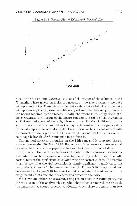
VERIFYING ASSUMPTIONS OF THE MODEL 103
Figure 3.18 Normal Plot of Effects with Vertical Gap
runs in the design, and %vname1 is a list of the names of the columns in theX matrix. These macro variables are needed by the macro. Finally the dataset representing the X matrix is copied into a data set called x1 and the dataset representing the response variable is copied into the data set y. These arethe names required by the macro. Finally the macro is called by the state-ment %gapmth. The output of the macro consists of a table of the regressioncoefficients and a test of their significance, a test for the significance of thegap in the normal plot, and when the gap is determined to be significant, acorrected response table and a table of regression coefficients calculated withthe corrected data is produced. The corrected response table is shown on thenext page below the SAS commands to produce it.
The method detected an outlier on the 13th run, and it corrected the re-sponse by changing 59.15 to 52.15. Reanalysis of the corrected data resultedin the table shown on the page that follows the table of corrected data.
The macro also produces half-normal plots of the regression coefficientscalculated from the raw data and corrected data. Figure 3.19 shows the half-normal plot of the coefficients calculated with the corrected data. In this plotit can be seen that the AC interaction is clearly significant in addition to themain effects B and C, that were identified in Figure 3.18. They could notbe detected in Figure 3.18 because the outlier inflated the estimates of theinsignificant effects and the AC effect was buried in the noise.
Whenever an outlier is discovered, using this method or residual plots, andthe conclusions of the analysis change when the outlier is removed or corrected,the experimenter should proceed cautiously. When there are more than two
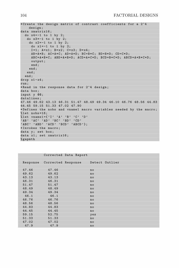
104 FACTORIAL DESIGNS
*Create the design matrix of contrast coefficients for a 2^4design;
data xmatrix16;do x4=-1 to 1 by 2;do x3=-1 to 1 by 2;do x2=-1 to 1 by 2;do x1=-1 to 1 by 2;I=1; A=x1; B=x2; C=x3; D=x4;AB=A*B; AC=A*C; AD=A*D; BC=B*C; BD=B*D; CD=C*D;ABC=A*B*C; ABD=A*B*D; ACD=A*C*D; BCD=B*C*D; ABCD=A*B*C*D;output;end;
end;end;
end;drop x1-x4;run;*Read in the response data for 2^4 design;data box;input y @@;datalines;47.46 49.62 43.13 46.31 51.47 48.49 49.34 46.10 46.76 48.56 44.8344.45 59.15 51.33 47.02 47.90*Defines the nobs and vname1 macro variables needed by the macro;%let nobs =16;%let vname1 =’I’ ’A’ ’B’ ’C’ ’D’’AB’ ’AC’ ’AD’ ’BC’ ’BD’ ’CD’’ABC’ ’ABD’ ’ACD’ ’BCD’ ’ABCD’;*Invokes the macro;data y; set box;data x1; set xmatrix16;%gapmth
Corrected Data Report
Response Corrected Response Detect Outlier
47.46 47.46 no49.62 49.62 no43.13 43.13 no46.31 46.31 no51.47 51.47 no48.49 48.49 no49.34 49.34 no46.1 46.1 no
46.76 46.76 no48.56 48.56 no44.83 44.83 no44.45 44.45 no59.15 52.75 yes51.33 51.33 no47.02 47.02 no47.9 47.9 no

VERIFYING ASSUMPTIONS OF THE MODEL 105
Effect Report
HalfLabel Effect Abs(Effect) Sig(at 0.05)
A -9E-16 89E-17 noB -1.71 1.71 yesC 1.455 1.455 yesD 0.105 0.105 noAB 0.055 0.055 noAC -0.845 0.845 yesAD 0.11 0.11 noBC -9E-16 89E-17 noBD -0.19 0.19 noCD 0.345 0.345 noABC 0.2 0.2 noABD -0.04 0.04 noACD 0.6 0.6 noBCD -0.39 0.39 noABCD 0.36 0.36 no
Lawson , Grimshaw & Burt Rn Statistic =1.62695th percentile of Rn= 1.201
replicates at the same factor settings where the outlier was found, it may beclear that something is amiss. However, if there are two or less observationsat factor settings where the outlier was found, it may be advisable to rerunthe questionable experiment.
Figure 3.19 half-normal Plot of Coefficients Calculated with Corrected Data
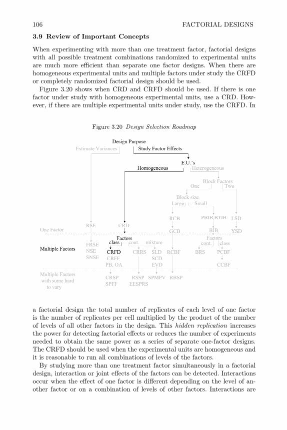
106 FACTORIAL DESIGNS
3.9 Review of Important Concepts
When experimenting with more than one treatment factor, factorial designswith all possible treatment combinations randomized to experimental unitsare much more efficient than separate one factor designs. When there arehomogeneous experimental units and multiple factors under study the CRFDor completely randomized factorial design should be used.
Figure 3.20 shows when CRD and CRFD should be used. If there is onefactor under study with homogeneous experimental units, use a CRD. How-ever, if there are multiple experimental units under study, use the CRFD. In
Figure 3.20 Design Selection Roadmap
Design PurposeEstimate Variances Study Factor Effects
E.U.’s
Block Factors
One Factor
Multiple Factors
Multiple Factorswith some hard
to vary
Block size
Homogeneous Heterogeneous
Large Small
RCB
GCB
PBIB,BTIB
BIB
LSD
YSDRSE CRD
FactorsFRSENSESNSE
CRFD CRRS SLD RCBF BRS PCBFCRFF SCD
PB, OA EVD CCBF
CRSP RSSP SPMPV RBSPSPFF EESPRS
One Two
class cont. mixture cont. classFactors
a factorial design the total number of replicates of each level of one factoris the number of replicates per cell multiplied by the product of the numberof levels of all other factors in the design. This hidden replication increasesthe power for detecting factorial effects or reduces the number of experimentsneeded to obtain the same power as a series of separate one-factor designs.The CRFD should be used when the experimental units are homogeneous andit is reasonable to run all combinations of levels of the factors.
By studying more than one treatment factor simultaneously in a factorialdesign, interaction or joint effects of the factors can be detected. Interactionsoccur when the effect of one factor is different depending on the level of an-other factor or on a combination of levels of other factors. Interactions are

REVIEW OF IMPORTANT CONCEPTS 107
common in the real world, and ignoring them by experimenting with one fac-tor at a time can be very misleading. Examples in this chapter show that it iseasy to describe or interpret the meaning of an interaction by comparing orcontrasting the effect of one factor over the levels of another factor. Interactiongraphs are helpful in describing interactions.
The model for analysis of a factorial with two factors can be written as
yijk = µ+ αi + βj + αβij + εijk
and can be easily extended to multiple factors. The assumptions for the analy-sis are homogeneity and normality of experimental errors, and can be checkedusing the residual plots described in Chapter 2. When there is an equal num-ber of replications per cell or treatment combination, the proc glm type I ortype III sums of squares can be used to test the main effects and interactions,and the means or lsmeans statements can be used to get unbiased estimatesof cell means and marginal means. However, if there is an unequal number ofreplicates per cell, the type III sums of squares and lsmeans must be used.
When multiple factors are studied in a factorial experiment, often onlytwo levels of each factor are used in order to reduce the total amount ofexperimentation required. In that case, the model simplifies to a regressionmodel
y = β0 + βAXA + βBXB + βABXAXB + βCXC + βACXAXC + βBCXBXC
+ βABCXAXBXC + ε
and the regression coefficients are exactly one half the effect or difference inthe average response between the low and high levels of the factors. Interactioneffects are also easily defined as differences of averages in this case. There isa shortcut formula for approximating the power in two-level factorials, andwhen there is only one replicate per treatment combination, the significance ofeffects and interactions can be determined using normal or half-normal plots.

108 FACTORIAL DESIGNS
3.10 Exercises
1. A consultant was called to assist the police department of a large metropoli-tan city in evaluating its human relations course for new officers. He planneda 2-factor factorial experiment where the treatments were A the type beatto which officers were assigned, and B the length of the human relationscourse. A sample of 45 new officers was chosen, and 5 were randomly as-signed to each of the 9 treatment combinations. A test was developed tomeasure officers’ attitude toward minority groups and was administered tothe participating officers after their training had ended and they had ex-perienced two weeks on their beat. Better attitudes result in higher scoreson this test. Analysis of the data revealed a significant A×B interactioneffect between the type beat and length of human relations course. Thetable below shows the mean test scores for the 9 combinations of treatmentlevels.
Length of human relations courseType beat 5 hours 10 hours 15 hoursupper-class beat 34.4 35.5 39.2middle-class beat 30.2 32.4 34.7inner-city beat 20.1 39.4 54.3
(a) Construct an interaction graph.(b) Write an interpretation of the interaction in a few complete sentences.
2. A wooden catapult can be used to flip a foam ball. The catapult has threefactors that can be adjusted: the start angle, the stop angle, and the pivotheight. The distance the ball travels can be measured with a tape measure.
Start Angle
Stop Angle
PivotHeight
(a) If experiments were to be conducted with the catapult by flipping theball and measuring the distance, what would the experimental unit be?
(b) Using the numbers 1, 2 and 3 to represent the levels of start angle andstop angle, and holding the pivot height constant at its high level, makea randomized list of experiments for a 3×3 factorial experiment withr = 2 replicates per cell.

EXERCISES 109
(c) If the variance of the experimental error in the measured distance wasσ2 = 12 inches, calculate the number of replicates you would need tohave a power of 0.90 for detecting a difference in 10 inches in cell means.
(d) Calculate the number of replicates you would need to have a power of0.90 for detecting a difference of 24 inches in marginal means for eitherfactor.
(e) If a catapult is available, conduct the list of experiments you wrote inpart (b).
(f) Calculate the ANOVA with your resulting data and test the main effectsand interaction.
(g) Explain or interpret any significant effects (use graphs if necessary toaid in your explanation).
3. In an experiment to maximize the Y= resolution of a peak on a gas Chro-matograph, a significant interaction between A = column temperature andC = gas flow rate was found. The table below shoes the mean resolutionin each combination of column temperature and gas flow rate.
Column Gas Flow RateTemperature Low High120 10 13180 12 18
(a) Construct an interaction graph.(b) Write a sentence, or two, to interpret this interaction.
4. Consider performing experiments to determine the effect of popcorn brand,power level, and time on the percentage of edible popcorn (unpopped orburnt is not edible) kernels made in a microwave oven. The object is tomaximize the proportion of edible kernels. Start with 1
3 cup of kernels anddo pilot experiments to determine the range of the factors you would like tostudy and an estimate of the standard deviation of replicates made underthe same conditions.
(a) What is the experimental unit for this experiment?(b) Determine how many replicates will be required to detect a maximum
difference in marginal (main effect) means of 0.25.(c) Determine the number of levels of the factors you would like to study,
and create a randomized list of the experiments for a factorial design.(d) Actually perform the experiments and collect the data.(e) Analyze the data. Partition any significant effects of power level and
time into orthogonal polynomial contrasts. Interpret the results, anddetermine the optimum combination of factor levels from among thoseyou tested.

110 FACTORIAL DESIGNS
(f) How many experiments would it have taken to get the same power formain effects using a vary one-factor-at-a-time plan? Would you detectthe same optimum using the vary one-factor-at-a-time plan?
5. Use proc glmpower to verify that the power would be 0.80 for detectingdifferences in marginal means of ∆ = 1.0 in. in the paper helicopter exper-iments with four levels of wing length, four levels of body width, and r = 2replicates per cell (as shown in Section 3.5.2).
6. In a continuation of the experiments to investigate the effect of plant growthregulators and spear bud scales on spear elongation in asparagus, describedin exercise 4 of Chapter 2, Yang-Gyu and Woolley (2006) conducted a 4×3factorial experiment varying the concentration of the plant growth regulatorCPPU in the solution, and the time the asparagus spears were dipped inthe solution. The results are shown in the table below.
dipping time (sec)CPPU conc. 30 60 900 (control) 92.5 92.9 91.30.5 ppm 97.8 94.9 101.31.0 ppm 97.0 98.5 101.610.0 ppm 103.4 102.9 98.6
(a) Partition the sums of squares for CPPU concentration and dipping timeinto orthogonal polynomial contrasts. Partition the interaction of CPPUconc. by dipping time into linear×linear, quadratic×linear, cubic×linear,linear×quadratic, quadratic×quadratic, and cubic×quadratic. Pool (sum)all sums of squares but the linear×linear portion to form an error sumof squares and use it to test the linear×linear part of the interaction andthe polynomial contrasts you found for the main effects. Interpret yourresults.
(b) Use the %tukeysdf macro to test the significance of the interaction.(c) Based on the results you obtained in (a) and (b) would you recommend
the additive model for this data?
7. Kenett and Steinberg (1987) describe a two-level factorial experiment con-ducted by students to study the time required to boil 1 qt of water. Factorswere A=flame level (low or high), B=pan size (small or large), C=pan cover(none or glass cover) and D=salt added to water (no or yes).
(a) If the standard deviation in boiling time (tested at the same conditions)was found to be σ=0.236 minutes, use the shortcut formula to determinehow many experiments you will need to perform in order to have powerof 0.95 for detecting effects of size ∆=0.50 minutes. Would this answerchange if you decided to only perform an experiment with 3 of the 4factors?

EXERCISES 111
(b) Create a list of experiments in random order for performing these ex-periments.
(c) Actually perform the experiments by boiling the water and collect thedata.
(d) Analyze the data to determine which effects and interactions are signif-icant.
(e) Interpret and explain any significant effects you find.
8. Consider the data in Table 3.9 with the third observation (90) replaced byan atypical value (78) for those factor settings.
(a) Calculate the effects for this data.(b) Make a normal or half-normal plot of the effects.(c) What effects do you judge to be significant?(d) Run the SAS macro for Daniel’s method of detecting and correcting an
outlier with this data.

112 FACTORIAL DESIGNS
3.11 Appendix–SAS Macro for Tukey’s Single df Test
%macro tukeysdf;****************************************************************;** Input for this macro is a file called file1 that has a ***;** variable A for Factor A levels , a variable B for Factor B **;** levels and a variable y for the response variable **;****************************************************************;*computes ANOVA for additive model;proc glm data=file1;class A B;model y=A B;ods output ModelANOVA=SumS;ods output OverallANOVA=ESums;*gets Error SS and df from ANOVA;data ssE; set Esums;if Source=’Error ’ ;ssE=SS; dfe=df;keep ssE dfe;*gets sum of squares and df for Factor A from ANOVA;data ssA; set SumS;if HypothesisType =1; if Source=’A’;ssA=SS; dfa=df;keep ssA dfa;*gets sum of squares and df for Factor B from ANOVA;data ssB; set SumS;if HypothesisType =1; if Source=’B’;ssB=SS;dfb=df;keep ssB dfb;*creates marginal means for factor A;proc sort data=file1; by A;proc means noprint; var y; by A;output out=m1 mean=ybaridot;*calculates number of levels of factor A;proc means noprint data=m1; var ybaridot;output out=mA n=a;*creates marginal means for Factor B;proc sort data=file1; by B;proc means noprint; var y; by B;output out=m2 mean=ybardotj;*calculates number of levels of factor B;proc means noprint data=m2; var ybardotj;output out=mB n=b;*note creates grand mean;proc means noprint data=file1; var y;output out=m3 mean=ybardd;*note merges marginal means to original data;proc sort data=file1; by A;data B; merge file1 m1; by A;proc sort data=B; by B;data C; merge B m2; by B;yijyidydj=y*ybaridot*ybardotj;proc means data=C noprint; var yijyidydj;output out=s1 sum=sp1;*combines Summary info and calculates single df interaction SS;data comb; merge s1 ssA ssB ssE mA mB m3;msA=ssA/dfa; msB=ssB/dfB; msE=ssE/dfe;SSAB=(a*b*(sp1 -(ssA+ssB+a*b*ybardd**2)*ybardd)**2)/(ssA*ssB);ssR=ssE -SSAB; dfn=1; dfr=dfe -1; msR=ssR/dfr;FA=msA/msR; FB=msB/msR; FAB=SSAB/msR;probA=1-probf(FA,dfa ,dfr); probB=1-probF(FB,dfb ,dfr);probAB=1-probf(FAB ,dfn ,dfr);

APPENDIX–SAS MACRO FOR TUKEY’S SINGLE DF TEST 113
data _null_; set comb end=eof;file print notitles;put @20 ’ Tukey’’s single df test for additivity ’
/// @15 ’Source df SS MS FPR>F’
/;put @ 15 ’A’ @32 dfa @38 ssA best7. @50 msA best7 .;put @ 15 ’B’ @32 dfb @38 ssB best7. @50 msB best7 .;put @ 15 ’Error’ @32 dfe @38 ssE best7. @50 msE best7.;put @ 15 ’NonAdditivity ’ @32 dfn @38 SSAB best7. @50 SSAB best7.
@62 FAB best5.@71 probAB best5 .;put @ 15 ’Residual ’ @32 dfr @38 ssR best7. @50 msR best7 .;run;%mend tukeysdf;


CHAPTER 4
Randomized Block Designs
4.1 Introduction
In order to eliminate as much of the natural variation as possible and increasethe sensitivity of experiments, it would be advisable to choose the experimen-tal units for a study to be as homogeneous as possible. In mathematical termsthis would reduce the variance, σ2, of the experimental error and increase thepower for detecting treatment factor effects. On the other hand, most exper-imenters would like the conclusions of their work to have wide applicability.Consider the following example. An experimenter would like to compare sev-eral methods of aerobic exercise to see how they affect the stress and anxietylevel of experimental subjects. Since there is wide variability in stress andanxiety levels in the general population, as measured by standardized testscores, it would be difficult to see any difference among various methods ofexercise unless the subjects recruited to the study were a homogeneous groupeach similar in their level of stress. However, the experimenter would like tomake general conclusions from his study to people of all stress levels in thegeneral population.
Blocking can be used in this situation to achieve both objectives. Blockingis the second technique that falls in the category of error control defined inSection 1.4. In a randomized block design, a group of heterogeneous exper-imental units is used so that the conclusions can be more general; however,these heterogeneous experimental units are grouped into homogeneous sub-groups before they are randomly assigned to treatment factor levels. The actof grouping the experimental units together in homogeneous groups is calledblocking. Randomly assigning treatment factor levels to experimental unitswithin the smaller homogeneous subgroups of experimental units, or blocks,has the same effect as using only homogeneous units, yet it allows the conclu-sions to be generalized to the entire class of heterogeneous experimental unitsused in the study.
If experimental units represent physical entities, blocking or grouping bysimilar physical characteristics often results in more homogeneous groups.For example, plots of land in agricultural experiments are usually blocked byproximity because plots in close proximity normally have similar soil char-acteristics. When experimental units are animals, the grouping of geneticallysimilar animals, such as litter-mates, often reduces variability within groups.When experimental units are simply trials, or points in time where treatments
115

116 RANDOMIZED BLOCK DESIGNS
will be applied, they are often blocked by time since many lurking variablesmay change over time and trials in close temporal proximity are more alike.
In a randomized complete block design, or RCB, with one treatment factor,when the factor has t levels there will be b blocks (or subgroups of homo-geneous experimental units) that each contain exactly t experimental unitsfor a total of t × b experimental units. The t experimental units within eachblock are as similar as possible, and the groups of experimental units varyenough from block to block to allow general conclusions to be drawn. Therandomization of experimental units to treatment factor levels, described inChapter 2, is performed within each block. Fisher first proposed block de-signs for agricultural experiments where the experimental units were plots ofground. Blocks represented compact plots in close proximity which were sim-ilar. Variability among blocks represented the range of conditions over whichconclusions would be generalized.
If there are more than t experimental units within each block, so that treat-ment factor levels are replicated r times within each block, there will be a totalof r × t × b experimental units. In this situation we call the design a generalcomplete block design. Normally the RCB would be preferred over the generalcomplete block design because smaller blocks of experimental units allow forgreater homogeneity within the blocks and thus smaller experimental errorand more precise tests and estimates.
4.2 Creating an RCB in SAS
The randomization of experimental units to treatment factor levels in a ran-domized block design can be accomplished using the SAS data step similarto what was shown in Chapter 2, or using SAS proc plan. To illustrate howthis is done, consider the following experimental situation. A student wantedto investigate wives’ tales of methods for extending the life of cut flowers. Thetreatment factor was the liquid to fill the vase. The levels were:
1. Tap water
2. Tap water with one spoonful of sugar added
3. Tap water with one cup of carbonated water
4. Tap water with one cup of 7-up
The experimental units were single flowers and the response was the time indays until the flower wilted. The student wanted the conclusions of his studyto apply to many types of flowers, so she used an RCB design. The blockswere:
1. Rose
2. Carnation
3. Daisy
4. Tulip
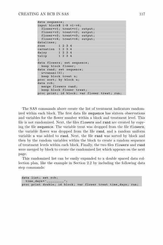
CREATING AN RCB IN SAS 117
data sequence;input block$ 1-9 v1 -v4;
flower=v1; treat=v1; output;flower=v2; treat=v2; output;flower=v3; treat=v3; output;flower=v4; treat=v4; output;
datalines;rose 1 2 3 4carnation 1 2 3 4daisy 1 2 3 4tulip 1 2 3 4;data flowers; set sequence;
keep block flower;data rand; set sequence;
u=ranuni (0);keep block treat u;
proc sort; by block u;data rcb;
merge flowers rand;keep block flower treat;
proc print; id block; var flower treat; run;
The SAS commands above create the list of treatment indicators random-ized within each block. The first data file sequence has sixteen observationsand variables for the flower number within a block and treatment level. Thisfile is not randomized. Next, the files flowers and rand are created by copy-ing the file sequence. The variable treat was dropped from the file flowers,the variable flower was dropped from the file rand, and a random uniformvariable u was added to rand. Next, the file rand was sorted by block andthen by the random variables within the block to create a random sequenceof treatment levels within each block. Finally, the two files flowers and randwere merged by block to create the randomized list which appears on the nextpage.
This randomized list can be easily expanded to a double spaced data col-lection plan, like the example in Section 2.2 by including the following datastep commands:
data list; set rcb;time_days=’_________’;
proc print double; id block; var flower treat time_days; run;

118 RANDOMIZED BLOCK DESIGNS
block flower treat
carnation 1 1carnation 2 4carnation 3 2carnation 4 3daisy 1 2daisy 2 1daisy 3 3daisy 4 4rose 1 3rose 2 2rose 3 1rose 4 4tulip 1 3tulip 2 2tulip 3 4tulip 4 1
To use this list, the student would number the flowers in each block from1 to 4. Then using the above list the carnation number 1 would be placed ina vase with treatment factor level 1 or plain tap water. Carnation number 2would be placed in a vase with treatment level four or tap water with one cupof 7-up, etc.
To create the randomization for a general complete block design, repeat thesequence 1 2 3 4 in datalines for the file sequence as many times as youhave replicates, and expand the list v1-v4 and the following output statementsaccordingly.
SAS proc plan can also be used as a quick way of randomizing treatmentlevels within a block. For example, a plan similar to the one given above canbe created using the SAS commands:
proc plan seed =27321 ordered;factors block=4 flower =4;treatments treatment =4 random;output out=rcb blockcvals=(’carnation ’ ’daisy’ ’rose’ ’tulip ’);
run;proc print data=rcb; id block; run;
The output from proc plan appears on the next page. Here it can be seenthat the first flower in block 1 receives treatment level 2, the second flowerin block 1 receives treatment level 4, etc. When printed, the output data set(rcb) created by proc plan looks similar to the list shown above.

MODEL FOR RCB 119
The PLAN Procedure
Plot Factors
Factor Select Levels Order
block 4 4 Orderedflower 4 4 Ordered
Treatment Factors
Factor Select Levels Order
treatment 4 4 Random
block --flower -- --treatment --
1 1 2 3 4 2 4 1 32 1 2 3 4 1 3 4 23 1 2 3 4 2 3 4 14 1 2 3 4 3 1 4 2
4.3 Model for RCB
The model for the analysis of an RCB design is
yij = µ+ bi + τj + εij , (4.1)
where, bi represent the block effects, τj represent the treatment effects. Theusual assumptions of normality of experimental error and homogeneity ofvariance of experimental error across levels of the treatment factors and blocksare required for this model. These assumptions can be checked with residualplots as shown in Section 2.4.
Notice that this is an additive model which does not include the interactionbetween block and treatment. Since there are only t × b experimental units,there would be zero degrees of freedom for the error term ssE if a block bytreatment interaction term were included in the model. However, the block bytreatment interaction is in fact the correct error term for testing the treatmenteffects. The experimenter wants to generalize his conclusions about treatmenteffects over all the experimental units, so the average treatment effects shouldbe larger than any differences in treatment effects among blocks of experimen-tal units. The difference in treatment effects among blocks is exactly what theinteraction measures and is therefore the correct error term. By leaving theinteraction out of the model, the ssE becomes identical to the interactionsums of squares.
The ANOVA table for an RCB design is shown symbolically in Table 4.1.Representations for the type I sums of squares for blocks and treatments areshown in the table, similar to what was shown in Section 3.5.1, but they

120 RANDOMIZED BLOCK DESIGNS
will be identical to the type III sums of squares for this design. The errorsums of squares ssE = y′y − β′X′y = y′(I −X(X′X)−X′)y, where β =(X ′X)−X ′y.
Table 4.1 Analysis of Variance Table
Sum of MeanSource df Squares Squares F-ratio
Blocks b− 1 ssBlk ssBlk/(b− 1)R(b|µ)
Treatments t− 1 ssT ssT/(t− 1) msT/msER(τ |b, µ)
Error (b− 1)(t− 1) ssE ssE/(b− 1)(t− 1)
The degrees of freedom for the error (b−1)(t−1) is smaller than it would bein a completely randomized design with b replicates of each treatment level;however, if the groups of experimental units within the blocks are more homo-geneous, the msE should be smaller and the power for detecting differencesamong the treatment levels higher.
The estimate of the variance of the homogeneous experimental units withineach block is given by
σ2rcb =
ssE
(b− 1)(t− 1)(4.2)
An estimate of the variance of the entire group of heterogenous experimentalunits can be made from the mean squares in the RCB ANOVA. It is given bythe formula
σ2crd =
(b− 1)msBlk + b(t− 1)msEtb− 1
(4.3)
which is a weighted average of the mean square for blocks and the mean squarefor error. However, the weights are not simply the degrees of freedom for eachmean square. If the msBlk is zero, it can be seen that σ2
crd < σ2rcb. The ratio
of σ2crd and σ2
rcb is a measure of the efficacy of blocking.The error degrees of freedom for the RCB is νrcb = (b− 1)(t− 1), and the
error degrees of freedom for a completely randomized design (CRD) with thesame number of experimental units would be νcrd = t(b − 1). The relativeefficiency of the RCB is then given by the formula:
RE =(νrcb + 1)(νcrd + 3)(νrcb + 3)(νcrd + 1)
σ2crd
σ2rcb
(4.4)
RE can be used to determine the number of observations that would be re-quired in a CRD, with heterogeneous experimental units, in order to have the
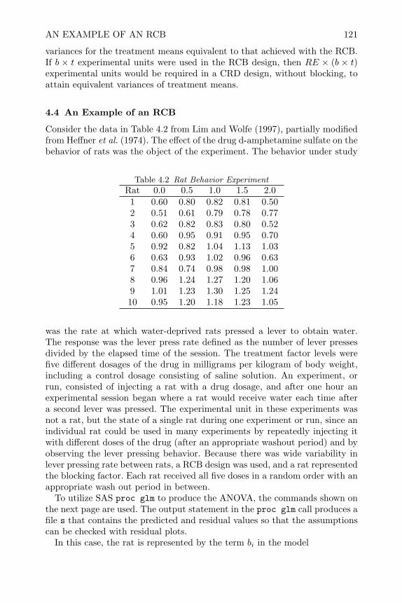
AN EXAMPLE OF AN RCB 121
variances for the treatment means equivalent to that achieved with the RCB.If b × t experimental units were used in the RCB design, then RE × (b × t)experimental units would be required in a CRD design, without blocking, toattain equivalent variances of treatment means.
4.4 An Example of an RCB
Consider the data in Table 4.2 from Lim and Wolfe (1997), partially modifiedfrom Heffner et al. (1974). The effect of the drug d-amphetamine sulfate on thebehavior of rats was the object of the experiment. The behavior under study
Table 4.2 Rat Behavior Experiment
Rat 0.0 0.5 1.0 1.5 2.01 0.60 0.80 0.82 0.81 0.502 0.51 0.61 0.79 0.78 0.773 0.62 0.82 0.83 0.80 0.524 0.60 0.95 0.91 0.95 0.705 0.92 0.82 1.04 1.13 1.036 0.63 0.93 1.02 0.96 0.637 0.84 0.74 0.98 0.98 1.008 0.96 1.24 1.27 1.20 1.069 1.01 1.23 1.30 1.25 1.2410 0.95 1.20 1.18 1.23 1.05
was the rate at which water-deprived rats pressed a lever to obtain water.The response was the lever press rate defined as the number of lever pressesdivided by the elapsed time of the session. The treatment factor levels werefive different dosages of the drug in milligrams per kilogram of body weight,including a control dosage consisting of saline solution. An experiment, orrun, consisted of injecting a rat with a drug dosage, and after one hour anexperimental session began where a rat would receive water each time aftera second lever was pressed. The experimental unit in these experiments wasnot a rat, but the state of a single rat during one experiment or run, since anindividual rat could be used in many experiments by repeatedly injecting itwith different doses of the drug (after an appropriate washout period) and byobserving the lever pressing behavior. Because there was wide variability inlever pressing rate between rats, a RCB design was used, and a rat representedthe blocking factor. Each rat received all five doses in a random order with anappropriate wash out period in between.
To utilize SAS proc glm to produce the ANOVA, the commands shown onthe next page are used. The output statement in the proc glm call produces afile s that contains the predicted and residual values so that the assumptionscan be checked with residual plots.
In this case, the rat is represented by the term bi in the model

122 RANDOMIZED BLOCK DESIGNS
data drug;input rat r1 -r5;
dose =0.0; rate=r1; output; dose =0.5; rate=r2; output;dose =1.0; rate=r3; output; dose =1.5; rate=r4; output;dose =2.0; rate=r5; output; keep rat dose rate;
datalines;1 .60 .80 .82 .81 .502 .51 .61 .79 .78 .77
. . . etc.proc glm;
class rat dose;model rate=rat dose;output out=s p=prate r=rrate;
run;
yij = µ+bi+τj+εij . The experimental error, represented by εij , is the effect ofthe state of rat i during the run when it received dose j. If data were presentedwithout describing the experimental unit and the randomization process, themodel could be easily misspecified as yij = µ+ τi + εij resulting in the wronganalysis and conclusions.
The ANOVA table resulting from the correct model specification in SASappears below. The table of type III sums of squares is not shown because itis identical to the type I sums of squares. The F -tests show that there is asignificant difference in treatment factor levels.
Sum ofSource DF Squares Mean Square F Value Pr > FModel 13 2.12866600 0.16374354 19.61 <.0001Error 36 0.30055200 0.00834867CorrectedTotal 49 2.42921800
Source DF Type I SS Mean Square F Value Pr > Frat 9 1.66845800 0.18538422 22.21 <.0001dose 4 0.46020800 0.11505200 13.78 <.0001
To interpret the differences in treatment factor levels comparisons of meansshould be made. Since the factor levels are quantitative, orthogonal polynomialcontrasts as described in Section 2.8 are useful. The results of the estimatestatement calculating the linear, quadratic, and cubic contrasts are shown atthe top of the next page. They show that there is a quadratic trend in leverpress rate over the dose of the drug. This trend can be visualized by plottingthe means as a function of dose.
The SAS commands below the output table on the next page produce thegraph in Figure 4.1. Here the quadratic trend line, produced by the degree=2option on the reg statement, is added to the plot and shows that the lever pressrate increases as a function of dose until it reaches a maximum somewherebetween 1.0 and 1.5 milligrams per kilogram of body weight.
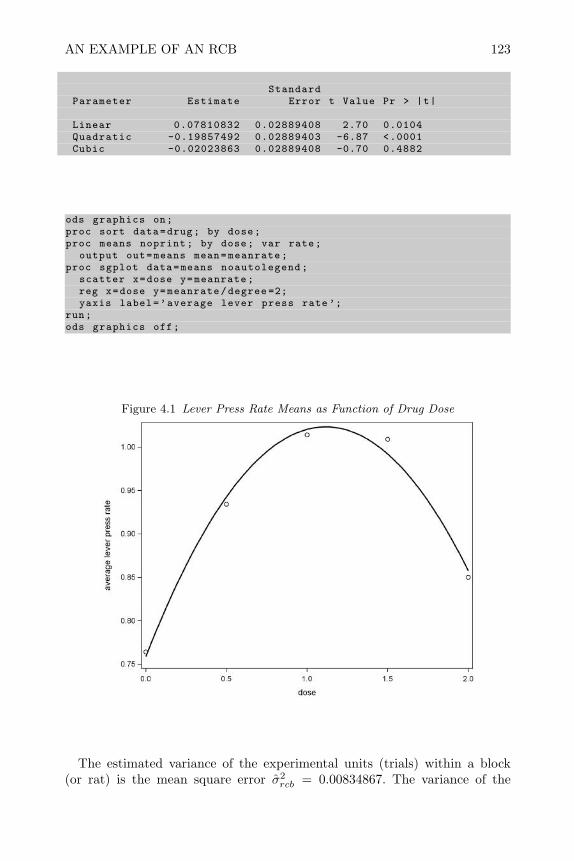
AN EXAMPLE OF AN RCB 123
StandardParameter Estimate Error t Value Pr > |t|
Linear 0.07810832 0.02889408 2.70 0.0104Quadratic -0.19857492 0.02889403 -6.87 <.0001Cubic -0.02023863 0.02889408 -0.70 0.4882
ods graphics on;proc sort data=drug; by dose;proc means noprint; by dose; var rate;
output out=means mean=meanrate;proc sgplot data=means noautolegend;
scatter x=dose y=meanrate;reg x=dose y=meanrate/degree =2;yaxis label=’average lever press rate’;
run;ods graphics off;
Figure 4.1 Lever Press Rate Means as Function of Drug Dose
The estimated variance of the experimental units (trials) within a block(or rat) is the mean square error σ2
rcb = 0.00834867. The variance of the
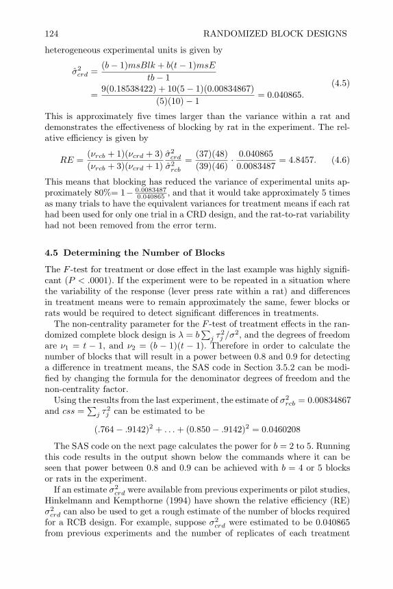
124 RANDOMIZED BLOCK DESIGNS
heterogeneous experimental units is given by
σ2crd =
(b− 1)msBlk + b(t− 1)msEtb− 1
=9(0.18538422) + 10(5− 1)(0.00834867)
(5)(10)− 1= 0.040865.
(4.5)
This is approximately five times larger than the variance within a rat anddemonstrates the effectiveness of blocking by rat in the experiment. The rel-ative efficiency is given by
RE =(νrcb + 1)(νcrd + 3)(νrcb + 3)(νcrd + 1)
σ2crd
σ2rcb
=(37)(48)(39)(46)
· 0.0408650.0083487
= 4.8457. (4.6)
This means that blocking has reduced the variance of experimental units ap-proximately 80%= 1− 0.0083487
0.040865 , and that it would take approximately 5 timesas many trials to have the equivalent variances for treatment means if each rathad been used for only one trial in a CRD design, and the rat-to-rat variabilityhad not been removed from the error term.
4.5 Determining the Number of Blocks
The F -test for treatment or dose effect in the last example was highly signifi-cant (P < .0001). If the experiment were to be repeated in a situation wherethe variability of the response (lever press rate within a rat) and differencesin treatment means were to remain approximately the same, fewer blocks orrats would be required to detect significant differences in treatments.
The non-centrality parameter for the F -test of treatment effects in the ran-domized complete block design is λ = b
∑j τ
2j /σ
2, and the degrees of freedomare ν1 = t − 1, and ν2 = (b − 1)(t − 1). Therefore in order to calculate thenumber of blocks that will result in a power between 0.8 and 0.9 for detectinga difference in treatment means, the SAS code in Section 3.5.2 can be modi-fied by changing the formula for the denominator degrees of freedom and thenon-centrality factor.
Using the results from the last experiment, the estimate of σ2rcb = 0.00834867
and css =∑j τ
2j can be estimated to be
(.764− .9142)2 + . . .+ (0.850− .9142)2 = 0.0460208
The SAS code on the next page calculates the power for b = 2 to 5. Runningthis code results in the output shown below the commands where it can beseen that power between 0.8 and 0.9 can be achieved with b = 4 or 5 blocksor rats in the experiment.
If an estimate σ2crd were available from previous experiments or pilot studies,
Hinkelmann and Kempthorne (1994) have shown the relative efficiency (RE)σ2crd can also be used to get a rough estimate of the number of blocks required
for a RCB design. For example, suppose σ2crd were estimated to be 0.040865
from previous experiments and the number of replicates of each treatment
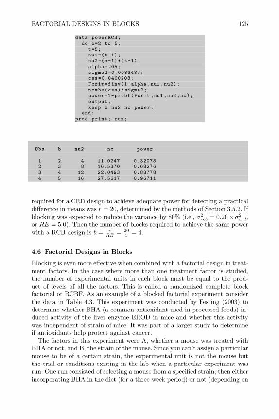
FACTORIAL DESIGNS IN BLOCKS 125
data powerRCB;do b=2 to 5;
t=5;nu1=(t-1);nu2=(b-1)*(t-1);alpha =.05;sigma2 =0.0083487;css =0.0460208;Fcrit=finv(1-alpha ,nu1 ,nu2);nc=b*(css)/sigma2;power=1-probf(Fcrit ,nu1 ,nu2 ,nc);output;keep b nu2 nc power;
end;proc print; run;
Obs b nu2 nc power
1 2 4 11.0247 0.320782 3 8 16.5370 0.682763 4 12 22.0493 0.887784 5 16 27.5617 0.96711
required for a CRD design to achieve adequate power for detecting a practicaldifference in means was r = 20, determined by the methods of Section 3.5.2. Ifblocking was expected to reduce the variance by 80% (i.e., σ2
rcb = 0.20×σ2crd,
or RE = 5.0). Then the number of blocks required to achieve the same powerwith a RCB design is b = r
RE = 205 = 4.
4.6 Factorial Designs in Blocks
Blocking is even more effective when combined with a factorial design in treat-ment factors. In the case where more than one treatment factor is studied,the number of experimental units in each block must be equal to the prod-uct of levels of all the factors. This is called a randomized complete blockfactorial or RCBF. As an example of a blocked factorial experiment considerthe data in Table 4.3. This experiment was conducted by Festing (2003) todetermine whether BHA (a common antioxidant used in processed foods) in-duced activity of the liver enzyme EROD in mice and whether this activitywas independent of strain of mice. It was part of a larger study to determineif antioxidants help protect against cancer.
The factors in this experiment were A, whether a mouse was treated withBHA or not, and B, the strain of the mouse. Since you can’t assign a particularmouse to be of a certain strain, the experimental unit is not the mouse butthe trial or conditions existing in the lab when a particular experiment wasrun. One run consisted of selecting a mouse from a specified strain; then eitherincorporating BHA in the diet (for a three-week period) or not (depending on

126 RANDOMIZED BLOCK DESIGNS
Table 4.3 Activity of EROD Liver Enzyme in Control and BHA-Treated MiceBlock 1 Block 2
Strain Treated Control Treated ControlA/J 18.7 7.7 16.7 6.4
129/Ola 17.9 8.4 14.4 6.7NIH 19.2 9.8 12.0 8.1
BALB/c 26.3 9.7 19.8 6.0
what was specified); and finally humanely sacrificing the mouse and perform-ing an autopsy to determine the activity level of the enzyme EROD in theliver. Since the results of in vivo experiments like this can vary substantiallyfrom time to time in the same laboratory due to differences in reagents usedfor the enzyme analysis, calibration of instruments, and environmental factorsin the animal husbandry, the experiments were blocked in time. Two mice wereselected from each of four strains, one was randomly chosen to receive BHAin the diet, and eight trials or runs were conducted simultaneously. This rep-resented one block. Three months later, the whole process was repeated for asecond block of runs. Since there are two levels of the treatment factor (BHAtreated or control) and four levels of the factor strain, there were 2 × 4 = 8experimental units or runs per block.
The model for analysis of a two-factor factorial in a randomized block de-sign, like that shown in Table 4.3, is
yijk = µ+ bi + αj + βk + αβjk + εijk, (4.7)
where bi represents the block effect, αj represents the treatment factor effectand βk represents the strain factor effect. This model is easily generalized tomulti-factor factorial designs in randomized blocks. Notice that in the model(4.7) there is an interaction αβjk between the two factorial factors, but thereis no interaction between the block factor, bi, and the factorial factors, αj andβk. The interactions with blocks are the error term for the analysis and if theyare included in the model there will be zero degrees of freedom for ssE.
The SAS commands to read this data and perform the analysis are shownon the next page with the resulting ANOVA table. There it can be seen thatBHA treatment, strain, and the interaction are significant. The block sums ofsquares is also large resulting in a relative efficiency RE = 2.11. This meansthat it would take approximately three times as many mice to have the samepower or sensitivity if the experiments were not blocked by time.
Figure 4.2 helps in interpreting the factorial effects and interaction. It canbe seen that on the average, BHA added to the diet increases activity of theenzyme EROD in the mouse liver. However, this increase is nearly doubledfor mice of strain BALB/c.
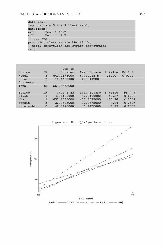
FACTORIAL DESIGNS IN BLOCKS 127
data bha;input strain $ bha $ block erod;datalines;A/J Yes 1 18.7A/J No 1 7.7
... etc.proc glm; class strain bha block;
model erod=block bha strain bha*strain;run;
Sum ofSource DF Squares Mean Square F Value Pr > FModel 8 543.2175000 67.9021875 26.20 0.0002Error 7 18.1400000 2.5914286CorrectedTotal 15 561.3575000
Source DF Type I SS Mean Square F Value Pr > Fblock 1 47.6100000 47.6100000 18.37 0.0036bha 1 422.3025000 422.3025000 162.96 <.0001strain 3 32.9625000 10.9875000 4.24 0.0527strain*bha 3 40.3425000 13.4475000 5.19 0.0337
Figure 4.2 BHA Effect for Each Strain

128 RANDOMIZED BLOCK DESIGNS
4.7 Generalized Complete Block Design
When experimental units represent physical entities, smaller groups or blocksof experimental units usually result in greater homogeneity. The larger thegroup, the more likely it is to have many experimental units that are widelydifferent than the norm or average. For that reason it is unadvisable to haveblocked designs with more than the minimum, t, experimental units per block,where t is the number of levels or combination of levels of treatment factors.However, in some cases where experimental units represent trials rather thanphysical entities and the experimental runs can be made quickly, larger blocksizes may not increase the variability of experimental units within a block.In that case, a design with replicates of each treatment level within a block(called a generalized complete block design or GCB) can be used.
Consider the following example from Golf Magazine (Bastable, 2006, June).An experiment was conducted to determine the ideal tee height for driving agolf ball as far as possible. The purpose was to recommend to all readers ofthe article what tee height they should use. The treatment factor was the teeheight as shown in Table 4.4.
Table 4.4 Treatment Factor Levels for Golf Experiment
Level Tee Height1 Entire ball below crown2 Half the ball above the crown3 Bottom of ball at top of club-face
An experiment consisted of a golfer hitting a golf ball from a specifiedheight, and the response was the distance the ball traveled. To make a generalconclusion, a representative group of golfers had to be used rather than onegolfer. Since the ability to drive the ball by the golfers used in the studydiffered, it made sense to group or block the trials by golfer and randomizethe order that each golfer hit a ball from each of the tee heights. However,since hitting more than three golf balls would not be likely to fatigue a golferand cause more variability in his driving distance, there was no need to restricta golfer to hitting just three balls. Instead, each golfer hit r = 5 golf balls fromeach of t = 3 tee heights. The results from this experiment are shown in theappendix. Nine golfers were used in this part of the study; each golfer hit fiveballs from each tee height (15 balls total) in a random order.
Since there are replicate experimental units for each treatment in each block,it is possible to fit the model
yijk = µ+ bi + τj + bτij + εijk (4.8)

GENERALIZED COMPLETE BLOCK DESIGN 129
However, this leaves a dilemma. The msE in the traditional ANOVA and thedenominator for the F -tests for treatment effect and the block by treatmentinteraction is based on the variability of experimental units within the sametreatment and block (in this case golfer). If the interaction between block(golfer) and treatment factor (tee height) were significant, its interpretationwould imply that the optimal tee height could be different for different golfers.The golfers in the study were just a sample of golfers, and if the optimaltee height were different for them, there would be no way to recommendan optimal tee height for all readers of the Golf Magazine article. To makea general recommendation, the treatment factor should be tested using theblock by treatment interaction mean square as the denominator of the F -test (another justification for using the block by treatment interaction as thedenominator of the F -test for treatment will be given in Chapter 5, Section 8).An F -test for treatments constructed in this way is not made automaticallyin proc glm, but can be specified using the test statement as shown in theSAS commands below where id represents block or golfer id.
data rcb;input id teehgt cdistance;datalines;1 1 142.0... etc.
proc glm data=rcb;class id teehgt;model cdistance=id teehgt id*teehgt;test h=teehgt e=id*teehgt;lsmeans teehgt/pdiff adjust=tukey e=id*teehgt;
run;
The h=teehgt and e=id*teehgt in the test statement specify the hypoth-esis to be H0 : τ1 = τ2 = τ3 and the error term to be bτij . The e=id*teehgt inthe lsmeans statement also specifies the error term to be bτij . The results ofthis analysis are shown on the next page. The table of type I sums of squareswas left out since it was identical to the type III sums of squares.
There it can be seen that the tee height is significant at the α = 0.0124level. This is much different than the incorrect F -test in the table of type IIIsums of squares. There the tee height effect is significant at α < 0.0001 level.Sometimes the F -test for treatments may be significant in the type III tablebut insignificant in the result of the test statement. In that case, the resultof the test statement should be used if you want to generalize conclusions.
Sometimes there is a more powerful test of treatment effects than can beobtained using the test statement to create F -test. If the block by treatmentinteraction term is insignificant, the additive model yijk = µ + bi + τj + εijkcan be fit to the data and the default F -test for treatments will use an msEterm that is a pooled or weighted average of the interaction and error termfrom model (4.8). If the interaction is negligible, the interaction mean square

130 RANDOMIZED BLOCK DESIGNS
Sum ofSource DF Squares Mean Square F Value Pr > FModel 26 128821.4813 4954.6724 72.90 <.0001Error 108 7340.7520 67.9699CorrectedTotal 134 136162.2333
Source DF Type III SS Mean Square F Value Pr > FID 8 124741.4493 15592.6812 229.41 <.0001TEEHGT 2 1723.9320 861.9660 12.68 <.0001ID*TEEHGT 16 2356.1000 147.2563 2.17 0.0102
Tests of Hypotheses Using the Type III MS for ID*TEEHGT as anError Term
Source DF Type III SS Mean Square F Value Pr > FTEEHGT 2 1723.932000 861.966000 5.85 0.0124
is estimating the same experimental error as the error mean square. In thatcase, pooling these two mean squares increases the degrees of freedom for theerror term and increases the power or sensitivity of the F -test for treatmenteffects. Normally the preliminary F -test of the interaction, which is used todecide whether to fit the additive model or not, is conducted at a highersignificance level like α = 0.25. If the interaction is significant at the α = 0.25level, use the test statement to create the appropriate F -test for treatmenteffects. If the interaction is not significant at α = 0.25, fit the additive modeland use the F -test from the type I or type III table of sums of squares. Thisprocedure is called the “Pool or not to Pool” procedure.
For the golf experiment, the interaction sum of squares is significant at theα = 0.0102 < 0.25 level, and thus the additive model should not be fit, andthere is no more powerful F -test for treatments than the one that can be madeusing the test statement.
To interpret the meaning of the significant treatment effect in the golf exper-iment, the lsmeans teehgt/pdiff adjust=tukey e=id*teehgt; statementwas used. This results in the table of means and the Tukey pairwise compar-isons of means shown on the next page. The e=id*teehgt option specifies theerror term to be the means square for block by treatment interaction.
The least squares means show the average driving distance for the teeheight = 1 (entire ball below crown) is 171.45 yards. It is significantly lessthan the average driving distance (177.8 yds.) for tee height = 3 (bottom ofball at top of club-face) at the α = 0.0125 level and marginally significantlyless than the distance (179.8 yds.) for tee height = 2 (half the ball above thecrown). The average distance for tee heights 2 and 3 were not significantlydifferent α = 0.7192. Therefore the recommendation to readers of the articlewas to tee their golf ball up so that at least half the ball is above the crownof the driver club-face in order to maximize their driving distance.

TWO BLOCK FACTORS LSD 131
Least Squares MeansAdjustment for Multiple Comparisons: Tukey
Standard Errors and Probabilities Calculated Usingthe Type III MS for ID*TEEHGT as an Error Term
CDISTANCE LSMEANTEEHGT LSMEAN Number1 171.457778 12 177.837778 23 179.837778 3
Least Squares Means for effect TEEHGTPr > |t| for H0: LSMean(i)= LSMean(j)
Dependent Variable: CDISTANCEi/j 1 2 3
1 0.0590 0.01252 0.0590 0.71923 0.0125 0.7192
4.8 Two Block Factors LSD
It was first shown in agricultural experiments (Fisher, 1935) that the processof grouping experimental plots into homogeneous blocks might profitably beduplicated. For example, on the left side of Figure 4.3 we see a representationof a randomized block design RCB laid out in a field. In this design, one field,roughly square in shape, is divided into four rectangular blocks. Each blockis further divided into four plots and the treatment levels (A, B, C, D) arerandomly assigned to one plot within each block. In the figure the randomassignment within the block is represented by each letter only appearing oncein each row that represents a block. If there is a fertility gradient runningfrom top to bottom in this field, the plots within a block will be more alikein fertility than plots in different blocks or rows, and the randomized blockdesign would work well to reduce the variance of experimental errors withina block.
If there were no clear gradient in the field, but adjacent plots tended to be
Figure 4.3 Comparison of RCB and Latin Square Designs
RCB Latin Square
1
2
3
4
Block
B
A
B
C
C
D
D
B
A
C
A
D A
B
C
D
B D C A
D C A B
C A B D
A B D C

132 RANDOMIZED BLOCK DESIGNS
more alike than plots at different ends of the same block, a design like the oneshown on the right side of Figure 4.3 assigns each treatment level only once toeach row and once to each column. In that way, the variability from column tocolumn can also be removed from the error sums of squares, further increasingthe sensitivity for detecting treatment effects. The design shown on the rightside of Figure 4.3 is called a Latin square design or LSD, and it is blocked bothhorizontally and vertically. The restriction with a LSD is that the number ofrow blocks equals the number of column blocks, which equals the number oflevels of the treatment factor. This restriction will be relaxed in Chapter 7,where more general row-column blocking schemes will be discussed.
The model for a LSD is written
yijk = µ+ ri + cj + τk + εijk (4.9)
where ri represents the row blocking factor, cj represents the column blockingfactor, and τk represents the treatment factor. Like model (4.1) for the RCBdesign, no interactions are included in the model so that any differences intreatment factor levels can be generalized over rows and columns.
Latin square designs can be used whenever there are two independent block-ing factors that can be used to group experimental units. For example, if anexperiment were being conducted to determine the effect of tread design onthe wear life of automobile tires, the experimental unit would be a wheel ona car and the treatment factor would be the tread design of the tire mountedon that wheel. It would make sense to block the experimental units by typeof automobile, since tires may wear faster on heavier cars than they do onlighter cars. It would also make sense to block by position of the tire on a carsince front right tires wear at a different rate than left rear tires, etc. Theseare independent blocking factors because all four wheel positions exist on anytype car. To use a LSD, the number of tread types compared and the numberof car types used in the study must be four in order to equal the number ofwheel positions on a car. The row blocking factor in the Latin square wouldrepresent the type of car, with four alternatives ranging over the class of carsto which the experimenter would like to make inference. The column blockingfactor would represent the position of a tire on the car (FL, FR, RL, RR),and the treatment factor would represent the four different tread designs beingtested.
4.8.1 Creating and Randomizing Latin Square Designs
Latin square designs are easy to create by cyclically rotating the letters orsymbols used to represent the treatment factor levels. For example, for a 5×5Latin square, let the letters A, B, C, D, E, represent the levels of the treatmentfactor. Then the design is created as:
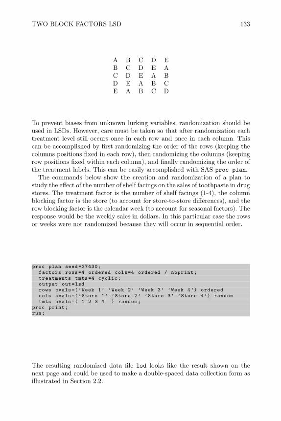
TWO BLOCK FACTORS LSD 133
A B C D EB C D E AC D E A BD E A B CE A B C D
To prevent biases from unknown lurking variables, randomization should beused in LSDs. However, care must be taken so that after randomization eachtreatment level still occurs once in each row and once in each column. Thiscan be accomplished by first randomizing the order of the rows (keeping thecolumns positions fixed in each row), then randomizing the columns (keepingrow positions fixed within each column), and finally randomizing the order ofthe treatment labels. This can be easily accomplished with SAS proc plan.
The commands below show the creation and randomization of a plan tostudy the effect of the number of shelf facings on the sales of toothpaste in drugstores. The treatment factor is the number of shelf facings (1-4), the columnblocking factor is the store (to account for store-to-store differences), and therow blocking factor is the calendar week (to account for seasonal factors). Theresponse would be the weekly sales in dollars. In this particular case the rowsor weeks were not randomized because they will occur in sequential order.
proc plan seed =37430;factors rows=4 ordered cols=4 ordered / noprint;treatments tmts=4 cyclic;output out=lsdrows cvals=(’Week 1’ ’Week 2’ ’Week 3’ ’Week 4’) orderedcols cvals=(’Store 1’ ’Store 2’ ’Store 3’ ’Store 4’) randomtmts nvals=( 1 2 3 4 ) random;
proc print;run;
The resulting randomized data file lsd looks like the result shown on thenext page and could be used to make a double-spaced data collection form asillustrated in Section 2.2.
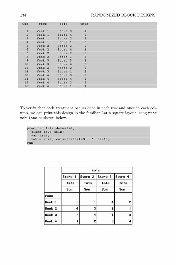
134 RANDOMIZED BLOCK DESIGNS
Obs rows cols tmts
1 Week 1 Store 3 42 Week 1 Store 4 23 Week 1 Store 2 14 Week 1 Store 1 35 Week 2 Store 3 26 Week 2 Store 4 17 Week 2 Store 2 38 Week 2 Store 1 49 Week 3 Store 3 1
10 Week 3 Store 4 311 Week 3 Store 2 412 Week 3 Store 1 213 Week 4 Store 3 314 Week 4 Store 4 415 Week 4 Store 2 216 Week 4 Store 1 1
To verify that each treatment occurs once in each row and once in each col-umn, we can print this design in the familiar Latin square layout using proctabulate as shown below.
proc tabulate data=lsd;class rows cols;var tmts;table rows , cols*(tmts*f=8.) / rts =10;
run;

TWO BLOCK FACTORS LSD 135
4.8.2 Analysis of a Latin Square Design
Latin square designs are frequently used in steer or dairy cow feeding exper-iments and in bioequivalence studies to compare different formulations of adrug in phase II clinical trials. In these studies the column blocking factor istime and the row blocking factor is animal or human subject. In some casesthe treatment administered in one time period may have a carry-over effecton the response in the next period. However, if there is a sufficient washoutperiod between column blocks, there will be no carry-over effects and the datacan be analyzed as a traditional Latin square.
To illustrate the analysis of data from a Latin Square, consider the followingbioequivalence study. The data is shown in Table 4.5 (taken from Selwyn andHall, 1984).
Table 4.5 Treatment and Resulting AUC for Bioequivalence StudyPeriod
Subject 1 2 31 A 1186 B 642 C 11832 B 984 C 1135 A 13053 C 1426 A 1540 B 873
A=solution, B=tablet, C=capsule
The purpose was to test the bioequivalence of three formulations (A=solution,B=tablet, C=capsule) of a drug as measured by the AUC or area under thecurve, which relates the concentration of the drug in the blood as a func-tion of the time since dosing. Three volunteer subjects took each formulationin succession with a sufficient washout period between. After dosing, bloodsamples were obtained every half-hour for four hours and analyzed for drugconcentration. AUC was calculated with the resulting data. Since there maybe large variation in metabolism of the drug from subject to subject, subjectwas used as a row blocking factor. Since the absorbtion and metabolism of adrug will vary from time to time for a particular subject, time was used as acolumn blocking factor.
The SAS commands to read the data and fit model (4.9) and the resultingoutput are shown on the next page. The results indicate that there is nodifference in the three formulations.
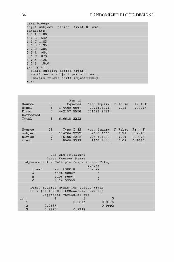
136 RANDOMIZED BLOCK DESIGNS
data bioeqv;input subject period treat $ auc;datalines;1 1 A 11861 2 B 6421 3 C 11832 1 B 11352 2 C 13052 3 A 9843 1 C 8733 2 A 14263 3 B 1540proc glm;
class subject period treat;model auc = subject period treat;lsmeans treat/ pdiff adjust=tukey;
run;
Sum ofSource DF Squares Mean Square F Value Pr > FModel 6 174460.6667 29076.7778 0.13 0.9774Error 2 442157.5556 221078.7778CorrectedTotal 8 616618.2222
Source DF Type I SS Mean Square F Value Pr > Fsubject 2 114264.2222 57132.1111 0.26 0.7946period 2 45196.2222 22598.1111 0.10 0.9073treat 2 15000.2222 7500.1111 0.03 0.9672
The GLM ProcedureLeast Squares Means
Adjustment for Multiple Comparisons: TukeyLSMEAN
treat auc LSMEAN NumberA 1198.66667 1B 1105.66667 2C 1120.33333 3
Least Squares Means for effect treatPr > |t| for H0: LSMean(i)= LSMean(j)
Dependent Variable: auci/j 1 2 3
1 0.9687 0.97762 0.9687 0.99923 0.9776 0.9992

TWO BLOCK FACTORS LSD 137
4.8.3 Determining the Number of Replicates
The number of replicates of each treatment factor level, in a LSD with t rowsand t columns must be equal to t. The only way the power for detecting differ-ences in treatment means can be increased would be to increase the numberof rows or columns. In the last example the row blocking factor representedsubjects, and the column blocking factor represented periods. One way of in-creasing the power for detecting differences in treatment means would be toincrease the number of subjects. If the number of subjects, r, were doubled,i.e., r = 2t, it would be essentially the same as replicating the Latin squarewith t additional subjects.
In general if we consider a replicated Latin square to have r = nt rows(where n is an integer), t columns and t levels of the treatment factor, themodel for the data will still be Equation (4.9), but the degrees of freedomfor the error term will be ν2 = (r − 2)(t − 1). The non-centrality factor forthe F -test of no treatment effects is λ = nt
∑k τ
2k/σ
2 where n is the numberof times the square has been repeated. Therefore in order to calculate thenumber of replicates of the square, n, that will result in a power between 0.8and 0.9 for detecting a difference in treatment means, the SAS code in Section3.5.2 can be modified by changing the formula for the denominator degrees offreedom and the non-centrality factor.
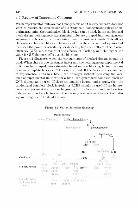
138 RANDOMIZED BLOCK DESIGNS
4.9 Review of Important Concepts
When experimental units are not homogeneous and the experimenter does notwant to restrict the conclusions of his study to a homogeneous subset of ex-perimental units, the randomized block design can be used. In the randomizedblock design, heterogenous experimental units are grouped into homogeneoussubgroups or blocks prior to assigning them to treatment levels. This allowsthe variation between blocks to be removed from the error sums of squares andincreases the power or sensitivity for detecting treatment effects. The relativeefficiency (RE) is a measure of the efficacy of blocking, and the higher thevalue for RE the more effective the blocking.
Figure 4.4 illustrates when the various types of blocked designs should beused. When there is one treatment factor and the heterogeneous experimentalunits can be grouped into categories based on one blocking factor the ran-domized complete block or RCB design is used. If the block size, or numberof experimental units in a block, can be larger without increasing the vari-ance of experimental units within a block the generalized complete block orGCB design can be used. If there are multiple factors under study, then therandomized complete block factorial or RCBF should be used. If the hetero-geneous experimental units can be grouped into classifications based on twoindependent blocking factors and there is only one treatment factor, the Latinsquare design or LSD should be used.
Figure 4.4 Design Selection Roadmap
Design Purpose
Estimate Variances Study Factor Effects
E.U.’s
Block Factors
One Factor
Multiple Factors
Multiple Factorswith some hard
to vary
Block size
Homogeneous Heterogeneous
Large Small
RCB
GCB
PBIB,BTIB
BIB
LSD
YSDRSE CRD
FactorsFRSENSESNSE
CRFD CRRS SLD RCBF BRS PCBFCRFF SCD
PB, OA EVD CCBF
CRSP RSSP SPMPV RBSPSPFF EESPRS
One Two
class cont. mixture cont. classFactors

REVIEW OF IMPORTANT CONCEPTS 139
A randomized complete block design or RCB has only one experimen-tal unit per treatment level per block. The model for the RCB design isyij = µ+bi+τj+εij , which does not include the interaction between block andtreatment because this is the correct error for testing treatment effects if theexperimenter wants general conclusions. In a generalized complete block de-sign, replicates of each treatment level within each block are included. Becauseof the replicates in the GCB, the interaction between block and treatment canbe included in the model, yijk = µ + bi + τj + bτij + εijk, but it should stillbe used as the error term for testing the treatment effects and this can beaccomplished by using the test statement in SAS proc glm.
In RCBF every combination of levels of the factors is randomized to ex-perimental units within a block. The model for analysis is the usual factorialmodel with the addition of a block term, yijk = µ+ bi+αj +βk +αβjk + εijk.No interaction between blocks and factorial effects or interactions should beincluded in the model if the experimenter wants general conclusions. Writinga model that does not represent the way the experiment was conducted canresult in using the wrong mean squares in the denominators of the F -testsand may cause the wrong conclusions to be drawn.
With two independent blocking factors, LSDs can be used to further de-crease the variance of experimental error. The model for the Latin square isyijk = µ+ri+cj +τk+εijk, and again no interaction between row blocks, col-umn blocks or treatment factors is included in the model. When randomizinga list of experiments for a LSD, care must be taken so that after randomiza-tion each treatment factor level still occurs exactly once in each row block andeach column block.

140 RANDOMIZED BLOCK DESIGNS
4.10 Exercises
1. Consider planning an experiment to determine how the flavor duration ofgum is affected by the characteristics of the gum such as Factor A (typeof gum stick or tablet), Factor B (flavor of gum), and Factor C (regular orsugar-free), see Rogness and Richardson (2003).
(a) If several subjects were recruited to participate in the study and eachwas asked to chew and record the flavor duration (in minutes) of one ormore types of gum, what would the experimental unit be?
(b) How could experimental units be blocked to reduce the variance of ex-perimental error and increase the power for detecting differences?
(c) Choose at least two of the factors listed above and provide a randomizedlist for an RCB design.
(d) Recruit subjects and actually perform the experiment within a week.(e) Analyze your data. Did treatment factors and interactions affect the
flavor duration? Was the blocking scheme you employed effective at re-ducing experimental error?
2. Consider room temperature as an additional blocking factor for the cut-flower experiment described in Section 4.2.
(a) What design could you use to incorporate the two blocking factors offlower type and room temperature?
(b) Set up a randomization plan to conduct this experiment.(c) What is the model you would use to analyze the data resulting from this
experiment?
3. The data on the next page show the yields of five varieties of barley in a ran-domized complete block experiment carried out in Minnesota reported inThe Journal of the American Society of Agronomy by Immer et al. (1934).
(a) What would be the purpose of running these experiments in differentlocations and years?
(b) How was variance of experimental error reduced in these experiments?(c) Compute the ANOVA for the RCB design model (4.1) and determine if
there is a significant difference in varieties.(d) Calculate the Relative Efficiency, RE, and determine how many exper-
iments would have been needed to have the same power using a com-pletely randomized (CRD) design.
(e) Use the Tukey method to make pairwise comparisons of the variety meanyields.
4. Horiuchi et al. (2005) conducted an experiment during Japan’s 2004 UpperHouse election. The purpose of the experiment was to test the hypothesisthat voter turnout is influenced by the amount of information available
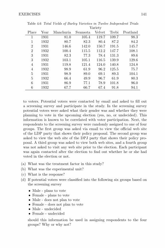
EXERCISES 141
Table 4.6 Total Yields of Barley Varieties in Twelve Independent TrialsVariety
Place Year Manchuria Svansota Velvet Trebi Peatland1 1931 81.0 105.4 119.7 109.7 98.31 1932 80.7 82.3 80.4 87.2 84.22 1931 146.6 142.0 150.7 191.5 145.72 1932 100.4 115.5 112.2 147.7 108.13 1931 82.3 77.3 78.4 131.3 89.63 1932 103.1 105.1 116.5 139.9 129.64 1931 119.8 121.4 124.0 140.8 124.84 1932 98.9 61.9 96.2 125.5 75.75 1931 98.9 89.0 69.1 89.3 104.15 1932 66.4 49.9 96.7 61.9 80.36 1931 86.9 77.1 78.9 101.8 96.06 1932 67.7 66.7 67.4 91.8 94.1
to voters. Potential voters were contacted by email and asked to fill outa screening survey and participate in the study. In the screening surveypotential voters were asked what their gender was and whether they wereplanning to vote in the upcoming election (yes, no, or undecided). Thisinformation is known to be correlated with voter participation. Next, therespondents to the screening survey were randomly assigned to one of fourgroups. The first group was asked via email to view the official web siteof the LDP party that shows their policy proposal. The second group wasasked to view the web site of the DPJ party that shows their policy pro-posal. A third group was asked to view both web sites, and a fourth groupwas not asked to visit any web site prior to the election. Each participantwas again contacted after the election to find out whether he or she hadvoted in the election or not.
(a) What was the treatment factor in this study?(b) What was the experimental unit?(c) What is the response?(d) If potential voters were classified into the following six groups based on
the screening survey
• Male - plans to vote• Female - plans to vote• Male - does not plan to vote• Female - does not plan to vote• Male - undecided• Female - undecided
should this information be used in assigning respondents to the fourgroups? Why or why not?
142 RANDOMIZED BLOCK DESIGNS
(e) Explain how you would analyze the resulting data. What model wouldyou use, what is the distribution of the dependent variable, etc.?
5. Lew (2007) presents the data from an experiment to determine whethercultured cells respond to two drugs. The experiment was conducted usinga stable cell line plated onto Petri dishes, with each experimental run in-volving assays of responses in three Petri dishes: one treated with drug 1,one treated with drug 2, and one untreated serving as a control. The dataare shown in the table below:
Control Drug 1 Drug 2Experiment 1 1147 1169 1009Experiment 2 1273 1323 1260Experiment 3 1216 1276 1143Experiment 4 1046 1240 1099Experiment 5 1108 1432 1385Experiment 6 1265 1562 1164
(a) Analyze the data as if it came from a completely randomized design usingthe model yij = µ+ τi + εij . Is there a significant difference between thetreatment groups?
(b) Analyze the data as a RCB design, where experiment number representsa blocking factor.
(c) Is there any difference in the results you obtain in (a) and (b)? If soexplain what may be the cause of the difference in the results and whichmethod would you recommend?
6. le Riche and Csima (1964) evaluated four hypnotic drugs and a placeboto determine their effect on quality of sleep in elderly patients. The treat-ment levels were labeled (A=Placebo, B=Ethchlorvynol, C=Glutethimide,D=Chloral hydrate and E=Secobarbitol sodium). Elderly patients weregiven one of the capsules for five nights in succession and their quality ofsleep was rated by a trained nurse on a four-point scale (0=poor to 3=excel-lent) each night. An average score was calculated for each patient over thefive nights in a week. Each patient received all five treatments in successiveweeks. A Latin-square design was used to account for patient-to-patientdifferences and week-to-week effects. The design and the response (meanquality of sleep rating) are shown in the table on the next page.
(a) What is the appropriate model for this data?(b) Complete the ANOVA and determine if there are any significant differ-
ences among the treatments.(c) Use an appropriate method to determine if there is a significant difference
between the placebo and the average of the other drugs, and if there aresignificant differences among the four drugs.
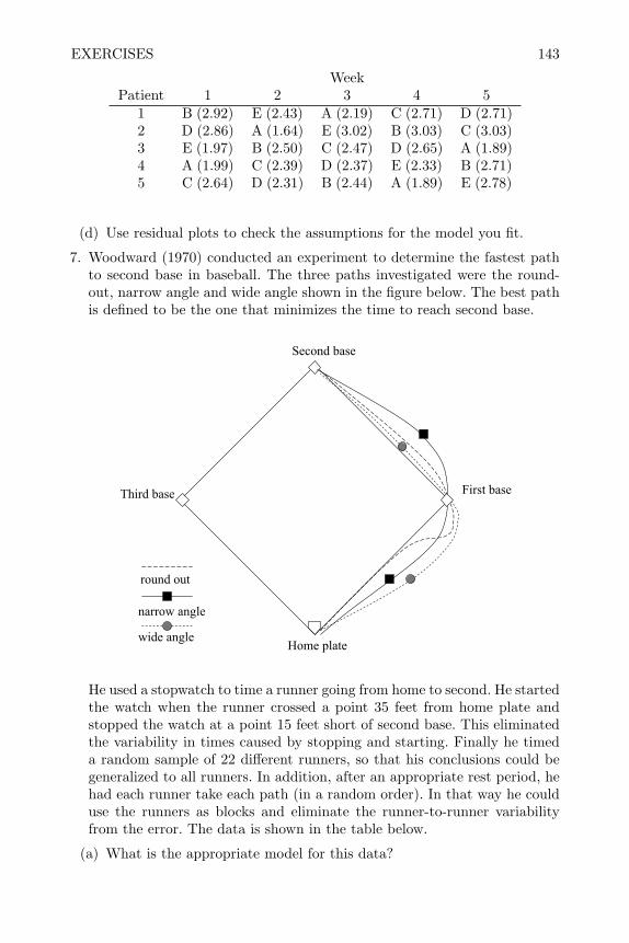
EXERCISES 143
WeekPatient 1 2 3 4 5
1 B (2.92) E (2.43) A (2.19) C (2.71) D (2.71)2 D (2.86) A (1.64) E (3.02) B (3.03) C (3.03)3 E (1.97) B (2.50) C (2.47) D (2.65) A (1.89)4 A (1.99) C (2.39) D (2.37) E (2.33) B (2.71)5 C (2.64) D (2.31) B (2.44) A (1.89) E (2.78)
(d) Use residual plots to check the assumptions for the model you fit.
7. Woodward (1970) conducted an experiment to determine the fastest pathto second base in baseball. The three paths investigated were the round-out, narrow angle and wide angle shown in the figure below. The best pathis defined to be the one that minimizes the time to reach second base.
round out
narrow angle
wide angleHome plate
First base
Second base
Third base
He used a stopwatch to time a runner going from home to second. He startedthe watch when the runner crossed a point 35 feet from home plate andstopped the watch at a point 15 feet short of second base. This eliminatedthe variability in times caused by stopping and starting. Finally he timeda random sample of 22 different runners, so that his conclusions could begeneralized to all runners. In addition, after an appropriate rest period, hehad each runner take each path (in a random order). In that way he coulduse the runners as blocks and eliminate the runner-to-runner variabilityfrom the error. The data is shown in the table below.
(a) What is the appropriate model for this data?
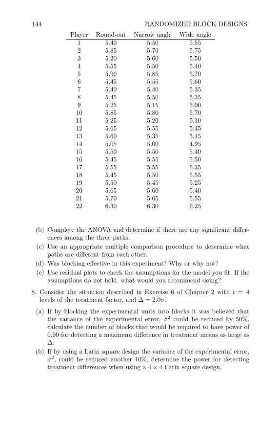
144 RANDOMIZED BLOCK DESIGNS
Player Round-out Narrow angle Wide angle1 5.40 5.50 5.552 5.85 5.70 5.753 5.20 5.60 5.504 5.55 5.50 5.405 5.90 5.85 5.706 5.45 5.55 5.607 5.40 5.40 5.358 5.45 5.50 5.359 5.25 5.15 5.0010 5.85 5.80 5.7011 5.25 5.20 5.1012 5.65 5.55 5.4513 5.60 5.35 5.4514 5.05 5.00 4.9515 5.50 5.50 5.4016 5.45 5.55 5.5017 5.55 5.55 5.3518 5.45 5.50 5.5519 5.50 5.45 5.2520 5.65 5.60 5.4021 5.70 5.65 5.5522 6.30 6.30 6.25
(b) Complete the ANOVA and determine if there are any significant differ-ences among the three paths.
(c) Use an appropriate multiple comparison procedure to determine whatpaths are different from each other.
(d) Was blocking effective in this experiment? Why or why not?(e) Use residual plots to check the assumptions for the model you fit. If the
assumptions do not hold, what would you recommend doing?
8. Consider the situation described in Exercise 6 of Chapter 2 with t = 4levels of the treatment factor, and ∆ = 2.0σ.
(a) If by blocking the experimental units into blocks it was believed thatthe variance of the experimental error, σ2 could be reduced by 50%,calculate the number of blocks that would be required to have power of0.90 for detecting a maximum difference in treatment means as large as∆.
(b) If by using a Latin square design the variance of the experimental error,σ2, could be reduced another 10%, determine the power for detectingtreatment differences when using a 4× 4 Latin square design.
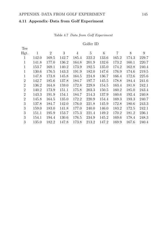
APPENDIX–DATA FROM GOLF EXPERIMENT 145
4.11 Appendix–Data from Golf Experiment
Table 4.7 Data from Golf Experiment
Golfer IDTeeHgt. 1 2 3 4 5 6 7 8 9
1 142.0 169.5 142.7 185.4 222.2 133.6 165.2 174.3 229.71 141.8 177.0 136.2 164.8 201.9 132.6 173.2 160.1 220.71 153.7 169.1 140.2 173.9 192.5 135.0 174.2 162.8 240.41 130.6 176.5 143.3 191.9 182.0 147.6 176.9 174.6 219.51 147.8 173.8 145.8 164.5 224.8 136.7 166.4 172.6 225.62 142.7 185.6 137.8 184.7 197.7 145.5 178.8 184.4 241.62 136.2 164.8 159.0 172.8 229.8 154.5 163.4 181.8 242.12 140.2 173.9 151.1 175.8 203.3 150.5 160.2 185.0 243.42 143.3 191.9 154.1 184.7 214.3 137.9 160.6 192.4 240.82 145.8 164.5 135.0 172.2 220.9 154.4 169.3 193.3 240.73 137.8 184.7 142.0 176.0 221.8 145.9 172.8 180.6 243.33 159.0 183.0 141.8 177.0 240.0 146.0 183.2 172.5 242.13 151.1 195.9 153.7 175.3 221.4 149.2 170.2 181.2 236.13 154.1 194.4 130.6 176.5 234.9 145.2 169.6 178.4 248.33 135.0 182.2 147.8 173.8 213.2 147.2 169.9 167.6 240.4

CHAPTER 5
Designs to Study Variances
5.1 Introduction
In the experiments described in Chapters 2 through 4, the purpose was tocompare the response between different levels of controllable variables or fac-tors in order to predict what the response might be in the future at specificlevels of the factors, or to recommend the best factor level for future use.Another purpose of experimentation is to study sources of variability in theresponse. For example, cholesterol, blood glucose, and other diagnostic testsmade by doctors are known to vary with the procedures and the equipmentused to make the measurements. Experiments might be conducted to find outhow much of the variability is due to equipment and how much is due to pro-cedure. Symbolically σ2
T = σ2p + σ2
e where σ2T is the total variance, σ2
p and σ2e
are the portions of the total due to procedure and equipment, respectively.σ2p and σ2
e are called the components of variance or variance components. Anexperiment can be conducted to collect data so that the variance componentscan be estimated. In this type of experiment, there might not be any inter-est in the difference in average diagnostic readings between specific pieces ofequipment because there are (and will continue to be) many in use.
There are at least three reasons for conducting experiments to study thesources of variability. In some cases the purpose may be descriptive, and thevariance components have value in themselves. A second reason for quantifyingthe sources of variability is to gain insight into how to reduce the varianceof the response. A third reason for studying the sources of variability is tostimulate ideas about the causes of variability that could be tested in furtherexperiments.
Two examples of where variance components are useful as descriptive mea-sures are in genetics and in educational and psychological testing (see Searleet al., 1992). In dairy cow breeding, the variability in milk production can bepartitioned into the amount due to the sire and the daughter, i.e., σ2
T = σ2s+σ2
d.The ratio of h = 4σ2
s/(σ2s + σ2
d) is called the heritability and is highly impor-tant to dairy farmers. In psychological and educational testing the variabilityin test scores can be partitioned into the person-to-person variability andthe repeat test scores for the same person, i.e., σ2
T = σ2p + σ2
r . In this case,σ2p/(σ
2p + σ2
r) is called the intra-class correlation, and high values of it implyreliability of the testing procedure.
In industrial quality control there is a need to reduce variability in in-processmeasurements of key product and process characteristics. If one cannot mea-
147
148 DESIGNS TO STUDY VARIANCES
sure accurately, there is no hope of controlling or improving quality. Totalmeasurement variability within a plant can be attributed to the measurementequipment (or gage) and the operator (or inspector) making the measurement,i.e., σ2
T = σ2g + σ2
o . In order to reduce measurement variability, managementneeds to know where to concentrate its efforts. If the major proportion of vari-ability is σ2
g , perhaps effort needs to be placed on re-calibrating measurementequipment or buying more new and more precise and consistent equipment.On the other hand, if the major source of measurement variability is σ2
o , per-haps better training of operator-inspectors may solve the problem.
In some cases a researcher would like to conduct an experiment like thosedescribed in Chapters 2-4 to compare the average response caused by differentlevels of controllable factors; however, he or she has such limited knowledgeabout the mechanism under study that it is difficult to hypothesize whatfactors or levels of factors to study. In this situation, determining the sources ofvariability in the response may prompt ideas about what factors would be mostprofitable to study. For example, knowing whether the majority of variabilityin an industrial process is batch-to-batch or within a batch would give insightas to whether factors that could be varied within a batch, or factors thatcould be varied from one batch to another, should be studied in optimizationexperiments. In cases where one factor experiment or a factorial experimenthas been conducted and nothing was found to be significant, Leitnaker andCooper (2005) suggest that a follow-up sampling study (to classify the sourcesof variability in the response) may explain why no significant factors werefound.
5.2 Random Factors and Random Sampling Experiments
When the purpose of experimentation is to study differences in the averageresponse caused by differences in factor levels (like the experiments describedin Chapters 2-4), the factors in the experiment are called fixed factors. Thelevels of these factors are specifically selected by the experimenter. On theother hand, when the purpose of experimentation is to study the variancecaused by changing levels of a factor, the factor is called a random factor . Forexample, the model yij = µ + τi + εij in Chapter 2, the factor τi would beconsidered a fixed factor. Although we haven’t called it a factor before, theterm εij in this model would be considered a random factor. εij representsthe effect of the jth experimental unit within the ith level of the treatmentfactor. In the bread rise experiment described in Chapter 2, the experimentalunit was the loaf of bread. Replicate loaves (i.e., j = 1, . . . , 4) were used inthis experiment so that σ2, the variance of the experimental units, could beestimated and used to judge the significance of the fixed factor (rise time).Since the purpose of including multiple levels (or loaves) within each rise timewas to estimate σ2, εij is considered a random factor.
Whereas the levels of fixed factors are specifically chosen by the experi-menter, the levels of random factors are just samples of possible levels that

RANDOM FACTORS AND RANDOM SAMPLING EXPERIMENTS 149
could have been used. For example, in the bread rise experiment, the ex-perimenter chose 35, 40 and 45 minutes to study for the levels of rise time.However, the four replicate loaves used for each rise time represent only asample of the loaves that could have been used in the experiment. For thisreason experiments that are used to study variances can be thought of as ran-dom sampling experiments or RSE since the factor levels are just a sample ofpossible levels. For example, consider the data in Table 5.1 patterned after theinternational survey of apolipoproteins conducted in 1984-85 (see Hendersonet al., 1987). Apo A-I is known to help clear cholesterol from arteries. However,the apo genotype yields poor predictive values when screening for clinicallydefined atherosclerosis. This may be in part due to difficulty in measurement.
Table 5.1 Measured Apo A-I Concentrations by Laboratory Code
Lab A B C D1.195 1.155 1.021 1.1631.144 1.173 1.037 1.1711.167 1.171 1.022 1.1821.249 1.175 1.064 1.1841.177 1.153 1.094 1.1751.217 1.139 0.992 1.1341.187 1.185 1.072 1.169
1.144 1.136
The purpose of the study was to examine and quantify the variation amonglaboratories with respect to their measurement of an international referencematerial for apo A-I and B. Several measurements of the relative concen-trations of preparations of the reference material were made by twenty-eightselected laboratories. Table 5.1 shows data from four representative labs. Themodel for the data can be written as:
yij = µ+ ti + εij , (5.1)
where yij is the jth measurement of apo A-I concentration at the ith labo-ratory, µ is the overall average measured concentration, ti is the laboratoryeffect, and εij is the effect of the jth measurement in the ith lab. There wasno interest in comparing measured apo A-I concentrations among the specificlaboratories in the study since they can be considered a random sample, orrepresentative sample, of several labs around the world. Since the purposeof including several labs was to estimate the component of variance, σ2
t , inmeasured concentration due to lab, ti can be considered a random factor andthe experiment can be thought of as a sampling experiment. Note that theRoman letter ti was used to represent the random region effect, whereas inmodel (2.2) in Chapter 2 the Greek letter τi was used to represent the fixedtreatment factor. The replicate measurements of apo A-I made in each lab areonly samples of the possible measurements that could be made in that lab.Since multiple measurements were made in each lab in order to estimate σ2,

150 DESIGNS TO STUDY VARIANCES
εij can also be considered a random factor. Except for the ε used to representthe random experimental unit, the convention in this book will be to use Ro-man letters to represent random factors and Greek letters to represent fixedfactors.
The usual assumptions regarding model (5.1) are that the random effects,ti and εij , are independent and normally distributed with zero means andvariances equal to the variance components σ2 and σ2
t , respectively. Since thevariance of a sum of independent random variables is the sum of the variances,σ2y = σ2
t + σ2. Data from sampling experiments can be used to partition thevariance in the response, σ2
y, into the two variance components of which it iscomposed.
5.3 One-Factor Sampling Designs
One-factor sampling experiments can be used to partition variability into twosources. As an example of partitioning variance into two sources, consider thepaper helicopter experiments described in Exercise 2.1. In that exercise theremight have been some differences in the description of the experimental unitamong students. Some might argue that the experimental unit was a sheetof paper from which a helicopter design was cut. Others might argue thatit was the trial, or air conditions, at the time a helicopter was dropped andtimed. If the first definition was used, then replicate experiments would con-sist of making, dropping, and timing several helicopters of the same designonce, where each one was made from a different sheet of paper. If the seconddefinition was used, replicate experiments would consist of repeatedly drop-ping and timing one helicopter. One practical way to decide how to definethe experimental unit would be to partition the variability in drop times intohelicopter-to-helicopter variability and variability among repeat drops of thesame helicopter. If a substantial part of the variability was among helicoptersof the same design cut from different pieces of paper, there would be reasonto make multiple helicopters for replicates. If, on the other hand, all of thevariability was among drop times of the same helicopter, there would be noreason to make multiple helicopters of the same design for replicates. In thatcase, repeat drops of the same helicopter could be considered replicates.
The variability in helicopter drop times can be partitioned into the helicopter-to-helicopter variability and within helicopter variability using a one-factorsampling experiment. To do this, first randomly select six sheets of paper.From each of these sheets, cut and fold one standard helicopter with bodywidth = 4.25”, tail length = 4.0”, and wing length = 6.5”. Drop and timeeach of the six helicopters three times each according to a randomized orderlike that created in Section 2.2.
As a second example of partitioning variability into two sources, considerthe following example presented by Davies (1949). A dye manufacturer wantedto know if there was an appreciable contribution to variability in dyestuff coloryields owing to the quality of the intermediate acid batch used. It was a two-

ESTIMATING VARIANCE COMPONENTS 151
step process. Intermediate acid batches were produced in one step, and in alater step the acid was used to produce the dyestuff. The goal was to keepdyestuff color yields consistently high. If the majority of variation was causedby differences among the intermediate acid batches, then improvement effortsshould be concentrated on the process that makes the acid batches. If the ma-jority of variation was within preparations of the dyestuff made from the sameacid batch, improvement efforts should be focused on the process step of mak-ing the dyestuff. A sampling experiment was run wherein six representativesamples of H acid intermediate were taken from the step manufacturing pro-cess that produces it. From each acid sample, five preparations of the dyestuffNaphthalene 12B were made in a laboratory, and these were representativeof the preparations that could be made with each sample. The data from thesampling experiment is shown in Table 5.2. The yields are given in grams ofstandard color.
Table 5.2 Yields of Naphthalene Black 12B
Sample of H acid 1 2 3 4 5 6Individual yields in 1440 1490 1510 1440 1515 1445grams of standard 1440 1495 1550 1445 1595 1450
color 1520 1540 1560 1465 1625 14551545 1555 1595 1545 1630 14801580 1560 1605 1595 1635 1520
5.4 Estimating Variance Components
The model (5.1) can be expressed in matrix terms as:
y = Xβ + ε, (5.2)
where β′ = (µ, t′) and t′ is the vector of random effects, and the independenceand normality assumptions can be expressed as:(
tε
)∼MVN
((00
),
(σ2t It 00 σ2In
)), (5.3)
where MVN represents the multivariate normal distribution, It is a t×t iden-tity matrix, t is the number of levels of the random factor ti, and n = tr isthe total number of experiments or runs. With the independence and normal-ity assumptions, there are several methods of estimating variance componentsfrom the data obtained in sampling experiments.
5.4.1 Method of Moments Estimators
Fisher was the first to show how to estimate the variance components froman analysis of variance. To do this, the method of moments is used. The
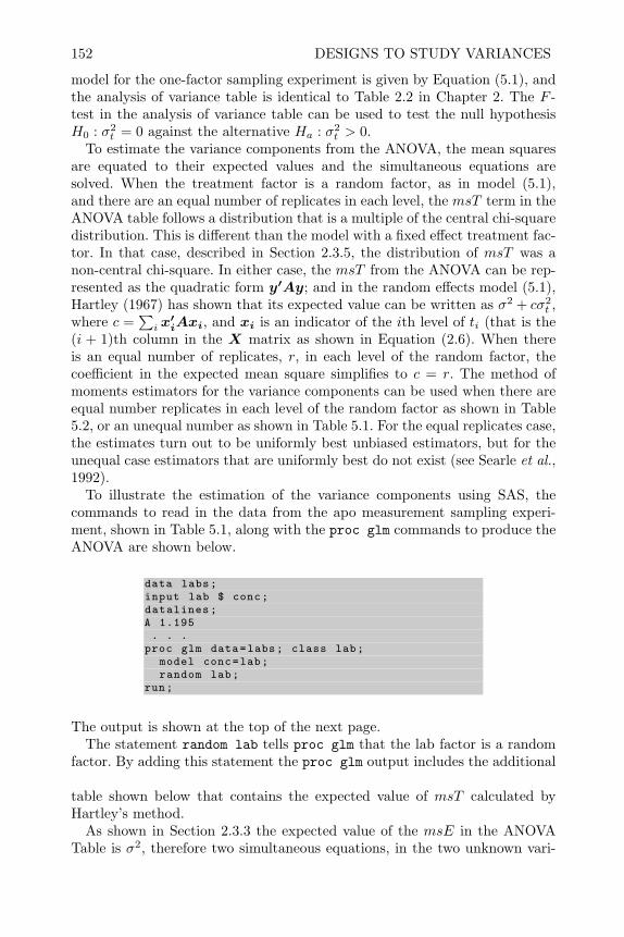
152 DESIGNS TO STUDY VARIANCES
model for the one-factor sampling experiment is given by Equation (5.1), andthe analysis of variance table is identical to Table 2.2 in Chapter 2. The F -test in the analysis of variance table can be used to test the null hypothesisH0 : σ2
t = 0 against the alternative Ha : σ2t > 0.
To estimate the variance components from the ANOVA, the mean squaresare equated to their expected values and the simultaneous equations aresolved. When the treatment factor is a random factor, as in model (5.1),and there are an equal number of replicates in each level, the msT term in theANOVA table follows a distribution that is a multiple of the central chi-squaredistribution. This is different than the model with a fixed effect treatment fac-tor. In that case, described in Section 2.3.5, the distribution of msT was anon-central chi-square. In either case, the msT from the ANOVA can be rep-resented as the quadratic form y′Ay; and in the random effects model (5.1),Hartley (1967) has shown that its expected value can be written as σ2 + cσ2
t ,where c =
∑i x′iAxi, and xi is an indicator of the ith level of ti (that is the
(i + 1)th column in the X matrix as shown in Equation (2.6). When thereis an equal number of replicates, r, in each level of the random factor, thecoefficient in the expected mean square simplifies to c = r. The method ofmoments estimators for the variance components can be used when there areequal number replicates in each level of the random factor as shown in Table5.2, or an unequal number as shown in Table 5.1. For the equal replicates case,the estimates turn out to be uniformly best unbiased estimators, but for theunequal case estimators that are uniformly best do not exist (see Searle et al.,1992).
To illustrate the estimation of the variance components using SAS, thecommands to read in the data from the apo measurement sampling experi-ment, shown in Table 5.1, along with the proc glm commands to produce theANOVA are shown below.
data labs;input lab $ conc;datalines;A 1.195. . .
proc glm data=labs; class lab;model conc=lab;random lab;
run;
The output is shown at the top of the next page.The statement random lab tells proc glm that the lab factor is a random
factor. By adding this statement the proc glm output includes the additional
table shown below that contains the expected value of msT calculated byHartley’s method.
As shown in Section 2.3.3 the expected value of the msE in the ANOVATable is σ2, therefore two simultaneous equations, in the two unknown vari-
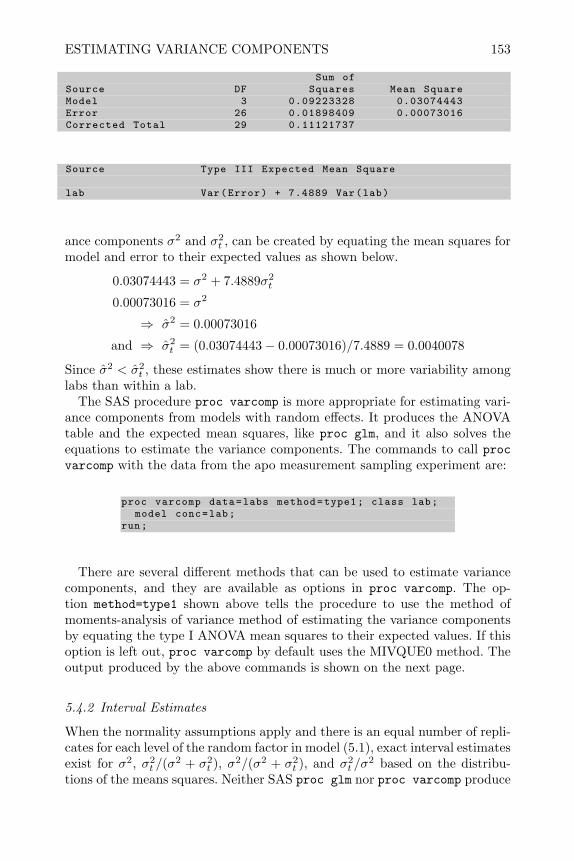
ESTIMATING VARIANCE COMPONENTS 153
Sum ofSource DF Squares Mean SquareModel 3 0.09223328 0.03074443Error 26 0.01898409 0.00073016Corrected Total 29 0.11121737
Source Type III Expected Mean Square
lab Var(Error) + 7.4889 Var(lab)
ance components σ2 and σ2t , can be created by equating the mean squares for
model and error to their expected values as shown below.
0.03074443 = σ2 + 7.4889σ2t
0.00073016 = σ2
⇒ σ2 = 0.00073016
and ⇒ σ2t = (0.03074443− 0.00073016)/7.4889 = 0.0040078
Since σ2 < σ2t , these estimates show there is much or more variability among
labs than within a lab.The SAS procedure proc varcomp is more appropriate for estimating vari-
ance components from models with random effects. It produces the ANOVAtable and the expected mean squares, like proc glm, and it also solves theequations to estimate the variance components. The commands to call procvarcomp with the data from the apo measurement sampling experiment are:
proc varcomp data=labs method=type1; class lab;model conc=lab;
run;
There are several different methods that can be used to estimate variancecomponents, and they are available as options in proc varcomp. The op-tion method=type1 shown above tells the procedure to use the method ofmoments-analysis of variance method of estimating the variance componentsby equating the type I ANOVA mean squares to their expected values. If thisoption is left out, proc varcomp by default uses the MIVQUE0 method. Theoutput produced by the above commands is shown on the next page.
5.4.2 Interval Estimates
When the normality assumptions apply and there is an equal number of repli-cates for each level of the random factor in model (5.1), exact interval estimatesexist for σ2, σ2
t /(σ2 + σ2
t ), σ2/(σ2 + σ2t ), and σ2
t /σ2 based on the distribu-
tions of the means squares. Neither SAS proc glm nor proc varcomp produce

154 DESIGNS TO STUDY VARIANCES
Sum ofSource DF Squares Mean Square Expected Mean Square
lab 3 0.092233 0.030744 Var(Error) + 7.4889 Var(lab)Error 26 0.018984 0.000730 Var(Error)Corrected Total 29 0.111217 . .
Type 1 EstimatesVariance Component Estimate
Var(lab) 0.0040078Var(Error) 0.0007302
these confidence intervals, but they can be easily calculated by hand from thestatistics produced in the ANOVA table. If there are i = 1, . . . , T levels of therandom factor and j = 1, . . . , r replicates in each level of the random factor,then Table 5.3 (that was taken from Searle et al. (1992)) contains exact for-mulas for confidence intervals on lines 1, 3-5, and an approximate formula online 2.
Table 5.3 Confidence Intervals for Functions of Variance Components in One-FactorRandom Model with Equal Replication
Confidence Interval
Lower Upper ConfidenceLine Parameter Limit Limit Coefficient
1 σ2 ssEχ2T (r−1),U
ssEχ2T (r−1),L
1− α
2 σ2t
ssT (1−FU/F )rχ2T−1,U
ssT (1−FL/F )rχ2T−1,L
1− 2α
3 σ2t
σ2t+σ2
F/FU−1r+F/FU−1
F/FL−1r+F/FL−1 1− α
4 σ2
σ2t+σ2
rr+F/FL−1
rr+F/FU−1 1− α
5 σ2t
σ2F/FU−1
rF/FL−1
r 1− α
Notation: F = msT/msE,
Prχ2ν,L ≤ χ2
ν ≤ χ2ν,U = 1− α
PrFL ≤ Fν1,ν2 ≤ FU = 1− α
As an example of calculating the confidence intervals, consider the data inthe sampling experiment shown in Table 5.2 to study the variability in dyestuff

ESTIMATING VARIANCE COMPONENTS 155
color yields. From the ANOVA ssT = 56, 358, ssE = 58, 830, T = 6, r = 5,and F = msT/msE = 4.59847. The upper 0.975 percentile of the chi-squaredistribution with 24 degrees of freedom is 39.36. This can be obtained in a SASdata step using the cinv function as chiU=cinv(.975,24);. The upper 0.975percentile of the F -distribution with 5 and 24 degrees of freedom is 3.15482.This can be obtained from the SAS data step using the finv function asFU=finv(.975,5,24);. The other percentiles of the F and chi-square can beobtained similarly. The exact 95% confidence interval on σ2 is given by:(
ssE
χ224,0.975
,ssE
χ224,0.025
)=(
5883039.6
,5883012.4
)= (1485.61, 4744.35).
The approximate 90% confidence interval on σ2t is given by:(
ssT (1− F5,24,0.975/F )rχ2
5,0.975
,ssT (1− F5,24,0.025/F )
rχ25,0.025
)
=(
56358(1− 3.15482/4.60)5(12.8325)
,56385(1− 0.15929/4.60)
5(0.83121)
)= (275.9551, 10, 914.1765),
and the exact 95% confidence interval on σ2t /(σ
2t + σ2) is given by:(
F/F5,24,0.975 − 1r + F/F5,24,0.975 − 1
,F/F5,24,0.025 − 1
r + F/F5,24,0.025 − 1
)=(
4.59847/3.15482− 16 + 4.59847/3.15482− 1
,4.59847/0.15929− 1
6 + 4.59847/0.15929− 1
)= (0.07086, 0.822844).
Notice the interval estimate of σ2t is much wider than the interval estimate of
σ2. This is because ssT only has 5 degrees of freedom in the ANOVA, whilessE has 24 degrees of freedom.
5.4.3 Maximum Likelihood and REML Estimators
Although the method of moments estimators are uniformly best unbiasedestimators, they have one unfortunate property. When msT is less than msEin the analysis of variance, the estimator of σ2
t will be negative. This canhappen quite frequently if σ2
t /σ2 ≤ 0.10, and there are less than T = 10 levels
of the random factor ti. Maximum likelihood (ML) and (reduced or restricted)maximum likelihood (REML) are preferred methods of estimation that avoidthis problem. REML is an adaptation of the maximum likelihood techniquethat maximizes part of the likelihood. The fact that maximum likelihoodestimators cannot lie outside their parameter space prevents both the ML andREML methods from obtaining negative estimates of σ2
t . To understand howmaximum likelihood and REML work, we will consider the equal replication
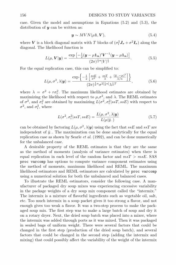
156 DESIGNS TO STUDY VARIANCES
case. Given the model and assumptions in Equations (5.2) and (5.3), thedistribution of y can be written as:
y ∼MVN(µ1,V ), (5.4)
where V is a block diagonal matrix with T blocks of (σ2tJr + σ2Ir) along the
diagonal. The likelihood function is
L(µ,V |y) =exp
[− 1
2 (y − µ1n)′V −1(y − µ1n)]
(2π)12n|V | 12
. (5.5)
For the equal replication case, this can be simplified to:
L(µ, σ2, λ|y) =exp
− 1
2
[ssEσ2 + ssT
λ + (y··−µ)2
λ/n
](2π)
12nσ2[ 12n]λ
12T
, (5.6)
where λ = σ2 + rσ2t . The maximum likelihood estimates are obtained by
maximizing the likelihood with respect to µ,σ2, and λ. The REML estimatesof σ2, and σ2
t are obtained by maximizing L(σ2, σ2t |ssT, ssE) with respect to
σ2, and σ2t , where
L(σ2, σ2t |ssT, ssE) =
L(µ, σ2, λ|y)L(µ|y··)
(5.7)
can be obtained by factoring L(µ, σ2, λ|y) using the fact that ssE and ssT areindependent of y··. The maximization can be done analytically for the equalreplication case as shown by Searle et al. (1992), and can be done numericallyfor the unbalanced case.
A desirable property of the REML estimates is that they are the sameas the method of moments (analysis of variance estimates) when there isequal replication in each level of the random factor and msT > msE. SASproc varcomp has options to compute variance component estimates usingthe method of moments, maximum likelihood and REML. The maximumlikelihood estimators and REML estimators are calculated by proc varcompusing a numerical solution for both the unbalanced and balanced cases.
To illustrate the REML estimators, consider the following case. A man-ufacturer of packaged dry soup mixes was experiencing excessive variabilityin the package weights of a dry soup mix component called the “intermix.”The intermix is a mixture of flavorful ingredients such as vegetable oil, salt,etc. Too much intermix in a soup packet gives it too strong a flavor, and notenough gives too weak a flavor. It was a two-step process to make the pack-aged soup mix. The first step was to make a large batch of soup and dry iton a rotary dryer. Next, the dried soup batch was placed into a mixer, wherethe intermix was added through ports as it was mixed. Then it was packagedin sealed bags of uniform weight. There were several factors that could bechanged in the first step (production of the dried soup batch), and severalfactors that could be changed in the second step (adding the intermix andmixing) that could possibly affect the variability of the weight of the intermix
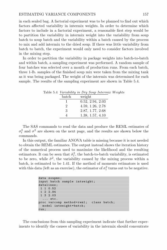
ESTIMATING VARIANCE COMPONENTS 157
in each sealed bag. A factorial experiment was to be planned to find out whichfactors affected variability in intermix weights. In order to determine whichfactors to include in a factorial experiment, a reasonable first step would beto partition the variability in intermix weight into the variability from soupbatch to soup batch and the variability within a batch caused by the processto mix and add intermix to the dried soup. If there was little variability frombatch to batch, the experiment would only need to consider factors involvedin the mixing step.
In order to partition the variability in package weights into batch-to-batchand within batch, a sampling experiment was performed. A random sample offour batches was selected over a month of production runs. From each batch,three 1-lb. samples of the finished soup mix were taken from the mixing tankas it was being packaged. The weight of the intermix was determined for eachsample. The results of the sampling experiment are shown in Table 5.4.
Table 5.4 Variability in Dry Soup Intermix Weights
batch weight1 0.52, 2.94, 2.032 4.59, 1.26, 2.783 2.87, 1.77, 2.684 1.38, 1.57, 4.10
The SAS commands to read the data and produce the REML estimates ofσ2t and σ2 are shown on the next page, and the results are shown below the
commands.In this output, the familiar ANOVA table is missing because it is not needed
to obtain the REML estimates. The output instead shows the iteration historyof the numerical process used to maximize the likelihood and the resultingestimators. It can be seen that σ2
t , the batch-to-batch variability, is estimatedto be zero, while σ2, the variability caused by the mixing process within abatch, is estimated to be 1.41. If the method of moments estimators is usedwith this data (left as an exercise), the estimator of σ2
t turns out to be negative.
data soupmx;input batch sample intweight;datalines;1 1 0.521 2 2.941 3 2.03... etc.
proc varcomp method=reml; class batch;model intweight=batch;
run;
The conclusions from this sampling experiment indicate that further exper-iments to identify the causes of variability in the intermix should concentrate
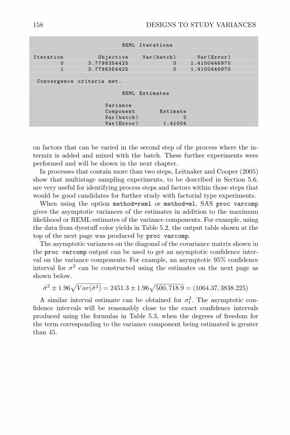
158 DESIGNS TO STUDY VARIANCES
REML Iterations
Iteration Objective Var(batch) Var(Error)0 3.7798354425 0 1.41004469701 3.7798354425 0 1.4100446970
Convergence criteria met.
REML Estimates
VarianceComponent EstimateVar(batch) 0Var(Error) 1.41004
on factors that can be varied in the second step of the process where the in-termix is added and mixed with the batch. These further experiments wereperformed and will be shown in the next chapter.
In processes that contain more than two steps, Leitnaker and Cooper (2005)show that multistage sampling experiments, to be described in Section 5.6,are very useful for identifying process steps and factors within those steps thatwould be good candidates for further study with factorial type experiments.
When using the option method=reml or method=ml, SAS proc varcompgives the asymptotic variances of the estimates in addition to the maximumlikelihood or REML estimates of the variance components. For example, usingthe data from dyestuff color yields in Table 5.2, the output table shown at thetop of the next page was produced by proc varcomp.
The asymptotic variances on the diagonal of the covariance matrix shown inthe proc varcomp output can be used to get an asymptotic confidence inter-val on the variance components. For example, an asymptotic 95% confidenceinterval for σ2 can be constructed using the estimates on the next page asshown below.
σ2 ± 1.96√V ar(σ2) = 2451.3± 1.96
√500, 718.9 = (1064.37, 3838.225)
A similar interval estimate can be obtained for σ2t . The asymptotic con-
fidence intervals will be reasonably close to the exact confidence intervalsproduced using the formulas in Table 5.3, when the degrees of freedom forthe term corresponding to the variance component being estimated is greaterthan 45.
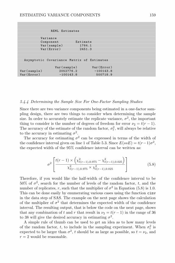
ESTIMATING VARIANCE COMPONENTS 159
REML Estimates
VarianceComponent EstimateVar(sample) 1764.1Var(Error) 2451.3
Asymptotic Covariance Matrix of Estimates
Var(sample) Var(Error)Var(sample) 2052776.2 -100143.8Var(Error) -100143.8 500718.9
5.4.4 Determining the Sample Size For One-Factor Sampling Studies
Since there are two variance components being estimated in a one-factor sam-pling design, there are two things to consider when determining the samplesize. In order to accurately estimate the replicate variance, σ2, the importantthing to consider is the number of degrees of freedom for error ν2 = t(r − 1).The accuracy of the estimate of the random factor, σ2
t , will always be relativeto the accuracy in estimating σ2.
The accuracy for estimating σ2 can be expressed in terms of the width ofthe confidence interval given on line 1 of Table 5.3. Since E(ssE) = t(r−1)σ2,the expected width of the 95% confidence interval can be written as:
σ2
t(r − 1)×(χ2t(r−1),0.975 − χ
2t(r−1),0.025
)χ2t(r−1),0.975 × χ
2t(r−1),0.025
(5.8)
Therefore, if you would like the half-width of the confidence interval to be50% of σ2, search for the number of levels of the random factor, t, and thenumber of replicates, r, such that the multiplier of σ2 in Equation (5.8) is 1.0.This can be done easily by enumerating various cases using the function cinvin the data step of SAS. The example on the next page shows the calculationof the multiplier of σ2 that determines the expected width of the confidenceinterval. The resulting output, that is below the code on the next page, showsthat any combination of t and r that result in ν2 = t(r− 1) in the range of 36to 38 will give the desired accuracy in estimating σ2.
A simple rule of thumb can be used to get an idea as to how many levelsof the random factor, t, to include in the sampling experiment. When σ2
t isexpected to be larger than σ2, t should be as large as possible, so t = ν2, andr = 2 would be reasonable.
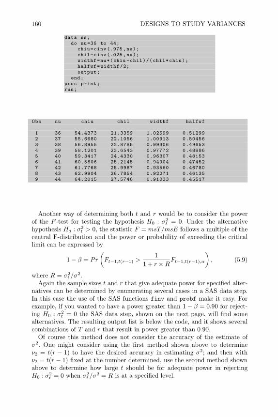
160 DESIGNS TO STUDY VARIANCES
data ss;do nu=36 to 44;
chiu=cinv (.975 ,nu);chil=cinv (.025 ,nu);widthf=nu*(chiu -chil)/(chil*chiu);halfwf=widthf/2;output;
end;proc print;run;
Obs nu chiu chil widthf halfwf
1 36 54.4373 21.3359 1.02599 0.512992 37 55.6680 22.1056 1.00913 0.504563 38 56.8955 22.8785 0.99306 0.496534 39 58.1201 23.6543 0.97772 0.488865 40 59.3417 24.4330 0.96307 0.481536 41 60.5606 25.2145 0.94904 0.474527 42 61.7768 25.9987 0.93560 0.467808 43 62.9904 26.7854 0.92271 0.461359 44 64.2015 27.5746 0.91033 0.45517
Another way of determining both t and r would be to consider the powerof the F -test for testing the hypothesis H0 : σ2
t = 0. Under the alternativehypothesis Ha : σ2
t > 0, the statistic F = msT/msE follows a multiple of thecentral F-distribution and the power or probability of exceeding the criticallimit can be expressed by
1− β = Pr
(Ft−1,t(r−1) >
11 + r ×R
Ft−1,t(r−1),α
), (5.9)
where R = σ2t /σ
2.Again the sample sizes t and r that give adequate power for specified alter-
natives can be determined by enumerating several cases in a SAS data step.In this case the use of the SAS functions finv and probf make it easy. Forexample, if you wanted to have a power greater than 1− β = 0.90 for reject-ing H0 : σ2
t = 0 the SAS data step, shown on the next page, will find somealternatives. The resulting output list is below the code, and it shows severalcombinations of T and r that result in power greater than 0.90.
Of course this method does not consider the accuracy of the estimate ofσ2. One might consider using the first method shown above to determineν2 = t(r − 1) to have the desired accuracy in estimating σ2; and then withν2 = t(r − 1) fixed at the number determined, use the second method shownabove to determine how large t should be for adequate power in rejectingH0 : σ2
t = 0 when σ2t /σ
2 = R is at a specified level.
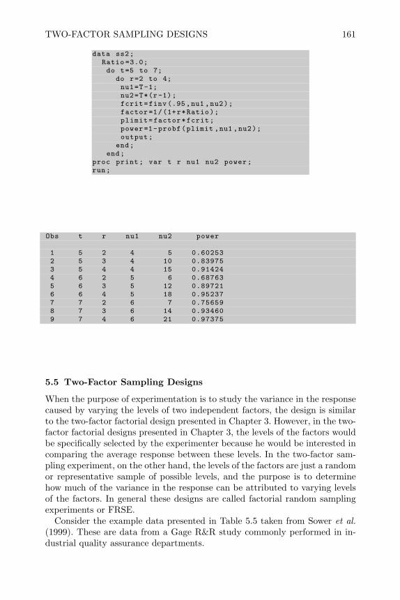
TWO-FACTOR SAMPLING DESIGNS 161
data ss2;Ratio =3.0;do t=5 to 7;
do r=2 to 4;nu1=T-1;nu2=T*(r-1);fcrit=finv (.95,nu1 ,nu2);factor =1/(1+r*Ratio);plimit=factor*fcrit;power=1-probf(plimit ,nu1 ,nu2);output;
end;end;
proc print; var t r nu1 nu2 power;run;
Obs t r nu1 nu2 power
1 5 2 4 5 0.602532 5 3 4 10 0.839753 5 4 4 15 0.914244 6 2 5 6 0.687635 6 3 5 12 0.897216 6 4 5 18 0.952377 7 2 6 7 0.756598 7 3 6 14 0.934609 7 4 6 21 0.97375
5.5 Two-Factor Sampling Designs
When the purpose of experimentation is to study the variance in the responsecaused by varying the levels of two independent factors, the design is similarto the two-factor factorial design presented in Chapter 3. However, in the two-factor factorial designs presented in Chapter 3, the levels of the factors wouldbe specifically selected by the experimenter because he would be interested incomparing the average response between these levels. In the two-factor sam-pling experiment, on the other hand, the levels of the factors are just a randomor representative sample of possible levels, and the purpose is to determinehow much of the variance in the response can be attributed to varying levelsof the factors. In general these designs are called factorial random samplingexperiments or FRSE.
Consider the example data presented in Table 5.5 taken from Sower et al.(1999). These are data from a Gage R&R study commonly performed in in-dustrial quality assurance departments.

162 DESIGNS TO STUDY VARIANCES
Table 5.5 Data from Gage R & R StudyOperator
Part 1 2 31 0.71 0.56 0.52
0.69 0.57 0.542 0.98 1.03 1.04
1.00 0.96 1.013 0.77 0.76 0.81
0.77 0.76 0.814 0.86 0.82 0.82
0.94 0.78 0.825 0.51 0.42 0.46
0.51 0.42 0.496 0.71 1.00 1.04
0.59 1.04 1.007 0.96 0.94 0.97
0.96 0.91 0.958 0.86 0.72 0.78
0.86 0.74 0.789 0.96 0.97 0.84
0.96 0.94 0.8110 0.64 0.56 1.01
0.72 0.52 1.01
In these studies the purpose is to classify the variability in measured fea-tures of manufactured products or product components. Assuming the gageor measuring instrument is properly calibrated, a measured value determinedduring a quality control inspection can be considered to be a function of thetrue feature dimension, the gage repeatability and the gage reproducibility.Gage repeatability is the ability of a single operator to obtain the same mea-surement value multiple times using the same measuring instrument (or gage)on the same feature of a single manufactured component (or part). Gage re-producibility is the ability of different operators to obtain the same measuredvalue multiple times using the same gage on the same part. If the variabilityin measurements caused by the gage repeatability plus the gage reproducibil-ity is more than 10% of the tolerance range, the measurements may not beaccurate enough to be used in monitoring product quality.
The Gage R&R sampling experiment consists of selecting a set of manufac-tured parts or components that are representative of the part-to-part variabil-ity in normal manufacturing. In Table 5.5, a sample of ten parts was selectedand these parts represent the levels of the first factor in the sampling experi-ment. Next, a random or representative sample of inspectors is selected. Theinspectors or operators represent the levels of the second factor in the sam-
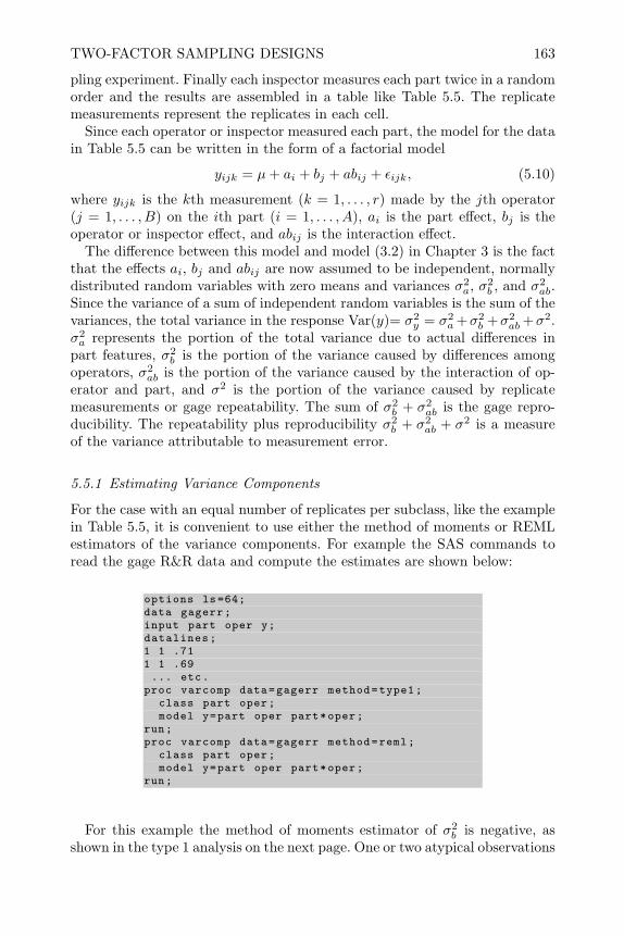
TWO-FACTOR SAMPLING DESIGNS 163
pling experiment. Finally each inspector measures each part twice in a randomorder and the results are assembled in a table like Table 5.5. The replicatemeasurements represent the replicates in each cell.
Since each operator or inspector measured each part, the model for the datain Table 5.5 can be written in the form of a factorial model
yijk = µ+ ai + bj + abij + εijk, (5.10)
where yijk is the kth measurement (k = 1, . . . , r) made by the jth operator(j = 1, . . . , B) on the ith part (i = 1, . . . , A), ai is the part effect, bj is theoperator or inspector effect, and abij is the interaction effect.
The difference between this model and model (3.2) in Chapter 3 is the factthat the effects ai, bj and abij are now assumed to be independent, normallydistributed random variables with zero means and variances σ2
a, σ2b , and σ2
ab.Since the variance of a sum of independent random variables is the sum of thevariances, the total variance in the response Var(y)= σ2
y = σ2a+σ2
b +σ2ab+σ2.
σ2a represents the portion of the total variance due to actual differences in
part features, σ2b is the portion of the variance caused by differences among
operators, σ2ab is the portion of the variance caused by the interaction of op-
erator and part, and σ2 is the portion of the variance caused by replicatemeasurements or gage repeatability. The sum of σ2
b + σ2ab is the gage repro-
ducibility. The repeatability plus reproducibility σ2b + σ2
ab + σ2 is a measureof the variance attributable to measurement error.
5.5.1 Estimating Variance Components
For the case with an equal number of replicates per subclass, like the examplein Table 5.5, it is convenient to use either the method of moments or REMLestimators of the variance components. For example the SAS commands toread the gage R&R data and compute the estimates are shown below:
options ls=64;data gagerr;input part oper y;datalines;1 1 .711 1 .69... etc.
proc varcomp data=gagerr method=type1;class part oper;model y=part oper part*oper;
run;proc varcomp data=gagerr method=reml;
class part oper;model y=part oper part*oper;
run;
For this example the method of moments estimator of σ2b is negative, as
shown in the type 1 analysis on the next page. One or two atypical observations
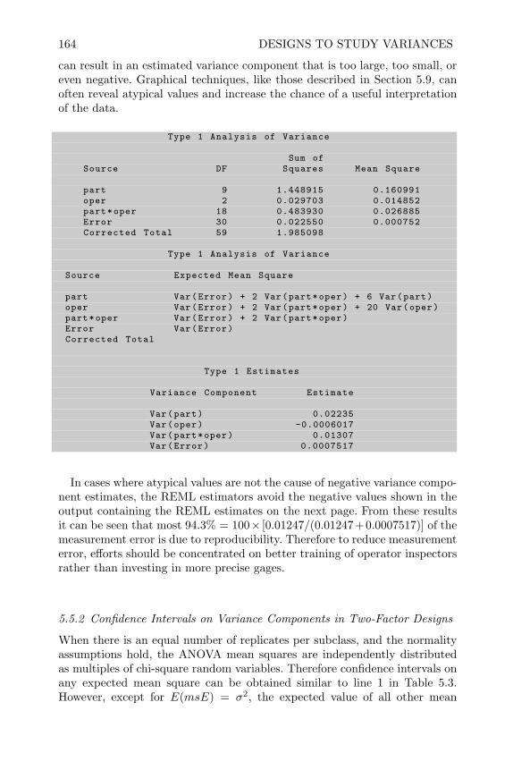
164 DESIGNS TO STUDY VARIANCES
can result in an estimated variance component that is too large, too small, oreven negative. Graphical techniques, like those described in Section 5.9, canoften reveal atypical values and increase the chance of a useful interpretationof the data.
Type 1 Analysis of Variance
Sum ofSource DF Squares Mean Square
part 9 1.448915 0.160991oper 2 0.029703 0.014852part*oper 18 0.483930 0.026885Error 30 0.022550 0.000752Corrected Total 59 1.985098
Type 1 Analysis of Variance
Source Expected Mean Square
part Var(Error) + 2 Var(part*oper) + 6 Var(part)oper Var(Error) + 2 Var(part*oper) + 20 Var(oper)part*oper Var(Error) + 2 Var(part*oper)Error Var(Error)Corrected Total
Type 1 Estimates
Variance Component Estimate
Var(part) 0.02235Var(oper) -0.0006017Var(part*oper) 0.01307Var(Error) 0.0007517
In cases where atypical values are not the cause of negative variance compo-nent estimates, the REML estimators avoid the negative values shown in theoutput containing the REML estimates on the next page. From these resultsit can be seen that most 94.3% = 100× [0.01247/(0.01247+0.0007517)] of themeasurement error is due to reproducibility. Therefore to reduce measurementerror, efforts should be concentrated on better training of operator inspectorsrather than investing in more precise gages.
5.5.2 Confidence Intervals on Variance Components in Two-Factor Designs
When there is an equal number of replicates per subclass, and the normalityassumptions hold, the ANOVA mean squares are independently distributedas multiples of chi-square random variables. Therefore confidence intervals onany expected mean square can be obtained similar to line 1 in Table 5.3.However, except for E(msE) = σ2, the expected value of all other mean
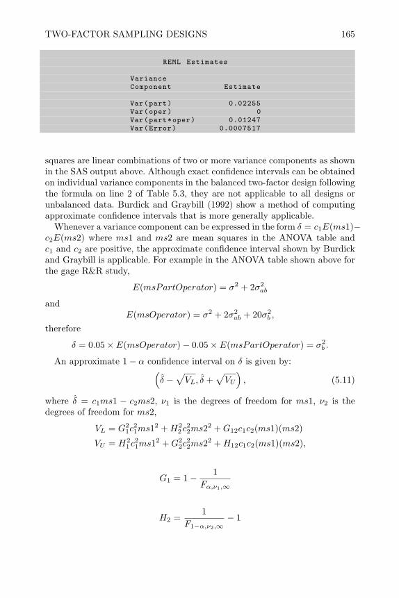
TWO-FACTOR SAMPLING DESIGNS 165
REML Estimates
VarianceComponent Estimate
Var(part) 0.02255Var(oper) 0Var(part*oper) 0.01247Var(Error) 0.0007517
squares are linear combinations of two or more variance components as shownin the SAS output above. Although exact confidence intervals can be obtainedon individual variance components in the balanced two-factor design followingthe formula on line 2 of Table 5.3, they are not applicable to all designs orunbalanced data. Burdick and Graybill (1992) show a method of computingapproximate confidence intervals that is more generally applicable.
Whenever a variance component can be expressed in the form δ = c1E(ms1)−c2E(ms2) where ms1 and ms2 are mean squares in the ANOVA table andc1 and c2 are positive, the approximate confidence interval shown by Burdickand Graybill is applicable. For example in the ANOVA table shown above forthe gage R&R study,
E(msPartOperator) = σ2 + 2σ2ab
andE(msOperator) = σ2 + 2σ2
ab + 20σ2b ,
therefore
δ = 0.05× E(msOperator)− 0.05× E(msPartOperator) = σ2b .
An approximate 1− α confidence interval on δ is given by:(δ −
√VL, δ +
√VU
), (5.11)
where δ = c1ms1 − c2ms2, ν1 is the degrees of freedom for ms1, ν2 is thedegrees of freedom for ms2,
VL = G21c
21ms1
2 +H22 c
22ms2
2 +G12c1c2(ms1)(ms2)
VU = H21 c
21ms1
2 +G22c
22ms2
2 +H12c1c2(ms1)(ms2),
G1 = 1− 1Fα,ν1,∞
H2 =1
F1−α,ν2,∞− 1

166 DESIGNS TO STUDY VARIANCES
G12 =(Fα,ν1,ν2 − 1)2 −G2
1F2α,ν1,ν2 −H
22
Fα,ν1,ν2
H1 =1
F1−α,ν1,∞− 1
G2 = 1− 1Fα,ν2,∞
and
H12 =(1− F1−α,ν1,ν2)2 −H2
1F21−α,ν1,ν2−G2
2
F1−α,ν1,ν2.
Although these formulas look formidable, they can easily be evaluated in athe SAS data step. A SAS, macro %vci, listed in the appendix of this chapter,will compute confidence intervals using these formulas. The input to the macrois a SAS data set called meansq that contains the variables confl=1 − α,c1=c1, ms1=ms1, nu1=ν1, c2=c2, ms2=ms2, and nu2=ν2. To see how to usethis macro consider making confidence intervals on the variance componentfor operator, and the variance component for the part by operator interactionin the gage R&R study data.
To get a confidence interval on the variance component for operator, σ2b ,
ms1=0.014852 with 2 degrees of freedom, ms2=0.026885 with 18 degrees offreedom. These are read into a SAS data set as follows:
data meansq;input confl c1 ms1 nu1 c2 ms2 nu2;datalines;.90 .05 .014852 2 .05 .026885 18%vci;
The %vci statement calls the macro and produces the following results:
Obs delta L U
1 -.00060165 -.001579783 .005717457
This shows that even though the method of moments estimator for σ2b is
negative, the upper 90% confidence bound is positive.The 90% confidence interval for σ2
ab is found to be (0.008936 − 0.021895)using the same approximation formula.
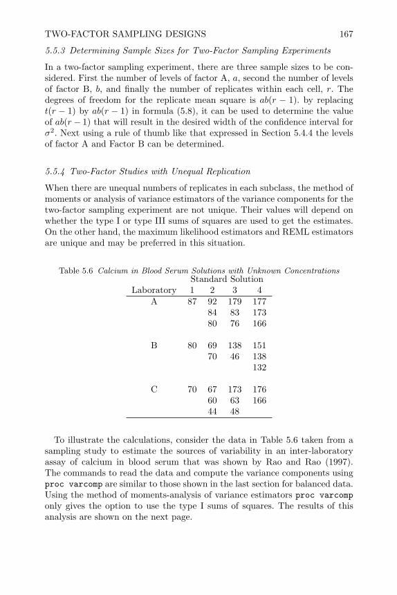
TWO-FACTOR SAMPLING DESIGNS 167
5.5.3 Determining Sample Sizes for Two-Factor Sampling Experiments
In a two-factor sampling experiment, there are three sample sizes to be con-sidered. First the number of levels of factor A, a, second the number of levelsof factor B, b, and finally the number of replicates within each cell, r. Thedegrees of freedom for the replicate mean square is ab(r − 1). by replacingt(r − 1) by ab(r − 1) in formula (5.8), it can be used to determine the valueof ab(r− 1) that will result in the desired width of the confidence interval forσ2. Next using a rule of thumb like that expressed in Section 5.4.4 the levelsof factor A and Factor B can be determined.
5.5.4 Two-Factor Studies with Unequal Replication
When there are unequal numbers of replicates in each subclass, the method ofmoments or analysis of variance estimators of the variance components for thetwo-factor sampling experiment are not unique. Their values will depend onwhether the type I or type III sums of squares are used to get the estimates.On the other hand, the maximum likelihood estimators and REML estimatorsare unique and may be preferred in this situation.
Table 5.6 Calcium in Blood Serum Solutions with Unknown ConcentrationsStandard Solution
Laboratory 1 2 3 4A 87 92 179 177
84 83 17380 76 166
B 80 69 138 15170 46 138
132
C 70 67 173 17660 63 16644 48
To illustrate the calculations, consider the data in Table 5.6 taken from asampling study to estimate the sources of variability in an inter-laboratoryassay of calcium in blood serum that was shown by Rao and Rao (1997).The commands to read the data and compute the variance components usingproc varcomp are similar to those shown in the last section for balanced data.Using the method of moments-analysis of variance estimators proc varcomponly gives the option to use the type I sums of squares. The results of thisanalysis are shown on the next page.
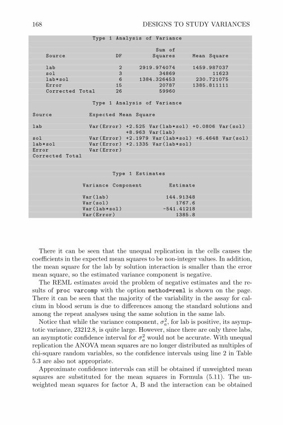
168 DESIGNS TO STUDY VARIANCES
Type 1 Analysis of Variance
Sum ofSource DF Squares Mean Square
lab 2 2919.974074 1459.987037sol 3 34869 11623lab*sol 6 1384.326453 230.721075Error 15 20787 1385.811111Corrected Total 26 59960
Type 1 Analysis of Variance
Source Expected Mean Square
lab Var(Error) +2.525 Var(lab*sol) +0.0806 Var(sol)+8.963 Var(lab)
sol Var(Error) +2.1979 Var(lab*sol) +6.4648 Var(sol)lab*sol Var(Error) +2.1335 Var(lab*sol)Error Var(Error)Corrected Total
Type 1 Estimates
Variance Component Estimate
Var(lab) 144.91348Var(sol) 1767.6Var(lab*sol) -541.41218Var(Error) 1385.8
There it can be seen that the unequal replication in the cells causes thecoefficients in the expected mean squares to be non-integer values. In addition,the mean square for the lab by solution interaction is smaller than the errormean square, so the estimated variance component is negative.
The REML estimates avoid the problem of negative estimates and the re-sults of proc varcomp with the option method=reml is shown on the page.There it can be seen that the majority of the variability in the assay for cal-cium in blood serum is due to differences among the standard solutions andamong the repeat analyses using the same solution in the same lab.
Notice that while the variance component, σ2a, for lab is positive, its asymp-
totic variance, 23212.8, is quite large. However, since there are only three labs,an asymptotic confidence interval for σ2
a would not be accurate. With unequalreplication the ANOVA mean squares are no longer distributed as multiples ofchi-square random variables, so the confidence intervals using line 2 in Table5.3 are also not appropriate.
Approximate confidence intervals can still be obtained if unweighted meansquares are substituted for the mean squares in Formula (5.11). The un-weighted mean squares for factor A, B and the interaction can be obtained
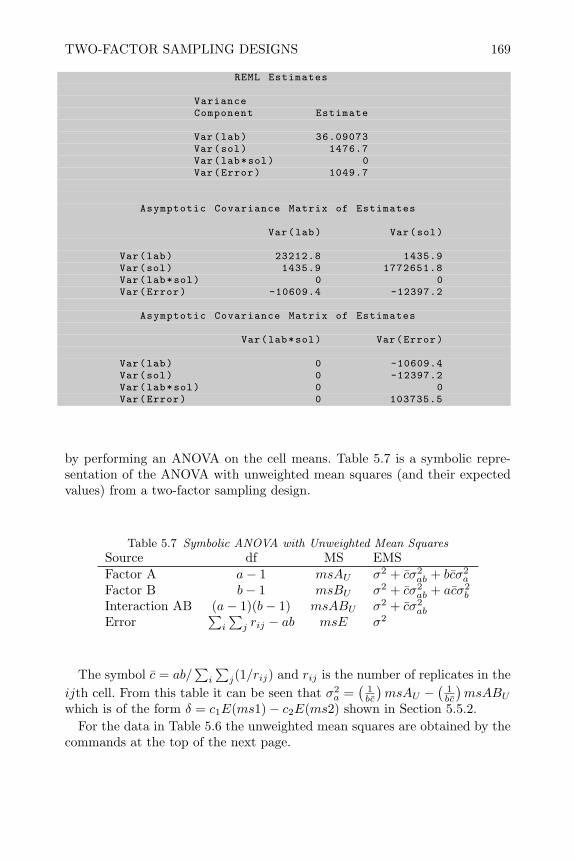
TWO-FACTOR SAMPLING DESIGNS 169
REML Estimates
VarianceComponent Estimate
Var(lab) 36.09073Var(sol) 1476.7Var(lab*sol) 0Var(Error) 1049.7
Asymptotic Covariance Matrix of Estimates
Var(lab) Var(sol)
Var(lab) 23212.8 1435.9Var(sol) 1435.9 1772651.8Var(lab*sol) 0 0Var(Error) -10609.4 -12397.2
Asymptotic Covariance Matrix of Estimates
Var(lab*sol) Var(Error)
Var(lab) 0 -10609.4Var(sol) 0 -12397.2Var(lab*sol) 0 0Var(Error) 0 103735.5
by performing an ANOVA on the cell means. Table 5.7 is a symbolic repre-sentation of the ANOVA with unweighted mean squares (and their expectedvalues) from a two-factor sampling design.
Table 5.7 Symbolic ANOVA with Unweighted Mean SquaresSource df MS EMSFactor A a− 1 msAU σ2 + cσ2
ab + bcσ2a
Factor B b− 1 msBU σ2 + cσ2ab + acσ2
b
Interaction AB (a− 1)(b− 1) msABU σ2 + cσ2ab
Error∑i
∑j rij − ab msE σ2
The symbol c = ab/∑i
∑j(1/rij) and rij is the number of replicates in the
ijth cell. From this table it can be seen that σ2a =
(1bc
)msAU −
(1bc
)msABU
which is of the form δ = c1E(ms1)− c2E(ms2) shown in Section 5.5.2.For the data in Table 5.6 the unweighted mean squares are obtained by the
commands at the top of the next page.

170 DESIGNS TO STUDY VARIANCES
proc sort data=bloods; by lab sol;proc means noprint; by lab sol;
var conc;output out=uss mean=yijbar;
proc glm data=uss;class lab sol;model yijbar=lab sol lab*sol;
run;
which result in maAU = 872.68056, msABU = 638.93056. The factor
c = ab/∑i
∑j
(1/rij)
=(3)(4)(
11 + 1
3 + 13 + 1
3 + 11 + 1
2 + 12 + 1
3 + 11 + 1
3 + 13 + 1
2
)= 1.846,
and c1 = c2 = 1bc = 1
4(1.846) = 0.13541. Thus the data needed in the SAS datafile meansq to calculate a 90% confidence interval for σ2
a is:
data meansq;input confl c1 ms1 nu1 c2 ms2 nu2;datalines;.90 .1354166 872.68056 2 .1354166 638.93056 6%vci;
and the resulting confidence interval is (-124.862, 1035.82). Therefore, al-though the point estimates of σ2
a are positive, the confidence interval shows itis not significantly different than zero.
5.6 Nested Sampling Experiments (NSE)
Many sampling experiments with more than one factor use nested factors ora hierarchical design. The levels of a nested factor are physically differentdepending on the level of factor it is nested within. That wasn’t the casefor the factors described in the last section. For example, in the gage R&Rstudy, each operator measured each part; therefore, the operator number wasuniquely defined and referred to the same operator regardless of which part hemeasured. We would call the operator and part in the gage R&R study crossedfactors. To change the design so that operator was a nested factor, consider anexperiment where n parts were selected and each part was measured by twooperators, although it doesn’t have to be the same two operators measuringeach part. This might be a more convenient way to conduct the samplingexperiment if parts were selected over a long period of time and the same

NESTED SAMPLING EXPERIMENTS (NSE) 171
operators were not always present to make the measurements. The fact thatthe operators differ depending upon the part number being measured makesthe operator a nested factor (nested within part). The first operator measuringthe first part is not physically the same person as the first operator measuringa subsequent part. Another common example where a nested design occursis when the measurements are destructive. In that case, each operator mustmeasure a different set of parts, and the part becomes the nested factor (nestedwithin operator) because the first part measured by the first operator is notphysically the same as the first part measured by subsequent operators. Thistype of sampling design is called a nested sampling experiment or NSE.
One example where we have already seen nested factors is in the term εij inthe models we have used thus far. It represents the effect of the jth replicateexperimental unit, and since different experimental units are used for eachfactor level or combination of factor levels, the experimental unit is alwaysnested within another factor level or cell in the design.
When two factors are crossed factors we can include their interaction inthe model to represent the extra variability caused by changes in the level ofone factor between levels of the other factor. However, if a factor is nestedwithin another factor we cannot include an interaction between them becausethe nested factor includes the degrees of freedom that could be taken by theinteraction. The model for a two-stage nested design with factor B nestedwithin factor A is written as:
yijk = µ+ ai + b(i)j + εijk (5.12)
and if there is an equal number of replicates, r, per cell, the ANOVA table forthe nested model can be represented as:
Table 5.8 Symbolic ANOVA for Two-Factor Nested DesignSource df MS EMSFactor A a− 1 msA σ2 + rσ2
b + brσ2a
Factor B a(b− 1) msB σ2 + rσ2b
Error ab(r − 1) msE σ2
Here it can be seen that the degrees of freedom for Factor B,
a(b− 1) = (b− 1) + (a− 1)(b− 1)
is equal to the degrees of freedom for a crossed factor plus the degrees for theinteraction AB.
Nested or hierarchical designs can easily be extended to include severalstages or factors. For example Table 5.9 shows the results of a four-stagenested sampling study on the variability of properties of crude rubber, takenfrom Bennett and Franklin (1954). In this study a sample of four batches of
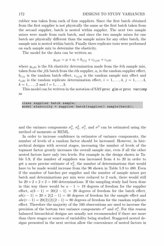
172 DESIGNS TO STUDY VARIANCES
rubber was taken from each of four suppliers. Since the first batch obtainedfrom the first supplier is not physically the same as the first batch taken fromthe second supplier, batch is nested within supplier. The next two samplemixes were made from each batch, and since the two sample mixes for onebatch are physically different than the sample mixes for any other batch, thesample mix is nested within batch. Finally three replicate tests were performedon each sample mix to determine the elasticity.
The model for the data can be written as:
yijkl = µ+ ai + b(i)j + c(ij)k + εijkl
where yijkl is the lth elasticity determination made from the kth sample mix,taken from the jth batch from the ith supplier, ai is the random supplier effect,b(i)j is the random batch effect, c(ij)k is the random sample mix effect andεijkl is the random replicate determination effect, i = 1, . . . , 4, j = 1, . . . , 4,k = 1, . . . , 2 and l = 1, . . . , 3.
This model can be written in the notation of SAS proc glm or proc varcompas
class supplier batch sample;model elasticity = supplier batch(supplier) sample(batch);
and the variance components σ2a, σ2
b , σ2c , and σ2 can be estimated using the
method of moments or REML.In order to increase confidence in estimates of variance components, the
number of levels of a random factor should be increased. However, in hier-archical designs with several stages, increasing the number of levels of thetopmost factor greatly increases the overall sample size, even if all the othernested factors have only two levels. For example in the design shown in Ta-ble 5.9, if the number of suppliers was increased from 4 to 20 in order toget a more precise estimate of σ2
a, the number of determinations that wouldhave to be made would increase from the 96 shown in Table 5.9 to 480. Evenif the number of batches per supplier and the number of sample mixes perbatch and determinations per mix were reduced to 2 each, there would stillbe 20× 2× 2× 2 = 160 determinations. If the sampling study had been donein this way there would be a − 1 = 19 degrees of freedom for the suppliereffect, a(b − 1) = 20(2 − 1) = 20 degrees of freedom for the batch effect,ab(c − 1) = 20 × 2(2 − 1) = 40 degrees of freedom for the sample effect andabc(r− 1) = 20(2)(2)(2− 1) = 80 degrees of freedom for the random replicateeffect. Therefore the majority of the 160 observations are used to increase theprecision of the bottom two variance components σ2 and σ2
c . For this reasonbalanced hierarchical designs are usually not recommended if there are morethan three stages or sources of variability being studied. Staggered nested de-signs presented in the next section allow the convenience of nested factors in
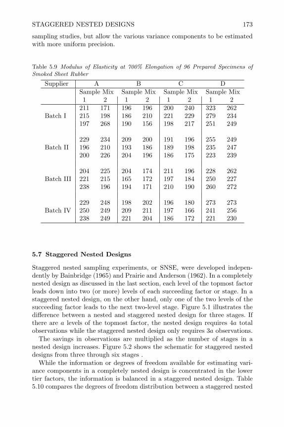
STAGGERED NESTED DESIGNS 173
sampling studies, but allow the various variance components to be estimatedwith more uniform precision.
Table 5.9 Modulus of Elasticity at 700% Elongation of 96 Prepared Specimens ofSmoked Sheet Rubber
Supplier A B C DSample Mix Sample Mix Sample Mix Sample Mix1 2 1 2 1 2 1 2
211 171 196 196 200 240 323 262Batch I 215 198 186 210 221 229 279 234
197 268 190 156 198 217 251 249
229 234 209 200 191 196 255 249Batch II 196 210 193 186 189 198 235 247
200 226 204 196 186 175 223 239
204 225 204 174 211 196 228 262Batch III 221 215 165 172 197 184 250 227
238 196 194 171 210 190 260 272
229 248 198 202 196 180 273 273Batch IV 250 249 209 211 197 166 241 256
238 249 221 204 186 172 221 230
5.7 Staggered Nested Designs
Staggered nested sampling experiments, or SNSE, were developed indepen-dently by Bainbridge (1965) and Prairie and Anderson (1962). In a completelynested design as discussed in the last section, each level of the topmost factorleads down into two (or more) levels of each succeeding factor or stage. In astaggered nested design, on the other hand, only one of the two levels of thesucceeding factor leads to the next two-level stage. Figure 5.1 illustrates thedifference between a nested and staggered nested design for three stages. Ifthere are a levels of the topmost factor, the nested design requires 4a totalobservations while the staggered nested design only requires 3a observations.
The savings in observations are multiplied as the number of stages in anested design increases. Figure 5.2 shows the schematic for staggered nesteddesigns from three through six stages .
While the information or degrees of freedom available for estimating vari-ance components in a completely nested design is concentrated in the lowertier factors, the information is balanced in a staggered nested design. Table5.10 compares the degrees of freedom distribution between a staggered nested

174 DESIGNS TO STUDY VARIANCES
Figure 5.1 Comparison of 3 Stage Nested and 3 Stage Staggered Nested Design
Figure 5.2 Staggered Nested Designs for 3 to 6 Stages
design and a completely nested design where each factor except the topmosthas only two levels.
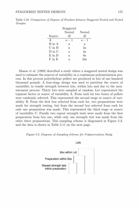
STAGGERED NESTED DESIGNS 175
Table 5.10 Comparison of Degrees of Freedom between Staggered Nested and NestedDesigns
StaggeredNested Nested
Source df dfA a− 1 a− 1B in A a aC in B a 2aD in C a 4aE in D a 8aF in E a 16a
Mason et al. (1989) described a study where a staggered nested design wasused to estimate the sources of variability in a continuous polymerization pro-cess. In this process polyethylene pellets are produced in lots of one hundredthousand pounds. A four-stage design was used to partition the source ofvariability in tensile strength between lots, within lots and due to the mea-surement process. Thirty lots were sampled at random. Lot represented thetopmost factor or source of variability A. From each lot two boxes of pelletswere randomly selected. This represented the second stage or source of vari-ability B. From the first box selected from each lot, two preparations weremade for strength testing, but from the second box selected from each lotonly one preparation was made. This represented the third stage or sourceof variability C. Finally two repeat strength tests were made from the firstpreparation from box one, while only one strength test was made from theother three preparations. This sampling scheme is diagramed in Figure 5.3,and the data is shown in Table 5.11 on the next page.
Figure 5.3 Diagram of Sampling Scheme for Polymerization Study
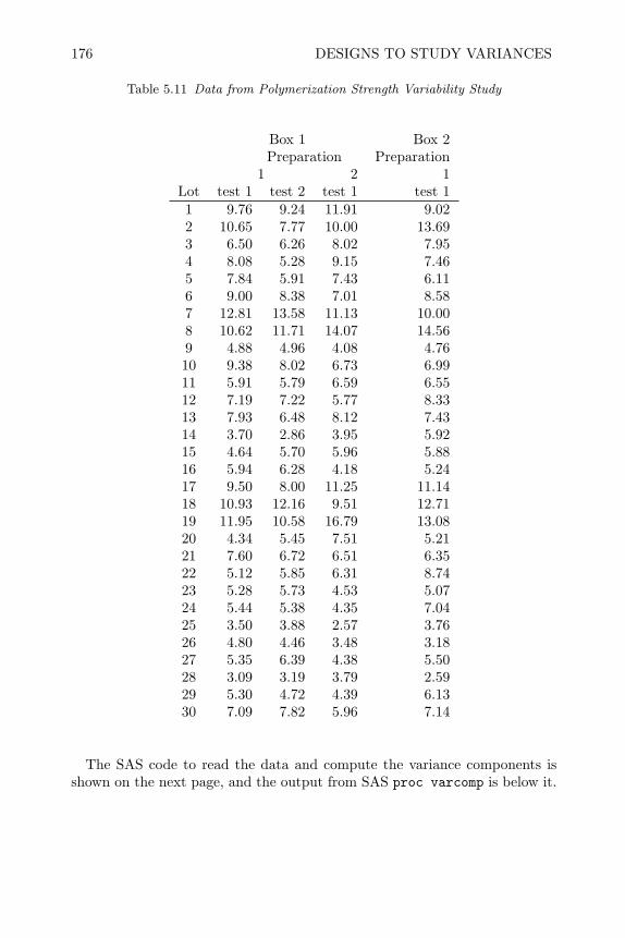
176 DESIGNS TO STUDY VARIANCES
Table 5.11 Data from Polymerization Strength Variability Study
Box 1 Box 2Preparation Preparation
1 2 1Lot test 1 test 2 test 1 test 11 9.76 9.24 11.91 9.022 10.65 7.77 10.00 13.693 6.50 6.26 8.02 7.954 8.08 5.28 9.15 7.465 7.84 5.91 7.43 6.116 9.00 8.38 7.01 8.587 12.81 13.58 11.13 10.008 10.62 11.71 14.07 14.569 4.88 4.96 4.08 4.7610 9.38 8.02 6.73 6.9911 5.91 5.79 6.59 6.5512 7.19 7.22 5.77 8.3313 7.93 6.48 8.12 7.4314 3.70 2.86 3.95 5.9215 4.64 5.70 5.96 5.8816 5.94 6.28 4.18 5.2417 9.50 8.00 11.25 11.1418 10.93 12.16 9.51 12.7119 11.95 10.58 16.79 13.0820 4.34 5.45 7.51 5.2121 7.60 6.72 6.51 6.3522 5.12 5.85 6.31 8.7423 5.28 5.73 4.53 5.0724 5.44 5.38 4.35 7.0425 3.50 3.88 2.57 3.7626 4.80 4.46 3.48 3.1827 5.35 6.39 4.38 5.5028 3.09 3.19 3.79 2.5929 5.30 4.72 4.39 6.1330 7.09 7.82 5.96 7.14
The SAS code to read the data and compute the variance components isshown on the next page, and the output from SAS proc varcomp is below it.
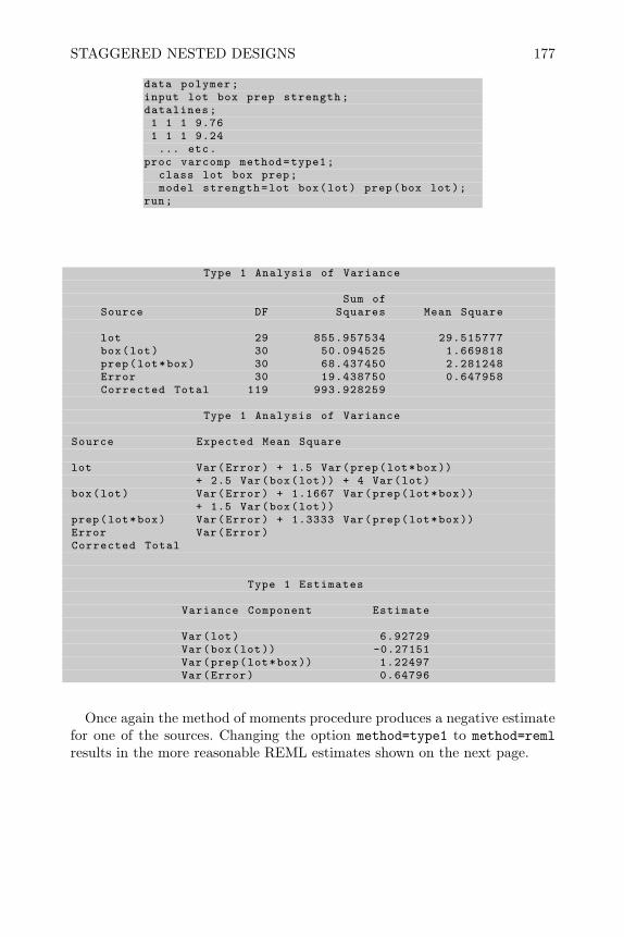
STAGGERED NESTED DESIGNS 177
data polymer;input lot box prep strength;datalines;1 1 1 9.761 1 1 9.24... etc.
proc varcomp method=type1;class lot box prep;model strength=lot box(lot) prep(box lot);
run;
Type 1 Analysis of Variance
Sum ofSource DF Squares Mean Square
lot 29 855.957534 29.515777box(lot) 30 50.094525 1.669818prep(lot*box) 30 68.437450 2.281248Error 30 19.438750 0.647958Corrected Total 119 993.928259
Type 1 Analysis of Variance
Source Expected Mean Square
lot Var(Error) + 1.5 Var(prep(lot*box))+ 2.5 Var(box(lot)) + 4 Var(lot)
box(lot) Var(Error) + 1.1667 Var(prep(lot*box))+ 1.5 Var(box(lot))
prep(lot*box) Var(Error) + 1.3333 Var(prep(lot*box))Error Var(Error)Corrected Total
Type 1 Estimates
Variance Component Estimate
Var(lot) 6.92729Var(box(lot)) -0.27151Var(prep(lot*box)) 1.22497Var(Error) 0.64796
Once again the method of moments procedure produces a negative estimatefor one of the sources. Changing the option method=type1 to method=remlresults in the more reasonable REML estimates shown on the next page.
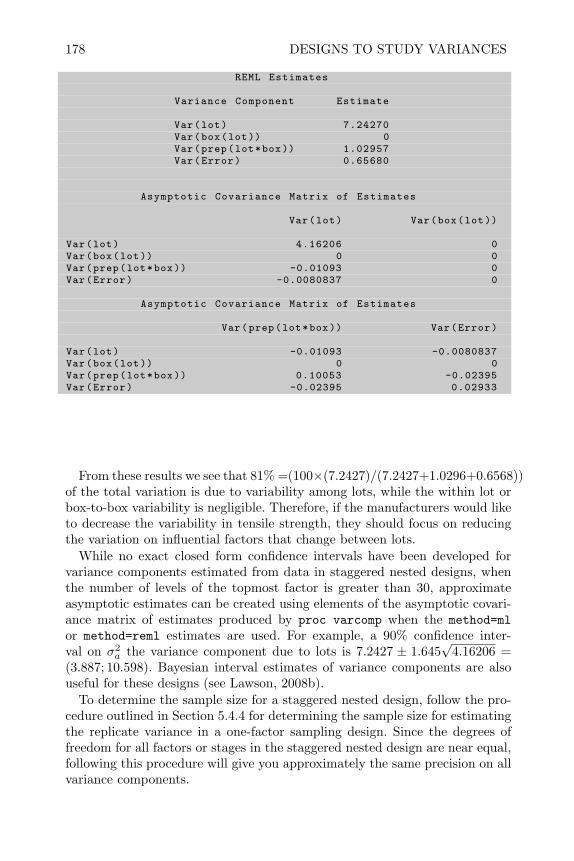
178 DESIGNS TO STUDY VARIANCES
REML Estimates
Variance Component Estimate
Var(lot) 7.24270Var(box(lot)) 0Var(prep(lot*box)) 1.02957Var(Error) 0.65680
Asymptotic Covariance Matrix of Estimates
Var(lot) Var(box(lot))
Var(lot) 4.16206 0Var(box(lot)) 0 0Var(prep(lot*box)) -0.01093 0Var(Error) -0.0080837 0
Asymptotic Covariance Matrix of Estimates
Var(prep(lot*box)) Var(Error)
Var(lot) -0.01093 -0.0080837Var(box(lot)) 0 0Var(prep(lot*box)) 0.10053 -0.02395Var(Error) -0.02395 0.02933
From these results we see that 81% =(100×(7.2427)/(7.2427+1.0296+0.6568))of the total variation is due to variability among lots, while the within lot orbox-to-box variability is negligible. Therefore, if the manufacturers would liketo decrease the variability in tensile strength, they should focus on reducingthe variation on influential factors that change between lots.
While no exact closed form confidence intervals have been developed forvariance components estimated from data in staggered nested designs, whenthe number of levels of the topmost factor is greater than 30, approximateasymptotic estimates can be created using elements of the asymptotic covari-ance matrix of estimates produced by proc varcomp when the method=mlor method=reml estimates are used. For example, a 90% confidence inter-val on σ2
a the variance component due to lots is 7.2427 ± 1.645√
4.16206 =(3.887; 10.598). Bayesian interval estimates of variance components are alsouseful for these designs (see Lawson, 2008b).
To determine the sample size for a staggered nested design, follow the pro-cedure outlined in Section 5.4.4 for determining the sample size for estimatingthe replicate variance in a one-factor sampling design. Since the degrees offreedom for all factors or stages in the staggered nested design are near equal,following this procedure will give you approximately the same precision on allvariance components.

DESIGNS WITH FIXED AND RANDOM FACTORS 179
5.8 Designs with Fixed and Random Factors
In some cases where fixed treatment factors are being studied in an experi-mental design like those discussed in Chapters 2 through 4, random factorsare also introduced in the model by the way the experiment is conducted.For example consider the data in Table 5.12 that resulted from an experi-ment comparing different formulations and methods of applying a pesticideto the leaves of cotton plants. The goal was to increase the amount of activepesticide remaining on cotton plant leaves one week after application. Thepesticide being studied degrades in sunlight and a certain additive to the for-mulation retards this process. Different application techniques may differ inthe amount of pesticide delivered to the plant leaves. The treatment factorsin this experiment were two different formulations of the pesticide and twodifferent application methods, resulting in a 22 factorial experiment.
The experimental unit was a 20’ row of cotton plants called a plot, becausethis was a convenient area within which the application of pesticide could becontrolled. Eight plots were selected and two were randomly assigned to eachof the four treatment combinations, resulting in two replicates per treatmentcombination. One week after application, the experimenters were ready to de-termine the pesticide residue remaining on the plant leaves. However, therewas too much plant material in an entire plot to send to the lab for analy-sis. Therefore, two samples of leaves in an amount convenient for laboratoryanalysis of pesticide residues were selected from each plot. Each sample wassent to the lab resulting in the data shown in Table 5.12.
Formulation, application technique and their interaction are fixed factorsbecause the experimenters were interested in comparing the average responsebetween levels of these factors. The plot, on the other hand, is a randomfactor that represents differences in experimental units. It is nested within thecombinations of formulation by application technique. There is no interestin comparing experimental units within each combination of formulation andapplication. Instead multiple plots per treatment combination were includedin the design so that the variance caused by differing plots could be estimatedand used to judge significance of formulation and application effects. Thereplicate samples taken from each plot were for convenience in conducting theexperiment. They would be classified as sub-samples or observational unitsdefined in Chapter 1.
The simplest way of analyzing the data would be to average the two sub-samples and proceed as illustrated in Section 3.5. However, if the sub-samplescan be assumed independent and it is desirable to include all the data (shownin Table 5.12) in the analysis, then an additional term for sample must beincluded in the model. Sample is another random effect since there is nospecific interest in comparing the response between the two samples fromeach plot.
The model for the data can be written in the form
yijkl = µ+ αi + βj + αβij + p(ij)k + εijkl, (5.13)

180 DESIGNS TO STUDY VARIANCES
Table 5.12 Pesticide Residue on Cotton Plants
Application SampleFormulation Technique Plot 1 2
A 1 1 0.237 0.252A 1 2 0.281 0.274B 1 1 0.247 0.294B 1 2 0.321 0.267A 2 1 0.392 0.378A 2 2 0.381 0.346B 2 1 0.351 0.362B 2 2 0.334 0.348
where yijkl is the pesticide residue found on the lth sample taken from the kthplot, treated with formulation level i and application technique j. In generali = 1, . . . , a, j = 1, . . . , b, k = 1, . . . , r, and l = 1, . . . , s. In this specificexample, a = 2, b = 2, r = 2, and s = 2, αi is the formulation effect, βj isthe application effect, αβij is the interaction effect, p(ij)k is the random ploteffect, and εijkl is the random sample effect.
The model can be written in matrix notation as:
y = Xβ +Zγ + ε, (5.14)
.where
y =
y1111
y1112
y1121
y1122
y2111
y2112
y2121
y2122
y1211
y1212
y1221
y1222
y2211
y2212
y2221
y2222
, X =
1 1 0 1 0 1 0 0 01 1 0 1 0 1 0 0 01 1 0 1 0 1 0 0 01 1 0 1 0 1 0 0 01 0 1 1 0 0 1 0 01 0 1 1 0 0 1 0 01 0 1 1 0 0 1 0 01 0 1 1 0 0 1 0 01 1 0 0 1 0 0 1 01 1 0 0 1 0 0 1 01 1 0 0 1 0 0 1 01 1 0 0 1 0 0 1 01 0 1 0 1 0 0 0 11 0 1 0 1 0 0 0 11 0 1 0 1 0 0 0 11 0 1 0 1 0 0 0 1
, β =
µα1
α2
β1
β2
αβ11
αβ21
αβ12
αβ22
,

DESIGNS WITH FIXED AND RANDOM FACTORS 181
Z =
1 0 0 0 0 0 0 01 0 0 0 0 0 0 00 1 0 0 0 0 0 00 1 0 0 0 0 0 00 0 1 0 0 0 0 00 0 1 0 0 0 0 00 0 0 1 0 0 0 00 0 0 1 0 0 0 00 0 0 0 1 0 0 00 0 0 0 1 0 0 00 0 0 0 0 1 0 00 0 0 0 0 1 0 00 0 0 0 0 0 1 00 0 0 0 0 0 1 00 0 0 0 0 0 0 10 0 0 0 0 0 0 1
, γ =
p(11)1
p(11)2
p(21)1
p(21)2
p(12)1
p(12)2
p(22)1
p(22)2
, ε =
ε1111
ε1112
ε1121
ε1122
ε2111
ε2112
ε2121
ε2122
ε1211
ε1212
ε1221
ε1222
ε2211
ε2212
ε2221
ε2222
.
β represents the vector of fixed effects, while γ and ε represent the vec-tors of random effects. The assumption of independent and normally dis-tributed random effects can be expressed by γ ∼ MVN(0, σ2
pIabr), and ε ∼MVN(0, σ2Iabrs); therefore, y ∼MVN(Xβ,V ), where V = Z(σ2
pIabr)Z′+
σ2Iabrs. The least squares estimator of β would be β = (X′V −1X)−X′V −1y;however, σ2
p, σ2 are unknown, and therefore V is unknown.SAS proc glm solves the problem by treating both β and γ as fixed. Then
the least squares estimates are given by(βγ
)=(X′X X′ZZ′X Z′Z
)−(X′yZ′y
). (5.15)
The type I ANOVA sums of squares for each term in the model are similarto those shown in Table 3.2. The commands to read the data from Table5.12, and analyze it using SAS proc glm are shown below. For this examplethe type I and type III sums of squares will be the same since there is equalreplication and sub-samples.
data pesticide;input form $ app plot sample residue;datalines;A 1 1 1 .237A 1 1 2 .252... etc.
proc glm;class form app plot;model residue=form app form*app plot(form*app);random plot(form*app)/test;
run;
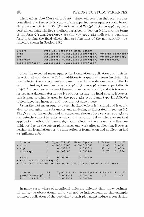
182 DESIGNS TO STUDY VARIANCES
The random plot(form*app)/test; statement tells glm that plot is a ran-dom effect, and the result is a table of the expected mean squares shown below.Here the coefficients for Var(Error)=σ2 and Var(plot(form*app)=σ2
p weredetermined using Hartley’s method described in Section 5.4.1, and the termsof the form Q(form,form*app) are the way proc glm indicates a quadraticform involving the fixed effects that are functions of the non-centrality pa-rameters shown in Section 3.5.2.
Source Type III Expected Mean Squareform Var(Error) +2Var(plot(form*app)) +Q(form ,form*app)app Var(Error) +2Var(plot(form*app)) +Q(app ,form*app)form*app Var(Error) +2Var(plot(form*app)) +Q(form*app)plot(form*app) Var(Error) +2Var(plot(form*app))
Since the expected mean squares for formulation, application and their in-teraction all contain σ2 + 2σ2
p in addition to a quadratic form involving thefixed effects, the correct mean square to use for the denominator of the F-ratio for testing these fixed effects is plot(form*app) whose expectation isσ2 +2σ2
p. The expected value of the error mean square is σ2, and it is too smallfor use as a denominator in the F-ratio for testing the fixed effects. However,this is exactly what is used by the proc glm type I and type III ANOVAtables. They are incorrect and they are not shown here.
Using the plot mean square to test the fixed effects is justified and is equiv-alent to averaging the subsamples and analyzing as illustrated in Section 3.5.The /test option on the random statement shown above causes proc glm tocompute the correct F-ratios as shown in the output below. There we see thatapplication method did have a significant effect on the amount of active pes-ticide residue on the cotton plant leaves one week after application. However,neither the formulation nor the interaction of formulation and application hada significant effect.
Source DF Type III SS Mean Square F Value Pr > F* form 1 0.000018063 0.000018063 0.03 0.8692* app 1 0.032310 0.032310 55.14 0.0018
form*app 1 0.002186 0.002186 3.73 0.1256
Error 4 0.002344 0.000586Error: MS(plot(form*app))* This test assumes one or more other fixed effects are zero.
Source DF Type III SS Mean Square F Value Pr > Fplot(form*app) 4 0.002344 0.000586 1.31 0.3432Error: MS(Error) 8 0.003569 0.000446
In many cases where observational units are different than the experimen-tal units, the observational units will not be independent. In this example,common application of the pesticide to each plot might induce a correlation,

DESIGNS WITH FIXED AND RANDOM FACTORS 183
E(εijkl × εijkl′) = ρ, between sub-samples from the same plot. Even thoughthe independence assumption is violated, Casella (2008) shows the F -test onfixed effects using the plot mean square as the denominator is still valid.
In this example where the application method was found significant, weshould look at the least squares means or in this case the marginal meansfor application (since there is equal replication) in order to determine whichapplication method was best. The marginal means can be expressed as y·1··and y·2··. The expected value E(y·j··) = µ+βj+αβ·j , the variance V ar(y·j··) =σ2p/ars + σ2/ars, and the variance of the difference in two marginal means
would be 2(σ2p/ars + σ2/ars). However, the standard error of the difference
in means reported by the estimate statements in proc glm is√
2σ2/ars .proc glm does not estimate the variance component for σ2
p, since plot wastreated as a fixed effect in the calculations. A similar problem occurs with allthe standard errors of estimable functions of fixed effects in the model whenusing the estimate statements in proc glm.
When there are both fixed and random effects in the model, due to the waythe experiment was conducted, we call it a mixed model and SAS proc mixedis a better option for analysis. By default proc mixed uses the REML methodto estimate the variance components for the random effects in the model, andthen estimates the fixed effects using the formula β = (X′V −1X)−X′V −1y.The correct standard errors for estimable functions are produced by procmixed, and the correct F-ratios for testing the fixed effects; however, as whenusing proc varcomp with the REML option, no ANOVA table is produced.
The commands to run proc mixed with the data in Table 5.12 are shownbelow.
proc mixed data=pesticide;class form app plot;model residue=form app form*app;random plot(form*app)/solution;lsmeans app;estimate ’application effect ’ app -1 1;
run;
These commands are similar to the commands for proc glm shown earlier,except the random effect plot(form*app) is removed from the model state-ment. It is still shown in the random statement. The /test option is alsoremoved from the random statement since proc mixed automatically calcu-lates the correct F-ratios for the fixed effects.
The result of the REML estimation is shown on the next page, and we seethat σ2
p = 0.000070 and σ2 = 0.000446.
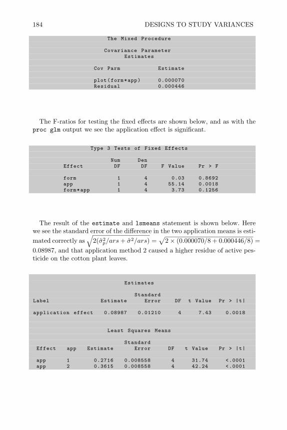
184 DESIGNS TO STUDY VARIANCES
The Mixed Procedure
Covariance ParameterEstimates
Cov Parm Estimate
plot(form*app) 0.000070Residual 0.000446
The F-ratios for testing the fixed effects are shown below, and as with theproc glm output we see the application effect is significant.
Type 3 Tests of Fixed Effects
Num DenEffect DF DF F Value Pr > F
form 1 4 0.03 0.8692app 1 4 55.14 0.0018form*app 1 4 3.73 0.1256
The result of the estimate and lsmeans statement is shown below. Herewe see the standard error of the difference in the two application means is esti-mated correctly as
√2(σ2
p/ars+ σ2/ars) =√
2× (0.000070/8 + 0.000446/8) =0.08987, and that application method 2 caused a higher residue of active pes-ticide on the cotton plant leaves.
Estimates
StandardLabel Estimate Error DF t Value Pr > |t|
application effect 0.08987 0.01210 4 7.43 0.0018
Least Squares Means
StandardEffect app Estimate Error DF t Value Pr > |t|
app 1 0.2716 0.008558 4 31.74 <.0001app 2 0.3615 0.008558 4 42.24 <.0001

DESIGNS WITH FIXED AND RANDOM FACTORS 185
Another design whose model contains both fixed and random effects is therandomized block designs discussed in the last chapter. For example considerthe example from Golf Magazine discussed in Section 4.6. In that experimentthe treatment factor (tee height) can be considered to be a fixed effect, sincethe object of the experiment was to determine if there is any difference indriving distance caused by different tee heights. However, there was no interestin comparing the specific golfers used in the experiment since they just denoteda sample of representative golfers. Therefore the block factor, or golfer, canbe considered to be a random effect. The interaction between a random andfixed effect is also defined to be a random effect. Therefore the interaction ofgolfer and tee height should also be considered a random effect, and the modelfor golf experiment can be written as:
yijk = µ+ bi + τj + bτij + εijk, (5.16)where bi represents the random golfer effect, τj represents the fixed tee heighteffect, bτij represents the random interaction effect, and εijk represents therandom repeat hit effect, i = 1, . . . , 3, j = 1, . . . , 9, and k = 1, . . . , 5. Byassuming the random golfer, interaction, and repeat hit effects to be indepen-dent and normally distributed with variances σ2
b , σ2bτ and σ2, respectively, the
expected value and variance of yijk are given by:
E(yijk) = µ+ τi
V ar(yijk) = σ2b + σ2
bτ + σ2
The expected values for the ANOVA mean squares are given in Table 5.13,where Q(τ) = 8
∑3i=1(τi − τ·)2/(3− 1).
Table 5.13 Expected Mean Squares for Randomized Block Design with Replicateswithin a Block
Source df Expected Mean SquareGolfer (bi) (9-1)=8 σ2 + 5σ2
bτ + 3σ2b
Tee Height (τj) (3-1)=2 σ2 + 5σ2bτ +Q(τ)
Golfer×Tee Height (bτij) 8×2=16 σ2 + 5σ2bτ
Repeat (εijk=Error) (5-1)×16=64 σ2
These expected mean squares show that to test the hypothesis of no differ-ence in tee height effect, i.e., H0 : τ1 = τ2 = τ3, the correct denominator forthe F-ratio would be the interaction Golfer×Tee Height, as used in Section 4.6,and not the error mean square that is used by default in the proc glm type Iand type III ANOVA tables. Also the variance of a difference in marginal orleast squares means for different tee heights V ar(yi·· − yi′··) = 2
(σ2bτ
45 + σ2
45
).
By default proc glm does not estimate σ2bτ . Therefore in Chapter 4, the test
h=teehgt e=id*teehgt statement was used in proc glm was used in order to

186 DESIGNS TO STUDY VARIANCES
get the correct F -test for tee height. Another way of getting the correct F -testwould be to use the random id id*teehgt/test; statement in proc glm oruse proc mixed. In Chapter 4, the lsmeans teehgt/pdiff adjust=tukeye=id*teehgt statement was used in order to get correct standard error forTukey comparison of means after the ANOVA. Using proc mixed the lsmeansteehgt/pdiff adjust=tukey; automatically uses the correct standard errorfor the difference in tee height means.
5.9 Graphical Methods to Check Model Assumptions
Graphical analysis of data from sampling experiments to study variances areuseful for checking assumptions of the statistical models and identifying atyp-ical observations which may have a heavy influence on the resulting variancecomponent estimates. Snee (1983) explains that another important advantageof graphical analysis is that it forces the analyst to become more familiar withthe data, and think critically about the mechanisms to explain the observedvariation. He suggests simple graphical tools such as half normal plots, gammaplots in the analysis of nested sampling designs. Normal plots can also be usedto check the normality assumption for random effects.
5.9.1 Simple Plots
Consider again the data in Table 5.2. Model (5.1) is appropriate for the datafrom this experiment, where the random sample effects, ti, and the randomexperimental errors, εij , are assumed to be normally distributed. The assump-tion of constant variance of εijs across the various samples is also implied byεij ∼ N(0, σ2). A simple way to verify these assumptions is to make a simpleplot of the data like that shown in Figure 2.3. There, nonconstant variancesor outlier observations can be quickly detected. The normality of the εij canalso be checked with a normal probability plot like that shown in Figure 2.5.
For the gage R&R two-factor sampling experiment presented in Section5.5 using the method of moments resulted in a negative variance componentestimate for σ2
b the variance due to operators. This estimate was negativebecause the mean square for interaction of part by operator was larger thanthe mean square for operator. A simple interaction plot like Figures 3.4 or 3.6can facilitate an explanation of this result. Figure 5.4 shows the interactionplot for part by operator. An interaction is characterized by the fact that thetrace of the average response across the levels of one factor plotted separatelyfor each level of the other factor will not be parallel. In Figure 5.4, it can beseen that the line segments are close to parallel, except for the segments joiningparts 5 through 7 and 9 through 10. This is due to the fact that operator 1had a much lower average measurement on part number 6 than the other twooperators, and operator 3 had a much higher measurement on part number10 than the other two operators.
When the interaction mean square is largely due to one or two observations,

GRAPHICAL METHODS TO CHECK MODEL ASSUMPTIONS 187
Figure 5.4 Interaction Plot for Part by Operator
Table 5.14 Comparison of Method of Moments and REML Estimates on Gage R&RStudy after Eliminating Parts 6 and 10
Method of Moments REMLComponent Estimator Estimatorpart (σ2
a) 0.03191 0.02808oper (σ2
b ) 0.0008601 0.0008089part*oper (σ2
ab) 0.0020045 0.0020082Error (σ2) 0.0004062 0.0004063
as it is in this case, it might be wise to question the results. Table 5.14 showsthe variance component estimates from the data from the gage R&R studyafter eliminating parts 6 and 10. With these parts eliminated, the method ofmoments does not produce a negative variance component estimate, and theresults obtained from the method of moments and REML are quite similar.In a situation like this, if the parts are still available, it might be wise to havethe operators remeasure parts 6 and 10 to see if there were mistakes.
5.9.2 Gamma and Half-Normal Plots to Check Constant VarianceAssumption
Wilk et al. (1962) proposed gamma probability plots as effective tools forinvestigating homogeneity of groups of variances. Sample of variances, with νdegrees of freedom, follow the gamma distribution with shape parameter ν/2,
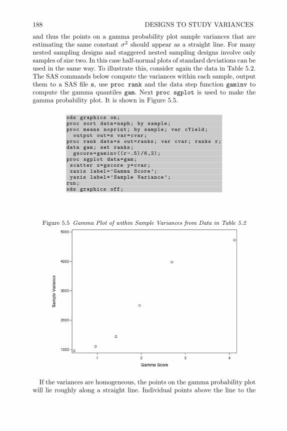
188 DESIGNS TO STUDY VARIANCES
and thus the points on a gamma probability plot sample variances that areestimating the same constant σ2 should appear as a straight line. For manynested sampling designs and staggered nested sampling designs involve onlysamples of size two. In this case half-normal plots of standard deviations can beused in the same way. To illustrate this, consider again the data in Table 5.2.The SAS commands below compute the variances within each sample, outputthem to a SAS file s, use proc rank and the data step function gaminv tocompute the gamma quantiles gam. Next proc sgplot is used to make thegamma probability plot. It is shown in Figure 5.5.
ods graphics on;proc sort data=naph; by sample;proc means noprint; by sample; var cYield;
output out=s var=cvar;proc rank data=s out=ranks; var cvar; ranks r;data gam; set ranks;
gscore=gaminv ((r-.5)/6,2);proc sgplot data=gam;scatter x=gscore y=cvar;xaxis label=’Gamma Score’;yaxis label=’Sample Variance ’;
run;ods graphics off;
Figure 5.5 Gamma Plot of within Sample Variances from Data in Table 5.2
If the variances are homogeneous, the points on the gamma probability plotwill lie roughly along a straight line. Individual points above the line to the

GRAPHICAL METHODS TO CHECK MODEL ASSUMPTIONS 189
far right would indicate variances that are larger than the norm. In Figure 5.5with only 6 points it appears that the points fall fairly close to a straight lineindicating constant variances.
For an example where there are more variances to plot, consider the poly-merization study shown in Table 5.11. The methods of moments estimatorfor the box within lot for this staggered nested sampling study was negative.As with the gage R&R study, one or two atypical values may be the cause ofthis result, and a graphical analysis of the data may reveal that. The meansquares in the type I ANOVA presented in Section 5.7 are pooled estimatesof the variances for each source in the design. If the four observations for lotnumber i are denoted by Y1i, Y2i, Y3i, and Y4i as shown below,
Box 1 Box 2Preparation Preparation
1 2 1Lot test 1 test 2 test 1 test 1i Y1i Y2i Y3i Y4i
Snee (1983) shows that the variances to be pooled from each source to createthe ANOVA mean squares are given by:
Source Variance s2i
Error or test(prep) (Y2i − Y1i)2/2
prep(box) 23
(Y3i − (Y1i+Y2i)
2
)2
box 34
(Y4i − (Y1i+Y2i+Y3i)
3
)2
The SAS commands to string the data out as shown above and computethe standard deviation within each source are shown on the next page alongwith the commands to make a half-normal plot of the standard deviations forprep within box.
The method of moments estimator of the box within lot was negative be-cause the mean square for prep within box and lot was larger than the meansquare for box. This would suggest an investigation of the variances that arepooled to form the mean square for prep within box. The standard deviationsdue to prep within box for each lot are labeled sd2 in the SAS commands onthe next page.
In the plot, shown in Figure 5.6, we see a relatively straight line of pointsextending from the lower left of the plot, except there is one standard deviationthat sticks out above the line at the right side. Examination of the proc printresults of the file of standard deviations, on the page following the graph, showsthat this large standard deviation is in lot 19 and is primarily due to the highresult for y3=16.79, the first test of the second preparation for box 1.
If lot number 19 is removed from the data, the method of moments estimate
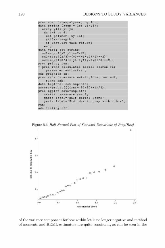
190 DESIGNS TO STUDY VARIANCES
proc sort data=polymer; by lot;data string (keep = lot y1-y4);
array y(4) y1-y4;do i=1 to 4;set polymer; by lot;y(i)=strength;if last.lot then return;
end;data vars; set string;
sd1=sqrt((y2-y1)**2/2);sd2=sqrt ((2/3)*(y3 -(y1+y2)/2)**2);sd3=sqrt ((3/4)*(y4 -(y1+y2+y3)/3)**2);
proc print; run;* proc rank calculates normal scores for
parameter estimates ;ods graphics on;proc rank data=vars out=hnplots; var sd2;
ranks rnk;data hnplots; set hnplots;zscore=probit ((((rnk -.5)/30) +1)/2);proc sgplot data=hnplots;
scatter x=zscore y=sd2;xaxis label=’Half -Normal Score’;yaxis label=’Std. due to prep within box’;
run;ods listing off;
Figure 5.6 Half-Normal Plot of Standard Deviations of Prep(Box)
of the variance component for box within lot is no longer negative and methodof moments and REML estimators are quite consistent, as can be seen in the
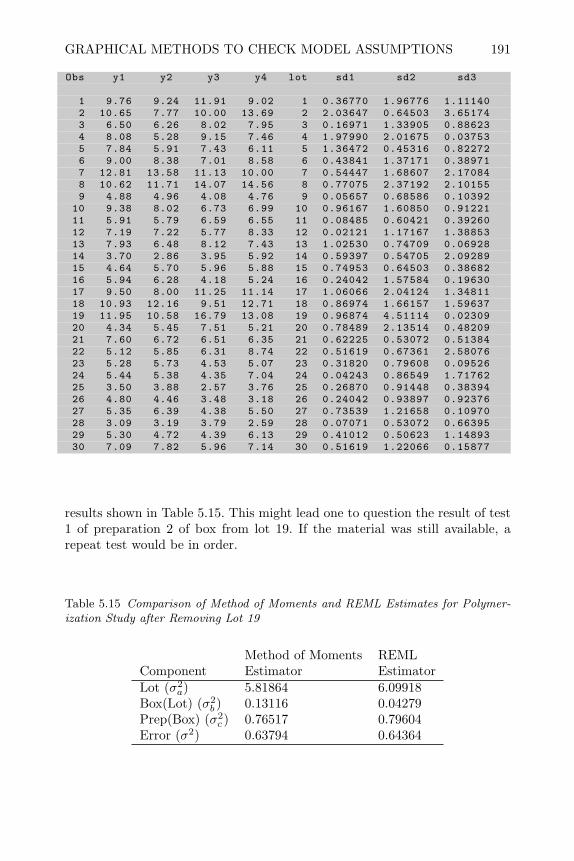
GRAPHICAL METHODS TO CHECK MODEL ASSUMPTIONS 191
Obs y1 y2 y3 y4 lot sd1 sd2 sd3
1 9.76 9.24 11.91 9.02 1 0.36770 1.96776 1.111402 10.65 7.77 10.00 13.69 2 2.03647 0.64503 3.651743 6.50 6.26 8.02 7.95 3 0.16971 1.33905 0.886234 8.08 5.28 9.15 7.46 4 1.97990 2.01675 0.037535 7.84 5.91 7.43 6.11 5 1.36472 0.45316 0.822726 9.00 8.38 7.01 8.58 6 0.43841 1.37171 0.389717 12.81 13.58 11.13 10.00 7 0.54447 1.68607 2.170848 10.62 11.71 14.07 14.56 8 0.77075 2.37192 2.101559 4.88 4.96 4.08 4.76 9 0.05657 0.68586 0.10392
10 9.38 8.02 6.73 6.99 10 0.96167 1.60850 0.9122111 5.91 5.79 6.59 6.55 11 0.08485 0.60421 0.3926012 7.19 7.22 5.77 8.33 12 0.02121 1.17167 1.3885313 7.93 6.48 8.12 7.43 13 1.02530 0.74709 0.0692814 3.70 2.86 3.95 5.92 14 0.59397 0.54705 2.0928915 4.64 5.70 5.96 5.88 15 0.74953 0.64503 0.3868216 5.94 6.28 4.18 5.24 16 0.24042 1.57584 0.1963017 9.50 8.00 11.25 11.14 17 1.06066 2.04124 1.3481118 10.93 12.16 9.51 12.71 18 0.86974 1.66157 1.5963719 11.95 10.58 16.79 13.08 19 0.96874 4.51114 0.0230920 4.34 5.45 7.51 5.21 20 0.78489 2.13514 0.4820921 7.60 6.72 6.51 6.35 21 0.62225 0.53072 0.5138422 5.12 5.85 6.31 8.74 22 0.51619 0.67361 2.5807623 5.28 5.73 4.53 5.07 23 0.31820 0.79608 0.0952624 5.44 5.38 4.35 7.04 24 0.04243 0.86549 1.7176225 3.50 3.88 2.57 3.76 25 0.26870 0.91448 0.3839426 4.80 4.46 3.48 3.18 26 0.24042 0.93897 0.9237627 5.35 6.39 4.38 5.50 27 0.73539 1.21658 0.1097028 3.09 3.19 3.79 2.59 28 0.07071 0.53072 0.6639529 5.30 4.72 4.39 6.13 29 0.41012 0.50623 1.1489330 7.09 7.82 5.96 7.14 30 0.51619 1.22066 0.15877
results shown in Table 5.15. This might lead one to question the result of test1 of preparation 2 of box from lot 19. If the material was still available, arepeat test would be in order.
Table 5.15 Comparison of Method of Moments and REML Estimates for Polymer-ization Study after Removing Lot 19
Method of Moments REMLComponent Estimator EstimatorLot (σ2
a) 5.81864 6.09918Box(Lot) (σ2
b ) 0.13116 0.04279Prep(Box) (σ2
c ) 0.76517 0.79604Error (σ2) 0.63794 0.64364

192 DESIGNS TO STUDY VARIANCES
5.9.3 Probability Plots of Empirical Best Linear Unbiased Estimates ofRandom Effects
In Section 2.4 the assumption that the experimental errors follow a normaldistribution, a normal probability plot of the residuals was made. In matrixnotation, the vector of residuals can be written as:
ε = y −Xβ. (5.17)
When there are random terms in the model in addition to the experimentalerror term, ε, we can check the normality of these random effects by makingnormal probability plots of the estimated random effects. A straight line ofpoints in this plot would justify the assumption of normality for the randomeffect in question. This graphical technique will be useful in detecting atypicalobservations or departures from normality when there are at least 12 to 15points on the plot. In the model
y = Xβ +Zγ + ε (5.18)
the empirical best linear unbiased predictors (EBLUPs) of the random effectsγ are given by the equation
γ = GZ′V −1(y −Xβ) (5.19)
where G is the estimated variance covariance matrix of γ. SAS proc varcompdoes not calculate the EBLUPs but proc mixed does and it can be used formodels with all random effects as well as for models with both fixed andrandom effects. On the next page are the commands for fitting the nestedrandom effects model for the polymerization data using proc mixed. Noticeno terms are specified in the model statement since the model statement inproc mixed is used for specifying the fixed effects. The random statementincludes all the terms in the model. The /solution option on the randomstatement causes proc mixed to calculate and print a table of EBLUPs. Theods output statement creates a SAS data file containing the table of printedEBLUPs. In the next data step, the SAS file prep is created that contains asubset of the EBLUPs for prep within box. Next the calls to proc rank andproc sgplot are similar to the ones used to produce a normal plot of theresiduals in Section 2.4.
The points on the normal plot of the EBLUPs for prep within box shownin Figure 5.7 nearly follow a straight line. However, there are two apparentoutliers on the upper right tail of the plot. When comparing the values ofthese two EBLUPs to the table printed out by proc mixed it can be seenthat the largest EBLUP (2.2488) corresponds to the first test of the secondpreparation for box 1 in lot 19.
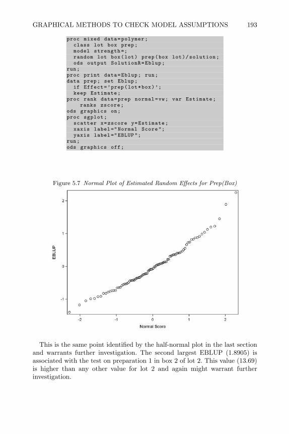
GRAPHICAL METHODS TO CHECK MODEL ASSUMPTIONS 193
proc mixed data=polymer;class lot box prep;model strength =;random lot box(lot) prep(box lot)/solution;ods output SolutionR=Eblup;
run;proc print data=Eblup; run;data prep; set Eblup;
if Effect=’prep(lot*box)’;keep Estimate;
proc rank data=prep normal=vw; var Estimate;ranks zscore;
ods graphics on;proc sgplot;
scatter x=zscore y=Estimate;xaxis label=" Normal Score";yaxis label="EBLUP";
run;ods graphics off;
Figure 5.7 Normal Plot of Estimated Random Effects for Prep(Box)
This is the same point identified by the half-normal plot in the last sectionand warrants further investigation. The second largest EBLUP (1.8905) isassociated with the test on preparation 1 in box 2 of lot 2. This value (13.69)is higher than any other value for lot 2 and again might warrant furtherinvestigation.

194 DESIGNS TO STUDY VARIANCES
5.10 Review of Important Concepts
Sampling experiments are conducted to estimate variances and to partitionvariances into various sources called variance components. Sometimes estimat-ing variances or partitioning variances into various sources may be the endgoal. In other cases partitioning the variance may be an intermediate step in astudy trying to reduce the variance or an intermediate step in a study seekingto determine the causes of variability. The factors in a sampling experimentare called random factors as opposed to fixed factors described in chapters1-4. The purpose for including random factors in a design is to estimate thevariability caused by varying levels of the random factor. Levels of the randomfactor are a representative sample of possible levels.
When the goal is to partition variance into two sources, one factor randomsampling experiments, or RSE, are useful. Two sample sampling experimentsor factorial random sampling experiments (FRSE), like those used in classi-cal gage R&R studies, are used to partition variance into three independentsources. Nested sampling experiments, or NSE, are used when it is more con-venient to use a different set of levels of one factor for each level of anotherfactor. Several stages of nesting can be utilized in one design to partition vari-ance into several sources. Staggered nested sampling experiments, or SNSE,are a variation of nested designs that balance the information collected overthe various sources. Figure 5.8 illustrates where these designs should be usedin relation to the designs described in earlier chapters.
Variance components can be estimated using the analysis of variance methodof moments or the maximum likelihood or REML methods. This can be ac-complished using SAS proc varcomp. Formulas were presented in the chap-ter for exact confidence intervals on variance components estimated from onefactor random sampling experiments RSE. Formulas were presented for ap-proximate confidence limits on variance components from two-factor FRSE,or nested designs NSE, and a SAS macro was introduced for evaluating theseformulas. Asymptotic confidence intervals can be calculated for variance com-ponents estimated by maximum likelihood or REML. These intervals will bereasonably accurate when there are 30-40 degrees of freedom associated withthe term in question.
Sample sizes for sampling experiments can be determined to make the widthof the confidence interval for σ2 the desired multiple of σ2. The number oflevels for other random factors in the design should be chosen to partition thedegrees of freedom among the various sources in the design according to theirperceived importance relative to the replicate variance σ2.
In designs to study the effects of fixed factors, random factors can be intro-duced into the model by the way the experiment is conducted. For example,when response measurements are made on sub-samples of experimental unitsan additional nested error term must be included in the model for analysis.Block terms and block by treatment interactions in randomized block experi-ments would normally be considered to be random factors. When both fixed

REVIEW OF IMPORTANT CONCEPTS 195
Figure 5.8 Design Selection Roadmap
Design Purpose
Estimate Variances Study Factor Effects
E.U.’s
Block Factors
One Factor
Multiple Factors
Multiple Factorswith some hard
to vary
Block size
Homogeneous Heterogeneous
Large Small
RCB
GCB
PBIB,BTIB
BIB
LSD
YSDRSE CRD
FactorsFRSENSESNSE
CRFD CRRS SLD RCBF BRS PCBFCRFF SCD
PB, OA EVD CCBF
CRSP RSSP SPMPV RBSPSPFF EESPRS
One Two
class cont. mixture cont. classFactors
and random effects are included in the model, the expected values of theANOVA mean squares (EMS) show which mean square should be used in thedenominator of the F -test for each fixed effect or interaction in the model.SAS proc mixed is most useful for analyzing data from designs that includefixed and random factors. The REML method is used for estimating the vari-ance components of the random effects by proc mixed and it automaticallycomputes the correct standard error for estimable functions of fixed effects.
Atypical response values can have a heavy influence on variance componentestimates from sampling experiments. Simple plots, such as plots of the re-sponse versus the level in one-factor designs or interaction plots for two-factordesigns, can help to identify atypical response values. For nested designs (orstaggered nested designs), gamma plots of sample variances (or half-normalplots of standard deviations) within each source are useful for checking ho-mogeneity of variances and identifying cells where atypical values may occur.Normal probability plots of empirical best linear unbiased estimators of ran-dom effects (EBLUPs) are useful for checking normality assumptions andagain for identifying cells where atypical response values may lie.

196 DESIGNS TO STUDY VARIANCES
5.11 Exercises
1. Carry out the sampling experiment described in Section 5.3 to partitionthe variability in paper helicopter flight times.
(a) Read your data into SAS and estimate the variance components usingthe method of moments.
(b) Using proc varcomp, estimate the variance components using the REMLmethod.
(c) Using the formulas in Table 5.3, calculate 90% confidence intervals forthe two variance components.
(d) Write your conclusions. What should you use as the experimental unitin future studies to optimize flight time?
2. Read the data from Table 5.2 into SAS and
(a) Calculate the ANOVA sums of squares and mean squares used in calcu-lating the confidence limits in Section 5.4.2.
(b) Use proc varcomp to calculate and compare the method of momentsand REML estimates of the variance components.
3. Using the mean squares and expected mean squares from the gage R&Rstudy presented in Section 5.5, use the macro in the appendix of this chapterto compute a 90% confidence interval on the variance component for theinteraction of operator and part.
4. Plan a sampling experiment to partition the source of variability in autogas milage in your community between drivers, cars, and replicates.
(a) Describe how you would plan the study if drivers and cars were crossedfactors.
(b) Describe how you would plan the study if drivers were nested withincars.
(c) Determine the number of degrees of freedom you would need for the erroror replicate term in your model if you desire the width of the confidenceinterval on the variance component for replicate to be 75% of σ2.
5. Consider the data in Table 5.9.
(a) Enter the data into SAS and use proc varcomp to estimate the variancecomponents σ2
a, σ2b , σ2
c , and σ2.(b) What are the major source or sources of variability?(c) Is there any difference between the method of moments or REML esti-
mators of the variance components?
6. Consider the data (Anderson and McLean, 1974) in the following table tocome from a sampling study to determine the source of variability in theaverage amount spent on healthcare per year in thousands of dollars. Townsare nested within state and households are nested within town.

EXERCISES 197
State1 2 3
Town Town Town1 2 1 2 1 2
Household1 10 7 6 6 15 122 13 12 5 12 18 153 16 11 9 7 20 184 12 9 3 10 19 16
(a) Use the method of moments and REML methods to determine the vari-ance components for state, town and household.
(b) What percent of the total variance is due to households? Towns andhouseholds?
(c) Using formula (5.11) obtain a 90% confidence interval on the variancecomponent due to towns.
7. Consider the data from Smith and Beverly (1981) taken from a staggerednested design to investigate the sources of variability in impurities in rawmaterials received at a plant in trailer loads. Two samples of material weretaken from each of 9 trailer loads of pellets. Two measurement of impuritieswas made on the first sample from each trailer but only on measurementfor the second sample from each trailer.
Table 5.16 Variability in Impurities in Received PelletsSample
1 2Measurement Measurement
Trailer 1 2 11 47.06 44.37 49.32 47.43 50.35 50.423 48.90 48.05 50.644 52.32 52.26 53.475 46.53 45.60 53.986 46.99 50.87 51.877 47.49 51.55 58.578 47.41 47.63 48.639 48.37 51.03 50.1510 54.80 51.57 54.52
(a) Write the model for the data.(b) Analyze the data using proc varcomp using the option method=type1
and estimate the three variance components.

198 DESIGNS TO STUDY VARIANCES
(c) Analyze the data using proc varcomp using the option method=remland check to see if your estimates remain the same.
(d) Make half-normal plots of the square root of the variances pooled to getthe mean squares for sample(trailer) and measurement(sample). Doesthe assumption of homogeneous variances appear reasonable?
(e) Re-analyze the data using proc mixed; calculate the EBLUPs for therandom trailer effect and make a normal plot to check the normalityassumption. What is your conclusion?
8. Reanalyze the data from the golf experiment, presented in the appendixof Chapter 4, using proc mixed. Check to see if you get the same P-valuesand conclusions shown in Section 4.7.
5.12 Appendix
%macro vci;****************************************************************;** Macro for computing confidence interval for **;** delta = c1*E(ms1) - c2*E(ms2) **;** where c1 , c2 >=0 **;** Input for this macro is a file called meansq that includes **;*one line containing variables confl , c1, ms1 , nu1 , c2, ms2 , nu2;data conf; set meansq;delta=c1*ms1 -c2*ms2;alpha=1-confl;Falpha1=finv(confl ,nu1 ,10000000);Falpha12=finv(confl ,nu1 ,nu2);Fconf2=finv(alpha ,nu2 ,10000000);Fconf12=finv(alpha ,nu1 ,nu2);Falpha2=finv(confl ,nu2 ,10000000);Fconf1=finv(alpha ,nu1 ,10000000);Fconf12=finv(alpha ,nu1 ,nu2);G1=1-(1/Falpha1);H2=(1/Fconf2) -1;G12 =(( Falpha12 -1)**2-G1**2*Falpha12**2-H2**2)/Falpha12;VL=G1**2*c1**2*ms1**2+H2**2*c2**2*ms2**2+G12*c1*c2*ms1*ms2;H1=(1/Fconf1) -1;G2=1-(1/Falpha2);H12=((1- Fconf12)**2-H1**2*Fconf12**2-G2**2)/Fconf12;VU=H1**2*c1**2*ms1**2+G2**2*c2**2*ms2**2;L=delta -sqrt(VL);U=delta+sqrt(VU);proc print; var delta L U; run;%mend vci;
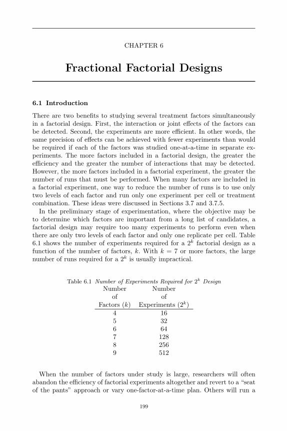
CHAPTER 6
Fractional Factorial Designs
6.1 Introduction
There are two benefits to studying several treatment factors simultaneouslyin a factorial design. First, the interaction or joint effects of the factors canbe detected. Second, the experiments are more efficient. In other words, thesame precision of effects can be achieved with fewer experiments than wouldbe required if each of the factors was studied one-at-a-time in separate ex-periments. The more factors included in a factorial design, the greater theefficiency and the greater the number of interactions that may be detected.However, the more factors included in a factorial experiment, the greater thenumber of runs that must be performed. When many factors are included ina factorial experiment, one way to reduce the number of runs is to use onlytwo levels of each factor and run only one experiment per cell or treatmentcombination. These ideas were discussed in Sections 3.7 and 3.7.5.
In the preliminary stage of experimentation, where the objective may beto determine which factors are important from a long list of candidates, afactorial design may require too many experiments to perform even whenthere are only two levels of each factor and only one replicate per cell. Table6.1 shows the number of experiments required for a 2k factorial design as afunction of the number of factors, k. With k = 7 or more factors, the largenumber of runs required for a 2k is usually impractical.
Table 6.1 Number of Experiments Required for 2k DesignNumber Number
of ofFactors (k) Experiments (2k)
4 165 326 647 1288 2569 512
When the number of factors under study is large, researchers will oftenabandon the efficiency of factorial experiments altogether and revert to a “seatof the pants” approach or vary one-factor-at-a-time plan. Others will run a
199

200 FRACTIONAL FACTORIAL DESIGNS
factorial experiment with a subset of the factors, chosen from the longer listby guessing which ones may be more important. However, these approachesare less than optimal and do not retain the benefits of factorial experimentswith a large number of factors. A better solution to this problem is to use afraction of the experiments, or runs, required for a full factorial experiment.To be effective, the fraction of runs used must be carefully selected in orderto preserve some of the benefits of a full factorial experiment.
One of the desirable properties of a 2k factorial plan is that factor effectsare not obscured by (or correlated with) planned changes in other factors.This property was called orthogonality in Section 3.7.
6.2 Half-Fractions of 2k Designs
Consider first choosing a half-fraction of a 2k factorial experiment. Carelesschoice of half the n = 2k runs may not retain the desirable orthogonalityproperty of a 2k design. One way to preserve this property, when selectinga one-half fraction of a 2k factorial experiment, is to choose the runs wherethe coded factor levels for an interaction term (preferably the highest orderinteraction) are constant.
Table 6.2 illustrates this procedure. On the left side of the table is a repre-sentation of the coded factor levels for a 24 design. On the right side of thetable are the runs that have a constant (+) value for XA ×XB ×XC ×XD.These runs represent the half-fraction. The order of the runs on the right sideof the table have been reordered so that it can be easily seen that the standardfactorial pattern is present in the first three columns. Therefore it can be seenthat the orthogonality property is preserved for the first three columns. Byfurther inspection, it can be seen that fourth factor is also orthogonal to theother three.
With 16 runs in a full 24 factorial, 15 effects can be estimated in additionto the grand mean. The 15 effects consist of the four main effects, six two-factor interaction effects, four three-factor interactions and one four-factorinteraction. In a half-fraction of a 24 experiment, however, there are only 8runs. Thus only 7 effects can be estimated in addition to the grand mean.By choosing the runs from a full factorial that have a constant value foran interaction, we automatically lose the ability to estimate that interactioneffect. By studying the right half of Table 6.2, it can also be seen that the codedfactor levels or column of signs for XD is exactly the product of signs in thefirst three columns, i.e., XD = XA × XB × XC . This means that the effectwe can estimate for XD will be completely obscured or confused by the three-factor interaction XAXBXC . This is not all. As will be shown later, each maineffect and interaction in the design is obscured or confounded with one otherinteraction. This is the price we pay for running one-half the total number ofexperiments. However, in preliminary experiments where a large number offactors are included in order to find out which ones are truly important, thismay not be a serious price to pay.
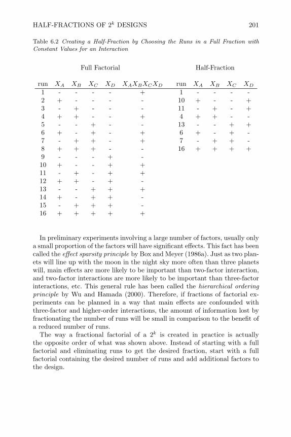
HALF-FRACTIONS OF 2k DESIGNS 201
Table 6.2 Creating a Half-Fraction by Choosing the Runs in a Full Fraction withConstant Values for an Interaction
Full Factorial Half-Fraction
run XA XB XC XD XAXBXCXD run XA XB XC XD
1 - - - - + 1 - - - -2 + - - - - 10 + - - +3 - + - - - 11 - + - +4 + + - - + 4 + + - -5 - - + - - 13 - - + +6 + - + - + 6 + - + -7 - + + - + 7 - + + -8 + + + - - 16 + + + +9 - - - + -10 + - - + +11 - + - + +12 + + - + -13 - - + + +14 + - + + -15 - + + + -16 + + + + +
In preliminary experiments involving a large number of factors, usually onlya small proportion of the factors will have significant effects. This fact has beencalled the effect sparsity principle by Box and Meyer (1986a). Just as two plan-ets will line up with the moon in the night sky more often than three planetswill, main effects are more likely to be important than two-factor interaction,and two-factor interactions are more likely to be important than three-factorinteractions, etc. This general rule has been called the hierarchical orderingprinciple by Wu and Hamada (2000). Therefore, if fractions of factorial ex-periments can be planned in a way that main effects are confounded withthree-factor and higher-order interactions, the amount of information lost byfractionating the number of runs will be small in comparison to the benefit ofa reduced number of runs.
The way a fractional factorial of a 2k is created in practice is actuallythe opposite order of what was shown above. Instead of starting with a fullfactorial and eliminating runs to get the desired fraction, start with a fullfactorial containing the desired number of runs and add additional factors tothe design.

202 FRACTIONAL FACTORIAL DESIGNS
For example, to construct a one-half fraction of a 2k design, denoted by 122k
or 2k−1, the procedure is as follows:
1. Write down the base design, a full factorial plan in k − 1 factors using thecoded factor levels (−) and (+).
2. Add the kth factor to the design by making its coded factor levels equal tothe product of the other factor levels (i.e., the highest order interaction).
3. Use these k columns to define the design.
A complete list of interactions confounded with each main effect and inter-action in a half-fractional factorial is called the confounding pattern or aliasstructure of the design. This list is easy to construct based on the assignmentof the kth factor in item 2 of the list above. For example, in the 24−1 design, ifthe levels of the fourth factor are equal to the product of the levels of the firstthree factors in the design, we write symbolically D = ABC. This is calledthe generator of the design. Multiplying on both sides of the generator we get:
D2 = ABCD
orI = ABCD
where I represents a column of pluses and is the multiplicative identity forelementwise products of columns of coded factor levels. The equation, I =ABCD, is called the defining relation for the fractional factorial design, andby multiplying on both sides of this equation, the interaction confounded withany main effect or interaction can be determined. For example, multiplyingby the first factor on both sides of the defining relation we see
A(I) = A(ABCD)or
A = BCD
This means that the effect of the first factor A is confounded with the three-factor interaction BCD. When data is collected, the effect of factor A isestimated as the difference in the average response at the high and low levelsof factor A. However, that effect really estimates the sum of the effects of factorA and the three-factor interaction. Therefore we write it as A + BCD. Thecomplete alias pattern for this 24−1 design can be determined by multiplyingthe defining relation by each main effect and interaction resulting in:

HALF-FRACTIONS OF 2k DESIGNS 203
I +ABCD
A+BCD
B +ACD
C +ABD
D +ABC
AB + CD
AC +BD
AD +BC
There are only eight unique results, and they represent the eight effects (I be-ing the overall mean) that can be estimated from the 8-run fractional factorialdesign.
Replicates are not included in a one-half fractional factorial design becausereplicates would take as many additional experiments as it would to completethe full factorial. Therefore, there is no estimate of σ2, the variance of ex-perimental error, when running a fractional factorial. In order to judge thesignificance of the effects in a fractional factorial design, graphical methodslike those described in Section 3.7.5 should be used. The effects found to besignificant should be interpreted with the hierarchical ordering principle inmind. For example, if the effect for B +ACD were found to be significant, itwill be assumed to represent the effect of factor B rather than the three-wayinteraction.
Using the procedure outlined on the last page, it is easy to create a 2k−1
fractional factorial design in the data step of SAS. For example, the SAS codebelow creates a list of treatment combinations for a 25−1 experiment.
*Create 2^(5 -1) design in standard order;data design;do x4=-1 to 1 by 2;do x3=-1 to 1 by 2;do x2=-1 to 1 by 2;do x1=-1 to 1 by 2;A=x1; B=x2; C=x3; D=x4; E=A*B*C*D;output;end;
end;end;
end;keep A B C D E;proc print; run;
In practice the treatment combinations should be randomized to the exper-imental units, and a randomized list created like the one shown in Section 3.4

204 FRACTIONAL FACTORIAL DESIGNS
should be used. This design is then called a completely randomized fractionalfactorial design of CRFF. The design resulting from the code above is shownbelow in standard order (not randomized).
Obs A B C D E
1 -1 -1 -1 -1 12 1 -1 -1 -1 -13 -1 1 -1 -1 -14 1 1 -1 -1 15 -1 -1 1 -1 -16 1 -1 1 -1 17 -1 1 1 -1 18 1 1 1 -1 -19 -1 -1 -1 1 -1
10 1 -1 -1 1 111 -1 1 -1 1 112 1 1 -1 1 -113 -1 -1 1 1 114 1 -1 1 1 -115 -1 1 1 1 -116 1 1 1 1 1
To illustrate the analysis of a 2k−1 design, consider a continuation of the drysoup mix example presented in Section 5.4.3. In that example, the majority ofvariability in the soup “intermix” was found to be within a batch rather thanbetween batches. The researchers responsible for the project made a list offactors that they thought might influence the variability within a batch (seeHare, 1988). These were options that could be changed on the mixer where abatch was mixed and the intermix was added through ports. The list consistedof: (1) the number of ports where intermix was added, (2) the temperatureof the mixer (that could be controlled by adding cooling water to the jacketsurrounding it), (3) the mixing time, (4) weight of the batch, and (5) the delaytime between mixing and packaging. The response or variability in fill weightsof the intermix was obtained by taking five consecutive samples of the soupmix every 15 minutes as the batch was being packaged. The factor labels andlevels are shown in Table 6.3.
Table 6.3 Factors and Levels for Soup Mix 25−1 ExperimentFactor Label Name Low Level High LevelA Number of Ports 1 3B Temperature Cooling Water AmbientC Mixing Time 60 sec. 80 sec.D Batch Weight 1500 lbs 2000 lbsE Delay Days 7 1

HALF-FRACTIONS OF 2k DESIGNS 205
The normal batch size was 2000 lbs and the normal mixing time was 60seconds. Since this experiment was to be run in a production facility, theresearch and production staff both had to agree to the plan. The factor levelscould be changed between batches with relatively little effort and they werenot a problem. The requested reduction in batch weight and the increase inmixing time for some batches in the planned list of experiments would notseriously interfere with the production schedule if the list was short, but itwould slow production if a 32-run design were used. For this reason a 16-runfractional factorial plan was agreed upon. The alias structure for the 25−1
plan shown above is:
A+BCDE
B +ACDE
C +ABDE
D +ABCE
E +ABCD
AB + CDE
AC +BDE
AD +BCE
AE +BCD
BC +ADE
BD +ACE
BE +ACD
CD +ABE
CE +ABD
DE +ABC
Therefore, if three-factor and four-factor interactions could be assumed negli-gible, estimates of all main effects and two-factor interactions could be made.The experimental unit for this experiment was the batch of dried soup mix putin the mixer, and Table 6.4 shows a randomized list of the 25−1 experimentsin actual factor levels. The response σp was an estimate of the standard devi-ation of fill weight within a batch, computed from the sampling study madeduring packaging of each batch.
The SAS commands, to read in the data (in standard order) and to mergeit with the design in coded factor levels created earlier, are shown on the nextpage.

206 FRACTIONAL FACTORIAL DESIGNS
data process;input s @@;datalines;1.13 1.25 .97 1.70 1.47 1.28 1.18 .98.78 1.36 1.85 .62 1.09 1.10 .76 2.1data soup; merge design process;
Table 6.4 25−1 Experiment To Determine Which Factors Are Associated with FillVariation in Random Order
(A) (B) (C) (D) (E)Number Mixing Batch
of Time Weight Delay ResponseBatch Ports Temperature (sec) (lbs) (days) σp
1 1 Cool Water 60 2000 7 0.782 3 Cool Water 80 2000 7 1.103 3 Ambient 60 1500 1 1.704 3 Cool Water 80 1500 1 1.285 1 Ambient 60 1500 7 0.976 1 Cool Water 80 1500 7 1.477 1 Ambient 60 2000 1 1.858 3 Ambient 80 2000 1 2.109 1 Ambient 80 2000 7 0.7610 3 Ambient 60 2000 7 0.6211 1 Cool Water 80 2000 1 1.0912 1 Cool Water 60 1500 1 1.1313 3 Cool Water 60 1500 7 1.2514 3 Ambient 80 1500 7 0.9815 3 Cool Water 60 2000 1 1.3616 1 Ambient 80 1500 1 1.18
The SAS commands, to fit the model in the main effects and two-factorinteractions and to make a normal probability plot of the regression coeffi-cients, are shown on the next page. This is the same thing that was done inSection 3.7.5, except only 15 terms are included in the model rather than thefull model which would contain main effects and interactions up to order 5.Each effect in this model is confounded with one other interaction as shownin the alias pattern on the previous page. Therefore only 15 effects can beestimated.
As can be seen in the normal plot of effects, the main effect E (Delay Timebetween mixing and packaging), BE (the interaction between Temperatureand Delay Time), and DE (the interaction between Batch Weight and DelayTime) appear to be significant. If the hierarchical effect ordering can be as-
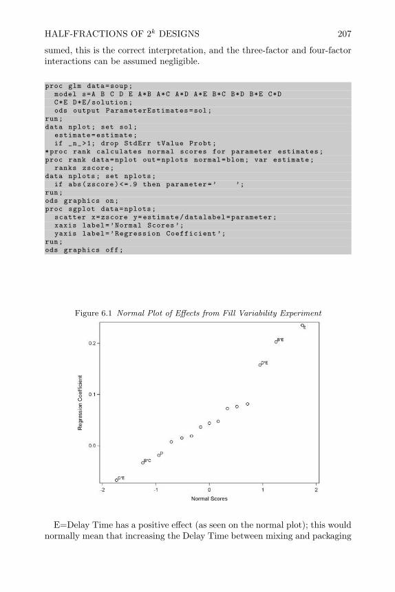
HALF-FRACTIONS OF 2k DESIGNS 207
sumed, this is the correct interpretation, and the three-factor and four-factorinteractions can be assumed negligible.
proc glm data=soup;model s=A B C D E A*B A*C A*D A*E B*C B*D B*E C*DC*E D*E/solution;ods output ParameterEstimates=sol;
run;data nplot; set sol;
estimate=estimate;if _n_>1; drop StdErr tValue Probt;
*proc rank calculates normal scores for parameter estimates;proc rank data=nplot out=nplots normal=blom; var estimate;
ranks zscore;data nplots; set nplots;
if abs(zscore)<=.9 then parameter=’ ’;run;ods graphics on;proc sgplot data=nplots;
scatter x=zscore y=estimate/datalabel=parameter;xaxis label=’Normal Scores ’;yaxis label=’Regression Coefficient ’;
run;ods graphics off;
Figure 6.1 Normal Plot of Effects from Fill Variability Experiment
E=Delay Time has a positive effect (as seen on the normal plot); this wouldnormally mean that increasing the Delay Time between mixing and packaging

208 FRACTIONAL FACTORIAL DESIGNS
would increase the response (or within batch variation). However, due to theunconventional assignment of 7 to the low (coded) level of factor E and 1 tothe high (coded) level in Table 6.3, it actually tells us that on the averageincreasing the delay time between mixing and packaging decreases the withinbatch variability. Since the interactions BE and DE also appear to be signif-icant, the average main effect of factor E does not tell the whole story. Figure6.2 shows the interaction plot for Temperature and Delay Time. Here it canbe seen that Delay Time has little effect on the within batch variability if themixer is cooled with cooling water during mixing. However, the within batchvariability is decreased substantially by increasing delay time between mixingand packaging if the mixing was done at ambient temperature.
Figure 6.2 Interaction Plot for Mixing Temperature by Delay Time
Figure 6.3 shows the interaction plot for Batch Weight and Delay Time. Hereit can be seen that increasing the delay time between mixing and packaginghas little effect on the variability within a batch for small (1500 lbs) batches,while increasing the delay time between mixing and packaging decreases withinbatch variability for large (2000 lbs) batches.
Based on the results of this study, the minimum variation of intermix withina batch could be obtained by using the larger batch size (2000 lbs), the ambienttemperature at mixing, and a 7-day delay between mixing and packaging. Itdid not answer a new question prompted by the results: does it take a full 7-daydelay between mixing and packaging or could a 3-day or 4-day delay reducevariability just as much? However, the production and research staff agreedthat the current results made sense, since the uniformity of intermix relatedto the hardness of the vegetable oil which is affected by temperature and

QUARTER AND HIGHER FRACTIONS OF 2k DESIGNS 209
agitation. Production staff implemented the optimal conditions while researchcontinued investigating the new question.
It is interesting to think that neither of the interactions would have beendetected if one-factor-a-time experiments had been conducted, rather thanthe fractional factorial plan. The conclusions of one-factor-at-a-time type ex-periments may not be reproducible because it would not be realized that theeffects (or absence of effects) seen could depend on other factor settings thatare deemed to be insignificant.
Figure 6.3 Interaction Plot for Batch Weight by Delay Time
6.3 Quarter and Higher Fractions of 2k Designs
In 2k−1 designs only half the experimental runs are made, and each effect thatcan be estimated is confounded with one interaction. Likewise, in a quarterfraction 2k−2 design, only one-fourth the experimental runs from the full 2k
design are run, and each effect that can be estimated is confounded withthree other interactions. In a one-eighth fraction, only one-eighth of the runsin the full factorial are made and each estimated effect will be confounded withseven other interactions, and so on. These designs may sound confusing at firstbecause of the large number of effects confounded with each estimable effect.However, they are used quite frequently in practice, and by following the effectsparsity principle and the hierarchical ordering principle useful conclusions canusually be reached after just a fraction of the total runs required for a fullfactorial.
To construct a quarter fraction of a 2k design, start with a base design in2k−2 factors, then add two additional factors by making their coded factor

210 FRACTIONAL FACTORIAL DESIGNS
levels equal to two interactions among the first k − 2 columns, as illustratedbelow.
XD XE
XA XB XC
︷ ︸︸ ︷XAXB
︷ ︸︸ ︷XAXC XBXC XAXBXC
− − − + + + −+ − − − − + +− + − − + − ++ + − + − − −− − + + − − ++ − + − + − −− + + − − + −+ + + + + + +
⇓XA XB XC XD XE
− − − + ++ − − − −− + − − ++ + − + −− − + + −+ − + − +− + + − −+ + + + +
There are two generators for the design created as above, D = AB and E =AC. From these it can be seen that I = ABD and I = ACE. Also, since I2 = Ia third equality, called the generalized interaction, is I = ABD(ACE) orI = BCDE. Combining the three equations obtained from the two generatorsand the generalized interaction results in the defining relation for the designI = ABD = ACE = BCDE. The confounding pattern, or alias structure, forthe design is found by multiplying through the defining relation by each effectthat can be estimated:
A+BD + CE +ABCDE
B +AD +ABCE + CDE
C +ABCD +AE +BDE
D +AB +ACDE +BCE
E +ABDE +AC +BCD
BC +ACD +ABE +DE
BE +ADE +ABC + CD
Construction of one-eighth and higher fractions is similar. To construct aone-eighth fraction of a 26 design or 26−3 design, start with a base design in6−3 = 3 factors, then add three additional factors by confounding them with

CRITERIA FOR CHOOSING GENERATORS FOR 2k−p DESIGNS 211
interactions. For example, if we choose the generators D = AB, E = AC, andF = BC, the SAS code below could be used to generate the design.
data frac;do x1=-1 to 1 by 2;do x2=-1 to 1 by 2;do x3=-1 to 1 by 2;A=x3; B=x2; C=x1;D=A*B; E=A*C; F=B*C; output;end;
end;end;
keep A B C D E F;proc print; run;
There are eight runs in this design, and seven effects in addition to the over-all mean can be estimated. Each effect will be aliased with seven interactions.To find what interactions are aliased with each effect that can be estimated,first find the defining relation. From the generators I = ABD = ACE =BCF . The two-factor generalized interactions are ABD(ACE) = BCDE,ABD(BCF ) = ACDF , and ACE(BCF ) = ABEF . The three-factor gener-alized interaction is ABD(ACE)(BCF ) = DEF . Combining the equationsfound from the generators and the generalized interactions the defining rela-tion is:
I = ABD = ACE = BCF = BCDE = ACDF = ABEF = DEF
Multiplying through the defining relation by the main effects (A−F ), and thethree-factor interaction (ABC), the aliases for the seven effects that may beestimated can be determined. One quick way to do this in SAS is to use theautomated ADX system. This is a point-and-click interface which automatescreation and analysis 2k−p designs and other types of designs. Examples ofthe completed input forms for ADX creation and analysis of 2k−p designs areshown in the lecture slides accompanying this book.
6.4 Criteria for Choosing Generators for 2k−p Designs
There is more than one alternative when selecting the generators for a 2k−p
design. For example, to create a quarter fraction of a 26 design the generatorsE = ABC and F = ABD could be used, or the generators E = AB andF = ACD could be used. The first selection results in the defining relation

212 FRACTIONAL FACTORIAL DESIGNS
and alias structure (for the main effects only) shown below:
I = ABCE = ABDF = CDEF
A+BCE +BDF +ACDEF
B +ACE +ADF +BCDEF
C +ABE +ABCDF +DEF
D +ABCDE +ABF + CEF
E +ABC +ABDEF + CDF
F +ABCEF +ABD + CDE
The second set of generators results in the defining relation and alias structure(for the main effects only) below:
I = ABE = ACDF = BCDEF
A+BE + CDF +ABCDEF
B +AE +ABCDF + CDEF
C +ABCE +ADF +BDEF
D +ABDE +ABF + CEF
E +ABC +ACF +ABEF
F +ABEF +ACD +BCDE
Both generators result in sixteen run fractional factorials, but the first setof generators might be preferable, since each main effect is confounded withthree-factor interactions and higher order interactions, while using the secondset of generators results in a design where main effects A and B are confoundedwith one two-factor interaction each. The first design has a smaller chance forconfusion since the hierarchical ordering principle tells us that three-factorinteractions are less likely to be important than two-factor interactions.
Three general criteria have been proposed for guiding the choice among thevarious possible sets of generators for any possible 2k−p design. These criteriaare the resolution criteria, the aberration criteria and the clear effects criteria.
Box and Hunter (1961) first proposed the resolution criteria. The resolutionof the design is defined to be the length of the shortest word in the definingrelation. For example, in the first defining relation for a 26−2 design shownabove, the shortest word has length 4. Thus it is a resolution IV design. Theshortest word for the second defining relation for a 26−2 design shown abovehas length 3, and it is therefore a resolution III design. In general, if the numberof runs in two designs is the same, the design with the higher resolution ispreferred.
In a resolution R design no effect involving i factors is aliased with effects oforder less than R− i. For example, in designs with resolution V, main effectsare aliased with four-factor interactions and higher order interactions, and

CRITERIA FOR CHOOSING GENERATORS FOR 2k−p DESIGNS 213
two-factor interactions are aliased with three-factor interactions and higherorder interactions. Therefore if all three-factor and higher order interactionscan be assumed negligible, all main effects and two-factor interactions can beestimated from a resolution V design. In resolution IV designs, main effectsare aliased with three-factor and higher order interactions. While in a res-olution III design, main effects are confounded with two-factor interactions.Resolution III designs are normally used only in screening experiments wherethe purpose is to discover which factors are important enough to be studiedfurther in follow-up experiments.
The projective property of a fractional factorial is another attribute thatcan be determined from its resolution. In a resolution R design, any subset ofk = R− 1 factors will form a full 2k design (with possible replication of someruns). Therefore, if an experiment is started with a resolution R fractionalfactorial design and only R − 1 of the factors appear to be significant, thenthe data can be reanalyzed including only the R− 1 significant factors. Sincethe design in these factors is a full factorial, interactions of all orders possibleamong the R− 1 factors can be examined.
When two or more designs, created with different sets of generators, havethe same number of runs and the same resolution, Fries and Hunter (1980)proposed another criteria for deciding which design is preferable. They calledthis criteria the minimum aberration criteria. If the number of words of lengthr in the defining relation of a design is defined to be Ar, then a design d1 is saidto have less aberration than a design d2 if r is the smallest integer such thatAr(d1) 6= Ar(d2) and Ar(d1) < Ar(d2). For example, if d1 is a resolution IV27−2 design created with the generators F = ABCD and G = ABCE, it hasless aberration than design d2, created with the generators F = ABC and G =ADE, since the defining relation for d1 (I = ABCDF = ABCEG = DEFG)has only 1 word of length 4, while the defining relation for d2 (I = ABCF =ADEG = BCDEFG) has two words of length 4. For any k and p thereis always a minimum aberration 2k−p design that has less aberration thanany other 2k−p design. For two designs of the same resolution, the minimumaberration design will have less confounding of main effects with low orderinteractions and is generally preferred.
A final criterion that is useful selecting the generators for a 2k−p design isthe number of clear effects. Chen et al. (1993) define an effect to be clear if noneof its aliases are main effects or two-factor interactions. In some cases a designthat is not the minimum aberration design may have more clear effects thanthe minimum aberration design. For example, Wu and Hamada (2000) explainthat the 26−2 design with defining relation I = ABCE = ABDF = CDEFhas all six main effects clear, while the 26−2 design with defining relationI = ABE = ACDF = BCDEF has three main effects (C, D, and F ) clearalong with six two-factor interactions BC, BD, BF , CE, DE, and EF . Incases where some two-factor interactions are believed to be important a priori,the second design may be preferred over the first. Wu and Hamada (2000)’sTable 4A lists the generators for the minimum aberration design and the

214 FRACTIONAL FACTORIAL DESIGNS
design with the maximum number of clear effects (if different) for 8-run to64-run designs.
When the SAS ADX automated system is used to create a 2k−p fractionalfactorial design, the user first specifies the number of factors k. Next, theprogram presents the user with a limited set of choices of p. Once the userchooses the value of p, the program recalls the generators from an internallystored table. These stored generators are the ones for the highest resolutionminimum aberration design. If the user would like to choose a different set ofgenerators, he can do this by choosing the Create User Design option. Thelecture slides for this book show examples of how to do that.
SAS proc factex can also create minimum aberration designs. proc factexdoes not allow the user specify the generators for the design, as can be donein ADX or in the data step like the examples in Sections 6.2 and 6.3. How-ever, when the resolution is specified in the model statement along with theminimum aberration option, as shown in the commands below, proc factexuses an algorithm, similar to that proposed by Franklin (1985), to search fora set of generators for the design. The output statement causes the designto be stored in the SAS file ff. The examine aliasing(3) confounding;
proc factex;factors A B C D E F G H;size design =16;model resolution =4/ minabs;examine aliasing (3) confounding;output out=ff;
run;
will print the generators the procedure found and the aliases up to order 3,as shown in the output on the next page. If no design can be found that sat-isfies the criteria specified, the message WARNING: No such design found.is printed in the SAS log. This will happen if the factors statement aboveis changed to factors A B C D E F G H I;, since there is no resolution IV29−5 design.
Consider the following example of the design and analysis of a 28−4 frac-tional factorial. AlmeidaeSilva et al. (1998) conducted an experiment to findthe optimal conditions for culturing Paecilomyces variotii (a fungus commonlyfound in the air and soils of tropical countries) on eucalyptus hemicellulosichydrolyzate with a view to producing microbial protein. Only 51.6% of totaldry mass of eucalyptus wood is utilized by Brazilian industry while the rest(branches leaves, small trees, etc.) is left in the fields. The hemicellulose frac-tion of this waste can be easily removed by acid treatment, and the resultinghydrolyzate is rich in fermentable sugars. The fungus P. variotii was selectedfrom among 21 species of yeasts and filamentous fungus for its performanceon eucalyptus hemicellulose hydrolyzate. Protein biomass produced by thisfungus during 72 hours of fermentation has an amino acid profile that is equalto or exceeds conventional products used for animal feed. The purpose of the

CRITERIA FOR CHOOSING GENERATORS FOR 2k−p DESIGNS 215
Factor Confounding Rules
E = B*C*DF = A*C*DG = A*B*DH = A*B*C
Aliasing Structure
A = B*C*H = B*D*G = B*E*F = C*D*F = C*E*G = D*E*H = F*G*HB = A*C*H = A*D*G = A*E*F = C*D*E = C*F*G = D*F*H = E*G*HC = A*B*H = A*D*F = A*E*G = B*D*E = B*F*G = D*G*H = E*F*HD = A*B*G = A*C*F = A*E*H = B*C*E = B*F*H = C*G*H = E*F*GE = A*B*F = A*C*G = A*D*H = B*C*D = B*G*H = C*F*H = D*F*GF = A*B*E = A*C*D = A*G*H = B*C*G = B*D*H = C*E*H = D*E*GG = A*B*D = A*C*E = A*F*H = B*C*F = B*E*H = C*D*H = D*E*FH = A*B*C = A*D*E = A*F*G = B*D*F = B*E*G = C*D*G = C*E*FA*B = C*H = D*G = E*FA*C = B*H = D*F = E*GA*D = B*G = C*F = E*HA*E = B*F = C*G = D*HA*F = B*E = C*D = G*HA*G = B*D = C*E = F*HA*H = B*C = D*E = F*G
experiments was to study the influence of inhibitors, nutrients and fermenta-tion time on the biomass growth produced by P. variotii. Table 6.5 shows thefactors and levels that were to be studied.
Table 6.5 Factors and Levels for Biomass ExperimentLevels
Label Factors − +A Inhibitors (Furfural and Acetic Acid) 1.25g/L 7.8g/LB Rice Bran 10.0g/L 30.0g/LC Urea 0.0g/L 2.0g/LD Magnesium Sulfate 0.0g/L 1.5g/LE Ammonium Sulfate 0.0g/L 2.0g/LF Potassium Nitrate 0.0g/L 2.0g/LG Sodium Phosphate 0.0g/L 2.0g/LH Fermentation Time 72 hrs. 96 hrs.
A 28−4 fractional factorial design was used with generators E = BCD,F = ACD, G = ABC, and H = ABD. This is the minimum aberrationresolution IV design, and the clear effects in this design are the eight main

216 FRACTIONAL FACTORIAL DESIGNS
effects plus the seven aliased strings of two-factor interactions shown below.
CG+DH +AB + EF
AC +BG+DF + EH
CF +AD + EG+BH
CH +DG+AE +BF
CD +GH +AF +BE
BC +AG+DE + FH
CE + FG+AH +BD
The design as created in the SAS ADX window appears in Figure 6.4. Thelist can be ordered randomly by clicking on the Edit Responses button andthen choosing the Design→Randomize Design. . .
Figure 6.4 28−4 Paecilomyces variotii Culture Experiment
Figure 6.5 shows the effects (average response at high factor level minusaverage response at low factor levels) computed by the SAS ADX tool.
Figure 6.6 shows a normal plot of effects, also produced by the SAS ADX. Areference line is automatically added to the normal plot by ADX. In this plot,there are no effects that obviously stick out from the reference line. However,main effects for B-Rice Bran, E-Ammonium Sulfate, H-Fermentation time,and the confounded string of interactions CF + AD + EG + BH are largestin absolute value and are in the tails of the normal distribution of estimated
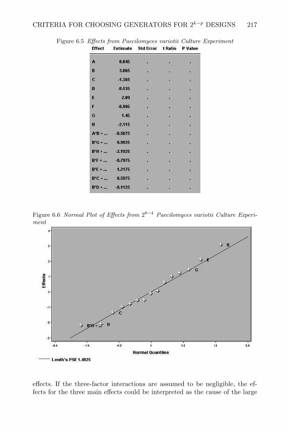
CRITERIA FOR CHOOSING GENERATORS FOR 2k−p DESIGNS 217
Figure 6.5 Effects from Paecilomyces variotii Culture Experiment
Figure 6.6 Normal Plot of Effects from 28−4 Paecilomyces variotii Culture Experi-ment
effects. If the three-factor interactions are assumed to be negligible, the ef-fects for the three main effects could be interpreted as the cause of the large

218 FRACTIONAL FACTORIAL DESIGNS
effects, but it is unclear what the string of confounded two-factor interactionsrepresents.
The authors of the article felt that the experiment had given them evidencethat factor A (the inhibitor) had little effect, and they confirmed this by citingother published reports. They also felt the experiment showed main effects D(magnesium sulfate) and F (potassium nitrite) were insignificant. However,due to the confounding of two-factor interactions with the second largest effect(in absolute value) and the fact that nothing clearly stuck out on the normalplot of effects, no definite conclusions could be drawn. They decided to runanother resolution V 25−1 follow-up experiment using factors B, C, E, G andH with defining relation I = BCEGH and factors A, D and F held constantat the mid-point of the levels used in the first experiment. This was a 16-rundesign, but if it could be safely assumed that main effects A, D and F werenegligible in the first set of sixteen experiments, then eight of the sixteen runsfor the proposed follow-up design were already completed.
Figure 6.7 shows the 25−1 design as created in SAS ADX. Run numbers 3,4, 7, 8, 11, 12, 15 and 16 were already completed in the 28−4 design as runs14, 7, 6, 15, 13, 8, 12 and 16, respectively. The remaining eight experimentswere completed in random order to get the results shown. Since this designis resolution V, all main effects and two-factor interactions are clear and canbe estimated if three-factor and higher order interactions can be assumednegligible.
Figure 6.7 25−1 Paecilomyces variotii Culture Experiment
Figure 6.8 shows the normal plot of effect from the follow-up design pro-duced by SAS ADX. Here it can be seen that the main effects for B-Rice Bran,E-Ammonium Sulfate, G-Sodium Phosphate along with the interactions BH

CRITERIA FOR CHOOSING GENERATORS FOR 2k−p DESIGNS 219
(Rice Bran×Fermentation Time), EG (Ammonium Sulfate×Sodium Phos-phate), and CH (Urea×Fermentation Time) stick out from the reference lineand appear to be significant.
Figure 6.8 Normal Plot of Effects from 25−1 Paecilomyces variotii Culture Experi-ment
Since there appear to be significant interactions the main effects shouldnot be interpreted in isolation. Figure 6.9 is an interaction plot created bySAS ADX. It shows how the effect of fermentation time depends upon thelevel of rice bran. When there is only 10 g/L of rice bran in the growth
Figure 6.9 Interaction Plot for Fermentation Time and Level of Rice Bran

220 FRACTIONAL FACTORIAL DESIGNS
medium, it can be seen that increasing the fermentation time from 72 to 96hrs increases the biomass produced. However, if there are 30 g/L of rice branin the growth medium, increasing the fermentation time actually decreasesthe biomass produced.
Figure 6.10 shows how the effect of ammonium sulfate upon biomass pro-duction depends upon the level of sodium phosphate. Here it can be seen thatincreasing the level of ammonium sulfate from 0.0 to 2.0 g/L causes a greaterincrease in biomass when there is no sodium phosphate added to the nutrientsthan when 2.0 g/L of sodium phosphate is added to the nutrients. However,since adding sodium phosphate also causes an increase in biomass, the max-imum biomass appears to result when there is 2.0 g/L of sodium phosphateand 2.0 g/L of ammonium sulfate.
Figure 6.10 Interaction Plot for Ammonium Sulfate and Sodium Phosphate
Figure 6.11 shows the interaction plot of fermentation time and urea, CH.On the average, it can be seen that increasing fermentation time seems tohave little effect on biomass production. Also, on the average, adding ureato the growth medium seems to have little effect on the biomass produced.However, as can be seen in the graph, the effect of fermentation time uponbiomass depends upon whether urea is present, and its effect appears to beexactly opposite depending on whether 2.0 g/L of urea is added to the growthmedium.
While it is possible to have an interaction between two factors that donot have significant main effects (like the example shown in Figure 6.11), itis rare. Usually interactions occur between factors where at least one of thetwo main effects are significant. This has been described as the effect heredityprinciple by Hamada and Wu (1992). In this experiment since the two-factorinteraction between fermentation time and urea is confounded with the three-factor interaction between rice bran, ammonium sulfate and sodium phosphate(i.e., CH = BEG), and all three of the latter factors have significant main
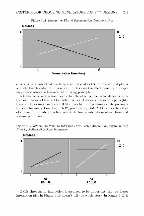
CRITERIA FOR CHOOSING GENERATORS FOR 2k−p DESIGNS 221
Figure 6.11 Interaction Plot of Fermentation Time and Urea
effects, it is possible that the large effect labeled as CH on the normal plot isactually the three-factor interaction. In this case the effect heredity principlemay overshadow the hierarchical ordering principle.
A three-factor interaction means that the effect of one factor depends uponthe combination of levels of two other factors. A series of interaction plots (likethose in the example in Section 3.6) are useful for explaining or interpreting athree-factor interaction. Figure 6.12, produced by SAS ADX, shows the effectof ammonium sulfate upon biomass at the four combinations of rice bran andsodium phosphate.
Figure 6.12 Interaction Plots To Interpret Three-Factor Ammonium Sulfate by RiceBran by Sodium Phosphate Interaction
If this three-factor interaction is assumed to be important, the two-factorinteraction plot in Figure 6.10 doesn’t tell the whole story. In Figure 6.12 it

222 FRACTIONAL FACTORIAL DESIGNS
can be seen that adding 2.0 g/L of ammonium sulfate to the growth mediumincreases the biomass produced in general. However, this effect is greatestwhen there is 30 g/L of rice bran and no sodium phosphate in the growthmedium. The optimum result appears to be with a fermentation time of 72hours, 30 g/L of rice bran, 2.0 g/L of ammonium sulfate and 0.0 g/L of sodiumphosphate in the growth medium. There the biomass yield was 11.57 g/L.
The authors of the article continued experimenting with three of the fourfactors (rice bran, ammonium sulfate and fermentation time) in a responsesurface experiment to further optimize the production of biomass protein.These experiments and results will be described in Chapter 10.
To recap this example, the researchers started with eight factors with twolevels each as shown in Table 6.5. It would have required 28 = 256 experimentsto complete a full factorial experiment. The effect sparsity principle and thehierarchical ordering principle suggest that this many experiments is probablynot needed. With eight factors, it is doubtful that all main effects and alarge number of interactions would be significant. A series of two fractionalfactorial experiments, employing a total of 24 runs, reveal that four of themain effects are significant and at most three interactions. Interaction graphshelped make a plausible interpretation of the results and identification of factorlevels for optimal results. The interpretation of the interactions was criticalfor identification of optimal results and would never have been discovered if aseat-of-the-pants approach or vary one-factor-at-a-time plan had been utilized.
6.5 Augmenting Fractional Factorials
The last example introduced the idea of augmenting fractional factorial de-signs with additional experiments in order to de-confound certain main effectsor interactions. In this section some formal procedures will be described thatallow this to be done. Section 6.5.1 describes procedures that will preservethe optimal orthogonality property of the augmented design. Section 6.5.2 de-scribes a procedure that may require fewer additional experiments, but maynot preserve the orthogonality.
6.5.1 Augmenting by Foldover or Mirror Image Designs
In a resolution III fractional factorial design, main effects are confounded withsome two-factor interactions. If more than one effect appears to be significant,after the analysis of data from a resolution III design, it is not clear whetherall effects are due to main effects or whether some could be two-factor in-teractions. For example in an eight-run resolution III design in six factors(designated by 26−3
III ) with generators D = AB, E = AC, and F = BC, thedefining relation is
I = ABD = ACE = BCF = DEF = BCDE = ACDF = ABEF.

AUGMENTING FRACTIONAL FACTORIALS 223
If after analysis of data from this design, effects B and D appear to be signifi-cant, it could be that the two main effects are the active effects. However, theeffect heredity principle tells us there are two alternative explanations. Thefirst alternative is the following. Since D is confounded with AB and EF ,it could be that main effect B and the AB interaction are the active effectsand that D only appears large because it is confounded with AB. The secondalternative is that main effect D and the AD interaction are the active effectsand B only appears large because it is confounded with AD and CF . With-out additional experiments, there is no way to determine which of the threeexplanations of the data is correct.
One way to break the confounding between main effects and two-factorinteractions is to run an additional set of experiments that is the same asthe first except that the coded factor levels on one or more factors has beenreversed (Box et al., 1978). This is called a foldover fraction. For example, inthe 26−3
III described in the last paragraph, if the signs were reversed for factor B,the defining relation would become I = −ABD = ACE = −BCF = DEF =−BCDE = ACDF = −ABEF . If the two eight-run designs were combined,as shown in Table 6.6, the resulting sixteen-run design would have definingrelation I = ACE = DEF = ACDF . Although this is still a resolution IIIdesign, main effect B is clear, and main effect D is no longer confounded withthe AB interaction.
Table 6.6 26−3III Design Augmented by 26−3
III Design with Signs Reversed on Factor B
Run A B C D E F1 - - - + + +2 + - - - - +3 - + - - + -4 + + - + - -5 - - + + - -6 + - + - + -7 - + + - - +8 + + + + + +9 - + - + + +10 + + - - - +11 - - - - + -12 + - - + - -13 - + + + - -14 + + + - + -15 - - + - - +16 + - + + + +
In general, augmenting a resolution III design with another resolution IIIdesign, with the coded factor levels for one factor reversed, will make that fac-tor and all of its two-factor interactions clear of other two-factor interactions.

224 FRACTIONAL FACTORIAL DESIGNS
Montgomery and Runger (1996) show the defining relation for the combineddesign from the original plus foldover will contain those effects in the originaldesign that were not sign reversed in the foldover fraction.
If a resolution III design is augmented with another resolution III design,with the coded factor levels reversed for all factors (called the mirror imagedesign), the combined design will be resolution IV and all main effects will beclear of two-factor interactions. The defining relation for the combined designin this situation will only contain even length words from the original definingrelation. For example, the 25−2
III design with generators D = AB, E = AChas defining relation I = ABD = ACE = BCDE. If it is combined with itsmirror image fraction where the signs of all the coded factor levels have beenreversed, the defining relation of the combined design will be I = BCDE.The SAS code below shows how this design can be created in the SAS datastep. It is also possible to create foldover and mirror image designs in the SASADX tool.
data orig;do x1 = -1 to 1 by 2;do x2 = -1 to 1 by 2;do x3 = -1 to 1 by 2;A=x3; B=x2; C=x1; D=A*B; E=A*C; Block =1; output;end;
end;end;
keep A B C D E Block;data fold; set orig;A=-A; B=-B; C=-C; D=-D; E=-E; Block =2;data comb; set orig fold;proc print; run;
When creating a resolution IV design by combining a resolution III designwith its mirror image (i.e., signs reversed on all factors), it is possible to addone additional blocking factor that can account for any difference in the av-erage response between the two sets of experiments. By having an additionalfactor, the experiments can be performed sequentially. The original resolutionIII design is completed first and the data analyzed. If there is only one factorthat appears to be significant, there may be no need for additional experi-ments. If, on the other hand, two or more effects appear significant, the mirrorimage design can be completed to clear all main effects from two-factor inter-actions. The additional factor can account for any changes in the experimentalenvironment that have occurred since the first set of experiments. Including itin the analysis will prevent any unanticipated changes from biasing the effectsof the factors studied.
Augmenting a resolution IV design with its mirror image design will nothelp to break strings of aliased two-factor interactions since the signs will notchange on the two-factor interactions. However, augmenting a resolution IV

AUGMENTING FRACTIONAL FACTORIALS 225
designs by a foldover fraction can be used to break strings of aliased two-factorinteractions, when the signs are changed on only one or two of the factors.For example, the 28−4
IV design with E = BCD, F = ACD, G = ABC, andH = ABD has seven strings of confounded two-factor interactions in groupsof 4, i.e.,
AB + EF + CG+DH
AC +DF +BG+ EH
CD +BE +AF +GH
AD + CF + EG+BH
AE +BF +DG+ CH
BC +DE +AG+ FH
BD + CE + FG+AH.
If this design is augmented with another design where the signs are reversedon factor A, all the two-factor interactions involving factor A will be clear ofother two-factor interactions.
In general, Montgomery and Runger (1996) show that the alias sets for thecombined design are obtained from a partition of the alias sets in the originalfraction by grouping effects that are sign reversed. For example, in the 26−2
IV
design with generators E = ABC, and F = BCD the aliases for the 16 effectsthat can be estimated (up to three-factor interactions) are:
I +ABCE +BCDF +ADEF
A+BCE +DEF
B +ACE + CDF
C +BDF +ABE
D +BCF +AEF
E +ABC +ADF
F +BCD +ADE
CE +AB
AC +BE
AD + EF
BC +AE +DF
DE +AF
CF +BD
CD +BF
ABD + CDE +ACF +BEF
ACD +BDE + CEF +ABF

226 FRACTIONAL FACTORIAL DESIGNS
If this design were augmented by the foldover design with all signs for factorA reversed, 32 effects could be estimated, and the aliases for each of them couldbe determined from the list above. Every effect containing A changes signs.Group effects with like signs together to get the following 32 groups.
ABCE +ADEF, I +BCDF
A, BCE +DEF
ACE, B + CDF
ABE, C +BDF
AEF, D +BCF
ABC +ADF, E
ADE, F +BCD
AB, CE
AC, BE
AD, EF
AE, BC +DF
AF, DE+ACDE +ABEF, CF +BD
ABDE +ACEF, CD +BF
ABD +ACF, CDE +BEF
ACD +ABF, BDE + CEF
If the 26−2IV design were augmented by the same design with signs reversed on
factors A and B, effects containing a single A or a single B will reverse signs.Effects containing both A and B or neither A nor B will not reverse signs,and the aliases for the 32 estimable effects will be different than those shownabove. When only a few effects are found significant after analysis of datafrom a resolution IV design, a foldover that will separate the significant maineffects from two-factor interactions (that involve the significant main effects)can usually be found.
Consider two designs used to optimize a drinking water filter to illustratethe augmenting of a fractional factorial to estimate interactions. High con-centrations of arsenic are reported in ground water in countries such as Ar-gentina, Bangladesh, Chile, China, India, Japan, Mexico, Mongolia, Nepal,Poland, Taiwan, Vietnam, and some parts of the United States, and stud-ies have shown people exposed to high levels of arsenic are prone to developvarious forms of cancer. Iron oxide coated sand (IOCS) has been used toremove arsenic from ground water in simple household filtration systems inBangladesh. Ramakrishna et al. (2006) conducted a study with the objectiveof systematically studying the effects of several factors on the arsenic removalrate for (IOCS).
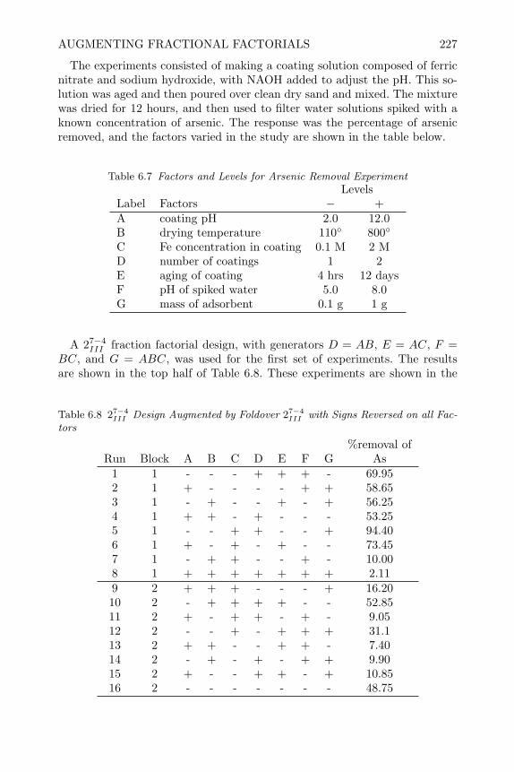
AUGMENTING FRACTIONAL FACTORIALS 227
The experiments consisted of making a coating solution composed of ferricnitrate and sodium hydroxide, with NAOH added to adjust the pH. This so-lution was aged and then poured over clean dry sand and mixed. The mixturewas dried for 12 hours, and then used to filter water solutions spiked with aknown concentration of arsenic. The response was the percentage of arsenicremoved, and the factors varied in the study are shown in the table below.
Table 6.7 Factors and Levels for Arsenic Removal ExperimentLevels
Label Factors − +A coating pH 2.0 12.0B drying temperature 110 800
C Fe concentration in coating 0.1 M 2 MD number of coatings 1 2E aging of coating 4 hrs 12 daysF pH of spiked water 5.0 8.0G mass of adsorbent 0.1 g 1 g
A 27−4III fraction factorial design, with generators D = AB, E = AC, F =
BC, and G = ABC, was used for the first set of experiments. The resultsare shown in the top half of Table 6.8. These experiments are shown in the
Table 6.8 27−4III Design Augmented by Foldover 27−4
III with Signs Reversed on all Fac-tors
%removal ofRun Block A B C D E F G As
1 1 - - - + + + - 69.952 1 + - - - - + + 58.653 1 - + - - + - + 56.254 1 + + - + - - - 53.255 1 - - + + - - + 94.406 1 + - + - + - - 73.457 1 - + + - - + - 10.008 1 + + + + + + + 2.119 2 + + + - - - + 16.2010 2 - + + + + - - 52.8511 2 + - + + - + - 9.0512 2 - - + - + + + 31.113 2 + + - - + + - 7.4014 2 - + - + - + + 9.9015 2 + - - + + - + 10.8516 2 - - - - - - - 48.75

228 FRACTIONAL FACTORIAL DESIGNS
standard order, not the random order in which they were run.A half-normal plot of the effects calculated from the first eight runs (left
as an exercise) revealed that factors B (temperature of drying the coatedsand) and F (pH of the arsenic spiked water) appeared to be significant. Bothfactors had negative effects and the high level of each resulted in a lowerpercentage of arsenic removal. This implies that percent arsenic removed isonly influenced by the temperature of drying the coated sand and by the pHof the spiked water solution. However, interpreting the results to mean thatonly the two main effects are active could be misleading. B is confoundedwith three two-factor interactions AD+CF +EG and F is confounded withBC+DE+AG. According to the effect heredity principle, the model includingB, and BC (which imply arsenic removal is influenced by the temperature ofdrying the coated sand and by the Fe concentration in the coating), and themodel including F and CF (which imply arsenic removal is influenced by thepH of the spiked water and by the Fe concentration in the coating) are alsoplausible explanations of the data. From the eight experiments in the 27−3
III itis impossible to tell which of the three plausible models is appropriate sincethe effects are completely confounded.
The original eight experiments were augmented with the mirror image de-sign, shown in the bottom half of Table 6.8, in order to de-confound the maineffects from strings of two-factor interactions. An additional blocking factor isincluded in the combined design to account for any difference in the two setsof experiments. A half-normal plot of the effects calculated from the combinedexperiments (left as an exercise) revealed that the blocking factor represent-ing the difference in the two groups of experiments, main effect F (pH of thearsenic spiked water), main effect B (temperature of drying the coated sand),main effect A (pH of the coating), and the effect representing the confoundedstring of interactions AD + CF + EG all appeared to be significant. The ef-fect heredity principle would suggest two plausible models to explain the data(ignoring the block term). The first model is (F , B, A, AD), or:
% removal = 37.76− 12.99(pHs− 7.0
2.0
)− 11.76
(temp− 455
345
)− 8.89
(pHc− 7.0
5.0
)− 10.09
(pHs− 7.0
2.0
)(number coats− .75
.5
).
This model suggests that increasing the pH of the ferric nitrate sodium hy-droxide solution used to coat the sand has little effect on arsenic removal whenthe sand is only coated once, but that it substantially decreases the arsenicremoval when the sand is coated twice. This can be visualized in the left sideof Figure 6.13. If this model is correct, it would imply that maximum arsenicremoval in a sand filtration system can be achieved when the coated sand isdried at the low temperature (B = −), the coating solution has a low pH(A = −), and the sand is coated twice (D = +).

AUGMENTING FRACTIONAL FACTORIALS 229
The second plausible model is (F , B, A, CF ), or:
% removal =37.76− 12.99(pHs− 7.0
2.0
)− 11.76
(temp− 455
345
)− 8.89
(pHc− 7.0
5.0
)− 10.09
(Fe− 1.05M
0.95M
)(pHs− 7.0
2.0
).
This model suggests that increasing the Fe concentration in the coating so-lution, increases the arsenic removal when the pH of the water being filteredis low, but decreases it when the pH of the water being filtered is high. Thiscan be visualized in the right side of Figure 6.13. If this model is correct, itwould imply that maximum arsenic removal in a sand filtration system canbe achieved when the coated sand is dried at the low temperature (B = −),and when the Fe concentration in the coating solution is high if the pH ofthe water to be filtered is low, or when the Fe concentration in the coatingsolution is low if the pH of the water to be filtered is high.
Figure 6.13 Plausible Interaction Plots for Arsenic Removal Experiment
0.1 C = Fe conc. 2of coating
1D
= n
umbe
r of
2co
atin
gs
56.8 18.8
36.5 38.9
36.5 13.1
42.3 59.2
2.0 A = Coating pH 12.0
5.0
F
= p
H o
f spi
ked
9.0
wat
er
AD Interaction CF Interaction
The two models are contradictory. The first model implies that the pH ofthe coating solution and the number of times the sand is coated influencethe percent of arsenic the sand filter can remove. However, the second modelimplies the pH of the coating solution and the number of times the sand iscoated does not affect arsenic removal; rather, the Fe concentration of thecoating solution does matter. The optimum level of this concentration mustbe determined by the pH of the water to be filtered.
In sixteen experiments the researchers were able to narrow down the listof factors that influence arsenic removal from the original seven down to five.But, because the two interactions AD and CF are completely confounded,there is no way from the results of these two sets of experiments to determinewhich model is correct and what is the best way to coat sand for a filtration
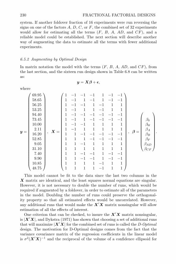
230 FRACTIONAL FACTORIAL DESIGNS
system. If another foldover fraction of 16 experiments were run reversing thesigns on one of the factors A, D, C, or F , the combined set of 32 experimentswould allow for estimating all the terms (F , B, A, AD, and CF ), and areliable model could be established. The next section will describe anotherway of augmenting the data to estimate all the terms with fewer additionalexperiments.
6.5.2 Augmenting by Optimal Design
In matrix notation the model with the terms (F , B, A, AD, and CF ), fromthe last section, and the sixteen run design shown in Table 6.8 can be writtenas:
y = Xβ + ε,
where
y =
69.9558.6556.2553.2594.4073.4510.002.11
16.2052.859.05
31.107.409.90
10.8548.75
, X =
1 −1 −1 −1 1 −1 −11 −1 1 −1 1 −1 −11 −1 −1 1 −1 1 11 −1 1 1 −1 1 11 −1 −1 −1 −1 −1 −11 −1 1 −1 −1 −1 −11 −1 −1 1 1 1 11 −1 1 1 1 1 11 1 −1 −1 −1 −1 −11 1 1 −1 −1 −1 −11 1 −1 1 1 1 11 1 1 1 1 1 11 1 −1 −1 1 −1 −11 1 −1 −1 1 −1 −11 1 1 1 −1 1 11 1 1 1 −1 1 1
, β =
β0
βblβAβBβFβADβCF
.
This model cannot be fit to the data since the last two columns in theX matrix are identical, and the least squares normal equations are singular.However, it is not necessary to double the number of runs, which would berequired if augmented by a foldover, in order to estimate all of the parametersin the model. Doubling the number of runs could preserve the orthogonal-ity property so that all estimated effects would be uncorrelated. However,any additional runs that would make the X ′X matrix nonsingular will allowestimation of all the effects of interest.
One criterion that can be checked, to insure the X ′X matrix nonsingular,is |X ′X|, and Dykstra (1971) has shown that choosing a set of additional runsthat will maximize |X ′X| for the combined set of runs is called the D-Optimaldesign. The motivation for D-Optimal designs comes from the fact that thevariance covariance matrix of the regression coefficients in the linear modelis σ2(X ′X)−1 and the reciprocal of the volume of a confidence ellipsoid for
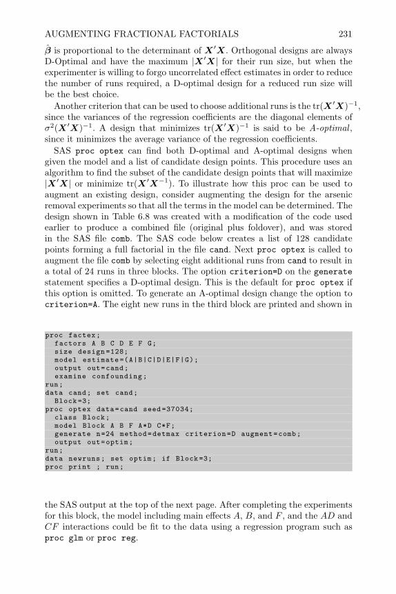
AUGMENTING FRACTIONAL FACTORIALS 231
β is proportional to the determinant of X ′X. Orthogonal designs are alwaysD-Optimal and have the maximum |X ′X| for their run size, but when theexperimenter is willing to forgo uncorrelated effect estimates in order to reducethe number of runs required, a D-optimal design for a reduced run size willbe the best choice.
Another criterion that can be used to choose additional runs is the tr(X ′X)−1,since the variances of the regression coefficients are the diagonal elements ofσ2(X ′X)−1. A design that minimizes tr(X ′X)−1 is said to be A-optimal ,since it minimizes the average variance of the regression coefficients.
SAS proc optex can find both D-optimal and A-optimal designs whengiven the model and a list of candidate design points. This procedure uses analgorithm to find the subset of the candidate design points that will maximize|X ′X| or minimize tr(X ′X−1). To illustrate how this proc can be used toaugment an existing design, consider augmenting the design for the arsenicremoval experiments so that all the terms in the model can be determined. Thedesign shown in Table 6.8 was created with a modification of the code usedearlier to produce a combined file (original plus foldover), and was storedin the SAS file comb. The SAS code below creates a list of 128 candidatepoints forming a full factorial in the file cand. Next proc optex is called toaugment the file comb by selecting eight additional runs from cand to result ina total of 24 runs in three blocks. The option criterion=D on the generatestatement specifies a D-optimal design. This is the default for proc optex ifthis option is omitted. To generate an A-optimal design change the option tocriterion=A. The eight new runs in the third block are printed and shown in
proc factex;factors A B C D E F G;size design =128;model estimate =(A|B|C|D|E|F|G);output out=cand;examine confounding;
run;data cand; set cand;
Block =3;proc optex data=cand seed =37034;
class Block;model Block A B F A*D C*F;generate n=24 method=detmax criterion=D augment=comb;output out=optim;
run;data newruns; set optim; if Block =3;proc print ; run;
the SAS output at the top of the next page. After completing the experimentsfor this block, the model including main effects A, B, and F , and the AD andCF interactions could be fit to the data using a regression program such asproc glm or proc reg.

232 FRACTIONAL FACTORIAL DESIGNS
Obs A B F D C Block1 -1 -1 -1 1 -1 32 -1 -1 -1 -1 1 33 -1 1 1 1 1 34 -1 1 1 -1 -1 35 1 -1 1 -1 1 36 1 -1 1 1 -1 37 1 1 -1 -1 -1 38 1 1 -1 1 1 3
6.6 Plackett-Burman (PB) Screening Designs
Resolution III 2k−p fractional factorial designs are often used for screeningexperiments where the objective is to determine which factors (from a list as-sembled by brainstorming) are important enough to be studied in more detailin follow-up experiments. However, the number of runs in an 2k−p fractionalfactorial design is always a power of 2, i.e., 8, 16, 32 etc., and these limitedchoices for run size can be restrictive in screening experiments. For example, toexamine 8 factors requires at least 16 experiments, and to examine 16 factorsrequires 32 experiments when using a fractional factorial design.
Resolution III Plackett and Burman (1946) designs, or PB designs, areavailable in run sizes that are multiples of 4, i.e., 8, 12, 16, 20, etc. Thesedesigns were originally discovered by two British statisticians during WorldWar II while studying the effect of a number of factors on the performance ofanti-aircraft proximity fuse prototypes. Like 2k−p fractional factorial designs,these designs have two levels for each factor; and for run sizes that are powersof 2, they are the same as a 2k−p design. For other run sizes, they retainthe desirable orthogonality property of 2k−p designs, but they do not havegenerators or a defining relation. The designs for run sizes of 12, 20 and 24can be created by cyclically rotating the factor levels for the first run. Table6.9 shows the factor levels for the first run in these designs. Table 6.10 shows
Table 6.9 Factor Levels for First Run of Plackett-Burman DesignRun size Factor Levels
12 +−+−−−+ + +−+20 +−+ +−−−−+−+−+ + + +−−+24 +−−−−+−+−−+ +−−+ +−+−+ + + +
how these factor levels are used to create a 12-run Plackett-Burman Designin 11 factors. The factor levels for the first run are copied directly from thefirst line of Table 6.9. In the second run, the level for the first factor (A) is thelevel of the eleventh factor (L) in the first run, and the factor levels for factorsB through L for the second run are the factor levels for factors A throughK from the first run. This pattern is continued, cyclically rotating the factorlevels for each run to create the factor levels for the next run until the lastrun. For run number 12, all the factors are set to their low (−) level. To create

PLACKETT-BURMAN (PB) SCREENING DESIGNS 233
Table 6.10 12 Run Plackett-Burman Designrun A B C D E F G H J K L
1 + - + - - - + + + - +2 + + - + - - - + + + -3 - + + - + - - - + + +4 + - + + - + - - - + +5 + + - + + - + - - - +6 + + + - + + - + - - -7 - + + + - + + - + - -8 - - + + + - + + - + -9 - - - + + + - + + - +
10 + - - - + + + - + + -11 - + - - - + + + - + +12 - - - - - - - - - - -
a 12-run design in k factors, where k < 11, proceed exactly as above, but useonly k columns in the design to define factor setting. To create a 20 or 24-runPlackett-Burman Design proceed exactly as before, but start with the row inTable 6.9 with the correct run size.
These designs can be created easily in the SAS data step. The code at thetop of the next page shows how to create a 12-run design like that shown inTable 6.10. The first data step reads in the factor levels for run 1 that werecopied from Table 6.9. The second data step creates the factor levels for runs1 through 11 by cyclically rotating the levels for the first run. The factor levelsfor the final run are all set to -1.
There are SAS macros included in the AUTOCALL library that can alsobe used to create Plackett-Burman Designs. These macros can be included inyour SAS code by simply typing the file name preceded by a %. The ADXPBDmacro creates a Plackett-Burman design with the statement %adxpbd(file,nf ),where file is the name of the SAS file that will contain the design and nf is thenumber of factors. For example, to create a 28-run Plackett-Burman designwith 25 factors, simply enter the commands
%adxgen%adxff%adxinit%adxpbd(pb28 ,25)proc print data=pb28; run;
These macros are the basis for the SAS ADX graphical user interface, andit also can be used to create Plackett-Burman designs. In practice, the orderof the runs in a Plackett-Burman Design should be randomized to reduce thechance of bias from unknown factors before conducting the experiments justas they would be in any other design.

234 FRACTIONAL FACTORIAL DESIGNS
* Create 12-run Plackett -Burman Design in Data Step;* first reads factor levels for first line from ;* Table 6.9 ;data lis;
input f1 -f11;datalines;
1 -1 1 -1 -1 -1 1 1 1 -1 1data pb11; set lis;* Next cyclically rotates factor levels;
array f11 f1-f11;array t11 t1-t11;do i=1 to 11;do j= 1 to 11;if j<i then k=11-i+1+j;else k=j-i+1;tj=fk;
end;output;
end;do i=1 to 11;
ti=-1;end;output;
keep t1-t11;proc print; run;
As an example of the use of a Plackett-Burman design, consider the data inTable 6.11, which comes from a study by Hunter et al. (1982) of the fatiguelife of weld-repaired castings. Seven factors were assigned to the last sevencolumns of the Plackett-Burman design matrix shown in Table 6.10, and thefirst four columns were not assigned to factors in defining the experiments.The purpose of the experiments was to identify the factors that affect thefatigue life of the weld repairs. The response, y, is the log of the lifetime ofeach weld repair. We will use this data to illustrate the analysis of data froma Plackett-Burman Design. Analysis of this data has been presented in theliterature by several others.
Although there is no defining relation in a Plackett-Burman design, it isa resolution III design and the unassigned columns in Table 6.11 representconfounded strings of interactions. A first step in the analysis would be tocalculate an effect for each of the 11 columns in Table 6.11 and make a half-normal plot.
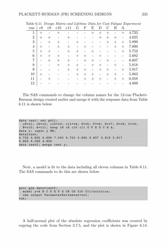
PLACKETT-BURMAN (PB) SCREENING DESIGNS 235
Table 6.11 Design Matrix and Lifetime Data for Cast Fatigue Experimentrun c8 c9 c10 c11 G F E D C B A
1 + - + - - - + + + - + 4.7332 + + - + - - - + + + - 4.6253 - + + - + - - - + + + 5.8994 + - + + - + - - - + + 7.0005 + + - + + - + - - - + 5.7526 + + + - + + - + - - - 5.6827 - + + + - + + - + - - 6.6078 - - + + + - + + - + - 5.8189 - - - + + + - + + - + 5.917
10 + - - - + + + - + + - 5.86311 - + - - - + + + - + + 6.05812 - - - - - - - - - - - 4.809
The SAS commands to change the column names for the 12-run Plackett-Burman design created earlier and merge it with the response data from Table6.11 is shown below.
data cast; set pb11;c8=t1; c9=t2; c10=t3; c11=t4; G=t5; F=t6; E=t7; D=t8; C=t9;B=t10; A=t11; keep c8 c9 c10 c11 G F E D C B A;
data y; input y @@;datalines;4.733 4.625 5.899 7.000 5.752 5.682 6.607 5.818 5.9175.863 6.058 4.809data castf; merge cast y;
Next, a model is fit to the data including all eleven columns in Table 6.11.The SAS commands to do this are shown below.
proc glm data=castf;model y=A B C D E F G C8 C9 C10 C11/solution;ods output ParameterEstimates=sol;
run;
A half-normal plot of the absolute regression coefficients was created bycopying the code from Section 3.7.5, and the plot is shown in Figure 6.14.

236 FRACTIONAL FACTORIAL DESIGNS
Figure 6.14 Half-Normal Plot of Absolute Regression Coefficients from Cast FatigueExperiment
The plot shows that main effect F is clearly significant and that the nextlargest effect is main effect D. The authors of the original article concludedthat the model including these two factors was the correct model, and theyfit it to the data by regression obtaining an R2 = .5867. However, the samecaution should be exercised that was illustrated in the water filtration examplepresented in Section 6.5. Because this Plackett-Burman design has resolutionIII, two-factor interactions are confounded with main effects and there maybe other plausible models for the data. A mirror image design could be addedto the Plackett-Burman design in order to clear main effects of two-factorinteractions; however, this is not necessary due to the complex aliasing forthis type design.
By complex aliasing we mean that each interaction is partially confoundedwith many main effects rather than being completely confounded with onemain effect as it would be in a 2k−pIII design. Lin and Draper (1992) and Wangand Wu (1995) showed that designs with complex aliasing have a hidden pro-jection property. The hidden projection property allows some interactions tobe estimated even though the design is resolution III. For Plackett-Burmandesigns where only a subset of the factors appear to be important, Wang andWu have shown that a model can be fit to the data by regression which in-cludes the main effects and all two-factor interactions involving the importantmain effects. When interaction terms are included in the model, the design be-

PLACKETT-BURMAN (PB) SCREENING DESIGNS 237
comes non-orthogonal and effects must be estimated by regression, but Wangand Wu have shown that the D-efficiency remains quite high. Usually sometype of regression subset selection procedure is used in order to identify themost appropriate model. For the data in Table 6.11, the SAS commands be-low, create interaction columns and use proc reg to perform an all-subsetsregression.
data castf; set castf;*Note Defines Interactions;
AB=A*B; AC=A*C; AD=A*D; AE=A*E; AF=A*F; AG=A*G;BC=B*C; BD=B*D; BE=B*E; BF=B*F; BG=B*G;
CD=C*D; CE=C*E; CF=C*F; CG=C*G;DE=D*E; DF=D*F; DG=D*G;
EF=E*F; EG=E*G;FG=F*G;
proc reg data=castf;model y=A B C D E F G AB AC AD AE AF AG BC BD BE BF BG CD CECF CG DE DF DG EF EG FG/selection=rsquare best=4 stop =4;
run;
The results shown below indicate that when two variables are consideredin the model, the model which includes main effect F and the interaction FGfits best and has an R2 = 0.8925, compared to the R2 = 0.5867 for the modelthat the authors fit to the data (which included main effects D and F ). Thebest model with three variables in the equation only raises R2 from 0.8925 to0.9526 and the third variable is probably not needed. The model including Fand FG is the model found in the other papers which have reanalyzed thisdata by various procedures.
Number inModel R-Square Variables in Model
1 0.4474 FG1 0.4451 F1 0.4377 AE1 0.1812 BC
----------------------------------------2 0.8925 F FG2 0.6638 AE FG2 0.6621 F AE2 0.6239 BD FG
----------------------------------------3 0.9526 F AE FG3 0.9313 F BD FG3 0.9190 D F FG3 0.9116 F DG FG
----------------------------------------4 0.9686 F AE EF FG4 0.9660 F AE CD FG4 0.9643 F AD AE FG4 0.9642 F BD CF FG
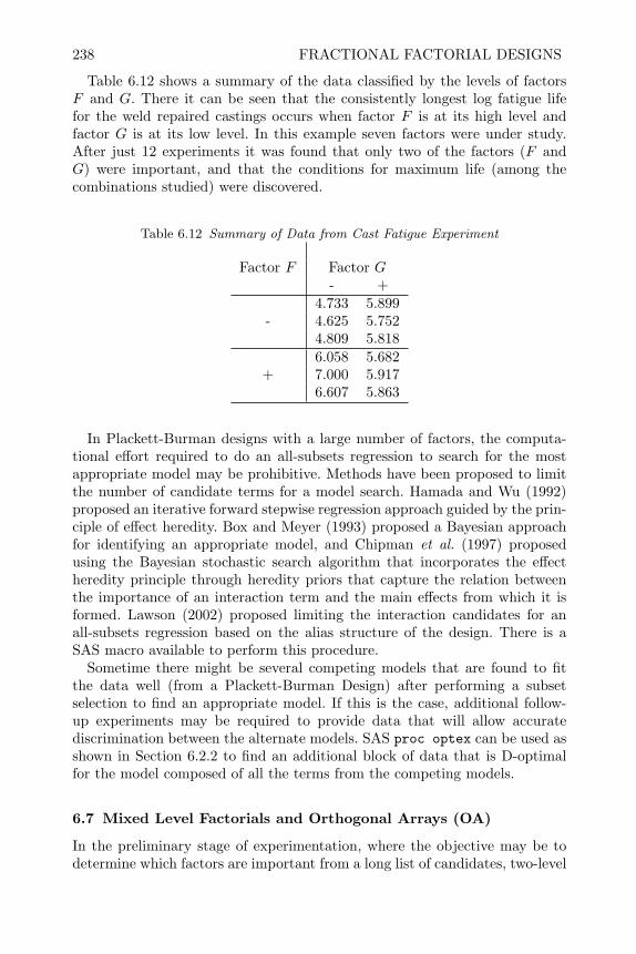
238 FRACTIONAL FACTORIAL DESIGNS
Table 6.12 shows a summary of the data classified by the levels of factorsF and G. There it can be seen that the consistently longest log fatigue lifefor the weld repaired castings occurs when factor F is at its high level andfactor G is at its low level. In this example seven factors were under study.After just 12 experiments it was found that only two of the factors (F andG) were important, and that the conditions for maximum life (among thecombinations studied) were discovered.
Table 6.12 Summary of Data from Cast Fatigue Experiment
Factor F Factor G- +
4.733 5.899- 4.625 5.752
4.809 5.8186.058 5.682
+ 7.000 5.9176.607 5.863
In Plackett-Burman designs with a large number of factors, the computa-tional effort required to do an all-subsets regression to search for the mostappropriate model may be prohibitive. Methods have been proposed to limitthe number of candidate terms for a model search. Hamada and Wu (1992)proposed an iterative forward stepwise regression approach guided by the prin-ciple of effect heredity. Box and Meyer (1993) proposed a Bayesian approachfor identifying an appropriate model, and Chipman et al. (1997) proposedusing the Bayesian stochastic search algorithm that incorporates the effectheredity principle through heredity priors that capture the relation betweenthe importance of an interaction term and the main effects from which it isformed. Lawson (2002) proposed limiting the interaction candidates for anall-subsets regression based on the alias structure of the design. There is aSAS macro available to perform this procedure.
Sometime there might be several competing models that are found to fitthe data well (from a Plackett-Burman Design) after performing a subsetselection to find an appropriate model. If this is the case, additional follow-up experiments may be required to provide data that will allow accuratediscrimination between the alternate models. SAS proc optex can be used asshown in Section 6.2.2 to find an additional block of data that is D-optimalfor the model composed of all the terms from the competing models.
6.7 Mixed Level Factorials and Orthogonal Arrays (OA)
In the preliminary stage of experimentation, where the objective may be todetermine which factors are important from a long list of candidates, two-level

MIXED LEVEL FACTORIALS AND ORTHOGONAL ARRAYS (OA) 239
fractional factorial designs or Plackett-Burman designs are often appropriate.If a factor has quantitative levels, the two levels are denoted symbolically by(−) and (+), where (−) represents the lowest level the experimenter wouldconsider, and (+) represents the highest level the experimenter would consider.The high and low are usually spread out as far as feasibly possible in orderto accentuate the signal or difference in response between the two levels. If afactor has qualitative levels, the (−) and (+) designations are arbitrary, butthe two levels chosen normally would be two that the experimenter believesshould result in the maximum difference in response.
Sometimes, however, two-levels for each factor may not be adequate. In caseswhere the experimenter would like to consider non-linear effects of quantita-tive factors or qualitative factors with more than two alternatives, two-levelfractional designs will not be suitable. For example, Fannin et al. (1981) re-port an experiment investigating the effects of four three-level factors and twotwo-level factors upon the rate of bacterial degradation of phenol for the pur-pose of evaluating the fate of chemicals in aquatic ecosystems. A full factorialwould require 34 × 22 = 324 experiments; however, the study was completedusing only a fraction of these runs by utilizing a mixed level fractional factorialdesign based on an orthogonal array. Taguchi (1986) describes an experimentto determine the factors that affect the durability of an auto clutch spring.The factors and levels are shown in the table below. The levels of factors A,
Factor Description LevelsA Shape 3 alternativesB Hole ratio 2 possibilitiesC Coining 2 possibilitiesD Stress σt 90 65 40E Stress σc 200 170 140F Shop peening 3 alternativesG Outer Perimeter planing 3 alternatives
C, F and G represented discrete alternatives that were of interest. Factors B,D and E were continuous factors and three levels were included in order todetermine whether there was a curvilinear relation between these factor levelsand durability of the clutch springs. There was also interest in the interactionbetween factors D and F and the interaction between factors D and G. A fullfactorial would require 35 × 22 = 972 experiments, but Taguchi was able toget valid data with a fractional design that included only 27 experiments.
An orthogonal array OA(N, sm11 , . . . , s
mγγ , 2) of strength 2 is an N ×m ma-
trix, m = m1 + · · · + mγ where column mi has si(≥ 2) symbols (or levels)such that for any subset of two columns all possible combinations of the sym-bols occur equally often in the matrix. These designs are orthogonal in themain effects and are of resolution III. However, in some cases like the Plackett-Burman designs, they can be used to estimate a limited number of interactionsas well.

240 FRACTIONAL FACTORIAL DESIGNS
A necessary condition for the existence of an orthogonal array is that num-ber of runs N be divisible by the product of each possible pair of factor levels.For example, in the experiment described by Taguchi, with five three-level fac-tors and two two-level factors, 35×22, no orthogonal array fractional factorialexists with N = 54 runs because 54 is not divisible by 2× 2 = 4. In addition,no orthogonal array exists with N = 24 runs because 24 is not divisible by3 × 3 = 9. However an orthogonal array with N = 36 happens to exist since36 is divisible by 4, 6, and 9.
Entire books have been written on methods for obtaining particular or-thogonal array designs; however, SAS macros exist that will do the work.Specifically macro %mktRuns finds the number of runs required by an orthog-onal array for a given number of factors and levels and displays alternativearrays from a vast catalog of designs that are stored or can be created by thesoftware. Macro %mktEx actually finds the array given the number of runs inaddition to the number of factors and levels. These macros have the prefixMkt because orthogonal array designs are commonly used in market researchstudies such as conjoint analysis and stated choice experiments. These macrosare described by Kuhfeld (2009) and the algorithms used by these macrosare described by Kuhfeld and Tobias (2005). The call of the macro %mktRunsbelow illustrates the use of these macros to find a fractional factorial arraydesign that includes five three-level factors and two two-level factors.
%mktruns (3**5 2**2)
Part of the resulting output is shown below.
Saturated = 13Full Factorial = 972
Some Reasonable Cannot BeDesign Sizes Violations Divided By
36 * 072 * 018 1 454 1 424 10 948 10 960 10 930 11 4 942 11 4 966 11 4 913 S 28 2 3 4 6 9
* - 100% Efficient design can be made with the MktEx macro.S - Saturated Design - The smallest design that can be made.
Note that the saturated design is not one of therecommended designs for this problem. It is shownto provide some context for the recommended sizes.

MIXED LEVEL FACTORIALS AND ORTHOGONAL ARRAYS (OA) 241
The output shows that there are a total of 13 = 1 + 5× (3− 1) + 2× (2− 1)degrees of freedom required to estimate the mean and the six main effects,and that the number of runs required for a full factorial would be 972. Next,the results show that the orthogonal array with the minimum number of runsfor studying five three-level factors and two two-level factors is 36, and thatanother orthogonal array with 72 runs exists.
Another part of the output, which is not shown here, lists all of the known36-run and 72-run orthogonal array designs. Once the user decides how manyruns to include in the orthogonal array, the %mktEx macro can be used toactually create the design as shown below.
%mktex(3**5 2**2, n=36)proc print data=randomized; run;
The output of %mktEx indicates that a 100% D-efficient (or orthogonal de-sign) for this run size was found. The design is not automatically printed out,but is stored in the SAS data set design and in a random order in the SASdata set randomized. The proc print statement above prints the contentsof this randomized data file.
Sometimes when the purpose of experimentation is to screen the impor-tant factors in a preliminary experiment, the number of runs required for anorthogonal array may be more that the experimenter is willing to run. Forexample, in the 35×22 experiment, only 13 degrees of freedom are required toestimate all the main effects. If the experimenter, relying on the effect sparsityprinciple, believes that only one or two factors and their interaction will beimportant (like the last example presented), then 36 runs may be more thannecessary. The output of the %mktRuns macro listed one 18-run design thathad only one violation to the requirement for an orthogonal array. This meansthat an 18-run design can be constructed, but it will not be an orthogonalarray. Sometimes designs with fewer runs than required for an orthogonal ar-ray, can still allow for uncorrelated estimates of main effects. These designsare called orthogonal main effect plans.
Although there are methods of constructing orthogonal main effect plansmanually, a simple alternative is to use the %mktEx macro. It uses an algo-rithm to find an 18-run design that is as close to orthogonal as possible byusing several methods including proc optex, selecting the method that worksbest for the problem, and then performing more iterations with the selectedmethod. The macro call to produce this design is:
%mktex(3**5 2**2,n=18, maxiter =100, seed =104)

242 FRACTIONAL FACTORIAL DESIGNS
The output of %mktEx shown below indicates that the macro found a designthat is 99.9045% D-efficient.
AveragePrediction
Design StandardNumber D-Efficiency A-Efficiency G-Efficiency Error----------------------------------------------------------------
1 99.9045 99.8081 99.0521 0.8498
D-efficiency is defined as:
100× 1
N |(X′X)−1|1p
,
where N is the number of runs in the design and p is the number of degreesof freedom for the mean and main effects. |(X′X)−1| = 1
Np for an orthogonaldesign, thus orthogonal designs are 100% D-efficient. For this example the18-run design is not orthogonal, but is close. The design can be printed withthe command:
proc print data=design; run;
or
proc print data=randomized; run;
The %mktEx macro can also search for a fractional design that will allowestimation of some interactions. For example to find a 27-run design for the35 × 22 design that will allow estimation of the DE and DF interactions,similar to the one used by Taguchi, issue the macro call:
%mktex(3 2**2 3**4, interact=x4*x5 x4*x6 , n=27)proc print data=randomized; run;
As an example of the use of a design created with the Mkt macros, considera conjoint analysis described by Wang et al. (2004). These types of studiesare commonly done in market research to determine the relative importanceof different product attributes to a customer’s preference for the product.The purpose of this particular study was to assess the market potential forusing low-grade hardwood lumber (with knots and other character marks)to produce fine furniture since the low-grade hardwood is under-utilized. The

MIXED LEVEL FACTORIALS AND ORTHOGONAL ARRAYS (OA) 243
products studied were hardwood chairs, and the product attributes (or factors)and levels are shown in Table 6.13.
A questionnaire was developed where potential customers were asked torate product alternatives, composed of combinations of the levels shown inTable 6.13, on a seven-point scale (1 = least preferred to 7 = most preferred).The surveys were conducted in the Vermont state fair where an exhibit boothwas set up where respondents were able to see the design and character markdensity of the chairs and ask questions about them. A label was attached toeach chair indicating the price and guarantee policy. Potential respondentswere enticed into filling out the survey by giving them a chance to enter araffle to win the chair of their choice.
Table 6.13 Product Attributes and Levels for Conjoint StudyFactor Product Attribute LevelsA Design 1 = Rocking Chair
2 = Arm Chair3 = Office Chair I4 = Office Chair II
B Price 1 = $350.002 = $425.003 = $500.004 = $575.00
C Density of Marks 1 = Clear2 = Medium3 = Heavy
D Guarantee policy 1 = 1-year2 = Unconditional
There are 42 × 3 × 2 = 96 possible combinations of levels of the factorsshown in Table 6.13, which would be too many to ask a respondent to rate.Twelve profiles or product alternatives were created from these levels using amixed-level fractional factorial design.
The following macro calls were issued to look for an orthogonal array andcreate a design. The smallest orthogonal array for examining a 42×3×2 designwas 48, which is still too many to ask a respondent to rate. A 12-run designwas created using the %mktEx macro, and was found to be 94.8% D-efficient.
%mktruns (4 4 3 2)%mktex(4 4 3 2, n=12, seed =2013)
Table 6.14 shows the design in actual factor levels. These 12 combinations
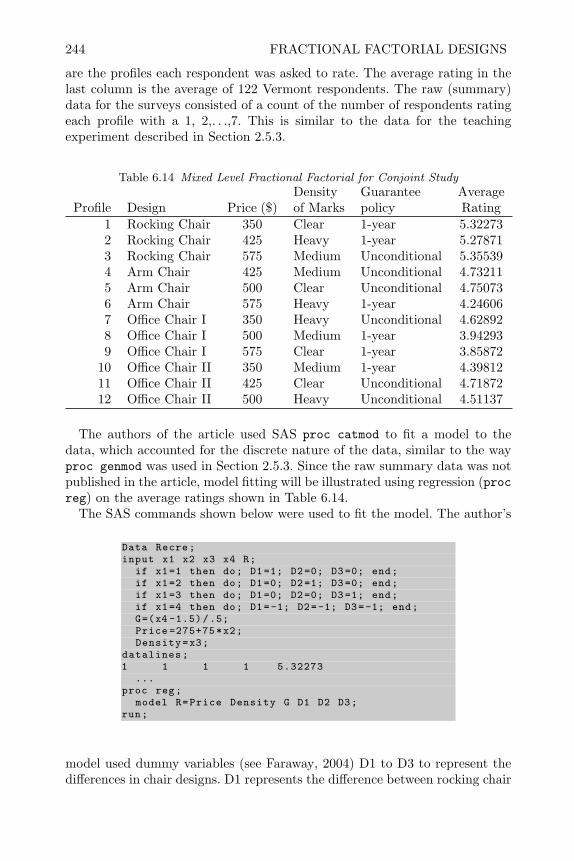
244 FRACTIONAL FACTORIAL DESIGNS
are the profiles each respondent was asked to rate. The average rating in thelast column is the average of 122 Vermont respondents. The raw (summary)data for the surveys consisted of a count of the number of respondents ratingeach profile with a 1, 2,. . .,7. This is similar to the data for the teachingexperiment described in Section 2.5.3.
Table 6.14 Mixed Level Fractional Factorial for Conjoint StudyDensity Guarantee Average
Profile Design Price ($) of Marks policy Rating1 Rocking Chair 350 Clear 1-year 5.322732 Rocking Chair 425 Heavy 1-year 5.278713 Rocking Chair 575 Medium Unconditional 5.355394 Arm Chair 425 Medium Unconditional 4.732115 Arm Chair 500 Clear Unconditional 4.750736 Arm Chair 575 Heavy 1-year 4.246067 Office Chair I 350 Heavy Unconditional 4.628928 Office Chair I 500 Medium 1-year 3.942939 Office Chair I 575 Clear 1-year 3.85872
10 Office Chair II 350 Medium 1-year 4.3981211 Office Chair II 425 Clear Unconditional 4.7187212 Office Chair II 500 Heavy Unconditional 4.51137
The authors of the article used SAS proc catmod to fit a model to thedata, which accounted for the discrete nature of the data, similar to the wayproc genmod was used in Section 2.5.3. Since the raw summary data was notpublished in the article, model fitting will be illustrated using regression (procreg) on the average ratings shown in Table 6.14.
The SAS commands shown below were used to fit the model. The author’s
Data Recre;input x1 x2 x3 x4 R;
if x1=1 then do; D1=1; D2=0; D3=0; end;if x1=2 then do; D1=0; D2=1; D3=0; end;if x1=3 then do; D1=0; D2=0; D3=1; end;if x1=4 then do; D1=-1; D2=-1; D3=-1; end;G=(x4 -1.5)/.5;Price =275+75*x2;Density=x3;
datalines;1 1 1 1 5.32273
...proc reg;
model R=Price Density G D1 D2 D3;run;
model used dummy variables (see Faraway, 2004) D1 to D3 to represent thedifferences in chair designs. D1 represents the difference between rocking chair

MIXED LEVEL FACTORIALS AND ORTHOGONAL ARRAYS (OA) 245
and office chair II. D2 represents the difference between arm chair and officechair II, and D3 represents the difference between office chair I and office chairII. A dummy variable G was used to represent the difference between a 1-yearand unconditional guarantee. Linear functions of both price and a ranking ofthe density of character marks (1 = clear, 2 = medium, and 3 = heavy) werealso included in the author’s model.
The SAS output of proc reg shown below is similar to what the authorsobtained.
Parameter StandardVariable DF Estimate Error t Value Pr > |t|
Intercept 1 5.36301 0.12194 43.98 <.0001Price 1 -0.00156 0.00024024 -6.49 0.0013Density 1 0.00177 0.02326 0.08 0.9423G 1 0.18688 0.02014 9.28 0.0002D1 1 0.71637 0.03371 21.25 <.0001D2 1 -0.07290 0.03476 -2.10 0.0901D3 1 -0.42007 0.03371 -12.46 <.0001
These results showed that while price, guarantee policy and chair designhad a significant effect on customer preference, the density of character marksdid not. This meant that there would be a market for hardwood furnituremade with low-grade wood. The regression model could be used to predictthe preference (demand) for the different chair designs, and the regressioncoefficient for price indicated the price elasticity.
In general, orthogonal array designs and orthogonal main effect plans areresolution III designs for fractions of mixed level factorials. Like Plackett-Burman designs, they have no defining relation. Except for fractions of 4k×2p
designs, the alias structure is complex in that each interaction is partiallyconfounded with many main effects. They also share the hidden projectionproperty with Plackett-Burman Designs, and even though these designs areresolution III, some interactions may be detected using the methods of analysisdescribed by Hamada and Wu (1992), Box and Meyer (1993), Chipman et al.(1997), and Lawson (2002).
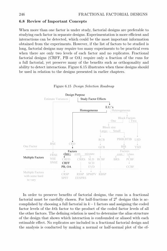
246 FRACTIONAL FACTORIAL DESIGNS
6.8 Review of Important Concepts
When more than one factor is under study, factorial designs are preferable tostudying each factor in separate designs. Experimentation is more efficient andinteractions can be detected, which could be the most important informationobtained from the experiments. However, if the list of factors to be studied islong, factorial designs may require too many experiments to be practical evenwhen there are only two levels of each factor and no replicates. Fractionalfactorial designs (CRFF, PB or OA) require only a fraction of the runs fora full factorial, yet preserve many of the benefits such as orthogonality andability to detect interactions. Figure 6.15 illustrates when these designs shouldbe used in relation to the designs presented in earlier chapters.
Figure 6.15 Design Selection Roadmap
Design PurposeEstimate Variances Study Factor Effects
E.U.’s
Block Factors
One Factor
Multiple Factors
Multiple Factorswith some hard
to vary
Block size
Homogeneous Heterogeneous
Large Small
RCB
GCB
PBIB,BTIB
BIB
LSD
YSDRSE CRD
FactorsFRSENSESNSE
CRFD CRRS SLD RCBF BRS PCBFCRFF SCD
PB, OA EVD CCBF
CRSP RSSP SPMPV RBSPSPFF EESPRS
One Two
class cont. mixture cont. classFactors
In order to preserve benefits of factorial designs, the runs in a fractionalfactorial must be carefully chosen. For half-fractions of 2k designs this is ac-complished by choosing a full factorial in k−1 factors and assigning the codedfactor levels of the kth factor to the product of the coded factor levels of allthe other factors. The defining relation is used to determine the alias structureof the design that shows which interaction is confounded or aliased with eachestimable effect. No replicates are included in a fractional factorial design andthe analysis is conducted by making a normal or half-normal plot of the ef-

REVIEW OF IMPORTANT CONCEPTS 247
fects estimated by regression. The principles of effect sparsity and hierarchicalordering help in interpreting the results.
The subset of runs for one-quarter and higher fractions of 2k factorials canalso be carefully selected by choosing generators that confound p added factorsto interactions among the k−p factors in the base design. From the generatorsthe defining relation and alias structure for the design can be determined. SASADX system automatically generates designs that have the highest resolutionand minimum aberration among all 2k−p designs with the same number ofruns. Designs of resolution R confound main effects with R − 1 and higherorder interactions. These designs also have a projective property. When onlyR − 1 factors or less appear significant after running a resolution R design,the insignificant factors can be ignored and a full factorial in R − 1 factorswill remain. The 2k−p fractional factorial projects to a 2R−1 full factorial inR− 1 factors.
After analysis of data from a resolution III fractional factorial, the interpre-tation may be straightforward if only one factor appears to have a significanteffect. When more than one factor appears to have a significant effect, theinterpretation may be more difficult due to aliasing of interactions with maineffects. Augmenting a resolution III fractional factorial with a foldover or mir-ror fraction can often eliminate the confounding between apparently importantmain effects and interactions, and can allow for a simple interpretation of theeffects after only a fraction of the runs needed for a full factorial.
When confounded strings of two-factor interactions appear significant whenanalyzing data from a resolution IV design, augmenting the design with cer-tain foldover fractions or D-Optimal subsets of runs can provide the data todetermine which interactions are significant.
Plackett-Burman designs preserve many of the benefits of factorial and frac-tional factorial designs such as orthogonality among main effects and the pro-jective property. In addition, these designs are available in run sizes that aremultiples of 4 rather than powers of 2 as they are for fractional factorialdesigns. If more than one factor is significant after the analysis of a Plackett-Burman design, significant interactions can sometimes be detected using re-gression subset selection techniques without requiring additional experimentssuch as a foldover or D-Optimal fraction.
Finally, when more than two levels are required for some factors, mixedlevel fractional factorials can be created using orthogonal array and orthogonalmain effect plans that are generated with the SAS Mkt macros. These designsare similar to Plackett-Burman designs in that they are orthogonal in themain effects and have no defining relation. Many of these designs also havea projective property, and interactions can be detected without additionalexperiments using methods of analysis similar to those used for Plackett-Burman designs.

248 FRACTIONAL FACTORIAL DESIGNS
6.9 Exercises
1. Consider a 23−1 factional factorial design,
(a) Modify the SAS code in Section 6.2 to create a list of the runs in thedesign.
(b) Determine the defining relation.(c) Determine the complete alias pattern.(d) Use SAS ADX to create this design.(e) Examine the Alias Structure in SAS ADX.
2. Melo et al. (2007) used a 24−1 factional factorial design with generatorD = ABC to study the factors that influence the production of levan byaerobic fermentation using the yeast Zymomonas mobilis. Levan is a sugarpolymer of the fructan group which has been shown to have anti-tumoractivity against sarcoma and Ehrlich carcinoma in Swiss albino mice. Thefactors varied in the fermentation medium and their levels are shown in thetable below.
LevelsLabel Factor − +A Sucrose initial concentration(g.L−1) 150 250B Temperature(C) 20 30C Yeast extract initial concentration(g.L−1) 2.0 5.0D Agitation(rpm) 50 100
(a) What is the defining relation and complete alias structure for this design?(b) What is the resolution of this design?(c) The fermentations were carried out batchwise in Pyrex flasks. After
72 hours of fermentation, the levan produced was extracted from thefermented medium and its dry weight was determined. The results (ing.L−1) for the 8 experiments (in standard order) were: 4.70, 14.67, 1.71,3.73, 9.47, 7.61, 0.15, 4.78. From this data, calculate the 7 effects andmake a normal probability plot to determine what is significant.
(d) Delete the smallest three effects and fit the model again. Are the foureffects left in the model significant?
(e) Based on the effect heredity principle, what do you think the significantstring of aliased two-factor interactions could represent?
(f) Can the design be collapsed to a full factorial by ignoring insignificantfactors?
(g) Based on what you said in (e) write an interpretation of the significanteffects and interaction. Based on your model determine the factor levelsthat will produce the maximum dry weight of levan.
3. Use SAS ADX to create a quarter fraction 25−2 design.
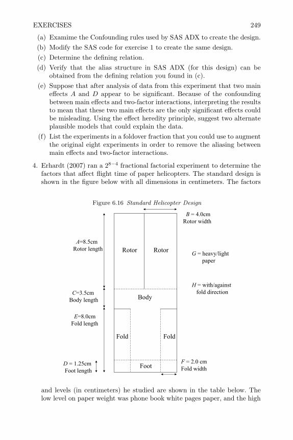
EXERCISES 249
(a) Examime the Confounding rules used by SAS ADX to create the design.(b) Modify the SAS code for exercise 1 to create the same design.(c) Determine the defining relation.(d) Verify that the alias structure in SAS ADX (for this design) can be
obtained from the defining relation you found in (c).(e) Suppose that after analysis of data from this experiment that two main
effects A and D appear to be significant. Because of the confoundingbetween main effects and two-factor interactions, interpreting the resultsto mean that these two main effects are the only significant effects couldbe misleading. Using the effect heredity principle, suggest two alternateplausible models that could explain the data.
(f) List the experiments in a foldover fraction that you could use to augmentthe original eight experiments in order to remove the aliasing betweenmain effects and two-factor interactions.
4. Erhardt (2007) ran a 28−4 fractional factorial experiment to determine thefactors that affect flight time of paper helicopters. The standard design isshown in the figure below with all dimensions in centimeters. The factors
Figure 6.16 Standard Helicopter Design
RotorRotor
Body
FoldFold
Foot
A=8.5cmRotor length
C=3.5cmBody length
E=8.0cmFold length
D = 1.25cmFoot length
B = 4.0cmRotor width
F = 2.0 cmFold width
G = heavy/lightpaper
H = with/againstfold direction
and levels (in centimeters) he studied are shown in the table below. Thelow level on paper weight was phone book white pages paper, and the high

250 FRACTIONAL FACTORIAL DESIGNS
level was standard copy paper. The fold direction was against (opposite to)or with the direction of rotation.
LevelsLabel Factor − +A Rotor length 5.5 11.5B Rotor width 3.0 5.0C Body length 1.5 5.5D Foot length 0.0 2.5E Fold Length 5.0 11.0F Fold width 1.5 2.5G Paper weight telephone book page copy paperH Fold direction against with
(a) What would you recommend for the generators of a 28−4 design?(b) Create the design you recommend in (a) and randomize the order of the
runs. What is the experimental unit?(c) List the aliases (up to three-factor interactions) for the 15 effects that
can be estimated.(d) Actually run the experiments by making the helicopters and timing them
with a stopwatch.(e) Calculate the effects (or regression coefficients) and make a half-normal
plot of the effects.(f) Using the principle of effect heredity, try to determine what any strings
of aliased two-factor interactions, that appear significant on your plot,represent.
(g) Which factors would you include in a follow-up design to determine thecombination of factor levels that produces the optimum flight time.
5. Create a 27−3IV design in the SAS data step with generators E = ABC,
F = ABD, G = ACD.
(a) Determine the defining relation for this design.(b) Determine the confounded strings of two-factor interactions that can be
estimated from this design.(c) Suppose that after the analysis of data from this experiment, the signifi-
cant effects appear to be B, BC+AE+FG and BE+AC+DG. Whatfoldover fraction would you recommend in order to determine which spe-cific interactions are causing the two strings of confounded interactionsto appear significant.
(d) List the experiments in the foldover fraction you recommend in part (c).
6. Consider the experiment to study factors that affect the percent removalof arsenic from drinking water using a iron coated sand filter.
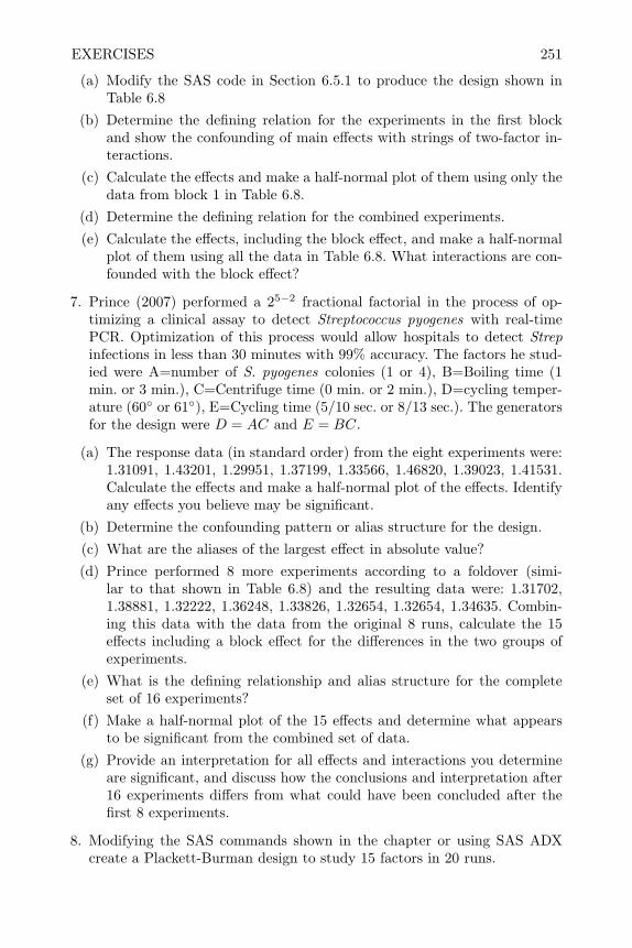
EXERCISES 251
(a) Modify the SAS code in Section 6.5.1 to produce the design shown inTable 6.8
(b) Determine the defining relation for the experiments in the first blockand show the confounding of main effects with strings of two-factor in-teractions.
(c) Calculate the effects and make a half-normal plot of them using only thedata from block 1 in Table 6.8.
(d) Determine the defining relation for the combined experiments.(e) Calculate the effects, including the block effect, and make a half-normal
plot of them using all the data in Table 6.8. What interactions are con-founded with the block effect?
7. Prince (2007) performed a 25−2 fractional factorial in the process of op-timizing a clinical assay to detect Streptococcus pyogenes with real-timePCR. Optimization of this process would allow hospitals to detect Strepinfections in less than 30 minutes with 99% accuracy. The factors he stud-ied were A=number of S. pyogenes colonies (1 or 4), B=Boiling time (1min. or 3 min.), C=Centrifuge time (0 min. or 2 min.), D=cycling temper-ature (60 or 61), E=Cycling time (5/10 sec. or 8/13 sec.). The generatorsfor the design were D = AC and E = BC.
(a) The response data (in standard order) from the eight experiments were:1.31091, 1.43201, 1.29951, 1.37199, 1.33566, 1.46820, 1.39023, 1.41531.Calculate the effects and make a half-normal plot of the effects. Identifyany effects you believe may be significant.
(b) Determine the confounding pattern or alias structure for the design.(c) What are the aliases of the largest effect in absolute value?(d) Prince performed 8 more experiments according to a foldover (simi-
lar to that shown in Table 6.8) and the resulting data were: 1.31702,1.38881, 1.32222, 1.36248, 1.33826, 1.32654, 1.32654, 1.34635. Combin-ing this data with the data from the original 8 runs, calculate the 15effects including a block effect for the differences in the two groups ofexperiments.
(e) What is the defining relationship and alias structure for the completeset of 16 experiments?
(f) Make a half-normal plot of the 15 effects and determine what appearsto be significant from the combined set of data.
(g) Provide an interpretation for all effects and interactions you determineare significant, and discuss how the conclusions and interpretation after16 experiments differs from what could have been concluded after thefirst 8 experiments.
8. Modifying the SAS commands shown in the chapter or using SAS ADXcreate a Plackett-Burman design to study 15 factors in 20 runs.

252 FRACTIONAL FACTORIAL DESIGNS
9. Consider the data from the chemical reaction experiment from Box andMeyer (1993) shown in the table below. The first five columns defined thefactor settings for the experiment, and the remaining unassigned columnsrepresent aliased interactions.
Table 6.15 Design Matrix Response for Reactor Experimentrun A B C D E 6 7 8 9 10 11 %Reacted
1 + - + - - - + + + - + 562 + + - + - - - + + + - 933 - + + - + - - - + + + 674 + - + + - + - - - + + 605 + + - + + - + - - - + 776 + + + - + + - + - - - 657 - + + + - + + - + - - 958 - - + + + - + + - + - 499 - - - + + + - + + - + 44
10 + - - - + + + - + + - 6311 - + - - - + + + - + + 6312 - - - - - - - - - - - 61
(a) Use proc glm to calculate the effects for all eleven columns and make ahalf-normal plot.
(b) Use proc reg to perform an all subsets regression using all main effectsand two-factor interactions as candidate variables.
(c) What model do you feel is appropriate for the data?(d) What factor settings would you recommend to maximize the %Reacted.
10. Curtis et al. (1982) proposed to conduct an experiment to study the effectof four factors in the software development process upon the software lifecycle cost and the number of residual errors. The factors and levels areshown in the table below:
LevelsLabel Factor − +A Design methodology functionally structured data structuredB Programming language Ada CMS-2C Source language debugger No YesD Testing strategy Functional Structural
(a) A 24−1 fractional factorial design was proposed to study these factorssince the cost of building and testing a multi-module system can be quitehigh. The author proposed to use a design with generator C = AB.Suggest a better design generator and explain why you think it wouldbe better.

EXERCISES 253
(b) If the number of levels for factorA=Design methodologies andB=Programinglanguages were three rather than two, what is the minimum number ofruns required for an orthogonal array design for studying two factors atthree levels and two factors at two levels (i.e., 32 × 22)?
(c) Use the SAS Mkt macros to create a 12-run fractional factorial designfor a 32 × 22.
11. Kamohara et al. (2001) used an 18 run orthogonal fractional factorial toinvestigate the effect of 8 factors (37×2) upon the Vt variance of MOSFETs(metaloxidesemiconductor field-effect transistor). The list of factors andnumber of levels is shown below. The list of experiments and the response,
Label Factor Number of LevelsA SD Energy 2B SDE Energy and Dose 3C Halo Energy 3D Halo Dose 3E Halo Tilt Angle 3F Vt-Impala. Dose 3G Vt-Impala. Energy 3H SD Dose 3
S/N, is shown in the table below. The purpose of the experiments was tofind factor level settings to maximize S/N.
Run A B C D E F G H S/N1 1 1 1 1 1 1 1 1 -0.662 1 1 2 2 2 2 2 2 -0.663 1 1 3 3 3 3 3 3 -0.694 1 2 1 1 2 2 3 3 -0.675 1 2 2 2 3 3 1 1 -0.826 1 2 3 3 1 1 2 2 -0.697 1 3 1 2 1 3 2 3 -0.758 1 3 2 3 2 1 3 1 -0.659 1 3 3 1 3 2 1 2 -0.66
10 2 1 1 3 3 2 2 1 -0.8011 2 1 2 1 1 3 3 2 -0.6712 2 1 3 2 2 1 1 3 -0.6513 2 2 1 2 3 1 3 2 -1.0414 2 2 2 3 1 2 1 3 -0.6915 2 2 3 1 2 3 2 1 -0.6716 2 3 1 3 2 3 1 2 -0.6717 2 3 2 1 3 1 2 3 -0.6818 2 3 3 2 1 2 3 1 -0.71

254 FRACTIONAL FACTORIAL DESIGNS
(a) Read the data into SAS and create coded factor levels for the two-level factor A and linear and quadratic contrasts variables for the three-level factors in the SAS data step (i.e., if B=1 then do; Bl=-.707107;Bq=.4082483; end; if B=2 then do; Bl=0; Bq=-.816497; end; etc.)using the contrast coefficients as shown in Section 2.8.1.
(b) Fit a regression model to the data using the coded factor levels for thetwo-level factor and the linear and quadratic contrast variables for eachthree-level factor in the design.
(c) Fit the model including only the five independent variables with thehighest absolute t-statistics that you found in (b).
(d) Fit the model that includes the coded factor levels for A, the linearcontrast on C, the quadratic contrast on D, the interaction or productof the quadratic contrasts for B and D, the interaction or product of thelinear contrast of F and the quadratic contrast on H, and experimentwith a few other models of your choice.
(e) Do you think a plausible model can be found for the data after these 18experiments? Why or why not?

CHAPTER 7
Incomplete and Confounded BlockDesigns
7.1 Introduction
One of the two purposes for randomized block designs, described in Chapter4, was to group heterogeneous experimental units together in homogeneoussubgroups called blocks. This increases the power or precision for detectingdifferences in treatment groups. The overall F -test for comparing treatmentmeans, in a randomized block design, is a ratio of the variability among treat-ment means to the variability of experimental units within the homogeneousblocks.
One restriction on randomized block designs is that the number of experi-mental units in the block must be greater than or equal to the number of levelsof the treatment factor. For the RCB design the number of experimental unitsper block, t, is equal to the number of levels of the treatment factor, and forthe GCB design the number of experimental units per block is equal to thenumber of levels of the treatment factor times the number of replicates perblock, tr.
When the number of levels of the treatment factor is large in a randomizedblock design, the corresponding number of experimental units per block mustalso be large. This could cause a problem. For example, frequently in agri-cultural field tests of new hybrid crops (called varietal trials) the number ofhybrids could be very large (50-100). Since the experimental units are plotsof land, the larger the number of plots included in a block the more diversethese plots will likely be since they cover a wider physical area. When experi-mental units are small animals, it is possible to group them into small blocksof litter mates that are genetically more homogeneous. However, when largerblock sizes are required, animals from different litters will be included withina block, making the groups less homogeneous. Less homogeneity within theblocks results in more variability among the experimental units within a blockand defeats one of the purposes for using a randomized block design.
One solution to the problem is to construct block designs where each blockonly contains a subset of the possible levels of the treatment factor. In that waythe number of experimental units per block, or block size, can be kept small.Designs that do this are called incomplete block designs. There are two basictypes of incomplete block designs. The first type is called a balanced incom-plete block design or BIB, and the other type is called a partially balancedincomplete block design or PBIB. Incomplete block designs are also useful
255

256 INCOMPLETE AND CONFOUNDED BLOCK DESIGNS
when the physical requirements of experimentation make it impossible to testall levels of the treatment factor within each block of experimental units. In-complete block designs are commonly used in agricultural experimentation,animal science, educational testing and food science.
As an example of a situation where an incomplete block design would beuseful, consider the following situation. In food science, taste panels are oftenused to test palatability of new recipes for new food products. In these panels,subjects are asked to taste and rate different recipes. The different recipesrepresent the levels of the treatment factor. A random sample of subjects (orthe experimental units) is included to represent the potential market. Sincethere is wide variability in taste among subjects it is better to use a blockeddesign where each subject tastes and rates each recipe. However, if there aremany recipes to be tested, subjects will lose their ability to discriminate andit will be difficult to detect any differences. A solution is to have each subject(block) taste only a subset of the recipes.
7.2 Balanced Incomplete Block (BIB) Designs
Care must be taken when choosing the subset of treatment combinationstested in each block of an incomplete block design. If one treatment factorlevel is left out of every block, it cannot be compared to the other treatmentlevels. If different treatment levels are unequally represented, some compar-isons of factor levels will have more precision than others.
The optimal way to create an incomplete block design is to have each treat-ment level equally replicated and appearing within a block with every othertreatment level an equal number of times. This is called a balanced incompleteblock design or BIB. By doing this, all pairwise differences of least squarestreatment means will have the same standard error, and the power for detect-ing a difference in any two means will be the same.
The simplest way to construct a BIB for the case where there are t levelsof the treatment factor and k < t experimental units per block is to formall possible subsets of k treatment levels chosen from t. For example, in thetaste panel described above, if there were t = 6 recipes to be tested, and itwas determined that each subject could taste at most k = 3 recipes withoutlosing discriminatory power,
(63
)= 20 subjects would be required. All possible
subsets are listed below.(1 2 3), (1 2 4), (1 2 5), (1 2 6), (1 3 4)(1 3 5), (1 3 6), (1 4 5), (1 4 6), (1 5 6)(2 3 4), (2 3 5), (2 3 6), (2 4 5), (2 4 6)(2 5 6), (3 4 5), (3 4 6), (3 5 6), (4 5 6)
Thus, subject one would taste recipes 1, 2 and 3 in a random order; subject2 would taste recipes 1, 2 and 4, etc. This plan is completely balanced inthat each treatment level or recipe is replicated r = 10 times (or tasted by 10subjects) and each pair of treatment levels occurs together in the same blockλ = 4 times. For example, treatment levels 1 and 2 occur together only in the

BALANCED INCOMPLETE BLOCK (BIB) DESIGNS 257
first four blocks on the first line above. By inspection, it can be seen that allpairs of treatment levels occur together in only four blocks.
Although taking all possible subsets of size k chosen from t is the simplestway to form a balanced incomplete block design, there may be other balancedincomplete block designs that require fewer blocks. If the precision of thedesign does not require as many as
(bk
)blocks, there would be no need to
use that many. For example, if a practical size difference in recipes could bedetected with less than 20 subjects and 10 replicates of each treatment level,in the taste test panel, perhaps a BIB design could be found with less than20 blocks. If r is the number of times a treatment level is replicated in anincomplete block design, λ is the number of times each treatment level occurswith every other treatment level in the same block, t is the number of levels ofthe treatment factor, k is the number of experimental units in a block, and bis the number of blocks, then the following requirements must be met in orderfor that design to be a BIB design.
b ≥ t (7.1)tr = bk (7.2)
λ(t− 1) = r(k − 1) (7.3)
These relations can be used to find the minimum number of blocks requiredfor a BIB design. Since r and λ must be integers, by Equation (7.3) we seethat λ(t − 1) must be divisible by k − 1. If t = 6 and k = 3, as in the tastetest panel, 5λ must be divisible by 2. The smallest integer λ for which thisis satisfied is λ = 2. Therefore, it may be possible to find a BIB with λ = 2,r = 10/2 = 5, and b = (6 × 5)/3 = 10. In versions of SAS 9.2 and later themacro %Mktbsize provides a quick way of finding values of λ and r to satisfyEquations (7.1) to (7.3) when given the number of levels of the treatmentfactor t and the blocksize k. For example the command: tries values of b from
%mktbsize(t=6, k=3, b=6 to 100)
6 to 100 until a solution is found. The results are shown below.
nt k b r Lambda Total
Number of Block Number Treatment Pairwise SampleTreatments Size of Blocks Frequency Frequencies Size
6 3 10 5 2 30
Fisher (1940) showed that even though Equations (7.1) - (7.3) are satisfiedfor some combination of t, b, r, λ and k, a corresponding BIB may not exist.If a BIB does exist, Kiefer (1958) and Kshirsager (1958) have shown that it isD-optimal, thus it can be found using SAS proc optex that was described in
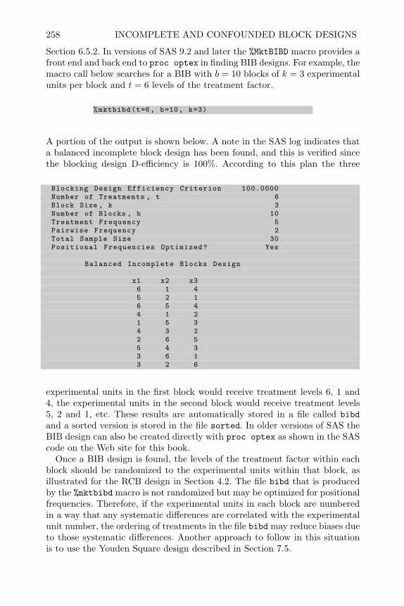
258 INCOMPLETE AND CONFOUNDED BLOCK DESIGNS
Section 6.5.2. In versions of SAS 9.2 and later the %MktBIBD macro provides afront end and back end to proc optex in finding BIB designs. For example, themacro call below searches for a BIB with b = 10 blocks of k = 3 experimentalunits per block and t = 6 levels of the treatment factor.
%mktbibd(t=6, b=10, k=3)
A portion of the output is shown below. A note in the SAS log indicates thata balanced incomplete block design has been found, and this is verified sincethe blocking design D-efficiency is 100%. According to this plan the three
Blocking Design Efficiency Criterion 100.0000Number of Treatments , t 6Block Size , k 3Number of Blocks , b 10Treatment Frequency 5Pairwise Frequency 2Total Sample Size 30Positional Frequencies Optimized? Yes
Balanced Incomplete Blocks Design
x1 x2 x36 1 45 2 16 5 44 1 21 5 34 3 22 6 55 4 33 6 13 2 6
experimental units in the first block would receive treatment levels 6, 1 and4, the experimental units in the second block would receive treatment levels5, 2 and 1, etc. These results are automatically stored in a file called bibdand a sorted version is stored in the file sorted. In older versions of SAS theBIB design can also be created directly with proc optex as shown in the SAScode on the Web site for this book.
Once a BIB design is found, the levels of the treatment factor within eachblock should be randomized to the experimental units within that block, asillustrated for the RCB design in Section 4.2. The file bibd that is producedby the %mktbibd macro is not randomized but may be optimized for positionalfrequencies. Therefore, if the experimental units in each block are numberedin a way that any systematic differences are correlated with the experimentalunit number, the ordering of treatments in the file bibd may reduce biases dueto those systematic differences. Another approach to follow in this situationis to use the Youden Square design described in Section 7.5.

ANALYSIS OF INCOMPLETE BLOCK DESIGNS 259
7.3 Analysis of Incomplete Block Designs
The model for an incomplete block design is
yij = µ+ bi + τj + εij (7.4)
which is identical to the model for a randomized complete block design givenin Section 4.3. However, the analysis is slightly different due to the missingobservations.
7.3.1 An Example
Consider the data from a taste panel experiment reported by Moskowitz(1988), shown in Table 7.1. This experiment is a BIB with t=4 levels of thetreatment factor or recipe, and blocksize k=2. Thus each panelist tastes onlytwo of the four recipes in a random order, and assigns a category scale score.Category scales are commonly used in assessing food likes or dislikes and con-sist of numbers 1 to 10 that represent descriptive categories. Only
(42
)= 6
blocks or panelists are required for a BIB, but in this experiment that numberwas doubled in order to increase the power for detecting differences. Thus thefirst six panelists and the last six are a repeat of the same BIB design. Subjectsparticipating in the taste panel were randomly assigned to panelist numbersand the order of the two recipes tasted by each panelist was randomized.
Table 7.1 Data from BIB Taste TestRecipe
Panelist A B C D1 5 5 - -2 7 - 6 -3 5 - - 44 - 6 7 -5 - 6 - 46 - - 8 67 6 7 - -8 5 - 8 -9 4 - - 510 - 7 7 -11 - 6 - 512 - - 7 4
When analyzing the data from an incomplete block design, the marginal treat-ment means are not unbiased estimators of the estimable effects µ + τi. Forexample, in Table 7.1 the marginal mean for recipe A could be biased low
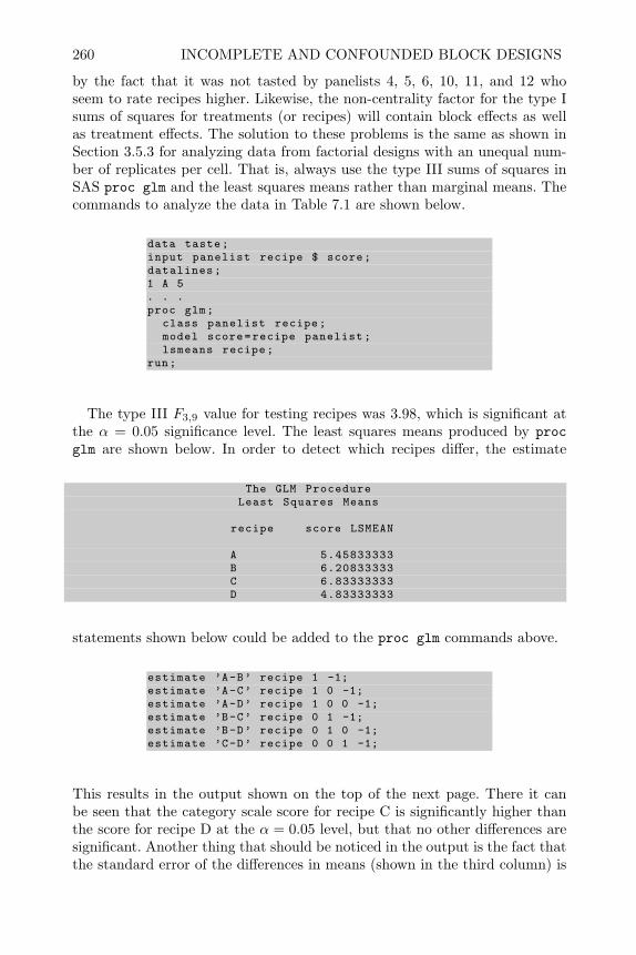
260 INCOMPLETE AND CONFOUNDED BLOCK DESIGNS
by the fact that it was not tasted by panelists 4, 5, 6, 10, 11, and 12 whoseem to rate recipes higher. Likewise, the non-centrality factor for the type Isums of squares for treatments (or recipes) will contain block effects as wellas treatment effects. The solution to these problems is the same as shown inSection 3.5.3 for analyzing data from factorial designs with an unequal num-ber of replicates per cell. That is, always use the type III sums of squares inSAS proc glm and the least squares means rather than marginal means. Thecommands to analyze the data in Table 7.1 are shown below.
data taste;input panelist recipe $ score;datalines;1 A 5. . .proc glm;
class panelist recipe;model score=recipe panelist;lsmeans recipe;
run;
The type III F3,9 value for testing recipes was 3.98, which is significant atthe α = 0.05 significance level. The least squares means produced by procglm are shown below. In order to detect which recipes differ, the estimate
The GLM ProcedureLeast Squares Means
recipe score LSMEAN
A 5.45833333B 6.20833333C 6.83333333D 4.83333333
statements shown below could be added to the proc glm commands above.
estimate ’A-B’ recipe 1 -1;estimate ’A-C’ recipe 1 0 -1;estimate ’A-D’ recipe 1 0 0 -1;estimate ’B-C’ recipe 0 1 -1;estimate ’B-D’ recipe 0 1 0 -1;estimate ’C-D’ recipe 0 0 1 -1;
This results in the output shown on the top of the next page. There it canbe seen that the category scale score for recipe C is significantly higher thanthe score for recipe D at the α = 0.05 level, but that no other differences aresignificant. Another thing that should be noticed in the output is the fact thatthe standard error of the differences in means (shown in the third column) is

PBIB-BTIB DESIGNS 261
the same for all pairs of means. This is a result of the fact that a BIB designwas used.
StandardParameter Estimate Error t Value Pr > |t|
A-B -0.75000000 0.61801654 -1.21 0.2558A-C -1.37500000 0.61801654 -2.22 0.0531A-D 0.62500000 0.61801654 1.01 0.3383B-C -0.62500000 0.61801654 -1.01 0.3383B-D 1.37500000 0.61801654 2.22 0.0531C-D 2.00000000 0.61801654 3.24 0.0102
7.3.2 Determining the Number of Replicates
A rough estimate of the number of replicates of each treatment level, r = bkt ,
or the number of blocks, b = trk , required for adequate power for detecting
a practical difference in treatment means in a BIB design can be determinedusing the following strategy. If an estimate of σ2, the variance of heterogeneousexperimental units, and ∆, the size of a practical difference in two treatmentmeans are available, then use the method of Section 3.5.2 to determine thenumber of replicates, rcrd, required for a completely randomized design.
If blocking the heterogeneous experimental units into small blocks of size kis expected to reduce the variance of experimental units within the blocks bya percentage equal to 100× (1− 1
RE ), then following Section 4.5, the numberof replicates required for the blocked design would be r = rcrd/RE and thenumber of blocks of size k in an incomplete block would be b = tr/k.
7.4 PBIB-BTIB Designs
Sometimes a BIB design requires more blocks or experimental units than areavailable or needed to obtain adequate power for detecting practical differ-ences in treatment means. In this situation, the number of blocks and ex-perimental units can be reduced by relaxing the requirements that: (1) eachtreatment level be equally replicated and (2) that it appears within a blockwith every other treatment level the same number of times. By relaxing theserequirements, each treatment level will occur more frequently in a block withsome treatment levels than it will with other treatment levels. Therefore somepairwise comparisons of treatment means will have smaller standard errorsthan others. When this is the case, the design is called a partially balancedincomplete block design or PBIB. PBIB designs are also useful in situationswhere the physical constraints of experimentation prevent some treatmentlevels from being tested together within the same block. For example, an ex-periment was conducted to compare the reading of a portable home use blood

262 INCOMPLETE AND CONFOUNDED BLOCK DESIGNS
pressure monitor to other automatic blood pressure monitors in supermarketpharmacies in order to determine if readings from the portable monitor werebiased high. The experimental unit was the pressure in a subject’s veins atthe time it was measured, and the treatment factor levels were the monitorsused to make the measurement.
Blood pressure is known to vary widely from person to person and within aperson at different times throughout a day. Blood pressure is most consistentin one person within a short period of time. Therefore the experimental unitswere blocked into homogeneous groups by subject and time. The portableblood pressure monitor could be carried into a store and a subject’s bloodpressure could be checked within a short period of time by both the auto-matic monitor within the store and the portable monitor. However, the mon-itors from two stores could not be compared within a block, or short periodof time, because the stores were physically separate. Driving between storescould completely change a subject’s blood pressure, so the partially balanceddesign shown in Table 7.2 was utilized. The response (diastolic blood) pres-sure is shown in the table. Here it can be seen that treatment level 1 (portable
Table 7.2 PBIB Design with Blood Pressure MonitorsTreatment
Portable Store A Store B Store CBlock monitor monitor monitor monitor1=(subject 1, time 1) 85 77 - -2=(subject 2, time 1) 80 75 - -3=(subject 1, time 2) 89 - 73 -4=(subject 2, time 2) 80 - 70 -5=(subject 1, time 3) 78 - - 766=(subject 2, time 3) 80 - - 70
monitor) appears in a block with every other treatment level, but the othertreatment levels never appear together in a block. The analysis of the datausing commands similar to those used for the BIB example results in the fol-lowing table of estimates. Here it can be seen that the standard errors of thedifferences between the portable monitor mean and the means for the othermonitors are smaller than the standard errors of the other comparisons.
StandardParameter Estimate Error t Value Pr > |t|
Portable -Store A 13.0000000 3.01385689 4.31 0.0229Portable -Store B 6.0000000 3.01385689 1.99 0.1406Portable -Store C 6.5000000 3.01385689 2.16 0.1199Store A-Store B -4.0000000 3.80058475 -1.05 0.3331Store A-Store C -2.0000000 3.80058475 -0.53 0.6176Store B-Store C 2.0000000 3.80058475 0.53 0.6176

PBIB-BTIB DESIGNS 263
The design for the blood pressure monitor experiment is a special case of aPBIB design that Bechhofer and Tamhane (1981) have called a BTIB (bal-anced with respect to test treatments). In these designs one treatment levelis designated as the control level and there is more interest in comparing eachof the other treatment levels with the control than there is in comparing theother treatment levels. In a BTIB design each treatment must appear thesame number of times (λ0) in a block with the control treatment, and eachtest treatment must occur the same number of times (λ1) in a block withevery other test treatment. This results in a design that is more efficient incomparing each treatment with the control but less efficient in comparisonsamong the other treatment levels. One way to form a PTIB design with tlevels of the treatment factor and block size k is to combine a control level toeach block of a BIB design with t− 1 levels of the treatment factor and blocksize k − 1.
In general there are multiple ways of creating PBIB designs. Bose et al.(1954) have published tables of some of the most useful plans. Jarrett andHall (1978) have described a class of PBIB designs called generalized cyclicincomplete block designs which have good statistical properties and are easyto create in SAS. Generalized cyclic incomplete block designs with block sizek and b = t blocks or b = n blocks, where t factors into t = m×n, and m < ncan be created following the steps listed below.
1. To form a generalized cyclic design with b = t,
(a) Start with a subset of k treatment factor levels as the initial block.
(b) Add 1 (modulo t) to each treatment level in the initial block to form thenext block.
(c) Continue adding blocks until you have t blocks.
2. To form a generalized cyclic design with b = n, where t = m×n, and m < n
(a) Start with a subset of k treatment factor levels as the initial block.
(b) Add m (modulo t) to each treatment level in the initial block to formthe next block.
(c) Continue adding blocks until you have n blocks.
To illustrate this consider creating an incomplete block design with t = 6and k = 3. The BIB design with the smallest number of blocks for this combi-nation is found (solving Equations (7.1) to (7.3) to be b = 10). A generalizedcyclical incomplete block design for testing t = 6 levels of the treatment factorcan be found with b = t = 6 blocks or b = n = 3 blocks since 6 = 2 × 3. Tofind a design with 6 blocks, following the steps above, start with a subset ofk = 3 levels of the treatment factor to be tested in the initial block, i.e.,
(1 2 4)

264 INCOMPLETE AND CONFOUNDED BLOCK DESIGNS
Next add one to each treatment level to get the treatment levels in the nextblock, i.e.,
(2 3 5)Continue this modulo 6 (i.e., 7 modulo 6 = 1, etc.) to form the following
blocks.Block Treatments
1 1 2 42 2 3 53 3 4 64 4 5 15 5 6 26 6 1 3
The treatment levels in each block would be randomized to the three exper-imental units in each block. SAS proc plan can create a generalized cyclicdesign and print the randomization. For example, the code below shows thecommands to create a generalized cyclic design with t = 6, b = 3. This codecan be modified to create the design above with t = 6 and b = 6 by changingthe specification of m and b.
proc plan seed =33373;*Note (1 2 4) are contents of the initial block , m=2;
treatments treat=3 of 6 cyclic (1 2 4) 2;*Note block=3 specifies b=n=3 blocks , EU=3 specifies k=3;
factors block=3 EU=3;output out=PBIB;
proc print data=PBIB; run;
The proc plan stores the design in a SAS data file PBIB and produces theoutput shown below.
Treatment FactorsInitialBlock /
Factor Select Levels Order Incrementtreat 3 6 Cyclic (1 2 4) / 2
block --EU - -treat -3 3 2 1 1 2 41 3 1 2 3 4 62 2 1 3 5 6 2

YOUDEN SQUARE DESIGNS (YSD) 265
The results under -treat- are the treatment factor levels in each block, andthe results under -EU- is a randomized list of the experimental units in eachblock. This can be read as follows: in block 3, the first experimental unit wouldget treatment level 4, experimental unit 2 would get treatment level 2, andexperimental 3 would get treatment level 1, etc. The proc print statementprints the randomized list shown below. This can be modified in a data stepto create a data collection worksheet.
Obs block EU treat
1 3 3 12 3 2 23 3 1 44 1 3 35 1 1 46 1 2 67 2 2 58 2 1 69 2 3 2
The analysis of PBIB designs is the same as the examples shown above. Thetype III sums of squares for treatment and the least squares means should beused. The model and assumptions are the same as for the RCB design, andthe assumptions of normality and homogeneity of experimental error variancecan be checked with the residual plots described in Section 2.4.
7.5 Youden Square Designs (YSD)
Latin square designs with two independent blocking factors were described inChapter 4. These designs could increase the precision in detecting differencesamong treatments by adjusting for variability in experimental units in twoways. However, the restriction on Latin square designs was that the numberof levels of the row blocking factor, the number of levels of the column blockingfactor, and the number of levels of the treatment factor all had to be equal.This restriction may be impractical in some situations.
In Chapter 4 an experiment was described where the purpose was to studythe effect of shelf facing on the sales of toothpaste in drug stores. In thatexample, four levels of the treatment factor (shelf facings), four levels of therow blocking factor (stores), and four levels of the column blocking factor(week of sales) were used. If the researchers desired to expand their study totest 6 different shelf facings instead of 4, they could easily increase the numberof levels of the row blocking factor and include 6 stores. However, increasingthe number of weeks would prolong the study and could be undesirable.
An alternate design called a Youden square design or YSD utilizes a com-plete block design in the column blocks, but an incomplete block design inthe row blocks. It is created by randomly dropping one or more columns from

266 INCOMPLETE AND CONFOUNDED BLOCK DESIGNS
a Latin square design. This type design can also be created and randomizedby SAS proc plan. The code below is a modification of the example shownin Chapter 4.
proc plan seed =37430;factors rows=8 ordered cols=4 ordered/noprint;treatments tmts=8 cyclic;output out=YSrows cvals=(’Store 1’ ’Store 2’ ’Store 3’ ’Store 4’’Store 5’ ’Store 6’ ’Store 7’ ’Store 8’) randomcols cvals=(’Week 1’ ’Week 2’ ’Week 3’ ’Week 4’) orderedtmts nvals =(1 2 3 4 5 6 7 8) random;
run;
This creates the design shown in the Output below. The randomized list is inthe SAS file YS and can be used to create a data collection worksheet.
The model and analysis of YSDs is identical to the model and analysis ofLatin square designs described in Chapter 4, with the exception that type IIItreatment sums of squares and least squares treatment means should be useddue to the fact that the row blocks are incomplete and do not contain all levelsof the treatment factor.
7.6 Confounded 2k and 2k−p Designs
When the experimental units are heterogeneous and can be grouped intoblocks, frequently there are too few experimental units per block to accommo-

CONFOUNDED 2k AND 2k−p DESIGNS 267
date all the treatment combinations in 2k factorial or 2k−p fractional factorialdesign. Therefore, it is impossible to use complete block designs, like thosedescribed in Section 4.5. One solution is to use an incomplete block designdescribed in the first part of this chapter with t = 2k. However this usuallyresults in many more blocks than are necessary. The effect sparsity principleand hierarchical ordering principle tell us that it is unlikely that all interac-tions (especially those above order 3) will be important. If we are willing tosacrifice the ability to estimate some interactions, 2k factorial designs can beblocked in a minimum number of blocks as long as the number of experimentalunits in each block is a power of 2.
For example, a 23 factorial design has 8 treatment combinations. By con-founding the three-factor interaction with blocks, this design can be run intwo blocks of size 4 as shown in Table 7.3 below.
Table 7.3 23 in Two Blocks of Size 4A B C Block=ABC- - - 1 -+ - + 1 -- + + 1 -+ + - 1 -- - - - - - - - - - - - - - - - - -- - + 2 ++ - - 2 +- + - 2 ++ + + 2 +
In this design, the ABC interaction effect is completely confounded betweenthe two blocks and cannot be estimated. However, since interactions betweenblock and treatment effects are assumed negligible, all the other main effectsand two-factor interactions are not confounded. Detecting the significant ef-fects from an experiment like this can be done using the graphical methodsillustrated in Section 3.7.5 and Chapter 6.
7.6.1 Confounding 2k Designs
In general a 2k factorial can be run in blocks of size 2q by choosing k − qinteraction contrasts to confound with blocks. These interactions are calledblock defining contrasts. When a 2k is run in blocks of size 2q, there will be2k/2q = 2k−q blocks. Therfore, there will be 2k−q − 1 degrees of freedom forblocks. These 2k−q − 1 degrees of freedom are accounted for by the k − qdefining block contrasts and all their generalized interactions.
As an example consider confounding a 24 factorial in blocks of size 4=22.Since k = 4 and q = 2, k − q = 2 defining block contrasts must be chosen. Ifthe three-factor interactions ABD and BCD are chosen as the block defining
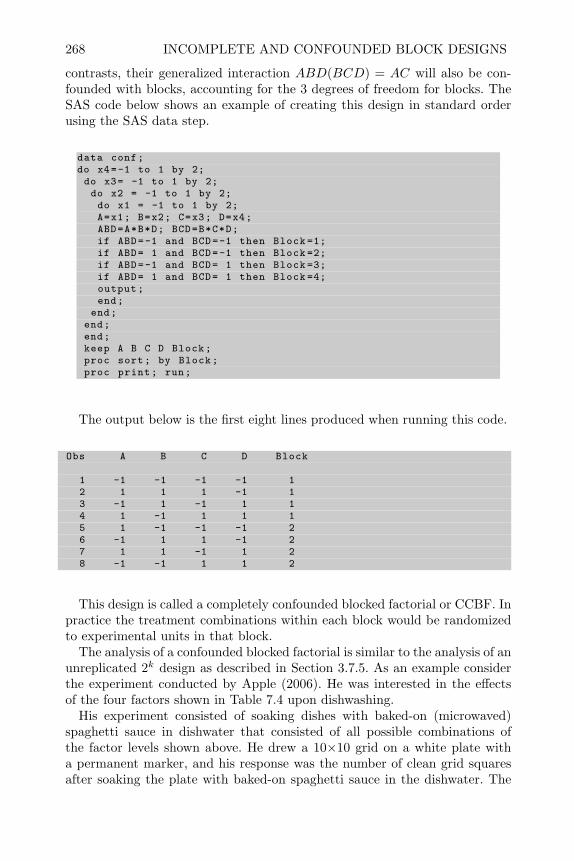
268 INCOMPLETE AND CONFOUNDED BLOCK DESIGNS
contrasts, their generalized interaction ABD(BCD) = AC will also be con-founded with blocks, accounting for the 3 degrees of freedom for blocks. TheSAS code below shows an example of creating this design in standard orderusing the SAS data step.
data conf;do x4=-1 to 1 by 2;do x3= -1 to 1 by 2;do x2 = -1 to 1 by 2;do x1 = -1 to 1 by 2;A=x1; B=x2; C=x3; D=x4;ABD=A*B*D; BCD=B*C*D;if ABD=-1 and BCD=-1 then Block =1;if ABD= 1 and BCD=-1 then Block =2;if ABD=-1 and BCD= 1 then Block =3;if ABD= 1 and BCD= 1 then Block =4;output;end;
end;end;end;keep A B C D Block;proc sort; by Block;proc print; run;
The output below is the first eight lines produced when running this code.
Obs A B C D Block
1 -1 -1 -1 -1 12 1 1 1 -1 13 -1 1 -1 1 14 1 -1 1 1 15 1 -1 -1 -1 26 -1 1 1 -1 27 1 1 -1 1 28 -1 -1 1 1 2
This design is called a completely confounded blocked factorial or CCBF. Inpractice the treatment combinations within each block would be randomizedto experimental units in that block.
The analysis of a confounded blocked factorial is similar to the analysis of anunreplicated 2k design as described in Section 3.7.5. As an example considerthe experiment conducted by Apple (2006). He was interested in the effectsof the four factors shown in Table 7.4 upon dishwashing.
His experiment consisted of soaking dishes with baked-on (microwaved)spaghetti sauce in dishwater that consisted of all possible combinations ofthe factor levels shown above. He drew a 10×10 grid on a white plate witha permanent marker, and his response was the number of clean grid squaresafter soaking the plate with baked-on spaghetti sauce in the dishwater. The

CONFOUNDED 2k AND 2k−p DESIGNS 269
Table 7.4 Factors for Dishwashing ExperimentLevels
Factor (−) (+)A-Water Temperature 60 Deg F 115 Deg FB-Soap Amount 1 tbs 2tbsC-Soaking Time 3 min 5 minD-Soap Brand WF UP
experimental unit was the baked-on spaghetti sauce, and in order to generalizehis conclusions, he included four blocks which consisted of combinations oftwo different brands of spaghetti sauce and two different baking times in themicrowave, as shown in the table below. In this experiment, it would have
Table 7.5 Blocks for Dishwashing ExperimentBlock Type Sauce Microwave Time
1 Store Brand 1 min2 Premium Brand 1 min3 Store Brand 1:30 min4 Premium Brand 1:30 min
been possible to run a complete block factorial design where all combinationsof the treatment factor levels from Table 7.4 were included in each block. Thiswould have taken a total of 4×16=64 experiments. However, considering thehierarchical ordering principle, some interactions were confounded in order toreduce the total number of experiments. Using the same design shown earlier,ABD and BCD and their generalized interaction ABD(BCD) = AC wereconfounded with blocks, resulting in 16 experiments or plates grouped into4 blocks with 4 experimental units in each block. The design and response(number of clean grid squares) is shown in Table 7.6 on the next page.
To analyze the data, the factorial model was fit that included all maineffects and interactions, except ABD, BCD and AC that are confoundedwith blocks. The SAS proc glm commands to do this are shown below.
proc glm data =comb;class Block;model y=Block A B C D A*B A*D B*C B*D C*DA*B*C A*C*D A*B*C*D/solution;ods output ParameterEstimates=sol;
run;
Since there were no replicates in the experiment, a half-normal plot of theeffects was used to determine the significant effects and interactions. The SAScode below Table 7.6 produces the half-normal plot. It is the same as the code
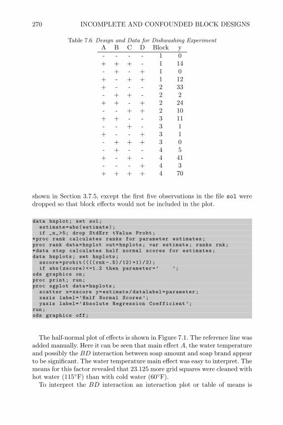
270 INCOMPLETE AND CONFOUNDED BLOCK DESIGNS
Table 7.6 Design and Data for Dishwashing ExperimentA B C D Block y- - - - 1 0+ + + - 1 14- + - + 1 0+ - + + 1 12+ - - - 2 33- + + - 2 2+ + - + 2 24- - + + 2 10+ + - - 3 11- - + - 3 1+ - - + 3 1- + + + 3 0- + - - 4 5+ - + - 4 41- - - + 4 3+ + + + 4 70
shown in Section 3.7.5, except the first five observations in the file sol weredropped so that block effects would not be included in the plot.
data hnplot; set sol;estimate=abs(estimate);if _n_>5; drop StdErr tValue Probt;
*proc rank calculates ranks for parameter estimates;proc rank data=hnplot out=hnplots; var estimate; ranks rnk;*data step calculates half normal scores for estimates;data hnplots; set hnplots;
zscore=probit ((((rnk -.5)/12) +1)/2);if abs(zscore)<=1.2 then parameter=’ ’;
ods graphics on;proc print; run;proc sgplot data=hnplots;
scatter x=zscore y=estimate/datalabel=parameter;xaxis label=’Half Normal Scores ’;yaxis label=’Absolute Regression Coefficient ’;
run;ods graphics off;
The half-normal plot of effects is shown in Figure 7.1. The reference line wasadded manually. Here it can be seen that main effect A, the water temperatureand possibly the BD interaction between soap amount and soap brand appearto be significant. The water temperature main effect was easy to interpret. Themeans for this factor revealed that 23.125 more grid squares were cleaned withhot water (115F) than with cold water (60F).
To interpret the BD interaction an interaction plot or table of means is

CONFOUNDED 2k AND 2k−p DESIGNS 271
Figure 7.1 Half-Normal Plot of Absolute Regression Coefficients from DishwashingExperiment
required. Figure 7.2 shows the interaction plot. Here it can be seen that in-creasing the amount of WF brand soap from 1 tablespoon to 2 tablespoonsactually decreases the number of clean grid squares on the plate being soaked,while increasing the amount of UP brand soap from 1 tablespoon to 2 table-spoons has the opposite effect and increases the number of clean grid squares.According to the effect heredity principle, it would be unusual to have aninteraction between two factors that don’t have significant main effects. This,along with the fact that the BD interaction does not appear to be signifi-cant using the graphical techniques of Box and Meyer (1986a), Lawson et al.(1998) or Lenth (1989), would justify ignoring this unusual finding. Therefore,the only thing that seems to have a significant effect on the ease of removingbaked-on spaghetti sauce is the temperature of the dishwater.
Blocks (not shown in the normal plot) also accounted for a large proportionof the sums of squares. If the block term were not included in the model, noneof the factor effects would be determined significant. If experimental units hadbeen restricted to one brand of spaghetti sauce and one microwave time, theconclusions regarding the dishwater would only apply to that brand of sauceand baking time.

272 INCOMPLETE AND CONFOUNDED BLOCK DESIGNS
Figure 7.2 Interaction Plot for Soap Amount × Soap Brand
7.6.2 Confounding in 2k−p Designs
A 2k−p fractional factorial can also be easily blocked by confounding inter-actions if the block size is a power of two. For example, consider the 25−2
fractional factorial shown in Section 6.3. In Table 7.7 the eight runs in thisdesign are split into two blocks by using the BC interaction as the block defin-ing contrast. When there is only one block defining contrast in a full factorial
Table 7.7 Blocked 25−2 DesignA B C D E Block=BC− − − + + 2 ++ − − − − 2 +− + − − + 1 −+ + − + − 1 −− − + + − 1 −+ − + − + 1 −− + + − − 2 ++ + + + + 2 +
design, only that interaction is confounded with the difference in blocks. How-ever, in a one-fourth fractional factorial, each effect that can be estimated is

CONFOUNDED 2k AND 2k−p DESIGNS 273
aliased with three other effects due to the fractionation. In the example abovethe generators for the quarter fraction were D = AB and E = AC, result-ing in the defining relation for the fraction I = ABD = ACE = BCDE.Multiplying through the defining relation for the fractional factorial by theblock defining contrast, we see that BC = ACD = ABE = DE and that fourinteractions are actually confounded with the blocks.
In general, when a 2k−p fractional factorial is blocked into blocks of size2q, there will be 2k−p/2q = 2k−p−q blocks. k − p − q interactions must bechosen as block defining contrasts. The block defining contrasts and all theirgeneralized interactions will account for the 2k−p−q − 1 degrees of freedomfor blocks, and each interaction that is confounded will also be aliased with2p − 1 other interactions due to the fractionization. These designs are calledcompletely confounded blocked fractional factorial or CCBFF.
To illustrate the design and analysis of a confounded 2k−p design, considerthe experiment described by Porter and Busch (1978). The purpose was toexplore the effects of the eight variables shown in Table 7.8 on survival andgrowth of neonatal deer mice. Knowledge of survival and growth of any speciesmay aid in understanding aspects of animal distribution. They used a 1
16 thfractional factorial design to identify variables affecting the ability of wildfemale deer mice to raise young to weaning. This was a screening experimentwith the purpose of identifying significant main effects that would be studiedlater in further experiments.
Table 7.8 Factors and Levels for Mouse Growth ExperimentLevels
Factor Description − +A Sprouts None Free AccessB Frequency of weighing Once per day Once per 3 daysC Nest box No YesD Remove young No YesE Male presence Yes NoF Exercise wheel Locked FreeG Available food 80 percent Free accessH Available water 80 percent Free access
The generators for the 28−4 fractional design were E = BCD, F = ACD,G = ABC, and H = ABD, resulting in the defining relation
I = BCDE = ACDF = ABCG = ABDH = ABEF = ADEG = ACEH
= BDFG = BCFH = CDGH = CEFG = DEFH = BEGH = AFGH
= ABCDEFGH
This was a resolution IV fraction and the eight main effects were confoundedwith strings of three-factor and higher-order interactions. In addition, there

274 INCOMPLETE AND CONFOUNDED BLOCK DESIGNS
were 7 strings of estimable confounded two-factor interactions listed below.
AB + CG+DH + EF
AC +BG+DF + EH
BC +AG+DE + FH
AD +BH + CF + EG
BD +AH + CE + FG
CD +AF +BE +GH
CH +AE +BF +DG
The experimenters desired to block the experiments into 8 blocks of 21 = 2runs each. This would allow them to prevent biases from uncontrolled vari-ables, such as time of year, over the duration of their experiments. Doing thiswould require choosing k−p−q = 8−4−1 = 3 block defining contrasts. Theseblock defining contrasts, along with their generalized interactions, would ac-count for the 8-1=7 degrees of freedom for blocks.
The block defining contrasts that were chosen were AB + CG + DH +EF , AC + BG + DF + EH, and AD + BH + CF + EG. The two-factorgeneralized interactions are AB(AC) = BC (or BC + AG + DE + FH),AB(AD) = BD (or BD + AH + CE + FG), and AC(AD) = CD (or CD +AF + BE + GH). Finally, the three-factor generalized interaction can beidentified by substituting BH for AD, since AD is confounded with BHto get AB(AC)(AD) = AB(AC)(BH) = CH, or CH + AE + BF + DG.Therefore, using the three block defining contrasts AB + CG + DH + EF ,AC+BG+DF+EH, and AD+BH+CF+EG actually confounds all of the 7confounded strings of two-factor interactions (shown above) with blocks. Theresearchers were willing to give up information on all two-factor interactionsto prevent biases because this was a screening experiment where they weresatisfied to get information about the relative importance of the main effects.
Each run of the design was started on the day a female’s young were bornand terminated either when they had all died or otherwise at 21 days. Theresponse was the weight at weaning. The design and results are shown in Table7.9. Mice were grouped into blocks of two sequentially as they gave birth. Thetwo treatment combinations within each block were randomized to the micein that block.

CONFOUNDED 2k AND 2k−p DESIGNS 275
Table 7.9 Design and Results for Mouse Growth ExperimentFactors
Block A B C D E F G H weight1 + − − − − + + + 9.01 − + + + + − − − 0.0
- - - - - - - - - - - - - - - - - - - - - - - - - - - - - - - - -2 − − + + − − + + 9.252 + + − − + + − − 4.90
- - - - - - - - - - - - - - - - - - - - - - - - - - - - - - - - -3 + − + − + − − + 8.803 − + − + − + + − 4.35
- - - - - - - - - - - - - - - - - - - - - - - - - - - - - - - - -4 − − − + + + − + 0.04 + + + − − − + − 7.43
- - - - - - - - - - - - - - - - - - - - - - - - - - - - - - - - -5 − + + − − + − + 5.355 + − − + + − + − 9.90
- - - - - - - - - - - - - - - - - - - - - - - - - - - - - - - - -6 + + − + − − − + 2.606 − − + − + + + − 7.43
- - - - - - - - - - - - - - - - - - - - - - - - - - - - - - - - -7 − + − − + − + + 6.807 + − + + − + − − 3.93
- - - - - - - - - - - - - - - - - - - - - - - - - - - - - - - - -8 + + + + + + + + 10.208 − − − − − − − − 4.87
The SAS data step commands to create this blocked fractional factorial areshown on the next page.
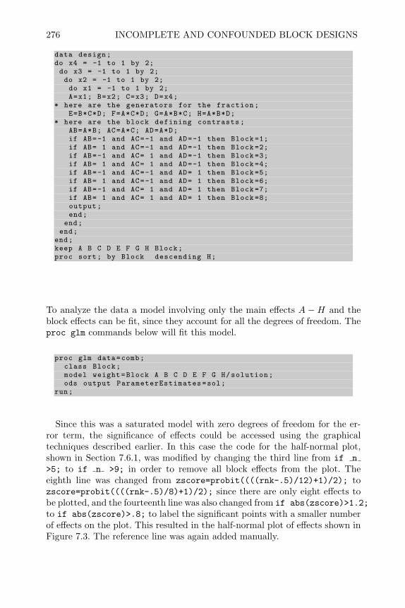
276 INCOMPLETE AND CONFOUNDED BLOCK DESIGNS
data design;do x4 = -1 to 1 by 2;do x3 = -1 to 1 by 2;do x2 = -1 to 1 by 2;do x1 = -1 to 1 by 2;A=x1; B=x2; C=x3; D=x4;
* here are the generators for the fraction;E=B*C*D; F=A*C*D; G=A*B*C; H=A*B*D;
* here are the block defining contrasts;AB=A*B; AC=A*C; AD=A*D;if AB=-1 and AC=-1 and AD=-1 then Block =1;if AB= 1 and AC=-1 and AD=-1 then Block =2;if AB=-1 and AC= 1 and AD=-1 then Block =3;if AB= 1 and AC= 1 and AD=-1 then Block =4;if AB=-1 and AC=-1 and AD= 1 then Block =5;if AB= 1 and AC=-1 and AD= 1 then Block =6;if AB=-1 and AC= 1 and AD= 1 then Block =7;if AB= 1 and AC= 1 and AD= 1 then Block =8;output;end;
end;end;
end;keep A B C D E F G H Block;proc sort; by Block descending H;
To analyze the data a model involving only the main effects A −H and theblock effects can be fit, since they account for all the degrees of freedom. Theproc glm commands below will fit this model.
proc glm data=comb;class Block;model weight=Block A B C D E F G H/solution;ods output ParameterEstimates=sol;
run;
Since this was a saturated model with zero degrees of freedom for the er-ror term, the significance of effects could be accessed using the graphicaltechniques described earlier. In this case the code for the half-normal plot,shown in Section 7.6.1, was modified by changing the third line from if n>5; to if n >9; in order to remove all block effects from the plot. Theeighth line was changed from zscore=probit((((rnk-.5)/12)+1)/2); tozscore=probit((((rnk-.5)/8)+1)/2); since there are only eight effects tobe plotted, and the fourteenth line was also changed from if abs(zscore)>1.2;to if abs(zscore)>.8; to label the significant points with a smaller numberof effects on the plot. This resulted in the half-normal plot of effects shown inFigure 7.3. The reference line was again added manually.

CONFOUNDED 2k AND 2k−p DESIGNS 277
Figure 7.3 Half-Normal Plot of Absolute Regression Coefficients from Mouse GrowthExperiment
From the half-normal plot it is clear that the only factor having a significanteffect on the weaning weight was G - available food. The calculated effectshowed that the weaning weight was on the average 4.24g higher for pups offemale mice given free access to food compared to pups of mice whose foodintake was restricted to 80% of normal. This is the same conclusion that theauthors of the article had reached.
7.6.3 Criteria for Choosing Block Defining Contrasts
Care must be exercised when choosing the block defining contrasts for 2k fullfactorial or 2k−p fractional factorial designs. To illustrate why, consider thefollowing two examples.
Example 1 consists of blocking a 25 factorial into 8 blocks of size 22 =4. To do this k − q = 5 − 2 = 3 block defining contrasts must be chosen.Suppose the interactions ABC, CDE and ABCDE are chosen as the blockdefining contrasts. Their two-factor generalized interactions ABC(CDE) =ABDE, ABC(ABCDE) = DE, CDE(ABCDE) = AB, and their three-factor generalized interaction ABC(CDE)(ABCDE) = ABC(AB) = C arealso confounded, accounting for the 7 degrees of freedom for blocks. The blockdefining contrasts were all three-factor interactions and above, yet one of theirgeneralized interactions is main effect C that we would not want to confound

278 INCOMPLETE AND CONFOUNDED BLOCK DESIGNS
with blocks. A better choice would be to choose ACE, BCE and ABCD asblock defining contrasts. Their generalized interactions include no main effects.
Example 2 consists of blocking a 26−2 fractional factorial in four blocksof size 22 = 4. To do this k − p − q = 6 − 2 − 2 = 2 block definingcontrasts must be chosen. If the generators for the fractional factorial areE = ABC and F = ABD, the defining relation for the fractional factorial isI = ABCE = ABDF = CDEF . If the block defining contrasts chosen areBDE and ACDE, they and their generalized interaction BDE(ACDE) =ABC will account for the three degrees of freedom for blocks. However, be-cause of the fractionation we see that all of the following aliases also becomeconfounded with blocks.
BDE = ACD = AEF = BCF
ACDE = BD = BCEF = AF
ABC = E = CDF = ABDEF
Again we can see that this choice of generators results in confounding maineffect E with blocks. This was an unintended result. A better choice of blockdefining contrasts would be ACD and AB, which will not result in any maineffects being confounded with blocks.
There are many choices for block defining contrasts and fractional facto-rial generators, and each will result in different set of interactions being con-founded with blocks and a different alias structure for the design. Some choiceswill be better than others and will result in fewer low-order interactions beingconfounded with blocks and main effects. However, to find the best generatorsand block defining contrasts for a particular design problem is not a simpletask. Fortunately, statisticians have provided tables that show choices thatare optimal in certain respects.
Box et al. (1978) provide tables for block defining contrasts that will resultin a minimal number of low-order interactions being confounded with blocksin a blocked 2k design. Wu and Hamada (2000) provide a more extensive tablethat was generated by the algorithm described by Chen et al. (1993). In somecases, such as the 26 blocked into 16 blocks of size 4, Wu and Hamada’s tablesprovide a set of block defining contrasts that are better (in the sense thatfewer two-factor interactions are confounded with blocks) than the contrastsshown in Box, Hunter and Hunter’s tables.
It is more difficult to find fractional factorial generators and block definingcontrasts for 2k−p fractional factorial designs, because of the combination ofconfounding due to the block effects and fractionization. However, Wu andHamada’s book also has tables for the generators for fractional factorial 2k−p
designs along with the corresponding block defining contrasts that will resultin highest estimability order . They say that a design with estimability of ordere is one in which all factorial effects of order e or less are estimable; that isthey are not confounded with blocks or factorial effects of order less than e+1.These plans were again obtained using the algorithm of Chen et al. (1993).
SAS ADX automatically chooses block defining contrast for blocked 2k de-

CONFOUNDED 2k AND 2k−p DESIGNS 279
signs based on Box, Hunter and Hunter’s table. For 2k−p designs ADX alsochooses a reasonable set of block defining contrasts and design generatorswhich are in many cases equivalent to the optimal selection given in Wu andHamada’s tables, but in other cases are slightly worse. For example to create a26−1 design, blocked into 4 blocks of 8 experimental units each, simply define6 factors in the new two-level menu. Then, when selecting the design, clickthe show blocked designs option, as shown in Figure 7.4, and select the 32 runhalf-fraction in 4 blocks.
Figure 7.4 SAS ADX Select Design Menu
SAS ADX then generates a 26−1 design using the generator F = ABCDEand the block defining contrasts BCDE and ACDE. This is a resolutionVI fractional factorial, and if this were run in a completely randomized de-sign, all main effects and two-factor interactions would be estimable assumingfour-factor and higher-order interactions were negligible. A design like thismight be used if the experimenter was interested in estimating two-factor in-teractions. However if experimental units are heterogeneous, more power orprecision for detecting factorial effects and interactions could be achieved bysacrificing some interactions and confounding them with blocks. The blockdefining contrasts chosen by SAS ADX, are both four-factor interactions, andat first glance, it appears that no two-factor interactions will be sacrificed.However, the generalized interaction BCDE(ACDE) = AB accounts for thethird degree of freedom for blocks and due to the fractionization each interac-tion confounded with blocks has an alias that is also confounded with blocks.In this case the defining relation for the fractional factorial is I = ABCDEFand we see that BCDE = AF , ACDE = BF and AB = CDEF . So in realitythree two-factor interactions AB, AF and BF will be confounded with blocksand lost using this design.
On the other hand, Wu and Hamada’s table gives F = ABCDE as the gen-

280 INCOMPLETE AND CONFOUNDED BLOCK DESIGNS
erator of the half-fraction and ACD, BCD as the block defining contrasts forthe first 26−1 design in 4 blocks listed in their table. This plan only confoundsone two-factor interaction with blocks and is therefore slightly better than thedesign created by SAS ADX. Knowing the fraction generator and the blockdefining contrasts, this design could be created in the SAS data step like themouse growth experiment shown in Section 7.6.2.
Given information about the effects the experimenter would like to be ableto estimate, SAS proc factex uses an algorithm similar to the one proposedby Franklin (1985) to search for an acceptable set of block defining contrastsand design generators, and then to produce the resulting design. For exam-ple, the code below finds the same design produced by SAS ADX. The sizedesign=32; statement tells proc factex to create a half-fraction, and themodel resolution=max; statement tells it to search for the design and blockgenerators that will result in the highest resolution.
*this code creates 2^(6 -1) in 4 blocks of 8;proc factex;
factors A B C D E F;model resolution=max;size design =32blocks nblocks =4;output out=bd;examine aliasing;
7.7 Confounding 3 Level and p Level Factorial Designs
If every factor in a factorial has 3 levels we call the design a symmetric 3k
design. These designs can be run in blocks (CCBF) using the same strategyas shown in Section 7.6.1 by confounding portions of interactions with blocks.Confounded 3k designs can only be run in blocks of size 3q where q < k. Toillustrate the method of confounding, consider a 32 design with factors A andB, each with 3 levels. Since k = 2, this design can only be blocked in blocks ofsize 3, resulting in 3 blocks. In order to prevent main effect A and B from beingcompletely confounded with blocks, the two-factor interaction AB should beconfounded with blocks. However, there are (3 − 1) × (3 − 1) = 4 degrees offreedom for the two-factor interaction while there are only 3−1 = 2 degrees offreedom for blocks. Therefore, only part of the interaction need be confoundedwith blocks. The four degrees of freedom for AB can be partitioned into two2 degrees of freedom contrasts A + B and A + 2B, and one of these can beused to define the blocks.
If the levels of the factors A and B are represented symbolically by 0, 1 and2. The levels of the two contrasts are given by A + B modulo 3 and A + 2Bmodulo 3, as shown in the table on the top of the next page. The levels ofthese two contrasts can each be seen to have 2 degrees of freedom because theydivide the treatment combinations into three groups similar to the way thelevels of main effects A and B divide the treatments combinations into three

CONFOUNDING 3 LEVEL AND P LEVEL FACTORIAL DESIGNS 281
A B A+B A+ 2B0 0 0 00 1 1 20 2 2 11 0 1 01 1 2 01 2 0 22 0 2 22 1 0 12 2 1 0
groups. Both of these contrasts are orthogonal to main effects A and B sinceall three levels of each main effect are represented within each level of bothcontrasts. Therefore if either of these contrasts is used to define blocks neithermain effect will be confounded with blocks. The SAS code below shows howa blocked factorial could be created in the data step confounding blocks withthe A+B contrast.
data blockdes;do A = 0 to 2;do B = 0 to 2;Block=mod(A+B,3);output;end;
end;
The model, represented in SAS proc glm notation for this design, wouldbe y = Block A B;. The AB interaction, that is confounded with blocks, isleft out of the model just as it would have been in the confounded 2k and2k−p designs. Main effect A would have 2 degrees of freedom, main effect Bwould have 2 degrees of freedom, blocks would have 2 degrees of freedom, andthe error would have 2 degrees of freedom. For this design to be useful theinteraction AB would be assumed negligible.
In general when confounding 3k experiments in blocks of size 3q, k − pblock defining contrasts must be chosen. They and all of their generalizedinteractions will also be confounded with blocks. It would be difficult to choosea set of block defining contrasts by trial and error that will result in thefewest low-order interactions being confounded with blocks. Wu and Hamada(2000) give tables of block defining contrasts and design generators for 3k and3k−p designs blocked into blocks of size 3q that will result in the maximumnumber of estimable effects. These tables were determined using the algorithmdescribed by Chen et al. (1993). SAS proc factex uses a different algorithmto search for an acceptable set of block defining contrasts and design generatorsand then to produce the resulting design. For example, the code below createsa 34 design in 9 blocks of 9.
The factors statement defines the factor names and the nlev=3 option

282 INCOMPLETE AND CONFOUNDED BLOCK DESIGNS
*this code creates 3^4 in 9 blocks of 9;proc factex;
factors A B C D/nlev =3;model estimate =(A B C D A*B A*C A*D B*C B*D C*D);blocks nblocks =9;output out=tf;examine aliasing;
declares all factors to have three levels. In proc factex the number of levelsof the factors must always be a prime number (i.e., 2, 3, 5 etc.). The modelstatement declares which effects the experimenter would like to be able toestimate. In other words, these should not be confounded with block effectsor other main effects. In this case, a design is sought for that allows all maineffects and two-factor interactions to be estimated. There are three ways todefine the model. One is to list the effects to be estimated as shown above.The other two, more relevant for fractional factorial designs, are to declare theresolution desired or the fact that a minimum abberation design is requested.The blocks statement declares the number blocks in the design to be created.This will always be a power of the number of levels of the factors. The examinealiasing; option prints out a table that shows the block defining contraststhat proc factex used to come up with the design. In this example theywere A + 2B + C, A + B + 2D, A + 2C + D, and B + C + D, which areall contrasts from three-factor interactions. Since each of these contrasts has2 degrees of freedom, together they account for the 8 degrees of freedom forblocks. Therefore, the model (represented in SAS proc glm notation) thatcould be fit to the data collected using this design would be y = Block A BC D A*B A*C A*D B*C B*D C*D; or y = Block A B C D A*B A*C A*D B*CB*D C*D A*B*C*D; since neither two-factor interactions nor the four-factorinteraction are confounded with blocks.proc factex uses an algorithm to search for an appropriate set of design
generators and block defining contrasts. If it cannot find a set that will satisfythe requirements specified in the model statement, a message will be printedin the SAS log stating that no design was found.
Since proc factex allows for designs where all factors have p levels, wherep is a prime number, the code above could be changed to block a 54 factorialin 25 blocks by changing the following options: (1) change the factors optionfrom nlev=3 to nlev=5, and (2) change the number of blocks specified fromnblocks=9 to nblocks=25.
In practice, 3k or 3k−p designs and pk or pk−s designs are rarely used becauseit is unusual for all factors in a factorial design to have the same number oflevels, unless the number of levels is two. 2k and 2k−p designs are commonlyused in practice because experimenters reduce the number of levels of eachfactor to two (by choosing the two levels they feel will exhibit the maximumdifference) in order to reduce the total number of experiments. In cases wherethe number of levels of some factors cannot be reduced to 2, because they

BLOCKING MIXED-LEVEL FACTORIALS AND OAS 283
represent a discrete set of alternatives such as machine settings, mixed levelor asymmetric factorials result. The principles shown in this section, to block3k or pk experiments by confounding portions of interactions can be extendedto the mixed level factorials as shown in the next section.
7.8 Blocking Mixed-Level Factorials and OAs
A mixed level or asymmetric factorial can be represented as sm11 × sm2
2 ×· · · smγγ involving n =
∑γi=1mi factors where mi factors each has si levels. For
example, a 23 × 32 × 41 × 61 is a factorial with three factors with two levels,two factors with three levels, one factor with four levels, and one factor withsix levels. The number of levels of every factor in a mixed-level factorial iseither a prime number or a product of prime numbers. If the number of theith factor si =
∏ml=1 pl where pl are prime numbers, then the levels of the
factor si can be represented by the combination of levels of m pseudo factorseach with a prime number of levels. For example, in the 23 × 32 × 41 × 61
factorial the first three factors (A B and C) have two levels, where two is aprime number. The fourth and fifth factors (D and E) have three levels, wherethree is a prime number. The sixth factor (F ) has four levels, and 4 = 2 × 2is the product of two prime numbers. Finally, the seventh factor (G) has sixlevels, and 6 = 2 × 3 is also a product of prime numbers. The levels of thefour- and six-level factors F and G can be represented as combinations of thelevels of two- and three-level pseudo factors f1, f2, g1 and g2 as shown below.
F f1 f2 G g1 g2
————— —————0 0 0 0 0 01 1 0 1 1 12 0 1 2 0 23 1 1 3 1 0
4 0 15 1 2
7.8.1 Blocking Mixed-Level Factorials
Since the levels of each factor in a mixed-level factorial can be represented bya combination of the levels of pseudo factors with a prime number of levels,the entire factorial can be represented by a pn1
1 ×pn22 ×· · · p
ngg factorial, where
all the factors have a prime number of levels. For example the 23 × 32 ×41 × 61 factorial can be represented by a 26 × 33 factorial. The pnii are calledsub-experiments, and the classical method of confounding a mixed-level orasymmetric factorial is to apply the method described in the last section toeach sub-experiment and then combine the blocks from each sub-experiment to

284 INCOMPLETE AND CONFOUNDED BLOCK DESIGNS
form the blocks of the entire completely confounded blocked factorial (CCBF).This method will result in the greatest efficiency for estimating the effectsand interactions that are not confounded with blocks in that they will becompletely orthogonal to blocks.
Asymmetric factorials of the form sm11 × s
m22 ×· · · s
nγγ can be blocked into b
blocks of size k. However, to avoid confounding or partially confounding anymain effect, the block size k must be divisible by all the prime numbers p1 -pr that represent the number of levels of the factors or number of levels of thepseudo factors used to represent a factor.
To illustrate the classical method of blocking a mixed-level factorial, con-sider blocking the 36 treatment combinations of a 22×32 factorial. This facto-rial can be represented as a product of two sub-experiments: a 22 comprised oftwo factors A and B each at 2 levels; and a 32 comprised of two factors C andD each at 3 levels. Since the levels of all factors are prime, the block size mustbe divisible by both 2 and 3. The blocks can be found by confounding withineach sub-experiment. Since there are only two factors in each sub-experiment,and it would be undesirable to confound main effects with blocks, there isonly one interaction that can be confounded in each sub-experiment.
Confounding AB in the 22 sub-experiment results in two blocks of size 2.Confounding the C + D contrast in the 32 sub-experiment results in threeblocks of size 3. The combination of each block from the first sub-experimentwith each block of the second sub-experiment results in blocks of size k = 6,which is divisible by both 2 and 3. The interactions confounded in the completefactorial will be AB, two degrees of freedom from CD and two degrees offreedom from the product ABCD. The main effects A, B, C, D and the AC,AD, BC, BD two-factor interactions and the ABC, ABD, ACD and BCDthree-factor interactions are not confounded with blocks and are estimable.The code at the top of the next page shows how to create this design in SASproc factex.
The first use of proc factex creates a blocked design in two three-level fac-tors C and D and stores it in the SAS file d1. Specification of resolution=maxon the model statement and the nblocks=3 on the blocks statement causesproc factex to select the C + D contrast to confound this sub-experimentinto three blocks. This can be determined by examining the table printed bythe examine aliasing; statement. The second use of proc factex createsa blocked experiment in two two-level factors A and B (the default in procfactex). The option pointrep=d1 in the output statement tells proc factexto combine every block from the design d1 with every block in the design be-ing created and then store the combined result in the SAS file d2. This resultsin a design with block size 6. The block divisions from the first use of procfactex are in the variable block, while the block divisions from the seconduse of proc factex are in the variable block2. The final data step createsthe six-level blocking factor from the original two. The final result from thefile df is shown at the top of the next page. It can be the basis for creating arandomized data collection worksheet.

BLOCKING MIXED-LEVEL FACTORIALS AND OAS 285
proc factex;factors C D/nlev =3;blocks nblocks =3;model resolution=max;examine aliasing; output out=d1 ;
proc factex;factors A B;blocks nblocks =2;model resolution =max;examine aliasing; output out=d2 pointrep=d1;
data df; set d2;blk=(block -1)*3+ block2;keep blk A B C D;
proc sort; by blk;proc print; run;
Obs A B C D blk1 -1 1 -1 -1 12 -1 1 0 1 13 -1 1 1 0 14 1 -1 -1 -1 15 1 -1 0 1 16 1 -1 1 0 17 -1 1 -1 1 28 -1 1 0 0 29 -1 1 1 -1 2
10 1 -1 -1 1 211 1 -1 0 0 212 1 -1 1 -1 213 -1 1 -1 0 314 -1 1 0 -1 315 -1 1 1 1 316 1 -1 -1 0 317 1 -1 0 -1 318 1 -1 1 1 319 -1 -1 -1 -1 420 -1 -1 0 1 421 -1 -1 1 0 422 1 1 -1 -1 423 1 1 0 1 424 1 1 1 0 425 -1 -1 -1 1 526 -1 -1 0 0 527 -1 -1 1 -1 528 1 1 -1 1 529 1 1 0 0 530 1 1 1 -1 531 -1 -1 -1 0 632 -1 -1 0 -1 633 -1 -1 1 1 634 1 1 -1 0 635 1 1 0 -1 636 1 1 1 1 6

286 INCOMPLETE AND CONFOUNDED BLOCK DESIGNS
This design will allow estimation of all the terms in the model y = A B CD A*C A*D B*C B*D, but the interactions A*B and C*D are confounded withblocks and cannot be estimated.
When the levels of one or more factors in a mixed-level factorial are a prod-uct of prime powers, and can be represented by the combination of levels ofpseudo factors, no interactions among pseudo factors that represent the samefactor can be confounded in any sub-experiment. If any interaction amongpseudo factors that represents a factor is confounded, then that main effectwill also be confounded. For example, consider blocking the 72 combinationsof factor levels in a 3× 4× 6 factorial. Factor A has three levels, factor B hasfour levels, and can be represented by all combinations of two two-level pseudofactors b1 and b2, and factor C has six levels that can be represented by allcombinations of a two-level pseudo factor c1 and a three-level pseudo factor c2.Using the pseudo factors, the 3×4×6 factorial can be represented by a 23×32
factorial in prime level factors and prime level pseudo factors. The block sizemust be divisible by the prime numbers 2 and 3 to avoid confounding a maineffect, therefore blocks of size 6 or 12 may be possible.
The first sub-experiment is a 23 composed of two-level pseudo factors b1,b2, c1 and the second sub-experiment is a 32 composed of factor A and pseudofactor c2. The first sub-experiment can only be blocked into 2 blocks of 4in order to avoid confounding the b1 × b2 interaction and therefore the Bmain effect. Thus the three-factor interaction b1× b2× c1 must be confoundedwith blocks in the first sub-experiment. In the second sub-experiment theA+ c2 contrast of the AC interaction must be confounded to create 3 blocksof 3. The combination of each block from the first sub-experiment combinedwith each block from the second sub-experiment results in six blocks of 12treatment combinations, and this is the only block size that is possible withoutconfounding a main effect.
The interactions confounded with the five degrees of freedom for blocksin the combined factorial will be BC (with one degree of freedom) from thefirst sub-experiment, two degrees of freedom from AC from the second sub-experiment, and two degrees of freedom from the product ABC (i.e., b1×b2×c1× (A+ c2)). The SAS code on the next page illustrates how this design canbe created using proc factex and is similar to the previous example.
By default proc factex assigns the levels (−1, 1) to two-level factors and(−1, 0, and 1) to three-level factors, etc. The first three assignment statementsin the data step that creates the SAS file df assign the levels (0, 1, 2 ...) to thefactors A, B, and C based on the default levels or combination of levels of thepseudo factors b1 and b2, and c1 and c2 that were created by proc factex.The final assignment statement combines the block indicators from the firstfile d1 and the second file d2 to get block indicators for the combined file.
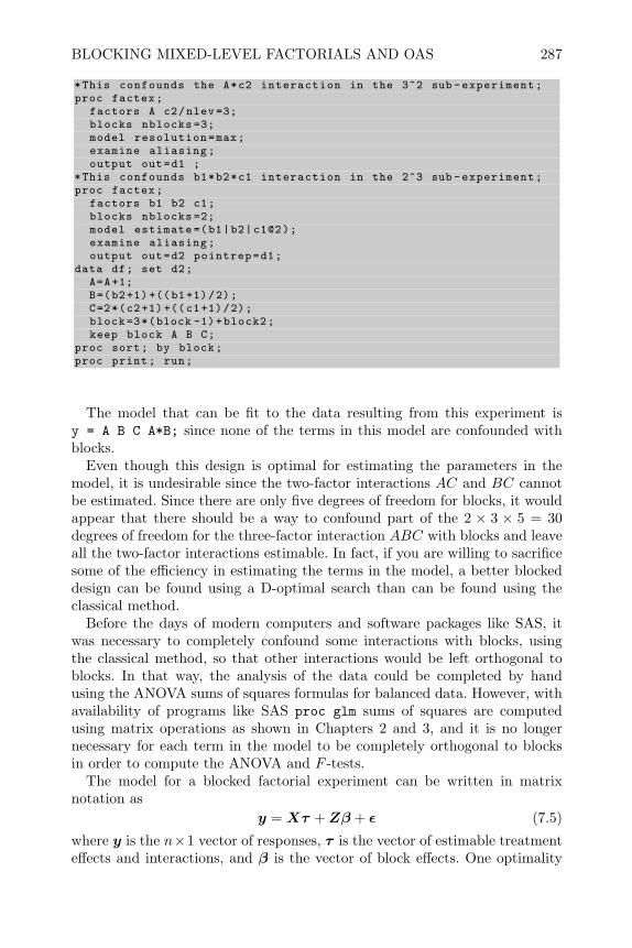
BLOCKING MIXED-LEVEL FACTORIALS AND OAS 287
*This confounds the A*c2 interaction in the 3^2 sub -experiment;proc factex;
factors A c2/nlev =3;blocks nblocks =3;model resolution=max;examine aliasing;output out=d1 ;
*This confounds b1*b2*c1 interaction in the 2^3 sub -experiment;proc factex;
factors b1 b2 c1;blocks nblocks =2;model estimate =(b1|b2|c1@2);examine aliasing;output out=d2 pointrep=d1;
data df; set d2;A=A+1;B=(b2+1)+((b1+1)/2);C=2*(c2+1) +((c1+1)/2);block=3*(block -1)+block2;keep block A B C;
proc sort; by block;proc print; run;
The model that can be fit to the data resulting from this experiment isy = A B C A*B; since none of the terms in this model are confounded withblocks.
Even though this design is optimal for estimating the parameters in themodel, it is undesirable since the two-factor interactions AC and BC cannotbe estimated. Since there are only five degrees of freedom for blocks, it wouldappear that there should be a way to confound part of the 2 × 3 × 5 = 30degrees of freedom for the three-factor interaction ABC with blocks and leaveall the two-factor interactions estimable. In fact, if you are willing to sacrificesome of the efficiency in estimating the terms in the model, a better blockeddesign can be found using a D-optimal search than can be found using theclassical method.
Before the days of modern computers and software packages like SAS, itwas necessary to completely confound some interactions with blocks, usingthe classical method, so that other interactions would be left orthogonal toblocks. In that way, the analysis of the data could be completed by handusing the ANOVA sums of squares formulas for balanced data. However, withavailability of programs like SAS proc glm sums of squares are computedusing matrix operations as shown in Chapters 2 and 3, and it is no longernecessary for each term in the model to be completely orthogonal to blocksin order to compute the ANOVA and F -tests.
The model for a blocked factorial experiment can be written in matrixnotation as
y = Xτ +Zβ + ε (7.5)
where y is the n×1 vector of responses, τ is the vector of estimable treatmenteffects and interactions, and β is the vector of block effects. One optimality

288 INCOMPLETE AND CONFOUNDED BLOCK DESIGNS
criterion that has been proposed for blocked designs is the Ds criteria (seeAtkinson et al., 2007). A Ds optimal design is one that minimizes the covari-ance matrix of the least squares estimator for τ or equivalently maximizes thedeterminant of
X′QX (7.6)
where
Q = I − Z(Z′Z)−1Z′. (7.7)
Designs where blocks are orthogonal to treatment effects, or X′Z = 0, are100% Ds efficient.
Applying the classical method separately to symmetric sub-experimentsresults in designs that have known confounding patterns and are 100% Ds
efficient for estimating the effects and interactions, τ , that are not confoundedwith the block differences (since they will be orthogonal to blocks). However,in practical situations, use of the classical approach does not provide muchflexibility in the choice of block size or in the choice of interactions to beconfounded with block differences. Since the sub-experiments are often definedin terms of pseudo-factors, interactions of interest often become confoundedwith blocks.
Cook and Nachtsheim (1989) describe a more general computer algorithmfor creating blocked designs by beginning with a non-singular starting design,then sequentially exchanging treatment combinations assigned to one blockwith those assigned to other blocks in order to maximize |X′QX|. The designsresulting from this algorithm may not be 100% Ds efficient for estimating τ ,but greater choices of block sizes and estimable interactions are possible.
SAS proc optex is capable of creating blocked designs using the algorithmof Cook and Nachtsheim (1989). The next example illustrates the use of thisprocedure. In the data step shown on the next page, the commands create acandidate set composed of a 3 × 4 × 6 factorial. The model statement in theproc optex call specifies that all two-factor interactions be estimable. Theblocks statement requests six blocks of size 12.
Since there is more than one treatment factor in the model, proc optexdoes not print the block design D-efficiency, but rather the Ds-efficiency. Theresult (which is not shown here) indicates that proc optex found a design thatwas 87.35%Ds-efficient for the treatments or terms in the model. Although not100% efficient (implying all terms in the model are completely orthogonal toblocks), like the design found using the classical method, at least all of the two-factor interactions are estimable. If the code is modified by changing the optionon the blocks statement from structure=(6)12; to structure=(12)6;, procoptex finds a 3 × 4 × 6 factorial blocked in 12 blocks of six that still allowsestimation of all two-factor interactions. The Ds-efficiency for the treatmentsin this design was 78.94%, but this is far better than could be accomplishedwith the classical method. The only way the classical method could block the3× 4× 6 factorial into blocks of size 6 would be to confound part of the main

BLOCKING MIXED-LEVEL FACTORIALS AND OAS 289
effect for factor B. If reducing the block size to 6 reduces the variance of theexperimental units within a block, the sacrifice in efficiency will be worthwhile.
data cdesign;do C = 0 to 5;do B = 0 to 3;do A=0 to 3 ;output;end;
end;end;*creates a design with 6 blocks of size 12 i.e., structure =(b)k;*Although not orthogonal to blocks two -factor interactionsare estimable ;
proc optex data=cdesign coding=orthcan seed =73565;class A B C;model A B C A*B A*C B*C;blocks structure =(6) 12;generate n=72;output out=bdesign blockname=blk;
proc print; run;
When using the Ds-optimal approach to finding a confounded block designfor a mixed-level factorial, it is no longer required that the block size bedivisible by all the prime numbers that represent factor levels in the sub-experiments. If the block size that is most convenient for reducing variabilityof experimental units within a block is not divisible by the number of levels ofall factors, it may prevent finding a design where all factors and interactionsof interest are orthogonal to blocks. However, a design found using the Ds-optimal search will usually not have all effects in the model orthogonal toblocks anyway. As long as the treatment Ds-efficiency is not zero, the termsspecified in the model will be estimable. Due to the non-orthogonality of thesedesigns, the type III sums of squares and least squares means should be usedwhen analyzing data.
7.8.2 Blocking Orthogonal Arrays, Orthogonal Main Effect Plans and NearlyOrthogonal Main Effect Plans
Orthogonal array designs, orthogonal main effect plans and nearly orthogonalplans discussed in Section 6.7 can also be blocked into CCBFF designs in orderto reduce the variation of experimental units within blocks or to allow the listof experiments to be completed on different days or with different batches ofraw materials, etc. One way to accomplish this is to include the block factoras one of the factors when initially creating a design using the SAS %mktExmacro.
For example, to create a blocked fraction of 41 × 61 × 23 × 32 experiment,first use the macro call %mktruns(4 6 2**3 3**2 ) to find that there is areasonable design, that is close to orthogonal with only 24 runs, that will allow

290 INCOMPLETE AND CONFOUNDED BLOCK DESIGNS
estimation of all 15 degrees of freedom for main effects. If you want to blockthis experiment into 3 blocks of 8 treatment combinations (or experimentalunits), add another three-level factor to the request and use the macro call%mktruns(4 6 2**3 3**3). Again, this reveals there is a reasonable 24-runplan that will allow for estimation of all 15 degrees of freedom for main effectsand 2 degrees of freedom for blocks. The first macro calls below creates thedesign, and the second macro call labels the last three-level variable as Block.The %mktlab macro can be used to change the default names x1 - x8 in theSAS data set randomized that is produced by the %mktex macro. The SASlog shows that the data set with the newly labeled variables are stored in theSAS data set final. Finally the sort and print commands shown below printthe results sorted by blocks.
%mktex(4 6 2**3 3**3, n=24)%mktlab(vars=A B C D E F G Block)proc sort data=final; by Block;proc print data=final; run;
Another way to block a design that has already been created by the %mktexmacro is to use the %mktblock macro. This macro tries to create a blockingvariable that has the least correlation with each factor in the design. Forexample if the 24-run fraction of the 41 × 61 × 23 × 32 was created using thefirst macro call below, the second macro call will block the design into three
%mktex(4 6 2**3 3**2, n=24)%mktblock(data=randomized , nblocks =3)
blocks of 8. The result is printed and automatically stored in the SAS fileblocked. Since this nearly orthogonal main effect plan allows estimation ofthe block effect and all main effects, the data resulting from this experimentcan be analyzed using the main effects model in proc glm as shown below.
proc glm;class Block x1-x7;model y = Block x1 -x7;
7.9 Partially Confounded Blocked Factorial (PCBF)
One of the main purposes for running a factorial experiment with few factorsis to estimate all interactions. Yet if the design is confounded into blocks,the experimenter will lose the ability to estimate some interactions. However,including a few additional blocks in the design will allow estimation of all maineffects and interactions using the method of partial confounding. This methodconsists of confounding one or more effects or interactions in one set of blocks,and confounding different effects or interactions in additional sets of blocks

PARTIALLY CONFOUNDED BLOCKED FACTORIAL (PCBF) 291
(or replicates). By combining all the replicates, all effects and interactions willbe estimable, although not orthogonal to blocks.
For example, if an experiment were to be performed to study the effect of twolevels of A=calcium supplements and two levels of B=potassium supplementsupon the blood pressure of hypertensive subjects, a 22 factorial experimentwould be performed in order to estimate the two main effects and the interac-tion. However, if the experiments were blocked into 2 blocks of 2 experimentalunits (e.g., two pairs of identical twins) by confounding AB, this interactionwould be lost. One way to remedy the problem would be to include four addi-tional blocks, confounding main effect A with the difference in two additionalblocks, and main effect B with the difference in two more blocks. Combiningthe six blocks, both main effects and their interaction would be estimable.This design is shown in the Table 7.10, and this general class of designs iscalled partially confounded blocked factorials or PCBF.
Table 7.10 Partially Confounded 22 in 6 Blocks of 2Block A B
1 − −1 + + Rep 1
- - - - - - - - - - - confounds2 − + AB2 + −3 − −3 − + Rep 2
- - - - - - - - - - - confounds4 + − A4 + +5 − −5 + − Rep 3
- - - - - - - - - - - confounds6 − + B6 + +
The model y = Block A B A*B could then be fit to data from the combinedset of blocks. The type III sums of squares and least squares means would beused to analyze the data since the effects are not completely orthogonal toblocks.
If each effect and interaction in the model is confounded an equal number oftimes in different sets of blocks, as in the example shown above, Butler (2006)shows the design will have favorable properties and the maximum treatmentD-efficiency for estimating the factorial effects. Therefore, a design like thiscould be created using Cook and Nachtsheim’s algorithm. The example belowshows how this could be done using proc optex.
For mixed-level factorial plans Das (1960) has provided a method for con-

292 INCOMPLETE AND CONFOUNDED BLOCK DESIGNS
data cdesign;do A = 0 to 1;do B = 0 to 1;output;
end;end;*creates a design with 6 blocks of size 2 i.e., structure =(b)k;proc optex data=cdesign coding=orthcan seed =73462;
class A B;model A|B;blocks structure =(6)2;generate n=12;output out=bdesign blockname=block;
proc sort; by block;proc print data=bdesign; run;
structing balanced confounded designs where (1) the information recoveredfor each degree of freedom for any partially confounded interaction is thesame, and (2) any contrast of a partially confounded interaction is estimableindependently of any contrast of another partially confounded interaction.The information recovered for the ith degree of freedom in the model (7.5)is calculated as cii/c′ii. cii is the diagonal of X′X−1 matrix corresponding toparticular single degree of freedom, and σ2cii is the variance of τi in a de-sign where the treatment effects are orthogonal to blocks. c′ii is the diagonalX′QX
−1, and σ′2c′ii is the variance of τi in the partially confounded designwhere Q is defined in Equation (7.7). In partially confounded designs c′ii > cii,but σ′2 should be much smaller than σ2 due to the fact that the experimentalunits are more homogeneous within the blocks of reduced size.
Constructing a design using Das’s method consists of converting the asym-metrical factorial into a fraction of a symmetrical factorial. The partial con-founding is performed in replicates of the symmetrical factorial, and then eachreplicate is reduced by fractionation. Lawson et al. (2009) show how Das’smethod can be implemented with proc plan and the SAS data step. Theyalso provide a SAS macro for generating Das’s balanced confounded designs.Creating designs by this method will allow all interactions in the model to beestimated and will result in a design with equal precision for each single degreeof freedom of partially confounded effects and interactions. One disadvantagefor using this method is that the total number of treatment combinations,N = sm1
1 × sm22 × · · · snγγ must always be divisible by the block size. This can
require a large number of blocks in some cases.Cook and Nachtsheim’s algorithm can also be used to find a partially con-
founded mixed-level factorial that will allow estimation of all interactions, andthere is no restriction on the block size. Using this method can sometimes pro-duce a balanced confounded design like Das’s method, and in other cases itwill find an approximately balanced design with more choices for the block sizeand total number of runs. Lawson et al. (2009) illustrate how partially con-founded designs can be created with Cook and Nachtsheim’s algorithm using

PARTIALLY CONFOUNDED BLOCKED FACTORIAL (PCBF) 293
SAS proc plan and proc optex, and they compare the properties of designscreated by this method to designs created by Das’s method. The examplebelow shows the use of proc plan and proc optex to construct a partiallyconfounded 3× 22 factorial blocked in 12 blocks of 4.
* Create Candidate set with proc plan ;proc plan;
factors A=2 B=2 C=3;output out=cdesign A nvals =(0 1)
B nvals =(0 1)C nvals =(0 1 2);
*creates a balanced confounded design with 12 blocks;* of size 4: structure =(b)k using prior option;proc optex data=cdesign coding=orthcan seed =73462;
class A B C;model A, B C B*C, A*B A*C A*B*C/prior=0, 12, 36;blocks structure =(12)4 noexchange niter =1000 keep =10;generate n=48;output out=bdesign blockname=blk; run;
proc print; run;
The prior=0, 12, 36; option on the model statement prompts proc optexto search for a balanced confounded design, which may exist for certain blocksizes and number of runs. If the prior option is removed, proc optex willfind an approximately balanced confounded design where the information re-covered will be approximately equal for all degrees of freedom in the model.
As an example of the design and analysis of a partially confounded factorial,consider an experiment performed by Dossett et al. (2007). They were investi-gating methods of storing apple slices in brown bag lunches. The problem wasthat the apple slices in a sack lunch turn brown and look unappetizing beforelunchtime. They wanted to compare the effects of dipping the slices in differ-ent treatment solutions prior to storage and to compare the effects of storingthem in different storage containers to see if they could find conditions to re-duce the amount of browning. The combination of levels of the two treatmentfactors shown in Table 7.11 comprise a 4× 3 factorial. They thought that dif-
Table 7.11 Levels of Factors for Apple Slice Browning ExperimentFactor
—————————————————–Factor Level A=pre treatment solution B=storage container
0 none none - open air1 weak lemon juice Ziploc bag2 salt water Tupperware3 baking soda water —
ferent varieties of apples might brown at different rates and therefore wantedto block by apple. Their apple slicer cut the apples into six slices, therefore all

294 INCOMPLETE AND CONFOUNDED BLOCK DESIGNS
4 × 3 = 12 treatment combinations could not be tested within each block orapple. Since they were interested in the possible interaction of their treatmentfactors, they ran a partially confounded design. The SAS code below Table7.11 was used to create a 4×3 factorial design in 4 blocks of size 6 using procoptex. The blocks represented four different varieties of apples namely Fuji,Braeburn, Red Delicious and Granny Smith. The experimental units were thesix slices from each apple, and these were each randomly assigned to one ofthe treatment combinations designated for that block by proc optex.
* Create candidate set using the data step;data cdesign;do B = 0 to 2;do A = 0 to 3;output;end;
end;* Create approximately balanced design with 4 blocks;* of 6 E.U.’s per block ;proc optex data=cdesign coding=orthcan seed =73462;
class A B;model A|B;blocks structure =(4)6 noexchange niter =1000 keep =10;generate n=24;output out=bdesign blockname=block;
proc print; run;
After storing their treated apple slices for an hour and forty-five minutes,each slice was compared to photographs of an apple slice at various stagesof browning and assigned a rating between 1 and 11. The lowest rating wasfor the least amount of browning and the highest was for the most. All threeteam members independently rated the slices and the response was the averagerating. The results of the experiment are shown in Table 7.12.
The data were analyzed using the model rating = block A B A*B in procglm, and the resulting type III ANOVA table is shown below.
Source DF Type III SS Mean Square F Value Pr >
BLOCK 3 3.0069875 1.0023292 0.14 0.933A 3 145.9635560 48.6545187 6.77 0.011B 2 2.2054486 1.1027243 0.15 0.859A*B 6 7.7347144 1.2891191 0.18 0.975
It can be seen that the only thing significant was the treatment solution.Table 7.13 shows the least squares means for the treatment solution.
The Tukey’s HSD method was used to make the pairwise comparisons ofthe differences in means, and the results are summarized by the underlines inthe table. It can be seen that dipping the apple slices in salt water reducesbrowning the most, but the amount of browning for slices dipped in lemon
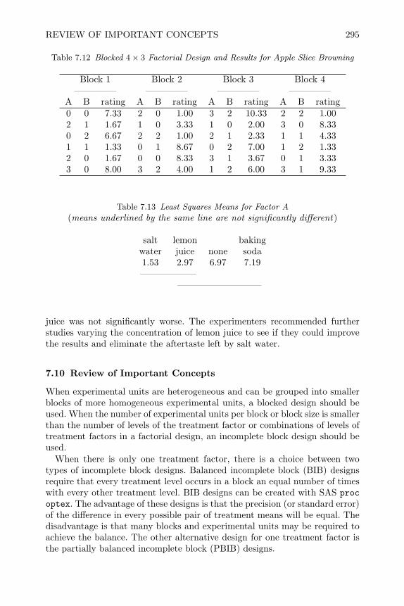
REVIEW OF IMPORTANT CONCEPTS 295
Table 7.12 Blocked 4× 3 Factorial Design and Results for Apple Slice Browning
Block 1 Block 2 Block 3 Block 4————– ————– ————– ————–
A B rating A B rating A B rating A B rating0 0 7.33 2 0 1.00 3 2 10.33 2 2 1.002 1 1.67 1 0 3.33 1 0 2.00 3 0 8.330 2 6.67 2 2 1.00 2 1 2.33 1 1 4.331 1 1.33 0 1 8.67 0 2 7.00 1 2 1.332 0 1.67 0 0 8.33 3 1 3.67 0 1 3.333 0 8.00 3 2 4.00 1 2 6.00 3 1 9.33
Table 7.13 Least Squares Means for Factor A
(means underlined by the same line are not significantly different)
salt lemon bakingwater juice none soda1.53 2.97 6.97 7.19——————
—————————
juice was not significantly worse. The experimenters recommended furtherstudies varying the concentration of lemon juice to see if they could improvethe results and eliminate the aftertaste left by salt water.
7.10 Review of Important Concepts
When experimental units are heterogeneous and can be grouped into smallerblocks of more homogeneous experimental units, a blocked design should beused. When the number of experimental units per block or block size is smallerthan the number of levels of the treatment factor or combinations of levels oftreatment factors in a factorial design, an incomplete block design should beused.
When there is only one treatment factor, there is a choice between twotypes of incomplete block designs. Balanced incomplete block (BIB) designsrequire that every treatment level occurs in a block an equal number of timeswith every other treatment level. BIB designs can be created with SAS procoptex. The advantage of these designs is that the precision (or standard error)of the difference in every possible pair of treatment means will be equal. Thedisadvantage is that many blocks and experimental units may be required toachieve the balance. The other alternative design for one treatment factor isthe partially balanced incomplete block (PBIB) designs.

296 INCOMPLETE AND CONFOUNDED BLOCK DESIGNS
The advantage of PBIB designs is that the total number of blocks andexperimental units required can be reduced. The disadvantage is that thestandard error of differences in pairs of treatment means will not be constant.There are many different methods of creating PBIB designs, and some ofthe more useful designs have been tabled. One type of PBIB called a BTIB(balanced with respect to test treatments) can be easily created from a BIBdesign. This design is useful when there is more interest in comparing onetreatment level (such as a control) to all other treatment levels than thereis in comparisons among the other treatment levels. Another class of PBIBdesigns that can be easily created using SAS proc plan is called generalizedcyclic designs.
Latin square designs introduced in Chapter 4 have two orthogonal block-ing factors, and contain a complete block design in both the row blocks andcolumn blocks. If an incomplete block design is required in either the row orcolumn blocks, a Youden square design (YSD) can be utilized. A YSD can beconstructed by deleting one or more columns from a Latin square design.
When experimenting with multiple factors and the block size is not largeenough to accommodate all possible treatment combinations, there are twoalternative methods for creating an incomplete block design. The first methodis to completely confound some interactions with blocks in a completely con-founded blocked factorial (CCBF) design, or a completely confounded blockedfractional factorial (CCBFF) design. The advantage of these designs is thatthe total number of blocks and experimental units can be minimized. Thedisadvantage is that some interactions will be completely confounded withblocks and will be inestimable. The other method is to use a partially con-founded blocked factorial (PCBF) design. Figure 7.5 illustrates when thesedesigns should be used in relation to the designs presented in other chapters.
When each factor has only two or three levels, there is a classical methodfor creating completely confounded factorial designs, and tables are availablefor block defining contrasts that will minimize the number of low order inter-actions confounded. For factorials where all factors have p (a prime number)of levels, or where the experiment can be broken down into sub-experimentswhere all factors have the same prime number of levels, the classical method forcreating a completely confounded design can also be used. SAS proc factexcan be used to find block defining contrasts, if they exist, that will allow esti-mation of the effects and interactions of interest. A D-optimal search can alsobe used to create a confounded design to estimate all effects and interactionsof interest and confound others with blocks. The advantage of this approachis that it has a higher possibility of finding a design capable of estimating aspecified list of effects and interactions, and it is more flexible in terms of blocksizes available. The disadvantage of designs created with a D-optimal search isthat treatment levels are not orthogonal to blocks and they are estimated lessefficiently than they would be in a design created with the classical method.
Partially confounded blocked factorials are used in factorials where thereare only a few factors, like two or three, and there is a need to estimate all

REVIEW OF IMPORTANT CONCEPTS 297
Figure 7.5 Design Selection Roadmap
Design Purpose
Estimate Variances Study Factor Effects
E.U.’s
Block Factors
One Factor
Multiple Factors
Multiple Factorswith some hard
to vary
Block size
Homogeneous Heterogeneous
Large Small
RCB
GCB
PBIB, BTIB
BIB
LSD
YSDRSE CRD
FactorsFRSENSESNSE
CRFD CRRS SLD RCBF BRS PCBFCRFF SCD
PB, OA EVD CCBF
CRSP RSSP SPMPV RBSPSPFF EESPRS
One Two
class cont. mixture cont. classFactors
interactions. These designs require more blocks and experimental units thancompletely confounded designs, but do allow estimation of all interactions.These designs can be created by confounding all estimable effects an equalnumber of times in different replicates of blocks or by using a D-optimalsearch.
The analysis of incomplete block designs and partially confounded factorialdesigns is similar to the analysis of complete block designs, except care must betaken to always use the type III sums of squares and least squares means. Forcompletely confounded factorial designs, the interactions that are confoundedwith blocks must be left out of the model, and the significant effects can beidentified by graphical techniques such as a half-normal plot of effects.

298 INCOMPLETE AND CONFOUNDED BLOCK DESIGNS
7.11 Exercises
1. An experimenter wanted to determine how the gear selected on a 10 speedbike would affect the time it takes a rider to pedal up a long, gradual hill.The experimental unit will be the trial or point in time when a rider willride up the hill. Treatment will be the gear selected on bicycle. Since theexperimenter would like his conclusions to apply to all riders, he would liketo run a blocked experiment where several riders (blocks) test each gear.However, if each rider who participates in his study must test all gears inseparate trials, he or she will become fatigued and variability in time toclimb the hill will increase. Therefore, the experimenter decided to do anincomplete block design wherein each rider participating in his study willtest only a subset of 4 of the 10 gears.
(a) If the experimenter were to use a balanced incomplete block (BIB) designby choosing all possible subsets of 4 selected from 10 as his blocks, howmany riders or blocks would he need to recruit to his study?
(b) Using Equations (7.1) to (7.3), determine the minimum possible numberof blocks that would be required for BIB design.
(c) Modify the SAS code in Section 7.2 to create a BIB with the number ofblocks you found in (b) using proc optex.
2. Consider an incomplete block design with t=10 levels of the treatmentfactor.
(a) If a balanced incomplete block design (BIB) was constructed using thesimplest method of forming blocks as all possible combinations of
(10k
),
how many blocks would be required for the cases where k=3, 4, 5, or 6?(b) Using Equations (7.1) to (7.3), determine the minimum number of blocks
that could possibly be required for a BIB with t=10, and k=3, 4, 5, or6?
(c) Is it possible to find a BIB with t=10, and k=3, 4, 5, or 6, by modifyingthe SAS code in Section 7.2?
(d) Can one or more generalized cyclic incomplete block design with t=10and k=3 be found with less blocks than required for a BIB design? Whatnumber of blocks would be required for these designs? Using SAS procplan as illustrated in Section 7.4, find these designs.
3. Consider blocking a 25 factorial into 8 blocks with 4 experimental units perblock using the block defining contrasts ACE, BCE and ABCD (shownin Section 7.6.2). Show that the generalized interactions of these contrasts,which would be confounded with blocks, contain no main effects.
4. Consider blocking a 26−2 fractional factorial, with generators E = ABC,and F = ABD, into 4 blocks of size 4. If the block defining contrasts areACD and AB (shown in Section 7.6.1), show all interactions and theiraliases that will be confounded with blocks.

EXERCISES 299
5. Choice based conjoint studies (see Section 6.7 for an example and de-scription of conjoint analysis) are frequently used in marketing research.In choice based conjoint studies, potential customers are asked to chooseamong several alternatives. The alternatives are combinations of levels ofseveral product characteristics. The response for each combination of prod-uct characteristics is a count of the number of potential customers whochoose that alternative. Analysis of the data helps marketing researchersdetermine what product characteristics have the most influence on cus-tomer choices and what mix of alternatives they should offer in order tosatisfy the needs of the market. Consider the following scenario describedby Street and Burgess (2007). Researchers want to study how the attributesof a take-out pizza outlet affect consumer choice of where they buy theirpizza. The table below lists the product characteristics (i.e., factors in ex-perimental design terminology) and their levels.
LevelsAttribute − +Pizza type Traditional GourmetType of crust Thin ThickIngredients Some canned All freshSize of pizza One size only Three sizesPrice $13 $17Delivery time 30 minutes 45 minutes
The alternatives that customers must choose from in a survey are all 26
combinations of attribute levels.
(a) Since it would be impractical to ask a potential customer to choose froma list of 26 = 64 combinations, it would be better to have each customersurveyed make a choice from 4 alternatives. Create a blocked 26 designwith block size 4, so that each customer surveyed must only choose fromamong the 4 combinations of attribute levels in one block.
(b) Since higher-order interactions are unlikely to be important, constructa 16-run 26−2 design blocked into 4 blocks of size 4. Are all main effectsestimable from your design?
(c) Block a 16-run 26−2 design blocked into 8 blocks of size 2, so that eachcustomer surveyed only has to choose between two alternatives. Are allmain effects estimable from this design?
(d) If the number of alternatives of the type of crust and the size of pizzawere increased from 2 to 3, the factorial combination of all attributelevels would change from a 26 to a 24 × 32 factorial. Using the %mktmacros, create a 24-run fraction of a 24×32 factorial, blocked in 8 blocksof 3, for this problem.
(e) What model in SAS proc glm would you use for the analysis of dataarising from the design you created in (d)?

300 INCOMPLETE AND CONFOUNDED BLOCK DESIGNS
6. For a 26−1 experiment with generator F = ABCDE that is blocked intofour blocks with 8 experimental units per block using the block definingcontrasts ACD and BCD,
(a) Determine the defining relation for the fractional factorial.(b) Determine the complete alias structure for the fractional factorial.(c) Determine the generalized interaction of the block defining contrasts.(d) Show what interactions are confounded with blocks.
7. Consider blocking a 2 × 32 × 4 factorial into six blocks of 12 treatmentcombinations each.
(a) Naming the factors A, B, C, and D, which factors must be representedby pseudo factors in order to block using the classical method?
(b) What are the two sub-experiments composed of factorials with primenumber of levels?
(c) What interactions of factors and pseudo factors would you confound ineach sub-experiment in order to allow estimation of the main effects?What effects and interactions will be unconfounded with blocks andestimable?
(d) Create the design using SAS proc factex.(e) Can you create a design using proc optex that has six blocks of 12 and
allows estimation of all two-factor interactions?
8. Show why it is impossible to block a 3 × 4 × 6 into blocks of size 6 usingthe classical method without confounding a main effect.
9. Create a partially confounded 23 design in 14 blocks of size 4. Generaterandom data, and use proc glm to illustrate that all main effects and in-teractions can be estimated from the design you created.
10. Using the proc optex create a partially confounded 2 × 32 factorial in 6blocks of size 6.
11. Consider the apple slice browning experiment shown in Section 7.9.
(a) If the apple slicer made eight slices of each apple instead of six, find apartially confounded 4× 3 factorial in three blocks of eight (instead of 4blocks of 6) by modifying the proc optex code shown in that example.
(b) Analyze the data from the experiment shown in the text and verify theresults shown.
(c) Check the equal variance and normality assumptions. Is a transformationwarranted? If so, what transformation would you use and does it changethe conclusions?
CHAPTER 8
Split-Plot Designs
8.1 Introduction
A factorial design is a powerful tool for aiding a researcher. Use of a factorialdesign in experimentation can dramatically increase the power of detectingfactor main effects through hidden replication, while additionally affording aresearcher the ability to detect interactions or joint effects of factors. Whenthere is an interaction between two factors, the effect of one factor will dependon the level of the other factor, and determination of optimal factor combi-nations must take that into account. Interactions occur frequently in the realworld and they can only be quantified through factorial designs.
In the factorial and fractional factorial designs discussed in Chapters 3, 4,6 and 7, it was assumed that combinations of factor levels in the design couldbe randomly assigned to the experimental units within a block for a blockedfactorial design, or to the entire group of experimental units for a completelyrandomized factorial design. Randomization of treatment combinations to ex-perimental units guarantees the validity of the conclusions reached from theanalysis of data. However, sometimes the levels of one or more factors in thedesign are more difficult to change or require more experimental material toevaluate. In this situation complete randomization of factor-level combinationsto experimental units could make the experiment much more time consum-ing or perhaps impossible to conduct. This is the case frequently in processimprovement studies where the process consists of several steps, and somefactors in an experiment relate to one process step while others relate to alater process step.
When treatment combinations cannot be completely randomized to experi-mental units due to one or more hard-to-vary factors, the experimental unit isdifferent for the hard-to-vary factors than it is for the easy-to-vary factors. Inorder to ensure validity, the design of the experiment and the analysis of thedata must take into account these different experimental units. The designsthat do this are called split-plot experiments. The name split-plot comes fromthe original application in agricultural experiments, where the levels of somefactors (called whole-plot factors) could only be varied between plots of land,while the levels of other factors could be varied within a plot (see Yates, 1937).
A compromise is made in split-plot experiments. The randomization is suchthat the hard-to-vary factors are not changed as frequently as easy-to-varyfactors. This makes it more convenient to conduct the list of experiments,but there is less efficiency or power for detecting effects of the hard-to-vary
301
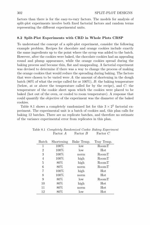
302 SPLIT-PLOT DESIGNS
factors than there is for the easy-to-vary factors. The models for analysis ofsplit-plot experiments involve both fixed factorial factors and random termsrepresenting the different experimental units.
8.2 Split-Plot Experiments with CRD in Whole Plots CRSP
To understand the concept of a split-plot experiment, consider the followingexample problem. Recipes for chocolate and orange cookies include exactlythe same ingredients up to the point where the syrup was added to the batch.However, after the cookies were baked, the chocolate cookies had an appealinground and plump appearance, while the orange cookies spread during thebaking process and became thin, flat and unappealing. A factorial experimentwas devised to determine if there was a way to change the process of makingthe orange cookies that would reduce the spreading during baking. The factorsthat were chosen to be varied were A: the amount of shortening in the doughbatch (80% of what the recipe called for or 100%), B: the baking temperature(below, at or above the temperature called for by the recipe), and C: thetemperature of the cookie sheet upon which the cookies were placed to bebaked (hot out of the oven, or cooled to room temperature). A response thatcould quantify the objective of the experiment was the diameter of the bakedcookies.
Table 8.1 shows a completely randomized list for this 3 × 22 factorial ex-periment. The experimental unit is a batch of cookies and, this plan calls forbaking 12 batches. There are no replicate batches, and therefore no estimateof the variance experimental error from replicates in this plan.
Table 8.1 Completely Randomized Cookie Baking ExperimentFactor A Factor B Factor C
Batch Shortening Bake Temp. Tray Temp.1 100% low RoomT2 100% low Hot3 100% norm RoomT4 100% high RoomT5 80% high RoomT6 80% norm RoomT7 100% high Hot8 100% norm Hot9 80% low RoomT10 80% high Hot11 80% norm Hot12 80% low Hot
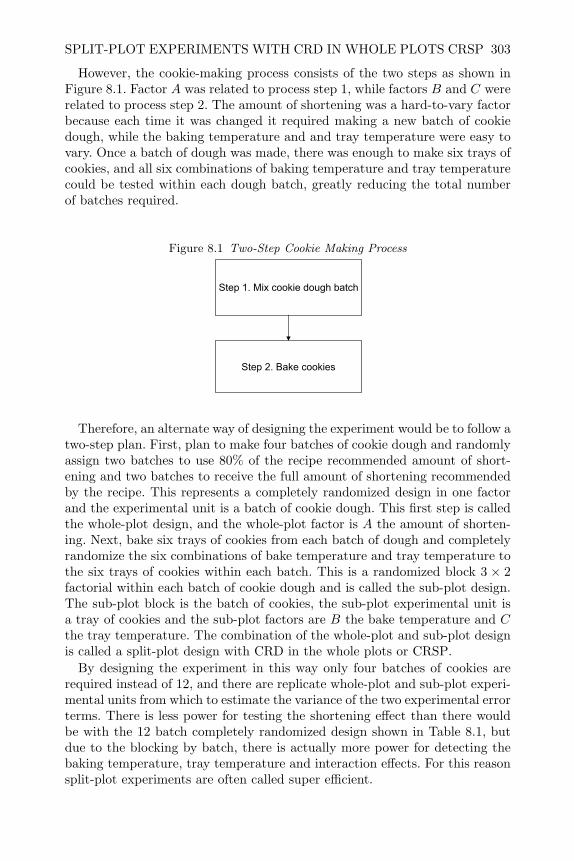
SPLIT-PLOT EXPERIMENTS WITH CRD IN WHOLE PLOTS CRSP 303
However, the cookie-making process consists of the two steps as shown inFigure 8.1. Factor A was related to process step 1, while factors B and C wererelated to process step 2. The amount of shortening was a hard-to-vary factorbecause each time it was changed it required making a new batch of cookiedough, while the baking temperature and and tray temperature were easy tovary. Once a batch of dough was made, there was enough to make six trays ofcookies, and all six combinations of baking temperature and tray temperaturecould be tested within each dough batch, greatly reducing the total numberof batches required.
Figure 8.1 Two-Step Cookie Making Process
Step 1. Mix cookie dough batch
Step 2. Bake cookies
Therefore, an alternate way of designing the experiment would be to follow atwo-step plan. First, plan to make four batches of cookie dough and randomlyassign two batches to use 80% of the recipe recommended amount of short-ening and two batches to receive the full amount of shortening recommendedby the recipe. This represents a completely randomized design in one factorand the experimental unit is a batch of cookie dough. This first step is calledthe whole-plot design, and the whole-plot factor is A the amount of shorten-ing. Next, bake six trays of cookies from each batch of dough and completelyrandomize the six combinations of bake temperature and tray temperature tothe six trays of cookies within each batch. This is a randomized block 3 × 2factorial within each batch of cookie dough and is called the sub-plot design.The sub-plot block is the batch of cookies, the sub-plot experimental unit isa tray of cookies and the sub-plot factors are B the bake temperature and Cthe tray temperature. The combination of the whole-plot and sub-plot designis called a split-plot design with CRD in the whole plots or CRSP.
By designing the experiment in this way only four batches of cookies arerequired instead of 12, and there are replicate whole-plot and sub-plot experi-mental units from which to estimate the variance of the two experimental errorterms. There is less power for testing the shortening effect than there wouldbe with the 12 batch completely randomized design shown in Table 8.1, butdue to the blocking by batch, there is actually more power for detecting thebaking temperature, tray temperature and interaction effects. For this reasonsplit-plot experiments are often called super efficient.
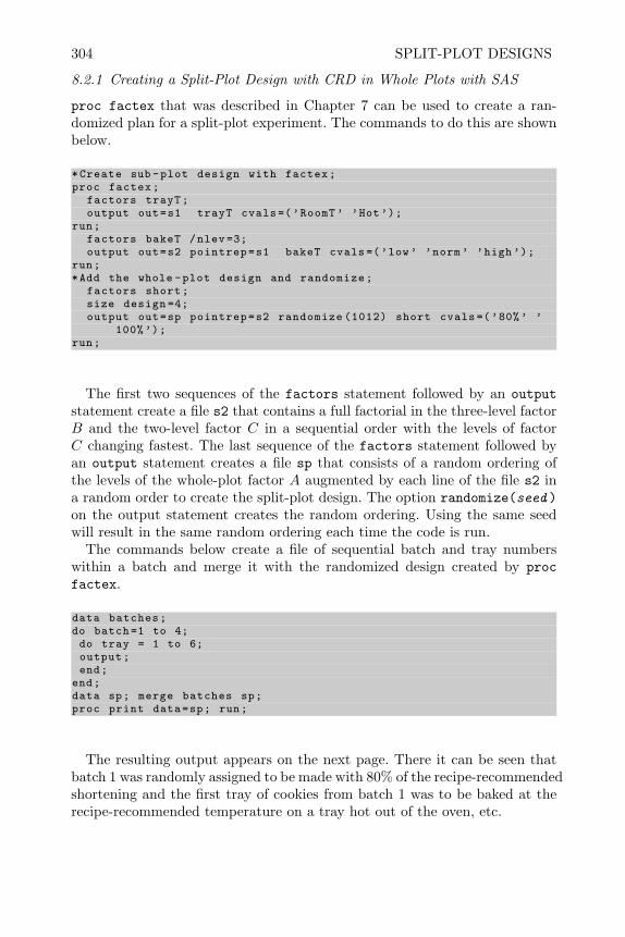
304 SPLIT-PLOT DESIGNS
8.2.1 Creating a Split-Plot Design with CRD in Whole Plots with SAS
proc factex that was described in Chapter 7 can be used to create a ran-domized plan for a split-plot experiment. The commands to do this are shownbelow.
*Create sub -plot design with factex;proc factex;
factors trayT;output out=s1 trayT cvals =(’RoomT’ ’Hot’);
run;factors bakeT /nlev =3;output out=s2 pointrep=s1 bakeT cvals=(’low’ ’norm’ ’high’);
run;*Add the whole -plot design and randomize;
factors short;size design =4;output out=sp pointrep=s2 randomize (1012) short cvals =(’80%’ ’
100%’);run;
The first two sequences of the factors statement followed by an outputstatement create a file s2 that contains a full factorial in the three-level factorB and the two-level factor C in a sequential order with the levels of factorC changing fastest. The last sequence of the factors statement followed byan output statement creates a file sp that consists of a random ordering ofthe levels of the whole-plot factor A augmented by each line of the file s2 ina random order to create the split-plot design. The option randomize(seed )on the output statement creates the random ordering. Using the same seedwill result in the same random ordering each time the code is run.
The commands below create a file of sequential batch and tray numberswithin a batch and merge it with the randomized design created by procfactex.
data batches;do batch=1 to 4;do tray = 1 to 6;output;end;
end;data sp; merge batches sp;proc print data=sp; run;
The resulting output appears on the next page. There it can be seen thatbatch 1 was randomly assigned to be made with 80% of the recipe-recommendedshortening and the first tray of cookies from batch 1 was to be baked at therecipe-recommended temperature on a tray hot out of the oven, etc.
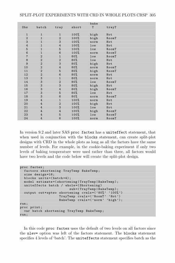
SPLIT-PLOT EXPERIMENTS WITH CRD IN WHOLE PLOTS CRSP 305
bakeObs batch tray short T trayT
1 1 1 100% high Hot2 1 2 100% high RoomT3 1 3 100% norm Hot4 1 4 100% low Hot5 1 5 100% low RoomT6 1 6 100% norm RoomT7 2 1 80% low RoomT8 2 2 80% low Hot9 2 3 80% high Hot
10 2 4 80% norm RoomT11 2 5 80% high RoomT12 2 6 80% norm Hot13 3 1 80% norm Hot14 3 2 80% low RoomT15 3 3 80% high Hot16 3 4 80% high RoomT17 3 5 80% low Hot18 3 6 80% norm RoomT19 4 1 100% norm Hot20 4 2 100% high Hot21 4 3 100% low Hot22 4 4 100% high RoomT23 4 5 100% low RoomT24 4 6 100% norm RoomT
In version 9.2 and later SAS proc factex has a uniteffect statement, thatwhen used in conjunction with the blocks statement, can create split-plotdesigns with CRD in the whole plots as long as all the factors have the samenumber of levels. For example, in the cookie-baking experiment if only twolevels of baking temperature were used rather than three, all factors wouldhave two levels and the code below will create the split-plot design.
proc factex;factors shortening TrayTemp BakeTemp;size design =16;blocks units =( batch =4);model estimate =( shortening|TrayTemp|BakeTemp);uniteffects batch / whole =( Shortening)
sub=( TrayTemp|BakeTemp);output out=sptwo shortening cvals =(’80%’ ’100%’)
TrayTemp cvals =(’RoomT’ ’Hot’)BakeTemp cvals =(’norm’ ’high’);
run;proc print;
var batch shortening TrayTemp BakeTemp;run;
In this code proc factex uses the default of two levels on all factors sincethe nlev= option was left of the factors statement. The blocks statementspecifies 4 levels of ‘batch’. The uniteffects statement specifies batch as the

306 SPLIT-PLOT DESIGNS
whole-plot experimental unit. The option whole = (Shortening)sub=(TrayTemp|BakeTemp); specifies that the factor Shortening will be aliasedwith differences in the whole-plot experimental units, and that TrayTemp,BakeTemp and their interaction will be sub-plot factors that are independent(or varied within levels) of the whole-plot experimental units.
8.2.2 Model for a Split-Plot Experiment with CRD in Whole Plots
It is easy to write the model for a split-plot design with a completely random-ized design in the whole plots by following the same two-step procedure usedto create the design. The first step was to create a completely randomizeddesign in the whole plots by assigning the levels of the whole-plot factor atrandom to the whole plots. The model for this step can be represented as
yij = µ+ αi + w(i)j (8.1)
where yij represents the average response for the ith level of the whole-plotfactor and the jth whole plot, αi represents the fixed effect of the whole-plotfactor A, w(i)j represents the effect of the nested random effect of the jthwhole plot assigned to the ith level of the whole-plot factor. This is the samemodel used for the completely randomized design in Chapter 2.
The second step in creating the design was to split the whole plots andassign each sub-plot at random to one of the levels of the sub-plot factor(or combination of levels of the sub-plot factors if there are more than one).Added to the model at this step is the effect of the sub-plot factor and theinteraction between the whole-plot and sub-plot factor which are includedafter the random block term w(i)j to arrive at the final model shown below
yijk = µ+ αi + w(i)j + βk + αβik + εijk (8.2)
where yijk is the measured response for the ith level of the whole-plot factorand the kth level of the split-plot factor within the jth whole plot. βk is theeffect of the fixed split-plot factor, αβik is the fixed interaction effect, andεijk is the random effect of the kth split plot within the jth plot. If there aremore than one sub-plot factors, as in the cookie-baking experiment describedabove, the model would be:
yijkl = µ+ αi + w(i)j + βk + γl + βγkl + αβik + αγil + αβγikl + εijkl (8.3)
and if there are more than one whole-plot factors the model would be writtenas:
yijkl = µ+ αi + βj + αβij + w(ij)k + γl + αγil + βγjl + αβγijl + εijkl (8.4)
and likewise for other combinations of numbers of whole-plot and sub-plotfactors.
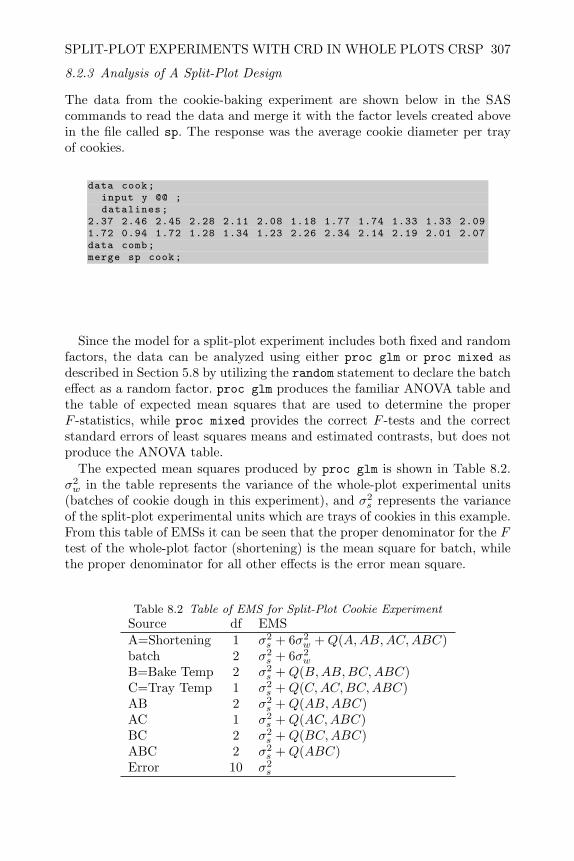
SPLIT-PLOT EXPERIMENTS WITH CRD IN WHOLE PLOTS CRSP 307
8.2.3 Analysis of A Split-Plot Design
The data from the cookie-baking experiment are shown below in the SAScommands to read the data and merge it with the factor levels created abovein the file called sp. The response was the average cookie diameter per trayof cookies.
data cook;input y @@ ;datalines;
2.37 2.46 2.45 2.28 2.11 2.08 1.18 1.77 1.74 1.33 1.33 2.091.72 0.94 1.72 1.28 1.34 1.23 2.26 2.34 2.14 2.19 2.01 2.07data comb;merge sp cook;
Since the model for a split-plot experiment includes both fixed and randomfactors, the data can be analyzed using either proc glm or proc mixed asdescribed in Section 5.8 by utilizing the random statement to declare the batcheffect as a random factor. proc glm produces the familiar ANOVA table andthe table of expected mean squares that are used to determine the properF -statistics, while proc mixed provides the correct F -tests and the correctstandard errors of least squares means and estimated contrasts, but does notproduce the ANOVA table.
The expected mean squares produced by proc glm is shown in Table 8.2.σ2w in the table represents the variance of the whole-plot experimental units
(batches of cookie dough in this experiment), and σ2s represents the variance
of the split-plot experimental units which are trays of cookies in this example.From this table of EMSs it can be seen that the proper denominator for the Ftest of the whole-plot factor (shortening) is the mean square for batch, whilethe proper denominator for all other effects is the error mean square.
Table 8.2 Table of EMS for Split-Plot Cookie ExperimentSource df EMSA=Shortening 1 σ2
s + 6σ2w +Q(A,AB,AC,ABC)
batch 2 σ2s + 6σ2
w
B=Bake Temp 2 σ2s +Q(B,AB,BC,ABC)
C=Tray Temp 1 σ2s +Q(C,AC,BC,ABC)
AB 2 σ2s +Q(AB,ABC)
AC 1 σ2s +Q(AC,ABC)
BC 2 σ2s +Q(BC,ABC)
ABC 2 σ2s +Q(ABC)
Error 10 σ2s
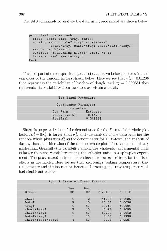
308 SPLIT-PLOT DESIGNS
The SAS commands to analyze the data using proc mixed are shown below.
proc mixed data= comb;class short bakeT trayT batch;model y =short bakeT trayT short*bakeT
short*trayT bakeT*trayT short*bakeT*trayT;random batch(short);estimate ’Shortening Effect ’ short -1 1;lsmeans bakeT short*trayT;
run;
The first part of the output from proc mixed, shown below, is the estimatedvariances of the random factors shown below. Here we see that σ2
w = 0.01236that represents the variability of batches of dough, and σ2
s = 0.009634 thatrepresents the variability from tray to tray within a batch.
The Mixed Procedure
Covariance ParameterEstimates
Cov Parm Estimatebatch(short) 0.01233Residual 0.009831
Since the expected value of the denominator for the F -test of the whole-plotfactor, σ2
s + 6σ2w, is larger than σ2
s , and the analysis of the data ignoring therandom whole plots uses σ2
s as the denominator for all F -tests, the analysis ofdata without consideration of the random whole-plot effect can be completelymisleading. Generally the variability among the whole-plot experimental unitsis larger than the variability among the sub-plot units in a split-plot experi-ment. The proc mixed output below shows the correct F -tests for the fixedeffects in the model. Here we see that shortening, baking temperature, traytemperature and the interaction between shortening and tray temperature allhad significant effects.
Type 3 Tests of Fixed Effects
Num DenEffect DF DF F Value Pr > F
short 1 2 41.07 0.0235bakeT 2 10 10.44 0.0036trayT 1 10 68.15 <.0001short*bakeT 2 10 2.78 0.1095short*trayT 1 10 19.96 0.0012bakeT*trayT 1 10 2.60 0.1236short*bakeT*trayT 4 10 0.04 0.9587

RCB IN WHOLE PLOTS RBSP 309
proc mixed calculates the correct standard errors of estimable functions.Shown in the top two lines of output below is the estimate of the averagechange in cookie diameter as the amount shortening increases from 80% to100%. Its standard error is a function of both σ2
s and σ2w. proc mixed also
computes the correct standard errors of the least squares means. The last partof the output shows the least squares means for the factor bake temperature.There, it can be seen that reducing the bake temperature reduces the cookiediameter.
Estimates
StandardLabel Estimate Error DF t Value Pr > |t|Shortening Effect -0.7575 0.1182 2 -6.41 0.0235
Least Squares Means
bake StandardEffect T Estimate Error DF t Value Pr > |t|bakeT high 1.9287 0.06566 10 29.37 <.0001bakeT low 1.7212 0.06566 10 26.21 <.0001bakeT norm 1.9037 0.06566 10 28.99 <.0001
Since there is a significant interaction between shortening and tray temper-ature, the effect of shortening depends upon the tray temperature. The bestway of depicting this is through the interaction plot shown in Figure 8.2.
There it can be seen that reducing the amount of shortening from 100% to80% of that called for in the recipe reduces the cookie diameter more whenusing room temperature trays than when using trays hot out of the oven. Italso can be seen that the smallest diameter cookies are the result of using80% of the recommended shortening and placing the cookie dough on a roomtemperature tray before baking.
8.3 RCB in Whole Plots RBSP
A second way to run a split-plot experiment is to utilize a randomized completeblock design in the whole plots. To illustrate this design consider anothersimple example. A fisherman performed an experiment to determine the effect
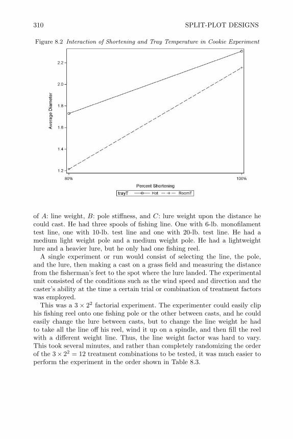
310 SPLIT-PLOT DESIGNS
Figure 8.2 Interaction of Shortening and Tray Temperature in Cookie Experiment
of A: line weight, B: pole stiffness, and C: lure weight upon the distance hecould cast. He had three spools of fishing line. One with 6-lb. monofilamenttest line, one with 10-lb. test line and one with 20-lb. test line. He had amedium light weight pole and a medium weight pole. He had a lightweightlure and a heavier lure, but he only had one fishing reel.
A single experiment or run would consist of selecting the line, the pole,and the lure, then making a cast on a grass field and measuring the distancefrom the fisherman’s feet to the spot where the lure landed. The experimentalunit consisted of the conditions such as the wind speed and direction and thecaster’s ability at the time a certain trial or combination of treatment factorswas employed.
This was a 3× 22 factorial experiment. The experimenter could easily cliphis fishing reel onto one fishing pole or the other between casts, and he couldeasily change the lure between casts, but to change the line weight he hadto take all the line off his reel, wind it up on a spindle, and then fill the reelwith a different weight line. Thus, the line weight factor was hard to vary.This took several minutes, and rather than completely randomizing the orderof the 3× 22 = 12 treatment combinations to be tested, it was much easier toperform the experiment in the order shown in Table 8.3.

RCB IN WHOLE PLOTS RBSP 311
Table 8.3 Casting ExperimentTrial Line Wgt Pole Stiffness Lure Wgt
1 10lb. medium light heavy2 10lb. medium light light3 10lb. light light4 10lb. light heavy5 20lb. light light6 20lb. medium light light7 20lb. medium light heavy8 20lb. light heavy9 6lb. light light
10 6lb. medium light light11 6lb. light heavy12 6lb. medium light heavy
Here the 10-lb. weight line was randomly chosen to be used for the first fourcasts. The order of the four combinations of pole stiffness and lure weight wererandomized in the first four trials. Next the 20-lb. weight line was randomlyselected to be used for the next four trials and again the order of the fourcombinations of pole stiffness and lure weight were randomized in these trials.Finally, the last four casts were made using the 6-lb. weight line. By conduct-ing the experiments in this way the fisherman had inadvertently created asplit-plot experiment. The whole-plot experimental unit is a collection of fourindividual trials or casts and the sub-plot experimental unit is an individualtrial or cast.
The problem is that there is no replication of the whole-plot units. If thewind speed or direction changed during the course of the trials, the line weighteffect could be biased, and there is no estimate of whole-plot variability fromreplicates. There is no bias of the pole stiffness and lure weight effects, however,since the four combinations of pole stiffness and lure weight are repeated ina random order within each of the three blocks. To get unbiased estimates ofthe whole-plot factor effect and gain an estimate of whole-plot experimentalerror, the fisherman could repeat the whole experiment again as a secondblock. This was done and the second set of casting trials were completed bya second fisherman so that the results could be generalized to more than onefisherman.
By repeating the experiments with a second fisherman doing the casting, arandomized complete block experiment design is created in the whole plots.The Fisherman represents the block factor, and each line weight is testedby each fisherman in a random order. All four combinations of the sub-plotfactors of pole stiffness and lure weight are tested in a random order withineach combination of fisherman and line weight.
The model for this experiment is shown in Equation (8.5).

312 SPLIT-PLOT DESIGNS
yijkl = µ+ bi+αj + bαij +βk +γl +αβjk +αγjl +βγkl +αβγjkl + εijkl (8.5)
Here bi is the random block or fisherman effect, αj is the fishing line weighteffect, bαij is the random block by treatment interaction term which representsthe whole-plot error term. The first three terms of the model are the same asthe model for a RCB design shown in Section 4.3. β is the pole stiffness effectand γl is the lure weight effect. These are sub-plot factors along with all theinteractions. The error term for the sub-plot factors and interactions is εijkl.
8.3.1 Creating a Split-Plot Design with RCB in Whole Plots with SAS
The code below creates the split-plot design with an RCB design in the wholeplots or a RBSP design. Each block of the whole-plot design is created witha separate use of proc factex, and the blocks are concatenated in the datastep. The different seeds (in parentheses following the randomize option ofthe output statement) creates a different randomization for each block. Eachfisherman performing the experiment would be randomly assigned to one ofthe two blocks.
*Create Block 1 of Whole Plot;proc factex;*Create sub -plot design;
factors PoleStiff LureWgt;output out=s1 PoleStiff cvals=(’light’ ’medlgt ’)
LureWgt cvals=(’light ’ ’heavy ’);run;*Create whole -plot design for block 1;
factors LineWgt /nlev =3;size design =3;output out=b1 pointrep=s1 randomize (101)LineWgt cvals=(’6lb.’ ’10lb.’ ’20lb.’);
run;*Create Block 2 of whole -plot;proc factex;*Create sub -plot design;
factors PoleStiff LureWgt;output out=s2 PoleStiff cvals=(’light’ ’medlgt ’)
LureWgt cvals=(’light ’ ’heavy ’);run;*Create whole -plot design for block 2;
factors LineWgt /nlev =3;size design =3;output out=b2 pointrep=s2 randomize (201)LineWgt cvals=(’6lb.’ ’10lb.’ ’20lb.’);
run;data spdesign;set b1(in=in1) b2(in=in2);if in1 then Block_Fisherman =1;if in2 then Block_Fisherman =2;proc print; run;
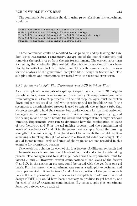
RCB IN WHOLE PLOTS RBSP 313
The commands for analyzing the data using proc glm from this experimentwould be:
class Fisherman LineWgt PoleStiff LureWgt;model y=Fisherman LineWgt Fisherman*LineWgtPoleStiff LureWgt LineWgt*PoleStiff LineWgt*LureWgtPoleStiff*LureWgt LineWgt*PoleStiff*LureWgt;random Fisherman Fisherman*LineWgt/test;
These commands could be modified to use proc mixed by leaving the ran-dom terms Fisherman Fisherman*LineWgt out of the model statement andremoving the option test from the random statement. The correct error termfor testing the whole-plot (line weight) effect is the interaction of the whole-plot factor with the block term fisherman. This is the same error term shownfor the analysis of the generalized complete block design in Section 5.8. Thesub-plot effects and interactions are tested with the residual error term.
8.3.2 Example of a Split-Plot Experiment with RCB in Whole Plots
As an example of the analysis of a split-plot experiment with an RCB design inthe whole plots, consider an example from industry. Sausage casings are madefrom collagen in a two-step process. In the first step, collagen must be brokendown and reconstituted as a gel with consistent and predictable traits. In thesecond step, a sophisticated process is used to extrude the gel into a tube thatis strong enough to hold the sausage, but tender enough for the final customer.Sausages can be cooked in many ways from steaming to deep-fat frying, andthe casing must be able to handle the stress and temperature changes withoutbursting. Experiments were run to determine how the combination of levelsof two factors A and B in the gel-making process, and the combination oflevels of two factors C and D in the gel-extrusion step affected the burstingstrength of the final casing. A combination of factor levels that would result inachieving a bursting strength at or above a threshold value was sought. Theactual factor names, levels and units of the response are not provided in thisexample for proprietary reasons.
Two levels were chosen for each of the four factors. A different gel batch hadto be made for each combination of levels of factors A and B in the gel-makingprocess. The collagen used to make a gel batch was the experimental unit forfactors A and B. However, several combinations of the levels of the factorsC and D, in the extrusion process, could be tested with the gel from one gelbatch. For this reason, the experiment was run as a split-plot experiment andthe experimental unit for factors C and D was a portion of the gel from eachbatch. If the experiments had been run as a completely randomized factorialdesign (CRFD), it would have been necessary to produce 16 gel batches, onefor each of the 24 treatment combinations. By using a split-plot experimentfewer gel batches were required.
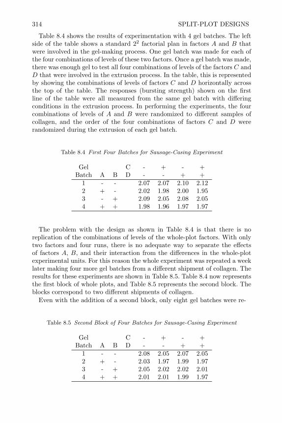
314 SPLIT-PLOT DESIGNS
Table 8.4 shows the results of experimentation with 4 gel batches. The leftside of the table shows a standard 22 factorial plan in factors A and B thatwere involved in the gel-making process. One gel batch was made for each ofthe four combinations of levels of these two factors. Once a gel batch was made,there was enough gel to test all four combinations of levels of the factors C andD that were involved in the extrusion process. In the table, this is representedby showing the combinations of levels of factors C and D horizontally acrossthe top of the table. The responses (bursting strength) shown on the firstline of the table were all measured from the same gel batch with differingconditions in the extrusion process. In performing the experiments, the fourcombinations of levels of A and B were randomized to different samples ofcollagen, and the order of the four combinations of factors C and D wererandomized during the extrusion of each gel batch.
Table 8.4 First Four Batches for Sausage-Casing Experiment
Gel C - + - +Batch A B D - - + +
1 - - 2.07 2.07 2.10 2.122 + - 2.02 1.98 2.00 1.953 - + 2.09 2.05 2.08 2.054 + + 1.98 1.96 1.97 1.97
The problem with the design as shown in Table 8.4 is that there is noreplication of the combinations of levels of the whole-plot factors. With onlytwo factors and four runs, there is no adequate way to separate the effectsof factors A, B, and their interaction from the differences in the whole-plotexperimental units. For this reason the whole experiment was repeated a weeklater making four more gel batches from a different shipment of collagen. Theresults for these experiments are shown in Table 8.5. Table 8.4 now representsthe first block of whole plots, and Table 8.5 represents the second block. Theblocks correspond to two different shipments of collagen.
Even with the addition of a second block, only eight gel batches were re-
Table 8.5 Second Block of Four Batches for Sausage-Casing Experiment
Gel C - + - +Batch A B D - - + +
1 - - 2.08 2.05 2.07 2.052 + - 2.03 1.97 1.99 1.973 - + 2.05 2.02 2.02 2.014 + + 2.01 2.01 1.99 1.97
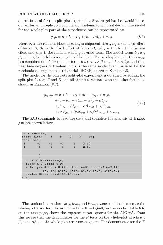
RCB IN WHOLE PLOTS RBSP 315
quired in total for the split-plot experiment. Sixteen gel batches would be re-quired for an unreplicated completely randomized factorial design. The modelfor the whole-plot part of the experiment can be represented as:
yijk = µ+ bi + αj + βk + αβjk + wijk (8.6)
where bi is the random block or collagen shipment effect, αj is the fixed effectof factor A, βk is the fixed effect of factor B, αβjk is the fixed interactioneffect and wijk is the random whole-plot error term. The model terms bi, αj ,βk, and αβjk each has one degree of freedom. The whole-plot error term wijkis a combination of the random terms b×αij , b× βik, and b×αβijk and thushas three degrees of freedom. This is the same model that was used for therandomized complete block factorial (RCBF) shown in Section 4.6.
The model for the complete split-plot experiment is obtained by adding thesplit-plot factors C and D and all their interactions with the other factors asshown in Equation (8.7).
yijklm = µ+ bi + αj + βk + αβjk + wijk
+ γl + δm + γδlm + αγjl + αδjm
+ βγkl + βδkm + αβγjkl + αβδjkm
+ αγδjkl + βγδklm + αβγδjklm + εijklm
(8.7)
The SAS commands to read the data and complete the analysis with procglm are shown below.
data sausage;input Block A B C D ys;datalines;1 -1 -1 -1 1 2.101 -1 -1 1 1 2.12
.
.
.proc glm data=sausage;
class A B Block C D;model ys=Block A B A*B Block(A*B) C D C*D A*C A*D
B*C B*D A*B*C A*B*D A*C*D B*C*D A*B*C*D;random Block Block(A*B)/test;
run;
The random interactions bαij , bβik, and bαβijk were combined to create thewhole-plot error term by using the term Block(A*B) in the model. Table 8.6,on the next page, shows the expected mean squares for the ANOVA. Fromthis we see that the denominator for the F tests on the whole-plot effects αj ,βk, and αβjk is the whole-plot error mean square. The denominator for the F

316 SPLIT-PLOT DESIGNS
tests on all other effects and interactions in the model is the mean square forthe split-plot error term.
Table 8.6 Expected Mean Squares for Sausage ExperimentSource df Type III Expected Mean SquareBlock 1 σ2 + 4σ2
W + 16σ2B
A 1 σ2 + 4σ2W +Q(A,AB,AC,AD,ABC,ABD,ACD,ABCD)
B 1 σ2 + 4σ2W +Q(B,AB,BC,BD,ABC,ABD,BCD,ABCD)
AB 1 σ2 + 4σ2W +Q(AB,ABC,ABD,ABCD)
Whole Plot 3 σ2 + 4σ2W
ErrorC 1 σ2 +Q(C,CD,AC,BC,ABC,ACD,BCD,ABCD)D 1 σ2 +Q(D,CD,AD,BD,ABD,ACD,BCD,ABCD)CD 1 σ2 +Q(CD,ACD,BCD,ABCD)AC 1 σ2 +Q(AC,ABC,ACD,ABCD)AD 1 σ2 +Q(AD,ABD,ACD,ABCD)BC 1 σ2 +Q(BC,ABC,BCD,ABCD)BD 1 σ2 +Q(BD,ABD,BCD,ABCD)ABC 1 σ2 +Q(ABC,ABCD)ABD 1 σ2 +Q(ABD,ABCD)ACD 1 σ2 +Q(ACD,ABCD)BCD 1 σ2 +Q(BCD,ABCD)ABCD 1 σ2 +Q(ABCD)Split-Plot 12 σ2
Error
The commands for the analysis using proc mixed are shown below.
proc mixed data=sausage;class A B Block C D;model ys=A B A*B C D C*D A*C A*D B*C B*D A*B*C A*B*D
A*C*D B*C*D A*B*C*D;random Block Block(A*B);lsmeans A;lsmeans C;lsmeans A*B*C;run;
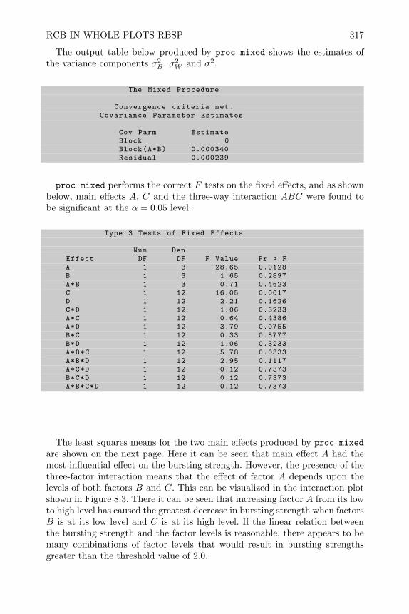
RCB IN WHOLE PLOTS RBSP 317
The output table below produced by proc mixed shows the estimates ofthe variance components σ2
B , σ2W and σ2.
The Mixed Procedure
Convergence criteria met.Covariance Parameter Estimates
Cov Parm EstimateBlock 0Block(A*B) 0.000340Residual 0.000239
proc mixed performs the correct F tests on the fixed effects, and as shownbelow, main effects A, C and the three-way interaction ABC were found tobe significant at the α = 0.05 level.
Type 3 Tests of Fixed Effects
Num DenEffect DF DF F Value Pr > FA 1 3 28.65 0.0128B 1 3 1.65 0.2897A*B 1 3 0.71 0.4623C 1 12 16.05 0.0017D 1 12 2.21 0.1626C*D 1 12 1.06 0.3233A*C 1 12 0.64 0.4386A*D 1 12 3.79 0.0755B*C 1 12 0.33 0.5777B*D 1 12 1.06 0.3233A*B*C 1 12 5.78 0.0333A*B*D 1 12 2.95 0.1117A*C*D 1 12 0.12 0.7373B*C*D 1 12 0.12 0.7373A*B*C*D 1 12 0.12 0.7373
The least squares means for the two main effects produced by proc mixedare shown on the next page. Here it can be seen that main effect A had themost influential effect on the bursting strength. However, the presence of thethree-factor interaction means that the effect of factor A depends upon thelevels of both factors B and C. This can be visualized in the interaction plotshown in Figure 8.3. There it can be seen that increasing factor A from its lowto high level has caused the greatest decrease in bursting strength when factorsB is at its low level and C is at its high level. If the linear relation betweenthe bursting strength and the factor levels is reasonable, there appears to bemany combinations of factor levels that would result in bursting strengthsgreater than the threshold value of 2.0.
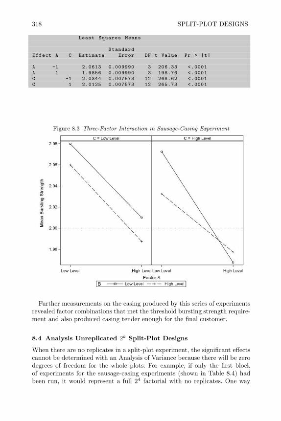
318 SPLIT-PLOT DESIGNS
Least Squares Means
StandardEffect A C Estimate Error DF t Value Pr > |t|
A -1 2.0613 0.009990 3 206.33 <.0001A 1 1.9856 0.009990 3 198.76 <.0001C -1 2.0344 0.007573 12 268.62 <.0001C 1 2.0125 0.007573 12 265.73 <.0001
Figure 8.3 Three-Factor Interaction in Sausage-Casing Experiment
Further measurements on the casing produced by this series of experimentsrevealed factor combinations that met the threshold bursting strength require-ment and also produced casing tender enough for the final customer.
8.4 Analysis Unreplicated 2k Split-Plot Designs
When there are no replicates in a split-plot experiment, the significant effectscannot be determined with an Analysis of Variance because there will be zerodegrees of freedom for the whole plots. For example, if only the first blockof experiments for the sausage-casing experiments (shown in Table 8.4) hadbeen run, it would represent a full 24 factorial with no replicates. One way
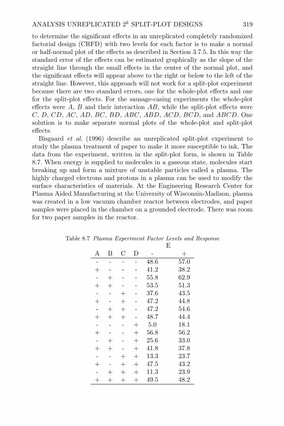
ANALYSIS UNREPLICATED 2k SPLIT-PLOT DESIGNS 319
to determine the significant effects in an unreplicated completely randomizedfactorial design (CRFD) with two levels for each factor is to make a normalor half-normal plot of the effects as described in Section 3.7.5. In this way thestandard error of the effects can be estimated graphically as the slope of thestraight line through the small effects in the center of the normal plot, andthe significant effects will appear above to the right or below to the left of thestraight line. However, this approach will not work for a split-plot experimentbecause there are two standard errors, one for the whole-plot effects and onefor the split-plot effects. For the sausage-casing experiments the whole-ploteffects were A, B and their interaction AB, while the split-plot effects wereC, D, CD, AC, AD, BC, BD, ABC, ABD, ACD, BCD, and ABCD. Onesolution is to make separate normal plots of the whole-plot and split-ploteffects.
Bisgaard et al. (1996) describe an unreplicated split-plot experiment tostudy the plasma treatment of paper to make it more susceptible to ink. Thedata from the experiment, written in the split-plot form, is shown in Table8.7. When energy is supplied to molecules in a gaseous state, molecules startbreaking up and form a mixture of unstable particles called a plasma. Thehighly charged electrons and protons in a plasma can be used to modify thesurface characteristics of materials. At the Engineering Research Center forPlasma Aided Manufacturing at the University of Wisconsin-Madison, plasmawas created in a low vacuum chamber reactor between electrodes, and papersamples were placed in the chamber on a grounded electrode. There was roomfor two paper samples in the reactor.
Table 8.7 Plasma Experiment Factor Levels and ResponseE
A B C D - +- - - - 48.6 57.0+ - - - 41.2 38.2- + - - 55.8 62.9+ + - - 53.5 51.3- - + - 37.6 43.5+ - + - 47.2 44.8- + + - 47.2 54.6+ + + - 48.7 44.4- - - + 5.0 18.1+ - - + 56.8 56.2- + - + 25.6 33.0+ + - + 41.8 37.8- - + + 13.3 23.7+ - + + 47.5 43.2- + + + 11.3 23.9+ + + + 49.5 48.2

320 SPLIT-PLOT DESIGNS
The factors under study in the experiment were A: low and high pressure,B: low and high power, C: low and high gas flow rate, D: type of gas oxygenor SiCl4, and E: paper type. The response, wettability of the paper, wasmeasured by placing a droplet of water on the treated paper and measuringthe contact angle between the droplet and the paper surface with a specialmicroscope. Because the plasma was created in a vacuum, it takes up to ahalf an hour of pumping to get the reactor down to the appropriate vacuumlevel each time the chamber is opened to insert new paper samples. Therefore,rather than completing a completely randomized 25 factorial, the experimentswere completed in the following way. The experimenter first randomized theorder of the combinations of factors A to D to 16 reactor runs. During eachrun two samples of paper were placed in the reactor (one of each type), anda coin was tossed to determine which paper type was placed on the rightor left side of the reactor. By doing this a split-plot experiment was createdwhere the experimental unit for factors A to D was a reactor run, while theexperimental unit for factor E, the paper type, was the position inside thereactor for a particular run.
The main effects A, B, C, D, and all their interactions are whole-plot fac-tors, and their significance should be tested with the whole-plot error term.Factor E and its interactions with A, B, C, D, and all their interactions, aresplit-plot factors, and their significance should be tested with the split-ploterror term. The SAS code below illustrates how to make separate normal plotsof the whole-plot and split-plot effects. The first commands fit the saturatedmodel exactly as was done in Section 3.7.5.
data plasma;input A B C D E y;datalines;-1 -1 -1 -1 -1 48.61 -1 -1 -1 -1 41.2
. . .proc glm;*fit the full factorial model;
model y=A|B|C|D|E;*this ouputs the parameter estimates to a file;
ods output ParameterEstimates=sol;run;
The next section of code, shown at the top of the following page, selectsthe whole-plot calculated effects A, B, AB, C, AC, BC, ABC, D, AD, BD,ABD, CD, ACD, BCD, ABCD, which are the second through sixteenthestimates on the output, and makes a normal plot of them. Other than thestatement if 1< n <17 used to select the whole-plot effects, this code is thesame as that shown in Section 3.7.5. The resulting plot, with a manually addedreference line, is shown in Figure 8.4. It can be seen that the whole-plot maineffects A: pressure, D: type of gas, and their interaction appear significant.
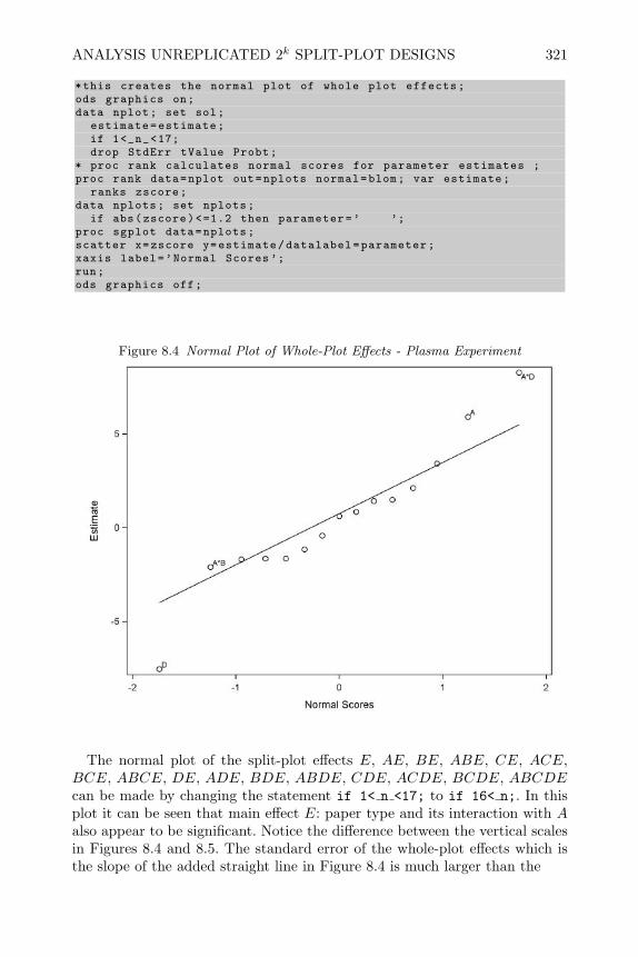
ANALYSIS UNREPLICATED 2k SPLIT-PLOT DESIGNS 321
*this creates the normal plot of whole plot effects;ods graphics on;data nplot; set sol;
estimate=estimate;if 1<_n_<17;drop StdErr tValue Probt;
* proc rank calculates normal scores for parameter estimates ;proc rank data=nplot out=nplots normal=blom; var estimate;
ranks zscore;data nplots; set nplots;
if abs(zscore)<=1.2 then parameter=’ ’;proc sgplot data=nplots;scatter x=zscore y=estimate/datalabel=parameter;xaxis label=’Normal Scores ’;run;ods graphics off;
Figure 8.4 Normal Plot of Whole-Plot Effects - Plasma Experiment
The normal plot of the split-plot effects E, AE, BE, ABE, CE, ACE,BCE, ABCE, DE, ADE, BDE, ABDE, CDE, ACDE, BCDE, ABCDEcan be made by changing the statement if 1< n <17; to if 16< n;. In thisplot it can be seen that main effect E: paper type and its interaction with Aalso appear to be significant. Notice the difference between the vertical scalesin Figures 8.4 and 8.5. The standard error of the whole-plot effects which isthe slope of the added straight line in Figure 8.4 is much larger than the
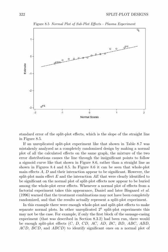
322 SPLIT-PLOT DESIGNS
Figure 8.5 Normal Plot of Sub-Plot Effects - Plasma Experiment
standard error of the split-plot effects, which is the slope of the straight linein Figure 8.5.
If an unreplicated split-plot experiment like that shown in Table 8.7 wasmistakenly analyzed as a completely randomized design by making a normalplot of all the calculated effects on the same graph, the mixture of the twoerror distributions causes the line through the insignificant points to followa sigmoid curve like that shown in Figure 8.6, rather than a straight line asshown in Figures 8.4 and 8.5. In Figure 8.6 it can be seen that whole-plotmain effects A, D and their interaction appear to be significant. However, thesplit-plot main effect E and the interaction AE that were clearly identified tobe significant on the normal plot of split-plot effects now appear to be buriedamong the whole-plot error effects. Whenever a normal plot of effects from afactorial experiment takes this appearance, Daniel and later Bisgaard et al.(1996) warned that the treatment combinations may not have been completelyrandomized, and that the results actually represent a split-plot experiment.
In this example there were enough whole-plot and split-plot effects to makeseparate normal plots. In other unreplicated 2k split-plot experiments thismay not be the case. For example, if only the first block of the sausage-casingexperiment (that was described in Section 8.3.2) had been run, there wouldbe enough split-plot effects (C, D, CD, AC, AD, BC, BD, ABC, ABD,ACD, BCD, and ABCD) to identify significant ones on a normal plot of

ANALYSIS UNREPLICATED 2k SPLIT-PLOT DESIGNS 323
Figure 8.6 Normal Plot of All Effects - Plasma Experiment
effects, however, there were not enough whole-plot effects (A, B, and AB) toeffectively identify the significant ones on a plot.
One strategy to use in this situation is the following. If any interactions be-tween whole-plot factors and split-plot factors appear significant in the nor-mal plot of split-plot effects, the effect heredity principle might imply thatthe involved whole-plot main effect may also be significant. If the suspectedwhole-plot main effect has a relatively large effect this hypothesis is furthersupported, and it may be fruitful to include that main effect in the model be-fore calculating the least squares interaction cell means and interpreting thesignificant interaction. Any other whole-plot effects that are larger in magni-tude than the whole-plot main effect involved in a significant interaction mayalso be considered to be significant.
Another strategy can be used in this situation if there is some prior knowl-edge about variability to be expected in whole-plot units. For example, if theexperiment is performed in a two-step manufacturing process, and there ishistory (such as control charts) maintained on the output of the first processstep, then Gilmour and Goos (2006) propose using a Bayesian analysis withan informative prior on the whole-plot error random effects.

324 SPLIT-PLOT DESIGNS
8.5 2k−p Fractional Factorials in Split Plots (FFSP)
The 2k−p fractional factorial experiments described in Chapter 6 assumed thattreatment combinations could be assigned to experimental units completelyat random. However, sometimes this is impractical for the same reasons citedin Section 8.1. In this case a fractional factorial split-plot (FFSP) design canbe utilized. There are many ways to create a fractional factorial split-plotdesign with the same number of factors and runs. One method is shown inTable 8.8 which is similar in format to Tables 8.4 and 8.5. Here the whole-plotfactors are labeled A, B, and C, while the sub-plot factors are labeled P , Q,and R. A 23−1 fractional factorial is created with the whole-plot factors usingthe defining relation I = ABC. The four whole-plot treatment combinationswould then be assigned at random to whole-plot experimental units. Eachwhole plot is divided into four sub-plots which are assigned at random toreceive one of the four treatment combinations in the 23−1 fractional factorialcreated with the sub-plot factors using defining relation I = PQR.
Table 8.8 Cartesian Product Fractional Factorial Split-Plot Design
(I = PQR)P − + − +
(I = ABC) Q − − + +A B C R + − − −− − + x x x x+ − − x x x x− + − x x x x+ + + x x x x
Since the same four combinations of sub-plot treatment factors are used ineach whole plot, this design is called a cartesian product design and the “x”sin Table 8.8 indicate which treatment combinations are used. With six factorsand a total of sixteen treatment combinations, this design is a 1
4 fraction. Theoverall defining relation can be obtained by multiplying the defining relationfor the whole-plot fraction by the defining relation for the sub-plot fraction,i.e., (I + ABC) × (I + PQR) = I + ABC + PQR + ABCPQR. Thus, thedesign has resolution III and all main effects are confounded with one two-factor interaction, one four-factor interaction and one-five factor interaction.
A better confounding pattern can be obtained by using whole-plot factorsin the sub-plot generators as shown in Table 8.9. Here a different fractionof the combinations of sub-plot factors is used in each whole plot. This is

2k−p FRACTIONAL FACTORIALS IN SPLIT PLOTS (FFSP) 325
similar to the way a fractional factorial was augmented with a mirror imagedesign in Section 6.5. By using the fraction of sub-plot factors obtained withthe generator P = −QR when whole-plot factor A is at its low level, and byusing the fraction obtained with the generator P = +QR when the whole-plotfactor A is at its high level, it is equivalent to using the generator P = AQRor the defining relation I+APQR for the fractional factorial in the sub-plots.This method is called split-plot confounding by Bisgaard (2000).
Table 8.9 Split-Plot Confounding in Fractional Factorial Split-Plot Design
(I = ABC)A B C
− − + I = −PQR+ − − I = +PQR− + − I = −PQR+ + + I = +PQR
This design can be randomized similar to the way the design shown in Table8.8 can be randomized. The four whole-plot treatment combinations shouldbe assigned at random to whole-plot experimental units. Each whole-plot isdivided into four sub-plots which are assigned at random to receive one of thefour sub-plot treatment combinations in the 23−1 fractional factorial createdusing the generator P = +QR if the whole-plot received the high level offactor A, or to receive one of the four sub-plot treatment combinations in the23−1 fractional factorial created with generator P = −QR if the whole-plotreceived the low level of factor A. This design can be created easily in the SASdata step using the commands shown at the top of the next page.
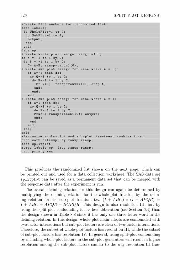
326 SPLIT-PLOT DESIGNS
*Create Plot numbers for randomized list;data labels;do WholePlot =1 to 4;do SubPlot =1 to 4;output;
end;end;
data wp;*Create whole -plot design using I=ABC;do A = -1 to 1 by 2;do B = -1 to 1 by 2;
C= A*B; ranwp=ranuni (0);*Create sub -plot design for case where A = -;
if A=-1 then do;do Q=-1 to 1 by 2;do R=-1 to 1 by 2;
P=-Q*R; ransp=ranuni (0); output;end;
end;end;
*Create sub -plot design for case where A = +;if A=1 then do;do Q=-1 to 1 by 2;
do R=-1 to 1 by 2;P=Q*R; ransp=ranuni (0); output;end;
end;end;
end;end;*Randomize whole -plot and sub -plot treatment combinations;proc sort data=wp; by ranwp ransp;data splitplot;merge labels wp; drop ranwp ransp;proc print; run;
This produces the randomized list shown on the next page, which canbe printed out and used for a data collection worksheet. The SAS data setsplitplot can be saved as a permanent data set that can be merged withthe response data after the experiment is run.
The overall defining relation for this design can again be determined bymultiplying the defining relation for the whole-plot fraction by the defin-ing relation for the sub-plot fraction, i.e., (I + ABC) × (I + APQR) =I + ABC + APQR + BCPQR. This design is also resolution III, but byusing the split-plot confounding it has less abberation (see Section 6.4) thanthe design shown in Table 8.8 since it has only one three-letter word in thedefining relation. In this design, whole-plot main effects are confounded withtwo-factor interactions but sub-plot factors are clear of two-factor interactions.Therefore, the subset of whole-plot factors has resolution III, while the subsetof sub-plot factors has resolution IV. In general, using split-plot confoundingby including whole-plot factors in the sub-plot generators will result in higherresolution among the sub-plot factors similar to the way resolution III frac-
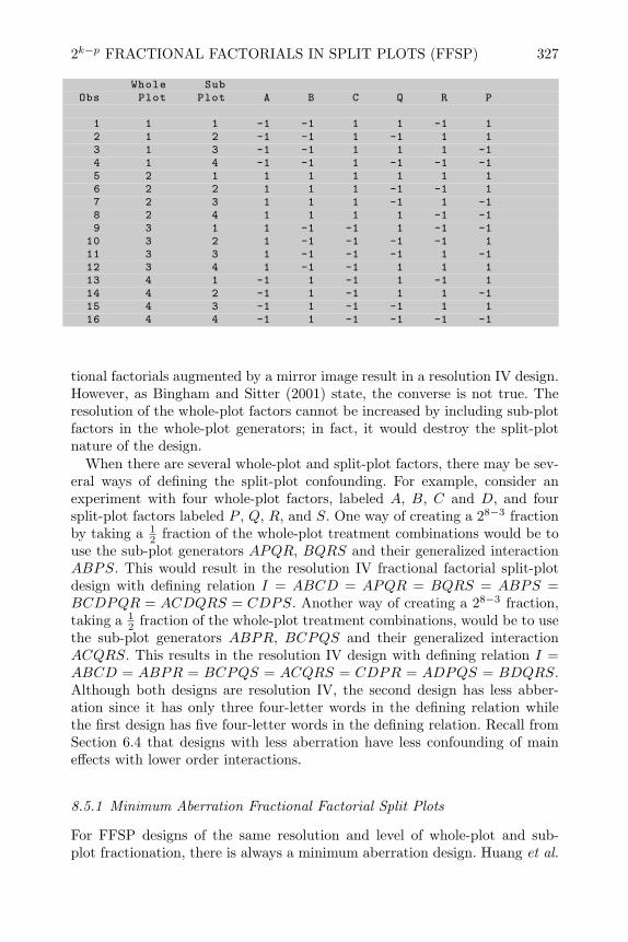
2k−p FRACTIONAL FACTORIALS IN SPLIT PLOTS (FFSP) 327
Whole SubObs Plot Plot A B C Q R P
1 1 1 -1 -1 1 1 -1 12 1 2 -1 -1 1 -1 1 13 1 3 -1 -1 1 1 1 -14 1 4 -1 -1 1 -1 -1 -15 2 1 1 1 1 1 1 16 2 2 1 1 1 -1 -1 17 2 3 1 1 1 -1 1 -18 2 4 1 1 1 1 -1 -19 3 1 1 -1 -1 1 -1 -1
10 3 2 1 -1 -1 -1 -1 111 3 3 1 -1 -1 -1 1 -112 3 4 1 -1 -1 1 1 113 4 1 -1 1 -1 1 -1 114 4 2 -1 1 -1 1 1 -115 4 3 -1 1 -1 -1 1 116 4 4 -1 1 -1 -1 -1 -1
tional factorials augmented by a mirror image result in a resolution IV design.However, as Bingham and Sitter (2001) state, the converse is not true. Theresolution of the whole-plot factors cannot be increased by including sub-plotfactors in the whole-plot generators; in fact, it would destroy the split-plotnature of the design.
When there are several whole-plot and split-plot factors, there may be sev-eral ways of defining the split-plot confounding. For example, consider anexperiment with four whole-plot factors, labeled A, B, C and D, and foursplit-plot factors labeled P , Q, R, and S. One way of creating a 28−3 fractionby taking a 1
2 fraction of the whole-plot treatment combinations would be touse the sub-plot generators APQR, BQRS and their generalized interactionABPS. This would result in the resolution IV fractional factorial split-plotdesign with defining relation I = ABCD = APQR = BQRS = ABPS =BCDPQR = ACDQRS = CDPS. Another way of creating a 28−3 fraction,taking a 1
2 fraction of the whole-plot treatment combinations, would be to usethe sub-plot generators ABPR, BCPQS and their generalized interactionACQRS. This results in the resolution IV design with defining relation I =ABCD = ABPR = BCPQS = ACQRS = CDPR = ADPQS = BDQRS.Although both designs are resolution IV, the second design has less abber-ation since it has only three four-letter words in the defining relation whilethe first design has five four-letter words in the defining relation. Recall fromSection 6.4 that designs with less aberration have less confounding of maineffects with lower order interactions.
8.5.1 Minimum Aberration Fractional Factorial Split Plots
For FFSP designs of the same resolution and level of whole-plot and sub-plot fractionation, there is always a minimum aberration design. Huang et al.

328 SPLIT-PLOT DESIGNS
(1998) and Bingham and Sitter (1999) have given tables of the generators forminimum abberation split-plot designs for a small to moderate size numberof factors. SAS ADX automatically generates the minimum aberration split-plot designs using the generators found in these tables. SAS proc factex, inSAS versions 9.2 and later, can sometimes find the same generators using analgorithm (see Section 6.3).
Once the number of whole-plot factors and the number of sub-plot factorshas been decided upon, there are other things to consider when generatinga FFSP design with SAS ADX. One is the degree of fractionation of thewhole-plot factors and the number of whole plots. Another is the degree offractionation of the sub-plot factors and the number of sub-plots per wholeplot. For example, if we define four whole-plot factors and four sub-plot fac-tors by choosing the Create New Split-Plot Design menu and filling out thetemplate tabs for Whole Plot Factor and Sub-plot Factor as shown in Figure8.7.
Figure 8.7 SAS ADX Define Variables Template for Split-Plot Design

2k−p FRACTIONAL FACTORIALS IN SPLIT PLOTS (FFSP) 329
SAS ADX lists four alternate minimum aberration designs as shown inFigure 8.8.
Figure 8.8 SAS ADX Split-Plot Design Specification Template
The first design uses a one-half fraction of the combinations of whole-plottreatment levels with defining relation I = ABCD, resulting in eight wholeplots each split into two sub-plots. By clicking on this design and then theDesign Details ... button the information shown in Figure 8.9 is shown on thedesign properties tab. Here it can be seen that this design uses the split-plot
Figure 8.9 SAS ADX Design Details Results for 24−1 × 24−3 Design
confounding generators found in Bingham and Sitter’s tables. The design isresolution IV but no two factor-interactions are estimable clear of other two-factor interactions. Clicking on the Alias Structure tab, the aliases among thetwo-factor interactions are shown in Figure 8.10.

330 SPLIT-PLOT DESIGNS
Figure 8.10 SAS ADX Alias Structure for 24−1 × 24−3 Design
SAS proc factex finds the same generators and the same design whenusing the commands below.
proc factex;factors A B C D P Q R S;size design =16;blocks units =( Block =8);model resolution =4/minabs;uniteffect Block / whole=(A B C D)
sub=(P Q R S);examine aliasing (2) confounding;output out=sp;
proc print; run;
Figure 8.11 shows the results of checking the design details for the seconddesign shown in Figure 8.8. It utilizes a full factorial in the whole-plot factorsresulting in 16 whole plots each divided into two sub-plots. This design wascreated using the generators in the tables of Huang et al. (1998).
It can be seen that the design is also resolution IV, but 13 of the 28 two-factor interactions are estimable clear of other two-factor interactions. Thiscan be seen by examining the defining relation. This is a 1
8 th fraction and whatSAS ADX labels as the defining relation in Figure 8.11 is actually a list ofthe three generators for the design. The complete defining relation, includingall generalized interactions is: I = ABPQ = ACPR = BCDPS = BCQR =ACDQS = ABDRS = DPQRS. The estimable effects (up to two-factorinteractions except for the case where no effect of order two or less is aliasedwith the given effect) are shown below Figure 8.11.
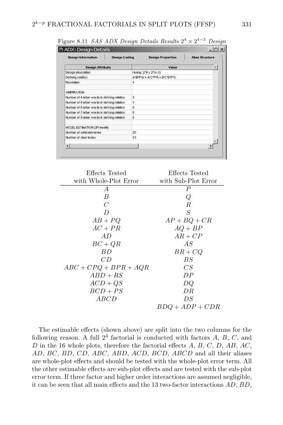
2k−p FRACTIONAL FACTORIALS IN SPLIT PLOTS (FFSP) 331
Figure 8.11 SAS ADX Design Details Results 24 × 24−3 Design
Effects Tested Effects Testedwith Whole-Plot Error with Sub-Plot Error
A PB QC RD S
AB + PQ AP +BQ+ CRAC + PR AQ+BP
AD AR+ CPBC +QR AS
BD BR+ CQCD BS
ABC + CPQ+BPR+AQR CSABD +RS DPACD +QS DQBCD + PS DRABCD DS
BDQ+ADP + CDR
The estimable effects (shown above) are split into the two columns for thefollowing reason. A full 24 factorial is conducted with factors A, B, C, andD in the 16 whole plots, therefore the factorial effects A, B, C, D, AB, AC,AD, BC, BD, CD, ABC, ABD, ACD, BCD, ABCD and all their aliasesare whole-plot effects and should be tested with the whole-plot error term. Allthe other estimable effects are sub-plot effects and are tested with the sub-ploterror term. If three factor and higher order interactions are assumed negligible,it can be seen that all main effects and the 13 two-factor interactions AD, BD,

332 SPLIT-PLOT DESIGNS
CD, RS, QS, PS, AS, BS, CS, DP , DQ, DR, and DS can be estimatedclear of main effects or two-factor interactions. This is what is referred to bythe number of clear terms in Figure 8.11.
The third design shown in Figure 8.8 is also resolution IV, but by utiliz-ing a one-half fraction of the combinations of whole-plot treatment levels andthen splitting each whole-plot into four sub-plots, only eight whole plots arerequired. The generators for this design are ABCD, ABPR, and BCPQS.In this design seven effects, namely main effects A, B, C, and D and con-founded strings of interactions AB + CD + PR, AC + BD, and AD + BC,are estimated less precisely and should be compared to whole-plot variabil-ity for testing significance. This design also allows estimation of 13 of the 28two-factor interactions clear of main effects and other two-factor interactions,so it appears to be similar to the second design listed in Figure 8.8. However,because of the reduced number of whole plots and the increased number ofsub-plots all 13 of the clear two-factor interactions can be tested with themore precise sub-plot error term, whereas in the second design six of the cleartwo-factor interactions (namely AD, BD, CD, RS, QS, and PS) must betested with the less precise whole-plot error term.
The fourth and last design shown in Figure 8.8 consists of a full factorialin the four whole-plot factors A, B, C and D in 16 whole plots each dividedinto 4 sub-plots. The defining relation for this design is I = ABCPR =ADPQS = BCDRQS. This design is resolution V, and all main effects andtwo-factor interactions can be estimated clear of other main effects and two-factor interactions.
The choice between these four alternative designs would depend upon therelative cost of whole plot and sub-plot experimental units and the precisiondesired for the various estimable two-factor interactions. For more discussionon this topic, see Kulahci et al. (2006), Bisgaard (2000) and Bingham andSitter (2001).
When using proc factex, the user does not have a choice about the degreeof fractionation in the whole-plot and sub-plot design. proc factex only al-lows choice of the overall degree of fractionation. For example, the code belowcreates a 28−3 fractional factorial with four whole-plot factors and four sub-plot factors. The search algorithm in proc factex only finds a 24−1 × 24−2
proc factex;factors A B C D P Q R S;size design =32;blocks units =( Block =16);model resolution =4/minabs;uniteffect Block / whole=(A B C D)
sub=(P Q R S);examine aliasing (2) confounding;output out=sp;
proc print; run;

2k−p FRACTIONAL FACTORIALS IN SPLIT PLOTS (FFSP) 333
design with generators ABCD, ABPQ, and ACRS. The complete definingrelation for this design is I = ABCD = CDPQ = BDRS = ADPQRS =ABPQ = ACRS = BCPQRS which is not the minimum aberration design.For a 28−3 split-plot fractional factorial, SAS ADX gave a choice of a 24×24−3
split-plot design or a 24−1 × 24−2 split-plot design. Both of these designs areminimum aberration. The generators for the 24−1 × 24−2 created by ADXcome from Huang et al. (1998)’s tables. It has only three four-letter words inthe defining relation and is better than the design found by proc factex.
8.5.2 Analysis of a Fractional Factorial Split-Plot
Bingham and Sitter (2001) describe an experiment to study effects of five fac-tors upon the geometric distortion of drive gears. The factors were A: furnacetrack, B: tooth size, C: part positioning, P : carbon potential and Q: operat-ing mode. It was more efficient to perform the experimental trials by keepinglevels of factors A, B and C constant in blocks and varying factors P and Qwithin the blocks. A schematic of the 23× 22−1 design is shown in Table 8.10.
Table 8.10 Fractional Factorial Split-Plot Design for Gear DistortionP − + − +
A B C Q − − + +− − − x x+ − − x x− + − x x+ + − x x− − + x x+ − + x x− + + x x+ + + x x
This is a split-plot design due to the fact that factors A, B and C areconstant in blocks of runs. It is also evident that split-plot confounding hasbeen utilized by the fact that a different subset of the combinations sub-plotfactor levels is used in each whole plot. The defining relation for the design isI = ABCPQ, and the response was the dishing of the gears. This design isone of the minimum aberration designs in Bingham and Sitter (2001)’s tablesand can be easily generated using SAS ADX, or proc factex.
SAS ADX cannot perform an analysis of the data of a FFSP design whenthere are no replicates of the whole plots. Therefore if the design shown inTable 8.10 is created in ADX, it must be exported to a SAS data file foranalysis. The ADX examples on the lecture slides for this book illustrate howto export SAS ADX designs. Alternatively, the design can be created directlyin a SAS data file using proc factex. The commands to do that are shown

334 SPLIT-PLOT DESIGNS
below. In this case, the algorithm used by proc factex comes up with thesame minimum aberration design shown in Bingham and Sitter (2001)’s tables.A randomized data collection form can be created from the data file sp bymodifying the last three lines of the SAS code in Section 8.5.
proc factex;factors A B C P Q;size design =16;blocks units =( Block =8);model resolution =5/minabs;uniteffect Block / whole=(A B C)
sub=(P Q);examine aliasing (3) confounding;output out=sp;
run;proc print; var Block A B C P Q; run;
The design is a half-fraction with defining relation I = ABCPQ, and theestimable whole-plot and sub-plot effects are shown in Table 8.11.
Table 8.11 Estimable Effects for Gear Distortion ExperimentWhole-Plot Sub-Plot
Effects EffectsA+BCPQ P +ABCQB +ACPQ Q+ABCPC +ABPQ AP +BCQAB + CPQ AQ+BCPAC +BPQ BP +ACQBC +APQ BQ+ACPABC + PQ CP +ABQ
CQ+ABP
The model for the experiment written in the split-plot form is shown inEquation (8.8).
yijklm = µ+ αi + βj + γk + αβij + αγik + βγjk + αβγijk + wijk
+ ρl + φm + αρjl + αφim + βρjl + βφjm + γρkl + γφkm + ρφlm + εijklm(8.8)
Since there are no replicates of the whole plots, wijk cannot be estimated, and
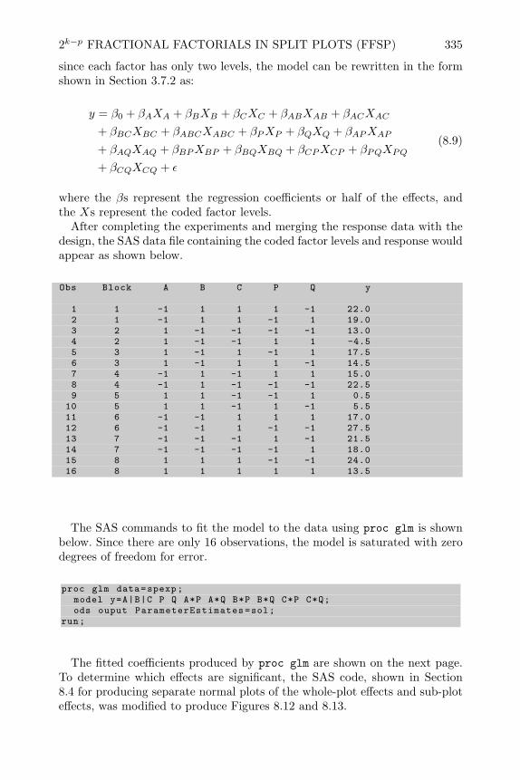
2k−p FRACTIONAL FACTORIALS IN SPLIT PLOTS (FFSP) 335
since each factor has only two levels, the model can be rewritten in the formshown in Section 3.7.2 as:
y = β0 + βAXA + βBXB + βCXC + βABXAB + βACXAC
+ βBCXBC + βABCXABC + βPXP + βQXQ + βAPXAP
+ βAQXAQ + βBPXBP + βBQXBQ + βCPXCP + βPQXPQ
+ βCQXCQ + ε
(8.9)
where the βs represent the regression coefficients or half of the effects, andthe Xs represent the coded factor levels.
After completing the experiments and merging the response data with thedesign, the SAS data file containing the coded factor levels and response wouldappear as shown below.
Obs Block A B C P Q y
1 1 -1 1 1 1 -1 22.02 1 -1 1 1 -1 1 19.03 2 1 -1 -1 -1 -1 13.04 2 1 -1 -1 1 1 -4.55 3 1 -1 1 -1 1 17.56 3 1 -1 1 1 -1 14.57 4 -1 1 -1 1 1 15.08 4 -1 1 -1 -1 -1 22.59 5 1 1 -1 -1 1 0.5
10 5 1 1 -1 1 -1 5.511 6 -1 -1 1 1 1 17.012 6 -1 -1 1 -1 -1 27.513 7 -1 -1 -1 1 -1 21.514 7 -1 -1 -1 -1 1 18.015 8 1 1 1 -1 -1 24.016 8 1 1 1 1 1 13.5
The SAS commands to fit the model to the data using proc glm is shownbelow. Since there are only 16 observations, the model is saturated with zerodegrees of freedom for error.
proc glm data=spexp;model y=A|B|C P Q A*P A*Q B*P B*Q C*P C*Q;ods ouput ParameterEstimates=sol;
run;
The fitted coefficients produced by proc glm are shown on the next page.To determine which effects are significant, the SAS code, shown in Section8.4 for producing separate normal plots of the whole-plot effects and sub-ploteffects, was modified to produce Figures 8.12 and 8.13.

336 SPLIT-PLOT DESIGNS
Parameter Estimate
Intercept 15.40625000A -4.90625000B -0.15625000A*B 0.53125000C 3.96875000A*C 2.90625000B*C 0.40625000A*B*C 0.59375000P -2.34375000Q -3.40625000A*P -0.90625000A*Q -0.34375000B*P 1.09375000B*Q 0.15625000C*P -0.28125000C*Q 0.78125000
Figure 8.12 Normal Plot of Whole-Plot Effects - Gear Distortion Experiment

2k−p FRACTIONAL FACTORIALS IN SPLIT PLOTS (FFSP) 337
Figure 8.13 Normal Plot of Sub-Plot Effects - Gear Distortion Experiment
Here it can be seen that whole-plot effects A and C along with their interactionappear to be significant along with sub-plot factors P and Q.
The interpretation of the significant effects can be explained as follows.Factor P : carbon potential has a negative regression coefficient in the procglm output, so increasing the carbon potential decreases the response geardishing. Factor Q: operating mode also had a negative coefficient so usingthe operating mode represented by the +1 level of this factor also reducesgear dishing. Since there is an interaction between factors A and C, we mustconsider the interaction plot shown in Figure 8.14 to interpret their effects.In that figure, it can be seen that changing from the low to high levels ofeither A:furnace track or C:part positioning will decrease gear dishing, but ifthe high level of both these factors is chosen there will be a disproportionatedecrease in gear dishing. Therefore, to decrease gear dishing the high levels offactors A:furnace track, P : carbon potential, and Q: operating mode shouldbe selected, and the low level of factor C:part positioning.
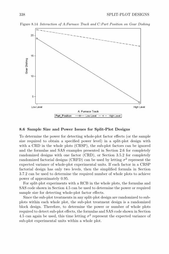
338 SPLIT-PLOT DESIGNS
Figure 8.14 Interaction of A:Furnace Track and C:Part Position on Gear Dishing
8.6 Sample Size and Power Issues for Split-Plot Designs
To determine the power for detecting whole-plot factor effects (or the samplesize required to obtain a specified power level) in a split-plot design withwith a CRD in the whole plots (CRSP), the sub-plot factors can be ignoredand the formulas and SAS examples presented in Section 2.6 for completelyrandomized designs with one factor (CRD), or Section 3.5.2 for completelyrandomized factorial designs (CRFD) can be used by letting σ2 represent theexpected variance of whole-plot experimental units. If each factor in a CRSPfactorial design has only two levels, then the simplified formula in Section3.7.2 can be used to determine the required number of whole plots to achievepower of approximately 0.95.
For split-plot experiments with a RCB in the whole plots, the formulas andSAS code shown in Section 4.5 can be used to determine the power or requiredsample size for detecting whole-plot factor effects.
Since the sub-plot treatments in any split-plot design are randomized to sub-plots within each whole plot, the sub-plot treatment design is a randomizedblock design. Therefore, to determine the power or number of whole plotsrequired to detect sub-plot effects, the formulas and SAS code shown in Section4.5 can again be used, this time letting σ2 represent the expected variance ofsub-plot experimental units within a whole plot.

REVIEW OF IMPORTANT CONCEPTS 339
8.7 Review of Important Concepts
When the levels of one or more treatment factors are difficult to change or re-quire more experimental material for evaluation than other treatment factors,it may be impractical to completely randomize the order of experiments in afactorial or fractional factorial design. This is frequently the case in processimprovement studies where some treatment factors belong to one process stepand others belong to a later process step. Split-plot designs allow for restrictedrandomization where some factor levels are varied more frequently than oth-ers, and the models for split-plot designs will allow accurate assessment ofthe significance of both hard and easy-to-vary factors despite the restrictedrandomization.
In split-plot designs the experimental unit are larger for the hard-to-varyfactors and are called whole plots (based on the agricultural origins of thedesigns). The levels of the easy-to-vary factors can be varied within partsof whole plots (called sub-plots) which are the experimental units for thesefactors. Whole plots (like blocks of homogeneous experimental units) are gen-erally more variable than sub-plots within whole plots, and therefore there isless power for detecting differences in the hard-to-vary (or whole-plot factors)than there is for the sub-plot factors in split-plot designs.
If the whole-plot experimental units are homogeneous and can be assignedat random to the levels or combinations of levels of the whole-plot factorsthe design that should be used is split-plot with CRD in the whole plots ora CRSP design as shown in Figure 8.15. The model for a CRSP design withone whole-plot factor and one sub-plot factor is written as:
yijk = µ+ αi + w(i)j + βk + αβik + εijk (8.10)
where the first three terms in the model are the same as the model for aCRD given in Chapter 2. In the analysis of data using this model, then meansquare for the random whole-plot error term w(i)j is the denominator for theF -test for αi, while the means square for the sub-plot error term εijk is thedenominator for F -test of the sub-plot factor βk.
If whole-plot experimental units are not homogeneous and can be groupedinto more uniform blocks, such as groups in time, the whole plots should berandomized to levels or combinations of levels of whole-plot factors withineach block. This results in a split-plot design with a RCB in the whole plotsor a RBSP design as shown in Figure 8.15. The model for a RBSP design withone whole-plot factor, α, and one sub-plot factor β is:
yijk = µ+ bi + αj + bαij + βk + αβik + εijk (8.11)
where the random block effect is bi and the random block by treatment in-teraction, bαij is the error term for testing the significance of the whole-ploteffect α.
When there are no replicates of the levels or combination of levels of whole-plot treatments the analysis of split-plot experiments is accomplished by mak-ing separate normal plots of the whole-plot effects and the sub-plot effects.
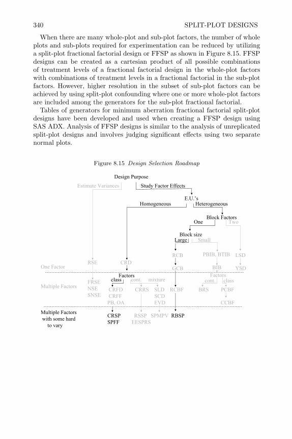
340 SPLIT-PLOT DESIGNS
When there are many whole-plot and sub-plot factors, the number of wholeplots and sub-plots required for experimentation can be reduced by utilizinga split-plot fractional factorial design or FFSP as shown in Figure 8.15. FFSPdesigns can be created as a cartesian product of all possible combinationsof treatment levels of a fractional factorial design in the whole-plot factorswith combinations of treatment levels in a fractional factorial in the sub-plotfactors. However, higher resolution in the subset of sub-plot factors can beachieved by using split-plot confounding where one or more whole-plot factorsare included among the generators for the sub-plot fractional factorial.
Tables of generators for minimum aberration fractional factorial split-plotdesigns have been developed and used when creating a FFSP design usingSAS ADX. Analysis of FFSP designs is similar to the analysis of unreplicatedsplit-plot designs and involves judging significant effects using two separatenormal plots.
Figure 8.15 Design Selection Roadmap
Design Purpose
Estimate Variances Study Factor Effects
E.U.’s
Block Factors
One Factor
Multiple Factors
Multiple Factorswith some hard
to vary
Block size
Homogeneous Heterogeneous
Large Small
RCB
GCB
PBIB, BTIB
BIB
LSD
YSDRSE CRD
FactorsFRSENSESNSE
CRFD CRRS SLD RCBF BRS PCBFCRFF SCD
PB, OA EVD CCBF
CRSP RSSP SPMPV RBSPSPFF EESPRS
One Two
class cont. mixture cont. classFactors

EXERCISES 341
8.8 Exercises
1. Why wouldn’t you treat the diameter of each cookie as the response in thecookie-baking experiment described in Section 8.2? What would you callthe individual measurements on each cookie on each tray?
2. Modify the SAS code in Section 8.2.1 to create
(a) A randomized list for a split-plot experiment with a completely random-ized whole plots where there is one whole-plot factor A with 3 levels andtwo replicate whole plots for each level, and one split-plot factor B withthree levels. Label the levels with the nvals=(1 2 3) rather than thecvals=( ) shown in Section 8.2.1.
(b) Write the model for the design you created in (a).(c) A randomized list for a split-plot experiment with a completely random-
ized whole plots where there are two whole-plot factors A and B eachwith two levels and two replicate whole plots per treatment combinationand two split-plot treatments C and D each with three levels.
(d) Write the model for the design you created in (c).
3. Kuehl (2000) reports the results of an experiment conducted at a largeseafood company to investigate the effect of storage temperature and typeof seafood upon bacterial growth on oysters and mussels. Three storagetemperatures were studied (0C, 5C, and 10C). Three cold storage unitswere randomly assigned to be operated at each temperature. Within eachstorage unit, oysters and mussels were randomly assigned to be stored onone of the two shelves. The seafood was stored for two weeks at the assignedtemperature, and at the end of the time the bacterial count was obtainedfrom a sample on each shelf. The resulting data (log bacterial count) isshown below.
Storage Seafood TypeUnit Temp. Oysters Mussels
1 0 3.6882 0.35652 0 1.8275 1.70233 0 5.2327 4.57804 5 7.1950 5.01695 5 9.3224 7.95196 5 7.4195 6.38617 10 9.7842 10.13528 10 6.4703 5.04829 10 9.4442 11.0329
(a) What is the experimental unit for temperature?(b) Why was it necessary to include 9 storage units instead of 3?(c) What is the experimental unit for seafood type?

342 SPLIT-PLOT DESIGNS
(d) Write the model for the data.(e) Analyze the data to determine what temperature and type of seafood
have significant effects.(f) Interpret any significant effects.(g) Check the assumptions of the model you used for analysis.
4. Modify the SAS code in Section 8.3.1 to create the design for the sausage-casing experiment with two whole-plot factors, two blocks in the wholeplots and two split-plot factors. Each factor has only two levels. Label thefactor levels with cvals=(’-’ ’+’).
5. Ramirez and Tobias (2007) present the data shown below from an experi-ment to compare performance, based on a quality characteristic, of a newand old film type and three manufacturing pressures. One film type was
Time FilmBlock Type P1 P2 P3
1 Old 15.39 15.49 15.391 New 15.40 15.62 15.142 Old 15.97 15.79 14.992 New 15.25 15.37 15.553 Old 15.88 15.91 15.483 New 15.92 15.26 15.434 Old 15.36 15.51 15.474 New 15.30 15.53 15.665 Old 15.86 15.19 14.935 New 15.42 15.03 15.266 Old 15.53 15.61 15.496 New 15.32 15.55 15.507 Old 15.91 16.06 15.537 New 15.75 15.54 15.688 Old 16.03 15.55 15.498 New 15.75 15.31 15.62
selected at random and it was run through the manufacturing process ran-domly assigning each pressure to 1
3rd of the roll. Quality measurementswere made on each third of the roll. Next, the other film type was runthrough the process again randomly assigning each pressure to 1
3rd of theroll. This two-step experimental process was repeated eight different times.
(a) Was this a completely randomized or randomized block design in thewhole plots?
(b) What is the model for the data?(c) Analyze the data to determine if type or pressure have any effect on the
quality characteristic measured.
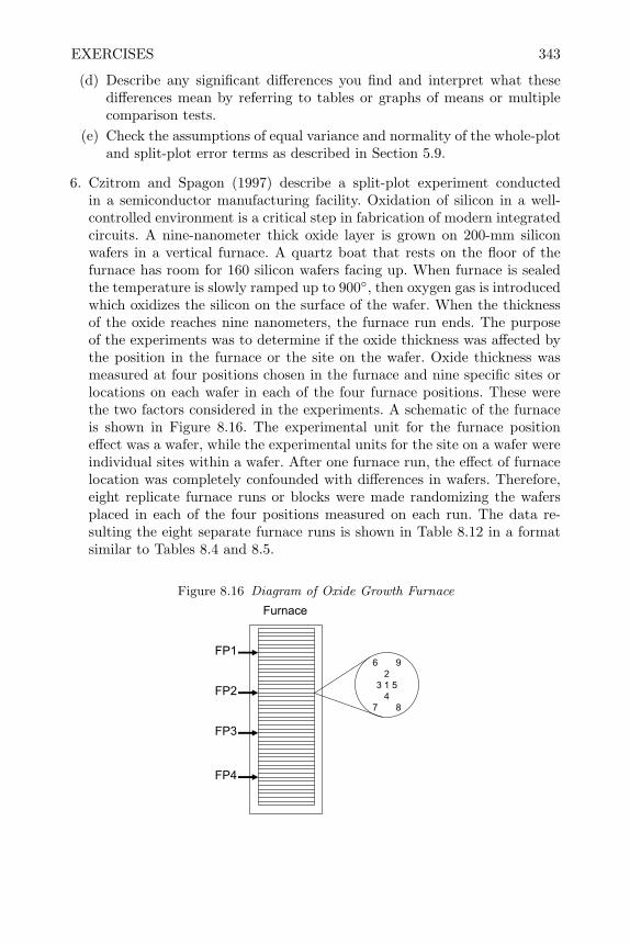
EXERCISES 343
(d) Describe any significant differences you find and interpret what thesedifferences mean by referring to tables or graphs of means or multiplecomparison tests.
(e) Check the assumptions of equal variance and normality of the whole-plotand split-plot error terms as described in Section 5.9.
6. Czitrom and Spagon (1997) describe a split-plot experiment conductedin a semiconductor manufacturing facility. Oxidation of silicon in a well-controlled environment is a critical step in fabrication of modern integratedcircuits. A nine-nanometer thick oxide layer is grown on 200-mm siliconwafers in a vertical furnace. A quartz boat that rests on the floor of thefurnace has room for 160 silicon wafers facing up. When furnace is sealedthe temperature is slowly ramped up to 900, then oxygen gas is introducedwhich oxidizes the silicon on the surface of the wafer. When the thicknessof the oxide reaches nine nanometers, the furnace run ends. The purposeof the experiments was to determine if the oxide thickness was affected bythe position in the furnace or the site on the wafer. Oxide thickness wasmeasured at four positions chosen in the furnace and nine specific sites orlocations on each wafer in each of the four furnace positions. These werethe two factors considered in the experiments. A schematic of the furnaceis shown in Figure 8.16. The experimental unit for the furnace positioneffect was a wafer, while the experimental units for the site on a wafer wereindividual sites within a wafer. After one furnace run, the effect of furnacelocation was completely confounded with differences in wafers. Therefore,eight replicate furnace runs or blocks were made randomizing the wafersplaced in each of the four positions measured on each run. The data re-sulting the eight separate furnace runs is shown in Table 8.12 in a formatsimilar to Tables 8.4 and 8.5.
Figure 8.16 Diagram of Oxide Growth Furnace
Furnace
FP1
FP2
FP3
FP4
6 92
3 1 54
7 8
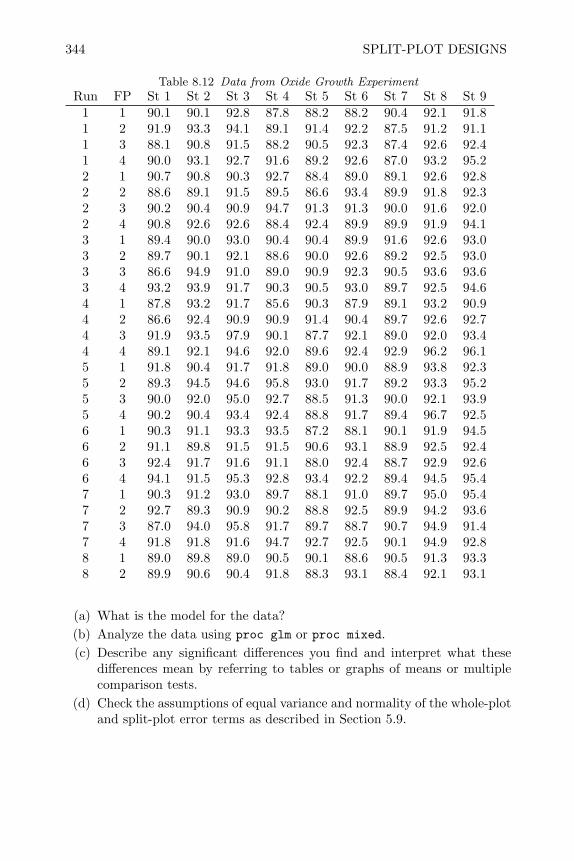
344 SPLIT-PLOT DESIGNS
Table 8.12 Data from Oxide Growth ExperimentRun FP St 1 St 2 St 3 St 4 St 5 St 6 St 7 St 8 St 9
1 1 90.1 90.1 92.8 87.8 88.2 88.2 90.4 92.1 91.81 2 91.9 93.3 94.1 89.1 91.4 92.2 87.5 91.2 91.11 3 88.1 90.8 91.5 88.2 90.5 92.3 87.4 92.6 92.41 4 90.0 93.1 92.7 91.6 89.2 92.6 87.0 93.2 95.22 1 90.7 90.8 90.3 92.7 88.4 89.0 89.1 92.6 92.82 2 88.6 89.1 91.5 89.5 86.6 93.4 89.9 91.8 92.32 3 90.2 90.4 90.9 94.7 91.3 91.3 90.0 91.6 92.02 4 90.8 92.6 92.6 88.4 92.4 89.9 89.9 91.9 94.13 1 89.4 90.0 93.0 90.4 90.4 89.9 91.6 92.6 93.03 2 89.7 90.1 92.1 88.6 90.0 92.6 89.2 92.5 93.03 3 86.6 94.9 91.0 89.0 90.9 92.3 90.5 93.6 93.63 4 93.2 93.9 91.7 90.3 90.5 93.0 89.7 92.5 94.64 1 87.8 93.2 91.7 85.6 90.3 87.9 89.1 93.2 90.94 2 86.6 92.4 90.9 90.9 91.4 90.4 89.7 92.6 92.74 3 91.9 93.5 97.9 90.1 87.7 92.1 89.0 92.0 93.44 4 89.1 92.1 94.6 92.0 89.6 92.4 92.9 96.2 96.15 1 91.8 90.4 91.7 91.8 89.0 90.0 88.9 93.8 92.35 2 89.3 94.5 94.6 95.8 93.0 91.7 89.2 93.3 95.25 3 90.0 92.0 95.0 92.7 88.5 91.3 90.0 92.1 93.95 4 90.2 90.4 93.4 92.4 88.8 91.7 89.4 96.7 92.56 1 90.3 91.1 93.3 93.5 87.2 88.1 90.1 91.9 94.56 2 91.1 89.8 91.5 91.5 90.6 93.1 88.9 92.5 92.46 3 92.4 91.7 91.6 91.1 88.0 92.4 88.7 92.9 92.66 4 94.1 91.5 95.3 92.8 93.4 92.2 89.4 94.5 95.47 1 90.3 91.2 93.0 89.7 88.1 91.0 89.7 95.0 95.47 2 92.7 89.3 90.9 90.2 88.8 92.5 89.9 94.2 93.67 3 87.0 94.0 95.8 91.7 89.7 88.7 90.7 94.9 91.47 4 91.8 91.8 91.6 94.7 92.7 92.5 90.1 94.9 92.88 1 89.0 89.8 89.0 90.5 90.1 88.6 90.5 91.3 93.38 2 89.9 90.6 90.4 91.8 88.3 93.1 88.4 92.1 93.1
(a) What is the model for the data?(b) Analyze the data using proc glm or proc mixed.(c) Describe any significant differences you find and interpret what these
differences mean by referring to tables or graphs of means or multiplecomparison tests.
(d) Check the assumptions of equal variance and normality of the whole-plotand split-plot error terms as described in Section 5.9.

EXERCISES 345
7. In SAS ADX create a new split-plot design defining four whole-plot factorsA, B, C, and D, and four sub-plot factors P , Q, R, and S as shown inFigure 8.7.
(a) Click on the Select Design button to see the four alternate designs shownin Figure 8.10.
(b) What are the generators shown on the Design Properties tab for thethird design (24−1 × 24−2) shown in Figure 8.8?
(c) From the generators find the complete defining relation including allgeneralized interactions, and compare this to the defining relation forthe 24−1 × 24−2 design created by proc factex in Section 8.5.1.
(d) List the seven effects and all their aliases that would be tested with thewhole-plot error.
(e) List the remaining 24 effects that would be tested with the sub-ploterror.
8. In SAS ADX create a new 16-run split-plot design defining three whole-plotfactors A, B, and C, and four sub-plot factors P , Q, R, and S.
(a) What alternate split-plot fractional factorial designs are listed?(b) Which one would you prefer, and why?(c) From the design you recommend, list the effects that must be tested
with whole-plot error and those that must be tested with sub-plot error.(d) Can you create the same design using proc factex? If so, show the
commands to do it.(e) If whole-plot experimental units cost four times more than that of sub-
plot experimental units, and only information on whole-plot main effectsis desired, which ADX design would you recommend?
(f) Can you create the same design using proc factex? If so, show thecommands to do it.
(g) Show the complete defining relation for the design created by ADX.
9. Bisgaard and Kulahci (2001) describe an experiment conducted by a man-ufacturer of boxed cake mixes. The manufacturer wanted to find a way tomake the recipe more robust so that if customers bake at a slightly dif-ferent temperature or time from that recommended on the box, the cakewould still taste good. The manufacturer varied F :the amount of flour,S:the amount of shortening, and E:the amount of egg powder in the recipe.These factors were varied according to a 23 design illustrated in the left-hand side of the table above. For each of the eight recipes, a large batchof dough was made. From each dough batch two cakes were baked, one ateach of the T :temperature and t:time conditions listed across the top of thetable. Since a different combination of levels of T :temperature and t:timewere used depending on the sign of FSE, it can be seen that split-plotconfounding was utilized. There were 16 cakes baked in total representinga 25−1 fraction. The responses shown in the table below are averages of

346 SPLIT-PLOT DESIGNS
DesignFactors T : − + − +
Recipe F S E FSE t: − − + +1 − − − − - 1.4 1.0 -2 + − − + 1.8 - - 6.13 − + − + 1.7 - - 2.14 + + − − - 3.7 4.0 -5 − − + + 1.9 - - 4.76 + − + − - 6.4 6.2 -7 − + + − - 2.1 2.3 -8 + + + + 4.9 - - 5.7
scores between 1 and 7 obtained from a taste panel. The higher the scorethe better.
(a) What is the generator and defining relation for this design?(b) List the estimable effects and their aliases.(c) Separate the list of estimable effects into two subgroups: first the group
that would be tested with whole-plot error and second the group thatwould be tested with sub-plot error.
(d) Use SAS proc glm to calculate the 15 estimable effects.(e) Modify the SAS code in Section 8.4 to produce separate normal plots of
the whole-plot effects and sub-plot effects. Does anything appear to besignificant?
(f) Interpret any significant main effects and interactions using an interac-tion plot if needed.

CHAPTER 9
Crossover and Repeated MeasuresDesigns
9.1 Introduction
Crossover and repeated measures designs are usually used in situations whereruns are blocked by human subjects or large animals. The purpose of crossoverdesigns (COD) is to increase the precision of treatment comparisons by com-paring them within each subject or animal. In a crossover design, each sub-ject or animal will receive all treatments in a different sequence, but the pri-mary aim is to compare the effects of the treatments and not the sequences.Crossover designs are used frequently in pharmaceutical research, sensory eval-uation of food products, animal feeding trials, and psychological research.
The primary purpose of repeated measures designs, on the other hand, isto compare trends in the response over time rather than to look at a snapshotat a particular point in time. Each subject or animal receives the same treat-ment throughout the experiment, and repeated measures are taken on eachsubject over time. Repeated measures experiments are similar to split-plotexperiments in that there are two sources of error, treatments are comparedto the less precise subject to subject error, and the comparison of trends overtime between treatments will be compared to the more precise within subjectexperimental error.
9.2 Crossover Designs (COD)
Crossover designs (CODs) are useful for comparing a limited number of treat-ments, usually from two to six. Since each subject (that will be referred toas the block or whole-plot experimental unit) will receive each treatment se-quentially in time, the number of levels of the treatment factor must remainsmall, otherwise drop-outs over time will cause problems in the analysis of thedata. For this reason CODs are usually not used for factorial treatment plansother than simple 22 factorials.
Since the treatments are applied sequentially over time to each block orwhole-plot experimental unit, CODs are only useful for comparing temporarytreatments of a chronic condition. For example, if a clinical trial was performedto compare pain relievers for the treatment of headaches, there would be nosymptom to treat in the second period if the treatment given in the first periodcured the headache.
The aspect of crossover trials that requires special attention is the fact that
347
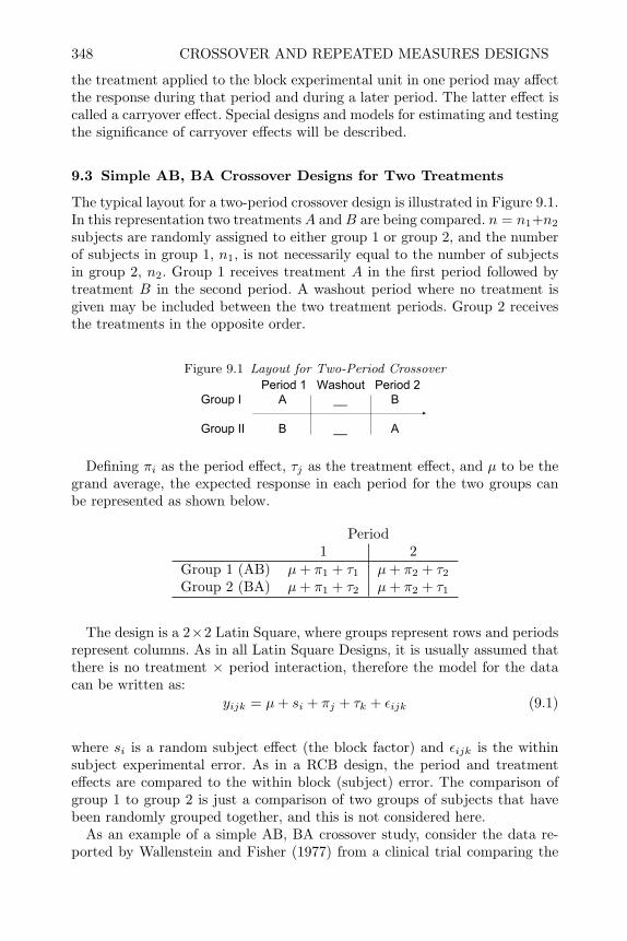
348 CROSSOVER AND REPEATED MEASURES DESIGNS
the treatment applied to the block experimental unit in one period may affectthe response during that period and during a later period. The latter effect iscalled a carryover effect. Special designs and models for estimating and testingthe significance of carryover effects will be described.
9.3 Simple AB, BA Crossover Designs for Two Treatments
The typical layout for a two-period crossover design is illustrated in Figure 9.1.In this representation two treatmentsA andB are being compared. n = n1+n2
subjects are randomly assigned to either group 1 or group 2, and the numberof subjects in group 1, n1, is not necessarily equal to the number of subjectsin group 2, n2. Group 1 receives treatment A in the first period followed bytreatment B in the second period. A washout period where no treatment isgiven may be included between the two treatment periods. Group 2 receivesthe treatments in the opposite order.
Figure 9.1 Layout for Two-Period CrossoverPeriod 1 Washout Period 2
Group I A __ B
Group II B __ A
Defining πi as the period effect, τj as the treatment effect, and µ to be thegrand average, the expected response in each period for the two groups canbe represented as shown below.
Period1 2
Group 1 (AB) µ+ π1 + τ1 µ+ π2 + τ2Group 2 (BA) µ+ π1 + τ2 µ+ π2 + τ1
The design is a 2×2 Latin Square, where groups represent rows and periodsrepresent columns. As in all Latin Square Designs, it is usually assumed thatthere is no treatment × period interaction, therefore the model for the datacan be written as:
yijk = µ+ si + πj + τk + εijk (9.1)
where si is a random subject effect (the block factor) and εijk is the withinsubject experimental error. As in a RCB design, the period and treatmenteffects are compared to the within block (subject) error. The comparison ofgroup 1 to group 2 is just a comparison of two groups of subjects that havebeen randomly grouped together, and this is not considered here.
As an example of a simple AB, BA crossover study, consider the data re-ported by Wallenstein and Fisher (1977) from a clinical trial comparing the

SIMPLE AB, BA CROSSOVER DESIGNS FOR TWO TREATMENTS 349
plasma levels of two formulations of an antifungal agent. Seventeen normalmale volunteers were randomly assigned to two groups. The first group re-ceived formulation A for 13 days, followed by a 13-day washout period, andthen formulation B for 13 days. Group two received the treatments in theB,A order. The response shown was the area under the 12-hour plasma curvetaken on the last day of each period.
Table 9.1 Data from Two-Period Crossover Study of Antifungal AgentGroup Subject Period 1 Period 2
1 2 12.8 8.21 3 16.5 13.11 6 18.7 15.91 8 11.6 14.21 11 13.6 12.81 12 9.8 15.31 16 12.8 14.01 18 12.1 12.02 1 10.9 12.32 4 13.5 11.52 5 13.7 16.02 7 12.2 14.82 9 12.6 16.22 10 13.0 17.52 14 10.7 7.52 15 14.2 12.42 17 12.2 12.8
The following commands can be used to read the data from the format inTable 9.1.
data antifungal;input group subject p1 p2;if group=1 then do;period =1; pl=p1; treat=’A’; output;period =2; pl=p2; treat=’B’; output;
end;if group=2 then do;period =1; pl=p1; treat=’B’; output;period =2; pl=p2; treat=’A’; output;
end;keep group subject period treat pl;datalines;1 2 12.8 8.21 3 16.5 13.1. . .
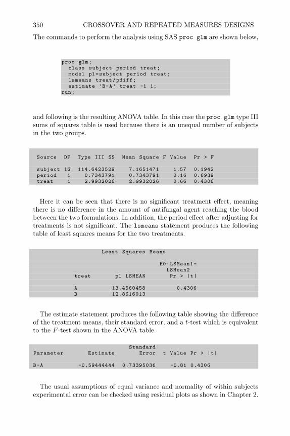
350 CROSSOVER AND REPEATED MEASURES DESIGNS
The commands to perform the analysis using SAS proc glm are shown below,
proc glm;class subject period treat;model pl=subject period treat;lsmeans treat/pdiff;estimate ’B-A’ treat -1 1;
run;
and following is the resulting ANOVA table. In this case the proc glm type IIIsums of squares table is used because there is an unequal number of subjectsin the two groups.
Source DF Type III SS Mean Square F Value Pr > F
subject 16 114.6423529 7.1651471 1.57 0.1942period 1 0.7343791 0.7343791 0.16 0.6939treat 1 2.9932026 2.9932026 0.66 0.4306
Here it can be seen that there is no significant treatment effect, meaningthere is no difference in the amount of antifungal agent reaching the bloodbetween the two formulations. In addition, the period effect after adjusting fortreatments is not significant. The lsmeans statement produces the followingtable of least squares means for the two treatments.
Least Squares Means
H0:LSMean1=LSMean2
treat pl LSMEAN Pr > |t|
A 13.4560458 0.4306B 12.8616013
The estimate statement produces the following table showing the differenceof the treatment means, their standard error, and a t-test which is equivalentto the F -test shown in the ANOVA table.
StandardParameter Estimate Error t Value Pr > |t|
B-A -0.59444444 0.73395036 -0.81 0.4306
The usual assumptions of equal variance and normality of within subjectsexperimental error can be checked using residual plots as shown in Chapter 2.

SIMPLE AB, BA CROSSOVER DESIGNS FOR TWO TREATMENTS 351
9.3.1 Sample Size Estimation
Since the test for difference in treatment effects can be reduced to a t-test inthe two-period crossover design, the number of subjects required to attain agiven power for detecting a difference, ∆, in treatment means can be deter-mined using the non-central t-distribution. For example, the SAS code below,modified from Jones and Kenward (2003), creates a table of the power of thetest for treatments as a function of n = n1 +n2, the significance level (α), theexpected difference in treatment means ∆ = µ··1 − µ··2, and the within pa-tient variance. In the example shown below, α = 0.05, ∆ = 10, and σ2 = 326.The table that results from running this code shows that a power of 0.8 fordetecting a treatment difference of 10 can be achieved with a sample size ofn = 54, and a power of 0.9 can be achieved with a sample size of n = 72.
*Sample Size Estimation;data sampsize;* alpha (two sided);alpha =0.05;* within -patient variance;sigma2 =326;* size of a difference to detect;delta =10;* sample size (total number of patients);do n=40 to 80 by 2;* standard error of a difference;stderrdiff=sqrt(2*sigma2/n);* degrees of freedom for t-test;df=n-2;* critical value of the t-distribution;* (two -sided alpha level);t1=tinv(1-alpha/2,df);* noncentrality parameter;gamma=delta/(stderrdiff);* power;power=1-probt(t1,df ,gamma);output;end;run;proc print data=sampsize;var alpha n delta power;run;
These results can also be reproduced using proc power or the SAS Powerand Sample Size Application.
9.3.2 Carryover Effects
In cases where the effect of the treatment given in the first period persistsand affects the response in the second period, a simple model for the expectedresponse for the two groups in the two periods can be written as shown in thetable on the next page,
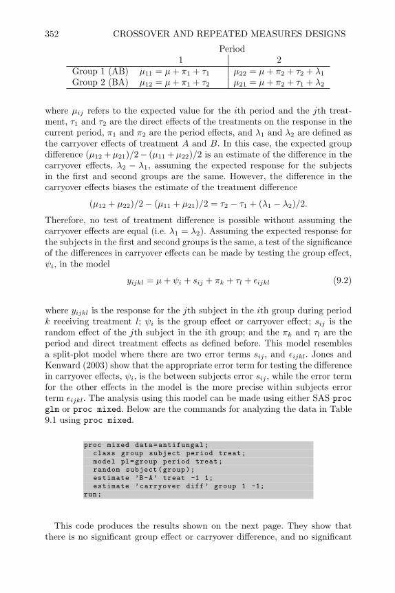
352 CROSSOVER AND REPEATED MEASURES DESIGNS
Period1 2
Group 1 (AB) µ11 = µ+ π1 + τ1 µ22 = µ+ π2 + τ2 + λ1
Group 2 (BA) µ12 = µ+ π1 + τ2 µ21 = µ+ π2 + τ1 + λ2
where µij refers to the expected value for the ith period and the jth treat-ment, τ1 and τ2 are the direct effects of the treatments on the response in thecurrent period, π1 and π2 are the period effects, and λ1 and λ2 are defined asthe carryover effects of treatment A and B. In this case, the expected groupdifference (µ12 +µ21)/2− (µ11 +µ22)/2 is an estimate of the difference in thecarryover effects, λ2 − λ1, assuming the expected response for the subjectsin the first and second groups are the same. However, the difference in thecarryover effects biases the estimate of the treatment difference
(µ12 + µ22)/2− (µ11 + µ21)/2 = τ2 − τ1 + (λ1 − λ2)/2.
Therefore, no test of treatment difference is possible without assuming thecarryover effects are equal (i.e. λ1 = λ2). Assuming the expected response forthe subjects in the first and second groups is the same, a test of the significanceof the differences in carryover effects can be made by testing the group effect,ψi, in the model
yijkl = µ+ ψi + sij + πk + τl + εijkl (9.2)
where yijkl is the response for the jth subject in the ith group during periodk receiving treatment l; ψi is the group effect or carryover effect; sij is therandom effect of the jth subject in the ith group; and the πk and τl are theperiod and direct treatment effects as defined before. This model resemblesa split-plot model where there are two error terms sij , and εijkl. Jones andKenward (2003) show that the appropriate error term for testing the differencein carryover effects, ψi, is the between subjects error sij , while the error termfor the other effects in the model is the more precise within subjects errorterm εijkl. The analysis using this model can be made using either SAS procglm or proc mixed. Below are the commands for analyzing the data in Table9.1 using proc mixed.
proc mixed data=antifungal;class group subject period treat;model pl=group period treat;random subject(group);estimate ’B-A’ treat -1 1;estimate ’carryover diff’ group 1 -1;
run;
This code produces the results shown on the next page. They show thatthere is no significant group effect or carryover difference, and no significant

SIMPLE AB, BA CROSSOVER DESIGNS FOR TWO TREATMENTS 353
direct treatment effect. The between subjects variance component, σ2s , is es-
timated to be 1.5078, while the within subject variance component, σ2, isestimated to be 4.563. The estimate statement produces results that are equiv-alent to the REML F -tests.
The Mixed ProcedureCovariance Parameter
Estimates
Cov Parm Estimatesubject(group) 1.5078Residual 4.5630
Type 3 Tests of Fixed EffectsNum Den
Effect DF DF F Value Pr > Fgroup 1 15 0.13 0.7262period 1 15 0.16 0.6939treat 1 15 0.66 0.4306
Estimates
StandardLabel Estimate Error DF t Value Pr > |t|B-A -0.5944 0.7340 15 -0.81 0.4306carryover diff 0.3375 0.9459 15 0.36 0.7262
Notice the standard error of the carryover difference effect is larger than thestandard error for the direct treatment effects since it includes both variancecomponents. Therefore, the group or carryover effect is like a whole-plot effectthat is estimated less precisely. The direct effects are estimated more preciselywith the within subject variability.
Grizzle (1965) proposed a preliminary test of the carryover difference atan inflated significance level, like α = 0.10, followed by a different test ofthe direct treatment effects depending on the outcome of the preliminarytest of carryover difference. However, because the of the low power for thepreliminary test of carryover differences, Freeman (1989) showed that thistwo-stage procedure inflates the type I error and produces biased estimatesof the direct treatment effects, and Senn (2002) recommends against using it.Therefore, the simple AB, BA crossover trial should only be used when thecarryover effects can be assumed to be equal.
9.3.3 Modified Designs When Carryover Is Possible
The disadvantage of the simple two-period crossover design presented in thelast section is that the direct treatment effects are biased by any difference incarryover effects, and that the test for carryover effects lacks power because

354 CROSSOVER AND REPEATED MEASURES DESIGNS
it is tested with the between subjects error term. Jones and Kenward (2003)show higher order designs which include additional sequence groups or periods.These designs allow for within-subject estimators of both the carryover anddirect treatment effects. Some designs that are optimal in terms of providingminimum variance unbiased least squares estimates of the difference in directand carryover treatment effects are shown below.
Table 9.2 Design 1Sequence Period
1 21 A A2 B B3 A B4 B A
Table 9.3 Design 2Sequence Period
1 2 31 A B B2 B A A
Table 9.4 Design 3Sequence Period
1 2 31 A B B2 B A A3 A A B4 B B A
Design 3 allows for an independent estimate of the direct treatment byperiod interaction in addition to the direct and carryover treatment effects.Following Grizzle (1965), the model for higher order two-treatment designscan be written in the form
yijk = µ+ ψi + s(i)k + πj + τd(i,j) + λd(i,j−1) + εijk (9.3)
where yijk is the response of the kth subject in the ith group and jth period.ψi is the sequence group effect. sij is the subject within group or block effectwhich can be treated as a fixed or random factor. πj is the period effect, d(i, j)

SIMPLE AB, BA CROSSOVER DESIGNS FOR TWO TREATMENTS 355
is the treatment assigned to period j for sequence group i, τl is the effect of thelth treatment, and λl is the first-order carryover effect of the lth treatment.
As an example of the use of this model, consider the data in Table 9.5 thatcomes from a bioequivalence study presented by Chi (1994), where half of the36 subjects were randomly assigned to the ABB sequence and the other halfto the BAA sequence in design 2.
In order to fit model 9.3 to the data the treatment, d(i, j), given in the jthperiod and the ith treatment group, is created in the SAS data step as thedata is read in. The carryover effect, d(i, j − 1) in the jth period and the ithtreatment group is simply the treatment given in the j−1st period (if one wasgiven) or none. The SAS code below shows how to read the data and createthe treatment and carryover indicators.
data bioequiv;input group subject y1 y2 y3;
if group =1 then do;period =1; y=y1; treat=’A’; carry=’none’; output;period =2; y=y2; treat=’B’; carry=’A’; output;period =3; y=y3; treat=’B’; carry=’B’; output;
end;if group = 2 then do;period =1; y=y1; treat=’B’; carry=’none’; output;period =2; y=y2; treat=’A’; carry=’B’; output;period =3; y=y3; treat=’A’; carry=’A’; output;
end;drop y1 y2 y3;datalines;1 2 112.25 106.36 88.591 3 153.71 150.13 151.31. . .
proc print; run;
A portion of the proc print results are shown below, and we can see thecarryover indicator is always labeled none in the first period. In the secondperiod the carryover indicator is the treatment given in the first period, and inthe third period the carryover indicator is the treatment given in the secondperiod.
Obs group subject period y treat carr
1 1 2 1 112.25 A none2 1 2 2 106.36 B A3 1 2 3 88.59 B B4 1 3 1 153.71 A none5 1 3 2 150.13 B A6 1 3 3 151.31 B B
. . .

356 CROSSOVER AND REPEATED MEASURES DESIGNS
Table 9.5 Data from Bioequivalence Study Where Subjects in Sequence Group 1 wereGiven ABB and Subjects in Sequence Group 2 were Given BAA
Group Subject Period 1 Period 2 Period 31 2 112.25 106.36 88.591 3 153.71 150.13 151.311 6 278.65 293.27 295.351 8 30.25 35.81 34.661 10 65.51 52.48 47.481 12 35.68 41.79 42.791 13 96.03 75.87 82.811 14 111.57 115.92 118.141 18 72.98 70.69 74.201 19 148.98 157.70 178.621 21 140.22 119.83 139.481 23 60.44 44.09 35.531 26 136.10 161.76 163.571 28 111.19 101.83 101.701 31 85.87 99.60 107.481 34 111.25 114.90 135.941 36 58.79 96.42 122.601 129 299.50 303.45 385.342 1 52.66 47.65 13.912 4 128.44 173.22 140.442 5 233.18 88.18 31.932 7 53.87 89.18 70.082 9 62.07 54.99 73.392 11 183.30 153.88 122.412 15 51.91 73.01 23.102 16 90.75 89.70 111.942 17 59.51 56.26 48.872 24 83.01 73.85 71.302 25 85.37 86.67 92.062 27 84.85 75.41 79.452 30 70.33 40.80 46.912 32 110.04 102.61 113.182 33 93.58 87.31 87.582 35 66.54 43.29 84.072 120 59.67 56.86 69.492 122 49.02 50.29 51.71
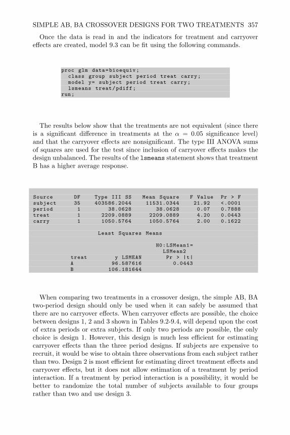
SIMPLE AB, BA CROSSOVER DESIGNS FOR TWO TREATMENTS 357
Once the data is read in and the indicators for treatment and carryovereffects are created, model 9.3 can be fit using the following commands.
proc glm data=bioequiv;class group subject period treat carry;model y= subject period treat carry;lsmeans treat/pdiff;
run;
The results below show that the treatments are not equivalent (since thereis a significant difference in treatments at the α = 0.05 significance level)and that the carryover effects are nonsignificant. The type III ANOVA sumsof squares are used for the test since inclusion of carryover effects makes thedesign unbalanced. The results of the lsmeans statement shows that treatmentB has a higher average response.
Source DF Type III SS Mean Square F Value Pr > Fsubject 35 403586.2044 11531.0344 21.92 <.0001period 1 38.0628 38.0628 0.07 0.7888treat 1 2209.0889 2209.0889 4.20 0.0443carry 1 1050.5764 1050.5764 2.00 0.1622
Least Squares Means
H0:LSMean1=LSMean2
treat y LSMEAN Pr > |t|A 96.587616 0.0443B 106.181644
When comparing two treatments in a crossover design, the simple AB, BAtwo-period design should only be used when it can safely be assumed thatthere are no carryover effects. When carryover effects are possible, the choicebetween designs 1, 2 and 3 shown in Tables 9.2-9.4, will depend upon the costof extra periods or extra subjects. If only two periods are possible, the onlychoice is design 1. However, this design is much less efficient for estimatingcarryover effects than the three period designs. If subjects are expensive torecruit, it would be wise to obtain three observations from each subject ratherthan two. Design 2 is most efficient for estimating direct treatment effects andcarryover effects, but it does not allow estimation of a treatment by periodinteraction. If a treatment by period interaction is a possibility, it would bebetter to randomize the total number of subjects available to four groupsrather than two and use design 3.

358 CROSSOVER AND REPEATED MEASURES DESIGNS
9.4 Crossover Designs for Multiple Treatments
Many designs, with more than two treatments, have been proposed in theliterature for crossover studies. Which design is best depends upon the as-sumptions made. For the two-treatment crossover design presented in the lastsection, only first-order carryover effects were assumed. That is to say, thetreatment in a given period may affect the response in that period or the nextperiod, but will not persist beyond that. Other more complicated models mayassume second- or- third-order carryover effects, or interactions between thecarryover effect and the treatment given in the current period. These assump-tions will result in more complicated designs. In this section designs will bedescribed for the simple first-order carryover effects. For guidance on designsfor more complicated models refer to Jones and Kenward (2003).
One desirable characteristic of a crossover design is variance balance wherethe variance of a difference in any pair of direct (or carryover) treatmenteffects is the same regardless of the pair. This balance can be achieved ifevery treatment is preceded by every treatment an equal number of times.For example, the simple AB, BA two-period crossover design is not balanced,because treatment A is only preceded by treatment B, and treatment B isonly preceded by A. By adding the third period as in design 2, treatment A ispreceded by B once and A once in the second sequence group, and treatmentB is preceded by A once and B once in the first sequence group. Thereforedesign 2 is balanced.
9.4.1 Williams’ Latin Square Crossover Designs
Balanced designs in t treatments and p = t periods can be created from Latinsquare designs. If there are no carryover effects, then a variance balanced de-sign for direct treatment effects can be achieved by choosing any arbitrary t×tLatin square design. If carryover effects are possible, then variance balance canonly be achieved when each treatment is preceded by every other treatmentan equal number of times. Williams (1949) showed that this property couldbe achieved with only one particular Latin Square if t is an even number,and two particular Latin squares if t is an odd number. An easy algorithmfor constructing these particular squares was described by Sheehe and Bross(1961) and is described below.
1. Number the treatments from 1 to t.
2. Start with a cyclic Latin square design where the treatments in the ith roware i, i+ 1, . . . , t, 1, . . . , i− 1.
3. Create another Latin square whose rows are the mirror images of the rowsin the first Latin square; e.g., the mirror image of (1,2,3,4) is (4,3,2,1).
4. Interlace each row of the first Latin Square with the corresponding rowof the second Latin square to produce a t × 2t rectangle. For example,interlacing (1, 2, 3, 4) with (4, 3, 2, 1) results in (1, 4, 2, 3, 3, 2, 4, 1).
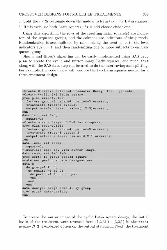
CROSSOVER DESIGNS FOR MULTIPLE TREATMENTS 359
5. Split the t× 2t rectangle down the middle to form two t× t Latin squares.6. If t is even use both Latin squares, if t is odd choose either one.
Using this algorithm, the rows of the resulting Latin square(s) are indica-tors of the sequence groups, and the columns are indicators of the periods.Randomization is accomplished by randomizing the treatments to the levelindicators 1, 2, . . . , t, and then randomizing one or more subjects to each se-quence group.
Sheehe and Bross’s algorithm can be easily implemented using SAS procplan to create the cyclic and mirror image Latin squares, and proc sortalong with the SAS data step can be used to do the interleaving and splitting.For example, the code below will produce the two Latin squares needed for athree-treatment design.
*Create Williams Balanced Crossover Design for 3 periods;*Create cyclic 3x3 latin square;proc plan seed =12345;
factors group=3 ordered period =3 ordered;treatments treat=3 cyclic;output out=lsd treat nvals =(1 2 3) ordered;
run;data lsd; set lsd;
square =1;*Create mirror image of 3x3 latin square;proc plan seed =12345;
factors group=3 ordered period =3 ordered;treatments treat=3 cyclic 2;output out=lsdm treat nvals =(3 2 1) ordered;
run;data lsdm; set lsdm;
square =2;*Interlace each row with mirror image;data comb; set lsd lsdm;proc sort; by group period square;*make new period square designations;data d;
do group=1 to 3;do square =1 to 2;do period =1 to 3; output;end;
end;end;
data design; merge comb d; by group;proc print data=design;run;
To create the mirror image of the cyclic Latin square design, the initiallevels of the treatment were reversed from (1,2,3) to (3,2,1) in the treatnvals=(3 2 1)ordered option on the output statement. Next, the treatment
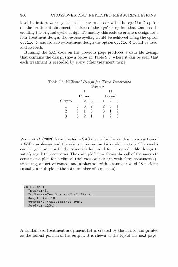
360 CROSSOVER AND REPEATED MEASURES DESIGNS
level indicators were cycled in the reverse order with the cyclic 2 optionon the treatment statement in place of the cyclic option that was used increating the original cyclic design. To modify this code to create a design for afour-treatment design, the reverse cycling would be achieved using the optioncyclic 3, and for a five-treatment design the option cyclic 4 would be used,and so forth.
Running the SAS code on the previous page produces a data file designthat contains the design shown below in Table 9.6, where it can be seen thateach treatment is preceded by every other treatment twice.
Table 9.6 Williams’ Design for Three TreatmentsSquare
I IIPeriod Period
Group 1 2 3 1 2 31 1 3 2 2 3 12 2 1 3 3 1 23 3 2 1 1 2 3
Wang et al. (2009) have created a SAS macro for the random construction ofa Williams design and the relevant procedure for randomization. The resultscan be generated with the same random seed for a reproducible design tosatisfy regulatory concerns. The example below shows the call of the macro toconstruct a plan for a clinical trial crossover design with three treatments (atest drug, an active control and a placebo) with a sample size of 18 patients(usually a multiple of the total number of sequences).
%WILLIAMS(TmtsNum=3,TmtNames=TestDrg ActCtrl Placebo ,SampleSize =18,OutRtf=D:\ WilliamsN18.rtf ,SeedNum =1234);
A randomized treatment assignment list is created by the macro and printedas the second portion of the output. It is shown at the top of the next page.
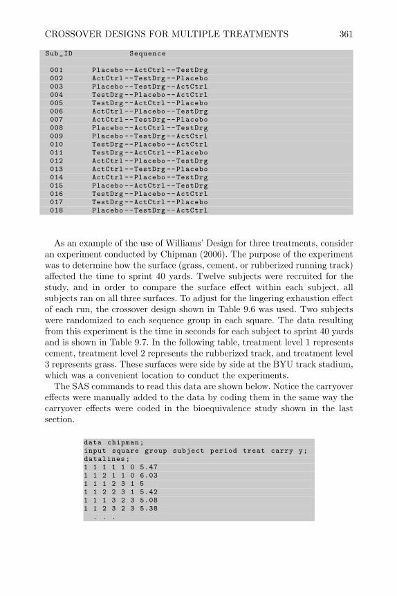
CROSSOVER DESIGNS FOR MULTIPLE TREATMENTS 361
Sub_ID Sequence
001 Placebo --ActCtrl --TestDrg002 ActCtrl --TestDrg --Placebo003 Placebo --TestDrg --ActCtrl004 TestDrg --Placebo --ActCtrl005 TestDrg --ActCtrl --Placebo006 ActCtrl --Placebo --TestDrg007 ActCtrl --TestDrg --Placebo008 Placebo --ActCtrl --TestDrg009 Placebo --TestDrg --ActCtrl010 TestDrg --Placebo --ActCtrl011 TestDrg --ActCtrl --Placebo012 ActCtrl --Placebo --TestDrg013 ActCtrl --TestDrg --Placebo014 ActCtrl --Placebo --TestDrg015 Placebo --ActCtrl --TestDrg016 TestDrg --Placebo --ActCtrl017 TestDrg --ActCtrl --Placebo018 Placebo --TestDrg --ActCtrl
As an example of the use of Williams’ Design for three treatments, consideran experiment conducted by Chipman (2006). The purpose of the experimentwas to determine how the surface (grass, cement, or rubberized running track)affected the time to sprint 40 yards. Twelve subjects were recruited for thestudy, and in order to compare the surface effect within each subject, allsubjects ran on all three surfaces. To adjust for the lingering exhaustion effectof each run, the crossover design shown in Table 9.6 was used. Two subjectswere randomized to each sequence group in each square. The data resultingfrom this experiment is the time in seconds for each subject to sprint 40 yardsand is shown in Table 9.7. In the following table, treatment level 1 representscement, treatment level 2 represents the rubberized track, and treatment level3 represents grass. These surfaces were side by side at the BYU track stadium,which was a convenient location to conduct the experiments.
The SAS commands to read this data are shown below. Notice the carryovereffects were manually added to the data by coding them in the same way thecarryover effects were coded in the bioequivalence study shown in the lastsection.
data chipman;input square group subject period treat carry y;datalines;1 1 1 1 1 0 5.471 1 2 1 1 0 6.031 1 1 2 3 1 51 1 2 2 3 1 5.421 1 1 3 2 3 5.081 1 2 3 2 3 5.38
. . .
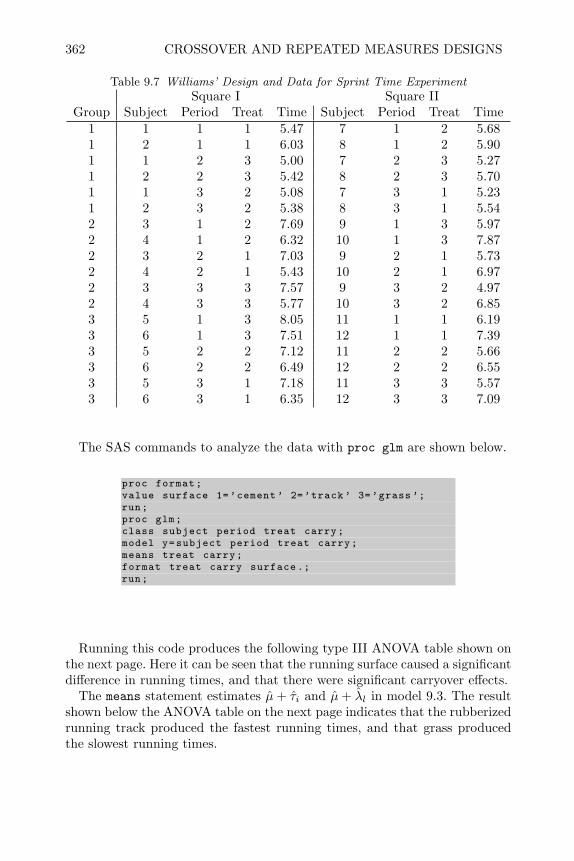
362 CROSSOVER AND REPEATED MEASURES DESIGNS
Table 9.7 Williams’ Design and Data for Sprint Time ExperimentSquare I Square II
Group Subject Period Treat Time Subject Period Treat Time1 1 1 1 5.47 7 1 2 5.681 2 1 1 6.03 8 1 2 5.901 1 2 3 5.00 7 2 3 5.271 2 2 3 5.42 8 2 3 5.701 1 3 2 5.08 7 3 1 5.231 2 3 2 5.38 8 3 1 5.542 3 1 2 7.69 9 1 3 5.972 4 1 2 6.32 10 1 3 7.872 3 2 1 7.03 9 2 1 5.732 4 2 1 5.43 10 2 1 6.972 3 3 3 7.57 9 3 2 4.972 4 3 3 5.77 10 3 2 6.853 5 1 3 8.05 11 1 1 6.193 6 1 3 7.51 12 1 1 7.393 5 2 2 7.12 11 2 2 5.663 6 2 2 6.49 12 2 2 6.553 5 3 1 7.18 11 3 3 5.573 6 3 1 6.35 12 3 3 7.09
The SAS commands to analyze the data with proc glm are shown below.
proc format;value surface 1=’cement ’ 2=’track’ 3=’grass ’;run;proc glm;class subject period treat carry;model y=subject period treat carry;means treat carry;format treat carry surface .;run;
Running this code produces the following type III ANOVA table shown onthe next page. Here it can be seen that the running surface caused a significantdifference in running times, and that there were significant carryover effects.
The means statement estimates µ+ τi and µ+ λl in model 9.3. The resultshown below the ANOVA table on the next page indicates that the rubberizedrunning track produced the fastest running times, and that grass producedthe slowest running times.

CROSSOVER DESIGNS FOR MULTIPLE TREATMENTS 363
Source DF Type III SS Mean Square F Value Pr > F
subject 11 24.25471000 2.20497364 86.01 <.0001period 1 0.00183750 0.00183750 0.07 0.7920treat 2 0.63916333 0.31958167 12.47 0.0004carry 2 0.23320556 0.11660278 4.55 0.0252
The GLM Procedure
Level of --------------y--------------treat N Mean Std Dev
cement 12 6.21166667 0.76463697grass 12 6.39916667 1.12486329track 12 6.14083333 0.83989673
The carryover effects are summarized in the following table of means. Sub-tracting the grand mean from these estimates, it can be seen that the carryovereffects of grass and cement are negative which means that the sprinting timeswill be slightly faster in the sprint following one on grass or cement. The “0”level of carryover means no prior treatment. This is where the longest sprinttimes occur.
Level of --------------y--------------carry N Mean Std Dev
0 12 6.67250000 0.94744753cement 8 5.97375000 0.92968409grass 8 5.94250000 0.80331012track 8 6.20250000 0.80786756
9.4.2 Designs with p > t or t > p
One problem with Williams’ designs is that the direct treatment effects andthe carryover effects are not orthogonal. The type III ANOVA table makesa test for significance of treatment effects adjusted for carryover and a testfor carryover adjusted for treatments; however, SAS proc glm is unable toproduce least squares (adjusted) means for treatments and carryover due tothe imbalance in these factors. In addition the direct treatment effects areestimated more precisely than the carryover effects since each marginal meanis the average of 12 observations for the direct effects but only 8 for thecarryover effects.
Lucas (1957) proposed a solution to this problem by simply adding an extraperiod where all sequence groups receive the same treatment that they receivedin the tth period. This makes the design completely balanced in the sensethat every treatment follows every other treatment an equal number of times,
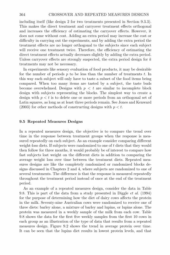
364 CROSSOVER AND REPEATED MEASURES DESIGNS
including itself (like design 2 for two treatments presented in Section 9.3.3).This makes the direct treatment and carryover treatment effects orthogonaland increases the efficiency of estimating the carryover effects. However, itdoes not come without cost. Adding an extra period may increase the cost ordifficulty in carrying out the experiments, and by adding the extra period thetreatment effects are no longer orthogonal to the subjects since each subjectwill receive one treatment twice. Therefore, the efficiency of estimating thedirect treatment effects actually decreases slightly by adding the extra period.Unless carryover effects are strongly suspected, the extra period design for ktreatments may not be necessary.
In experiments like sensory evaluation of food products, it may be desirablefor the number of periods p to be less than the number of treatments t. Inthis way each subject will only have to taste a subset of the food items beingcompared. When too many items are tasted by a subject, the taste budsbecome overwhelmed. Designs with p < t are similar to incomplete blockdesign with subjects representing the blocks. The simplest way to create adesign with p < t is to delete one or more periods from an orthogonal set ofLatin squares, as long as at least three periods remain. See Jones and Kenward(2003) for other methods of constructing designs with p < t.
9.5 Repeated Measures Designs
In a repeated measures design, the objective is to compare the trend overtime in the response between treatment groups when the response is mea-sured repeatedly on each subject. As an example consider comparing differentweight-loss diets. If subjects were randomized to one of t diets that they wouldthen follow for three months, it would probably be of interest to compare howfast subjects lost weight on the different diets in addition to comparing theaverage weight loss over time between the treatment diets. Repeated mea-sures designs are like the completely randomized or randomized blocks de-signs discussed in Chapters 2 and 4, where subjects are randomized to one ofseveral treatments. The difference is that the response is measured repeatedlythroughout the treatment period instead of once at the end of the treatmentperiod.
As an example of a repeated measures design, consider the data in Table9.8. This is part of the data from a study presented in Diggle et al. (1994)for the purpose of determining how the diet of dairy cows affects the proteinin the milk. Seventy-nine Australian cows were randomized to receive one ofthree diets: barley alone, a mixture of barley and lupins, or lupins alone. Theprotein was measured in a weekly sample of the milk from each cow. Table9.8 shows the data for the first five weekly samples from the first 10 cows ineach group as an illustration of the type of data that results from a repeatedmeasures design. Figure 9.2 shows the trend in average protein over time.It can be seen that the lupins diet results in lowest protein levels, and that
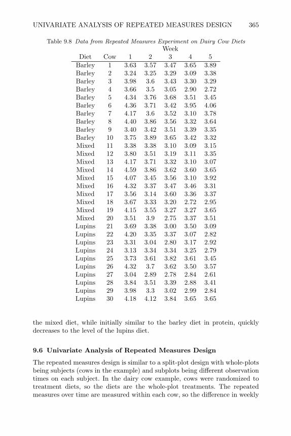
UNIVARIATE ANALYSIS OF REPEATED MEASURES DESIGN 365
Table 9.8 Data from Repeated Measures Experiment on Dairy Cow DietsWeek
Diet Cow 1 2 3 4 5Barley 1 3.63 3.57 3.47 3.65 3.89Barley 2 3.24 3.25 3.29 3.09 3.38Barley 3 3.98 3.6 3.43 3.30 3.29Barley 4 3.66 3.5 3.05 2.90 2.72Barley 5 4.34 3.76 3.68 3.51 3.45Barley 6 4.36 3.71 3.42 3.95 4.06Barley 7 4.17 3.6 3.52 3.10 3.78Barley 8 4.40 3.86 3.56 3.32 3.64Barley 9 3.40 3.42 3.51 3.39 3.35Barley 10 3.75 3.89 3.65 3.42 3.32Mixed 11 3.38 3.38 3.10 3.09 3.15Mixed 12 3.80 3.51 3.19 3.11 3.35Mixed 13 4.17 3.71 3.32 3.10 3.07Mixed 14 4.59 3.86 3.62 3.60 3.65Mixed 15 4.07 3.45 3.56 3.10 3.92Mixed 16 4.32 3.37 3.47 3.46 3.31Mixed 17 3.56 3.14 3.60 3.36 3.37Mixed 18 3.67 3.33 3.20 2.72 2.95Mixed 19 4.15 3.55 3.27 3.27 3.65Mixed 20 3.51 3.9 2.75 3.37 3.51Lupins 21 3.69 3.38 3.00 3.50 3.09Lupins 22 4.20 3.35 3.37 3.07 2.82Lupins 23 3.31 3.04 2.80 3.17 2.92Lupins 24 3.13 3.34 3.34 3.25 2.79Lupins 25 3.73 3.61 3.82 3.61 3.45Lupins 26 4.32 3.7 3.62 3.50 3.57Lupins 27 3.04 2.89 2.78 2.84 2.61Lupins 28 3.84 3.51 3.39 2.88 3.41Lupins 29 3.98 3.3 3.02 2.99 2.84Lupins 30 4.18 4.12 3.84 3.65 3.65
the mixed diet, while initially similar to the barley diet in protein, quicklydecreases to the level of the lupins diet.
9.6 Univariate Analysis of Repeated Measures Design
The repeated measures design is similar to a split-plot design with whole-plotsbeing subjects (cows in the example) and subplots being different observationtimes on each subject. In the dairy cow example, cows were randomized totreatment diets, so the diets are the whole-plot treatments. The repeatedmeasures over time are measured within each cow, so the difference in weekly
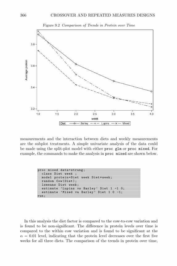
366 CROSSOVER AND REPEATED MEASURES DESIGNS
Figure 9.2 Comparison of Trends in Protein over Time
measurements and the interaction between diets and weekly measurementsare the subplot treatments. A simple univariate analysis of the data couldbe made using the split-plot model with either proc glm or proc mixed. Forexample, the commands to make the analysis in proc mixed are shown below.
proc mixed data=strung;class Diet week ;model protein=Diet week Diet*week;random Cow(Diet);lsmeans Diet week;estimate ’Lupins vs Barley ’ Diet 1 -1 0;estimate ’Mixed va Barley ’ Diet 1 0 -1;
run;
In this analysis the diet factor is compared to the cow-to-cow variation andis found to be non-significant. The difference in protein levels over time iscompared to the within cow variation and is found to be significant at theα = 0.01 level, indicating that the protein level decreases over the first fiveweeks for all three diets. The comparison of the trends in protein over time,
UNIVARIATE ANALYSIS OF REPEATED MEASURES DESIGN 367
or the interaction that is shown in Figure 9.2, is also compared to the withincow variation and is not significant.
The usual assumptions for analysis of variance are that the experimentalerror terms should have equal variance and be independent and normally dis-tributed. For split-plot models, the assumptions of normality and equal vari-ance can be checked by making residual plots and plots EBLUPs (as describedin Section 5.9.3). However, in past chapters the independence assumption wasnever checked. For completely randomized designs, the randomization guar-anteed independence of experimental error. In split-plot designs, subplot ex-perimental units are usually not independent because observations on pairsof subplots within the same whole plot will be correlated. However, random-ization of subplot treatments to subplots in a split-plot design equalizes thecorrelation between all possible pairs of subplots. This, along with equal vari-ances of subplot responses, creates a condition that is called compound sym-metry of the covariance matrix of subplot observations. This condition, likeindependence of experimental error, justifies the normal analysis by ANOVAor REML as shown in Chapter 8.
With repeated measures designs, however, the subplot treatments are re-peated measures over time, and they cannot be randomized. They must beobserved in temporal order. Therefore, the compound symmetry conditionthat justified the normal split-plot analysis may not be satisfied for repeatedmeasures designs.
9.6.1 Test of Huynh-Feldt Condition
Huynh and Feldt (1970) showed the conditions justifying the usual analysisof variance of repeated measures designs are less stringent than compoundsymmetry. They showed that if repeated measures at different times, yi andyj , satisfy the condition
σ2(yi−yj) = 2λ for i 6= j (9.4)
for some λ > 0, then the covariance matrix of the repeated measures is saidto obey the Huynh-Feldt condition. The usual split-plot analysis of repeatedmeasures data is justified if the Huynh-Feldt condition is satisfied.
The Mauchly (1940) sphericity test can be used to test whether the covari-ance matrix of the repeated measures has the Huynh-Feldt condition. SASproc glm has an option to perform the sphericity test. To do this, read therepeated measures as different variables as in the data step shown on the nextpage. Next all the repeated measures variables are listed as dependent vari-ables in the proc glm model statement, and the repeated statement, with theoption printe, prints the correlation matrix and performs the sphericity test.
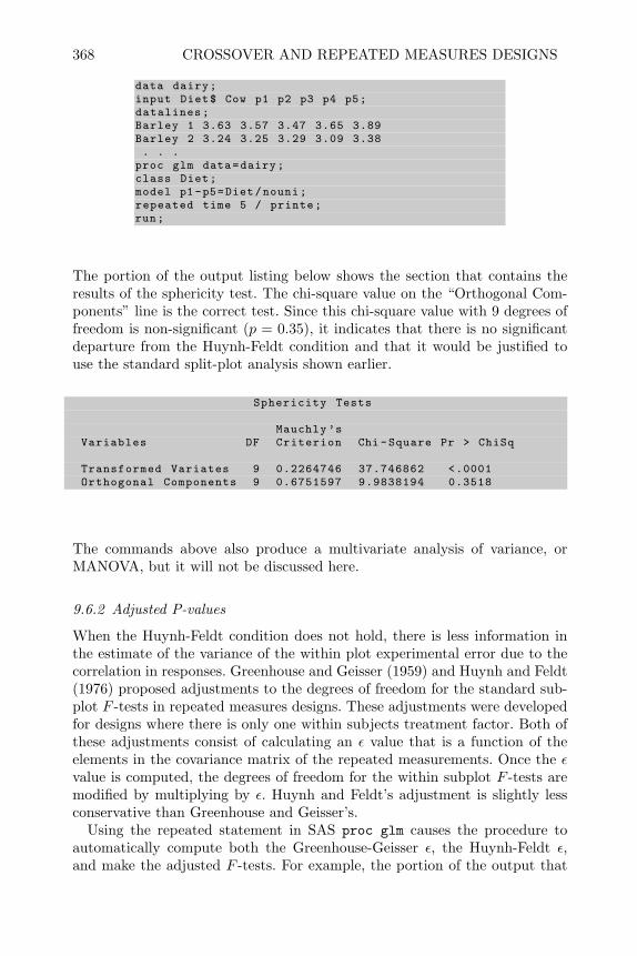
368 CROSSOVER AND REPEATED MEASURES DESIGNS
data dairy;input Diet$ Cow p1 p2 p3 p4 p5;datalines;Barley 1 3.63 3.57 3.47 3.65 3.89Barley 2 3.24 3.25 3.29 3.09 3.38. . .
proc glm data=dairy;class Diet;model p1 -p5=Diet/nouni;repeated time 5 / printe;run;
The portion of the output listing below shows the section that contains theresults of the sphericity test. The chi-square value on the “Orthogonal Com-ponents” line is the correct test. Since this chi-square value with 9 degrees offreedom is non-significant (p = 0.35), it indicates that there is no significantdeparture from the Huynh-Feldt condition and that it would be justified touse the standard split-plot analysis shown earlier.
Sphericity Tests
Mauchly ’sVariables DF Criterion Chi -Square Pr > ChiSq
Transformed Variates 9 0.2264746 37.746862 <.0001Orthogonal Components 9 0.6751597 9.9838194 0.3518
The commands above also produce a multivariate analysis of variance, orMANOVA, but it will not be discussed here.
9.6.2 Adjusted P-values
When the Huynh-Feldt condition does not hold, there is less information inthe estimate of the variance of the within plot experimental error due to thecorrelation in responses. Greenhouse and Geisser (1959) and Huynh and Feldt(1976) proposed adjustments to the degrees of freedom for the standard sub-plot F -tests in repeated measures designs. These adjustments were developedfor designs where there is only one within subjects treatment factor. Both ofthese adjustments consist of calculating an ε value that is a function of theelements in the covariance matrix of the repeated measurements. Once the εvalue is computed, the degrees of freedom for the within subplot F -tests aremodified by multiplying by ε. Huynh and Feldt’s adjustment is slightly lessconservative than Greenhouse and Geisser’s.
Using the repeated statement in SAS proc glm causes the procedure toautomatically compute both the Greenhouse-Geisser ε, the Huynh-Feldt ε,and make the adjusted F -tests. For example, the portion of the output that

UNIVARIATE ANALYSIS OF REPEATED MEASURES DESIGN 369
shows these adjusted F -tests for the dairy cow experiment in Table 9.9 isshown below.
The GLM ProcedureRepeated Measures Analysis of Variance
Univariate Tests of Hypotheses for Within Subject Effects
Type Mean Adj Pr > FSource DF III SS Square F Pr > F G - G H - F
time 4 6.562 1.640 30.95 <.0001 <.0001 <.0001time*Diet 8 0.413 0.051 0.98 0.4594 0.4511 0.4594Error(time) 108 5.723 0.052
Greenhouse -Geisser Epsilon 0.8168Huynh -Feldt Epsilon 1.0115
The Greenhouse-Geisser ε = 0.8168 and the Huynh-Feldt ε = 1.0115. TheP -values for the Greenhouse-Geisser adjusted F -test is listed under the G - Gcolumn in the output, and the Huynh-Feldt adjusted F -test is listed under theH - F column in the output. In this example, both ε values are close to 1.0,and the P -values for the adjusted F -tests are almost the same as the valuesfor the unadjusted F -tests. This is due to the fact that the covariance matrixof the repeated measures seems to satisfy the Huynh-Feldt condition, whichjustified the unadjusted F -tests.
9.6.3 Conservative Analysis of Summary Statistics
One simple way to overcome the problem of correlated observations over timewithin each subject is to summarize the observations over time. This is similarto averaging correlated observational units as discussed in Section 5.8. Con-sider a simple case. When testing the effectiveness of a treatment, the responsemay be measured before and after treatment on each subject as illustrated inTable 9.9, the normal two-sample t-statistic
t2(n−1) =y·1 − y·2sp√
2/n
where
s2p = [
n∑i=1
(yi1 − y·1)2 +n∑i=1
(yi2 − y·2)2]/2(n− 1)
would not be appropriate because the before and after observations on eachsubject are correlated and the two samples of data are not independent.
The normal solution to this problem is to use the paired t-test statistic
tn−1 = d/sd,
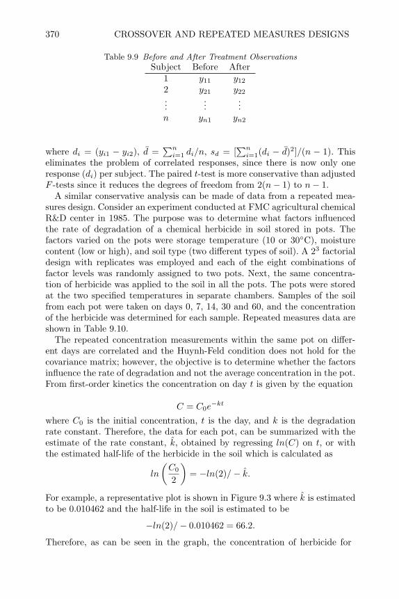
370 CROSSOVER AND REPEATED MEASURES DESIGNS
Table 9.9 Before and After Treatment ObservationsSubject Before After
1 y11 y12
2 y21 y22
......
...n yn1 yn2
where di = (yi1 − yi2), d =∑ni=1 di/n, sd = [
∑ni=1(di − d)2]/(n − 1). This
eliminates the problem of correlated responses, since there is now only oneresponse (di) per subject. The paired t-test is more conservative than adjustedF -tests since it reduces the degrees of freedom from 2(n− 1) to n− 1.
A similar conservative analysis can be made of data from a repeated mea-sures design. Consider an experiment conducted at FMC agricultural chemicalR&D center in 1985. The purpose was to determine what factors influencedthe rate of degradation of a chemical herbicide in soil stored in pots. Thefactors varied on the pots were storage temperature (10 or 30C), moisturecontent (low or high), and soil type (two different types of soil). A 23 factorialdesign with replicates was employed and each of the eight combinations offactor levels was randomly assigned to two pots. Next, the same concentra-tion of herbicide was applied to the soil in all the pots. The pots were storedat the two specified temperatures in separate chambers. Samples of the soilfrom each pot were taken on days 0, 7, 14, 30 and 60, and the concentrationof the herbicide was determined for each sample. Repeated measures data areshown in Table 9.10.
The repeated concentration measurements within the same pot on differ-ent days are correlated and the Huynh-Feld condition does not hold for thecovariance matrix; however, the objective is to determine whether the factorsinfluence the rate of degradation and not the average concentration in the pot.From first-order kinetics the concentration on day t is given by the equation
C = C0e−kt
where C0 is the initial concentration, t is the day, and k is the degradationrate constant. Therefore, the data for each pot, can be summarized with theestimate of the rate constant, k, obtained by regressing ln(C) on t, or withthe estimated half-life of the herbicide in the soil which is calculated as
ln
(C0
2
)= −ln(2)/− k.
For example, a representative plot is shown in Figure 9.3 where k is estimatedto be 0.010462 and the half-life in the soil is estimated to be
−ln(2)/− 0.010462 = 66.2.
Therefore, as can be seen in the graph, the concentration of herbicide for
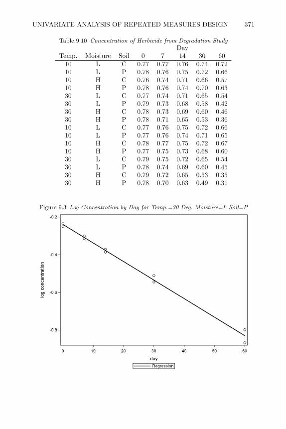
UNIVARIATE ANALYSIS OF REPEATED MEASURES DESIGN 371
Table 9.10 Concentration of Herbicide from Degradation StudyDay
Temp. Moisture Soil 0 7 14 30 6010 L C 0.77 0.77 0.76 0.74 0.7210 L P 0.78 0.76 0.75 0.72 0.6610 H C 0.76 0.74 0.71 0.66 0.5710 H P 0.78 0.76 0.74 0.70 0.6330 L C 0.77 0.74 0.71 0.65 0.5430 L P 0.79 0.73 0.68 0.58 0.4230 H C 0.78 0.73 0.69 0.60 0.4630 H P 0.78 0.71 0.65 0.53 0.3610 L C 0.77 0.76 0.75 0.72 0.6610 L P 0.77 0.76 0.74 0.71 0.6510 H C 0.78 0.77 0.75 0.72 0.6710 H P 0.77 0.75 0.73 0.68 0.6030 L C 0.79 0.75 0.72 0.65 0.5430 L P 0.78 0.74 0.69 0.60 0.4530 H C 0.79 0.72 0.65 0.53 0.3530 H P 0.78 0.70 0.63 0.49 0.31
Figure 9.3 Log Concentration by Day for Temp.=30 Deg. Moisture=L Soil=P

372 CROSSOVER AND REPEATED MEASURES DESIGNS
this combination of factor levels has degraded to just over half the originalconcentration by day 60 (the last measurement).
The SAS data step commands below read the data from Table 9.10 andcalculate the degradation rate constant and estimated half-life for each pot.
*Reads data from Table 9.10 and calculatesrate constant k and half life;
data residue;input temp moisture $ soil$ c1 c2 c3 c4 c5;
*Calculate Log concentration;lc1=log(c1); lc2=log(c2); lc3=log(c3); lc4=log(c4); lc5=log(c5);
*Calculate degradation rate constant by least squares;sp=7*lc2 +14*lc3+30*lc4 +60*lc5; *sum of products;sm=lc1+lc2+lc3+lc4+lc5; *sum log concentrations;num=5*sp -111*sm;den=5*4745 -(111)**2;k=num/den;half_life=-log (2)/k;logHL=log(half_life);T=(Temp -20)/10; if moisture=’L’ then M=-1; else M=1;if soil =’C’ then S=-1; else S=1;
datalines;10 L C 0.77 0.77 0.76 0.74 0.7210 L P 0.78 0.76 0.75 0.72 0.66. . .
proc print; Var temp moisture soil k half_life;run;
The resulting summary statistics for each pot are shown in the output of procprint shown on the next page.
Either of these summary statistics can be analyzed to determine if the rateconstant is influenced by the factors. The following commands can be used tofit the model to the log half-life with proc glm
proc glm data=residue;class temp moisture soil;model logHL=temp|moisture|soil;lsmeans temp moisture;
run;
This analysis showed that increasing temperature and increasing soil mois-ture both had significant effects in increasing the rate of degradation. The soiltype and all of the interactions had no significant effects on degradation at theα = 0.05 level, so the additive model can be used to predict the degradationrate for any combination of temperature and moisture.
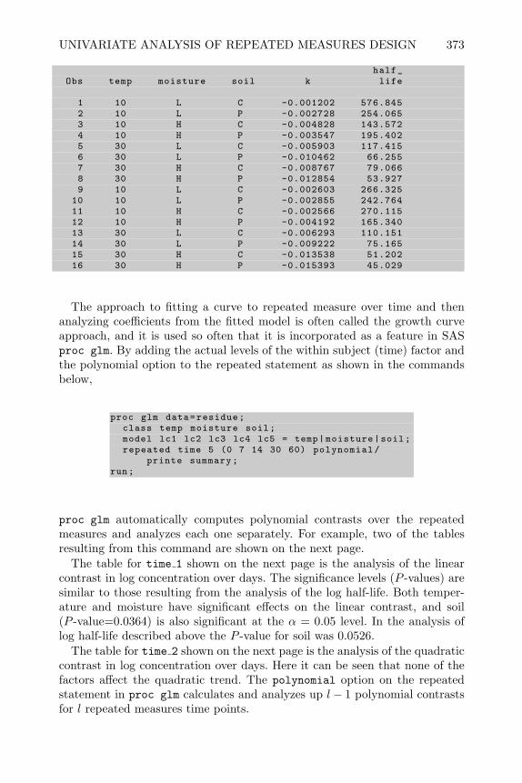
UNIVARIATE ANALYSIS OF REPEATED MEASURES DESIGN 373
half_Obs temp moisture soil k life
1 10 L C -0.001202 576.8452 10 L P -0.002728 254.0653 10 H C -0.004828 143.5724 10 H P -0.003547 195.4025 30 L C -0.005903 117.4156 30 L P -0.010462 66.2557 30 H C -0.008767 79.0668 30 H P -0.012854 53.9279 10 L C -0.002603 266.325
10 10 L P -0.002855 242.76411 10 H C -0.002566 270.11512 10 H P -0.004192 165.34013 30 L C -0.006293 110.15114 30 L P -0.009222 75.16515 30 H C -0.013538 51.20216 30 H P -0.015393 45.029
The approach to fitting a curve to repeated measure over time and thenanalyzing coefficients from the fitted model is often called the growth curveapproach, and it is used so often that it is incorporated as a feature in SASproc glm. By adding the actual levels of the within subject (time) factor andthe polynomial option to the repeated statement as shown in the commandsbelow,
proc glm data=residue;class temp moisture soil;model lc1 lc2 lc3 lc4 lc5 = temp|moisture|soil;repeated time 5 (0 7 14 30 60) polynomial/
printe summary;run;
proc glm automatically computes polynomial contrasts over the repeatedmeasures and analyzes each one separately. For example, two of the tablesresulting from this command are shown on the next page.
The table for time 1 shown on the next page is the analysis of the linearcontrast in log concentration over days. The significance levels (P -values) aresimilar to those resulting from the analysis of the log half-life. Both temper-ature and moisture have significant effects on the linear contrast, and soil(P -value=0.0364) is also significant at the α = 0.05 level. In the analysis oflog half-life described above the P -value for soil was 0.0526.
The table for time 2 shown on the next page is the analysis of the quadraticcontrast in log concentration over days. Here it can be seen that none of thefactors affect the quadratic trend. The polynomial option on the repeatedstatement in proc glm calculates and analyzes up l− 1 polynomial contrastsfor l repeated measures time points.

374 CROSSOVER AND REPEATED MEASURES DESIGNS
The GLM ProcedureRepeated Measures Analysis of Variance
Analysis of Variance of Contrast Variables
time_N represents the nth degree polynomial contrast for time
Contrast Variable: time_1
Source DF Type III SS Mean Square F Value Pr > F
Mean 1 1.63058592 1.63058592 297.79 <.0001temp 1 0.47804051 0.47804051 87.30 <.0001moisture 1 0.08498935 0.08498935 15.52 0.0043temp*moisture 1 0.02381646 0.02381646 4.35 0.0705soil 1 0.03448920 0.03448920 6.30 0.0364temp*soil 1 0.01821844 0.01821844 3.33 0.1056moisture*soil 1 0.00126468 0.00126468 0.23 0.6437temp*moisture*soil 1 0.00000176 0.00000176 0.00 0.9861Error 8 0.04380496 0.00547562
Contrast Variable: time_2
Source DF Type III SS Mean Square F Value Pr > F
Mean 1 0.00004201 0.00004201 1.91 0.2045temp 1 0.00000785 0.00000785 0.36 0.5669moisture 1 0.00004169 0.00004169 1.89 0.2061temp*moisture 1 0.00000005 0.00000005 0.00 0.9644soil 1 0.00000268 0.00000268 0.12 0.7361temp*soil 1 0.00000068 0.00000068 0.03 0.8647moisture*soil 1 0.00001497 0.00001497 0.68 0.4335temp*moisture*soil 1 0.00003402 0.00003402 1.55 0.2490Error 8 0.00017615 0.00002202
9.7 Review of Important Concepts
The crossover and repeated measures designs presented in this chapter arespecial cases of the randomized complete block (RCB), Latin square design(LSD), and split-plot (CRSP, RBSP) designs presented in Chapters 4 and 8and highlighted in Figure 9.4. These designs are used in situations where theblocking factor is a human subject or large animal, and the subplot experi-mental units are successive periods of time.
Crossover designs are most useful when a more precise test of the treat-ment effects is desired and each subject can be assigned each treatment insuccessive periods. Crossover experiments should not be used in cases wherethe experimental subjects are permanently changed by the initial treatment.Otherwise, the result of applying following treatments will not be the same asit would be if they had been applied first. Except for the simple two-periodAB, BA case, the levels of the whole-plot factor in crossover experiments arejust random groupings of subjects and can usually be ignored in the analysis.Therefore, the model for the analysis of crossover experiments, except for the
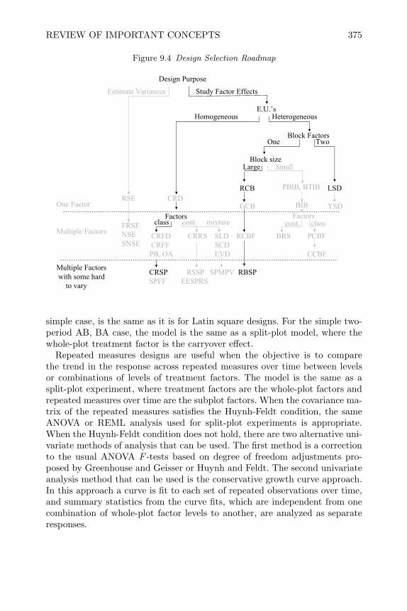
REVIEW OF IMPORTANT CONCEPTS 375
Figure 9.4 Design Selection Roadmap
Design Purpose
Estimate Variances Study Factor Effects
E.U.’s
Block Factors
One Factor
Multiple Factors
Multiple Factorswith some hard
to vary
Block size
Homogeneous Heterogeneous
Large Small
RCB
GCB
PBIB, BTIB
BIB
LSD
YSDRSE CRD
FactorsFRSENSESNSE
CRFD CRRS SLD RCBF BRS PCBFCRFF SCD
PB, OA EVD CCBF
CRSP RSSP SPMPV RBSPSPFF EESPRS
One Two
class cont. mixture cont. classFactors
simple case, is the same as it is for Latin square designs. For the simple two-period AB, BA case, the model is the same as a split-plot model, where thewhole-plot treatment factor is the carryover effect.
Repeated measures designs are useful when the objective is to comparethe trend in the response across repeated measures over time between levelsor combinations of levels of treatment factors. The model is the same as asplit-plot experiment, where treatment factors are the whole-plot factors andrepeated measures over time are the subplot factors. When the covariance ma-trix of the repeated measures satisfies the Huynh-Feldt condition, the sameANOVA or REML analysis used for split-plot experiments is appropriate.When the Huynh-Feldt condition does not hold, there are two alternative uni-variate methods of analysis that can be used. The first method is a correctionto the usual ANOVA F -tests based on degree of freedom adjustments pro-posed by Greenhouse and Geisser or Huynh and Feldt. The second univariateanalysis method that can be used is the conservative growth curve approach.In this approach a curve is fit to each set of repeated observations over time,and summary statistics from the curve fits, which are independent from onecombination of whole-plot factor levels to another, are analyzed as separateresponses.
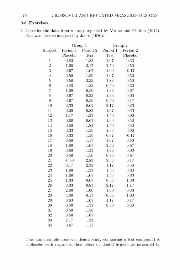
376 CROSSOVER AND REPEATED MEASURES DESIGNS
9.8 Exercises
1. Consider the data from a study reported by Varma and Chilton (1974),that was later re-analyzed by Jones (1980).
Group 1 Group 2Subject Period 1 Period 2 Period 1 Period 2
Placebo Test Test Placebo1 0.83 1.83 1.67 0.332 1.00 2.17 2.50 0.503 0.67 1.67 1.00 -0.174 0.50 1.50 1.67 0.505 0.50 2.33 1.83 0.506 0.83 1.83 0.50 0.337 1.00 0.50 1.33 0.678 0.67 0.33 1.33 0.009 0.67 0.50 0.50 0.1710 0.33 0.67 2.17 0.8311 0.00 0.83 1.67 0.3312 1.17 1.33 1.50 0.0013 0.00 0.67 1.33 0.5014 0.50 1.83 1.50 0.5015 0.33 1.50 1.33 0.0016 0.33 1.50 0.67 -0.1717 0.50 1.17 1.67 0.5018 1.00 1.67 2.50 0.6719 0.00 1.33 1.83 0.0020 0.50 1.50 0.83 0.6721 -0.50 2.83 2.33 0.1722 0.17 2.33 1.17 0.5023 1.00 1.33 1.33 0.0024 1.00 1.67 1.33 0.8325 1.33 0.67 0.33 1.3326 0.33 0.83 2.17 1.1727 2.00 1.00 1.00 0.3328 4.00 0.17 0.33 1.0029 0.83 1.67 1.17 0.1730 0.50 1.33 0.50 0.5031 0.50 1.5032 0.50 1.6733 2.17 1.3334 0.67 1.17
This was a simple crossover dental study comparing a test compound toa placebo with regard to their effect on dental hygiene as measured by

EXERCISES 377
the change in a dental hygiene index. There were thirty-four patients ran-domized to the first group and thirty patients randomized to the secondgroup.
(a) Use proc glm to analyze the data from this experiment.(b) Is there a difference of the test compound and placebo with respect to
their effect on dental hygiene? If so, which produces the larger changein the index?
(c) Is there any evidence of carryover effect of the test compound?
2. Lucas (1957) presented data from an extra-period crossover study on dairycows. Three diet treatments were being compared and the response was theaverage daily production of FCM. The data is shown in the table below.
Table 9.11 Dairy Cow Experiment - Response Is Average Daily FCM Production inPounds, the Treatment Indicator Is in Parentheses
PeriodGroup Cow 1 2 3 4
1 1 (1) 38.66 (2) 37.43 (3) 34.39 (3) 31.301 2 (1) 25.72 (2) 26.13 (3) 23.35 (3) 18.692 3 (2) 48.85 (3) 46.88 (1) 41.99 (1) 39.612 4 (2) 30.80 (3) 29.29 (1) 26.41 (1) 23.163 5 (3) 34.64 (1) 32.27 (2) 28.50 (2) 27.133 6 (3) 25.35 (1) 26.00 (2) 23.86 (2) 19.924 7 (1) 35.19 (3) 33.50 (2) 28.41 (2) 25.124 8 (1) 21.80 (3) 23.91 (2) 21.69 (2) 17.555 9 (2) 32.90 (1) 33.12 (3) 27.52 (3) 25.105 10 (2) 21.37 (1) 21.97 (3) 19.38 (3) 16.576 11 (3) 30.40 (2) 29.50 (1) 26.70 (1) 23.096 12 (3) 22.84 (2) 20.97 (1) 18.59 (1) 16.10
(a) Does every treatment follow every other treatment, including itself?(b) Analyze the data using proc glm. Are the treatment and carryover ef-
fects orthogonal? Check by comparing their type I and type III sums ofsquares.
(c) Use the lsmeans statement to get least squares adjusted means for treat-ments. Why is this possible when it was not possible for the example inSection 9.4.1 ?
3. Consider planning an experiment to compare the taste of chocolate brownierecipes. The treatments will consist of three brands of boxed brownie mixesand one from-scratch home recipe. A panel of tasters will be used to evaluatethe brownies. Each taster will taste each brownie and give it a rating from1 to 10 (10 being the best possible).

378 CROSSOVER AND REPEATED MEASURES DESIGNS
(a) Why do you think it might be appropriate to use a crossover design forthis study? What is the alternative?
(b) Modify the SAS code in Section 9.4.1 to create Williams’ crossover designfor four treatments to use for this experiment.
(c) Decide how many subjects to include in your study and create a ran-domized list assigning each subject to one of the four sequence groups.
(d) Write the model you would use to analyze this data.(e) Make a data input form and show how you would code the indicators
for the subject, period, treatment and carryover effects.
4. Consider the data from the repeated measures design shown in Table 9.10.
(a) Use proc glm to compute the sphericity test and determine if the Huynh-Feldt condition holds.
(b) Use proc glm to make the Greenhouse-Geisser and Huynh-Feldt ad-justed F -tests of the subplot effects.
(c) Do you find more terms significant using the adjusted F -tests than werefound using the growth curve analysis shown in the text? If so, explainwhy.
5. Consider the results of the repeated measurements experiment from Us-age note: Stat-40 (1997) from the University of Texas at Austin. In thisexperiment the purpose was to determine how diet and exercise affect thepulse of subjects. Eighteen subjects were randomly assigned to one of threeexercises (1=aerobic stair climbing, 2=racquetball, 3=weight training) andone of two diets (1=include meat, 2=vegetarian). After a training periodwhere all subjects followed their assigned exercise and diet routine, theirpulse was measured three successive times (once after a warm-up, againafter jogging and finally after running). The results are shown in the tableon the next page.
(a) Make a plot of the average trend in pulse over the three repeat measuresfor each of the six combinations of diet and exercise.
(b) Do a normal split-plot analysis of the data treating diet and exercise aswhole-plot factors and the repeated measurements as a subplot factor.
(c) Use the sphericity test to determine if the normal analysis is justified.(d) Make the Huynh-Feldt and Greenhouse-Geisser adjusted F -tests for the
subplot effects. Are the results different than the unadjusted tests?(e) Do a conservative growth-curve analysis of the linear contrast in pulse
measurements over time. Do the results of this analysis confirm whatyou found in (b) and (d)? If not, why?

EXERCISES 379
Exercise Diet Pulse 1 Pulse 2 Pulse 31 1 112 166 2151 1 111 166 2251 1 89 132 1891 2 95 134 1861 2 66 109 1501 2 69 119 1772 1 125 177 2412 1 85 117 1862 1 97 137 1852 2 93 151 2172 2 77 122 1782 2 78 119 1733 1 81 134 2053 1 88 133 1803 1 88 157 2243 2 58 99 1313 2 85 132 1863 2 78 110 164


CHAPTER 10
Response Surface Designs
10.1 Introduction
In a response surface experiment, the independent variables or factors can bevaried over a continuous range. The goal is to determine the factor settingsthat produce a maximum or minimum response or to map the relationshipbetween the response and the factor settings over this contiguous factor space.As a practical matter, if we want to know a lot about the relationship betweenthe factors and the response, it will require many experiments. For that reason,response surface designs are rarely conducted with more than six factors.
Response surface experiments are normally used at the last stage of exper-imentation. The important factors have already been determined in earlierexperiments, and at this stage of experimentation the purpose is to describein detail the relationship between the factors and the response. It is usuallyknown or assumed that a simple linear model, even with interactions, is notgood enough to represent that relationship. In order to locate maximums orminimums in the response as a function of the factor settings, at least threelevels of each factor should be utilized.
Response surface methods generally refer to a complete package of statisticaldesign and analysis tools that are used for the following three steps.1. Design and collection of data to fit an equation to approximate the rela-
tionship between the factors and response.2. Regression analysis to fit a model to describe the data.3. Examination of the fitted relationship through graphical and numerical
techniques.Response surface methods have found considerable use in industry especiallyin chemical processes where the reaction yield or cost of production can be op-timized as a function of the settings of controllable process factors. Since theirorigin these designs have also found successful applications in food science, en-gineering, biology, psychology, textiles, education and many other areas.
10.2 Fundamentals of Response Surface Methodology
10.2.1 Empirical Quadratic Model
In response surface methods, the relationship between the response (y) andthe factor settings (x’s) is assumed to be a nonlinear equation given by y =f(x)+ε. For two factors or independent variables we could write this equation
381

382 RESPONSE SURFACE DESIGNS
as
y = f(x1, x2) + ε (10.1)
where f is a nonlinear function and ε is the random effect of experimentalerror. When f is unknown it can be approximated near the point (x10, x20)using the two-term Taylor series approximation, i.e.,
f(x1, x2) ≈ f(x10, x20) + (x1 − x10)∂f(x1, x2)
∂x1
∣∣∣x1=x10,x2=x20
+ (x2 − x20)∂f(x1, x2)
∂x2
∣∣∣x1=x10,x2=x20
+(x1 − x10)2
2∂2f(x1, x2)
∂x21
∣∣∣x1=x10,x2=x20
+(x2 − x20)2
2∂2f(x1, x2)
∂x22
∣∣∣x1=x10,x2=x20
+(x1 − x10)(x2 − x20)
2∂2f(x1, x2)∂x1∂x2
∣∣∣x1=x10,x2=x20
,
(10.2)
which leads to a general quadratic equation of the form
y = β0 + β1x1 + β2x2 + β11x21 + β22x
22 + β12x1x2 + ε
(10.3)
where β1 = ∂f(x1,x2)∂x1
∣∣∣x1=x10,x2=x20
, etc. If the region of interest is of moderate
size, this general quadratic equation will provide a good approximation to fand can be used for interpolation within this region. The general quadraticequation is quite flexible and with appropriate coefficients it can describe awide variety of surfaces such as hilltops, valleys, rising or falling ridges, orsaddle points as shown with contour plots in Figure 10.1.
With k factors or independent variables the general quadratic equation canbe written in the form
y = β0 +k∑i=1
βixi +k∑i=1
βiix2i +
k∑ k∑i<j
βijxixj + ε, (10.4)
and unless the function f is known, this equation forms the basis of responsesurface methods. Response surface designs were created to provide data toapproximate this equation, and mathematical tools were created to explorethe fitted surface represented by this equation.

FUNDAMENTALS OF RESPONSE SURFACE METHODOLOGY 383
Figure 10.1 Surfaces That Can Be Described by General Quadratic Equation
80
50
60
70
40
50
6070
50
60
80
80
60
60
60
60
70
70
70
70
80
80
80
80
60
70
60
50
10.2.2 Design Considerations
The first requirement of a response surface design is that it should providedata that will allow estimation of the coefficients in model (10.4). This modelhas 1+2k+k(k−1)/2 coefficients, thus any response surface design must haveat least three levels for each factor (to allow estimation of quadratic terms)and at least 1+2k+k(k−1)/2 total runs. 3k factorial designs have three levelsfor every factor. However, Box and Wilson (1951) showed that they were lesssatisfactory as a response surface design than an alternative design they calledthe central composite design. The central composite will be the first standardresponse surface design we will discuss in the next section.
Normally the factors or independent variables (xi) in the general quadraticEquation (10.4) are coded and scaled as shown in Sections 3.7.2 and 3.7.3 sothat the experimental region is a hyper-cube or hyper-sphere with radius Rin the coded space. This general quadratic model can be written in matrixterms as
y = xb + x′Bx + ε (10.5)
where x′ = (1, x1, x2, . . . , xk), b′ = (β0, β1, . . . , βk) and the symmetric matrix

384 RESPONSE SURFACE DESIGNS
B =
β11 β12/2 · · · β1k/2
β22 · · · β2k/2. . .
βkk
.
When fitting a linear regression model of the form y = xb, the design pointsare chosen to minimize the variance of the fitted coefficients b = (X′X)−1X′y.Since the variance covariance matrix of estimated regression coefficients isσ2(X′X)−1, this means the design points should be chosen such that the(X′X) matrix is diagonal, or that the design is orthogonal like the 2k designsdiscussed in Chapter 3 and the 2k−p designs discussed in Chapter 6. When the(X′X) matrix is diagonal, the diagonal elements of (X′X)−1 will be minimized.
On the other hand, when fitting the general quadratic model, the primarypurpose is not to understand the mechanism of the underlying relationshipbetween the response and the factors. Therefore, the specific coefficients in thegeneral quadratic model are of less importance. What is more important in aresponse surface study is to develop a prediction equation with the eventualgoal of determining the optimum operating conditions. Thus, the variance of apredicted value at ,x, that is given by the equation V ar[y(x)] = σ2x′(X′X)−1xis of more importance than the variance of the fitted coefficients.
Since it is not known before the experiment is conducted where the optimumwill lie in the design region, one desirable property of a response surface designis to have the variance of a predicted value nearly the same everywhere in thedesign region. In this way the precision in predicting the optimum will notdepend upon its unknown position in the design region. The first step inequalizing the variance of prediction over the design region is to find a designthat is rotatable (Myers and Montgomery, 2002). A rotatable design is one inwhich the variance of the predicted value at the point x is only a function ofthe distance from the design origin to x. Box and Wilson’s central compositedesign and other standard response surface designs have this property.
Box and Hunter (1957) showed that certain rotatable designs could be modi-fied to have uniform precision, which means the variance of a predicted value isthe same at the origin and at the radius of one in the coded design region. A de-sign with uniform precision is close to having the variance of the response equalthroughout the design region. Many standard response surface designs havethis property or are close to having this property. When creating response sur-face designs using a computer algorithm, the G-optimality criterion is similarto uniform precision. A G-optimal design is one that minimizes the maximumvariance of a predicted value in the design region. Computer code for creatingG-optimal designs is not normally used, but in the limit G-optimality andD-optimality are equivalent. Programs, such as SAS proc optex, are widelyused for creating D-optimal designs, and when a standard response surfacedesign does not meet the needs of an experimenter, the D-optimality criterioncan be used in a computer search to create a design. Giovannitti-Jensen and

STANDARD DESIGNS FOR SECOND ORDER MODELS 385
Myers (1989) and Myers et al. (1992) describe a variance dispersion plot whichcan be used to visually evaluate whether any response surface design is closeto having the properties of rotatability and uniform precision.
In addition to providing a good distribution of the variance of a predictedvalue, two other desirable properties of response surface designs are (1) toprovide an estimate of the “pure” experimental error so the adequacy of thegeneral quadratic model can be checked, and (2) to allow for blocking so thatan experimenter can begin with a linear design and add a second block toestimate curvature if necessary. To estimate pure error, at least one designpoint must be replicated. When blocking, the first block would consist ofa design such as a 2k or 2k−p augmented with center points that allow forchecking the adequacy of the linear model. If the linear model is adequate,no further experimentation is required. If the linear model is not adequate, asecond block of experiments can be added which will allow estimation of thequadratic coefficients in the general quadratic model.
10.3 Standard Designs for Second Order Models
This section presents some of the more popular completely randomized re-sponse surface designs (CRRS).
10.3.1 Central Composite Design (CCD)
Box and Wilson (1951)’s central composite design (CCD) consists of a 2k
factorial or 2k−p fractional factorial design augmented with center points andaxial points as shown in Figure 10.2. The 2k or resolution V 2k−p design allows
Figure 10.2 CCD in Two and Three Dimensions
Factorial Center Points Axial Points
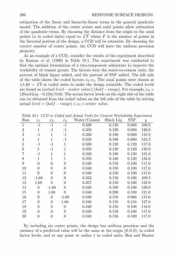
386 RESPONSE SURFACE DESIGNS
estimation of the linear and linear-by-linear terms in the general quadraticmodel. The addition of the center points and axial points allow estimationof the quadratic terms. By choosing the distance from the origin to the axialpoints (α in coded units) equal to 4
√F where F is the number of points in
the factorial portion of the design, a CCD will be rotatable. By choosing thecorrect number of center points, the CCD will have the uniform precisionproperty.
As an example of a CCD, consider the results of the experiment describedby Kamon et al. (1999) in Table 10.1. The experiment was conducted tofind the optimal formulation of a two-component admixture to improve theworkabilty of cement grouts. The factors were the water-to-cement ratio, thepercent of black liquor added, and the percent of SNF added. The left sideof the table shows the coded factors x1-x3. The axial points were chosen at±1.68 = 4
√8 in coded units to make the design rotatable. The coded levels
are found as (actual level− center value)/(half − range). For example, x2 =(BlackLiq.−0.150)/0.03. The actual factor levels on the right side of the tablecan be obtained from the coded values on the left side of the table by solvingactual level = (half − range)× xi + center value.
Table 10.1 CCD in Coded and Actual Units for Cement Workability ExperimentRun x1 x2 x3 Water/Cement Black Liq. SNF y
1 -1 -1 -1 0.330 0.120 0.080 109.52 1 -1 -1 0.350 0.120 0.080 120.03 -1 1 -1 0.330 0.180 0.080 110.54 1 1 -1 0.350 0.180 0.080 124.55 -1 -1 1 0.330 0.120 0.120 117.06 1 -1 1 0.350 0.120 0.120 130.07 -1 1 1 0.330 0.180 0.120 121.08 1 1 1 0.350 0.180 0.120 132.09 0 0 0 0.340 0.150 0.100 117.010 0 0 0 0.340 0.150 0.100 117.011 0 0 0 0.340 0.150 0.100 115.012 -1.68 0 0 0.323 0.150 0.100 109.513 1.68 0 0 0.357 0.150 0.100 132.014 0 -1.68 0 0.340 0.100 0.100 120.015 0 1.68 0 0.340 0.200 0.100 121.016 0 0 -1.68 0.340 0.150 0.066 115.017 0 0 1.68 0.340 0.150 0.134 127.018 0 0 0 0.340 0.150 0.100 116.019 0 0 0 0.340 0.150 0.100 117.020 0 0 0 0.340 0.150 0.100 117.0
By including six center points, the design has uniform precision and thevariance of a predicted value will be the same at the origin (0, 0, 0), in codedfactor levels, and at any point at radius 1 in coded units. Box and Hunter
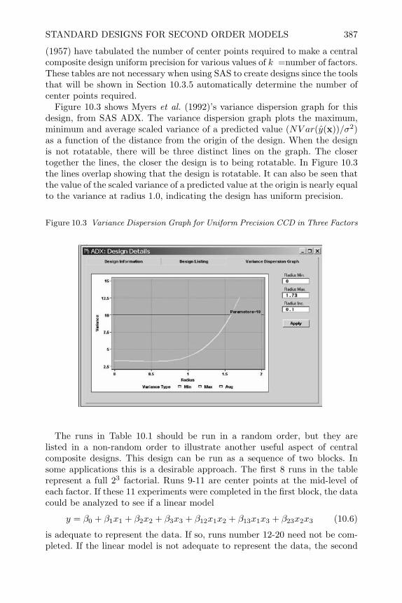
STANDARD DESIGNS FOR SECOND ORDER MODELS 387
(1957) have tabulated the number of center points required to make a centralcomposite design uniform precision for various values of k =number of factors.These tables are not necessary when using SAS to create designs since the toolsthat will be shown in Section 10.3.5 automatically determine the number ofcenter points required.
Figure 10.3 shows Myers et al. (1992)’s variance dispersion graph for thisdesign, from SAS ADX. The variance dispersion graph plots the maximum,minimum and average scaled variance of a predicted value (NV ar(y(x))/σ2)as a function of the distance from the origin of the design. When the designis not rotatable, there will be three distinct lines on the graph. The closertogether the lines, the closer the design is to being rotatable. In Figure 10.3the lines overlap showing that the design is rotatable. It can also be seen thatthe value of the scaled variance of a predicted value at the origin is nearly equalto the variance at radius 1.0, indicating the design has uniform precision.
Figure 10.3 Variance Dispersion Graph for Uniform Precision CCD in Three Factors
The runs in Table 10.1 should be run in a random order, but they arelisted in a non-random order to illustrate another useful aspect of centralcomposite designs. This design can be run as a sequence of two blocks. Insome applications this is a desirable approach. The first 8 runs in the tablerepresent a full 23 factorial. Runs 9-11 are center points at the mid-level ofeach factor. If these 11 experiments were completed in the first block, the datacould be analyzed to see if a linear model
y = β0 + β1x1 + β2x2 + β3x3 + β12x1x2 + β13x1x3 + β23x2x3 (10.6)
is adequate to represent the data. If so, runs number 12-20 need not be com-pleted. If the linear model is not adequate to represent the data, the second

388 RESPONSE SURFACE DESIGNS
set of experiments can be completed and a block variable added to the modelto account for any changes in background variables that occurs between thefirst and second set of experiments.
10.3.2 Box-Behnken Design
Whereas the CCD requires five levels (−α, −1, 0, +1, +α) for each factor,Box and Behnken (1960) developed some three level designs that will allow es-timation of the general quadratic model. These designs consist of 22 factorialsin each pair of factors with all other factors held constant at their mid-levelplus a few center points. No Box-Behnken design exists for only two factors.An example of a Box-Behnken design in three coded factors is shown in Table10.2.
Table 10.2 Box-Behnken Design in Three Factorsrun x1 x2 x3
1 -1 -1 02 1 -1 03 -1 1 04 1 1 05 -1 0 -16 1 0 -17 -1 0 18 1 0 19 0 -1 -1
10 0 1 -111 0 -1 112 0 1 113 0 0 014 0 0 015 0 0 0
Box-Behnken designs have two advantages over CCDs. The first advantageis that they only require that factors be varied over three levels. This maymake experimentation less costly if actual prototypes are being constructedin the experimentation. The second advantage is that they usually (exceptfor the five-factor case) require less total runs than the central compositedesign. For example, the three-factor CCD required twenty runs whereas thethree-factor Box-Behnken design only required 15 runs.
A disadvantage of a Box-Behnken design compared to a central compositedesign is that it cannot be built up in two steps beginning with a 2k design.This can be visualized in Figure 10.4, which diagrams a three-factor Box-Behnken design. A 23 design consists of runs at all corners of the cube asshown in Section 3.7.1, but as can be seen in Figure 10.4 the Box-Behnkendesign does not include those points. Therefore a Box-Behnken design should
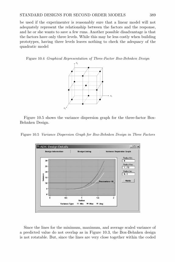
STANDARD DESIGNS FOR SECOND ORDER MODELS 389
be used if the experimenter is reasonably sure that a linear model will notadequately represent the relationship between the factors and the response,and he or she wants to save a few runs. Another possible disadvantage is thatthe factors have only three levels. While this may be less costly when buildingprototypes, having three levels leaves nothing to check the adequacy of thequadratic model
Figure 10.4 Graphical Representation of Three-Factor Box-Behnken Design
x1
x3
x2
Figure 10.5 shows the variance dispersion graph for the three-factor Box-Behnken Design.
Figure 10.5 Variance Dispersion Graph for Box-Behnken Design in Three Factors
Since the lines for the minimum, maximum, and average scaled variance ofa predicted value do not overlap as in Figure 10.3, the Box-Behnken designis not rotatable. But, since the lines are very close together within the coded
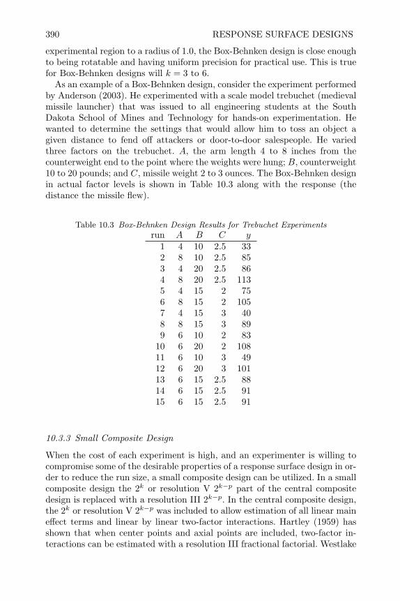
390 RESPONSE SURFACE DESIGNS
experimental region to a radius of 1.0, the Box-Behnken design is close enoughto being rotatable and having uniform precision for practical use. This is truefor Box-Behnken designs will k = 3 to 6.
As an example of a Box-Behnken design, consider the experiment performedby Anderson (2003). He experimented with a scale model trebuchet (medievalmissile launcher) that was issued to all engineering students at the SouthDakota School of Mines and Technology for hands-on experimentation. Hewanted to determine the settings that would allow him to toss an object agiven distance to fend off attackers or door-to-door salespeople. He variedthree factors on the trebuchet. A, the arm length 4 to 8 inches from thecounterweight end to the point where the weights were hung; B, counterweight10 to 20 pounds; and C, missile weight 2 to 3 ounces. The Box-Behnken designin actual factor levels is shown in Table 10.3 along with the response (thedistance the missile flew).
Table 10.3 Box-Behnken Design Results for Trebuchet Experimentsrun A B C y
1 4 10 2.5 332 8 10 2.5 853 4 20 2.5 864 8 20 2.5 1135 4 15 2 756 8 15 2 1057 4 15 3 408 8 15 3 899 6 10 2 83
10 6 20 2 10811 6 10 3 4912 6 20 3 10113 6 15 2.5 8814 6 15 2.5 9115 6 15 2.5 91
10.3.3 Small Composite Design
When the cost of each experiment is high, and an experimenter is willing tocompromise some of the desirable properties of a response surface design in or-der to reduce the run size, a small composite design can be utilized. In a smallcomposite design the 2k or resolution V 2k−p part of the central compositedesign is replaced with a resolution III 2k−p. In the central composite design,the 2k or resolution V 2k−p was included to allow estimation of all linear maineffect terms and linear by linear two-factor interactions. Hartley (1959) hasshown that when center points and axial points are included, two-factor in-teractions can be estimated with a resolution III fractional factorial. Westlake

STANDARD DESIGNS FOR SECOND ORDER MODELS 391
(1965) obtained additional small composite designs by substituting irregularfractions for the factorial portion of the design, and Draper (1985) and Draperand Lin (1990) substituted Plackett-Burman Designs for the factorial portionto come up with even more small composite designs.
Figure 10.6 shows a comparison of the central composite design for k = 2and the small composite design for k = 2. The central composite design hasfive center points for a total of thirteen runs, while the small composite designhas three center points with a total of nine runs.
Figure 10.6 Graphical Comparison of CCD and Small Composite (with I = AB) fork=2
-1 0 1 -1 0 1
central composite k=2 small composite k=2
Figure 10.7 compares the variance dispersion graph for the central com-posite and small composite designs with k = 2 factors. Here it can be seenthe central composite is rotatable and has uniform precision while beyond aradius of 0.75 in coded units, the scaled variance of a predicted value dependson the location for a small composite design. The coefficients for the generalquadratic model can still be estimated when a small composite design is used,but the variance of a predicted value is not as uniform as it is for a centralcomposite design. This is the sacrifice for decreasing the number of runs.
10.3.4 Hybrid Design
Roquemore (1976) developed hybrid designs that require even fewer runs thanthe small composite designs. These designs were constructed by making acentral composite design in k − 1 factors and adding a kth factor so that theX′X has certain properties and the design is near rotatable. Table 10.4 showsan example of the Roquemore 310 design. It is labeled 310 because it has 3factors and 10 runs. It can be seen that there is a central composite design incolumns 1 and 2. This design is near rotatable as shown in Figure 10.8, butsince it only has 10 runs, there are zero degrees of freedom for estimating theexperimental error. Some of the Roquemore hybrid designs leave one degreeof freedom for estimating experimental error, but none of them have purereplicates that are required for testing the adequacy of the general quadraticmodel. Therefore these designs should only be used when the experimenter isconfident that the general quadratic model will represent the data well, andthere is an independent estimate of experimental error from previous data.

392 RESPONSE SURFACE DESIGNS
Figure 10.7 Comparison of Variance Dispersion Graph for CCD and Small Com-posite Design with k=2
Table 10.4 Roquemore 310 DesignRun x1 x2 x3
1 0 0 1.29062 0 0 -0.13603 -1 -1 0.63864 1 -1 0.63865 -1 1 0.63866 1 1 0.63867 1.736 0 -0.92738 -1.736 0 -0.92739 0 1.736 -0.9273
10 0 -1.736 -0.9273
10.4 Creating Standard Designs in SAS
Central Composite Designs (if you know the axial distance and number ofcenter points) and Box-Behnken designs can be easily created in the SASdata step by following the descriptions in the last section. There are alsoSAS macros in the AUTOCALL library that can produce central compositedesigns. For example, the commands below will produce the central compositedesign in uncoded units shown in Table 10.1.
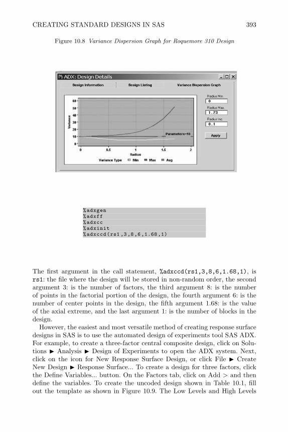
CREATING STANDARD DESIGNS IN SAS 393
Figure 10.8 Variance Dispersion Graph for Roquemore 310 Design
%adxgen%adxff%adxcc%adxinit%adxccd(rs1 ,3,8,6,1.68,1)
The first argument in the call statement, %adxccd(rs1,3,8,6,1.68,1), isrs1: the file where the design will be stored in non-random order, the secondargument 3: is the number of factors, the third argument 8: is the numberof points in the factorial portion of the design, the fourth argument 6: is thenumber of center points in the design, the fifth argument 1.68: is the valueof the axial extreme, and the last argument 1: is the number of blocks in thedesign.
However, the easiest and most versatile method of creating response surfacedesigns in SAS is to use the automated design of experiments tool SAS ADX.For example, to create a three-factor central composite design, click on Solu-tions I Analysis I Design of Experiments to open the ADX system. Next,click on the icon for New Response Surface Design, or click File I CreateNew Design I Response Surface... To create a design for three factors, clickthe Define Variables... button. On the Factors tab, click on Add > and thendefine the variables. To create the uncoded design shown in Table 10.1, fillout the template as shown in Figure 10.9. The Low Levels and High Levels

394 RESPONSE SURFACE DESIGNS
shown in the template are the extremes of the factorial portion of the designfor a central composite design.
Figure 10.9 Add Factors Template from SAS ADX
When finished with the Add Factors template, click the Ok button and clickthe Yes button in response to the question, “Do you want to save changes?”Next, click on the Select Design button, and the template shown in Figure10.10 will appear. This template shows all the completely randomized responsesurface designs available for three factors.
The central composite-uniform precision is the design shown in Table 10.1.The other option for a central composite design (central composite-orthogonal)will create a central composite design that has a diagonal X′X when the cor-rect axial value is chosen and the factors, interactions and squared factor levelsare properly scaled. Before the widespread use of computer programs to fit thegeneral quadratic equation, orthogonality was important because it simplifiedthe calculations required to obtain least squares estimates of the coefficientsin the model. Using SAS, orthogonality is not important and the uniform pre-cisions design should be chosen if a central composite is to be used. It canalso be seen that the Box-Behnken, Small Composite and Roquemore designsdiscussed in the last section are available choices.
To choose a design on the Select Design template, single left click on theline for the design you want. You can see a description of the design, a listingof the runs in the design or the variance dispersion graph for the design byclicking the Design Details... button. When you have decided what design youwould like to use, click on the line listing the design and then click on the “x”
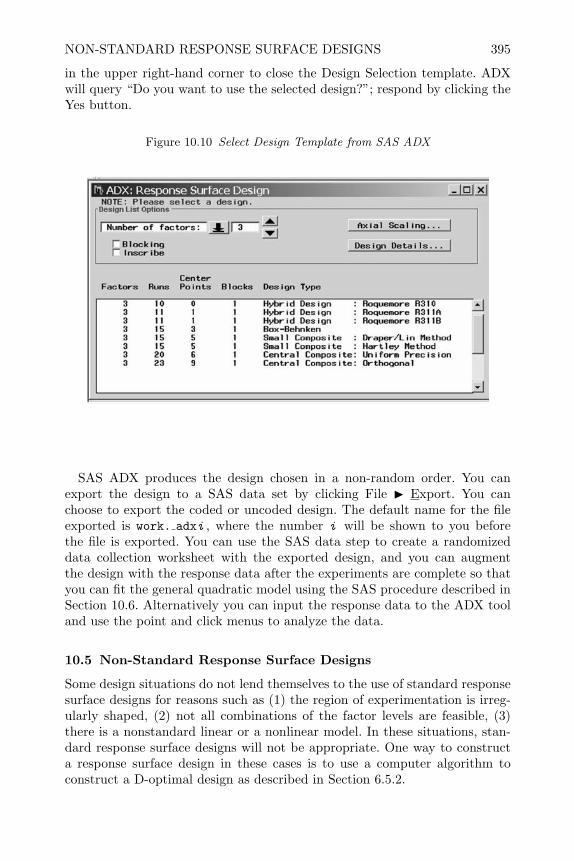
NON-STANDARD RESPONSE SURFACE DESIGNS 395
in the upper right-hand corner to close the Design Selection template. ADXwill query “Do you want to use the selected design?”; respond by clicking theYes button.
Figure 10.10 Select Design Template from SAS ADX
SAS ADX produces the design chosen in a non-random order. You canexport the design to a SAS data set by clicking File I Export. You canchoose to export the coded or uncoded design. The default name for the fileexported is work. adxi , where the number i will be shown to you beforethe file is exported. You can use the SAS data step to create a randomizeddata collection worksheet with the exported design, and you can augmentthe design with the response data after the experiments are complete so thatyou can fit the general quadratic model using the SAS procedure described inSection 10.6. Alternatively you can input the response data to the ADX tooland use the point and click menus to analyze the data.
10.5 Non-Standard Response Surface Designs
Some design situations do not lend themselves to the use of standard responsesurface designs for reasons such as (1) the region of experimentation is irreg-ularly shaped, (2) not all combinations of the factor levels are feasible, (3)there is a nonstandard linear or a nonlinear model. In these situations, stan-dard response surface designs will not be appropriate. One way to constructa response surface design in these cases is to use a computer algorithm toconstruct a D-optimal design as described in Section 6.5.2.
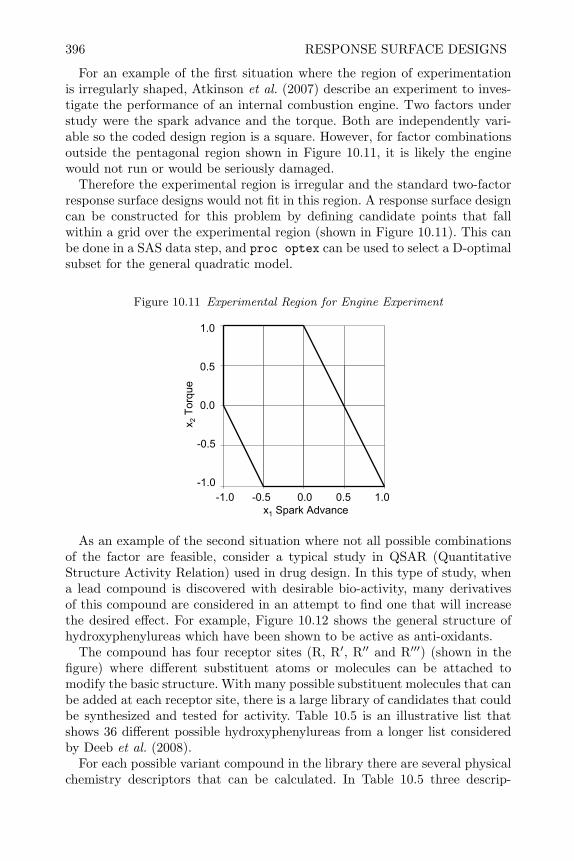
396 RESPONSE SURFACE DESIGNS
For an example of the first situation where the region of experimentationis irregularly shaped, Atkinson et al. (2007) describe an experiment to inves-tigate the performance of an internal combustion engine. Two factors understudy were the spark advance and the torque. Both are independently vari-able so the coded design region is a square. However, for factor combinationsoutside the pentagonal region shown in Figure 10.11, it is likely the enginewould not run or would be seriously damaged.
Therefore the experimental region is irregular and the standard two-factorresponse surface designs would not fit in this region. A response surface designcan be constructed for this problem by defining candidate points that fallwithin a grid over the experimental region (shown in Figure 10.11). This canbe done in a SAS data step, and proc optex can be used to select a D-optimalsubset for the general quadratic model.
Figure 10.11 Experimental Region for Engine Experiment
-1.0 -0.5 0.0 0.5 1.0x1 Spark Advance
1.0
0.5
0.0
-0.5
-1.0
x 2T
orqu
e
As an example of the second situation where not all possible combinationsof the factor are feasible, consider a typical study in QSAR (QuantitativeStructure Activity Relation) used in drug design. In this type of study, whena lead compound is discovered with desirable bio-activity, many derivativesof this compound are considered in an attempt to find one that will increasethe desired effect. For example, Figure 10.12 shows the general structure ofhydroxyphenylureas which have been shown to be active as anti-oxidants.
The compound has four receptor sites (R, R′, R′′ and R′′′) (shown in thefigure) where different substituent atoms or molecules can be attached tomodify the basic structure. With many possible substituent molecules that canbe added at each receptor site, there is a large library of candidates that couldbe synthesized and tested for activity. Table 10.5 is an illustrative list thatshows 36 different possible hydroxyphenylureas from a longer list consideredby Deeb et al. (2008).
For each possible variant compound in the library there are several physicalchemistry descriptors that can be calculated. In Table 10.5 three descrip-

NON-STANDARD RESPONSE SURFACE DESIGNS 397
Figure 10.12 General Structure of Hydroxyphenylureas
R’’
R’
HO
R
N
O O
N
H H
(CH2)n N N R’’’
tors are shown: Hydration Energy (HE), Molecular Dipole Moment at the z-direction (DMz), and Symmetry Index (S0K). The objective of a QSAR studywould be to (1) synthesize a subset of the molecules from the large libraryand test them to determine their ability to scavenge oxygen FRs as measuredby the binding constant logKapp, and (2) fit a model relating the responselogKapp to several physical chemistry descriptors (in this case, the variablesHE, DMz, and S0K). Once a model relating the response as a function of theindependent variables has been found, the combination of the independentvariables that is predicted to give the maximum response can be determined.Compounds in the large library that have values of the physical chemistrydescriptors (independent variables) closest to those predicted to result in amaximum response can then be synthesized and tested for activity. In thisway variant compounds that have increased activity are discovered.
In QSAR studies a standard response surface designs cannot be used be-cause not all potential combinations of the independent variables are possible.Only a subset of the combinations of independent variables that exist in thelarge library can be chosen in a subset or experimental design to be tested.Again proc optex can be utilized to create a D-optimal subset of the largerlibrary. In this case the list of candidates will be all the compounds in thelibrary.
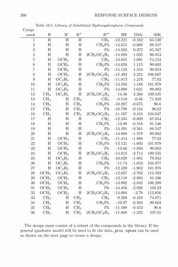
398 RESPONSE SURFACE DESIGNS
Table 10.5 Library of Substituted Hydroxyphenylurea CompoundsComp-
ound R R′ R′′ R′′′ HE DMz S0K1 H H H CH3 -12.221 -0.162 64.1382 H H H CH2Ph -14.015 -0.068 88.5473 H H H Ph -14.502 0.372 85.5674 H H H 2CH3OC6H4 -14.893 1.035 96.0535 H OCH3 H CH3 -12.855 1.091 74.1246 H OCH3 H CH2Ph -14.628 1.115 99.0027 H OCH3 H Ph -15.123 1.554 96.0538 H OCH3 H 2CH3OC6H4 -15.492 2.221 106.6079 H OC2H5 H CH3 -11.813 1.219 77.02
10 H OC2H5 H CH2Ph -13.593 1.188 101.97811 H OC2H5 H Ph -14.088 1.621 99.00212 CH3 OC2H5 H 2CH3OC6H4 -14.46 2.266 109.53513 CH3 H CH3 CH3 -8.519 -0.56 71.94914 CH3 H CH3 CH2Ph -10.287 -0.675 96.615 CH3 H CH3 Ph -10.798 -0.134 96.6216 CH3 H CH3 2CH3OC6H4 -11.167 0.418 104.04717 H H H CH3 -12.245 -0.609 67.05418 H H H CH2Ph -13.98 -0.518 91.54619 H H H Ph -14.491 -0.561 88.54720 H H H 2CH3OC6H4 -14.888 -1.478 99.00221 H OCH3 H CH3 -11.414 -1.888 77.0222 H OCH3 H CH2Ph -13.121 -1.692 101.97823 H OCH3 H Ph -13.66 -1.893 99.00224 H OCH3 H 2CH3OC6H4 -14.012 -2.714 109.53525 H OC2H5 H CH3 -10.029 -1.891 79.94226 H OC2H5 H CH2Ph -11.74 -1.652 104.97727 H OC2H5 H Ph -12.329 -1.902 101.97828 OCH3 OC2H5 H 2CH3OC6H4 -12.637 -2.762 112.49229 OCH3 OCH3 H CH3 -12.118 -2.994 81.10630 OCH3 OCH3 H CH2Ph -13.892 -2.845 106.29931 OCH3 OCH3 H Ph -14.456 -2.926 103.2332 OCH3 OCH3 H 2CH3OC6H4 -14.804 -3.78 113.85633 CH3 H CH3 CH3 -9.209 -0.423 74.87134 CH3 H CH3 CH2Ph -10.97 -0.302 99.60335 CH3 H CH3 Ph -11.488 -0.453 96.636 CH3 H CH3 2CH3OC6H4 -11.868 -1.322 107.01
The design must consist of a subset of the compounds in the library. If thegeneral quadratic model will be used to fit the data, proc optex can be usedas shown on the next page to create a design.
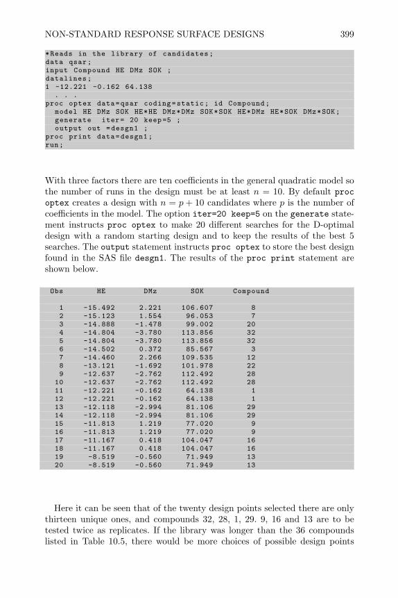
NON-STANDARD RESPONSE SURFACE DESIGNS 399
*Reads in the library of candidates;data qsar;input Compound HE DMz SOK ;datalines;1 -12.221 -0.162 64.138
. . .proc optex data=qsar coding=static; id Compound;
model HE DMz SOK HE*HE DMz*DMz SOK*SOK HE*DMz HE*SOK DMz*SOK;generate iter= 20 keep=5 ;output out =desgn1 ;
proc print data=desgn1;run;
With three factors there are ten coefficients in the general quadratic model sothe number of runs in the design must be at least n = 10. By default procoptex creates a design with n = p + 10 candidates where p is the number ofcoefficients in the model. The option iter=20 keep=5 on the generate state-ment instructs proc optex to make 20 different searches for the D-optimaldesign with a random starting design and to keep the results of the best 5searches. The output statement instructs proc optex to store the best designfound in the SAS file desgn1. The results of the proc print statement areshown below.
Obs HE DMz SOK Compound
1 -15.492 2.221 106.607 82 -15.123 1.554 96.053 73 -14.888 -1.478 99.002 204 -14.804 -3.780 113.856 325 -14.804 -3.780 113.856 326 -14.502 0.372 85.567 37 -14.460 2.266 109.535 128 -13.121 -1.692 101.978 229 -12.637 -2.762 112.492 28
10 -12.637 -2.762 112.492 2811 -12.221 -0.162 64.138 112 -12.221 -0.162 64.138 113 -12.118 -2.994 81.106 2914 -12.118 -2.994 81.106 2915 -11.813 1.219 77.020 916 -11.813 1.219 77.020 917 -11.167 0.418 104.047 1618 -11.167 0.418 104.047 1619 -8.519 -0.560 71.949 1320 -8.519 -0.560 71.949 13
Here it can be seen that of the twenty design points selected there are onlythirteen unique ones, and compounds 32, 28, 1, 29. 9, 16 and 13 are to betested twice as replicates. If the library was longer than the 36 compoundslisted in Table 10.5, there would be more choices of possible design points
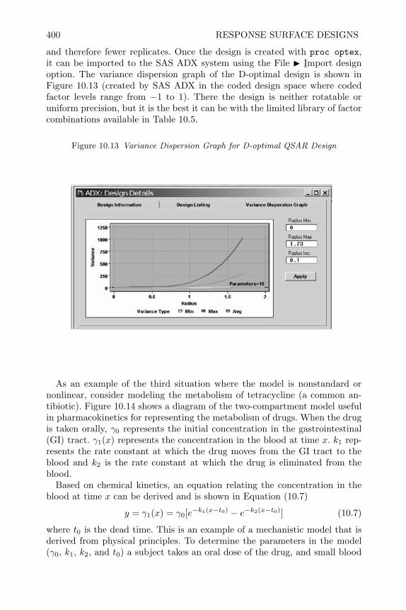
400 RESPONSE SURFACE DESIGNS
and therefore fewer replicates. Once the design is created with proc optex,it can be imported to the SAS ADX system using the File I Import designoption. The variance dispersion graph of the D-optimal design is shown inFigure 10.13 (created by SAS ADX in the coded design space where codedfactor levels range from −1 to 1). There the design is neither rotatable oruniform precision, but it is the best it can be with the limited library of factorcombinations available in Table 10.5.
Figure 10.13 Variance Dispersion Graph for D-optimal QSAR Design
As an example of the third situation where the model is nonstandard ornonlinear, consider modeling the metabolism of tetracycline (a common an-tibiotic). Figure 10.14 shows a diagram of the two-compartment model usefulin pharmacokinetics for representing the metabolism of drugs. When the drugis taken orally, γ0 represents the initial concentration in the gastrointestinal(GI) tract. γ1(x) represents the concentration in the blood at time x. k1 rep-resents the rate constant at which the drug moves from the GI tract to theblood and k2 is the rate constant at which the drug is eliminated from theblood.
Based on chemical kinetics, an equation relating the concentration in theblood at time x can be derived and is shown in Equation (10.7)
y = γ1(x) = γ0[e−k1(x−t0) − e−k2(x−t0)] (10.7)
where t0 is the dead time. This is an example of a mechanistic model that isderived from physical principles. To determine the parameters in the model(γ0, k1, k2, and t0) a subject takes an oral dose of the drug, and small blood
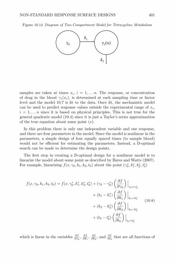
NON-STANDARD RESPONSE SURFACE DESIGNS 401
Figure 10.14 Diagram of Two-Compartment Model for Tetracycline Metabolism
γ0 γ1(x)k1
k2
samples are taken at times xi, i = 1, . . . n. The response, or concentrationof drug in the blood γ1(xi), is determined at each sampling time or factorlevel and the model 10.7 is fit to the data. Once fit, the mechanistic modelcan be used to predict response values outside the experimental range of xi,i = 1, . . . n since it is based on physical principles. This is not true for thegeneral quadratic model (10.4) since it is just a Taylor’s series approximationof the true equation about some point (x).
In this problem there is only one independent variable and one response,and there are four parameters in the model. Since the model is nonlinear in theparameters, a simple design of four equally spaced times (to sample blood)would not be efficient for estimating the parameters. Instead, a D-optimalsearch can be made to determine the design points.
The first step in creating a D-optimal design for a nonlinear model is tolinearize the model about some point as described by Bates and Watts (2007).For example, linearizing f(x, γ0, k1, k2, t0) about the point (γ∗0 , k
∗1 , k∗2 , t∗0)
f(x, γ0, k1, k2, t0) = f(x, γ∗0 , k∗1 , k∗2 , t∗0) + (γ0 − γ∗0 )
(∂f
∂γ0
) ∣∣∣γ0=γ∗0
+ (k1 − k∗1)(∂f
∂k1
) ∣∣∣k1=k∗1
+ (k2 − k∗2)(∂f
∂k2
) ∣∣∣k2=k∗2
+ (t0 − t∗0)(∂f
∂t0
) ∣∣∣t0=t∗0
(10.8)
which is linear in the variables ∂f∂γ0
, ∂f∂k1
, ∂f∂k2
, and ∂f∂t0
that are all functions of

402 RESPONSE SURFACE DESIGNS
x. For the compartment model in Equation (10.7)
∂f
∂γ0= e−k1(x−t0) − e−k2(x−t0)
∂f
∂k1= −γ0(x− t0)e−k1(x−t0)
∂f
∂k2= −γ0(x− t0)e−k2(x−t0)
∂f
∂t0= γ0k1e
−k1(x−t0) − γ0k2e−k2(x−t0)
The strategy is to create a grid of candidates in the independent variable x,calculate the values of the four partial derivatives using initial guesses of theparameter values at each candidate point, and then use proc optex to selecta D-optimal subset of the grid. In the SAS code below the initial parameterestimates γ0
0 = 2.65, k01 = .15, k0
2 = .72 and t00 = 0.41 were used.
*Create a candidate grid in partial derivatives;data grid;
k1=.15; k2=.72; gamma0 =2.65; t0=.41;do x=1 to 25 by 1;dfdk1=-gamma0*exp(-k1*(x-t0))*(x-t0);dfdk2=gamma0*exp(-k2*(x-t0))*(x-t0);dfdgamma0=exp(-k1*(x-t0))-exp(-k2*(x-t0));dfdt0=gamma0*exp(-k1*(x-t0))*k1-gamma0*exp(-k2*(x-t0))*k2;output;
end;*Create D-optimal p point Design;proc optex data=grid coding=orth;
model dfdk1 dfdk2 dfdgamma0 dfdt0/noint;generate n=4;id x;output out=desnl; run;
proc print data=desnl; run;
Since there are p = 4 parameters in the model, proc optex will always gen-erate at most p = 4 distinct design points, therefore the option n=4 is usedon the generate statement to eliminate any replicates in the file desnl. Anexperimenter can then replicate each design point as many times as necessaryto get an estimate of experimental error. The code above results in the fourdistinct times for taking blood samples (1, 2, 5 and 13), and due to the formof the model and initial guesses of the parameters these points are far fromequally spaced.
As stated by Bates and Watts (2007), the efficiency of the design for thenonlinear model will depend on the stage at which a researcher is in theinvestigation. If the form of the equation is known but not the parametervalues, the design created by proc optex will be called an initial design. After
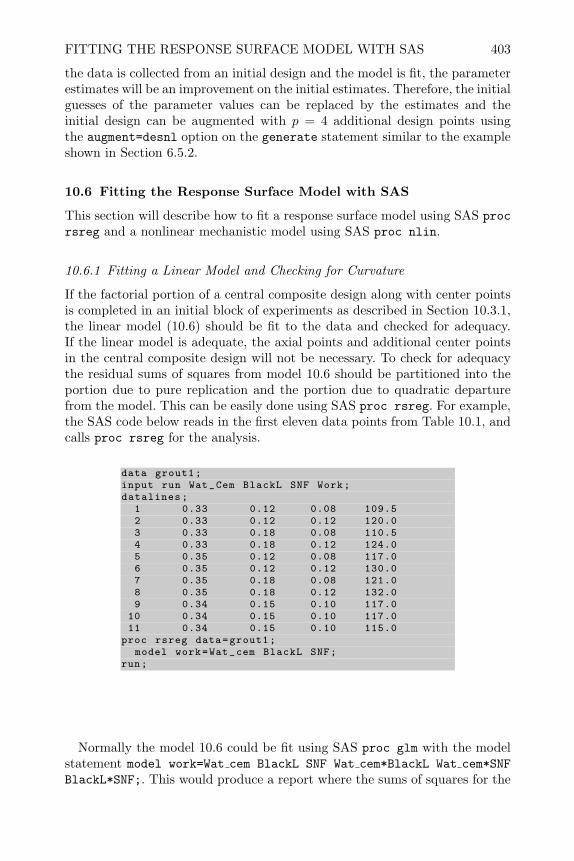
FITTING THE RESPONSE SURFACE MODEL WITH SAS 403
the data is collected from an initial design and the model is fit, the parameterestimates will be an improvement on the initial estimates. Therefore, the initialguesses of the parameter values can be replaced by the estimates and theinitial design can be augmented with p = 4 additional design points usingthe augment=desnl option on the generate statement similar to the exampleshown in Section 6.5.2.
10.6 Fitting the Response Surface Model with SAS
This section will describe how to fit a response surface model using SAS procrsreg and a nonlinear mechanistic model using SAS proc nlin.
10.6.1 Fitting a Linear Model and Checking for Curvature
If the factorial portion of a central composite design along with center pointsis completed in an initial block of experiments as described in Section 10.3.1,the linear model (10.6) should be fit to the data and checked for adequacy.If the linear model is adequate, the axial points and additional center pointsin the central composite design will not be necessary. To check for adequacythe residual sums of squares from model 10.6 should be partitioned into theportion due to pure replication and the portion due to quadratic departurefrom the model. This can be easily done using SAS proc rsreg. For example,the SAS code below reads in the first eleven data points from Table 10.1, andcalls proc rsreg for the analysis.
data grout1;input run Wat_Cem BlackL SNF Work;datalines;
1 0.33 0.12 0.08 109.52 0.33 0.12 0.12 120.03 0.33 0.18 0.08 110.54 0.33 0.18 0.12 124.05 0.35 0.12 0.08 117.06 0.35 0.12 0.12 130.07 0.35 0.18 0.08 121.08 0.35 0.18 0.12 132.09 0.34 0.15 0.10 117.0
10 0.34 0.15 0.10 117.011 0.34 0.15 0.10 115.0
proc rsreg data=grout1;model work=Wat_cem BlackL SNF;
run;
Normally the model 10.6 could be fit using SAS proc glm with the modelstatement model work=Wat cem BlackL SNF Wat cem*BlackL Wat cem*SNFBlackL*SNF;. This would produce a report where the sums of squares for the
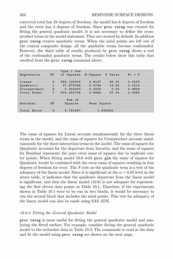
404 RESPONSE SURFACE DESIGNS
corrected total has 10 degrees of freedom, the model has 6 degrees of freedomand the error has 4 degrees of freedom. Since proc rsreg was created forfitting the general quadratic model, it is not necessary to define the cross-product terms in the model statement. They are created by default. In additionproc rsreg creates quadratic terms. When the axial points are left out ofthe central composite design, all the quadratic terms become confounded.However, the third table of results produced by proc rsreg shows a testof the confounded quadratic terms. The results below show this table thatresulted from the proc rsreg command above.
Type I SumRegression DF of Squares R-Square F Value Pr > F
Linear 3 465.125000 0.9137 80.31 0.0023Quadratic 1 37.878788 0.0744 19.62 0.0214Crossproduct 3 0.250000 0.0005 0.04 0.9859Total Model 7 503.253788 0.9886 37.24 0.0065
Sum ofResidual DF Squares Mean Square
Total Error 3 5.791667 1.930556
The sums of squares for Linear account simultaneously for the three linearterms in the model, and the sums of squares for Crossproduct account simul-taneously for the three interaction terms in the model. The sums of squares forQuadratic accounts for the departure from linearity, and the sums of squaresfor Residual represents the pure error sums of squares due to replicate cen-ter points. When fitting model 10.6 with proc glm the sums of squares forQuadratic would be combined with the error sums of squares resulting in fourdegrees of freedom for error. The F -test on the quadratic term is a test of theadequacy of the linear model. Since it is significant at the α = 0.05 level in theabove table, it indicates that the quadratic departure from the linear modelis significant, and thus the linear model (10.6) is not adequate for represent-ing the first eleven data points in Table 10.1. Therefore, if the experimentsshown in Table 10.1 were to be run in two blocks, it would be necessary torun the second block that includes the axial points. This test for adequacy ofthe linear model can also be made using SAS ADX.
10.6.2 Fitting the General Quadratic Model
proc rsreg is most useful for fitting the general quadratic model and ana-lyzing the fitted surface. For example, consider fitting the general quadraticmodel to the trebuchet data in Table 10.3. The commands to read in the dataand fit the model using proc rsreg are shown on the next page.
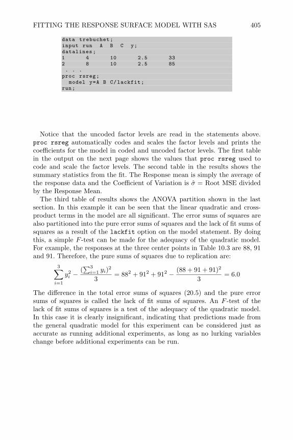
FITTING THE RESPONSE SURFACE MODEL WITH SAS 405
data trebuchet;input run A B C y;datalines;1 4 10 2.5 332 8 10 2.5 85. . .
proc rsreg;model y=A B C/lackfit;
run;
Notice that the uncoded factor levels are read in the statements above.proc rsreg automatically codes and scales the factor levels and prints thecoefficients for the model in coded and uncoded factor levels. The first tablein the output on the next page shows the values that proc rsreg used tocode and scale the factor levels. The second table in the results shows thesummary statistics from the fit. The Response mean is simply the average ofthe response data and the Coefficient of Variation is σ = Root MSE dividedby the Response Mean.
The third table of results shows the ANOVA partition shown in the lastsection. In this example it can be seen that the linear quadratic and cross-product terms in the model are all significant. The error sums of squares arealso partitioned into the pure error sums of squares and the lack of fit sums ofsquares as a result of the lackfit option on the model statement. By doingthis, a simple F -test can be made for the adequacy of the quadratic model.For example, the responses at the three center points in Table 10.3 are 88, 91and 91. Therefore, the pure sums of squares due to replication are:
3∑i=1
y2i −
(∑3i=1 yi)
2
3= 882 + 912 + 912 − (88 + 91 + 91)2
3= 6.0
The difference in the total error sums of squares (20.5) and the pure errorsums of squares is called the lack of fit sums of squares. An F -test of thelack of fit sums of squares is a test of the adequacy of the quadratic model.In this case it is clearly insignificant, indicating that predictions made fromthe general quadratic model for this experiment can be considered just asaccurate as running additional experiments, as long as no lurking variableschange before additional experiments can be run.
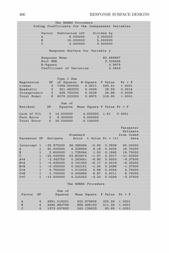
406 RESPONSE SURFACE DESIGNS
The RSREG ProcedureCoding Coefficients for the Independent Variables
Factor Subtracted off Divided byA 6.000000 2.000000B 15.000000 5.000000C 2.500000 0.500000
Response Surface for Variable y
Response Mean 82.466667Root MSE 2.024846R-Square 0.9975Coefficient of Variation 2.4554
Type I SumRegression DF of Squares R-Square F Value Pr > FLinear 3 7299.000000 0.9011 593.41 <.0001Quadratic 3 351.483333 0.0434 28.58 0.0014Crossproduct 3 428.750000 0.0529 34.86 0.0009Total Model 9 8079.233333 0.9975 218.95 <.0001
Sum ofResidual DF Squares Mean Square F Value Pr > F
Lack of Fit 3 14.500000 4.833333 1.61 0.4051Pure Error 2 6.000000 3.000000Total Error 5 20.500000 4.100000
ParameterEstimate
Standard from CodedParameter DF Estimate Error t Value Pr > |t| Data
Intercept 1 -35.875000 38.386494 -0.93 0.3929 90.00000A 1 35.500000 4.339859 8.18 0.0004 19.75000B 1 2.600000 1.735944 1.50 0.1945 19.75000C 1 -24.500000 22.803874 -1.07 0.3317 -11.50000A*A 1 -2.343750 0.263441 -8.90 0.0003 -9.37500B*A 1 -0.625000 0.101242 -6.17 0.0016 -6.25000B*B 1 -0.055000 0.042151 -1.30 0.2488 -1.37500C*A 1 4.750000 1.012423 4.69 0.0054 4.75000C*B 1 2.700000 0.404969 6.67 0.0011 6.75000C*C 1 -13.500000 4.215052 -3.20 0.0239 -3.37500
The RSREG Procedure
Sum ofFactor DF Squares Mean Square F Value Pr > F
A 4 3691.519231 922.879808 225.09 <.0001B 4 3465.980769 866.495192 211.34 <.0001C 4 1372.557692 343.139423 83.69 <.0001

FITTING THE RESPONSE SURFACE MODEL WITH SAS 407
When the lack of fit test is significant, it indicates that the general quadraticmodel is not adequate for prediction. This could be due to the fact that theexperimental region is so large that the quadratic model does not provide agood approximation to the true response function over the entire region, ordue to outliers, or extreme nonlinearity in certain corners of the experimentalregion where the approximate function does not fit. These conditions can bedetected by making residual plots to check the least squares assumptions or byfitting the model using a “robust” technique such as M-estimators, for detailsand discussion see Lawson (1982).
The fourth table shows the estimates of individual coefficients in the generalquadratic model along with their standard errors, t-values, and P-values. Theestimated coefficients for the model fit to the uncoded factor levels are shownin the third column and the coefficients for the model fit to the coded factorlevels are shown in the last column. Some statisticians advocate dropping theinsignificant terms from the model and refitting, but this is not possible withproc rsreg. Other statisticians advocate retaining all terms in the generalquadratic model, whether significant or not, since the individual model termshave no physical meaning. A compromise is to eliminate a model factor ifall linear, quadratic and interaction terms involving that factor are insignif-icant. By eliminating a factor the response surface model is reduced from pdimensions to p− 1 dimensions.proc rsreg automatically performs a test on the factors as shown in the
fifth table in the output. Each term has 4 degrees of freedom representing thelinear quadratic and interaction term involving each factor. All the factorsin this model are seen to be significant. If any factor had been found to beinsignificant, it could be eliminated from the proc rsreg model statementand the response surface equation would simplify from three dimensions totwo.
Block terms can also be included in the proc rsreg model statement. If, forexample, the experiments on cement grout shown in Table 10.1 were completedin two blocks, where the first block consisted of the factorial plus center pointsshown in runs 1-11 and the second block consisted of the axial and centerpoints shown in runs 12-20. The commands to read the data and fit the modelare shown at the top of the next page.
The block term is entered first in the model, and the covar=1 option onthe model statement tells proc rsreg not to create square and interactionterms for the first term in the model. The block factor will then account forany average differences between the first and second group of experiments.
If the response surface design is created in SAS ADX or imported to SASADX, the general quadratic model can also be fit using the point and clickinterface. ADX provides the table of model coefficients and standard errorsand by clicking on the Model I Fit Details, after fitting the model ADXautomatically creates a table showing the lack of fit test. However, ADX does

408 RESPONSE SURFACE DESIGNS
not provide a table partitioning the sums of squares to test each factor asproc rsreg does.
data grout2;input run block Wat_Cem BlackL SNF Work;datalines;
1 1 0.33 0.12 0.08 109.5. . .
11 1 0.34 0.15 0.10 115.012 2 0.32318 0.15000 0.10000 109.513 2 0.35682 0.15000 0.10000 132.0
. . .20 2 0.34000 0.15000 0.10000 117.0
proc rsreg data=grout2;model work=block Wat_cem BlackL SNF/covar =1;
run;
10.6.3 Fitting a Nonlinear Mechanistic Model
The general quadratic model is linear in the coefficients (β’s), and the X′Xis full rank so the least square estimates are obtained by solving the normalequations through straightforward matrix inversion. When the model is non-linear like the two-compartment model shown in Equation (10.7), the leastsquares estimates are more difficult to obtain and must be found by iterativenumerical techniques. However, SAS proc nlin makes this all transparent tothe user. For example, to fit the two-compartment model to the data fromWagner (1967) shown in Table 10.6, use the following commands.
data Tetracycline;input x conc;datalines;1 .7. . .
16 .3proc nlin data=Tetracycline best =5;
parms k1 =.05 to .25 by .05k2 =.25 to .75 by .05gamma0 = 0 to 20 by 5t0 = 0 to 1 by .25;
model conc=gamma0*(exp(-k1*(x-t0))-exp(-k2*(x-t0)));output out=results p=pconc;
proc print data=results; run;
The parms statement specifies a range of initial guesses for the parametervalues. proc nlin begins by making a grid search over this space of guesses
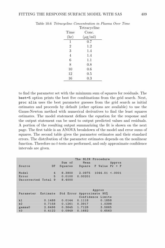
FITTING THE RESPONSE SURFACE MODEL WITH SAS 409
Table 10.6 Tetracycline Concentration in Plasma Over TimeTetracycline
Time Conc.(hr) (µg/ml)
1 0.72 1.23 1.44 1.46 1.18 0.810 0.612 0.516 0.3
to find the parameter set with the minimum sum of squares for residuals. Thebest=5 option prints the best five combinations from the grid search. Next,proc nlin uses the best parameter guesses from the grid search as initialestimates and proceeds by default (other options are available) to use theGauss-Newton method with numerical derivatives to find the least squaresestimates. The model statement defines the equation for the response andthe output statement can be used to output predicted values and residuals.A portion of the resulting output summarizing the fit is shown on the nextpage. The first table is an ANOVA breakdown of the model and error sums ofsquares. The second table gives the parameter estimates and their standarderrors. The distribution of the parameter estimates depends on the nonlinearfunction. Therefore no t-tests are performed, and only approximate confidenceintervals are given.
The NLIN ProcedureSum of Mean Approx
Source DF Squares Square F Value Pr > F
Model 4 8.3900 2.0975 1044.01 <.0001Error 5 0.0100 0.00201Uncorrected Total 9 8.4000
ApproxParameter Estimate Std Error Approximate 95%
Confidence Limitsk1 0.1488 0.0144 0.1118 0.1858k2 0.7158 0.1261 0.3917 1.0398gamma0 2.6496 0.3645 1.7128 3.5865t0 0.4122 0.0949 0.1682 0.6563
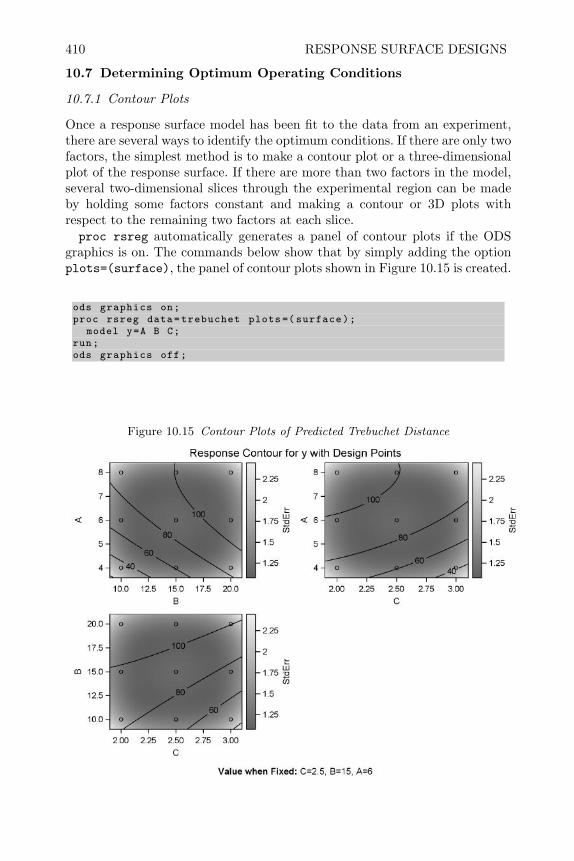
410 RESPONSE SURFACE DESIGNS
10.7 Determining Optimum Operating Conditions
10.7.1 Contour Plots
Once a response surface model has been fit to the data from an experiment,there are several ways to identify the optimum conditions. If there are only twofactors, the simplest method is to make a contour plot or a three-dimensionalplot of the response surface. If there are more than two factors in the model,several two-dimensional slices through the experimental region can be madeby holding some factors constant and making a contour or 3D plots withrespect to the remaining two factors at each slice.proc rsreg automatically generates a panel of contour plots if the ODS
graphics is on. The commands below show that by simply adding the optionplots=(surface), the panel of contour plots shown in Figure 10.15 is created.
ods graphics on;proc rsreg data=trebuchet plots=( surface);
model y=A B C;run;ods graphics off;
Figure 10.15 Contour Plots of Predicted Trebuchet Distance
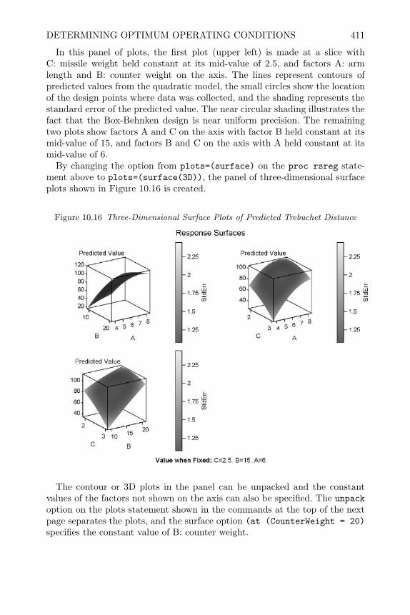
DETERMINING OPTIMUM OPERATING CONDITIONS 411
In this panel of plots, the first plot (upper left) is made at a slice withC: missile weight held constant at its mid-value of 2.5, and factors A: armlength and B: counter weight on the axis. The lines represent contours ofpredicted values from the quadratic model, the small circles show the locationof the design points where data was collected, and the shading represents thestandard error of the predicted value. The near circular shading illustrates thefact that the Box-Behnken design is near uniform precision. The remainingtwo plots show factors A and C on the axis with factor B held constant at itsmid-value of 15, and factors B and C on the axis with A held constant at itsmid-value of 6.
By changing the option from plots=(surface) on the proc rsreg state-ment above to plots=(surface(3D)), the panel of three-dimensional surfaceplots shown in Figure 10.16 is created.
Figure 10.16 Three-Dimensional Surface Plots of Predicted Trebuchet Distance
The contour or 3D plots in the panel can be unpacked and the constantvalues of the factors not shown on the axis can also be specified. The unpackoption on the plots statement shown in the commands at the top of the nextpage separates the plots, and the surface option (at (CounterWeight = 20)specifies the constant value of B: counter weight.

412 RESPONSE SURFACE DESIGNS
data decrip; set trebuchet;rename y=Distance A=ArmLength B=CounterWeight C=MissileWeight ;proc print; run;ods graphics on/imagefmt=png border=off;ods listing style=journal2 image_dpi =250;proc rsreg data=decrip plots(unpack)=( surface (at (
CounterWeight = 20)));model Distance=ArmLength CounterWeight MissileWeight;
run;ods graphics off;
The resulting contour plot at a slice with B: counterweight = 20lbs. is shownin Figure 10.17. In this plot it can be seen that with a counterweight of 20lbs.,the predicted maximum distance will be achieved using a missile weight ofabout 2.375 ounces and an arm length of about 7.5 inches. The predicteddistance at these conditions is about 115 feet, with a standard error of about1.5 feet.
Figure 10.17 Contour Plot of Predicted Trebuchet Distance with Counter-weight=20lbs.
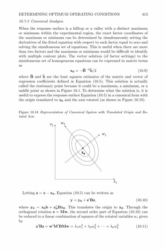
DETERMINING OPTIMUM OPERATING CONDITIONS 413
10.7.2 Canonical Analysis
When the response surface is a hilltop or a valley with a distinct maximumor minimum within the experimental region, the exact factor coordinates ofthe maximum or minimum can be determined by simultaneously setting thederivatives of the fitted equation with respect to each factor equal to zero andsolving the simultaneous set of equations. This is useful when there are morethan two factors and the maximum or minimum would be difficult to identifywith multiple contour plots. The vector solution (of factor settings) to thesimultaneous set of homogeneous equations can be expressed in matrix termsas
x0 = −B−1b/2 (10.9)
where B and b are the least squares estimates of the matrix and vector ofregression coefficients defined in Equation (10.5). This solution is actuallycalled the stationary point because it could be a maximum, a minimum, or asaddle point as shown in Figure 10.1. To determine what the solution is, it isuseful to express the response surface Equation (10.5) in a canonical form withthe origin translated to x0 and the axis rotated (as shown in Figure 10.18).
Figure 10.18 Representation of Canonical System with Translated Origin and Ro-tated Axis
x1
x2
w1
w2
x0
Letting z = x− x0, Equation (10.5) can be written as
y = y0 + z′Bz, (10.10)
where y0 = x0b + x′0Bx0. This translates the origin to x0. Through theorthogonal rotation z = Mw, the second order part of Equation (10.10) canbe reduced to a linear combination of squares of the rotated variables wi givenby
z′Bz = w′M′BMw = λ1w21 + λ2w
22 + · · ·+ λkw
2k (10.11)
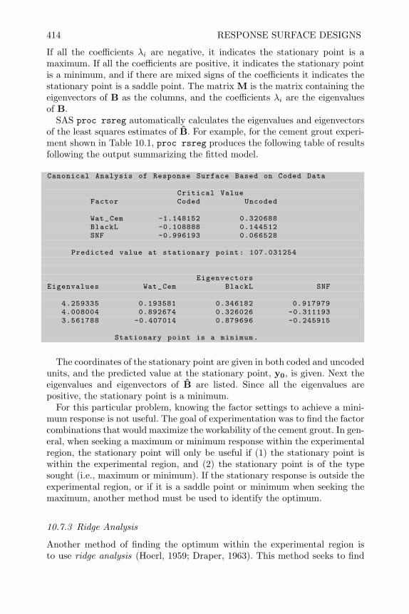
414 RESPONSE SURFACE DESIGNS
If all the coefficients λi are negative, it indicates the stationary point is amaximum. If all the coefficients are positive, it indicates the stationary pointis a minimum, and if there are mixed signs of the coefficients it indicates thestationary point is a saddle point. The matrix M is the matrix containing theeigenvectors of B as the columns, and the coefficients λi are the eigenvaluesof B.
SAS proc rsreg automatically calculates the eigenvalues and eigenvectorsof the least squares estimates of B. For example, for the cement grout experi-ment shown in Table 10.1, proc rsreg produces the following table of resultsfollowing the output summarizing the fitted model.
Canonical Analysis of Response Surface Based on Coded Data
Critical ValueFactor Coded Uncoded
Wat_Cem -1.148152 0.320688BlackL -0.108888 0.144512SNF -0.996193 0.066528
Predicted value at stationary point: 107.031254
EigenvectorsEigenvalues Wat_Cem BlackL SNF
4.259335 0.193581 0.346182 0.9179794.008004 0.892674 0.326026 -0.3111933.561788 -0.407014 0.879696 -0.245915
Stationary point is a minimum.
The coordinates of the stationary point are given in both coded and uncodedunits, and the predicted value at the stationary point, y0, is given. Next theeigenvalues and eigenvectors of B are listed. Since all the eigenvalues arepositive, the stationary point is a minimum.
For this particular problem, knowing the factor settings to achieve a mini-mum response is not useful. The goal of experimentation was to find the factorcombinations that would maximize the workability of the cement grout. In gen-eral, when seeking a maximum or minimum response within the experimentalregion, the stationary point will only be useful if (1) the stationary point iswithin the experimental region, and (2) the stationary point is of the typesought (i.e., maximum or minimum). If the stationary response is outside theexperimental region, or if it is a saddle point or minimum when seeking themaximum, another method must be used to identify the optimum.
10.7.3 Ridge Analysis
Another method of finding the optimum within the experimental region isto use ridge analysis (Hoerl, 1959; Draper, 1963). This method seeks to find
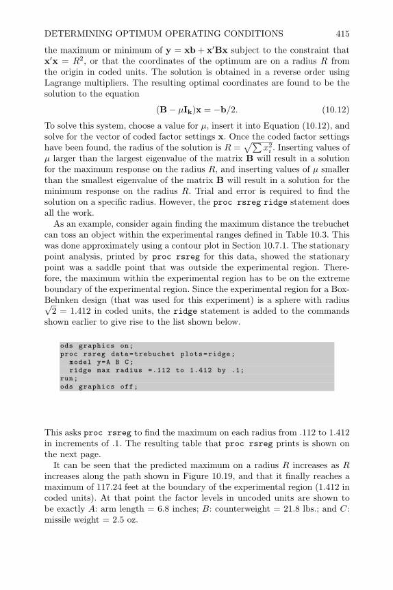
DETERMINING OPTIMUM OPERATING CONDITIONS 415
the maximum or minimum of y = xb + x′Bx subject to the constraint thatx′x = R2, or that the coordinates of the optimum are on a radius R fromthe origin in coded units. The solution is obtained in a reverse order usingLagrange multipliers. The resulting optimal coordinates are found to be thesolution to the equation
(B− µIk)x = −b/2. (10.12)
To solve this system, choose a value for µ, insert it into Equation (10.12), andsolve for the vector of coded factor settings x. Once the coded factor settingshave been found, the radius of the solution is R =
√∑x2i . Inserting values of
µ larger than the largest eigenvalue of the matrix B will result in a solutionfor the maximum response on the radius R, and inserting values of µ smallerthan the smallest eigenvalue of the matrix B will result in a solution for theminimum response on the radius R. Trial and error is required to find thesolution on a specific radius. However, the proc rsreg ridge statement doesall the work.
As an example, consider again finding the maximum distance the trebuchetcan toss an object within the experimental ranges defined in Table 10.3. Thiswas done approximately using a contour plot in Section 10.7.1. The stationarypoint analysis, printed by proc rsreg for this data, showed the stationarypoint was a saddle point that was outside the experimental region. There-fore, the maximum within the experimental region has to be on the extremeboundary of the experimental region. Since the experimental region for a Box-Behnken design (that was used for this experiment) is a sphere with radius√
2 = 1.412 in coded units, the ridge statement is added to the commandsshown earlier to give rise to the list shown below.
ods graphics on;proc rsreg data=trebuchet plots=ridge;
model y=A B C;ridge max radius =.112 to 1.412 by .1;
run;ods graphics off;
This asks proc rsreg to find the maximum on each radius from .112 to 1.412in increments of .1. The resulting table that proc rsreg prints is shown onthe next page.
It can be seen that the predicted maximum on a radius R increases as Rincreases along the path shown in Figure 10.19, and that it finally reaches amaximum of 117.24 feet at the boundary of the experimental region (1.412 incoded units). At that point the factor levels in uncoded units are shown tobe exactly A: arm length = 6.8 inches; B: counterweight = 21.8 lbs.; and C:missile weight = 2.5 oz.
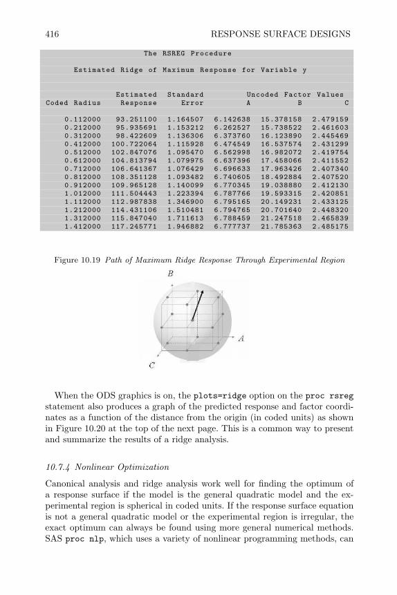
416 RESPONSE SURFACE DESIGNS
The RSREG Procedure
Estimated Ridge of Maximum Response for Variable y
Estimated Standard Uncoded Factor ValuesCoded Radius Response Error A B C
0.112000 93.251100 1.164507 6.142638 15.378158 2.4791590.212000 95.935691 1.153212 6.262527 15.738522 2.4616030.312000 98.422609 1.136306 6.373760 16.123890 2.4454690.412000 100.722064 1.115928 6.474549 16.537574 2.4312990.512000 102.847076 1.095470 6.562998 16.982072 2.4197540.612000 104.813794 1.079975 6.637396 17.458066 2.4115520.712000 106.641367 1.076429 6.696633 17.963426 2.4073400.812000 108.351128 1.093482 6.740605 18.492884 2.4075200.912000 109.965128 1.140099 6.770345 19.038880 2.4121301.012000 111.504443 1.223394 6.787766 19.593315 2.4208511.112000 112.987838 1.346900 6.795165 20.149231 2.4331251.212000 114.431106 1.510481 6.794765 20.701640 2.4483201.312000 115.847040 1.711613 6.788459 21.247518 2.4658391.412000 117.245771 1.946882 6.777737 21.785363 2.485175
Figure 10.19 Path of Maximum Ridge Response Through Experimental Region
When the ODS graphics is on, the plots=ridge option on the proc rsregstatement also produces a graph of the predicted response and factor coordi-nates as a function of the distance from the origin (in coded units) as shownin Figure 10.20 at the top of the next page. This is a common way to presentand summarize the results of a ridge analysis.
10.7.4 Nonlinear Optimization
Canonical analysis and ridge analysis work well for finding the optimum ofa response surface if the model is the general quadratic model and the ex-perimental region is spherical in coded units. If the response surface equationis not a general quadratic model or the experimental region is irregular, theexact optimum can always be found using more general numerical methods.SAS proc nlp, which uses a variety of nonlinear programming methods, can
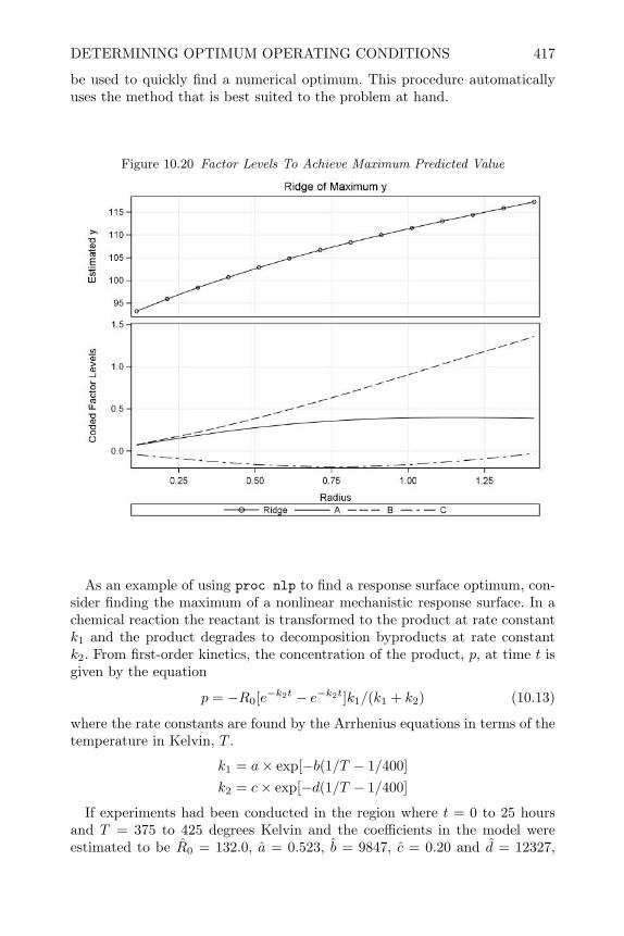
DETERMINING OPTIMUM OPERATING CONDITIONS 417
be used to quickly find a numerical optimum. This procedure automaticallyuses the method that is best suited to the problem at hand.
Figure 10.20 Factor Levels To Achieve Maximum Predicted Value
As an example of using proc nlp to find a response surface optimum, con-sider finding the maximum of a nonlinear mechanistic response surface. In achemical reaction the reactant is transformed to the product at rate constantk1 and the product degrades to decomposition byproducts at rate constantk2. From first-order kinetics, the concentration of the product, p, at time t isgiven by the equation
p = −R0[e−k2t − e−k2t]k1/(k1 + k2) (10.13)
where the rate constants are found by the Arrhenius equations in terms of thetemperature in Kelvin, T .
k1 = a× exp[−b(1/T − 1/400]k2 = c× exp[−d(1/T − 1/400]
If experiments had been conducted in the region where t = 0 to 25 hoursand T = 375 to 425 degrees Kelvin and the coefficients in the model wereestimated to be R0 = 132.0, a = 0.523, b = 9847, c = 0.20 and d = 12327,

418 RESPONSE SURFACE DESIGNS
then the proc nlp statements below can be used to find the maximum productconcentration. The parms statement gives starting values of the factors in thecenter of the experimental region. The bounds statement gives the bounds onthe experimental region.
proc nlp;max p;parms time Temp= 12.5 400;bounds 0 <= time <=25,
375 <=Temp <=425;k1=.523*exp( -9847*((1/Temp) -(1/400)));k2=.2*exp ( -12327*((1/Temp) -(1/400)));p=-132*(exp(-k1*time)-exp(-k2*time))*k1/(k1-k2);
run;
The results show the maximum product concentration, p, within the exper-imental region is p = 82.88 at t = 18.16 hours and T = 375 degrees Kelvin.
Since this problem only has two factors (time and temperature) the resultscan be visualized in the contour plot shown in Figure 10.21 which displaysthe maximum at the boundary of the experimental region.
Figure 10.21 Maximum Product Concentration
Maximump=82.9
x
A rough approximation to numerical optimization can be made by doinga grid search. Create a fine grid of the experimental region in a SAS datastep and then evaluate the response surface function at each grid point to get
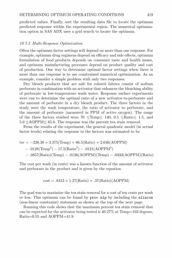
DETERMINING OPTIMUM OPERATING CONDITIONS 419
predicted values. Finally, sort the resulting data file to locate the optimumpredicted response within the experimental region. The numerical optimiza-tion option in SAS ADX uses a grid search to locate the optimum.
10.7.5 Multi-Response Optimization
Often the optimum factor settings will depend on more than one response. Forexample, optimum drug regimens depend on efficacy and side effects, optimumformulation of food products depends on consumer taste and health issues,and optimum manufacturing processes depend on product quality and costof production. One way to determine optimal factor settings when there ismore than one response is to use constrained numerical optimization. As anexample, consider a simple problem with only two responses.
Dry bleach products that are safe for colored fabrics consist of sodiumperborate in combination with an activator that enhances the bleaching abilityof perborate in low-temperature wash water. Response surface experimentswere run to determine the optimal ratio of a new activator-to-perborate andthe amount of perborate in a dry bleach product. The three factors in thestudy were the wash temperature, the ratio of activator to perborate, andthe amount of perborate (measured in PPM of active oxygen). The rangeof the three factors studied were 70 ≤Temp≤ 140, 0.5 ≤Ratio≤ 1.5, and5.0 ≤AOPPM≤ 65.0. The response was the percent tea stain removal.
From the results of the experiment, the general quadratic model (in actualfactor levels) relating the response to the factors was estimated to be
tsr = −226.38 + 3.375(Temp) + 86.5(Ratio) + 2.646(AOPPM)
− .0128(Temp2)− 17.5(Ratio2)− .0121(AOPPM2)− .3857(Ratio)(Temp)− .0126(AOPPM)(Temp)− .0333(AOPPM)(Ratio)
The cost per wash (in cents) was a known function of the amount of activatorand perborate in the product and is given by the equation
cost = .8313 + 1.27(Ratio) + .37(Ratio)(AOPPM)
The goal was to maximize the tea stain removal for a cost of ten cents per washor less. This optimum can be found by proc nlp by including the nlincon(non-linear constraint) statement as shown at the top of the next page.
Running this code shows that the maximum percent tea stain removal thatcan be expected for the activator being tested is 40.27% at Temp=103 degrees,Ratio=0.55 and AOPPM=41.9.
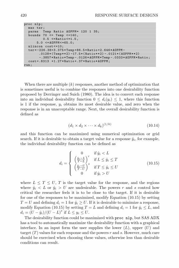
420 RESPONSE SURFACE DESIGNS
proc nlp;max tsr;parms Temp Ratio AOPPM= 120 1 35;bounds 70 <= Temp <=140,
0.5 <=Ratio <=1.5,5.0 <=AOPPM <=65.0;
nlincon cost<=10;tsr = -226.38+3.375*Temp +86.5*Ratio +2.646*AOPPM -
.0128*(Temp**2) -17.5*(Ratio**2) -.0121*(AOPPM**2)-.3857*Ratio*Temp -.0126*AOPPM*Temp -.0333*AOPPM*Ratio;
cost =.8313 +1.27*Ratio +.37*Ratio*AOPPM;run;
When there are multiple (k) responses, another method of optimization thatis sometimes useful is to combine the responses into one desirability functionproposed by Derringer and Suich (1980). The idea is to convert each responseinto an individual desirability function 0 ≤ di(yi) ≤ 1, where this functionis 1 if the response, yi obtains its most desirable value, and zero when theresponse is in an unacceptable range. Next, the overall desirability function isdefined as
(d1 × d2 × · · · × dk)(1/k) (10.14)
and this function can be maximized using numerical optimization or gridsearch. If it is desirable to obtain a target value for a response yi, for example,the individual desirability function can be defined as
di =
0 if yi < L(
yi−LT−L
)rif L ≤ yi ≤ T(
yi−UT−U
)sif T ≤ yi ≤ U
0 if yi > U
(10.15)
where L ≤ T ≤ U , T is the target value for the response, and the regionswhere yi < L or yi > U are undesirable. The powers r and s control howcritical the researcher feels it is to be close to the target. If it is desirablefor one of the responses to be maximized, modify Equation (10.15) by settingT = U and defining di = 1 for yi ≥ U . If it is desirable to minimize a response,modify Equation (10.15) by setting T = L and defining di = 1 for yi ≤ L, anddi = (U − yi)/(U − L)s if L ≤ yi ≤ U .
The desirability function could be maximized with proc nlp, but SAS ADXhas a tool to automatically maximize the desirability function with a graphicalinterface. In an input form the user supplies the lower (L), upper (U) andtarget (T ) values for each response and the powers r and s. However, much careshould be exercised when choosing these values, otherwise less than desirableconditions can result.

BLOCKED RESPONSE SURFACE (BRS) DESIGNS 421
10.8 Blocked Response Surface (BRS) Designs
When experimental units are not homogeneous, it is always advantageous togroup them into more homogeneous blocks and use a blocked experimentaldesign. Earlier it was mentioned that the three-factor central composite de-signs could be run in two blocks; the factorial portion plus three center pointsin one block, and the axial portion and remaining center points in the otherblock. This is actually an example of an incomplete block design, like thosedescribed in Chapter 7, since not all the treatment combinations are repre-sented in each block. It is possible to create an incomplete block design outof any response surface design so that the coefficients can be estimated moreprecisely.
Standard response surface designs such as the central composite designs(CCDs) and Box-Behnken designs (BBDs) have been blocked in a way thatthe blocks are orthogonal to the coded factor levels, squares of coded factorlevels, and interactions among coded factor levels. In this way the least squaresestimates of the parameters of the general quadratic model are not correlatedwith the block effects and these standard designs are 100% Ds efficient asdescribed in Section 7.8.1. The example described earlier, where the three-factor central composite design was blocked into two blocks with block sizes11 and 9, is not 100% Ds efficient. In order to achieve 100% efficiency, someadditional restrictions must be made in terms of the number of blocks, theblock sizes, and the axial radius. This will affect the distribution of the varianceof a predicted value over the design region, and a compromise must be made.Table 10.7 shows the number of blocks and block sizes for orthogonally blockedCCDs and BBDs with k = 2 to 5 factors.
Table 10.7 Number of Blocks and Block Sizes for Orthogonally Blocked CCD andBBD Designs
Number CCD BBDFactors No. Blocks Block Sizes No. Blocks Block Sizes
2 2 7,73 3 6, 6, 84 3 10, 10, 10 3 9, 9, 95 2 22, 11 2 23, 23
These designs can be created easily with the SAS ADX tool. It will automati-cally use the optimal block size and axial radius. To create a blocked response

422 RESPONSE SURFACE DESIGNS
surface design, check the Blocking box on the ADX Select Design Template,as shown in Figure 10.22, and you will see the blocked designs available.
Figure 10.22 Design Selection Template with Blocking Box Checked
The number of blocks and block sizes available for orthogonally blockedCCD and BBD designs may be too restrictive for some applications. For ex-ample, Gilmour and Trinca (2000) presented the data from an experiment todetermine how the characteristics of pastry dough depended upon parametersof the mixing process. In the experiment three factors were varied, the feedflow rate (FR), the initial moisture content (MC) and the screw speed (SS).One of the responses (y) measured light reflectance of the resulting dough inparticular bands of the spectrum in order to see how the color of the doughwas affected by the mixing parameters. Only four runs or experiments could beconducted on one day and the experimenters anticipated day to day variation.None of the designs in Table 10.7 have blocks of size four. Thus the experi-menters ran the modified design shown in Table 10.8, with the coded factorvalues x1 = (FR− 37.5)/7.5, x2 = (MC − 21)/3, and x3 = (SS − 350)/50.
This is an example of a face-centered cube design that is a special case of acentral composite design with the axial points (in coded units) pulled in to theface of the cube at ±1. The 23 factorial portion of this design was replicatedand there were six center points. The twenty-eight runs of this design wereblocked into seven blocks (days) of four runs in a way that the main effects areorthogonal to the blocks. However, as Goos (2002) pointed out, the quadraticand interaction terms of the general quadratic model are not orthogonal toblocks and a better way of blocking the twenty-eight experiments design canbe achieved using a Ds optimal design. This can be done using proc optex.
First create the face centered cube design using the %adxccd macro as shownin the code below Table 10.8 on the next page. This macro creates all twenty-eight design points shown in Table 10.8 and stores them in the SAS file fccdwith the factors labeled t1, t2, and t3.

BLOCKED RESPONSE SURFACE (BRS) DESIGNS 423
Table 10.8 Design and Response for Pastry Dough ExperimentBlock x1 x2 x3 y
1 -1 -1 -1 12.921 -1 1 1 13.911 1 -1 1 11.661 1 1 -1 14.482 -1 -1 1 10.762 -1 1 -1 14.412 1 -1 -1 12.272 1 1 1 12.133 -1 1 -1 14.223 0 -1 0 12.353 1 0 0 13.53 0 0 1 12.544 1 -1 1 10.554 -1 0 0 13.334 0 1 0 13.844 0 0 -1 14.195 -1 -1 -1 11.465 1 1 1 11.325 0 0 0 11.935 0 0 0 11.636 -1 -1 1 12.26 1 1 -1 14.786 0 0 0 14.946 0 0 0 14.617 -1 1 1 12.177 1 -1 -1 11.287 0 0 0 11.857 0 0 0 11.64
%adxgen%adxff%adxcc%adxinit%adxccd(fccd ,3,16,6,1.0,1)
Next use proc optex to group the runs into seven blocks of four runs as shownon the next page. The noexchange option on the blocks statement tells procoptex to keep all the runs in the file fccd in the design and arrange theminto seven blocks of four in a way to maximize the Ds efficiency.
To create a blocked response surface design that is a subset of the possibleruns in a file of candidates, replace the file fccd in the commands above

424 RESPONSE SURFACE DESIGNS
proc optex data=fccd coding=orthcan seed =2347;model t1 t2 t3 t1*t1 t1*t2 t1*t3 t2*t2 t2*t3 t3*t3;blocks structure =(7)4 noexchange niter =1000 keep =10;generate n=28 augment=fccd;output out=bpastry blockname=block; run;
proc print data=bpastry;run;
by the file of candidates and remove the noexchange option of the blocksstatement. For example, to block the experiments in the QSAR example inSection 10.5 so that they could be run in five different labs (that may havediffering measurements of bio-activity) modify the code from Section 10.5 asshown below.
proc optex data=qsar; id Compound;model HE DMz SOK HE*HE DMz*DMz SOK*SOK HE*DMz HE*SOK DMz*SOK;blocks structure =(5)4;generate n=20 iter =200 keep =5;output out =desgn1 ;
proc print data=desgn1; run;
To analyze a blocked design with more than two blocks using proc rsreg,create dummy variables for the blocks as shown below for the pastry doughexperiment shown in Table 10.8.
data pastry;input Block x1 x2 x3 y;b1=( Block =1);b2=( Block =2);b2=( Block =2);b3=( Block =3);b4=( Block =4);b5=( Block =5);b6=( Block =6);b7=( Block =7);datalines;1 -1 -1 -1 12.92. . .
proc rsreg;model y1=b1-b6 x1 x2 x3/covar =6;
run;
10.9 Response Surface Split-Plot (RSSP) Designs
When response surface designs contain factors from different process stepsor some factors are hard to vary, it may be costly or inconvenient to com-pletely randomize the runs in a standard response surface design. For ex-

RESPONSE SURFACE SPLIT-PLOT (RSSP) DESIGNS 425
ample, consider a simple response surface design to identify the baking tem-perature and baking time that would result in the optimal moist cake. Thedesign and data are shown in Table 10.9 where x1 = (bake temp. − 350)/25,x2 = (bake time− 31.5)/4, and y is the reading from a moisture tester.
Table 10.9 Data for Cake Baking ExperimentOven run x1 x2 y
1 -1 -1 2.71 -1 1 2.51 -1 0 2.72 1 -1 2.92 1 1 1.32 1 0 2.23 0 -1 3.73 0 1 2.94 0 0 2.94 0 0 2.84 0 0 2.9
The design is a face-centered cube design with three levels for each factorand three center points. The experiments were not performed in a randomorder. Once the oven temperature was set and the oven was preheated, asmany as four cakes could be baked at once. Performing the experiments in acompletely random order would have required eleven oven runs, but by bakingas many as three cakes at the same time (as shown in the table) only fouroven runs were required. The oven runs were performed in a random orderwith the two or three cakes for each run placed in random positions in theoven. The cakes in each run were withdrawn from the oven at different bakingtimes except for oven run 4 when all cakes were baked for 31.5 minutes.
By running the experiments in this way, a response surface split-plot (RSSP)type design results , where x1, the baking temperature, is the whole-plot factorand x2, baking time, is the subplot factor. Since the same subplot treatmentcombinations are not run in each whole plot, Letsinger et al. (1996) show thatthe least squares estimates of the model parameters, which would be obtainedby proc rsreg, will be unsatisfactory if the ratio of the whole-plot to subploterror variances is greater than one. They recommend using REML estimators,which can be computed in proc mixed.
Combining the coefficients for the linear, quadratic, and interaction termsin the same vector, the general quadratic model for a completely randomizedresponse surface design can be written in matrix form as
y = Xβ + ε (10.16)
When the response surface design is run as a split plot, like the example in

426 RESPONSE SURFACE DESIGNS
Table 10.9, the general quadratic model can be written in the form
y = Xβ + ω + ε (10.17)
where β is the vector of regression coefficients for the whole-plot and subploteffects, ω is a vector of random whole-plot errors, and ε is a vector of randomsubplot errors. It is assumed that ω+ε has zero mean and variance covariancematrix given by Σ = σ2I + σ2
ωJ, where σ2ω and σ2 are the variances of the
whole-plot and subplot experimental units and
J =
111′1 0 . . . 0
0 121′2 . . . 0. . .
0 0 . . . 1m1′m
The length of 1i is ni the number of subplot runs within the ith whole
plot. The least squares estimates of β is (X′X)−1X′y, while the best linearunbiased estimate of β is
β = (X′Σ−1X)−1X′Σ−1y (10.18)and its variance covariance matrix is given by
V ar(β) = (X′Σ−1X)−1 (10.19)
σ2, σ2ω must be known in order to compute the best linear unbiased estimate
of β. However, estimates of σ2, σ2ω, and the large sample best linear unbiased
estimates that is found by substituting σ2, and σ2ω into Equation (10.18) can
be obtained using the REML method that was described in Chapter 5 and isavailable in proc mixed. The commands to fit the general quadratic model tothe data in Table 10.9 using proc mixed are shown below.
data CakeBake;input wp x1 x2 y;datalines;1 -1 -1 2.7. . .
proc mixed;class wp;model y=x1 x2 x1*x1 x2*x2 x1*x2/
solution;random wp;
run;
A comparison of the parameter estimates obtained by the least squaresmethod and REML is shown in Table 10.10. Here it can be seen that theestimated linear main effects are the same for both methods, but the standarderrors are much smaller for the subplot effect and larger for the whole-ploteffect using the more correct REML method. The other estimates differ andagain the tests for the subplot effects are more sensitive using REML and the
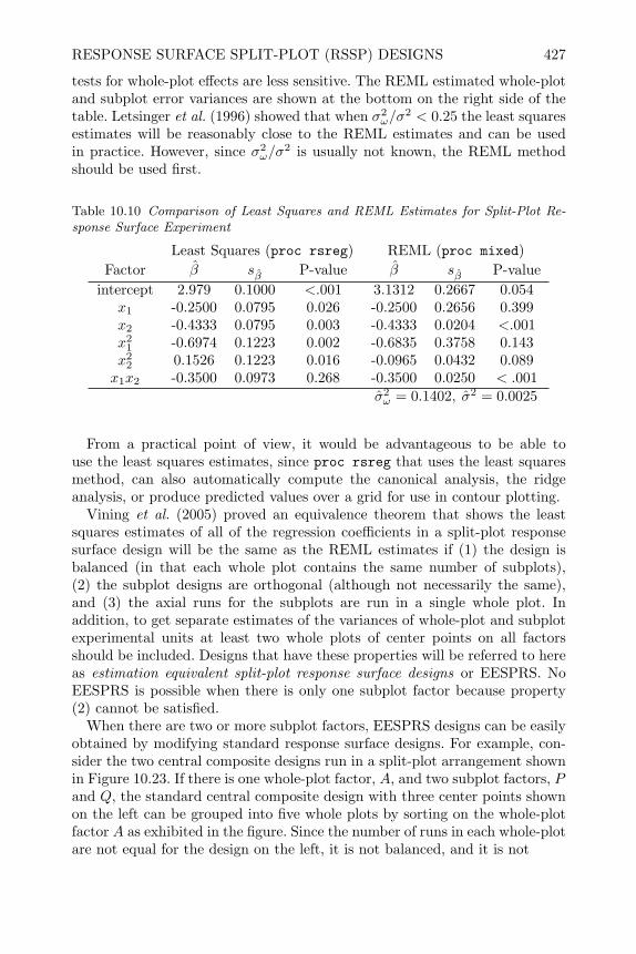
RESPONSE SURFACE SPLIT-PLOT (RSSP) DESIGNS 427
tests for whole-plot effects are less sensitive. The REML estimated whole-plotand subplot error variances are shown at the bottom on the right side of thetable. Letsinger et al. (1996) showed that when σ2
ω/σ2 < 0.25 the least squares
estimates will be reasonably close to the REML estimates and can be usedin practice. However, since σ2
ω/σ2 is usually not known, the REML method
should be used first.
Table 10.10 Comparison of Least Squares and REML Estimates for Split-Plot Re-sponse Surface Experiment
Least Squares (proc rsreg) REML (proc mixed)Factor β sβ P-value β sβ P-value
intercept 2.979 0.1000 <.001 3.1312 0.2667 0.054x1 -0.2500 0.0795 0.026 -0.2500 0.2656 0.399x2 -0.4333 0.0795 0.003 -0.4333 0.0204 <.001x2
1 -0.6974 0.1223 0.002 -0.6835 0.3758 0.143x2
2 0.1526 0.1223 0.016 -0.0965 0.0432 0.089x1x2 -0.3500 0.0973 0.268 -0.3500 0.0250 < .001
σ2ω = 0.1402, σ2 = 0.0025
From a practical point of view, it would be advantageous to be able touse the least squares estimates, since proc rsreg that uses the least squaresmethod, can also automatically compute the canonical analysis, the ridgeanalysis, or produce predicted values over a grid for use in contour plotting.
Vining et al. (2005) proved an equivalence theorem that shows the leastsquares estimates of all of the regression coefficients in a split-plot responsesurface design will be the same as the REML estimates if (1) the design isbalanced (in that each whole plot contains the same number of subplots),(2) the subplot designs are orthogonal (although not necessarily the same),and (3) the axial runs for the subplots are run in a single whole plot. Inaddition, to get separate estimates of the variances of whole-plot and subplotexperimental units at least two whole plots of center points on all factorsshould be included. Designs that have these properties will be referred to hereas estimation equivalent split-plot response surface designs or EESPRS. NoEESPRS is possible when there is only one subplot factor because property(2) cannot be satisfied.
When there are two or more subplot factors, EESPRS designs can be easilyobtained by modifying standard response surface designs. For example, con-sider the two central composite designs run in a split-plot arrangement shownin Figure 10.23. If there is one whole-plot factor, A, and two subplot factors, Pand Q, the standard central composite design with three center points shownon the left can be grouped into five whole plots by sorting on the whole-plotfactor A as exhibited in the figure. Since the number of runs in each whole-plotare not equal for the design on the left, it is not balanced, and it is not
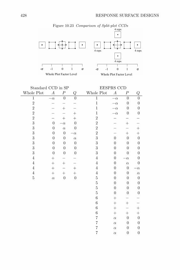
428 RESPONSE SURFACE DESIGNS
Figure 10.23 Comparison of Split-plot CCDs
- -1 0 1
Whole Plot Factor Level- -1 0 1
Whole Plot Factor Level
4 reps
4 reps4 reps
4 reps
Standard CCD in SP EESPRS CCDWhole Plot A P Q Whole Plot A P Q
1 −α 0 0 1 −α 0 02 − − − 1 −α 0 02 − + − 1 −α 0 02 − − + 1 −α 0 02 − + + 2 − − −3 0 −α 0 2 − + −3 0 α 0 2 − − +3 0 0 −α 2 − + +3 0 0 α 3 0 0 03 0 0 0 3 0 0 03 0 0 0 3 0 0 03 0 0 0 3 0 0 04 + − − 4 0 −α 04 + + − 4 0 α 04 + − + 4 0 0 −α4 + + + 4 0 0 α5 α 0 0 5 0 0 0
5 0 0 05 0 0 05 0 0 06 + − −6 + + −6 + − +6 + + +7 α 0 07 α 0 07 α 0 07 α 0 0

RESPONSE SURFACE SPLIT-PLOT (RSSP) DESIGNS 429
an EESPRS design. By removing the center point from the whole plot thathas the axial points for the subplot factors P and Q, adding replicates tothe whole plots that contain the axial points for the whole-plot factor A, andadding replicates in the whole plots that contain center points, the design onthe right becomes balanced. Since the columns for the two subplot factorsP and Q are orthogonal (i.e.,
∑i piqi = 0) within each whole plot, and all
the axial points for the subplot factors are in the same whole plot, this is anEESPRS design. Duplicate whole plots ( 3 & 5) containing all center pointsmake it possible to estimate σ2
ω and σ2 using the REML method in procmixed.
While the least squares and REML estimates of the regression coefficientsare the same when an EESPRS design is used, the standard errors of thecoefficients will not be the same, because the covariance matrix of the leastsquares estimates, σ2(X′X)−1, is not the same as the covariance of the REMLestimates (X′Σ−1X)−1. Therefore, if an EESPRS design is used, proc mixedshould be used to make hypothesis tests about the parameters (in order todetermine if the model can be simplified), but proc rsreg can be used fordoing a canonical analysis, ridge analysis or contour plots.
In a balanced EESPRS design, the number of whole plots is m and thenumber of subplots within each whole plot is n, making the total number ofruns N = nm. The number of factors is k = k1 + k2, where k1 is the numberof whole-plot factors and k2 is the number of subplot factors. In an estimationequivalence central composite design, the number of runs in each whole plotwill be 2 × k2, since one whole plot must contain all the axial runs for thesubplot factors. Table 10.11 on the next page shows some EESPRS designsthat can be constructed by modifying standard central composite designs.The designation k1(k2) in the first column refers to the number of whole andsubplot factors.
The design in the first row of Table 10.11 is the design in the right sideof Figure 10.22 that has one whole-plot factor and two subplot factors. Inthis design, the factorial portion (whole plots 2 and 6) has the four treatmentcombinations of a full 22 factorial in the subplot factors, randomized to the foursubplots. In other designs shown in Table 10.11, the subplots in the factorialportion of the design may contain a fractional factorial in the subplot factors,or a fractional factorial in the subplot factors augmented by two center pointsas indicated in the last column in the table.
Using Table 10.11 as a guide, these designs can be created easily in theSAS data step. The example code below Table 10.11 on the next page createsthe design in row four of the table which has two whole-plot factors and twosubplot factors in a non-random order. In this code each whole plot is createdin a separate data step, and all the whole plots are combined in the last datastep.
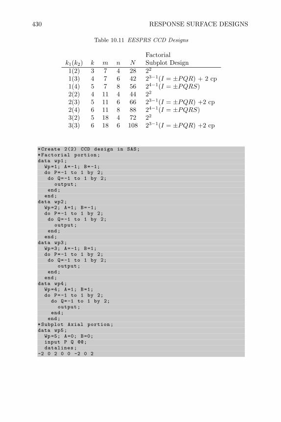
430 RESPONSE SURFACE DESIGNS
Table 10.11 EESPRS CCD Designs
Factorialk1(k2) k m n N Subplot Design1(2) 3 7 4 28 22
1(3) 4 7 6 42 23−1(I = ±PQR) + 2 cp1(4) 5 7 8 56 24−1(I = ±PQRS)2(2) 4 11 4 44 22
2(3) 5 11 6 66 23−1(I = ±PQR) +2 cp2(4) 6 11 8 88 24−1(I = ±PQRS)3(2) 5 18 4 72 22
3(3) 6 18 6 108 23−1(I = ±PQR) +2 cp
*Create 2(2) CCD design in SAS;*Factorial portion;data wp1;
Wp=1; A=-1; B=-1;do P=-1 to 1 by 2;do Q=-1 to 1 by 2;
output;end;
end;data wp2;
Wp=2; A=1; B=-1;do P=-1 to 1 by 2;do Q=-1 to 1 by 2;
output;end;
end;data wp3;
Wp=3; A=-1; B=1;do P=-1 to 1 by 2;do Q=-1 to 1 by 2;
output;end;
end;data wp4;
Wp=4; A=1; B=1;do P=-1 to 1 by 2;
do Q=-1 to 1 by 2;output;
end;end;
*Subplot Axial portion;data wp5;
Wp=5; A=0; B=0;input P Q @@;datalines;
-2 0 2 0 0 -2 0 2
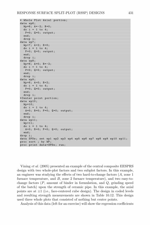
RESPONSE SURFACE SPLIT-PLOT (RSSP) DESIGNS 431
* Whole Plot Axial portion;data wp6;
Wp=6; A=-2; B=0;do i = 1 to 4;P=0; Q=0; output;
end;drop i;
data wp7;Wp=7; A=2; B=0;do i = 1 to 4;P=0; Q=0; output;
end;drop i;
data wp8;Wp=8; A=0; B=-2;do i = 1 to 4;P=0; Q=0; output;
end;drop i;
data wp9;Wp=6; A=0; B=2;do i = 1 to 4;P=0; Q=0; output;
end;drop i;
*Center point portion;data wp10;
Wp=10;do i = 1 to 4;A=0; B=0; P=0; Q=0; output;
end;drop i;
data wp11;Wp=11;do i = 1 to 4;A=0; B=0; P=0; Q=0; output;
end;drop i;data SPDs; set wp1 wp2 wp3 wp4 wp5 wp6 wp7 wp8 wp9 wp10 wp11;proc sort ; by WP;proc print data=SPDs; run;
Vining et al. (2005) presented an example of the central composite EESPRSdesign with two whole-plot factors and two subplot factors. In this example,an engineer was studying the effects of two hard-to-change factors (A, zone 1furnace temperature, and B, zone 2 furnace temperature), and two easy-to-change factors (P , amount of binder in formulation, and Q, grinding speedof the batch) upon the strength of ceramic pipe. In this example, the axialpoints are at ±1 (i.e., face-centered cube design). The design in coded levelsand resulting strength measurements are shown in Table 10.12. This designused three whole plots that consisted of nothing but center points.
Analysis of this data (left for an exercise) will show the regression coefficients
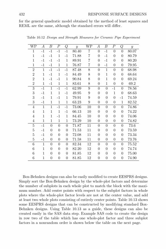
432 RESPONSE SURFACE DESIGNS
for the general quadratic model obtained by the method of least squares andREML are the same, although the standard errors will differ.
Table 10.12 Design and Strength Measures for Ceramic Pipe Experiment
WP A B P Q y WP A B P Q y1 -1 -1 -1 -1 80.40 7 0 -1 0 0 80.071 -1 -1 1 -1 71.88 7 0 -1 0 0 80.791 -1 -1 -1 1 89.91 7 0 -1 0 0 80.201 -1 -1 1 1 76.87 7 0 -1 0 0 79.952 1 -1 -1 -1 87.48 8 0 1 0 0 68.982 1 -1 1 -1 84.49 8 0 1 0 0 68.642 1 -1 -1 1 90.84 8 0 1 0 0 69.242 1 -1 1 1 83.61 8 0 1 0 0 69.23 -1 1 -1 -1 62.99 9 0 0 -1 0 78.563 -1 1 1 -1 49.95 9 0 0 1 0 68.633 -1 1 -1 1 79.91 9 0 0 0 -1 74.593 -1 1 1 1 63.23 9 0 0 0 1 82.524 1 1 -1 -1 73.06 10 0 0 0 0 74.864 1 1 1 -1 66.13 10 0 0 0 0 74.224 1 1 -1 1 84.45 10 0 0 0 0 74.064 1 1 1 1 73.29 10 0 0 0 0 74.825 -1 0 0 0 71.87 11 0 0 0 0 73.65 -1 0 0 0 71.53 11 0 0 0 0 73.595 -1 0 0 0 72.08 11 0 0 0 0 73.345 -1 0 0 0 71.58 11 0 0 0 0 73.766 1 0 0 0 82.34 12 0 0 0 0 75.526 1 0 0 0 82.20 12 0 0 0 0 74.746 1 0 0 0 81.85 12 0 0 0 0 75.006 1 0 0 0 81.85 12 0 0 0 0 74.90
Box-Behnken designs can also be easily modified to create EESPRS designs.Simply sort the Box-Behnken design by the whole-plot factors and determinethe number of subplots in each whole plot to match the block with the maxi-mum number. Add center points with respect to the subplot factors in wholeplots where the whole-plot factor levels are not at the center value, and addat least two whole plots consisting of entirely center points. Table 10.13 showssome EESPRS designs that can be constructed by modifying standard Box-Behnken designs. Using Table 10.13 as a guide, these designs can also becreated easily in the SAS data step. Example SAS code to create the designin row two of the table which has one whole-plot factor and three subplotfactors in a nonrandom order is shown below the table on the next page.
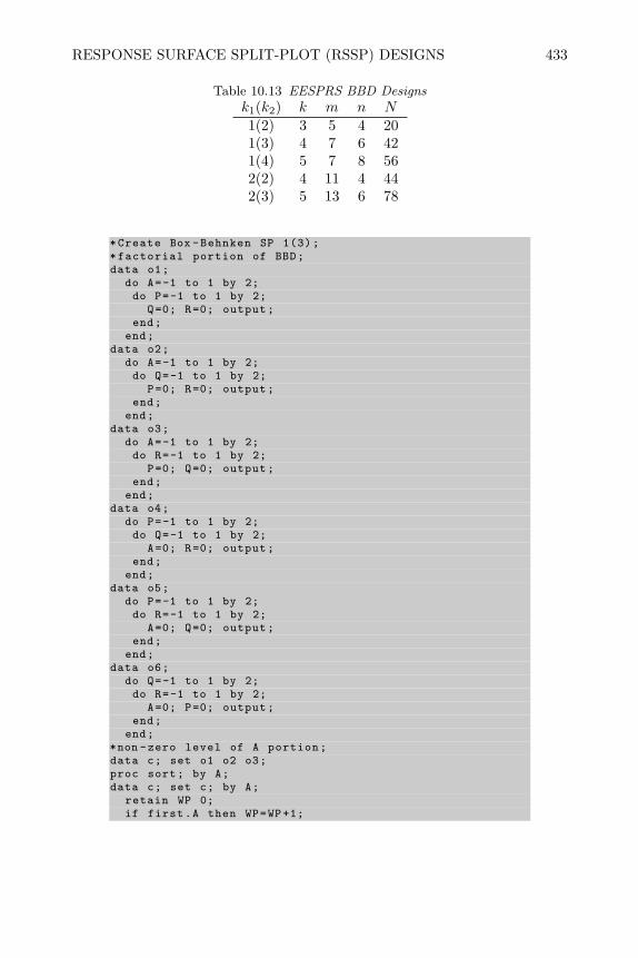
RESPONSE SURFACE SPLIT-PLOT (RSSP) DESIGNS 433
Table 10.13 EESPRS BBD Designsk1(k2) k m n N
1(2) 3 5 4 201(3) 4 7 6 421(4) 5 7 8 562(2) 4 11 4 442(3) 5 13 6 78
*Create Box -Behnken SP 1(3);*factorial portion of BBD;data o1;
do A=-1 to 1 by 2;do P=-1 to 1 by 2;
Q=0; R=0; output;end;
end;data o2;
do A=-1 to 1 by 2;do Q=-1 to 1 by 2;
P=0; R=0; output;end;
end;data o3;
do A=-1 to 1 by 2;do R=-1 to 1 by 2;
P=0; Q=0; output;end;
end;data o4;
do P=-1 to 1 by 2;do Q=-1 to 1 by 2;
A=0; R=0; output;end;
end;data o5;
do P=-1 to 1 by 2;do R=-1 to 1 by 2;
A=0; Q=0; output;end;
end;data o6;
do Q=-1 to 1 by 2;do R=-1 to 1 by 2;
A=0; P=0; output;end;
end;*non -zero level of A portion;data c; set o1 o2 o3;proc sort; by A;data c; set c; by A;
retain WP 0;if first.A then WP=WP+1;

434 RESPONSE SURFACE DESIGNS
*zero level of A portion;data ic; set o4(in=in4) o5(in=in5) o6(in=in6);
if in4 then WP=3;if in5 then WP=4;if in6 then WP=5;
data au1;WP=3;do i =1 to 2;
A=0; P=0; Q=0; R=0; output;end;drop i;WP=4;do i =1 to 2;
A=0; P=0; Q=0; R=0; output;end;drop i;WP=5;do i =1 to 2;
A=0; P=0; Q=0; R=0; output;end;drop i;
*center point whole plots;data wp6;
do i=1 to 6;WP=6; A=0; P=0; Q=0; R=0; output;
end;drop i;
data wp7;do i=1 to 6;
WP=7; A=0; P=0; Q=0; R=0; output;end;drop i;
data sp ; set c ic au1 wp6 wp7;proc sort ; by WP;proc print data=sp; run;
In cases where the designs shown in Tables 10.11 and 10.13 are not flex-ible enough in terms of the number of subplots per whole plot, Goos andVandebroek (2001) and Goos (2002) describe a computer algorithm to createoptimal split-plot designs.
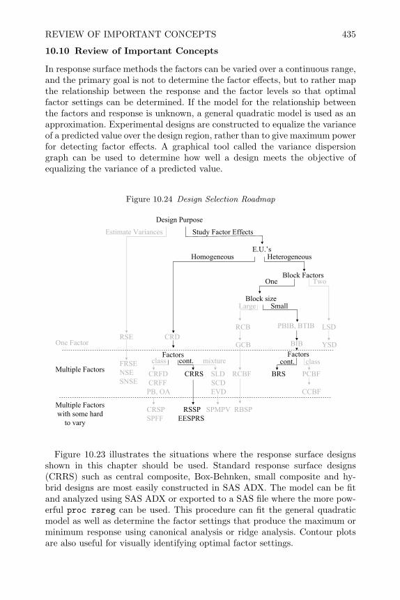
REVIEW OF IMPORTANT CONCEPTS 435
10.10 Review of Important Concepts
In response surface methods the factors can be varied over a continuous range,and the primary goal is not to determine the factor effects, but to rather mapthe relationship between the response and the factor levels so that optimalfactor settings can be determined. If the model for the relationship betweenthe factors and response is unknown, a general quadratic model is used as anapproximation. Experimental designs are constructed to equalize the varianceof a predicted value over the design region, rather than to give maximum powerfor detecting factor effects. A graphical tool called the variance dispersiongraph can be used to determine how well a design meets the objective ofequalizing the variance of a predicted value.
Figure 10.24 Design Selection Roadmap
Design Purpose
Estimate Variances Study Factor Effects
E.U.’s
Block Factors
One Factor
Multiple Factors
Multiple Factorswith some hard
to vary
Block size
Homogeneous Heterogeneous
Large Small
RCB
GCB
PBIB, BTIB
BIB
LSD
YSDRSE CRD
FactorsFRSENSESNSE
CRFD CRRS SLD RCBF BRS PCBFCRFF SCD
PB, OA EVD CCBF
CRSP RSSP SPMPV RBSPSPFF EESPRS
One Two
class cont. mixture cont. classFactors
Figure 10.23 illustrates the situations where the response surface designsshown in this chapter should be used. Standard response surface designs(CRRS) such as central composite, Box-Behnken, small composite and hy-brid designs are most easily constructed in SAS ADX. The model can be fitand analyzed using SAS ADX or exported to a SAS file where the more pow-erful proc rsreg can be used. This procedure can fit the general quadraticmodel as well as determine the factor settings that produce the maximum orminimum response using canonical analysis or ridge analysis. Contour plotsare also useful for visually identifying optimal factor settings.

436 RESPONSE SURFACE DESIGNS
Nonstandard response surface designs are used when a non-standard model(such as a nonlinear model) is used or the experimental region is irregular orconsists of a discrete set of candidates. SAS proc optex can be used to finda design in these situations. Nonlinear models can be fit with the SAS procnlin. Finding the optimal factor settings in irregular design regions or with anonlinear model can be accomplished using nonlinear programming with SASproc nlp.
When experimental units are not homogeneous, blocked response surface(BRS) designs should be utilized. SAS ADX can be used to create orthogo-nally blocked response surface designs for central composite and Box-Behnkendesigns. When the number of blocks and block sizes are not flexible enough forthe problem at hand, proc optex can be used to create Ds optimal blockedresponse surface designs.
When there are hard-to-vary factors which make it inconvenient or costly tocompletely randomize a response surface design, a split-plot response surface(RSSP) design results. In general, the coefficients in the quadratic model for asplit-plot design should be determined using the REML method of estimationdescribed in Chapter 5. However, if the design satisfies the three conditionsdescribed by Vining et al. (2005), the coefficients (but not the standard errors)estimated by least squares will be the same as the coefficients estimated bythe REML method. Therefore, when using this type of EESPRS design procmixed should be used for hypothesis tests concerning the model coefficients forpurposes of model simplification, but proc rsreg can be used for explorationof the fitted surface using canonical or ridge analysis.

EXERCISES 437
10.11 Exercises
1. Create a central composite design for two factors using SAS ADX or datastep commands.
(a) Create the uniform precision CCD and store the design along with ran-dom numbers (simulated response) in a SAS file.
(b) Create a fine grid of points over the unit square and augment your CCDdesign with this grid (leaving the simulated response variable as missingvalues).
(c) Use proc reg to fit the general quadratic model and output the standarderrors of the predicted value over the unit square.
(d) Make a contour plot of the standard errors of the predicted values overthe unit square.
(e) Repeat (a) through (d) for a face-centered cube design (i.e., CCD withaxial points at ±1).
(f) Based on the contour plots you made, which design do you prefer? Statethe reason.
2. Compare characteristics of standard response surface designs for four fac-tors.
(a) Create a uniform precision central composite design, a Box-Behnkendesign, a small composite design, and a hybrid design in SAS ADX.
(b) Compare the variance dispersion graphs for each design, the number oflevels and total number of runs.
(c) Choose one of the designs you have created, export it to a SAS data setand use it to print a randomized data collection for the design.
3. Following up on the experiments described in Section 6.4, AlmeidaeSilvaet al. (2003) ran a response surface design to find the optimum nutrientlevels and fermentation time for producing biomass by fermentation of eu-calyptus hemicellulosic hydrolyzate. The data is shown in the table on thenext page. RB stands for the rice bran (g/l), AS is the ammonium sul-fate (g/l), FT is fermentation time in hours, and Biomass is the mass ofmicroorganisms produced. This was a face-centered cube design (fccd).
(a) Fit the general quadratic model using proc rsreg. Check the model tosee if it is adequate. Determine whether the model can be simplified bydropping any factor from the model.
(b) Do the canonical analysis, ridge analysis or numerical optimization todetermine the conditions that produce the maximum biomass within thecubical experimental region.
(c) If the model can be simplified repeat (a) and (b) with the simpler model.Do the coordinates of the optimum change much? If the model has beensimplified by eliminating one factor, make a contour plot of the responseversus the two factors left in the model, holding the eliminated factor atits mid-level.

438 RESPONSE SURFACE DESIGNS
RB AS FT Biomass10 0 72 3.8330 0 72 5.7110 2 72 6.7430 2 72 5.1310 0 96 5.5530 0 96 7.7610 2 96 12.4530 2 96 12.4710 1 84 11.5430 1 84 9.7920 0 84 7.1320 2 84 10.120 1 72 6.2920 1 96 13.0220 1 84 10.6620 1 84 10.1520 1 84 10.97
4. Consider performing a response surface experiment using the paper heli-copters described in exercise 1 of Chapter 2 and Sections 3.2 and 3.3.
(a) Create a response surface design of your choice by varying wing lengthbetween 3.5 inches and 7 inches and the width of the helicopters from2.25 inches to 5.5 inches. Randomize your list.
(b) Construct and test your helicopters by measuring their flight time witha stopwatch.
(c) Fit the general quadratic model to your data, and test the adequacy ofyour model.
(d) Using canonical analysis, ridge analysis or numerical optimization, de-termine the helicopter dimensions that you predict would result in themaximum flight time. Make a contour plot to visually verify your pre-dicted optimum.
(e) Actually construct a helicopter of the dimensions you predict to be op-timal. Test this helicopter by dropping it repeatedly and recording theflight time. Are the flight times comparable to your predictions?
5. Consider conducting a response surface experiment with the wooden cat-apult described in exercise 2 of Chapter 3. The three factors that can bevaried on the catapult are the start angle, stop angle and pivot height. Eachfactor has three possible levels. A full 33 factorial would allow estimationof all coefficients in the general quadratic model, but it would require 27experiments with no replicates to check the model lack-of-fit.
(a) Construct a face-centered cube (central composite) design for this prob-lem.

EXERCISES 439
(b) Construct a Box-Behnken design for this problem.(c) Since there are only 27 candidate design points, construct a 10-run design
that is a D-optimal subset of the 27 candidates. Suggest one of the pointsthat could be replicated three times to test lack of fit.
(d) Use SAS ADX to make variance dispersion graphs for each design. Whatdesign do you prefer? Why?
(e) Use a catapult to actually run the experiments you have planned.(f) Fit the general quadratic model to the data, using proc rsreg and check
the adequacy of the model.(g) Using numerical optimization, contour plots or simply evaluating your
prediction equation over the 27 possible settings, determine the settings(one of the 27 possible) that you predict would result in a distance closestto exactly 12 feet.
(h) Test the settings you determined in (g). Is the distance close to yourpredictions?
6. Consider the experimental region shown in Figure 10.11, where −1 < x1 <1, −1 < x2 < 1, and x2 ≥ −2x1 − 2, x2 ≤ −2x1 + 1.
(a) Construct a grid ± 12 of candidate points in the (x1, x2) design region.
(b) Construct a D-optimal subset of the candidate points for fitting thegeneral quadratic model.
7. Consider the nonlinear model y = f(x1, x2) = β1eβ2x1 − β3e
β4x2 .
(a) Linearize the model by taking the partial derivatives ∂f∂βi
, i = 1, 4.
(b) Construct a grid of candidate points in the experimental region range1 ≤ x1 ≤ 7, 1 ≤ x2 ≤ 7.
(c) Use proc optex to construct a D-optimal nonlinear design for this modelusing the initial estimates β1 = 10.0, β2 = −0.5, β3 = 5.0, and β4 =−2.0.
8. Consider the data in Table 10.1.
(a) Fit the general quadratic model using proc rsreg as shown in Section10.6.1.
(b) Use canonical analysis or ridge analysis to determine the conditions thatresult in the maximum workability of the cement grout within the spher-ical region −1.73 ≤ xi ≤ 1.73 for i = 1, to 3 in coded units.
9. Consider the model for the chemical reaction in Section 10.7.4.
(a) Use the data shown on the next page that was obtained by running 20experiments to fit model 10.13.
(b) Make a contour plot of predicted concentration over the experimentalregion.

440 RESPONSE SURFACE DESIGNS
time temperature Conc.2.5 380 26.622.5 287.5 36.002.5 395 38.832.5 405 40.995.0 380 43.205.0 387.5 50.605.0 395 51.125.0 405 27.11
10.0 380 57.7110.0 387.5 51.7110.0 395 46.3410.0 405 7.132.5 420 12.825.0 420 1.61
10.0 420 0.0220.0 380 54.3220.0 387.5 30.4720.0 395 9.2420.0 405 0.3825.0 425 0.00
(c) Use nonlinear programming to find the time and temperature (withinthe experimental limits) that maximize the predicted concentration ofproduct. Does this result agree with your contour plot?
10. Create a blocked response surface design for four factors.
(a) Use SAS ADX to create an orthogonally blocked central composite de-sign. How many runs are in this design, and how many runs are in eachblock?
(b) Use SAS ADX to create an orthogonally blocked Box-Behnken design.How many runs are in this design, and how many runs are in each block?
(c) Supposing that only 6 runs can be made in each block, take the centralcomposite design you created in (a) and use proc optex to block it intofive blocks of six runs each.
(d) Take the Box-Behnken design you created in (b), and add three centerpoints, and then use proc optex to block the runs into five blocks of sixruns each.
(e) Import the designs you created in (c) and (d) into SAS ADX, create thevariance dispersion graphs, and compare them to the variance dispersiongraphs of the orthogonally blocked designs you created in (a) and (b).Do you lose much by reducing the block size?
11. Fit the general quadratic model to the data from the pastry dough experi-ment given in Table 10.8.

EXERCISES 441
(a) Use proc rsreg to fit the model including dummy variables for the blockeffects and check the adequacy of the model.
(b) Use canonical analysis or ridge analysis to determine the maximum re-sponse within the cubical experimental region.
12. A study was conducted to find the optimum ration of chloride and al-kaline reserves (AR) in a product that was designed to add alkalinity tolivestock rations. A small composite design was planned with the factorsx1 = 1/
√chloride and x2 = ln(AR), but one combination of x1 and x2,
had to be dropped from the study, and formulation problems with the othercombinations resulted in an irregular design. Forty-eight cattle were blockedinto 8 blocks based on initial weight and hip height. Three cattle had tobe dropped from the study due to chronic health problems that were notrelated to the treatment. The goal was to find the combination of x1 andx2 that resulted in the highest average daily gain in weight (ADG) over thecourse of the study. The data from the study are shown on the next page.
(a) Analyze the data with proc rsreg including dummy variables for theblocks, and check the assumptions of the fitted model.
(b) Find the predicted maximum ADG.(c) Import the data to SAS ADX and make a variance dispersion graph.
How far from rotatable is the irregular design?(d) Make a contour plot to visually confirm the coordinates of your predicted
optimum.
13. Find the optimal moist cake for the data in Table 10.9.
(a) Do the canonical analysis and make a contour plot of the moisture read-ing, y, using the least squares coefficients shown on the left side of Table10.10.
(b) Do the canonical analysis and make a contour plot of the moisture read-ing, y, using the REML estimates of the coefficients shown on the rightside of Table 10.10.
14. Fit the general quadratic model to the ceramic pipe data in Table 10.12.
(a) Fit the model with proc mixed including the random whole plot effects.(b) Fit the model in proc rsreg ignoring the random whole plot effects.(c) Verify that the regression coefficients are the same for both models, but
that the standard errors of the coefficients are different.(d) What procedure would you use to fit the model in order to determine if
the model can be simplified by dropping a factor?(e) What procedure would you use to do a canonical or ridge analysis to
determine the strongest pipe?
15. Follow Table 10.11 and use the SAS data step to create an EESPRS split-plot central composite design with one whole-plot factor and three subplotfactors.
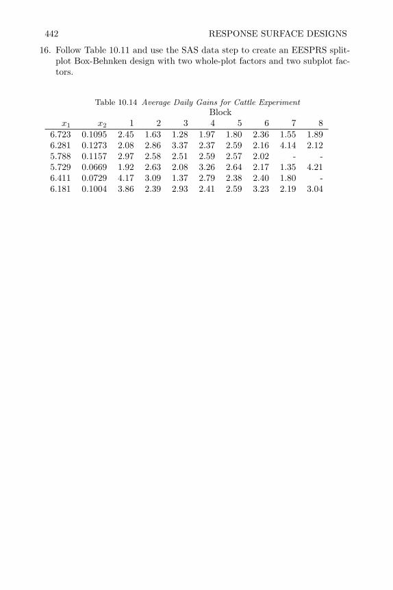
442 RESPONSE SURFACE DESIGNS
16. Follow Table 10.11 and use the SAS data step to create an EESPRS split-plot Box-Behnken design with two whole-plot factors and two subplot fac-tors.
Table 10.14 Average Daily Gains for Cattle ExperimentBlock
x1 x2 1 2 3 4 5 6 7 86.723 0.1095 2.45 1.63 1.28 1.97 1.80 2.36 1.55 1.896.281 0.1273 2.08 2.86 3.37 2.37 2.59 2.16 4.14 2.125.788 0.1157 2.97 2.58 2.51 2.59 2.57 2.02 - -5.729 0.0669 1.92 2.63 2.08 3.26 2.64 2.17 1.35 4.216.411 0.0729 4.17 3.09 1.37 2.79 2.38 2.40 1.80 -6.181 0.1004 3.86 2.39 2.93 2.41 2.59 3.23 2.19 3.04
CHAPTER 11
Mixture Experiments
11.1 Introduction
Many products, such as textile fiber blends, explosives, paints, polymers, andceramics are made by mixing or blending two or more components or ingredi-ents together. For example, a cotton-poly fabric is made by mixing cotton andpolyester fibers together. The characteristics of a product that is composedof a mixture of components is usually a function of the proportion of eachcomponent in the mixture and not the total amount present.
If the proportion of the ith component is xi, and there are k componentsin a mixture, then the proportions must satisfy the constraints
0.0 ≤ xi ≤ 1.0, for each component, andk∑i=1
xi = 1.0. (11.1)
For example, in a three-component mixture, 0.0 ≤ x1 ≤ 1.0, 0.0 ≤ x2 ≤ 1.0,0.0 ≤ x3 ≤ 1.0, and x1 + x2 + x3 = 1.0.
If an experiment is conducted by varying the mixture components in an at-tempt to determine their effect on the product characteristics, the constraintsprevent using standard factorial or response surface experimental design. Ifeach component in the mixture can range from 0.0 to 100.0 percent of thetotal, a 23 factorial experiment would consist of all possible combinations ofproportions 0.00 and 1.00 resulting in the corners of the cube (shown graphi-cally in Figure 11.1).
However, the constraint x1+x2+x3 = 1.0 reduces the three-dimensional ex-perimental region to the two-dimensional shaded equilateral triangular planeshown in Figure 11.1. The coordinate system in this triangular experimentalregion can be represented as shown in Figure 11.2.
In this coordinate system, the proportion of component 3 can be read onthe bottom or horizontal axis, the proportion of component 2 can be read onthe left axis, and the proportion of component 1 can be read on the right axis.The proportion of component 1 is constant along horizontal lines that extendfrom the axis for component 2 on the left across to the axis for component 1on the right. The proportion of component 2 is constant along diagonal linesthat extend from the component 2 axis on the left down to the component3 axis on the bottom, and the proportion of component 3 is constant alongdiagonal lines that extend up from the component 3 axis on the bottom tothe component 1 axis on the right.
Along the line where the proportion of one component is constant, the
443
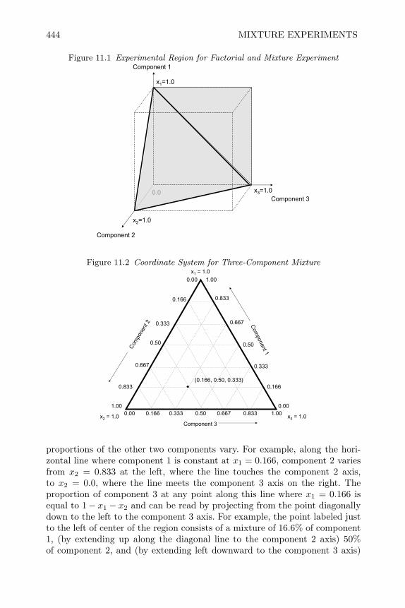
444 MIXTURE EXPERIMENTS
Figure 11.1 Experimental Region for Factorial and Mixture Experiment
Component 3
Component 2
Component 1
0.0 x3=1.0
x2=1.0
x1=1.0
Figure 11.2 Coordinate System for Three-Component Mixture
Com
ponent 1
Com
pone
nt2
Component 3
0.00 0.166 0.333 0.50 0.667 0.833 1.00
0.166
0.333
0.50
0.667
0.833
0.00
0.00
0.833
0.667
0.50
1.00
1.00
0.166
0.333
(0.166, 0.50, 0.333)
x2 = 1.0
x1 = 1.0
x3 = 1.0
proportions of the other two components vary. For example, along the hori-zontal line where component 1 is constant at x1 = 0.166, component 2 variesfrom x2 = 0.833 at the left, where the line touches the component 2 axis,to x2 = 0.0, where the line meets the component 3 axis on the right. Theproportion of component 3 at any point along this line where x1 = 0.166 isequal to 1− x1 − x2 and can be read by projecting from the point diagonallydown to the left to the component 3 axis. For example, the point labeled justto the left of center of the region consists of a mixture of 16.6% of component1, (by extending up along the diagonal line to the component 2 axis) 50%of component 2, and (by extending left downward to the component 3 axis)
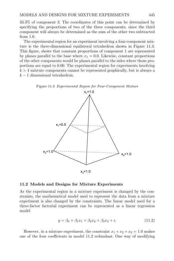
MODELS AND DESIGNS FOR MIXTURE EXPERIMENTS 445
33.3% of component 3. The coordinates of this point can be determined byspecifying the proportions of two of the three components, since the thirdcomponent will always be determined as the sum of the other two subtractedfrom 1.0.
The experimental region for an experiment involving a four-component mix-ture is the three-dimensional equilateral tetrahedron shown in Figure 11.3.This figure, shows that constant proportions of component 1 are representedby planes parallel to the base where x1 = 0.0. Likewise, constant proportionsof the other components would be planes parallel to the sides where those pro-portions are equal to 0.00. The experimental region for experiments involvingk > 4 mixture components cannot be represented graphically, but is always ak − 1 dimensional tetrahedron.
Figure 11.3 Experimental Region for Four-Component Mixture
x4=1.0x2=1.0
x3=1.0
x1=1.0
x1=0.5
11.2 Models and Designs for Mixture Experiments
As the experimental region in a mixture experiment is changed by the con-straints, the mathematical model used to represent the data from a mixtureexperiment is also changed by the constraints. The linear model used for athree-factor factorial experiment can be represented as a linear regressionmodel
y = β0 + β1x1 + β2x2 + β3x3 + ε. (11.2)
However, in a mixture experiment, the constraint x1 +x2 +x3 = 1.0 makesone of the four coefficients in model 11.2 redundant. One way of modifying

446 MIXTURE EXPERIMENTS
the model is to substitute (1− x1 − x2) for x3, resulting in the so-called slackvariable model
y = β∗0 + β∗1x1 + β∗2x2 + ε. (11.3)
In this model, the variable x3 is the slack variable, and it is usually chosen torepresent the most inert mixture component.
Many find the slack variable model objectionable because the coefficientsβ∗1 and β∗2 do not represent the effects of components x1 and x2 as they wouldin a factorial experiment, but rather they represent the effects of x1 and x2
confounded with the opposite of the effect of the slack variable x3.Scheffe (1958) described more suitable polynomial models for mixture ex-
periments. In his form of the model, the coefficient for β0 in Equation (11.2)is 1, and by substituting x1 + x2 + x3 for 1, the model can be written in theScheffe form as
y = β∗1x1 + β∗2x2 + β∗3x3 + ε. (11.4)
From this point on, the asterisks will be removed from the β∗i as they wereused to distinguish the coefficients in a mixture model from the coefficients inthe general regression model.
Again the coefficients in the Scheffe form of the linear model do not representthe effects of the variables x1, x2, and x3, as in a linear regression model, and acoefficient that is zero, or not significantly different from zero, does not meanthat changing the corresponding mixture component will not affect productcharacteristics. Alternately, in the mixture model βi represents the predictedresponse at the vertex of the experimental region where xi = 1.0. This can berepresented graphically for the three-component mixture in Figure 11.4 wherethe predicted response is a plane above the mixture experimental region.
Figure 11.4 Interpretation of Coefficients in Scheffe Linear Model
x1=1.0x2=1.0
x3=1.0β1
β2
β3
If the response surface over the mixture region is nonlinear, the generalquadratic model in three variables,

MODELS AND DESIGNS FOR MIXTURE EXPERIMENTS 447
y = β0 + β1x1 + β2x2 + β3x3 + β1x21 + β2x
22 + β3x
23 + β12x1x2
+ β13x1x3 + β23x2x3 + ε, (11.5)
usually used as an empirical response surface model for a nonlinear surface,is also different for mixture experiments. Multiplying β0 by x1 + x2 + x3 andsubstituting x1×(1− x2 − x3) for x2
1, etc., in model 11.5 results in the Scheffequadratic model shown in Equation (11.6).
y = β1x1 + β2x2 + β3x3 + β12x1x2 + β13x1x3 + β23x2x3 + ε. (11.6)
For k mixture components this model can be written as
y =k∑i=1
βixi +k∑ k∑i<j
βijxixj + ε. (11.7)
The coefficients of the product terms xixj represent the quadratic curvaturealong an edge of the simplex experimental region, as illustrated for a three-component mixture in Figure 11.5.
Figure 11.5 Interpretation of Coefficients of Product Terms inScheffe Quadratic Model
x1=1.0x2=0.0
x1=0.0x2=1.0
β1
β2
x1=0.5x2=0.5
β12__4
11.2.1 Experimental Designs To Fit Scheffe Models
Based on the interpretation of the coefficients in the linear and quadraticmodels for mixture experiments, Scheffe (1958) proposed the simplex-lattice
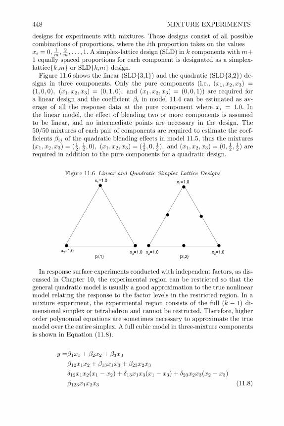
448 MIXTURE EXPERIMENTS
designs for experiments with mixtures. These designs consist of all possiblecombinations of proportions, where the ith proportion takes on the valuesxi = 0, 1
m ,2m , . . . , 1. A simplex-lattice design (SLD) in k components with m+
1 equally spaced proportions for each component is designated as a simplex-latticek,m or SLDk,m design.
Figure 11.6 shows the linear (SLD3,1) and the quadratic (SLD3,2) de-signs in three components. Only the pure components (i.e., (x1, x2, x3) =(1, 0, 0), (x1, x2, x3) = (0, 1, 0), and (x1, x2, x3) = (0, 0, 1)) are required fora linear design and the coefficient βi in model 11.4 can be estimated as av-erage of all the response data at the pure component where xi = 1.0. Inthe linear model, the effect of blending two or more components is assumedto be linear, and no intermediate points are necessary in the design. The50/50 mixtures of each pair of components are required to estimate the coef-ficients βij of the quadratic blending effects in model 11.5, thus the mixtures(x1, x2, x3) = (1
2 ,12 , 0), (x1, x2, x3) = (1
2 , 0,12 ), and (x1, x2, x3) = (0, 1
2 ,12 ) are
required in addition to the pure components for a quadratic design.
Figure 11.6 Linear and Quadratic Simplex Lattice Designsx1=1.0
x3 x0.1= 3=1.0x2=1.0 x2=1.0
x1=1.0
2,31,3
In response surface experiments conducted with independent factors, as dis-cussed in Chapter 10, the experimental region can be restricted so that thegeneral quadratic model is usually a good approximation to the true nonlinearmodel relating the response to the factor levels in the restricted region. In amixture experiment, the experimental region consists of the full (k − 1) di-mensional simplex or tetrahedron and cannot be restricted. Therefore, higherorder polynomial equations are sometimes necessary to approximate the truemodel over the entire simplex. A full cubic model in three-mixture componentsis shown in Equation (11.8).
y =β1x1 + β2x2 + β3x3
β12x1x2 + β13x1x3 + β23x2x3
δ12x1x2(x1 − x2) + δ13x1x3(x1 − x3) + δ23x2x3(x2 − x3)β123x1x2x3 (11.8)

MODELS AND DESIGNS FOR MIXTURE EXPERIMENTS 449
The coefficients δij represent the cubic blending of binary mixtures along theedges of the simplex as shown in Figure 11.7.
Figure 11.7 Cubic Blending of Binary Mixture of Components i and j
xi=1 3/4 2/4 1/4 0
xj=0 1/4 2/4 3/4 1
3δij__32
3δij__32
-
The β123 coefficient represents the ternary blending of components 1, 2, and3 in the interior of the simplex.
To estimate the coefficients in the full cubic model requires an SLD3,3design consisting of the points
(x1, x2, x3) =(1, 0, 0), (0, 1, 0), (0, 0, 1), (13,
23, 0), (
23,
13, 0), (
13, 0,
23
)
(23, 0,
13
), (0,13,
23
), (0,23,
13, 0), (
13,
13,
13
).
When the coefficients δij are insignificant in the cubic Scheffe model, justi-fying a less complicated model, the simpler special cubic model can be used.The equation for the special cubic model in k mixture components is shownin Equation (11.9).

450 MIXTURE EXPERIMENTS
y =k∑i=1
βixi +k∑ k∑i≤j
βijxixj +k∑ k∑ k∑i<j<l
βijlxixjxl + ε. (11.9)
An alternate design, discussed by Cornell (2002), that allows estimation ofall coefficients in the special cubic model is the simplex centroid design orSCD. A simplex centroid design in three-mixture components consists of the(
31
)pure component blends (1,0,0), (0,1,0), and (0,0,1), the
(32
)binary mixtures
( 12 ,
12 , 0),( 1
2 , 0,12 ), and (0, 1
2 ,12 ), and the
(33
)ternary mixture (1
3 ,13 ,
13 ).
An SCD in k mixture components (SCDk) consists of the(k1
)pure com-
ponents, the(k2
)permutations of the binary mixtures ( 1
2 ,12 , 0, . . . , 0), the
(k3
)permutations of the ternary mixtures ( 1
3 ,13 ,
13 , 0, . . . , 0), etc., up to the k-nary
mixture ( 1k ,
1k ,
1k , . . . ,
1k ).
The (SCDk) always includes the k-nary mixture, or centroid, which isinterior to the design region, and it supports estimation of the coefficients ina polynomial model of the general form shown in Equation (11.10).
y =k∑i=1
βixi +k∑ k∑i<j
βijxixj +k∑ k∑ k∑i<j<l
βijlxixjxl + · · ·+
β12...kx1x2x3 · · ·xk + ε (11.10)
One criticism of quadratic simplex lattice designs in three components isthat they do not contain any design points in the interior of the simplex designregion where the accuracy of a fitted model can be tested. For this reason,these designs are often augmented by the overall centroid ( 1
3 ,13 ,
13 ) and axial
points of the form (1−∆, ∆2 ,
∆2 ), (∆
2 , 1−∆, ∆2 ), and (∆
2 ,∆2 , 1−∆) as shown
in Figure 11.8.
11.2.2 Alternate Models for Mixture Experiments
Claringbold (1955), who was the first to use a simplex-type design for study-ing three-mixture components, described a two-step procedure for translatingthe origin and orthogonally rotating the axis of the component space to pro-duce independent factors as shown graphically in Figure 11.9. The first stepof the procedure is to translate the origin to the centroid of the simplex bysubtracting the centroid value from each component and multiplying by thenumber of components. The second step is to post multiply the vector oftranslated coordinates by an orthogonal matrix O to rotate the axis. In threecomponents, the rotated and translated axis labeled w3 is perpendicular tothe two-dimensional simplex experimental region, and all points in the exper-imental region will have w3 = 0 in the translated and rotated factor space.

MODELS AND DESIGNS FOR MIXTURE EXPERIMENTS 451
Figure 11.8 Simplex Lattice3,2 Augmented with Centroid and Axial Points
x2=1.0 x3=1.0
x1=1.0
∆
∆∆
Figure 11.9 Translation and Rotation of Axis To Form Independent Factors
2~x
1~x
3~x
2x
1x
3x
1w
2w
3w
)(~1. JXX −= k OXW ~)1(.2 −= k
3x
1x
2x
2w
1w
Cornell (2002) shows the translation and rotation from the k dimensionalmixture component space to k − 1 dimensional space for the independentfactor space can be written as k− 1 contrasts of the mixture components. Forexample, in three-mixture components (x1, x2, x3),
w1 =√
6(2x1 − x2 − x3) (11.11)
w2 =√
18(x2 − x3). (11.12)

452 MIXTURE EXPERIMENTS
The quadratic model can be written in the independent factors as shown inEquation (11.15), which is the same as model 10.2,
y = β0 + β1w1 + β2w2 + β11w21 + β22w
22 + β12w1w2 + ε, (11.13)
and standard regression programs and contour plotting programs like SASproc gcontour can be used to fit the model and produce contour plots overthe simplex experimental region. This fact is illustrated in an example in theappendix of this chapter.
Sometimes the response in a mixture experiment may increase or decreaserapidly as one or more of the mixture components approach their lower bound-ary. These are called edge effects. Edge effects can cause a lack of fit in first-and second-degree polynomial models. Rather than increasing the order of thepolynomial model, Draper and John (1977) suggested including inverse termsin the model, as shown in Equation (11.14), to model edge effects.
y = β1x1 + β2x2 + β3x3 + β−1x−11 + β−2x
−12 + β−3x
−13 + ε (11.14)
Including inverse terms when there are edge effects can greatly improve thefit of the model as will be demonstrated in an exercise.
11.3 Creating Mixture Designs in SAS
Simplex lattice and simplex centroid designs can be easily created using theSAS macros included in the AUTOCALL library or with the SAS ADX auto-mated system. The example SAS code below uses the macros to first createan SLD3,2 in three components x1, x2, and x3, and stores it in the filework.sld. The code then creates an SCD in four components and prints theresulting file work.scd.
%adxgen%adxmix%adxinit%adxsld(sld ,x1 x2 x3 ,2)%adxgen%adxmix%adxinit%adxscd(scd ,x1 x2 x3 x4 ,4)proc print data=scd; run;
The output at the top of the next page shows the simplex-centroid design.
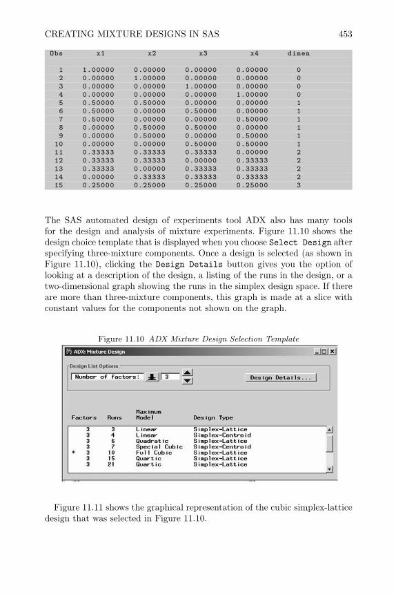
CREATING MIXTURE DESIGNS IN SAS 453
Obs x1 x2 x3 x4 dimen
1 1.00000 0.00000 0.00000 0.00000 02 0.00000 1.00000 0.00000 0.00000 03 0.00000 0.00000 1.00000 0.00000 04 0.00000 0.00000 0.00000 1.00000 05 0.50000 0.50000 0.00000 0.00000 16 0.50000 0.00000 0.50000 0.00000 17 0.50000 0.00000 0.00000 0.50000 18 0.00000 0.50000 0.50000 0.00000 19 0.00000 0.50000 0.00000 0.50000 1
10 0.00000 0.00000 0.50000 0.50000 111 0.33333 0.33333 0.33333 0.00000 212 0.33333 0.33333 0.00000 0.33333 213 0.33333 0.00000 0.33333 0.33333 214 0.00000 0.33333 0.33333 0.33333 215 0.25000 0.25000 0.25000 0.25000 3
The SAS automated design of experiments tool ADX also has many toolsfor the design and analysis of mixture experiments. Figure 11.10 shows thedesign choice template that is displayed when you choose Select Design afterspecifying three-mixture components. Once a design is selected (as shown inFigure 11.10), clicking the Design Details button gives you the option oflooking at a description of the design, a listing of the runs in the design, or atwo-dimensional graph showing the runs in the simplex design space. If thereare more than three-mixture components, this graph is made at a slice withconstant values for the components not shown on the graph.
Figure 11.10 ADX Mixture Design Selection Template
Figure 11.11 shows the graphical representation of the cubic simplex-latticedesign that was selected in Figure 11.10.

454 MIXTURE EXPERIMENTS
Figure 11.11 ADX Design Description Template
11.4 Analysis of Mixture Experiment
In attempting to find a pesticide formulation that would spread evenly on theleaves of cotton plants, researchers experimented by combining a syntheticpyrethroid insecticide with a mixture of three Niagara emulsifiers. They usedan SLD3,2 design, augmented by an overall centroid and six axial points.The experimental runs and the measured surface tension from each mixture isshown in Table 11.1. The formulations were made and tested in a completelyrandom order.
Table 11.1 Data Pesticide Formulation Experimentsurface tension
Run x1 x2 x3 (dyne/cm)1 1.00000 0.00000 0.00000 48.72 0.80000 0.10000 0.10000 49.53 0.60000 0.20000 0.20000 50.24 0.50000 0.00000 0.50000 52.85 0.50000 0.50000 0.00000 49.36 0.33333 0.33333 0.33333 51.17 0.30000 0.20000 0.50000 52.78 0.30000 0.50000 0.20000 50.39 0.10000 0.10000 0.80000 60.7
10 0.10000 0.80000 0.10000 49.911 0.00000 0.00000 1.00000 64.912 0.00000 0.50000 0.50000 53.513 0.00000 1.00000 0.00000 50.6

ANALYSIS OF MIXTURE EXPERIMENT 455
The research goal was to determine how the proportions of the three Niagaraemulsifiers affected the surface tension of the pesticide formulation. The lowerthe surface tension, the more likely the formulation would spread evenly onthe cotton leaves.
The data analysis will first be illustrated with the ADX automated design ofexperiments tool. Since this specific design cannot be created easily in ADX,the SAS data step was used to read the data in Table 11.1 into the SAS dataset work.form; from there, it was imported to the ADX system. Figure 11.12shows the data in the ADX system.
Figure 11.12 Pesticide Formulation Data in ADX
Clicking first on the Design Details button followed by the Design Pointstab shows a graphical representation of the design points in the simplex region.The axial points can be seen in Figure 11.13.
The SLD3,2 design augmented by the overall centroid supports fittingthe special cubic model. A general strategy to follow when modeling the datafrom mixture experiments is to first fit the highest order model supportedby the design, then try to simplify if higher order terms are insignificant. Thevariance of predicted values will be lower for simpler models with fewer terms.
The model can be selected in ADX by clicking the Model I Change mastermodel menus. ADX allows the user to choose the linear, quadratic, specialcubic or full cubic models as defined earlier in Equations 11.4, 11.7, 11.8, and11.9, respectively. Figure 11.14 below shows the result of fitting the Scheffespecial cubic model. ADX fits the model by the method of least squares,and the same methods for checking the assumptions of the least squares fit(described in Chapter 2) can be accomplished within the ADX system. Ifthere are replicated points, ADX automatically performs the lack of fit testas explained in Section 10.6.2. In the results shown in Figure 11.14, the β123
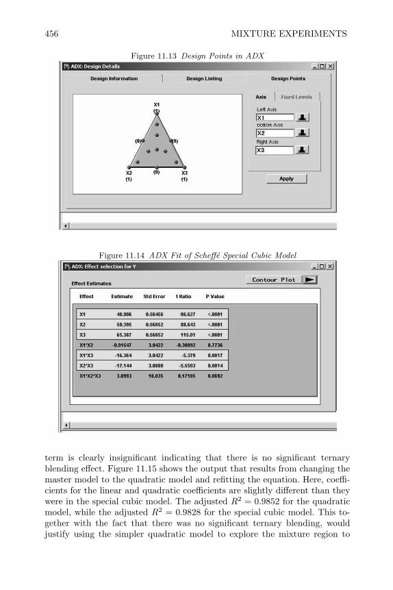
456 MIXTURE EXPERIMENTS
Figure 11.13 Design Points in ADX
Figure 11.14 ADX Fit of Scheffe Special Cubic Model
term is clearly insignificant indicating that there is no significant ternaryblending effect. Figure 11.15 shows the output that results from changing themaster model to the quadratic model and refitting the equation. Here, coeffi-cients for the linear and quadratic coefficients are slightly different than theywere in the special cubic model. The adjusted R2 = 0.9852 for the quadraticmodel, while the adjusted R2 = 0.9828 for the special cubic model. This to-gether with the fact that there was no significant ternary blending, wouldjustify using the simpler quadratic model to explore the mixture region to
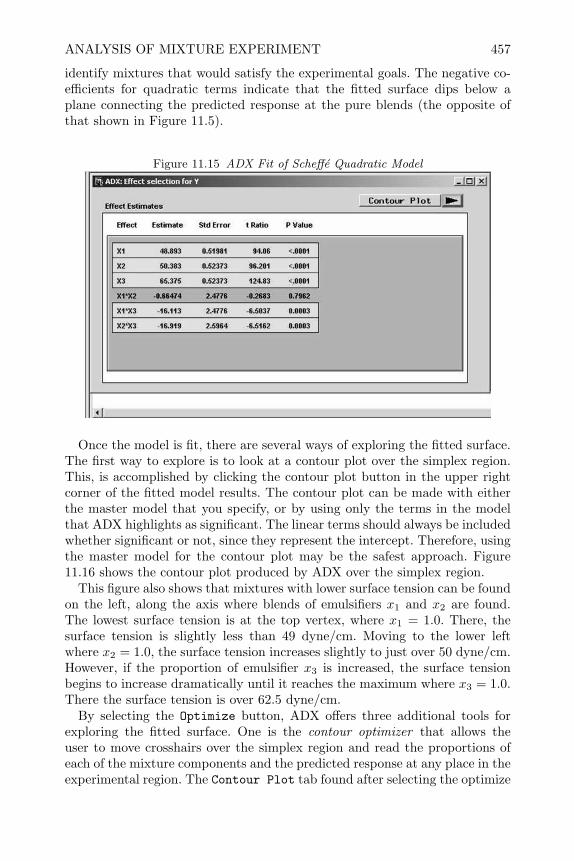
ANALYSIS OF MIXTURE EXPERIMENT 457
identify mixtures that would satisfy the experimental goals. The negative co-efficients for quadratic terms indicate that the fitted surface dips below aplane connecting the predicted response at the pure blends (the opposite ofthat shown in Figure 11.5).
Figure 11.15 ADX Fit of Scheffe Quadratic Model
Once the model is fit, there are several ways of exploring the fitted surface.The first way to explore is to look at a contour plot over the simplex region.This, is accomplished by clicking the contour plot button in the upper rightcorner of the fitted model results. The contour plot can be made with eitherthe master model that you specify, or by using only the terms in the modelthat ADX highlights as significant. The linear terms should always be includedwhether significant or not, since they represent the intercept. Therefore, usingthe master model for the contour plot may be the safest approach. Figure11.16 shows the contour plot produced by ADX over the simplex region.
This figure also shows that mixtures with lower surface tension can be foundon the left, along the axis where blends of emulsifiers x1 and x2 are found.The lowest surface tension is at the top vertex, where x1 = 1.0. There, thesurface tension is slightly less than 49 dyne/cm. Moving to the lower leftwhere x2 = 1.0, the surface tension increases slightly to just over 50 dyne/cm.However, if the proportion of emulsifier x3 is increased, the surface tensionbegins to increase dramatically until it reaches the maximum where x3 = 1.0.There the surface tension is over 62.5 dyne/cm.
By selecting the Optimize button, ADX offers three additional tools forexploring the fitted surface. One is the contour optimizer that allows theuser to move crosshairs over the simplex region and read the proportions ofeach of the mixture components and the predicted response at any place in theexperimental region. The Contour Plot tab found after selecting the optimize

458 MIXTURE EXPERIMENTS
Figure 11.16 ADX Contour Plot of Quadratic Model Predictions
X1(1)
(0)
(0)
X2(1)
(0)
X3(1)
50
50
55
55
57.5
57.5
60
60
62.5
62.5
Y
button, as well as the contour optimizer, allows the user to specify whichmixture components to place on the left, right, and top vertices of the simplexregion. Here the user can select three components for plotting, and to fixadditional components when there are more than three mixture componentsin the problem. A third tab that appears after clicking the optimize buttonis the prediction profiler. This is a very useful tool that allows the user tosee the response trace along the direction through the simplex introducedby Cox (1971) and illustrated in Figure 11.17. This tool plots the predictedvalue of the response and the 95% prediction intervals for the prediction usingthe directions shown in Figure 11.17. It is also very useful in visualizing theresults of varying the mixture components when there are more than threecomponents in the mixture, and the results cannot be displayed as a singlecontour plot.
Figure 11.18 shows the response trace for the three components in the pesti-cide formulation problem, and it can be seen that increasing the proportion ofemulsifier x2 has relatively little effect. Increasing the proportion of emulsifierx1 has a slightly negative effect on surface tension, and increasing the pro-portion of emulsifier x3 causes a large increase in surface tension. Therefore,just as can be seen on the contour plot, the conclusion reached by looking atthe response traces would be to choose 100% of emulsifier x1 or a blend ofemulsifiers x1 and x2 to reach the lowest levels of surface tension.
In mixture experiments with several components, it is important to deter-mine which components are most influential. This can simplify the problemand allow the experimenters to focus on optimization with respect to themost important mixture components. Since the coefficients in the models for

ANALYSIS OF MIXTURE EXPERIMENT 459
Figure 11.17 Cox Directions Through Three-Dimensional Simplex
0.11 =x
0.12 =x 0.13 =x
x 1D
irect
ion
x 2Direction x
3 Direction
Figure 11.18 ADX Response Trace Plots for Quadratic Model
mixture experiments do not represent effects in the same way as they do forindependent factors, tests of the significance of linear coefficients in the modelare not a good way to determine the important components. However, theresponse trace is a good tool to use for this purpose. When a linear design isused as a screening experiment for several components, and the Scheffe linearmodel is fit to the data, the response traces will be straight lines and the leastimportant components will have traces with relatively flat slopes, while theimportant components will have traces with steep slopes. Thus, the response

460 MIXTURE EXPERIMENTS
trace plots can be used as a graphical tool to determine the important com-ponents similar to the way that the normal or half-normal plot of effects isused for screening experiments with independent factors. Cornell (2002) andSnee and Marquardt (1976) discuss other strategies for screening with mixtureexperiments.
The least squares fits performed by ADX for mixture experiments (illus-trated in Figures 11.14 and 11.15) are designed specifically for fitting Scheffemodels. Cornell (2002) explains that standard regression programs like SASproc glm or SAS proc reg do not provide the correct analysis because whenthe no-constant option (model option /noint) is used, the fitted model sumsof squares and total sums of squares are not corrected for the overall mean.Therefore, the R2 value is inflated and gives the impression that the modelfits better than it actually does. For example, Table 11.2 shows a comparisonof the sums of squares and R2 statistic produced by SAS ADX, proc glm,and proc reg when fitting the Scheffe quadratic model to the data in Table11.1 and using the model /noint option with proc glm and proc reg.
Table 11.2 Comparison of Different Programs for Fitting Scheffe Quadratic Modelto Data in Table 11.1
Program Model df Model SS Error SS Total SS R2
ADX Mixture 5 275.64 2.41 278.05 0.9913proc glm 6 36285.60 2.41 36288 0.9999proc reg 6 36285.60 2.41 36288 0.9999
One way the correct sums of squares and R2 can be computed using procreg or proc glm is to fit the model
y = β0 + β1x1 + β2x2 + β12x1x2 + β13x1x3 + β23x2x3 + ε. (11.15)
By including an intercept and removing x3 from the model, the coefficientsβ0, β1, and β2 take on a different meaning than in the Scheffe model shownin Equation (11.6). β0 takes on the value of β3 in Equation (11.6), and βirepresents the difference of β0− βi. The code for fitting this model with procglm and estimating β1, β2, and β3 is shown in the listing on the next page.
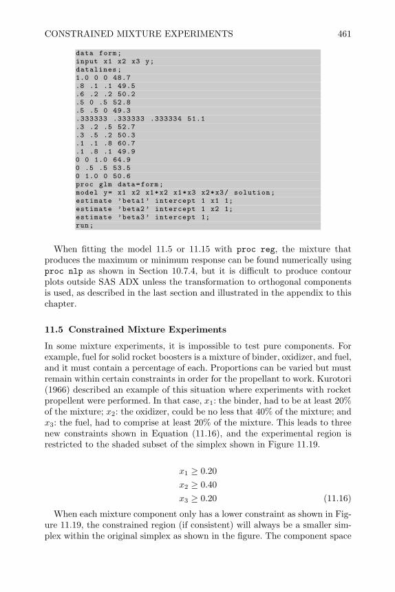
CONSTRAINED MIXTURE EXPERIMENTS 461
data form;input x1 x2 x3 y;datalines;1.0 0 0 48.7.8 .1 .1 49.5.6 .2 .2 50.2.5 0 .5 52.8.5 .5 0 49.3.333333 .333333 .333334 51.1.3 .2 .5 52.7.3 .5 .2 50.3.1 .1 .8 60.7.1 .8 .1 49.90 0 1.0 64.90 .5 .5 53.50 1.0 0 50.6proc glm data=form;model y= x1 x2 x1*x2 x1*x3 x2*x3/ solution;estimate ’beta1’ intercept 1 x1 1;estimate ’beta2’ intercept 1 x2 1;estimate ’beta3’ intercept 1;run;
When fitting the model 11.5 or 11.15 with proc reg, the mixture thatproduces the maximum or minimum response can be found numerically usingproc nlp as shown in Section 10.7.4, but it is difficult to produce contourplots outside SAS ADX unless the transformation to orthogonal componentsis used, as described in the last section and illustrated in the appendix to thischapter.
11.5 Constrained Mixture Experiments
In some mixture experiments, it is impossible to test pure components. Forexample, fuel for solid rocket boosters is a mixture of binder, oxidizer, and fuel,and it must contain a percentage of each. Proportions can be varied but mustremain within certain constraints in order for the propellant to work. Kurotori(1966) described an example of this situation where experiments with rocketpropellent were performed. In that case, x1: the binder, had to be at least 20%of the mixture; x2: the oxidizer, could be no less that 40% of the mixture; andx3: the fuel, had to comprise at least 20% of the mixture. This leads to threenew constraints shown in Equation (11.16), and the experimental region isrestricted to the shaded subset of the simplex shown in Figure 11.19.
x1 ≥ 0.20x2 ≥ 0.40x3 ≥ 0.20 (11.16)
When each mixture component only has a lower constraint as shown in Fig-ure 11.19, the constrained region (if consistent) will always be a smaller sim-plex within the original simplex as shown in the figure. The component space

462 MIXTURE EXPERIMENTS
Figure 11.19 Constrained Region for Rocket Propellant Experiment
x1 = Fuel
x2 = Oxidizer x3 = Binder
0.2
0.4
0.6
0.8
0.2 0.4 0.6 0.8
0.2
0.4
0.6
0.8
Constrained Region
within this smaller simplex can be conveniently transformed into a pseudo-component space where the same simplex lattice and simplex centroid designscan be used for an experimental design. If the lower constraint for mixturecomponent xi is defined to be li, then the ith pseudo component is defined tobe
x′i =xi − li
1−∑ki=1 li
, (11.17)
where k is the number of mixture components. A simplex lattice design can beconstructed in the pseudo-components and the actual mixtures to be testedcan then be obtained by solving Equation (11.17) for xi as
xi = li +
(1−
k∑i=1
li
)x′i, (11.18)
For example, Table 11.3 shows an SLD3,2 design in pseudo-componentstranslated into a design with the actual components for the rocket propellentexperiment using the lower bounds given in Equation (11.16). The experimentswere run by making each mixture of fuel oxidizer and binder, then measuringthe resulting elasticity. The general quadratic or special cubic model can befit to either the pseudo or actual components.
11.5.1 Upper and Lower Constraints
In some special cases when there are only upper constraints or both upper andlower constraints, the constrained experimental region will result in a smallerinverted simplex within the simplex component space. However, in the morecommon situation, the constrained region will be an irregular hyperpolyhe-dron. In this case, McLean and Anderson (1966) recommend a design thatconsists of the extreme vertices (EVD) of the experimental region, possibly
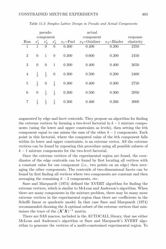
CONSTRAINED MIXTURE EXPERIMENTS 463
Table 11.3 Simplex Lattice Design in Pseudo and Actual Components
pseudo- actualcomponent component response
Run x′1 x′2 x′3 x1=Fuel x2=Oxidizer x3=Binder elasticity1 1 0 0 0.400 0.400 0.200 2350
2 0 1 0 0.200 0.600 0.200 2450
3 0 0 1 0.200 0.400 0.400 2650
4 12
12 0 0.300 0.500 0.200 2400
5 12 0 1
2 0.300 0.400 0.300 2750
6 0 12
12 0.200 0.500 0.300 2950
7 13
13
13 0.266 0.466 0.266 3000
augmented by edge and facet centroids. They propose an algorithm for findingthe extreme vertices by forming a two-level factorial in k− 1 mixture compo-nents (using the lower and upper constraints as levels), then setting the kthcomponent equal to one minus the sum of the other k − 1 components. Eachpoint in this factorial, where the computed value of the kth component fallswithin its lower and upper constraints, is an extreme vertex. All the extremevertices can be found by repeating this procedure using all possible subsets ofk − 1 mixture components for the two-level factorial.
Once the extreme vertices of the experimental region are found, the coor-dinates of the edge centroids can be found by first locating all vertices witha constant value for one component (i.e., two points on an edge) then aver-aging the other components. The centroids of two-dimensional facets can befound by first finding all vertices where two components are constant and thenaveraging the remaining k − 2 components, etc.
Snee and Marquardt (1974) defined the XVERT algorithm for finding theextreme vertices, which is similar to McLean and Anderson’s algorithm. Whenthere are many components in the mixture problem, there may be many moreextreme vertices in the experimental region than there are coefficients in theScheffe linear or quadratic model. In that case Snee and Marquardt (1974)recommended choosing the A-optimal subset of the extreme vertices that min-imizes the trace of the (X ′X)−1 matrix.
There are SAS macros, included in the AUTOCALL library, that use eitherMcLean and Anderson’s algorithm or Snee and Marquardt’s XVERT algo-rithm to generate the vertices of a multi-constrained experimental region. To
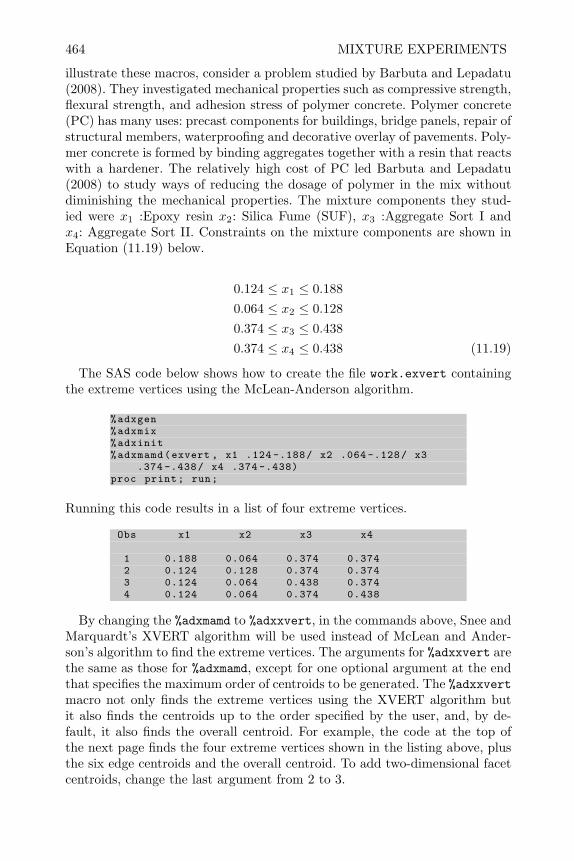
464 MIXTURE EXPERIMENTS
illustrate these macros, consider a problem studied by Barbuta and Lepadatu(2008). They investigated mechanical properties such as compressive strength,flexural strength, and adhesion stress of polymer concrete. Polymer concrete(PC) has many uses: precast components for buildings, bridge panels, repair ofstructural members, waterproofing and decorative overlay of pavements. Poly-mer concrete is formed by binding aggregates together with a resin that reactswith a hardener. The relatively high cost of PC led Barbuta and Lepadatu(2008) to study ways of reducing the dosage of polymer in the mix withoutdiminishing the mechanical properties. The mixture components they stud-ied were x1 :Epoxy resin x2: Silica Fume (SUF), x3 :Aggregate Sort I andx4: Aggregate Sort II. Constraints on the mixture components are shown inEquation (11.19) below.
0.124 ≤ x1 ≤ 0.1880.064 ≤ x2 ≤ 0.1280.374 ≤ x3 ≤ 0.4380.374 ≤ x4 ≤ 0.438 (11.19)
The SAS code below shows how to create the file work.exvert containingthe extreme vertices using the McLean-Anderson algorithm.
%adxgen%adxmix%adxinit%adxmamd(exvert , x1 .124 -.188/ x2 .064 -.128/ x3
.374 -.438/ x4 .374 -.438)proc print; run;
Running this code results in a list of four extreme vertices.
Obs x1 x2 x3 x4
1 0.188 0.064 0.374 0.3742 0.124 0.128 0.374 0.3743 0.124 0.064 0.438 0.3744 0.124 0.064 0.374 0.438
By changing the %adxmamd to %adxxvert, in the commands above, Snee andMarquardt’s XVERT algorithm will be used instead of McLean and Ander-son’s algorithm to find the extreme vertices. The arguments for %adxxvert arethe same as those for %adxmamd, except for one optional argument at the endthat specifies the maximum order of centroids to be generated. The %adxxvertmacro not only finds the extreme vertices using the XVERT algorithm butit also finds the centroids up to the order specified by the user, and, by de-fault, it also finds the overall centroid. For example, the code at the top ofthe next page finds the four extreme vertices shown in the listing above, plusthe six edge centroids and the overall centroid. To add two-dimensional facetcentroids, change the last argument from 2 to 3.

CONSTRAINED MIXTURE EXPERIMENTS 465
%adxgen%adxmix%adxinit%adxxvert(exvert , x1 .124 -.188/ x2 .064 -.128/ x3 .374 -.438/
x4 .374 -.438 ,2)proc print; run;
For many constrained mixture problems, the number of extreme vertices andedge centroids will be much greater than the number of coefficients in theScheffe quadratic model. To reduce the number of mixtures and still allowfitting a quadratic model to the resulting data, a D-optimal subset can beselected using proc optex as shown in the example below. In this example, aD-optimal subset of 14 mixtures from the file work.exvert will be output tothe file work.dmax.
proc optex data=exvert;model x1 x2 x3 x4 x1*x2 x1*x3 x1*x4 x2*x3 x2*x4 x3*x4/
noint;generate n=14 ;output out=dmax; run;
proc print data=dmax; run;
If the constraint equations such as Equation (11.19) are inconsistent, therewill be no feasible points within the constrained region. In that case, the SASlog will indicate the file exvert.test has zero observations.
The SAS ADX tool can also create a list of candidate design points forconstrained mixture experiments composed of extreme vertices and centroids.To illustrate ADX, which can also graph the feasible region, consider thethree-component mixture studied by Juan et al. (2006).
They studied consumer acceptance of polvoron composed of a mixture ofx1: sugar, x2: peanut fines, and x3: butter. Polvoron is a Philippine ethnicdessert or candy usually composed of milk powder, toasted flour, sugar, andbutter. Ground nuts can be added to vary its flavor and texture properties. Ifacceptable to consumers, utilizing peanut fines (which are usually a discardedbyproduct of the roasted peanut process) in polvoron could reduce waste andcreate an additional product line. The constraints on the mixture space areshown in Equation (11.20).
0.00 ≤ x1 ≤ 0.800.10 ≤ x2 ≤ 0.950.05 ≤ x3 ≤ 0.50 (11.20)
Selecting three-mixture components and entering the constraints listed inEquation (11.20) into ADX, the constrained region is graphed as shown inFigure 11.20.
Table 11.4 shows data from the article. The response, overall liking, wasthe average ranking of 115 taste panelists who ranked the mixtures on a 9-point scale where 1 = dislike extremely, 5 = neither like nor dislike, and 9 =extremely like. Three additional mixtures in the interior of the simplex (that
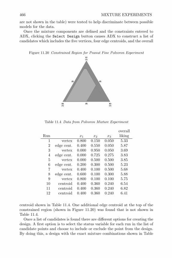
466 MIXTURE EXPERIMENTS
are not shown in the table) were tested to help discriminate between possiblemodels for the data.
Once the mixture components are defined and the constraints entered toADX, clicking the Select Design button causes ADX to construct a list ofcandidates which includes the five vertices, four edge centroids, and the overall
Figure 11.20 Constrained Region for Peanut Fine Polvoron ExperimentX1(1)
(0)
(0)
X2(1)
(0)
X3(1)
Table 11.4 Data from Polvoron Mixture Experiment
overallRun x1 x2 x3 liking
1 vertex 0.800 0.150 0.050 5.332 edge cent. 0.400 0.550 0.050 5.873 vertex 0.000 0.950 0.050 3.694 edge cent. 0.000 0.725 0.275 3.835 vertex 0.000 0.500 0.500 3.856 edge cent. 0.200 0.300 0.500 5.237 vertex 0.400 0.100 0.500 5.688 edge cent. 0.600 0.100 0.300 5.889 vertex 0.800 0.100 0.100 5.75
10 centroid 0.400 0.360 0.240 6.5411 centroid 0.400 0.360 0.240 6.8212 centroid 0.400 0.360 0.240 6.41
centroid shown in Table 11.4. One additional edge centroid at the top of theconstrained region (shown in Figure 11.20) was found that is not shown inTable 11.4.
Once a list of candidates is found there are different options for creating thedesign. A first option is to select the status variable for each run in the list ofcandidate points and choose to include or exclude the point from the design.By doing this, a design with the exact mixture combinations shown in Table
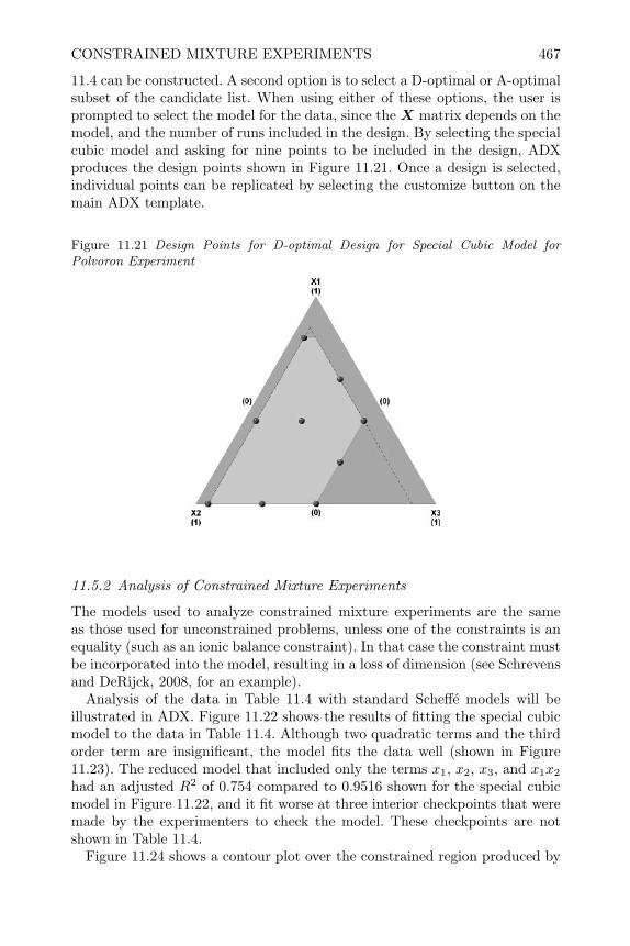
CONSTRAINED MIXTURE EXPERIMENTS 467
11.4 can be constructed. A second option is to select a D-optimal or A-optimalsubset of the candidate list. When using either of these options, the user isprompted to select the model for the data, since the X matrix depends on themodel, and the number of runs included in the design. By selecting the specialcubic model and asking for nine points to be included in the design, ADXproduces the design points shown in Figure 11.21. Once a design is selected,individual points can be replicated by selecting the customize button on themain ADX template.
Figure 11.21 Design Points for D-optimal Design for Special Cubic Model forPolvoron Experiment
11.5.2 Analysis of Constrained Mixture Experiments
The models used to analyze constrained mixture experiments are the sameas those used for unconstrained problems, unless one of the constraints is anequality (such as an ionic balance constraint). In that case the constraint mustbe incorporated into the model, resulting in a loss of dimension (see Schrevensand DeRijck, 2008, for an example).
Analysis of the data in Table 11.4 with standard Scheffe models will beillustrated in ADX. Figure 11.22 shows the results of fitting the special cubicmodel to the data in Table 11.4. Although two quadratic terms and the thirdorder term are insignificant, the model fits the data well (shown in Figure11.23). The reduced model that included only the terms x1, x2, x3, and x1x2
had an adjusted R2 of 0.754 compared to 0.9516 shown for the special cubicmodel in Figure 11.22, and it fit worse at three interior checkpoints that weremade by the experimenters to check the model. These checkpoints are notshown in Table 11.4.
Figure 11.24 shows a contour plot over the constrained region produced by
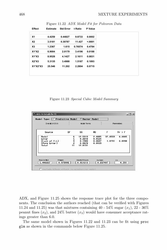
468 MIXTURE EXPERIMENTS
Figure 11.22 ADX Model Fit for Polvoron Data
Effect Estimate Std Error t Ratio P Value
X1 4.4259 0.44827 9.8733 0.0002
X2 3.5181 0.30787 11.427 <.0001
X3 1.2367 1.615 0.76574 0.4784
X1*X2 6.9004 2.0179 3.4196 0.0188
X1*X3 8.9528 4.1427 2.1611 0.0831
X2*X3 5.3135 3.4988 1.5187 0.1893
X1*X2*X3 25.546 11.202 2.2804 0.0715
Figure 11.23 Special Cubic Model Summary
ADX, and Figure 11.25 shows the response trace plot for the three compo-nents. The conclusion the authors reached (that can be verified with Figures11.24 and 11.25) was that mixtures containing 40 - 54% sugar (x1), 22 - 36%peanut fines (x2), and 24% butter (x3) would have consumer acceptance rat-ings greater than 6.0.
The same model shown in Figures 11.22 and 11.23 can be fit using procglm as shown in the commands below Figure 11.25.
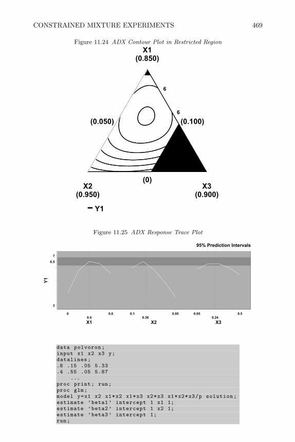
CONSTRAINED MIXTURE EXPERIMENTS 469
Figure 11.24 ADX Contour Plot in Restricted Region
X1(0.850)
(0)
(0.100)
X2(0.950)
(0.050)
X3(0.900)
6
6
Y1
Figure 11.25 ADX Response Trace Plot
0.4 0.36 0.24
6.5
3
7
Y1
95% Prediction Intervals
8.00
X1
59.01.0
X2
5.050.0
X3
data polvoron;input x1 x2 x3 y;datalines;.8 .15 .05 5.33.4 .55 .05 5.87
...proc print; run;proc glm;model y=x1 x2 x1*x2 x1*x3 x2*x3 x1*x2*x3/p solution;estimate ’beta1’ intercept 1 x1 1;estimate ’beta2’ intercept 1 x2 1;estimate ’beta3’ intercept 1;run;

470 MIXTURE EXPERIMENTS
By leaving x3 out of the model and not using the /noint option, proc glmwill calculate R2 correctly for the Scheffe model, and by including the threeestimate statements, proc glm will produce the estimates of β1, β2, and β3
from the Scheffe quadratic model.
11.6 Blocking Mixture Experiments
Whenever experimental units for a mixture experiment (which may simplybe the conditions that exist at the time a mixture is made and tested) arenot homogeneous, a blocked design should be used. Levels of a blocking factorcould include things such as the batches of mixture components or the times ordifferent pieces of equipment used to test and measure a response. If runs canbe blocked into groups that are large enough to include a complete replicateof the mixture experiment, a complete block design can be utilized. On theother hand, if the block size is smaller than a complete replicate of the mixturedesign, some kind of incomplete block design must be used.
In the discussion of incomplete block designs for 2k factorials in Section 7.6and of standard response surface experiments in Section 10.8, an importantfeature of the blocked design was to have the blocks orthogonal to the codedfactor levels. In this way, the factor effects were unconfounded with the blockeffects or unaffected by the block differences. It is more difficult to achieveorthogonal incomplete block designs for mixture experiments because, exceptfor the SLDk,1, the mixture designs themselves are not orthogonal.
If a mixture experiment in which N not necessarily unique mixture blendsare to be arranged in t blocks, where the wth block contains nw blends andn1 + n2 + · · · + nt = N , then Nigam (1970), Nigam (1977) and John (1984)suggested conditions on the moments that ensure orthogonal blocks. For theScheffe second-degree model these conditions are
nw∑u=1
xui = ci for each block, i = 1, 2, . . . , k
nw∑u=1
xuixuj = cij for each block, i, j = 1, 2, . . . , k; i 6= j. (11.21)
This means that the sum of proportions for component i must be the samevalue, ci, in each of the blocks, but it is not necessary that c1 = c2, . . . = ck;and the sum of the products of proportions for components i and j are thesame within each block, but it is not necessary that cij = ci′j′ .
Cornell (2002) presented an example of an orthogonally blocked mixturedesign in three components (shown in Table 11.5). From this table, it can beverified that the conditions shown in Equation (11.21) hold, and this designcan be visualized in Figure 11.26. The first block consists of all the mixtures inan SLD3,2 design, and the second block consists of an SLD3,1 augmentedwith three axial points. While the order of making and testing the mixtures fordesigns presented earlier in this chapter should be conducted in a completely
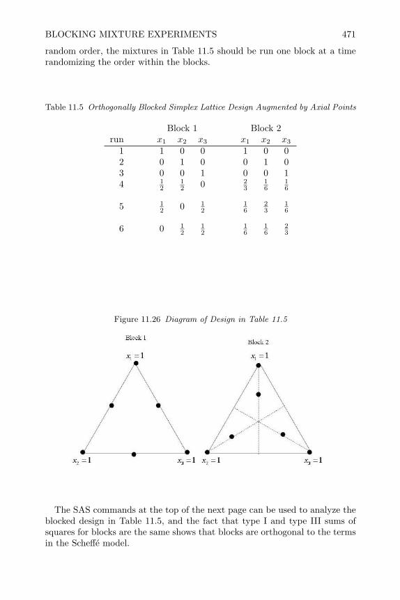
BLOCKING MIXTURE EXPERIMENTS 471
random order, the mixtures in Table 11.5 should be run one block at a timerandomizing the order within the blocks.
Table 11.5 Orthogonally Blocked Simplex Lattice Design Augmented by Axial Points
Block 1 Block 2run x1 x2 x3 x1 x2 x3
1 1 0 0 1 0 02 0 1 0 0 1 03 0 0 1 0 0 14 1
212 0 2
316
16
5 12 0 1
216
23
16
6 0 12
12
16
16
23
Figure 11.26 Diagram of Design in Table 11.5
The SAS commands at the top of the next page can be used to analyze theblocked design in Table 11.5, and the fact that type I and type III sums ofsquares for blocks are the same shows that blocks are orthogonal to the termsin the Scheffe model.
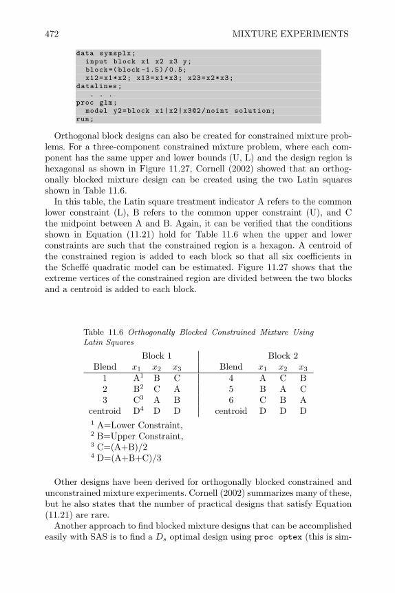
472 MIXTURE EXPERIMENTS
data symsplx;input block x1 x2 x3 y;block=(block -1.5)/0.5;x12=x1*x2; x13=x1*x3; x23=x2*x3;
datalines;. . .
proc glm;model y2=block x1|x2|x3@2/noint solution;
run;
Orthogonal block designs can also be created for constrained mixture prob-lems. For a three-component constrained mixture problem, where each com-ponent has the same upper and lower bounds (U, L) and the design region ishexagonal as shown in Figure 11.27, Cornell (2002) showed that an orthog-onally blocked mixture design can be created using the two Latin squaresshown in Table 11.6.
In this table, the Latin square treatment indicator A refers to the commonlower constraint (L), B refers to the common upper constraint (U), and Cthe midpoint between A and B. Again, it can be verified that the conditionsshown in Equation (11.21) hold for Table 11.6 when the upper and lowerconstraints are such that the constrained region is a hexagon. A centroid ofthe constrained region is added to each block so that all six coefficients inthe Scheffe quadratic model can be estimated. Figure 11.27 shows that theextreme vertices of the constrained region are divided between the two blocksand a centroid is added to each block.
Table 11.6 Orthogonally Blocked Constrained Mixture UsingLatin Squares
Block 1 Block 2Blend x1 x2 x3 Blend x1 x2 x3
1 A1 B C 4 A C B2 B2 C A 5 B A C3 C3 A B 6 C B A
centroid D4 D D centroid D D D1 A=Lower Constraint,2 B=Upper Constraint,3 C=(A+B)/24 D=(A+B+C)/3
Other designs have been derived for orthogonally blocked constrained andunconstrained mixture experiments. Cornell (2002) summarizes many of these,but he also states that the number of practical designs that satisfy Equation(11.21) are rare.
Another approach to find blocked mixture designs that can be accomplishedeasily with SAS is to find a Ds optimal design using proc optex (this is sim-
BLOCKING MIXTURE EXPERIMENTS 473
Figure 11.27 Orthogonally Blocked Constrained Mixture Design
11 =x
12 =x 13 =x
Block 1 Block 2
L
U
ilar to what was done for response surface designs in Section 10.8). Atkinsonet al. (2007) show several examples of D-optimal blocked mixture experiments.Although D-optimal blocked designs are not orthogonally blocked, Goos andDonev (2006) show that they are actually more efficient in the sense of reduc-ing variances of the estimated coefficients, and they can be created for a widevariety of situations. For example, the SAS code below shows how to createan unconstrained mixture experiment in three components blocked into twoblocks of 4. In this example, a set of candidate mixtures is created using asimplex lattice3,3 design or SLD3,3 (created by the macro %adxsld) aug-mented by interior points created by the macro %adxfill that averages eachpair of points.
%adxgen%adxmix%adxinit%adxsld(scd ,x1 x2 x3 ,3)%adxfill(scd ,x1 x2 x3)proc print; run;proc optex data=scd coding=orthcan seed =2347;
model x1|x2|x3@2/noint;blocks structure =(2)4;generate n=8 niter =1000 keep =10;output out=bdesign blockname=block; run;
proc print data=bdesign; run;
The D-optimal design is not unique, but it always consists of points aroundthe perimeter of the simplex, as shown in Figure 11.28, rather than includinginterior points, as did the orthogonally blocked design shown in Figure 11.26.

474 MIXTURE EXPERIMENTS
Figure 11.28 D-optimal Blocked Mixture Experiment
11 =x
12 =x 13 =x 13 =x12 =x
11 =x
Block 1Block 2
By changing the file of candidate mixtures, D-optimal blocked designs forconstrained mixture experiments can also be created easily. To illustrate this,consider the example presented by Goos and Donev (2006). The experimentinvestigated the surface adhesive properties of polypropylene used in the Bel-gian car industry. The mixture components were x1: talcum, x2: mica, andx3: polypropylene. The following constraints applied:
0.0 ≤x1 ≤ 0.10.0 ≤x2 ≤ 0.1
0.0 ≤ x1 + x2 ≤ 0.15
Ten tests could be run in two days, so the experiment had to be blocked intwo sets of five.
The SAS code below creates a candidate file of extreme vertices, using themacro %adxxvert, augmented with interior points created by %adxfill. Thenext data step removes the vertices that violate the last constraint, and finallyproc optex is used to create the design in two blocks of 5.
%adxgen%adxmix%adxxvert(ev ,x1 0-.1/ x2 0-.1/x3);%adxfill(ev,x1 x2 x3);data ev; set ev;if 0 <= x1+x2 <= 0.1501;proc optex data=ev coding=orthcan seed =2347;
model x1|x2|x3@2/noint;blocks structure =(2)5;generate n=10 niter =1000 keep =10;output out=bdesign blockname=block; run;
proc print data=bdesign; run;
A printout of the resulting file work.bdesign is shown on the next page.
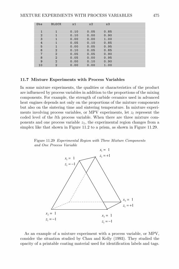
MIXTURE EXPERIMENTS WITH PROCESS VARIABLES 475
Obs BLOCK x1 x2 x3
1 1 0.10 0.05 0.852 1 0.10 0.00 0.903 1 0.00 0.00 1.004 1 0.05 0.10 0.855 1 0.00 0.05 0.956 2 0.10 0.05 0.857 2 0.05 0.05 0.908 2 0.05 0.00 0.959 2 0.00 0.10 0.90
10 2 0.00 0.00 1.00
11.7 Mixture Experiments with Process Variables
In some mixture experiments, the qualities or characteristics of the productare influenced by process variables in addition to the proportions of the mixingcomponents. For example, the strength of carbide ceramics used in advancedheat engines depends not only on the proportions of the mixture componentsbut also on the sintering time and sintering temperature. In mixture experi-ments involving process variables, or MPV experiments, let zl represent thecoded level of the lth process variable. When there are three mixture com-ponents and one process variable z1, the experimental region changes from asimplex like that shown in Figure 11.2 to a prism, as shown in Figure 11.29.
Figure 11.29 Experimental Region with Three Mixture Componentsand One Process Variable
11
1
3
−==
zx
11
1
3
+==
zx
11
1
1
+==
zx
11
1
2
−==
zx
11
1
1
−==
zx
As an example of a mixture experiment with a process variable, or MPV,consider the situation studied by Chau and Kelly (1993). They studied theopacity of a printable coating material used for identification labels and tags.
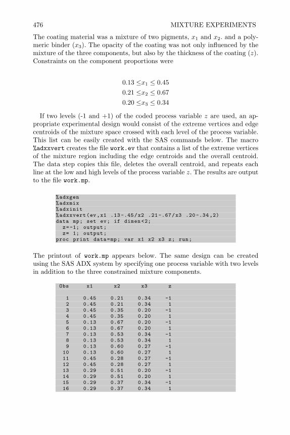
476 MIXTURE EXPERIMENTS
The coating material was a mixture of two pigments, x1 and x2. and a poly-meric binder (x3). The opacity of the coating was not only influenced by themixture of the three components, but also by the thickness of the coating (z).Constraints on the component proportions were
0.13 ≤x1 ≤ 0.450.21 ≤x2 ≤ 0.670.20 ≤x3 ≤ 0.34
If two levels (-1 and +1) of the coded process variable z are used, an ap-propriate experimental design would consist of the extreme vertices and edgecentroids of the mixture space crossed with each level of the process variable.This list can be easily created with the SAS commands below. The macro%adxxvert creates the file work.ev that contains a list of the extreme verticesof the mixture region including the edge centroids and the overall centroid.The data step copies this file, deletes the overall centroid, and repeats eachline at the low and high levels of the process variable z. The results are outputto the file work.mp.
%adxgen%adxmix%adxinit%adxxvert(ev ,x1 .13 -.45/x2 .21 -.67/x3 .20 -.34 ,2)data mp; set ev; if dimen <2;
z=-1; output;z= 1; output;
proc print data=mp; var x1 x2 x3 z; run;
The printout of work.mp appears below. The same design can be createdusing the SAS ADX system by specifying one process variable with two levelsin addition to the three constrained mixture components.
Obs x1 x2 x3 z
1 0.45 0.21 0.34 -12 0.45 0.21 0.34 13 0.45 0.35 0.20 -14 0.45 0.35 0.20 15 0.13 0.67 0.20 -16 0.13 0.67 0.20 17 0.13 0.53 0.34 -18 0.13 0.53 0.34 19 0.13 0.60 0.27 -1
10 0.13 0.60 0.27 111 0.45 0.28 0.27 -112 0.45 0.28 0.27 113 0.29 0.51 0.20 -114 0.29 0.51 0.20 115 0.29 0.37 0.34 -116 0.29 0.37 0.34 1

MIXTURE EXPERIMENTS WITH PROCESS VARIABLES 477
11.7.1 Models for Mixture Experiments With Process Variables
The model for a mixture experiment with process variables results from cross-ing the model for the mixture components and the model for the processvariables. For fixed levels of the process variables, the model for the mixturecomponents is
ηx = f(x), (11.22)
and the model for the process variables is
ηz = g(z), (11.23)
where f(x) is the Scheffe linear, quadratic, or cubic mixture model, and g(z) isthe linear or general quadratic model for independent factors. The combinedmodel is then found as the cross-product ηxz = (f(x))× (g(z)). For example,assuming a quadratic mixture model for the coating experiment where therewere three mixture components and one two-level process variable,
f(x) = β1x1 + β2x2 + β3x3 + β12x1x2 + β13x1x3 + β23x2x3,
andg(z) = α0 + α1z.
The combined model is
ηxz =β1(z)x1 + β2(z)x2 + β3(z)x3 + β12(z)x1x2 + β13(z)x1x3
+ β23(z)x2x3, (11.24)
where βi(z) = βi × (α0 + α1z).
Multiplying the terms we can write this model as:
ηxz =γ01x1 + γ0
2x2 + γ03x3 + γ0
12x1x2 + γ013(z)x1x3 + γ0
23(z)x2x3+
γ11x1z + γ1
2x2z + γ13x3z + γ1
12x1x2z + γ113x1x3z + γ0
23x2x3z, (11.25)
where γ0i = βi × α0 and γ1
i = βi × α1.In this model, the first six terms represent the linear and quadratic blending
of the mixture components since these terms involve only the mixture com-ponents. The last six terms in the model represent the changes in the linearand quadratic blending effects caused by changes in the process variable.
If the process variable has a constant effect on the response, which wouldcause the same change in all blends of the mixture components, there is noterm in model 11.25 that can represent the constant effect of the processvariable. Gorman and Cornell (1982) have suggested an alternate form of themodel substituting (1 − x2 − x3) for x1 in the term γ1
1x1z, resulting in themodel

478 MIXTURE EXPERIMENTS
ηxz =γ01x1 + γ0
2x2 + γ03x3 + γ0
12x1x2 + γ013(z)x1x3 + γ0
23(z)x2x3+
γ11z + γ2
2x2z + γ23x3z + γ1
12x1x2z + γ113x1x3z + γ0
23x2x3z, (11.26)
where γ2i = γ1
i − γ11 for i = 2, 3. If the process variable has a constant effect
on the response, the last five terms in the model would be zero, and γ11 will
represent the constant effect of the process variable.Another model that allows isolation of process variable effects can be ob-
tained by first translating the mixture components (x1, x2, and x3) to indepen-dent factors (w1, w2) as shown in Section 11.2.2, then writing the combinedmodel as the cross-product of the model for the w’s and the z’s.
11.7.2 Multiple Process Variables and Mixture Components
Figure 11.30 shows the design for an MPV with three mixture componentsand two process variables. The 6-run SLD3,2 for the mixture components iscrossed with a 4-run 22 design in the process variables, resulting in a productarray of 6 × 4 = 24 experiments. The runs in the design can be representedgraphically as a 22 design with a simplex-lattice repeated at each corner, asshown on the left side of the figure, or as a simplex lattice with a 22 designrepeated at each lattice point as shown on the right side of the figure.
Figure 11.30 Experimental Region with Three Mixture Components and Two ProcessVariables
This design can be easily created in SAS by repeating the six runs of thesimplex-lattice at each run of a 22 factorial created by proc factex as shownin the code at the top of the next page.

MIXTURE EXPERIMENTS WITH PROCESS VARIABLES 479
*Create Simplex -lattice design;%adxgen%adxmix%adxinit%adxsld(sld , x1 x2 x3 ,2)*Repeat the sld for each run in a 2x2 factorial
design;proc factex;
factors z1 z2;size design =4; model estimate =(z1|z2);output out=combdes pointrep=sld;
proc print; run;
However, as the number of mixture components and process variables in-creases, cross-product designs can become unwieldy. For example, if there arefour mixture components and five process variables, the simplex-lattice4,2design has only 10 runs, but the 25 design in the process variables has 32 runs,and the cross-product design has 320 runs.
In most industrial experimentation, restrictions due to time and cost pro-hibit such large designs. Cornell and Gorman (1984) proposed running frac-tions of the 2p design in the process variables. Linear designs in the mixturecomponents can also be employed to reduce the total number of runs. For ex-ample, in the case of four mixture components and five process variables, if an8-run resolution III fractional factorial in the process variables is substitutedfor the 25 design, and a 4-run SLD4,1 is substituted for the SLD4,2, thetotal number of experiments could be reduced to 4× 8 = 32 and would allowfor fitting the model
ηxz =γ01x1 + γ0
2x2 + γ03x3 + γ0
4x4+
γ11x1z1 + γ1
2x2z1 + γ13x3z1 + γ1
4x4z1+
γ21x1z2 + γ2
2x2z2 + γ23x3z2 + γ2
4x4z2+
γ31x1z3 + γ3
2x2z3 + γ33x3z3 + γ3
4x4z3+
γ41x1z4 + γ4
2x2z4 + γ43x3z4 + γ4
4x4z4+
γ51x1z5 + γ5
2x2z5 + γ53x3z5 + γ5
4x4z5
But, this model only allows for linear blending and seeing how the predictedresponse at the pure components (as shown in Figure 11.4) is affected bythe process variables. On the other hand, if the experimenter can proposea reasonable model to investigate, an economical design can be found usingoptimal design theory.
For example, the 40-term model in Equation (11.27) on the next page,that is a subset of the terms in an expanded version of Equation (11.26),was proposed by Kowalski et al. (2000). It includes the quadratic mixturemodel as well as interactions among the main effects of the process variables

480 MIXTURE EXPERIMENTS
and interactions between the main effects of the process variables and thelinear blending terms of the mixture components. In their article, Kowalskiet al. (2000) considered a simple situation with three mixture componentsand two process variables, and they proposed two specific designs to allowfitting a subset of model 11.27. Their designs performed well in terms of D-efficiency for the specific situation with three mixture components and twoprocess variables, but for the more general case, a D-optimal search will finda reasonable design.
ηxz =γ01x1 + γ0
2x2 + γ03x3 + γ0
4x4 + γ012x1x2 + γ0
13x1x3 + γ014x1x4 + γ0
23x2x3
+ γ024x2x4 + γ0
34x3x4 + γ112z1z2 + γ1
13z1z3 + γ114z1z4 + γ1
15z1z5 + γ123z2z3
+ γ124z2z4 + γ1
25z2z5 + γ134z3z4 + γ1
35z3z5 + γ145z4z5 + γ2
11x1z1 + γ212x1z2
+ γ213x1z3 + γ2
14x1z4 + γ215x1z5 + γ2
21x2z1 + γ222x2z2 + γ2
23x2z3 + γ224x2z4
+ γ225x2z5 + γ2
31x3z1 + γ232x3z2 + γ2
33x3z3 + γ234x3z4 + γ2
35x3z5 + γ241x4z1
+ γ242x4z2 + γ2
43x4z3 + γ244x4z4 + γ2
45x5z5 (11.27)
At least 40 experiments must be performed to collect the data necessary forestimating the coefficients in model 11.27, and a 44-run D-optimal set can beeasily obtained using proc optex as shown in the commands below.
*Create Simplex -lattice design;%adxgen%adxmix%adxinit%adxsld(sld , x1 x2 x3 x4 ,2)*Repeat sld for each run in 2^5 factorial design;proc factex;
factors z1 z2 z3 z4 z5;size design =32;output out=combdes pointrep=sld;
run;*Use Combined Design as candidates and find D-optimal design;proc optex data=combdes coding=orthcan seed =2347;
model x1|x2|x3|x4@2 z1*z2 z1*z3 z1*z4 z1*z5 z2*z3 z2*z4z2*z5 z3*z4 z3*z5 z4*z5 x1*z1 x1*z2 x1*z3 x1*z4x1*z5 x2*z1 x2*z2 x2*z3 x2*z4 x2*z5 x3*z1 x3*z2x3*z3 x3*z4 x3*z5 x4*z1 x4*z2 x4*z3 x4*z4 x4*z5/noint;
generate n=44 niter =1000 keep =10;output out=dopt; run;
proc print data=dopt; run;
In these commands, the %adxsld macro is used to create the 10-run SLD4,2design, and proc factex is used to combine this design with the 25 design.This combined design, (work.combdes) is used as a set of candidates for procoptex, which finds a 44-run D-optimal subset.
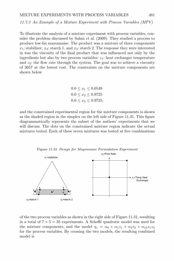
MIXTURE EXPERIMENTS WITH PROCESS VARIABLES 481
11.7.3 An Example of a Mixture Experiment with Process Variables (MPV)
To illustrate the analysis of a mixture experiment with process variables, con-sider the problem discussed by Sahni et al. (2009). They studied a process toproduce low-fat mayonnaise. The product was a mixture of three componentsx1: stabilizer, x2: starch 1, and x3: starch 2. The response they were interestedin was the viscosity of the final product that was influenced not only by theingredients but also by two process variables: z1: heat exchanger temperatureand z2: the flow rate through the system. The goal was to achieve a viscosityof 3657 at the lowest cost. The constraints on the mixture components areshown below
0.0 ≤ x1 ≤ 0.05490.0 ≤ x2 ≤ 0.97250.0 ≤ x3 ≤ 0.9725,
and the constrained experimental region for the mixture components is shownas the shaded region in the simplex on the left side of Figure 11.31. This figurediagrammatically represents the subset of the authors’ experiments that wewill discuss. The dots on the constrained mixture region indicate the actualmixtures tested. Each of these seven mixtures was tested at five combinations
Figure 11.31 Design for Mayonnaise Formulation Experiment
x2=starch 1
x1=stabilizer
x3=starch 2
3
542
7 1 6
z1=Temp Heat Exchanger
z2=Flow Rate
of the two process variables as shown in the right side of Figure 11.31, resultingin a total of 7× 5 = 35 experiments. A Scheffe quadratic model was used forthe mixture components, and the model ηz = α0 + α1z1 + α2z2 + α12z1z2
for the process variables. By crossing the two models, the resulting combinedmodel is
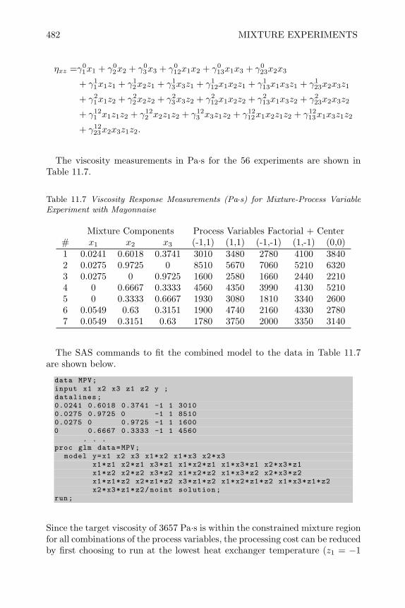
482 MIXTURE EXPERIMENTS
ηxz =γ01x1 + γ0
2x2 + γ03x3 + γ0
12x1x2 + γ013x1x3 + γ0
23x2x3
+ γ11x1z1 + γ1
2x2z1 + γ13x3z1 + γ1
12x1x2z1 + γ113x1x3z1 + γ1
23x2x3z1
+ γ21x1z2 + γ2
2x2z2 + γ23x3z2 + γ2
12x1x2z2 + γ213x1x3z2 + γ2
23x2x3z2
+ γ121 x1z1z2 + γ12
2 x2z1z2 + γ123 x3z1z2 + γ12
12x1x2z1z2 + γ1213x1x3z1z2
+ γ1223x2x3z1z2.
The viscosity measurements in Pa·s for the 56 experiments are shown inTable 11.7.
Table 11.7 Viscosity Response Measurements (Pa·s) for Mixture-Process VariableExperiment with Mayonnaise
Mixture Components Process Variables Factorial + Center# x1 x2 x3 (-1,1) (1,1) (-1,-1) (1,-1) (0,0)1 0.0241 0.6018 0.3741 3010 3480 2780 4100 38402 0.0275 0.9725 0 8510 5670 7060 5210 63203 0.0275 0 0.9725 1600 2580 1660 2440 22104 0 0.6667 0.3333 4560 4350 3990 4130 52105 0 0.3333 0.6667 1930 3080 1810 3340 26006 0.0549 0.63 0.3151 1900 4740 2160 4330 27807 0.0549 0.3151 0.63 1780 3750 2000 3350 3140
The SAS commands to fit the combined model to the data in Table 11.7are shown below.
data MPV;input x1 x2 x3 z1 z2 y ;datalines;0.0241 0.6018 0.3741 -1 1 30100.0275 0.9725 0 -1 1 85100.0275 0 0.9725 -1 1 16000 0.6667 0.3333 -1 1 4560
. . .proc glm data=MPV;
model y=x1 x2 x3 x1*x2 x1*x3 x2*x3x1*z1 x2*z1 x3*z1 x1*x2*z1 x1*x3*z1 x2*x3*z1x1*z2 x2*z2 x3*z2 x1*x2*z2 x1*x3*z2 x2*x3*z2x1*z1*z2 x2*z1*z2 x3*z1*z2 x1*x2*z1*z2 x1*x3*z1*z2x2*x3*z1*z2/noint solution;
run;
Since the target viscosity of 3657 Pa·s is within the constrained mixture regionfor all combinations of the process variables, the processing cost can be reducedby first choosing to run at the lowest heat exchanger temperature (z1 = −1

MIXTURE EXPERIMENTS WITH PROCESS VARIABLES 483
in coded units) and the fastest flow rate (z2 = +1 in coded units). By settingz1 = −1 and z2 = +1, the fitted equation simplifies to
Predicted viscosity =229186.40x1 + 11487.06x2 + 817.8356x3 − 346975x1x2
− 194919x1x3 − 12628.5x2x3.
Additional costs were incurred for the three raw materials and they couldbe summarized in the simple equation shown below (in units of NorwegianKroner, NOK), where mixture component x1: stabilizer is the most costlyingredient.
Raw Material Cost = 54.59x1 + 5.69x2 + 7.49x3
To find the mixture combination that minimizes cost while meeting the tar-get viscosity, nonlinear optimization similar to the example shown in Section10.7.5 can be used. The SAS proc nlp commands to find the optimum areshown in the listing below. This example uses proc nlp to minimize cost ofthe raw materials subject to constraints. The bounds on the mixture com-ponents are given in the bounds statement, the constraint that the mixturecomponents add to one is given as a linear constraint, and the constraint thatthe predicted viscosity is 3657 is given as a nonlinear constraint.
proc nlp;min cost;parms x1 x2 x3 = .0241 .6018 .3741;bounds 0 <= x1 <= 0.0549 ,
0 <= x2 <= 0.9725 ,0 <= x3 <= 0.9725;
lincon x1+x2+x3=1;nlincon viscos =3657;viscos =229186.4*x1 +11487.06*x2 +817.8356*x3 -346975*x1*x2 -194919
*x1*x3 -12628.5*x2*x3;cost =54.59*x1+5.69*x2+7.49*x3;run;
The resulting minimum cost for raw materials is 6.49 NOK at the combinationof mixture components x1 = 0.0, x2 = 0.558, and x3 = 0.442, where none ofthe more expensive stabilizer is used. This optimum can be visualized on thecontour plot of predicted viscosity over the constrained mixture region shownin Figure 11.32.
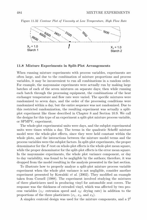
484 MIXTURE EXPERIMENTS
Figure 11.32 Contour Plot of Viscosity at Low Temperature, High Flow Rate
X2 = 1.0Starch 1
X3 = 1.0Starch 2
11.8 Mixture Experiments in Split-Plot Arrangements
When running mixture experiments with process variables, experiments areoften large, and due to the combination of mixture proportions and processvariables, it may be inconvenient to run all combinations in a random order.For example, the mayonnaise experiments were actually run by making largebatches of each of the seven mixtures on separate days; then while runningeach batch through the processing equipment, the combinations of the heatexchanger temperature and flow rate were varied. The specific mixtures wererandomized to seven days, and the order of the processing conditions wererandomized within a day, but the entire sequence was not randomized. Due tothis restricted randomization, the resulting experiment was actually a split-plot experiment like those described in Chapter 8 and Section 10.9. We callthe designs for this type of an experiment a split-plot mixture process variable,or SPMPV, experiment.
The whole-plot experimental units were days, and the subplot experimentalunits were times within a day. The terms in the quadratic Scheffe mixturemodel were the whole-plot effects, since they were held constant within thewhole plots, and the interactions between the mixture model terms and theprocess variables were the subplot factors. In split-plot experiments, the properdenominator for the F -test on whole-plot effects is the whole-plot mean square,while the proper denominator for the split-plot effects is the error mean square.In the mayonnaise experiments, the whole plot variance component, or dayto day variability, was found to be negligible by the authors; therefore, it wasdropped from the model resulting in the analysis presented in the last section.
To illustrate how to properly analyze a split-plot mixture process variableexperiment when the whole plot variance is not negligible, consider anotherexperiment presented by Kowalski et al. (2002). They modified an exampletaken from Cornell (1988). The experiment involved studying the mixturesof three plasticizers used in producing vinyl for automobile seat covers. Theresponse was the thickness of extruded vinyl, which was affected by two pro-cess variables (z1: extrusion speed and z2: drying rate) in addition to theproportions of the three plasticizers (x1, x2, and x3).
A simplex centroid design was used for the mixture components, and a 22

MIXTURE EXPERIMENTS IN SPLIT-PLOT ARRANGEMENTS 485
factorial plus three replicate center points were used for the process variables.In this example, the process variables were hard to change and were heldconstant in blocks, while a random subset of the mixtures in the simplexcentroid design was formulated and processed. With this scheme, the processvariables were the whole-plot effects, and the mixture components, which werevaried within each set of constant process variable settings, were the subploteffects.
To combine the simplex-centroid in the mixture components, with the 22
factorial plus three replicate center points in the process variables would re-quire a total of 7×7 = 49 runs. However, to fit a model of the form of Equation(11.28) (the general form of equation 11.27 proposed by Kowalski et al. (2000))with only k = 3 mixture components and n = 2 process variables does notrequire that many experiments.
ηzx =k∑i=1
βixi +∑ k∑i<j
βijxixj +∑ n∑l<m
αlmzlzm +k∑i=1
n∑l=1
γilxizl (11.28)
The 28 experiments listed data in Table 11.8 are sufficient. This table showsthe thickness measurements taken from a fractional split-plot design suggestedby Kowalski et al. (2002) for fitting a model of the form of Equation 11.28with three mixture components and three process variables. The table showsthat the vertices of the simplex-centroid design plus one centroid were selectedto be run in the whole plots where z1: extrusion speed was low and z2: dryingtime was high (and vice versa), while the binary mixtures plus the centroidwere selected to be run in the whole plots where both process variables wereeither at their high or low settings. Four replicates of the mixture centroidwere run in the three whole plots where both process variables were at theirmid settings.
Table 11.8 Vinyl Thickness Values for Example Experiment
Mixture Component Combinationsz1 z2 (100) (010) (001) ( 1
2120) ( 1
20 12 ) (0 1
212 ) ( 1
313
13 )
-1 1 10 8 3 81 -1 10 5 9 91 1 5 4 7 10-1 -1 7 8 4 70 0 8, 7
7, 80 0 7, 8
9, 90 0 12, 10
9, 11

486 MIXTURE EXPERIMENTS
In order to get accurate estimates of the effects and their standard errorswith data from a split-plot mixture process variable experiment, proc mixedcan be used, which by default uses the REML method described in Section10.9. For example, the SAS commands to fit the model to the data in Table11.8 are shown below.
data SPMPV;input WP z1 z2 x1 x2 x3 y ;datalines;1 -1 1 1.00 0.00 0.00 101 -1 1 0.00 1.00 0.00 81 -1 1 0.00 0.00 1.00 31 -1 1 0.33 0.33 0.34 82 1 -1 1.00 0.00 0.00 102 1 -1 0.00 1.00 0.00 52 1 -1 0.00 0.00 1.00 92 1 -1 0.33 0.33 0.34 9
...5 0 0 0.33 0.33 0.34 85 0 0 0.33 0.33 0.34 75 0 0 0.33 0.33 0.34 75 0 0 0.33 0.33 0.34 86 0 0 0.33 0.33 0.34 76 0 0 0.33 0.33 0.34 86 0 0 0.33 0.33 0.34 96 0 0 0.33 0.33 0.34 97 0 0 0.33 0.33 0.34 127 0 0 0.33 0.33 0.34 107 0 0 0.33 0.33 0.34 97 0 0 0.33 0.33 0.34 11proc mixed;
class wp;model y=z1*z2 x1 x2 x3 x1*x2 x1*x3 x2*x3 x1*z1 x2*z1 x3*z1x1*z2 x2*z2 x3*z2/noint solution ddfm=kenwardroger;random wp;
run;
A portion of the resulting output is shown on the next page. There, it can beseen that the variance of whole-plot experimental units is estimated as σ2
wp =1.578 and the variance of subplot experimental is estimated as σ2
sp = 1.9014.If the standard least squares estimates are used, rather than the REML esti-mates, the subplot effects will be estimated inaccurately, and their standarderrors will be underestimated, as was the case for split-plot response surfacedesigns shown in Table 10.10.
The design shown in Table 11.8 is balanced, in that the whole simplex-centroid design in mixture components is repeated for both levels of one pro-cess variable when the other is ignored, and it has center points at xi = 1
3 andzj = 0 for i = 1, 3 and j = 1, 2, which allow for testing the goodness of fit ofmodel 11.28. However, Goos and Donev (2007) point out two shortcomings ofthe design shown in Table 11.8. The first shortcoming is that the parametersof interest in model 11.28 are not estimated precisely with this design becausehalf of the runs in the design are center points used to estimate pure error andtest lack of fit. The second shortcoming is that this design is not flexible forpractical situations in which the number of runs possible within each whole
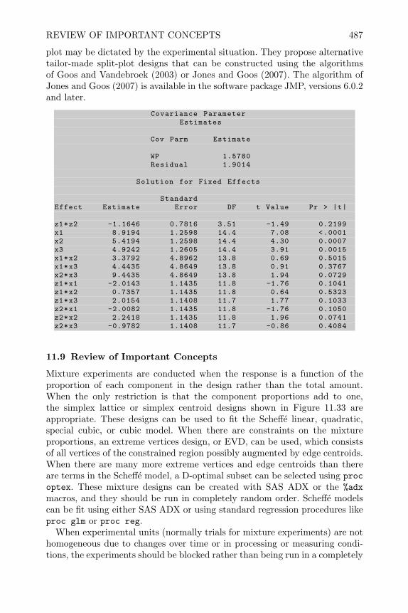
REVIEW OF IMPORTANT CONCEPTS 487
plot may be dictated by the experimental situation. They propose alternativetailor-made split-plot designs that can be constructed using the algorithmsof Goos and Vandebroek (2003) or Jones and Goos (2007). The algorithm ofJones and Goos (2007) is available in the software package JMP, versions 6.0.2and later.
Covariance ParameterEstimates
Cov Parm Estimate
WP 1.5780Residual 1.9014
Solution for Fixed Effects
StandardEffect Estimate Error DF t Value Pr > |t|
z1*z2 -1.1646 0.7816 3.51 -1.49 0.2199x1 8.9194 1.2598 14.4 7.08 <.0001x2 5.4194 1.2598 14.4 4.30 0.0007x3 4.9242 1.2605 14.4 3.91 0.0015x1*x2 3.3792 4.8962 13.8 0.69 0.5015x1*x3 4.4435 4.8649 13.8 0.91 0.3767x2*x3 9.4435 4.8649 13.8 1.94 0.0729z1*x1 -2.0143 1.1435 11.8 -1.76 0.1041z1*x2 0.7357 1.1435 11.8 0.64 0.5323z1*x3 2.0154 1.1408 11.7 1.77 0.1033z2*x1 -2.0082 1.1435 11.8 -1.76 0.1050z2*x2 2.2418 1.1435 11.8 1.96 0.0741z2*x3 -0.9782 1.1408 11.7 -0.86 0.4084
11.9 Review of Important Concepts
Mixture experiments are conducted when the response is a function of theproportion of each component in the design rather than the total amount.When the only restriction is that the component proportions add to one,the simplex lattice or simplex centroid designs shown in Figure 11.33 areappropriate. These designs can be used to fit the Scheffe linear, quadratic,special cubic, or cubic model. When there are constraints on the mixtureproportions, an extreme vertices design, or EVD, can be used, which consistsof all vertices of the constrained region possibly augmented by edge centroids.When there are many more extreme vertices and edge centroids than thereare terms in the Scheffe model, a D-optimal subset can be selected using procoptex. These mixture designs can be created with SAS ADX or the %adxmacros, and they should be run in completely random order. Scheffe modelscan be fit using either SAS ADX or using standard regression procedures likeproc glm or proc reg.
When experimental units (normally trials for mixture experiments) are nothomogeneous due to changes over time or in processing or measuring condi-tions, the experiments should be blocked rather than being run in a completely
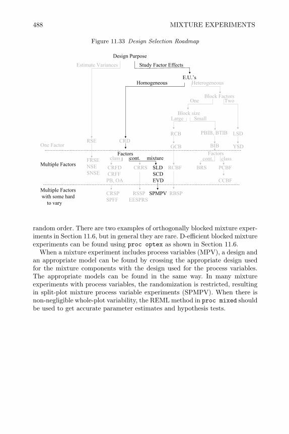
488 MIXTURE EXPERIMENTS
Figure 11.33 Design Selection Roadmap
Design Purpose
Estimate Variances Study Factor Effects
E.U.’s
Block Factors
One Factor
Multiple Factors
Multiple Factorswith some hard
to vary
Block size
Homogeneous Heterogeneous
Large Small
RCB
GCB
PBIB, BTIB
BIB
LSD
YSDRSE CRD
FactorsFRSENSESNSE
CRFD CRRS SLD RCBF BRS PCBFCRFF SCD
PB, OA EVD CCBF
CRSP RSSP SPMPV RBSPSPFF EESPRS
One Two
class cont. mixture cont. classFactors
random order. There are two examples of orthogonally blocked mixture exper-iments in Section 11.6, but in general they are rare. D-efficient blocked mixtureexperiments can be found using proc optex as shown in Section 11.6.
When a mixture experiment includes process variables (MPV), a design andan appropriate model can be found by crossing the appropriate design usedfor the mixture components with the design used for the process variables.The appropriate models can be found in the same way. In many mixtureexperiments with process variables, the randomization is restricted, resultingin split-plot mixture process variable experiments (SPMPV). When there isnon-negligible whole-plot variability, the REML method in proc mixed shouldbe used to get accurate parameter estimates and hypothesis tests.

EXERCISES 489
11.10 Exercises
1. A mixture experiment was run in three components: x1, x2, and x3.
(a) If the Scheffe model that best represented the data was y = 13.5x1 +3.2x2 + 9.8x3, then what is the predicted response at the pure blendx2 = 1.0? What is the predicted response at the 50-50 blend of x1 andx2?
(b) If the Scheffe model that best represented the data was y = 13.5X1 +3.2x2 +9.8x3−2.9x1x2 +8.7X1x3 +0.9x2x3, and the goal was to increasethe response y, then does blending x1 and x2 have an synergistic effector an antagonistic effect? Does blending x1 and x3 have a synergisticeffect or an antagonistic effect? What is the predicted response at themixture of equal proportions for all three components?
2. Belloto et al. (1985) studied the relation between y= Soluability of pheno-barbital and mixture components x1: ethanol, x2: propylene gycol and x3:water.
(a) Use the %adx macros to list the experiments required to fit a linearScheffe model.
(b) Use the %adx macros to list the experiments required to fit a Scheffequadratic model.
(c) Use the %adx macros to list the experiments required to fit a specialcubic model.
(d) Use the %adx macros to list the experiments required to fit a full cubicmodel.
3. Cornell (2002) describes an experiment to make a fruit punch composed ofthree types of juice: x1: watermellon, x2: pineapple, and x3: orange. Thegeneral acceptance of the fruit punch was to be determined by a taste panelthat would rate them on a 1 to 9 scale where 1=dislike extremely, 5=neitherlike nor dislike and 9=like extremely. If the proportions of the three juicesare restricted by cost according to the inequalities below
0.20 ≤ x1 ≤ 0.800.10 ≤ x2 ≤ 0.400.10 ≤ x3 ≤ 0.50
(a) Graph the restricted experimental region within the simplex.
(b) Create a design appropriate for fitting the Scheffe linear model.
(c) Create a design appropriate for fitting the Scheffe quadratic model.
(d) Would there be any value in including an overall centroid or other interiorpoints in the design?

490 MIXTURE EXPERIMENTS
4. In agricultural field tests, two or more herbicides are often mixed togetherin so-called tank mixes in order to find a mixture that is more effective thanindividual herbicides in controlling a multitude of pest weeds. In a specifictest, various mixtures of x1: a herbicide formulated to control broad leafweeds, x2: a herbicide formulated to control grass seedlings, and x3: ageneral-purpose herbicide were tested. The data from the tests are shownin the table below. The response is the proportion of weeds controlled.
Table 11.9 Data from Herbicide Tank Mix Experiment
Mixture Component % Weed ControlRun x1 x2 x3 x1 y
1 1 0 0 732 0 1 0 683 0 0 1 804 1
212 0 77
5 12 0 1
2 86
6 0 12
12 75
7 13
13
13 92
8 13
13
13 93
9 13
13
13 88
(a) Create the design shown in the table above using SAS ADX.
(b) Input the data and fit the Scheffe special cubic model.
(c) Make a contour plot of your fitted model and identify a mixture thatwould result in the highest % weed control.
(d) Transform the mixture components to independent factors and fit thegeneral quadratic model in the independent factors using proc glm orproc reg.
(e) Make a contour plot in the independent factor using proc gcontour asshown in the appendix of this chapter.
5. Consider the problem discussed by Anik and Sukumar (1981). They studiedthe solubility of a butoconazole nitrate imidazole antifungal agent in amixture of x1: polyethylene glycol 400, x2: glycerin, x3: polysorbate 60, x4:water, and x5: poloxamer 407. Constraints on the mixture components areshown below.
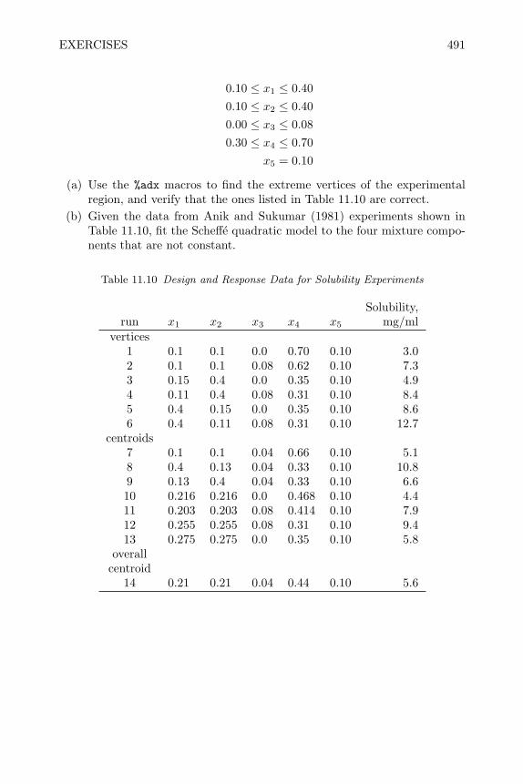
EXERCISES 491
0.10 ≤ x1 ≤ 0.400.10 ≤ x2 ≤ 0.400.00 ≤ x3 ≤ 0.080.30 ≤ x4 ≤ 0.70
x5 = 0.10
(a) Use the %adx macros to find the extreme vertices of the experimentalregion, and verify that the ones listed in Table 11.10 are correct.
(b) Given the data from Anik and Sukumar (1981) experiments shown inTable 11.10, fit the Scheffe quadratic model to the four mixture compo-nents that are not constant.
Table 11.10 Design and Response Data for Solubility Experiments
Solubility,run x1 x2 x3 x4 x5 mg/ml
vertices1 0.1 0.1 0.0 0.70 0.10 3.02 0.1 0.1 0.08 0.62 0.10 7.33 0.15 0.4 0.0 0.35 0.10 4.94 0.11 0.4 0.08 0.31 0.10 8.45 0.4 0.15 0.0 0.35 0.10 8.66 0.4 0.11 0.08 0.31 0.10 12.7
centroids7 0.1 0.1 0.04 0.66 0.10 5.18 0.4 0.13 0.04 0.33 0.10 10.89 0.13 0.4 0.04 0.33 0.10 6.610 0.216 0.216 0.0 0.468 0.10 4.411 0.203 0.203 0.08 0.414 0.10 7.912 0.255 0.255 0.08 0.31 0.10 9.413 0.275 0.275 0.0 0.35 0.10 5.8
overallcentroid
14 0.21 0.21 0.04 0.44 0.10 5.6
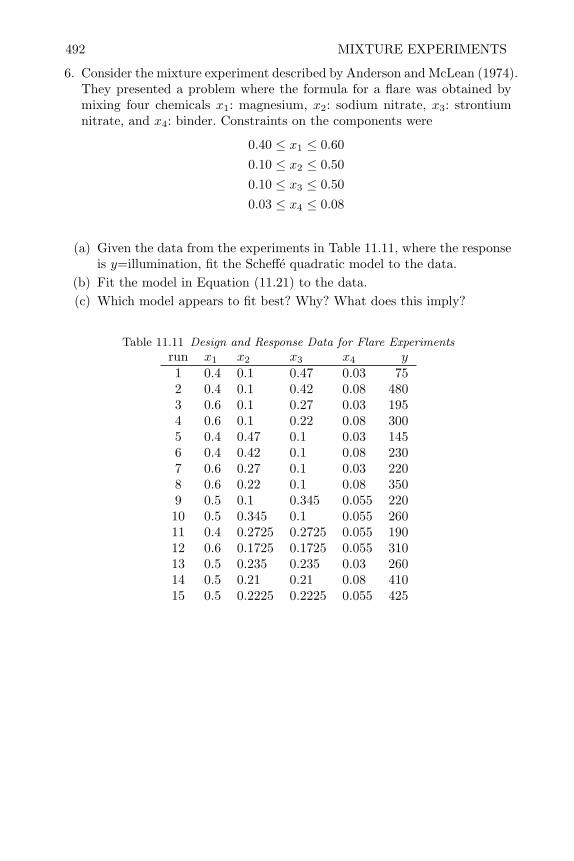
492 MIXTURE EXPERIMENTS
6. Consider the mixture experiment described by Anderson and McLean (1974).They presented a problem where the formula for a flare was obtained bymixing four chemicals x1: magnesium, x2: sodium nitrate, x3: strontiumnitrate, and x4: binder. Constraints on the components were
0.40 ≤ x1 ≤ 0.600.10 ≤ x2 ≤ 0.500.10 ≤ x3 ≤ 0.500.03 ≤ x4 ≤ 0.08
(a) Given the data from the experiments in Table 11.11, where the responseis y=illumination, fit the Scheffe quadratic model to the data.
(b) Fit the model in Equation (11.21) to the data.(c) Which model appears to fit best? Why? What does this imply?
Table 11.11 Design and Response Data for Flare Experimentsrun x1 x2 x3 x4 y
1 0.4 0.1 0.47 0.03 752 0.4 0.1 0.42 0.08 4803 0.6 0.1 0.27 0.03 1954 0.6 0.1 0.22 0.08 3005 0.4 0.47 0.1 0.03 1456 0.4 0.42 0.1 0.08 2307 0.6 0.27 0.1 0.03 2208 0.6 0.22 0.1 0.08 3509 0.5 0.1 0.345 0.055 22010 0.5 0.345 0.1 0.055 26011 0.4 0.2725 0.2725 0.055 19012 0.6 0.1725 0.1725 0.055 31013 0.5 0.235 0.235 0.03 26014 0.5 0.21 0.21 0.08 41015 0.5 0.2225 0.2225 0.055 425
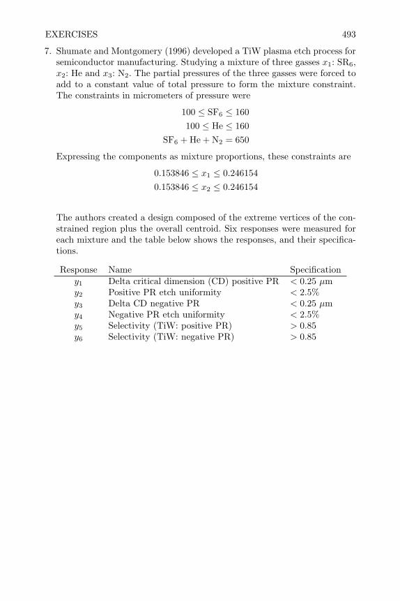
EXERCISES 493
7. Shumate and Montgomery (1996) developed a TiW plasma etch process forsemiconductor manufacturing. Studying a mixture of three gasses x1: SR6,x2: He and x3: N2. The partial pressures of the three gasses were forced toadd to a constant value of total pressure to form the mixture constraint.The constraints in micrometers of pressure were
100 ≤ SF6 ≤ 160100 ≤ He ≤ 160
SF6 + He + N2 = 650
Expressing the components as mixture proportions, these constraints are
0.153846 ≤ x1 ≤ 0.2461540.153846 ≤ x2 ≤ 0.246154
The authors created a design composed of the extreme vertices of the con-strained region plus the overall centroid. Six responses were measured foreach mixture and the table below shows the responses, and their specifica-tions.
Response Name Specificationy1 Delta critical dimension (CD) positive PR < 0.25 µmy2 Positive PR etch uniformity < 2.5%y3 Delta CD negative PR < 0.25 µmy4 Negative PR etch uniformity < 2.5%y5 Selectivity (TiW: positive PR) > 0.85y6 Selectivity (TiW: negative PR) > 0.85
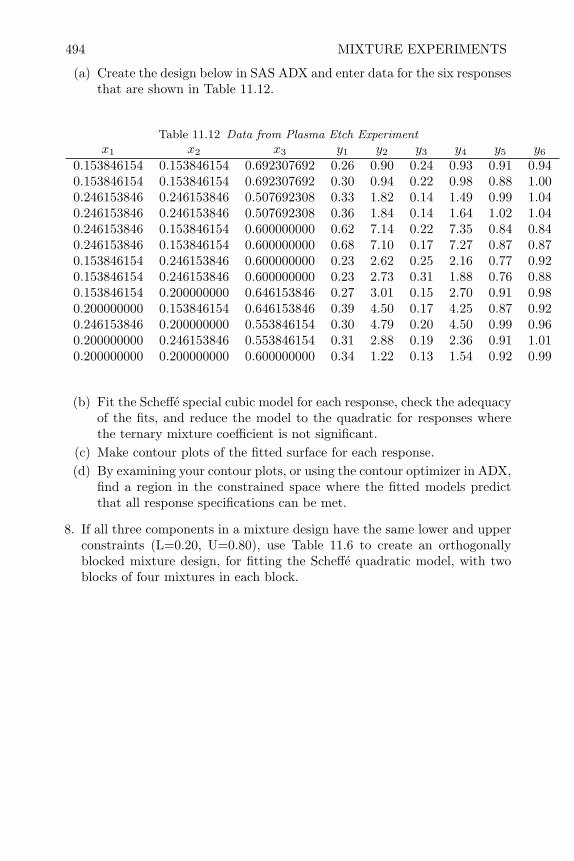
494 MIXTURE EXPERIMENTS
(a) Create the design below in SAS ADX and enter data for the six responsesthat are shown in Table 11.12.
Table 11.12 Data from Plasma Etch Experimentx1 x2 x3 y1 y2 y3 y4 y5 y6
0.153846154 0.153846154 0.692307692 0.26 0.90 0.24 0.93 0.91 0.940.153846154 0.153846154 0.692307692 0.30 0.94 0.22 0.98 0.88 1.000.246153846 0.246153846 0.507692308 0.33 1.82 0.14 1.49 0.99 1.040.246153846 0.246153846 0.507692308 0.36 1.84 0.14 1.64 1.02 1.040.246153846 0.153846154 0.600000000 0.62 7.14 0.22 7.35 0.84 0.840.246153846 0.153846154 0.600000000 0.68 7.10 0.17 7.27 0.87 0.870.153846154 0.246153846 0.600000000 0.23 2.62 0.25 2.16 0.77 0.920.153846154 0.246153846 0.600000000 0.23 2.73 0.31 1.88 0.76 0.880.153846154 0.200000000 0.646153846 0.27 3.01 0.15 2.70 0.91 0.980.200000000 0.153846154 0.646153846 0.39 4.50 0.17 4.25 0.87 0.920.246153846 0.200000000 0.553846154 0.30 4.79 0.20 4.50 0.99 0.960.200000000 0.246153846 0.553846154 0.31 2.88 0.19 2.36 0.91 1.010.200000000 0.200000000 0.600000000 0.34 1.22 0.13 1.54 0.92 0.99
(b) Fit the Scheffe special cubic model for each response, check the adequacyof the fits, and reduce the model to the quadratic for responses wherethe ternary mixture coefficient is not significant.
(c) Make contour plots of the fitted surface for each response.(d) By examining your contour plots, or using the contour optimizer in ADX,
find a region in the constrained space where the fitted models predictthat all response specifications can be met.
8. If all three components in a mixture design have the same lower and upperconstraints (L=0.20, U=0.80), use Table 11.6 to create an orthogonallyblocked mixture design, for fitting the Scheffe quadratic model, with twoblocks of four mixtures in each block.

EXERCISES 495
9. The numbers in parentheses below are the responses for the design shownin Figure 11.26.
11 =x
12 =x 13 =x 13 =x12 =x
11 =x
Block 1Block 2
(77)
(42) (68)
(29) (46) (56)
(76)
(61)
(27) (55)
(38) (58)
(a) Use the SAS code below Figure 11.26 to fit the Scheffe quadratic modelto the data above.
(b) Verify that the design blocks orthogonally by checking to see that thetype I and type III sums of squares for blocks are the same.
10. The Table 11.13 below shows the results of Chau and Kelly (1993) mixtureprocess variable experiments (MPV) with printable coating material, whichwere described in Section 11.7.
Table 11.13 Mixture Experiments with Printable Coating MaterialRun x1 x2 x3 z Opacity
1 0.13 0.53 0.34 -1 0.6982 0.13 0.53 0.34 -1 0.7113 0.13 0.53 0.34 1 0.9124 0.13 0.53 0.34 1 0.9305 0.13 0.60 0.27 -1 0.7006 0.13 0.67 0.20 -1 0.7107 0.13 0.67 0.20 -1 0.6808 0.13 0.67 0.20 1 0.9089 0.13 0.67 0.20 1 0.90110 0.29 0.37 0.34 -1 0.77211 0.29 0.51 0.20 -1 0.77212 0.45 0.21 0.34 -1 0.82313 0.45 0.21 0.34 -1 0.79814 0.45 0.21 0.34 1 0.99215 0.45 0.28 0.27 -1 0.81816 0.45 0.35 0.20 -1 0.80217 0.45 0.35 0.20 1 0.97618 0.45 0.35 0.20 1 0.940

496 MIXTURE EXPERIMENTS
(a) Create this design and merge the response values.(b) Fit a simplified model of the form of Equation (11.28) with only one
process variable z.(c) Does the process variable thickness affect the opacity?(d) Make a contour plot over constrained mixture space holding the process
variable thickness constant at is midpoint (i.e., coded value z=0).(e) Can you identify a region where predicted opacity > 0.86?
11. Steiner et al. (2007) describe a mixture-process variable (MPV) experimentconducted by students to find an optimal homemade bubble solution foruse in a battery operated bubble-blowing toy. The response was the averagenumber of bubbles produced by the bubble-blowing toy. The homemadebubble solution was made as a mixture of x1: dish soap, x2: water, and x3:glycerin. The following constraints were placed on the mixture components,based on recipes found in children’s books and cost,
0.04 ≤ x1 ≤ 0.350.60 ≤ x2 ≤ 0.980.00 ≤ x3 ≤ 0.15.
Two process variables were also included in the study, which were z1: brandof soap (-1=Joy, +1=Ivory) and z2: type of water (-1=spring water, +1=tapwater).
(a) Create a design for this experiment by crossing a design appropriate forfitting a Scheffe quadratic model in the mixture components and a 22
factorial in the process variables.(b) Write the model that can be fit from the design you created.(c) Given the actual data from Steiner et al. (2007) experiments shown in
Table 11.14, that were run in a completely random order, fit the modelyou propose in (b) to the data.
(d) Is the process water significant? Can it be safely removed from themodel?
(e) Make a contour plot over the constrained mixture space for each level ofthe process variable soap type.
(f) Make a recommendation for the optimal bubble solution.
12. Cornell (1988) presented the original example of mixture experiment forproducing vinyl for automobile seat covers. The data is shown in Table11.15, and the variable names are the same as those given in Section 11.8.
(a) Given that this is a cross between an extreme vertices design (plus theoverall centroid appropriate for fitting a Scheffe linear model in the mix-ture components) and a 22 factorial in the process variables, what is theappropriate model for this data?

EXERCISES 497
Table 11.14 Data from Mixture Process Experiments with Bubble Mixturez1: -1 -1 1 1z2: -1 1 -1 1
x1 x2 x3
0.350 0.600 0.05 23.8 14.2 4.2 3.60.250 0.600 0.15 12.6 13.6 2.6 3.40.350 0.650 0.00 7.8 10.6 2.4 1.00.250 0.650 0.10 12.0 12.0 5.8 2.60.250 0.750 0.05 12.8 15.4 4.0 4.40.150 0.700 0.15 10.8 9.2 3.2 3.40.145 0.775 0.08 8.8 11.2 4.4 3.00.200 0.800 0.00 10.2 13.6 3.8 2.20.040 0.810 0.15 2.4 4.0 3.0 4.20.120 0.850 0.03 12.8 8.0 1.6 3.40.040 0.880 0.08 2.0 4.6 0.6 0.60.050 0.950 0.00 4.0 2.8 3.0 3.0
(b) Fit the model by least squares using proc glm.(c) In this experiment, the runs were not made in a completely random
order, but rather randomized within whole plots and run as a split-plotexperiment. Refit the model using proc mixed including a random termfor whole plots like the example shown in Section 11.8. Is there anydifference in the parameter estimates you get in (b) and (c)? What doesthis imply?
Table 11.15 Data for Mixture Experiments for Producing Vinylz1: 1 -1 -1 1z2: -1 1 -1 1
Whole plot x1 x2 x3
1 0.85 0 0.15 8 12 7 122 0.72 0 0.28 6 9 7 103 0.6 0 0.15 10 13 9 144 0.47 0.25 0.28 4 6 5 65 0.66 0.125 0.215 11 15 9 136 0.85 0 0.15 7 10 8 117 0.72 0 0.28 5 8 6 98 0.6 0 0.15 11 12 10 129 0.47 0.25 0.28 5 3 4 510 0.66 0.125 0.215 10 11 7 9
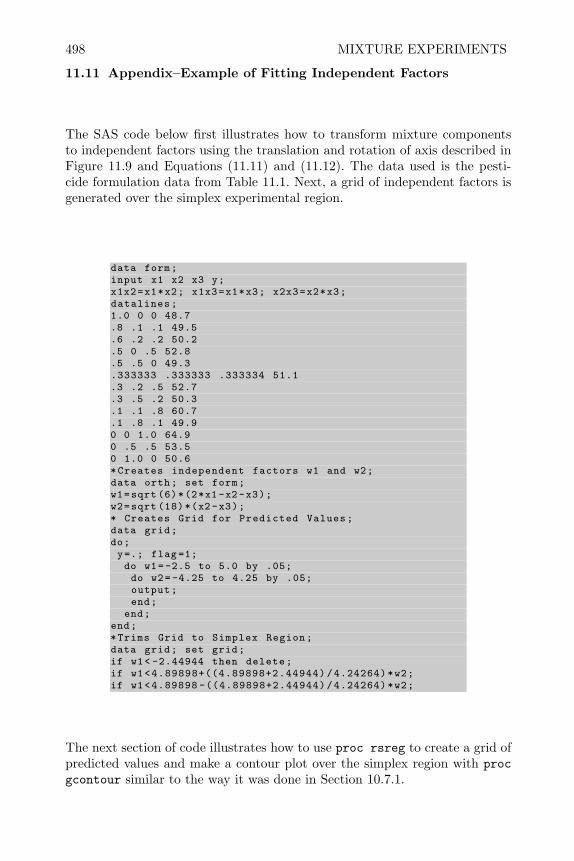
498 MIXTURE EXPERIMENTS
11.11 Appendix–Example of Fitting Independent Factors
The SAS code below first illustrates how to transform mixture componentsto independent factors using the translation and rotation of axis described inFigure 11.9 and Equations (11.11) and (11.12). The data used is the pesti-cide formulation data from Table 11.1. Next, a grid of independent factors isgenerated over the simplex experimental region.
data form;input x1 x2 x3 y;x1x2=x1*x2; x1x3=x1*x3; x2x3=x2*x3;datalines;1.0 0 0 48.7.8 .1 .1 49.5.6 .2 .2 50.2.5 0 .5 52.8.5 .5 0 49.3.333333 .333333 .333334 51.1.3 .2 .5 52.7.3 .5 .2 50.3.1 .1 .8 60.7.1 .8 .1 49.90 0 1.0 64.90 .5 .5 53.50 1.0 0 50.6*Creates independent factors w1 and w2;data orth; set form;w1=sqrt (6)*(2*x1 -x2-x3);w2=sqrt (18)*(x2-x3);* Creates Grid for Predicted Values;data grid;do;y=.; flag =1;do w1=-2.5 to 5.0 by .05;do w2= -4.25 to 4.25 by .05;output;end;
end;end;*Trims Grid to Simplex Region;data grid; set grid;if w1< -2.44944 then delete;if w1<4.89898+((4.89898+2.44944)/4.24264)*w2;if w1<4.89898 -((4.89898+2.44944)/4.24264)*w2;
The next section of code illustrates how to use proc rsreg to create a grid ofpredicted values and make a contour plot over the simplex region with procgcontour similar to the way it was done in Section 10.7.1.

APPENDIX–EXAMPLE OF FITTING INDEPENDENT FACTORS 499
* Combines data with Grid ;data grid; set grid orth;*Uses proc rsreg to fit quadratic model in w1 and w1
andfile of predicted values;
proc rsreg data=grid out=predict noprint;model y=w1 w2/predict;id flag;run;*Reverses direction of w2 axis to match ADX results;data plot;
set predict;w2=-w2;*Uses proc gcontour to make the contour plot;goptions reset=all
htext =1.3ftext=swiss;
proc gcontour data=plot(where =(flag =1));plot w1*w2=y/nlevels =6 nolegend autolabellevels =50 to 62.5 by 2.5vaxis=axis1 haxis=axis2;
axis1 label=(a=90 h=2.0) value =(h=2.0);axis2 label=(h=2.0) value=(h=2.0) ;
symbol1 height =2.0 color=black;symbol2 height =2.0 color=black;symbol3 height =2.0 color=black;symbol4 height =2.0 color=black;symbol5 height =2.0 color=black;symbol5 height =2.0 color=black;symbol7 height =2.0 color=black;run;
Figure 11.34 below shows the resulting contour plot. The upper boundaries ofthe simplex region were added manually using the edit graph menu in SAS.
Figure 11.34 Contour Plot of Pesticide Formulation Data

CHAPTER 12
Robust Parameter Design Experiments
12.1 Introduction
In this chapter no new designs are presented, but rather a slightly differentapplication of previous designs is demonstrated. In Chapter 5, sampling ex-periments were presented for the purpose of characterizing the variability inthe response. In the other chapters, the main purpose has been to establishcause and effect relationships between the factors and the average response,so that in the future the average response at selected levels of the factors canbe predicted, or the levels of the factors can be chosen to produce a desiredvalue of the response. In this chapter the purpose is to determine what levelsof the factors should be chosen to simultaneously produce a desired value ofthe response and at the same minimize the variability of the response.
After World War II, as Japan was attempting to re-establish telephonecommunications throughout the country, many problems were encounteredbecause of the poor quality switching systems that had been manufactured inJapan. American advisors such as W.E. Deming visited Japan and taught theprinciples of quality control that were most useful to Americans during the warproduction effort. During this industrial recovery period, a Japanese engineerfrom the Electrical Communications Laboratory, Genichi Taguchi, came todevote his life’s work to the application of designed experiments in industry(see Taguchi, 1987). Quality control has been traditionally thought of as anactivity that is performed in the manufacturing process, but Taguchi tookthe ideas of experimental design that he learned at the Statistical ResearchLaboratory in India and at the Bell Telephone laboratories in the UnitedStates and directed them to quality improvement activities upstream in theproduct design stage. This was a more cost effective way that is now referredto as off-line quality control. In off-line quality control, experimental designtechniques are utilized to find nominal settings of system parameters that willmake the products robust to noise encountered in the manufacturing processand in the use environment.
To show appreciation for what the American advisors had done for theJapanese after WWII, Taguchi introduced his ideas for optimizing the designof products and production processes in a cost effective way to the UnitedStates in 1980. He not only presented his methods but also sought appraisaland comments (see Taguchi, 1987). Since then, Taguchi’s contributions havebeen recognized as major advances in the history of engineering and man-ufacturing industries. However, some of the statistical design and analysis
501

502 ROBUST PARAMETER DESIGN EXPERIMENTS
methods recommended by Taguchi have been found to be somewhat ineffi-cient, and suggestions have been made for simpler, more efficient alternativesto implement some of Taguchi’s ideas. In this chapter, Taguchi’s engineer-ing philosophy is presented and illustrated, when necessary, by more modernstatistical methods.
12.2 Noise-Sources of Functional Variation
Taguchi has defined quality as the loss a product causes society after it isshipped (see Taguchi, 1986). We might think of this more as a definition ofthe lack of quality. By loss, Taguchi specifically means (1) loss caused byvariability in function or (2) loss due to harmful side effects. For example,losses to a customer could occur due to subpar performance, early failure,or product deterioration, while losses to third parties (or society in general)could be caused by things such as emitted pollutants or safety concerns. Vari-ation in product function is caused by what is commonly called noise. Taguchihas defined three distinct classes of noise that cause functional variation inproducts and manufacturing processes. These classes are (1) inner or deteri-oration noise, (2) outer or environmental noise, and (3) variational noise orpiece-to-piece variation caused in manufacturing.
Inner noise or deterioration noise refers to changes in product or componentsthat occur as the product ages or wears out preventing it from achievingits target function. Outer or environmental noise refers to external factorsin the use environment such as temperature, humidity, vibration or humantreatment that affect product performance. Finally, variational noise refersto manufacturing imperfections. As an example, Phadke (1989) described thethree sources of noise in a refrigerator temperature control. The inner noisewould consist of things such as the leakage of refrigerant and mechanicalwear of compressor parts. The outer noise would consist of things such asthe number of times the door is opened and closed, the amount of food kept,the ambient temperature, and the voltage supply variation. The variationalnoise would consist of the tightness of the door closure, quality of the seals onthe refrigerant, amount of refrigerant charged, and the fit and finish of movingparts in the compressor.
Taguchi pointed out that only variational noise can be reduced with tra-ditional quality control activities in manufacturing, but that in the productdesign stage it may be possible to find counter-measures for all three sources ofnoise using experimental design techniques. This is done through a procedurecalled robust parameter design.
The performance of products and manufacturing processes are affected byfactors that are controlled by the designers of these products and processes(called control factors) and by other hard-to-control factors such as environ-mental conditions, raw material quality and aging (often called noise factorsor environmental factors). In conducting a robust parameter design exper-iment, the levels of the noise factors are varied systematically to represent

NOISE-SOURCES OF FUNCTIONAL VARIATION 503
their variation in normal conditions. The levels of the control factors are var-ied over levels which are thought to include the optimal levels. The purposeof the parameter design experiment is to discover interactions between thecontrol factors and the noise factors. Once discovered, these interactions canbe exploited to reduce variation in the product or process function caused byhard-to-control variation in the noise factors.
The model for a robust design experiment can be represented symbolicallyas
y = Xβ + Zγ + ε, (12.1)
where y is the response or vector of measures of the product or process func-tion. X represents the design matrix for the control factors and β representsthe control factor effects or regression coefficients. Z represents the design ma-trix for the noise factors and the interactions between the noise factors andcontrol factors. Obviously variation in the levels of the noise factors will betransmitted to variation in the response y. If there are interactions betweenthe control factors and the noise factors, it may be possible to reduce variationin the response caused by changes in the levels of the noise factors throughchoice of the levels of the control factors.
The procedure for conducting a parameter design is shown below:
1. Select control factors that are easily controlled.
2. Determine the sources of noise, and choose the most important noise sourcesto be represented as factors in the design. This sometimes requires some in-genuity to define factors that will represent the inner, outer, and variationalnoise you are trying to mitigate.
3. Select an appropriate experimental design.
4. Perform the experiment.
5. Analyze the data and detect significant main effects and interactions.
6. Select levels of the control factors to reduce variation caused by the noisefactors and meet the target performance.
The aspect that is different about parameter design experiments is the em-phasis on including noise factors in the design, and the ability to determinecontrol factor settings that not only ensure that the response will achieve thetarget level but will also reduce variation in the response caused by the sourcesof noise.
Two experimental strategies have been used in parameter design experi-ments. One is to use a cartesian product design which is composed of allcombinations of levels of the control factors (in a control factor array) with allcombinations of levels of the noise factors (in a noise factor array). The otherapproach is to combine both control and noise factors into one single arraydesign. Two separate analysis strategies have been used. One strategy is calledthe loss model approach or location-dispersion modeling. This strategy can beused when the experiment is conducted as a product array. A second analysisstrategy that has been used is called the response modeling strategy, and is
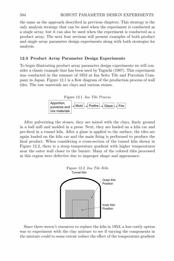
504 ROBUST PARAMETER DESIGN EXPERIMENTS
the same as the approach described in previous chapters. This strategy is theonly analysis strategy that can be used when the experiment is conducted asa single array, but it can also be used when the experiment is conducted as aproduct array. The next four sections will present examples of both productand single array parameter design experiments along with both strategies foranalysis.
12.3 Product Array Parameter Design Experiments
To begin illustrating product array parameter design experiments we will con-sider a classic example that has been used by Taguchi (1987). This experimentwas conducted in the summer of 1953 at Ina Seito Tile and Porcelain Com-pany in Japan. Figure 12.1 is a flow diagram of the production process of walltiles. The raw materials are clays and various stones.
Figure 12.1 Ina Tile Process
Apportion,pulverize andmix materials
Mold Prefire Glaze Fire
After pulverizing the stones, they are mixed with the clays, finely groundin a ball mill and molded in a press. Next, they are loaded on a kiln car andpre-fired in a tunnel kiln. After a glaze is applied to the surface, the tiles areagain loaded on the kiln car and the main firing is performed to produce thefinal product. When considering a cross-section of the tunnel kiln shown inFigure 12.2, there is a steep temperature gradient with higher temperaturesnear the outer wall closer to the burner. Many of the colored tiles processedin this region were defective due to improper shape and appearance.
Figure 12.2 Ina Tile KilnTunnel Kiln
Inner KilnPosition
Outer KilnPosition
Since there weren’t resources to replace the kiln in 1953, a less costly optionwas to experiment with the clay mixture to see if varying the components inthe mixture could to some extent reduce the effect of the temperature gradient
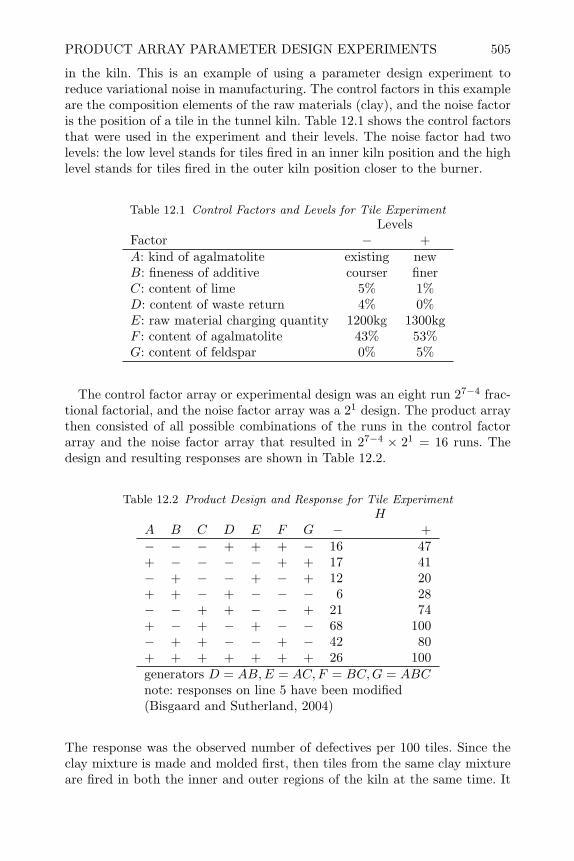
PRODUCT ARRAY PARAMETER DESIGN EXPERIMENTS 505
in the kiln. This is an example of using a parameter design experiment toreduce variational noise in manufacturing. The control factors in this exampleare the composition elements of the raw materials (clay), and the noise factoris the position of a tile in the tunnel kiln. Table 12.1 shows the control factorsthat were used in the experiment and their levels. The noise factor had twolevels: the low level stands for tiles fired in an inner kiln position and the highlevel stands for tiles fired in the outer kiln position closer to the burner.
Table 12.1 Control Factors and Levels for Tile ExperimentLevels
Factor − +A: kind of agalmatolite existing newB: fineness of additive courser finerC: content of lime 5% 1%D: content of waste return 4% 0%E: raw material charging quantity 1200kg 1300kgF : content of agalmatolite 43% 53%G: content of feldspar 0% 5%
The control factor array or experimental design was an eight run 27−4 frac-tional factorial, and the noise factor array was a 21 design. The product arraythen consisted of all possible combinations of the runs in the control factorarray and the noise factor array that resulted in 27−4 × 21 = 16 runs. Thedesign and resulting responses are shown in Table 12.2.
Table 12.2 Product Design and Response for Tile ExperimentH
A B C D E F G − +− − − + + + − 16 47+ − − − − + + 17 41− + − − + − + 12 20+ + − + − − − 6 28− − + + − − + 21 74+ − + − + − − 68 100− + + − − + − 42 80+ + + + + + + 26 100generators D = AB,E = AC,F = BC,G = ABCnote: responses on line 5 have been modified(Bisgaard and Sutherland, 2004)
The response was the observed number of defectives per 100 tiles. Since theclay mixture is made and molded first, then tiles from the same clay mixtureare fired in both the inner and outer regions of the kiln at the same time. It

506 ROBUST PARAMETER DESIGN EXPERIMENTS
should be recognized that this particular product array design is a split-plotdesign that is quite similar to the experiment used to formulate a boxed cakemix (presented in exercise 9 of Chapter 8). Bisgaard and Sutherland (2004)noticed unusual observations on line five in the original Ina tile data. Theseobservations have been modified in Table 12.2 to simplify the discussion ofthe analysis in the next section.
As a second example of a product array, consider an experiment describedby Taguchi and Byrne (1984) to optimize the installation procedure for anelastomeric connector used in the automotive industry. The desire was tomaximize the separation pull-off force and minimize the variability in thisforce. There were four control factors and three noise factors. These factorsare shown in Table 12.3 and illustrated in Figure 12.3.
Table 12.3 Control and Noise Factors for Connector ExperimentControl Factors: levels
A: Interference Low Medium HighB: Connector wall thickness Thin Medium ThickC: Insertion depth Shallow Medium DeepD: Percentage of adhesive Low Medium High
Noise Factors: levelsE: Conditioning time 24 hours 120 hoursF : Conditioning temperature 72F 150FG: Conditioning relative humidity 25% 75%
The interference (or allowance between the force fit elastometric connector andthe metal tube it is connected to), the wall thickness of the connector, inser-tion depth of the connector onto the metal tube, and percent adhesive that isin the solution the connector is dipped into before insertion on the metal tubeare specified by the designer and are therefore designated as control factors.The conditioning or set-up time, the temperature during the set-up time, andthe relative humidity during the set-up time may affect the pull-off force butare usually difficult to control during routine production conditions. There-fore these three factors are designated as noise factors. During the parameterdesign experiments, extra care was taken to control these factors.
The complete layout of the control factor array, noise factor array and re-sulting data is shown in Figure 12.4. There, the control and noise factor arraysare shown in symbolic levels (1, 2, etc.) and actual levels. The control factorarray was a 34−2 fractional factorial. The noise factor array is a full 23 factorialwhere the symbolic levels are 1, and 2 rather than − and +. The run numbersfor the two designs are shown in the far left and top rows, respectively. Therandomization of runs in this experiment was not restricted, and each of the34−2 × 23 = 72 runs could have been run in a completely random order.
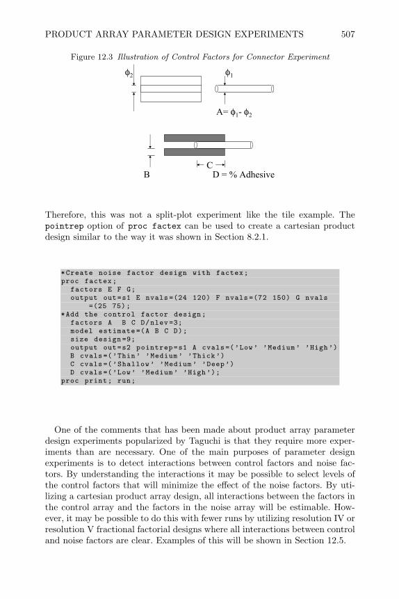
PRODUCT ARRAY PARAMETER DESIGN EXPERIMENTS 507
Figure 12.3 Illustration of Control Factors for Connector Experiment
φ1φ2
A= φ1- φ2
BC
D = % Adhesive
Therefore, this was not a split-plot experiment like the tile example. Thepointrep option of proc factex can be used to create a cartesian productdesign similar to the way it was shown in Section 8.2.1.
*Create noise factor design with factex;proc factex;
factors E F G;output out=s1 E nvals =(24 120) F nvals =(72 150) G nvals
=(25 75);*Add the control factor design;
factors A B C D/nlev =3;model estimate =(A B C D);size design =9;output out=s2 pointrep=s1 A cvals=(’Low’ ’Medium ’ ’High’)B cvals=(’Thin’ ’Medium ’ ’Thick’)C cvals=(’Shallow ’ ’Medium ’ ’Deep’)D cvals=(’Low’ ’Medium ’ ’High’);
proc print; run;
One of the comments that has been made about product array parameterdesign experiments popularized by Taguchi is that they require more exper-iments than are necessary. One of the main purposes of parameter designexperiments is to detect interactions between control factors and noise fac-tors. By understanding the interactions it may be possible to select levels ofthe control factors that will minimize the effect of the noise factors. By uti-lizing a cartesian product array design, all interactions between the factors inthe control array and the factors in the noise array will be estimable. How-ever, it may be possible to do this with fewer runs by utilizing resolution IV orresolution V fractional factorial designs where all interactions between controland noise factors are clear. Examples of this will be shown in Section 12.5.
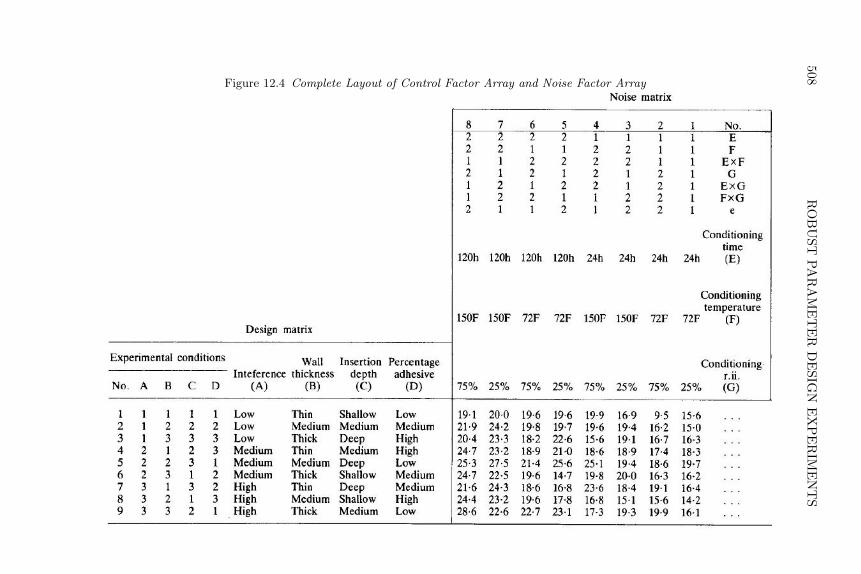
508R
OB
UST
PAR
AM
ET
ER
DE
SIGN
EX
PE
RIM
EN
TS
Figure 12.4 Complete Layout of Control Factor Array and Noise Factor Array

PRODUCT ARRAY PARAMETER DESIGN EXPERIMENTS 509
One situation where product arrays are actually more efficient is when theexperiment is a split-plot. For example, in the Ina tile experiment, the noisefactor array consisted of simply measuring the response (number of defectivetiles in a sample of 100) once for tiles produced in the inner kiln position andagain for tiles produced in the outer kiln position. Therefore no additionalexperimental effort was required. Only eight batches of clay were mixed andmolded, but more information was produced by measuring multiple responsesfor each run of the control factor array. Split-plot designs are sometimes de-scribed as super efficient since the sup-plot factors and interactions betweensub-plot and whole-plot factors can be tested with the (usually) smaller sub-plot error term.
A third example of a product array parameter design experiment involvesthe design of a product. The product is the simple circuit for a temperaturecontroller that uses resistance thermometer RT . The circuit diagram thatis shown in Figure 12.5 was described by Taguchi and Phadke (1985). The
Figure 12.5 Temperature Controller Circuit
E0 E2
R3
RT
R1
R2
RELAY
R4
response, or measure of product performance, is the resistance value of RT atwhich the relay turns on. Through circuit relations, the response is given bythe rational function
RT =R3R2(E2R4 + E0R1)
R1(E2R2 + E2R4 − E0R2).
(12.2)
The adjustment factor is R3, which is known by the circuit relations. Thecontrol factors that a designer can specify are the nominal ratings of theresistors and diodes A = R1, B = R2/R1, C=R4/R1, D = E0 and F = E2.The noise factors are deviations from the nominal values of the control factorsthat would be expected due to manufacturing imperfections and deteriorationwhile the product is in use. The objective was to find the nominal settings ofthe control factors that minimize the variation in RT since the desired valueof RT can always be obtained by adjusting R3. This is an example of the
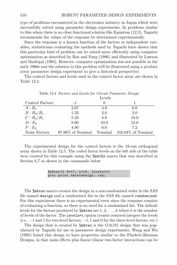
510 ROBUST PARAMETER DESIGN EXPERIMENTS
type of problems encountered in the electronics industry in Japan which weresuccessfully solved using parameter design experiments. In problems similarto this where there is no clear functional relation like Equation (12.2), Taguchirecommends the values of the response be determined experimentally.
Since the response is a known function of the factors or independent vari-ables, statisticians evaluating the methods used by Taguchi have shown thatthis particular kind of problem can be solved more efficiently using computeroptimization as described by Box and Fung (1986) and illustrated by Lawsonand Madrigal (1994). However, computer optimization was not possible in theearly 1960s and the solution to this problem will be illustrated using a productarray parameter design experiment to give a historical perspective.
The control factors and levels used in the control factor array are shown inTable 12.4.
Table 12.4 Factors and Levels for Circuit Parameter DesignLevels
Control Factors -1 0 1A : R1 2.67 4.0 6.0B : R2/R1 1.33 2.0 3.0C : R4/R1 5.33 8.0 16.0D : E0 8.00 10.0 12.0F : E2 4.80 6.0 7.2Noise Factors 97.96% of Nominal Nominal 102.04% of Nominal
The experimental design for the control factors is the 18-run orthogonalarray shown in Table 12.5. The coded factor levels on the left side of the tablewere created for this example using the %mktEx macro that was described inSection 6.7 as shown in the commands below
%mktex(2 3**7, n=18, levels=i)proc print data=design; run;
The %mktex macro creates the design in a non-randomized order in the SASfile named design and a randomized list in the SAS file named randomized.For this experiment there is no experimental error since the response consistsof evaluating a function, so there is no need for a randomized list. The defaultlevels for the factors produced by %mktex are 1, 2, . . . , k where k is the numberof levels of the factor. The levels=i option creates centered integers the levels(i.e., −1 and 1 for two-level factors, −1, 1 and 0 for the three-level factors, etc.)
The design that is created by %mktex is the OA(18) design that was pop-ularized by Taguchi for use in parameter design experiments. Wang and Wu(1995) found this design to have properties similar to the Plackett-BurmanDesigns, in that main effects plus linear×linear two-factor interactions can be

PRODUCT ARRAY PARAMETER DESIGN EXPERIMENTS 511
Table 12.5 OA18 Design for Control FactorsCoded Factor Levels Actual Factor Levels
X1 X2 X3 X4 X5 X6 X7 X8 A B C D F
-1 -1 -1 -1 -1 -1 -1 -1 2.67 1.33 5.33 8 4.8-1 -1 -1 1 0 0 1 0 2.67 1.33 16 10 6-1 -1 0 1 1 -1 0 1 2.67 2 16 12 4.8-1 1 -1 0 0 1 -1 1 6 1.33 8 10 7.2-1 1 1 1 1 1 1 -1 6 3 16 12 7.2-1 1 1 0 -1 -1 0 0 6 3 8 8 4.8-1 0 1 -1 -1 0 1 1 4 3 5.33 8 6-1 0 0 -1 1 1 -1 0 4 2 5.33 12 7.2-1 0 0 0 0 0 0 -1 4 2 8 10 61 -1 1 -1 0 1 0 0 2.67 3 5.33 10 7.21 -1 1 0 1 0 -1 -1 2.67 3 8 12 61 -1 0 0 -1 1 1 1 2.67 2 8 8 7.21 1 -1 -1 1 0 0 1 6 1.33 5.33 12 61 1 0 -1 0 -1 1 -1 6 2 5.33 10 4.81 1 0 1 -1 0 -1 0 6 2 16 8 61 0 -1 1 -1 1 0 -1 4 1.33 16 8 7.21 0 -1 0 1 -1 1 0 4 1.33 8 12 4.81 0 1 1 0 -1 -1 1 4 3 16 10 4.8
fit using subset selection regression analysis even though the design is reso-lution III. Since there were only five three-level factors in this problem, the−1’s, 0’s and 1’s in columns X2 through X6 were replaced by the actual factorlevels in Table 12.4 to form the design shown in the right half of Table 12.5,and X1, X7, and X8 were unassigned or not used in this problem.
The experimental design in coded factor levels for the noise factors is thesame OA(18) used for the control factors. The effect of changing levels ofthe noise factors is a perturbation of the levels of the control factors. Forexample, when the coded level of the noise factor is −1, the nominal settingsof the control factors are modified by multiplying them by 0.9796. When thecoded level of the noise factor is 1, the nominal settings of the control factorsare modified by multiplying them by 1.0204. When the noise factor is at the 0,or mid-level, the nominal value of the control factor is left unchanged. This isdone to simulate the noise environment where the actual values of the controlfactors may differ from the specified nominal values by a tolerance of ±2.04%due to manufacturing imperfections and deterioration over time in use. Fora particular run in the control factor design, a set of modified control factorlevels are calculated for each run in the noise factor array and the response,RT , is calculated using Equation (12.2).
In product array parameter design experiments the noise factor array is usu-ally shown horizontally across the top similar to Figure 12.4. For this examplethe product array is too large (18×18) to represent as a single table. In Table
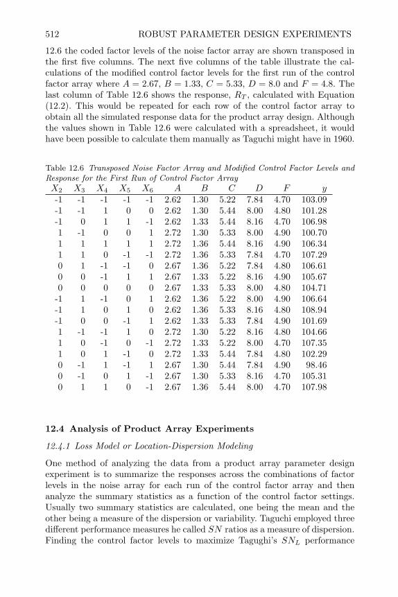
512 ROBUST PARAMETER DESIGN EXPERIMENTS
12.6 the coded factor levels of the noise factor array are shown transposed inthe first five columns. The next five columns of the table illustrate the cal-culations of the modified control factor levels for the first run of the controlfactor array where A = 2.67, B = 1.33, C = 5.33, D = 8.0 and F = 4.8. Thelast column of Table 12.6 shows the response, RT , calculated with Equation(12.2). This would be repeated for each row of the control factor array toobtain all the simulated response data for the product array design. Althoughthe values shown in Table 12.6 were calculated with a spreadsheet, it wouldhave been possible to calculate them manually as Taguchi might have in 1960.
Table 12.6 Transposed Noise Factor Array and Modified Control Factor Levels andResponse for the First Run of Control Factor ArrayX2 X3 X4 X5 X6 A B C D F y-1 -1 -1 -1 -1 2.62 1.30 5.22 7.84 4.70 103.09-1 -1 1 0 0 2.62 1.30 5.44 8.00 4.80 101.28-1 0 1 1 -1 2.62 1.33 5.44 8.16 4.70 106.981 -1 0 0 1 2.72 1.30 5.33 8.00 4.90 100.701 1 1 1 1 2.72 1.36 5.44 8.16 4.90 106.341 1 0 -1 -1 2.72 1.36 5.33 7.84 4.70 107.290 1 -1 -1 0 2.67 1.36 5.22 7.84 4.80 106.610 0 -1 1 1 2.67 1.33 5.22 8.16 4.90 105.670 0 0 0 0 2.67 1.33 5.33 8.00 4.80 104.71
-1 1 -1 0 1 2.62 1.36 5.22 8.00 4.90 106.64-1 1 0 1 0 2.62 1.36 5.33 8.16 4.80 108.94-1 0 0 -1 1 2.62 1.33 5.33 7.84 4.90 101.691 -1 -1 1 0 2.72 1.30 5.22 8.16 4.80 104.661 0 -1 0 -1 2.72 1.33 5.22 8.00 4.70 107.351 0 1 -1 0 2.72 1.33 5.44 7.84 4.80 102.290 -1 1 -1 1 2.67 1.30 5.44 7.84 4.90 98.460 -1 0 1 -1 2.67 1.30 5.33 8.16 4.70 105.310 1 1 0 -1 2.67 1.36 5.44 8.00 4.70 107.98
12.4 Analysis of Product Array Experiments
12.4.1 Loss Model or Location-Dispersion Modeling
One method of analyzing the data from a product array parameter designexperiment is to summarize the responses across the combinations of factorlevels in the noise array for each run of the control factor array and thenanalyze the summary statistics as a function of the control factor settings.Usually two summary statistics are calculated, one being the mean and theother being a measure of the dispersion or variability. Taguchi employed threedifferent performance measures he called SN ratios as a measure of dispersion.Finding the control factor levels to maximize Tagughi’s SNL performance

ANALYSIS OF PRODUCT ARRAY EXPERIMENTS 513
measure was designed to make the response as large as possible, and finding thecontrol factor levels to maximize his SNS was designed to make the responseas small as possible. However, because these performance measures confusethe mean response level and variability about the mean, Box (1988) has shownthey are inefficient. Wu and Hamada (2000) instead recommend a two-stepprocedure shown below:
1. Select the levels of the control factors (that affect the variation in the re-sponse) to minimize the variation.
2. Select the levels of the control factors (that affect the mean response but notthe variation) to bring the response to the desired target.
In the first step the control factors that affect ln(s2), where the samplevariance s2 is calculated across the levels of the noise factor array for each runin the control factor array, are identified and their factor levels are chosen tominimize ln(s2). Other factors may affect the average response but not ln(s2).These control factors are called adjustment factors. The second step involvesidentifying the levels of the adjustment factors that bring the response tothe desired target level. When the objective is to minimize or maximize theresponse with minimum variability, the order of the two steps is reversed.
To illustrate this procedure, consider the data in the Ina tile experiment.Since the responses were binomial counts, the sin−1
√y/n transformation de-
scribed in Section 2.5.2 was used. The SAS commands to read the data andcreate the transformed values are.
data tile;input A B C D E F G y1 y2 ;y1=arsin(sqrt(y1/100)); y2=arsin(sqrt(y2/100));ybar=(y1+y2)/2; lns2=log(((y1 -y2)**2)/2);datalines;-1 -1 -1 1 1 1 -1 16 47
...
Table 12.7 shows the control factor settings, the transformed response, andthe two summary statistics y and ln(s2).

514 ROBUST PARAMETER DESIGN EXPERIMENTS
Table 12.7 Control Factor Array and Summary StatisticsH
A B C D E F G − + y ln(s2)− − − + + + − 0.412 0.755 0.583 -2.828+ − − − − + + 0.425 0.695 0.560 -3.312− + − − + − + 0.354 0.464 0.409 -5.109+ + − + − − − 0.247 0.558 0.402 -3.035− − + + − − + 0.476 1.036 0.756 -1.854+ − + − + − − 0.970 1.570 1.270 -1.711− + + − − + − 0.705 1.107 0.906 -2.515+ + + + + + + 0.535 1.571 1.053 -0.623
The commands to fit the model to the average response are shown below.
proc glm;model ybar = A B C D E F G/solution;ods output ParameterEstimates=sol;
run;
The resulting output is shown below and Figure 12.6 shows a half-normalplot of the regression coefficients.
StandardParameter Estimate Error t Value Pr > |t|
Intercept 0.7424626418 . . .A 0.0789317559 . . .B -.0498971676 . . .C 0.2538069161 . . .D -.0437639741 . . .E 0.0863475789 . . .F 0.0331447819 . . .G -.0480989659 . . .
Here it can be seen that control factor C, the content of lime, appears to bethe only one to have a significant effect on the mean response. Since the effectis positive and the low level was defined in Table 12.1 as 5%, the number ofdefective tiles can be reduced by mixing 5% of lime in the clay mixture ratherthan 1% as was previously the practice. Since the objective is to minimize thenumber of defective tiles, the first step in the procedure shown above wouldbe to choose the 5% level of lime in the clay mix.
The second step starts by identifying the control factors that affect the logvariance. The output below the figure on the next page shows the results offitting the same model using the summary statistic ln(s2) as the response.Here, it can again be seen that control factor C has the largest effect.
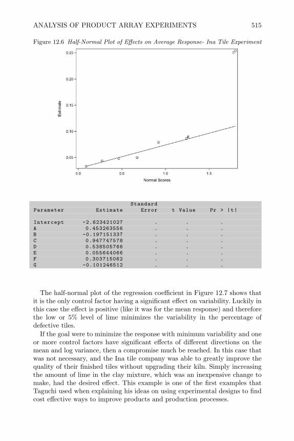
ANALYSIS OF PRODUCT ARRAY EXPERIMENTS 515
Figure 12.6 Half-Normal Plot of Effects on Average Response- Ina Tile Experiment
StandardParameter Estimate Error t Value Pr > |t|
Intercept -2.623421027 . . .A 0.453263556 . . .B -0.197151337 . . .C 0.947747578 . . .D 0.538505766 . . .E 0.055644066 . . .F 0.303715062 . . .G -0.101246512 . . .
The half-normal plot of the regression coefficient in Figure 12.7 shows thatit is the only control factor having a significant effect on variability. Luckily inthis case the effect is positive (like it was for the mean response) and thereforethe low or 5% level of lime minimizes the variability in the percentage ofdefective tiles.
If the goal were to minimize the response with minimum variability and oneor more control factors have significant effects of different directions on themean and log variance, then a compromise much be reached. In this case thatwas not necessary, and the Ina tile company was able to greatly improve thequality of their finished tiles without upgrading their kiln. Simply increasingthe amount of lime in the clay mixture, which was an inexpensive change tomake, had the desired effect. This example is one of the first examples thatTaguchi used when explaining his ideas on using experimental designs to findcost effective ways to improve products and production processes.
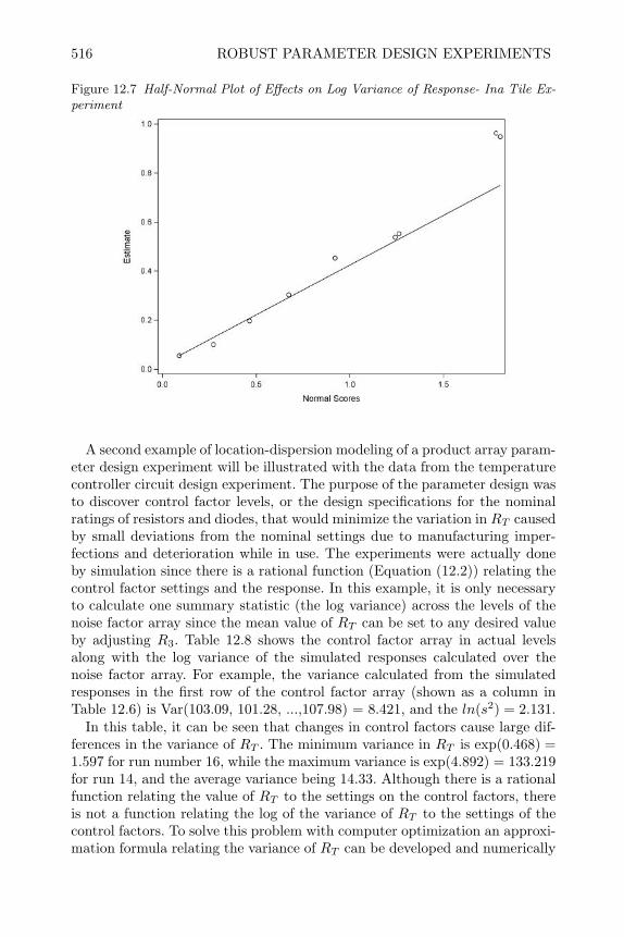
516 ROBUST PARAMETER DESIGN EXPERIMENTS
Figure 12.7 Half-Normal Plot of Effects on Log Variance of Response- Ina Tile Ex-periment
A second example of location-dispersion modeling of a product array param-eter design experiment will be illustrated with the data from the temperaturecontroller circuit design experiment. The purpose of the parameter design wasto discover control factor levels, or the design specifications for the nominalratings of resistors and diodes, that would minimize the variation in RT causedby small deviations from the nominal settings due to manufacturing imper-fections and deterioration while in use. The experiments were actually doneby simulation since there is a rational function (Equation (12.2)) relating thecontrol factor settings and the response. In this example, it is only necessaryto calculate one summary statistic (the log variance) across the levels of thenoise factor array since the mean value of RT can be set to any desired valueby adjusting R3. Table 12.8 shows the control factor array in actual levelsalong with the log variance of the simulated responses calculated over thenoise factor array. For example, the variance calculated from the simulatedresponses in the first row of the control factor array (shown as a column inTable 12.6) is Var(103.09, 101.28, ...,107.98) = 8.421, and the ln(s2) = 2.131.
In this table, it can be seen that changes in control factors cause large dif-ferences in the variance of RT . The minimum variance in RT is exp(0.468) =1.597 for run number 16, while the maximum variance is exp(4.892) = 133.219for run 14, and the average variance being 14.33. Although there is a rationalfunction relating the value of RT to the settings on the control factors, thereis not a function relating the log of the variance of RT to the settings of thecontrol factors. To solve this problem with computer optimization an approxi-mation formula relating the variance of RT can be developed and numerically
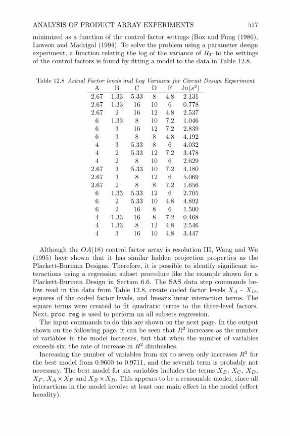
ANALYSIS OF PRODUCT ARRAY EXPERIMENTS 517
minimized as a function of the control factor settings (Box and Fung (1986),Lawson and Madrigal (1994). To solve the problem using a parameter designexperiment, a function relating the log of the variance of RT to the settingsof the control factors is found by fitting a model to the data in Table 12.8.
Table 12.8 Actual Factor levels and Log Variance for Circuit Design ExperimentA B C D F ln(s2)
2.67 1.33 5.33 8 4.8 2.1312.67 1.33 16 10 6 0.7782.67 2 16 12 4.8 2.537
6 1.33 8 10 7.2 1.0466 3 16 12 7.2 2.8396 3 8 8 4.8 4.1924 3 5.33 8 6 4.0324 2 5.33 12 7.2 3.4784 2 8 10 6 2.629
2.67 3 5.33 10 7.2 4.1802.67 3 8 12 6 5.0692.67 2 8 8 7.2 1.656
6 1.33 5.33 12 6 2.7056 2 5.33 10 4.8 4.8926 2 16 8 6 1.5004 1.33 16 8 7.2 0.4684 1.33 8 12 4.8 2.5464 3 16 10 4.8 3.447
Although the OA(18) control factor array is resolution III, Wang and Wu(1995) have shown that it has similar hidden projection properties as thePlackett-Burman Designs. Therefore, it is possible to identify significant in-teractions using a regression subset procedure like the example shown for aPlackett-Burman Design in Section 6.6. The SAS data step commands be-low read in the data from Table 12.8, create coded factor levels XA - XD,squares of the coded factor levels, and linear×linear interaction terms. Thesquare terms were created to fit quadratic terms to the three-level factors.Next, proc reg is used to perform an all subsets regression.
The input commands to do this are shown on the next page. In the outputshown on the following page, it can be seen that R2 increases as the numberof variables in the model increases, but that when the number of variablesexceeds six, the rate of increase in R2 diminishes.
Increasing the number of variables from six to seven only increases R2 forthe best model from 0.9600 to 0.9711, and the seventh term is probably notnecessary. The best model for six variables includes the terms XB , XC , XD,XF , XA×XF and XB×XD. This appears to be a reasonable model, since allinteractions in the model involve at least one main effect in the model (effectheredity).
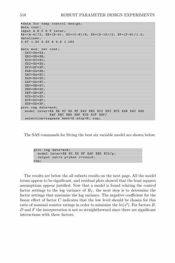
518 ROBUST PARAMETER DESIGN EXPERIMENTS
*data for temp control design;data cont;input A B C D F lnvar;XA=(A-4)/2; XB=(B-2); XC=(C-8)/8; XD=(D-10)/2; XF=(F-6)/1.2;datalines;2.67 1.33 5.33 8 4.8 1.163
. . .data mod; set cont;
XA2=XA*XA;XB2=XB*XB;XC2=XC*XC;XD2=XD*XD;XF2=XF*XF;XAB=XA*XB;XAC=XA*XC;XAD=XA*XD;XAF=XA*XF;XBC=XB*XC;XBD=XB*XD;XBF=XB*XF;XCD=XC*XD;XCF=XC*XF;XDF=XD*XF;
proc reg data=mod;model lnvar=XA XB XC XD XF XA2 XB2 XC2 XD2 XF2 XAB XAC XAD
XAF XBC XBD XBF XCD XCF XDF/selection=rsquare best=4 stop =8; run;
The SAS commands for fitting the best six variable model are shown below.
proc reg data=mod;model lnvar=XB XC XD XF XAF XBD XC2/p;output out=s p=yhat r=resid;
run;
The results are below the all subsets results on the next page. All the modelterms appear to be significant, and residual plots showed that the least squaresassumptions appear justified. Now that a model is found relating the controlfactor settings to the log variance of RT , the next step is to determine thefactor settings that minimize the log variance. The negative coefficient for thelinear effect of factor C indicates that the low level should be chosen for thisratio of nominal resistor ratings in order to minimize the ln(s2). For factors B,D and F the interpretation is not so straightforward since there are significantinteractions with these factors.
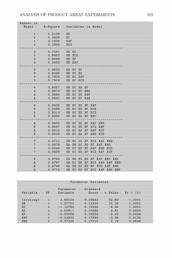
ANALYSIS OF PRODUCT ARRAY EXPERIMENTS 519
Number inModel R-Square Variables in Model
1 0.5106 XB1 0.2436 XC1 0.1936 XAF1 0.1848 XC2
---------------------------------------------------2 0.7541 XB XC2 0.6953 XB XC22 0.6068 XB XF2 0.5842 XB XAC
---------------------------------------------------3 0.8504 XB XC XF3 0.8245 XB XC XD3 0.7924 XB XC XAC3 0.7916 XB XF XC2
---------------------------------------------------4 0.9207 XB XC XD XF4 0.8679 XB XC XF XBD4 0.8660 XB XC XD XAF4 0.8641 XB XC XF XAB
---------------------------------------------------5 0.9425 XB XC XD XF XAF5 0.9396 XB XC XD XF XCD5 0.9313 XB XC XD XF XC25 0.9295 XB XC XD XF XBC
---------------------------------------------------6 0.9600 XB XC XD XF XAF XBD6 0.9547 XB XC XD XF XC2 XAF6 0.9515 XB XC XD XF XAF XCF6 0.9509 XB XC XD XF XBD XCD
---------------------------------------------------7 0.9711 XB XC XD XF XC2 XAF XBD7 0.9676 XA XB XC XD XF XAF XBD7 0.9645 XB XC XD XF XAF XBD XCD7 0.9638 XB XC XD XF XC2 XAF XCF
---------------------------------------------------8 0.9799 XA XB XC XD XF XAF XBC XBD8 0.9797 XB XC XD XF XC2 XAD XAF XBD8 0.9786 XA XB XC XD XF XC2 XAF XBD8 0.9774 XB XC XD XF XC2 XAF XBD XBF
Parameter Estimates
Parameter StandardVariable DF Estimate Error t Value Pr > |t|
Intercept 1 2.89028 0.08842 32.69 <.0001XB 1 1.27702 0.12303 10.38 <.0001XC 1 -1.10764 0.15933 -6.95 <.0001XD 1 0.50917 0.10585 4.81 0.0005XF 1 -0.53056 0.10539 -5.03 0.0004XAF 1 -0.52822 0.17849 -2.96 0.0130XBD 1 0.37328 0.17012 2.19 0.0506

520 ROBUST PARAMETER DESIGN EXPERIMENTS
The prediction equation for the fitted model can be written as
ln(s2) = 2.890 + 1.277(B − 2
1
)− 1.108
(C − 8
8
)+ .509
(D − 10
2
)− .531
(F − 6
1.2
)− .528
(A− 4
2
)(F − 6
1.2
)+ .373
(B − 2
1
)(D − 10
2
).
(12.3)
Using this equation with factors A, C and F held constant at their mid-levels, the predicted ln(s2) shown in Table 12.9 were calculated. Here it canbe seen that the combination of factors B and D that are predicted to havethe lowest ln(s2) is B = 1.33 (or the nominal rating of resistor R2 should bespecified as 1.33×R1) and D = 8.0 (or the nominal rating of diode E0 shouldbe specified as 8.0).
Table 12.9 Predicted ln(s2) as Function of B and D
B=R2/R1
1.33 3.08.0 1.776 3.285
D=E0
12.0 2.294 5.050
A similar table of predicted values for the four combinations of low and highlevels for factors A and F reveals that factor A should be set at its high level(or the nominal rating of R1 should be specified as 6.0) and factor F should beset at its high level (or the nominal rating for diode E2 should be specified as7.2). Therefore, the optimum combination of factor levels for minimizing thelog variation in RT is (A=6.0, B=1.33, C=16, D=8.0, and F=7.2). The factorsettings for the 16th run in the control factor design shown in Table 12.8 arepractically the same, the only difference being A=4.0 instead of A=6.0, andit had the smallest log variance (0.468) of any of the experimental conditions.Testing the predicted optimal conditions in Equation (12.2) across all thevalues in the noise factor array resulted in exactly the same predicted meanand log variance response, since the level for A can be factored from thenumerator and denominator of Equation (12.2) and canceled.
Although not the optimal way of solving this problem, the parameter designexperiment would enable a circuit designer to find settings for the nominalratings of the resistors and diodes that will reduce the variance in RT tenfoldover the average control factor settings in Table 12.8, and make the circuitperform much more consistently in the presence of variation from the nominalratings caused by manufacturing imperfections and deterioration in use.

ANALYSIS OF PRODUCT ARRAY EXPERIMENTS 521
12.4.2 Response Modeling
The other method of analyzing data from a product array parameter designexperiment is to analyze the response directly as a function of the control andnoise factor settings rather than analyze a summary statistic calculated overthe levels of the noise factor array. This is the approach that has been usedfor analysis of all the experimental data discussed prior to this chapter. Forparameter design experiments special attention will be given to discoveringinteractions between control and noise factors and to interpreting these inter-actions in order to find control factor settings that minimize the effect of noisefactors.
As an example consider a re-analysis of the data from the Ina tile experi-ment. The experiment was a split plot and the whole-plot factors or controlfactors were A through G shown in Table 12.1 that defined the clay mixture.The whole-plot design or control factor array was a 27−3 saturated resolutionIII fractional factorial. The noise factor array or sub-plot design consisted ofone factor, H:position of tile in the kiln, with two levels that specified wherethe tiles were sampled. The split-plot cartesian product design guarantees thatall interactions between the control factors and noise factor will be estimable.The model for this split-plot design can be written in the form
yijklmnop = µ+ αi + βj + γk + δl + ξm + φn + ηo + wijklmno
+ πp + απip + βπjp + γπkp + δπlp + ξπmp + φπnp + ηπop + εijklmnop,
(12.4)
where α-η represent the control factor effects, π represents the noise factoreffect, wijklmno is the whole-plot error term, and εijklmnop is the sub-ploterror term. Since there were no replicates in this experiment, wijklmno andεijklmnop cannot be estimated, and the significance of effects must be judgedwith normal plots like the examples in Section 8.4 and Section 8.5.2. TheSAS commands to fit Equation (12.4) to the data are shown below and theresulting parameter estimates are shown on the next page.
Data strng;set tile;H=-1; y=y1; output;H=1; y=y2; output;keep A B C D E F G H y;
run;proc glm data=strng;
model y=A B C D E F G H A*H B*H C*H D*H E*H F*H G*H/solution;ods output ParameterEstimates=sol;
run;
A half-normal plot of the whole-plot or control factor effects is shown inFigure 12.8. Here it can be seen that Factor C, the content of lime, appears to
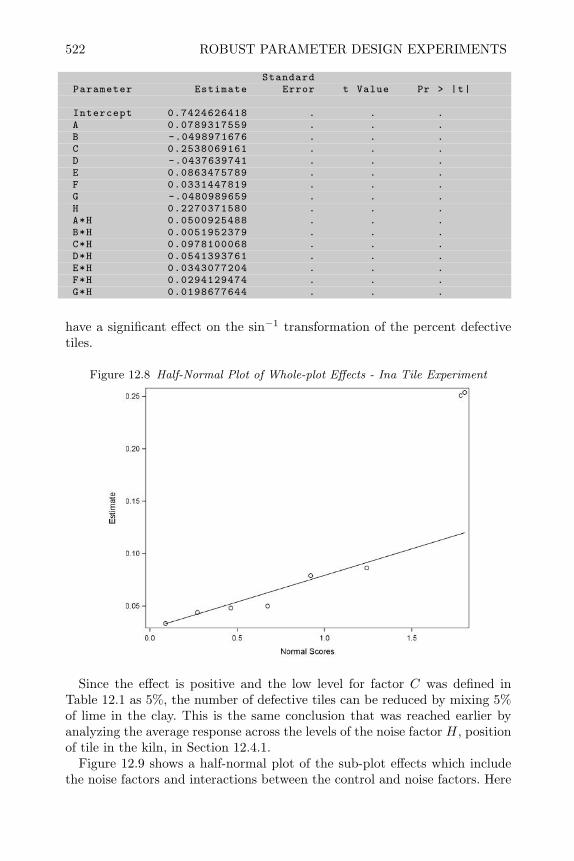
522 ROBUST PARAMETER DESIGN EXPERIMENTS
StandardParameter Estimate Error t Value Pr > |t|
Intercept 0.7424626418 . . .A 0.0789317559 . . .B -.0498971676 . . .C 0.2538069161 . . .D -.0437639741 . . .E 0.0863475789 . . .F 0.0331447819 . . .G -.0480989659 . . .H 0.2270371580 . . .A*H 0.0500925488 . . .B*H 0.0051952379 . . .C*H 0.0978100068 . . .D*H 0.0541393761 . . .E*H 0.0343077204 . . .F*H 0.0294129474 . . .G*H 0.0198677644 . . .
have a significant effect on the sin−1 transformation of the percent defectivetiles.
Figure 12.8 Half-Normal Plot of Whole-plot Effects - Ina Tile Experiment
Since the effect is positive and the low level for factor C was defined inTable 12.1 as 5%, the number of defective tiles can be reduced by mixing 5%of lime in the clay. This is the same conclusion that was reached earlier byanalyzing the average response across the levels of the noise factor H, positionof tile in the kiln, in Section 12.4.1.
Figure 12.9 shows a half-normal plot of the sub-plot effects which includethe noise factors and interactions between the control and noise factors. Here
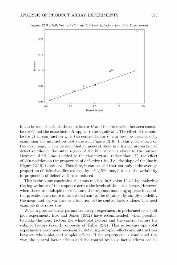
ANALYSIS OF PRODUCT ARRAY EXPERIMENTS 523
Figure 12.9 Half-Normal Plot of Sub-Plot Effects - Ina Tile Experiment
it can be seen that both the noise factor H and the interaction between controlfactor C and the noise factor H appear to be significant. The effect of the noisefactor H in conjunction with the control factor C can best be visualized byexamining the interaction plot shown in Figure 12.10. In this plot, shown onthe next page, it can be seen that in general there is a higher proportion ofdefective tiles in the outer region of the kiln which is closer to the burner.However, if 5% lime is added to the clay mixture, rather than 1%, the effectof kiln position on the proportion of defective tiles (i.e., the slope of the line inFigure 12.10) is reduced. Therefore, it can be said that not only is the averageproportion of defective tiles reduced by using 5% lime, but also the variabilityin proportion of defective tiles is reduced.
This is the same conclusion that was reached in Section 12.4.1 by analyzingthe log variance of the response across the levels of the noise factor. However,when there are multiple noise factors, the response modeling approach can of-ten provide much more information than can be obtained by simply modelingthe mean and log variance as a function of the control factors alone. The nextexample illustrates this.
When a product array parameter design experiment is performed as a splitplot experiment, Box and Jones (1992) have recommended, when possible,to make the noise factors the whole-plot factors and the control factors thesubplot factors (exactly opposite of Table 12.2). This is because split-plotexperiments have more precision for detecting sub-plot effects and interactionsbetween whole-plot and subplot effects. If the experiment is conducted thisway, the control factor effects and the control-by-noise factor effects can be
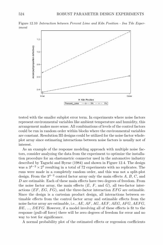
524 ROBUST PARAMETER DESIGN EXPERIMENTS
Figure 12.10 Interaction between Percent Lime and Kiln Position - Ina Tile Exper-iment
tested with the smaller subplot error term. In experiments where noise factorsrepresent environmental variables like ambient temperature and humidity, thisarrangement makes more sense. All combinations of levels of the control factorscould be run in random order within blocks where the environmental variablesare constant. Resolution III designs could be utilized for the noise factor whole-plot array since estimating interactions between noise factors is usually not ofinterest.
As an example of the response modeling approach with multiple noise fac-tors, consider analyzing the data from the experiment to optimize the installa-tion procedure for an elastometric connector used in the automotive industrydescribed by Taguchi and Byrne (1984) and shown in Figure 12.4. The designwas a 34−2 × 23 resulting in a total of 72 experiments with no replicates. Theruns were made in a completely random order, and this was not a split-plotdesign. From the 34−2 control factor array only the main effects A, B, C, andD are estimable. Each of these main effects have two degrees of freedom. Fromthe noise factor array, the main effects (E, F , and G), all two-factor inter-actions (EF , EG, FG), and the three-factor interaction EFG are estimable.Since the design is a cartesian product design, all interactions between es-timable effects from the control factor array and estimable effects from thenoise factor array are estimable, i.e., AE, AF , AG, AEF , AEG, AFG, AEFG,BE, ..., DEFG. However, if a model involving all of these effects is fit to theresponse (pull-off force) there will be zero degrees of freedom for error and noway to test for significance.
A normal probability plot of the estimated effects or regression coefficients
ANALYSIS OF PRODUCT ARRAY EXPERIMENTS 525
can be used to get an initial idea about which effects may be significant. How-ever, it is not as straightforward as the normal plots of regression coefficientsdescribed previously in Chapters 3 and 6. When all the factors have two levelsas the examples shown in Chapters 3 and 6, each regression coefficient rep-resents one single degree of freedom. When there are factors with more thantwo levels, like the control factors in the elastometric connector problem, themain effects and interactions have more than one degree of freedom so the firststep in making a normal plot is to represent each main effect by an orthogonalset of single-degree-of-freedom contrasts. This can be accomplished by usingthe orthogonal polynomial contrasts described in Section 2.8.1. Since the con-trol factor main effects have three levels the commands below illustrate thecreation of linear and quadratic contrasts for main effect A, creation of thecoded factor level, XE , for main effect E, and the creation of the linear×XE
and quadratic×XE parts of the A × E interaction. The linear and quadraticcontrasts for the other control factors, coded factor levels for the other noisefactors and the remainder of the interactions were created similarly.
data prod;input A B C D E F G pf;
if A=1 then Al = -.707107;if A=2 then Al=0;if A=3 then Al =.707107;if A=2 then Aq = -.816497; else Aq =.4082483;XE=(E -1.5)/.5;AlXE=Al*XE;AqXE=Aq*XE;
. . .datalines;1 1 1 1 1 1 1 15.6
When all the factors have two levels, the X matrix for the regression ismade up of orthogonal columns of −1’s and 1’s, and the X′X matrix isdiagonal with n on the diagonal where n is the total number of runs in theunreplicated design. The variance of the regression coefficient βi is σ2 × ciiwhere cii is the ith diagonal of X′X−1. Even though σ2 cannot be estimatedin an unreplicated 2k or 2k−p design, all the regression coefficients have thesame theoretical variance since diagonal elements cii are all equal to 1/n.Because they all have the same variance, they can be plotted on a normalplot.
However, when some of the regression coefficients represent orthogonal poly-nomial contrasts of factors with more than two levels and other regressioncoefficients represent coded two-level factors, their variances are not equal.For example, the sum of squares of the linear contrast for a three-level factorwill be equal to r × ((−.707107)2 + 02 + .7071072), where r is the number oftimes each level of the factor is repeated in the design, the sum of squaresfor the quadratic contrast for a three-level factor will be r × (.40824832 +(−.816497)2 + .40824832), and the sum of squares for a coded two-level factor

526 ROBUST PARAMETER DESIGN EXPERIMENTS
will be q × ((−1)2 + 12), where q is the number of times each level of thetwo-level factor is repeated in the design.
Since the sum of squares ((−.707107)2 + 02 + .7071072) = (.40824832 +.(−.816497)2 + .40824832) = 1, and there are 24 replicates of each level of thethree-level factors in the 72 runs of the design, the diagonal elements of X′Xfor each contrast of the three-level factors is 24. Since there are 36 replicatesof each level of the two-level factors in the 72 runs, the diagonal element ofthe X′X for each two-level factor and interaction between two-level factors is72. All of the regression coefficients in the 72-run design can be standardizedto have the same variance by dividing each contrast by the square root ofthe diagonal element of the unstandardized X′X matrix. For example, in thecommands below this is illustrated for factors A, B and E and F . This wasdone for all the coded factor levels and contrasts in the design resulting in anX′X that is equal to a 72 × 72 identity matrix. Recall that no interactionswere created between three-level control factors because they are not estimablefrom the 34−1 control factor array.
data prodstd; set prod;Al=Al/sqrt (24);Aq=Aq/sqrt (24);Bl=Bl/sqrt (24);Bq=Bq/sqrt (24);E=XE/sqrt (72);F=XF/sqrt (72);EF=XEF/sqrt (72);AlE=AlXE/sqrt (24);AqE=AqXE/sqrt (24);AlF=AlXF/sqrt (24);AqF=AqXF/sqrt (24);AlEF=AlXEF/sqrt (24);AqEF=AqXEF/sqrt (24);BlE=BlXE/sqrt (24);BqE=BqXE/sqrt (24);BlF=BlXF/sqrt (24);BqF=BqXF/sqrt (24);BlEF=BlXEF/sqrt (24);BqEF=BqXEF/sqrt (24);. . .keep pf Al Aq Bl Bq Cl Cq Dl Dq E F G EF EG FG EFGAlE AqE AlF AqF AlG AqG AlEF AqEF AlEG AqEG AlFG AqFG AlEFG AqEFGBlE BqE BlF BqF BlG BqG BlEF BqEF BlEG BqEG BlFG BqFG BlEFG BqEFGClE CqE ClF CqF ClG CqG ClEF CqEF ClEG CqEG ClFG CqFG ClEFG CqEFGDlE DqE DlF DqF DlG DqG DlEF DqEF DlEG DqEG DlFG DqFG DlEFG DqEFG
;
The estimated regression coefficients were determined by proc glm andoutput to a file for plotting similar to the examples in Chapters 3 and 6 usingthe commands shown at the top of the next page.
The normal plot of the 71 regression coefficients (excluding the intercept)was constructed by modifying the code from Section 3.7.5 and the result isshown in Figure 12.11. Examining the plot and the list of coefficients printed
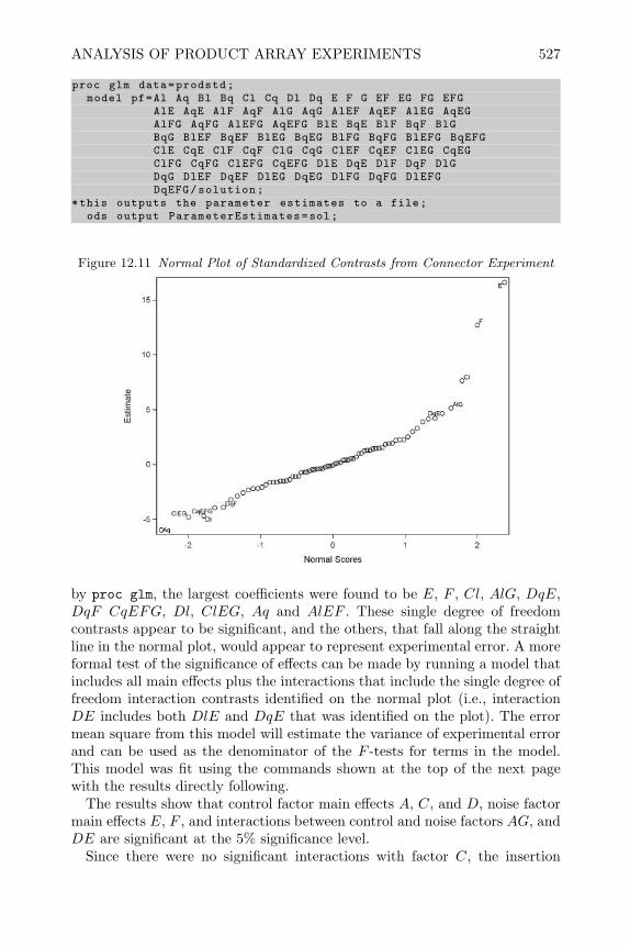
ANALYSIS OF PRODUCT ARRAY EXPERIMENTS 527
proc glm data=prodstd;model pf=Al Aq Bl Bq Cl Cq Dl Dq E F G EF EG FG EFG
AlE AqE AlF AqF AlG AqG AlEF AqEF AlEG AqEGAlFG AqFG AlEFG AqEFG BlE BqE BlF BqF BlGBqG BlEF BqEF BlEG BqEG BlFG BqFG BlEFG BqEFGClE CqE ClF CqF ClG CqG ClEF CqEF ClEG CqEGClFG CqFG ClEFG CqEFG DlE DqE DlF DqF DlGDqG DlEF DqEF DlEG DqEG DlFG DqFG DlEFGDqEFG/solution;
*this outputs the parameter estimates to a file;ods output ParameterEstimates=sol;
Figure 12.11 Normal Plot of Standardized Contrasts from Connector Experiment
by proc glm, the largest coefficients were found to be E, F , Cl, AlG, DqE,DqF CqEFG, Dl, ClEG, Aq and AlEF . These single degree of freedomcontrasts appear to be significant, and the others, that fall along the straightline in the normal plot, would appear to represent experimental error. A moreformal test of the significance of effects can be made by running a model thatincludes all main effects plus the interactions that include the single degree offreedom interaction contrasts identified on the normal plot (i.e., interactionDE includes both DlE and DqE that was identified on the plot). The errormean square from this model will estimate the variance of experimental errorand can be used as the denominator of the F -tests for terms in the model.This model was fit using the commands shown at the top of the next pagewith the results directly following.
The results show that control factor main effects A, C, and D, noise factormain effects E, F , and interactions between control and noise factors AG, andDE are significant at the 5% significance level.
Since there were no significant interactions with factor C, the insertion
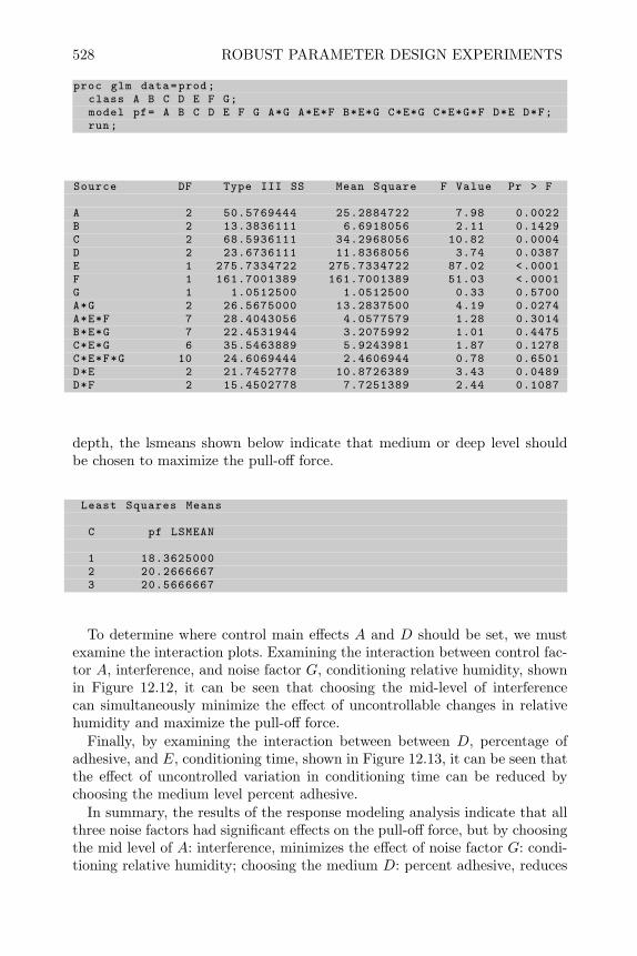
528 ROBUST PARAMETER DESIGN EXPERIMENTS
proc glm data=prod;class A B C D E F G;model pf= A B C D E F G A*G A*E*F B*E*G C*E*G C*E*G*F D*E D*F;run;
Source DF Type III SS Mean Square F Value Pr > F
A 2 50.5769444 25.2884722 7.98 0.0022B 2 13.3836111 6.6918056 2.11 0.1429C 2 68.5936111 34.2968056 10.82 0.0004D 2 23.6736111 11.8368056 3.74 0.0387E 1 275.7334722 275.7334722 87.02 <.0001F 1 161.7001389 161.7001389 51.03 <.0001G 1 1.0512500 1.0512500 0.33 0.5700A*G 2 26.5675000 13.2837500 4.19 0.0274A*E*F 7 28.4043056 4.0577579 1.28 0.3014B*E*G 7 22.4531944 3.2075992 1.01 0.4475C*E*G 6 35.5463889 5.9243981 1.87 0.1278C*E*F*G 10 24.6069444 2.4606944 0.78 0.6501D*E 2 21.7452778 10.8726389 3.43 0.0489D*F 2 15.4502778 7.7251389 2.44 0.1087
depth, the lsmeans shown below indicate that medium or deep level shouldbe chosen to maximize the pull-off force.
Least Squares Means
C pf LSMEAN
1 18.36250002 20.26666673 20.5666667
To determine where control main effects A and D should be set, we mustexamine the interaction plots. Examining the interaction between control fac-tor A, interference, and noise factor G, conditioning relative humidity, shownin Figure 12.12, it can be seen that choosing the mid-level of interferencecan simultaneously minimize the effect of uncontrollable changes in relativehumidity and maximize the pull-off force.
Finally, by examining the interaction between between D, percentage ofadhesive, and E, conditioning time, shown in Figure 12.13, it can be seen thatthe effect of uncontrolled variation in conditioning time can be reduced bychoosing the medium level percent adhesive.
In summary, the results of the response modeling analysis indicate that allthree noise factors had significant effects on the pull-off force, but by choosingthe mid level of A: interference, minimizes the effect of noise factor G: condi-tioning relative humidity; choosing the medium D: percent adhesive, reduces
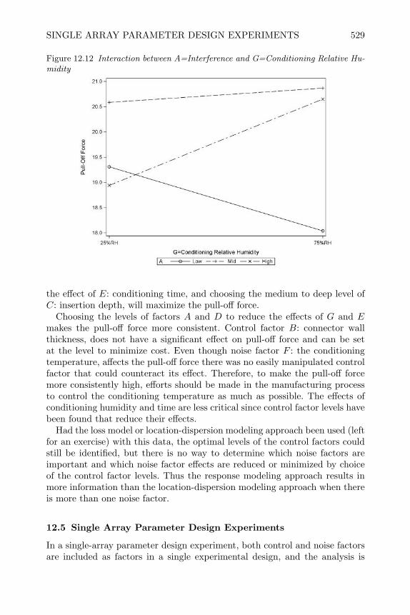
SINGLE ARRAY PARAMETER DESIGN EXPERIMENTS 529
Figure 12.12 Interaction between A=Interference and G=Conditioning Relative Hu-midity
the effect of E: conditioning time, and choosing the medium to deep level ofC: insertion depth, will maximize the pull-off force.
Choosing the levels of factors A and D to reduce the effects of G and Emakes the pull-off force more consistent. Control factor B: connector wallthickness, does not have a significant effect on pull-off force and can be setat the level to minimize cost. Even though noise factor F : the conditioningtemperature, affects the pull-off force there was no easily manipulated controlfactor that could counteract its effect. Therefore, to make the pull-off forcemore consistently high, efforts should be made in the manufacturing processto control the conditioning temperature as much as possible. The effects ofconditioning humidity and time are less critical since control factor levels havebeen found that reduce their effects.
Had the loss model or location-dispersion modeling approach been used (leftfor an exercise) with this data, the optimal levels of the control factors couldstill be identified, but there is no way to determine which noise factors areimportant and which noise factor effects are reduced or minimized by choiceof the control factor levels. Thus the response modeling approach results inmore information than the location-dispersion modeling approach when thereis more than one noise factor.
12.5 Single Array Parameter Design Experiments
In a single-array parameter design experiment, both control and noise factorsare included as factors in a single experimental design, and the analysis is
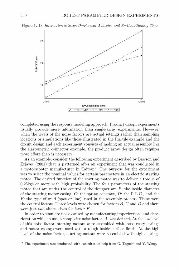
530 ROBUST PARAMETER DESIGN EXPERIMENTS
Figure 12.13 Interaction between D=Percent Adhesive and E=Conditioning Time
completed using the response modeling approach. Product design experimentsusually provide more information than single-array experiments. However,when the levels of the noise factors are actual settings rather than samplinglocations or simulations like those illustrated in the Ina tile example and thecircuit design and each experiment consists of making an actual assembly likethe elastometric connector example, the product array design often requiresmore effort than is necessary.
As an example, consider the following experiment described by Lawson andErjavec (2001) that is patterned after an experiment that was conducted ina motorscooter manufacturer in Taiwan∗. The purpose for the experimentwas to select the nominal values for certain parameters in an electric startingmotor. The desired function of the starting motor was to deliver a torque of0.25kgs or more with high probability. The four parameters of the startingmotor that are under the control of the designer are B: the inside diameterof the starting motor casing, C: the spring constant, D: the R.L.C., and theE: the type of weld (spot or line), used in the assembly process. These werethe control factors. Three levels were chosen for factors B, C and D and therewere just two alternatives for factor E.
In order to simulate noise caused by manufacturing imperfections and dete-rioration while in use, a composite noise factor, A, was defined. At the low levelof this noise factor, starting motors were assembled with loose rusty springsand motor casings were used with a rough inside surface finish. At the highlevel of the noise factor, starting motors were assembled with tight springs
∗ The experiment was conducted with consultation help from G. Taguchi and Y. Wang.
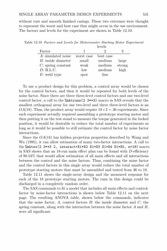
SINGLE ARRAY PARAMETER DESIGN EXPERIMENTS 531
without rust and smooth finished casings. These two extremes were thoughtto represent the worst and best case that might occur in the use environment.The factors and levels for the experiment are shown in Table 12.10.
Table 12.10 Factors and Levels for Motorscooter Starting Motor Experimentlevels
Factor 1 2 3A: simulated noise worst case best caseB: inside diameter small medium largeC: spring constant weak medium strongD: R.L.C. low medium highE: weld type spot line
To use a product design for this problem, a control array would be chosenfor the control factors, and then it would be repeated for both levels of thenoise factor. Since there are three three-level control factors and one two-levelcontrol factor, a call to the %mktruns(2 3**3) macro in SAS reveals that thesmallest orthogonal array for one two-level and three three-level factors is anOA(18). Thus, the product array would require 18×2 = 36 experiments. Sinceeach experiment actually required assembling a prototype starting motor andthen putting it on the test stand to measure the torque generated in the lockedposition, it would be desirable to reduce the total number of experiments aslong as it would be possible to still estimate the control factor by noise factorinteractions.
Since the OA(18) has hidden projection properties described by Wang andWu (1995), it can allow estimation of many two-factor interactions. A call tothe %mktex(2 3**3 2, interact=X1*X2 X1*X3 X1*X4 X1*X5, n=18) macroin SAS shows that an 18-run main effect plan can be found with D-efficiencyof 98.53% that would allow estimation of all main effects and all interactionsbetween the control and the noise factors. Thus, combining the noise factorand the control factors in this single array would reduce the total number ofprototype starting motors that must be assembled and tested from 36 to 18.
Table 12.11 shows the single-array design and the measured response foreach of the 18 prototype starting motors. The runs in this design could bedischarged in a completely random order.
The SAS commands to fit a model that includes all main effects and control-factor by noise-factor interactions is shown below Table 12.11 on the nextpage. The resulting ANOVA table, shown below the commands, indicatesthat the noise factor, A, control factors B: the inside diameter and C: thespring constant, along with the interaction between the noise factor A and B,were all significant.

532 ROBUST PARAMETER DESIGN EXPERIMENTS
Table 12.11 Single Array for Starting Motor DesignRun A B C D E torque
1 1 1 1 1 1 0.2253532 1 1 2 2 2 0.2571853 1 1 3 3 2 0.2760324 1 2 1 1 2 0.2244855 1 2 2 2 2 0.2422036 1 2 3 3 1 0.2587917 1 3 1 2 1 0.2086738 1 3 2 3 2 0.2319729 1 3 3 1 2 0.25737710 2 1 1 3 2 0.24102611 2 1 2 1 1 0.25937312 2 1 3 2 2 0.28407313 2 2 1 2 2 0.26684514 2 2 2 3 1 0.27835915 2 2 3 1 2 0.30710116 2 3 1 3 2 0.24825617 2 3 2 1 2 0.27057518 2 3 3 2 1 0.293259
Data Smotor;input Run A B C D E torque;datalines;1 1 1 1 1 1 0.225353
. . .proc glm;
class A B C D E;model torque=A B C D E A*B A*C A*D A*E;
run;
Source DF Type III SS Mean Square F Value Pr > F
A 1 0.00342407 0.00342407 467.76 0.0021B 2 0.00038172 0.00019086 26.07 0.0369C 2 0.00320145 0.00160072 218.68 0.0046D 2 0.00002682 0.00001341 1.83 0.3531E 1 0.00004227 0.00004227 5.77 0.1382A*B 2 0.00100676 0.00050338 68.77 0.0143A*C 2 0.00000312 0.00000156 0.21 0.8241A*D 2 0.00000518 0.00000259 0.35 0.7388A*E 1 0.00002577 0.00002577 3.52 0.2015

SINGLE ARRAY PARAMETER DESIGN EXPERIMENTS 533
The least squares means (shown below) for factor C: the spring constantshow that the torque generated by the starting motor increases nearly linearlyas the spring constant increases. Therefore, the strong level of the springconstant should be used to maximize the torque.
torqueC LSMEAN
1 0.236799752 0.254242253 0.27848238
The interaction between A and B should be studied in order to determinewhich level of B, inside diameter, that should be used. The output below showsthe least squares means for the different combinations of levels of factors Aand B and Figure 12.14 shows the interaction plot.
torqueA B LSMEAN
1 1 0.251492251 2 0.240461921 3 0.231309582 1 0.261322672 2 0.283933672 3 0.27052867
In the plot (shown in Figure 12.14) it can be seen that on the average thetorque is higher when the noise factor is set at the best case than it is whenthe noise factor is set at the worst case. However, when the inside diameteris small, the difference in the torque generated at the best and worst casesfor the noise factor is minimized. Although the average torque appears to beslightly higher when B: the inside diameter is at the medium level, the rangein differences (0.28393367-0.24046192=0.04347175) caused by the noise factoris over four times larger than it is when B is set at its small level (0.26132267-0.25149225=0.00983042). Therefore, in order to maximize the probability thatthe starting motor will deliver a torque of 0.25kgs or more, the small insidediameter should be used.
As a second example of a single-array parameter design, consider an ex-periment described by Montgomery (1990) to improve an injection moldingprocess for producing plastic parts. Prior to the experiment there was exces-sive shrinkage of parts after molding that was causing downstream assemblyproblems. Four factors that could easily be controlled in the process were A:mold temperature; B: screw speed; C: holding time ; and D: gate size. Thesewere the control factors. Process variables that could affect shrinkage but that
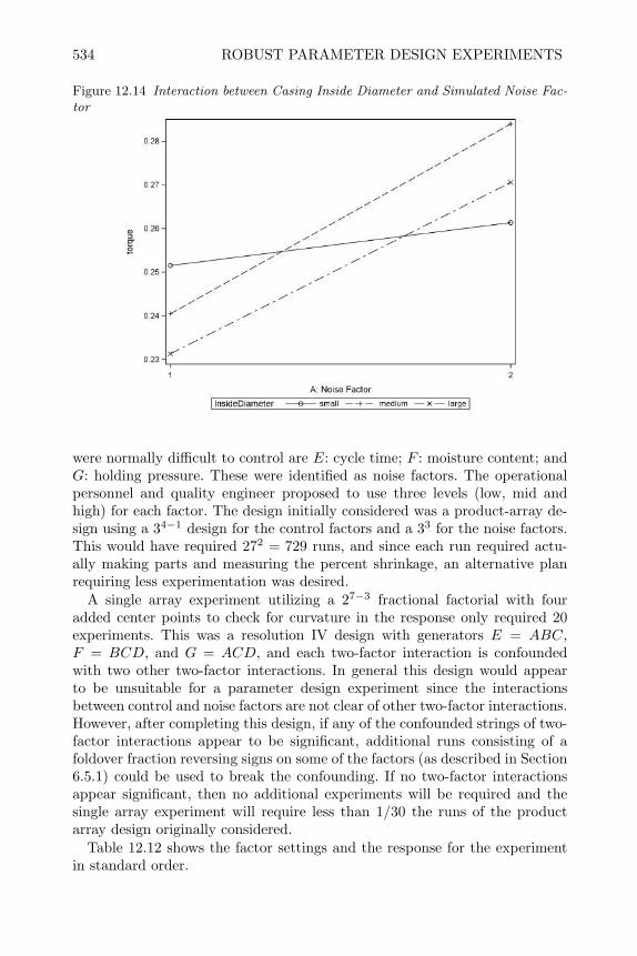
534 ROBUST PARAMETER DESIGN EXPERIMENTS
Figure 12.14 Interaction between Casing Inside Diameter and Simulated Noise Fac-tor
were normally difficult to control are E: cycle time; F : moisture content; andG: holding pressure. These were identified as noise factors. The operationalpersonnel and quality engineer proposed to use three levels (low, mid andhigh) for each factor. The design initially considered was a product-array de-sign using a 34−1 design for the control factors and a 33 for the noise factors.This would have required 272 = 729 runs, and since each run required actu-ally making parts and measuring the percent shrinkage, an alternative planrequiring less experimentation was desired.
A single array experiment utilizing a 27−3 fractional factorial with fouradded center points to check for curvature in the response only required 20experiments. This was a resolution IV design with generators E = ABC,F = BCD, and G = ACD, and each two-factor interaction is confoundedwith two other two-factor interactions. In general this design would appearto be unsuitable for a parameter design experiment since the interactionsbetween control and noise factors are not clear of other two-factor interactions.However, after completing this design, if any of the confounded strings of two-factor interactions appear to be significant, additional runs consisting of afoldover fraction reversing signs on some of the factors (as described in Section6.5.1) could be used to break the confounding. If no two-factor interactionsappear significant, then no additional experiments will be required and thesingle array experiment will require less than 1/30 the runs of the productarray design originally considered.
Table 12.12 shows the factor settings and the response for the experimentin standard order.
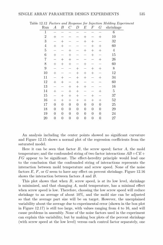
SINGLE ARRAY PARAMETER DESIGN EXPERIMENTS 535
Table 12.12 Factors and Response for Injection Molding ExperimentRun A B C D E F G shrinkage
1 − − − − − − − 62 + − − − + − + 103 − + − − + + − 324 + + − − − + + 605 − − + − + + + 46 + − + − − + − 157 − + + − − − + 268 + + + − + − − 609 − − − + − + + 810 + − − + + + − 1211 − + − + + − + 3412 + + − + − − − 6013 − − + + + − − 1614 + − + + − − + 515 − + + + − + − 3716 + + + + + + + 5217 0 0 0 0 0 0 0 2518 0 0 0 0 0 0 0 2919 0 0 0 0 0 0 0 2420 0 0 0 0 0 0 0 27
An analysis including the center points showed no significant curvatureand Figure 12.15 shows a normal plot of the regression coefficients from thesaturated model.
Here it can be seen that factor B, the screw speed; factor A, the moldtemperature; and the confounded string of two factor interactions AB+CE+FG appear to be significant. The effect-heredity principle would lead oneto the conclusion that the confounded string of interactions represents theinteraction between mold temperature and screw speed. None of the noisefactors E, F , or G seem to have any effect on percent shrinkage. Figure 12.16shows the interaction between factors A and B.
This plot shows that when B, screw speed, is at its low level, shrinkageis minimized, and that changing A, mold temperature, has a minimal effectwhen screw speed is low. Therefore, choosing the low screw speed will reduceshrinkage to an average of about 10%, and the mold size can be adjustedso that the average part size will be on target. However, the unexplainedvariability about the average due to experimental error (shown in the box plotin Figure 12.17) is still too large, with values ranging from 4 to 16, and willcause problems in assembly. None of the noise factors used in the experimentcan explain this variability, but by making box plots of the percent shrinkage(with screw speed at the low level) versus each control factor separately, one
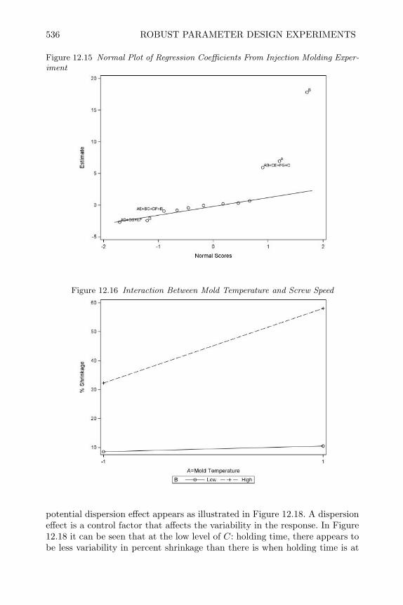
536 ROBUST PARAMETER DESIGN EXPERIMENTS
Figure 12.15 Normal Plot of Regression Coefficients From Injection Molding Exper-iment
Figure 12.16 Interaction Between Mold Temperature and Screw Speed
potential dispersion effect appears as illustrated in Figure 12.18. A dispersioneffect is a control factor that affects the variability in the response. In Figure12.18 it can be seen that at the low level of C: holding time, there appears tobe less variability in percent shrinkage than there is when holding time is at
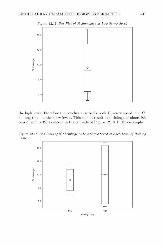
SINGLE ARRAY PARAMETER DESIGN EXPERIMENTS 537
Figure 12.17 Box Plot of % Shrinkage at Low Screw Speed
the high level. Therefore the conclusion is to fix both B: screw speed, and C:holding time, at their low levels. This should result in shrinkage of about 9%plus or minus 3% as shown in the left side of Figure 12.18. In this example
Figure 12.18 Box Plots of % Shrinkage at Low Screw Speed at Each Level of HoldingTime

538 ROBUST PARAMETER DESIGN EXPERIMENTS
there were no significant noise factors, and no significant interactions betweenthe control and noise factors. Therefore, variability in percent shrinkage couldnot be accomplished by reducing or nullifying the effect of the suspected noisefactors used in the experiment. However, there are obviously other unknown orlurking noise factors that are causing variability in the response. By identifyinga dispersion effect and choosing the level which minimizes the variability, oneactually reduces the effects of the unknown noise factors resulting in a moreconsistent response.
Box and Meyer (1986b) described a more formal method of detecting dis-persion effects. They propose to first fit a model to the response (for thisexample A, B, and A×B) and calculate the residuals from the model. Next,they calculate the dispersion statistic for each factor as the natural log of theratio of the sample variances of the residuals at the high and low levels withthe formula
F ∗i = lnS2(i+)S2(i−)
, (12.5)
where S2(i+) is the sample variance of the residuals at the high level of factori and S2(i−) is the sample variance of the residuals at the low level of factor i.They show that these statistics are approximately normally distributed withmean zero and standard deviation 1.
12.6 Joint Modeling of Mean and Dispersion Effects
12.6.1 Joint Modeling
One of the assumptions that justifies fitting a linear model by least squaresis constancy of the variance of the experimental error across all levels of thefactors in the model. If there is a dispersion effect, this assumption will obvi-ously be violated. Therefore, the accuracy of the coefficients in the model forthe average response will be reduced because too much weight will be givento minimizing errors in prediction in regions where the variance is larger.Nelder and Lee (1998) and Lee and Nelder (2003) have suggested an iterativeweighted least squares approach to estimation. This consists of:
1. Fitting a modelβ = (X ′X)−1X ′y (12.6)
which includes all terms that affect the mean response, and calculating andstoring the residuals from this model.
2. Fitting a modelγ = (X ′X)−1X ′z (12.7)
which includes all dispersion effects is fit, using zi = ln r2i as the response,
where ri are the residuals from the model 12.6. The predicted values fromthis model, zi are calculated and stored.
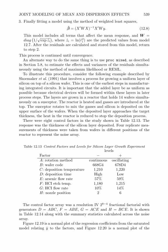
JOINT MODELING OF MEAN AND DISPERSION EFFECTS 539
3. Finally fitting a model using the method of weighted least squares,
β = (X ′WX)−1X ′Wy. (12.8)
This model includes all terms that affect the mean response, and W =diag
(1/√
exp zi), where zi = ln(r2
i ) are the predicted values from model12.7. After the residuals are calculated and stored from this model, returnto step 2.
This process is continued until convergence.An alternate way to do the same thing is to use proc mixed, as described
in Section 5.8, to estimate the effects and variances of the residuals simulta-neously using the method of maximum likelihood or REML.
To illustrate this procedure, consider the following example described byShoemaker et al. (1991) that involves a process for growing a uniform layer ofsilicon on top of a silicon wafer. This is one of the earliest steps in manufactur-ing integrated circuits. It is important that the added layer be as uniform aspossible because electrical devices will be formed within these layers in laterprocess steps. The layers are grown in a reactor that holds 14 wafers simulta-neously on a susceptor. The reactor is heated and gasses are introduced at thetop. The susceptor rotates to mix the gasses and silicon is deposited on theupper surface of the wafers. When the deposited layer approaches the targetthickness, the heat in the reactor is reduced to stop the deposition process.
There were eight control factors in the study shown in Table 12.13. Theresponse was the thickness of the silicon layer deposited. Four replicate mea-surements of thickness were taken from wafers in different positions of thereactor to represent the noise array.
Table 12.13 Control Factors and Levels for Silicon Layer Growth Experimentlevels
Factor − +A: rotation method continuous oscillatingB: wafer code 668G4 678D4C: deposition temperature 1,210 1,220D: deposition time High LowE: arsenic flow rate 57% 59%F : HCI etch temp. 1,180 1,215G: HCI flow rate 10% 14%H: nozzle position 2 6
The control factor array was a resolution IV 28−4 fractional factorial withgenerators D = ABC, F = ABE, G = ACE and H = BCE. It is shownin Table 12.14 along with the summary statistics calculated across the noisearray.
Figure 12.19 is a normal plot of the regression coefficients from the saturatedmodel relating y to the factors, and Figure 12.20 is a normal plot of the

540 ROBUST PARAMETER DESIGN EXPERIMENTS
Table 12.14 Mean and Variance for Each Row in Control ArrayA B C D E F G H y s2
i
− − − − − − − − 14.804 0.00171+ − − + − + + − 13.979 0.10942− − − − + + + + 14.880 0.00372+ − − + + − − + 14.120 0.10615− + − + − + − + 14.158 0.00060+ + − − − − + + 14.766 0.19199− + − + + − + − 13.837 0.00612+ + − − + + − − 14.846 0.22907− − + + − − + + 14.034 0.00305+ − + − − + − + 14.792 0.38227− − + + + + − − 13.891 0.00096+ − + − + − + − 14.348 0.21191− + + − − + + − 14.728 0.00144+ + + + − − − − 13.738 0.26182− + + − + − − + 14.884 0.01923+ + + + + + + + 13.973 0.07569
regression coefficients from the saturated model relating ln(s2i ) to the factors.
In Figure 12.19 it can be seen that D: deposition time and H: nozzle positionappear to have significant effects on the average thickness. In Figure 12.20it can be seen that A: rotation method appears to have a positive effect onln(s2
i ). This is a dispersion effect and should be set to its low level (continuous)to minimize variability of the silicon layer thickness.
The levels of the adjustment factors (D: deposition time, and H: nozzleposition) can be chosen to bring the average thickness to the desired target.However, since A: rotation method affects ln(s2
i ), the variance of the residualswill not be constant and the assumptions required for the least squares esti-mates of the D and H effects are violated. Therefore, inaccuracy will result ifthe least squares coefficients for D and H are used in predicting the levels ofD and H needed to bring the average thickness to the desired target.
In the commands below, use of the repeated/group=A; statement causesproc mixed to simultaneously compute weighted least squares estimates of the
proc mixed data=epitaxstr;class A;model y=D H/ solution;repeated/group=A;
run;
adjustment factor effects and REML estimates of the variance of the residualswithin each level of the dispersion factor. A portion of the output is shownfollowing Figure 12.20.
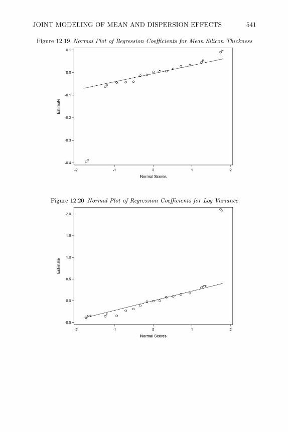
JOINT MODELING OF MEAN AND DISPERSION EFFECTS 541
Figure 12.19 Normal Plot of Regression Coefficients for Mean Silicon Thickness
Figure 12.20 Normal Plot of Regression Coefficients for Log Variance

542 ROBUST PARAMETER DESIGN EXPERIMENTS
Covariance Parameter Estimates
Cov Parm Group Estimate
Residual A -1 0.006409Residual A 1 0.1772
Null Model Likelihood Ratio Test
DF Chi -Square Pr > ChiSq
1 59.24 <.0001
Solution for Fixed Effects
StandardEffect Estimate Error DF t Value Pr > |t|
Intercept 14.3993 0.01390 61 1035.69 <.0001D -0.4202 0.01390 61 -30.22 <.0001H 0.08713 0.01390 61 6.27 <.0001
In the output above the weighted least squares estimates of the adjust-ment factors are shown, and it can be seen that the σ2
(A=−) = 0.006409 andσ2
(A=+) = 0.1772. From these coefficients, the coded level of D: depositiontime, and H: nozzle position, can be determined by solving the equation:
desired thickness = 14.3993− 0.4202XD + 0.08713XH (12.9)
for XD and XH .
12.6.2 Designing a Noise Array
When the noise-factor array consists of replicate samples over time or spacelike the tile experiment or the silicon layer growth experiment, and the analysisis to be completed using the location-dispersion modeling approach, a frac-tional factorial or orthogonal array design may not be the most efficient way todesign the noise array. When the analysis is completed using the location dis-persion modeling, the purpose of the noise array is not to efficiently estimatethe effects of the noise factors, but rather to allow accurate estimation of thevariance in the response across the noise space. Therefore, rather than usingan orthogonal array or fractional factorial that distributes points in the noisespace to the extremes, a plan that provides representative points from thenoise space would be better. Wang et al. (1995) introduced the concept of aquantizer to select optimally representative points from the noise space. Theytabulated their representative points for practical use. Table 12.15, shown onthe next page, is a part of their table of representative points.

JOINT MODELING OF MEAN AND DISPERSION EFFECTS 543
Table 12.15 Optimal Representative Points in [0,1]k Assuming Uniform Distribution
Numberof runs Number of Noise Factors kn 1 2 3 4 5 63 0.1667
0.50000.8333
4 0.1250 0.3750 0.8750 0.62500.3750 0.8750 0.6250 0.12500.6250 0.1250 0.3750 0.87500.8750 0.6250 0.1250 0.3750
5 0.1000 0.3000 0.7000 0.50000.3000 0.7000 0.5000 0.10000.5000 0.1000 0.3000 0.70000.7000 0.5000 0.1000 0.30000.9000 0.9000 0.9000 0.9000
6 0.0833 0.4167 0.2500 0.9167 0.5833 0.75000.2500 0.9167 0.5833 0.7500 0.0833 0.41670.4167 0.2500 0.9167 0.5833 0.7500 0.08330.5833 0.7500 0.0833 0.4167 0.2500 0.91670.7500 0.0833 0.4167 0.2500 0.9167 0.58330.9167 0.5833 0.7500 0.0833 0.4167 0.2500
7 0.0714 0.3571 0.2143 0.7857 0.5000 0.64290.2143 0.7857 0.5000 0.6429 0.0714 0.35710.3571 0.2143 0.7857 0.5000 0.6429 0.07140.5000 0.6429 0.0714 0.3571 0.2143 0.78570.6429 0.0714 0.3571 0.2143 0.7857 0.50000.7857 0.5000 0.6429 0.0714 0.3571 0.21430.9286 0.9286 0.9286 0.9286 0.9286 0.9286
8 0.0625 0.4375 0.8125 0.1875 0.9375 0.56250.1875 0.9375 0.5625 0.4375 0.8125 0.06250.3125 0.3125 0.3125 0.6875 0.6875 0.68750.4375 0.8125 0.0625 0.9375 0.5625 0.18750.5625 0.1875 0.9375 0.0625 0.4375 0.81250.6875 0.6875 0.6875 0.3125 0.3125 0.31250.8125 0.0625 0.4375 0.5625 0.1875 0.93750.9375 0.5625 0.1875 0.8125 0.0625 0.4375
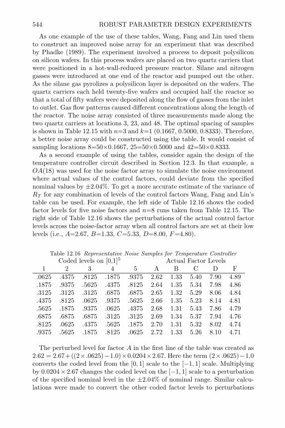
544 ROBUST PARAMETER DESIGN EXPERIMENTS
As one example of the use of these tables, Wang, Fang and Lin used themto construct an improved noise array for an experiment that was describedby Phadke (1989). The experiment involved a process to deposit polysiliconon silicon wafers. In this process wafers are placed on two quartz carriers thatwere positioned in a hot-wall-reduced pressure reactor. Silane and nitrogengasses were introduced at one end of the reactor and pumped out the other.As the silane gas pyrolizes a polysilicon layer is deposited on the wafers. Thequartz carriers each held twenty-five wafers and occupied half the reactor sothat a total of fifty wafers were deposited along the flow of gasses from the inletto outlet. Gas flow patterns caused different concentrations along the length ofthe reactor. The noise array consisted of three measurements made along thetwo quartz carriers at locations 3, 23, and 48. The optimal spacing of samplesis shown in Table 12.15 with n=3 and k=1 (0.1667, 0.5000, 0.8333). Therefore,a better noise array could be constructed using the table. It would consist ofsampling locations 8=50×0.1667, 25=50×0.5000 and 42=50×0.8333.
As a second example of using the tables, consider again the design of thetemperature controller circuit described in Section 12.3. In that example, aOA(18) was used for the noise factor array to simulate the noise environmentwhere actual values of the control factors, could deviate from the specifiednominal values by ±2.04%. To get a more accurate estimate of the variance ofRT for any combination of levels of the control factors Wang, Fang and Lin’stable can be used. For example, the left side of Table 12.16 shows the codedfactor levels for five noise factors and n=8 runs taken from Table 12.15. Theright side of Table 12.16 shows the perturbations of the actual control factorlevels across the noise-factor array when all control factors are set at their lowlevels (i.e., A=2.67, B=1.33, C=5.33, D=8.00, F=4.80).
Table 12.16 Representative Noise Samples for Temperature ControllerCoded levels on [0,1]5 Actual Factor Levels
1 2 3 4 5 A B C D F.0625 .4375 .8125 .1875 .9375 2.62 1.33 5.40 7.90 4.89.1875 .9375 .5625 .4375 .8125 2.64 1.35 5.34 7.98 4.86.3125 .3125 .3125 .6875 .6875 2.65 1.32 5.29 8.06 4.84.4375 .8125 .0625 .9375 .5625 2.66 1.35 5.23 8.14 4.81.5625 .1875 .9375 .0625 .4375 2.68 1.31 5.43 7.86 4.79.6875 .6875 .6875 .3125 .3125 2.69 1.34 5.37 7.94 4.76.8125 .0625 .4375 .5625 .1875 2.70 1.31 5.32 8.02 4.74.9375 .5625 .1875 .8125 .0625 2.72 1.33 5.26 8.10 4.71
The perturbed level for factor A in the first line of the table was created as2.62 = 2.67+((2× .0625)−1.0)×0.0204×2.67. Here the term (2× .0625)−1.0converts the coded level from the [0, 1] scale to the [−1, 1] scale. Multiplyingby 0.0204×2.67 changes the coded level on the [−1, 1] scale to a perturbationof the specified nominal level in the ±2.04% of nominal range. Similar calcu-lations were made to convert the other coded factor levels to perturbations
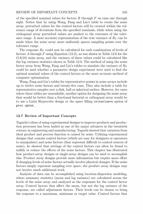
REVIEW OF IMPORTANT CONCEPTS 545
of the specified nominal values for factors B through F on runs one througheight. Notice that by using Wang, Fang and Lin’s table to create the noisearray, perturbed values for the control factors will be created within the tol-erance range of deviations from the specified nominals, while when using theorthogonal array perturbed values are pushed to the extremes of the toler-ance range. A more accurate representation of the true variance of RT can bemade when the noise array more uniformly spaces sampling points over thetolerance range.
The response RT could now be calculated for each combination of levels offactors A through F using Equation (12.2), as was shown in Table 12.6 for theOA(18) noise array, and the variance of these values could be calculated likethe log variance statistics shown in Table 12.8. The method of using the noisefactor array from Wang, Fang and Lin’s tables to simulate the variance of RTcould be used whether a parameter design experiment were used to find theoptimal nominal values of the control factors or the more accurate method ofcomputer optimization.
Wang, Fang and Lin’s tables for representative points in noise arrays includeup to twelve noise factors and twenty-five runs. They also include a table forrepresentative samples over a disk, ball or spherical surface. However, for caseswhere these tables are unavailable, another option for designing the noise arraythat would be better than a fractional factorial or orthogonal array would beto use a Latin Hypercube design or the space filling criterion=u option ofproc optex.
12.7 Review of Important Concepts
Taguchi’s ideas of using experimental designs to improve products and produc-tion processes has been hailed as one of the major advances in the twentiethcentury in engineering and manufacturing. Taguchi showed that variation fromideal product and process function is caused by noise. Utilizing experimentaldesigns that contain control factors (which are easy for designers or operatorsto manipulate) and noise factors (that represent difficult to control sources ofnoise), he showed that settings of the control factors can often be found tonullify or reduce the effects of the noise factors. This chapter has illustratedhow product-array designs or single-array designs can be used to accomplishthis. Product array designs provide more information but require more effortif changing levels of noise factors actually involve physical changes. If the noisefactors simply represent sampling over space, the product array designs maynot involve much additional work.
Analysis of data can be accomplished using location-dispersion modeling,where summary statistics (mean and log variance) are calculated across thelevels of the noise array and analyzed as the responses for the control factorarray. Control factors that affect the mean, but not the log variance of theresponse, are called adjustment factors. Their levels can be chosen to bringthe response to a maximum, minimum or target value. Control factors that

546 ROBUST PARAMETER DESIGN EXPERIMENTS
affect the log variance should be set at a level that will minimize the variancein the response. A two-step procedure is usually used to identify the optimallevels of the control factors and adjustment factors.
The other method of analysis is to use the response model which is thesame as described in the other chapters of this book. When using the responsemodeling approach, identifying interactions between control and noise factorsbecomes very important. The levels of control factors that interact with noisefactors can sometimes be selected to minimize the effect of the noise factor.When using the response modeling approach, it is easier to determine exactlywhat noise factors cause functional variation, and what control factor settingscan reduce their effects. When no significant noise factors can be found, butexperimental error is too high and there is too much functional variation atoptimal control factor settings, residuals should be plotted versus the levelsof each control factor to identify any dispersion effects. Dispersion effects arefactors that have an effect on the variation of the response. Choosing the levelof the dispersion effect to minimize residual variation will reduce the effect ofunknown or lurking noise factors.
When levels of the noise factors represent replicate samples over the noisespace, the product array may actually be more efficient than a single-arraydesign. When analyzing product arrays using location-dispersion modeling,Wang, Fang, and Lin’s tables, or uniformly spaced points generated by procoptex, will give better estimates of the variance in the response over the noisearray.
Sometimes product arrays are actually split-plot experiments, and whenmodeled using the response modeling, they should be analyzed as a split-plot experiment. Box and Jones (1992) have recommended, when possible, toconduct product array parameter design experiments with the noise factorsas the whole-plot factors and the control factors as the subplot factors. Thisway the control factor effects and the control-by-noise factor effects can betested with the smaller subplot error term.

EXERCISES 547
12.8 Exercises
1. Consider the commercial product test of erasers conducted by Sachiyo andKosaka in 1971 and discussed by Taguchi (1987). The purpose of the testwas to determine the quality of erasure when lines of the same lengthdrawn on different types of paper were rubbed with different erasers. Forthe experiment lines of the same length were drawn on each type of paperby different pencils. The lines were rubbed three times back and forth byeach eraser and then judged for quality. A response of 0 = top means thatno pencil trace was left on the paper. A response of 1 = middle meansonly a faint pencil trace was left on the paper, and response of 2 = bottommeans it did not erase very well.Factors and levels for the experiment are shown in Table 12.17. The hopewas to identify the brand and material that produced the best qualityerasure consistently regardless of the type of paper or the hardness of thepencil lead used.
Table 12.17 Factors and Levels for Commercial Product Test of ErasersLevels
Factor 1 2 3 4 5Control Factors:A: Manufacturer Rabbit StaedtlerB: Material Rubber PlasticNoise Factors:C: Paper Note Paper Tracing PaperD: Lead Hardness 4H 2H HB 2B 4B
The control-factor array was a 22 factorial. One cell is missing since onemanufacturer did not make rubber erasers, and one cell is duplicated sincethe other manufacturer made two types of plastic erasers. The noise factorarray was a 2 × 5 full factorial. The product array design and the judgedresponses are shown in Table 12.18.
Table 12.18 Product Array Design and Response For Commercial Product TestC 1 2
A B D 1 2 3 4 5 1 2 3 4 51 1 1 0.5 1 1 1 0 0.5 0.5 2 1.51 2 0.5 1 1 1 1 0 0 0 0.5 1.52 2 0 0 0 0 0.5 0 0 0 0.5 01 2 0 0.5 1 1 0 0 0 0.5 1.5 1.5
(a) Analyze the data using location-dispersion modeling.(b) Use the two-step procedure in Section 12.4.1 to identify the brand and
material that produce the best quality erasure.

548 ROBUST PARAMETER DESIGN EXPERIMENTS
(c) Repeat the analysis using the response modeling approach.(d) Are there significant interactions between control and noise factors? Can
they be exploited to reduce the effect of the noise factors?(e) Is there an adjustment factor?
2. Reconsider the cake mix experiment described in exercise 9 of Chapter 8.The control factors that can be selected by the manufacturer are F : theamount of flour; S: the amount of shortening; and E: the amount of eggpowder in the mix. The noise factors are T : baking temperature, and t:baking time.
(a) Did you detect any control-by-noise interactions in the split-plot analysisconducted in Chapter 8? If so, can these interactions be exploited toreduce the effects of variation in baking time or baking temperature?
(b) Reanalyze the data using the location-dispersion modeling approach. Doyou reach the same conclusion about the optimal choice of levels of F ,S and E?
(c) Which method of analysis gives you more information?
3. Lawson (1990) describes an experiment in a chemical process with theaim of producing less byproduct tars. The control factors were A, reactiontemperature; B, catalyst concentration; and C, excess of reagent 1. Thenoise factors were E, purity of the recycled solvent; and D, purity of reagent1 that comes from a supplier. A product-array design was used for theexperiment that is shown in Table 12.19. The control-factor array is a Box-Behnken design that will allow estimation of all terms in a full quadraticmodel involving factors A, B and C. The noise factor array is a 22 factorial.
(a) What interactions are estimable in this design?(b) Analyze the data using the response modeling method. Are there any
interactions between control and noise factors that would allow you toreduce or nullify the effect of uncontrollable variability in the purity ofthe solvent stream and purity of reagent 1?
(c) Reanalyze the data using the location-dispersion modeling method. Doyou reach the same conclusions about optimal settings of the controlfactors? Is any information lost in analyzing the data in this way?
(d) Explain how the response modeling analysis would change if this exper-iment had been conducted as a split-plot design, where the noise factorswere the whole-plot factors and the control factors were the sub-plotfactors? Is there any advantage to running a product array split-plot de-sign with the noise factors as the whole-plot factors, rather than havingthe control factors as the whole-plot factors as in the Ina tile examplepresented in Section 12.3?
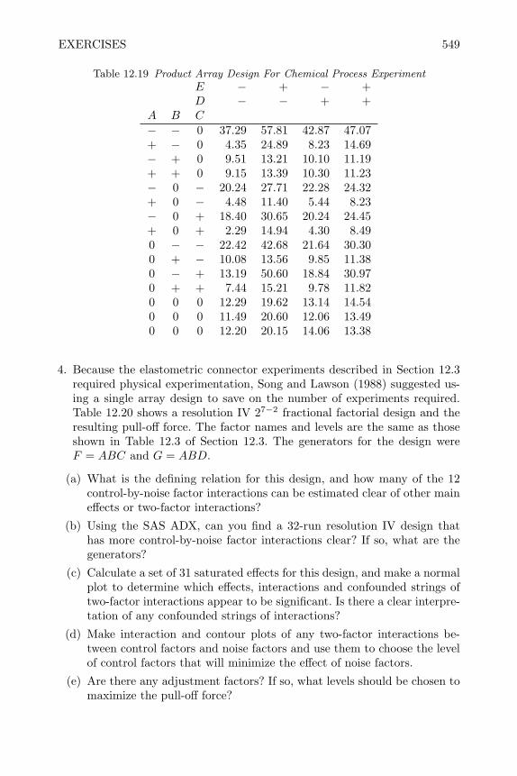
EXERCISES 549
Table 12.19 Product Array Design For Chemical Process ExperimentE − + − +D − − + +
A B C
− − 0 37.29 57.81 42.87 47.07+ − 0 4.35 24.89 8.23 14.69− + 0 9.51 13.21 10.10 11.19+ + 0 9.15 13.39 10.30 11.23− 0 − 20.24 27.71 22.28 24.32+ 0 − 4.48 11.40 5.44 8.23− 0 + 18.40 30.65 20.24 24.45+ 0 + 2.29 14.94 4.30 8.490 − − 22.42 42.68 21.64 30.300 + − 10.08 13.56 9.85 11.380 − + 13.19 50.60 18.84 30.970 + + 7.44 15.21 9.78 11.820 0 0 12.29 19.62 13.14 14.540 0 0 11.49 20.60 12.06 13.490 0 0 12.20 20.15 14.06 13.38
4. Because the elastometric connector experiments described in Section 12.3required physical experimentation, Song and Lawson (1988) suggested us-ing a single array design to save on the number of experiments required.Table 12.20 shows a resolution IV 27−2 fractional factorial design and theresulting pull-off force. The factor names and levels are the same as thoseshown in Table 12.3 of Section 12.3. The generators for the design wereF = ABC and G = ABD.
(a) What is the defining relation for this design, and how many of the 12control-by-noise factor interactions can be estimated clear of other maineffects or two-factor interactions?
(b) Using the SAS ADX, can you find a 32-run resolution IV design thathas more control-by-noise factor interactions clear? If so, what are thegenerators?
(c) Calculate a set of 31 saturated effects for this design, and make a normalplot to determine which effects, interactions and confounded strings oftwo-factor interactions appear to be significant. Is there a clear interpre-tation of any confounded strings of interactions?
(d) Make interaction and contour plots of any two-factor interactions be-tween control factors and noise factors and use them to choose the levelof control factors that will minimize the effect of noise factors.
(e) Are there any adjustment factors? If so, what levels should be chosen tomaximize the pull-off force?
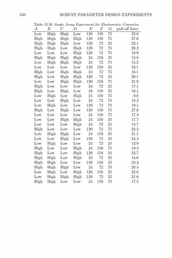
550 ROBUST PARAMETER DESIGN EXPERIMENTS
Table 12.20 Single Array Experiment for Elastometric ConnectorA B C D E F G pull-off forceLow High High Low 120 150 75 22.0High High High High 120 150 75 27.6High High High Low 120 72 25 22.1High High Low High 120 72 75 20.2Low Low Low High 120 72 75 18.9High High High High 24 150 25 13.8Low High High High 24 72 75 15.2Low Low Low Low 120 150 25 23.1High Low High High 24 72 75 16.1High Low High High 120 72 25 20.1Low Low High High 120 150 75 21.9High Low Low Low 24 72 25 17.1High Low High Low 24 150 25 18.1Low High Low High 24 150 75 9.6Low Low High Low 24 72 75 18.3Low High Low Low 120 72 75 19.1High Low High Low 120 150 75 27.0Low Low Low Low 24 150 75 17.3Low Low High High 24 150 25 17.7Low Low Low High 24 72 25 14.7High Low Low Low 120 72 75 22.2Low High High Low 24 150 25 21.1Low Low High Low 120 72 25 24.3Low High Low Low 24 72 25 13.9High Low Low High 24 150 75 19.4High Low Low High 120 150 25 22.7High High Low High 24 72 25 14.6High High Low Low 120 150 25 23.3High High High Low 24 72 75 20.4Low High Low High 120 150 25 22.6Low High High High 120 72 25 21.0High High Low Low 24 150 75 17.5

EXERCISES 551
5. Taguchi (1987) described an experiment to find the source of clutch slip-ping in automobiles. Prototype clutches were assembled using some newcomponents and some components taken from disassembled clutches thathad complaints. Each prototype was tested and the response, y, was ob-tained by dividing the slipping time by the number of revolutions of theengine and then multiplying by 10,000. The control and noise factors andtheir levels are shown in Table 12.21.
Table 12.21 Factors and Levels for Auto Clutch Slipping
LevelsControl Factors: − +B:Spring Allignment 5 levelsA:Force current +50kgD:Clutch Plate Running Distance ≤10,000km ≥30,000kmF :Cover Running Distance ≤10,000km ≥30,000km
LevelsNoise Factors: − +C:Clutch Plate ordinary product object of complaintE:Cover ordinary product object of complaint
A 20-run orthogonal array (shown in Table 12.22) was used to study bothcontrol and noise factors in a single array.
(a) Read the data into a SAS data set and construct −1 and +1 coded factorlevels for factors A, D, F , C and 4 orthogonal polynomial contrasts forfactor B. Create columns for the interactions between control and noisefactors.
(b) Find a model for the data using an all-subsets regression, as shown foranalysis of a Plackett-Burman design in Section 6.6 and for the analysisof the log variance for the temperature controller circuit in Section 12.4.
(c) From your model, identify any significant adjustment factors and control-by-noise interactions, and determine the levels of the control factors thatwill minimize clutch slippage with minimum variation.
(d) Are all control-by-noise factor interactions estimable from this design?If not, construct an orthogonal-array design or orthogonal main-effectplan that allows estimation of all control by noise interactions by usingthe interact= option of the %mktex macro as shown in Section 6.7.
6. An experiment originally performed by the National Railway Corporationof Japan (Taguchi and Wu, 1980) was re-analyzed by Box and Meyer(1986b). The control factors in the design were A, kind of welding rods;
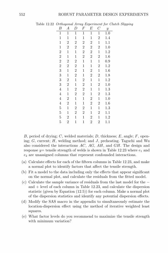
552 ROBUST PARAMETER DESIGN EXPERIMENTS
Table 12.22 Orthogonal Array Experiment for Clutch SlippingB A D F E C y
1 1 1 1 1 1 1.01 1 1 1 1 2 1.41 2 2 2 2 1 1.11 2 2 2 2 2 1.02 1 1 2 2 1 1.22 1 1 2 2 2 1.62 2 2 1 1 1 0.92 2 2 1 1 2 1.23 1 2 1 2 1 1.63 1 2 1 2 2 1.83 2 1 2 1 1 1.23 2 1 2 1 2 1.04 1 2 2 1 1 1.34 1 2 2 1 2 1.34 2 1 1 2 1 1.04 2 1 1 2 2 1.65 1 2 2 1 1 1.35 1 2 2 1 2 1.15 2 1 1 2 1 1.25 2 1 1 2 2 1.1
B, period of drying; C, welded materials; D, thickness; E, angle; F , open-ing; G, current; H, welding method; and J , preheating. Taguchi and Wualso considered the interactions AC, AG, AH, and GH. The design andresponse y= tensile strength of welds is shown in Table 12.23 where e1 ande2 are unassigned columns that represent confounded interactions.
(a) Calculate effects for each of the fifteen columns in Table 12.23, and makea normal plot to identify factors that affect the tensile strength.
(b) Fit a model to the data including only the effects that appear significanton the normal plot, and calculate the residuals from the fitted model.
(c) Calculate the sample variance of residuals from the last model for the −and + level of each column in Table 12.23, and calculate the dispersionstatistic (given by Equation (12.5)) for each column. Make a normal plotof the dispersion statistics and identify any potential dispersion effects.
(d) Modify the SAS macro in the appendix to simultaneously estimate thelocation-dispersion effect using the method of iterative weighted leastsquares.
(e) What factor levels do you recommend to maximize the tensile strengthwith minimum variation?

EXERCISES 553
Table 12.23 Design and Tensile Strength for Weld Experiment
D H G A F GH AC E AH AG J B C e1 e2 y− − − − + + − + + + − − + + − 43.7+ − − − − + + − + + + − − − + 40.2− + − − + − + + − + − + − − + 42.4+ + − − − − − − − + + + + + − 44.7− − + − − − + + + − + + − + − 42.4+ − + − + − − − + − − + + − + 45.9− + + − − + − + − − + − + − + 42.2+ + + − + + + − − − − − − + − 40.6− − − + + + − − − − + + − + + 42.4+ − − + − + + + − − − + + − − 45.5− + − + + − + − + − + − + − − 43.6+ + − + − − − + + − − − − + + 40.6− − + + − − + − − + − − + + + 44.0+ − + + + − − + − + + − − − − 40.2− + + + − + − − + + − + − − − 42.5+ + + + + + + + + + + + + + + 46.5
7. In the design of a thin film redistribution layer (cited by J. Lorenzen,IBM Kingston and discussed by Lawson and Madrigal (1994)), the cir-cuit impedance (Z) is a function of three design factors: the A, insulatorthickness; B, linewidth; and C, line height as shown in Figure 12.21. Fromengineering first principles, it can be shown that the impedance is given byEquation (12.10), where ε is the dielectric constant of the insulator and isassumed to be constant at 3.10.
Z = f(A,B,C) =87.0√ε+ 1.41
ln(
5.98A0.8B + C
)(12.10)
Figure 12.21 Thin Film Distribution Layer
The nominal or mean values of A, B, and C can be specified by the designengineer, but in actual circuits these characteristics will vary from theirnominal values due to manufacturing imperfections and wear during use.The table above shows the feasible range and tolerance limits for thesevariables.

554 ROBUST PARAMETER DESIGN EXPERIMENTS
Low-CostFeasible ToleranceRange Range
Control Factor (µm) (µm)A: Insulator thickness 20-30 ±1.0B: Linewidth 12.5-17.5 ±0.67C: Line height 4-6 ±0.33
(a) Construct a control-factor array using a 23 factorial design.(b) Construct a noise-factor array (in deviations from the nominal settings
in the control-factor array) using the table of Wang, Fang and Lin.(c) Evaluate Equation (12.10) for each combination of values in the product
array, and calculate the mean and log variance impedance across thenoise-factor array for each of the eight points in the control-factor array.
(d) Fit a model to the mean and log variance and identify the control fac-tor settings that will make the impedance equal to 85Ω with minimumvariability.
(e) Approximate the variance of Z, using the formula σ2Z ≈
(∂f∂A
)2
σ2A +(
∂f∂B
)2
σ2B+
(∂f∂C
)2
σ2C (where σ2
A=tolerance range/6, etc.), and use non-linear programming (proc nlp as described in Chapter 10) to minimizeσ2Z as a function of A, B, and C subject to the constraint that Z = 85Ω.
Do the results differ substantially from the answer you got in (d)?
8. Consider the data for the product array design for the elastometric connec-tor shown in Figure 12.4.
(a) Calculate the mean pull-off force and log variance of the pull-off forceacross the noise array for each run in the control-factor array.
(b) Analyze the data using the location-dispersion modeling method.(c) Do you find the same optimal levels of the control factors as identified
in Section 12.4.2?(d) Is any information lost when analyzing this data using location-dispersion
modeling?
9. Reconsider the data from the injection molding experiment in Table 12.12.
(a) Fit the model y = β0 +βAXA+βBXB +βA×BXAXB in the adjustmentfactors using the method of least squares.
(b) Simultaneously estimate the variance of the residuals at each level of thedispersion factor, C, and compute the weighted least squares estimatesof the coefficients in the model in (a) using proc mixed as shown inSection 12.6.1.

CHAPTER 13
Experimental Strategies for IncreasingKnowledge
13.1 Introduction
Experimental designs are the basis for collecting data to discover cause andeffect relationships. A number of different experimental designs have been pre-sented in this book. The experimental design most appropriate for a particularsituation will depend upon the circumstances. Throughout this book, the de-sign selection roadmap (Figure 1.2) has been used to indicate when specificexperimental designs should be used based on the number of factors, homo-geneity of the experimental units, and the ease of randomizing treatments toexperimental units. However, another way of viewing experimental designs isas a collection of tools that are useful for increasing the state of knowledgeabout a particular phenomenon.
The appropriate design (or tool) depends on how much knowledge is avail-able, and what additional information the experimenter would like to discover.The different experimental designs and corresponding methods of data anal-ysis presented in this book can be used in a sequence to advance knowledge,often referred to as sequential experimentation. This chapter presents an out-line of how experimental designs can be used in sequential experimentation.No detailed examples are presented in this chapter, but reference is made tospecific examples that have been presented in previous chapters.
13.2 Sequential Experimentation
Figure 13.1 illustrates the state of knowledge about a phenomenon as a contin-uous line that goes from zero knowledge on the left to a high state of knowledgeon the right. The purpose for experimenting is to advance the state of knowl-edge. Various stages along the line, descriptive names for the stages, purposesfor experimenting at each stage, and appropriate experimental designs for eachstage are shown below the knowledge line in the figure.
When there is a very low state of knowledge, the experimenter may knowthat the response is variable but he or she may not know what factors causevariability in the response. When this is the case, determining the sources ofvariability may give an experimenter clues to potential factors. Random sam-pling experiments, nested, and staggered nested designs described in Chapter5 are useful for determining sources of variability.
When the experimenter has a list of potential factors that could influence
555
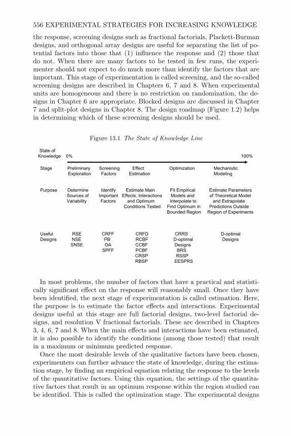
556 EXPERIMENTAL STRATEGIES FOR INCREASING KNOWLEDGE
the response, screening designs such as fractional factorials, Plackett-Burmandesigns, and orthogonal array designs are useful for separating the list of po-tential factors into those that (1) influence the response and (2) those thatdo not. When there are many factors to be tested in few runs, the experi-menter should not expect to do much more than identify the factors that areimportant. This stage of experimentation is called screening, and the so-calledscreening designs are described in Chapters 6, 7 and 8. When experimentalunits are homogeneous and there is no restriction on randomization, the de-signs in Chapter 6 are appropriate. Blocked designs are discussed in Chapter7 and split-plot designs in Chapter 8. The design roadmap (Figure 1.2) helpsin determining which of these screening designs should be used.
Figure 13.1 The State of Knowledge Line
Stage Preliminary Screening Effect Optimization MechanisticExploration Factors Estimation Modeling
Purpose Determine Identify Estimate Main Fit Empirical Estimate ParametersSources of Important Effects, Interactions Models and of Theoretical ModelVariability Factors and Optimum Interpolate to and Extrapolate
Conditions Tested Find Optimum in Predictions OutsideBounded Region Region of Experiments
Useful RSE CRFF CRFD CRRS D-optimal Designs NSE PB RCBF D-optimal Designs
SNSE OA CCBF DesignsSPFF PCBF BRS
CRSP RSSPRBSP EESPRS
State ofKnowledge 0% %001
In most problems, the number of factors that have a practical and statisti-cally significant effect on the response will reasonably small. Once they havebeen identified, the next stage of experimentation is called estimation. Here,the purpose is to estimate the factor effects and interactions. Experimentaldesigns useful at this stage are full factorial designs, two-level factorial de-signs, and resolution V fractional factorials. These are described in Chapters3, 4, 6, 7 and 8. When the main effects and interactions have been estimated,it is also possible to identify the conditions (among those tested) that resultin a maximum or minimum predicted response.
Once the most desirable levels of the qualitative factors have been chosen,experimenters can further advance the state of knowledge, during the estima-tion stage, by finding an empirical equation relating the response to the levelsof the quantitative factors. Using this equation, the settings of the quantita-tive factors that result in an optimum response within the region studied canbe identified. This is called the optimization stage. The experimental designs

SEQUENTIAL EXPERIMENTATION 557
useful for this stage are the response surface designs and mixture experimentdesigns discussed in Chapters 10 and 11.
Box and Wilson (1951), who were the first to propose response surfacemethods, also described an intermediate stage of experimentation betweenthe estimation of effects and optimization. They proposed to estimate first thedirection of maximum improvement from the 2k design run in the estimationstage, and next conduct a series of one-at-a-time experiments outside theoriginal experimental region along this path as illustrated in Figure 13.2. Whenthe response from individual experiments continues to improve, additionalexperiments are run along the path. When the response from experimentsalong the path stops improving, a second order or response surface experimentis then conducted to identify the optimum conditions. This whole process iscalled the method of steepest ascent. Myers and Montgomery (2002) show thedetails of how to determine the path of steepest ascent. In many cases themethod of steepest ascent is impractical because (1) the experimental errormakes it very difficult to determine if individual experiments are improving ornot, and (2) sometimes it is impossible to go outside the range of the originalexperiments.
Figure 13.2 The Method of Steepest Ascent
90
92
x1
x2
40
60
72
81
89
87
When it is not possible to experiment outside the region used in the es-timation stage, the transition from the estimation stage to the optimizationstage can be accomplished by running a standard response surface design inblocks. This is illustrated in Figure 13.3. The first block includes a 2k−p frac-tional factorial design plus center points involving the quantitative factors.
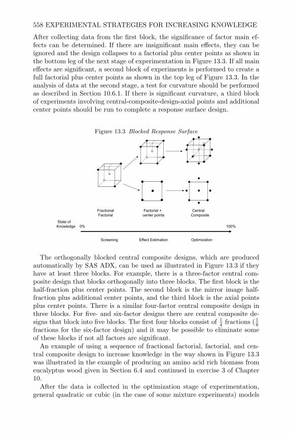
558 EXPERIMENTAL STRATEGIES FOR INCREASING KNOWLEDGE
After collecting data from the first block, the significance of factor main ef-fects can be determined. If there are insignificant main effects, they can beignored and the design collapses to a factorial plus center points as shown inthe bottom leg of the next stage of experimentation in Figure 13.3. If all maineffects are significant, a second block of experiments is performed to create afull factorial plus center points as shown in the top leg of Figure 13.3. In theanalysis of data at the second stage, a test for curvature should be performedas described in Section 10.6.1. If there is significant curvature, a third blockof experiments involving central-composite-design-axial points and additionalcenter points should be run to complete a response surface design.
Figure 13.3 Blocked Response Surface
State ofKnowledge 0% %001
Screening Effect Estimation Optimization
Fractional Factorial + Central Factorial center points Composite
The orthogonally blocked central composite designs, which are producedautomatically by SAS ADX, can be used as illustrated in Figure 13.3 if theyhave at least three blocks. For example, there is a three-factor central com-posite design that blocks orthogonally into three blocks. The first block is thehalf-fraction plus center points. The second block is the mirror image half-fraction plus additional center points, and the third block is the axial pointsplus center points. There is a similar four-factor central composite design inthree blocks. For five- and six-factor designs there are central composite de-signs that block into five blocks. The first four blocks consist of 1
4 fractions (18
fractions for the six-factor design) and it may be possible to eliminate someof these blocks if not all factors are significant.
An example of using a sequence of fractional factorial, factorial, and cen-tral composite design to increase knowledge in the way shown in Figure 13.3was illustrated in the example of producing an amino acid rich biomass fromeucalyptus wood given in Section 6.4 and continued in exercise 3 of Chapter10.
After the data is collected in the optimization stage of experimentation,general quadratic or cubic (in the case of some mixture experiments) models
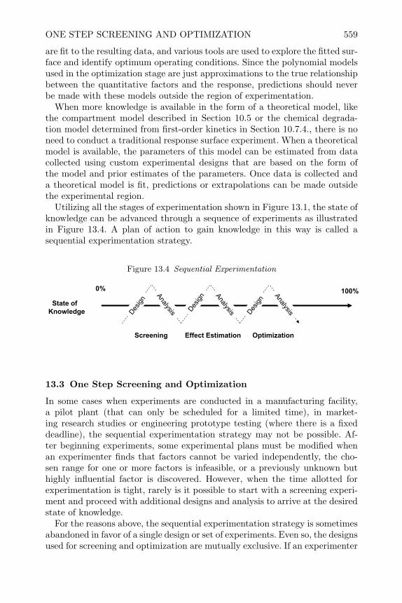
ONE STEP SCREENING AND OPTIMIZATION 559
are fit to the resulting data, and various tools are used to explore the fitted sur-face and identify optimum operating conditions. Since the polynomial modelsused in the optimization stage are just approximations to the true relationshipbetween the quantitative factors and the response, predictions should neverbe made with these models outside the region of experimentation.
When more knowledge is available in the form of a theoretical model, likethe compartment model described in Section 10.5 or the chemical degrada-tion model determined from first-order kinetics in Section 10.7.4., there is noneed to conduct a traditional response surface experiment. When a theoreticalmodel is available, the parameters of this model can be estimated from datacollected using custom experimental designs that are based on the form ofthe model and prior estimates of the parameters. Once data is collected anda theoretical model is fit, predictions or extrapolations can be made outsidethe experimental region.
Utilizing all the stages of experimentation shown in Figure 13.1, the state ofknowledge can be advanced through a sequence of experiments as illustratedin Figure 13.4. A plan of action to gain knowledge in this way is called asequential experimentation strategy.
Figure 13.4 Sequential Experimentation
Screening Effect Estimation Optimization
State ofKnowledge
0% 100%
Des
ign
Des
ign
Des
ign
Analysis
Analysis
Analysis
13.3 One Step Screening and Optimization
In some cases when experiments are conducted in a manufacturing facility,a pilot plant (that can only be scheduled for a limited time), in market-ing research studies or engineering prototype testing (where there is a fixeddeadline), the sequential experimentation strategy may not be possible. Af-ter beginning experiments, some experimental plans must be modified whenan experimenter finds that factors cannot be varied independently, the cho-sen range for one or more factors is infeasible, or a previously unknown buthighly influential factor is discovered. However, when the time allotted forexperimentation is tight, rarely is it possible to start with a screening experi-ment and proceed with additional designs and analysis to arrive at the desiredstate of knowledge.
For the reasons above, the sequential experimentation strategy is sometimesabandoned in favor of a single design or set of experiments. Even so, the designsused for screening and optimization are mutually exclusive. If an experimenter
560 EXPERIMENTAL STRATEGIES FOR INCREASING KNOWLEDGE
can only afford to run one set of experiments, he is forced to choose betweenone objective or the other. If the experimenter chooses a classical responsesurface design, he must select a subset of the factors to work with, and herisks the possibility of missing other important factors. On the other hand, ifthe experimenter chooses a screening experiment to avoid missing importantfactors, important interactions and quadratic effects will be missed.
It would be desirable in some situations to have experimental design plansthat allow for (1) screening a reasonably large number of factors to identifythe important ones, and (2) refitting a model to the data in only the importantfactors, so that important interactions or optimum operating conditions canbe determined after one set of experiments. Recent literature has shown thisis possible using certain orthogonal array main effect plans.
Lawson (2003) illustrates how screening followed by estimation of interac-tions can be accomplished using Plackett-Burman Designs. The example inSection 6.6 illustrates how this can be accomplished. Cheng and Wu (2001)proposed a strategy for using non-regular fractions of 3k designs for simulta-neous screening and response surface exploration. Lawson (2003) presents 18-,27- and 36-run examples of these non-regular fractions and an example usingChen and Wu’s strategy with an 18-run design. Many additional non-regularfractions of 3k designs are stored in a vast catalog by SAS and can be ac-cessed using the %mkt macros described in Section 6.7. For example, the SAScommands below search for an orthogonal array design with seven factors atthree levels, and then create an 18-run design.
*Search for orthogonal arrays in catalog of designs;%mktruns (3**7)*Find an 18 run design for 7 factors with 3 levels;%mktex(3**7,n=18)*Print a randomized list of the runs;proc print data=randomized; run;
The analysis of data from non-regular fractions of 3k designs, like this, issimilar to the analysis of Plackett-Burman Designs as illustrated in Section6.6.
13.4 Evolutionary Operation
The idea of using optimization experiments, or any experimentation for thatmatter, is often met with resistance in an operating manufacturing facility. Inmanufacturing, the key process variables thought to influence production areusually tightly controlled in order to ensure the quality of the manufacturedproduct. Tampering or experimenting with the levels of key process variablescould result in the production of off-grade or scrap product. However, thelevels at which the process variables are controlled in a manufacturing process,may not be optimal. These levels may have been determined in pilot plant orlaboratory experiments where conditions may differ in many ways from theactual manufacturing facility. In other cases, where the levels of key process

EVOLUTIONARY OPERATION 561
variables were actually determined through preliminary experiments in themanufacturing facility, they may no longer be optimal due to drift over timein raw materials or environmental conditions. Therefore, although acceptableproduct is being produced with current process variable settings, there maybe benefits in experimenting to obtain improved settings or to counteract driftover time.
Box (1957) proposed a method for finding improved settings of key processvariables without upsetting production. He believed that a manufacturing pro-cess should not only produce product, but also information that can be usedto improve the process over time. Data is normally collected in manufactur-ing facilities regarding (1) the settings of key process variables during eachproduction run (to ensure operating procedures are being followed) and (2)measured characteristics of product (to monitor quality). While recording thisinformaton, Box suggested making small perturbations in key process variablesettings from time to time according to a statistical plan like a 22 or 23 ex-periment. The planned changes in the key process variables would be smallenough that the product output would not be degraded, yet large enough thatpotential process improvements could be recognized after a number of cyclesthrough the planned settings. He called this method Evolutionary Operationor EVOP for short.
When using EVOP, the center point in a 22 or 23 design is assigned tothe current operating conditions (in terms of what is believed to be the keyprocess variables). Figure 13.5 illustrates the plan for two process variables.The five different process settings would each be run during one block ofmanufacturing. Running all five of these conditions completes one cycle of theEVOP.
Figure 13.5 A 22 Plan for EVOP
Process Variable 1+-
Pro
cess
Var
iabl
e 2
-
+
(2)
(1)
(5)
(4) (3)
If the average measure of product characteristic is yijk during the kth EVOPcycle at process variable settings i and j, then after two or more cycles, the

562 EXPERIMENTAL STRATEGIES FOR INCREASING KNOWLEDGE
main effect of process variable 1 (y+··−y−··), the main effect of process variable2 (y·+· − y·−·), their interaction effect ((y++· + y−−·) − (y+−· + y−+·) andthe curvature effect (y00· − y···) can be calculated. The standard error of themain effect and interaction estimates is 2sp/
√4× r, and the standard error
of the curvature effect is 2sp ×√
1/r + 1/4r, where sp is the pooled standarddeviation over the five treatment combinations and r is the number of cycles ofEVOP performed. The statistical significance of the effects can be determinedby dividing the effect by its appropriate standard error and comparing to thereference t-distribution with 5 × (r − 1) degrees of freedom. Since r is in thedenominator of the standard errors, they will decrease as the number of cyclesof EVOP increases.
If after five or more cycles of EVOP there is no practical or statistically sig-nificant effects, then either the process performance is optimal and stable overthe experimental region, or improved operating conditions may exist outsidethe current experimental region. If it is believed that further improvementmay be possible outside the range of the current EVOP, the ranges on thekey process variables should be increased and another phase of EVOP shouldbegin. If the effects of the key process variables (or their interaction effect)are statistically significant after two or more cycles of EVOP, a new phase ofEVOP should begin where the center point of the new phase is selected tobe the process condition that produced the optimum result in the last phase.If the curvature effect is statistically significant after several cycles of EVOP,and the measured product characteristics are better at the center point, thecurrent operating conditions are optimal and EVOP should be discontinued.
Given the objective and sufficient training, EVOP should be carried out bythe operators in the manufacturing facility without intervention from engi-neering or production management. In their book on EVOP, Box and Draper(1969) provide detailed worksheets which facilitate the EVOP calculationsin a manufacturing environment. These can also be carried out simply in amodern spreadsheet program. Box and Draper suggest displaying a bulletinboard in plain sight where the current EVOP status can be displayed. Thiswill motivate the operators conducting the EVOP and inform them of thelatest results.
13.5 Concluding Remarks
For each type of experimental design presented in this book, there are exam-ples of SAS commands to create the design. Earlier chapters emphasized howto randomize lists of experiments to avoid bias from unknown factors and en-sure valid analyses of data. In later chapters, the need for randomization wasassumed, but the specific details were not emphasized since they are the sameas shown in Chapter 2. In Chapter 4, the purpose for blocking experimentaldesigns was described and the methods to create blocked designs in SAS wereillustrated. The importance of blocking was emphasized throughout the re-

CONCLUDING REMARKS 563
mainder of the book, and situations where blocking should be used with eachtype of design were discussed and illustrated in the appropriate chapters.
For each type of experimental design presented, an appropriate model forthe data analysis was given and a description of the way to fit that model us-ing SAS software. In Chapter 8, restricted randomization or split-plot designswere discussed and it was shown how to construct designs and analyze thedata when randomization is restricted. Again the situations where this occursand the means to handle them were emphasized in the remaining chaptersof the book with all the types of designs presented. In addition, this bookemphasizes the interpretation and presentation of results which is amply de-scribed and demonstrated in every chapter. The exercises at the end of eachchapter provide practice for design creation and analysis and interpretation ofdata. They were selected to reinforce all the concepts presented in the book.
In the author’s experience, the experimental design topics presented in thebook cover most of the situations encountered in practice. With the powerof the software in SAS Stat, SAS QC, SAS OR, SAS Graph, the automatedSAS ADX system and the %adx and %mkt macros, a researcher has a powerfulset of tools that simplify most research design and data analysis problems.By emphasizing where to use each of the different types of experimental de-signs, illustrating the creation of designs and analysis of data with SAS, andpresenting many examples of interpretation and presentation of results, thisbook provides an updated guide to researchers when compared to the earlierbooks by Fisher (1935), Cochran and Cox (1950), and Kempthorne (1952).
After completing the study of this book, you should be able to (1) choose anexperimental design that is appropriate for a research problem; (2) constructthe design (including performing proper randomization and determining theproper number of replicates); (3) execute the plan (or advise a colleague todo it); (4) determine a model appropriate for the data; (5) fit the model tothe data; (6) interpret the results; and (7) present them in a meaningful wayto answer the research question at hand. The use of SAS software simplifiesmany of these tasks, demonstrated by the examples throughout the book.


Bibliography
AlmeidaeSilva, J. B., Lima, U. A., S., M. E., Taqueda, and Guaragna, F. G.(1998). Use of fractional factorial design for selection of nutrients for cultur-ing Paecilomyces variotii in eucalyptus hemicellulosic hydrolysate. Brazil-ian Journal of Chemical Engineering , 15, 273–279.
AlmeidaeSilva, J. B., Lima, U. A., Taqueda, M. E. S., and Guaragna, F. G.(2003). Use of response surface methodology for selection of nutrient levelsfor culturing Paecilomyces variotii in eucalyptus hemicellulosic hydrolyzate.Biosource Technology , 87, 45–50.
Anderson, M. (2003). Messing with medieval missle machines. Stateaser ,Sept. URL www.statease.com.
Anderson, V. L. and McLean, R. A. (1974). Design of Experiments: A RealisticApproach. Marcel Dekker, Inc., New York.
Anik, S. T. and Sukumar, L. (1981). Extreme vertexes design in formula-tion development: Solubility of butoconazole nitrate in a multi-componentsystem. Journal of Pharmaceutical Sciences, 70, 897–900.
Apple, D. (2006). Dish detergent experiment. Term Paper Stat 431, BYUDept. of Statistics.
Atkinson, A. C., Donev, A. N., and Tobias, R. D. (2007). Optimum Experi-mental Designs with SAS . Oxford University Press, Oxford.
Bainbridge, T. R. (1965). Staggered nested designs for estimating variancecomponents. Industrial Quality Control , 22, 12–20.
Barbuta, M. and Lepadatu, D. (2008). Mechanical characteristics investiga-tion of polymer concrete using mixture design of experiments and responsesurface method. Journal of Applied Sciences, 8, 2242–2249.
Bastable, A. (2006). Tee it high or low. Golf Magazine, June, 173–179.
Bates, D. M. and Watts, D. G. (2007). Nonlinear Regression and Its Applica-tions. John Wiley & Sons, Hoboken N.J.
Bechhofer, R. E. and Tamhane, A. C. (1981). Incomplete block designs forcomparing treatments with a control: General theory. Technometrics, 23,45–57.
Belloto, J., Dean, R. J., Moustafa, M. A., Molokhia, A. M., Gouda, M. W.,and Sokoloski, T. D. (1985). Statistical techniques applied to solubility pre-dictions and pharmaceutical formulations: An approach to problem solving
565

566 BIBLIOGRAPHY
using mixture response surface methodology. International Journal of Phar-maceutics, 23, 195–207.
Bennett, C. A. and Franklin, N. L. (1954). Statistical Analysis in Chemistryand the Chemical Industry . John Wiley & Sons, New York.
Bingham, D. R. and Sitter, H. R. (1999). Minimum aberration two-levelfractional factorial split-plot designs. Technometrics, 41, 62–70.
Bingham, D. R. and Sitter, H. R. (2001). Design issues in fractional factorialsplit-plot experiments. Journal of Quality Technology , 33, 2–15.
Bisgaard, S. (1999). Quality quandries-proposals: A mechanism for achievingbetter experiments. Quality Engineering , 11, 645–649.
Bisgaard, S. (2000). The design and analysis of 2k−p × 2q−r split plot experi-ments. Quality Engineering , 8, 705–708.
Bisgaard, S. and Kulahci, M. (2001). Quality quandries: Robust productdesign saving trials with split-plot confounding. Quality Engineering , 13,525–530.
Bisgaard, S. and Sutherland, M. (2004). Quality quandries-split plot experi-ments: Taguchi’s Ina tile experiment reanalyzed. Quality Engineering , 16,157–164.
Bisgaard, S., Fuller, H. T., and Barrios, E. (1996). Quality quandries: Two-level factorials run as split plot experiments. Journal of Quality Technology ,32, 39–55.
Bose, R. C., Clatworthy, W. H., and Shrikhande, S. S. (1954). Tables ofpartially balanced designs with two associate classes. Technical report,North Carolina Agricultural Experiment Station. Technical Bulletin 107.
Box, G. E. P. (1957). Evolutionary operation: A method for increasing indus-trial productivity. Applied Statistics, 6, 81–101.
Box, G. E. P. (1988). Signal-to-noise ratios, performance criteria, and trans-formations. Technometrics, 30, 1–17.
Box, G. E. P. (1991). George’s column: Finding bad values in factorial designs.Quality Engineering , 3, 249–254.
Box, G. E. P. and Behnken, D. W. (1960). Some new three level designs forthe study of quantitative variables. Technometrics, 2, 455–460.
Box, G. E. P. and Cox, D. R. (1964). An analysis of transformations. Journalof the Royal Statistical Society, Series B , 26, 15–20.
Box, G. E. P. and Draper, N. R. (1969). Evolutionary Operation. John Wiley& Sons, New York, first edition.
Box, G. E. P. and Fung, C. A. (1986). Minimizing transmitted variation byparameter design. Technical Report 8, Center for Quality and ProductivityImprovement, University of Wisconsin-Madison.
Box, G. E. P. and Hunter, J. S. (1957). Multifactor experimental designs forexploring response surfaces. Annals of Mathematical Statistics, 28, 195–241.

BIBLIOGRAPHY 567
Box, G. E. P. and Hunter, J. S. (1961). The 2k−p fractional factorial designs.Technometrics, 3, 311–351 and 449–458.
Box, G. E. P. and Jones, S. (1992). Split-plot designs for robust productexperimentation. Journal of Applied Statistics, 19, 3–26.
Box, G. E. P. and Meyer, R. D. (1986a). An analysis for unreplicated fractionalfactorials. Technometrics, 28, 11–18.
Box, G. E. P. and Meyer, R. D. (1986b). Dispersion effects from fractionaldesigns. Technometrics, 28, 19–27.
Box, G. E. P. and Meyer, R. D. (1993). Finding the active factors in fraction-ated screening experiments. Journal of quality technology , 25, 94–105.
Box, G. E. P. and Wilson, K. B. (1951). On experimental attainment ofoptimum conditions. Journal of the Royal Statistical Society B , 13, 1–45.
Box, G. E. P., Hunter, W. G., and Hunter, J. S. (1978). Statistics for Exper-imenters. John Wiley & Sons, New York, first edition.
Burdick, R. and Graybill, F. (1992). Confidence Intervals on Variance Com-ponents. Marcel Dekker, Inc., New York.
Butler, N. A. (2006). Optimal blocking of two-level factorial designs.Biometrika, 93, 289–302.
Casella, G. (2008). Statistical Design. Springer, New York.Chau, K. W. and Kelly, W. R. (1993). Formulating printable coatings via
d-optimality. Journal of Coatings Technology , 65, 71–78.Chen, J., Sun, D. X., and Wu, C. F. J. (1993). A catalogue of two-level
and three-level fractional factorial designs with small runs. InternationalStatistical Review , 61, 131–145.
Cheng, S. and Wu, C. F. J. (2001). Factor screening and response surfaceexploration. Statistica Sinica, 11, 553–604.
Chi, E. M. (1994). M-estimation in cross-over trials. Biometrics, 50, 486–493.Chipman, H., Hamada, M., and Wu, C. F. J. (1997). A Bayesian variable-
selection approach for analyzing designed experiments with complex alias-ing. Technometrics, 39, 372–381.
Chipman, J. (2006). Sprinting experiment. Term Paper Stat 431, BYU Dept.of Statistics.
Claringbold, P. J. (1955). Use of the simplex design in the study of the jointaction of related hormones. Biometrics, 11, 174–185.
Cochran, W. G. and Cox, G. M. (1950). Experimental Designs. John Wiley& Sons, New York, first edition.
Cook, R. D. and Nachtsheim, C. J. (1989). Computer-aided blocking of fac-torial and response surface designs. Technometrics, 31, 339–346.
Cornell, J. A. (1988). Analyzing data from mixture experiments containingprocess variables: A split-plot approach. Journal of Quality Technology , 20,2–23.

568 BIBLIOGRAPHY
Cornell, J. A. (2002). Experiments with Mixtures: Designs Models and Analysisof Mixture Data. John Wiley & Sons, New York, third edition.
Cornell, J. A. and Gorman, J. W. (1984). Fractional design plans for processvariables in mixture experiments. Journal of Quality Technology , 16, 20–38.
Cox, D. R. (1971). A note on polynomial response functions for mixtures.Biometrika, 58, 155–159.
Curtis, B., Warburton, R., Gannon, J., Gloss-Soler, S., Goel, A., Miyamoto, I.,and Panzl, D. (1982). The application of fractional factorial techniques tothe design of software experiments. Software Engineering Notes, 7, 21–30.
Czitrom, V. and Spagon, P. D. (1997). Statistical Case Studies for IndustrialProcess Improvement- Chapter 8 . Siam, Philadelphia.
Daniel, C. (1959). Use of half-normal plots in interpreting factorial two-levelexperiments. Technometrics, 1, 311–341.
Daniel, C. (1960). Locating outliers in factorial experiments. Technometrics,2, 149–156.
Daniel, C. (1976). Applications of Statistics to Industrial Experimentation.John Wiley & Sons, New York, first edition.
Das, M. N. (1960). Fractional replicates as asymmetrical factorial designs.Journal of the Indian Society of Agricultural Statistics, 12, 159–174.
Davies, O. L. (1949). Statistical Methods in Research and Production. Oliverand Boyd, Edinburg, first edition.
Deeb, O., Youssef, K. M., and Hemmateenejad, B. (2008). QSAR of novelhydroxyphenylureas as antioxidant agents. QSAR Combinatorial Science,27, 417–424.
Derringer, G. and Suich, R. (1980). Simultaneous optimization of severalresponse variables. Journal of Quality Technology , 12, 214–219.
Derringer, G. C. (1974). An empirical model for viscosity of filled and plas-ticized elastomer compounds. Journal of Applied Polymer Science, 18,1083–1101.
Diggle, P. J., Liang, K., and Zeger, S. L. (1994). The Analysis of LongitudinalData. Oxford University Press, Oxford.
Dossett, T., Lefler, R., and Moore, P. (2007). Apple browning experiment.Term Paper Stat 431, BYU Dept. of Statistics.
Draper, N. R. (1963). Ridge analysis of response surfaces. Technometrics, 5,469–479.
Draper, N. R. (1985). Small composite designs. Technometrics, 27, 173–180.
Draper, N. R. and John, R. C. S. (1977). A mixtures model with inverseterms. Technometrics, 19, 37–46.
Draper, N. R. and Lin, D. K. J. (1990). Small response surface designs.Technometrics, 32, 187–194.

BIBLIOGRAPHY 569
Dunnett, C. W. (1955). A multiple comparison procedure for comparing sev-eral treatments with a control. Journal of the American Statistical Associ-ation, 509, 1096–1121.
Dykstra, O. (1971). The augmentation of experimental data to maximize|XTX|. Technometrics, 13, 682–688.
Easterling, R. G. (2004). Teaching experimental design. The American Statis-tician, 58, 244–252.
Erhardt, E. B. (2007). Designing a better paper helicopter using responsesurface methodology. Stats, 48, 14–21.
Fannin, T. E., Marcus, M. D., Anderson, D. A., and Bergman, H. L. (1981).Use of a fractional factorial design to evaluate interactions of environmentalfactors affecting biodegradation rates. Applied and Environmental Micro-biology , 42, 936–943.
Faraway, J. (2004). Linear Models with R. Chapman & Hall/CRC, BocaRaton, FL.
Festing, M. F. (2003). Principles: The need for better experimental design.Trends Pharmacol Sci , 24, 341–345.
Fisher, R. A. (1926). The arrangement of field experiments. Journal of theMinistry of Agriculture of Great Britain, 33, 503–513.
Fisher, R. A. (1935). The Design of Experiments. Oliver and Boyd, Edinburgh,first edition.
Fisher, R. A. (1940). An examination of possible different solutions of aproblem in incomplete blocks. Annals of Eugenics, 9, 353–400.
Franklin, M. F. (1985). Selecting defining contrasts and confounded effects inpn−m factorial experiments. Technometrics, 27, 165–172.
Freeman, P. (1989). The performance of the two-stage analysis of two treat-ment two period crossover trials. Statistics in Medicine, 8, 1421–1432.
Freund, R. J. and Littell, R. C. (1981). SAS for Linear Models: A Guide toANOVA and GLM Procedures. SAS Institute, Cary, NC, first edition.
Fries, A. and Hunter, W. G. (1980). Minimum aberation 2k−p designs. Tech-nometrics, 22, 601–608.
Gilmour, S. G. and Goos, P. (2006). Analysis of data from nonorthogonalmulti-stratum designs. Technical report, Faculty of Applied Economics Uni-versiteit Antwerpen Belgium. Tech. Rep. 2006/05.
Gilmour, S. G. and Trinca, L. A. (2000). Some practical advice on polynomialregression analysis from blocked response surface designs. Comunicationsin Statistics: Theory and Methods, 29, 2157–2180.
Giovannitti-Jensen, A. and Myers, R. H. (1989). Graphical assessment ofthe prediction capability of response surface designs. Technometrics, 31,159–171.

570 BIBLIOGRAPHY
Goodnight, J. H. (1980). Tests of hypothesis in fixed effects linear models.Communication in Statistics - Theory and Methods, A9, 167–180.
Goos, P. (2002). The Optimal Design of Blocked and Split Plot Experiments.Springer, New York.
Goos, P. and Donev, A. N. (2006). The d-optimal design of blocked ex-periments with mixture components. Journal of Quality Technology , 38,319–332.
Goos, P. and Donev, A. N. (2007). Tailor-made split plot designs for mixtureand process variables. Journal of Quality Technology , 39, 326–339.
Goos, P. and Vandebroek, M. (2001). Optimal split-plot designs. Journal ofQuality Technology , 33, 436–450.
Goos, P. and Vandebroek, M. (2003). D-optimal split plot designs with givennumbers and sizes of whole plots. Technometrics, 45, 235–245.
Gorman, J. W. and Cornell, J. A. (1982). A note on model reduction forexperiments with both mixture components and process variables. Techno-metrics, 24, 243–247.
Greenhouse, S. W. and Geisser, S. (1959). On methods in the analysis ofprofile data. Psychometrika, 24, 95–112.
Grizzle, J. E. (1965). The two-period change-over design and its use in clinicaltrials. Biometrics, 21, 467–480.
Hamada, M. and Wu, C. F. J. (1992). Analysis of designed experiments withcomplex aliasing. Journal of Quality Technology , 24, 130–137.
Hare, L. B. (1988). In the soup: A case study to identify contributors to fillingvariability. Journal of Quality Technology , 20, 36–43.
Hartley, H. O. (1959). Smallest composite design for quadratic response sur-faces. Biometrics, 15, 611–624.
Hartley, H. O. (1967). Expectations, variances and covariances of ANOVAmean squares by synthesis. Biometrics, 34, 105–114.
Heffner, T. G., Drawbaugh, R. B., and Zigmond, M. J. (1974). Amphetamineand operant behavior in rats: Relationship between drug effect and controlresponse rate. Journal of Comparative and Physiological Psychology , 86,1031–1043.
Henderson, L. O., Hannon, W., Smith, S. J., and Cooper, G. R. (1987). Aninternational collaborative study on standardization of apolipoproteins a-iand b. part ii. evaluation of contributions of antisers to among-laboratoryvariance components. Clinical Chemistry , 33, 2250–2256.
Hinkelmann, K. and Kempthorne, O. (1994). Design and Analysis of Experi-ments Volume I . John Wiley & Sons, New York.
Hoerl, A. E. (1959). Optimum solution of many variables equations. ChemicalEngineering Progress, 55, 69–78.

BIBLIOGRAPHY 571
Horiuchi, Y., Imai, K., and Taniguchi, N. (2005). Designing and analyzing ran-domized experiments. In Proceedings of the Annual Meeting of the AmericanPolitical Science Association. American Political Science Association.
Hsu, J. C. (1984). Constrained simultaneous confidence intervals for multiplecomparisons with the best. Annals of Statistics, 12, 1136–1144.
Huang, P., Chen, D., and Voelkel, J. (1998). Minimum aberration two-levelsplit-plot designs. Technometrics, 40, 314–326.
Hunter, G. B., Hodi, F. S., and Eager, T. W. (1982). High-cycle fatigue ofweld repaired cast t–6a1-4v. Metallurgical Transactions, 13A, 1589–1594.
Hunter, J. S. (1989). Let’s all beware the latin square. Quality Engineering ,1, 453–465.
Huynh, H. and Feldt, L. S. (1970). Conditions under which mean square ratiosin repeated measurements designs have exact f -distributions. Journal of theAmerican Statistical Association, 65, 1582–1589.
Huynh, H. and Feldt, L. S. (1976). Estimation of the box correction for degreesof freedom from sample data in the randomized block and split-plot designs.Journal of Educational Statistics, 1, 69–82.
Immer, F. R., Hayes, H. K., and Powers, L. R. (1934). Statistical determi-nation of barley varietal adaptation. Journal of the American Society ofAgronomy , 25, 403–419.
Jarrett, R. G. and Hall, W. B. (1978). Generalized cyclic incomplete blockdesigns. Biometrika, 65, 397–401.
John, P. W. M. (1984). Experiments with mixtures involving process vari-ables. Technical report, Center for Statistical Sciences, University of Texas,Austin. Technical Report #8.
Jones, B. (1980). The crossover experiment for clinical trials. Biometrics, 36,69–79.
Jones, B. and Goos, P. (2007). A candidate-set-free algorithm for generatingd-optimal split plot designs. Journal of the Royal Statistical Society, SeriesC: Applied Statistics, 56, 347–364.
Jones, B. and Kenward, M. G. (2003). Design and Analysis of CrossoverTrials. Chapman & Hall/CRC, Boca Raton, FL, second edition.
Juan, E. M. S., Edra, E. V., Sales, J. M., Lustre, A. O., and Resurreccion,A. V. A. (2006). Utilization of peanut fines in the optimization of peanutpolvoron using mixture respose surface methodology. International Journalof Food Science and Technology , 41, 768–774.
Kamohara, S., Kawakami, M., Kosaka, E., Ito, F., Okuyama, K., and Ohji, Y.(2001). Robust design of 0.18 µm ASIC MOSFETs using Taguchi methodwith TCAD. In Statistical Methodology, IEEE International Workshop,pages 21–24, Kyoto, Japan. IEEE.

572 BIBLIOGRAPHY
Kamon, A., Samet, B., Bouaziz, J., and Chaabouni, M. (1999). Application ofa rotatable orthogonal central composite design to the optimization of theformulation and utilization of a useful plasticizer for cement. EDP Sciences,27, 91–96.
Kempthorne, O. (1952). The Design and Analysis of Experiments. John Wiley& Sons, New York, first edition.
Kenett, R. S. and Steinberg, D. M. (1987). Some experiences teaching factorialdesign in introductory statistics courses. Journal of Applied Statistics, 14,219–227.
Kerry, S. M. and Bland, J. M. (1998). Analysis of a trial randomized inclusters. British Journal of Medicine, 316, 54–54.
Keuls, M. (1952). The use of the studentized range in connection with analysisof variance. Euphytica, 1, 112–122.
Kiefer, J. (1958). On the nonrandomized optimality and randomized nonop-timality of symmetrical designs. Annals of Mathematical Statistics, 29,675–699.
Kowalski, S. M., Cornell, J. A., and Vining, G. G. (2000). A new model andclass of designs for mixture experiments with process variables. Communi-cations in Statistics-Theory and Methods, 29, 2255–2280.
Kowalski, S. M., Cornell, J. A., and Vining, G. G. (2002). Split-plot designsand estimation methods for mixture experiments with process variables.Technometrics, 44, 72–79.
Kshirsager, A. M. (1958). A note on incomplete block designs. Annals ofMathematical Statistics, 29, 907–910.
Kuehl, R. O. (2000). Design of Experiments Statistical Principles of ResearchDesign and Analysis. Duxbury, Pacific Grove, CA, second edition.
Kuhfeld, W. F. (2009). Marketing research methods in SAS - report mr2009.Technical report, SAS Institute, Cary, NC. URL http://support.sas.com/resources/papers/tnote/tnote marketresearch.html.
Kuhfeld, W. F. and Tobias, R. D. (2005). Large factorial designs for productengineering and marketing research applications. Technometrics, 47, 132–141.
Kulahci, M., Ramirez, J. G., and Tobias, R. (2006). Split plot fractionaldesigns: Is minimum aberration enough? Journal of Quality Technology ,38, 56–64.
Kurotori, I. S. (1966). Experiments with mixtures of components having lowerbounds. Industrial Quality Control , 22, 592–596.
Kutner, M. H., Nachtsheim, C. J., and Neter, J. (2004). Applied Linear Re-gression Models. McGraw-Hill Irwin, Boston, fourth edition.
Lawson, J. (1982). Applications of robust regression in designed industrialexperiments. Journal of Quality Technology , 14, 19–33.

BIBLIOGRAPHY 573
Lawson, J. (1990). Improve a chemical process through use of a designedexperiment. Quality Engineering , 3, 215–235.
Lawson, J. (2002). Regression analysis of experiments with complex confound-ing patterns guided by the alias matrix. Computational Statistics and DataAnalysis, 39, 227–241.
Lawson, J. (2008a). SAS macros for analysis of unreplicated 2k and 2k−p
designs with a possible outlier. Journal of Statistical Software, 25(13), 1–17.
Lawson, J. and Erjavec, J. (2001). Modern Statistics for Engineering andQuality Improvement . Duxbury, Pacific Grove, CA, first edition.
Lawson, J., Grimshaw, S., and Burt, J. (1998). A quantitative method foridentifying active contrasts in unreplicated factorial experiments based onthe half normal plot. Computational Statistics and Data Analysis, 26, 425–436.
Lawson, J. S. (2003). One step screening and process optimization experi-ments. The American Statistician, 57, 15–20.
Lawson, J. S. (2008b). Bayesian interval estimates of variance componentsused in quality improvement studies. Quality Engineering , 20, 334–345.
Lawson, J. S. and Gatlin, J. (2006). Finding bad values in factorials - revisited.Quality Engineering , 18, 491–501.
Lawson, J. S. and Madrigal, J. L. (1994). Robust design through optimizationtechniques. Quality Engineering , 6, 593–608.
Lawson, J. S., Schaalje, G. B., and Collings, B. J. (2009). Blocking mixedlevel factorials with SAS. Journal of Statistical Software, 32, 1–19.
le Riche, W. H. and Csima, A. (1964). A clinical evaluation of four hypnoticagents, using a Latin square design. Canadian Medical Association Journal ,91, 435–438.
Lee, Y. and Nelder, J. A. (2003). Robust design via generalized linear models.Journal of Quality Technology , 35, 2–12.
Leitnaker, M. G. and Cooper, A. (2005). Using statistical thinking and de-signed experiments to understand process operation. Quality Engineering ,17, 279–289.
Lenth, R. V. (1989). Quick and easy analysis of un-replicated factorials. Tech-nometrics, 31, 469–473.
Letsinger, J. D., Myers, R. H., and Letner, M. (1996). Response surfacemethods for bi-randomization structures. Journal of Quality Technology ,28, 381–397.
Lew, M. (2007). Good statistical practice in pharmacology problem 2. BritishJournal of Pharmacology , 152, 299–303.
Lim, D. H. and Wolfe, D. A. (1997). Nonparametric tests for comparingumbrella pattern treatment effects with a control in a randomized blockdesign. Biometrics, 53, 410–418.

574 BIBLIOGRAPHY
Lin, D. K. J. and Draper, N. R. (1992). Projection properties of Plackett-Burman designs. Technometrics, 34, 423–428.
Lin, L. I. and Stephenson, W. R. (1998). Validating an assay of viral con-tamination. In R. Peck, L. D. Haugh, and A. Goodman, editors, StatisticalCase Studies: A Collaboration Between Academe and Industry , pages 43–48.SIAM, Philadelphia.
Lucas, H. L. (1957). Extra-period Latin square change-over designs. Journalof Dairy Science, 40, 225–239.
Mason, R. L., Gunst, R. F., and Hess, J. L. (1989). Statistical Design and Anal-ysis of Experiments: with Applications to Engineering and Science. JohnWiley & Sons, New York.
Mauchly, J. W. (1940). Significance test for sphericity of a normal n-variatedistribution. Annals of Mathematical Statistics, 11, 204–209.
McCullagh, P. and Nelder, J. A. (1989). Generalized Linear Models. Chapman& Hall, London, second edition.
McLean, R. A. and Anderson, V. L. (1966). Extreme vertices designs ofmixture experiments. Technometrics, 8, 447–454.
Meier, P. (1972). The biggest health experiment ever: The 1954 field trial ofthe salk polio vaccine. In J. M. Tanur, F. Mosteller, W. H. Kruskal, R. F.Link, and R. Pieters, editors, Statistics: A Guide to the Unknown, pages2–13. Holden Day, San Francisco.
Melo, I. R., Pimentel, M. F., Lopes, C. E., G., and Calazans, M. T. (2007).Application of fractional factorial design to levan production by Zymomonasmobilis. Brazilian Journal of Microbiology , 38, 45–51.
Montgomery, D. C. (1990). Using fractional factorial designs for robust processdevelopment. Quality Engineering , 3, 193–205.
Montgomery, D. C. and Runger, G. C. (1996). Foldovers of 2k−p resolution ivexperimental designs. Journal of Quality Technology , 28, 446–450.
Moskowitz, H. (1988). Applied Sensory Analysis of Foods. CRC Press, BocaRaton, FL.
Myers, R. H. and Montgomery, D. C. (2002). Response Surface Methodology:Process and Product Optimization Using Designed Experiments. John Wiley& Sons, New York, second edition.
Myers, R. H., Vining, G. G., Giovannitti-Jensen, A., and Myers, S. L. (1992).Variance dispersion properties of second order response surface designs.Journal of Quality Technology , 24, 1–11.
Nelder, J. A. and Lee, Y. (1998). Letter to the editor. Technometrics, 40,168–175.
Newman, D. (1939). The distribution of the range in samples from a nor-mal population, expressed in terms of an independent estimate of standarddeviation. Biometrika, 31, 20–20.

BIBLIOGRAPHY 575
Nigam, A. K. (1970). Block designs for mixture experiments. Annals ofMathematical Statistics, 41, 1861–1869.
Nigam, A. K. (1977). Corrections to blocking conditions for mixture experi-ments. Annals of Mathematical Statistics, 47, 1294–1295.
Phadke, M. S. (1989). Quality Engineering Using Robust Design. PrenticeHall, New York.
Plackett, R. L. and Burman, J. P. (1946). The design of optimum multifac-torial experiments. Biometrika, 33, 305–325.
Porter, W. P. and Busch, R. L. (1978). Fractional factorial analysis of growthand weaning success in Peromyscus maniculatus. Science, 202, 907–910.
Prairie, R. R. and Anderson, R. L. (1962). Optimal designs to estimate vari-ance components and to reduce product variability for nested classifications.North Carolina State College, Raleigh, Inst. of Stat Mimeo Series, 313, 80–81.
Prince, E. (2007). Real-time PCR optimization for S. pyogenes detectionassay - a fractional factorial approach. Term Paper Stat 431, BYU Dept.of Statistics.
Ramakrishna, D. M., Viraraghavan, T., and Jin, Y. (2006). Iron oxide coatedsand for arsenic removal: Investigation of coating parameters using a fac-torial design approach. Practice Periodical of Hazardous, Toxic, and Ra-dioactive Waste Management , 10, 198–206.
Ramirez, J. G. and Tobias, R. (2007). Split and conquer! using SAS/QC todesign quality into complex manufacturing processes. In Global Forum Pa-per 190-2007 . SAS Institute. URL:www2.sas.com/proceedings/forum/190-2007.pdf.
Rao, P. S. and Rao, R. S. (1997). Variance Component Estimation. Chapman& Hall, London, first edition.
Rogness, N. and Richardson, M. (2003). Using chewing gum to illustrateintermediate statistical concepts. Proceedings of the 2003 Joint StatisticalMeetings - Section on Statistical Education, pages 3545–3547.
Roquemore, K. G. (1976). Hybrid designs for quadratic response surfaces.Technometrics, 18, 419–423.
Sahni, N. S., Piepel, G. F., and Naes, T. (2009). Product and process im-provement using mixture-process variable methods and robust optimizationtechniques. Journal of Quality Technology , 41, 181–197.
SAS Institute (2004a). Gantt Procedure SAS/QC . Cary, NC.
SAS Institute (2004b). Ishakawa Procedure SAS/QC . Cary, NC.
Scheffe, H. (1958). Experiments with mixtures. Journal of the Royal StatisticalSociety, Series B , 20, 344–360.
Scheffe, H. (1959). The Analysis of Variance. John Wiley & Sons, New York,first edition.

576 BIBLIOGRAPHY
Schrevens, E. and DeRijck, G. (2008). Defining nutrient solutions as con-strained double mixture amount systems. In Proceedings of the Section onPhysical and Engineeing Statistics. American Statistical Association.
Searle, S. R., Casella, G., and McCulloch, C. E. (1992). Variance Components.John Wiley & Sons, New York, first edition.
Selwyn, M. R. and Hall, N. R. (1984). On Bayesian methods for bioequiva-lence. Biometrics, 40, 1103–1108.
Senn, S. (2002). Cross-over Trials in Clinical Research. John Wiley & Sons,New York, second edition.
Sheehe, P. R. and Bross, I. D. J. (1961). Latin squares to balance immediateresiduals and other effects. Biometrics, 17, 405–414.
Shoemaker, A. C., Tsui, K. L., and Wu, C. F. J. (1991). Economical experi-mentation methods for robust design. Technometrics, 33, 415–427.
Shumate, D. A. and Montgomery, D. C. (1996). Development of a TiW plasmaetch process using a mixture experiment and response surface optimization.IEEE Transactions on Semiconductor Manufacturing , 9, 335–343.
Smith, J. R. and Beverly, J. M. (1981). The use and analysis of staggerednested designs. Journal of Quality Technology , 13, 166–173.
Snee, R. D. (1983). Graphical analysis of process variation studies. Journalof Quality Technology , 15, 76–88.
Snee, R. D. and Marquardt, D. W. (1974). Extreme vertices designs for linearmixture models. Technometrics, 16, 399–408.
Snee, R. D. and Marquardt, D. W. (1976). Screening concepts and designsfor experiments with mixtures. Technometrics, 18, 19–29.
Song, J. and Lawson, J. (1988). Use of 2k−p designs in parameter design.Quality and Reliability Engineering International , 4, 151–158.
Sower, V. E., Savoie, M. J., and Renick, S. (1999). An Introduction to QualityManagement and Engineering . Prentice Hall, Upper Saddle River, NJ.
Steiner, S. H., Hamada, M., White, B. J. G., Kutsyy, V., Mosesova, S., andSalloum, G. (2007). A bubble mixture experiment project for use in anadvanced design of experiments class. Journal of Statistical Education, 15,1–18.
Street, D. J. and Burgess, L. (2007). The Construction of Optimal StatedChoice Experiments. John Wiley & Sons, Hoboken, N.J.
Taguchi, G. (1986). Introduction to Quality Engineering, Designing Qualityinto Products and Processes. Asian Productivity Organization, Tokyo.
Taguchi, G. (1987). System of Experimental Design: Engineering Methodsto Optimize Quality and Minimize Costs. UNIPUB/Kraus InternationalPublications, White Plains, New York.
Taguchi, G. and Phadke, M. S. (1985). Quality engineering through designoptimization. The International Quality Forum, 11, 27–48.

BIBLIOGRAPHY 577
Taguchi, G. and Wu, Y. (1980). Introduction to Off-Line Quality Control .Central Japan Quality Control Association, Nagoya Japan.
Taguchi, S. and Byrne, D. (1984). The concept of parameter design. AutoDivision Newsletter of ASQC , pages 5–7.
Tukey, J. W. (1949a). Comparing individual means in the analysis of variance.Biometrics, 5, 99–114.
Tukey, J. W. (1949b). One degree of freedom for non-additivity. Biometrics,5, 232–242.
unknown (1937). Rothamstead experimental station report.
Usage note: Stat-40 (1997). Usage note: Stat-40. University of Texas at AustinStatistical Services, 45-9372. Copywright 1995-1997 ACITS.
Varma, A. O. and Chilton, N. W. (1974). Crossover designs involving twotreatments. Journal of Periodontal Research, 14, 160–170.
Vining, G. G., Kowalski, S. M., and Montgomery, D. C. (2005). Responsesurface designs within a split-plot structure. Journal of Quality Technology ,37, 115–129.
Wagner, J. G. (1967). Use of computers in pharmacokinetics. Journal ofClinical Pharmacology and Therapeutics, 8, 201–220.
Wallenstein, S. and Fisher, A. C. (1977). The analysis of the two-periodrepeated measures crossover design with application to clinical trials. Bio-metrics, 33, 261–269.
Wang, B., Wang, X., and Gong, L. (2009). The construction of a Williamsdesign and randomization in cross-over clinical trials using SAS. Journal ofStatistical Software, 29(Code Snippet 1), 1–10.
Wang, J. C. and Wu, C. F. J. (1995). A hidden projection property of Plackett-Burman and related designs. Statistica Sinica, 5, 235–250.
Wang, Q., Shi, G., and Chan-Halbrendt, C. (2004). Market potential for finefurniture manufactured from low-grade hardwood: Evidence from a conjointanalysis in the northeastern United States. Forest Products Journal , 54,19–25.
Wang, Y., Lin, D. K. J., and Fang, K. (1995). Designing outer array points.Journal of Quality Technology , 27, 226–241.
Westlake, W. J. (1965). Composite designs based on irregular fractions offactorials. Biometrics, 21, 324–336.
Wheeler, R. E. (1974). Portable power. Technometrics, 16, 193–201.
Wilk, M. B., Gnanadesikan, R., and Huyett, M. J. (1962). Probability plotsfor the gamma distribution. Technometrics, 4, 1–20.
Williams, E. J. (1949). Experimental designs balanced for the estimation ofresidual effects of treatments. Australian Journal of Scientific Research, 2,149–168.

578 BIBLIOGRAPHY
Woodward, W. F. (1970). A Comparison of Base Running Methods in Base-ball . Master’s thesis, Florida State University.
Wu, C. F. J. and Hamada, M. (2000). Experiments-Planning, Analysis, andParameter Design Optimization. John Wiley & Sons, New York.
Yang-Gyu, K. and Woolley, D. J. (2006). Effect of plant growth regulators andspear bud scales on growth of asparagus officinalis. Scientia Horticulturae,108, 238–242.
Yates, F. (1937). The Design and Analysis of Factorial Experiments. Hafner,Harpenden Herts, England. Bulletin 35, Imperial Bureau of Soil Science.