description of the relation of wind, wave and current...

Description of the relation of Wind,Wave and Current Characteristics

at the Offshore Wind Farm Egmond aan Zee(OWEZ) Location in 2006

S. Barth, P.J. Eecen

ECN-E-07-104OWEZ_R_122_Wave_2006_20080409

Abstract

NoordzeeWind carries out an extensive measurement and evaluation program as part of the Off-shore Wind Farm Egmond aan Zee (OWEZ) project.

The technical part of the measurement and evaluation program considers topics as climate statis-tics, wind and wave loading, detailed performance monitoring of the wind turbines, etc.

The datasets are available in the public domain. The data that are analyzed in this report tocharacterize wind, wave and currents, are taken from a 116m height meteorological mast, located18km offshore for the coast of Egmond aan Zee, the Netherlands.

According to the measurement and evaluation program the measured data should be reportedperiodically. This report represents the first of those periodic reports on wave measurements.Since from June 2005 to December 2006 only little data are available this report includes allavailable data for that period.

PrincipalNoordzeeWind2e Havenstraat 5b1976 CE IJMuiden

Project InformationContract number: NZW-16-C-C-R01ECN project number: 7.9433

2 ECN-E-07-104OWEZ_R_122_Wave_2006_20080409

Contents

List of Symbols 7

1 Introduction 9

2 Definitions 11

2.1 Standard error of the mean . . . . . . . . . . . . . . . . . . . . . . . . . . . . . 11

2.2 Significant wave height . . . . . . . . . . . . . . . . . . . . . . . . . . . . . . . 11

2.3 Zero upcrossing wave period . . . . . . . . . . . . . . . . . . . . . . . . . . . . 11

2.4 Stability . . . . . . . . . . . . . . . . . . . . . . . . . . . . . . . . . . . . . . . 11

3 Measured data 13

3.1 Measured signals . . . . . . . . . . . . . . . . . . . . . . . . . . . . . . . . . . 13

3.2 Measurement sectors . . . . . . . . . . . . . . . . . . . . . . . . . . . . . . . . 14

3.2.1 Meteorological mast . . . . . . . . . . . . . . . . . . . . . . . . . . . . 14

3.2.2 Derived wind data . . . . . . . . . . . . . . . . . . . . . . . . . . . . . 14

3.2.3 Wave and current data . . . . . . . . . . . . . . . . . . . . . . . . . . . 15

4 Wind and wave climate in the reporting period 17

4.1 Wind speed frequency distributions . . . . . . . . . . . . . . . . . . . . . . . . 17

4.2 Wind direction frequency distributions . . . . . . . . . . . . . . . . . . . . . . . 19

4.3 Wave height comparison with measurements from IJmuiden . . . . . . . . . . . 21

4.4 Wave height frequency distributions . . . . . . . . . . . . . . . . . . . . . . . . 23

4.5 Wave direction frequency distributions . . . . . . . . . . . . . . . . . . . . . . . 24

4.6 Misalignment between wave and wind direction . . . . . . . . . . . . . . . . . . 25

4.7 Current direction frequency distributions . . . . . . . . . . . . . . . . . . . . . . 27

4.8 Relation between wave height, wave period and wind speed . . . . . . . . . . . 28

5 Time series 31

6 Conclusions 35

ECN-E-07-104OWEZ_R_122_Wave_2006_20080409

3

List of Figures

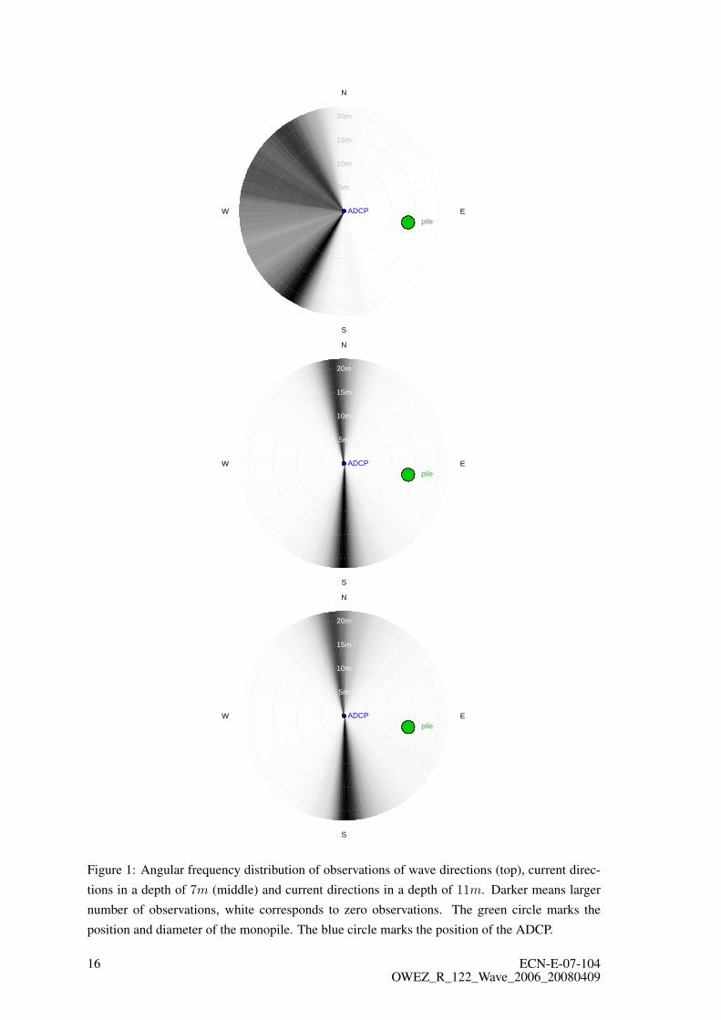
1 Angular frequency distribution of observations of wave directions (top), currentdirections in a depth of 7m (middle) and current directions in a depth of 11m.Darker means larger number of observations, white corresponds to zero obser-vations. The green circle marks the position and diameter of the monopile. Theblue circle marks the position of the ADCP. . . . . . . . . . . . . . . . . . . . . 16

2 Weibull scale parameter (blue) and Weibull shape parameter (green). . . . . . . . 17

3 Wind speed frequency distribution at the height of 116m (top), 70m (middle) and21m (bottom) for the period from 5 May 2006 to 30 October 2006. The bluelines show fitted Weibull distributions. Fitting parameters are given in the topright corner, respectively. . . . . . . . . . . . . . . . . . . . . . . . . . . . . . . 18

4 Wind direction frequency distribution at the height of 116m (top), 70m (middle)and 21m (bottom) for the period from 5 May 2006 to 30 October 2006. Radialunits are given in probability densities (center is zero). . . . . . . . . . . . . . . 20

5 Map of the wave measurement locations of the National Institute for Coastal andMarine Management. The ammunition dump of IJmuiden and the OWEZ loca-tion are marked with a red bullet. . . . . . . . . . . . . . . . . . . . . . . . . . . 21

6 Scatter plot of the significant wave height measured by OWEZ and at IJmuiden,together with a linear fit (red) and the q-q plot (blue) . . . . . . . . . . . . . . . 22

7 Wave height frequency distributions for all atmospheric conditions (left) andwithout stable conditions (right). Blue lines show a fitted Weibull distribution.Fitting parameters are given in the top right corner respectively. . . . . . . . . . 23

8 Wave direction frequency distribution. Radial units are given in probability den-sities. . . . . . . . . . . . . . . . . . . . . . . . . . . . . . . . . . . . . . . . . 24

9 Histograms of misalignments between wind direction at the height of 21m andthe measured wave direction for conditionally unstable, unstable and stable at-mospheric conditions (from top to bottom). . . . . . . . . . . . . . . . . . . . . 26

10 Current direction frequency distribution for 7m water depth (top) and 11m waterdepth (bottom). Radial units are given in probability densities. . . . . . . . . . . 27

11 Different view angles of the 3D scatter plot of wave height, wave period and windspeed at 21m. The colors black, red and green refer to conditionally unstable,unstable and stable atmospheric conditions respectively. . . . . . . . . . . . . . 28

12 Significant wave height as function of wind speed (left) and wave period (right)for conditionally unstable, unstable and stable atmospheric conditions (top to bot-tom). . . . . . . . . . . . . . . . . . . . . . . . . . . . . . . . . . . . . . . . . . 29

13 Time serie of 10 minutes averages of water level (top) and water temperature(bottom). Also shown are the histograms of the time series (barplots at the rightside, units are numbers of observations). . . . . . . . . . . . . . . . . . . . . . . 31

ECN-E-07-104OWEZ_R_122_Wave_2006_20080409

5

14 Time serie of 10 minutes averages of wave height (top), wave period (middle)and wave direction (bottom). Also shown are the histograms of the time series(barplots at the right side, units are numbers of observations). . . . . . . . . . . . 32

15 Time serie of 10 minutes averages of current velocity at the depth of 7m (top) andcurrent direction at the depth of 7m (bottom). Also shown are the histograms ofthe time series (barplots at the right side, units are numbers of observations). . . . 33

16 Time serie of 10 minutes averages of current velocity at the depth of 11m (top)and current direction at the depth of 11m (bottom). Also shown are the his-tograms of the time series (barplots at the right side, units are numbers of obser-vations). . . . . . . . . . . . . . . . . . . . . . . . . . . . . . . . . . . . . . . . 34

6 ECN-E-07-104OWEZ_R_122_Wave_2006_20080409

List of Symbols

A Weibull scale parameterE EastE(f) spectral densityHs significant wave height mN number of data points or NorthS SouthSE standard error of the meanT absolut temperature KTz wave period sW West

f frequency s−1

h height mk Weibull shape parametermn nth momentp probability densityu wind speed ms−1

% correlation coefficientσ standard deviation

ECN-E-07-104OWEZ_R_122_Wave_2006_20080409

7

1 Introduction

NoordzeeWind carries out an extensive measurement and evaluation program (NSW-MEP) aspart of the OWEZ project. NoordzeeWind contracted Bouwcombinatie Egmond (BCE) to buildand operate an offshore meteorological mast at the location of the OWEZ wind farm. BCEcontracted Mierij Meteo to deliver and install the instrumentation in the meteorological mast.After the data have been validated, BCE delivers the measured 10 minutes statistics data toNoordzeeWind.

A 116m high meteorological mast has been installed to measure the wind conditions. This mastis in operation since the summer of 2005. The measurements from the 116m high mast have beenmade available by Noordzeewind. This report intents to fulfill requirements which are specifiedin the measurement and evaluation program [1]. One of the requirements is to report periodicallythe wave conditions combined with the measured wind conditions at the met mast. During theperiod summer 2005 to December 2006 wave data are only available for the period 5 May 2006to 30 October 2006. Those data are here reported graphically and tabularly. Note that during thisperiod the wind farm has been installed, but has not been operational yet. Therefore the measuredwind conditions at the mast are not disturbed by wakes.

In section 2 definitions used in this report are given.

In section 3 the measured signals are described and the instrument codes are given. From themeasurements with several anemometers and vanes at each measurement level, a wind speed andwind direction is constructed that reduces the effect of flow distortion due to the mast and neigh-boring sensors. The definitions of derived wind speed and derived wind direction are described.

In section 4 the wind and wave climate during the period under consideration is described.

In section 5 the time series of water level and temperature, wave height, period and direction andcurrent velocity and direction are shown.

ECN-E-07-104OWEZ_R_122_Wave_2006_20080409

9

2 Definitions

Unless mentioned differently the following definitions have been used in this report.

2.1 Standard error of the mean

The standard error of the mean of a sample from a population is the standard deviation of thesample divided by the square root of the sample size

SE =σ√N, (1)

with N being the number of observations [2].

Note that all error bars within this report refer to this standard error, unless mentioned differently.

2.2 Significant wave height

Wave heights are given as significant wave heights, which are defined by the energy spectrum [3]

Hs = 4

√∫E(f)df. (2)

As not mentioned differently within this report, wave height always means significant waveheight.

2.3 Zero upcrossing wave period

Wave periods are given as zero upcrossing periods, which are defined by [3]

Tz = 2π ·√m0

m2, mn =

∫fnE(f)df, n = 0, 2. (3)

As not mentioned differently within this report, wave period always means zero upcrossing waveperiod.

2.4 Stability

The stability or instability of a layer of the atmosphere or of the atmosphere as a whole is astate with respect to the reaction of a volume of air to a vertical displacement. The atmosphericstability determines the probability of convection, atmospheric turbulence and mixing. Duringhighly unstable conditions a lifted parcel of air will be warmer than the surrounding air. It willcontinue to rise upward, away from its original position. Therefore a lot of atmospheric turbulenceis likely to occur, which goes a along with strong mixing.

For highly stable conditions a lifted volume of air will be cooler than the surrounding air. It willsink back to its original vertical position. Distortions to the vertical position of an air volume willtherefore be damped, which can lead to decoupled layers within the atmosphere.

ECN-E-07-104OWEZ_R_122_Wave_2006_20080409

11

During conditionally unstable conditions saturated air volumes can still rise due to moisture.

Note that there exists a large variety of methods to estimate atmospheric stability from measure-ments and that this topic is still ongoing research. Four different methods are tested to estimateatmospheric stability:

• the relation between water surface temperature and air temperature

• the ratio of potential to kinetic energy [5]

• best fit of the velocity profile [4]

• environmental lapse rate (variation of temperature with height)

The environmental lapse rate turned out to be the method that coincides best with the analyses.Therefore stability within this report is based on the variation of temperature with height:

− dT/dh < 6K/km ≡ stable atmospheric conditions (4)

6K/km < −dT/dh < 10K/km ≡ conditionally unstable atmospheric conditions

−dT/dh > 10K/km ≡ unstable atmospheric conditions.

12 ECN-E-07-104OWEZ_R_122_Wave_2006_20080409

3 Measured data

3.1 Measured signals

The instrumentation codes of the sensors in the 116m high meteorological mast at the offshorewind farm location OWEZ are indicated in the following table. The instrumentation is describedin [6].

Channel Instrumentation Code Parameter Unit

0 3D WM4/NW/21 wind direction ◦

1 3D WM4/NW/21 horizontal wind speed ms−1

2 3D WM4/NW/21 vertical wind speed ms−1







9 WS 018/NW/116 wind speed ms−1

10 WS 018/NE/116 wind speed ms−1

11 WS 018/S/116 wind speed ms−1







18 RHTT 261/S/116 ambient temperature ◦C



21 RHTT 261/S/116 relative humidity %22 RHTT 261/S/70 relative humidity %23 RHTT 261/S/21 relative humidity %24 DP910 ambient air pressure mbar

25 PD 205/NW/70 precipitation boolean

26 PD 205/NE/70 precipitation boolean

27 ST 808/NW/-3.8 sea water temperature ◦C

28 AC SB2i/T/116 acceleration (north - south) ms−2

29 AC SB2i/T/116 acceleration (west - east) ms−2

ECN-E-07-104OWEZ_R_122_Wave_2006_20080409

13

30 WD 524/NW/116 wind direction ◦

31 WD 524/NE/116 wind direction ◦

32 WD 524/S/116 wind direction ◦







50 ADCP water level m

51 ADCP water temperature ◦C

52 ADCP wave height m

53 ADCP wave period s

54 ADCP wave direction ◦

55 ADCP current velocity 7m ms−1

56 ADCP current velocity 11m ms−1

57 ADCP current direction ◦

58 ADCP current direction ◦

Channel Instrumentation Code Parameter Unit

3.2 Measurement sectors

3.2.1 Meteorological mast

The meteorological mast is a lattice tower with booms at three heights: 21m, 70m and 116mabove mean sea level (MSL). At each height, three booms are installed in the directions north-east(NE), south (S) and north-west (NW). Sensors attached to the meteorological mast are describedin [6]. The location of the meteorological mast is given in the following table.

UTM31 ED50 WGS 84

x 594195 4◦23′22, 7′′ Longitude Easty 5829600 52◦36′22, 9′′ Latitude North

3.2.2 Derived wind data

The wind speeds and wind directions at each height are measured with more than one sensor. Forcertain wind directions the wind vanes and cups are in the wake of the mast or neighboring sensorsor are otherwise significantly disturbed. It is necessary to select one of the cup anemometersand wind vanes depending on the actual wind direction in order to establish a wind speed thatminimizes the distortion. The constructed wind speed and wind direction are used within thisreport. The selection of signals is indicated in the following table.

14 ECN-E-07-104OWEZ_R_122_Wave_2006_20080409

Wind direction Selected sensors

330 to 30 ◦ average of wind vanes NW and NE boom30 to 90 ◦ average of wind vanes S and NW boom90 to 150 ◦ average of wind vanes S and NE boom150 to 210 ◦ average of wind vanes NW and NE boom210 to 270 ◦ average of wind vanes NW and S boom270 to 330 ◦ average of wind vanes NE and S boom

0 to 120 ◦ cup anemometer in NE boom120 to 240 ◦ cup anemometer in S boom240 to 360 ◦ cup anemometer in NW boom

Averaging over two vanes reduces the effect of the distortion by the mast on the wind directionmeasurement.

For the selection of the wind speed sensor it is important that at the direction where the windspeed sensor is changed from one sensor to the other, the ratio of the wind speeds is close toone. Furthermore, the wind speed may not be measured in the wake of the mast or a neighboringsensor.

3.2.3 Wave and current data

Seen from the monopile of the measurement mast the ADCP is placed in a distance of 13.75m inthe direction of 280◦. As it can be seen in Figure 1 the monopile stands in a sector seen from theADCP where almost no wave or current data have been measured. Therefore the influence of themonopile on the measurements can be neglected.

ECN-E-07-104OWEZ_R_122_Wave_2006_20080409

15

5m

10m

15m

20m

ADCPpile

N

S

EW

5m

10m

15m

20m

ADCPpile

N

S

EW

5m

10m

15m

20m

ADCPpile

N

S

EW

Figure 1: Angular frequency distribution of observations of wave directions (top), current direc-tions in a depth of 7m (middle) and current directions in a depth of 11m. Darker means largernumber of observations, white corresponds to zero observations. The green circle marks theposition and diameter of the monopile. The blue circle marks the position of the ADCP.

16 ECN-E-07-104OWEZ_R_122_Wave_2006_20080409

4 Wind and wave climate in the reporting period

The intention of this report is to describe the measured wave conditions at the measurementmastof NSW periodically. During a limited period from 5 May 2006 to 30 October 2006 wave dataare available. In the following subsections the wind conditions during this period are described.The long-term wind climate will be reported in a separate report.

4.1 Wind speed frequency distributions

In this subsection the wind speeds are depicted for the period which coincides with the availabilityof wave date.

Figure 3 shows the wind speed frequency distributions for the three measurement heights h =116m, h = 70m and h = 21m, together with a fitted Weibull distribution

p(u) =k

A

( uA

)k−1exp

(−( uA

)k), (5)

with u being the horizontal wind speed, k the shape parameter and A the scale parameter.

According to the distributions and the fitting parameters, the scale parameter increases (exponen-tially) with height, while the shape parameter decreases with height, see Figure 2.

●

●

●

2040

6080

100

heig

ht [m

]

8.5 8.75 9 9.25 9.5 9.75 10 10.25

●

●

●

2040

6080

100

heig

ht [m

]

2.25 2.3 2.35 2.4 2.45 2.5k

A

Figure 2: Weibull scale parameter (blue) and Weibull shape parameter (green).

ECN-E-07-104OWEZ_R_122_Wave_2006_20080409

17

u[m/s]

prob

abili

ty d

ensi

ty 1

16m

0.00

0.02

0.04

0.06

0.08

0.10

0.12

0.25 2.75 5.25 8.25 10.75 13.25 16.25 18.75 21.25 24.25

k = 2.27A = 10.21

u[m/s]

prob

abili

ty d

ensi

ty 7

0m

0.00

0.02

0.04

0.06

0.08

0.10

0.12

0.25 2.25 4.75 7.25 9.25 11.75 14.25 16.25 18.75 21.25

k = 2.36A = 9.71

u[m/s]

prob

abili

ty d

ensi

ty 2

1m

0.00

0.02

0.04

0.06

0.08

0.10

0.12

0.25 2.25 4.25 6.25 8.25 10.75 12.75 14.75 16.75 19.25

k = 2.43A = 8.58

Figure 3: Wind speed frequency distribution at the height of 116m (top), 70m (middle) and 21m(bottom) for the period from 5 May 2006 to 30 October 2006. The blue lines show fitted Weibulldistributions. Fitting parameters are given in the top right corner, respectively.

18 ECN-E-07-104OWEZ_R_122_Wave_2006_20080409

4.2 Wind direction frequency distributions

In this subsection the wind directions are depicted for the period which coincides with the avail-ability of wave date.

Figure 4 shows the wind direction frequency distributions for the three measurement heightsh = 116m, h = 70m and h = 21m. The prevailing wind direction is south west.

As expected a change in orientation of the prevailing wind direction to the West can be observedwith increasing height (Ekman spiral). Furthermore, the variation in wind directions increaseswith height, meaning that a prevailing wind direction is less pronounced for high altitudes.

ECN-E-07-104OWEZ_R_122_Wave_2006_20080409

19

wind rose 116m height

N

S

W E0

0.05

u<5 m/su<10 m/su<15 m/sall


N

S

W E0

0.05



N

S

W E0

0.05


Figure 4: Wind direction frequency distribution at the height of 116m (top), 70m (middle) and21m (bottom) for the period from 5 May 2006 to 30 October 2006. Radial units are given inprobability densities (center is zero).

20 ECN-E-07-104OWEZ_R_122_Wave_2006_20080409

4.3 Wave height comparison with measurements from IJmuiden

As a first order check on the quality of the wave data the significant wave heights measured byOWEZ have been compared with those measured at the same time at the ammunition dump ofIJmuiden. That station is located in a distance of 23km in 254.5◦ direction with respect to theOWEZ location, see Figure 5. Further information on that station can be found at [7].

Figure 5: Map of the wave measurement locations of the National Institute for Coastal and MarineManagement. The ammunition dump of IJmuiden and the OWEZ location are marked with a redbullet.

Figure 6 shows the scatter plot of both measurements, together with a linear fit and the quantile-quantile plot. Quantile-quantile plots (also called q-q plots) are used to determine if two data setscome from populations with a common distribution. In such a plot, points are formed from thequantiles of the data. If the resulting points lie roughly on a line with slope 1, then the distributionsare the same.

ECN-E-07-104OWEZ_R_122_Wave_2006_20080409

21

0 1 2 3 4

12

34

Hs−−OWEZ,, [m]

Hs−−

IJm

uide

n,, [m

]

Hs−−IJmuiden == 1.01 ⋅⋅ Hs−−OWEZ ++ 0.08qqplot

Figure 6: Scatter plot of the significant wave height measured by OWEZ and at IJmuiden, togetherwith a linear fit (red) and the q-q plot (blue)

The correlation coefficient % between both signals has been found to be 0.97. This means that thesignificant wave heights at OWEZ are quite similar to the significant wave heights measured atIJmuiden. Also a linear fit and the quantile-quantile plot provide evidence in the validity of themeasurements.

22 ECN-E-07-104OWEZ_R_122_Wave_2006_20080409

4.4 Wave height frequency distributions

Figure 7 shows the frequency distribution of significant wave heights. The large probability forsmall (< 0.5m) wave heights correspond to stable atmospheric conditions1, where due to thedecoupling of different air layers the friction on water surface is expected to be reduced.

Hs [m]

prob

abili

ty d

ensi

ty

0.0

0.2

0.4

0.6

0.8

1.0

0 0.5 1 1.5 2 2.5 3 3.5 4

k = 1.58A = 1.1

Hs [m]pr

obab

ility

den

sity

0.0

0.2

0.4

0.6

0 0.5 1 1.5 2 2.5 3 3.5 4

k = 1.99A = 1.35

Figure 7: Wave height frequency distributions for all atmospheric conditions (left) and withoutstable conditions (right). Blue lines show a fitted Weibull distribution. Fitting parameters aregiven in the top right corner respectively.

1for the definition of stability see section 2.4

ECN-E-07-104OWEZ_R_122_Wave_2006_20080409

23

4.5 Wave direction frequency distributions

In Figure 8 the wave direction frequency distribution is shown. Due to the presence of the coastin the east, waves generally come from the west. This can easily be seen in Figure 8. The largestwaves predominantly come from Noth-West or South-West directions.

wave rose

N

S

W E0

0.05

0.1

Hs<0.25 m/sHs<0.5 m/sHs<0.75 m/sall

Figure 8: Wave direction frequency distribution. Radial units are given in probability densities.

24 ECN-E-07-104OWEZ_R_122_Wave_2006_20080409

4.6 Misalignment between wave and wind direction

Offshore wind turbines are exited by wave loads acting on the tower and wind loads mainly actingon the rotor. Therefore it is important to gain knowledge on the relative alignment of these forces.

Figure 9 shows histograms of misalignments between wind direction at the height of 21m and themeasured wave direction

misalignment = |directionwind21m− directionwave|. (6)

It can clearly be seen that the misalignment depends on stability2 of the atmospheric boundarylayer, as it is predicted by theory.

For unstable periods the misalignment is found to be the smallest, since due to the turbulentmixing a coupling between different heightsexists.

For stable situations the misalignment is almost equally distributed, which is due to the fact thatlayers in different heightscan be decoupled and therefore winds in higher altitudes have no directimpact on winds above sea level, which are driving the waves.

2for the definition of stability see section 2.4

ECN-E-07-104OWEZ_R_122_Wave_2006_20080409

25

misalignment [°]

prob

abili

ty d

ensi

ty c

ond.

uns

tabl

e

0.00

00.

002

0.00

40.

006

0.00

80.

010

0.01

2

2.5 12.5 22.5 32.5 42.5 52.5 62.5 72.5 82.5 92.5 102.5 112.5 122.5 132.5 142.5 152.5 162.5 172.5

misalignment [°]

prob

abili

ty d

ensi

ty u

nsta

ble

0.00

00.

005

0.01

00.

015

0.02

0

2.5 12.5 22.5 32.5 42.5 52.5 62.5 72.5 82.5 92.5 102.5 112.5 122.5 132.5 142.5 152.5 162.5 172.5

misalignment [°]

prob

abili

ty d

ensi

ty s

tabl

e

0.00

00.

001

0.00

20.

003

0.00

40.

005

0.00

6

2.5 12.5 22.5 32.5 42.5 52.5 62.5 72.5 82.5 92.5 102.5 112.5 122.5 132.5 142.5 152.5 162.5 172.5

Figure 9: Histograms of misalignments between wind direction at the height of 21m and themeasured wave direction for conditionally unstable, unstable and stable atmospheric conditions(from top to bottom).

26 ECN-E-07-104OWEZ_R_122_Wave_2006_20080409

4.7 Current direction frequency distributions

Another force on the turbines originates from the water current. Although of limited effect theinformation is essential for a proper description. In Figure 10 the current direction frequencydistributions are shown for the depth of 7m as well as 11m. A strong confinement of currentdirections along the North-South axis is observed and coincides with the knowledge on currentsalong the Dutch North Sea coast.

current rose 7m depth

N

S

W E0

0.05

0.1

0.15

0.2

0.25

0.3

cs<0.25 m/scs<0.5 m/scs<0.75 m/sall

current rose 11m depth

N

S

W E0

0.05

0.1

0.15

0.2

0.25

0.3

cs<0.25 m/scs<0.5 m/scs<0.75 m/sall

Figure 10: Current direction frequency distribution for 7mwater depth (top) and 11mwater depth(bottom). Radial units are given in probability densities.

ECN-E-07-104OWEZ_R_122_Wave_2006_20080409

27

4.8 Relation between wave height, wave period and wind speed

In figure 11 the 3D scatter plot of wave height, wave period and wind speed is shown.

wind speed [m/s]510

15wave.period [s]

2

3

45

6

wav

e he

ight

[m]

1

2

3

wind speed [m/s]5 10 15

wave.period [s]

2

3

4

5

6

wav

e he

ight

[m]

1

2

3

wind speed [m/s]

510

15

wave.period [s]

2

3

45

6

wav

e he

ight

[m]

1

2

3

wind speed [m/s]

5

10

15

wave.perio

d [s]

2

3

4

5

6

wave height [m

]

1

2

3

wind speed [m/s]

5 10 15wave.

perio

d [s]

2

3

4

56

wave height [m

]

1

2

3

wind speed [m/s]5

10

15

wave.period [s] 2

3

4

5

6

wave height [m

]

1

2

3

wind speed [m/s]

5

10

15 wav

e.pe

riod

[s]

2

3

4

5

6

wave height [m

] 1

2

3

wind speed [m/s]5 10 15

wav

e.pe

riod

[s]

2

3

4

5

6

wave height [m

]

1

2

3

wind speed [m

/s]

5

10

15

wave.period [s]

2

3

4

5

6

wave height [m

] 1

2

3

Figure 11: Different view angles of the 3D scatter plot of wave height, wave period and windspeed at 21m. The colors black, red and green refer to conditionally unstable, unstable and stableatmospheric conditions respectively.

A detailed view of the dependence of wave height and wave period as well as wave height andwind speed can be found in Figure 12.

28 ECN-E-07-104OWEZ_R_122_Wave_2006_20080409

0 5 10 15 20

01

23

45

u [m/s]

Hs

[m]

10min. valuesmeanmedian

0 5 10 15 20

01

23

45

u [m/s]

Hs

[m]


0 5 10 15 20

01

23

45

u [m/s]

Hs

[m]


2 3 4 5 6

01

23

45

wave period [s]

Hs

[m]


2 3 4 5 6

01

23

45

wave period [s]

Hs

[m]


2 3 4 5 6

01

23

45

wave period [s]

Hs

[m]


Figure 12: Significant wave height as function of wind speed (left) and wave period (right) forconditionally unstable, unstable and stable atmospheric conditions (top to bottom).

ECN-E-07-104OWEZ_R_122_Wave_2006_20080409

29

It can be seen that during periods of stable conditions of the marine atmospheric boundary layerthe frictional coupling over the sea decreases. This means that during stable atmospheric condi-tions the wind has a minimal impact on the water surface and therefore the probability of largewave heights is very low.

Nevertheless, is must be mentioned that due to the limited amount of available data points, thesignificance of Figures 1112 is rather limited.

30 ECN-E-07-104OWEZ_R_122_Wave_2006_20080409

5 Time series

In this section the time series of the ADCP channels are shown for the period from 1 May 2006until 30 October 2006. During this period the ADCP has recorded data successfully. The timeseries of the remaining channels can be found in the half year reports ’Meteorological Measure-ments OWEZ’ [8][9][10][11].

16.5

17.0

17.5

18.0

18.5

day of 2006

wat

er le

vel [

m]

124 150 200 250 0 250 500

1012

1416

1820

day of 2006

wat

er te

mpe

ratu

re [°

C]

124 150 200 250 0 500 1250

Figure 13: Time serie of 10 minutes averages of water level (top) and water temperature (bottom).Also shown are the histograms of the time series (barplots at the right side, units are numbers ofobservations).

ECN-E-07-104OWEZ_R_122_Wave_2006_20080409

31

12

34

day of 2006

wav

e he

ight

[m]

124 150 200 250 0 250 750

23

45

6

day of 2006

wav

e pe

riod

[s]

124 150 200 250 0 250 500

5010

015

020

025

030

035

0

day of 2006

wav

e di

rect

ion

[°]

124 150 200 250 0 250 750

Figure 14: Time serie of 10 minutes averages of wave height (top), wave period (middle) andwave direction (bottom). Also shown are the histograms of the time series (barplots at the rightside, units are numbers of observations).

32 ECN-E-07-104OWEZ_R_122_Wave_2006_20080409

0.0

0.2

0.4

0.6

0.8

1.0

day of 2006

curr

ent v

eloc

ity 7

m [m

/s]

124 150 200 250 0 250 500 750

050

100

150

200

250

300

350

day of 2006

curr

ent d

irect

ion

7m [°

]

124 150 200 250 0 750 1750

Figure 15: Time serie of 10 minutes averages of current velocity at the depth of 7m (top) andcurrent direction at the depth of 7m (bottom). Also shown are the histograms of the time series(barplots at the right side, units are numbers of observations).

ECN-E-07-104OWEZ_R_122_Wave_2006_20080409

33

0.0

0.2

0.4

0.6

0.8

1.0

day of 2006

curr

ent v

eloc

ity 1

1m [m

/s]

124 150 200 250 0 250 500

050

100

150

200

250

300

350

day of 2006

curr

ent d

irect

ion

11m

[°]

124 150 200 250 0 750 1500

Figure 16: Time serie of 10 minutes averages of current velocity at the depth of 11m (top) andcurrent direction at the depth of 11m (bottom). Also shown are the histograms of the time series(barplots at the right side, units are numbers of observations).

34 ECN-E-07-104OWEZ_R_122_Wave_2006_20080409

6 Conclusions

Based on the limited number of data points the following conclusions can be drawn for the OWEZlocation:

• According to the wind speed Weibull distributions and the fitting parameters of which, thescale parameter increases (exponentially) with height, while the shape parameter decreaseswith height.

• The orientation of the prevailing wind direction changes to the West with increasing height(Ekman spiral). Furthermore, the variation in wind directions increases with height, mean-ing that a prevailing wind direction is less pronounced for high altitudes.

• Simultaneous wave measurements at IJmuiden and OWEZ are highly correlated, givinggood confidence in the quality of the OWEZ wave measurements.

• Wave directions are strongly influenced by the orientation of the coast and occur almostonly in north-west or south-west directions.

• Wind and wave misalignment is strongly influenced by atmospheric stability. For unstablesituations wave directions and wind directions are strongly coupled, while for unstablesituations wave and wind directions are independent.

• Water currents are bi-directional in north-south direction.

ECN-E-07-104OWEZ_R_122_Wave_2006_20080409

35

References

[1] NOORDZEEWIND

The NSW-MEP Technologywww.noordzeewind.nl/files/Common/Data/Overview_MEP_T_V2.pdf

[2] STÖCKER

Taschenbuch der PhysikVerlag Harri Deutsch (1994)

[3] K. ARGYIADIS

Recommendations for design of offshore wind turbinesExternal Conditions, state of the artGermanischer Lloyd (2003)

[4] H.A. PANOFSKY AND J.A. DUTTON

Atmospheric TurbulenceModels and Methods for Engineering ApplicationsJohn Wiley & Sons (1983)

[5] J.R. GARRAT

The atmospheric boundary layerCambridge University Press (1999)

[6] H.J. KOUWENHOVEN

User manual data files meteorological mast NoordzeeWindDocument code: NZW-16-S-4-R03www.noordzeewind.nl/files/Common/......Data/NZW-16-S-4-R03 Manual data files meteo mast NoordzeeWind.pdf

[7] NATIONAL INSTITUTE FOR COASTAL AND MARINE MANAGEMENT

www.golfklimaat.nl

[8] P.J. EECEN, L.A.H. MACHIELSE AND A.P.W.M. CURVERS

Meteorological Measurements OWEZHalf year report (01-07-2005 - 31-12-2005)ECN - report ECN-E–07-073





ECN-E-07-104OWEZ_R_122_Wave_2006_20080409

37



38 ECN-E-07-104OWEZ_R_122_Wave_2006_20080409

description of the relation of wind, wave and current...

Documents