Atmospheric Environment Vol. 25A, No. 12, pp. 2749 2759, 1991. 0004-6981/91 $3.00+0.00 Printed in Great Britain. Pergamon Press pie

DEPOSITION VELOCITY AND THE COLLISION MODEL OF ATMOSPHERIC DISPERSION--I. FRAMEWORK AND

APPLICATION TO CASES WITH CONSTANT TURBULENT VELOCITY SCALE

B. Y. UNDERWOOD SRD, AEA Technology, Wigshaw Lane, Culcheth, Warrington WA3 4NE, U.K.

(First received 2 November 1990 and in final form 10 February 1991)

Al~tract--This work shows how to apply the concept of deposition velocity to the collision model of turbulent dispersion, the latter being an alternative to the Langevin-equation approach for retaining a finite memory of turbulent velocity. In terms of the Monte Carlo (MC) solution to the model, this development obviates tracking particles into regions of complex behaviour near the true lower boundary in two- or three-dimensional dispersion-deposition problems. The approach is illustrated for pollutant dispersing in a homogeneous layer with a totally-absorbing lower boundary.

In addition, it is shown how the deposition velocity itself can be calculated within the Lagrangian-particle model by solving a one-dimensional equation. Illustrative MC solutions are given for a homogeneous layer and for the neutral surface layer of the atmosphere, for pollutant which is totally absorbed at a lower boundary; these are found to be closely similar to K-theory predictions, as expected for these cases.

Key word index: Deposition velocity, turbulent dispersion, Lagrangian-particle model, Monte Carlo simulation, eddy-diffusivity theory, gravitational settling.

NOMENCLATURE x horizontal coordinate in direction of mean wind (m)

b Height of the absorbing lower boundary y random deviate uniform on the range 0-1 (m) z vertical coordinate (m)

f+ (z, w+ )dw + relative number of particles crossing level z z c height of a particle's last collision (m) with upward velocity in the range w+ to Zo roughness length (m) w+ + dw + z m reference height at which deposition velo-

f_ (z, w _ ) dw _ relative number of particles crossing level z city specified (m) with downward velocity in the range w_ to zd upper boundary of the vertical domain (m) w_ + dw_ B normalized value of b, the height of the

k von Karman's constant absorbing boundary n + (z, w+ )dw + number of particles per unit range of x C(z) x-independent, crosswind-integrated, time-

crossing level z upwards with velocity in integrated concentration per unit release the range w+ to w++dw+ (m -1) (sm -2)

n_ (z, w_ )dw_ number of particles per unit range of x F constant value of the x-independent, cross- crossing level z downwards with velocity in wind-integrated, time-integrated net down- the range w_ to w_ + dw_ (m - 1 ) ward flux per unit release (m- 1 )

p(w)dw probability of a particle emerging from a J(x) function representing the equilibrium de- collision with vertical velocity in the range pendence of concentration and flux on x w to w + dw K,(z) vertical eddy-diffusivity (m 2 s - 1 )

p+(w+)dw+ probability of particle emerging from a N+(z) total number of particles per unit range of collision travelling upwards with velocity x crossing upwards across level z ( m - l ) in the range w + to w+ + dw + N_ (z) total number of particles per unit range of

p_ (w_)dw_ probability of particle emerging from a x crossing downwards across level z (m- 1) collision travelling downwards with velo- Q(t, w, z) probability of particle with vertical velo- city in the range w_ to w_ +dw_ city w after its last collision at z surviving a

t time to next collision (s) time t before its next collision u, friction velocity (m s - 1 ) V v normalized deposition velocity Vd deposition velocity (m s - 1 ) V s normalized settling velocity vs settling velocity (m s - 1 ) W+ normalized upward vertical velocity w an arbitrary vertical velocity (m s - 1 ) W_ normalized downward vertical velocity w c post-collision vertical velocity of a particle Z normalized height

carried with the air (m s - 1 ) ZD normalized value of Zd Wp¢ post-collision vertical velocity of a particle Z u normalized value of Zm

moving with respect to the current 'eddy' fl ratio a/u. (m s-1) ~' constant entering into Equation (21)

w+ an upward velocity (m s - l ) e(z) probability of emergence after crossing be- w_ a downward velocity (m s - 1 ) low level z

2749

2750 B.Y. UNDERWOOD

a r.m.s. Eulerian vertical turbulent velocity dC (m s-1 ) K, ( z ) ~ (z) = F (const), (2)

z L Lagrangian decorrelation time-scale (s) Z(x,z) crosswind-integrated, time-integrated con- where X(x,z)=J(x)C(z) and the cross-wind-inte-

centration per unit release (s m-2) grated downward flux is written as J (x)F, in accord Ax, distance to exit after crossing below given

level (m). with the condition that the vertical concentration profile is independent of x.

For the simple case of a neutral boundary layer (i.e. K , = ku. z, where k is von Karman's constant and u. is

l. INTRODUCTION the friction velocity) and with ~( zero at Z=Zo, this yields:

Models for the dispersion of airborne pollutants in the atmosphere from given source configurations gen- Vd(Zm)=ku./ln(Zm/Zo). (3)

erally do not attempt to include a detailed description 1Iv d can be identified as the aerodynamic resistance of what happens very close to the ground. In the case from z m down to zo, if the eddy diffusivity for the of dry-depositing pollutants, the need to model these pollutant is the same as that for momentum. In reality, details is circumvented by the introduction of the Equation (2) must be supplemented by further model- deposition velocity, Vd, at a specified height, z. , where ling for behaviour in the immediate vicinity of surface v a is defined as the ratio of downward flux to the roughness elements (or of a smooth surface), but the surface to the concentration at %. By this means, the problem remains one-dimensional. full dispersion problem is 'factorized' into (a) disper- A well-known drawback of the eddy-diffusivity ap- sion in the bulk atmosphere--with a boundary condi- proach is its failure to represent the finite time-scale tion at z m given in terms of vd--and (b) the measure- over which Lagrangian velocities are correlated, and ment or separate calculation of Vd(Z=). in recent years there has been an increasing use of

It is well known (e.g. Doran, 1977) that this factoriz- 'Lagrangian particle' descriptions of turbulent disper- ation of the problem is only applicable when the flux sion, which offer the opportunity of examining this of material becomes sufficiently constant below Zm, limitation. The most favoured approach to date has which in the case of an elevated point source, for been based on solution of a stochastic differential example, only obtains sufficiently far downwind of the equation (SDE) (Sawford, 1985, reviews the develop- source. At this range, the concentration profile up to ment of this approach): turbulent dispersion is con- the height z= has come into equilibrium with the sidered to be analogous to Brownian motion, where underlying surface and the ratio of flux to concentra- the persistence of velocity is continually eroded by tion becomes virtually independent of distance. An stochastic inputs. equivalent statement of the above criterion--which As an alternative, however, 'particles'--represent- follows from the continuity condition--is that along- ing elements of pollutant--can be envisaged as ex- wind gradients in (cross-wind integrated) pollutant periencing 'collisions' after lengths of time chosen concentration below the height Zm should have a randomly from a distribution governed by the La- sufficiently small impact on the vertical concentration grangian time-scale (Smith, 1982). At each collision-- profile, which may be pictured as a particle entering a new

Three aspects of deposition modelling stem from eddy--all memory of previous turbulent velocity is this: (i) for a given source configuration, at what range lost; between collisions perfect correlation is retained. is the above criterion satisfied (for a given specifica- This model, which has formal analogies to the treat- tion of 'sufficiently' in the above); (ii) what is the ment of neutron and photon transport in scattering specification of the boundary condition in terms of Vd; media, gives Taylor's result for mean-square displace- and (iii) how is Vd calculated in terms of the near- ment in homogeneous turbulence (Underwood, 1991), surface details? and has been used to good effect in modelling disper-

In the framework of eddy-diffusivity theory, for sion in the neutral atmosphere (Underwood, 1990). A example, question (ii) is answered via: type of collision model has been used in several non-

~X atmospheric flow situations, including turbulent flow Kz(zm)~-~z (x, Zm)-----1)dX(X, Zm), (1) in pipes (Kallio and Reeks, 1989) and turbulent jets

(Shuen et al., 1983). Although the model covers much where K,(z) is the eddy diffusivity of the pollutant the same ground as the SDE approach, it may be (ignoring the possibility of sedimentation of particles possible to formulate, and answer, some questions for the moment) and X is (cross-wind integrated) con- more easily within its framework. centration; past work has investigated question (i) for There are several ways to mathematically formulate an elevated point source (Doran, 1977). Regarding each of the above two Lagrangian-particle models, (iii), if the diffusivity framework applies all the way but their representation as 'random walk' processes down to the lower boundary, for example, va can be allows use of the versatile solution technique of calculated by solving the one-dimensional equation Monte Carlo (MC) simulation. For dry-depositing representing constancy of downward flux: pollutants, then, it is natural to seek a factorization of

Collision model of atmospheric dispersion--I 2751

the dispersion--deposition problem so that there is no entering below Zm with the velocity w_ then this need in two- or three-dimensional situations to track would afford one type of factorization of the problem. particles into regions very close to the ground, where Thereby, irrespective of source height, particles would conditions differ significantly from those in the bulk not need to be tracked below Zm: every time a particle atmosphere and where strong gradients are present, crossed below, its weight would be multiplied by the In other words, issues (i)-(iii) are also pertinent to probability of return corresponding to its w_, a ran- these Lagrangian-particle models. Below, questions dom choice would be made from the corresponding (ii) and (iii) will be addressed for the collision model; distribution of w+ values and the particle would em- this provides a framework for examining issue (i), but erge at a distance Axr from its point of entry chosen the latter is not pursued further here. from the appropriate distribution. These distributions

The aim is not only to develop a framework but generally contain much more information than is also to calculate deposition velocities using the colli- provided by a value of deposition velocity at z m. sion model for some simple cases, to illustrate the For a given source height, the distribution of w_ technique and to compare the results with those of values at Zm will depend on x and the dependence will eddy-diffusivity theory, be strong close to the source; for a given x it will

depend on source height. Far enough downwind, however, the distribution will approach an 'equilib-

2. THE DEPOSITION BOUNDARY CONDITION rium' form, independent of source height and of x, governed by the properties of the turbulence and of

Consider thehomogeneoustwo-dimensionaldisper- the surface. This distribution will be labelled sion--deposition situation in which pollutant emitted f - (Zm, W_), where f_ (Zm, w_) dw_ is the relative from an elevated point source moves with uniform number of particles crossing level Zm with downward velocity u in the x direction whilst being subjected to velocity in the range w_ to w_ + dw_. Beyond that vertical turbulent transfer; dry deposition occurs at distance it becomes possible to deal with only one the ground. In the collision model, particle trajector- value of ~ and one distribution of upward-moving ies consist of straight-line segments (see Fig. 1). Par- particles at Zm, namely those obtained by suitably tieles with vertical velocity w_ downwards crossing averaging over the distribution f_ (Zm, W_). These will into the region below Zm at x may emerge from this be labelled e(Zm) and f÷ (Zm, W+), respectively. Any region with a range of upward vertical velocities and particle reaching Zm, whatever its w_, can be returned after a range of times, i.e. at a range of distances with its weight multiplied by ~(Zm) and with a vertical downwind of x. Some particles may not emerge at all. velocity chosen according to the f+ (Zm, W +) distribu- The probability of emergence, e, the distribution of tion. upward vertical velocities (w+) on emergence and the Similarly, a realistic representation of the displace- distribution ofdistance-to-exit(Axr)will all dependof ment Axr would be vitally important close to the w_ generally, source where horizontal gradients in concentration

If the above quantities were found by running a are strong, but, far enough downwind, ignoring this two-dimensional MC simulation, for each of a repres- displacement will have negligible influence:particles entative set of w_ values, on an ensemble of particles can be returned at their point of entry.

wind speed, u

source

. . . . . w _ w._

/ I S / / / / / / / _ l X / / / / / / / / ~, / / / / I-- xl ~ _Jl I

' - x2 ~ [ - , ~ ~x r - - - - ~

Fig. 1. Illustration of particle trajectories, according to the collision model, for contaminant subject to deposition at the ground. Particle (1) does not re-emerge after crossing below Zm at x~; particle (2) z'c-emerges a distance

Axr from its point of entry, with vertical velocity w+.

2752 B.Y. UNDERWOOD

The above two conditions are equivalent to those The equivalent equation for n_ (z, w_) is: given earlier for the validity of a v d factorization of the

dn_(z,w_) -n_(z,w_) problem, and it now becomes possible to relate e(Zm) --~L = +p_(w_)C(z). (7) to Vd(Zm). Moreover, ~(z) and the f_(z,w_) and dz Iw-I

f+ (z, w +) distributions can be calculated as a function Integrating (5) over all w+, (7) over w_ and adding of z from a one-dimensional equation, equivalent to yields: Equation (2), as shown below.

dF ~L -~z = -- C ( z ) + C ( z ) = 0, (8)

3. T H E R E L A T I O N S H I P O F ~ T O v a where F is the cross-wind-integrated, time-integrated net downward flux given by:

The reduction to an essentially one-dimensional problem arises because, for steady conditions, par- F ( z ) = N_ ( z ) - N ÷ (z), (9)

tides lost from one side of a slice dx are balanced on with N_ (z) and N÷ (z) the total number of particles average by particles entering from the other side (as a per unit range of x crossing level z downwards and result of the negligible x-gradient). Conservation of upwards, respectively, in turn given by: particles can therefore be applied separately in the vertical, f'_ f l ~

Let n÷(z, w+)dw+ be the number of particles per N_(z )= n_(z, w)dw; N+(z)= n+(z, w)dw. oo

unit range of x crossing level z upwards with vertical (10) velocity in the range w÷ to w÷ +dw+ and n_(z, w_)

The previously introduced distributions f÷ and f_ are the equivalent distribution for downward-moving particles. Then, in the collision model, the following related to n÷ and n_ simply via:

equation applies: f_ (z, w_ ) = n_ (z, w_ )/N_ (z);

n+(z+dz, w+)dw+= f+(z,w+)=n+(z,w+)/N+(z). (11)

dzdw ÷ Equation (8) confirms that this one-dimensional prob- n + (z, w + ) dw + - n ÷ (z, w +) w + z-----~ lem corresponds to a constant-flux regime.

From the definition of vd,

fo + n+(z, w') W'Z------L p+(w+)dw+ dw' va(z)=[N-(z)-N+(z)]/

J-t' w) ['t--LW~ ~ [N_(z) < 1/Iw-1> + N+(z)< 1/w + >'], (12) + n_(z, ' - - p + ( w + ) d w + d w ' , (4) where < > denotes the average over all particles

crossing level z; i.e.

where p+(w+)dw+ is the probability of emerging Vd(Z)=[1--~(Z)]/[<I/Iw-I> +e(Z)<I/w+ > 1 (13) from a collision with upward vertical velocity in the

which leads to: range w+ to w+ +dw+ (and similarly for p_ ). TL is the decorrelation time-scale, set equal to the Lagrangian e(z)=[1-va<l/Iw_l>]/[l+vd< 1/<w+ >] . (14) time-scale for the layer (still working with the homo, geneous-layer example). The second term in the right- At first sight it appears that, in contrast to the eddy- hand side of (4) represents particles scattered out of diffusivity case, the 'factorization' of this model can- dw + and the third and fourth terms represent particles not be carried out when the only information avail- scattered into dw÷ from positive and negative values able is a measured deposition velocity at a given level:

the whole f÷ (Zm, w+) distribution needs to be known of w respectively. Equation (4) can be simplified to: in order to continue particle trajectories after return

dn+(z, w+) -n+(z, w+) t-p+(w+)C(z), (5) from the level z, and the mean values of the upward dz w÷ and downward distributions need to be known in

order to calculate 4. In practice, however, the situation where C(z) is the cross-wind-integrated concentration is more favourable, as will emerge in section 4. (strictly speaking, a time-integrated concentration, i.e. It is worth noting that Equations (5) and (7) can be dosage, but the term 'concentration' will be retained re-cast as a one-dimensional integral equation for C, below), defined through: amenable to numerical solution by discretization,

~° ~ n_(z, w) showing the link to the original formulation of the C(z)= J o n+(z---'W) dw+ j_ - - d w . (6) collision model (Smith, 1982). Typically, the nu-

w ® Iwl merical solution requires more computer storage than

The interpretation of C as a (time-integrated) concen- MC simulation--a significant factor if the aim is to tration follows from considering the time that par- implement the solution on a microcomputer--but, for tides spend in an element of depth dz (and unit length problems of simple geometry, is computationally in x). more efficient. Generally, the efficiency balance tilts

Collision model of atmospheric dispersion--I 2753

towards MC techniques as geometrical complexity left-hand side of Equation (5) will become small com- increases as, would arise, for example, in the present pared to either term on the right-hand side, above context if there were many vertical regions of differing which point: turbulence characteristics, n + (z, w + ) ~ w + p (w + ); (16a)

n_(z,w_) ~lw-lp(w-); (16b) 4. MONTE CARLO SOLUTION OF THE can be assumed to hold. (N.B. These asymptotic dis-

ONE-DIMENSIONAL EQUATION tributions would obtain at all z for a perfectly-reflec- ting lower boundary.)

Equations (5) and (7) can be solved by an MC Thus, in the MC simulation, particles are 'injected' simulation which is a one-dimensional expression of at a suitably high value of z, z d say, with a downward the collision model: particles move only vertically, vertical velocity distribution given by (16b), i.e. How this simulation is implemented is illustrated below by some simple examples, f_ (Zd, W_):~-~ exp F (w_)2 ] ,

J (17) 4.1. Homooeneous layer

In the first instance, a layer of homogeneous turbu- which is easily sampled: w_ is obtained from:

lence will be assumed. A set of 'scoring' levels are w_ = - ~ r [ - 2 1 n ( y ) ] 1/2. (18) defined at which quantities such as concentration, flux, ~, Vd, upward and downward velocity distribu- A particle history terminates when it is either ab- tions, etc. are required. Particles enter moving down- sorbed at the lower boundary or re-emerges from the wards at some upper level and are tracked through a upper boundary. An indication in absolute terms of

whether the upper boundary has been set high enough vertical random walk, recording the necessary para- meters when they cross any of the levels of interest, is provided by how close the outooino velocity dis- For example, 'concentration' at a given level is ob- tribution satisfies Equation (16a). In practice, how- tained via scoring 1/I w l for every particle crossing the ever, it is only necessary to ensure that the quantities level, of interest at the levels of interest have converged to

4.1.1. Time to next collision. In line with the model's an acceptable degree as the height of the upper basic concept, the time-to-next-collision, t, is chosen boundary is increased; this will entail some iteration from an exponential distribution with characteristic in general, but that is not a major drawback for a time-scale ~L, i.e. simulation that is only one-dimensional.

One check on the computer code that implements t=--~L ln(y), (15) the MC simulation is to arrange that particles are

where y is chosen randomly in the range 0-1. Clearly, returned from the lower boundary with f+ (0, w+) the average time-step along a particle's trajectory is given by (16a)---or, equivalently, to simply 'reflect' ~L, whereas in the SDE approach it is considerably particles at z-- 0 (i.e. reverse the sign of w). In this case, less than ~L" the concentration should turn out to be constant with

4.1.2. Post-collision vertical velocity. The p + and p_ height within sampling accuracy. distributions are assumed to be the same (denoted by 4.1.4. Results--comparison with K-theory. Table 1 p below), given by a Gaussian probability distribution shows the dimensionless resistance (1/VD) calculated of standard deviation a, the r.m.s. Eulerian vertical from the model at a set of levels up to Z = 10, for three turbulent velocity. This is sampled from using the values of ZD the (dimensionless)upper boundary. For ratio-of-uniforms method (Kinderman and Monahan, each ZD, 105 particle histories were run in 10 batches 1977). In principle, other distributions could readily of 104 in order to estimate the sampling error, typic- be used, for example ones that are bounded (as in ally 1-1.5%. Even for ZD= 11, the values equal those Smith, 1982). for ZD= 50 within the sampling accuracy.

For convenience in the simulation, velocities are Equivalent K-theory predictions are obtained b y normalized by a and distances by aZL. Normalized taking the eddy-diffusivity Kz, to be given by: variables below will be denoted by upper-case sym- bols. K~ = tr 2 ZL, (19)

4.1.3. Boundary conditions. For illustration, the in accord with Taylor's result. For this sample case simple lower boundary condition of total absorption C(z) is proportional to z; in dimensionless terms at z = 0 is applied. (The problem then has a straight- forward solution in K-theory.) 1/I 'D= Z. (20)

The upper boundary requires some thought. For The MC results also show linearity of 1/V D vs Z the lower boundary given above, it is not difficult to within the sampling accuracy, except for Z < 1, but show that the concentration increases with height with an intercept of 1.4. Conversely, if the absorbing approximately linearly with z. (In K-theory with a boundary were to be set at Z = 1.4 in the MC simu- constant eddy diffusivity, there is strict propor- lation, the agreement with K-theory would be near- tionality.) Thus, far enough away from the surface, the perfect above Z = 2. The close similarity of the MC

2754 B.Y. UNDERWOOD

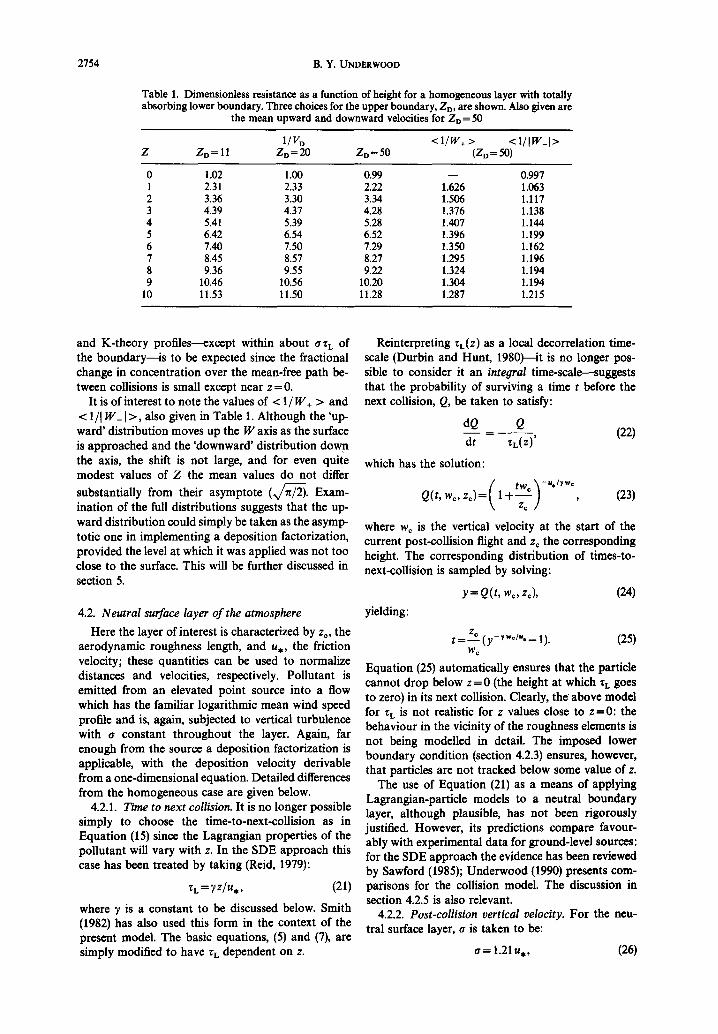
Table 1. Dimensionless resistance as a function of height for a homogeneous lay0r with totally absorbing lower boundary. Three choices for the upper boundary, ZD, are shown. Also given are

the mean upward and downward velocities for Z D = 50

1/VD <l /W+> < l / [W-I> Z ZI) = 11 ZI) = 20 ZD = 50 (Z D = 50)

0 1.02 1.00 0.99 - - 0.997 1 2.31 2.33 2.22 1.626 1.063 2 3.36 3.30 3:34 1.506 1.117 3 4.39 4.37 4.28 1.376 1.138 4 5.41 5.39 5.28 1.407 1.144 5 6.42 6.54 6.52 1.396 1.199 6 7.40 7.50 7.29 1.350 1.162 7 8.45 8.57 8.27 1.295 1.196 8 9.36 9.55 9.22 1.324 1.194 9 10.46 10.56 10.20 1.304 1.194

10 11.53 11.50 11.28 1.287 1.215

and K-theory profiles--except within about ~ZL of Reinterpreting ZL(Z) as a local decorrelation time- the boundary-- is to be expected since the fractional scale (Durbin and Hunt, 1980)--it is no longer pos- change in concentration over the mean-free path be- s ine to consider it an intearal time-scale--suggests tween collisions is small except near z = 0. that the probability of surviving a time t before the

It is of interest to note the values of < 1/W+ > and next collision, Q, be taken to satisfy: < 1/] W_ [ > , also given in Table 1. Although the 'up- dQ Q ward' distribution moves up the W axis as the surface . . . . (22) is approached and the 'downward' distribution down dt *L(Z)' the axis, the shift is not large, and for even quite which has the solution: modest values of Z the mean values do not differ

( . twc'Vu*l" ~o substantially from their asymptote ( , r ~ . Exam- Q(t, w c, zc)= 1+- -~- ) , (23) ination of the full distributions suggests that the up-

ward distribution could simply be taken as the asymp- where wc is the vertical velocity at the start of the totic one in implementing a deposition factorization, current post-collision flight and z c the corresponding provided the level at which it was applied was not too height. The corresponding distribution of times-to- close to the surface. This will be further discussed in next-collision is sampled by solving: section 5.

y= Q(t, wc, z,), (24)

4.2. Neutral surface layer of the atmosphere yielding:

Here the layer of interest is characterized by Zo, the t - z ~ (Y-~wo/,,_ 1). (25) aerodynamic roughness length, and u. , the friction - w c

velocity; these quantities can be used to normalize Equation (25)automatically ensures that the particle distances and velocities, respectively. Pollutant is emitted from an elevated point source into a flow cannot drop below z = 0 (the height at which xL goes

to zero) in its next collision. Clearly, the above model which has the familiar logarithmic mean wind speed for ZL is not realistic for z values close to z=O: the profile and is, again, subjected to vertical turbulence behaviour in the vicinity of the roughness elements is with ¢ constant throughout the layer. Again, far not being modelled in detail. The imposed lower enough from the source a deposition factorization is boundary condition (section 4.2.3) ensures, however, applicable, with the deposition velocity derivable

that particles are not tracked below some value of z. from a one-dimensional equation. Detailed differences The use of Equation (21) as a means of applying from the homogeneous case are given below. Lagrangian-particle models to a neutral boundary

4.2.1. Time to next collision. It is no longer possible layer, although plausible, has not been rigorously simply to choose the time-to-next-coUision as in justified. However, its predictions compare favour- Equation (15) since the Lagrangian properties of the ably with experimental data for ground-level sources: pollutant will vary with z. In the SDE approach this for the SDE approach the evidence has been reviewed case has been treated by taking (Reid, 1979): by Sawford (1985); Underwood (1990) presents com-

zL=yz/u. , (21) parisons for the collision model. The discussion in section 4.2.5 is also relevant.

where y is a constant to be discussed below. Smith 4.2.2. Post-collision vertical velocity. For the neu- (1982) has also used this form in the context of the tral surface layer, ¢ is taken to be: present model. The basic equations, (5) and (7), are simply modified to have z L dependent on z. a = 1.21u,, (26)

Collision model of atmospheric dispersion--I 2755

an estimate deduced by Reid (1979) and not signific- empirical result if momentum is treated as if it were antJy different from the value 1.25 u, given by Panof- totally absorbed at Zo itself. sky (1974). Below, the value of~ is taken as 0.27 for the neutral

4.2.3. Boundary conditions. It is assumed that the surface layer. particle is lost once it drops below z---b, where b is a 4.2.5. Results and comparison with K-theory. Tab- few times zo. Although a simple 'total absorption' le 2 shows the MC prediction of the inverse of the boundary condition is introduced here for illustrative dimensionless deposition velocity for a selected set of purposes, it appears to be a reasonable approxima- levels. Again, 105 particle histories were tracked in 10 tion to reality for pollutant aerosol in a size range batches of 104 to obtain an estimate of the sampling where the particles ultimately deposit by inertial error. It was found that an upper boundary of Z D impaction onto roughness elements, thereby short- =200 is sufficient to ensure convergence to the circuiting the resistance afforded by buffer and viscous asymptotic value of the results up to Z = 100, within a layers (Chamberlain, 1967). As an example, b is taken tolerance less than the sampling error (around 1%). as 3Zo. Also shown are the eddy-diffusivity predictions for

The argument in section 4.1.3 regarding the upper the same case, i.e. the dimensionless aerodynamic boundary still applies here: even if ZL increases line- resistance between the chosen level and the lower arly with z, there is some distance above which the boundary, left-hand side of (5) becomes small compared to either 1 1 ( Z ) term on the right-hand side, and thus (16) applies. (In - - = - In (28) this case, however, it is more appropriate to use V o k ' logarithmic steps in seeking the desired convergence.) where the upper-case symbols denote normalization

4.2.4. Value of 7. Only the choice of a value of 7 by u. and Zo for velocities and distances, respectively. remains to complete the specification of the simu- As expected from the discussion in section 4.2.4 above, lation. Smith (1982) advocates a value satisfying: the simulation results exhibit a closely logarithmic

a2rL=ku.z. (27) profile down to quite close to the absorbing bound- ary; in the logarithmic region, the discrepancy in the

This is analogous to (19), although the rationale is less K-theory results is equivalent to a simple shift in the clear-cut in the inhomogeneous case. height of the boundary (from 3.0zo to 1.9Zo).

Taking k=0.4, gives 7=0.27. In the SDE approach, That K-theory results in this case differ little in 7 has tended to be treated as an adjustable parameter, essence from those obtained using a finite decorre- and values somewhat larger than 0.27 have often lation time derives from the fact that the fractional emerged (Reid, 1979; Wilson et al., 1981). However, change in concentration over one 'mean-free-path' is use of the latter value in the collision model does give modest except close to the boundary. A companion good agreement with the Porton experimental results paper considers the case of turbulent transport of for a near-ground-level source (Underwood, 1990). pollutants within a vegetative canopy, where this con- Equation (27) was used by Legg (1983) in the context dition may not be satisfied. of the SDE approach, following an unpublished ana- K-theory can be viewed as the limit of the collision lysis by M. R. Raupach, and was found to lead to model as z L approaches zero, subject to the constraint good agreement with wind-tunnel data. that:

Alternatively, 7 can be derived from the require- ~,2fl=k, (29) ment that the one-dimensional model applied to the

where fl is the ratio a/u. . Also shown in Table 2, transport of horizontal momentum should reproduce the empirically-observed logarithmic wind speed pro- therefore, are the results for y =0.05 and 7 =0.01, with file. To simulate momentum transport, the lower corresponding values of fl obtained from Equation boundary condition is taken initially to be total (29). The approach to the K-theory result with B = 3 is absorption at z = Zo. Figure 2 shows the resulting di- evident.

As with the homogeneous case, f_ (z, w_) and mensionless aerodynamic resistance as a function of height when 7 takes the values of 0.2, 0.27 and 0.4 f+ (z, w+)only become significantly different from the compared to (I/k) ln(z/Zo). The profiles are indistin- asymptotic forms quite close to the surface, as indi- guishable from a logarithmic form in each case, except cated by the values of < I / W + > and < l / W _ >

shown in Table 2. very close to the boundary (i.e. Z<2) . Clearly, to reproduce the desired slope a value of 7 near 0.27 is

4.3. Inclusion of sedimentation required; closer examination confirms this value to within a few per cent. The correct intercept, however, In K-theory, the 'first-order' approach to including is not reproduced: the totally-absorbing boundary gravitational settling of larger particles in calculating must be set at 1.6zo to produce the 'empirical' inter- deposition velocity is via the equation: cept. There is no contradiction involved here, since dC the model does not purport to describe realistically Kz(z) ~ z + V s C = F , (30) the detailed behaviour close to the lower boundary. Nor does K-theory, although the latter yields the where v s is the magnitude of settling velocity and K z is

2756 B.Y. UNDERWOOD

I I I I I ~ w i

15

10 A " ~ /

IIVD / / /

/

5 ¢ f

/ / ~ -- ~ In (Zllk 1 / /

0 i '/' I I I I = t z J 1 2 3 5 10 100

Z Fig. 2. Dimensionless resistance vs dimensionless height obtained from the collision model for a neutral surface layer for three values of 7 [defined in Equation (21)]. A straight line has been drawn by eye through each set of points above Z = 2. The dashed line represents the logarithmic wind speed profile with k = 0.4.

Table 2. Dimensionless resistance as a function of height for a neutral surface layer with total absorption at Z = B . K-theory predictions shown for B=3 and B= 1.9; MC results shown for B=3 for three values for 7 and fl calculated from Equation (29). Also shown are the mean upward and downward velocities of particles

crossing the given levels, for 7=0.27

K-theory MC results y=0.27 7=0.05 7=0.01

l l n ( Z ~ _ l l n ( Z ~ /}=1.21 fl=2.83 fl=6.33 Z 1/Vo <l/W+ > <Z/IW-I> Z/V~ 1/V D

k \ 3 / k \ 1 . 9 /

3 0 1.14 0.82 - - 0.818 0.36 0.16 5 1.28 2.42 2.40 1.297 0.925 1.83 1.44

10 3.01 4.15 4.19 1.148 0.965 3.55 3.19 20 4.74 5.88 5.91 1.109 0.975 5.26 4.95 50 7.03 8.18 8.27 1.084 1.000 7.51 7.23

100 8.77 9.91 9.92 1.068 1.030 9.16 8.80

Sampling accuracy 1% 1% 1.5%

the eddy-diffusivity of momentum, as before. The Equat ion (30) may be an adequate way of account- fundamental assumption in this extension is that the ing for sedimentation when v, is small, but it has long settling particles are dispersed with the same effect- been recognized (Csanady, 1963) that larger particles iveness as are dilute gaseous pollutants, tend to 'fall out ' of eddies (the so-called trajectory-

Collision model of atmospheric dispersion--I 2757

crossing effect) and also experience a time-lag in neutral boundary layer, (25) applies to the two-phase reaching the velocity of the surrounding air (the in- approach with w e interpreted as the 'eddy' velocity, ertia effect), whereas w e is replaced by Wpe in the pseudo-fluid

Only the inclusion of sedimentation ignoring tra- approach. jectory-crossing and inertia effects will be discussed (iii) In a homogeneous layer, the 'asymptotic' dis- here. A rationale for not considering larger particles in tribution of downward velocities applied at the upper the present work is that the range of interest in the full boundary has to be modified to

two-dimensional dispersion-deposition problem is n_ (z, w_ )~tlw_ I p(w- + vs), (32) likely to occur before the 'equilibrium' situation is attained, and the deposition factorization offers little for both ways of including settling, which can be seen benefit. Nevertheless, the collision model applied to by reformulating (7) to include settling. In the neutral the full two-dimensional problem offers some inter- boundary layer, (32) still applies to the pseudo-fluid esting insights into the impact of trajectory-crossing approach, but the equivalent for the two-phase ap- and inertia effects (Underwood, 1990). proach cannot be given in closed form, although (32)

Two ways of including the 'first-order' type of sedi- is approximately valid. In MC simulation of the latter mentation modelling in the collision model spring to case, advantage can be taken of the fact that as long as mind. The most natural method adopts a 'two-phase' the upper boundary is sufficiently far above the region viewpoint, with the time-to-next-collision determined of interest the results are not sensitive to errors in the by the 'air eddy' in which the particle resides. The 'injection' distribution. 'first-order' approximation here consists of an as- Results for the neutral surface layer are shown in sumption that particles immediately take up post- Table 3 for Vs=0.01 and 0.1 (where Vs=vffu,), with collision a vertical velocity that is vs downwards com- total absorption at Z = 3, for both ways of including pared to the current eddy (i.e. very short response settling. Also shown are the predictions from K- time) and that the time a particle resides in the current theory, which in this case are given by:

eddy is never curtailed by particle falling out of the Vo= Vs/(1-(B/Z)Vs/k). (33) eddy.

An alternative viewpoint arises from the recogni- The results from the pseudo-fluid approach can be tion that v~ in (30) appears as a 'convective' fluid brought into agreement (within sampling accuracy) velocity. Thus, in the collision model, settling particles with those from K-theory if the effective absorbing can be taken to represent elements of a 'pseudo-fluid' boundary in the latter is set at 1.9 z o rather than 3z o. moving downwards, i.e. having a spectrum of vertical This is the same shift as required to bring the results velocities with a non-zero mean. Although somewhat in line when settling is absent, demonstrating how the artificial, this approach is of interest in that it is a close pseudo-fluid approach mimics the manner in which analogue of (30). The difference between the two ap- settling enters in (30). On the other hand, the dis- proaches highlights the benefits of being able to treat crepancy between results obtained from the more the Lagrangian behaviour of particles in a two-phase realistic two-phase approach and those from K- manner, theory do not amount to a simple shift in the height of

The following modifications to the MC simulation the absorbing boundary. apply.

(i) Immediately after a collision, the particle vertical

ve loc i t y , Wpc , takes the value: 5. IMPLEMENTATION OF A DEPOSITION BOUNDARY

Wpc = w e - v s. (31) CONDITION

(ii) In the homogeneous case, the sampling of times If the details of near-surface behaviour are known to next collision is unchanged, i.e. as in (15). For the and can be represented within the framework of the

Table 3. Dimensionless resistance as a function of height for particles with given settling velocities, Its, in the neutral surface layer, with absorbing boundary at Z = 3. Superscript • denotes the 'two-phase' manner of including settling, t denotes the 'pseudo-fluid' approach. Also shown are the K-theory predictions for an absorbing boundary at Z = 3 (K1) and Z = 1.9 (K2)

Vs=0.0t Vs=0.1 Z (1/VD)* (1/VD)'I" K1 K2 (1/Vo)* (1/VD) t K1 K2

3 0.83 0.83 0 1.13 0.81 0.83 0 1.08 5 2.34 2.39 1.26 2.39 2.03 2.18 1.20 2.15

I0 4.09 4.11 2.97 4.07 3.21 3.49 2.60 3.40 20 5.80 5.79 4.63 5.71 4.18 4.52 3.78 4.45 50 7.87 7.89 6.79 7.85 5.17 5.61 5.05 5.58

100 9.40 9.49 8.39 9.43 5.89 6.24 5.84 6.29

Sampling accuracy ~ 1% ~ 1% ~ 1% ~ 1%

2758 B.Y. UNDERWOOD

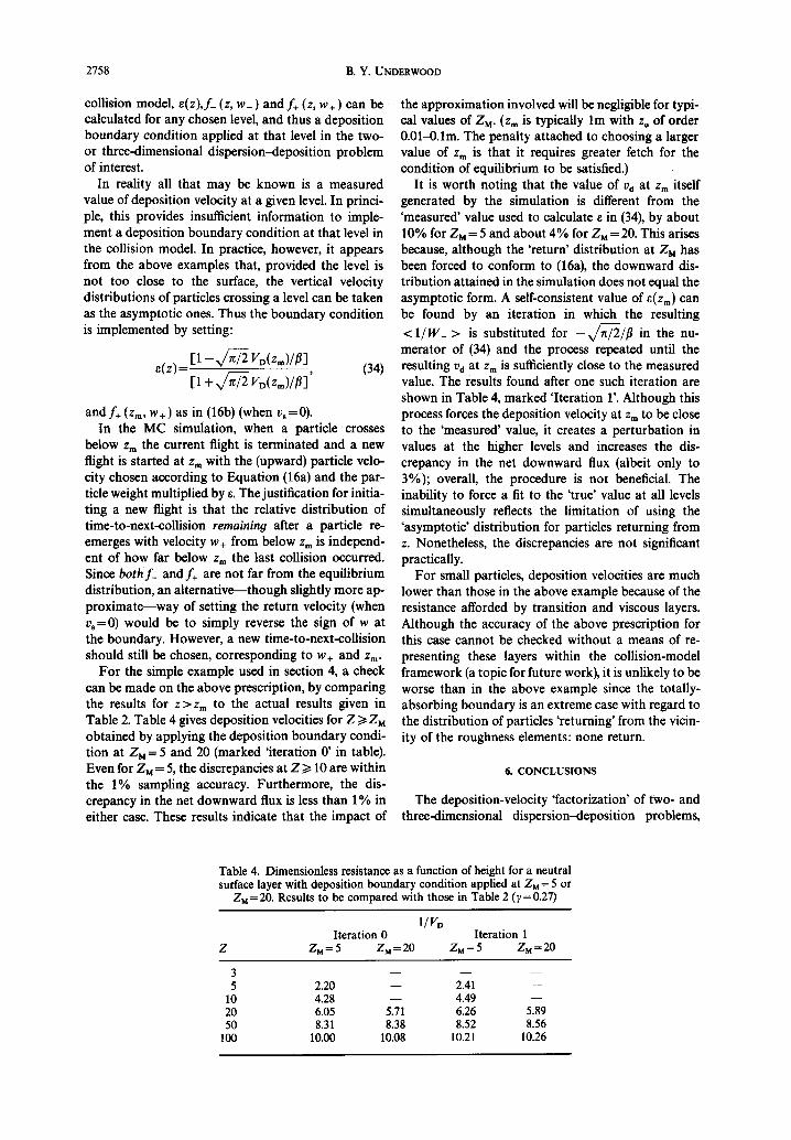
collision model, e(z),f_ (z, w_ ) and f+ (z, w+ ) can be the approximation involved will be negligible for typi - calculated for any chosen level, and thus a deposition cal values of Z M. (z= is typically lm with Zo of order boundary condition applied at that level in the two- 0.01-0.1m. The penalty attached to choosing a larger or three-dimensional dispersion-deposition problem value of z= is that it requires greater fetch for the of interest, condition of equilibrium to be satisfied.)

In reality all that may be known is a measured It is worth noting that the value of Vd at z= itself value of deposition velocity at a given level. In princi- generated by the simulation is different from the ple, this provides insufficient information to imple- 'measured' value used to calculate e in (34), by about ment a deposition boundary condition at that level in 10% for Z M = 5 and about 4% for Z M = 20. This arises the collision model. In practice, however, it appears because, although the 'return' distribution at Z M has from the above examples that, provided the level is been forced to conform to (16a), the downward dis- not too close to the surface, the vertical velocity tribution attained in the simulation does not equal the distributions of particles crossing a level can be taken asymptotic form. A self-consistent value of t(Zm) can as the asymptotic ones. Thus the boundary condition be found by an iteration in which the resulting is implemented by setting: <l/W_ > is substituted for - ~ n - ~ / / ~ in the nu-

merator of (34) and the process repeated until the ~(z) = [1 - x / ~ VD(z=)/~] (34) resulting vd at z= is sufficiently close to the measured

[1 + x / / ~ VD(Z=)/[3]' value. The results found after one such iteration are shown in Table 4, marked 'Iteration 1'. Although this

and f÷ (Zm, w+ ) as in (16b) (when v, =0). process forces the deposition velocity at z= to be close In the MC simulation, when a particle crosses to the 'measured' value, it creates a perturbation in

below z= the current flight is terminated and a new values at the higher levels and increases the dis- flight is started at zm with the (upward) particle velo- crepancy in the net downward flux (albeit only to city chosen according to Equation (16a) and the par- 3%); overall, the procedure is not beneficial. The title weight multiplied by 5. The justification for initia- inability to force a fit to the 'true' value at all levels ring a new flight is that the relative distribution of simultaneously reflects the limitation of using the time-to-next-collision remaining after a particle re- 'asymptotic' distribution for particles returning from emerges with velocity w+ from below z= is independ- z. Nonetheless, the discrepancies are not significant ent of how far below zm the last collision occurred, practically. Since both f_ and f÷ are not far from the equilibrium For small particles, deposition velocities are much distribution, an alternative--though slightly more ap- lower than those in the above example because of the proximate--way of setting the return velocity (when resistance afforded by transition and viscous layers. v, = 0) would be to simply reverse the sign of w at Although the accuracy of the above prescription for the boundary. However, a new time-to-next-collision this case cannot be checked without a means of re- should still be chosen, corresponding to w+ and zm. presenting these layers within the collision-model

For the simple example used in section 4, a check framework (a topic for future work), it is unlikely to be can be made on the above prescription, by comparing worse than in the above example since the totally- the results for Z>Zm to the actual results given in absorbing boundary is an extreme case with regard to Table 2. Table 4 gives deposition velocities for Z t> ZM the distribution of particles 'returning' from the vicin- obtained by applying the deposition boundary condi- ity of the roughness elements: none return. tion at ZM = 5 and 20 (marked 'iteration 0' in table). Even for Z~- - 5, the discrepancies at Z >1 10 are within 6. CONCLUSIONS the 1% sampling accuracy. Furthermore, the dis- crepancy in the net downward flux is less than 1% in The deposition-velocity 'factorization' of two- and either case. These results indicate that the impact of three-dimensional dispersion-deposition problems,

Table 4. Dimensionless resistance as a function of height for a neutral surface layer with deposition boundary condition applied at Z M = 5 or

ZM=20. Results to be compared with those in Table 2 (~=0.27)

1/VD Iteration 0 Iteration 1

Z Z M = 5 Z M = 20 Z M = 5 Z M = 20

3 . . . .

5 2.20 - - 2.41 - - 10 4.28 - - 4.49 - - 20 6.05 5.71 6.26 5.89 50 8.31 8.38 8.52 8.56

100 10.00 10.08 10.21 10.26

Collision model of atmospheric dispersion--I 2759

which is widely applied in the K-theory framework, for the SDE approach, enabling the use of deposition can also be developed for the 'collision' model, where velocities to be put on a firm foundation there also. the latter is an alternative to the stochastic differ- ential-equation (SDE) approach for retaining a finite Acknowledgements--This work was partly funded by the

Radiation Protection Programme, Directorate General for Lagrangian memory of turbulent velocity. In terms of Science, Research and Development, Commission of the the Monte Carlo (MC) solution to the Lagrangian European Communities, under contract BI6.0131.UK and model, this obviates tracking particles into regions of partly funded by the Department of Energy through the complex behaviour near the 'true' lower boundary by General Nuclear Safety Research Programme Letter.

introducing an effective boundary at some height above it. REFERENCES

In principle, the factorization in this case cannot be accomplished entirely in terms of the deposition velo- Chamberlain A. C. (1967) Transport of Lycopodium spores city, vd(zm), in contrast to the K-theory situation, but and other small particles to rough surfaces. Proc. R. Soc.

London A296, 45-70. in practice the prescription can be specified in terms Csanady G. T. (1963) Turbulent diffusion of heavy particles. of vd alone to a good approximation provided the ef- J. atoms. Sci. 20, 201-208. fective boundary is sufficiently far above the true Doran J. C. (1977) Limitations on the determination of boundary, deposition velocities. Boundary-Layer Met. 12, 365-371.

Durbin P. A. and Hunt J. C. R. (1980) Dispersion from The deposition velocity itself can be calculated by elevated sources in turbulent boundary layers. J. de Me-

solving a one-dimensional equation provided the de- canique 19, 679--695. tails of near-surface behaviour can be formulated Kallio G. A. and Reeks M. W. (1989) A numerical simulation within the collision model. In the absence of gravita- of particle deposition in turbulent boundary layers. Int. J. tional settling the MC results for the simple cases of a Multiphase Flow 15, 433--446.

Kinderman A. J. and Monahan J. F. (1977) Computer gen- homogeneous layer and the neutral surface layer of eration of random variables using the ratio of uniform the atmosphere, both with totally absorbing lower deviates. A.C.M. Trans. Math. Software 3, 257-260. boundary, are not essentially different in form from Legg B. J. (1983) Turbulent dispersion from an elevated line the K-theory results except very close to the bound- source: Markov chain simulations of concentration and

flux profiles. Q. dl R. met. Soc. 109, 645-660. ary. This is a consequence of the fractional change in Panofsky H. A. (1974) The atmospheric boundary layer concentration over one 'mean-free-path' being not below 150 m. Ann. Rev. Fluid Mech. 6, 147-177. large in these cases. Reid J. D. (1979) Markov chain simulations of vertical

The above remains true if gravitational settling is dispersion in the neutral surface layer for surface and elevated releases. Boundary-Layer Met. 16, 3-22. introduced into the collision model by the pseudo- Sawford B. L. (1985) Lagrangian statistical simulation of

fluid approach, directly analogous to how it appears concentration mean and fluctuation fields. J. Clim. appl. in K-theory. However, within the collision-model Met. 24, 1152-1166. framework it is possible to treat the two-phase nature Shuen J. S., Chen L. D. and Faeth G. M. (1983) Evaluation of of settling particles in a more rigorous manner, and stochastic model of particle dispersion in a turbulent

round jet. A.I.Ch.E.J. 29, 167-170. this introduces additional differences from the K- Smith F. B. (1982) The integral equation of diffusion. Proc. theory results. 13th NATO/CCMS Conf. on Air Pollution and its Applica-

The groundwork has been laid here for calculating tion. Plenum, New York. deposition velocities in more complex situations such Underwood B. Y. (1990) Gravitational settling of particles as pollutant transfer within crop canopies, where ef- dispersing from an elevated point source in the neutral

surface layer of the atmosphere. SRD R516. SRD, AEA fects due to the persistence of Lagrangian velocity Technology. may be more pronounced. To treat these cases, how- Underwood B. Y. (1991) Discussion on 'An interpretation of ever, the extension of the model to treat a non- Taylor's statistical analysis of particle dispersion'. Atmo- uniform tr must first be carried out; this is the subject spheric Environment 25A, 1129-1130.

Wilson J. D., Thurtell G. W. and Kidd G. E. (1981) Nu- of a companion paper, merical simulation of particle trajectories in inhomo-

Finally, no doubt a parallel formulation to the one geneous turbulence--l: systems with constant turbulent given here for the collision model can be worked out velocity scales. Boundary-Layer Met. 21, 295-313.