department of electronics & tele- comm. engineering lab ...digital signal processing lab 3...

Department of Electronics & Tele- Comm.Engineering

LAB MANUAL

SUBJECT: DIGITAL SIGNAL PROCESSING USING MATLAB

B.Tech III Year – V Semester(Branch: ETE)

KCT College Engineering & TechnologyFatehgarh (sangrur)

KCT college of Engineering and Technology Department ETE

DIGITAL SIGNAL PROCESSING LAB 2

TABLE OF CONTENTS

SNo.

Topic PageNo.

1. Exp No. 1(a): To study important commands of MATLABsoftware

2. Exp No. 1(b): To develop elementary signal function modules(m-files) for unit sample, unit step, exponential and unitramp sequences.

3. Exp No.3: To develop program for discrete convolution andcorrelation

4. Exp No.4: To develop program for finding response of theLTI system described by the difference equation

5. Exp No.5: To develop program for computing inverse Z-transform

6. Exp No.6: To develop program for finding magnitude andphase response of LTI system described by system functionH(z)

7. Exp No.7: To develop program for computing DFT and IDFT

8. Exp No.8: To develop program for computing circularconvolution

9. Exp No.11: To develop program for designing FIR filter.

10. Exp No.12: To develop program for designing IIR filter



EC-316 DSP LABExperiment No 1 A

Aim : To study important commands of MATLAB software.

Apparatus : PC having MATLAB software.

1. Introduction :MATLAB is a high-performance language for technical computing. It integrates computation,

visualization, and programming in an easy-to-use environment where problems and solutions areexpressed in familiar mathematical notation.Typical uses include Math and computation, Algorithm development, Data acquisition, Modeling,simulation, and prototyping, Data analysis, exploration, and visualization, Scientific and engineeringgraphics, Application development, including graphical user interface building.

MATLAB is an interactive system whose basic data element is an arraythat does not require dimensioning. This allows you to solve many technical computing problems,especially those with matrix and vector formulations, in a fraction of the time it would take to writea program in a scalar non interactive language such as C or Fortran. The name MATLAB stands formatrix laboratory.

Starting MATLAB on Windows platforms, start MATLAB by double-clicking the MATLABshortcut icon on your Windows desktop.

Quitting MATLAB: To end your MATLAB session, select File > Exit MATLAB in the desktop, ortype quit in the Command Window. You can run a script file named finish.m each time MATLABquits that, for example, executes functions to save the workspace.2. MATLAB desktop:On starting MATLAB the MATLAB desktop appears, containing tools (graphical user interfaces )for managing files , variables and applications associated with MATLAB. It contains :(i) Command Window and Command HistoryCommand Window : Use the Command Window to enter variables and to run functions and M-filescripts. Press the up arrow key to recall a statement previously typed. Edit the statement as neededand then press Enter to run it.Command History : Statements entered in the Command Window are logged in the CommandHistory. From the Command History, previously run statements can be viewed, copied andexecuted. M-file can be created from selected statements.

(ii) Current Directory Browser and Search Path : MATLAB file operations use the current directoryand the search path as reference points. Any file required to run must either be in the currentdirectory or on the search path.(iii) Workspace Browser and Array Editor :The MATLAB workspace consists of the set of variables(named arrays) built up during a MATLAB session and stored in memory. The variables can beadded to the workspace by using functions, running M-files, and loading saved workspaces. Todelete variables from the workspace, select the variables and select Edit > Delete.



Array Editor : Double-click a variable in the Workspace browser, or use open var variable name, tosee it in the Array Editor. Use the Array Editor to view and edit a visual representation of variablesin the workspace.(iv) Editor/Debugger : Editor/Debugger is used to create and debug M-files, which areprograms to run MATLAB functions. The Editor/Debugger provides a graphicaluser interface for text editing, as well as for M-file debugging. To create or edit an M-file use File >New or File > Open, or use the edit function.The important commands/ functions are as below :

1. clc (Remove items from workspace, freeing up system memory) clears all input and outputfrom the Command Window display, giving "clean screen." After using clc, the scroll barcannot be used to see the history of functions, but still the up arrow can be used to recallstatements from the command history.

2. close (Remove specified figure): close deletes the current figure or the specified figure(s). Itoptionally returns the status of the close operation.

3. xlabel, ylabel, zlabel (Label x-, y-, and z-axis) : Each axes graphics object can have one labelfor the x-, y-, and z-axis. The label appears beneath its respective axis in a two-dimensional plotand to the side or beneath the axis in a three-dimensional plot.xlabel('string') labels the x-axis of the current axes.ylabel(...) and zlabel(...) label the y-axis and z-axis, respectively, of the current axes.

4. title( Add title to current axes) : Each axes graphics object can have one title. The title is locatedat the top and in the center of the axes.title('string') outputs the string at the top and in the center of the current axes.

5. figure (create figure graphics object) : figure creates figure graphics objects. Figure objects arethe individual windows on the screen in which MATLAB displays graphical output.

6. subplot (Create axes in tiled positions): subplot divides the current figure into rectangular panesthat are numbered row wise. Each pane contains an axes object. Subsequent plots are output tothe current pane.h = subplot(m,n,p) or subplot(mnp) breaks the figure window into an m-by-n matrix of smallaxes, selects the pth axes object for the current plot, and returns the axes handle. The axes arecounted along the top row of the figure window, then the second row, etc. For example,subplot(2,1,1), plot(income)subplot(2,1,2), plot(outgo) plots income on the top half of the window and outgo on the bottomhalf.

7. stem (Plot discrete sequence data) : A two-dimensional stem plot displays data as linesextending from a baseline along the x-axis. A circle (the default) or other marker whose y-position represents the data value terminates each stem.stem(Y) Plots the data sequence Y as stems that extend from equally spaced and automaticallygenerated values along the x-axis. When Y is a matrix, stem plots all elements in a row againstthe same x value.stem(X,Y) plots X versus the columns of Y. X and Y must be vectors or matrices of the samesize. Additionally, X can be a row or a column vector and Y a matrix with length(X) rows.

8. bar(Plot bar graph (vertical and horizontal)) : A bar graph displays the values in a vector ormatrix as horizontal or vertical bars.bar(Y) draws one bar for each element in Y. If Y is a matrix, bar groups the bars produced bythe elements in each row. The x-axis scale ranges from 1 up to length(Y) when Y is a vector, and1 to size(Y,1), which is the number of rows, when Y is a matrix.



barh(...) and h = barh(...) create horizontal bars. Y determines the bar length. The vector x is avector defining the y-axis intervals for horizontal bars.

9. plot ( 2-D line plot) :plot(Y) Plots the columns of Y versus their index if Y is a real number. If Y is complex, plot(Y)

is equivalent to plot(real(Y),imag(Y)). In all other uses of plot, the imaginary component isignored.

plot(X1,Y1,...) Plots all lines defined by Xn versus Yn pairs. If only Xn or Yn is a matrix, thevector is plotted versus the rows or columns of the matrix,depending on whether the vector's row or column dimension matches the matrix. If Xn is a scalarand Yn is a vector, disconnected line objects are created and plotted as discrete points verticallyat Xn.

10. input (Request user input) : The response to the input prompt can be any MATLABexpression, which is evaluated using the variables in the current workspace.

user_entry = input('prompt') Displays prompt as a prompt on the screen, waits for inputfrom the keyboard, and returns the value entered in user_entry. user_entry = input('prompt', 's')returns the entered string as a text variable rather than as a variable name or numerical value.

11. zeros (Create array of all zeros) :B = zeros(n) Returns an n-by-n matrix of zeros. An error message appears if n is not a scalar.

12. ones (Create array of all ones) :Y = ones(n) Rreturns an n-by-n matrix of 1s. An error message appears if n is not a scalar.

13. exp (Exponential) :Y = exp(X) The exp function is an elementary function that operates element-wise on arrays.Its domain includes complex numbers.Y = exp(X) returns the exponential for each element of X.

14. disp (Display text or array) :disp(X) Displays an array, without printing the array name. If X contains a text string, thestring is displayed. Another way to display an array on the screen is to type its name, but thisprints a leading "X=," which is not always desirable. Note that disp does not display emptyarrays.

15. conv (Convolution and polynomial multiplication) :w = conv(u,v) convolves vectors u and v. Algebraically, convolution is the same operation as

multiplying the polynomials whose coefficients are the elements of u and v.16. xcorr (Cross-correlation) :

c = xcorr(x,y) returns the cross-correlation sequence in a length 2*N-1 vector, where x and yare length N vectors (N>1). If x and y are not the same length, the shorter vector is zero-paddedto the length of the longer vector.

17. filter (1-D digital filter) :y = filter(b,a,X) filters the data in vector X with the filter described by numerator coefficient

vector b and denominator coefficient vector a. If a(1) is not equal to 1, filter normalizes the filtercoefficients by a(1). If a(1) equals 0, filter returns an error.

18. poly (Polynomial with specified roots) :r = roots(p) which returns a column vector whose elements are the roots of the polynomial

specified by the coefficients row vector p. For vectors, roots and poly are inverse functions ofeach other, up to ordering, scaling, and round off error.

19. tf(Convert unconstrained MPC controller to linear transfer function) :sys=tf(MPCobj) The tf function computes the transfer function of the linear controller

ss(MPCobj) as an LTI system in tf form corresponding to the MPC controller when the



constraints are not active. The purpose is to use the linear equivalent control in Control SystemToolbox for sensitivity and other linear analysis.

20. freqz (Frequency response of filter ) :[h,w] = freqz(ha) returns the frequency response vector h and the corresponding frequency

vector w for the adaptive filter ha. When ha is a vector of adaptive filters, freqz returns thematrix h. Each column of h corresponds to one filter in the vector ha.

21. abs (Absolute value and complex magnitude) :abs(X) returns an array Y such that each element of Y is the absolute value of the

corresponding element of X.22. fft (Discrete Fourier transform) :

Y = fft(X) Y = fft(X) returns the discrete Fourier transform (DFT) of vector X, computed witha fast Fourier transform (FFT) algorithm.

23. mod (Modulus after division) :M = mod(X,Y) returns X - n.*Y where n = floor(X./Y). If Y is not an integer and the quotient

X./Y is within round off error of an integer, then n is that integer. The inputs X and Y must bereal arrays of the same size, or real scalars.

24. sqrt (Square root) :B = sqrt(X) returns the square root of each element of the array X. For the elements of X that

are negative or complex, sqrt(X) produces complex results.25. ceil (Round toward infinity) :

B = ceil(A) rounds the elements of A to the nearest integers greater than or equal to A. Forcomplex A, the imaginary and real parts are rounded independently.

26. fir1(Window-based finite impulse response filter design) :b = fir1(n,Wn) returns row vector b containing the n+1 coefficients of an order n lowpass FIRfilter. This is a Hamming-window based, linear-phase filter with normalized cutoff frequency Wn.The output filter coefficients, b, are ordered in descending powers of z.

27. buttord (Butterworth filter order and cutoff frequency) :[n,Wn] = buttord(Wp,Ws,Rp,Rs) returns the lowest order, n, of the digital Butterworth filterthat loses no more than Rp dB in the passband and has at least Rs dB of attenuation in thestopband. The scalar (or vector) of corresponding cutoff frequencies, Wn, is also returned. Use theoutput arguments n and Wn in butter.

28. fliplr (Flip matrix left to right) :B = fliplr(A) returns A with columns flipped in the left-right direction, that is, about a verticalaxis.If A is a row vector, then fliplr(A) returns a vector of the same length with the order of itselements reversed. If A is a column vector, then fliplr(A) simply returns A.

29. min ( Smallest elements in array) :C = min(A) returns the smallest elements along different dimensions of an array. If A is a

vector, min(A) returns the smallest element in A.If A is a matrix, min(A) treats the columns of Aas vectors, returning a row vector containing the minimum element from each column. If A is amultidimensional array, min operates along the first nonsingleton dimension.

30. max ( Largest elements in array) :C = max(A) returns the largest elements along different dimensions of an array.If A is a vector,max(A) returns the largest element in A.If A is a matrix, max(A) treats the columns of A asvectors, returning a row vector containing the maximum element from each column. If A is amultidimensional array, max(A) treats the values along the first non-singleton dimension asvectors, returning the maximum value of each vector.

31. find (Find indices and values of nonzero elements) :



ind = find(X) locates all nonzero elements of array X, and returns the linear indices of thoseelements in vector ind. If X is a row vector, then ind is a row vector; otherwise, ind is a columnvector. If X contains no nonzero elements or is an empty array, then ind is an empty array.

32. residuez (z-transform partial-fraction expansion ) :residuez converts a discrete time system, expressed as the ratio of two polynomials, to partialfraction expansion, or residue, form. It also converts the partial fraction expansion back to theoriginal polynomial coefficients.[r,p,k] = residuez(b,a) finds the residues, poles, and direct terms of a partial fraction expansionof the ratio of two polynomials, b(z) and a(z). Vectors b and a specify the coefficients of thepolynomials of the discrete-time system b(z)/a(z) in descending powers of z.

33. angle (Phase angle) :P = angle(Z) returns the phase angles, in radians, for each element of complex array Z. Theangles lie between + π and – π.

34. log (Natural logarithm ) :Y = log(X) returns the natural logarithm of the elements of X. For complex or negative z, where z= x +y*i , the complex logarithm is returned.

.

EC-316 DSP LAB

Experiment No. 1 B

Aim : To develop elementary signal function modules (m-files) for unit sample, unit step, exponentialand unit ramp sequences.


Program :

% program for generation of unit sampleclc;clear all;close all;t = -3:1:3;y = [zeros(1,3),ones(1,1),zeros(1,3)];subplot(2,2,1);stem(t,y);ylabel('Amplitude------>');xlabel('(a)n ------>');title('Unit Impulse Signal');% program for genration of unit step of sequence [u(n)- u(n)-N]t = -4:1:4;



y1 = ones(1,9);subplot(2,2,2);stem(t,y1);ylabel('Amplitude------>');xlabel('(b)n ------>');title('Unit step');% program for generation of ramp signaln1 = input('Enter the value for end of the seqeuence '); %n1 = <any value>7 %x = 0:n1;subplot(2,2,3);stem(x,x);ylabel('Amplitude------>');xlabel('(c)n ------>');title('Ramp sequence');% program for generation of exponential signaln2 = input('Enter the length of exponential seqeuence '); %n2 = <any value>7 %t = 0:n2;a = input('Enter the Amplitude'); %a=1%y2 = exp(a*t);subplot(2,2,4);stem(t,y2);ylabel('Amplitude------>');xlabel('(d)n ------>');title('Exponential sequence');disp('Unit impulse signal');ydisp('Unit step signal');y1disp('Unit Ramp signal');xdisp('Exponential signal');x

Output :

Enter the value for end of the seqeuence 6

Enter the length of exponential seqeuence 4

Enter the Amplitude1

Unit impulse signal y = 0 0 0 1 0 0 0

Unit step signal y1 = 1 1 1 1 1 1 1 1 1

Unit Ramp signal x = 0 1 2 3 4 5 6

Exponential signal x = 0 1 2 3 4 5 6



Graph:

-4 -2 0 2 40

0.5

1A

mpl

itude

------

>

(a)n ------>

Unit Impulse Signal

-4 -2 0 2 40

0.5

1

Am

plitu

de---

--->

(b)n ------>

Unit step

0 2 4 60

2

4

6

Am

plitu

de---

--->

(c)n ------>

Ramp sequence

0 1 2 3 40

20

40

60

Am

plitu

de---

--->

(d)n ------>

Exponential sequence

EC-316 DSP LAB

Experiment No. 3

Aim : To develop program for discrete convolution and correlation.


Program :

% program for discrete convolution% of x= [1 2] and h = [1 2 4]clc;clear all;close all;x = input('Enter the 1st sequence : '); %[1 2]h = input('Enter the 2nd sequence : '); %[1 2 4]y =conv(x,h);subplot(2,3,1);stem(x);ylabel('(x) ------>');xlabel('(a)n ------>');subplot(2,3,2);stem(h);ylabel('(h) ------>');



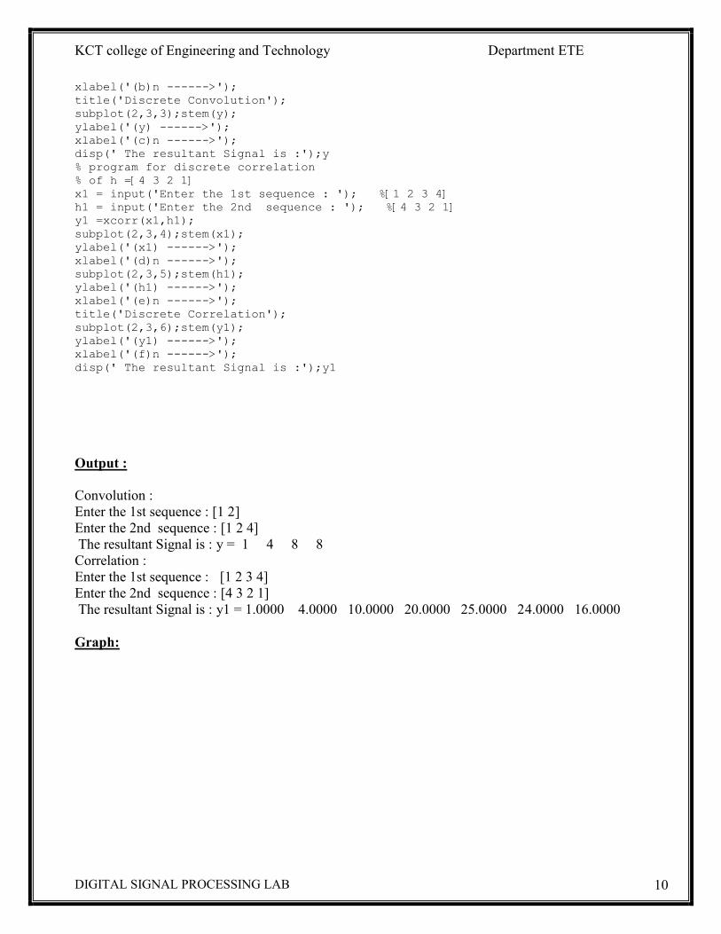
xlabel('(b)n ------>');title('Discrete Convolution');subplot(2,3,3);stem(y);ylabel('(y) ------>');xlabel('(c)n ------>');disp(' The resultant Signal is :');y% program for discrete correlation% of h =[4 3 2 1]x1 = input('Enter the 1st sequence : '); %[1 2 3 4]h1 = input('Enter the 2nd sequence : '); %[4 3 2 1]y1 =xcorr(x1,h1);subplot(2,3,4);stem(x1);ylabel('(x1) ------>');xlabel('(d)n ------>');subplot(2,3,5);stem(h1);ylabel('(h1) ------>');xlabel('(e)n ------>');title('Discrete Correlation');subplot(2,3,6);stem(y1);ylabel('(y1) ------>');xlabel('(f)n ------>');disp(' The resultant Signal is :');y1

Output :

Convolution :Enter the 1st sequence : [1 2]Enter the 2nd sequence : [1 2 4]The resultant Signal is : y = 1 4 8 8

Correlation :Enter the 1st sequence : [1 2 3 4]Enter the 2nd sequence : [4 3 2 1]The resultant Signal is : y1 = 1.0000 4.0000 10.0000 20.0000 25.0000 24.0000 16.0000

Graph:



1 1.5 20

0.5

1

1.5

2(x

) --

----

>

(a)n ------>1 2 3

0

1

2

3

4

(h)

----

-->

(b)n ------>

Discrete Convolution

0 2 40

2

4

6

8

(y)

----

-->

(c)n ------>

0 2 40

1

2

3

4

(x1)

---

--->

(d)n ------>0 2 4

0

1

2

3

4(h

1) -

----

->

(e)n ------>

Discrete Correlation

0 5 100

10

20

30

(y1)

---

--->

(f)n ------>



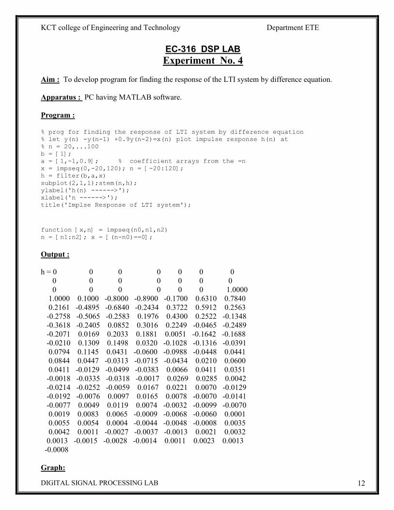
EC-316 DSP LABExperiment No. 4

Aim : To develop program for finding the response of the LTI system by difference equation.


Program :

% prog for finding the response of LTI system by difference equation% let y(n) -y(n-1) +0.9y(n-2)=x(n) plot impulse response h(n) at% n = 20,...100b = [1];a = [1,-1,0.9]; % coefficient arrays from the =nx = impseq(0,-20,120); n = [-20:120];h = filter(b,a,x)subplot(2,1,1);stem(n,h);ylabel('h(n) ------>');xlabel('n ------>');title('Implse Response of LTI system');

function [x,n] = impseq(n0,n1,n2)n = [n1:n2]; x = [(n-n0)==0];

Output :

h = 0 0 0 0 0 0 00 0 0 0 0 0 00 0 0 0 0 0 1.0000

1.0000 0.1000 -0.8000 -0.8900 -0.1700 0.6310 0.78400.2161 -0.4895 -0.6840 -0.2434 0.3722 0.5912 0.2563

-0.2758 -0.5065 -0.2583 0.1976 0.4300 0.2522 -0.1348-0.3618 -0.2405 0.0852 0.3016 0.2249 -0.0465 -0.2489-0.2071 0.0169 0.2033 0.1881 0.0051 -0.1642 -0.1688-0.0210 0.1309 0.1498 0.0320 -0.1028 -0.1316 -0.03910.0794 0.1145 0.0431 -0.0600 -0.0988 -0.0448 0.04410.0844 0.0447 -0.0313 -0.0715 -0.0434 0.0210 0.06000.0411 -0.0129 -0.0499 -0.0383 0.0066 0.0411 0.0351

-0.0018 -0.0335 -0.0318 -0.0017 0.0269 0.0285 0.0042-0.0214 -0.0252 -0.0059 0.0167 0.0221 0.0070 -0.0129-0.0192 -0.0076 0.0097 0.0165 0.0078 -0.0070 -0.0141-0.0077 0.0049 0.0119 0.0074 -0.0032 -0.0099 -0.00700.0019 0.0083 0.0065 -0.0009 -0.0068 -0.0060 0.00010.0055 0.0054 0.0004 -0.0044 -0.0048 -0.0008 0.00350.0042 0.0011 -0.0027 -0.0037 -0.0013 0.0021 0.0032

0.0013 -0.0015 -0.0028 -0.0014 0.0011 0.0023 0.0013-0.0008

Graph:



-20 0 20 40 60 80 100 120-1

-0 .5

0

0 .5

1

h(n

) --

----

>

n ------>

Im p ls e R es pons e o f LTI s y s tem



EC-316 DSP LAB

Experiment No. 5

Aim : To develop program for computing inverse Z-transformApparatus : PC having MATLAB software.Program :%prog for computing the inverse Z-transform by using residuez function%let x(z) = 1/((1-0.9z-1)^2(1+0.9z-1)) |z|>0.9b =1;a = poly([0.9,0.9,-0.9]) % denominator of the polynomial calculated by % poly

function[R,p,C] =residuez(b,a)[delta,n]= impseq(0,0,7) %call impseqx = filter(b,a,delta)

Output :

a = 1.0000 -0.9000 -0.8100 0.7290

R = 0.25000.50000.2500

p = 0.90000.9000

-0.9000C = []

delta = 1 0 0 0 0 0 0 0

n = 0 1 2 3 4 5 6 7

x = 1.0000 0.9000 1.6200 1.4580 1.9683 1.7715 2.1258 1.9132



EC-316 DSP LAB

Experiment No. 6

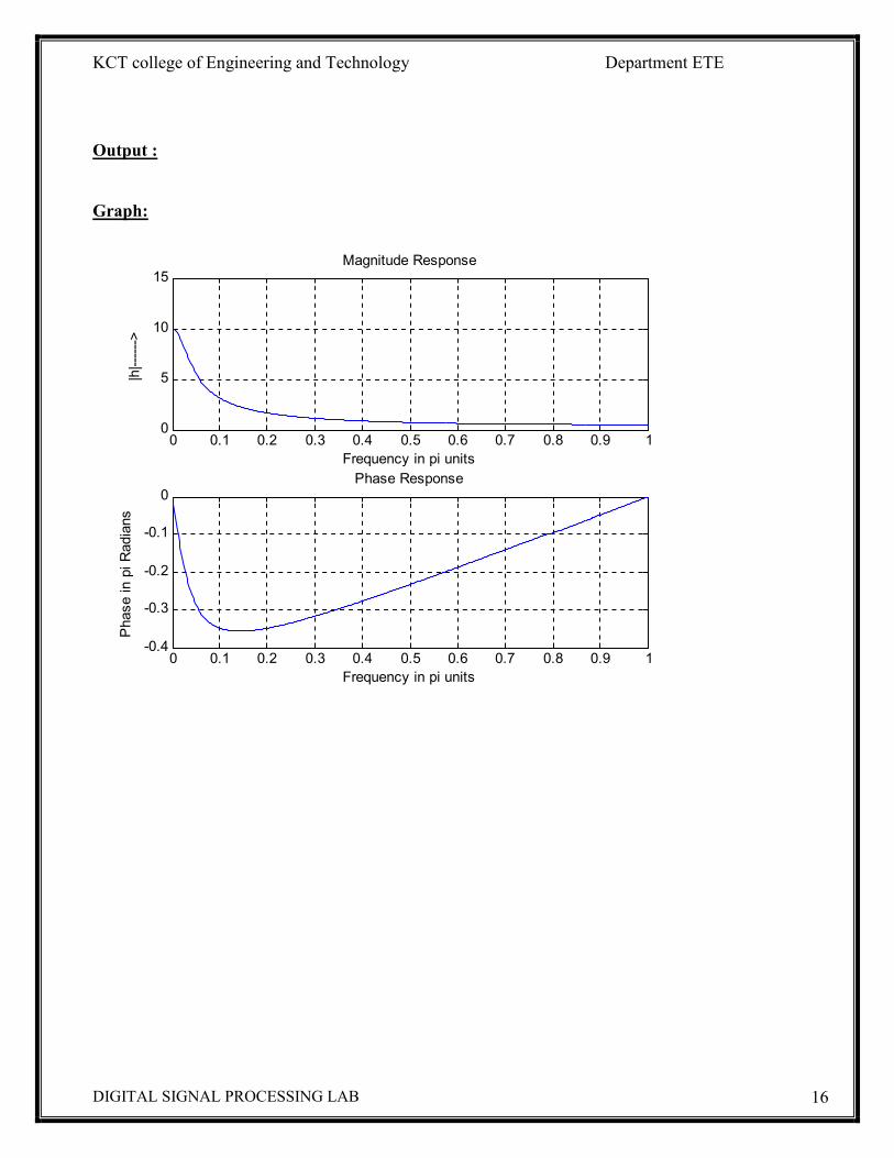
Aim : To develop program for finding the magnitude and phase response of LTI system described bythe system function h(z).


Program :

%prog for finding the magnitude and phase response of LTI system by%h(n) =(0.9)^n*u(n)w =[0:1:500]*pi/500; %[0,pi] axis divided into 501 pointsh =exp(j*w)./(exp(j*w)-0.9*ones(1,501));magh =abs(h); angh =angle(h);subplot(2,1,1);plot(w/pi,magh);grid;ylabel('|h|------>');xlabel('(Frequency in pi units');title('Magnitude Response');subplot(2,1,2);plot(w/pi,angh/pi);grid;ylabel('Phase in pi Radians');xlabel('(Frequency in pi units');title('Phase Response');



Output :

Graph:

0 0.1 0.2 0.3 0.4 0.5 0.6 0.7 0.8 0.9 10

5

10

15

|h|--

---->

Frequency in pi units

Magnitude Response

0 0.1 0.2 0.3 0.4 0.5 0.6 0.7 0.8 0.9 1-0.4

-0.3

-0.2

-0.1

0

Pha

se in

pi R

adia

ns

Frequency in pi units

Phase Response



EC-316 DSP LAB

Experiment No. 7

Aim : To develop program for computing discrete Fourier Transform (DFT) and inverse discreteFourier Transform (IDFT).


Program :

DFT :%prog for computing discrete Fourier Transformclc;clear all;close all;x =input('Enter the sequence '); %x =[0 1 2 3 4 5 6 7]n = input('Enter the length of Fourier Transform ') %n =8 has to be same as%the length of sequencex =fft(x,n);stem(x);ylabel('imaginary axis------>');xlabel('(real axis------>');title('Exponential sequence');disp('DFT is');x

IDFT :

% prog for inverse discrete Fourier Transform (IDFT)clc;clear all;close all;x =input('Enter length of DFT '); % for best results in power of 2t = 0:pi/x:pi;num =[0.05 0.033 0.008];den =[0.06 4 1];trans = tf(num,den);[freq,w] =freqz(num,den,x); grid on;subplot(2,1,1);plot(abs(freq),'k');disp(abs(freq));ylabel('Magnitude');xlabel('Frequency index');title('Magnitude Response');



Output :DFT :

Enter the sequence [0 1 2 3 4 5 6 7]Enter the length of Fourier Transform 8n = 8

DFT is x = 28.0000 -4.0000 + 9.6569i -4.0000 + 4.0000i -4.0000 + 1.6569i-4.0000 -4.0000 - 1.6569i -4.0000 - 4.0000i -4.0000 - 9.6569i

IDFT :

Enter length of DFT 4 = 0.01800.01660.01300.0093

Graph:DFT :

1 2 3 4 5 6 7 8-10

-8

-6

-4

-2

0

2

4

6

8

10

Ima

gin

ary

ax

is--

----

>

R ea l ax is ------>

D is c re te F ourie r Trans fo rm



IDFT :

1 1 . 5 2 2 . 5 3 3 . 5 40 . 0 0 5

0 . 0 1

0 . 0 1 5

0 . 0 2

Ma

gn

itu

de

F re q u e n c y in d e x

M a g n i t u d e R e s p o n s e




Aim : To develop program for computing circular convolution.


Program :

%prog for computing circular convolution of sequence% g =[1 -3 4 2 0 -2] and h =[3 0 1 -1 2 1]clc;clear all;close all;g =[1 -3 4 2 0 -2];h =[3 0 1 -1 2 1];for i = 1:6,

y(i) =0;for k = 1:6,

z =mod(6-k+i,6)+1;y(i)=y(i)+g(z)*h(k);

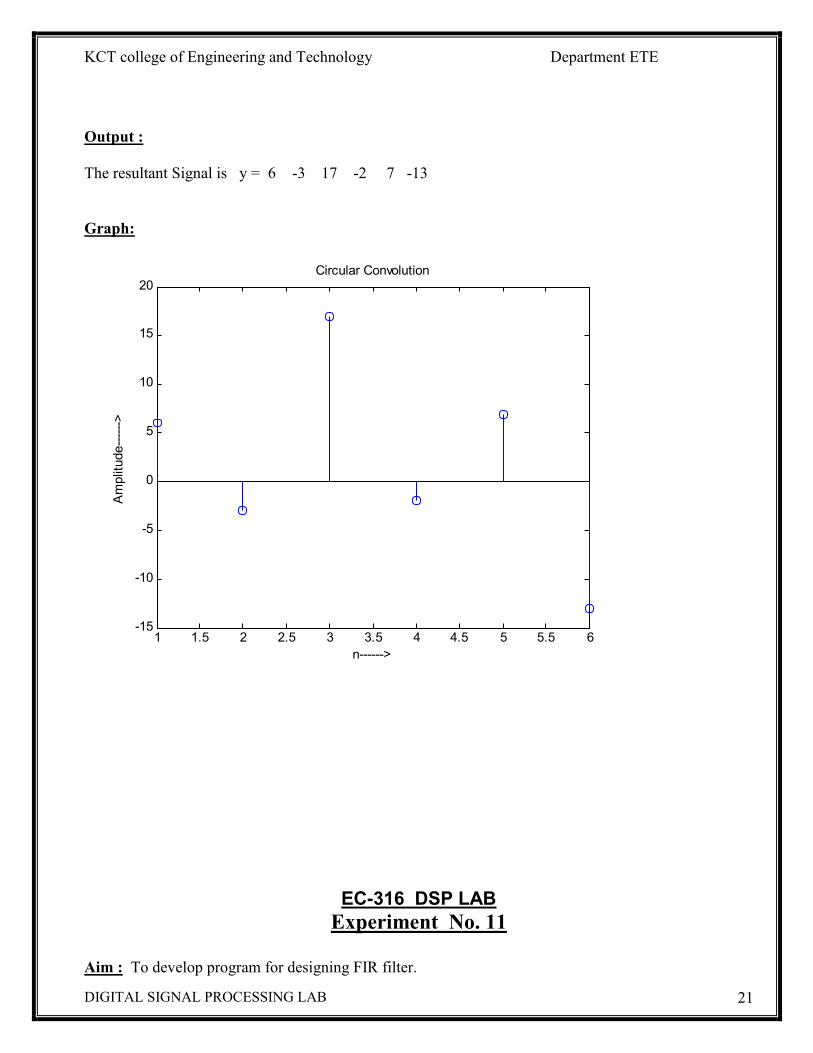
endenddisp('The resultant Signal is ');ystem(y);ylabel('Amplitude------>');xlabel('n------>');title('Circular Convolution');



Output :

The resultant Signal is y = 6 -3 17 -2 7 -13

Graph:

1 1.5 2 2.5 3 3.5 4 4.5 5 5.5 6-15

-10

-5

0

5

10

15

20

Am

plitu

de---

--->

n------>

Circular Convolution


Aim : To develop program for designing FIR filter.




Program :

%prog for designing of FIR low pass% filters using rectangular windowclc;clear all;close all;rp =input('Enter the pass band ripple ');rs =input('Enter the stop band ripple ');fp =input('Enter the pass band freq ');fs =input('Enter the stop band freq ');f =input('Enter the sampling freq ');wp = 2*fp/f;ws = 2*fs/f;num = -20*log10(sqrt(rp*rs))-13;dem = 14.6*(fs-fp)/f;n = ceil(num/dem);n1 = n+1;if (rem(n,2)~=0)

n1 =n;n = n-1;

endy = boxcar(n1);% low pass filterb = fir1(n,wp,y);[h,o] = freqz(b,1,256);m = 20*log(abs(h));subplot(2,2,1);plot(o/pi,m);ylabel('Gain in dB ------>');xlabel('(a) Normalised freq ---->');



Output :Enter the pass band ripple 0.05Enter the stop band ripple 0.04Enter the pass band freq 1500Enter the stop band freq 2000Enter the sampling freq 9000

Graph:

0 0 . 5 1- 2 0 0

- 1 0 0

0

1 0 0

Ga

in i

n d

B -

----

->

( a ) N o r m a l i s e d fr e q - - - - >




Aim : To develop program for for designing IIR filter.


Program :

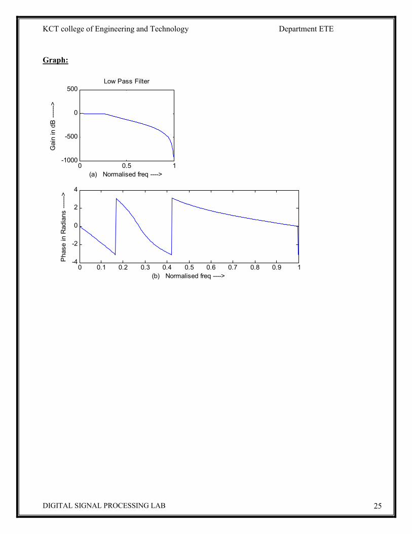
%prog for designing of IIR low pass% filters using rectangular windowclc;clear all;close all;rp =input('Enter the pass band ripple ');rs =input('Enter the stop band ripple ');wp =input('Enter the pass band freq ');ws =input('Enter the stop band freq ');fs =input('Enter the sampling freq ');w1 =2*wp/fs; w2 = 2*ws/fs;[n,wn] = buttord(w1,w2,rp,rs);[b,a] = butter(n,wn);w =0:0.01:pi;[h,om] = freqz(b,a,w);m = 20*log(abs(h));an = angle(h);subplot(2,2,1);plot(om/pi,m);ylabel('Gain in dB ------>');xlabel('(a) Normalised freq ---->');title('Low Pass Filter');subplot(2,1,2);plot(om/pi,an);ylabel('Phase in Radians ------>');xlabel('(b) Normalised freq ---->');

Output :

Enter the pass band ripple 0.5Enter the stop band ripple 50Enter the pass band freq 1200Enter the stop band freq 2400Enter the sampling freq 10000



Graph:

0 0.5 1-1000

-500

0

500

Gai

n in

dB

-----

->

(a) Normalised freq ---->

Low Pass Filter

0 0.1 0.2 0.3 0.4 0.5 0.6 0.7 0.8 0.9 1-4

-2

0

2

4

Pha

se in

Rad

ians

-----

->

(b) Normalised freq ---->

department of electronics & tele- comm. engineering lab ...digital signal processing lab 3...

Documents