Job Displacement, Family Dynamics and Spousal Labor Supply

by

Martin HALLA

Julia SCHMIEDER

Andrea WEBER

Working Paper No. 1816 November 2018

DEPARTMENT OF ECONOMICS

JOHANNES KEPLER UNIVERSITY OF

LINZ

Johannes Kepler University of Linz Department of Economics

Altenberger Strasse 69 A-4040 Linz - Auhof, Austria

www.econ.jku.at

martin.halla@jku.at

Job Displacement, Family Dynamics

and Spousal Labor Supply∗

Martin Halla†, Julia Schmieder‡, Andrea Weber§

This version: October 17, 2018

Abstract

We study the effectiveness of intra-household insurance among married couples

when the husband loses his job due to a mass layoff or plant closure. Empirical results

based on Austrian administrative data show that husbands suffer persistent employment

and earnings losses, while wives’ labor supply increases moderately due to extensive

margin responses. Wives’ earnings gains recover only a tiny fraction of the household

income loss and, in the short-term, public transfers and taxes are a more important form

of insurance. We show that the presence of children in the household is a crucial deter-

minant of the wives’ labor supply response.

Keywords: Firm Events, Household Labor Supply, Intra-household Insurance, Added

Worker Effect.

JEL classification: D19, J22, J65.

∗For helpful discussions and comments, we would like to thank Monica Costa Dias, Itzik Fad-

lon, Peter Haan, Juan F. Jimeno, Magne Mogstad, Andreas Steinhauer, Federico Tagliati, Katharina

Wrohlich, and many conference and seminar participants. The usual disclaimer applies. We gratefully

acknowledge financial support from the German Research Foundation within its priority program 1764:

The German Labor Market in a Globalized World.†Johannes Kepler University Linz, IZA and GOG; e-mail: martin.halla@jku.at‡DIW Berlin, WU Vienna and IZA; e-mail: jschmieder@diw.de§Central European University, CEPR and IZA; e-mail: WeberA@ceu.edu

1 Introduction

An important economic motive for marriage is the opportunity to share risk within

a couple. If one partner is affected by an unexpected shock, such as illness or job

loss, the second partner can increase her labor supply as an insurance against a drop

in household consumption. Other economic motives for marriage, such as the desire

to have children and raise a family as well as the division of labor between home

production and market work (Weiss, 1997), might, however, interfere with the risk

sharing potential within marriage. For example, if preferences for spending time with

children are unequally distributed in the couple, the spouses might not be willing

to switch roles in response to an income shock. More generally, gender norms and

role models might limit the flexibility of spouses to respond to changes in economic

conditions.

From a policy perspective, the risk sharing potential of marriage is important, as

strong intra-household insurance reduces the need for public insurance. Thus, the em-

pirical literature has long sought to assess the importance of the risk sharing potential

of marriage studying the so-called added worker effect (henceforth AWE). Early stud-

ies provide evidence of a negative correlation between employment of married women

and men across labor markets and over time (Mincer, 1962; Heckman and Macurdy,

1980), while later work focuses on the timing of spousal transitions between employ-

ment and unemployment within couples (Lundberg, 1985; Stephens, 2002; Juhn and

Potter, 2007; Bredtmann et al., 2018). The findings from these studies are mixed, de-

pending on the economic context and institutional framework. However, most studies

indicate small employment responses by wives and little evidence for a substantial

AWE.1 In contrast to these empirical results, recent studies estimating structural life-

cycle family labor supply models based on earnings and consumption data identify

family labor supply as one of the major factors allowing married households to smooth

consumption, even when they are facing persistent income shocks (Haan and Prowse,

2015; Blundell et al., 2016).

The literature provides several arguments why the risk sharing channel via family

labor supply might be less relevant in practice. One is the generous availability of

social insurance programs that crowd out self-insurance or family insurance (Cullen

and Gruber, 2000; Autor et al., 2017). A second argument are correlated shocks at the

household level, for example, due to economic recessions. Children and fixed gen-

1See Appendix Table A1 for an overview of cross-elasticity estimates in the literature.

1

der roles within the household might also reduce the potential to share risk, but they

receive comparably less attention in the literature. Blundell et al. (2018) address the

importance of children in understanding family labor supply decisions over the life-

cycle, within a unified model framework that captures the trade-offs between provid-

ing child care and insuring consumption against shocks within the household. Indeed,

their findings confirm that families with children respond differently to income shocks

than families without children.

In this paper, we try to disentangle the roles of different channels in the responses

to income shocks within married households, paying special attention to the effects of

children. Our evidence is based on a quasi-experimental setup of married couples in

Austria, where the husband loses a job due to a plant closure or mass layoff. These

layoff events provide credibly exogenous shocks to household income, allowing us

to disregard problems with reverse causality. In addition, the timing of the shock is

precisely defined. A large literature documents persistent employment and earnings

losses due to job displacement Ruhm (1991); Jacobson et al. (1993); Ichino et al.

(2017); Lachowska et al. (2018). Thus, we have a setup in which couples face large,

persistent, and unexpected shocks to household income, allowing us to explore the

response of both partners around the time of the shock.

We show that, in the Austrian case, layoff events affect couples at different stages

of the life-cycle. In particular, we observe many young couples with children, for

whom we can study the trade-offs between insurance and child care. This is partic-

ularly interesting, as Austria is a very conservative society with strong gender iden-

tity norms (Akerlof and Kranton, 2000). The typical Austrian household follows the

characterization of the male breadwinner model, where wives mostly enter the labor

market as secondary earners and in part-time jobs (Bertrand et al., 2016). This social

model is supported by Austrian welfare and family policies, which provide a gener-

ous parental leave system, but low levels of subsidized child care. As an illustration

of the importance of gender norms and family values, Figure 1 shows the share of

individuals who agree with the assessment that ‘a pre-school child is likely to suffer

if his or her mother works’ for several countries. In this comparison, Austria stands

out with more than a third of respondents who strongly agree. In Scandinavian and

Anglo-Saxon countries, less than 10 percent of survey respondents agree with this

statement. In terms of labor market institutions, Austria has a universal UI system and

an individual based income tax system.

Our empirical analysis is based on detailed data from linked Austrian registers,

which allow us to identify partners in marriages and divorces as well as plant closure

2

and mass layoff events at the plant level. In total, we have a sample of about 48,000

married couples where the husband is laid off. The data indicate strong specialization

in market and household work within the couples. Only 50% of wives are working

before the husband loses the job and a large fraction of wives are working part-time.

We show that our setup of high volatility in female life-cycle labor supply profiles,

with mothers dropping out from the labor force after childbirth for extended periods,

requires a careful choice for a control group to measure responses to the displacement

shock. In the empirical analysis, we use three different control groups to confirm

the robustness of our results. Following the literature, the first control group consists

of couples with the husband working in a firm without mass layoff or plant closure.

The second control group consists of couples where the husband works in a plant

with a mass layoff, but is not laid off himself. The third control group exploits the

randomness in the timing of displacement, following the strategy applied by Fadlon

and Nielsen (2017). We compare outcomes in couples who marry in the same year,

but in one case the husband is displaced earlier than in the other, and we use the time

between the two displacement events as counterfactual.

Our main results are remarkably consistent across the three control groups. We

find that husbands lose on average 21 to 24% of earnings over a five year period after

displacement and have a 16 to 17% lower employment rate relative to the control

group. The labor supply responses of wives are positive and statistically significant,

but small compared to the husbands’ losses. On average, the female employment

rate increases by 1% and earnings by about 2%. We find that wives mainly respond

at the extensive margin and are more likely to enter the labor market, if they were

not employed before the husbands’ job loss. The implied participation elasticity with

respect to the husband’s earnings shock is very small, roughly -0.04 in the full sample

and -0.07 in the sample of wives not employed at displacement.

The intra-household insurance mechanism plays a negligible role compared to

public insurance via government transfers and taxes, as the wives’ labor supply re-

covers only a tiny fraction of the overall loss in household income. In particular, UI

benefits cover the large initial drop in household income following the job loss. How-

ever, due to time-limited benefit durations, the longer term losses in household income

are not covered by government transfers.

Overall, these results indicate a small role of risk-sharing within married couples

in Austria. To disentangle the importance of mechanisms that limit the risk sharing

potential, we consider several channels. First, we investigate the stability of the fam-

ily structure with respect to the husband’s job loss. If the shock leads to divorce or

3

changes in fertility plans, this could explain the limited scope of the insurance mech-

anism. We find a small increase in the probability of divorce comparing displaced

couples with couples where the husband works in a firm without mass layoff or plant

closure. However, there is no increase in the divorce rate of displaced couples rela-

tive to those where the husband works in a plant with mass-layoff, indicating some

spill-over effects. Furthermore, we do not see any effects of the husband’s job loss on

fertility, which indicates that couples are not willing to revise fertility plans.

Second, we investigate heterogeneity in responses by the age of the youngest child

in the household. The wife’s labor force participation before the husband’s job dis-

placement varies greatly in size by the age of children in the household. Women with

very young kids below the age of 3 are mostly on parental leave and only 18% of

them are employed. In contrast, wives with children above compulsory schooling age

or without children have a much higher employment rate of 66%. We find that the

most responsive group are mothers with children between age 3 and 15, who increase

their employment rates and earnings persistently after the husband’s job loss. We find

no response among mothers of very young children or among women without children

or with older children. This seems to imply that some trade off in child care provided

by the mother and by formal channel occurs, especially among women who bring for-

ward their entry into the labor market after a maternity break. Notably, we find no

evidence on substitution in child-care responsibilities between mothers and fathers of

very young children for whom no formal child care is available.

Third, it could be the case that labor market shocks are correlated among wives and

husbands. Assortative matching and the fact that they work in the same labor market

could reduce employment opportunities for wives. Indeed, we do not find any female

labor supply responses in couples where the husband loses the job in a market with

a high unemployment rate. Even in markets with low unemployment, the additional

earnings from the wife’s employment covers just a tiny fraction of the total household

income loss. We further find that wives with high earnings potential, i.e. those with

high earnings before marriage, respond more strongly to the husband’s job loss. In

addition, the wife’s labor supply response is stronger in couples, where the husband

loses a well-paid job from a firm that pays above average wages to all their other

workers. If labor market shocks within couples were strongly correlated, we would

not expect to find heterogeneity along these two dimensions.

Our paper relates to the large literatures on family labor supply and on the long-

term effects of job displacement, to which we contribute clean quasi-experimental

evidence on the effects of job loss on family labor supply in married coupes. We also

4

contribute to the emerging literature on the role of social norms and gender identities

in shaping labor market outcomes (Bertrand et al., 2016; Kleven et al., 2018). In our

setup, we show that the traditional male breadwinner model of the family can severely

limit the insurance potential of marriage. Further, we contribute to the literature on the

motives of marriage and fertility (Weiss, 1997). In particular, we provide empirical

evidence that in Austria fertility decisions often precede marriage decisions.

The remainder of the paper is organized as follows: Section 2 discusses relevant

aspects of the institutional setting. Section 3 introduces our data sources. We also

discuss how we identify plant closures and mass-layoffs, subsequently providing de-

scriptive statistics for the key outcome variables. Section 4 describes the life-cycle

patterns of women of displaced husbands and motivates our three alternative quasi-

experimental counterfactual scenarios. Section 5 outlines our estimation strategy. Sec-

tion 6 presents our main estimation results along with a number of robustness checks

and three extensions. First, we examine consequences of husband’s displacement on

households’ disposable income by accounting for changes in taxes and benefits. Sec-

ond, we explore the underlying mechanisms of the AWE that go beyond an income

effect and affect the family structure. Third, we investigate heterogeneity in responses

for different types of households. This last step helps us to understand the reasons for

the limited responses by wives. The final Section 7 concludes the paper and discusses

potential policy implications.

2 Institutional setting

In this section, we provide background information on several aspects of the institu-

tional setting in Austria. This information helps to put our results into perspective.2

Trends in household formation Austria witnessed trends in marriage and fertility

behavior that are quite comparable to other high-income countries. Both the age at

first marriage and at first birth have increased substantially over time, while other

patterns have remained stable. The vast majority of Austrian females will be married

at some point in their lives and will give birth to at least one child. About 90 percent

of females 45 years of age or older have been married at some point (see Census 1981,

1991 and 2001). An almost comparable share of this age group gave birth to at least

one child. The relative timing of marriage and first birth also remained constant. Most

women give birth to their first child within the first two years following marriage. A

2Time-constrained readers may appreciate the five most important stylized facts at the end of this

section and skip to Section 3.

5

sizeable (but declining) fraction of these women give birth to a second child a couple

of years later. The birth timing gives rise to drastic changes in women’s labor market

participation in the years following marriage, as we will see below.

Development of the female labor force participation In 1990, about 64 percent

of all Austrian women between the ages of 25 and 54 were participating in the labor

market. This rate has increased over time and, since the early 2000s, the female labor

force participation has been consistently above 80 percent.3 However, even in 2018,

the female participation rate is still well below the male rate of 92.5. Moreover, at

any point in time, there is much more heterogeneity in the female than in the male

participation rate. The most important dimensions predicting labor force participation

are women’s age, marital status, and the number and age of children. Married women

with children, especially those with young children, are the group with the lowest

participation rates (see Appendix Figure A1).

Gender identity norms and beliefs about child care One potential explanation

for the rather low participation rates of (married) women with children are prevailing

gender identity norms and beliefs about the quality of child care. Using data from

the European and World Values Surveys, Appendix Table A2 shows that a large share

of Austrians believe that ‘a pre-school child is likely to suffer if his or her mother

works’, while few agree with the statement that ‘a working mother can establish just

as warm and secure a relationship with her children as a mother who does not work’.

A comparison with figures from other high-income countries reveals that Austrians

hold a comparably high degree of conservatism toward gender roles and the labor force

participation of mothers. In line with this, relatively few Austrians consider ‘sharing

household chores’, as ‘important for [a] successful marriage’. This is supported by

the evidence presented by Bertrand et al. (2016), who classify Austria, based on a

series of measure of gender attitudes, as a high-sexism country. These patterns are

not only very robust across sub-populations defined by sex and marital status, but also

hardly change over the available sample period from 1990 to 1999.

Maternity and parental leave policies Another explanation, for the rather low

participation rates of (married) women with children, is the generous parental leave

system. Austrian law mandates a compulsory maternity leave period of eight weeks

before and after delivery for all working mothers (Lalive et al., 2014). Subsequently,

eligible parents are entitled to paid and job-protected parental leave up to the child’s

third birthday. In the vast majority of the cases, it is the mother who takes the leave.

3All figures are according to estimates of the International Labour Office, Source: ILOSTAT

Database (accessed on September 20, 2016).

6

Thus, almost all women leave the labor market at least temporary after the birth of a

child, while a significant share also leaves the labor market permanently. The latter

particularly applies to mothers with two or more children (see above).

child care The Austrian system of formal child care distinguishes between facil-

ities for children below the age of three (nurseries) and for those aged three to six

(kindergarten). While the vast majority of communities have offered a kindergarten

since the 1980s, the local availability of nurseries has been traditionally much lower.

In 1995, only about 3 percent of communities had nurseries. These nurseries were

predominantly located in more densely populated areas and covered about 35 per-

cent of the total population. A widespread problem with both types of institutions are

oversubscriptions, short opening hours (until noon) and long holidays.

Taxation of families The Austrian tax system follows the standard of individual

income taxation, which means that partners in married couples are taxed separately.

Thus, the entry tax rate for the second earner is lower, all other things equal, than in

joint or family-based taxation systems. In addition, basic family allowances are re-

warded universally and independent from the level or distribution of earnings (OECD

Economic Surveys: Austria 2015). Both aspects of the tax system should promote

dual-earner households. On the other hand, certain characteristics of the tax and ben-

efit system work in favor of single-earner household or a ‘1.5 model’. In particular,

the quite high marginal tax wedge for medium incomes promotes part-time work.

Unemployment insurance In Austria, all private sector workers are automatically

enrolled in the universal UI system. Eligibility for and duration of unemployment ben-

efits depends on the individual’s work history and age. UI payments replace around

55% of the previous net wage and are subject to a maximum and minimum. Job

losers in our samples can receive UI benefits for 20 to 39 weeks. After exhausting

regular unemployment benefits, job losers can obtain means-tested income support,

unemployment assistance (UA), that pays a lower level of benefits indefinitely. Un-

employment assistance is reduced euro for euro by the amount of any other family

income (Card et al., 2007).

The five most important stylized facts are: First, within the typical Austrian couple,

the man is still the primary earner. Second, women in the age range between 20 to

35 have complex employment patterns. This is particularly true in the initial years

after marriage and first birth. Third, Austrians have on average very traditional views

on gender roles, and prefer mothers of (young) children not to participate in the labor

market. Fourth, supply of formal child care facilities for children below the age of

three does not meet demand. Fifth, married couples are taxed individually.

7

3 Data sources, firm events, and descriptive statistics

Our empirical analysis is based on combined data from several administrative regis-

ters. Information on individual labor market careers is provided by the Austrian Social

Security Data (ASSD). This is a linked employer-employee database that covers the

universe of Austrian workers in the private sector from 1972 onward (Zweimuller

et al., 2009).4 The data record individual employment spells on a daily basis along

with an employer identifier, as well al individual earnings per calendar year and em-

ployer. In addition, the data include information on other social security relevant

events such as unemployment, retirement, parental leave, and, in the case of women,

births. Information on a worker’s marital status and the identity of their partner is

provided by the Austrian Marriage Register and the Austrian Divorce Register.

3.1 Plant closures and mass layoffs

We make use of the linked employer-employee structure of the ASSD to identify plant

closures and mass layoffs. Our identification strategy relies on an approach inves-

tigating detailed flows of workers between employer identifiers that is described in

Fink et al. (2010).5 In particular, we organize plant level information from ASSD

employment records in a quarterly panel measuring the number of blue- and white-

collar employees at each employer identifier on February 10, May 10, August 10, and

November 10 of each year.

Plant closures are observed in the quarter when an employer identifier vanishes

from the ASSD. We analyze the flows of workers from the exiting identifier to subse-

quent employer identifiers to distinguish “true” closures from identifier reassignments

or mergers with existing plants. We refer to the closing quarter as the last quarter in

which the plant employs workers. To define our sample of closing plants, we consider

all closures in the period from 1990 to 2007, restricting the sample to plants with at

least five employees during the last four quarters of their existence.

Mass layoffs are defined by a similar approach. We identify large drops in plant

4The ASSD comprises only incomplete information on self-employed and civil servants (Beamte).

Since we do not observe earnings for these two groups, we exclude them from our main analysis.

Notably, the majority of persons employed with public authorities today are not civil servants, but

so-called contractual civil servants (Vertragsbedienstete). Since we have precise information for this

group, we include them in our main analysis.5In the ASSD, we cannot distinguish between firms and establishments as there is no uniform rule

for recording employer identifiers. As the vast majority of identifiers refers to small units, a plant in

most cases will refer to an establishment (Fink et al., 2010).

8

size in the quarterly time series, but exclude events in which a large group of employ-

ees moves to the same employer identifier. The exact thresholds to define a reduction

in plant size between two quarters as a mass layoff is inspired by the Austrian system

of advance layoff reporting. Employers planning to lay off an unusually large number

of workers within the next month must provide advance notice to the employment of-

fice if the number of layoffs exceeds a threshold that depends on the size of the plant.6

In analogy to the closing quarter, we define a mass layoff quarter as the quarter im-

mediately before the large drop in employment. In our sample, we consider all mass

layoff events between 1990 and 2007. As the Austrian labor market is characterized

by strong seasonality in employment, which makes it difficult to distinguish closures

or mass layoffs from purely seasonal employment fluctuations, we exclude plants from

sectors with a high share or seasonal employment (i. e. agriculture, construction, and

tourism).

Restrictions on the sample of displaced workers At the individual level, we define

workers as being affected by a plant closure if they are employed at a closing plant on

the closure date or in the two preceding quarters. Workers affected by a mass layoff

are employed on the mass layoff date, but leave the plant in the subsequent quarter.

Our sample of displaced workers consists of men displaced by a plant closure or mass

layoff, who have been married for at least two years, and who have at least one year

of tenure at layoff. We further restrict the age at displacement to 25–55 for husbands

and to 25–50 for wives, selecting the upper age limits to exclude transitions into early

retirement.7 Some individuals are displaced by firm events multiple times over their

careers. We only consider the first displacement event for each husband, as subsequent

outcomes might be influenced by the first displacement. We also drop couples who

are displaced by the same firm event.8 Our final sample comprises 18,466 couples,

with the husband displaced by a plant closure and 30,027 couples with the husband

6Our definition only considers plants with more than 10 employees in the quarter before the mass

layoff and we apply the following rules for size reductions. In plants with 11 to 20 employees, the size

must decline by at least three individuals; in plants with 21 to 100 employees, the size has to decline

by a minimum of five individuals; in plants with 100-600 employees the size has to decrease by at least

5%. In firms with more than 600 employees, the number of employees between two quarters has to

decline by at least 30 employees. In the robustness analysis in Appendix B, we present our main results

with a more restrictive definition of mass layoffs.7Our data suggests that this age restriction is reasonable: Less than 1% of all husbands and wives

in our sample receive pensions when they are last observed in our sample. On average, 0.7% and 0.5%

of husbands and wives, respectively, receive pensions in any quarter in our sample period.8663 couples are affected by the same plant closure and 344 by the same mass layoff. Relative to

all households that experience a plant closure (mass layoff) these are 3.47% and 1.13%, respectively.

9

displaced by mass layoff.9

3.2 Outcome variables and sample characteristics

The main outcome variables considered in our analysis are employment and earnings

of husbands and wives. We organize individual observations at the quarterly level and

define employment by an indicator equal to one if the individual is employed at the

quarter date (Feb 10, May 10, Aug 10, Nov 10). Earnings refer to average monthly

real earnings in Euro (2000 prices) over the quarter with the main employer. Note

that the ASSD do not provide information on working hours. Thus, our earnings mea-

sure combines wages and hours. For each individual we collect quarterly observations

in the 5 years before and after the displacement. We define the individual reference

quarter by the mass layoff quarter or closing quarter or by the quarter in which the in-

dividual is last employed in the case of workers, who leave before the closing quarter.

In further analysis, we also analyze registered unemployment, receipt of UI benefits

and unemployment assistance, household income, divorce, and fertility.

Table 1 presents the main descriptive characteristics measured at the reference

quarter. Columns (1) and (2) list the plant closure and mass layoff samples, respec-

tively. Both groups of displaced workers are quite similar in the personal charac-

teristics of husbands and wives, but firm characteristics are different. Mass layoffs

tend to happen in larger plants than closures and in plants with a different industry

and regional composition. Mass layoff plants also pay higher wages to their average

workers. This is reflected in the difference in husbands’ pre-displacement earnings of

both groups.

Displaced couples in our sample are relatively young: husbands are on average

aged about 39 years and their wives are roughly 2.5 years younger. Note that median

age of husbands and wives is slightly younger than the mean. At displacement, the

average couple has been married for 12 years (median is 11 years) and they have 1.4

children. Looking at the distribution of the age of the youngest child in the household,

we can see that about 18% of couples have a child below the age of three, 57% have

children between age 3 and 15, and roughly a quarter of households either have no

child or children aged 16 or older.

Furthermore, the employment rate among wives prior to the husband’s job dis-

placement is low, with only 50% of wives working. If they are employed their earn-

9The highest numbers of displacements are observed in the late 1990s and early 2000s (see Fig-

ure A2 in the Web Appendix). There is evidence of seasonality in the number of displacements with

peaks in the fourth quarter of each year.

10

ings are significantly lower than their husband’s. On average, a working wife earns

about 62% of her husband’s earnings, which corresponds to 38% of the household’s

labor income. The large earning gap within couples can only be explained by a high

share of part-time work among wives.

4 Family dynamics around displacement and defini-

tion of control groups

Fertility plans and the presence of young children typically affect household labor

supply decisions. Therefore, we investigate marriage durations and the timing of first

births in our sample of couples with displaced husbands. The mode of marriage du-

rations in the sample is around 5 years and the distribution has a long right tail. This

implies that even though we only consider couples, who have been married for at least

2 years, the majority are relatively recently married when the husband experiences the

job displacement.10 How quickly after marriage do couples have their first child? Fig-

ure 2 showing the distribution of the time between marriage and birth of the first child

demonstrates that in Austria the marriage date is very strongly related to the birth of a

child. While a few couples have their first child before marriage, we see a big spike in

births 4 to 8 months after the marriage date and then a relatively long right tail. This

pattern suggests that in many couples, marriage follows the fertility decision rather

than the other way round. Overall, about 64 percent of first births occur within five

years after marriage and 30 percent occur in the first year. Due to the aforementioned

generous Austrian parental leave system, fertility is also strongly related to female

labor force participation. Together, the high prevalence of short marriage durations,

the presence of young children in the household, and long parental leave periods im-

ply that we observe the husband’s job displacement shock during a period of high

volatility in household labor supply. The next set of figures illustrates this argument

by investigating husband’s and wife’s employment around the displacement date.

Figure 3a plots the husband’s employment probability around job displacement.

We restrict displaced workers to be employed for at least one year at the plant closure

or mass layoff event and, therefore, the graph shows full employment prior to the ref-

erence date and slightly lower employment rates in earlier years. After displacement,

we see a sharp drop in employment of about 30 percentage points. This is followed

by a quick recovery over the next 4 quarters. In the longer run, however, displaced

10The distribution of marriage durations at the reference date is shown in Appendix Figure A3.

11

workers cannot fully recover and their post-displacement employment levels are about

20 to 25 percentage points below full employment.

Figure 4 examines the employment of the wives of displaced husbands. To point

out variation in female labor supply around childbirth and marriage, we plot employ-

ment rates for 5 groups with different marriage durations. The figure reveals substan-

tial heterogeneity across groups. Starting with the group with the shortest marriage

duration of 2 to 4 years, we can see that the average employment probability of women

drops shortly after marriage — in line with the arrival of children — and then slowly

recovers after maternity leave. This pattern is repeated in groups with longer mar-

riage durations, by parallel shifts to the right of the wives’ employment trajectories.11

Thus, the life-cycle pattern creates huge variation in female labor supply over time.

Depending on the duration of marriage, the wife’s employment probability at the time

of the husband’s displacement varies between 40% and 50%, rising almost linearly

for each group after the reference quarter. Prior to husband’s displacement there is a

lot of variation in wife’s employment across the different groups.

Figure 3b shows the average quarterly employment probability aggregated over all

groups of wives. After having investigated different marriage cohorts, it is clear that

the aggregate pattern of wives’ employment rates is not at all informative about their

response to husbands’ job displacement.12

Because a simple event study design without control group is highly sensitive to

female life-cycle patterns, our empirical strategy relies on the choice of appropriate

control groups of couples who did not suffer a job displacement. The idea is to com-

pare labor market outcomes of couples with and without displacement of the husband

holding fixed the stage in the life-cycle. As we lack a design with full randomization

of job displacements, we control for the complex counterfactual pattern in female em-

ployment using three different control groups: (i) households who are not affected by

a firm event, (ii) households with husbands employed during a mass layoff, but not

displaced themselves, and (iii) households who experience a displacement through a

11Alternatively, we show in Appendix Figure A4 the employment probability of wives around their

husbands’ displacement by the age of the youngest child in the household. Given the close relationship

between marriage and fertility established above, the patterns look very similar.12The latter interpretation is supported by Appendix Figure A5. This graph shows quarterly means

of the employment probability around displacement, while flexibly adjusting for marriage duration and

the calendar quarter of observation. While husbands’ employment results are hardly changed by the

adjustment (see Panel a), wives’ results now show a very different pattern (see Panel b). After the

reference date employment of wives still increases, but only by about 3 percentage points in the long-

term. This indicates that the displacement effect on wives’ employment is one order of magnitude

smaller than that on husbands.

12

firm event in the near future.

Control group 1: Non-displaced husbands without firm event. The first con-

trol group consists of couples fulfilling the same age, tenure, and marriage duration

restrictions as our displaced sample. Husbands are employed at any reference quarter

from 1990–2007 at firms that are not experiencing a closure or a mass layoff. Because

this is a large group, where many couples are observed repeatedly, we draw a ten per-

cent random sample. Workers in control group 1 are not affected by a displacement

event, neither themselves, nor in their plant. Table 1 column (3) reports descriptive

statistics showing that their characteristics differ from those of displaced workers in

terms of age, labor market experience, job stability, and earnings. Importantly, non-

displaced workers are employed by larger firms that pay higher wages also to their av-

erage workers. Appendix Figure A6 illustrates that firms that do not experience a mass

layoff or closure are substantially larger and pay on average higher wages than event

firms. Wives of non-displaced workers in control group 1 are slightly older than wives

of displaced workers, but overall the difference in wives’ characteristics are smaller

than among husbands.13 The differences in observable characteristics between dis-

placed couples and control group 1 couples gives rise to concerns that workers might

be sorting into more and less risky firms and jobs also on the basis of unobservable

characteristics.

Control group 2: Non-displaced husbands in mass layoff firms. To confront

the concern of workers sorting into different firms, we define the second control group

by husbands employed in mass layoff plants at the mass layoff date, who do not leave

their employer in the subsequent quarter. As the number of non-layoff workers at the

mass layoff plant typically exceeds the number of layoffs, we draw a 40% random

sample of all observations. The reference date for this control group is defined by the

mass layoff date.14 Workers in control group 2 suffer a mass layoff at their plant, but

do not lose their jobs. As we see in column (4) of Table 1, these workers share average

firm characteristics with workers displaced by mass layoffs. The mean firm size differs

between columns (2) and (4), because larger firms tend to have more workers who

13Family dynamics, i.e. the marriage duration at the reference date and the time between marriage

and first birth, are similarly distributed for households that experience displacement and for those in

the control groups. See Appendix Figures A7 and A8 for a comparison.14We also exclude workers who are ever displaced from a plant closure or mass layoff over our

observation period from control groups 1 and 2. However, individuals can be in the control group in

more than one reference quarter. This happens for about 10% of the individuals in control group 1 and

26% of individuals in control group 2.

13

survive a mass layoff event. With the definition of control group 2, we do not worry

about selection into firms, but we might worry about selection into layoff. Many firms

apply ‘last-in first-out’ or similar policies to determine mass layoffs (Sorensen, 2018).

A further concern is that economic and psychological shocks related to a mass layoff

can also affect non-displaced workers and their spouses, due to increased uncertainty

or stress or because of a general deterioration of labor market conditions.15

Control group 3: Husbands displaced at a later date. For the third control

group we do not sample individuals who were not displaced, rather, we exploit the

timing of firm events and construct control groups of workers who are displaced them-

selves, but at a later date. Our approach is inspired by Fadlon and Nielsen (2017) and

Hilger (2016), who exploit the timing of events to investigate the effects of spousal

health shocks on employment and the effect of father’s displacement on child out-

comes, respectively. Under the assumption that the process determining involuntary

job loss does not vary over time, workers who are displaced in later periods should not

differ in unobserved characteristics from those who are displaced in the base period.

Thus, the confounding effects of unobserved heterogeneity should be accounted for

by a comparison of workers displaced at different times (Ruhm, 1991).

Our strategy to construct control group 3 is as follows. We start with a cohort of

couples getting married in a fixed quarter and define households with husband dis-

placed in a (reference) quarter h as the displaced group. The control group is given

by the set of households in the same marriage cohort, who experience husband’s dis-

placement in the near future, in h + ∆. We then assign a placebo shock at h to the

households in the control group. It is important to hold the marriage date of the dis-

placed and control group fixed to make sure that they are at the same stage of their

life-cycle at date h. The choice of ∆ is restricted by the trade-off between the length of

the horizon over which we can observe post-displacement outcomes and the compara-

bility of displaced and control couples. The two groups should be highly comparable

if there is only little time difference between displacements, i.e. if ∆ is short. How-

ever, a short ∆ also limits the period over which the counterfactual outcome can be

observed. We experimented with values for ∆ between 4 and 16 quarters, selecting

only multiples of 4 because of the seasonality in mass layoffs and plant closures (see

Appendix Figure A2 and the robustness analysis summarized in Appendix B). As we

do not find much evidence for reduced comparability, we present the main results

15Gathmann et al. (2018) show that mass layoffs worsen the local labor market situation in a causal

way. They find that mass layoffs have sizeable negative effects on the regional economy, especially of

firms in the same sector.

14

for ∆ = 16. We repeat the construction of the control group for every combination of

marriage quarter and reference quarter h and construct weights such that the displaced

and control group size is balanced within each cell.

Due to the sample restrictions on marriage duration and tenure at displacement,

we must put two additional restrictions on households in control group 3. This has

implications for the comparability in the case of some of the outcome variables. First,

the restriction on the husband’s job tenure in control group 3 has to hold in quarter h

and in quarter h + ∆, which implies that there is full employment among husbands

in control group 3 in the 4 quarters preceding h + ∆. Therefore, we cannot directly

compare the husband’s employment and earnings outcomes in control group 3 with

the displaced group. Second, due to the restriction on a marriage duration of at least

2 years prior to displacement, households in control group 3 are continuously married

between h and h+∆. If job displacement has an effect on the probability of divorce,

this cannot be measured by a comparison of couples with a displaced husband and

couples in control group 3. We return to these arguments in the results section.

5 Estimation strategy

We measure the effects of the husband’s job displacement by comparing outcome

variables at the individual wife or husband level, as well as family outcomes for the

displaced and control couples in the quarters before and after the reference date. In the

results section, we present a set of graphical results that are quantified by regression

estimates.

Our graphical results are based on the following regression model

Yik = θDi +

20∑

l=−20

γq

l I{k = l}+

20∑

l=−20

l 6=0

δq

lDi ∗ I{k = l}+ υik, (1)

where Yik is the outcome of individual or household i in quarter k ∈ [−20, 20]16, k

measures the number of quarters relative to the reference quarter, Di is an indicator

equal to one if the husband is displaced at k = 0, I{.} is the indicator function,

and υik is the error term. The parameter θ estimates the overall mean difference in

the outcome between displaced and controls, the parameters γq

l measure the quarterly

time profile of the outcome in the control group and δq

l measure the difference in time

16In the estimations with control group 3, we compare the displaced and control group only for four

years around the reference date. Hence, l varies only from −16 to 16 in (1) and from -4 to 4 in (2).

15

profiles between the displaced and the control group relative to the reference quarter.

For the presentation of our quantitative estimation results, we average the differ-

ence between displaced and control individuals relative to the reference date over the

20 quarters after displacement. In addition, the model controls for the full set of in-

dustry and calendar quarter interactions, λtj . The model is given by

Yik = θDi+20∑

l=−20

γq

l I{k = l}+−1∑

l=−20

δq

lDi∗I{k = l}+δpostDi∗I{k > 0}+λtj+υik.

(2)

By construction, average household characteristics do not differ between control

group 3 and the displaced households. However, we show in Table 1 that the other two

control groups differ from displaced households in terms of their observed character-

istics. To control for these differences, we apply a propensity score weighting strategy

following Imbens (2004). In particular, we estimate flexible logit specification for the

probability that the household is in the displaced group based on a large set of family

and individual characteristics measured at the reference quarter and characteristics of

the husband’s employer one year prior to the reference date. A plant closure or mass

layoff does not come as a complete surprise and households might be able to foresee

the event. To allow for responses of the wife in anticipation of the husband’s displace-

ment, we only control for the husband’s time-invariant characteristics, his employment

outcomes prior the reference date, his employer characteristics, and overall household

characteristics at the reference date such as marriage duration and the number of chil-

dren in yearly age categories. But we do not condition on labor market outcomes of

the wives before the reference date.17

Appendix Figure A9 shows the distributions of the estimated propensity scores in

17We estimate the probability that the husband in a household is displaced by plant closure or mass

layoff using a logit model separately for control groups 1 and 2 based on the following variables:

i. Husband characteristics: Interaction of year and season of displacement dummies, age (cubic),

tenure in current job (dummies for deciles), employment experience (5 dummies), experience in

unemployment (4 dummies), number of previous jobs (4 dummies), number of previous mass

layoff events (7 dummies), indicator for blue-collar status in last job, and for the years -4, -3,

-2 and -1 before the reference date: monthly wage, indicator for being employed and for being

unemployed.

ii. Wife characteristics: Labor market experience measured in last quarter of employment (5 dum-

mies), age distance to husband (5 dummies).

iii. Household characteristics: Marriage duration (30 dummies), number of children aged

0,1,2,...,12 (13 dummies) and total number of children under 18 at the reference date.

iv. Husband’s employer variables: Indicators for industry and region, firm age (16 dummies), firm

age and industry interactions.

16

the displaced group versus control group 1 and control group 2. The distributional

overlap in pre-determined characteristics is closer between control group 2 and the

displaced group than between control group 1 and the displaced. This is mainly due

to the similarities in firm characteristics.

Based on predicted propensity scores from the logit models, we construct weights

for members of the control groups such that the distribution of observable charac-

teristics in each control group equals the distribution among displaced households.

Using the weights, we estimate weighted regressions of equations 1 and 2. Hence,

the estimated parameters reflect the treatment effect on the treated. In all weighted

regressions, standard errors are bootstrapped (500 replications) with clustering at the

household level.

6 Empirical results

To measure the shock of the husband’s job loss on household income, we start by

investigating the effect of job displacement on husband’s employment and earnings

outcomes up to five years after displacement. Next, we turn to labor supply responses

of wives, reporting employment, earnings, and job search outcomes.

6.1 Husbands’ employment and earnings responses

Figure 5 compares quarterly employment rates before and after job displacement for

husbands in the displaced group and in control groups 1 and 2. The graphs on the left

present employment profiles in the displaced group (blue line) and the control groups

(red lines). The graphs on the right show the absolute difference between displaced

and controls along with the corresponding 95% confidence intervals. A comparison

across panels (a) and (b) confirms that the results do not differ by the choice of control

group. Prior to job displacement, the weighted difference in employment rates is close

to zero, but immediately after the event the employment rate in the displaced group

drops by more than 30%. We see a rapid recovery in subsequent quarters, which stalls

after about 3 to 4 years. Employment rates also decline in the control group after the

reference date, but more gradually.

In Table 2, we summarize estimation results of equation (2) for the mean effects of

We impose common support. Based on the estimated propensity score p, we assign control group

households weights equal to p

1−p. The normalization ensures that the weights of the control group add

up to 1.

17

job displacement on employment (in Panel A) and earnings (in Panel B). As we do not

observe working hours in our data, we use monthly earnings in Euro (in 2000 prices)

as dependent variable and set the earnings of individuals who are not employed equal

to zero. Columns (1) and (3) show the estimated effects for husbands referring to con-

trol group 1 and 2, respectively. The estimated coefficients of Displaced×Post report

the difference between displaced and control individuals relative to the reference date

averaged over the twenty quarters after displacement. Compared to the control group

displaced husbands suffer an average employment loss of about 16 to 17 percentage

points over the first five years. The equivalent estimate for earnings amounts to, 22

to 25% of the pre-displacement mean earnings, depending on the control group. The

relative magnitude of the earnings loss from job displacement, mirror the husbands’

employment losses, which indicates that lower employment rates are the main driver

of earnings drops.18 Appendix Tables A3 and A4 present the effects of the husband’s

job displacement on his labor market outcomes by year. This set of results confirm

that employment and earnings of the displaced and control groups evolve similarly in

the years prior to displacement. The largest employment and earnings losses occur in

the first year after displacement, with a decreasing trend thereafter.

6.2 Wives’ labor supply responses

6.2.1 Wives’ employment and earnings

The graphs on the left hand side in Figure 6 shows the employment rates of wives

in the displaced group and in each of the three control groups around the reference

date. Irrespective of husbands’ job loss, wives’ employment rates in all groups follow

the same upward sloping pattern, which confirms the importance of controlling for

life-cycle profiles in female labor supply. Prior to the reference date, differences in

employment rates between the displaced and each of the control groups are close to

zero (see the right hand side in Figure 6).19 After the reference date a significant gap

18The estimated employment effects are similar in magnitude to those reported for male Austrian

workers displaced in the 1980s by Schwerdt et al. (2010). These estimated effects on male earnings

are of comparable size to those reported in Jacobson et al. (1993) and slightly smaller than in Davis

and von Wachter (2011) for the US. They are also a bit larger than those reported in Sullivan and von

Wachter (2009) for Germany.19Note that we adjust for differences in observed characteristics between the displaced group and

control groups 1 and 2 by propensity score weighting on family, husband, and employer characteristics,

which eliminates differences in wives’ employment rates prior to the husbands’ displacement. We do

not correct for pre-displacement differences in observable characteristics between the displaced group

and control group 3, as this control group is drawn from the same pool of couples and, thus, pre-

displacement mean differences are zero by construction.

18

between the displaced and control groups opens and persists over the 5 year horizon.

This gap is remarkably similar across all three control groups, which makes us confi-

dent that we can interpret it as the wife’s labor supply response to the husband’s job

loss.

These findings are confirmed by the estimation results summarized in Table 2.

The estimated effects shown in columns (2), (4), and (5) show that wives of displaced

husbands increase their employment on average by about one percentage point during

the first twenty quarters after displacement (see Panel A). While the employment ef-

fects are small, they are precisely estimated and highly robust to the choice of control

group. Compared to the displaced husbands’ employment losses, the gains in wives’

employment are small. Along with increases in employment earnings increase by 1.5

and 2% (see Panel B). The estimated effects are again similar across all three con-

trol groups. Comparing wives’ earnings gains with husbands’ earnings losses makes

clear that the shift in labor supply within a household is hardly able to cover losses in

household income.20

As explained in Section 3, the ASSD only records earnings consistently for em-

ployees in the private sector. To check the importance of self-employment as an alter-

native source of income after job displacement, we can examine the participation in

self-employment. We find that self-employment increases among displaced husbands

relatively rapidly after a job loss. However, the overall effect is rather small; five years

after displacement, the self-employment rate is 5 percentage points higher among dis-

placed husbands than in the control groups. The rate of self-employment is very low

among wives in both the displaced and the control groups (see Appendix Figure A10).

6.2.2 Anticipation of husbands’ job displacement and job search

In the job displacement literature, which typically identifies job displacements from

major firm events characterized by sudden drops in the employment level, it is difficult

to deal with the anticipation of a worker’s own job loss (Schwerdt et al., 2010). This

is problematic in the light of Hendren (2017), who provides evidence from several

sources that individuals have some knowledge about their future job loss. Evidence

from married spouses offers an opportunity to assess the importance of anticipation at

the household level, as the second spouse is not restricted to respond at a particular

point in time and can start searching for job before the first spouse is displaced. Here,

20Results for the effects of husbands’ displacement on their wives’ employment and earnings over

time are provided in Appendix Tables A3 and A4. They confirm the patterns observed in Figure 6.

19

we investigate job search and employment responses of wives prior to the husbands’

displacement.

An important feature in Figures 6 is that the gap in wives’ employment rates opens

only after the husband’s displacement. Thus, there is no evidence of wives’ anticipa-

tion of the household shock, at least in terms of employment. This could be due to

unawareness of the shock itself or of its magnitude and persistence. But job search

takes time and wives’ entry into employment could be delayed due to labor market

frictions, even if they are aware of their husbands’ job displacement in advance.

To confirm the lack of anticipation at the household level, we investigate responses

in registered job search, as an alternative measure of the wife’s labor supply that

should be less affected by labor market frictions. In the ASSD, we observe job search

by individuals, who register as unemployed at the employment office. Registered in-

dividuals are not necessarily eligible for unemployment benefits, but can receive all

job search counseling services. If the wife learns about her husband’s planned job

displacement, she can immediately register with the employment office. Thus, this

measure should convey more direct information about anticipation of the household

shock.

In Figure 7, we plot the quarterly patterns of wife’s registered unemployment. Let

us first consider wives of displaced husbands, shown by the blue line in the graphs

on the left. Job search rates among wives in the displaced group remain small and

stable until one quarter prior to the husband’s displacement. Job search rates start

increasing in the final quarter before displacement and rise until the first quarter after

displacement, thereafter they remain stable over the next five years. Thus, even in

terms of job search, there is little evidence of anticipatory responses. Panels (a) to (c)

consider the three different control groups. Among wives in control groups 1 and 3, we

see no corresponding reactions. Their job search rates remain rather flat throughout.

Wives in control group 2, whose husbands were not affected by the mass layoff in their

plant, raise their job search rates with some delay after the reference date. This could

indicate spillovers from the mass-layoff event to unaffected households, who react

to rising uncertainty. The graphs on the right show the absolute difference between

displaced and controls and provide a 95% confidence intervals to assess statistical

significance. Table 2 summarizes the mean effects for the twenty quarters after the

reference date. Depending on the control group used, the estimated average difference

in job search rates is between 0.3 and 0.7 percentage points. Given pre-treatment

means of around 4 percent, these responses correspond to an increase in wives’ job

search by 7 to 17 percent. See Appendix Table A5 for a more elaborate specification.

20

6.2.3 Intensive versus extensive margin labor supply responses

From the evidence in the previous section, we conclude that anticipation of the income

shock due to the husband’s displacement is moderate and does not affect the wife’s

labor supply prior to the displacement event. Given that, in the year when their hus-

bands are displaced, only about 50% of wives in our sample participate in the labor

force, this offers an opportunity to investigate whether wives’ earnings respond at the

intensive or the extensive margin. Put differently, we analyze to which extent already

participating wives increase their working hours or switch to higher paying jobs ver-

sus how many previously inactive wives join the labor force. In Table 1, we show

that employed wives earn less than 40% of household labor income prior to the hus-

band’s displacement, probably due to part time work. This means that in both groups

of households there should be room for labor supply responses, either on the intensive

margin or at the extensive margin.

To identify the margin of response, we split the sample and distinguish between

couples in which wives worked in the year before their husbands’ job loss and those

with inactive wives. Specifically, we define a woman as employed if she is employed

in all four quarters before the reference date. As before, we weight each control group

to resemble the observable characteristics of the displaced households and estimate

equation (2) for each subgroup. Table 3 presents results by the wife’s employment

status before the reference quarter comparing women with displaced husbands with

those in control groups 1 and 2. The estimated coefficients report the average differ-

ence between displaced and control groups relative to the reference date over the first

five years after displacement.

Results in columns (1) and (4) of Table 3 show that earnings losses of husbands are

similar in the two types of households. This indicates that the husband’s labor supply

after job displacement is independent of the wife’s labor market status at displacement.

Results for wives in columns (2), (3), (5), and (6) show that positive employment and

earnings responses among wives are driven by couples, in which the wife was not

working prior to the husband’s job loss. Point estimates for the group of couples with

wives employed in the year prior to husband’s displacement are even negative, but

small in magnitude and only marginally significant. Thus, we conclude that wives’

labor supply responses are concentrated at the extensive margin, as wives who were

not employed prior to husbands’ displacement enter the labor market.

The interpretation of wives’ labor supply responses to husbands’ displacement as

extensive margin responses allows us to compute a semi-elasticity of female labor

force participation with respect to the husband’s earnings. We relate the absolute

21

change in the wife’s employment rate to the husband’s relative earnings loss averaging

over the five years following job displacement for the group of couples with employed

wives prior to the displacement shock. The estimated elasticity, ηparticipation, is reported

in Table 3. Depending on the control group, the elasticity estimates range from -0.07

to -0.08. As about half of the total sample consists of couples with working wives, who

are unresponsive to the husbands’ job displacement, the corresponding participation

elasticity for the full sample, reported in Table 2, is about half as big in absolute terms

with -0.04, but still significantly different from zero.

6.3 Household income after displacement

Next, we explore what fraction of the overall household earnings loss due to the hus-

band’s job displacement is covered by the tax and transfer system. If benefits are

very generous and taxes progressive, intra-household insurance might be crowded out

by public social insurance. In particular, we account for the role of income taxes

and the receipt of unemployment benefits (UB) and unemployment assistance (UA)

at the household level. In the data, net earnings and benefit income are only recorded

from 2000 onward. As we want to observe outcomes for at least one year before the

husband’s job displacement, this part of the analysis focuses on households with a ref-

erence date of 2001 or later. As before, we weight couples in control groups 1 and 2

to have the same average predetermined characteristics as households in the displaced

group.

Starting with benefit incomes, Figure 8 shows the quarterly probability that any

household member receives unemployment benefits or unemployment assistance in

graphs (a) and (b), respectively. The share of household receiving benefits is low

prior to the displacement date, but in the displaced group UB receipt shoots up to

more than 30% in the first few quarters following displacement. The potential du-

ration of unemployment benefits is limited to 30 or 39 weeks for most unemployed

workers in Austria, therefore we see a relative sharp decline in the UI benefit rate

after the initial quarters. In the long run, UI receipt is higher among the displaced

households than in the control group, which can be explained with the lower stabil-

ity of post-displacement jobs. Unemployment assistance benefits become available

once UI expires, which is reflected in the delay with which UA receipt sets in after

job displacement. However, note that the peak in the probability of receiving UA is

at about 6%, which is much lower than the peak in UI. Only a relatively small frac-

tion of households transit from UI to UA benefits after UI benefit exhaustion. The

estimated effects summarized in Table 4 show that over the first five years after job

22

displacement, the average rate of UI benefit receipt is 8 percentage points higher in

the displaced group and the average UA benefit receipt is 2 percentage points higher

than in the control group. This already suggests that benefit income cannot fully cover

the long-term earnings loss experienced by displaced households.21

Figure 9 shows the quarterly pattern of the estimated difference in household in-

come between the displaced group and control group 1. The left panel plots the treat-

ment effects in absolute terms and the right panel provides a relative comparison to the

corresponding pre-event level of household income. The blue line with the sharpest

drop shows gross household labor earnings. This is the income measure we used, sep-

arately for husband and wife, in the analysis above.22 Husband and wife’s combined

gross labor earnings drop sharply after the husband’s displacement, recover in the next

few quarters (see column 3 in Appendix Table A6). The average difference over the

five years after displacement is about 21 percent (see column 3 in Table 4).

The red line in Figure 9 shows net household labor income. After income taxes

and social security contributions, the average absolute gap in household income be-

tween displaced and control groups is smaller than the gap in gross earnings. Due to

progressive income taxation, the relative income gap is also smaller for net income

and amounts to about 19% over the first five years (column 4 in Table 4). If we add

UI and UA benefits received by the household to the net labor income, shown by the

green line in Figure 9 and column 5 in Table 4), we see that public social insurance

primarily covers the large initial income shock suffered by displaced households, but

it hardly affects household income in the long run. After five years the red and green

lines in Figure 9 almost overlap. See also columns (5) in Table 4 and in Appendix

Table A6.23

Overall the Austrian tax and transfer system covers a larger fraction of the house-

hold income loss than intra-household insurance mechanism, especially in the short

21Appendix Figure A11 replicates Figure 8 for control group 2. The Appendix Tables A6 and A7

report in the first two columns estimation results based on a more elaborate specification for control 1

and 2, respectively.22Notice that the reported average household income measures and the effects of displacement on

the former are larger than those for the sum of husband’s and wife’s gross earnings in Section 6. There

are two reasons for that. First, we only look here at events in 2001–2007, whereas we previously

considered events in 1990–2007. Appendix Figure A6 shows that median real earnings were increasing

over the relevant time period. Hence, they are on average larger for later observations. Second, we use

data from tax records for the income measures in this section, while we use earnings records from the

ASSD in Section 6. The latter are top-coded at the maximum threshold for social security contributions;

whereas the former are not.23Control group 2 provides very similar results, see also Appendix Figure A12 and Appendix Ta-

ble A7.

23

run.

6.4 Effects of husband’s job displacement on family structure

Husband’s displacement may affect household outcomes other than his wife’s labor

supply. In particular, we consider fertility and divorce. These outcomes could be me-

diators that lie on the causal pathway between displacement, the associated negative

income shock, and the wife’s labor supply response. Alternatively, the female labor

supply response could be a mediator in the causal effect of displacement on these other

outcomes. Let us consider divorce, for example. Negative earnings shocks may cause

divorce due to changes in the expected gains from marriage (Charles and Stephens,

2004; Rege et al., 2007; Eliason, 2012). This change in marital status could in turn

affect women’s labor supply behavior. Alternatively, the negative income shock due

to displacement and the associated labor supply response of the wife might trigger

marital breakdown. In either case, the wife’s labor supply adjustment and divorce are

causally related to the husband’s displacement, but the order in the causal chain dif-

fers. While a full mediation analysis is beyond the scope of this paper, we investigate

the effect of displacement on family stability and fertility to provide more context for

the estimated effects in our main analysis.

Divorce

Our sample includes couples who have been married for at least 2 years at reference

date; thus, we investigate the probability of divorce in the subsequent years. The left

panels of Figure 10 show the divorce rate over 20 quarters for the displaced group and

for control groups 1 and 2.24 In Panel (a), we see a gradual increase in divorce proba-

bility among control group 1 couples, where husbands are employed in firms without

mass-layoff or closure at the reference date. After five years, about 6% of these cou-

ples are divorced. Among couples with displaced husbands, the rise in the divorce

probability is slightly steeper over the five year horizon. However, the gap between

both groups opens gradually, rather than immediately after the displacement shock.

After five years, the divorce probability is about half a percentage point higher in the

displaced group than in control group 1. This corresponds to an average difference in

the probability of divorce of 0.04 percentage points, as shown in column (1) of Ta-

ble 5. Interestingly, control group 2 couples, with husbands employed in mass layoff

24In the case of divorce, control group 3 does by construction not provide a valid counterfactual. By

assumption, control households remain married up to four years after the reference date.

24

firms but not laid off themselves, face the same divorce rate patterns as the displaced

group, which is shown in the left graph in panel (b) of Figure 10. These couples are

potentially exposed to higher uncertainty and stress themselves, which may change

their gains from marriage and affect their divorce decisions.

Overall, we do not find evidence of strong effects of husband’s job displacement

on divorce; thus, we conclude that husbands’ job displacement is affecting relatively

stable households whose partners share the income shock over a five year period.25

Marital stability after the displacement shock also implies the enforceability of intra-

household insurance contracts.

Fertility

In Austria, fertility and women’s labor supply decisions are strongly related, as we

discuss above. Therefore, it is interesting to investigate whether the husband’s dis-

placement leads to an adjustment of fertility decisions. The right hand side panels

of Figure 10 contrast the number of births per quarter in the displaced group versus

control groups 1 and 2. Consistent with the evidence from Figure 2, fertility rates in

our sample of married couples decline over time for all groups. At the reference quar-

ter, about 1 in 100 women gives birth to a child. Given the low baseline fertility rate,

it is perhaps not surprising that we find no indication of an impact of the husband’s

job loss on fertility. In Figure 10 fertility patterns in the displaced group follow the

controls very closely. This is confirmed by the estimation results in column (2) of

Table 5, which show a precise zero effect on fertility.26 This result implies that house-

holds do not adjust fertility plans to cope with the income shock from the husband’s

25In the case of divorce, Austrian divorce law may mandate some redistribution of income between

the former spouses depending on the grounds of divorce. There are three main types of divorce: i.

divorce by mutual consent; ii. divorce on the ground of fault; and iii. divorce on the grounds of

irretrievable breakdown. Divorce by mutual consent is the simplest and cheapest way to obtain divorce

and is the most popular type of divorce. Since 1985, between 80 and 90% of all divorces were divorces

by mutual consent. In the case of this type of divorce, law does not regulate alimony. However, an

agreement on alimony is a condition to obtain such a divorce. In the case of the other types of divorce,

typically the spouse who the court found to be (solely or primarily) at fault must pay alimony to the

other spouse if the latter does not have sufficient income or assets to live on. The amount of alimony

depends on the spouses’ financial circumstances. Spouses with no income of their own are entitled

to 33% of the net income of the other spouse. Spouses who are employed are entitled to 40% of

the common income, less their own income. Additional support obligations for children or another

ex-spouse will reduce alimony payments by 3 to 4%.26Existing evidence for Austria (Del Bono et al., 2012) points to small negative and not very robust

effect of job displacement on paternity of male workers in a sample that also includes non-married

workers. In Finish data, no effects are found (Huttunen and Kellokumpu, 2016). Notably, the focus of

both studies is the effect of women’s own displacement on subsequent fertility, which is found to be

statistically significantly negative in both studies.

25

job displacement.

6.5 Heterogeneity

Our results based on the full sample indicate that intra-household insurance against

husband’s job displacement is almost negligible in Austria. To understand the reasons

for the limited responses by wives and to identify impediments to the intra-household

insurance mechanism, we investigate heterogeneity in responses for different types of

households with the goal of identifying more and less responsive groups in the overall

population. In particular, we seek to capture the impact of children on household labor

supply decisions (Blundell et al., 2018), the role played by the earnings potential of

the wife, by heterogeneity in the magnitude of the income shock (Lachowska et al.,

2018), and by correlated shocks at the household level.

6.5.1 Heterogeneity by the age of youngest child

We document in Section 4 that labor supply patterns of young wives vary substantially

over time and are largely determined by the timing of births. Thus, it is important to

analyze how the wife’s response to the husband’s job displacement interacts with the

presence of children in the household. To guide our analysis and the interpretation

of results, we refer to the model of household labor supply with children introduced

by Blundell et al. (2018). In this model, both partners in the household split their

time between market work, child care provided at home, and leisure. Model estimates

for the US indicate complementarity in husbands’ and wives’ leisure decisions, but

substitutability in the spouses’ time input in child care services. If the husband suffers

a negative wage shock, this model predicts that the wife will increase her labor supply

and, thus, partially insure the household against the income shock. If children are

present in the household, there are two additional factors that boost the wife’s labor

supply. First, as the husband’s earnings drop and he works less, the husband takes over

some of the wife’s child care responsibilities at home. Second, the wife substitutes

some of her time at home with the children with formal child care from outside of

the household. Together these effects result in stronger predicted female labor supply

responses in household with children.

Now we translate the model predictions to the Austrian case, which is character-

ized by generous parental leave regulations, a scarce supply of formal child care for

children below age 3, and by traditional gender roles within the household. Accord-

ing to the model, we expect the wife’s labor supply responses to vary by the age of

26

the child in the following way. First, a strong driver of labor supply responses among

women with very young children should be the substitutability of home provided child

care within the household. In this group, most mothers are on parental leave with the

option of returning to their previous job, however with poor availability of formal

child care. These households have the option to respond by spouses switching roles

after the husband’s job loss with the wife returning to her job and the husband taking

over child care at home.

Second, in households with older children for whom formal child care is more

widely available, mothers have the additional option of substituting their child-care

time at home with child care outside the household, if they want to increase their

labor supply. Third, among couples with children too old to require child care or

without children, we should see wives’ labor supply responses to the income loss after

taking into account leisure complementarities with their husbands. A factor that might

limit labor responses within all household are gender roles and differences in gender

specific preferences for spending time with children. This might be relevant in the

Austrian case, where almost 40 percent of all Austrians agree that ‘a pre-school child

is likely to suffer if his or her mother works’ (see Figure 1).

To test these predictions, we start by defining three categories of households with

children below compulsory schooling age, where the youngest child is (a) 0–2 years

old and parents are eligible for parental leave; (b) 3–9 years old; (c) 10-15 years old,

and an extra fourth category (d) of households with no child or all children aged 16

years or older. As before, we weight the corresponding subsamples in control groups

1 and 2 to resemble the observable pre-determined characteristics of the displaced

households for each category. Figure 11 plots employment rates of mothers in the

displaced group and in control group 1 by the age of the youngest child.27 Table 6,

summarizes the corresponding estimation results of the average effects of husbands’

job displacement on wives’ employment probabilities for each of the three control

groups in panels A to C.

A comparison of wives’ average employment rates at the reference date across the

four categories of households in Table 6, highlights the amount of heterogeneity in

wives’ labor supply over the life-cycle. Only 18% of the mothers of very young kids

are employed at the reference date. If employed, they work few hours, as reflected in

the wives’ earnings, which are less than a third of the overall household labor earnings

prior to the husband’s job displacement. Wives’ employment rates at the reference

27Equivalent graphs for the other two control groups are provided in Appendix Figures A13 and

A14.

27

date rise with the age of the youngest child as mothers outgrow their maternity breaks.

However, the wives’ earnings are still low compared to their husbands’, as wives on

average contribute slightly more than a third of household labor income, if they are

employed. We see the highest employment rates among wives, who have no children

or all children above the compulsory schooling age; among those women the employ-

ment rate is 66% at the reference date and their share in household labor earnings is

41%, if they are employed.

The blue and red lines in Figure 11, show employment rates in the displaced group

and control group, reflecting the wife’s labor supply responses after the husband’s

job displacement. We can see small and positive employment gaps opening after the

husband’s displacement in panels (b) and (c) among mothers with a youngest child

aged 3 and older. However, no gap appears for mothers with very young children

in panel (a) or for wives without school age children in panel (d). The graphical

results are confirmed by estimates in Table 6. The response is close to zero and never

statistically significant for the household category with very young children aged 0 to

2 in column (1). The wives’ employment response increases in the groups with older

children across all three control group comparisons in columns (2) and (3) where we

see small positive and mostly statistically significant employment responses among

couples with children aged 3 to 9 and 10 to 15. The corresponding participation

elasticities, estimated for control groups 1 and 2 for which we can identify husbands’

earnings losses, range between -0.03 and -0.07. In the fourth category of household

without children of compulsory schooling age, column (4), the wife’s employment

responses are precisely estimated zeros in all three control group comparisons. The

corresponding participation elasticities are also close to zero.28

Overall, we find evidence for heterogeneity in the wife’s labor supply response

by the age of the youngest child. The only caveat is that the sample split reduces

the number of observations and decreases statistical power, thus differences between

columns are never statistically significant. If we interpret the estimates in the light

of the predictions from the model by Blundell et al. (2018), we draw the following

conclusions.

First, couples who are eligible for parental leave are unlikely to switch roles after

the husband’s job displacement, and the mother prefers to stay at home with the child

28Appendix Table A8 reports detailed estimation results of the husband’s earnings loss, wife’s em-

ployment and earnings responses in each of the four categories of households using our three different

comparison group. These result document zero earnings responses among wives in the category with

no children or all children aged 16 years or older, which confirms the absence of intensive margin labor

supply responses even in the group of women with the highest employment rates.

28

in any case. Thus, there is no evidence for mothers and fathers substituting child care

at home, at least among couples with children younger than three. For these children,

the mother holds the main child-care responsibilities, even if the husband reduces his

time in the labor market. Notably, in the sample of wives who are on parental leave

at the time of the husband’s displacement, we find no evidence for any employment

response (these results are available on request).29

Second, the main respondents are mothers of children age 3 to 15, who still face

child-care needs. These mothers respond to the trade-off between time spent on child

care and time spent in the labor market after the husband’s job displacement and sub-

stitute time at home with children and time in the labor market. Interestingly, this is

also the group of wives on a strongly upward sloping profile in their life-cycle labor

supply as shown in Figure 4. These mothers are planning a return to the labor market

after their maternity break and their husbands’ job loss might induce them to return

sooner than otherwise, which is also in line with the evidence of extensive margin

labor supply responses.

Third, we find smaller responses in the wife’s labor supply to a permanent shock of

the husband’s wage for couples without children. This might not be surprising, given

the relatively high employment rate of wives prior to the husband’s job displacement

in this category. The magnitude of effects in Austrian households is smaller than those

reported by Blundell et al. (2018) for the US, as we discuss below.

6.5.2 Heterogeneity by wife’s earnings potential

Next, we test whether the intra-household insurance mechanism is more important, if

the wife has a higher earnings potential or has a higher chance to cover the income

loss. We use three different definitions of the wife’s earnings potential: (i) relative

earnings of wife and husband before marriage; (ii) years of wife’s labor market ex-

perience before marriage; and (iii) wife’s educational attainment. Information about

education is, however, only available at the date of first birth and, thus, we can only

measure education for mothers. Along each measure of earnings potential, we split

29In Austria, labor supply of young mothers may not only be restricted by low substitutability of

child-care time within the couple but also by the lack formal child care. Therefore, we also check

whether the mother’s willingness to return to employment depends on the availability of formal child

care for under three-year-olds. We split the sub-sample of mothers of young children by the availability

of a nursery in in the residential community. In neither subsample do we find a significant employment

response among mothers (see Appendix Table A9). However, is hard to tell whether this results can

be explained by selection into different types of communities or by the shortage of child-care slots in

communities with existing facilities.

29

the sample into two groups with high and low earnings potential and measure the re-

sponses in terms of the average husband’s earnings, the wife’s average probability of

employment, and the wife’s average earnings in the first 5 years after the husband’s job

displacement. Results comparing the displaced group with control group 1 are shown

in Table 7.30 For all three measures, the husbands’ earning losses are slightly higher

in the group of households with high wives’ earnings potential, which might be due to

assortative matching. However, there is also a clear difference in the wives’ responses

across both types of households. Wives with high earnings potential are more likely

to be employed and have higher earnings after the husbands’ job loss than wives with

low earnings potential. The difference is strongest if we measure earnings potential by

the wife’s labor earnings relative to her husband’s in the year prior to marriage. Wives

who used to have well-paid jobs before marriage are twice as likely to be employed

after their husbands’ job loss than wives who had no job or low earnings. Their par-

ticipation elasticity is -0.07. Further, their earnings increase significantly. However,

even though wives with high earnings potential respond more strongly, their earnings

gain is small relative to their husbands’ earnings loss.

6.5.3 Heterogeneity by magnitude of the income shock

To investigate whether the wife’s labor supply response varies by the magnitude of the

income shock experienced by the household, we exploit variation in the average wage

paid at the husband’s pre-displacement firm. Card et al. (2013) document systematic

differences in wage levels across employers that are unrelated to the workers own

productivity level. The idea is that an individual who loses a job in a firm that pays

high wages to their average workers should suffer a larger shock than an individual

who loses a job in a firm that only pays moderate wages (Lachowska et al., 2018).

We define firm types by estimating employer-specific fixed effects from an AKM

type wage decomposition (Abowd et al., 1999).31 In Panel A of Table 8, we distinguish

between two groups of households where the husbands are displaced by firms with

estimated fixed effects below (columns 1 to 3) versus above the median (columns 4

to 6) fixed effect. Results are shown for comparisons with control groups 1 and 2,

respectively. As expected, husbands’ average earnings losses in the first five years

after displacement are larger, if they lose a job in a high-paying firm. Wives’ labor

supply responses are also significantly stronger in this group. A comparison of the

30Estimations results based on control group 2 provide similar results (see Appendix Table A10).31See Haller (2017) for documentation of the wage decompositions in the ASSD.

30

wife’s employment gain relative to the husband’s earnings loss results in participation

elasticities that are also larger for the group of households that suffer the larger income

shock. The participation elasticity is -0.03 among households suffering a small shock

and varies between -0.04 and -0.06 in the group with a large shock, depending on the

control group.

6.5.4 Heterogeneity by local labor market conditions

The moderate female employment responses to the husband’s job displacement could

be due to correlated shocks affecting both partners. In a depressed labor market, every

worker faces difficulties finding jobs. Even if secondary earners are willing to enter

the labor market, there might be few job opportunities. To assess the potential impact

of correlated shocks at the household level, we investigate the correlation between

female and male labor markets outcomes, and present a heterogeneity analysis by

predicted job opportunities for wives.

We start by investigating female and male local labor market conditions among the

couples in our sample. Overall, we find that labor markets are strongly segregated by

gender. Only 8% of couples where both partners are employed before the husband’s

displacement work in the same 4-digit industry. For control group 1 and 2, we find

similar rates of 10% and 8%, respectively. At the reference date, the correlation be-

tween occupation-specific male and female unemployment rates in the same district

is positive, but not very large at 0.5. Again, this result is similar across displaced and

control groups.

To evaluate the wife’s response to husband’s displacement by local labor market

conditions, we split our sample by male unemployment rates (measured in the dis-

trict of the pre-displacement employer). Panel B of Table 8 summarizes estimation

results of the effect of displacement on husband’s earnings, and wife’s employment

and earnings. The first three columns refer to observations in districts with a low

unemployment, and the last three columns to those with high unemployment. The

upper panel uses control group 1, while the lower panel focuses on control group 2.

Husbands’ average earnings losses are comparable across both types of local labor

markets. However, we consistently find that in depressed labor markets, with male

unemployment rates above the median, wives face indeed difficulties in entering the

labor market. Their employment responses are small and insignificant. In contrast, in

local labor markets with male unemployment rates below the median, female employ-

ment and earnings respond positively.

31

6.6 Discussion and comparison to the literature

Our results for married couples hit by the husband’s job loss indicate positive, but

small, labor supply responses by wives predominantly at the extensive margin as wives

enter the labor force after the husband’s job loss. Among couples where the wife did

not work when the husband lost his job, we estimate a participation elasticity of -0.07,

while among couples where the wife worked the response is zero. The heterogeneity

analysis above identified certain groups of households with stronger responses. How-

ever, even among those groups, the participation elasticity of wives is around -0.07 and

there is no group where the wife’s labor supply response covers a significant share of

the household’s income loss.

How do the Austrian findings compare to the literature? In Appendix Table A1, we

collect elasticity estimates from three types of studies, categorized by the type of vari-

ation in husband’s earnings, which is used to identify the wife’s labor supply response.

They cover results from different countries, time periods, population groups, and they

are based on both administrative as well as survey data. Most reported elasticities

refer to the aggregate hours or earnings response, while some studies also distinguish

between extensive and intensive margins. Most estimated elasticities are negative,

but a few studies find elasticities with the opposite sign (Eliason, 2011; Hardoy and

Schøne, 2014; Bredtmann et al., 2018). Interestingly, the studies reporting positive

elasticities identify household labor supply responses from income variation due to a

job displacement of the primary earner, taking an empirical approach similar to ours.

A potential explanation for the overall negative labor supply response at the house-

hold could be correlated shocks or adverse labor market conditions for all household

members, the so-called discouraged worker effect.

The average elasticity estimate across all studies that find evidence for an added

worker effect is -0.4, which is an order of magnitude larger in absolute terms than our

main estimates. Haan and Prowse (2015) is the only other study that finds a nega-

tive elasticity with an absolute value below -0.1. In a setup is similar to ours, Haan

and Prowse (2015) estimate a structural model exploiting income variation from hus-

bands’ involuntary job loss based on data from Germany.32 Blundell et al. (2018)

report somewhat larger responses on the extensive than the intensive margin, espe-

cially among households with children. We can confirm this result, but what stands

out in the Austrian case is the absence of evidence of intensive margin responses.

32Unfortunately the paper does not report the earnings loss of the husband and we assume an earn-

ings drop of 20% to calculate the elasticity.

32

Wives who already participated in the labor force when the husband was displaced, do

not increase their labor earnings relative to the control groups. Given that most wives

work part time, this is a surprising finding. We also fail to find earnings responses in

the group of women without children or children above the compulsory schooling age,

who have the highest employment rates at the reference date. This seems to indicate

that gender roles within the household are relatively fixed and even large shocks to

husband’s income are not able to reverse these patterns.

7 Conclusions

This paper investigates how different motives of marriage shape the labor market re-

sponses to an income shock within the family. If the insurance motive dominates, we

would expect the second earner to increase her labor supply if the main earner in the

household loses his job. If, however, other motives, such as child care or housework,

are more important and the roles within the family are clearly defined, the responses

to an income shock should be more moderate.

We test this hypothesis in a setup of married couples in Austria, where husbands

lose their job from mass layoffs or plant closures. The setup allows for a precise timing

of the shock to the household and a clean quasi-experimental identification of the

displacement effect. We document that the husband’s job displacement leads to large

and persistent drop in his earnings and employment. The wife’s employment responds

positively, in line with the insurance motive, but the additional earnings generated

by the wife only cover a very small fraction of the total income loss. Taxes and

government transfers are far more important as insurance against income shocks, at

least in the initial period following job displacement.

To find explanations for the low insurance value of female labor supply within

the household, we investigate additional outcomes, such as job search, fertility, and

divorce, and analyze the heterogeneity in responses by household characteristics. Our

results indicate that gender roles, preferences for time spent with children, and avail-

ability of formal child care play a strong role in the wives’ labor supply decisions.

Wives and husbands are not willing to switch roles in the care of small children in re-

sponse to a shift in relative wages, when parental leave benefits are available but child

care outside the home is absent. Nor are wives without children, who are already par-

ticipating in the labor market prior to the husband’s income shock, willing to extend

their hours and increase their earnings. The most responsive group are mothers of

children aged 3 and older, who are in the process of reentering the labor market after

33

a maternity break. These women are willing to bring the re-entry the labor market at

higher rates.

In our heterogeneity analysis, we can identify certain groups of women who show

stronger labor market responses to the husband’s job loss. In particular, wives with

higher earnings potential are able to cover a larger share of the household income

loss, wives of husbands who lost well-paid jobs, and wives who face more favorable

labor market conditions are more responsive. Overall, we find that the intra-household

insurance mechanism is muted in Austria, compared to evidence from other countries.

This may be explained by traditional gender norms that determine the role of women

in the household in line with evidence by Bertrand et al. (2016), on the importance

of the male breadwinner model, and by Kleven et al. (2018), on the impact of gender

inequality in Denmark.

Based on these findings, we identify different types of policies that might strengthen

the intra-household insurance channel. The first type of policies target the re-entry of

mothers into the labor market after a maternity period, by strengthening the job guar-

antee after parental leave (Lalive et al., 2014), expanding subsidized child care, and

providing active labor market programs for mothers after a maternity break. A sec-

ond type of policies targets fathers’ involvement in child care at home, for example

by reserving part of parental leave benefits for fathers (daddy months). Finally, poli-

cies targeting unemployed workers directly should take the household situation into

account and also extend job search counseling to wives of unemployed married men..

References

Abowd, J. M., F. Kramarz, and D. N. Margolis (1999). High Wage Workers and High

Wage Firms. Econometrica 67(2), 251–333.

Akerlof, G. A. and R. E. Kranton (2000). Economics and Identity. Quarterly Journal

of Economics 115(3), 715–753.

Autor, D., A. R. Kostøl, M. Mogstad, and B. Setzler (2017). Disability Benefits,

Consumption Insurance, and Household Labor Supply. NBER Working Paper No.

23466, National Bureau of Economic Research, Cambridge, MA.

Bertrand, M., P. Cortes, C. Olivetti, and J. Pan (2016). Social Norms, Labor Market

Opportunities, and the Marriage Gap for Skilled Women. NBER Working Paper

No. 22015, National Bureau of Economic Research, Cambridge, MA.

34

Blundell, R., L. Pistaferri, and I. Saporta-Eksten (2016). Consumption Inequality and

Family Labor Supply. American Economic Review 106(2), 387–435.

Blundell, R., L. Pistaferri, and I. Saporta-Eksten (2018). Children, Time Allocation,

and Consumption Insurance. Journal of Political Economy 126(S1), S73–S115.

Bredtmann, J., S. Otten, and C. Rulff (2018). Husbands Unemployment and Wifes

Labor Supply: The Added Worker Effect across Europe. ILR Review 71(5), 1201–

1231.

Card, D., R. Chetty, and A. Weber (2007). Cash-on-Hand and Competing Models of

Intertemporal Behavior: New Evidence from the Labor Market. Quarterly Journal

of Economics 122(4), 1511–1560.

Card, D., J. Heining, and P. Kline (2013). Workplace Heterogeneity and the Rise of

West German Wage Inequality. Quarterly Journal of Economics 128(3), 967–1015.

Charles, K. K. and M. Stephens (2004). Job Displacement, Disability, and Divorce.

Journal of Labor Economics 22(2), 489–522.

Cullen, J. B. and J. Gruber (2000). Does Unemployment Insurance Crowd out Spousal

Labor Supply? Journal of Labor Economics 18(3), 546–572.

Davis, S. and T. von Wachter (2011). Recessions and the Costs of Job Loss. Brookings

Papers on Economic Activity 43(2), 1–72.

Del Bono, E., A. Weber, and R. Winter-Ebmer (2012). Clash of Career and Family:

Fertility Decisions after Job Displacement. Journal of the European Economic

Association 10(4), 659–683.

Eliason, M. (2011). Income after Job Loss: The Role of the Family and the Welfare

State. Applied Economics 43(5), 603–618.

Eliason, M. (2012). Lost Jobs, Broken Marriages. Journal of Population Eco-

nomics 25(4), 1365–1397.

Fadlon, I. and T. H. Nielsen (2017). Family Labor Supply Responses to Severe Health

Shocks. NBER Working Paper No. 21352, National Bureau of Economic Research,

Cambridge, MA.

Fink, M., E. Kalkbrenner, A. Weber, and C. Zulehner (2010). Extracting Firm Infor-

mation from Administrative Records: The ASSD Firm Panel. Working Paper 1004,

The Austrian Center for Labor Economics and the Analysis of the Welfare State.

35

Gathmann, C., I. Helm, and U. Schonberg (2018). Spillover Effects of Mass Layoffs.

Journal of the European Economic Association, forthcoming.

Haan, P. and V. Prowse (2015). Optimal Social Assistance and Unemployment Insur-

ance in a Life-Cycle Model of Family Labor Supply and Savings. IZA Discussion

Paper 8980, Institute of Labor Economics, Bonn.

Haller, J. (2017). Firm Heterogeneity, Job Mobility, and Wage Growth of Young

Workers. Unpublished manuscript, University of Mannheim.

Hardoy, I. and P. Schøne (2014). Displacement and Household Adaptation: Insured

by the Spouse or the State? Journal of Population Economics 27(3), 683–703.

Heckman, J. J. and T. E. Macurdy (1980). A Life Cycle Model of Female Labour

Supply. Review of Economic Studies 47(1), 47–74.

Hendren, N. (2017, July). Knowledge of Future Job Loss and Implications for Unem-

ployment Insurance. American Economic Review 107(7), 1778–1823.

Hilger, N. G. (2016). Parental Job Loss and Children’s Long-Term Outcomes: Ev-

idence from 7 Million Fathers’ Layoffs. American Economic Journal: Economic

Policy 8(3), 247–283.

Huttunen, K. and J. Kellokumpu (2016). The Effect of Job Displacement on Couples’

Fertility Decisions. Journal of Labor Economics 34(2), 403–442.

Ichino, A., G. Schwerdt, R. Winter-Ebmer, and J. Zweimuller (2017). Too Old to

Work, Too Young to Retire? Journal of the Economics of Ageing 9, 14–29.

Imbens, G. W. (2004). Nonparametric Estimation of Average Treatment Effects Under

Exogeneity: A Review. Review of Economics & Statistics 86(1), 4–29.

Jacobson, L. S., R. J. LaLonde, and D. G. Sullivan (1993). Earnings Losses of Dis-

placed Workers. American Economic Review 83(4), 685–709.

Juhn, C. and S. Potter (2007). Is There Still an Added Worker Effect? Staff Report

310, Federal Reserve Bank of New York.

Kleven, H., C. Landais, and J. Søgaard (2018). Children and Gender Inequality: Evi-

dence from Denmark. AEJ: Applied Economics, forthcoming.

36

Lachowska, M., A. Mas, and S. A. Woodbury (2018). Sources of Displaced Workers’

Long-Term Earnings Losses. NBER Working Paper No. 24217, National Bureau

of Economic Research, Cambridge, MA.

Lalive, R., A. Schlosser, A. Steinhauer, and J. Zweimuller (2014). Parental Leave and

Mothers’ Careers: The Relative Importance of Job Protection and Cash Benefits.

The Review of Economic Studies 81(1), 219–265.

Lundberg, S. (1985). The Added Worker Effect. Journal of Labor Economics 3(1),

11–37.

Mincer, J. (1962). Labor Force Participation of Married Women: A Study of Labor

Supply. In Aspects of Labor Economics, pp. 63–105. Princeton University Press.

Rege, M., K. Telle, and M. Votruba (2007). Plant Closure and Marital Dissolution.

Discussion Paper 514, Statistics Norway.

Ruhm, C. J. (1991). Displacement Induced Joblessness. Review of Economics and

Statistics 73(3), 517–522.

Schwerdt, G., A. Ichino, O. Ruf, R. Winter-Ebmer, and J. Zweimuller (2010). Does

the Color of the Collar Matter? Employment and Earnings After Plant Closure.

Economics Letters 108(2), 137–140.

Sorensen, J. (2018). Firms’ Layoff Rules, the Cost of Job Loss, and Asymmetric

Employer Learning. Unpublished manuscript, UC Berkeley.

Stephens, M. (2002). Worker Displacement and the Added Worker Effect. Journal of

Labor Economics 20(3), 504–537.

Sullivan, D. and T. von Wachter (2009). Job Displacement and Mortality: An Analysis

Using Administrative Data. Quarterly Journal of Economics 124(3), 1265–1306.

Weiss, Y. (1997). The Formation and Dissolution of Families: Why Marry? Who

Marries Whom? And What Happens Upon Divorce. In M. R. Rosenzweig and

O. Stark (Eds.), Handbook of Population and Family Economics, Volume 1, pp.

81–123. Elsevier.

Zweimuller, J., R. Winter-Ebmer, R. Lalive, A. Kuhn, J.-P. Wuellrich, O. Ruf, and

S. Buchi (2009). Austrian Social Security Database. Working Paper 0903, The

Austrian Center for Labor Economics and the Analysis of the Welfare State.

37

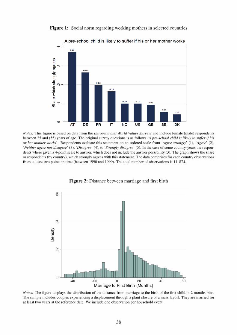
Figure 1: Social norm regarding working mothers in selected countries

Notes: This figure is based on data from the European and World Values Surveys and include female (male) respondents

between 25 and (55) years of age. The original survey questions is as follows ‘A pre-school child is likely to suffer if his

or her mother works’. Respondents evaluate this statement on an ordered scale from ‘Agree strongly’ (1), ‘Agree’ (2),

‘Neither agree nor disagree’ (3), ‘Disagree’ (4), to ‘Strongly disagree’ (5). In the case of some country-years the respon-

dents where given a 4-point scale to answer, which does not include the answer possibility (3). The graph shows the share

or respondents (by country), which strongly agrees with this statement. The data comprises for each country observations

from at least two points in time (between 1990 and 1999). The total number of observations is 11, 574.

Figure 2: Distance between marriage and first birth

Notes: The figure displays the distribution of the distance from marriage to the birth of the first child in 2 months bins.

The sample includes couples experiencing a displacement through a plant closure or a mass layoff. They are married for

at least two years at the reference date. We include one observation per household event.

38

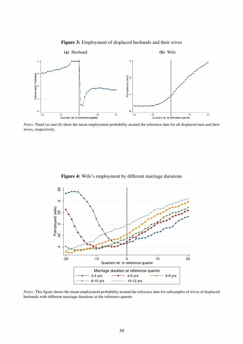
Figure 3: Employment of displaced husbands and their wives

(a) Husband (b) Wife

Notes: Panel (a) and (b) show the mean employment probability around the reference date for all displaced men and their

wives, respectively.

Figure 4: Wife’s employment by different marriage durations

Notes: This figure shows the mean employment probability around the reference date for subsamples of wives of displaced

husbands with different marriage durations at the reference quarter.

39

Figure 5: Employment of displaced husbands with control groups

(a) CG1: No firm event

(b) CG2: Non-displaced in mass layoff

Notes: Comparison of the probability to be employed of men that are displaced (blue, square) to men without firm event

at the reference date (red, x) in panel (a) and to non-displaced men working in mass layoff firms at the reference date in

(b) based on estimation equation (1). Control groups are reweighted to resemble the displaced group in time-invariant

husband and wife characteristics, household composition, employment outcomes of the husband and characteristics of

husband’s employer (see Footnote 17 for details). The employment probability of the control group is adjusted by its

mean difference relative to the displaced group. The graphs to the right plot the difference between the two lines with the

corresponding 95% confidence interval.

40

Figure 6: Employment of displaced husbands’ wives with control groups

(a) CG1: No firm event

(b) CG2: Non-displaced in mass layoff

(c) CG3: Displaced in the future

Notes: Comparison of the probability to be employed of wives with displaced husbands (blue, square) to those with

husbands without firm event at the reference date (red, x) in panel (a), with non-displaced husbands working in mass

layoff firms at the reference date in (b), and with husbands displaced 16 quarters after the reference date in (c) based on

estimation equation (1). CG1 and CG2 are reweighted to resemble the displaced group as explained in Figure 5. The

employment probability of the control group is adjusted by its mean difference relative to the displaced group. The graphs

to the right plot the difference between the two lines with the corresponding 95% confidence interval.

41

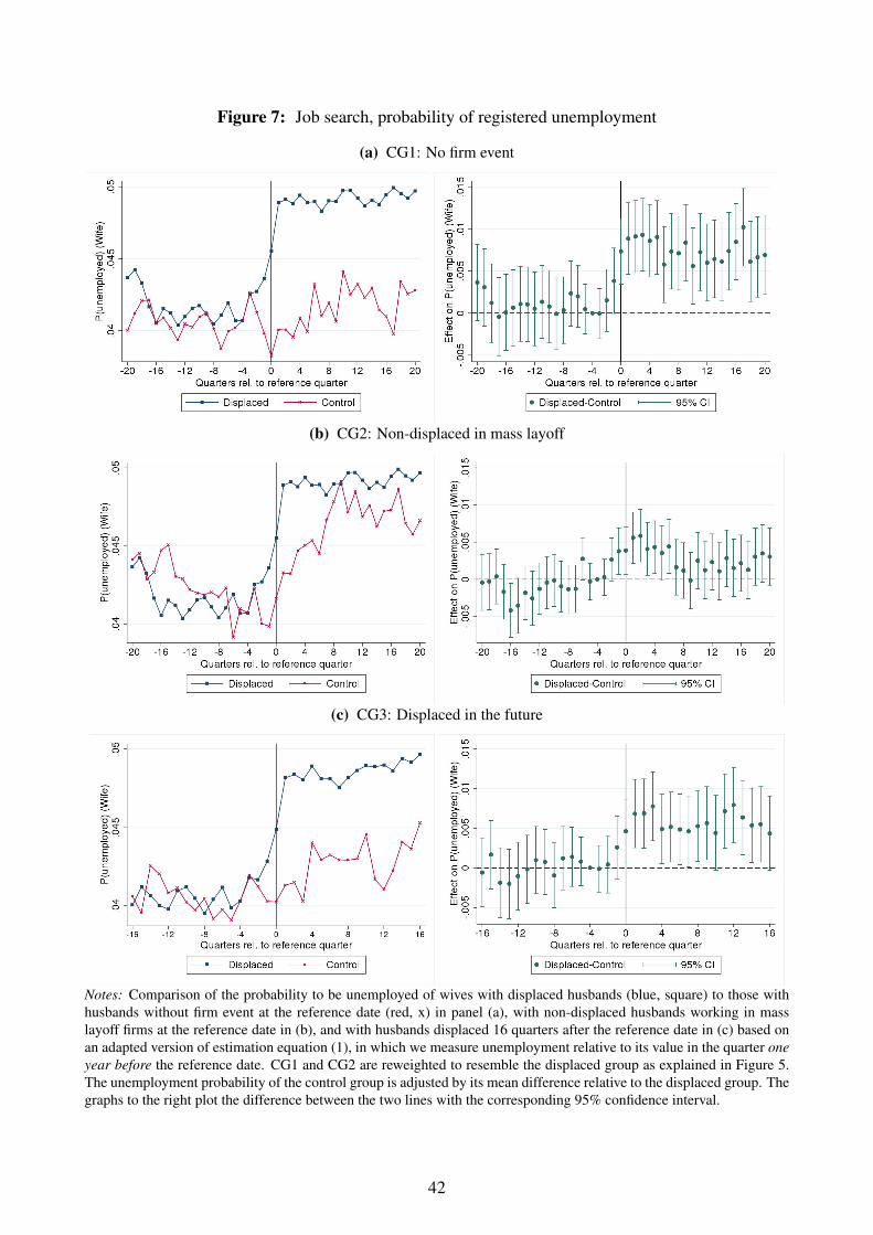
Figure 7: Job search, probability of registered unemployment

(a) CG1: No firm event

(b) CG2: Non-displaced in mass layoff

(c) CG3: Displaced in the future

Notes: Comparison of the probability to be unemployed of wives with displaced husbands (blue, square) to those with

husbands without firm event at the reference date (red, x) in panel (a), with non-displaced husbands working in mass

layoff firms at the reference date in (b), and with husbands displaced 16 quarters after the reference date in (c) based on

an adapted version of estimation equation (1), in which we measure unemployment relative to its value in the quarter one

year before the reference date. CG1 and CG2 are reweighted to resemble the displaced group as explained in Figure 5.

The unemployment probability of the control group is adjusted by its mean difference relative to the displaced group. The

graphs to the right plot the difference between the two lines with the corresponding 95% confidence interval.

42

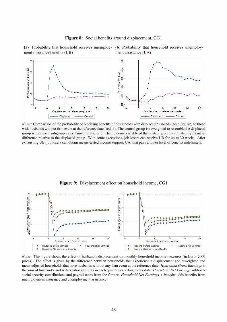
Figure 8: Social benefits around displacement, CG1

(a) Probability that household receives unemploy-

ment insurance benefits (UB)

(b) Probability that household receives unemploy-

ment assistance (UA)

Notes: Comparison of the probability of receiving benefits of households with displaced husbands (blue, square) to those

with husbands without firm event at the reference date (red, x). The control group is reweighted to resemble the displaced

group within each subgroup as explained in Figure 5. The outcome variable of the control group is adjusted by its mean

difference relative to the displaced group. With some exceptions, job losers can receive UB for up to 30 weeks. After

exhausting UB, job losers can obtain means-tested income support, UA, that pays a lower level of benefits indefinitely.

Figure 9: Displacement effect on household income, CG1

Notes: This figure shows the effect of husband’s displacement on monthly household income measures (in Euro, 2000

prices). The effect is given by the difference between households that experience a displacement and reweighted and

mean-adjusted households that have husbands without any firm event at the reference date. Household Gross Earnings is

the sum of husband’s and wife’s labor earnings in each quarter according to tax data. Household Net Earnings subtracts

social security contributions and payroll taxes from the former. Household Net Earnings + benefits adds benefits from

unemployment insurance and unemployment assistance.

43

Figure 10: Divorce and fertility around displacement

(a) CG1: No firm event

(b) CG2: Non-displaced in mass layoff

Notes: Comparison of the probability to live in divorce (left) and the number of births (right) for households with husbands

experiencing a displacement (blue, square) to households with husbands without firm event (red, x) at the reference date

in panel (a) and with non-displaced husbands working in mass layoff firms at the reference date in (b). CG1 and CG2

are reweighted to resemble the displaced group as explained in Figure 5. The number of births of the control group is

adjusted by its mean difference relative to the displaced group. Divorce is only displayed after the reference date, since

couples are required not to divorce until that date.

44

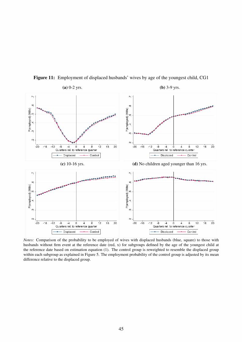
Figure 11: Employment of displaced husbands’ wives by age of the youngest child, CG1

(a) 0-2 yrs. (b) 3-9 yrs.

(c) 10-16 yrs. (d) No children aged younger than 16 yrs.

Notes: Comparison of the probability to be employed of wives with displaced husbands (blue, square) to those with

husbands without firm event at the reference date (red, x) for subgroups defined by the age of the youngest child at

the reference date based on estimation equation (1). The control group is reweighted to resemble the displaced group

within each subgroup as explained in Figure 5. The employment probability of the control group is adjusted by its mean

difference relative to the displaced group.

45

Table 1: Sample characteristics

Displaced Control

Closure Mass layoff Group 1 Group 2(1) (2) (3) (4)

I. Husband

Age (yrs) 39.41 39.05 40.09 39.74[38.95] [38.54] [39.84] [39.44](6.75) (6.79) (6.63) (6.67)

Experience in employment (yrs) 16.97 16.70 18.54 18.06[17.03] [16.75] [18.61] [18.36](6.77) (6.72) (6.61) (6.46)

Tenure (yrs) 6.92 6.92 9.66 8.77[4.58] [4.73] [6.86] [8.11](6.24) (6.06) (6.91) (6.70)

Number of previous jobs 4.44 4.11 2.90 3.14(4.34) (4.17) (3.29) (3.49)

Number of previous mass layoffs 1.41 1.92 0.53 1.94(2.26) (2.39) (1.31) (2.46)

Share blue collar 0.47 0.48 0.38 0.44(0.50) (0.50) (0.49) (0.50)

Real Monthly Earnings (e) 2443.16 2500.61 2706.99 2672.92[2319.86] [2455.63] [2722.46] [2649.97](918.09) (776.33) (725.15) (722.34)

Censored earnings 0.16 0.20 0.25 0.24(0.37) (0.40) (0.43) (0.43)

II. Wife

Age (yrs) 36.66 36.39 36.99 37.40[36.38] [35.97] [36.77] [37.23](6.14) (6.20) (6.14) (6.13)

Experience in employment (yrs) 9.50 9.41 9.95 9.72[8.50] [8.37] [8.94] [8.73](6.15) (6.06) (6.28) (6.19)

Number previous jobs 1.57 1.52 1.49 1.53(2.64) (2.49) (2.46) (2.56)

Employed 0.49 0.50 0.50 0.50(0.50) (0.50) (0.50) (0.50)

Blue collar | employed 0.31 0.31 0.28 0.31(0.46) (0.46) (0.45) (0.46)

Real monthly earnings (e) | employed 1320.50 1343.11 1321.56 1320.63[1196.09] [1232.67] [1181.57] [1207.13](788.78) (800.86) (806.11) (795.31)

Earnings rel. to husband | employed 0.63 0.61 0.52 0.53(0.67) (0.66) (0.39) (0.44)

Censored earnings | employed 0.02 0.02 0.02 0.02(0.13) (0.15) (0.14) (0.14)

III. Household composition

Marriage duration (yrs) 12.20 12.00 13.06 12.84[11.20] [10.93] [12.40] [12.13](6.80) (6.76) (6.92) (6.84)

Number of children 1.39 1.38 1.41 1.38(1.00) (1.00) (0.99) (0.99)

Share with youngest child 0–2 0.18 0.19 0.16 0.16(0.38) (0.39) (0.37) (0.37)

Share with youngest child 3–9 0.36 0.36 0.35 0.35(0.48) (0.48) (0.48) (0.48)

Share with youngest child 10–16 0.20 0.20 0.22 0.22(0.40) (0.40) (0.41) (0.41)

Continued on next page.

46

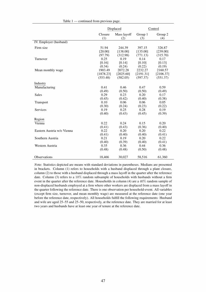
Table 1 — continued from previous page.

Displaced Control

Closure Mass layoff Group 1 Group 2(1) (2) (3) (4)

IV. Employer (husband)

Firm size 51.94 244.39 397.15 326.87[20.00] [138.00] [135.00] [239.00](97.79) (312.98) (771.13) (315.70)

Turnover 0.25 0.19 0.14 0.17[0.16] [0.14] [0.10] [0.13](0.34) (0.24) (0.22) (0.19)

Mean monthly wage 1903.49 2072.28 2232.27 2160.57[1878.23] [2025.60] [2191.31] [2106.37](553.48) (582.05) (597.37) (551.37)

Industry

Manufacturing 0.41 0.46 0.47 0.59(0.49) (0.50) (0.50) (0.49)

Sales 0.29 0.23 0.20 0.17(0.45) (0.42) (0.40) (0.38)

Transport 0.10 0.06 0.06 0.05(0.30) (0.24) (0.23) (0.22)

Services 0.19 0.25 0.28 0.19(0.40) (0.43) (0.45) (0.39)

Region

Vienna 0.22 0.24 0.15 0.20(0.41) (0.43) (0.36) (0.40)

Eastern Austria w/o Vienna 0.22 0.20 0.20 0.22(0.41) (0.40) (0.40) (0.41)

Southern Austria 0.21 0.19 0.20 0.22(0.40) (0.39) (0.40) (0.41)

Western Austria 0.35 0.36 0.44 0.36(0.48) (0.48) (0.50) (0.48)

Observations 18,466 30,027 58,516 61,360

Note: Statistics depicted are means with standard deviations in parentheses. Medians are presented

in brackets. Column (1) refers to households with a husband displaced through a plant closure,

column (2) to those with a husband displaced through a mass layoff in the quarter after the reference

date. Column (3) refers to a 10% random subsample of households with husbands without a firm

event in the quarter after the reference date. Households in column (4) are a 40% random sample of

non-displaced husbands employed at a firm where other workers are displaced from a mass layoff in

the quarter following the reference date. There is one observation per household-event. All variables

(except firm size, turnover, and mean monthly wage) are measured at the reference date (one year

before the reference date, respectively). All households fulfill the following requirements: Husband

and wife are aged 25–55 and 25–50, respectively, at the reference date. They are married for at least

two years and husbands have at least one year of tenure at the reference date.

47

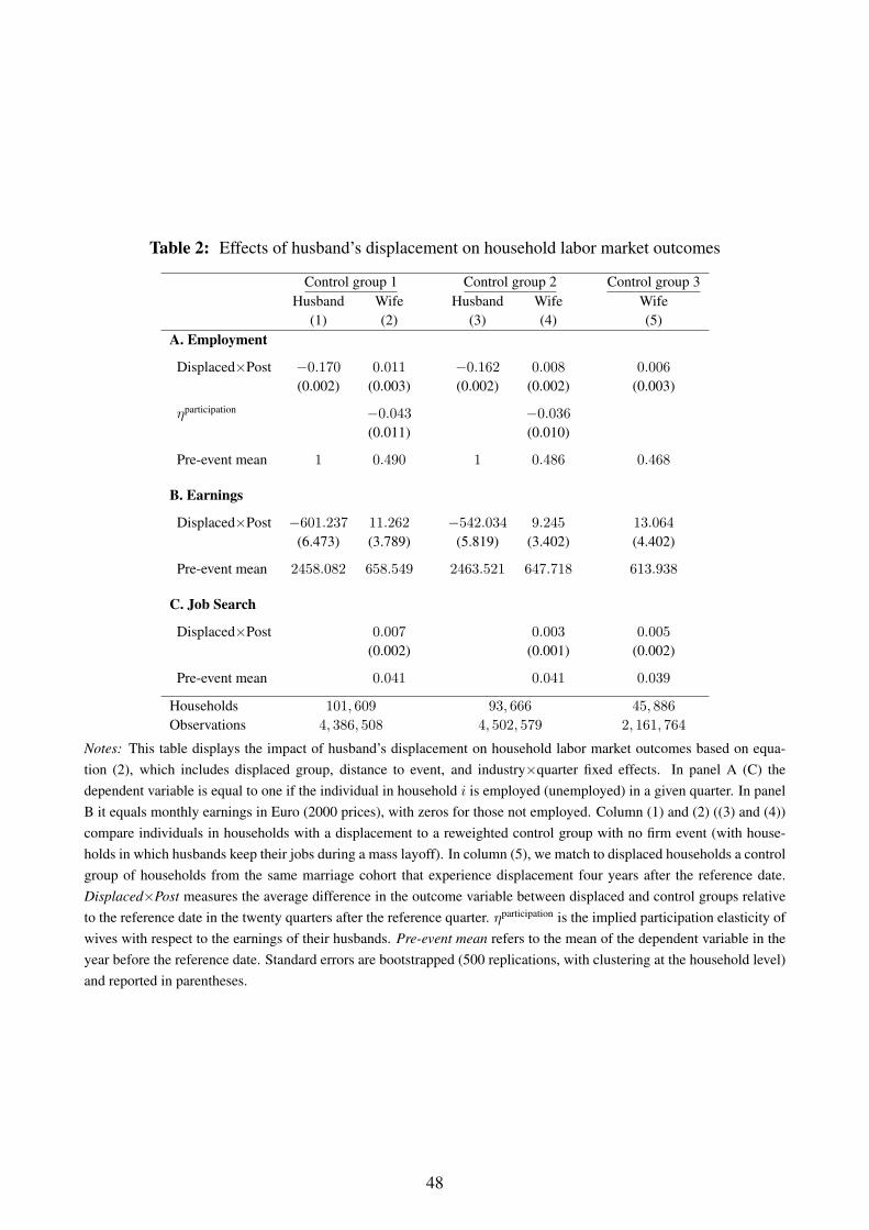
Table 2: Effects of husband’s displacement on household labor market outcomes

Control group 1 Control group 2 Control group 3

Husband Wife Husband Wife Wife

(1) (2) (3) (4) (5)

A. Employment

Displaced×Post −0.170 0.011 −0.162 0.008 0.006

(0.002) (0.003) (0.002) (0.002) (0.003)

ηparticipation −0.043 −0.036

(0.011) (0.010)

Pre-event mean 1 0.490 1 0.486 0.468

B. Earnings

Displaced×Post −601.237 11.262 −542.034 9.245 13.064

(6.473) (3.789) (5.819) (3.402) (4.402)

Pre-event mean 2458.082 658.549 2463.521 647.718 613.938

C. Job Search

Displaced×Post 0.007 0.003 0.005

(0.002) (0.001) (0.002)

Pre-event mean 0.041 0.041 0.039

Households 101, 609 93, 666 45, 886

Observations 4, 386, 508 4, 502, 579 2, 161, 764

Notes: This table displays the impact of husband’s displacement on household labor market outcomes based on equa-

tion (2), which includes displaced group, distance to event, and industry×quarter fixed effects. In panel A (C) the

dependent variable is equal to one if the individual in household i is employed (unemployed) in a given quarter. In panel

B it equals monthly earnings in Euro (2000 prices), with zeros for those not employed. Column (1) and (2) ((3) and (4))

compare individuals in households with a displacement to a reweighted control group with no firm event (with house-

holds in which husbands keep their jobs during a mass layoff). In column (5), we match to displaced households a control

group of households from the same marriage cohort that experience displacement four years after the reference date.

Displaced×Post measures the average difference in the outcome variable between displaced and control groups relative

to the reference date in the twenty quarters after the reference quarter. ηparticipation is the implied participation elasticity of

wives with respect to the earnings of their husbands. Pre-event mean refers to the mean of the dependent variable in the

year before the reference date. Standard errors are bootstrapped (500 replications, with clustering at the household level)

and reported in parentheses.

48

Table 3: Displacement effects by wife’s employment status prior reference date

Wife employed Wife not employed

Outcome Husband Wife Husband Wife

Earnings P(employed) Earnings Earnings P(employed) Earnings

(1) (2) (3) (4) (5) (6)

A. Control group 1

Displaced×Post −610.110 −0.008 −10.793 −595.601 0.019 22.378

(9.853) (0.003) (6.060) (8.120) (0.004) (5.002)

ηparticipation −0.079

(0.016)

Pre-event mean 2490.909 1 1376.356 2435.549 0.111 122.813

Households 43,366 59,165

B. Control group 2

Displaced×Post −549.429 −0.005 −4.616 −536.020 0.015 16.652

(8.979) (0.003) (5.207) (7.539) (0.003) (4.479)

ηparticipation −0.069

(0.015)

Pre-event mean 2495.640 1 1365.551 2441.058 0.113 124.521

Households 40,492 55,237

Notes: This table displays the impact of husband’s displacement on own earnings, spousal employment and earnings by

the employment status of the wife before the reference date. The left panel refers to the group of households in which the

wife was employed in all four quarters before the reference date. The panel to the right refers to the group of households

in which the wife was not employed in any of the four quarters before the reference date. Cluster-robust (at the household

level) standard errors are bootstrapped (500 replications) and reported in parentheses.

Table 4: Effects of husband’s displacement on household income

Prob. of HH receiving Monthly household income

UB UA Gross Net Net + benefits

(1) (2) (3) (4) (5)

A. Control group 1

Displaced×Post 0.077 0.023 −769.902 −474.298 −429.653

(0.003) (0.002) (18.332) (11.442) (11.164)

Pre-event mean 0.040 0.015 3701.048 2515.338 2530.745

Households 40, 771

B. Control group 2

Displaced×Post 0.066 0.021 −711.126 −441.015 −401.320

(0.003) (0.002) (17.695) (11.046) (10.789)

Pre-event mean 0.040 0.015 3772.018 2553.295 2575.851

Households 34, 031

Notes: This table displays the impact of husband’s displacement on household income measures based on (2) for the

subsample of households with a reference date in 2001 or later. The dependent variable is equal to one if the household

receives unemployment insurance benefits and unemployment assistance in column (1) and (2), respectively. In column

(3), the outcome is household gross earnings (sum of the couple’s labor earnings). Household net earnings in column (4)

are gross earnings minus social security contributions and payroll taxes. In column (5), we add unemployment benefits

and assistance to the former. All income variables are measured in Euro (2000 prices) on a monthly basis. In panel A

(B) we compare individuals in households with a displacement to a reweighted control group of households with no firm

event (with households in which husbands keep their jobs during a mass layoff). Standard errors are bootstrapped (500

replications, with clustering at the household level) and reported in parentheses.

49

Table 5: Effects of husband’s displacement on divorce and fertility

P(Divorce) No. of births

(1) (2)

A. Control group 1

Displaced×Post 0.004 −0.001

(0.001) (0.001)

Pre-event mean 0.000 0.014

Households 101, 609

B. Control group 2

Displaced×Post −0.001 −0.000

(0.001) (0.001)

Pre-event mean 0.000 0.014

Households 93, 666

Notes: This table displays the impact of husband’s displacement on the risk to be divorced in a given quarter in column

(1) and the number of births per quarter in (2). The upper (lower) panel compare households with a displacement to a

reweighted control group with no firm event (with households in which husbands keep their jobs during a mass layoff).

Standard errors are clustered at the household level and reported in parentheses.

50

Table 6: Wife’s employment response by age of youngest child

0–2 years 3–9 years 10–15 years None younger

than 16 years

(1) (2) (3) (4)

A. Control group 1

Displaced×Post 0.011 0.008 0.009 0.001

(0.008) (0.005) (0.005) (0.004)

ηparticipation −0.054 −0.033 −0.034 −0.005

(0.038) (0.022) (0.020) (0.015)

Pre-event mean 0.182 0.466 0.584 0.659

Earnings rel. to husband | employed 0.491 0.514 0.539 0.709

Households 18,248 36,950 22,031 26,894

B. Control group 2

Displaced×Post 0.005 0.007 0.015 0.005

(0.007) (0.004) (0.004) (0.004)

ηparticipation −0.031 −0.035 −0.065 −0.020

(0.034) (0.019) (0.019) (0.016)

Pre-event mean 0.181 0.465 0.585 0.661

Earnings rel. to husband | employed 0.482 0.515 0.548 0.699

Households 17,623 34,883 20,560 25,153

C. Control group 3

Displaced×Post -0.001 0.013 0.011 0.006

(0.008) (0.005) (0.007) (0.007)

Pre-event mean 0.178 0.447 0.567 0.656

Households 11,927 20,619 10,844 11,536

Notes: This table displays the impact of husband’s displacement on spousal employment for subgroups defined by the

age of the youngest child at the reference date. The first (second) panel compare households with a displacement to a

reweighted control group with no firm event (with households in which husbands keep their jobs during a mass layoff).

The third panel compares the displaced group to a control group of households that experience displacement four years

after that date. Standard errors are bootstrapped (500 replications, with clustering at the household level) and reported in

parentheses.

51

Table 7: Displacement effects by wife’s earnings potential, CG1

Low High

Outcome Husband Wife Husband Wife

Earnings P(employed) Earnings Earnings P(employed) Earnings

(1) (2) (3) (4) (5) (6)

A. Measure 1: Earnings

Displaced×Post −558.957 0.008 7.241 −649.244 0.017 20.328

(7.531) (0.003) (4.616) (15.287) (0.006) (11.338)

ηparticipation −0.035 −0.072

(0.014) (0.025)

Pre-event mean 2384.058 0.459 548.609 2711.692 0.580 1008.921

Households 68,925 20,959

B. Measure 2: Experience

Displaced×Post −562.861 0.008 2.656 −598.032 0.012 16.496

(9.725) (0.004) (6.365) (9.077) (0.004) (6.238)

ηparticipation −0.035 −0.049

(0.019) (0.017)

2424.419 0.464 593.651 2491.314 0.510 714.223

Households 44,013 45,800

C. Measure 3: Education

Displaced×Post −505.811 0.010 9.704 −659.886 0.015 16.063

(8.900) (0.004) (5.478) (12.267) (0.005) (9.059)

ηparticipation −0.045 −0.063

(0.020) (0.021)

Pre-event mean 2306.676 0.405 468.030 2700.320 0.502 699.960

Households 43,822 29,762

Notes: This table displays the impact of husband’s displacement on own earnings, spousal employment and earnings by

measures of wife’s earnings potential. Measure 1: High indicates that the wife earned more than 33% of the wage of

husbands in the year before marriage. Measure 2: High indicates above median experience compared to other wives in

the year before marriage. Measure 3: High indicates that the completed education of the wife is beyond compulsory

schooling and apprenticeship education. Pre-marriage wage and experience are only available for those married after

1974. Education is only available for women with children. Results based on control group 2 are in Table A10. Standard

errors are bootstrapped (500 replications, with clustering at the household level) and reported in parentheses.

52

Table 8: Displacement effects by plant wage level and unemployment rate at reference date

Below median Above median

Outcome Husband Wife Husband Wife

Earnings P(employed) Earnings Earnings P(employed) Earnings

(1) (2) (3) (4) (5) (6)

A. Subgroups by plant wage level at reference date

Control group 1

Displaced×Post −485.974 0.007 1.737 −767.597 0.015 19.703

(9.787) (0.004) (6.289) (10.888) (0.005) (6.653)

ηparticipation −0.032 −0.055

(0.018) (0.017)

Pre-event mean 2239.607 0.505 676.410 2785.463 0.515 711.476

Households 40,939 40,903

Control group 2

Displaced×Post −466.395 0.006 2.484 −693.665 0.010 13.905

(9.293) (0.004) (5.889) (10.852) (0.004) (5.966)

ηparticipation −0.028 −0.042

(0.018) (0.015)

Pre-event mean 2287.456 0.506 677.026 2796.831 0.507 692.800

Households 38,013 34,830

B. Subgroups by male unemployment rate at reference date

Control group 1

Displaced×Post −613.381 0.017 14.903 −587.012 0.006 9.024

(9.652) (0.004) (5.747) (8.486) (0.004) (5.245)

ηparticipation −0.067 −0.025

(0.016) (0.015)

Pre-event mean 2463.174 0.466 607.385 2457.220 0.511 702.639

Households 50,906 51,311

Control group 2

Displaced×Post −550.786 0.010 12.033 −540.268 0.006 6.975

(8.944) (0.003) (4.662) (8.183) (0.003) (5.086)

ηparticipation −0.048 −0.026

(0.016) (0.016)

Pre-event mean 2478.804 0.465 605.749 2494.340 0.505 689.418

Households 46,973 46,544

Notes: This table displays the impact of husband’s displacement on own earnings, spousal employment and earnings for

different subgroups. In panel A the wage level at plants are employer-specific fixed effects estimated based on the AKM

approach (Abowd et al., 1999), and provided by Haller (2017). These estimates are available only after 1994. In panel B

the male unemployment rate is measured at the husband’s employment district in the year of the reference date. Standard

errors are bootstrapped (500 replications, with clustering at the household level) and reported in parentheses.

53

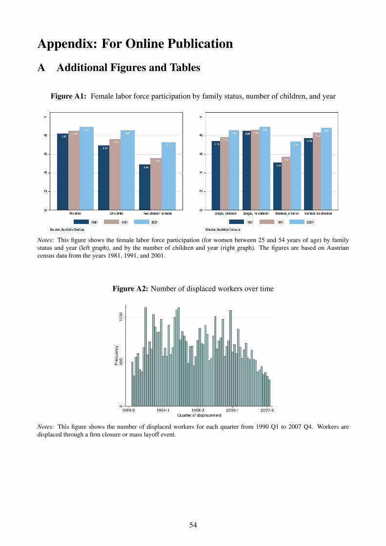
Appendix: For Online Publication

A Additional Figures and Tables

Figure A1: Female labor force participation by family status, number of children, and year

Notes: This figure shows the female labor force participation (for women between 25 and 54 years of age) by family

status and year (left graph), and by the number of children and year (right graph). The figures are based on Austrian

census data from the years 1981, 1991, and 2001.

Figure A2: Number of displaced workers over time

Notes: This figure shows the number of displaced workers for each quarter from 1990 Q1 to 2007 Q4. Workers are

displaced through a firm closure or mass layoff event.

54

Figure A3: Marriage duration at the reference quarter

Notes: The figure shows the distribution of marriage durations at the reference date in years.

Figure A4: Wives’ employment by different ages of the youngest child

Notes: This figure shows the mean employment probability for subsamples of wives of displaced husbands with different

ages of their youngest child at the reference date.

55

Figure A5: Employment of displaced husbands and their wives controlling for marriage duration and

quarter fixed effects

(a) Husband (b) Wife

Notes: Panel (a) and (b) plot the probability that a displaced husband and his wife, respectively, is employed relative to

the reference date holding constant the marriage duration and quarter of observation. We obtain the former by regressing

an indicator of husband/wife being employed on indicators for the quarterly distance to the reference quarter, indicators

for the marriage duration, and indicators for the quarter of observation.

Figure A6: Employment and wages of firms around the reference date

Notes: This figure plots the median number of employees and the average median monthly wage (in Euro, 2000 prices)

over time for the employers in our sample. Plant Closure refers to firms that close down the quarter following the

reference date. Mass Layoff refers to firms that reduce employment by at least 5% of their workforce the quarter after the

reference date. No Event firms have neither a mass layoff nor closure the quarter following the reference date. For each

quarter around the reference date, we include one observation per existing firm. We include any firm that employs at least

one husband of our sample.

56

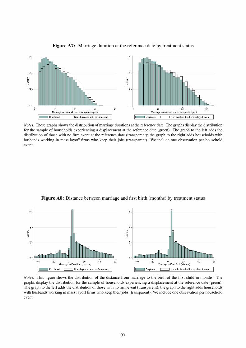
Figure A7: Marriage duration at the reference date by treatment status

Notes: These graphs shows the distribution of marriage durations at the reference date. The graphs display the distribution

for the sample of households experiencing a displacement at the reference date (green). The graph to the left adds the

distribution of those with no firm event at the reference date (transparent); the graph to the right adds households with

husbands working in mass layoff firms who keep their jobs (transparent). We include one observation per household

event.

Figure A8: Distance between marriage and first birth (months) by treatment status

Notes: This figure shows the distribution of the distance from marriage to the birth of the first child in months. The

graphs display the distribution for the sample of households experiencing a displacement at the reference date (green).

The graph to the left adds the distribution of those with no firm event (transparent); the graph to the right adds households

with husbands working in mass layoff firms who keep their jobs (transparent). We include one observation per household

event.

57

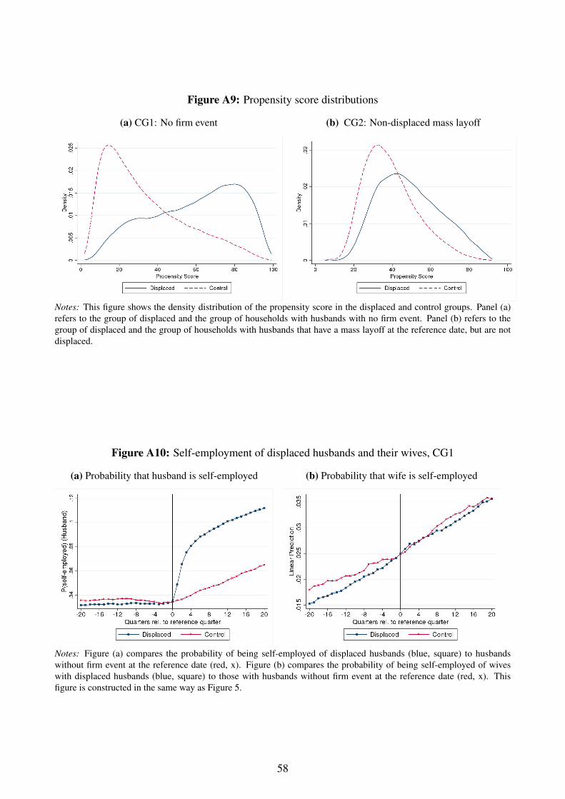
Figure A9: Propensity score distributions

(a) CG1: No firm event (b) CG2: Non-displaced mass layoff

Notes: This figure shows the density distribution of the propensity score in the displaced and control groups. Panel (a)

refers to the group of displaced and the group of households with husbands with no firm event. Panel (b) refers to the

group of displaced and the group of households with husbands that have a mass layoff at the reference date, but are not

displaced.

Figure A10: Self-employment of displaced husbands and their wives, CG1

(a) Probability that husband is self-employed (b) Probability that wife is self-employed

Notes: Figure (a) compares the probability of being self-employed of displaced husbands (blue, square) to husbands

without firm event at the reference date (red, x). Figure (b) compares the probability of being self-employed of wives

with displaced husbands (blue, square) to those with husbands without firm event at the reference date (red, x). This

figure is constructed in the same way as Figure 5.

58

Figure A11: Social benefits around displacement, CG2

(a) Probability that household receives unemploy-

ment insurance benefits (UB)

(b) Probability that household receives unemploy-

ment assistance (UA)

Notes: Comparison of the probability of receiving benefits of households with displaced husbands (blue, square) to those

with non-displaced husbands working at mass layoff employers at the reference date (red, x). The control group is

reweighted to resemble the displaced group within each subgroup as explained in Figure 5. The employment probability

of the control group is adjusted by its mean difference relative to the displaced group. With some exceptions, job losers

can receive UB for up to 30 weeks. After exhausting UB, job losers can obtain means-tested income support, UA, that

pays a lower level of benefits indefinitely.

Figure A12: Displacement effect on household income, CG2

Notes: This figure shows the effect of husband’s displacement on monthly household income measures (in Euro, 2000

prices). The effect is given by the difference between households that experience a displacement and reweighted and

mean-adjusted households with non-displaced husbands who work at mass layoff employers at the reference date. House-

hold Gross Earnings is the sum of husband’s and wife’s labor earnings in each quarter according to tax data. Household

Net Earnings subtracts social security contributions and payroll taxes from the former. Household Net Earnings + benefits

adds benefits from unemployment insurance and unemployment assistance.

59

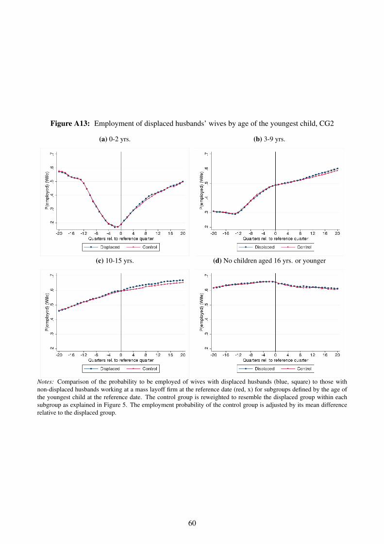
Figure A13: Employment of displaced husbands’ wives by age of the youngest child, CG2

(a) 0-2 yrs. (b) 3-9 yrs.

(c) 10-15 yrs. (d) No children aged 16 yrs. or younger

Notes: Comparison of the probability to be employed of wives with displaced husbands (blue, square) to those with

non-displaced husbands working at a mass layoff firm at the reference date (red, x) for subgroups defined by the age of

the youngest child at the reference date. The control group is reweighted to resemble the displaced group within each

subgroup as explained in Figure 5. The employment probability of the control group is adjusted by its mean difference

relative to the displaced group.

60

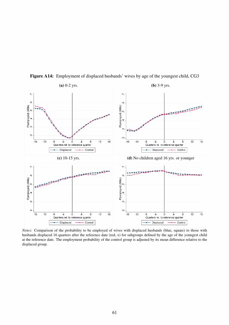
Figure A14: Employment of displaced husbands’ wives by age of the youngest child, CG3

(a) 0-2 yrs. (b) 3-9 yrs.

(c) 10-15 yrs. (d) No children aged 16 yrs. or younger

Notes: Comparison of the probability to be employed of wives with displaced husbands (blue, square) to those with

husbands displaced 16 quarters after the reference date (red, x) for subgroups defined by the age of the youngest child

at the reference date. The employment probability of the control group is adjusted by its mean difference relative to the

displaced group.

61

Table A1: Wife’s Labor Supply Elasticities in Added Worker Effect Studies

Country Time Data Sample households Wife’s labor supply (semi-)elasticity Comments

1.Variation in spousal income in a structural life-cycle model of household labor supply

Haan and Prowse (2015) DE 1991-2005 GSOEP Married couples aged Participation −0.025a Comparison of simulated optimal behavior

16–65 with labor market expe-

rience

without leisure comple-

mentarity−0.056a

when spouse is vs. is not subject to unanticipated job

destruction

Blundell et al. (2016) US 1999-2009 PSIDHouseholds with participating

and married maleHours (total response) −0.75

Permanent shock in spousal wage process identified

in structural model

head aged 30–57 Extensive margin −0.168

Blundell et al. (2018) US 1999-2015 PSIDMarried couples with wife

aged 25–65

Permanent shock in spousal wage process identified

in structural model

with children aged ≤ 10 Hours (total response) −0.296

Extensive margin −0.193

Intensive margin −0.170

no children aged ≤ 10 Hours (total response) −0.14

Extensive margin −0.065

Intensive margin −0.088

2.Quasi-experimental variation in spousal income through job displacements

Stephens (2002) US 1968-1992 PSID Married couples aged 25–65 Hours −0.50Displacement through plant closure/moving, layoff,

firing

Kohara 2010b JP 1993-2004 Panel survey Wife aged 24-35 in 1993 Hours −0.893a Layoff, plant closure, and bankruptcy

Eliason (2011) SE 1987 Admin panel Married couples aged 25–51 Earnings 0.44 Plant closure

Hardoy and Schøne (2014) NO 2002 Admin panel Married couples aged 25–55 Employment 0.09 Closure, mass layoff; couple requiredEarnings 0.07 to stay married in post-treatment period

with wife not employed at dis-

placementEarnings −0.5

Bredtmann et al. (2018) C-EU 2004-2013 EU-SILCMarried/cohabiting couples

aged 16–65Employment 0.12a

Continental Europe (C-EU) refers to AT, BE, DE, FR,

LU, and the NL

3.Quasi-experimental variation in spousal income through social insurance benefits

Cullen and Gruber (2000) US1984-88,

1990-92SIPP Married couples aged 25–54 Hours [−0.49,−1.07]

Lower and upper bound estimates, variation in

spousal UI benefits

Autor et al. (2017) NO 1989-2011 Admin panel

Married couples, one spouse

(< 62) applying for DI bene-

fits

Employment −0.345

Simulated response to permanent change in spousal

income in structural model, no separate elasticities by

sex

Fadlon and Nielsen (2017) DK 1980-2011 Admin panel

Married/cohabiting couples,

widows (< 67) with spouse

dying at age 45–80

Participation −0.13 Variation in spousal survivor benefits

Notes: The (semi-)elasticity refers to the change in wife’s labor supply to a 1% change in husband’s income. For the elasticity of hours and earnings, the wife’s response is relative to the baseline mean (in %). For the participation

and employment elasticity, the response is in absolute terms (in percentage points). a Assuming a mean husband’s income loss of 20%. b This study is published in the Journal of Population Economics Volume 23(4). The detailsfor all other listed studies can be found in the List of References in the paper.

62

Table A2: Gender identity norms and beliefs on child-care in Austria and some selected high-income countries

Share of survey respondents which strongly agreeswith the respective statement across countries

AT DE DK FR IT NO SE GB US Total

1.) A pre-school child is likely to suffer if [. . . ] mother works 0.37 0.26 0.04 0.20 0.16 0.10 0.05 0.09 0.10 0.17

2.) A working mother [as good as] a mother who does not work 0.23 0.18 0.56 0.51 0.19 0.47 0.51 0.23 0.29 0.32

3.) Important for successful marriage: Sharing household chores 0.28 0.23 0.45 0.39 0.30 0.34 0.55 0.45 0.49 0.36

4.) Both husband and wife should contribute to household income 0.29 0.17 0.26 0.39 0.25 0.35 0.54 0.14 0.23 0.28

Notes: These figures are based on data from the European and World Values Surveys and include male respondents between 25 and 55 years of age, and female respondents between

25 and 50 years of age. The original survey questions on statement 1 is as follows ‘A pre-school child is likely to suffer if his or her mother works’. The original survey questions on

statement 2 is as follows ‘A working mother can establish just as warm and secure a relationship with her children as a mother who does not work’. The original survey questions

on statement 3 is as follows ‘Important for successful marriage: Sharing household chores’. Respondents are asked to evaluate this statement on an ordered scale from ‘Very’ (1),

‘Rather’ (2), to ‘Not very’ (3). The table summarizes the share or respondents (by country), which strongly agrees with statements 1 to 3, and which answers statement 4 with very

important. The original survey questions on statement 4 is as follows ‘Both the husband and wife should contribute to household income’. Respondents are asked to evaluate these three

statements on an ordered scale from ‘Agree strongly’ (1), ‘Agree’ (2), ‘Neither agree nor disagree’ (3), ‘Disagree’ (4), to ‘Strongly disagree’ (5). In the case of some country-years the

respondents where given a 4-point scale to answer, which does not include the answer possibility ‘Neither agree nor disagree’. The data comprises for each country observations from

at least two points in time. The first period is for each country the year 1990. The second (and third) period is AT: 1999, DE: 1997 and 1999, DK: 1999, FR: 1999, IT: 1999, NO: 1996,

SE: 1996 and 1999, GB: 1998 and 1999, US: 1995 and 1996. The total number of observations varies across questions (Min: 11, 574, Max: 16, 729).

63

Table A3: Effects of husband’s displacement on household employment

Control group 1 Control group 2 Control group 3

Husband Wife Husband Wife Wife

(1) (2) (3) (4) (5)

Prior event

δ−5 −0.008 0.002 −0.009 −0.002

(0.002) (0.004) (0.001) (0.003)

δ−4 −0.003 0.002 −0.004 0.002 −0.004

(0.001) (0.004) (0.001) (0.003) (0.005)

δ−3 −0.002 0.001 −0.005 0.001 −0.002

(0.001) (0.004) (0.001) (0.003) (0.004)

δ−2 −0.002 −0.000 −0.003 −0.000 0.001

(0.001) (0.003) (0.001) (0.003) (0.004)

δ−1 −0.000 0.001 0.000 −0.001 −0.000

(0.000) (0.002) (0.000) (0.002) (0.002)

Post event

δ1 −0.280 0.004 −0.278 0.004 0.005

(0.002) (0.002) (0.002) (0.002) (0.002)

δ2 −0.173 0.009 −0.162 0.007 0.007

(0.002) (0.003) (0.002) (0.002) (0.003)

δ3 −0.144 0.013 −0.132 0.009 0.008

(0.003) (0.003) (0.002) (0.003) (0.004)

δ4 −0.131 0.014 −0.123 0.009 0.006

(0.003) (0.004) (0.002) (0.003) (0.004)

δ5 −0.123 0.013 −0.116 0.010

(0.003) (0.004) (0.003) (0.003)

Pre-event mean 1 0.490 1 0.486 0.468

Households 101, 609 93, 666 45, 886

Observations 4, 386, 508 4, 502, 579 2, 161, 764

Notes: This table displays the impact of husband’s displacement on own and spousal employment based on equation (2),

which includes displaced group, distance to event, and industry×quarter fixed effects. The dependent variable is equal to

one if husband/wife in household i is employed in a given quarter. Column (1) and (2) ((3) and (4)) compare individuals

in households with a displacement to a reweighted control group with no firm event (with households in which husbands

keep their jobs during a mass layoff). In column (5), we match to displaced households a control group of households from

the same marriage cohort that experience displacement four years after the reference date. The coefficient δl measures

the average difference between employment in displaced and reweighted control groups l years to the reference quarter

relative to the difference at the reference quarter. Pre-event mean refers to the mean employment in the year before the

reference date. Standard errors are bootstrapped (500 replications, with clustering at the household level) and reported in

parentheses.

64

Table A4: Effects of husband’s displacement on household earnings

Control group 1 Control group 2 Control group 3

Husband Wife Husband Wife Wife

(1) (2) (3) (4) (5)

Prior event

δ−5 −6.642 5.572 −3.709 −4.608

(4.983) (6.223) (5.540) (4.848)

δ−4 9.554 4.556 5.236 0.606 −3.661

(3.833) (5.853) (5.202) (4.679) (6.814)

δ−3 9.840 1.943 2.542 −1.637 −1.202

(3.538) (5.389) (4.639) (4.155) (5.982)

δ−2 9.687 −1.050 5.231 −1.866 4.143

(3.011) (4.360) (3.686) (3.671) (4.908)

δ−1 −2.522 −0.694 −1.990 −1.148 1.391

(1.702) (2.647) (1.925) (2.457) (3.001)

Post event

δ1 −810.046 5.201 −783.445 5.618 11.390

(6.049) (2.696) (5.564) (2.283) (3.153)

δ2 −612.960 9.363 −554.224 7.261 11.581

(6.611) (4.071) (6.382) (3.552) (4.768)

δ3 −554.129 13.180 −482.088 9.510 15.370

(7.308) (4.547) (6.944) (4.120) (5.643)

δ4 −523.447 15.659 −454.925 10.312 14.027

(8.092) (5.122) (7.372) (4.600) (6.212)

δ5 −504.559 12.939 −434.683 13.541

(8.370) (5.385) (7.774) (4.923)

Pre-event mean 2458.082 658.549 2463.521 647.718 613.938

Households 101, 609 93, 666 45, 886

Observations 4, 386, 508 4, 502, 579 2, 161, 764

Notes: This table displays the impact of husband’s displacement on own and spousal monthly earnings in Euro (2000

prices) based on equation (2), which includes displaced group, distance to event, and industry×quarter fixed effects. The

dependent variable is set to zero if an individual is not employed. This table is constructed in the same way as Table A3.

Pre-event mean refers to the mean earnings in the year before the reference date. Standard errors are bootstrapped (500

replications, with clustering at the household level) and reported in parentheses.

65

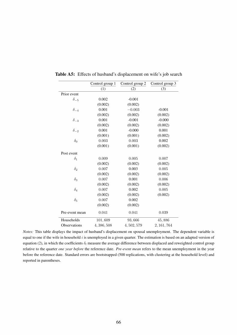
Table A5: Effects of husband’s displacement on wife’s job search

Control group 1 Control group 2 Control group 3

(1) (2) (3)

Prior event

δ−5 0.002 -0.001

(0.002) (0.002)

δ−4 0.001 −0.003 -0.001

(0.002) (0.002) (0.002)

δ−3 0.001 -0.001 -0.000

(0.002) (0.002) (0.002)

δ−2 0.001 -0.000 0.001

(0.001) (0.001) (0.002)

δ0 0.003 0.003 0.002

(0.001) (0.001) (0.002)

Post event

δ1 0.009 0.005 0.007

(0.002) (0.002) (0.002)

δ2 0.007 0.003 0.005

(0.002) (0.002) (0.002)

δ3 0.007 0.001 0.006

(0.002) (0.002) (0.002)

δ4 0.007 0.002 0.005

(0.002) (0.002) (0.002)

δ5 0.007 0.002

(0.002) (0.002)

Pre-event mean 0.041 0.041 0.039

Households 101, 609 93, 666 45, 886

Observations 4, 386, 508 4, 502, 579 2, 161, 764

Notes: This table displays the impact of husband’s displacement on spousal unemployment. The dependent variable is

equal to one if the wife in household i is unemployed in a given quarter. The estimation is based on an adapted version of

equation (2), in which the coefficients δl measure the average difference between displaced and reweighted control group

relative to the quarter one year before the reference date. Pre-event mean refers to the mean unemployment in the year

before the reference date. Standard errors are bootstrapped (500 replications, with clustering at the household level) and

reported in parentheses.

66

Table A6: Effects of husband’s displacement on household income, control group 1

Prob. of HH receiving Monthly household income

UB UA Gross Net Net + benefits

(1) (2) (3) (4) (5)

Prior event

δ−1 -0.004 0.001 −17.208 −0.588 −2.297

(0.003) (0.002) (7.634) (4.988) (4.923)

Post event

δ1 0.223 0.015 −835.031 −530.986 −422.586

(0.004) (0.002) (14.467) (9.102) (8.483)

δ2 0.069 0.038 −794.45 −489.393 −442.212

(0.004) (0.002) (19.488) (12.243) (11.867)

δ3 0.037 0.024 −770.498 −472.311 −443.354

(0.004) (0.003) (20.720) (13.008) (12.682)

δ4 0.028 0.018 −734.077 −445.916 −425.226

(0.004) (0.003) (22.537) (14.106) (13.780)

δ5 0.025 0.017 −715.350 −432.797 −414.887

(0.004) (0.003) (23.667) (14.803) (14.518)

Pre-event mean 0.040 0.015 3701.048 2515.338 2530.745

Households 40, 771

Observations 1, 049, 450

Notes: This table displays the impact of husband’s displacement on household income measures based on (2) for the

subsample of households with a reference date in 2001 or later. The dependent variable is equal to one if the household

receives unemployment insurance benefits and unemployment assistance in column (1) and (2), respectively. In column

(3), the outcome is household gross earnings (sum of the couple’s labor earnings). Household net earnings in column (4)

are gross earnings minus social security contributions and payroll taxes. In column (5), we add unemployment benefits

and assistance to the former. All income variables are measured in Euro (2000 prices) on a monthly basis. We compare

individuals in households with a displacement to a reweighted control group of households with no firm event. The

coefficient δl measures the average difference between the outcome variable in the displaced and the reweighted control

group l years to the reference date relative to the corresponding difference at the reference quarter. Pre-event mean refers

to the mean outcome in the year before the reference date. Standard errors are bootstrapped (500 replications, with

clustering at the household level) and reported in parentheses.

67

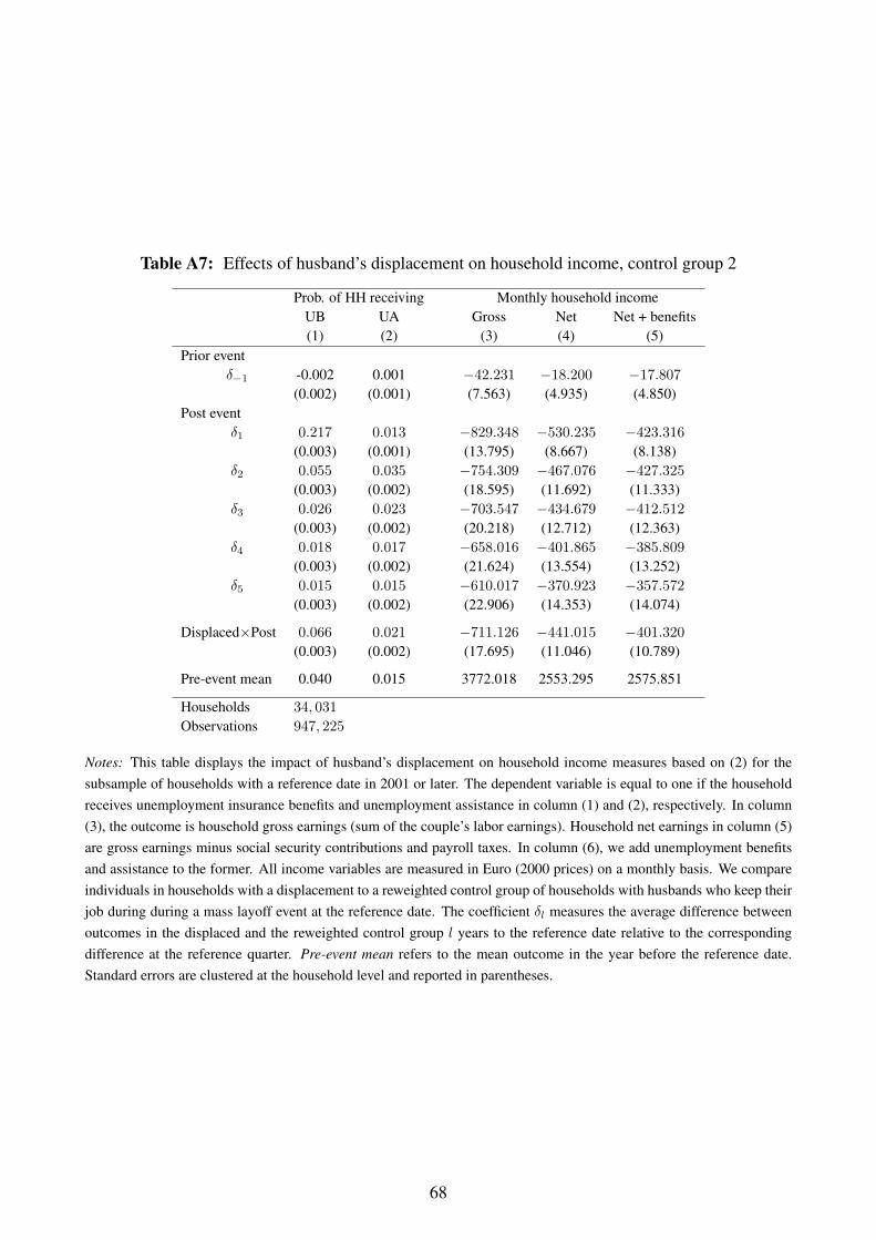
Table A7: Effects of husband’s displacement on household income, control group 2

Prob. of HH receiving Monthly household income

UB UA Gross Net Net + benefits

(1) (2) (3) (4) (5)

Prior event

δ−1 -0.002 0.001 −42.231 −18.200 −17.807

(0.002) (0.001) (7.563) (4.935) (4.850)

Post event

δ1 0.217 0.013 −829.348 −530.235 −423.316

(0.003) (0.001) (13.795) (8.667) (8.138)

δ2 0.055 0.035 −754.309 −467.076 −427.325

(0.003) (0.002) (18.595) (11.692) (11.333)

δ3 0.026 0.023 −703.547 −434.679 −412.512

(0.003) (0.002) (20.218) (12.712) (12.363)

δ4 0.018 0.017 −658.016 −401.865 −385.809

(0.003) (0.002) (21.624) (13.554) (13.252)

δ5 0.015 0.015 −610.017 −370.923 −357.572

(0.003) (0.002) (22.906) (14.353) (14.074)

Displaced×Post 0.066 0.021 −711.126 −441.015 −401.320

(0.003) (0.002) (17.695) (11.046) (10.789)

Pre-event mean 0.040 0.015 3772.018 2553.295 2575.851

Households 34, 031

Observations 947, 225

Notes: This table displays the impact of husband’s displacement on household income measures based on (2) for the

subsample of households with a reference date in 2001 or later. The dependent variable is equal to one if the household

receives unemployment insurance benefits and unemployment assistance in column (1) and (2), respectively. In column

(3), the outcome is household gross earnings (sum of the couple’s labor earnings). Household net earnings in column (5)

are gross earnings minus social security contributions and payroll taxes. In column (6), we add unemployment benefits

and assistance to the former. All income variables are measured in Euro (2000 prices) on a monthly basis. We compare

individuals in households with a displacement to a reweighted control group of households with husbands who keep their

job during during a mass layoff event at the reference date. The coefficient δl measures the average difference between

outcomes in the displaced and the reweighted control group l years to the reference date relative to the corresponding

difference at the reference quarter. Pre-event mean refers to the mean outcome in the year before the reference date.

Standard errors are clustered at the household level and reported in parentheses.

68

Table A8: Displacement effects by youngest child

Outcome Husband Wife

Earnings P(employed) Earnings

(1) (2) (3)

Control group 1

age 0− 2 −509.603 0.011 7.949

(15.118) (0.008) (11.793)

age 3− 9 −552.944 0.008 12.988

(10.531) (0.005) (6.477)

age 10− 15 −652.137 0.009 6.222

(14.648) (0.005) (7.414)

No child −707.224 0.001 -6.027

(12.433) (0.005) (8.154)

Control group 2

age 0− 2t −473.784 0.005 6.828

(13.840) (0.007) (9.986)

age 3− 9 −501.594 0.007 11.157

(10.004) (0.004) (5.325)

age 10− 15 −585.793 0.015 14.937

(13.394) (0.004) (6.393)

No child −615.452 0.005 0.324

(12.210) (0.004) (7.418)

Control group 3

age 0− 2 −625.170 -0.001 25.420

(13.635) (0.008) (11.193)

age 3− 9 −681.030 0.013 21.459

(9.822) (0.005) (6.683)

age 10− 15 −778.636 0.011 14.136

(13.567) (0.007) (8.661)

No child −839.497 0.006 6.401

(12.906) (0.007) (11.360)

Notes: This table displays the impact of husband’s displacement for subgroups defined by the age of the youngest child

at the reference date. It is similar to Table 6, but it additionally includes the effects on husband’s earnings (1) and wife’s

earnings (3). The estimates measure the average difference in the corresponding outcome variable between displaced and

reweighted control groups after the reference quarter rel. to the difference at the reference date.

69

Table A9: Displacement effects by availability of nursery at reference date

No nursery in district Nursery in district

Outcome Husband Wife Husband Wife

Earnings P(employed) Earnings Earnings P(employed) Earnings

(1) (2) (3) (4) (5) (6)

Control group 1

Displaced×Post −503.182 0.005 20.075 −526.537 0.011 -7.443

(18.987) (0.010) (12.455) (25.127) (0.014) (21.868)

ηparticipation −0.020 −0.053

(0.045) (0.065)

Pre-event mean 2333.331 0.164 166.678 2496.618 0.206 243.037

Households 11,058 7,170

Control group 2

Displaced×Post −460.569 0.008 12.111 −482.589 0.003 4.978

(17.073) (0.008) (10.093) (22.442) (0.011) (17.933)

ηparticipation −0.044 −0.021

(0.040) (0.058)

Pre-event mean 2339.078 0.162 162.721 2497.289 0.205 241.980

Households 10,754 6,892

Notes: This table displays the impact of husband’s displacement on own earnings, spousal employment and earnings

by the availability of nurseries at the reference date. Nurseries provide child care for the under-three-year-old. The

availability is measured at the community level. We only look at wives with children aged 0–3 at the reference date.

Standard errors are bootstrapped (500 replications, with clustering at the household level) and reported in parentheses.

70

Table A10: Displacement effects by wife’s earnings potential, control group 2

Low High

Outcome Husband Wife Husband Wife

Earnings P(employed) Earnings Earnings P(employed) Earnings

(1) (2) (3) (4) (5) (6)

Measure 1: Earnings before marriage

Displaced×Post −511.376 0.007 6.656 −592.745 0.010 13.671

(6.587) (0.003) (3.848) (15.434) (0.005) (9.707)

ηparticipation −0.034 −0.045

(0.014) (0.024)

Pre-event mean 2390.720 0.456 544.524 2718.341 0.579 1002.762

Households 63,911 17,986

Measure 2: Experience before marriage

Displaced×Post −518.182 0.006 6.614 −539.480 0.010 9.419

(8.613) (0.004) (5.680) (9.089) (0.003) (5.340)

ηparticipation −0.024 −0.046

(0.018) (0.016)

Pre-event mean 2428.900 0.458 581.638 2496.457 0.507 706.263

Households 40,263 41,594

Measure 3: Education

Displaced×Post −453.777 0.008 7.848 −619.957 0.010 13.339

(8.453) (0.004) (4.808) (12.191) (0.005) (8.780)

ηparticipation −0.042 −0.043

(0.020) (0.020)

Pre-event mean 2315.542 0.399 457.583 2696.034 0.500 697.313

Households 40,168 26,208

Notes: This table displays the impact of husband’s displacement on own earnings, spousal employment and earnings by

measures of wife’s earnings potential. Measure 1: High indicates that the wife earned more than 33% of the wage of

husbands in the year before marriage. Measure 2: High indicates above median experience compared to other wives in

the year before marriage. Measure 3: High indicates that the completed education of the wife is beyond compulsory

schooling and apprenticeship education. Pre-marriage wage and experience are only available for those married after

1974. Education is only available for women with children. Standard errors are bootstrapped (500 replications, with

clustering at the household level) and reported in parentheses.

71

B Robustness analysis

In this section, we briefly summarize robustness checks using alternative defi-

nitions of displaced and control workers and variations in the weighting proce-

dure.

We start with sensitivity checks of our estimations using control group 1 and

2. First, we use an alternative, more restrictive measure to identify mass layoffs.

Now firms experience a mass layoff, if at least ten and at most fifty percent of

all workers are displaced from one quarter to the other.1 The graphical evidence

(see Figure B1a) and the corresponding estimates (see column (1) of Table B1)

illustrate that our main estimation results are robust to a change in the definition

of mass layoffs. Second, we match (in addition to the variables used in the main

specification, see footnote 17) also on employment outcomes of wives up to one

year before the reference date. The resulting estimates (see Figure B1b) are sim-

ilar and not statistically significantly different from the ones in the main specifi-

cation. Third, we focus on displaced workers from plant closures. Workers who

got displaced due to a mass layoff events are more prone to selection issues,

since the underlying process determining leavers and stayers within struggling

firms might be endogenous to workers’ labor market outcomes. In contrast,

there is no selection within a firm when it closes down, since all employees

are eventually displaced. The resulting estimates (see Figure B1c) are slightly

smaller and not as precisely estimated as in the main specification, but they are

indicating that results are robust. Fourth, we focus alternatively on displaced

workers from mass layoffs and exclude those from plant closures. Cases from

plant closure might be more selective at the firm level. For instance, we can

observe that these firms are typically much smaller than other firms with a mass

layoff event or no event at all (see Figure A6). In addition, we also match on

the firm size up to one year before the reference quarter. The resulting estimates

(see Figure B1d) are very comparable to those from our main results.

We now explore the robustness of our estimation result based on control

1Again, this relative cutoff applies to all establishments with 100 to 600 workers in the base

quarter. For smaller firms, the cutoffs are more than 6 workers leaving in firms with less than 20

employees and more than 10 if the establishment has more than 20 and less than 100 workers.

For establishments with more than 600 workers, at least 60 employees have to leave the firm in

order to make it count as mass layoff.

72

group 3. This approach exploits the timing of displacement and requires the

choice of a duration ∆ between the events of the households in the treatment

and the control group. Importantly, there is a trade-off in this choice: With a

smaller ∆, the treatment and control group’s displacement is closer in time and

there are hence more likely to be comparable. A larger distance in the date of

event allows us to compare outcomes of the two groups for more periods (Fadlon

and Nielsen, 2017). In our baseline specification we choose a ∆ of 16 quarters.

Now we consider values of 4, 8, and 12. It turns out that the specific choice of

∆ is not crucial (see Figure B2 and Table B2).

73

Figure B1: Displaced husband’s wife employment, robustness checks

(a) Stricter mass layoff cutoffs(b) Reweighting includes wives’ pre-event employ-

ment

(c) Displaced from plant closures only(d) Displaced and non-displaced from mass layoff

firms only

Notes: This figure provides robustness checks to Figure 6a and 6b. In Panel (a), we apply a stricter cutoff for mass

layoffs. In Panel (b), we additionally include employment outcomes of wives (up to one year before the reference date)

in the weighting procedure. In Panel (c), the group of displaced workers includes only those with a displacement due to

a plant closure. In Panel (d), we only look at displaced and non-displaced workers at firms that have a mass layoff in the

quarter after the reference date. We also match on the firm size up to one year before the reference quarter. The graphs

are constructed in the same way as in Figure 6.

74

Figure B2: Displaced husband’s wife employment, robustness checks (cont’d)

(a) Control group displaced in ∆ = 4 (b) Control group displaced in ∆ = 8

(c) Control group displaced in ∆ = 12 (d) Control group displaced in ∆ = 16

Notes: This figure provides robustness checks to Figure 6c by showing the effect of husband’s displacement on wife’s

employment for different choices of ∆. We compare wives of men that are displaced at the reference date (blue, square)

to that of men displaced ∆ quarters after that date (red, x). The employment pattern of the control group is adjusted by

its mean difference relative to the displaced group.

75

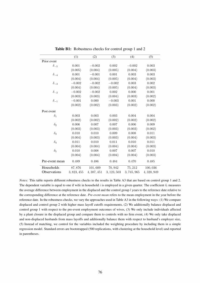
Table B1: Robustness checks for control group 1 and 2

(1) (2) (3) (4) (5)

Prior event

δ−5 0.001 −0.002 0.002 −0.002 0.003

(0.005) (0.004) (0.005) (0.004) (0.003)

δ−4 0.001 −0.001 0.001 0.003 0.003

(0.004) (0.004) (0.005) (0.004) (0.003)

δ−3 −0.002 −0.002 −0.002 0.003 0.002

(0.004) (0.004) (0.005) (0.004) (0.003)

δ−2 −0.002 −0.002 0.002 0.000 0.001

(0.003) (0.003) (0.004) (0.003) (0.002)

δ−1 −0.001 0.000 −0.003 0.001 0.000

(0.002) (0.002) (0.003) (0.002) (0.002)

Post event

δ1 0.003 0.003 0.003 0.004 0.004

(0.002) (0.002) (0.002) (0.002) (0.002)

δ2 0.006 0.007 0.007 0.006 0.009

(0.003) (0.003) (0.003) (0.003) (0.002)

δ3 0.010 0.010 0.009 0.008 0.011

(0.004) (0.003) (0.003) (0.004) (0.003)

δ4 0.011 0.010 0.011 0.010 0.011

(0.004) (0.004) (0.004) (0.004) (0.003)

δ5 0.010 0.008 0.007 0.007 0.010

(0.004) (0.004) (0.004) (0.004) (0.003)

Pre-event mean 0.489 0.486 0.484 0.470 0.485

Households 87, 876 101, 609 70, 942 75, 212 100, 036

Observations 3, 823, 455 4, 387, 451 3, 123, 503 3, 745, 965 4, 320, 949

Notes: This table reports different robustness checks to the results in Table A3 that are based on control group 1 and 2.

The dependent variable is equal to one if wife in household i is employed in a given quarter. The coefficient δl measures

the average difference between employment in the displaced and the control group l years to the reference date relative to

the corresponding difference at the reference date. Pre-event mean refers to the mean employment in the year before the

reference date. In the robustness checks, we vary the approaches used in Table A3 in the following ways: (1) We compare

displaced and control group 2 with higher mass layoff cutoffs requirements, (2) We additionally balance displaced and

control group 1 with respect to the pre-event employment outcomes of wives, (3) We only include individuals affected

by a plant closure in the displaced group and compare them to controls with no firm event, (4) We only take displaced

and non-displaced husbands from mass layoffs and additionally balance them with respect to husband’s employer size,

(5) Instead of matching, we control for the variables included the weighting procedure by including them in a simple

regression model. Standard errors are bootstrapped (500 replications, with clustering at the household level) and reported

in parentheses.

76

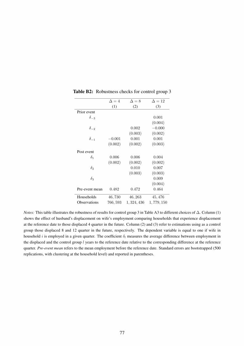
Table B2: Robustness checks for control group 3

∆ = 4 ∆ = 8 ∆ = 12

(1) (2) (3)

Prior event

δ−3 0.001

(0.004)

δ−2 0.002 −0.000

(0.003) (0.002)

δ−1 −0.001 0.001 0.001

(0.002) (0.002) (0.003)

Post event

δ1 0.006 0.006 0.004

(0.002) (0.002) (0.002)

δ2 0.010 0.007

(0.003) (0.003)

δ3 0.009

(0.004)

Pre-event mean 0.482 0.472 0.464

Households 46, 730 46, 263 45, 476

Observations 766, 593 1, 324, 436 1, 779, 150

Notes: This table illustrates the robustness of results for control group 3 in Table A3 to different choices of ∆. Column (1)

shows the effect of husband’s displacement on wife’s employment comparing households that experience displacement

at the reference date to those displaced 4 quarter in the future. Column (2) and (3) refer to estimations using as a control

group those displaced 8 and 12 quarter in the future, respectively. The dependent variable is equal to one if wife in

household i is employed in a given quarter. The coefficient δl measures the average difference between employment in

the displaced and the control group l years to the reference date relative to the corresponding difference at the reference

quarter. Pre-event mean refers to the mean employment before the reference date. Standard errors are bootstrapped (500

replications, with clustering at the household level) and reported in parentheses.

77