department of agriculture household food security in the ... · robert mislevy also provided...
TRANSCRIPT

Measuring Food Security in the United States
United States Department of Agriculture Food and Nutrition Service Office of Analysis, Nutrition, and Evaluation
Household Food Security in the United States, 1995-1997
Technical Issues and
Statistical Report

Contract No.: 53-3198-7-007 MPR Reference No.: 8463-080
Measuring Food Security in the United States Household Food Security in the United States, 1995-1997: Technical Issues and Statistical Report
Final Report of the Project to Analyze 1996 and 1997 Food Security Data December 2001
James Ohls Larry Radbill Allen Schirm
Submitted to:
U.S. Department of Agriculture Food and Nutrition Service 3101 Park Center Drive Alexandria, VA 22302
Project Officer: Gary Bickel
Submitted by:
Mathematica Policy Research, Inc. P.O. Box 2393 Princeton, NJ 08543-2393 Telephone: (609) 799-3535
Facsimile: (609) 799-0005
Project Director: James Ohls


iii
ACKNOWLEDGMENTS
The authors would like to thank Gary Bickel, the project officer for the study, for guidance andsuggestions throughout the work. Valuable advice and comments were also received from MarkNord and Steven Carlson. The advice of our Advisory Committee members also proved extremelyuseful at certain key points in the research. They included Christine Olson, Ben Wright, and CherylWehler. Robert Mislevy also provided critical suggestions on Rasch modeling and the interpretationof Rasch model results, and Don Rubin made suggestions about dealing with missing data. JeffPassel assisted in calculating correct weights from the CPS files. In addition to people alreadynamed, the following provided important advice at a research conference where parts of this materialwere presented: Susan Mayer, Christopher Jencks, Margaret Andrews, David Smallwood, JeanPierre Habicht, and Helen Jensen.
Extraordinary programming support was provided by Abhijay Prakash, Jean Knab, and JeanneBellotti.
Roy Grisham edited the manuscript and substantially improved the clarity of the exposition.Key production support was provided by Jane Nelson, Jill Miller, and Marjorie Mitchell.

v
CONTENTS
Chapter Page
EXECUTIVE SUMMARY . . . . . . . . . . . . . . . . . . . . . . . . . . . . . . . . . . . . . . . . xv
I INTRODUCTION . . . . . . . . . . . . . . . . . . . . . . . . . . . . . . . . . . . . . . . . . . . . . . . . . 1
A. PURPOSE OF THE REPORT . . . . . . . . . . . . . . . . . . . . . . . . . . . . . . . . . . . . 1
B. OVERVIEW OF REPORT . . . . . . . . . . . . . . . . . . . . . . . . . . . . . . . . . . . . . . . 2
II BACKGROUND . . . . . . . . . . . . . . . . . . . . . . . . . . . . . . . . . . . . . . . . . . . . . . . . . 5
A. A BRIEF SUMMARY OF THE LITERATURE INFORMINGTHE FOOD SECURITY CONCEPT . . . . . . . . . . . . . . . . . . . . . . . . . . . . . . . 6
B. THE CPS DATA ON FOOD SECURITY . . . . . . . . . . . . . . . . . . . . . . . . . . 10
C. THE ONE-PARAMETER LOGISTIC ITEM RESPONSE THEORY (RASCH) MODEL . . . . . . . . . . . . . . . . . . . . . . . . . . . . . . . . . . . . . . . . . . . . 13
D. RELATIONSHIP BETWEEN IRT MODELING AND THE FOOD INSECURITY PREVALENCE ESTIMATES . . . . . . . . . . . . . 15
E. CONVENTIONS USED IN THIS REPORT . . . . . . . . . . . . . . . . . . . . . . . . 17
III STABILITY OF ESTIMATED MODEL PARAMETERS OVER TIME . . . . . 19
IV STANDARD BENCHMARK METHODOLOGY . . . . . . . . . . . . . . . . . . . . . . 23
A. THE BASIC GOVERNMENT METHOD (NO RECALIBRATIONOF THE MODEL) . . . . . . . . . . . . . . . . . . . . . . . . . . . . . . . . . . . . . . . . . . . . . 24
1. Check and Edit the Data . . . . . . . . . . . . . . . . . . . . . . . . . . . . . . . . . . . . . 242. Construct Binary Variables from the Raw Data for Each of
the 18 Food Security Variables . . . . . . . . . . . . . . . . . . . . . . . . . . . . . . . . 243. Screening . . . . . . . . . . . . . . . . . . . . . . . . . . . . . . . . . . . . . . . . . . . . . . . . . 244. Impute Missing Data . . . . . . . . . . . . . . . . . . . . . . . . . . . . . . . . . . . . . . . . 25
CONTENTS (continued)
Chapter Page
vi
IV 5. For Each Household, Count the Number of Affirmative(Continued) Answers to the 18 Food Security Variables . . . . . . . . . . . . . . . . . . . . . . 25
6. Determine the Continuous Scale Score and Food Security Classification . . . . . . . . . . . . . . . . . . . . . . . . . . . . . . . . . . . . . . . . . . . . . . 25
B. CHECKING THE CALIBRATION OF THE MODEL ONTHE DATA SETS . . . . . . . . . . . . . . . . . . . . . . . . . . . . . . . . . . . . . . . . . . . . . 30
1. Edit the Data . . . . . . . . . . . . . . . . . . . . . . . . . . . . . . . . . . . . . . . . . . . . . . 302. Construct Binary Variables from the Raw Data for Each
of the 18 Food Security Variables . . . . . . . . . . . . . . . . . . . . . . . . . . . . . . 303. Screening . . . . . . . . . . . . . . . . . . . . . . . . . . . . . . . . . . . . . . . . . . . . . . . . . 304. Estimate the Rasch Model Parameters . . . . . . . . . . . . . . . . . . . . . . . . . . 30
V DEFINING “CUTPOINTS” OVER TIME . . . . . . . . . . . . . . . . . . . . . . . . . . . . . 33
1. Earlier Work . . . . . . . . . . . . . . . . . . . . . . . . . . . . . . . . . . . . . . . . . . . . . . 332. Generalization of Cutpoints to Other Years . . . . . . . . . . . . . . . . . . . . . . 353. Alternative Approaches to Setting Cutpoints . . . . . . . . . . . . . . . . . . . . . 37
VI CONCLUSION . . . . . . . . . . . . . . . . . . . . . . . . . . . . . . . . . . . . . . . . . . . . . . . . . . 41
A. STRENGTHS AND LIMITATIONS OF THE METHODOLOGY . . . . . . . 41
B. DIRECTIONS FOR FURTHER RESEARCH . . . . . . . . . . . . . . . . . . . . . . . 44
REFERENCES . . . . . . . . . . . . . . . . . . . . . . . . . . . . . . . . . . . . . . . . . . . . . . . . . . 47
APPENDIX A: SUMMARY OF SALIENT PARTS OF ITEM RESPONSETHEORY AND RELATED MEASUREMENT ISSUES . . . . 51
APPENDIX B: METHOD FOR SCREENING HOUSEHOLDS INTO THEFOOD SECURITY ANALYSIS . . . . . . . . . . . . . . . . . . . . . . . . 79
APPENDIX C: IMPUTING MISSING FOOD SECURITY DATA . . . . . . . . . 91
APPENDIX D: HOW “MODAL” ARE HOUSEHOLD RESPONSEPATTERNS? . . . . . . . . . . . . . . . . . . . . . . . . . . . . . . . . . . . . . . 97

CONTENTS (continued)
Chapter Page
vii
APPENDIX E: ITEM SEVERITY LEVELS BY SUBGROUPS . . . . . . . . . . 107
APPENDIX F: PREVALENCE ESTIMATES AND THEIR STANDARD ERRORS . . . . . . . . . . . . . . . . . . . . . . . . . . . . 129


ix
TABLES
Table Page
II.1 PREVALENCE OF FOOD SECURITY FOR HOUSEHOLDS,BY YEAR . . . . . . . . . . . . . . . . . . . . . . . . . . . . . . . . . . . . . . . . . . . . . . . . . . . . . . . 9
II.2 CPS SAMPLE SIZES . . . . . . . . . . . . . . . . . . . . . . . . . . . . . . . . . . . . . . . . . . . . . 12
III.1 COMPARISON OF ITEM CALIBRATIONS ESTIMATED FROM APRIL 1995, SEPTEMBER 1996, AND APRIL 1997 CPS FOODSECURITY DATA . . . . . . . . . . . . . . . . . . . . . . . . . . . . . . . . . . . . . . . . . . . . . . . 20
IV.1 THRESHOLDS USED TO CLASSIFY HOUSEHOLDS AS “POOR,”AND DHHS POVERTY GUIDELINES AT TIME OF SURVEY . . . . . . . . . . . 26
IV.2 CONTINUOUS SCALE SCORES BASED ON THE NUMBER OFAFFIRMATIVE ANSWERS . . . . . . . . . . . . . . . . . . . . . . . . . . . . . . . . . . . . . . . . 29
B.1 THRESHOLDS USED TO CLASSIFY HOUSEHOLDS AS “POOR”AND DHHS POVERTY GUIDELINES AT TIME OF SURVEY . . . . . . . . . . . 82
B.2 CRITERIA USED IN 1995-1997 SURVEYS TO SCREENHOUSEHOLDS INTO THE FOOD SECURITY MODULE . . . . . . . . . . . . . . . 84
B.3 FOOD SECURITY PREVALENCE ESTIMATES WITH ALTERNATIVEDEFINITIONS OF THE ANALYSIS SAMPLE . . . . . . . . . . . . . . . . . . . . . . . . . 87
D.1 PERCENT OF HOUSEHOLDS BY THE MINIMUM NUMBER OFNONMODAL RESPONSES TO THE FOOD SECURITY ITEMS . . . . . . . . . . 99
D.2 ANALYSIS OF MODALITY BY NUMBER OF YES RESPONSESTO FOOD SECURITY ITEMS . . . . . . . . . . . . . . . . . . . . . . . . . . . . . . . . . . . . . 100
D.3 MINIMUM AND MAXIMUM FOOD INSECURITY PREVALENCEESTIMATES . . . . . . . . . . . . . . . . . . . . . . . . . . . . . . . . . . . . . . . . . . . . . . . . . . . 102
E.1 THRESHOLD PARAMETER ESTIMATES FOR 18-ITEM 12-MONTHFOOD SECURITY SCALE BY RACE/ETHNIC GROUP . . . . . . . . . . . . . . . 108
E.2 ITEM ORDERING FOR RACE/ETHNIC GROUPS AND FULLPOPULATION . . . . . . . . . . . . . . . . . . . . . . . . . . . . . . . . . . . . . . . . . . . . . . . . . 109
E.3 CROSS-GROUP DIFFERENCES IN THRESHOLD PARAMETERESTIMATES BY RACE/ETHNIC GROUP . . . . . . . . . . . . . . . . . . . . . . . . . . . 110

TABLES (continued)
Table Page
x
E.4 THRESHOLD PARAMETER ESTIMATES FOR 12-MONTH FOODSECURITY SCALE BY HOUSEHOLD TYPES . . . . . . . . . . . . . . . . . . . . . . . 114
E.5 ITEM ORDERING FOR THREE HOUSEHOLD TYPES AND FULLPOPULATION . . . . . . . . . . . . . . . . . . . . . . . . . . . . . . . . . . . . . . . . . . . . . . . . . . 115
E.6 CROSS-GROUP DIFFERENCES IN THRESHOLD PARAMETERESTIMATES BY HOUSEHOLD TYPE . . . . . . . . . . . . . . . . . . . . . . . . . . . . . . 116
E.7 THRESHOLD PARAMETER ESTIMATES FOR 18-ITEM 12 MONTHFOOD SECURITY SCALE BY METROPOLITAN STATUS . . . . . . . . . . . . 119
E.8 ITEM ORDERING BY METROPOLITAN STATUS AND FULLPOPULATION . . . . . . . . . . . . . . . . . . . . . . . . . . . . . . . . . . . . . . . . . . . . . . . . . . 120
E.9 CROSS-GROUP DIFFERENCES IN THRESHOLD PARAMETERESTIMATES BY METROPOLITAN STATUS . . . . . . . . . . . . . . . . . . . . . . . . 121
E.10 THRESHOLD PARAMETER ESTIMATES FOR 18-ITEM 12-MONTHFOOD SECURITY SCALE BY REGION . . . . . . . . . . . . . . . . . . . . . . . . . . . . 123
E.11 ITEM ORDERING FOR 4 REGIONS AND FULL POPULATION . . . . . . . . 124
E.12 CROSS-GROUP DIFFERENCES IN THRESHOLD PARAMETERESTIMATES BY REGION . . . . . . . . . . . . . . . . . . . . . . . . . . . . . . . . . . . . . . . . 125

xi
FIGURES
Figure Page
A.1 ITEM CHARACTERISTIC CURVES . . . . . . . . . . . . . . . . . . . . . . . . . . . . . . . . 57
A.2 ITEM CHARACTERISTIC CURVES . . . . . . . . . . . . . . . . . . . . . . . . . . . . . . . . 58
A.3 TEST CHARACTERISTIC CURVES . . . . . . . . . . . . . . . . . . . . . . . . . . . . . . . . 60
A.4 TEST CHARACTERISTIC CURVES . . . . . . . . . . . . . . . . . . . . . . . . . . . . . . . . 61
A.5 THREE EQUIVALENT IRT SCALES . . . . . . . . . . . . . . . . . . . . . . . . . . . . . . . . 64
A.6 ITEM INFORMATION CURVES . . . . . . . . . . . . . . . . . . . . . . . . . . . . . . . . . . . 66
A.7 ITEM INFORMATION CURVES . . . . . . . . . . . . . . . . . . . . . . . . . . . . . . . . . . . 67
A.8 TEST INFORMATION CURVE . . . . . . . . . . . . . . . . . . . . . . . . . . . . . . . . . . . . . 69
A.9 TEST INFORMATION CURVE . . . . . . . . . . . . . . . . . . . . . . . . . . . . . . . . . . . . . 70
A.10 18- AND 10-ITEM TEST CHARACTERISTIC CURVES . . . . . . . . . . . . . . . . 71
E.1 ITEM CALIBRATIONS FOR 3 RACE/ETHNIC GROUPS . . . . . . . . . . . . . . 112
E.2 ITEM CALIBRATIONS FOR HOUSEHOLD TYPE GROUPS . . . . . . . . . . . 117
E.3 ITEM CALIBRATIONS BY METROPOLITAN STATUS . . . . . . . . . . . . . . . 122
E.4 ITEM CALIBRATIONS BY REGION . . . . . . . . . . . . . . . . . . . . . . . . . . . . . . . 126


xiii
EXHIBITS
Exhibit Page
IV.1 SCREENS USED IN THE CPS SURVEYS . . . . . . . . . . . . . . . . . . . . . . . . . . . . 27
IV.2 ALGORITHM FOR IMPUTING MISSING FOOD SECURITY DATA . . . . . . 28


xv
EXECUTIVE SUMMARY
This is the Final Report for the project, “Analysis of the Current Population Survey Data forFood Security and Hunger Measurement” conducted by Mathematica Policy Research, Inc. (MPR)for the USDA Food and Nutrition Service (FNS), beginning in 1997. The project provided USDAwith technical support and statistical estimation work for analyzing the 1996 and 1997 data on foodsecurity collected in the U.S. Census Bureau, Current Population Survey (CPS) Food SecuritySupplement. More broadly, the work examined a number of analytic and empirical issues relevantto analyzing the first three years of CPS food security data available—those for 1995, 1996, and1997.
It was originally intended that the Final Report would provide the main vehicle fordissemination of the substantive findings on the prevalence of food insecurity based on the 1996 and1997 data. However, because of the importance of making these results available as early aspossible, USDA elected to issue an “Advance Report,” thus making the results of the 1996 and 1997analyses conducted by MPR available before completion of the overall project. In addition, since1999, a number of publications have become available that present estimates of food insecurityprevalence, as well as discussions of the methods used in computing food security estimates ingeneral. Most important, Andrews et al. (2000) provides a comparative analysis of the annual datafor the five-year period 1995 through 1999, while Bickel et al. (2000) provides a how-to guide formeasuring food security that incorporates relevant work done prior to that time, including earlierwork from the current project. Selected issues in food security are also considered in Ohls et al.1999.
In light of these developments, USDA suggested that MPR recast this Final Report to focus onseveral selected topics related to the 1995-1997 data, rather than provide comprehensive treatmentof the overall research, much of which has since been incorporated in later publications. The FinalReport has been organized around these suggestions.
Among the issues addressed in the report are:
C The stability of the food security measurement scale over time
C Temporal adjustments to the categories or designated ranges of severity on theunderlying continuous scale used to classify households by food security status
C Screening issues related to ensuring a strictly comparable analysis sample over the1995-1997 CPS food security samples
C Alternative imputation strategies for dealing with missing data
C The degree to which household responses to the food security questions are “modal,”in the sense that households consistently respond affirmatively to questions involving

xvi
less severe food insecurity whenever they respond affirmatively to questions involvingrelatively more severe food insecurity
C The degree to which the estimated parameters of the model used to measure the severityof food insecurity vary across different groups of households, defined by ethnicity andother characteristics
The first section below provides background information about the analysis. Subsequent sectionssummarize findings on each of the above issues.
BACKGROUND
The analysis in this report is based on a statistical procedure which assigns households to foodsecurity status, based on their answers to a series of 18 survey questions. The food securitycategories used are:
C Food secure
C Food insecure—no hunger
C Food insecure with hunger
The data used for national-level analysis of food security are from annual supplements to the CPS,which is fielded monthly to more than 40,000 U.S. households.
Households are classified by food security status in the analysis, based on a procedure, Raschmodeling, which has a long history in the statistical literature. The first work in applying the Raschmodel to food security data was undertaken under an earlier contract let by USDA (Hamilton et al.1997). The Rasch model, as used in that work, posits that there is a single, one-dimensional attributeamong households that indicates food insecurity. The model then uses a set of assumptions andstatistical methods to assign “severity levels” to each of a series of 18 survey questions relating tofood insecurity and hunger. A continuous food security measure is then assigned to each householdin the data set, based on households’ replies to the 18 questions. Supplemental proceduresdeveloped by Hamilton et al. are then used to translate the continuous scale score into a limitednumber of discrete food security statuses.
The objectives of the current project were to extend the analysis to 1996 and 1997 data and toaddress a number of related issues associated with measuring food security over time. Our findingsin selected areas are summarized below.

xvii
STABILITY OF THE PARAMETERS OF THE MODEL OVER TIME
An important issue in examining the validity of the Rasch modeling approach is whether themodel parameter estimates are stable over time. The underlying theory on which the Rasch modelis based posits that, if the wording of an item does not change, its estimated level of severity shouldnot change. For example, even if food insecurity became more prevalent over time, a household ata given level of insecurity this year is expected to answer each item the same way a household at thatlevel of insecurity did a year earlier. Due to sampling variability and other factors, such as minorwording changes, we do not expect estimated model parameters to remain exactly the same overtime; but a finding of major changes over time would call into question the validity of the model.Particularly problematic would be a finding of important changes in the ordering of the items byseverity.
To examine issues of model stability, we estimated the model independently on three CPS datasets (1995-1997), using consistent conventions as to statistical scaling. Some variation across yearswas found, as expected. In general, however, the estimated parameters of the model were quitestable. Also, the estimated order of severity of the different questions remained largely constant,with the only changes in severity order occurring among questions that were very close to each otheron the severity scale in the original estimation work. The conclusion of this component of theresearch is that the food security model is sufficiently temporally stable to make it a reasonable toolto use in time series analysis.
ADJUSTING “CUT POINTS” USED TO CLASSIFY HOUSEHOLDS INTO A LIMITEDNUMBER OF FOOD SECURITY STATUS CATEGORIES
The Rasch model places each household on a continuous numeric food security scale. Forpurposes of policy analysis, it is also useful to establish numerical “cut points” that assignhouseholds to a small number of designated categories which summarize their food security status.To create this categorical measure, Hamilton et al. (1997a and 1997b) specified four categories: foodsecure, food insecure without hunger, food insecure with moderate hunger, and food insecure withsevere hunger. More recently, the latter two categories have usually been collapsed to form a singlecategory, while additional scale development work has identified a new nested category, foodinsecure with children’s hunger (Nord and Bickel 1999 and 2001).
A key issue that arises in this work is whether it is appropriate to keep the same continuous scalecut points over time, or whether, alternatively, some temporal adjustments may be needed. Theanalysis of the body of the report concludes that, at least in some situations, it is not optimal toattempt to classify households based on the same cutpoints over time.
While the Rasch model places households on a continuous food security scale, due to certainstatistical properties of the model substantial numbers of households tend to be clustered at certainpoints in the scale. If cut points are held constant, there is a risk that, because of chance statisticalvariation, the score assigned to one of these clusters of households might accidentally cross one ofthe cutpoints in a given year, causing considerable instability in estimates of food securityprevalence.

The 1995-1997 files used in the current report, like the corresponding public use files available1
on the CPS website, have one further adjustment which is designed to make them more comparableto the 1998 data. In the 1998 survey, households were not asked relatively severe food securityquestions if they had already consistently answered “no” to blocks of less severe questions. The1995-1997 data were edited to emulate this screening by replacing answers to the more severequestions with missing value codes for questions which would have been skipped in 1998. See:www.bls.census.gov/cps/foodsecu/1997/agnote.htm (“Food Security, Scales and ScreenerVariables”).
xviii
Chapter V of the Final Report identifies several technical approaches for avoiding this difficulty.The discussion is based on the principle that a household with a given pattern of survey answersshould always be classified into the same food security grouping, independent of when the data arecollected.
SCREENING HOUSEHOLDS INTO THE SAMPLE IN THE 1995-1997 SURVEYS
The food security supplements in the 1995-1997 CPS had two general sections. The first sectiongathered information about food expenditures, participation in several programs aimed at providingfood to needy families (for example, food stamps and school meal programs), and the sufficiencyof food eaten during the preceding 12 months. The second section gathered more-detailedinformation about food insecurity and coping behaviors during the previous 12 months and prior 30days. Not all households were asked this second set of questions, which includes the questions usedto construct the food security scale. In order to minimize respondent burden, households who, onthe basis of earlier questions, appeared to have a high likelihood of being food secure were excludedfrom the more detailed questions and were assumed to be food secure in the analysis. This pre-screening applied to higher income households in all three years, 1995-1997, and in one year, 1996,it was applied to lower-income households as well. Beginning in 1998 and continuing consistentlysince then, the CPS Food Security Supplement has included a new, less restrictive, pre-screenapplied to higher-income households.
To ensure comparability in the analysis samples for the three years, the current researchdeveloped a common screen, such that any households giving survey answers that passed thiscommon screen would have been tracked into the food security module in any of the three years.Households that did not pass the common screen were, for purposes of the analysis, treated as if theyhad not been tracked into the food security module of the survey—essentially, they were assumedto be food secure. Technical details concerning how this common screen was constructed areprovided in Appendix B of the Final Report.
While use of the common screen has the desired effect of ensuring consistency in the 1995-1997analysis samples, it also has the effect of treating as food secure a number of households who, duringthe survey, gave indications of experiencing food insecurity. Across the three years, use of thecommon screen was found to result in estimates of the prevalence of food insecurity which arebetween 1.0 and 1.5 percentage points lower than those that are obtained when the maximumavailable samples are used in the estimation.1
xix
IMPUTING MISSING DATA
Most households gave complete answers to the food security questions they were asked in theCPS; however, a limited number did not. Appendix C of the report examines a number of alternativeapproaches for including households with partially missing data in the analysis. One approach isreliance on the Rasch model itself, which has the capacity to assign food security scale scores toobservations with incomplete data. However, as is noted in Appendix C, in some instances, thedeterminations made within the model for cases with substantial amounts of missing data may lackface validity. Also, as a practical matter, many researchers may not have easy access to the softwareneeded to implement the model.
An alternative algorithm for dealing with missing data has therefore been developed. Dependingon the exact configuration of food security module answers given by the respondent, this alternativealgorithm essentially involves imputing missing data items based on either (a) the highest severityitem, in terms of level of food security severity, that the respondent answered positively; or (b) thelowest severity item answered negatively.
“MODALITY” OF HOUSEHOLD FOOD SECURITY RESPONSE PATTERNS
The Rasch model implies that many households will exhibit item response patterns that arereasonably “modal” in the sense that if a household answers “yes” to any of the items, it will tendto answer “yes” to the less severe items, then answer “no” to the more severe items. A householdthat exhibits this pattern exactly—a string of all “yes” answers followed by a string of all “no”answers—is said to be a “modal” household. There is nothing in Rasch theory that predicts that allhouseholds will be modal; indeed, the model cannot be estimated if all households are exactly modal.Still, it is of interest in understanding the data to examine the degree of modality present. A largenumber of strongly nonmodal response patterns could call into question the validity of the model.
Analysis of the 1997 data indicates that most household response patterns tend to be eitherexactly or approximately modal. Of those households in the 1997 data who gave an affirmativeanswer to at least one question, approximately 39 percent households provided answer patterns thatwere exactly modal, while another 36 percent gave sets of answers which had only a singlenonmodal response.
CONSISTENCY OF ESTIMATED FOOD SECURITY MODEL PARAMETERS ACROSSPOPULATION SUBGROUPS
Essentially, the analysis conducted with the aggregated CPS data sets assumes that differentsubgroups of the population are similar with regard to how they experience food insecurity. To testthis assumption, the Rasch model was estimated separately for subgroups of the population, definedaccording to (a) race/ethnicity; (b) household composition; (c) metropolitan status; and (d) regionof country.

Note, however, that there has not yet been an opportunity to assess temporal stability in the2
context of anything other than a strong economy.
xx
The results of this analysis indicate considerable robustness of the analysis to this kind ofdisaggregation. In general, estimated severity levels for the individual questions were found to haveconsistent patterns across different subgroups, and the magnitudes of the parameters do not changesubstantially.
There is no clear statistical test of how much difference in the estimated subpopulation modelswould affect confidence in the overall modeling approach. However, the judgment of statisticalexperts who have used the Rasch model extensively in other contexts is that the findings of thesubgroup analyses can reasonably be judged to be highly consistent with one another.
CONCLUSION: REFLECTIONS ON THE STRENGTHS AND LIMITATIONS OF THE FOOD SECURITY METHODOLOGY
We conclude by discussing the strengths and limitations of the use of the Rasch model as a basisfor food security measurement. Possible directions for future research are also noted.
The food security scale reflects more than 10 years of methodological development by bothgovernment and private groups. The use of the Rasch model methodology has made it possible toguide the development of the food security estimates with a thoroughly studied model that has well-understood statistical properties. In terms of goodness-of-fit criteria, the mathematical form of themeasurement model shows strong correspondence on “fit” to the empirical data. The approach hasundergone extensive review by experts in both the public and the private sector. In general, theseexperts consider the model an appropriate application of the IRT methodology, and they have viewedthe analysis results as reasonable.
Another important strength, as established by the current project, is that the estimated itemparameters of the IRT model are robust across time and population subgroups. The values obtainedfrom the 1996 and 1997 data are essentially the same as the original 1995 values. In addition to2
stability over time, there is stability across subgroups, defined by such characteristics asrace/ethnicity, household composition, and region of the country.
Tempering these strengths are a number of limitations which should also be recognized. Mostof these, if not all, are a matter of careful interpretation of what the food security measure does anddoes not do. For example, the CPS indicator questions for food insecurity and hunger and the scaledeveloped from them are designed to provide a household-level measure of the severity of conditionsas experienced within U.S. households. This is in line with the conceptual understanding of foodinsecurity as a condition of deprivation or stress experienced by households in meeting members’basic food needs. However, the experience of hunger as such, which appears only at a more severestage of food insecurity, is strictly individual. The household classification, “food insecure withhunger” refers to that more severe range where evidence of reduced food intake and hunger hasappeared for one or more household members. But this is a collective measure which may apply toall household members, to adult members only, or to as few as one (adult) member.

xxi
Second, the basic measure is designed to capture respondents’ experiences over the course ofa year, while household circumstances can change markedly during such a period. Accordingly, the12-month measure—designed to provide reliable benchmark and trend figures—may not representthe current situation of given households. Similarly, the “food insecure with hunger”designation can,in principle, result from just one serious episode during the year, although for most such householdsevidence of a repeated pattern of reduced (adult) food intakes during the year must be established.
In addition, a number of issues of interpretation flow from the need to have a simple categoricalmeasure as a means of classifying households for purposes of manageable data reporting andmonitoring, in addition to the underlying continuous scaled measure. The categorical measure wascreated to make the scale more accessible to non-technical users and more convenient to users whoseneeds could be better served by a simple categorical variable than by the detailed continuousmeasure. The categorical measure as such is straightforward: it represents designated ranges ofseverity along the continuous scale (i.e., qualitatively differing severity levels of “food insecure”),plus the category of households that either show no evidence of food problems within the CPS dataset, and hence can be deemed to be “food secure,” or that show only one or two indications of foodstress, which is deemed insufficient as evidence to establish confidently their status as “foodinsecure.”
The interpretive problems with the categorical measure stem from at least three sources. First,the designation of appropriate severity ranges, and their exact delineation in operational form basedon the available set of indicators, is inherently judgmental and thus leaves room for disagreement.
Second, the Rasch model employs a probabilistic logic in generating the continuous scalemeasure of severity of household food insecurity; similarly, the corresponding severity-rangesummary categories share this probabilistic nature. However, the naming conventions adopted forthe severity-range categories are determinate in form, which can be misleading.
Thirdly, a misplaced specificity and determinateness can easily be attributed to the individualindicator items as well, causing a misunderstanding of their actual role in the measurement process.
To illustrate this last point, straightforward names adopted for the severity-range categories raiseissues of face validity when they seemingly contradict the clear language of particular indicator itemsembedded within the measurement scale. For instance, it is technically possible for a household tobe classified “food insecure with hunger,” even though the respondent has answered “no” to theparticular question, “In the last 12 months were you ever hungry but didn’t eat because you couldn’tafford enough food?” In this case, the respondent either must have replied “yes” to a series ofincreasingly severe indicators of food insufficiency, including at least three items indicating reducedfood intake for themselves and/or other adult members of the household, one of which establishesa repeated pattern of such reduced intakes over the year, or they must have replied “yes” to most ofthe foregoing, plus one or more of the items that are more severe than the explicit hunger question.The categorical measure (and its naming convention) reflects the judgment that, on the balance ofthis evidence, one or more adult members of the household has, with high probability, experiencedresource-constrained hunger sometime during the year. Conversely, the opposite case also can occur:the household can be classified “food insecure without hunger,” based on its overall pattern of

xxii
response and the resulting scale score, even though the respondent has answered “yes” to the explicithunger question as such.
In creating the scale, a number of steps were taken to minimize the effects of these factors. Forinstance the numerical cutpoints defining the categories were set to be conservative, in the sense thatthere must be three answers to questions thought to indicate food insecurity before a household isclassified as food insecure, and similarly for the hunger classification. Also, analysis presented inthe text of the report indicates that substantial numbers of respondents follow close-to-expected,response patterns, which do not lead to any apparent anomalies in classification. Nevertheless, roomfor disagreement remains as to what types of answers to the questions should be construed asreflecting the language used in designating the three scale categories.
A possible solution to some of these issues would be to state the category names inmore-probabilistic terms, such as “probably food insecure” or “a high likelihood of hunger.” Thiswould be in keeping with the probabilistic nature of the underlying model, and it might help ease theconcerns of those who are bothered by the anomalies posed by apparently inconsistent patterns ofquestion responses. However, such category name changes might also interfere with the clarity ofmeaning of the categories themselves, thus reducing their effectiveness.
Overall, it is important to recognize that these limitations have not prevented the food securityscale from becoming an important, widely used research and policy tool. Questions to support thescale have been included in an increasing number of national surveys and scale results are frequentlycited in the policy process. This evidence suggests that many policy analysts have found the scaleto be a valuable tool for measuring an important aspect of material deprivation among America’spoor.

1
I. INTRODUCTION
For decades, ensuring that everyone in the United States has effective access to adequate,
nutritious food has been a major policy goal of the federal government. More recently, increased
attention has been paid to developing ways of measuring how well this goal is being achieved. A
growing body of literature has emerged from work done in the late l980s, aimed at measuring
households’ “food security.” As part of this literature, the U.S. Department of Agriculture (USDA)
has begun publishing estimated rates of food security and food insecurity in the United States. The
research reported below was undertaken to continue this work.
A. PURPOSE OF THE REPORT
This is the Final Report for the project, “Analysis of the Current Population Survey Data for
Food Security and Hunger Measurement” conducted by Mathematica Policy Research, Inc. (MPR)
for the USDA Food and Nutrition Service (FNS) beginning in 1997. The project provided USDA
with technical support and statistical estimation work for analyzing the 1996 and 1997 data on food
security collected in the annual Food Security Supplement to the U.S. Census Bureau, Current
Population Survey (CPS). More broadly, the work examined a number of analytic and empirical
issues relevant to analyzing the first three years of CPS food security data available—those for 1995,
1996, and 1997.
It was originally intended that the Final Report would provide the vehicle for the main
dissemination of the substantive analytical findings on the prevalence of food insecurity based on
the 1996 and 1997 data. However, because of the importance of making these results available as
early as possible, USDA eventually elected to issue an “Advance Report,” thus making the results
of the 1996 and 1997 analyses conducted by MPR available before completion of the overall project.

2
The Advance Report also included comparable results based on 1998 data. In addition, since 1999,
a number of other publications have become available which present estimates of food insecurity
prevalence, as well as discussions of the methods used in computing food security estimates in
general. Most important, Andrews et al. (2000) provide a comparative analysis of the annual data
for the five-year period 1995 through 1999, while Bickel et al. (2000) provide a “how to” guide for
measuring food security that incorporates relevant work done prior to that time, including earlier
work from the current project. Other important contributions include Ohls et al. (1999) and Prell and
Andrews (2001).
In light of these developments, USDA suggested that MPR recast this final report to focus on
several selected topics related to the 1995-1997 data, rather than providing a comprehensive
treatment of the overall research, much of which has either been reported previously or incorporated
in later publications. This report has been organized around these suggestions.
B. OVERVIEW OF REPORT
Chapter II provides a brief summary of the past work in the food security area and of the
methods currently being used to measure food security; it thus provides a context for the subsequent
material. Chapter III presents results that describe the stability of the estimated food security scale
across different years. Chapter IV provides a summary of “benchmark” methods that can be used
to estimate the food security scale on different data sets and with different assumptions as to which
parameters are to be held constant and which are not. Chapter V discusses issues related to adjusting
the food security model over time, to accommodate both the availability of new data and possible
developments in the underlying methodology. Chapter VI provides some broad conclusions about
the food security scale.

3
Appendices provide new tabulations of the data and explore additional methodological issues,
such as:
� Summary of salient parts of item response theory and related measurement issues
� Screening households into the food security analysis
� Imputing missing food security data
� How “modal” are household response patterns?
� Item-severity levels, by subgroup


5
II. BACKGROUND
The publication of the U.S. Department of Agriculture (USDA) 1997 report on food security
levels in the United States (Hamilton et al. 1997a and 1997b; and Price et al. 1997) has spurred
widespread interest in measuring food security for various groups in the U.S. population. Using data
from the April 1995 Current Population Survey (CPS), that set of reports presented a comprehensive
method for measuring food security levels. Other major surveys that have measured food security
or plan to do so are the Panel Study of Income Dynamics, the National Health and Nutrition
Examination Survey, the Continuing Survey of Food Intakes by Individuals, the Survey of Program
Dynamics, and the Early Childhood Longitudinal Study.
The 1997 USDA report was based on a single CPS data set, that for April 1995. Important next
steps in food security research have been to extend that analysis to later years, and to develop a
method for measuring changes in food security over time. Major research questions include:
� Are estimated model parameters stable over time?
� What method is most appropriate for assessing changes in the prevalence of foodinsecurity in the U.S. population?
� How sensitive are prevalence estimates to alternative ways of implementing theprocedures used in the 1997 report?
This chapter gives background information that will be useful in addressing these issues.
Section A provides background for our work, describing the roots of the food security concept in
prior research. The CPS data used for the current study are described in Section B, while Section
C describes the Rasch model used in both the original analysis of the 1995 data and the current work
measuring the severity of food insecurity as experienced within households.

6
A. A BRIEF SUMMARY OF THE LITERATURE INFORMING THE FOOD SECURITYCONCEPT
Although hunger has long been a concern of American social and nutrition policy, attempts to
measure it systematically have posed major challenges to advocates and policy analysts alike. Early
attempts to equate hunger directly to malnutrition were not successful, because they encountered
conceptual difficulties in defining malnutrition and operational difficulties in developing reliable and
inexpensive ways of measuring people’s nutrient intake. Furthermore, as additional discussion took
place, it was recognized that feeling physical “hunger,” a sensation experienced by most people fairly
frequently, is not equivalent to the experience of hunger resulting from lack of resources to obtain
food, a situation more closely related to economic deprivation. Obviously, refinement of the concept
was needed.
From the late 1970s through the early 1980s, there was growing interest in broadening the
concept of hunger to the more general construct of resource-constrained food insecurity. This
broader concept came to be defined in terms of the phenomena and experiences associated with food
stress for the households, as well as household members actually experiencing hunger. Lacking
access to food because of resource constraints also came to be included in most analysts’ definition
of “hunger” as a policy issue.
The broadening of the relevant concepts took place partly within the U.S. government, with the
inclusion of a basic question related to food insecurity in the two most recent administrations of the
Nationwide Food Consumption Survey and a small set of such questions in the Third National
Health and Nutrition Examination Survey and the Survey of Income and Program Participation. Two
private research efforts gave substantial impetus to the evolving focus on food insecurity. First, the
Community Childhood Hunger Identification Project (CCHIP)—organized by the Food Research
and Action Center and funded by local and national business and philanthropic
7
organizations—demonstrated that reasonable and consistent answers could be obtained using a set
of survey questions designed to measure food insecurity (Wehler et al. 1991). Second, work at
Cornell University provided additional theoretical support and advanced the development of
measurement scales based on answers to survey questions about food security (Radimer et al. 1992).
Beginning in 1992, a federal interagency working group on food security measurement—under
the leadership of the USDA Food and Nutrition Service (FNS) and the DHHS Centers for Disease
Control and Prevention, National Center for Health Statistics (NCHS)—began a systematic effort
to develop a battery of questions about food insecurity based on the prior research, which could be
administered regularly in government-conducted surveys. Drawing on previous research findings
about food insecurity, together with additional research commissioned from outside researchers,
USDA staff assembled the full range of food security survey questions that had been used, and
identified sets of items that held promise as reliable indicators for use with U.S. state- or national-
level populations. The Federal Interagency Group was assisted in this work by an expert panel that
included many leading food security researchers.
FNS passed an important milestone when it won approval from the U.S. Office of Management
and Budget (OMB) for a supplement to the April 1995 CPS containing a set of questions designed
to measure food security. The supplement gathered information about households’ shopping patterns
and various aspects of food insufficiency and insecurity during the 30 days and 12 months prior to
the interview.
In 1995, Abt Associates, assisted by staff from Tufts University and Cornell University and
CAW and Associates, Inc., was engaged by the USDA to analyze the 1995 CPS data. Faced with
a questionnaire containing more than 50 items, the Abt team worked with the USDA to further refine
the underlying concepts of food insufficiency and food insecurity. Along with this conceptual work,

The food security supplement has been fielded by the U.S. Census Bureau on an annual basis,1
including the August 1998, April 1999, September 2000, and April 2001 CPS. Current plans callfor food security data to be collected henceforth in the same month each year, beginning inDecember 2001.
8
the team had to identify which of the CPS questionnaire items could reliably measure food
insecurity. In the early stages of their work, they relied heavily on factor analysis to identify a group
of items that, taken together, appeared to measure food insecurity. Next, the Abt team applied a
scaling procedure (described later) to assign a food security measure to each household. Based on
these measures, households were classified into four categories—food secure; food insecure without
hunger; food insecure with moderate hunger; and food insecure with severe hunger—and the Abt
team was able to estimate the prevalence of these four designated levels of food security/insecurity.
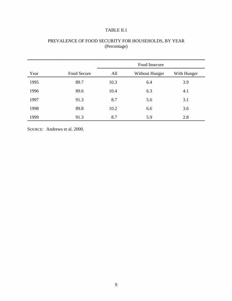
Table II.1 summarizes the published food insecurity prevalence estimates for the five years for
which data have been analyzed. As shown in the table, depending on the year of estimation,
approximately 89 to 91 percent of U.S. households are estimated to be food secure. The rate of food
insecurity with hunger is estimated to be in the range of 3 to 4 percent. The remaining households,
approximately 5 to 7 percent, are in the less severe range where there are signs of food insecurity but
the households are not classified as hungry.
This report extends the research of the CCHIP, Cornell, USDA, and Abt researchers. The work
done by the Abt team was focused on developing and implementing a measure of the severity of food
insecurity using data from the April 1995 CPS. The present report analyzes data from two additional
rounds of surveys: the September 1996 and April 1997 CPS. With these additional data, the focus1
shifts to issues that arise in the development of a stable and consistent ongoing social indicator. The
issues examined here are of the kind that can be critical when prevalence is measured on a routine
basis and changes in prevalence are closely monitored by policymakers. The availability of food-
9
TABLE II.1
PREVALENCE OF FOOD SECURITY FOR HOUSEHOLDS, BY YEAR(Percentage)
Food Insecure
Year Food Secure All Without Hunger With Hunger
1995 89.7 10.3 6.4 3.9
1996 89.6 10.4 6.3 4.1
1997 91.3 8.7 5.6 3.1
1998 89.8 10.2 6.6 3.6
1999 91.3 8.7 5.9 2.8
SOURCE: Andrews et al. 2000.

More formally, the CPS sample is actually one of geographic addresses rather than households.2
If sample members move to a new address, they are not interviewed at that new address and theythus leave the sample. However, the address those sample members moved from remains in thesample, and the new residents are interviewed. These are known as “replacement households.”
10
security data from three years in sequence has made it possible to address issues that arise when
tracking changes over time.
B. THE CPS DATA ON FOOD SECURITY
Data for the current study come from the USDA-sponsored Food Security Supplement to the
CPS. The CPS is a monthly survey of about 50,000 households conducted by the U.S. Census
Bureau for the Bureau of Labor Statistics. The sample is designed to represent the civilian,
noninstitutional population of the United States. Each monthly sample is divided into eight
representative subsamples, or rotation groups. A given rotation group is interviewed for a total of
eight months: it is in the sample for 4 consecutive months, leaves the sample during the following
8 months, then returns for another 4 consecutive months. In each monthly sample, one of the eight
rotation groups is in the first month, another rotation group is in the second month, and so on.2
Under this system, 75 percent of the sample is common from month to month, and 50 percent is
common from year to year for the same month.
The primary purpose of the CPS is to provide information about the labor force characteristics
of the U.S. population. In each month, however, a supplement is added to the core questionnaire.
In March of each year, for instance, the Census Bureau sponsors the Annual Demographic
Supplement. This survey is the data source for the official income and poverty statistics published
by the Census Bureau each year. In April 1995, September 1996, April 1997, August 1998, April
1999, September 2000, and April 2001, a special supplement was added to the CPS core

11
questionnaire which included questions about household food sufficiency, food security, food
expenditures, food program participation, and several other related items. The structure of the food
security supplement used in these surveys was as follows:
1. Food expenditures during the prior week
2. Participation in food assistance programs (food stamps, meal programs for the elderly,school meal programs, and the Special Supplemental Food Program for Women, Infants,and Children)
3. Food insufficiency during the prior 12 months and ways of coping with thatinsufficiency
4. Food security and hunger indicator questions for the prior 12 months and the prior 30days
Not all households were asked the full set of questions in the supplement. To minimize
respondent burden, a set of preliminary screening questions was used in some cases to determine
whether there was evidence that a household might have experienced food insecurity. If there was
no such evidence, the subsequent food security questions were skipped. This preliminary screen has
been applied to higher-income households in every year and was applied to lower-income
households as well in one year (1996). Across the three CPS samples in 1995, 1996, and 1997,
different screening procedures were used. Beginning in 1998, the structure of the food security
questionnaire was redesigned in a more fundamental way (but with content unchanged), including
a basic change in screening procedure, now expected to remain constant.
Table II.2 shows unweighted sample sizes for the three CPS samples used here. The initial
sample size for the April 1995 CPS was 53,665 households. Budget cuts in January 1996 resulted
in reduced sample sizes, which are reflected in the initial sample sizes for September 1996 and April
1997 shown in Table II.2. The initial sample for September 1996 was 47,795; for April 1997, it was

12
TABLE II.2
CPS SAMPLE SIZESUnweighted Number of Households
April Sept. April 1995 1996 1997
Full CPS 53,665 47,795 47,306
Households in Supplement 44,730 41,811 41,146
Households Tracked Into Food Security Module 18,453 10,957 11,175Answered all key questions asked 18,179 10,685 10,937a
Answered at least half of key questions asked, but not all 195 203 171a
Answered fewer than half of key questions asked 79 69 67a
There are 18 key questions for households with children and 10 for those without children.a

The sample attrition at this stage is due mainly to households in the CPS being told that they3
are about to start a new module, and declining to do so.
13
47,306. In all three samples, roughly 85 percent of the core households entered the Food Security
Supplement. Of those households, about 40 percent of the April 1995 sample passed the screening3
questions and were asked the balance of the Food Security Supplement. For the 1996 and 1997
surveys, tighter screening procedures resulted in only about 26 percent of households being asked
the rest of questions in the Food Security Supplement. In all cases, there is a presumption that
households failing to pass the screen are food secure. The differences in the screening procedures
used across these three samples have important implications for the consistent measurement of food
insecurity during the 1995-1997 period, a necessary prerequisite for measuring the changes in food
insecurity across those years. These issues are discussed in more detail in Appendix B.
Most of the research reported below is based on 18 key questions (items) that are used for the
measurement of household food insecurity. Households with one or more children are asked all
these questions; childless households are asked only the 10 items that do not pertain to children.
Once the differences between households with and without children were taken into account, there
was little item nonresponse. In all three samples, more than 97 percent of the households that passed
the initial screen responded to all the items used to measure food insecurity that they were asked.
However, the fact that childless households responded to only 10 of the 18 items asked of
households with children presents an additional complication, as discussed below.
C. THE ONE-PARAMETER LOGISTIC ITEM RESPONSE THEORY (RASCH) MODEL
The Food Security Supplement to the April 1995 CPS contained more than 65 questions, of
which about 50 were potential indicators of food insufficiency, insecurity, or actual hunger and thus

For summaries of IRT theory, see Hambleton (1993) and Wright and Masters (1982).4
14
were candidates for inclusion in the measurement scale. Of the entire question set, four questions
were used as a preliminary screen to identify households that showed no indication of food insecurity
during the prior 12 months, and thus were not to be burdened with additional questions. Of the
remaining items, 18 are used directly to measure households’ food insecurity levels over the prior
12 months. (Of the questions not used in the measurement scale, some apply only to the 30 days
prior to the interviews; others were found during preliminary analysis not useful in developing the
full food insecurity scale.)
An important objective achieved in the first round of research on the 1995 data was to develop
a method for combining answers on the 18 items into a single scale measuring the level of severity
of household food insecurity as experienced within the U.S. population. In doing this, it was
necessary to take the following factors into account:
� Not all questions apply to all households; in particular, eight of the questions are notrelevant to households that do not have children
� The data included some item nonresponse involving households that did not answer allthe questions asked.
In developing the desired food security scale, the researchers involved drew heavily on a rich
body of procedures developed originally in the educational testing literature called “Item Response
Theory” (IRT). IRT methods have been widely used in educational contexts, such as the Scholastic
Aptitude Tests (SAT) and the National Assessment of Educational Progress, to measure student
attributes (such as math ability), using tests which, for test security reasons and other factors, are not
identical. In applying IRT methods to the food security measurement context discussed in the4
Some researchers view Rasch modeling as a subset of IRT theory; others disagree with that5
characterization. In any event, they clearly are closely related.
15
present report, the attribute being examined is food insecurity and the test items are the individual
food security questions on the CPS supplement.
The methods used in the original analysis of the 1995 food security data, which are also applied
in the present report, involve a closely related technique called “Rasch modeling.” The salient5
characteristic of the Rasch model is that the model involves estimating only a single parameter, often
called the “severity” level, which is used to characterize each question on the scale. Other versions
of IRT theory estimate either two or three parameters per question.
Appendix A provides a more detailed summary of the Rasch model. We conclude this section
by noting certain salient properties of Rasch models that are relevant to the following discussion:
� The scale measure for households with complete data can be calculated based only onthe number of questions about food insecurity which they answer affirmatively.
� The scale measure determined by the model is unique up to a linear transformation; oncea scale is developed, any linear transformation of the scale conveys the sameinformation.
� In a Rasch model, each household’s level of food security, and each item’s level ofseverity, are determined simultaneously within the model.
D. RELATIONSHIP BETWEEN IRT MODELING AND THE FOOD INSECURITYPREVALENCE ESTIMATES
As noted above, this report covers a number of different topics in food security measurement,
some of which are related principally to the IRT-based model estimation and some of which relate
more directly to food security prevalence estimates. As a context for these discussions, it is useful
to provide an overview of the relationship between the model and the prevalence estimates. The

16
IRT-based model played several important roles in the development of the food security scale
currently being used. First, it helped establish the order of severity for different individual questions
in the CPS module, thus facilitating the work done by the initial research team in identifying ranges
of responses corresponding to various food security levels. Second, the IRT-based model provided
a formal way to calibrate food security levels for households without children on the same scale as
households with children, even though some of the CPS questions were not applicable to the former
group.
Third, the model provided a mechanism for dealing with item non-response on the survey
(though this was of limited importance, given that, as discussed later in the report, item nonresponse
was quite low). Fourth, the IRT model has provided a way of partially testing the stability of the
index over time and across subgroups. In addition, the IRT model may be useful in the future for
continuing to examine the stability of the processes which determine levels of food security.
These uses of the IRT-based modeling having been stated, it may be noted that repeated
application of the measurement model is not needed for the ongoing measurement and monitoring
of food security, or for the measurement of food security on the same basis in local areas. As
summarized earlier, now that the model estimation work has been done, and the underlying
measurement scale created the actual scale measure for a specific household with complete data on
the food security questions can be calculated simply by counting the number of affirmative answers
to the questions; no further estimation work is needed. This greatly simplifies the ongoing work of
making annual food insecurity prevalence estimates.
17
E. CONVENTIONS USED IN THIS REPORT
Because the scaling of parameters can be changed using any linear transformation without losing
meaning, a convention is needed as to scaling when comparing parameters estimated with different
data sets. The convention used in this report, unless otherwise noted, is that the mean of the item
parameters is set to 7 and the slopes of the item response curves at their inflection points (see
Appendix A) are equal to 1.
Also, because different sample screening procedures were used in different years of the CPS,
a convention is needed as to how to make the data sets comparable across years. Except when
otherwise noted, the convention used is to define the sample using the “common screen” as
described in Appendix B.


19
III. STABILITY OF ESTIMATED MODEL PARAMETERS OVER TIME
An important issue in examining the validity of the Rasch modeling approach is whether the
model parameter estimates are stable over time. The underlying theory on which the Rasch model
is based posits that, if the wording of an item does not change, its estimated severity level should not
change. For example, even if food insecurity became more prevalent over time, a household at a
given level of severity this year is assumed to answer each item the same way as a household at that
same level of severity did a year earlier. Due to sampling variability and other factors, such as minor
wording changes, we do not expect estimated model parameters to remain exactly the same over
time; but a finding of major changes over time would call into question the validity of the model.
Particularly problematic would be a finding of important changes in the ordering of the items by
severity.
Table III.1 shows estimated item parameters based on separate estimation for each of the three
years. For each year, only data from that year are used in the estimation. The estimates use the
common screen as described in Appendix B. Each set of item parameters has been scaled in the
standard way used in this report, with the mean set at 7 and the slopes of the item characteristics
curves at their inflection points set at 1.
Of particular interest in our analysis was whether the severity ranking of the items remained
reasonably constant. This was of interest, both as a general indication of parameter stability and
because the item order had been drawn on substantially in the original Hamilton et al. (1997) work
in designing the algorithm that translates the continuous Rasch model into the designated categorical
household food security levels. (See Chapter V.)

Stan
dard
Stan
dard
Stan
dard
Stan
dard
Item
Para
met
erE
rror
Para
met
erE
rror
Para
met
erE
rror
Para
met
erE
rror
tPr
( |T
|>|t|
)50
Chi
ld n
ot e
at w
hole
day
11.4
630.
220
11.1
670.
192
11.2
840.
245
-0.1
80.
330
-0.5
430.
587
44 C
hild
ski
pped
mea
l, 3+
mon
ths
10.2
060.
106
10.1
680.
208
9.87
30.
187
-0.3
30.
215
-1.5
500.
121
43 C
hild
ski
pped
mea
l9.
662
0.10
49.
687
0.15
59.
293
0.17
0-0
.37
0.20
0-1
.849
0.06
529
Adu
lt n
ot e
at w
hole
day
, 3+
mon
ths
8.99
90.
086
9.04
30.
059
8.99
90.
073
0.00
0.11
30.
004
0.99
747
Chi
ld h
ungr
y8.
641
0.08
38.
995
0.06
98.
957
0.11
10.
320.
139
2.27
40.
023
28 A
dult
not
eat
who
le d
ay8.
448
0.07
48.
452
0.07
08.
516
0.07
20.
070.
103
0.66
00.
509
40 C
ut s
ize
of c
hild
's m
eals
8.38
60.
116
8.58
70.
102
8.56
40.
087
0.18
0.14
51.
231
0.21
938
Adu
lt lo
st w
eigh
t8.
294
0.04
98.
158
0.09
58.
168
0.08
7-0
.13
0.10
0-1
.267
0.20
635
Adu
lt h
ungr
y bu
t did
n't e
at7.
227
0.04
27.
227
0.07
97.
297
0.06
00.
070
0.07
40.
952
0.34
157
Chi
ld n
ot e
atin
g en
ough
6.95
40.
096
7.02
20.
045
6.91
50.
094
-0.0
40.
134
-0.2
880.
774
20
25 A
dult
cut
siz
e or
ski
pped
mea
ls, i
n 3+
mon
ths
6.38
80.
042
6.41
60.
036
6.46
30.
054
0.08
0.06
81.
099
0.27
232
Adu
lt e
at le
ss th
an f
elt t
hey
shou
ld5.
643
0.04
05.
614
0.05
35.
663
0.03
60.
020.
054
0.36
50.
715
56 C
ould
n't f
eed
chil
d ba
lanc
ed m
eals
5.61
00.
050
5.61
30.
056
5.81
80.
075
0.21
0.09
02.
310
0.02
124
Adu
lt c
ut s
ize
or s
kipp
ed m
eals
5.59
00.
046
5.50
50.
040
5.58
60.
047
0.00
0.06
5-0
.063
0.95
058
Adu
lt f
ed c
hild
few
low
cos
t foo
ds4.
334
0.05
94.
361
0.05
64.
522
0.05
70.
190.
081
2.30
90.
021
55 A
dult
not
eat
bal
ance
d m
eals
3.97
70.
042
3.94
00.
055
4.07
90.
066
0.10
0.07
81.
300
0.19
454
Foo
d bo
ught
did
n't l
ast
3.71
90.
048
3.68
60.
039
3.70
00.
070
-0.0
20.
085
-0.2
260.
821
53 W
orri
ed f
ood
wou
ld r
un o
ut2.
461
0.08
12.
363
0.05
22.
306
0.08
7-0
.16
0.11
9-1
.307
0.19
2
Mea
n7.
000
7.00
07.
000
0.00
0
Std
Dev
2.46
72.
474
2.41
30.
181
Sam
ple
size
6,50
76,
203
5,42
9
1995
1996
1997
Cha
nge
(199
5 to
199
7)
CO
MPA
RIS
ON
OF
ITE
M C
AL
IBR
AT
ION
S E
STIM
AT
ED
FR
OM
APR
IL 1
995,
SE
PTE
MB
ER
199
6, A
ND
APR
IL 1
997
CPS
FO
OD
SE
CU
RIT
Y D
AT
A
TA
BL
E I
II.1

21
The items in Table III.1 are listed in their 1995 estimated order of severity. Inspection of Table
III.1 reveals one “inversion” of adjacent items in the 1995 ordering when the model is estimated with
1996 data and two in the 1997 results. In the 1996 estimates, the estimated severity level of Item 40
rises considerably, while the level of Item 28 does not, causing Item 40 to move ahead of Item 28
in the severity ranking. The same inversion happens in 1997, as well as one between Items 32 and
56, where Item 56 is estimated to be less severe than Item 32 in 1995, but somewhat more severe in
1997. In assessing the significance of these changes in item ordering within each of the two pairs
of items, it is important to note that each pair of items began (in the 1995 analysis) very close
together. The distance on the severity scale separating Items 28 and 40 was less than .10 in 1995
(8.448 versus 8.386), on a scale that spans approximately 9 units. This is smaller than the standard
error of Item 40, by itself. Items 32 and 56 were even closer together in 1995 (5.643 versus 5.610).
Thus, the inversions that occurred could easily be due to statistical sampling error.
Furthermore, as shown in the table, not only is the item order quite stable, the magnitudes of the
estimated item parameters do not change substantially. While there is some change over time, the
degree of variation is small, relative to the overall range of the scale. For instance, the severity of
the most severe (and least precisely estimated) item, Item 50, fluctuates only relatively slightly.
From a value of 11.463 in 1995, it drops to 11.167 in 1996, then rises to 11.284 in 1997.
Fluctuations are greater for some other items. The largest difference over time is for Item 43, which
changes by .37 units 2.65 to 2.29 between 1995 and 1997.
While the fluctuations in parameters are relatively small, three are statistically significant with
a 95 percent level test. They are Q47, Q56, and Q58, each of which has associated “t” statistics of
about 2.3. This is due in part to the very large sample sizes in the CPS.

22
It appears that these differences are not large enough to materially affect the conclusions of the
analysis. However, to further assess the issue of whether changes in the item parameters of the
magnitudes observed in Table III.1 should be judged large enough to be pertinent to the substantive
analysis, we sought the advice of two experts who have worked with the Rasch model extensively
and who are generally regarded as leading national authorities on its use: Dr. Benjamin Wright,
professor of education at the University of Chicago, and Dr. Robert Mislevy, principal scientist at
Educational Testing Service. Both experts view the food security results as remarkably stable, given
their overall experience with similar models.

Under the contract for the current research, the work presented in this report includes analysis1
only of the surveys done through 1997.
Although it is unnecessary, Rasch model software could be used, if desired.2
23
IV. STANDARD BENCHMARK METHODOLOGY
As an aid to those doing research related to food security measurement, this chapter summarizes
the steps involved in starting with raw survey data and producing household food security scores and
category assignments. This material is consistent with, and provides a summary of, the material in
the food security measurement guide revised by USDA in 2000 (Bickel et al. 2000). It should be
noted that this material applies directly only to data collected using the 1995-1997 CPS data
collection instrument. Certain changes were made in the 1998 and subsequent surveys, particularly1
in the screening questions. For a discussion of how these changes can be treated, see Bickel et al.
2000.
In Section A, we describe estimation procedures to be used if a researcher wishes to score raw
survey data, using all the conventions and calibrations that are part of the official government
method used in producing national food security statistics—as presented, for instance, in Andrews
et al. (2000). In this situation, use of the Rasch model is not necessary; the required steps are2
described in Section A. In Section B, we describe the processing steps needed if a researcher wishes
to reestimate the underlying model as part of the analysis. This might be done, for example, if a
researcher wishes to check whether there have been any substantial changes in the underlying
population parameters (that is, the “severity levels” of individual survey items) since the basic model
was calibrated, or if the parameters for a sample group display distinctive characteristics different
from the national patterns.

These screening procedures apply to data collected with the CPS instruments used in 1995-3
1997. They may have to be adapted for instruments with different screeners. See, for example,Bickel et al. 2000.
24
A. THE BASIC GOVERNMENT METHOD (NO RECALIBRATION OF THEMODEL)
The following steps are needed in order to apply the conventions used in this report to a raw-
data set.
1. Check and Edit the Data
The first step is to examine the data to make sure that all relevant variables are within the ranges
permitted by the survey and that the skip logic is consistent. Any problems should be resolved
before proceeding to the next step.
2. Construct Binary Variables from the Raw Data for Each of the 18 Food SecurityVariables
All the variables used to calculate scores and assign households to categories have just two
values—an affirmative and a negative (ignoring, for now, missing value codes). However, some of
the survey questions have more than two possible responses. For instance, there are several
questions in the food security module with response categories of “often true,” “sometimes true,”
and “never true.” These variables must be recoded to binary form. In the preceding example, for
instance, both the “often true,” and “sometimes true” categories are coded to “1” (that is,
affirmatively), with the third category coded to “0.” The rules for doing this recoding are presented
in Bickel et al. (2000, p. 28), which lists the wording of each question and its answer categories.
3. Screening3
Apply the following criteria to each household:

25
3a. Determine whether the household is “poor,” as defined by Table IV.1.
3b. Now apply the screens in Exhibit IV.1, as follows:
If the household is “poor” and if the household passed Screen 2 from Exhibit IV.1,then retain the household in the sample for the detailed food security analysis.
If the household is non-poor, and if the household passed Screen 1 from the ExhibitIV.1, then retain the household in the sample for the detailed food security analysis.
3c. If neither of the conditions in Step 3b applies, then classify the household as food secure,and do not compute a score for the household on the continuous food security scale.
4. Impute Missing Data
If a case has at least one valid answer for the 18 food security variables—but if there are missing
data for some of the relevant variables—the next step is to impute values for the missing values.
This is done using the algorithm presented in Exhibit IV.2.
5. For Each Household, Count the Number of Affirmative Answers to the 18 Food SecurityVariables
Next, for each household, compute the total number of affirmative answers.
6. Determine the Continuous Scale Score and Food Security Classification
The scale score and food security classification for a household can then be determined from
the number of affirmative answers, using Table IV.2. The scale score for a household with all
negatives (18 for a household with children, 10 for a household without children) is technically
undefined because such a household is outside the range that can be measured using the CPS food
security supplement; however this score is set to 0 as an approximation . The score assigned in the
table to households with all affirmatives is also not derived from the Rasch model but, rather, reflects
the judgment of a reasonable score that reflects the situation of the small number of households who
respond to the question in this way.

26
TABLE IV.1
THRESHOLDS USED TO CLASSIFY HOUSEHOLDS AS “POOR,” ANDDHHS POVERTY GUIDELINES AT TIME OF SURVEY
Threshold as a Percent of Poverty Guideline
Household Size (in Dollars): 1994 1995 1996 1997
“Poor” if FamilyIncome Below
1 15,000 204 201 194 190
2 20,000 203 199 193 189
3 25,000 203 199 193 188
4 30,000 203 198 192 187
5 35,000 203 198 192 186
6 40,000 202 197 192 186
7 50,000 225 219 213 207
8 50,000 202 197 192 186
9 60,000 221 215 209 202
10+ 75,000 253 246 239 232
Average 212 207 201 195
Average for HouseholdsWith 6 or Fewer Persons 203 199 193 188

27
EXHIBIT IV.1
SCREENS USED IN THE CPS SURVEYS
Screen 1
Households reporting any one of the following passed the screen:
• Sometimes or often not enough to eat; or• Ran out of food in last 12 months; or • Not always the right kind of food and ran short of money.
Screen 2
Households reporting any one of the following passed the screen:
• Sometimes or often not enough to eat; or• Ran out of food in last 12 months; or• Not always the right kind of food; or• Ran short of money.

28
EXHIBIT IV.2
ALGORITHM FOR IMPUTING MISSING FOOD SECURITY DATA
1. Items are ranked by increasing severity (see below)a
2. Only cases with 1+ nonmissing responses are processed. For each of those cases, do thefollowing:
3. Find the most severe “yes” response.4. Find the least severe “no” response.5. Identify the less severe of steps #3 and #4, above.6. For all missing items less severe than step #5, impute a “yes.”7. For all missing items more severe than step #5, impute a “no.”8. Do not change any nonmissing items.
The item ranking used in implementing the above is:
Q53Q54Q55Q58Q24Q56Q32Q25Q57Q35Q38Q40Q28Q47Q29Q43Q44Q50
The items that refer to children are only used for households with children.a

29
TABLE IV.2
CONTINUOUS SCALE SCORES BASED ON THE NUMBER OFAFFIRMATIVE ANSWERS
Number of Yes Responses
Household with Household with Scale Value for Standard Food Security StatusChild No Child Computational Metric Category
0 0 0.0
Food secure1 1.71 1.4
2 2.62 3.1
3 3.4
Food insecure without5 4.8hunger4 5.2
4 4.13 4.2
6 5.47 6.0
5 6.28 6.6
Food insecure with10 7.7hunger, moderate7 8.0
6 7.19 7.2
11 8.312 8.8
8 9.013 9.3
Food insecure with15 10.4hunger, severe10 11.1
14 9.89 10.1
16 11.117 12.218 13.0
SOURCE: Bickel et al. 2000.

30
B. CHECKING THE CALIBRATION OF THE MODEL ON THE DATA SETS
As noted earlier, reestimation of the item parameters of the model is not necessary for scoring
a new data set using the standard government method. It is sometimes useful, however, to run the
model on new data sets as they become available, in order to assess whether any substantial changes
have occurred in item calibration that might signal changes in the underlying phenomena of food
insecurity and hunger being examined. Also, some researchers may wish to reestimate the model
as part of a strategy to use different imputation methods than those used in this report. Below, we
describe the steps involved in computing food insecurity scores when reestimation of the model is
desired.
1. Edit the Data
Same as under Section A above.
2. Construct Binary Variables from the Raw Data for Each of the 18 Food SecurityVariables
Same as under Section A above.
3. Screening
Same as under Section A above.
4. Estimate the Rasch Model Parameters
The next step in the process is to estimate both household parameters and item parameters for
the Rasch model. This can be accomplished using one of several software programs currently

For instance: BIGSTEPS Rasch-Model Computer Program, MESA Press, 5835 Kimbark Ave.,4
Chicago IL. 60637-1609. BILOG Scientific Software International, 7833 N. Lincoln Ave., Suite100, Lincolnwood, IL 60712-1704.
31
available. Following are some guidelines for doing this:4
C Some software packages allow estimation of IRT models involving more than oneparameter. However, if a Rasch model comparable to that which has been used in thisreport is desired, a one-parameter logistic IRT model should be specified.
C As noted earlier, a Rasch scale is unique only up to a linear transformation. Eachsoftware package has its own default normalization for fixing this scale. Theconventions used for this purpose in this report are: (a) the mean of the item parametersis set equal to 7; (b) the slope of the item response functions at their inflection points areset equal to 1. This normalization facilitates the assessment of parameter values incomparison to the national benchmark values by utilizing the same metric (unit ofmeasure).
C The software produces both item parameters and household parameters. The itemparameters are the question-severity levels; the household parameters are the householdscores on the continuous household scale.


33
V. DEFINING “CUTPOINTS” OVER TIME
The Rasch model places each household in a continuous numeric food security scale. For
purposes of policy analysis, it is also useful to assign households to a small number of categories
corresponding to designated ranges of severity on the underlying continuous scale, that can
summarize their food security status. To create this categorical measure, Hamilton et al. (1997a)
specified four categories: food secure, food insecure without hunger, food insecure with moderate
hunger, and food insecure with severe hunger. More recently, the latter two categories have usually
been collapsed to form a single category.
In this chapter, we first summarize the work done by Hamilton et al. in categorizing households
based on the output of the Rasch model. An essential step in that work was the specification of
“cutpoints,” which partition the continuous food security scale into the designated categories. After
describing how Hamilton et al. established cutpoints, we highlight several key issues that arise in
defining cutpoints, and then present alternative approaches to dealing with these issues.
1. Earlier Work
Hamilton et al. (1997a) established numerical “cutpoints” on the continuous food security scale
and placed households in categories based on their numerical scores in relation to these cutpoints.
For instance, on a 0 to 10 scaling of the continuous variable as used in that work, households with
scores less than approximately 2.1 were ranked as food secure, those with scores between
approximately 2.1 and 4.5 were ranked as food insecure without hunger, and so on.
These cutpoints were set by a group of experts that included members of the Abt Associates
research team, academic consultants, and staff from the USDA Food and Nutrition Service (FNS),
the Economic Research Service (ERS), and other Federal agencies. The process they went through

A methodologically less stringent (“more liberal”) determination would hold that any one or1
two indications of the recognized and measurable conditions of food insecurity should be deemedsufficient to classify the household as food-insecure. Similarly, a methodologically more stringentdetermination (“more conservative”) might require four or five separate indicators as the observablethreshold for the condition. In setting three indicators as the operational rule for identifying theseverity threshold (and scale cutpoint) for food insecurity, the technical team attempted to lean inthe direction of methodological conservatism. This was done in order to hold to a very low level thelikelihood of “false positive” classifications occurring with the method adopted.
34
was based on a detailed analysis of the content of the food security module questions, as that content
related to the conceptual basis of the food security severity-range categories being developed.
Members of the team focused largely on “modal” households—namely, households that
answered negatively to all the more severe questions, once they had answered any single question
negatively. (Such a response pattern may not be modal in the statistical sense of “most frequent.”)
Through careful analysis of the content of the question sequence, the working group assessed how
modal households answering affirmatively to varying numbers of questions in the sequence should
be classified.
In locating these cutpoints, the team was concerned to identify the threshold level of credible
evidence needed to identify the particular conditions of food insecurity described by each designated
category, or range of severity, on the underlying empirically determined scale. For example, in
locating the threshold degree of severity for classifying a household as “food-insecure,” it was judged
that affirmative responses to at least three independent indicators of food insecurity was sufficient
to identify the condition of food insecurity. (Most food-insecure households show more than three
of the scaled indicators of the condition, but all households classified as food insecure must show
at least three.)1
Following the same logic, the technical team next identified the “hunger threshold” for
households within the sequence of these scale items, ordered by measured severity level, that capture
reported reductions in quantity of food intakes for adults in the household. The same procedural rule

Essentially, the working group defined each cutpoint as being between two adjacent groups of2
households on the continuous scale, such as the group of households with two affirmative answersand the group with three affirmative answers. Technical staff then chose specific points betweenthese boundaries.
35
was adopted as for the food-insecurity threshold—that is, multiple separate indications of reduced
food intake for adults, including a repeated pattern of cutting or skipping meals in three or more
months, were judged sufficient for defining the measurement category and for classifying households
to the category, “food insecure with hunger evident.”
In the context of Rasch measurement of the severity of a phenomenon, these operational rules
become extremely simple for households that answer completely all questions in the scale sequence
(that is, item nonresponse of zero).
The substantive analysis described above led to decisions on approximate values as to where
the numerical scale cutpoints should fall. Final exact values of the cutpoints were then determined
by Abt technical staff.2
2. Generalization of Cutpoints to Other Years
During the current contract, as the research was extended to the 1996 and 1997 data, the issue
arose as to whether it was appropriate to use the same 1995 numerical cutpoint values for the later
years. The conclusion reached was that, if the Rasch model were recalibrated on the new data sets,
use of the same numerical cutpoints might not necessarily be feasible. The reasons for this, and the
alternative procedures considered, are described below.
Background. A key basis for the following discussion is that, for any given Rasch model
calibration, households with complete data that give the same number of affirmative responses are
assigned the same score, independent of which questions are answered affirmatively. This
characteristic means that, ignoring cases with missing data for now, all households with children

Households at the extremes, with 0 or 18 affirmative answers, cannot be assigned a specific3
place on the scale. This does not affect the argument in the text; thus, for ease of exposition, weignore it.
36
were assigned to 1 of only 17 points on the continuous scale, corresponding to the possible range of
affirmative answers from 1 to 17. Similarly, households without children were assigned to one of3
nine locations on the scale. Thus, the complete-data households, which are nearly all the households,
are not distributed smoothly across the continuous scale; rather, the distribution is “lumpy,” with 26
clusters of households.
The only households not assigned to 1 of these 26 clusters are the relatively few with missing
items on the food security data items. Because scores assigned to cases with missing data depend
both on how many items they are missing and which items they are missing, their scores tend to be
distributed across the scale, without significant clustering.
Why Constant Numerical Cutpoints May Not Be Feasible. In principle, if a Rasch model
is correctly specified, the estimated item-severity levels should not change when the model is
estimated on different years’ data. In practice, however, some changes between years in these
parameters may be inevitable, due to statistical sampling error and, probably, to at least some modest
changes in the phenomenon being studied. This, in turn, implies that there will be at least slight
changes between years in the points on the continuous scale to which households with any given
numbers of affirmative answers are assigned.
This leads to the following analytic possibility: if a cutpoint happened to be located on the food
security scale very near the score for a cluster of households, then it is possible that a slight
movement in the cluster’s score from one year to the next, perhaps caused entirely by sampling error,
could lead to all the households in the cluster being placed in a different category. The lumpiness

37
in the distribution of scores could cause food security prevalence estimates to be more unstable than
the real underlying characteristics being measured.
A generalization of the concern is as follows:
If the model is reestimated on a different data set, but the cutpoints used in assigninghouseholds to categories are not changed, there is a risk that households with the sameanswer patterns could be assigned to different categories in the two versions of themodel, because of changes in the model’s estimated item parameters.
In practice, it is not clear exactly how serious the risk is in the current application. Because of
the high degree of model stability observed from one year to the next (see Chapter III), the numeric
scale values associated with any given response pattern change relatively little. Indeed, experiments
conducted with the 1995-through-1997 data suggest that it would have been possible to use the 1995
cutpoints developed in Hamilton et al. (1997) with models based on each of the three years of data,
without encountering the problem of large clusters of households with the same answer pattern being
assigned to different categories in different years. However, there is nothing in the Rasch modeling
process to ensure that this would not happen in the future, if cutpoints values are held constant.
3. Alternative Approaches to Setting Cutpoints
As noted above, the algorithm for translating from the Food Security Module question responses
to the food security categories was originally developed in terms of the content of the question
sequence. In light of this, it would appear that a highly desirable objective of the food security
measurement process should be to develop a method which ensures that, at least for cases with
complete data, the same pattern of responses is consistently translated into the same food security
category classifications. This feature is particularly desirable for households with complete data,
since, as described above, these cases are clustered at only 26 points on the numerical scale, and,

38
therefore, a change in food security classification for one of these clusters of households could have
substantial implications for estimates of food security prevalence levels.
As noted above, reestimating the model each year, but keeping the same cutpoints, does not
guarantee that the objective of a constant relationship of question response patterns to assigned food
security levels is met. How can this objective be achieved? Four possible approaches for doing this
are described here:
1. Hold the model calibration and cutpoints constant. As long as the model parametersused to assign numerical food security scores to households are kept constant over time,this will guarantee that the same response patterns are equated to the same numericalscores. If the cutpoints are held constant, this, in turn, ensures that the same answerpatterns are equated to the same household classifications. In the current application,for instance, if the 1995 parameters are consistently used, the cutpoints established withthe 1995 data will always achieve the desired objectives. Under this approach, a simplealgorithm can be specified for complete-data households that maps the number ofaffirmative responses into a category assignment. For households with missing data,however, Rasch model software can be used to obtain numerical scores for comparisonwith specified cutpoints.
2. Define the classifications of household response patterns into food security levelsdirectly, without going through the intermediate step of a numerical score. Thisessentially defines away the cutpoint problem. However, by itself, it does not providea method for dealing with cases with missing data. In the Rasch model, the scoreassigned to a household with missing data depends on the exact number of missingitems and their severity levels.
3. Impute responses for the missing items, then define the classification of householdsas in the previous alternative. This method, which is part of the government’sbenchmark methodology described in Chapter IV, involves developing a relativelysimple algorithm for imputing missing data and then translating from the number ofaffirmative answers (including any imputed affirmatives) to a food securityclassification. It is similar to Alternative 2, but includes a solution to the problem ofdealing with missing data cases.
4. Recalibrate the model and the cutpoints with each new application. The fourthalternative is to set new cutpoints with each new application of the model. One way ofdoing this would be to place the cutpoints between the scale scores assigned tohouseholds that “bound” the edges of the food security categories. For instance, underthe procedures used in the Hamilton et al. analysis and in this report, a complete-datahousehold with seven affirmatives is categorized as food insecure without hunger, and

39
one with eight affirmatives is categorized as food insecure with hunger. Therefore, forany given Rasch model calibration, the numerical cutpoint that will ensure thesehouseholds are categorized as desired, must be between the numerical score assignedin that new model calibration to households with seven affirmatives and the scoreassigned to households and with eight affirmatives. Where within this range to assignthe cutpoint is arbitrary; however, the midpoint has some attraction as a practicalsolution, because it is likely to reduce the sensitivity of classifications of missing datahouseholds.
Summary. All but the second of the four methods outlined above represent reasonable
approaches to the issue of how to ensure that households with the same response patterns are
grouped into the same food security categories from one year to another. The first and third are the
same, except in the treatment of missing data. From among these two, the third is recommended,
because it is simpler and more intuitive and because it makes the method more accessible to other
researchers by not requiring use of Rasch model software.
The disadvantage of the second approach is that, by itself, it does not provide a solution for
dealing with missing data cases. Finally, the fourth alternative, like the first, has the disadvantage
of requiring Rasch model software for implementation. This alternative also involves the cutpoints
changing somewhat over time, which could potentially be confusing to some users of the analysis.
An advantage of the last approach, however, is that it captures the effect of changes over time in item
parameters.


Note, however, that there has not yet been an opportunity to assess temporal stability in the1
context of anything other than a strong economy.
41
VI. CONCLUSION: REFLECTING ON THE STRENGTHS AND LIMITATION OF THE FOOD SECURITY METHODOLOGY
In this concluding chapter, we draw upon the results of our research, together with related work,
to discuss the strengths and limitations of the use of the Rasch model as a basis for food security
measurement. Possible directions for future research are also noted.
A. STRENGTHS AND LIMITATIONS OF THE METHODOLOGY
As indicated earlier, the food security scale reflects more than 10 years of methodological
development by both government and private groups. Use of the IRT methodology has made it
possible to guide the development of the food security estimates with a thoroughly studied model
that has well-understood statistical properties. The approach has undergone extensive review by
experts in both the public and the private sector. In general, these experts consider the model an
appropriate application of the IRT methodology, and they have viewed the analysis results as
reasonable.
Another important strength, which has been revealed by the current project, is that the estimated
item parameters of the IRT model are robust across time and population subgroups. The values
obtained from the 1996 and 1997 data are essentially the same as the original 1995 values. In1
addition to stability over time, there is stability across subgroups defined by such characteristics as
race/ethnicity, household composition, and region of the country. (See Appendix E.)
Tempering these strengths are several limitations that should be recognized (as noted earlier on
pp. xx-xxi). Perhaps the most important of these limitations occurs as a result of the process used
to translate the continuous food security scale score into food security categories (that is, food secure,

42
food insecure without hunger, and food insecure with hunger). The process of developing rules for
translating the values on the continuous scale into these categories was inherently much more
judgmental than the process of deriving continuous scale scores. To be sure, the location of each
boundary was carefully set by a broad-based group of experts to reflect the consensus of their
judgment about how the words in the conceptual basis of the designated severity range categories
should be interpreted, defined operationally, based on the observed sequence of indicator items
available in the CPS data. However, room for disagreement remains as to what patterns of response
to the questions should be construed as reflecting appropriately the naming conventions used in
designating the severity-range categories.
This problem is exacerbated by the fact that many households do not exhibit response patterns
that are exactly consistent with the item hierarchy. While such “nonmodal” answers are to be
expected, given the underlying probabilistic model (in the same way that a student has a chance of
getting a hard math problem right after getting an easier problem wrong), nonmodal answers
sometimes create patterns that defy easy classification into the prevalence groups. An example of
this type of difficulty is that it is possible for a household to be classified as “food insecure with
hunger,” even though the respondent may have answered negatively the question, “In the past 12
months, .....were you ever hungry but didn’t eat because you couldn’t afford enough food?” For this
to happen, the respondent either must have replied “yes” to a series of increasingly severe indicators
of food insufficiency, including at least three items indicating reduced food intake for themselves
and/or other adult members of the household, one of which establishes a repeated pattern of such
reduced intakes over the year; or they must have replied “yes” to most of the foregoing, plus one or
more of the items that are more severe than the explicit hunger question. The categorical measure
(and its naming convention) reflects the judgment that, on the balance of this evidence, one or more

43
adult members of the household has, with high probability, experienced resource-constrained hunger
sometime during the year. Conversely, the opposite case also can occur: the household can be
classier “food insecure without hunger,” based on its overall pattern of response and the resulting
scale score, even though the respondent has answered “yes” to the explicit hunger question as such.
They have argued that probabilistic labels for the categories would be more accurate, and certainly
more consistent with the underlying probabilistic model.
An additional limitation of the food security data available for the years 1995-1997 stems from
the use in the CPS data collection of a preliminary screen for high-income households which was
changed slightly in each of the first three years of data collection, as well as a (somewhat looser)
screen applied to low-income households in one year (1996). The need to use a common screen for
the 1995-1997 period to compensate for differences in the survey screens tested during these years
requires imposing the assumption that certain households are food secure, even though they gave
survey responses indicating the contrary. While this convention is necessary to ensure strict
comparability in analysis findings across this time, the use of the screens involves discarding
information, and the method used of retroactively applying a common screen, results in estimated
prevalence rates that are lower than they would otherwise be. Tests of the sensitivity of the findings
to differences in various assumptions and procedures found that the screening procedure used,
especially in 1996, tend to have a relatively large impact. This problem is exacerbated by
weaknesses in the income data present on the relevant CPS files, since some households probably
are being misclassified as to income level, on which the application of the preliminary screen is
based.

44
B. DIRECTIONS FOR FURTHER RESEARCH
Several potential directions for future research are suggested by these analyses. One important
activity will be to continue to estimate food security prevalence rates for future years, in order to
monitor trends in U.S. and state-level food security. Associated with this, we recommend continuing
to estimate the IRT model item parameters each year, as data become available. In contrast to the
approach adopted in this report, in which the prevalence rates are estimated without reestimating the
model, the reestimation process is, in our judgment, important for monitoring whether underlying
structural changes are occurring that would warrant reassessing the model itself.
An additional line of research that is of considerable interest, and that has already begun (Nord
and Bickel 1999), is to develop a measure for estimating the prevalence of hunger among children.
It is possible that adults respond differently to food insecurity, depending on whether there are
children (especially young children) in the household, and separate scales based on adults and child-
specific indicators could reflect these differences.
A more substantial extension of the current work, which would be valuable, is to develop food
security models for individuals as well as households as the units of observation. There is
considerable interest in the policy community in obtaining estimates of particular categories of adults
and (especially) of children who are food insecure. The work done so far—based on survey
questions asked mostly about all household members collectively—provides only a likely upper
bound on such estimates. For instance, while we can estimate the number of children living in
households that are food insecure with hunger, we cannot yet directly estimate the number of
children who themselves have been hungry due to lack of household resources. The latter number
may be significantly smaller than the former, for instance, if parents to shield some of their children

45
from hunger more than others, or if older children shield younger children, even at the cost of
experiencing greater hunger themselves.
Making substantial headway on the individual scales will require a different data collection
instrument than the current CPS Food Security Supplement, since most questions on that supplement
are asked at the household level. Experimental work in this direction was undertaken with one
rotation group in that survey. More extensive work developing individual scales can be carried out
with data from the Fourth National Health and Nutrition Examination Survey (NHANES4) and the
most recent Continuing Survey of Food Intakes by Individuals. Both of these data sources are
collecting key food security items at the personal as well as household level.

47
REFERENCES
Anderson, J.J., C.A. Wehler, and R.I. Scott. “Scaling and Indexing to Measure the Severity of FoodInsecurity and Hunger.” In conference on Food Security Measurement Research: Papers andProceedings, January 21-22, 1994. Alexandria, VA: U.S. Department of Agriculture, Food andConsumer Service, 1995.
Andrews, Margaret, Mark Nord, Gary Bickel, and Steven Carlson. Household Food Security in theUnited States, 1999. Washington, DC: U.S. Government Printing Office, 2000.
Bickel, Gary, Mark Nord, Cristofer Price, William Hamilton, and John Cook. Guide to MeasuringHousehold Food Security. Washington, DC: U.S. Department of Agriculture, Food andNutrition Service, March 2000.
Hambleton, Ronald H. “Principles and Selected Applications of Item Response Theory.” InEducational Measurement, Third Edition, edited by Robert Linn. New York: CollierMacMillan, 1993.
Hamilton, William L., John Cook, William L. Thompson, Lawrence F. Buron, Edward A. Frongillo,Jr., Christine M. Olson, and Cheryl A. Wehler. Household Food Security in the United Statesin 1995: Summary Report of the Food Security Measurement Project. Cambridge, MA: AbtAssociates, 1997a.
Hamilton, William L., John Cook, William L. Thompson, Lawrence F. Buron, Edward A. Frongillo,Jr., Christine M. Olson, and Cheryl A. Wehler. Household Food Security in the United Statesin 1995: Technical Report of the Food Security Measurement Project. Cambridge, MA: AbtAssociates, 1997b.
Nord, Mark, and Gary Bickel. “The Prevalence of Children’s Hunger in U.S. Households, 1995-1999.” Washington, DC: U.S. Department of Agriculture, Economic Research Service, August9, 2000.
Ohls, Jim, Allen Schirm, Abhijay Prakash, and Larry Radbill. “Methodogical Findings and EarlyConclusions Based on the 1995, 1996, and 1997 Food Security Data.” Paper presented at theSecond Food Security Measurement and Research Conference sponsored by the EconomicResearch Service and Food and Nutrition Service, United States Department of Agriculture,Alexandria, VA, February 1999.
Price, Cristofer, W. Hamilton, and J. Cook. Guide to Implementing the Core Food Security Model.Cambridge, MA: Abt Associates, 1997.
Radimer, K., C. Olson, J. Greene, C. Campbell, and J. Habicht. “Understanding Hunger andDeveloping Indicators to Assess It in Women and Children.” Journal of Nutrition Education,vol. 24, supplement, January/February 1992, pp. 35S-45S.

48
U.S. Department of Agriculture, Food and Nutrition Service. “Measuring Food Security in theUnited States. Household Food Security in the United States 1995-1998 (Advance Report).”Washington, DC: USDA, July 1999.
Wehler, C., R. Scott, J. Anderson, and L. Parker. Community Childhood Hunger IdentificationProject: A Survey of Childhood Hunger in the United States. Washington, DC: Food Researchand Action Center, 1991.
Wright, Benjamin D., and Geofferey N. Masters. Rating Scale Analysis. Rasch Measurement. Chicago: Mesa Press, 1982.

APPENDIX A
SUMMARY OF SALIENT PARTS OF ITEM RESPONSE THEORY AND RELATEDMEASUREMENT ISSUES


For more complete discussions of item response theory models, see Hambleton (1993) and1
Wright and Masters (1982).
51
SUMMARY OF SALIENT PARTS OF ITEM RESPONSE THEORY AND RELATEDMEASUREMENT ISSUES
Item response theory (IRT) has played an important role in the development of the food
insecurity scale and forms the basis of the continuous form of the scale. In the original analysis of
the 1995 CPS data, Hamilton et al. (1997) used IRT modeling, in conjunction with other analytic
techniques, to identify a core set of items that could be used to construct a scale to measure the
relative degrees of food insecurity of different households. IRT models were also used in that work
to “calibrate” the model and perform initial analyses of the stability of the index across several key
demographic groups.
In the analysis of the 1996 and 1997 data, we have relied on IRT methods to assess the temporal
stability of the models and to assess the sensitivity of the index to different screening procedures
used in the April 1995, September 1996, and April 1997 CPS food security supplements. We have
also used IRT to analyze the stability of the index across demographic groups.
This appendix presents an introduction to IRT, since it may not be familiar to some readers. Our
presentation emphasizes those aspects of the theory and models that are most pertinent to the use of
IRT models in measuring food insecurity.1
The balance of this appendix is organized as follows. Section 1 provides an overview of IRT
methods. Section 2 describes in greater detail the variant of IRT methods that has been used in the
food security research. Section 3 discusses methods for estimating parameters.
The assumption of a single underlying dimension can be tested using principal2
component/factor analysis models.
52
1. Overview of IRT
IRT models are a subset of a broader group of latent variable models that includes LISREL
models and other factor analytic models used in the social sciences. IRT begins by assuming the
existence of some characteristic that cannot be measured directly but can be assessed indirectly. The
objective is to measure this latent trait. For example, IRT methods have been used most extensively
in educational testing to measure student ability levels. They are used, for instance, by Educational
Testing Service (ETS) for scoring and test development work with the Scholastic Aptitude Tests
(SAT). IRT models are also used to measure trends in cognitive achievement among U.S. children
in the National Assessment of Educational Progress (NAEP). We will be focusing on a specific IRT
model: the one-parameter logistic model, also known as the Rasch model (named for Georg Rasch,
who introduced the model in the 1950s) (Wright and Masters 1982).
The IRT model is based on the assumption that the latent trait is a unidimensional continuum.2
In traditional educational testing applications, the characteristic is some type of ability or aptitude
(such as the quantitative skills tested in parts of the SAT exams). In our application, the
characteristic is a household’s relative level of “food insecurity.”
It is also assumed that the characteristic being measured is associated with
respondents—students in the traditional testing applications, but households in our application—and
that, in principle, it is possible to determine where every respondent falls on the underlying
continuum relative to every other respondent. The continuum is measured as an interval level scale,
which means that we cannot determine the absolute quantity of the characteristic that each
respondent has, but we can determine the relative differences between respondents. In other words,

In more formal terms, all model parameters are estimated using maximum likelihood3
procedures. The form of the likelihood function allows the item parameters to be integrated out ofthe expression when estimating the respondent parameters. In similar fashion, the respondentparameters can be integrated out of the likelihood expression when the item parameters areestimated. We discuss estimation of the model parameters later, in Section 3.
53
we can compare the positions of respondents A, B, and C and then determine how much closer (and
in which direction) A is to C than B is to C. For example, A might be twice as far below C as B is
above C (as would be the case, for instance, if A = -1, B = 2, and C = 1).
While the characteristic itself cannot be measured directly, there are indirect indicators that can
be observed and that can provide information about the characteristic. In traditional applications,
these indicators are responses to test questions; in the current application, they are responses to
questions on a household survey. Just as respondents have locations on the underlying scale, these
indicators also have locations on the same underlying scale as the respondents. In traditional testing
applications, we think of this in terms of the relative difficulty of different test items. In our
application, some survey questions ask about behaviors associated with more severe levels of food
insecurity than are asked about by other questions.
In the current application, the Rasch model has two important advantages over other latent
variable approaches, such as LISREL models. First, because the “ability” of students and the
“difficulty” of test items can be estimated independently of each other, this IRT model provides a
framework for assessing how test items function, across groups, over time, and relative to each
other. For example, with IRT models, it is possible to address each of the following questions:3
� Do all respondents of the same ability find a given item equally difficult?
� Do this year’s respondents find an item more or less difficult than respondents of thesame ability found it last year?

However, as we discuss below, using test items that properly target the ability level of the4
respondent results in more efficient estimates (that is, estimates with smaller standard errors) of thatrespondent’s ability than do test items with difficulty levels that are far from the respondent’s ability.
54
� If item A was more difficult than item B last year, is it still more difficult this year? Hasits difficulty relative to Item B changed?
The key in all three examples is the assumption that the evaluation of the item is independent of the
ability of the students taking the test. If one group of students have much higher ability than a
second group, the first group will be more likely than the second group to answer each of the test
questions correctly. The Rasch model provides a way to determine whether the test items are more
(or less) difficult for one group, relative to another group, after accounting for their different
abilities. In the current application, the model provides the means by which survey questions can
be evaluated across groups with different degrees of food insecurity, and over time, even when the
prevalence of food insecurity changes. In similar fashion, the evaluation of respondent ability is
independent of the difficulty of the items used to construct the test.4
A second advantage of the IRT models is that they allow for “test equating.” In traditional
applications, students may be given different sets of test questions to discourage cheating.
Computerized “adaptive” tests, under which each student receives a test that is tailored to his or her
own ability level, are increasingly being used to achieve greater testing efficiency. In these
applications, there is a need to score all students on the same scale, despite their having been given
different tests. In the current application, childless households were not asked the eight food security
questions that refer specifically to children. Despite this, there is a need to assess the level of food
insecurity of all households, regardless of whether children are present. The IRT model used here

Probability (Correct Response|bj) �e
(bj�di)
1 � e(bj�di)
,
In earlier work on food security, Hamilton et al. (1997) also used IRT models, in conjunction5
with other models, to identify the specific questionnaire items to be used for constructing the foodinsecurity index.
There are many different values for b and d that yield the same probability. All such pairs of6j i
values are linear functions of each other. In order to estimate unique values for b and d it isj i,
necessary to impose two constraints. One commonly used constraint is to reposition all the d so thati
they have a mean of 0. A second constraint that is commonly used fixes the slope of the responsefunction shown in Equation 1, evaluated at its inflection point (where b equals d ), to be equal to 1.j i
In the next section, we discuss in greater detail how b and d are estimated.j i
55
provides a way to equate the 10-item test administered to childless households with the 18-item test
administered to households with children.5
2. Formal Properties of the One-Parameter Logistic IRT Model
Formal Statement of Model
The IRT model used here is built from the following assumptions:
� There is a unidimensional variable that is not observed directly (for example,quantitative aptitude or food insecurity).
� Each respondent (student or household) has a position on that latent variable, denotedby b , where the subscript j identifies each respondent. The b are referred to as thej j
respondent parameters in the model, and a value for b is estimated for each respondent.In educational testing, b is the respondent’s ability.
� Each test item has a position on the latent variable, denoted by d , where the subscripti
i identifies each item. The d are referred to as the item parameters in the model, and ai
value for d is estimated for each item. In educational testing, d is the item’s difficulty.
� The probability that a given respondent “correctly” answers a specific test item is onlya function of the difference between that respondent’s ability (b) and that test item’sdifficulty (d). Specifically,6
(1)
or, equivalently,
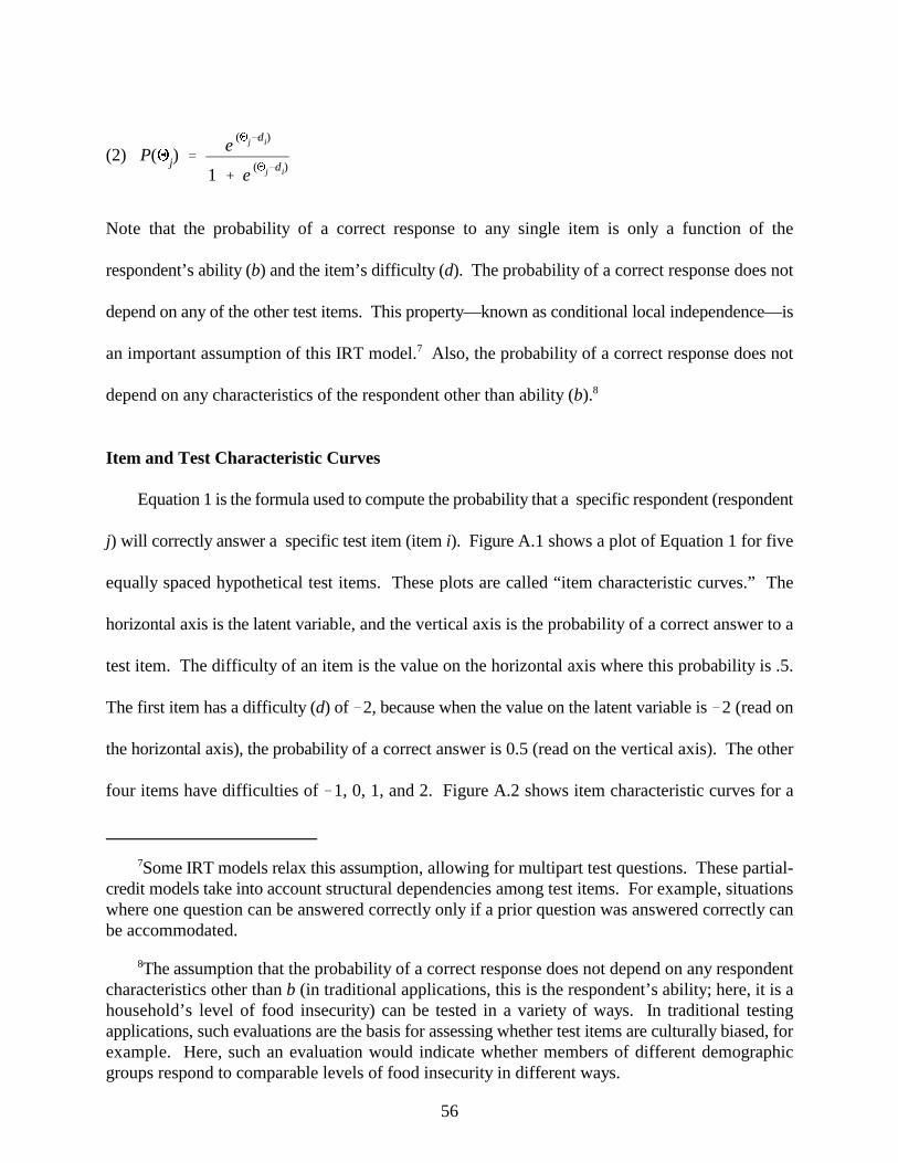
P( j) �e
( j�di)
1 � e( j�di)
Some IRT models relax this assumption, allowing for multipart test questions. These partial-7
credit models take into account structural dependencies among test items. For example, situationswhere one question can be answered correctly only if a prior question was answered correctly canbe accommodated.
The assumption that the probability of a correct response does not depend on any respondent8
characteristics other than b (in traditional applications, this is the respondent’s ability; here, it is ahousehold’s level of food insecurity) can be tested in a variety of ways. In traditional testingapplications, such evaluations are the basis for assessing whether test items are culturally biased, forexample. Here, such an evaluation would indicate whether members of different demographicgroups respond to comparable levels of food insecurity in different ways.
56
(2)
Note that the probability of a correct response to any single item is only a function of the
respondent’s ability (b) and the item’s difficulty (d). The probability of a correct response does not
depend on any of the other test items. This property—known as conditional local independence—is
an important assumption of this IRT model. Also, the probability of a correct response does not7
depend on any characteristics of the respondent other than ability (b).8
Item and Test Characteristic Curves
Equation 1 is the formula used to compute the probability that a specific respondent (respondent
j) will correctly answer a specific test item (item i). Figure A.1 shows a plot of Equation 1 for five
equally spaced hypothetical test items. These plots are called “item characteristic curves.” The
horizontal axis is the latent variable, and the vertical axis is the probability of a correct answer to a
test item. The difficulty of an item is the value on the horizontal axis where this probability is .5.
The first item has a difficulty (d) of �2, because when the value on the latent variable is �2 (read on
the horizontal axis), the probability of a correct answer is 0.5 (read on the vertical axis). The other
four items have difficulties of �1, 0, 1, and 2. Figure A.2 shows item characteristic curves for a
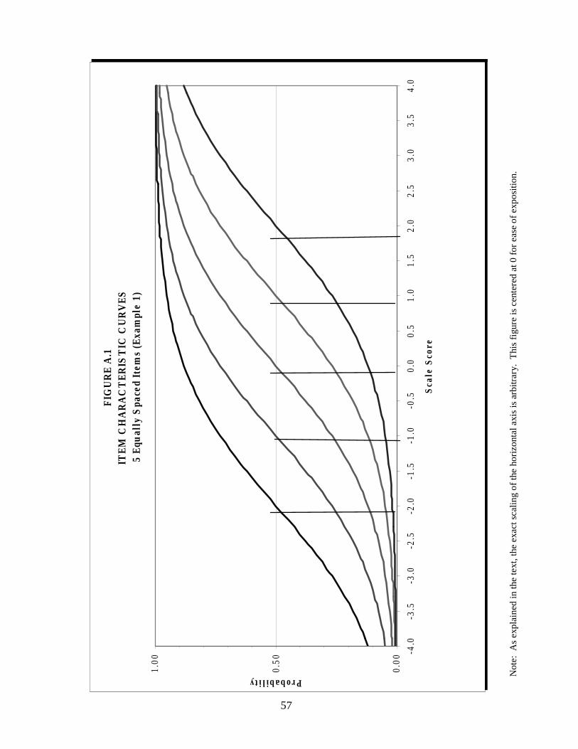
FIG
UR
E A
.1IT
EM
CH
AR
AC
TE
RIS
TIC
CU
RV
ES
5
Equ
ally
Spa
ced
Item
s (E
xam
ple
1)
0.00
0.50
1.00
-4.0
-3.5
-3.0
-2.5
-2.0
-1.5
-1.0
-0.5
0.0
0.5
1.0
1.5
2.0
2.5
3.0
3.5
4.0
Sca
le S
core
Probability Not
e: A
s ex
plai
ned
in th
e te
xt, t
he e
xact
sca
ling
of th
e ho
rizo
ntal
axi
s is
arb
itrar
y. T
his
figu
re is
cen
tere
d at
0 f
or e
ase
of e
xpos
ition
.
57

FIG
UR
E A
.2IT
EM
CH
AR
AC
TE
RIS
TIC
CU
RV
ES
5 It
ems,
3 V
ery
Clo
se T
oget
her
(Exa
mpl
e 2)
0.00
0.50
1.00
-4.0
-3.5
-3.0
-2.5
-2.0
-1.5
-1.0
-0.5
0.0
0.5
1.0
1.5
2.0
2.5
3.0
3.5
4.0
Sca
le S
core
Probability
58
Not
e: A
s ex
plai
ned
in th
e te
xt, t
he e
xact
sca
ling
of th
e ho
rizo
ntal
axi
s is
arb
itrar
y. T
his
figu
re is
cen
tere
d at
0 f
or e
ase
of e
xpos
ition
.

Actually, there is no difference in the two situations. In both cases, the vertical axis measures9
the expected value of the outcome. In the case of the item characteristic curves, those expectedvalues are between 0 and 1. For test characteristic curves, the expected values range between 0 andthe number of items in the test. Item characteristic curves can be summed to create a testcharacteristic curve because expected values are additive.
59
different set of five hypothetical items. In this example, the items are not equally spaced: while the
first and last items still have difficulties of -2 and 2, the middle three items are clustered close to 0:
they have difficulties of �0.1, 0.0, and 0.1.
Just as multiple items can be combined to form a test, multiple-item characteristic curves can
be combined to produce a test characteristic curve. Raw test scores are computed by summing the
number of correct answers, and the test characteristic curve is created by summing the characteristic
curves of the items included in the test. Figure A.3 shows the test characteristic curve that results
when the items shown in Figure A.1 constitute the test. Figure A.4 shows a similar curve for the test
that results when the five items from Figure A.2 are combined. The interpretation of the vertical axis
of the test characteristic curve is slightly different from its interpretation in the context of item
characteristic curves. Rather than represent the probability of a correct response to a single item, the
vertical axis represents the expected number of correct responses to all items included in the test—
the expected value of the respondent’s raw score on the test.9
Just as an item characteristic curve relates the probability of a correct (or “positive” in the food
security context) answer to a respondent’s estimated location on the latent variable, a test
characteristic curve relates the number of correct answers on a test to a respondent’s location on the
latent variable. For example, in Figure A.3, respondents who answer one of the five items correctly
(read on the vertical axis) are assigned a scale score of �1.9 (on the horizontal axis). Respondents
with raw scores of 2, 3, and 4 are assigned scale scores of �0.5, 0.6, and 2.0, respectively. (While

FIG
UR
E A
.3T
EST
CH
AR
AC
TE
RIS
TIC
CU
RV
ESu
m o
f Ite
m C
hara
cter
isti
c C
urve
s5
Equ
ally
Spa
ced
Item
s (E
xam
ple
1)
012345 -4.0
-3.5
-3.0
-2.5
-2.0
-1.5
-1.0
-0.5
0.0
0.5
1.0
1.5
2.0
2.5
3.0
3.5
4.0
Sca
le S
core
Raw Score
60
Not
e: A
s ex
plai
ned
in th
e te
xt, t
he e
xact
sca
ling
of th
e ho
rizo
ntal
axi
s is
arb
itrar
y. T
his
figu
re is
cen
tere
d at
0 f
or e
ase
of e
xpos
ition
.

FIG
UR
E A
.4T
EST
CH
AR
AC
TE
RIS
TIC
CU
RV
ESu
m o
f Ite
m C
hara
cter
isti
c C
urve
s 5
Item
s, 3
Ver
y C
lose
Tog
ethe
r (E
xam
ple
2)
012345
-4.0
-3.5
-3.0
-2.5
-2.0
-1.5
-1.0
-0.5
0.0
0.5
1.0
1.5
2.0
2.5
3.0
3.5
4.0
Sca
le S
core
Raw Score
61
Not
e: A
s ex
plai
ned
in th
e te
xt, t
he e
xact
sca
ling
of th
e ho
rizo
ntal
axi
s is
arb
itrar
y. T
his
figu
re is
cen
tere
d at
0 f
or e
ase
of e
xpos
ition
.

62
it may not be intuitively obvious, it can be shown mathematically that these are maximum likelihood
estimates of the respondents’ latent trait values.)
Impossibility of Scoring “Extreme” Response Patterns
Several important points should be noted. First, using this test and this IRT model, respondents
with raw scores of 0 or 5 cannot be assigned scale scores. In the case of no correct responses, all we
know is that the respondent’s scale score ability is below the range that can be measured by this test.
The problem is, the model is completely uninformative about how far below the range of this test
the respondent’s score lies. In the case of a perfect score (a correct response for each of the five
items), all we know is that the respondent’s scale score is above the range that can be measured by
this test. Again, however, the model provides no information about how far above.
In the current food security application, it is clear that the IRT model cannot provide scale scores
to households that answered “Yes” to every item they were asked. Because there are very few such
households, this presents no real problem. However, the model also cannot provide scale scores for
households that answer “No” to all items (households with raw scores of zero). This is a limitation,
because nearly 90 percent of the sample falls in this category. It is clear that such households should
be classified as “food secure,” and they are so identified in the ordinal variable that classifies
households into one of the three food-insecurity categories. However, the IRT results are
uninformative about how much more secure they are than the households that answered “Yes” to
only one item. The model is also uninformative about whether all such households are equally
secure. Although none of the households reported any behaviors that are symptomatic of food
insecurity, some are undoubtedly at greater risk than others.

It is appropriate, however, to recognize that a test item provides more information about10
respondents with locations on the latent scales close to the difficulty of the item, and less informationabout respondents with locations far from the item’s difficulty. The key point to recognize here isthat a test item provides information about a range of abilities, not a single point. We will discussthis issue in more detail later.
63
Lack of a Direct Relationship Between Item Scores and Respondent Scores
Another important feature to note is that the scale scores assigned to respondents do not have
any simple relationship to the difficulties of the items. In Figure A.1, the five items had difficulties
of �2, �1, 0, 1, and 2; but the scores assigned to respondents in Figure A.3 are �1.9, �0.5, 0.6, and
2.0 (and notice that the score of 2.0 is assigned to students with 4 positive answers, not 5). The lack
of an obvious relationship between the item parameters and the respondent parameters can be seen
even more clearly by comparing Figures A.2 and A.4. While the items in Figure A.2 had difficulties
of �2, �0.1, 0, 0.1, and 2, the scale scores assigned to respondents are �1.8, �0.5, 0.5, and 1.8.
Respondents with two positive answers are assigned a scale score (�0.5) that is actually below the
difficulty level of the second item in the test (�0.1). Partly because of the lack of a simple
relationship between item difficulties and respondent scale scores, it is not useful to think of test
items as directly measuring a specific level of ability.10
5. The Scaling of the Latent Variable Is Arbitrary
Scaling of the IRT parameters is arbitrary. We noted above that the latent variable is measured
as an interval-level scale. We also noted that many pairs of values for b and d produce the same
probability, and those pairs are each linear functions of each other. The three hypothetical IRT scales
shown in Figure A.5 are all equivalent: in every case, the difference between the first and fourth
numbers is twice the difference between the first and third numbers.

Ii( ) �[Pi’( )]2
Pi( )[1�Pi( )],
Ii( )
Pi’( )
Pi( )
This is also the formula for Fisher’s Information for the IRT models discussed here.11
64
THREE EQUIVALENT IRT SCALES
� �1 5 8 17
� 11 17 20 29 (added 12 to line 1)
� 10 70 100 190 (added 2 to line 1, then multiplied by 10)
FIGURE A. 5
In most of this report, we use a different scaling convention than Hamilton et al. (1997) used
in their work. Therefore, some of the IRT parameters presented in this report appear to be
substantially different from those derived in the earlier work, when, in fact, our estimates are close
to those reported by Hamilton et al.
Maximizing Information Content of Items
Although each test item provides information about respondents with a range of abilities, the
amount of information depends on how close a respondent’s ability is to a test item’s difficulty. The
amount of information provided by an item reaches its maximum for respondents with ability levels
equal to the item’s difficulty. This relationship can be formalized, and is shown in Equation 3:
(3)
where is the information provided by item i at the point on the latent variable,
is the slope of the item response function (Equation 1) evaluated at ,
and is the probability of a correct response to item i by a respondent with ability .11
In the Rasch model, Equation 3 simplifies to Equation 4:
Ii( ) � Pi( ) [1�Pi( )],
Pi( )
IT( ) � �k
i�1Ii( ).
IT( )
SE( j) �1
IT ( j).
65
(4)
which reaches a maximum at = .5, the point on the graph where the respondents’ ability equals
the items’ difficulty.
Figure A.6 illustrates the form of the information function for the five hypothetical items
originally presented in Figure A.1, and Figure A.7 shows the information curves for the five
hypothetical items from Figure A.2. In each case, note that an item’s information reaches a
maximum at the item’s location—that is, its estimated difficulty. But also note that each item
provides information about a range of values along the latent variable.
Just as item characteristic curves are summed to arrive at a test characteristic curve, the item
information curves are summed to arrive at a test information curve:
(5)
In Equation 5, is the total test information evaluated at . To put this in more familiar terms,
the test information is inversely related to the standard error of the estimated value of for
respondent j:
(6)

FIG
UR
E A
.6IT
EM I
NF
OR
MA
TIO
N C
UR
VE
S
5 E
qual
ly S
pace
d It
ems
(Exa
mpl
e 1)
0.00
00
0.05
00
0.10
00
0.15
00
0.20
00
0.25
00
0.30
00
-4.0
-3.5
-3.0
-2.5
-2.0
-1.5
-1.0
-0.5
0.0
0.5
1.0
1.5
2.0
2.5
3.0
3.5
4.0
Sca
le S
core
Information
66
Not
e: A
s ex
plai
ned
in th
e te
xt, t
he e
xact
sca
ling
of th
e ho
rizo
ntal
axi
s is
arb
itrar
y. T
his
figu
re is
cen
tere
d at
0 f
or e
ase
of e
xpos
ition
.

FIG
UR
E A
.7IT
EM
IN
FO
RM
AT
ION
CU
RV
ES
5
item
s, 3
Ver
y C
lose
Tog
eth
er (
Exa
mpl
e 2)
0.00
00
0.05
00
0.10
00
0.15
00
0.20
00
0.25
00
0.30
00
-4.0
-3.5
-3.0
-2.5
-2.0
-1.5
-1.0
-0.5
0.0
0.5
1.0
1.5
2.0
2.5
3.0
3.5
4.0
Sca
le S
core
Information
67
Not
e: A
s ex
plai
ned
in th
e te
xt, t
he e
xact
sca
ling
of th
e ho
rizo
ntal
axi
s is
arb
itrar
y. T
his
figu
re is
cen
tere
d at
0 f
or e
ase
of e
xpos
ition
.

68
In other words, when a test provides more information about a respondent’s ability, that respondent’s
ability (scale score) is estimated more precisely.
Figures A.8 and A.9 show the test information curves for the hypothetical tests depicted in
Figures A.6 and A.7. The curve shown in Figure A.9 has a higher maximum than the curve shown
in Figure A.8 (0.96 for the curve shown in Figure A.9, compared to 0.85 for the Figure A.8 curve).
This is a result of having the three middle test items much more tightly clustered in the Figure A.9
example than in the Figure A.8 example: the Figure A.9 test provides more information about that
part of the ability scale where the test items are clustered.
In both examples, it is clear that the amount of information a test provides about a respondent
is a function of that respondent’s ability relative to the difficulty of the test items. For example, the
test information curve shown in Figure A.8 illustrates how much more information the five-item test
provides about a respondent with an ability of 0.1 (where the test information is close to its
maximum value of 0.85) than a respondent with an ability of 3.6 (where the test information is only
0.25). In general, the standard error of the estimate of a respondent’s scale score is inversely related
to the number of test items (longer tests yield more precise estimates than shorter tests) and how well
the difficulty of the test items match the ability of the respondent (questions from a second-grade
reading test would yield highly imprecise estimates of sixth-grade reading ability).
The test information curves for the two versions of the food security test are shown in
Figure A.10. The information curve for the 18-item test administered to households with children
is above the curve for the 10-item test over the entire range of the food insecurity scale: the 18-item
test yields estimates of household food insecurity that are substantially more precise than the 10-item
test. The curves also show that the 18-item test attains its maximum information at a more extreme
level of food insecurity than does the 10-item test. This happens because the items that ask about

FIG
UR
E A
.8T
EST
INFO
RM
AT
ION
CU
RV
ES
um o
f Ite
m In
form
atio
n C
urve
s5
Equa
lly
Spa
ced
Item
s
0.0
000
0.1
000
0.2
000
0.3
000
0.4
000
0.5
000
0.6
000
0.7
000
0.8
000
0.9
000
1.0
000
-4.0
-3.5
-3.0
-2.5
-2.0
-1.5
-0.9
-0.4
0.1
0.6
1.1
1.6
2.1
2.6
3.1
3.6
Sca
le S
core
Information
69
Not
e: A
s ex
plai
ned
in th
e te
xt, t
he e
xact
sca
ling
of th
e ho
rizo
ntal
axi
s is
arb
itrar
y. T
his
figu
re is
cen
tere
d at
0 f
or e
ase
of e
xpos
ition
.0

FIG
UR
E A
.9T
EST
INFO
RM
AT
ION
CU
RV
ES
um o
f Ite
m In
form
atio
n C
urve
s 5
item
s, 3
Ver
y C
lose
Tog
ethe
r
0.00
00
0.10
00
0.20
00
0.30
00
0.40
00
0.50
00
0.60
00
0.70
00
0.80
00
0.90
00
1.00
00
-4.0
-3.5
-3.0
-2.5
-2.0
-1.5
-0.9
-0.4
0.1
0.6
1.1
1.6
2.1
2.6
3.1
3.6
Sca
le S
core
Information
70
Not
e: A
s ex
plai
ned
in th
e te
xt, t
he e
xact
sca
ling
of th
e ho
rizo
ntal
axi
s is
arb
itrar
y. T
his
figu
re is
cen
tere
d at
0 f
or e
ase
of e
xpos
ition
.

FIG
UR
E A
.10
18-
AN
D 1
0-IT
EM T
EST
CH
AR
AC
TER
ISTI
C C
UR
VES
Bas
ed o
n 1
995
Item
Cal
ibra
tion
s
0123456789101112131415161718
-5.0
-4.0
-3.0
-2.0
-1.0
0.0
1.0
2.0
3.0
4.0
5.0
Food
In
secu
rity
Sco
re
Number of "Yes" Responses
71
Not
e: A
s ex
plai
ned
in th
e te
xt, t
he e
xact
sca
ling
of th
e ho
rizo
ntal
axi
s is
arb
itrar
y. T
his
figu
re is
cen
tere
d at
0 f
or e
ase
of e
xpos
ition
.

This can be seen by examining the property noted at the end of Section 2 above—that the test12
characteristics curves can be used to assign respondent scores based on the number of correctanswers to test items.
While the IRT model provides no basis for assigning scores beyond the range of the test, other13
statistical techniques can sometimes be used. For example, if student scale scores are believed tohave a specific distributional form, scale scores can be assigned to students with extreme raw scoresso that, when the student scores are combined with the scores assigned by the model, the scores do,in fact, have the assumed distribution.
72
children have severity levels that are higher, on average, than the items that do not ask specifically
about children.
Mapping Raw Scores to Scale Scores
Another aspect of the Rasch model to note is that, except for respondents who did not answer
some of the questions, all respondents with the same raw score are assigned the same scale score,
regardless of which items they answered positively. This one-to-one mapping between raw scores12
and respondent scale scores with the Rasch model means that, when all respondents take the same
test and all answer the same questions, the number of correct responses completely determines the
scale score assigned to a respondent. Even though the scale scores appear to be drawn from a
continuous, interval-level variable, only a small number of actual scores are assigned when the test
has a small number of items. If a test has only five items, all respondents answering all the questions
(except for those at the extremes with either zero or five correct answers) will be assigned one of
four different scale scores because model-based scale scores can be assigned only for those
respondents with raw scores from 1, 2, 3, or 4.13
Equating Scores from Different Tests
The use of test characteristic curves is the key to scoring respondents on a common scale when
they take different tests. Once the difficulty of each test item, relative to every other item, is known,

In principle, it is possible to have different tests with no common items. For example, when14
tests are used to monitor student progress through elementary school, it is possible to test first-gradestudents and sixth-grade students using separate, grade-appropriate tests that measure studentperformance on a common scale. For this to work, there must be at least one test with someoverlapping content at an earlier stage. In the example of monitoring student progress throughelementary school, there would likely be at least one test per year with some overlapping content ineach pair of adjacent tests. Item calibrations from those tests establish the relative difficulty of testitems. Then, using those calibrations as fixed reference points, all other test items can be calibratedrelative to those reference points. Once all items have been calibrated with respect to each other, thescores assigned to students will all be measured on a common scale.
In April 1997, essentially two additional tests were administered. Because of an error in the15
questionnaire, two of the CPS rotation groups—about a quarter of the sample—were not asked oneof the food security questions. For the households affected, this resulted in a 17-question versionof the test being administered to households with children, and a 9-question version administeredto households without children.
73
test characteristic curves can be constructed for any combination of those items. Each test
characteristic curve translates raw scores—the number of current responses—into scale scores for
respondents. Because all test items are calibrated on the same scale, the resulting respondent scores
are also on a common scale, even when the tests taken by different respondents have few test items
in common.14
In the current application, there are basically two different versions of the test: (1) an 18-item
test administered to households with children, and (2) a 10-item test administered to households
without children. Figure A.10 shows the two resulting test characteristic curves that are used for15
assigning household scores based on households’ responses to the food insecurity questions. Using
these curves, a raw score of 9 is mapped to a scale score of about 0.0 for households with children,
but is mapped to a scale score of about 2.0 for households without children. Using the upper curve
in Figure A.10, households with children are assigned 1 of 17 different scale scores. Using the lower
curve, childless households are assigned 1 of 9 different scale scores.

For instance: BIGSTEPS Rasch-Model Computer Program, MESA Press, 5835 Kimbark Ave.,16
Chicago IL. 60637-1609. BILOG Scientific Software International, 7833 N. Lincoln Ave., Suite100, Lincolnwood, IL 60712-1704.
74
3. ESTIMATION OF RESPONDENT AND ITEM PARAMETERS
Up to this point, the discussion has been about the properties of the IRT model, assuming that
the model parameters (or at least the item parameters) were already known. In many applications,
the model parameters—both the respondent parameters and the item parameters—need to be
estimated. In this section, we briefly describe how those parameters are estimated. Specialized
software for estimating these models is readily available and easily used.16
Several approaches have been devised for estimating the parameters of the IRT models used
here, all of which are different variations of maximum likelihood estimators. The goal in maximum
likelihood estimation is to choose the values of the model parameters that maximize the likelihood
of yielding the observed sample. For example, if a trait has a uniform distribution in the population,
then the maximum likelihood estimate for the population mean value is the mean value observed in
the sample itself. Any other estimate of the population mean (such as the mean from some other
sample, the median from the current sample, or even the mean from a census) would result in a lower
likelihood of observing the current sample. One important point to notice in this example is that it
begins by assuming a specific distribution for the trait in the population (in this case, the trait is
assumed to be uniformly distributed). This is a strong assumption; in many applications, results are
not robust to different distributional assumptions that usually cannot be fully tested. An assumption
about the underlying distribution is always a necessary starting point in maximum likelihood

1N
N
i�1(x̄�xi)
2 1N�1
N
i�1(x̄�xi)
2
P (Uij�1 |bj)�e
(bj�di)
1�e(bj�di)
�Pij
P(Uij�0 |bj)� (1�Pij)�Qij.
L�j i
PUij
ij Q1�Uij
ij ,
For example, the maximum likelihood estimator for the variance of a normally distributed17
variable is . An unbiased estimator, however, is .
75
estimation. Maximum likelihood estimators are often not unbiased. However, Rasch model17
parameters estimated using conditional likelihood procedures are unbiased, consistent, and efficient.
The likelihood expression for the Rasch model uses Equation 1 as its starting point. Equation
1 expresses the probability of a current response by a specific individual to a single test item as a
function of that item’s difficulty and that person’s ability. If U is the response (and equals 1 for aij
correct response, 0 for an incorrect response), then, from Equation 1, we have:
(7)
Thus, we represent the probability of a correct response by respondent j to item i as P , and theij
probability of an incorrect response as Q . If there are five test items, person j’s responses might beij
something like (1,1,0,1,0). The associated probabilities would be (P P Q P Q ). The1j, 2j, 3j, 4j, and 5j
probability of this specific string of responses would then be the product of the five
probabilities—that is, Pr(1,1,0,1,0) = P P Q P Q . Generalizing from this example, the likelihood1j 2j 3j 4j 5j
of a sample is the product of the probabilities across all sample members of each person’s response
string. The likelihood function, then, has the following form:
(8)

ln(L)�j i
[Uijln(Pij)]� [(1�Uij)ln(Qij)].
76
where P and Q are defined in Equation 7.
The product over i gives the probability of person i’s response string. The product over j
multiplies the response string probabilities for everybody who took the test. Rather than maximize
Equation 8 directly, the log of the likelihood function is generally used:
(9)
The goal, then, is to find the values of b and d that maximize the expression in Equation 9.j i
Generally, the problem is broken into two parts, so that item parameters (d ) are first estimated (usingi
either marginal or conditional maximum likelihood); then, using those estimated item parameters,
the respondent parameters are estimated (using a numerical procedure equivalent to translating raw
scores into scale scores, using the test characteristic function). Joint estimation of the item and
person parameters is also an option and may be statistically more efficient than the two- stage
procedure just described. All these estimation strategies are easily implemented with the current
generation of IRT software.

APPENDIX B
METHOD FOR SCREENING HOUSEHOLDS INTO THE FOOD SECURITY ANALYSIS


79
METHODS FOR SCREENING HOUSEHOLDS INTO THE FOOD SECURITYANALYSIS
The food security supplements in the 1995-1997 CPS had two general sections. The first section
gathered information about food expenditures, participation in several programs aimed at providing
food to needy families (for example, food stamps and school meal programs), and the sufficiency
of food eaten during the preceding 12 months. The second section gathered more-detailed
information about food security and coping behaviors during the previous 12 months and prior 30
days. Not all households were asked this second set of questions, which includes the questions used
to construct the food security scale. In order to minimize respondent burden, households who, on
the basis of earlier questions, appeared to have a high likelihood of being food secure were excluded
from the more detailed questions and were implicitly assumed to be food secure in the analysis.
The screening procedures used to determine which households were asked the second set of
questions were different in each of the three CPS samples (1995-1997) analyzed for this report; this
section describes the analytic techniques we have developed to put these samples on a consistent
basis for analysis purposes. We begin in the next section by providing background information.
Then we describe the screening procedures used in each of these three CPS samples and identify a
“greatest common denominator” screen. The latter is an analysis “screen” that can be applied
uniformly across all the samples, to ensure that the samples used in the analytic work are
comparable. (A standard screening procedure, which as been used consistently in all subsequent
years, was adopted in 1998.)
Parts of this material overlap with information provided in Chapter IV. However, the discussion
here provided additional detail not presented in that earlier, summary treatment.

The CPS is designed to visit the same addresses over time, not the same people. When the1
members of a household move to a new address, they leave the CPS sample (unless they happen tomove into another CPS address). The new residents of the CPS address are a replacementhousehold, and are interviewed for that address’s remaining, planned interviews.
80
(I am going to read a list of income categories.) Which category represents (your/name of referenceperson/the total combined income) (total combined income during the past 12 months/of all membersof this FAMILY during the past 12 months)? This includes money from jobs, net income frombusiness, farm or rent, pensions, dividends, interest, social security payments, and any other moneyincome received (by members of this FAMILY who are 15 years of age or older).
<1> Less than $5,000 <2> $5,000 to $7,499 <3> $7,500 to $9,999 <4> $10,000 to $12,499 <5> $12,500 to $14,999 <6> $15,000 to $19,999 <7> $20,000 to $24,999 <8> $25,000 to $29,999 <9> $30,000 to $34,999 <10> $35,000 to $39,999<11> $40,000 to $49,999<12> $50,000 to $59,999<13> $60,000 to $74,999<14> $75,000 or more
1. Background
Measuring Income in the CPS Core
As will be described below, the food security supplement screening procedures were based
partly on income. Therefore, we begin by describing the income data used.
Income is measured in the CPS core questionnaire, not the food security supplement. The
income measure that is a part of the CPS core is quite limited. The only question about income is
one that allows only categorical responses, is asked only of the household reference person, and is
asked only when the household rotates into the CPS sample (in month 1 and in month 5 of the CPS
sample rotation). For all other households, information from the most recent response is carried
forward to the current interview month. Income information for replacement households is1
collected when the household first appears in the CPS sample. The income question is:

The DHHS Poverty Guidelines are widely used to determine program eligibility (for example,2
by the Food Stamp Program, WIC, and the National School Lunch Program).
81
Defining “Poor” Households in the Food Security Supplement
Screening in the 1995-1997 data depended, in part, on whether households were “poor,” as
defined by the criteria set up for the screening. Each version of the food security supplement applied
different screening criteria to households categorized as “poor” and those categorized as “nonpoor.”
Here we describe the definitions used. Table B.1 shows the thresholds used to define households
as poor. All the supplements used the same set of thresholds. Table B.1 also shows the threshold
levels as a percentage of the DHHS Poverty Guidelines published in 1994, 1995, and 1996. Within2
each year, the thresholds across households of different sizes, up through six people, are nearly
constant multiples of the poverty guidelines. For the small number of households with 7, 9, or 10+
members, much higher thresholds were used.
Because thresholds set at constant nominal dollars were used over this period, the criteria used
to classify households as “poor” were increasingly stringent (in real terms) over time, as shown in
the decreasing percentages across rows of Table B.1. Because the categories for the CPS income
variable are fixed at the same nominal levels across the three CPS samples, it is not possible to apply
an income screen at a constant real value.
Even with the limitations noted, however, it is a fair approximation to describe the “poor” (or
low-income) households as those reporting incomes less than about 200 percent of the poverty
guideline.
Measuring Food Sufficiency
Several different versions of the basic food sufficiency questions were administered, but the
general form of them is the same. All ask about household experiences over the prior 12 months and

82
TABLE B.1
THRESHOLDS USED TO CLASSIFY HOUSEHOLDS AS “POOR” ANDDHHS POVERTY GUIDELINES AT TIME OF SURVEY
Threshold as a Percent of Poverty Guideline
Household Size (in Dollars): 1994 1995 1996 1997
“Poor” if FamilyIncome Below
1 15,000 204 201 194 190
2 20,000 203 199 193 189
3 25,000 203 199 193 188
4 30,000 203 198 192 187
5 35,000 203 198 192 186
6 40,000 202 197 192 186
7 50,000 225 219 213 207
8 50,000 202 197 192 186
9 60,000 221 215 209 202
10+ 75,000 253 246 239 232
Average 212 207 201 195
Average for HouseholdsWith 6 or Fewer Persons 203 199 193 188

83
ask the respondent (the household reference person) to choose the statement that best describes the
household’s experience. The response categories are:
1. Enough of the kinds of food we want to eat2. Enough but not always the kinds of food we want to eat3. Sometimes not enough to eat4. Often not enough to eat5. Don’t know6. Refused7. No response
In the following discussion of screening procedures, we will refer to response 2 as “Not always the
kind of food we want.” Responses 3 and 4 will be referred to jointly as “Sometimes or often not
enough to eat.”
Two other related items were also used in the screening process. One item asks:
“In the last 12 months, did you ever run short of money and try to make your food or yourmoney go further?”
We will refer to this item as “Ran short of money.” The second item asks:
“In the last 12 months, did you ever run out of the foods that you needed to makea meal and didn’t have enough money to get more?”
We will refer to this item as “Ran out of food.”
Across the 1995-1997 supplements, these items were combined at various times and with
various groups of households to create two screens:
Screen 1
C Sometimes or often not enough to eat; orC Ran out of food; orC Not always the kind of food we want and ran short of money.

Households reporting any one of the following passed the (incorrect) screen: 1. Sometimes not3
enough to eat (incorrectly omitting "often not enough to eat") ; or 2. Ran out of food in last 12months; or 3. Enough to eat (instead of "Not always the right kind of food") and ran short of money.
84
Screen 2
C Sometimes or often not enough to eat; orC Ran out of food; orC Not always the kind of food we want; orC Ran short of money.
Note that the screens are identical except that, under Screen 1, it is necessary to both not eat the kind
of food we want and run out of money, whereas either condition is sufficient under Screen 2. Thus,
Screen 2 is more liberal, allowing more households to pass, while Screen 1 is more restrictive.
2. Application of the Screens
Table B.2 summarizes the screening procedures used in each of the CPS samples:
TABLE B.2
CRITERIA USED IN 1995-1997 SURVEYS TO SCREEN HOUSEHOLDS INTO THE FOOD SECURITY MODULE
“Poor” Households “Nonpoor” Households
April 1995 All “poor” households entered the Screen 1sample.
September Screen 2 Rotation groups 1, 2, 3, 5, 6, 7:1996 Screen 1
Rotation groups 4 and 8: Screen 2.
April 1997 Screen 2 Rotation groups 1, 5, and 7: Screen 1.
Rotation groups 2, 4, 6, and 8: Screen 2.
Rotation group 3 used an incorrectvariant of Screen 1.3
Note: See text for definitions of screens.
The concern here is with changes in the composition of the responding population that are an4
artifact of the screening procedures used, rather than those that reflect real changes in populationcomposition.
85
The procedures were designed to screen out households that showed no indication of any food
insufficiency. A household passing the applicable screen was asked the remaining questions in the
food security supplement. In effect, to avoid the food-security questions a household had to say
“No” to all screening questions. Households that had missing data for the screening items (including
“Don’t know” or “Refused” responses) passed the screen.
3. A Consistent Screen for 1995-1997
Applying consistent screening procedures across all the CPS samples is important in two
different contexts. First, to the extent that estimated item parameters differ across the three CPS
samples, it is important to know whether those differences reflect changes, over time, in how the
items are functioning or differences in the composition of the population responding to those items.4
Second, to the extent that estimates of the prevalence of food insecurity and hunger differ across the
CPS samples, it is important to know whether those changes reflect real changes, over time, in
prevalence or differences in the size (and composition) of the population for which the condition was
measured.
To allow consistency in the analysis, we have developed an algorithm for screening households
that can be applied uniformly across the 1995-1997 CPS samples. All households failing to pass the
screen are categorized as food secure and are assigned the same score as households that answered
“No” to all the applicable food-security questions. The screen is the following:
“Pass into the sample if
(a) household is poor and passes Screen 2, or

86
(b) household is not poor and passes Screen 1”
4. A “Tighter,” Consistent Screen
The common screen described above utilizes the CPS income data to determine exactly which
screening criteria to apply to a case. However, as noted in Section 1, there are significant limitations
in the quality of these income data. Therefore, a different, considerably “tighter” screen was
considered in parts of the analysis, which consisted of applying “Screen 1” regardless of income.
However, this screen has not been used in the main parts of the analysis because of the loss of
sample size involved in applying it.
5. Impacts on Prevalence Estimates
Relative to the other assumptions, conventions, and choices of analysis procedures discussed
in this report, the screening conventions described above tend to have relatively substantial impacts
on estimates of food security prevalence. Table B.3 compares the basic prevalence estimates based
on the common screen presented earlier with “full sample” estimates, based on all the available
information. Since, in certain cases, the imposition of the common screen essentially involves
automatically coding the food security answers to be negative (that is, to indicate no evidence of food
insecurity), the imposition of the common screen must, by definition, lead to higher estimated
prevalences of food security. As shown in the table, estimated rates of food security are reduced by
approximately 1 to 1.5 percentage point when the maximum samples are used rather than the
samples defined by the common denominator.
How the differences in prevalence should be interpreted depends on one’s view of the accuracy
of the information contained in the cases that were screened out. Since these screened-out cases are

87
TABLE B.3
FOOD SECURITY PREVALENCE ESTIMATES WITH ALTERNATIVE DEFINITIONSOF THE ANALYSIS SAMPLE
Using Alternative Household Screening Conventions(Entries are Percentages)
Food Insecure
Food Without With Secure All Hunger Hunger
1995
Common Denominator Sources 89.6 10.3 6.4 3.9
Maximum Sample 88.1 11.8 7.6 4.2
1996
Common Denominator Sources 89.5 10.5 6.4 4.1
Maximum Sample 88.6 11.3 7.0 4.3
1997
Common Denominator Sources 91.2 8.8 5.7 3.1
Maximum Sample 90.3 9.6 6.4 3.2

88
households with relatively higher income and/or little evidence of food insufficiency, it is possible
that some of the households that answered affirmatively to 3 or more of the detailed 18 items of food
security information may, for some reason, have been confused or gave misleading answers. In this
case, using the lower food security estimates, based on the common screen, may be appropriate. On
the other hand, to the extent that the answers given by these screened-out households are accurate,
the “full sample” estimates may provide a better picture of food security in America. Our decision
to focus on the estimates based on the common screen was based principally on the importance of
having a consistent measure of food security over time. It does not reflect any assessment of which
of the two sets of estimates more accurately reflects the underlying phenomenon of interest.

APPENDIX C
IMPUTING MISSING FOOD SECURITY DATA


The percentage in the text ignores the problem created by answers to questions on one item in1
1997, where the item was incorrectly administered to about 25 percent of the sample.
91
IMPUTING MISSING FOOD SECURITY DATA
More than 99 percent of the households in the 1995-1997 CPS data sets have complete
responses to the questions used to construct the Food Security Index. The remaining households,1
however, must either be dropped from the analysis or have their missing items imputed. This section
discusses two alternative approaches to dealing with item nonresponse and describes the approach
used in the current study.
1. Alternative 1: Using the Rasch Model to Impute Missing Items
As long as at least one relevant question has been answered, the Rasch model is capable of
estimating a food security level for a household with missing data, as part of its maximum likelihood
estimation approach. However, a potential drawback of using an imputation approach based on the
Rasch model is that, when the number of unanswered questions is large, the standard error of the
estimated household food security level tends to become large; and, in some cases, the estimated
household score can lack face validity, in terms of the questions on which they are based. Hamilton
et al. (1997) dealt with this problem by estimating scores only for those households with at least half
the relevant items answered (9 out of 18 items for households with children, and 5 out of 10 items
for households without children).
Another drawback of using the Rasch model for imputation is that it fails to use all the
available data. Under quite general assumptions, it is reasonable to believe that imputation accuracy
can be improved by drawing both on information about the answers to the food-security questions

The approach used in the current study, as described later in the text, also ignores this2
information.
92
with valid answers and on available data on household characteristics. The Rasch approach ignores
the latter source of information.2
Another issue in using the Rasch model to estimate household scores for households with
missing data is that the approach requires the user to have available software for estimating the
Rasch model. While such software is relatively easy to obtain, this may present an obstacle to some
users who do not already have this software up and running for other purposes.
2. Alternative 2: An Algorithm Based on Modality Assumptions for Imputing Missing Data
An alternative approach to dealing with missing responses to food security items is to impute
responses outside the Rasch model, then treat the households as complete data households when
assigning scores and categories. This method--which, with one exception, noted below, is the one
used in the present study--has the advantages: (a) it can be specified so as to ensure that imputations
have face validity; and (b) it can be implemented without Rasch software, thus increasing its
accessibility. Below, we describe the algorithm we have used, first in intuitive terms and then more
formally.
The basic imputation approach relies on the notion that the most sensible response patterns are
those that are “modal.” That is, if the questions are ordered by their severity levels, households with
any affirmative responses tend to answer affirmatively to the items with the lowest severity levels
and then at some point begin answering negatively to the more severe items. In this context, our
imputation method assumes that, as a general rule, the highest affirmative answer indicates the
household’s true level of food insecurity, and the method fills in missing data below that affirmative
with other affirmatives and missing data above the highest affirmative with negatives. There is,

In converting the continuous scores of these households into food security categories, we used3
the midpoints of the boundary categories as the cutpoints.
93
however, an important exception to this general rule. If there is a negative answer below the highest
affirmative answer, then the imputation takes this as suggesting a lower overall level of food
insecurity than that implied by the highest affirmative. In the latter case, the algorithm selects the
lowest negative response and fills in affirmatives for missing data below that negative response and
negatives above it.
A more formal statement of this algorithm was presented in Chapter IV of the text of the report
as Exhibit IV.1.
3. Details of Procedures Used in Current Analysis
In general, in the work summarized in this report, we have used the imputation method outlined
immediately above, in Subsection 2. This method is substantially easier to implement than the
Rasch-based approach, and the differences in analysis results are negligible, given (a) the small
number of cases involved, and (b) that both methods tend to yield similar classifications of
households.
There is one exception, however. In the 1997 sample, roughly a quarter of the cases were
incorrectly asked one of the questions. For these cases, we first implemented the imputation
algorithm in Section 2 above, ignoring the question that had been asked incorrectly (Question 35;
“Respondent was hungry but didn’t eat”). We then used Rasch model software to calculate
continuous food security scores for those households, using the standard item calibrations utilized
throughout this study. These numerical scores were then translated into food security categories,
based on the table relating numbers of answers to continuous scores and food security categories.3

APPENDIX D
HOW “MODAL” ARE HOUSEHOLD RESPONSE PATTERNS?


97
HOW “MODAL” ARE HOUSEHOLD RESPONSE PATTERNS?
The Rasch model implies that many households will exhibit item response patterns that are
reasonably “modal,” in the sense that if a household answers “yes” to any of the items, it will tend
to answer “yes” to the least severe items first, and then answer “no” to all of the more severe items.
A household that exhibits this pattern exactly—a string of all “yes” answers followed by a string of
all “no” answers--is said to be a “modal” household. There is nothing in the Rasch theory that
predicts that all households will be modal; (indeed, the probabilistic Rasch model cannot be
estimated if all households are exactly modal). Still, it is of interest in understanding the data to
examine the degree of modality that is present. A large number of strongly nonmodal response
patterns could call into question the validity of the model.
A. NUMBER OF RESPONSE CHANGES TO MAKE HOUSEHOLD MODEL.
One approach to examining the degree to which households exhibit modal answers is to
calculate for each household the minimum number of answers that would have to be different in
order to make the household responses be modal. Of course, if the household’s answers are already
perfectly modal, then the number of answers that would have to be changed is zero. However,
consider, as an example, a household with the following response pattern: three “yes” answers, then
a “no,” then a “yes,” then all “no’s.” For such a household, only one item (the first “no” or the last
“yes”) would have had to be changed to make the response pattern modal. Similarly, to take a
second example, suppose a household has two “no” answers, then four “yes” answers, then all “no,”
answers. It would require at least two changes (the first two “no” answers) to make the household
modal.

Of course, for a household with just one nonmodal answer, that answer could be severely1
nonmodal (a “no” at the beginning of a long string of “yes” answers, or a “yes” many items after theprevious “yes”). We examine the severity of nonmodality shortly.
98
Table D.1 tabulates the minimum number of answer changes required to make the households
in the 1997 sample modal. It shows that 39 percent of the households in the 1997 data are perfectly
modal. For another 36 percent there is only one discrepancy between their scores and a modal
pattern. Fifteen percent have two such discrepancies, while 9 percent have three or more. Overall,
this suggests substantial adherence to modal response patterns.1
Households without children appear to exhibit greater modality than those with children.
However, this may be due to the fact that there are many fewer questions applicable to the group
without children (10, rather than 18, for households with children), and hence fewer opportunities
for nonmodality.
Table D.2 presents a more detailed look at these issues, focusing on households with children.
The central section of the table shows, for each possible number of “yes” answers, the frequency
distribution of the highest item (in terms of severity) to which the nonmodal households with
children answered “yes.” For instance, the fifth row shows that, when one considers the 233
nonmodal households that gave 5 “yes” answers, for 57 of them, the highest “yes” answer was on
Item 6, while for another 44, the highest “yes” answer was Item 7, and so on.
The shading in the table reflects the fact that certain cell entries are logically impossible—if, for
instance, there are five “yes” answers, the highest nonmodal item with a “yes” answer cannot come
before the sixth item. To the extent that the nonmodal households are “almost” modal, we would
expect households to be clustered just to the right of the shaded area. For instance, using a

Number of Nonmodal
Responsesa All HouseholdsHouseholds Without
Children Households With Children
0 39 50 30
1 36 38 33
2 15 9 21
3 6 2 9
4 2 0 4
5 1 0 2
6+ 0 0 1
Total 100 100 100
a Minimum number of responses that would have to be changed for the household to be modal.
TABLE D.1
PERCENT OF HOUSEHOLDS BY THE MINIMUM NUMBER OF NONMODALRESPONSES TO THE FOOD SECURITY ITEMS
(Percentages; 1997 Data)
99

Num
ber
of Y
esH
H%
HH
%2
34
56
78
910
1112
1314
1516
1718
HH
%1
600
20.4
%36
742
.5%
5669
827
711
00
10
00
00
00
023
311
.2%
248
516
.5%
204
23.6
%77
111
2216
384
44
13
10
00
00
281
13.5
%3
372
12.6
%10
412
.0%
117
3029
5415
116
22
11
00
00
268
12.9
%4
320
10.9
%72
8.3%
1871
7542
159
57
22
00
11
248
11.9
%5
241
8.2%
80.
9%57
4448
3220
126
100
20
20
233
11.2
%6
236
8.0%
80.
9%35
4898
149
93
36
12
022
811
.0%
717
86.
0%10
1.2%
3949
3022
68
55
31
016
88.
1%8
132
4.5%
333.
8%20
2224
1010
47
02
099
4.8%
100
912
94.
4%32
3.7%
2117
154
1219
44
197
4.7%
1068
2.3%
101.
2%4
142
1516
25
058
2.8%
1162
2.1%
70.
8%8
214
159
52
552.
6%12
441.
5%1
0.1%
110
165
110
432.
1%13
281.
0%0
0.0%
512
18
228
1.3%
1422
0.7%
00.
0%7
210
322
1.1%
1514
0.5%
50.
6%1
53
90.
4%16
80.
3%0
0.0%
44
80.
4%17
20.
1%0
0.0%
22
0.1%
183
0.1%
30.
3%0
0.0%
TO
TA
L2,
944
10
0.0%
864
100.
0%56
146
310
7718
025
719
622
912
796
8044
7110
528
6018
2,08
0
100.
0%2.
7%7.
0%14
.9%
3.7%
8.7%
12.4
%9.
4%11
.0%
6.1%
4.6%
3.8%
2.1%
3.4%
5.0%
1.3%
2.9%
0.9%
AL
LM
OD
AL
NO
NM
OD
AL
TA
BL
E D
.2
AN
AL
YSI
S O
F M
OD
AL
ITY
BY
NU
MB
ER
OF
YE
S R
ESP
ON
SES
TO
FO
OD
SE
CU
RIT
Y I
TE
MS
(199
7 D
ata:
Unw
eigh
ted
Hou
seho
lds
with
Chi
ldre
n)
NO
NM
OD
AL
- H
IGH
EST
YE
S R
ESP
ON
SE I
TE
M

In contrast, the Rasch model would assign this household the same insecurity score as any other2
household with six “yes” answers (and no missing responses), effectively treating it as though it hadthe modal response pattern of “yes” to the first 6 items and “no” to the last 12.
101
previous example, a household with five “yes” answers that has the sixth item as its highest “yes”
answer has only one nonmodal answer in its overall string of answers. For most rows in the table,
nonmodal households do cluster near the shaded diagonal, suggesting that the nonmodal response
patterns are not severely nonmodal. About 47 percent of nonmodal households are in the first two
off-diagonal cells, and an additional 22 percent are in the third cell.
B. BOUNDS ON THE EFFECTS OF NONMODALITY ON PREVALENCE ESTIMATES.
A useful way to understand the implications of nonmodal response patterns is to assess their
effects on prevalence estimates. Accordingly, in this section, we calculate for each household the
minimum and maximum food-insecurity levels that can be obtained by making the household’s
response pattern modal (Table D.3). To obtain the minimum insecurity level, we classify a
household based on the items before its first “no” answer. This effectively converts all higher “yes”
answers to “no” answers, giving a modal pattern. To obtain the maximum insecurity level, we
classify a household based on the items up to and including its last “yes” answer. This effectively
converts all lower “no” answers to “yes” answers, again giving a modal pattern.
Consider, as an example, a household with children that answers “yes” to the first two items,
“no” to the third and fourth items, “yes” to the next four items, and “no” to the last ten items (for six
“yes” answers in all). For this household, the minimum food insecurity level is based on the modal
pattern of “yes” to the first 2 items and “no” to the last 16 items. The maximum food insecurity level
is based on the modal pattern of “yes” to the first 8 items and “no” to the last 10 items. Likewise,2

Food Security Status
Base Estimate
Estimate Involving Minimum Estimate of Food
Insecurity
Estimate Involving Maximum Estimate of
Food Insecurity
Food Secure 89.6 90.47 87.30Food Insecure, Hunger Not Evident 6.4 6.67 6.03Food Insecure, Hunger Evident 3.9 2.66 6.66Food Security Status Not Determined 0.1 0.20
Food Secure 89.5 90.50 87.22Food Insecure, Hunger Not Evident 6.4 6.55 6.14Food Insecure, Hunger Evident 4.1 2.69 6.64Food Security Status Not Determined 0.1 0.26
Food Secure 91.2 92.00 88.21Food Insecure, Hunger Not Evident 5.7 5.75 4.01Food Insecure, Hunger Evident 3.1 2.09 7.79Food Security Status Not Determined 0.1 0.16
NOTES: To compute the maximum estimate of food insecurity, households were classified based on themost severe item with "yes" response.
To compute the minimum estimate of food insecurity, households were classified based on themost severe "yes" item preceding the least severe "no" response.
Percentages may not add to 100 due to rounding.
1995
1996
1997
TABLE D.3
MINIMUM AND MAXIMUM FOOD INSECURITY PREVALENCE ESTIMATES(Percent of Households)
102

103
when every household is classified at its maximum food insecurity level, the overall prevalence of
insecurity is at a maximum. In each of the three years, going to the "minimum insecurity" scenario
tends to raise the proportion of households that are classified as food secure by about 1 percentage
point compared to the "base" estimates, and there is a decrease in the proportion classified as
experiencing hunger of between 1 and 2 percentage points. Going to the scenario with "maximum
insecurity" raises the proportion with hunger by between 2 and 5 percentage points, depending on
the year.
Interestingly, the scenario that involves the minimum food insecurity category causes the
proportion of households in the middle category--food insecure without hunger--to go up in each of
the three years. This is because more households move into this category from the most severe
category than leave it to enter the food secure category.


APPENDIX E
ITEM SEVERITY LEVELS BY SUBGROUPS


107
ITEM- SEVERITY LEVELS, BY SUBGROUPS
In addition to examining the stability of the model parameters over time, it is important to
examine model stability for key subgroups in the population, in order to test whether the data support
the aggregation of various components of the population into a single model, as has been done so
far in the discussion. Here, we report findings from estimating models for subsets of households
classified by (1) race/ethnicity; (2) household composition, including the presence of children; (3)
metropolitan versus nonmetropolitan locations; and (4) region.
Our overall conclusions are that the results obtained from the Rasch model are reasonably robust
when examined by subgroup. The next section presents our results for the race/ethnicity
classification in some detail; we then more briefly review the findings from the other groupings. We
focus on the race/ethnicity classification because of its intrinsic importance and because we
anticipated prior to the analysis that the differences between groups might be most pronounced with
this classification.
1. Findings When Households Are Classified by Race
Table E.1 presents the raw item scores for 1997 for the 18 questions used in the food security
scale—first, for all households, then for each of four race/ethnicity subgroups. For purposes of
comparison, these scores have been normalized, using the standard procedures summarized in
Chapter II of the main report. They are estimated based on the 1997 CPS data, using the common
screen.
Table E.2 summarizes the order of severity in which each item enters the model, both for the
sample as a whole and for each of the subgroups, defined by ethnicity. Table E.3 shows the

Item Estimate Std Err Estimate Std Err Estimate Std Err Estimate Std Err Estimate Std Err50 11.284 0.245 11.599 0.561 10.805 0.684 11.527 0.815 12.372 2.24444 9.873 0.187 10.301 0.232 9.833 0.287 9.301 0.431 10.000 0.72543 9.293 0.170 9.647 0.183 9.075 0.186 8.890 0.392 10.000 0.72529 8.999 0.073 8.735 0.106 9.363 0.137 9.196 0.259 9.013 0.46647 8.957 0.111 8.870 0.139 9.025 0.237 9.186 0.233 8.346 0.35028 8.516 0.072 8.286 0.115 8.716 0.106 8.899 0.165 8.182 0.34240 8.564 0.087 8.754 0.133 8.526 0.232 8.125 0.120 9.470 0.72438 8.168 0.087 7.852 0.108 8.474 0.201 8.688 0.232 7.958 0.39435 7.297 0.060 6.859 0.097 7.871 0.140 7.911 0.155 6.955 0.24457 6.915 0.094 7.354 0.093 6.701 0.168 6.213 0.235 6.818 0.32725 6.463 0.054 6.279 0.079 6.577 0.104 6.692 0.129 6.223 0.25232 5.663 0.036 5.437 0.075 5.804 0.108 5.943 0.144 5.542 0.25856 5.818 0.075 5.941 0.102 5.763 0.163 5.478 0.228 5.478 0.30424 5.586 0.047 5.316 0.070 5.756 0.107 5.996 0.133 5.400 0.30358 4.522 0.057 4.548 0.066 4.419 0.139 4.316 0.257 4.664 0.34655 4.079 0.066 4.059 0.097 4.064 0.152 3.875 0.172 3.700 0.40454 3.700 0.070 3.847 0.075 3.277 0.124 3.365 0.294 3.791 0.43053 2.306 0.087 2.316 0.112 1.952 0.170 2.400 0.244 2.092 0.699
Mean 7.000 7.000 7.000 7.000 7.000Std Dev 2.413 2.481 2.475 2.473 2.651
Sample size 5,429 3,347 1,079 779 225
Constrained UnconstrainedAll Households White Black Hispanic Other
Model
TABLE E.1
THRESHOLD PARAMETER ESTIMATES FOR 18-ITEM 12-MONTH FOOD SECURITY SCALEBY RACE/ETHNIC GROUP
April 1997 CPS Data, Common Denominator Screen
108

Full
Popu
lati
onW
hite
Bla
ckH
ispa
nic
Oth
erq5
0 C
hild
not
eat
who
le d
ay1
11
11
q44
Chi
ld s
kipp
ed m
eal,
3+ m
onth
s2
22
22
q43
Chi
ld s
kipp
ed m
eal
33
46
2q2
9 A
dult
not e
at w
hole
day
, 3+
mon
ths
46
33
5q4
7 C
hild
hun
gry
54
54
6q2
8 A
dult
not e
at w
hole
day
77
65
7q4
0 C
ut s
ize
of c
hild
's m
eals
65
78
4q3
8 A
dult
lost
wei
ght
88
87
8q3
5 A
dult
hung
ry b
ut d
idn'
t eat
910
99
9q5
7 C
hild
not
eat
ing
enou
gh10
910
1110
109
q25
Adu
lt cu
t siz
e or
ski
pped
mea
ls, i
n 3+
mon
ths
1111
1110
11q3
2 A
dult
eat l
ess
than
fel
t the
y sh
ould
1313
1213
12q5
6 C
ould
n't f
eed
child
bal
ance
d m
eals
1212
1314
13q2
4 A
dult
cut s
ize
or s
kipp
ed m
eals
1414
1412
14q5
8 A
dult
fed
child
few
low
cos
t foo
ds15
1515
1515
q55
Adu
lt no
t eat
bal
ance
d m
eals
1616
1616
17q5
4 F
ood
boug
ht d
idn'
t las
t17
1717
1716
q53
Wor
ried
foo
d w
ould
run
out
1818
1818
18
Bas
ed o
n w
eigh
ted
1997
dat
a us
ing
Bilo
gMG
cal
ibra
tions
.
TA
BL
E E
. 2IT
EM
OR
DE
RIN
G F
OR
RA
CE
/ET
HN
IC G
RO
UPS
AN
D F
UL
L P
OPU
LA
TIO
NA
pril
199
7 C
PS, 1
2-M
onth
Sca
le
Que
stio
n

Variable Estimate Std Err Pr(|T|>|t|) Estimate Std Err Pr(|T|>|t|) Estimate Std Err Pr(|T|>|t|)50 0.794 0.731 0.278 0.072 1.023 0.944 -0.773 2.391 0.74744 0.468 0.354 0.187 1.000 0.503 0.047 0.302 0.744 0.68543 0.573 0.209 0.006 0.757 0.396 0.056 -0.352 0.693 0.61129 -0.628 0.188 0.001 -0.460 0.283 0.104 -0.278 0.424 0.51247 -0.155 0.290 0.594 -0.316 0.214 0.141 0.524 0.366 0.15328 -0.430 0.161 0.008 -0.613 0.213 0.004 0.104 0.325 0.75040 0.229 0.246 0.352 0.629 0.204 0.002 -0.715 0.763 0.34938 -0.622 0.221 0.005 -0.837 0.243 0.001 -0.107 0.430 0.80435 -1.012 0.179 0.000 -1.052 0.189 0.000 -0.096 0.272 0.72557 0.654 0.183 0.000 1.141 0.195 0.000 0.536 0.329 0.10425 -0.298 0.114 0.009 -0.413 0.147 0.005 0.056 0.290 0.84632 -0.367 0.141 0.009 -0.506 0.183 0.006 -0.105 0.290 0.71856 0.178 0.172 0.300 0.463 0.261 0.077 0.464 0.325 0.15424 -0.441 0.130 0.001 -0.680 0.132 0.000 -0.084 0.305 0.78358 0.129 0.147 0.381 0.232 0.252 0.357 -0.116 0.356 0.74555 -0.005 0.153 0.975 0.185 0.195 0.344 0.360 0.424 0.39754 0.569 0.129 0.000 0.482 0.269 0.074 0.056 0.424 0.89553 0.364 0.188 0.053 -0.084 0.233 0.717 0.224 0.686 0.744
Black - White Hispanic - White Other - White
TABLE E.3
CROSS-GROUP DIFFERENCES IN THRESHOLD PARAMETER ESTIMATES
April 1997 CPS Data, Common Denominator Screen
BY RACE/ETHNIC GROUP
110

The horizontal coordinate of the triangle discussed in the text is the location of the least severe1
item (Item 53) when parameters are estimated using the full sample. The vertical coordinate of thediamond is the location of the parameter when the estimation is done only over the Black subsample.
111
difference between estimated parameters, as well as estimates of the statistical significance of the
differences.
When the item orderings for Black households are compared to those for Whites, half of the
items remain in exactly the same locations. Most of the remaining items differ in order between the
two groups by only one or two places. (For instance, Item 40 is ordered at position 15 in the analysis
for the White sample and position 17 for the Black sample.) Only one item, Item 29, changes by
more than two places. Similar patterns holds when comparisons are made between the White sample
and the Hispanic sample.
As shown in Table E.3, about half the Black-White differences and more than half of the
Hispanic-White differences are statistically significant. However, in general, the differences are
relatively modest.
Figure E.1 provides a visual representation of the calibration of each item for the full sample,
as plotted against each subgroup calibration. For instance, the lowest point designated with a
triangle indicates that, for the least severe item ( Item 53) the Black subgroup parameter for that item
is slightly below the calibration of the full group or the other subgroups. The closeness with which1
the lines in the figure track each other provides an additional way of confirming that the separately
estimated item parameters for the different racial/ethnic groups are very similar to each another.
Despite the heuristic appeal of both the tabular and the graphic comparisons of the item
calibrations across groups, what really matters, we believe, is whether differences of the type and
size we are observing are likely to have any substantial effects on the overall food security
measurement process. Given the complexity of the issues underlying this question, there appears

FIG
UR
E E
.1IT
EM
CA
LIB
RA
TIO
NS
FO
R 3
RA
CE
/ET
HN
IC G
RO
UP
Svs
. Ful
l Pop
ulat
ion
Item
Cal
ibra
tion
sA
pril
1997
CP
S, 1
2-M
onth
Sca
le
0.00
0
2.00
0
4.00
0
6.00
0
8.00
0
10.0
00
12.0
00
14.0
00
0.00
02.
000
4.00
06.
000
8.00
010
.000
12.0
0014
.000
Ful
l Pop
ulat
ion
Item
Cal
ibra
tion
Sub-Group Item Calibration
All
Whi
teB
lack
His
pani
c
112

The ten items applicable to households without children have an average value of 6.077 in the2
estimates for all households with children, as compared to the average of 7.000 for the entire set of18 items.
113
not to be a definitive, formal statistical test available to answer it. Therefore, we have appealed to
the judgment of the two members of the project Advisory Committee, Benjamin Wright and Robert
Mislevy, who have extensive experience using this type of model in a broad range of applications.
Both have expressed the view that differences across subgroups of the magnitude shown in the above
tables are not large enough to seriously interfere with the measurement process that we are pursuing.
Therefore, we have concluded that, on balance, the results of our analysis by race/ethnicity
subgroup tend to support the overall modeling exercise being undertaken.
2. Other Findings
The rest of the tables in this section present comparable analysis results for several other
subgroup classifications. Three tables and a figure are presented for each. In general, the observed
differences across subgroups are either similar to, or smaller than, the differences for race/ethnicity.
Household composition. When a similar analysis is done, based on household composition,
the item order for the subgroups track very closely with each other, with no item changing its order
by more than one place (Tables E.4, E.5, E.6, and Figure E.2). In general, as shown in Table E.4,
the estimated absolute values of the items for households without children tends to be higher than
those for households with children. However, this arises from the arbitrary scaling convention of
ensuring a mean of 7 for the items, coupled with the fact that the 10 items applicable to households
without children happen, on average to be of lower than average severity.2
Metropolitan status. When the analysis is disaggregated according the metropolitan versus
nonmetropolitan residence, ten of the items stay in the same positions across the two relevant

Item Estimate Std Err Estimate Std Err Estimate Std Err Estimate Std Err50 11.284 0.245 11.211 0.24644 9.873 0.187 9.819 0.18443 9.293 0.170 9.247 0.16829 8.999 0.073 8.926 0.099 10.103 0.161 10.070 0.13247 8.957 0.111 8.915 0.11128 8.516 0.072 8.478 0.096 9.753 0.160 9.481 0.11340 8.564 0.087 8.528 0.08638 8.168 0.087 8.328 0.145 9.401 0.168 8.861 0.09035 7.297 0.060 7.233 0.082 8.763 0.135 8.157 0.07757 6.915 0.094 6.904 0.09625 6.463 0.054 6.598 0.066 7.188 0.122 7.273 0.06232 5.663 0.036 5.720 0.046 6.416 0.070 6.560 0.10456 5.818 0.075 5.818 0.07824 5.586 0.047 5.690 0.062 6.649 0.111 6.250 0.06658 4.522 0.057 4.530 0.06155 4.079 0.066 4.323 0.070 4.244 0.191 4.860 0.08854 3.700 0.070 3.715 0.094 4.390 0.144 4.675 0.09553 2.306 0.087 2.017 0.102 3.092 0.164 3.813 0.108
Mean 7.000 7.000 7.000 7.000Std Dev 2.413 2.404 2.500 2.144
Sample size 5,429 2,944 874 1,611
Notes: Standard errors have been estimated using a balanced replication procedure to account for the complexsample design of the CPS .
Constrained UnconstrainedAll Households Kids Elderly Others
Model
TABLE E.4
THRESHOLD PARAMETER ESTIMATES FOR 12-MONTH FOOD SECURITY SCALEBY HOUSEHOLD TYPE
April 1997 CPS Data, Common Denominator Screen
114

Full Population Kids Elderly Others
q50 Child not eat whole day 1 1q44 Child skipped meal, 3+ months 2 2q43 Child skipped meal 3 3q29 Adult not eat whole day, 3+ months 4 4 1 1q47 Child hungry 5 5q28 Adult not eat whole day 7 7 2 2q40 Cut size of child's meals 6 6q38 Adult lost weight 8 8 3 3q35 Adult hungry but didn't eat 9 9 4 4q57 Child not eating enough 10 10q25 Adult cut size or skipped meals, in 3+ months 11 11 5 5q32 Adult eat less than felt they should 13 13 7 6q56 Couldn't feed child balanced meals 12 12q24 Adult cut size or skipped meals 14 14 6 7q58 Adult fed child few low cost foods 15 15q55 Adult not eat balanced meals 16 16 9 8q54 Food bought didn't last 17 17 8 9q53 Worried food would run out 18 18 10 10
Based on weighted 1997 data using BilogMG calibrations.
TABLE E.5ITEM ORDERING FOR THREE HOUSEHOLD TYPES AND FULL POPULATION
April 1997 CPS, 12-Month Scale
Question
115

Variable Estimate Std Err Pr(|T|>|t|) Estimate Std Err Pr(|T|>|t|)50444329 -0.033 0.193 0.865 0.000 0.171 0.9994728 -0.168 0.161 0.298 0.103 0.155 0.5074038 -0.004 0.205 0.986 0.537 0.153 0.00035 -0.565 0.154 0.000 0.041 0.112 0.7135725 0.328 0.126 0.009 0.242 0.094 0.01032 0.150 0.082 0.068 0.007 0.108 0.9495624 -0.114 0.111 0.304 0.285 0.091 0.0025855 0.832 0.178 0.000 0.215 0.121 0.07654 0.039 0.191 0.839 -0.244 0.099 0.01353 -0.466 0.175 0.008 -1.187 0.121 0.000
Kids-Elderly Kids-Others
TABLE E.6
CROSS-GROUP DIFFERENCES IN THRESHOLD PARAMETER ESTIMATES
April 1997 CPS Data, Common Denominator Screen
BY HOUSEHOLD TYPE
116
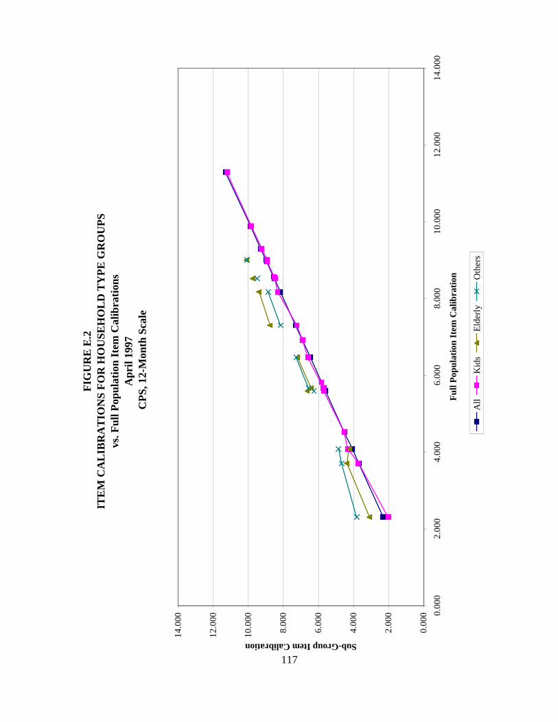
FIG
UR
E E
.2IT
EM
CA
LIB
RA
TIO
NS
FO
R H
OU
SEH
OL
D T
YP
E G
RO
UP
Svs
. Ful
l Pop
ulat
ion
Item
Cal
ibra
tion
sA
pril
1997
CP
S, 1
2-M
onth
Sca
le
0.00
0
2.00
0
4.00
0
6.00
0
8.00
0
10.0
00
12.0
00
14.0
00
0.00
02.
000
4.00
06.
000
8.00
010
.000
12.0
0014
.000
Ful
l Pop
ulat
ion
Item
Cal
ibra
tion
Sub-Group Item Calibration
All
Kid
sE
lder
lyO
ther
s
117

118
subgroups, and no change in order is more than two positions (Tables E.7, E.8, and E.9, and Figure
E.3).
Region of Country. When the analysis is done by region of the country, no item switches by
more than a one position (Tables E.10, E.11, E.12, and Figure E.4).
Summary. Overall, these findings suggest that there is considerable robustness in the model,
when it is estimated for various population subgroups.

Item Estimate Std Err Estimate Std Err Estimate Std Err50 11.284 0.245 11.087 0.369 11.751 1.01744 9.873 0.187 9.742 0.241 10.721 0.61143 9.293 0.170 9.145 0.190 10.087 0.47829 8.999 0.073 9.123 0.124 8.772 0.25747 8.957 0.111 8.954 0.166 9.074 0.27228 8.516 0.072 8.612 0.097 8.227 0.22040 8.564 0.087 8.523 0.101 8.961 0.28438 8.168 0.087 8.113 0.120 8.355 0.17635 7.297 0.060 7.342 0.080 7.036 0.20357 6.915 0.094 6.858 0.129 6.813 0.12925 6.463 0.054 6.430 0.070 6.441 0.12532 5.663 0.036 5.724 0.053 5.486 0.19256 5.818 0.075 5.800 0.099 5.533 0.17924 5.586 0.047 5.541 0.060 5.733 0.15758 4.522 0.057 4.553 0.078 4.188 0.27355 4.079 0.066 4.141 0.079 3.721 0.30254 3.700 0.070 3.766 0.097 3.415 0.30653 2.306 0.087 2.549 0.109 1.687 0.443
Mean 7.000 7.000 7.000Std Dev 2.413 2.344 2.730
Sample size 5,429 3,140 1,493
Notes: Standard errors have been estimated using a balanced replication procedure to account fothe complex sample design of the CPS.
Constrained UnconstrainedAll Households Metro NonMetro
Model
TABLE E.7
THRESHOLD PARAMETER ESTIMATES FOR 18-ITEM 12-MONTH FOOD SECURITY SCALEBY METROPOLITAN STATUS
April 1997 CPS Data, Common Denominator Screen
119

Full Population Metro NonMetro
q50 Child not eat whole day 1 1 1q44 Child skipped meal, 3+ months 2 2 2q43 Child skipped meal 3 3 3q29 Adult not eat whole day, 3+ months 4 4 6q47 Child hungry 5 5 4q28 Adult not eat whole day 7 6 8q40 Cut size of child's meals 6 7 5q38 Adult lost weight 8 8 7q35 Adult hungry but didn't eat 9 9 9q57 Child not eating enough 10 10 10q25 Adult cut size or skipped meals, in 3+ months 11 11 11q32 Adult eat less than felt they should 13 13 14q56 Couldn't feed child balanced meals 12 12 13q24 Adult cut size or skipped meals 14 14 12q58 Adult fed child few low cost foods 15 15 15q55 Adult not eat balanced meals 16 16 16q54 Food bought didn't last 17 17 17q53 Worried food would run out 18 18 18
Based on weighted 1997 data using BilogMG calibrations.
TABLE E.8ITEM ORDERING BY METROPOLITAN STATUS AND FULL POPULATION
April 1997 CPS, 12-Month Scale
Question
120

Variable Estimate Std Err Pr(|T|>|t|)50 -0.664 1.057 0.53044 -0.979 0.646 0.13043 -0.943 0.508 0.06429 0.352 0.324 0.27947 -0.120 0.336 0.72128 0.384 0.245 0.11840 -0.438 0.302 0.14738 -0.242 0.256 0.34435 0.306 0.237 0.19757 0.045 0.175 0.79525 -0.011 0.139 0.93632 0.238 0.213 0.26556 0.267 0.212 0.20824 -0.192 0.164 0.24158 0.365 0.290 0.20955 0.420 0.309 0.17454 0.350 0.310 0.25953 0.861 0.446 0.054
NonMetro-Metro
TABLE E.9
CROSS-GROUP DIFFERENCES IN THRESHOLD PARAMETER ESTIMATES
April 1997 CPS Data, Common Denominator Screen
BY METROPOLITAN STATUS
121

FIG
UR
E E
.3IT
EM
CA
LIB
RA
TIO
NS
BY
ME
TR
OP
OL
ITA
N S
TA
TU
Svs
. Ful
l Pop
ulat
ion
Item
Cal
ibra
tion
sA
pril
1997
CP
S, 1
2-M
onth
Sca
le
0.00
0
2.00
0
4.00
0
6.00
0
8.00
0
10.0
00
12.0
00
14.0
00
0.00
02.
000
4.00
06.
000
8.00
010
.000
12.0
0014
.000
Ful
l Pop
ulat
ion
Item
Cal
ibra
tion
Sub-Group Item Calibration
All
Met
roN
onM
etro
122

Item Estimate Std Err Estimate Std Err Estimate Std Err Estimate Std Err Estimate Std Err50 11.284 0.245 10.666 0.522 12.397 1.662 11.197 0.466 11.670 0.28544 9.873 0.187 9.955 0.381 9.484 0.265 10.326 0.222 9.538 0.62143 9.293 0.170 9.619 0.443 9.305 0.237 9.407 0.153 8.888 0.50129 8.999 0.073 8.892 0.176 9.066 0.205 8.988 0.156 9.017 0.07347 8.957 0.111 9.018 0.357 8.710 0.185 9.128 0.158 8.850 0.29428 8.516 0.072 8.532 0.210 8.580 0.215 8.429 0.118 8.548 0.09740 8.564 0.087 8.801 0.216 8.514 0.251 8.698 0.143 8.226 0.14838 8.168 0.087 7.895 0.254 8.369 0.130 8.285 0.166 8.000 0.08635 7.297 0.060 7.282 0.146 7.060 0.163 7.463 0.106 7.220 0.10957 6.915 0.094 6.922 0.199 7.000 0.147 6.767 0.066 7.003 0.33325 6.463 0.054 6.309 0.106 6.449 0.126 6.499 0.095 6.475 0.14832 5.663 0.036 5.505 0.070 5.579 0.213 5.711 0.069 5.707 0.08056 5.818 0.075 5.887 0.163 5.675 0.211 5.769 0.134 5.895 0.15224 5.586 0.047 5.512 0.084 5.462 0.210 5.668 0.076 5.551 0.14258 4.522 0.057 4.499 0.146 4.375 0.334 4.460 0.102 4.668 0.11655 4.079 0.066 4.361 0.174 3.992 0.375 3.899 0.071 4.132 0.16854 3.700 0.070 3.822 0.095 3.695 0.389 3.437 0.065 3.918 0.22153 2.306 0.087 2.523 0.171 2.289 0.509 1.871 0.106 2.695 0.242
Mean 7.000 7.000 7.000 7.000 7.000Std Dev 2.413 2.335 2.543 2.544 2.316
Sample size 5,429 1,023 1,136 1,821 1,449
Notes: Standard errors have been estimated using a balanced replication procedure to account for the complexsample design of the CPS.
Model
TABLE E.10
THRESHOLD PARAMETER ESTIMATES FOR 18-ITEM 12-MONTH FOOD SECURITY SCALEBY REGION
April 1997 CPS Data, Common Denominator Screen
Constrained UnconstrainedAll Households Northeast Midwest South West
123

Full Population Northeast Midwest South West
q50 Child not eat whole day 1 1 1 1 1q44 Child skipped meal, 3+ months 2 2 2 2 2q43 Child skipped meal 3 3 3 3 4q29 Adult not eat whole day, 3+ months 4 5 4 5 3q47 Child hungry 5 4 5 4 5q28 Adult not eat whole day 7 7 6 7 6q40 Cut size of child's meals 6 6 7 6 7q38 Adult lost weight 8 8 8 8 8q35 Adult hungry but didn't eat 9 9 9 9 9q57 Child not eating enough 10 10 10 10 10q25 Adult cut size or skipped meals, in 3+ months 11 11 11 11 11q32 Adult eat less than felt they should 13 14 13 13 13q56 Couldn't feed child balanced meals 12 12 12 12 12q24 Adult cut size or skipped meals 14 13 14 14 14q58 Adult fed child few low cost foods 15 15 15 15 15q55 Adult not eat balanced meals 16 16 16 16 16q54 Food bought didn't last 17 17 17 17 17q53 Worried food would run out 18 18 18 18 18
Based on weighted 1997 data using BilogMG calibrations.
TABLE E.11ITEM ORDERING FOR 4 REGIONS AND FULL POPULATION
April 1997 CPS, 12-Month Scale
Question
124

Y REGION
Variable Estimate Std Err Pr(|T|>|t|) Estimate Std Err Pr(|T|>|t|) Estimate Std Err Pr(|T|>|t|)50 -1.731 1.763 0.326 -0.531 0.688 0.440 -1.004 0.577 0.08244 0.471 0.457 0.303 -0.370 0.431 0.391 0.417 0.737 0.57243 0.314 0.491 0.523 0.211 0.469 0.652 0.730 0.675 0.27929 -0.174 0.276 0.528 -0.096 0.238 0.687 -0.125 0.192 0.51747 0.308 0.397 0.438 -0.110 0.394 0.780 0.168 0.457 0.71328 -0.048 0.306 0.875 0.104 0.242 0.669 -0.016 0.233 0.94540 0.287 0.331 0.386 0.103 0.260 0.691 0.575 0.258 0.02638 -0.474 0.279 0.090 -0.390 0.306 0.203 -0.105 0.262 0.68935 0.222 0.223 0.320 -0.181 0.179 0.312 0.062 0.175 0.72357 -0.078 0.254 0.760 0.156 0.209 0.456 -0.080 0.390 0.83725 -0.140 0.170 0.412 -0.189 0.143 0.184 -0.166 0.181 0.36032 -0.074 0.231 0.750 -0.205 0.095 0.031 -0.202 0.097 0.03856 0.212 0.272 0.436 0.118 0.210 0.575 -0.008 0.225 0.97224 0.050 0.234 0.831 -0.156 0.111 0.160 -0.039 0.162 0.81158 0.124 0.371 0.739 0.039 0.177 0.827 -0.169 0.185 0.36155 0.369 0.423 0.384 0.462 0.185 0.013 0.228 0.240 0.34254 0.128 0.419 0.761 0.385 0.110 0.001 -0.096 0.240 0.69053 0.235 0.561 0.676 0.653 0.199 0.001 -0.172 0.294 0.559
Northeast-Midwest Northeast-South Northeast-West
TABLE E.12
CROSS-GROUP DIFFERENCES IN THRESHOLD PARAMETER ESTIMATES
April 1997 CPS Data, Common Denominator Screen
BY REGION
125

FIG
UR
E E
.4IT
EM
CA
LIB
RA
TIO
NS
BY
RE
GIO
Nvs
. Ful
l Pop
ulat
ion
Item
Cal
ibra
tion
sA
pril
1997
CP
S, 1
2-M
onth
Sca
le
0.00
0
2.00
0
4.00
0
6.00
0
8.00
0
10.0
00
12.0
00
14.0
00
0.00
02.
000
4.00
06.
000
8.00
010
.000
12.0
0014
.000
Ful
l Pop
ulat
ion
Item
Cal
ibra
tion
Sub-Group Item Calibration
All
Nor
thea
stM
idw
est
Sout
hW
est
126

APPENDIX F
PREVALENCE ESTIMATES AND THEIR STANDARD ERRORS


The 1995-1997 files used in the current report, like the corresponding public use files available1
on the CPS website, have one further adjustment which is designed to make them more comparableto the 1998 data. In the 1998 survey, under certain circumstances, households were not askedrelatively severe food security questions if they had already consistently answered “no” to blocks ofless severe questions. The 1995-1997 data were edited to emulate this screening by replacinganswers to the more severe questions with missing value codes for questions which would have beenskipped in 1998. See: www.bls.census.gov/cps/foodsecu/1997/agnote.htm ( “Food Security, Scalesand Screener Variables”).
129
This appendix presents detailed food security prevalence tables and the corresponding standard
error estimates for the 1995-1997 period. The estimates are disaggregated by year and income group.
The exact prevalence estimates may, in some instances, vary slightly from those issued in the
“Advance Report” which was issued by USDA in July 1999, with preliminary findings. These
differences are due to additional editing and are not substantial.
Totals of food secure and food insecure cases do not quite add to population totals, because
there were a very small number of households for which food insecurity status could not be
calculated. All percentages are based on using all cases, including those with missing food security
data, as the denominator.
Tabulations based on metropolitan status do not add to national totals, because for many
households inside metropolitan areas, the CPS data do not indicate whether or not the household is
in the central city.
The data for 1995-1997 are adjusted to reflect the screening adopted in 1998 and thereafter.
Essentially, this means that certain households who answered “no” to all of the less severe food
security questions are coded as having missing values for the more severe items. This is analogue
to what would have been their treatment in the 1998 and subsequent years, when such households
were skipped out of the later questions, based on their negative answers to the earlier ones.1

130
The following shows the table numbers for the various tables:
Year Prevalence Table Standard Error TableAll Income Groups 1995 F.1 F.22
1996 F.2 F.231997 F.3 F.24
Under 100 Percent of Poverty1995 F.4 F.251996 F.5 F.261997 F.6 F.27
Over 100 Percent of Poverty1995 F.7 F.281996 F.8 F.291997 F.9 F.30
Under 130 Percent of Poverty1995 F.10 F.311996 F.11 F.321997 F.12 F.33
Over 130 Percent of Poverty1995 F.13 F.341996 F.14 F.351997 F.15 F.36
Under 185 Percent of Poverty1995 F.16 F.371996 F.17 F.381997 F.18 F.39
Over 185 Percent of Poverty1995 F.19 F.401996 F.20 F.411997 F.21 F.42

Tot
al(0
00)
(000
)P
erce
nt(0
00)
Per
cent
(000
)P
erce
nt(0
00)
Per
cent
All
Hou
seho
lds
100,
445
89,9
69
89
.610
,392
10.3
6,43
7
6.4
3,95
5
3.9
Hou
seho
ld C
ompo
siti
onW
ith
Chi
ldre
n <
618
,353
15
,199
82.8
3,11
6
17.0
2,17
7
11.9
939
5.1
Wit
h C
hild
ren
< 1
838
,181
32
,230
84.4
5,91
1
15.5
3,99
3
10.5
1,91
8
5.0
Mar
ried
Cou
ple
Fam
ilie
s27
,222
24
,460
89.9
2,74
3
10.1
1,99
2
7.3
751
2.8
Fem
ale
Hea
d, N
o Sp
ouse
8,57
8
5,80
8
67.7
2,76
4
32.2
1,75
1
20.4
1,01
3
11.8
Mal
e H
ead,
No
Spo
use
1,83
6
1,53
5
83.6
288
15.8
201
11.0
87
4.8
Oth
er H
ouse
hold
s w
ith C
hild
ren
545
428
78.7
116
21.3
49
9.0
67
12.3
131
Wit
h N
o C
hild
ren
< 1
862
,264
57
,739
92.7
4,48
0
7.2
2,44
4
3.9
2,03
6
3.3
Mor
e T
han
One
Adu
lt36
,777
34
,826
94.7
1,92
4
5.2
1,14
8
3.1
776
2.1
Wom
en L
ivin
g A
lone
15,1
61
13,7
08
90
.41,
447
9.
681
1
5.
463
6
4.
2M
en L
ivin
g A
lone
10,3
25
9,20
4
89.1
1,10
8
10.7
484
4.7
624
6.0
Hou
seho
lds
with
Eld
erly
23,7
76
22,5
70
94
.91,
192
5.
074
2
3.
145
0
1.
9E
lder
ly L
ivin
g A
lone
10,0
69
9,48
9
94.2
576
5.8
327
3.3
249
2.5
Rac
e an
d H
ispa
nic
Eth
nici
tyW
hite
Non
-His
pani
c78
,100
72
,266
92.5
5,79
9
7.4
3,61
8
4.6
2,18
1
2.8
Bla
ck N
on-H
ispa
nic
11,9
06
9,32
1
78.3
2,56
9
21.6
1,52
1
12.8
1,04
8
8.8
His
pani
c7,
753
5,
971
77
.01,
749
22
.61,
136
14
.761
3
7.
9O
ther
Non
-His
pani
c2,
686
2,
411
89
.827
3
10
.216
1
6.
011
2
4.
2
Food
Ins
ecur
e
TA
BL
E F
.1
PRE
VA
LE
NC
E O
F FO
OD
SE
CU
RIT
Y, F
OO
D I
NSE
CU
RIT
Y, A
ND
HU
NG
ER
BY
SE
LE
CT
ED
CH
AR
AC
TE
RSI
TIC
S O
F H
OU
SEH
OL
DS,
199
5U
SIN
G T
HE
CO
MM
ON
DE
NO
MIN
AT
OR
SC
RE
EN
Food
Sec
ure
All
With
out H
unge
rW
ith H
unge
r

TA
BL
E F
.1 (
cont
inue
d)
Tot
al(0
00)
(000
)P
erce
nt(0
00)
Per
cent
(000
)P
erce
nt(0
00)
Per
cent
Hou
seho
ld I
ncom
e-to
-Pov
erty
Rat
ioU
nder
0.5
05,
603
3,
467
61
.92,
113
37
.71,
177
21
.093
6
16
.7U
nder
1.0
015
,924
10
,717
67.3
5,15
4
32.3
3,08
1
19.3
2,07
3
13.0
Und
er 1
.30
21,9
53
15,4
80
70
.56,
413
29
.23,
823
17
.42,
590
11
.8U
nder
1.8
532
,182
24
,030
74.7
8,08
0
25.1
4,93
5
15.3
3,14
5
9.8
1.85
and
Ove
r58
,400
56
,615
96.9
1,77
7
3.0
1,17
6
2.0
601
1.0
Inco
me
Not
Kno
wn
9,86
3
9,32
4
94.5
534
5.4
325
3.3
209
2.1
132
Are
a of
Res
iden
ceIn
side
Met
ropo
litan
Are
aIn
Cen
tral
City
24,7
01
21,1
68
85
.73,
525
14
.32,
149
8.
71,
376
5.
6N
ot in
Cen
tral
City
37,0
59
34,0
92
92
.02,
935
7.
91,
757
4.
71,
178
3.
2O
utsi
de M
etro
poli
tan
Are
a22
,658
20
,173
89.0
2,46
0
10.8
1,59
0
7.0
870
3.8
Cen
sus
Geo
grap
hica
l Reg
ion
Nor
thea
st19
,491
17
,776
91.2
1,69
4
8.7
1,05
6
5.4
638
3.3
Mid
wes
t23
,656
21
,442
90.6
2,21
2
9.3
1,37
5
5.8
837
3.5
Sou
th
35,8
91
31,9
06
88
.93,
966
11
.12,
498
7.
01,
468
4.
1W
est
21,4
07
18,8
45
88
.025
2111
.71,
508
7.
01,
013
4.
7
Sour
ce:
Tab
ulat
ions
of
Cur
rent
Pop
ulat
ion
Surv
ey, F
ood
Secu
rity
Sup
plem
ent d
ata.
Food
Ins
ecur
eFo
od S
ecur
eA
llW
ithou
t Hun
ger
With
Hun
ger

Tot
al(0
00)
(000
)P
erce
nt(0
00)
Per
cent
(000
)P
erce
nt(0
00)
Per
cent
All
Hou
seho
lds
101,
508
90,8
09
89
.510
,592
10.5
6,46
2
6.4
4,13
0
4.1
Hou
seho
ld C
ompo
siti
onW
ith
Chi
ldre
n <
617
,871
14
,703
82.3
3,12
7
17.5
2,17
6
12.2
951
5.3
Wit
h C
hild
ren
< 1
838
,196
32
,205
84.3
5,92
2
15.5
3,97
4
10.4
1,94
8
5.1
Mar
ried
Cou
ple
Fam
ilie
s27
,187
24
,326
89.5
2,81
7
10.4
1,98
5
7.3
832
3.1
Fem
ale
Hea
d, N
o Sp
ouse
8,48
8
5,79
3
68.2
2,66
9
31.4
1,69
9
20.0
970
11.4
Mal
e H
ead,
No
Spo
use
1,93
6
1,60
4
82.9
332
17.1
219
11.3
113
5.8
Oth
er H
ouse
hold
s w
ith C
hild
ren
585
481
82.3
104
17.7
71
12.1
33
5.6
133
Wit
h N
o C
hild
ren
< 1
863
,312
58
,604
92.6
4,67
0
7.3
2,48
8
3.9
2,18
2
3.4
Mor
e T
han
One
Adu
lt37
,806
35
,743
94.5
2,04
4
5.4
1,15
3
3.0
891
2.4
Wom
en L
ivin
g A
lone
14,9
61
13,4
57
89
.91,
496
10
.079
5
5.
370
1
4.
7M
en L
ivin
g A
lone
10,5
45
9,40
4
89.2
1,13
1
10.7
540
5.1
591
5.6
Hou
seho
lds
with
Eld
erly
24,0
87
22,8
49
94
.91,
219
5.
077
9
3.
244
0
1.
8E
lder
ly L
ivin
g A
lone
9,76
0
9,18
5
94.1
574
5.9
353
3.6
221
2.3
Rac
e an
d H
ispa
nic
Eth
nici
tyW
hite
Non
-His
pani
c77
,830
72
,056
92.6
5,73
7
7.3
3,46
0
4.4
2,27
7
2.9
Bla
ck N
on-H
ispa
nic
12,0
83
9,33
2
77.2
2,70
9
22.4
1,68
4
13.9
1,02
5
8.5
His
pani
c8,
165
6,
340
77
.61,
805
22
.11,
101
13
.570
4
8.
6O
ther
Non
-His
pani
c3,
430
3,
082
89
.834
2
9.
921
7
6.
312
5
3.
6
Food
Ins
ecur
e
TA
BL
E F
.2
PRE
VA
LE
NC
E O
F FO
OD
SE
CU
RIT
Y, F
OO
D I
NSE
CU
RIT
Y, A
ND
HU
NG
ER
BY
SE
LE
CT
ED
CH
AR
AC
TE
RSI
TIC
S O
F H
OU
SEH
OL
DS,
199
6U
SIN
G T
HE
CO
MM
ON
DE
NO
MIN
AT
OR
SC
RE
EN
Food
Sec
ure
All
With
out H
unge
rW
ith H
unge
r

TA
BL
E F
.2 (
cont
inue
d)
Tot
al(0
00)
(000
)P
erce
nt(0
00)
Per
cent
(000
)P
erce
nt(0
00)
Per
cent
Hou
seho
ld I
ncom
e-to
-Pov
erty
Rat
ioU
nder
0.5
06,
442
3,
932
61
.02,
480
38
.51,
342
20
.81,
138
17
.7U
nder
1.0
014
,548
9,
390
64
.55,
106
35
.12,
951
20
.32,
155
14
.8U
nder
1.3
020
,282
13
,868
68.4
6,35
3
31.4
3,72
6
18.4
2,62
7
13.0
Und
er 1
.85
32,8
14
24,4
49
74
.58,
290
25
.35,
038
15
.43,
252
9.
91.
85 a
nd O
ver
57,1
23
55,3
79
96
.91,
743
3.
11,
082
1.
966
1
1.
2In
com
e N
ot K
now
n11
,571
10
,982
94.9
558
4.8
341
2.9
217
1.9
134
Are
a of
Res
iden
ceIn
side
Met
ropo
litan
Are
aIn
Cen
tral
City
26,2
62
22,6
11
86
.13,
614
13
.72,
139
8.
11,
475
5.
6N
ot in
Cen
tral
City
40,9
56
37,6
04
91
.83,
291
8.
01,
968
4.
81,
323
3.
2O
utsi
de M
etro
poli
tan
Are
a19
,958
17
,698
88.7
2,25
6
11.3
1,46
1
7.3
795
4.0
Cen
sus
Geo
grap
hica
l Reg
ion
Nor
thea
st19
,740
18
,169
92.0
1,54
8
7.9
938
4.8
610
3.1
Mid
wes
t24
,132
22
,029
91.3
2,09
2
8.7
1,28
1
5.3
811
3.4
Sou
th
35,7
92
31,4
60
87
.94,
274
12
.02,
644
7.
41,
630
4.
6W
est
21,8
44
19,1
51
87
.72,
677
12
.21,
598
7.
31,
079
4.
9
Sour
ce:
Tab
ulat
ions
of
Cur
rent
Pop
ulat
ion
Surv
ey, F
ood
Secu
rity
Sup
plem
ent d
ata.
Food
Ins
ecur
eFo
od S
ecur
eA
llW
ithou
t Hun
ger
With
Hun
ger

Tot
al(0
00)
(000
)P
erce
nt(0
00)
Per
cent
(000
)P
erce
nt(0
00)
Per
cent
All
Hou
seho
lds
102,
373
93,3
19
91
.28,
963
8.
85,
831
5.
73,
132
3.
1
Hou
seho
ld C
ompo
siti
onW
ith
Chi
ldre
n <
617
,538
15
,133
86.3
2,39
6
13.6
1,81
3
10.3
583
3.3
Wit
h C
hild
ren
< 1
838
,195
33
,237
87.0
4,92
0
12.9
3,53
8
9.3
1,38
2
3.6
Mar
ried
Cou
ple
Fam
ilie
s26
,859
24
,751
92.2
2,09
5
7.8
1,58
5
5.9
510
1.9
Fem
ale
Hea
d, N
o Sp
ouse
8,71
5
6,26
4
71.9
2,43
3
27.9
1,65
3
19.0
780
8.9
Mal
e H
ead,
No
Spo
use
2,10
5
1,79
3
85.2
312
14.8
248
11.8
64
3.0
Oth
er H
ouse
hold
s w
ith C
hild
ren
516
429
83.2
81
15.7
52
10.1
29
5.6
135
Wit
h N
o C
hild
ren
< 1
864
,178
60
,082
93.6
4,04
2
6.3
2,29
3
3.6
1,74
9
2.7
Mor
e T
han
One
Adu
lt37
,788
36
,034
95.4
1,73
9
4.6
1,08
6
2.9
653
1.7
Wom
en L
ivin
g A
lone
15,4
11
14,1
44
91
.81,
245
8.
169
0
4.
555
5
3.
6M
en L
ivin
g A
lone
10,9
80
9,90
4
90.2
1,05
9
9.6
517
4.7
542
4.9
Hou
seho
lds
with
Eld
erly
24,4
20
23,2
78
95
.31,
125
4.
677
5
3.
235
0
1.
4E
lder
ly L
ivin
g A
lone
10,3
23
9,79
5
94.9
517
5.0
335
3.2
182
1.8
Rac
e an
d H
ispa
nic
Eth
nici
tyW
hite
Non
-His
pani
c78
,021
73
,234
93.9
4,74
9
6.1
2,96
7
3.8
1,78
2
2.3
Bla
ck N
on-H
ispa
nic
12,2
89
9,96
6
81.1
2,29
6
18.7
1,50
0
12.2
796
6.5
His
pani
c8,
383
6,
737
80
.41,
624
19
.41,
174
14
.045
0
5.
4O
ther
Non
-His
pani
c3,
680
3,
382
91
.929
4
8.
019
0
5.
210
4
2.
8
Food
Sec
ure
All
With
out H
unge
rW
ith H
unge
rFo
od I
nsec
ure
TA
BL
E F
.3
PRE
VA
LE
NC
E O
F FO
OD
SE
CU
RIT
Y, F
OO
D I
NSE
CU
RIT
Y, A
ND
HU
NG
ER
BY
SE
LE
CT
ED
CH
AR
AC
TE
RSI
TIC
S O
F H
OU
SEH
OL
DS,
199
7U
SIN
G T
HE
CO
MM
ON
DE
NO
MIN
AT
OR
SC
RE
EN

TA
BL
E F
.3 (
cont
inue
d)
Tot
al(0
00)
(000
)P
erce
nt(0
00)
Per
cent
(000
)P
erce
nt(0
00)
Per
cent
Hou
seho
ld I
ncom
e-to
-Pov
erty
Rat
ioU
nder
0.5
06,
206
4,
070
65
.62,
121
34
.21,
313
21
.280
813
.0U
nder
1.0
014
,157
9,
828
69
.44,
297
30
.42,
676
18
.916
2111
.5U
nder
1.3
020
,158
14
,753
73.2
5,36
6
26.6
3,38
7
16.8
1979
9.8
Und
er 1
.85
31,5
60
24,6
29
78
.06,
878
21
.84,
471
14
.224
077.
61.
85 a
nd O
ver
58,9
80
57,4
67
97
.41,
504
2.
699
5
1.
750
90.
9In
com
e N
ot K
now
n11
,833
11
,223
94.8
581
4.9
365
3.1
216
1.8
136
Are
a of
Res
iden
ceIn
side
Met
ropo
litan
Are
aIn
Cen
tral
City
26,3
14
23,1
83
88
.13,
093
11
.71,
876
7.
112
174.
6N
ot in
Cen
tral
City
41,3
54
38,5
31
93
.22,
786
6.
81,
854
4.
593
22.
3O
utsi
de M
etro
poli
tan
Are
a20
,148
18
,260
90.6
1,87
8
9.3
1,30
7
6.5
571
2.8
Cen
sus
Geo
grap
hica
l Reg
ion
Nor
thea
st19
,897
18
,298
92.0
1,57
6
7.9
992
5.0
584
2.9
Mid
wes
t24
,555
22
,678
92.4
1,86
1
7.6
1,15
6
4.7
705
2.9
Sou
th
35,8
44
32,4
18
90
.43,
403
9.
42,
276
6.
311
273.
1W
est
22,0
77
19,9
25
90
.32,
122
9.
61,
407
6.
471
53.
2
Sour
ce:
Tab
ulat
ions
of
Cur
rent
Pop
ulat
ion
Surv
ey, F
ood
Secu
rity
Sup
plem
ent d
ata.
Food
Ins
ecur
eFo
od S
ecur
eA
llW
ithou
t Hun
ger
With
Hun
ger

Tot
al(0
00)
(000
)P
erce
nt(0
00)
Per
cent
(000
)P
erce
nt(0
00)
Per
cent
All
Hou
seho
lds
15,9
24
10,7
17
67
.35,
154
32
.33,
081
19
.32,
073
13
.0
Hou
seho
ld C
ompo
siti
onW
ith
Chi
ldre
n <
64,
648
2,
752
59
.21,
866
40
.21,
198
25
.866
8
14
.4
Wit
h C
hild
ren
< 1
87,
856
4,
653
59
.23,
173
40
.42,
001
25
.51,
172
14
.9M
arri
ed C
oupl
e Fa
mil
ies
3,08
1
1,96
3
63.7
1,10
8
35.9
746
24.2
362
11.7
Fem
ale
Hea
d, N
o Sp
ouse
4,15
0
2,31
2
55.7
1,83
1
44.1
1,12
5
27.1
706
17.0
Mal
e H
ead,
No
Spo
use
463
277
59.8
174
37.5
108
23.3
66
14.2
Oth
er H
ouse
hold
s w
ith C
hild
ren
162
101
62.6
61
37.4
22
13.5
39
23.9
137
Wit
h N
o C
hild
ren
< 1
88,
067
6,
064
75
.21,
981
24
.61,
080
13
.490
1
11
.2M
ore
Tha
n O
ne A
dult
3,18
5
2,43
6
76.5
737
23.2
432
13.6
305
9.6
Wom
en L
ivin
g A
lone
3,27
4
2,49
8
76.3
773
23.6
458
14.0
315
9.6
Men
Liv
ing
Alo
ne1,
608
1,
130
70
.347
1
29
.319
0
11
.828
1
17
.5
Hou
seho
lds
with
Eld
erly
4,09
4
3,43
0
83.8
663
16.2
425
10.4
238
5.8
Eld
erly
Liv
ing
Alo
ne2,
432
2,
096
86
.233
5
13
.819
1
7.
914
4
5.
9
Rac
e an
d H
ispa
nic
Eth
nici
tyW
hite
Non
-His
pani
c8,
633
6,
183
71
.62,
433
28
.21,
457
16
.997
6
11
.3B
lack
Non
-His
pani
c4,
178
2,
653
63
.51,
516
36
.385
7
20
.565
9
15
.8H
ispa
nic
2,59
2
1,50
0
57.9
1,06
8
41.2
692
26.7
376
14.5
Oth
er N
on-H
ispa
nic
522
382
73.3
138
26.3
75
14.3
63
12.0
Food
Ins
ecur
e
TA
BL
E F
.4
PRE
VA
LE
NC
E O
F FO
OD
SE
CU
RIT
Y, F
OO
D I
NSE
CU
RIT
Y, A
ND
HU
NG
ER
BY
SE
LE
CT
ED
CH
AR
AC
TE
RSI
TIC
S O
F H
OU
SEH
OL
DS,
199
5FO
R T
HO
SE F
AM
ILIE
S U
ND
ER
100
PE
RC
EN
T O
F PO
VE
RT
Y T
HR
ESH
HO
LD
USI
NG
TH
E C
OM
MO
N D
EN
OM
INA
TO
R S
CR
EE
N
Food
Sec
ure
All
With
out H
unge
rW
ith H
unge
r

TA
BL
E F
.4 (
cont
inue
d)
Tot
al(0
00)
(000
)P
erce
nt(0
00)
Per
cent
(000
)P
erce
nt(0
00)
Per
cent
Hou
seho
ld I
ncom
e-to
-Pov
erty
Rat
ioU
nder
0.5
05,
603
3,
467
61
.92,
113
37
.71,
177
21
.093
616
.7U
nder
1.0
015
,924
10
,717
67.3
5,15
4
32.3
3,08
1
19.3
2073
13.0
Und
er 1
.30
15,9
24
10,7
17
67
.35,
154
32
.33,
081
19
.320
7313
.0U
nder
1.8
515
,924
10
,717
67.3
5,15
4
32.3
3,08
1
19.3
2073
13.0
1.85
and
Ove
r-
-
0.0
-
0.
0-
0.0
-
0.
0In
com
e N
ot K
now
n-
-
0.0
-
0.
0-
0.0
-
0.
0
138
Are
a of
Res
iden
ceIn
side
Met
ropo
litan
Are
aIn
Cen
tral
City
5,33
2
3,43
8
64.5
1,89
1
35.5
1,12
0
21.0
771
14.5
Not
in C
entr
al C
ity3,
632
2,
446
67
.41,
166
32
.165
4
18
.051
214
.1O
utsi
de M
etro
poli
tan
Are
a4,
599
3,
205
69
.71,
380
30
.086
5
18
.851
511
.2
Cen
sus
Geo
grap
hica
l Reg
ion
Nor
thea
st2,
670
1,
785
66
.987
9
32
.952
9
19
.835
013
.1M
idw
est
3,36
4
2,35
5
70.0
1,00
8
30.0
605
18.0
403
12.0
Sout
h 6,
606
4,
515
68
.32,
079
31
.51,
247
18
.983
212
.6W
est
3,28
4
2,06
3
62.8
1,18
8
36.2
699
21.3
489
14.9
Sour
ce:
Tab
ulat
ions
of
Cur
rent
Pop
ulat
ion
Surv
ey, F
ood
Secu
rity
Sup
plem
ent d
ata.
Food
Ins
ecur
eFo
od S
ecur
eA
llW
ithou
t Hun
ger
With
Hun
ger
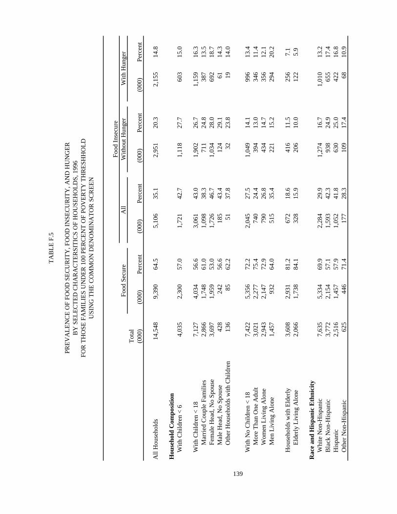
Tot
al(0
00)
(000
)P
erce
nt(0
00)
Per
cent
(000
)P
erce
nt(0
00)
Per
cent
All
Hou
seho
lds
14,5
48
9,39
0
64.5
5,10
6
35.1
2,95
1
20.3
2,15
5
14.8
Hou
seho
ld C
ompo
siti
onW
ith
Chi
ldre
n <
64,
035
2,
300
57
.01,
721
42
.71,
118
27
.760
3
15
.0
Wit
h C
hild
ren
< 1
87,
127
4,
034
56
.63,
061
43
.01,
902
26
.71,
159
16
.3M
arri
ed C
oupl
e Fa
mil
ies
2,86
6
1,74
8
61.0
1,09
8
38.3
711
24.8
387
13.5
Fem
ale
Hea
d, N
o Sp
ouse
3,69
7
1,95
9
53.0
1,72
6
46.7
1,03
4
28.0
692
18.7
Mal
e H
ead,
No
Spo
use
428
242
56.6
185
43.4
124
29.1
61
14.3
Oth
er H
ouse
hold
s w
ith C
hild
ren
136
85
62.2
51
37.8
32
23.8
19
14.0
139
Wit
h N
o C
hild
ren
< 1
87,
422
5,
356
72
.22,
045
27
.51,
049
14
.199
6
13
.4M
ore
Tha
n O
ne A
dult
3,02
1
2,27
7
75.4
740
24.4
394
13.0
346
11.4
Wom
en L
ivin
g A
lone
2,94
3
2,14
7
72.9
790
26.8
434
14.7
356
12.1
Men
Liv
ing
Alo
ne1,
457
93
2
64
.051
5
35
.422
1
15
.229
4
20
.2
Hou
seho
lds
with
Eld
erly
3,60
8
2,93
1
81.2
672
18.6
416
11.5
256
7.1
Eld
erly
Liv
ing
Alo
ne2,
066
1,
738
84
.132
8
15
.920
6
10
.012
2
5.
9
Rac
e an
d H
ispa
nic
Eth
nici
tyW
hite
Non
-His
pani
c7,
635
5,
334
69
.92,
284
29
.91,
274
16
.71,
010
13
.2B
lack
Non
-His
pani
c3,
772
2,
154
57
.11,
593
42
.393
8
24
.965
5
17
.4H
ispa
nic
2,51
6
1,45
7
57.9
1,05
2
41.8
630
25.0
422
16.8
Oth
er N
on-H
ispa
nic
625
446
71.4
177
28.3
109
17.4
68
10.9
Food
Ins
ecur
e
TA
BL
E F
.5
PRE
VA
LE
NC
E O
F FO
OD
SE
CU
RIT
Y, F
OO
D I
NSE
CU
RIT
Y, A
ND
HU
NG
ER
BY
SE
LE
CT
ED
CH
AR
AC
TE
RSI
TIC
S O
F H
OU
SEH
OL
DS,
199
6FO
R T
HO
SE F
AM
ILIE
S U
ND
ER
100
PE
RC
EN
T O
F PO
VE
RT
Y T
HR
ESH
HO
LD
USI
NG
TH
E C
OM
MO
N D
EN
OM
INA
TO
R S
CR
EE
N
Food
Sec
ure
All
With
out H
unge
rW
ith H
unge
r

TA
BL
E F
.5 (
cont
inue
d)
Tot
al(0
00)
(000
)P
erce
nt(0
00)
Per
cent
(000
)P
erce
nt(0
00)
Per
cent
Hou
seho
ld I
ncom
e-to
-Pov
erty
Rat
ioU
nder
0.5
06,
442
3,
932
61
.02,
480
38
.51,
342
20
.811
3817
.7U
nder
1.0
014
,548
9,
390
64
.55,
106
35
.12,
951
20
.321
5514
.8U
nder
1.3
014
,548
9,
390
64
.55,
106
35
.12,
951
20
.321
5514
.8U
nder
1.8
514
,548
9,
390
64
.55,
106
35
.12,
951
20
.321
5514
.81.
85 a
nd O
ver
-
-
0.
0-
0.0
-
0.
0-
0.0
Inco
me
Not
Kno
wn
-
-
0.
0-
0.0
-
0.
0-
0.0
140
Are
a of
Res
iden
ceIn
side
Met
ropo
litan
Are
aIn
Cen
tral
City
5,17
1
3,25
8
63.0
1,89
3
36.6
1,11
3
21.5
780
15.1
Not
in C
entr
al C
ity3,
724
2,
344
62
.91,
355
36
.473
7
19
.861
816
.6O
utsi
de M
etro
poli
tan
Are
a3,
663
2,
457
67
.11,
205
32
.973
9
20
.246
612
.7
Cen
sus
Geo
grap
hica
l Reg
ion
Nor
thea
st2,
426
1,
724
71
.169
2
28
.537
6
15
.531
613
.0M
idw
est
2,91
8
1,94
7
66.7
963
33.0
561
19.2
402
13.8
Sout
h 5,
990
3,
783
63
.22,
179
36
.31,
260
21
.091
915
.3W
est
3,21
4
1,93
6
60.2
1,27
1
39.6
754
23.5
517
16.1
Sour
ce:
Tab
ulat
ions
of
Cur
rent
Pop
ulat
ion
Surv
ey, F
ood
Secu
rity
Sup
plem
ent d
ata.
Food
Ins
ecur
eFo
od S
ecur
eA
llW
ithou
t Hun
ger
With
Hun
ger

Tot
al(0
00)
(000
)P
erce
nt(0
00)
Per
cent
(000
)P
erce
nt(0
00)
Per
cent
All
Hou
seho
lds
14,1
57
9,82
8
69.4
4,29
7
30.4
2,67
6
18.9
1,62
1
11.5
Hou
seho
ld C
ompo
siti
onW
ith
Chi
ldre
n <
64,
058
2,
675
65
.91,
378
33
.999
6
24
.538
2
9.
4
Wit
h C
hild
ren
< 1
87,
036
4,
435
63
.02,
590
36
.81,
790
25
.480
0
11
.4M
arri
ed C
oupl
e Fa
mil
ies
2,63
2
1,85
0
70.3
778
29.5
572
21.7
206
7.8
Fem
ale
Hea
d, N
o Sp
ouse
3,81
9
2,20
9
57.8
1,60
7
42.0
1,05
9
27.7
548
14.3
Mal
e H
ead,
No
Spo
use
463
303
65.3
160
34.7
125
27.1
35
7.6
Oth
er H
ouse
hold
s w
ith C
hild
ren
122
74
60.4
45
37.2
34
28.3
11
8.9
141
Wit
h N
o C
hild
ren
< 1
87,
121
5,
392
75
.71,
708
23
.988
6
12
.482
2
11
.5M
ore
Tha
n O
ne A
dult
2,79
3
2,14
7
76.9
639
22.9
348
12.5
291
10.4
Wom
en L
ivin
g A
lone
2,75
9
2,13
1
77.2
620
22.5
339
12.3
281
10.2
Men
Liv
ing
Alo
ne1,
569
1,
114
71
.044
8
28
.519
8
12
.625
0
15
.9
Hou
seho
lds
with
Eld
erly
3,32
6
2,76
8
83.2
556
16.7
385
11.6
171
5.1
Eld
erly
Liv
ing
Alo
ne2,
023
1,
746
86
.327
6
13
.717
5
8.
710
1
5.
0
Rac
e an
d H
ispa
nic
Eth
nici
tyW
hite
Non
-His
pani
c7,
026
5,
154
73
.31,
863
26
.51,
061
15
.180
2
11
.4B
lack
Non
-His
pani
c3,
810
2,
461
64
.61,
340
35
.287
2
22
.946
8
12
.3H
ispa
nic
2,68
4
1,73
6
64.7
937
34.9
641
23.9
296
11.0
Oth
er N
on-H
ispa
nic
637
477
74.9
157
24.7
101
15.9
56
8.8
Food
Sec
ure
All
With
out H
unge
rW
ith H
unge
rFo
od I
nsec
ure
TA
BL
E F
.6
PRE
VA
LE
NC
E O
F FO
OD
SE
CU
RIT
Y, F
OO
D I
NSE
CU
RIT
Y, A
ND
HU
NG
ER
BY
SE
LE
CT
ED
CH
AR
AC
TE
RSI
TIC
S O
F H
OU
SEH
OL
DS,
199
7FO
R T
HO
SE F
AM
ILIE
S U
ND
ER
100
PE
RC
EN
T O
F PO
VE
RT
Y T
HR
ESH
HO
LD
USI
NG
TH
E C
OM
MO
N D
EN
OM
INA
TO
R S
CR
EE
N

TA
BL
E F
.6 (
cont
inue
d)
Tot
al(0
00)
(000
)P
erce
nt(0
00)
Per
cent
(000
)P
erce
nt(0
00)
Per
cent
Hou
seho
ld I
ncom
e-to
-Pov
erty
Rat
ioU
nder
0.5
06,
206
4,
070
65
.62,
121
34
.21,
313
21
.280
813
.0U
nder
1.0
014
,157
9,
828
69
.44,
297
30
.42,
676
18
.916
2111
.5U
nder
1.3
014
,157
9,
828
69
.44,
297
30
.42,
676
18
.916
2111
.5U
nder
1.8
514
,157
9,
828
69
.44,
297
30
.42,
676
18
.916
2111
.51.
85 a
nd O
ver
-
-
0.
0-
0.0
-
0.
0-
0.0
Inco
me
Not
Kno
wn
-
-
0.
0-
0.0
-
0.
0-
0.0
142
Are
a of
Res
iden
ceIn
side
Met
ropo
litan
Are
aIn
Cen
tral
City
4,95
1
3,26
7
66.0
1,67
3
33.8
989
20.0
684
13.8
Not
in C
entr
al C
ity3,
526
2,
419
68
.61,
094
31
.072
0
20
.437
410
.6O
utsi
de M
etro
poli
tan
Are
a3,
609
2,
642
73
.296
5
26
.862
7
17
.433
89.
4
Cen
sus
Geo
grap
hica
l Reg
ion
Nor
thea
st2,
487
1,
678
67
.580
2
32
.348
0
19
.332
213
.0M
idw
est
2,72
8
1,90
3
69.7
815
29.9
498
18.3
317
11.6
Sout
h 5,
714
4,
092
71
.61,
616
28
.31,
043
18
.357
310
.0W
est
3,22
8
2,15
5
66.8
1,06
4
33.0
655
20.3
409
12.7
Sour
ce:
Tab
ulat
ions
of
Cur
rent
Pop
ulat
ion
Surv
ey, F
ood
Secu
rity
Sup
plem
ent d
ata.
Food
Ins
ecur
eFo
od S
ecur
eA
llW
ithou
t Hun
ger
With
Hun
ger

Tot
al(0
00)
(000
)P
erce
nt(0
00)
Per
cent
(000
)P
erce
nt(0
00)
Per
cent
All
Hou
seho
lds
74,6
58
69,9
28
93
.74,
704
6.
33,
031
4.
11,
673
2.
2
Hou
seho
ld C
ompo
siti
onW
ith
Chi
ldre
n <
612
,557
11
,412
90.9
1,13
6
9.1
886
7.1
250
2.0
Wit
h C
hild
ren
< 1
827
,630
25
,162
91.1
2,45
9
8.9
1,77
8
6.4
681
2.5
Mar
ried
Cou
ple
Fam
ilie
s22
,106
20
,622
93.3
1,47
6
6.7
1,12
0
5.1
356
1.6
Fem
ale
Hea
d, N
o Sp
ouse
3,96
1
3,12
4
78.9
837
21.1
551
13.9
286
7.2
Mal
e H
ead,
No
Spo
use
1,22
7
1,12
6
91.7
101
8.3
84
6.9
17
1.4
Oth
er H
ouse
hold
s w
ith C
hild
ren
335
291
86.7
45
13.3
23
6.9
22
6.4
143
Wit
h N
o C
hild
ren
< 1
847
,028
44
,766
95.2
2,24
4
4.8
1,25
2
2.7
992
2.1
Mor
e T
han
One
Adu
lt29
,217
28
,141
96.3
1,06
7
3.6
654
2.2
413
1.4
Wom
en L
ivin
g A
lone
9,88
5
9,28
2
93.9
600
6.0
321
3.2
279
2.8
Men
Liv
ing
Alo
ne7,
926
7,
343
92
.657
9
7.
327
8
3.
530
1
3.
8
Hou
seho
lds
with
Eld
erly
16,0
38
15,5
59
97
.047
1
3.
028
4
1.
818
7
1.
2E
lder
ly L
ivin
g A
lone
6,07
5
5,85
9
96.4
211
3.5
117
1.9
94
1.6
Rac
e an
d H
ispa
nic
Eth
nici
tyW
hite
Non
-His
pani
c61
,416
58
,293
94.9
3,11
1
5.1
2,00
6
3.3
1,10
5
1.8
Bla
ck N
on-H
ispa
nic
6,87
0
5,93
7
86.4
928
13.5
599
8.7
329
4.8
His
pani
c4,
512
3,
948
87
.555
6
12
.435
5
7.
920
1
4.
5O
ther
Non
-His
pani
c1,
860
1,
750
94
.111
0
5.
971
3.
839
2.
1
Food
Ins
ecur
e
TA
BL
E F
.7
PRE
VA
LE
NC
E O
F FO
OD
SE
CU
RIT
Y, F
OO
D I
NSE
CU
RIT
Y, A
ND
HU
NG
ER
BY
SE
LE
CT
ED
CH
AR
AC
TE
RSI
TIC
S O
F H
OU
SEH
OL
DS,
199
5FO
R T
HO
SE F
AM
ILIE
S O
VE
R 1
00 P
ER
CE
NT
OF
POV
ER
TY
TH
RE
SHH
OL
DU
SIN
G T
HE
CO
MM
ON
DE
NO
MIN
AT
OR
SC
RE
EN
Food
Sec
ure
All
With
out H
unge
rW
ith H
unge
r

TA
BL
E F
.7 (
cont
inue
d)
Tot
al(0
00)
(000
)P
erce
nt(0
00)
Per
cent
(000
)P
erce
nt(0
00)
Per
cent
Hou
seho
ld I
ncom
e-to
-Pov
erty
Rat
ioU
nder
0.5
0-
-
0.0
-
0.
0-
0.0
00.
0U
nder
1.0
0-
-
0.0
-
0.
0-
0.0
00.
0U
nder
1.3
06,
030
4,
763
79
.01,
259
20
.974
2
12
.351
78.
6U
nder
1.8
516
,258
13
,313
81.9
2,92
6
18.0
1,85
4
11.4
1072
6.6
1.85
and
Ove
r58
,400
56
,615
96.9
1,77
7
3.0
1,17
6
2.0
601
1.0
Inco
me
Not
Kno
wn
-
-
0.
0-
0.0
-
0.
0-
0.0
144
Are
a of
Res
iden
ceIn
side
Met
ropo
litan
Are
aIn
Cen
tral
City
17,0
56
15,6
16
91
.61,
434
8.
490
9
5.
352
53.
1N
ot in
Cen
tral
City
29,1
05
27,5
51
94
.71,
547
5.
396
5
3.
358
22.
0O
utsi
de M
etro
poli
tan
Are
a16
,249
15
,214
93.6
1,02
4
6.3
697
4.3
327
2.0
Cen
sus
Geo
grap
hica
l Reg
ion
Nor
thea
st14
,543
13
,822
95.0
710
4.9
474
3.3
236
1.6
Mid
wes
t18
,024
16
,908
93.8
1,11
5
6.2
732
4.1
383
2.1
Sou
th
25,8
29
24,1
31
93
.41,
691
6.
51,
117
4.
357
42.
2W
est
16,2
61
15,0
66
92
.71,
186
7.
270
7
4.
347
92.
9
Sour
ce:
Tab
ulat
ions
of
Cur
rent
Pop
ulat
ion
Surv
ey, F
ood
Secu
rity
Sup
plem
ent d
ata.
Food
Ins
ecur
eFo
od S
ecur
eA
llW
ithou
t Hun
ger
With
Hun
ger

Tot
al(0
00)
(000
)P
erce
nt(0
00)
Per
cent
(000
)P
erce
nt(0
00)
Per
cent
All
Hou
seho
lds
75,3
88
70,4
38
93
.44,
928
6.
53,
169
4.
21,
759
2.
3
Hou
seho
ld C
ompo
siti
onW
ith
Chi
ldre
n <
612
,467
11
,151
89.4
1,30
3
10.5
980
7.9
323
2.6
Wit
h C
hild
ren
< 1
827
,836
25
,206
90.6
2,61
2
9.4
1,88
3
6.8
729
2.6
Mar
ried
Cou
ple
Fam
ilie
s22
,082
20
,460
92.7
1,61
1
7.3
1,18
8
5.4
423
1.9
Fem
ale
Hea
d, N
o Sp
ouse
4,06
6
3,22
6
79.3
832
20.5
581
14.3
251
6.2
Mal
e H
ead,
No
Spo
use
1,29
7
1,17
1
90.3
125
9.7
84
6.5
41
3.2
Oth
er H
ouse
hold
s w
ith C
hild
ren
392
349
89.0
43
11.0
29
7.5
14
3.5
145
Wit
h N
o C
hild
ren
< 1
847
,552
45
,232
95.1
2,31
7
4.9
1,28
7
2.7
1,03
0
2.2
Mor
e T
han
One
Adu
lt29
,709
28
,575
96.2
1,13
1
3.8
673
2.3
458
1.5
Wom
en L
ivin
g A
lone
9,97
6
9,35
1
93.7
624
6.3
318
3.2
306
3.1
Men
Liv
ing
Alo
ne7,
867
7,
305
92
.956
1
7.
229
6
3.
826
5
3.
4
Hou
seho
lds
with
Eld
erly
16,2
92
15,8
20
97
.147
0
2.
931
3
1.
915
7
1.
0E
lder
ly L
ivin
g A
lone
5,94
1
5,73
6
96.6
205
3.4
121
2.0
84
1.4
Rac
e an
d H
ispa
nic
Eth
nici
tyW
hite
Non
-His
pani
c60
,975
57
,828
94.8
3,13
9
5.2
1,98
8
3.3
1,15
1
1.9
Bla
ck N
on-H
ispa
nic
6,90
1
5,93
0
85.9
960
13.9
651
9.4
309
4.5
His
pani
c5,
005
4,
313
86
.268
7
13
.744
2
8.
824
5
4.
9O
ther
Non
-His
pani
c2,
508
2,
366
94
.414
1
5.
688
3.
553
2.
1
Food
Ins
ecur
e
TA
BL
E F
.8
PRE
VA
LE
NC
E O
F FO
OD
SE
CU
RIT
Y, F
OO
D I
NSE
CU
RIT
Y, A
ND
HU
NG
ER
BY
SE
LE
CT
ED
CH
AR
AC
TE
RSI
TIC
S O
F H
OU
SEH
OL
DS,
199
6FO
R T
HO
SE F
AM
ILIE
S O
VE
R 1
00 P
ER
CE
NT
OF
POV
ER
TY
TH
RE
SHH
OL
DU
SIN
G T
HE
CO
MM
ON
DE
NO
MIN
AT
OR
SC
RE
EN
Food
Sec
ure
All
With
out H
unge
rW
ith H
unge
r
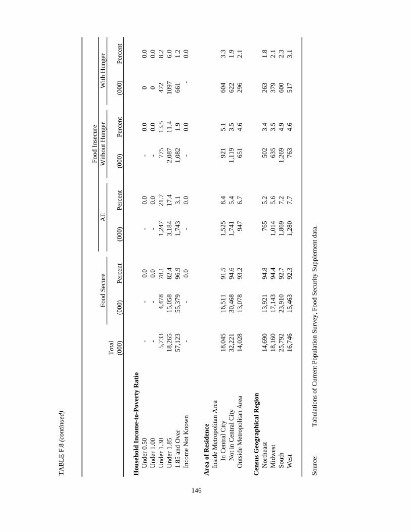
TA
BL
E F
.8 (
cont
inue
d)
Tot
al(0
00)
(000
)P
erce
nt(0
00)
Per
cent
(000
)P
erce
nt(0
00)
Per
cent
Hou
seho
ld I
ncom
e-to
-Pov
erty
Rat
ioU
nder
0.5
0-
-
0.0
-
0.
0-
0.0
00.
0U
nder
1.0
0-
-
0.0
-
0.
0-
0.0
00.
0U
nder
1.3
05,
733
4,
478
78
.11,
247
21
.777
5
13
.547
28.
2U
nder
1.8
518
,265
15
,058
82.4
3,18
4
17.4
2,08
7
11.4
1097
6.0
1.85
and
Ove
r57
,123
55
,379
96.9
1,74
3
3.1
1,08
2
1.9
661
1.2
Inco
me
Not
Kno
wn
-
-
0.
0-
0.0
-
0.
0-
0.0
146
Are
a of
Res
iden
ceIn
side
Met
ropo
litan
Are
aIn
Cen
tral
City
18,0
45
16,5
11
91
.51,
525
8.
492
1
5.
160
43.
3N
ot in
Cen
tral
City
32,2
21
30,4
68
94
.61,
741
5.
41,
119
3.
562
21.
9O
utsi
de M
etro
poli
tan
Are
a14
,028
13
,078
93.2
947
6.7
651
4.6
296
2.1
Cen
sus
Geo
grap
hica
l Reg
ion
Nor
thea
st14
,690
13
,921
94.8
765
5.2
502
3.4
263
1.8
Mid
wes
t18
,160
17
,143
94.4
1,01
4
5.6
635
3.5
379
2.1
Sou
th
25,7
92
23,9
10
92
.71,
869
7.
21,
269
4.
960
02.
3W
est
16,7
46
15,4
63
92
.31,
280
7.
776
3
4.
651
73.
1
Sour
ce:
Tab
ulat
ions
of
Cur
rent
Pop
ulat
ion
Surv
ey, F
ood
Secu
rity
Sup
plem
ent d
ata.
Food
Ins
ecur
eFo
od S
ecur
eA
llW
ithou
t Hun
ger
With
Hun
ger

Tot
al(0
00)
(000
)P
erce
nt(0
00)
Per
cent
(000
)P
erce
nt(0
00)
Per
cent
All
Hou
seho
lds
76,3
83
72,2
68
94
.64,
084
5.
42,
790
3.
71,
294
1.
7
Hou
seho
ld C
ompo
siti
onW
ith
Chi
ldre
n <
612
,153
11
,237
92.5
913
7.5
729
6.0
184
1.5
Wit
h C
hild
ren
< 1
827
,964
25
,902
92.6
2,05
6
7.4
1,55
7
5.6
499
1.8
Mar
ried
Cou
ple
Fam
ilie
s21
,892
20
,730
94.7
1,15
7
5.3
897
4.1
260
1.2
Fem
ale
Hea
d, N
o Sp
ouse
4,25
3
3,52
5
82.9
727
17.1
531
12.5
196
4.6
Mal
e H
ead,
No
Spo
use
1,49
9
1,36
2
90.9
136
9.1
111
7.4
25
1.7
Oth
er H
ouse
hold
s w
ith C
hild
ren
320
285
88.9
35
11.1
17
5.5
18
5.6
147
Wit
h N
o C
hild
ren
< 1
848
,420
46
,366
95.8
2,02
8
4.1
1,23
3
2.5
795
1.6
Mor
e T
han
One
Adu
lt29
,845
28
,915
96.9
923
3.1
621
2.1
302
1.0
Wom
en L
ivin
g A
lone
10,2
95
9,72
8
94.5
557
5.4
324
3.1
233
2.3
Men
Liv
ing
Alo
ne8,
279
7,
723
93
.354
7
6.
628
8
3.
525
9
3.
1
Hou
seho
lds
with
Eld
erly
16,7
42
16,2
62
97
.147
3
2.
933
1
2.
014
2
0.
9E
lder
ly L
ivin
g A
lone
6,37
4
6,14
6
96.4
220
3.5
144
2.3
76
1.2
Rac
e an
d H
ispa
nic
Eth
nici
tyW
hite
Non
-His
pani
c61
,383
58
,802
95.8
2,57
0
4.2
1,72
8
2.8
842
1.4
Bla
ck N
on-H
ispa
nic
7,33
1
6,51
0
88.8
810
11.0
530
7.2
280
3.8
His
pani
c5,
036
4,
443
88
.258
5
11
.645
7
9.
112
8
2.
5O
ther
Non
-His
pani
c2,
634
2,
513
95
.412
0
4.
676
2.
944
1.
7
Food
Sec
ure
All
With
out H
unge
rW
ith H
unge
rFo
od I
nsec
ure
TA
BL
E F
.9
PRE
VA
LE
NC
E O
F FO
OD
SE
CU
RIT
Y, F
OO
D I
NSE
CU
RIT
Y, A
ND
HU
NG
ER
BY
SE
LE
CT
ED
CH
AR
AC
TE
RSI
TIC
S O
F H
OU
SEH
OL
DS,
199
7FO
R T
HO
SE F
AM
ILIE
S O
VE
R 1
00 P
ER
CE
NT
OF
POV
ER
TY
TH
RE
SHH
OL
DU
SIN
G T
HE
CO
MM
ON
DE
NO
MIN
AT
OR
SC
RE
EN

TA
BL
E F
.9 (
cont
inue
d)
Tot
al(0
00)
(000
)P
erce
nt(0
00)
Per
cent
(000
)P
erce
nt(0
00)
Per
cent
Hou
seho
ld I
ncom
e-to
-Pov
erty
Rat
ioU
nder
0.5
0-
-
0.0
-
0.
0-
0.0
-
0.
0U
nder
1.0
0-
-
0.0
-
0.
0-
0.0
-
0.
0U
nder
1.3
06,
001
4,
925
82
.11,
068
17
.871
1
11
.835
76.
0U
nder
1.8
517
,403
14
,801
85.0
2,58
0
14.8
1,79
5
10.3
785
4.5
1.85
and
Ove
r58
,980
57
,467
97.4
1,50
4
2.6
995
1.7
509
0.9
Inco
me
Not
Kno
wn
-
-
0.
0-
0.0
-
0.
0-
0.0
148
Are
a of
Res
iden
ceIn
side
Met
ropo
litan
Are
aIn
Cen
tral
City
18,2
41
17,0
11
93
.31,
216
6.
776
2
4.
245
42.
5N
ot in
Cen
tral
City
32,6
60
31,1
85
95
.51,
466
4.
599
8
3.
146
81.
4O
utsi
de M
etro
poli
tan
Are
a14
,368
13
,543
94.3
821
5.7
613
4.3
208
1.4
Cen
sus
Geo
grap
hica
l Reg
ion
Nor
thea
st14
,434
13
,796
95.6
626
4.4
412
2.9
214
1.5
Mid
wes
t18
,784
17
,855
95.1
929
5.0
594
3.2
335
1.8
Sou
th
26,4
06
24,8
57
94
.11,
539
5.
81,
079
4.
146
01.
7W
est
16,7
59
15,7
60
94
.099
0
5.
970
5
4.
228
51.
7
Sour
ce:
Tab
ulat
ions
of
Cur
rent
Pop
ulat
ion
Surv
ey, F
ood
Secu
rity
Sup
plem
ent d
ata.
Food
Ins
ecur
eFo
od S
ecur
eA
llW
ithou
t Hun
ger
With
Hun
ger

Tot
al(0
00)
(000
)P
erce
nt(0
00)
Per
cent
(000
)P
erce
nt(0
00)
Per
cent
All
Hou
seho
lds
21,9
53
15,4
80
70
.56,
413
29
.23,
823
17
.42,
590
11
.8
Hou
seho
ld C
ompo
siti
onW
ith
Chi
ldre
n <
65,
823
3,
602
61
.82,
190
37
.61,
430
24
.676
0
13
.0
Wit
h C
hild
ren
< 1
810
,064
6,
202
61
.63,
830
38
.02,
419
24
.01,
411
14
.0M
arri
ed C
oupl
e Fa
mil
ies
4,44
6
2,96
9
66.8
1,46
3
32.9
986
22.2
477
10.7
Fem
ale
Hea
d, N
o Sp
ouse
4,79
9
2,70
1
56.3
2,09
0
43.5
1,27
2
26.5
818
17.0
Mal
e H
ead,
No
Spo
use
601
395
65.8
193
32.1
126
21.0
67
11.1
Oth
er H
ouse
hold
s w
ith C
hild
ren
219
136
62.2
82
37.7
34
15.7
48
22.0
149
Wit
h N
o C
hild
ren
< 1
811
,889
9,
278
78
.02,
584
21
.71,
404
11
.81,
180
9.
9M
ore
Tha
n O
ne A
dult
4,77
1
3,77
8
79.2
978
20.5
590
12.4
388
8.1
Wom
en L
ivin
g A
lone
4,80
1
3,83
7
79.9
959
20.0
553
11.5
406
8.5
Men
Liv
ing
Alo
ne2,
317
1,
662
71
.864
7
27
.926
1
11
.338
6
16
.6
Hou
seho
lds
with
Eld
erly
6,49
5
5,61
9
86.5
872
13.4
538
8.3
334
5.1
Eld
erly
Liv
ing
Alo
ne3,
878
3,
413
88
.046
5
12
.025
7
6.
620
8
5.
4
Rac
e an
d H
ispa
nic
Eth
nici
tyW
hite
Non
-His
pani
c12
,902
9,
669
74
.93,
209
24
.91,
906
14
.81,
303
10
.1B
lack
Non
-His
pani
c5,
076
3,
289
64
.81,
776
35
.01,
022
20
.175
4
14
.9H
ispa
nic
3,29
5
2,02
1
61.3
1,25
0
37.9
792
24.0
458
13.9
Oth
er N
on-H
ispa
nic
681
501
73.6
177
26.0
102
15.0
75
11.0
Food
Ins
ecur
e
TA
BL
E F
.10
PRE
VA
LE
NC
E O
F FO
OD
SE
CU
RIT
Y, F
OO
D I
NSE
CU
RIT
Y, A
ND
HU
NG
ER
BY
SE
LE
CT
ED
CH
AR
AC
TE
RSI
TIC
S O
F H
OU
SEH
OL
DS,
199
5FO
R T
HO
SE F
AM
ILIE
S U
ND
ER
130
PE
RC
EN
T O
F PO
VE
RT
Y T
HR
ESH
HO
LD
USI
NG
TH
E C
OM
MO
N D
EN
OM
INA
TO
R S
CR
EE
N
Food
Sec
ure
All
With
out H
unge
rW
ith H
unge
r

TA
BL
E F
.10
(con
tinu
ed)
Tot
al(0
00)
(000
)P
erce
nt(0
00)
Per
cent
(000
)P
erce
nt(0
00)
Per
cent
Hou
seho
ld I
ncom
e-to
-Pov
erty
Rat
ioU
nder
0.5
05,
603
3,
467
61
.92,
113
37
.71,
177
21
.093
616
.7U
nder
1.0
015
,924
10
,717
67.3
5,15
4
32.3
3,08
1
19.3
2073
13U
nder
1.3
021
,953
15
,480
70.5
6,41
3
29.2
3,82
3
17.4
2590
11.8
Und
er 1
.85
21,9
53
15,4
80
70
.56,
413
29
.23,
823
17
.425
9011
.81.
85 a
nd O
ver
-
-
0.
0-
0.0
-
0.
00
0In
com
e N
ot K
now
n-
-
0.0
-
0.
0-
0.0
00
150
Are
a of
Res
iden
ceIn
side
Met
ropo
litan
Are
aIn
Cen
tral
City
6,96
7
4,64
4
66.7
2,32
0
33.3
1,38
6
19.9
934
13.4
Not
in C
entr
al C
ity5,
247
3,
754
71
.51,
471
28
.181
7
15
.665
412
.5O
utsi
de M
etro
poli
tan
Are
a6,
410
4,
666
72
.81,
727
26
.91,
077
16
.865
010
.1
Cen
sus
Geo
grap
hica
l Reg
ion
Nor
thea
st3,
692
2,
642
71
.61,
038
28
.161
7
16
.742
111
.4M
idw
est
4,80
1
3,48
9
72.7
1,31
1
27.4
790
16.5
521
10.9
Sout
h 8,
888
6,
291
70
.82,
585
29
.11,
549
17
.410
3611
.7W
est
4,57
2
3,05
9
66.9
1,47
9
32.4
867
19.0
612
13.4
Sour
ce:
Tab
ulat
ions
of
Cur
rent
Pop
ulat
ion
Surv
ey, F
ood
Secu
rity
Sup
plem
ent d
ata.
Food
Ins
ecur
eFo
od S
ecur
eA
llW
ithou
t Hun
ger
With
Hun
ger

Tot
al(0
00)
(000
)P
erce
nt(0
00)
Per
cent
(000
)P
erce
nt(0
00)
Per
cent
All
Hou
seho
lds
20,2
82
13,8
68
68
.46,
353
31
.43,
726
18
.42,
627
13
.0
Hou
seho
ld C
ompo
siti
onW
ith
Chi
ldre
n <
65,
345
3,
253
60
.92,
073
38
.71,
360
25
.471
3
13
.3
Wit
h C
hild
ren
< 1
89,
434
5,
675
60
.23,
720
39
.52,
355
25
.01,
365
14
.5M
arri
ed C
oupl
e Fa
mil
ies
4,27
5
2,76
9
64.8
1,48
2
34.7
975
22.8
507
11.9
Fem
ale
Hea
d, N
o Sp
ouse
4,40
3
2,43
9
55.4
1,94
7
44.2
1,18
6
26.9
761
17.3
Mal
e H
ead,
No
Spo
use
568
336
59.2
231
40.8
157
27.7
74
13.1
Oth
er H
ouse
hold
s w
ith C
hild
ren
189
130
68.8
59
31.2
37
19.5
22
11.7
151
Wit
h N
o C
hild
ren
< 1
810
,847
8,
193
75
.52,
633
24
.21,
371
12
.61,
262
11
.6M
ore
Tha
n O
ne A
dult
4,46
1
3,50
9
78.7
947
21.3
539
12.1
408
9.2
Wom
en L
ivin
g A
lone
4,30
6
3,29
0
76.4
1,00
9
23.4
534
12.4
475
11.0
Men
Liv
ing
Alo
ne2,
080
1,
394
67
.067
7
32
.529
8
14
.337
9
18
.2
Hou
seho
lds
with
Eld
erly
5,69
3
4,83
3
84.9
854
15.0
531
9.3
323
5.7
Eld
erly
Liv
ing
Alo
ne3,
291
2,
864
87
.042
7
13
.025
9
7.
916
8
5.
1
Rac
e an
d H
ispa
nic
Eth
nici
tyW
hite
Non
-His
pani
c11
,354
8,
320
73
.33,
014
26
.51,
703
15
.01,
311
11
.5B
lack
Non
-His
pani
c4,
768
2,
865
60
.11,
870
39
.31,
128
23
.774
2
15
.6H
ispa
nic
3,32
1
2,06
0
62.0
1,25
3
37.7
764
23.0
489
14.7
Oth
er N
on-H
ispa
nic
840
622
74.1
215
25.7
131
15.7
84
10.0
Food
Ins
ecur
e
Tab
le F
.11
PRE
VA
LE
NC
E O
F FO
OD
SE
CU
RIT
Y, F
OO
D I
NSE
CU
RIT
Y, A
ND
HU
NG
ER
BY
SE
LE
CT
ED
CH
AR
AC
TE
RSI
TIC
S O
F H
OU
SEH
OL
DS,
199
6FO
R T
HO
SE F
AM
ILIE
S U
ND
ER
130
PE
RC
EN
T O
F PO
VE
RT
Y T
HR
ESH
HO
LD
USI
NG
TH
E C
OM
MO
N D
EN
OM
INA
TO
R S
CR
EE
N
Food
Sec
ure
All
With
out H
unge
rW
ith H
unge
r

TA
BL
E F
.11
(con
tinu
ed)
Tot
al(0
00)
(000
)P
erce
nt(0
00)
Per
cent
(000
)P
erce
nt(0
00)
Per
cent
Hou
seho
ld I
ncom
e-to
-Pov
erty
Rat
ioU
nder
0.5
06,
442
3,
932
61
.02,
480
38
.51,
342
20
.811
3817
.7U
nder
1.0
014
,548
9,
390
64
.55,
106
35
.12,
951
20
.321
5514
.8U
nder
1.3
020
,282
13
,868
68.4
6,35
3
31.4
3,72
6
18.4
2627
13.0
Und
er 1
.85
20,2
82
13,8
68
68
.46,
353
31
.43,
726
18
.426
2713
.01.
85 a
nd O
ver
-
-
0.
0-
0.0
-
0.
0-
0.0
Inco
me
Not
Kno
wn
-
-
0.
0-
0.0
-
0.
0-
0.0
152
Are
a of
Res
iden
ceIn
side
Met
ropo
litan
Are
aIn
Cen
tral
City
6,83
0
4,52
9
66.3
2,27
7
33.3
1,33
4
19.5
943
13.8
Not
in C
entr
al C
ity5,
479
3,
703
67
.61,
745
31
.898
7
18
.075
813
.8O
utsi
de M
etro
poli
tan
Are
a5,
087
3,
608
70
.91,
477
29
.191
9
18
.155
811
.0
Cen
sus
Geo
grap
hica
l Reg
ion
Nor
thea
st3,
404
2,
532
74
.486
0
25
.347
3
13
.938
711
.4M
idw
est
4,17
7
2,97
7
71.3
1,19
2
28.5
699
16.7
493
11.8
Sout
h 8,
239
5,
504
66
.82,
701
32
.81,
632
19
.810
6913
.0W
est
4,46
2
2,85
5
64.0
1,60
0
35.9
922
20.7
678
15.2
Sour
ce:
Tab
ulat
ions
of
Cur
rent
Pop
ulat
ion
Surv
ey, F
ood
Secu
rity
Sup
plem
ent d
ata.
Food
Ins
ecur
eFo
od S
ecur
eA
llW
ithou
t Hun
ger
With
Hun
ger

Tot
al(0
00)
(000
)P
erce
nt(0
00)
Per
cent
(000
)P
erce
nt(0
00)
Per
cent
All
Hou
seho
lds
20,1
58
14,7
53
73
.25,
366
26
.63,
387
16
.81,
979
9.
8
Hou
seho
ld C
ompo
siti
onW
ith
Chi
ldre
n <
65,
178
3,
543
68
.41,
628
31
.51,
194
23
.143
4
8.
4
Wit
h C
hild
ren
< 1
89,
245
6,
162
66
.73,
071
33
.32,
141
23
.293
0
10
.1M
arri
ed C
oupl
e Fa
mil
ies
3,81
8
2,78
3
72.9
1,02
8
26.9
767
20.1
261
6.8
Fem
ale
Hea
d, N
o Sp
ouse
4,60
6
2,80
1
60.8
1,80
2
39.1
1,18
4
25.7
618
13.4
Mal
e H
ead,
No
Spo
use
635
453
71.3
182
28.6
144
22.6
38
6.0
Oth
er H
ouse
hold
s w
ith C
hild
ren
186
125
67.0
59
31.4
47
25.0
12
6.4
153
Wit
h N
o C
hild
ren
< 1
810
,913
8,
591
78
.72,
295
21
.01,
246
11
.41,
049
9.
6M
ore
Tha
n O
ne A
dult
4,51
6
3,60
5
79.8
901
20.0
524
11.6
377
8.4
Wom
en L
ivin
g A
lone
4,21
1
3,40
2
80.8
797
18.9
452
10.7
345
8.2
Men
Liv
ing
Alo
ne2,
186
1,
583
72
.459
6
27
.226
9
12
.332
7
14
.9
Hou
seho
lds
with
Eld
erly
5,39
3
4,63
8
86.0
749
13.9
528
9.8
221
4.1
Eld
erly
Liv
ing
Alo
ne3,
377
2,
979
88
.239
5
11
.725
9
7.
713
6
4.
0
Rac
e an
d H
ispa
nic
Eth
nici
tyW
hite
Non
-His
pani
c10
,962
8,
503
77
.62,
450
22
.31,
429
13
.01,
021
9.
3B
lack
Non
-His
pani
c4,
815
3,
224
66
.91,
580
32
.81,
026
21
.355
4
11
.5H
ispa
nic
3,51
5
2,36
7
67.3
1,13
2
32.2
799
22.7
333
9.5
Oth
er N
on-H
ispa
nic
865
659
76.2
204
23.5
133
15.3
71
8.2
Food
Ins
ecur
e
TA
BL
E F
.12
PRE
VA
LE
NC
E O
F FO
OD
SE
CU
RIT
Y, F
OO
D I
NSE
CU
RIT
Y, A
ND
HU
NG
ER
BY
SE
LE
CT
ED
CH
AR
AC
TE
RSI
TIC
S O
F H
OU
SEH
OL
DS,
199
7FO
R T
HO
SE F
AM
ILIE
S U
ND
ER
130
PE
RC
EN
T O
F PO
VE
RT
Y T
HR
ESH
HO
LD
USI
NG
TH
E C
OM
MO
N D
EN
OM
INA
TO
R S
CR
EE
N
Food
Sec
ure
All
With
out H
unge
rW
ith H
unge
r
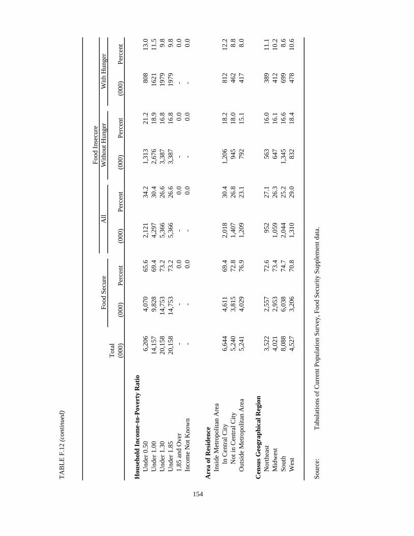
TA
BL
E F
.12
(con
tinu
ed)
Tot
al(0
00)
(000
)P
erce
nt(0
00)
Per
cent
(000
)P
erce
nt(0
00)
Per
cent
Hou
seho
ld I
ncom
e-to
-Pov
erty
Rat
ioU
nder
0.5
06,
206
4,
070
65
.62,
121
34
.21,
313
21
.280
813
.0U
nder
1.0
014
,157
9,
828
69
.44,
297
30
.42,
676
18
.916
2111
.5U
nder
1.3
020
,158
14
,753
73.2
5,36
6
26.6
3,38
7
16.8
1979
9.8
Und
er 1
.85
20,1
58
14,7
53
73
.25,
366
26
.63,
387
16
.819
799.
81.
85 a
nd O
ver
-
-
0.
0-
0.0
-
0.
0-
0.0
Inco
me
Not
Kno
wn
-
-
0.
0-
0.0
-
0.
0-
0.0
154
Are
a of
Res
iden
ceIn
side
Met
ropo
litan
Are
aIn
Cen
tral
City
6,64
4
4,61
1
69.4
2,01
8
30.4
1,20
6
18.2
812
12.2
Not
in C
entr
al C
ity5,
240
3,
815
72
.81,
407
26
.894
5
18
.046
28.
8O
utsi
de M
etro
poli
tan
Are
a5,
241
4,
029
76
.91,
209
23
.179
2
15
.141
78.
0
Cen
sus
Geo
grap
hica
l Reg
ion
Nor
thea
st3,
522
2,
557
72
.695
2
27
.156
3
16
.038
911
.1M
idw
est
4,02
1
2,95
3
73.4
1,05
9
26.3
647
16.1
412
10.2
Sout
h 8,
088
6,
038
74
.72,
044
25
.21,
345
16
.669
98.
6W
est
4,52
7
3,20
6
70.8
1,31
0
29.0
832
18.4
478
10.6
Sour
ce:
Tab
ulat
ions
of
Cur
rent
Pop
ulat
ion
Surv
ey, F
ood
Secu
rity
Sup
plem
ent d
ata.
Food
Ins
ecur
eFo
od S
ecur
eA
llW
ithou
t Hun
ger
With
Hun
ger

Tot
al(0
00)
(000
)P
erce
nt(0
00)
Per
cent
(000
)P
erce
nt(0
00)
Per
cent
All
Hou
seho
lds
68,6
28
65,1
65
95
.03,
444
5.
02,
288
3.
31,
156
1.
7
Hou
seho
ld C
ompo
siti
onW
ith
Chi
ldre
n <
611
,381
10
,563
92.8
812
7.1
653
5.7
159
1.4
Wit
h C
hild
ren
< 1
825
,422
23
,613
92.9
1,80
3
7.0
1,36
0
5.3
443
1.7
Mar
ried
Cou
ple
Fam
ilie
s20
,742
19
,615
94.6
1,12
1
5.4
880
4.2
241
1.2
Fem
ale
Hea
d, N
o Sp
ouse
3,31
1
2,73
4
82.6
577
17.5
403
12.2
174
5.3
Mal
e H
ead,
No
Spo
use
1,09
0
1,00
8
92.5
82
7.5
66
6.1
16
1.4
Oth
er H
ouse
hold
s w
ith C
hild
ren
279
256
91.8
23
8.2
11
3.8
12
4.4
155
Wit
h N
o C
hild
ren
< 1
843
,206
41
,552
96.2
1,64
1
3.8
928
2.1
713
1.7
Mor
e T
han
One
Adu
lt27
,630
26
,799
97.0
826
3.0
496
1.8
330
1.2
Wom
en L
ivin
g A
lone
8,35
8
7,94
3
95.0
414
4.9
226
2.7
188
2.2
Men
Liv
ing
Alo
ne7,
217
6,
810
94
.440
2
5.
620
6
2.
919
6
2.
7
Hou
seho
lds
with
Eld
erly
13,6
38
13,3
70
98
.026
2
2.
017
1
1.
391
0.
7E
lder
ly L
ivin
g A
lone
4,62
8
4,54
3
98.2
83
1.8
52
1.1
31
0.7
Rac
e an
d H
ispa
nic
Eth
nici
tyW
hite
Non
-His
pani
c57
,147
54
,807
95.9
2,33
5
4.1
1,55
8
2.7
777
1.4
Bla
ck N
on-H
ispa
nic
5,97
2
5,30
0
88.8
666
11.2
433
7.3
233
3.9
His
pani
c3,
809
3,
426
90
.037
4
9.
825
4
6.
712
0
3.
1O
ther
Non
-His
pani
c1,
701
1,
632
95
.969
4.
043
2.
526
1.
5
Food
Sec
ure
All
With
out H
unge
rW
ith H
unge
rFo
od I
nsec
ure
TA
BL
E F
.13
PRE
VA
LE
NC
E O
F FO
OD
SE
CU
RIT
Y, F
OO
D I
NSE
CU
RIT
Y, A
ND
HU
NG
ER
BY
SE
LE
CT
ED
CH
AR
AC
TE
RSI
TIC
S O
F H
OU
SEH
OL
DS,
199
5FO
R T
HO
SE F
AM
ILIE
S O
VE
R 1
30 P
ER
CE
NT
OF
POV
ER
TY
TH
RE
SHH
OL
DU
SIN
G T
HE
CO
MM
ON
DE
NO
MIN
AT
OR
SC
RE
EN

TA
BL
E F
.13
(con
tinu
ed)
Tot
al(0
00)
(000
)P
erce
nt(0
00)
Per
cent
(000
)P
erce
nt(0
00)
Per
cent
Hou
seho
ld I
ncom
e-to
-Pov
erty
Rat
ioU
nder
0.5
0-
-
0.0
-
0.
0-
0.0
00.
0U
nder
1.0
0-
-
0.0
-
0.
0-
0.0
00.
0U
nder
1.3
0-
-
0.0
-
0.
0-
0.0
00.
0U
nder
1.8
510
,228
8,
550
83
.61,
667
16
.31,
112
10
.955
55.
41.
85 a
nd O
ver
58,4
00
56,6
15
96
.91,
777
3.
01,
176
2.
060
11.
0In
com
e N
ot K
now
n-
-
0.0
-
0.
0-
0.0
00.
0
156
Are
a of
Res
iden
ceIn
side
Met
ropo
litan
Are
aIn
Cen
tral
City
15,4
21
14,4
10
93
.41,
005
6.
664
3
4.
236
22.
4N
ot in
Cen
tral
City
27,4
89
26,2
42
95
.51,
242
4.
580
2
2.
944
01.
6O
utsi
de M
etro
poli
tan
Are
a14
,437
13
,753
95.3
677
4.7
485
3.4
192
1.3
Cen
sus
Geo
grap
hica
l Reg
ion
Nor
thea
st13
,521
12
,965
95.9
551
4.1
386
2.9
165
1.2
Mid
wes
t16
,587
15
,775
95.1
813
4.9
548
3.3
265
1.6
Sou
th
23,5
47
22,3
55
94
.91,
186
5.
181
6
3.
537
01.
6W
est
14,9
73
14,0
70
94
.089
5
6.
053
9
3.
635
62.
4
Sour
ce:
Tab
ulat
ions
of
Cur
rent
Pop
ulat
ion
Surv
ey, F
ood
Secu
rity
Sup
plem
ent d
ata.
Food
Ins
ecur
eFo
od S
ecur
eA
llW
ithou
t Hun
ger
With
Hun
ger

Tot
al(0
00)
(000
)P
erce
nt(0
00)
Per
cent
(000
)P
erce
nt(0
00)
Per
cent
All
Hou
seho
lds
69,6
55
65,9
60
94
.73,
681
5.
22,
394
3.
41,
287
1.
8
Hou
seho
ld C
ompo
siti
onW
ith
Chi
ldre
n <
611
,157
10
,199
91.4
951
8.5
738
6.6
213
1.9
Wit
h C
hild
ren
< 1
825
,529
23
,565
92.3
1,95
3
7.6
1,43
0
5.6
523
2.0
Mar
ried
Cou
ple
Fam
ilie
s20
,673
19
,440
94.0
1,22
7
6.0
925
4.5
302
1.5
Fem
ale
Hea
d, N
o Sp
ouse
3,36
1
2,74
5
81.7
611
18.2
429
12.8
182
5.4
Mal
e H
ead,
No
Spo
use
1,15
7
1,07
7
93.1
79
6.8
51
4.4
28
2.4
Oth
er H
ouse
hold
s w
ith C
hild
ren
339
303
89.5
36
10.5
25
7.4
11
3.1
157
Wit
h N
o C
hild
ren
< 1
844
,126
42
,395
96.1
1,72
7
3.9
964
2.2
763
1.7
Mor
e T
han
One
Adu
lt28
,269
27
,343
96.7
924
3.3
528
1.9
396
1.4
Wom
en L
ivin
g A
lone
8,61
3
8,20
8
95.3
404
4.7
217
2.5
187
2.2
Men
Liv
ing
Alo
ne7,
244
6,
843
94
.540
1
5.
522
0
3.
018
1
2.
5
Hou
seho
lds
with
Eld
erly
14,2
08
13,9
18
98
.028
7
2.
019
8
1.
489
0.
6E
lder
ly L
ivin
g A
lone
4,71
6
4,61
1
97.8
105
2.2
68
1.4
37
0.8
Rac
e an
d H
ispa
nic
Eth
nici
tyW
hite
Non
-His
pani
c57
,256
54
,842
95.8
2,41
0
4.2
1,56
0
2.7
850
1.5
Bla
ck N
on-H
ispa
nic
5,90
5
5,21
9
88.4
682
11.5
461
7.8
221
3.7
His
pani
c4,
201
3,
710
88
.348
5
11
.530
7
7.
317
8
4.
2O
ther
Non
-His
pani
c2,
293
2,
190
95
.510
3
4.
566
2.
937
1.
6
Food
Ins
ecur
e
TA
BL
E F
.14
PRE
VA
LE
NC
E O
F FO
OD
SE
CU
RIT
Y, F
OO
D I
NSE
CU
RIT
Y, A
ND
HU
NG
ER
BY
SE
LE
CT
ED
CH
AR
AC
TE
RSI
TIC
S O
F H
OU
SEH
OL
DS,
199
6FO
R T
HO
SE F
AM
ILIE
S O
VE
R 1
30 P
ER
CE
NT
OF
POV
ER
TY
TH
RE
SHH
OL
DU
SIN
G T
HE
CO
MM
ON
DE
NO
MIN
AT
OR
SC
RE
EN
Food
Sec
ure
All
With
out H
unge
rW
ith H
unge
r
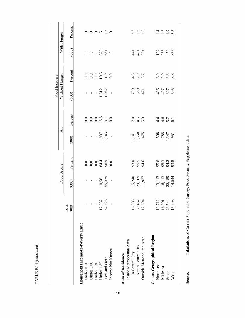
TA
BL
E F
.14
(con
tinu
ed)
Tot
al(0
00)
(000
)P
erce
nt(0
00)
Per
cent
(000
)P
erce
nt(0
00)
Per
cent
Hou
seho
ld I
ncom
e-to
-Pov
erty
Rat
ioU
nder
0.5
0-
-
0.0
-
0.
0-
0.0
00
Und
er 1
.00
-
-
0.
0-
0.0
-
0.
00
0U
nder
1.3
0-
-
0.0
-
0.
0-
0.0
00
Und
er 1
.85
12,5
32
10,5
81
84
.41,
937
15
.51,
312
10
.562
55
1.85
and
Ove
r57
,123
55
,379
96.9
1,74
3
3.1
1,08
2
1.9
661
1.2
Inco
me
Not
Kno
wn
-
-
0.
0-
0.0
-
0.
00
0
158
Are
a of
Res
iden
ceIn
side
Met
ropo
litan
Are
aIn
Cen
tral
City
16,3
85
15,2
40
93
.01,
141
7.
070
0
4.
344
12.
7N
ot in
Cen
tral
City
30,4
67
29,1
09
95
.51,
350
4.
586
9
2.
948
11.
6O
utsi
de M
etro
poli
tan
Are
a12
,604
11
,927
94.6
675
5.3
471
3.7
204
1.6
Cen
sus
Geo
grap
hica
l Reg
ion
Nor
thea
st13
,712
13
,113
95.6
598
4.4
406
3.0
192
1.4
Mid
wes
t16
,901
16
,113
95.3
785
4.6
497
2.9
288
1.7
Sou
th
23,5
44
22,1
89
94
.21,
347
5.
789
7
3.
845
01.
9W
est
15,4
98
14,5
44
93
.895
1
6.
159
5
3.
835
62.
3
Sour
ce:
Tab
ulat
ions
of
Cur
rent
Pop
ulat
ion
Surv
ey, F
ood
Secu
rity
Sup
plem
ent d
ata.
Food
Ins
ecur
eFo
od S
ecur
eA
llW
ithou
t Hun
ger
With
Hun
ger

Tot
al(0
00)
(000
)P
erce
nt(0
00)
Per
cent
(000
)P
erce
nt(0
00)
Per
cent
All
Hou
seho
lds
70,3
82
67,3
43
95
.73,
016
4.
32,
079
3.
093
7
1.
3
Hou
seho
ld C
ompo
siti
onW
ith
Chi
ldre
n <
611
,033
10
,369
94.0
664
6.0
531
4.8
133
1.2
Wit
h C
hild
ren
< 1
825
,755
24
,175
93.9
1,57
6
6.1
1,20
6
4.7
370
1.4
Mar
ried
Cou
ple
Fam
ilie
s20
,706
19
,797
95.6
906
4.4
702
3.4
204
1.0
Fem
ale
Hea
d, N
o Sp
ouse
3,46
6
2,93
3
84.6
532
15.3
406
11.7
126
3.6
Mal
e H
ead,
No
Spo
use
1,32
6
1,21
2
91.4
115
8.7
93
7.0
22
1.7
Oth
er H
ouse
hold
s w
ith C
hild
ren
256
234
91.3
22
8.7
5
2.1
17
6.6
159
Wit
h N
o C
hild
ren
< 1
844
,627
43
,167
96.7
1,44
0
3.3
873
2.0
567
1.3
Mor
e T
han
One
Adu
lt28
,122
27
,458
97.6
661
2.4
445
1.6
216
0.8
Wom
en L
ivin
g A
lone
8,84
3
8,45
6
95.6
380
4.3
211
2.4
169
1.9
Men
Liv
ing
Alo
ne7,
662
7,
253
94
.739
9
5.
221
7
2.
818
2
2.
4
Hou
seho
lds
with
Eld
erly
14,6
76
14,3
92
98
.128
0
1.
918
7
1.
393
0.
6E
lder
ly L
ivin
g A
lone
5,01
9
4,91
3
97.9
102
2.0
60
1.2
42
0.8
Rac
e an
d H
ispa
nic
Eth
nici
tyW
hite
Non
-His
pani
c57
,446
55
,453
96.5
1,98
3
3.5
1,36
0
2.4
623
1.1
Bla
ck N
on-H
ispa
nic
6,32
6
5,74
7
90.9
570
9.0
376
5.9
194
3.1
His
pani
c4,
204
3,
811
90
.639
0
9.
329
9
7.
191
2.
2O
ther
Non
-His
pani
c2,
405
2,
331
96
.974
3.
145
1.
929
1.
2
Food
Sec
ure
All
With
out H
unge
rW
ith H
unge
rFo
od I
nsec
ure
TA
BL
E F
.15
PRE
VA
LE
NC
E O
F FO
OD
SE
CU
RIT
Y, F
OO
D I
NSE
CU
RIT
Y, A
ND
HU
NG
ER
BY
SE
LE
CT
ED
CH
AR
AC
TE
RSI
TIC
S O
F H
OU
SEH
OL
DS,
199
7FO
R T
HO
SE F
AM
ILIE
S O
VE
R 1
30 P
ER
CE
NT
OF
POV
ER
TY
TH
RE
SHH
OL
DU
SIN
G T
HE
CO
MM
ON
DE
NO
MIN
AT
OR
SC
RE
EN

TA
BL
E F
.15
(con
tinu
ed)
Tot
al(0
00)
(000
)P
erce
nt(0
00)
Per
cent
(000
)P
erce
nt(0
00)
Per
cent
Hou
seho
ld I
ncom
e-to
-Pov
erty
Rat
ioU
nder
0.5
0-
-
0.0
-
0.
0-
0.0
00.
0U
nder
1.0
0-
-
0.0
-
0.
0-
0.0
00.
0U
nder
1.3
0-
-
0.0
-
0.
0-
0.0
00.
0U
nder
1.8
511
,402
9,
876
86
.61,
512
13
.31,
084
9.
542
83.
81.
85 a
nd O
ver
58,9
80
57,4
67
97
.41,
504
2.
699
5
1.
750
90.
9In
com
e N
ot K
now
n-
-
0.0
-
0.
0-
0.0
00.
0
160
Are
a of
Res
iden
ceIn
side
Met
ropo
litan
Are
aIn
Cen
tral
City
16,5
49
15,6
68
94
.786
9
5.
354
4
3.
332
52.
0N
ot in
Cen
tral
City
30,9
46
29,7
88
96
.31,
153
3.
777
3
2.
538
01.
2O
utsi
de M
etro
poli
tan
Are
a12
,735
12
,156
95.5
576
4.5
448
3.5
128
1.0
Cen
sus
Geo
grap
hica
l Reg
ion
Nor
thea
st13
,399
12
,917
96.4
477
3.6
329
2.5
148
1.1
Mid
wes
t17
,491
16
,805
96.1
686
3.9
446
2.5
240
1.4
Sou
th
24,0
32
22,9
12
95
.31,
111
4.
677
8
3.
233
31.
4W
est
15,4
60
14,7
10
95
.174
3
4.
852
7
3.
421
61.
4
Sour
ce:
Tab
ulat
ions
of
Cur
rent
Pop
ulat
ion
Surv
ey, F
ood
Secu
rity
Sup
plem
ent d
ata.
Food
Ins
ecur
eFo
od S
ecur
eA
llW
ithou
t Hun
ger
With
Hun
ger

Tot
al(0
00)
(000
)P
erce
nt(0
00)
Per
cent
(000
)P
erce
nt(0
00)
Per
cent
All
Hou
seho
lds
32,1
82
24,0
30
74
.78,
080
25
.14,
935
15
.33,
145
9.
8
Hou
seho
ld C
ompo
siti
onW
ith
Chi
ldre
n <
68,
202
5,
519
67
.32,
645
32
.31,
804
22
.084
1
10
.3
Wit
h C
hild
ren
< 1
814
,634
9,
860
67
.44,
736
32
.33,
105
21
.21,
631
11
.1M
arri
ed C
oupl
e Fa
mil
ies
7,71
3
5,65
5
73.3
2,03
9
26.4
1,42
8
18.5
611
7.9
Fem
ale
Hea
d, N
o Sp
ouse
5,79
9
3,42
4
59.0
2,36
8
40.9
1,47
7
25.5
891
15.4
Mal
e H
ead,
No
Spo
use
840
595
70.9
231
27.6
156
18.6
75
9.0
Oth
er H
ouse
hold
s w
ith C
hild
ren
282
186
65.9
96
34.1
43
15.1
53
19.0
161
Wit
h N
o C
hild
ren
< 1
817
,548
14
,170
80.8
3,34
4
19.0
1,83
0
10.4
1,51
4
8.6
Mor
e T
han
One
Adu
lt7,
682
6,
331
82
.41,
334
17
.481
4
10
.652
0
6.
8W
omen
Liv
ing
Alo
ne6,
470
5,
295
81
.81,
171
18
.167
1
10
.450
0
7.
7M
en L
ivin
g A
lone
3,39
5
2,54
4
74.9
840
24.8
345
10.2
495
14.6
Hou
seho
lds
with
Eld
erly
8,80
1
7,77
6
88.3
1,01
6
11.6
632
7.2
384
4.4
Eld
erly
Liv
ing
Alo
ne5,
033
4,
518
89
.851
1
10
.228
6
5.
722
5
4.
5
Rac
e an
d H
ispa
nic
Eth
nici
tyW
hite
Non
-His
pani
c20
,384
16
,079
78.9
4,28
2
21.1
2,62
0
12.9
1,66
2
8.2
Bla
ck N
on-H
ispa
nic
6,44
9
4,32
6
67.1
2,10
9
32.7
1,24
1
19.2
868
13.5
His
pani
c4,
384
2,
871
65
.51,
481
33
.895
2
21
.752
9
12
.1O
ther
Non
-His
pani
c96
5
75
4
78
.121
0
21
.712
3
12
.787
9.
0
Food
Sec
ure
All
With
out H
unge
rW
ith H
unge
rFo
od I
nsec
ure
TA
BL
E F
.16
PRE
VA
LE
NC
E O
F FO
OD
SE
CU
RIT
Y, F
OO
D I
NSE
CU
RIT
Y, A
ND
HU
NG
ER
BY
SE
LE
CT
ED
CH
AR
AC
TE
RSI
TIC
S O
F H
OU
SEH
OL
DS,
199
5FO
R T
HO
SE F
AM
ILIE
S U
ND
ER
185
PE
RC
EN
T O
F PO
VE
RT
Y T
HR
ESH
HO
LD
USI
NG
TH
E C
OM
MO
N D
EN
OM
INA
TO
R S
CR
EE
N

TA
BL
E F
.16
(con
tinu
ed)
Tot
al(0
00)
(000
)P
erce
nt(0
00)
Per
cent
(000
)P
erce
nt(0
00)
Per
cent
Hou
seho
ld I
ncom
e-to
-Pov
erty
Rat
ioU
nder
0.5
05,
603
3,
467
61
.92,
113
37
.71,
177
21
.093
616
.7U
nder
1.0
015
,924
10
,717
67.3
5,15
4
32.3
3,08
1
19.3
2073
13U
nder
1.3
021
,953
15
,480
70.5
6,41
3
29.2
3,82
3
17.4
2590
11.8
Und
er 1
.85
32,1
82
24,0
30
74
.78,
080
25
.14,
935
15
.331
459.
81.
85 a
nd O
ver
-
-
0.
0-
0.0
-
0.
0-
0.0
Inco
me
Not
Kno
wn
-
-
0.
0-
0.0
-
0.
0-
0.0
162
Are
a of
Res
iden
ceIn
side
Met
ropo
litan
Are
aIn
Cen
tral
City
9,48
9
6,67
8
70.4
2,80
4
29.5
1,70
2
17.9
1102
11.6
Not
in C
entr
al C
ity8,
287
6,
257
75
.52,
005
24
.21,
143
13
.886
210
.4O
utsi
de M
etro
poli
tan
Are
a9,
433
7,
296
77
.32,
114
22
.41,
368
14
.574
67.
9
Cen
sus
Geo
grap
hica
l Reg
ion
Nor
thea
st5,
427
4,
133
76
.21,
281
23
.678
7
14
.549
49.
1M
idw
est
7,20
6
5,47
9
76.0
1,72
5
24.0
1,07
1
14.9
654
9.1
Sou
th
12,7
62
9,58
3
75.1
3,16
2
24.8
1,95
1
15.3
1211
9.5
Wes
t6,
787
4,
834
71
.21,
911
28
.21,
125
16
.678
611
.6
Sour
ce:
Tab
ulat
ions
of
Cur
rent
Pop
ulat
ion
Surv
ey, F
ood
Secu
rity
Sup
plem
ent d
ata.
Food
Ins
ecur
eFo
od S
ecur
eA
llW
ithou
t Hun
ger
With
Hun
ger

Tot
al(0
00)
(000
)P
erce
nt(0
00)
Per
cent
(000
)P
erce
nt(0
00)
Per
cent
All
Hou
seho
lds
32,8
14
24,4
49
74
.58,
290
25
.35,
038
15
.43,
252
9.
9
Hou
seho
ld C
ompo
siti
onW
ith
Chi
ldre
n <
67,
795
5,
126
65
.82,
642
33
.91,
810
23
.283
2
10
.7
Wit
h C
hild
ren
< 1
814
,321
9,
458
66
.04,
813
33
.63,
162
22
.11,
651
11
.5M
arri
ed C
oupl
e Fa
mil
ies
7,42
2
5,27
0
71.0
2,12
3
28.6
1,46
1
19.7
662
8.9
Fem
ale
Hea
d, N
o Sp
ouse
5,76
5
3,39
6
58.9
2,34
9
40.8
1,46
4
25.4
885
15.4
Mal
e H
ead,
No
Spo
use
846
578
68.4
267
31.6
185
21.9
82
9.7
Oth
er H
ouse
hold
s w
ith C
hild
ren
288
214
74.2
74
25.8
52
18.1
22
7.7
163
Wit
h N
o C
hild
ren
< 1
818
,492
14
,990
81.1
3,47
7
18.8
1,87
6
10.1
1,60
1
8.7
Mor
e T
han
One
Adu
lt8,
524
7,
127
83
.61,
390
16
.381
2
9.
557
8
6.
8W
omen
Liv
ing
Alo
ne6,
730
5,
498
81
.71,
224
18
.266
0
9.
856
4
8.
4M
en L
ivin
g A
lone
3,23
8
2,36
5
73.0
864
26.7
405
12.5
459
14.2
Hou
seho
lds
with
Eld
erly
9,88
5
8,82
3
89.3
1,05
4
10.6
676
6.8
378
3.8
Eld
erly
Liv
ing
Alo
ne5,
269
4,
758
90
.351
0
9.
731
5
6.
019
5
3.
7
Rac
e an
d H
ispa
nic
Eth
nici
tyW
hite
Non
-His
pani
c20
,635
16
,367
79.3
4,24
4
20.6
2,53
1
12.3
1,71
3
8.3
Bla
ck N
on-H
ispa
nic
6,34
7
4,09
8
64.6
2,21
4
34.9
1,35
7
21.4
857
13.5
His
pani
c4,
617
3,
043
65
.91,
561
33
.998
1
21
.358
0
12
.6O
ther
Non
-His
pani
c1,
215
94
2
77
.527
1
22
.316
9
13
.910
2
8.
4
Food
Ins
ecur
e
TA
BL
E F
.17
PRE
VA
LE
NC
E O
F FO
OD
SE
CU
RIT
Y, F
OO
D I
NSE
CU
RIT
Y, A
ND
HU
NG
ER
BY
SE
LE
CT
ED
CH
AR
AC
TE
RSI
TIC
S O
F H
OU
SEH
OL
DS,
199
6FO
R T
HO
SE F
AM
ILIE
S U
ND
ER
185
PE
RC
EN
T O
F PO
VE
RT
Y T
HR
ESH
HO
LD
USI
NG
TH
E C
OM
MO
N D
EN
OM
INA
TO
R S
CR
EE
N
Food
Sec
ure
All
With
out H
unge
rW
ith H
unge
r

TA
BL
E F
.17
(con
tinu
ed)
Tot
al(0
00)
(000
)P
erce
nt(0
00)
Per
cent
(000
)P
erce
nt(0
00)
Per
cent
Hou
seho
ld I
ncom
e-to
-Pov
erty
Rat
ioU
nder
0.5
06,
442
3,
932
61
.02,
480
38
.51,
342
20
.811
3817
.7U
nder
1.0
014
,548
9,
390
64
.55,
106
35
.12,
951
20
.321
5514
.8U
nder
1.3
020
,282
13
,868
68.4
6,35
3
31.4
3,72
6
18.4
2627
13.0
Und
er 1
.85
32,8
14
24,4
49
74
.58,
290
25
.35,
038
15
.432
529.
91.
85 a
nd O
ver
-
-
0.
0-
0.0
-
0.
0-
0.0
Inco
me
Not
Kno
wn
-
-
0.
0-
0.0
-
0.
0-
0.0
164
Are
a of
Res
iden
ceIn
side
Met
ropo
litan
Are
aIn
Cen
tral
City
10,2
00
7,27
1
71.3
2,90
0
28.4
1,72
6
16.9
1174
11.5
Not
in C
entr
al C
ity9,
567
7,
136
74
.62,
393
25
.01,
424
14
.996
910
.1O
utsi
de M
etro
poli
tan
Are
a8,
211
6,
322
77
.01,
885
22
.91,
219
14
.866
68.
1
Cen
sus
Geo
grap
hica
l Reg
ion
Nor
thea
st5,
605
4,
454
79
.51,
139
20
.369
1
12
.344
88.
0M
idw
est
7,12
1
5,53
4
77.7
1,57
6
22.1
939
13.2
637
8.9
Sou
th
12,8
38
9,31
5
72.6
3,48
2
27.1
2,16
2
16.8
1320
10.3
Wes
t7,
250
5,
146
71
.02,
094
28
.91,
247
17
.284
711
.7
Sour
ce:
Tab
ulat
ions
of
Cur
rent
Pop
ulat
ion
Surv
ey, F
ood
Secu
rity
Sup
plem
ent d
ata.
Food
Ins
ecur
eFo
od S
ecur
eA
llW
ithou
t Hun
ger
With
Hun
ger

Tot
al(0
00)
(000
)P
erce
nt(0
00)
Per
cent
(000
)P
erce
nt(0
00)
Per
cent
All
Hou
seho
lds
31,5
60
24,6
29
78
.06,
878
21
.84,
471
14
.22,
407
7.
6
Hou
seho
ld C
ompo
siti
onW
ith
Chi
ldre
n <
67,
460
5,
406
72
.52,
046
27
.41,
515
20
.353
1
7.
1
Wit
h C
hild
ren
< 1
813
,975
10
,004
71.6
3,95
6
28.3
2,81
1
20.1
1,14
5
8.2
Mar
ried
Cou
ple
Fam
ilie
s6,
953
5,
399
77
.71,
544
22
.21,
145
16
.539
9
5.
7Fe
mal
e H
ead,
No
Spou
se5,
754
3,
657
63
.62,
093
36
.41,
423
24
.767
0
11
.7M
ale
Hea
d, N
o S
pous
e1,
000
75
8
75
.824
2
24
.219
1
19
.151
5.
1O
ther
Hou
seho
lds
with
Chi
ldre
n26
9
19
0
70
.776
28
.152
19
.324
8.
8
165
Wit
h N
o C
hild
ren
< 1
817
,585
14
,625
83.2
2,92
2
16.6
1,66
0
9.4
1,26
2
7.2
Mor
e T
han
One
Adu
lt7,
708
6,
553
85
.01,
143
14
.870
8
9.
243
5
5.
6W
omen
Liv
ing
Alo
ne6,
478
5,
476
84
.598
7
15
.255
7
8.
643
0
6.
6M
en L
ivin
g A
lone
3,39
9
2,59
7
76.4
792
23.3
395
11.6
397
11.7
Hou
seho
lds
with
Eld
erly
9,49
4
8,53
5
89.9
949
10.0
664
7.0
285
3.0
Eld
erly
Liv
ing
Alo
ne5,
346
4,
852
90
.848
7
9.
231
8
6.
016
9
3.
2
Rac
e an
d H
ispa
nic
Eth
nici
tyW
hite
Non
-His
pani
c19
,194
15
,762
82.1
3,41
7
17.8
2,13
5
11.1
1,28
2
6.7
Bla
ck N
on-H
ispa
nic
6,34
5
4,46
7
70.4
1,86
3
29.3
1,21
4
19.1
649
10.2
His
pani
c4,
753
3,
383
71
.21,
351
28
.596
3
20
.338
8
8.
2O
ther
Non
-His
pani
c1,
268
1,
017
80
.224
8
19
.515
9
12
.589
7.
0
Food
Sec
ure
All
With
out H
unge
rW
ith H
unge
rFo
od I
nsec
ure
TA
BL
E F
.18
PRE
VA
LE
NC
E O
F FO
OD
SE
CU
RIT
Y, F
OO
D I
NSE
CU
RIT
Y, A
ND
HU
NG
ER
BY
SE
LE
CT
ED
CH
AR
AC
TE
RSI
TIC
S O
F H
OU
SEH
OL
DS,
199
7FO
R T
HO
SE F
AM
ILIE
S U
ND
ER
185
PE
RC
EN
T O
F PO
VE
RT
Y T
HR
ESH
HO
LD
USI
NG
TH
E C
OM
MO
N D
EN
OM
INA
TO
R S
CR
EE
N

TA
BL
E F
.18
(con
tinu
ed)
Tot
al(0
00)
(000
)P
erce
nt(0
00)
Per
cent
(000
)P
erce
nt(0
00)
Per
cent
Hou
seho
ld I
ncom
e-to
-Pov
erty
Rat
ioU
nder
0.5
06,
206
4,
070
65
.62,
121
34
.21,
313
21
.280
813
.0U
nder
1.0
014
,157
9,
828
69
.44,
297
30
.42,
676
18
.916
2111
.5U
nder
1.3
020
,158
14
,753
73.2
5,36
6
26.6
3,38
7
16.8
1979
9.8
Und
er 1
.85
31,5
60
24,6
29
78
.06,
878
21
.84,
471
14
.224
077.
61.
85 a
nd O
ver
-
-
0.
0-
0.0
-
0.
0-
0.0
Inco
me
Not
Kno
wn
-
-
0.
0-
0.0
-
0.
0-
0.0
166
Are
a of
Res
iden
ceIn
side
Met
ropo
litan
Are
aIn
Cen
tral
City
9,58
7
7,12
3
74.3
2,44
4
25.5
1,48
7
15.5
957
10.0
Not
in C
entr
al C
ity9,
189
7,
255
79
.01,
911
20
.81,
288
14
.062
36.
8O
utsi
de M
etro
poli
tan
Are
a8,
119
6,
529
80
.41,
584
19
.51,
099
13
.548
56.
0
Cen
sus
Geo
grap
hica
l Reg
ion
Nor
thea
st5,
449
4,
282
78
.61,
155
21
.270
6
13
.044
98.
2M
idw
est
6,74
0
5,32
2
79.0
1,40
8
20.8
893
13.2
515
7.6
Sou
th
12,4
22
9,75
6
78.5
2,65
5
21.4
1,79
0
14.4
865
7.0
Wes
t6,
949
5,
269
75
.81,
661
23
.91,
082
15
.657
98.
3
Sour
ce:
Tab
ulat
ions
of
Cur
rent
Pop
ulat
ion
Surv
ey, F
ood
Secu
rity
Sup
plem
ent d
ata.
Food
Ins
ecur
eFo
od S
ecur
eA
llW
ithou
t Hun
ger
With
Hun
ger

Tot
al(0
00)
(000
)P
erce
nt(0
00)
Per
cent
(000
)P
erce
nt(0
00)
Per
cent
All
Hou
seho
lds
58,4
00
56,6
15
96
.91,
777
3.
01,
176
2.
060
1
1.
0
Hou
seho
ld C
ompo
siti
onW
ith
Chi
ldre
n <
69,
002
8,
645
96
.035
7
4.
028
0
3.
177
0.
9
Wit
h C
hild
ren
< 1
820
,852
19
,956
95.7
896
4.3
674
3.2
222
1.1
Mar
ried
Cou
ple
Fam
ilie
s17
,475
16
,930
96.9
545
3.1
438
2.5
107
0.6
Fem
ale
Hea
d, N
o Sp
ouse
2,31
1
2,01
2
87.1
299
13.0
198
8.6
101
4.4
Mal
e H
ead,
No
Spo
use
851
808
94.9
43
5.0
36
4.2
7
0.8
Oth
er H
ouse
hold
s w
ith C
hild
ren
216
206
95.7
9
4.3
2
1.1
7
3.2
167
Wit
h N
o C
hild
ren
< 1
837
,547
36
,659
97.6
881
2.3
502
1.3
379
1.0
Mor
e T
han
One
Adu
lt24
,719
24
,247
98.1
470
1.9
272
1.1
198
0.8
Wom
en L
ivin
g A
lone
6,68
9
6,48
5
96.9
201
3.0
107
1.6
94
1.4
Men
Liv
ing
Alo
ne6,
139
5,
928
96
.620
9
3.
412
2
2.
087
1.
4
Hou
seho
lds
with
Eld
erly
11,3
31
11,2
13
99
.011
8
1.
177
0.
741
0.
4E
lder
ly L
ivin
g A
lone
3,47
3
3,43
7
98.9
36
1.0
22
0.6
14
0.4
Rac
e an
d H
ispa
nic
Eth
nici
tyW
hite
Non
-His
pani
c49
,664
48
,397
97.4
1,26
2
2.5
844
1.7
418
0.8
Bla
ck N
on-H
ispa
nic
4,59
9
4,26
3
92.7
333
7.3
214
4.7
119
2.6
His
pani
c2,
720
2,
576
94
.714
4
5.
395
3.
549
1.
8O
ther
Non
-His
pani
c1,
417
1,
379
97
.437
2.
623
1.
614
1.
0
Food
Sec
ure
All
With
out H
unge
rW
ith H
unge
rFo
od I
nsec
ure
TA
BL
E F
.19
PRE
VA
LE
NC
E O
F FO
OD
SE
CU
RIT
Y, F
OO
D I
NSE
CU
RIT
Y, A
ND
HU
NG
ER
BY
SE
LE
CT
ED
CH
AR
AC
TE
RSI
TIC
S O
F H
OU
SEH
OL
DS,
199
5FO
R T
HO
SE F
AM
ILIE
S O
VE
R 1
85 P
ER
CE
NT
OF
POV
ER
TY
TH
RE
SHH
OL
DU
SIN
G T
HE
CO
MM
ON
DE
NO
MIN
AT
OR
SC
RE
EN

TA
BL
E F
.19
(con
tinu
ed)
Tot
al(0
00)
(000
)P
erce
nt(0
00)
Per
cent
(000
)P
erce
nt(0
00)
Per
cent
Hou
seho
ld I
ncom
e-to
-Pov
erty
Rat
ioU
nder
0.5
0-
-
0.0
-
0.
0-
0.0
-
0.
0U
nder
1.0
0-
-
0.0
-
0.
0-
0.0
-
0.
0U
nder
1.3
0-
-
0.0
-
0.
0-
0.0
-
0.
0U
nder
1.8
5-
-
0.0
-
0.
0-
0.0
-
0.
01.
85 a
nd O
ver
58,4
00
56,6
15
96
.91,
777
3.
01,
176
2.
060
1
1.
0In
com
e N
ot K
now
n-
-
0.0
-
0.
0-
0.0
-
0.
0
168
Are
a of
Res
iden
ceIn
side
Met
ropo
litan
Are
aIn
Cen
tral
City
12,8
99
12,3
76
95
.952
1
4.
032
7
2.
519
4
1.
5N
ot in
Cen
tral
City
24,4
50
23,7
39
97
.170
8
2.
847
6
1.
923
2
0.
9O
utsi
de M
etro
poli
tan
Are
a11
,414
11
,123
97.4
289
2.5
194
1.7
95
0.8
Cen
sus
Geo
grap
hica
l Reg
ion
Nor
thea
st11
,786
11
,474
97.3
308
2.6
216
1.8
92
0.8
Mid
wes
t14
,182
13
,784
97.2
398
2.8
266
1.9
132
0.9
Sou
th
19,6
74
19,0
63
96
.960
8
3.
141
3
2.
119
5
1.
0W
est
12,7
57
12,2
95
96
.446
3
3.
628
1
2.
218
2
1.
4
Sour
ce:
Tab
ulat
ions
of
Cur
rent
Pop
ulat
ion
Surv
ey, F
ood
Secu
rity
Sup
plem
ent d
ata.
Food
Ins
ecur
eFo
od S
ecur
eA
llW
ithou
t Hun
ger
With
Hun
ger

Tot
al(0
00)
(000
)P
erce
nt(0
00)
Per
cent
(000
)P
erce
nt(0
00)
Per
cent
All
Hou
seho
lds
57,1
23
55,3
79
96
.91,
743
3.
1
1,
082
1.
966
1
1.
2
Hou
seho
ld C
ompo
siti
onW
ith
Chi
ldre
n <
68,
708
8,
326
95
.638
2
4.
4
28
8
3.
394
1.
1
Wit
h C
hild
ren
< 1
820
,642
19
,782
95.8
860
4.1
623
3.0
237
1.1
Mar
ried
Cou
ple
Fam
ilie
s17
,525
16
,939
96.7
587
3.3
439
2.5
148
0.8
Fem
ale
Hea
d, N
o Sp
ouse
1,99
8
1,78
8
89.5
210
10.5
152
7.6
58
2.9
Mal
e H
ead,
No
Spo
use
878
835
95.1
43
4.9
23
2.6
20
2.3
Oth
er H
ouse
hold
s w
ith C
hild
ren
240
220
91.6
21
8.4
10
4.0
11
4.4
169
Wit
h N
o C
hild
ren
< 1
836
,481
35
,597
97.6
884
2.5
459
1.3
425
1.2
Mor
e T
han
One
Adu
lt24
,206
23
,725
98.0
481
2.0
255
1.1
226
0.9
Wom
en L
ivin
g A
lone
6,18
9
6,00
0
96.9
190
3.1
92
1.5
98
1.6
Men
Liv
ing
Alo
ne6,
086
5,
873
96
.521
2
3.
5
11
2
1.
810
0
1.
7
Hou
seho
lds
with
Eld
erly
10,0
16
9,92
9
99.1
87
0.8
52
0.5
35
0.3
Eld
erly
Liv
ing
Alo
ne2,
738
2,
716
99
.222
0.
8
12
0.
410
0.
4
Rac
e an
d H
ispa
nic
Eth
nici
tyW
hite
Non
-His
pani
c47
,975
46
,795
97.5
1,18
0
2.4
732
1.5
448
0.9
Bla
ck N
on-H
ispa
nic
4,32
6
3,98
6
92.2
339
7.9
232
5.4
107
2.5
His
pani
c2,
905
2,
727
93
.917
7
6.
1
90
3.
187
3.
0O
ther
Non
-His
pani
c1,
917
1,
871
97
.647
2.
4
28
1.
419
1.
0
Food
Ins
ecur
e
Tab
le F
.20
PRE
VA
LE
NC
E O
F FO
OD
SE
CU
RIT
Y, F
OO
D I
NSE
CU
RIT
Y, A
ND
HU
NG
ER
BY
SE
LE
CT
ED
CH
AR
AC
TE
RSI
TIC
S O
F H
OU
SEH
OL
DS,
199
6FO
R T
HO
SE F
AM
ILIE
S O
VE
R 1
85 P
ER
CE
NT
OF
POV
ER
TY
TH
RE
SHH
OL
D
Food
Sec
ure
All
With
out H
unge
rW
ith H
unge
r

TA
BL
E F
.20
(con
tinu
ed)
Tot
al(0
00)
(000
)P
erce
nt(0
00)
Per
cent
(000
)P
erce
nt(0
00)
Per
cent
Hou
seho
ld I
ncom
e-to
-Pov
erty
Rat
ioU
nder
0.5
0-
-
0.0
-
-
-
0.
0-
0.0
Und
er 1
.00
-
-
0.
0-
-
-
0.0
-
0.
0U
nder
1.3
0-
-
0.0
-
-
-
0.
0-
0.0
Und
er 1
.85
-
-
0.
0-
-
-
0.0
-
0.
01.
85 a
nd O
ver
57,1
23
55,3
79
96
.91,
743
3.
1
1,
082
1.
966
1
1.
2In
com
e N
ot K
now
n-
-
0.0
-
-
-
0.
0-
0.0
170
Are
a of
Res
iden
ceIn
side
Met
ropo
litan
Are
aIn
Cen
tral
City
13,0
16
12,4
98
96
.051
8
4.
0
30
8
2.
421
0
1.
6N
ot in
Cen
tral
City
26,3
79
25,6
76
97
.370
3
2.
6
43
2
1.
627
1
1.
0O
utsi
de M
etro
poli
tan
Are
a9,
480
9,
213
97
.226
7
2.
8
17
1
1.
896
1.
0
Cen
sus
Geo
grap
hica
l Reg
ion
Nor
thea
st11
,511
11
,192
97.2
319
2.7
188
1.6
131
1.1
Mid
wes
t13
,957
13
,556
97.1
401
2.8
257
1.8
144
1.0
Sou
th
18,9
45
18,3
79
97
.056
6
3.
0
36
7
1.
919
9
1.
1W
est
12,7
10
12,2
53
96
.445
8
3.
6
27
1
2.
118
7
1.
5
Sour
ce:
Tab
ulat
ions
of
Cur
rent
Pop
ulat
ion
Surv
ey, F
ood
Secu
rity
Sup
plem
ent d
ata.
Food
Ins
ecur
eFo
od S
ecur
eA
llW
ithou
t Hun
ger
With
Hun
ger

Tot
al(0
00)
(000
)P
erce
nt(0
00)
Per
cent
(000
)P
erce
nt(0
00)
Per
cent
All
Hou
seho
lds
58,9
80
57,4
67
97
.41,
504
2.
699
5
1.
750
9
0.
9
Hou
seho
ld C
ompo
siti
onW
ith
Chi
ldre
n <
68,
750
8,
505
97
.224
5
2.
821
0
2.
435
0.
4
Wit
h C
hild
ren
< 1
821
,025
20
,334
96.7
691
3.3
537
2.6
154
0.7
Mar
ried
Cou
ple
Fam
ilie
s17
,571
17
,181
97.8
390
2.2
324
1.8
66
0.4
Fem
ale
Hea
d, N
o Sp
ouse
2,31
8
2,07
7
89.6
241
10.4
167
7.2
74
3.2
Mal
e H
ead,
No
Spo
use
962
907
94.3
54
5.7
45
4.7
9
1.0
Oth
er H
ouse
hold
s w
ith C
hild
ren
173
168
97.1
5
2.9
-
0.
05
2.
9
171
Wit
h N
o C
hild
ren
< 1
837
,955
37
,133
97.8
813
2.1
459
1.2
354
0.9
Mor
e T
han
One
Adu
lt24
,930
24
,510
98.3
419
1.6
261
1.0
158
0.6
Wom
en L
ivin
g A
lone
6,57
6
6,38
3
97.1
190
2.9
106
1.6
84
1.3
Men
Liv
ing
Alo
ne6,
449
6,
240
96
.820
3
3.
191
1.
411
2
1.
7
Hou
seho
lds
with
Eld
erly
10,5
75
10,4
95
99
.280
0.
851
0.
529
0.
3E
lder
ly L
ivin
g A
lone
3,05
0
3,04
0
99.7
10
0.3
1
0.0
9
0.3
Rac
e an
d H
ispa
nic
Eth
nici
tyW
hite
Non
-His
pani
c49
,215
48
,194
97.9
1,01
6
2.0
654
1.3
362
0.7
Bla
ck N
on-H
ispa
nic
4,79
5
4,50
4
93.9
288
6.0
189
3.9
99
2.1
His
pani
c2,
967
2,
796
94
.217
2
5.
713
5
4.
537
1.
2O
ther
Non
-His
pani
c2,
002
1,
974
98
.629
1.
418
0.
911
0.
5
Food
Sec
ure
All
With
out H
unge
rW
ith H
unge
rFo
od I
nsec
ure
TA
BL
E F
.21
PRE
VA
LE
NC
E O
F FO
OD
SE
CU
RIT
Y, F
OO
D I
NSE
CU
RIT
Y, A
ND
HU
NG
ER
BY
SE
LE
CT
ED
CH
AR
AC
TE
RSI
TIC
S O
F H
OU
SEH
OL
DS,
199
7FO
R T
HO
SE F
AM
ILIE
S O
VE
R 1
85 P
ER
CE
NT
OF
POV
ER
TY
TH
RE
SHH
OL
DU
SIN
G T
HE
CO
MM
ON
DE
NO
MIN
AT
OR
SC
RE
EN

TA
BL
E F
.21
(con
tinu
ed)
Tot
al(0
00)
(000
)P
erce
nt(0
00)
Per
cent
(000
)P
erce
nt(0
00)
Per
cent
Hou
seho
ld I
ncom
e-to
-Pov
erty
Rat
ioU
nder
0.5
0-
-
0.0
-
0.
0-
0.0
-
0.
0U
nder
1.0
0-
-
0.0
-
0.
0-
0.0
-
0.
0U
nder
1.3
0-
-
0.0
-
0.
0-
0.0
-
0.
0U
nder
1.8
5-
-
0.0
-
0.
0-
0.0
-
0.
01.
85 a
nd O
ver
58,9
80
57,4
67
97
.41,
504
2.
699
5
1.
750
9
0.
9In
com
e N
ot K
now
n-
-
0.0
-
0.
0-
0.0
-
0.
0
172
Are
a of
Res
iden
ceIn
side
Met
ropo
litan
Are
aIn
Cen
tral
City
13,6
06
13,1
55
96
.744
3
3.
226
3
1.
918
0
1.
3N
ot in
Cen
tral
City
26,9
98
26,3
48
97
.664
9
2.
443
0
1.
621
9
0.
8O
utsi
de M
etro
poli
tan
Are
a9,
858
9,
656
98
.020
1
2.
014
1
1.
460
0.
6
Cen
sus
Geo
grap
hica
l Reg
ion
Nor
thea
st11
,471
11
,191
97.6
274
2.4
186
1.6
88
0.8
Mid
wes
t14
,773
14
,436
97.7
336
2.2
199
1.3
137
0.9
Sou
th
19,6
98
19,1
93
97
.450
1
2.
633
3
1.
716
8
0.
9W
est
13,0
39
12,6
46
97
.039
2
3.
027
7
2.
111
5
0.
9
Sour
ce:
Tab
ulat
ions
of
Cur
rent
Pop
ulat
ion
Surv
ey, F
ood
Secu
rity
Sup
plem
ent d
ata.
Food
Ins
ecur
eFo
od S
ecur
eA
llW
ithou
t Hun
ger
With
Hun
ger

Stan
dard
Stan
dard
Stan
dard
Per
cent
Err
orP
erce
ntE
rror
Per
cent
Err
or
All
Hou
seho
lds
89.6
0.25
26.
40.
177
3.9
0.12
6
Hou
seho
ld C
ompo
siti
onW
ith
Chi
ldre
n <
682
.80.
534
11.9
0.38
55.
10.
277
Wit
h C
hild
ren
< 1
884
.40.
424
10.5
0.34
25.
00.
208
Mar
ried
Cou
ple
Fam
ilie
s89
.90.
309
7.3
0.31
92.
80.
184
Fem
ale
Hea
d, N
o S
pous
e67
.71.
039
20.4
0.92
311
.80.
526
Mal
e H
ead,
No
Spo
use
83.6
1.75
911
.01.
393
4.8
1.05
0O
ther
Hou
seho
lds
wit
h C
hild
ren
78.7
3.96
59.
02.
139
12.3
3.61
5
173
Wit
h N
o C
hild
ren
< 1
892
.70.
221
3.9
0.12
93.
30.
143
Mor
e T
han
One
Adu
lt94
.70.
243
3.1
0.17
12.
10.
140
Wom
en L
ivin
g A
lone
90.4
0.38
95.
40.
347
4.2
0.15
3M
en L
ivin
g A
lone
89.1
0.53
64.
70.
394
6.0
0.54
8
Hou
seho
lds
wit
h E
lder
ly94
.90.
202
3.1
0.14
21.
90.
154
Eld
erly
Liv
ing
Alo
ne94
.20.
429
3.3
0.26
32.
50.
317
Rac
e an
d H
ispa
nic
Eth
nici
tyW
hite
Non
-His
pani
c92
.50.
204
4.6
0.15
22.
80.
102
Bla
ck N
on-H
ispa
nic
78.3
0.83
212
.80.
690
8.8
0.53
4H
ispa
nic
77.0
1.27
614
.70.
996
7.9
0.68
6O
ther
Non
-His
pani
c89
.81.
309
6.0
0.99
04.
20.
586
TA
BL
E F
.22
STA
ND
AR
D E
RR
OR
S O
F PR
EV
AL
EN
CE
EST
IMA
TE
S O
F FO
OD
SE
CU
RIT
Y, F
OO
D I
NSE
CU
RIT
Y, A
ND
HU
NG
ER
BY
SE
LE
CT
ED
CH
AR
AC
TE
RSI
TIC
S O
F H
OU
SEH
OL
DS,
199
5
Food
Sec
ure
With
out H
unge
rW
ith H
unge
rFo
od I
nsec
ure
USI
NG
TH
E C
OM
MO
N D
EN
OM
INA
TO
R S
CR
EE
N

TA
BL
E F
.22
(con
tinu
ed)
Stan
dard
Stan
dard
Stan
dard
Per
cent
Err
orP
erce
ntE
rror
Per
cent
Err
or
Hou
seho
ld I
ncom
e-to
-Pov
erty
Rat
ioU
nder
0.5
061
.91.
155
21.0
1.19
016
.70.
722
Und
er 1
.00
67.3
0.79
919
.30.
611
13.0
0.41
7U
nder
1.3
070
.50.
702
17.4
0.48
311
.80.
435
Und
er 1
.85
74.7
0.52
815
.30.
383
9.8
0.32
21.
85 a
nd O
ver
96.9
0.09
82.
00.
091
1.0
0.07
0In
com
e N
ot K
now
n94
.50.
469
3.3
0.38
52.
10.
243
174
Are
a of
Res
iden
ceIn
side
Met
ropo
litan
Are
aIn
Cen
tral
Cit
y85
.70.
431
8.7
0.34
35.
60.
308
Not
in C
entr
al C
ity
92.0
0.27
14.
70.
223
3.2
0.20
3O
utsi
de M
etro
poli
tan
Are
a89
.00.
542
7.0
0.37
13.
80.
287
Cen
sus
Geo
grap
hica
l Reg
ion
Nor
thea
st91
.20.
464
5.4
0.34
53.
30.
184
Mid
wes
t90
.60.
461
5.8
0.42
13.
50.
200
Sou
th
88.9
0.46
47.
00.
295
4.1
0.26
6W
est
88.0
0.61
47.
00.
373
4.7
0.27
4
Sour
ce:
Tab
ulat
ions
of
Cur
rent
Pop
ulat
ion
Surv
ey, F
ood
Secu
rity
Sup
plem
ent d
ata.
Food
Ins
ecur
eFo
od S
ecur
eW
ithou
t Hun
ger
With
Hun
ger

Stan
dard
Stan
dard
Stan
dard
Per
cent
Err
orP
erce
ntE
rror
Per
cent
Err
or
All
Hou
seho
lds
89.5
0.16
16.
40.
110
4.1
0.09
9
Hou
seho
ld C
ompo
siti
onW
ith
Chi
ldre
n <
682
.30.
410
12.2
0.31
55.
30.
299
Wit
h C
hild
ren
< 1
884
.30.
334
10.4
0.17
75.
10.
246
Mar
ried
Cou
ple
Fam
ilie
s89
.50.
279
7.3
0.27
03.
10.
130
Fem
ale
Hea
d, N
o S
pous
e68
.20.
751
20.0
0.71
511
.40.
610
Mal
e H
ead,
No
Spo
use
82.9
2.37
711
.31.
410
5.8
1.76
3O
ther
Hou
seho
lds
wit
h C
hild
ren
82.3
2.28
912
.11.
873
5.6
1.34
6
175
Wit
h N
o C
hild
ren
< 1
892
.60.
159
3.9
0.10
63.
40.
113
Mor
e T
han
One
Adu
lt94
.50.
196
3.0
0.13
52.
40.
168
Wom
en L
ivin
g A
lone
89.9
0.44
55.
30.
308
4.7
0.24
0M
en L
ivin
g A
lone
89.2
0.43
95.
10.
365
5.6
0.40
5
Hou
seho
lds
wit
h E
lder
ly94
.90.
220
3.2
0.20
11.
80.
112
Eld
erly
Liv
ing
Alo
ne94
.10.
436
3.6
0.35
92.
30.
238
Rac
e an
d H
ispa
nic
Eth
nici
tyW
hite
Non
-His
pani
c92
.60.
147
4.4
0.11
22.
90.
065
Bla
ck N
on-H
ispa
nic
77.2
0.64
813
.90.
523
8.5
0.39
1H
ispa
nic
77.6
0.79
913
.50.
530
8.6
0.70
2O
ther
Non
-His
pani
c89
.80.
687
6.3
0.49
33.
60.
418
Food
Ins
ecur
e
USI
NG
TH
E C
OM
MO
N D
EN
OM
INA
TO
R S
CR
EE
N
TA
BL
E F
.23
STA
ND
AR
D E
RR
OR
S O
F PR
EV
AL
EN
CE
EST
IMA
TE
S O
F FO
OD
SE
CU
RIT
Y, F
OO
D I
NSE
CU
RIT
Y, A
ND
HU
NG
ER
BY
SE
LE
CT
ED
CH
AR
AC
TE
RSI
TIC
S O
F H
OU
SEH
OL
DS,
199
6
Food
Sec
ure
With
out H
unge
rW
ith H
unge
r

Tab
le F
.23
(con
tinu
ed)
Stan
dard
Stan
dard
Stan
dard
Per
cent
Err
orP
erce
ntE
rror
Per
cent
Err
or
Hou
seho
ld I
ncom
e-to
-Pov
erty
Rat
ioU
nder
0.5
061
.00.
882
20.8
0.75
217
.70.
748
Und
er 1
.00
64.5
0.78
320
.30.
555
14.8
0.50
8U
nder
1.3
068
.40.
567
18.4
0.41
513
.00.
377
Und
er 1
.85
74.5
0.30
015
.40.
266
9.9
0.25
71.
85 a
nd O
ver
96.9
0.11
61.
90.
092
1.2
0.05
5In
com
e N
ot K
now
n94
.90.
357
2.9
0.31
21.
90.
181
176
Are
a of
Res
iden
ceIn
side
Met
ropo
litan
Are
aIn
Cen
tral
Cit
y86
.10.
312
8.1
0.31
85.
60.
294
Not
in C
entr
al C
ity
91.8
0.23
34.
80.
173
3.2
0.13
4O
utsi
de M
etro
poli
tan
Are
a88
.70.
320
7.3
0.31
14.
00.
224
Cen
sus
Geo
grap
hica
l Reg
ion
Nor
thea
st92
.00.
266
4.8
0.22
03.
10.
125
Mid
wes
t91
.30.
297
5.3
0.21
93.
40.
213
Sou
th
87.9
0.32
57.
40.
194
4.6
0.21
6W
est
87.7
0.30
07.
30.
238
4.9
0.11
6
Sour
ce:
Tab
ulat
ions
of
Cur
rent
Pop
ulat
ion
Surv
ey, F
ood
Secu
rity
Sup
plem
ent d
ata.
Food
Sec
ure
With
out H
unge
rW
ith H
unge
rFo
od I
nsec
ure

Stan
dard
Stan
dard
Stan
dard
Per
cent
Err
orP
erce
ntE
rror
Per
cent
Err
or
All
Hou
seho
lds
91.2
0.16
85.
70.
115
3.1
0.10
7
Hou
seho
ld C
ompo
siti
onW
ith
Chi
ldre
n <
686
.30.
412
10.3
0.38
53.
30.
182
Wit
h C
hild
ren
< 1
887
.00.
303
9.3
0.23
13.
60.
196
Mar
ried
Cou
ple
Fam
ilie
s92
.20.
349
5.9
0.30
21.
90.
140
Fem
ale
Hea
d, N
o S
pous
e71
.90.
800
19.0
0.92
88.
90.
518
Mal
e H
ead,
No
Spo
use
85.2
1.42
611
.81.
199
3.0
0.79
1O
ther
Hou
seho
lds
wit
h C
hild
ren
83.2
2.86
510
.12.
408
5.6
1.41
5
177
Wit
h N
o C
hild
ren
< 1
893
.60.
153
3.6
0.11
62.
70.
112
Mor
e T
han
One
Adu
lt95
.40.
189
2.9
0.14
71.
70.
155
Wom
en L
ivin
g A
lone
91.8
0.35
04.
50.
341
3.6
0.24
6M
en L
ivin
g A
lone
90.2
0.66
54.
70.
344
4.9
0.50
0
Hou
seho
lds
wit
h E
lder
ly95
.30.
210
3.2
0.20
31.
40.
116
Eld
erly
Liv
ing
Alo
ne94
.90.
320
3.2
0.28
51.
80.
172
Rac
e an
d H
ispa
nic
Eth
nici
tyW
hite
Non
-His
pani
c93
.90.
139
3.8
0.12
92.
30.
082
Bla
ck N
on-H
ispa
nic
81.1
0.78
512
.20.
570
6.5
0.43
8H
ispa
nic
80.4
0.79
914
.00.
621
5.4
0.48
4O
ther
Non
-His
pani
c91
.90.
634
5.2
0.55
52.
80.
430
TA
BL
E F
.24
PRE
VA
LE
NC
E O
F FO
OD
SE
CU
RIT
Y, F
OO
D I
NSE
CU
RIT
Y, A
ND
HU
NG
ER
BY
SE
LE
CT
ED
CH
AR
AC
TE
RSI
TIC
S O
F H
OU
SEH
OL
DS,
199
7U
SIN
G T
HE
CO
MM
ON
DE
NO
MIN
AT
OR
SC
RE
EN
Food
Ins
ecur
eFo
od S
ecur
eW
ithou
t Hun
ger
With
Hun
ger

TA
BL
E F
.24
(con
tinu
ed)
Stan
dard
Stan
dard
Stan
dard
Per
cent
Err
orP
erce
ntE
rror
Per
cent
Err
or
Hou
seho
ld I
ncom
e-to
-Pov
erty
Rat
ioU
nder
0.5
065
.61.
061
21.2
0.93
813
.00.
698
Und
er 1
.00
69.4
0.69
318
.90.
610
11.5
0.44
9U
nder
1.3
073
.20.
633
16.8
0.51
29.
80.
428
Und
er 1
.85
78.0
0.38
514
.20.
354
7.6
0.24
41.
85 a
nd O
ver
97.4
0.12
61.
70.
082
0.9
0.08
7In
com
e N
ot K
now
n94
.80.
529
3.1
0.33
61.
80.
375
178
Are
a of
Res
iden
ceIn
side
Met
ropo
litan
Are
aIn
Cen
tral
Cit
y88
.10.
446
7.1
0.29
24.
60.
273
Not
in C
entr
al C
ity
93.2
0.23
84.
50.
184
2.3
0.17
4O
utsi
de M
etro
poli
tan
Are
a90
.60.
434
6.5
0.37
22.
80.
155
Cen
sus
Geo
grap
hica
l Reg
ion
Nor
thea
st92
.00.
290
5.0
0.28
92.
90.
158
Mid
wes
t92
.40.
301
4.7
0.26
02.
90.
117
Sou
th
90.4
0.30
26.
30.
207
3.1
0.14
2W
est
90.3
0.43
26.
40.
147
3.2
0.39
7
Sour
ce:
Tab
ulat
ions
of
Cur
rent
Pop
ulat
ion
Surv
ey, F
ood
Secu
rity
Sup
plem
ent d
ata.
Food
Ins
ecur
eFo
od S
ecur
eW
ithou
t Hun
ger
With
Hun
ger
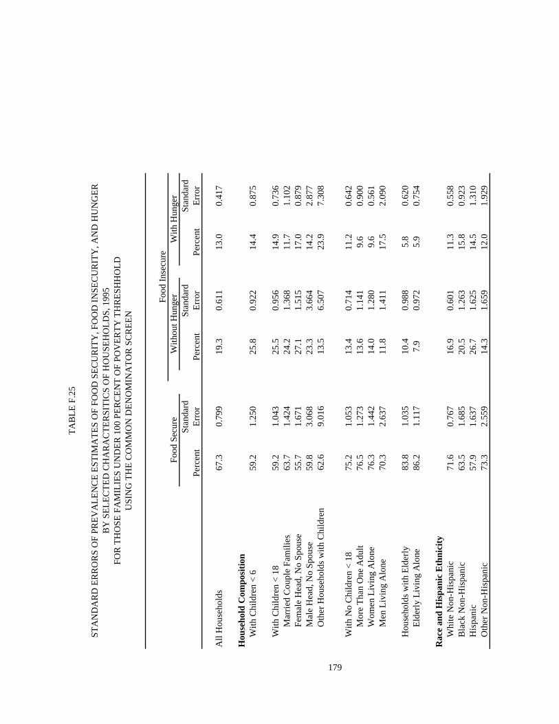
Stan
dard
Stan
dard
Stan
dard
Per
cent
Err
orP
erce
ntE
rror
Per
cent
Err
or
All
Hou
seho
lds
67.3
0.79
919
.30.
611
13.0
0.41
7
Hou
seho
ld C
ompo
siti
onW
ith
Chi
ldre
n <
659
.21.
250
25.8
0.92
214
.40.
875
Wit
h C
hild
ren
< 1
859
.21.
043
25.5
0.95
614
.90.
736
Mar
ried
Cou
ple
Fam
ilie
s63
.71.
424
24.2
1.36
811
.71.
102
Fem
ale
Hea
d, N
o S
pous
e55
.71.
671
27.1
1.51
517
.00.
879
Mal
e H
ead,
No
Spo
use
59.8
3.06
823
.33.
664
14.2
2.87
7O
ther
Hou
seho
lds
wit
h C
hild
ren
62.6
9.01
613
.56.
507
23.9
7.30
8
179
Wit
h N
o C
hild
ren
< 1
875
.21.
053
13.4
0.71
411
.20.
642
Mor
e T
han
One
Adu
lt76
.51.
273
13.6
1.14
19.
60.
900
Wom
en L
ivin
g A
lone
76.3
1.44
214
.01.
280
9.6
0.56
1M
en L
ivin
g A
lone
70.3
2.63
711
.81.
411
17.5
2.09
0
Hou
seho
lds
wit
h E
lder
ly83
.81.
035
10.4
0.98
85.
80.
620
Eld
erly
Liv
ing
Alo
ne86
.21.
117
7.9
0.97
25.
90.
754
Rac
e an
d H
ispa
nic
Eth
nici
tyW
hite
Non
-His
pani
c71
.60.
767
16.9
0.60
111
.30.
558
Bla
ck N
on-H
ispa
nic
63.5
1.68
520
.51.
263
15.8
0.92
3H
ispa
nic
57.9
1.63
726
.71.
625
14.5
1.31
0O
ther
Non
-His
pani
c73
.32.
559
14.3
1.65
912
.01.
929
TA
BL
E F
.25
STA
ND
AR
D E
RR
OR
S O
F PR
EV
AL
EN
CE
EST
IMA
TE
S O
F FO
OD
SE
CU
RIT
Y, F
OO
D I
NSE
CU
RIT
Y, A
ND
HU
NG
ER
BY
SE
LE
CT
ED
CH
AR
AC
TE
RSI
TIC
S O
F H
OU
SEH
OL
DS,
199
5
Food
Sec
ure
With
out H
unge
rW
ith H
unge
r
FOR
TH
OSE
FA
MIL
IES
UN
DE
R 1
00 P
ER
CE
NT
OF
POV
ER
TY
TH
RE
SHH
OL
D
Food
Ins
ecur
e
USI
NG
TH
E C
OM
MO
N D
EN
OM
INA
TO
R S
CR
EE
N

TA
BL
E F
.25
(con
tinu
ed)
Stan
dard
Stan
dard
Stan
dard
Per
cent
Err
orP
erce
ntE
rror
Per
cent
Err
or
Hou
seho
ld I
ncom
e-to
-Pov
erty
Rat
ioU
nder
0.5
061
.91.
155
21.0
1.19
016
.70.
722
Und
er 1
.00
67.3
0.79
919
.30.
611
13.0
0.41
7U
nder
1.3
067
.30.
799
19.3
0.61
113
.00.
417
Und
er 1
.85
67.3
0.79
919
.30.
611
13.0
0.41
71.
85 a
nd O
ver
0.0
na0.
0na
0.0
naIn
com
e N
ot K
now
n0.
0na
0.0
na0.
0na
180
Are
a of
Res
iden
ceIn
side
Met
ropo
litan
Are
aIn
Cen
tral
Cit
y64
.51.
280
21.0
1.05
514
.51.
063
Not
in C
entr
al C
ity
67.4
0.82
518
.00.
938
14.1
0.79
7O
utsi
de M
etro
poli
tan
Are
a69
.71.
397
18.8
0.86
311
.20.
875
Cen
sus
Geo
grap
hica
l Reg
ion
Nor
thea
st66
.92.
233
19.8
1.70
113
.11.
071
Mid
wes
t70
.01.
223
18.0
1.21
312
.00.
806
Sou
th
68.3
1.45
718
.91.
086
12.6
0.69
2W
est
62.8
1.02
821
.30.
578
14.9
0.80
5
Sour
ce:
Tab
ulat
ions
of
Cur
rent
Pop
ulat
ion
Surv
ey, F
ood
Secu
rity
Sup
plem
ent d
ata.
Food
Ins
ecur
eFo
od S
ecur
eW
ithou
t Hun
ger
With
Hun
ger

Stan
dard
Stan
dard
Stan
dard
Per
cent
Err
orP
erce
ntE
rror
Per
cent
Err
or
All
Hou
seho
lds
64.5
0.78
320
.30.
555
14.8
0.50
8
Hou
seho
ld C
ompo
siti
onW
ith
Chi
ldre
n <
657
.01.
694
27.7
1.30
915
.00.
931
Wit
h C
hild
ren
< 1
856
.61.
047
26.7
0.67
516
.30.
779
Mar
ried
Cou
ple
Fam
ilie
s61
.01.
249
24.8
1.11
713
.51.
085
Fem
ale
Hea
d, N
o S
pous
e53
.01.
158
28.0
1.31
518
.71.
004
Mal
e H
ead,
No
Spo
use
56.6
4.56
329
.13.
616
14.3
3.93
0O
ther
Hou
seho
lds
wit
h C
hild
ren
62.2
7.10
323
.85.
762
14.0
4.30
6
181
Wit
h N
o C
hild
ren
< 1
872
.20.
969
14.1
0.67
013
.40.
850
Mor
e T
han
One
Adu
lt75
.41.
361
13.0
1.20
611
.41.
280
Wom
en L
ivin
g A
lone
72.9
1.61
414
.70.
931
12.1
1.04
8M
en L
ivin
g A
lone
64.0
1.70
815
.21.
670
20.2
2.09
4
Hou
seho
lds
wit
h E
lder
ly81
.20.
829
11.5
0.81
77.
10.
566
Eld
erly
Liv
ing
Alo
ne84
.11.
063
10.0
0.80
15.
90.
762
Rac
e an
d H
ispa
nic
Eth
nici
tyW
hite
Non
-His
pani
c69
.90.
897
16.7
0.73
313
.20.
516
Bla
ck N
on-H
ispa
nic
57.1
1.40
024
.91.
004
17.4
0.98
1H
ispa
nic
57.9
2.37
425
.01.
349
16.8
1.50
0O
ther
Non
-His
pani
c71
.42.
536
17.4
1.63
810
.91.
731
TA
BL
E F
.26
STA
ND
AR
D E
RR
OR
S O
F PR
EV
AL
EN
CE
EST
IMA
TE
S O
F FO
OD
SE
CU
RIT
Y, F
OO
D I
NSE
CU
RIT
Y, A
ND
HU
NG
ER
BY
SE
LE
CT
ED
CH
AR
AC
TE
RSI
TIC
S O
F H
OU
SEH
OL
DS,
199
6
Food
Sec
ure
With
out H
unge
rW
ith H
unge
r
FOR
TH
OSE
FA
MIL
IES
UN
DE
R 1
00 P
ER
CE
NT
OF
POV
ER
TY
TH
RE
SHH
OL
D
Food
Ins
ecur
e
USI
NG
TH
E C
OM
MO
N D
EN
OM
INA
TO
R S
CR
EE
N

TA
BL
E F
.26
(con
tinu
ed)
Stan
dard
Stan
dard
Stan
dard
Per
cent
Err
orP
erce
ntE
rror
Per
cent
Err
or
Hou
seho
ld I
ncom
e-to
-Pov
erty
Rat
ioU
nder
0.5
061
.00.
882
20.8
0.75
217
.70.
748
Und
er 1
.00
64.5
0.78
320
.30.
555
14.8
0.50
8U
nder
1.3
064
.50.
783
20.3
0.55
514
.80.
508
Und
er 1
.85
64.5
0.78
320
.30.
555
14.8
0.50
81.
85 a
nd O
ver
0.0
na0.
0na
0.0
naIn
com
e N
ot K
now
n0.
0na
0.0
na0.
0na
182
Are
a of
Res
iden
ceIn
side
Met
ropo
litan
Are
aIn
Cen
tral
Cit
y63
.01.
025
21.5
1.08
615
.10.
854
Not
in C
entr
al C
ity
62.9
1.71
419
.81.
183
16.6
1.04
0O
utsi
de M
etro
poli
tan
Are
a67
.11.
183
20.2
1.22
412
.70.
809
Cen
sus
Geo
grap
hica
l Reg
ion
Nor
thea
st71
.11.
359
15.5
1.36
813
.01.
207
Mid
wes
t66
.71.
373
19.2
1.35
813
.80.
659
Sou
th
63.2
1.58
921
.00.
915
15.3
0.91
2W
est
60.2
1.09
823
.50.
786
16.1
1.13
9
Sour
ce:
Tab
ulat
ions
of
Cur
rent
Pop
ulat
ion
Surv
ey, F
ood
Secu
rity
Sup
plem
ent d
ata.
Food
Ins
ecur
eFo
od S
ecur
eW
ithou
t Hun
ger
With
Hun
ger

Stan
dard
Stan
dard
Stan
dard
Per
cent
Err
orP
erce
ntE
rror
Per
cent
Err
or
All
Hou
seho
lds
69.4
0.69
318
.90.
610
11.5
0.44
9
Hou
seho
ld C
ompo
siti
onW
ith
Chi
ldre
n <
665
.91.
135
24.5
0.99
69.
40.
721
Wit
h C
hild
ren
< 1
863
.00.
823
25.4
0.95
611
.40.
727
Mar
ried
Cou
ple
Fam
ilie
s70
.31.
483
21.7
1.27
87.
80.
654
Fem
ale
Hea
d, N
o S
pous
e57
.81.
461
27.7
1.69
814
.31.
001
Mal
e H
ead,
No
Spo
use
65.3
3.51
527
.13.
546
7.6
1.98
3O
ther
Hou
seho
lds
wit
h C
hild
ren
60.4
6.95
128
.36.
232
8.9
5.17
9
183
Wit
h N
o C
hild
ren
< 1
875
.70.
864
12.4
0.66
611
.50.
595
Mor
e T
han
One
Adu
lt76
.91.
179
12.5
1.23
110
.41.
111
Wom
en L
ivin
g A
lone
77.2
1.18
412
.31.
012
10.2
0.70
2M
en L
ivin
g A
lone
71.0
2.37
312
.61.
662
15.9
2.21
7
Hou
seho
lds
wit
h E
lder
ly83
.21.
188
11.6
1.14
35.
10.
524
Eld
erly
Liv
ing
Alo
ne86
.31.
229
8.7
1.10
35.
00.
740
Rac
e an
d H
ispa
nic
Eth
nici
tyW
hite
Non
-His
pani
c73
.31.
048
15.1
0.97
311
.40.
502
Bla
ck N
on-H
ispa
nic
64.6
1.38
622
.91.
149
12.3
0.91
8H
ispa
nic
64.7
1.98
423
.91.
715
11.0
1.21
5O
ther
Non
-His
pani
c74
.92.
347
15.9
2.01
68.
81.
943
TA
BL
E F
.27
STA
ND
AR
D E
RR
OR
S O
F PR
EV
AL
EN
CE
EST
IMA
TE
S O
F FO
OD
SE
CU
RIT
Y, F
OO
D I
NSE
CU
RIT
Y, A
ND
HU
NG
ER
BY
SE
LE
CT
ED
CH
AR
AC
TE
RSI
TIC
S O
F H
OU
SEH
OL
DS,
199
7
Food
Sec
ure
With
out H
unge
rW
ith H
unge
r
FOR
TH
OSE
FA
MIL
IES
UN
DE
R 1
00 P
ER
CE
NT
OF
POV
ER
TY
TH
RE
SHH
OL
D
Food
Ins
ecur
e
USI
NG
TH
E C
OM
MO
N D
EN
OM
INA
TO
R S
CR
EE
N

TA
BL
E F
.27
(con
tinu
ed)
Stan
dard
Stan
dard
Stan
dard
Per
cent
Err
orP
erce
ntE
rror
Per
cent
Err
or
Hou
seho
ld I
ncom
e-to
-Pov
erty
Rat
ioU
nder
0.5
065
.61.
061
21.2
0.93
813
.00.
698
Und
er 1
.00
69.4
0.69
318
.90.
610
11.5
0.44
9U
nder
1.3
069
.40.
693
18.9
0.61
011
.50.
449
Und
er 1
.85
69.4
0.69
318
.90.
610
11.5
0.44
91.
85 a
nd O
ver
0.0
na0.
0na
0.0
naIn
com
e N
ot K
now
n0.
0na
0.0
na0.
0na
184
Are
a of
Res
iden
ceIn
side
Met
ropo
litan
Are
aIn
Cen
tral
Cit
y66
.01.
305
20.0
0.87
813
.80.
815
Not
in C
entr
al C
ity
68.6
1.15
120
.41.
363
10.6
0.73
8O
utsi
de M
etro
poli
tan
Are
a73
.21.
405
17.4
1.26
89.
40.
700
Cen
sus
Geo
grap
hica
l Reg
ion
Nor
thea
st67
.52.
012
19.3
1.88
513
.00.
998
Mid
wes
t69
.71.
668
18.3
1.53
811
.60.
821
Sou
th
71.6
0.89
918
.30.
945
10.0
0.51
8W
est
66.8
1.49
120
.30.
777
12.7
1.38
3
Sour
ce:
Tab
ulat
ions
of
Cur
rent
Pop
ulat
ion
Surv
ey, F
ood
Secu
rity
Sup
plem
ent d
ata.
Food
Ins
ecur
eFo
od S
ecur
eW
ithou
t Hun
ger
With
Hun
ger

Stan
dard
Stan
dard
Stan
dard
Per
cent
Err
orP
erce
ntE
rror
Per
cent
Err
or
All
Hou
seho
lds
93.7
0.18
14.
10.
158
2.2
0.09
0
Hou
seho
ld C
ompo
siti
onW
ith
Chi
ldre
n <
690
.90.
367
7.1
0.35
72.
00.
201
Wit
h C
hild
ren
< 1
891
.10.
309
6.4
0.29
82.
50.
137
Mar
ried
Cou
ple
Fam
ilie
s93
.30.
256
5.1
0.22
21.
60.
158
Fem
ale
Hea
d, N
o S
pous
e78
.91.
392
13.9
1.24
07.
20.
672
Mal
e H
ead,
No
Spo
use
91.7
1.10
16.
91.
085
1.4
0.46
6O
ther
Hou
seho
lds
wit
h C
hild
ren
86.7
2.74
86.
92.
330
6.4
2.37
4
185
Wit
h N
o C
hild
ren
< 1
895
.20.
158
2.7
0.13
92.
10.
125
Mor
e T
han
One
Adu
lt96
.30.
202
2.2
0.16
61.
40.
135
Wom
en L
ivin
g A
lone
93.9
0.26
73.
20.
258
2.8
0.19
0M
en L
ivin
g A
lone
92.6
0.60
73.
50.
384
3.8
0.49
2
Hou
seho
lds
wit
h E
lder
ly97
.00.
218
1.8
0.20
01.
20.
130
Eld
erly
Liv
ing
Alo
ne96
.40.
479
1.9
0.34
21.
60.
277
Rac
e an
d H
ispa
nic
Eth
nici
tyW
hite
Non
-His
pani
c94
.90.
168
3.3
0.14
91.
80.
080
Bla
ck N
on-H
ispa
nic
86.4
0.83
98.
70.
702
4.8
0.55
2H
ispa
nic
87.5
0.59
77.
90.
557
4.5
0.41
4O
ther
Non
-His
pani
c94
.11.
324
3.8
1.04
52.
10.
414
TA
BL
E F
.28
STA
ND
AR
D E
RR
OR
S O
F PR
EV
AL
EN
CE
EST
IMA
TE
S O
F FO
OD
SE
CU
RIT
Y, F
OO
D I
NSE
CU
RIT
Y, A
ND
HU
NG
ER
BY
SE
LE
CT
ED
CH
AR
AC
TE
RSI
TIC
S O
F H
OU
SEH
OL
DS,
199
5
Food
Sec
ure
With
out H
unge
rW
ith H
unge
r
FOR
TH
OSE
FA
MIL
IES
OV
ER
100
PE
RC
EN
T O
F PO
VE
RT
Y T
HR
ESH
HO
LD
Food
Ins
ecur
e
USI
NG
TH
E C
OM
MO
N D
EN
OM
INA
TO
R S
CR
EE
N

TA
BL
E F
.28
(con
tinu
ed)
Stan
dard
Stan
dard
Stan
dard
Per
cent
Err
orP
erce
ntE
rror
Per
cent
Err
or
Hou
seho
ld I
ncom
e-to
-Pov
erty
Rat
ioU
nder
0.5
00.
0na
0.0
na0.
0na
Und
er 1
.00
0.0
na0.
0na
0.0
naU
nder
1.3
079
.01.
072
12.3
0.85
98.
60.
672
Und
er 1
.85
81.9
0.61
711
.40.
522
6.6
0.33
11.
85 a
nd O
ver
96.9
0.09
82.
00.
091
1.0
0.07
0In
com
e N
ot K
now
n0.
0na
0.0
na0.
0na
186
Are
a of
Res
iden
ceIn
side
Met
ropo
litan
Are
aIn
Cen
tral
Cit
y91
.60.
254
5.3
0.26
53.
10.
217
Not
in C
entr
al C
ity
94.7
0.23
83.
30.
175
2.0
0.16
9O
utsi
de M
etro
poli
tan
Are
a93
.60.
408
4.3
0.34
52.
00.
165
Cen
sus
Geo
grap
hica
l Reg
ion
Nor
thea
st95
.00.
240
3.3
0.18
31.
60.
123
Mid
wes
t93
.80.
551
4.1
0.47
62.
10.
185
Sou
th
93.4
0.20
54.
30.
257
2.2
0.16
9W
est
92.7
0.40
64.
30.
230
2.9
0.20
6
Sour
ce:
Tab
ulat
ions
of
Cur
rent
Pop
ulat
ion
Surv
ey, F
ood
Secu
rity
Sup
plem
ent d
ata.
Food
Ins
ecur
eFo
od S
ecur
eW
ithou
t Hun
ger
With
Hun
ger

Stan
dard
Stan
dard
Stan
dard
Per
cent
Err
orP
erce
ntE
rror
Per
cent
Err
or
All
Hou
seho
lds
93.4
0.15
64.
20.
110
2.3
0.10
4
Hou
seho
ld C
ompo
siti
onW
ith
Chi
ldre
n <
689
.40.
501
7.9
0.39
42.
60.
257
Wit
h C
hild
ren
< 1
890
.60.
243
6.8
0.21
52.
60.
164
Mar
ried
Cou
ple
Fam
ilie
s92
.70.
285
5.4
0.24
11.
90.
135
Fem
ale
Hea
d, N
o S
pous
e79
.30.
944
14.3
1.07
26.
20.
701
Mal
e H
ead,
No
Spo
use
90.3
1.46
16.
51.
010
3.2
1.06
2O
ther
Hou
seho
lds
wit
h C
hild
ren
89.0
1.98
17.
52.
159
3.5
1.12
4
187
Wit
h N
o C
hild
ren
< 1
895
.10.
154
2.7
0.11
12.
20.
109
Mor
e T
han
One
Adu
lt96
.20.
157
2.3
0.12
01.
50.
090
Wom
en L
ivin
g A
lone
93.7
0.41
43.
20.
263
3.1
0.32
9M
en L
ivin
g A
lone
92.9
0.48
83.
80.
363
3.4
0.33
5
Hou
seho
lds
wit
h E
lder
ly97
.10.
209
1.9
0.16
51.
00.
115
Eld
erly
Liv
ing
Alo
ne96
.60.
397
2.0
0.31
41.
40.
287
Rac
e an
d H
ispa
nic
Eth
nici
tyW
hite
Non
-His
pani
c94
.80.
145
3.3
0.11
21.
90.
079
Bla
ck N
on-H
ispa
nic
85.9
0.75
89.
40.
575
4.5
0.50
9H
ispa
nic
86.2
0.51
28.
80.
565
4.9
0.59
6O
ther
Non
-His
pani
c94
.40.
518
3.5
0.45
32.
10.
350
TA
BL
E F
.29
STA
ND
AR
D E
RR
OR
S O
F PR
EV
AL
EN
CE
EST
IMA
TE
S O
F FO
OD
SE
CU
RIT
Y, F
OO
D I
NSE
CU
RIT
Y, A
ND
HU
NG
ER
BY
SE
LE
CT
ED
CH
AR
AC
TE
RSI
TIC
S O
F H
OU
SEH
OL
DS,
199
6
Food
Sec
ure
With
out H
unge
rW
ith H
unge
r
FOR
TH
OSE
FA
MIL
IES
OV
ER
100
PE
RC
EN
T O
F PO
VE
RT
Y T
HR
ESH
HO
LD
Food
Ins
ecur
e
USI
NG
TH
E C
OM
MO
N D
EN
OM
INA
TO
R S
CR
EE
N

TA
BL
E F
.29
(con
tinu
ed)
Stan
dard
Stan
dard
Stan
dard
Per
cent
Err
orP
erce
ntE
rror
Per
cent
Err
or
Hou
seho
ld I
ncom
e-to
-Pov
erty
Rat
ioU
nder
0.5
00.
0na
0.0
na0.
0na
Und
er 1
.00
0.0
na0.
0na
0.0
naU
nder
1.3
078
.10.
839
13.5
0.66
88.
20.
879
Und
er 1
.85
82.4
0.47
311
.40.
435
6.0
0.37
31.
85 a
nd O
ver
96.9
0.11
61.
90.
092
1.2
0.05
5In
com
e N
ot K
now
n0.
0na
0.0
na0.
0na
188
Are
a of
Res
iden
ceIn
side
Met
ropo
litan
Are
aIn
Cen
tral
Cit
y91
.50.
277
5.1
0.31
43.
30.
288
Not
in C
entr
al C
ity
94.6
0.22
83.
50.
187
1.9
0.11
1O
utsi
de M
etro
poli
tan
Are
a93
.20.
288
4.6
0.26
32.
10.
168
Cen
sus
Geo
grap
hica
l Reg
ion
Nor
thea
st94
.80.
423.
40.
267
1.8
0.24
9M
idw
est
94.4
0.39
23.
50.
234
2.1
0.24
2S
outh
92
.70.
221
4.9
0.20
92.
30.
149
Wes
t92
.30.
237
4.6
0.14
43.
10.
228
Sour
ce:
Tab
ulat
ions
of
Cur
rent
Pop
ulat
ion
Surv
ey, F
ood
Secu
rity
Sup
plem
ent d
ata.
Food
Ins
ecur
eFo
od S
ecur
eW
ithou
t Hun
ger
With
Hun
ger

Stan
dard
Stan
dard
Stan
dard
Per
cent
Err
orP
erce
ntE
rror
Per
cent
Err
or
All
Hou
seho
lds
94.6
0.16
43.
70.
108
1.7
0.09
5
Hou
seho
ld C
ompo
siti
onW
ith
Chi
ldre
n <
692
.50.
430
6.0
0.38
21.
50.
183
Wit
h C
hild
ren
< 1
892
.60.
333
5.6
0.24
11.
80.
160
Mar
ried
Cou
ple
Fam
ilie
s94
.70.
364
4.1
0.31
01.
20.
126
Fem
ale
Hea
d, N
o S
pous
e82
.91.
041
12.5
0.91
24.
60.
528
Mal
e H
ead,
No
Spo
use
90.9
1.65
87.
41.
819
1.7
0.70
7O
ther
Hou
seho
lds
wit
h C
hild
ren
88.9
3.40
05.
52.
046
5.6
2.54
3
189
Wit
h N
o C
hild
ren
< 1
895
.80.
146
2.5
0.14
51.
60.
104
Mor
e T
han
One
Adu
lt96
.90.
135
2.1
0.13
41.
00.
076
Wom
en L
ivin
g A
lone
94.5
0.35
03.
10.
361
2.3
0.28
9M
en L
ivin
g A
lone
93.3
0.56
73.
50.
341
3.1
0.34
8
Hou
seho
lds
wit
h E
lder
ly97
.10.
184
2.0
0.17
50.
90.
107
Eld
erly
Liv
ing
Alo
ne96
.40.
339
2.3
0.32
51.
20.
230
Rac
e an
d H
ispa
nic
Eth
nici
tyW
hite
Non
-His
pani
c95
.80.
130
2.8
0.11
41.
40.
063
Bla
ck N
on-H
ispa
nic
88.8
0.86
87.
20.
630
3.8
0.44
6H
ispa
nic
88.2
1.24
59.
10.
940
2.5
0.49
7O
ther
Non
-His
pani
c95
.40.
674
2.9
0.49
91.
70.
509
TA
BL
E F
.30
STA
ND
AR
D E
RR
OR
S O
F PR
EV
AL
EN
CE
EST
IMA
TE
S O
F FO
OD
SE
CU
RIT
Y, F
OO
D I
NSE
CU
RIT
Y, A
ND
HU
NG
ER
BY
SE
LE
CT
ED
CH
AR
AC
TE
RSI
TIC
S O
F H
OU
SEH
OL
DS,
199
7
Food
Sec
ure
With
out H
unge
rW
ith H
unge
r
FOR
TH
OSE
FA
MIL
IES
OV
ER
100
PE
RC
EN
T O
F PO
VE
RT
Y T
HR
ESH
HO
LD
Food
Ins
ecur
e
USI
NG
TH
E C
OM
MO
N D
EN
OM
INA
TO
R S
CR
EE
N

TA
BL
E F
.30
(con
tinu
ed)
Stan
dard
Stan
dard
Stan
dard
Per
cent
Err
orP
erce
ntE
rror
Per
cent
Err
or
Hou
seho
ld I
ncom
e-to
-Pov
erty
Rat
ioU
nder
0.5
00.
0na
0.0
na0.
0na
Und
er 1
.00
0.0
na0.
0na
0.0
naU
nder
1.3
082
.10.
917
11.8
0.65
06.
00.
648
Und
er 1
.85
85.0
0.45
110
.30.
401
4.5
0.23
01.
85 a
nd O
ver
97.4
0.12
61.
70.
082
0.9
0.08
7In
com
e N
ot K
now
n0.
0na
0.0
na0.
0na
190
Are
a of
Res
iden
ceIn
side
Met
ropo
litan
Are
aIn
Cen
tral
Cit
y93
.30.
558
4.2
0.34
42.
50.
310
Not
in C
entr
al C
ity
95.5
0.16
53.
10.
118
1.4
0.12
5O
utsi
de M
etro
poli
tan
Are
a94
.30.
440
4.3
0.36
61.
40.
174
Cen
sus
Geo
grap
hica
l Reg
ion
Nor
thea
st95
.60.
267
2.9
0.17
71.
50.
127
Mid
wes
t95
.10.
247
3.2
0.25
81.
80.
082
Sou
th
94.1
0.39
54.
10.
207
1.7
0.28
5W
est
94.0
0.18
94.
20.
153
1.7
0.21
3
Sour
ce:
Tab
ulat
ions
of
Cur
rent
Pop
ulat
ion
Surv
ey, F
ood
Secu
rity
Sup
plem
ent d
ata.
Food
Ins
ecur
eFo
od S
ecur
eW
ithou
t Hun
ger
With
Hun
ger

Stan
dard
Stan
dard
Stan
dard
Per
cent
Err
orP
erce
ntE
rror
Per
cent
Err
or
All
Hou
seho
lds
70.5
0.70
217
.40.
483
11.8
0.43
5
Hou
seho
ld C
ompo
siti
onW
ith
Chi
ldre
n <
661
.81.
138
24.6
0.77
113
.00.
800
Wit
h C
hild
ren
< 1
861
.60.
886
24.0
0.79
014
.00.
677
Mar
ried
Cou
ple
Fam
ilie
s66
.81.
261
22.2
1.26
810
.70.
900
Fem
ale
Hea
d, N
o S
pous
e56
.31.
395
26.5
1.31
517
.00.
852
Mal
e H
ead,
No
Spo
use
65.8
3.62
321
.03.
540
11.1
2.39
6O
ther
Hou
seho
lds
wit
h C
hild
ren
62.2
7.12
015
.75.
076
22.0
6.16
7
191
Wit
h N
o C
hild
ren
< 1
878
.00.
931
11.8
0.49
99.
90.
565
Mor
e T
han
One
Adu
lt79
.21.
011
12.4
0.80
48.
10.
674
Wom
en L
ivin
g A
lone
79.9
1.28
411
.51.
080
8.5
0.43
1M
en L
ivin
g A
lone
71.8
2.12
911
.31.
175
16.6
2.09
5
Hou
seho
lds
wit
h E
lder
ly86
.50.
813
8.3
0.50
95.
10.
686
Eld
erly
Liv
ing
Alo
ne88
.01.
156
6.6
0.60
65.
40.
855
Rac
e an
d H
ispa
nic
Eth
nici
tyW
hite
Non
-His
pani
c74
.90.
620
14.8
0.46
510
.10.
471
Bla
ck N
on-H
ispa
nic
64.8
1.53
020
.11.
095
14.9
0.97
3H
ispa
nic
61.3
2.27
424
.01.
552
13.9
1.45
4O
ther
Non
-His
pani
c73
.63.
540
15.0
2.16
111
.01.
902
TA
BL
E F
.31
STA
ND
AR
D E
RR
OR
S O
F PR
EV
AL
EN
CE
EST
IMA
TE
S O
F FO
OD
SE
CU
RIT
Y, F
OO
D I
NSE
CU
RIT
Y, A
ND
HU
NG
ER
BY
SE
LE
CT
ED
CH
AR
AC
TE
RSI
TIC
S O
F H
OU
SEH
OL
DS,
199
5
Food
Sec
ure
With
out H
unge
rW
ith H
unge
r
FOR
TH
OSE
FA
MIL
IES
UN
DE
R 1
30 P
ER
CE
NT
OF
POV
ER
TY
TH
RE
SHH
OL
D
Food
Ins
ecur
e
USI
NG
TH
E C
OM
MO
N D
EN
OM
INA
TO
R S
CR
EE
N

TA
BL
E F
.31
(con
tinu
ed)
Stan
dard
Stan
dard
Stan
dard
Per
cent
Err
orP
erce
ntE
rror
Per
cent
Err
or
Hou
seho
ld I
ncom
e-to
-Pov
erty
Rat
ioU
nder
0.5
061
.91.
155
21.0
1.19
016
.70.
722
Und
er 1
.00
67.3
0.79
919
.30.
611
13.0
0.41
7U
nder
1.3
070
.50.
702
17.4
0.48
311
.80.
435
Und
er 1
.85
70.5
0.70
217
.40.
483
11.8
0.43
51.
85 a
nd O
ver
0.0
na0.
0na
0.0
naIn
com
e N
ot K
now
n0.
0na
0.0
na0.
0na
192
Are
a of
Res
iden
ceIn
side
Met
ropo
litan
Are
aIn
Cen
tral
Cit
y66
.71.
386
19.9
0.87
613
.41.
124
Not
in C
entr
al C
ity
71.5
0.61
615
.60.
812
12.5
0.68
7O
utsi
de M
etro
poli
tan
Are
a72
.81.
166
16.8
0.74
210
.10.
764
Cen
sus
Geo
grap
hica
l Reg
ion
Nor
thea
st71
.61.
566
16.7
1.15
311
.40.
804
Mid
wes
t72
.70.
703
16.5
0.86
710
.90.
845
Sou
th
70.8
1.29
017
.40.
894
11.7
0.73
7W
est
66.9
1.71
119
.00.
843
13.4
1.02
1
Sour
ce:
Tab
ulat
ions
of
Cur
rent
Pop
ulat
ion
Surv
ey, F
ood
Secu
rity
Sup
plem
ent d
ata.
Food
Ins
ecur
eFo
od S
ecur
eW
ithou
t Hun
ger
With
Hun
ger

Stan
dard
Stan
dard
Stan
dard
Per
cent
Err
orP
erce
ntE
rror
Per
cent
Err
or
All
Hou
seho
lds
68.4
0.56
718
.40.
415
13.0
0.37
7
Hou
seho
ld C
ompo
siti
onW
ith
Chi
ldre
n <
660
.91.
450
25.4
1.16
913
.30.
755
Wit
h C
hild
ren
< 1
860
.20.
878
25.0
0.55
114
.50.
754
Mar
ried
Cou
ple
Fam
ilie
s64
.80.
999
22.8
0.90
611
.90.
921
Fem
ale
Hea
d, N
o S
pous
e55
.40.
950
26.9
1.12
117
.30.
926
Mal
e H
ead,
No
Spo
use
59.2
4.38
427
.72.
965
13.1
3.53
5O
ther
Hou
seho
lds
wit
h C
hild
ren
68.8
5.17
319
.54.
211
11.7
3.15
0
193
Wit
h N
o C
hild
ren
< 1
875
.50.
639
12.6
0.50
111
.60.
501
Mor
e T
han
One
Adu
lt78
.70.
925
12.1
0.75
99.
20.
897
Wom
en L
ivin
g A
lone
76.4
1.14
512
.40.
764
11.0
0.67
7M
en L
ivin
g A
lone
67.0
1.43
814
.31.
332
18.2
1.60
7
Hou
seho
lds
wit
h E
lder
ly84
.90.
659
9.3
0.65
95.
70.
475
Eld
erly
Liv
ing
Alo
ne87
.00.
925
7.9
0.68
45.
10.
650
Rac
e an
d H
ispa
nic
Eth
nici
tyW
hite
Non
-His
pani
c73
.30.
680
15.0
0.56
711
.50.
376
Bla
ck N
on-H
ispa
nic
60.1
1.23
923
.70.
832
15.6
0.92
4H
ispa
nic
62.0
1.84
323
.01.
263
14.7
1.29
3O
ther
Non
-His
pani
c74
.11.
972
15.7
1.36
310
.01.
377
TA
BL
E F
.32
STA
ND
AR
D E
RR
OR
S O
F PR
EV
AL
EN
CE
EST
IMA
TE
S O
F FO
OD
SE
CU
RIT
Y, F
OO
D I
NSE
CU
RIT
Y, A
ND
HU
NG
ER
BY
SE
LE
CT
ED
CH
AR
AC
TE
RSI
TIC
S O
F H
OU
SEH
OL
DS,
199
6
Food
Sec
ure
With
out H
unge
rW
ith H
unge
r
FOR
TH
OSE
FA
MIL
IES
UN
DE
R 1
30 P
ER
CE
NT
OF
POV
ER
TY
TH
RE
SHH
OL
D
Food
Ins
ecur
e
USI
NG
TH
E C
OM
MO
N D
EN
OM
INA
TO
R S
CR
EE
N

TA
BL
E F
.32
(con
tinu
ed)
Stan
dard
Stan
dard
Stan
dard
Per
cent
Err
orP
erce
ntE
rror
Per
cent
Err
or
Hou
seho
ld I
ncom
e-to
-Pov
erty
Rat
ioU
nder
0.5
061
.00.
882
20.8
0.75
217
.70.
748
Und
er 1
.00
64.5
0.78
320
.30.
555
14.8
0.50
8U
nder
1.3
068
.40.
567
18.4
0.41
513
.00.
377
Und
er 1
.85
68.4
0.56
718
.40.
415
13.0
0.37
71.
85 a
nd O
ver
0.0
na0.
0na
0.0
naIn
com
e N
ot K
now
n0.
0na
0.0
na0.
0na
194
Are
a of
Res
iden
ceIn
side
Met
ropo
litan
Are
aIn
Cen
tral
Cit
y66
.30.
788
19.5
0.86
213
.80.
959
Not
in C
entr
al C
ity
67.6
1.35
118
.01.
022
13.8
0.70
4O
utsi
de M
etro
poli
tan
Are
a70
.90.
910
18.1
0.95
911
.00.
623
Cen
sus
Geo
grap
hica
l Reg
ion
Nor
thea
st74
.40.
953
13.9
0.91
511
.40.
389
Mid
wes
t71
.31.
159
16.7
1.13
311
.80.
728
Sou
th
66.8
1.16
419
.80.
662
13.0
0.76
6W
est
64.0
0.52
620
.70.
649
15.2
0.61
1
Sour
ce:
Tab
ulat
ions
of
Cur
rent
Pop
ulat
ion
Surv
ey, F
ood
Secu
rity
Sup
plem
ent d
ata.
Food
Ins
ecur
eFo
od S
ecur
eW
ithou
t Hun
ger
With
Hun
ger
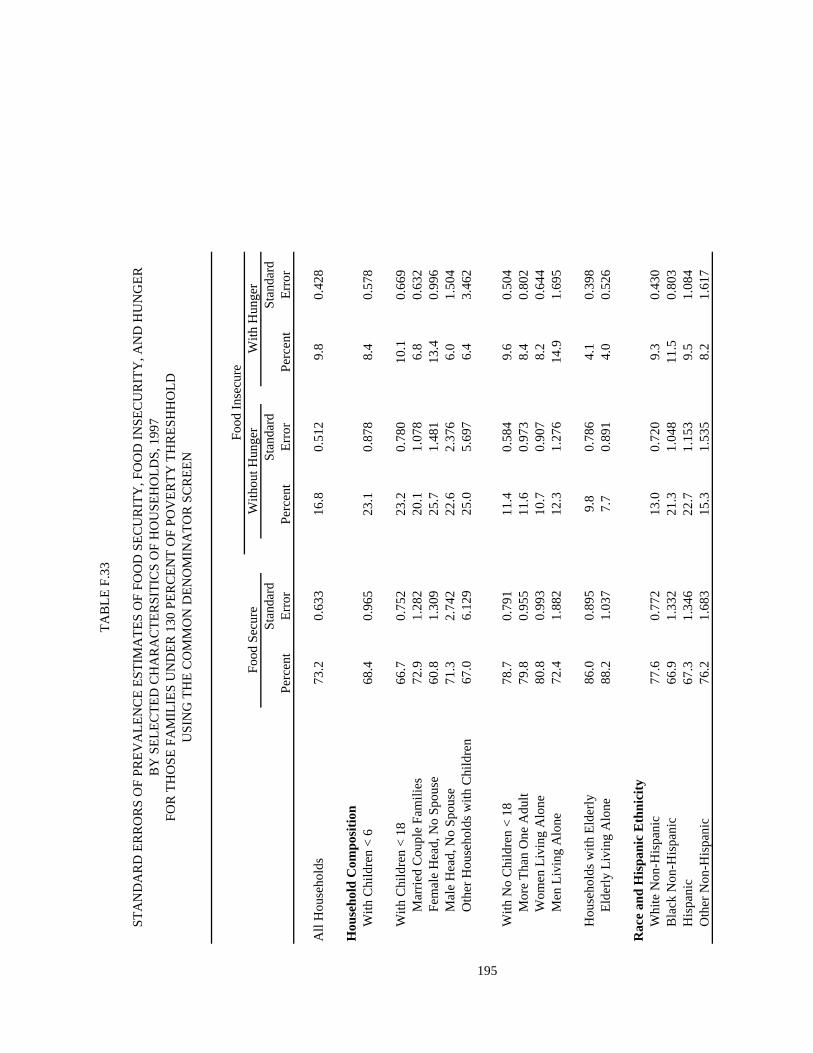
Stan
dard
Stan
dard
Stan
dard
Per
cent
Err
orP
erce
ntE
rror
Per
cent
Err
or
All
Hou
seho
lds
73.2
0.63
316
.80.
512
9.8
0.42
8
Hou
seho
ld C
ompo
siti
onW
ith
Chi
ldre
n <
668
.40.
965
23.1
0.87
88.
40.
578
Wit
h C
hild
ren
< 1
866
.70.
752
23.2
0.78
010
.10.
669
Mar
ried
Cou
ple
Fam
ilie
s72
.91.
282
20.1
1.07
86.
80.
632
Fem
ale
Hea
d, N
o S
pous
e60
.81.
309
25.7
1.48
113
.40.
996
Mal
e H
ead,
No
Spo
use
71.3
2.74
222
.62.
376
6.0
1.50
4O
ther
Hou
seho
lds
wit
h C
hild
ren
67.0
6.12
925
.05.
697
6.4
3.46
2
195
Wit
h N
o C
hild
ren
< 1
878
.70.
791
11.4
0.58
49.
60.
504
Mor
e T
han
One
Adu
lt79
.80.
955
11.6
0.97
38.
40.
802
Wom
en L
ivin
g A
lone
80.8
0.99
310
.70.
907
8.2
0.64
4M
en L
ivin
g A
lone
72.4
1.88
212
.31.
276
14.9
1.69
5
Hou
seho
lds
wit
h E
lder
ly86
.00.
895
9.8
0.78
64.
10.
398
Eld
erly
Liv
ing
Alo
ne88
.21.
037
7.7
0.89
14.
00.
526
Rac
e an
d H
ispa
nic
Eth
nici
tyW
hite
Non
-His
pani
c77
.60.
772
13.0
0.72
09.
30.
430
Bla
ck N
on-H
ispa
nic
66.9
1.33
221
.31.
048
11.5
0.80
3H
ispa
nic
67.3
1.34
622
.71.
153
9.5
1.08
4O
ther
Non
-His
pani
c76
.21.
683
15.3
1.53
58.
21.
617
TA
BL
E F
.33
STA
ND
AR
D E
RR
OR
S O
F PR
EV
AL
EN
CE
EST
IMA
TE
S O
F FO
OD
SE
CU
RIT
Y, F
OO
D I
NSE
CU
RIT
Y, A
ND
HU
NG
ER
BY
SE
LE
CT
ED
CH
AR
AC
TE
RSI
TIC
S O
F H
OU
SEH
OL
DS,
199
7
Food
Sec
ure
With
out H
unge
rW
ith H
unge
r
FOR
TH
OSE
FA
MIL
IES
UN
DE
R 1
30 P
ER
CE
NT
OF
POV
ER
TY
TH
RE
SHH
OL
D
Food
Ins
ecur
e
USI
NG
TH
E C
OM
MO
N D
EN
OM
INA
TO
R S
CR
EE
N

TA
BL
E F
.33
(con
tinu
ed)
Stan
dard
Stan
dard
Stan
dard
Per
cent
Err
orP
erce
ntE
rror
Per
cent
Err
or
Hou
seho
ld I
ncom
e-to
-Pov
erty
Rat
ioU
nder
0.5
065
.61.
601
21.2
0.93
813
.00.
698
Und
er 1
.00
69.4
0.69
318
.90.
610
11.5
0.44
9U
nder
1.3
073
.20.
633
16.8
0.51
29.
80.
428
Und
er 1
.85
73.2
0.63
316
.80.
512
9.8
0.42
81.
85 a
nd O
ver
0.0
na0.
0na
0.0
naIn
com
e N
ot K
now
n0.
0na
0.0
na0.
0na
196
Are
a of
Res
iden
ceIn
side
Met
ropo
litan
Are
aIn
Cen
tral
Cit
y69
.41.
093
18.2
0.68
112
.20.
696
Not
in C
entr
al C
ity
72.8
1.01
818
.01.
032
8.8
0.71
0O
utsi
de M
etro
poli
tan
Are
a76
.91.
097
15.1
1.03
68.
00.
556
Cen
sus
Geo
grap
hica
l Reg
ion
Nor
thea
st72
.61.
711
16.0
1.46
511
.10.
985
Mid
wes
t73
.41.
622
16.1
1.55
410
.20.
924
Sou
th
74.7
0.70
716
.60.
717
8.6
0.28
6W
est
70.8
1.56
818
.40.
575
10.6
1.44
7
Sour
ce:
Tab
ulat
ions
of
Cur
rent
Pop
ulat
ion
Surv
ey, F
ood
Secu
rity
Sup
plem
ent d
ata.
Food
Ins
ecur
eFo
od S
ecur
eW
ithou
t Hun
ger
With
Hun
ger

Stan
dard
Stan
dard
Stan
dard
Per
cent
Err
orP
erce
ntE
rror
Per
cent
Err
or
All
Hou
seho
lds
95.0
0.15
23.
30.
123
1.7
0.07
9
Hou
seho
ld C
ompo
siti
onW
ith
Chi
ldre
n <
692
.80.
355
5.7
0.30
11.
40.
141
Wit
h C
hild
ren
< 1
892
.90.
279
5.3
0.25
31.
70.
118
Mar
ried
Cou
ple
Fam
ilie
s94
.60.
247
4.2
0.22
01.
20.
113
Fem
ale
Hea
d, N
o S
pous
e82
.61.
255
12.2
1.07
75.
30.
665
Mal
e H
ead,
No
Spo
use
92.5
0.94
66.
10.
969
1.4
0.51
1O
ther
Hou
seho
lds
wit
h C
hild
ren
91.8
2.06
13.
81.
794
4.4
1.97
7
197
Wit
h N
o C
hild
ren
< 1
896
.20.
133
2.1
0.10
91.
70.
100
Mor
e T
han
One
Adu
lt97
.00.
152
1.8
0.13
71.
20.
128
Wom
en L
ivin
g A
lone
95.0
0.37
42.
70.
226
2.2
0.24
6M
en L
ivin
g A
lone
94.4
0.51
92.
90.
296
2.7
0.39
1
Hou
seho
lds
wit
h E
lder
ly98
.00.
197
1.3
0.16
00.
70.
107
Eld
erly
Liv
ing
Alo
ne98
.20.
402
1.1
0.29
10.
70.
220
Rac
e an
d H
ispa
nic
Eth
nici
tyW
hite
Non
-His
pani
c95
.90.
140
2.7
0.11
11.
40.
078
Bla
ck N
on-H
ispa
nic
88.8
0.76
67.
30.
660
3.9
0.53
8H
ispa
nic
90.0
0.64
86.
70.
416
3.1
0.29
5O
ther
Non
-His
pani
c95
.90.
721
2.5
0.71
51.
50.
370
TA
BL
E F
.34
STA
ND
AR
D E
RR
OR
S O
F PR
EV
AL
EN
CE
EST
IMA
TE
S O
F FO
OD
SE
CU
RIT
Y, F
OO
D I
NSE
CU
RIT
Y, A
ND
HU
NG
ER
BY
SE
LE
CT
ED
CH
AR
AC
TE
RSI
TIC
S O
F H
OU
SEH
OL
DS,
199
5
Food
Sec
ure
With
out H
unge
rW
ith H
unge
r
FOR
TH
OSE
FA
MIL
IES
OV
ER
130
PE
RC
EN
T O
F PO
VE
RT
Y T
HR
ESH
HO
LD
Food
Ins
ecur
e
USI
NG
TH
E C
OM
MO
N D
EN
OM
INA
TO
R S
CR
EE
N

TA
BL
E F
.34
(con
tinu
ed)
Stan
dard
Stan
dard
Stan
dard
Per
cent
Err
orP
erce
ntE
rror
Per
cent
Err
or
Hou
seho
ld I
ncom
e-to
-Pov
erty
Rat
ioU
nder
0.5
00.
0na
0.0
na0.
0na
Und
er 1
.00
0.0
na0.
0na
0.0
naU
nder
1.3
00.
0na
0.0
na0.
0na
Und
er 1
.85
83.6
0.67
610
.90.
259
5.4
0.35
61.
85 a
nd O
ver
96.9
0.09
82.
00.
091
1.0
0.07
0In
com
e N
ot K
now
n0.
0na
0.0
na0.
0na
198
Are
a of
Res
iden
ceIn
side
Met
ropo
litan
Are
aIn
Cen
tral
Cit
y93
.40.
340
4.2
0.25
62.
40.
275
Not
in C
entr
al C
ity
95.5
0.24
92.
90.
161
1.6
0.18
2O
utsi
de M
etro
poli
tan
Are
a95
.30.
339
3.4
0.28
01.
30.
152
Cen
sus
Geo
grap
hica
l Reg
ion
Nor
thea
st95
.90.
217
2.9
0.18
01.
20.
102
Mid
wes
t95
.10.
358
3.3
0.30
71.
60.
125
Sou
th
94.9
0.20
03.
50.
240
1.6
0.11
8W
est
94.0
0.43
03.
60.
184
2.4
0.26
0
Sour
ce:
Tab
ulat
ions
of
Cur
rent
Pop
ulat
ion
Surv
ey, F
ood
Secu
rity
Sup
plem
ent d
ata.
Food
Ins
ecur
eFo
od S
ecur
eW
ithou
t Hun
ger
With
Hun
ger

Stan
dard
Stan
dard
Stan
dard
Per
cent
Err
orP
erce
ntE
rror
Per
cent
Err
or
All
Hou
seho
lds
94.7
0.14
33.
40.
109
1.8
0.07
5
Hou
seho
ld C
ompo
siti
onW
ith
Chi
ldre
n <
691
.40.
496
6.6
0.40
91.
90.
198
Wit
h C
hild
ren
< 1
892
.30.
269
5.6
0.23
12.
00.
131
Mar
ried
Cou
ple
Fam
ilie
s94
.00.
306
4.5
0.26
91.
50.
125
Fem
ale
Hea
d, N
o S
pous
e81
.71.
003
12.8
1.08
35.
40.
731
Mal
e H
ead,
No
Spo
use
93.1
1.30
54.
40.
714
2.4
1.10
1O
ther
Hou
seho
lds
wit
h C
hild
ren
89.5
2.25
57.
42.
362
3.1
0.88
2
199
Wit
h N
o C
hild
ren
< 1
896
.10.
144
2.2
0.11
91.
70.
081
Mor
e T
han
One
Adu
lt96
.70.
147
1.9
0.10
71.
40.
095
Wom
en L
ivin
g A
lone
95.3
0.30
52.
50.
218
2.2
0.20
8M
en L
ivin
g A
lone
94.5
0.53
53.
00.
342
2.5
0.36
3
Hou
seho
lds
wit
h E
lder
ly98
.00.
187
1.4
0.14
70.
60.
088
Eld
erly
Liv
ing
Alo
ne97
.80.
335
1.4
0.24
50.
80.
198
Rac
e an
d H
ispa
nic
Eth
nici
tyW
hite
Non
-His
pani
c95
.80.
125
2.7
0.10
91.
50.
065
Bla
ck N
on-H
ispa
nic
88.4
0.81
87.
80.
607
3.7
0.43
1H
ispa
nic
88.3
0.43
87.
30.
457
4.2
0.42
7O
ther
Non
-His
pani
c95
.50.
537
2.9
0.41
81.
60.
303
TA
BL
E F
.35
STA
ND
AR
D E
RR
OR
S O
F PR
EV
AL
EN
CE
EST
IMA
TE
S O
F FO
OD
SE
CU
RIT
Y, F
OO
D I
NSE
CU
RIT
Y, A
ND
HU
NG
ER
BY
SE
LE
CT
ED
CH
AR
AC
TE
RSI
TIC
S O
F H
OU
SEH
OL
DS,
199
6
Food
Sec
ure
With
out H
unge
rW
ith H
unge
r
FOR
TH
OSE
FA
MIL
IES
OV
ER
130
PE
RC
EN
T O
F PO
VE
RT
Y T
HR
ESH
HO
LD
Food
Ins
ecur
e
USI
NG
TH
E C
OM
MO
N D
EN
OM
INA
TO
R S
CR
EE
N

TA
BL
E F
.35
(con
tinu
ed)
Stan
dard
Stan
dard
Stan
dard
Per
cent
Err
orP
erce
ntE
rror
Per
cent
Err
or
Hou
seho
ld I
ncom
e-to
-Pov
erty
Rat
ioU
nder
0.5
00.
0na
0.0
na0.
0na
Und
er 1
.00
0.0
na0.
0na
0.0
naU
nder
1.3
00.
0na
0.0
na0.
0na
Und
er 1
.85
84.4
0.57
310
.50.
544
5.0
0.33
01.
85 a
nd O
ver
96.9
0.11
61.
90.
092
1.2
0.05
5In
com
e N
ot K
now
n0.
0na
0.0
na0.
0na
200
Are
a of
Res
iden
ceIn
side
Met
ropo
litan
Are
aIn
Cen
tral
Cit
y93
.00.
304
4.3
0.30
82.
70.
212
Not
in C
entr
al C
ity
95.5
0.23
12.
90.
215
1.6
0.10
1O
utsi
de M
etro
poli
tan
Are
a94
.60.
316
3.7
0.28
41.
60.
130
Cen
sus
Geo
grap
hica
l Reg
ion
Nor
thea
st95
.60.
361
3.0
0.29
11.
40.
163
Mid
wes
t95
.30.
352
2.9
0.20
01.
70.
200
Sou
th
94.2
0.20
13.
80.
193
1.9
0.10
7W
est
93.8
0.25
73.
80.
195
2.3
0.13
5
Sour
ce:
Tab
ulat
ions
of
Cur
rent
Pop
ulat
ion
Surv
ey, F
ood
Secu
rity
Sup
plem
ent d
ata.
Food
Ins
ecur
eFo
od S
ecur
eW
ithou
t Hun
ger
With
Hun
ger

Stan
dard
Stan
dard
Stan
dard
Per
cent
Err
orP
erce
ntE
rror
Per
cent
Err
or
All
Hou
seho
lds
95.7
0.15
83.
00.
112
1.3
0.07
9
Hou
seho
ld C
ompo
siti
onW
ith
Chi
ldre
n <
694
.00.
420
4.8
0.39
51.
20.
202
Wit
h C
hild
ren
< 1
893
.90.
291
4.7
0.21
61.
40.
149
Mar
ried
Cou
ple
Fam
ilie
s95
.60.
298
3.4
0.26
51.
00.
119
Fem
ale
Hea
d, N
o S
pous
e84
.61.
067
11.7
0.91
23.
60.
647
Mal
e H
ead,
No
Spo
use
91.4
1.52
77.
01.
771
1.7
0.77
4O
ther
Hou
seho
lds
wit
h C
hild
ren
91.3
3.69
32.
11.
281
6.6
3.12
4
201
Wit
h N
o C
hild
ren
< 1
896
.70.
162
2.0
0.13
71.
30.
077
Mor
e T
han
One
Adu
lt97
.60.
151
1.6
0.13
40.
80.
064
Wom
en L
ivin
g A
lone
95.6
0.41
42.
40.
372
1.9
0.26
0M
en L
ivin
g A
lone
94.7
0.54
12.
80.
374
2.4
0.29
9
Hou
seho
lds
wit
h E
lder
ly98
.10.
194
1.3
0.16
90.
60.
114
Eld
erly
Liv
ing
Alo
ne97
.90.
334
1.2
0.28
00.
80.
249
Rac
e an
d H
ispa
nic
Eth
nici
tyW
hite
Non
-His
pani
c96
.50.
115
2.4
0.09
91.
10.
063
Bla
ck N
on-H
ispa
nic
90.9
0.84
85.
90.
617
3.1
0.47
6H
ispa
nic
90.6
1.03
97.
10.
732
2.2
0.49
2O
ther
Non
-His
pani
c96
.90.
568
1.9
0.44
91.
20.
449
TA
BL
E F
.36
STA
ND
AR
D E
RR
OR
S O
F PR
EV
AL
EN
CE
EST
IMA
TE
S O
F FO
OD
SE
CU
RIT
Y, F
OO
D I
NSE
CU
RIT
Y, A
ND
HU
NG
ER
BY
SE
LE
CT
ED
CH
AR
AC
TE
RSI
TIC
S O
F H
OU
SEH
OL
DS,
199
7
Food
Sec
ure
With
out H
unge
rW
ith H
unge
r
FOR
TH
OSE
FA
MIL
IES
OV
ER
130
PE
RC
EN
T O
F PO
VE
RT
Y T
HR
ESH
HO
LD
Food
Ins
ecur
e
USI
NG
TH
E C
OM
MO
N D
EN
OM
INA
TO
R S
CR
EE
N

TA
BL
E F
.36
(con
tinu
ed)
Stan
dard
Stan
dard
Stan
dard
Per
cent
Err
orP
erce
ntE
rror
Per
cent
Err
or
Hou
seho
ld I
ncom
e-to
-Pov
erty
Rat
ioU
nder
0.5
00.
0na
0.0
na0.
0na
Und
er 1
.00
0.0
na0.
0na
0.0
naU
nder
1.3
00.
0na
0.0
na0.
0na
Und
er 1
.85
86.6
0.58
59.
50.
534
3.8
0.23
51.
85 a
nd O
ver
97.4
0.12
61.
70.
082
0.9
0.08
7In
com
e N
ot K
now
n0.
0na
0.0
na0.
0na
202
Are
a of
Res
iden
ceIn
side
Met
ropo
litan
Are
aIn
Cen
tral
Cit
y94
.70.
446
3.3
0.31
42.
00.
266
Not
in C
entr
al C
ity
96.3
0.17
42.
50.
126
1.2
0.12
2O
utsi
de M
etro
poli
tan
Are
a95
.50.
350
3.5
0.32
91.
00.
153
Cen
sus
Geo
grap
hica
l Reg
ion
Nor
thea
st96
.40.
295
2.5
0.14
31.
10.
175
Mid
wes
t96
.10.
264
2.5
0.25
71.
40.
110
Sou
th
95.3
0.35
83.
20.
216
1.4
0.16
9W
est
95.1
0.21
93.
40.
212
1.4
0.14
0
Sour
ce:
Tab
ulat
ions
of
Cur
rent
Pop
ulat
ion
Surv
ey, F
ood
Secu
rity
Sup
plem
ent d
ata.
Food
Ins
ecur
eFo
od S
ecur
eW
ithou
t Hun
ger
With
Hun
ger

Stan
dard
Stan
dard
Stan
dard
Per
cent
Err
orP
erce
ntE
rror
Per
cent
Err
or
All
Hou
seho
lds
74.7
0.52
815
.30.
383
9.8
0.32
2
Hou
seho
ld C
ompo
siti
onW
ith
Chi
ldre
n <
667
.30.
776
22.0
0.56
110
.30.
560
Wit
h C
hild
ren
< 1
867
.40.
591
21.2
0.53
511
.10.
485
Mar
ried
Cou
ple
Fam
ilie
s73
.30.
646
18.5
0.67
67.
90.
606
Fem
ale
Hea
d, N
o S
pous
e59
.01.
192
25.5
1.08
615
.40.
735
Mal
e H
ead,
No
Spo
use
70.9
2.80
618
.62.
699
9.0
1.85
7O
ther
Hou
seho
lds
wit
h C
hild
ren
65.9
6.72
715
.14.
472
19.0
5.64
4
203
Wit
h N
o C
hild
ren
< 1
880
.80.
692
10.4
0.42
78.
60.
422
Mor
e T
han
One
Adu
lt82
.40.
886
10.6
0.71
36.
80.
421
Wom
en L
ivin
g A
lone
81.8
1.07
710
.40.
891
7.7
0.33
1M
en L
ivin
g A
lone
74.9
1.42
310
.20.
938
14.6
1.57
1
Hou
seho
lds
wit
h E
lder
ly88
.30.
546
7.2
0.37
34.
40.
400
Eld
erly
Liv
ing
Alo
ne89
.80.
853
5.7
0.49
94.
50.
601
Rac
e an
d H
ispa
nic
Eth
nici
tyW
hite
Non
-His
pani
c78
.90.
545
12.9
0.40
88.
20.
355
Bla
ck N
on-H
ispa
nic
67.1
1.19
219
.20.
955
13.5
0.74
9H
ispa
nic
65.5
1.86
521
.71.
316
12.1
1.13
9O
ther
Non
-His
pani
c78
.12.
211
12.7
1.56
99.
01.
201
TA
BL
E F
.37
STA
ND
AR
D E
RR
OR
S O
F PR
EV
AL
EN
CE
EST
IMA
TE
S O
F FO
OD
SE
CU
RIT
Y, F
OO
D I
NSE
CU
RIT
Y, A
ND
HU
NG
ER
BY
SE
LE
CT
ED
CH
AR
AC
TE
RSI
TIC
S O
F H
OU
SEH
OL
DS,
199
5
Food
Sec
ure
With
out H
unge
rW
ith H
unge
r
FOR
TH
OSE
FA
MIL
IES
UN
DE
R 1
85 P
ER
CE
NT
OF
POV
ER
TY
TH
RE
SHH
OL
D
Food
Ins
ecur
e
USI
NG
TH
E C
OM
MO
N D
EN
OM
INA
TO
R S
CR
EE
N

TA
BL
E F
.37
(con
tinu
ed)
Stan
dard
Stan
dard
Stan
dard
Per
cent
Err
orP
erce
ntE
rror
Per
cent
Err
or
Hou
seho
ld I
ncom
e-to
-Pov
erty
Rat
ioU
nder
0.5
061
.91.
155
21.0
1.19
016
.70.
722
Und
er 1
.00
67.3
0.79
919
.30.
611
13.0
0.41
7U
nder
1.3
070
.50.
702
17.4
0.48
311
.80.
435
Und
er 1
.85
74.7
0.52
815
.30.
383
9.8
0.32
21.
85 a
nd O
ver
0.0
na0.
0na
0.0
naIn
com
e N
ot K
now
n0.
0na
0.0
na0.
0na
204
Are
a of
Res
iden
ceIn
side
Met
ropo
litan
Are
aIn
Cen
tral
Cit
y70
.40.
938
17.9
0.62
711
.60.
770
Not
in C
entr
al C
ity
75.5
0.62
313
.80.
622
10.4
0.55
5O
utsi
de M
etro
poli
tan
Are
a77
.30.
971
14.5
0.69
27.
90.
562
Cen
sus
Geo
grap
hica
l Reg
ion
Nor
thea
st76
.21.
282
14.5
0.91
79.
10.
579
Mid
wes
t76
.00.
913
14.9
0.78
19.
10.
647
Sou
th
75.1
0.88
215
.30.
658
9.5
0.57
1W
est
71.2
1.32
916
.60.
767
11.6
0.71
7
Sour
ce:
Tab
ulat
ions
of
Cur
rent
Pop
ulat
ion
Surv
ey, F
ood
Secu
rity
Sup
plem
ent d
ata.
Food
Ins
ecur
eFo
od S
ecur
eW
ithou
t Hun
ger
With
Hun
ger

Stan
dard
Stan
dard
Stan
dard
Per
cent
Err
orP
erce
ntE
rror
Per
cent
Err
or
All
Hou
seho
lds
74.5
0.30
015
.40.
266
9.9
0.25
7
Hou
seho
ld C
ompo
siti
onW
ith
Chi
ldre
n <
665
.80.
891
23.2
0.79
010
.70.
576
Wit
h C
hild
ren
< 1
866
.00.
502
22.1
0.39
011
.50.
498
Mar
ried
Cou
ple
Fam
ilie
s71
.00.
635
19.7
0.72
68.
90.
403
Fem
ale
Hea
d, N
o S
pous
e58
.90.
889
25.4
1.06
115
.40.
841
Mal
e H
ead,
No
Spo
use
68.4
3.91
721
.92.
453
9.7
2.62
1O
ther
Hou
seho
lds
wit
h C
hild
ren
74.2
3.84
718
.13.
073
7.7
2.30
6
205
Wit
h N
o C
hild
ren
< 1
881
.10.
424
10.1
0.35
18.
70.
352
Mor
e T
han
One
Adu
lt83
.60.
707
9.5
0.54
96.
80.
715
Wom
en L
ivin
g A
lone
81.7
0.75
89.
80.
559
8.4
0.44
1M
en L
ivin
g A
lone
73.0
1.11
412
.50.
918
14.2
1.23
0
Hou
seho
lds
wit
h E
lder
ly89
.30.
405
6.8
0.40
93.
80.
237
Eld
erly
Liv
ing
Alo
ne90
.30.
639
6.0
0.51
63.
70.
404
Rac
e an
d H
ispa
nic
Eth
nici
tyW
hite
Non
-His
pani
c79
.30.
356
12.3
0.31
58.
30.
253
Bla
ck N
on-H
ispa
nic
64.6
1.00
421
.40.
684
13.5
0.75
4H
ispa
nic
65.9
1.21
521
.31.
114
12.6
0.96
2O
ther
Non
-His
pani
c77
.51.
820
13.9
1.31
08.
41.
005
TA
BL
E F
.38
STA
ND
AR
D E
RR
OR
S O
F PR
EV
AL
EN
CE
EST
IMA
TE
S O
F FO
OD
SE
CU
RIT
Y, F
OO
D I
NSE
CU
RIT
Y, A
ND
HU
NG
ER
BY
SE
LE
CT
ED
CH
AR
AC
TE
RSI
TIC
S O
F H
OU
SEH
OL
DS,
199
6
Food
Sec
ure
With
out H
unge
rW
ith H
unge
r
FOR
TH
OSE
FA
MIL
IES
UN
DE
R 1
85 P
ER
CE
NT
OF
POV
ER
TY
TH
RE
SHH
OL
D
Food
Ins
ecur
e
USI
NG
TH
E C
OM
MO
N D
EN
OM
INA
TO
R S
CR
EE
N

TA
BL
E F
.38
(con
tinu
ed)
Stan
dard
Stan
dard
Stan
dard
Per
cent
Err
orP
erce
ntE
rror
Per
cent
Err
or
Hou
seho
ld I
ncom
e-to
-Pov
erty
Rat
ioU
nder
0.5
061
.00.
882
20.8
0.75
217
.70.
748
Und
er 1
.00
64.5
0.78
320
.30.
555
14.8
0.50
8U
nder
1.3
068
.40.
567
18.4
0.41
513
.00.
377
Und
er 1
.85
74.5
0.30
015
.40.
266
9.9
0.25
71.
85 a
nd O
ver
0.0
na0.
0na
0.0
naIn
com
e N
ot K
now
n0.
0na
0.0
na0.
0na
206
Are
a of
Res
iden
ceIn
side
Met
ropo
litan
Are
aIn
Cen
tral
Cit
y71
.30.
694
16.9
0.87
311
.50.
608
Not
in C
entr
al C
ity
74.6
0.82
214
.90.
605
10.1
0.47
7O
utsi
de M
etro
poli
tan
Are
a77
.00.
606
14.8
0.69
08.
10.
439
Cen
sus
Geo
grap
hica
l Reg
ion
Nor
thea
st79
.50.
767
12.3
0.62
58.
00.
365
Mid
wes
t77
.70.
759
13.2
0.56
38.
90.
717
Sou
th
72.6
0.43
516
.80.
438
10.3
0.46
1W
est
71.0
0.55
917
.20.
568
11.7
0.30
3
Sour
ce:
Tab
ulat
ions
of
Cur
rent
Pop
ulat
ion
Surv
ey, F
ood
Secu
rity
Sup
plem
ent d
ata.
Food
Ins
ecur
eFo
od S
ecur
eW
ithou
t Hun
ger
With
Hun
ger

Stan
dard
Stan
dard
Stan
dard
Per
cent
Err
orP
erce
ntE
rror
Per
cent
Err
or
All
Hou
seho
lds
78.0
0.38
514
.20.
354
7.6
0.24
4
Hou
seho
ld C
ompo
siti
onW
ith
Chi
ldre
n <
672
.50.
764
20.3
0.67
27.
10.
444
Wit
h C
hild
ren
< 1
871
.60.
603
20.1
0.56
68.
20.
432
Mar
ried
Cou
ple
Fam
ilie
s77
.70.
811
16.5
0.71
95.
70.
378
Fem
ale
Hea
d, N
o S
pous
e63
.61.
136
24.7
1.26
011
.70.
830
Mal
e H
ead,
No
Spo
use
75.8
2.28
619
.11.
841
5.1
1.22
4O
ther
Hou
seho
lds
wit
h C
hild
ren
70.7
4.53
319
.34.
110
8.8
2.36
5
207
Wit
h N
o C
hild
ren
< 1
883
.20.
466
9.4
0.42
17.
20.
337
Mor
e T
han
One
Adu
lt85
.00.
600
9.2
0.61
15.
60.
491
Wom
en L
ivin
g A
lone
84.5
0.68
38.
60.
689
6.6
0.47
1M
en L
ivin
g A
lone
76.4
1.59
311
.60.
809
11.7
1.35
0
Hou
seho
lds
wit
h E
lder
ly89
.90.
481
7.0
0.48
03.
00.
240
Eld
erly
Liv
ing
Alo
ne90
.80.
624
6.0
0.60
93.
20.
317
Rac
e an
d H
ispa
nic
Eth
nici
tyW
hite
Non
-His
pani
c82
.10.
483
11.1
0.45
86.
70.
193
Bla
ck N
on-H
ispa
nic
70.4
1.16
319
.10.
985
10.2
0.67
0H
ispa
nic
71.2
0.85
220
.30.
853
8.2
0.64
5O
ther
Non
-His
pani
c80
.21.
480
12.5
1.17
47.
01.
159
TA
BL
E F
.39
STA
ND
AR
D E
RR
OR
S O
F PR
EV
AL
EN
CE
EST
IMA
TE
S O
F FO
OD
SE
CU
RIT
Y, F
OO
D I
NSE
CU
RIT
Y, A
ND
HU
NG
ER
BY
SE
LE
CT
ED
CH
AR
AC
TE
RSI
TIC
S O
F H
OU
SEH
OL
DS,
199
7
Food
Sec
ure
With
out H
unge
rW
ith H
unge
r
FOR
TH
OSE
FA
MIL
IES
UN
DE
R 1
85 P
ER
CE
NT
OF
POV
ER
TY
TH
RE
SHH
OL
D
Food
Ins
ecur
e
USI
NG
TH
E C
OM
MO
N D
EN
OM
INA
TO
R S
CR
EE
N

TA
BL
E F
.39
(con
tinu
ed)
Stan
dard
Stan
dard
Stan
dard
Per
cent
Err
orP
erce
ntE
rror
Per
cent
Err
or
Hou
seho
ld I
ncom
e-to
-Pov
erty
Rat
ioU
nder
0.5
065
.61.
061
21.2
0.93
813
.00.
698
Und
er 1
.00
69.4
0.69
318
.90.
610
11.5
0.44
9U
nder
1.3
073
.20.
633
16.8
0.51
29.
80.
428
Und
er 1
.85
78.0
0.38
514
.20.
354
7.6
0.24
41.
85 a
nd O
ver
0.0
na0.
0na
0.0
naIn
com
e N
ot K
now
n0.
0na
0.0
na0.
0na
208
Are
a of
Res
iden
ceIn
side
Met
ropo
litan
Are
aIn
Cen
tral
Cit
y74
.30.
896
15.5
0.62
310
.00.
553
Not
in C
entr
al C
ity
79.0
0.61
814
.00.
634
6.8
0.45
9O
utsi
de M
etro
poli
tan
Are
a80
.40.
925
13.5
0.78
86.
00.
395
Cen
sus
Geo
grap
hica
l Reg
ion
Nor
thea
st78
.60.
976
13.0
1.05
18.
20.
520
Mid
wes
t79
.01.
114
13.2
1.04
27.
60.
536
Sou
th
78.5
0.54
714
.40.
473
7.0
0.16
4W
est
75.8
0.58
915
.60.
418
8.3
0.83
3
Sour
ce:
Tab
ulat
ions
of
Cur
rent
Pop
ulat
ion
Surv
ey, F
ood
Secu
rity
Sup
plem
ent d
ata.
Food
Ins
ecur
eFo
od S
ecur
eW
ithou
t Hun
ger
With
Hun
ger

Stan
dard
Stan
dard
Stan
dard
Per
cent
Err
orP
erce
ntE
rror
Per
cent
Err
or
All
Hou
seho
lds
96.9
0.09
82.
00.
091
1.0
0.07
0
Hou
seho
ld C
ompo
siti
onW
ith
Chi
ldre
n <
696
.00.
326
3.1
0.27
70.
90.
150
Wit
h C
hild
ren
< 1
895
.70.
233
3.2
0.21
81.
10.
088
Mar
ried
Cou
ple
Fam
ilie
s96
.90.
179
2.5
0.19
10.
60.
085
Fem
ale
Hea
d, N
o S
pous
e87
.11.
232
8.6
1.03
14.
40.
553
Mal
e H
ead,
No
Spo
use
94.9
0.80
14.
20.
867
0.8
0.44
9O
ther
Hou
seho
lds
wit
h C
hild
ren
95.7
1.96
41.
11.
088
3.2
1.76
4
209
Wit
h N
o C
hild
ren
< 1
897
.60.
104
1.3
0.07
41.
00.
090
Mor
e T
han
One
Adu
lt98
.10.
130
1.1
0.08
70.
80.
117
Wom
en L
ivin
g A
lone
96.9
0.39
91.
60.
211
1.4
0.26
4M
en L
ivin
g A
lone
96.6
0.37
02.
00.
292
1.4
0.27
1
Hou
seho
lds
wit
h E
lder
ly99
.00.
125
0.7
0.11
90.
40.
076
Eld
erly
Liv
ing
Alo
ne98
.90.
242
0.6
0.19
80.
40.
146
Rac
e an
d H
ispa
nic
Eth
nici
tyW
hite
Non
-His
pani
c97
.40.
103
1.7
0.08
40.
80.
067
Bla
ck N
on-H
ispa
nic
92.7
0.67
64.
70.
628
2.6
0.43
6H
ispa
nic
94.7
0.63
43.
50.
605
1.8
0.28
1O
ther
Non
-His
pani
c97
.40.
753
1.6
0.69
71.
00.
338
TA
BL
E F
.40
STA
ND
AR
D E
RR
OR
S O
F PR
EV
AL
EN
CE
EST
IMA
TE
S O
F FO
OD
SE
CU
RIT
Y, F
OO
D I
NSE
CU
RIT
Y, A
ND
HU
NG
ER
BY
SE
LE
CT
ED
CH
AR
AC
TE
RSI
TIC
S O
F H
OU
SEH
OL
DS,
199
5
Food
Sec
ure
With
out H
unge
rW
ith H
unge
r
FOR
TH
OSE
FA
MIL
IES
OV
ER
185
PE
RC
EN
T O
F PO
VE
RT
Y T
HR
ESH
HO
LD
Food
Ins
ecur
e
USI
NG
TH
E C
OM
MO
N D
EN
OM
INA
TO
R S
CR
EE
N

TA
BL
E F
.40
(con
tinu
ed)
Stan
dard
Stan
dard
Stan
dard
Per
cent
Err
orP
erce
ntE
rror
Per
cent
Err
or
Hou
seho
ld I
ncom
e-to
-Pov
erty
Rat
ioU
nder
0.5
00.
0na
0.0
na0.
0na
Und
er 1
.00
0.0
na0.
0na
0.0
naU
nder
1.3
00.
0na
0.0
na0.
0na
Und
er 1
.85
0.0
na0.
0na
0.0
na1.
85 a
nd O
ver
96.9
0.09
82.
00.
091
1.0
0.07
0In
com
e N
ot K
now
n0.
0na
0.0
na0.
0na
210
Are
a of
Res
iden
ceIn
side
Met
ropo
litan
Are
aIn
Cen
tral
Cit
y95
.90.
165
2.5
0.21
11.
50.
186
Not
in C
entr
al C
ity
97.1
0.16
81.
90.
131
0.9
0.12
0O
utsi
de M
etro
poli
tan
Are
a97
.40.
266
1.7
0.17
80.
80.
154
Cen
sus
Geo
grap
hica
l Reg
ion
Nor
thea
st97
.30.
189
1.8
0.18
20.
80.
121
Mid
wes
t97
.20.
249
1.9
0.25
90.
90.
136
Sou
th
96.9
0.13
82.
10.
142
1.0
0.13
6W
est
96.4
0.22
32.
20.
114
1.4
0.15
5
Sour
ce:
Tab
ulat
ions
of
Cur
rent
Pop
ulat
ion
Surv
ey, F
ood
Secu
rity
Sup
plem
ent d
ata.
Food
Ins
ecur
eFo
od S
ecur
eW
ithou
t Hun
ger
With
Hun
ger

Stan
dard
Stan
dard
Stan
dard
Per
cent
Err
orP
erce
ntE
rror
Per
cent
Err
or
All
Hou
seho
lds
96.9
0.11
61.
90.
092
1.2
0.05
5
Hou
seho
ld C
ompo
siti
onW
ith
Chi
ldre
n <
695
.60.
452
3.3
0.38
31.
10.
167
Wit
h C
hild
ren
< 1
895
.80.
254
3.0
0.19
61.
10.
109
Mar
ried
Cou
ple
Fam
ilie
s96
.70.
279
2.5
0.20
60.
80.
114
Fem
ale
Hea
d, N
o S
pous
e89
.51.
014
7.6
0.83
12.
90.
795
Mal
e H
ead,
No
Spo
use
95.1
1.45
12.
60.
811
2.3
1.26
9O
ther
Hou
seho
lds
wit
h C
hild
ren
91.6
1.66
04.
02.
084
4.4
1.22
7
211
Wit
h N
o C
hild
ren
< 1
897
.60.
131
1.3
0.10
51.
20.
071
Mor
e T
han
One
Adu
lt98
.00.
128
1.1
0.12
10.
90.
074
Wom
en L
ivin
g A
lone
96.9
0.33
01.
50.
227
1.6
0.27
3M
en L
ivin
g A
lone
96.5
0.48
41.
80.
325
1.7
0.37
4
Hou
seho
lds
wit
h E
lder
ly99
.10.
109
0.5
0.10
60.
30.
059
Eld
erly
Liv
ing
Alo
ne99
.20.
242
0.4
0.20
70.
40.
124
Rac
e an
d H
ispa
nic
Eth
nici
tyW
hite
Non
-His
pani
c97
.50.
117
1.5
0.08
90.
90.
060
Bla
ck N
on-H
ispa
nic
92.2
0.93
85.
40.
698
2.5
0.43
6H
ispa
nic
93.9
0.43
03.
10.
391
3.0
0.34
0O
ther
Non
-His
pani
c97
.60.
489
1.4
0.43
01.
00.
244
TA
BL
E F
.41
STA
ND
AR
D E
RR
OR
S O
F PR
EV
AL
EN
CE
EST
IMA
TE
S O
F FO
OD
SE
CU
RIT
Y, F
OO
D I
NSE
CU
RIT
Y, A
ND
HU
NG
ER
BY
SE
LE
CT
ED
CH
AR
AC
TE
RSI
TIC
S O
F H
OU
SEH
OL
DS,
199
6
Food
Sec
ure
With
out H
unge
rW
ith H
unge
r
FOR
TH
OSE
FA
MIL
IES
OV
ER
185
PE
RC
EN
T O
F PO
VE
RT
Y T
HR
ESH
HO
LD
Food
Ins
ecur
e
USI
NG
TH
E C
OM
MO
N D
EN
OM
INA
TO
R S
CR
EE
N
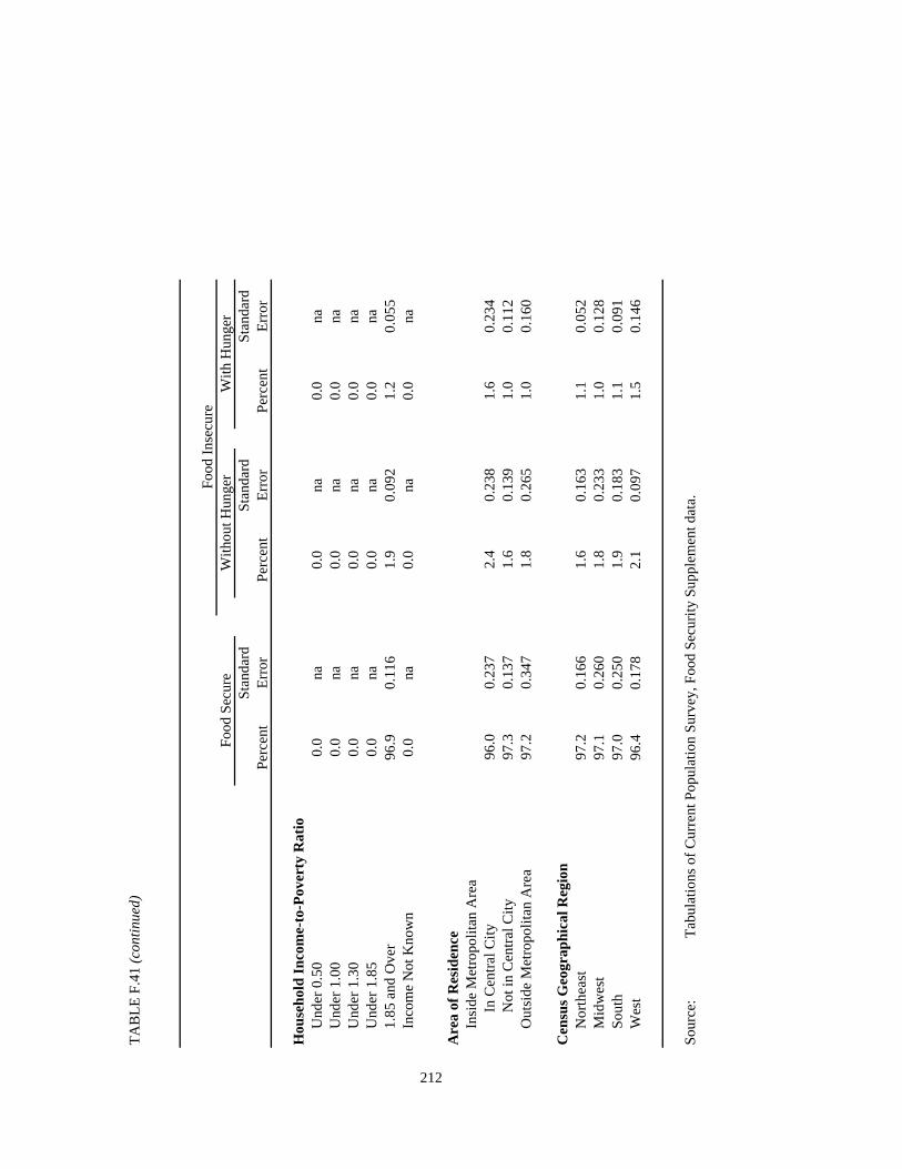
TA
BL
E F
.41
(con
tinu
ed)
Stan
dard
Stan
dard
Stan
dard
Per
cent
Err
orP
erce
ntE
rror
Per
cent
Err
or
Hou
seho
ld I
ncom
e-to
-Pov
erty
Rat
ioU
nder
0.5
00.
0na
0.0
na0.
0na
Und
er 1
.00
0.0
na0.
0na
0.0
naU
nder
1.3
00.
0na
0.0
na0.
0na
Und
er 1
.85
0.0
na0.
0na
0.0
na1.
85 a
nd O
ver
96.9
0.11
61.
90.
092
1.2
0.05
5In
com
e N
ot K
now
n0.
0na
0.0
na0.
0na
212
Are
a of
Res
iden
ceIn
side
Met
ropo
litan
Are
aIn
Cen
tral
Cit
y96
.00.
237
2.4
0.23
81.
60.
234
Not
in C
entr
al C
ity
97.3
0.13
71.
60.
139
1.0
0.11
2O
utsi
de M
etro
poli
tan
Are
a97
.20.
347
1.8
0.26
51.
00.
160
Cen
sus
Geo
grap
hica
l Reg
ion
Nor
thea
st97
.20.
166
1.6
0.16
31.
10.
052
Mid
wes
t97
.10.
260
1.8
0.23
31.
00.
128
Sou
th
97.0
0.25
01.
90.
183
1.1
0.09
1W
est
96.4
0.17
82.
10.
097
1.5
0.14
6
Sour
ce:
Tab
ulat
ions
of
Cur
rent
Pop
ulat
ion
Surv
ey, F
ood
Secu
rity
Sup
plem
ent d
ata.
Food
Ins
ecur
eFo
od S
ecur
eW
ithou
t Hun
ger
With
Hun
ger

Stan
dard
Stan
dard
Stan
dard
Per
cent
Err
orP
erce
ntE
rror
Per
cent
Err
or
All
Hou
seho
lds
97.4
0.12
61.
70.
082
0.9
0.08
7
Hou
seho
ld C
ompo
siti
onW
ith
Chi
ldre
n <
697
.20.
289
2.4
0.24
10.
40.
115
Wit
h C
hild
ren
< 1
896
.70.
215
2.6
0.14
20.
70.
155
Mar
ried
Cou
ple
Fam
ilie
s97
.80.
199
1.8
0.16
10.
40.
090
Fem
ale
Hea
d, N
o S
pous
e89
.60.
967
7.2
0.86
43.
20.
784
Mal
e H
ead,
No
Spo
use
94.3
1.17
94.
71.
403
1.0
0.68
8O
ther
Hou
seho
lds
wit
h C
hild
ren
97.1
2.46
00.
0na
2.9
2.46
0
213
Wit
h N
o C
hild
ren
< 1
897
.80.
128
1.2
0.10
80.
90.
079
Mor
e T
han
One
Adu
lt98
.30.
116
1.0
0.11
40.
60.
076
Wom
en L
ivin
g A
lone
97.1
0.42
41.
60.
343
1.3
0.24
8M
en L
ivin
g A
lone
96.8
0.36
71.
40.
265
1.7
0.29
2
Hou
seho
lds
wit
h E
lder
ly99
.20.
123
0.5
0.12
00.
30.
101
Eld
erly
Liv
ing
Alo
ne99
.70.
180
0.0
0.04
30.
30.
174
Rac
e an
d H
ispa
nic
Eth
nici
tyW
hite
Non
-His
pani
c97
.90.
093
1.3
0.07
30.
70.
064
Bla
ck N
on-H
ispa
nic
93.9
0.71
33.
90.
470
2.1
0.44
7H
ispa
nic
94.2
1.00
94.
50.
771
1.2
0.52
6O
ther
Non
-His
pani
c98
.60.
384
0.9
0.23
40.
50.
290
TA
BL
E F
.42
STA
ND
AR
D E
RR
OR
S O
F PR
EV
AL
EN
CE
EST
IMA
TE
S O
F FO
OD
SE
CU
RIT
Y, F
OO
D I
NSE
CU
RIT
Y, A
ND
HU
NG
ER
BY
SE
LE
CT
ED
CH
AR
AC
TE
RSI
TIC
S O
F H
OU
SEH
OL
DS,
199
7
Food
Sec
ure
With
out H
unge
rW
ith H
unge
r
FOR
TH
OSE
FA
MIL
IES
OV
ER
185
PE
RC
EN
T O
F PO
VE
RT
Y T
HR
ESH
HO
LD
Food
Ins
ecur
e
USI
NG
TH
E C
OM
MO
N D
EN
OM
INA
TO
R S
CR
EE
N

TA
BL
E F
.42
(con
tinu
ed)
Stan
dard
Stan
dard
Stan
dard
Per
cent
Err
orP
erce
ntE
rror
Per
cent
Err
or
Hou
seho
ld I
ncom
e-to
-Pov
erty
Rat
ioU
nder
0.5
00.
0na
0.0
na0.
0na
Und
er 1
.00
0.0
na0.
0na
0.0
naU
nder
1.3
00.
0na
0.0
na0.
0na
Und
er 1
.85
0.0
na0.
0na
0.0
na1.
85 a
nd O
ver
97.4
0.12
61.
70.
082
0.9
0.08
7In
com
e N
ot K
now
n0.
0na
0.0
na0.
0na
214
Are
a of
Res
iden
ceIn
side
Met
ropo
litan
Are
aIn
Cen
tral
Cit
y96
.70.
394
1.9
0.24
61.
30.
257
Not
in C
entr
al C
ity
97.6
0.22
41.
60.
150
0.8
0.10
1O
utsi
de M
etro
poli
tan
Are
a98
.00.
208
1.4
0.16
50.
60.
122
Cen
sus
Geo
grap
hica
l Reg
ion
Nor
thea
st97
.60.
170
1.6
0.07
70.
80.
127
Mid
wes
t97
.70.
154
1.3
0.15
20.
90.
105
Sou
th
97.4
0.30
51.
70.
193
0.9
0.19
4W
est
97.0
0.24
32.
10.
137
0.9
0.20
9
Sour
ce:
Tab
ulat
ions
of
Cur
rent
Pop
ulat
ion
Surv
ey, F
ood
Secu
rity
Sup
plem
ent d
ata.
Food
Ins
ecur
eFo
od S
ecur
eW
ithou
t Hun
ger
With
Hun
ger