Key Performance Indicators as Supplements to Earnings: Incremental informativeness,

Demand Factors, Measurement Issues, and Properties of Their Forecasts

Dan Givoly

Pennsylvania State University

Yifan Li

San Francisco State University

Ben Lourie

University of California-Irvine

Alex Nekrasov

University of Illinois at Chicago

Published in Review of Accounting Studies, 2019, 24: 1147–1183

Abstract

The documented decline in the information content of earnings numbers has paralleled the

emergence of disclosures, mostly voluntary, of industry-specific key performance indicators

(KPIs). We find that the incremental information content conveyed by KPI news is significant for

many KPIs yet diminished when details about the computation of the KPI are absent or when the

computation changes over time. Consistent with analysts responding to investor information

demand, we find that analysts are more likely to produce forecasts for a KPI when that KPI has

more information content and when earnings are less informative. We also analyze the properties

of analysts’ KPI forecasts and find that KPI forecasts are more accurate than mechanical forecasts

and their accuracy exceeds that of earnings forecasts. Our study contributes to the literature on the

information content of KPIs as well as research on the properties of analysts’ forecasts. We provide

evidence on whether and how to regulate voluntary disclosures.

Keywords: Key Performance Indicators, KPI, Measurement Issues, Analyst Forecasts, KPI

Surprises, Announcement Surprises, Non-Financial Forecasts

We are grateful to Richard Sloan (the editor) and two anonymous reviewers for their useful comments and

suggestions. We further thank Elizabeth Chuk, Paul Griffin, Mort Pincus, Devin Shanthikumar, Terry

Shevlin, Siew Hong Teoh, participants at the 2018 AAA Annual Meeting, and seminar participants at the

University of California-Irvine and the University of Toronto for their helpful comments. We gratefully

acknowledge the financial support provided by the Paul Merage School of Business at the University of

California-Irvine, University of Illinois at Chicago, and Pennsylvania State University. We thank Thomson

Reuters Inc. for providing the analyst forecasts data.

1

1. Introduction

Research has documented a decline in the information content of earnings over the last few

decades. Researchers have offered various explanations for this phenomenon, and most of these

relate to financial reporting standards and conventions. These explanations include reporting

features such as unrecorded intangible assets, the shift of standards toward the “balance sheet

approach,” the move toward fair value measurement, the increase in conditional conservatism, the

frequency of losses, and the reporting of one-time special items.1

While the decline in the information content of earnings should be a concern for standard

setters, it is unlikely they would decide to drastically change their measurement framework in

response to this decline. A more practical, less controversial (and thus more promising) path for

improving the reporting of financial performance is likely to be found in encouraging or mandating

the disclosure of supplemental measures of performance that would help users project future

earnings and cash flows. Academics have urged the inclusion of such measures, which are often

indicative of longer-term performance (e.g., Amir and Lev 1996; Lev and Gu 2016). This is also

one of the recommendations of the Special Committee on Financial Reporting (the Jenkins

Committee; see AICPA, 1994).

In practice, many firms regularly and voluntarily report information on key performance

indicators (KPIs) specific to their industry or company. These measures, in most cases, cannot be

gleaned from their financial statements. Examples include the average daily production of oil (in

barrels) of an oil and gas company, the same-store sales growth of a retail chain, and the passenger

load factor of an airline. KPIs are disclosed, often prominently,2 through different channels as part

1 See, for example, Collins, Maydew, and Weiss (1997); Dichev and Tang (2008); Donelson, Jennings, and McInnis

(2011); Francis and Schipper (1999); Givoly and Hayn (2000); Lev and Zarowin (1999); and Lev and Gu (2016). 2 For example, in its earnings announcement on January 25, 2018, American Airlines Group mentions available seat

miles (ASM) 42 times.

2

of earnings announcements, press releases, conference calls, or the MD&A section of the 10-K/Q

filings. Managers use these measures extensively to assess the performance of the entire company

or some of its internal units,3 and an increasing number of analysts routinely follow and forecast

important KPIs (Hand et al., 2018).

One of the main recommendations of the SEC Advisory Committee on Improvements to

Financial Reporting (SEC, 2008) was to enhance the usefulness of corporate reporting by

developing and disclosing relevant, consistent, and comparable KPIs. In line with this

recommendation, the SEC, in a recent concept release (SEC, 2016), sought comments and advice

from the public on the costs and benefits of mandating the disclosure of standardized, industry-

specific KPIs.

In this study, we provide evidence relevant to the potential regulation of KPI measurement

and disclosure. We start by assessing the incremental information content of KPIs. Studies have

examined the relevance of a select number of KPIs for stock valuation by testing the association

between KPIs and the current period’s stock returns. Our study is more comprehensive, as it covers

multiple KPIs and industries. We also use the event study methodology, which offers insights not

only into the value relevance of KPIs but also into the “innovation” of KPI information. We further

supplement these market tests on the information content of KPIs through a test that relies on

analysts’ responses to KPI news in the form of forecast revisions.

One issue relevant for the regulation of KPIs is whether their disclosure should remain

voluntary. With voluntary disclosure, the definition and measurement of KPIs may vary across

firms and may change over time for a given firm.4 To illuminate how the information content of

3 A search on Amazon.com yields close to 300 book titles dealing with or relating to “key performance indicators.”

The popularity of the subject is apparently at such a high level that it warranted the publication of yet another book,

Key Performance Indicators for Dummies (March 2015). 4 The measurement of some KPIs, particularly financial ones, are uniformly defined and measured. For example,

KPIs such as “exploration expense” or “production expense” in the oil and gas industry are uniformly based on GAAP.

3

KPIs is influenced by the uniformity and consistency of their computation, we use hand-collected

data on the computational details of an important KPI: the same-store sales growth rate (coded as

SSS).

Information about the properties of these forecasts is important, because our examination

of the information content of KPIs and the factors affecting this content rely on the use of analysts’

forecasts of KPIs as a representative of market expectations. A large body of research deals with

the properties of analyst earnings forecasts: their accuracy, bias, and dispersion; their performance

relative to naïve forecasts; and their relationship to revenue and cash flow forecasts. Very little is

known, however, about the properties of KPI forecasts: their superiority, if any, over mechanical

forecasts; the factors that influence analysts to produce them; and the extent to which their

production enhances the accuracy of the analyst’s earnings and revenue forecasts. We provide

evidence on these characteristics, and we contrast them with characteristics found by research on

analysts’ earnings forecasts.

Using new I/B/E/S data on forecasts and realizations of KPIs for the years 2005 to 2016

(depending on the industry), we identify 28 industry-specific KPIs in four industries that are

followed frequently by analysts: airline, oil and gas, pharmaceutical, and retail.5,6

To examine whether the surprises of important KPIs in an industry have, collectively,

information content incremental to that of earnings and revenue surprises, we construct a

composite measure of KPI surprises for each firm–quarter based on the three most-followed KPIs

in the industry. We find an incremental response to these KPI surprises in three of the four

The measurement of other KPIs may be determined by the regulator. For example, the value of “Capital Tier 1” is

dictated by bank regulators, and the measurement of “proved reserves” in the oil and gas industry is prescribed in

great detail by the SEC. The measurement of other KPIs may sometimes vary across firms and over time (e.g., same-

store sales in the retail industry). 5 These four industries are the only nonfinancial industries with sufficient observations. 6 Industry-focused research has several advantages, including greater comparability of firms within the industry and

ability to consider the economic context in which the performance measures are reported (Shevlin 1996).

4

industries and in the entire sample, consisting of all four industries. The results suggest that news

in many important KPIs is incrementally informative. We corroborate the above results using

analysts’ reactions to KPI surprises (in the form of forecast revisions) as an alternative gauge for

the informativeness of KPIs, and we find evidence consistent with the results from our market tests.

We also test the market response to the release of an important KPI in the retail industry,

SSSM, which is the monthly rate of growth in same-store sales, relative to the same month in the

previous year. The use of this monthly sample alleviates the need to control for other information

released with the earnings announcement. Consistent with the results obtained for quarterly SSS,

we find that the market reaction to the standalone SSSM surprises is positive and highly significant.

This finding also highlights the value of the more timely monthly KPI announcements that partially

preempt the news in subsequent earnings announcements.

Based on hand-collected data on SSS, we find that the information content of this KPI

appears to be diminished when there is no disclosure of its computational details and when the

firm changes the way it computes that KPI. These findings suggest that standardization of the

definition of individual KPIs is needed to enhance their information content, regardless of whether

KPI disclosure remains voluntary. Standardization, coupled with its enforcement, may also

dampen the ability of management to manipulate KPIs. Indeed, there are indications that the SEC

has recently given greater attention to the validity of corporate KPI disclosures.7

Our findings show that the most important determinant of analysts’ decisions to produce a

KPI forecast is the information content of that KPI, which is consistent with analysts responding

to investors’ demand for these forecasts. We further find that the production of KPI forecasts is

7 See Clarkson and Matelis (2018). In June and August 2018, two companies that offer web hosting and online and

email marketing products were the targets of SEC enforcement action for artificially inflating the rate of growth in

subscribers (one of their important KPIs) by changing the definition of a “paying subscriber.” The case was eventually

settled (see https://www.sec.gov/litigation/admin/2018/33-10504.pdf).

5

also related to the importance that management attributes to the KPI as captured by the number of

mentions of that KPI in the press release. Consistent with the demand effect, we find that more

analysts issue KPI forecasts in periods when the company reports a loss, thus rendering the

earnings number less informative (Hayn 1995). Also consistent with the demand effect, we find

that more analysts issue KPI forecasts in cases with large absolute accruals that denote situations

with a large discrepancy between earnings and cash flow from operations. Finally, we provide only

weak evidence that analysts who issue KPI forecasts produce more accurate EPS and revenue

forecasts.

Our next set of tests focuses on the properties of analysts’ forecasts of KPI. We find that

the average accuracy of KPI forecasts is, in most cases, greater than that of EPS forecasts. This

suggests that either KPIs are relatively easy to forecast or analysts exert effort to make more

accurate KPI forecasts. In contrast to the finding of prior research that early-in-the-period EPS

forecasts are optimistic (Brown 2001; Bartov, Givoly, and Hayn 2002; Matsumoto 2002;

Richardson, Teoh, and Wysocki 2004), we find that KPI forecasts made early in the period are

pessimistic on average.

Finally, an examination of additional features of analysts’ KPI forecasts reveals the

following. First, similar to short-term EPS forecasts, forecasts of KPIs are more accurate than

random walk models, and the market reacts more strongly to surprises based on these forecasts.

We also find that analysts’ two- and three-year-ahead KPI forecasts are superior to a naïve

extrapolation of analysts’ KPI forecasts from the current year to these two future years. This

contrasts with the findings of Bradshaw, Drake, Myers, and Myers (2012) of a limited value of

analyst earnings forecasts for longer horizons.

Our study makes a number of contributions to the literature. First, it contributes to the

research on the quality of voluntary disclosures and the extent to which they supplement GAAP

6

measures of performance, whose information content has been shown to decline over time. We

provide evidence on the incremental information content of KPIs, beyond earnings and revenues,

and by showing how the informativeness of a KPI diminishes in the absence of its computational

details and in the presence of intertemporal inconsistency in its computation. These findings are

relevant to the regulation of KPI disclosures and to the continuing debate on the need for mandating

them.

Our study also contributes to the empirical studies on the value-relevance of individual

KPIs (Amir and Lev 1996; Francis, Schipper, and Vincent 2003; Rajgopal, Venkatachalam, and

Kotha 2003b; Patatoukas, Sloan, and Zha 2015). We extend those studies in three ways. First, we

gauge the informativeness of KPI disclosures by employing the event-study methodology to

observe the market reaction to their announcements. Second, we extend the examination from a

single KPI or a few KPIs in a single industry to many KPIs in different industries. Last, we capture

the informativeness and timeliness of KPI disclosures using a nonreturn measure—the extent to

which KPI disclosures affect analysts’ revisions of their earnings and revenue forecasts.

This study also contributes to the research on the role of analysts in the capital markets.

First, by modeling and testing the determinants of analysts’ decisions to issue KPI forecasts, our

study extends the research on the effect of the value relevance of information to investors on the

supply of products by analysts (e.g., forecasts) (Chapman and Green 2015; DeFond and Hung

2003; Ehinger, Lee, Somberg, and Towrey 2017; Ertimur, Mayew, and Stubben 2011). Second, our

study contributes to the literature on analysts’ forecasts by examining the properties of analysts’

forecasts of KPIs as compared to their earnings and revenue forecasts. (For recent reviews of this

literature, see Bradshaw (2011) and Kothari, So, and Verdi (2016).)

7

2. Investor and regulatory interest and related research

2.1 Investor and regulatory interest in KPI disclosures

There is a consensus in the investment community that disclosures of industry-specific

KPIs are important to decision making. An Ernst & Young (2015) survey conducted by

Institutional Investor Research (IIR) shows that almost three-quarters of institutional investors

considered industry-specific reporting and KPIs to be very or somewhat beneficial.8 As one

analyst stated, “To truly understand the company, it’s important to have not only top and bottom

line guidance, but also a clear description of the KPIs that drive the growth and success of the

business” (Gaertner 2016).

Growing investor interest in KPI information has drawn attention from regulators (FASB

2001; AAA Financial Accounting Standards Committee 2002; SEC 2003, 2008, and 2016). In its

guidance regarding MD&A, the SEC expects companies to identify and discuss KPIs, including

nonfinancial measures that management uses (SEC, 2003).9 Doing so should allow investors to

view the company through the eyes of its management. Since KPIs vary by industry, and

sometimes by company, the SEC suggests that companies should discuss key variables, both

financial and nonfinancial, that are specific to their industry or company.

While in principle, companies should disclose all material information, including all

material industry-specific measures of performance, there are no requirements for KPI disclosure.

The SEC may ask a company to disclose and discuss KPIs in its SEC filings when those metrics

are included in the company’s communication with investors outside the SEC filings (e.g., a press

release or a website). Further, when a company refers to a KPI when analyzing its performance in

8 The survey covered more than 200 institutional investors, including portfolio managers, equity analysts, chief

investment officers, and managing directors. 9 Similar guidance is offered by the EU Directive (2003) and by the IASB (see IASB, 2010).

8

the MD&A section of the 10-K, the SEC staff often asks it to define the KPI and discuss its

computations and limitations. So, as it stands now, the disclosure of KPIs is largely voluntary.

Even when KPIs are disclosed and discussed by a company, there are no standards that assure

comparability across companies and consistency over time within a company.

The SEC Committee on Improvements in Financial Reporting (SEC 2008) recommends

the development of industry-wide KPIs that are consistently defined and disclosed, so investors

can more easily interpret them and compare them across companies. Consistent with this

recommendation, the SEC is considering the development of rules and guidelines concerning KPI

disclosures. In its Concept Release on April 13, 2016 (SEC 2016), the SEC requested public

comments on whether registrants should be required to disclose and comment on KPIs important

to their business, what types of users are likely to benefit from such information, and how to

identify those industry KPIs that should be standardized.10,11

2.2 Related research

Several studies examine the role of certain individual KPIs in explaining company

valuations and predicting future financial performance. Amir and Lev (1996) find that, in the

wireless industry, the size of the population in the specific area where wireless services are

available and the penetration rate (i.e., the ratio of the number of subscribers to the total population

in that area) help explain the cross-sectional variability of the market values of firms. Ittner and

Larcker (1998) examine the information content of customer satisfaction scores. Other researchers

10 Our reading of comment letters suggests the following. While there seems to be general support for a principle-

based approach that emphasizes materiality, the majority of respondents, including Big Four auditors, did not

recommend prescriptive requirements for disclosure of specific KPIs. Their concerns included a potential reduction

in the flexibility for the registrants to select variables that they consider most important and difficulties in identifying

KPIs that apply to all firms in the industry. 11 Regulators abroad are equally concerned about the disclosure and standardization of KPIs, and these regulators

either require or suggest adequate disclosures of them (e.g., IASB 2010; the EU Accounts Modernization Directive

2003; Section 417 of the Companies Act (2006) in the United Kingdom).

9

examine and document the value relevance of web traffic (Trueman, Wong, and Zhang 2001;

Rajgopal et al. 2003b), order backlog (Rajgopal, Shevlin, and Venkatachalam 2003a), and

discounted cash flow estimates of oil and gas royalty trusts (Patatoukas et al. 2015). Curtis,

Lundholm, and McVay (2015) show that components of sales (e.g., growth in same-store sales,

the number of stores, and new stores open) are useful in predicting sales.

We extend the research on the value relevance of KPIs by examining a broader set of KPIs

in multiple industries. Rather than using market valuation tests or annual returns to assess the

information relevance of firm-produced KPIs, we rely on the market response to news on

economically important KPIs (as captured by the extent of their analyst following). The use of an

event-study methodology improves the reliability of the inferences on the information content by

alleviating the need to control for a multitude of valuation drivers, many of which are highly

correlated. It further allows the determination of the innovation contained in the release of the KPI.

We further consider an alternative measure of the informativeness of KPIs that is not return based,

in the form of analysts’ responses to KPI news. Our paper also extends the literature on the

properties of analysts’ forecasts by analyzing the accuracy and bias of KPI forecasts and

contrasting them with analysts’ revenue and earnings forecasts.

An issue of regulatory importance that has not be addressed by past research on KPIs is the

effect of the cross-sectional uniformity and consistency over time in defining and measuring a KPI

on its information content. It is generally recognized that a lack of uniformity in voluntarily

disclosed measures and inconsistency over time in the definition and computation of a KPI

diminish the informativeness of these measures. A number of studies point to the need to

standardize voluntary disclosures in other areas, such as intangibles (Lev, 2001), corporate social

responsibility (CSR), and sustainability (Langer, 2006). With respect to voluntary disclosure of

KPIs, Elzahar, Hussainey, Mazzi, and Tsalavoutas (2015) develop a model for the quality of such

10

disclosures in which quality includes the characteristics of year-to-year consistency and calculation

comparability.

The lack of standards and regulation make KPI measurement also susceptible to

manipulation. For example, Schilit and Perler (2010) note that companies can manipulate SSS by

changing the definition of existing stores. One definition of an existing store may be a store that

has been open for at least 12 months, but this definition may be changed to a store that has been

open for at least, say, 18 months. We provide empirical evidence on whether uniformity and

consistency in the definition of KPI over time enhances its informativeness.

3. Data and sample selection

We obtained quarterly and monthly forecasts of industry-specific KPIs and quarterly

earnings and revenue forecasts as well as the actual values of these forecasts from the respective

I/B/E/S detail files.12 Stock prices and returns are obtained from CRSP, and company financial

data are obtained from Compustat.

Table 1 presents details of the sample construction. As the table shows, the initial sample

consists of all industry-specific KPIs available from the I/B/E/S KPI database for nonfinancial

industries.13,14 This initial sample consists of 615,635 analyst forecasts of quarterly KPIs for 1,215

firms. We define the median of the contemporaneous individual forecasts as the consensus forecast.

We exclude from the consensus measure stale KPI forecasts, defined as forecasts issued more than

90 days before the announcement date,15 and we omit observations that have missing KPIs or lack

12 The KPI data were obtained directly from Thomson Reuters in February 2016. 13 I/B/E/S non-industry-specific KPIs relate to financial statement items (e.g., cost of goods sold, R&D expense, cash

flow from operations), financial ratios (e.g., price-to-sales ratio, return on capital), and other variables not specific to

any particular industry (e.g., free cash flow, number of shares outstanding). These “KPIs” are excluded because they

do not represent information beyond that which is available or directly derived from the financial statements. 14 We exclude the financial industry because the majority of KPIs provided by I/B/E/S for that industry can be directly

inferred from financial statements. For example, the three most forecasted KPIs in the financial industry are net interest

income, loan loss provisions, and non-interest expense, all of which can be directly inferred from financial statements. 15 The results are very similar when we do not delete stale forecasts.

11

any of the necessary financial data. Finally, to be included in the final sample, we require each KPI

to have at least 100 firm-quarter observations with available values for both the forecasted and the

realized KPI. This requirement is designed to ensure that the KPI is of a sufficient economic

importance to be widely followed by analysts.16 Our final sample contains 28 KPIs, 129,184 KPI-

firm-quarter analyst forecasts, and 17,018 KPI-firm-quarter consensus forecasts for 659 distinct

firms. Appendix A contains a description of KPI measures and variable definitions.

Table 2 Panel A presents the distribution of sample observations by industry. The sample

includes four I/B/E/S industries: airline, oil and gas, pharmaceutical, and retail.17 The largest

number of sample observations are found in the retail and the oil and gas industries. To

accommodate the inter-industry differences, we conduct empirical tests for the entire (all-industry)

sample as well as for each industry separately. On average, sample firms in the pharmaceutical

(retail) industry are the largest (smallest), with a median market capitalization of $12.741 ($2.008)

billion. Firms in the oil and gas industry have the highest book-to-market ratios (i.e., they are value

firms), and firms in the pharmaceutical industry have the lowest book-to-market ratios (i.e., they

are growth firms).

The available KPI forecast data for different industries (see Table 2 Panel B) spans over

somewhat different periods. The airlines sample covers 2013–2016, oil and gas covers 2012–2016,

retail covers 2008–2016, and pharmaceutical covers 2005–2016. With the exception of the

pharmaceutical industry, the number of analyst KPI forecasts grows over time (the numbers for

16 The requirement eliminates approximately 2.7% of KPI-firm-quarter observations. The five most populated KPIs

excluded from our analysis are revenue per passenger mile in the airline industry, capacity for refining crude oil

(measured in barrels per day), upstream income, refining income, and downstream income in the oil and gas industry. 17 Excluding financial industries, I/B/E/S reports industry KPIs for five industries: airline, oil and gas, pharmaceutical,

retail, and technology. I/B/E/S uses a proprietary industry classification to construct these five industries. The oil and

gas industry includes integrated oil and gas, exploration and production, and refining and marketing. The retail

industry includes retail stores and restaurants. None of KPIs in the technology industry have 100 firm-quarters with

analyst forecasts; therefore we exclude them from our analyses.

12

2016 relate to the early part of the year), which is consistent with these performance measures

becoming more popular. The coverage of KPI forecasts available on I/B/E/S database for the

pharmaceutical industry is quite erratic (likely due to the fact that the collected data were obtained

in part through acquisitions of other data providers), with a discontinuity in coverage in 2011 and

considerably reduced coverage in later years.18

Table 2 Panel C shows the available sample size for each KPI in terms of firm-quarters,

number of firms, number of analysts, and number of forecasts. The individual KPI with the largest

number of available firm-quarter observations is available seat miles (ASM) in the airline industry,

distributable cash flow (DCF) in the oil and gas industry, pharmaceutical sales (SAL) in the

pharmaceutical industry, and the rate of growth in same-store sales (SSS) in the retail industry.

The number of firms in our sample that disclosed a given KPI varies from 13 (revenue per available

seat mile (RASM)) to 231 (distributable cash flow (DCF)), and the number of analysts who issued

forecasts for a given KPI ranges from 17 (cost per seat miles (CPA) and revenue per available seat

mile (RASM)) to 557 (same-store sales growth rate (SSS)).

4. The incremental information content of KPIs

4.1. Measuring the information content of KPI news based on stock price response

We assess the incremental informativeness of KPIs using an event-study methodology,

whereby we gauge the incremental information content by the market response to KPI surprises,

after controlling for other news that is concurrently disclosed (typically earnings and revenue).

We define the KPI surprise (the KPI news), SURP_KPIijt, for firm j that belongs to industry

i in quarter t, as the forecast error. That error is calculated as the realized KPI announced by firm j

18 Our inferences remain intact when we delete observations in 2010–2016 in the pharmaceutical industry or when

we exclude the pharmaceutical industry from the sample.

13

for quarter t minus the corresponding analyst consensus forecast, scaled by the average absolute

value of the two variables.19 Analyst consensus forecast is calculated as the median of the most

recent forecasts made by individual analysts at the time of the KPI announcement. We exclude

from the consensus forecast those forecasts that were made more than 90 days before the KPI

announcement.

For each KPI, we rank KPI surprises across all firm-quarter observations in industry i, and

we assign the rank values of 0, 0.5, and 1 to observations in the bottom (i.e., the most negative),

middle, and top (i.e., the most positive) terciles, respectively. The resulting variable is denoted

SURPrank_KPIijt. Using these rank scores mitigates the influence of extreme surprises. It also

facilitates the interpretation of the regression coefficient on SURPrank_KPI as the increase in the

dependent variable (e.g., the announcement period return), as the KPI surprise moves from the

bottom to the top tercile of the KPI surprise distribution.20

To determine whether the surprises of important KPIs in an industry collectively have

information content incremental to that of earnings and revenue surprises, we first identify for each

industry the KPIs that are likely to matter to market participants. Specifically, for each industry,

we select the three KPIs that are most followed by analysts, based on the number of firm-quarter

forecasts for the KPI in the industry. We then average in each firm-quarter the surprises of these

three KPIs and, similar to the construction of SUPRrank_KPI, we rank the average surprises across

all firm-quarter observations in industry i, and we assign the rank values of 0, 0.5, and 1 to

observations in the bottom (i.e., the most negative), middle, and top (i.e., the most positive) terciles

19 Many KPI, such as available seat miles and oil production per day, are measured in unscaled nonmonetary numbers;

others such as same store sales and passenger load factor are measured as a growth rate or a ratio; while others—such

as Distributable Cash Flow—reflect dollar amounts. Given this heterogeneity, scaling by average absolute value of

the actual and forecasted value makes more sense than scaling by share price as is typically done for earnings and

revenue surprises. 20 We use terciles rather than deciles to ensure a sufficient number of sample observations in each KPI surprise group,

as some KPI have a relatively small number of observations. The results are robust to using deciles or quintiles.

14

of the distribution of this average surprise, respectively. We denote the resulting measure as

SURPrank_3-KPI and use it to test for the collective information content of these potentially

important industry KPIs.21 We use SURPrank_3-KPI to conduct tests at the industry level and for

the entire (all-industry) sample.

We calculate earnings (revenue) surprise as the difference between the actual number

announced by the company and the latest analyst consensus forecast before the earnings (revenue)

announcement, scaled by the stock price (total market value of equity) at the end of the fiscal

quarter. Similar to the ranking of the KPI surprises, we rank the earnings and revenue surprises

into terciles and assign them scores of 0, 0.5, and 1 to form SURPrank_EPS and SURPrank_REV,

respectively.

One of our KPIs, SAL (i.e., sales per drug, in the pharmaceutical industry), is reported for

individual drugs, rather than for the company as a whole. When there is more than one drug with

available forecast and actual (thus more than one drug with a SAL surprise), we use the SAL

surprise in our analysis for the drug that has the most analyst forecasts, which presumably indicates

that sales of that drug are likely to be most important to market participants.

We estimate the incremental information content of KPI announcements through the

following pooled regression of announcement returns estimated from all firm-quarter observations

within a given industry or across industries.

CAR(-1,+1)jt = α1 + β1 SURPrank_3-KPIijt (or SURPrank_KPIjt)+ β2 SURPrank_EPSjt

+ β3 SURPrank_REVjt + εjt, (1)

where CAR(-1,+1) is the cumulative abnormal return over the three-day window centered on the

announcement date. We control for the revenue surprise, in addition to our control for the earnings

21 Aside from capturing the collective information content of the industry KPIs, using the average surprise has the

advantage of alleviating the difficulty (created by the high correlation between the industry KPI surprises) of

identifying the incremental information content of individual KPIs.

15

surprise, since research indicates that investors react more strongly to a revenue surprise than to

an expense surprise of the same magnitude (Ertimur, Livnat, and Martikainen 2003).

Some KPIs reflect favorable aspects of performance, while others reflect expenses (i.e.,

cost per seat miles (CPA), maintenance capital expenditures (MCX), lease operating expense

(LOE), exploration expense (EXP), production tax (PTX), and production expense (PEX)) or

unfavorable developments (i.e., number of stores closed/relocated (NSC)). To allow for a uniform

interpretation of the sign for all KPIs, we multiply these unfavorable surprises by −1 before

estimating Regression (1) and subsequent related tests.22 We expect the coefficients on earnings

and revenue surprises to be positive. If KPI surprises have incremental information content to that

contained in earnings and revenue surprises, we expect the coefficient on SURPrank_KPI (or on

SURPrank_3-KPI) to be positive as well.

Table 3 reports the results of estimating Regression (1), where announcement window

return is regressed on SURPrank_3-KPI, SURPrank_EPS, and SURPrank_REV. The regression is

estimated within industries and for the overall (all-industry) sample. The variable SURPrank_3-KPI

is significant in all industries except pharmaceutical. Moreover, SURPrank_3-KPI is positive and

significant in the overall sample. The results are consistent with KPI surprises containing

significant information that is incremental to earnings and revenue news.23

The (untabulated) results of estimating Regression (1) for individual KPIs (i.e.,

SURPrank_KPI) reveal the following. First, the univariate regressions of announcement returns on

KPI surprises show that a number of KPIs (12 out of 28) have a significant association with the

22 Higher maintenance capital expenditures and higher production tax may convey positive information to investors,

so there might be some ambiguity about the expected signs for these KPIs. 23 We also explored the market reaction in the post-announcement window (over the interval [+2,+63]) and did not

find a significant drift in the market response to KPI surprises, EPS surprises, or revenue surprises in our sample. The

absence of a significant drift could be due to insufficient test power.

16

announcement period returns.24 None of the coefficients of the KPIs, whose sign is expected to

be positive, has a significant negative sign. Importantly, the KPIs most frequently forecasted by

analysts in each of the four industries all have a significant association with the announcement

returns. Second, the regressions of announcement returns on KPI surprises, earnings surprise, and

revenue surprise show that surprises in eight KPIs (ASM, RPM, DCF, EBX, EXP, TPP, RZP, and

SSS) are significant at the 10% level or better, suggesting that these KPIs contain information that

is incremental to earnings and revenue. Notably, the market reaction to surprises in these KPIs is

more pronounced than the reaction to the revenue surprise. Revenue surprise is insignificant when

we control for surprises in ASM, RPM, DCF, EBX, EXP, or TPP. Surprises in SSS and REV are

incremental to each other, with the response coefficient on SSS surprises being more than twice

the response coefficient on revenue surprise.

4.2 Measuring the information content of KPI news based on analysts’ revisions of earnings and

revenue forecasts

To provide further evidence on the information content of KPI surprises, we use an

additional measure of informativeness, namely, the extent of analysts’ responses to KPI surprises

when revising their EPS and revenue forecasts. We estimate the following regression from all firm-

quarter observations within a given industry as well as across industries.

EPS (REV) Forecast Revisionjt+1 = α1 + β1 SURPrank_3-KPIijt

+ β2 SURPrank_EPSjt + β3 SURPrank_REVjt + εjt, (2)

where EPS (REV) Forecast Revisionjt+1 is the median analyst forecast for firm j quarter t+1 EPS

(revenue) issued within 10 days after the quarter t earnings announcement date minus the median

of the latest analyst EPS (revenue) forecast for firm j quarter t+1 (revenue), issued within 90 days

24 The significant KPIs are ASM, RPM, DCF, OPD, RPG, EBX, EXP, TPP, RZP, SAL, SSS, and RES.

17

before the quarter t earnings announcement date, scaled by the stock price (market value of equity)

at the end of quarter t, and multiplied by 100.

If analysts respond incrementally to KPI surprises when revising their forecasts of next-

quarter EPS and revenue, we expect β1 to be positive and significant. KPI surprises are likely to

be correlated with earnings surprises (and possibly with revenue surprises), thus we expect them

to induce revisions in the forecasts of these variables. In fact, research suggests that some KPIs

(e.g., same-store sales, change in number of stores) are used in a bottom-up model of forecasting

earnings and revenues (Curtis, Lundholm, and McVay 2014; Lundholm and Sloan 2004). However,

it is less clear whether KPI surprises incrementally lead to revisions in earnings or revenue

forecasts, after controlling for earnings and revenue surprises.

The results from estimating Regression (2) are reported in Table 4. Panel A of the table

shows the results of the regression of EPS forecast revision. The coefficient on SURPrank_3-KPI is

positive and significant in the airline and retail industries as well as in the overall sample that

includes all industries. In the regression of revenue forecast revision in Panel B, SURPrank_3-KPI

is positive and significant in the pharmaceutical and retail industries and in the all-industries

sample. Overall, these findings suggest that analysts find KPI surprises value relevant and

incorporate them as inputs in their revisions of earnings and revenue forecasts. These results are

consistent with those from Regression (1) in demonstrating the incremental information content of

KPIs.

5. The effect of the disclosure, consistency, and uniformity of the KPI’s computational details

and its information content

The information content of voluntary disclosure of a KPI by firms is likely to depend on

the extent of the disclosure, period-to-period consistency, and cross-sectional uniformity of the

18

KPI’s computational details. This is particularly true for nonfinancial KPIs. The absence of a

detailed disclosure about how a KPI is computed, changes over time in its computation, and lack

a standardized definition are all likely to create some degree of ambiguity among investors in

interpreting this KPI, rendering this signal noisier. This ambiguity is exacerbated when the

reporting firm has incentives to misrepresent.25 We expect such ambiguity to reduce the usefulness

of KPIs for investors.

To examine these attributes of KPIs and evaluate their impact on the KPI’s information

content, we had to manually collect data from firms’ KPI disclosures in the annual MD&A.

Because this involves a massive hand-collection of data, we focused on one industry and one KPI:

the retail industry and its most commonly disclosed KPI, SSS. We collected data on the

computation of SSS from the MD&A of over 1,300 10-K forms.

Our examination shows that not all SSS announcements provide the computational details

of this KPI, that in many instances its definition changes from year to year, and that there is no

standard for computing it across all firms. The upper two rows in Panel A of Table 5 show the

frequency among all firm-quarter observations for which the MD&A for the year includes

computation details. The table shows that for 400 (or about 14%) of the 2,829 firm-quarters that

belong to years for which we examine the MD&A, there was no detailed disclosure on how SSS

is computed. Fifty-nine firms have SSS computations that are not explained for at least one year

(out of the 10 years for each firm in the retail industry for which we have KPI data).

The bottom two rows in Panel A of Table 5 show the extent of year-to-year consistency in

the computation of SSS across observations for which the firm discloses the computational details

of SSS. We focus on consistency in the definition of same stores, that is, the definition of the group

25 As discussed in Section 2.2, these problems are common to other voluntary and nonfinancial disclosures, such as

those pertaining to intangible assets or to corporate social responsibility.

19

of stores for which the rate of growth in sales is computed. As the panel shows, in about 10% of

the observations with disclosed details about SSS computation (222 out of 2,429), there is a change

in the computation of this KPI, relative to the previous year. Panel B of Table 6 presents the results

about the uniformity of the definition of SSS across firms.

Panel B of Table 5 shows that there is some variation in the definition of same store. In

nearly 50% of firm-quarters, the same-store base includes stores that have been in operation for at

least 12 months; however, other firms use 13 months or more in their definitions (and in 4% of the

firm-quarters, the applicable definition is 24 months).

Next, we examine how the information content of SSS news is affected by the absence of

detailed disclosures on how SSS is computed or by a lack of consistency of the firm’s definition

of “same store” over time. For this examination, we estimate the following versions of regressions

(1) and (2).

CAR(-1,+1)jt = α1 + β1 SURPrank_SSSjt + β3 LOW_DISCLOSUREjt (or

CHANGE_COMP) + β4 LOW_DISCLOSUREjt (or CHANGE_COMP)

*SURPrank_SSS jt + β2 SURPrank_EPSjt + β3 SURPrank_REVjt + εjt (3a)

EPS (REV) Forecast Revisionjt+1 = α1 + β1 SURPrank_SSSjt + β3

LOW_DISCLOSUREjt (or CHANGE_COMP)+ β4 LOW_DISCLOSUREjt (or

CHANGE_COMP) *SURPrank_SSSjt + β2 SURPrank_EPSjt + β3 SURPrank_REVjt +

εjt, (3b)

where LOW_DISCLOSURE (CHANGE_COMP) is an indicator variable that receives the value of

1 if the annual disclosure in the year to which the quarter belongs does not provide computation

details of SSS (represents a change from the previous year’s definition) and 0 otherwise. All other

variables are the same as in Regressions (1) and (2).

The results from estimating Regressions (3a) and 3(b) are shown in Panels A and B of

20

Table 6. These results show that the information content of SSS surprises is lower when there is

limited disclosure on the computational details of this KPI in the MD&A. The coefficient of the

interaction term between LOW_DISCLOSURE and the SSS surprise is negative and significant

when information content is gauged by the market response to the SSS announcement. It is also

negative (but not significant) when information content is proxied by the extent of revision in

analysts’ forecasts of EPS for the following quarter issued in the wake of the SSS surprise. When

information content is measured in this manner, the regression results show that the coefficient of

CHANGE_COMP*SURPrank_SSS is negative and significant, indicating reduced information

content of SSS news when the definition of this KPI changes. While these results pertain to one

KPI, they suggest that incomplete disclosure about the measurement of KPIs and a lack of

consistency in computation detract from the incremental information content of KPIs to investors.

The effect of the lack of a standardized definition of same store on the information content

of SSS is not obvious as long as there is a disclosure of this choice. However, using a longer

operating period in the definition of same store may be more informative, because the SSS may

be noisier when it includes stores that have been in operation for a short period. To test whether

this is indeed the case, we estimate the following versions of regressions (3a) and (3b).

CAR(-1,+1)jt = α1 + β1 SURPrank_SSSjt + β3

LONGER_TIME_IN_OPERATION + β4 LONGER_TIME_IN_OPERATION

*SURPrank_SSS jt + β2 SURPrank_EPSjt + β3 SURPrank_REVjt + εjt, (3a’)

EPS (REV) Forecast Revisionjt+1 = α1 + β1 SURPrank_SSSjt + β3

LONGER_TIME_IN_OPERATION + β4 LONGER_TIME_IN_OPERATION

*SURPrank_SSSjt + β2 SURPrank_EPSjt + β3 SURPrank_REVjt + εjt, (3b’)

where LONGER_TIME_IN_OPERATION is an indicator variable that equals 1 if the minimum

time required before a store is classified as a same-store is greater than 13 months and 0 otherwise.

21

All other variables are the same as in Regressions (3a) and (3b).

The results reported in Panel C of Table 6 suggest a higher information content of SSS

when stores are required to be in operations for a longer time (14 months or more) before they are

included in the same store base. The coefficient on the interaction

LONGER_TIME_IN_OPERATION *SURPrank_SSS is positive and significant. The coefficient on

the interaction term is also positive but not significant when information content is proxied by

analysts’ forecasts revisions.

6. Determinants and properties of analysts’ forecasts KPIs

6.1. Identifying the determinants of analysts’ decisions to forecast KPIs

Financial analysts produce an array of products, including earnings forecasts, stock

recommendations, and target prices. The scope of financial and nonfinancial variables forecasted

by analysts has been expanded over the years beyond earnings, other financial statement variables

(e.g., revenues, cash flows, various measures of earnings such as EBIT and EBITDA), and

effective tax rate. Analysts’ production of these forecasts is not universal, and this likely reflects

variation in the demand by investors. In fact, in our sample, 65.5% of the firm-quarter observations

of firms that report KPIs and have at least one EPS forecast do not have KPI forecasts. A number

of studies examine the determinants of analysts’ decisions to supplement their earnings forecasts

with forecasts of cash flow (e.g., DeFond and Hung 2003) and revenue (Ertimur, Mayew, and

Stubben 2011). The examined determinants include firms’ characteristics that presumably reduce

the informativeness of earnings (e.g., the magnitude of discretionary accruals and earnings

volatility) and financial distress.

We follow this literature as we identify the determinants of the issuance of KPI forecasts.

Since the demand for KPI forecasts is likely to be driven mostly by the incremental value of KPI

22

to investors, we add to the list of determinants a summary measure of that value obtained from

estimating Regression (1), as explained below. This measure allows us to use a reduced set of

variables to reflect the other determinants. Specifically, we estimate the following regressions

across firm-quarter-KPIs.

(KPI_to_EPS)jtk = f {INF_KPIjtk, SIZEjt, VOLjt_EARNjt, LOSSjt, AB_ACCRjt, DISTRESSjt},

(4)

where (KPI_to_EPS)jtk is the ratio for firm j in quarter t between the number of KPI analysts and

the number of EPS analysts. The ratio for the firm-quarter is computed from analysts who produce

EPS forecasts for the firm-quarter.

The first determinant, INF_KPI, is the incremental explanatory power of the KPI surprise

(SURPrank_KPI) in Regression (1) in explaining the variation in the regression’s dependent

variable, CAR (-1,+1). The incremental explanatory power is computed based on Shapley’s value

(Shapley 1953).26 The variable INF_KPI is expressed as the fraction of the regression’s R2

contributed by the KPI surprise. We expect that INF_KPI will be positively associated with the

propensity of analysts to issue its forecasts.

The variable SIZE is the natural logarithm of the market value of the firm’s equity at the

beginning of the quarter. The variable VOL_EARN is the coefficient of the variation of earnings,

computed as their standard deviation over the most recent eight quarters, deflated by their absolute

mean value over the same period. We expect that the demand for KPI forecasts will be greater;

therefore we also expect their production to be more common when the volatility of earnings is

higher.

26 When the explanatory variables in the regression are uncorrelated, the contribution of an individual explanatory

variable, Xi, to the multiple regression R2 is the R2 of the regression of Y on Xi. Shapley values can be used to assess

the contribution of the explanatory variables in the more common case when the explanatory variables are not

independent of each other. A convenient feature of the Shapley values is that they sum up to the regression R2. For

a good introduction to Shapley values, see Israeli (2007).

23

The variable LOSS is an indicator that receives the value of 1 if income before

extraordinary items is negative in quarter t−1 and 0 otherwise. Given the reduced information

content of the earnings number when the firm reports a loss (Hayn, 1995), we expect that KPI

information will be more in demand in a loss period.

The variable AB_TACCR is the absolute value of total accruals in quarter t−1 deflated by

beginning total assets. The variable DISTRESS is an indicator variable that receives the value of 1

when the Altman Z-score is below 1.81 (an indication of distress) at beginning of quarter t and 0

otherwise. Similar to losses, financial distress reduces the predictive power of the conventional

measure of performance; therefore we expect DISTRESS to be positively associated with the

demand for and the corresponding supply of KPI forecasts.

The results from estimating Regression (4) are reported in Table 7. The regression is

estimated from firm-quarters with at least one forecast for the KPI. The results show that the

regression model exhibits a satisfactory explanatory power (adjusted R2 close to 0.6). The table

also shows that an important and significant determinant of analysts’ decision to issue a KPI

forecast (in addition to their EPS forecast) is the incremental information content of the KPI. In

fact, this determinant alone explains this decision more than all other hypothesized determinants

collectively explain. When Regression (4) is estimated with INF_KPI, as a single independent

variable, the R2 of the regression is 0.582. Adding all other variables increases the explanatory

power of the regression only marginally to 0.583.

Among the other determinants, LOSS and AB_TACCR, both of which point to situations in

which the information content of earnings is lower, are positive and significant. This is consistent

with the notion that, in these situations, there is likely to be a stronger demand for supplementary

measures of performance (DeFond and Hung 2003; Ertimur, Mayew, and Stubben 2011). The

variable DISTRESS, which also indicates situations in which earnings are less informative, has a

24

negative coefficient, which is ostensibly inconsistent with this notion. However, this negative

coefficient may suggest that, in periods of distress, analysts are more concerned with cash flow,

rather than with noncash measures such as KPIs (similar to their lower reliance on earnings when

bankruptcy risk is high—see DeFond and Hung 2003).

6.2. Accuracy and bias of analysts’ forecasts of KPI

A large body of research deals with the accuracy and bias in analysts’ forecasts of earnings.

We assess the accuracy and bias of KPI forecasts and contrast them with those associated with

analysts’ earnings forecasts. Comparing the accuracy of forecasting these performance measures

would indicate both the relative inherent difficulty in forecasting each of them and the relative

amount of attention and resources devoted to these forecasts. Similar to the assessment by past

studies of the superiority of analysts’ earnings forecasts over mechanical time-series models

(Bradshaw et al. 2012; Fried and Givoly 1982), we also compare analyst KPI forecast accuracy

vis-à-vis the accuracy of time-series forecasts.

Research has documented an optimistic bias in earnings forecasts made early in the period

(e.g., Brown 2001; Bartov et al. 2002; Matsumoto 2002; Richardson et al. 2004; Bradshaw, Lee,

and Peterson 2016). While there is no consensus on the reasons for this bias, a common explanation

for the bias (and for the prevalence of buy recommendations) is that sell-side analysts attempt to

curry favor with management to gain better access to information or to promote the purchase of

stock through their brokerages (Easterwood and Nutt 1999; O’Brian 1988). If this is true, we

should find a similar optimistic bias in KPI forecasts.

Table 8 reports descriptive statistics for all KPIs in our sample, their analyst forecasts, and

the accuracy and bias of these forecasts. The table presents these properties for the earliest and the

latest forecasts made for the quarter. The forecast error is computed as the difference, actual minus

25

forecast, deflated by the average of the absolute values of these two values.27 The absolute errors

capture accuracy, while the signed errors measure the bias. To maintain a uniform interpretation

of the direction of the bias (i.e., optimistic or pessimistic) across KPIs, we reversed the sign of the

forecast errors for KPIs that represent costs, expenses, or losses, so that a negative (positive)

forecast error for all KPIs would connote optimistic (pessimistic) bias.

The average median signed (absolute) error of a KPI (across the 28 KPIs examined) is

0.8% (12.5%) for the earliest forecast in the quarter and 0.7% (11.9%) for the latest forecast in the

quarter. The average of the median signed (absolute) forecast error (across the 17,018 firm-quarter-

KPI observations) is 0.1% (9.3%) for the earliest forecast and 0.1% (8.3%) for the latest forecast

in the quarter. These numbers are generally lower than the corresponding errors in forecasting EPS.

The greater accuracy in forecasting KPIs could be explained either by the lower variability in KPIs

or by the attention that analysts give to projections of KPIs, given that they serve as a basis (in

bottom-up forecasting models) for earnings forecasts. Or both explanations may apply. As should

be expected, the accuracy of the forecasts made late in the quarter are consistently higher than

those made early in the quarter. The KPI signed error of forecasts made early in the quarter is, on

average, positive, indicating a pessimistic bias.

In an additional (untabulated) analysis, we find that firm-level fixed effects explain more

of the variation in KPI forecast accuracy than analyst-level fixed effects, suggesting that

forecasting difficulty across firms plays a greater role in explaining KPI forecast accuracy than

differences across analysts following the firm.

Focusing on the most frequently forecasted KPIs in their respective industries, we find that,

in the airline industry, the median errors associated with forecasting available seat miles (ASM)

27 Similar results (untabulated) are obtained when we use the standardized error, computed as the difference above

deflated by the standard deviation of the time series of the actual values.

26

and the passenger load factor (PLF) are relatively very small for both early- and late-in-quarter

forecasts. In the oil and gas industry, the forecasts of distributable cash flow (DCF) and barrels of

oil per day (OPD), are of similar accuracy to all KPIs in the four industries. The same is true for

the accuracy of the forecasts of pharmaceutical sales (SAL) in the pharmaceutical industry.

However, the forecast accuracy of SSS in the retail industry is relatively low. The average of the

median firm-quarter absolute forecast error at both ends of the quarter is fairly high (33.3% and

39.1% for the earliest and the latest forecast in the quarter, respectively). One reason for this low

accuracy of SSS forecasts is that SSS is expressed as a growth percentage, so the deflator of its

forecast error is often a low number, magnifying the error measure.

6.3. Does the production of KPI forecasts help improve the accuracy of EPS and revenue forecasts?

Research shows that analysts who forecast cash flow from operations, in addition to

forecasting earnings, produce more accurate earnings forecasts (Call, Chen, and Tong 2009; Pae,

Wang, and Yoo 2007). The explanation given for this finding is that a separate formal cash flow

forecast indicates that analysts adopt a more structured and disciplined approach to forecasting

earnings, resulting in greater forecast accuracy of earnings. Only a subset of analysts issue

forecasts of KPIs, raising the question of whether forecasting KPIs by this subset of analysts helps

them achieve a higher accuracy in their forecasts of earnings and revenue, compared to other

analysts who produce forecasts of earnings and revenue for the firm but do not also produce KPI

forecasts for that firm. We test the association between KPI forecasting and the accuracy of the

corresponding earnings forecasts by estimating the following regression of analysts’ relative

forecast accuracy from all analyst-firm-quarter observations within a given industry or across

industries.

Relative Accuracy of EPS (REV) Forecastmjt = α1 + β1 D_KPI_Forecastmjt+ εmjt, (5)

27

where Relative Accuracy of EPS (REV) Forecastmjt is the difference between the average absolute

EPS (REV) forecast error for firm j quarter t across all analysts included in the consensus forecast

for that firm-quarter and analyst m’s absolute EPS (REV) forecast error for firm j quarter t, scaled

by the standard deviation of absolute EPS (REV) forecast errors for firm j quarter t across all these

analysts. All forecast errors are computed as the actual value minus the forecasted value. The

analyst m’s absolute EPS (REV) forecast error is the absolute value of the difference between

actual EPS (REV) and analyst m’s last forecast within 90 days before the earnings announcement.

The variable D_KPI_Forecastmjt is an indicator that equals 1 if analyst m issues a forecast of at

least one KPI for firm j quarter t and 0 otherwise. If, relative to other analysts, analysts who issue

KPI forecasts produce relatively more accurate EPS (or revenue) forecasts, we expect β1 to be

positive.

The results of estimating Regression (5) (untabulated) show only weak evidence of

association between the accuracy of an analyst’s earnings and revenue forecasts and the issuance

of KPI forecasts by the same analyst. The coefficient on D_KPI_Forecast in regression (5), β1, is

significantly negative, which indicates a higher accuracy of the earnings forecasts issued by

analysts who also produce KPI forecasts, when compared to analysts who do not. However, this

difference is minor. When estimated from all firm-quarter observations, β1 is −2.86%. This

indicates that the forecast error of EPS forecasts produced by analysts who also forecast KPIs is

lower on average by 2.86%, when compared to analysts who do not forecast KPIs. A similar small

(but significant) improvement, 3.25%, is observed in the revenue forecasts of KPI forecasters.

These are trivial improvements in accuracy. Further, the adjusted R2 of the regressions is below

0.1%. When we estimate the regression within each industry, we find significance only in one

industry: retail.

Research shows that the production of forecasts for the operating cash flow of the firm,

28

another performance measure, improves the analysts’ accuracy in predicting earnings (Call et al.

2009). Therefore it is somewhat surprising that the analysts’ production of forecasts of firms’ KPIs

is not associated with an enhanced accuracy of their contemporaneous earnings.28

7. Additional analyses

7.1. Number of SSS mentions in earnings press releases and analysts’ decisions to forecast SSS

The results reported in Section 6.1 show that analysts are more likely to produce forecasts

for KPI that are more value relevant, where value relevance is inferred from the market response

in Regression (1). As an alternative indicator of value relevance, we examine the extent to which

management provides a detailed discussion of a KPI in the earnings press release. We use the

number of times the KPI is mentioned in the earnings press release as an indication of the

importance that management assigns to that KPI. Research shows how the content of earnings

announcements and conference calls as well as the quality and emphasis of management

disclosures made therein affect analyst forecasts (e.g., Barron, Kile, and O’Keefe 1999; Bowen,

Davis, and Matsumoto 2002; Ehinger et al. 2017; Healy, Hutton, and Palepu 1999). We use the

number of times a KPI is mentioned in the earnings press release as a measure of that KPI’s

importance in the eyes of management.

We hand-collected the number of mentions in earnings press releases of same-store sales

(SSS). We re-estimate the determinant model (Regression (4)) by substituting the information

content variable, INF_KPI, which is based on the market response to KPI news, with the number

28 One explanation for this finding could be that the I/B/E/S data on KPIs are incomplete, because they omit the better

KPI forecasts issued by analysts who prefer to share them only with their preferred clients rather than contribute them

to I/B/E/S. This explanation is not very compelling, however, given the improved coverage of I/B/E/S in recent years

and the fact that these better KPI forecasters still contribute their earnings and revenue forecasts to I/B/E/S.

29

of mentions of the KPI in the earnings release.29 Table 9 Panel A provides some descriptive

statistics on the number of mentions and their positioning in the text of the press release.

The average number of SSS mentions in an earnings press release is 9.0, with a significant

variation indicated by the interquartile range of 4 to 11. Among earnings press releases that disclose

SSS, 63.5% of them mention this KPI in the heading or in the first paragraph of the release, 47.8%

mention it in a table, and 19.8% have a separate table designated for this KPI.

Table 9 Panel B shows the results from the determinant model based on a variation of

Regression (4), in which the natural logarithm of the number of mentions of SSS in the quarterly

press releases substitutes for INF_KPI, the market-based measure for the information content of

the SSS. Since the number of mentions of SSS is hypothesized to affect analysts’ production of

SSS forecasts, we use in the regression the number of mentions of SSS in the earnings release in

the most recent quarter, quarter t−1, as a predictor of the dependent variable, the ratio of SSS to

EPS forecasts for quarter t. That is, the regression takes the following form.

(KPI_to_EPS)jt,SSS = α1 + β1 Ln_of_SSS_Mentionsjt-1 + Controlsjt + εjt, (6)

where Ln_of_SSS_Mentions is the natural logarithm of the number of times SSS is mentioned in

the earnings press release. All other variables are the same as in Regression (4).

The results presented in Panel B show a positive association between the number of SSS

mentions and the propensity of analysts to issue SSS forecasts. The coefficient on SSS mentions

is significant both before and after the inclusion of firm fixed effects (Columns (1) and (2),

respectively). These results suggest that analysts are more likely to produce SSS forecasts when

29 The use of a single KPI, SSS in this case, for the analysis has the advantage of allowing variability of the

informativeness of the KPI (as gauged in the case of SSS by the number of its mentions) over firm-quarters to affect

analysts’ decision on whether to forecast the KPI.

30

SSS is more important to the firm, as proxied by the frequency of SSS mentions in the earnings

press release.

7.2 The Information content of monthly SSS (SSSM)

We also examine the information content of monthly surprises of SSS (SSSM) in the retail

industry (i.e., the growth rate in same-store sales, relative to the same period in the previous year).

As discussed earlier, except for very few cases, which we remove for the purpose of this

examination, the monthly announcements of this KPI do not coincide with the release of the

quarterly earnings announcements. This alleviates the need to control for financial information

contained in interim reports. The results, not tabulated, are consistent with the results in Table 4

on the information content of quarterly KPIs, with the coefficient on the firm-level SSSM surprise

being positive and highly significant.

Similar to our analysis of the information content of KPI news, we also assess the extent

to which the SSSM news is informative, as indicated by subsequent revisions in analysts’ forecasts

of earnings and revenue. The results, not tabulated, are consistent with the results in Table 5 for

the analyst forecast revisions around quarterly press releases. The coefficient on the SSSM surprise

is positive and significant for the current-quarter EPS and REV forecast revisions and the next-

quarter EPS and REV forecast revisions.

In some cases, firms report SSSM for segments, in addition to SSSM at the firm level, and

analysts produce forecasts of these segment SSSM as well.30 We test the incremental information

content of segment-level SSSM for the three segments most followed by analysts, by estimating

the market reaction regression with both segment- and firm-level SSSM surprises. The untabulated

results show all four slope coefficients are positive and significant. The result suggests that surprise

30 For example, GAP Inc. reports SSSM for its three segments: Gap Global, Banana Republic Global, and Old Navy

Global.

31

in a segment-level SSSM contains value-relevant information that is incremental to the firm-level

SSSM and the SSSM for other segments of the firm.

7.3 Superiority of analysts’ KPI forecasts over mechanical forecasts

Starting with Fried and Givoly (1982), there is a widely held belief that analysts’ EPS

forecasts are superior to random-walk time-series forecasts. However, recent evidence suggests

that this may not be true for long-term earnings forecasts: Bradshaw et al. (2012) show that a naïve

extrapolation of analysts’ one-year-ahead EPS forecasts outperforms two- and three-year-ahead

forecasts. To find out whether these results also hold for KPI forecasts, we examine the accuracy

of KPI forecasts, relative to random-walk time-series models, for different forecast horizons.

Table 10 Panel A reports mean absolute errors for KPI forecasts for quarters Q+1, Q+2,

Q+3 and years Y+1, Y+2, and Y+3. The column Analysts’ Forecasts reports absolute errors for

analyst forecasts. The column Random Walk Forecasts reports absolute errors for random walk

forecasts. And the last column reports the difference between the two. The results suggest that

analysts’ forecasts of KPI are superior to a simple random-walk forecast for all horizons up to

three years.

In Panel B, we follow Bradshaw et al. (2012) and examine whether analysts’ long-term

KPI forecasts (two- and three-year-ahead forecasts) are superior to a naïve extrapolation of their

one-year-ahead forecast. Contrary to Bradshaw et al. (2012), we find that analysts’ long-term

forecasts of KPIs are superior to a naïve extrapolation of their one-year-ahead forecast.

Next, we examine whether the market reacts more strongly to a KPI surprise based on

analysts’ forecasts of KPI or a random-walk model. Panel C reports the results of the regressions

of announcement window abnormal returns, CAR(-1,+1) on SURPrank_3-KPI, SURPrank_EPS, and

SURPrank_REV. The KPI surprise is based on the random walk forecasts (first row) or analyst

forecasts (second row). The chi-square test is a test of the difference between the coefficients on

32

SURPrank_3-KPI in the two regressions. We find that the market reacts more strongly to KPI

surprises based on analysts’ forecasts than random-walk forecasts. (The difference is significant at

the 1% level.)

Overall, the results show that (i) analysts’ forecasts of KPIs are more accurate than random-

walk models and (ii) the market reacts more strongly to the surprise based on these forecasts. These

results suggest that analysts devote attention and resources to forecasting KPIs, and this

strengthens our findings on the importance of KPI forecasts.

8. Conclusion

Many firms disclose industry-specific KPIs to inform outsiders about key aspects of firm

operations and performance. In this paper, we examine the information content of KPIs and how

it is influenced by investor uncertainty about their measurement. We find that surprises in many

KPIs have a statistically significant and economically important association with announcement

period’s returns. We corroborate these findings by providing evidence that analysts react to KPI

surprises when revising their earnings and revenue forecasts. Based on hand-collected data of

same-store sales growth, an important KPI in the retail industry, we find that the information

content of this KPI is diminished when the firm does not provide its computational details or

changes them.

Analysts do not produce KPI forecasts for all KPIs and all firms. We find that analysts are

more likely to issue such forecasts when the information content of the KPI is high and when

earnings are less informative. After analyzing the properties of analysts’ KPI forecasts, we find

that they tend to be more accurate than earnings forecasts and they outperform random-walk

forecasts for both short- and long-term horizons. We also find only weak evidence consistent with

the notion that the production of KPI forecasts helps analysts generate more accurate earnings and

33

revenue forecasts.

Our study contributes to the debate about the regulation of voluntary disclosures of

industry-specific performance measures by providing evidence on the quality of these disclosures.

(KPI disclosures are, by and large, discretionary.) This evidence is relevant to policymakers who

are concerned about the lack of regulation that would define relevant KPIs and assure their uniform

definition across firms and consistency in measuring them over time. The findings of our study

should also be of interest to company managers, investor relations departments, and financial

intermediaries responsible for communicating and processing key aspects of firm operations to the

investment community.

Given the incremental information content of KPI, further research on issues such as the

properties of management forecasts of KPI, the incremental effect of KPI news on long-term

earnings forecasts, and the degree by which insiders appear to trade on KPI news, would be

worthwhile undertakings.

34

References

American Accounting Association (AAA), Financial Accounting Standards Committee. 2002.

Recommendations on Disclosure of Nonfinancial Performance Measures. Accounting Horizons

16, 353–362.

Amir, E., and B. Lev. 1996. Value-Relevance of Nonfinancial Information: The Wireless

Communications Industry. Journal of Accounting and Economics 22: 3–30.

Barron O., C. Kile, and T. O’Keefe. 1999. MD&A Quality as Measured by the SEC and Analysts’

Earnings Forecasts. Contemporary Accounting Research 16: 75–109.

Bartov, E., D. Givoly, and C. Hayn. 2002. The Rewards to Meeting or Beating Earnings

Expectations. Journal of Accounting and Economics 33: 173–204.

Bowen R., Davis A., and D. Matsumoto. 2002. Do Conference Calls Affect Analysts’ Forecasts?

The Accounting Review 77(2): 285–316.

Bradshaw, M. 2011. Analysts’ Forecasts: What Do We Know After Decades of Work? Working

paper, Boston College.

Bradshaw M., M. Drake, J. Myers, and L. Myers. 2012. A Re-Examination of Analysts’ Superiority

over Time-Series Forecasts of Annual Earnings. Review of Accounting Studies 17 (4): 944–968.

Bradshaw, M., L. Lee, and K. Peterson. 2016. The Interactive Role of Difficulty and Incentives in

Explaining the Annual Earnings Forecast Walkdown. The Accounting Review 91: 995–1021.

Brown, L. 2001. A Temporal Analysis of Earnings Surprises: Profits versus Losses. Journal of

Accounting Research 393: 221–241.

Call, A., S. Chen, and Y. Tong. 2009. Are Analysts’ Earnings Forecasts More Accurate when

Accompanied by Cash Flow Forecasts? Review of Accounting Studies 14: 358–391.

Chiu, P., B. Lourie, A. Nekrasov, and S. Teoh. 2018. Cater to Thy client: Analyst Responsiveness

to Institutional Investor Attention. Working paper.

Chapman, K., and J. Green. 2015. Analysts’ Influence on Firm’s Voluntary Disclosure. Working

paper.

Clarkson, B., and J. Matelis. 2018. Signs of Renewed SEC Interest in Key Performance Indicators.

Law360, September 21. Available at https://www.law360.com/articles/1084908/signs-of-renewed-

sec-interest-in-key-performance-indicators.

Clarkson, P., A. Nekrasov, A. Simon, and I. Tutticci. 2015. Target Price Forecasts: Fundamental

and Non-Fundamental Factors. Working paper.

Collins, D., E. Maydew, and I. Weiss. 1997. Changes in the Value-Relevance of Earnings and Book

Values over the Past Forty Years. Journal of Accounting and Economics 24: 39–68.

35

Companies Act. 2006. UK Companies Act 2006, London, UK. Available at

http://www.legislation.gov.uk/ukpga/2006/46/pdfs/ukpga_20060046_en.pdf

Curtis, A., R. Lundholm, and S. McVay. 2014. Forecasting Sales: A Model and Some Evidence

from the Retail Industry. Contemporary Accounting Research 31: 581–608.

DeFond, M., and M. Hung. 2003. An Empirical Analysis of Analysts’ Cash Flow Forecasts.

Journal of Accounting and Economics 35: 73–100.

Dichev, I., and V. Tang. 2008. Matching and the Changing Properties of Accounting Earnings over

the Last 40 years. The Accounting Review 83: 1425–1460.

Donelson, D., R. Jennings, and J. McInnis. 2011. Changes over Time in the Revenue-Expense

Relation: Accounting or Economics? The Accounting Review 86: 945–974.

Easterwood, J.C., and S. R. Nutt. 1999. Inefficiency in Analysts’ Earnings Forecasts: Systematic

Miscreaction or Systematic Optimism? Journal of Finance 5: 1777–1797.

Ehinger, A., J. A. Lee, B. Stomberg, and E. Towery. 2017. Let’s Talk About Tax: The Determinants

and Consequences of Income Tax Mentions During Conference Call. Working paper.

Elzahar H., K. Hussainey, F. Mazzi, and I. Tsalavoutas. 2015. Economic Consequences of Key

Performance Indicators’ Disclosure Quality. International Review of Financial Analysis 39: 96–

112.

Ernst & Young. 2015. Tomorrow’s Investment Rules 2.0. Available at:

http://www.ey.com/Publication/vwLUAssets/EY-tomorrows-investment-rules-2/$FILE/EY-

tomorrows-investment-rules-2.0.pdf.

Ertimur, Y., J. Livnat, and M. Martikainen. 2003. Differential Market Reactions to Revenue and

Expense Surprises. Review of Accounting Studies 8: 185–211.

Ertimur, Y., W. Mayew, and S. Stubben. 2011. Analyst Reputation and the Issuance of

Disaggregated Earnings Forecasts to I/B/E/S. Review of Accounting Studies 16: 29–58.

European Union Accounting and Modernisation Directive, 2003. Directive 2003/51/EC of the

European Parliament and of the Council. Available at http://eur-

lex.europa.eu/LexUriServ/LexUriServ.do?uri=OJ:L:2003:178: 0016:0022:EN:PDF

Financial Accounting Standards Board. 2001. Business and Financial Reporting: Challenges from

the New Economy.

Francis, J., and K. Schipper. 1999. Have Financial Statements Lost Their Relevance? Journal of

Accounting Research 37: 319–352.

Francis, J., K. Schipper, and L. Vincent. 2003. The Relative and Incremental Information Content

of Alternative (to Earnings) Performance Measures. Contemporary Accounting Research 20: 121–

164.

36

Fried, D., and D. Givoly. 1982. Financial Analysts’ Forecasts of Earnings: A Better Surrogate for

Market Expectations. Journal of Accounting and Economics 4 (2): 85–107.

Gaertner, J. 2016. Panel Review: Use of guidance and Key Performance Indicators (KPIs).

National Investor Relations Institute. January 9. Available at: http://nirisv.org/blog/panel-review-

use-of-guidance-and-key-performance-indicators-kpis/

Givoly, D., and C. Hayn. 2000. The Changing Time-Series Properties of Earnings, Cash Flows and

Accruals: Has Financial Reporting Become More Conservative? Journal of Accounting and

Economics 29: 287–320.

International Accounting Standards Board (IASB). 2010. IFRS Practice Statement. Management

Commentary: A framework for presentation. International Accounting Standards Board

Foundation, London, U.K.

Hand J., H. Laurion, A. Lawrence, and N. Martin. 2018. Analyst Forecast Data Feeds Are Not

What They Used To Be. Working paper.

Hayn, C. 1995. The Information Content of Losses. The Accounting Review 20 (2): 125–153.

Healy, P., A. Hutton, and K. Palepu. 1999. Stock Performance and Intermediation Changes

Surrounding Sustained Increases in Disclosure. Contemporary Accounting Research 16 (3): 485–

520.

Israeli, O. 2007. A Shapley-Based Decomposition of the R-square of a Linear Regression. The

Journal of Economic Inequality 5: 199–212.

Ittner, C., and D. Larcker. 1998. Are Nonfinancial Measures Leading Indicators of Financial

Performance? An Analysis of Customer Satisfaction. Journal of Accounting Research 36: 1–35.

Kim, J., A. Nekrasov, P. Shroff, and A. Simon. 2018. Valuation Implications of Unconditional

Accounting Conservatism: Evidence from Analysts' Target Prices. Working paper.

Kothari, S., E. So, and R. Verdi. 2016. Analysts’ Forecasts and Asset Pricing: A Survey. The Annual

Review of Financial Economics 8: 197–219.

Langer M. 2006. Comparability of Sustainability Reports. A Comparative Content Analysis of

Austrian Sustainability Reports. In Sustainability Accounting and Reporting, Schaltegger S,

Bennet M, Burrit R (eds). Springer: Dordrecht; 581–602

Lev, B. 2001. Intangibles: Measurement, Management, and Reporting. Brookings Institution,

Washington D.C.

Lev, B., and F. Gu. 2016. The End of Accounting and the Path Forward for Investors and

Managers. John Wiley & Sons, Hoboken, NJ.

Lev, B., and P. Zarowin. 1999. The Boundaries of Financial Reporting and How to Extend

Them. Journal of Accounting Research 37: 353–386.

37

Lundholm, R. J., and R. G. Sloan. 2004. Equity Valuation and Analysis with eVal. McGraw-Hill

New York, NY.

Matsumoto, D., 2002. Management’s Incentives to Avoid Negative Earnings Surprises. The

Accounting Review 77: 483–513.

O’Brian, P. C. 1988. Analysts’ Forecasts as Earnings Expectations. Journal of Accounting and

Economics 10: 53–83. Pae, J., S. Wang, and C. Yoo. 2007. Do Analysts Who Issue Cash Flow Forecasts Predict

More Accurate Earnings? Working paper.

Patatoukas, P., R. Sloan, and J. Zha. 2015. On the Pricing of Mandatory DCF Disclosures:

Evidence from Oil and Gas Royalty Trusts. The Accounting Review 90: 2449–2482.

Rajgopal, S., T. Shevlin, and M. Venkatachalam. 2003a. Does the Stock Market Fully Appreciate

the Implications of Leading Indicators for Future Earnings? Evidence from Order Backlog. Review

of Accounting Studies 8 (4): 461–492.

Rajgopal, S., M. Venkatachalam, and S. Kotha. 2003b. The Value Relevance of Network

Advantages: The Case of E-Commerce Firms. Journal of Accounting Research 41 (1): 135–162.

Richardson S., S. Teoh, and P. Wysocki. 2004. The Walk‐Down to Beatable Analyst Forecasts: The

Role of Equity Issuance and Insider Trading Incentives. Contemporary Accounting Research 21:

885–924.

Schilit, H. M., and J. Perler. 2010. Financial Shenanigans, Third Edition. McGraw-Hill New York,

NY.

Securities and Exchange Commission. 2003. Interpretation: Commission Guidance Regarding

Management’s Discussion and Analysis of Financial Condition and Results of Operations.

Available at https://www.sec.gov/rules/interp/33-8350.htm

Securities and Exchange Commission. 2008. Final report of the advisory committee on

improvements to financial reporting to the United States Securities and Exchange Commission.

Available at http://www.sec.gov/about/offices/oca/acifr/acifr-finalreport.pdf

Securities and Exchange Commission. 2016. Business and Financial Disclosure Required by

Regulation S-K. Available at https://www.sec.gov/rules/concept/2016/33-10064.pdf

Shevlin, T. 1996. The Value-Relevance of Nonfinancial Information: A Discussion. Journal of

Accounting and Economics 22: 31–42.

Trueman, B., F. Wong, and X. J. Zhang. 2001. The Eyeballs Have It: Searching for the Value in

Internet Stocks. Journal of Accounting Research 38: 137–162.

Wald, A. 1943. Tests of Statistical Hypotheses Concerning Several Parameters When the Number

of Observations Is Large. Transactions of the American Mathematical Society 54: 426–482.

38

Appendix A: Variable Definitions and KPI Descriptions

Variable Descriptions

A. Definition of Variables

AB_TACCR The absolute value of total accruals in quarter t−1 deflated by beginning

total assets.

B/M The book-to-market ratio at the end of the fiscal quarter.

CAR(-1,+1) The cumulative abnormal return over the three-day window centered on

the announcement date, where daily abnormal returns are raw stock

returns minus the market value-weighted return.

CHANGE_COMP An indicator variable that equals 1 in the year in which a change from the

previous year in how the firm calculates SSS occurs and 0 otherwise.

DISTRESS An indicator variable that equals 1 when the Altman Z-score is below

1.81 (an indication of distress) at beginning of quarter t and 0 otherwise.

D_KPI_Forecasts D_KPI_Forecastmjt is the indicator variable that equals 1 if analyst m

issues a forecast of at least one KPI for firm j quarter t and 0 otherwise.

EPS Forecast Revision Analyst EPS forecast revision around the earnings announcement date,

calculated as the median analyst’s EPS forecast for firm j quarter t+1

issued within 10 days after the quarter t earnings announcement date

minus the median analyst’s EPS forecast for firm j quarter t+1 issued

within 90 days before the quarter t earnings announcement date, scaled

by the stock price at the end of quarter t, and multiplied by 100.

Forecast Error The actual value announced by the company minus the analyst forecast,

scaled by the average absolute value of the two variables. The analyst

forecast is calculated as the median across all analyst forecasts made

either early or late in the quarter (depending on the analysis). For KPIs

that reflect expenses, costs, or losses, we multiply the forecast error by

−1.

INF_KPI A measure of the information content of a KPI. It is the explanatory

power (R2) of the KPI surprise, represented by the variable SURPrank_KPI

in Regression (1), relative to the total power of that regression to explain

variations in its dependent variable, CAR(−1,+1). The decomposition of

the regression R2 is based on Shapley’s decomposition procedure

(Shapley 1953).

LONGER_TIME_IN_OPERATION An indicator variable that equals 1 if the minimum time in operation

required before a store is included in the same store base is greater than

13 months and 0 otherwise.

LOSS An indicator variable that equals 1 if income before extraordinary items

is negative in quarter t−1 and 0 otherwise.

LOW_DISCLOSURE An indicator variable that equals 1 if the annual disclosure in the year to

which the quarter belongs does not provide computation details of SSS

and 0 otherwise.

39

Ln_of_SSS_Mentions The natural logarithm of the number of times SSS is mentioned in the

earnings press release.

Relative Accuracy of EPS Forecast Analyst’s EPS forecast accuracy, relative to other analysts’ EPS forecasts

for the same firm and quarter. Calculated as (Avg. EPS Forecast Errorj,t

– EPS Forecast Errormjt) ÷ STD EPS Forecast Errorjt, where EPS

Forecast Errormjt is the analyst m’s absolute EPS forecast error (actual

EPS minus analyst m’s earliest-in-the-quarter forecast (within 90 days

before the earnings announcement for the quarter) for firm j quarter t;

Avg. EPS Forecast Errorjt is the average absolute forecast errors across

all analysts’ EPS forecasts for firm j quarter t; and STD EPS Forecast

Errorjt is the standard deviation of the absolute forecast errors across all

analysts’ EPS forecasts for firm j quarter t.

Relative Accuracy of REV

Forecast

Analyst’s revenue forecast accuracy, relative to other analysts’ revenue

forecasts for the same firm and quarter. Calculated similar to Relative

Accuracy of EPS Forecast.

REV Forecast Revision Analyst revenue forecast revision around the earnings announcement

date, calculated as the median analyst’s revenue forecast for firm j quarter

t+1 revenue issued within 10 days after the quarter t earnings

announcement date minus the median analyst’s revenue forecast for firm

j quarter t+1 revenue issued within 90 days before the quarter t earnings

announcement date, scaled by the market value of equity at the end of

quarter t, and multiplied by 100.

SIZE The natural logarithm of market value of equity at the beginning of the

fiscal quarter.

SURPrank_EPS The difference between the actual EPS and the analyst consensus, scaled

by the stock price at the end of the fiscal quarter, and ranked into terciles

with observations in the bottom, middle, and top terciles assigned a rank

of 0, 0.5, and 1, respectively. Analyst consensus is calculated as the

median of the most recent forecasts of individual analysts. Forecasts

older than 90 days are excluded from the consensus.

SURP_KPI The surprise measure for a given firm-quarter-KPI. The surprise is

calculated as the difference between the actual KPI announced by the

company and the analyst consensus forecast (actual – forecast), scaled by

the average absolute value of the two variables. Analyst consensus is

calculated as the median of the most recent forecasts of individual

analysts. Forecasts older than 90 days are excluded from the consensus.

For KPIs that reflect expenses or negative developments (i.e., cost per

seat miles (CPA), maintenance CapEx (MCX), lease operating expense

(LOE), exploration expense (EXP), production tax (PTX), production

expense (PEX), and number of stores closed/relocated (NSC)), we

multiply the surprise by −1.

SURPrank_KPI The ranked surprise measure for a given firm-quarter-KPI.

SURPrank_KPIiit for a firm j that belongs to industry i in quarter t is

calculated by ranking SURP_KPIiit across all firms in industry i in quarter

t, and assigning them into terciles with observations in the bottom,

middle, and top terciles assigned a rank of 0, 0.5, and 1, respectively.

40

SURPrank_3-KPI Surprise KPI score for a given firm-quarter. SURPrank_3-KPIiit for a firm

j that belongs to industry i in quarter t is calculated as the average of

SURP_KPI for firm j in quarter t across the three KPIs that are most

frequently forecasted in industry i. The most frequently forecasted KPIs

in the industry are those that have the most firm-quarters with both actual

value and at least one forecast available. Surprise scores are then ranked

across all firms in industry i in quarter t, and assigned into terciles with

observations in the bottom, middle, and top terciles assigned a rank of 0,

0.5, and 1, respectively.

SURPrank_REV The difference between the actual revenue and the analyst consensus,

scaled by the market value of equity at the end of the fiscal quarter, and

ranked into terciles with observations in the bottom, middle, and top

terciles assigned a rank of 0, 0.5, and 1, respectively. Analyst consensus

is calculated as the median of the most recent forecasts of individual

analysts. Forecasts older than 90 days are excluded from the consensus.

VOL_EARN The coefficient of the variation of earnings, computed as their standard

deviation over the most recent eight quarters, deflated by their absolute

mean value over the same period.

B. Description of KPI

Airlines

ASM Available seat miles. Passenger-carrying capacity of the flights flown

during the period measured in miles. The total number of seats available

multiplied by the total number of miles traveled.

RPM Revenue passenger miles. Total passenger traffic measured in miles.

Calculated by multiplying the total number of revenue-paying passengers

by the distance they travel.

PLF Passenger load factor. The number of revenue passenger miles traveled

as a percentage of the available seat miles flown.

CPA Operating expense per available seat mile.

RASM Passenger revenue per available seat mile.

Oil and Gas

DCF Distributable cash flow. This is the cash flow available to be paid to

common shareholders.

OPD Oil production per day. Average oil production per day during the period.

Measured in barrels of oil equivalent and considered to be upstream

operations.

TPD Total production per day. Average daily production of oil, gas, and natural

gas liquids production expressed in barrels of oil equivalent and

considered to be upstream operations.

GPD Gas production per day. Average gas production per day during the

period. Measures in cubic feet or equivalent and considered to be

upstream operations.

41

RPO Realized price oil. The average price received (as opposed to the average

market price) per unit during the period. The price is expressed in dollars

per barrel of oil.

RPG Realized price gas. The average price received (as opposed to the average

market price) per unit during the period. The price is expressed in dollars

per 1,000 cubic feet.

EBX An abbreviation of EBITDAX: Earnings before interest, taxes,

depreciation, amortization, and exploration expense.

NPP Natural gas liquids production per day. Average natural gas liquids

production per day during the period. Measured in barrels of oil

equivalent and considered to be upstream operations.

MCX Maintenance Capex. The investments required by a company to maintain

existing physical assets used for day-to-day operations.

LOE Lease operating expense. The costs of maintaining and operating

property and equipment on a producing oil and gas lease.

EXP Exploration expense. Costs incurred in identifying areas to assess for

potential oil and gas reserves, including exploration drills and well

installations. Considered to be upstream operations.

TPP Total production per day. The daily average production of oil, gas, and

natural gas liquids per day. This is expressed in barrels of oil equivalent

per day and is considered to be upstream operations.

PTX Production tax.

RZP Realized price. The average price received (as opposed to the average

market price) per barrel of oil equivalent during the period.

PEX Production expense.

Pharmaceutical

SAL Pharmaceutical sales. The revenue associated with an individual

pharmaceutical drug unit’s products.

Retail

SSS Same-store sales. A percentage sales growth for retail stores (or

restaurants) that have been open for more than one year (or over another

period defined by the reporting firm).

NOS Number of stores. Total number of open stores.

FLS Floor space. Total floor space of company stores (in square feet).

NOO Number of stores opened during the period.

RES Retail sales. Revenue from retail sales (i.e., the number excludes

wholesale sales).

NAS Net sales per average square foot. Net sales per average square foot of

retail premises.

NSC Number of stores closed/relocated. Total number of stores closed or

relocated during the period.

42

Table 1. Sample Construction

No. of

firms

No. of

firm-

quarters

No. of

KPI-firm-

quarters

No. of

individual

analysts’ KPI

forecasts

Industry-specific KPI forecasts

available on I/B/E/S, excluding

those of financial services and

utilities firms

1,215

18,498 46,067

615,635

Less:

Missing KPI actuals (410) (8,650) (21,834) (171,147)

Stale KPI forecasts (issued more

than 90 days before the release

of actual) (43) (1,415) (3,292) (289,794)

Missing EPS forecasts (87) (1,861) (3,436) (23,945)

Missing CRSP stock returns - (5) (20) (144)

KPI with less than 100 firm-

quarter observations with full

data (16) (95) (467) (1,421)

Final sample 659 6,472 17,018 129,184

43

Table 2. Sample Distribution

Panel A: Distribution of Quarterly KPI by Industry

Airlines

Oil and

Gas Pharmaceutical Retail

No. of firms 16 376 72 195

No. of firm-quarters 147 2,651 598 3,076

No. of industry-specific KPIs (in

2016)

5 15 1 7

No. of KPI-firm-quarters 655 10,729 598 5,036

No. of analyst KPI forecasts 3,462 84,556 5,604 35,562

Avg. no. of forecasts per KPI-firm-

quarter

5.3 7.9 9.4 7.1

Mean firm size ($ millions) 9,876 10,598 34,327 9,572

Median firm size 4,559 2,527 12,741 2,008

Mean B/M 0.5054 0.6281 0.2613 0.4011

Median B/M 0.3324 0.5517 0.2379 0.3387

Panel B: Distribution of Quarterly KPI Forecasts by Forecast Formation Year

Airlines Oil and Gas Pharmaceutical Retail All Industries

2005 - - 106 - 106

2006 - - 1,276 - 1,276

2007 - - 1,428 244 1,672

2008 - - 1,215 16 1,231

2009 - - 1,097 1,645 2,742

2010 - - 147 4,684 4,831

2011 - - 0 3,854 3,854

2012 - 213 48 3,307 3,568

2013 267 7,162 63 3,841 11,333

2014 1,314 26,616 121 7,576 35,627

2015 1,479 35,213 56 6,742 43,490

2016 402 15,352 47 3,653 19,454

Total 3,462 84,556 5,604 35,562 129,184

44

Panel C: Distribution of Quarterly KPIs by KPI Measure

KPI Description

No. of firm–

quarter obs.

No. of

firms

No. of

distinct

analysts

No. of

analyst

forecasts of

KPI

Airlines

ASM Available seat miles 140 15 19 723

RPM Revenue passenger miles 134 15 18 774

PLF Passenger load factor 131 16 20 631

CPA Cost per seat miles 130 15 17 617

RASM Revenue per available seat mile 120 13 17 717

Oil and Gas

DCF Distributable cash flow 1,342 231 267 6,178

OPD Oil production per day 975 125 188 8,797

TPD Total production per day 967 127 228 11,881

GPD Gas production per day 953 122 180 8,909

RPO Realized price oil 807 114 145 9,198

RPG Realized price gas 793 112 143 8,285

EBX EBITDAX 754 110 149 7,030

NPP Natural gas prod. per day 685 90 150 5,219

MCX Maintenance Capex 674 148 144 1,760

LOE Lease operating expense 620 90 134 4,982

EXP Exploration expense 611 80 173 3,379

TPP Total production per day 582 108 138 3,505

PTX Production tax 421 78 111 3,548

RZP Realized price 331 71 56 1,241

PEX Production expense 214 51 62 644

Pharmaceutical

SAL Pharmaceutical sales 598 72 372 5,604

Retail

SSS Same-store sales’ growth rate 2,829 177 557 28,759

NOS Number of stores 880 115 168 3,589

FLS Floor space 333 67 92 1,016

NOO Number of stores opened 329 81 71 536

RES Retails sales 306 60 124 908

NAS Net sales per average sq. foot 193 60 59 538

NSC Num. of stores closed/relocated 166 46 40 216

The table reports the distribution of KPIs by industry, year, and KPI measure for the quarterly KPI sample.

Descriptions of KPIs are provided in Appendix A.

45

Table 3. Market Reaction to KPI Surprises:

Summary Results from Regression (1):

CAR(−1,+1)jt = α1 + β1 SURPrank_3-KPI jt + β2 SURPrank_EPSjt

+ β3 SURPrank_REVjt + εjt

Industry

N

SURPrank_

3-KPI

(x100)

SURPrank_

EPS

(x100)

SURPrank_

REV

(x100) Adj.R2

Airlines 142 2.60 ** 3.92 ** 2.40 10.2%

Oil and Gas 2,336 1.30 ** 3.94 *** 0.79 ** 3.9%

Pharmaceutical 596 1.03 3.65 *** 2.38 *** 10.2%

Retail 2,673 3.70 *** 7.39 *** 2.82 *** 18.4%

All Industries 5,707 2.72 *** 5.44 *** 2.21 *** 10.6%

The table reports the results of Regression (1) in which announcement window abnormal returns,

CAR(−1,+1), are regressed on surprises in Key Performance Indicators SURPrank_3-KPI (the average

ranked surprise across the three most followed KPIs in the industry), earnings surprises (SURPrank_EPS),

and revenue surprises (SURPrank_REV). Standard errors are clustered by year-quarter. The SURP variables

are the forecast errors based on the median across individual analysts of their most recent forecast at the

announcement date. Variable definitions are provided in Appendix A. *, **, *** denote significance at the

10%, 5%, and 1% levels, respectively, based on two-tailed tests.

46

Table 4. Forecast Revision Tests: Summary Results for Regression (2):

EPS/REV Forecast Revisionjt+1 = α1 + β1 SURPrank_3-KPIjt

+ β2 SURPrank_EPSjt + β3 SURPrank_REVjt + εjt

Panel A: The Dependent Variable is Earnings Forecast Revision

SURPrank_3-

KPI

SURPrank_

EPS

SURPrank_

REV N Adj.R2

Airlines 0.200 * 0.040 0.110 115 3.7%

Oil and Gas 0.057 0.445 *** 0.063 1,623 6.5%

Pharmaceutical 0.031 0.040 * 0.079 ** 410 2.3%

Retail 0.138 *** 0.089 ** 0.090 ** 2,404 3.8%

All Industries 0.089 *** 0.175 *** 0.102 *** 4,552 4.5%

Panel B: The Dependent Variable is Revenue Forecast Revision

SURPrank_3-

KPI

SURPrank_

EPS

SURPrank_

REV N Adj.R2

Airlines 0.362 −0.137 0.075 115 −1.2%

Oil and Gas 0.053 0.251 ** 1.153 *** 1,615 8.1%

Pharmaceutical 0.078 ** 0.009 0.205 *** 410 15.5%

Retail 0.475 *** 0.055 0.770 *** 2,400 10.2%

All Industries 0.260 *** 0.098 ** 0.847 *** 4,540 8.8%

The table reports the results of regressions of EPS or REV forecast revisions around the earnings

announcement date on the KPI surprise score, SURPrank_3-KPI, earnings surprises (SURPrank_EPS), and

revenue surprises (SURPrank_REV). Standard errors are clustered by year–quarter. Variable definitions are

provided in Appendix A. *, **, *** denote significance at the 10%, 5%, and 1% levels, respectively, based

on two-tailed tests.

47

Table 5.

Descriptive Statistics on the Frequency of Disclosure of the Definition of Quarterly SSS, its

Year-to-Year Consistency, and its Uniformity across Firms

Panel A: Frequency of Disclosure on the Computational Details and the Consistency in the

SSS Computation

Number of Firm-Quarters Number of Unique Firms

SSS

computation

details are

disclosed in

the MD&A

in that year

SSS

computation

details are

not disclosed

in that year Total

SSS

computation

details are

disclosed in

the MD&A

in all years

SSS

computation

details are not

disclosed in

all years

Total

2,429 400 2,829 160 59 177

SSS

computation

is the same

as last year

SSS

computation

changed

from last

year

SSS

computation

is always the

same as last

year

SSS

computation

changed in at

least one year

2,207 222 2,429 154 16 160

Panel B: Uniformity in the Definition of “Same Store” Across Firms

Minimum number

of months of

operations

required for a store

to be included in

“Same Store”

group

12 13 14 15 16 18 19 19.5 24 Total

# of Firm-Quarters 1,109 525 231 275 23 136 27 7 96 2,429

% 46% 22% 10% 11% 1% 6% 1% 0% 4% 100%

48

Table 6.

Effect of Computational Details on the Information Content of SSS News

Panel A: Lack of Computational Details

CAR [−1,+1] EPS Forecast Revision

(Regression 3a) (Regression 3b)

SURPrank_SSS 0.048 *** 0.683 ***

LOW_DISCLOSURE 0.015 −0.002

LOW_DISCLOSURE *SURPrank_SSS −0.034 ** −0.103

SURPrank_EPS 0.069 *** 0.012

SURPrank_REV 0.019 *** 0.308 ***

N 2,806 2,173

R-squared 0.187 0.162

Panel B: Change in the Computation of SSS

CAR [−1,+1] EPS Forecast Revision

(Regression 3a) (Regression 3b)

SURPrank_SSS 0.047 *** 0.175 ***

CHANGE_COMP −0.004 0.101

CHANGE_COMP*SURPrank_SSS 0.001 −0.176 ***

SURPrank_EPS 0.068 *** 0.084 **

SURPrank_REV 0.021 *** 0.087 **

N 2,408 1,863

R-squared 0.211 0.049

Panel C: Computation That Requires a Longer Time in Operation Before Stores Are

Included the Same Store Base

CAR [−1,+1] EPS Forecast Revision

(Regression 3a) (Regression 3b)

SURPrank_SSS 0.037 *** 0.151 ***

LONGER_TIME_IN_OPERATION −0.015 * -0.023

LONGER_TIME_IN_OPERATION

*SURPrank_SSS 0.030 ** 0.027

SURPrank_EPS 0.068 *** 0.085 **

SURPrank_REV 0.021 *** 0.087 **

N 2,408 1,863

R-squared 0.214 0.047

LOW_DISCLOSURE equals 1 if the firm does not provide details on how it calculates SSS in the 10-K filings for that year and 0 otherwise. CHANGE_COMP equals 1 in the year that represents a change from last year in how the firm calculates SSS and 0 otherwise. LONGER_TIME_IN_OPERATION equals 1 if the minimum length of operation required for a store to be defined as “same-store” is greater than 13 months and 0 otherwise. The number of observations varies across panels, due to different data requirements imposed in each regression. In Panel A, the sample of Regression 3a includes all quarterly SSS observations with nonmissing returns and SSS/EPS/Revenue surprises. Sample of Regression 3b is further restricted to observations with EPS forecasts for the next quarter. In Panels B and C, observations without details on how the firm calculates SSS are dropped for both models. The regressions are estimated with year fixed effects and standard errors clustered by firm. *, **, *** denote significance at the 10%, 5%, and 1% levels, respectively, based on two-tailed tests.

49

Table 7.

Determinants of Analysts’ Decisions to Issue KPI Forecasts:

Summary Results from Regression (4)

Variable

Y = Number of KPI Analysts / Number of EPS Analysts

(1) (2) (3)

INF_KPI 0.011 *** 0.011 ***

SIZE 0.000 −0.001

VOL_EARN −0.000 −0.000

LOSS 0.018 ** 0.016 ***

AB_TACCR 0.122 ** 0.101 **

DISTRESS −0.042 *** −0.029 **

N 12,384 12,384 12,384

Adj. R2 0.582 0.398 0.583

FE Year + Firm

The table reports the results of regressions of the availability of KPI forecasts and the ratio of the numbers of

KPI analysts and EPS analysts for a given firm-quarter-KPI. The regression is estimated from a pooled sample

of firm-quarter-KPI observations. Standard errors are clustered by firm. The ratio for the firm-quarter is

computed from analysts that produce EPS forecasts for the firm-quarter. INF_KPI is the relative explanatory

power of the KPI surprise (SURPrank_KPI) in Regression (1), as measured by Shapley value of this variable

divided by the regression’s R2. SIZE is the natural logarithm of the market value of the firm’s equity at the

beginning of the quarter. VOL_EARN is the coefficient of variation of the earnings, computed as their standard

deviation over the most recent eight quarters, deflated by its absolute mean value of over that same period.

AB_TACCR is the absolute value of total accruals in quarter t−1 deflated by beginning total assets. DISTRESS is

an indicator variable that receives the value of 1 when the Altman Z-score is below 1.81 (indication of distress)

at beginning of quarter t and 0 otherwise. *, **, *** denote significance at the 10%, 5%, and 1% levels,

respectively, based on two-tailed tests.

50

Table 8. Accuracy and Bias of KPI Forecasts

KPI Description

Actual

Forecast Error

- based on the latest forecasts for the

quarter

Forecast Error

- based on the earliest forecasts for the

quarter

N Mean

Actual

Median

Actual

Median Forecast

Error**

Median Absolute

Forecast Error

Median Forecast

Error**

Median Absolute

Forecast Error

Average across all Median KPIs 28 N.A. N.A. 0.7% 11.9% 0.8% 12.5%

Average across all firm–quarter

KPIs 17,018 N.A. N.A. 0.1% 8.3% 0.1% 9.3%

Average EPS across firm–quarters* 17,018 0.34 0.23 2.5% 17.0% 1.5% 21.4%

Airlines

ASM Available seat miles 140 25,956 10,354 0.0% 0.5% 0.2% 0.7%

RPM Revenue passenger miles 134 22,142 8,770 0.0% 1.1% 0.2% 1.3%

PLF Passenger load factor 131 82.95 83.10 0.0% 0.0% 0.0% 0.2%

CPA Cost per seat miles 130 1.57 0.11 0.1% 3.4% 0.2% 3.6%

RASM Revenue per available seat mile 120 1.90 0.13 3.3% 8.3% 2.9% 8.4%

Oil and Gas

DCF Distributable cash flow 1342 103 48 2.7% 8.1% 2.6% 8.4%

OPD Oil production per day 975 278 16 0.2% 3.6% 0.1% 4.0%

TPD Total production per day 967 1193 49 0.8% 2.6% 1.0% 3.0%

GPD Gas production per day 953 642 80 −0.2% 5.1% −0.4% 5.4%

RPO Realized price oil 807 67 67 −1.1% 4.7% −2.0% 5.9%

RPG Realized price gas 793 2 2 −9.3% 13.7% −11.1% 16.0%

EBX EBITDAX 754 430 98 −3.8% 13.1% −5.6% 14.6%

NPP Natural gas prod. per day 685 57 8 1.8% 7.5% 2.3% 7.9%

MCX Maintenance Capex 674 16 7 4.0% 25.0% 4.5% 24.5%

LOE Lease operating expense 620 53 17 6.5% 11.8% 6.7% 11.4%

EXP Exploration expense 611 76 7 7.2% 50.0% 7.5% 50.3%

TPP Total production per day 582 919 274 0.0% 3.0% 0.1% 3.4%

PTX Production tax 421 15 6 6.4% 11.8% 8.3% 14.1%

RZP Realized price 331 47 43 −0.5% 6.3% −0.8% 7.3%

PEX Production expense 214 113 38 5.5% 14.3% 5.2% 15.1%

Pharmaceutical

SAL Pharmaceutical sales 598 292 152 1.4% 4.9% 1.4% 5.2%

Retail

51

KPI Description

Actual

Forecast Error

- based on the latest forecasts for the

quarter

Forecast Error

- based on the earliest forecasts for the

quarter

N Mean

Actual

Median

Actual

Median Forecast

Error**

Median Absolute

Forecast Error

Median Forecast

Error**

Median Absolute

Forecast Error

SSS Same-store sales’ growth rate 2,829 1.38 1.70 0.0% 33.3% 1.9% 39.1%

NOS Number of stores 880 1634 853 0.0% 0.4% 0.0% 0.4%

FLS Floor space 333 48 6 −0.5% 2.7% −0.4% 2.6%

NOO Number of stores opened 329 23 10 0.0% 22.2% 0.0% 22.2%

RES Retails sales 306 4722 604 0.2% 1.9% 0.1% 2.0%

NAS Net sales per average sq. foot 193 254 100 −0.3% 6.3% −0.2% 6.3%

NSC Num. of stores closed/relocated 166 11 4 −4.9% 66.7% −1.7% 66.7%

*Computed for firm-quarter-KPI observations.

** The sign of the forecast errors for KPIs that represent costs, expenses, or losses (specifically, CPA, MCX, LOE, EXP, PTX, PEX, and NSC) is

flipped so that a negative (positive) forecast error for all KPIs connotes optimistic (pessimistic) bias.

The table reports means and medians of actual reported KPIs, median KPI forecast errors (actual minus forecast), and median absolute KPI forecast

errors. Variable definitions are provided in Appendix A.

52

Table 9.

SSS Mentions and Determinants of SSS Forecasts

Panel A: Distribution and Frequency of the number of SSS Mentions in Quarterly

Earnings Press Releases

(Based on 3,618 firm–quarter earnings releases)

Per quarterly earnings release Mean Median p25 p75

Fraction of firm–

quarters

Number of Mentions 9.0 7 4 11

Prominence of appearance: Number

appearances in:

Headings or first paragraph 1.3 1 0 2 0.635

Part of a table 1.3 0 0 2 0.478

A separate table 0.3 0 0 0 0.198

The statistics are for all firm–quarters (with SSS actual and EPS forecast regardless of whether there is an SSS

forecast)

Panel B: Determinants of SSS Forecasts

Y= Number of SSS forecasts / Number of EPS forecasts

(1) (2)

Ln_of_SSS_Mentions 0.028 *** 0.041 ***

SIZE −0.045 *** −0.007

B/M −0.018 −0.042

VOL_EARN −0.000 0.000

LOSS 0.001 −0.004

AB_TACCR 0.220 0.359 **

DISTRESS −0.072 *** 0.004

N 2,616 2,616

Adj. R2 0.119 0.290

FE No Firm

The regression is estimated across firm-quarters with SSS forecasts. Standard errors are clustered by firm. The

dependent variable is the ratio of the numbers of SSS forecasts and EPS forecasts for a given firm-quarter.

Ln_of_SSS_Mentions is the natural logarithm of the number of mentions of SSS in the earnings announcement.

SIZE is the natural logarithm of the market value of the firm’s equity at the beginning of the quarter. VOL_EARN

is the coefficient of variation of the earnings, computed as their standard deviation over the most recent eight

quarters, deflated by its absolute mean value of over that same period. AB_TACCR is the absolute value of total

accruals in quarter t−1 deflated by beginning total assets. DISTRESS is an indicator variable that receives the

value of 1 when the Altman Z-score is below 1.81 (indication of distress) at beginning of quarter t−1 and 0

otherwise. *, **, *** denote significance at the 10%, 5%, and 1% levels, respectively, based on two-tailed tests.

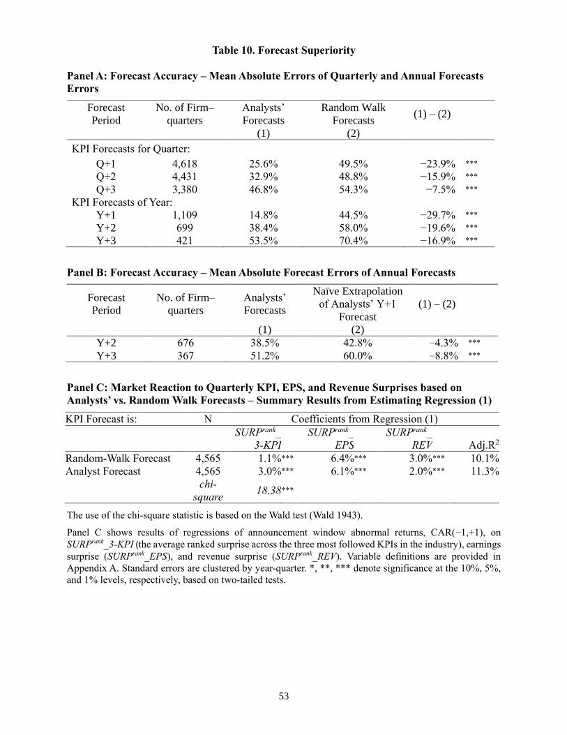
53

Table 10. Forecast Superiority

Panel A: Forecast Accuracy – Mean Absolute Errors of Quarterly and Annual Forecasts

Errors

Forecast

Period

No. of Firm–

quarters

Analysts’

Forecasts

Random Walk

Forecasts (1) – (2)

(1) (2)

KPI Forecasts for Quarter:

Q+1 4,618 25.6% 49.5% −23.9% ***

Q+2 4,431 32.9% 48.8% −15.9% ***

Q+3 3,380 46.8% 54.3% −7.5% ***

KPI Forecasts of Year:

Y+1 1,109 14.8% 44.5% −29.7% ***

Y+2 699 38.4% 58.0% −19.6% ***

Y+3 421 53.5% 70.4% −16.9% ***

Panel B: Forecast Accuracy – Mean Absolute Forecast Errors of Annual Forecasts

Forecast

Period

No. of Firm–

quarters

Analysts’

Forecasts

Naïve Extrapolation

of Analysts’ Y+1

Forecast

(1) – (2)

(1) (2)

Y+2 676 38.5% 42.8% −4.3% ***

Y+3 367 51.2% 60.0% −8.8% ***

Panel C: Market Reaction to Quarterly KPI, EPS, and Revenue Surprises based on

Analysts’ vs. Random Walk Forecasts – Summary Results from Estimating Regression (1)

KPI Forecast is: N Coefficients from Regression (1)

SURPrank_

3-KPI

SURPrank_

EPS

SURPrank_

REV Adj.R2

Random-Walk Forecast 4,565 1.1% *** 6.4% *** 3.0% *** 10.1%

Analyst Forecast 4,565 3.0% *** 6.1% *** 2.0% *** 11.3%

chi-

square 18.38 ***

The use of the chi-square statistic is based on the Wald test (Wald 1943).

Panel C shows results of regressions of announcement window abnormal returns, CAR(−1,+1), on

SURPrank_3-KPI (the average ranked surprise across the three most followed KPIs in the industry), earnings

surprise (SURPrank_EPS), and revenue surprise (SURPrank_REV). Variable definitions are provided in

Appendix A. Standard errors are clustered by year-quarter. *, **, *** denote significance at the 10%, 5%,

and 1% levels, respectively, based on two-tailed tests.