Supply & Demand -Key Factors andApproaches

Austin CareyPlanning Analyst IICentral Arizona Project

EMS Basin Study Supply & Demand TeamMeeting #3March 12, 2019

Ken SeasholesManager, Resource Planning & AnalysisCentral Arizona Project

Goals of Today’s Meeting

Begin to develop a comprehensive list of factors affecting: • Supply• Demand• Reliability

Discuss approaches for how each of these factors might be assessed and represented in the model

2

Factors

Data and Approach

Model Representation

Questions to Consider

3

How might the EMS Basin water supply, demand and reliability be affected by:

? Agricultural trends? Rate & location of growth? Residential demand factors? Commercial & industrial uses? Climate Variability? Shortage Impacts? ….

Pinal AMA Water Use (2017)

4

Muni35,596 Industrial

22,166

Non-Indian Ag

878,911

Tribal149,846

Source: ADWR "Pinal AMA Historic Templateand Summary for web.xls"

5

-

250,000

500,000

750,000

1,000,000

1,250,000

Acre

-Fee

tPinal AMA Crop Water Use

Groundwater Surface water CAP (Tribal) CAP (GSF) CAP (Ag Pool)

Source: ADWR "Pinal AMA Historic Templateand Summary for web.xls"

Agricultural Demand Factors

Development on Ag land

Land fallowing

Changes in crop types

Changes in irrigation technology/efficiency

Cropping intensity

Pumping costs/DTW

Water quality

Other?

6

Agricultural Data

ADWR Annual Reports

- Use by supply type for IGFRs & Districts

- Well pumpage by #55- BMP practices

Crop Coefficients- ADWR & FAO

CAP Data- Ag Pool deliveries- GSF deliveries and

partnerships

GIS Layers

- District & IGFR boundaries

- Canals & Laterals

Ag District Data

- Irrigation techniques?

Satellite Data

- NASS CropScape

Other

7

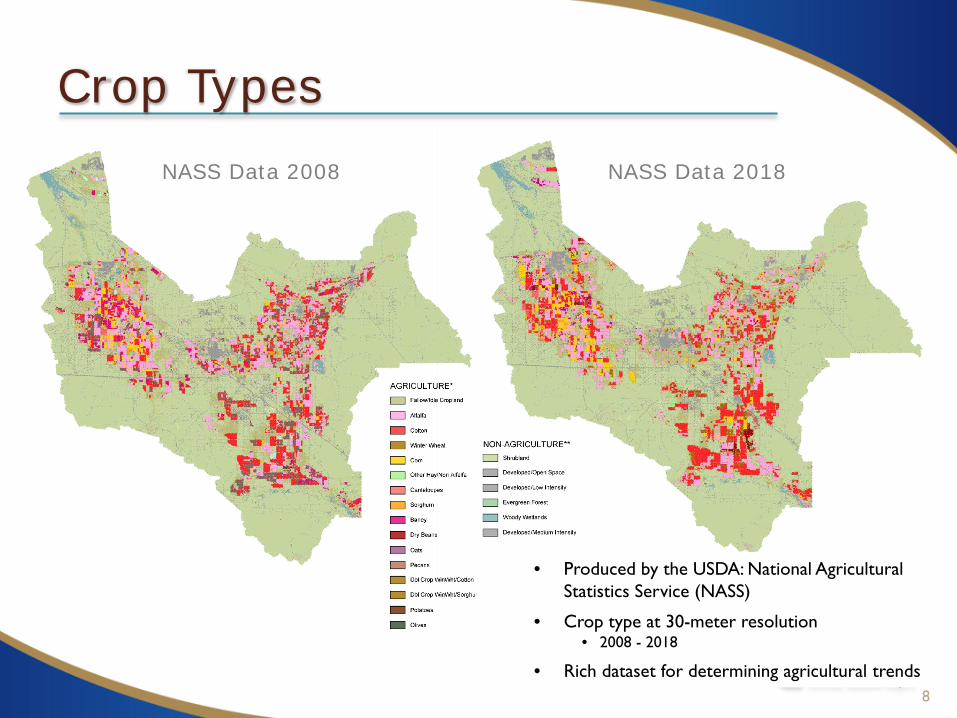
Crop Types

8

NASS Data 2018NASS Data 2008

• Produced by the USDA: National Agricultural Statistics Service (NASS)

• Crop type at 30-meter resolution• 2008 - 2018

• Rich dataset for determining agricultural trends

Cropping Intensity

9

Maricopa Stanfield Irrigation District

Overlay ADWR Model Grid (0.5 mile)

Development on Ag Land

10

Development mixed with some road noise

Maricopa development

Only a very small fraction (~2.6%) of land has been taken out of production from 2008 – 2018. How is this expected to change moving forward?

Growth

11

Municipal◦ Rate of growth in Central Arizona

◦ Spatial distribution Official growth pattern? Spillover from Phoenix? Growth along transportation corridor? Expanded local manufacturing? Constraints on growth…?

Industrial◦ Where is industry expected?

◦ What is the status of these projects?

Growth Data

12

0

1,000,000

2,000,000

3,000,000

4,000,000

5,000,000

6,000,000

7,000,000

8,000,000

9,000,000

10,000,00019

8419

8619

8819

9019

9219

9419

9619

9820

0020

0220

0420

0620

0820

1020

1220

1420

1620

1820

2020

2220

2420

2620

2820

3020

3220

3420

3620

3820

4020

4220

4420

4620

4820

50

Projected ►◄ Actual

AZ Department of Administration (Low, Med, High Series)

Growth Rate Adjustments

13

In CAP:SAM growth is represented by housing unit projections

Annual housing unit growth can be adjusted in a variety of ways:

Growth Distribution

14

CAG TAZ Level Projections: Change in Population Density 2010 vs 2040

SpilloverOrdinary Growth

Growth Along Transportation

Corridor

??

Do these distributions look reasonable?

Alternative Growth Scenarios

15

Change From Baseline Scenario

Slower Growth- 75,000 Housing Units

Faster Growth+ 75,000 Housing Units

Developed by Applied Economics, Based on a Socioeconomic Allocation Model

Outward GrowthInfill Scenario

Urban Redevelopment

Development Projects

16

Which projects:◦ Are anticipated?◦ Under construction? ◦ Have become active?

CAG 2014 Pinal County Development Projects

Data Source: Pinal County

Development Projects

17

Comprehensive Plan: Community Development Projects

Data Source: Pinal County

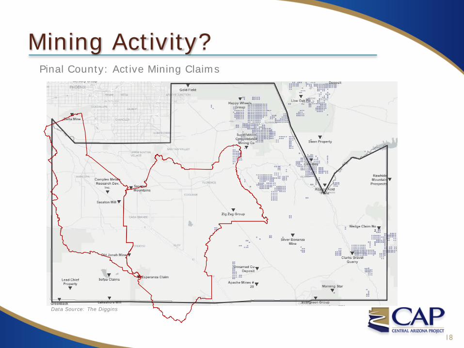
Mining Activity?

18

Pinal County: Active Mining Claims

Data Source: The Diggins

CAP:SAM Dashboard

19

Changes in Demand Factors

20

0

0.05

0.1

0.15

0.2

0.25

0.3

0.35

Acre

-Fee

t per

per

son

Per Capita Use(Total Municipal Sector Use / Population)

How is demand expected to change?◦ Existing GPHUD

◦ New GPHUD

Climate Variability

21

Effect on demand:◦ Crop evapotranspiration

◦ Change in per capita water use Exterior demand change from higher temperatures

and longer growing season

Shortages to Water Supply◦ Frequency, duration and severity of CAP shortage

◦ Availability of surface water for SCIDD

22

Global Circulation Models (GCMs)

Colorado River Simulation System

(CRSS) CAP:SAM

Regional Downscaling (Statistical or Dynamical;

VIC; etc.)

Distribution of Pumping & Recharge

Arizona On-River Uses

Groundwater Flow Model (MODFLOW)

Distribution of Streambed & Mnt.

Recharge

Pumping & Rechargeby Entity

Land Use, Housing & Pop (COGs, Census, Applied Economics)

Supply & Demand by Entity

GW LevelsWater Supply

Portfolios, Use, etc.(ADWR, CAP)

0

250000

500000

750000

1000000

2015

2017

2019

2021

2023

2025

2027

2029

2031

2033

2035

2037

2039

2041

2043

2045

2047

2049

2051

2053

2055

2057

2059

Shor

tage

Vol

ume

(AF)

Time

Example Periodic CO River Shortages

No Shortage

Significant Reductions to CAP Supply

CRSS simulates a range of hydrologic scenarios to account for future hydrologic uncertainty

◦ Periodic shortages vs deep and sustained

23

Summary

Applied EconomicsSocioeconomic Allocation Model• Outward Growth Scenario• Infill Scenario• Urban Redevelopment Scenario

Housing Unit Projection by TAZCounty Association of Governments• MAG and CAG (2010-2040)• PAG (2010-2050)

Gallons Per Housing Unit Per DayNew and Existing• Annual % Change• Cumulative Max Change• Absolute Min Limit

Housing Unit Projection• Start Year Housing Units by WP• Housing Recovery Rate (Fast/Medium/Slow)• Growth Rate After Recovery• Growth Rate After 50 Years• “Ordinary” Growth Rate• UofA Housing Projections

Municipal Effluent Demand• Non-potable demand scenarios: Flat growth

versus tied to annual or cumulative growth

Agricultural Demand• Development on Irrigated Acres• Intensity of use• Replacement rate of high water use crops• Replacement crop water use (AF/ac)• Adjust crop efficiency

Supply Availability & Entitlements• Set or calculate surface water supplies• Effluent availability for reuse• LTSA Balance• Leases and exchanges (including future

Reallocations)

Request for Supplies• User preferences on accumulation or use of

LTSCs• User preference for CAP utilization• Storage facility preference

Factors that can currently be adjusted in the CAP:SAM Model

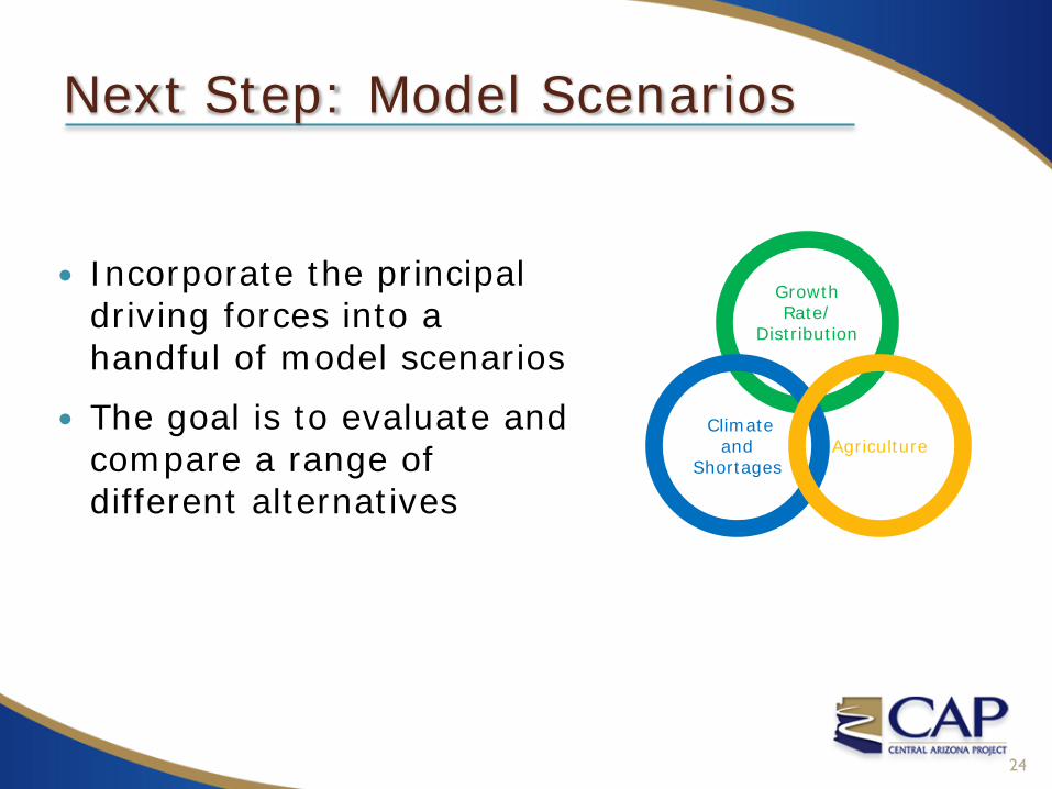
Next Step: Model Scenarios

24

Incorporate the principal driving forces into a handful of model scenarios

The goal is to evaluate and compare a range of different alternatives

Growth Rate/

Distribution

Climate and

ShortagesAgriculture

Scenario Categories

25

Water Demand

Wat

er S

uppl

y

High Demand,Low Supply

Low Demand,Low Supply

High Demand,High Supply

Low Demand,Low Supply

Example Scenario Development

26

Scenario Low Med High None (Historic)

Hot/Dry

Warm/Wet Low Med High

A X X X

B X X X

C X X X

D X X X

E X X X

…

Growth Climate Change AG Urbanization