Copyright © 2012 by author(s).

University of California, Berkeley Department of Agricultural &

Resource Economics

CUDARE Working Papers Year 2012 Paper 1122

Demand and Price Volatility:

Rational Habits in International Gasoline Demand

K. Rebecca Scott

Demand and Price Volatility: Rational Habits in International

Gasoline Demand

K. Rebecca Scott

8 July 2011

Key Words: gasoline demand, rational habits, price elasticity

JEL Classification: H30, Q40, Q41, Q50, R40

Abstract

The combination of habits and a forward outlook suggests that consumers will be sensitive not

just to prices but to price dynamics. In particular, rational habits models suggest 1. that price

volatility and uncertainty will reduce demand for a habit-forming good and 2. that such volatility

will dampen demand’s responsiveness to price. These two implications can be tested by augmenting a

traditional partial-adjustment or error-correction model of demand. I apply this augmented model to

data on gasoline consumption, as rational habits provide a succinct representation for the investment

and behavioral decisions that determine gasoline usage. The trade-offs among 2SLS, system GMM,

and pooled mean group (PMG) estimators are considered, and my preferred PMG estimator provides

evidence for the two implications of rational habits in a panel of 29 countries for the years 1990-2009.

The sensitivity of certain results to the choice of estimator offers a cautionary illustration of the cost

of assumptions such as coeffi cient heterogeneity. Given the evidence uncovered in favor of rational

gasoline habits, such habits may help to explain some of the cross-country variation in "total" price

elasticity. These habits also imply that the effect of price volatility must be taken into account when

projecting the impacts of potential policies on gasoline consumption.

1 Introduction

The same consumer behavior that shapes gasoline demand also shapes the effectiveness of policies for

controlling gasoline demand. Reducing this demand has become a widespread policy goal, driven by

environmental concerns both global and local; and the intricacies of demand behavior are now of very

practical interest.

Although this interest has generated a great deal of empirical work measuring the effects of income

and prices on gasoline consumption, less attention has been devoted to the deeper behaviors underlying

gasoline demand. Consumers may purchase fuel at the pump, but in fact they make their gasoline-buying

decisions almost everywhere but the gas station. They make these decisions in the form of discrete,

infrequent choices about what type of vehicle to buy and where to live in relation to work, as well as in

nearly-continuous choices about daily routines– carpooling, driving style, how much non-essential travel

to undertake and whether to cycle or take the car. The investment nature of the former decisions and

the habitual nature of the latter help to explain consumers’sluggish responses to changes in the gasoline

price, and also suggest that models of gasoline demand should allow for the effects of long-run choices.

One way to incorporate these effects is a rational habits model, in which consumers’utility for a

particular good– in this case, gasoline– is a function of how much of the good they consumed in the past.

1

Since past investment decisions affected past consumption, the habit setup captures both investment-

and habit-influenced behaviors. The model assumes consumers are ‘rational’, or forward-looking; and

therefore when deciding their current gasoline consumption, they consider how this consumption will

affect their future utility. The future burden of a gasoline habit depends upon future market conditions,

and so demand in this model depends upon consumers’expectations of the future, particularly of future

prices.

If rational habits do in fact shape gasoline demand, then studies that confine themselves to the effects

of income and contemporary prices on demand may overlook nuances of behavior that are relevant to

policy. Given rational habits, demand will be affected by the process by which prices are generated as

well as by the current price level, and differences in price elasticity across countries may be driven by

differences in price regimes as well as by differences in environment and infrastructure.

The ideal way to examine the hypothesis of rational habits would be to estimate or calibrate a

structural model, such as the one introduced in Scott (2010). Unfortunately, this model can only be

solved numerically, and so its parameters cannot not be estimated using traditional estimation methods.

More problematically, the model contains too many parameters to be calibrated precisely using available

data– eight, plus any parameters necessary to model the gasoline price process. Even to identify each of

these parameters would be a stretch.

Fortunately, however, rational habits models suggest two implications that are easily testable by

augmenting a traditional demand model with extra variables. If consumers are forward-looking,

1. demand for a habit-forming good will decline with the uncertainty in its (future) price, and

2. responsiveness to price changes will be dampened by price uncertainty and the expectation that

price changes will be short-lived.

The first of these implications is proved by Coppejans et al. (2007), who consider a mean-preserving

spread in the distribution of future prices and find that this reduces consumption of the habit-forming

good. This first implication is also demonstrated in Scott (2010), where the level of demand is shown

to decline with the variance of future prices (Figure 2.10). To test whether price uncertainty in fact

reduces demand for gasoline, I introduce a measure of price uncertainty into a traditional, non-structural

dynamic model of gasoline demand. Coppejans et al. take a similar approach in examining the effect

of price uncertainty on smoking behavior, augmenting a static demand model with an estimate of the

expected one-period-ahead standard deviation of price.

The second implication above is demonstrated in Scott (2010), where the magnitude of price elasticity

is shown to be negatively related to the variance of the future price distribution (Figures 2.8 and 2.9)

and positively related to the expected duration of price changes (Figure 2.7). To test whether price

uncertainty dampens consumers’responsiveness to prices in practice, I augment my demand model with

an interaction between a price-uncertainty measure and the gasoline price. The "total" elasticity with

respect to price is therefore given by a combination of the price and interaction coeffi cients.

To capture the sluggish adjustment associated with any habits model, rational or myopic, I can add

these two rational-habits regressors to a partial-adjustment, or ADL, model. Partial-adjustment models

are frequently used to estimate gasoline demand, and my augmented version takes the form

git = λgi,t−1 + δ1yit + δ2pit + δ3σ̂it + δ4 (pit − pi) σ̂it + µi + εit (1)

where g is log gasoline consumption per capita, yit is log real income or expenditure per capita, p is

the log real gasoline price, and σ̂ is a measure of price uncertainty. For simplicity I will sometimes refer

to the de-meaned gasoline price, (pit − pi), as p̃it. (Coeffi cients in (1) are restricted to be homogeneous

2

across countries; later I will relax this assumption.) The rational habits model implies that δ3 should be

negative, with price uncertainty discouraging gasoline consumption, and δ4 should be positive, with the

interaction term offsetting some of the negative effect of prices:

git = λ︸︷︷︸+,<1

gi,t−1 + δ1︸︷︷︸+

yit + δ2︸︷︷︸_

pit + δ3︸︷︷︸_

σ̂it + δ4︸︷︷︸+

(pit − pi) σ̂it + µi + εit (2)

Short-run income elasticity is given here by δ1; short-run "uncertainty elasticity", by δ3; and short-run

"total" price elasticity, by∂git∂pit

= δ2 + δ4σ̂it

Corresponding long-run elasticities are calculated, of course, by dividing each short-run elasticity by

1− λ.Estimating this model entails some complications, and to address these I will reparameterize (1) into

an error-correction model. I discuss alternative formulations of the model in Section 4.3. For now, I begin

with a brief review of the literature on estimating gasoline demand and a discussion of my data set, which

is a country-level panel. I then revisit the specification of my model and consider possible estimation

methods, weighing the advantages and disadvantages of three approaches: least squares and system GMM

estimation of the ADL model in (1) and maximum-likelihood estimation of an error-correction model

allowing for coeffi cient heterogeneity. My preference is for the error-correction model with heterogeneous

short-run coeffi cients, but I report the results of all these estimators in order to be transparent about the

sensitivity of my results to the specification of the model– and to illustrate the potential pitfalls of certain

approaches. For ease of comparison with the literature, I also estimate a "standard", non-habits version

of the error-correction specification. Before concluding, finally, I use country-specific price volatilities to

interpolate country-specific price elasticities, and I consider the extent to which cross-country variation

in price volatility predicts cross-country variation in elasticity.

2 Gasoline Demand Literature Review

The predominant focus in the gasoline demand literature is on measuring the effects of income and

prices on consumption. Little attention has been directed at structural models in which consumers

choose consumption to maximize expected utility.

Neither myopic nor rational habits have been investigated as a potentially demand-shaping behav-

ior. Although Breunig and Gisz (2009) use an unobservable habit stock variable in a petrol demand

regression, they insert this directly into a nonstructural demand model rather than into the consumer’s

utility-maximization problem. The habit stock in this scenario simply substitutes for the ADL model’s

directly-observed lags of consumption, allowing for gradual adjustment. Breunig and Gisz focus on the

econometric complications generated by this unobserved stock, which implies that the error terms have

a moving-average form. This correlation of the errors across time is analogous to that implied by the

inclusion of lagged consumption in the usual ADL model (see Section 4). Breunig and Gisz estimate

an ECM-type model using maximum likelihood to account for moving-average errors, and argue that,

because this approach yields less precise elasticities than OLS estimates of an ADL-type model, the latter

must be spuriously precise. Yet they do not establish that the OLS estimates owe their precision to a

disregard of intertemporal error correlations rather than to their basis in a model with ten fewer para-

meters. Across the standard ADL and Breunig and Gisz’s model, moreover, point estimates of long-run

elasticities are about the same: -0.25 and -0.20, respectively, for price; and 0.34 and 0.27, respectively,

for income.

3

Table 1: Average elasticities in gasoline demand literature reviewsAverage price elasticity Average income elasticity

Study Short run Long run Short run Long runDahl and Sterner (1991)a -0.24 -0.80 0.45 1.31

Goodwin (1992)b -0.27 -0.71Espey (1998) -0.26 -0.58 0.42 0.88

Goodwin, Dargay and Hanly (2004)c -0.25 -0.64 0.39 1.08Brons et al. (2008) -0.34 -0.84

aLagged endogenous models, annual. bTime series modelscPrice: time series models; income: dynamic models

As a determinant of gasoline demand, therefore, habits have not been introduced into the litera-

ture; and the effects of habit-related variables such as price uncertainty and price expectations remain

unexamined. The typically-acknowledged determinants of demand– income and price– have received

wide attention, however; and studies measuring income and price elasticities abound. In her 1998 meta-

analysis, for instance, Espey (1998) considers 363 short- or medium-run and 277 long-run price elasticity

estimates, along with similar numbers of income elasticity estimates. In the past there have been so

many studies that simultaneous literature reviews have even managed, as Goodwin (1992) recalls, to

draw on nearly-disjoint sets of papers. More recently, simultaneous reviews by Goodwin, Dargay and

Hanly (2004) and Graham and Glaister (2004), commissioned by the same source for the same purpose,

have continued to draw from a pool of literature large enough to allow substantial differences in their

samples.

In this large literature, gasoline demand elasticities have run a wide gamut, with own-price elasticity

estimates ranging from 0 to -1.36 in the short run and 0 to -2.72 in the long run, and income elasticities

ranging from 0 to 2.91 in the short run and 0 to 2.73 in the long run (Espey 1998). Overall, however,

the reviews are in basic agreement about average elasticities. Average own-price elasticity, these reviews

find, is around -0.25 to -0.30 in the short run and -0.6 to -0.8 in the long run; average income elasticity is

around 0.4 in the short run and somewhere around unit elastic in the long run. Some of these averages

are summarized in Table 1.

Although much of the variation in estimated elasticities has not been explained– and may, in fact,

arise from rational habits and variation in price volatility– literature surveys have uncovered some trends.

Studies based on a panel of countries, for instance, tend to produce price elasticities that are similar

to single-country elasticities for the long run but of higher magnitude for the short run (Espey 1998).

Short-run price responsiveness seems to be relatively low in the United States and relatively high in

Europe (Espey 1998). Including a measure of vehicle ownership and/or the characteristics of the vehicle

stock affects the resulting estimates (Dahl and Sterner 1991, Espey 1998). And price elasticities may be

changing over time: Espey (1998) observes that short-run price elasticities appear to have decreased in

magnitude, and long-run price elasticities increased in magnitude, since the 1970s and 1980s. Hughes,

Knittel and Sperling (2006) corroborate this shift in short-run price elasticities for the U.S.

The majority of the studies summarized in these reviews are based on partial adjustment models.

In recent years, increasing attention has been diverted toward error-correction models and questions of

cointegration. So far it seems all these studies have looked at single countries (or the world as a whole)

rather than panels, and their estimates are summarized in Table 2. The most striking difference between

these ECM-based price elasticity estimates and the average elasticities reported in the literature reviews is

that the ECM-based elasticities are generally smaller in magnitude. Whether the ECM model is actually

responsible for this difference, however, is not clear: the preponderance of single-country ECM studies

and the tendency for single-country studies to yield smaller-magnitude short-run price elasticities (Espey

4

Table 2: Gasoline demand studies based on cointegration and error-correction modelsPrice elasticity Income elasticity

Study Country Short run Long run Short run Long runAkinboade, Ziramba and Kumo (2008) South Africa -0.47 0.36Alves and Bueno (2003) Brazil -0.0919 -0.465 0.122g 0.122g

Bentzen (1994)a Denmark -0.32 -0.41 0.89 1.04Cheung and Thomson (2004) China -0.19 -0.56 1.64 0.97De Vita, Endresen, and Hunt (2006)b Namibia -0.794 0.957Eltony and Mutairi (1995) Kuwait -0.37 -0.46 -0.47 0.92Krichene (2002)c World -0.02 -0.005 1.54 1.2Nadaud (2004)d France -0.06 -0.09 0.27 0.28Polemis (2006) Greece -0.10 -0.38 0.36 0.79Ramanathan (1999) India -0.209 -0.319 1.178 2.682Ramanathan and Subramanian (2003)d Oman -0.05 -0.52 0.35 0.96Rao and Rao (2009) Figi -0.159 0.427

to -0.244 to 0.462Samimi (1995)e Australia -0.2 -0.12 0.25 0.52Wadud, Graham, and Noland (2009)f US -0.085 -0.116 0.520 0.592aElasticities with respect to vehicles per capita substituted for income elasticities.b1990q1-2002q4cEstimates elasticity of demand for crude oil, not gasoline. Results for 1973-1999.dAs reported in Wadud, Graham, and Noland (2009).eEnergy for transport, not just gasoline.fSingle-step nonlinear least squares, post-1978.gReported short- and long-run elasticities in fact the same.

1998) might also explain some of the difference. In Section 5 I will report ECM results that are consistent

with a story in which the panel dimension, rather than the choice of an ECM, drives this difference. Not

only do my panel-based ECM price estimates turn out to be relatively high in magnitude, but those

of my estimators that exploit cross-section variation (PMG and DFE) yield elasticities that are higher

in magnitude than those elasticities based on single-country regressions (MG). The differences between

these estimators will be explored in Section 4.

3 Data and Specification of Variables

3.1 Data

My data set consists of a panel of 29 countries for the period 1990-2009. As price data for some countries

is limited, the actual series length ranges from fifteen to twenty years, with an average of 18.7 years. A

list of included countries is provided in Appendix 7.

In order to focus as much as possible on passenger vehicles rather than freight, data is isolated

to gasoline, not diesel. Information on gasoline consumption1 is taken from the International Energy

Agency (IEA)’s Oil Information (2009) and transformed into per capita terms using annual population

estimates from the UN’sWorld Population Prospects (2009). Only annual consumption data is provided;

quarterly observations are not available. Data on gasoline prices and taxes, broken down by product and

grade, is taken from the IEA’s Energy Prices and Taxes (2009Q4). International differences in product

definitions and regulations mean that data availability for each product varies by country. Depending on

1This series ("motor gasoline demand") explicitly excludes aviation gasoline.

5

this availability, I use either regular unleaded or 95 RON to create a price series for each country. These

choices are discussed further in Appendix 7.

As a measure of income, I take GDP from the World Bank’s World Development Indicators (2009)

and transform this into real per capita terms. When crude oil prices are used, these are the spot prices

for the Brent stream, taken again from the IEA’s Energy Prices and Taxes (2009Q4). I concentrate on

this stream because the Brent is used extensively as a pricing benchmark.2

For reasons explained below, I consider regressions based both in a common currency and in real

local currencies. When dealing in a common currency, I convert the IEA’s USD-denominated series into

real 2005 USD. When dealing in local currencies, I convert all prices and income from nominal to real

terms using country-specific CPIs taken from the IEA’s Energy Prices and Taxes (2009Q4).

Further specifics about my data and data sources are provided in Appendix 7.

3.2 Measuring Price Volatility

In order to begin examining the model in (1), I need a measure of the price uncertainty or volatility

faced by gasoline consumers. The simplest measure of volatility would, of course, be the country-

specific variance or standard deviation of the (log) gasoline price. Such a measure, taken over the entire

sample period and constant over time, however, would hold two disadvantages: first, it would imply that

consumers had information about future prices that they do in reality not have; and second, it would

make identification of price volatility effects impossible without restrictive assumptions. Instead, I use

a measure of the rolling standard deviation of log prices. This constrains consumers’information about

volatility to current and past prices, and also captures the evolution in price volatility over time.

Annual price observations mask volatility within each year. In the extreme case, two countries with

identical annual price series could have wildly different price paths from month to month or quarter to

quarter. Relying on annual data to construct a measure of price volatility, therefore, may yield a measure

that is biased toward zero, with the size of the ‘bias’increasing with ‘true’volatility. To mitigate this

problem, I exploit the availability of quarterly price data to construct the rolling standard deviation

measure. This has the added advantage of allowing me to keep several years of data at the beginning of

the period that I would otherwise lose to measuring volatility.

I construct the rolling standard deviation for each quarter, denoted σ̂iq, as

σ̂iq =√σ̂2iq , where (3)

σ̂2iq =1

x

x∑j=1

(pi,q−j − piq

)2and piq =

1

x

x∑j=1

pi,q−j+1

where x is the number of quarters in the rolling window and piq is the log real price of gasoline in quarter

q. As a sensible default, I choose x = 4. In this case, the fourth-quarter rolling standard deviation in

any year is the standard deviation of the year’s prices from their year-long mean, and it is this that I use

as my measure of annual rolling standard deviation. As an alternative, one could average σ̂iq over the

quarters in each year. (The chief difference of this alternative method lies in the mean price, piq, from

which each quarter’s deviations are calculated: in the alternative method, prices are always compared to

a past average. In the default measure, each quarter’s price is compared to the mean price for the entire

2The West Texas Intermediate (WTI) stream is widely used in North America. Using this stream instead of or alongsidethe Brent, however, makes little difference in the resulting estimates.

6

year, which for the first three quarters includes lead prices.) As an alternative, one could, of course,

lengthen the window of the rolling standard deviation beyond x = 4.

A further alternative would be to consider price predictability rather than volatility– that is, to

measure the performance of price forecasts in each country. This would entail modelling each country’s

price series, generating rolling forecasts, and calculating root mean squared forecasting error for each

period. One could also consider modelling the evolution of price volatility over time and incorporating

price-volatility forecasts into the demand model. This would be a particularly worthwhile exercise as

the theory developed in Scott (2010) posits a relationship between demand and expected future price

volatility, not current volatility: the rolling-volatility measure used at present functions as a proxy for

expected future volatility, a very simple forecast. Better volatility forecasts may be possible, particularly

if gasoline prices follow an ARCH-type process and tend to move between periods of high and low

volatility. If consumers are aware of better forecasts, then the current proxy may contain substantial

measurement error. Even if this measurement error is white noise, it will bias estimates of volatility’s

effects toward 0. The rolling-volatility proxy may, therefore, render the current model susceptible to

underestimating the influence of uncertainty on demand. Although I stick to the rolling-volatility measure

for now, price forecastability measures and explicit volatility forecasts are well worth examining in the

future.

One extension I do consider now is the use of before-tax prices rather than total prices to calculate

σ̂iq. This variation is of interest because "volatility" is not synonymous with "uncertainty": tax increases

may, for example, contribute to price volatility within the year they come into effect but actually lead

to a reduction in price uncertainty. If this is the case, then there is, in effect, a systematic measurement

error in σ̂iq that will bias the coeffi cient on the interaction term downward and make consumers’price

elasticity appear less sensitive to price volatility. Using before-tax prices to construct σ̂iq circumvents

this danger, and so I will consider this alternative definition as a check.

3.3 Currency Issues

The international nature of the panel leads to an additional consideration, namely how to deal with

prices, price volatility, and income denominated in different currencies. These variables must be treated

in a way that allows comparisons across countries, and ideally they should capture real prices and income,

and variation therein, as perceived locally.

One approach is to transpose all variables into a common currency. Indeed, this is the approach

toward which convention in the gasoline- and energy demand literature leans,3 and it is the approach I

shall adopt for my main discussion. Measuring all monetary variables in the same units (in this case,

real (2005) US dollars) has the advantage that it does not introduce restrictions on the type of estimator

that can be deployed; and it has the side benefit, of course, of allowing easy comparisons of price and

income levels across countries.

Provided care is taken in the choice of estimator, however, another option is to work in log real local

currency. As a check on my common-currency findings, I also estimate local-currency versions, with

results reported in Appendix 8. To see that the local-currency approach can be valid, imagine that each

country i has a real gasoline price Pit, denominated in real local currency units, and let the real exchange

rate with respect to some common currency be given by rt = rieit. The time-invariant component, ri,

represents the long-run exchange rate, and eit represents fluctuations away from relative PPP. At any

3See, for example, Angelier and Sterner (1990), Baltagi and Griffi n (1983, 1997), Dahl (2011), Johanssen and Schipper(1997), Judson, Schmalensee, and Stoker (1999), Narayan and Smyth (2007), Nguyen-Van (2010), and Storchmann (2005).

7

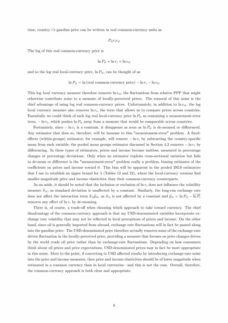
time, country i’s gasoline price can be written in real common-currency units as

Pitrieit

The log of this real common-currency price is

lnPit + ln ri + ln eit

and so the log real local-currency price, lnPit, can be thought of as

lnPit = ln (real common-currency price)− ln ri − ln eit

This log local currency measure therefore removes ln eit, the fluctuations from relative PPP that might

otherwise contribute noise to a measure of locally-perceived prices. The removal of this noise is the

chief advantage of using log real common-currency prices. Unfortunately, in addition to ln eit, the log

local currency measure also removes ln ri, the term that allows us to compare prices across countries.

Essentially we could think of each log real local-currency price lnPit as containing a measurement-error

term, − ln ri, which pushes lnPit away from a measure that would be comparable across countries.

Fortunately, since − ln ri is a constant, it disappears as soon as lnPit is de-meaned or differenced.

Any estimator that does so, therefore, will be immune to this "measurement-error" problem. A fixed-

effects (within-groups) estimator, for example, will remove − ln ri by subtracting the country-specific

mean from each variable; the pooled mean groups estimator discussed in Section 4.3 removes − ln ri by

differencing. In these types of estimators, prices and income become unitless, measured in percentage

changes or percentage deviations. Only when an estimator exploits cross-sectional variation but fails

to de-mean or difference is the "measurement-error" problem really a problem, biasing estimates of the

coeffi cients on prices and income toward 0. This bias will be apparent in the pooled 2SLS estimators

that I use to establish an upper bound for λ (Tables 12 and 22), where the local-currency versions find

smaller-magnitude price and income elasticities than their common-currency counterparts.

As an aside, it should be noted that the inclusion or exclusion of ln ri does not influence the volatility

measure σ̂it, as standard deviation is unaffected by a constant. Similarly, the long-run exchange rate

does not affect the interaction term σ̂itp̃it, as σ̂it is not affected by a constant and p̃it = lnPit − lnPi

removes any effect of ln ri by de-meaning.

There is, of course, a trade-off when choosing which approach to take toward currency. The chief

disadvantage of the common-currency approach is that my USD-denominated variables incorporate ex-

change rate volatility that may not be reflected in local perceptions of prices and income. On the other

hand, since oil is generally imported from abroad, exchange rate fluctuations will in fact be passed along

into the gasoline price. The USD-denominated price therefore actually removes some of the exchange-rate

driven fluctuation in the locally-perceived price, providing a measure that focuses on price changes driven

by the world crude oil price rather than by exchange-rate fluctuations. Depending on how consumers

think about oil prices and price expectations, USD-denominated prices may in fact be more appropriate

in this sense. More to the point, if converting to USD affected results by introducing exchange-rate noise

into the price and income measures, then price and income elasticities should be of lower magnitude when

estimated in a common currency than in local currencies– and this is not the case. Overall, therefore,

the common-currency approach is both clear and appropriate.

8

3.4 A Brief Overview of the Data

Gasoline consumption per capita shows a reasonable amount of variation, both across countries and over

time. Annual consumption in the sample ranges from a low of 31.7 kg per person (Turkey, 2008) to a high

of 1352.4 kg per person (Luxembourg, 1994), with an overall mean of 295.9 kg per person. Over time,

per-capita consumption has been slightly decreasing in most countries, and the 1990 average of 37.5 kg

per person has fallen to a 2008 average of 34.4 kg. Figure 2 plots the path of log gasoline consumption

over time for each of the 29 countries in the sample.

Prices, like consumption, have shown considerable variation, with much of the cross-sectional variation

driven by tax differences (see Figure 1) and much of the variation over time driven by fluctuations in

the crude oil price. The overall mean real price in the sample is 1.11 Y2005-USD per liter, and country-

averaged prices range from 0.47 Y2005-USD per liter in the United States to 1.52 Y2005-USD per liter

in Norway. The volatility measure, too, has both cross-sectional and cross-time variation that should

allow us to identify its effect. The four-period rolling standard deviation of price, as defined in (3),

has an average over all observations of 0.048 Y2005-USD per liter, with a comparatively-high standard

deviation of 0.037. Country-specific mean volatilities range from a low of 0.035 for Mexico to a high of

0.063 for the United States, and annual average volatility ranges from low of 0.022 in 1998 to a high of

0.14 in 2008. The time paths of the gasoline price and the volatility measure are plotted in Figures 3

and 4, respectively.

Income per capita, finally, has generally been increasing, and this upward trend is depicted in Figure

6.

9

Figure 1: Mean gasoline prices, by tax- and non-tax components

10

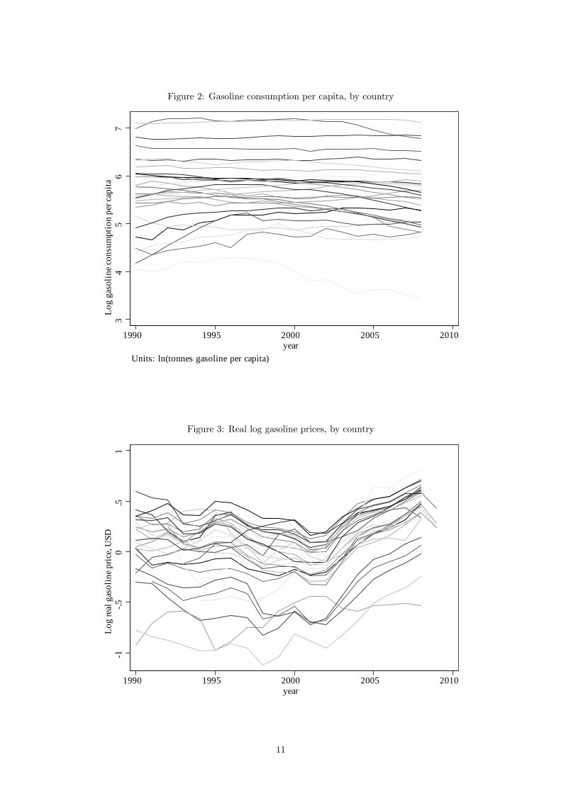
Figure 2: Gasoline consumption per capita, by country

34

56

7Lo

g ga

solin

e con

sum

ptio

n pe

r cap

ita

1990 1995 2000 2005 2010year

Units: ln(tonnes gasoline per capita)

Figure 3: Real log gasoline prices, by country

­1­.5

0.5

1Lo

g re

al g

asol

ine p

rice, 

USD

1990 1995 2000 2005 2010year

11

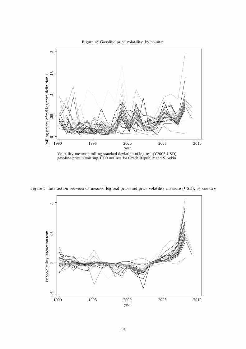
Figure 4: Gasoline price volatility, by country

0.0

5.1

.15

.2Ro

lling

 std 

dev 

of re

al lo

g pr

ice, 

defin

ition

 1

1990 1995 2000 2005 2010year

Volatility measure: rolling standard deviation of log real (Y2005­USD)gasoline price. Omitting 1990 outliers for Czech Republic and Slovkia

Figure 5: Interaction between de-meaned log real price and price volatility measure (USD), by country

­.05

0.0

5.1

Pric

e­vo

latil

ity in

tera

ctio

n te

rm

1990 1995 2000 2005 2010year

12

Figure 6: Real income per capita, by country

89

1011

12Lo

g in

com

e per

 capi

ta

1990 1995 2000 2005 2010year

Income measure: log GDP per capita, real USD

13

4 Models and Estimation

I consider several strategies to examine gasoline demand for the effects implied by a rational habits model.

These strategies vary by model specification as well as by estimation method. To start, I estimate a partial

adjustment (ADL) model using standard least-squares panel methods. Next I estimate the same model

using Arellano & Bover (1995) and Blundell and Bond’s (1998) system GMM estimator. Finally I turn

to an error-correction version of the model, which I estimate under a range of coeffi cient-homogeneity

restrictions using Pesaran and Smith’s (1995) mean groups method; Pesaran, Shin, and Smith’s (1999)

pooled mean group method; and a dynamic fixed effects method. Each of these ways of specifying and

estimating the model has its advantages and trade-offs, but, as I will discuss in Section 5, the least-

squares and GMM methods’weaknesses are troublesome in this application, and I prefer the pooled

mean group estimator of the ECM.

4.1 Least Squares

The model laid out in Section 1 was formulated as a partial adjustment model– specifically, as an

ADL(1,0) model:

git = λgi,t−1 + δ1yit + δ2pit + δ3σ̂it + δ4 (pit − pi) σ̂it + µi + εit (4)

where g is log per-capita gasoline consumption, y is log per-capita income, p is the log real gasoline price,

σ̂ is a measure of volatility in the log real gasoline price, and µi is a time-invariant country-specific effect.

I shall also consider a version of this model that includes a common time trend,

git = λgi,t−1 + δ1yit + δ2pit + δ3σ̂it + δ4 (pit − pi) σ̂it + δ5t+ µi + εit (5)

and a version that includes country-specific time trends,

git = λgi,t−1 + δ1yit + δ2pit + δ3σ̂it + δ4 (pit − pi) σ̂it + δ5it+ µi + εit (6)

Short-run elasticities in these models are given by the δ coeffi cients, and long-run elasticities can be

calculated as δ1−λ .

On each of these models I first employ a within-groups (fixed-effects) estimator, eliminating the fixed

effects µi by de-meaning each variable by its country-specific average. A within-groups estimator makes

more sense in this situation than a GLS/random-effects estimator because, even putting aside the issue

of the lagged endogenous variable, the country-specific effects are likely to be correlated with the other

regressors. Indeed, a Hausman test soundly rejects the equivalence of fixed- and random-effects estimates

of a static version of (4); see Table 3. (The same non-equivalence holds for the dynamic version of the

model.) Since the random-effects estimator of the static model is consistent only if µi is in fact random

in relation to the exogenous variables, and the fixed-effects estimator is consistent either way, rejecting

the equivalence of the resulting estimates confirms that µi is not random.

4.1.1 Addressing Price Endogeneity

The simple within-groups estimator is still affl icted by two problems. The first of these is the potential

endogeneity of prices: unless the gasoline supply schedule is flat, any positive demand shock will drive

up prices, and vice versa. The gasoline supply schedule is unlikely to be flat when ‘individuals’ are

national aggregates rather than single households, and so causality runs from consumption to prices as

14

Table 3: Random- vs. fixed-effects estimator, static model, USD

(1) (2) (3) (4)Static Static Dynamic Dynamic

Random effects Fixed effects Random effects Fixed effects

gt−1 λ 0.957** 0.906**(0.0113) (0.0175)

[0.000] [0.000]

y δ1 0.523** 0.372** 0.0284** 0.0428**(0.0329) (0.0368) (0.0107) (0.0156)

[0.000] [0.000] [0.008] [0.006]

p δ2 -0.574** -0.419** -0.0717** -0.0894**(0.0508) (0.0515) (0.0177) (0.0207)

[0.000] [0.000] [0.000] [0.000]

σ̂ δ3 0.0418 -0.0280 -0.118+ -0.105(0.182) (0.172) (0.0714) (0.0729)

[0.818] [0.871] [0.098] [0.151]

σ̂p̃ δ4 -2.348** -2.197** -0.132 -0.236(0.479) (0.453) (0.172) (0.175)

[0.000] [0.000] [0.444] [0.179]

R2 0.8558 0.8564 0.9949 0.9947

Hausman 77.85 19.07testa [0.000] [0.002]

Standard errors in parentheses; P-values in brackets.

** p<0.01, * p<0.05, + p<0.1aUnder H0 that random- and fixed-effects estimates equivalent,

χ2(4) for static model, χ2(4) for dynamic.

well as from prices to consumption. Ignoring this endogeneity may lead us to underestimate consumers’

responsiveness to price changes.

Fortunately, a strength of the current approach is that it allows us to address the endogeneity of

prices by instrumenting for them using outside variables. Two obvious instrument candidates are the

tax level and the crude oil price. Both should be highly relevant, as they are major determinants of the

local gasoline price. Both should also be exogenous, insofar as an individual country’s demand does not

drive its tax level or the world crude oil price. (Exogeneity may, of course, be violated if demand-driven

political pressure affects the tax level or if an individual country’s gasoline consumption is great enough

to affect the world oil market.) I use tax instruments and crude-price instruments, therefore, to estimate

2SLS within-groups versions of (4) through (6).

The use of log prices slightly complicates the specification of these instruments. In order to create a

good first-stage fit for log prices, note that the real price level Pit can be decomposed into the tax level,

Taxit, and the before-tax price level, BeforeTaxit:

Pit = Taxit +BeforeTaxit , or

Pit =

(1 +

TaxitBeforeTaxit

)BeforeTaxit

15

pit = lnPit = ln

(1 +

TaxitBeforeTaxit

)+ lnBeforeTaxit (7)

Assuming the crude oil price is linearly related to the before-tax gasoline price, the log real crude oil price

is a sensible instrument for the second term in (7). In the first term, the appearance of the before-tax

price means the tax component of log price is still endogenous– assuming, of course, that taxes are levied

predominantly as level amounts rather than as percentages. To eliminate the endogeneity introduced by

the before-tax price, I define the tax instrument as

TaxIVit = ln

(1 +

Taxit̂BeforeTaxit

)

where ̂BeforeTaxit is predicted using the coeffi cients estimated by a fixed-effects regression ofBeforeTaxiton the crude oil price:

BeforeTaxit = β0 + β1crude(i)t + µi + eit

Note that when the model is estimated using local-currency data, the real crude oil price (crudeit) differs

across countries; when a common currency is used, the real crude oil price (crudet) is the same for all.

As instruments for the price-volatility interaction term, finally, I construct interactions between the

volatility measure σ̂it and a de-meaned version of each of the price instruments.

The resulting estimates of models (4) through (6) are reported in Table 11 (USD) and Table 21 (local

currencies). All least-squares estimates are computed in Stata using Schaffer’s (2010) xtivreg2.

4.1.2 An Aside on the Potential Reverse Causality of Price Volatility

At this point it is worth considering the potential for the causality between price volatility and price

elasticity to run in reverse. In a closed market, if a country with an inherently low elasticity experiences

a supply shock, its prices will have to undergo relatively large changes in order to re-balance supply and

demand. In this sense, price elasticity could actually be driving price volatility, rather than the reverse.

Fortunately, by and large the integration of the world oil market rescues the original interpretation

of causality. Oil is a globally-traded commodity: following a supply shock (or a global demand shock),

it is the world crude oil price that must change in order to re-balance world supply and demand. In

response to such a shock, therefore, the change in a country’s gasoline price should not depend much on

the country’s individual price elasticity.

Of course, this only applies to shocks that are in fact global: local supply shocks, for example refinery

disruptions, may feed into gasoline price changes that vary with local price elasticity. Refining shocks,

however, do not seem to be the major source of gasoline price variation, at least at the annual level;

Kilian (2010), for example, finds that on a 12-month horizon, only 11% of variability in the U.S. gasoline

price can be attributed to refining shocks. Reverse causality, therefore, is likely to explain at most a

small portion of the correlation between price volatility and elasticity.

4.1.3 Lagged Endogenous Variable and the Small-T Bias

The second problem affl icting the within-groups estimator of the ADL model is the small-T bias that

arises because lagged gasoline consumption is included as a regressor. To see why this occurs, observe

that, by definition, lagged gasoline consumption is positively correlated with the fixed effect µi and the

idiosyncratic error term εi,t−1:

gi,t−1 = λgi,t−2 + δ1yi,t−1 + δ2pi,t−1 + δ3σ̂i,t−1 + δ4 (pi,t−1 − pi) σ̂i,t−1 + µi + εi,t−1

16

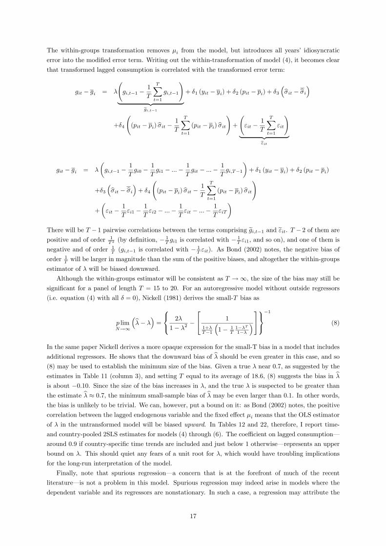
The within-groups transformation removes µi from the model, but introduces all years’ idiosyncratic

error into the modified error term. Writing out the within-transformation of model (4), it becomes clear

that transformed lagged consumption is correlated with the transformed error term:

git − gi = λ

(gi,t−1 −

1

T

T∑t=1

gi,t−1

)︸ ︷︷ ︸

g̃i,t−1

+ δ1 (yit − yi) + δ2 (pit − pi) + δ3

(σ̂it − σ̂i

)

+δ4

((pit − pi) σ̂it −

1

T

T∑t=1

(pit − pi) σ̂it

)+

(εit −

1

T

T∑t=1

εit

)︸ ︷︷ ︸

ε̃it

git − gi = λ

(gi,t−1 −

1

Tgi0 −

1

Tgi1 − ...−

1

Tgit − ...−

1

Tgi,T−1

)+ δ1 (yit − yi) + δ2 (pit − pi)

+δ3

(σ̂it − σ̂i

)+ δ4

((pit − pi) σ̂it −

1

T

T∑t=1

(pit − pi) σ̂it

)

+

(εit −

1

Tεi1 −

1

Tεi2 − ...−

1

Tεit − ...−

1

TεiT

)There will be T − 1 pairwise correlations between the terms comprising g̃i,t−1 and ε̃it. T − 2 of them are

positive and of order 1T 2 (by definition, −

1T gi1 is correlated with −

1T εi1, and so on), and one of them is

negative and of order 1T (gi,t−1 is correlated with − 1

T εit). As Bond (2002) notes, the negative bias of

order 1T will be larger in magnitude than the sum of the positive biases, and altogether the within-groups

estimator of λ will be biased downward.

Although the within-groups estimator will be consistent as T →∞, the size of the bias may still besignificant for a panel of length T = 15 to 20. For an autoregressive model without outside regressors

(i.e. equation (4) with all δ = 0), Nickell (1981) derives the small-T bias as

p limN→∞

(λ̂− λ

)=

2λ

1− λ2−

1

1+λT−1

(1− 1

T1−λT1−λ

)−1

(8)

In the same paper Nickell derives a more opaque expression for the small-T bias in a model that includes

additional regressors. He shows that the downward bias of λ̂ should be even greater in this case, and so

(8) may be used to establish the minimum size of the bias. Given a true λ near 0.7, as suggested by the

estimates in Table 11 (column 3), and setting T equal to its average of 18.6, (8) suggests the bias in λ̂

is about −0.10. Since the size of the bias increases in λ, and the true λ is suspected to be greater than

the estimate λ̂ ≈ 0.7, the minimum small-sample bias of λ̂ may be even larger than 0.1. In other words,

the bias is unlikely to be trivial. We can, however, put a bound on it: as Bond (2002) notes, the positive

correlation between the lagged endogenous variable and the fixed effect µi means that the OLS estimator

of λ in the untransformed model will be biased upward. In Tables 12 and 22, therefore, I report time-

and country-pooled 2SLS estimates for models (4) through (6). The coeffi cient on lagged consumption–

around 0.9 if country-specific time trends are included and just below 1 otherwise– represents an upper

bound on λ. This should quiet any fears of a unit root for λ, which would have troubling implications

for the long-run interpretation of the model.

Finally, note that spurious regression– a concern that is at the forefront of much of the recent

literature– is not a problem in this model. Spurious regression may indeed arise in models where the

dependent variable and its regressors are nonstationary. In such a case, a regression may attribute the

17

variables’similar but unrelated evolution over time to a relationship amongst the variables. In fact, as

I’ll show in section (4.3), both my dependent variable g and several of the explanatory variables are

nonstationary in levels. Because these I(1) variables are cointegrated, however (see Section (4.3)), the

relationships estimated amongst these variables are not spurious; and as Pesaran and Shin (1999) and

Bentzen and Engsted (2001) demonstrate, the ADL model remains valid.

4.2 System GMM

To address the bias generated by the inclusion of lagged endogenous variables in models such as (4), the

dynamic panel literature has come up with several alternative estimators. The first of these was Anderson

and Hsiao’s (1981) estimator, which in this case calls for differencing the model and then using the second

lag of the level of consumption as an instrument for the included endogenous variable, which has been

transformed into the first lag of differenced consumption. This instrument should be both relevant and

exogenous, as gi,t−2 is correlated with ∆gi,t−1 = gi,t−1 − gi,t−2 by definition but uncorrelated (providedthe model is properly specified) with the contemporary error term ∆εit = εit−εi,t−1. Subsequent papers(e.g., Holtz-Eakin, Newey and Rosen 1988 and Arellano and Bond 1991) pointed out that all lags of the

endogenous variable beyond the first should be independent of the contemporary differenced error term,

and that this independence could be exploited using GMM.

Even more moment conditions were suggested by Ahn and Schmidt (1995) and Arellano and Bover

(1995)– nonlinear moment conditions in the case of Ahn and Schmidt, and "levels" moment conditions

in the case of Arellano and Bover. These latter "levels" moment conditions are particularly useful in

cases where the coeffi cient on the lagged endogenous variable is near 1, which is exactly the case at

hand. In such a situation, Blundell and Bond (1998) point out, the included endogenous variable’s level

provides little information about its future evolution, and so lags of the endogenous variable are weak

instruments. By contrast, lagged differences of the included endogenous variable will be informative

about its future level, and this relationship can be used to construct a set of moment conditions for the

non-differenced model. Combining these "levels" moment conditions with Arellano and Bond’s (1991)

"difference" moment conditions yields the "system GMM" estimator. Blundell, Bond, and Windmeijer

(2000) show using Monte Carlo simulations that system GMM is more precise and less biased than

difference GMM when λ is high and the model includes outside regressors.

I therefore construct a system GMM estimator for (4) based on these difference and level moment

conditions, as well as on additional "IV-style" moment conditions based upon the outside instruments

for the gasoline price and price-volatility interaction term:

Difference moment conditions: E [gi,t−k∆εit] = 0, k = 2, ..., T (9)

Levels moment conditions: E [(µi + εit) ∆gi,t−1] = 0 (10)

IV-style moment conditions: E [∆wit∆εit] = 0 ∀ t and E [witεit] = 0 ∀ t (11)

where w represents each of the price instruments discussed in Section 4.1.1. The validity of the difference

moment conditions requires that the εit are not serially correlated; the levels moment conditions further

require that the relationship between git and the fixed effect µi is constant over time; and the IV-style

moment conditions require that each w fulfills the standard conditions for 2SLS instruments.

Estimates based on this system GMM estimator, computed in Stata using Roodman’s (2011) xtabond2,

are reported in Tables 13 (USD) and 24 (local currencies). The two-step version of the system GMM

estimator is known to produce downward-biased standard errors (Arellano and Bond 1991, Blundell and

Bond 1998), so I apply Windmeijer’s (2005) correction. To address the problem of overfitting, which

18

arises in difference and system GMM when moment conditions proliferate (Roodman 2006, 2007), I also

report a version in which the difference moment conditions are restricted to k = 2, 3, 4 and a version

based on a ‘collapsed’instrument matrix. The meaning and implications of collapsing the instrument

matrix are discussed in Roodman (2007).

Discussion of the system GMM results is postponed to Section 5. For now, note that addressing

the endogeneity of lagged consumption has cost us considerable precision. Few of the coeffi cients in the

system GMM estimates differ significantly from 0, even those coeffi cients that the least-squares estimates

found to be highly significant. Despite the bias inherent in estimates that do not specifically address the

endogeneity of gi,t−1, therefore, these methods are more informative– and probably preferable, as the

nature of the bias is known.

4.3 Heterogeneous Coeffi cients and the Error-Correction Model

Neither the least-squares nor the GMM methods discussed above allow for cross-country heterogeneity

in the coeffi cients. If coeffi cients indeed vary by country and regressors are autocorrelated, then, as

Pesaran and Smith (1995) prove, estimators that assume homogeneity will be biased and inconsistent.

In particular, fixed-effects models such as (4), which constrain all coeffi cients except the country-fixed

effects to be the same across countries, will produce downward-biased estimates for the coeffi cients on the

outside regressors (δ1, ..., δ4). The fixed-effects model will also yield a biased estimate of the coeffi cient on

the lagged endogenous variable (λ), the direction of which will be positive if the autocorrelations of the

other regressors are positive. These biases do not go away as the sample size and sample period increase,

and their practical effect will be to exaggerate the difference between short- and long-run responses. The

intuition for this practical effect is simple: if the coeffi cient on lagged consumption is biased upward, the

speed of adjustment will appear slower, and this will magnify artificially-small short-run responses into

artificially-large long-run responses.

If regressors are I(1), moreover, these biases are potentially severe. As the autocorrelation coeffi cient

of an outside regressor approaches a unit root, Pesaran and Smith (1995) show, the estimator for the

coeffi cient on the lagged endogenous variable converges in probability to 1, while the estimators for the

coeffi cients on the outside regressors converge to 0. Many of my regressors are in fact I(1), as I’ll show

shortly, and so the consequences of coeffi cient heterogeneity are potentially grave.

To address the problem of coeffi cient heterogeneity, Pesaran, Shin and Smith (1999) suggest a pooled-

mean group (PMG) estimator that allows short-run responses to vary across individuals. Since the PMG

estimator and its alternatives are derived and discussed in the literature in terms of an error-correction

model, I turn to an ECM model of gasoline demand– the unrestricted version of which is equivalent to

an ADL(1,1). To demonstrate the relationship between the former ADL(1,0) specification and the ECMand the ECM’s equivalence to an ADL(1,1), I first re-write the existing model (4) to allow coeffi cientsto vary by country:

git = λigi,t−1 + δ1iyit + δ2ipit + δ3iσ̂it + δ4i (σ̂p̃)it + µi + εit (12)

(For notational simplicity, define p̃it = pit − pi.) Next, subtracting gi,t−1 from each side of (12), then

adding and subtracting δ1iyi,t−1, δ2ipi,t−1, δ3iσ̂i,t−1, and δ4iσ̂p̃i,t−1 from the right-hand side, yields

∆git = (λi − 1) gi,t−1 + δ1iyi,t−1 + δ2ipi,t−1 + δ3iσ̂i,t−1 + δ4i (σ̂p̃)i,t−1

+δ1i∆yit + δ2i∆pit + δ3i∆σ̂it + δ4i∆ (σ̂p̃)it + µi + εit

19

which can be factored into

∆git = − (1− λit)︸ ︷︷ ︸φi

gi,t−1 − δ1i1− λi︸ ︷︷ ︸θ1i

yi,t−1 −δ2i

1− λi︸ ︷︷ ︸θ2i

pi,t−1 −δ3i

1− λi︸ ︷︷ ︸θ3i

σ̂i,t−1 −δ4i

1− λi︸ ︷︷ ︸θ4i

(σ̂p̃)i,t−1

(13)

+δ1i∆yit + δ2i∆pit + δ3i∆σ̂it + δ4i∆ (σ̂p̃)it + µi + εit

This is an ECM with no coeffi cient-homogeneity restrictions, but it can be factored just as easily into

ADL(1,1) form:

git = (φi + 1) gi,t−1 + δ1iyit − (φiθ1i + δ1i) yi,t−1 + δ2ipit − (φiθ2i + δ2i) pi,t−1 (14)

+δ3iσ̂it − (φiθ3i + δ3i) σ̂i,t−1 + δ4i (σ̂p̃)it − (φiθ4i + δ4i) (σ̂p̃)i,t−1 + µi + εit

Estimates based on the ECM differ from those based on ADL(1,0) by virtue of slightly different underlyingmodels, therefore, as well as by different coeffi cient-homogeneity restrictions.

In the unrestricted ECM given by (13), the new coeffi cient φi is the error-correction term. It should

be negative, and its magnitude is the speed of adjustment, or the portion of long-run adjustment that

takes place during the first period after a change in one of the regressors. The new coeffi cients θ1i through

θ4i are long-run elasticities, and as before the coeffi cients δ1i through δ4i are short-run elasticities.

Although Pesaran, Shin and Smith’s (1999) estimator allows regressors to be I(0) or I(1), it does re-

quire a cointegrating relationship among I(1) variables– that is, it requires a stable long-run relationship

between the dependent and explanatory variables. Before checking for cointegration, I check the order

of integration of each of my variables.

The classical tests for a unit root in a single time series are the Dickey-Fuller and Augmented Dickey-

Fuller, which test for the stationarity of an AR(1) and an AR(p) process, respectively. The Dickey-Fuller

tests H0 : ρ− 1 = 0 (nonstationarity) vs. Ha : |(ρ− 1)| < 0 (stationarity) in the transformed model

∆xt = (ρ− 1)xt−1 + (α0 + α1t) + εt

whereas the Augmented Dickey-Fuller uses the same null and alternative hypotheses for the transformed

model

∆xt = (ρ− 1)xt−1 +

p−1∑i=j

βi∆xt−j + (α0 + α1t) + εt

Alternately, the Phillips-Perron (1988) test makes it possible to test for nonstationarity in an AR(p)

process without knowing p. In this test, corrections for serial correlation in εt allow ρ̂ estimated for an

AR(1) to be used to to test ρ = 1 for any AR(p).

When x is a panel variable, the cross-section dimension introduces several complications, which

have prompted the development of a variety of panel unit root tests.4 One complication is whether to

consider a single autocorrelation coeffi cient for the panel as a whole or to consider each individual i as

a separate time series with its own coeffi cient ρi. Tests taking the former route include Levin, Lin, and

Chu (2002) and Harris and Tzavalis (1999). Tests taking the latter route include Im, Pesaran and Shin

(2003), Maddala and Wu (1999) and Choi (2001), all of which involve performing a separate test for

each individual and aggregating the results. Im, Pesaran and Shin (2003) perform this aggregation by

averaging the test statistics for individual (A)DF tests; Maddala and Wu (1999) and Choi (2001) perform

the aggregation over the p-values associated with (A)DF or other individual unit root tests. These tests

4For a thorough overview of these tests, see Baltagi and Kao (2000).

20

based on p-values are known collectively as Fisher-type tests, and weigh a null hypothesis that all panels

are nonstationary against the alternative that one or more panels are stationary.

To explore the order of integration of my variables, I use a Fisher-type test based on individual

Phillips-Perron tests, with and without a trend. The choice of the Phillips-Perron test protects my

results from the ADF’s sensitivity to the choice of lag length p. The choice of a Fisher-type test has the

advantages of high power compared to tests based on ADF test statistics (Choi 2001) and, crucially, the

flexibility to deal with series whose length varies across individuals. Results of these tests, performed

using Stata’s (2009) xtunitroot, are reported in Tables 4 and 5. Where the test does not reject a variable’s

nonstationarity in levels, I repeat the test on first differences. In each instance the second test does reject

nonstationarity, and so for the USD-denominated variables I am able to conclude that volatility is I(0)

with or without trend and the remaining variables are I(1) with or without trend. For the common-

currency variables, results are somewhat different: g and p are I(1) with or without trend; y is I(1)

without trend and I(0) with; and σ̂ and σ̂p̃ are I(0) with or without trend.

Table 4: Fisher-style Phillips-Perron unit root tests, currency in USD

Without trendsLevel First Difference

Variable Test Statistic* P-Value Test Statistic* P-Value Order of Integrationg 68.0062 0.1732 364.1834 0.0000 I(1)p 17.8696 1.0000 148.7426 0.0000 I(1)y 11.8702 1.0000 220.1072 0.0000 I(1)σ̂ 190.6238 0.0000 I(0)σ̂p̃ 19.1043 1.0000 199.4135 0.0000 I(1)

With time trendsLevel First Difference

Variable Test Statistic* P-Value Test Statistic* P-Value Order of Integrationg 71.6704 0.1071 507.0169 0.0000 I(1)p 14.6156 1.0000 136.2582 0.0000 I(1)y 24.2946 1.0000 156.7488 0.0000 I(1)σ̂ 195.1116 0.0000 I(0)σ̂p̃ 12.0569 1.0000 211.9994 0.0000 I(1)

*Inverse χ2 with 58 degrees of freedom.Phillips-Perron tests conducted using 3 lags for the Newey-West standard errors.

Since a regression involving nonstationary variables may be spurious, and since Pesaran, Shin and

Smith’s (1999) estimator requires cointegration of any I(1) variables, I turn now to checking for cointe-

gration. One approach to cointegration testing involves estimating a static model and then checking the

residuals for nonstationarity. This was in fact the first approach to cointegration testing, introduced by

Engle and Granger (1987) for single time series and later adapted to panels by Kao (1999) and others.

Pedroni (2004) expanded this two-step, residual-based approach to allow for cross-sectional heterogeneity

of coeffi cients. Meanwhile, a second approach to cointegration testing has been to check whether the

error-correction term in an ECM– e.g., φi in (13), or αi in (15)– is zero. Banerjee, Dolado and Mestre

(1998) develop this approach for single time series, and Westerlund (2007) adapts it to panels, basing

his tests on a model of the form

∆yit = αiyi,t−1 + λ′

ixi,t−1 +

qi∑j=1

αij∆yi,t−j +

qi∑j=0

γ′

ij∆xi,t−j + µi + πit+ εit (15)

21

Table 5: Fisher-style Phillips-Perron unit root tests, local currencies

Without trendsLevel First Difference

Variable Test Statistic* P-Value Test Statistic* P-Value Order of Integrationg 68.0062 0.1732 364.1834 0.0000 I(1)p 72.0861 0.1010 343.6998 0.0000 I(1)y 21.1883 1.0000 412.3704 0.0000 I(1)σ̂ 313.8033 0.0000 I(0)σ̂p̃ 183.9754 0.0000 I(0)

Fisher-style unit root tests on modelsWith time trendsLevel First Difference

Variable Test Statistic* P-Value Test Statistic* P-Value Order of Integrationg 71.6704 0.1071 507.0169 0.0000 I(1)p 81.6818 0.0219 316.9540 0.0000 I(1)y 165.6083 0.0000 I(0)σ̂ 450.9815 0.0000 I(0)σ̂p̃ 229.8273 0.0000 I(0)

*Inverse χ2 with 58 degrees of freedom.Phillips-Perron tests conducted using 3 lags for the Newey-West standard errors.

where x and y comprise the variables to be examined for possible cointegration. Westerlund’s approach

has the advantages of high power and flexibility: not only does it allow cross-sectional heterogeneity

in coeffi cients, but, unlike the two-step residual-based approaches, it does not impose a common factor

restriction on the relationship between short- and long-run adjustment. For these reasons I choose

Westerlund’s test to check for cointegration of my I(1) variables.

Westerlund’s (2007) test actually has several varieties. The "group mean" variety (G) allows the

error-correction term to vary across individuals, and tests against the alternative hypothesis that the

error-correction term is smaller than zero for at least one individual; the "panel" variety (P ), by contrast,

constrains the error-correction term to be the same across individuals, testing against the alternative

hypothesis that this single term is smaller than zero. In both cases, the null hypothesis is that the

error-correction term is zero, and that the variables in question are not cointegrated. Given my small

sample size, the extra precision afforded by constraining the error-correction term to be constant across

countries appears to be important, and so I focus on this variety. For each of these varieties, Westerlund

suggests two different test statistics: a t-statistic version, denoted with the subscript τ , which is simply

the estimated error-correction term divided by its standard error (or, for the group mean version, the

average of these quotients); and a less intuitive version, denoted with the subscript α, that controls for

the panel length T(i). I report both of these test statistics.

Tests are performed in Stata with Persyn and Westerlund’s (2008) xtwest, using standard errors

that have been bootstrapped to allow cross-sectional dependence (see Westerlund 2007 and Persyn and

Westerlund 2008). Results are reported in Tables 6 and 7. Note that some countries’series are insuffi -

ciently long to be used in certain versions of the tests; these omissions are listed in the tables. Using the

panel-variety tests, I can clearly reject the hypothesis of non-cointegration of the I(1) variables in the

local-currency version of the model. In the common-currency version, the panel-variety tests reject the

hypothesis of non-cointegration provided that the lag qi in (15), chosen for each country using the AIC,

22

is allowed to be as high as 2.5 ,6

Table 6: Cointegration tests, USD

Variables Lag length qi Omitted Test Value P-Value Bootstrappeda

Countries p-valueg, y, p, σ̂p̃ Chosen by AIC Czech Republic Gτ -0.036 1.000 1.000

from 0 and 1 Gα -0.203 1.000 1.000Pτ -1.431 1.000 0.720Pα -0.427 0.999 0.730

g, y, p, σ̂p̃ Chosen by AIC Australia, Czech Republic, Gτ -1.991 0.103 0.390from 0-2 Hungary, Mexico, Poland, Gα -0.057 1.000 0.630

Spain, Sweden, Turkey Pτ -0.144 1.000 0.010Pα -0.051 0.999 0.010

g, y, p, σ̂p̃ Chosen by AIC Australia, Czech Republic, Gτ -0.071 1.000 0.990from 0 and 1 Hungary, Mexico, Poland, Gα -0.091 1.000 1.000

Spain, Sweden, Turkey Pτ -1.708 1.000 0.580Pα -0.566 0.996 0.560

a100 draws

Table 7: Cointegration tests, local currencies

Variables Lag length qi Omitted Countries Test Value P-Value Bootstrappeda

p-valueg, y, p Chosen by AIC none Gτ -1.460 0.344 0.340

from 0 and 1 Gα -3.833 0.975 0.320Pτ -9.074 0.001 0.000Pα -3.501 0.136 0.050

g, y, p Chosen by AIC none Gτ -1.540 0.207from 0-2 Gα -3.244 0.995

Pτ -9.074 0.001Pα -3.501 0.136

g, y, p Chosen by AIC Australia, Hungary, Poland, Gτ -1.311 0.627 0.420from 0-3 Spain, Sweden, Turkey Gα -0.961 1.000 0.260

Pτ -6.129 0.109 0.000Pα -2.520 0.492 0.000

a100 draws

Given this evidence that a long-run relationship amongst the variables of my model does exist, I

move on to estimating the ECM. Pesaran, Shin and Smith’s (1999) pooled mean group estimator uses

maximum likelihood, based on the assumption that the εit are independent and normal, to estimate

∆yit = φi

[gi,t−1 − θ1yi,t−1 − θ2pi,t−1 − θ3σ̂i,t−1 − θ4 (σ̂p̃)i,t−1

](16)

+δ1i∆yit + δ2i∆pit + δ3i∆σ̂it + δ4i∆ (σ̂p̃)it + µi + εit

5Allowing qi to be as high as 2, unfortunately, forces me to drop several countries from the sample. It does not appearto be the omission of these countries that is responsible for the rejection of non-cointegration, however, as running the testfor qi ≤ 1 with the same countries omitted does not lead to rejection.

6Persyn and Westerlund (2008) observe that the Westerlund tests are sensitive to their specification in "small" Tsituations. As my T is only two thirds that of Persyn and Westerlund’s example, and I am attempting to test forcointegration amongst a larger number of variables, I suspect that my inability to reject non-cointegration in certainspecifications (e.g., qi ≤ 1) arises from this sensitivity and relatively low power, and not from a lack of a long-run relationshipamongst the variables. The strong rejection of non-cointegration amongst the local-currency variables, moreover, suggeststhat a cointegrating relationship does exist.

23

Table 8: Restrictions on the error-correction model

Model RestrictionsPooled mean-group (PMG) Long-run parameters homogenous:

θ1i = θ1,θ2i = θ2,θ3i = θ3,θ4i = θ4Mean-Group (MG) None

Dynamic Fixed-Effect (DFE) All parameters homogenous:θ1i = θ1,θ2i = θ2,θ3i = θ3,θ4i = θ4;

δ1i = δ1, δ2i = δ2, δ3i = δ3, δ4i = δ4;φi = φ

Note that (16) is simply the general ECM from (13) with the long-run coeffi cients θ1i, θ2i, θ3i, and θ4iconstrained to be equal across individuals.

The resulting pooled mean group estimates are reported in Tables 14, 15, and 25. Table 14 reports

results for all countries; Table 15 reports results when the four countries with the worst fit from the

ADL are omitted. The short run elasticities (δ̂1 through δ̂4) reported in these tables are the means of

the country-specific short-run elasticities; individual short-run elasticities are reported in Appendix 10.

To examine the value of the assumption that the long-run coeffi cients are homogenous (which dras-

tically reduces the number of parameters to be estimated), I also report mean group estimates of the

ECM model. The mean group estimator simply estimates (13) separately for each country and forms an

average of the resulting coeffi cient estimates. To examine the value and cost of restricting both the long-

and the short-run coeffi cients to be homogenous, as the ADL inherently did, I also estimate a dynamic

fixed-effects version of the ECM. The restrictions imposed by these various estimators are summarized

in Table 8. Results are reported alongside the PMG results.

All estimates of the ECM– pooled mean groups, mean groups, and dynamic fixed-effects– are com-

puted in Stata using Blackburne and Frank’s (2007b) xtpmg.

5 Results and Discussion

Results, particularly with respect to the habits-related parameters, vary considerably across these model

specifications and estimation methods. Although each approach does have its advantages (summarized

in Table 9), not all the advantages are equal; and after weighing each approach’s advantages and disad-

vantages, my preference is for the pooled mean group estimates of the error-correction model.

Table 9: Advantages of various estimation approaches

Fixed-effects 2SLSwith instrumenting GMM Pooled mean group

Advantage for price estimator of ECMCorrects for endogeneity of prices XAddresses endogeneity of gt−1 XAddresses coeffi cient heterogeneity XPrecision X X

5.1 Least-Squares Estimates of the ADL Model

The unique advantage of the fixed-effects estimator of the ADL model is that it allows me to use outside

instruments to address the endogeneity of the price variables. In practice, however, it is not clear that

24

instrumenting for prices is very valuable. Tests for endogeneity7 do, by and large, reject that prices

are exogenous, and may or may not, depending on the specification of the trend, reject that price and

the price-volatility interaction are jointly exogenous. The instruments used to address the apparent

endogeneities, moreover, do appear to be relevant, as underidentification is rejected8 no matter how the

trend is specified. The problems arise when it comes to the instruments’ exogeneity: overidentifying

restrictions tests strongly reject that all the instruments are exogenous. The endogeneity, it becomes

clear when the regressions are re-run using subsets of the instruments, lies in the instruments based on

crude oil prices. Unfortunately, omitting the crude-oil instruments and basing price identification solely

on the tax instruments yields estimates that are nonsensical and uninformative, with most coeffi cients’

p-values around 0.9.

In theory, it’s possible that an instrument that is not perfectly exogenous may nonetheless remove

some of the instrumented variable’s endogeneity, and therefore retain some value. Alas, this is not such

a case. Any endogeneity in the price should bias its coeffi cient upwards towards 0, and yet the price

coeffi cients in the non-instrumented ADL models (Table 10) are more negative than their instrumented

counterparts. The implied long-run price elasticity from the instrumented version of the individual-trend

model, moreover, is of a smaller magnitude than the long-run elasticity estimated using PMG on the

error-correction model. Though price endogeneity is an issue, it appears we are better off ignoring it than

addressing it– or, rather, better off merely acknowledging it than addressing it using the instruments at

hand.

The actual fixed-effects 2SLS estimates, it should be noted, are nonsensical unless country-specific

trends are included. With no trend or a homogenous trend, prices have no statistically-significant

effect; and with no trend, even income does not have a statistically-significant effect. Moreover, none

of the fixed-effects 2SLS results– common or local currency, with or without any type of trend– finds

the rational-habits variables, σ̂ and σ̂p̃, to have a statistically-significant effect. Although this might

ordinarily be taken as a sign that σ̂ and σ̂p̃ are not relevant to gasoline demand, the weakness of the

price and income effects suggests that the estimated effects of σ̂ and σ̂p̃ should not be trusted, either.

Overall, I discount the findings of the fixed-effects 2SLS estimator of the ADL.

5.2 System GMM Estimates of the ADL Model

The unique advantage of the system GMM estimator is that it addresses the endogeneity of lagged con-

sumption. That endogeneity should, as previously discussed, bias the coeffi cient on lagged consumption

upward, and therefore make adjustment seem slower than it truly is. As expected, the system GMM

estimates of λ are higher than the least-squares estimates. Troublingly, in fact, the GMM estimates of λ

are in most cases higher than 1. But although these estimates have been pushed upward by the removal

of a downward bias, they have also been pushed upward by the GMM estimator’s own shortcomings.

One of these shortcomings is that the system GMM estimator, like the least-squares estimator, imposes

homogeneity of coeffi cients across countries. Given that the other regressors are positively autocorre-

lated, this will lead to an upward bias on λ̂ (Pesaran and Smith 1995). Another shortcoming is that,

unlike the least-squares estimator, the system GMM estimator does not allow me to identify a model with

country-specific trends,9 which in the least-squares case reduced λ̂ considerably. The GMM estimator

merely trades one bias for another, therefore, and it does so at an incredibly high cost of precision: in

7That is, difference-in-Sargan/Hansen tests comparing a regression in which the variable(s) in question are treated asendogenous to a regression in which they are assumed to be exogenous.

8Kleibergen-Paap (2006) tests are used to test for underidentification.9Country-specific trends require the estimation of an extra 28 parameters, which system GMM cannot handle given my

sample size.

25

Table 10: Within-groups (fixed-effects) estimates, USD

(1) (2) (3)No Common Individualtrend trend trends

gt−1 λ 0.911** 0.888** 0.727**(0.0249) (0.0230) (0.0372)

[0.000] [0.000] [0.000]

y δ1 0.0404+ 0.105** 0.183**(0.0217) (0.0233) (0.0318)

[0.064] [0.000] [0.000]

p δ2 -0.117** -0.135** -0.198**(0.0312) (0.0299) (0.0331)

[0.000] [0.000] [0.000]

σ̂ δ3 -0.178+ -0.0470 -0.0592(0.0931) (0.0904) (0.0792)

[0.056] [0.604] [0.455]

σ̂p̃ δ4 0.260 0.263 -0.00520(0.288) (0.275) (0.244)

[0.367] [0.340] [0.983]

t -0.00426**(0.000524)

[0.000]

R2 0.891 0.904 0.938Robust standard errors in parentheses;

P-values in brackets.

** p<0.01, * p<0.05, + p<0.1

26

Table 11: Within-groups (fixed effects) estimates with 2SLS instrumenting for price, USD

(1) (2) (3)No trend Common trend Individual trends

gt−1 λ 0.941** 0.922** 0.681**(0.0288) (0.0274) (0.0417)

[0.000] [0.000] [0.000]

y δ1 0.0347 0.0770** 0.196**(0.0251) (0.0265) (0.0368)

[0.167] [0.004] [0.000]

p δ2 0.0479 0.0361 -0.168**(0.101) (0.0928) (0.0520)

[0.635] [0.698] [0.001]

σ̂ δ3 0.283 0.342 0.0906(0.318) (0.295) (0.142)

[0.374] [0.248] [0.525]

σ̂p̃ δ4 -2.313 -2.062 -0.868(1.572) (1.442) (0.680)

[0.142] [0.153] [0.202]

t -0.00364** [country-specific(0.000550) trends][0.000]

R2 0.871 0.886 0.934

Implied long-run elasticities

y δ11−λ 0.585 0.983* 0.614**

(0.462) (0.422 ) ( 0.125)

[0.207] [0.020 ] [0.000]

p δ21−λ 0 .807 0.460 -0.528**

(1.762) (1.208) (0.165)

[0.647] [0.703] [0.001]

Tests

Endogeneity: 4.081 0.297 7.396pricea [0.0434] [0.5859] [0.0065]

Endogeneity: 4.230 4.477 7.675price & interactionb [0.1206] [0.1066] [0.0215]

Underidentificationc 8.159 8.341 19.689[0.0428] [0.0395] [0.0002]

Exogeneityd 22.997 7.175 7.919[0.000] [0.0277] [0.0191]

Robust standard errors in parentheses; p-values in brackets.

** p<0.01, * p<0.05, + p<0.1aDifference-in-Sargan/Hansen χ2(1) under H0.bDifference-in-Sargan/Hansen χ2(2) under H0.cKleibergen-Paap (2006) rk statistic; χ2(3) under H0.dOveridentifying restrictions test (Hansen J statistic); χ2(2) under H0.

27

Table 12: Pooled estimates with 2SLS instrumenting for prices, USD

(1) (2) (3)No trend Common Individual

trend trends

gt−1 λ 0.997** 0.991** 0.924**(0.00957) (0.00910) (0.0143)

[0.000] [0.000] [0.000]

y δ1 -0.00216 0.00318 0.0569**(0.00879) (0.00834) (0.0122)

[0.806] [0.703] [0.000]

p δ2 -0.0292* -0.0341* -0.0806**(0.0140) (0.0134) (0.0181)

[0.037] [0.011] [0.000]

σ̂ δ3 -0.0575 -0.0309 -0.0247(0.0957) (0.0953) (0.0889)

[0.548] [0.746] [0.781]

σ̂p̃ δ4 -0.260 0.0969 0.201(0.209) (0.224) (0.228)

[0.213] [0.666] [0.379]

t -0.00223** [country-specific(0.000503) trends][0.000]

R2 0.996 0.996 0.997Robust standard errors in parentheses;

p-values in brackets.

** p<0.01, * p<0.05, + p<0.1

28

nearly all variants of the system GMM estimator, in fact, λ̂ is the only coeffi cient that’s statistically

significantly different from 0. Overall, the system GMM estimates are useless in this application.

Table 13: System GMM, USD

(1) (2) (3) (4) (5) (6) (7) (8)No trend With trend No trend With trend No trend With trend

Collapsed Collapsed Reduced Reduced No outside No outside

No trend With trend IV matrix IV matrix IV count IV count IVs IVs

gt−1 λ 1.031** 1.010** 1.085** 1.055** 1.042** 1.032** 0.995** 0.966**(0.0331) (0.0240) (0.0532) (0.0693) (0.0402) (0.0326) (0.0359) (0.0337)

[0.000] [0.000] [0.000] [0.000] [0.000] [0.000] [0.000] [0.000]

y δ1 -0.0394+ -0.0177 -0.0451 -0.0116 -0.0445 -0.0158 -0.000187 0.0354(0.0220) (0.0168) (0.0432) (0.0325) (0.0262) (0.0190) (0.0302) (0.0327)

[0.084] [0.301] [0.306] [0.725] [0.101] [0.414] [0.995] [0.288]

p δ2 0.0233 -0.00381 0.0740 0.0435 0.0345 0.0139 -0.0758 -0.108**(0.0383) (0.0282) (0.0624) (0.0633) (0.0478) (0.0328) (0.0485) (0.0380)

[0.548] [0.894] [0.246] [0.498] [0.476] [0.675] [0.129] [0.008]

σ̂ δ3 -0.145 -0.0776 0.0843 0.160 -0.0232 0.0671 -0.133 -0.0168(0.123) (0.121) (0.204) (0.225) (0.146) (0.155) (0.0890) (0.108)

[0.248] [0.527] [0.683] [0.483] [0.875] [0.668] [0.145] [0.877]

σ̂p̃ δ4 -0.201 0.119 -0.824 -0.450 -0.421 -0.103 0.237 0.563(0.296) (0.263) (0.592) (0.651) (0.318) (0.341) (0.346) (0.340)

[0.503] [0.653] [0.175] [0.496] [0.196] [0.765] [0.498] [0.109]

t -0.00215* -0.00280 -0.00276* -0.00367*(0.00103) (0.00175) (0.00106) (0.00142)

[0.046] [0.120] [0.014] [0.015]

Sargan 377.2 368.4 97.30 86.25 267.3 253.3 427.4 391.3Sargan df 169 168 17 16 64 63 165 164Sargan P 0.000 0.000 0.000 0.000 0.000 0.000 0.000 0.000Hansen 25.39 23.91 22.65 23.51 25.89 22.26 26.10 25.42Hansen df 169 168 17 16 64 63 165 164Hansen P 1 1 0.161 0.101 1.000 1.000 1 1AR(2) test -0.522 -0.495 -0.596 -0.556 -0.550 -0.528 -0.283 -0.304AR(2) P 0.602 0.621 0.551 0.578 0.582 0.597 0.778 0.761

Standard errors in parentheses; p-values in brackets.

** p<0.01, * p<0.05, + p<0.1

5.3 Error-Correction Model

Turning to the error correction model, note that pooled mean group, mean group, and dynamic fixed

effects estimators are all affected by the endogeneity of lagged consumption, just as the least squares

estimators of the ADL were. It would be ideal to correct for the resulting biases, and this may become

possible as relevant bias corrections are developed in the literature. At the moment, however, it does not

seem that appropriate corrections have been derived. Bias corrections for the (not-pooled) mean group

estimator are worked out in Pesaran and Zhao (1999); these corrections perform well when λ < 0.8

29

but not at all when λ ≥ 0.8, which appears likely in the case of gasoline demand. Moreover, the

assumption of homogeneity of the long-run coeffi cients appears to be important in this application (as

will be discussed shortly), and so a mean group estimator that allows heterogeneity of the long-run

coeffi cients is inappropriate. Recent work by Choi, Mark and Sul (2010) offers bias corrections that

constrain the long-run coeffi cients to be homogenous, but unfortunately they also constrain the short-

run coeffi cients and speed of adjustment to be homogenous. For now, I will have to accept estimates of

the ECM (and ADL) as they are.

Despite the endogeneity of gt−1, pooled mean group estimates of the ECM yield reasonable results.

As expected, the speed of adjustment implied by PMG estimates based on all countries (with or without

trend) is slightly faster than the speed of adjustment implied by 2SLS on the ADL. This is because

the PMG approach is not susceptible to the false assumption of coeffi cient homogeneity that biases the

2SLS estimate of λ upward. Similarly, the PMG estimates of the error-correction model imply slightly

faster adjustment than their DFE (dynamic fixed effects) counterparts. (That is, the PMG estimates of

the error-correction term φ are more negative than the DFE estimates.) Although the PMG estimates

imply slightly faster adjustment, however, the difference is not so great as to beggar belief. The pooled

2SLS estimates of the ADL (Table 12) establish lower bounds for the speed of adjustment of 0.3 to 7.6

percent in the first year, and we know that these estimates are biased toward 0 in two ways. In that

light, the speeds of adjustment estimated by PMG– 5.4 to 33.7 percent of adjustment occurring in the

first year– do not seem suspiciously fast.

My preferred specification is, therefore, the pooled mean group estimator of the ECM. The PMG

estimator’s distinct advantage, as has been mentioned, is that by allowing for heterogeneity in the short-

run coeffi cients, it avoids some of the heterogeneity-induced bias of least squares or system GMM. The

PMG estimator does, of course, restrict long-run coeffi cients to be the same across countries; and another

matter to consider is whether this restriction is acceptable. A Hausman test comparing the common-

currency PMG and MG estimates fails to reject the hypothesis that the estimates are equivalent for the

model without trend (p = 0.71) but squarely rejects the equivalence of the models with trend (p = 0.00),

so it is not clear whether the restrictions are entirely true. The effi ciency gains offered by the long-run

restrictions if they are true, however, are huge; and without them, the MG estimator has trouble even

establishing statistically-significant price effects. This is unsurprising, as the MG estimator is based

on individual regressions in which time series of 15 to 19 observations are used to estimate the short-

and long-run effects of four different variables, plus intercept and time trend. The relatively short

length of this panel makes the restrictions necessary, whether or not the long-run coeffi cients are purely

homogenous. On a positive note, PMG does at least introduce a considerable relaxation of homogeneity

in comparison to estimators that assume homogeneity of all coeffi cients; and as Pesaran, Shin and Smith

(1999) observe, PMG is not as sensitive to outliers as MG.

Although PMG is not as sensitive to outliers as MG, it is not entirely insensitive to them, either; and

so in addition to estimates based on all countries in my data set (Table 14), I report estimates omitting

the four countries that consistently suffered the worst fit in least-squares estimates– the Czech Republic,

Poland, Slovakia, and Turkey (Table 15). The latter three countries are, incidentally, the three poorest

in my sample,10 and the Czech Republic is the sixth-poorest. The first three, moreover, were beginning

their political and economic transformations away from communism at the beginning of the sample

period in 1990, and so it is not surprising that their gasoline-consumption patterns would be atypical

of the broader sample. In response to the removal of these four countries, the PMG estimates do in

fact change a bit, with the long-run income, price, and price-volatility interaction elasticities increasing

in magnitude. Unless otherwise noted, the following discussion refers to the PMG estimates with these

10As measured by mean real GDP per capita, USD, over the course of the sample.

30

outlier countries removed.

By and large, my long-run coeffi cients are not out of line with the literature. To facilitate comparisons,

I report estimates of an ECM in the form of (16) with price volatility and the price-volatility interaction

term omitted (Tables 16, 17, and 26). The resulting model contains only the variables standardly

included in gasoline demand models. The PMG estimates of this model, omitting the four worst-fitting

countries (Table 17), suggest a long-run income elasticity of 0.7 to 1. These nearly-unit-elastic estimates

fit neatly within the values usually estimated in the literature. Meanwhile, the estimated long-run price

elasticities, ranging from -0.6 to -1.3, span the middle to upper end (in magnitude) of estimates in the

literature. Although the PMG estimator is more reliable in its long-run than its short-run estimates, the

short-run elasticities in Table 17 are plausible, with short-run income elasticities somewhat lower than

the literature’s averages and short-run price elasticities ranging from low (in magnitude) to average.

Returning to the model that includes the rational-habits variables, long-run results with respect to

income and prices appear, again, reasonable. In the no-trend and homogenous-trend models, long-run

income elasticities of 0.8 and 0.9 closely match the literature. In the same models, long-run "total"

price elasticities are again on the high-magnitude end, hovering around unit elastic. Since these high-

magnitude price elasticities are also found in the "standard" model without the rational-habits variables,

the difference from the literature can be ascribed to my panel data set and the choice of an ECM

with heterogeneous short-run coeffi cients rather than to the inclusion of σ̂ and σ̂p̃. In the model with

heterogeneous trends, results look somewhat different but still plausible, with long-run income elasticity

on the low end and long-run price elasticity near the literature average.

The parameters of primary interest are, of course, the coeffi cients on price volatility and the price-

volatility interaction term, which allow us to test for the behaviors implied by a rational habits model.

The rational habits model implies, first, that price uncertainty should reduce demand for the habit-

forming good, and this is indeed borne out by the regressions: trend or no trend, all countries or all-

but-four, the PMG estimate of the long-run effect of price volatility, θ3, is negative and statistically

significant. Depending on the specification, values of θ̂3 range from −0.7 to −1.9, suggesting that a 0.1

increase in σ̂ is associated with a 7 to 19% reduction in gasoline consumption.

Evidence on rational habits’second implication, that the magnitude of price elasticity should decline

with price uncertainty, is not clear-cut. When a time trend is included in the USD-denominated model,

the PMG estimate of the long-run coeffi cient on the price-volatility interaction term, θ̂4, is not statistically

significant. Absent the trend, θ̂4 is positive and highly significant when the four outlier-countries are

omitted but not statistically significant when they are included.11 Given that these four countries

experienced some of the highest price volatilities in the sample at a time when their economies were

rapidly expanding, it is easy to imagine that they might skew the effect of volatility on price elasticity.

It seems reasonable, therefore, to put greater faith on the estimates of θ̂4 that omit these countries.

Recall the possibility that tax changes might contribute to measured price volatility while actually

decreasing price uncertainty. To check whether this problem is hiding some of the effect of price volatility

on price elasticity, I estimate a version of the model in which before-tax prices are used to construct an

alternative measure of price volatility, σ̂BT . In Table 18 I report results using the before-tax volatility

term a. both in the interaction term and on its own and b. only in the interaction term, with total-price

volatility used on its own. Continuing to use total-price volatility on its own seems reasonable, as rational

habits imply that it is overall price volatility that dampens consumption– that is, high volatility that

11 In the local-currency models (Table 25), as in the USD-denominated models, the coeffi cient on the interaction termis sensitive to the specification of the trend. With no trend, θ̂4 in the local-currency model is not statistically significant;with a homogenous trend, it is very negative; and with heterogenous trends, it is positive. This pattern is, confusinglyenough, nearly opposite to that in the USD-denominated models, where θ̂4 is only positive and statistically significant ifthe trend is excluded.

31

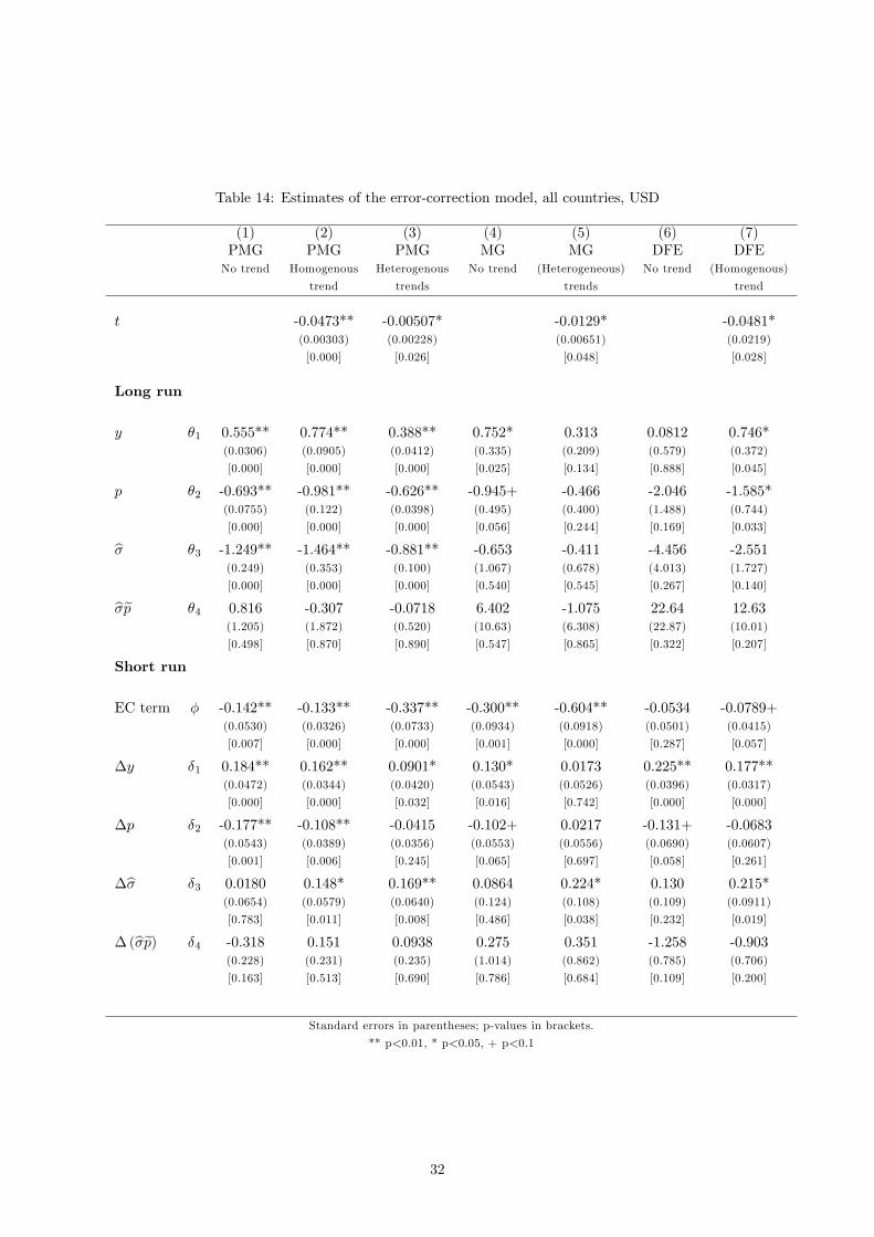
Table 14: Estimates of the error-correction model, all countries, USD

(1) (2) (3) (4) (5) (6) (7)PMG PMG PMG MG MG DFE DFENo trend Homogenous Heterogenous No trend (Heterogeneous) No trend (Homogenous)

trend trends trends trend

t -0.0473** -0.00507* -0.0129* -0.0481*(0.00303) (0.00228) (0.00651) (0.0219)

[0.000] [0.026] [0.048] [0.028]

Long run

y θ1 0.555** 0.774** 0.388** 0.752* 0.313 0.0812 0.746*(0.0306) (0.0905) (0.0412) (0.335) (0.209) (0.579) (0.372)

[0.000] [0.000] [0.000] [0.025] [0.134] [0.888] [0.045]

p θ2 -0.693** -0.981** -0.626** -0.945+ -0.466 -2.046 -1.585*(0.0755) (0.122) (0.0398) (0.495) (0.400) (1.488) (0.744)

[0.000] [0.000] [0.000] [0.056] [0.244] [0.169] [0.033]

σ̂ θ3 -1.249** -1.464** -0.881** -0.653 -0.411 -4.456 -2.551(0.249) (0.353) (0.100) (1.067) (0.678) (4.013) (1.727)

[0.000] [0.000] [0.000] [0.540] [0.545] [0.267] [0.140]

σ̂p̃ θ4 0.816 -0.307 -0.0718 6.402 -1.075 22.64 12.63(1.205) (1.872) (0.520) (10.63) (6.308) (22.87) (10.01)

[0.498] [0.870] [0.890] [0.547] [0.865] [0.322] [0.207]

Short run

EC term φ -0.142** -0.133** -0.337** -0.300** -0.604** -0.0534 -0.0789+(0.0530) (0.0326) (0.0733) (0.0934) (0.0918) (0.0501) (0.0415)

[0.007] [0.000] [0.000] [0.001] [0.000] [0.287] [0.057]

∆y δ1 0.184** 0.162** 0.0901* 0.130* 0.0173 0.225** 0.177**(0.0472) (0.0344) (0.0420) (0.0543) (0.0526) (0.0396) (0.0317)

[0.000] [0.000] [0.032] [0.016] [0.742] [0.000] [0.000]

∆p δ2 -0.177** -0.108** -0.0415 -0.102+ 0.0217 -0.131+ -0.0683(0.0543) (0.0389) (0.0356) (0.0553) (0.0556) (0.0690) (0.0607)

[0.001] [0.006] [0.245] [0.065] [0.697] [0.058] [0.261]

∆σ̂ δ3 0.0180 0.148* 0.169** 0.0864 0.224* 0.130 0.215*(0.0654) (0.0579) (0.0640) (0.124) (0.108) (0.109) (0.0911)

[0.783] [0.011] [0.008] [0.486] [0.038] [0.232] [0.019]

∆ (σ̂p̃) δ4 -0.318 0.151 0.0938 0.275 0.351 -1.258 -0.903(0.228) (0.231) (0.235) (1.014) (0.862) (0.785) (0.706)

[0.163] [0.513] [0.690] [0.786] [0.684] [0.109] [0.200]

Standard errors in parentheses; p-values in brackets.

** p<0.01, * p<0.05, + p<0.1

32

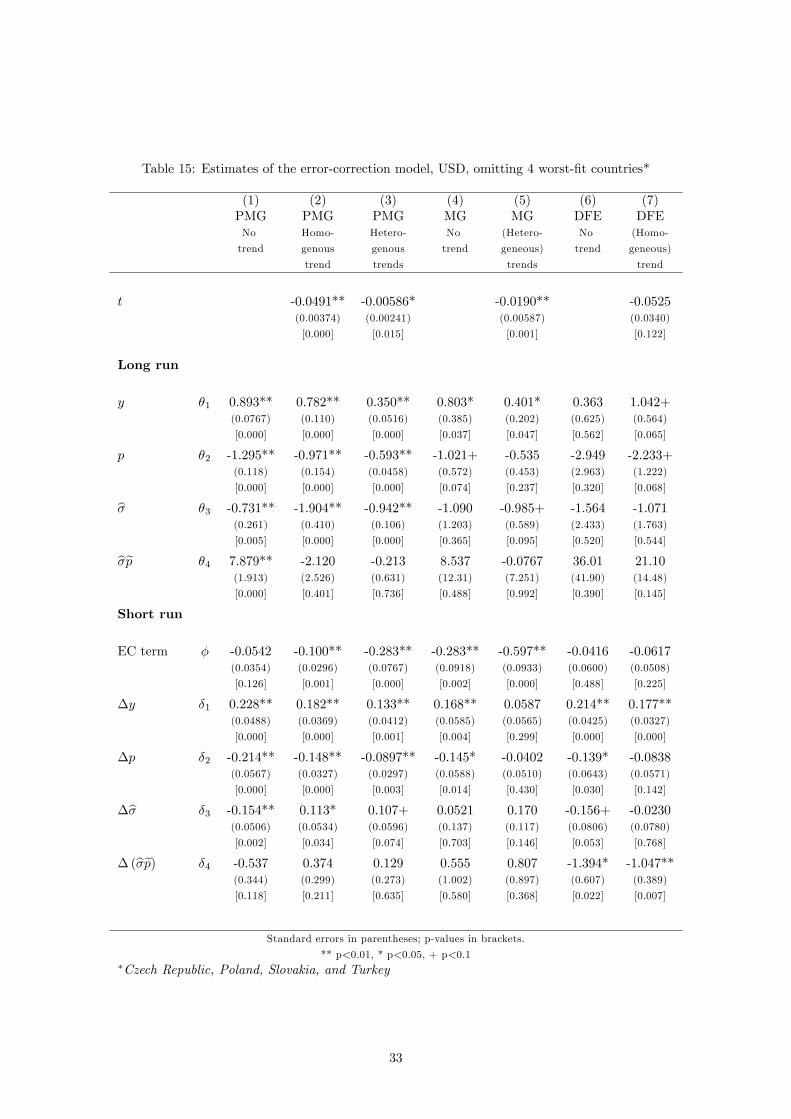
Table 15: Estimates of the error-correction model, USD, omitting 4 worst-fit countries*

(1) (2) (3) (4) (5) (6) (7)PMG PMG PMG MG MG DFE DFENo Homo- Hetero- No (Hetero- No (Homo-

trend genous genous trend geneous) trend geneous)

trend trends trends trend

t -0.0491** -0.00586* -0.0190** -0.0525(0.00374) (0.00241) (0.00587) (0.0340)

[0.000] [0.015] [0.001] [0.122]

Long run

y θ1 0.893** 0.782** 0.350** 0.803* 0.401* 0.363 1.042+(0.0767) (0.110) (0.0516) (0.385) (0.202) (0.625) (0.564)

[0.000] [0.000] [0.000] [0.037] [0.047] [0.562] [0.065]

p θ2 -1.295** -0.971** -0.593** -1.021+ -0.535 -2.949 -2.233+(0.118) (0.154) (0.0458) (0.572) (0.453) (2.963) (1.222)

[0.000] [0.000] [0.000] [0.074] [0.237] [0.320] [0.068]

σ̂ θ3 -0.731** -1.904** -0.942** -1.090 -0.985+ -1.564 -1.071(0.261) (0.410) (0.106) (1.203) (0.589) (2.433) (1.763)

[0.005] [0.000] [0.000] [0.365] [0.095] [0.520] [0.544]

σ̂p̃ θ4 7.879** -2.120 -0.213 8.537 -0.0767 36.01 21.10(1.913) (2.526) (0.631) (12.31) (7.251) (41.90) (14.48)

[0.000] [0.401] [0.736] [0.488] [0.992] [0.390] [0.145]

Short run

EC term φ -0.0542 -0.100** -0.283** -0.283** -0.597** -0.0416 -0.0617(0.0354) (0.0296) (0.0767) (0.0918) (0.0933) (0.0600) (0.0508)

[0.126] [0.001] [0.000] [0.002] [0.000] [0.488] [0.225]

∆y δ1 0.228** 0.182** 0.133** 0.168** 0.0587 0.214** 0.177**(0.0488) (0.0369) (0.0412) (0.0585) (0.0565) (0.0425) (0.0327)

[0.000] [0.000] [0.001] [0.004] [0.299] [0.000] [0.000]

∆p δ2 -0.214** -0.148** -0.0897** -0.145* -0.0402 -0.139* -0.0838(0.0567) (0.0327) (0.0297) (0.0588) (0.0510) (0.0643) (0.0571)

[0.000] [0.000] [0.003] [0.014] [0.430] [0.030] [0.142]

∆σ̂ δ3 -0.154** 0.113* 0.107+ 0.0521 0.170 -0.156+ -0.0230(0.0506) (0.0534) (0.0596) (0.137) (0.117) (0.0806) (0.0780)

[0.002] [0.034] [0.074] [0.703] [0.146] [0.053] [0.768]

∆ (σ̂p̃) δ4 -0.537 0.374 0.129 0.555 0.807 -1.394* -1.047**(0.344) (0.299) (0.273) (1.002) (0.897) (0.607) (0.389)

[0.118] [0.211] [0.635] [0.580] [0.368] [0.022] [0.007]

Standard errors in parentheses; p-values in brackets.

** p<0.01, * p<0.05, + p<0.1∗Czech Republic, Poland, Slovakia, and Turkey

33

Table 16: Estimates of error-correction model with only the standard regressors, USD

(1) (2) (3) (4) (5) (6) (7)PMG PMG PMG MG MG DFE DFENo Homo- Hetero- No (Hetero- No (Homo-

trend genous geneous trend geneous) trend genous)

trend trends trends trend

t -0.0523** -0.00558** 0.0261 -0.0446*(0.00432) (0.00169) (0.0465) (0.0200)

[0.000] [0.001] [0.575] [0.025]

Long run

y θ1 -0.908** 0.863** 0.647** 0.0733 -0.712 0.0468 0.786**(0.140) (0.117) (0.0658) (0.429) (0.851) (0.526) (0.277)

[0.000] [0.000] [0.000] [0.864] [0.403] [0.929] [0.005]

p θ2 0.139 -1.075** -0.834** -0.302 0.0632 -1.039* -0.985**(0.129) (0.0961) (0.0567) (0.336) (0.363) (0.454) (0.261)

[0.282] [0.000] [0.000] [0.369] [0.862] [0.022] [0.000]

Short run

EC term φ -0.0505+ -0.116** -0.286** -0.288** -0.480** -0.0557 -0.0822+(0.0282) (0.0263) (0.0527) (0.0649) (0.0746) (0.0523) (0.0435)

[0.073] [0.000] [0.000] [0.000] [0.000] [0.287] [0.059]

∆y δ1 0.272** 0.164** 0.0819* 0.137* 0.0260 0.222** 0.173**(0.0365) (0.0339) (0.0404) (0.0547) (0.0537) (0.0382) (0.0340)

[0.000] [0.000] [0.043] [0.012] [0.628] [0.000] [0.000]

∆p δ2 -0.229** -0.0990* -0.0353 -0.0759 0.0126 -0.196** -0.126**(0.0442) (0.0402) (0.0403) (0.0501) (0.0493) (0.0483) (0.0424)

[0.000] [0.014] [0.381] [0.129] [0.799] [0.000] [0.003]

Standard errors in parentheses; p-values in brackets.

** p<0.01, * p<0.05, + p<0.1

34

Table 17: Estimates of error-correction model with only the standard regressors, USD, omitting 4 worst-fitting countries*

(1) (2) (3) (4) (5) (6) (7)PMG PMG PMG MG MG DFE DFENo Homo- Hetero- No (Hetero— No (Homo-

trend genous geneous trend geneous) genous)

trend trends trends trend trend

t -0.0530** -0.00486** 0.0331 -0.0551(0.00501) (0.00106) (0.0539) (0.0393)

[0.000] [0.000] [0.540] [0.161]

Long run

y θ1 0.710** 0.769** 1.020** -0.270 -0.929 -0.143 0.936+(0.0695) (0.148) (0.0871) (0.410) (0.983) (1.097) (0.538)

[0.000] [0.000] [0.000] [0.509] [0.344] [0.896] [0.082]

p θ2 -0.866** -1.046** -0.982** -0.0222 0.197 -1.283 -1.080*(0.0632) (0.122) (0.0681) (0.324) (0.416) (1.494) (0.550)

[0.000] [0.000] [0.000] [0.945] [0.635] [0.390] [0.050]

Short run

EC term φ -0.0645+ -0.0845** -0.177** -0.238** -0.427** -0.0336 -0.0600(0.0387) (0.0209) (0.0285) (0.0616) (0.0758) (0.0630) (0.0540)

[0.095] [0.000] [0.000] [0.000] [0.000] [0.593] [0.267]

∆y δ1 0.243** 0.184** 0.109** 0.168** 0.0586 0.224** 0.173**(0.0497) (0.0346) (0.0395) (0.0586) (0.0589) (0.0424) (0.0312)

[0.000] [0.000] [0.006] [0.004] [0.320] [0.000] [0.000]

∆p δ2 -0.237** -0.136** -0.107** -0.124** -0.0458 -0.200** -0.133**(0.0491) (0.0298) (0.0316) (0.0462) (0.0470) (0.0528) (0.0434)

[0.000] [0.000] [0.001] [0.008] [0.329] [0.000] [0.002]

Standard errors in parentheses; p-values in brackets.

** p<0.01, * p<0.05, + p<0.1∗Czech Republic, Poland, Slovakia, and Turkey

35

arises from low tax rates will still dampen consumption. Either way, however, the use of before-tax

volatility actually decreases the coeffi cient on the interaction term, so it does not seem as if tax-driven

price volatility is masking the effect of "true" price volatility. The models based on total-price volatility

therefore remain my preferred specifications.

If, as the version of the preferred model with trend suggests, people’s responsiveness to prices is

immune to the volatility of prices, then θ2 is a perfectly serviceable measure of price elasticity. On the

other hand, if price elasticity does vary with price uncertainty– as the model without trend implies– then

total long-run price elasticity is not θ2, but θ2 + θ4σ̂it. This is analogous to the total price elasticities

derived for the ADL:

Short run price elasticity:∂git∂pit

= δ2 + δ4σ̂it

Long run price elasticity:δ2 + δ4σ̂it

1− λ

The model without trend implies, therefore, that the "total" long-run elasticity with respect to price is

θ̂2 + θ̂4σ̂ = −0.918 (17)

where σ̂ is the mean rolling price standard deviation across all countries and time periods. This total

elasticity is, of course, smaller in magnitude than θ̂2, but still on the relatively high end of price elasticity

estimates when compared to the literature.

Although the PMG estimator constrains long-run coeffi cients to be homogenous, we can substitute

country-specific averages σ̂i into (17) to interpolate the variation in "total" price elasticity due to volatility

differences. These country-specific total price elasticities are plotted in Figure 7. Over time, volatility

levels within a country evolve and may thereby alter total price elasticities; and so Figure 7 also depicts

the range of total price elasticities implied by each country’s range of price volatilities σ̂it. (Some of these

ranges extend into positive price elasticities, but the worst offenders, the Czech Republic and Slovakia, are

actually omitted from the regression, and so their implied wrong-sign elasticities should not cast doubt

on the model as a whole.) It should be observed that the United States, whose price responsiveness is

generally found to be low in comparison to other countries’, has the highest average price volatility in

the sample, and so by construction its total elasticity is of comparatively low magnitude. Although this

does not establish that rational habits are responsible for the United States’low price responsiveness,

the model does at least correctly predict this phenomenon.

The remaining long-term parameter, the time trend, is about −0.05 and statistically significantly.

All other things equal, this implies, per-capita gasoline consumption has been declining about 5% per

year. This negative trend seems to have been widespread: in the version of the ECM with heterogeneous

trends, the majority of country-specific trends are negative (as are nearly all the country-specific trends

estimated using 2SLS on the ADL). There are variety of potential explanations for these downward

trends. Demographic shifts, for instance, might have reduced the number of drivers in ageing populations

or pushed populations towards locations that demanded less driving. The more probable explanation

is that technological innovations, tightening fuel-economy standards, and individual investments in fuel

effi ciency have dampened gasoline demand.

The short-run coeffi cients reported in Table 15, which are the averages of the country-specific short-

run coeffi cients, are (like MG estimates) not as reliable as the long-run estimates, since each country’s

short-run coeffi cients have been estimated using relatively little data. Nonetheless, estimates of δ1 and

δ2 appear to be very reasonable: the short-run income elasticity of around 0.2 is approximately a quarter

the long-run income elasticity; the short-run price elasticity (non-"total") of −0.15 to −0.21 is roughly

36

Table 18: Estimates of error-correction model with before-tax volatilities, USD

(1) (2) (3) (4)PMG PMG PMG PMG

Homogenous Heterogeneous Homogeneous trend, Heterogeneous trends,trend trends σ̂BT only in interaction σ̂BT only in interaction

t -0.0660** -0.00316** -0.0506** -0.00346*(0.00995) (0.00122) (0.00408) (0.00164)

[0.000] [0.009] [0.000] [0.035]

Long run

y θ1 0.623** 0.460** 0.707** 0.220**(0.193) (0.0377) (0.121) (0.0225)

[0.001] [0.000] [0.000] [0.000]

p θ2 -0.428+ -0.188** -0.834** -0.0738**(0.260) (0.0591) (0.155) (0.0247)

[0.100] [0.001] [0.000] [0.003]

σ̂BT θ3 0.200 -0.298**(0.413) (0.101)

[0.629] [0.003]

σ̂ θ3 -1.367** 0.181**(0.422) (0.0380)

[0.001] [0.000]

σ̂BT p̃ θ4 -5.018* -3.609** -1.309 -1.160**(2.031) (0.521) (1.198) (0.237)

[0.013] [0.000] [0.274] [0.000]

Short run

EC term φ -0.0567** -0.275** -0.102** -0.317**(0.0207) (0.0429) (0.0276) (0.0622)

[0.006] [0.000] [0.000] [0.000]

∆y δ1 0.195** 0.108** 0.187** 0.171**(0.0296) (0.0370) (0.0320) (0.0379)

[0.000] [0.004] [0.000] [0.000]

∆p δ2 -0.155** -0.178** -0.138** -0.176**(0.0340) (0.0362) (0.0390) (0.0476)

[0.000] [0.000] [0.000] [0.000]

∆σ̂BT δ3 0.0421 0.0923*(0.0365) (0.0362)

[0.249] [0.011]

∆σ̂ δ3 0.125* -0.0185(0.0509) (0.0528)

[0.014] [0.726]

∆ (σ̂BT p) δ4 0.0224 0.647** 0.181 0.157(0.257) (0.202) (0.184) (0.188)

[0.931] [0.001] [0.324] [0.404]

Standard errors in parentheses; p-values in brackets.

** p<0.01, * p<0.05, + p<0.1

37

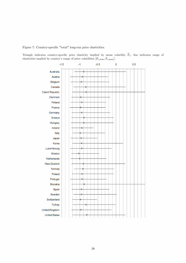
Figure 7: Country-specific "total" long-run price elasticities.

Triangle indicates country-specific price elasticity implied by mean volatility σ̂i; line indicates range ofelasticities implied by country’s range of price volatilities [σ̂i,min, σ̂i,max] .

38

fifteen to twenty percent of the long-run price elasticity.

The unreliability of the short-run estimates does show up in the remaining coeffi cients, however: in

the short run, the effect of price volatility is estimated to be negative if a trend is excluded and positive

if it is included; the effect of the price-volatility interaction term is statistically insignificant in either

case. The relative unreliability of the short-run estimates seems to be a worthwhile trade-off, however,

for the heterogeneity that improves the long-run estimates of primary interest.

6 Conclusion

Consumers’gasoline consumption is decided by a multitude of choices– some large, some small; some

in the form of investment decisions, others in the form of everyday routines. All of these choices can

be swept into a habits framework, which highlights the importance of price uncertainty and volatility in

shaping the demand of forward-looking consumers.

The rational habits framework suggests two major implications for consumer behavior. This

paper has tested for both: first, that price uncertainty will depress demand; and second, that price

uncertainty will dampen the price responsiveness of demand. Evidence for the first implication is strong.

In the long run, price volatility does depress gasoline demand; the effect of the rolling-standard-deviation

measure on demand is not only statistically significant but of a similar magnitude to price elasticity itself.

Evidence for the second implication is not as unequivocal. In some of my preferred specifications,

it does indeed appear that total price responsiveness is greater when prices are less volatile. The estimated

effect of price volatility on price elasticity, however, is quite sensitive to the model specification and

estimation method. Future work on consumer habits should keep this sensitivity in mind and give

careful thought to choosing an appropriate estimator.

It should be noted again– particularly in light of the fragile estimates of price volatility’s effect

on price elasticity– that this paper has based all its tests for rational habits on a price-uncertainty

measure that uses the rolling standard deviation of prices as a proxy for anticipated future price volatility.

The appropriateness of this proxy is therefore key to the results. Imperfections in this proxy, even

imperfections that amount to well-behaved measurement error, introduce a downward bias (in magnitude)

to estimates of uncertainty’s effects, and may therefore disguise habits’ influence on price elasticity.

Future work on consumer habits should keep this in mind as well: thoughtful, explicit modelling of

consumers’expectations may bring evidence of rational habits into starker relief.

Altogether, there is compelling evidence that consumers around the world exhibit at least some

of the behaviors associated with rational gasoline habits. In light of these habits, policymakers should

heed the role of price uncertainty in shaping gasoline demand. Policies to stabilize gasoline prices may

have the undesired effect of increasing demand, and to offset this increase there may be a need for

further intervention. This intervention may be made easier, however, by the increased effectiveness of

price instruments when price volatility is low. Given rational habits, in fact, stable price increases are

a longer policy lever than traditionally-measured price elasticity suggests. Not only may gasoline taxes

explain some of the variation in price elasticity around the world, but their influence on price volatility

may allow them to re-shape one country’s demand to look like another’s.

39

7 Further Data Exposition

7.1 Geographic Scope

The twenty-nine countries in my sample are Australia, Austria, Belgium, Canada, the Czech Republic,

Denmark, Finland, France, Germany, Greece, Hungary, Ireland, Italy, Japan, Korea, Luxembourg, Mex-

ico, the Netherlands, New Zealand, Norway, Poland, Portugal, Slovakia, Spain, Sweden, Switzerland,

Turkey, the United Kingdom, and the United States.

7.2 Grades and Prices

The IEA reports price and tax data by product, i.e. by petrol type and grade. The availability of data on

any product naturally depends on the product’s availability to consumers, which in turn depends upon

local regulations. For a number of countries– including Finland, France, Ireland, Italy, Luxembourg,

and the U.K.– data on unleaded gasoline is not available until 1990. To avoid the problems associated

with switching from a measure of price based solely on leaded gasoline to a measure based on unleaded

gasoline (or some average of leaded and unleaded), I concentrate on the period 1990 onwards.

Even in this later period, however, data availability varies by product and country, with this variation

driven by differences in regulation and definition. In Australia, for example, "95 RON" is considered

premium, and regular unleaded gasoline is 91 RON (MotorMouth 2010); in the UK, "95 RON" is

regular unleaded (Boulter and Latham 2009). Such differences in reported octane ratings may exaggerate

differences in the actual content of the fuels, as the definition of the Research Octane Number (RON)

varies by country, and its definition tends to be lower-skewing in countries that define "regular unleaded"

by a lower RON. Whatever the differences in definition across countries, I need a price series for each

country that is measured by a constant definition, since varying the definition over time would introduce

false price variation (unless, of course, such variations reflected actual changes in the type of gasoline in

use). Where annual data for "regular unleaded" is available from 1990 on– however "regular unleaded"

may be defined locally– I use this as the product. Where annual data on regular unleaded is not available

contiguously from 1990 but data on 95 RON is, I use 95 RON. Where data on neither regular unleaded

nor 95 RON is available contiguously from 1990, I use whichever product has the longer contiguous

availability. After determining which product to use for annual data, I use the same product for quarterly

data. Table 19 shows the product for which each country’s price measures are taken.

Table 19: Gasoline product used for price and tax data

Regular Unleaded 95 RONAustralia Belgium NorwayAustria Czech Republic PolandCanada Finland PortugalDenmark France Slovak RepublicGermany Greece SpainJapan Hungary SwedenKorea Ireland SwitzerlandMexico Italy TurkeyNew Zealand Luxembourg United KingdomUnited States Netherlands

40

8 Local-currency Estimates

This appendix reports local-currency results corresponding to the common-currency results presented in

the main text. As noted in Section 3.3, not all the estimators applied to the common-currency data can

be sensibly applied to the local-currency data: in particular, the random-effects estimator of Table 20

and the pooled 2SLS estimator of Table 22 are both biased because of their comparison of non-differenced

log prices and log income across different currencies.

That said, the remaining results should not be subject to the currency-generated bias. The within-

groups (fixed-effects) 2SLS results (Table 21), in fact, make a little bit more sense than their common-

currency counterparts, with negative and statistically-significant price effects no matter the specification

of the trend. The results with respect to income and the rational-habits variables, however, show a

pattern similar to the common-currency results, with income’s effect becoming more pronounced as

a homogenous and then a heterogeneous trend is introduced, and the rational-habits variables never

showing a statistically-significant effect.

Turning to system GMM (Table 24), the estimators are just as uninformative when applied to local-

currency data as they were when applied to common-currency data.

Moving on to the preferred estimator, namely the pooled mean group estimator applied to the ECM,

there are some interesting contrasts to the common-currency results. Generally speaking, I find lower-

magnitude long-run income and price elasticities in the local-currency data. In the "standard" model

without rational-habits variables, the long-run income elasticity is about 0.3, which is considerably

below both the literature’s averages and most of the common-currency estimates. Similarly, the long-run

price elasticities from the "standard" model with no trend or heterogeneous trends (-0.65 and -0.14,

respectively) are smaller than the corresponding common-currency results.

There is a confounding blip in the homogenous-trend versions of the local-currency estimates, with

price elasticity in the "standard" model shooting to -1.28 and "total" price elasticity in the rational-habits

model shooting to -1.08. The latter is driven almost entirely by an implausibly-sized and incorrectly-

signed coeffi cient on σ̂p̃, and so I am inclined to be suspicious of these homogenous-trend results.

With respect to the rational habits variables, the local-currency results are less conclusive than

their common-currency counterparts. Whereas the coeffi cient on σ̂ was negative and highly statistically

significant in all common-currency estimates of the ECM, when using local currencies the coeffi cient

on σ̂ is nowhere near statistically significant unless heterogeneous trends are included– and even then

the p-value is 0.065. With respect to the interaction term σ̂p̃, the local-currency data produces the

expected positive coeffi cient (p = 0.07) only when heterogeneous trends are included. Without a trend,

the coeffi cient on σ̂p̃ is indistinguishable from 0; and with a homogenous trend, as has been noted, the

coeffi cient on σ̂p̃ is hugely negative.

Overall, it seems that in practice the local-currency approach may be less reliable than the common-

currency approach.

41

Table 20: Random- vs. fixed-effects estimator, static model, local currencies

(1) (2) (3) (4)Static Static Dynamic Dynamic

Random effects Fixed effects Random effects Fixed effects

gt−1 λ 0.992** 0.905**(0.00660) (0.0160)[0.000] [0.000]

y δ1 0.298** 0.265** 0.00672 -0.0178(0.0413) (0.0429) (0.00609) (0.0160)[0.000] [0.000] [0.270] [0.267]

p δ2 -0.494** -0.586** -0.00261 -0.169**(0.0508) (0.0635) (0.00601) (0.0282)[0.000] [0.000] [0.664] [0.000]

σ̂ δ3 -0.216 -0.169 -0.185* -0.0772(0.267) (0.266) (0.0937) (0.0944)[0.419] [0.527] [0.048] [0.414]

σ̂p̃ δ4 -0.410 0.335 -1.469** 0.331(0.693) (0.752) (0.275) (0.407)[0.554] [0.656] [0.000] [0.417]

R2 0.2892 0.2274 0.9951 0.8288

Hausman 11.21 74.79testa [0.024] [0.000]

Standard errors in parentheses; P-values in brackets.** p<0.01, * p<0.05, + p<0.1

aUnder H0 that random- and fixed-effects estimates equivalent,χ2(4) for static model, χ2(4) for dynamic.

42

Table 21: Within-groups (fixed effects) estimates with 2SLS instrumenting for price, local currencies(1) (2) (3)

No trend Common trend Individual trends

gt−1 0.906** 0.908** 0.697**(0.0287) (0.0279) (0.0418)[0.000] [0.000] [0.000]

y -0.00128 0.0566* 0.235**(0.0217) (0.0272) (0.0595)[0.953] [0.038] [0.000]

p -0.203** -0.158** -0.210**(0.0459) (0.0524) (0.0482)[0.000] [0.003] [0.000]

σ̂ -0.0667 -0.0322 -0.000603(0.125) (0.127) (0.125)[0.595] [0.800] [0.996]

σ̂p̃ 0.419 0.305 -0.454(0.513) (0.513) (0.523)[0.415] [0.552] [0.386]

t -0.00245* [country-specific(0.00103) trends][0.017]

R2 0.899 0.902 0.935

Implied long-run elasticities

y δ11−λ -.0136 .616 .776

(0.232) (0.292) (0.186)[0.953] [0.036] [0.000]

p δ21−λ -2.165 -1.715 -0.695

(0.656) (0.653) (0.161)[0.001] [0.009] [0.000]

TestsEndogeneity: 9.769 4.228 6.198pricea [0.0018] [0.0398] [0.0128]

Endogeneity: 11.735 6.557 8.041price & interactionb [0.0028] [0.0377] [0.0179]

Underidentificationc 125.510 92.181 98.878[0.000] [0.0000] [0.000]

Exogeneityd 5.653 8.344 4.362[0.0592] [0.0154] [0.113]

Robust standard errors in parentheses; p-values in brackets.** p<0.01, * p<0.05, + p<0.1

aDifference-in-Sargan/Hansen χ2(1) under H0.bDifference-in-Sargan/Hansen χ2(2) under H0.cKleibergen-Paap (2006) rk statistic; χ2(3) under H0.dOveridentifying restrictions test (Hansen J statistic); χ2(2) under H0.

43

Table 22: Pooled estimates with 2SLS instrumenting for prices, local currencies

(1) (2) (3)No Common Individualtrend trend trends

gt−1 λ 1.002** 1.001** 0.959**(0.00662) (0.00675) (0.0168)[0.000] [0.000] [0.000]

y δ1 0.00454 0.00443 0.00922(0.00675) (0.00676) (0.0156)[0.501] [0.513] [0.555]

p δ2 -0.00118 -0.000166 -0.0142(0.00673) (0.00670) (0.0166)[0.861] [0.980] [0.393]

σ̂ δ3 -0.0981 -0.0139 -0.194(0.117) (0.117) (0.124)[0.401] [0.906] [0.119]

σ̂p̃ δ4 -1.800** -0.929* -0.866*(0.469) (0.434) (0.390)[0.000] [0.033] [0.027]

t -0.00216** [country-specific(0.000620) trends][0.001]

R2 0.996 0.996 0.997Robust standard errors in parentheses;

p-values in brackets.** p<0.01, * p<0.05, + p<0.1

Table 23: Within-groups (fixed-effects) estimates, local currencies

(1) (2) (3)No Common Individualtrend trend trends

gt−1 λ 0.905** 0.893** 0.729**(0.0218) (0.0231) (0.0358)[0.000] [0.000] [0.000]

y δ1 -0.0178 0.0559+ 0.255**(0.0215) (0.0287) (0.0606)[0.408] [0.052] [0.000]

p δ2 -0.169** -0.156** -0.168**(0.0377) (0.0397) (0.0392)[0.000] [0.000] [0.000]

σ̂ δ3 -0.0772 -0.00558 -0.0446(0.117) (0.119) (0.114)[0.510] [0.963] [0.695]

σ̂p̃ δ4 0.331 0.386 -0.348(0.422) (0.402) (0.432)[0.433] [0.337] [0.420]

t -0.00280**(0.00103)[0.007]

R2 0.903 0.905 0.938Robust standard errors in parentheses; p-values in brackets.

** p<0.01, * p<0.05, + p<0.1

44

Table 24: System GMM, local currencies(1) (2) (3) (4) (5) (6) (7) (8)

No trend With trend No trend With trend No trend With trendNo trend With trend Collapsed Collapsed Reduced Reduced No outside No outside

IV matrix IV matrix IV count IV count IVs IVs

gt−1 λ 1.005** 0.991** 1.035** 0.928** 1.006** 0.724 1.002** 0.977**(0.00733) (0.0143) (0.0271) (0.136) (0.149) (0.575) (0.0180) (0.0410)[0.000] [0.000] [0.000] [0.000] [0.000] [0.218] [0.000] [0.000]

y δ1 0.0100 0.0569 0.0311 0.234 0.167 0.602 0.0151+ 0.0423(0.00814) (0.0364) (0.0378) (0.189) (0.297) (0.981) (0.00863) (0.0349)[0.228] [0.129] [0.417] [0.227] [0.579] [0.545] [0.091] [0.236]

p δ2 -0.00597 -0.0451 -0.0184 -0.201 -0.133 -0.535 -0.0157 -0.0298(0.00701) (0.0319) (0.0320) (0.170) (0.259) (0.892) (0.0206) (0.0312)[0.402] [0.168] [0.571] [0.248] [0.610] [0.554] [0.454] [0.348]

σ̂ δ3 -0.146 0.0971 -0.191 0.0145 -1.463 -1.224 -0.106 0.160(0.191) (0.203) (0.257) (0.232) (2.323) (2.302) (0.240) (0.252)[0.451] [0.636] [0.464] [0.951] [0.534] [0.599] [0.660] [0.530]

σ̂p̃ δ4 -1.649* -0.421 -1.995* -0.00918 -0.455 3.255 -2.904* -1.773+(0.655) (0.678) (0.955) (1.367) (4.162) (7.916) (1.144) (0.881)[0.018] [0.540] [0.046] [0.995] [0.914] [0.684] [0.017] [0.054]

t -0.00399** -0.00640 -0.0125 -0.00352*(0.00139) (0.00479) (0.0190) (0.00135)[0.008] [0.192] [0.514] [0.014]

Sargan 420.4 380.5 90.69 59.02 10.38 10.65 411.6 378.2Sargan df 169 168 17 16 3 2 165 164Sargan P 0 0 0 7.65e-07 0.0156 0.00487 0 0Hansen 26.77 23.08 20.45 22.96 7.894 5.770 25.96 23.87Hansen df 169 168 17 16 3 2 165 164Hansen P 1 1 0.252 0.115 0.0482 0.0558 1 1AR(2) test -0.415 -0.503 -0.371 -0.311 0.399 0.436 -0.297 -0.419AR(2) P 0.678 0.615 0.711 0.756 0.690 0.663 0.767 0.675

Standard errors in parentheses; p-values in brackets.** p<0.01, * p<0.05, + p<0.1

45

Table 25: Estimates of the error-correction model, all countries, local currencies

(1) (2) (3) (4) (5) (6) (7)PMG PMG PMG MG MG DFE DFENo (Homo- (Hetero- No trend (Hetero- No (Homo-trend genous) genous) geneous) trend geneous)

trend trends trends trend

t -0.0499** -0.00140 -0.0126 -0.0376+(0.00648) (0.00136) (0.00872) (0.0212)[0.000] [0.302] [0.149] [0.076]

Long run

y θ1 0.258** 0.560* 0.0594 -0.286 0.190 -0.815 0.300(0.0343) (0.268) (0.0746) (0.402) (0.483) (0.646) (0.545)[0.000] [0.037] [0.426] [0.476] [0.694] [0.207] [0.582]

p θ2 -0.501** -0.0955 -0.440** -0.0252 0.111 -1.666 -1.112(0.0809) (0.231) (0.0640) (0.433) (0.549) (1.013) (0.728)[0.000] [0.679] [0.000] [0.954] [0.839] [0.100] [0.126]

σ̂ θ3 -0.359 -0.376 -0.354+ -0.0753 1.458 1.214 1.791(0.279) (0.841) (0.192) (1.978) (1.111) (2.166) (1.687)[0.199] [0.655] [0.065] [0.970] [0.189] [0.575] [0.288]

σ̂p̃ θ4 -1.457 -27.64** 2.258+ -35.85+ -15.25 4.331 3.088(2.102) (5.587) (1.244) (19.67) (21.12) (9.114) (7.007)[0.488] [0.000] [0.070] [0.068] [0.470] [0.635] [0.659]

Short run

EC term φ -0.130** -0.0890** -0.252** -0.452** -0.515** -0.0663+ -0.0820*(0.0479) (0.0215) (0.0483) (0.0726) (0.0938) (0.0342) (0.0359)[0.007] [0.000] [0.000] [0.000] [0.000] [0.052] [0.022]

∆y δ1 0.267** 0.407** 0.272** 0.272+ 0.271 0.379** 0.379**(0.0625) (0.0711) (0.0836) (0.154) (0.169) (0.0794) (0.0822)[0.000] [0.000] [0.001] [0.077] [0.110] [0.000] [0.000]

∆p δ2 -0.139** -0.147** -0.0670+ -0.111+ -0.102 -0.117* -0.105*(0.0515) (0.0316) (0.0394) (0.0643) (0.0698) (0.0498) (0.0477)[0.007] [0.000] [0.089] [0.085] [0.143] [0.019] [0.028]

∆σ̂ δ3 -0.00355 0.0783 0.103* -0.110 -0.0395 -0.000811 0.00461(0.0599) (0.0759) (0.0520) (0.123) (0.135) (0.111) (0.115)[0.953] [0.303] [0.047] [0.371] [0.769] [0.994] [0.968]

∆ (σ̂p̃) δ4 -1.045* 0.720 -0.739+ 1.655 1.784 -0.144 -0.00948(0.501) (0.644) (0.419) (1.843) (2.013) (0.347) (0.352)[0.037] [0.264] [0.078] [0.369] [0.375] [0.679] [0.979]

Standard errors in parentheses; p-values in brackets.** p<0.01, * p<0.05, + p<0.1

46

Table 26: Estimates of error-correction model with only the standard regressors, local currencies

(1) (2) (3) (4) (5) (6) (7)PMG PMG PMG MG MG DFE DFENo Homo- Hetero- No (Hetero- No (Homo-

genous geneous geneous) genous)trend trend trends trend trends trend trend

t -0.0463** -0.00383* 0.0620 -0.0342(0.00817) (0.00163) (0.0968) (0.0212)[0.000] [0.019] [0.522] [0.106]

Long run

y θ1 0.301** 0.283 0.275** -0.246 -1.565 -0.741 0.307(0.0321) (0.320) (0.0436) (0.625) (1.815) (0.637) (0.543)[0.000] [0.375] [0.000] [0.694] [0.388] [0.245] [0.571]

p θ2 -0.648** -1.283** -0.139** -0.660** -1.569 -1.435* -0.981*(0.0389) (0.165) (0.0237) (0.217) (1.311) (0.662) (0.468)[0.000] [0.000] [0.000] [0.002] [0.231] [0.030] [0.036]

Short run

EC term φ -0.142** -0.0803** -0.295** -0.376** -0.507** -0.0681+ -0.0820*(0.0508) (0.0175) (0.0642) (0.0638) (0.0713) (0.0362) (0.0377)[0.005] [0.000] [0.000] [0.000] [0.000] [0.060] [0.030]

∆y δ1 0.273** 0.384** 0.286** 0.330** 0.239** 0.350** 0.358**(0.0600) (0.0575) (0.0726) (0.0659) (0.0880) (0.0518) (0.0578)[0.000] [0.000] [0.000] [0.000] [0.007] [0.000] [0.000]

∆p δ2 -0.138* -0.0992** -0.0875* -0.0109 -0.00316 -0.109** -0.0880*(0.0569) (0.0371) (0.0425) (0.0456) (0.0422) (0.0411) (0.0385)[0.016] [0.007] [0.039] [0.812] [0.940] [0.008] [0.022]

Standard errors in parentheses; p-values in brackets.** p<0.01, * p<0.05, + p<0.1

47

9 Implementation of Estimation and Tests

All estimation has been performed in Stata 11 (2009). The panel unit root tests reported in Tables 4

and 5 are implemented using the Stata (2009) program xtunitroot. The cointegration tests reported in

Tables 6 and 7 are implemented using Persyn and Westerlund’s program xtwest, detailed in Persyn and

Westerlund (2008). The PMG, MG, and DFE estimators of the error-correction models are implemented

using Blackburne and Frank’s xtpmg (2007b), detailed in Blackburne and Frank (2007a). GMM estimates

of the ADL are computed using Roodman’s (2011) xtabond2, and least-squares estimates are computed

using Schaffer’s xtivreg2.

48

10 PMGEstimates with Individual Country-Specific Short-Run

Coeffi cients

Table 27 (pp. 50-64) reports the country-specific short-run ECM coeffi cients estimated by PMG, averages

of which are reported in Tables 14 and 25.

49

Table 27: Pooled mean group estimates of error-correction model with reporting of individual short-runparameters

(1) (2) (3) (4) (5) (6)Local Local Local

USD USD USD currency currency currencyNo Homogenous Heterogeneous No Homogenous Heterogeneoustrend trend trends trend trend trends

Long Run

y 0.555** 0.774** 0.388** 0.258** 0.560* 0.0594(0.0306) (0.0905) (0.0412) (0.0343) (0.268) (0.0746)[0.000] [0.000] [0.000] [0.000] [0.037] [0.426]

p -0.693** -0.981** -0.626** -0.501** -0.0955 -0.440**(0.0755) (0.122) (0.0398) (0.0809) (0.231) (0.0640)[0.000] [0.000] [0.000] [0.000] [0.679] [0.000]

σ̂ -1.249** -1.464** -0.881** -0.359 -0.376 -0.354+(0.249) (0.353) (0.100) (0.279) (0.841) (0.192)[0.000] [0.000] [0.000] [0.199] [0.655] [0.065]

σ̂p̃ 0.816 -0.307 -0.0718 -1.457 -27.64** 2.258+(1.205) (1.872) (0.520) (2.102) (5.587) (1.244)[0.498] [0.870] [0.890] [0.488] [0.000] [0.070]

t -0.0473** -0.0499**(0.00303) (0.00648)[0.000] [0.000]

Individual Short-Run EstimatesAustralia

EC term -0.220* -0.0444+ -0.175** -0.384** -0.0367+ -0.636**(0.0903) (0.0227) (0.0645) (0.101) (0.0212) (0.136)[0.015] [0.051] [0.007] [0.000] [0.083] [0.000]

∆y 0.0463 0.0671 0.0842 0.0927 0.578 -0.00186(0.0814) (0.0854) (0.0767) (0.309) (0.471) (0.341)[0.570] [0.432] [0.272] [0.764] [0.220] [0.996]

∆p 0.0162 0.00870 0.0151 0.129 0.0933 0.241*(0.0745) (0.0777) (0.0690) (0.102) (0.127) (0.0988)[0.828] [0.911] [0.827] [0.206] [0.464] [0.015]

∆σ̂ -0.292 -0.368 -0.256 -0.325+ -0.336 -0.219(0.222) (0.224) (0.207) (0.185) (0.230) (0.173)[0.189] [0.100] [0.218] [0.079] [0.144] [0.205]

∆ (σ̂p̃) 0.942+ 1.048* 1.123* 1.571 1.032 -0.0404(0.514) (0.501) (0.452) (1.391) (1.785) (1.238)[0.067] [0.036] [0.013] [0.259] [0.563] [0.974]

t -0.00148 0.00101(0.000985) (0.00151)[0.134] [0.504]

50

(1) (2) (3) (4) (5) (6)USD USD USD Local Local Local currencyNo Homogenous Heterogeneous currency currency Heterogeneoust t trends No t With t trends

Austria

EC term -0.0802 -0.0468 -0.202* -0.106 -0.00346 -0.202(0.0574) (0.0675) (0.0963) (0.0708) (0.0634) (0.158)[0.162] [0.488] [0.036] [0.136] [0.956] [0.199]

∆y 0.640** 0.624** 0.579** 0.522 0.625 0.544(0.176) (0.188) (0.169) (0.607) (0.645) (0.603)[0.000] [0.001] [0.001] [0.389] [0.332] [0.366]

∆p -0.458* -0.446* -0.362* -0.443+ -0.512* -0.422+(0.178) (0.194) (0.178) (0.227) (0.245) (0.227)[0.010] [0.021] [0.043] [0.050] [0.037] [0.063]

∆σ̂ -0.0487 0.0784 0.0216 -0.310 -0.208 -0.242(0.280) (0.308) (0.272) (0.414) (0.450) (0.421)[0.862] [0.799] [0.937] [0.454] [0.644] [0.566]

∆ (σ̂p̃) -1.349 -0.743 -0.514 -3.304 -1.122 -1.937(1.316) (1.515) (1.337) (5.616) (8.261) (6.326)[0.306] [0.624] [0.701] [0.556] [0.892] [0.759]

t -0.00426 -0.00264(0.00308) (0.00390)[0.167] [0.497]

Belgium

EC term 0.202** -0.486** -0.270+ 0.151** -0.373** -0.122(0.0624) (0.117) (0.160) (0.0513) (0.0803) (0.124)[0.001] [0.000] [0.091] [0.003] [0.000] [0.326]

∆y 0.497** -0.0812 0.153 -0.380 -0.412 -0.210(0.162) (0.159) (0.179) (0.828) (0.506) (0.717)[0.002] [0.610] [0.393] [0.646] [0.416] [0.769]

∆p -0.390* 0.163 0.0120 -0.524** -0.117 -0.208(0.165) (0.180) (0.196) (0.194) (0.140) (0.216)[0.018] [0.367] [0.951] [0.007] [0.401] [0.336]

∆σ̂ -0.319 0.161 -0.00887 0.0339 0.826* 0.464(0.477) (0.419) (0.421) (0.485) (0.343) (0.456)[0.504] [0.701] [0.983] [0.944] [0.016] [0.309]

∆ (σ̂p̃) 2.305 1.726 1.072 2.536 5.328* -0.426(1.417) (1.512) (1.218) (3.846) (2.711) (3.676)[0.104] [0.254] [0.379] [0.510] [0.049] [0.908]

t -0.0170** -0.0108*(0.00564) (0.00458)[0.002] [0.019]

51

(1) (2) (3) (4) (5) (6)USD USD USD Local Local Local currencyNo Homogenous Heterogeneous currency currency Heterogeneoust t trends No t With t trends

Canada

EC term -0.0606 0.0251 -0.101** 0.0719 0.0244** -0.365**(0.0585) (0.0163) (0.0375) (0.0635) (0.00845) (0.0843)[0.301] [0.123] [0.007] [0.258] [0.004] [0.000]

∆y 0.0939 0.121 -0.141 0.431* 0.423** -0.0604(0.158) (0.145) (0.124) (0.172) (0.114) (0.117)[0.553] [0.404] [0.256] [0.013] [0.000] [0.606]

∆p -0.0606 -0.117 -0.00868 -0.122 -0.120* 0.0478(0.102) (0.0910) (0.0717) (0.0757) (0.0526) (0.0547)[0.552] [0.198] [0.904] [0.107] [0.022] [0.382]

∆σ̂ 0.0399 -0.132 -0.0586 -0.0929 -0.114 -0.0130(0.120) (0.109) (0.0810) (0.0990) (0.0827) (0.0721)[0.740] [0.226] [0.469] [0.348] [0.167] [0.857]

∆ (σ̂p̃) 0.0155 -0.419 -0.116 -0.926+ -1.462** -0.797+(0.358) (0.348) (0.263) (0.558) (0.489) (0.470)[0.966] [0.228] [0.658] [0.097] [0.003] [0.090]

t 0.00339** 0.00502**(0.000785) (0.000941)[0.000] [0.000]

Czech Republic

EC term -1.225** -0.338** -1.092** -0.888** -0.269** -0.847**(0.148) (0.0622) (0.211) (0.0921) (0.0530) (0.0790)[0.000] [0.000] [0.000] [0.000] [0.000] [0.000]

∆y -0.358** 0.177 -0.227 0.732** 1.351** 0.763**(0.127) (0.145) (0.150) (0.211) (0.413) (0.165)[0.005] [0.223] [0.130] [0.001] [0.001] [0.000]

∆p 0.635** 0.353 0.454** 0.300** -0.00226 0.255**(0.193) (0.251) (0.158) (0.0924) (0.159) (0.0691)[0.001] [0.160] [0.004] [0.001] [0.989] [0.000]

∆σ̂ 0.825** 0.308 0.776** -0.110 -0.755* 0.254+(0.155) (0.219) (0.164) (0.195) (0.329) (0.143)[0.000] [0.159] [0.000] [0.572] [0.022] [0.077]

∆ (σ̂p̃) -0.528 0.698 1.371 -0.508 -1.172 -0.703(1.733) (1.454) (1.061) (0.647) (1.310) (0.489)[0.761] [0.631] [0.196] [0.433] [0.371] [0.150]

t 0.00975+ 0.00692**(0.00580) (0.00256)[0.093] [0.007]

52

(1) (2) (3) (4) (5) (6)USD USD USD Local Local Local currencyNo Homogenous Heterogeneous currency currency Heterogeneoust t trends No t With t trends

Denmark

EC term -0.292** -0.0722** -0.117+ -0.247** -0.0617** -0.0891**(0.0573) (0.00847) (0.0670) (0.0403) (0.00622) (0.0298)[0.000] [0.000] [0.081] [0.000] [0.000] [0.003]

∆y -0.00514 0.150** 0.126* 0.0107 0.0316 0.0812(0.0760) (0.0423) (0.0618) (0.177) (0.1000) (0.0919)[0.946] [0.000] [0.041] [0.952] [0.752] [0.376]

∆p -0.0439 -0.135** -0.111* 0.00923 -0.155** -0.103**(0.0764) (0.0414) (0.0550) (0.0664) (0.0330) (0.0385)[0.566] [0.001] [0.044] [0.890] [0.000] [0.007]

∆σ̂ -0.0448 0.0979 0.0550 -0.0526 -0.223* -0.143(0.190) (0.120) (0.115) (0.197) (0.108) (0.105)[0.814] [0.414] [0.633] [0.789] [0.040] [0.175]

∆ (σ̂p̃) -0.249 0.119 0.128 -3.058+ 1.348 -1.064(0.677) (0.410) (0.386) (1.675) (0.976) (0.955)[0.713] [0.772] [0.741] [0.068] [0.167] [0.265]

t -0.00308** -0.00281**(0.000782) (0.000417)[0.000] [0.000]

Finland

EC term -0.0424 -0.0163 -0.0364 -0.425** -0.00120 -0.477*(0.0603) (0.0242) (0.0919) (0.154) (0.0107) (0.197)[0.482] [0.500] [0.692] [0.006] [0.911] [0.015]

∆y 0.229** 0.258** 0.244** 0.0924 0.152* 0.0637(0.0590) (0.0461) (0.0630) (0.0658) (0.0709) (0.0731)[0.000] [0.000] [0.000] [0.160] [0.032] [0.384]

∆p -0.179* -0.191** -0.183* -0.152+ -0.345** -0.156+(0.0754) (0.0715) (0.0810) (0.0853) (0.0497) (0.0914)[0.017] [0.008] [0.024] [0.075] [0.000] [0.088]

∆σ̂ 0.0557 0.108 0.0884 -0.146 -0.270* -0.223+(0.106) (0.141) (0.144) (0.133) (0.135) (0.129)[0.598] [0.444] [0.539] [0.270] [0.046] [0.083]

∆ (σ̂p̃) -0.877+ -0.731 -0.726 1.192 0.792 0.305(0.528) (0.588) (0.666) (0.870) (0.931) (0.862)[0.097] [0.214] [0.276] [0.171] [0.395] [0.724]

t -0.000520 0.00115(0.00119) (0.00131)[0.663] [0.379]

53

(1) (2) (3) (4) (5) (6)USD USD USD Local Local Local currencyNo Homogenous Heterogeneous currency currency Heterogeneoust t trends No t With t trends

France

EC term 0.0308+ -0.142* -0.190 0.0763** -0.184** -0.0171(0.0160) (0.0592) (0.122) (0.0140) (0.0590) (0.0660)[0.054] [0.016] [0.119] [0.000] [0.002] [0.796]

∆y 0.174** 0.111+ 0.112+ 0.784** 0.821** 0.864**(0.0594) (0.0595) (0.0648) (0.196) (0.222) (0.195)[0.003] [0.061] [0.085] [0.000] [0.000] [0.000]

∆p -0.253** -0.211** -0.185** -0.158** -0.153* -0.133*(0.0623) (0.0623) (0.0682) (0.0602) (0.0690) (0.0600)[0.000] [0.001] [0.007] [0.009] [0.027] [0.027]

∆σ̂ -0.0110 0.170 0.143 0.205 0.249 0.231+(0.0952) (0.123) (0.117) (0.133) (0.164) (0.128)[0.908] [0.167] [0.222] [0.123] [0.129] [0.071]

∆ (σ̂p̃) -0.585 -0.192 -0.278 -1.630 1.784 -1.781(0.423) (0.501) (0.428) (1.355) (2.105) (1.339)[0.167] [0.701] [0.516] [0.229] [0.397] [0.184]

t -0.00884+ -0.00347(0.00479) (0.00237)[0.065] [0.143]

Germany

EC term 0.136+ -0.0553** -1.005** 0.215** -0.0499** -0.0106(0.0782) (0.0185) (0.330) (0.0824) (0.0132) (0.105)[0.081] [0.003] [0.002] [0.009] [0.000] [0.920]

∆y 0.297** 0.196** -0.147 0.564 0.112 0.202(0.0907) (0.0726) (0.133) (0.374) (0.322) (0.345)[0.001] [0.007] [0.268] [0.132] [0.729] [0.558]

∆p -0.490** -0.331** 0.104 -0.405** -0.270** -0.256*(0.0952) (0.0874) (0.171) (0.105) (0.0828) (0.109)[0.000] [0.000] [0.543] [0.000] [0.001] [0.019]

∆σ̂ -0.375* -0.120 0.214 0.147 0.175 0.156(0.176) (0.182) (0.207) (0.143) (0.121) (0.119)[0.033] [0.510] [0.300] [0.306] [0.148] [0.192]

∆ (σ̂p̃) 0.971 0.964+ 1.649* -0.0582 0.673 -0.206(0.601) (0.524) (0.760) (0.983) (0.860) (0.906)[0.106] [0.066] [0.030] [0.953] [0.434] [0.820]

t -0.0128** -0.00297+(0.00378) (0.00155)[0.001] [0.055]

54

(1) (2) (3) (4) (5) (6)USD USD USD Local Local Local currencyNo Homogenous Heterogeneous currency currency Heterogeneoust t trends No t With t trends

Greece

EC term -0.0373 0.0110 -0.0536 0.0120 0.0114 -0.232**(0.0496) (0.0170) (0.0485) (0.0369) (0.0128) (0.0877)[0.453] [0.518] [0.269] [0.744] [0.374] [0.008]

∆y 0.0741 0.0927* 0.0576 0.156 0.0927 -0.263(0.0467) (0.0425) (0.0448) (0.159) (0.171) (0.184)[0.113] [0.029] [0.199] [0.329] [0.587] [0.153]

∆p 0.0198 -0.0193 -0.000402 0.1000 0.115 0.157*(0.0577) (0.0573) (0.0551) (0.0740) (0.0750) (0.0623)[0.731] [0.737] [0.994] [0.177] [0.124] [0.012]

∆σ̂ 0.00219 -0.0914 -0.0867 -0.0539 -0.0626 -0.0281(0.108) (0.118) (0.109) (0.0979) (0.0957) (0.0836)[0.984] [0.438] [0.424] [0.582] [0.513] [0.736]

∆ (σ̂p̃) -0.819+ -1.039** -0.705 -4.121** -4.807** -4.518**(0.425) (0.401) (0.431) (1.563) (1.683) (1.199)[0.054] [0.009] [0.102] [0.008] [0.004] [0.000]

t 0.00159+ 0.00736**(0.000905) (0.00239)[0.078] [0.002]

Hungary

EC term -0.330** 0.0995 -0.184* -0.372** 0.104* -0.263**(0.0640) (0.0684) (0.0788) (0.0958) (0.0448) (0.0926)[0.000] [0.146] [0.020] [0.000] [0.020] [0.004]

∆y 0.0910 0.239* 0.135+ 0.187 0.486* 0.280+(0.0699) (0.108) (0.0700) (0.193) (0.225) (0.166)[0.193] [0.027] [0.054] [0.331] [0.031] [0.093]

∆p -0.179* -0.148 -0.223* -0.0187 -0.274+ -0.174(0.0886) (0.144) (0.0928) (0.116) (0.148) (0.110)[0.043] [0.306] [0.016] [0.872] [0.064] [0.113]

∆σ̂ 0.335** -0.0608 0.132 0.508** 0.503* 0.459**(0.121) (0.208) (0.128) (0.195) (0.230) (0.156)[0.006] [0.770] [0.302] [0.009] [0.029] [0.003]

∆ (σ̂p̃) 0.240 -1.359 -0.233 -4.514 0.138 -0.478(0.618) (1.020) (0.679) (4.393) (5.460) (4.016)[0.698] [0.183] [0.731] [0.304] [0.980] [0.905]

t 0.00519** 0.00496**(0.00147) (0.00124)[0.000] [0.000]

55

(1) (2) (3) (4) (5) (6)USD USD USD Local Local Local currencyNo Homogenous Heterogeneous currency currency Heterogeneoust t trends No t With t trends

Ireland

EC term -0.407** -0.110+ -0.385** -0.0739 -0.0327 -0.0219(0.107) (0.0630) (0.118) (0.0823) (0.0360) (0.147)[0.000] [0.080] [0.001] [0.369] [0.364] [0.882]

∆y -0.0688 0.00939 -0.0484 0.634** 0.621** 0.657**(0.139) (0.182) (0.154) (0.208) (0.214) (0.195)[0.620] [0.959] [0.753] [0.002] [0.004] [0.001]

∆p 0.116 0.0914 0.0895 0.134 0.127 0.125(0.137) (0.192) (0.162) (0.210) (0.208) (0.209)[0.395] [0.634] [0.580] [0.524] [0.543] [0.548]

∆σ̂ -0.350 -0.123 -0.551 0.00360 0.000763 0.00220(0.319) (0.480) (0.433) (0.324) (0.323) (0.324)[0.273] [0.798] [0.203] [0.991] [0.998] [0.995]

∆ (σ̂p̃) -3.333* -1.547 -3.303* -2.308 -1.633 -2.008(1.375) (1.805) (1.655) (5.267) (5.404) (5.453)[0.015] [0.391] [0.046] [0.661] [0.763] [0.713]

t 0.00472 -0.000825(0.00298) (0.00508)[0.114] [0.871]

Italy

EC term 0.176+ -0.302** -0.117* 0.149 -0.222** -0.0801+(0.0910) (0.0460) (0.0559) (0.0912) (0.0342) (0.0416)[0.054] [0.000] [0.037] [0.102] [0.000] [0.055]

∆y 0.587** 0.160 0.239* -0.0250 0.847* 0.407(0.198) (0.121) (0.0965) (0.918) (0.432) (0.372)[0.003] [0.188] [0.013] [0.978] [0.050] [0.274]

∆p -0.718** -0.198 -0.227* -0.775* -0.383* -0.379*(0.223) (0.142) (0.114) (0.354) (0.176) (0.149)[0.001] [0.164] [0.046] [0.028] [0.029] [0.011]

∆σ̂ -0.200 0.311 0.181 -0.728 0.296 0.0596(0.358) (0.229) (0.165) (0.742) (0.397) (0.310)[0.576] [0.175] [0.272] [0.326] [0.457] [0.848]

∆ (σ̂p̃) 0.715 1.162 0.932 3.215 6.720 4.213(1.627) (1.004) (0.709) (10.24) (5.062) (4.197)[0.660] [0.247] [0.189] [0.753] [0.184] [0.315]

t -0.0114** -0.00953**(0.00135) (0.000960)[0.000] [0.000]

56

(1) (2) (3) (4) (5) (6)USD USD USD Local Local Local currencyNo Homogenous Heterogeneous currency currency Heterogeneoust t trends No t With t trends

Japan

EC term -0.125** -0.0384** -0.132** -0.126** -0.0291** -0.340**(0.0234) (0.00934) (0.0408) (0.0266) (0.00785) (0.120)[0.000] [0.000] [0.001] [0.000] [0.000] [0.005]

∆y 0.0723 0.0523 0.110 0.0529 -0.0450 0.168(0.0517) (0.0659) (0.0686) (0.130) (0.142) (0.146)[0.162] [0.427] [0.109] [0.685] [0.752] [0.249]

∆p -0.0138 -0.0207 -0.0567 0.0162 -0.0330 0.0796(0.0525) (0.0629) (0.0611) (0.0524) (0.0530) (0.0599)[0.793] [0.742] [0.354] [0.758] [0.534] [0.184]

∆σ̂ 0.0889 0.0528 0.0538 0.111 0.110 0.0798(0.0594) (0.0642) (0.0618) (0.113) (0.125) (0.112)[0.135] [0.411] [0.384] [0.330] [0.379] [0.476]

∆ (σ̂p̃) -0.435 -0.327 -0.204 -0.505 -0.428 -1.206(0.348) (0.386) (0.371) (0.725) (0.809) (0.757)[0.212] [0.396] [0.581] [0.486] [0.597] [0.111]

t 0.000127 0.00389+(0.000905) (0.00215)[0.888] [0.071]

Korea

EC term -0.265** -0.173** -0.136** -0.196** -0.125** -0.156**(0.0448) (0.0186) (0.0457) (0.0390) (0.0256) (0.0460)[0.000] [0.000] [0.003] [0.000] [0.000] [0.001]

∆y 0.165 0.232** 0.318** 0.935** 0.802* 0.841*(0.123) (0.0828) (0.0912) (0.360) (0.357) (0.379)[0.180] [0.005] [0.000] [0.009] [0.025] [0.026]

∆p -0.192 -0.196 -0.218 -0.0285 -0.261 -0.171(0.212) (0.147) (0.155) (0.162) (0.175) (0.199)[0.365] [0.183] [0.159] [0.860] [0.135] [0.389]

∆σ̂ 0.175 0.409* 0.487* 0.577 0.993* 0.731(0.291) (0.202) (0.224) (0.497) (0.464) (0.505)[0.548] [0.043] [0.030] [0.245] [0.032] [0.148]

∆ (σ̂p̃) 0.971 2.484* 2.343* 1.900 5.086** 2.209(1.388) (1.026) (1.060) (1.854) (1.829) (1.911)[0.484] [0.015] [0.027] [0.305] [0.005] [0.248]

t -0.00981** -0.00384(0.00264) (0.00330)[0.000] [0.245]

57

(1) (2) (3) (4) (5) (6)USD USD USD Local Local Local currencyNo Homogenous Heterogeneous currency currency Heterogeneoust t trends No t With t trends

Luxembourg

EC term 0.103 -0.250** -0.504** 0.00355 -0.177** -0.167(0.155) (0.0485) (0.137) (0.160) (0.0403) (0.106)[0.505] [0.000] [0.000] [0.982] [0.000] [0.117]

∆y 0.276 0.0307 -0.114 0.522 0.346 0.392(0.237) (0.134) (0.153) (0.486) (0.285) (0.317)[0.245] [0.820] [0.454] [0.283] [0.226] [0.217]

∆p -0.535* -0.144 0.0589 -0.440 -0.297* -0.191(0.209) (0.132) (0.158) (0.268) (0.144) (0.185)[0.010] [0.275] [0.709] [0.101] [0.039] [0.303]

∆σ̂ -0.225 0.378 0.309 -0.258 0.0763 -0.0114(0.342) (0.248) (0.216) (0.478) (0.309) (0.320)[0.511] [0.128] [0.153] [0.589] [0.805] [0.972]

∆ (σ̂p̃) 0.637 0.975 -0.126 0.388 5.536* 0.971(1.476) (0.916) (0.843) (3.924) (2.459) (2.733)[0.666] [0.287] [0.881] [0.921] [0.024] [0.722]

t -0.0121** -0.00825**(0.00194) (0.00177)[0.000] [0.000]

Mexico

EC term -0.319** 0.0943** -0.102 -0.0364 0.0853** -0.0792(0.0792) (0.0334) (0.0782) (0.116) (0.0293) (0.0717)[0.000] [0.005] [0.191] [0.755] [0.004] [0.269]

∆y 0.228+ 0.445** 0.336** 0.488** 0.381** 0.210(0.123) (0.112) (0.0980) (0.188) (0.141) (0.149)[0.065] [0.000] [0.001] [0.009] [0.007] [0.159]

∆p -0.133 -0.272* -0.175+ -0.243 -0.291 -0.387+(0.109) (0.113) (0.0983) (0.284) (0.226) (0.209)[0.219] [0.017] [0.074] [0.393] [0.198] [0.063]

∆σ̂ 0.473* 0.0422 0.195 0.561 0.530 0.481(0.204) (0.260) (0.224) (0.554) (0.443) (0.398)[0.020] [0.871] [0.384] [0.312] [0.231] [0.226]

∆ (σ̂p̃) -1.005 -1.928* -1.673* -9.593 -7.624 -7.228(0.874) (0.979) (0.812) (11.63) (9.268) (8.368)[0.250] [0.049] [0.039] [0.409] [0.411] [0.388]

t 0.00395** 0.00469**(0.00106) (0.00120)[0.000] [0.000]

58

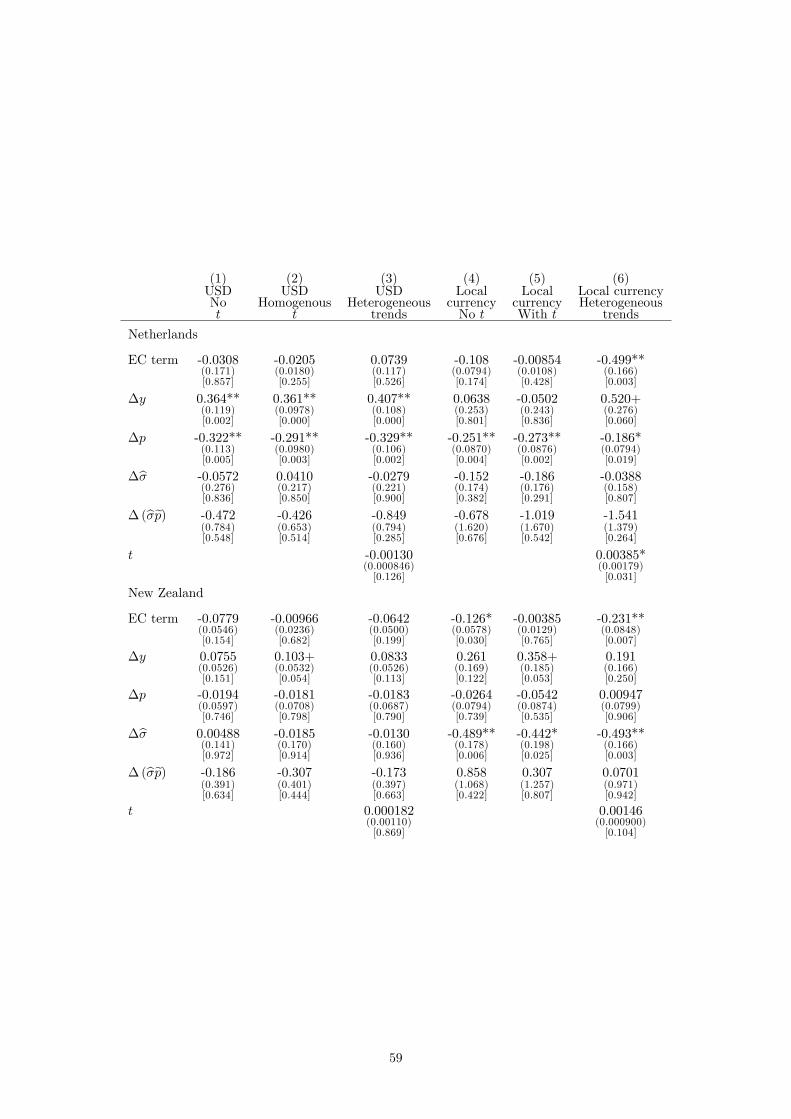
(1) (2) (3) (4) (5) (6)USD USD USD Local Local Local currencyNo Homogenous Heterogeneous currency currency Heterogeneoust t trends No t With t trends

Netherlands

EC term -0.0308 -0.0205 0.0739 -0.108 -0.00854 -0.499**(0.171) (0.0180) (0.117) (0.0794) (0.0108) (0.166)[0.857] [0.255] [0.526] [0.174] [0.428] [0.003]

∆y 0.364** 0.361** 0.407** 0.0638 -0.0502 0.520+(0.119) (0.0978) (0.108) (0.253) (0.243) (0.276)[0.002] [0.000] [0.000] [0.801] [0.836] [0.060]

∆p -0.322** -0.291** -0.329** -0.251** -0.273** -0.186*(0.113) (0.0980) (0.106) (0.0870) (0.0876) (0.0794)[0.005] [0.003] [0.002] [0.004] [0.002] [0.019]

∆σ̂ -0.0572 0.0410 -0.0279 -0.152 -0.186 -0.0388(0.276) (0.217) (0.221) (0.174) (0.176) (0.158)[0.836] [0.850] [0.900] [0.382] [0.291] [0.807]

∆ (σ̂p̃) -0.472 -0.426 -0.849 -0.678 -1.019 -1.541(0.784) (0.653) (0.794) (1.620) (1.670) (1.379)[0.548] [0.514] [0.285] [0.676] [0.542] [0.264]

t -0.00130 0.00385*(0.000846) (0.00179)[0.126] [0.031]

New Zealand

EC term -0.0779 -0.00966 -0.0642 -0.126* -0.00385 -0.231**(0.0546) (0.0236) (0.0500) (0.0578) (0.0129) (0.0848)[0.154] [0.682] [0.199] [0.030] [0.765] [0.007]

∆y 0.0755 0.103+ 0.0833 0.261 0.358+ 0.191(0.0526) (0.0532) (0.0526) (0.169) (0.185) (0.166)[0.151] [0.054] [0.113] [0.122] [0.053] [0.250]

∆p -0.0194 -0.0181 -0.0183 -0.0264 -0.0542 0.00947(0.0597) (0.0708) (0.0687) (0.0794) (0.0874) (0.0799)[0.746] [0.798] [0.790] [0.739] [0.535] [0.906]

∆σ̂ 0.00488 -0.0185 -0.0130 -0.489** -0.442* -0.493**(0.141) (0.170) (0.160) (0.178) (0.198) (0.166)[0.972] [0.914] [0.936] [0.006] [0.025] [0.003]

∆ (σ̂p̃) -0.186 -0.307 -0.173 0.858 0.307 0.0701(0.391) (0.401) (0.397) (1.068) (1.257) (0.971)[0.634] [0.444] [0.663] [0.422] [0.807] [0.942]

t 0.000182 0.00146(0.00110) (0.000900)[0.869] [0.104]

59

(1) (2) (3) (4) (5) (6)USD USD USD Local Local Local currencyNo Homogenous Heterogeneous currency currency Heterogeneoust t trends No t With t trends

Norway

EC term 0.0901** -0.277** -0.424* 0.170** -0.133** 0.371**(0.0318) (0.0827) (0.173) (0.0342) (0.0500) (0.120)[0.005] [0.001] [0.014] [0.000] [0.008] [0.002]

∆y 0.464** 0.480** 0.388** 0.111 0.203 0.00589(0.127) (0.108) (0.115) (0.111) (0.140) (0.122)[0.000] [0.000] [0.001] [0.319] [0.147] [0.962]

∆p -0.504** -0.486** -0.352** -0.257* -0.241+ -0.235*(0.134) (0.110) (0.130) (0.119) (0.134) (0.109)[0.000] [0.000] [0.007] [0.030] [0.073] [0.032]

∆σ̂ -0.392** -0.104 -0.110 0.289* 0.330* 0.344**(0.149) (0.166) (0.163) (0.138) (0.156) (0.127)[0.008] [0.530] [0.501] [0.036] [0.034] [0.007]

∆ (σ̂p̃) -0.131 0.532 0.0883 -2.880 -2.949 -2.015(0.663) (0.762) (0.585) (2.110) (2.412) (2.026)[0.843] [0.485] [0.880] [0.172] [0.222] [0.320]

t -0.0127** 0.00153(0.00402) (0.00189)[0.002] [0.420]

Poland

EC term -0.416** -0.133* -0.429** -0.342** -0.0370 -0.312*(0.118) (0.0600) (0.136) (0.114) (0.0358) (0.131)[0.000] [0.026] [0.002] [0.003] [0.301] [0.017]

∆y -0.289* -0.108 -0.256* 0.339 0.650* 0.358(0.130) (0.131) (0.130) (0.274) (0.308) (0.302)[0.026] [0.407] [0.050] [0.216] [0.035] [0.235]

∆p 0.306 0.192 0.344 0.399** 0.181 0.406**(0.200) (0.232) (0.214) (0.138) (0.151) (0.157)[0.127] [0.409] [0.109] [0.004] [0.232] [0.010]

∆σ̂ 0.988** 1.140** 1.052** 0.587+ 0.849* 0.643+(0.208) (0.253) (0.221) (0.309) (0.372) (0.337)[0.000] [0.000] [0.000] [0.057] [0.022] [0.056]

∆ (σ̂p̃) -0.774 0.0465 0.215 -3.091 -2.628 -3.598(0.783) (0.923) (0.822) (2.469) (3.249) (2.674)[0.323] [0.960] [0.793] [0.210] [0.419] [0.178]

t -0.00127 -0.00145(0.00339) (0.00239)[0.709] [0.544]

60

(1) (2) (3) (4) (5) (6)USD USD USD Local Local Local currencyNo Homogenous Heterogeneous currency currency Heterogeneoust t trends No t With t trends

Portugal

EC term -0.0402 -0.209** -0.254* -0.0706 -0.175** -0.0600(0.172) (0.0487) (0.114) (0.135) (0.0272) (0.0590)[0.815] [0.000] [0.026] [0.600] [0.000] [0.309]

∆y 0.713** 0.223 0.245+ 0.539 0.215 0.0249(0.157) (0.150) (0.137) (0.404) (0.210) (0.246)[0.000] [0.137] [0.075] [0.182] [0.307] [0.919]

∆p -0.803** -0.145 -0.204 -0.832** -0.218 -0.323+(0.158) (0.185) (0.159) (0.266) (0.138) (0.170)[0.000] [0.435] [0.198] [0.002] [0.115] [0.058]

∆σ̂ -0.512** 0.283 0.0209 -0.184 0.260 0.147(0.188) (0.235) (0.172) (0.299) (0.175) (0.183)[0.007] [0.229] [0.903] [0.539] [0.138] [0.421]

∆ (σ̂p̃) -0.523 0.295 -0.229 0.0261 2.656+ -0.646(0.717) (0.604) (0.465) (2.971) (1.553) (1.777)[0.465] [0.625] [0.623] [0.993] [0.087] [0.716]

t -0.00728** -0.00735**(0.00165) (0.00127)[0.000] [0.000]

Slovakia

EC term -0.575** -0.147 -0.917** -0.669** -0.189+ -0.887**(0.197) (0.106) (0.217) (0.214) (0.0985) (0.280)[0.004] [0.166] [0.000] [0.002] [0.055] [0.002]

∆y -0.0991 0.155 -0.260 -0.538 0.590 -1.205(0.233) (0.243) (0.210) (0.645) (0.647) (0.925)[0.671] [0.525] [0.216] [0.404] [0.361] [0.193]

∆p -0.156 -0.468 0.0658 -0.0584 -0.146 -0.155(0.302) (0.327) (0.280) (0.270) (0.315) (0.284)[0.605] [0.153] [0.814] [0.829] [0.643] [0.584]

∆σ̂ 0.577+ 0.404 0.495+ -0.181 -0.477 -0.0233(0.328) (0.369) (0.277) (0.480) (0.537) (0.480)[0.079] [0.272] [0.074] [0.707] [0.374] [0.961]

∆ (σ̂p̃) 0.236 2.592 1.035 2.791 0.186 4.486(2.080) (2.430) (1.921) (2.131) (2.359) (2.762)[0.910] [0.286] [0.590] [0.190] [0.937] [0.104]

t 0.0115* 0.0151+(0.00523) (0.00783)[0.029] [0.054]

61

(1) (2) (3) (4) (5) (6)USD USD USD Local Local Local currencyNo Homogenous Heterogeneous currency currency Heterogeneoust t trends No t With t trends

Spain

EC term 0.0182 -0.643** -1.720** 0.102 -0.300* -0.386*(0.0766) (0.219) (0.200) (0.0631) (0.134) (0.194)[0.812] [0.003] [0.000] [0.105] [0.025] [0.046]

∆y 0.169 -0.137 -0.302** 0.0863 0.623 1.089+(0.160) (0.159) (0.0897) (0.543) (0.518) (0.604)[0.288] [0.388] [0.001] [0.874] [0.229] [0.071]

∆p -0.311 0.0458 0.204+ -0.157 -0.303 -0.0451(0.214) (0.199) (0.113) (0.312) (0.281) (0.267)[0.147] [0.818] [0.071] [0.613] [0.280] [0.866]

∆σ̂ -0.331 0.820+ 1.069** -0.0823 -0.0307 0.0330(0.320) (0.447) (0.242) (0.443) (0.410) (0.378)[0.302] [0.067] [0.000] [0.853] [0.940] [0.930]

∆ (σ̂p̃) 0.0726 2.363 2.587* -1.094 9.539 0.601(1.207) (1.701) (1.101) (6.998) (7.807) (6.003)[0.952] [0.165] [0.019] [0.876] [0.222] [0.920]

t -0.0558** -0.0137**(0.00646) (0.00523)[0.000] [0.009]

Sweden

EC term 0.0105 -0.0518* -0.203** -0.332+ -0.0323+ -0.466*(0.0921) (0.0230) (0.0710) (0.169) (0.0182) (0.210)[0.909] [0.024] [0.004] [0.050] [0.076] [0.026]

∆y 0.185+ 0.141 0.0914 0.00603 -0.223 -0.216(0.102) (0.0865) (0.0776) (0.248) (0.267) (0.249)[0.068] [0.102] [0.239] [0.981] [0.405] [0.384]

∆p -0.106 -0.0316 0.0177 -0.0587 -0.0968 0.0772(0.0922) (0.0860) (0.0768) (0.107) (0.100) (0.121)[0.252] [0.714] [0.817] [0.582] [0.334] [0.524]

∆σ̂ 0.0889 0.256 0.265 -0.0162 -0.0551 -0.0289(0.216) (0.201) (0.170) (0.183) (0.179) (0.171)[0.681] [0.203] [0.120] [0.930] [0.758] [0.866]

∆ (σ̂p̃) -0.466 -0.236 0.153 0.385 0.455 -1.142(0.794) (0.665) (0.607) (1.761) (1.733) (1.585)[0.557] [0.723] [0.801] [0.827] [0.793] [0.471]

t -0.00309** -0.000878(0.000945) (0.00136)[0.001] [0.518]

62

(1) (2) (3) (4) (5) (6)USD USD USD Local Local Local currencyNo Homogenous Heterogeneous currency currency Heterogeneoust t trends No t With t trends

Switzerland

EC term -0.338** -0.00812 -0.589** -0.316+ -0.0652* -0.267+(0.123) (0.0239) (0.160) (0.177) (0.0313) (0.153)[0.006] [0.734] [0.000] [0.074] [0.037] [0.081]

∆y -0.0475 0.0874 -0.0963 0.0168 0.904+ 0.741(0.0921) (0.0924) (0.0866) (0.385) (0.516) (0.504)[0.606] [0.345] [0.266] [0.965] [0.080] [0.142]

∆p -0.186 -0.375** -0.0702 -0.0467 -0.257+ -0.121(0.117) (0.111) (0.119) (0.153) (0.134) (0.143)[0.113] [0.001] [0.555] [0.759] [0.054] [0.399]

∆σ̂ -0.107 -0.296+ 0.0892 -0.235 0.0279 -0.00775(0.150) (0.177) (0.170) (0.252) (0.278) (0.259)[0.474] [0.096] [0.600] [0.352] [0.920] [0.976]

∆ (σ̂p̃) 0.909 1.621 2.073* -0.298 3.189 0.606(0.882) (1.062) (0.844) (2.444) (2.756) (2.452)[0.303] [0.127] [0.014] [0.903] [0.247] [0.805]

t -0.00265* -0.00391*(0.00118) (0.00176)[0.024] [0.026]

Turkey

EC term -0.0712 -0.441** -0.345** 0.0170 -0.221* -0.333**(0.0936) (0.138) (0.129) (0.0986) (0.0878) (0.115)[0.447] [0.001] [0.008] [0.863] [0.012] [0.004]

∆y 0.246+ 0.0189 0.119 0.0535 0.0720 0.341(0.128) (0.128) (0.114) (0.323) (0.266) (0.250)[0.054] [0.882] [0.297] [0.868] [0.787] [0.174]

∆p -0.183 0.212 0.104 -0.0538 0.0464 0.295(0.159) (0.176) (0.164) (0.283) (0.237) (0.230)[0.249] [0.227] [0.523] [0.849] [0.845] [0.199]

∆σ̂ 0.124 0.427 0.265 -0.197 -0.233 -0.0379(0.358) (0.315) (0.298) (0.446) (0.375) (0.335)[0.730] [0.176] [0.375] [0.658] [0.534] [0.910]

∆ (σ̂p̃) -4.037** -1.636 -1.535 -4.459 0.623 -1.650(1.427) (1.562) (1.381) (3.419) (3.361) (2.657)[0.005] [0.295] [0.267] [0.192] [0.853] [0.535]

t -0.0193** -0.0228**(0.00658) (0.00619)[0.003] [0.000]

63

(1) (2) (3) (4) (5) (6)USD USD USD Local Local Local currencyNo Homogenous Heterogeneous currency currency Heterogeneoust t trends No t With t trends

United Kingdom

EC term 0.0921 -0.0638+ -0.0655 0.112+ -0.0711** -0.0634(0.0637) (0.0335) (0.153) (0.0587) (0.0233) (0.122)[0.148] [0.057] [0.669] [0.056] [0.002] [0.605]

∆y 0.0532 -0.0441 -0.0272 0.515 0.707+ 0.665(0.145) (0.124) (0.156) (0.464) (0.400) (0.433)[0.713] [0.723] [0.862] [0.266] [0.077] [0.125]

∆p 0.00828 0.0698 0.0653 -0.0459 -0.00489 0.00366(0.140) (0.134) (0.147) (0.138) (0.118) (0.129)[0.953] [0.601] [0.657] [0.739] [0.967] [0.977]

∆σ̂ -0.00265 0.107 0.0853 0.480 0.424 0.426(0.124) (0.142) (0.136) (0.328) (0.277) (0.302)[0.983] [0.451] [0.531] [0.144] [0.126] [0.158]

∆ (σ̂p̃) -1.158 -1.031 -1.087 -1.867 0.512 -1.430(0.773) (0.749) (0.735) (3.101) (2.827) (2.847)[0.134] [0.169] [0.139] [0.547] [0.856] [0.616]

t -0.00301 -0.00322+(0.00228) (0.00184)[0.186] [0.080]

United States

EC term -0.0211 -0.00496 -0.0354+ -0.0235 -0.00488 -0.0756(0.0148) (0.00519) (0.0201) (0.0153) (0.00309) (0.0532)[0.155] [0.339] [0.079] [0.124] [0.114] [0.155]

∆y 0.466** 0.530** 0.405** 0.499** 0.534** 0.422*(0.145) (0.139) (0.155) (0.140) (0.136) (0.166)[0.001] [0.000] [0.009] [0.000] [0.000] [0.011]

∆p -0.0108 -0.0171 -0.0126 -0.0129 -0.0226 0.00303(0.0227) (0.0225) (0.0216) (0.0215) (0.0198) (0.0298)[0.634] [0.447] [0.560] [0.547] [0.255] [0.919]

∆σ̂ 0.0119 0.00159 0.00873 0.00738 0.0116 -0.00607(0.0376) (0.0373) (0.0355) (0.0351) (0.0358) (0.0364)[0.751] [0.966] [0.806] [0.833] [0.745] [0.868]

∆ (σ̂p̃) -0.320* -0.330* -0.300* -0.266+ -0.174 -0.485*(0.133) (0.137) (0.131) (0.146) (0.176) (0.193)[0.016] [0.016] [0.022] [0.069] [0.324] [0.012]

t 0.000553 0.000910(0.000555) (0.000786)[0.319] [0.247]

Standard errors in parentheses; p-values in brackets.** p<0.01, * p<0.05, + p<0.1

64

References

[1] Ahn, Seung C., and Peter Schmidt. 1995. Effi cient estimation of models for dynamic panel data.

Journal of Econometrics 68: 5-27.

[2] Akinboade, Olude A., Emmanuel Ziramba, and Wolassa L. Kumo. 2008. The demand for gasoline

in South Africa: An empirical analysis using co-integration techniques. Energy Economics 30: 3222-

3229.

[3] Alves, Denisard C.O., and Rodrigo De Losso da Silveira Bueno. 2003. Short-run, long-run and cross

elasticities of gasoline demand in Brazil. Energy Economics 25:191—199.

[4] Anderson, T. W., and Cheng Hsiao. 1981. Estimation of dynamic models with error components.

Journal of the American Statistical Association 76(375): 598-606.

[5] Angelier, Jean Pierre, and Thomas Sterner. 1990. Tax harmonization for petroleum products in the

EC. Energy Policy 18(6): 500-505.

[6] Arellano, Manuel, and Steven Bond. 1991. Some tests of specification for panel data: Monte Carlo

evidence and an application to employment equations. The Review of Economic Studies 58(2):

277-297.

[7] Arellano, Manuel, and Olympia Bover. 1995. Another look at the instrumental variable estimation

of error-components models. Journal of Econometrics 68 : 29-51.

[8] Baltagi, Badi H., and James M. Griffi n. 1983. Gasoline demand in the OECD application of pooling

and testing procedures. European Economic Review 22(2): 117-137.

[9] Baltagi, Badi H., and James M. Griffi n. 1997. Pooled estimators vs. their heterogeneous counterparts

in the context of dynamic demand for gasoline. Journal of Econometrics 77(2): 303-327.

[10] Baltagi, Badi H., and Chihwa Kao. Nonstationary panels, cointegration in panels and dynamic pan-

els: A Survey. 2000. Advances in Econometrics, Vol. 25: Nonstationary Panels, Panel Cointegration,

and Dynamic Panels (ed. Badi H. Baltagi).New York: Elsevier.

[11] Banerjee, Anindya, Juan J. Dolado, and Ricardo Mestre. 1998. Error-Correction Mechanism Tests

for Cointegration in a Single-Equation Framework. Journal of Time Series Analysis 19(3): 267-283.

[12] Bentzen, Jan. 1994. An empirical analysis of gasoline demand in Denmark using cointegration tech-

niques. Energy Economics 16(2): 139-143.

[13] Bentzen, Jan, and Tom Engsted. 2001. A revival of the autoregressive distributed lag model in

estimating energy demand relationships. Energy 26: 45-55.

[14] Blackburne, Edward F., and Mark W. Frank. 2007a. Estimation of nonstationary heterogeneous

panels. Stata Journal 7(2): 197-208.

[15] Blackburne, Edward F., and Mark W. Frank. 2007b. XTPMG: Stata module for estimation of

nonstationary heterogeneous panels. Statistical Software Components S456868, Boston College De-

partment of Economics.

[16] Blundell, Richard, Steve Bond, and FrankWindmeijer. 2000. Estimation in dynamic panel data mod-

els: Improving on the performance of the standard GMM estimator. IFS Working Papers W00/12,

Institute for Fiscal Studies.

65

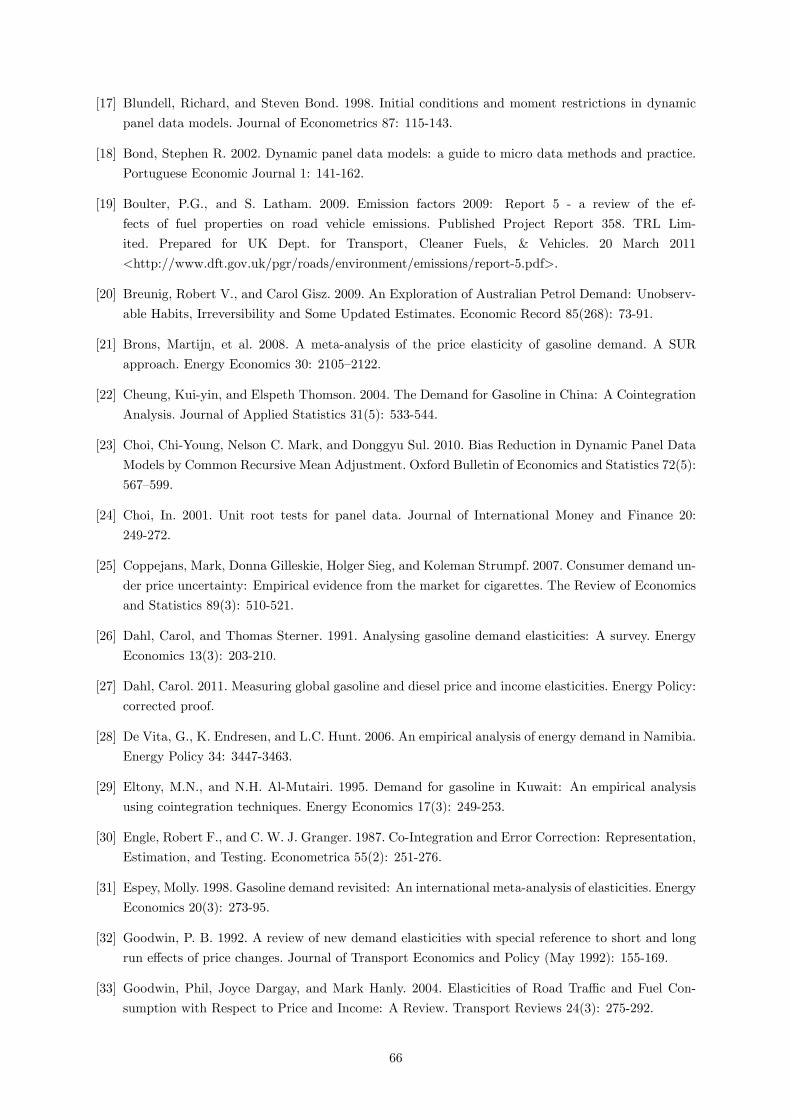
[17] Blundell, Richard, and Steven Bond. 1998. Initial conditions and moment restrictions in dynamic

panel data models. Journal of Econometrics 87: 115-143.

[18] Bond, Stephen R. 2002. Dynamic panel data models: a guide to micro data methods and practice.

Portuguese Economic Journal 1: 141-162.

[19] Boulter, P.G., and S. Latham. 2009. Emission factors 2009: Report 5 - a review of the ef-

fects of fuel properties on road vehicle emissions. Published Project Report 358. TRL Lim-

ited. Prepared for UK Dept. for Transport, Cleaner Fuels, & Vehicles. 20 March 2011

<http://www.dft.gov.uk/pgr/roads/environment/emissions/report-5.pdf>.

[20] Breunig, Robert V., and Carol Gisz. 2009. An Exploration of Australian Petrol Demand: Unobserv-

able Habits, Irreversibility and Some Updated Estimates. Economic Record 85(268): 73-91.

[21] Brons, Martijn, et al. 2008. A meta-analysis of the price elasticity of gasoline demand. A SUR

approach. Energy Economics 30: 2105—2122.

[22] Cheung, Kui-yin, and Elspeth Thomson. 2004. The Demand for Gasoline in China: A Cointegration

Analysis. Journal of Applied Statistics 31(5): 533-544.

[23] Choi, Chi-Young, Nelson C. Mark, and Donggyu Sul. 2010. Bias Reduction in Dynamic Panel Data

Models by Common Recursive Mean Adjustment. Oxford Bulletin of Economics and Statistics 72(5):

567—599.

[24] Choi, In. 2001. Unit root tests for panel data. Journal of International Money and Finance 20:

249-272.

[25] Coppejans, Mark, Donna Gilleskie, Holger Sieg, and Koleman Strumpf. 2007. Consumer demand un-

der price uncertainty: Empirical evidence from the market for cigarettes. The Review of Economics

and Statistics 89(3): 510-521.

[26] Dahl, Carol, and Thomas Sterner. 1991. Analysing gasoline demand elasticities: A survey. Energy

Economics 13(3): 203-210.

[27] Dahl, Carol. 2011. Measuring global gasoline and diesel price and income elasticities. Energy Policy:

corrected proof.

[28] De Vita, G., K. Endresen, and L.C. Hunt. 2006. An empirical analysis of energy demand in Namibia.

Energy Policy 34: 3447-3463.

[29] Eltony, M.N., and N.H. Al-Mutairi. 1995. Demand for gasoline in Kuwait: An empirical analysis

using cointegration techniques. Energy Economics 17(3): 249-253.

[30] Engle, Robert F., and C. W. J. Granger. 1987. Co-Integration and Error Correction: Representation,

Estimation, and Testing. Econometrica 55(2): 251-276.

[31] Espey, Molly. 1998. Gasoline demand revisited: An international meta-analysis of elasticities. Energy

Economics 20(3): 273-95.

[32] Goodwin, P. B. 1992. A review of new demand elasticities with special reference to short and long

run effects of price changes. Journal of Transport Economics and Policy (May 1992): 155-169.

[33] Goodwin, Phil, Joyce Dargay, and Mark Hanly. 2004. Elasticities of Road Traffi c and Fuel Con-

sumption with Respect to Price and Income: A Review. Transport Reviews 24(3): 275-292.

66

[34] Graham, Daniel J., and Stephen Glaister. 2004. Road Traffi c Demand Elasticity Estimates: A

Review. Transport Reviews 24(3): 261—274.

[35] Harris, Richard D.F., and Elias Tzavalis. 1999. Inference for unit roots in dynamic panels where the

time dimension is fixed. Journal of Econometrics 91: 201-226.

[36] Holtz-Eakin, Douglas, Whitney Newey, and Harvey S. Rosen. 1988. Estimating vector autoregres-

sions with panel data. Econometrica 56(6): 1371-95.

[37] Hughes, Jonathan E., Christopher R. Knittel, and Daniel Sperling. 2006. Evidence of a shift in the

short-run price elasticity of gasoline demand. CSEM Working Paper 159. September 2006.

[38] Im, Kyung So, M. Hashem Pesaran, and Yongcheol Shin. 2003. Testing for unit roots in heteroge-

neous panels. Journal of Econometrics 115: 53-74.

[39] Johansson, Olof, and Lee Schipper. 1997. Measuring the Long-Run Fuel Demand of Cars: Separate

Estimations of Vehicle Stock, Mean Fuel Intensity, and Mean Annual Driving Distance. Journal of

Transport Economics and Policy 31(3): 277-292.

[40] Judson, Ruth A., Richard Schmalensee, and Thomas M. Stoker. 1999. Economic development and

the structure of the demand for commercial energy. Energy Journal 20(2): 29-57.

[41] Kao, Chihwa. 1999. Spurious regression and residual-based tests for cointegration in panel data.

Journal of Econometrics 90: 1-44.

[42] Kilian, Lutz. 2010. Explaining Fluctuations in Gasoline Prices: A Joint Model of the Global Crude

Oil Market and the U.S. Retail Gasoline Market. The Energy Journal 31(2): 103-128.

[43] Kleibergen, Frank, and Richard Paap. 2006. Generalized reduced rank tests using the singular value

decomposition. Journal of Econometrics 133: 97—126

[44] Krichene, Noureddine. 2002. World crude oil and natural gas: a demand and supply model. Energy

Economics 24: 557-576.

[45] Levin, Andrew, Chien-Fu Lin, and Chia-Shang James Chu. 2002. Unit root tests in panel

data:asymptotic and finite-sample properties. Journal of Econometrics 108: 1-24.

[46] Liu, Gang. 2004. Estimating Energy Demand Elasticities for OECD Countries: A Dynamic Panel

Approach. Statistics Norway Resarch Department Discussion Papers No. 373, March 2004.

[47] Maddala, G. S. , and Shaowen Wu. 1999. A comparative study of unit root tests with panel data

and a new simple test. Oxford Bulletin of Economics and Statistics, Special Issue, 1999: 631-652.

[48] MotorMouth. 2010. “Fuel Types.”8 Dec 2010<http://motormouth.com.au/myresources/fueltypes.aspx>.

[49] Nadaud, F. 2004. The demand for car gasoline in France: a long run econometric perspective, 6th

IAEE European Energy Conference, 2—3 September, Zurich, Switzerland.

[50] Narayan, Paresh Kumar, and Russell Smyth. 2007. A panel cointegration analysis of the demand

for oil in the Middle East. Energy Policy 35: 6258—6265.

[51] Nguyen-Van, Phu. 2010. Energy consumption and income: A semiparametric panel data analysis.

Energy Economics 32: 557—563.

[52] Nickell, Stephen. 1981. Biases in Dynamic Models with Fixed Effects. Econometrica 49(6): 1417-

1426.

67

[53] Pedroni, Peter. 2004. Panel cointegration: Asymptotic and finite sample properties of pooled time

series tests with an application to the PPP hypothesis. Econometric Theory 20: 597—625.

[54] Persyn, Damiaan, and Joakim Westerlund. 2008. Error Correction Based Cointegration Tests for

Panel Data. Stata Journal 8(2): 232-241.

[55] Pesaran, M. Hashem, and Yongcheol Shin. 1999. An autoregressive distributed lag modelling ap-

proach to cointegration analysis. Chapter 11 in Econometrics and Economic Theory in the 20th

Century: The Ragnar Frisch Centennial Symposium, Strom S (ed). Cambidge, UK: Cambridge UP.

Accessed version revised January 1997 at <http://www.econ.cam.ac.uk/faculty/pesaran/ardl.pdf>,

24 February 2011.

[56] Pesaran, M. Hashem, Yongcheol Shin, and Richard J. Smith. 1999. Pooled Mean Group Estimation

of Dynamic Heterogeneous Panels. Journal of the American Statistical Association 94(446): 621-634.

[57] Pesaran, M. Hashem, and Ron Smith. 1995. Estimating long-run relationships from dynamic het-

erogenous panels. Journal of Econometrics 68: 79-113.

[58] Pesaran, M. Hashem, and Zhongyun Zhao. 1999. Bias Reduction in Estimating Long- Run Relation-

ships From Dynamic Heterogeneous Panels. In Analysis of Panels and Limited Dependent Variables:

A Volume in Honour of G. S. Maddala, eds. Cheng Hsiao et al. Cambridge, UK: Cambridge UP.

[59] Phillips, Peter C. B., and Pierre Perron. 1988. Testing for a Unit Root in Time Series Regression.

Biometrika 75(2): 335-346.

[60] Polemis, Michael L. 2006. Empirical assessment of the determinants of road energy demand in

Greece. Energy Economics 28: 385-403.

[61] Ramanathan, R. 1999. Short- and long-run elasticities of gasoline demand in India: An empirical

analysis using cointegration techniques. Energy Economics 21: 321-330.

[62] Ramanathan, R. and G. Subramanian, G. 2003. An empirical analysis of gasoline demand in the

Sultanate of Oman using cointegration techniques. Pacific and Asian Journal of Energy 13: 33—41.

[63] Rao, B. Bhaskara, and Gyaneshwar Rao. 2009. Cointegration and the demand for gasoline. Energy

Policy 37: 3978-3983.

[64] Roodman, David. 2006. How to do xtabond2: An introduction to “Difference” and “System”

GMM in Stata. Center for Global Development, Working Paper No. 103. Available from

http://www.cgdev.org/files/11619_file_HowtoDoxtabond6_12_1_06.pdf.

[65] Roodman, David. 2007. A short note on the theme of too many instru-

ments. Center for Global Development, Working Paper No. 125. Available from

http://www.cgdev.org/content/publications/detail/14256.

[66] Roodman, David. 2011 (first version 2003). XTABOND2: Stata module to extend

xtabond dynamic panel data estimator. Center for Global Development, Washington.

http://econpapers.repec.org/software/bocbocode/s435901.htm.

[67] Samimi, Rodney. 1995. Road transport energy demand in Australia: A cointegration approach.

Energy Economics 17(4): 329-339.

[68] Schaffer, Mark E. 2010. xtivreg2: Stata module to perform extended IV/2SLS, GMM

and AC/HAC, LIML and k-class regression for panel data models. Available from

http://ideas.repec.org/c/boc/bocode/s456501.html.

68

[69] Scott, K. Rebecca. 2010. Rational Habits and Uncertain Relative Prices: Simulating Petrol Con-

sumption Behavior. In Essays in Consumption Habits and the Environment - Thesis (D.Phil.),

University of Oxford, 2011.

[70] Stata. 2009. Stata Longitudinal-Data/Panel-Data Reference Manual, Stata User’s Guide, Release

11. College Station, TX: Stata Press. 523-522.

[71] StataCorp. 2009. Stata Statistical Software: Release 11. College Station, TX: StataCorp LP.

[72] Storchmann, Karl. 2005. Long-run gasoline demand for passenger cars: the role of income distribu-

tion. Energy Economics 27(1): 25—58.

[73] Wadud, Zia, Daniel J. Graham, and Robert B. Noland. 2009. A cointegration analysis of gasoline

demand in the United States. Applied Economics 41(26): 3327-3336.

[74] Westerlund, Joakim. 2007. Testing for Error Correction in Panel Data. Oxford Bulletin of Economics

and Statistics 69(6): 709-748.

[75] Windmeijer, Frank. 2005. A finite sample correction for the variance of linear effi cient two-step

GMM estimators. Journal of Econometrics 126(1): 25-51.

Data

[76] International Energy Agency (IEA). 2009. Energy Prices and Taxes (2009Q4). ESDS International,

(Mimas) University of Manchester.

[77] International Energy Agency (IEA). 2009. Oil Information (2009). ESDS International, (Mimas)

University of Manchester.

[78] United Nations, Department of Economic and Social Affairs, Population Division. 2009.

World Population Prospects: The 2008 Revision, CD-ROM Edition. 9 March 2010

<http://esa.un.org/unpd/wpp2008/peps_stock-indicators.htm>.

[79] World Bank. 2009. World Development Indicators (WDI) (2009). ESDS International, (Mimas)

University of Manchester.

69