Deficits, Debt Financing, Monetary Policy and Inflation inDeveloping Countries: Internal or External Factors?

Amir Kia

Department of EconomicsCarleton University

Ottawa, ON, Canada K1S 5B6Tel.: (613) 747-9625Fax: (613) 747-1352

akia@ccs.carleton.ca

October 2004

Abstract:

This paper focuses on internal and external factors, which influence the inflation rate indeveloping countries. A monetary model of inflation rate, capable of incorporating bothmonetary and fiscal policies as well as other internal and external factors, was developedand tested on three developing countries: Egypt, Iran and Turkey. The model performedwell on the data of these countries. It was found that government debt and deficits alongwith other factors are important determinants of inflation. Furthermore, most sources ofinflation in these countries are domestic factors.

Keywords: Demand for money, inflation, fiscal and monetary policies, external andinternal factors

JEL Codes: E31, E41 and E62

Deficits, Debt Financing, Monetary Policy and Inflation inDeveloping Countries: Internal or External Factors?

I. Introduction

The determinants of inflation rate in developing countries are extremely important

for policy makers as when the causes of inflation are correctly specified the appropriate

policy change can be easily diagnosed and effectively implemented. Inflation in a small-

open economy can be influenced by both internal and external factors. Internal factors

include, among others, government deficits, debt financing, monetary policy, institutional

economics (shirking, opportunism, economic freedom, risk, etc.) and structural regime

changes (revolution, political regime changes, policy constraints, etc.). External factors

include terms of trade and foreign interest rate as well as the attitude of the rest of the

world (sanctions, risk generating activities, wars, etc.) toward the country. The objective

of this paper is to develop and test a model of inflation rate, which takes into account all

of these factors. To the best knowledge of the author, no such study for developing or

developed countries exists.

The impact of government deficits and debt financing on inflation rate can be

thought of through different channels. Higher government deficits result in higher interest

rates, which then leads to lower domestic investment. This crowding-out effect of deficits

will eventually translate into a lower formation of capital and lead to a lower aggregate

supply and a higher price. However, the impact of deficit on interest rates is still

debatable. For example, Bradley (1986) lists twenty-one studies on the deficit-interest

rate link and finds that only four provided supporting evidence for a positive and

2

statistically significant impact of the deficit on interest rates. The rest of the studies finds

either no evidence of a significant impact or produces mixed results, including the

absence of any linkage. The literature on the deficit-interest rate link for a small-open

economy under capital mobility is limited to theoretical studies. Empirical studies pertain

to either large open, or closed economy models, see Evans (1985), Giannaros et al.

(1985), Tanzi (1985), Cebula (1985), Hoelscher (1986) and Bradley (1986).

The second channel in which deficits and debt financing can affect the inflation

rate is through the monetization of the deficit/debt. Monetary authority must then act to

ensure that the government’s intertemporal budget is balanced, i.e., a situation of fiscal

dominance. With fiscal dominance, an increase in government debt will eventually

require an increase in seigniorage. King and Plosser (1985) and Grier and

Neiman (1987), e.g., found mixed evidence for fiscal dominance in the United States;

however, Ashra et al. (2004) find no systematic relationship between money and fiscal

deficits in India. It is also believed that the uncertainty as to the time the deficits are

financed can influence the rate of inflation. For example, Dornbush et al. (1990) and

Drazen and Helpman (1990) find such an uncertainty creates fluctuation in the inflation

rate.

The third channel is the wealth effect of deficits/debt financing. When deficits and

debts are financed by issuing bonds and bondholders do not consider bonds as future

taxes (a non-Ricardian view), the wealth of the nation is perceived to have gone up. A

higher wealth effect increases the demand for goods and services and drives prices up.

However, Tekin-Koru and Ozmen (2003) find no support for the linkage between the

budget deficit and inflation through the wealth effect in Turkey. Instead, they found that

3

deficit financing leads to a higher growth of interest-bearing broad money, but not

currency seigniorage. Finally, institutional economics reduces information costs,

encourages capital formation and capital mobility, allows risks to be priced and shared

and facilitates cooperation. These institutions improve aggregate economic performance,

see North and Thomas (1973), North (1990), Drobak and Nye (1997), Levine (1997) and

Klein and Luu (2003). Improvements in aggregated economic performance should lead to

a lower inflation rate.

External factors include terms of trade and foreign interest rate besides, among

others, sanctions and wars. The countries, especially developing countries, for which the

economy depends heavily on the import of capital, are subject to higher prices through

the supply effect (cost-push inflation), as the price of imported capital goods goes up. For

example, Senhadji (2003) argues that a stylized developing economy relies heavily on

imports for the capital formation and since it faces an upward-sloping supply function of

foreign loans, its debt accumulation increases with the size of debt and the cost of

servicing the debt. If an unfavorable change in the terms of trade increases the cost of the

imported capital then the formation of capital will suffer. This in turn suppresses the

aggregate supply and causes inflation. The same result can be obtained with a hike in

foreign interest rates, as such hikes make the financing of the imported capital (foreign

loans) more expensive. Finally, an unfavorable change in the terms of trade can result in

an imported inflation. Bahmani-Oskooee (1995), e.g., finds the world price has a positive

impact over the long run on the consumer price in Iran and Arize et al. (2004) find

inflation in 82 countries responds positively to the volatility of real and nominal

exchange rates. Finally, sanctions, wars, etc. clearly generate, through the supply effect, a

4

higher inflation. For example, Berument and Kilinc (2004) find shocks in the industrial

production of Germany, the United States and the rest of the world will affect positively

the inflation rate in Turkey. To the best knowledge of the author there is no study so far

in the literature that investigates the impact of all the above-mentioned factors on the

inflation rate for developing or developed countries.

The purpose of this study is to develop an empirically testable model for three

small-open economy countries, i.e., Egypt, Iran and Turkey. Egypt, with more than 90%

of the country being desert land, relies mostly on tourism; Iran, on oil exports and

Turkey, on agricultural products. The model used in this study is an augmented version of

the monetarist model which, contrary to the existing literature, is designed in such a way

to incorporate both external and internal factors, which cause inflation in the country.

Furthermore, since the model also incorporates government deficits and debt we could

test Sargent and Wallace’s (1986) views that (i) the tighter is the current monetary policy,

the higher must the inflation rate be eventually and (ii) that government deficits and debt

will be eventually monetized over the long run.

It was found that our model is successful in capturing the impact of fiscal

instruments, i.e., deficits, debt and debt management, and of monetary instruments on the

inflation rate in developing countries. Furthermore, a policy toward a stronger currency is

deflationary and most sources of inflation in the countries under study are domestic

factors. Finally, it was found Sargent and Wallace’s view on a tight monetary policy

leading to higher inflation over the long run is accepted for Egypt and Turkey. Moreover,

their view on government deficits and debt being eventually monetized over the long run

applies only to Egypt.

5

The following section deals with the development of the theoretical model.

Section III describes the data and the long-run empirical methodology and results.

Section IV is devoted to the short-run dynamic models for these countries. The final

section provides some concluding remarks. The appendix fully describes the data.

II. The ModelMany studies on inflation rate for both developed and developing countries used

different versions of the monetarist approach. For example, for developed countries, see,

McGuire (1976), Meltzer (1977) and Korteweg and Meltzer (1978). For developing

countries, see, e.g., Harberger (1963), Bomberger and Makinen (1979), Sheehey (1979),

Nugent and Glezakos (1979), Saini (1982), Ize and Salas (1985), McNelis (1987), Darrat

and Arize (1990), Bahmani-Oskooee and Malixi (1992), Bahmani-Oskooee (1995) and

Ashra et al. (2004).

The monetarist approach to inflation determination is based on the quantity

equation, which relates the current rates of change of aggregate expenditure, m + v, to the

nominal value of current income, π + y, where m, v, π and y are the growth rate of

nominal money supply, velocity of money, price and real income, respectively. In this

approach, the inflation rate is related to the growth rate of money in excess of the growth

rate of income. Along a steady growth path, the fully anticipated rate of price change

remains constant. Departures from long-run equilibrium give rise to an excess demand

for, or supply of, money and goods. Another approach is based on the equilibrium in the

money market where the demand for money is derived from individual optimization and

the supply of money is exogenous. Then again, departures from long-run equilibrium

give rise to an excess demand for, or supply of, money and goods. Prices should adjust so

6

that the markets will be cleared again. To avoid an ad-hoc determination the latter

approach will be followed in this paper.

For the sake of simplicity, following Hueng (1999) among many others, we

assume that labor is supplied inelastically. Consider an economy with a single consumer,

representing a large number of identical consumers. The consumer maximizes the

following utility function:

E { )}*m t , mt k t , g t ,*c t, ct U(

0t

β t∑∞

=

, (1)

where ct and c*t are single, non-storable, real domestic and foreign consumption goods,

respectively. mt and m*t are the holdings of domestic real (M/p) and foreign real (M*/p*)

cash balances, respectively. E is the expectation operator, and the discount factor satisfies

0<β<1. g is the real government expenditure on goods and services and it is assumed to

be a “good”. Including government expenditure in preferences is based on the assumption

that individuals benefit from government services in their consumption, say, clean and

safe roads, foods which have been inspected, etc. provide a higher utility to consumers.

Alternatively, following the literature, we can consider g as public demand for public

goods. In fact, allowing consumer preferences to depend on government spending is not

new in the literature, see, e.g., Barro (1981), Aschaurer (1985), Christiano and

Eichenbaum (1992), Baxter and King (1993), Karras (1994), Ahmed and Yoo (1995),

Ambler and Cardia (1997), Amano and Wirjanto (1997, 1998), and Cardia, et al. (2003).

Following Kim (2000), variable kt, which summarizes risk associated to holding

domestic money is also included. However, in contrast with Kim, we assume variable k is

7

a function of anticipated variables over the long run and policy and political regime

changes over the short run. Specifically, we postulate that over the long run:

log (kt) = k0 defgdpt + k1 debtgdpt + k2 fdgdpt. (2)

Equation (2) is held subject to a short-run dynamic system, which is a function of a set of

variables included in DUM as well as all other predetermined short-run (stationary)

variables known to individuals. These variables include the growth of money supply,

changes in fiscal variables per GDP, the growth in exchange rate, domestic and foreign

inflation as well as changes in interest rates.

The set of seasonal and interventional dummies DUM includes dummy variables

which account for wars, sanctions, political and technical changes, innovations as well as

policy regime changes which influence services of money. Note that DUM appears only

in the short-run dynamic of the system. Variables defgdp, debtgdp and fdgdp are real

government deficits per GDP, the government debt outstanding per GDP and the

government foreign-financed debt per GDP, respectively. We assume government debt

pays the same interest rate as deposits at the bank (i.e., R). In a risky environment agents

substitute real or interest-bearing assets for money.

For example, as the government deficit per GDP increases agents perceive higher

future taxes or money supply (inflation). At the same time, the higher is the outstanding

government debt relative to the size of the economy, the riskier the environment will be

perceived. Individuals may hold these bonds to bridge the gap between the future labor

income and expenditures, including tax expenditures. Consequently, we hypothesize

constant coefficients k0>0 and k1>0. Furthermore, an increase in the amount of

government debt held by foreign investors/governments may be considered a cause for

8

future devaluation of the domestic currency. Consequently, demand for domestic money,

may fall, implying k2>0.

The utility function is assumed to be increasing in all its arguments, except

variable k that is decreasing, and is strictly concave and continuously differentiable. The

demand for monetary services S [= m and m*, following Sidrauski (1967)] will always be

positive if we assume lims→0 Us(c, c*, g, k m, m*) = ∞, for all c and c*, where

Us = ∂U(c, c*, g, k m, m*)/∂s. Assume also that the U.S. dollar represents foreign

currency and that, following Stockman (1980), Lucas (1982), Guidotti (1993) and Hueng

(1999), purchases of domestic and foreign goods are made with domestic and foreign

currencies, respectively.

Given g, defgdp, debtgdp and fdgdp, the consumer maximizes (1) subject to the

following budget constraint:

τt + yt + (1 + πt)-1 mt-1 + qt (1 + π*t)-1 m*t-1 + (1 + πt)-1 (1 + Rt-1) dt-1 +

qt (1 + π*t)-1 (1 + R*t-1) d*t-1 = ct + qt ct* + mt + qt mt* + dt + qt dt*, (3)

where τt is the real value of any lump-sum transfers/taxes received/paid by consumers, qt

is the real exchange rate, defined as Et pt*/pt, Et is the nominal market (non-official/black-

market rate in some developing countries) exchange rate (domestic price of foreign

currency), pt* and pt are the foreign and domestic price levels of foreign and domestic

goods, respectively, yt is the current real endowment (income) received by the individual,

m*t-1 is the foreign real money holdings at the start of the period, dt is the one-period real

domestically financed government debt which pays R rate of return and dt* is the real

foreign issued one-period bond which pays a risk-free interest rate Rt*. Assume further

that dt and dt* are the only two storable financial assets.

9

Define Uc = ∂U(c, c*, g, k m, m*)/∂c, Uc* = ∂U(c, c*, g, k m, m*)/∂c*,

Um = ∂U(c, c*, g, k m, m*)/∂m, Um* = ∂U(c, c*, g, k m, m*)/∂m* and λt = the marginal

utility of wealth at time t. Maximizing the preferences with respect to m, c, m*, c*, d and

d*, and subject to budget constraint (3) for the given output and fiscal variables, will

yield the first-order conditions:

Uct + λt = 0 (4)

Uc*t + λt qt = 0 (5)

Umt + λt - βλet+1 (1 + πe

t+1)-1 = 0 (6)

Um*t + λt qt - βλet+1qe

t+1 (1 + π*et+1)-1 = 0 (7)

λt - βλet+1 (1 + Rt) (1 + πe

t+1)-1 = 0 (8)

λt qt - βλet+1 qe

t+1 (1 + R*t) (1 + π*et+1)-1 = 0. (9)

Note that xet+1 = E (xt+1│It) is the conditional expectations of xt+1, given current

information It. From (4) and (5) we can write:

Uct/Uc*t = 1/qt. (10)

Equation (10) indicates that the marginal rate of substitution between domestic and

foreign goods is equal to their relative price. Solving (5), (7) and (9) yields:

Uc*t (1 + R*t)-1 + Um*t = Uc*t. (11)

Equation (11) implies that the expected marginal benefit of adding to foreign currency

holdings at time t must equal the marginal utility from consuming foreign goods at time t.

Note that the holdings of foreign currency directly yield utility through its services (Um*t).

Furthermore, from (9) and (5) we have -Uc*t = βλet+1 qe

t+1 (1 + R*t) (1 + π*et+1)-1 which

implies that the expected real foreign currency invested in foreign bonds has a forgone

10

value of -Uc*t. Consequently, the total marginal benefit of holding money at time t is

Uc*t + Um*t.

Similarly, from (4), (6) and (8), we have:

Uct (1 + rt)-1 + Umt = Uct. (12)

Equation (12) implies that the expected marginal benefit from adding to domestic

currency holdings at time t must equal the marginal utility of consuming domestic goods

at time t.

To construct a parametric demand for real balances, assume the utility has an

instantaneous function as:

U(ct, ct*, gt, kt mt, mt*) = (1- α)-1 (ctα1

c*t α2

gt α3)1-α

+ ξ kt-η (1- η) -1(mt

η1 m*tη2)1-η, (13)

where α1, α2, α3, α, η1, η2, η and ξ are positive parameters and 0.5<α <1, 0.5<η <1. The

latter assumption (0.5<α <1, 0.5<η <1) is needed to ensure a standard demand for money.

Since none of the following results is sensitive to the magnitude of α1, α2, α3, η1 and η2 for

the sake of simplicity we assume these parameters are all equal to one.

A few words on the parametric function (13) are worth mentioning. This utility

is in the general class of utility functions used by Fischer (1979). However, here the

utility function includes the consumption of public and foreign goods as well as the

holding of foreign real balances. Furthermore, it allows individuals to get satisfaction

from the consumption of domestic and foreign goods as well as public goods even in the

absence of money, but with money the satisfaction will obviously increase. It seems, in

specification (13), variable kt, which summarizes risk associated with holding domestic

money also affects the holding of foreign money. This is, in fact, true since when the risk

11

associated with holding domestic currency rises individuals can also substitute foreign

currency besides interest-bearing assets or other real assets. Perhaps a more accurate

specification for the second expression of (13) would be ξ (1- η) -1((mt/ kt) η1 m*t

η2)1-η.

This specification was also tried and the final result, i.e., Equation (16) below, was

obtained in the exact functional form, but we needed to impose an extra restriction [i.e.,

η1<η(1- η)-1] in order to determine the sign of the coefficients theoretically. With this

extra restriction, coefficients have the same sign as Equation (16) below. The derivation

process is available upon request.

Using (10) and (13) we have:

ct* = ct qt-1. (14)

Using (11), (13) and (14) we have:

m*t = (R*t/1+ R*t)-1/η (ct 1- 2α gt

1- α qtα)-1/ η ( ξ1/η kt

-1 mt(1-η)/ η) (15)

Using (12), (13), (14) and (15), and assuming the domestic real consumption (ct)

is some constant proportion (ω) of the domestic real income (yt), where for simplicity we

assume ω=1, we will have:

mt 1-(1-η/ η) (1-η/ η) = (it) -1/η yt[(2α-1)/ η]+[(2α-1)(1-η)/ η η] gt

[(α+1)/ η]+ (α-1)(1-η)/ η η

(qt)-[α (1-η)/η η] – [(α-1)/η] (ξ kt-η) (1/η) + (1-η/η η) (i*)η-1/η η, or

log(mt) = m0 + m1 it + m2 log(yt) + m3 log(g t) + m4 log(k t) + m5 log(qt)

+ m6 i*t. (16)

Where, i*t = log(R*t/1+ R*t), it = log(Rt/1+ Rt) and,

m0 = -1 /(1-2η) log(ξ)>0, m1 = - η/(2η-1)<0, m2 = (1-2α)/(1-2η)>0,

m3 = (1-α)/(1-2η)< 0, m4 = - η / (2η – 1) <0, m5 = (α-η)/(1-2η)=?,

m6 = (1-η)/(1-2η)< 0.

12

Equilibrium in the money market requires t

t

pMs =

t

t

pMd = mt, where Mst and Mdt

are nominal money supply (M1) and money demand, respectively. This implies that

log(pt) = log(Mst) - log(mt). (17)

Substitute log(qt) [=log(Et) + log(pt*) –log(pt)] and (2) in (16) and the resulting equation

in (17) to get:

lpt = β0 + β1 lMst + β2 it + β3 lyt + β4 lEt + β5 i*t + β6 lp*t + β7 lgt + β8 defgdpt

+ β9 debtgdpt + β10 fdgdpt + β11 trend + ut, (18)

where an l before a variable means the logarithm of that variable and u is a disturbance

term assumed to be white noise with zero mean. βs are the parameters to be estimated

and are defined as:

β0 = -m0/m7, where m7 = 1 – m5 = (1 - α -η)/(1 - 2η) >0,

β1 = m7 –1>0, β2 = - m1/m7>0, β3 = - m2/m7 <0, β4 = – m5/m7=?, β5 = - m6/m7 >0,

β6 = -m5/m7=?, β7 = - m3/m7 >0, β8 = - m4/m7 k0 >0, β9 = - m4/m7 k1 >0,

β10 = - m4/m7 k2 >0. To capture technological changes we also added a linear trend to the

equation. Equation (18) is a long-run relationship between the inflation rate and its

determinants. Note that according to this model β4 = β6. However, we will not put this

restriction in our estimation so that we can distinguish between imported inflation which

is purely exogenous to the country and exchange rate which is a policy variable, but we

added the error term ut which is assumed to be white noise.

According to the model, a higher money supply and a higher interest rate (tight

monetary policy) increase the price level over the long run. This confirms the theoretical

model of Sargent and Wallace’s (1986, p. 160) view that “[…] given the time path of

13

fiscal policy and given that government interest-bearing debt can be sold only at a real

interest rate exceeding the growth rate n, the tighter is current monetary policy, the higher

must the inflation rate be eventually.” A higher real income results in a higher real

demand for money and a lower price level. We cannot determine theoretically the impact

of the exchange rate and the foreign price level on the domestic price level. A higher

government spending results in a higher price level. The impact of deficit, outstanding

government debt and debt financed externally, for a given output level, on the price level

according to our model is positive. Consequently, these fiscal variables, according to our

theoretical model are inflationary. Note that since real government expenditure is

considered a “good”, in fact, a public good, its level influences the price, while deficits

and debt are measures for future taxes and inflation and so their proportions to GDP may

influence the price level.

III. Data, Long-Run Empirical Methodology and Results

The model is tested for three developing countries, Egypt (1975Q1-1999Q3), Iran

(1970Q1-2002Q4) and Turkey (1970Q1-2003Q3). All observations are quarterly and the

sample period for each country is chosen according to the availability of the data. The

sources of data, unless specified, are the International Financial Statistics (IFS) online.

Some of the variables were available on an annual basis and, therefore, quarterly

observations were interpolated, using the statistical process developed by RATS. This

procedure keeps the final value fixed within each full period. The appendix gives the

description and the sources of the variables. lp is the logarithm of Consumer Price Index

(CPI), lMs is the logarithm of nominal M1, i is the logarithm of (R/1+R), where R is the

discount rate at the annual rate, in decimal points, for Egypt and Turkey. For Iran,

14

because of the abolition of fixed-predetermined interest rates, the domestic interest rate is

irrelevant. Note that the only reason the discount rate was chosen, as a measure for the

domestic interest rate, is because of its data availability in the sample period. Quarterly

data on other more relevant interest rates is only available for a very short part of the

sample period. For instance, Treasury Bills rates are available from 1997Q1 for Egypt

and from 1985Q4 for Turkey.

Variable y is the real GDP, which is the nominal GDP divided by CPI. Variable g

is the real (nominal deflated by CPI) government expenditures on goods and services, E

is the nominal market exchange rate (the black market rate for part of the sample period,

see the description of dummy variables in Section IV), which is equal to the domestic

currency in terms of $US for all three countries. Foreign rate i* is the logarithm of

(R*/1+R*), where R* is the LIBOR (3-month London interbank) rate at the annual rate,

in decimal points, for all three countries. Note that in Iran the rate on foreign deposits in

the domestic banking system is LIBOR, see Kia (2003). For the sake of consistency and

comparison purposes, we also assume LIBOR as a measure for foreign interest rate for

Egypt and Turkey. Following Bahmani-Oskooee (1995), among others, the industrial

countries unit value export price index was used as a measure for the foreign price p*.

Variables defgdp, debtgdp and fdgdp are deficits, outstanding debt and foreign debt per

GDP, respectively. For Turkey, data on outstanding debt is available, but for Egypt and

Iran this variable is calculated, see data appendix.

We used Augmented Dickey-Fuller and non-parametric Phillips-Perron tests to

investigate the stationarity property of the variables. According to the test results, all

variables are integrated of degree one (non-stationary). They are, however, first-

15

difference stationary. For the sake of brevity, these results are not reported, but are

available upon request.

We analyze a p-dimensional vector autoregressive model with Gaussian errors of

the form

X t = A1 X t-1+… + Ak X t-k+ µ + φ DUMt + ut, ut ~niid(0, Σ), (19)

where X t = [lpt, lMst, it, lyt, lEt, lgt, defgdpt, debtgdpt, fdgdpt], µ is p×1 constant vector

representing a linear trend in the system.

The p-dimensional Gaussian Xt is modeled conditionally on long-run exogenous

variables i*t, lp*t and the short-run set of DUMt = (Q1t, …, Q4t, intervention dummies

and other regressors that we can consider fixed and non-stochastic), where Q’s are

centered quarterly seasonal dummy variables. Parameters A1,…, Ak, φ, and Σ are

assumed to vary without restriction. The error correction form of the model is

∆X t = Γ1 ∆X t-1+… + Γk-1 ∆X t-k+1+ ΠX t-k + µ + φ DUMt + ut, (20)

where ∆ is the first difference notation, the first k data points X t-1,…, X 0 are considered

fixed and the likelihood function is calculated for given values of these data points.

Parameters Γ1,...,Γk-1 and Π are also assumed to vary without restriction. However, the

hypotheses of interest are formulated as restriction on Π.

Note that the set of dummy variables that constitutes the set of DUM affects only

the short-run dynamic of the system. Except Q’s these dummy variables vary for each

country. They account for institutional and policy regime changes, which could affect

inflation rate in these countries, see the next section for a complete description of these

dummy variables.

16

In determining a long-run relation between the domestic price level and its

determinants, conditional on the foreign price level and the interest rate, we need to test

whether the domestic price level contributes to the cointegrating relation. If Π has a

reduced rank we want to test whether some combinations of Xt have stationary

distributions for a suitable choice of initial distribution, while others are non-stationary.

Consequently, we need to find the rank of Π, i.e., r.

In determining the lag length one should verify if the lag length is sufficient to get

white noise residuals. As it was recommended by Hansen and Juselius (1995, p. 26), set

p=r in Equation (19) and test for autocorrelation. LM(1) and LM(4) will be employed to

confirm the choice of lag length. The order of cointegration (r) will be determined by

using Trace and λmax tests developed in Johansen and Juselius (1991). Following Cheung

and Lai (1993), both tests were adjusted in order to correct a potential bias possibly

generated by a small sample error. Tables 1 to 3 report the result of λmax and Trace tests

as well as the identified long-run relationships in space.

According to diagnostic tests reported in these tables, the lag length 4 for Egypt

and Iran and 5 for Turkey was sufficient to ensure that errors are not autocorrelated.

According to normality test results (not reported, but available upon request), the errors

are not normally distributed for Iran and Turkey data. However, as it was mentioned by

Johansen (1995a), a departure from normality is not very serious in cointegration tests,

see also, e.g., Hendry and Mizon (1998). For Egypt, (Table 1) both λmax and Trace tests

reject r≤4 at 5% level while we cannot reject r≤5, implying that r=5. As for Iran and

17

Turkey, however, tables 2 and 3, both λmax and Trace test results reject r≤3 at 5% level

while we cannot reject r≤4, implying that r=4.1

Tables 1 to 3 about here

Since we found more than one cointegrating relationship we need to identify the

estimated cointegrating vectors. Namely, in order for the estimated coefficients of

cointegrating equations to be, in fact, economically meaningful, identifying restrictions

must be imposed to ensure the uniqueness of both ß and α. Following, e.g., Johansen and

Juselius (1991) and Johansen (1995b), among many others, we can test for the existence

of possible economic hypotheses among the cointegrating vectors in the system. The

bottom panel of tables 1 to 3 reports the identified relationships for each country. As the

Chi-squared in each table indicates, restrictions are jointly accepted, the system is

identified and according to Theorem 3 of Johansen (1995b), the rank condition is

satisfied. For the sake of brevity, the rank conditions are not reported, but are available

upon request.

Figures 1 to 3 plot the calculated values of the recursive test statistics for the

long-run identified relationships for Egypt, Iran and Turkey, respectively. Note that these

statistics are recursive likelihood-ratios normalized by the 5% critical value. Thus,

calculated statistics that exceed unity imply the rejection of the null hypothesis and

suggest unstable cointegrating vectors. The broken line curve (BETA_Z) plots the actual

disequilibrium as a function of all short-run dynamics including seasonal dummy

variables, while the solid line curve (BETA_R) plots the “clean” disequilibrium that

corrects for short-run effects. We hold up the first fifteen years for the initial estimation.

18

As the figures show, all these identified equations appear stable over the long run when

the models are corrected for short-run effects.

Figures 1 to 3 about here

Having established that the long-run equations are stable, we will analyze the

identified long-run equations in all three countries.

(A) Long-Run Price Determination

The first row of the bottom panel in tables 1 to 3 reports the identified long-run

price determination.

(i) Monetary policy: According to our theoretical model, we would expect both

the level of money supply and interest rate to have a positive influence on the price level

over the long run. Based on our estimation result for Iran and Turkey, the supply of

money has a positive impact on the price level, though it is not statistically significant for

Iran. For Egypt, however, while the money supply is not statistically significant, it

reduces the price level. To the best knowledge of the author, there is no study for Egypt,

but the result for Iran is consistent with Bahmani-Oskooee’s (1995) finding, though he

uses M2.

Our result for Turkey confirms Baydur and Süslü’s (2004) finding, i.e., the tight

monetary policy in Turkey over the period 1989 to 1995 resulted in a rise in the general

price level because of an outflow of foreign resources. However, their analysis is mostly

a short-term study, while our finding (Table 3) is a long-run conclusion. The impact of

the level of interest rate on the price level is positive and consistent with our model.

However, the estimated coefficient for Egypt is not statistically significant. Note that the

1 Since unrestricted cointegrated equations, when r is more than one, are meaningless they were not

19

impact of the domestic interest rate on the price level, due to the abolishment of interest

rates, is not relevant for Iran in our sample period. Consequently, Sargent and Wallace’s

view that “[…] the tighter is current monetary policy, the higher must the inflation rate be

eventually” cannot be rejected at least for Turkey among these three countries.

Considering the exchange rate as a monetary instrument, a depreciation of the

domestic currency in all these countries leads to an increase in the price level. The

positive impact of the exchange rate on the price level confirms the finding of Bahmani-

Oskooee (1995). So far, we found the domestic monetary policy, including the exchange

rate policy, has been a major contributor to inflation over the long run in these countries,

especially in Turkey. Note that according to our model, the coefficients of the exchange

rate and of the foreign price should be the same. However, when we imposed this

restriction, either the rank condition was violated (case of Turkey and Iran) or the joint

restriction was not accepted. Consequently, we left these coefficients unrestricted.

(ii) Fiscal policy: The long-run estimated coefficient of the log of real government

expenditures is positive, as our model predicts, and statistically significant for Egypt and

Iran. However, this coefficient is statistically insignificant for Turkey. To the best

knowledge of the author, no study has dealt with the impact of the government

expenditures on the price level for these countries and so comparison is not possible.

The long-run estimated coefficient of deficits per GDP for Egypt is negative, but

is statistically insignificant. This coefficient is estimated to be positive for Iran and

Turkey, and statistically significant. This result confirms our theoretical model. The result

on Turkey is consistent with the finding of Tekin-Koru and Ozmen (2003). The estimated

reported but are available upon request.

20

coefficient of government debt per GDP is statistically significant for all three countries,

but it has a positive sign only for Egypt, confirming our theoretical model. This implies

that a higher government debt in Egypt is associated with a riskier environment while in

Turkey and Iran the opposite is true [see Equation (2)]. The estimated coefficient of

externally financed government debt per GDP is not statistically significant for any of

these countries over the long run. However, as we will see later in this paper the situation

is different over the short run. So far, we found both monetary and fiscal policies have an

effective impact on inflation rate in Egypt, Iran and Turkey. More interestingly, our

finding indicates that, in Turkey, not only the money supply, but also the level of interest

rate, when government debt and deficits exist, cause inflation over the long run.

(iii) External factors: Foreign interest rate, contrary to what our theoretical model

predicts, has a negative impact on the price level in these countries. However, the

estimated coefficient is not statistically significant for Turkey. One possible explanation

for this result is that as foreign interest rate increases demand for foreign deposits/bonds

will go up and the demand for goods and services, therefore, will fall with a depressing

impact on price. The estimated long-run coefficient of foreign price is statistically

significant for Egypt and Turkey and is positive for Egypt and Iran (i.e., imported

inflation exists for these countries), but it is negative for Turkey. The negative impact of

the foreign price on the domestic inflation rate in Turkey could be the result of the impact

of the foreign price on the aggregate supply over the long run. This is due to the fact that

the foreign price, according to our estimated long-run aggregate demand equation (third

identified equation in the bottom panel of Table 3), has a positive impact on the demand

21

price in Turkey. Our result for Iran confirms Bahmani-Oskooee’s (1995) finding that

imported inflation is a source of inflation in Iran.

In general, so far we found domestic factors, controlled by monetary and fiscal

authorities, can be very effective in curbing inflation in developing countries, at least for

Egypt, Iran and Turkey. Finally, the impact of real GDP as expected theoretically is

negative and statistically significant for all three countries. This result confirms the

findings of Bahmani-Oskooee (1995) for Iran and Neyapti (2004) for Turkey.

(B) A Long-Run Demand for Money

The second row of the bottom panel in tables 1 to 3 reports a long-run demand for

money. Restricting the log of the price level to one might result in an estimate of a

long-run demand for real balances among our cointegrating relationships. Note that

according to our model the demand for real balances should be a function of the real

exchange rate. Here in the cointegration system we have nominal exchange rate and

foreign price. Consequently, this restricted equation is not equivalent to the long-run

demand for real balances of Equation (16). For the sake of identification, we are

restricted to this equation.

The estimated coefficient of the domestic interest rate, not relevant for Iran, has a

correct sign for Turkey (see Table 3) and is statistically significant. However, for Egypt,

it is not statistically significant and has a wrong sign. This is also true for the scale

variable (log of real income) for Egypt. The scale variable for Iran and Turkey has a

correct sign, but is statistically significant only for Iran. The coefficient of the nominal

exchange rate and the foreign price is statistically significant for all three countries, but

has a positive sign for Iran and a negative sign for Egypt and Turkey. Note that we could

22

not determine the sign of the real exchange rate in Equation (16). Furthermore, the

estimated identifying equation reported in tables 1 to 3, as explained above, is not an

exact estimate of Equation (16).

The estimated coefficient of foreign interest rate is statistically significant for all

three countries, but has a wrong sign for Turkey and Egypt implying that as the foreign

rate goes up agents substitute domestic money for foreign money in their portfolios. The

estimated coefficient of the real government expenditures has a correct sign and is

statistically significant for Iran and Turkey, but it has a wrong sign for Egypt and is not

statistically significant. The estimated coefficient of deficits per GDP and debt financed

externally per GDP is not statistically significant for any of these countries. The

estimated coefficient of debt per GDP while not statistically significant for Egypt, is

statistically significant for both Iran and Turkey. But this coefficient is positive for Iran

and negative for Turkey. This result implies that for two different economic systems, a

traditional one in Turkey and a non traditional one in Iran, the government debt is

perceived differently in demanding money if we can really consider this long-run

restricted equation a demand-for-money relationship.

(C) Long-Run Aggregate Demand and Supply

The third identified equation for Egypt and Iran, third row of the bottom panel of

tables 1 and 2, resembles an aggregate supply relationship. To obtain an identified

system, we needed to restrict the government expenditures and the foreign financed debt

for Egypt and Iran, respectively. For Egypt, a higher exchange rate (a lower value for

domestic currency) and an increase in the foreign price (imported inflation) and in the

domestic interest rate result in an upward shift in the aggregate supply over the long run.

23

Since the estimated coefficient of the real government expenditures in Iran is negative

and is statistically significant, we can conclude that as government expenditures increase,

the aggregate supply will shift to the right. Consequently, an increase in real government

expenditures in Iran will raise the output over the long run. As for external factors, the

estimated coefficient of foreign interest rate is negative and statistically significant for

both Egypt and Iran implying that a higher foreign interest rate leads to higher economic

activities in these countries. This may be due to the fact that as foreign interest rates go

up foreign financing becomes more expensive and investors/governments rely more on

domestic resources. Note that the coefficient of foreign financed debt is statistically

significant and positive (a depressing effect) for Egypt.

We also checked Sargent and Wallace’s (1996) view that government deficits and

debt will be eventually monetized over the long run. However, with this hypothesis, we

could get an identified system only for Egypt. As the fourth identified equation, Table 1,

bottom panel, fourth row shows, the hypothesis is accepted as all fiscal variables have

positive and statistically significant estimated coefficients. We also checked this

hypothesis as an independent long-run relationship for Iran and Turkey. For both

countries (for Iran, χ2 (2) =16.28, p-value=0.00 and for Turkey, χ2 (3)=17.27,

p-value=0.00) the hypothesis was rejected. Consequently, Sargent and Wallace’s view

that government deficits and debt will be eventually monetized over the long run applies

only to Egypt.

The final identified equation for Egypt (Table 1) and the third identified equation

for Turkey (Table 3) may resemble an aggregate demand relationship. The coefficient of

both money supply and interest rate is statistically significant in both countries.

24

Interestingly, while an expansionary monetary policy depresses the aggregate demand in

Egypt it stimulates the aggregate demand in Turkey, everything else being equal.

However, the estimated coefficient of domestic interest rate is positive for both countries

implying that a higher domestic interest rate results in an upward shift in aggregated

demand in both countries over the long run. Consequently, Sargent and Wallace’s view

that “[…] the tighter is current monetary policy, the higher must the inflation rate be

eventually” cannot be rejected again for Egypt and Turkey. The estimated coefficient of

the nominal exchange rate is statistically significant in both countries, but it is negative

for Egypt and positive for Turkey. This implies that a devaluation of currency in Egypt

does not improve the balance of trade while it does in Turkey, indicating, perhaps, the

Marshall-Lerner condition may not be satisfied in Egypt. The estimated coefficient of the

foreign interest rate is negative and is statistically significant for both countries indicating

that as the cost of external borrowing increases aggregate demand falls in these countries

over the long run.

The estimated coefficient of the foreign price is statistically significant in both

countries and as one would expect theoretically, the aggregate demand shifts to the right

in Turkey, but the reverse is true for Egypt. Considering the estimated aggregate supply

equation above for Egypt, it seems the imported inflation (the impact of the foreign price)

in Egypt influences the domestic price level through the aggregate supply rather than

through the aggregate demand. The estimated coefficient of the real government

expenditures is statistically significant in both countries, but the increase in government

expenditures is expansionary in Turkey, as one would expect, but has a depressing effect

in Egypt. For the sake of identification, we needed to allow the government deficits and

25

outstanding debt to influence the aggregate demand in Egypt. While the estimated

coefficient of government deficits was found to be statistically insignificant, the

estimated coefficient of the outstanding debt is statistically significant and is negative. As

it was found earlier in this paper, a higher government debt in Egypt is associated with a

riskier environment and so agents will increase their demand for interest-bearing assets as

the outstanding debt increases and, everything else being the same, the demand for goods

and services will fall.

(D) Long-Run Exchange Rate Relationship

The last identified equation for Iran (Table 2) and Turkey (Table 3) may resemble

an exchange rate determination in these countries. Note that variable E is the

market-determined exchange rate. The estimated coefficient of the domestic price level,

as one would expect theoretically, is positive and statistically significant for both

countries. The estimated coefficient of the domestic interest rate, not relevant for Iran, is

statistically significant for Turkey and has a positive sign, indicating that a higher interest

rate over the long run causes a depreciation of the domestic currency. One possible

explanation is that perhaps the financial capital is not as mobile as to help the inflow of

capital to cause the value of currency to go up as the interest rate increases.

The estimated coefficient of the level of the real income is statistically significant

in both countries, but has a negative sign for Iran and a positive sign for Turkey. This

implies that as the income in Turkey goes up the demand for imports, and so the demand

for U.S. dollars, goes up, and causes the currency to depreciate, but this is not necessarily

true for Iran for which crude oil is the major export. In Iran, a higher income could be due

to a higher oil price which by itself would help to appreciate the value of the domestic

26

currency in terms of the U.S. dollars, noting that U.S. is a net importer of crude oil and so

the value of its currency falls as oil price rises. This result is consistent with Bahmani-

Oskooee’s (1996) finding if we normalize Case 2 of his Table 1 on market exchange rate.

The estimated coefficients of foreign price and interest rate are statistically

significant for both countries. As one would expect theoretically, the estimated

coefficient of foreign interest rate is positive and the estimated coefficient of foreign

price is negative for both countries. Finally, the estimated coefficient of debt financed

externally is statistically significant for both countries. However, it seems as the level of

the foreign-financed debt in Iran increases its currency appreciates over the long run, but

the reverse is true for Turkey.

IV. Short-Run Dynamic Models of Inflation Rate

Having established in the previous section that long-run and identified

relationships to describe the price level and its determinants for each country exist, we

need to specify the ECM (error correction model) that is implied by our cointegrating

vectors. Following Granger (1986), we should note that if small equilibrium errors can be

ignored, while reacting substantially to large ones, the error correcting equation is non

linear. All possible kinds of non linear specifications, i.e., squared, cubed and fourth

powered of the equilibrium errors (with statistically significant coefficients) as well as the

products of those significant equilibrium errors were included.

In estimating ECMs, several concerns are important. First, to avoid biased results,

we allow for a lag profile of four quarters. Second, having too many coefficients can also

lead to inefficient estimates. To guard against this problem and ensure parsimonious

estimations, we select the final ECMs on the basis of Hendry’s General-to-Specific

27

approach. Tables (4) to (6) assemble the results from estimating ECMs for Egypt, Iran

and Turkey, respectively.

In these tables, White is White’s (1980) general test for heteroskedasticity, ARCH

is five-order Engle’s (1982) test, Godfrey is five-order Godfrey’s (1978) test, REST is

Ramsey’s (1969) misspecification test, Normality is Jarque-Bera’s (1987) normality

statistic, Li is Hansen’s (1992) stability test for the null hypothesis that the estimated

ith coefficient or variance of the error term is constant and Lc is Hansen’s (1992) stability

test for the null hypothesis that the estimated coefficients as well as the error variance are

jointly constant. None of these diagnostic checks is significant. According to Hansen’s

stability test result, all of the coefficients, individually or jointly, are stable. Both level

and interactive combinations of the dummy variables included in the set DUM were tried

for the impact of these potential shift events in the models. As it was mentioned in the

previous section, DUM also appeared in the short-run dynamic of the system in our

cointegration regression.

Tables 4 to 6 about here

(A) Short-Run Dynamic of Inflation Rate in Egypt

For the dummy variables included in the set of DUM which account for

regime/institutional changes, we consider six major changes that have characterized

Egypt during our sample period (see The Middle East and North Africa, 2004). (i) On

March 26, 1979, Egypt signed a peace treaty with Israel under U.S. auspices. Dummy

variable peace = 1 since 1979Q2, and = 0, otherwise, accounts for this political change.

(ii) In February 1991, new market related currency exchange arrangements as a prelude

to a single unified rate, with full convertibility no later than February 1992, were

28

introduced. The arrangements allowed for the determination, by the commercial banks, of

a free-market rate of exchange, although an ‘official’ Central Bank rate continued to be

set at not more than 5% less than the commercial bank rate. This two-tier system resulted

in an effective devaluation of nearly 40% compared with the official rate in the previous

year. Dummy variable flex = 1 since 1991Q1, and = 0, otherwise, was developed to

account for this policy regime change.

(iii) A new sales tax of between 5% and 30% was introduced on most goods and

services in May 1991. Dummy variable price = 1 for 1991Q2, and = 0 otherwise,

accounts for a jump in price for this fiscal policy change. (iv) In late 1994, price subsidies

were eliminated or substantially reduced throughout the public sector, and schedules

existed for the removal of the remaining subsidies. This fiscal policy resulted in a hike in

price level in late 1994 and early 1995. Dummy variable pricesub = 1 for the period

1994Q4 and 1995Q1, and = 0 otherwise, accounts for this policy change.

(v) In July 1993, the government’s declared aim was to reduce Egypt's maximum

import tariff from 80% (to which the maximum tariff had been cut from 100% earlier in

1993) to 50% over a four-year period. In February 1994, the maximum import tariff

actually lowered from 80% to 70%. In January 1996, as part of its drive to stimulate

industrial investment, the government cut import tariffs on capital goods from 20%-40%

to 10%, and thirteen free-trade zones were approved. To account for this policy regime

change, dummy variable tariff was constructed. It is zero up to 1993Q1 and is equal to

0.25 in 1993Q2, increases linearly to 1 in 1996Q1 and remains 1 for the rest of the

period. (vi) In mid-1998, Egypt was admitted to the Common Market for Eastern and

29

Southern Africa (COMESA). Dummy variable common = 1 since 1998Q2 and = 0

otherwise, was constructed to account for this event.

According to our estimation results reported in Table 4, the error-correction term

is significant for only the error term generated from the first identified equation, see

Table 1. None of the other equilibrium errors was found to be statistically significant.

Interestingly, the error term is non linear implying that individuals in Egypt may ignore a

small deviation from equilibrium, but react drastically to a large deviation. According to

a positive estimated coefficient of money supply growth, this variable is a determinant of

the inflation rate in Egypt over the short run. The change in interest rate has a negative

estimated coefficient implying that a tight monetary policy reduces the inflation rate over

the short run. Since the estimated coefficient of real GDP is positive, as the growth of real

GDP increases the inflation rate in Egypt increases. The growth in the depreciation of the

domestic currency (the growth of exchange rate) results in a higher inflation rate in

Egypt, as the estimated coefficient of this variable is positive. Since the estimated

coefficient of the foreign inflation rate is positive, the imported inflation rate is also a

major cause of the inflation rate in Egypt over the short run as it is over the long run, see

Table 1.

As the estimated coefficient of the change in deficits per GDP indicates, this

variable affects negatively the inflation rate after a quarter, and after three quarters it will

raise the inflation rate, but again after a year, it causes the inflation rate to fall. The

overall coefficient (the sum of these coefficients) is negative. This finding confirms our

long-run result, even though the long-run coefficient was found to be statistically

insignificant (Table 1). As the estimated coefficient of the debt per GDP indicates, this

30

fiscal policy variable causes the inflation rate to go up after three quarters, but after a year

it has a depressing effect on the inflation rate with an overall negative impact on the

inflation rate over the short run. However, as we found earlier over the long run

(Table 1), this fiscal variable has a positive impact on the inflation rate over the long run.

As for institutional and other changes, the introduction of a single market

determined exchange rate, finalized in February 1992, helped to reduce the inflation rate

because the growth of real government expenditures was found, since then, to lower

inflation rate. This is due to the negative estimated coefficient of the real growth in

government expenditures after the introduction of this policy, see the coefficient of

(∆lg) (flex) in Table 4. Furthermore, since the intercept flex is also negative we can

conclude that the inflation rate fell in general when this policy went into effect. However,

the introduction of a new sales tax in May 1991 as well as the elimination of price

subsidies in late 1994 resulted in an increase in the inflation rate, as the estimated

coefficient of these dummy variables is positive. Finally, the estimated coefficient of

foreign financing after the peace agreement with Israel is negative implying that the

treaty helped the foreign financing of debt to have a negative impact on inflation. None of

the other policy regime and institutional changes has any impact on the inflation rate in

Egypt. The overall conclusion is that the sources of inflation in Egypt are mostly internal

and include both fiscal and monetary policies.

(B) Short-Run Dynamic of Inflation Rate in Iran

For the dummy variables included in the set of DUM which account for

regime/institutional changes, we consider seven major policy regime changes that have

characterized Iran [see various publications of the Central Bank of the Islamic Republic

31

of Iran, including Economic Trends, and Kia, (2003)]: (i) The revolution of April 1979.

(ii) The first formal U.S. sanctions against Iran ordered by President Carter in April 1980,

following the break in diplomatic relations between the two countries. (iii) The

Islamization of the banking system that began in March 1984. (iv) The Iraq-Iran war over

the period 1980-1988. (v) The unification of official and market-determined foreign

exchange rates since late March 1993. (vi) The introduction of inflation targeting by the

Central Bank over the period March 1995 through March 1998, and (vii) the introduction

of the first privately owned financial institution in September 1997. Accordingly, we use

the following dummy variables to represent these potential policy regime shifts and

exogenous shocks: Rev = 1 from 1979Q2- 2001Q4, and = 0, otherwise, san = 1 since

1980Q2 and = 0, otherwise, Zero = 1 from 1984Q1- 2001Q4, and = 0, otherwise, War = 1

from 1980Q4-1988Q3, and = 0, otherwise, Ue = 1 from 1993Q1, and = 0, otherwise,

Inflation = 1 from 1995Q2-1998Q1, and = 0, otherwise, and Private = 1 from 1997Q3-

2001Q4, and = 0, otherwise.

According to our estimation results reported in Table 5, the error-correction term

is significant for only the error term generated from the first identified equation, see

Table 2. None of the other equilibrium errors was found to be statistically significant.

Furthermore, as the growth of real GDP increases the inflation rate increases. The growth

of money supply does not have any impact on the inflation rate in Iran over the short-run

as none of the estimated coefficients of this variable was found to be statistically

significant. The only external factor effect on the inflation rate over the short run is the

foreign interest rate since, according to the estimated positive coefficient of the foreign

interest rate, as it increases the inflation rate will increase in Iran. Over the long run,

32

however, we found (Table 2) the foreign interest rate has a depressing impact on the price

level in Iran.

As for the fiscal variables, the estimated coefficient of the growth of real

government expenditures is statistically significant only during the increase in oil price in

late 1973 and early 1974, implying that it caused the inflation rate to increase.

Furthermore, the impact of the oil price increase in that period, as the estimated

coefficient of dummy variable oil indicates, is an upward pressure on the inflation rate.

The change in the deficits per GDP affects negatively, similar to Egypt, the inflation rate

after a quarter. Furthermore, as the estimated coefficient of this variable after the

imposition of sanctions indicates, the change in the government deficit per GDP resulted

in a further reduction in the inflation rate. According to the estimated coefficient of the

debt financed externally per GDP, as this variable increases, and as our theoretical model

indicates, the demand for real balances falls and the inflation rate increases but, after a

second quarter, the inflation rate falls with an overall coefficient (the sum of two

coefficients) estimated to be positive. The impact of the externally financed debt after the

imposition of sanctions is an upward pressure on the inflation rate.

As for institutional and other changes, the estimated coefficient of lagged inflation

rate after the revolution is positive after one and three quarters indicating that the

revolution resulted in a higher inflation rate in Iran. No other institutional or other change

was found to have any impact on the inflation rate. During the third and fourth quarters of

the year (second and third Iranian quarters), the inflation rate was found to be lower in

Iran as the estimated coefficient of seasonal dummy variable Q3 and Q4 is negative.

Dummy variables Nor 1973Q1, Nor 1977Q2 and Nor 1978Q4 reflect mostly oil price

33

shocks. The estimated coefficients of these dummy variables are all positive, indicating

the oil price shocks created a higher inflation rate in Iran.

To conclude, the sources of inflation in Iran are both external and internal factors.

The foreign interest rate and sanctions are external factors. Fiscal policy, as an internal

factor, could be the most effective tool over the short run to fight inflation in Iran. The

government debt financed externally, while reducing the price level over the long run,

creates more uncertainty over the short run and causes the inflation rate to increase.

(C) Short-Run Dynamic of Inflation Rate in Turkey

For the dummy variables included in the set of DUM which account for

regime/institutional changes, we consider five major policy regime changes that have

characterized Turkey (see The Middle East and North Africa, 2004): (i) In 1984Q4 the

government introduced a value-added tax to replace the previous unwieldy system of

production taxes. (ii) Two U.S. credit rating agencies downgraded Turkey's credit rating,

which resulted in a run of foreign currencies. The value of the lira was officially devalued

by 12% against the US dollar; however, the currency continued to plummet. Interest rates

rose to 150% - 200% as the government and the Central Bank desperately tried to bring

the financial markets under control. In April 1994, the government announced a program

of austerity measures to reduce the budget deficit, lower inflation and restore domestic

and international confidence in the economy. The program included a freezing of wages,

price increases of up to 100% on state monopoly goods, as well as longer-term

restructuring measures such as the closure of loss-making state enterprises and an

accelerated privatization process.

34

(iii) In July 1995, the new government approved a raise in the minimum wage and

salary increases of 50% for state workers and pensioners. The government stated that the

main aspects of its economic program were: a commitment to a free-market economy,

lower inflation and a steady growth rate, lower taxation for producers, greater efforts to

attract foreign investment, an acceleration in the privatization program and an emphasis

on investment in infrastructure projects. (iv) In January 2000, as part of the anti-inflation

program, a new exchange rate substitution policy took effect under which the managed

peg used since 1994 was abandoned in favor of a peg set according to a pre-determined

devaluation rate (20% in 2000), itself set against a basket of the US dollar and the euro.

(v) In February 2001, following a public clash between the President and the

Prime Minister, the financial system went into near-meltdown in Turkey's worst

economic crisis in recent years. A massive flight of capital forced the government to float

the lira and accept an immediate devaluation of the currency. Consequential consumer

price increases sparked widespread protest demonstrations, amidst rumors that another

military takeover was imminent. The interest rate rose to the equivalent of 4,000%

annually. On February 22, the government ended the crawling peg with the US dollar and

allowed the lira to float freely, with the result that its value fell by 36% over two days.

Accordingly, we use the following dummy variables to represent these potential policy

regime shifts and exogenous shocks: vtax = 1 from 1984Q4 and = 0, otherwise,

fcrisis = 1 for 1994Q2 and = 0, otherwise, pwd = 1 for 1995Q2-1995Q3 and = 0,

otherwise, MEX = 1 for 1994Q4-1999Q4 and = 0, otherwise, PEX = 1 for 2000Q1-

2000Q4 and = 0, otherwise, flex = 1 since 2001Q1 and = 0, otherwise.

35

According to our estimation results reported in Table 6, the error-correction term

is significant for only the error term generated from the first identified equation (the

overall price level) and the third identified equation (aggregate demand), see Table 3.

None of the other equilibrium errors was found to be statistically significant.

Interestingly, the error term from the long-run overall price is non linear implying that

individuals in Turkey may ignore a small deviation from equilibrium, but react drastically

to a large deviation. However, the coefficient of both the linear and non-linear error terms

is positive, indicating that a deviation from the equilibrium price over the long term may

cause further deviation from equilibrium. The error term generated from the aggregate

demand relationship, however, brings the system back to equilibrium.

As for the monetary policy effect, according to the estimation result reported in

Table 6, the money supply growth is a determinant of the inflation rate in Turkey over the

short run, but only after the introduction of the value-added tax in 1984. The estimated

coefficient of the change in interest rate is negative after three quarters and is positive

after four quarters. Namely, a higher interest rate (a tight monetary policy) reduces the

inflation rate after three quarters, but will cause it to go up after four quarters. The

coefficient of the growth of exchange rate is negative, implying that a depreciation in the

value of domestic currency reduces the inflation rate. None of the fiscal policy variables

was found to have any impact on the short-run dynamic. Consequently, it seems the

inflation in Turkey is a monetary phenomenon over the short run.

The estimated coefficient of the real growth of GDP is positive after a quarter and

negative after two quarters with an overall positive effect. Consequently, as the growth of

real GDP increases, the inflation rate in Turkey increases first and then falls. However,

36

during the managed exchange rate period of 1994-1999 and the current flexible exchange

rate period (since 2001), the real growth of GDP resulted in a higher inflation rate in

Turkey, as the coefficient of the growth rate became steeper, after two quarters and four

quarters, respectively, in these periods. No other policy regime or institutional change

was found to influence the inflation rate in Turkey. The financial crisis of 1994 had a

positive shock on the inflation rate.

As for external factors, the imported inflation has a negative impact on the

inflation rate. The coefficient of the foreign inflation rate is negative after two quarters.

This result is similar to our long-run estimation result. In general, the inflation rate is

higher during the last quarter of the year as the positive estimated coefficient of our

seasonal dummy indicates. Dummy variable Nor 1980Q1, which accounts for the outlier

in the data, has a positive estimated coefficient. To the best knowledge of the author, no

event reflects this outlier.

The overall conclusion is that the sources of inflation in Turkey are all internal

factors. They arise mostly from the monetary policy, including the exchange rate policy.

The effect of external factors is actually deflationary both over the short and the long run.

V. Conclusions

This paper focuses on internal and external factors, which influence the inflation

rate in developing countries. A monetary model of inflation rate, capable of incorporating

both monetary and fiscal policies as well as other internal and external factors, was

developed and tested on three developing countries: Egypt, Iran and Turkey. These

countries have different economic structures. Egypt, with more than 90% of the country

37

being desert land, relies mostly on tourism; Iran, on oil exports and Turkey, on

agricultural products. The model tested on the data of these countries and the estimation

results proved the validity of the model as it is unique in this literature. Therefore, the

first contribution of this paper is the development of the model. It should, however, be

mentioned that since these countries have different economic structures and cultures

some of the coefficients have different signs.

For instance, we found over the long run, a higher exchange rate (lower value of

domestic currency) leads to a higher price in all these countries. So a policy regime that

leads to a stronger currency can help to lower inflation in all three countries. However, a

higher money supply can only lead to a higher price level in Turkey over the long run,

but it has no significant impact in Egypt or Iran. This is also true for the domestic interest

rate. Consequently, the reduction in the growth of the money supply is a very important

tool in fighting inflation in Turkey, but not the other two countries.

It is also found that the fiscal policy is very effective in Egypt and Iran to fight

inflation as the increase in the real government expenditures cause inflation in these

countries, but no apparent impact in Turkey. Furthermore, government deficits in Iran

and Turkey are inflationary over the long run, but not in Egypt. More interestingly, it was

found, for the debt management policy, that, while a higher outstanding government debt

in Egypt is considered by economic agents as a higher risky environment (i.e., demand

for real balances falls), it is considered a higher asset in Iran and Turkey (i.e., demand for

real balances increases) over the long run. Therefore, a high debt per GDP in Egypt is

inflationary, but is deflationary in Iran and Turkey. As for the foreign financing of the

government debt, we found no price impact in any of these countries over the long run. In

38

general, we found the major factors affecting inflation in developing countries, at least

for Egypt, Iran and Turkey over the long run, are internal rather than external factors. For

example, the foreign interest rate has a deflationary effect in these countries over the long

run. Imported inflation exists only for Egypt.

Moreover, we found that over the short run the money supply growth and the

interest rate as well as the exchange rate policy can effectively influence the inflation rate

in Egypt. Fiscal variables like deficits per GDP and debt per GDP negatively affect the

inflation rate in Egypt. As for the external factors, imported inflation is also a major

cause of inflation in Egypt over the short run.

We found that the introduction of a single market determined exchange rate,

finalized in February 1992, among institutional and policy regime changes which affect

the short-run dynamic of the system, helped to reduce the inflation rate in Egypt.

However, the introduction of a new sales tax in May 1991 as well as the elimination of

price subsidies in late 1994 resulted in an increase of the inflation rate in Egypt. Finally,

the peace treaty with Israel helped the foreign financing of debt in having a negative

impact on inflation.

The overall conclusion over the short run for Iran is that the sources of inflation

are both external and internal factors. The external factors include the foreign interest rate

and sanctions. The fiscal policy as an internal factor has been the most effective tool over

the short run to fight inflation in Iran. The government debt financed externally, while

reducing the price level over the long run, creates more uncertainty over the short run and

causes the inflation rate to increase.

39

The money supply growth is a determinant of the inflation rate in Turkey over the

short run, but only after the introduction of a value-added tax in 1984. An increase in the

interest rate while over the long run leads to a higher price level will reduce the inflation

rate over the short run in Turkey. None of the fiscal policy variables was found to have

any impact on the short run dynamic of the inflation rate. Consequently, it seems the

inflation in Turkey is a monetary phenomenon even over the short run. The policy regime

changes over the managed exchange rate period of 1994-1999 had an upward pressure on

the short-run dynamic of inflation in Turkey similar to the current flexible exchange rate

period (since 2001). Another domestic shock to inflation was found to be the financial

crisis of 1994. The overall conclusion is that the sources of inflation in Turkey are all

internal factors. They arise mostly from the monetary policy, including the exchange rate

policy. The world effect is actually deflationary both over the short and the long run.

40

Data Appendix

The data are not seasonally adjusted and are from the International Financial

Statistics (IFS) online, compiled by IMF. Data on outstanding debt (Debt) for Egypt and

Iran were not available and therefore were constructed according to the following

formulas:

Debtt = Debtt-1[1 + R t-1(=interest rate on debt)] + gct (=government spending on goods

and services and transfer payments) - Tt(=government tax revenues) - ∆MBt (=change in

monetary base)

= Debtt-1 + deficitst (=R t-1 Debtt-1 + gct - Tt) - ∆MBt.

It was assumed that Debt0 (debt at the first observation) is zero. Some missing

data for all three countries were taken from the Word Development Indicator (WDI).

Some missing observations for Turkey were also taken from the State Institute of

Statistics of Turkey (SIS) or IMF – Economic and Financial Data for Turkey. When

some observations within a series were missing they were interpolated. Data series on

GDP, government deficits and expenditures as well as debt financed externally and

outstanding government debt (for Turkey) are only available yearly. Quarterly

observations were, consequently, interpolated using the statistical process developed by

RATS. This procedure keeps the final value fixed within each full period.

Information on institutional and policy changes in Egypt and Turkey were taken

from The Middle East and North Africa (2004) and for Iran, from various Central Bank

publications, including Economic Trends, as well as from Kia (2003).

41

References

Ahmed, S and B.S. Yoo (1995), “Fiscal Trends and Real Economic Aggregates”, Journal

of Money, Credit and Banking, 27, 985-1001.

Amano, R.A. and T.S. Wirjanto (1997), “Intertemporal Substitution and Government

Spending”, The Review of Economics and Statistics, 1, 605-609.

__________ (1998), “Government Expenditures and the Permanent-Income Model”,

Review of Economic Dynamics, 1, 719-730.

Ambler, S. and E. Cardia (1997), “Optimal Public Spending in a Business Cycle Model”,

Business Cycle and Macroeconomic Stability: Should We Rebuild Built-in

Stabilizers?, edited by J.-O. Hairault, P.-Y. Hénin, and F. Portier, Kluwer

Academic Press.

Arize, Augustine C., John Malindretos and Srinivas Nippani (2004) “Variations in

Exchange Rates and Inflation in 82 Countries: An Empirical Investigation”, The

North American Journal of Economics And Finance (2004), 15, 227-247.

Aschauer, D. (1985), “Fiscal Policy and Aggregate Demand”, American Economic

Review, 75, 117-127.

Ashra, Sunil, Saumen Chattopadhyay and Kausik Chaudhuri (2004) “Deficit, Money and

Price: the Indian Experience”, Journal of Policy Modeling, 26, 289-299.

Bahmani-Oskooee, Mohsen (1996), “The Black Market Exchange Rate and Demand for

Money in Iran”, Journal of Macroeconomics, Vol. 18, No. 1, 171-176.

__________ (1995), “Source of Inflation in Post-Revolutionary Iran”, International

Economic Journal, 9, No 2, summer, 61-72.

42

__________, and M. Malixi (1992), “Inflationary Effects of Changes in Effective

Exchange Rates: LDCs Experience”, Applied Economics, April, 465-471.

Barro, R. (1981), “Output Effects of Government Purchases”, Journal of Political

Economy, 89, 1086-1121.

Baxter, M. and R.G. King (1993), “Fiscal Policy in General Equilibrium”, American

Economic Review, 83, 315-334.

Baydur, Cem Mehmet and Bora Süslü (2004), “The View of Sargent and Wallace on

Monetary Policy: Tight Monetary Policy Does not Stop Inflation: an Evaluation

of CBRT’s Monetary Policy for 1987-2002”, Journal of Policy Modeling, 26,

191-208.

Berument, Hakan and Zubeyir Kilinc (2004), “The Effect of Foreign Income on

Economic Performance of a Small-Open Economy: Evidence from Turkey”,

Applied Economics Letters, 11, 483-488.

Bomberger, W.A., and G.E. Makinen (1979), “Some Further Tests of the Harberger

Inflation Model Using Quarterly Data”, Economic Development and Cultural

Change, July, 629-644.

Bradley, Michael D. (1986), “Government Spending or Deficit Financing: Which Causes

Crowding Out”, Journal of Economics and Business, August, 203-214.

Cardia, E., N. Kozhaya, and F. Ruge-Murcia (2003), “Distortionary Taxation and Labor

Supply”, Journal of Money, Credit and Banking, 35, 763-785.

Cebula, Richard J. (1985), “New Evidence on Financial Crowding Out”, Public Choice,

46, 305-309.

43

Cheung, Y. and K.S. Lai (1993), “Finite-sample Sizes of Johansen’s Likelihood Ratio

Tests for Cointegration”, Oxford Bulletin of Economics and Statistics, 55,

313-328.

Christiano, L. and M. Eichenbaum (1992), “Cyclical Effects of Government’s

Employment and Good Purchases”, American Economic Review, 82, 430-450.

Darrat, A. F. and A. Arize (1990), “Domestic and International Sources of Inflation in

Developing Countries: Some Evidence from the Monetary Approach”,

International Economic Journal, Winter, 55-69.

Dornbush, Rudiger, Sturzenegger, Fedrico, Wolf, Holger, Fischer, Stanley and Robert

Barro (1990), “Extreme Inflation: Dynamics and Stabilization”, Brookings Papers

on Economic Activity, Vol. 1990, No. 2, 1-84.

Drazen, Allan and Elhanan Helpman (1990), “Inflationary Consequences of Anticipated

Policies”, The Review of Economics Studies, Vol. 57, No. 1, January, 147-164.

Drobak, J. N. and J. V. Nye (1997), The Frontiers of the New Institutional Economics.

San Diago: Harcourt Brace.

Engle, Robert F. (1982), “Autoregressive Conditional Heteroskedasticity With Estimates

of the Variance of United Kingdom Inflation”, Econometrica, July, 987-1007.

Evans, Paul (1985), “Do Large Deficits Produce High Interest Rates?”, The American

Economic Review, March, 68-87.

Fischer, S. (1979), “Capital Accumulation on the Transition Path in a Monetary

Optimizing Model”, Econometrica, 47, No. 6, November, 1433-1439.

44

Giannaros, Demetrios S. and Bharat R. Kolluri (1985), “Deficit Spending, Money, and

Inflation: Some International Empirical Evidence”, Journal of Macroeconomics,

7, No. 3, 401-417.

Godfrey, Les G. (1978), “Testing Against General Autoregressive And Moving Average

Error Models When the Regressors Include Lagged Dependent Variables”,

Econometrica, November, 1293-1301.

Godfrey, Les G. (1988) Misspecification Tests in Econometrics, New York, Cambridge

University Press.

Granger, Clive W.J. (1986) Developments in the Study of Cointegrated Economic

Variables, Oxford Bulletin of Economics and Statistics, August, 213-218.

Grier, Kevin B. and Howard E. Neiman (1987), “Deficits, Politics and Money Growth”,

Economic Inquiry, 25, No. 2, April, 201-214.

Guidotti, P.E. (1993), “Currency Substitution and Financial Innovation”, Journal of

Money, Credit and Banking, 25, 109-124.

Hansen, Bruce E. (1992), “Testing for Parameter Instability in Linear Models”, Journal

of Political Modeling, Vol. 14, No. 4, 517-533.

Hansen, Henrik and Katarina Juselius (1995), CATS in RATS Cointegration Analysis of

Time Series, Evanston, Estima.

Harberger, A. (1963), “The Dynamics of Inflation in Chile”, in Measurement in

Economics, C.F. Christ, ed., Stanford, Stanford University Press.

Hendry, David F. and Grayham E. Mizon (1998) “Exogeneity, Causality, and

Co-breaking in Economic Policy Analysis of a Small Econometric Model of

Money in the UK”, Empirical Economics, Vol. 23, No, 3, 267-294.

45

Hoelscher, Gregory (1986), “New Evidence on Deficits and Interest Rates”, Journal of

Money, Credit and Banking, 18, No. 1, February, 1-16.

Hueng, C. J. (1999), “Money Demand in an Open-Economy Shopping-Time Model: An

Out-of-Sample-Prediction Application to Canada”, Journal of Economics and

Business, 51, 489-503.

Ize, Alain and Javier Salas (1985), “Prices and Output in the Mexican Economy:

Empirical Tests of Alternative Hypotheses”, Journal of Development Economics,

April, 175-199.

Jarque, Carlos M. and Anil K. Bera (1987), “A Test for Normality of Observations and

Regression Residuals”, International Statistical Review, Vol. 55, No. 2, August,

163-172.

Johansen, Soren (1995a) Likelihood-Based Inference in Cointegrated Vector

Autoregressive Models, Oxford University Press, Oxford.

Johansen, Soren (1995b) Identifying Restrictions of Linear Equations With Applications

to Simulations Equations and Cointegration, Journal of Econometrics, 69,

111-132.

Johansen, Soren and Katarina Juselius (1991), “Testing Structural Hypotheses in a

Multivariate Cointegration Analysis of the PPP and the UIP for UK”, Journal of

Econometrics, 53, 211-244.

Karras, G. (1994), “Government Spending and Private Consumption: Some International

Evidence”, Journal of Money, Credit and Banking, 26, 9-22.

46

Kia, Amir (2003), Interest-Free and Interest-Bearing Money Demand: Policy Invariance

and Stability, ERF Working Paper 0214,

http://www.erf.org.eg/database/paperresult.asp?d_code=200214.

Kim, Jinill (2000), “Constructing and estimating a realistic optimizing model of monetary

policy”, Journal of Monetary Economics, 45, 329-359.

King, R. G., and C. I. Plosser (1985), “Money, Deficits, and Inflation”,

Carnegie-Rochester Conference Series on Public Policy, 22, Spring, 147-196.

Klein, Peter G. and Hung Luu (2003), “Politics and Productivity”, Economic Inquiry, 41,

No. 3, 433-447.

Korteweg, Pieter, and Allan H. Meltzer (1978), “Inflation and Price Changes: Some

Preliminary Estimates and Tests of Alternative Theories”, in The Problem of

Inflation, Karl Brunner and Allan H. Meltzer, eds., Carnegie-Rochester

Conference Series on Public Policy, New York: North-Holland Publishing

Company, 325-353.

Levine, R. (1997), “Financial Development and Economic Growth: Views and Agenda”,

Journal of Economic Literature, 35, 688-726.

Lucas Jr., Robert E. (1982), “Interest Rates and Currency Prices in a Two-Country

World”, Journal of Monetary Economics, 10, 335-359.

McGuire, T.W. (1976), “On Estimating the Effects of Controls”, Carnegie-Rochester

Conference Series, 2, K. Brunner and A.H. Meltzer, eds. Amsterdam: North-

Holland Publishing Company.

McNelis, Paul D. (1987), “Indexing, Exchange Rate Policy and Inflationary Feedback

Effects in Latin America”, World Development, August, 1107-1117.

47

Meltzer, A.h. (1977), “Anticipated Inflation and Unanticipated Price Change: A Test of

the Price-Specie Flow Theory and the Phillips Curve”, Journal of Money, Credit

and Banking, 9(2), 182-205.

The Middle East and North Africa (2004), London, Europa Publications.

Neyapti, Bilin (2004), Fiscal Decentralization, Central Bank Independence and Inflation:

A Panel Investigation”, Economics Letters, 82, 227-230.

North, D. C (1990) Institutions, Institutional Change and Economic Performance.

Cambridge, Cambridge University Press.

__________ and R. P. Thomas (1973) The Rise of the Western World: A New Economic

History. Cambridge: Cambridge University Press.

Nugent, Jeffrey B. and Constantine Glezakos (1979), “A Model of Inflation and

Expectations in Latin America”, Journal of Development Economics, September,

431-446.

Osterwald-Lenum, Michael (1992) Practitioners, Corner: A Note With Quantiles of the

Asymptotic Distribution of the Maximum Likelihood Cointegration Rank Test

Statistics, Oxford Bulletin of Economics and Statistics, Vol. 54, No. 3, 461-472.

Ramsey, J.B. (1969) Tests for Specification Errors in Classical Linear Least-squares

Regression Analysis, Journal of Royal Statistical Society, Series B, Vol. 31,

No. 2, 350-371.

Sargent, Thomas J. and Neil Wallace (1996), “Some Unpleasant Monetarist Arithmetic”,

Chapter 5 of Sargent, Thomas, Rational Expectations and Inflation, Harper &

Row, Publisher, New York.

48

Saini, Krishan G. (1982), “The Monetarist Explanation of Inflation: The Experience of

Six Asian Countries”, World Development, October, 871-884.

Senhadji, Abdelhak S. (2003), “External Shocks and Debt Accumulation in a Small Open

Economy”, Review of Economic Dynamics, 6, 207-239.

Sheehey, Edmund J. (1979), “On the Measurement of Imported Inflation in Developing

Countries”, Weltwirtschaftliches Archiv, Heft 1, 68-80.

Sidrauski, Miguel (1967), “Rational Choice and Patterns of Growth in a Monetary

Economy”, The American Economic Review, 57, Issue 2, 534-544.

Stockman, A. (1980), “A Theory of Exchange Determination” Journal of Political

Economy, 88, 673-698.

Tanzi, Vito (1985), “The Deficit Experience in Industrial Countries”, International

Monetary Fund, Fiscal Affairs Department.

Tekin-Koru, Ayca and Erdal Ozmen (2003), “Budget Deficit, Money Growth and

Inflation: the Turkish Evidence”, Applied Economics, 35, 591-596.

White, Halbert (1980) A Heteroskedasticity-Consistent Covariance Matrix Estimator and

a Direct Test for Heteroskedasticity, Econometrica, May, 817-837.

49

Figure 1: Recursive Likelihood Ratio Tests for Egypt

Figure 2: Recursive Likelihood Ratio Tests for Iran

Figure 3: Recursive Likelihood Ratio Tests for Turkey

Test of known beta eq. to beta(t)

1 is the 5% significance level1995 1996 1997 1998 1999

0.0

0.5

1.0

1.5

2.0

2.5

3.0

3.5BETA_ZBETA_R

Test of known beta eq. to beta(t)

1 is the 5% significance level1995 1996 1997 1998 1999 2000 2001 2002

0.0

0.5

1.0

1.5

2.0

2.5BETA_ZBETA_R

Test of known beta eq. to beta(t)

1 is the 5% significance level1995 1996 1997 1998 1999 2000 2001 2002 2003

-1

0

1

2

3

4

5

6

7

8BETA_ZBETA_R

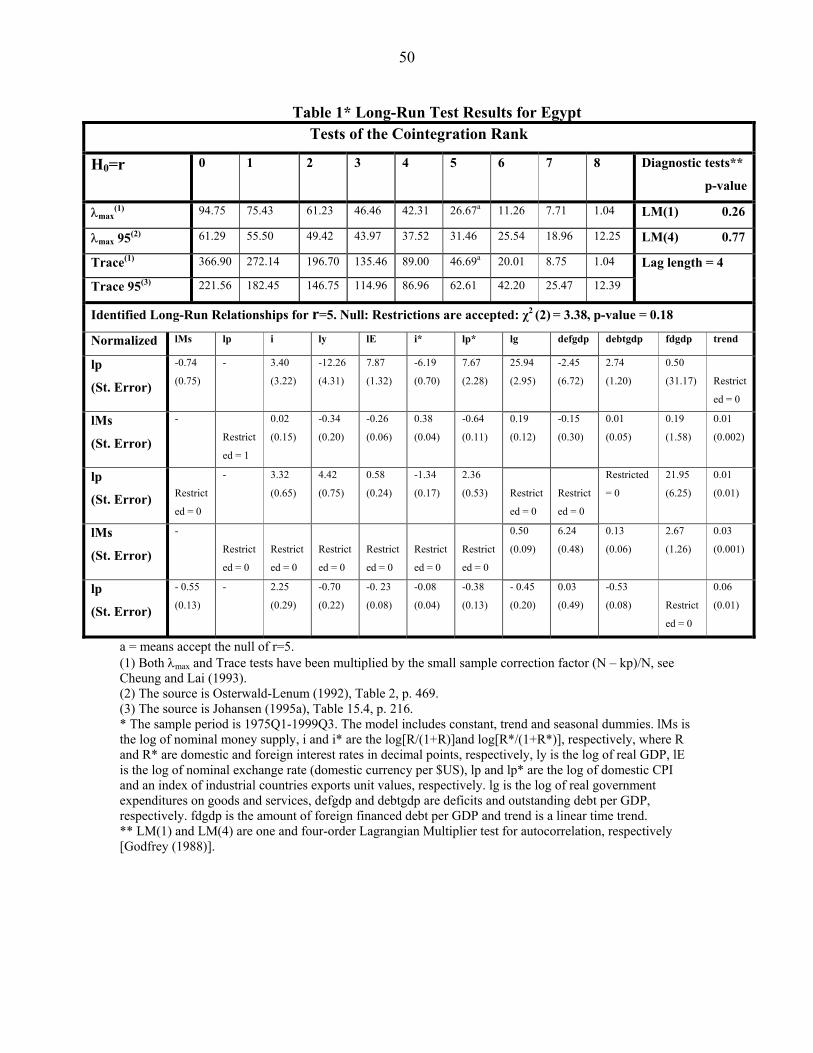
50

Table 1* Long-Run Test Results for EgyptTests of the Cointegration Rank

H0=r 0 1 2 3 4 5 6 7 8 Diagnostic tests**

p-value

λmax(1) 94.75 75.43 61.23 46.46 42.31 26.67a 11.26 7.71 1.04 LM(1) 0.26

λmax 95(2) 61.29 55.50 49.42 43.97 37.52 31.46 25.54 18.96 12.25 LM(4) 0.77

Trace(1) 366.90 272.14 196.70 135.46 89.00 46.69a 20.01 8.75 1.04

Trace 95(3) 221.56 182.45 146.75 114.96 86.96 62.61 42.20 25.47 12.39

Lag length = 4

Identified Long-Run Relationships for r=5. Null: Restrictions are accepted: χ2 (2) = 3.38, p-value = 0.18

Normalized lMs lp i ly lE i* lp* lg defgdp debtgdp fdgdp trend

lp

(St. Error)

-0.74

(0.75)

- 3.40

(3.22)

-12.26

(4.31)

7.87

(1.32)

-6.19

(0.70)

7.67

(2.28)

25.94

(2.95)

-2.45

(6.72)

2.74

(1.20)

0.50

(31.17) Restrict

ed = 0

lMs

(St. Error)

-

Restrict

ed = 1

0.02

(0.15)

-0.34

(0.20)

-0.26

(0.06)

0.38

(0.04)

-0.64

(0.11)

0.19

(0.12)

-0.15

(0.30)

0.01

(0.05)

0.19

(1.58)

0.01

(0.002)

lp

(St. Error) Restrict

ed = 0

- 3.32

(0.65)

4.42

(0.75)

0.58

(0.24)

-1.34

(0.17)

2.36

(0.53) Restrict

ed = 0

Restrict

ed = 0

Restricted

= 0

21.95

(6.25)

0.01

(0.01)

lMs

(St. Error)

-

Restrict

ed = 0

Restrict

ed = 0

Restrict

ed = 0

Restrict

ed = 0

Restrict

ed = 0

Restrict

ed = 0

0.50

(0.09)

6.24

(0.48)

0.13

(0.06)

2.67

(1.26)

0.03

(0.001)

lp

(St. Error)

- 0.55

(0.13)

- 2.25

(0.29)

-0.70

(0.22)

-0. 23

(0.08)

-0.08

(0.04)

-0.38

(0.13)

- 0.45

(0.20)

0.03

(0.49)

-0.53

(0.08) Restrict

ed = 0

0.06

(0.01)

a = means accept the null of r=5.(1) Both λmax and Trace tests have been multiplied by the small sample correction factor (N – kp)/N, seeCheung and Lai (1993). (2) The source is Osterwald-Lenum (1992), Table 2, p. 469.(3) The source is Johansen (1995a), Table 15.4, p. 216.* The sample period is 1975Q1-1999Q3. The model includes constant, trend and seasonal dummies. lMs isthe log of nominal money supply, i and i* are the log[R/(1+R)]and log[R*/(1+R*)], respectively, where Rand R* are domestic and foreign interest rates in decimal points, respectively, ly is the log of real GDP, lEis the log of nominal exchange rate (domestic currency per $US), lp and lp* are the log of domestic CPIand an index of industrial countries exports unit values, respectively. lg is the log of real governmentexpenditures on goods and services, defgdp and debtgdp are deficits and outstanding debt per GDP,respectively. fdgdp is the amount of foreign financed debt per GDP and trend is a linear time trend. ** LM(1) and LM(4) are one and four-order Lagrangian Multiplier test for autocorrelation, respectively[Godfrey (1988)].

51

Table 2* Long-Run Test Results for IranTests of the Cointegration Rank

H0=r 0 1 2 3 4 5 6 7 Diagnostic tests**

p-value

λmax(1) 99.33 71.42 65.05 43.62 31.09a 19.75 10.35 1.27 LM(1) 0.18

λmax 95(2) 55.50 49.42 43.97 37.52 31.46 25.54 18.96 12.25 LM(4) 0.62

Trace(1) 341.89 242.56 171.12 106.07 62.45a 31.37 11.62 1.27

Trace 95(3) 182.45 146.75 114.96 86.96 62.61 42.20 25.47 12.39

Lag length = 4

Identified Long-Run Relationships for r=4. Null: Restrictions are accepted: χ2 (1) = 0.02, p-value = 0.89

Normalized lMs lp ly lE i* lp* lg defgdp debtgdp fdgdp trend

lp

(St. Error)

0.05

(0.17)

- -0.88

(0.35)

1.19

(0.15)

-0.42

(0.11)

0.17

(0.32)

1.38

(0.28)

6.70

(0.94)

-0.66

(0.10)

-0.25

(2.43) Restrict

ed = 0

lMs

(St. Error)

-

Restrict

ed = 1

7.35

(0.64)

4.57

(0.28)

-0.62

(0.26)

6.80

(0.72)

-2.63

(0.39)

-4.24

(2.30)

2.62

(0.20)

0.28

(3.52)

-0.28

(0.02)

lp

(St. Error) Restrict

ed = 0

- 0.37

(0.06)

1.40

(0.002)

-0.34

(0.06)

2.21

(0.15)

-0.02

(0.002) Restrict

ed = 0

Restricted

= 0 Restrict

ed = 0

-0.04

(0.002)

lE

(St. Error) Restrict

ed = 0

0.71

(0.01)

-0.26

(0.04)

- 0.24

(0.05)

-1.58

(0.11) Restrict

ed = 0

Restrict

ed = 0

Restricted

= 0

-0.06

(0.01)

0.03

(0.002)

a =means accept the null of r=4.(1) Both λmax and Trace tests have been multiplied by the small sample correction factor (N – kp)/N, seeCheung and Lai (1993). (2) The source is Osterwald-Lenum (1992), Table 2, p. 469.(3) The source is Johansen (1995a), Table 15.4, p. 216.* The sample period is 1970Q1-2002Q4. See footnote to Table 1 for the mnemonics and other information.** LM(1) and LM(4) are one and four-order Lagrangian Multiplier test for autocorrelation, respectively[Godfrey (1988)].

52

Table 3* Long-Run Test Results for TurkeyTests of the Cointegration Rank

H0= r 0 1 2 3 4 5 6 7 8 Diagnostic tests**

p-value

λmax(1) 93.44 71.01 54.72 45.05 35.30a 19.22 13.19 8.69 4.18 LM(1) 0.02

λmax 95(2) 61.29 55.50 49.42 43.97 37.52 31.46 25.54 18.96 12.25 LM(4) 0.07

Trace(1) 344.82 251.38 180.36 125.64 80.59a 45.28 26.06 12.87 4.18

Trace 95(3) 221.56 182.45 146.75 114.96 86.96 62.61 42.20 25.47 12.39

Lag length = 5

Identified Long-Run Relationships for r=4. Null: Restrictions are accepted: χ2 (1) = 0.00, p-value = 1.00

Normalized lMs lp i ly lE i* lp* lg defgdp debtgdp fdgdp trend

lp

(St. Error)

0.81

(0.06)

- 0.16

(0.06)

-0.37

(0.10)

0.31

(0.06)

-0.01

(0.03)

-0.37

(0.12)

0.07

(0.04)

3.45

(0.46)

-0.85

(0.15)

-0.77

(1.86) Restrict

ed = 0

lMs

(St. Error)

-

Restrict

ed = 1

-1.47

(0.12)

0.07

(0.26)

-0.22

(0.09)

0.56

(0.08)

-1.00

(0.37)

-1.33

(0.09)

-0.40

(0.99)

-2.35

(0.31)

-0.10

(3.62)

0.08

(0.01)

lp

(St. Error)

0.63

(0.03)

- 0.32

(0.04)

-0.51

(0.07)

0.57

(0.03)

-0.21

(0.02)

0.80

(0.08)

0.43

(0.03)

Restricted

= 0

Restricted

= 0 Restrict

ed = 0

-0.03

(0.01)

lE

(St. Error) Restrict

ed = 0

0.44

(0.08)

0.20

(0.10)

1.75

(0.27)

- 0.47

(0.09)

-3.85

(0.32) Restrict

ed = 0

12.13

(1.08)

Restricted

= 0

17.72

(4.57)

0.07

(0.01)

a =means accept the null of r=4.(1) Both λmax and Trace tests have been multiplied by the small sample correction factor (N – kp)/N, seeCheung and Lai (1993). (2) The source is Osterwald-Lenum (1992), Table 2, p. 469.(3) The source is Johansen (1995a), Table 15.4, p. 216.* The sample period is 1970Q1-2003Q3. See footnote to Table 1 for the mnemonics and other information.** LM(1) and LM(4) are one and four-order Lagrangian Multiplier test for autocorrelation, respectively[Godfrey (1988)].

53

Table 41: Error Correction Model for EgyptDependent Variable = ∆lp

Variable Coefficient StandardError

p-value for Hansen’s(1992) stability Li test

∆lMst-1 0.15 0.06 0.18

∆it-4 -0.14 0.05 0.19

∆lyt-1 0.46 0.07 1.00

∆lEt-4 0.05 0.02 1.00

∆lp*t-1 0.14 0.07 0.15

(∆lg) (flex)t-1 -0.53 0.14 0.07

∆defgdpt-1 -0.50 0.17 1.00

∆defgdpt-3 0.79 0.17 1.00

∆defgdpt-4 -0.44 0.19 1.00

∆debtgdpt-3 0.15 0.05 1.00

∆debtgdpt-4 -0.21 0.06 1.00

(∆fdgdp) (peace)t-2 -4.95 1.46 1.00

(ECP)3t-1 -0.0004 0.00004 1.00

flex -0.02 0.01 1.00

psub 0.04 0.01 1.00

price 0.07 0.02 0.10

Hansen’s (1992) stability Li test on the variance = 0.45 p-value = 0.06Joint (coefficients and the error variance)Hansen’s (1992) stability Lc test = 3.15 p-value = 1.00

1 The sample period is 1975Q1-1999Q3. Mean of dependent variable=0.03. ∆ means the first difference, ∆lp is the changein the log of CPI, ∆lp* is the change in the log of an index of industrial countries exports unit values, ∆lMs is the change inthe log of nominal money supply, ∆i is the change in the log[R/(1+R)], where R is the nominal interest rate in decimalpoints. ∆lE is the change in the log of the nominal exchange rate (domestic currency per $US), and ∆ly is the change in thelog of real GDP. ∆lg is the change in real government expenditures, ∆defgdp, ∆debtgdp and ∆fdgdp are the change indeficits, outstanding debt and foreign financed debt per GDP, respectively. ECP is the error-correction term generated fromthe first identified long-run relationship in the cointegration space, normalized on the log of domestic price (see Table 1).None of the other error correction terms were statistically significant. Dummy variable peace is equal to 1 since 1979Q2when Egypt signed a peace treaty with Israel and to zero, otherwise. Dummy variable flex is equal to 1 since 1991Q1 andto zero, otherwise. Dummy variable price is equal to 1 in 1991Q2 and is zero otherwise. psub is equal to 1 from 1994Q4 to1995Q1. The estimation method is Ordinary Least Squared. R 2=0.53, σ=0.02, DW=2.18, Godfrey(5)=0.31 (significancelevel=0.92), White=87.69 (significance level=0.99), ARCH(5)=1.04 (significance level=0.96), RESET=0.24 (significancelevel=0.87) and Normality, χ2=1.28 (significance level=0.53). Note that R 2, σ and DW, respectively, denote the adjustedsquared multiple correlation coefficient, the residual standard deviation and the Durbin-Watson statistic. White is White’s(1980) general test for heteroskedasticity, ARCH is five-order Engle’s (1982) test, Godfrey is five-order Godfrey’s (1978)test, REST is Ramsey’s (1969) misspecification test, Normality is Jarque and Bera’s (1987) normality statistic, Li isHansen’s (1992) stability test for the null hypothesis that the estimated coefficient or variance of the error term is constantand Lc is Hansen’s (1992) stability test for the null hypothesis that the estimated coefficients as well as the error varianceare jointly constant.

54

Table 51: Error Correction Model for IranDependent Variable = ∆lp

Variable Coefficient StandardError

p-value for Hansen’s(1992) stability Li test

∆lyt-1 0.28 0.05 1.00

∆i*t-1 0.06 0.02 1.00

(∆lp)(rev)t-1 0.38 0.07 1.00

(∆lp)(rev)t-3 0.36 0.06 1.00

(∆lg) (oil)t-4 0.36 0.10 1.00

∆defgdpt-1 -0.97 0.24 1.00

(∆defgdp) (san)t-4 -2.12 0.36 1.00

∆fdgdpt-1 5.52 1.22 1.00

∆fdgdpt-2 -3.00 0.86 1.00

(∆fdgdp) (san)t-2 63.66 17.11 1.00

ECPt-1 -0.003 0.0005 1.00

oil 0.08 0.03 1.00

Q3 -0.05 0.01 1.00

Q4 -0.03 0.01 1.00

Nor 1973Q1 0.09 0.03

Nor 1977Q2 0.11 0.02

Nor 1978Q4 0.06 0.02

To avoid nonsingular matrixthe dependent variable wasadjusted for these dummyvariables

Hansen’s (1992) stability Li test on the variance = 0.26 p-value = 0.18Joint (coefficients and the error variance)Hansen’s (1992) stability Lc test = 2.57 p-value = 1.00

1 The sample period is 1970Q1-2002Q4. Mean of dependent variable=0.04. ∆ means the first difference, ∆ly is the changeof the log of real GDP, ∆i* is the change in log[R*/(1+R*)], ∆lp is the change in the log of CPI and ∆lE is the change inthe log of market exchange rate (rials per $US). ∆lg is the change in real government expenditures. ∆defgdp, and ∆fdgdpare the change in the log of deficits and foreign financed debt per GDP, respectively. ECP is the error correction termgenerated from the long-run price determination (see the first identified equation in Table 2). None of the other errorcorrection terms were statistically significant. Dummy variable rev is equal to 1 since 1979Q2 and to zero, otherwise.Dummy variable oil is equal to 1 for the period 1973Q4-1974Q1, and to zero, otherwise. Dummy variable san is equal to 1since 1980Q2 and to zero, otherwise. Q3 and Q4 are equal to 1, in the third and fourth quarters of the year, respectively,and to zero, otherwise. Nor 1973Q1, Nor 1977Q2 and Nor 1978Q4 are equal to 1 in the quarters indicated to eliminate theoutliers in the data. The estimation method is Ordinary Least Squared. R 2=0.70, σ=0.02, DW=1.98, Godfrey(5)=0.52(significance level=0.79), White=99.66 (significance level=1.00), ARCH(5)=7.65 (significance level=0.18), RESET=0.19(significance level=0.90) and Normality, χ2=4.98 (significance level=0.08). For other information see footnote of Table 4.

55

Table 61: Error Correction Model for TurkeyDependent Variable = ∆lp

Variable Coefficient StandardError

p-value for Hansen’s(1992) stability Li test

∆lpt-1 0.65 0.09 1.00

(∆lp) (vtax)t-1 -0.27 0.09 1.00

(∆lMs) (vtax)t-1 0.15 0.03 1.00

(∆lMs) (vtax)t-2 0.13 0.03 1.00

∆it-3 -0.07 0.04 1.00

∆it-4 0.08 0.04 1.00

∆lyt-1 0.12 0.05 1.00

∆lyt-2 -0.11 0.06 0.17

(∆ly) (mex)t-2 0.22 0.09 1.00

(∆ly) (flex)t-4 0.82 0.26 1.00

∆lEt-2 -0.13 0.036 1.00

∆lp*t-2 -0.26 0.09 0.15

ECPt-1 0.35 0.10 1.00

(ECP)2t-1 0.08 0.03 1.00

ECdt-1 -0.07 0.02 1.00

fcrisis 0.22 0.03 0.15

Q4 0.03 0.01 0.08

Nor 1980Q1 0.18 0.03 0.01

Hansen’s (1992) stability Li test on the variance = 0.23 1.00 (p-value)Joint (coefficients and the error variance)Hansen’s (1992) stability Lc test = 3.67 0.20 (p-value)

1 The sample period is 1970Q1-2003Q3. Mean of dependent variable=0.10. ∆ means the first difference, ∆lp is the changein the log of CPI, ∆lMs is the change in the log of nominal money supply, ∆i is the change in the log[R/(1+R)], where R isthe nominal interest rate in decimal points , ∆ly is the change in the log of real GDP, ∆lE is the change in the log of marketexchange rate (liras per $US) and ∆lp* is the change in the log of index of industrial countries exports unit values. ECP isthe error-correction term generated from the first identified long-run relationship in the cointegration space, normalized onthe log of CPI (see Table 3). ECd is the error-correction term generated from the third identified long-run relationship inthe cointegration space, normalized on the log of real demand for money. The other error correction term was notstatistically significant. Dummy variable vtax is equal to 1 since 1984Q4 and to zero, otherwise. Dummy variable mex isequal to 1 for the period of 1994Q4-1999Q4 and to zero, otherwise. Dummy variable flex is equal to 1 since 2001Q1 and tozero, otherwise. fcrisis is equal to 1 for 1994Q2 and to zero, otherwise. Q4 is a dummy variable equal to 1, in the fourthquarter of the year, and to zero, otherwise. Nor 1980Q1 is equal to 1 in the first quarter of 1980 to eliminate the outliers inthe data. The estimation method is the Ordinary Least Squared. R 2=0.74, σ=0.03, DW=1.92, Godfrey(5)=0.31(significance level=0.93), White=129.99 (significance level=0.99), ARCH(5)=4.72 (significance level=0.45), RESET=0.36(significance level=0.78) and Normality, χ2 =1.62 (significance level=0.45). For other information see footnote of Table 4.