Decomposing the Global TIAM-Macro Model Decomposing the Global TIAM Macro Model to Assess Climate Change Mitigation

International Energy Workshop, Paris, June 2013Socrates Kypreos (PSI) & Antti Lehtila (VTT)Socrates Kypreos (PSI) & Antti Lehtila (VTT)

2

Presentation Outline The global ETSAP-TIAM PE model and the Macro GE model Linking TIMES with MacroMain features of TIAM-Macro Quadratic Supply Cost Functions (QSF)

Th M S d Al d l The Macro-Stand-Alone model Calibration algorithm

Emplo ing Negishi elfare eights Employing Negishi welfare weights Decomposition algorithm

Illustrative climate policy analysis case Illustrative climate policy analysis case Performance of the algorithm Conclusions and future workConclusions and future work

3

The Global ETSAP-TIAM PE Modeland the Macro GE Model

ETSAP-TIAM: A global multi-regional partial equilibrium model Based on the TIMES energy system modeling tools of IEA-ETSAPBased on the TIMES energy system modeling tools of IEA ETSAP 15 world regions with trade in energy commodities Detailed in technology representation in all sectors Own price elasticities for useful energy demand Maximizes the cumulative discounted surplus of cons. & prods.

I t t d li t d l f i li t i t Integrated climate module for assessing climate impactsMACRO: An optimal growth dynamic general equilibrium model

Origins in the Eta-Macro model by Alan S Manne Origins in the Eta-Macro model by Alan S. Manne A single-sector neoclassical optimal growth model,

i.e. a dynamic inter-temporal GE model Maximizes the cumulative discounted utility of a generic consumer

4

Linking TIMES and Macro

Hard-linking: direct integration of data and functional relationships in a single integrated modeling framework: E.g. MARKAL-Macro, TIMES-Macro, TIMES+Merge

Soft-linking: combined use of two models that have been d l d i d d tl f th d b t d ldeveloped independently from another and can be run stand-alone Usually heterogeneous in complexity and accounting methods E g TIAM + GEMINI-E3 GTAP-E Italy + MARKAL-Italy etc E.g. TIAM + GEMINI-E3, GTAP-E Italy + MARKAL-Italy etc.

Hybrid linking based on decomposition: Direct integration in a single consistent modeling frameworkg g g Solution by using a decomposition algorithm TIAM-Macro (comparable implementation: Message-Macro)

5

Main Features of TIAM-Macro Characteristics of the integrated model:

A global, multi regional LP-formulated energy system model fully integrated with an NLP macro economic modelfully integrated with an NLP macro-economic model

A hybrid growth model combining ‘bottom-up’ & ‘top-down’ approaches in a consistent framework

Provides Pareto optimal solutions for second-best policies, maximizing the Negishi-weighted global welfare

Includes trade in energy commodities (oil gas synthetic fuels Includes trade in energy commodities (oil, gas, synthetic fuels, coal, bio-fuels), in CO2 permits, and in the numéraire good representing all other non-energy exports

Hybrid linking of TIAM and Macro based on decomposition: Solved iteratively by decomposing the overall model into

LP and NLP sub problemsLP and NLP sub-problems

6

D fi i th Q d ti S l F tiDefining the Quadratic Supply Functions (QSF)

As the energy systems in TIAM and in TIAM-Macro are the same, the full TIAM can be replaced by a QSF, defined as:

( )

sa e, e u ca be ep aced by a QS , de ed as2

,,,,,, itri

itrtrtr DMEC

The derivative of the Energy Cost EC with respect to demand DM defines the equilibrium price P at the TIAM solution:

,,

,,,,,,,,, 2/

itr

itritritritrtr

PDMPDMEC

2

,,

,,,, 2

itittt

itritr

DMEC

DM

,,,,,, itritrtrtr DMEC

7

Maximize the global welfare U defined as the Negishi weighted

The TIMES-Macro Stand-Alone ModelMaximize the global welfare U defined as the Negishi-weighted

cumulative discounted log of regional consumption:

Tt

trtrtreCpwtnwtUMax ,)ln(

Subject to the following constraints:

t r

trtr eCpwtnwtUMax1

, )ln(

DbLKaY rrrrrr:functionProduction /1)1(

IINKK

nmrNTXECICY

DbLKaY

NNrtrtrtrtrt

rtii

rirtrtrtrt

))1((50)1(f if iC i l

)( :output of Use

:function Production

DMEC

IgKIINKK

rTrTrTrT

rtN

rttrtN

rttt

:functionsupplyquadraticThe

)( :T periodlast for condition Terminal))1((5.0)1( :functionformation Capital

2

11

ddfDDM

DMEC

t

Nirrtirti

rtii

rtirtrt

)1( :factors decoupling Demand

:functionsupply quadraticThe

1

trdtNTXr

trdrt

t

, ; 0 :balancemust NTX exportsnet Global ,

,1

8

Calibration Algorithm for TIAM-Macro Calibration of the demand decoupling factors (DDFs) is based

on the following decisions / observations (Kypreos, 1996): The energy system in TIAM and TIAM Macro should be the same The energy system in TIAM and TIAM-Macro should be the same The following two equations (definition of DDF and the first order

maximization condition of CES) can be solved for the unknown DDF factors: )1( ,,,,

,1,,,,,,

itritr

t

Niritritr

P

FDddfDDM

r

Iteration between the two models not necessary for calibration,

0, ,1,,

,,,

1,,,,

itrir

itrtritritr ddf

bP

YFDM r

y ,but the TIAM-LP Baseline needs to solved only once The Macro model needs to be solved iteratively until the DDF

f t d l b th tfactors and labor growth rates converge

9

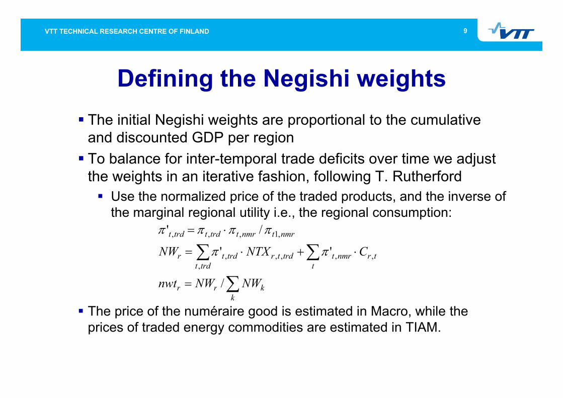
Defining the Negishi weights The initial Negishi weights are proportional to the cumulative

and discounted GDP per regionT b l f i t t l t d d fi it ti dj t To balance for inter-temporal trade deficits over time we adjust the weights in an iterative fashion, following T. Rutherford Use the normalized price of the traded products and the inverse ofUse the normalized price of the traded products, and the inverse of

the marginal regional utility i.e., the regional consumption: nmrtnmrttrdttrdt /' ,1,,,

krr

trt

nmrttrdtrtrdt

trdtr

NWNWnwt

CNTXNW

/

'' ,,,,,

,

The price of the numéraire good is estimated in Macro, while the prices of traded energy commodities are estimated in TIAM.

k

krr

10

Decomposition Algorithm Solving the Baseline Calibration: First, solve TIAM as LP defining the Quadratic Supply Functions

(QSF) for the useful energy demands in all regions(QSF) for the useful energy demands in all regions Next, define the initial DDF and labor growths, and solve the Macro

model with the QSF as an NLP welfare maximization problemTh it t dj ti f DDF l b th d th N i hi Then iterate adjusting for DDF, labor growths and the Negishi weights until demands and growths stabilize together with the NW

Solving the Policy Scenarios:g y First, solve the partial equilibrium TIAM under policy constraints,

and calculate initial QSFs for the Macro sub-model Next solve the Macro sub problem applying the calibrated DDFs Next, solve the Macro sub-problem applying the calibrated DDFs

and labor growth rates, deriving adjusted demand levels Then, iterate between the TIAM LP and Macro NLP sub-problems

until the demand levels and Negishi weights stabilize

11

Climate Policy Test CaseThe hybrid model tested with global TIAM scenarios until 2060,The hybrid model tested with global TIAM scenarios until 2060,

under two different Climate Policy cases: A: Regional targets for CO2 emissions, roughly resembling the

l t l d i t i h t dlong-term pledges various countries have presented B: Global target on maximum level of radiative forcing, roughly

corresponding to the 550 ppm concentration limit target

60%

80%

20%

40%

p g pp g

Case A Case B

0%

20%

40%

60%

-20%

0%

20%

2030

80%

-60%

-40%

-20%

-80%

-60%

-40% 2040

2050

From

-100%

-80%

AFR

AUS

CAN CH

I

CSA

EEU

FSU

IND

JPN

MEA

MEX

OD

A

SKO

USA

WEU

-100%

80%

AFR

AUS

CAN CH

I

CSA

EEU

FSU

IND

JPN

MEA

MEX

OD

A

SKO

USA

WEU

2005

12

Cli t P li T t CClimate Policy Test Case:Evolution of Radiative Forcing

4 5

5.0

B li

4.0

4.5

/m2

Baseline

Case A

3.5

cing

, W/ Case A

Case B

2 5

3.0Forc Case B

2.0

2.5

2000 2010 2020 2030 2040 2050 2060

13

Cli t P li T t CClimate Policy Test Case:GDP Loss Compared to Baseline

Case A Case B0% 1% 2% 3% 4% 5% 6%

AFR

0% 1% 2% 3% 4% 5%

AFRAFR

AUS

CAN

CHI

AFR

AUS

CAN

CHICHI

CSA

EEU

FSU

2030

CHI

CSA

EEU

FSU

IND

JPN

MEA

2040

2050

IND

JPN

MEA

MEX

ODA

SKO

MEX

ODA

SKO

USA

WEU

USA

WEU

14

Cli t P li T t CClimate Policy Test Case:Impacts on Annual Energy System Costs

Case A Case B-8% -6% -4% -2% 0% 2% 4% 6% 8%

AFR

-8% -6% -4% -2% 0% 2% 4%

AFRAFR

AUS

CAN

CHI

AFR

AUS

CAN

CHI

CSA

EEU

FSU

2030CSA

EEU

FSU

IND

JPN

MEA

2040

2050

IND

JPN

MEA

MEX

ODA

SKO

MEX

ODA

SKO

USA

WEU

USA

WEU

15

Performance of the AlgorithmT t ith b t f th ETSAP TIAM d l ( 2060)Test runs with subsets of the ETSAP-TIAM model (→2060): Single-region model for the USA (run also with TIMES-Macro) Six-region model (EEU + WEU + USA + AFR + CHI + MEA)g ( ) Ten-region model (6 above + JPN + CSA +IND +ODA) Full 15-region model (10 above + AUS + CAN + FSU + MEX+ SKO)

The USA model results validated well against TIMES-MacroThe USA model results validated well against TIMES-MacroTest results indicate that TIMES-MSA may be even 100 times

faster than the hard-linked TIMES-Macro (~170 min. for USA)

TIAM-Macro Model size Run time (minutes)Test model Equations Variables Calibration Policy runTIAM USA 30 500 52 800 <1 2TIAM-USA 30,500 52,800 <1 2TIAM-6R 198,900 508,300 4 28TIAM-10R 318,200 674,100 7 58TIAM 15R 457 600 864 000 11 89TIAM-15R 457,600 864,000 11 89(Windows 7 64-bit workstation, solution in single thread)

16

Conclusions and Future Work Key accomplishments: Any TIMES-Macro models can now be calibrated and solved

efficiently just by activating a switch in the model run andefficiently just by activating a switch in the model run and by defining a few macroeconomic input parameters

For the first time, the Global TIAM-Macro can be solved ,efficiently to get Pareto optimal solutions for second-best policies with full technological details by region from TIAMU d t f Cli t M d l li i ti d i l ith Update of Climate Module linearization during algorithm

Possible future work: Add an option to include also (non-linear) damage costs Add an option to include also (non-linear) damage costs

from climate change in the global welfare maximization Implement MSA using MCP formulation instead of NLP Derive estimates of elasticity effects for TIAM PE formulation

17

Th k Y !Thank You!