decomposing culture: an analysis of gender,...
TRANSCRIPT
Decomposing culture An analysis of gender language and
labor supply in the household
Victor Gaylowast Daniel L Hicksdagger Estefania Santacreu-VasutDagger Amir Shohamsect
Abstract
Despite broad progress in closing many dimensions of the gender gap around the globe recent research has shownthat traditional gender roles can still exert a large influence on female labor force participation even in developedeconomies This paper empirically analyzes the role of culture in determining the labor market engagement of womenwithin the context of collective models of household decision making In particular we use the epidemiologicalapproach to study the relationship between gender in language and labor market participation among married femaleimmigrants to the US We show that the presence of gender in language can act as a marker for culturally acquiredgender roles and that these roles are important determinants of household labor allocations Female immigrants whospeak a language with sex-based grammatical rules exhibit lower labor force participation hours worked and weeksworked Our strategy of isolating one component of culture allows us to shed light on several important mechanismsinfluencing womenrsquos economic engagement including the role of bargaining power in the household and the impactof ethnic enclaves Our results further suggest that language may influence behavior in both of these contexts
Keywords Language Gender gap Labor force participation Immigrants
JEL classification F22 J16 Z13
lowastDepartment of Economics The University of Chicago 5757 S University Ave Chicago IL 60637 USAdaggerDepartment of Economics University of Oklahoma 308 Cate Center Drive Norman OK 73019 USADaggerCorresponding Author Department of Economics ESSEC Business School and THEMA 3 Avenue Bernard Hirsch 95021 Cergy-Pontoise
France (santacreuvasutessecedu)sectTemple University and COMAS 1801 N Broad St Philadelphia PA 19122 USA
1
1 Introduction
The labor force participation rate of married women has increased spectacularly during the second half of the 20th
century both in the US and around the world (Goldin 2014) Nevertheless wide differences across countries remain
with the gender gap closing faster in some countries than others and a number of developing nations such as India
lagging behind (Field et al 2016) Among the factors used to explain these differences the role of cultural norms
has been shown to play a crucial role (Fernaacutendez 2007 Fernaacutendez amp Fogli 2009 Alesina et al 2013 Farreacute amp Vella
2013 Fernaacutendez 2013) In particular scholars have begun employing the epidemiological approach to distinguish the
impact of cultural factors from that of other institutional forces (Fernaacutendez amp Fogli 2009 Fernaacutendez 2011)1
When analyzing married couples both individual and spousal culture are thought to play an important role in
explaining labor market decisions Early collective models of labor supply emphasize the importance of taking into
account the distribution of bargaining power within the household (Chiappori et al 2002 Blundell et al 2007) Re-
cently however these models have been extended to investigate whether their main predictions depend not only on
bargaining power but also on the surrounding cultural context (Oreffice 2014) as well as on social and institutional
constraints related to traditional gender roles (Field et al 2016) These norms may influence women to allocate more
labor to household production relative to the formal market at either the intensive or extensive margin
This paper studies the impact of gender roles on the labor force participation of married female immigrants in
the US within a collective labor supply framework We explore culturally acquired gender roles as those embod-
ied by the presence of grammatical gender in language spoken Recent work has documented correlations between
linguistic structure and individual behavior (Lupyan amp Dale 2010 Chen 2013 Ladd et al 2015) with the presence
and intensity of gender in grammatical structures correlating with gender gaps in compensation and promotions divi-
sion of household labor educational attainment and political empowerment (Givati amp Troiano 2012 Santacreu-Vasut
et al 2013 Santacreu-Vasut et al 2014 Hicks et al 2015 Mavisakalyan 2015 van der Velde et al 2015 Davis amp
Reynolds 2016)
The mechanisms underlying these associations are largely unresolved Perhaps the most compelling question
whether language may causally influence behavior remains a subject of debate2 Linguistic correlations could reflect
historically acquired cultural norms of behavior that became codified in language or language itself could represent an
institutional force influencing and perpetuating a set of behaviors
From a methodological point of view because language is observed at the individual level it is possible to isolate
its effect from the influence of aggregate correlated historical cultural and biological forces This is an exercise
we undertake in this analysis following the epidemiological approach Furthermore because language acts a cultural
marker for gender roles we show that this barometer of norms allows us to examine labor market predictions of the
collective household model in the presence or absence of these cultural influences This yields new insights regarding
their relative influence
1Gay et al (2016) provides an in-depth discussion of the epidemiological approach in this context2Theoretically language structures could influence preference formation information processing categorization of social reality and the salienceof certain categories of words These impacts could alter a speakerrsquos decision making and behavior (Mavisakalyan amp Weber 2016)
2
To do this we examine labor market outcomes for nearly half a million married female immigrants to the US aged
25 to 49 in the American Community Surveys (ACS) between 2005 and 2015 In our analysis we focus on married
foreign born individuals who speak a language other than English in the home With the assistance of linguists and
drawing on information contained in the World Atlas of Linguistic Structures database (WALS) we assign to these
speakers consistent measures of the presence and intensity of gender in the grammatical structure of their language
There are several novel empirical advances to the approach taken in this paper First this analysis relies on an
incredibly detailed set of microeconomic data which provides a rich set of covariates and substantial variation to
control for many potential confounding factors These include many of the individual spousal and household level
variables analyzed in the past as well as measures which may influence the decision to migrate in the country of
origin and measures of the location to which the immigrant has moved Moreover the unique sample also allows us to
include country fixed effects to capture a wide array of unobservable cultural forces A second advantage is reliance
on the epidemiological approach in this setting which helps ameliorate a fundamental problem of identification when
examining the impact of language on behavior
The takeaways from this exercise are several First we show that married female immigrants speaking a language
with sex-based distinctions in its grammar are less likely to participate in the labor market This is true even after con-
trolling for observable characteristics such as traditional household measures husband characteristics and bargaining
power measures as well as when controlling for a vast set of unobservable cultural forces through country of origin
fixed effects3 When we empirically decompose the relationship between gender in language and gendered behavior
in this manner it suggests that roughly two thirds of this relationship can be explained by correlated cultural factors
with about one third potentially explained by language having a causal impact
Second using language as a measure of culturally acquired gender roles allows us to speak to and test the role
of bargaining power within the household relative to the impact of cultural norms We demonstrate that both are
important and that their impacts are distinct from one another
Third focusing on language spoken allows to also study the behavior of female immigrants in both linguistically
homogeneous and heterogeneous couples We exploit linguistic heterogeneity within the household to show that the
presence of gender in language has an association with a wifersquos behavior both when husbands and wives speak a
gendered language and when they speak languages with different structures Our findings suggest that while there
is an independent effect on a wifersquos behavior when she alone has a gender marked language gender marking in the
husbandrsquos language enhances this effect
Finally using language as a measure of gender roles but recognizing it as a network technology allows us to exam-
ine the role that ethnic enclaves play in influencing female labor force participation In theory enclaves may improve
labor market outcomes by providing information about formal jobs and reducing social stigma on employment At the
same time enclaves are likely to reinforce immigrant language usage and thus may enhance the impact of gender in
language or provide isolation from US norms We present evidence implying that the latter effect is present which
3One of the challenges of the literature on culture and economic behavior has been to measure culture An advantage of using language overexisting alternatives is that language is defined at the individual level and is not an outcome measure It allows us to control for country of origincharacteristics including time varying ones
3
suggests that the impact of language is stronger when it is shared with the surrounding community4
These findings speak to several literatures Mavisakalyan amp Weber (2016) review of the nascent field of linguistic
relativity and economics and point out that the mechanisms behind the associations between language and economic
behavior remain largely unresolved Despite the current studyrsquos ability to account for both time-invariant and time-
variant country of origin factors in a more rigorous manner than previous analyses the correlation between language
and behavior remains significant and negative This means that while we can demonstrate that most of this association
can be explained by language as a cultural market for correlated gender norms we cannot formally disprove that the
behavioral channel may explain some of the remaining correlation (Roberts amp Winters 2013 Hicks et al 2015 Roberts
et al 2015)5
Our research also directly contributes to literature that investigates whether the impact of intra-household bargain-
ing power on the labor supply depends on culture In particular our results imply that the standard prediction that
the spouse with higher bargaining power will substitute labor for leisure due to an income effect as in Oreffice (2014)
applies only to native born couples in the US and to immigrant couples with gender roles similar to the US Interest-
ingly our results confirm that in couples coming from countries classified as exhibiting strong traditional gender roles
the influence of bargaining power on household collective labor supply may be culturally dependent and that some of
these standard predictions may not hold for these groups
While Oreffice (2014) focuses on the intensive labor supply among couples where both spouses are working we
focus mainly on the extensive margin and how bargaining power influences female labor force participation Field
et al (2016) study the extensive margin of the labor supply among married female in India and model the impact
of bargaining power distribution within the household with social constraints related to traditional gender norms
Our findings complement these studies by empirically showing that the married female immigrants with stronger
bargaining power are more likely to work not less and that the impact of bargaining power is reinforced when
traditional gender roles are embodied in the language spoken
This paper is structured as follows Section 2 presents summary statistics for both the ACS and linguistic data
and details the empirical strategy Section 3 presents the empirical results - decomposing the impact of language from
other cultural influences presenting a wide range of robustness checks and then using gender in language as a cultural
marker to study labor supply within the household Section 4 concludes
2 Methodology
21 Data
211 Economic and demographic data
We combine data from several sources in our analysis First we obtain detailed demographic and economic data for
the immigrant population to the US from the American Community Surveys (ACS) 1 samples from 2005 to 2015
4This result is not solely attributable to selection since it holds for women married prior to migrationmdashsometimes referred to as ldquotied womenrdquo5See Everett (2013) for a review of the linguistics literature
4
(Ruggles et al 2015)
Table 1 Summary StatisticsFemale Immigrants Married Spouse Present Aged 25-49
Mean Sd Min Max Obs SB1-SB0
A Individual characteristics
Age 377 66 25 49 480618 -10Years since immigration 148 93 0 50 480618 -00Age at immigration 228 89 0 49 480618 -10
Educational AttainmentCurrent student 006 024 0 1 480618 -002Years of schooling 124 37 0 17 480618 -13No schooling 005 021 0 1 480618 000Elementary 012 032 0 1 480618 010High school 037 048 0 1 480618 010College 046 050 0 1 480618 -019
Race and ethnicityAsian 029 046 0 1 480618 -065Black 002 014 0 1 480618 001White 047 050 0 1 480618 041Other 021 041 0 1 480618 024Hispanic 053 050 0 1 480618 063
Ability to speak EnglishNot at all 011 032 0 1 480618 008Not well 024 043 0 1 480618 002Well 025 043 0 1 480618 -008Very well 040 049 0 1 480618 -002
Labor market outcomesLabor participant 060 049 0 1 480618 -010Employed 055 050 0 1 480618 -012Yearly weeks worked (excl 0) 4416 132 7 51 302653 -16Yearly weeks worked (incl 0) 2718 239 0 51 480618 -58Weekly hours worked (excl 0) 3657 114 1 99 302653 -18Weekly hours worked (incl 0) 2251 199 0 99 480618 -51Labor income (thds) 253 285 00 5365 282057 -88
B Household characteristics
Years since married 124 75 0 39 352059 014Number of children aged lt 5 042 065 0 6 480618 004Number of children 187 126 0 9 480618 038Household size 426 162 2 20 480618 039Household income (thds) 610 596 -310 15303 480618 -208
Table 1 notes The summary statistics are computed using sample weights (PERWT) provided in theACS (Ruggles et al 2015) except those for household characteristics which are computed usinghousehold weights (HHWT) The last column reports the estimate β from regressions of the typeXi = α +β SBI+ ε where Xi is an individual level characteristic Robust standard errors are notreported See appendix A for details on variable sources and definitionslowastlowastlowast Significant at the 1 percent level
We restrict the analysis to female respondents aged 25 to 49 born abroad from non-American parents living in
married-couple family households in which the husband is present and who report speaking a language other than
English in the home Moreover we only keep respondents that report uniquely identifiable countries of birth and
5
languages and for which we have information on the grammatical structure of the language reported Appendix A11
provides an exhaustive list of these sample restrictions and details the precise process taken to construct the regression
sample It also provides precise definitions for all variables employed6
The main dependent variable used throughout the analysis is a measure of labor market engagement labor force
participation which is defined as an indicator equal to one if the respondent is either employed or actively looking for
a job7 In some specifications we also analyze other labor market outcomes such as yearly weeks worked and usual
weekly hours worked both including and excluding zeros to capture both the extensive and intensive margins of the
labor supply8
Table 1 presents summary statistics for the demographic and economic characteristics of the respondents in the
regression sample On average the typical married women in our sample is in her upper 30s immigrated around 15
years before and has over 12 years of education 60 of these respondents participate in the labor force with 55
reporting formal employment As can be seen from the last column of Table 1 there is a large difference in means be-
tween the labor market outcomes for sex-based speakers and non sex-based speakers with the former group exhibiting
far lower levels of economic engagement There is also sizeable variation in English proficiency as well as in racial
and ethnic composition for this sample Mean household income is just over $60000 and the average duration of the
current marriage is 12 years Many households have children with the mean being almost two Overall the popu-
lation studied contains rich variation with over 480000 adult female immigrants originating from 135 countries and
speaking 63 different languages Appendix Table C1 provides the distribution of languages spoken in the regression
sample and highlights the extensive variation in languages spoken by immigrants to the US Moreover while they are
not the primary groups of interest in this analysis we further provide similar summary statistics for the respondentsrsquo
husbands in Appendix Table C3 as well as various within-household gender gap measures in Appendix Table C4
both of which are used in subsequent analysis
212 Linguistic data
Next we follow Gay et al (2013) and Hicks et al (2015) and assign to each language measures that quantify the
presence and frequency of gender distinctions in its grammatical rules We construct these measures using information
compiled by linguists in the World Atlas of Language Structures (WALS Dryer amp Haspelmath 2011) We expand
the original WALS dataset in collaboration with linguists for several additional languages making the sample more
representative9
Our primary measure of gender in language is an indicator for whether a language employs a grammatical gender
6Formal checks suggest that the regression sample is not biased by the availability of the country of birth and the linguistic data Appendix TableC2 provides summary statistics comparable to those in Table 1 without dropping the respondents for which the country of birth or languageare not precisely identifiable which is about 678 of the uncorrected regression sample The last column of this table demonstrates that dataconstraintsmdashie needing to know language spoken and country of birthmdashdo not meaningfully bias the sample in any way along these observables
7This is the LABFORCE variable in the ACS (Ruggles et al 2015) See appendix A21 for more details8The yearly weeks worked correspond to the WKSWORK2 variable in the ACS (Ruggles et al 2015) Because this variable is given in intervals wedefine yearly weeks worked as the midpoint of those intervals The usual weekly hours worked correspond to the UHRSWORK variable in the ACS(Ruggles et al 2015) Appendix A21 provides additional details
9The languages for which some variables were compiled are detailed in appendix B For robustness we have also verified that the exclusion of ournewly assigned languages in favor of the original WALS set of languages does not alter the main findings of the analysis
6
system based on biological sex (SB) We also investigate gender distinctions in other features of the grammatical
structure For instance languages with only a male and a female gender force speakers to make more sex-based
distinctions than those which include a neuter gender NG is an indicator variable equal to one for languages with
exactly two genders and equal to zero otherwise Similarly there is heterogeneity across languages in the presence
and quantity of gendered personal pronouns This feature is given by the variable GP which captures rules related to
gender agreement with pronouns Finally some languages assign gender due to semantic reasons only while others
assign gender due to both semantic and formal reasons making gender more recurrent in the latter case This feature
is given by the variable GA which captures the rules for gender assignment10
Finally we employ a measure of grammatical gender intensity similar to the one built by Gay et al (2013) This
measure captures how many of the above features are present in a language It is defined as
Intensity= SBtimes (GP+GA+NG)
where Intensity is a categorical variable that ranges from 0 to 311 The Intensity measure allows us to capture
the ranking of intensity of female male distinctions in the grammatical rules as follows If a language has a sex-
based gender system its intensity score is the sum of its scores on the three other gender features Hence a strictly
positive score captures languages that have strong female male distinctions Table 2 provides summary statistics for
the language variables contained in the regression sample
Table 2 Summary Statistics Language VariablesFemale Immigrants Married Spouse Present Aged 25-49
Definition Mean Sd Min Max Obs
SB Sex-based 083 037 0 1 480618NG Number of genders 072 045 0 1 480618GA Gender assignment 076 043 0 1 480618GP Gender pronouns 057 050 0 1 478883
Intensity (GP + GA + NG) times SB 204 121 0 3 478883
Table 2 notes The summary statistics are computed using sample weights (PERWT) providedin the ACS (Ruggles et al 2015)
There is substantial linguistic heterogeneity in terms of grammatical gender in the sample We demonstrate the
robustness of our main findings across all of these measures with additional checks presented in Appendix Table C7
22 Empirical Strategy
Our empirical strategy follows the epidemiological approach to culture (Fernaacutendez amp Fogli 2009 Fernaacutendez 2011
Blau et al 2011 Blau amp Kahn 2015) This approach compares outcomes across immigrants with varying geograph-
ical origins but living in a common institutional legal and social environment thereby allowing to separate cultural
10More detailed definitions of these individual measures can be found in Hicks et al (2015)11This measure should not be taken as measuring absolute intensity but rather as a ranking of relative intensity across languages grammar The
discussion of the measure is extended in Appendix discussion of Table C7
7
influences acquired prior to migration from confounding institutional forces In the baseline specifications we include
a set of controls that are common in analyzing decision making in the collective household framework Moreover to
help isolate the role of language from other cultural forces we include fixed effects by country of birth of the respon-
dents These fixed effects allow us to obtain identification off heterogeneity in the structure of languages spoken across
immigrants from the same country of birth We generate our core results by estimating the following specification
Yi jlcst = α +β SBil +γγγprimeXi j +δδδ
primeWc +ηηηprimeSs +θθθ
primeZt + εi jlcst (1)
where Yi jlcst is a measure of labor market participation Subscript i indexes respondents l languages spoken j
households c countries of birth s states of residence t ACS survey years Xi j corresponds to the characteristics
of respondent i in household j This vector contains the following variables age age squared five-years age group
indicators race indicators a Hispanic indicator age at immigration to the US years since in the US a student
indicator years of schooling level of English proficiency decade of immigration indicators number of children aged
less than 5 years old in the household and household size Wc corresponds to a vector of indicators for the respondentrsquos
country of birth c Ss corresponds to a vector of indicators for the respondentrsquos state of residence s and Zt corresponds
to a vector of indicators for the ACS survey year t Appendices A22 and A23 provide details on how these variables
are constructed
To help the interpretation of regression coefficients we additionally report in all regression tables the average of
the outcome variable for the relevant sample Moreover to facilitate the comparison of magnitudes across coefficients
from a given regression we also report the coefficients when standardizing continuous variables between zero and
onemdashwe keep indicator variables unstandardized for ease of interpretation
3 Empirical results
31 Decomposing language from other cultural influences
311 Main results
Table 3 contains our baseline empirical analysis In the first column we examine the naiumlve association between gender
in language and labor force participation These results are naiumlve in the sense that we are not yet accounting for any
confounding factors and simply represent the difference in means across groups The raw correlation implies that
married immigrant women who speak a language that has a sex-based gender structure are 10 percentage points less
likely to participate in the formal labor market This is about 17 of the average labor force participation rate for the
full regression sample
Moving across columns in the table the analysis includes an increasingly stringent set of controls for both ob-
servable and unobservable factors which may impact a womanrsquos decision to participate in the labor market The
specification reported in column (2) controls for the individual characteristics of the vector Xi j described in Section
22 After this inclusion the impact of the SB variable remains statistically significant and negative while its mag-
8
Table 3 Gender in Language and Economic Participation Individual LevelFemale Immigrants Married Spouse Present 25-49 (2005-2015)
Dependent variable Labor force participation
(1) (2) (3) (4) (5) (6) (7)
Sex-based -0101 -0069 -0045 -0027 -0024 -0021[0002] [0003] [0004] [0007] [0007] [0008]
β -coef -0045
COB LFP 0002 0002[0000] [0000]
β -coef 0041 0039
Past migrants LFP 0005 0005[0000] [0000]
β -coef 0063 0062
Respondent charAge No Yes Yes Yes Yes Yes YesRace and ethnicity No Yes Yes Yes Yes Yes YesEducation No Yes Yes Yes Yes Yes YesYears since immig No Yes Yes Yes Yes Yes YesAge at immig No Yes Yes Yes Yes Yes YesDecade of immig No Yes Yes Yes Yes Yes YesEnglish prof No Yes Yes Yes Yes Yes Yes
Household charChildren aged lt 5 No Yes Yes Yes Yes Yes YesHousehold size No Yes Yes Yes Yes Yes YesState No Yes Yes Yes Yes Yes Yes
COB charGeography No No Yes Yes No No NoFertility No No Yes Yes No No NoMigration rate No No Yes Yes No No NoEducation No No Yes Yes No No NoGDP per capita No No Yes Yes No No NoCommon language No No Yes Yes No No NoGenetic distance No No Yes Yes No No No
COB FE No No No No Yes Yes Yes
COB times decade mig FE No No No No No Yes Yes
County FE No No No No No No Yes
Observations 480618 480618 451048 451048 480618 480618 382556R2 0006 0110 0129 0129 0132 0138 0145
Mean 060 060 060 060 060 060 060SB residual variance 0150 0098 0049 0013 0012 0012
Table 3 notes The estimates are computed using sample weights (PERWT) provided in the ACS (Ruggles et al 2015) β -coefdenotes the coefficients from using standardized values of continuous variables in the regressions COB denotes country ofbirth LFP denotes female labor participation and FE denotes fixed effects See appendix A for details on variable sourcesand definitionslowastlowastlowast Significant at the 1 percent level lowastlowast Significant at the 5 percent level lowast Significant at the 10 percent level
nitude decreases This suggests that part of the correlation between language and labor force participation emanates
from the influence of individual characteristics correlated with both language structure and behavior The decline in
the magnitude of the coefficient is largely driven by the inclusion of controls for race not by the addition of the other
9
respondent or household characteristics12 Note that while we only report the coefficient of interest the estimates on
the other variables have the expected sign and magnitude For instance more educated respondents are more likely to
be in the labor force and those with more children aged less than five years old are less likely to be in the labor force
The coefficients for these variables are shown in Appendix Table C6
Table 3 also reports a measure of residual variance in the SB variable in the last row This measure gives a sense
of the variation left in the independent variable that is used in the identification of the coefficients after its correlation
with other regressors has been accounted for For instance while the initial variance in the SB variable is 0150mdashsee
column (1)mdash adding the rich set of household and respondent characteristics in column (2) removes roughly one third
of its variation
As the historical development of languages was intertwined with cultural and biological forces the observed
associations in column (2) could reflect the impact of language the influence of environmental gender norms acquired
prior to migration through other channels or both As a first step in disentangling these potential channels column
(3) controls for the average female labor participation rate in the respondentsrsquo country of birth This variable has
been the most widely used proxy to capture labor-related gender norms in an immigrantrsquos country of birth by the
epidemiological approach to culture (Fernaacutendez amp Fogli 2009 Fernaacutendez 2011 Blau amp Kahn 2015)13 To ensure
the consistency of this measure across time and countries we use the ratio of female to male labor participation rates
rather than the raw female labor participation rates Moreover we assign the value of this variable at the time of
immigration of the respondent to better capture the conditions in which she formed her preferences regarding gender
roles We also control for the average labor participation rate of married female immigrants to the US from the
respondentrsquos country of birth a decade before the time of her migration We construct this variable using the US
censuses from 1940 to 2000 and the ACS from 2010 to 2014 (Ruggles et al 2015) This approach allows us to address
potential forms of selection regarding the culture of the country of origin of respondents that may be different from the
culture of the average citizen since immigrants are a selected pool It also allows us to capture some degree of oblique
cultural transmission by looking at whether the behavior of same country immigrants that arrived to the US a decade
earlier than the respondent could play an independent role To account for the influence of historical contact across
populations and the development of gender norms among groups we also control for a measure of genetic distance
from the US (Spolaore amp Wacziarg 2009 2016)14 We further control for various country-level characteristics such
as GDP per capita total fertility rate an indicator for whether the country of birth shares a common language with
12Indeed as can be seen in the last column of Table 1 Asian immigrants are more likely to speak a non sex-based language Since they have onaverage higher levels of labor force participation than other respondents this explains part of the decline in magnitude
13To capture cultural variation in gender roles existing studies have proxied culture with female outcomes in the country of origin For instanceFernaacutendez amp Fogli (2009) use for country of origin female labor force participation to capture the culture of second generation immigrants to theUS Blau amp Kahn (2015) additionally control for individual labor force participation prior to migration to separate culture from social capitalOreffice (2014) create an index of gender roles in the country of origin as a function of several gender outcomes This literature posits thatimmigrants carry with them some of the attitudes from their home country to the US and in the case of second generation immigrants thatimmigrants transmit some of these attitudes to their children
14Alternatively we checked the robustness of our results to measures of linguistic distance between languages from Adsera amp Pytlikova (2015)including a Linguistic proximity index constructed using data from Ethnologue and a Levenshtein distance measure developed by the Max PlanckInstitute for Evolutionary Anthropology This data covers 42 languages out of the 63 in our regression sample Even with a reduced sample size(435899 observations instead of 480619 observations) the results from the baseline regressionmdashthe regression from Table 3 column (5) withcountry of birth fixed effectsmdashare essentially unchanged Because of such a lower coverage of languages the use of linguistic distance as a controlwould entail we do not include these measures throughout the analysis
10
those spoken by at least 9 of the population in the USmdashEnglish and Spanishmdash years of schooling in the country
of birth and various geographic measuresmdashlatitude longitude and bilateral distance to the US15 It is important to
include these factors since they can control for some omitted variables that correlate with country of origin gender
norms
We find that a one standard deviation increase in female labor force participation rates in onersquos country of birth
(18) is associated with a 4 percentage points increase in onersquos labor force participation Our results imply a larger
magnitude for the correlation with the labor force participation of married female immigrants that migrated a decade
prior to the respondent wherein a one standard deviation increase in their average labor participation rate (12) is
associated with a 5 percentage points increase in labor force participation These results largely confirm previous
findings in the literature using the epidemiological approach to culture (Fernaacutendez amp Fogli 2009 Blau amp Kahn 2015)
In column (4) we add the SB measure to compare the magnitude of its impact on individual behavior to that of
the usual country-level proxies used in the literature Including these variables altogether imposes a very stringent
test on the data To see this refer again to the bottom of Table 3 which reports the residual variation in SB used for
identification This metric is cut in half as we move from column (2) to column (4) implying a correlation between
language structure and the usual country-level proxies of gender roles used in the literature16 In spite of this while
the coefficient on sex-based language diminishes somewhat in magnitude it remains highly statistically significant
sizeable and negative even after adding these controls This suggests that language structure may capture unobservable
cultural characteristics at the country-level beyond the proxies used in the literature This is promising as it shows that
language likely captures some cultural features not previously uncovered
Nevertheless while column (4) controls for an exhaustive list of country of birth characteristics as well as language
structure there may still be some unobservable cultural components that vary systematically across countries and that
can be captured neither by language nor by country of birth controls Since immigrants from the same country may
speak languages with varying structures our analysis can uniquely address this issue by further including a set of
country of birth fixed effects and exploiting within country variation in the structure of language spoken in the pool of
immigrants in the US Because these fixed effects absorb the impact of all time invariant factors at the country level
this means that identification of any language effect relies on heterogeneity in the structure of language spoken within
a pool of immigrants from the same country of origin The addition of 134 country of birth fixed effects noticeably
reduce the potential sources of identification as the residual variance in SB is only one tenth of its original value Yet
again the impact of language remains highly significant and economically meaningful Gender assigned females are
27 percentage points less likely to participate in the labor force than their non-gender assigned counterparts This
suggests that while the cultural components common to all immigrants from the same origin country carried in the
structure of language drive a large part the results compared to the estimates in column (2) about one third of the
effect can still be attributed to either more local components of culture or to alternative channels such as a cognitive
mechanism through which language would impact behavioral outcomes directly15See Appendix A26 for more details about the sources and the construction of the country-level variables See also appendix Table C5 which
reports summary statistics for these variables16This is not surprising given the cross-country results in Gay et al (2013) which show that country-level female labor participation rates are
correlated with the linguistic structure of the majority language
11
Note that because identification now comes from within country variation in the structure of languages spoken
the estimates while gaining in credibility could be decreasing in representativeness For instance they no longer
provide information about the impact of language structure on the working behavior of female immigrants that are
from linguistically homogeneous countries To better understand the extent to which each country of birth contributes
to the identification we adapt Aronow amp Samiirsquos (2016) procedure to uncover the ldquoeffective samplerdquo used in the
regression This procedure generates regression weights by computing the relative size of the residual variance in the
SB variable for each country of birth in the sample Not surprisingly we find that immigrants born in linguistically
heterogeneous countries are the prime contributors in building the estimate In fact empirical identification in the full
fixed effect regressions comes from counties such as India the Philippines Vietnam China Afghanistan and Canada
Appendix Figure D1 makes this point clearer by mapping these regression weights
Despite the fact that culture is a slow-moving institution it can evolve and language may itself constrain or
facilitate cultural evolution in certain directions We check that this does not impact our results by adding country of
birth fixed effects interacted with decade of migration in column (6) This allows us to capture to some extent country-
level cultural aspects that could be time variant The results are largely unchanged by this addition suggesting that
language structure captures permanent aspects that operate at the individual level
Finally note that all the regressions reported in Table 3 include state of residence fixed effects to account for
the possibility that location choices are endogenous to the language spoken by the community of immigrants that
the respondent belongs to However this phenomenon could operate at a lower geographic level than that of the
state Therefore we include county of residence fixed effects in column (7) so that we can effectively compare female
immigrants that reside in the same county but speak a language with a varying structure Unfortunately the ACS do not
systematically provide respondentsrsquo county of residence so that we are only able to include 80 of the respondents in
the original regression samplemdashsee Appendix A23 for more details As a results the regression coefficient in column
(7) is not fully comparable with the results in other specifications Nevertheless the magnitude and significance of the
estimate on the SB variable remains largely similar to the one in column (6) suggesting that if there is selection into
location it does not drive our main results
Overall our findings strongly suggest that while sex-based distinctions in language are deeply rooted in historical
cultural forces gender in language appears to retain a distinct association with gender in behavior which is independent
of these other factors
312 Robustness checks
Alternative language variables and labor market outcomes This section presents an extensive list of robustness
checks of the main results in Table 3 column (5)mdasha specification that includes country of birth fixed effects First
Table 4 reports the results when using alternative measures of female labor participation together with alternative
language variables
Columns (1) and (2) of Table 4 show the results for two measures of the extensive margin labor force participation
and an indicator for being employed respectively We obtain quantitatively and statistically comparable results for
12
Table 4 Gender in Language and Economic Participation Additional OutcomesReplication of Column 5 of Table 3 All Language Variables
Extensive margin Intensive margins
Including zeros Excluding zeros
Dependent variable LFP Employed Weeks Hours Weeks Hours(1) (2) (3) (4) (5) (6)
Panel A Sex-based
SB -0027 -0028 -101 -0813 -024 -0165[0007] [0007] [034] [0297] [024] [0229]
Observations 480618 480618 480618 480618 302653 302653R2 0132 0135 0153 0138 0056 0034
Panel B Number of genders
NG -0018 -0023 -100 -0708 -051 -0252[0005] [0005] [022] [0193] [016] [0136]
Observations 480618 480618 480618 480618 302653 302653R2 0132 0135 0154 0138 0056 0034
Panel C Gender assignment
GA -0011 -0017 -069 -0468 -051 -0335[0005] [0005] [025] [0219] [018] [0155]
Observations 480618 480618 480618 480618 302653 302653R2 0132 0135 0153 0138 0056 0034
Panel D Gender pronouns
GP -0019 -0013 -044 -0965 012 -0849[0009] [0009] [042] [0353] [031] [0275]
Observations 478883 478883 478883 478883 301386 301386R2 0132 0135 0153 0138 0056 0034
Panel E Intensity
Intensity -0010 -0012 -051 -0416 -026 -0222[0003] [0003] [012] [0105] [009] [0076]
Observations 478883 478883 478883 478883 301386 301386R2 0132 0135 0153 0138 0056 0034
Respondent char Yes Yes Yes Yes Yes YesHousehold char Yes Yes Yes Yes Yes YesRespondent COB FE Yes Yes Yes Yes Yes Yes
Mean 060 055 272 2251 442 3657
Table 4 notes The estimates are computed using sample weights (PERWT) provided in the ACS (Ruggleset al 2015) See appendix A for details on variable sources and definitionslowastlowastlowast Significant at the 1 percent level lowastlowast Significant at the 5 percent level lowast Significant at the 10 percentlevel
both measures when using our main language variable SB which confirms our previous analysis Regarding the
intensive margin we also use the number of weeks worked and hours worked as dependent variables including zeros
in columns (3) and (4) and excluding zeros in columns (5) and (6) This provides various measures for whether
language influences not only whether women work but also how much The impact of language is stronger for the
extensive margin than for the intensive margin For instance although the impact of language is not precisely estimated
when the dependent variable is the number of weeks worked excluding zeros in column (5) the magnitude is very small
13
as female immigrants with a gender-based language work on average one and a half day less per year This corresponds
to only half a percent of the sample mean This suggests that language acts as a vehicle for traditional gender roles
that tend to ascribe women to the household and to exclude them from the labor market Once they overcome such
roles by participating in the labor force the impact of language remains although it is weaker This is potentially due
to gender norms that unevenly distribute the burden of household tasks even among couples where both partners work
decreasing the labor supply of those female workers (Hicks et al 2015)
In panels B C and D of Table 4 we replicate our analysis of panel A with each of the individual measures
of gender marking discussed in Section 21 In all cases we obtain consistent results married female immigrants
speaking a language with gender distinctions are less likely to work and conditional on working they are doing so
less intensivelymdashalthough the magnitude of the impact of language on the intensive margin is smaller than that on
the extensive margin Finally panel E reports the results when using the composite index Intensity described in
section 21 The results in column (1) show that in comparison to those speaking a gender marked language with
the lowest intensity (Intensity = 0) female immigrants speaking a language with the highest gender intensity
(Intensity = 3) are 3 percentage points less likely to be in the labor force The results are similar when using
alternative outcome variables Moreover the estimates are more precisely estimated than with the indicator variables
for language structures In Appendix Table C7 we show that the results in panel E are not sensitive to the specification
of the Intensity measure as the results hold with four alternative specifications of the index
Alternative samples Appendix table C8 explores the robustness of our main results from column (5) of Table 3 to
alternative samples17 We use a wider age window (15-59) for the sample in column (2) Results are similar to the
baseline suggesting that education and retirement decisions are not impacted by language in a systematic direction
In column (3) we check that identification is not driven by peculiar migrants by restricting the sample to respondents
speaking a language that is indigenous to their country of birth where we define a language as not indigenous to a
country if it is not listed as a principal language spoken in a country in the Encyclopedia Britannica Book of the Year
(2010 pp 766-770) We also checked that the results are not driven by outliers and robust to excluding respondents
from countries with less than 100 observationsmdashthis is the case for 1064 respondentsmdashand respondents speaking
a language that is spoken by less than 100 observationsmdashthis is the case for 86 respondents The results are again
similar We run the baseline specification on other subsamples as well we include English speaking immigrants in
column (4) exclude Mexican immigrants in column (5) include all types of households in column (6) and exclude
languages that have been imputed as indicated by the quality flag QULANGUAG in the ACS (Ruggles et al 2015) The
results are robust to these alternative samples
Alternative functional forms We also undertook robustness checks concerning the empirical specification In par-
ticular we replicate in Appendix Table C9 the main results in columns (1) and (5) of Table 3 using both a probit and
logit model The marginal estimates evaluated at the mean are remarkably consistent with the estimates obtained via
17See Appendix A12 for more details on how we constructed these subsamples
14
the OLS linear probability models We take this as evidence that the functional form is not critical18
Respondents husbandsrsquo labor supply Another important robustness check concerns the impact of language on
the labor supply of the respondentsrsquo husbands It is important to rule out the possibility that we observe the same
effects than for the female respondents namely that sex-based language speaking husbands are less likely to engage
in the labor force as well This would indicate that our results are spurious and unrelated to traditional gender norms
To verify this Appendix Table C10 replicates columns (1) (2) and (5) of Table 3 with the labor supply of the
respondentsrsquo husbands as the dependent variable and with their characteristics as controls So that the sample is
qualitatively similar to the one used in the baseline analysis we exclude native husbands as well as English speaking
husbands We find a significant positive association between husbandsrsquo SB language variable and their labor force
participation for the specifications without husband country of birth fixed effects This suggests that our language
variable captures traditional gender roles in that it leads couples to a traditional division of labor where wives stay
home and husbands work Yet once we control for husband country of birth fixed effects the association is no longer
statistically significant suggesting that the influence of this cultural trait is larger for women Overall this analysis
reassures us that our results are not driven by some correlated factor which would lead speakers of sex-based language
to decrease their labor market engagement regardless of their own gender
Heterogeneity across marital status Finally we also explore potential heterogeneity in the impact of language
structure across marital status Although married women represent 83 of the original uncorrected sample it is worth
analyzing whether the impact of language is similar for unmarried women In Appendix Table C11 we replicate
column (5) of Table 3 with an additional indicator variable for unmarried respondents as well as the interaction of this
indicator with the SB variable Depending on the specification it reveals that unmarried women are 8 to 14 percentage
points more likely to participate in the labor force compared to married women Second sex-based speakers are
less likely than their counterparts to be in the labor force when they are married but the reverse is true when they
are unmarried while married women speaking a sex-based language are 5 percentage points less likely to be in the
labor force than their counterparts unmarried women speaking a sex-based language are 8 percentage points more
likely to work than their counterparts When paired with the findings for single women in Hicks et al (2015) this
result suggests that some forms of gender roles may be ldquodormantrdquo when unmarriedmdashthe pressure to not work to raise
children to provide household goodsmdashand that these forces may activate for married women but not be present for
unmarried women Other gender norms and choices such as deciding how much time to devote to household chores
such as cleaning may be established earlier in life and may appear even in unmarried households (Hicks et al 2015)
32 Language and the household
Given the failure of the unitary model of household decision-making standard theory has developed frameworks where
bargaining is key to explaining household behavior (Chiappori et al 2002 Blundell et al 2007) In this section we
18We maintain the OLS throughout the paper however as it is computationally too intensive to run these models with the inclusion of hundreds offixed effects in most of our specifications
15
analyze whether the impact of language is mediated by household characteristics in the following ways First house-
hold bargaining power may mediate or influence the impact of language For example females with high bargaining
power may not be bound by the gender roles that languages can embody To shed light on the mechanism behind the
association between language and female labor supply we analyze in section 321 the impact of the distribution of
bargaining power within the household Second we investigate in section 322 the impact of the language spoken by
the husband While the majority of immigrant households in the data are linguistically homogeneous roughly 20
are not This variation allows us to analyze the relative role of the language structures of both spouses potentially
shedding additional light on whether language use within the household matters Since marriage is more likely among
individuals who share the same language we need to rule out the possibility that our results overestimate the impact of
language via selection effects This could be the case if marriages into linguistically homogeneous languages reflected
attachment to onersquos own culture To deal with such selection issues we compare the behavior of these two types of
households and exploit information on whether marriage predates migration
321 Language and household bargaining power
In this section we examine the impact of language taking into account bargaining power characteristics within the
household Throughout we restrict the sample to households where both spouses speak the same language We
consider these households to avoid conflating other potential language effects This exercise complements recent
theoretical advances by analyzing whether the impact of bargaining power in the household is culturally dependent
In particular the collective model of labor supply predicts that women with lower bargaining power work more while
those with higher bargaining power work less since they are able to substitute leisure for work At the same time these
model typically do not consider social norms This may be problematic as Field et al (2016) show that including
social norms into a collective labor supply model can lead to the opposite prediction namely that women with lower
bargaining power work less19
For the sake of comparison we report in column (1) of Table 5 the results when replicating column (5) of Table
3 with this alternative sample of linguistically homogeneous households Women speaking a sex-based language are
31 percentage points less likely to participate in the labor force than their non-gender assigned counterparts This is
slightly larger in magnitude than in the unrestricted sample where the effect is of 27 percentage points
To capture bargaining power within the household we follow Oreffice (2014) and control for the age gap as well
as the non-labor income gap between spouses20 In column (2) we exclude the language variable to derive a baseline
when using these new controls These regressions include controls for husbands characteristics similar to those of the
respondents used in Table 321 Consistent with previous work we find that the larger the age gap and the larger the
19Field et al (2016) implement a field experiment in India where traditional gender norms bound women away from the labor market and investigatehow a change in their bargaining power stemming from an increase in their control over their earnings can allow them to free themselves from thetraditional gender norms
20We focus on the non-labor income gap because it is relatively less endogenous than the labor income gap (Lundberg et al 1997) We do notinclude the education gap for the same reason Appendix Table C4 presents descriptive statistics for various gender gap measures within thehousehold Other variables such as physical attributes have been shown to influence female labor supply (Oreffice amp Quintana-Domeque 2012)Unfortunately they are not available in the ACS (Ruggles et al 2015)
21Appendix Table C3 presents descriptive statistics for these husband characteristics
16
Table 5 Language Structure and Household BargainingSame Language Married Couples (2005-2015)
Dependent variable Labor force participation
(1) (2) (3) (4) (5) (6)
Sex-based -0031 -0027 -0022 -0021 -0023[0008] [0008] [0009] [0013] [0009]
β -coef -0031 -0027 -0022 -0021 -0022
Age gap -0003 -0003 -0006 0003 -0007[0001] [0001] [0001] [0002] [0001]
β -coef -0018 -0018 -0034 0013 -0035
Non-labor income gap -0001 -0001 -0001 -0001 -0001[0000] [0000] [0000] [0000] [0000]
β -coef -0021 -0021 -0021 -0018 -0015
Age gap times SB 0000[0000]
β -coef 0002
Non-labor income gap times SB -0000[0000]
β -coef -0008
Respondent char Yes Yes Yes Yes Yes YesHousehold char Yes Yes Yes Yes Yes YesRespondent COB FE Yes Yes Yes Yes Yes Yes
Husband char No Yes Yes Yes Yes YesHusband COB FE No No No Yes Yes Yes
Sample mar before mig No No No No Yes No
Observations 409017 409017 409017 409017 154983 409017R2 0134 0145 0145 0147 0162 0147
Mean 059 059 059 059 055 059SB residual variance 0011 0011 0010 0012 0013
Table 5 notes The estimates are computed using sample weights (PERWT) provided in the ACS (Ruggles et al 2015)See appendix A for details on variable sources and definitionslowastlowastlowast Significant at the 1 percent level lowastlowast Significant at the 5 percent level lowast Significant at the 10 percent level
non-labor income gap the less likely women are to participate in the labor force a one standard deviation increase
in the age gap is associated with a reduction in the wifersquos labor force participation of 18 percentage point Similarly
a one standard deviation increase in the non-labor income gap is associated with a reduction in the wifersquos labor force
participation of 21 percentage points These results corroborate Oreffice (2014) and Field et al (2016) which show
that the impact of bargaining power is different in households with traditional gender roles relative to the US and
that female immigrants with low bargaining power are less likely to participate in the labor market22
In column (3) we add the SB variable The coefficient is largely unchanged compared to column (1) as women
speaking a sex-based language are 27 percentage points less likely to participate in the labor force than their non-
gender assigned counterparts This suggests that language has an impact that is not mediated by the distribution of
22This also consistent with findings in Hicks et al (2015) wherein the division of household labor was shown to be heavily skewed against femalesin households coming from countries with a dominantly sex-based language suggesting that languages could potentially constrain females to atraditional role within the household
17
bargaining power within the household Furthermore the impact of language is of comparable magnitude as that of
either the non-labor income gap or the age gap suggesting that cultural forces are equally important than bargaining
measures in determining female labor forces participation
In 16 of households where both spouses speak the same language spouses were born in different countries
To account for any impact this may have on the estimates we add husband country of birth fixed effects in column
(4) Reassuringly the results are largely unchanged by this addition Similarly some of the observed effect may
result from selection into same culture marriages To assess whether such selection effect drives the results we run
the specification of column (4) on the subsample of spouses that married before migration Since female immigrants
married to their husbands prior to migration (ldquotied womenrdquo) may have different motivations this subsample should
provide a window into whether we should worry about selection among couples after migration Note that because this
information is only available in the ACS after 2008 the resulting estimate is not fully comparable to others in Table
5 Nevertheless the magnitude of the estimate on the language variable remains largely unchangedmdashalthough the
dramatic reducation in the sample size reduces our statistical power The impact of non-labor income gap also remains
roughly similar while the age gap coefficient becomes insignificant and positive Overall these results suggest that
our main findings are not driven by selection into linguistically homogeneous marriages
Again motivated by Oreffice (2014) and Field et al (2016) we investigate the extent to which gender roles as
embodied by gender in language are reinforced in households where the wife has weak bargaining power or vice
versa In column (6) of Table 5 we add interaction terms between the SB language variable and the non-labor income
gap as well as the age gap After this addition the estimate on the language measure remains identical to the one in
column (4) suggesting that language has a direct effect that is not completely mediated through bargaining power
The only significant interaction is between the language variable and the non-labor income gap In particular a one
standard deviation increase in the size of the non-labor income gap leads to an additional decrease of 08 percentage
points in the labor participation of women speaking a sex-based language compared to others that does not While
the effect is arguably small in magnitude it does confirm Field et al (2016) insofar as married females with low
bargaining power are more likely to be bound by traditional gender roles and less likely to participate in the labor
market Appendix Table C12 replicates the analysis carried out in column (6) alternative measures of labor market
engagement As in previous analyses the results are similar for the extensive margin but less clear for the intensive
margin
322 Evidence from linguistic heterogeneity within the household
So far we have shown that the impact of gender in language on gender norms regarding labor market participation
was robust to controlling for husband characteristics as well as husband country of origin fixed effects In this section
we analyze the role of gender norms embodied in a husbandrsquos language on his wifersquos labor participation Indeed
Fernaacutendez amp Fogli (2009) find that gender roles in the husbandrsquos country of origin characteristics play an important
role in determining the working behavior of his wife
In Table 6 we pool together all households and compare households where both spouses speak a sex-based
18
language to households where only one speaker does so paying attention to whether this speaker is the husband or the
wife23 We also consider husbands that speak English Because English speaking husbands may provide assimilation
services to their wives we include an indicator for English speaking husbands to sort out the impact of the language
structure from these assimilation services
Table 6 Linguistic Heterogeneity in the HouseholdImmigrant Households (2005-2015)
Dependent variable Labor force participation
(1) (2) (3) (4) (5)
Same times wifersquos sex-based -0068 -0069 -0070 -0040 -0015[0003] [0003] [0003] [0005] [0008]
Different times wifersquos sex-based -0043 -0044 -0015 0006[0014] [0014] [0015] [0016]
Different times husbandrsquos sex-based -0031 -0032 -0008 0001[0011] [0011] [0012] [0011]
Respondent char Yes Yes Yes Yes YesHousehold char Yes Yes Yes Yes YesHusband char Yes Yes Yes Yes Yes
Respondent COB char No No No Yes NoRespondent COB FE No No No No Yes
Observations 387037 387037 387037 364383 387037R2 0122 0122 0122 0143 0146
Mean 059 059 059 059 059SB residual variance 0095 0095 0095 0043 0012
Table 6 notes The estimates are computed using sample weights (perwt) provided in the ACS (Ruggleset al 2015) See appendix A for details on variable sources and definitionslowastlowastlowast Significant at the 1 percent level
In column (1) of Table 6 the wifersquos language variable SB is interacted with two indicators that capture whether a
wife and her spouse both speak a language that has the same grammatical structure24 Women speaking a sex-based
language in a household with a husband speaking a sex-based language as well are almost 7 percentage points less
likely to be in the labor force Conversely women speaking a sex-based language in a household with a husband
speaking a non sex-based language are only 43 percentage points less likely to be part of the labor force To further
explore the role of the husbandsrsquo languages we run in column (2) the same specification as in column (1) except that
we use the husbandrsquos language variable rather than the wifersquos The results are very close to those in column (1) but
suggest that while a husbandrsquos gender norms matter for a wifersquos behavior they seem to play a slightly weaker albeit
still significant role Column (3) includes both spousesrsquo language variables Overall this suggests that the impact
of language structure is stronger when the languages of both spouses are sex-based Furthermore when speaking
23Throughout the table we sequentially add female country of birth characteristics and female country of birth fixed effects We do not add therespondentrsquos husband country of birth fixed characteristics because only 20 of the sample features husbands and wives speaking differentstructure languages In that case our analysis does not have sufficient statistical power precisely identify the coefficients While many non-English speaking couples share the same language in the household we focus on the role of gender marking to learn about the impact of husbandsand wives gender norms as embodied in the structure of their language
24Instead of simply comparing households where husbands and wives speak the same language versus those without this approach allows us bothto include households with English speakers and to understand whether the observed mechanisms operate through grammatical gender
19
languages with different gender structures the impact of the respondentrsquos language is bigger than the impact of the
husbandrsquos language suggesting cultural spillovers within the household Finally columns (4) and (5) of Table 6 add
country of birth characteristics and country of birth fixed effects respectively The impact of the husbandrsquos language
remains significant in linguistically homogeneous households but not in heterogeneous ones Nevertheless it seems
that part of this loss in precision is due to the steep decline in statistical power as testified by the decline in the residual
variance in SB25
33 Language and social interactions
Immigrants tend to cluster in ethnic enclaves partly because doing so allows them to access a network were infor-
mation is exchanged (Edin et al 2003 Munshi 2003) Within those networks speaking a common language may
facilitate such exchanges Furthermore language itself is a network technology which value increases with the num-
ber of speakers Being able to communicate within a dense ethnic network may be particularly important for female
immigrants to share information communicate about job opportunities and reduce information asymmetries between
job seekers and potential employers This effect may encourage female labor force participation At the same time
sharing the same linguistic and cultural background within a dense ethnic network may reinforce the social norms that
the language act as a vehicle for This is even more so if increasing language use makes gender categories more salient
or if sharing the same cultural background makes social norms bind more strongly As a result female immigrants
living in an ethnic enclave may face a trade-off between on the one hand increased job opportunities through informal
network channels and on the other hand increased peer pressure to conform with social norms This second effect
may itself depend on the extent to which the ethnic group social norms are biased in favor of traditional gender roles
that encourage women to stay out of the labor force
This potential trade-off guides the empirical analysis presented in Table 7 In what follows we rely on the subsam-
ple of immigrants residing in the counties that are identifiable in the ACS This corresponds to roughly 80 percent of
the initial sample26 To capture the impact of social interactions we build two measures of local ethnic and linguistic
network density Density COB is the ratio of the immigrant population born in the respondentrsquos country of birth and
residing in the respondentrsquos county to the total number of immigrants residing in the respondentrsquos county Similarly
Density language is the ratio of the immigrant population speaking the respondentrsquos language and residing in the
respondentrsquos county to the total number of immigrants residing in the respondentrsquos county27
Throughout Table 7 we control for respondent characteristics and household characteristics In the full specifica-
tion we also control for respondent country of birth fixed effects In column (1) of Table 7 we exclude the language
variable and include the density of the respondentrsquos country of birth network The density of the network has a neg-
ative impact on the respondentrsquos labor participation suggesting that peer pressure from immigrants coming from the
25In all cases however when a wife speaks a sex-based language she exhibits on average lower female labor force participation26See Appendix A23 for more details on the number of identifiable counties in the ACS Although estimates on this subsample may not be
comparable with those obtained with the full sample the results column (7) of Table 3 being so similar to those in column (6) gives us confidencethat selection into county does not drive the results
27In both measures we use the total number of immigrants that are in the workforce because it is more relevant for networking and reducinginformation asymmetries regarding labor market opportunities See Appendix A27 for more details
20
same country of origin to comply with social norms may be stronger than improvements in access to job opportuni-
ties In column (2) we add both the language variable and the interaction term between language and the network
density measure The magnitude of the coefficients imply that language and network densities play different roles that
reinforce each other In particular the results suggest that peer pressure to comply with social norms may be stronger
among female immigrants that speak a sex-based language as the interaction term is negative Also the impact of
the respondentrsquos network is now strongly positive suggesting that on its own living in a county with a dense ethnic
network does increase labor force participation once cultural factors are taken into account Finally the coefficient
on the language variable is still negative and significant and has the same magnitude as in all other specifications In
columns (3) and (4) we repeat the same exercise using instead the network density in language spoken as criteria to
define ethnic density The results and interpretation are broadly similar to the previous ones Finally we add both
types of network density measures together in columns (5) and (6) The results suggest that ethnic networks defined
using country of birth matter more than networks defined purely along linguistic lines
Table 7 Language and Social InteractionsRespondents In Identifiable Counties (2005-2015)
Dependent variable Labor force participation
(1) (2) (3) (4) (5) (6)
Sex-based -0023 -0037 -0026 -0016[0003] [0003] [0003] [0008]
β -coef -0225 -0245 -0197 -0057
Density COB -0001 0009 0009 0003[0000] [0000] [0001] [0001]
β -coef -0020 0223 0221 0067
Density COB times SB -0009 -0010 -0002[0000] [0001] [0001]
β -coef -0243 -0254 -0046
Density language 0000 0007 -0000 -0000[0000] [0000] [0001] [0001]
β -coef 0006 0203 -0001 -0007
Density language times SB -0007 0001 -0000[0000] [0001] [0001]
β -coef -0201 0038 -0004
Respondent char Yes Yes Yes Yes Yes YesHousehold char Yes Yes Yes Yes Yes YesRespondent COB FE No No No No No Yes
Observations 382556 382556 382556 382556 382556 382556R2 0110 0113 0110 0112 0114 0134
Mean 060 060 060 060 060 060SB residual variance 0101 0101 0101 0013
Table 7 notes The estimates are computed using sample weights (PERWT) provided in the ACS (Ruggleset al 2015) See appendix A for details on variable sources and definitionslowastlowastlowast Significant at the 1 percent level lowastlowast Significant at the 5 percent level lowast Significant at the 10 percent level
21
4 Conclusion
This paper contributes to the existing literature on the relationship between grammatical features of language and
economic behavior by examining the behavior of immigrants who travel with acquired cultural baggage including
their language While no quasi-experimental study is likely to rule out all potential sources of endogeneity our data
driven fixed effects epidemiological analysis advances the existing frontier in the economic analysis of language and
provides suggestive evidence that the study of language deserves further attention
We provide support for the nascent strand of literature in which languages serve not only to reflect but also
possibly to reinforce and transmit culture In particular our quantitative exercise isolates the fraction of this association
attributable to gendered language from the portion associated with other cultural and gender norms correlated with
language We find that about two thirds of the correlation between language and labor market outcomes can be
attributed to the latter while at most one third can be attributed to the direct impact of language structure or other
time-variant cultural forces not captured by traditional observables or by the wide array of additional checks we
employ Whether by altering preference formation or by perpetuating inefficient social norms language and other
social constructs clearly have the potential to hinder economic development and stymie progress of gender equality
We frame our analysis within a collective household labor supply model and demonstrate that language has a direct
effect that is not strongly influenced by either husband characteristics or the distribution of bargaining power within
the household This suggests that language and more broadly acquired gender norms should be considered in their
own right in analyses of female labor force participation In this regard language is especially promising since it
allows researchers to study a cultural trait which is observable quantifiable and varies at the individual level
Furthermore we show that the labor market associations with language are larger in magnitude than some factors
traditionally considered to capture bargaining power in line with Oreffice (2014) who finds that culture can mediate
the relationship between bargaining power and the labor supply Indeed our findings regarding the impact of language
in linguistically homogeneous and heterogeneous households suggests that the impact of onersquos own language is the
most robust predictor of behavior although the spousersquos language is also associated with a partnerrsquos decision making
Finally recognizing that language is a network technology allows us to examine the role that ethnic enclaves play
in influencing female labor force participation In theory enclaves may improve labor market outcomes by providing
information about formal jobs and reducing social stigma on employment At the same time enclaves are likely to
provide isolation from US norms and to reinforce gender norms that languages capture enhancing the impact of
gender in language We present evidence suggesting that the latter effect is present Explaining the role of language
within social networks therefore may shed new light on how networks may impose not only benefits but also costs on
its members by reinforcing cultural norms
Our results have important implications for policy Specifically programs designed to promote female labor force
participation and immigrant assimilation could be more appropriately designed and targeted by recognizing the exis-
tence of stronger gender norms among subsets of speakers Future research may consider experimental approaches to
further analyze the impact of language on behavior and in particular to better understand the policy implications of
movements for gender neutrality in language Another interesting avenue for research might be to study the impact of
22
gendered grammatical features in a marriage market framework as in Grossbard (2015) which studies intermarriage
among immigrants along linguistic lines
References
Adsera A amp Pytlikova M (2015) lsquoThe role of language in shaping international migrationrsquo The Economic Journal
125(586) F49ndashF81
Alesina A Giuliano P amp Nunn N (2013) lsquoOn the origins of gender roles women and the ploughrsquo The Quarterly
Journal of Economics 128(2) pp 469ndash530
Aronow P M amp Samii C (2016) lsquoDoes regression produce representative estimates of causal effectsrsquo American
Journal of Political Science 60(1) 250ndash267
Blau F D amp Kahn L M (2015) lsquoSubstitution between individual and source country characteristics Social capital
culture and us labor market outcomes among immigrant womenrsquo Journal of Human Capital 9(4) pp 439ndash482
Blau F Kahn L amp Papps K (2011) lsquoGender source country characteristics and labor market assimilation among
immigrantsrsquo The Review of Economics and Statistics 93(1) pp 43ndash58
Blundell R Chiappori P-A Magnac T amp Meghir C (2007) lsquoCollective labour supply Heterogeneity and non-
participationrsquo The Review of Economic Studies 74(2) pp 417ndash445
Chen M K (2013) lsquoThe effect of language on economic behavior Evidence from savings rates health behaviors
and retirement assetsrsquo American Economic Review 103(2) pp 690ndash731
Chiappori P-A Fortin B amp Lacroix G (2002) lsquoMarriage market divorce legislation and household labor supplyrsquo
Journal of Political Economy 110(1) pp 37ndash72
Davis L amp Reynolds M (2016) Gendered language and the educational gender gap Technical report
Dryer M amp Haspelmath M (2011) lsquoThe world atlas of language structures onlinersquo
Edin P-A Fredriksson P amp Aringslund O (2003) lsquoEthnic enclaves and the economic success of immigrantsmdashevidence
from a natural experimentrsquo The Quarterly Journal of Economics 118(1) 329ndash357
Everett C (2013) Linguistic relativity Evidence across languages and cognitive domains Vol 25 Walter de Gruyter
Farreacute L amp Vella F (2013) lsquoThe intergenerational transmission of gender role attitudes and its implications for female
labour force participationrsquo Economica 80(318) pp 219ndash247
Fernaacutendez R (2007) lsquoAlfred marshall lecture women work and culturersquo Journal of the European Economic Asso-
ciation 5(2-3) pp 305ndash332
23
Fernaacutendez R (2011) Chapter 11 - does culture matter Vol 1 of Handbook of social economics pp 481ndash510
Fernaacutendez R (2013) lsquoCultural change as learning The evolution of female labor force participation over a centuryrsquo
The American Economic Review 103(1) pp 472ndash500
Fernaacutendez R amp Fogli A (2009) lsquoCulture An empirical investigation of beliefs work and fertilityrsquo American
Economic Journal Macroeconomics 1(1) pp 146ndash177
Field E Pande R Rigol N Schaner S amp Moore C T (2016) On her account Can strengthening womenrsquos
financial control boost female labor supply Technical report
Gay V Hicks D amp Santacreu-Vasut E (2016) Migration as a window into the coevolution between language
and behavior in S Roberts C Cuskley L McCrohon L Barceloacute-Coblijn O Feheacuter amp T Verhoef eds lsquoThe
evolution of language Proceedings of the 11th international conference (EVOLANGX11)rsquo Online at http
evolangorgneworleanspapers120html
Gay V Santacreu-Vasut E amp Shoham A (2013) The grammatical origins of gender roles Technical report
Givati Y amp Troiano U (2012) lsquoLaw economics and culture Theory of mandated benefits and evidence from
maternity leave policiesrsquo Journal of Law and Economics 55(2) pp 339ndash364
Goldin C (2014) lsquoA grand gender convergence Its last chapterrsquo The American Economic Review 104(4) pp 1091ndash
1119
Grossbard S (2015) The marriage motive A price theory of marriage How marriage markets affect employment
consumption and savings Springer
Hicks D L Santacreu-Vasut E amp Shoham A (2015) lsquoDoes mother tongue make for womenrsquos work linguistics
household labor and gender identityrsquo Journal of Economic Behavior amp Organization 110 pp 19ndash44
Inc E B (2010) 2010 Britannica book of the year Vol 35 Encyclopaedia britannica
Ladd D R Roberts S G amp Dediu D (2015) lsquoCorrelational studies in typological and historical linguisticsrsquo Annu
Rev Linguist 1(1) pp 221ndash241
Lundberg S J Pollak R A amp Wales T J (1997) lsquoDo husbands and wives pool their resources evidence from the
united kingdom child benefitrsquo The Journal of Human Resources 323 pp 463ndash480
Lupyan G amp Dale R (2010) lsquoLanguage structure is partly determined by social structurersquo PloS one 5(1)
Mavisakalyan A (2015) lsquoGender in language and gender in employmentrsquo Oxford Development Studies 43(4) pp
403ndash424
Mavisakalyan A amp Weber C (2016) Linguistic relativity and economics Technical report
24
Munshi K (2003) lsquoNetworks in the modern economy Mexican migrants in the us labor marketrsquo The Quarterly
Journal of Economics 118(2) 549ndash599
Oreffice S (2014) lsquoCulture and household decision making balance of power and labor supply choices of us-born
and foreign-born couplesrsquo Journal of Labor Research 35(2) pp 162ndash184
Oreffice S amp Quintana-Domeque C (2012) lsquoFat spouses and hours of work are body and pareto weights corre-
latedrsquo IZA Journal of Labor Economics 1(1) 6
Roberts S G Winters J amp Chen K (2015) lsquoFuture tense and economic decisions controlling for cultural evolu-
tionrsquo PloS one 10(7)
Roberts S amp Winters J (2013) lsquoLinguistic diversity and traffic accidents Lessons from statistical studies of cultural
traitsrsquo PloS one 8(8)
Ruggles S Genadek K Goeken R Grover J amp Sobek M (2015) Integrated public use microdata series Version
60
Santacreu-Vasut E Shenkar O amp Shoham A (2014) lsquoLinguistic gender marking and its international business
ramificationsrsquo Journal of International Business Studies 45(9) pp 1170ndash1178
Santacreu-Vasut E Shoham A amp Gay V (2013) lsquoDo femalemale distinctions in language matter evidence from
gender political quotasrsquo Applied Economics Letters 20(5) pp 495ndash498
Spolaore E amp Wacziarg R (2009) lsquoThe diffusion of developmentrsquo The Quarterly Journal of Economics 124(2) pp
469ndash529
Spolaore E amp Wacziarg R (2016) Ancestry and development new evidence Technical report Department of
Economics Tufts University
van der Velde L Tyrowicz J amp Siwinska J (2015) lsquoLanguage and (the estimates of) the gender wage gaprsquo Eco-
nomics Letters 136 pp 165ndash170
25
Decomposing culture An analysis of gender language and
labor supply in the household
Appendix
Victor Gaylowast Danliel L Hicksdagger Estefania Santacreu-VasutDagger Amir Shohamsect
A Data appendix 2
A1 Samples 2
A11 Regression sample 2
A12 Alternative samples 4
A2 Variables 5
A21 Outcome variables 5
A22 Respondent control variables 6
A23 Household control variables 8
A24 Husband control variables 8
A25 Bargaining power measures 9
A26 Country of birth characteristics 9
A27 County-level variables 12
B Missing language structures 12
C Appendix tables 13
D Appendix figure 25
lowastDepartment of Economics The University of Chicago 5757 S University Ave Chicago IL 60637 USAdaggerDepartment of Economics University of Oklahoma 308 Cate Center Drive Norman OK 73019 USADaggerCorresponding Author Department of Economics ESSEC Business School and THEMA 3 Avenue Bernard Hirsch 95021 Cergy-Pontoise
France (santacreuvasutessecedu)sectTemple University and COMAS 1801 N Broad St Philadelphia PA 19122 USA
1
A Data appendix
A1 Samples
A11 Regression sample
To build the regression sample we use the following restrictions on the variables from the 1 ACS samples between
2005 and 2015 (Ruggles et al 2015)
bull Immigrants to the US
We keep respondents born abroad ie those for which BPLD ge 15000 We also drop respondents born in
US Pacific Trust Territories (BPLD between 71040 and 71049) US citizens born abroad (CITIZEN = 1) and
respondents for which the citizenship status is unavailable (CITIZEN = 0)
bull Married women in married-couple family households with husband present
We keep female respondents (SEX = 2) not living in group quarters (GQ = 1 2 or 5) and that are part of
married-couple family households (HHTYPE = 1) in which the husband is present (MARST = 1 and MARST_SP =
1)1
bull Non-English speaking respondents aged 25 to 49
We drop respondents who report speaking English in the home (LANGUAGE = 1) and keep those with AGE
between 25 and 49 Under the above restrictions we are left with 515572 respondents in the uncorrected
sample
bull Precise country of birth
We drop respondents who report an imprecise country of birth This is the case for the following BPLD codes
North America nsnec (19900) Central America (21000) Central America ns (21090) West Indies (26000)
BritishWest Indies (26040) British West Indies nsnec (26069) Other West Indies (26070) Dutch Caribbean
nsnec (26079) Caribbean nsnec (26091) West Indies ns (26094) Latin America ns (26092) Americas ns
(29900) South America (30000) South America ns (30090) Northern Europe ns (41900) Western Europe
ns (42900) Southern Europe ns (44000) Central Europe ns (45800) Eastern Europe ns (45900) Europe ns
(49900) East Asia ns (50900) Southeast Asia ns (51900) Middle East ns (54700) Southwest Asia necns
(54800) Asia Minor ns (54900) South Asia nec (55000) Asia necns (59900) Africa (60000) Northern
Africa (60010) North Africa ns (60019) Western Africa ns (60038) French West Africa ns (60039) British
Indian Ocean Territory (60040) Eastern Africa necns (60064) Southern Africa (60090) Southern Africa ns
(60096) Africa nsnec (60099) Oceania nsnec (71090) Other nec (95000) Missingblank (99900) This
concerns 4597 respondents that is about 089 of the uncorrected sample2
1We also drop same-sex couples (SEX_SP = 2)2Note that we do not drop respondents whose husband has a country of birth that is not precisely defined This is the case for 1123 respondentsrsquohusbands
2
Some countries of birth are detailed at a lower level than a country In these cases we use the following rules
to assign sub-national levels to countries using the BPLD codes we group Canadian provinces (15010-15083)
into Canada (15000) Panama Canal Zone (21071) into Panama (21070) Austrian regions (45010-45080) into
Austria (45000) Berlin districts (45301-45303) into Germany (45300) West-German regions (45311-45333)
into West- Germany (45310) East-German regions (45341-45353) into East-Germany (45300) Polish regions
(45510-45530) into Poland (45500) and Transylvania (45610) into Romania (45600)
bull Precise language spoken
We need the LANGUAGE code to identify a precise language in order to assign the language variables from WALS
(Dryer amp Haspelmath 2011) to each respondent In general the general language code LANGUAGE identifies a
unique language However in some cases it identifies a grouping and only the detailed code LANGUAGED allows
us to identify a unique language This is the case for the following values of LANGUAGE We also indicate the
relevant LANGUAGED codes that we use instead of the general LANGUAGE code
ndash French (11) French (1100) Walloon French (1110mdashmerged with French) Provenccedilal (1120) Patois
(1130mdashmerged with French) and Haitian Creole (1140)
ndash Other Balto-Slavic (26) Bulgarian (2610) Sorbian (2620) Macedonian (2630)
ndash Other Persian dialects (30) Pashto (3010) Kurdish (3020) Baluchi (3030) Tajik (3040) Ossetic (3050)
ndash Hindi and related (31) Hindi (3102) Urdu (3103) Bengali (3112) Penjabi (3113) Marathi (3114) Gu-
jarati (3115) Magahi (3116) Bagri (3117) Oriya (3118) Assamese (3119) Kashmiri (3120) Sindhi
(3121) Dhivehi (3122) Sinhala (3123) Kannada (3130)
ndash Other Altaic (37) Chuvash (3701) Karakalpak (3702) Kazakh (3703) Kirghiz (3704) Tatar (3705)
Uzbek (3706) Azerbaijani (3707) Turkmen (3708) Khalkha (3710)
ndash Dravidian (40) Brahui (4001) Gondi (4002) Telugu (4003) Malayalam (4004) Tamil (4005) Bhili
(4010) Nepali (4011)
ndash Chinese (43) Cantonese (4302) Mandarin (4303) Hakka (4311) Fuzhou (4314) Wu (Changzhou)
(4315)
ndash Thai Siamese Lao (47) Thai (4710) Lao (4720)
ndash Other EastSoutheast Asian (51) Ainu (5110) Khmer (5120) Yukaghir (5140) Muong (5150)
ndash Other Malayan (53) Taiwanese (5310) Javanese (5320) Malagasy (5330) Sundanese (5340)
ndash Micronesian Polynesian (55) Carolinian (5502) Chamorro (5503) Kiribati (5504) Kosraean (5505)
Marshallese (5506) Mokilese (5507) Nauruan (5509) Pohnpeian (5510) Chuukese (5511) Ulithian
(5512) Woleaian (5513) Yapese (5514) Samoan (5522) Tongan (5523) Tokelauan (5525) Fijian (5526)
Marquesan (5527) Maori (5529) Nukuoro (5530)
ndash Hamitic (61) Berber (6110) Hausa (6120) Beja (6130)
3
ndash Nilotic (63) Nubian (6302) Fur (6304) Swahili (6308) Koranko (6309) Fula (6310) Gurung (6311)
Beacuteteacute (6312) Efik (6313) Sango (6314)
ndash Other Indian languages (91) Yurok (9101) Makah (9112) Kutenai (9120) Haida (9130) Yakut (9131)
Yuchi (9150)
ndash Mayan languages (9210) Pureacutepecha (9220) Mapudungun (9230) Oto (9240) Quechua (9250) Arawak
(9270) Muisca (9280) Guaraniacute (9290)
In some cases even the detailed codes do not provide a unique language We drop respondents who report
speaking such languages This is the case for the following LANGUAGE and LANGUAGED codes Slavic unkown
(27) Other Balto-Slavic (26000) India nec (3140) Pakistan nec (3150) Other Indo-European (3190)
Dravidian (4000) Micronesian (5501) Melanesian (5520) Polynesian (5521) Other Pacific (5590) Nilotic
(6300) Nilo-Hamitic (6301) Saharan (6303) Khoisan (6305) Sudanic (6306) Bantu (6307) Other African
(6390) African ns (64) American Indian (70) Other Penutian (77) Tanoan languages (90) Mayan languages
(9210) American Indian ns (93) Native (94) No language (95) Other or not reported (96) Na or blank (0)
This concerns 3633 respondents that is about 070 of the uncorrected sample
bull Linguistic structure available
We drop respondents who report speaking a language for which we do not have the value for the SB gram-
matical variable This is the case for the following languages Haitian Creole (1140) Cajun (1150) Slovak
(2200) Sindhi (3221) Sinhalese (3123) Nepali (4011) Korean (4900) Trukese (5511) Samoan (5522) Ton-
gan (5523) Syriac Aramaic Chaldean (5810) Mande (6309) Kru (6312) Ojibwa Chippewa (7213) Navajo
(7500) Apache (7420) Algonquin (7490) Dakota Lakota Nakota Sioux (8104) Keres (8300) and Cherokee
(8480) This concerns 27671 respondents who report a precise language that is about 537 of the uncorrected
sample
Once we drop the 34954 respondents that either do not report a precise country of birth a precise language
or a language for which the value for the SB grammatical variable is unavailable we are left with 480618
respondents in the regression sample or about 9322 of the uncorrected sample
A12 Alternative samples
bull Sample married before migration
This sample includes only respondents that got married prior to migrating to the US We construct the variable
marbef that takes on value one if the year of last marriage (YRMARR) is smaller than the year of immigration to
the the US (YRIMMIG) Because the YRMARR variable is only available between 2008 and 2015 this subsample
does not include respondents for the years 2005 to 2007
bull Sample of indigenous languages
4
The sample of indigenous languages drops respondents who report a language that is not indigenous to their
country of birth We define a language as not indigenous to a country if it is not listed as a language spoken in a
country in the Encyclopedia Britannica Book of the Year (2010 pp 766-770)
bull Sample including all households
The sample including all households is similar to the regression sample described in section A11 except that
we keep all household types (HHTYPE) regardless of the presence of a husband
bull Sample excluding language quality flags
The sample excluding language quality flags only keeps respondents for which the LANGUAGE variable was not
allocated (QLANGUAG = 4)
A2 Variables
A21 Outcome variables
We construct labor market outcomes from the variables in the ACS 1 samples 2005-2015 (Ruggles et al 2015)
Throughout the paper we use six outcome variables Our variables are in lowercase while the original ACS variables
are in uppercase
bull Labor participant (lfp)
lfp is an indicator variable equal to one if the respondent was in the labor force the week before the census
(LABFORCE = 2)
bull Employed (emp)
emp is an indicator variable equal to one if the respondent was employed the week before the census (EMPSTAT
= 1)
bull Yearly weeks worked (wks and wks0)
We create measures for yearly weeks worked by using the WKSWORK2 variable It indicates the number of weeks
that the respondent worked during the previous year by intervals We use the midpoints of these intervals
to build our measures The first measure wks is constructed as follows It takes on a missing value if the
respondent did not work at least one week during the previous year (WKSWORK2 = 0) and takes on other values
according to the following rules
ndash wks = 7 if WKSWORK2 = 1 (1-13 weeks)
ndash wks = 20 if WKSWORK2 = 2 (14-26 weeks)
ndash wks = 33 if WKSWORK2 = 3 (27-39 weeks)
ndash wks = 435 if WKSWORK2 = 4 (40-47 weeks)
5
ndash wks = 485 if WKSWORK2 = 5 (48-49 weeks)
ndash wks = 51 if WKSWORK2 = 6 (50-52 weeks)
The variable wks0 is similarly defined except that it takes on value zero if the respondent did not work at least
one week during the previous year (WKSWORK2 = 0)
bull Weekly hours worked (hrs and hrs0)
We create measures for weekly hours worked by using the UHRSWORK variable It indicates the number of hours
per week that the respondent usually worked if the respondent worked during the previous year It is top-coded
at 99 hours (this is the case for 266 respondents in the regression sample) The first measure hrs takes on a
missing value if the respondent did not work during the previous year while the second measure hrs0 takes
on value zero if the respondent did not work during the previous year
A22 Respondent control variables
We construct respondent characteristics from the variables in the ACS 1 samples 2005-2015 (Ruggles et al 2015)
They are used as control variables throughout the empirical analysis (except the non-labor income variable nlabinc)
Our variables are in lowercase while the original ACS variables are in uppercase
bull Age (age age_sq age_2529 age_3034 age_3539 age_4044 age_4549)
Respondentsrsquo age is from the AGE variable Throughout the empirical analysis we further control for age squared
(age_sq) as well as for indicators for the following age groups 30-34 (age_3034) 35-39 (age_3539) 40-44
(age_4044) 45-49 (age_4549) The age group 25-29 (age_2529) is the excluded category
bull Race and ethnicity (race and hispan)
We create race and ethnicity variables race and hispan from the RACE and HISPAN variables Our race
variable contains four categories White (RACE = 1) Black (RACE = 2) Asian (RACE = 4 5 or 6) and Other
(RACE = 3 7 8 or 9) In the regressions Asian is the excluded category We additionally control throughout
for an indicator (hispan) for the respondent being of Hispanic origin (HISPAN gt 0)
bull Education (educyrs and student)
We measure education with the respondentsrsquo educational attainment (EDUC) We translate the EDUC codes into
years of education as follows Note that we donrsquot use the detailed codes EDUCD because they are not comparable
across years (eg grades 7 and 8 are distinct from 2008 to 2015 but grouped from 2005 to 2007)
ndash educyrs = 0 if EDUC = 0 No respondent has a value EDUCD = 1 ie there is no missing observation in
the regression sample
ndash educyrs = 4 if EDUC = 1 This corresponds to nursery school through grade 4
ndash educyrs = 8 if EDUC = 2 This corresponds to grades 5 through 8
6
ndash Between grade 9 (educyrs = 9) and 4 years of college (educyrs = 16) each EDUC code provides the
exact educational attainment
ndash educyrs = 17 if EDUC = 11 This corresponds to 5+ years of college
We also create an indicator variable student equal to one if the respondent is attending school This informa-
tion is given by the variable SCHOOL
Note that we also provide categories of educational attainment in the summary statistics tables They are defined
as follows
ndash No scholling if EDUC is 0 or 1
ndash Elementary if EDUC is 2
ndash High School if EDUC is between 3 and 6
ndash College if EDUC is between 7 and 11
bull Years since immigration (yrsusa)
We measure the number of years since immigration by the number of years since the respondent has been living
in the US which is given by the variable YRSUSA1
bull Age at immigration (ageimmig)
We measure the age at immigration as ageimmig = YEAR - YRSUSA1 - BIRTHYR where YEAR is the ACS
year YRSUSA1 is the number of years since the respondent has been living in the US and BIRTHYR is the
respondentrsquos year of birth
bull Decade of immigration (dcimmig)
We compute the decade of migration by using the first two digits of YRIMMIG which indicates the year in which
the respondent entered the US In the regressions the decade 1950 is the excluded category
bull English proficiency (englvl)
We build a continuous measure of English proficiency using the SPEAKENG variable It provides 5 levels of
English proficiency We code our measure between 0 and 4 as follows
ndash englvl = 0 if SPEAKENG = 1 (Does not speak English)
ndash englvl = 1 if SPEAKENG = 6 (Yes but not well)
ndash englvl = 2 if SPEAKENG = 5 (Yes speaks well)
ndash englvl = 3 if SPEAKENG = 4 (Yes speaks very well)
ndash englvl = 4 if SPEAKENG = 2 (Yes speaks only English)
7
bull Non-labor income (nlabinc)
We construct the non-labor income variable as the difference between the respondentrsquos total personal income
(INCTOT) and the respondentrsquos wage and salary income (INCWAG) for the previous year Both variables are
adjusted for inflation and converted to 1999 $ using the CPI99 variable We assign a value of zero to the
INCWAG variable if the respondent was not working during the previous year Note that total personal income
(INCTOT) is bottom coded at -$19998 in the ACS This is the case for 14 respondents in the regression sample
Wage and salary income (INCWAG) is also top coded at the 995th Percentile in the respondentrsquos State
A23 Household control variables
We construct household characteristics from the variables in the ACS 1 samples 2005-2015 (Ruggles et al 2015)
They are used as control variables throughout the empirical analysis (except time since married timemarr and
county of residence county) Our variables are in lowercase while the original ACS variables are in uppercase
These variables are common to the respondent and her husband
bull Children aged lt 5 (nchild_l5)
The number of own children aged less than 5 years old in the household is given by the NCHLT5 variable
bull Household size (hhsize)
The number of persons in the household is given by the NUMPREC variable
bull State of residence (state)
The State of residence is given by the STATEICP variable
bull Time since married (timemarr)
The number of years since married is given by the YRMARR variable It is only available for the years 2008-2015
bull County of residence (county)
The county of residence variable county is constructed from the COUNTY together with the STATEICP vari-
ables However not all counties are identifiable For 2005-2011 384 counties are identifiable while for 2012-
2015 434 counties are identifiable (see the excel spreadsheet provided by Ruggles et al 2015) About 796
of the respondents in the regression sample reside in identifiable counties
A24 Husband control variables
We construct the husbands characteristics from the variables in the ACS 1 samples 2005-2015 (Ruggles et al 2015)
They are used as control variables in the household-level analyses Our variables are in lowercase while the original
ACS variables are in uppercase In general the husband variables are similarly defined as the respondent variables
with the extension _sp added to the variable name We only detail the husband control variables that differ from the
respondent control variables
8
bull Years since immigration (yrsusa_sp)
It is similarly defined as yrsusa except we assign the value of age_sp to yrsusa_sp if the respondentrsquos
husband was born in the US
bull Age at immigration (ageimmig_sp)
It is similarly defined as ageimmig except we assign a value of zero to ageimmig_sp if the respondentrsquos
husband was born in the US
A25 Bargaining power measures
bull Age gap (age_gap)
The age gap between spouses is defined as the age difference between the husband and the wife age_gap =
age_sp - age
bull Non-labor income gap (nlabinc_gap)
The non-labor income gap between spouses is defined as the difference between the husbandrsquos non-labor income
and the wifersquos non-labor income nlabinc_gap = nlabinc_sp - nlabinc We assign a value zero to the 16
cases in which one of the non-labor income measures is missing
A26 Country of birth characteristics
bull Labor force participation
ndash Country of birth female labor force participation (ratio_lfp)
We assign the value of female labor participation of a respondentrsquos country of birth at the time of her decade
of migration to the US More precisely we gather data for each country between 1950 and 2015 from the
International Labor Organization Then we compute decade averages for each countrymdashmany series have
missing years Finally for the country-decades missing values we impute a weighted decade average of
neighboring countries where the set of neighboring countries for each country is from the contig variable
from the dyadic GEODIST dataset (Mayer amp Zignago 2011) To avoid measurement issues across countries
we compute the ratio of female to male participation rates in each country
ndash Past migrants female labor force participation (lfp_cob)
We compute the female labor force participation of a respondentrsquos ancestor migrants by computing the
average female labor participation rate (LABFORCE) of immigrant women to the US aged 25 to 49 living
in married-couple family households (HHTYPE = 1) that are from the respondentrsquos country of birth at the
time of the census prior to the respondentrsquos decade of migration We use the following samples from
Ruggles et al (2015) the 1940 100 Population Database the 1950 1 sample the 1960 1 sample the
1970 1 state fm1 sample the 1980 5 sample the 1990 5 sample the 2000 5 sample and the 2014
5-years ACS 5 sample for the 2010 decade
9
bull Education
ndash Country of birth female education (yrs_sch_ratio)
We assign the value of female years of schooling of a respondentrsquos country of birth at the time of her year
of migration to the US More precisely we gather data for female and male years of schooling aged 15
and over for each country between 1950 and 2010 from the Barro-Lee Educational Attainment Dataset
(Barro amp Lee 2013) which provides five years averages The original data is available here and here
We impute a weighted average of neighboring countries for the few missing countries where the set of
neighboring countries for each country is from the contig variable from the dyadic GEODIST dataset
(Mayer amp Zignago 2011) Finally to avoid measurement issues across countries we compute the ratio of
female to male years of schooling in each country
ndash Past migrants female education (educyrs_cob)
We compute the female years of schooling of a respondentrsquos ancestor migrants by computing the average
female educational attainment (EDUC) of immigrant women to the US aged 25 to 49 living in married-
couple family households (HHTYPE = 1) that are from the respondentrsquos country of birth at the time of the
census prior to the respondentrsquos decade of migration We use the same code conversion convention as
with the educyrs variable We use the following samples from Ruggles et al (2015) the 1940 100
Population Database the 1950 1 sample the 1960 1 sample the 1970 1 state fm1 sample the 1980
5 sample the 1990 5 sample the 2000 5 sample and the 2014 5-years ACS 5 sample for the 2010
decade
bull Fertility (tfr)
We assign the value of total fertility rate of a respondentrsquos country of birth at the time of her decade of migration
to the US More precisely we gather data for each country between 1950 and 2015 from the Department of
Economic and Social Affairs of the United Nations (DESA 2015) which provides five years averages The
original data is available here We impute a weighted average of neighboring countries for the few missing
countries where the set of neighboring countries for each country is from the contig variable from the dyadic
GEODIST dataset (Mayer amp Zignago 2011)
bull Net migration rate (mig)
We assign the value of net migration rate of a respondentrsquos country of birth at the time of her decade of migration
to the US More precisely we gather data for each country between 1950 and 2015 from the Department of
Economic and Social Affairs of the United Nations (DESA 2015) which provides five years averages The
original data is available here We impute a weighted average of neighboring countries for the few missing
countries where the set of neighboring countries for each country is from the contig variable from the dyadic
GEODIST dataset (Mayer amp Zignago 2011)
bull Geography
10
ndash Latitude (lat)
The latitude (in degrees) of the respondentrsquos country of birth is the lat variable at the level of the countryrsquos
capital from the country-specific GEODIST dataset (Mayer amp Zignago 2011) The original data is available
here
ndash Longitude (lon)
The longitude (in degrees) of the respondentrsquos country of birth is the lon variable at the level of the
countryrsquos capital from the country-specific GEODIST dataset (Mayer amp Zignago 2011) The original data
is available here
ndash Continent (continent)
The continent variable takes on five values Africa America Asia Europe and Pacific It is the
continent variable from the country-specific GEODIST dataset (Mayer amp Zignago 2011) The original
data is available here When the continent variable is used in the regressions Africa is the excluded
category
ndash Bilateral distance (distcap)
The distcap variable is the bilateral distance in kilometers between the respondentrsquos country of birth
capital and Washington DC It is the distcap variable from the dyadic GEODIST dataset (Mayer amp
Zignago 2011) The original data is available here
bull GDP per capita (gdpko)
We assign the value of the GDP per capita of a respondentrsquos country of birth at the time of her decade of
migration to the US More precisely we gather data for each country between 1950 and 2014 from the Penn
World Tables (Feenstra et al 2015) We build the gdpko variable by dividing the output-side real GDP at chained
PPPs in 2011 US$ (rgdpo) by the countryrsquos population (pop) The original data is available here We impute a
weighted average of neighboring countries for the few missing countries where the set of neighboring countries
for each country is from the contig variable from the dyadic GEODIST dataset (Mayer amp Zignago 2011)
bull Genetic distance (gendist_weight)
We assign to each respondent the population weighted genetic distance between her country of birth and the
US as given by the new_gendist_weighted variable from Spolaore amp Wacziarg (2016) The original data is
available here
bull Common language (comlang_ethno)
The comlang_ethno variable is an indicator variable equal to one if a language is spoken by at least 9 of the
population both in the respondentrsquos country of birth and in the US It is the comlang_ethno variable from the
dyadic GEODIST dataset (Mayer amp Zignago 2011) The original data is available here
11
A27 County-level variables
bull County-level country of birth density (sh_bpl_w)
The sh_bpl_w variable measures the density of immigrant workers from the same country of birth as a respon-
dent in her county of residence For a respondent from country c residing in county e it is computed as
sh_bpl_wce =Immigrants from country c in county e
Immigrants in county etimes100
where the sample is the pooled 2005-2015 1 ACS samples (Ruggles et al 2015) of immigrants above age 16
of both sexes that are in the labor force
bull County-level language density (sh_lang_w)
The sh_lang_w variable measures the density of immigrant workers speaking the same language as a respondent
in her county of residence For a respondent speaking language l residing in county e it is computed as
sh_lang_wle =Immigrants speaking language l in county e
Immigrants in county etimes100
where the sample is the pooled 2005-2015 1 ACS samples (Ruggles et al 2015) of non-English speaking
immigrants above age 16 of both sexes that are in the labor force
B Missing language structures
While our main source for language structures is WALS (Dryer amp Haspelmath 2011) we complement our dataset
from other source in collaboration with linguists as well as with Mavisakalyan (2015) We scrupulously followed the
definitions in WALS (Dryer amp Haspelmath 2011) when inputting missing values The linguistic sources used for each
language as well as the values inputted are available in the data repository The languages for which at least one of
the four linguistic variables were inputted by linguists are the following Albanian Bengali Bulgarian Cantonese
Czech Danish Gaelic Guarati Italian Japanese Kurdish Lao Malayalam Marathi Norwegian Panjabi Pashto
Polish Portuguese Romanian Serbian-Croatian Swahili Swedish Taiwanese Tamil Telugu Ukrainian Urdu and
Yiddish Mavisakalyan (2015) was used to input the GP variable for the following languages Fula Macedonian and
Uzbek
12
C Appendix tables
Table C1 Language Distribution by Family in the Regression Sample
Language Genus Respondents Percent Language Genus Respondents Percent
Afro-Asiatic Indo-European
Beja Beja 716 015 Albanian Albanian 1650 034Arabic Semitic 9567 199 Armenian Armenian 2386 050Amharic Semitic 2253 047 Latvian Baltic 524 011Hebrew Semitic 1718 036 Gaelic Celtic 118 002
German Germanic 5738 119Total 14254 297 Dutch Germanic 1387 029
Altaic Swedish Germanic 716 015Danish Germanic 314 007
Khalkha Mongolic 3 000 Norwegian Germanic 213 004Turkish Turkic 1872 039 Yiddish Germanic 168 003Uzbek Turkic 63 001 Greek Greek 1123 023
Hindi Indic 12233 255Total 1938 040 Urdu Indic 5909 123
Austro-Asiatic Gujarati Indic 5891 123Bengali Indic 4516 094
Khmer Khmer 2367 049 Panjabi Indic 3454 072Vietnamese Viet-Muong 18116 377 Marathi Indic 1934 040
Persian Iranian 4508 094Total 20483 426 Pashto Iranian 278 006
Austronesian Kurdish Iranian 203 004Spanish Romance 243703 5071
Chamorro Chamorro 9 000 Portuguese Romance 8459 176Tagalog Greater Central Philippine 27200 566 French Romance 6258 130Indonesian Malayo-Sumbawan 2418 050 Romanian Romance 2674 056Hawaiian Oceanic 7 000 Italian Romance 2383 050
Russian Slavic 12011 250Total 29634 617 Polish Slavic 6392 133
Dravidian Serbian-Croatian Slavic 3289 068Ukrainian Slavic 1672 035
Telugu South-Central Dravidian 6422 134 Bulgarian Slavic 1159 024Tamil Southern Dravidian 4794 100 Czech Slavic 543 011Malayalam Southern Dravidian 3087 064 Macedonian Slavic 265 006Kannada Southern Dravidian 1279 027
Total 342071 7117Total 15582 324 Tai-Kadai
Niger-CongoThai Kam-Tai 2433 051
Swahili Bantoid 865 018 Lao Kam-Tai 1773 037Fula Northern Atlantic 175 004
Total 1040 022 Total 4206 088Sino-Tibetan Uralic
Tibetan Bodic 1724 036 Finnish Finnic 249 005Burmese Burmese-Lolo 791 016 Hungarian Ugric 856 018Mandarin Chinese 34878 726Cantonese Chinese 5206 108 Total 1105 023Taiwanese Chinese 908 019
Japanese Japanese 6793 141Total 43507 905
Aleut Aleut 4 000Zuni Zuni 1 000
13
Table C2 Summary Statistics No Sample SelectionReplication of Table 1
Mean Sd Min Max Obs Difference
A Individual characteristics
Age 377 66 25 49 515572 -005Years since immigration 147 93 0 50 515572 010Age at immigration 230 89 0 49 515572 -015
Educational AttainmentCurrent student 007 025 0 1 515572 -000Years of schooling 125 37 0 17 515572 -009No schooling 005 021 0 1 515572 000Elementary 011 032 0 1 515572 001High school 036 048 0 1 515572 000College 048 050 0 1 515572 -001
Race and ethnicityAsian 031 046 0 1 515572 -002Black 004 020 0 1 515572 -002White 045 050 0 1 515572 003Other 020 040 0 1 515572 001Hispanic 049 050 0 1 515572 003
Ability to speak EnglishNot at all 011 031 0 1 515572 001Not well 024 043 0 1 515572 000Well 025 043 0 1 515572 -000Very well 040 049 0 1 515572 -000
Labor market outcomesLabor participant 061 049 0 1 515572 -000Employed 055 050 0 1 515572 -000Yearly weeks worked (excl 0) 442 132 7 51 325148 -001Yearly weeks worked (incl 0) 272 239 0 51 515572 -005Weekly hours worked (excl 0) 366 114 1 99 325148 -003Weekly hours worked (incl 0) 226 199 0 99 515572 -005Labor income (thds) 255 286 00 5365 303167 -011
B Household characteristics
Years since married 123 75 0 39 377361 005Number of children aged lt 5 042 065 0 6 515572 -000Number of children 186 126 0 9 515572 001Household size 425 161 2 20 515572 002Household income (thds) 613 599 -310 15303 515572 -021
Table C2 notes The summary statistics are computed using sample weights (PERWT) pro-vided in the ACS (Ruggles et al 2015) except those for household characteristics which arecomputed using household weights (HHWT) The last column reports the difference in meansbetween the uncorrected sample and the regression sample along with stars indicating thesignificance level of a t-test of differences in means See appendix A for details on variablesources and definitionslowastlowastlowast Significant at the 1 percent level lowastlowast Significant at the 5 percent level lowast Significant at the10 percent level
14
Table C3 Summary Statistics HusbandsReplication of Table 1
Mean Sd Min Max Obs SB1-SB0
A Individual characteristics
Age 411 83 15 95 480618 -18Years since immigration 145 111 0 83 480618 -32Age at immigration 199 122 0 85 480618 -46
Educational AttainmentCurrent student 004 020 0 1 480618 -002Years of schooling 124 38 0 17 480618 -16No schooling 005 022 0 1 480618 001Elementary 012 033 0 1 480618 010High school 036 048 0 1 480618 010College 046 050 0 1 480618 -021
Race and ethnicityAsian 025 043 0 1 480618 -068Black 003 016 0 1 480618 001White 052 050 0 1 480618 044Other 021 040 0 1 480618 022Hispanic 051 050 0 1 480618 059
Ability to speak EnglishNot at all 006 024 0 1 480618 002Not well 020 040 0 1 480618 002Well 026 044 0 1 480618 -008Very well 048 050 0 1 480618 004
Labor market outcomesLabor participant 094 024 0 1 480598 002Employed 090 030 0 1 480598 002Yearly weeks worked (excl 0) 479 88 7 51 453262 -02Yearly weeks worked (incl 0) 453 138 0 51 480618 11Weekly hours worked (excl 0) 429 103 1 99 453262 -01Weekly hours worked (incl 0) 405 139 0 99 480618 10Labor income (thds) 406 437 00 5365 419762 -101
B Household characteristics
Years since married 124 75 0 39 352059 -054Number of children aged lt 5 042 065 0 6 480618 004Number of children 187 126 0 9 480618 030Household size 426 162 2 20 480618 028Household income (thds) 610 596 -310 15303 480618 -159
Table C3 notes The summary statistics are computed using husbands sample weights(PERWT_SP) provided in the ACS (Ruggles et al 2015) except those for household char-acteristics which are computed using household weights (HHWT) The last column reportsthe estimate β from regressions of the type Xi = α +β SBI+ ε where Xi is an individuallevel characteristic where SBI is the wifersquos Robust standard errors are not reported Seeappendix A for details on variable sources and definitionslowastlowastlowast Significant at the 1 percent level lowastlowast Significant at the 5 percent level lowast Significant atthe 10 percent level
15
Tabl
eC
4S
umm
ary
Stat
istic
sH
ouse
hold
sw
ithFe
mal
eIm
mig
rant
sM
arri
edS
pous
ePr
esen
tA
ged
25-4
9H
hus
band
Ww
ife
Defi
nitio
nM
ean
Sd
Min
M
ax
Obs
SB
1-SB
0
Age
gap
Hag
e-W
age
35
57
-33
6448
061
8-0
9
A
mer
ican
husb
and
H=
US
citi
zen
018
038
01
480
618
003
Whi
tehu
sban
dH=
whi
tean
dW6=
whi
te0
050
230
148
061
8-0
05
O
rigi
nho
mop
hily
HC
OB=
WC
OB
073
044
01
480
618
-00
0L
ingu
istic
hom
ophi
lyH
lang
uage
=W
lang
uage
087
034
01
480
618
006
Edu
catio
nga
pH
educ
atio
n-W
educ
atio
n0
053
05-1
717
480
618
-04
3
Lab
orpa
rtic
ipat
ion
gap
HL
FP-W
LFP
034
054
-11
480
598
013
Em
ploy
men
tgap
Hem
ploy
men
t-W
empl
oym
ent
035
059
-11
480
598
014
Wee
ksga
pH
wee
ksw
orke
d-W
wee
ksw
orke
d3
715
3-4
444
284
275
14
H
ours
gap
Hho
urs
wor
ked
-Who
urs
wor
ked
64
142
-93
9728
427
51
6
Lab
orin
com
ega
p(t
hds
)H
labo
rinc
ome
-Wla
bori
ncom
e15
540
9-4
2652
125
016
4-1
8
N
onla
borp
artic
ipat
ion
gap
(thd
s)
Hno
nla
bori
ncom
e-W
non
labo
rinc
ome
29
193
-414
515
480
618
-04
Tabl
eC
4no
tes
The
sum
mar
yst
atis
tics
are
com
pute
dus
ing
hous
ehol
dsa
mpl
ew
eigh
ts(HHW
T)pr
ovid
edin
the
AC
S(R
uggl
eset
al2
015)
T
hela
stco
lum
nre
port
sth
ees
timat
eβ
from
regr
essi
ons
ofth
ety
peX i
=α+
βSB
I+
εw
here
X iis
anin
divi
dual
leve
lcha
ract
eris
ticR
obus
tsta
ndar
der
rors
are
notr
epor
ted
See
appe
ndix
Afo
rdet
ails
onva
riab
leso
urce
san
dde
finiti
ons
lowastlowastlowast
Sign
ifica
ntat
the
1pe
rcen
tlev
ellowastlowast
Sign
ifica
ntat
the
5pe
rcen
tlev
ellowast
Sign
ifica
ntat
the
10pe
rcen
tlev
el
16
Table C5 Summary Statistics Country and County-Level VariablesFemale Immigrants Married Spouse Present Aged 25-49
Variable Unit Mean Sd Min Max Obs
COB LFP Ratio female to male 5325 1820 4 118 474003Ancestry LFP 5524 1211 0 100 467378COB fertility Number of children 314 127 1 9 479923Ancestry fertility Number of children 208 057 1 4 467378COB education Ratio female to male 8634 1513 7 122 480618Ancestry educaiton Years of schooling 1119 252 1 17 467378COB migration rate -221 421 -63 109 479923COB GDP per capita PPP 2011 US$ 8840 11477 133 3508538 469718COB and US common language Indicator 071 045 0 1 480618Genetic distance COB to US 003 001 001 006 480618Bilateral distance COB to US Km 6792 4315 737 16371 480618COB latitude Degrees 2201 1457 -44 64 480618COB longitude Degrees -1603 8894 -175 178 480618County COB density 2225 2600 0 94 382556County language density 3272 3026 0 96 382556
Table C5 notes The summary statistics are computed using sample weights (PERWT) provided in the ACS (Ruggleset al 2015) See appendix A26 for more details on variables sources and definitions
Table C6 Gender in Language and Economic Participation Individual LevelReplication of Columns 1 and 2 of Table 3
Dependent variable Labor force participation
(1) (2) (3) (4) (5)
Sex-based -0101 -0076 -0096 -0070 -0069[0002] [0002] [0002] [0002] [0003]
β -coef -0101 -0076 -0096 -0070 -0069
Years of schooling 0019 0020 0010[0000] [0000] [0000]
β -coef 0072 0074 0037
Number of children lt 5 -0135 -0138 -0110[0001] [0001] [0001]
β -coef -0087 -0089 -0071
Respondent char No No No No YesHousehold char No No No No Yes
Observations 480618 480618 480618 480618 480618R2 0006 0026 0038 0060 0110
Mean 060 060 060 060 060SB residual variance 0150 0148 0150 0148 0098
Table C6 notes The estimates are computed using sample weights (PERWT) providedin the ACS (Ruggles et al 2015) See appendix A for details on variable sources anddefinitionslowastlowastlowast Significant at the 1 percent level lowastlowast Significant at the 5 percent level lowast Significant atthe 10 percent level
17
Table C7 Gender in Language and Economic Participation Additional OutcomesReplication of Column 5 of Table 3 Language Indices
Extensive margin Intensive margins
Including zeros Excluding zeros
Dependent variable LFP Employed Weeks Hours Weeks Hours(1) (2) (3) (4) (5) (6)
Panel A Intensity_1 = (SB + GP + GA + NG) times SB
Intensity_1 -0009 -0010 -043 -0342 -020 -0160[0002] [0002] [010] [0085] [007] [0064]
Observations 478883 478883 478883 478883 301386 301386R2 0132 0135 0153 0138 0056 0034
Panel B Intensity_2 = (SB + GP + NG) times SB
Intensity_2 -0013 -0015 -060 -0508 -023 -0214[0003] [0003] [014] [0119] [010] [0090]
Observations 478883 478883 478883 478883 301386 301386R2 0132 0135 0153 0138 0056 0034
Panel C Intensity = (GP + GA + NG) times SB
Intensity -0010 -0012 -051 -0416 -026 -0222[0003] [0003] [012] [0105] [009] [0076]
Observations 478883 478883 478883 478883 301386 301386R2 0132 0135 0153 0138 0056 0034
Panel D Intensity_PCA
Intensity_PCA -0008 -0009 -039 -0314 -019 -0150[0002] [0002] [009] [0080] [006] [0060]
Observations 478883 478883 478883 478883 301386 301386R2 0132 0135 0153 0138 0056 0034
Panel E Top_Intensity = 1 if Intensity = 3 = 0 otherwise
Top_Intensity -0019 -0013 -044 -0965 012 -0849[0009] [0009] [042] [0353] [031] [0275]
Observations 478883 478883 478883 478883 301386 301386R2 0132 0135 0153 0138 0056 0034
Respondent char Yes Yes Yes Yes Yes YesHousehold char Yes Yes Yes Yes Yes YesRespondent COB FE Yes Yes Yes Yes Yes Yes
Mean 060 055 272 2251 442 3657
Table C7 notes The estimates are computed using sample weights (PERWT) provided in the ACS (Ruggleset al 2015) See appendix A for details on variable sources and definitionslowastlowastlowast Significant at the 1 percent level lowastlowast Significant at the 5 percent level lowast Significant at the 10 percentlevel
In the main analysis we use the following measure of intensity of female and male distinctions in the language
grammar Intensity = SBtimes (GP+GA+NG) where Intensity is a categorical variable that ranges from 0 to 3
The reason why we chose this specification instead of a purely additive specification such as in Gay et al (2013) is
that in a non-sex-based gender system the agreements in a sentence do not relate to female male categories They
may instead depend on whether the type of noun of animate or inanimate human or non-human When a grammatical
gender system is organized around a construct other than biological gender SB = 0 In this case Intensity = 0
18
since SB enters multiplicatively in the equation In these cases the intensity of female and male distinctions in the
grammar is zero since such distinctions are not an organizing principle of the grammatical gender system When a
grammatical gender system is sex-based SB= 1 In this case the intensity measure can range from 0 to 3 depending
on how the rest of rules of the system force speakers to code female male distinctions
Appendix Table C7 replicates the column (5) of Table 3 for all labor outcome variables using these alternative
measures Intensity_1 is defined as Intensity_1= SBtimes (SB+GP+GA+NG) where Intensity is a categorical
variable that ranges from 0 to 4 The only difference with Intensity is that it assigns a value of 1 for a language with
a sex based language but no intensity in the other individual variables Panel A presents results using Intensity_1
Intensity_2 is defined as Intensity_2= SBtimes (SB+GP+NG) where Intensity_2 is a categorical variable that
ranges from 0 to 3 The only difference with Intensity is that it excludes the variable GA since this individual variable
is not available for a number of languages Panel B presents results using Intensity_2 Intensity_PCA is the prin-
cipal component of the four individual variables SB GP GA and NG Panel D presents results using Intensity_PCA
Top_Intensity is a dummy variable equal to 1 if Intensity is equal to 3 (corresponding to the highest intensity)
and 0 otherwise3 Panel E presents results using Top_Intensity These alternative measure should not be taken
as measuring absolute intensity but rather as a ranking of relative intensity across languages grammar As Appendix
Table C7 shows our main results are robust to these alternative specifications providing reassuring evidence that the
specification we use is not driving the results
3We thanks an anonymous referee suggesting this alternative specification
19
Table C8 Gender in Language and Economic Participation Alternative SamplesReplication of Column 5 of Table 3
(1) (2) (3) (4) (5) (6) (7)
Panel A Labor force participation
Sex-based -0027 -0029 -0045 -0073 -0027 -0028 -0026[0007] [0006] [0017] [0005] [0007] [0006] [0008]
Observations 480618 652812 411393 555527 317137 723899 465729R2 0132 0128 0137 0129 0124 0118 0135Mean 060 061 060 062 066 067 060
Panel B Employed
Sex-based -0028 -0030 -0044 -0079 -0029 -0029 -0027[0007] [0006] [0017] [0005] [0007] [0006] [0008]
Observations 480618 652812 411393 555527 317137 723899 465729R2 0135 0131 0140 0131 0126 0117 0138Mean 055 056 055 057 061 061 055
Panel C Weeks worked including zeros
Sex-based -101 -128 -143 -388 -106 -124 -0857[034] [029] [082] [025] [034] [028] [0377]
Observations 480618 652812 411393 555527 317137 723899 465729R2 0153 0150 0159 0149 0144 0136 0157Mean 272 274 270 279 302 300 2712
Panel D Hours worked including zeros
Sex-based -0813 -1019 -0578 -2969 -0879 -1014 -0728[0297] [0255] [0690] [0213] [0297] [0247] [0328]
Observations 480618 652812 411393 555527 317137 723899 465729R2 0138 0133 0146 0134 0131 0126 0142Mean 2251 2264 2231 2310 2493 2489 2247
Panel E Weeks worked excluding zeros
Sex-based -024 -036 -085 -124 -022 -020 -0034[024] [020] [051] [016] [024] [019] [0274]
Observations 302653 413396 258080 357049 216919 491369 292959R2 0056 0063 0057 0054 0054 0048 0058Mean 442 444 441 443 449 446 4413
Panel F Hours worked excluding zeros
Sex-based -0165 -0236 0094 -0597 -0204 -0105 -0078[0229] [0197] [0524] [0154] [0227] [0188] [0260]
Observations 302653 413396 258080 357049 216919 491369 292959R2 0034 0032 0034 0033 0039 0035 0035Mean 3657 3663 3639 3671 3709 3699 3656
Sample Baseline Age 15-59 Indig Include Exclude All Quallang English Mexicans hh flags
Respondent char Yes Yes Yes Yes Yes Yes YesHousehold char Yes Yes Yes Yes Yes Yes YesRespondent COB FE Yes Yes Yes Yes Yes Yes Yes
Table C8 notes The estimates are computed using sample weights (PERWT) provided in the ACS (Ruggleset al 2015) See appendix A for details on variable sources and definitionslowastlowastlowast Significant at the 1 percent level lowastlowast Significant at the 5 percent level lowast Significant at the 10 percent level
20
Table C9 Gender in Language and Economic Participation Logit and ProbitReplication of Columns 1 and 5 of Table 3
OLS Logit Probit
(1) (2) (3) (4) (5) (6)
Panel A Labor force participation
Sex-based -0101 -0027 -0105 -0029 -0105 -0029[0002] [0007] [0002] [0008] [0002] [0008]
Observations 480618 480618 480618 480612 480618 480612R2 0006 0132 0005 0104 0005 0104Mean 060 060 060 060 060 060
Panel B Employed
Sex-based -0115 -0028 -0118 -0032 -0118 -0032[0002] [0007] [0002] [0008] [0002] [0008]
Observations 480618 480618 480618 480612 480618 480612R2 0008 0135 0006 0104 0006 0104Mean 055 055 055 055 055 055
Respondent char No Yes No Yes No YesHousehold char No Yes No Yes No Yes
Respondent COB FE No Yes No Yes No Yes
Table C9 notes This table replicates table 3 with additional outcomes and with different estimators Theestimates are computed using sample weights (PERWT) provided in the ACS (Ruggles et al 2015) Seeappendix A for details on variable sources and definitionslowastlowastlowast Significant at the 1 percent level lowastlowast Significant at the 5 percent level lowast Significant at the 10 percentlevel
Table C10 Gender in Language and Economic Participation Individual LevelHusbands of Female Immigrants Married Spouse Present 25-49 (2005-2015)
Dependent variable Labor force participation
(1) (2) (3)
Sex-based 0026 0009 -0004[0001] [0002] [0004]
Husband char No Yes YesHousehold char No Yes Yes
Husband COB FE No No Yes
Observations 385361 385361 384327R2 0002 0049 0057
Mean 094 094 094
Table C10 notes The estimates are computed using sam-ple weights (PERWT_SB) provided in the ACS (Ruggles et al2015) See appendix A for details on variable sources and def-initions The husband characteristics are analogous to the re-spondent characteristics in Table 3 The sample is the sameas in Table 3 except that we drop English-speaking and nativehusbandslowastlowastlowast Significant at the 1 percent level lowastlowast Significant at the 5percent level lowast Significant at the 10 percent level
21
Table C11 Gender in Language and Economic ParticipationReplication of Column 5 of Table 3
Dependent variable Labor force participation
(1) (2) (3) (4)
Sex-based -0028 -0025 -0046[0006] [0006] [0006]
Unmarried 0143 0143 0078[0001] [0001] [0003]
Sex-based times unmarried 0075[0004]
Respondent char Yes Yes Yes YesHousehold char Yes Yes Yes Yes
Respondent COB FE Yes Yes Yes Yes
Observations 723899 723899 723899 723899R2 0118 0135 0135 0136Mean 067 067 067 067
Table C11 notes The estimates are computed using sample weights (PERWT) pro-vided in the ACS (Ruggles et al 2015) See appendix A for details on variablesources and definitionslowastlowastlowast Significant at the 1 percent level lowastlowast Significant at the 5 percent level lowast Signifi-cant at the 10 percent level
22
Table C12 Language and Household BargainingReplication of Column 3 of Table 5
Extensive margin Intensive margins
Including zeros Excluding zeros
Dependent variable LFP Employed Weeks Hours Weeks Hours(1) (2) (3) (4) (5) (6)
Sex-based -0027 -0026 -1095 -0300 -0817 -0133[0009] [0009] [0412] [0295] [0358] [0280]
β -coef -0027 -0028 -0047 -0020 -0039 -0001
Age gap -0004 -0004 -0249 -0098 -0259 -0161[0001] [0001] [0051] [0039] [0043] [0032]
β -coef -0020 -0021 -0056 -0039 -0070 -0076
Non-labor income gap -0001 -0001 -0036 -0012 -0034 -0015[0000] [0000] [0004] [0002] [0004] [0003]
β -coef -0015 -0012 -0029 -0017 -0032 -0025
Age gap times SB 0000 -0000 0005 0008 0024 0036[0000] [0000] [0022] [0015] [0019] [0015]
β -coef 0002 -0001 0001 0003 0006 0017
Non-labor income gap times SB -0000 -0000 -0018 0002 -0015 -0001[0000] [0000] [0005] [0003] [0005] [0004]
β -coef -0008 -0008 -0014 0003 -0014 -0001
Respondent char Yes Yes Yes Yes Yes YesHousehold char Yes Yes Yes Yes Yes YesHusband char Yes Yes Yes Yes Yes YesRespondent COB FE Yes Yes Yes Yes Yes Yes
Observations 409017 409017 409017 250431 409017 250431R2 0145 0146 0164 0063 0150 0038
Mean 059 054 2640 4407 2182 3644SB residual variance 0011 0011 0011 0011 0011 0011
Table C12 notes The estimates are computed using sample weights (PERWT) provided in the ACS (Ruggles et al2015) See appendix A for details on variable sources and definitionslowastlowastlowast Significant at the 1 percent level lowastlowast Significant at the 5 percent level lowast Significant at the 10 percent level
23
Table C13 Linguistic Heterogeneity in the HouseholdReplication of Column 3 of Table 6
Extensive margin Intensive margins
Including zeros Excluding zeros
Dependent variable LFP Employed Weeks Hours Weeks Hours(1) (2) (3) (4) (5) (6)
Same times wifersquos sex-based -0070 -0075 -3764 -2983 -0935 -0406[0003] [0003] [0142] [0121] [0094] [0087]
Different times wifersquos sex-based -0044 -0051 -2142 -1149 -1466 -0265[0014] [0015] [0702] [0608] [0511] [0470]
Different times husbandrsquos sex-based -0032 -0035 -1751 -1113 -0362 0233[0011] [0011] [0545] [0470] [0344] [0345]
Respondent char Yes Yes Yes Yes Yes YesHousehold char Yes Yes Yes Yes Yes YesHusband char Yes Yes Yes Yes Yes Yes
Observations 387037 387037 387037 387037 237307 237307R2 0122 0124 0140 0126 0056 0031
Mean 059 054 2640 2184 4411 3649SB residual variance 0095 0095 0095 0095 0095 0095
Table C13 notes The estimates are computed using sample weights (PERWT) provided in the ACS (Ruggles et al 2015)See appendix A for details on variable sources and definitionslowastlowastlowast Significant at the 1 percent level lowastlowast Significant at the 5 percent level lowast Significant at the 10 percent level
24
D Appendix figure
Figure D1 Regression Weights for Table 3 column (5)
Regression Weight
00 - 08
09 - 24
25 - 65
66 - 240
To better understand the extent to which each country of birth contributes to the identification of the coefficient
in column (5) table 3 we apply Aronow amp Samiirsquos (2016) procedure to uncover the ldquoeffective samplerdquo used in the
regression This procedure generates regression weights by computing the relative size of the residual variance of the
SB variable for each country of birth in the sample Appendix figure D1 shows regression weights for each country
of birth resulting from the regression of column (5) in Table 3 This specification includes respondent country of birth
fixed effects Therefore the weights inform us of the countries where identification is coming from and whether these
are multilingual countries or not As the figure shows identification mostly comes from multilingual countries such
as India followed by the Philippines Vietnam China Afghanistan and Canada
25
References
Aronow P M amp Samii C (2016) lsquoDoes regression produce representative estimates of causal effectsrsquo American
Journal of Political Science 60(1) 250ndash267
Barro R J amp Lee J W (2013) lsquoA new data set of educational attainment in the world 1950ndash2010rsquo Journal of
development economics 104 pp 184ndash198
DESA (2015) lsquoUnited nations department of economic and social affairs population division World population
prospects The 2015 revisionrsquo
Dryer M amp Haspelmath M (2011) lsquoThe world atlas of language structures onlinersquo
Feenstra R C Inklaar R amp Timmer M P (2015) lsquoThe next generation of the penn world tablersquo The American
Economic Review 105(10) pp 3150ndash3182
Gay V Santacreu-Vasut E amp Shoham A (2013) The grammatical origins of gender roles Technical report
Inc E B (2010) 2010 Britannica book of the year Vol 35 Encyclopaedia britannica
Mavisakalyan A (2015) lsquoGender in language and gender in employmentrsquo Oxford Development Studies 43(4) pp
403ndash424
Mayer T amp Zignago S (2011) Notes on cepiirsquos distances measures The geodist database Working Papers 2011-25
CEPII
Ruggles S Genadek K Goeken R Grover J amp Sobek M (2015) Integrated public use microdata series Version
60
Spolaore E amp Wacziarg R (2016) Ancestry and development new evidence Technical report Department of
Economics Tufts University
26
- Introduction
- Methodology
-
- Data
-
- Economic and demographic data
- Linguistic data
-
- Empirical Strategy
-
- Empirical results
-
- Decomposing language from other cultural influences
-
- Main results
- Robustness checks
-
- Language and the household
-
- Language and household bargaining power
- Evidence from linguistic heterogeneity within the household
-
- Language and social interactions
-
- Conclusion
- Appendix_2017_01_31_Revisionpdf
-
- Data appendix
-
- Samples
-
- Regression sample
- Alternative samples
-
- Variables
-
- Outcome variables
- Respondent control variables
- Household control variables
- Husband control variables
- Bargaining power measures
- Country of birth characteristics
- County-level variables
-
- Missing language structures
- Appendix tables
- Appendix figure
-
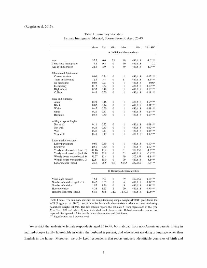
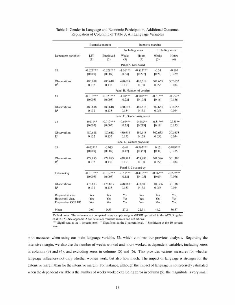
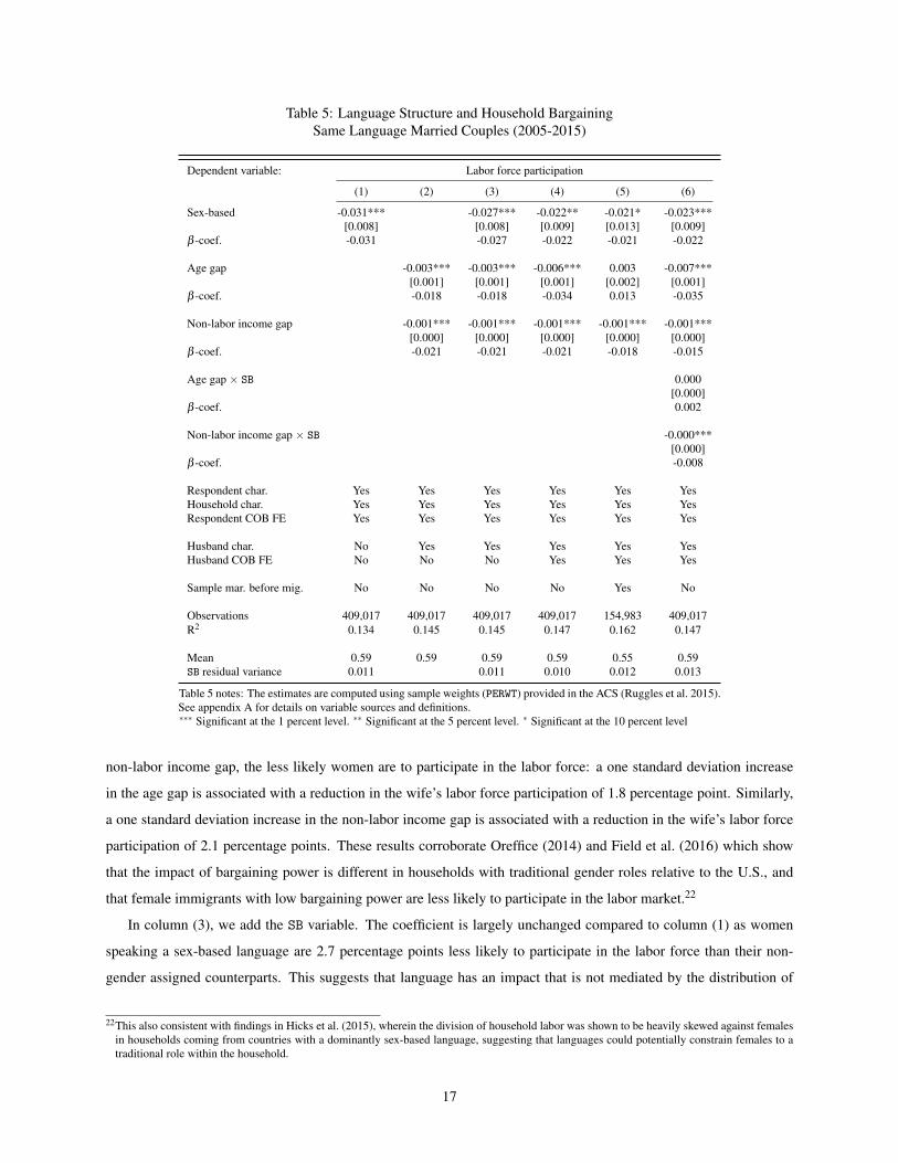
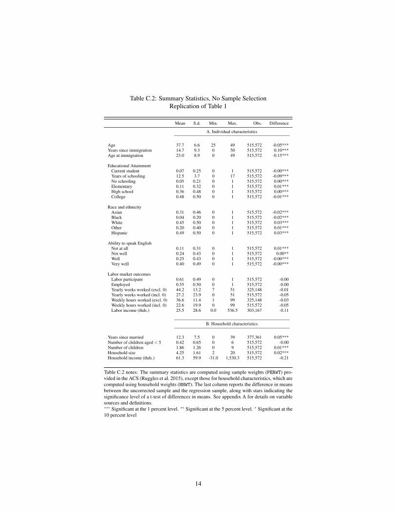

Tabl
eC
4S
umm
ary
Stat
istic
sH
ouse
hold
sw
ithFe
mal
eIm
mig
rant
sM
arri
edS
pous
ePr
esen
tA
ged
25-4
9H
hus
band
Ww
ife
Defi
nitio
nM
ean
Sd
Min
M
ax
Obs
SB
1-SB
0
Age
gap
Hag
e-W
age
35
57
-33
6448
061
8-0
9
A
mer
ican
husb
and
H=
US
citi
zen
018
038
01
480
618
003
Whi
tehu
sban
dH=
whi
tean
dW6=
whi
te0
050
230
148
061
8-0
05
O
rigi
nho
mop
hily
HC
OB=
WC
OB
073
044
01
480
618
-00
0L
ingu
istic
hom
ophi
lyH
lang
uage
=W
lang
uage
087
034
01
480
618
006
Edu
catio
nga
pH
educ
atio
n-W
educ
atio
n0
053
05-1
717
480
618
-04
3
Lab
orpa
rtic
ipat
ion
gap
HL
FP-W
LFP
034
054
-11
480
598
013
Em
ploy
men
tgap
Hem
ploy
men
t-W
empl
oym
ent
035
059
-11
480
598
014
Wee
ksga
pH
wee
ksw
orke
d-W
wee
ksw
orke
d3
715
3-4
444
284
275
14
H
ours
gap
Hho
urs
wor
ked
-Who
urs
wor
ked
64
142
-93
9728
427
51
6
Lab
orin
com
ega
p(t
hds
)H
labo
rinc
ome
-Wla
bori
ncom
e15
540
9-4
2652
125
016
4-1
8
N
onla
borp
artic
ipat
ion
gap
(thd
s)
Hno
nla
bori
ncom
e-W
non
labo
rinc
ome
29
193
-414
515
480
618
-04
Tabl
eC
4no
tes
The
sum
mar
yst
atis
tics
are
com
pute
dus
ing
hous
ehol
dsa
mpl
ew
eigh
ts(HHW
T)pr
ovid
edin
the
AC
S(R
uggl
eset
al2
015)
T
hela
stco
lum
nre
port
sth
ees
timat
eβ
from
regr
essi
ons
ofth
ety
peX i
=α+
βSB
I+
εw
here
X iis
anin
divi
dual
leve
lcha
ract
eris
ticR
obus
tsta
ndar
der
rors
are
notr
epor
ted
See
appe
ndix
Afo
rdet
ails
onva
riab
leso
urce
san
dde
finiti
ons
lowastlowastlowast
Sign
ifica
ntat
the
1pe
rcen
tlev
ellowastlowast
Sign
ifica
ntat
the
5pe
rcen
tlev
ellowast
Sign
ifica
ntat
the
10pe
rcen
tlev
el
16
Table C5 Summary Statistics Country and County-Level VariablesFemale Immigrants Married Spouse Present Aged 25-49
Variable Unit Mean Sd Min Max Obs
COB LFP Ratio female to male 5325 1820 4 118 474003Ancestry LFP 5524 1211 0 100 467378COB fertility Number of children 314 127 1 9 479923Ancestry fertility Number of children 208 057 1 4 467378COB education Ratio female to male 8634 1513 7 122 480618Ancestry educaiton Years of schooling 1119 252 1 17 467378COB migration rate -221 421 -63 109 479923COB GDP per capita PPP 2011 US$ 8840 11477 133 3508538 469718COB and US common language Indicator 071 045 0 1 480618Genetic distance COB to US 003 001 001 006 480618Bilateral distance COB to US Km 6792 4315 737 16371 480618COB latitude Degrees 2201 1457 -44 64 480618COB longitude Degrees -1603 8894 -175 178 480618County COB density 2225 2600 0 94 382556County language density 3272 3026 0 96 382556
Table C5 notes The summary statistics are computed using sample weights (PERWT) provided in the ACS (Ruggleset al 2015) See appendix A26 for more details on variables sources and definitions
Table C6 Gender in Language and Economic Participation Individual LevelReplication of Columns 1 and 2 of Table 3
Dependent variable Labor force participation
(1) (2) (3) (4) (5)
Sex-based -0101 -0076 -0096 -0070 -0069[0002] [0002] [0002] [0002] [0003]
β -coef -0101 -0076 -0096 -0070 -0069
Years of schooling 0019 0020 0010[0000] [0000] [0000]
β -coef 0072 0074 0037
Number of children lt 5 -0135 -0138 -0110[0001] [0001] [0001]
β -coef -0087 -0089 -0071
Respondent char No No No No YesHousehold char No No No No Yes
Observations 480618 480618 480618 480618 480618R2 0006 0026 0038 0060 0110
Mean 060 060 060 060 060SB residual variance 0150 0148 0150 0148 0098
Table C6 notes The estimates are computed using sample weights (PERWT) providedin the ACS (Ruggles et al 2015) See appendix A for details on variable sources anddefinitionslowastlowastlowast Significant at the 1 percent level lowastlowast Significant at the 5 percent level lowast Significant atthe 10 percent level
17
Table C7 Gender in Language and Economic Participation Additional OutcomesReplication of Column 5 of Table 3 Language Indices
Extensive margin Intensive margins
Including zeros Excluding zeros
Dependent variable LFP Employed Weeks Hours Weeks Hours(1) (2) (3) (4) (5) (6)
Panel A Intensity_1 = (SB + GP + GA + NG) times SB
Intensity_1 -0009 -0010 -043 -0342 -020 -0160[0002] [0002] [010] [0085] [007] [0064]
Observations 478883 478883 478883 478883 301386 301386R2 0132 0135 0153 0138 0056 0034
Panel B Intensity_2 = (SB + GP + NG) times SB
Intensity_2 -0013 -0015 -060 -0508 -023 -0214[0003] [0003] [014] [0119] [010] [0090]
Observations 478883 478883 478883 478883 301386 301386R2 0132 0135 0153 0138 0056 0034
Panel C Intensity = (GP + GA + NG) times SB
Intensity -0010 -0012 -051 -0416 -026 -0222[0003] [0003] [012] [0105] [009] [0076]
Observations 478883 478883 478883 478883 301386 301386R2 0132 0135 0153 0138 0056 0034
Panel D Intensity_PCA
Intensity_PCA -0008 -0009 -039 -0314 -019 -0150[0002] [0002] [009] [0080] [006] [0060]
Observations 478883 478883 478883 478883 301386 301386R2 0132 0135 0153 0138 0056 0034
Panel E Top_Intensity = 1 if Intensity = 3 = 0 otherwise
Top_Intensity -0019 -0013 -044 -0965 012 -0849[0009] [0009] [042] [0353] [031] [0275]
Observations 478883 478883 478883 478883 301386 301386R2 0132 0135 0153 0138 0056 0034
Respondent char Yes Yes Yes Yes Yes YesHousehold char Yes Yes Yes Yes Yes YesRespondent COB FE Yes Yes Yes Yes Yes Yes
Mean 060 055 272 2251 442 3657
Table C7 notes The estimates are computed using sample weights (PERWT) provided in the ACS (Ruggleset al 2015) See appendix A for details on variable sources and definitionslowastlowastlowast Significant at the 1 percent level lowastlowast Significant at the 5 percent level lowast Significant at the 10 percentlevel
In the main analysis we use the following measure of intensity of female and male distinctions in the language
grammar Intensity = SBtimes (GP+GA+NG) where Intensity is a categorical variable that ranges from 0 to 3
The reason why we chose this specification instead of a purely additive specification such as in Gay et al (2013) is
that in a non-sex-based gender system the agreements in a sentence do not relate to female male categories They
may instead depend on whether the type of noun of animate or inanimate human or non-human When a grammatical
gender system is organized around a construct other than biological gender SB = 0 In this case Intensity = 0
18
since SB enters multiplicatively in the equation In these cases the intensity of female and male distinctions in the
grammar is zero since such distinctions are not an organizing principle of the grammatical gender system When a
grammatical gender system is sex-based SB= 1 In this case the intensity measure can range from 0 to 3 depending
on how the rest of rules of the system force speakers to code female male distinctions
Appendix Table C7 replicates the column (5) of Table 3 for all labor outcome variables using these alternative
measures Intensity_1 is defined as Intensity_1= SBtimes (SB+GP+GA+NG) where Intensity is a categorical
variable that ranges from 0 to 4 The only difference with Intensity is that it assigns a value of 1 for a language with
a sex based language but no intensity in the other individual variables Panel A presents results using Intensity_1
Intensity_2 is defined as Intensity_2= SBtimes (SB+GP+NG) where Intensity_2 is a categorical variable that
ranges from 0 to 3 The only difference with Intensity is that it excludes the variable GA since this individual variable
is not available for a number of languages Panel B presents results using Intensity_2 Intensity_PCA is the prin-
cipal component of the four individual variables SB GP GA and NG Panel D presents results using Intensity_PCA
Top_Intensity is a dummy variable equal to 1 if Intensity is equal to 3 (corresponding to the highest intensity)
and 0 otherwise3 Panel E presents results using Top_Intensity These alternative measure should not be taken
as measuring absolute intensity but rather as a ranking of relative intensity across languages grammar As Appendix
Table C7 shows our main results are robust to these alternative specifications providing reassuring evidence that the
specification we use is not driving the results
3We thanks an anonymous referee suggesting this alternative specification
19
Table C8 Gender in Language and Economic Participation Alternative SamplesReplication of Column 5 of Table 3
(1) (2) (3) (4) (5) (6) (7)
Panel A Labor force participation
Sex-based -0027 -0029 -0045 -0073 -0027 -0028 -0026[0007] [0006] [0017] [0005] [0007] [0006] [0008]
Observations 480618 652812 411393 555527 317137 723899 465729R2 0132 0128 0137 0129 0124 0118 0135Mean 060 061 060 062 066 067 060
Panel B Employed
Sex-based -0028 -0030 -0044 -0079 -0029 -0029 -0027[0007] [0006] [0017] [0005] [0007] [0006] [0008]
Observations 480618 652812 411393 555527 317137 723899 465729R2 0135 0131 0140 0131 0126 0117 0138Mean 055 056 055 057 061 061 055
Panel C Weeks worked including zeros
Sex-based -101 -128 -143 -388 -106 -124 -0857[034] [029] [082] [025] [034] [028] [0377]
Observations 480618 652812 411393 555527 317137 723899 465729R2 0153 0150 0159 0149 0144 0136 0157Mean 272 274 270 279 302 300 2712
Panel D Hours worked including zeros
Sex-based -0813 -1019 -0578 -2969 -0879 -1014 -0728[0297] [0255] [0690] [0213] [0297] [0247] [0328]
Observations 480618 652812 411393 555527 317137 723899 465729R2 0138 0133 0146 0134 0131 0126 0142Mean 2251 2264 2231 2310 2493 2489 2247
Panel E Weeks worked excluding zeros
Sex-based -024 -036 -085 -124 -022 -020 -0034[024] [020] [051] [016] [024] [019] [0274]
Observations 302653 413396 258080 357049 216919 491369 292959R2 0056 0063 0057 0054 0054 0048 0058Mean 442 444 441 443 449 446 4413
Panel F Hours worked excluding zeros
Sex-based -0165 -0236 0094 -0597 -0204 -0105 -0078[0229] [0197] [0524] [0154] [0227] [0188] [0260]
Observations 302653 413396 258080 357049 216919 491369 292959R2 0034 0032 0034 0033 0039 0035 0035Mean 3657 3663 3639 3671 3709 3699 3656
Sample Baseline Age 15-59 Indig Include Exclude All Quallang English Mexicans hh flags
Respondent char Yes Yes Yes Yes Yes Yes YesHousehold char Yes Yes Yes Yes Yes Yes YesRespondent COB FE Yes Yes Yes Yes Yes Yes Yes
Table C8 notes The estimates are computed using sample weights (PERWT) provided in the ACS (Ruggleset al 2015) See appendix A for details on variable sources and definitionslowastlowastlowast Significant at the 1 percent level lowastlowast Significant at the 5 percent level lowast Significant at the 10 percent level
20
Table C9 Gender in Language and Economic Participation Logit and ProbitReplication of Columns 1 and 5 of Table 3
OLS Logit Probit
(1) (2) (3) (4) (5) (6)
Panel A Labor force participation
Sex-based -0101 -0027 -0105 -0029 -0105 -0029[0002] [0007] [0002] [0008] [0002] [0008]
Observations 480618 480618 480618 480612 480618 480612R2 0006 0132 0005 0104 0005 0104Mean 060 060 060 060 060 060
Panel B Employed
Sex-based -0115 -0028 -0118 -0032 -0118 -0032[0002] [0007] [0002] [0008] [0002] [0008]
Observations 480618 480618 480618 480612 480618 480612R2 0008 0135 0006 0104 0006 0104Mean 055 055 055 055 055 055
Respondent char No Yes No Yes No YesHousehold char No Yes No Yes No Yes
Respondent COB FE No Yes No Yes No Yes
Table C9 notes This table replicates table 3 with additional outcomes and with different estimators Theestimates are computed using sample weights (PERWT) provided in the ACS (Ruggles et al 2015) Seeappendix A for details on variable sources and definitionslowastlowastlowast Significant at the 1 percent level lowastlowast Significant at the 5 percent level lowast Significant at the 10 percentlevel
Table C10 Gender in Language and Economic Participation Individual LevelHusbands of Female Immigrants Married Spouse Present 25-49 (2005-2015)
Dependent variable Labor force participation
(1) (2) (3)
Sex-based 0026 0009 -0004[0001] [0002] [0004]
Husband char No Yes YesHousehold char No Yes Yes
Husband COB FE No No Yes
Observations 385361 385361 384327R2 0002 0049 0057
Mean 094 094 094
Table C10 notes The estimates are computed using sam-ple weights (PERWT_SB) provided in the ACS (Ruggles et al2015) See appendix A for details on variable sources and def-initions The husband characteristics are analogous to the re-spondent characteristics in Table 3 The sample is the sameas in Table 3 except that we drop English-speaking and nativehusbandslowastlowastlowast Significant at the 1 percent level lowastlowast Significant at the 5percent level lowast Significant at the 10 percent level
21
Table C11 Gender in Language and Economic ParticipationReplication of Column 5 of Table 3
Dependent variable Labor force participation
(1) (2) (3) (4)
Sex-based -0028 -0025 -0046[0006] [0006] [0006]
Unmarried 0143 0143 0078[0001] [0001] [0003]
Sex-based times unmarried 0075[0004]
Respondent char Yes Yes Yes YesHousehold char Yes Yes Yes Yes
Respondent COB FE Yes Yes Yes Yes
Observations 723899 723899 723899 723899R2 0118 0135 0135 0136Mean 067 067 067 067
Table C11 notes The estimates are computed using sample weights (PERWT) pro-vided in the ACS (Ruggles et al 2015) See appendix A for details on variablesources and definitionslowastlowastlowast Significant at the 1 percent level lowastlowast Significant at the 5 percent level lowast Signifi-cant at the 10 percent level
22
Table C12 Language and Household BargainingReplication of Column 3 of Table 5
Extensive margin Intensive margins
Including zeros Excluding zeros
Dependent variable LFP Employed Weeks Hours Weeks Hours(1) (2) (3) (4) (5) (6)
Sex-based -0027 -0026 -1095 -0300 -0817 -0133[0009] [0009] [0412] [0295] [0358] [0280]
β -coef -0027 -0028 -0047 -0020 -0039 -0001
Age gap -0004 -0004 -0249 -0098 -0259 -0161[0001] [0001] [0051] [0039] [0043] [0032]
β -coef -0020 -0021 -0056 -0039 -0070 -0076
Non-labor income gap -0001 -0001 -0036 -0012 -0034 -0015[0000] [0000] [0004] [0002] [0004] [0003]
β -coef -0015 -0012 -0029 -0017 -0032 -0025
Age gap times SB 0000 -0000 0005 0008 0024 0036[0000] [0000] [0022] [0015] [0019] [0015]
β -coef 0002 -0001 0001 0003 0006 0017
Non-labor income gap times SB -0000 -0000 -0018 0002 -0015 -0001[0000] [0000] [0005] [0003] [0005] [0004]
β -coef -0008 -0008 -0014 0003 -0014 -0001
Respondent char Yes Yes Yes Yes Yes YesHousehold char Yes Yes Yes Yes Yes YesHusband char Yes Yes Yes Yes Yes YesRespondent COB FE Yes Yes Yes Yes Yes Yes
Observations 409017 409017 409017 250431 409017 250431R2 0145 0146 0164 0063 0150 0038
Mean 059 054 2640 4407 2182 3644SB residual variance 0011 0011 0011 0011 0011 0011
Table C12 notes The estimates are computed using sample weights (PERWT) provided in the ACS (Ruggles et al2015) See appendix A for details on variable sources and definitionslowastlowastlowast Significant at the 1 percent level lowastlowast Significant at the 5 percent level lowast Significant at the 10 percent level
23
Table C13 Linguistic Heterogeneity in the HouseholdReplication of Column 3 of Table 6
Extensive margin Intensive margins
Including zeros Excluding zeros
Dependent variable LFP Employed Weeks Hours Weeks Hours(1) (2) (3) (4) (5) (6)
Same times wifersquos sex-based -0070 -0075 -3764 -2983 -0935 -0406[0003] [0003] [0142] [0121] [0094] [0087]
Different times wifersquos sex-based -0044 -0051 -2142 -1149 -1466 -0265[0014] [0015] [0702] [0608] [0511] [0470]
Different times husbandrsquos sex-based -0032 -0035 -1751 -1113 -0362 0233[0011] [0011] [0545] [0470] [0344] [0345]
Respondent char Yes Yes Yes Yes Yes YesHousehold char Yes Yes Yes Yes Yes YesHusband char Yes Yes Yes Yes Yes Yes
Observations 387037 387037 387037 387037 237307 237307R2 0122 0124 0140 0126 0056 0031
Mean 059 054 2640 2184 4411 3649SB residual variance 0095 0095 0095 0095 0095 0095
Table C13 notes The estimates are computed using sample weights (PERWT) provided in the ACS (Ruggles et al 2015)See appendix A for details on variable sources and definitionslowastlowastlowast Significant at the 1 percent level lowastlowast Significant at the 5 percent level lowast Significant at the 10 percent level
24
D Appendix figure
Figure D1 Regression Weights for Table 3 column (5)
Regression Weight
00 - 08
09 - 24
25 - 65
66 - 240
To better understand the extent to which each country of birth contributes to the identification of the coefficient
in column (5) table 3 we apply Aronow amp Samiirsquos (2016) procedure to uncover the ldquoeffective samplerdquo used in the
regression This procedure generates regression weights by computing the relative size of the residual variance of the
SB variable for each country of birth in the sample Appendix figure D1 shows regression weights for each country
of birth resulting from the regression of column (5) in Table 3 This specification includes respondent country of birth
fixed effects Therefore the weights inform us of the countries where identification is coming from and whether these
are multilingual countries or not As the figure shows identification mostly comes from multilingual countries such
as India followed by the Philippines Vietnam China Afghanistan and Canada
25
References
Aronow P M amp Samii C (2016) lsquoDoes regression produce representative estimates of causal effectsrsquo American
Journal of Political Science 60(1) 250ndash267
Barro R J amp Lee J W (2013) lsquoA new data set of educational attainment in the world 1950ndash2010rsquo Journal of
development economics 104 pp 184ndash198
DESA (2015) lsquoUnited nations department of economic and social affairs population division World population
prospects The 2015 revisionrsquo
Dryer M amp Haspelmath M (2011) lsquoThe world atlas of language structures onlinersquo
Feenstra R C Inklaar R amp Timmer M P (2015) lsquoThe next generation of the penn world tablersquo The American
Economic Review 105(10) pp 3150ndash3182
Gay V Santacreu-Vasut E amp Shoham A (2013) The grammatical origins of gender roles Technical report
Inc E B (2010) 2010 Britannica book of the year Vol 35 Encyclopaedia britannica
Mavisakalyan A (2015) lsquoGender in language and gender in employmentrsquo Oxford Development Studies 43(4) pp
403ndash424
Mayer T amp Zignago S (2011) Notes on cepiirsquos distances measures The geodist database Working Papers 2011-25
CEPII
Ruggles S Genadek K Goeken R Grover J amp Sobek M (2015) Integrated public use microdata series Version
60
Spolaore E amp Wacziarg R (2016) Ancestry and development new evidence Technical report Department of
Economics Tufts University
26
- Introduction
- Methodology
-
- Data
-
- Economic and demographic data
- Linguistic data
-
- Empirical Strategy
-
- Empirical results
-
- Decomposing language from other cultural influences
-
- Main results
- Robustness checks
-
- Language and the household
-
- Language and household bargaining power
- Evidence from linguistic heterogeneity within the household
-
- Language and social interactions
-
- Conclusion
- Appendix_2017_01_31_Revisionpdf
-
- Data appendix
-
- Samples
-
- Regression sample
- Alternative samples
-
- Variables
-
- Outcome variables
- Respondent control variables
- Household control variables
- Husband control variables
- Bargaining power measures
- Country of birth characteristics
- County-level variables
-
- Missing language structures
- Appendix tables
- Appendix figure
-
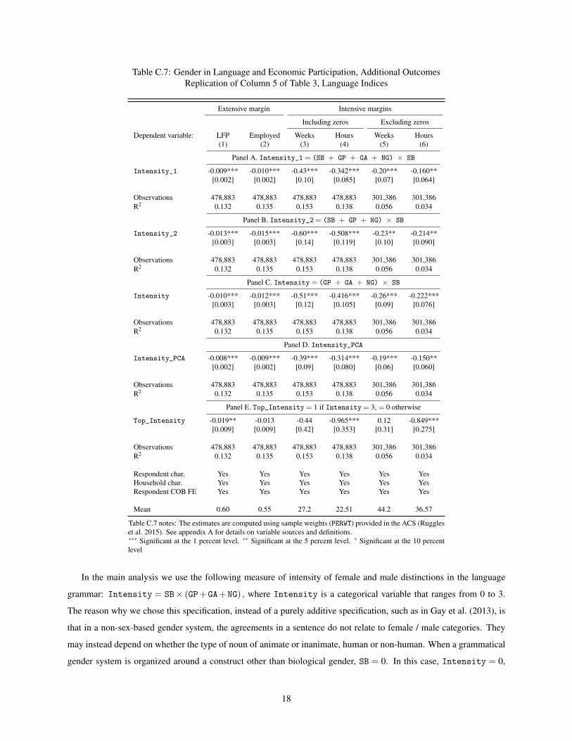
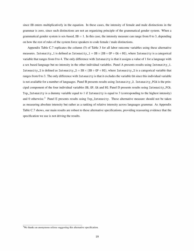
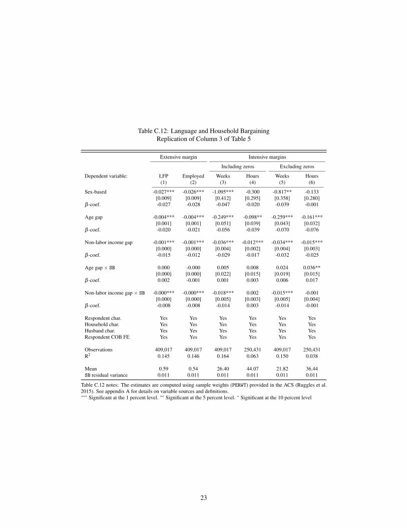
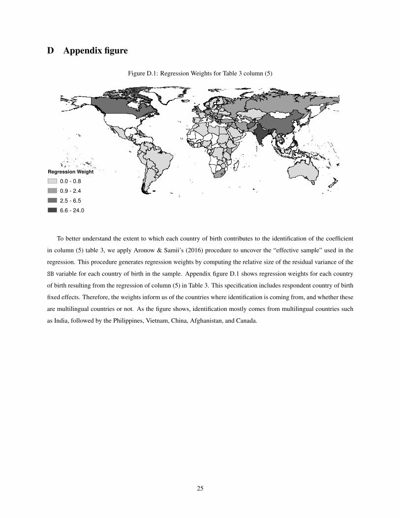