decision making.ppt - sihombing15's (haery sihombing) economy studies. decision making is...

4/18/2011

1

Engineering Economy

Copyright ©2009 by Pearson Education, Inc.Upper Saddle River, New Jersey 07458

All rights reserved.

Engineering Economy, Fourteenth EditionBy William G. Sullivan, Elin M. Wicks, and C. Patrick Koelling

Chapter : DECISION MAKING

The objective of this chapter is to discuss and illustrate several probabilistic methods that are useful in analyzing risk and




y guncertainty associated with

engineering economy studies.

Decision making is fraught with risk and uncertainty.

• Decisions under risk are those where the decision maker can estimate probabilities of occurrence of particular outcomes.




p• Decisions under uncertainty are those

where estimates of probabilities of the several unknown future states cannot be estimated.

Four major sources of uncertainty are present in engineering economy studies

• Possible inaccuracy of cash-flow estimates• The type of business involved in relation to

the future health of the economy




the future health of the economy• The type of physical plant and equipment

involved• The length of the study period used in the

analysis

Factors such as revenues, costs, salvage values, etc., can often be considered

random variables.

For discrete random variables X, the probability X takes on any particular value




xi is

where

Some other properties of discrete random variables.

Probability mass function




Cumulative distribution function

4/18/2011

2

For continuous random variables…




The probability that X takes on any particular value is 0.

The cumulative distribution function (CDF) is

which leads to




which leads to

The expected value (mean, central moment), E(X), and variance (measure of dispersion), V(X), of a random variable

X, are




Some properties of the mean and variance.




Acme manufacturing has installed a much-needed new CNC machine. The initial investment in this

machine is $180,000 and annual expenses are $12,000. The life of the machine is expected to be 5

years, with a $20,000 market value at that time. Acme’s MARR is 10%. Possible revenues follow

the probabilities given below




the probabilities given below.

Revenue Probability$35,000 0.1$44,000 0.3$50,000 0.4

$60,000 0.2

What are the expected value and variance of Acme’s revenue?




4/18/2011

3

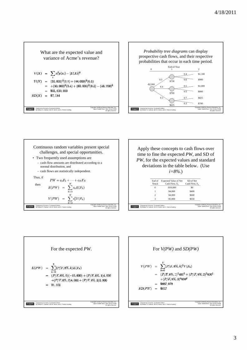
What are the expected value and variance of Acme’s revenue?




Probability tree diagrams can display prospective cash flows, and their respective probabilities that occur in each time period.

End-of-Year0 1 2

0.4 $1,100




0.5

0.5

0.6

$700

$825

$800

$1,000

$9000.3

0.4

0.3

0.3

0.7

$625

$700

$750-$2,000

Continuous random variables present special challenges, and special opportunities.

• Two frequently used assumptions are– cash-flow amounts are distributed according to a

normal distribution, and– cash flows are statistically independent.




Thus, if

then

Apply these concepts to cash flows over time to fine the expected PW, and SD of PW, for the expected values and standard

deviations in the table below. (Use i=8%.)




End of Year,k

Expected Value of Net Cash Flow, Fk

SD of Net Cash Flow, Fk

0 -$10,000 $01 $4,000 $4002 $4,000 $6003 $5,000 $650

For the expected PW.




For V(PW) and SD(PW)




4/18/2011

4

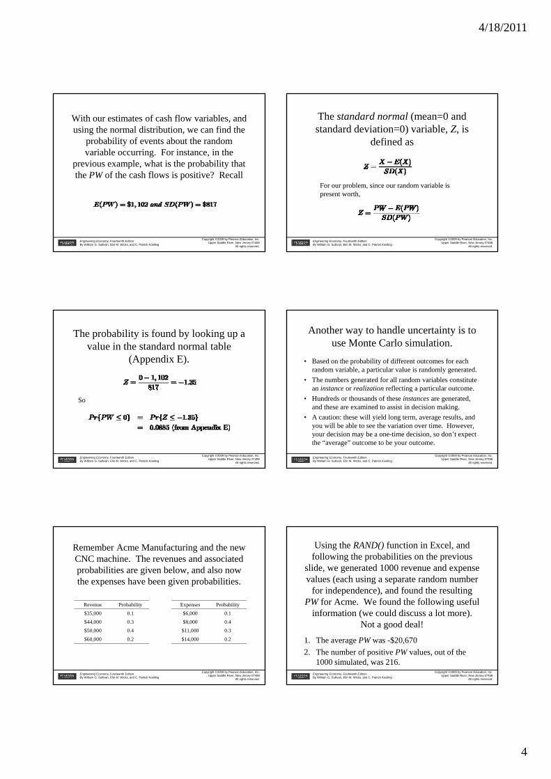
With our estimates of cash flow variables, and using the normal distribution, we can find the

probability of events about the random variable occurring. For instance, in the

previous example, what is the probability that th PW f th h fl i iti ? R ll




the PW of the cash flows is positive? Recall

The standard normal (mean=0 and standard deviation=0) variable, Z, is

defined as




For our problem, since our random variable is present worth,

The probability is found by looking up a value in the standard normal table

(Appendix E).




So

Another way to handle uncertainty is to use Monte Carlo simulation.

• Based on the probability of different outcomes for each random variable, a particular value is randomly generated.

• The numbers generated for all random variables constitute an instance or realization reflecting a particular outcome




an instance or realization reflecting a particular outcome.• Hundreds or thousands of these instances are generated,

and these are examined to assist in decision making.• A caution: these will yield long term, average results, and

you will be able to see the variation over time. However, your decision may be a one-time decision, so don’t expect the “average” outcome to be your outcome.

Remember Acme Manufacturing and the new CNC machine. The revenues and associated probabilities are given below, and also now the expenses have been given probabilities.

Revenue Probability Expenses Probability




Revenue Probability$35,000 0.1$44,000 0.3$50,000 0.4

$60,000 0.2

Expenses Probability$6,000 0.1$8,000 0.4$11,000 0.3

$14,000 0.2

Using the RAND() function in Excel, and following the probabilities on the previous

slide, we generated 1000 revenue and expense values (each using a separate random number

for independence), and found the resulting PW for Acme. We found the following useful




ginformation (we could discuss a lot more).

Not a good deal!1. The average PW was -$20,6702. The number of positive PW values, out of the

1000 simulated, was 216.

4/18/2011

5

Monte Carlo simulation is very flexible.• The example used a discrete distribution, but there is a way

to use any discrete or continuous distribution. If Excel is used, it has several special functions that generate random variates (e.g., NORMINV to generate normal random variates and BETAINV for beta random variates.)Th l k h f f




• There are many ways to look at the performance of an alternative using Monte Carlo simulation (we examined only two in the previous example). Graphs can be especially valuable.

• Generate lots of data, through many trials. When average values converge to a fairly constant amount, you probably have enough data.

Decision trees can be helpful in examining sequential decision problems

with outcomes that vary over time.• Break down large problems into a series of smaller

problems.




• Provide objective analysis that explicitly considers the risk and effect of the future.

• A decision tree is built from a series of nodes, where decisions are made (square symbols) or chance outcomes are noted (circle symbols), and branches, which specify outcomes.

Revisiting Acme Manufacturing and their CNC machine decision.

Acme already has a machine they can use that is adequate for their needs. However, they wish to make a decision about their purchase of the new machine. The time horizon is 4 years, and they know that they won’t replace their existing machine if there is only one years of the




their existing machine if there is only one years of the time horizon remaining. So, they will make a decision today, and at the end of the first and second years regarding the new machine. We assume no chance elements, only a deterministic decision tree. The tree on the following slide depicts the situation. Cash inflows and durations are above the arrows, and capital investments below the arrows.

Acme’s decision tree.

Old: 30k/yr1 yr

Old: 25k/yr1 yr

Old: 20k/yr2 yr

-15k -20k -30k 0 1 2




New: 55k/yr4 yr

New: 70k/yr3 yr

New: 70k/yr2 yr

Analyze decision trees from the last decision, backward to the first.

Decision Point Alternative Monetary Outcome Choice

2Old $20k(2)-$30k = $10k

Old




New $70k(2)-$180k = -$40k

1Old $10k+$25k(1)-$20k = $15k

NewNew $70k(3)-$180k = $30k

0Old $30k+$30k(1)-$15k = $45k

OldNew $55k(4)-$180k = $40k

Acme should keep their current machine for one more year.

• The table reveals that at decision point 2, if Acme still has the old machine, they should keep it.

• At decision point 1, purchasing the new machine provides greater return than keeping the old one.




• At decision point 0 (today), it is more advantageous to keep the old (current) machine for one more year, given that the best decision at decision point 1 is to get the new machine.

• It would be appropriate to include the time value of money, so cash flows should be discounted to the present and the analysis performed again.

4/18/2011

6

Adding probabilities to decision trees.• Most decisions also include chance outcomes, so we use

chance nodes.• All alternatives emanating from either a decision or chance

node must be mutually exclusive (no more than one may be selected) and exhaustive (contain all possible outcomes).




• The probabilities on the branches from a chance node must sum to one (like probability tree diagrams).

• The value assigned to a chance node is the expected value of the possible outcomes along each of the branches leaving the node.

Mitselfik, Inc. believes new scheduling software (at a cost of $150,000) will allow them to better manage

product flow and therefore increase sales. The projection of increased annual sales (for the next 5 years), and the associated probabilities, are below. The following slide shows the decision tree, and

resulting PW at a MARR of 12%




resulting PW at a MARR of 12%.

Increased annual sales Probability$75,000 0.35$60,000 0.45

$40,000 0.15$30,000 0.05

New

Sales increase

75,000 $120,360

$68,992

PW Probability

0.45

0.15

0.35

40,000

60,000 $66,288

$5 808




software

0.05 30,000

$0

$0Current software

-$5,808

-$41,856 $68,992

Mitselfik should purchase the software; the expected PW of the investment is

$68,992.• The PW of each annual sales increase amount is

given in the far right of the tree.• The expected value of the annual sales increase is




The expected value of the annual sales increase is $218,992 (the sum of the probabilities times the respective PW).

• Subtracting the initial cost yields a net PW of $68,992, which is superior to “do nothing” (which is eliminated, signified by the double lines on that decision branch).

How much would we pay to have perfect information about the future?

• Perhaps with additional information we might have a better estimate of sales, or exact knowledge of sales (“perfect” information).




• The cost of reducing the uncertainty must be balanced against the value.

• Perfect information is not obtainable, so the expected value of perfect information (EVPI) is an upper limit on what we would consider spending.

• EVPI = the value of the decision based on perfect information minus the value without the information.

Mitselfik could make the right decision with perfect information.

Decision with perfect information

Increased sales Probability Decision Outcome

Prior decision




y$75,000 0.35 Purchase $120,360 $120,360

$60,000 0.45 Purchase $66,288 $66,288

$40,000 0.15 No purchase $0 -$5,808

$30,000 0.05 No purchase $0 -$41,856

Expected Value $71,956 $68,992

4/18/2011

7

How much should Mitselfik pay for perfect information?

• If Mitselfik had perfect information they would decide not to purchase the software if the increase in sales were $30,000 or $40 000




$40,000.• EVPI = $71,956 - $68,992 = $2,964.• It is possible to find the expected value of

any additional information that is not “perfect.” This is discussed in detail in the text.

Decision trees can be used to assist in analyzing real options.

• Real options, similar to financial call options, allow decision makers to invest capital now or postpone all or part of the




p p p pinvestment until later.

• When a firm makes an irreversible capital investment that could be postponed, it exercises its call option, which has value by virtue of the flexibility it gives the firm.

A good example of postponable investment is a plant addition.

Consider Mitselfik, Inc., which in addition to purchasing software needs to expand the facility. It can complete the entire expansion




y p pnow at a cost of $7 million, leading to anticipated net cash flows (after tax) of $1.2 million for the next ten years. At an after-tax MARR of 12%, is this an attractive investment?

This does not look attractive for Mitselfik.




What if demand should change, rising higher than originally anticipated? Perhaps Mitselfik, Inc. could be prepared and have an option available that would allow them to respond to this increased demand.

Assume that demand could balloon to $3.5 million (or, it could go to zero). The original expansion could handle sales of $1.5 million, and Mitselfik could acquire additional space (an option) to handle the additional increased demand of $2 million at a cost of $4 million If this additional demand did not




cost of $4 million. If this additional demand did not materialize, the original expansion could be sold for $1 million. What is the best decision for Mitselfik?

This is modeled as a decision tree on the next slide.

Mitselfik’s decision tree

Buildinge

$9.20mil

-$3.79mil

$1.48mil

-$6.55mil Sales

$2.1mil

Add

Continue

Abandon

Add

PW

$9.20mil

-$0.22mil




gxpansion

-$10.6mil

-$0.22mil

-$6.11mil with option

Negligible sales

Sales $1.2mil

Add

Continue

Continue

Abandon

Abandon

-$7.00mil

-$6.11mil

Expected value = $0.96mil if all outcomes are equally likely.

-$6.11mil

4/18/2011

8

Mitselfik should strongly consider investing since the option to add capacity

can provide a positive return.

• Using the decision tree model to assess the option reveals that the expected return given the best




reveals that the expected return, given the best decisions along the way, is $960,000.

• However, losses could be large, and there is a 2/3 chance of a loss (if all outcomes are equally likely). Issues like this are covered in Chapter 14.

4/18/2011

1

Decision-Making Tools

Decision-Making Tools

PowerPoint presentation to accompany PowerPoint presentation to accompany

A - 1© 2011 Pearson Education, Inc. publishing as Prentice Hall

o e o t p ese tat o to acco pa yo e o t p ese tat o to acco pa yHeizer and Render Heizer and Render Operations Management, 10e Operations Management, 10e Principles of Operations Management, 8ePrinciples of Operations Management, 8e

PowerPoint slides by Jeff Heyl

OutlineOutline

The Decision Process in OperationsFundamentals of Decision Making


Decision Tables

Outline Outline –– ContinuedContinued

Types of Decision-Making Environments

Decision Making Under Uncertainty


Decision Making Under RiskDecision Making Under CertaintyExpected Value of Perfect Information (EVPI)

Outline Outline –– ContinuedContinued

Decision TreesA More Complex Decision TreeUsing Decision Trees in Ethical


gDecision MakingThe Poker Decision Problem

Learning ObjectivesLearning ObjectivesWhen you complete this module you When you complete this module you should be able to:should be able to:

1. Create a simple decision tree2 B ild d i i t bl


2. Build a decision table3. Explain when to use each of the three

types of decision-making environments

4. Calculate an expected monetary value (EMV)

Learning ObjectivesLearning ObjectivesWhen you complete this module you When you complete this module you should be able to:should be able to:

5. Compute the expected value of perfect information (EVPI)


perfect information (EVPI)6. Evaluate the nodes in a decision tree7. Create a decision tree with sequential

decisions

4/18/2011

2

Decision to Go All InDecision to Go All In


The Decision Process in The Decision Process in OperationsOperations

1. Clearly define the problems and the factors that influence it

2. Develop specific and measurable objectives


objectives3. Develop a model4. Evaluate each alternative solution5. Select the best alternative6. Implement the decision and set a

timetable for completion

Fundamentals of Fundamentals of Decision MakingDecision Making

1. Terms:a. Alternative – a course of action or

strategy that may be chosen by the


strategy that may be chosen by the decision maker

b. State of nature – an occurrence or a situation over which the decision maker has little or no control

Fundamentals of Fundamentals of Decision MakingDecision Making

2. Symbols used in a decision tree:a. – decision node from which one

of several alternatives may be


of several alternatives may be selected

b. – a state-of-nature node out of which one state of nature will occur

Decision Tree ExampleDecision Tree Example

Favorable market

Unfavorable market

A decision node A state of nature node


Favorable market

Unfavorable market

Construct small plant

Figure A.1

Decision Table ExampleDecision Table Example

State of NatureAlternatives Favorable Market Unfavorable Market

Construct large plant $200,000 –$180,000


Table A.1

Construct small plant $100,000 –$ 20,000Do nothing $ 0 $ 0

4/18/2011

3

DecisionDecision--Making Making EnvironmentsEnvironments

Decision making under uncertaintyComplete uncertainty as to which state of nature may occur


Decision making under riskSeveral states of nature may occurEach has a probability of occurring

Decision making under certaintyState of nature is known

UncertaintyUncertainty1. Maximax

Find the alternative that maximizes the maximum outcome for every alternative


Pick the outcome with the maximum numberHighest possible gainThis is viewed as an optimistic approach

UncertaintyUncertainty2. Maximin

Find the alternative that maximizes the minimum outcome for every alternative


Pick the outcome with the minimum numberLeast possible lossThis is viewed as a pessimistic approach

UncertaintyUncertainty

3. Equally likelyFind the alternative with the highest average outcome


Pick the outcome with the maximum numberAssumes each state of nature is equally likely to occur

Uncertainty ExampleUncertainty ExampleStates of Nature

Favorable Unfavorable Maximum Minimum RowAlternatives Market Market in Row in Row AverageConstruct

large plant $200,000 -$180,000 $200,000 -$180,000 $10,000Construct


1. Maximax choice is to construct a large plant2. Maximin choice is to do nothing3. Equally likely choice is to construct a small plant

Maximax Maximin Equally likely

Constructsmall plant $100,000 -$20,000 $100,000 -$20,000 $40,000

Do nothing $0 $0 $0 $0 $0

RiskRisk

Each possible state of nature has an assumed probabilityStates of nature are mutually exclusive


Probabilities must sum to 1Determine the expected monetary value (EMV) for each alternative

4/18/2011

4

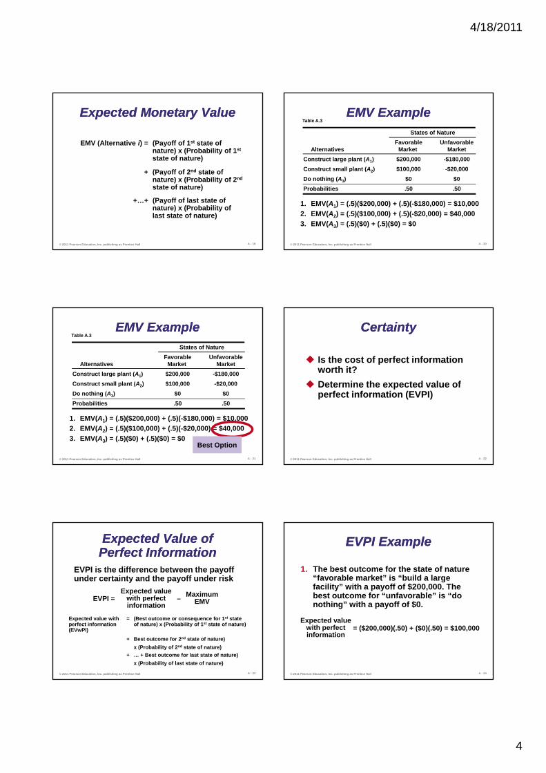
Expected Monetary ValueExpected Monetary Value

EMV (Alternative i) = (Payoff of 1st state of nature) x (Probability of 1st

state of nature)

+ (Payoff of 2nd state of


+ (Payoff of 2nd state of nature) x (Probability of 2nd

state of nature)

+…+ (Payoff of last state of nature) x (Probability of last state of nature)

EMV ExampleEMV ExampleTable A.3

States of NatureFavorable Unfavorable

Alternatives Market MarketConstruct large plant (A1) $200,000 -$180,000Construct small plant (A2) $100,000 -$20,000


1. EMV(A1) = (.5)($200,000) + (.5)(-$180,000) = $10,0002. EMV(A2) = (.5)($100,000) + (.5)(-$20,000) = $40,0003. EMV(A3) = (.5)($0) + (.5)($0) = $0

p ( 2) $ , $ ,Do nothing (A3) $0 $0Probabilities .50 .50

EMV ExampleEMV ExampleTable A.3

States of NatureFavorable Unfavorable

Alternatives Market MarketConstruct large plant (A1) $200,000 -$180,000Construct small plant (A2) $100,000 -$20,000


1. EMV(A1) = (.5)($200,000) + (.5)(-$180,000) = $10,0002. EMV(A2) = (.5)($100,000) + (.5)(-$20,000) = $40,0003. EMV(A3) = (.5)($0) + (.5)($0) = $0

Best Option

p ( 2) $ , $ ,Do nothing (A3) $0 $0Probabilities .50 .50

CertaintyCertainty

Is the cost of perfect information worth it?Determine the expected value of


Determine the expected value of perfect information (EVPI)

Expected Value of Expected Value of Perfect InformationPerfect Information

EVPI is the difference between the payoff under certainty and the payoff under risk

EVPI = –Expected value

with perfect Maximum EMV


pinformation EMV

Expected value with perfect information (EVwPI)

= (Best outcome or consequence for 1st state of nature) x (Probability of 1st state of nature)

+ Best outcome for 2nd state of nature) x (Probability of 2nd state of nature)

+ … + Best outcome for last state of nature) x (Probability of last state of nature)

EVPI ExampleEVPI Example

1. The best outcome for the state of nature “favorable market” is “build a large facility” with a payoff of $200,000. The best outcome for “unfavorable” is “do

$


nothing” with a payoff of $0.

Expected value with perfect information

= ($200,000)(.50) + ($0)(.50) = $100,000

4/18/2011

5

EVPI ExampleEVPI Example

2. The maximum EMV is $40,000, which is the expected outcome without perfect information. Thus:

M i


= $100,000 – $40,000 = $60,000

EVPI = EVwPI – Maximum EMV

The most the company should pay for perfect information is $60,000

Decision TreesDecision Trees

Information in decision tables can be displayed as decision treesA decision tree is a graphic display of the decision process that indicates decision


alternatives, states of nature and their respective probabilities, and payoffs for each combination of decision alternative and state of natureAppropriate for showing sequential decisions

Decision TreesDecision Trees


Decision TreesDecision Trees1. Define the problem2. Structure or draw the decision tree3. Assign probabilities to the states of

nature


4. Estimate payoffs for each possible combination of decision alternatives and states of nature

5. Solve the problem by working backward through the tree computing the EMV for each state-of-nature node

Decision Tree ExampleDecision Tree Example= (.5)($200,000) + (.5)(-$180,000)EMV for node 1

= $10,000

Payoffs

$200,000Favorable market (.5)

Unfavorable market (.5)1


EMV for node 2= $40,000 = (.5)($100,000) + (.5)(-$20,000)

-$180,000

$100,000

-$20,000

$0

Construct small plant

Unfavorable market (.5)

Favorable market (.5)

Unfavorable market (.5)2

Figure A.2

Complex Complex Decision Decision

Tree Tree ExampleExample


Figure A.3

4/18/2011

6

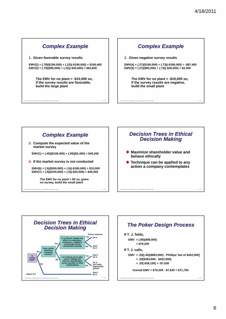
Complex ExampleComplex Example

1. Given favorable survey results

EMV(2) = (.78)($190,000) + (.22)(-$190,000) = $106,400EMV(3) = (.78)($90,000) + (.22)(-$30,000) = $63,600


The EMV for no plant = -$10,000 so, if the survey results are favorable, build the large plant

Complex ExampleComplex Example

2. Given negative survey results

EMV(4) = (.27)($190,000) + (.73)(-$190,000) = -$87,400EMV(5) = (.27)($90,000) + (.73)(-$30,000) = $2,400


The EMV for no plant = -$10,000 so, if the survey results are negative, build the small plant

Complex ExampleComplex Example3. Compute the expected value of the

market survey

EMV(1) = (.45)($106,400) + (.55)($2,400) = $49,200


The EMV for no plant = $0 so, given no survey, build the small plant

4. If the market survey is not conducted

EMV(6) = (.5)($200,000) + (.5)(-$180,000) = $10,000EMV(7) = (.5)($100,000) + (.5)(-$20,000) = $40,000

Decision Trees in Ethical Decision Trees in Ethical Decision MakingDecision Making

Maximize shareholder value and behave ethically


Technique can be applied to any action a company contemplates

Yes

No

Decision Trees in Ethical Decision Trees in Ethical Decision MakingDecision Making

Yes

Is it ethical? (Weigh the affect on employees, customers, suppliers,

community verses shareholder benefit)

D ti

Do it

Don’t do it

Action outcome


No

Yes

NoIs it ethical not to take

action? (Weigh the harm to shareholders

verses benefits to other stakeholders)No

YesDoes action

maximize company returns?

Is action legal?

Figure A.4Don’t do it

Don’t do it

Do it, but notify appropriate parties

do it

The Poker Design ProcessThe Poker Design ProcessIf T. J. folds,

EMV = (.80)($99,000)= $79,200


If T. J. calls,EMV = .20[(.45)($853,000) - Phillips’ bet of $422,000]

= .20[$383,850 - $422,000]= .20[-$38,150] = -$7,630

Overall EMV = $79,200 - $7,630 = $71,750

4/18/2011

7


All rights reserved. No part of this publication may be reproduced, stored in a retrieval system, or transmitted, in any form or by any means, electronic, mechanical, photocopying,

recording, or otherwise, without the prior written permission of the publisher. Printed in the United States of America.

4/18/2011

1

Make or Buy DecisionMake or Buy Decision

EVALUATING ALTERNATIVE

Example:1• Ayam Galing restaurant is experiencing a boom in business.

The owner expects to serve 80,000 meals this year. Although the kitchen is operating at 100 % capacity, the dining room can handle 105,000 dinners per year. Forecasted demand for the next years is 90,000 meals for next year, followed by a 10,000-meal increase in each of the succeeding years. One alternative is to expand both the kitchen and the dining room now, b i i th i it t 130 000 l Thbringing their capacity up to 130,000 meals per year. The initial would be RM 200,000, made at the end of this years (year 0). The average meal is priced at RM 10, and the before-tax profit margin is 20%. The 20% figure was arrived at by determining that, for each RM 10 meal, RM 6 covers variable costs and RM 2 goes toward fixed costs (other than depreciation). The remaining RM2 goes to pretax profit.

• What are the pretax cash flows from this project for the next five years compared to those of the base case of doing nothing?

• Solution:Recall that the base case of doing nothing results in losing all potential sales beyond 80,000. With the new capacity, the cash flow would equal the extra meals served by having a 130,000-meal capacity, multiplied by a profit of RM 2 per meal. In year 0, the only cash flow is –RM200,000 or the initial investment. In year 1, the 90,000-meal demand will be completely satisfied by the expanded capacity, so the incremental cash flow is (90,000 – 80,000)

Example:1

by the expanded capacity, so the incremental cash flow is (90,000 80,000) (RM 2) = RM 20,000. For subsequent years, the figures are as follows:

Year 2 :Demand = 100,000; Cash flow = (100,000 – 80,000) RM2 = RM40,000Year 3: Demand = 110,000; Cash flow = (110,000 – 80,000) RM2 = RM60,000Year 4 :Demand = 120,000; Cash flow = (120,000 – 80,000) RM2 = RM80,000Year 5 :Demand = 130,000; Cash flow = (130,000 – 80,000) RM2 = RM100,000

• If the capacity were smaller than the expected demand in any year, we would subtract the base case capacity from the new capacity (rather than the demand).

• NPV = -200,000 + [(20,000/1.1)] + [40,000/(1.1)2]+ [60,000/(1.1)3]+ [80,000/(1.1)4]+ [100,000/(1.1)5]

Example:1

= -200,000 +18,181.82 + 33,057.85 + 45,078.89 + 54,641.07 + 62,092.13

= RM 13,051.76

• An operations manager's staff has compiled the information below for four manufacturing alternatives (E, F, G, and H) that vary by production technology and the capacity of the machinery. All choices enable the same level of total production and have the same lifetime. The four states of nature represent four levels of consumer acceptance of the firm's products. Values in the table are net present value of future profits in millions of dollars. Forecasts indicate that there is a 0.1 probability of acceptance level 1, 0.2 chance of acceptance level 2, 0.4 chance of acceptance level 3, and 0.3 change of acceptance level 4.

St t f t

Example:2

States of nature

1 2 3 4 Alternative E 50 50 70 60 Alternative F 30 50 80 130Alternative G 70 80 70 60Alternative H -140 -10 150 220

• Using the criterion of expected monetary value, which production alternative should be chosen?

• The expected values are:

• E = .1*50 + .2*50 + .4*70 + .3*60 = 5 + 10 + 28 + 18= 61

• F = .1*30 + .2*50 + .4*80 + .3*130 = 3 + 10 + 32 + 39 = 84

Example:2

= 84• G = .1*70 + .2*80 + .4*70 + .3*60 = 7 + 16 + 28 + 18

= 69• H = .1 *-140 + .2*-10 + .4*150 + .3*220 = -10 -2 + 60 + 66

= 110

The highest of these occurs with production alternative H.

4/18/2011

2

• A toy manufacturer makes stuffed kittens and puppies which have relatively lifelike motions. There are three different mechanisms which can be installed in these "pets." These toys will sell for the same price regardless of the mechanism installed, but each mechanism has its own variable cost and setup cost. Profit, therefore, is dependent upon the choice of mechanism and upon the level of demand The manufacturer has in hand a

Example:3

level of demand. The manufacturer has in hand a forecast of demand that suggests a 0.2 probability of light demand, a 0.45 probability of moderate demand, and a probability of 0.35 of heavy demand. Payoffs for each mechanism-demand combination appear in the table as follows:

Example:3Demand Wind-up action Pneumatic

actionElectronic

actionLight $250,000 $90,000 -$100,000

Moderate 400,000 440,000 400,000

Heavy 650 000 740 000 780 000Heavy 650,000 740,000 780,000

• Construct the appropriate decision tree to analyze this problem. Use standard symbols for the tree. Analyze the tree to select the optimal decision for the manufacturer.

0.2Light demand

250000250,000 250000

0.45Wind-up Moderate demand

4000000 457500 400,000 400000

0.35Heavy demand

650000650,000 650000

0.2Light demand

9000090,000 90000

0.45Pneumatic Moderate demand

Example:3

eu at c ode ate de a d2 440000

475000 0 475000 440,000 440000

0.35Heavy demand

740000740,000 740000

0.2Light demand

-100000-100,000 -100000

0.45Electronic Moderate demand

4000000 433000 400,000 400000

0.35Heavy demand

780000780,000 780000The best choice is Pneumatic, $475,000.

• Earl Shell owns his own Sno-Cone business and lives 30 miles from a beach resort. The sale of Sno-Cones is highly dependent upon his location and upon the weather. At the resort, he will profit $120 per day in fair weather, $10 per day in bad weather. At home, he will profit $60 in fair weather $35 in bad weather Assume

Example:4

profit $60 in fair weather, $35 in bad weather. Assume that on any particular day, the weather service suggests a 40% chance of foul weather.

• a. Construct Earl's decision tree.• b. What decision is recommended by the expected value

criterion?

• Resort has a higher EMV ($76) than HomeExample:4

• A toy manufacturer has three different mechanisms that can be installed in a doll that it sells. The different mechanisms have three different setup costs (overheads) and variable costs and, therefore, the profit from the dolls is d d t th l f l Th

Example:5

dependent on the volume of sales. The anticipated payoffs are as follows.

4/18/2011

3

Light Demand Moderate Demand Heavy Demand

Probability 0.25 0.45 0.3Wind-up action $325,000 $190,000 $170,000 Pneumatic action $300,000 $420,000 $400,000

Example:5

Electrical action -$400,000 $240,000 $800,000

a. What is the EMV of each decision alternative?b. Which action should be selected?c. What is the expected value under certainty?d. What is the expected value of perfect information?

• (a) Wind-up =.25*$325,000 + .45*$190,000 + .3*$170,000 = $217,750Pneumatic =.25*$300,000 + .45*$420,000 + .3*$400,000 = $384,000 Electrical =.25*(-$400,000) + .45*$240,000 + .3*$800,000 =

$248,000.

Example:5

• (b) Pneumatic has the best EMV at $384,000.

• (c) Expected value under certainty is .25*$325,000 + .45* $420,000 + .3* $800,000 = $510,250

• (d) EVPI =$510,250 - $384,000 = $126,250.

decision making.ppt - sihombing15's (haery sihombing) economy studies. decision making is...

Documents